WATER RESOURCES RESEARCH, VOL. 33, NO. 11, PAGES 2429-2445 NOVEMBER 1997

Stochastic analysis of one-dimensional transport of kinetically adsorbing solutes in chemically heterogeneous aquifers

Carlos Espinoza and Albert J. Valocchi Hydros);stems Laboratory, Department of Civil Engineering, University of Illinois at Urbana-Champaign

Abstract. A small perturbation approach is used to analyze the impact of chemical heterogeneity on the one-dimensional transport of a pollutant that undergoes linear kinetic adsorption. We make an important simplifying assumption that the aquifer is physically homogeneous but chemically heterogeneous. The aquifer is assumed to be comprised of two distinct zones: reactive and nonreactive; a Bernoulli random process is used to characterize the spatial distribution of reactive zones along the aquifer. We develop analytical solutions to study the distribution of the ensemble mean, standard deviation, and coefficient of variation of the dissolved concentration after an instantaneous injection of contaminant. In addition, numerical solutions based on a Monte Carlo approach are used to determine the validity of the analytical solutions. Finally, an analysis involving temporal and spatial moments is used to derive expressions for the large-scale effective parameters (velocity and dispersion) that capture the impact of chemical heterogeneity. Temporal moment analysis provides closed-form analytical expressions for the asymptotic effective velocity and dispersion, while spatial moment analysis explains the effect of chemical heterogeneity on the preasymptotic value of these effective parameters. A key result from our analysis shows that chemical heterogeneity creates "pseudokinetic" or "macrokinetic" conditions characterized by a time-dependent effective retardation coefficient even when the local equilibrium assumption is invoked.

1. Introduction

The impact of small-scale spatial variability upon field-scale transport is widely recognized as a key problem in groundwater research and practice. Although initial research [e.g., Gelbar and Axness, 1983; Dagan, 1984] focused upon nonreactive sol- utes and variability in hydraulic conductivity, recent work has emphasized reactive solutes and variability in aquifer chemical properties [e.g., Tompson et al., 1996; Miralies-Wilhelm and Gelbar, 1996]. This work has been motivated by limited field observations showing that adsorption parameters may exhibit spatial variability [Robin et al., 1991; Mackay et al., 1986; Barber et al., 1992; Davis et al., 1993]. One significant cause of porous medium reactivity is the presence of organic or metal oxyhy- droxide coatings on particles. The spatial distribution of these surface coatings can be highly erratic; for example, Tompson et al. [1996] present a photo of an Atlantic coastal plain sandy outcrop which shows iron oxides present in discrete bands separated by zones of uncoated material.

Uncertainty about the precise spatial distribution of reactive soil properties will lead to uncertainty in transport calculations. One way to address this problem is to use a stochastic ap- proach in which the adsorption parameters are modeled as random fields. The resulting set of transport-reaction equa- tions involve stochastic partial differential equations which can be solved by approximate analytical techniques or a numerical Monte Carlo approach. Much of the published literature deals with a single species undergoing linear adsorption reactions

Copyright 1997 by the American Geophysical Union.

Paper number 97WR02169. 0043-1397/97/97WR-02169509.00

[Chrysikopoulos et al., 1990; Hu et al., 1995; Miralies-Wilhelm and Gelhar, !996; Kabala and Sposito, 1991; Quinodoz and Valocchi, 1993; Bellin et al., 1993; Bosma et al., 1993; Dagan et al., 1992]; in this case perturbation-based techniques can be used to develop approximate analytical solutions. Monte Carlo techniques have been used for more complicated problems involving multicomponent species and nonlinear adsorption [e.g., Tompson et al., 1996].

In this study we consider the transport of a single reactive species that undergoes linear kinetic adsorption. We make an important simplification by assuming that the aquifer is phys- ically homogeneous but chemically heterogeneous. Making this simplifying assumption will enable us to derive analytical results that focus upon the impact of chemical heterogeneity. Furthermore, we assume that the aquifer is comprised of a random assemblage of two different sites: reactive and nonre- active. Our analytical derivation follows the same line as Chrysikopoulos et al.'s [1990], in which the expected value of the concentration distribution was calculated assuming equi- librium conditions for the adsorption process, and Hu et al.'s [1995], which includes a more general linear kinetic adsorption model. The main difference between Chrysikopoulos et al.'s and Hu et al.'s solutions and the one presented here is the derivation of expressions not only for the expected value of the concentration field but for the variances and cross covariances

as well. As described by Vomvoris and Gelhar [1990] and Kapoor and Gelhar [1994a, b], evaluation of the concentration variance is necessary in order to assess the practical applica- bility of the ensemble averaged results to predict point con- centration values in an aquifer. Another important objective of this paper is to use temporal and spatial moment analysis of the mean concentration equation in order to define large-scale

2429

2430 ESPINOZA AND VALOCCHI: STOCHASTIC ANALYSIS OF ONE-DIMENSIONAL TRANSPORT

effective parameters that capture the impact of chemical het- erogeneity.

2. Governing Equations and Random Fields The starting point for this derivation is the well known ad-

vection-dispersion equation (ADE) written in one dimension as

Oc as O2c Oc

o--[ + • = O b-•- u Ox (1)

where c (x, t) is the dissolved or aqueous concentration, s (x, t) is the adsorbed concentration, D is the mechanical disper- sion coefficient, u is the flow velocity, x is the spatial coordi- nate, and t is time. In (1) we assume that the porosity is constant and that c and s have the same units. Adsorption is a kinetic process which can be represented by the following expression:

Os

o• = k•c - k•s = k•(K•c - s) (2)

where ke and kR are the forward and reverse adsorption rates, respectively, and K a is the distribution coefficient (ke/kR). As mentioned in the introduction we will assume a physically homogeneous (i.e., velocity and dispersion are constant through the aquifer) but chemically heterogeneous porous me- dium (i.e., adsorption takes place in a limited portion of the aquifer). This simplifying assumption enables us to focus solely on the impact of spatially variable chemical properties of the porous medium without the added complexity of spatially vari- able permeability. Since the aquifer is comprised of distinct reactive and nonreactive zones, (2) must be modified as

Os

a• = k•epc - k•s = k•(K•epc - s) (3)

where •(w; x) is a Bernoulli random process which represents the distribution of reactive sites within the aquifer. Comparing (3) with (2) we see that Kar k can be considered as a random distribution coefficient. The random process •(w; x) can take two possible values:

1 with probability/3 ß (w; x) = 0 with probability 1 -/3 (4) in which 1 represents a reactive site and 0 represents a nonre- active one; /3 represents the probability of having a reactive site. The argument w in the distribution of reactive sites, •(w; x), shows the random nature of the stochastic process. The statis- tical properties of this random field are

E[cI)(w; x)] = (I) =/3

E[(•(w, x) - •)2] = Var(•) = •(1 - •) = (r,•

E[(cI)(w, x) - •)(•(w, x') - (I))] = (r}, x 1

(5)

(6)

(7)

E[(•(w, x) - q•)(ep(w, x') - •)] = o'•, x 0 otherwise

where ;t is the correlation length associated with the Bernoulli model.

Boundary conditions for this problem are specified as null concentration on the extremes of the domain, that is,

c(_+•,t) =0 s(_+•,t) =0 (8)

For the initial condition we assume the contaminant is input instantaneously into the aquifer; hence the dissolved concen- tration can be described by a Dirac pulse such that

c(x, O) = Co•(X) (9)

and for the adsorbed phase

s(x, o) = o

where c 0 is the mass per unit cross-sectional area injected into the aquifer.

Dimensionless equations can be used to enhance our under- standing of the impact of various parameters and processes upon transport problem solutions. In this particular case, (1) and (3) can be made dimensionless by using space scales and timescales based upon the longitudinal dispersion and pore water velocity and by using a concentration scale given by Co:

xu u2t c

X = O r = O C = (11) Co

where X, T, and C are nondimensional variables. The dimen- sionless expressions for (1) and (3) are

OC OS 02C OC

0-7 + o-7 = ox ox os

0-•-- •a(gdf])C - S) (]3)

where • a is a dimensionless Damkohler parameter, defined as

•D •D/u - = (14) •a -- /•2 /•

where D/u has been used for the characteristic length scale. From this definition we note that the Damkohler number mea-

sures the importance of the adsorption process compared to the advective and dispersive mechanisms. In addition to this dimensionless parameter we also use the same scaling to define the dimensionless correlation length, A, associated with the Bernoulli model:

•u

A = D (15)

Because of the random nature of •(w; x), the original system of partial differential equations described by (1) and (2) is transformed into a system of stochastic partial differential equations given by (1) and (3) or (12) and (13). The solution to this problem is no longer deterministic, and therefore classical techniques to solve differential equations must be modified to account for the random component. In the next section we use the small random perturbations approach, which has been adopted by many researchers [e.g., Gelhar and Axness, 1983; Hu et al., 1995], in order to derive approximate analytical solutions for our problem.

3. Small Random Perturbations Approach We define the following expressions for the dependent vari-

ables and parameters in terms of their mean (denoted by an overbar) and a small random perturbation:

ESPINOZA AND VALOCCHI: STOCHASTIC ANALYSIS OF •NE-DIMENSIONAL TRANSPORT 2431

C(w; X, T) = C(X, T) + C'(w; X, T)

S(w; X, T) = S(X, T) + S'(w; X, T)

(16)

(•7)

ß (w; X) = •(X) + •' (w; X) (•8)

where the expected value (E[ turbations is zero, that is,

]) of the small random per-

C' (w; X, T) = S' (w; X, T) = cI)' (w; X) = 0 (19)

In the remainder of this paper the argument w will be dropped, but we should keep in mind that C (X, T), S (X, T), and cI) (X) are random processes.

Now we substitute expressions (16)-(18) into (12) and (13) to obtain governing equations in terms of the mean and the random perturbations. Since the governing advection- dispersion (12) does not involve the product of random com- ponents, the mean and perturbation of C and S will each satisfy this equation. On the other hand, the kinetic rate ex- pression (13) involves the random distribution of reactive sites. Substituting the approximations (16) to (18) into the kinetic reaction equation (13) and taking the expected value we ob- tain:

O T = •a(KaOP C + KaC"I)' - S) (20)

where C' tI)' is the cross variance between cI)' (X) and C' (X, T). An alternative notation for this variable is

C' cI)' = œ[C' (x, t)cI)' (x)] = tr•.(X, r) (2•)

We can reorganize (20) to obtain

OS •*) •] (22) Finally, if we compare (22) and (13) we can define the follow- ing equivalent distribution coefficient:

Kd_e•=Kd(•+• --*) (23) We note that (22) with the above effective parameter provides a deterministic model for the linear kinetic law which includes

the full impact of the stochastic distribution of reactive sites. This effective parameter is composed of two terms: The mean value of the random process •(X) defines a very simple first- order model (Kd_ef f '- Karl) ) while the second term is a higher-order correction which is used to define the so-called second-order approximation. In order to compute this higher- order correction term we must compute the cross variance between cI)' (X) and C'(X, T).

Subtracting (20) from (3) yields the kinetic adsorption equa- tion written in terms of small perturbations:

OS'

O T = fi) '• ( K a ( tI) C ' + CtI)') + K a ( C ' tI) ' - C'tI)') - S') (24)

In this equation we have one term involving the difference between the product of two perturbations and its mean value (C' tI)' - C' tI)'). We assume that this term is very small compared to the others in this equation, and therefore it can be neglected without seriously affecting the approximation. On the basis of this we can modify (24) to get

OS'

OT = •a(K•(I)C' - S' + K•CtI)') (25)

In summary, we have reduced the original stochastic prob- lem into a set of sequential problems, one based on the mean value and the other on the random perturbations. After adding the initial and boundary conditions we can write the following mean value problem:

OC OS 02C OC

0-• + 0• = OX 2 OX (26)

O•= •a Ka • + -- •- • (27)

C ( +_ •, T) = 0 S ( _+ •, T) = 0 (28)

C(X, O)= ,5(X) S(X, 0)= 0 (29)

At the same time we can write the following perturbation problem in which the dependent variables and parameters are the random perturbations of the original values:

oc' os' o2c ' oc'

0-7- + o-• = ox '• ox (30) OS'

OT = •a(K,a.C' - s' + K,C•')

C'(_+c•, T) = 0 S'(_+c•, T) = 0

c'(x. o)= o s'(x. o)

(3•)

(32)

(33)

The sequential solution of the sets (26)-(29) and (30)-(33) allows us to analyze the effect of chemical heterogeneity upon the value of the mean and variance of the dissolved phase concentration. This analytical solution is described in the fol- lowing sections.

4. Mean Value Problem: Solution Procedure

On the basis of (26)-(29) we can obtain an approximate analytical expression for the mean value of C as a function of X, T and some of the statistical properties of the random process •(X). If we neglect the effect of the higher-order correction term in (27) (i.e., assume that rr•./C is negligible compared to •), the solution to the mean value problem re- duces to the so-called first-order approximation (FO). The first-order approximation is mathematically identical to the deterministic solution of the transport problem but instead of using the original value of the distribution coefficient, Kd, we use a reduced value given by Kd•. That is, this approximation assumes that sorption takes place uniformly th__roughout the aquifer with a distribution coefficient equal to Kd•. The solution to the first-order approximation has been derived by many investigators [e.g., Goltz and Roberts, 1987]. The one- dimensional solution can be written in the Laplace space as

Ceo(X, p) = 5 • exp(bX - b. lxI) (34) where

Ka•a/ • b v = (n 2 + b2) 1/2 n2=p 1 +p + •a/ b = • (35) in which the Laplace transform of CFo(X, t) is defined as

2432 ESPINOZA AND VALOCCHI: STOCHASTIC ANALYSIS OF ONE-DIMENSIONAL TRANSPORT

f0 +• •'eo(X, p) = C--eo(X, T)e -pT dT (36)

The second-order approximation (SO) results if the effect of the higher-order correction (see (27)) is incorporated into the mean value problem. The resulting Laplace domain solution is

ofX, p) = :ofX, p) - P+•a

ß f+•' •7•o(e , p)•'2oi,(X- e, p) de (37)

To obtain the second-order solution for the mean dissolved

concentration we need to determine an analytical solution for the covariance o-•(X, T). In order to do this we must solve the perturbation problem, given by (30)-(33).

The complete solution to the perturbation problem is pre- sented in detail by Espinoza [1997]. After application of Fou- rier and Laplace transforms to (30)-(33), the following Laplace domain solution is found for C'(X, T):

C' (X, p) -- --Kd• a P+•a

ß •'eo(e, p)C(X- e, p)•' (X- e) de (38)

At this point we need to make some further _approximations in order to evaluate the analytical solution for C' (X, p). Later in this section the validity of these approximations will be tested by comparing the analytical solution to a numerical Monte Carlo solution. In particular we will assume in (38) that

•(X, p) • •eo(X, p) (39) that is, the mean dissolved concentration can be approximated by the solution of the first-order problem. We now can write (38) as

•t (X, p) •- --Kd• a P+•a

ß Ceo(e, p)Ceo(X- e, p)(I)' (X- e) de (40)

Equation (40) cannot be explicitly evaluated because it con- tains a random perturbation term which is not easy to handle. However, after some algebra, (40) can be used to compute the covariances o-•.(X, T) and Cftc(X, T). In particular, it is the covariance o-•.(X, T) which is required to complete the an- alytical solution for the mean dissolved concentration pre- sented in (37). Recall the definition of •-•.(X, p) in the Laplace space:

•-•.(X, p) = E[•' (X, p)•' (X)] (41)

Therefore we multiply (40) by •' (x) and take the expected value. After interchanging the expectation and integration op- erators we obtain

•2c.(X, p) = --Kd• a P+•a

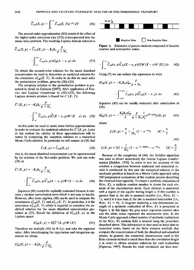
I Reactive Sites [--] Non Reactive Sites Figure 1. Schematic of porous medium composed of discrete reactive and nonreactive zones.

ß Ceo(e,p)•eo(X- e,p)E[Op'(X- e)tI)'(X)]de

Using (7) we can reduce this expression to write

•'2c•(X, p) -- --Kd•aO-• P P+•a

(42)

+A/2 • • ß Cro(e, p)Cro(X- e, p) de (43) d -A/2

Equation (43) can be readily evaluated after substitution of (34):

Ka• aO'•, p 1 •2c*(X' P) = - 4 P + •a bp 2 eøX-ø"fl(X' p) (44) where

A 1 A

fl(X, p) -- -•- + •p (1 - e -^b,) IXt > 2 (45)

1

fl(X, p) = IXI + •pp (2 - e -(^-2•)b, - e -^b,) A

Because of the complexity of (44), the Stehfest algorithm was used to obtain numerically the inverse Laplace transfor- mation [Stehfest, 1970]. In order to test the accuracy of this solution a comparison between analytical and numerical re- sults is conducted. In this case the numerical solution to the

stochastic problem is based on a Monte Carlo approach using 500 independent realizations of the random process describing the chemical heterogeneity. To create a synthetic realization of ß (w; X), a uniform random number is drawn for each ele- ment of the discretization mesh. Each element is associated

with a region of the aquifer having length X. If this number is greater than/3, the site is assumed reactive (i.e., •(w; X) - 1), and if it is less than/3, the site is assumed nonreactive (i.e., ß (w; X) = 0). A diagram depicting a one-dimensional ex- ample of a synthetic realization of •(w; X) is presented in Figure 1. In this figure the gray zones represent reactive sites and the white zones represent the nonreactive sites. In the Monte Carlo approach a fixed number of synthetic realizations of the •(w; X) random field is created using the procedure described above. This information is then used as input data to numerical codes, based on the finite element method, that compute the concentration of both the dissolved and adsorbed phases. In general, the numerical discretization used in the finite element method is much finer than the correlation length X in order to obtain accurate solutions for each realization

[Espinoza, 1997]. Results for each simulation are then aver-

ESPINOZA AND VALOCCHI: STOCHASTIC ANALYSIS OF ONE-DIMENSIONAL TRANSPORT 2433

0.10

0.05

x 0.00

-0.05

-0.10

0

0.04

0.02

x•' 0.00

0.02

a) O2ce(X,T) versus X (T= 25)

Monte-Carlo

Analytical

ß I a I i I a

40 80 120

X

c) O2ce(X,T) versus X (T= 75)

.=. __

-0.04 ' ' , • , ' ,

o 40 80 120

X

Figure 2.

b) O2ce(X,T) versus X (T= 50) 0.10 ß , ß , ß , .

o.oo

-0.05

-0.10 ß i . ! i J

160 40 80 120

ß

160

X

d) O2ce(X,T) versus X (T=100) 0.04

0.02 ß i ß i ß i ß

,

I I I I • I

o.oo

-0.02

-0.04 j 0 160 40 80 120 160

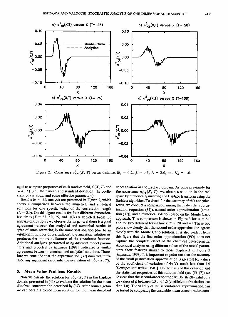
Covariance o-•.(X, T) versus distance. •a = 0.2, /3 = 0.5, A = 2.0, and Kd = 1.0.

aged to compute properties of each random field, C (X, T) and S(X, T) (i.e., their mean and standard deviation, the coeffi- cient of variation, and some effective parameters).

Results from this analysis are presented in Figure 2, which shows a comparison between the numerical and analytical solutions for one specific value of the correlation length (A - 2.0). On this figure results for four different dimension- less times (T = 25, 50, 75, and 100) are depicted. From the analysis of this figure we observe that in general there is a good agreement between the analytical and numerical results; in spite of some scattering in the numerical solution (due to an insufficient number of realizations), the analytical solution re- produces the important features of the covariance function. Additional analyses, performed using different model param- eters and reported by Espinoza [1997], indicated a similar agreement between numerical and analytical solutions. There- fore we conclude that the approximation (39) does not intro- duce any significant error into the evaluation of tr,•,(X, T).

5. Mean Value Problem: Results

Now we can use the solution for o-•(X, T) in the Laplace domain presented in (44) to evaluate the solution for the mean dissolved concentration described by (37). After some algebra we can obtain a closed form solution for the mean dissolved

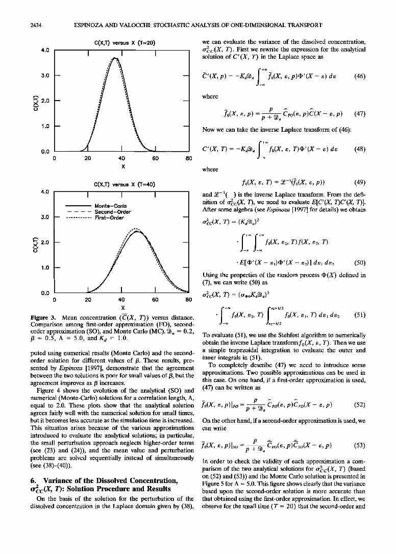
concentration in the Laplace domain. As done previously for the covariance o-•.(X, T), we obtain a solution in the real space by numerically inverting the Laplace transform using the Stehfest algorithm. To check for the accuracy of this analytical result, we conduct a comparison among the first-order approx- imation (equation (34)), second-order approximation (equa- tion (37)), and a numerical solution based on the Monte Carlo approach. This comparison is shown in Figure 3 for A = 5.0 and for two different travel times: T = 20 and 40. These two

plots show clearly that the second-order approximation agrees closely with the Monte Carlo solution. It is also evident from this figure that the first-order approximation (FO) does not capture the complete effect of the chemical heterogeneity. Additional analyses using different values of the model param- eters show features similar to those displayed in Figure 3 [Espinoza, 1997]. It is important to point out that the accuracy of the small perturbation approximation is greatest for values of the coefficient of variation of (I)(X) much less than 1.0 [Dettinger and Wilson, 1981]. On the basis of this criterion and the statistical properties of this random field (see (5)-(7)) we observe that the second-order solution will be strictly valid only for values of/3 between 0.5 and 1.0 (coefficient of variation less than 1.0). The validity of the second-order approximation can be tested by comparing the ensemble mean concentration com-

2434 ESPINOZA AND VALOCCHI: STOCHASTIC ANALYSIS OF ONE-DIMENSIONAL TRANSPORT

4.0

3.0

2.0

1.0

0.0

C(X,T) versus X (T=20)

I I I

20 40 60

X

8O

we can evaluate the variance of the dissolved concentration, O'•c(X, T). First we rewrite the expression for the analytical solution of C' (X, T) in the Laplace space as

•' (X, p)= -K,!•a f0(X, s, p)•' (X- s) as (46)

where

- = P •ro(e, p)•(X- s p) (47) fo(X, e, p) P +-•a ' Now we can take the inverse Laplace transform of (46):

C'(X, T)= -rolla fo(X, s, r)•'(X- s) ds - o•

(48)

where

4.0

3.0

2.0

1.0

0.0

C(X,T) versus X ('1'=40)

I I I

Monte-Corlo Second-Order First-Order

0 20 40 60 80

Figure 3. Mean concentration (C(X, T)) versus distance. Comparison among first-order approximation (FO), second- order approximation (SO), and Monte Carlo (MC). •a = 0.2, /3 = 0.5, A = 5.0, and Ka = 1.0.

puted using numerical results (Monte Carlo) and the second- order solution for different values of/3. These results, pre- sented by Espinoza [1997], demonstrate that the agreement between the two solutions is poor for small values of/3, but the agreement improves as/3 increases.

Figure 4 shows the evolution of the analytical (SO) and numerical (Monte-Carlo) solutions for a correlation length, A, equal to 2.0. These plots show that the analytical solution agrees fairly well with the numerical solution for small times, but it becomes less accurate as the simulation time is increased.

This situation arises because of the various approximations introduced to evaluate the analytical solutions; in particular, the small perturbation approach neglects higher-order terms (see (23) and (24)), and the mean value and perturbation problems are solved sequentially instead of simultaneously (see (38)-(40)).

6. Variance of the Dissolved Concentration, O'•c(X , T)' Solution Procedure and Results

On the basis of the solution for the perturbation of the dissolved concentration in the Laplace domain given by (38),

fo(X, s, T)= •-•(•0(X, s, p)) (49)

and •-1( ) is the inverse Laplace transform. From the defi- nition of O'2cc(X, T), we need to evaluate E[C'(X, T)C'(X, T)]. After some algebra (see Espinoza [1997] for details) we obtain

•(x. r)= (•c•.) •

fo(X, s•, T)f(X, s2, T)

ß E[ep'(X - •,)a,'(X - •2)] a•, a•2 (50)

Using the properties of the random process •(X) defined in (7), we can write (50) as

,,•c(X. T): (•,••a) •

f+o, Ie2+M2 ß fo(X, s2, T) fo(X, s•, T) ds• ds2 -o0 e2-M2

(5•)

To evaluate (51), we use the Stehfest algorithm to numerically obtain the inverse Laplace transform fo (X, s, T). Then we use a simple trapezoidal integration to evaluate the outer and inner integrals in (51).

To completely describe (47) we need to introduce some approximations. Two possible approximations can be used in this case. On one hand, if a first-order approximation is used, (47) can be written as

•0(X, s, p)lFo = P+•a -- •ro(S, p)•ro(X - s, p) (52)

On the other hand, if a second-order approximation is used, we can write

fo(x, e, p)lso -p + •• Cro(e, p)Cso(X- s, p) (53)

In order to check the validity of each approximation a com- parison of the two analytical solutions for O'•c(X, T) (based on (52) and (53)) and the Monte Carlo solution is presented in Figure 5 for A = 5.0. This figure shows clearly that the variance based upon the second-order solution is more accurate than that obtained using the first-order approximation. In effect, we observe for the small time (T = 20) that the second-order and

ESPINOZA AND VALOCCHI: STOCHASTIC ANALYSIS OF ONE-DIMENSIONAL TRANSPORT 2435

a) C(X,T) versus X (T= 25) b) C(X,T) versus X (T= 50) 4.0

3.0

•'- 2.0

1.0

0.0

Monte-Carlo ........... Second-Order

0 40

I I I

80 120 160

3.0

2.0

1.0

0.0

40 80

i .. I

120 160

c) C(X,T) versus X (T= 75) d) C(X,T) versus X (T=100) 2.0

1.5

1.o

0.5

2.0 ß i ß i ß i

ß

40 80 120

1.5

1.o

0.5

0.0 ..... - 0.0 ß

0 16O 0 16O 40 80 120

X X

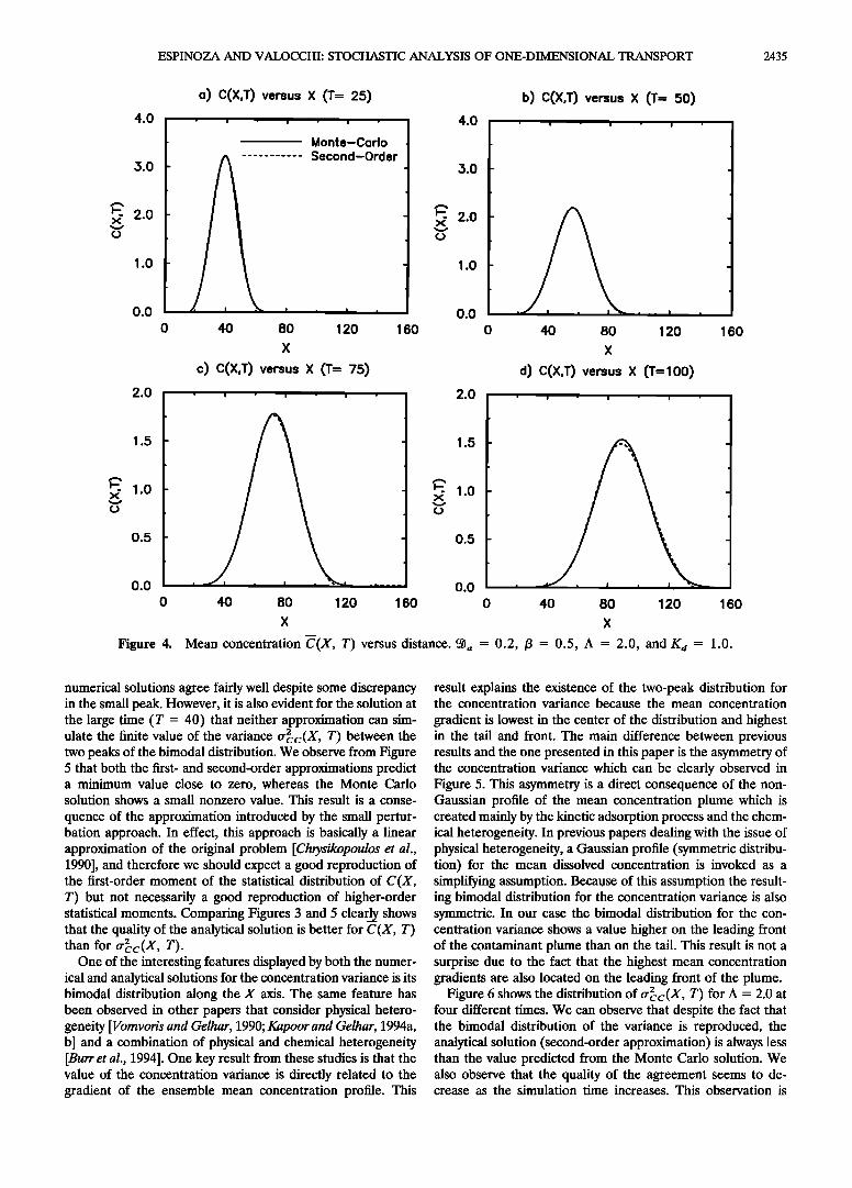
Figure 4. Mean concentration C(X, T) versus distance. •a = 0.2, /3 = 0.5, A = 2.0, and K a = 1.0.

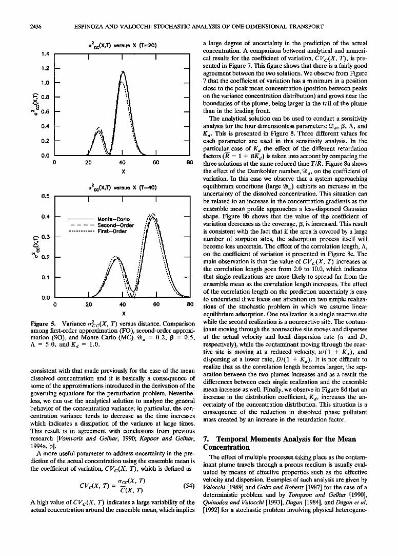
numerical solutions agree fairly well despite some discrepancy in the small peak. However, it is also evident for the solution at the large time (T = 40) that neither approximation can sim- ulate the finite value of the variance tr•c(X, T) between the two peaks of the bimodal distribution. We observe from Figure 5 that both the first- and second-order approximations predict a minimum value close to zero, whereas the Monte Carlo solution shows a small nonzero value. This result is a conse-

quence of the approximation introduced by the small pertur- bation approach. In effect, this approach is basically a linear approximation of the original problem [Chrysikopoulos et al., 1990], and therefore we should expect a good reproduction of the first-order moment of the statistical distribution of C(X, T) but not necessarily a good reproduction of higher-order statistical moments. Comparing Figures 3 and 5 clearly shows that the quality of the analytical solution is better for C(X, T) than for tr•c(X, T).

One of the interesting features displayed by both the numer- ical and analytical solutions for the concentration variance is its bimodal distribution along the X axis. The same feature has been observed in other papers that consider physical hetero- geneity [Vomvoris and Gelhar, 1990; Kapoor and Gelhar, 1994a, b] and a combination of physical and chemical heterogeneity [Burr et al., 1994]. One key result from these studies is that the value of the concentration variance is directly related to the gradient of the ensemble mean concentration profile. This

result explains the existence of the two-peak distribution for the concentration variance because the mean concentration

gradient is lowest in the center of the distribution and highest in the tail and front. The main difference between previous results and the one presented in this paper is the asymmetry of the concentration variance which can be clearly observed in Figure 5. This asymmetry is a direct consequence of the non- Gaussian profile of the mean concentration plume which is created mainly by the kinetic adsorption process and the chem- ical heterogeneity. In previous papers dealing with the issue of physical heterogeneity, a Gaussian profile (symmetric distribu- tion) for the mean dissolved concentration is invoked as a simplifying assumption. Because of this assumption the result- ing bimodal distribution for the concentration variance is also symmetric. In our case the bimodal distribution for the con- centration variance shows a value higher on the leading front of the contaminant plume than on the tail. This result is not a surprise due to the fact that the highest mean concentration gradients are also located on the leading front of the plume.

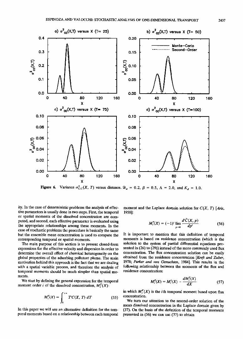
Figure 6 shows the distribution of O'•c(X, T) for A = 2.0 at four different times. We can observe that despite the fact that the bimodal distribution of the variance is reproduced, the analytical solution (second-order approximation) is always less than the value predicted from the Monte Carlo solution. We also observe that the quality of the agreement seems to de- crease as the simulation time increases. This observation is

2436 ESPINOZA AND VALOCCHI: STOCHASTIC ANALYSIS OF ONE-DIMENSIONAL TRANSPORT

1.4

1.2

1.0

•'. 0.8

"o 0.6

0.4

0.2

0.0

O2cc(X,T) versus X (1=20) I I I

0 20 40 60 80

0.5

0.4

0.3

0.2

0.1

0.0

a2cc(X,T) versus X (T=40) I I I

-- Monte-Carlo ,,"/• -- .... Second-Order ; I! ;•

-- First-Order

- i/ ,2

0 20 40 60 80

Figure 5. Variance tr}c(X, T) versus distance. Comparison among first-order approximation (FO), second-order approxi- mation (SO), and Monte Carlo (MC). •a = 0.2, /3 = 0.5, A = 5.0, and Ka = 1.0.

consistent with that made previously for the case of the mean dissolved concentration and it is basically a consequence of some of the approximations introduced in the derivation of the gOVerning equations for the perturbation problem...Neverthe- less, we can use the analytical solution to analyze the general behavior of the concentration variance; in particular, the con- centration variance tends to decrease as the time increases

which indicates a dissipation of the variance at large times. This result is in agreement with conclusions from previous research [Vomvoris and Gelhar, 1990; Kapoor and Gelhar, 1994a, b].

A more useful parameter to address uncertainty in the pre- diction of the actual concentration using the ensemble mean is the coefficient of variation, CVc(X, T), which is defined as

•rcc(X, T) CVc(X, T)= (54)

C(X, T)

A high value of CVc(X, T) indicates a large variability of the actual concentration around the ensemble mean, which implies

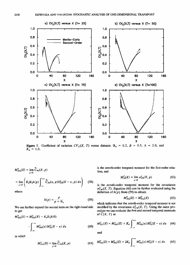
a large degree of uncertainty in the prediction of the actual concentration. A comparison between analytical and numeri- cal results for the coefficient of variation, CV½(X, T), is pre- sented in Figure 7. This figure shows that there is a fairly good agreement between the two solutions. We observe from Figure 7 'that the coefficient of variation has a minimum in a position close to the peak mean concentration (position between peaks on the variance concentration distribution) and grows near the boundaries of the plume, being larger in the tail of the plume than in the leading front.

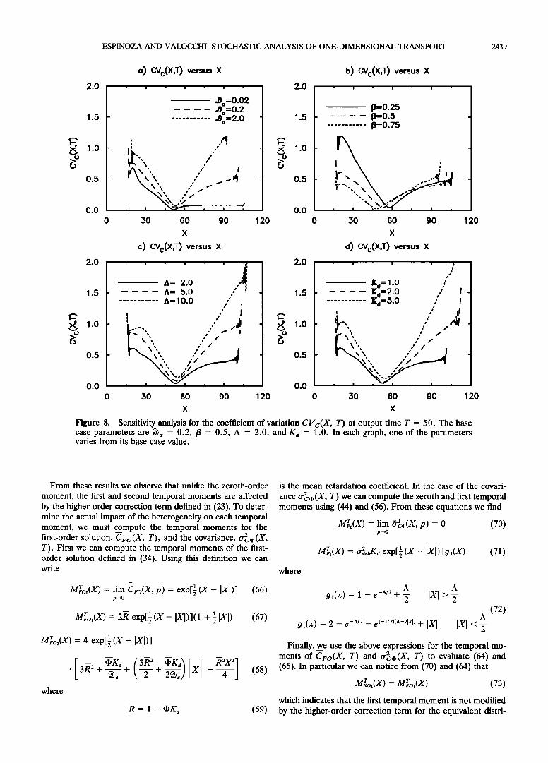
The analytical solution can be used to conduct a sensitivity analysis for the four dimensionless parameters: •a, /3, A, and Ka. This is presented in Figure 8. Three different values for each parameter are used in this sensitivity analysis. In the particular case of Ka the effect of the different retardation factors (R = 1 + 13Ka) is taken into accountby comparing the three solutions at the same reduced time T/R. Figure 8a shows the effect of the Damkohler number, •a, on the coefficient of variation. In this case we observe that a system approaching equilibrium conditions (large •a) exhibits an increase in the uncertainty of the dissolved concentration. This situation can be related to an increase in the concentration gradients as the ensemble mean profile approaches a less-dispersed Gaussian shape. Figure 8b shows that the value of the coefficient of variation decreases as the coverage,/3, is increased. This result is consistent with the fact that if the area is covered by a large number of sorption sites, the adsorption process itself will become less uncertain. The effect of the correlation length, A, on the coefficient of variation is presented in Figure 8c. The main observation is that the value of CVc(X, T) increases as the correlation length goes from 2.0 to 10,0, which indicates that single realizations are more likely to spread far from the ensemble mean as the correlation length increases. The effect of the correlation length on the prediction uncertainty is easy to understand if we focus our attention on two simple realiza- tions of the stochastic problem in which we assume linear equilibrium adsorption. One realization is a single reactive site while the second realization is a nonreactive site. The contam-

inant moving through the nonreactive site moves and disperses at the actual velocity and local dispersion rate (u and D, respectively), while the contaminant moving through the reac- tive site is moving at a reduced velocity, u/(1 + Ka), and dispersing at a lower rate, D/(1 + Ka). It is not difficult to realize that as the correlation length becomes larger, the sep- aration between the two plumes increases and as a result the differences between each single realization and the ensemble mean increase as well. Finally, we observe in Figure 8d that an increase in the distribution coefficient, Ka, increases the un- certainty of the concentration distribution. This situation is a consequence of the reduction in dissolved phase pollutant mass created by an increase in the retardation factor.

7. Temporal Moments Analysis for the Mean Concentration

The effect of multiple processes taking place as the contam- inant plume travels through a porous medium is usually eval- uated by means of effective properties such as the effective velocity and dispersion. Examples of such analysis are given by Valocchi [1989] and Goltz and Roberts [1987] for the case of a deterministic problem and by Tompson and Gelhar [1990], Quinodoz and Valocchi [1993], Dagan [1984], and Dagan et al. [1992] for a stochastic problem involving physical heterogene-

ESPINOZA AND VALOCCHI: STOCHASTIC ANALYSIS OF ONE-DIMENSIONAL TRANSPORT 2437

0.4 '

0.3

0.1

0.0

0.10 .

0.08

•.. 0.06 x

• 0.04

0.02

o) O2cc(X,T) versus X (T= 25) ß i ß i ß i ß

40 80 120 160

X

c) O2cc(X,T) versus X (T= 75) i i i ß

0.20 ß ,

=

0.15

x• 0.10

0.05

0.00 "

0 40

ß i

40 80 120

X

0.10

0.08

•.. 0.06 x

• 0.04

0.02

0,00 ' 0,00

0 160 0

b) O2cc(X,T) versus X (T= 50) , ,

Monte-Carlo Second-Order

ß

80

X

I

120

d) O2cc(X,T) versus X (T=100)

40 80 120

X

Figure 6. Variance (r•c(X , T) versus distance. •a = 0.2, /3 = 0.5, A = 2.0, and K a = 1.0.

160

160

ity. In the case of deterministic problems the analysis of effec- tive parameters is usually done in two steps. First, the temporal or spatial moments of the dissolved concentration are com- puted, and second, each effective parameter is evaluated using the appropriate relationships among these moments. In the case of stochastic problems the procedure is basically the same but the ensemble mean concentration is used to compute the corresponding temporal or spatial moments.

The main purpose of this section is to present closed-form expressions for the effective velocity and dispersion in order to determine the overall effect of chemical heterogeneity on the global properties of the adsorbing pollutant plume. The main motivation behind this approach is the fact that we are dealing with a spatial variable process, and therefore the analysis of temporal moments should be much simpler than spatial mo- ments.

We start by defining the general expression for the temporal moment order i of the dissolved concentration, M•r(X) ß

M•r(X) = T'C(X, T) d T (55)

In this paper we will use an alternative definition for the tem- poral moments based on a relationship between each temporal

moment and the Laplace domain solution for C(X, T) [Aris, 1958]:

d'• (X, p) M•T(x) = (-- 1)' lim (56) œ--->0 dP i

It is important to mention that this definition of temporal moments is based on residence concentration (which is the solution to the system of partial differential equations pre- sented in (26) to (29)) instead of the more commonly used flux concentration. The flux concentration solution can be easily obtained from the residence concentration [Kreft and Zuber, 1978; Parker and van Genuchten, 1984]. This results in the following relationship between the moments of the flux and residence concentration:

dMir(X) Mf (X) = Mir(X) - dX (57)

in which M•(X) is the ith temporal moment based upon flux concentration.

We turn our attention to the second-order solution of the

mean dissolved concentration in the Laplace domain given by (37). On the basis of the definition of the temporal moments presented in (56) we can use (37) to obtain

2438 ESPINOZA AND VALOCCHI: STOCHASTIC ANALYSIS OF ONE-DIMENSIONAL TRANSPORT

1.0

0.8

0.6

0.4

0.2

0.0

0

1.0

0.8

0.6

0.4 -

0.2 -

0.0

0

Figure 7. Kd = 1.0.

o) CVc(X,T ) versus X (T-- 25) b) CVc(X,T ) versus X (T= 50) ß i ß i ß i ß

Monte-Corlo ........... Second-Order

I I I I

80 120 160

1.0

0.8

0.6

>ø0.4

0.2

0.0

!

i

0 40 80

I

120 160

c) CVc(X,T ) versus X (T-- 75) d) CVc(X,T ) versus X (T--100) ß ! ß i ß ! ß

i i

# ii i

i

.•\\

1.0

0.8

0.6

0.2

0.0

40 80 120 160 0 40 80 120 160

X X

Coefficient of variation CVc(X, T) versus distance. •a = 0.2, /3 = 0.5, A = 2.0, and

M•'oo(X) = lim C Fo(X, p) p-->o

- lim Ka•ah(p) CFo(S, p)&•,i,(X- s, p) ds (58)

where

P

h (p) = P + •)a (59) We can further expand the second term on the right-hand side to get

m•'oo(X) = mrroo(X) - Ka•ah (0)

ß Mrroo(s)Mvro(X- s) ds (60)

in which

Mrroo(X) = lim •ro(X, p) (61) p-->0

is the zeroth-order temporal moment for the first-order solu- tion, and

Mvro(X) = lim o-•.(X, p) (62) p-->0

is the zeroth-order temporal moment for the covariance tr•ti,(X, T). Equation (60) can be f-urther evaluated using the definition of h (p) from (59) to obtain

m•oo(X) = mvroo(X) (63)

which indicates that the zeroth-order temporal moment is not modified by the covariance tr•,(X, T). Using the same pro- cedure we can evaluate the first and second temporal moments of C(X, T) as

M•'o•(X) = mrro•(X) + Ka mrroo(s)M•o(X - s) ds (64)

and

M•o2(m) = MFTo2(X) q- 2Ka Mvroo(S)Mvr•(X - s) ds (65)

ESPINOZA AND VALOCCHI: STOCHASTIC ANALYSIS OF ONE-DIMENSIONAL TRANSPORT 2439

2.0

1.5

1.0

o) CVo(X,T ) versus X i ß i ß

.80=0.02 .... ß 80=0.2

.80=2.0

2.0

1.5

! !

It ssS

0.5 %,,, ,' 0.5 ß s ss • • sS• •

0.0 ß ' •k%• ß I '? 0.0 0 30 60 90 120 0

c) CVc(X,T ) versus X

1.0

2.0 2.0

1.5

ß I ß I ß i ß

A= 2.0 - A= 5.0 ,," - ........... A=10.0 ,'

ß ,

0.0 ' ' 0.0

0 30 60 90 120 0

1.5

1.0

0.5

1.0

0.5

b) CVc(X.T ) versus X

1•=0.25 1•=0.5 p=o.75

30 60 90 120

d) CVc(X.T ) versus X

J .

30 60 90 120

X X

Figure 8. Sensitivity analysis for the coefficient of variation CVc(X, T) at output time T = 50. The base case parameters are •a -- 0.2, /3 = 0.5, A = 2.0, and Ka = 1.0. In each graph, one of the parameters varies from its base case value.

From these results we observe that unlike the zeroth-order

moment, the first and second temporal moments are affected by the higher-order correction term defined in (23). To deter- mine the actual impact of the heterogeneity on each temporal moment, we must compute the temporal moments for the first-order solution, CFo(X, T), and the covariance, o-•(i,(X, T). First we can compute the temporal moments of the first- order solution defined in (34). Using this definition we can write

MLo(X) = lim •Fo(X, p): exp[l• (X- IxI)] p->0

(66)

1

Mrro•(X) = 2R exp[ 1• (X - IxI) + IxI) (67)

MFTo2(X) : 4 exp[l• (X- IxI)]

(68)

where

R= I +dPKa (69)

is the mean retardation coefficient. In the case of the covari-

ance o-•a,(X, T) we can compute the zeroth and first temporal moments using (44) and (56). From these equations we find

Mvro(X) = lim •-•(X, p) = 0 (70) p-->0

Myra(X) = o',•,d-Q exp[ 1• (X - IxI) ] g•(X) (7•)

where

A A

gl(x): 1 - e -^/2 + -•- IxI > 2

gl(X) = 2 -- e -^/2-- e (-1/2)(^-2•q) q-Ixl A

(72)

Finally, we use the above expressions for the temporal mo- ments of CFo(X, T) and o-•(i,(X, T) to evaluate (64) and (65). In particular we can notice from (70) and (64) that

Msro•(X) = M•ro•(X) (73)

which indicates that the first temporal moment is not modified by the higher-order correction term for the equivalent distri-

2440 ESPINOZA AND VALOCCHI: STOCHASTIC ANALYSIS OF ONE-DIMENSIONAL TRANSPORT

bution coefficient. On the other hand, we observe that the second temporal moment is increased by the chemical heter- ogeneity. To compute the second temporal moment we can use the expressions presented in (66) and (71) to evaluate the integral term in (65); this shows that the contribution of the higher correction term in the effective distribution coefficient (measured by the covariance function cr•.(X, T) in (23)) will lead to an increase in the spreading of the adsorbing pollutant as compared to an equivalent homogeneous condition (first- order solution).

To quantify the effect of the heterogeneity on the spread of the adsorbing pollutant the effective velocity and dispersion will be computed. The relation between these effective param- eters and the temporal moments have been given by Valocchi [1985] as

Veff(X ) X U /.• i(X)

(74)

Oeff(X•)=l•2(X) (Veff(•X) ) 2 D 2 /.• 1 (X)

where /-•i(X) and/z2(X) are the normalized first and second central temporal moments defined using temporal moments based upon flux concentration as

MsFo1(X) /.Li(X ) = MsVoo(X)

(7s)

M•o2(X) IM•o1(X)I 2 /x2(X) = M•oo(X ) - M•oo(X ) In using these definitions we can easily find the value of the effective parameters as a function of the distance from the injection point. The detailed expressions for these parameters are too lengthy to present in this paper, but they are given by Espinoza [1987]. More simple and useful expressions for the effective velocity and dispersion are obtained if we take the limit for a long distance from the injection point. On the basis of this we obtain the following for the asymptotic effective velocity and dispersion:

tieg X .•> Or:)) 1 - (76)

u R

- -- + + 1 - e + (77) D R k3•a k 3 •

The above result can be rewritten using the original dimen- sional variables as

I - e-uM2D q- U•) (78)

The last asymptotic result clearly shows that the higher order correction term (o-•.(X, T)) increases the rate of spreading of a reactive pollutant in a groundwater aquifer, but it does not have any effect on the asymptotic effective velocity. Equation (76) shows that the asymptotic velocity is only affected by the strength of the adsorptio__n process described by the reduced distribution coefficient, tI)Kd. Equations (77) and (78) show that the effective dispersion is composed of three terms, with the last one being a direct contribution of the higher-order

correction for the equivalent distribution coefficient presented in (23). The first two contributions to the overall effective dispersion coefficient have been previously obtained for the case of a homogeneous aquifer [Valocchi, 1989; Goltz and Roberts, 1987]. The first term describes the retardation effect introduced by linear adsorption taking place along the aquifer. As for the effective velocity this term is just an extension of the result presented previously for linear equilibrium cases in which the actual retardation factor is replaced by the arith- metic mean (see (69)). The second term describes the effect of sorption kinetics on the spreading of the breakthrough curve. We observe that this term looks very similar to the result presented by Goltz and Roberts [1987] for a chemically homo- geneous aquifer. ,In fact, the only difference between the two results is the use of mean parameters ((I)Kd and R instead of the actual parameters (Ka and R). If we focus on the first two terms of (77), we realize that they represent the effective dis- persion obtained using a equivalenthomogeneous system with a distribution coefficient equal to tI)Ka (i.e., first-order solu- tion). As stated before, the third term in (77) and (78) repre- sents the impact of the spatial distribution of reactive sites on the spread of a reactive pollutant as it migrates through the aquifer. As expected, this term contains specific information about the distribution of reactive sites (variance and correla- tion length of (I)(X)), and some flow properties. Another im- portant observation is that the kinetics of the adsorption pro- cess does not play any role in this term and, in effect, we observe that this term depends only on the strength of the adsorption which is given by the distribution coefficient, Ka. Another interesting aspect is that this term depends upon the local dispersion coefficient, and, in fact, this term is not ob- tained if one neglects local dispersion as is commonly done in many stochastic studies of solute transport. We note that a similar kind of asymptotic result was previously reported by Chrysikopoulos et al. [1992b] for a spatially periodic porous medium. This suggests that the use of a deterministic spatially periodic model to represent randomly distributed properties is a valid option for analytical studies of asymptotic transport behavior. This point is examined further by Espinoza [1997].

It is possible to demonstrate that results (77) and (78) over- estimate the actual dispersion experienced by the plume. This demonstration is analogous to that of Rajaram and Gelhar [1993a, b], who considered spatial moments for nonreactive transport. The normalized second central temporal moment, tx2(X), is based upon temporal moments of the ensemble- averaged concentration, whereas the more relevant estimate is the ensemble average of the variance of the breakthrough curve in each realization. By following Rajaram and Gelhat [1993a, b], we can show that tx2(X) evaluated at a large dis- tance equals the ensemble average of the variance plus an extra spreading term that is due to the variability in the mean break- through time. Details of this analysis are given by Espinoza [1997]. Using a simple particle-tracking approach we can com- pute the ensemble variance of the mean breakthrough time. The contribution of this term to the effective dispersion coef- ficient turns out to be equal to the last term in (77) and (78). Elimination of this term yields the following result for the asymptotic value of the effective dispersion:

Oe•X '--> o•) 1 tI)Ka -^/2) (79) ---+-- + 1 e D R R3•a •3 ( -

or in terms of the original variables:

ESPINOZA AND VALOCCHI: STOCHASTIC ANALYSIS OF ONE-DIMENSIONAL TRANSPORT 2441

D (I)Kau 2 2 2 D o'•,•X,• . -ux/ w) (80) De•X --> oo) = = + __ + i - e R R3k• •3 ( In the next section a comparison among these asymptotic re- suits and numerical solutions for the stochastic problem will be presented.

8. Spatial Moments Analysis for the Mean Concentration

The previous analysis focused on the asymptotic effect of the chemical heterogeneity on the effective velocity and dispersion for large travel distances. In order to study the preasymptotic behavior of the effective parameters spatial moment analysis of the mean dissolved concentration can be used. On the basis of

this analysis we can determine how fast the asymptotic condi- tions computed from the temporal moments analysis are at- tained, and we can examine if the temporal evolution of the effective parameters is affected by the variability of the adsorp- tion properties.

This analysis will be conducted using the original mean value problem presented i__n (26)-(29). This system of partial differ- ential equations in C(X, T) and S(X, T) can be reduced to a system of ordinary differential equations for the spatial mo- ments using the methodology presented by Valocchi [1989]. After this analysis we reduce the advection-dispersion equa- tion (26) to

dmi dni d--•- + •-•= i(i - 1)mi_2 + imi-1 (81)

and the linear kinetic adsorption (27) to

dni d T = •b aKdrYPm i -t- •b aKdm co ' - •b art i (82)

We apply Laplace transforms to the system of ordinary dif- ferential equations (81) and (82) to obtain after some algebra

8(i) i(i - 1)

ffti(P) = G(p• + G(p• t7ti-2(P) i

+ G(p)/•ti-l(P) -- H(p)•c.,(p) (86) where

•) aKdrYP I G(p) =p 1 +p + •)a/ (87)

•) aK d H(p) = (88)

p + •aKd• + •a

and 8(i) is the Kronecker delta. Expression (86) is a recursive equation in the Laplace domain which is solved sequentially for each spatial moment of C(X, T) starting from the zeroth- order moment. The only unknown in this expression is the spatial moment of the covariance rr•,v(X, T) in the Laplace domain. This can be obtained by substituting (44) into the Laplace transform of the definition (84). The resulting expres- sion can be evaluated as detailed by Espinoza [1997].

Our interest is to compute the lower order spatial moments of the mean dissolved concentration, C(X, T), in order to study the global effect of the chemical heterogeneity on the effective velocity and__dispersion. On the basis of the first three spatial moments of C(X, T) we can define the following ef- fective parameters [Tompson and Gelhat, 1990]'

Veff( T) d/xl(T) u dT

De•T) 1 d/x2(T) D 2 dt

(89)

where we have introduced the following definitions for the spatial moments:

mi(T) = X•C (X, T) dX

n i(T) = XiS (X, T) dX

(83)

mca,,(T) = X•o'•a,(X, T) dX (84)

Finally, for the initial conditions we have

1 i= 0 (85) mi(O) = 0 otherwise rti(O ) = 0 V i

It is important to point out that this solution approach will provide the spatial moments based on the second-order ap- proximation; that is, the higher correction term given by rr•,v(X, T) is incorporated into the analysis. To obtain spatial moments for the first-order approximation (i.e., neglecting this correction term) we simply use the solution by Goltz and Roberts [1987] with an effective distribution coefficient equal to Kd•.

where/x I(T) and/x2(T) are the normalized first and second central spatial moments of the mean dissolved concentration, respectively, which are defined as

/Xl(T ) = ml(T) mo(T)

m2(T) [ml(T)] /x2(T) = mo(T) mo(T) (90)

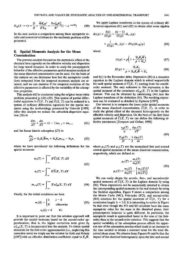
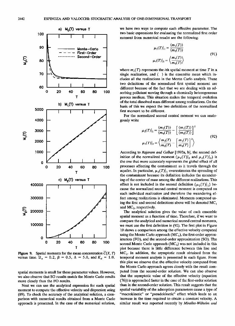
We can easily obtain the zeroth-, first-, and second-order spatial moments of C(X, T) in the Laplace domain by using (86). These expressions can be numerically inverted to obtain the corresponding spatial moments in the real domain by using the Stehfest algorithm. Figure 9 shows a comparison among the Monte Carlo (MC), first-order (FO), and second-order (SO) solutions for the spatial moments of C(X, T) for a correlation length A = 5.0. It is interesting to notice in Figure 9a that even though the FO and SO solutions have the same asymptotic value for the mass in the dissolved phase, their preasymptotic behavior is quite different. In particular, the asymptotic result is approached faster in the case of the first- order than in the second-order solution. This suggests that the spatial variability of the adsorption process affects the appar- ent rate of the adsorption process which leads to an increase in the time needed to obtain a constant value for the total dis-

solved phase mass. We observe from Figures 9b and 9c that the impact of the chemical heterogeneity upon the first and second

2442 ESPINOZA AND VALOCCHI: STOCHASTIC ANALYSIS OF ONE-DIMENSIONAL TRANSPORT

lOO a) Mo(T ) versus T

I I I I

90 Monte-Carlo .... First-Order

........... Second-Order 80

70

60

0 20 40 60 80 1 O0

5OOO

4OOO

3000

2000

1 ooo

b) M•(T) versus T

I I I I

0 20 40 60 80 1 O0

T

c) M2(T) versus T 400000 I I I I

300000 -- • •

v 200000 --

100000

0

0 20 40 60 80 100

T

Figure 9. Spatial moments for the mean concentration C(X, T) versus time. •a = 0.2, /3 = 0.5, A = 5.0, and Ka = 1.0.

spatial moments is small for these parameter values. However, we also observe that SO results match the Monte Carlo results

more closely than the FO results. Next we can use the analytical expression for each spatial

moment to compute the effective velocity and dispersion using (89). To check the accuracy of the analytical solution, a com- parison with numerical results obtained from a Monte Carlo approach is presented. In the case of the numerical solution,

we have two ways to compute each effective parameter. The two basic expressions for evaluating the normalized first order moment from numerical results are the following:

(m•(r)) (mo(T))

(91)

Im•(T)I (T)12 = mo(r) where mi(T) represents the ith spatial moment at time T in a single realization, and ( ) is the ensemble mean which in- cludes all the realizations in the Monte Carlo analysis. These two definitions of the normalized first spatial moment are different because of the fact that we are dealing with an ad- sorbing pollutant moving through a chemically heterogeneous porous medium. This situation makes the temporal evolution of the total dissolved mass different among realizations. On the basis of this we expect the two definitions of the normalized first moment to be different.

For the normalized second central moment we can analo-

gously write

(m2(T)> [ 2(r)l = (m0(T))]

m2(T) /J, 2(T) 12: m0(T) [ ml(r)] 2 ) m0(T) /

(92)

According to Rajaram and Gelhar [1993a, b], the second def- inition of the normalized moment (/x•(r)[ 2 and/x2(r)12) is the one that more accurately represents the global effect of all processes affecting the contaminant as it travels through the aquifer. In particular,/x2(r)l• overestimates the spreading of the contaminant because its definition includes the meander-

ing of the center of mass among the different realizations. This effect is not included in the second definition (/x2(T)I•) be- cause the normalized second central moment is computed on each individual realization and therefore the meandering ef- fect among realizations is eliminated. Moments computed us- ing the first and second definitions above will be denoted MC• and MC2, respectively.

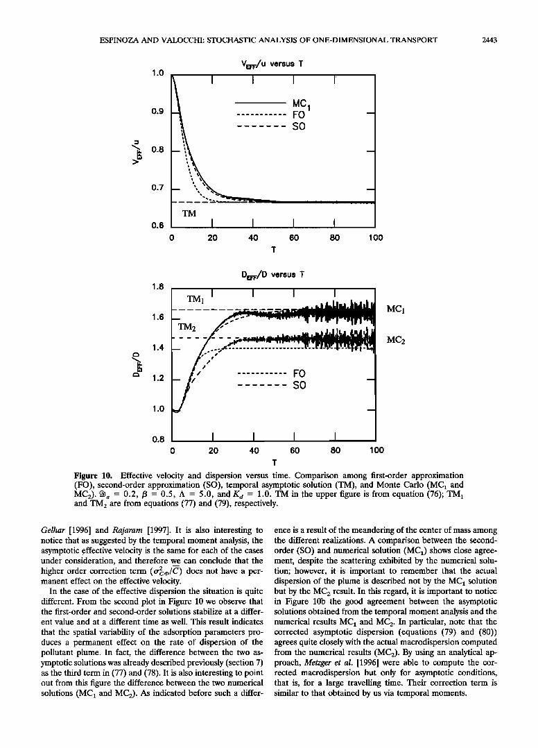
The analytical solution gives the value of each ensemble spatial moment as a function of time. Therefore, if we want to compare the analytical and numerical second central moments, we must use the first definition in (92). The first plot in Figure 10 shows a comparison among the effective velocity computed using the Monte Carlo approach (MC0, the first-order approx- imation (FO), and the second-order approximation (SO). The second Monte Carlo approach (MC2) was not included in this plot because there is little difference between this line and MC•. In addition, the asymptotic result obtained from the temporal moment analysis is presented in each figure. From this plot we observe that the effective velocity computed from the Monte Carlo approach agrees closely with the result com- puted from the second-order solution. We can also observe that the asymptotic value of the effective velocity (equation (76)) is approached faster in the case of the first-order solution than in the second-order solution. This result suggests that the spatial variability of the adsorption parameters cause a type of "macrokinetic" or "pseudokinetic" effect which leads to an increase in the time required to obtain a constant velocity. A similar result was reported recently by Miralies-Wilhelm and

ESPINOZA AND VALOCCHI: STOCHASTIC ANALYSIS OF ONE-DIMENSIONAL TRANSPORT 2443

1.0

0.9

0.8

0.7

0.6

VEFr/U versus T

___: ....... _

0 20 40 60 80 100

T

DErr/D versus T 1.8

- - MC•

.t/ ........... FO

....... SO -

1.6

MC2 1.4

1.2

1.0

0.8

0 2o 40 6o 8o 100

Figure 10. Effective velocity and dispersion versus time. Comparison among first-order approximation (FO), second-order approximation (SO), temporal asymptotic solution (TM), and Monte Carlo (MC• and MC2)- •a = 0.2, •3 = 0.5, A = 5.0, and Ka = 1.0. TM in the upper figure is from equation (76); TM• and TM 2 are from equations (77) and (79), respectively.

Gelhar [1996] and Rajaram [1997]. It is also interesting to notice that as suggested by the temporal moment analysis, the asymptotic effective velocity is the same for each of the cases under consideration, and therefore we can conclude that the higher order correction term ((r•,/C) does not have a per- manent effect on the effective velocity.

In the case of the effective dispersion the situation is quite different. From the second plot in Figure 10 we observe that the first-order and second-order solutions stabilize at a differ-

ent value and at a different time as well. This result indicates

that the spatial variability of the adsorption parameters pro- duces a permanent effect on the rate of dispersion of the pollutant plume. In fact, the difference between the two as- ymptotic solutions was already described previously (section 7) as the third term in (77) and (78). It is also interesting to point out from this figure the difference between the two numerical solutions (MC• and MC2). As indicated before such a differ-

ence is a result of the meandering of the center of mass among the different realizations. A comparison between the second- order (SO) and numerical solution (MC 0 shows close agree- ment, despite the scattering exhibited by the numerical solu- tion; however, it is important to remember that the actual dispersion of the plume is described not by the MC• solution but by the MC 2 result. In this regard, it is important to notice in Figure 10b the good agreement between the asymptotic solutions obtained from the temporal moment analysis and the numerical results MC• and MC 2. In particular, note that the corrected asymptotic dispersion (equations (79) and (80)) agrees quite closely with the actual macrodispersion computed from the numerical results (MC2). By using an analytical ap- proach, Metzger et al. [1996] were able to compute the cor- rected macrodispersion but only for asymptotic conditions, that is, for a large travelling time. Their correction term is similar to that obtained by us via temporal moments.

2444 ESPINOZA AND VALOCCHI: STOCHASTIC ANALYSIS OF ONE-DIMENSIONAL TRANSPORT

9. Discussion and Conclusions

Our results demonstrate that spatial variability of the ad- sorption parameters (chemical hctcrogcn½ity) produces sev- eral important effects upon pollutant transport. Such effects are evident when the first- and second-order approximations are used to compute the effective velocity and dispersion from the spatial and temporal moments analyses. The most inter- esting result is the one obtained using the temporal moment approach in which simple closed-form expressions for the ef- fective velocity and dispersion as a function of dimensionless parameters are obtained (equations (76) and (79), respective- ly). These expressions show that the chemical heterogeneity increases the long-term rate of spreading, described by the asymptotic effective dispersion, but that it has no permanent effect on the effective velocity. In addition, these results show that the variability of the adsorption properties produces an additive effect upon the plume spreading caused by local dis- persion and sorption kinetics; this effect depends not only upon the parameters describing the particular random sorp- tion reaction but also upon the local dispersion coefficient. It is noteworthy that these results are very similar to those obtained by Chrysikopoulos et al. [1992a, b], who assumed a spatially periodic retardation factor. In effect, if we modify Chrysiko- poulos et al.'s solution to reproduce the on/off periodicity exhibited by the Bernoulli random process, we end up with an effective dispersion that looks similar to the one presented in (80). This result clearly suggests that the extra dispersion term obtained in the temporal moments analysis is a direct result of the alternation of reactive sites (on/off adsorption). Moreover, the fact that this alternation is random (our work) or periodic [Chrysikopoulos et al., 1992a, b] produces the slight difference between the two solutions. In fact, Espinoza [1997] shows that for large values of A the two solutions are the same.

Spatial moment analysis was used to show that a stable value for the effective velocity and dispersion is eventually obtained after the plume has moved through the aquifer for a certain period of time. In fact, results from this analysis allow us to confirm that the stable value obtained is identical to the as-

ymptotic expression obtained from the temporal moment anal- ysis. In the particular case of the effective velocity, our results indicate that the time to reach asymptotic conditions is in- creased significantly when chemical heterogeneity is taking into account (see Figure 10).

Our results also show that if local equilibrium conditions ,re assumed at the level of the reactive sites (ke and k• are increased keeping Ka constant), chemical heterogeneity cre- ates "pseudokinetic" or "macrokinetic" conditions in which a time dependent retardation coefficient is obtained. This result agrees with previous findings by Kabala and $posito [1991] and Miralies-Wilhelm and Gelhar [1996], in which the pseudokinetic conditions have been described in a physically and chemically heterogeneous porous medium. The result presented in this paper states that the pseudokinetic or macrokinetic con- ditions are a direct result of the chemical heterogeneity alone an d do not require cross correlation between chemical and physical heterogeneity; however, such cross correlations can enhance these conditions. The solution of Miralies-Wilhelm

and Gelhar, simplified by neglecting physical heterogeneity, shows macrokinetic behavior for the first spatial moments that is quite similar to that for our solution.

Solutions for the ensemble mean, variance, and coefficient of variation of the dissolved concentration were also presented

in this paper. A comparison between the analytical (second- order approximation) and the numerical (Monte Carlo analy- sis) allows us to verify the validity of some of the approxima- tions introduced in the derivation of the analytical solution. As a result of this analysis we find out that these assumptions have a larger impact on the solution for the variance than for the ensemble mean concentration. This situation reflects the fact

that the main approximations in this analysis were introduced in the solution for the perturbation of the dissolved concen- tration, C'(X, T), which is the key element in the definition of the concentration variance (equation (51)). In addition, we also observe that the accuracy of the analytical solution for the ensemble mean and variance tends to decrease as the simula-

tion time increases. Despite this situation we also verify from this analysis that the second-order approximation reproduces fairly well the main features of both the ensemble mean and variance of the dissolved concentration. The coefficient of vari-

ation, CV½(X, T), is used to analyze the impact of chemical heterogeneity on the concentration uncertainty. A comparison between numerical and analytical results is presented in Figure 7. This figure shows that the agreement between the two re- sults is fairly good. Finally, a sensitivity analysis to show the effect of some dimensionless parameters on the coefficient of variation (CV½) was performed. One interesting result shows that the concentration uncertainty increases as the adsorption process approaches an equilibrium condition (•a goes to in- finity).

The most important conclusions from this paper are sum- marized below:

1. The small perturbation approach can be applied to study the effect of chemical heterogeneity on the transport of a kinetically adsorbing pollutant in a physically homogeneous porous medium.

2. Solutions for the ensemble mean and the variance of the

dissolved concentration are computed using a one-dimensional framework. Comparison of the analytical and numerical solu- tions show that they agree fairly well in most of the cases. The small perturbation solution becomes more accurate as the vari- ability of the sorption heterogeneity decreases. The quality of the solution tends to decrease as the plume moves farther from the initial injection point, which can be related to the validity of some of the assumptions introduced during the analysis.

3. In order to obtain an accurate solution for the ensemble

mean, we developed the second-order (SO) solution, in which cross correlations between the concentration and reactivity are incorporated (see (23)). Results presented in Figure 3 clearly show that the SO solution is more accurate than the simple FO solution, in which the mean distribution coefficient is used in the deterministic reaction rate expression. However, when the uncertainty about the mean is considered (see Figures 6 and 7), it is possible that the differences between the FO and SO solutions are not statistically significant.

4. Concentration uncertainty is addressed by means of the coefficient of variation, CV½(X, T). The effect of four dimen- sionless parameters (•)a, ]3, A, and Ka) on this coefficient is studied. This analysis showed that the relative uncertainty of the dissolved concentration along the leading front of the pol- lutant plume increases when adsorption approaches equilib- rium conditions (large fi)a), the coverage is reduced (small/3), the correlation length increases, or the distribution coefficient increases.

5. Chemical heterogeneity has a significant impact on the overall characteristics of the pollutant plume. This impact can

ESPINOZA AND VALOCCHI: STOCHASTIC ANALYSIS OF ONE-DIMENSIONAL TRANSPORT 2445

be estimated using temporal and spatial moments analysis. The former provides closed-form analytical expressions for the ef- fective velocity and dispersion which can be written in terms of relevant dimensionless parameters. The latter explains the ef- fect of the chemical heterogeneity on the preasymptotic value of these effective parameters.

6. There is a "pseudokinetic" or "macrokinetic" effect that is a result of the spatial variability of the adsorption properties despite the fact that the local equilibrium assumption is in- voked. Our results show that this effect is a direct consequence of the chemical heterogeneity.

7. Temporal moments analysis shows that the spatial vari- ability of the adsorption parameters produces a permanent effect on the value of the asymptotic dispersion. A simple closed-form expression for this asymptotic property, as a func- tion of basic dimensionless parameters, is derived in this paper.

Acknowledgments. This paper is based upon research supported by the Subsurface Science Program, Office of Health and Environ- mental Research, U.S. Department of Energy. The continued support of Frank J. Wobber is greatly appreciated. The first author gratefully acknowledges the financial support of the Agencia de Cooperaci6n Internacional de Chile and the Fulbright Commission. The manuscript was improved greatly by the comments of Hernfin Quinodoz and one anonymous reviewer. We also thank Shunji Oya for his assistance with preparing the final version of the paper.

References

Aris, R., On the dispersion of linear kinematic waves, Proc. R. Soc. London A, 245, 268-277, 1958.

Barber, L. B., E. M. Thurman, and D. D. RunnelIs, Geochemical heterogeneity in a sand and gravel aquifer: Effect of sediment min- eralogy and particle size on the sorption of chlorobenzenes, J. Con- tarn. Hydrol., 9(1/2), 35-54, 1992.

Bellin, A., A. Rinaldo, W. J.P. Bosrna, S. A. T. M. van der Zee, and Y. Rubin, Linear equilibrium adsorbing solute transport in physi- cally and chemically heterogeneous porous formations, 1, Analytical solutions, Water Resour. Res., 29(12), 4019-4030, 1993.

Bosma, W. J.P., A. Bellin, S. A. T. M. van der Zee, and A. Rinaldo, Linear equilibrium adsorbing solute transport in physically and chemically heterogeneous porous formations, 2, Numerical results, Water Resour. Res., 29(12), 4031-4043, 1993.

Burr, D. T., E. A. Sudicky, and R. L. Naff, Nonreactive and reactive solute transport in three-dimensional heterogeneous porous media: Mean displacement, plume spreading, and uncertainty, Water Re- sour. Res., 30(3), 791-815, 1994.

Chrysikopoulos, C., P. Kitanidis, and P. Roberts, Analysis of one- dimensional solute transport through porous media with spatially variable retardation factor, Water Resour. Res., 26(2), 437-446, 1990.

Chrysikopoulos, C., P. Kitanidis, and P. Roberts, Macrodispersion of sorbing solutes in heterogeneous porous formations with spatially periodic retardation factor and velocity field, Water Resour. Res., 28(6), 1517-1529, 1992a.

Chrysikopoulos, C., P. Kitanidis, and P. Roberts, Generalized Taylor- Aris moment analysis of the transport of sorbing solutes through porous media with spatially-periodic retardation factor, Transp. Po- rous Media, 7, 163-185, 1992b.

Dagan, G., Solute transport in heterogeneous porous formations, J. Fluid Mech., 145, 151-157, 1984.

Dagan, G., V. Cvetkovic, and A. Shapiro, A solute flux approach to transport in heterogeneous formations, 1, The general framework, Water Resour. Res., 28(5), 1369-1376, 1992.

Davis, J. A., C. C. Fuller, J. A. Coston, K. M. Hess, and E. Dixon, Spatial heterogeneity of geochemical and hydrologic parameters affecting metal transport in groundwater, Environ. Res. Brief EPA/ 600/2-91/006, Environ. Prot. Agency, Washington, D.C., Aug. 1993.

Dettinger, M., and J. Wilson, First order analysis of uncertainty in numerical models of groundwater flow, 1, Mathematical develop- ment, Water Resour. Res,, 17(1), 149-161, 1981.

Espinoza, C., Stochastic analysis of the transport of adsorbing pollut- ants in aquifers having spatially variable chemical properties, Ph.D.

thesis, Dep. of Civ. and Environ. Eng., Univ. of Ill. at Urbana- Champaign, 1997.

Gelhar, L. W., and C, Axness, Three-dimensional stochastic analysis of macrodispersion in aquifers, Water Resour. Res., 19(1), 161-180, 1983.

Goltz, M., and P. Roberts, Using the method of the moments to analyze three-dimensional diffusion-limited solute transport from temporal and spatial perspectives, Water Resour. Res., 23(8), 1575- 1585, 1987.

Hu, B., F.-W. Deng, and J. Cushman, Nonlocal reactive transport with physical and chemical heterogeneity: Linear nonequilibrium sorp- tion with random Ka, Water Resour. Res., 31(9), 2239-2252, 1995.

Kabala, Z., and G. Sposito, A stochastic model of reactive solute transport with time-varying velocity in a heterogeneøus aquifer, Wa- ter Resour. Res., 27(3), 341-350, 1991.

Kapoor, V., and L. W. Gelbar, Transport in three-dimensionally het- erogeneous aquifer, 1, Dynamics of concentration fluctuations, Wa- ter Resour. Res., 30(6), 1775-1788, 1994a.

Kapoor, V., and L. W. Gelhar, Transport in three-dimensionally het- erogeneous aquifers, 2, Predictions and observations of concentra- tion fluctuations, Water Resour. Res., 30(6), 1789-1801, 1994b.

Kreft, A., and A. Zuber, On the physical meaning of the dispersion equation and its solutions for different initial and boundary condi- tions, Chem. Eng. Sci., 33, 1471-1480, 1978.

Mackay, D. M., D. L. Freyberg, P. V. Roberts, and J. A. Cherry, A natural gradient experiment on solute transport in a sand aquifer, 1, Approach and overview of plume migration, Water Resour. Res., 22(13), 2017-2029, 1986.

Metzger, D., H. Kinzelbach, and W. Kinzelbach, Effective dispersion of a solute cloud in a chemically heterogeneous porous medium: Comparison of two ensemble-averaging procedures, Water Resour. Res., 32(11), 3311-3319, 1996.

Miralies-Wilhelm, F., and L. W. Geihar, Stochastic analysis of sorption macrokinetics in heterogeneous aquifers, Water Resour. Res., 32(6), 1541-1549, 1996.

Parker, J. C., and M. T. van Genuchten, Flux-averaged and volume- averaged concentrations in continuum approaches to solute trans- port, Water Resour. Res., 20(7), 866-872, 1984.

Quinodoz, H., and A. Valocchi, Stochastic analysis of the transport of kinetically sorbing solutes in aquifers with randomly heterogeneous hydraulic conductivity, Water Resour. Res., 29(9), 3227-3240, 1993.

Rajaram, H., Time and scale dependent effective retardation factors in heterogeneous aquifers, Adv. Water Resour., 20(4), 217-230, 1997.

Rajaram, H., and L. Gelhar, Plume scale-dependent in heterogeneous aquifers, 1, Lagrangian analysis in a stratified aquifer, Water Resour. Res., 29(9), 3249-3260, 1993a.

Rajaram, H., and L. Gelhar, Plume scale-dependent in heterogeneous aquifers, 2, Eulerian analysis and three-dimensional aquifers, Water Resour. Res., 29(9), 3261-3276, 1993b.

Robin, M. J. L., E. A. Sudicky, R. W. Gillham, and R. G. Kachanoski, Spatial variability of strontium distribution coefficients and their correlation with hydraulic conductivity in the Canadian Forces Base Borden Aquifer, Water Resour, Res., 27(10), 2619-2632, 1991.

Stehfest, H., Numerical inversion of Laplace transforms, Commun. ACM, 13(1), 47-49, 1970.

Tompson, A., and L. Gelhar, Numerical simulation of solute transport in three-dimensional, randomly heterogeneous porous media, Water Resour. Res., 26(10), 2541-2562, 1990.

Tompson, A. F. B., A. L. Schafer, and R. W. Smith, Impacts of physical and chemical heterogeneity on cocontaminant transport in a sandy porous medium, Water Resour. Res., 32(4), 801-818, 1996.

Valocchi, A. J., Validity of the local equilibrium assumption for mod- eling sorbing solutes transport through homogeneous soils, Water Resour. Res., 21(6), 808'820, 1985.

Valocchi, A,, Spatial moment analysis of the transport of kinetically absorbing solutes through stratified aquifers, Water Resour. Res., 25(2), 273-279, 1989.

Vomvoris, E., and L. W. Gelhar, Stochastic analysis of the concentra- tion variability in a three-dimensional heterogeneous aquife r, Water Resour. Res., 26(10), 2591-2602, 1990.

C. Espinoza and A. J. Valocchi, Department of Civil Engineering, University of Illinois, 205 N. Mathews Ave., Urbana, IL 61801. (e-mail: valocchi@uiuc.edu)

(Received August 5, 1996; revised July 21, 1997; accepted July 30, 1997.)