ABSTRACT: The ability to apply a hydrologic model to largenumbers of basins for forecasting purposes requires a quickand effective calibration strategy. This paper presents a stepwise, multiple objective, automated procedure for hydrologicmodel calibration. This procedure includes the sequential cali-bration of a model’s simulation of solar radiation (SR), potentialevapotranspiration (PET), water balance, and daily runoff. Theprocedure uses the Shuffled Complex Evolution global searchalgorithm to calibrate the U.S. Geological Survey’s PrecipitationRunoff Modeling System in the Yampa River basin of Colorado.This process assures that intermediate states of the model (SRand PET on a monthly mean basis), as well as the water bal-ance and components of the daily hydrograph are simulatedconsistently with measured values.(KEY TERMS: Precipitation Runoff Modeling System; ShuffledComplex Evolution; Colorado; optimization; solar radiation;potential evapotranspiration; water balance; runoff.)

Hay, Lauren E., George H. Leavesley, Martyn P. Clark, Steve L.Markstrom, Roland J. Viger, and Makiko Umemoto, 2006. Step Wise Multiple Objective Calibration of a Hydrologic Modelfor a Snowmelt Dominated Basin. Journal of the AmericanWater Resources Association (JAWRA) 42(4):877-890.

INTRODUCTION

Runoff from winter snowpack is the main supply ofwater in the intermountain western United States(U.S.). NOAA National Weather Service (NWS) andUSDA National Resources Conservation Service

(NRCS) issue runoff forecasts for the western U.S.Both of these agencies are attempting to modernizetheir runoff forecasting tools by incorporating morespatially distributed hydrologic modeling techniques(e.g. Spatially Distributed Hydrologic Modeling,USDA-NRCS, 1998; Carter, 2005). To this end, theNRCS is currently configuring a version of the U.S.Geological Survey’s (USGS) Precipitation Runoff Mod-elling System (PRMS) for 35 snowmelt dominatedbasins by 2006 with the possible extension to theentire western U.S. (K. Rojas and F. Geber, NRCS,personnel communication, May 2005). PRMS is a dis-tributed parameter, physically based hydrologicmodel. The ability to apply a distributed hydrologicmodel to a large numbers of basins in a timely andefficient manner for runoff forecasting purposesrequires a quick and effective calibration strategy.

Traditional approaches to calibration and evalua-tion of distributed hydrologic models comparedobserved and simulated runoff at the outlet of thebasin. This traditional approach is not sufficient byitself in the evaluation of distributed hydrologic mod-els (Refsgaard, 1997). While incorporation of spatialdata into the calibration and evaluation process isideal, research in this area has occurred mainly inheavily instrumented research basins (Refsgaard,2000). In general, the data available for calibrationand evaluation of distributed hydrologic models arelimited for the basins in which NOAA and NRCS areforecasting runoff.

Gupta et al. (1998) proclaimed that hydrologicmodel calibration must consider the multiple objectivenature of the problem. The use of multiple objective

1Paper No. 04221 of the Journal of the American Water Resources Association (JAWRA) (Copyright © 2006). Discussions are open untilFebruary 1, 2007.

2Respectively, Hydrologist (Hay and Leavesley), U.S. Geological Survey, Box 25046, MS 412, Lakewood, Colorado 80225; Geographer, Cen-ter for Science and Technology Policy Research, Cooperative Institute for Research in the Environmental Science, University of Colorado,Boulder, Colorado 80309; and Hydrologist, Geographer, and Student Contractor, U.S. Geological Survey, Box 25046, MS 412, Lakewood, Col-orado 80225 (E-Mail/Hay: lhay@usgs.gov).

JOURNAL OF THE AMERICAN WATER RESOURCES ASSOCIATION 877 JAWRA

JOURNAL OF THE AMERICAN WATER RESOURCES ASSOCIATIONAUGUST AMERICAN WATER RESOURCES ASSOCIATION 2006

STEP WISE, MULTIPLE OBJECTIVE CALIBRATION OF A HYDROLOGICMODEL FOR A SNOWMELT DOMINATED BASIN1

Lauren E. Hay, George H. Leavesley, Martyn P. Clark, Steve L. Markstrom,Roland J. Viger, and Makiko Umemoto2

functions in the calibration of hydrologic models hasbecome increasingly popular. For example, Hogue etal. (2000) examined recessions and low flows, higherflows, and base flows; Turcotte et al. (2000) examineddroughts, annual and monthly flow volumes, highflows, high flow synchronization, and snowmeltrunoff; Madsen (2000) examined the water balance,hydrograph shape, peak flows, and low flows; andBoyle et al. (2000; 2003) examined three componentsof the hydrograph described as driven, nondrivenquick, and nondriven slow. While these studies usedmultiple objectives, the only data used was runoff –different portions and time steps of the hydrographwere configured for the multiple objective calibra-tions. Intermediate variables computed by the hydro-logic model (such as solar radiation, potentialevapotranspiration, snow water equivalent, snow cov-ered area, and soil moisture) could be characterizedby parameter values that do not replicate thosehydrological processes in the physical system.

Is this paper, a multiple objective calibration strat-egy that incorporates additional, easily obtainable,data sets is presented. Four variables simulated byPRMS are used as calibration data sets: (1) solar radi-ation (SR), (2) potential evapotranspiration (PET), (3) water balance, and (4) daily runoff components.The SR and PET datasets are monthly mean valuesderived from nationwide data sets, making themreadily accessible for application in a large number ofbasins. The parameters influencing each of the modelvariables are calibrated in a step wise, multiple objec-tive procedure similar to that presented by Hogue etal. (2000). This process gives the user higher confi-dence in the model output by assuring that intermedi-ate states of the model (as described by monthly meanvalues of SR and PET), as well as the water balanceand components of the daily hydrograph are simulat-ed consistently with measured values.

STUDY AREA

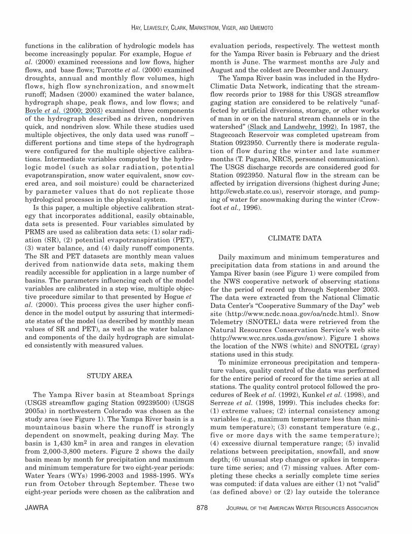
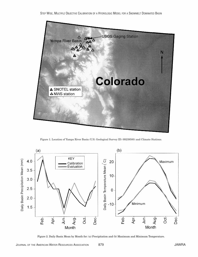
The Yampa River basin at Steamboat Springs(USGS streamflow gaging Station 09239500) (USGS2005a) in northwestern Colorado was chosen as thestudy area (see Figure 1). The Yampa River basin is amountainous basin where the runoff is stronglydependent on snowmelt, peaking during May. Thebasin is 1,430 km2 in area and ranges in elevationfrom 2,000-3,800 meters. Figure 2 shows the dailybasin mean by month for precipitation and maximumand minimum temperature for two eight-year periods:Water Years (WYs) 1996-2003 and 1988-1995. WYsrun from October through September. These twoeight-year periods were chosen as the calibration and

evaluation periods, respectively. The wettest monthfor the Yampa River basin is February and the driestmonth is June. The warmest months are July andAugust and the coldest are December and January.

The Yampa River basin was included in the Hydro-Climatic Data Network, indicating that the stream-flow records prior to 1988 for this USGS streamflowgaging station are considered to be relatively “unaf-fected by artificial diversions, storage, or other worksof man in or on the natural stream channels or in thewatershed” (Slack and Landwehr, 1992). In 1987, theStagecoach Reservoir was completed upstream fromStation 0923950. Currently there is moderate regula-tion of flow during the winter and late summermonths (T. Pagano, NRCS, personnel communication).The USGS discharge records are considered good forStation 0923950. Natural flow in the stream can beaffected by irrigation diversions (highest during June;http://cwcb.state.co.us), reservoir storage, and pump-ing of water for snowmaking during the winter (Crow-foot et al., 1996).

CLIMATE DATA

Daily maximum and minimum temperatures andprecipitation data from stations in and around theYampa River basin (see Figure 1) were compiled fromthe NWS cooperative network of observing stationsfor the period of record up through September 2003.The data were extracted from the National ClimaticData Center’s “Cooperative Summary of the Day” website (http://www.ncdc.noaa.gov/oa/ncdc.html). SnowTelemetry (SNOTEL) data were retrieved from theNatural Resources Conservation Service’s web site(http://www.wcc.nrcs.usda.gov/snow). Figure 1 showsthe location of the NWS (white) and SNOTEL (gray)stations used in this study.

To minimize erroneous precipitation and tempera-ture values, quality control of the data was performedfor the entire period of record for the time series at allstations. The quality control protocol followed the pro-cedures of Reek et al. (1992), Kunkel et al. (1998), andSerreze et al. (1998, 1999). This includes checks for:(1) extreme values; (2) internal consistency amongvariables (e.g., maximum temperature less than mini-mum temperature); (3) constant temperature (e.g.,five or more days with the same temperature); (4) excessive diurnal temperature range; (5) invalidrelations between precipitation, snowfall, and snowdepth; (6) unusual step changes or spikes in tempera-ture time series; and (7) missing values. After com-pleting these checks a serially complete time serieswas computed: if data values are either (1) not “valid”(as defined above) or (2) lay outside the tolerance

JAWRA 878 JOURNAL OF THE AMERICAN WATER RESOURCES ASSOCIATION

HAY, LEAVESLEY, CLARK, MARKSTROM, VIGER, AND UMEMOTO

JOURNAL OF THE AMERICAN WATER RESOURCES ASSOCIATION 879 JAWRA

STEP WISE, MULTIPLE OBJECTIVE CALIBRATION OF A HYDROLOGIC MODEL FOR A SNOWMELT DOMINATED BASIN

Figure 1. Location of Yampa River Basin (U.S. Geological Survey ID: 09239500) and Climate Stations.

Figure 2. Daily Basin Mean by Month for: (a) Precipitation and (b) Maximum and Minimum Temperature.

limits from the aerial consistency check, then they arereplaced with an interpolated value. Suspicious datawas replaced with data interpolated from surroundingstations.

HYDROLOGIC MODEL

The hydrologic model chosen for this study is theU.S. Geological Survey’s Precipitation Runoff Model-ing System (PRMS) (Leavesley et al., 1983; Leavesleyand Stannard, 1995). PRMS is a distributed parame-ter, physically-based watershed model. Distributedparameter capabilities are provided by partitioningthe watershed into Hydrologic Response Units(HRUs). Each HRU is assumed homogenous withrespect to its hydrologic response. PRMS is conceptu-alized as a series of reservoirs (impervious zone, soilzone, subsurface, and ground water) whose outputscombine to produce runoff. For each HRU, a water bal-ance is computed each day and an energy balance iscomputed twice each day. The sum of the water bal-ances of all HRUs, weighted by unit area, producesthe daily watershed response.

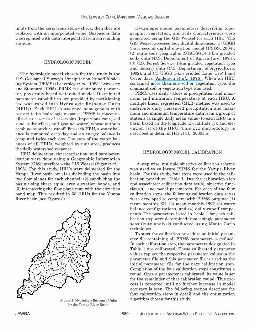
HRU delineation, characterization, and parameter-ization were done using a Geographic InformationSystem (GIS) interface – the GIS Weasel (Viger et al.,1998). For this study, HRUs were delineated for theYampa River basin by: (1) subdividing the basin intotwo flow planes for each channel, (2) subdividing thebasin using three equal area elevation bands, and (3) intersecting the flow plane map with the elevationband map. This resulted in 68 HRUs for the YampaRiver basin (see Figure 3).

Hydrologic model parameters describing topo-graphic, vegetation, and soils characteristics weregenerated using the GIS Weasel for each HRU. TheGIS Weasel accesses four digital databases: (1) USGS3-arc second digital elevation model (USGS, 2004); (2) state soils geographic (STATSGO) 1-km griddedsoils data (U.S. Department of Agriculture, 1994); (3) U.S. Forest Service 1-km gridded vegetation typeand density data (U.S. Department of Agriculture,1992); and (4) USGS 1-km gridded Land Use/ LandCover data (Anderson et al., 1976). When an HRUcontained more than one soil or vegetation type, thedominant soil or vegetation type was used.

PRMS uses daily values of precipitation and maxi-mum and minimum temperature at each HRU. Amultiple linear regression (MLR) method was used todistribute daily measured precipitation and maxi-mum and minimum temperature data from a group ofstations (a single daily mean value) to each HRU in abasin based on the longitude (x), latitude (y), and ele-vation (z) of the HRU. This xyz methodology isdescribed in detail in Hay et al. (2000a,b).

HYDROLOGIC MODEL CALIBRATION

A step wise, multiple objective calibration schemewas used to calibrate PRMS for the Yampa Riverbasin. For this study, four steps were used in the cali-bration procedure. Table 1 lists the calibration stepand associated: calibration data set(s), objective func-tions(s), and model parameters. For each of the fourcalibration steps, the following calibration data set(s)were developed to compare with PRMS outputs: (1)mean monthly SR, (2) mean monthly PET, (3) waterbalance configurations, and (4) daily runoff compo-nents. The parameters listed in Table 1 for each cali-bration step were determined from a single parametersensitivity analysis conducted using Monte Carlotechniques.

To start the calibration procedure an initial param-eter file containing all PRMS parameters is defined.In each calibration step, the parameters designated inTable 1 are calibrated. These calibrated parametervalues replace the respective parameter values in theparameter file and this parameter file is used as theinitial parameter file for the next calibration step.Completion of the four calibration steps constitutes around. Once a parameter is calibrated, its value is setfor the remainder of that calibration round. This pro-cess is repeated until no further increase in modelaccuracy is seen. The following section describes thefour calibration steps in detail and the optimizationalgorithm chosen for this study.

JAWRA 880 JOURNAL OF THE AMERICAN WATER RESOURCES ASSOCIATION

HAY, LEAVESLEY, CLARK, MARKSTROM, VIGER, AND UMEMOTO

Figure 3. Hydrologic Response Unitsfor the Yampa River Basin.

Calibration Step 1 -- Solar Radiation (SR)

The first step in the calibration procedure usedmean monthly SR values. The snowmelt and evapo-transpiration computations in PRMS require dailyvalues of SR. For this study, daily SR values were cal-culated in PRMS from daily air temperature data(Leavesley et al., 1983). Where available, daily SR canbe input directly into PRMS, but in general, thesedata are not available.

Measured monthly SR values are available for 217stations in the U.S. (http://rredc.nrel.gov/solar/old_data/nsrdb/redbook/mon2/). A data set of mean

monthly SR values at each of the climate station sites(SNOTEL and NWS) in the U.S. was developed. Amultiple linear regression (MLR) was developedbetween measured monthly SR values at the 217 sta-tions and independent variables (climate statisticscalculated using climate stations co-located with themeasured solar radiation). For each month a separateMLR equation was developed, choosing from the fol-lowing independent variables: latitude, longitude, ele-vation, mean precipitation (days > 0˚C), meanprecipitation, number of rain days, mean maximumtemperature, and the difference between mean maxi-mum and mean minimum temperature. Adjusted R2

values ranged from 0.83-0.98. Mean monthly SR

JOURNAL OF THE AMERICAN WATER RESOURCES ASSOCIATION 881 JAWRA

STEP WISE, MULTIPLE OBJECTIVE CALIBRATION OF A HYDROLOGIC MODEL FOR A SNOWMELT DOMINATED BASIN

TABLE 1. Parameters Calibrated in Each Step of the Calibration Process.

ParametersCalibration Used to Calibrate

Step Data Set Objective Function Model State Parameter Description

1 Basin mean monthly Sum of the absolute difference dday_intcp Intercept in temperature degree-day relationshipsolar radiation (SR) in the logarithms of observed tmax_index Index temperature used to determine

and simulated SR precipitation adjustments to solar radiation

2 Basin mean monthly Sum of the absolute difference jh_coef Coefficient used in Jensen-Haise PETpotential evapotrans- in the logarithms of observed computationspiration (PET) and simulated PET

3 Water balance: Sum of the absolute value of adjust_rain Precipitation adjustment factor for rain days1. Annual the Normalized Residuals adjust_snow Precipitation adjustment factor for snow days2. April-September (ANR) psta_nuse Binary indicator for using station in precipitation3. February-July distribution calculations4. High ANR computed for each of the psta_freq_nuse Binary indicator for using station in precipitation

four water balance components frequency calculationsand summed

4 Daily flow: Normalized Root Mean Square adjmix_rain Factor to adjust rain proportion in mixed rain/1. All flows Error (NRMSE) snow event2. Low flows tmax_allrain If HRU maximum temperature exceed this value,3. Peak flows NRMSE is computed for each precipitation assumed rain

of the three daily flow compo- tmax_allsnow If HRU maximum temperature is below thisnents and summed value, precipitation assumed snow

tsta_nuse Binary indicator for using station in temperature distribution calculations

cecn_coef Convection condensation energy coefficient emis_noppt Emissivity of air on days without precipitationfreeh2o_cap Free water holding capacity of snowpack potet_sublim Proportion of PET that is sublimated from snow

surfacesmidx_coef Coefficient in nonlinear surface runoff contribut-

ing area algorithmsmidx_exp Exponent in nonlinear surface runoff contribution

area algorithmgwflow_coef Ground water routing coefficientssrcoef_sq Coefficient to route subsurface storage to stream-

flowsoil2gw_max Maximum rate of soil water excess moving to

ground watersoil_moist_max Maximum available water holding capacity of soil

profilesoil_rechr_max Maximum available water holding capacity for soil

recharge zone

values were calculated at each SNOTEL and NWS cli-mate station site using the monthly MLR equations.

As noted earlier in this paper, there is a lack ofadditional data sources for model calibration andevaluation in nonresearch oriented basins. Meanmonthly values of SR are used for calibration andevaluation purposes in this study because these val-ues are available for the entire U.S. and the ability toapply this calibration procedure to numerous basinsacross the U.S. depends on having a data source forSR in each of these basins.

SR output from the station closest to the centroid ofthe Yampa River basin (23 km) was used as the cali-bration data set for the first step in the calibrationprocess. These SR values are referred to as interpolat-ed values in the text.

A PRMS parameter sensitivity analysis showedthree parameters influencing the SR calculations inPRMS. Two of these parameters are the slope and they-intercept of the line that expresses the relationbetween monthly maximum air temperature and adegree day coefficient. For this study, the slope wascalculated using the interpolated SR output at thestation closest to the Yampa River basin centroid andthe y-intercept was calibrated. This left two parame-ters for calibrating SR (Table 1). These parametersalso influence the other PRMS outputs tested in thisstudy, but their purpose is in calculating SR andtherefore their values are set in the first calibrationstep.

The objective function used to calibrate the meanmonthly SR values produced in PRMS is described as:

where OFsr is the objective function, m is the month,and INT and SIM are the mean monthly interpolatedand simulated SR values, respectively.

Note that the choices of objective functions in thispaper were made based on the authors past experi-ence with PRMS. Choice in objective function shouldbe based on the purpose of the study. There are 12monthly values used in the SR objective function com-putation. The sum of the absolute difference in thelogarithms of monthly interpolated and simulated SRwas chosen because it gave a more proportional mea-sure of error for low and high values.

Calibration Step 2 – Potential Evapotranspiration(PET)

The second step in the calibration procedure used acalibration data set consisting of mean monthly PET

values for the Yampa River basin. The basin meanmonthly PET values were calculated from PET mapsprovided by the NWS. The NWS derived the PET val-ues from the free water evaporation atlas ofFarnsworth et al. (1982). These PET maps were usedfor calibration and evaluation purposes in this studybecause these values are available for the entire U.S.and the ability to apply this calibration procedure tonumerous basins across the U.S. depends on having adata source for PET.

Daily estimates of PET in PRMS are produced fromSR using a procedure developed by Jensen and Haise(1963). This procedure uses one parameter, which isdescribed in Table 1. This parameter also influencesother PRMS outputs, but its purpose is in calculatingPET and therefore its value is set in this step of thecalibration.

The objective function, OFPET, is calculated in amanner similar to that for SR

where INT is the mean monthly PET value interpo-lated for the Yampa River basin from the PET mapsand SIM is the mean monthly PET value simulatedfor the Yampa River basin.

Calibration Step 3 -- Water Balance

The third step in the calibration procedure usedfour calibration data sets calculated from USGSstreamflow gaging Station 0923950. Table 1 lists thefour parameters influencing the water balance calcu-lations in PRMS. The first calibration data set usedannual runoff volumes (based on water year). Thethree additional calibration data sets were includedbecause the Bureau of Reclamation is interested inthese runoff volumes for forecasting (Tom Hicks,Bureau of Reclamation, personnel communication,January 2005). These include volumes calculatedfrom daily flow values that occurred between Apriland September and February and July and volumescalculated when daily flow values were greater than aselected low flow value (Qlow). Figure 4 shows aschematic of the Qlow calculation. In Figure 4, mea-sured daily runoff values were sorted and plotted. Thelocation where the grey lines in Figure 4 intersect wasassigned the Qlow value.

The water balance objective function (OFWB, Equa-tion 3) is the sum of the four objective functions: (1)OFann (annual water volumes); (2) OFas (volumescomputed for April-September); (3) OFfj (volumes

JAWRA 882 JOURNAL OF THE AMERICAN WATER RESOURCES ASSOCIATION

HAY, LEAVESLEY, CLARK, MARKSTROM, VIGER, AND UMEMOTO

OF abs INT SIMsr m mm

= ( ) − ( )( )=

∑ log log1

12(1)

OF abs INT SIMPET m mm

= ( ) − ( )( )=

∑ log log1

12(2)

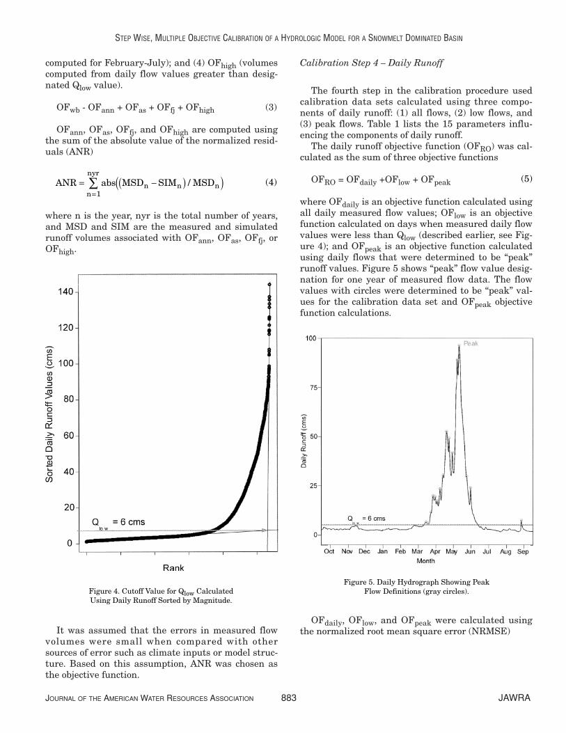
computed for February-July); and (4) OFhigh (volumescomputed from daily flow values greater than desig-nated Qlow value).

OFwb - OFann + OFas + OFfj + OFhigh

OFann, OFas, OFfj, and OFhigh are computed usingthe sum of the absolute value of the normalized resid-uals (ANR)

where n is the year, nyr is the total number of years,and MSD and SIM are the measured and simulatedrunoff volumes associated with OFann, OFas, OFfj, orOFhigh.

It was assumed that the errors in measured flowvolumes were small when compared with othersources of error such as climate inputs or model struc-ture. Based on this assumption, ANR was chosen asthe objective function.

Calibration Step 4 – Daily Runoff

The fourth step in the calibration procedure usedcalibration data sets calculated using three compo-nents of daily runoff: (1) all flows, (2) low flows, and(3) peak flows. Table 1 lists the 15 parameters influ-encing the components of daily runoff.

The daily runoff objective function (OFRO) was cal-culated as the sum of three objective functions

OFRO = OFdaily +OFlow + OFpeak

where OFdaily is an objective function calculated usingall daily measured flow values; OFlow is an objectivefunction calculated on days when measured daily flowvalues were less than Qlow (described earlier, see Fig-ure 4); and OFpeak is an objective function calculatedusing daily flows that were determined to be “peak”runoff values. Figure 5 shows “peak” flow value desig-nation for one year of measured flow data. The flowvalues with circles were determined to be “peak” val-ues for the calibration data set and OFpeak objectivefunction calculations.

OFdaily, OFlow, and OFpeak were calculated usingthe normalized root mean square error (NRMSE)

JOURNAL OF THE AMERICAN WATER RESOURCES ASSOCIATION 883 JAWRA

STEP WISE, MULTIPLE OBJECTIVE CALIBRATION OF A HYDROLOGIC MODEL FOR A SNOWMELT DOMINATED BASIN

(3)

ANR abs MSD SIM MSDn n nn

nyr= −( )( )

=∑ /

1(4)

Figure 4. Cutoff Value for Qlow CalculatedUsing Daily Runoff Sorted by Magnitude.

(5)

Figure 5. Daily Hydrograph Showing PeakFlow Definitions (gray circles).

where n is the day; ndays is the total number of days;and MSD, SIM, and MN are the measured, simulated,and mean daily values associated with OFdaily, OFlow,or OFpeak. If NRMSE = 0, then the measured valuesare equal to the simulated values (MSD = SIM). Avalue of NRMSE > 1 indicates that simulated valuesare as good as using the average value of all the mea-sured data.

Optimization Algorithm

For this study, the Shuffled Complex Evolutiontechnique (SCE) (Duan et al., 1992,1993,1994) waschosen as the optimization algorithm. The SCEmethod has been used successfully by a number ofresearchers (e.g., Yapo et al., 1996; Kuczera, 1997;Hogue et al., 2000; and Madsen, 2003). The SCEmethod selects a population of points distributed ran-domly throughout the parameter space. The popula-tion is partitioned into several complexes. Each ofthese complexes “evolves” using the downhill simplexalgorithm. The population is periodically “shuffled” toform new complexes so that the information gained bythe previous complexes is shared. The evolution andshuffling steps repeat until prescribed convergencecriteria are satisfied. Further detailed explanation ofthe method is given in Duan et al. (1992,1993, 1994).

RESULTS

The step wise, multiple objective automated proce-dure described above was used to calibrate the hydro-logic model PRMS in the Yampa River basin. Yapo etal. (1996) found that approximately eight years ofdata were needed to achieve model calibrations thatare insensitive to the period selected. For this study, asplit sample test was used for calibration and evalua-tion of PRMS. Eight WYs (1996-2003) were chosen formodel calibration. WYs 1996-2003 included a highflow year (WY 97) as well a low flow year (WY 2002).Eight WYs (1988-1995) were chosen for model evalua-tion.

Four hydrologic model outputs were calibrated: (1) monthly mean SR, (2) monthly mean PET, (3) annual water balance components, and (4) dailyrunoff components. Four rounds of the step wise cali-bration procedure were needed to reach a minimumin each objective function tested.

Solar Radiation (SR)

Calibration of SR is the first step in the step wiseprocedure. Figure 6 shows the basin mean SR valuesby month for interpolated (gray line), calibrated(black solid line), and evaluated (black dashed line)SR values. The calibrated values (WYs 1996-2003) arealmost identical to those shown for interpolated SR.The evaluated values (WYs 1988-1995) show closeagreement with interpolated values as well.

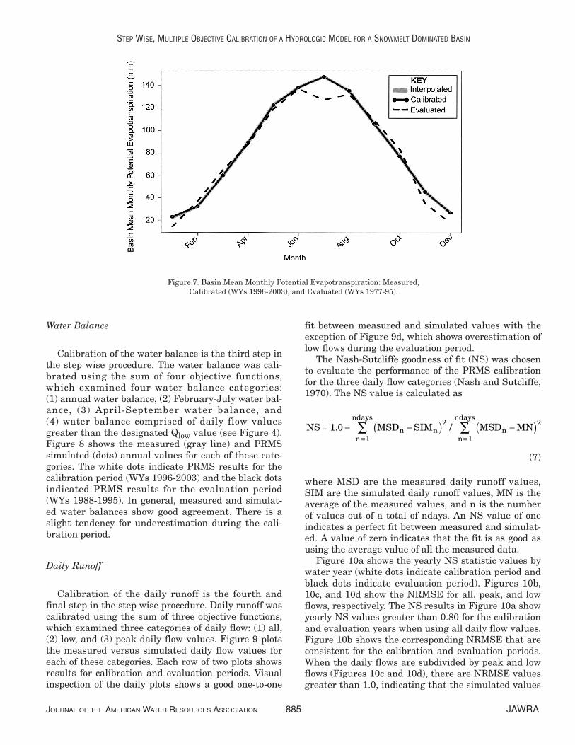
Potential Evapotranspiration (PET)

Calibration of PET is the second step in the stepwise procedure. Figure 7 shows the basin monthlyPET values by month for “measured” (gray line), cali-brated (black sold line), and evaluated (black dashedline) PET values. The calibrated values (WYs 1996-2003) are almost identical to those shown for mea-sured PET. PET values for the evaluation period(WYs 1988-1995) show a large discrepancy in July.Closer examination of SR for this month (Figure 6)shows the greatest discrepancies during July as well.Figure 2b shows the maximum and minimum dailybasin mean temperatures by month for the calibra-tion and evaluation periods. The temperature differ-ences between the calibration and evaluation periodsin July directly affect the PRMS simulated SR andPET in July.

JAWRA 884 JOURNAL OF THE AMERICAN WATER RESOURCES ASSOCIATION

HAY, LEAVESLEY, CLARK, MARKSTROM, VIGER, AND UMEMOTO

NRMSE MSD SIM MSD MNn n nn

ndays

n

ndays= −( ) −( )

⎛

⎝⎜

⎞

⎠⎟

==∑∑ 2 2

11

1 2

//

(6)

Figure 6. Basin Mean Monthly Solar Radiation: Interpolated,Calibrated (WYs 1996-2003), and Evaluated (WYs 1977-1995).

Water Balance

Calibration of the water balance is the third step inthe step wise procedure. The water balance was cali-brated using the sum of four objective functions,which examined four water balance categories: (1) annual water balance, (2) February-July water bal-ance, (3) April-September water balance, and (4) water balance comprised of daily flow valuesgreater than the designated Qlow value (see Figure 4).Figure 8 shows the measured (gray line) and PRMSsimulated (dots) annual values for each of these cate-gories. The white dots indicate PRMS results for thecalibration period (WYs 1996-2003) and the black dotsindicated PRMS results for the evaluation period(WYs 1988-1995). In general, measured and simulat-ed water balances show good agreement. There is aslight tendency for underestimation during the cali-bration period.

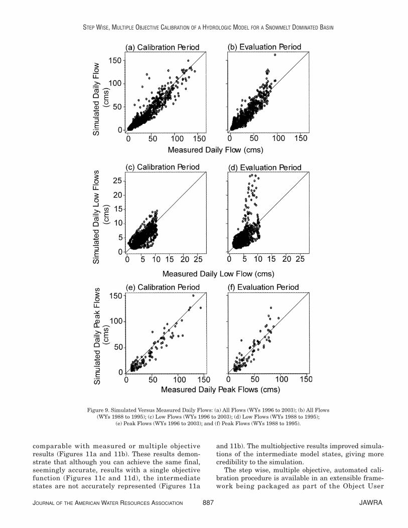
Daily Runoff

Calibration of the daily runoff is the fourth andfinal step in the step wise procedure. Daily runoff wascalibrated using the sum of three objective functions,which examined three categories of daily flow: (1) all,(2) low, and (3) peak daily flow values. Figure 9 plotsthe measured versus simulated daily flow values foreach of these categories. Each row of two plots showsresults for calibration and evaluation periods. Visualinspection of the daily plots shows a good one-to-one

fit between measured and simulated values with theexception of Figure 9d, which shows overestimation oflow flows during the evaluation period.

The Nash-Sutcliffe goodness of fit (NS) was chosento evaluate the performance of the PRMS calibrationfor the three daily flow categories (Nash and Sutcliffe,1970). The NS value is calculated as

where MSD are the measured daily runoff values,SIM are the simulated daily runoff values, MN is theaverage of the measured values, and n is the numberof values out of a total of ndays. An NS value of oneindicates a perfect fit between measured and simulat-ed. A value of zero indicates that the fit is as good asusing the average value of all the measured data.

Figure 10a shows the yearly NS statistic values bywater year (white dots indicate calibration period andblack dots indicate evaluation period). Figures 10b,10c, and 10d show the NRMSE for all, peak, and lowflows, respectively. The NS results in Figure 10a showyearly NS values greater than 0.80 for the calibrationand evaluation years when using all daily flow values.Figure 10b shows the corresponding NRMSE that areconsistent for the calibration and evaluation periods.When the daily flows are subdivided by peak and lowflows (Figures 10c and 10d), there are NRMSE valuesgreater than 1.0, indicating that the simulated values

JOURNAL OF THE AMERICAN WATER RESOURCES ASSOCIATION 885 JAWRA

STEP WISE, MULTIPLE OBJECTIVE CALIBRATION OF A HYDROLOGIC MODEL FOR A SNOWMELT DOMINATED BASIN

Figure 7. Basin Mean Monthly Potential Evapotranspiration: Measured,Calibrated (WYs 1996-2003), and Evaluated (WYs 1977-95).

NS MSD SIM MSD MNn nn

ndays

nn

ndays= − −( ) −( )

= =∑ ∑1 0 2

1

2

1. /

(7)

can be considered inferior to using a mean value. Thisis especially true for the low flows (Figure 10d). Muchof the fluctuation in the summer low flow values forthe Yampa River basin can be attributed to diversionsand returns during the summer months. Withoutdetailed information on these diversions, it is unreal-istic to be able match the daily variability in the lowflows. The lowest flow year (2002) also shows the low-est NS value (0.80). As indicated by Figure 8d, theannual low flow volumes are simulated accurately.

DISCUSSION

The step wise, multiple objective, automated cali-bration procedure may not actually improve the finalrunoff simulations when compared with a singleobjective calibration procedure. To demonstrate this, asingle objective function calibration procedure was

performed in which all parameters listed in Table 1were calibrated simultaneously with one objectivefunction (OFdaily using NRMSE from Equation 6).Figure 11 compares calibration period results (WYs1996-2003) from the single objective automated cali-bration procedure and the multiple objective, stepwise, automated calibration procedure. Figures 11aand 11b show mean monthly SR and PET resultsfrom single objective (dashed black line) and multipleobjective (black line) procedures. Figure 11c showsannual water volumes calculated from measured data(gray line) and single objective (white dots) and multi-ple objective (black dots) procedures. Figure 11dshows the annual Nash-Sutcliffe goodness of fitstatistic calculated with daily flow values simulatedusing single objective (white dots) and multiple objec-tive (black dots) procedures. Single objective and mul-tiple objective results for annual water volumes andNash-Sutcliffe values are similar (Figures 11c and11d). Single objective results for SR and PET are not

JAWRA 886 JOURNAL OF THE AMERICAN WATER RESOURCES ASSOCIATION

HAY, LEAVESLEY, CLARK, MARKSTROM, VIGER, AND UMEMOTO

Figure 8. Water Balance: Measured, Calibrated (WYs 1996 to 2003), and Evaluated (WYs 1988 to 1995) for(a) Annual Flows, (b) February-July Flows, (c) April-September Flows, and (d) Flows > Qlow.

comparable with measured or multiple objectiveresults (Figures 11a and 11b). These results demon-strate that although you can achieve the same final,seemingly accurate, results with a single objectivefunction (Figures 11c and 11d), the intermediatestates are not accurately represented (Figures 11a

and 11b). The multiobjective results improved simula-tions of the intermediate model states, giving morecredibility to the simulation.

The step wise, multiple objective, automated cali-bration procedure is available in an extensible frame-work being packaged as part of the Object User

JOURNAL OF THE AMERICAN WATER RESOURCES ASSOCIATION 887 JAWRA

STEP WISE, MULTIPLE OBJECTIVE CALIBRATION OF A HYDROLOGIC MODEL FOR A SNOWMELT DOMINATED BASIN

Figure 9. Simulated Versus Measured Daily Flows: (a) All Flows (WYs 1996 to 2003); (b) All Flows(WYs 1988 to 1995); (c) Low Flows (WYs 1996 to 2003); (d) Low Flows (WYs 1988 to 1995);

(e) Peak Flows (WYs 1996 to 2003); and (f) Peak Flows (WYs 1988 to 1995).

Interface (OUI) modeling framework (USGS, 2005b).OUI is a map-based modeling framework for models,modeling data, and associated tools. It provides acommon interface for running models as well asacquiring, browsing, organizing, and selecting spatialand temporal data. This allows users to modify thecalibration procedure to their own models, data, objec-tive functions, and calibration steps.

For example, a modification for a snowmelt domi-nated basin might include calibration steps for PRMSsimulated snow covered area (SCA) or snow waterequivalent (SWE). SCA and SWE data sets are avail-able from the National Operational HydrologicRemote Sensing Center (NOHRSC). The SCA andSWE NOHRSC products may not be appropriate fordata assimilation purposes in PRMS due to data accu-racy issues, but they may prove to be a valuable toolin documenting these intermediate model states.

Many of the data sets that could be used for inter-mediate model state identification are processed fromother data sources and therefore not available in realtime. The most appropriate use of these data sets

would be for model calibration. In addition, whenthere is no runoff data available for calibration pur-poses (ungaged basin), intermediate model states canbe calibrated and only the parameters associated withrunoff calibration steps need to be identified.

CONCLUSIONS

This paper presented an application of a calibra-tion procedure that used a multiple objective, stepwise, approach. The procedure used the ShuffledComplex Evolution global search algorithm to cali-brate the Precipitation Runoff Modeling System(PRMS) in the Yampa River basin of Colorado. Thebase application included the sequential calibrationof: (1) mean monthly solar radiation, (2) mean month-ly potential evapotranspiration, (3) annual water bal-ances, and (4) components of daily runoff simulatedby PRMS. The calibration procedure is available in anextensible framework, allowing for modification of the

JAWRA 888 JOURNAL OF THE AMERICAN WATER RESOURCES ASSOCIATION

HAY, LEAVESLEY, CLARK, MARKSTROM, VIGER, AND UMEMOTO

Figure 10. Evaluation of Daily Flow Values by Water Year: (a) Nash-Sutcliffe (NS) Goodness of Fit Test; (b) NormalizedRoot Mean Square Error (NRMSE) for All Flows; (c) NRMSE for Peak Flows; and (d) NRMSE for Low Flows.

models, data, objective functions, and calibrationsteps based on the users needs. For this paper, theprocedure not only produced realistic runoff, but italso documented intermediate states of the model ona monthly mean basis not normally calibrated inhydrologic models.

LITERATURE CITED

Anderson, J.R., E.E. Hardy, J.T. Roach, and R.E. Witmer, 1976. ALand Use Land Cover Classification System for Use WithRemote Sensor Data. U.S. Geological Survey Prof. Paper 964, 28pp.

Boyle, D.P., H.V. Gupta, and S. Sorooshian, 2000. Toward ImprovedCalibration of Hydrologic Models: Combining the Strengths ofManual and Automatic Methods. Water Resources Research36(12):3663-3674.

Boyle, D.P., H.V. Gupta, and S. Sorooshian, 2003. Multicriteria Cali-bration of Hydrologic Models. Calibration of Watershed Models,AGU Water Sciences and Applications, Volume 6, AmericanGeophysical Union, Washington D.C., pp. 185-196.

Carter G., 2005. NOAA Working Together to Deliver Critical Infor-mation for Living With a Limited Water Supply. In: 21st International Conference on Interactive Information Pro-cessing Systems (IIPS) for Meteorology, Oceanography, andHydrology. Available at http://ams.confex.com/ams/Annual2005/techprogram/paper_83244.htm. Accessed in May 2005.

Crowfoot, R.M., R.S. Ugland, W.S. Maura, R.A. Jenkins, and G.B.O’Neill, 1996. Water Resources Data Colorado Water Year 1995.U.S. Geological Survey Water-Data Report CO-95-2, 471 pp.

Duan, Q., V.K. Gupta, and S. Sorooshian, 1993. A Shuffled ComplexEvolution Approach for Effective and Efficient Global Minimiza-tion. Journal of Optimization Theory and Its Applications76(3):501-521.

Duan, Q., S. Sorooshian, and V. Gupta, 1992. Effective and EfficientGlobal Optimization for Conceptual Rainfall-Runoff Models.Water Resources Research 28(4):1015-1031.

Duan, Q., S. Sorooshian, and V.K. Gupta, 1994. Optimal Use of theSCE-UA Global Optimization Method for Calibrating WatershedModels. Journal of Hydrology 158:265-284.

Farnsworth, R.K., E.S. Thompson, and E.L Peck, 1982. EvaporationAtlas for the Contiguous 48 United States. NOAA Tech. Rep.NWS 33, U.S. Department of Commerce, Washington D.C.

JOURNAL OF THE AMERICAN WATER RESOURCES ASSOCIATION 889 JAWRA

STEP WISE, MULTIPLE OBJECTIVE CALIBRATION OF A HYDROLOGIC MODEL FOR A SNOWMELT DOMINATED BASIN

Figure 11. Comparison of Calibration Results From Single Objective and Multiple Objective Calibration Procedures:(a) Basin Mean Monthly Solar Radiation; (b) Basin Mean Monthly Potential Evapotranspiration (PET);

(c) Annual Water Balance; and (d) Nash-Sutcliffe Goodness of Fit Statistic Using Daily Flow Data.

Gupta, H.V, S. Sorooshian, and P.O. Yapo, 1998. Towards ImprovedCalibration of Hydrologic Models: Multiple Noncommensurable Measures of Information. Water Resources Research 34(4):751-763.

Hay, L., M. Clark, and G. Leavesley, 2000a. Use of AtmosphericForecasts in Hydrologic Models: Part 2. Case Study. In: WaterResources in Extreme Environments, Douglas L. Kane (Editor).American Water Resources Association, Middleburg, Virginia,pp. 221-226.

Hay, L.E., R.L. Wilby, and G.H. Leavesley, 2000b. A Comparison ofDelta Change and Downscaled GCM Scenarios for Three Moun-tainous Basins in the United States. Journal of the AmericanWater Resources Association (JAWRA) 36(2):387-397.

Hogue, T.S., S. Sorooshian, H. Gupta, A. Holz, and D. Braatz, 2000.A Multi-step Automatic Calibration Scheme for River Forecast-ing Models. Journal of Hydrometeorology 1:524-542.

Jensen, M.E. and H.R. Haise, 1963. Estimating EvapotranspirationFrom Solar Radiation. J. of Irrigation and Drainage 89(IR4):15-41.

Kuczera,G., 1997. Efficient Subspace Probabilistic Parameter Opti-mization for Catchment Models. Water Resour. Res. 33(1):177-186.

Kunkel, K.E., K. Andsager, G. Conner, W.L. Decker, H.J. Hillaker,Jr., P. Naber Knox, F.V. Nurnberger, J.C. Roger, K. Scheeringa,W.M. Wendland, J. Zandlo, Jr., and J.R. Angel, 1998. AnExpanded Digital Daily Database for Climate Resources Appli-cations in the Midwestern United States. Bulletin of the Ameri-can Meteorological Society 79:1357-1366.

Leavesley, G.H., R.W. Lichty, B.M. Troutman, and L.G. Saindon,1983. Precipitation-Runoff Modeling System: User’s Manual.U.S. Geological Survey Water Resources Investigation Report83- 4238.

Leavesley, G.H. and L.G. Stannard, 1995. The Precipitation-RunoffModeling System-PRMS. In: Computer Models of WatershedHydrology, V.P. Singh (Editor). Water Resources Publications,Highlands Ranch, Colorado, pp. 281-310.

Madsen, H., 2000. Automatic Calibration and Uncertainty Assess-ment in Rainfall-Runoff Modeling. 2000 Joint Conference onWater Resources Engineering and Water Resources Planningand Management, Section 38, Chapter 2.

Madsen, H., 2003. Parameter Estimation in Distributed Hydrologi-cal Catchment Modelling Using Automatic Calibration WithMultiple Objectives. Advances in Water Resources 26:205-216.

Nash, J.E. and J.V. Sutcliffe, 1970. River Flow Forecasting ThroughConceptual Models: Part I. A Discussion of Principles. J. of Hyd.10:282-290.

NCDC (National Climatic Data Center), 2005. Locate WeatherObservation Station Record. Available at http://www.ncdc.noaa.gov/oa/climate/stationlocator.html. Accessed in May 2005.

NOHRSC (National Operational Hydrologic Remote Sensing Cen-ter), 2004. Snow Data Assimilation System (SNODAS) DataProducts. National Snow and Ice Data Center, Digital Media,Boulder, Colorado.

National Renewable Energy Laboratory, 1994. Solar RadiationData Manual for Flat-Plate and Concentrating Collectors: 30-Year Average of Monthly Solar Radiation, 1961-1990. Availableat http://rredc.nrel.gov/solar/old_data/nsrdb/redbook/sum2/.Accessed in May 2005.

Reek, T., S.R. Doty, and T.W. Owen, 1992. A Deterministic Approachto the Validation of Historical Daily Temperature and Precipita-tion Data From the Cooperative Network. Bulletin of the Ameri-can Meteorological Society 73:753-762.

Refsgaard, J.C., 1997. Parameterization, Calibration and Validationof Distributed Hydrological Models. J. Hydrol. 198:69-97.

Refsgaard, J.C., 2000. Towards a Formal Approach to Calibrationand Validation of Models Using Spatial Data. In: Spatial Pat-terns in Catchment Hydrology: Observations and Modelling, R. Grayson and G. Bloschl (Editors). Cambridge UniversityPress, Cambridge, Massachusetts, pp. 329-54.

Serreze, M.C., M.P Clark, R.L. Armstrong, D.A. McGinnis, and R.L.Pulwarty, 1999. Characteristics of the Western U.S. SnowpackFrom Snowpack Telemetry (SNOTEL) Data. Water ResourcesResearch 35:2145-2160.

Serreze, M.C., M.P. Clark, D.A. Robinson, and D.L. McGinnis, 1998.Characteristics of Snowfall Over the Eastern Half of the UnitedStates and Relationships With Principal Modes of Low-Frequen-cy Atmospheric Variability. Journal of Climate 11:234-250.

Slack, J.R. and J.M. Landwehr, 1992. Hydro-Climatic Data Net-work: A U.S. Geological Survey Streamflow Data Set for theUnited States for the Study of Climate Variations, 1874-1988.U.S. Geological Survey Open-File Report 92-129.

Turcotte, R., A.N. Rousseau, J.P. Fortin, and J.P. Villeneuve, 2000.A Process-Oriented, Multiple-Objective Calibration StrategyAccounting for Model Structure. Calibration of Watershed Mod-els, AGU Water Sciences and Applications, Volume 6, AmericanGeophysical Union, Washington D.C., pp. 153-164.

USDA (U.S. Department of Agriculture), 1992. Forest Land Distri-bution Data for the United States. USDA Forest Service, Avail-able at http://www.epa.gov/docs/grd/forest_inventory/.

USDA (U.S. Department of Agriculture), 1994. State Soil Geograph-ic (STATSGO) Database – Data Use Information. NaturalResources Conservation Service, Misc. Pub. No. 1492, 107 pp.

USDA-NRCS (U.S. Department of Agriculture-Natural ResourcesConservation Service), 1998. Spatially Distributed HydrologicModeling. Available at http://www.wcc.nrcs.usda.gov/factpub/briefing.html. Accessed in June 2005.

USGS (U.S. Geological Survey), 2004. Seamless Data Distribution.Available at http://seamless.usgs.gov/website/seamless.Accessed in May 2005.

USGS (U.S. Geological Survey), 2005a. Daily Streamflow for theNation. Available at http://nwis.waterdata.usgs.gov/nwis/dis-charge/?site_no=09239500. Accessed in May 2005.

USGS (U.S. Geological Survey), 2005b. Modular Modeling System,A Modeling Framework for Multidisciplinary Research andOperational Applications: MMS Utilities, Object User Interface(OUI). Available at http://wwwbrr.cr.usgs.gov/mms/. Accessed inMay 2005.

Viger, R.J., S.L. Markstrom, and G.H. Leavesley, 1998. The GISWeasel - An Interface for the Treatment of Spatial InformationUsed in Watershed Modeling and Water Resource Management.Proceedings of the First Federal Interagency Hydrologic Model-ing Conference, Las Vegas, Nevada, Vol II, Chapter 7, pp. 73-80.

Yapo, P.O., H.V. Gupta, and S. Sorooshian, 1996. Automatic Cali-bration of Conceptual Rainfall-Runoff Models: Sensitivity toCalibration Data. J. of Hyd. 181:23-48.

JAWRA 890 JOURNAL OF THE AMERICAN WATER RESOURCES ASSOCIATION

HAY, LEAVESLEY, CLARK, MARKSTROM, VIGER, AND UMEMOTO