Status and Integrated Road-Map for Joints Modeling Research

SAND REPORTSAND2003-0897Unlimited ReleasePrinted March 2003

Status and Integrated Road-Map forJoints Modeling Research

Daniel J. Segalman, Thomas Paez, David Smallwood, Anton Sumali, and AngelUrbina

Prepared bySandia National LaboratoriesAlbuquerque, New Mexico 87185 and Livermore, California 94550

Sandia is a multiprogram laboratory operated by Sandia Corporation,a Lockheed Martin Company, for the United States Department of Energy’sNational Nuclear Security Administration under Contract DE-AC04-94-AL85000.

Approved for public release; further dissemination unlimited.

Issued by Sandia National Laboratories, operated for the United States Department ofEnergy by Sandia Corporation.

NOTICE: This report was prepared as an account of work sponsored by an agency ofthe United States Government. Neither the United States Government, nor any agencythereof, nor any of their employees, nor any of their contractors, subcontractors, or theiremployees, make any warranty, express or implied, or assume any legal liability or re-sponsibility for the accuracy, completeness, or usefulness of any information, appara-tus, product, or process disclosed, or represent that its use would not infringe privatelyowned rights. Reference herein to any speci£c commercial product, process, or serviceby trade name, trademark, manufacturer, or otherwise, does not necessarily constituteor imply its endorsement, recommendation, or favoring by the United States Govern-ment, any agency thereof, or any of their contractors or subcontractors. The views andopinions expressed herein do not necessarily state or re¤ect those of the United StatesGovernment, any agency thereof, or any of their contractors.

Printed in the United States of America. This report has been reproduced directly fromthe best available copy.

Available to DOE and DOE contractors fromU.S. Department of EnergyOf£ce of Scienti£c and Technical InformationP.O. Box 62Oak Ridge, TN 37831

Telephone: (865) 576-8401Facsimile: (865) 576-5728E-Mail: [email protected] ordering: http://www.doe.gov/bridge

Available to the public fromU.S. Department of CommerceNational Technical Information Service5285 Port Royal RdSpring£eld, VA 22161

Telephone: (800) 553-6847Facsimile: (703) 605-6900E-Mail: [email protected] ordering: http://www.ntis.gov/help/ordermethods.asp?loc=7-4-0#online

DEP

ARTMENT OF ENERGY

• • UN

ITED

STATES OF AM

ERIC

A

SAND2003-0897Unlimited ReleasePrinted March 2003

Status and Integrated Road-Map forJoints Modeling Research

Daniel Segalman, David Smallwood, and Anton SumaliStructrual Dynamics Research Department

Thomas Paez and Angel UrbinaValidation and Uncertainty Quantification Processes Department

Sandia National LaboratoriesP.O. Box 5800

Albuquerque, NM [email protected]

————————————————————————

Abstract

The constitutive behavior of mechanical joints is largely responsible for the

energy dissipation and vibration damping in weapons systems. For reasons

arising from the dramatically different length scales associated with those dissi-

pative mechanisms and the length scales characteristic of the overall structure,

this physics cannot be captured adequately through direct simulation of the

contact mechanics within a structural dynamics analysis.

The only practical method for accommodating the nonlinear nature of joint

mechanisms within structural dynamic analysis is through constitutive models

employing degrees of freedom natural to the scale of structural dynamics. This

document discusses a road-map for developing such constitutive models.

3

Acknowledgment

The author list includes only those people who have actually contributed text andfigures to this road map. Many additional people have contributed to the plans de-scribed. These include people formally on the joints team - experimentalists, analysts,and model developers - as well as others who have a stake in the exploitation of thesemodels. Some of those people also provided critical review of this document and help-ful suggestions. Among those who should be recognized in particular are FernandoBitsie, Dan Gregory, Ron Hopkins, Todd Simmermacher, and Howard Walter.

Two external parties need to be recognized as well. The joints research effortunder Prof. Lawrence Bergman at the University of Illinois has contributed to thefoundations of much of the plan presented here. In particular, they demonstratedthat “whole-interface” elements can capture transient response of jointed structures.Collaborative work with Prof. Dane Quinn of the University of Akron has lead toat least one candidate constitutive model for the special interface approach discussedhere.

Additionally those managers who have supported the joints research effort over thelast several years deserve an expression of appreciation. First among these is DavidMartinez, who provided moral and budgetary support at the inception of this project.He was also an indefatigable advocate during those crucial years. Also to be creditedis Jaime Moya who not only provided advocacy for the joints program, but has alsofunded an expanding experimental effort which provides a fundamental foundation forthe modeling program. There are several more managers who have provided supportfor the joints effort in recent years, these include Justine Johannes, Hal Morgan, andJim Redmond. Jim’s efforts in coordinating the overall joints research program andhelping transition it to the users are a major and continuing asset to the researchprogram.

4

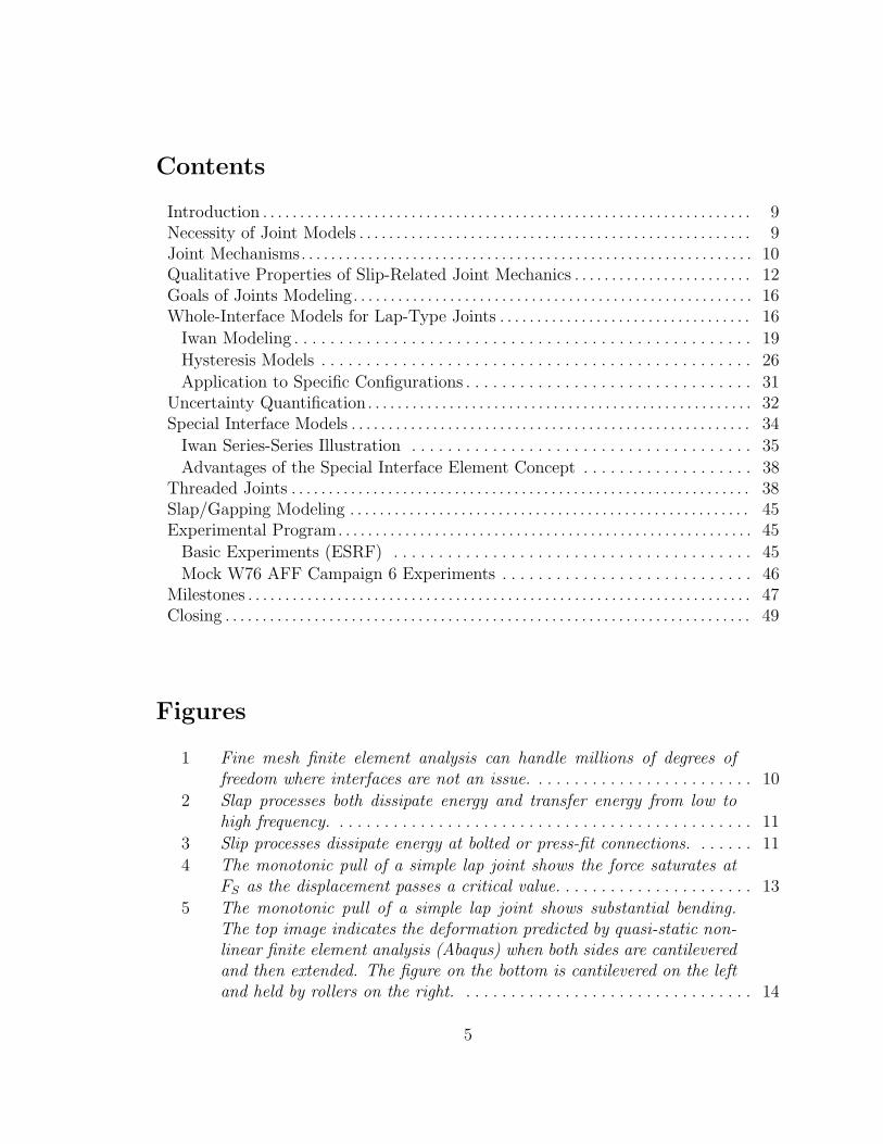
Contents

Introduction . . . . . . . . . . . . . . . . . . . . . . . . . . . . . . . . . . . . . . . . . . . . . . . . . . . . . . . . . . . . . . . . . . 9Necessity of Joint Models . . . . . . . . . . . . . . . . . . . . . . . . . . . . . . . . . . . . . . . . . . . . . . . . . . . . . 9Joint Mechanisms. . . . . . . . . . . . . . . . . . . . . . . . . . . . . . . . . . . . . . . . . . . . . . . . . . . . . . . . . . . . . 10Qualitative Properties of Slip-Related Joint Mechanics . . . . . . . . . . . . . . . . . . . . . . . . 12Goals of Joints Modeling. . . . . . . . . . . . . . . . . . . . . . . . . . . . . . . . . . . . . . . . . . . . . . . . . . . . . . 16Whole-Interface Models for Lap-Type Joints . . . . . . . . . . . . . . . . . . . . . . . . . . . . . . . . . . 16

Iwan Modeling . . . . . . . . . . . . . . . . . . . . . . . . . . . . . . . . . . . . . . . . . . . . . . . . . . . 19

Hysteresis Models . . . . . . . . . . . . . . . . . . . . . . . . . . . . . . . . . . . . . . . . . . . . . . . . 26

Application to Specific Configurations . . . . . . . . . . . . . . . . . . . . . . . . . . . . . . . . 31Uncertainty Quantification. . . . . . . . . . . . . . . . . . . . . . . . . . . . . . . . . . . . . . . . . . . . . . . . . . . . 32Special Interface Models . . . . . . . . . . . . . . . . . . . . . . . . . . . . . . . . . . . . . . . . . . . . . . . . . . . . . . 34

Iwan Series-Series Illustration . . . . . . . . . . . . . . . . . . . . . . . . . . . . . . . . . . . . . . 35

Advantages of the Special Interface Element Concept . . . . . . . . . . . . . . . . . . . 38Threaded Joints . . . . . . . . . . . . . . . . . . . . . . . . . . . . . . . . . . . . . . . . . . . . . . . . . . . . . . . . . . . . . . 38Slap/Gapping Modeling . . . . . . . . . . . . . . . . . . . . . . . . . . . . . . . . . . . . . . . . . . . . . . . . . . . . . . 45Experimental Program. . . . . . . . . . . . . . . . . . . . . . . . . . . . . . . . . . . . . . . . . . . . . . . . . . . . . . . . 45

Basic Experiments (ESRF) . . . . . . . . . . . . . . . . . . . . . . . . . . . . . . . . . . . . . . . . 45

Mock W76 AFF Campaign 6 Experiments . . . . . . . . . . . . . . . . . . . . . . . . . . . . 46Milestones . . . . . . . . . . . . . . . . . . . . . . . . . . . . . . . . . . . . . . . . . . . . . . . . . . . . . . . . . . . . . . . . . . . . 47Closing . . . . . . . . . . . . . . . . . . . . . . . . . . . . . . . . . . . . . . . . . . . . . . . . . . . . . . . . . . . . . . . . . . . . . . . 49

Figures

1 Fine mesh finite element analysis can handle millions of degrees offreedom where interfaces are not an issue. . . . . . . . . . . . . . . . . . . . . . . . . 10

2 Slap processes both dissipate energy and transfer energy from low tohigh frequency. . . . . . . . . . . . . . . . . . . . . . . . . . . . . . . . . . . . . . . . . . . . . . . 11

3 Slip processes dissipate energy at bolted or press-fit connections. . . . . . . 11

4 The monotonic pull of a simple lap joint shows the force saturates atFS as the displacement passes a critical value. . . . . . . . . . . . . . . . . . . . . . 13

5 The monotonic pull of a simple lap joint shows substantial bending.The top image indicates the deformation predicted by quasi-static non-linear finite element analysis (Abaqus) when both sides are cantileveredand then extended. The figure on the bottom is cantilevered on the leftand held by rollers on the right. . . . . . . . . . . . . . . . . . . . . . . . . . . . . . . . . 14

5

6 The displacements on the right hand sides of the specimens of Figure 5when subject to monotonic pull. Initially, almost all of the deformationis that associated with elastic bending. Once the force exceeds thatnecessary to initiate macro-slip, all the incremental deformation is dueto the joint. . . . . . . . . . . . . . . . . . . . . . . . . . . . . . . . . . . . . . . . . . . . . . . . . 14

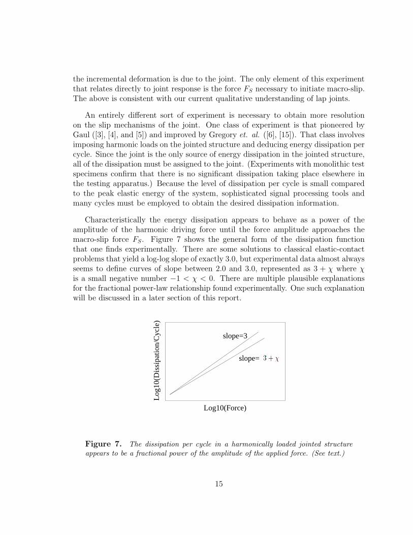
7 The dissipation per cycle in a harmonically loaded jointed structureappears to be a fractional power of the amplitude of the applied force.(See text.) . . . . . . . . . . . . . . . . . . . . . . . . . . . . . . . . . . . . . . . . . . . . . . . . . 15

8 The mock W76 AFF bolted joint and a finite element mesh used tosimulate that joint. . . . . . . . . . . . . . . . . . . . . . . . . . . . . . . . . . . . . . . . . . . 17

9 The dissipation per cycle in a harmonically loaded jointed structure ap-pears to be a fractional power of the amplitude of the applied force. Theexperimental data shown is from nine different but nominally identicallap joints (AFF 1, AFF 2, ...). . . . . . . . . . . . . . . . . . . . . . . . . . . . . . . . . 17

10 The “whole-interface” approach to simulation of joints reduces the num-ber of degrees of freedom at a joint to one in the direction of each de-gree of freedom. This approach would be applied to generalized lap-typejoints, including compression fits such as shown here. . . . . . . . . . . . . . . . 18

11 A parallel-series Iwan system . . . . . . . . . . . . . . . . . . . . . . . . . . . . . . . . . . . 21

12 The joint parameter KT is the slope of the hysteresis curve immediatelyafter a force reversal. . . . . . . . . . . . . . . . . . . . . . . . . . . . . . . . . . . . . . . . . . 22

13 A spectrum that is the sum of a truncated power law distribution anda Dirac delta function can be selected to satisfy asymptotic behavior atsmall and large force amplitudes. . . . . . . . . . . . . . . . . . . . . . . . . . . . . . . . . 23

14 Fit to dissipation data from a mock W76 AFF leg using an optimizationmethod within Matlab. . . . . . . . . . . . . . . . . . . . . . . . . . . . . . . . . . . . . . . . 24

15 Stepped specimen from which the data for the following figure (Figure16) was obtained. . . . . . . . . . . . . . . . . . . . . . . . . . . . . . . . . . . . . . . . . . . . . 25

16 Fit to dissipation data from a stepped specimen using an optimizationmethod within Matlab. . . . . . . . . . . . . . . . . . . . . . . . . . . . . . . . . . . . . . . . 25

17 Stiffness model . . . . . . . . . . . . . . . . . . . . . . . . . . . . . . . . . . . . . . . . . . . . . . 28

18 Hysteresis for waveform with third harmonic added . . . . . . . . . . . . . . . . . 30

19 A distributed jointed connection can be approximated as a distributionof whole-interface models. . . . . . . . . . . . . . . . . . . . . . . . . . . . . . . . . . . . . 31

20 Scheme for special interface elements to capture micro-macro slip em-ploying a relatively coarse mesh. . . . . . . . . . . . . . . . . . . . . . . . . . . . . . . . . 35

21 The series-series Iwan model is the basis for one possible interface model. 36

22 Spatially varying normal tractions result in corresponding distributionsof slider strength among the Jenkins elements. . . . . . . . . . . . . . . . . . . . . . 36

6

23 An interface element would be created from series-series Iwan systemsspanning each pair of quadrature points. . . . . . . . . . . . . . . . . . . . . . . . . . . 37

24 Interface elements could be integrated into the modeling of generalizedlap joints in a natural manner. . . . . . . . . . . . . . . . . . . . . . . . . . . . . . . . . . 39

25 Interface elements could be integrated into the modeling of tape jointsin a natural manner. . . . . . . . . . . . . . . . . . . . . . . . . . . . . . . . . . . . . . . . . . 39

26 Approximate mesh refinement necessary to capture detailed thread in-teractions. . . . . . . . . . . . . . . . . . . . . . . . . . . . . . . . . . . . . . . . . . . . . . . . . . . 40

27 Opposing buttress threads in joint. . . . . . . . . . . . . . . . . . . . . . . . . . . . . . . 4128 Corresponding finite element mesh. . . . . . . . . . . . . . . . . . . . . . . . . . . . . . . 4129 Pressure across thread interface. . . . . . . . . . . . . . . . . . . . . . . . . . . . . . . . . 4230 Shear stress across Thread Interface. . . . . . . . . . . . . . . . . . . . . . . . . . . . . 4231 The T0 element is created to have the same elastic properties of a

thread pair unit when the thread interface is ‘welded’ . . . . . . . . . . . . . . . 4332 Reduced-order model(T1) for unit-cell of thread pairs. Nodes indicated

in blue are sufficient to define internal thread deformation. . . . . . . . . . . 4333 Axi-symmetric application of reduced order thread interface elements. . . 4434 Basic lap joint test configuration. . . . . . . . . . . . . . . . . . . . . . . . . . . . . . . . 4635 Mock AFF test assembly . . . . . . . . . . . . . . . . . . . . . . . . . . . . . . . . . . . . . . 4736 Threaded shell and AFF base. . . . . . . . . . . . . . . . . . . . . . . . . . . . . . . . . . . 47

7

This page intentionally left blank

8

Status and IntegratedRoad-Map for Joints Modeling

Research

Introduction

In the context of the research plan presented here, joint mechanics refers to themechanical properties of joints commonly found in weapons systems and their impacton the structural response of the systems of which they are a part. The mechanics ofinterest are usually manifest as non-linear vibration damping, non-linear stiffness, or atransfer of mechanical energy from low frequency to high. All of these manifestationsmust be accounted for in the prediction of structural response of weapons systems,but no appropriate constitutive models for these phenomena exist as of now. It is thepurpose of the research planned out here to develop and implement such models.

The broad range of joint mechanisms and the hardware environments in whichthey are manifest requires that the research and modeling effort be strategicallystaged. It is envisioned that mechanisms will be addressed with tools of increas-ing sophistication and that emphasis will shift from one mechanism to another, asthe first come under control. This document will discuss the research and modelingdirections that are envisioned, and roughly the order in which they will be pursued.

Necessity of Joint Models

The constitutive behavior of mechanical joints is largely responsible for the energydissipation and vibration damping in weapons systems. For reasons arising from thedramatically different length scales associated with those dissipative mechanisms andthe length scales characteristic of the overall structure, this physics cannot be capturedthrough direct simulation of the contact mechanics within a large-scale structural dy-namics analysis. The difficulties manifest themselves either in terms of Courant timesorders of magnitude smaller than that necessary for structural dynamics analysis orthey may manifest themselves as intractable problems associated with matrices ofextraordinarily large condition number.

For instance, consider a crude solid-element model for an RV employing approx-imately 106 degrees of freedom. If the smallest element dimension is about 0.25

9

centimeter and has properties similar to aluminum, the maximum allowable timestep for explicit integration will be on the order of 10−7 seconds. If we add fiftyappropriately meshed joints, each having approximately 106 degrees of freedom, thetotal number of degrees of freedom is still manageable. The intractable problem isthat to capture the micro-mechanics that govern joint response, the elements mustbe on the order of 10−3 cm and the minimum time step is on the order of 4 × 10−10

seconds. This minimum time step makes practical calculations in reasonable timeimpossible. If this integration is performed implicitly, the difficulty is manifest asmatrix ill-conditioning.

The only practical method for accommodating the nonlinear nature of joint mech-anisms within structural dynamic analysis is through constitutive models employingdegrees of freedom natural to the scale of structural dynamics. In this way, devel-opment of constitutive models for joint response is a prerequisite for a predictivestructural dynamics capability.

Figure 1. Fine mesh finite element analysis can handle millions of degrees offreedom where interfaces are not an issue.

Joint Mechanisms

There are two canonical joint mechanisms typically encountered in structural vibra-tions. They are commonly referred to as “slip” and “slap” processes, illustrated inFigures 2 and 3.

Each process influences structural dynamic response in its own distinct manner.Slip processes introduce additional flexibility at high loads, but more importantly, slipis associated with energy dissipation that serves to moderate vibration amplitude.

10

Figure 2. Slap processes both dissipate energy and transfer energy from low tohigh frequency.

Figure 3. Slip processes dissipate energy at bolted or press-fit connections.

11

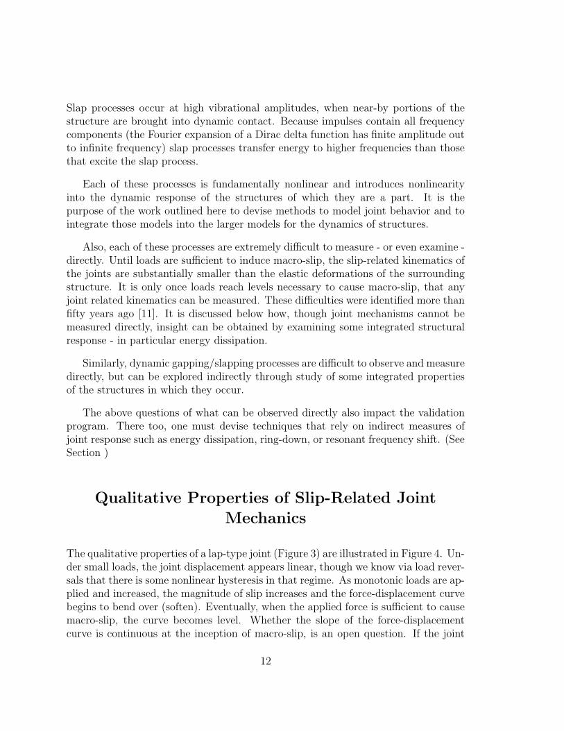
Slap processes occur at high vibrational amplitudes, when near-by portions of thestructure are brought into dynamic contact. Because impulses contain all frequencycomponents (the Fourier expansion of a Dirac delta function has finite amplitude outto infinite frequency) slap processes transfer energy to higher frequencies than thosethat excite the slap process.

Each of these processes is fundamentally nonlinear and introduces nonlinearityinto the dynamic response of the structures of which they are a part. It is thepurpose of the work outlined here to devise methods to model joint behavior and tointegrate those models into the larger models for the dynamics of structures.

Also, each of these processes are extremely difficult to measure - or even examine -directly. Until loads are sufficient to induce macro-slip, the slip-related kinematics ofthe joints are substantially smaller than the elastic deformations of the surroundingstructure. It is only once loads reach levels necessary to cause macro-slip, that anyjoint related kinematics can be measured. These difficulties were identified more thanfifty years ago [11]. It is discussed below how, though joint mechanisms cannot bemeasured directly, insight can be obtained by examining some integrated structuralresponse - in particular energy dissipation.

Similarly, dynamic gapping/slapping processes are difficult to observe and measuredirectly, but can be explored indirectly through study of some integrated propertiesof the structures in which they occur.

The above questions of what can be observed directly also impact the validationprogram. There too, one must devise techniques that rely on indirect measures ofjoint response such as energy dissipation, ring-down, or resonant frequency shift. (SeeSection )

Qualitative Properties of Slip-Related Joint

Mechanics

The qualitative properties of a lap-type joint (Figure 3) are illustrated in Figure 4. Un-der small loads, the joint displacement appears linear, though we know via load rever-sals that there is some nonlinear hysteresis in that regime. As monotonic loads are ap-plied and increased, the magnitude of slip increases and the force-displacement curvebegins to bend over (soften). Eventually, when the applied force is sufficient to causemacro-slip, the curve becomes level. Whether the slope of the force-displacementcurve is continuous at the inception of macro-slip, is an open question. If the joint

12

contains a bolt or other constraint that prevents indeterminate joint displacement,the period of macro-slip is very short. Once the macro-slip has exceeded the toleranceof the bolt in its hole, the force-displacement curve will reflect the elastic deforma-tions of the bolt and the bodies it connects. At that stage, the curve will take on alinear nature reflecting the uni-directional elasticity of those components.

Beginning of Macroslip

Pinning by Shank of Bolt

Microslip Regime

Forc

e

Displacement

(u ,F )S S

Figure 4. The monotonic pull of a simple lap joint shows the force saturates atFS as the displacement passes a critical value.

The previous section alluded to the difficulty of directly observing slip mechanisms.Joint mechanics are obscured in macroscopically measured forces and displacementsby the much larger elastic deformations of the structure. Figure 5 demonstrates thelarge elastic deformation, primarily bending, that results when a simple lap joint issubject to extension under two different pairs of boundary conditions.

The manner in which elastic deformations obscure the joint mechanics is illustratedin Figure 6 for the same problem. We see that initially, almost all of the deformationis that associated with elastic bending and only a small amount is micro-slip takingplace at the joint. Once the force exceeds that necessary to initiate macro-slip, all

13

Figure 5. The monotonic pull of a simple lap joint shows substantial bending.The top image indicates the deformation predicted by quasi-static nonlinear finiteelement analysis (Abaqus) when both sides are cantilevered and then extended. Thefigure on the bottom is cantilevered on the left and held by rollers on the right.

Figure 6. The displacements on the right hand sides of the specimens of Figure5 when subject to monotonic pull. Initially, almost all of the deformation is thatassociated with elastic bending. Once the force exceeds that necessary to initiatemacro-slip, all the incremental deformation is due to the joint.

14

the incremental deformation is due to the joint. The only element of this experimentthat relates directly to joint response is the force FS necessary to initiate macro-slip.The above is consistent with our current qualitative understanding of lap joints.

An entirely different sort of experiment is necessary to obtain more resolutionon the slip mechanisms of the joint. One class of experiment is that pioneered byGaul ([3], [4], and [5]) and improved by Gregory et. al. ([6], [15]). That class involvesimposing harmonic loads on the jointed structure and deducing energy dissipation percycle. Since the joint is the only source of energy dissipation in the jointed structure,all of the dissipation must be assigned to the joint. (Experiments with monolithic testspecimens confirm that there is no significant dissipation taking place elsewhere inthe testing apparatus.) Because the level of dissipation per cycle is small comparedto the peak elastic energy of the system, sophisticated signal processing tools andmany cycles must be employed to obtain the desired dissipation information.

Characteristically the energy dissipation appears to behave as a power of theamplitude of the harmonic driving force until the force amplitude approaches themacro-slip force FS. Figure 7 shows the general form of the dissipation functionthat one finds experimentally. There are some solutions to classical elastic-contactproblems that yield a log-log slope of exactly 3.0, but experimental data almost alwaysseems to define curves of slope between 2.0 and 3.0, represented as 3 + χ where χis a small negative number −1 < χ < 0. There are multiple plausible explanationsfor the fractional power-law relationship found experimentally. One such explanationwill be discussed in a later section of this report.

Log10(Force)

Log

10(D

issi

patio

n/C

ycle

)

slope=3

slope=

Figure 7. The dissipation per cycle in a harmonically loaded jointed structureappears to be a fractional power of the amplitude of the applied force. (See text.)

15

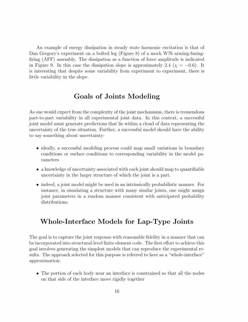
An example of energy dissipation in steady state harmonic excitation is that ofDan Gregory’s experiment on a bolted leg (Figure 8) of a mock W76 arming-fusing-firing (AFF) assembly. The dissipation as a function of force amplitude is indicatedin Figure 9. In this case the dissipation slope is approximately 2.4 (χ = −0.6). Itis interesting that despite some variability from experiment to experiment, there islittle variability in the slope.

Goals of Joints Modeling

As one would expect from the complexity of the joint mechanisms, there is tremendouspart-to-part variability in all experimental joint data. In this context, a successfuljoint model must generate predictions that lie within a cloud of data representing theuncertainty of the true situation. Further, a successful model should have the abilityto say something about uncertainty:

• ideally, a successful modeling process could map small variations in boundaryconditions or surface conditions to corresponding variability in the model pa-rameters

• a knowledge of uncertainty associated with each joint should map to quantifiableuncertainty in the larger structure of which the joint is a part.

• indeed, a joint model might be used in an intrinsically probabilistic manner. Forinstance, in simulating a structure with many similar joints, one might assignjoint parameters in a random manner consistent with anticipated probabilitydistributions.

Whole-Interface Models for Lap-Type Joints

The goal is to capture the joint response with reasonable fidelity in a manner that canbe incorporated into structural-level finite element code. The first effort to achieve thisgoal involves generating the simplest models that can reproduce the experimental re-sults. The approach selected for this purpose is referred to here as a “whole-interface”approximation:

• The portion of each body near an interface is constrained so that all the nodeson that side of the interface move rigidly together

16

Figure 8. The mock W76 AFF bolted joint and a finite element mesh used tosimulate that joint.

Figure 9. The dissipation per cycle in a harmonically loaded jointed structureappears to be a fractional power of the amplitude of the applied force. The experi-mental data shown is from nine different but nominally identical lap joints (AFF 1,AFF 2, ...).

17

• Those mutually constrained nodes are tied to a single node located approxi-mately at the center of the region of contact

• Each of the six degrees of freedom of the opposing nodes are connected to thecorresponding degrees of freedom of the opposite node by a scalar equation.

Figure 10. The “whole-interface” approach to simulation of joints reduces thenumber of degrees of freedom at a joint to one in the direction of each degree offreedom. This approach would be applied to generalized lap-type joints, includingcompression fits such as shown here.

The degrees of freedom associated with dissipation are connected by nonlinearscalar constitutive equations capable of reproducing the observed experimental dis-sipation and manifesting macro-slip at the appropriate load level. The remainingdegrees of freedom are connected by an elastic spring. This approach would be ap-propriate to a generalized class of ’lap-type’ joints, including compression joints suchas shown in Figure 10.

18

CURRENT STATUS OF WHOLE-JOINT MODELING

• All of the scalar equations are assumed to be independent.

• Two classes of nonlinear constitutive equation appropriate for whole-interfacemodeling have been developed. These are Dave Smallwood’s power-law hys-teresis model [16] and Segalman’s ([13] & [14]) class of Iwan model.

• Both of those constitutive models have been implemented in the Salinas struc-tural dynamics finite element code.

PLANNED RELATED ACTIVITIES

• It is anticipated that the loads associated with hostile environments - sucha potentially seen in the Stockpile-to-Target-Sequence (STS) - would exceedthose necessary to initiate macro-slip. An extension of the above formulationto accommodate such loads will be necessary. Also necessary to accommodatesuch environments will be accounting for time-varying normal loads. A strategyexists for dealing with these conditions in the context of Iwan models, but atime-line for implementation has not yet been set.

• An effort has been initiated to couple the nonlinear equations for the sheardegrees of freedom. It is envisioned that this coupling will be analogous to thatof flow surfaces in multi-dimensional plasticity.

A version of this coupled whole-interface formulation is targeted for third quar-ter FY04.

Iwan Modeling

To be useful, such constitutive models must have the following properties:

• They must be capable of reproducing the important features of joint response- dissipation and nonlinear stiffness.

• There must be a systematic method to deduce model parameters from joint-levelexperimental data or from very fine scale quasi-static, nonlinear finite elementmodeling of the joint region. (There are associated questions of the validationof that finite element code for each class of joint.)

19

• Integration into a structural-level finite element code must be practical.

A framework that has potential for providing that balance is that due to Iwan(1967,1968) and the work reported here addresses how that model-form can be ex-ploited to capture the important responses of mechanical joints.

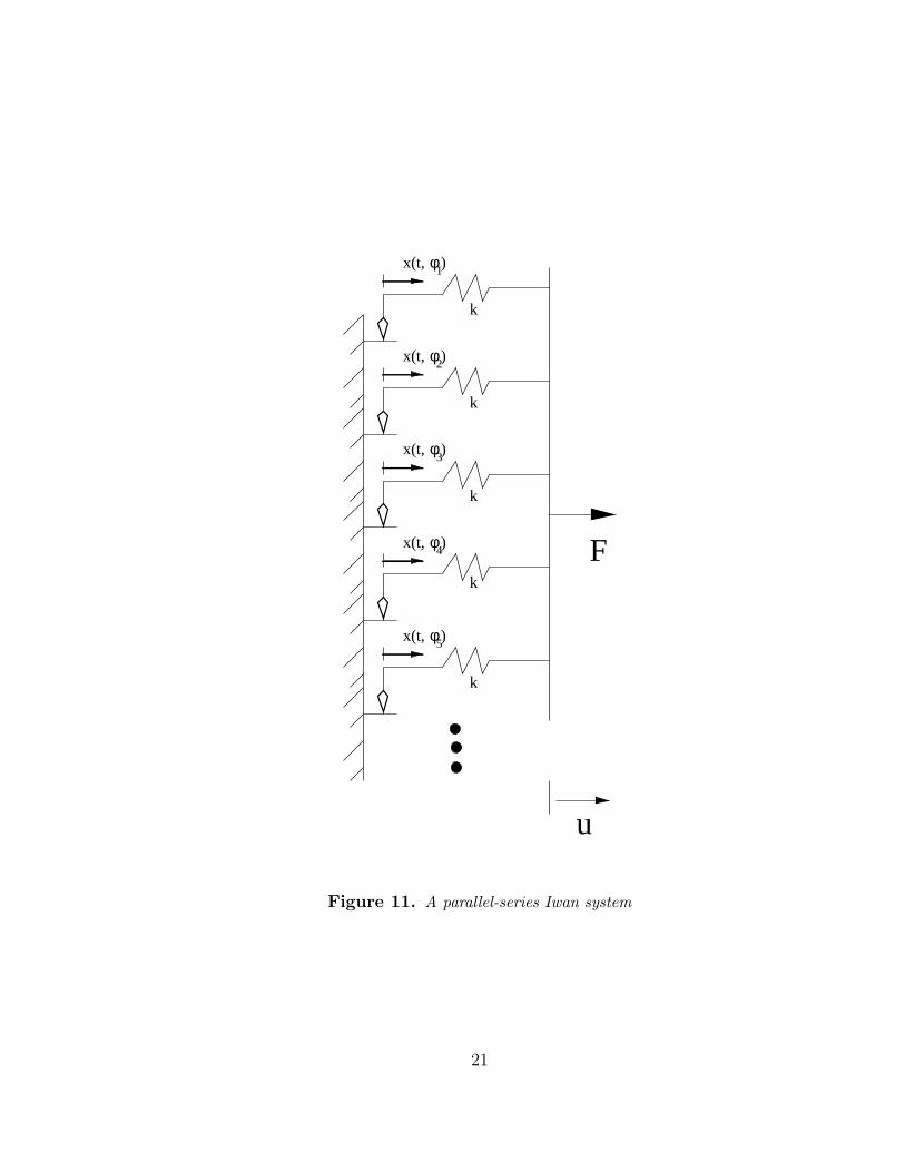
Iwan introduced constitutive models for metal elasto-plasticity that have sincebeen used in joint modeling. Of his models, the most prominent has been the parallelsystem of Jenkins elements, sometimes called the parallel-series Iwan model. As thename implies, such models consist of spring-slider units arranged in a parallel systemas indicated in Figure 11.

Mathematically, the constitutive form of the model is (Segalman, 2001)

F (t) =∫ ∞

0ρ(φ)[u(t)− x(t, φ)] dφ (1)

and

x(t, φ) =

{

u if ‖u− x(t, φ)‖ = φ0 if ‖u− x(t, φ)‖ < φ

(2)

We are now guaranteed that ‖u− x(t, φ)‖ ≤ φ. In the above, φ is a break-free forceand ρ(φ) is the population density of spring-slider pairs where the slider has strengthφ.

The parameter k was removed from the formulation through an appropriate changeof variables (Segalman, 2002). This change of variables alters the dimensions of theremaining model parameters: φ has dimensions of Length and ρ has dimensions ofForce/Length2.

Two overall parameters for the interface can be expressed in terms of the aboveintegral system. The force necessary to cause macro-slip (slipping of the whole in-terface) is denoted FS and the stiffness of the joint under small applied load (whereslip is infinitesimal) is denoted KT . For the parallel-series Iwan system, macro-slip ischaracterized by every element sliding:

u(t)− x(t, φ) = φ (3)

for all φ, so Equation 1 yields

FS =∫ ∞

0φρ(φ) dφ (4)

Similarly for the parallel-series Iwan system, no elements have slid at the inceptionof loading,

x(t, φ) = 0 (5)

20

x(t, )

x(t, )

x(t, )

x(t, )

x(t, )

u

φ1

F

φ

φ

φ

φ

2

3

4

5

k

k

k

k

k

Figure 11. A parallel-series Iwan system

21

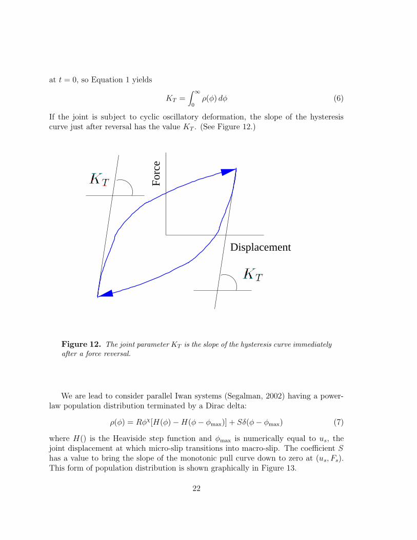
at t = 0, so Equation 1 yields

KT =∫ ∞

0ρ(φ) dφ (6)

If the joint is subject to cyclic oscillatory deformation, the slope of the hysteresiscurve just after reversal has the value KT . (See Figure 12.)

Displacement

Forc

e

Figure 12. The joint parameter KT is the slope of the hysteresis curve immediatelyafter a force reversal.

We are lead to consider parallel Iwan systems (Segalman, 2002) having a power-law population distribution terminated by a Dirac delta:

ρ(φ) = Rφχ[H(φ)−H(φ− φmax)] + Sδ(φ− φmax) (7)

where H() is the Heaviside step function and φmax is numerically equal to us, thejoint displacement at which micro-slip transitions into macro-slip. The coefficient Shas a value to bring the slope of the monotonic pull curve down to zero at (us, Fs).This form of population distribution is shown graphically in Figure 13.

22

��

��

��

��

��

��

φ

ρ(φ)

Figure 13. A spectrum that is the sum of a truncated power law distribution anda Dirac delta function can be selected to satisfy asymptotic behavior at small andlarge force amplitudes.

Substitution of Equation 7 into Equation 1 yields

F (t) =∫ φmax

0[u(t)− x(t, φ)]Rφχ dφ + S[u(t)− x(t, φmax)] (8)

Equation 2 remains unaltered.

The macro-slip force for the system becomes

FS =∫ φmax

0φρ(φ)dφ (9)

=Rφχ+2

max

(χ + 2)+ Sφmax (10)

= φmax

(

Rφχ+1max

χ + 1

)

[χ + 1

χ + 2+ β] (11)

where

β = S/

(

Rφmaxχ+1

χ + 1

)

(12)

Because χ and β are dimensionless and because FS can be measured or computedfairly directly, a preferred set of model parameters are {χ, β, FS, φmax}. For this

23

reason, one inverts Equation 11 to solve for R and employs Equation 12 to express Sappropriately:

R =FS(χ + 1)

φχ+2max (β + χ+1

χ+2)

(13)

and

S =

(

FS

φmax

)

β

β +(

χ+1χ+2

)

(14)

The interface stiffness can be computed as

KT =∫ φmax

0ρ(φ)dφ =

Rφχ+1max

(χ + 1)+ S =

Rφχ+1max

(χ + 1)(1 + β) =

FS(1 + β)

φmax(β + χ+1χ+2

)(15)

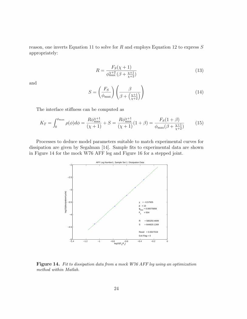
Processes to deduce model parameters suitable to match experimental curves fordissipation are given by Segalman [14]. Sample fits to experimental data are shownin Figure 14 for the mock W76 AFF leg and Figure 16 for a stepped joint.

−1.4 −1.2 −1 −0.8 −0.6 −0.4 −0.2 0−5

−4.5

−4

−3.5

−3

−2.5

−2AFF Leg Number1, Sample Set 1: Dissipation Data

log10(F0/F

s)

log1

0(di

ssip

atio

n/cy

cle)

χ = −0.57505

β = 10φ

max = 0.00075856

Fs = 504

R = 580250.4699

S = 644820.1269

Resid = 0.0027019

Exit Flag = 0

Figure 14. Fit to dissipation data from a mock W76 AFF leg using an optimizationmethod within Matlab.

24

Figure 15. Stepped specimen from which the data for the following figure (Figure16) was obtained.

Figure 16. Fit to dissipation data from a stepped specimen using an optimizationmethod within Matlab.

25

CURRENT STATUS OF IWAN MODELING

• The algorithm discussed above to fit experimental dissipation data has beenextended to capture the joint stiffness as well [14].

• That extended algorithm has been employed to find improved model parametersfor the individual legs of the Campaign 6 mock W76 AFF [14].

PLANNED RELATED ACTIVITIES

• A three legged mock W76 AFF will be subjected to transient excitation involv-ing multiple modes. The experimental results will be compared with structuraldynamics simulations where all three joints are modeled using the parametersdiscussed above.

• Research has begun on formulating a generalized model capable of accommo-dating multi-directional loading histories such as shear in two directions as wellas bending.

Hysteresis Models

A simple model that will yield a power law relationship is given by the following.

For an increasing displacement

Fu = k (d− di)− kn (d− di)n + Fi (16)

where k is a linear stiffness term, d is the displacement, di is the displacement at thelast displacement reversal, kn is a nonlinear stiffness, n is a nonlinear exponent, andFi is the force at the last reversal.

For a decreasing displacement

Fd = −k (dj − d) + kn (dj − d)n + Fj (17)

The values at the reversals are given by

Fj − Fi = k (dj − di)− kn (dj − di)n (18)

26

Equations 16 and 17 can be written as a single equation as

F − Fi = sgn(d− di) (k |di − d|+ kn |di − d|n) (19)

At the force and displacement reversals

Fu(di) = Fd(di) = Fi and Fu(dj) = Fd(dj) = Fj (20)

The forces and displacements match at the displacement reversals. The slope of theforce/displacement is

F ′u = k − nkn (d− di)

n−1 and F ′d = k − nkn (dj − d)n−1 (21)

where the prime denotes differentiation with respect to displacement. At the dis-placement reversals the slopes are

F ′u(di) = F ′

d(dj) = k and F ′u(dj) = F ′

d(di) = k + nkn(dj − di)n−1 (22)

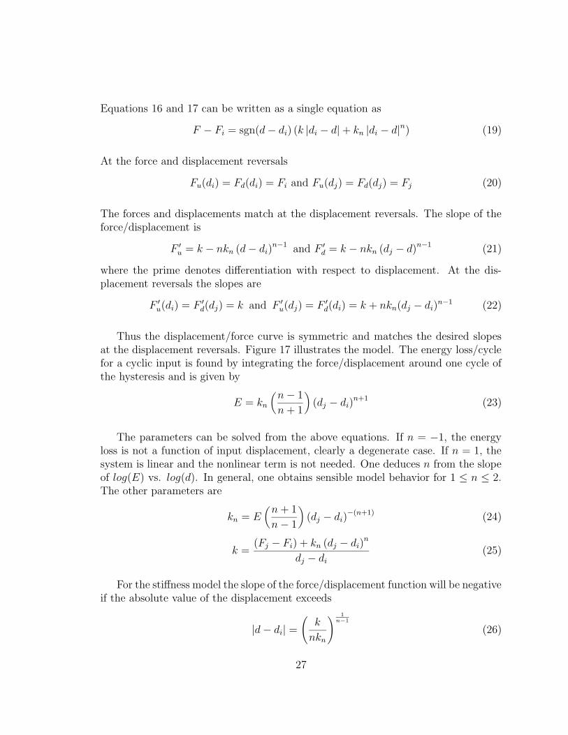
Thus the displacement/force curve is symmetric and matches the desired slopesat the displacement reversals. Figure 17 illustrates the model. The energy loss/cyclefor a cyclic input is found by integrating the force/displacement around one cycle ofthe hysteresis and is given by

E = kn

(

n− 1

n + 1

)

(dj − di)n+1 (23)

The parameters can be solved from the above equations. If n = −1, the energyloss is not a function of input displacement, clearly a degenerate case. If n = 1, thesystem is linear and the nonlinear term is not needed. One deduces n from the slopeof log(E) vs. log(d). In general, one obtains sensible model behavior for 1 ≤ n ≤ 2.The other parameters are

kn = E(

n + 1

n− 1

)

(dj − di)−(n+1) (24)

k =(Fj − Fi) + kn (dj − di)

n

dj − di(25)

For the stiffness model the slope of the force/displacement function will be negativeif the absolute value of the displacement exceeds

|d− di| =

(

k

nkn

)1

n−1

(26)

27

Figure 17. Stiffness model

|F − Fi| = k

(

k

nkn

)1

n−1

− kn

(

k

nkn

)n

n−1

(27)

If the displacement limit is reached, the force can be set to the limit force. Thelimit force can also be bounded by a coefficient of friction times the normal force asdiscussed in the next section. All the parameters of the model can be determinedby performing tests with a periodic force input and measuring the energy loss/cycleas a function of the peak input force. The model will correctly predict the energyloss/cycle as long as a power law relationship exists between the input force and theenergy loss.

To use this model one needs the following information: 1) The slope of the powerlaw relationship to derive n, 2) the energy dissipated at one peak-peak displacementlevel to derive kn. 3) The peak-peak relative displacement for a given peak-to-peakforce to derive k.

To compute the force one needs to know: 1) the displacement, 2) whether the dis-placement is increasing or decreasing, 3) whether the displacement is larger or smallerthan the displacement at the last displacement reversal, and 4) the displacement and

28

force at the last displacement reversal.

The equations can be written in a non-dimensional form as follows:

First normalize with respect to the force Fm expected to cause macro-slip. This canbe expressed in terms of the normal force, N , and the coefficient of friction, µ:

Fm = µN (28)

The displacement is normally dominated by the linear displacement term, hence areasonable displacement for normalization is the displacement calculated from thelinear term which will cause macro-slip.

dm = µN/k = Fm/k (29)

Equation 19 can now be written in a non-dimensional form as

F − Fi

Fm

= sgn(d− di)

(

|d− di|

dm

)

1− kn

(

|d− di|

dm

)n−1

(30)

where

kn = knF nm

kn−1(31)

Normally

kn

(

|d− di|

dm

)n−1

<< 1 (32)

One more modification is needed to make the model useful. If the hysteresis curvecrosses a previous hysteresis curve the reversal point must revert to the previousreversal. The following outlines the procedure.

Let dr(j) and Fr(j) be a history of reversals, where j is the latest reversal. The rever-sals will alternate between the displacement changing from increasing-to-decreasingand decreasing-to-increasing. Let d(i) be the latest displacement.

If F/Fm > 1we have macro-slip and the force is set to F = Fmsgn(F ) .

If the displacement is increasing (d(i) > d(i − 1)) and d(i) > dr(j − 1), or if thedisplacement is decreasing (d(i) < d(i− 1) ) and d(i) < dr(j − 1), then

Fr(j) = Fr(j − 2) and dr(j) = dr(j − 2) (33)

This is illustrated in Figure 18.

29

Figure 18. Hysteresis for waveform with third harmonic added

Generalization to include parameters which are a function of the normalforce

The model can be generalized to include parameters that are simple functions of thenormal force as follows. For the stiffness model let the parameters be a polynomialfunction of the normal force, N .

k =Mk∑

m=0

AmNm , kn =Mkn∑

m=0

BmNm and n =Mn∑

m=0

CmNm (34)

Normally only a very few terms will be included in the sums, probably 0, 1, or 2at most. If Mk = Mkn = Mn = 0, the model becomes the stiffness model discussedearlier.

Compliance Model

Smallwood has also developed a similar model based on compliance instead of stiff-ness. This nature of the model is similar to the stiffness formulation and is fullydocumented in [16].

30

Measurement of the model parameters from experiments

In a normal experiment the joint is in series with another structure. It is assumed thatthe experimental structure exclusive of the joint can be modeled as a linear stiffness,ks . The stiffness of the joint is modeled as, kj. The stiffness of the combined system iskc. Appropriate experiments can usually measure ks and kc , but rarely kj . Assumingthe elements are in series allows the stiffness of the joint to be calculated from

kj =kcks

ks − kc(35)

Application to Specific Configurations

The whole-interface models discussed above are designed in a manner that involvedlocal relative deformations. Such a formulation can be used in a finite element contextto capture more distributed contacts.

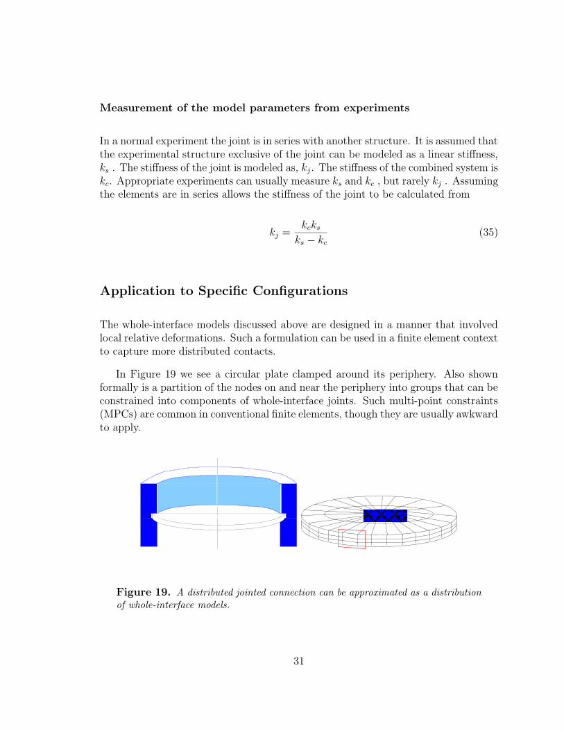
In Figure 19 we see a circular plate clamped around its periphery. Also shownformally is a partition of the nodes on and near the periphery into groups that can beconstrained into components of whole-interface joints. Such multi-point constraints(MPCs) are common in conventional finite elements, though they are usually awkwardto apply.

��

Figure 19. A distributed jointed connection can be approximated as a distributionof whole-interface models.

31

Uncertainty Quantification

For reasons discussed below, each joint model form must be accompanied by anassociated quantification of the uncertainty of calculations based on that model. Thefollowing addresses this issue in the context of the parallel-series Iwan model, butsimilar analysis can and must be done for any other joint model used in predictivestructural mechanics.

The form of the Iwan model described in this report is a deterministic frameworkfor simulating the dynamic behavior of mechanical lap joints. The current modelis cast in a four-parameter form, and it is hoped that it can accurately simulatemechanical response and energy dissipation in joints. When either the external forceon the joint or the external joint deformation is specified, then the non-specifiedquantity can be computed, and the two can be used to compute the energy dissipatedin the joint.

Of course, when either the force or deformation is specified as a deterministicsignal, then the other quantity is deterministic, and the energy dissipated is reckoneda deterministic quantity. This deterministic construct may be satisfactory undermany circumstances, however, real joint behavior is stochastic, and when the levelof stochasticity is relatively large, then it must be accounted for in modeling andanalysis. This stochasticity is reflected in measurements taken during physical exper-iments. Some of the stochasticity arises from reducible sources, and the remainderfrom irreducible sources. For example, one ever-present source of reducible random-ness is transducer measurement error. All measurements are contaminated with noisethat arises from electro-mechanical sources. Most of the data reduction proceduresin use today seek to diminish the effects of this noise source with increasing numbersof measurements or measurement duration.

There are many sources of irreducible randomness, but usually, the most substan-tial source is termed ”unit-to-unit variability.” Every structural system that consistsof an ensemble of realizations of nominally identical elements is actually composed ofelements that differ in their details. Sometimes these differences are great and some-times small. Sometimes the differences are reflected strongly in specific measures ofbehavior and weakly in others. Nevertheless, they are always present. Experimentson relatively simple structures have shown that unit-to-unit variability is the singlesource that contributes the most to structural randomness [1].

It is anticipated that mechanical joints are random in nature, and indeed, it isthought that they may be the major contributors to the randomness that arises fromunit-to-unit variability. In view of this, it is important to represent this randomness

32

in the Iwan (or other) model for mechanical joint behavior. This can be accomplishedby making the four parameters of the Iwan model random variables. In general, thefour model parameters R, S, χ, and φmax specified in Eq. 7, can be assumed random.(Alternatively, one could as well work with parameters FS, β, χ, and φmax.) The mostcomplete specification identifies their joint probability distribution. Any sufficientlyspecified form of a stochastic Iwan model would be capable of generating a plausiblerealization of mechanical joint behavior consistent with experimental results. Further,a probabilistic model should be capable of establishing probabilistic joint behaviorsderivable from the parameters.

Though the most complete specification of the Iwan model identifies the jointprobability distribution of the model parameters, the resources for accomplishingsuch a specification via the methods of statistics may not exist. Therefore, a partial,or approximate, probability model may provide the only practical alternative. Sucha probability model might consist of the marginal probability distributions of theindividual Iwan model parameters, along with the matrix of correlations between pairsof parameters. A model containing less information, and one that would be easier tospecify, would simply specify statistical moments (say, first and second order) of theIwan model parameters.

Because the Iwan model parameters may be non-Gaussian and strongly depen-dent, a useful approach to their probabilistic modeling may lie in the Karhunen-Loeve([2]) approach to stochastic modeling. This approach, in effect, creates a decompo-sition for the Iwan model parameters that permits their expression in terms of asequence of uncorrelated random variables. Whatever approach is taken to the prob-abilistic modeling of the Iwan joint, a statistical analysis that accounts for the limitedexperimental data used to identify the Iwan model parameters should be performed.The first investigation of the Iwan model will:

• Identify the parameters of the Iwan model from experimental data.

• Perform second-order statistical analysis on the parameter realizations.

• Specify a moment-based probability model with the results.

The above discussion has been fairly general in nature. As the modeling effort isrefined, the effort in uncertainty quantification will be refined also. As the uncertaintyquantification effort matures, it will provide tools necessary to initiate a rigorousvalidation effort.

33

Special Interface Models

The whole-interface models are the most sophisticated joint modeling tool availableat this time and offer capabilities for modeling of structures that have not existed upto this time. On the other hand, one can list the limitations of this approach andseek an approach that is not subject to those limitations. Among the limitations ofwhole-interface elements are

• The constitutive parameters are selected to reproduce the experimental (orminutely simulated) behavior of that specific joint under a specific type or blendof specific types of load history. In this sense the answer has to be known inadvance.

• With the multi-point constraints imposed on each side of the interface, stressrecovery in the joint and interface is precluded.

• This approach, developed for lap-type joints, would be difficult to generalize toother classes of joint.

• Implementation of this approach, though possible via Lagrange multipliers orpenalty functions in standard finite element architectures, is awkward to imple-ment.

• This approach is also awkward for the analyst, who must define the MPCs andspecify the governing equations to connect them.

One general strategy to overcome the above limitations would involve a classof interface elements that capture the artifacts of micro-slip without employing themicro-size mesh necessary to follow those kinematics. The strategy envisioned here isone where instantaneous normal traction is used as a proxy for the detailed kinematicsof the evolving contact kinematics, thus indirectly capturing the kinematics identifiedby Heinstein and Segalman [8]. The constitutive nature of such interface elementsis yet to be defined, but one can expect that among the parameters of the elementwill be the initial distribution of normal traction over the element and that the shearforce/shear traction response of the element will be modulated by the dynamic loadsseen at its nodes. Some of this vision is illustrated in Figure 20.

Of course, this approach can only be meaningful if the special interface elementsconverge; as one refines the mesh, the predicted structural response converges to thatof a very finely meshed conventional finite element analysis.

34

The first challenge is to find a constitutive model that is capable of yieldingthe appropriate dissipation behavior as shear and normal tractions are varied in acoordinated manner .

Interface Element

Time Varying Normal Loads:Part of Dynamics Calculations

Initial Normal Tractions:from preliminary non−linear statics calculations

Figure 20. Scheme for special interface elements to capture micro-macro slipemploying a relatively coarse mesh.

Iwan Series-Series Illustration

One very simple candidate constitutive model that might serve as a basis for theinterface model is a series-series model such as shown in Figure 21. This series ar-rangement of Jenkins elements opposing a series arrangements of elastic elements wasnever explicitly considered by Iwan, but it is in the same spirit of the parallel-seriesIwan systems discussed earlier.

Because of the spatial distribution of the Jenkins elements, a distribution of normaltraction over an element is also seen among the ordered Jenkins elements. If oneassumes that the strength of each slider is proportional to a local normal traction,the response of this system is seen to be modulated by any time-varying spatialdistribution of normal tractions. (See Figure 22.)

35

��

��

��

��

Figure 21. The series-series Iwan model is the basis for one possible interfacemodel.

��

��

��

Figure 22. Spatially varying normal tractions result in corresponding distributionsof slider strength among the Jenkins elements.

36

Preliminary calculations indicate that a spatially linearly varying normal trac-tion distribution acting on top of a steady uniform distribution and changing syn-chronously with shear loads on the boundaries will result in the fractional power-lawenergy distribution that one associates with joints.

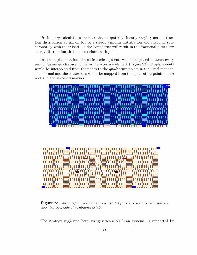
In one implementation, the series-series systems would be placed between everypair of Gauss quadrature points in the interface element (Figure 23). Displacementswould be interpolated from the nodes to the quadrature points in the usual manner.The normal and shear tractions would be mapped from the quadrature points to thenodes in the standard manner.

��

��

��

��

��

��

��

��

��

��

��

��

��

��

��

� !"

#$

Figure 23. An interface element would be created from series-series Iwan systemsspanning each pair of quadrature points.

The strategy suggested here, using series-series Iwan systems, is supported by

37

some encouraging preliminary calculations, but it is presented here primarily for thepurpose of illustration. It will probably be one of many approaches that will beexplored.

It should be mentioned that series-series Iwan systems could have been consid-ered for whole-interface modeling in much the same manner that parallel-series Iwanmodels were employed. On the other hand, the series-series systems offer a specialadvantage in building the above sort of interface element - they explicitly account forspatial gradients in the normal tractions. It does not appear that such a dependencecould be built into the parallel-series models.

Advantages of the Special Interface Element Concept

Special interface elements - if devised to have the features described above - wouldhave substantial advantages

• These elements should capture the necessary physics of joints in a manner em-ploying elements of size comparable to those elements used to capture the restof the structure.

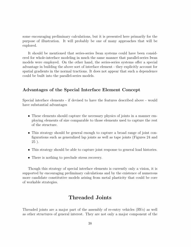
• This strategy should be general enough to capture a broad range of joint con-figurations such as generalized lap joints as well as tape joints (Figures 24 and25 ).

• This strategy should be able to capture joint response to general load histories.

• There is nothing to preclude stress recovery.

Though this strategy of special interface elements is currently only a vision, it issupported by encouraging preliminary calculations and by the existence of numerousmore candidate constitutive models arising from metal plasticity that could be coreof workable strategies.

Threaded Joints

Threaded joints are a major part of the assembly of re-entry vehicles (RVs) as wellas other structures of general interest. They are not only a major component of the

38

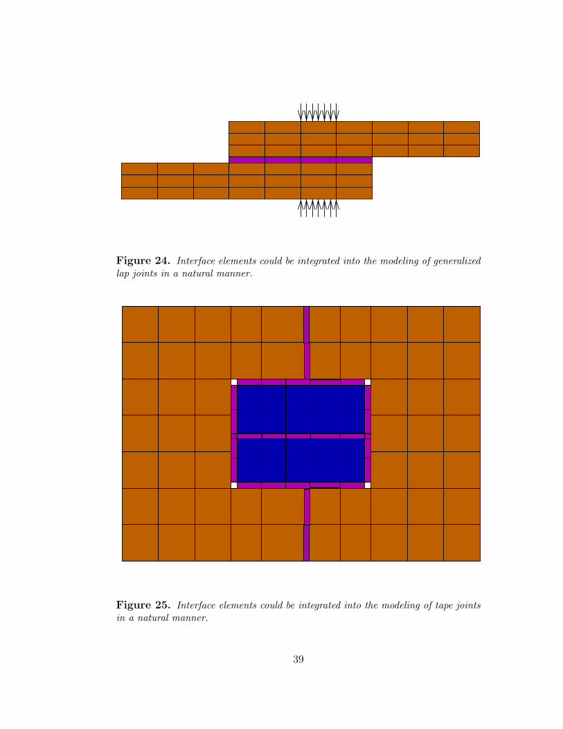
Figure 24. Interface elements could be integrated into the modeling of generalizedlap joints in a natural manner.

Figure 25. Interface elements could be integrated into the modeling of tape jointsin a natural manner.

39

mechanical integrity of the structure, but also a major path for mechanical energyflow through the system. In fact, the energy flow through a threaded joint mightbe a more important factor than mechanical energy dissipation since it is generallybelieved that there is very little energy dissipation in tightened threaded connections.(See [7] for an example.)

As is the case generally for joints, very finely meshed finite element analysis ofjoints can lend insight into joint mechanics and can even be used to deduce parametersfor lower order models, but such fine meshes would be impractical for direct usein structural dynamics modeling. The scale of the resolution necessary to capturethreaded joint mechanics with conventional finite element analysis is indicated by themesh in Figure 26.

Figure 26. Approximate mesh refinement necessary to capture detailed threadinteractions.

Since there is very little quantitative data on energy dissipation of threaded con-nections, the initial effort in threaded joint modeling focuses on

• capturing the manner in which statically indeterminate equilibrium is achieved

40

in a threaded joint

• quantitatively representing the manner of mechanical energy transmission throughthe joint

• predicting the energy dissipation in some rational manner.

Clearly this modeling effort must occur along with an active program of experi-mental investigation and validation.

The geometry of most immediate interest to Sandia’s mission is that of buttressthreads (Figure 27). Insight into the joint mechanisms is obtained by performingfinite element analysis (Figure 28) on a plain-strain representation for a single threadpair. When we constrain horizontal motion of the right and left sides of the threadpair and pull down on the member on the right and pull up on the member on theleft, we obtain the normal and shear stresses shown in Figures 29 and 30. We seethat the normal traction has the anticipated singularities at the edges of the contactpatch. The shear stress is nearly uniform within the contact patch.

Figure 27. Opposing buttress threadsin joint.

Figure 28. Corresponding finiteelement mesh.

We look for a simple, low order model that captures the general behavior gener-ated by the detailed finite-element model discussed above. We have considered two

41

Figure 29. Pressure across threadinterface.

Figure 30. Shear stress across ThreadInterface.

approaches

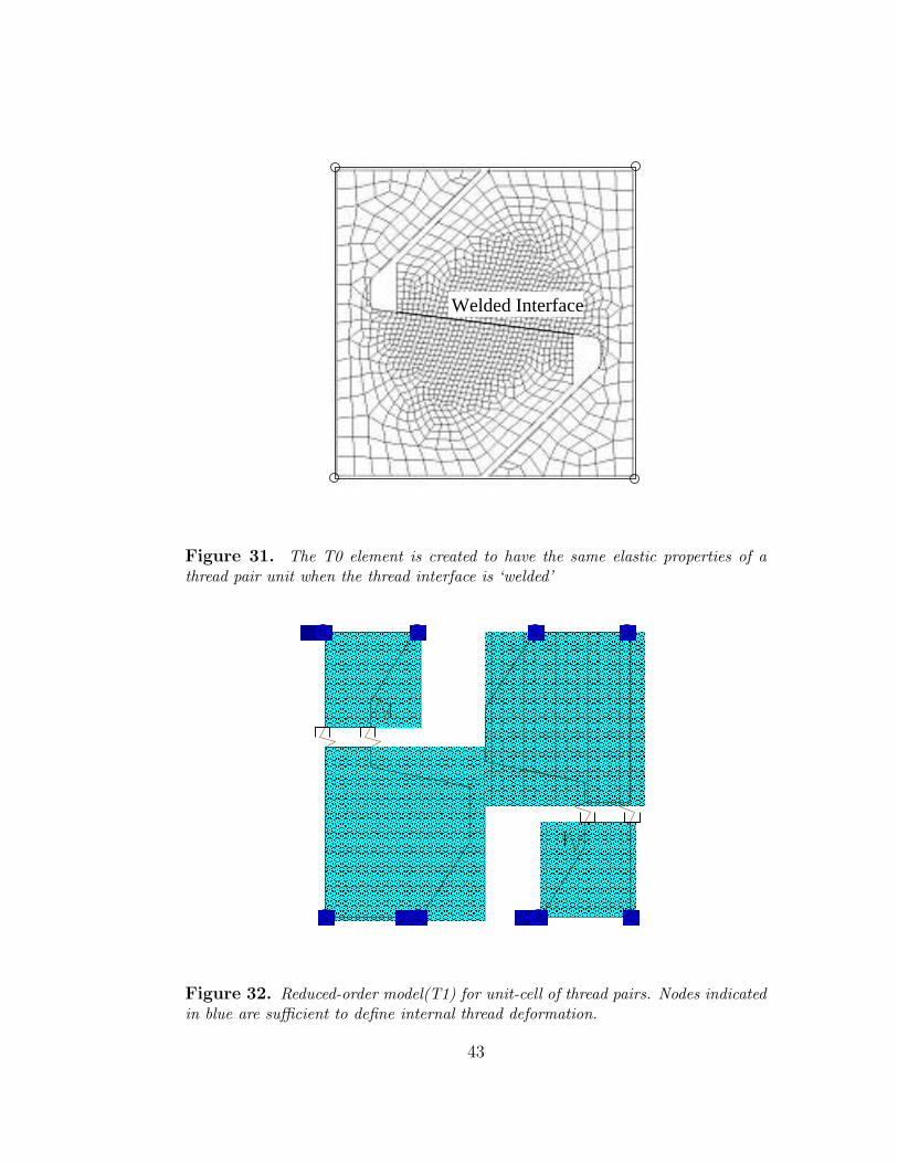
• Thread Model T0 Here we consider a four node quad element (8-node hex in3-dimensional analysis) whose nodal displacements correspond to those of thecorners of a unit thread pair. This elastic element will have the propertiesof the thread pair if the thread interface is ‘welded’. (See Figure 31) It isanticipated that this approach can be implemented in a straight-forward mannerand will be manifest in ASCI code in FY03. In the near term, implementationin analysis will involve a laborious process of specifying properties of equivalentanisotropic material. Later, a special element will be coded for which most ofthose specifications will be done automatically.

• Thread Model T1: For this we have begun investigating the low-order modelshown in Figure 32. This model - involving rigid components, preloaded slid-ers, linear springs, and uni-directional springs - does have the gross deforma-tional features and normal traction stress concentrations predicted by the finite-element model. The finite element results indicate a nearly uniform shear stressover the contact patch due to the specified loading; the two discrete slidersshould result in identical dissipation so long as the shear stress varies linearlyover the contact patch.

It has not yet been determined how to map this low order model into a finiteelement of conventional topology, and that is one of the foci of current research.

42

Welded Interface

Figure 31. The T0 element is created to have the same elastic properties of athread pair unit when the thread interface is ‘welded’

��

��

��

��

��

��

��

��

��

��

��

��

��

Figure 32. Reduced-order model(T1) for unit-cell of thread pairs. Nodes indicatedin blue are sufficient to define internal thread deformation.

43

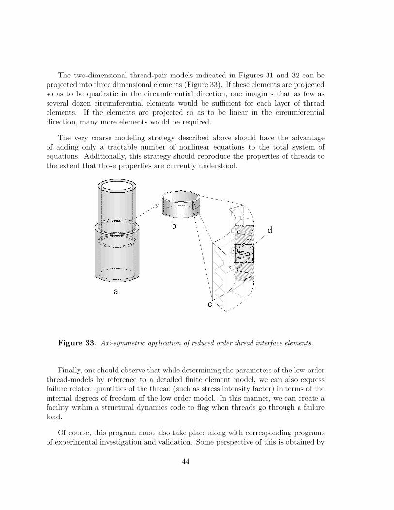
The two-dimensional thread-pair models indicated in Figures 31 and 32 can beprojected into three dimensional elements (Figure 33). If these elements are projectedso as to be quadratic in the circumferential direction, one imagines that as few asseveral dozen circumferential elements would be sufficient for each layer of threadelements. If the elements are projected so as to be linear in the circumferentialdirection, many more elements would be required.

The very coarse modeling strategy described above should have the advantageof adding only a tractable number of nonlinear equations to the total system ofequations. Additionally, this strategy should reproduce the properties of threads tothe extent that those properties are currently understood.

Figure 33. Axi-symmetric application of reduced order thread interface elements.

Finally, one should observe that while determining the parameters of the low-orderthread-models by reference to a detailed finite element model, we can also expressfailure related quantities of the thread (such as stress intensity factor) in terms of theinternal degrees of freedom of the low-order model. In this manner, we can create afacility within a structural dynamics code to flag when threads go through a failureload.

Of course, this program must also take place along with corresponding programsof experimental investigation and validation. Some perspective of this is obtained by

44

observing that the detailed finite element models from which low-order models willbe derived are themselves not yet validated.

Slap/Gapping Modeling

Slapping and gapping are processes that can be expected in most weapons systems,but they are generally expected in environments of high amplitude excitation. Slap-ping is observed most strongly through indirect evidence: when a built up structureis subject to high amplitude but frequency limited excitation, the measured accelera-tions at the far side of the structure include components at much higher frequencies.

Several ASCI codes (Adagio, Andante, Presto) have slap/gapping features builtin as core features of the code and similar features are being added to Salinas. Be-cause current codes (including the ASCI codes) address slapping through direct timeintegration, their time steps must be exceedingly small and their meshes exceedinglyfine. It is therefore prohibitive to compute the high-frequency response of continuingslapping processes over long times (seconds). This topic would appear to be veryfertile for a new mathematical formulation.

Another flavor of this problem has to do with gaps opening up and closing ona slow time scale, modulating stiffness of the structure as seen by higher frequencyevents.

These are important but difficult issues. Major efforts will focus on addressingthem as more urgent, slip-related milestones are accomplished.

Experimental Program

This document focuses on the road map of the joints modeling effort, but some wordsmust be said about the experimental program since so much of the progress of themodeling is contingent on experimental results.

Basic Experiments (ESRF)

Fundamental research experiments funded under Engineering Sciences Research Foun-dations have been collecting dissipation data on lap-type joints for several different

45

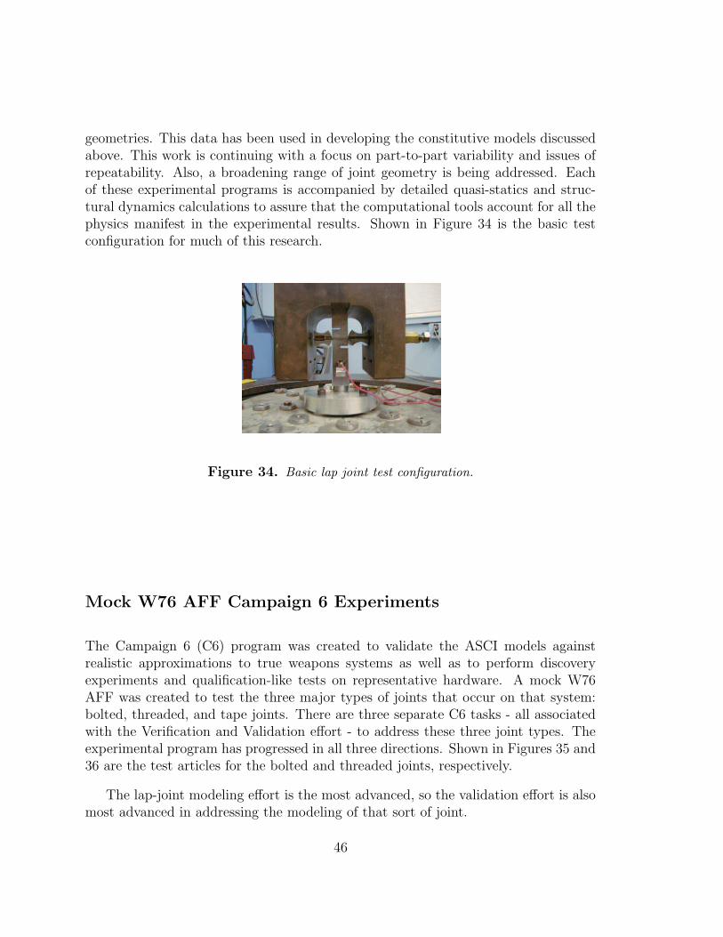
geometries. This data has been used in developing the constitutive models discussedabove. This work is continuing with a focus on part-to-part variability and issues ofrepeatability. Also, a broadening range of joint geometry is being addressed. Eachof these experimental programs is accompanied by detailed quasi-statics and struc-tural dynamics calculations to assure that the computational tools account for all thephysics manifest in the experimental results. Shown in Figure 34 is the basic testconfiguration for much of this research.

Figure 34. Basic lap joint test configuration.

Mock W76 AFF Campaign 6 Experiments

The Campaign 6 (C6) program was created to validate the ASCI models againstrealistic approximations to true weapons systems as well as to perform discoveryexperiments and qualification-like tests on representative hardware. A mock W76AFF was created to test the three major types of joints that occur on that system:bolted, threaded, and tape joints. There are three separate C6 tasks - all associatedwith the Verification and Validation effort - to address these three joint types. Theexperimental program has progressed in all three directions. Shown in Figures 35 and36 are the test articles for the bolted and threaded joints, respectively.

The lap-joint modeling effort is the most advanced, so the validation effort is alsomost advanced in addressing the modeling of that sort of joint.

46

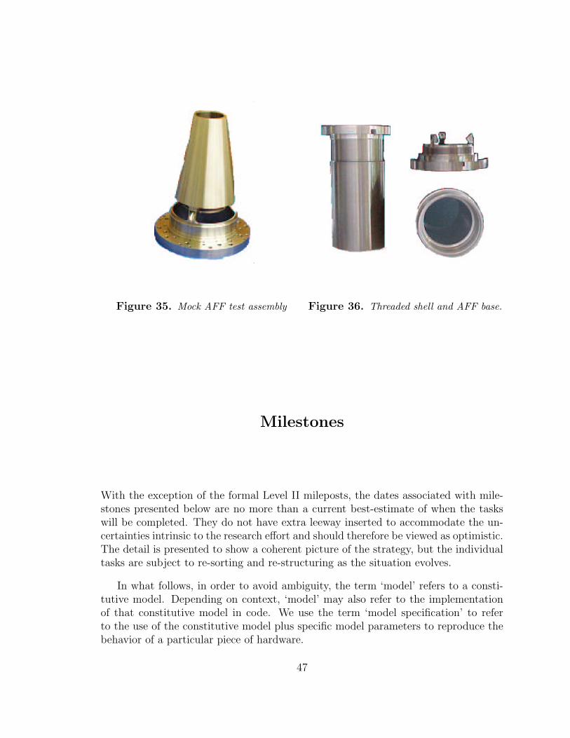
Figure 35. Mock AFF test assembly Figure 36. Threaded shell and AFF base.

Milestones

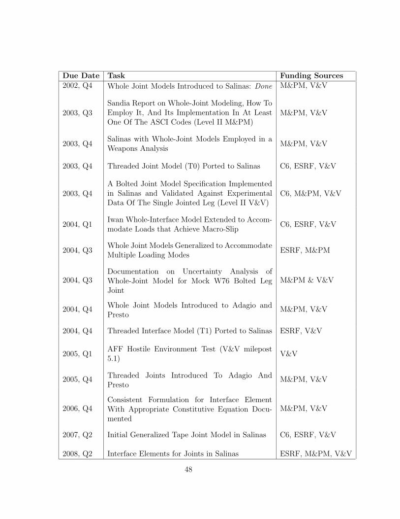
With the exception of the formal Level II mileposts, the dates associated with mile-stones presented below are no more than a current best-estimate of when the taskswill be completed. They do not have extra leeway inserted to accommodate the un-certainties intrinsic to the research effort and should therefore be viewed as optimistic.The detail is presented to show a coherent picture of the strategy, but the individualtasks are subject to re-sorting and re-structuring as the situation evolves.

In what follows, in order to avoid ambiguity, the term ‘model’ refers to a consti-tutive model. Depending on context, ‘model’ may also refer to the implementationof that constitutive model in code. We use the term ‘model specification’ to referto the use of the constitutive model plus specific model parameters to reproduce thebehavior of a particular piece of hardware.

47

Due Date Task Funding Sources2002, Q4 Whole Joint Models Introduced to Salinas: Done M&PM, V&V

2003, Q3Sandia Report on Whole-Joint Modeling, How ToEmploy It, And Its Implementation In At LeastOne Of The ASCI Codes (Level II M&PM)

M&PM, V&V

2003, Q4Salinas with Whole-Joint Models Employed in aWeapons Analysis

M&PM, V&V

2003, Q4 Threaded Joint Model (T0) Ported to Salinas C6, ESRF, V&V

2003, Q4A Bolted Joint Model Specification Implementedin Salinas and Validated Against ExperimentalData Of The Single Jointed Leg (Level II V&V)

C6, M&PM, V&V

2004, Q1Iwan Whole-Interface Model Extended to Accom-modate Loads that Achieve Macro-Slip

C6, ESRF, V&V

2004, Q3Whole Joint Models Generalized to AccommodateMultiple Loading Modes

ESRF, M&PM

2004, Q3Documentation on Uncertainty Analysis ofWhole-Joint Model for Mock W76 Bolted LegJoint

M&PM & V&V

2004, Q4Whole Joint Models Introduced to Adagio andPresto

M&PM, V&V

2004, Q4 Threaded Interface Model (T1) Ported to Salinas ESRF, V&V

2005, Q1AFF Hostile Environment Test (V&V milepost5.1)

V&V

2005, Q4Threaded Joints Introduced To Adagio AndPresto

M&PM, V&V

2006, Q4Consistent Formulation for Interface ElementWith Appropriate Constitutive Equation Docu-mented

M&PM, V&V

2007, Q2 Initial Generalized Tape Joint Model in Salinas C6, ESRF, V&V

2008, Q2 Interface Elements for Joints in Salinas ESRF, M&PM, V&V

48

Closing

The road map presented above shows a variation in detail and resolution from placeto place reflecting the current levels of effort in each aspect of the problem. It isanticipated that as the research effort progresses and as our understanding of eachjoint-related topic matures, the planning process will have more resolution in someareas and changed perspectives in others. Additionally, as new strategies arise and areweighed against those currently envisioned, the road map directions will be modifiedappropriately. For these reasons, it is expected that this document will undergoperiodic formal revisions.

One of the areas for which the road map will be refined further as the research effortmatures has to do with the intrinsic probabilistic nature of joint mechanics. Becauseof that nature of joints, the ultimate goal of the joint modeling effort will include theformulation and implementation of models that yield probabilistic predictions as wellas the formulation of methods to validate those probabilistic models.

Finally, a few comments should be made about the essential etiology of jointmechanics. As discussed in Section above, joint mechanisms cannot be observeddirectly. In other topics for which this is the case, a “first principles” understandingtends to come last, and the evolution of understanding occurs in the following broadsteps:

• A large number of experiments or observations is performed to obtain a generaland qualitative understanding of the underlying phenomena.

• Eventually sufficient study of the above observations yields to simple descriptiveequations that capture a preponderance of the trusted data.

• Finally, once the relevant research community has had time to digest the descrip-tive equations, it hones its understanding of the underlying physics to develop“first principles” explanations.

Such was the story of metal plasticity. The first names in the literature are ex-perimentalists who documented the phenomena (such as Ludwik, G. I. Taylor, andOrowan). The next slew of investigators who impacted metal plasticity were thosewho captured the experimental observations in empirical constitutive equations (suchas Westergaard, Prager, and Drucker). The dislocation theory of metal plasticitycame last. (A similar evolution is associated with celestial mechanics: Brahe →Kepler → Newton).

49

The above discussion of etiology suggests that investigation of joint mechanics willhave a similar evolution. The development of suitable joint models requires not onlya process of systematic investigation, but also the search for suitable concepts.

50

References

[1] R.J. Aumann, A. S. McCarty, and C. C. Olson, Identification of RandomVariation in Structures and Their Parameter Estimates, Proceedings of theXXI International Modal Analysis Conference, Orlando, Florida, 2003

[2] R. Ghanem and Spanos, Stochastic Finite Elements: A Spectral Approach,Springer-Verlag, New York, 1991

[3] L. Gaul and S. Bohlen, The Nonlinear Transmission Behavior of Joints,Zeitschrift fur Angewandte Mathematik und Mechanik, v. 64, No. 4, pp. T45-T48, 1984

[4] L. Gaul, J. Lenz, Nonlinear Dynamics of Structures Assembled by BoltedJoints, ACTA MECHANICA, 125, No. 1-4, pp. 169-181, 1997

[5] M. Hanss, S. Oexl, L. Gaul, Identification of a bolted-joint model with fuzzyparameters loaded normal to the contact interface, Mechanics Research Com-munications 29 pp. 177-187, 2002

[6] D. L. Gregory, D. O. Smallwood, M. A. Nusser, R. G. Coleman, ExperimentalDevice to Study the Damping in Bolted Joints, (DETC99/VIB-8190), pre-sented at the 1999 ASME Design Engineering Technical Conferences, Septem-ber 12-15, Las Vegas, Nevada, 1999. (Unfortunately, the report did not showup in the conference proceedings, but a copy of the paper can be obtainedfrom the lead author.)

[7] N. R. Hansen, V. I. Bateman, R. G. Bell, and F. A. Brown, Shock Trans-missibility of Threaded Joints, Proceedings of the 67th Shock and VibrationSymposium, Vol I, Monterey,CA, November 1996.

[8] M. W. Heinstein and D. J. Segalman, Bending Effects in the Frictional En-ergy Dissipation in Lap Joints, SAND2002-0083, Unlimited Release, PrintedJanuary 2002.

[9] W. D. Iwan, A Distributed-Element Model for Hysteresis and Its Steady-StateDynamic Response, Journal of Applied Mechanics Vol. 33, 1966, pp 893-900.

[10] W. D. Iwan, On a Class of Models for the Yielding Behavior of Continuous andComposite Systems, Journal of Applied Mechanics Vol. 34, 1967, pp 612-617.

[11] D. J. Mead, “Structural Damping and Damped Vibration”, Applied MechanicsReviews, Vol. 55, no 6, November 2002, R45-R54.

51

[12] M. Persson, New Scientist, vol. 160 no. 2156, p.30, 1998(http://fy.chalmers.se/ tfymp/Homepage/friction.html).

[13] D. J. Segalman, An Initial Overview of Iwan Modeling for Mechanical Joints,SAND2001-0811,Unlimited Release, March 2001

[14] D. J. Segalman, A Four-Parameter Iwan Model for Lap-Type Joints,SAND2002-3828, Unlimited Release, Printed November 2002

[15] D.O. Smallwood, D.L. Gregory, and R. G. Coleman, Ronald, Damping in-vestigations of a simplified frictional shear joint, Proceedings of the 71stShock and Vibration Symposium held in Arlington, VA, November 6-10, 2000(SAND2000-1929C)

[16] D.O. Smallwood, D.L. Gregory, and R.G. Coleman, A Three-Parameter Con-stitutive Model for a Joint which Exhibits a Power Law Relationship BetweenEnergy Loss and Relative Displacement, 72nd Shock and Vibration Sympo-sium, Destin, FL, Nov. 2001. (Available form SAVIAC).

52

DISTRIBUTION:

1 Prof. Adnan AkayMech. Engineering Dept.Carnegie Mellon Univ.Pittsburgh, PA 15213-3890

3 Prof. Lawrence A. BergmanUniv. of Illinois306 Talbot Lab104 S. Wright St.Urbana, IL 61801

1 Prof. Robert CarpickDept. Engineering Physics1500 Engineering DriveUniversity of WisconsinMadison, WI 53706

1 Dr. Luise CouchmanOffice of Naval ResearchBallston Centre Tower One800 North Quincy StreetArlington, VA 22217-5660

1 Dr. Scott DoeblingLos Alamos NationalLaboratory, MS P946Los Alamos, NM 87545

1 Professor Larissa GorbatikhDepartment of Mech. Engr.Mech. Eng. Bldg.The Univ. of New MexicoAlbuquerque, NM 87131

1 Dr. Steve GriffinBoeing SVS4411 The25 Way NESuite 350Albuquerque, NM 87109

1 Dr. Jason HinkleAerospace Engr. SciencesCampus Box 429Univ. of ColoradoBoulder, CO 80309-0429

1 Dr. Norman F. HunterLos Alamos National Labora-toriesMS C931 ESA-MTLos Alamos, NM 87545

1 Prof. Dan KammerDept. Engineering Physics1500 Engineering DriveUniversity of WisconsinMadison, WI 53706

1 Dr. Marie Levine-WestJet Propulsion LaboratoryScience and Technology De-velopment Section4800 Oak Grove DrivePasadena, CA 91109-8099

1 Dr. Dean MookAFOSR/NA4015 Wilson Boulevard,Mail Room 713Arlington VA 22203-1954

1 Prof. K.C. ParkAerospace Engr. SciencesCampus Box 429Univ. of ColoradoBoulder, CO 80309-0429

1 Prof. Lee PetersonAerospace Engr. SciencesCampus Box 429Univ. of ColoradoBoulder, CO 80309-0429

53

1 Dr. Chris PettitAFRL/VASD,Bldg. 146, 2210 Eighth St.,Wright Patterson AFBOH 45433

1 Prof. Michael PleshaDept. Engineering Physics1500 Engineering DriveUniversity of WisconsinMadison, WI 53706

1 Prof. D. Dane QuinnDepartment of Mech. Engr.College of Engr.The Univ. of Akron107b Auburn Science andEngr. CenterAkron, OH 44325-3903

1 Professor Henry SchreyerDepartment of Mech. Engr.Mech. Eng. Bldg.The Univ. of New MexicoAlbuquerque, NM 87131

1 Professor Andrew SmythColumbia Univ.,ÄMail Code 4709500 West 120th StreetNew York, NY 10027

1 Dr. W. Woytek TworzydloAltair Engr., Inc.7800 Shoal Creek Blvd, Suite290EAustin, TX 78757-1024

1 Dr. Y.C. YiuLockheed Martin Missiles &SpaceOrganization E4-20 Bldg. 1541111 Lockheed Martin WaySunnyvale, CA 94089

1 MS 139Lott, Stephen E , 9905

1 MS 553Bateman, Vesta I , 9126

1 MS 553Smallwood, David O , 9124

1 MS 555Garrett, Mark S , 9122

1 MS 555Gregory, Danny L , 9122

1 MS 555Stasiunas, Eric Carl , 9124

1 MS 557Baca, Thomas J , 9125

1 MS 557Carne, Thomas G , 9124

1 MS 557Epp, David S , 9125

1 MS 557Mayes, Randall L , 9125

1 MS 557O’Gorman, Christian, 9125

1 MS 557Paez, Thomas L , 9133

1 MS 557Simmermacher, Todd W ,9124

1 MS 557Sumali, Hartono , 9124

54

1 MS 557Urbina, Angel , 9133

1 MS 824Moya, Jaime L , 9130

1 MS 824Ratzel, Arthur C , 9110

1 MS 828Pilch, Martin , 9133

1 MS 834Johannes, Justine E , 9114

1 MS 835Alvin, Kenneth F , 9142

1 MS 835McGlaun, J Michael , 9140

1 MS 835Pierson, Kendall, 9142

1 MS 835Walsh, Timothy , 9142

1 MS 841Bickel, Thomas C , 9100

1 MS 847Adams, Charles , 9125

1 MS 847Attaway, Stephen W , 9134

1 MS 847Bhardwaj, Manoj K , 9142

1 MS 847Bitsie, Fernando , 9124

1 MS 847Dohrmann, Clark R , 9124

1 MS 847Fulcher, Clay W G , 9125

1 MS 847Heinstein, Martin W , 9142

1 MS 847Hinnerichs, Terry , 9126

1 MS 847Hopkins, Ronald N , 9125

1 MS 847Jung, Joseph , 9127

1 MS 847Koteras, Richard, 9142

1 MS 847May, Rodney A , 9126

1 MS 847Mitchell, John A , 9142

1 MS 847Morgan, Harold S , 9120

1 MS 847Ozdoganlar, O Burak ,9124

1 MS 847Red-Horse, John R , 9133

1 MS 847Redmond, James M , 9124

1 MS 847Reese, Garth M , 9142

10 MS 847Segalman, Daniel J , 9124

1 MS 847Starr, Michael J , 9124

55

1 MS 847Walther, Howard P , 9125

1 MS 847Wojtkiewicz, Steven, 9124

1 MS 893Lo, Chi , 9123

1 MS 1110Day, David M. , 9214

1 MS 1080Dohner, Jeffrey L, 1769

1 MS 1159Hedemann, Mark, 15344

1 MS 1360Resor, Brian R , 9122

1 MS 1393Chu, Tze Yao , 9100

1 MS 9042Lauffer, James P , 8727

56

1 MS 9018Central Technical Files,8945-1

2 MS 0899Technical Library, 9616

1 MS 0612Review & Approval Desk,9612

57

Status and Integrated Road-Map for Joints Modeling Research

Documents

Transcript of Status and Integrated Road-Map for Joints Modeling Research