Statistical Models for Analysis of Fatigue Life of Long Elements

+ model ARTICLE IN PRESS

Specimen length effect on parameter estimation in modelling

fatigue strength by Weibull distribution

Enrique Castillo a,*, Manuel Lopez-Aenlle b, Antonio Ramos b,

Alfonso Fernandez-Canteli b, Rolf Kieselbach c, Volker Esslinger c

a Department of Applied Mathematics and Computational Sciences, University of Cantabria and University of Castilla-La Mancha,

Avda. Castros sn, 39005 Santander, Spainb Department of Construction and Manufacturing Engineering, University of Oviedo, Oviedo, Spain

c EMPA, Dubendorf, Switzerland

Received 29 December 2004; received in revised form 23 November 2005; accepted 24 November 2005

Abstract

The paper deals with the problem of estimating the S–N field based on samples with different lengths and testing the hypothesis of length

independence of fatigue lifetimes. A Weibull model developed by Castillo et al. is used to discuss the problem and analyze two data samples of

prestressing wires and prestressing strands. The analysis shows that in the first case the length independence assumption cannot be accepted while

for the second case length independence seems to be a reasonable assumption. This shows that every case must be analyzed separately and that

assuming length independence can lead to unsafe design.

q 2005 Elsevier Ltd. All rights reserved.

Keywords: Weibull model; Size effect; Normalization; Censored data; Length independence analysis; Fatigue data evaluation; Staircase method; Bootstrap method

1. Introduction

The fatigue characterization of structural members or

mechanical components using the S–N field implies, unavoid-

ably, limited information, due to testing difficulties. When real

elements or components cannot be tested directly and have to

be replaced by reduced size specimens, the experimental

information obtained from the corresponding tests should be

used with caution, because these results can be strongly

dependent on the specimen size, material characteristics, and

test conditions. An extrapolation of the test results to other

conditions or sizes must be carefully done, and based on

empirical relations.

An interesting case of study is that of tendons in cable

stayed bridges, because the constituent elements of the

tendons—wires or cables—working conditions allow us to

establish a relatively simple model to derive, based on the

weakest link principle, the fatigue properties of the ensemble

from specimens much shorter than actual cables.

0142-1123/$ - see front matter q 2005 Elsevier Ltd. All rights reserved.

doi:10.1016/j.ijfatigue.2005.11.006

* Corresponding author. Tel.: C34 942201722; fax: C34 942201703.

E-mail address: [email protected] (E. Castillo).

The typical difficulty results from the material impossi-

bility of carrying out tests on specimens with actual long

lengths. One way to overcome this difficulty consists of

obtaining the fatigue resistance by testing short length

specimens and subsequently infer through extrapolation the

fatigue resistance of the real long elements. This is possible

only if a suitable model is available, which has to be based

on the weakest link model (see Fig. 1), according to which,

an element of length L can be considered to be divided into

a series of n fictitious sub-elements of small length L0, i.e.

LZnL0, and the failure occurs when the weakest sub-

element fails. Thus, the importance of performing a study

for comparing the life predictions for greater lengths based

on the theoretical model with the experimental results and

for checking the assumptions of the model, particularly the

statistical length independence assumption of the sub-

element strengths, becomes apparent.

The weakest link model may be based on statistical length

independence, asymptotic length independence, weak depen-

dence or any other assumptions related to the flaw distribution

among the different sub-elements [9]. By statistical length

independence we mean that the lifetime of different non-

overlapping pieces are statistically independent random

variables. If this property holds only for very long

International Journal of Fatigue xx (2006) 1–12

www.elsevier.com/locate/ijfatigue

http://www.elsevier.com/locate/ijfatigue

https://www.researchgate.net/publication/251117888_A_general_regression_model_for_lifetime_evaluation_and_prediction?el=1_x_8&enrichId=rgreq-554f487d7a4663e1dce22646f80ec1f7-XXX&enrichSource=Y292ZXJQYWdlOzIzOTM4NzAwMTtBUzoxMjcyMzE1MjMyOTkzMjhAMTQwNzM0NTc2NzYwMA==

Fig. 1. The weakest link model.

log N

log∆

σ βλδi

βkλkδik

β1λ1δi1

βnλnδin

β1=βk=βn=β

V

Fig. 3. S–N field showing schematically the cdfs of log N for different stress

ranges and their conversion to the normalized distribution.

Table 1

Results of the fatigue tests (in thousands of cycles) at constant stress ranges

[16]

Ds (N/mm2) Cycles

LZ140 mm LZ1960 mm LZ8540 mm

630 53, 63, 54, 73,

62

42, 48, 57

595 178

E. Castillo et al. / International Journal of Fatigue xx (2006) 1–122


non-overlapping pieces, we say that they are asymptotically

length independent.

However, in cases of not strong dependence the

asymptotic length independence assumption can be accepted

because it is supported by extreme value theory [4]. Its

application requires only the test length surpassing a

threshold length that has to be experimentally determined.

This length determines the boundary between the length

dependence and the length independence assumptions. In

such a case, the model used in the design can be notably

simplified. Consequently, in absence of a previous study, the

use of long test lengths is highly recommended with the

aim of minimizing, as much as possible, the risk of an

inappropriate extrapolation, based on the length indepen-

dence or other assumptions. Thus, the problem of length

dependence in the fatigue results is crucial and represents a

critical factor to be kept in mind in the fatigue design of

structural members. Frequently, these aspects are all ignored

what implies to consider fatigue results as length indepen-

dent. This means that accepting fatigue resistance results

obtained from short specimen lengths as valid for

considerably longer real lengths for life prediction, as it is

the case for cable stay or suspension bridges, can be

erroneous. The reasons for this worrying situation can be

found, firstly, in the insufficient statistical knowledge of the

designers, together with the lack of recognition of the

importance of the length effect on the safety of the structure

and, secondly, in the limited specimen length that can be

tested in standard test dynamic machines. It suffices to say

that fatigue studies reporting experimental results using

Fig. 2. Survival functions for different length rates L/L0Z1, 100, 1000 and N,

and range of failure probabilities implied in the extrapolation to very long

lengths from different length rates.

specimen lengths over 2 m are scarce in the literature

[11,14,16,19,20].

It is interesting to notice that carrying out tests using

larger specimen lengths [2] entails considerable advantages:

(a) lower cost due to shorter fatigue life of specimens, (b)

less runouts, (c) smaller scatter and a more reliable

estimates, and (d) more reliable extrapolation results. This

can be explained by the fact that when testing a specimen

550 377

520 321

500 404, 2000a

480 773, 849

470 332, 780, 2000a

460 626, 1082,

2000a

138

450 599, 2000a

440 473, 957, 515,

1226

430 1039, 1234

420 712, 725, 780,

1248, 2000a (4)

215

400 2000a(3)

380 300

360 281, 474, 359,

506, 364, 2000a

272, 332, 334

340 350, 619,

2000a(2)

320 512, 594, 431,

2000a

455, 49,200

300 455, 2000a(3) 909, 2000a(2)

a The limit number of cycles, 2.000, has been reached without failure.

https://www.researchgate.net/publication/245545027_Fatigue_characteristics_of_prestressing_strand?el=1_x_8&enrichId=rgreq-554f487d7a4663e1dce22646f80ec1f7-XXX&enrichSource=Y292ZXJQYWdlOzIzOTM4NzAwMTtBUzoxMjcyMzE1MjMyOTkzMjhAMTQwNzM0NTc2NzYwMA==

https://www.researchgate.net/publication/281000526_The_fatigue_strength_of_high_tensile_steel_wire_cable_subjected_to_stress_fluctuations_of_small_amplitude?el=1_x_8&enrichId=rgreq-554f487d7a4663e1dce22646f80ec1f7-XXX&enrichSource=Y292ZXJQYWdlOzIzOTM4NzAwMTtBUzoxMjcyMzE1MjMyOTkzMjhAMTQwNzM0NTc2NzYwMA==

https://www.researchgate.net/publication/274275395_Fatigue_Properties_of_Prestressing_Strand?el=1_x_8&enrichId=rgreq-554f487d7a4663e1dce22646f80ec1f7-XXX&enrichSource=Y292ZXJQYWdlOzIzOTM4NzAwMTtBUzoxMjcyMzE1MjMyOTkzMjhAMTQwNzM0NTc2NzYwMA==

Table 2

Model parameters according to Castillo et al. when analyzing prestressing

wires of lengths 1960 and 8540 mm

b B C l di

LZ1960 LZ8540

2.51 8.13 (3380

cycles)

18.93

(166.5 Mpa)

2.78 1.210 0.813

E. Castillo et al. / International Journal of Fatigue xx (2006) 1–12 3


of length nL0 we are really testing n pieces of length L0

(weakest link principle).

On the other side, carrying out these kind of tests with

longer specimens requires using special and more expensive

suitable equipment and testing at a lower test frequency,

due to the larger absolute oscillatory elongation of the free

length in the case of larger specimens. This involves a

slight increment of the costs for the same number of test

specimens but this number can be reduced when longer

specimens are tested. This illustrates that the optimal test

with respect to cost and reliability corresponds to long

specimens (see Fig. 2).

In all cases, including the cases of length independence or

asymptotic length independence hypotheses, the extrapolation

up to real lengths, will always be more reliable if performed

from long specimens, as it can easily be seen from Fig. 2, in

which the range of the probabilities implied in the extrapol-

ation is considerably shorter.

Note that when the length goes to infinity, the probability of

having the minimum lifetime goes to one, and this causes the

survival function to be vertical (see Fig. 2).

On the other hand, if S(x) is the survival function for a piece

of unit length and length independence is assumed, the survival

function of a specimen of length L is S(x)L. When L/N, S(x)

can only take values 0 (when S(x)!1) and 1 (when S(x)Z1).

This causes the vertical jump from 1 to 0 in Fig. 2.

It should also be borne in mind that extrapolation, although

necessary for design, is always problematic since the

theoretical results cannot be fully validated by laboratory

experiments on account of the much larger actual length of the

real structural members. In this paper, fatigue test results for

650600550

500

450

400

350

300

250

2001e+08

1e+07

1e+06

1e+05

1e+04

∆σ [

MP

a]

Number of cycles

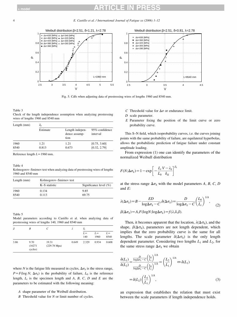
B=8.12 (3381 Cycles) C=18.93 (166 MPa) A=2.50 D=1.21 E=–2.29

P=0.05

P=0

P=0.5

P=0.95

FailureRunout

Expected Failure

L=1960 mm

Fig. 4. S–N fields when adjusting data of prestre

prestressing wires and strands with different lengths are

analyzed by means of the model proposed by Castillo et al.

[2,9], whereby the validity of the length independence

hypothesis will be checked.

2. The model of Castillo et al.

2.1. Modelling the S–N field

The S–N field deals with two variables related to each other:

the fatigue life, N, and the stress range, Ds. The problem

consists of developing a non-linear regression model to

describe the S–N field and to estimate the model parameters.

Castillo et al. [2,9], proposed a statistical model for the analysis

of fatigue results able to consider specimens with different

lengths. The model is based on the following physical and

statistical considerations:

(1) Weakest link principle. If a longitudinal element is

divided into ‘n’ sub-elements, the fatigue life of the

whole element corresponds to the fatigue life of the

weakest element.

(2) Stability. The cumulative distribution function (cdf)

model must be applicable to different lengths.

(3) Limit value. The cdf should encompass extreme lengths,

i.e. the case of a length going to infinity. Thus, the cdf

must belong to a family of asymptotic functions.

(4) Limited range of the random variables involved. The

variables Ds and N have a lower bound.

(5) Compatibility. The cdf related to the stress range E(N,

Ds) must be compatible with the cdf related to the fatigue

life F(Ds, N). The Weibull distributions fulfill the

requirements 1–4 and can be applied here.

The last condition allows us to establish a functional

equation. (see [1,3,5,9]) the solution of which leads, without

additional requirements to the following model for the cdf of

the fatigue life N at the stress range Dsk

FðlogN;DskÞZ1Kexp KLi

L0

ðlogNKBÞðlogDskKCÞ

DCE

� �A� �; (1)

650600550

500

450

400

350

300

250

2001e+08

1e+07

1e+06

1e+05

1e+04

∆σ [

MP

a]

Number of cycles

B=8.125 (3381 Cycles) C=18.93 (166 MPa) A=2.50 D=0.81 E=–3.42

P=0.05

P=0

P=0.5

P=0.95

FailureRunout

Expected Failure

L=8540 mm

ssing wires of lengths 1960 and 8540 mm.

https://www.researchgate.net/publication/268858039_Lifetime_Regression_Models_Based_on_a_Functional_Equation_of_Physical_Nature?el=1_x_8&enrichId=rgreq-554f487d7a4663e1dce22646f80ec1f7-XXX&enrichSource=Y292ZXJQYWdlOzIzOTM4NzAwMTtBUzoxMjcyMzE1MjMyOTkzMjhAMTQwNzM0NTc2NzYwMA==

https://www.researchgate.net/publication/234286453_Lectures_on_Functional_Equations_and_Their_Applications?el=1_x_8&enrichId=rgreq-554f487d7a4663e1dce22646f80ec1f7-XXX&enrichSource=Y292ZXJQYWdlOzIzOTM4NzAwMTtBUzoxMjcyMzE1MjMyOTkzMjhAMTQwNzM0NTc2NzYwMA==

0

0.2

0.4

0.6

0.8

1

2.5 3 3.5 4 4.5 5 5.5

P

V

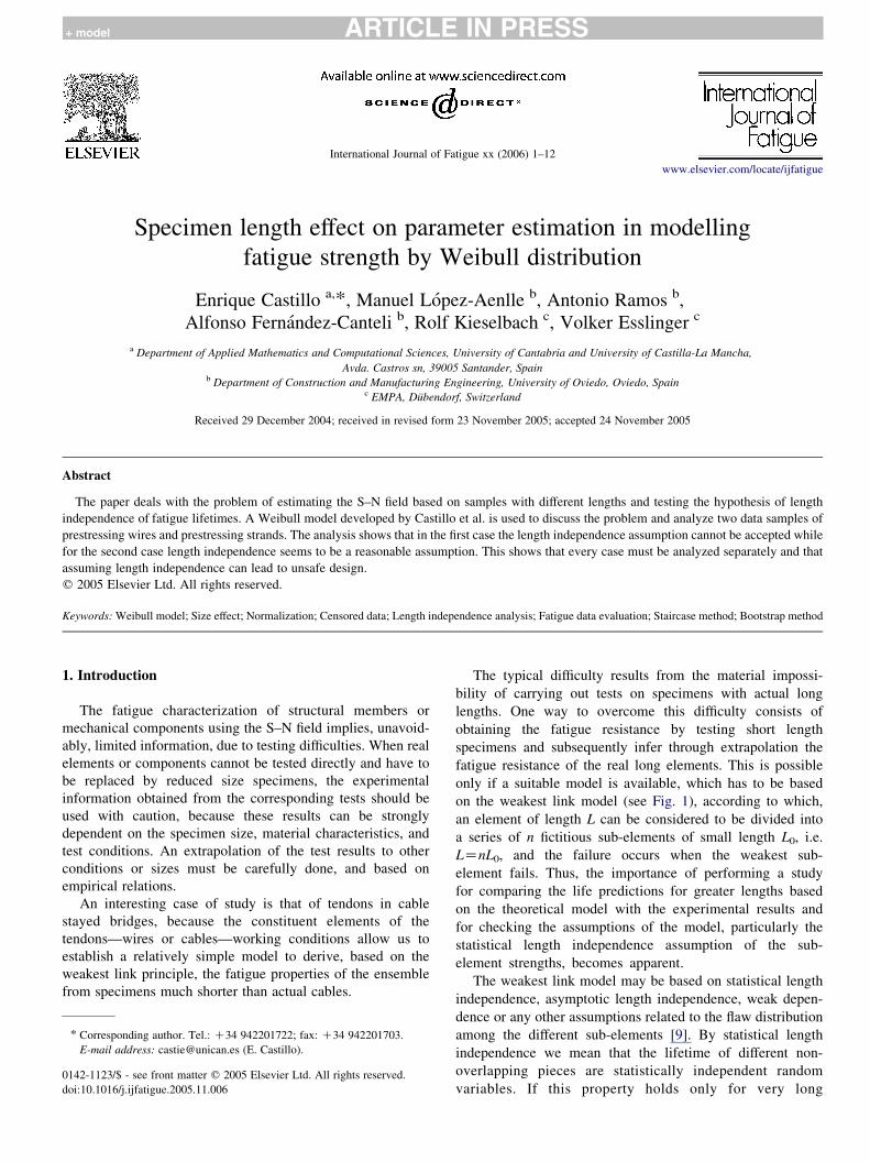
Weibull distribution:β=2.51, δ=1.21, λ=2.78

L=1960 mm

∆σ=630 [MPa]∆σ=460 [MPa]∆σ=420 [MPa]∆σ=380 [MPa]∆σ=360 [MPa]

∆σ=340 [MPa]∆σ=320 [MPa]∆σ=300 [MPa]∆σ=260 [MPa]

0

0.2

0.4

0.6

0.8

1

2.5 3 3.5 4 4.5

P

V


L=8540 mm


Fig. 5. Cdfs when adjusting data of prestressing wires of lengths 1960 and 8540 mm.

Table 3

Check of the length independence assumption when analyzing prestressing

wires of lengths 1960 and 8540 mm

Length (mm) dI

Estimate Length indepen-

dence assump-

tion

95%-confidence

interval

1960 1.21 1.21 [0.75, 3.60]

8540 0.813 0.673 [0.32, 2.79]

Reference length LZ1960 mm.

Table 4

Kolmogorov–Smirnov test when analyzing data of prestressing wires of lengths

1960 and 8540 mm

Length (mm) Kolmogorov–Smirnov test

K–S statistic Significance level (%)

1960 0.134 9.85

8540 0.113 69.75

Table 5

Model parameters according to Castillo et al. when analyzing data of

prestressing wires of lengths 140, 1960 and 8540 mm

b B C l di

LZ140

LZ1960

LZ8540

3.86 9.70

(16271

cycles)

19.31

(229.78 Mpa)

0.649 2.329 0.934 0.608



where N is the fatigue life measured in cycles, Dsk is the stress range,

PZF(log N; Dsk) is the probability of failure, L0 is the reference

length, Li is the specimen length and A, B, C, D and E are the

parameters to be estimated with the following meaning:

A shape parameter of the Weibull distribution.

B Threshold value for N or limit number of cycles.

C Threshold value for Ds or endurance limit.

D scale parameter.

E Parameter fixing the position of the limit curve or zero

probability curve.

This S–N field, which isoprobability curves, i.e. the curves joining

points with the same probability of failure, are equilateral hyperbolas,

allows the probabilistic prediction of fatigue failure under constant

amplitude loading.

From expression (1) one can identify the parameters of the

normalized Weibull distribution

FðN;DskÞZ1Kexp KLi

L0

VKlk

dik

� �bk

at the stress range Dsk with the model parameters A, B, C, D

and E:

lðDskÞZBKED

logDskKC;dðDskÞZ

D

logDskKC

L0

Li

� �1=A

;

bðDskÞZA;FðlogN;logDskÞZf ðl;d;bÞ:

(2)

Then, it becomes apparent that the location, l(Dsk), and the

shape, b(Dsk), parameters are not length dependent, which

implies that the zero probability curve is the same for all

lengths. The scale parameter d(Dsk) is the only length

dependent parameter. Considering two lengths L1 and L2, for

the same stress range Dsk we obtain

dðL1Þ

dðL2ÞZ

DlogDskKC

L0

L1

� �1=A

DlogDskKC

L0

L2

� �1=AZ

L2

L1

� �1=A

5dðL1Þ

ZdðL2ÞL2

L1

� �1=A

; (3)

an expression that establishes the relation that must exist

between the scale parameters if length independence holds.

650600550

500

450

400

350

300

250

200 1e+09

1e+08

1e+07

1e+06

1e+05

1e+04

∆σ [

MP

a]

Number of cycles

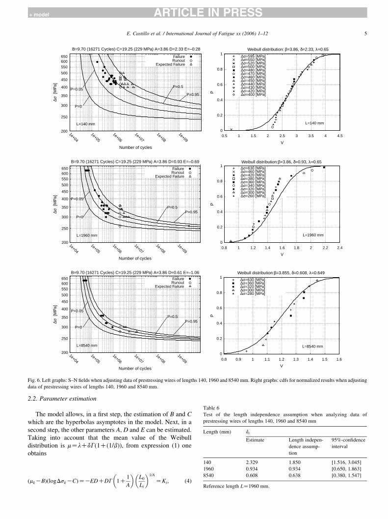
B=9.70 (16271 Cycles) C=19.25 (229 MPa) A=3.86 D=2.33 E=–0.28

P=0.05

P=0

P=0.5

P=0.95

L=140 mm

FailureRunout

Expected Failure

650600550

500

450

400

350

300

250

200 1e+09

1e+08

1e+07

1e+06

1e+05

1e+04

∆σ [

MP

a]

Number of cycles

B=9.70 (16271 Cycles) C=19.25 (229 MPa) A=3.86 D=0.93 E=–0.69

P=0.05

P=0

P=0.5P=0.95

L=1960 mm

FailureRunout

Expected Failure

0

0.2

0.4

0.6

0.8

1

0.8 1 1.2 1.4 1.6 1.8 2 2.2 2.4

P

V


L=1960 mm

∆σ=630 [MPa]∆σ=460 [MPa]∆σ=420 [MPa]∆σ=380 [MPa]∆σ=360 [MPa]∆σ=340 [MPa]∆σ=320 [MPa]∆σ=300 [MPa]∆σ=260 [MPa]

650600550

500

450

400

350

300

250

200 1e+09

1e+08

1e+07

1e+06

1e+05

1e+04

∆σ [

MP

a]

Number of cycles

B=9.70 (16271 Cycles) C=19.25 (229 MPa) A=3.86 D=0.61 E=–1.06

P=0.05

P=0

P=0.5P=0.95

L=8540 mm

FailureRunout

Expected Failure

0

0.2

0.4

0.6

0.8

1

0.8 0.9 1 1.1 1.2 1.3 1.4 1.5 1.6

P

V


L=8540 mm


0

0.2

0.4

0.6

0.8

1

0.5 1 1.5 2 2.5 3 3.5 4 4.5

P

V

Weibull distribution: β=3.86, δ=2.33, λ=0.65

L=140 mm

∆σ=595 [MPa]∆σ=550 [MPa]∆σ=520 [MPa]∆σ=500 [MPa]∆σ=480 [MPa]∆σ=470 [MPa]∆σ=460 [MPa]∆σ=450 [MPa]∆σ=440 [MPa]∆σ=430 [MPa]∆σ=420 [MPa]∆σ=400 [MPa]

Fig. 6. Left graphs: S–N fields when adjusting data of prestressing wires of lengths 140, 1960 and 8540 mm. Right graphs: cdfs for normalized results when adjusting

data of prestressing wires of lengths 140, 1960 and 8540 mm.

Table 6

Test of the length independence assumption when analyzing data of


Length (mm) di


dence assump-

tion

95%-confidence

interval



2.2. Parameter estimation

The model allows, in a first step, the estimation of B and C

which are the hyperbolas asymptotes in the model. Next, in a

second step, the other parameters A, D and E can be estimated.

Taking into account that the mean value of the Weibull

distribution is mZlCdG 1Cð1=bÞð Þ, from expression (1) one

obtains

140 2.329 1.850 [1.516, 3.045]

1960 0.934 0.934 [0.650, 1.863]

8540 0.608 0.638 [0.380, 1.547]

ðmkKBÞðlogDskKCÞZKEDCDG 1C
1

A

� �L0

Li

� �1=A

ZKi; (4)

Table 7





140 0.155 3.26

1960 0.180 5.27

8540 0.112 60.63

Table 8

Comparison between the stress level at 2!106 cycles (endurance limit)

calculated according to the model of Castillo et al. and the staircase method for

50% probability of failure

Length (mm) Ds (Mpa)

Castillo’s model

Using 1960 and

8540 mm

Using 140, 1960

and 8540 mm

Staircase

method [13]

140 – 410 420

1960 305 315 330

8540 290 295 305



where Ki, the expression between the two equality signs in (4),

is a length dependent constant, and mk is the mean value of

log N at stress range Dsk. This means that for every length the

probability curve associated with the mean value is also

represented by a hyperbola. Expression (4) suggests to estimate

first B and C by minimizing

QðB;C;K1;.;KtÞZXt

iZ1

Xn

kZ1

Xm

jZ1

logNikjKBKKi

logDskKC

� �2

(5)

with respect to B, C and K1, K2,., Kt, where t is the number of

different lengths considered here, n is the number of stress

ranges and m the number of tests conducted at each stress

range. Once the values of the parameters B and C are known,

Eq. (1) becomes a three parameter Weibull distribution and A,

D and E can be estimated by standard methods thanks to the

fact that results for different stress ranges and lengths can be

statistically normalized.

The model allows us to pool all the fatigue data points for

different stress ranges, into a unique population (stress range).

Note that all them belong to Weibull distributions with the

Table 9

Fatigue test results (in thousands of cycles) for prestressing strands for constant am

Ds (N/mm2) Cycles

LZ490 mm LZ1100 mm

630 56, 60, 62, 67, 84 59, 62, 64, 70, 7

460 95, 103, 106, 11

300 576, 727

290 1292, 2000a(4) 467, 494, 625, 1

(4)

280 513, 674, 2000a(

270 384, 989, 2000a

260 2000a(2)

250

230

a The limit number of cycles, 2.000, has been reached without failure.

same shape parameter, b, but different parameters for location

(l), and scale (d). This is called statistical normalization of the

S–N field (see Fig. 3). This procedure is based on the fact that

the Weibull distributions remains stable with respect to

location and scale transformations, that is, if a variable X

follows a Weibull distribution, W(b, d, l), that is denoted

XwW(b, d, l), and it is transformed by ZZ(XKa)/b, where a

and b are real constants, then ZwWðððlKaÞ=bÞ;ðd=bÞ;bÞ, i.e.

another Weibull distribution is obtained. The normalizing

process helps to overcome the limitation of the low number of

specimens tested at each different test level [9]. Thus, in the

evaluation of the Weibull parameters all the specimens are

pooled together, so that we have a larger sample size and then,

a better reliability of the evaluation is thus achieved.

Since unfortunately fatigue tests are scarce, costly and

lengthy normally available fatigue samples are small.

However, the model allows us using all the data lengths, i.e.

pooled together. This reduces the problem because then the

effective sample size is the sum of the sample sizes for all

lengths.

When the former transformation is applied to the fatigue

case, X is used to denote the original variable, that is the

number of cycles to failure, and Z is used to denote the

normalized variable. Different normalizations can be done,

simply, by assigning different values to the parameters a and b.

One possible normalized variable, denoted as V, can be defined

as VZ(log NKB)(log DsKC), that allows us to pool all the

data together as if they were tested at the same stress level.

Provided that the variable log N for the length Li follows a

Weibull distribution W(lk, dik, bk) at the stress range k, the

Weibull cdf for the new variable V is given by:

FðV;l;di;bÞZ1Kexp KVKl

di

� �b" #

(6)

Here, the normalized parameters l, di and b can be expressed

as a function of the model parameters, as lZKED,

diZDL0

Li

� �1=A

, bZA. Once l, d1, d2,.,dt and b are known,

the model parameters A, D and E can be calculated. It becomes

apparent that the parameters D and E depend of the reference

length. The estimation of l, d1, d2,.,dt and bmay succeed using

plitude loading [11]

LZ1960 mm LZ3860 mm

1 50, 57, 59, 65, 67 51, 63, 65, 74

5, 189

376, 508

294, 2000a 287, 309, 347, 440, 614 374, 696, 749, 2000a

3) 1984, 2000a

359, 870, 2000a

909, 2000a(2)

2000a

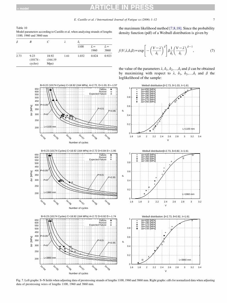
Table 10

Model parameters according to Castillo et al. when analyzing strands of lengths

1100, 1960 and 3860 mm

b B C l di

1100 LZ1960

LZ3860

2.73 9.23

(10174 -

cycles)

18.92

(164.19

Mpa)

1.61 1.032 0.824 0.923

650600550500

450

400

350

300

250

200

1e+09

1e+08

1e+07

1e+06

1e+05

1e+04

∆σ [

MP

a]

Number of cycles

B=9.22 (10174 Cycles) C=18.92 (164 MPa), A=2.72, D=1.03, E=–1.57

P=0.05

P=0

P=0.5P=0.95

L=1100 mm

FailureRunout

Expected Failure

650600550500

450

400

350

300

250

200

1e+09

1e+08

1e+07

1e+06

1e+05

1e+04

∆σ [

MP

a]

Number of cycles

B=9.23 (10174 Cycles) C=18.92 (164 MPa) A=2.72 D=0.84 E=–1.95

P=0.05

P=0

P=0.5P=0.95

L=1960 mm

FailureRunout

Expected Failure

650600550500

450

400

350

300

250

200

1e+09

1e+08

1e+07

1e+06

1e+05

1e+04

∆σ [

MP

a]

Number of cycles

B=9.23 (10174 Cycles) C=18.92 (164 MPa) A=2.72 D=0.92 E=–1.74

P=0.05

P=0

P=0.5P=0.95

L=3860 mm

FailureRunout

Expected Failure

Fig. 7. Left graphs: S–N fields when adjusting data of prestressing strands of lengths 1

data of prestressing wires of lengths 1100, 1960 and 3860 mm.



the maximum likelihood method [7,8,18]. Since the probability

density function (pdf) of a Weibull distribution is given by

f ðV ;l;d;bÞZexp KVKl

di

� �b" #

b1

di

VKl

di

� �bK1

; (7)

the value of the parameters l, d1, d2,.,dt and b can be obtained

by maximizing with respect to l, d1, d2,.,dt and b the

loglikelihood of the sample:

0

0.2

0.4

0.6

0.8

1

1.6 1.8 2 2.2 2.4 2.6 2.8 3 3.2

P

V

Weibull distributionβ=2.73, δ=0.82, λ=1.61

L=1960 mm


V

0

0.2

0.4

0.6

0.8

1

1.6 1.8 2 2.2 2.4 2.6 2.8 3 3.2 3.4

P


L=1100 mm

∆σ=630 [MPa]∆σ=460 [MPa]∆σ=300 [MPa]∆σ=290 [MPa]∆σ=280 [MPa]∆σ=270 [MPa]∆σ=260 [MPa]

0

0.2

0.4

0.6

0.8

1

1.6 1.8 2 2.2 2.4 2.6 2.8 3 3.2 3.4

P

V

Weibull distribution: β=2.73, δ=0.92, λ=1.61

L=3860 mm


100, 1960 and 3860 mm. Right graphs: cdfs for normalized data when adjusting

Table 11

Check of the length independence assumption when analyzing data of

prestressing strands of lengths 1100, 1960 and 3860 mm

Length (mm) di


dence assump-

tion

95%-confidence

interval

1100 1.030 1.030 [0.615, 2.538]

1960 0.824 0.834 [0.481, 2.339]

3860 0.923 0.650 [0.314, 2.014]


Table 12

Kolmogorov–Smirnov test when analyzing data of prestressing strands of

lengths 1100, 1960 and 3860 mm



1100 0.191 64.18

1960 0.135 52.73

3860 0.118 63.18


Table 13


prestressing strands of lengths 490, 1100, 1960 and 3860 mm

b B C l di

LZ490

LZ1100

LZ1960

LZ3860

3.2 10.31

(28608

cycles)

19.23

(220.

2 Mpa)

0.339 0.891 0.651 0.513 0.537



LZKXn

iZ1

ViKl

di

� �b

CðbK1ÞXn

iZ1

logViKl

di

� �Cnlogb

KXn

iZ1

logdi: (8)

The application of this procedure does not require the

assumption (3), related to the length independence assumption.

Nevertheless, once the parameters are estimated the length

independence assumption can be checked. Other methods for

the estimation of the model parameters have been developed by

Castillo et al. [7,8]. However, since the aim of the paper is to

study the length effect, the estimation method is not the main

point in the paper and any good estimation method can be used.

2.3. The case of censored data (runouts)

Experimental programs in fatigue usually involve the presence

of censored data, i.e. tests interrupted before failure of the

specimen occurs, due to accidental causes or because the limit

number of cycles has been reached. This type of data is called

censored data or runouts. In such cases, it is possible to resort to

specific statistical techniques, as for instance the E–M algorithm,

based on an iterative process to deal with these censored data in

the statistical analysis. This technique consists of:

(1) Estimate the model parameters considering only the results

associated with failures.

(2) Assign to the censored results their expected failure values,

based on the estimated model parameters.

(3) Re-estimate the model parameters but considering the data

associated with real failures plus the expected ones

associated with the runouts.

(4) Repeat steps 2 and 3 until convergence of the process.

For a limit number of cycles N0, the normalized variable for

runouts will be

V0ZðlogN0KBÞðlogDsKCÞ; (9)

and since the Weibull distribution for VRV0 is

FðVjvRV0ÞZ1Kexp KV0Kl

di

� �b

KVKl

di

� �b" #

;

VjvRV0;

(10)

and the expected value of the rth order statistic of a sample of

size q from an uniform distribution U(0,1) is r/(qC1), the

censored result V0 can be replaced by the V solutions, obtained

from

1Kexp KV0Kl

di

� �b

KVKl

di

� �b" #

Zr

qiC1;

rZ1;2;.;qi;

(11)

where qi is the number of runouts coinciding at the same stress

range, Dsk, and the same limit number of cycles, N for rZ1,

2,.,qi. Thus:

VZlCdi

V0Kl

di

� �b

Klog 1Kr

qiC1

� �" #;

rZ1;2;.;qi:

(12)

3. Examples of application of the proposed method

3.1. Prestressing wires

With the aim of validating the model for analyzing the

influence of the specimen length, the results of an experimental

fatigue program, carried out on prestressing wires with different

lengths [16] at the EMPA (Swiss Federal Testing and Materials

Laboratory), in Dubendorf (Switzerland), were evaluated. The

nominal value of the tensile strength of this material was RmZ1700 MPa. All the tests were conducted under constant

amplitude loading using specimens with three different lengths,



140, 1960 and 8540 mm, where the stress ranges and resulting

fatigue life in cycles are shown in Table 1.

For parameter estimation the techniques described in Section

2 were applied. The GAMS tool [6,18] was used to solve the

optimization problem. Initially, only the specimens with lengths

1960 and 8540 mm were considered in the analysis. The

parameter estimates are shown in Table 2.

Figs. 4 and 5 represent, respectively, the S–N field for each of

the two lengths studied and the cdf associated with the

normalized variable V. Assuming that the length independence

hypothesis is satisfied and taking as reference length that of

1960 mm, it is possible to calculate the value of the d parameter

associated with the length 8540 mm as d8540Zd1960(1960/8540)1/2.51Z0.673 as represented in Table 3. A

certain discrepancy can be observed between the value directly

estimated and the one resulting from the length independence

assumption. The validity of the length independence hypothesis

was checked using the bootstrap technique [10,12,15]. Thousand

bootstrap simulations were performed considering the par-

ameters in Table 2 for LZ1960 mm and using the length

independence assumption for LZ8540 mm. Thus, 1000 values

of d were simulated for every length and thousand values of the

Kolmogorov–Smirnov statistic were obtained. The 95%

confidence interval for the d estimates and for the Kolmo-

gorov–Smirnov statistic is included in Tables 3 and 4,

respectively.

650600550

500

450

400

350

300

250

200 1e+1

1e+09

1e+08

1e+07

1e+06

1e+05

1e+04

∆σ [

MP

a]

Number of cycles

B=10.26 (28575 Cycles) C=19.20 (220 MPa) A=3.2 D=0.89 E=–0.38

P=0.05

P=0

P=0.5P=0.95

L=490 mm

FailureRunout

Expected Failure

650600550

500

450

400

350

300

250

200 1e+09

1e+08

1e+07

1e+06

1e+05

1e+04

∆σ [

MP

a]

Number of cycles

B=10.26 (28575 Cycles) C=19.20 (220 MPa) A=3.2 D=0.53 E=–0.66

P=0.05

P=0

P=0.5P=0.95

L=1960 mm

FailureRunout

Expected Failure

Fig. 8. S–N fields when adjusting data of prestressing wires of lengths (f

From Table 3, it can be observed that the d estimates fall

inside the 95% confidence interval of the feasible values. Thus, it

can be assumed that the test results fulfill the length

independence assumption. This can also be verified by means

of the Kolmogorov–Smirnov test. For the length 1960 mm a

significance level of 9.85% was obtained, while it was 69.75% in

the case of a length 8540 mm. Consequently, the length

independence assumption can be accepted for a 5% significance

level, and then it can be concluded that the length independence

assumption can be used for extrapolation purposes from 1960 to

8540 mm, and therefore they can be jointly analyzed. Finally, all

the lengths 140, 1960 and 8540 mm, were analyzed together

giving the estimates in Table 5.

Fig. 6 represents the S–N fields on the left, and the cdfs,

associated with the normalized variable V for each of the lengths

on the right.

Table 6 shows the parameter estimates associated with

lengths 140 and 8540 mm when the length independence

assumption is assumed to hold and the reference length is

1960 mm. The results obtained from the simulations performed

by the bootstrap method are shown in Tables 6 and 7. It can be

noticed that the d estimates for lengths 1960 and 8540 mm fall

inside the 95% confidence interval. Table 7 shows the results

obtained by the Kolmogorov–Smirnov test. The estimate

corresponding to 140 mm cannot be accepted for a 5%

significance level. Thus, the consideration of this length in the

650600550

500

450

400

350

300

250

200 1e+09

1e+08

1e+07

1e+06

1e+05

1e+04

∆σ [

MP

a]

Number of cycles

B=10.26 (28575 Cycles) C=19.20 (220 MPa) A=3.2 D=0.65 E=–0.52

P=0.05

P=0

P=0.5P=0.95

L=1100 mm

FailureRunout

Expected Failure

650600550

500

450

400

350

300

250

200 1e+09

1e+08

1e+07

1e+06

1e+05

1e+04

∆σ [

MP

a]

Number of cycles

B=10.26 (28575 Cycles) C=19.20 (220 MPa) A=3.2 D=0.53 E=–0.66

P=0.05

P=0

P=0.5P=0.95

L=3860 mm

FailureRunout

Exp. Failure

rom left to right and top to bottom) 490, 1100, 1960 and 3860 mm.

0

0.2

0.4

0.6

0.8

1

0.4 0.6 0.8 1 1.2 1.4 1.6 1.8

P

V


L=140 mm

∆σ=630 [MPa]∆σ=290 [MPa]

0

0.2

0.4

0.6

0.8

1

0.4 0.6 0.8 1 1.2 1.4

P

V


L=1100 mm

∆σ=630 [MPa]∆σ=460 [MPa]∆σ=300 [MPa]∆σ=290 [MPa]∆σ=280 [MPa]∆σ=270 [MPa]∆σ=260 [MPa]

0

0.2

0.4

0.6

0.8

1

0.4 0.5 0.6 0.7 0.8 0.9 1 1.1 1.2 1.3

P

V


L=1960 mm


0

0.2

0.4

0.6

0.8

1

0.4 0.6 0.8 1 1.2

P

V


L=3860 mm


Fig. 9. Cdfs when adjusting data of prestressing strands of lengths 490, 1100, 1960 and 3860 mm.

Table 14

Check of the length independence assumption when analyzing data of

prestressing strands of lengths 490, 1100, 1960 and 3860 mm

Length (mm) di


dence assump-

tion

95%-confidence

interval

490 0.891 0.838 [0.777, 5.430]

1100 0.651 0.651 [0.643, 5.196]

1960 0.513 0.544 [0.563, 4.974]

3860 0.537 0.4398 [0.415, 4.881]

Reference length: LZ1960 mm.



joint analysis is not in line with the results for the other lengths

leading to a reduction of the significance level of these.

Therefore, it can be concluded that the results corresponding

to the 140 mm specimens do not fulfill the length independence

assumption. Nevertheless, it should be said that since 140 mm is

a fairly short length, the determination of the real free length of

the specimens is not exempt from error. Moreover, as mentioned

above, the test strategy adopted, rather oriented to the staircase

method, due to the lack of a suitable model at the time when the

tests were planned, caused an irregular distribution of the results

all over the S–N field and a high number of runouts relative to

the total number of data points. Finally, it should be also added

that the frequency resulting for testing the length 140 mm was

133 Hz, considerably higher than the frequencies used for the

remaining lengths 1960 and 8540 mm (6 and 0.4 Hz, respect-

ively). Table 8 illustrates a comparison between the values of the

endurance limit calculated for 50% probability of failure at 2!106 cycles using the model of Castillo et al. and the staircase

method (see [13,16,17]). In the light of these results, it can be

concluded that the results from the model proposed by Castillo et

al. show a good agreement with the results furnished by the

staircase method. Moreover, the former brings additional

advantages, since it allows us to calculate, for given probability

of failure, the number of cycles to failure for whatever stress

level all over the whole S–N field, including the possibility of

extrapolation concerning cycles or test lengths, something that is

not possible for the staircase method.

3.2. Prestressing strands

The study of fatigue of prestressing wires was then extended

to prestressing strands from the same experimental program

conducted at the Swiss Federal Testing and Materials

Laboratory EMPA in Dubendorf, Zurich (Switzerland) [16].

The nominal value of the tensile strength of this material was

RmZ1800 MPa. All the tests were conducted under constant

amplitude loading using four different lengths: 490, 1100, 1960

and 3860 mm, as shown in Table 9. The program strategy, as in

the case of prestressing wires, was focussed to the application of

the staircase method for determining the endurance limit. Also

here, the results are predominantly gathered in the lower part of

the S–N field with the same consequences as before. The

https://www.researchgate.net/publication/232485125_J_Introduction_to_Statistical_Analysis?el=1_x_8&enrichId=rgreq-554f487d7a4663e1dce22646f80ec1f7-XXX&enrichSource=Y292ZXJQYWdlOzIzOTM4NzAwMTtBUzoxMjcyMzE1MjMyOTkzMjhAMTQwNzM0NTc2NzYwMA==

Table 15

Kolmogorov–Smirnov test when analyzing data of prestressing strands of

lengths 490, 1100, 1960 and 3860 mm



490 0.158 59.45

1100 0.0934 60.55

1960 0.0965 87.05

3860 0.0838 89.25


Table 16

Comparison between the stress level at 2!106 cycles (endurance limit)

calculated according to the model of Castillo et al. and the staircase method for

50% probability of failure

Length (mm) Ds (MPa)

Castillo’s model

Using 1100,

1960 and

3860 mm

Using 490, 1100,

1960 and

3860 mm

Staircase

method [13]

490 – 290 –

1100 285 273 280

1960 270 265 260

3860 260 268 –



procedure described in Section 2 was applied for the parameter

estimation. Initially, test lengths of 1100, 1960 and 3860 mm

were considered in the analysis. The parameter estimates are

shown in Table 10. Fig. 7 represents the S–N field for each one

of the lengths studied and the cdf associated with the variable V,

respectively.

The values of the d parameter associated with test lengths

1100 and 3860 mm assuming length independence are shown in

Table 11 where 1960 mm has been taken as the reference length.

The estimate falls inside the 95% confidence interval for all the

lengths. Table 12 represents the results of the Kolmogorov–

Smirnov test. As can be seen all the estimates can be accepted at

5% significance levels. Then it can be concluded that the results

for the three lengths fulfill the length independence assumption

and therefore can be jointly analyzed.

Subsequently, a joint analysis considering all the lengths 490,

1100, 1960 and 3860 mm was undertaken. The resulting

parameters are shown in Table 13.

Figs. 8 and 9, represent the S–N field and the cdfs associated

to the variable V for each of the lengths, respectively.

As it can be observed, the quality of the adjustment for the S–

N field, as well as for the cdfs is acceptable for the four specimen

lengths, although, considering the low number of results related

to the shortest length, it seems risky to establish conclusions

concerning this length.

From Table 14, it can be observed that the d parameter

estimate falls inside the 50 and 95% confidence intervals of the

acceptable values. Thus, the test results confirm the length

independence assumption. This can be also verified by means of

the Kolmogorov–Smirnov test. Table 14 shows the results

obtained for the parameter d associated with lengths 490, 1960

and 3860 mm, assuming length independence and taken

1100 mm as the reference length. The result obtained for length

1960 mm is the only one that falls outside the 95% confidence

interval. Again, it can be verified that the presence of results that

do not fulfill the length independence assumption is not in line

with the adjustment of the rest of the results. In order to check

the quality of the estimate the results of the Kolmogorov–

Smirnov test are shown in Table 15. All of them can be accepted

for a 5% significance level.

It can be summarized that the four studied lengths cannot be

jointly analyzed, since they do not fulfill the length indepen-

dence assumption. This could be due to the fact that the length

490 mm is below the length independence threshold length, or,

that the number of results available related to this length is too

small and is concentrated in only two different stress levels.

Table 16 illustrates a comparison between the values of

the endurance limit calculated for 50% probability of failure

at 2!106 cycles using the model of Castillo et al. and the

staircase method [13,16,17]. This demonstrates a good

correspondence between both methods and the same

comments, expressed at the end of Section 3.1 are pertinent

here again.

4. Conclusions

The main conclusions of this work are the following:

(1) The applicability of the model proposed by Castillo et al.

for determining the S–N field of two different types of

prestressing steels, wires and strands, including different

lengths have been studied. The model allows us to

determine the S–N curves for both materials for different

probabilities of failure and different confidence intervals

by considering a relatively reduced number of tests even

if the test plan, set up in the absence of a general

regression model at the time of the research made, is far

from being optimal. The potential of the model of

Castillo et al. enabling to establish an adequate test

strategy is being developed at present by the authors.

(2) A methodology to check the length independence

hypothesis, based on the bootstrap technique, is proposed

here. This can be applied to determine the threshold

length, above which the length independence assumption

can be accepted. The analysis shows that the length

independence assumption cannot be accepted for the

prestressing wires data, while it is a reasonable

assumption for the prestressing strands data.

(3) The Kolmogorov–Smirnov test has been successfully

applied to check the quality of the adjustment.

(4) The results of the endurance limit, obtained using the

model of Castillo et al. and the staircase method are

compared here. A good agreement has been obtained.

Nevertheless, the superiority of the model presented here

is obvious since it allows us to calculate, for a given

probability of failure, the number of cycles to failure for

any stress level, all over the whole S–N field, and

additionally it makes feasible an extrapolation concerning




cycles or test lengths, which is outside the capacities of

the staircase method.

References

[1] Aczel J. Lectures in functional equations and their applications.

Mathematics in science and engineering, vol. 19. London: Academic

Press; 1966.

[2] Castillo E, Fernandez Canteli A, Esslinger V, Thurlimann, B. Statistical

model for fatigue analysis of wires, strands and cables. IABSE proceedings,

1985. p.82–5.

[3] Castillo E, Galambos J. Lifetime regression models based on a functional

equation of physical nature. J Appl Probab 1987;24:160–9.

[4] Castillo E, Hadi AS, Balakrishnan N, Sarabia, JM. Extreme values and

related models with applications in engineering and science. Wiley series in

probability and statistics; 2005.

[5] Castillo E, Iglesias A, Ruiz-Cobo MR. Functional equations in applied

sciences. Mathematics in science and engineering, vol. 199. Amsterdam:

Elsevier; 2005.

[6] Castillo E, Conejo A, Pedregal P, Garcia R, Alguacil N. Building and

solving mathematical programming models in engineering and science.

London: Wiley; 2001.

[7] Castillo E, Hadi AS. Modeling lifetime data with application to fatigue

models. J Am Stat Assoc 1995;90(4311):1041–54.

[8] Castillo E, Fernandez Canteli A, Hadi AS. On fitting a fatigue model to

data. Int J Fatigue 1999;21:97–106.

[9] Castillo E, Fernandez Canteli A. A general regression model for lifetime

evaluation and prediction. Int J Fract 2001;107:117–37.

[10] Chernick MR. Bootstrap methods. Wiley series in probability and statistics.

London: Wiley; 1999.

[11] Cullimore MSG. The fatigue strength of high tensile wire cable subjected to

stress fluctuations of small amplitude. Memoires Assoc Int de Ponts et

Charpentes 1976;32(1):49–56.

[12] Davison AC, Hinkley DV. Bootstrap methods and their application.

Cambridge series in statistical and probabilistic mathematics; 1997.

[13] Dixon WJ, Massey Jr FJ. Introduction to statistical analysis. 3rd ed. NY,

USA: McGraw-Hill; 1969.

[14] Edwards AD, Picard A. Fatigue characteristics of prestressing strand. Proc

Inst Civ Eng 1972;53:323–36.

[15] Efron B, Tibshirami RJ. An introduction to the bootstrap. London/Boca

Raton: Chapman & Hall/CRC; 1993.

[16] Fernandez Canteli A, Esslinger V, Thurlimann B. Ermudungsfestigkeit von

Bewehrungs- und Spannstahlen. Bericht Nr. 8002-1, Institut fur Baustatik

und Konstruktion, ETH Zurich; 1984.

[17] Huck M, Schutz W, Zenner HM. Ansatz und Auswertung von

Treppenstufenversuchen im Dauerfestigkeitsbereich. Industrieanlagen —

Betriebsgesellschaft mbH, Bericht b-TF-742B; February 1978.

[18] Lopez Aenlle M. Fatigue characterization of composites subject to random

and block loading (in Spanish). Doctoral thesis, University of Oviedo; 2000.

[19] Tide RHR, van Horn DA. A statistical study of the static and fatigue

properties of high strength prestressing strand. Fritz Eng. Laboratory.

Report No. 309.2, Lehigh University; June 1966.

[20] Warner RF, Hulsbos CL. Fatigue properties of prestressing strand. PCI J

1966;11(2):25–46.















Statistical Models for Analysis of Fatigue Life of Long Elements

Documents

Transcript of Statistical Models for Analysis of Fatigue Life of Long Elements