STATISTICAL LINKAGE OF DAILY PRECIPITATION IN BULGARIA TO ATMOSPHERIC CIRCULATION

Plamen Neytchev1, Neyko Neykov1, Walter Zucchini2, Hristo Hristov1

1National Institute of Meteorology and Hydrology, Bulgarian Academy of Sciences Sofia, Bulgaria

2Institute of Statistics and Econometrics, University of Göttingen Göttingen, Germany

plamen.neytchev@meteo.bg, neyko.neykov@meteo.bg, hristov_awc@abv.bg, wzucchi@uni-goettingen.de

Abstract

An eight state non-homogeneous hidden Markov model (NHMM) is developed for linking daily precipitation amounts data at a network of 32 stations broadly covering the territory of Bulgaria to large-scale atmospheric patterns. At each site a 40-year record 1960-2000 of daily October-March precipitation amounts is modeled. The paper is a continuation of Neytchev et al. (2006) who studied the cold half years period 1978-1988. The atmospheric data consists of daily sea-level pressure, geopotential height at 500 and 850 hPa, air temperature at 850 hPa and relative humidity at 700 and 850 hPa on a 2.5° x 2.5° grid based on NCEP-NCAR reanalysis data set covering the Europe-Atlantic sector 30°W–60°E, 20°N–70°N for the same period. The first 30 years data are used for model fitting purposes while the remaining 10 years are used for model evaluation. Detailed model validation is carried out on various aspects. The proposed model reproduces well the rainfall statistics for the observed and reserved data whereas the identified states are found to be physically interpretable in terms of regional climatology. Keywords: Hidden Markov Model, Precipitation Amounts Model. 1 INTRODUCTION NHMM links large-scale atmospheric patterns to daily precipitation data at a network of rain gauge stations, via several hidden (unobserved, latent) states called the “weather states” Hughes and Guttorp (1994). The evolution of these states is modeled as a first-order Markov process with state-to-state transition probabilities conditioned on some indices of the atmospheric variables. Due to these weather states the spatial precipitation dependence can be partially or completely captured. The NHMM weather states are identified as precipitation patterns that result from the model fitting procedure, while the role of synoptic atmospheric information is to influence the state transitions. This is in contrast with the traditional weather state models discussed in Bardossy and Plate (1992) where each day is classified a priori into a state, according to synoptic patterns and precipitation does not affect the state definition. The NHMM is used to model precipitation occurrences in Hughes and Guttorp (1994), whereas the intensity is modeled by Bellone et al. (2000), Charles et al. (2003), and Neytchev et al. (2006). More details about hidden Markov models and their applications can be found in MacDonald and Zucchini (1997).

22 23 24 25 26 27 28 29

41.0

41.5

42.0

42.5

43.0

43.5

44.0

44.5

Rain-Gauges

longitude

latit

ude

KrumovgradDgebel

Zlatograd

Panagurishte

Chepelare

Karlovo

Vidin

Pleven

Russe

Sandanski

Kneja

Chirpan

Targovishte

Kjustendil

Tarnovo

Blagoevgrad

Ihtiman

Ivailo

Kurdjali

OChiflik

TopolovgradElhovo

Svishtov

Silistra

Plovdiv

Zlatitsa Sliven

Shumen

SofiaBot

Sadovo

Varna

Figure 1. Map of rain gauge stations over the territory of Bulgaria.

At the XXIII Conference of the Danubian Countries, held in Belgrade, Neytchev et al. (2006) reported an eight states daily precipitation amounts NHMM for the cold (October-March) half years period 1978-1988 for the network of 32 rain gauge stations broadly covering the territory of Bulgaria, see Fig. 1. In the present study we calibrated our model on the daily precipitation totals over the same network of stations, however, for the cold half (October-March) years period 1960-1990, while the period 1991-2000 was reserved for model validation. We considered only the cool seasons as the precipitation process in that period of the year is not influenced by convective phenomena. As in the previous study the days with precipitation amounts greater than 0.1mm were treated as wet days, the remaining were considered as dry days. Each record value represents the precipitation total over a 24 hour period ending at 06 UTC. The daily atmospheric measures consists of sea-level pressure (slp), geopotential height at 500 and 850 (hgt.850) hPa, air temperature at 2m and 850 hPa (air.850), specific humidity at 2m, and relative humidity at 700 (rhum.700) and 850 (rhum.850) hPa from the gridded NCEP/NCAR Reanalysis data within an Europe-Atlantic (http://www.cru.uea.ac.uk/cru/data/ncep/) window from 30ºW-60ºE, 20ºN-70ºN on a 2.5º×2.5º latitude-longitude grid for the same period as the precipitation data. The aim of the paper is to update the previous results of Neytchev et al. (2006) and to present some new ones. Thus in sections 2 and 3 a model evaluation and interpretation is made on the background of simulation of precipitation occurrences and amounts, conditional on the value of some synoptic atmospheric variables, whereas the conclusions are made in section 4.

2 MODEL SELECTION Fitting NHMM to daily precipitation data involves the choice of a model order and of the atmospheric variables to be included. However, fitting the eight states NHMM to a network of 32 stations and 276 nodes of several atmospheric variables is computationally intractable. Thus, we continue to follow the hierarchical models fitting strategy described by Neytchev at al. (2006) which provides good starting values for the optimization procedures at each stage as the models are nested at each step. Bayesian information criterion (BIC) defined as TkLBIC log)ˆ(log2 −−= θ is used to compare the models, where )ˆ(θL is the maximized log-likelihood; k is the number of model parameters, and T is the number of days of data. Selecting an NHMM that minimizes the BIC provides a relatively parsimonious model that fits the data well. The final decision on how many and which of the resulting summary variables are to be included in the model is evaluated in terms of physical realism, distinctness of the weather state patterns and model interpretability. Fitting the NHMM with large number of atmospheric variables is a hard computational problem. Therefore, at first the data dimension is reduced applying the singular value decomposition (SVD) technique, described by Bretherton et al. (1992), to the correlation matrix between the precipitation occurrence (amounts) at station i for i=1,…,32 and the corresponding atmospheric variable at node j for j=1,…,276. In this way a few summary variables explain most of the correlation between each field and the precipitation process, as shown in Table1. For instance, the first summary variables of the coupled patterns (atmospheric - precipitation fields) included in the study account more than 90% of the correlation. Therefore at least 5 potential predictors could be used in fitting NHMM to the precipitation data. However, the first summary variables are highly correlated. Thus a standard principal components analysis was applied to the composed field based on the first summary variable of anyone field. As a consequence three scalar indices denoted by F1, F2 and F3 are extracted that account 95% of the total variance of this field as shown in Table 2. Table 1. Cumulative proportions of correlation [%] explained by the summary variables.

Eigenvalues: 1st 2nd 3rd Slp 93.09 97.79 99.33

hgt.850 94.63 97.40 98.75air.850 94.22 97.82 99.29

rhum.850 93.01 96.89 98.34rhum.700 92.15 96.42 98.07

Table 2. Cumulative proportion of variance [%] explained by the summary variables of the composite field based on slp, hgt.850, rhum.700, rhum.850 and air.850.

eigenvalues: F1 F2 F3 F4 F5

Composite 72.69 87.43 94.72 99.99 100.00

Now several NHMMs were fitted and some of the results are presented in Table 3. For comparison we presented also some of the results for the period 1978-1988. The models with acronym HMM.8 are related with eight-states amount homogeneous hidden Markov model whereas the remaining NHMMs are based on 7 and 8 states with F1 and F1, F2 and F3 summary variable as predictors into the transition

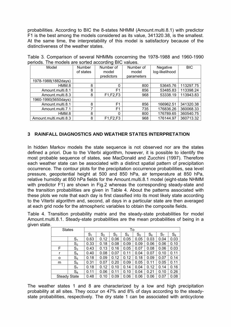
probabilities. According to BIC the 8-states NHMM (Amount.multi.8.1) with predictor F1 is the best among the models considered as its value, 341320.38, is the smallest. At the same time, the interpretability of this model is satisfactory because of the distinctiveness of the weather states. Table 3. Comparison of several NHMMs concerning the 1978-1988 and 1960-1990 periods. The models are sorted according BIC values.

Model Number of states

Number of model

predictors

Number of model

parameters

Negative log-likelihood

BIC

1978-1988(1882days) HMM.8 8 0 800 53645.76 113297.75

Amount.multi.8.1 8 F1 856 53485.83 113398.24Amount.multi.8.3 8 F1,F2,F3 968 53338.19 113943.83

1960-1990(5650days) Amount.multi.8.1 8 F1 856 166962.51 341320.38Amount.multi.7.1 7 F1 735 176836.26 360068.33

HMM.8 8 0 800 176789.65 360540.75Amount.multi.multi.8.3 8 F1,F2,F3 968 176144.97 360713.32

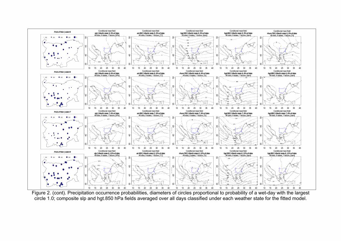
3 RAINFALL DIAGNOSTICS AND WEATHER STATES INTERPRETATION In hidden Markov models the state sequence is not observed nor are the states defined a priori. Due to the Viterbi algorithm, however, it is possible to identify the most probable sequence of states, see MacDonald and Zucchini (1997). Therefore each weather state can be associated with a distinct spatial pattern of precipitation occurrence. The contour plots for the precipitation occurrence probabilities, sea level pressure, geopotential height at 500 and 850 hPa, air temperature at 850 hPa, relative humidity at 850 hPa fields for the Amount.multi.8.1 model (eight-state NHMM with predictor F1) are shown in Fig.2 whereas the corresponding steady-state and the transition probabilities are given in Table 4. About the patterns associated with these plots we note that each day is first classified into its most likely state according to the Viterbi algorithm and, second, all days in a particular state are then averaged at each grid node for the atmospheric variables to obtain the composite fields. Table 4. Transition probability matrix and the steady-state probabilities for model Amount.multi.8.1. Steady-state probabilities are the mean probabilities of being in a given state.

States To S1 S2 S3 S4 S5 S6 S7 S8

S1 0.63 0.12 0.06 0.05 0.05 0.03 0.04 0.03 S2 0.33 0.18 0.08 0.09 0.09 0.06 0.06 0.10

F S3 0.43 0.13 0.16 0.05 0.07 0.08 0.06 0.03 r S4 0.40 0.08 0.07 0.11 0.04 0.07 0.10 0.11 o S5 0.18 0.09 0.12 0.12 0.18 0.09 0.07 0.14 m S6 0.31 0.07 0.20 0.09 0.05 0.11 0.05 0.11 S7 0.18 0.12 0.10 0.14 0.04 0.12 0.14 0.16 S8 0.11 0.06 0.11 0.10 0.04 0.21 0.10 0.26

Steady State 0.48 0.10 0.09 0.06 0.06 0.06 0.07 0.08 The weather states 1 and 8 are characterized by a low and high precipitation probability at all sites. They occur on 47% and 8% of days according to the steady-state probabilities, respectively. The dry state 1 can be associated with anticyclone

over Balkan Peninsula. The remaining states exhibit regional features variation of the precipitation probability and can be characterized by a lower mean sea level pressure values whereas the relative humidity values at 850 and 700 hPa levels are higher than 65% and 55%, respectively. The weather pattern related with state 2 can be associated with Mediterranean cyclones centered over Northern Italy moving to Hungary due to southwestern flow. In such synoptic situations, the precipitations are limited over Western Bulgaria and the slopes of mountain opposite to wind, according to hgt.850 plot. State 3 represents short term synoptic situation due to the atmospheric fronts of Baltic cyclones. The precipitations are mainly over the North-Eastern Bulgaria and the Black sea. Contrary to the other states with precipitations, the pressure field is without gradient and only upper-level trough marks the process. The states from 4 to 8 are associated with Mediterranean cyclones, centered over South Italy in the mean sea-level pressure field and an upper-level trough with different amplitude and tilt in the geopotential height at 850 hPa. The air flow possesses an east component at the sea level pressure and southwest direction at the upper levels. As regards the 7 and 8 states, the depression area is expanded to the Black sea as marked movements of the cyclone in this direction. Synoptic situations of this type are characterized with precipitations over the whole territory of Bulgaria. The transition probabilities given in Table 4 exhibit that the states can be classified according to cyclone evolution phases as initial (states 3 and 6), transitional (state 5 and 8) and final (state 7), some features of the precipitations due to different trajectories of the cyclone (state 5 and 8) or its blocking (state 3 and 6). Thus the sequences of states transitions 5→8→3, 5→8→7, 6→8→7 or 6→8→3 represent realistic well-known synoptic situations of Mediterranean cyclones with trajectories via Aegean Sea. Fig.3 shows that there is substantial interannual variability in the occurrence of weather states. The long-term trends suggest that states 1 and 3 have become steadily more frequent while the remaining states have declined throughout the period. These trends are indicative of a general reduction in rain day occurrence in the cold half-years over Bulgaria during the studied period. Further analysis of the weather state transition and steady-state probabilities and corresponding atmospheric predictor time-series will investigate the climatological mechanisms responsible for this observed decline. Some indications of how well the NHMM fits the data can be obtained from the comparison between observed and model-based precipitation probabilities and between observed and model-based log-odds ratios (Fig.4). The log-odds ratio is a common measure of association for binary variables to reflect the spatial correlation between occurrences at each pair of stations, see Bellone et al. (2000). It is seen that the simulated precipitation probabilities are reproduced well, while the odds ratios are modeled less adequately. A possible reason about might be that station Musala located at the highest pick on the Balkan Peninsula exhibits a distinct behavior in comparison with the remaining stations. Another reason about this indication is that the hypothesis of conditional spatial independence, given the weather state, may need to be modified. The common weather state seems to explain much of the correlation, but additional unexplained local spatial correlation remains.

Prob of Rain | state=1

0.2 0.4 0.6 0.8 1

10 15 20 25 30 35 40

3540

4550

Latit

ude

Conditional mean fieldslp | Viterbi state 1, 48% of dataAll sites, 8 states, 1 factors, [hPa]

10 15 20 25 30 35 40

3540

4550

attu

de

Conditional mean fieldair.850 | Viterbi state 1, 48% of data

All sites, 8 states, 1 factors, [°C]

10 15 20 25 30 35 40

3540

4550

attu

de

Conditional mean fieldrhum.700 | Viterbi state 1, 48% of data

All sites, 8 states, 1 factors, [%]

10 15 20 25 30 35 40

3540

4550

attu

de

Conditional mean fieldhgt.500 | Viterbi state 1, 48% of data

All sites, 8 states, 1 factors, [dam]

10 15 20 25 30 35 40

3540

4550

attu

de

Conditional mean fieldhgt.850 | Viterbi state 1, 48% of data

All sites, 8 states, 1 factors, [dam]

Prob of Rain | state=2

0.2 0.4 0.6 0.8 1

10 15 20 25 30 35 40

3540

4550

Latit

ude

Conditional mean fieldslp | Viterbi state 2, 8% of dataAll sites, 8 states, 1 factors, [hPa]

10 15 20 25 30 35 40

3540

4550

attu

de

Conditional mean fieldair.850 | Viterbi state 2, 8% of data

All sites, 8 states, 1 factors, [°C]

10 15 20 25 30 35 40

3540

4550

attu

de

Conditional mean fieldrhum.700 | Viterbi state 2, 8% of data

All sites, 8 states, 1 factors, [%]

10 15 20 25 30 35 40

3540

4550

attu

de

Conditional mean fieldhgt.500 | Viterbi state 2, 8% of data

All sites, 8 states, 1 factors, [dam]

10 15 20 25 30 35 40

3540

4550

attu

de

Conditional mean fieldhgt.850 | Viterbi state 2, 8% of data

All sites, 8 states, 1 factors, [dam]

Prob of Rain | state=3

0.2 0.4 0.6 0.8 1

10 15 20 25 30 35 40

3540

4550

Latit

ude

Conditional mean fieldslp | Viterbi state 3, 8% of dataAll sites, 8 states, 1 factors, [hPa]

10 15 20 25 30 35 40

3540

4550

attu

de

Conditional mean fieldair.850 | Viterbi state 3, 8% of data

All sites, 8 states, 1 factors, [°C]

10 15 20 25 30 35 40

3540

4550

attu

de

Conditional mean fieldrhum.700 | Viterbi state 3, 8% of data

All sites, 8 states, 1 factors, [%]

10 15 20 25 30 35 40

3540

4550

attu

de

Conditional mean fieldhgt.500 | Viterbi state 3, 8% of data

All sites, 8 states, 1 factors, [dam]

10 15 20 25 30 35 40

3540

4550

attu

de

Conditional mean fieldhgt.850 | Viterbi state 3, 8% of data

All sites, 8 states, 1 factors, [dam]

Prob of Rain | state=4

0.2 0.4 0.6 0.8 1

10 15 20 25 30 35 40

3540

4550

Latit

ude

Conditional mean fieldslp | Viterbi state 4, 6% of dataAll sites, 8 states, 1 factors, [hPa]

10 15 20 25 30 35 40

3540

4550

attu

de

Conditional mean fieldair.850 | Viterbi state 4, 6% of data

All sites, 8 states, 1 factors, [°C]

10 15 20 25 30 35 40

3540

4550

attu

de

Conditional mean fieldrhum.700 | Viterbi state 4, 6% of data

All sites, 8 states, 1 factors, [%]

10 15 20 25 30 35 40

3540

4550

attu

de

Conditional mean fieldhgt.500 | Viterbi state 4, 6% of data

All sites, 8 states, 1 factors, [dam]

10 15 20 25 30 35 40

3540

4550

attu

de

Conditional mean fieldhgt.850 | Viterbi state 4, 6% of data

All sites, 8 states, 1 factors, [dam]

Figure 2. Precipitation occurrence probabilities, diameters of circles proportional to probability of a wet-day with the largest circle

1.0; composite slp and hgt.850 hPa fields averaged over all days classified under each weather state for the fitted model.

Prob of Rain | state=5

0.2 0.4 0.6 0.8 1

10 15 20 25 30 35 40

3540

4550

Latit

ude

Conditional mean fieldslp | Viterbi state 5, 5% of dataAll sites, 8 states, 1 factors, [hPa]

10 15 20 25 30 35 40

3540

4550

attu

de

Conditional mean fieldair.850 | Viterbi state 5, 5% of data

All sites, 8 states, 1 factors, [°C]

10 15 20 25 30 35 40

3540

4550

attu

de

Conditional mean fieldhgt.500 | Viterbi state 5, 5% of data

All sites, 8 states, 1 factors, [dam]

10 15 20 25 30 35 40

3540

4550

attu

de

Conditional mean fieldhgt.850 | Viterbi state 5, 5% of data

All sites, 8 states, 1 factors, [dam]

10 15 20 25 30 35 40

3540

4550

attu

de

Conditional mean fieldrhum.700 | Viterbi state 5, 5% of data

All sites, 8 states, 1 factors, [%]

Prob of Rain | state=6

0.2 0.4 0.6 0.8 1

10 15 20 25 30 35 40

3540

4550

Latit

ude

Conditional mean fieldslp | Viterbi state 6, 6% of dataAll sites, 8 states, 1 factors, [hPa]

10 15 20 25 30 35 40

3540

4550

attu

de

Conditional mean fieldair.850 | Viterbi state 6, 6% of data

All sites, 8 states, 1 factors, [°C]

10 15 20 25 30 35 40

3540

4550

attu

de

Conditional mean fieldrhum.700 | Viterbi state 6, 6% of data

All sites, 8 states, 1 factors, [%]

10 15 20 25 30 35 40

3540

4550

attu

de

Conditional mean fieldhgt.500 | Viterbi state 6, 6% of data

All sites, 8 states, 1 factors, [dam]

10 15 20 25 30 35 40

3540

4550

attu

de

Conditional mean fieldhgt.850 | Viterbi state 6, 6% of data

All sites, 8 states, 1 factors, [dam]

Prob of Rain | state=7

0.2 0.4 0.6 0.8 1

10 15 20 25 30 35 40

3540

4550

Latit

ude

Conditional mean fieldslp | Viterbi state 7, 6% of dataAll sites, 8 states, 1 factors, [hPa]

10 15 20 25 30 35 40

3540

4550

attu

de

Conditional mean fieldair.850 | Viterbi state 7, 6% of data

All sites, 8 states, 1 factors, [°C]

10 15 20 25 30 35 40

3540

4550

attu

de

Conditional mean fieldrhum.700 | Viterbi state 7, 6% of data

All sites, 8 states, 1 factors, [%]

10 15 20 25 30 35 40

3540

4550

attu

de

Conditional mean fieldhgt.500 | Viterbi state 7, 6% of data

All sites, 8 states, 1 factors, [dam]

10 15 20 25 30 35 40

3540

4550

attu

de

Conditional mean fieldhgt.850 | Viterbi state 7, 6% of data

All sites, 8 states, 1 factors, [dam]

Prob of Rain | state=8

0.2 0.4 0.6 0.8 1

10 15 20 25 30 35 40

3540

4550

Latit

ude

Conditional mean fieldslp | Viterbi state 8, 12% of dataAll sites, 8 states, 1 factors, [hPa]

10 15 20 25 30 35 40

3540

4550

attu

de

Conditional mean fieldair.850 | Viterbi state 8, 12% of data

All sites, 8 states, 1 factors, [°C]

10 15 20 25 30 35 40

3540

4550

attu

de

Conditional mean fieldrhum.700 | Viterbi state 8, 12% of data

All sites, 8 states, 1 factors, [%]

10 15 20 25 30 35 40

3540

4550

attu

de

Conditional mean fieldhgt.500 | Viterbi state 8, 12% of data

All sites, 8 states, 1 factors, [dam]

10 15 20 25 30 35 40

3540

4550

attu

de

Conditional mean fieldhgt.850 | Viterbi state 8, 12% of data

All sites, 8 states, 1 factors, [dam]

Figure 2. (cont). Precipitation occurrence probabilities, diameters of circles proportional to probability of a wet-day with the largest circle 1.0; composite slp and hgt.850 hPa fields averaged over all days classified under each weather state for the fitted model.

1960 1965 1970 1975 1980 1985 1990

0.35

0.45

0.55

0.65

Annual Mean Probability of State 1

year

Pro

babi

lity

1960 1965 1970 1975 1980 1985 1990

0.04

0.08

0.12

Annual Mean Probability of State 2

year

Pro

babi

lity

1960 1965 1970 1975 1980 1985 1990

0.04

0.08

0.12

Annual Mean Probability of State 3

year

Pro

babi

lity

1960 1965 1970 1975 1980 1985 1990

0.03

0.05

0.07

0.09

Annual Mean Probability of State 4

year

Pro

babi

lity

1960 1965 1970 1975 1980 1985 1990

0.02

0.04

0.06

0.08

0.10

Annual Mean Probability of State 5

year

Pro

babi

lity

1960 1965 1970 1975 1980 1985 1990

0.02

0.04

0.06

0.08

Annual Mean Probability of State 6

year

Pro

babi

lity

1960 1965 1970 1975 1980 1985 1990

0.02

0.06

0.10

Annual Mean Probability of State 7

year

Pro

babi

lity

1960 1965 1970 1975 1980 1985 1990

0.05

0.10

0.15

0.20

Annual Mean Probability of State 8

year

Pro

babi

lity

Figure 3. Annual weather state probability series. Short dashed line is the smoothed fit.

0.24 0.28

0.24

0.28

Observed

Sim

ulat

ed

Probability of rainmulti-8.1.0.0

2 3 4 5

23

45

Observed

Sim

ulat

ed

Log-odds ratio of rainmulti-8.1.0.0

Figure 4. Comparison of some observed and model simulated rainfall statistics for the

historical period.

Temporal correlation in the data is also a feature that the model should capture. The distribution of wet spells, which is often important in hydrological applications, seems to be reproduced quite well at most rain gauges. Fig.5 shows the distribution of wet spells at selected stations for the historical period with the poorest fit. As usual wet spells are defined as the number of consecutive days with precipitation. Model-based wet spells were computed from simulations.

0 2 4 6 8 10

0.0

0.2

0.4

0.6

0.8

1.0

days

P(d

urat

ion>

=day

s)

Observed/Simulated Wet Periodssite:Varna ; model:multi-8.1.0.0

0 2 4 6 8 10

0.0

0.2

0.4

0.6

0.8

1.0

days

P(d

urat

ion>

=day

s)

Observed/Simulated Wet Periodssite:Silistra ; model:multi-8.1.0.0

0 2 4 6 8 10

0.0

0.2

0.4

0.6

0.8

1.0

days

P(d

urat

ion>

=day

s)

Observed/Simulated Wet Periodssite:Elhovo ; model:multi-8.1.0.0

Figure 5. Observed (solid lines) and model-based (dashed lines) wet spells duration

distribution at a representative stations. The gamma distribution is used to model the conditional distribution of precipitation amounts, given occurrence and the weather state. Fig.6 shows quantile-quantile plots (qq-plots) of observed versus model-based precipitation amounts at three representative stations from different geographical regions in Bulgaria. It can be seen that the fit varies from station to station. In general the model reproduces well the distribution of precipitation amounts, although the fits are not perfect concerning the extreme precipitation. This is a well known deficiency of the gamma distributions. A potential candidate for the amounts model that could be used as regards of extreme rainfalls might be a mixture of gamma and Generalized Pareto distributions. Research on this issue is ongoing.

0 10 20 30 40 50

010

2030

4050

Observed

Sim

ulat

edRainfall Q-Q plot

Varna

All states/multi-8.1.0.0

0 10 20 30 40 500

1020

3040

50Observed

Sim

ulat

ed

Rainfall Q-Q plotSilistra

All states/multi-8.1.0.0

0 20 40 60

020

4060

Observed

Sim

ulat

ed

Rainfall Q-Q plotElhovo

All states/multi-8.1.0.0

Figure 6. Quantile-quantile plots of observed versus model-based amounts (in mm)

at selected stations.

1960 1964 1968 1972 1976 1980 1984 1988

2040

6080

Winter Numbers of wet days for site: Varna

Years

days

1960 1964 1968 1972 1976 1980 1984 1988

100

300

500

Winter Rainfall Amounts for site: Varna

Years

mm

Figure 7. Observed (solid line) vs downscaled (box-plots) 1960–1990 cool seasons

wet-day frequencies and amounts for Varna station. Figure 7 presents conditional simulations, the range in simulated cool seasons wet-day frequencies and total rainfall amounts for station Varna. The box-plots depict the range of 500 simulation trials (the edges of the box represent the 25 and the 75 percentiles of the simulations) produced by the model. The model does well at capturing the interannual variability. Plots similar to those in Figures 5-7 were obtained using the validation data. The Amount.multi.8.1 was used to generate precipitation amounts via simulations for the cool periods 1991-2000. For this purpose the SVD weights obtained for the cold half years period 1960-1990 were applied to form the summary atmospheric variables from the sea level pressure, geopotential height at 500 and 850 hPa, air temperature at 850 hPa, and relative humidity at 700 and 850 hPa fields for the cool periods

1991-2000. A comparison of various statistics for the observed and generated 1991-2000 precipitation amounts indicates how well the model captures the characteristics of the reserved data. For instance, the plots in Figure 8 show the observed versus model-based precipitation probabilities. The model underestimates the precipitation probability at most stations. Although this, the distribution of wet spells presented on Figure 9 for the same stations as in Figure 5 shows that the occurrence model preserves reasonably well this important precipitation characteristics.

0.22 0.26 0.30

0.22

0.26

0.30

Observed

Sim

ulat

ed

Probability of rainmulti-8.1.0.0

2 3 4 5

23

45

Observed

Sim

ulat

ed

Log-odds ratio of rainmulti-8.1.0.0

Figure 8. Comparison of observed and model simulated rainfall statistics for the

reserved period.

0 2 4 6 8 10

0.0

0.2

0.4

0.6

0.8

1.0

days

P(d

urat

ion>

=day

s)

Observed/Simulated Wet Periodssite:Varna ; model:multi-8.1.0.0

0 2 4 6 8 10

0.0

0.2

0.4

0.6

0.8

1.0

days

P(d

urat

ion>

=day

s)

Observed/Simulated Wet Periodssite:Silistra ; model:multi-8.1.0.0

0 2 4 6 8

0.0

0.2

0.4

0.6

0.8

1.0

days

P(d

urat

ion>

=day

s)

Observed/Simulated Wet Periodssite:Elhovo ; model:multi-8.1.0.0

Figure 9. Observed (solid lines) and model-based (dashed lines) wet spells duration

distribution for the reserved period. Another characteristic of the reserved data that should be captured by the model is the conditional distribution of precipitation amounts, given occurrence. Fig.10 shows the qq-plots of observed versus model-based precipitation amounts at the same stations as in Fig.6 whereas the plots presented in Fig. 11 are about the simulated cool season’s wet-day frequencies and total rainfall amounts for station Varna as in Fig. 7. The model seems to reproduce the distribution of observed precipitation amounts reasonably well overall, although the fit varies from station to station and the extreme precipitations are not well accommodated. This is another indication that the gamma distribution is not an appropriate model choice concerning the amounts as regards the extreme precipitations.

0 10 20 30 40 50 60

010

2030

4050

60

Observed

Sim

ulat

edRainfall Q-Q plot

Varna

All states/multi-8.1.0.0

0 10 20 30 400

1020

3040

ObservedS

imul

ated

Rainfall Q-Q plotSilistra

All states/multi-8.1.0.0

0 10 20 30 40 50

010

2030

4050

Observed

Sim

ulat

ed

Rainfall Q-Q plotElhovo

All states/multi-8.1.0.0

Figure 10. Quantile-quantile plots of observed versus model-based amounts (in mm)

at selected stations for the reserved period.

1991 1993 1995 1997 1999

2040

6080

Winter Numbers of wet days for site: Varna

Years

days

1991 1993 1995 1997 1999

100

300

500

Winter Rainfall Amounts for site: Varna

Years

mm

Figure 10. Observed (solid line) vs downscaled (box-plots) cool seasons wet-day

frequencies and amounts for Varna station for the reserved period. 4 CONCLUSIONS As a result of this study we can confirm that the NHMM is a useful research tool for investigating the relationship between large-scale climatic processes and local climate variables, such as precipitation. Results for a 32-site network over the territory of Bulgaria indicate that the NHMM can successfully reproduce the at-site and inter-site statistics of daily precipitation. The weather states provide a regional climatology for Bulgaria, representing the dominant spatial patterns of daily precipitation occurrences. The patterns are related to climate variability via the

optimum selection of a small set of atmospheric predictors. Future applications of this technology could be used to assess water resource management in Bulgaria as a function of current and projected future climate simulated by the general circulation models.

Acknowledgements. The research of N. Neykov and P. Neytchev was supported by the grant 436 BUL 113/136/0-1 of the Deutsche Forschungsgemeinshchaft within the framework of cooperation between the Deutsche Forschungsgemeinshchaft and the Bulgarian Academy of Sciences.

References Bellone, E., Hughes, J. P., Guttorp, P. (2000): A hidden Markov model for relating synoptic scale patterns to precipitation amounts. Climate Research, Vol. 15, 1-12. Charles, S., Bates, B., Vilney, N. (2003): Linking atmospheric circulation to daily rainfall patterns across the Murrumbidgee River Basin, Water Science and Technology, Vol. 48, 223-240. Hughes,J. P., Guttorp, P. (1994): A class of stochastic models for relating synoptic atmospheric patterns to regional hydrologic phenomena. Water Resour. Res. Vol. 30, 1535-1546. MacDonald, I., Zucchini, W. (1997): Hidden Markov and other models for discrete-valued time series models. Chapman & Hall, London. Neytchev, P., Zucchini, W., Hristov, H. and Neykov, N. (2006): Development of a multisite daily precipitation model for Bulgaria using hidden Markov models. In: Proc. of the XXIII Conference of the Danubian Countries on the hydrological forecasting and hydrological bases of water management. Belgrade, Serbia, 28- 31 August, (The full paper is available on the conference CD). Zucchini, W., Guttorp, P. (1991): A hidden Markov model for space-time precipitation. Water Resour. Res., Vol. 27, 1917-1923.