Gene Mapping using Linkage Disequilibrium

Jules Hernández- Sanchez

B.Sc (Barcelona)

M.Sc. (Edinburgh)

I

Thesis presented for the degree of Doctor of Philosophy

University of Edinburgh

2002

Declaration . j Acknowledgments ................................................................................................................... ii Listof publications ................................................................................................................ iv Abstract ................................................................................................................................... 1 Chapter1 ................................................................................................................................. 3

1 . Literature review .......................................................................................................... 3 1 .1 Introduction .......................................................................................................... 3 1.2 Linkage disequilibrium mapping.......................................................................... 4 1.3 Factors affecting linkage disequilibrium .............................................................. 5

1 .3.1 Genetic drift .................................................................................................. 5 1 .3.2 Population history.........................................................................................6 1.3.3 Population structure, admixture and migration ............................................7 1 .3.4 Selection .......................................................................................................8 1.3.5 Recombination..............................................................................................8 1 .3.6 Mutation ....................................................................................................... 9 1.3.7 Gene conversion...........................................................................................9

1.4 Measures of linkage disequilibrium ................................................................... 10 1.4.1 Linkage disequilibrium D........................................................................... 10 1.4.2 Standardised linkage disequilibrium D' ..................................................... 10 1.4.3 Linkage disequilibrium in finite populations C.......................................... 11 1.4.4 Squared correlation coefficient r 2 ............................................................... 11 1.4.5 Robust linkage disequilibrium measure: 5 .................................................. 12 1.4.6 Applications of some linkage disequilibrium measures ............................. 13

1.5 The Transmission Disequilibrium Test (TDT) ................................................... 14 1 .5.1 Precursors of TDT ...................................................................................... 14 1.5.2 TDT for dichotomous traits ........................................................................ 16 1.5.3 Summary of TDT for dichotomous traits ................................................... 24 1.5.4 TDT for quantitative traits.......................................................................... 24 1.5.5 Summary of TDT for continuous traits ...................................................... 28

1.6 Linkage disequilibrium mapping via modelling population history................... 28 1.7 Haplotype analysis and gene cloning ................................................................. 31 1.8 Experimental design ........................................................................................... 33 1.9 Quantitative trait loci mapping in livestock using linkage disequilibrium......... 35 1.10 Objectives of the thesis....................................................................................... 36

Chapter2 ............................................................................................................................... 37 Power of association tests to detect Quantitative Trait Loci using Single Nucleotide Polymorphisms................................................................................................................... 37

2.1 Introduction ........................................................................................................ 37 2.2 Material and methods ......................................................................................... 40

2.2.1 Tests............................................................................................................ 40 2.2.2 Empirical power ......................................................................................... 42 2.2.3 Deterministic power ................................................................................... 42 2.2.4 Expected marker effects ............................................................................. 43 2.2.5 Non-centrality parameters (?.) ..................................................................... 45

2.3 Results ................................................................................................................ 47 2.3.1 Empirical power ......................................................................................... 47 2.3.2 Empirical versus deterministic power ........................................................ 50 2.3.3 Effect of sampling strategy on power......................................................... 52

2.4 Discussion........................................................................................................... 53 2.5 Appendix A: Probability of QTL genotypes of a child given marker genotypes inthe family trio............................................................................................................. 58 2.6 Appendix B: Non-centrality parameter for a two-way ANOVA........................ 60 2.7 Appendix C: TDTQ5 as a two-way ANOVA ...................................................... 63

2.8 Appendix D: Non-centrality parameter for TDT R ..............................................63 Chapter3 ............................................................................................................................... 65

Candidate gene analysis for quantitative traits using the transmission-disequilibrium test: the example of the Melanocortin 4-Receptor in pigs.......................................................... 65

3.1 Introduction ........................................................................................................ 65 3.2 Material and methods ......................................................................................... 66

3.2.1 Data............................................................................................................. 66 3.2.2 Methods ...................................................................................................... 67

3.3 Results ................................................................................................................ 70 3.3.1 Properties of bpD and bTD in analyses of simulated data ............................. 70 3.3.2 Analyses of MC4R data.............................................................................. 72

3.4 Discussion........................................................................................................... 75 3.5 Appendix A: Gibbs sampling convergence when generating missing parental genotypes.................................................................................................................... 78 3.6 Appendix B: Impact of stratification on bTD and bpD ...................................... 79

Chapter4 ............................................................................................................................... 81 Genome-wide search for markers associated with Bovine Spongiform Encephalopathy ..81

4.1 Introduction ........................................................................................................81 4.2 Material and methods .........................................................................................83

4.2.1 Samples and genotyping.............................................................................83 4.2.2 Statistical tests ............................................................................................ 84

4.3 Results ................................................................................................................85 4.4 Discussion...........................................................................................................88 4.5 Appendix A: Additional data..............................................................................92

Chapter 5 ............................................................................................................................... 95 Prediction of Identity By Descent based on Marker Information and Linked Gene Flow Theory: Potential Applications for Fine Mapping Quantitative Trait Loci........................ 95

5.1 Introduction ........................................................................................................ 95 5.2 Materials and methods........................................................................................ 96

5.2.1 Joint Inbreeding (Ft) ................................................................................... 96 5.2.2 Simulations................................................................................................. 99 5.2.3 Inbreeding per individual and locus ......................................................... 100 5.2.4 Prediction error variance of F .................................................................. 101

5.3 Results .............................................................................................................. 102 5.3.1 Validating F ............................................................................................. 102 5.3.2 Impact of marker information on the PEV(F,J) ......................................... 103

5.4 Discussion......................................................................................................... 104 5.5 Appendix A: Co-variance of IBD-IBS ............................................................. 106 5.6 Appendix B: Variance of Mendelian terms...................................................... 108

Chapter6 ............................................................................................................................. 110 6.1 Discussion............................................................................................................. 110

Bibliography ........................................................................................................................ 117

DECLARATION

I declare that this thesis is my own composition and is an account of analyses performed by

me whilst studying for the degree of Doctor of Philosophy at the University of Edinburgh.

ACKNOWLEDGMENTS

The Pig Improvement Company International Group (PIC-Sygen) and the Biolotechnology

and Biological Sciences Research Council (BBSRC) are gratefully acknowledged for their

financial support. Chris Haley, Peter Visscher, Olwen Southwood and Pieter Knap thanks for

your supervision, guidance and enlightenment.

I would like to thank Ricardo Pong-Wong for his invaluable help, especially for his advice

on Fortran 90, Gibbs sampling and endless discussions of different (scientific and not

scientific) issues. Thanks to Dave Waddington for helping me to understand complicated

statistical problems. Thanks also to Luc Janss for his brilliant inspiration.

Thanks to Kwan Suk Kim and Max Rothschild for providing the MC4R dataset. Thanks to

DEFRA (contract 5E1744) and the EC (contract FAIR CT97 3311) for funding the BSE

work, and also D. Mathews and J. Wilesmith for help obtaining the BSE samples and Daniel

Pomp and lain Maclean for technical assistance in genotyping.

Thanks to my fellow contemporary students in the Division of Genetics & Biometry,

Dimitrios Vagenas, Heli Walhrus and Pau Navarro for their friendship and companionship,

and to all staff (Liz, Katrin, Neil, John, Stephen, Valentin, DJ, Pam, Grant, Anthea, Caroline,

Geoff) for their support.

And last but not least, I really want to thank my parents, friends and especially Laura for

bearing with me all these years of hard work, frustration and, in the end, success.

11

'The best of science doesn't consist of mathematical models and experiments, as textbooks

make it seem. Those come later. It springs fresh from a more primitive mode of thought,

wherein the hunter's mind weaves ideas from old facts and fresh metaphors and the

scrambled crazy images of things recently seen. To move forward is to concoct new patterns

of thought, which in turn dictate the design of the models and experiments. Easy to say,

difficult to achieve'

Edward 0. Wilson

The diversity of life

111

LIST OF PUBLICATIONS

Hernández-Sánchez J, Waddington D, Wiener P, Haley CS, Williams JL (2002) Genome-

wide search for markers associated with bovine spongiform encephalopathy.

Mammalian Genome 13:164-168

Hernández-Sánchez J, Visscher PM, Plastow G, Haley CS (2002) Candidate gene analysis

for quantitative traits using the transmission disequilibrium test: the example of the

melanocortin 4-receptor in pigs. Genetics (in press)

Hernández-Sánchez J, Haley CS, Visscher PM (2002) Power of association tests to detect

QTL using SNP. (submitted)

Hernández-Sánchez J, Haley CS, Woolliams JA (2002) Prediction of identity by descent

based on marker information and linked gene flow theory: potential applications for

fine mapping quantitative trait loci. (in preparation)

Hernández-Sánchez J, Waddington D, Wiener P, Haley CS, Williams JL (2001) Genome-

wide search for markers associated with bovine spongiform encephalopathy. 7th

Quantitative Trait Locus Mapping and Marker Assisted Selection Workshop,

Valencia, Spain (www.ivia.es/qtlmas)

Hernández-Sánchez J, Haley CS, Woolliams JA (2002) Predicting inbreeding using markers

and long-term genetic contributions. British Society of Animal Science, York, UK

(www.bsas.org.uk)

Hernández-Sánchez J, Haley CS, Visscher PM (2002) Power of association and transmission

disequilibrium tests. 7th World Congress on Genetics Applied to Livestock

Production, Montpellier, France (www.wcgalp.org )

IV

ABSTRACT

Treatment of human diseases, study of evolutionary mechanisms, and artificial selection of

domestic breeds will benefit from a deeper understanding of the genetic architecture of traits.

The chromosomal regions harbouring gene(s) underlying continuous traits are known as

quantitative trait loci (QTL). QTL have been mapped analysing marker-trait linkage within

families, although with wide confidence intervals. Better QTL mapping resolution, i.e.

detecting tighter linkage, is possible utilising population-wide linkage disequilibrium (LD).

LD is the correlation between alleles at different linked loci. LD is influenced by

evolutionary factors such as drift, selection and mutation. Population admixture and/or

stratification can generate widespread spurious disequilibrium (disequilibrium without

linkage) that may lead to false positive results, e.g. when comparing cases versus unrelated

controls. The transmission disequilibrium test (TDT) is a LD-based method robust to the

confounding effects of admixture/stratification. Originally, the TDT was designed to detect

segregation distortion of alleles transmitted to affected progeny from heterozygous parents.

The power of QTL detection was studied both empirically and deterministically for several

methods. TDT was more powerful than a linkage test, but less powerful than a pure

association test. There were no great differences in power between TDTs. One of the TDTs

was implemented in BLUP (Best Linear Unbiased Prediction) to study the effect of a

candidate gene, the 4th melanocortin receptor (MC4R), on growth, appetite and fatness in

pigs. We found significant effects on growth and fatness but not on appetite. TDT uses

within families genetic variation. A novel parameter to estimate gene effects using between

families genetic variation was also included. If there is no spurious disequilibrium both

estimates should be identical, otherwise only the within-families estimator is unbiased. When

there was no parental information, it was more powerful to simulate missing parental

genotypes with Gibbs Sampling than analysing data with sib-ship TDTs, i.e. ignoring

parents. TDT was also used in a genome-wide search for markers associated with bovine

spongiform encephalopathy (BSE). TDT was implemented using logistic regressions, more

amenable to statistical modelling than the original form. Marker loci near the Prion Protein

gene did not show any association with BSE, however, markers located on chromosomes 5,

10 and 20, did. A second study that focused on these three chromosomal regions confirmed

the association for the marker on chromosome 5.

1

TDT has shown reasonable power and exceptional robustness when mapping QTL in

structured populations. Therefore TDT should be part of the gene cartographers'

continuously evolving arsenal of tools for gene mapping. However, previously published

TDTs were developed for analysing human populations, whereas domestic/wild populations

have different structures and histories that may require alternative statistical analyses. Linked

gene flow (LGF) theory can be used for predicting identity-by-descent (IBD) probabilities

between individuals. IBD probabilities are at the core of mixed model equations for mapping

QTL in outbred populations via variance components estimation. In this thesis, LGF theory

was used for determining inbreeding within each individual and chromosomal location using

multi-marker information, hence paving the way for further developments.

2

CHAPTER 1

1. Literature review

1.1 INTRODUCTION

There are two Mendelian laws in genetics: 1) the gene is the unit of inheritance, and 2) genes

segregate independently (Mendel 1866). Sturtevant (1913) and Payne (1918) first reported

violations of the second law by demonstrating that some genes are arranged linearly in

defined linkage groups. Hence, linkage could explain, for example, the association between

seed size and colour in the common bean (Sax 1923), and its absence the lack of association

between seed colour and shape in the common pea (Mendel 1866).

Shortly after discovering that the physical structure of genes was a long spiral molecule of

deoxyribonucleic acid (DNA) (Avery et al. 1944, Heshey and Chase 1952, Watson and Crick

1953), geneticists found that most of the mammalian DNA contained no genes. The fraction

of gene-free DNA was called, rather misleadingly, 'redundant' and 'junk' DNA. We know

now that the whole human genetic make-up consists of approximately 31,000 genes,

distributed among 23 pairs of chromosomes, constructed with only —5% of the total 3.2

Gigabases of our genome (Baltimore 2001).

Given this scenario, the task of finding and characterising individual genes may look

daunting. Nonetheless, new breakthroughs in statistics and genotyping are allowing us to

unravel the puzzles that millennia of evolution have assembled in the form of complex

genetic architectures, which are partially responsible for all the observed phenotypic

variation.

The best approach in gene mapping consists in comparing the inheritance pattern of a trait

with the inheritance pattern of chromosomal regions (Lander and Schork 1994). These

chromosomal regions can be identified with DNA markers that act as point labels. Ideally, a

DNA marker should be polymorphic, abundant, neutral and codominant (Falconer and

Mackay 1996). Marker-based methods have largely superseded marker-free methods, e.g.

complex segregation analysis (Elston 1990, Knott et al. 1991a,b), because the former are

more powerful and robust than the latter.

3

The estimate of a gene location is usually a more or less wide chromosomal segment that is

likely to contain that gene. When studying continuously distributed traits, these

chromosomal segments are called quantitative trait loci (QTL). This thesis focuses on a class

of statistical techniques, based on population-wide linkage disequilibrium, which have been

able to provide high precision (very narrow) estimates of QTL location under certain

conditions.

1.2 LINKAGE DISEQUILIBRIUM MAPPING

Linkage disequilibrium (LD) mapping is the study of marker(s)-trait association across

families, as opposed to the study of such associations within families, known as linkage

mapping (Hoeschele et al. 1997). In the context of human diseases, Risch and Merikangas

(1996) demonstrated that LD mapping could be more powerful than linkage at finding

disease genes, especially when the effects are modest, and the disease predisposing allele is

at low frequency. On the other hand, Terwilliger and Weiss (1998) argued that LD mapping

had worked well for rare and recessive monogenic diseases but that was not likely to work as

well for complex traits.

Complex traits are those in which a clear Mendelian segregation pattern between markers

and the causal mutation cannot be detected because of factors such as incomplete penetrance,

phenocopies, genetic heterogeneity, pleiotropy, epistasis, polygenic inheritance and/or gene

by environment interactions (Lander and Schork 1994, Ott 1996, Kruglyak 1997, Schork et

al. 1998). Moreover, in addition to Mendelian inheritance, other forms of genetic inheritance

may have to be considered, e.g. genetic imprinting (gene effect depends on parental origin),

mitochondrial inheritance (genes inherited via maternal lineage), and anticipation (e.g.

Huntington's disease becomes more severe as a pedigree develops due to a triplet codon

repeat expansion) (Lander and Schork 1994).

One of the main drawbacks of some LD-based tests is that a marker-trait association can

arise due to population structure rather than to linkage when using unrelated controls. The

transmission-disequilibrium tests (TDTs) overcome this problem by using intra-familial

controls (see Zhao 2000 for a review).

The key parameter in LD mapping is the extent of LD in the population. Although it is not

necessary to estimate LD in order to map genes, it is useful to know what is LD and how can

it be measured.

El

1.3 FACTORS AFFECTING LINKAGE DISEQUILIBRIUM

Neither the optimal marker density nor the most appropriate study design can be accurately

decided without knowing the patterns of LD in the population. LD patterns vary across

populations because the different forces shaping LD have probably acted with different

intensities across populations. These forces are: genetic drift, population demography,

admixture/migration, population structure, selection, recombination, mutation, and gene

conversion (Ardlie et al. 2000). Table 1.1 summarises the most important factors

determining LD patterns in populations.

Table 1.1 Main factors influencing patterns of linkage disequilibrium

Factor Main features Example references

Drift Creates LD at random Terwilliger et al. 1998 Hill and Weir 1994

Founder effect LD is greater in small isolates than in large Wright et al. 1999

populations due to inbreeding. Lonjou et al. 1999

Population structure New LD is created by migrations followed by Cavalli-Sforza et al. 1993 population admixture. Stephens et al. 1994

Selection LD is maintained by epistasis and hitchhiking. Zhu et al. 2001 Charlesworth et al. 1993

Recombination Main factor eroding LD Goldstein 2001 Johnson et al. 2001

Mutation Creates new LD Hill 1975 Gene conversion Reduces LD due to chromatid exchanges Przeworski and Wall 2001

1.3.1 Genetic drift

Genetic drift is the random change of allele frequencies over generations in a population

(Falconer and Mackay 1996). Drift is more intense in small populations, and increases LD

through loss of haplotype diversity. Terwilliger et al. (1998) proposed to identify genes

underlying common diseases by drift mapping, i.e. mapping in old populations of small size

where LD is more likely to have been produced by drift than by a founder effect. Slatkin

(1994) showed that drift mapping may be practicable with the current marker map densities,

i.e. extensive LD permits using sparser marker maps. On the contrary, gene mapping using

LD methods will not be so effective in large, old, and stable populations where drift is

negligible because most of the long-range LD will have disappeared, hence maximum

likelihood surfaces for LD will be flat, i.e. uninformative (Hill and Weir 1994).

5

1.3.2 Population history

Population isolates (e.g. Saami, Inuit) are expected to be genetically more homogeneous than

open populations (e.g. New Yorkers) (Jorde 1995, Wright et al. 1999). Genetic homogeneity

implies a reduction in residual genetic variation (i.e. genetic variation not caused by the gene

under study) and, as a consequence, increases the relative risk ratio or heritability of a

candidate gene. The work of Hästbacka et al. (1992, 1994) exemplifies the success of gene

mapping in isolated populations. However, population isolates tend to be small, and

consequently, there are fewer affected cases, less opportunity for replication, and more

stochastic variation than in large populations (Lonjou et al. 1999). Moreover, some studies

have reported no differences in the amount of LD between isolates and cosmopolitan

populations (Lonjou et al. 1999, Eaves et al. 2000, Boehnke 2000). Population isolates may

not be as genetically homogeneous as previously thought with regard to common traits

(Terwilliger et al. 1998), and although it can be possible to find even more extremely

isolated groups, e.g. Kuusamo community in northeast Finland (Hovatta et al. 1997, Hovatta

et al. 1998), their high level of relatedness can easily lead to false positive results, i.e. large

chromosomal regions are shared among individuals of that community so any comparison

with external controls will almost always show significant differences.

The type of mutations that can be mapped in population isolates also depends on the

population history. For example, population isolates that have expanded after a founder

event may be more suitable for mapping new mutations, and population isolates that have

remained with a constant, and small, size may be more suitable for mapping older mutations

(Laan and Piiäbo 1997). One could also estimate the age of the mutation (e.g. Guo 1997).

The effect of population expansion is to attenuate the effect of drift and to ensure that the

pattern of LD is mainly shaped by recombination (Slatkin 1999).

Genetic epidemiological studies are benefiting from the vast amount of data generated by the

human genome project, inasmuch as it is used to quantify and describe genetic variation

between and within populations (Harding and Sajantila 1998). Comparative studies across

populations are useful to unveil genetic heterogeneity, detect gene by environment

interactions, and choosing the most homogeneous populations for each specific gene

mapping study, especially when they utilise historical, ecological and genetic information

(Merriman et al. 1997, Valdes et al. 1997, Stengard et al. 1998, Szabo and King 1997).

1.3.3 Population structure, admixture and migration

An extreme hypothetical case will exemplify well the effect of population structure in

association studies. Let M and m be alleles at a neutral marker, and Q and q alleles at a QTL

where Q increases the value of a trait and q decreases it. Assume the marker and the QTL are

unlinked, and that there are two populations of equal size, one fixed for alleles M and Q, the

other fixed for alleles m and q. In the absence of admixture, disregarding this population split

will result in a positive association between allele M and allele Q, even though they are

completely unlinked.

Migration is very common in human history (Baiter 2001, Gibbons 2001), and leads to

population admixture or stratification. Admixture can be observed worldwide in the form of

dines, i.e. genetic variation on geographical gradients (Semino et al. 1996, Underhill et al.

1996, Jin et al. 1999). At least 5 clear genetic dines have been discovered across Europe.

The strongest dine is East-West bound, probably created by the agricultural expansion from

the Middle East 10,000 years ago. The second strongest dine is North-South bound,

probably created by the retreat of ice sheets 12,000 years ago followed by re-colonisation

(Cavalli-Sforza et al. 1993).

Admixture can generate widespread LD. In the first generation after admixture, and

assuming random mating, LD is proportional to the allele frequency differences between the

parental populations, and independent of genetic distance. Thereafter, LD decays at a rate of

(1 - c) per generation in a large population, where c is the recombination rate between loci.

Hence, spurious disequilibrium, i.e. disequilibrium between unlinked loci, is expected to

halve each generation. Stephens et al. (1994) concluded that the best scenario for gene

mapping in a population created by admixture 3 to 10 generations ago are: 1) markers spaced

10 to 20 cM apart, 2) minimum allele frequency difference between populations of 0.4, 3)

not admixture before 3 generations ago so that the level of spurious disequilibrium is low,

and 4) minimum sample size of 300 individuals. These conditions can be realistically

fulfilled. For example, Wilson and Goldstein (2000) studied the Lemba from South Africa,

which claim mixed Bantu and Semitic origin, and found sufficiently strong LD spanning —20

cM. Dean et al. (1994) used a panel of 257 evenly spaced RFLPs in a comparative study

between Caucasian, African American, Asian (Chinese), and American Indian (Cheyenne),

and found allele frequency differences ranging from 0.15 to 0.20.

7

The major concern for gene cartographers that work with admixed populations is the

potentially high level of spurious disequilibrium. For example, Knowler et al. (1988) found

the Gm haplotype associated with non-insulin-dependent Diabetes Mellitus in a case-control

study among Pima and Tohono O'odham native Indians from Arizona. Later, Hanson et al.

(1995) demonstrated that Gm was actually indicating Caucasian ancestors, for which the

incidence of diabetes is much lower than among native Indians.

Different risk alleles can be associated with different marker alleles across different

populations. For example, D'Errico et al. (1996) found extensive evidence in the literature of

ethnic differences in association between metabolic gene polymorphisms and various

cancers. Finally, high level of inbreeding increases the extent of LD and, hence, makes it

more difficult to map with high resolution (Nordborg et al. 2002).

1.3.4 Selection

Selection can increase LD in several ways, e.g. through epistasis, which favours particular

combinations of alleles (Zhu et al. 2001), through hitchhiking effect, which sweeps up the

frequency of haplotypes containing an allele that increases fitness (Parsch et al. 2001), and

through selection against deleterious variants, which reduces haplotype diversity

(Char!esworth et al. 1993).

1.3.5 Recombination

The rate of recombination varies across the human genome (Yu et al. 2001) as well as in

other taxa (Begun and Aquadro 1992, Tanksley et al. 1992, Nachman and Churchill 1996,

Copenhaver et al 1998). Although most gene mapping studies assume a ratio between

physical and genetic maps of 1 Mb/cM, in reality this ratio varies from 0 to 9 across the

human genome (Yu et al. 2001, Lonjou et al. 1998). Recombination events are highly

localised on chromosomal hotspots, separated by regions of low recombination. This

phenomenon generates a mosaic-like pattern of LD in humans (Goldstein 2001). For

example, Jeffreys et al. (2001) found blocks of conserved LD spanning 60-90 kb within a

216 kb segment in the class II major histocompatibility complex (MHC), and Rioux et al.

(2001) found blocks of 10-100 Kb within a region of 500 kb on chromosome 5.

On one hand, this mosaic-like pattern of LD can help association studies because most of the

haplotype diversity within blocks can be explained with very few, although carefully chosen,

polymorphic markers (Johnson et al. 2001, Daly et al. 2001, Patil et al. 2001). On the other,

it may hinder the localisation of causal mutations because several polymorphisms within a

block share similar levels of LD (Svejgaard and Ryder 1994, Rieder et al. 1999, Farrall et al.

1999).

A common assumption is that the locations of different crossovers are independent and

identically distributed. Although this assumption may be correct for long distances, chiasma

interference is increasingly important in higher resolution mapping studies (Speed et al.

1992). Chiasma interference has been incorporated into mapping functions in different ways,

but there is variation in intensity of interference within and between chromosomes, and

between species (Crow 1990).

Noor et al. (2001) demonstrated that, in D. melanogaster, variation in recombination rate and

non-random distribution of genes produces biased results when searching for QTL5, e.g.

strong QTL effects were more likely to be detected in regions with low recombination rate

and/or high gene density than in regions with low recombination and/or low gene density.

Because of this bias, the authors considered that results from QTL studies should be used as

hypotheses to be tested by additional genetic methods, particularly in species for which

detailed genetic and physical maps are not available.

1.3.6 Mutation

Hill (1975) showed that recurrent mutation at two linked loci increases the observed level of

LD when C = 4NeC is small, but have negligible effects when C is large. In general, the

higher the mutation rate, the more LD will be generated per generation. However, highly

mutable loci such as microsatellites and CpG dinucleotides are expected to show low levels

of LD, even in the absence of historical recombinations (Ardlie et al. 2002). Mutation seems

to be a less important cause of LD than gene history, which includes factors such as

selection, recombination, and demographic history (Reich et al. 2002).

1.3.7 Gene conversion

Gene conversion is the transfer of very short DNA segments between sister chromatids

during meisosis. It would be equivalent to a very tight double recombination event. Its high

rate in humans may explain why low levels of LD are sometimes found on regions where

only a few recombination events have been observed (Ardlie et al. 2001, Przeworski and

Wall 2001).

28

1.4 MEASURES OF LINKAGE DISEQUILIBRIUM

1.4.1 Linkage disequilibrium D

Let A and a be alleles at one neutral locus, with population frequencies p and (l-p),

respectively, and B and b alleles at another neutral locus, with population frequencies q, and

(1-q), respectively. If alleles A and a segregate independently from alleles B and b, then

alleles A and B will be sampled together with an expected frequency of p times q. Hence, the

deviation from expectation is D = PAB - p q, where PAB is the observed joint frequency of

alleles AB. D and other commonly used measures of LD are summarised in Table 1.2. In this

thesis, linkage disequilibrium (LD) denotes non-zero D between linked loci, and spurious

disequilibrium denotes non-zero D between unlinked loci (see Falconer and Mackay 1996,

Lynch and Walsh 1998). LD is useful for QTL mapping purposes, whereas spurious

disequilibrium may cause false positive results.

Table 1.2. Measures of linkage disequilibrium Measure Main features Example references

D Difference between observed and expected haplotype Falconer and Mackay 1996 frequencies Weir and Cockerham 1989

D as a proportion of its maximum attainable value Lewontin 1988

r, r2 Correlation and squared correlation between allele frequencies Hill and Robertson 1968 Weir 1996

CT 2

Expected , Ohta and Kimura 1969 Weir and Hill 1986

Q Probability of 11313at one locus given IBD at another locus Sved 1971 Sved and Feldman 1973

C Combines population size with recombination rate Ardlie et al. 2002 Kaplan and Weir 1992

ö Robust measure, less sensitive to allele frequencies Guo 1997 Morton et al. 2001

Higher-order LD measures involving alleles at three or more loci have also been developed,

although their calculation becomes rapidly cumbersome (e.g. Weir 1996). One weakness of

D as a measure of LD is that the values it can take depend on allele frequencies, thus D is not

adequate for comparing LD between populations with different allele frequencies.

1.4.2 Standardised linkage disequilibrium D'

An alternative parameter is the standardised D (D'), which is the ratio of the observed D to

its maximum possible value D,, where D,, = mm (p (1-q), (l-p) q) if D > 0, or Dm mm

(p (l-p), q (1-q)) if D < 0 (Lewontin 1988). D' ranges from -1 to 1 in all populations

10

regardless of allele frequencies, however two populations with identical D' may nevertheless

reflect different levels of LD (N.B. D,,,, may be very different in each population).

Moreover, D' estimates can be biased in small samples (Ardlie et al. 2002).

1.4.3 Linkage disequilibrium in finite populations C

Ardlie et al. 2002 suggested using C = 4NeC as a measure of LD because it is not based on

pairwise allelic measures, thus it facilitates the comparison between chromosomal regions.

However, in practice, C is difficult to measure, partly because Ne depends on certain

evolutionary assumptions that are difficult or impossible to prove. Furthermore, the

distribution of C is not yet fully understood.

1.4.4 Squared correlation coefficient r 2

A better measure of LD is the correlation between alleles in different loci

r = D/ ..,/p(l-p)q(1-q) , because it is less dependent on allele frequencies and less sensitive

to small sample size (Hill 1977). The squared correlation coefficient r2 ranges from 0 to a

maximum value of p(i - q)/(q(1 - p)), which is 1 only when p = q (Weir and Cockerham

1978). Furthermore, the squared correlation 1-2 is directly related to the amount of

information provided by one locus about the other. For example, it is necessary to increase

the sample size —hr2 to have the same power to detect association at a marker locus as to

detect association directly on the susceptibility locus (Ardlie et al. 2002). As a rule of thumb,

r2 > 1/3 has been suggested as indicating sufficient LD for gene mapping. However, two

tightly linked markers may have very different r2 values with a third one, and hence r2 is not

necessarily proportional to genetic distance between loci.

A problem with r2 is that its distribution is not well characterised. Hudson (1985) studied the

distribution of the population parameters D, D', r and r2, and their corresponding sample

statistics, via coalescent trees (Kingman 1982), and found that the

EID 2 1 approximation E[r2] 0.j, w here o = r

L \1' was valid conditioning on

Ep1 - p)q1 - qjj

polymorphic markers. Moreover, conditioning on minimum levels of polymorphism had two

other positive effects on LD measures: 1) they became independent from recurrent mutation,

and 2) the likelihood profile of C became more informative. However, Hudson warned that

there was not enough information in a sample of two-marker haplotypes to make inferences

about C, and Hill (1977) and Hill and Weir (1988, 1994) stated that, for instance, the use of

11

r2 to distinguish neutral evolution from selection (Avery and Hill 1979) is questionable due

to the large variance caused by evolutionary factors.

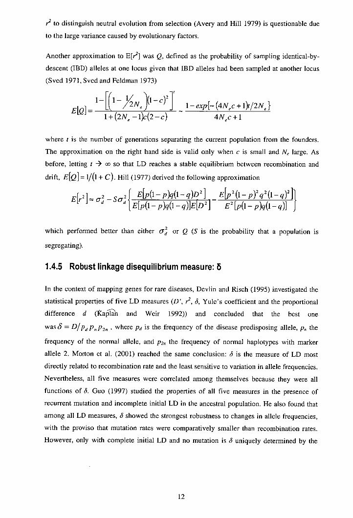
Another approximation to E[r2] was Q, defined as the probability of sampling identical-by-

descent (IBD) alleles at one locus given that IBD alleles had been sampled at another locus

(Sved 1971, Sved and Feldman 1973)

-it I _y

E]= -

1+ (2Ne - 1)c(2 - c) 1— exp{— (4NeC + 1 )t/2Ne }

4Ne C+1

where t is the number of generations separating the current population from the founders.

The approximation on the right hand side is valid only when c is small and Ne large. As

before, letting t -) co so that LD reaches a stable equilibrium between recombination and

drift, E[Q] = i/(i + c). Hill (1977) derived the following approximation

E[r2] o —So _E[p(1__ p )q(1_ q)D 2 ] E[p 2 (1_ p )2 q 2 (1_ q ) 2 ]

l E[p(1 - p)q(i - q)]E[D2 I - E [p(1 - p)q(1 - q )}

which performed better than either O or Q (S is the probability that a population is

segregating).

1.4.5 Robust linkage disequilibrium measure: 5

In the context of mapping genes for rare diseases, Devlin and Risch (1995) investigated the

statistical properties of five LD measures (D', r2 , ô, Yule's coefficient and the proportional

difference d (Kaplan and Weir 1992)) and concluded that the best one

was S = DI Pd p, p2 , , where Pd 15 the frequency of the disease predisposing allele, p, the

frequency of the normal allele, and P2n the frequency of normal haplotypes with marker

allele 2. Morton et al. (2001) reached the same conclusion: ö is the measure of LD most

directly related to recombination rate and the least sensitive to variation in allele frequencies.

Nevertheless, all five measures were correlated among themselves because they were all

functions of ô. Guo (1997) studied the properties of all five measures in the presence of

recurrent mutation and incomplete initial LD in the ancestral population. He also found that

among all LD measures, 6 showed the strongest robustness to changes in allele frequencies,

with the proviso that mutation rates were comparatively smaller than recombination rates.

However, only with complete initial LD and no mutation is ö uniquely determined by the

12

recombination fraction, and either high mutation rates or partial LD in the founders reduced

the accuracy of prediction of LD in all measures.

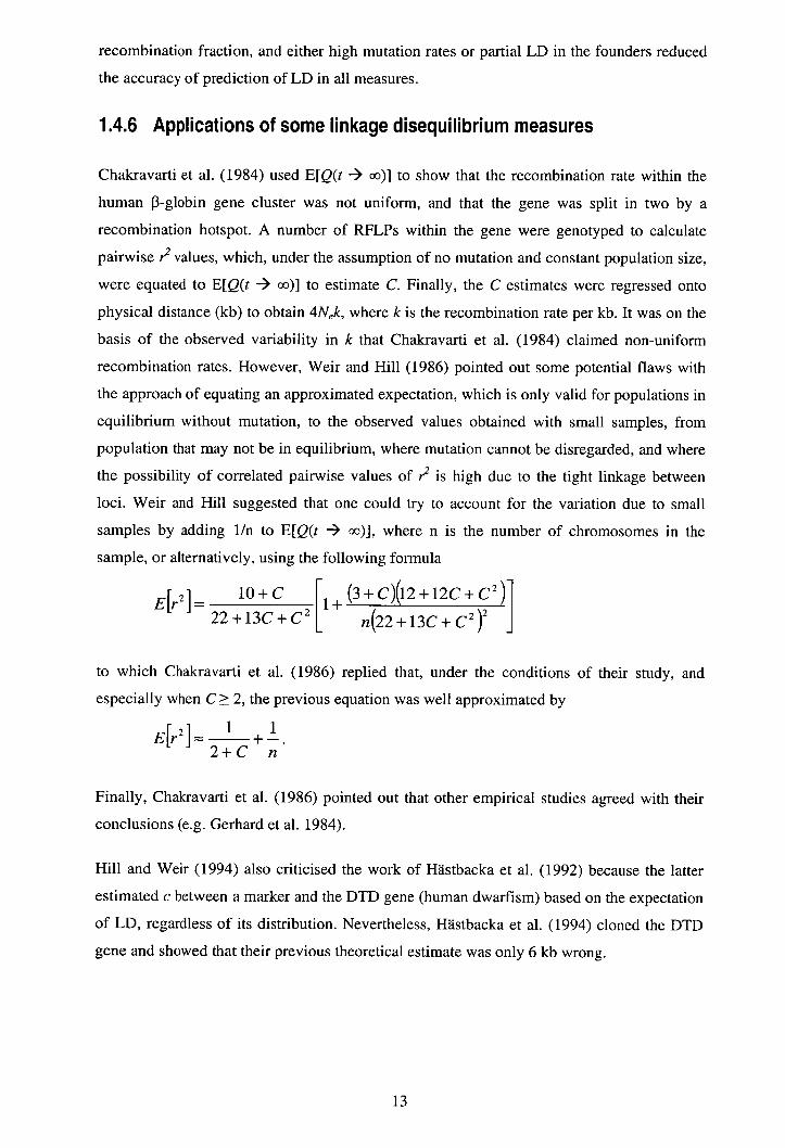
1.4.6 Applications of some linkage disequilibrium measures

Chakravarti et al. (1984) used E[Q(t - co)] to show that the recombination rate within the

human 3-globin gene cluster was not uniform, and that the gene was split in two by a

recombination hotspot. A number of RFLPs within the gene were genotyped to calculate

pairwise r2 values, which, under the assumption of no mutation and constant population size,

were equated to E[Q(t -) co)] to estimate C. Finally, the C estimates were regressed onto

physical distance (kb) to obtain 4Nek, where k is the recombination rate per kb. It was on the

basis of the observed variability in k that Chakravarti et al. (1984) claimed non-uniform

recombination rates. However, Weir and Hill (1986) pointed out some potential flaws with

the approach of equating an approximated expectation, which is only valid for populations in

equilibrium without mutation, to the observed values obtained with small samples, from

population that may not be in equilibrium, where mutation cannot be disregarded, and where

the possibility of correlated pairwise values of r2 is high due to the tight linkage between

loci. Weir and Hill suggested that one could try to account for the variation due to small

samples by adding 1/n to E[Q(t - co)], where n is the number of chromosomes in the

sample, or alternatively, using the following formula

E1r j21 = 1+

io+c (3 + C)(12 + 12C + C2)

22+13C+C2 n(22+13c+c2 )2

to which Chakravarti et al. (1986) replied that, under the conditions of their study, and

especially when C> 2, the previous equation was well approximated by

121 1 1 Er j +—. 2+C n

Finally, Chakravarti et al. (1986) pointed out that other empirical studies agreed with their

conclusions (e.g. Gerhard et al. 1984).

Hill and Weir (1994) also criticised the work of Hästbacka et al. (1992) because the latter

estimated c between a marker and the DTD gene (human dwarfism) based on the expectation

of LD, regardless of its distribution. Nevertheless, Hastbacka et al. (1994) cloned the DTD

gene and showed that their previous theoretical estimate was only 6 kb wrong.

IN

Finally, Kaplan et al. (1995) argued that these two studies (Chakravarti et al. 1984,

Hästbacka et al. 1992) may have just been the 'lucky' ones, and many more studies could

have been led astray by inaccurate theoretical approaches.

1.5 THE TRANSMISSION DISEQUILIBRIUM TEST (TDT)

1.5.1 Precursors of TDT

Association between a marker and a disease locus can be detected with a case/control study

(Schork et al. 2001). Under the null hypothesis (H0) of no association, the distribution of

allele frequencies (or genotype frequencies) is expected to be the same in both groups. The

main problem with this type of studies is that a significant association could be spurious if

controls are not chosen from within the same genetic group as cases. One solution to this

problem is to create internal controls by taking the two marker alleles transmitted to an

affected offspring to form a case genotype, and the non-transmitted alleles to form a control

genotype (matched tests). Table 1.3 summarises the main features of some TDT precursors.

Table 1.3. Main precursors of the Transmission-Disequilibrium Test

Test Main features References

MGRR Compares transmitted and not transmitted genotypes to an individual Rubinstein et al. 1981

GHRR Compares genotypes between cases and controls Falk and Rubinstein 1987

HHRR Compares alleles between cases and controls Terwilliger and Ott 1992 Thompson 1995

McNemar Compares alleles transmitted and not transmitted to an individual

Terwilliger and Ott 1992

Rubinstein et al. (1981) and Falk and Rubinstein (1987) designed the matched genotype

relative risk (MGRR) to test whether the frequency of a marker allele M differed

significantly between case and control genotypes, N.B. controls are created with the two

alleles no transmitted to cases, they are not real individuals. For example, if parents have the

genotypes Mm and mm and the case has the genotype Mm, then the conrrol is mm. There is

no distinction between a case (or a control) possessing one or two copies of M, and hence

homozygote MM and heterozygote Mm cases are given equal weight (Schaid and Sommer

1994). The data for the MGRR is outlined in Table 1.4. Another possibility is to use the

genotype-based haplotype relative risk (GHRR) (Table 1.5), where cases and controls are

unmatched, i.e. comparing the total number of genotypes with at least one M allele among

cases versus that number among controls. Note that entries in Tables 1.4 and 1.5 with the

14

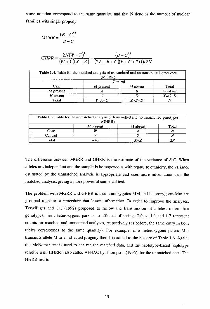
same notation correspond to the same quantity, and that N denotes the number of nuclear

families with single progeny.

B C MGRR=' " - /

B+C

GHRR= 2N(W-Y) 2 = (B-c) 2

(w+Y)(x+z) (2A+B+c)(B+c+2D)/2N

Table 1.4. Table for the matched analysis of transmitted and no transmitted genotypes (MGRR)

Case Control

Total M present M absent M present A B W=A+B M absent C D X=C+D

Total Y=A+C Z=B+D N

Table 1.5. Table for the unmatched analysis of transmitted and no transmitted genotypes (GHRR)

M present M absent Total Case W X N

Control Y Z N Total W+Y X+Z 2N

The difference between MGRR and GHRR is the estimate of the variance of B-C. When

alleles are independent and the sample is homogeneous with regard to ethnicity, the variance

estimated by the unmatched analysis is appropriate and uses more information than the

matched analysis, giving a more powerful statistical test.

The problem with MGRR and GHRR is that homozygotes MM and heterozygotes Mm are

grouped together, a procedure that losses information. In order to improve the analyses,

Terwilliger and Ott (1992) proposed to follow the transmission of alleles, rather than

genotypes, from heterozygous parents to affected offspring. Tables 1.6 and 1.7 represent

counts for matched and unmatched analyses, respectively (as before, the same entry in both

tables corresponds to the same quantity). For example, if a heterozygous parent Mm

transmits allele M to an affected progeny then 1 is added to the b score of Table 1.6. Again,

the McNemar test is used to analyse the matched data, and the haplotype-based haplotype

relative risk (HHRR), also called AFBAC by Thompson (1995), for the unmatched data. The

HHRR test is

15

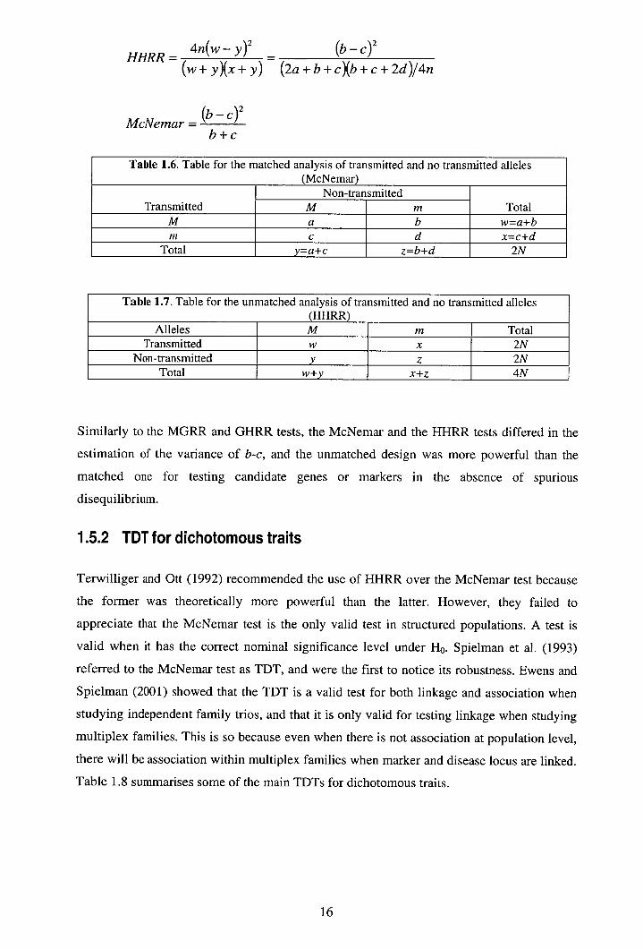
HHRR= 4n(w—y) 2 = (b—c) 2

(w+y)(x+y) (2a + b + c)(b + c + 2d)/4n

\

McNemar = I - C)

2

b+c

Table 1.6. Table for the matched analysis of transmitted and no transmitted alleles (McNemar)

Transmitted Non-transmitted

Total M m M a b w=a+b M c d x=c+d

Total y=a+c z=b+d 2N

Table 1.7. Table for the unmatched analysis of transmitted and no transmitted alleles (HHRR)

Alleles M m Total Transmitted w x 2N

Non-transmitted z 2N Total w+y x+z 4N

Similarly to the MGRR and GHRR tests, the McNemar and the HHRR tests differed in the

estimation of the variance of b-c, and the unmatched design was more powerful than the

matched one for testing candidate genes or markers in the absence of spurious

disequilibrium.

1.5.2 TDT for dichotomous traits

Terwilliger and Ott (1992) recommended the use of HHRR over the McNemar test because

the former was theoretically more powerful than the latter. However, they failed to

appreciate that the McNemar test is the only valid test in structured populations. A test is

valid when it has the correct nominal significance level under H0. Spielman et al. (1993)

referred to the McNemar test as TDT, and were the first to notice its robustness. Ewens and

Spielman (2001) showed that the TDT is a valid test for both linkage and association when

studying independent family trios, and that it is only valid for testing linkage when studying

multiplex families. This is so because even when there is not association at population level,

there will be association within multiplex families when marker and disease locus are linked.

Table 1.8 summarises some of the main TDTs for dichotomous traits.

16

Table 1.8. Transmission-Disequilibrium Tests for dichotomous traits Test Main features References TDT McNemar test in Table 1.3 Spielman et al. 1993

Testing the symmetry of cell counts in a multiallelic Bickeboller and Clerget- TDTC

version of Table 1.5 Darpoux 1995 Sham and Curtis 1995

Trpj,et Testing the symmetry of marginal subtotals in a

Spielman and Ewans 1996 multiallelic version of Table 1.5 T, Improved version of T,,,., et Sham 1997

Miscellaneous: allelic risk, maximum likelihood, Clayton and Jones 1999 Log-tests log-linear models Zhao 2000

Schaid and Rowland 2000 S Rao's efficient score statistic Schaid 1996

maxTDT Similar to Ts and Tmhet with unknown MOl Morris et al. 1997a, b

Z 1 , Z. TDT for sibship data and two or more alleles, Ewens and Spielman 199

Z.. respectively Laird et al. 1998

RC-TDT TDT for sibship data and reconstructed parental Knapp 1999 genotypes

SDT Sign test TDT for sibship data and multiallelic Horvath and Laird 1998 markers Curtis et al. 1999

zc Maximum discordant sib pair TDT Curtis 1997 AC2 Sibship TDT Boenhke and Langefeld 1998

TMSTDT Uses unaffected sibs as surrogates for missing

Monks et al. 1998 parental data PDT TDT for extended pedigrees Martin et al. 2000

Originally, TDT was developed for testing linkage in cases where disease association had

already been found. The TDT compares the number of times a marker allele is transmitted

from a heterozygous parent to her/his affected child versus the number of times it is not

transmitted. Under the H0 of no linkage E[b] = E[c] (Table 1.6), and TDT is distributed as a

x2 with 1 degree of freedom. Zhao (1999) re-interpreted the TDT in terms of allele risk

ratios, when considering a single parent, or in terms of genotype (multiplicative) penetrance

ratios, considering both parents.

Several extensions of the TDT have been proposed for analysing multi-allelic markers.

Sethuraman (1997) derived the probability for each cell in a multi-allelic version of Table

1.6 as

I(p 1 711 + + D,)—c(mD, —mD)J+) IK L(PI12 + P2' 'r22 )[m(mp2 + D1 )- c(mD 1 - mD

where Pi, P2, m, are the frequencies of alleles Q and q at the disease locus, and allele i at the

marker locus, respectively; ?r, Z12, 7r22 are the penetrances of disease genotypes QQ, Qq and

qq, respectively; K = + 2p1p2r12 +P

2 7r22 is the prevalence of the disease in the

17

population; D, is the linkage disequilibrium between marker allele i and disease allele Q. The

same expressions were used by Sham and Curtis (1995) in their logistic model, and by

Morris et al. (1997 b) in their likelihood ratio tests.

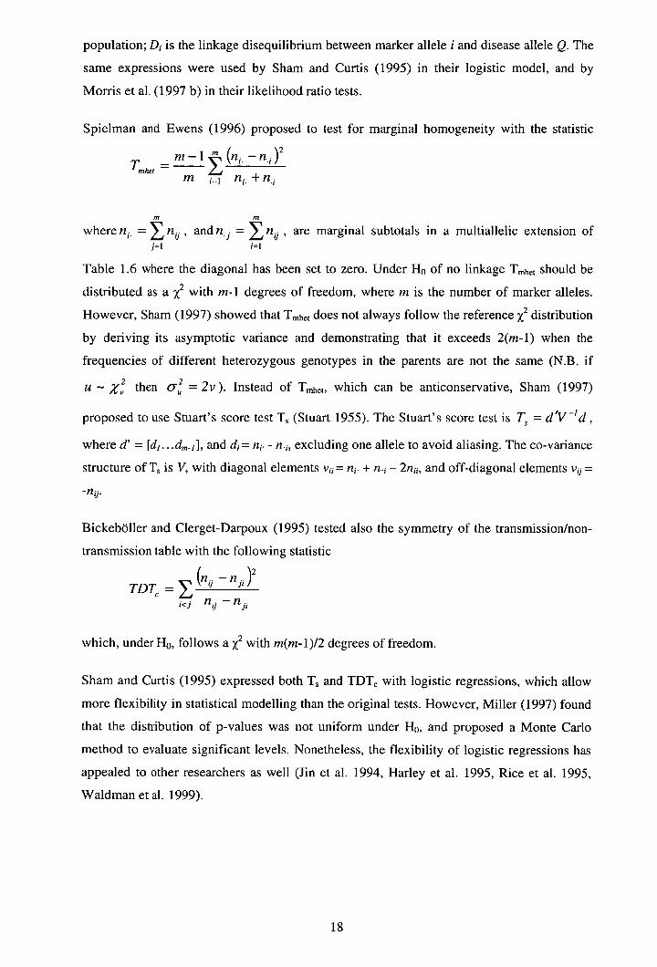
Spielman and Ewens (1996) proposed to test for marginal homogeneity with the statistic

T - m —1 (, 1 - n• )2

.het - m j1 n1 +

where n 1• =n, , and n.j = n,, , are marginal subtotals in a multiallelic extension of

Table 1.6 where the diagonal has been set to zero. Under H 0 of no linkage Tmiiet should be

distributed as a x2 with rn-i degrees of freedom, where m is the number of marker alleles.

However, Sham (1997) showed that Tmiet does not always follow the reference x2 distribution

by deriving its asymptotic variance and demonstrating that it exceeds 2(m-1) when the

frequencies of different heterozygous genotypes in the parents are not the same (N.B. if

U - X 2 2

T = 2v). Instead of Tmhet, which can be anticonservative, Sham (1997)

proposed to use Stuart's score test T (Stuart 1955). The Stuart's score test is T = d'V'd,

where d' = [d1 .. .dmj ], and di = n. - n.e, excluding one allele to avoid aliasing. The co-variance

structure of T is V, with diagonal elements v ii = n. + n. - and off-diagonal elements v 0 =

-flu .

Bickeboller and Clerget-Darpoux (1995) tested also the symmetry of the transmission/non-

transmission table with the following statistic

(

TDTC = n fl )

d ii

which, under H0, follows a x2 with m(m-1)/2 degrees of freedom.

Sham and Curtis (1995) expressed both T s and TDTC with logistic regressions, which allow

more flexibility in statistical modelling than the original tests. However, Miller (1997) found

that the distribution of p-values was not uniform under H 0, and proposed a Monte Carlo

method to evaluate significant levels. Nonetheless, the flexibility of logistic regressions has

appealed to other researchers as well (un et al. 1994, Harley et al. 1995, Rice et al. 1995,

Waldman et al. 1999).

18

Schaid (1996) used a conditional likelihood to model offspring genotype as a function of

parental genotypes and offspring disease status as follows:

P(gIg,gj,D)= P(DIg,g,g1 )P(gIg m ,g 1 )P(g,g j )

p(Dg*,g,gj)p(g*g,g1 )P(gm,g1)

g€G

where D denotes disease status, g, g, and g1 are the marker genotypes of the affected

offspring, mother and father, respectively, and g*

is one of the four possible genotypes G of

the child conditional on parental genotypes. Given P(DIg,g 1,g) = P(Dg), then the

above equation reduces to

P(gcIg,gj,D)= r(g) r(g *)

gEG

where r(g) is the relative risk of disease for genotype g. If g consists of two haplotypes i and

j, and assuming a multiplicative model, then log r(g) = log r(i,j) =,8i + ,8j (Zhao 2000),

and, more generally h[r(i,j)] = 8, + ,8 j = -- {h[r(i,i)]+ h[r(i,i)]} (Clayton and Jones 1999),

where h is an unspecified monotone increasing function.

Schaid (1996) proposed the following model

log r(g)= X'3

where X is the coded vector for the observed genotype g. The H 0 of no association, i.e. /3 = 0,

can be tested with Rao's efficient score statistic

S =U'V - 'U

Ia 2 lfl L alnL where U

= 1/3=0 and = —

E Lafl,afl1 /3=0

When the mode of inheritance is unknown, two statistics, the T discussed above and the

maxTDT statistic defined as

nwxTDT = max _(n - )2

, =

19

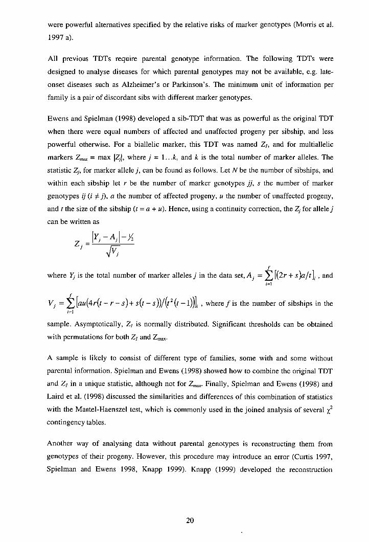
were powerful alternatives specified by the relative risks of marker genotypes (Morris et al.

1997 a).

All previous TDTs require parental genotype information. The following TDTs were

designed to analyse diseases for which parental genotypes may not be available, e.g. late-

onset diseases such as Alzheimer's or Parkinson's. The minimum unit of information per

family is a pair of discordant sibs with different marker genotypes.

Ewens and Spielman (1998) developed a sib-TDT that was as powerful as the original TDT

when there were equal numbers of affected and unaffected progeny per sibship, and less

powerful otherwise. For a biallelic marker, this TDT was named Z j , and for multiallelic

markers Z,,,., = max JZj I , where j = 1. . . k, and k is the total number of marker alleles. The

statistic Z,, for marker allele j, can be found as follows. Let N be the number of sibships, and

within each sibship let r be the number of marker genotypes jj, s the number of marker

genotypes zj (i j), a the number of affected progeny, u the number of unaffected progeny,

and t the size of the sibship (t = a + u). Hence, using a continuity correction, the Z for allelej

can be written as

Y. — A. —% j -

FVJ

where Yj is the total number of marker alleles j in the data set, A = [(2r + s)a/t]1 , and

= [au(4r(t - r - s)+ s(t - s))/(t2 (t - 1))] i , where f is the number of sibships in the

sample. Asymptotically, Zj is normally distributed. Significant thresholds can be obtained

with permutations for both Zj and Zmax .

A sample is likely to consist of different type of families, some with and some without

parental information. Spielman and Ewens (1998) showed how to combine the original TDT

and Zj in a unique statistic, although not for Z,. Finally, Spielman and Ewens (1998) and

Laird et al. (1998) discussed the similarities and differences of this combination of statistics

with the Mantel-Haenszel test, which is commonly used in the joined analysis of several x2 contingency tables.

Another way of analysing data without parental genotypes is reconstructing them from

genotypes of their progeny. However, this procedure may introduce an error (Curtis 1997,

Spielman and Ewens 1998, Knapp 1999). Knapp (1999) developed the reconstruction

20

combined TDT (RC-TDT), providing necessary and sufficient conditions for the observed

marker genotypes in the offspring to allow reconstruction of parental genotypes, and showed

that RC-TDT was more powerful than Z 1 and Z,. Parental genotypes could also be

reconstructed stochastically via Gibbs Sampling.

Bias can also be introduced when one parental genotype is missing and ambiguous families

are discarded (e.g. when the parent and the child have the same Mm genotype). Under this

circumstance, Curtis and Sham (1995) proposed discarding progeny with genotypes MM,

Mm and mm, when the only known parental genotype is Mm. Sun et al. (1998, 1999)

proposed two new tests to analyse families with one missing parental genotype. The power

of these tests was roughly equal to Z 1 and Z,na ,, when one affected and one unaffected sibs

were sampled, and both needed approximately twice as much records as TDT (Wang and

Sun 2000).

All methods described so far are based on comparing affected and unaffected sibs. Teng and

Risch (1999) suggested that there is additional information available in the sample from the

relative frequency of the different sibship genotype constellations. They showed that two

unaffected sibs without parents requires approximately 50% more families than when parents

are available, however their strategy of grouping records by combinations of progeny

genotypes may be sub-optimum (Zhao 2000).

Horvath and Laird (1998) developed the SDT (sibship disequilibrium test) to analyse

families without parental information. Let us assume two alleles, M and m, and let mA and

mu denote the average number of M alleles in affected and unaffected progeny, respectively.

For biallelic markers, the SDT is the following nonparametric sign test on differences d,

where d = MA - mu,

SDT= (b—c)2

b+c

where b is the number of sibships for which d> 0, and c is the number of sibships for which

d < 0. For a marker with k> 2 alleles, the sign test is

T=S'W'S

where S'= [s'. . .s'], and s i

sgn(d/) summing across all n sibships, the sign being 1, 0

or —1 when d > 0, d = 0 or d < 0, respectively, and W is a matrix with elements

21

w1 :--

sgn(d/) s gn(d 1'). Under H0 the expectation of S is 0 and T is asymptotically

distributed as a x2 with k-i degrees of freedom. The SDT can be combined with the TDT

when the data consist of a mixture of families with and without parental information, both

for biallelic markers (Horvath and Laird 1998) and for multiallelic markers (Curtis et al.

1999).

Curtis (1997) proposed to choose one affected progeny at random, and then select one

unaffected offspring whose marker genotype maximally differs from the affected one. Each

marker allele in the affected child is compared against his/her sibs, and if both alleles are the

same then they are ignored, but if they are different then ½ is added to T 1 , where i denotes

the allele from the affected child and j the allele from the unaffected one. For biallelic

markers, the test is

1 2 —(N 2 +N1 /2) C

jN2+N1/4

where Ni is the number of sibships that increase the test statistic of either T12 or T21 by i. For

multiallelic markers Curtis used a likelihood model such as in Sham and Curtis (1995),

however Monks et al. (1998) found a poor approximation of the likelihood ratio test to the x2

distribution.

For markers with k> 2 alleles, Boenhke and Langefeld (1998) constructed 2 x k contingency

tables where the rows represented disease status. The most powerful way of analysing these

tables was ignoring alleles shared between affected and unaffected sibs and only focusing in

those alleles from which sibs differed using the following statistic:

AC 2 = (n - n2

)2

j=I iJ + fl 2

where nj and n2j are counts of marker allele j in affected and unaffected sibs, respectively.

Significant thresholds were obtained permuting affection status among sibs.

Monks et al. (1998) proposed the TMSTDT and compared it with Z (Curtis 1997), Z 1 and Zmax

(Spielman and Ewens 1998) and AC 2 (Boehnke and Langefeld 1998). They found that, for

biallelic markers, these TDTs had similar power, however differences arose when testing

multiallelic markers. In general, AC 2 and TMSTDT had similar power in all scenarios; Zm was

more powerful than the previous two TDTs when one of the marker alleles was more

22

strongly associated with the disease allele than the rest of the alleles, and was less powerful

when all marker alleles were equally associated with the disease allele; and finally, Z was

the least powerful test in all situations.

Martin et al. (2000) developed the pedigree disequilibrium test (PDT) as a valid test for

linkage disequilibrium when the sample consists of multiple related nuclear families. PDT is

based on the average measure of LD calculated across all triads and discordant sib pairs.

PDT was more powerful than Z 1 and Z,,, (Spielman and Ewens 1998) and SDT (Horvath

and Laird 1998). PDT gives larger weight to larger sibships and nuclear families within a

pedigree, but equal weights to all pedigrees. It may be better to give more weight to more

informative pedigrees over less informative ones. PDT also gives equal weight to triad and

discordant sib-pairs, however if unaffected sibs may have been misclassified then it would

be a better approach to give higher weight to triad than sib-pairs.

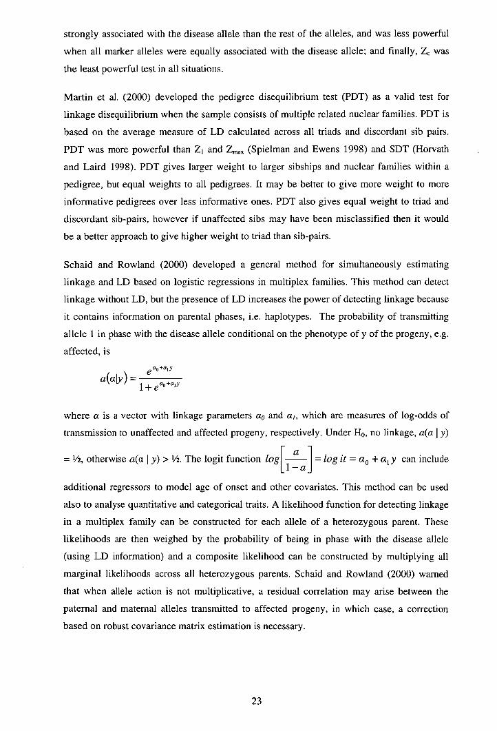
Schaid and Rowland (2000) developed a general method for simultaneously estimating

linkage and LD based on logistic regressions in multiplex families. This method can detect

linkage without LD, but the presence of LD increases the power of detecting linkage because

it contains information on parental phases, i.e. haplotypes. The probability of transmitting

allele 1 in phase with the disease allele conditional on the phenotype of y of the progeny, e.g.

affected, is

a0 +a 1 y , e

a(aLy)= 1 + ea0)

where a is a vector with linkage parameters a 0 and a 1 , which are measures of log-odds of

transmission to unaffected and affected progeny, respectively. Under H 0, no linkage, a(a I

= ½, otherwise a(a I y) > ½. The logit function log a aJ=

log it = a 0 + a 1 y can include [l—

additional regressors to model age of onset and other covariates. This method can be used

also to analyse quantitative and categorical traits. A likelihood function for detecting linkage

in a multiplex family can be constructed for each allele of a heterozygous parent. These

likelihoods are then weighed by the probability of being in phase with the disease allele

(using LD information) and a composite likelihood can be constructed by multiplying all

marginal likelihoods across all heterozygous parents. Schaid and Rowland (2000) warned

that when allele action is not multiplicative, a residual correlation may arise between the

paternal and maternal alleles transmitted to affected progeny, in which case, a correction

based on robust covariance matrix estimation is necessary.

23

1.5.3 Summary of TDT for dichotomous traits

TDT analyses the association between disease occurrence in progeny and transmission of a

particular marker allele from parents. Further extensions of the TDT have allowed the

analysis of multiallelic markers and/or missing parental genotypes (i.e. sib-TDTs). For

biallelic markers, a TDT using parental information can be combined with a sib-TDT.

Extended pedigrees can also be analysed after decomposing them into nuclear family units.

Although several TDTs have been developed as contingency tables, alternative

parameterisations based on linear and log-linear models offer greater flexibility (e.g.

correcting simultaneously for fixed effects). Finally, some tests allow for the joint estimation

of association and linkage.

1.5.4 TDT for quantitative traits

Many human diseases, e.g. obesity, osteoporosis, and most agricultural traits of interest, e.g.

growth, fatness, are continuously distributed. In order to analyse these traits several

quantitative TDTs have been developed. Table 1.9 summarises the main TDTs in this

section.

Table 1.9. Transmission-Disequilibrium Tests for quantitative traits Test Main features References

TDTQI.Q5 Tests with and without prior phenotypic Allison 1997 ascertainment.

Multiple regression Miscellaneous tests involving multiple George et al. 1999 Xiong et al. 1998 linear regressions. Yang et al. 2000

TDTR Correlation between allele transmission Rabinowitz 1997 and trait

TQp, TQS, TQPS TDT, sib-TDT and TDT that uses sib and Monks and Kaplan 2000 parent _information, _respectively

TDTG Contrast between group means regarding Xiong et al. 1998 transmitted allele Szyda et al. 1998

S Permutation-based TDT Allison et al. 1999

Variance-component TDT Estimates between and within QTL Fulker et al. 1999 Sham et al. 2000 variances

Abecasis et al. 2000

b, bpD Estimation of between and within (i.e. Janss (pers. comm.)

TDT) QTL fixed effects Hernández-Sánchez et al. 2002

Allison (1997) developed five different quantitative TDTs to analyse samples of family trios.

Tests TDTQ I to TDTQ4 required trios with a single heterozygous parent, and whereas TDTQ I

and TDTQ3 assumed random sampling of trios regarding the trait value, TDTQ2 and TDT

24

were analysed extreme phenotypic samples. The preferred test was TDT Q5 because: 1) it had

a consistently high power under all modes of inheritance, 2) it analysed together families

with either one or two heterozygous parents, and 3) statistical modelling was facilitated by

the multiple linear regression approach of TDT Q5 .

In the TDTQ5, the quantitative trait was first regressed to a dummy variable indicating the

type of informative parental genotype combination (i.e. MM x Mm, Mm x Mm, or mm x

Mm), and secondly, regressed to the same explanatory variable plus two additional variables

encoding allele transmission (one for modelling additive effects, the other dominant effects).

TDTQ5 is an F-test for comparing how much phenotypic variation is explained with the

extended model over the reduced one.

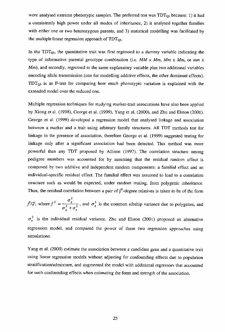
Multiple regression techniques for studying marker-trait associations have also been applied

by Xiong et al. (1998), George et al. (1999), Yang et al. (2000), and Zhu and Elston (2001).

George et al. (1999) developed a regression model that analysed linkage and association

between a marker and a trait using arbitrary family structures. All TDT methods test for

linkage in the presence of association, therefore George et al. (1999) suggested testing for

linkage only after a significant association had been detected. This method was more

powerful than any TDT proposed by Allison (1997). The correlation structure among

pedigree members was accounted for by assuming that the residual random effect is

composed by two additive and independent random components: a familial effect and an

individual-specific residual effect. The familial effect was assumed to lead to a correlation

structure such as would be expected, under random mating, from polygenic inheritance.

Thus, the residual correlation between a pair of jthdegree relatives is taken to be of the form

2

J'/2j, where f2 = 2g 2 and is the common sibship variance due to polygenes, and U +O e

ore is the individual residual variance. Zhu and Elston (2001) proposed an alternative

regression model, and compared the power of these two regression approaches using

simulations.

Yang et al. (2000) estimate the association between a candidate gene and a quantitative trait

using linear regression models without adjusting for confounding effects due to population

stratification/admixture, and augmented the model with additional regressors that accounted

for such confounding effects when estimating the form and strength of the association.

25

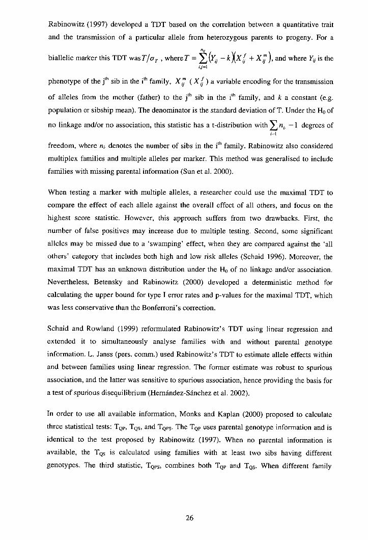
Rabinowitz (1997) developed a TDT based on the correlation between a quantitative trait

and the transmission of a particular allele from heterozygous parents to progeny. For a

nij biallelic marker this TDT wasT/a , where = (Y —kXX6 + X where Yjj the

ij=1

phenotype of the jth sib in the ith family, X, (X,) a variable encoding for the transmission

of alleles from the mother (father) to the jth sib in the ith family, and k a constant (e.g.

population or sibship mean). The denominator is the standard deviation of T. Under the H 0 of

no linkage and/or no association, this statistic has a t-distribution with n. —1 degrees of

freedom, where n. denotes the number of sibs in the ith family. Rabinowitz also considered

multiplex families and multiple alleles per marker. This method was generalised to include

families with missing parental information (Sun et al. 2000).

When testing a marker with multiple alleles, a researcher could use the maximal TDT to

compare the effect of each allele against the overall effect of all others, and focus on the

highest score statistic. However, this approach suffers from two drawbacks. First, the

number of false positives may increase due to multiple testing. Second, some significant

alleles may be missed due to a 'swamping' effect, when they are compared against the 'all

others' category that includes both high and low risk alleles (Schaid 1996). Moreover, the

maximal TDT has an unknown distribution under the H 0 of no linkage and/or association.

Nevertheless, Betensky and Rabinowitz (2000) developed a deterministic method for

calculating the upper bound for type I error rates and p-values for the maximal TDT, which

was less conservative than the Bonferroni's correction.

Schaid and Rowland (1999) reformulated Rabinowitz's TDT using linear regression and

extended it to simultaneously analyse families with and without parental genotype

information. L. Janss (pers. comm.) used Rabinowitz's TDT to estimate allele effects within

and between families using linear regression. The former estimate was robust to spurious

association, and the latter was sensitive to spurious association, hence providing the basis for

a test of spurious disequilibrium (Hernández-Sánchez et al. 2002).

In order to use all available information, Monks and Kaplan (2000) proposed to calculate

three statistical tests: TQP, TQS, and TQPS. The TQP uses parental genotype information and is

identical to the test proposed by Rabinowitz (1997). When no parental information is

available, the TQS is calculated using families with at least two sibs having different

genotypes. The third statistic, TQPS, combines both TQP and TQS. When different family

26

structures provided unequal amount of information to these statistics, a permutation

procedure was suggested for obtaining p-values. For multiallelic markers, Monks and Kaplan

followed the approach of Rabinowitz (1997), and suggested to calculate a maximal statistical

test.

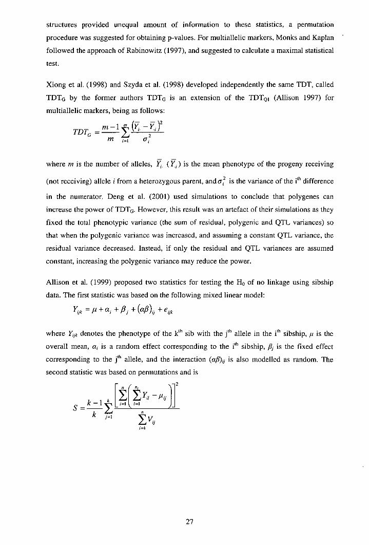
Xiong et al. (1998) and Szyda et al. (1998) developed independently the same TDT, called

TDTG by the former authors TDTG is an extension of the TDTQ I (Allison 1997) for

multiallelic markers, being as follows:

TDTG m_1t (. _7ii2 M j1 a1

where m is the number of alleles, Yi. (Y e.) is the mean phenotype of the progeny receiving

(not receiving) allele i from a heterozygous parent, and a, is the variance of the i th difference

in the numerator. Deng et al. (2001) used simulations to conclude that polygenes can

increase the power of TDTG . However, this result was an artefact of their simulations as they

fixed the total phenotypic variance (the sum of residual, polygenic and QTL variances) so

that when the polygenic variance was increased, and assuming a constant QTL variance, the

residual variance decreased. Instead, if only the residual and QTL variances are assumed

constant, increasing the polygenic variance may reduce the power.

Allison et al. (1999) proposed two statistics for testing the H0 of no linkage using sibship

data. The first statistic was based on the following mixed linear model:

jk =f1+a +fl +(a/3), +eUk

where Y,1k denotes the phenotype of the kth sib with the Jth allele in the ith sibship, 1u is the

overall mean, a 1 is a random effect corresponding to the i1h sibship, 83 is the fixed effect

corresponding to the j h allele, and the interaction (a,8), is also modelled as random. The

second statistic was based on permutations and is

)- 2

k

I i=1 1=1

k j=1 Vii

27

where P& and V13 are the mean and variance, from the jth sibship and j th allele, respectively.

The permutation-based statistic showed, in general, more power than the statistic based on a

mixed-linear model, and has the extra advantage of being distribution-free.

Fulker et al. (1999) used variance component methods to test for both linkage and

association of markers and QTL in sibships. They partitioned the sibship variation in

between and within sib-pair components, and constructed a robust test with the latter

component of variation. Sham et al. (2000) concluded that the power of detecting association

with this method was proportional to the QTL heritability and the square of LD, and the

power of detecting linkage was proportional to the square of the QTL heritability. Therefore,

confirming the idea that, when LD is strong, testing for association is more powerful than

testing for linkage. Abecasis et al. (2000) extended this method to accommodate any number

of sibs, with or without parental genotypes.

1.5.5 Summary of TDT for continuous traits

Continuously distributed traits can be analysed with TDT. Multiple regression techniques

have been widely used for this purpose. This statistical framework allows studying general

pedigrees (e.g. accounting for the correlation structure among sibs), simultaneous estimation

of association and linkage, sibship data, and multiple hypotheses testing. Moreover, TDTs

formulated more rigidly (e.g. Rabinowitz 1997) have been re-formulated with multiple

regressions (e.g. Schaid and Rowland 1999, L Janss (pers. comm.)). As in the case of

dichotomous traits, TDTs that use parental information or just sib information can be

combined together in complex pedigrees with several nuclear family structures. Finally,

comparing the power across TDTs has become crucial in order to discriminate among such a

prolific bibliography.

1.6 LINKAGE DISEQUILIBRIUM MAPPING VIA MODELLING

POPULATION HISTORY

Methods of analysis that do not take into account evolutionary variances and covariances,

particularly when studying large and heterogeneous populations, may be overoptimistic. For

example, Terwilliger (1995) developed a maximum likelihood (ML) method to obtain

recombination rate estimates between a marker locus and the hypothetical location of a

disease gene by measuring the excess frequency of a marker allele in a sample of affected

individuals with respect to the frequency in the whole population. Moreover, this ML

combined information from multiple, and multiallelic, markers per chromosomal region.

However, Devlin and Risch (1995) pointed out that, notwithstanding the similarities with the

approach of Kaplan et al. (1995), this ML did not explicitly model the evolutionary variance

in the population and, as a result, the likelihood profile was too sharp and the confidence

intervals for gene location too narrow.

Using historical information in gene mapping studies has been crucial in some cases. For

example, the most striking result of gene mapping by LD methods has been the mapping of

the Distrophy Dysplasia gene (DTD) (Hästbacka et al. 1992). DTD is a rare and recessive

condition characterised by dwarfism, which has a relatively high prevalence in Finland. A

previous linkage analysis had located the DTD gene within a broad region of chromosome 5.

A finer location of the DTD gene was not possible via linkage analysis because the sample

size could not be easily increased. Instead, estimates of recombination rates between markers

and the potential DTD locus were obtained by modelling the Finnish demographic history.

They assumed the current population had been steadily growing from a small group of

individuals that arrived in Finland 100 generations ago. A single copy of the DTD

predisposing allele was probably introduced then, and, therefore most of the DTD alleles

must be its direct descendents. Affected individuals not only inherited two copies of the

same DTD allele, but also common background haplotypes. The Finnish history was

modelled using the approach of Luria and Deibruck (1943), which was originally designed to

study the exponential growth phase of bacteria. The results were encouraging: the DTD gene

was predicted to lie within 70 Kb from the CSF1R marker. Finally, the DTD gene was

physically mapped at 64 kb from CSF1R (Hästbacka et al. 1994).

Despite this success, Hill and Weir (1994), Kaplan et al. (1995), and Kaplan and Weir (1995)

argued that Hästbacka and co-workers underestimated the upper confidence intervals for the

location of DTD. Instead, they modelled the evolution of the haplotype containing the DTD

allele as a Poisson branching process, assuming the frequency of normal haplotypes

remained constant over generations. The maximum likelihood (ML) estimator of the upper

confidence interval was twice as large as that obtained by Hästbacka et al. (1992). Although

ML estimators are preferable to point estimators, the Poisson branching model was still

based on population assumptions that are difficult to verify. Moreover, explicit derivations of

these likelihood functions are very difficult, and the authors used computationally

demanding Monte Carlo simulations.

WE

Xiong and Guo (1997) suggested the following approximated likelihood for estimating the

recombination rate between a marker and a disease locus, c, assuming the frequency of

normal haplotypes (p a) constant over generations, and modelling the variation in disease

haplotypes (Pd),

L(p,c) = L(pfl, ,7)+ !Tr[L'(pfl, 7r)Var(pd)]

where E[p] = 7t, and L"(p d ,t) is the matrix of second derivatives. Xiong and Guo

(1997) compared this approximated likelihood with a first order approximation, consisting of

the first term alone, which ignores stochastic changes in the frequency of disease haplotypes

over time. The first order approximation coincided with other deterministic methods

(Hästbacka et al. 1992, Terwilliger 1995). Moreover, Xiong and Guo (1997) showed how to

use information from several linked markers, multiple alleles per marker, and mutations at

both markers and disease loci.

Devlin et al. (1996) developed a composite maximum likelihood method (CML) based on

maximising the likelihood of —log((5), where S I122 1221 = and Jrjj is the frequency of

haplotypes with marker allele i and disease allele j (j = 1 is the disease-predisposing allele),

for each marker, given the recombination rate between marker and disease locus, and

multiplying across all markers. Although Devlin and colleagues were able to re-map

accurately genes underlying simple monogenic diseases, e.g. cystic fibrosis, DTD, on the

basis of published data, there were two main problems with their approach. First, all markers

were assumed independent, and second, they assumed a Gamma distribution for —log(ö),

which will produce a consistent estimator of variance only if the shape of the distribution is

correctly specified (Clayton 2000).

Collins and Morton (1998) and Lonjou et al. (1998) applied the Malecot model, originally

derived to describe kinship as a function of distance between populations, to gene mapping,

where distance is between marker and disease locus. The decay of association (p) between

marker i and disease locus over generations is predicted with the Malecot model

as p1 = (i - L)Me" + L, where p, = E[r1], L denotes the level of spurious association, M

denotes the probability of monophyletic origin of the disease gene, d, is the assumed genetic

distance between marker i and the disease locus, and sd = tc 1 where t is the number of

generations since the disease locus entered the population, and c, and d, are the

30

recombination rate and the physical distance between marker i and the disease locus,

respectively. Information from multiple linked markers was combined in a composite

likelihood that was a function of the joint distribution of p (assuming values for L, M, r), and

the allele frequencies at the marker and disease locus. The Malecot model re-mapped

accurately major genes, e.g. hemochromatosis, Huntington disease and cystic fibrosis,

although it was not tested with complex traits.

The coalescent process (Kingman 1982) has also been used to model the history of a sample

of haplotypes either in the context of diseases (Rannala and Slatkin 1998, Thompson and

Neel 1997, Graham and Thompson 1998) or quantitative traits (Zhang and Zhao 2001). In

the coalescent, a sample of haplotypes is brought backwards in time, allowing the histories

of pairs of haplotypes to meet (a coalescent event), and eventually reaches the single

common haplotype from which all the current ones descended. Each coalescence event

represents either a recombination or a mutation event.

1.7 HAPLOTYPE ANALYSIS AND GENE CLONING

Positional cloning has been defined as the isolation of a gene solely on the basis of its

chromosomal location (Lander and Schork 1994). The observed mosaic-like pattern of LD

may render association studies powerless for mapping the causal mutation, because long

stretches of conserved LD means that several polymorphisms can be strongly associated with

a trait. For example, the most studied polymorphism in the gene encoding angiotensin

converting enzyme (ACE), which hypothetically contributes to cardiovascular disease

(CVD) by controlling blood pressure, has been a 287 bp intronic insertion/deletion called

Alu. However, the effects of Alu on CVD have been contradictory (Schmidt et al. 1993,

Barley et at. 1996). There is absolute LD between Alu and 17 polymorphic SNPs in a region

covering exons 13 to 18 of the gene (Rieder et al. 1999). If a causal mutation were in that

area then an association study would find it very difficult to pinpoint it. Farrall et al. (1999)

discarded exons 1 to 5 from harbouring the causal mutation by demonstrating that from the 3

monophyletic Alu-deletion haplotypes, 2 were associated with similar ACE level in plasma,

and hence, the causal mutation was unlikely to be in the region differing between these two

clades. This region was studied by Zhu et at. (2001) and found that a SNP located upstream

from the 5' end of the ACE encoding gene explained 6% of the variance of ACE

concentration in plasma. In the same study, a second SNP located within exon 17, very close

to the Alu site, explained 19% of the variance of ACE concentration. The best model for

analysing marker-trait linkage included these two loci and an additive x additive interaction

31

between them. These two loci were significantly associated with blood pressure, although no

evidence for linkage was found. This study highlighted two things, 1) association studies can

be more powerful than linkage in regions of high LD, although mapping the causal mutation

may still be very difficult, and 2) that interactions (e.g. epistasis, genetic x environment) may

play an important role in mapping genes underlying complex traits such as hypertension.

A rare and recessive form of progressive epilepsy may be caused by a single mutation in the

ausosomal gene EPM1 (epilepsy mioclonus) (Lehesjoki et al. 1993). EPM1 was first located

on chromosome 21q22.3 with linkage analysis. Subsequently, more data were collected and

the region potentially locating EPM1 was narrowed down to 7 cM. Further resolution was

achieved by studying LD. A haplotype that included alleles from 4 tightly linked marker

loci, spanning —3 Kb, was found in 60% of the cases and only 1% of the controls. That

region was embedded within a slightly larger region of conserved LD. Although LD was

helpful for narrowing down the resolution of location estimates, physical cloning of EPM1

will need a more direct approach, e.g. sequencing all bases along the 3 kb region.

Even though several other studies (e.g. Copeman et al. 1995, Watkins et al. 1994, Snarey et

al. 1994, Yu et al. 1994) used LD for gene mapping in a similar way as shown in the

aforementioned studies (e.g. EPM1 and ACE), the physical localisation of causal mutations

is still a major undertaking (e.g. Kerem et al. 1989, MacDonald et al. 1991, HDCRG 1993).

Nevertheless, the study of haplotypes, as opposed to single markers, may help refining the

location of a causative SNP (Lynch and Walsh 1998). Templeton (1995) suggested creating

cladograms, or evolutionary tree, with the observed haplotypes. The rationale is that the

closer two haplotypes are, the higher the chance of them sharing the same QTL and, hence,

of having similar phenotypic effects. Meuwissen and Goddard (2000) compared the expected

covariances between haplotype effects given a postulated QTL position to the covariances

found in the data. These expected covariances were proportional to the probability that the

QTL is IBD given the marker haplotype information, and were calculated stochastically (i.e.

genedropping). This stochastic method was subsequently substituted by deterministic theory

based on Sved (1971) (Meuwissen and Goddard 2001). In one application of this method, a

QTL for twinning rate in Norwegian cattle was mapped within a 1.3 cM region on

chromosome 15, which is substantially narrower than the usual results reported from

standard linkage analysis.

Haplotypes are more informative than single markers, for example in obtaining IBD

estimates at specific point locations. However, the analysis of haplotypes brings new

problems, e.g. phase construction, high diversity, and optimal haplotype length. Ultimately,

the aim of LD mapping must be to estimate as far as possible the ancestry of chromosomes

carrying the gene of interest in the current sample, and to place marker mutations and

recombinations on this (Clayton 2000).

The total number of SNPs in the human genome exceeds 1.69 million (Chakravarti 1998,

Miller and Kwok 2001, The international SNP map working group 2001), accessible at

NCBI (www.ncbi.nlm.nih.gov/SNP) and ENSEMBL (www.ensembl.org ). Most of these

SNPs may be redundant for characterising blocks of conserved LD. Patil et al. (2001)

developed a strategy for selecting a minimum number of informative SNPs that could

explain most of the haplotype diversity on chromosome 21. They found that from a total of

35,989 SNPs identified in a sample of 20 chromosomes, 2793 SNPs sufficed to identify

common blocks, which covered 81% of the 32.4 Mb of chromosome 21. Concentrating in a

much smaller region of 135 Kb, but with a much larger sample size than the previous study,

and focusing on known genes rather than anonymous regions, Johnson et al. (2001),

managed to explain most of the haplotype variation observed with a total of 122 SNPs with

just 34 of them. In the future, optimisation algorithms may be developed to facilitate

researchers choosing among available SNPs a minimum number that contains most (e.g.

95%) of the LD information, hence reducing statistical thresholds due to multiple testing,

diminishing the level of complexity in haplotype analyses, and facilitating the interpretation

of results in association studies.

1.8 EXPERIMENTAL DESIGN

There has been a lot of debate about what marker densities, what family structures, what

traits, and what populations are ideal for LD mapping in humans. These issues have not been

explored yet in an agricultural context.

Based on simulations and assuming a constant demographic expansion since humans left

Africa 100,000 years ago, Kruglyak (1999) predicted that LD would be rare beyond -.3 kb. If

this was confirmed, at least 500,000 SNPs would be needed in genome-wide scans. On the

other hand, Ott (2000) criticised Kruglyak's assumptions, predicting LD over longer

distances, and reducing to 30,000 the minimum number of SNPs needed in genome-wide

scans. Finally, Jeffreys et al. (2001) speculated that if the pattern of LD on the MHC region

(i.e. LD blocks flanked by recombination hotspots) was the norm, then the human genome

could be a mosaic of about 40,000 recombinationally suppressed segments of DNA. In this

33

case, genome-wide association scans would be feasible with 80,000-200,000 SNPs, or an

average of 2 to 5 per LD domain.

Brown (1975) showed that relatively large samples were needed to detect LD, however

Konig et al. (2001) suggested that it was possible to reduce sample sizes by up to 20% using

optimised group sequential study designs, leading to considerable reductions in cost and

time. There are two ways in which a sequential study can be practised: 1) a genome-wide

analysis is performed with sparse marker maps, and only those promising regions are

followed up by adding new markers, and 2) the sample size is increased sequentially, starting

off with a few probands or cases, and increasing the sample only if results are not entirely

conclusive in either rejecting or accepting H 0 .

Olson and Wijsman (1994) and Chapman and Wijsman (1998) showed that the best scenario

for detecting an association between marker and disease loci was the following: 1) perfect

haplotype data, 2) 6-8 alleles per marker, especially for weak associations, 3) equal

frequency for all alleles at a marker, 4) equal number of cases and controls in case-control

studies, 5) rare, recessive, and monophyletic Mendelian diseases, 6) selected samples within

genetically homogeneous populations, and 7) young mutations, e.g. not older than 20

generations.

Goidgar and Easton (1997) studied the power for detecting association between a marker and

a disease locus A, under a two disease loci model (A and B). They considered different

nuclear family structures, and levels of information with respect to locus B, taking into

account all experimental costs in each scenario. Their conclusions were: 1) family trios (both

parents and a single child) were the best family structures to sample, 2) knowing the causal

polymorphism at locus B enhanced the chances of detecting locus A, and 3) recessive loci

were easier to map than dominant loci.

Finally, the power of QTL detection depends on the values for the QTL, polygenic and

residual variances, for instance polygenic variation can increase the power of association

studies when multiple sibs are sampled (Deng et al. 2001). Selection can maintain different

patterns of LD, which will impact upon the observed levels of polygenic variance of a trait

(Lynch and Walsh 1998). For instance, polygenic variation can be partially hidden,

compared to the level expected under random segregation of alleles, when selection favours

repulsive disequilibria, i.e. positive and negative alleles alternate on haplotypes (Bulmer

1971, 1976), or it can be increased when selection favours coupling disequilibria, i.e.

haplotypes contain either positive or negative alleles (Lynch and Deng 1994).

34

1.9 QUANTITATIVE TRAIT LOCI MAPPING IN LIVESTOCK

USING LINKAGE DISEQUILIBRIUM

The animal breeding industry is being revolutionised by the new advances in genomics, as it

has already happened in medicine and plant breeding. The advanced stage of research in

model organisms (e.g. Saccaromices cerevisiae, Caenorhabditis elegans, Drosophila

melanogaster, Mus musculus and Arabidopsis thaliana) is now benefiting genomic studies in

the main livestock species (e.g. pig, cattle, sheep and poultry) for example in terms of high

throughput genotyping technology and comparative mapping (Georges 2001).

The list of monogenic traits being characterised is continuously increasing

(www.angis.org.au/Databases/BIRX/omia or

http://probe.nalusda. gov: 8300/ani mal/omia.html) but the real challenge lies in characterising

complex traits affected by numerous genes interacting with each other as well as with the

environment. Although linkage analysis is well established among gene cartographers

interested in livestock populations (Haley 1995, Bovenhuis et al. 1997), this approach has

rendered very poor resolution (Baret and Hill 1997). On the other hand, LD mapping has

already been successful in high-resolution mapping of QTL, albeit sporadically (Farnir et al.

2000, Bink et al. 2000, Kim et al. 2002).

We agree with Baret and Hill (1997) in that 'the transposition of (LD) methods developed in

human genetics to livestock is dependent on the choice of studied populations and on

knowledge of their genetic history' but disagree in that 'potential applications in livestock

are limited to discrete traits in specific populations'. First, nowadays any trait can be studied

from a LD perspective. Second, most modern livestock populations originated from a past

hybridisation event between very distinct (pure?) breeds, potentially creating extensive LD.

Since then, animal breeders have kept some of these populations rather isolated (i.e.

genetically homogeneous) and moderately inbred (i.e. low Ne). Recombination, drift, and

selection, the latter in a more localised fashion, have shaped current LD patterns.

Theoretically, this population history can maintain levels of LD so that medium density

marker maps allow genome-wide scans (e.g. at least one order of magnitude less number of

markers would be required as in comparable human studies). Moreover, general guidelines

(Stephens et al. 1994) and notation (Ewens and Spielman 1995) have been developed in the

context of admixture-based gene mapping.

35

Finally, the rate of genetic progress that can be achieved through selection is determined by

four factors: genetic variation, selection accuracy, selection intensity, and generation interval

(Falconer and Mackay 1996). Molecular knowledge of QTL can favourably affect each of

these factors through MAI (marker assisted introgression; van Heelsum 1997a,b), MAS

(marker assisted selection; Hospital et al. 1992, Whittaker et al. 1995), and GAS (gene

assisted selection; Pong-Wong and Woolliams 1999).

In conclusion, we believe that LD mapping is a necessary tool for fine mapping QTL in

livestock populations that will improve current selection programs. However, the

applications of LD mapping have been limited to few theoretical (Du et al. 2002, Grapes et

al. 2002, Nsengimana and Baret 2002) and even fewer practical studies (Meuwissen and

Goddard 2002, Kim et al. 2002, Hernández-Sánchez et al. 2002) in animal breeding.

Nevertheless, we forecast a brighter future for LD mapping in livestock: LD mapping is here

to stay.

1.10 OBJECTIVES OF THE THESIS

This thesis focuses on the study and development of statistical tools for high resolution

mapping of QTL and disease genes. Linkage disequilibrium (LD) underlies population-wide

marker-trait association that can be utilised for fine mapping. The transmission-

disequilibrium test (TDT) is a single-marker test of population association that is robust to

spurious association (i.e. without linkage). Chapter two compares the power and robustness

of three TDTs and two ANOVAs for testing marker-trait association at population level.

Power was obtained by means of deterministic formulae and validated with stochastic

simulations. Chapter three explores how to implement a TDT within the BLUP-REML

framework, which is a more appropriate way of analysing livestock data. Moreover, in

Chapter three, allele substitution effects are estimated using within family variation, i.e. with

TDT, and between family variation, and shows how statistical differences between these two

estimators provide evidence of spurious association. Chapter four uses TDTs in a genome-

wide search for genes related to susceptibility to BSE in Holstein-Friesian cattle. Chapter

five sets the basis of a novel approach for high-resolution QTL mapping that combines

Linked Gene Flow (LGF) theory with IBD-based variance component methods. The LGF

theory provides a framework from which to obtain linkage disequilibrium information under

the assumption of a common history of the population.

36

CHAPTER 2

Power of association tests to detect

Quantitative Trait Loci using Single Nucleotide

Polymorphisms

2.1 INTRODUCTION

Geneticists have been successful in mapping genes underlying rare, monogenic disorders

showing a clear pattern of Mendelian inheritance (e.g. Kerem et al. 1989, Hastbäcka et al.

1992, 1994). However, mapping genes underlying complex traits, such as common

multifactorial diseases, has been more difficult (Terwilliger and Weiss 1998, Schork et al.

1998). Two broad strategies are currently employed in gene mapping: linkage and

association. Although both strategies exploit the cosegregation of markers and phenotypes,

there are some striking differences between them. For example, scanning the human genome

searching for significant associations could require between 30,000 to 500,000 single

nucleotide polymorphisms (SNPs) (Kruglyak 1999, Ott 2000), whereas significant linkage

may be detected with just 200 to 400 microsatellites (Neale et al. 1999). The main

disadvantage regarding linkage analysis is that the confidence intervals on location estimates

of a gene are usually wide (Boehnke 1994), whereas the main disadvantage regarding

association analysis is that some tests are not robust to genetic heterogeneity (Wright et al.

1999). Moreover, theoretical work suggested that a genome wide association scan employing

every polymorphic marker in the human genome may have greater power to detect complex

disease causing polymorphisms than a genome wide linkage scan, even after compensating

for the increased number of false positives expected from testing such a large number of

markers (Risch and Merikangas 1996). In deriving this conclusion, the authors assumed that

the causative polymorphism (or a marker in complete association with it) was one of the

markers tested.

Despite being less powerful, family-based association tests, such as the

transmissionldisequilibrium test (TDT) (Spielman et al. 1993), have been favoured, over

non-family-based association tests, e.g. case-control (Clayton 2001, Schork et al. 2000),

because the former are robust to spurious disequilibrium generated by population

37

stratification, or recent admixture. TDT gives the researcher confidence that an observed

SNP/phenotype association is not simply a population artefact and, therefore, it would be

prudent to confirm any population-level association with a TDT-type statistical test (Long

and Langley 1999).

Many epidemiological investigations of the common chronic diseases have focused on

continuously distributed risk factors of disease (e.g. ACE concentration levels and blood

pressure (Zhu et al. 2001)). Power studies of association tests for quantitative traits will aid

to elucidate statistical properties of these tests, to set appropriate experimental designs, and

to choose the most powerful, given the conditions of the experiment, among available tests.

Allison (1997) proposed five different TDTs for analysing quantitative traits under different

ascertainment conditions. We included the most powerful of these tests, named TDT Q5 , in

this study, and show how its power can be increased with respect to the original

implementation. Long and Langley (1999) studied the power of five non-family based

association tests and the TDT Q5 proposed in Allison (1997). They showed that TDTQ5 was

always less powerful than non-family based tests, and that, among the latter tests, it was

more powerful to analyse genotypes than either alleles or haplotypes. Nevertheless, these

authors also acknowledged that under genetically heterogeneous conditions, such as when

population stratification is present, the type-I error rate of non-family based tests can rise

above that nominally set for the experiment. Xiong et al. (1998) extended TDT QI (see

Allison 1997), to accommodate any number of sibs per family, any number of heterozygous

parents, and any number of alleles at the marker locus, naming it TDT G (see Szyda et al.

1998 for an application of TDTG in a cattle population). TDTG was always more powerful,

sometimes substantially so, than TDT Q1 , the Haseman-Elston linkage test (Haseman and

Elston 1972), and an extreme discordant sib pair test. However, TDT QI is less powerful than

TDTQ5 (Allison 1997), which is the test chosen to be studied here. Sham et a! (2000)

developed approximations for the non-centrality parameters of linkage and association tests

in the context of variance-components analysis when data consist of large sib-ships,

randomly sampled with regards to a normally distributed trait. They concluded that, for a

given experimental design, there could be more power to detect associations within sib-ships

than to detect linkage when the effect of the quantitative trait locus (QTL) is small. (N.B. It

is also possible to estimate associations between sib-ships, but they are not robust to spurious

associations due to population stratification and/or admixture). Page and Amos (1999)

compared different TDTs in terms of power via simulations. They showed that, in a

population where as much disequilibrium is being created by drift as it is being lost by

recombination, sampling from both extremes of the trait distribution greatly increases the

power of another test, the truncated measured allele (TMA). However, when corrected for

admixture, the TMA was less powerful than TDTQ3 (see Allison 1997).

Finally, TDT is valid for testing jointly linkage and association (i.e. linkage-disequilibrium)

when analysing independent family trios, where 'valid' denotes that the statistical

distribution of the test under H 0 is known. However, when multiplex families are analysed,

TDT is not a valid test of association because of the sibs' lack of independence (Ewens and

Spielman 2001). Martin et al. (1997) considered the set of transmissions to affected sibs in

the whole family, rather than the transmissions to each child separately, thus retaining the

necessary independence property. Other studies have also investigated the properties of more

sophisticated TDTs when sampling multiplex families (e.g. Monks and Kaplan 2000), or

extended pedigrees (e.g. George et al. 1999, Martin et al. 2000). Nevertheless, simpler TDTs

may still prove valid for testing association if permutation testing is used, instead of standard

statistical distributions, for setting significant thresholds (e.g. Doerge and Churchill 1996).

In summary, we have developed a deterministic approximation to predict power of several

association tests, and simulations have been used to validate its accuracy. This methodology

is sufficiently general to be used in predicting power of other association tests. In this study,

several tests of association, and for some also of linkage, (Table 2.1) have been compared in

terms of power, both empirically and deterministically.

Table 2.1. Main features of tests compared in this study

Abbreviation Testing a H0 Reference

One-way Genotype effects Association Sokal and Rohlf (1995)

Genotype effects after Linkage and TDTQ5 correcting for family Allison (1997)

effects association

TDTR Allele-phenotype Linkage and Rabinowitz (1997) correlation association

TDT0 Allele means Linkage and Xiong et al. (1998), difference association Szyda et al. (1998)

Nested Genotype effects Association within Sokal and Rohif (1995) within family type family type

a The null hypothesis (H0) for TDT is linkage and association when testing simplex families, but only linkage when testing multiples families (Ewens and Spielman 2001).

39

2.2 MATERIAL AND METHODS

2.2.1 Tests

The power of five tests to detect both linkage and population-wide association between a

marker locus and a QTL was studied empirically (via simulations) and deterministically.

These tests were the one-way analysis of variance (one-way), the nested analysis of variance

(nested), the TDT Q5 of Allison (1997), the TDT R of Rabinowitz (1997), and the TDT G

proposed independently by Xiong et al. (1998) and Szyda et al. (1998) (Table 2.1). A general

deterministic method for predicting power at a linked marker is proposed in this study, and

implementation examples are given for one-way, TDT R and TDTQ5 .

One-way ANOVA. The one-way contrasts marker genotype means among all progeny. This

is the simplest and most powerful test of association (Long and Langley 1999), although it is

prone to high rates of false positive results (type-1 errors) in the presence of spurious

association, viz, disequilibrium without linkage. This is so because the null hypothesis (H 0)

being tested by one-way is no association, independently of linkage. Therefore H0 could still

be rejected when testing unlinked marker loci (c = ½) if there was a sufficiently strong

population wide (spurious) association (D : ~ 0). This lack of robustness is a drawback

common to tests that do not use intra-familial controls, e.g. case-control studies (Shork et al.

2000) although some theoretical solutions to this problem have been proposed (Clayton

2001).

Nested ANOVA. A way of overcoming this problem with one-way is contrasting marker

genotype means among progeny within mating types, thus using a nested design. Mating

type represents the particular combination of parental marker genotypes within a family.

Thus, the H0 being tested by nested is no association within mating types. Nested is expected

to be robust to spurious associations created between families. There are six possible mating

types regarding a biallelic marker locus (Table 2.2). Nested uses only those families with at

least one heterozygous parent (referred to as informative families in what follows) because

there must be at least two progeny with different marker genotypes within each mating type

for there to be a contrast. This family ascertainment applies to all TDTs as well. However,

this type of ascertainment will reduce the number of residual degrees of freedom (residual

df) available for testing H 0, and, consequently, a loss of power is expected compared to one-

way.

40

TDTQS. The original statistic for TDT Q5 is (SS' - SS R

)/2 (Allison 1997), where SS R is (1 —SS F )/(n —5)

the sum of squares explained by a reduced model fitting an overall mean and mating type as

fixed factors, hence, at most, estimating three parameters (e.g. the overall mean and two

mating type means), and SS F is the sum of squares explained by a full model fitting the

reduced model plus two more factors, one to estimate additive gene effects, and the other to

estimate dominant gene effects (hence, at most, estimating five parameters). The total

number of informative families is n. Hence, TDT Q5 is testing whether a significant amount of

phenotypic variation can be explained by marker genotypes in the progeny, over and above

the variation already explained by mating type. When the residuals are normally distributed

and H0 is true, TDTQ5 follows a F2 _5 distribution. The TDTQ5 is equivalent to a two-way

cross-classified design analysis of variance (two-way) where the factors are mating type and

progeny marker genotype (Appendix c).

TDTR. The TDTR is calculated as T/cYT when the marker is biallelic, where T measures the

strength of the covariance between the transmission of an arbitrarily chosen allele from

heterozygous parents to progeny and the phenotype of these progeny, and U T is the standard

deviation of T. We will next describe TDT R in detail, as this information will be needed later

for further statistical developments. The numerator, T, is (y 1 —y)w , where y j is the

phenotype of the i1h child, 7 is a constant (usually the overall mean, or the mean among

informative families), and w, are weights for each trio given in Table 2.2. The sum is over all

n informative trios, assuming them unrelated and having been drawn at random with respect

i n to the phenotype from a wider population. The variance of T is c4 = _I (y1 - y)2 H 1

where H, is the number of heterozygous parents in a family (Table 2.2). When Ho is true,

TDTR follows a t-distribution with n-i degrees of freedom (Rabinowitz 1997).

TDTG. The last test being considered is TDTG, that for a biallelic marker is

(Y) 2 - - M m , where 'M and m are the means among progeny having inherited allele

( lM flm)

M or m from heterozygous parents, respectively, nM and n m are the number of times such

41

parents transmits allele M or m, respectively, and+ is the variance of ( M fl m)

Ym - "mS

Assuming the trait is normally distributed, and the sample size is large, TDT 0

follows a x2 with 1 df (Xiong et al. 1998, Szyda et al. 1998).

2.2.2 Empirical power

Power was empirically calculated as the proportion of significant results out of 1000

analyses of independent data sets generated under specific combinations of parameter values.

Genotypes were generated for all individuals, and phenotypes only in the progeny. We

considered a single QTL with alleles Q and q, and frequencies PQ and i. The difference

between both homozygous genotype means was 2a, and there was no dominance effect. The

residual variance was set to unity, and the polygenic variance to zero (no other QTLs were

simulated). A single biallelic marker with alleles M and m, and frequencies PM and Pm, was

simulated linked to the QTL with a recombination rate c. The level of association

(correlation) between alleles Q and M was given by the standardised linkage disequilibrium

parameter D' (Lewontin 1988). The total number of phenotypic records was n. The specific

set of parameter values used will be given in the Results section for each simulation.

Family trios (i.e. father, mother, child), also known as simplex families, are classified with

respect to particular combinations of marker genotypes in all three family members.

Although the basic unit of information was a family trio, we also investigated the effect on

power of including more progeny per family, and varying the number of families. All

informative families are treated as independent. Even if multiplex families are decomposed

into several simplex families, TDTs are still valid as tests for linkage, although not for

association (see Introduction).

2.2.3 Deterministic power

We have developed a compound method with two parts for predicting power of association

tests deterministically. The first part consisted in calculating the expected 'apparent' effect of

marker genotypes as functions of underlying QTL genotypes, conditional on population

parameters and family type. Family type was defined as each particular combination of

marker genotypes within family trios. The second part consisted in calculating the non-

centrality parameters (X) as functions of specific genotypic contrasts in each test. The first

part of the method can be used to predict power in other association tests, in addition to the

42

ones in this study. The second part of the method is test-specific, hence needs being

calculated in each test.

2.2.4 Expected marker effects

Every family trio can be classified regarding the marker genotypes of its members. For

example, there are 10 different types of trios at a biallelic marker (Table 2.2). Let X be a

vector with the marker genotypes of child, father, and mother in the j1h trio, e.g. X 1 =[MM,

MM, MM] (see Table 2.2). Let G 1 denote the ith QTL genotype of the child, i.e. G 1 = QQ, G

= Qq, and G3 = qq. Assuming a biallelic QTL with an additive effect of allele substitution

equal to a, and no dominance, the expected phenotype (Y) of a child given the ith trio is

E[YIX1]=a[P(G1 1X 1 )—P(G 3 1x 1 )] [11

The conditional probabilities P(G 1 jX1) and P(G31X) can be calculated using Tables A1-A4 in

Appendix A (Jayakar 1970, Hill 1975). For example, the probability of QTL genotype QQ

given X1 is

22 2 P(G1I XI) _1 ( 1)_hu1)M _h 1

- - P 4 2

M p4

where P(G 1 flX 1 ) is the joint probability of QTL genotype QQ in the child, and marker

genotype MM in all members of the family, P(X 1 ) is the probability of trio type 1, and h 1 is

the probability of drawing haplotype QM from the population, which assuming random

mating and no segregation distortion, is h 1 = h QM = PQPM + DQM (N.B. DQM = D' Dmax,

and if D' > 0 then D max = flMfl{PqPM, PQPm} (Weir 1996)). The joint probability P(G 1 flX 1 ) can

be obtained from Table 2.A4 by multiplying the third and the sixth columns and adding all

up. All the conditional probabilities P[G1lX], for i=1, 2, 3 and j =1... 10, are summarised in

Table 2.3.

43

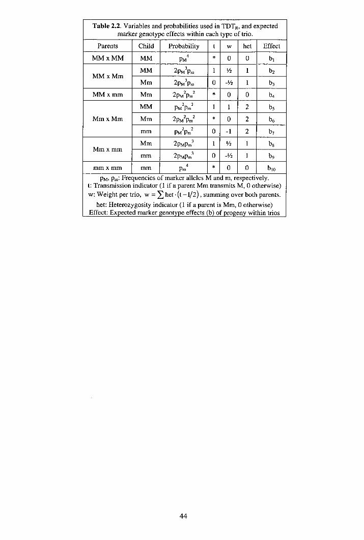
Table 2.2. Variables and probabilities used in TDT R , and expected marker genotype effects within each type of trio.

Parents Child Probability t w het Effect

MM x MM MM PM4 * 0 0 b

MMxMm MM 2PM3Pm 1 ½ 1 b2

Mm 2PM3Pm 0 -½ 1 b3

MM x mm Mm 2PM2Pm2 * 0 0 b

Mm x Mm

MM PM2Pm2 1 1 2 b5

Mm 2PM2Pm2 * 0 2 b6

mm PM2Pm2 0 -1 2 b7

Mm x mm Mm 2PMPm3 1 ½ 1 b8

mm 2PMPm3 0 ½ 1 b9

mm x mm mm Pm4 * 0 0 b 10

PM, Pm Frequencies of marker alleles M and m, respectively. t: Transmission indicator (1 if a parent Mm transmits M, 0 otherwise) w: Weight per trio, w = I het . (t - 1/2), summing over both parents.

het: Heterozygosity indicator (1 if a parent is Mm, 0 otherwise) Effect: Expected marker genotype effects (b) of progeny within trios

44

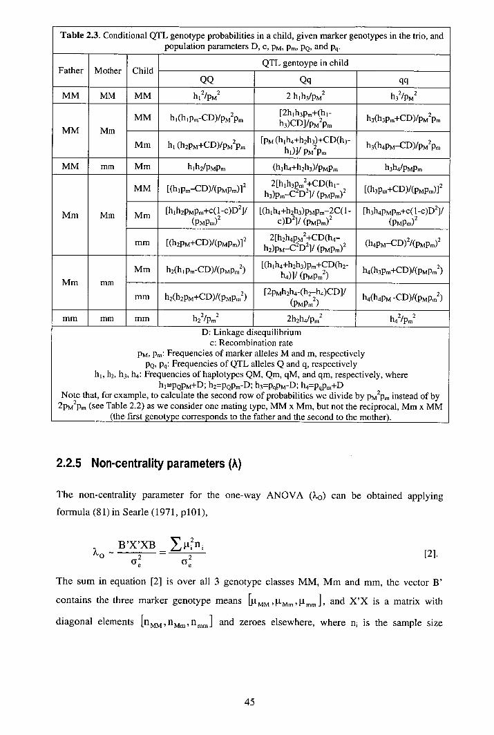
Table 2.3. Conditional QTL genotype probabilities in a child, given marker genotypes in the trio, and population parameters D, C, PM, Pm, pQ, and ic.

QTL gentoype in child Father Mother Child

QQ Qq qq

MM MM MM h1 2/pM2 2 hIh3/pM2 h32/pM2

MM Mm

MM li(li iPm CD)/PM2Pm [2hih3pm+(hi h3)CD]/PM2Pm h3(h3Pm+CD)/PM2Pm

Mm h 1 (h2PM+CD)/PM2Pm [PM (h1h4+h2h3)+CD(h3-

h1)]/PM2Pm h3(h.4PMCD)/PM2Pm

MM mm Mm h I h2/PMPm (hIh4+h2h3)/PMPm h3h4/PMPm

MM [(hIPmCD)/(PMPm)]2 2[hih3pm2+CD(h1 h3)pm C2D2]/_(PMP m)2 [(h3Pm+CD)/(PMPm)]2

Mm Mm Mm lh2PMPm+1D2 h1' [(h l h4+h2h3)PMPm 2C(1 [h3h4PMPm+C(1C)D2]/ ______ (PMPm)2 c)D2]/ (PMPm) 2 (PMPm)2

mm 7___________________

[(h2PM+CD)/(PMPm)]2 2[h2h4pM2+CD(h4— h2)PM—C2D2]/_(PMPm)2 (h4PM CD)2/(PMPm) 2

Mm mm

Mm h2(hIPmCD)/(PMPm2) [(hih4+h2h3)pm+CD(h2

h4)]/ (PMPm2) h4(h3Pm+CD )/(PMPm2)

mm h2(h2PM+CD)/(PMPm2) [2pMh2h4-(h2—h4)CD]/

(PMPm2) h4(h4pM CD)1(P MPm2)

mm mm mm h22/Pm2 2h2h41Pm2 h42/Pm2 D: Linkage disequilibrium

c: Recombination rate PM, Pm Frequencies of marker alleles M and m, respectively

Q, pq Frequencies of QTL alleles Q and q, respectively h 1 , h2, h3 , h4 : Frequencies of haplotypes QM, Qm, qM, and qm, respectively, where

hl=pQpM+D; h2=pQpm-D; h3pqpMD; h4pqpm+D Note that, for example, to calculate the second row of probabilities we divide by p m pm instead of by

2PM2Pm (see Table 2.2) as we consider one mating type, MM x Mm, but not the reciprocal, Mm x MM (the first genotype corresponds to the father and the second to the mother).

2.2.5 Non-centrality parameters (A)

The non-centrality parameter for the one-way ANOVA (X0) can be obtained applying

formula (81) in Searle (1971, pl 01 ),

B'X'XB = [2].

The sum in equation [2] is over all 3 genotype classes MM, Mm and mm, the vector B'

contains the three marker genotype means 6 MM , 11 MM '11mm]' and X'X is a matrix with

diagonal elements [nMM,nMm,nmm] and zeroes elsewhere, where n i is the sample size

45

corresponding to marker genotype i. Equation [2] represents the sum of squares due to both

the marker locus and the sample mean. The appropriate X o can be obtained after correcting

[2] for the sum of squares due to the sample mean (pt), i.e. N1t 2, where

N = n 4M + n Mm + n. In doing so, we are assessing how much variation is explained by a

model fiting an overall mean and genotypes as fixed factors over and above a model fiting

only the overall mean. When testing the QTL (i.e. conditioning on c = 0, D' = 1, and p =

PM), and assuming no dominance, equation [2] simplifies to

N

A0 = '2 [3] cY

where CY 2 = 2p Q pq a 2 (Falconer and Mackay 1996).

In Appendix C, we have shown that TDT Q5 is equivalent to a two-way ANOVA analysis,

where data are modelled fitting mating type and genotype as fixed factors, in addition to .t.

Taking this equivalence into account, the non-centrality parameter XQ5, derived in Appendix

B, is

10 6

=

[4]

where b1 is the marker genotype effect in the progeny of class i trios (see Table 2.2), n, is the

number of class i trios, is an indicator variable that takes the value 1 when the trio is

informative (viz, at least one heterozygous parent), and 0 otherwise, F is the mean value of

the jth family class, and f the number of these families (see Appendix B). Equation [4]

measures, in o units, the amount of total sum of squares explained by the marker, after

subtracting the family effect. When testing the QTL, equation [4] reduces to

2 Q

XQ5_.NTL - 2 _--- [5].

The non-centrality parameter for TDT R (XR) is approximately

XR[p2

2 (b 2 b3)+PMPm(b5 —b 7 )+p(b 8 _b 9 )1/_NPMPm [6] +

Cy 2 QTL

(Appendix D). When testing the QTL, equation [6] simplifies to

I_NPQPq

2+2/TL [7]. 2 2

\I a+ Qu

ms

Finally, the non-centrality parameter for TDT G (XG) is

N_[(1-2C)Da]2

PMPm( +) [8]

where D is the usual measure of linkage disequilibrium (Xiong et al. 1998). When testing the

QTL in family trios, the appropriate non-centrality parameter is

N - NQTLXG

- 1+(2/) [9]

(equation 10 in Xiong et al. 1998).

2.3 RESULTS

2.3.1 Empirical power

Empirical power was studied using combinations of three parameter values: allele

frequencies at the marker (PM) and the QTL (pa) (p = pQ = PM 0.5, 0.3, 0.11, standardised

linkage disequilibrium (D') (1, 0.5, 01, and a range of recombination rates (c) from 0 to 0.5,

in steps of 0.05. Each parameter combination was analysed 1000 times in each test. Two

hundred unrelated family trios were randomly sampled with respect to phenotypes and

genotypes. The difference between QTL homozygotes was 2a, and there was no dominance.

Table 2.4a shows power of the tests for a given c, whilst averaging across values of D' and p.

The most powerful test was one-way ANOVA, followed by TDT Q5 (N.B. Employing all

family trios), TDT0, TDTR, and nested ANOVA. The last row in Table 2.4a (where marker

and QTL were unlinked, i.e. c = ½) corresponds to the empirical proportion of false positive

results, or type-I error, for each test. The empirical error was expected to be —5% in all tests.

The one-way ANOVA was the only test for which the empirical error exceeded expectations

(e.g. —20%, averaged across D' and p), a fact that has also been documented elsewhere (e.g.

Long and Langley 1999). On the basis of this result, one-way ANOVA is not a valid test of

association when spurious association (D': ~ 0 and c = ½) is present in the population. As

expected, power declined steadily as c increased, because the amount of cm explained a

marker decreases as inter-loci distance increases. The ranking of tests regarding power was

maintained across all c values.

Table 2.4b shows power given D', whilst averaging across values of p and c. When D' = 1,

the power of one-way ANOVA reached —72% compared to just —39% for the second most

11 M

powerful test (TDTQ5). Undoubtedly, if spurious association is not an issue, significant extra

power can be obtained through testing genotype differences directly, as opposed to using

robust tests. In the absence of disequilibrium (D' = 0, last row in Table 2.4b), all tests,

including one-way ANOVA, showed —5% false positive results.

Finally, Table 2.4c shows power given p, whilst averaging across values of c and D'. Power

decays as allele frequency becomes more extreme because 1) the number of informative

families diminishes, and 2) from these informative families, the proportion with one

heterozygous parent increases, whilst the proportion with two decreases, and the within

family variation, which is the variation exploited by TDT, is expected to be lower in the

former than in the latter type of family, these factors mean that, for a fixed QTL effect, (YQTL

decreases (the trait becomes less genetic). Allison (1997) showed that, for dominant and

additive modes of inheritance, power increases as PM decreases. Note that Allison kept c QTL

constant, so when PM -* 1 (or PM 4 0) the additive genetic effect (a) of the QTL must

increase, rendering greater mean differences between marker genotypes, and hence, more

powerful contrasts.

Table 2.4. Empirical power (%) of tests per single parameter.

2.4a. Averaging across D' and p

c Oneway TDTQ5 TDT0 TDTR Nested

o 46.5 39.2 38.4 39.7 28.5

0.05 44.6 35.1 33.8 32.5 24

0.1 42.8 31.4 29.3 28.4 20.7

0.15 10.4 26.4 24.7 23.3 16.8

0.2 37.6 22.4 19.2 19.6 13.5

0.25 35.6 17.6 16.1 14.8 10

0.3 33.3 13.5 11.8 10.9 8.4

0.35 30.2 10.4 9.1 8.4 6.4

0.4 26.7 7.8 6.8 6.4 6.1

0.45 23.5 5.8 6 4.8 5.4

0.5 20.5 5.5 5.4 4.8 4.9

2.4b. Averaging across c and p

D' Oneway TDT05 TDTG TDTR Nested

1 71.9 38.6 35.5 34.1 25

0.5 27.2 15 14 13.1 9.2

0 5 5.1 5.2 4.7 5.2

2.4c. Averaging across D' and c

p Oneway TDTQ5 TDTG TDTR Nested

0.5 41.4 23.6 21.9 21.4 15.8

0.3 38.6 21.7 19.9 19.5 14.1

0.1 24.1 13.3 12.9 11.1 9.6

C: Recombination rate D': Standardised Linkage Disequilibrium

p: Frequency of alleles Q and M (assumed equal) Oneway: Oneway ANOVA

TDTQ5 : TDT in Allison (1997); analysis across all trios. TDTG: TDT in Xiong et al. (1998) TDTR: TDT in Rabinowitz (1997)

Nested: Nested ANOVA

The set of parameters given in Allison (1997) was also used to compare the power of these

tests when analysing a QTL. Table 2.5 shows simulation results across (as aQTL

proportion of the total phenotypic variance), pQ (frequency of the positive effect allele), and

N (number of informative trios).

49

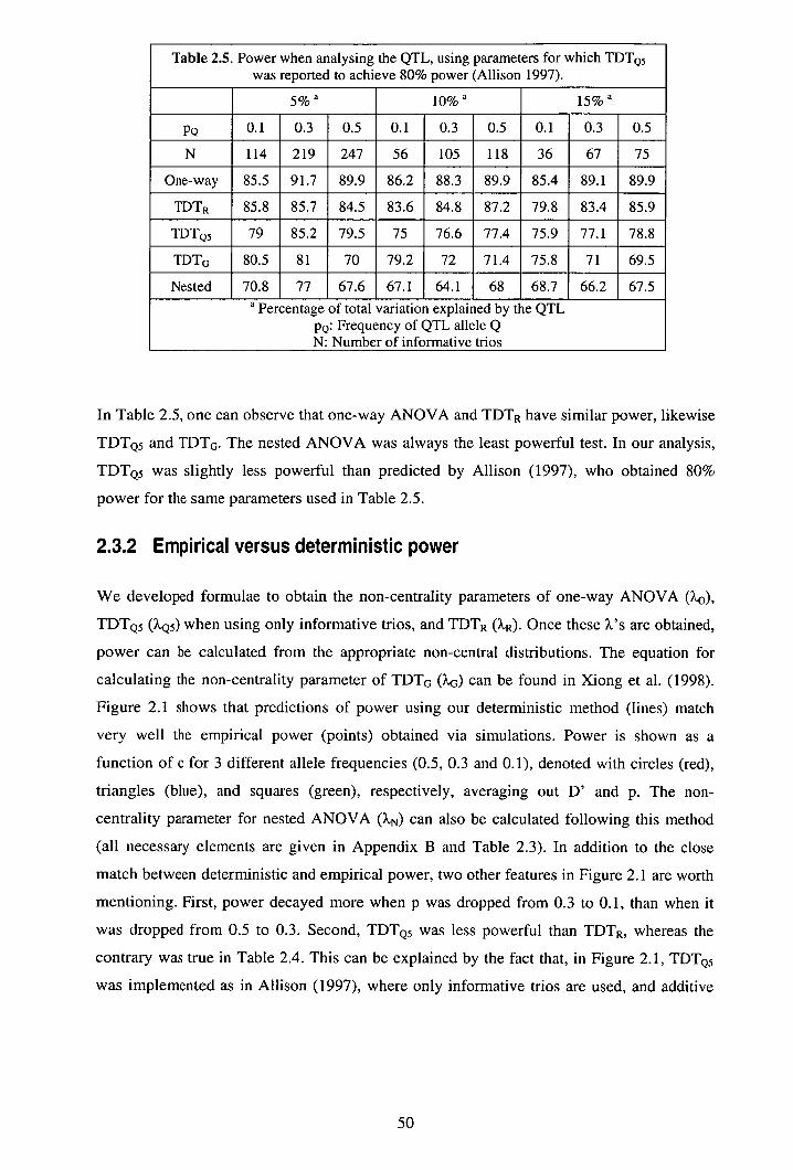
Table 2.5. Power when analysing the QTL, using parameters for which TDTQ5 was reported to achieve 80% power (Allison 1997).

a 3/0

a 1 /0

a 13 /0

PQ 0.1 0.3 0.5 0.1 0.3 0.5 0.1 0.3 0.5

N 114 219 247 56 105 118 36 67 75

One-way 85.5 91.7 89.9 86.2 88.3 89.9 85.4 89.1 89.9

TDTR 85.8 85.7 84.5 83.6 84.8 87.2 79.8 83.4 85.9

TDTQ5 79 85.2 79.5 75 76.6 77.4 75.9 77.1 78.8

TDT0 80.5 81 70 79.2 72 71.4 75.8 71 69.5

Nested 70.8 77 67.6 67.1 64.1 68 68.7 66.2 67.5 a Percentage of total variation explained by the QTL

pQ : Frequency of QTL allele Q N: Number of informative trios

In Table 2.5, one can observe that one-way ANOVA and TDT R have similar power, likewise

TDTQ5 and TDTG. The nested ANOVA was always the least powerful test. In our analysis,

TDTQ5 was slightly less powerful than predicted by Allison (1997), who obtained 80%

power for the same parameters used in Table 2.5.

2.3.2 Empirical versus deterministic power

We developed formulae to obtain the non-centrality parameters of one-way ANOVA ().),

TDTQS (X 5) when using only informative trios, and TDT R (XR). Once these X's are obtained,

power can be calculated from the appropriate non-central distributions. The equation for

calculating the non-centrality parameter of TDTG (X Q) can be found in Xiong et al. (1998).

Figure 2.1 shows that predictions of power using our deterministic method (lines) match

very well the empirical power (points) obtained via simulations. Power is shown as a

function of c for 3 different allele frequencies (0.5, 0.3 and 0.1), denoted with circles (red),

triangles (blue), and squares (green), respectively, averaging out D' and p. The non-

centrality parameter for nested ANOVA (X N) can also be calculated following this method

(all necessary elements are given in Appendix B and Table 2.3). In addition to the close

match between deterministic and empirical power, two other features in Figure 2.1 are worth

mentioning. First, power decayed more when p was dropped from 0.3 to 0.1, than when it

was dropped from 0.5 to 0.3. Second, TDTQ5 was less powerful than TDTR, whereas the

contrary was true in Table 2.4. This can be explained by the fact that, in Figure 2.1, TDT Q5

was implemented as in Allison (1997), where only informative trios are used, and additive

50

2.3.3 Effect of sampling strategy on power

Different sampling strategies can result in the same number of phenotypes and/or genotypes

being collected yet have radically different effects on power. For instance, one may sample

many and small unrelated families, as when studying humans, or few and large, frequently

related, families, as when studying domestic plants or animals. Which sampling strategy

conveys more power to detect marker-QTL association with TDTs?

For a fixed number of progeny, there are fewer parents sampled with the latter strategy (few

and large families) than with the former. The link between power and number of parents

resides in the relationship between linkage disequilibrium in the parents (D pen ) and linkage

disequilibrium in the progeny (Dprogeny). In a large population, where drift can be assumed

negligible, Dprogeny = Dparents (1-c), thus, if Dparents = 0 then there will be no association

between loci. However, the variance of D is proportional to 1/2N (Weir 1996), therefore,

even if D = 0 the actual value of D in any small sample is likely to be different from zero.

The effect of sampling strategy on power was studied via simulations. Assume a biallelic

marker completely linked (c = 0), and in linkage equilibrium (D' = 0), with a biallelic QTL

that explains 15% of the total phenotypic variance. Moreover, let us compare two very

different sampling schemes: 1) each one of two unrelated males is mated to two unrelated

females, and 75 progeny are born in each full-sib family (this mating system may be thought

of as resembling a cattle breeding program), and 2) there are 150 nuclear families with 2

progeny each. In both cases 300 progeny were phenotyped and genotyped. In the former case

only six parents were genotyped, whereas in the latter 300 parents were genotyped.

Furthermore, assume that at least one parent in each family is heterozygous (i.e. all families

are informative).

Table 2.6. Effect of sampling strategy on power of TDT

Strategy One-way TDTR TDTQS TDTG

I 49.1 64.5 42.9 42.3

II 6.2 5.1 5.6 5.5

Strategy I: Two unrelated males, each mated to 2 unrelated females, and 75 progeny per family Strategy II: 150 nuclear families, and 2 progeny per family

Parameters: pM=pQ=0.5, c=0, D'=O and a QTL effect explaining 15% of the phenotypic variance

Table 2.6 shows striking power differences in each test that can be explained by the

sampling strategy. It is expected that association tests will not detect significant effects at a

52

marker locus if the population is in linkage equilibrium (i.e. D' = 0), even if this marker is

completely linked (i.e. c = 0) to a gene that explains as much as 15% of the total phenotypic

variance. However, there was a 10-fold increase in power when 6 parents where sampled

(i.e. sampling 2 half-sib families twice), compared to the power when 300 parents were

sampled (i.e. 150 full-sib families). The variance of linkage disequilibrium in the parental

population, D , where x is the number of parents sampled, was —50 times greater when

x = 6 than when x = 300, e.g. a2 (D6parents ) - 1/6 and c 2 (D 3parents ) 1/300, thus

a 2 (D6parents )/(y2 ) - 50. A large a2 06pareflts ) meant that in any particular replicate

values of D 6 parents very different from zero were likely, and hence, the sample analysed with

TDT was no longer in linkage equilibrium.

The second striking feature in Table 2.6 is the different ranking of tests in terms of power.

When only informative trios were analysed, TDT R was the most powerful test, even ahead of

one-way ANOVA. It is now clear that most of the advantage in power of one-way ANOVA

with respect to TDT is that the latter cannot use families with two homozygous parents, and

therefore analyse less data than one-way ANOVA after ascertainment has taken place. In

Table 2.5, TDTQ5 was parameterised as in Allison (1997). However, such parameterisation is

slightly less powerful than the one we proposed above and, hence, any power difference

between TDTQ5 and TDT0 or TDTR disappeared.

2.4 DiscussioN

Complex traits, such as obesity and osteoporosis, are determined by multiple genetic factors

(also known as quantitative trait loci or QTL), environmental factors, and potential

interactions between both. These complex traits can be studied measuring quantitative

intermediate risk factors such as blood pressure, cholesterol level, or bone mineral density.

The greatest burden, both economically and in terms of human workload, for national health

services is due to multifactorial disorders, such as infectious and parasitic diseases (23.4% of

world-wide burden), neuropsychiatric disorders (11.5%) and cardiovascular diseases

(10.3%), for which a polygenic component is usually hypothesized (The World Health

Report 1999). On the other hand, monogenic diseases, although rare in humans, are

comparatively less problematical to study from a genetic standpoint. For example, the most

common monogenic disease among Caucasians is cystic fibrosis, affecting approximately

0.5-0.6 births every 1000, followed probably by phenylketonuria, which affects 0.2-0.5

births every 1000, all other monogenic diseases are even rarer (Underwood 1996).

53

Zhao (2000) comprehensively reviewed the family-based association methodology

developed in the 1990s, providing more than 60 references of association tests for diseases

caused by a single gene with clear pattern of Mendelian inheritance, and approximately six

time less references of association tests for complex (i.e. quantitative) traits. It is rather

paradoxical that most of the latest advances in statistical theory for gene mapping have

focused on a relatively rare group of diseases in humans (e.g. Hastbäcka et al. 1992).

The transmission disequilibrium test (TDT) is a test for linkage and/or linkage

disequilibrium that is being increasingly used to identify QTL5 underlying complex diseases

(Schaid 1998). TDT can be more powerful than other tests, e.g. affected-sib-pair linkage

analysis, when markers are very close to responsible QTLs (Risch and Merikangas 1996). In

addition, TDT is robust to spurious associations (Stephens et al. 1994) generated by common

demographic events such as population stratification and/or admixture (e.g. Wilson and

Goldstein 2000, Reich et al. 2001).

In this study, we have compared the power of three TDTs and two ANOVAs (analysis of

variance) in detecting association between a marker and a QTL. We have assumed that both

loci were biallelic, and shared the same allele frequencies. Moreover, we considered a

continuously distributed trait genetically determined by a single additive QTL, without a

polygenic component and no dominance. This simplistic scenario was chosen to facilitate the

derivation of deterministic equations for predicting power. Nonetheless, we recognise that in

order to get a more comprehensive picture of the properties of these TDTs, more realistic

situations will have to be explored. For example, Page and Amos (1999) and Deng et al.

(2001) concluded that polygenes have a negligible effect on power when using family trios.

The latter authors concluded that, when using multiplex families, polygenes increase the

power of TDTG, and that the larger the family, the more the power of TDT G increases

compared to a case without polygenes. However, the change in power due to the presence of

polygenic variance depends on the assumptions made regarding the size of the variance

components, and their distribution within and between families. For example, assume a

model where the phenotypic variance is the sum of QTL, polygenic, and residual variances,

i.e. = cY QTL + + . Then, for the sake of simplifying mathematical modelling, for a

fixed value of cTL one can fix either or o. Fixing , as in Deng et al. (2001), leads

to the conclusion that polygenes increase power of TDT. If, for example, we sampled

unrelated families with multiple progeny, then c would be equally distributed within and

54

between families, and a would reduce by to keep c constant. Hence, the residual

variance used in TDT analyses, i.e. the within family variance unexplained by the QTL,

would be - . If there are no polygenes acting on the trait then the power of TDT

reduces because the residual variance used in TDT analyses will be as opposed to

- . However, if , instead of , is fixed, the presence of polygenic variance will

lead to a reduction of the power of TDT because the residual variance used in TDT analyses

will be + , as opposed to when there is no polygenic variance.

Power was predicted via empirical simulations and deterministic equations, and both

methods rendered very similar answers. The advantages of deterministic methods over

stochastic ones are 1) ease of implementation, 2) instant predictions, and 3) direct

appreciation of the relationship between population parameters and power. However, in

complex scenarios where deriving deterministic methods becomes cumbersome, empirical

simulations may be invaluable. The deterministic method proposed in this study consists in

deriving non-centrality parameters (),'s) as functions of marker genotype contrasts specific to

each test. These X's can subsequently be used as input in computer routines to obtain power.

A common feature across all X's was the use of expected marker genotype means,

conditional on family information, under the assumptions of random mating and no

segregation distortion. These marker effects were functions of the standardised linkage

disequilibrium (D'), the recombination rate (c), the allele frequencies (pQ, PM), and the

additive gene effect (a). Allison (1997) derived a prediction of X for TDT Q5, simulation

shows that this derivation can be considerable less accurate than that derived here.

Rabinowitz (1997) derived X for TDT R although using parameters not included in his

simulations, leading to some confusion in terms of interpretation and calculation of X.

We have shown that our method is accurate and reliable, and that it contains a general part

(Table 2.3) that can be used to calculate X for other association tests. Moreover, our method

can readily include dominant QTL effects, and a polygenic component. Extensions to cope

with multiallelic markers are theoretically possible, however, future association studies in

human populations are more likely to employ vast arrays (e.g. microarrays) of biallelic single

nucleotide polymorphisms (SNPs) rather than multiallelic markers (Risch and Merikangas

1996, Weiss and Terwilliger 2000, Miller and Kwok 2001). Therefore, we think further

55

developments of this method ought to be directed, for instance, to cope with the problem of

simultaneous testing of several loci (e.g. Goidgar and Easton 1997), and the study of

haplotypes, rather than extending it to use multi-allelic loci.

The one-way ANOVA was usually the most powerful way of testing population association,

followed by the TDTs and, finally, by the nested ANOVA. However, one-way ANOVA was

also the only test having higher than expected levels of false positive results in the presence

of spurious association (i.e. association without linkage). The TDTs were very similar in

terms of power. However, the power of TDT Q5 was slightly improved by analysing all

families, regardless of the number of heterozygous parents, without altering the type-I error

rate in the presence of spurious association. In doing so, more data can be used to estimate

the error mean squares, thus augmenting the residual degrees of freedom of the test. A

further improvement in the power of TDT Q5 was still possible by dropping dominant effects

off the model (e.g. when they seem negligible), and estimating only additive gene effects. In

doing so, the numerator degrees of freedom of the test were reduced from 2 to 1. Although

Xiong et al. (1998) showed that TDT G is more powerful than TDT QI (Allison 1997), we

considered that it would be fairer to compare TDT 0 versus TDTQ5 because, as Allison

pointed out, TDTQ5 is more powerful than TDTQI , and because, as we have shown, the power

of TDTQ5 can be easily increased. In addition, Deng et al. (2001) noticed that analytical

power results showed in Tables 1-3 in Xiong et al. (1998) were overestimates, although their

deterministic formulae were correct.

Power was also affected by family structure. For a fixed number of phenotyped progeny,

sampling multiplex families reduces the number of parents available for genotyping

compared to sampling simplex families (i.e. trios). Imprecise estimates of parental linkage

disequilibrium (Dparents) are expected when very few families are sampled because the

variance of Dparent, is inversely proportional to twice the number of genotyped parents (viz.

linkage disequilibrium, D, extends further chromosomal distances within families than

across the entire population). This means that even when the population is in linkage

equilibrium, single families may still show high (or low) D parents levels. Given a sufficiently

large number of progeny D progeny = Dparents (1c), and Dprogeny is a key parameters determining

the power of TDT. Hence, even though power may increase, the mapping resolution is likely

to decrease, i.e. a QTL may be equally associated with close and distant markers. Indeed,

linkage analysis, a gene mapping method known to have low resolution (Boehnke 1994), is

the limiting case where associations are investigated only within families. In our simulations,

markers were found in association with a QTL when four large multiplex families were

56

sampled, despite having simulated a population in equilibrium. The same association was not

detectable when 150 simplex families were sampled from the same population.

In summary, a new and accurate method has been developed for obtaining deterministic

predictions of power of ANOVAs and TDTs for quantitative traits. We have shown that

TDTQ5 is equivalent to a two-way ANOVA, where mating type and progeny genotype are

the two factors in the model, and how a simple modification of TDT Q5 can increase power.

Finally, we have shown that TDTR may be the test of choice in certain circumstances, e.g.

when the sample consists of multiplex families.

57

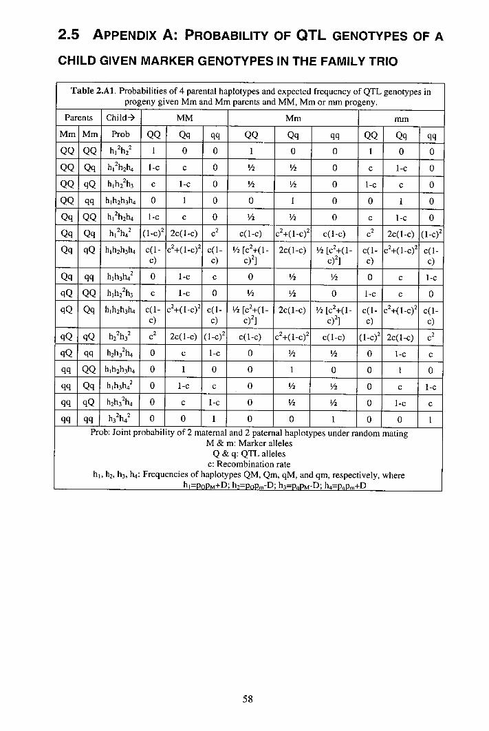
2.5 APPENDIX A: PROBABILITY OF QTL GENOTYPES OF A

CHILD GIVEN MARKER GENOTYPES IN THE FAMILY TRIO

Table 2.A1. Probabilities of 4 parental haplotypes and expected frequency of QTL genotypes in progeny given Mm and Mm parents and MM, Mm or mm progeny.

Parents Child- MM Mm mm

Mm Mm Prob QQ Qq qq QQ Qq qq QQ Qq qq

QQ QQ h 1 2 h2 1 0 0 1 0 0 1 0 0

QQ Qq h 1 2h2h4 1-c c 0 ½ ½ 0 c 1-c 0

QQ qQ h 1 h22h3 c 1-c 0 ½ ½ 0 1-c c 0

QQ qq h 1 h2h3h4 0 1 0 0 1 0 0 1 0

Qq QQ h 1 2h2h4 1-c c 0 ½ ½ 0 c 1-c 0

Qq Qq h 1 2h42 (1-c) 2 2c(1-c) c2 c(1-c) c2+(1-c) 2 c(1-c) c2 2c(1-c) (1-c) 2

Qq qQ h 1 h2h3h4 c(1- c)

c2+(1-c) 2 c(1- c)

½ [c2+(1- c) 2 ]

2c(1-c) ½ [c2+(1- c)2]

c(1- c)

c2+(1-c) 2 c(1- c)

Qq qq h 1 h3h42 0 1-c c 0 ½ ½ 0 c 1-c

qQ QQ h 1 h22h3 c 1-c 0 ½ ½ 0 1-c c 0

qQ Qq h 1 h2h3h4 c(1- c)

c2+(1-c) 2 c(1- c)

½ [c2-i-(1- c )2]

2c(1-c) ½ [c2+(1- c)2]

c(1- c)

c2+(1-c)2 c(1- c)

qQ qQ h22h32 c2 2c(1-c) (1-c) 2 c(1-c) c2+(1-c) 2 c(1-c) (1-c) 2 2c(1 -c) c2

qQ qq h2h3 2h4 0 c 1-c 0 ½ ½ 0 1-c c

qq QQ h 1 h2h3h4 0 1 0 0 1 0 0 1 0

qq Qq h 1 h3h42 0 1-c c 0 ½ ½ 0 c 1-c

qq qQ h2h32h4 0 c 1-c 0 ½ ½ 0 1-c c

qq qq h32h42 0 0 1 0 0 1 0 0 1 Prob: Joint probability of 2 maternal and 2 paternal haplotypes under random mating

M & m: Marker alleles Q & q: QTL alleles

c: Recombination rate h, h2, h3 , h4 : Frequencies of haplotypes QM, Qm, qM, and qm, respectively, where

h l=pppM+D; h2popm D; h3=pQpM-D; h4ppp m+D

58

Table 2.A2. Probabilities of 4 parental haplotypes and expected frequency of QTL genotypes in progeny given MM and Mm parents and MM or Mm progeny.

Parents Child - MM Mm

MM Mm Prob QQ Qq qq QQ Qq qq

QQ QQ h 3 h2 1 0 0 1 0 0

QQ Qq h 1 3 h4 1-c c 0 c 1-c 0

QQ qQ h 1 2 h2 h3 c 1-c 0 1-c c 0

QQ qq h 1 2 h3 h4 0 1 0 0 1 0

Qq QQ h 1 2 h2 h3 ½ ½ 0 ½ ½ 0

Qq Qq h 1 2 h3 h4 ½(1-c) ½ ½c ½c ½ ½(1-c)

Qq qQ h 1 h2 h3 2 ½c ½ ½(1-c) ½(1-c) ½ ½c

Qq qq h 1 h32 h4 0 ½ ½ 0 ½ ½

qQ QQ h 1 2 h2 h3 ½ ½ 0 ½ ½ 0

qQ Qq h 1 2 h3 h4 ½(1-c) ½ ½c ½c ½ ½(1-c)

qQ qQ h 1 h2 h3 2 ½c ½ ½(1-c) ½(1-c) ½ ½c

qQ qq h 1 h32 h4 0 ½ ½ 0 ½ ½

qq QQ h 1 h2 h3 2 0 1 0 0 1 0

qq Qq h 1 h3 2 h4 0 1-c c 0 c 1-c

qq qQ h2 h3 3 0 c 1-c 0 1-c c

qq qq h3 3 h4 0 0 1 0 0 1

Prob: Joint probability of 2 maternal and 2 paternal haplotypes under random mating M & m: Marker alleles

Q & q: QTL alleles C: Recombination rate

h 1 , h2 , h3 , h4 : Frequencies of haplotypes QM, Qm, qM, and qm, respectively, where hI=pppM+D; h2pop m D; h3=pQpM-D; h4P Q Pm+D

59

Table 2.A3. Probabilities of 4 parental haplotypes and expected frequency of QTL genotypes in progeny given MM and MM, or mm and mm, or MM and mm parents and the marker genotype in

their progeny.

Parents Prob Child

MM, MM mm, mm MM, mm QQ Qq qq

QQ QQ h, 4 h24 h 1 2 h22 1 0 0

QQ Qq h, 3 h3 h23 h4 h, 2 h2 h4 ½ ½ 0

QQ qQ h, 3 h3 h23 h4 h 1 2 h2 h4 ½ ½ 0

QQ qq h, 2 h32 h22 h42 h 1 2 h42 0 1 0

Qq QQ h, 3 h3 h2 3 h4 h,h22 h3 ½ ½ 0

Qq Qq h 1 2 h32 h22 h42 h, h2 h3 h4 '/i ½ ¼

Qq qQ h, 2 h32 h22 h42 h, h2 h3 h4 ¼ ½ ¼

Qq qq h, h33 h2 h43 h, h3 h42 0 ½ '/2

QQ QQ h, 3 h3 h23 h4 h,h22 h3 ½ ½ 0

QQ Qq h, 2 h32 h22 h42 h, h2 h3 h4 ¼ ½ ¼

QQ qQ h,2 h32 h22 h42 h, h2 h3 h4 ¼ ½ 14

QQ qq - h, h3 3 h2 h43 h, h3 h42 0 ½ ½

Qq QQ h, 2 h32 h22 h42 h22 h32 0 1 0

Qq Qq h, h33 h2 h43 h2 h3 2 h4 0 ½ ½

Qq qQ h, h3 3 h2 h43 h2 h32 h4 0 ½ ½

Qq qq h34 h44 h3 2 h42 0 0 1

Prob: Joint probability of 2 maternal and 2 paternal haplotypes under random mating M & m: Marker alleles

Q & q: QTL alleles C: Recombination rate

h,, h2 , h3 , h4 : Frequencies of haplotypes QM, Qm, qM, and qm, respectively, where h,=pppM+D; h2=pppm-D; h3=p QpM-D; h49 iPm+D

2.6 APPENDIX B: NON-CENTRALITY PARAMETER FOR A

TWO-WAY ANOVA

The non-centrality parameter ()) of two-way can be expressed as (Searle 197 1)

= (K'B)'[K'(x'x)'Kt'(K'B) 2 e

[1311.

Let Cy be unity. Let B' be the vector [jt,f 1 ,f2 ,f3 ,g 1 ,g 2 ,g 3 ] of parameters in the model,

where t is the sample mean, f1 is the mean of the family type, and gj the mean of the jth

Me

marker genotype across all family types. Let K be a matrix of parameter contrasts reflecting

the H0 being tested, for example if H 0 : 91 = 92 and 92 = 93, then

ro o o o 1 —1 o K'=I

[0 0 0 0 0 1 —1

The matrix X'X is

'i.. n n 2. 3. . l n .2 n 3

fl u. fl u. 0 0 fill n ,2 n ,3

'2. 0 n 2. 0 n 21 n 22 n 23

n 3. 0 0 n 3• n 31 n 32

fl .1 fl11 '2l 3I .l 0 0I

fl .2 fl 12 fl 22 fl 32 0 n 2 0

.3 i3 23 33 0 0 n 3

where nij is the number of records in the i °' family and j h marker genotype class. x'x is a

matrix of order 7 and rank 5, hence, there are 7 unknowns, and only 5 degrees of freedom

(i.e. once 5 parameters are estimated, the remaining 2 become known). An appropriate

generalisation of X'X is obtained deleting the first row and column, hence setting R = 0, and

the last row and column, hence setting 93 = 0 (Searle 1971, p264). Let G be the reduced X'X

matrix. This G matrix can be partitioned as follows

fl u. 0 0 n 11 n 12

G11 Gl21

0 n 2. 0 n 21 n 22

IG 21

G= G22j

0 0 n 3. n 31 n 32

'' ''ii n 2l n 3l fl .1 0

fl 12 22 32 0 '.2

Then, if c = G', K* is the matrix K' with the first and last columns deleted, and B* is the

vector B with the first and last elements deleted, then

= (K*'B *)'c-u K*'B * 22 [B2]

where C 22 = K*'CK* = (G22 — G 21 G II'G 12

)', and (K*'B*)'= [g1 9 21921.

When testing the QTL, equation [B2] gives

61

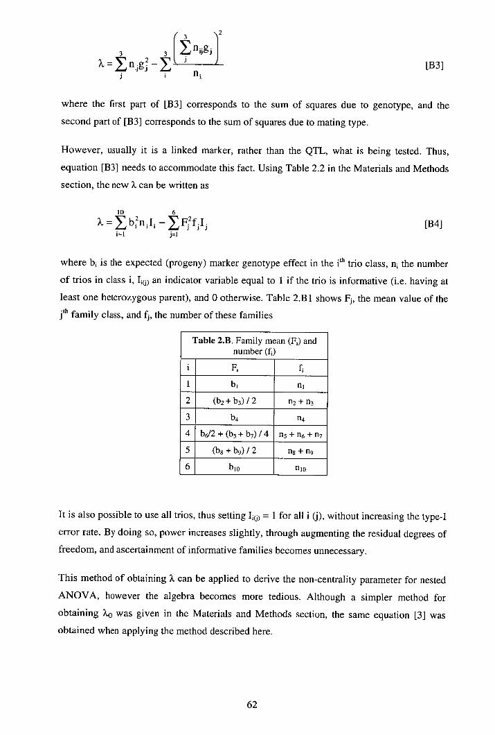
3

j ni. [B3]

where the first part of [B3] corresponds to the sum of squares due to genotype, and the

second part of [B3] corresponds to the sum of squares due to mating type.

However, usually it is a linked marker, rather than the QTL, what is being tested. Thus,

equation [B3] needs to accommodate this fact. Using Table 2.2 in the Materials and Methods

section, the new X can be written as

10 6

X=bn 1 I 1 F2 f I

[B4]

where b 1 is the expected (progeny) marker genotype effect in the ith trio class, n1 the number

of trios in class i, Ij an indicator variable equal to 1 if the trio is informative (i.e. having at

least one heterozygous parent), and 0 otherwise. Table 2.13 1 shows F, the mean value of the th family class, and f, the number of these families

Table 2.B. Family mean (F) and - number (f)

F, fi

1 b n 1

2 (b2 -i-b 3)/2 fl2+fl3

3 b n4

4 b6/2 +(b5 -- b7)/4 n5 +n6 +n7

5 (b8 +b9)12 n8 +n9

6 b 10 n 10

It is also possible to use all trios, thus setting = 1 for all i (j), without increasing the type-I

error rate. By doing so, power increases slightly, through augmenting the residual degrees of

freedom, and ascertainment of informative families becomes unnecessary.

This method of obtaining X can be applied to derive the non-centrality parameter for nested

ANOVA, however the algebra becomes more tedious. Although a simpler method for

obtaining X0 was given in the Materials and Methods section, the same equation [3] was

obtained when applying the method described here.

62

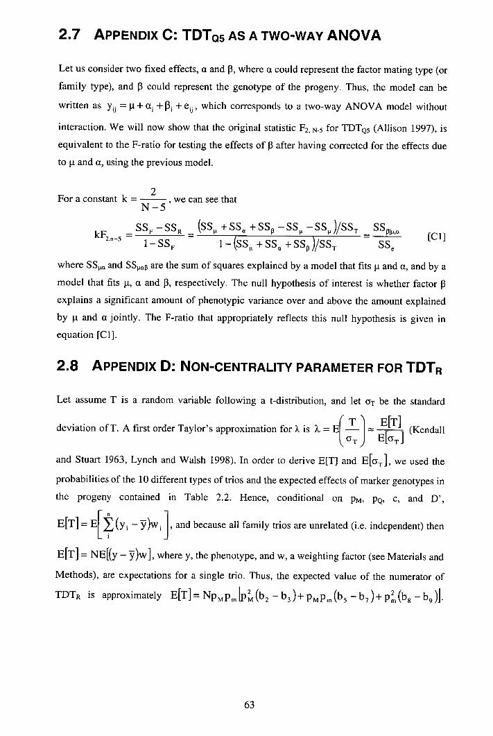
2.7 APPENDIX C: TDTQ5 AS A TWO-WAY ANOVA

Let us consider two fixed effects, a and I, where a could represent the factor mating type (or

family type), and 13 could represent the genotype of the progeny. Thus, the model can be

written as Yij = j.i + a 1 + P i + e 1 which corresponds to a two-way ANOVA model without

interaction. We will now show that the original statistic F 2 , N-5 for TDTQ5 (Allison 1997), is

equivalent to the F-ratio for testing the effects of 13 after having corrected for the effects due

to t and a, using the previous model.

For a constant k = 2 , we can see that N-5

2,n-5 = SSF —SSR - (ss +SS a +SS —SS SSj/SST - SSpia

l — SS F a - i—(SS +SS +SSD)/SST - SS, [Cl]

where SS a and SS Iap are the sum of squares explained by a model that fits t and a, and by a

model that fits t, a and 13, respectively. The null hypothesis of interest is whether factor 13 explains a significant amount of phenotypic variance over and above the amount explained

by ji and a jointly. The F-ratio that appropriately reflects this null hypothesis is given in

equation [C 1].

2.8 APPENDIX D: NON-CENTRALITY PARAMETER FOR TDTR

Let assume I is a random variable following a t-distribution, and let YT be the standard

deviation of T. A first order Taylor's approximation for X is ? = qT E[T] (Kendall T) E[(y1]

and Stuart 1963, Lynch and Walsh 1998). In order to derive E[T] and E{T], we used the

probabilities of the 10 different types of trios and the expected effects of marker genotypes in

the progeny contained in Table 2.2. Hence, conditional on PM pQ, c, and D',

E[T] = E[( i - Y)w i ] and because all family trios are unrelated (i.e. independent) then in

E[T] = NE[(y - )w], where y, the phenotype, and w, a weighting factor (see Materials and

Methods), are expectations for a single trio. Thus, the expected value of the numerator of

TDTR is approximately E[T]= NPMPm[(b2 b3)+PMPm(b5 —b 7 )+p(b 8 -b 9 )].

63

When analysing the QTL, and assuming no dominance, the previous equation simplifies to

E[T] = Np Q p q a.

The expected variance of T, E[ c4 ], is the same regardless whether the locus being tested is

the QTL or a marker. Equation A1.23a in Lynch and Walsh (1998) is

-3/2 _________ E[/] IjIi - , which reduces to E [1JJ jE[c4j if the second term is

ignored. Hence, E[c]= E[ (Y - ) 2

H 1 ] = - y)2 H] and, as the expectation of

a random variable X given another random variable Y is E[X] = E[E[X I Yfi (Casella and

Berger 1990), then E[(y - ) 2 H]= HPHE(y -

= PMPm( + Finally,

dividing E[T] by /E[cj we obtain

E[TDTR]=?R =[p (b2 b3)+PMPm(b5 —b 7 )+p(b 8 — b 9 )t/_NPMPm V (Ye GQTL

64

CHAPTER 3

Candidate gene analysis for quantitative traits

using the transmission-disequilibrium test: the

example of the Melanocortin 4-Receptor in pigs

3.1 INTRODUCTION

Population-wide associations between loci due to linkage disequilibrium can be used in high

resolution mapping of quantitative trait loci (QTL). Spurious associations between markers

and QTL can also arise as a consequence of population stratification, for example due to

admixture of two different populations. Associations between a genotype and a trait have

been frequently tested, after corrections, with simple one-way ANOVA models, e.g. testing

mean genotype differences directly. However, these types of analyses are prone to false

positive results due to confounding effects of population stratification/admixture (e.g. Deng

et al. 2001). Spielman et al. (1993) developed an allele-trait association test called

Transmission Disequilibrium Test (TDT) that is robust to these confounding effects.

Different TDTs have since been developed for dichotomous traits (Schaid 1996, Horvath and

Laird 1998, Martin et al. 2000, Lunetta et al. 2000, Zhao et al. 2000), and for quantitative

traits (Allison 1997, Rabinowitz 1997, Szyda 1998). However, most of these TDTs have

been formulated in a rather rigid form, hence reducing the scope for further statistical

modelling.

This work describes the use of a TDT (Rabinowitz 1997) to obtain robust estimates of

genetic effects within the statistically more flexible mixed linear model context. This

approach allows maximum likelihood estimates of genetic effects to be obtained via REML.

Additive allele substitution effects were estimated within (b ID for Transmission

Disequilibrium) and between families (bp D for Population Disequilibrium) with two

independent regression coefficients. Moreover, the rejection of the null hypothesis bTD = bpD

provides evidence for stratification/admixture and hence can be used to guard against false

positive results.

The analysis of the MC4R locus on pig chromosome 1 constitutes a practical demonstration

of this method. The interaction between melanocortins and their receptors (MC3R and

MC4R) at the hypothalamus is one of the main neuro-endocrinological pathways controlling

energy balance (Wardlaw 2001). In humans, different allelic variants of both MC4R and

MC3R have been associated with obesity (Vaisse et al. 1998, Yeo et al. 1998, Hinney et al.

1999, Li et al. 2000). In pigs, the seventh transmembrane region of the MC4R locus contains

a mutation at codon 298 that causes a change of aspartic acid for asparagine, i.e. Asp298Asn

(Kim et al. 1999). This region is highly conserved across all four types of melanocortin

receptors in humans (Gantz et al. 1993), and it is also very conserved between pigs and

humans (Kim et al. 2000). The Asp298Asn mutation has been associated with fatter and

faster growing pigs, having significant effects on backfat, days to 110 kg, test daily gain and

daily food intake in a study involving four different commercial pig lines from nucleus

breeding farms (Kim et al. 1999, 2000). However, the original analyses were performed with

methods that are potentially biased in the presence of population stratification. Here we

analyse an augmented data set using the new methodology to confirm and extend the original

findings.

3.2 MATERIAL AND METHODS

3.2.1 Data

Performance traits were recorded on four different commercial PlC pig lines in the same

farm over a five year period (1993-1998). The traits were lifetime daily gain (LDG), test

daily gain (TDG), daily food intake (DFI) and backfat depth (BF) at the 10th rib. All pigs

were performance tested for growth over a fixed period of 12 weeks, during which they were

fed ad lib and weighed at the beginning (on-test) and at the end (off-test) of that period. TDG

was calculated as off-test weight minus on-test weight divided by the number of days on test.

LDG was calculated as off-test weight minus one (assumed the average birth weight) divided

by the age of the pig (in days) at off-test. BF was measured ultrasonically in real time at off-

test, and it was normalised with the natural log transformation. DPI was electronically

recorded for some pigs over the testing period. The sample sizes by line and sex are given in

Table 3.1. In this data set, there were 726 extra records of BF, 574 of TDG and 44 of DFI,

with respect to the data set analysed by Kim et al. (2000). The Asp298Asn substitution

mutation is located within a TaqI restriction enzyme recognition site (Kim et al. 1999),

which was used to generate a codominant restriction fragment length polymorphism (RFLP)

to distinguish all three genotypic classes (Kim et al. 2000).

Table 3. 1. Number of pigs' (males/females/total) used in the analyses within each trait (BF, TDG, LDG or DFI), line (A, B, c or D) and MC4R genotype (11, 12 or 22).

MC4R LINE A LINE B LINE C LINE D All lines

Test Daily Gain (TDG)

11 3/22/25 27/28/55 89/349/438 155/25/180 274/424/698

12 9/146/155 38/79/117 11/177/188 152/44/196 210/446/656

22 9/245/254 12/57/69 0/32/32 37/22/59 58/356/414

Total 21/413/434 77/164/241 100/558/658 344/91/435 542/1226/1768

Lifetime Daily Gain (LDG) and Backfat at 10th rib (BF)

11 3/37/40 27152/79 89/504/593 155/25/180 274/618/892

12 9/266/275 38/145/183 11/250/261 152/44/196 210/705/915

22 9/392/401 12/117/129 0/50/50 37/22/59 58/581/639

Total 21/695/716 77/314/391 100/804/904 344/91/435 542/1904/2446

Daily Food Intake (DFI)

11 3/0/3 27/0/27 87/0/87 21/0/21 138/0/138

12 9/0/9 38/0/38 10/0/10 44/0/44 101/0/101

22 9/0/9 12/0/12 0/0/0 15/0/15 36/0/36

Total 21/0/21 77/0/77 97/0/97 80/0/80 275/0/275 a Line A is a Landrace-based population. Line B is a Large White-based population. Line c is a

synthetic population based on Duroc and Large White. Line D is a synthetic line based on several different populations including Landrace, Large White, Duroc, and Pietrain.

3.2.2 Methods

The effects of the Asp298Asn mutation on pig production traits were estimated with the

models used in Kim et al. (2000), which are not robust to population stratification/admixture,

and with new robust models. The latter models were a combination of the former models and

a TDT (Rabinowitz 1997).

ANOVA. The original models included sex, batch, line and genotype as fixed factors, and

sire as random effect. Backfat (BF) records were analysed both in the original scale and in

the log-transformed scale. The skewness and kurtosis of the untransformed distribution of

BF were 0.88 (± 0.049) and 1.96 (± 0.099), respectively. After transformation the

distribution of BF became more normal (skewness = -0.03 ± 0.049, kurtosis = 0.32 ± 0.099).

All two-way interactions between fixed factors were also included in the analyses. Non-

significant factors were dropped out from the models using a backwards elimination

procedure. The coefficients for genotypes can be found in the column with the heading A in

67

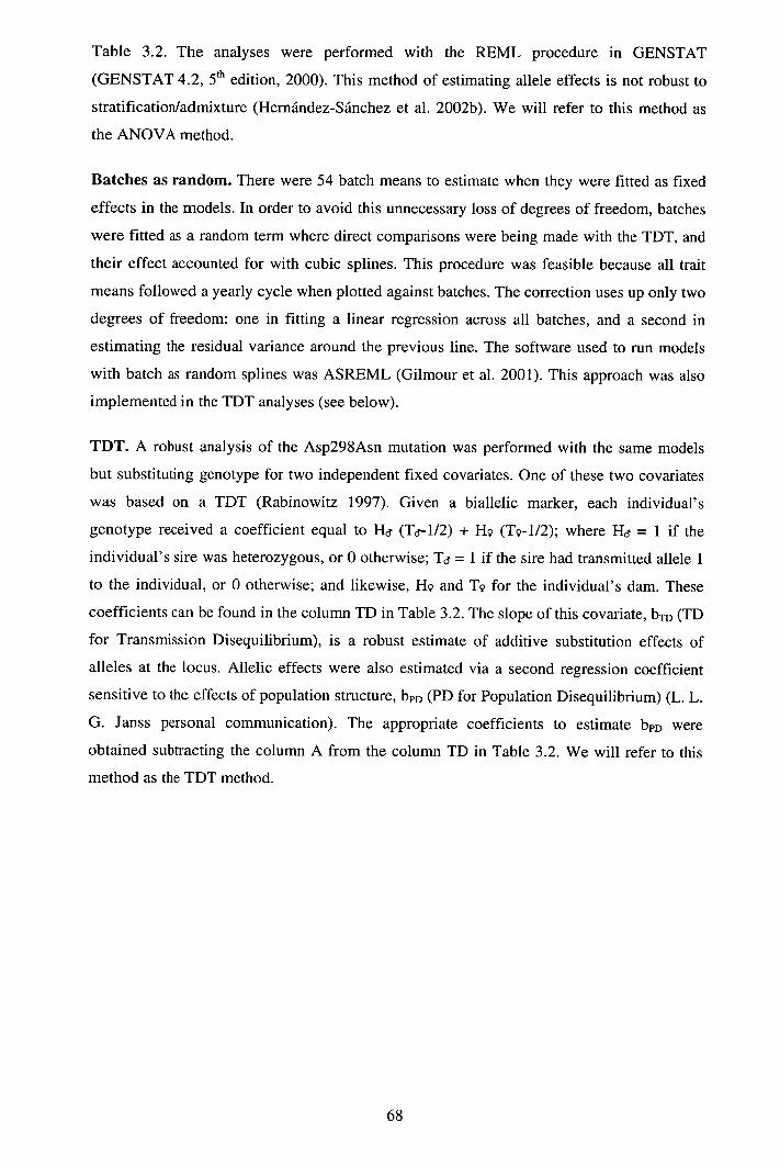
Table 3.2. The analyses were performed with the REML procedure in GENSTAT

(GENSTAT 4.2, 5th edition, 2000). This method of estimating allele effects is not robust to

stratification/admixture (Hernández-Sánchez et al. 2002b). We will refer to this method as

the ANOVA method.

Batches as random. There were 54 batch means to estimate when they were fitted as fixed

effects in the models. In order to avoid this unnecessary loss of degrees of freedom, batches

were fitted as a random term where direct comparisons were being made with the TDT, and

their effect accounted for with cubic splines. This procedure was feasible because all trait

means followed a yearly cycle when plotted against batches. The correction uses up only two

degrees of freedom: one in fitting a linear regression across all batches, and a second in

estimating the residual variance around the previous line. The software used to run models

with batch as random splines was ASREML (Gilmour et al. 2001). This approach was also

implemented in the TDT analyses (see below).

TDT. A robust analysis of the Asp298Asn mutation was performed with the same models

but substituting genotype for two independent fixed covariates. One of these two covariates

was based on a TDT (Rabinowitz 1997). Given a biallelic marker, each individual's

genotype received a coefficient equal to H (Tr-1/2) + H9 (T9-1/2); where He = 1 if the

individual's sire was heterozygous, or 0 otherwise; Te = 1 if the sire had transmitted allele 1

to the individual, or 0 otherwise; and likewise, H9 and T9 for the individual's dam. These

coefficients can be found in the column TD in Table 3.2. The slope of this covariate, bTD (TD

for Transmission Disequilibrium), is a robust estimate of additive substitution effects of

alleles at the locus. Allelic effects were also estimated via a second regression coefficient

sensitive to the effects of population structure, bpD (PD for Population Disequilibrium) (L. L.

G. Janss personal communication). The appropriate coefficients to estimate bpD were

obtained subtracting the column A from the column TD in Table 3.2. We will refer to this

method as the TDT method.

Table 3.2. Parameterisation of covariates A, TD, and PD given family genotypes.

Gf Gm Go A TD PD

11 11 11 1 0 1

11 12 11 1 '/2 ½

12 0 -½ ½

11 22 22 0 0 0

11 1 1 0

12 0 0 0 12 12

22 -1 -1 0

12 0 ½ -½ 12 22

22 -1 -½ -½

22 22 22 -1 0 1

Of: Paternal genotype Gm Maternal genotype G: Offspring genotype

One-way ANOVA A = 1, 0, -1 if Go = 11, 12, 22, respectively

TDT TD = H (T-1/2) + H9 (T9-1/2)

where He = 1 if Gf(m) = 12 and 0 otherwise Td (9) = 1 if offspring receives allele 1 from a 12 father

(mother) and 0 otherwise PD = A - TD

Generating parental genotype data. The TDT method requires parental genotype data,

which in the MC4R data set were mostly missing. Nevertheless, missing parental genotypes

could be generated using Gibbs sampling (e.g. Wang et al. 1994, Sorensen 1996). Gibbs

sampling was equivalent to integrating over all genotype probabilities of parents with

missing genotypes. Missing parental genotypes were sampled conditional on genotypes of

progeny and other relatives. Convergence was reached after 10 3 realisations after a burn-in

period of 100 realisations (see Appendix A). The autocorrelation in Gibbs sampling was

minimised by sampling one realisation every 50 consecutive ones, hence a total of 50 x 10 4

realisations were generated. The actual integration over missing genotype probabilities was

carried out by analysing the MC4R data set after each sampled realisation and averaging

results (i.e. p-values) across all realisations.

Simulation. A simulation study was carried out to investigate the properties of bpD and b10.

Population stratification was generated sampling from two separated populations with

different allele frequencies, and analysing the data jointly. Each population was characterised

by: 1)15 unrelated full-sib families, and 4 offspring per family (60 progeny in total), 2)

random mating, 3) a quantitative trait locus (QTL) and a linked neutral marker, both biallelic

and with allele frequency fixed to 0.9 in one population, and frequencies, at both loci, of 0.9,

0.7, 0.5, 0.3 and 0.1 in the other population 4) the recombination rate between loci was c = 0

or ½, 5) the standardised linkage disequilibrium in parents (D' = DfDm , Lewontin 1988)

was either 0 or 1, 6) the residual variance was 1 and the polygenic variance 0, and 7) the

QTL explained 5% (and in some cases 10%) of the total phenotypic variance. There were no

inter-population matings and all analyses were performed at the marker locus.

3.3 RESULTS

3.3.1 Properties of bpD and bID in analyses of simulated data

The power of estimating genetic effects through bpD and bTD in the simulated data is shown

in Figure 3.1, where F-ratios are plotted against the level of stratification S (allele frequency

difference between populations) across 4 different scenarios. Each dot in Figure 3.1 is the

average of 100 replicates. The significance threshold is based on the tabulated nominal 5%

threshold and is shown as a straight line. Figure 3.1a shows the results after analysing a

marker totally unlinked (c = ½) and with no association in the population (D' = 0) to a QTL.

In this situation, any significant effect is a type I error or due to bias. The FTD (i.e. the F-ratio

testing whether a significant amount of the total variation is explained by bTD) is

approximately 1 across all S values, which indicates that the marker did not have a

significant effect on the trait. On the contrary, FPD (i.e. the corresponding F-ratio test for bpD)

appeared positively correlated to the level of S. The effect was significant when S ~! 0.6. In

this case, spurious disequilibrium increases as stratification increases, and bpD cannot

distinguish between this sort of disequilibrium and disequilibrium due to linkage.

Figure 3.1b shows the results after analysing a marker totally unlinked (c = 0.5) but in

complete disequlibrium (D' = 1) in the parents. Here, FPD is always greater than FID, and this

difference increases with S. Moreover, the value of FPD was greater than 1 (approximately 2)

even without stratification (S = 0). This can be explained by considering that, on average, the

level of disequilibrium among offspring was ½, because D' is expected to be halved every

generation assuming no linkage and random mating. This feature suggests that bpD could

detect an effect given sufficient linkage disequilibrium between a marker and a QTL, even if

these two loci are totally unlinked, whereas bTD needs the joint occurrence of linkage and

linkage disquilibrium in order to estimate an effect.

70

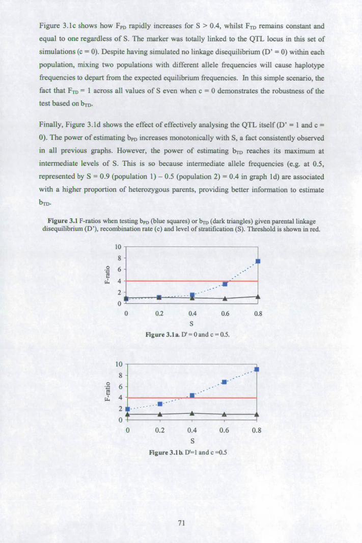
Figure 3.1c shows how FPD rapidly increases for S > 0.4, whilst F-rD remains constant and

equal to one regardless of S. The marker was totally linked to the QTL locus in this set of

simulations (c = 0). Despite having simulated no linkage disequilibrium (D' = 0) within each

population, mixing two populations with different allele frequencies will cause haplotype

frequencies to depart from the expected equilibrium frequencies. In this simple scenario, the

fact that FTD = 1 across all values of S even when c = 0 demonstrates the robustness of the

test based on b-rn.

Finally, Figure 3.1d shows the effect of effectively analysing the QTL itself (D' = 1 and c =

0). The power of estimating bpD increases monotonically with S, a fact consistently observed

in all previous graphs. However, the power of estimating b TD reaches its maximum at

intermediate levels of S. This is so because intermediate allele frequencies (e.g. at 0.5,

represented by S = 0.9 (population 1) - 0.5 (population 2) = 0.4 in graph ld) are associated

with a higher proportion of heterozygous parents, providing better information to estimate

bTD.

Figure 3.1 F-ratios when testing b 0 (blue squares) or bTD (dark triangles) given parental linkage disequilibrium (D'), recombination rate (c) and level of stratification (S). Threshold is shown in red.

10

8 0

0 0.2 0.4 0.6

0.8

S

Figure 3.1 a. D' = 0 and c = 0.5.

10

8

6

2

0

0 0.2 0.4 0.6

0.8

S

Figure 3.I b. D'l and c =0.5

71

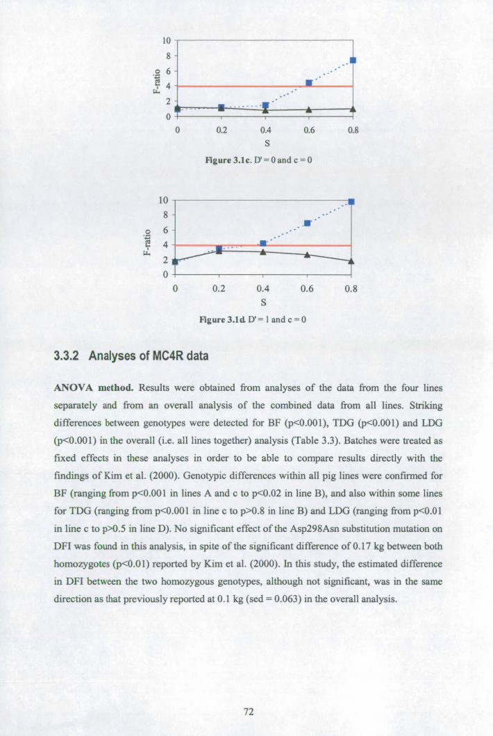
10

8

o 6

2

0

0 0.2 0.4 0.6 0.8

S

Figure 3.1 c. D' = 0 and c =0

10

8 -U...

• o 6

0 0.2 0.4 0.6 0.8

S

Figure 3.ldDl and c=0

3.3.2 Analyses of MC4R data

ANOVA method. Results were obtained from analyses of the data from the four lines

separately and from an overall analysis of the combined data from all lines. Striking

differences between genotypes were detected for BF (p<Z0.001), TDG (p<O.00l) and LDG

(p<0.001) in the overall (i.e. all lines together) analysis (Table 3.3). Batches were treated as

fixed effects in these analyses in order to be able to compare results directly with the

findings of Kim et al. (2000). Genotypic differences within all pig lines were confirmed for

BF (ranging from p<O.00I in lines A and c to p<0.02 in line B), and also within some lines

for TDG (ranging from p<0.001 in line c to p>0.8 in line B) and LDG (ranging from p<O.Ol

in line c to p>0.5 in line D). No significant effect of the Asp298Asn substitution mutation on

DFI was found in this analysis, in spite of the significant difference of 0.17 kg between both

homozygotes (p<0.01) reported by Kim et al. (2000). In this study, the estimated difference

in DFI between the two homozygous genotypes, although not significant, was in the same

direction as that previously reported at 0.1 kg (sed = 0.063) in the overall analysis.

72

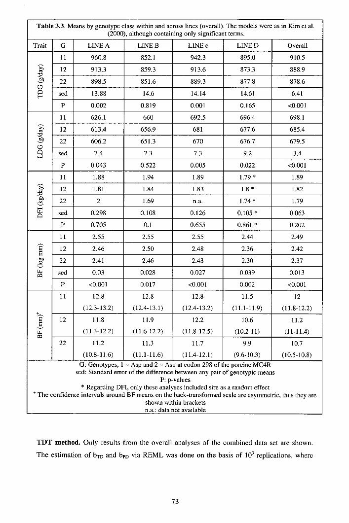
Table 3.3. Means by genotype class within and across lines (overall). The models were as in Kim et al. (2000), although containing only significant terms.

Trait G LINE A LINE B LINE c LINE D Overall

11 960.8 852.1 942.3 895.0 910.5

12 913.3 859.3 913.6 873.3 888.9

9 22 898.5 851.6 889.3 877.8 878.6 0

sed 13.88 14.6 14.14 14.61 6.41

P 0.002 0.819 0.001 0.165 <0.001

11 626.1 660 692.5 696.4 698.1

03 12 613.4 656.9 681 677.6 685.4

9 22 606.2 651.3 670 676.7 679.5 0

sed 7.4 7.3 7.3 9.2 3.4

P 0.043 0.522 0.005 0.022 <0.001

11 1.88 1.94 1.89 1.79 * 1.89

12 1.81 1.84 1.83 1.8 * 1.82

? 22 2 1.69 n.a. 1.74 * 1.79

sed 0.298 0.108 0.126 0.105 * 0.063

P 0.705 0.1 0.655 0.861 * 0.202

11 2.55 2.55 2.55 2.44 2.49

12 2.46 2.50 2.48 2.36 2.42

22 2.41 2.46 2.43 2.30 2.37

sed 0.03 0.028 0.027 0.039 0.013

P <o.00i 0.017 <0.001 0.002 <0.001

11 12.8 12.8 12.8 11.5 12

(12.3-13.2) (12.4-13.1) (12.4-13.2) (11.1-11.9) (11.8-12.2)

12 11.8 11.9 12.2 10.6 11.2

(11.3-12.2) (11.6-12.2) (11.8-12.5) (10.2-11) (11-11.4)

22 11.2 11.3 11.7 9.9 10.7

(10.8-11.6) (11.1-11.6) (11.4-12.1) (9.6-10.3) (10.5-10.8)

G: Genotypes, 1 - Asp and 2 - Asn at codon 298 of the porcine MC4R sed: Standard error of the difference between any pair of genotypic means

P: p-values * Regarding DFI, only these analyses included sire as a random effect

+ The confidence intervals around BF means on the back-transformed scale are asymmetric, thus they are shown within brackets n.a.: data not available

TDT method. Only results from the overall analyses of the combined data set are shown.

The estimation of bTD and bpD via REML was done on the basis of 10 3 replications, where

73

each replicate used a different population of parental genotypes generated with Gibbs

sampling. The average p values across these analyses are shown in Table 3.4. The ASREML

software does not perform hypothesis testing for fixed effects in the model although it

provides t-values and residual degrees of freedom. The p-values associated with genotypic

contrasts were obtained from the t-distribution. There were two independent null hypotheses

of interest: H: bPD = 0 and H 2 : bTD = 0, both were rejected for all traits except DFI (H:

BF p<0.0001, TDG p<O.Ol, LDG p<O.Ol and DPI p>0.5; H: BF p<0.0001, TDG p<0.001,

LDG p<O.Ol and DFI p>0.2). For the sake of comparison, Table 3.4 also incorporates results

from the ANOVA method (reported as regression coefficients rather than genotype means as

in Table 3.3). Both, the ANOVA and the TDT methods yielded similar results, although the

former was a slightly more powerful analysis (the standard errors were generally smaller).

Results in Tables 3 and 4 are of similar magnitude.

Table 3.4. Average effect of allele substitution for each trait using TDT (PD, TD) and ANOVA. Cycle was treated as random.

Trait Estimation b s.e.(b) T DF p-value

TDG

PD 16.1 5.84 2.76

2430

<0.01

TD 14.1 4.45 3.17 <0.01

ANOVA 14.8 3.66 4.05 <0.0001

LDG

PD 9.1 3.31 2.75

2423

<0.01

TD 8.8 2.38 3.69 <0.001

ANOVA 8.9 2.01 4.42 <0.0001

BF

PD 0.07 0.013 5.14

2423

<0.0001

TD 0.06 0.009 6.7 <0.0001

ANOVA 0.06 0.009 8.11 <0.0001

DR

PD 0.03 0.047 0.64

272

> 0.5

TD 0.08 0.061 1.26 > 0.2

ANOVA 1 0.05 0.037 1.28 >0.2

PD: Population Disequilibrium (between families gene effect) ID: Transmission-Disequilibrium (within families gene effect)

ANOVA: Genotype substituted covariates PD and ID b: allele substitution effect s.e. (b): standard error of b

T: t-statistic from testing b=0 vs. b#0 DF: Nominal residual degrees of freedom

p-value: the N(0,1) was used as an approximation to the t-distribution for TDG, LDG and BF

74

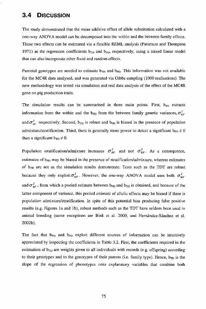
3.4 DiscussioN

The study demonstrated that the mean additive effect of allele substitution calculated with a

one-way ANOVA model can be decomposed into the within and the between family effects.

These two effects can be estimated via a flexible REML analysis (Patterson and Thompson

1971) as the regression coefficients b TD and bpD, respectively, using a mixed linear model

that can also incorporate other fixed and random effects.

Parental genotypes are needed to estimate bTD and bpD. This information was not available

for the MC4R data analysed, and was generated via Gibbs sampling (1000 realisations). The

new methodology was tested via simulation and real data analysis of the effect of the MC4R

gene on pig production traits.

The simulation results can be summarised in three main points. First, bTD extracts

information from the within and the bpD from the between family genetic variances, O,F

and OF respectively. Second, bTD is robust and bpD is biased in the presence of population

admixture/stratification. Third, there is generally more power to detect a significant bpD :~ 0

than a significant bTD : ~ 0.

Population stratification/admixture increases aF and not 0WF• As a consequence,

estimates of bpD may be biased in the presence of stratification/admixture, whereas estimates

of bTD are not as the simulation results demonstrate. Tests such as the TDT are robust

because they only exploit °WF. However, the one-way ANOVA model uses both °F

and aBF, from which a pooled estimate between bpD and bTD is obtained, and because of the

latter component of variance, this pooled estimate of allelic effects may be biased if there is

population admixture/stratification. In spite of this potential bias producing false positive

results (e.g. Figures la and lb), robust methods such as the TDT have seldom been used in

animal breeding (some exceptions are Bink et al. 2000, and Hernández-Sánchez et al.

2002b).

The fact that b TD and bpD exploit different sources of information can be intuitively

appreciated by inspecting the coefficients in Table 3.2. First, the coefficients required in the

estimation of bTD are weights given to all individuals with records (e.g. offspring) according

to their genotypes and to the genotypes of their parents (i.e. family type). Hence, b TD is the

slope of the regression of phenotypes onto explanatory variables that combine both

75

offspring's genotypes and family type. Second, the coefficients required in the estimation of

bpD can alternatively be obtained as , where G ij = ½, 0 or —½ if the genotype of the j b

parent in the ith family is 11, 12 or 22, respectively. Therefore bpD is the slope of the

regression of phenotypes onto family type.

More explicitly, let us model yj, the phenotype of the j th individual having the i t1' QTL

genotype, as y = 1u + g. + a, + e ii where p is the population mean, g, the effect of the i h

QTL genotype on the j th offspring, and a 11 and eij are the polygenic and residual random terms

drawn from two independent normal distributions with zero means and variances O and

o, respectively. Let there be random mating, no population stratification, and only additive

genetic effects at the QTL locus. Under these circumstances, the total additive genetic

variance splits equally between and within families, therefore E[c7F ]= cT. 12, and

E[a ,F j= c + a /2, where o = + o, and is the variance due to the QTL. If a

statistical model explains all cT then the additive genetic effects of the QTL will be fully

accounted for. However, if the model estimates additive effects only through either bTD or

bpD then U 2 will only be partially explained. For example, if bTD is the only estimator of

QTL effect then E[o,F ]=C2 +U2

/2 and E[aF ]=u'12, as only within-family

variation can be used to estimate bTD. If, on the other hand, bpD is the only estimator of QTL

effect then E[o, ]= o + o 12 and E[o ] = o 12, as only between-family variation

can be used to estimate bpD. These changes in the within and between family variances due

to estimation of bTD or bpD were validated via computer simulations (data not shown).

The situation is more complex when there is stratification within a population. Appendix B

shows how the proportion of the total phenotypic variation explained fitting a linear

regression, differed when either bTD or bpD was estimated in the presence of population

stratification.

Simulation results showed that testing the null hypothesis bpD = 0 tends to produce higher F-

ratios when it is not true than testing bpT = 0 (Figure 3.1). Nevertheless, the analysis of real

data showed the opposite effect (i.e. t-tests for bTD were always higher than those for bpD in

Table 3.4). This result is possible when there is no admixture/stratification, because b TD is

expected to be equivalent to bpD. Moreover, in simulations, the only between family

component was ½ of the total QTL variance, whereas in reality other factors (e.g. litter and

76

sow effects) may also increase 08F• The analysis of real data showed that b TD was very

similar to b 0 across all traits, and furthermore, that both estimates were also similar to

allelic effects obtained with ANOVA (Table 3.4). This suggests that there was no significant

stratification/admixture in the population, and that there were equivalent amounts of genetic

information between and within families.

Where estimates of bTD and bpD differ, a t-test could be used to test the null hypothesis bTD =

bpD. If no evidence to reject the null hypothesis were found then a more powerful one-way

ANOVA model could be safely implemented, i.e. there would be no evidence for

admixture/stratification in the population. Otherwise, robust approaches such as the one

proposed here, i.e. estimating bTD, or other TDTs, should be considered as the only reliable

methods of analysis.

A complication of this approach applied to many real data sets, including the MC4R data

used as an example, will be generating missing parental genotypes. Nevertheless, a Gibbs

sampling technique with 10 3 replications was simple to implement (and we know they were

accurate enough because 10 times more replicates did not affect the outcome) in this simple

scenario, i.e. a single biallelic marker, a maximum of three generations, few missing data.

Other robust tests that do not require parental genotypes, e.g. sib-TDTs (e.g. Schaid and

Rowland 1999, Spielman and Ewens 1998), were found to be less powerful than the method

outlined here in additional analyses of simulated data, e.g. FSIb = 5.5 vs. FTDPD = 7.7 (based

on 1000 replicates). Analysing more complex or unbalanced data sets will probably demand

more realisations of the Gibbs sampler and it will present an additional problem: testing

fixed effects in REML, because the asymptotic properties of t-test or Wald test could not be

guaranteed (see Kenward and Roger 1997, Welham and Thompson 1997, Elston 1998).

This approach was also tested with real data. There is strong evidence that the substitution-

mutation Asp298Asn in the MC4R gene affects production traits in the pig, e.g. backfat

(BF), growth (TDG, LDG), and appetite (DPI) (Kim et al. 2000). These effects were re-

estimated with extra records with respect to the original work. Significant effects were found

for BF, TDG and LDG across all lines (p <0.001), although not for all pig lines (ranging

from p < 0.001 to p> 0.8). DFI was the only trait not significant in this study (p > 0.2), even

after using the models described in Kim et al. (2000).

The lack of effect on DFI was unexpected given previously reported results (p <0.01), and

other reported associations of MC4R with appetite and feeding behaviour in macaques

77

(Koegler et al. 2001), rats (Todd et al. 1997), mice (Butler et al. 2001), and layer chicks

(Tachibana et al. 2001). One possible explanation for not detecting an effect on DFI is the

lack of power due to a small data set (n=275). Although there were less data (n=231) in the

study of Kim et al. (2000) than in this study, the difference is small and additional statistical

noise may have been introduced through factors such as data structure and/or chance. An

independent study that used a larger data set (n=619), found a significant (p<0.05) additive

gene effect of 0.075 kg/day on DEl (G. Plastow, personal communication). Further

experiments are needed in order to ascertain whether the Asp298Asn substitution mutation at

the MC4R locus is causative.

This study demonstrates that TDT can be implemented within the REML framework. As a

guideline, one should test associations with ANOVA only after having checked that bTD and

bpD are not significantly different from each other, i.e. making sure no false positive results

are being caused by population stratification.

3.5 Appendix A: Gibbs sampling convergence when generating missing

parental genotypes

Each missing parental genotype was stochastically generated with Gibbs sampling

conditioning on genotypes of his/her relatives. A total of 50 x 10 4 consecutive realisations

were obtained and only one every 50 was saved to reduce the autocorrelation of the chain.

The traits backfat (BF), test daily gain (TDG), lifetime daily gain (LDG) were analysed with

a TDT (Rabinowitz 1997) using the remaining 10 4 (independent) sets of parental genotypes.

For each trait a distribution of log-transformed p-values was obtained (dist-0). Three

different samples of size 10 3 were obtained from dist-0, they were: dist-1 containing the

initial 103 log-p-values, dist-2 containing the last 10 3 log-p-values, and dist-3 containing 10 3

log-p-values evenly spaced in the chain (one every 10 consecutive ones). The distributions

dist- 1, 2, and 3 were compared against dist-0 with the non-parametric Kolmogorov-Smirnoff

test (KOLMOG2 procedure in GENSTAT 4.1), which obtains the maximum absolute

difference between two cumulative density functions. If the two distributions are the same,

this difference follows a Z 2 distribution. There were no significant differences (Table 3.A)

between Dist-1, 2 or 3 and Dist-0 in any trait at a significance level of 0.017 (Bonferroni

correction for 3 comparisons within trait). These results ensure that 10 3 out of the 104

independent sets of parental genotypes provide an unbiased sample, and that if convergence

was reached after 104 realisations, then it was also reached after 10 3 realisations.

78

Table 3.A. P-values of the Kolmogorov-Smimoff test for differences between Dist-0 and Dist-1, 2, or 3

aBF 11TDG CLDG dDistl 0.02 0.13 0.66 eDist2 0.36 0.23 0.42 Dist-3 0.05 0.51 0.20

a Backfat b Test Daily Gain

' Lifetime Daily Gain d The first 10 3 log-p-values from Dist-0

The last 103 log-p-values from Dist-0 103 log-p-values from Dist-0, sampling 1 every 10 consecutive ones

Significant level = 0.05 / 3 = 0.017 (Bonferroni correction)

3.6 Appendix B: Impact of stratification on bID and bpD

Population stratification affects both the estimation of the effect via bpD and the power of that

estimation (s.e. bpD). We will assume the simplest scenario where a population is divided

into two subpopulations of equal size, where mating is at random within each subpopulation,

and there is no matings across subpopulations.

The expected mean square of a linear model that regresses Y onto a single explanatory

variable X is E[MSR] =07 + B2 1(x - x )2

, where B is the expected regression

parameter, and o the residual variance (Sokal and Rohif 1995). When n phenotypes (Y) are

simulated with gene effect (B) and cTe2 equal to one, then

E[MsR] = 1 + E[ (x - )2

]= 1 + n{E[X2 ]- (E[X ])2 }. Let us assume p1 is the frequency

of allele i at the trait locus in subpopulation 1, and q 1 the equivalent frequency in

subpopulation 2. Furthermore, let us assume PIt = (P 1)2 is the frequency of genotype 11 in

subpopulation 1, and qii the frequency of the equivalent genotype in subpopulation 2. Hence,

it can be shown that E[PD] = (Pi - P2 + qj - q) / 2, and that

E[PD2 ] = 0.5(p + p + + q ) + O.25(p 11 (i - p 11 ) + q1 , (i - q11 )). The same process

is followed to develop the expected mean squares when using TD, thus

E[TD2 1= (p + q )14, and E[TD] = 0. These two predictions were very similar to

simulation results (not shown). We can see the effect of stratification on E[MSR]TD and

E[MSR]pD for n=100 in Figures 3.bl and 3.b2. Figure 3.bl takes a hill-type shape (seen from

above) where the highest point is at the centre, and gradually decays in all directions away

from the centre. Figure 3.b2 takes a valley-type shape (seen from above) where the lowest

points are on the diagonal (in fact Figures 3.bl and 3.b2 are identical on the diagonal) and

79

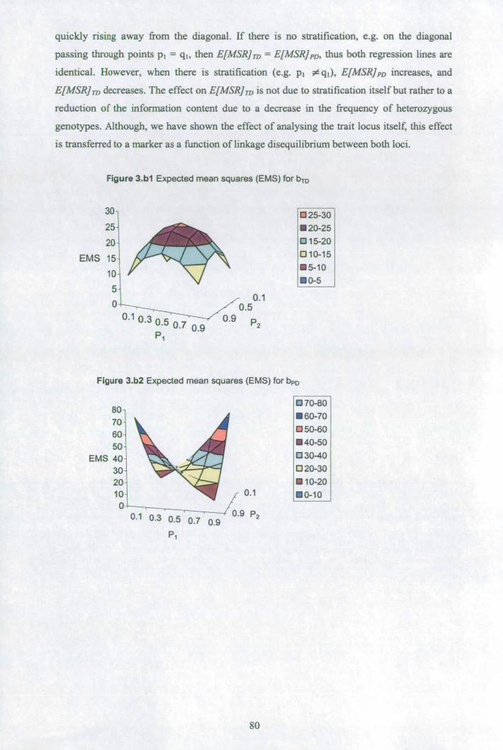
quickly rising away from the diagonal. If there is no stratification, e.g. on the diagonal

passing through points p i = q 1 , then E[MSR]p = E[MSR]pD, thus both regression lines are

identical. However, when there is stratification (e.g. p 1 ;d q 1 ), E[MSR]pD increases, and

E[MSRJ TD decreases. The effect on E[MSR]TD is not due to stratification itself but rather to a

reduction of the information content due to a decrease in the frequency of heterozygous

genotypes. Although, we have shown the effect of analysing the trait locus itself, this effect

is transferred to a marker as a function of linkage disequilibrium between both loci.

Figure 3.bl Expected mean squares (EMS) for bTD

30 D25-30

25 •20-25

20 1315-20

51

EMS 15

o 0.5

10 85-10

00-5

0.1 0.3 0.5 0.9 0.709 P2

P 1

Figure 3.b2 Expected mean squares (EMS) for bpD

80

70' 60 50

EMS 40 30 20 10 0

• 70-80

• 60-70

050-60

•40-50

o 30-40

020-30

U 10-20 0.1 •o-io

• -----------I 0.9 P2

0.1 0.3 0.5 0.7 0.9

P 1

80

CHAPTER 4

Genome-wide search for markers associated

with Bovine Spongiform Encephalopathy

4.1 INTRODUCTION

Bovine Spongiform Encephalopathy (BSE) is a slowly progressing, inevitably fatal,

neurodegenerative disorder characterised by deposition of an abnormal form of the host

pnon protein (PrP) in neurones, leading to a widespread sponge-like vacuolation of the

brain (Hunter 1999, www.bseinciuirv.gov.uklindex.htm). BSE belongs to a family of diseases

known as Transmissible Spongiform Encephalopathies (TSE5) that include scrapie, in sheep,

and Creutzfeldt-Jakob Disease (CJD), in humans. The prevailing hypothesis is that BSE is

not a genetic disease, but that there could be a genetic component conferring resistance to the

infectious agent (Ferguson et al. 1997, Donnelly et al. 1997). BSE can be experimentally

transmitted across species via an isoform of the prion protein found in scrapie-affected sheep

(PrPS) (Bruce et al. 1994) and it appears that the bovine form of PrPSC is also responsible for

a new variant of CJD (vCJD) (Bruce et al. 1997, Almond and Pattison 1997).

There is strong evidence that different polymorphisms in the PrP gene cause variable

incubation periods (IP) and, possibly, degrees of resistance to scrapie in sheep (Goldmann et

al. 1990, Goldmann et al. 1996) and to CJD in humans (Palmer et al. 1991). In particular

codons 136, 154 and 171 in the PrP gene are strongly associated with incidence of scrapie

(Goldmann et al. 1994). In humans, individuals homozygous at codon 129 of the PrP gene

are over-represented in CJD cases, whereas heterozygous individuals seem to be more

resistant to CJD (Palmer et al. 1991). All vCJD cases to date are homozygous for methionine

at this codon (Bruce et al. 1997).

The PrP gene is less polymorphic in cattle than in sheep or humans. So far, only two

polymorphisms, a variable number of an octapeptide repeat and an RFLP, have been found

in the coding region of the bovine PrP gene (Goldmann et al. 1991b, Ryan and Womack

1993). Two case-control studies (Hunter et al. 1994b, Neibergs et al. 1994) found no

association between the octapeptide-repeat and BSE, and only the latter study found a

significant association between BSE and the RFLP.

81

Recently, there has been evidence of genes other than PrP affecting susceptibility to an

experimental prion disease in mice. Stephenson et al. (2000) found Quantitative Trait Loci

(QTL) partially accounting for differences of IP in F 2 mice, derived from a cross between

two different parental strains with the same PrP gene, on Chr 9 and 11 using mouse-derived

PrPSC inocula. In a similar experiment, Lloyd et al. (2001) found significant evidence for

QTL influencing IP in mice on Chr 2, 11 and 12 plus suggestive evidence for QTL on Chr. 6

and 7. Manolakou et al. (2001) backcrossed Fl animals with their parental lines, identical

only at the PrP locus, and used PrPSC inocula from cattle. They reported QTL influencing IP

in mice on Chr 2, 4, 8 and 15, plus significant host environment factors (i.e. the age of the

host's mother, the age of the host at infection, and an X-cytoplasm interaction in the host).

The purpose of the study reported here was to perform a genome wide scan for BSE

susceptibility/resistance alleles in cattle through their associations with markers. The amount

of association between two linked loci is a function of the underlying linkage disequilibrium

(LD). In large and panmictic populations the expected range of LD for relatively old mutants

is very short, and simulation studies have predicted that between 30,000 and 500,000

biallelic markers would be required in genome-wide QTL scans (Ott 2000, Kruglyak 1999).

However, Riquet et al. (1999) predicted conserved chromosomal segments spanning 4.5-5

cM in one Holstein cattle population, and Farnir et al. (2000) found significant LD even

between markers up to 50 cM apart. These results were probably due to a recent history of

intensive artificial selection leading to high levels of inbreeding (Bradley and Cunningham

1999) and to a low effective population size (Roughsedge et al. 1999) leading to strong drift

effects. Hence, relatively sparse marker maps may still be sufficient for genome-wide QTL

scans in Holstein cattle.

Transmission-Disequilibrium Tests (TDTs) are tests for linkage in the presence of LD

between a marker and a trait locus that are robust to spurious associations (i.e. association

without linkage) due to population stratification. TDTs identify preferential transmission of

particular alleles from heterozygous parents to affected offspring across a sample of families.

Such a pattern of transmission is also known as segregation distortion, because alleles do not

segregate at random. Although the original TDT (Spielman et al. 1993, Terwilliger and Ott

1992) and its extensions for multiple alleles (Bickeboller and Clerget-Darpoux 1995) are

conceptually simple and easy to implement, more versatile TDTs have been developed based

on logistic regressions (Sham and Curtis 1995, Waldman et al. 1999). In this paper, we use

TDTs to assess the association between BSE and markers spanning the Holstein genome in

half-sib families.

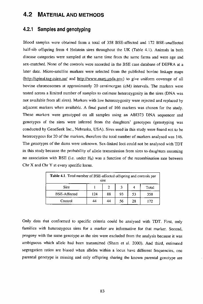
4.2 MATERIAL AND METHODS

4.2.1 Samples and genotyping

Blood samples were obtained from a total of 358 BSE-affected and 172 BSE-unaffected

half-sib offspring from 4 Holstein sires throughout the UK (Table 4.1). Animals in both

disease categories were sampled at the same time from the same farms and were age and

sex-matched. None of the controls were recorded in the BSE case database of DEFRA at a

later date. Micro-satellite markers were selected from the published bovine linkage maps

(http://spinal.tag.csiro.au/ and http://www.marc.usda.gov ) to give uniform coverage of all

bovine chromosomes at approximately 20 centimorgan (cM) intervals. The markers were

tested across a limited number of samples to estimate heterozygosity in the sires (DNA was

not available from all sires). Markers with low heterozygosity were rejected and replaced by

adjacent markers when available. A final panel of 166 markers was chosen for the study.

These markers were genotyped on all samples using an AB1373 DNA sequencer and

genotypes of the sires were inferred from the daughters' genotypes (genotyping was

conducted by GeneSeek Inc., Nebraska, USA). Sires used in this study were found not to be

heterozygous for 20 of the markers, therefore the total number of markers analysed was 146.

The genotypes of the dams were unknown. Sex-linked loci could not be analysed with TDT

in this study because the probability of allele transmission from sires to daughters assuming

no association with BSE (i.e. under H 0) was a function of the recombination rate between

Chr X and Chr Y at every specific locus.

Table 4.1. Total number of BSE-affected offspring and controls per sire

Sire 1 2 3 4 Total

BSE-Affected 124 88 93 53 358

Control 44 44 56 28 172

Only data that conformed to specific criteria could be analysed with TDT. First, only

families with heterozygous sires for a marker are informative for that marker. Second,

progeny with the same genotype as the sire were excluded from the analysis because it was

ambiguous which allele had been transmitted (Sham et al. 2000). And third, estimated

segregation ratios are biased when alleles within a locus have different frequencies, one

parental genotype is missing and only offspring sharing the known parental genotype are

excluded from the analysis (Curtis and Sham 1995). In these circumstances, homozygous

offspring were excluded from the analysis.

4.2.2 Statistical tests

The statistical tests used in this study derived from the McNemar-type TDT proposed by

Spielman et al. (1993) adapted for multi-allelic loci (Bickeböller and Clerget-Darpoux 1995)

and re-parameterisations of those TDTs within a logistic regression framework (Sham and

Curtis 1995, McCullagh and Nelder 1983). The latter procedure was further extended for

testing the interaction between transmission rate and disease status. Allelic transmission

probabilities can be studied within and across genotypes. The genotypic-TDT statistic, g-

TDT, assesses departures from random segregation of alleles within genotypes. Data from

sires with identical genotypes is pooled together. The g-TDT is asymptotically distributed as

a X 2distribution with degrees of freedom (dO equal to the number of different

heterozygous sires. The allelic-TDT statistic, a-TDT, is used to test departures from random

segregation of alleles across genotypes. Asymptotically, a-TDT follows a X distribution df

with df = a - 1, where a is the number of different alleles across all sires in the sample. Both

a-TDT and g-TDT were also implemented using logistic regressions for parameter estimation

and log-likelihood ratios for hypothesis testing assuming data to be binomially distributed.

These tests were named log-LR a and log-LR g , respectively. All likelihood ratios under H 0 are

distributed as with df equal to the difference between the number of parameters

estimated under H 1 (i.e. number of transmission probabilities estimated from data) and H 0

(i.e. no parameters estimated because all transmission probabilities are assumed to be ½).

The use of theoretical reference distributions (i.e. x2) for obtaining p-values was empirically

validated through simulations for all markers and two TDTs, g-TDT and log-LRa. For each

marker and each sire family, a particular allele was sampled from a binomial B (n, p), where

n was the total number of BSE-affected offspring within a sire family and p = ½, then both

TDTs analysed the sample and the process was repeated 1,000 times.

Logistic regressions could not be solved when a particular allele was not transmitted to any

offspring. Paradoxically, such observations are the most conclusive signals supporting a

BSE-marker association. In order to analyse that valuable information, an ad hoc solution

was to use 0.5 rather than 0 for an allele never transmitted to offspring, and N-0.5 rather than

N for the allele always transmitted to offspring (N is the number of B SE-affected offspring

in the analysis) (Cox 1970).

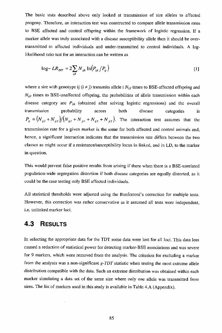
The basic tests described above only looked at transmission of sire alleles to affected

progeny. Therefore, an interaction test was constructed to compare allele transmission rates

to BSE affected and control offspring within the framework of logistic regression. If a

marker allele was truly associated with a disease susceptibility allele then it should be over-

transmitted to affected individuals and under-transmitted to control individuals. A log-

likelihood ratio test for an interaction can be written as

log— LR 1 . = 21 N, k ln(I Jk /P0 )

[1] ijk

where a sire with genotype ij (i # j) transmits allele i Nip times to B SE-affected offspring and

Nu2 times to B SE-unaffected offspring, the probabilities of allele transmission within each

disease category are Puk (obtained after solving logistic regressions) and the overall

transmission probability across both disease categories is

Pu = (N1. 1 + N,, 2 )/(N1 + N 11 + N 2 + N 2 ). The interaction test assumes that the

transmission rate for a given marker is the same for both affected and control animals and,

hence, a significant interaction indicates that the transmission rate differs between the two

classes as might occur if a resistance/susceptibility locus in linked, and in LD, to the marker

in question.

This would prevent false positive results from arising if there when there is a BSE-unrelated

population-wide segregation distortion if both disease categories are equally distorted, as it

could be the case testing only BSE affected individuals.

All statistical thresholds were adjusted using the Bonferroni' s correction for multiple tests.

However, this correction was rather conservative as it assumed all tests were independent,

i.e. unlinked marker loci.

4.3 RESULTS

In selecting the appropriate data for the TDT some data were lost for all loci. This data loss

caused a reduction of statistical power for detecting marker-BSE associations and was severe

for 9 markers, which were removed from the analysis. The criterion for excluding a marker

from the analysis was a non-significant g-TDT statistic when testing the most extreme allele

distribution compatible with the data. Such an extreme distribution was obtained within each

marker simulating a data set of the same size where only one allele was transmitted from

sires. The list of markers used in this study is available in Table 4.A (Appendix).

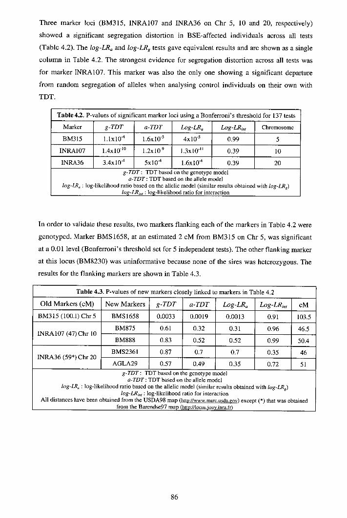
Three marker loci (BM315, INRA107 and INRA36 on Chr 5, 10 and 20, respectively)

showed a significant segregation distortion in BSE-affected individuals across all tests

(Table 4.2). The log-L& and log-LR g tests gave equivalent results and are shown as a single

column in Table 4.2. The strongest evidence for segregation distortion across all tests was

for marker INRA107. This marker was also the only one showing a significant departure

from random segregation of alleles when analysing control individuals on their own with

TDT.

Table 4.2. P-values of significant marker loci using a Bonferroni's threshold for 137 tests

Marker g-TDT a-TDT Log-L& Log-LR 11 Chromosome

BM315 1.1x10 1.6x10 5 4x1€15 0.99 5

INRA107 1.4x10' ° 1.2x10 9 1.3xl0" 0.39 10

INRA36 3.4x10 5x10-4 1.6xl0 0.39 20 g-TDT: TDT based on the genotype model

a-TDT: TDT based on the allele model log-L&: log-likelihood ratio based on the allelic model (similar results obtained with log-LR 8)

log-LR 1 ,: log-likelihood ratio for interaction

In order to validate these results, two markers flanking each of the markers in Table 4.2 were

genotyped. Marker BMS1658, at an estimated 2 cM from BM315 on Chr 5, was significant

at a 0.01 level (Bonferroni's threshold set for 5 independent tests). The other flanking marker

at this locus (BM8230) was uninformative because none of the sires was heterozygous. The

results for the flanking markers are shown in Table 4.3.

Table 4.3. P-values of new markers closely linked to markers in Table 4.2

Old Markers (cM) New Markers g-TDT a-TDT Log-LR Log-LR, 1 cm BM315 (100.1) Chr5 BMS1658 0.0033 0.0019 0.0013 0.91 103.5

INRA 107 (47) Chr 10 BM875 0.61 0.32 0.31 0.96 46.5

BM888 0.83 0.52 0.52 0.99 50.4

INRA36 (59*) Chr 20 BMS2361 0.87 0.7 0.7 0.35 46

AGLA29 0.57 0.49 0.35 0.72 51 g-TDT: TDT based on the genotype model

a-TDT: TDT based on the allele model log-LR: log-likelihood ratio based on the allelic model (similar results obtained with log-LR g)

log-LR 1,,: log-likelihood ratio for interaction All distances have been obtained from the USDA98 map (http://www.marc.usda.gov ) except (*) that was obtained

from the Barendse97 map (httix//Iocus.jouy.inra.fr )

Sample sizes and allele distribution among BSE-affected and control offspring for the 3

selected markers and their flanking markers are shown in Table 4.4.

Table 4.4. Counts of the number of times a particular allele (A or B) is transmitted from heterozygous sires to BSE-affected and control daughters for markers in Table 4.3

BM875 INRA 107 BM888

Genotype BSE Control Genotype BSE Control Genotype BSE Control

Sire A/B A B A B A/B A B A B A/B A B A B

1 127/127 ? ? ? ? 180/179 39 3 13 0 192/190 20 18 4 6

2 127/127 ? ? ? ? 180/179 29 8 9 1 192/190 12 13 10 6

3 127/127 ? ? ? ? ? ? ? ? 196/192 13 8 2 1

4 127/125 3 6 1 3 ? ? ? ? 192/190 12 10 7 4

BMS2361 INRA36 AGLA29

Genotype BSE Control Genotype BSE Control Genotype BSE Control

Sire MB A B A B A/B A B A B A/B A B A B

1 146/146 ? ? ? ? 210/188 8 11 1 3 178/170 31 19 7 11

2 150/142 26 30 13 6 210/188 9 6 4 5 178/166 20 22 10 6

3 144/140 23 24 5 9 190/188 27 5 10 1 174/170 27 23 5 4

4 148/140 13 19 9 4 210/188 7 1 0 4 174/166 13 15 8 4

BM8230 BM315 BMS1658

Genotype BSE Control Genotype BSE Control Genotype BSE Control

Sire MB A B A B A/B A B A B MB A B A B

1 ? ? ? ? 142/124 25 30 10 9 102/94 0 19 0 8

2 ? ? ? ? ? ? ? ? ? 106/102 28 23 7 7

3 ? ? ? ? ? 138/126 30 5 7 1 102/94 9 12 1 1

4 ? ? ? ? ? ? ? ? ? 92/92 ? ? ? ?

MB genotype of sire A number of transmissions of allele A B number of transmissions of allele B

? data not available because sire was either homozygote or had not been genotyped

Similar results were obtained using either theoretical x2 or empirical distributions as

reference distributions (results not shown). None of the 137 markers showed any significant

interaction between transmission and disease status.

LIM

4.4 DiscussioN

The objective of this study was to identify markers associated with BSE by screening the

entire bovine genome in a population of UK Holstein cows. TDTs were used because they

are robust to spurious associations due to population stratification or admixture (Warren and

Spielman 1995, Schork et al. 2001). A marker is associated with BSE when alleles at that

marker did not segregate at random in a sample of affected individuals. Segregation

distortion was tested within and across genotypes with g-TDT and a-TDT, respectively.

These two tests gave similar results, and were equivalent when none of the sires had alleles

in common. Both tests were also implemented within a logistic regression framework

because this facilitated statistical modelling. For instance, logistic regressions were extended

to analyse interactions between allele transmission rates and disease status. Moreover,

additional variables such as age and farm could be more easily incorporated in logistic

regressions than in g-TDT or a-TDT. In principle, logistic regressions would also allow

testing loci on Chr Y, however the estimation of allelic transmission probabilities under H 0

would have been inaccurate because genetic distances were not estimated in this study and

vary from population to population (Leach 1996).

Asymptotically, all these TDTs follow x2 distributions. However, there was a reduction in

sample size because, in this study, TDTs could only be used to analyse heterozygous

offspring from sires with a different heterozygous genotype. Therefore, the use of x2 as

reference distribution was verified through simulations for g-TDT and log-LRa. The p-values

obtained from empirical distributions in both TDTs were similar to p-values obtained from

x2 distributions (data not shown). It was not necessary to check a-TDT and log-LRg because

they are alternative parameterisations of log-LRa and g-TDT, respectively.

Three marker loci showed significant departures from random allelic segregation in BSE-

affected individuals and were selected for further study. The strongest evidence (lowest p-

value) came from marker INRA107 on Chr 10. Two sires with the same genotype were

informative at this locus and the same allele was over-represented in their affected offspring.

Furthermore, two candidate genes linked to INRA107 have homologues located on a region

of mouse Chr 9 that showed suggestive evidence of QTL affecting IP following an

experimental scrapie challenge (Stephenson et al. 2000). The homology data for this paper

were obtained from the Mouse Genome Database (MGD). One of these genes encodes for

the enzyme hexosaminidase A (HEXA), which is related to a progressive and lethal

neurodegenerative human disorder called Tay Sachs (Bach et al. 2001). Whether variation in

the HEXA gene is partly responsible for controlling IP of a PrPSCinduced disorder in mice

has yet to be tested, however the phenotypic effects on target tissues for TSEs makes it a

candidate for further study.

INRA107 was also the only marker for which a significant segregation distortion was found

in the control group, with the same allele being over-represented in both disease groups.

Thus, there may be a common underlying cause of segregation distortion affecting both

BSE-affected and control individuals, which may arise from sampling bias unrelated to BSE.

Indeed, the second linked gene from the mouse study is the cytochrome P450 family XIX

(CYP19). This gene is implicated in several human disorders such as reduced fertility and

sexual organ development (Genissel and Carreau 2001, Carreau 2001), neonatal

hypothyroidism (Ando et al. 2001), slow bone maturation and shorter adult height (Wickman

et al. 2001), and breast cancer (Kuerer et al. 2001). It is possible that alleles at the CYP19

locus have a detrimental effect on fitness, leading to differential survival and, hence, give a

spurious association of INRA 107 with BSE.

Two flanking markers were genotyped, at an estimated 1.5 and 3.4 cM from INRA107, but

neither was significantly associated with disease status (Table 4.3). These latter results were

unexpected, considering that the probability of a recombination event between INRA 107 and

either of the two flanking markers in one generation is small. However, this apparent

inconsistency can be explained by the fact that different families, different individuals within

families and, hence, different sample sizes within a family, were used in the analysis of each

of the markers. It should also be noted that the flanking markers were selected from the

published genetic maps, and in some cases the position of markers was estimated between

different maps. Thus, it is possible that the flanking markers were in fact further from the

original marker than the estimated distance.

A similar inconsistency was observed between the marker INRA36 on Chr 20 and its two

flanking markers. Despite a significant segregation distortion at the INRA36 locus, alleles at

both flanking markers segregated at random. Again, the fact that different individuals were

informative for the three loci may explain this discrepancy. Several QTL influencing milk

traits have already been mapped on Chr 20 (Arranz et al. 1998) and low productivity is an

important reason for culling, only second to reproduction problems (Young et al. 1983).

Therefore the observed distortion at INRA36 could be through culling and selecting within

herds favouring higher yielding individuals, rather than by association with BSE.

LIM

Two closely linked marker loci flanking the third significant locus, BM3 15 on Chr 5, were

also genotyped on the samples. One of the markers was totally uninformative, but the other,

at an estimated 2 cM from BM315, showed a significant effect at a 0.01 level. The number

of homologies between the bovine Chr 5 and the murine Chr 6 (reported by Lloyd et al.

2001) and Chr 15 (reported by Manolakou et al. 2001) are 5 and 3, respectively (MGD).

However, none of these genes seem to be functionally associated to BSE. Moreover, these

genes are outside the 95% confidence interval for the location of QTLs in the mouse studies,

and their distances from BM315 and BMS1658 cannot be precisely estimated as they only

appear in cytogenetic cattle maps. However the confirmation of an association with two

linked markers makes this chromosomal region worthy of further study.

As the PrP locus is involved in IP and development of TSEs in other species it is surprising

that none of the markers genotyped on Chr 13, where the PrP gene is located, were

associated with incidence of BSE in this analysis. To date there is little evidence that PrP

polymorphisms are involved in BSE susceptibility, and the lack of significant results on Chr

13 in this study also suggests that the PrP alleles present in cattle do not add variation to BSE

susceptibility.

It is necessary to interpret results obtained with TDT with care. TDTs cannot distinguish

between a marker associated with a disease and a marker where alleles segregate non-

randomly for other reasons. Indeed, if a marker is associated with a disease locus then its

alleles will show a segregation distortion within a sample of affected individuals. Such

distortion is entirely due to sample bias (testing only affected individuals) and needs not

exist at population level. However, if distortion exists at population level then we

recommend testing for an interaction because, unlike only testing affected individuals, it

would be an unbiased test if the same degree of disease-independent segregation distortion

was present in both affected and control individuals. It should be noted that although affected

animals had evidently been exposed to PrPSC in sufficient quantities to induce BSE, controls

may either be genetically resistant to BSE or may have not received sufficient challenge to

become infected despite being age, sex and cohort matched sibs from the same farms as

affected samples. The controls may also include animals with longer IP for the disease. We

checked the BSE case database at a later date and did not identify any of the controls being

reported as BSE cases. However, animals may have been culled for management reasons

prior to the onset of BSE. This uncertainty may have reduced the power for detecting

interaction effects in this study. Additionally, the total sample size of controls was smaller

all

than that of BSE-affected individuals, and neither more BSE-affected or more control

individuals in these families could be sampled due to the retrospective nature of this study.

We have demonstrated that TDTs can be used in QTL genome scans with low-density

marker maps. However, the success of the search depends, among other things, on having a

minimum marker coverage, e.g. at least one marker per region of relatively constant LD

(Goldstein 2001), and on the experimental design. Firstly, the minimum number of markers

needed in genome-wide QTL analyses is still unclear (e.g. Lander and Schork 1994, Risch

and Merikangas 1996, Chakravarti 1998, Terwilliger and Weiss 1998, Johnson et al. 2001)

but it certainly depends on the LD pattern in the population. Secondly, this study sheds light

on how the experimental design may impact on statistical power of TDTs, for example, not

knowing maternal genotypes restricted the amount of information that could be used. We are

also currently developing new statistical tests that use more of the information than TDTs,

and studying the level of LD in this cattle population.

In conclusion, 3 marker loci (Chr 5, 10 and 20) were associated with BSE in the TDT

analysis of a low-density genome scan. When these loci were tested further using flanking

markers one locus closely linked to BM315 on Chr 5 also showed significant association

with BSE. Neither of the loci on Chr 10 or 20 were confirmed by analysing flanking

markers. However these three loci should be studied in more detail by increasing the density

of markers in the regions of interest, and by examining transmission distortion in haplotypes.

91

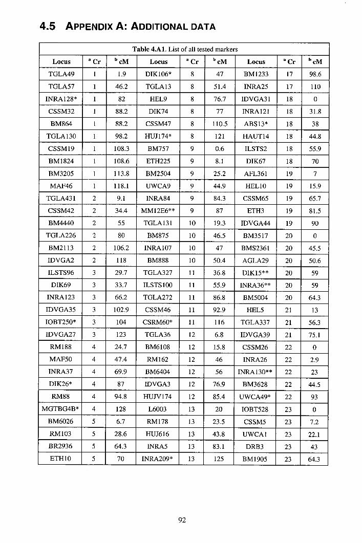
4.5 APPENDIX A: ADDITIONAL DATA

Table 4.A1. List of all tested markers

Locus a Cr b cm Locus a Cr b cm Locus a Cr b cm

TGLA49 1 1.9 DIK106* 8 47 BM1233 17 98.6

TGLA57 1 46.2 TGLA13 8 51.4 INRA25 17 110

INRA128* 1 82 HEL9 8 76.7 IDVGA31 18 0

CSSM32 1 88.2 D1K74 8 77 INRA121 18 31.8

BM864 1 88.2 CSSM47 8 110.5 ABS13* 18 38

TGLA130 1 98.2 HUJ174* 8 121 HAUT14 18 44.8

CSSM19 1 108.3 BM757 9 0.6 ILSTS2 18 55.9

BM1824 1 108.6 ETH225 9 8.1 D1K67 18 70

BM3205 1 113.8 BM2504 9 25.2 AFL361 19 7

MAF46 1 118.1 UWCA9 9 44.9 HELlO 19 15.9

TGLA431 2 9.1 INRA84 9 84.3 CSSM65 19 65.7

CSSM42 2 34.4 MM12E6** 9 87 ETH3 19 81.5

BM4440 2 55 TGLA131 10 19.3 IDVGA44 19 90

TGLA226 2 80 BM875 10 46.5 BM3517 20 0

BM2113 2 106.2 INRA107 10 47 BMS2361 20 45.5

IDVGA2 2 118 BM888 10 50.4 AGLA29 20 50.6

ILSTS96 3 29.7 TGLA327 11 36.8 DIK15** 20 59

D1K69 3 33.7 ILSTS100 11 55.9 INRA36** 20 59

INRA123 3 66.2 TGLA272 11 86.8 BM5004 20 64.3

IDVGA35 3 102.9 CSSM46 11 92.9 HEL5 21 13

10BT250* 3 104 CSRM60* 11 116 TGLA337 21 56.3

IDVGA27 3 123 TGLA36 12 6.8 IDVGA39 21 75.1

RM188 4 24.7 BM6108 12 15.8 CSSM26 22 0

MAF50 4 47.4 RM162 12 46 INRA26 22 2.9

INRA37 4 69.9 BM6404 12 56 INRA130** 22 23

D1K26* 4 87 IDVGA3 12 76.9 BM3628 22 44.5

RM88 4 94.8 HUJV174 12 85.4 UWCA49* 22 93

MGTBG4B* 4 128 L6003 13 20 10BT528 23 0

BM6026 5 6.7 RM178 13 23.5 CSSM5 23 7.2

RM103 5 28.6 HUJ616 13 43.8 UWCA1 23 22.1

BR2936 5 64.3 INRA5 13 83.1 DRB3 23 43

ETH10 5 70 INRA209* 13 125 BM1905 23 64.3

92

BM1819 5 77.6 D1K93* 13 144 TGLA351 24 8.6

BM8230 5 88.4 CSSM66* 14 17 CSSM23 24 18.4

BM315 5 100.1 RM11 14 27.7 INRA90 24 53.2

BMS1658 5 102 BM4630 14 30.1 BM4005 25 12.3

ETH2 5 108.5 PZ271** 14 59 TGLA40* 25 25

BM2830 5 113.5 D1K54** 14 81 1NRA222* 25 56

ILSTS93 6 0 ABS1O* 14 114 ABS12* 26 0

BM1329 6 35.5 BR3510 15 1 HEL11 26 20.7

D1K82* 6 67 JAB 15 20.8 RM26 26 37.3

RM28 6 74.3 IDVGA1O** 15 52 BM4505 26 39.7

AFR227 6 90.4 FSHB 15 59.9 RM209 27 15

BM2320 6 120.7 BM4513 15 62.5 BM203 27 64.1

BM7160 7 0 TGLA53 16 40.6 BP23 28 4.7

BP41 7 13.9 ETH11 16 56.5 IDVGA29 28 8.7

BM1853 7 85 BM719 16 78 JAB5* 29 0

ILSTS6 7 116 HUJ625 89.8 RM44 29 23.3

INRA53 7 123.5 PZ510 16 TGLA86* 29 25

IDVGA11 8 8.8 TGLA231*

d17

50

BM4006 8 41.7 IDVGA40 67 a Chromosome

b CentiMorgans Primary sources of information were http://sDinal.tag.csiro.au/ and http://www.marc.usda.gov , and

secondary sources of information were http://www.thearkdb.org (*) and http://locus.jouy.inra.fr (**)

Table 4.A2. Marker losses due to TDT data restrictions

Locus aCr b cM

TGLA49 1 1.9

BM3205 1 113.8

BP41 7 13.9

TGLA13 8 51.4

BM2504 9 52.2

L6003* 13 20

ETH11 16 56.5

UWCA1 23 22.1

INRA30** X 183

See Table 4.A for a definition of: a, b, "c , **

93

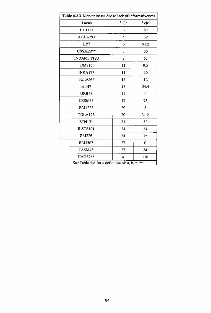
Table 4.A3. Marker losses due to lack of informativeness

Locus a Cr b cm HUJ117 3 87

AGLA293 5 32

BP7 6 91.2

CSSM29** 7 86

INRAMTT180 8 67

BM716 11 9.5

INRA177 11 26

TGLA6** 13 12

ETH7 13 54.4

URB48 17 0

CSSM33 17 75

BM1225 20 8

TGLA126 20 31.2

ETH131 21 32

ILSTS1O1 24 34

BM226 24 75

BM3507 27 0

CSSM43 27 34

HAU37** X 116

See Table 4.A for a definition of: a, b, , **

94

CHAPTER 5

Prediction of Identity By Descent based on

Marker Information and Linked Gene Flow

Theory: Potential Applications for Fine Mapping

Quantitative Trait Loci

5.1 INTRODUCTION

The linkage disequilibrium (LD) framework has become the new paradigm for fine

quantitative trait loci (QTL) mapping (Terwilliger and Weiss 1998, Cardon and Bell 2001,

Ardlie et al. 2002). Within this framework, families that are unrelated by a common pedigree

are assumed to share common ancestors in the past. Hence, in LD mapping, historical

recombination events are tracked down in the form of population-wide associations. In

contrast, in QTL mapping via linkage analysis, only those recombination events recorded

within known pedigrees are used (Hoeschele et al. 1997). As a consequence, linkage signals

can spread over long chromosomal distances, whereas association signals are expected only

over much shorter distances.

Meuwissen and Goddard (2000a) developed an original methodology for fine mapping QTL

by modelling the history of haplotypes, assuming a genetically homogeneous population

evolving by drift. They estimated the variance of QTL (a TL) using mixed linear models

(e.g. Grignola et al. 1996, George et al. 2000). The novelty of their approach was to model

the covariance due to the QTL as oTLHP, where H is a matrix of IBD probabilities

between all pairs of haplotypes at point p, estimated using identity-by-state (IBS)

information from surrounding markers. Although H was initially obtained stochastically,

Meuwissen and Goddard (2001) have also derived H deterministically based on Sved

(1971). Meuwissen and Goddard (2000b) put this method in practice and were able to map a

QTL for twinning rate in Norwegian cattle within a 1.3 cM region on chromosome 5, which

is considerably more precise than would have been expected with a linkage analysis

(Boehnke 1994).

95

The strengths of the method of Meuwissen and Goddard can be used together with a novel

and more flexible way of estimating IBD probabilities based on linked gene flow (LGF)

theory. This theory is an extension of the long-term genetic contributions theory used for

predicting genetic gain when practising artificial selection whilst restricting rates of

inbreeding (Bijma 2000).

In this work, we tested new developments in LGF theory with simulations, proved them

worth pursuing, and applied them to calculate inbreeding at a particular genomic location i

for a particular individual j (F,3). A multiple regression equation allowed us to use

neighbouring marker information when estimating F,3 . We also demonstrated that the

utilisation of linked markers for predicting F,3 increases the accuracy of prediction.

5.2 MATERIALS AND METHODS

5.2.1 Joint Inbreeding (Fj)

Approach I. Under the assumption of a constant effective population size (Ne) over

generations, the rate of accumulation of inbreeding per generation is AF =

(equation 2 N,

[4.1] in Falconer and Mackay 1996). The average level of inbreeding in the population at

generation t can be calculated as (equation [3.12] in Falconer and Mackay 1996)

F(t)=1— (1 — Z1F) [1]

Alternatively, Woolliams and Bijma (2000) expressed F(t) in terms of genetic contributions

(r1 ) and Mendelian sampling terms (a 1) of ancestors, as follows:

F(t) = - 1)r, 0 (f,t —1)A 120 + (m,t —1)r, (f,t — 1)a, [2] alleles i alleles u=1 i

where the first sum is over all alleles present at generation 0 (2N assuming unrelated

founders, where N is the number of founders), A 0 is the frequency of each allele present at

generation 0 within the i h founder (e.g. for allele 1, A, o = ½ for one founder and zero for all

other individuals), 1 0 (s,t —1) is the genetic contribution of founder ito parents of sex s at

generation t-1 (s = m,f denoting mother and father, respectively), and a i ' U is the Mendelian

sampling term of ancestor i at generation u ~! 1, i.e. a i,u = A1 - .! (A m + A 1 ). Nevertheless,

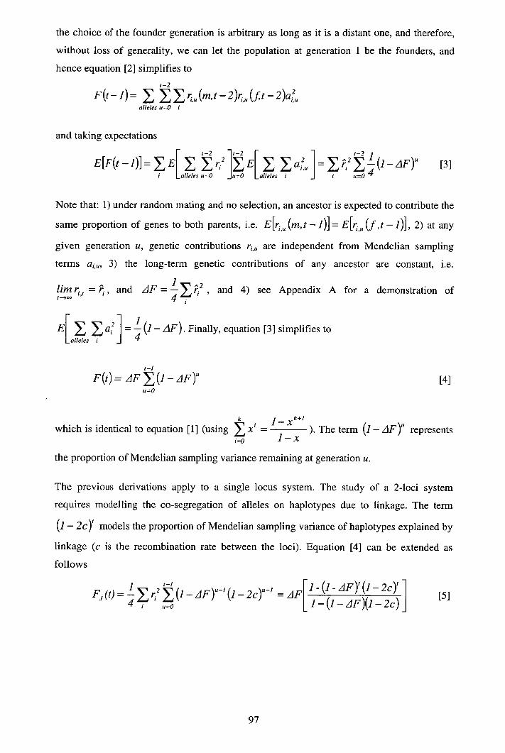
the choice of the founder generation is arbitrary as long as it is a distant one, and therefore,

without loss of generality, we can let the population at generation 1 be the founders, and

hence equation [2] simplifies to

1-2

F(t-1)= alleles u=O

and taking expectations

E[F(t_1)]=E[ r2]U=O

E[ [3] i alleles u=O alleles i i u=O

Note that: 1) under random mating and no selection, an ancestor is expected to contribute the

same proportion of genes to both parents, i.e. E[r (m,t - i)] = E[r (f,t - i)], 2) at any

given generation u, genetic contributions r iu are independent from Mendelian sampling

terms aj, 3) the long-term genetic contributions of any ancestor are constant, i.e.

tim i = P. AF =1 2 , I Pi and 4) see Appendix A for a demonstration of 4.

E[

a] = - (i - AF). Finally, equation [3] simplifies to alleles i

F(t)= /1F(1_z1F)u [4]

which is identical to equation [ 1 ] (using x = x

). The term (i - ZIF)u represents i=O 1—x

the proportion of Mendelian sampling variance remaining at generation u.

The previous derivations apply to a single locus system. The study of a 2-loci system

requires modelling the co-segregation of alleles on haplotypes due to linkage. The term

(i - 2c)t models the proportion of Mendelian sampling variance of haplotypes explained by

linkage (c is the recombination rate between the loci). Equation [4] can be extended as

follows

u—I F (t) = 1 r2 (i - AFr (i - 2c) = AF[I-(]- AF (i - 2 c )t 1

1— (i - AF)(1 - 2c) j [5]

97

where F(t) is the joint inbreeding at generation t. Formally, FAt) is the probability of

sampling two haplotypes (i.e. gametes) in generation t containing alleles that were originally

together on the same founder haplotype. This probability includes only founder haplotypes,

i.e. those that have not recombined since the founding of the population or have recombined

with other IBD haplotypes. Founder-like haplotypes may have also appeared at any

generation u, where 0 < u < t, due to recombination, although these are not included in the

probability calculations. The relative importance of the latter type of haplotypes will be

discussed in the light of simulation results.

Of particular interest is the steady-state equilibrium, i.e. where F(t) = F(t - i) for any

sufficiently large t. Letting t go to infinity we obtain (using = 1

when —1 <x < 1) i=O 1—x

F(t-3oo)= 1 1

[6] 1+4Ne C2C 1 + 4 N e C

where the approximation holds when c is small and Ne large. Equation [6] has already been

derived previously (e.g. Sved 1971). The parameter space of F (t —* is bounded

between AF and 1, for c = ½ and c = 0, respectively.

Approach II. Alternatively, Sved (1971) defined Q as the conditional probability of joint

IBD at two loci, given that one of them is IBD, moreover Q = E[r2 ], where r2 is the square

correlation between allele frequencies at two loci (Hill 1975). Sved clearly stated that he

considers only founder haplotypes, those without historical recombinations. This model is an

adaptation of a recurrent formula for predicting inbreeding at a locus under the assumption

of an infinite allele mutational model, i.e. neutral alleles are generated at a constant rate p

each generation, and each allele is different from all previous alleles (Hartl and Clark 1997

p175, Falconer and Mackay 1996 p79). The model is

Q(t) = (i - zlF)(1 - c)2 Q(t — i) + ziF(1 - [7]

where AF is equivalent to the probability of sampling twice the same haplotype, (1 - AF)Q(t-

1) is the probability of sampling two different haplotypes that were identical in the previous

generation, and (1-c)2 is the probability of zero or an even number of recombination events

in both haplotypes. Equation [6] can also be written as

t-1 21 1 11(1 z11')(l 2 1

Q(t)F(1_c)2(1_F)(_c) j - - c)

u=O 1—(1—AF)(1—c) 2

At the steady-state equilibrium, equation [7] is

Q(t-400)= (1—c) 2 - 1

2N eC(2C)+(1C)2 1 +4Ne C

Hence, both approaches predict the same equilibrium point when c is small and Ne large

(equations [6] and [8]). However, the parameter space of Q is bounded between 1

6N e +1

and 1, for c = ½ and c = 0, respectively, hence slightly differing from F

5.2.2 Simulations

We checked the validity of equation [5] via computer simulations. We followed the flow of

haplotypes through generations in an ideal population, and counted how many times two

haplotypes identical to a haplotype at generation t = 0 were inherited by an individual at

generation t, considering independently both ancestral (without historical recombinations)

and ancestral-like haplotypes (with historical recombinations).

Let us consider two neutral loci and unrelated founders, so that the first founder had

haplotypes {1,1} and {2,2}, the second founder haplotypes (3,3} and {4,4), etcetera. At

each generation, haplotypes were allowed to recombine before sampling among them at

random to create the parents for the next generation. Selfing was also permitted. The

population size (Ne) remained constant over time, and the generations were discrete. We

explored different combinations of parameters c and Ne , each one being replicated 1000

times.

5.2.3 Inbreeding per individual and locus

Two alleles that look alike but descend from different founders are said to be Identical-by-

state (IBS). The joint probability of two loci containing IBS alleles is (denoted by the area

shared between the circles in Figure 5.1)

'1BS =F +(F1 —F)P 21 +(F2 —F1 )P2,+(1—F1 —F2 [10]

where Fj is the probability of joint inbreeding, Fi is the inbreeding coefficient at locus i

calculated with equation [1], p1j is the frequency of allele j at locus i, and Pii is the

observed homozygosity at locus i. Equation [3] can be simplified as, on average, F1 = F2 = F,

and using 11. = p

= F, +(F—F)(rI1 4-H2 )-f-(1-2F+F)]1,]12 [11]

Figure 5.1. Different classes within homozygous genotypes at two loci. The area within the square excluding both circles denotes the 'IBS but not IBD' class. The area within the left (right) circle only, denotes IBD at locus 1 (locus 2) only. The area common to both circles denotes IBD at both loci. Within this area there are three subclasses: 1) Joint Inbreeding (F '), or the probability of sampling twice the same ancestral (non-recombinant) haplotype, 2) Pseudo Joint Inbreeding (Ps), or the probability of sampling twice the same recombinant haplotype that is IBS with an ancestral haplotype, and 3) Disjoint Inbreeding (F 0), or the probability of sampling twice the same recombinant haplotype that is not IBS with an ancestral haplotype.

The covariance matrix between two loci in terms of IBD and IBS is given in Table 5.1 (see

derivation in Appendix B). The inbreeding at locus i (i.e. the probability of IBD alleles at

locus i) in the j 1h individual is F, and can be predicted using IBS information from

neighbouring marker loci via a multiple regression technique (e.g. Draper and Smith 1966).

The linear model is

nk

F; =F+bk (IBSkJ —IBSk)+eJ [12]

where F is the average expected inbreeding in the population (equation [1]), flk is the number

of segregating marker loci for which IBS (i.e. homozygosity) is known, IBSk is 1 if

100

individual j is homozygous at locus k, or 0 otherwise, IBSk is the observed mean IBS at

locus k in the population, or alternatively, its expectation: E[IBSk ] = F + (1- F)JJk ), and

bk the regression coefficient relating IBS at locus k with IBD at locus i. If IBS information

comes from a single marker in the regression coefficient would be

b = lBD(i),IBS(m) - (F1 - F2 )

im IBS(m) - ( 1F)(F+(1F)Hm )

[13]

For k markers, the vector fi with regression coefficients bk (k = 1. . . fl,) can be calculated as '8

= V'G, where V 1 is the inverse of the variance-covariance matrix of IBS among markers,

i.e. bottom right quadrant in Table 5.1, and G is a vector containing the covariances (F -

F2)(141,), forj = 1. ..k, linking IBS at locus with IBD at locus i.

Table 5.1. Co-variance matrix of IBD and IBS between and within two loci

IBD IBS

Locus 1 2 1 2

IBD 1 F(1—F) Fr-F2 F(1—F)(l-f1 1 ) (F—F2)(1-11 2)

2 Fr-F2 F(I—F) (F—F2)(l-11 1 ) F(1-17)(1-1T12)

IBS 1 F( l—F)(l-[1 1 ) (F1—F2)( l-112) (l—F)( 1 -11 1 )(F+( 1—F)11 1 ) (F—F2)(l-fl 1 -f12+f1 1 f12)

2 (F—F2)( 1 -[T i ) F( 1—F)( 1-11 2) (F—F2 )( 1 41r112+lll[l2) (1F)( 1 fl2)(F+( lF)11 2 )

IBD: Identity By Descent IBS: Identity By State

F: Inbreeding coefficient within a locus, equation [1] Fj : Joint inbreeding at 2 loci, equation [2]

111 : Homozygosity at locus j

5.2.4 Prediction error variance of Fij

The prediction error variance of F, PEV(F1), was obtained via simulations. IBS was

simulated labelling alleles 0 or 1 at random in the founder population. Regarding IBS, the

founder population was in linkage equilibrium, i.e. D = 0. The frequency of allele 1 at u = 0

was ½, and the changes in IBS and IBD throughout generations were recorded. IBD was

predicted at locus i in each generation using equation [11]. The PEV was calculated as

(Fi fr/C)2

PEV(F.ii )= k=1

[14]

101

0.95

CZ 0.9

0.85

0.8

0 250 500 750 1000 Generation

C=0.0001

C=o.o1

0.8

0.6 Iz

0.4

0.2

o 0 250 500

Generation

C=0.0001

C=o.o1

11

750 1000

where Zr = 1000 were the number of replicates, J was the observed and the predicted

value of F, in the kth replicate, respectively.

5.3 RESULTS

5.3.1 Validating Fj

F1 has been defined as the probability of sampling two identical founder haplotypes at any

given generation. At equilibrium, Fj can be also interpreted as the probability that a

population is fixed for any founder haplotype. Changes of F1 over generations were

monitored for different combinations of parameters, Ne = [5, 50, 100] and C = [0.01, 0.0001].

There were 1000 replicates per parameter combination (Figure 5.2). Deterministic

predictions of F1 using formula [5] were closer to empirical results during early generations

with low c. The greatest difference between deterministic and empirical F1 occurs when

equilibrium is reached.

Figure 5.2. Changes of Fj over generations, results with equation [5] shown in grey, simulation results shown in black.

N=5

N=50

102

1

0.8

0.6

0.4

0.2

0

N=100

a.

C=0.0001

c=o.01

0 250 500 750 1000 Generation

5.3.2 Impact of marker information on the PEV(F11)

The amount of information to predict F(t) at locus i within individual j at generation t,

abbreviated as F,, increases with the number of genotyped markers, providing that they

segregate in the population, and with the degree of linkage between markers and locus i. The

prediction error variance of F1 , PEV(F,J) (Equation [14]), is a measure of how much

information is available for predicting F,,, e.g. large PEV(F,J) values correspond to little

information and vice-versa. In the absence of markers F,, is predicted by equation [1], and

with marker information F, is predicted by equation [5]. Note that F, may be outside the

range [0,1] when using marker information, however, rejecting those replicates in which F,

> 1 did not have a serious impact on PEV(F,J). Figure 5.3 shows the changes in PEV(F,J)

across 100 generations when using 0, 1 or 4 markers. In these simulations, the locus i was

surrounded by four markers, two on each side, with c values between each marker and locus

i equal to 0.2, 0.01, 0.001, and 0.1, from left to right, respectively. There were 1000

replicates per generation.

We always observed the same general pattern of changes in PEV(F,) over generations,

regardless of the number of markers used. At generation u = 0 PEV(F,J) = 0 because none of

the individuals in the population were inbred. For u > 0, PEV(F,J) increases until reaching a

peak, and steadily decreasing thereafter (Figure 5.4). The height of the peak depends on the

number of markers. In the long run, e.g. u - , PEV(F,J) = 0, as all individuals become

103

eventually inbred. It is important to notice that, except at the extremes (u = 0 or u - oc,

PEV(F) showed always the lowest curve when using 4 marker loci, and the highest when

using no markers. The relative drop in PEV(F) was larger when a single tightly linked

marker (c = 0.001) was used compared to a situation without marker information, than when

three markers, loosely linked to locus i (c = 0.01, 0.1, 0.2), were added to a system that

already contained a marker tightly linked (c = 0.001) to locus i. This result is highlighting the

fact that not only marker density is important for predicting F, but also tight linkage.

Figure 5.3. PEV(Fy) over generations, using none, one (c = 0.001) or four markers (c = 0.001, 0.0 1, 0. 1, 0.2)

0.3

0.2

0.I

0

0 Markers

I Marker 4 Markers

0 25 50 75 100

Generation

5.4 DiscussioN

The linked gene flow (LGF) theory provides information on identity-by-descent (IBD) in a

simple deterministic fashion. In this study we extend the existing theory based on Woolliams

et al. (1999), to encompass a finite number of linked loci. This methodology is the only

methodology that has predicted gene flows accurately over multiple generations in selected

populations. Bijma et al. (1999) demonstrated its accuracy and Bijma and Woolliams (2000)

demonstrated the weakness of a previous gene flow model (Hill 1974) to cope with gene

flow with selection. The gene flow model (Woolliams and Bijma 2000) has an added benefit

in that it naturally decomposes the population into genetic contributions and Mendelian

sampling terms. The former are sufficient statistics for IBD arising through pedigree

development, and are independent from the Mendelian sampling terms. Therefore it is a

natural choice as a basic model since it has the ability to grow with the development of the

applications.

This study demonstrates the accuracy of LGF theory in predicting IBD at a locus using

neighbouring marker information, for a typical range of parameters (e.g. t < 100), under

104

random mating conditions. We have, nevertheless, observed that when t - certain

parameter combinations, e.g. Ne = 100 and c = 0.005, empirical and deterministic predictions

of Fj are much more similar than for other parameter combinations, e.g. Ne = 5 and C = 0.01.

Although the theory predicts Fj better when c is small, the nature of this apparent

discrepancy between theory and simulations in certain situations requires further study. Fj is

explaining the proportion of Mendelian sampling variance due to allelic co-segregation via

linkage. However, genetic drift can generate allelic co-segregation independently from

linkage, by means of reducing the Mendelian sampling variance. We think that the inability

of the current theory in predicting Fj when c is large is solvable by developing another term

to take into account co-segregation due to drift. Meanwhile, Fj predicted with formula [5]

coincides with Q predicted with formula [8] when c is small, and both are very close to

simulation results. Yet, neither approach is satisfactory when c > 0.1.

An advantage of LGF theory over the theory used by Meuwissen and Goddard is that it

provides the framework from which more complete models can be developed, e.g. including

selection and/or mutation. For example, Wall et al. (2002) used LGF theory to estimate a

multivariate Mendelian sampling term to predict IBD in the course of gene introgression on

both QTL carrier and non-carrier chromosomes. Although introgression considers only

relatively short pedigrees it is nevertheless a process of selection based upon markers. We

wish to develop a linkage disequilibrium mapping method that utilizes the strengths of

Meuwissen and Goddard (2000) by complementing it with the strengths of LDF theory.

Hence, the basic mixed model methodology of George et al. (2000) will be extended to use a

haplotype model with an IBD covariance matrix at its heart, derived from LGF theory.

Additionally, we will extend the methodology to rapid calculation of IBD matrices in

complex pedigrees using the methodology of Pong-Wong et al. (2001).

We have shown how the prediction error variance (PEV) of estimates of point IBD within an

individual decreases as more marker information is used. Most of the information for

predicting Fij comes from tightly linked markers, although elucidating the optimum number

and distances to locus i needs further work. Given optimum marker coverage, accurate

multipoint IBD predictions along a chromosome (or genome) can be obtained. This

information could be used, for instance, to investigate the impact of selection in determining

patterns of localised inbreeding, and to increase the accuracy of estimation of average

relationship matrices.

105

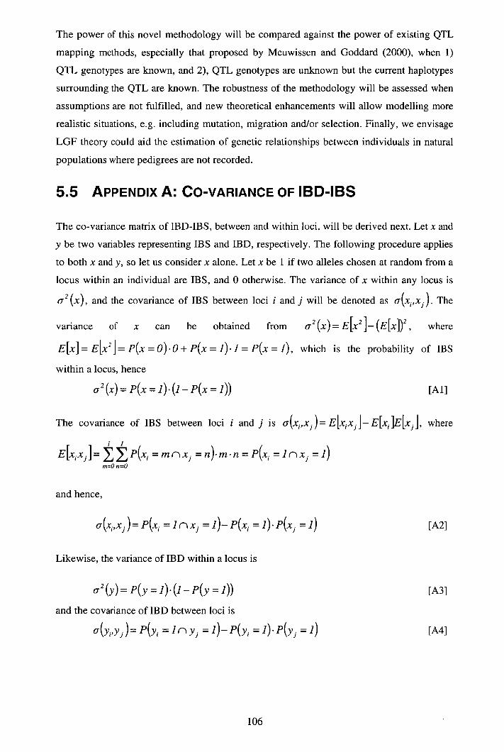
The power of this novel methodology will be compared against the power of existing QTL

mapping methods, especially that proposed by Meuwissen and Goddard (2000), when 1)

QTL genotypes are known, and 2), QTL genotypes are unknown but the current haplotypes

surrounding the QTL are known. The robustness of the methodology will be assessed when

assumptions are not fulfilled, and new theoretical enhancements will allow modelling more

realistic situations, e.g. including mutation, migration and/or selection. Finally, we envisage

LGF theory could aid the estimation of genetic relationships between individuals in natural

populations where pedigrees are not recorded.

5.5 APPENDIX A: Co-VARIANCE OF IBD-IBS

The co-variance matrix of IBD-IBS, between and within loci, will be derived next. Let x and

y be two variables representing IBS and IBD, respectively. The following procedure applies

to both x and y, so let us consider x alone. Let x be 1 if two alleles chosen at random from a

locus within an individual are IBS, and 0 otherwise. The variance of x within any locus is

(x), and the covariance of IBS between loci i and j will be denoted as The

variance of x can be obtained from cy2 (x) = E[x2 ]_ (E[x])2 , where

E[x] = E[x2] = P(x = o). 0 + P(x = 1).] = P(x = i), which is the probability of IBS

within a locus, hence

o 2 (x)=P(x=1).(1-P(x=1)) [Al]

The covariance of IBS between loci i and j is cr(x1,x3)= E[x1x]-E[x1]E[x1], where

= m n xj =n).m.n=P(x =lnx1 =i) m=On=O

and hence,

=lnx3 =1)-P(x1 = ]).P(x. =i) [A2]

Likewise, the variance of IBD within a locus is

= P(y = i). (i - P(y = 1))

[A3]

and the covariance of IBD between loci is

(y1,y)=P(y =iny =i)-(y =i).(y =i) [A4]

106

The covariance between IBD and IBS is

a(x1 y)=P(x, =iny3 =1)— P(x, =]).(y =i) [A5]

where j, j = 1, 2.

In what follows, we will drop '= 1' in equations [Al] to [A5] for clarity, as we are interested

in either IBS or IBD events, and not in the events non-IBS or non-IBD. Let us calculate the

following probabilities P(y), P(x), P(x1 nx3 ), P(y1 n y) and P(x1 n where i :~ I.

Figure 5.1 may help appreciating the following derivations.

The probability that alleles at a locus are IBD is precisely the inbreeding coefficent (F),

hence P(y) = F. At a locus, IBD alleles are also IBS alleles, although the opposite is not

necessarily true. Hence, the probability of simultaneous IBD and IBS at a locus is

P(x1 n y1 ) = F. The probability of IBS alleles at a locus is the probability of that locus

being homozygous. Two mutually exclusive events can generate homozygosity at a locus:

either alleles are IBD, so they are automatically IBS, or alleles are not IBD although they are

IBS. Hence P(x) = F + (i - F)H, where H = , and p, is the frequency of allele i.

The probability of joint IBD at two loci is P(y1,y ) = F , for i # j, where F) is given in

equation [5].

We have now all the necessary elements for calculating the co-variances between and within

loci for IBD and IBS, and they have been summarised in Table 5.A.

107

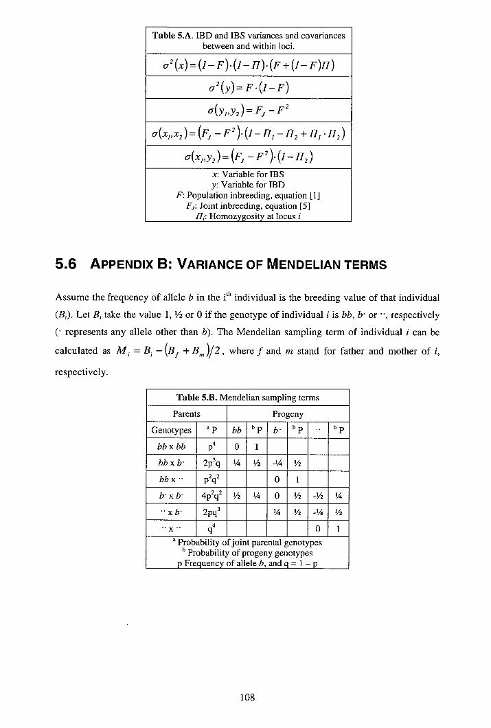
Table 5.A. IBD and IBS variances and covariances between and within loci.

ci2 (9 = (1— F). (1—H). (F + (1— F)H)

a2 (y)=F.(1—F)

a(y11y2 ) = F - F2

cr(xj ,x2 )=(Fj _F2).(1_H1 —H2+171. H2)

a(x1,y2)=(F1 F2).(1TI2)

Variable for IBS Variable for IBD

F: Population inbreeding, equation [1] Fj: Joint inbreeding, equation [5]

H: Homozygosity at locus i

5.6 APPENDIX B: VARIANCE OF MENDELIAN TERMS

Assume the frequency of allele b in the i1h individual is the breeding value of that individual

(B). Let B, take the value 1, ½ or 0 if the genotype of individual i is bb, b or ",respectively

( represents any allele other than b). The Mendelian sampling term of individual i can be

calculated as M i = B - (B 1 + B m )12, where f and m stand for father and mother of i,

respectively.

Table 5.B. Mendelian sampling terms

Parents Progeny

Genotypes a p bb b p b b p •. b p

bbxbb p4 0 1

bbxb 2p3q 1/4 ½ -¼ ½

bbx" p2q2 0 1

frxb 4p q2 ½ ¼ 0 ½ -½ ¼

"xb 2pq3 ¼ ½ -¼ ½

q4 0 1 a Probability of joint parental genotypes

b Probability of progeny genotypes p Frequency of allele b, and q = 1 - p

The variance of Mi is v(M 1 ) = E[Mi ]- E[M1 ]2

= E[Mfl, as the expectation of the

individual Mendelian sampling term is zero. Hence, E[Mj= fJE[MIJ I j] where j5 is

the probability of the jth set of parents and E[M,J 2 Ij] is the expected square Mendelian

sampling term of individual i conditional on the th set of parents (Table 5.B). Finally,

V[M 1 ] = R9., if there is no inbreeding, otherwise v[M1] = R9. (I - AF), where (1 - AF)

reflects the decay of Mendelian sampling variance in one generation. When considering all

alleles together VIM ]= L [PJ Pk J(1_ AF) = (i F) ,as the number of alleles is

large, i.e. j is large, J( Pj 1: Pk k*j )

109

CHAPTER 6

6.1 Discussion

Genetics is revolutionising the breadth and depth of agriculture, basic biology, biomedicine

and biotechnology. The accelerated rate of gene discovery is allowing geneticists to unravel

the genetic architecture of traits. This goal usually involves four steps: 1) localisation of

chromosomal regions likely to contain the gene of interest, 2) positional cloning of this gene,

3) the study of functional polymorphisms within the gene, and 4) the study of gene products.

Steps 1 and 2 comprise the area of gene mapping; steps 3 and 4 are the realm of genomics,

proteomics and physiology.

The benefits of one decade of gene mapping can already be seen, for example, in health care,

where mapping the cystic fibrosis gene (Kerem et al. 1989) has led to the development of

gene therapy treatments (e.g. Blair et al. 1998), and where drug design is now taking into

account both human evolutionary adaptations (Hofbauer and Huppertz 2002) and genetic

differences between individuals (Ensom et al. 2001). In agriculture, food production has

increased, diversified and become more efficient because of artificial selection based mainly

on individual performance (e.g. Bichard 2002, Khush 1999, Conway and Toenniessen 1999).

However, performance records can be difficult, time consuming and costly to collect, and the

accuracy of selection is reduced when environmental and genetic effects are confounded.

Hence, faster genetic gains are expected by direct selection of favourable combinations of

genes.

The scope of this thesis falls into step number one mentioned above, i.e. the localisation of

chromosomal regions likely to contain genes of interest. Specifically, we were interested in

the study and development of statistical techniques for refining the location of genes within

these chromosomal regions.

Genome-wide linkage analyses have rendered evidence for chromosomal regions harbouring

genes of interest, albeit with broad confidence intervals (CI) for their location estimates. Fine

mapping is concerned with reducing these Cl in order to facilitate positional cloning of

genes. One of the strategies in fine gene mapping is searching for population-wide

associations between markers and traits. This approach relies on the existence of sufficiently

strong LD between neutral and causal polymorphisms. However, errors in association studies

110

have led in many cases to lack of reproducible results. The commonest errors are: small

sample size, subgroup analysis, multiple testing, poorly matched control group, failure to

attempt study replication, failure to detect LD with adjacent loci, overinterpreting results,

positive publication bias, and unwarranted 'candidate gene' declaration after identifying

association in an arbritrary region (Cardon and Bell 2001).

In this thesis, we have focused our attention on a group of related statistics known as

trans mission-disequilibrium tests (TDT5), for which errors due to poorly matched control

groups do not occur. TDTs are tests for linkage in the presence of association. If the sample

consists of family trios, or sib-pairs, TDTs are also tests for linkage disequilibrium (LD), i.e.

joint linkage and association. LD is the non-random association of alleles at different loci on

the same haplotype. The original TDT (Terwilliger and Ott 1992, Spielman et al. 1993) was

designed to detect segregation distortion in alleles transmitted from heterozygous parents to

affected progeny. Later, new TDTs were developed to analyse quantitative traits, sibships,

and extended pedigrees. The most attractive feature of TDTs is their robustness in the

presence of spurious disequilibrium, i.e. disequilibrium without linkage, which can produce a

high rate of false positive results in other tests, e.g. case-control studies. This robustness

derives from the fact that TDTs contrast different transmitted alleles within families, i.e.

family-based controls, rather than using external controls.

The four main areas of research in this thesis were the following:

1. A comparative study of the power between different association tests both

empirically and deterministically. Given the myriad of association tests currently

available in the literature, studying their statistka1 properties, mainly power and

robustness, is essential in order to make the best choice. We compared five different

tests: a) a pure association test based on one-way classification analysis of variance

(one-way ANOVA), where progeny genotype was the only classification factor, and

b) four different TDTs, three of which were obtained from the literature (Rabinowitz

1997, Allison 1997, Szyda et al. 1998, Xiong et al. 1998), whilst the fourth was

based on a nested design analysis of variance (nested ANOVA), where progeny

genotypes were nested within mating types. The one-way and the nested ANOVAs

were the most and the least powerful tests across all scenarios, respectively. The

other TDTs shared a similar power and ranked between the two ANOVAs. The one-

way ANOVA was the only non-robust test in the presence of population

stratification, i.e. the rate of false positives was greater than the nominal 5% under

111

the null hypothesis of no linkage in the presence of association. All deterministic

predictions of power were validated empirically.

The estimation, using TDT (Rabinowitz 1997), of the effect of a point mutation

within the melanocortin 4-receptor on production traits in pigs. Data had to be pre-

corrected for environmental influences such as sex and month of birth prior to use of

the TDT. However, it is more efficient to estimate all parameters simultaneously.

Hence, a set of dummy variables was extracted from the TDT to model the

covariance between the mutation and each trait. In order to model this covariance,

parental genotypes were required, but as most of them were missing, a Gibbs

sampling technique was used to recover them. This covariance was estimated within

a sire mixed linear model that also included other fixed and random factors, and,

under an additive genetic model, it provided a direct estimate of allelic effects. This

estimator uses only within-family genetic variation. A complementary estimator of

allelic effects that uses between-family genetic variation was also developed and

included in the model. Under the null hypothesis of neither linkage nor association,

both estimators should be the same. Population stratification, a factor that generates

association without linkage, increases the between-family genetic variation, and

therefore has a proportional effect on the estimator that uses it. The within-family

variation is unaffected by the presence of population stratification, and therefore the

estimator that uses it remains robust to spurious association. Finally, we suggested

relying on the robust estimator only, if spurious association was detected, otherwise,

both estimators should be combined together in an overall and more powerful

estimator (e.g. derived from a one-way ANOVA model). There was no evidence for

admixture/stratification in this population, however this possibility should always be

checked to avoid spurious association results.

A genome-wide search of markers associated with bovine spongiform

encephalopathy (BSE) using TDTs. Humans that had been infected with the agent

that induces BSE, the presumptive prion protein, developed a lethal, early onset

variant of the Creutzfeldt-Jakob disease. Although it has been suggested that

association tests should be used mainly for testing candidate genes (as in the case of

MC4R), or for fine mapping within a chromosomal region for which there is prior

evidence of linkage, because of the large number of markers that would be required

otherwise, we have demonstrated here that a successful genome-wide scan with a

sparse marker map is also possible. The data were analysed with several different

112

TDTs (Sham and Curtis 1995, Bickeböller and Clerget-Darpoux 1995, Waldman et

al. 1999), and the same profile of p-values was obtained when using either reference

distributions (i.e. appealing to the asymptotic properties of these TDTs) or

permutation testing. We found a significantly higher risk of BSE associated with

three markers (on chromosomes 5, 10 and 20). In a subsequent and independent

study, a new marker adjacent to the one on chromosome 5 was also found

significantly associated with incidence of BSE. These promising results are currently

being used at the Roslin Institute and other research groups to pinpoint the genes

associated with BSE susceptibility.

4. A multiple regression technique was developed to predict identity-by-descent (IBD)

at specific chromosomal locations, within each individual, using marker information.

The regression coefficients were obtained using the theory of long-term genetic

contributions (Bijma 2000) and its extensions as linked gene flow (LOP) theory,

which takes into account the history of a population. It is reassuring that, in the

simplest case of a population evolving solely due to drift, LGP theory coincides with

classical quantitative theory (e.g. Sved 1971). Nevertheless, the benefit of using LGF

theory is that it provides a solid framework in which to explore the effects of

mutation and selection in estimating IBD. This work sprang from two key papers

(Meuwissen and Goddard 2000, 2001) in which a novel method for fine mapping

quantitative trait loci (QTL) utilising haplotype information was proposed. At the

core of this methodology there is the estimation of IBD by means of modelling the

history of a population under simplifying conditions. This section of the thesis could

be viewed as a successful preliminary study that encourages us to pursue this venture

even further.

Overall, this thesis covers the contemporary area of research encompassing gene mapping

via studying population-wide association, and explores in detail interesting statistical issues

ranging from power and robustness to evolutionary modelling, all within the context of fine

gene mapping. It is likely that the success of TDT as a LD-based method for gene mapping

has been due to its reputed robustness in the presence of population stratification/admixture,

and to its simplicity, which has facilitated understanding and prompted further

developments, e.g. including quantitative traits and any family structure. Despite the relative

success of LD methods in dealing with simple traits, complex multi-factorial traits have been

much more challenging. Therefore, as Terwilliger and Weiss (1998) put it, it may be possible

that "too many people are concentrating on simple mathematically tractable models that

113

assume the only difference between simple disease and complex disease is related to effect

size of a single allele per locus, whereas there is a looming danger that there is also a

substantial increase in complexity in both allelic and non-allelic heterogeneity, gene by

environment interactions, epistasis, pleiotropy, and variable expressivity of different alleles

in the same gene"

Despite this pessimistic view, agricultural populations may still be more amenable to LD

mapping than human populations for several reasons. Firstly, most of the current

breeds/strains with economic interest have been recently created after hybridising local ones

(e.g. Jones 1998), which is an ideal population history for LD mapping (e.g. Stephens et al.

1994). Secondly, the large population sizes and controlled mating designs in agriculture

provide greater power to detect meaningful associations than nuclear families in human

studies.

Notwithstanding the advantages of TDT, one of its problems continues to be the single-

marker analysis approach, which requires corrections, sometimes too conservative, to

account for multiple testing. In theory, TDT can be extended to analyse haplotype

transmission rates, e.g. Zhao et al. (2000) developed a TDT for multiple markers completely

linked. However, in the absence of complete linkage, the number of haplotype classes

increases geometrically, up to a maximum equal to the product of the number of alleles

across all loci. In order to keep the problem tractable, one could consider two markers at a

time, and look for preferential transmission of a joint pair of alleles over other pairs. In

principle, this approach should provide a better estimate of QTL location compared to a

single marker analysis, because the QTL could be located within two neighbouring markers.

The downside of testing haplotypes, as opposed to single markers, is the potential reduction

in power due to the increase in number of possible contrasts for a fixed sample size. One

option could be detecting significant markers using a single-marker TDT, followed by a

haplotype TDT analysis to discern which side the QTL is more likely to be.

Another problem is that TDT restricts its use of available information, e.g. discarding

families without heterozygous parents, in order to exploit only within-family variation, the

keypoint of the robustness of TDT. I have suggested in Chapter 3 a more powerful analysis,

instead of TDT, unless significant spurious disequilibrium is detected.

The theoretical limit of resolution of TDT, and of any other statistical method that relies on

population-wide LD, is a region with conserved maximum LD that includes the causative

mutation. For this reason, although still able to render higher mapping resolution than

114

linkage tests, LD-based tests may have difficulties differeciating between a causative

polymorphism and a marker in complete LD with it. Moreover, without information about

genetic diversity across populations and levels of usable LD across genomes, testing

population-wide associations may not be robust, and results can be hard to interpret.

The patterns of LD, e.g. measured as the chromosomal region in which LD between a locus

and other loci dacays to half the maximum value, vary within chromosomal regions across

populations, and across chromosomal regions within populations. Expected levels of LD

have been calculated assuming a uniform recombination rate across the genome, over

generations. However, phenomena such as non-uniform recombination rates, drift, ethnic

diversity, population admixture, and mating structures cause LD patterns to diverge from

their expectation. Therefore, it is preferable to assess LD empirically in each chromosomal

region within each population before carrying out a disease-mapping study, rather than

extrapolating from other chromosomal regions and/or experiments.

New molecular approaches (e.g. comparing the phenotypes between inbred mice lines

genetically different only at the QTL region, or the molecular activity between cell strains

with different candidate genes in the QTL region) and biotechlological advances (e.g. low

density microsatellite maps, medium and high density SNP maps, radiation hybrid maps,

expression sequence tags (EST) and cDNA transcript maps, yeast and bacterial artificial

chromosomes (YAC and BAC) libraries, microarrays, and fluorescent in sity hybridisation

(FISH)) are currently available for dissecting QTL into individual genetic components.

Even without a full dissection of a QTL into individual loci components, information on

QTL position and effect can be used for practical purposes. For example, in artificial

selection, QTL information has been incorporated in selection indeces as genetic scores that

assess the genetic value of prospective parents. This is particularly useful when phenotypic

data are difficult to collect, e.g. disease resistance, or the phenotype is not expressed in the

candidate, e.g. milk yield in bulls. Some areas in which partial QTL information has been

utilised are marker assisted selection (MAS), marker assisted introgression (MAI),

conservation programs, product identification, and crossbred performance prediction. Some

successful examples genes being used in animal breeding programs are the KIT gene (white

coat colour in pigs), the RYR1 or halothane gene (high lean tissue growth and maligna

hypertermia), the RN- gene (high lean tissue growth and poor quality of processed meat), the

IGF2 gene (an imprented gene responsible for high lean tissue growth), the callipyge gene

(double muscling in sheep), the miostatin gene (double muscling in cattle), the Inverdale

115

gene (increased ovulation rate in sheep), and the Booroola gene (increased ovulation rate and

litter size in sheep) (Anderson 2001).

However, at this early stage of application of molecular information into animal and plant

breeding programs, Dekkers and Hospital (2002) recommend 'cautious optimism', because

phenotypic information will still be the most important factor in selection decisions, and

because imprecise estimates of QTL locations and effects can diminish the response to

selection. Undoubtedly, a better knowledge of the genetic basis of traits will lead to a more

efficient design of breeding programs.

Finally, the future of statistical gene mapping may not lie within the mathematical domain of

TDT, but rather in more sophisticated statistical approaches for analysing complex traits

using genomic information, although QTL results should be confirmed using several

independent methods and experiments, and rely less on single statistical analyses (Makcay

2000). There are several pitfalls in QTL mapping (e.g. Flint and Mott 2001, Doerge 2002)

but genomic information is increasing both quantitatively and qualitatively as individual

genotyping becomes less costly thanks to high throughput DNA sequencing technology. This

has led to the accumulation of hundreds of thousands of polymorphisms publicly available to

be used in searching for associations and causal mutations (Ellsworth et al. 1997, Collins et

al. 1998).

Chapter 5 of this thesis explores the basis of a novel and promising venture, where a multi-

marker approach will be integrated together with evolutionary models to maximise the use of

all available information. However, this methodology is yet to be thoroughly assessed,

especially with regard to robustness to spurious association and power of QTL detection.

116

BIBLIOGRAPHY

Abecasis GR, Cardon LIZ, Cookson WO (2000) A general test of association for quantitative traits in

nuclear families. American Journal of Human Genetics 66:279-292

Allison DB (1997) Transmission-disequilibrium tests for quantitative traits. American Journal of

Human Genetics 60:676-690

Allison DB, Heo M, Kaplan N, Martin ER (1999) Sibling-based tests of linkage and association for

quantitative traits. American Journal of Human Genetics 64:1754-1764

Almond G, Pattison J (1997) Human BSE. Nature 389:437-438

Anderson L (2001) Genetic dissection of phenotypic diversity in farm animals. Nature Reviews

Genetics 2:130-138

Ando S, Sirianni R, Forastieri P, Casaburi I, Lanzino M, Rago V, Giordano F, Giordano C, Caprino

A, Pezzi V (2001) Aromatase expression in prepuberal Sertoli cells: effect of thyroid

hormone. Molecular and Cell Endocrinology 178:11-21

Ardlie KG, Liu-Cordero SN, Eberle MA, Daly M, Barrett J, Winchester E, Lander ES, Kruglyak L

(2001) Lower-than-expected linkage disequilibrium between tightly linked markers in

humans suggests a role for gene conversion. American Journal of Human Genetics 69:582-

589

Ardlie KG, Kruglyak L, Seielstad M (2002) Patterns of linkage disequilibrium in the human genome.

Nature Reviews 3:299-309

Arranz JJ, Coppieters W, Berzi P, Cambisano N, Grisart B, Karim L, Marcq F, Moreau L, Mezer C,

Riquet J, Simon P, Vanmanshoven P, Wagenaar D, Georges M (1998) A QTL affecting milk

yield and composition maps to bovine Chromosome 20: a confirmation. Animal Genetics

29:107-115

Avery OT, MacLeod CM, McCarty M (1944) Studies on the chemical nature of the substance

inducing transformation of pneumococcal types. Journal of Experimental Medicine 98:451 -

460

Avery PJ, Hill WG (1979) Distribution of linkage disequilibrium with selection and finite population

size. Genetical Research 33:29-48

Bach G, Tomczak J, Risch N, Ekstein J (2001) Tay-Sachs screening in the Jewish Ashkenazi

population: DNA testing is preferred procedure. American Journal of Medical Genetics

99:70-75

Balter M (2001) In search of the first Europeans. Science 291:1722-1725

117

Baltimore D (2001) Our genome unveiled. Nature News and Views 209:814-816

Baret PV, Hill WG (1997) Gametic disequilibrium mapping: potential applications in livestock.

Animal Breeding Abstracts 65:309-318

Barley J, Blackwood A, Miller M, Markandu ND, Carter ND, Jeffer 5, Cappuccio FP, MacGregor

GA, Sagnella GA (1996) Angiotensin converting enzyme gene LID polymorphism blood

pressure and the rennin-angiotensin system in Caucasian and Afro-Caribbean peoples.

Journal of Human Hypertension 10:31-35

Begun DJ, Aquadro CF (1992) Levels of naturally occurring DNA polymorphism correlate with

recombination rates in D. melanogaster. Nature 356:519-520

Betensky RA, Rabinowitz D (2000) Simple approximations for the maximal

transmission/disequilibrium test with a multi-allelic marker. Annals of Human Genetics

64:567-574

Bickeböller H, Clerget-Darpoux F (1995) Statistical properties of the allelic and genotypic

transmission/disequilibrium test for multiallelic markers. Genetic Epidemiology 12:865-870

Bijma P (2000) Long-term genetic contributions: prediction of rates of inbreeding and genetic gain in

selected populations. Doctoral Thesis, Department of Animal Sciences, Wageningen

University, The Netherlands

Bijma P, Woolliams JA (1999) Prediction of genetic contributions and generation intervals in

populations with overlapping generations under selection. Genetics 151:1197-1210

Bijma P, Woolliams JA (2000) A note on the relationship between gene flow and genetic gain.

Genetics, Selection and Evolution 32:99-104

Bink MCAM, Pas MFWT, Harders FL, Janss LLG (2000) A transmission/disequilibrium test

approach to screen for quantitative trait loci in two selected lines of Large White pigs.

Genetical Research 75:115-121

Boehnke M (1994) Limits of resolution of genetic linkage studies: implications for the positional

cloning of human disease genes. American Journal of Human Genetics 55:379-390

Boehnke M (2000) A look at linkage disequilibrium. Nature Genetics 25:246-247

Boehnke M, Langefeld CD (1998) Genetic association mapping based on discordant sib pairs: the

discordant-alleles test. American Journal of Human Genetics 62:950-961

Bovenhuis H, van Arendonk JAM, Davis 0, Elsen JM, Haley CS, Hill WG, Bartet PV, Hetzel DJS,

Nicholas FW (1997) Detection and mapping of quantitative trait loci in farm animals.

Livestock Production Science 52:135-144

Bradley DG, Cunningham EP (1999) Genetic aspects of domestication in The genetics of cattle Eds.

Fries R and Ruvinsky A, CAB International 15-31

118

Brown AHD (1975) Sample sizes required to detect linkage disequilibrium between two or three loci.

Theoretical Population Biology 8:184-201

Bruce ME, Chree A, McConnell I, Foster J, Pearson G, Fraser H (1994) Transmission of bovine

spongiform encephalopathy and scrapie to mice: strain variation and the species barrier.

Philosophical Transactions of the Royal Society of London Series B- Biological Sciences

343:405-411

Bruce ME, Will RG, Ironside JW, McConnell I, Drummond D, Suttie A, McCardle L, Chree A, Hope

J, Birkett C, Cousens 5, Fraser H, Bostock CJ (1997) Transmissions to mice indicate that

'new variant' CJD is caused by the BSE agent. Nature 389:488-501

(The) BSE enquiry: www.bseinciuiry.gov.uklindex.htm

Bulmer MG (197 1) The effect of selection on genetic variability. American Naturalists 105:201-211

Bulmer MG (1976) The effect of selection on genetic variability: a simulation study. Genetical

Research 28:101-117

Butler AA, Kesterson RA, Khong K, Cullen MJ, M. A. Pelleymounter MA et al. (2000) A unique

metabolic syndrome causes obesity in the melanocortin-3 receptor-deficient mouse.

Endocrinology 141:3518-3521

Cardon LR, Bell JI (2001) Association study designs for complex diseases. Nature Reviews: Genetics

2:91-99

Carreau S (2001) Germ cells: a new source of estrogens in the male gonad. Molecular and Cell

Endocrinology 178:65-72

Casella 0, Berger RL (1990) Multiple random variables. In: Barndorff-Nielsen OE, Bickel PJ,

Cleveland WS, Dudley RM (eds) Statistical inference. Wadsworth & Brooks/Cole Advanced

Books & Software, CA, pp 128-200

Cavalli-Sforza LL, Menozzi P, Piazza A (1993) Demic expansions and human evolution. Science

259:639-646

Chakravarti A (1998) It's raining SNPs, hallelujah? Nature Genetics 19:216-217

Chakravarti A, Buetow KH, Antonarakis SE, Waber PG, Boehm CD, Kazazian HH (1984)

Nonuniform recombination within the human 3-globin gene cluster. American Journal of

Human Genetics 36:1239-1258

Chakravarti A, Buetow KR, Antonarakis SE, Waber PG, Boehm CD, Kazazian HH (1986)

Nonuniform recombination within the human J3-globin gene cluster: a reply to B.S. Weir and

W.G. Hill. (Letter to the Editor) American Journal of Human Genetics 38:779-781

Chapman NH, Wijsman EM (1998) Genome scans using linkage disequilibrium tests: optimal marker

characteristics and feasibility. American Journal of Human Genetics 63:1872-1885

119

Charlesworth B, Morgan MT, Charlesworth D (1993) The effect of deleterious mutations on neutral

molecular variation. Genetics 134:1289-1303

Clayton D (2000) Linkage disequilibrium mapping of disease susceptibility genes in human

populations. International Statistical Review 68:23-43

Clayton D (2001) Population association. In Balding DJ, Bishop M, Cannings C (Eds) Handbook of

statistical genetics. John Wiley & Sons ltd., pp 5 19-540

Clayton D, Jones H (1999) Transmissionldisequilibrium tests for extended marker haplotypes.

American Journal of Human Genetics 65:1161-1169

Collins A, Morton NE (1998) Mapping a disease locus by allelic association. Proceedings of the

National Academy of Sciences USA 95:1741-1745

Copenhaver GP, Browne WE, Preuss D (1998) Assaying genome-wide recombination and cenromere

functions with Arabidopsis tetrads. Proceedings of the National Academy of Sciences USA

95:247-252

Coperman JB, Cucca F, Hearne CM, Comall RJ, Reed PW, Rønningen KS, Undlien DE et al. (1995)

Linkage disequilibrium mapping of a type 1 diabetes susceptibility gene (IDDM7) to

chromosome 2q31-q33. Nature Genetics 9:80-85

Cox DR (1970) Analysis of binary data. Methuen & Co Ltd.

Crow JF (1990) Mapping functions. Genetics 125:669-671

Curtis D (1997) Use of siblings as controls in case-control association studies. Annals of Human

Genetics 61:319-333

Curtis D, Miller MB, Sham PC (1999) Combining the sibling disequilibrium test and

transmission/disequilibrium test for multiallelic markers. American Journal of Human

Genetics 64:1785-1786

Daly MJ, Rioux JD, Schaffner SF, Hudson TJ, Lander ES (2001) High-resolution haplotype structure

in the human genome. Nature Genetics 29:229-232

Dean M, Stephens JC, Winkler C, Lomb DA, Ramsburgh M, Boaze R, Stewart C et al. (1994)

Polymorphic admixture typing in human ethnic populations. American Journal of Human

Genetics 55:788-808

Dekkers JCM, Hospital F (2002) The use of molecular genetics in the improvement of agricultural

populations. Nature Reviews Genetics 3:22-32

Deng HW, Li J, Recker RR (2001) Effect of polygenes on Xiong's transmission disequilibrium test of

a QTL in nuclear families with multiple children. Genetic Epidemiology 21:243-265

120

Deng HW, Chen WM and Recker RR (2001) Population admixture: detection by Hardy-Weinberg test

and its quantitative effects on linkage-disequilibrium methods for localising genes underlying

complex traits. Genetics 157:885-897

D'Errico A, Taioli E, Chen X, Vineis P (1996) Genetic metabolic polymorphisms and the risk of

cancer: a review of the literature. Biomarkers 1:149-173

Devlin B, Risch N (1995) A comparison of linkage disequilibrium measures for fine-scale mapping.

Genomics 29:311-322

Devlin B, Risch N, Roeder K (1996) Disequilibrium mapping: composite likelihood for pairwise

disequilibrium. Genomics 36:1-16

Doerge RW (2002) Mapping and analysis of quantitative trait loci in experimental populations. Nature

Reviews Genetics 3:43-51

Doerge RW, Churchill GA (1996) Permutation tests for multiple loci affecting a quantitative

character. Genetics 142:285-294

Donnelly CA, Ferguson NM, Ghani AC, Wilesmith JW, Anderson RM (1997) Analysis of dam-calf

pairs of BSE cases: confirmation of a maternal risk enhancement. Proceedings of the Royal

Society of London, Series B, 264:1647-1656

Draper NR, Smith H (1966) Applied regression analysis. John Wiley & Sons Inc., NY, USA

Du FX, Sorensen P, Thaller G, Hoeschele I (2002) Joint linkage disequilibrium and linkage mapping

of quantitative trait loci. 7 th World Congress of Genetics Applied to Livestock, Montpellier,

France

Eaves IA, Merriman TR, Barber RA, Nutland 5, Tuomilehto-Wolf E, Tuomilehto J, Cucca F, Todd

JA (2000) The genetically isolated populations of Finland and Sardinia may not be a panacea

for linkage disequilibrium mapping of common disease genes. Nature Genetics 25:320-323

Elston DA (1998) Estimation of denominator degrees of freedom of F-distributions for assessing

Wald statistics for fixed-effect factors in unbalanced mixed models. Biometrics 54:1085-

1096

Elston RC (1990) Models for discrimination between alternative modes of inheritance. In D. Gianola

and K. Hammond (Eds.), Advances in statistical methods for genetic improvement in

livestock, pp. 41-55. Springer-Verlag, Berlin

Ewens WJ, Spielman RS (1995) The transmission-disequilibrium test: history, subdivision and

admixture. American Journal of Human Genetics 57:455-464

Ewens WJ, Spielman RS (2001) The transmission-disequilibrium test. In Balding DJ, Bishop M,

Cannings C (Eds.) Handbook of statistical genetics. John Wiley & Sons ltd., pp 507-518

121

Falconer DS, Mackay TFC (1996) Introduction to quantitative genetics. 4th Edition, Longman Group

Ltd, England

Falk CT, Rubinstein P (1987) Haplotype relative risks: an easy reliable way to construct a proper

control sample for risk calculations. Annals of Human Genetics 51:227-233

Farnir F, Coppieters W, Arranz JJ, Berzi P, Cambisano N, Grisart B, Karim L, Marcq F, Moreau L,

Mni M, Nezer C, Simon P, Vanmanshoven P, Wagenaar D, Georges M (2000) Extensive

genome-wide linkage disequilibrium in cattle. Genome Research 10:220-227

Farrall M, Keavney B, McKenzie C, Delepine M, Matsuda F, Lathrop GM (1999) Fine mapping of an

ancestral recombination breakpoint in DCP1. Nature Genetics 23:270-271

Ferguson NM, Donnelly CA, Woolhouse MEJ, Anderson RM (1997) A genetic interpretation of

heightened risk of BSE in offspring of affected dams. Proceedings of the Royal Society of

London Series B, 24:1445-1455

Flint J, Mott R (2001) Finding the molecular basis of quantitative traits: successes and pitfalls. Nature

Reviews Genetics 2:437-445

Fulker DW, Cherny SS, Sham PC, Hewitt JK (1999) Combined linkage and association sib-pair

analysis for quantitative traits. American Journal of Human Genetics 64:259-267

Genissel C, Carreau S (2001) Regulation of the aromatase gene expression in mature Leydig cells.

Molecular and Cell Endocrinology 178:141-146

GENSTAT 5 Release 4.2, 5 th Edition (200 1) Lawes Agricultural Trust, England

George AW, Visscher PM, Haley CS (2000) Mapping quantitative trait loci in complex pedigrees: a

two-step variance component approach. Genetics 156:2081-2092

George V, Tiwari HD, Zhu X, Elston RC (1999) A test of transmission/disequilibrium for quantitative

traits in pedigree data, by multiple regression. American Journal of Human Genetics 65:236-

245

Georges M (2001) Recent progress in livestock genomics and potential impact on breeding programs.

Theriogenology 55:15-21

Gerhard DS, Kidd KK, Kidd JR, Egeland JA, Housman DE (1984) Identification of a recent

recombination event within the human f3-globin gene cluster. Proceedings of the National

Academy of Sciences USA 81:7875-7879

Gibbons A (2001) The riddle of coexistence. Science 291:1725-1729

Gilmour AR, Cullis BR, Welham SJ and Thompson R (2001) ASREML reference manual.

ftp.res.bbsrc.ac.uk in pub/aar

Goldgar DE, Easton DF (1997) Optimal strategies for mapping complex diseases in the presence of

multiple loci. American Journal of Human Genetics 69:1222-1232

122

Goldmann W, Hunter N, Foster JD, Salbaum JM, Beyreuther K, Hope J (1990) Two alleles of a

neural protein gene linked to scrapie in sheep. Proceedings of the National Academy of

Sciences USA 87:2476-2480

Goldmann W, Hunter N, Martin T, Dawson M, Hope J (1991) Different forms of the bovine PrP gene

have five or six copies of a short, G-C-rich element within the protein coding exon. Journal

of General Virology 72:201-204

Goldmann W, Hunter N, Smith G, Foster J, Hope J (1994) PrP genotype and agent effects in scrapie:

change in allelic interaction with different isolates of agent in sheep, a natural host of scrapie.

Journal of General Virology 75:989-995

Goldmann W, Martin T, Foster J, Hughes S. Smith G, Hughes K, Dawson M, Hunter N (1996) Novel

polymorphisms in the caprine PrP gene: a codon 142 mutation associated with scrapie

incubation period. Journal of General Virology 77:2885-2891

Goldstein DB (2001) Islands of linkage disequilibrium. Nature Genetics 29:109-111

Guo SW (1997) Linkage disequilibrium measures for fine-scale mapping: a comparison. Human

Heredity 47:301-314

Guo SW (1997) Estimating the age of mutant disease alleles based on linkage disequilibrium. Human

Heredity 47:35-337

Graham J, Thompson E (1998) Disequilibrium likelihoods for fine-scale mapping of a rare allele.

American Journal of Human Genetics 63:1517-1530

Grapes L, Fernando RL, Rothschild MF (2002) Analysis of methods for fine mapping quantitative

trait loci using linkage disequilibrium. 7th World Congress of Genetics Applied to Livestock,

Montpellier, France

Grignola FE, Hoeschele I, Tier B (1996) Mapping quantitative trait loci in outcross populations via

residual maximum likelihood: I. Methodology. Genetics Selection Evolution 28:479-490

Haley CS (1995) Livestock QTLs - bringing home the bacon? Trends In Genetics 11:488-492

Hanson L, Elston RC, Petitt DJ, Bennett PH, Knowler WC (1995) Segregation analysis of non-

insulin-dependent diabetes mellitus in Pima indians: evidence for a major-gene effect.

American Journal of Human Genetics 57:160-170

Harley JB, Moser KL, Neas BR (1995) Logistic transmission modelling of simulated data. Genetic

Epidemiology 12:607-612

Heshey AD, Chase M (1952) Independent functions of viral protein and nucleic acid in growth of

bacteriophage. Journal of Genetic Physiology 36:39-56

Harding RM, Sajantila A (1998) Human genome diversity - a Project? Nature Genetics 18:307-308

123

Hart! DL, Clark AG (1997) Principles of population genetics. Sinauer Associates, Inc., Sunderland,

Massachusetts

Haseman JK, Elston RC (1972) The investigation of linkage between a quantitative trait and a marker

locus. Behavioral Genetics 2:3-19

Hästbacka J, de la Chapelle A, Kaitila I, Sistonen P, Weaver A, Lander E (1992) Linkage

disequilibrium mapping in isolated founder populations: diastrophic dysplasia in Finland.

Nature Genetics 2:204-211

Hastbacka J, de la Chapelle A, Mahanti MM, Clines G, Reeve-Daly MP, Daly M, Kaitila I, Lander E

(1994) The diastrophic dysplasia gene encodes a novel sulfate transporter: positional cloning

by fine-structure linkage. Cell 78:1073-1087

Hästbacka J, de la Chapelle A, Mahtani MM, Clines G, Reeve-Daly MP, Daly M, Hamilton BA,

Kusumi K, Trivedi B, Weaver A, Coloma A, Lovett M, Buckler A, Kaitila I, Lander E

(1994) The Diastrophic Dysplasia gene encodes a novel sulfate transporter: positional

cloning by fine-structure linkage disequilibrium mapping. Cell 78:1073-1087

Hernández-Sánchez J, Visscher PM, Plastow 0, Haley CS (2002) Candidate gene analysis for

quantitative traits using the transmission disequilibrium test: the example of the Melanocortin

4-Receptor in pigs. Genetics, in press

Hernández-Sánchez J, Waddington D, Wiener P, Haley CS, Williams JL (2002) Genome-wide search

for markers associated with Bovine Spongiform Encephalopathy. Mammalian Genome

13:164-168

Hernández-Sánchez J, Haley CS, Visscher PM (2002) Power of association and transmission

disequilibrium tests. 7th World Congress of Genetics Applied to Livestock Production,

Montpellier, France

Hill AP (1975) Quantitative linkage: a statistical procedure for its detection and estimation. Annals of

Human Genetics 38:439-449

Hill WG (1974) Prediction and evaluation of response to selection with overlapping generations.

Animal Production 18:117-139

Hill WG (1975) Linkage disequilibrium among multiple neutral alleles produced by mutation in finite

populations. Theoretical Population Biology 8:117-126

Hill WG (1977) Correlation of gene frequencies between neutral linked genes in finite populations.

Theoretical Population Biology 11:239-248

Hill WG, Robertson A (1968) Linkage disequilibrium in finite populations. Theoretical and Applied

Genetics 38:226-231

124

Hill WG, Weir BS (1988) Variances and covariances of squared linkage disequilibria in finite

populations. Theoretical Population Biology 33:54-78

Hill WG, Weir BS (1994) Maximum-likelihood estimation of gene location by linkage disequilibrium.

American Journal of Human Genetics 54:705-7 14

Hinney A, Schmidt A, Nottebom K, Heibult 0, Becker I et al. (1999) Several mutations in the

melanocortin-4 receptor gene including a nonsense and a frameshift mutation associated with

dominantly inherited obesity in humans. Journal of Clinical Endocrinology and Metabolism

84:1483-1486

Hoeschele I, Uimari P. Grignola FE, Zhang Q, Cage KM (1997) Advances in statistical methods to

map quantitative trait loci in outbred populations. Genetics 147:1445-1457

Hospital F, Chevalet C, Mulsant P (1992) Using markers in gene introgression breeding programs.

Genetics 132:1199-1210

Horvath S, Laird NM (1998) A discordant-sibship test for disequilibrium and linkage: no need for

parental data. American Journal of Human Genetics 63:1886-1897

Hovatta I, Terwilliger JD, Lichtermann D, Makikyro T, Suvisaari J, Peltonen L, Lonnqvist J (1997)

Schizophrenia in the genetic isolate of Finland. American Journal of Medical Genetics

74:353-360

Hovatta I, Varilo 1, Suvisaari J, Terwilliger JD, 011ikainen V, Arajavi R, Juovinen H, Kokko Sahin

ML, Vaisänen L et al. (1998) A genomewide screen for schizophrenia genes in an isolated

Finnish subpopulation suggesting multiple susceptibility loci. American Journal of Human

Genetics 81:453-454

Hudson RR (1985) The sampling distribution of linkge disequilibrium under an infinite allele model

without selection. Genetics 109:611-631

Hunter N, Goldmann W, Smith G, Hope J (1994) Frequencies of PrP gene variants in healthy cattle

and cattle with BSE in Scotland. Veterinary Record 135:400-403

Hunter N (1999) Molecular Biology and Genetics of Bovine Spongiform Encephalopathy in The

Genetics of Cattle. Eds. Fries R and Ruvinsky A, CAB International 229-246

(The) Huntington's Disease Collaborative Research Group (1993) A novel gene containing a

trinucleotide repeat that is expanded and unstable on Huntington's disease chromosomes.

Cell 72:971-983

(The) International SNP Map Working Group (2001) A map of human genome sequence variation

containing 1.42 million single nucleotide polymorphisms. Nature 409:928-933

Jayakar SD (1970) On the detection and estimation of linkage between a locus influencing a

quantitative character and a marker locus. Biometrics 26:451-464

125

Jeffreys AJ, Kauppi L, Neumann R (2001) Intensely punctuated meiotic recombination in the class II

region of the major histocompatibility complex. Nature Genetics 29:217-222

Jin K, Speed TP, Klitz W, Thomson G (1994) Testing for segregation distortion in the HLA complex.

Biometrics 50:1189-1198

Jin L, Underhill PA, Doctor V, Davis RW, Shen P, Cavalli-Sforza LL, Oefner PJ (1999) Distribution

of haplotypes from a chromosome 21 region distinguishes multiple prehistoric human

migrations. Proceedings of the National Academy of Sciences USA 96:3796-3800

Johnson GCL, Esposito L, Barratt BJ, Smith AN, Heward J, Di Genova G, Ueda H et al. (2001)

Haplotype tagging for the identification of common disease genes. Nature Genetics 29:233-

237

Jones GF (1998) Genetics aspects of domestication, common breeds and their origin. In Rothschild

and Ruvinsky, (Eds.) p 17-50. The genetics of the pig. CABI, UK

Jorde LB (1995) Linkage disequilibrium as a gene-mapping tool. American Journal of Human

Genetics 56:11-14

Kaplan NL, Weir BS (1992) Expected behaviour of conditional linkage disequilibrium. American

Journal of Human Genetics 51:333-343

Kaplan NL, Hill WG, Weir BS (1995) Likelihood methods for locating disease genes in non-

equilibrium populations. American Journal of Human Genetics 56:18-32

Kaplan NL, Weir BS (1995) Are moment bounds on the recombination fraction between a marker and

a disease locus too good to be true? Allelic association mapping revisited for simple genetic

diseases in the Finnish population. American Journal of Human Genetics 57:1486-1498

Kaplan NL, Martin ER, Weir BS (1999) Power studies for the transmission/disequilibrium tests with

multiple alleles. American Journal of Human Genetics 60:691-702

Karlin 5, McGregor JL (1968) Rates and probabilities of fixation for two locus random mating finite

populations without selection. Genetics 58:141-159

Kendall MG, Stuart A (1963) The advanced theory of statistics. Volume 1: distribution theory.

Charles Griffin & Co ltd. London

Kenward MG, Roger JH (1997) Small sample inference for fixed effects from restricted maximum

likelihood. Biometrics 53:983-997

Kerem BS, Rommens JM, Buchanan JA, Markiewicz D, Cox TK, Chakravarti A, Buchwald M, Tsui

LC (1989) Identification of the Cystic Fibrosis gene: genetic analysis. Science 245:1073-

1080

126

Kim JJ, Farnir F, Coppieters W, Johnson D, Georges M (2002) Evaluation of a new QTL fine-

mapping method exploiting linkage disequilibrium on BTA14 and BTA20 in a dairy cattle.

7th World Congress of Genetics Applied to Livestock, Montpellier, France

Kim KS, Larsen HJ, Rothschild MF (1999) Rapid communication: linkage and physical mapping of

the porcine melanocortin-4 receptor (MC4R) gene. Journal of Animal Science 78:791

Kim KS, Larsen N, Short T, Plastow G, Rothschild MF (2000) A missense variant of the porcine

melanocortin-4 receptor (MC4R) gene is associated with fatness, growth and feed intake

traits. Mammalian Genome 11:131-135

Kingman J (1982) The coalescent. Stochastic Procedures and Applications 13:235-248

Knapp M (1999) A note on power approximations for the transmission/disequilibrium test. American

Journal of Human Genetics 64:1177-1185

Knapp M (1999) The transmission/disequilibrium test and parental-genotype reconstruction: the

reconstruction-combined transmission/disequilibrium test. American Journal of Human

Genetics 64:861-870

Knott SA, Haley CS, Thompson R (1991a) Methods of segregation analysis for animal breeding data:

parameter estimates. Heredity 68:313-320

Knott SA, Haley CS, Thompson R (1991b) Methods of segregation analysis for animal breeding data:

a comparison of power. Heredity 68:299-311

Knowler WC, Williams RC, Pettitt DJ, Steinberg AG (1988) Gm3-5,13,14 and type-2 diabetes

mellitus: an association in American-Indians with genetic admixture. American Journal of

Human Genetics 43:520-526

Koegler FH, Grove KL, Shiffmacher A, Smith MS, Cameron JL (2001) Central melanocortin

receptors mediate changes in food intake in the rhesus macaque. Endocrinology 142:2586-

2592

Konig IR, Schafer H, MUller HH, Ziegler A (2001) Optimised group sequential study designs for tests

of genetic linkage and association in complex diseases. American Journal of Human Genetics

69:590-600

Kruglyak L (1997) What is significant in whole-genome linkage disequilibrium studies? American

Journal of Human Genetics 61:810-812

Kruglyak L (1999) Prospects for whole-genome linkage disequilibrium mapping of common disease

genes. Nature Genetics 22:139-144

Laan M, Päabo S (1997) Demographic history and linkage disequilibrium in human populations.

Nature Genetics 17:435-438

Lander ES, Schork NJ (1994) Genetic dissection of complex traits. Science 265:2037-2048

127

Leach DRF (1996) Genetic recombination. Blackwell Science Ltd

Lehesjoki AE, Koskiniemi M, Norio R, Tirrito S, Sistonen P, Lander E, de la Chapelle A (1993)

Localization of the EPM1 gene for progressive myoclonus epilepsy on chromosome 21:

linkage disequilibrium allows high resolution mapping. Human Molecular Genetics 8:1229-

1234

Lewontin RC (1988) On measures of gametic disequilibrium. Genetics 120:849-852

Lewontin RC, Kojima K1 (1960) The evolutionary dynamics of complex polymorphisms. Evolution

14:458-472

Li WD, Joo EJ, Furlong EB, Galvin M, Abel K et al. (2000) Melanocortin 3 receptor (MC3R) gene

variants in extremely obese women. International Journal of Obesity and Related Metabolic

Disorders 24:206-210

Lloyd SE, Onwuazor ON, Beck JA, Mallinson G, Farrall M, Targonski P, Collinge J, Fishcer EMC

(2001) Identification of multiple quantitative trait loci linked to prion disease incubation

period in mice. Proceedings of the National Academy of Sciences USA 98:6279-6283

Long AD, Langley CH (1999) The power of association studies to detect the contribution of candidate

genetic loci to variation in complex traits. Genome Research 9:720-731

Lonjou c, Collins A, Ajioka RS, Jorde LB, Kushner JP, Morton NE (1998) Allelic association under

map error and recombinational heterogenity: a tale of two sites Proceedings of the Natioanal

Academy of Sciences USA 95:11366-11370

Lonjou C, Collins A, Morton NE (1999) Allelic association between marker loci. Proceedings of the

National Academy of Sciences USA 96:1621-1626

Lunetta KL, Faraone SV, Biederman J, Laird NM (2000) Family-based tests of association and

linkage that use unaffected sibs, covariates, and interactions. American Journal of Human

Genetics 66:605-614

Luria SE, Delbruck M (1943) Mutations of bacteria from virus sensitivity to virus resistance. Genetics

28:491-511

Lynch M, Deng HW (1994) Genetic slippage in response to sex. The American Naturalist 144:242-

261

Lynch M, Walsh B (1998) Genetics and analysis of quantitative traits. Sinauer Associates, Inc.

Sunderland, Massachusetts, USA

MacDonald ME, Lin C, Srinidhi L, Bates G, Altherr M, Whaley WL, Lehrach H, Wasmuth J, Gusella

JF (1991) Complex patterns of linkage disequilibrium in the Huntington disease region.

American Journal of Human Genetics 49:723-734

Mackay TFC (2001) Quantitative trait loci in Drosophila. Nature Reviews Genetics 2:11-20

128

Manolakou K, Beaton J, McConnell I, Farquar C, Manson J, Hastie N, Bruce M, Jackson I (2001)

Genetic and environmental factors modify bovine spongiform encephalopathy incubation

period in mice. Proceedings of the National Academy of Sciences USA 98:7402-7407

Martin ER, Kaplan NL, Weir BS (1997) Tests for linkage and association in nuclear families.

American Journal of Human Genetics 61:439-448

Martin ER, Monks SA, Warren LL, Kaplan NL (2000) A test for linkage and association in general

pedigrees: the pedigree disequilibrium test. American Journal of Human Genetics 67:146-

154

McCullagh P, Nelder JA (1983) Generalised Linear Models: monographs on statistics and applied

probability. 2 nd edition. Chapman and Hall

Mendel G (1866) Versuche fiber Pflanzenhybriden. In Experiments in plant hybridisation, Editor J. H.

Bennett, English version commented by R. A. Fisher, Oliver & Boyd, Edinburgh and

London, 1965

Merriman T, Twells R, Merriman M, Eaves I, Cox R, Cucca F, McKinney P et al. (1997) Evidence by

allelic association-dependent methods for a type 1 diabetes polygene (IDDM6) on

chomosome 18q21. Human Molecular Genetics 6:1003-1010

Meuwissen THE, Goddard ME (2000) Fine mapping of quantitative trait loci using linkage

disequilibria with closely linked marker loci. Genetics 155:421-430

Meuwissen THE, Goddard ME (2000) Combined linkage and linkage disequilibrium for fine scale

mapping of QTL. 5 1 t Annual Meeting of the European Association for Animal Production,

The Hague, Netherlands

Meuwissen THE, Goddard ME (2001) Prediction of identity by descent probabilities from marker -

haplotypes. Genetics, Selection and Evolution 33:605-634

Meuwissen THE, Goddard ME (2002) Mapping multiple QTL by combined linkage disequilibrium /

linkage analysis in outbred populations. 7t} World Congress of Genetics Applied to

Livestock, Montpellier, France

Miller MB (1997) Genomic scanning and the transmission/disequilibrium test: analysis of error rates.

Genetic Epidemiology 14:851-856

Miller RD, Kwok PY (2001) The birth and death of human single-nucleotide polymorphisms: new

experimental evidence and implications for human history and medicine. Human Molecular

Genetics 10:2195-2198

Monks SA, Kaplan NL, Weir BS (1998) A comparative study of sibship tests of linkage and/or

association. American Journal of Human Genetics 63:1507-1516

129

Monks SA, Kaplan NL (2000) Removing the sampling restrictions from family-based tests of

association for a quantitative-trait locus. American Journal of Human Genetics 66:576-592

Morris AP, Curnow RN, Whittaker JC (1997a) Randomization tests of disease-marker associations.

Annals of Human Genetics 61:49-60

Morris AP, Whittaker JC, Curnow RN (1997b) A likelihood ratio for detecting patterns of disease-

marker association. Annals of Human Genetics 61:335-350

Morton NE (1982) Estimation of demographic parameters from isolation by distance. Human

Heredity 32:37-41

Morton NE, Zhang W, Taillon-Miller P, Ennis 5, Kwok PY, Collins A (2001) The optimal measure of

allelic association. Proceedings of the National Academy of Sciences USA 98:5217-5221

(The) Mouse Genome Database (MGD), Mouse Genome Informatics, The Jackson Laboratory, Bar

Harbor, Maine, http://www.informatics.jax.org .

Nachman MW, Churchill GA (1996) Heterogeneity in rates of recombination across the mouse

genome. Genetics 142:537-548

Neale MC, Cherny SS, Sham PC, Whitfield JB, Heath AC, Birley AJ, Martin NG (1999)

Distinguishing population stratification from genuine allelic effects with MX: association of

ADH2 with alcohol consumption. Behavioral Genetics 29:233-243

Neibergs HL, Ryan AM, Womack JE, Spooner RL, Williams JL (1994) Polymorphism analysis of the

prion gene in BSE-affected and unaffected cattle. Animal Genetics 25:313-317

Nordborg M et al. (2002) The extent of linkage disequilibrium in Arabidopsis thaliana. Nature

Genetics 30:190-193

Noor MAF, Cunningham AL, Larkin JC (2001) Consequences of recombination rate variation on

quantitative trait locus mapping studies: simulations based on the Drosophila melanogaster

genome. Genetics 159:581-588

Nsengimana J, Baret PV (2002) Linkage disequilibrium in inbred populations: a geostatistical

approach. 7th World Congress of Genetics Applied to Livestock, Montpellier, France

Ohashi J, Tokunaga K (2001) The power of genome-wide association studies of complex disease

genes: statistical limitations of indirect approaches using SNP markers. Journal of Human

Genetics 46:478-482

Ohta T, Kimura M (1969) Linkage disequilibrium due to random genetic drift. Genetical Research

13:47-55

Olson JM, Wijsman EM (1994) Design and sample-size considerations in the detection of linkage

disequilibrium with a disease locus. American Journal of Human Genetics 55:574-580

Ott J (1996) Complex traits on the map. Nature 379:772-773

130

Ott J (2000) Predicting the range of linkage disequilibrium. Proceedings of the National Academy of

Sciences 97:2-3

Ott J, Rabinowitz D (1997) The effect of marker heterozygosity on the power to detect linkage

disequilibrium. Genetics 147:927-930

Page GP, Amos Cl (1999) Comparison of linkage-disequilibrium methods for localisation of genes

influencing traits in humans. American Journal of Human Genetics 64:1194-1205

Palmer MS, Dryden AJ, Hughes JT, Collinge J (1991) Homozygous prion protein genotype

predisposes to sporadic Creutzfelt-Jakob disease. Nature 352:340-342

Parsch J, Meiklejohn CD, Hard DL (2001) Patterns of DNA sequence variation suggest the recent

action of positive selection in the janus-ocnus region of Drosophila simulans. Genetics

159:647-657

Patil N, Berno AJ, Hinds DA, Barrett WA, Doshi JM, Hacker CR, Kautzer CR et al. Blocks of limited

haplotype diversity revealed by high-resolution scanning of human chromosome 21. Science

294:1719-1722

Patterson HD, Thompson R (197 1) Recovery of inter-block information when block sizes are unequal.

Biometrika 58:545-554

Payne F (1918) The effect of artificial selection on bristle number in Drosophila ampelophila and its

interpretation. Proceedings of the National Academy of Sciences USA 4:55-58

Pong-Wong R, Woolliams JA (1998) Response to mass selection when an identified major gene is

segregating. Genetic Selection Evolution 30:313-337

Pong-Wong R, George AW, Woolliams JA, Haley CS (2001) A simple and rapid method for

calculating identity-by-descent matrices using multiple markers. Genetic Selection Evolution

33:1-19

Przeworski M, Wall JD (2001) Why is there so little intragenic linkage disequilibrium in humans?

Genetical Research 77:143-151

Rabinowitz D. (1997) A transmission disequilibrium test for quantitative trait loci. Human Heredity

47:342-350

Rannala B, Slatkin M (1999) Likelihood analysis of disequilibrium mapping, and related problems.

American Journal of Human Genetics 62:459-473

Reich DE, Cargili M, Bolk 5, Ireland J, Sabeti PC, Richter DJ, Lavery T et al. (2001) Linkage

disequilibrium in the human genorne. Nature 411:199-204

Reich DE, Schaffner SF, Daly MJ, McVean G, Mullikin JC, Higgins TM, Richter DJ, Lander ES,

Altshuler D (2002) Human genome sequence variation and the influence of gene history,

mutation and recombination. Nature Genetics 32:135-142

131

Rice JP, Neuman RJ, Hoshaw SL, Daw EW, Gu C (1995) TDT with covariates and genomic screens

with mod scores: their behavior on simulated data. Genetic Epidemiology 12:659-664

Rioux JD, Daly MJ, Silverberg MS, Lindblad K, Steinhart H, Cohen Z, Delmonte T et al. (2001)

Nature Genetics 29:223-228

Riquet J, Coppieters W, Cambisano N, Arranz JJ, Berzi P, Davis SK, Grisart B, Farnir F, Karim L,

Mni M, Simon P, Taylor IF, Vanmanshoven P, Wagenaar D, Womack JE, Georges M (1999)

Fine-mapping of quantitative trait loci by identity by descent in outbred populations:

application to milk production in dairy cattle. Proceedings of the National Academy of

Sciences USA 96:9252-9257

Risch N, Merikangas K (1996) The future of genetic studies of complex human diseases. Science

273:1516-1517

Roughsedge T, Brotherstone 5, Visscher PM (1999) Quantifying genetic contributions to a dairy cattle

population using pedigree analysis. Livestock Production Science 60:359-369

Rubinstein P, Walker M, Carpenter C et al. (1981) Genetics of HLA disease associations: the use of

the haplotype relative risk (HRR) and the 'haplo-delta' (Dh) estimates in juvenile diabetes

from three racial groups. Human Immunology 3:384

Ryan AM, Womack JE (1993) Somatic cell mapping of the bovine prion protein gene and restriction

fragment length polymorphism studies in cattle and sheep. Animal Genetics 24:23-26

Sax K (1923) The association of size differences with seed-coat pattern and pigmentation in

Phaseolus vulgaris. Genetics 8:552-560

Schaid DJ (1996) General score tests for associations of genetic markers with disease using cases and

their parents. Genetic Epidemiology 13:423-449

Schaid DJ (1998) Transmission disequilibrium, family controls, and great expectations. American

Journal of Human Genetics 63:935-941

Schaid DJ, Rowland CM (1999) Quantitative trait transmission disequilibrium test: allowance for

missing parents. Genetic Epidemiology 17:307-312

Schaid DJ, Rowland CM (2000) Robust transmission regression models for linkage and association.

Genetic Epidemiology 19:78-84

Schaid DJ, Sommer SS (1994) Comparison of statistics for candidate-gene association studies using

cases and parents. 55:402-409

Schmidt 5, Van Hooft IM, Grobbee DE, Ganten D, Ritz E (1993) Polymorphism of the angiotensin I

converting enzyme gene is apparently not related to high blood pressure: Dutch hypertension

and Offspring Study. Journal of Hypertension 11:345-348

132

Schork NJ, Cardon LR, Xu X (1998) The future of genetic epidemiology. Trends In Genetics 14:266-

272

Schork NJ, Fallin D, Thiel B, Xu X, Broeckel U, Jacob HJ, Cohen D (2001) The future of genetic

case-control studies. In Advances in Genetics: Genetic dissection of complex traits, Vol. 42

Edited by Rao DC and Province MA, Ch. 14: 191-212 Academic Press

Searle SR (1971) Linear models. John Wiley & Sons, NY

Semino 0, Passarino G, Brega A, Fellous M, Santachiara-Benerecetti AS (1996) A view of the

Neolithic demic diffusion in Europe trhough two Y chromosome-specific markers. American

Journal of Human Genetics 59:964-968

Sethuraman B (1997) Topics in statistical genetics. University of California, Berkley, USA

Sham PC, Curtis D (1995) An extended transmission/disequilibrium test (TDT) for multi-allele

marker loci. Annals of Human Genetics 59:323-336

Sham PC, Cherny SS, Purcell S, Hewitt JK (2000) Power of linkage versus association analysis of

quantitative traits, by use of variance-component models, for sibship data. American Journal

of Human Genetics 66:1616-1630

Sham PC, Zhao JH, Waldman I, Curtis D (2000) Should ambiguous trios for the TDT be discarded?

Annals of Human Genetics 64:575-576

Slatkin M (1994) Linkage disequilibrium in growing and stable populations. Genetics 137:331-336

Slatkin M (1999) Disequilibrium mapping of a quantitative-trait locus in an expanding population.

American Journal of Human Genetics 64:1765-1773

Snarey A, Thomas S. Schneider MC, Pound SE, Barton N, Wright AF, Somlo 5, Germino GG, Harris

PC, Reeders ST, Frischauf AM (1994) Linkage disequilibrium in the region of the autosomal

dominant polycystic kidney disease gene (PKDI). American Journal of Human Genetics

55:365-371

Sokal RR, RohlfFJ (1995) Biometry. 2 d Edition. WH Freeman and Co., NY, USA

Sorensen D (1996) Gibbs sampling in quantitative genetics. Intern Rapport of the Danish Institute of

Animal Science n. 82

Spielman RS, McGinnis RE, Warren JE (1993) Transmission test for linkage disequilibrium: the

Insulin gene region and Insulin-dependent Diabetes Mellitus (IDDM). American Journal of

Human Genetics 52:506-516

Spielman RS, Ewens WJ (1996) The TDT and other family-based tests for linkage disequilibrium and

association. American Journal of Human Genetics 59:983-989

Spielman RS, Ewens WJ (1998) A sibship test for linkage in the presence of association: the sib

transmission/disequilibrium test. American Journal of Human Genetics 62:450-458

133

Stengard JH, Weiss KM, Sing CF (1998) An ecological study of association between coronary heart

disease mortality rates in men and the relative frequencies of common allelic variations in the

gene coding for apolipoprotein E. Human Genetics 103:234-241

Stephens JC, Briscoe D, O'Brien SJ (1994) Mapping by admixture linkage disequilibrium in human

populations: limits and guidelines. American Journal of Human Genetics 55:809-824

Stephenson DA, Chiotti K, Ebeling C, Groth D, DeArmond SJ, Prusiner SB, Carlson GA (2000)

Quantitative trait loci affecting prion incubation time in mice. Genomics 69:47-53

Stuart A (1955) A test of homogeneity of the marginal distribution in a two-way classification.

Biometrika 42:412-416

Sturtevant AH (1913) The linear arrangement of six sex-linked factors in drosophila, as shown by

their mode of association. Journal of Experimental Zoology 14:43-59

Sun FZ, Flanders WD, Yang QH, Khoury MJ (1998) A new method for estimating the risk ratio in

studies using case-parental control design. American Journal of Epidemiology 148:902-909

Sun FZ, Flanders WD, Yang QH, Khoury MJ (1999) Transmission disequilibrium test (TDT) when

only one parent is available: the 1-TDT. American Journal of Epidemiology 150:97-104

Sun FZ, Flanders WD, Yang QH, Zhao HY (2000) Transmission/disequilibrium tests for quantitative

traits. Annals of Human Genetics 64:555-565

Sved JA (1971) Linage disequilibrium and homozygosity of chromosome segments in finite

populations. Theoretical Population Biology 2:125-141

Sved JA, Feldman MW (1973) Correlation and probability methods for one and two loci. Theoretical

Population Biology 4:129-132

Svejgaard A, Ryder LP (1994) HLA and disease associations: detecting the strongest association.

Tissue Antigens 43:18-27

Szabo CI, King MC (1997) Population genetics of BRCA 1 and BRCA2. American Journal of Human

Genetics 60:1013-1020

Szyda J, Liu Z, Wild V (1998) Application of the transmission-disequilibrium test to detection of

major genes. European Association of Animal Production, Warsaw, Poland

Tachibana T, Sugahara K, Ohgushi A, Ando R, Kawakami S et al. (2001) Intracerebroventricular

injection of agouti-related protein attenuates the anorexigenic effect of alpha-melanocyte

stimulating hormone in neonatal chicks. Neuroscience Letters 305:131-134

Tanksley SD, Ganal MW, Prince JP, deVicente MC, Bonierbale MW et al. (1992) High density

molecular linkage maps of the tomato and potato genomes. Genetics 132:1141-1160

134

Templeton AR (1995) A cladistic analysis of phenotypic associations with haplotypes inferred from

restriction endonuclease mapping. V. Analysis of case/control sampling designs. Alzheimer's

disease and the apoprotein E locus. Genetics 140:403-409

Teng J, Risch N (1999) The relative power of family-based and case-contro designs for linkage

disequilibrium studies of complex human diseases. II. Individual Genotyping. Genome

Research 9:234-241

Terwilliger JD (1995) A powerful likelihood method for the analysis of linkage disequilibrium

between trait loci and one or more polymorphic marker loci. American Journal of Human

Genetics 56:777-787

Terwilliger JD, Ott J (1992) A haplotype-based 'haplotype relative risk' approach to detecting allelic

associations. Human Heredity 42:337-346

Terwilliger JD, Zollner S, Laan M, Paabo S (1998) Mapping genes through the use of linkage

disequilibrium generated by genetic drift: 'Drift Mapping' in small populations with no

demographic expansion. Human Heredity 48:138-154

Terwilliger JD, Weiss KM (1998) Linkage disequilibrium mapping of complex disease: fantasy or

reality? Current Opinion in Biotechnology 9:578-594

Thomson G (1995) Mapping disease genes: family based association studies. American Journal of

Human Genetics 57:487-498

Thompson E, Neel J (1997) Allelic disequilibrium and allele frequency distribution as a function of

social and demographic history. American Journal of Human Genetics 60:197-204

Underhill PA, Jin L, Zemans R, Oefner PJ, Cavalli-Sforza LL (1996) A pre-Columbian Y

chromosome-specific transition and its implications for human evolutionary history.

Proceedings of the National Academy of Sciences USA 93:196-200

Underwood JCE (1996) Genetic and environmental causes of disease. In Underwood JCE (Ed.)

General and systematic pathology. Churchill Livingstone, London, pp 31-60

Vaisse C, Clement K, Guy-Grand B, Froguel P (1998) A frameshift mutation in human MC4R is

associated with a dominant form of obesity. Nature Genetics 20:113-114

Valdes AM, McWeeney S. Thomson G (1997) HLA Class II DR-DQ amino acids and Insulin-

Dependent Diabetes Mellitus: application of the haplotype method. American Journal of

Human Genetics 60:717-728

van Heelsum AM, Visscher PM, Haley CS (1997a) Marker assisted introgression using non-unique

marker alleles I: selection on presence of linked marker alleles. Animal Genetics 28:181-187

135

van Heelsum AM, Visscher PM, Haley CS (1997b) Marker assisted introgression using non-unique

marker alleles I: selection on probability of presence of the introgressed allele. Animal

Genetics 28:188-194

Waldman ID, Robinson BF, Rowe DC (1999) A logistic regression based extension of the TDT for

continuous and categorical traits. Annals of Human Genetics 63:329-340

Wall EE, Vjsscher PM, Woolliams JA (2002) Homozygosity due to identity-by-descent around the

target locus in gene introgression programmes. 7th World Congress of Genetics Applied to

Livestock Production, Montpellier, France

Wang CS, Rutledge JJ, Gianola D (1994) Bayesian analysis of mixed linear models via Gibbs

sampling with an application to litter size in Iberian pigs. Genetic Selection Evolution 26:91-

115

Wang D, Sun F (2000) Sample sizes for the transmission disequilibrium tests: TDT, S-TDT and 1-

TDT. Communications in Statistics- Theory and Methods 29:1129-1142

Watkins WS, Zenger R, O'Brien E, Nyman D, Eriksson AW, Renlund M, Jorde LB (1994) Linkage

disequilibrium patterns vary with chromosomal location: a case study from the von

Willebrand factor region. American Journal of Human Genetics 55:348-355

Watson JD, Crick FHC (1953) Molecular structure of nucleic acids. Nature 171:737-738

Wardlaw SL (2001) Obesity as a neuroendocrine disease: lessons to be learned from

proopiomelanocortin and melanocortin receptor mutations in mice and men. Journal of

Clinical Endocrinology and Metabolism 86:1442-1446

Warren JE, Spielman RS (1995) The Transmission/Disequilibrium test: history, subdivision and

admixture. American Journal of Human Genetics 57:455-464

Weir BS, Cockerham c (1978) Testing hypotheses about linkage disequilibrium with multiple alleles.

Genetics 88:633-642

Weir BS, Cockerham C (1989) Complete characterization of disequilibrium at two loci. P. 86-110 in

M. E. Feldman (Editor) Mathematical Evolutionary Theory, Princeton University Press,

Princeton

Weir BS, Hill WG (1986) Nonuniform recombination within the human f3-globin gene cluster (Letter

to the Editor). American Journal of Human Genetics 38:776-778

Weir BS (1996) Genetic data analysis H. Sinauer Associates, Inc. Sunderland, Massachusetts, USA

Weiss KM, Terwilliger JD (2000) How many diseases does it take to map a gene with SNPs? Nature

Genetics 26:151-157

Weiham SJ, Thompson R (1997) Likelihood ratio tests for fixed model terms using residual maximum

likelihood. Journal of the Royal Statistical Society, Series B, 59:701-714

136

Whittaker JC, Curnow RN, Haley CS, Thompson R (1995) Using marker-maps in marker-assisted

selection. Genetical Research 66:255-265

Wilson IF, Goldstein B (2000) Consistent long-range disequilibrium generated by admixture in a

Bantu-Semitic hybrid population. American Journal of Human Genetics 67:926-935

Woolliams JA, Bijma P, Villanueva B (1999) Expected genetic contributions and their impact on gene

flow and genetic gain. Genetics 153:1009-1020

Woolliams JA, Bijma P (2000) Predicting rates of inbreeding in populations undergoing selection.

Genetics 154:1851-1864

(The) World Health Report (1999) Part Three: Statistical Annex. World Health Organisation.

www.who.int/whr/1999/en/report.htm

Wright AF, Carothers AD, Pirastu M (1999) Population choice in mapping genes for complex

diseases. Nature Genetics 23:397-404

Xiong M, Guo SW (1998) Fine-scale mapping based on linkage disequilibrium: theory and

applications. American Journal of Human Genetics 60:1513-1531

Xiong M, Krushkal J, Boerwinkle E (1998) TDT statistics for mapping quantitative trait loci. Annals

of Human Genetics 62:431-452

Young GB, Lee GJ, Waddington D, Sales DI, Bradley JS, Spooner RL (1983) Culling and wastage in

dairy cows in East Anglia. The Veterinary Record 113:107-111

Yang Q, Rabinowitz D, Isasi C, Shea S (2000) Adjusting for confounding due to population

admixture when estimating the effect of candidate genes on quantitative traits. Human

Heredity 50:227-233

Yeo GS, Farooqui IS, Aminian 5, Halsall DJ, Stanhope A et al. (1998) A frameshift mutation in

MC4R associated with dominantly inherited human obesity. Nature Genetics 20:111-112

Yu CE, Oshima J, Goddard KAB, Mild T, Nakura J, Ogihara T, Poot M et al. (1994) Linkage

disequilibrium and haplotype studies of chromosome 8p 11.1-12.1 markers and Werner

Syndrome. American Journal of Human Genetics 55:356-364

Yu A, Zhao c, Fan Y, Jang W, Mungall AJ, Deloukas P, Olsen A, Doggett NA, Ghebranious N,

Broman KW, Weber JL (2001) Comparison of human genetic and sequence-based physical

maps. Nature 409:951-953

Zhang SL, Zhao HY (2001) Quantitative similarity-based association tests using population samples.

American Journal of Human Genetics 69:601-614

Zhao H (1999) The interpretation of the parameters in the transmission/disequilibrium test. American

Journal of Human Genetics 64:326-328

Zhao H (2000) Family based association studies. Statistical Methods in Medical Research 9:563-587

137

Zhao H, Zhang S, Merikangas KR, Trixier M, Wildenauer DB et al. (2000)

Transmission/disequilibrium tests using multiple tightly linked markers. American Journal of

Human Genetics 67:936-946

Zhu X, Bouzelui N, Southam L, Cooper RS, Adeyemo A, McKenzie CA, Luke A, Chen G, Elston

RC, Ward R (2001) Linkage and association analysis of Angiotensin I-Converting Enzyme

(ACE)-gene polymorphisms with ACE concentration and blood pressure. American Journal

of Human Genetics 68:1139-1148

Zhu X, Elston RC (2000) Power comparisons of regression methods to test quantitative traits for

association and linkage. Genetic Epidemiology 18:322-330

Zhu X, Elston RC (2001) Transmission/disequilibrium test for quantitative traits. Genetic

Epidemiology 20:57-74

138