State Variable System Identification through Frequency ...
149
State Variable System Identification through Frequency Domain Techniques A thesis presented to the faculty of the Russ College of Engineering and Technology of Ohio University In partial fulfillment of the requirements for the degree Master of Science Trevor Joseph Bihl June 2011 © 2011 Trevor Joseph Bihl. All Rights Reserved.
-
Upload
khangminh22 -
Category
Documents
-
view
0 -
download
0
Transcript of State Variable System Identification through Frequency ...
State Variable System Identification through Frequency Domain Techniques
A thesis presented to
the faculty of
the Russ College of Engineering and Technology of Ohio University
In partial fulfillment
of the requirements for the degree
Master of Science
Trevor Joseph Bihl
June 2011
© 2011 Trevor Joseph Bihl. All Rights Reserved.

2
This thesis entitled
State Variable System Identification through Frequency Domain Techniques
by
TREVOR JOSEPH BIHL
has been approved for
the School of Electrical Engineering and Computer Science
and the Russ College of Engineering and Technology by
Jerrel R. Mitchell
Professor of Electrical Engineering and Computer Science
Dennis Irwin
Dean, Russ College of Engineering and Technology

3
ABSTRACT
BIHL, TREVOR J., M.S., June 2011, Electrical Engineering
State Variable System Identification through Frequency Domain Techniques
Director of Thesis: Jerrel R. Mitchell
The thesis develops, tests and implements a hybrid frequency domain and state
space system identification method. A frequency domain least squares system
identification algorithm, along with a coherence function technique for eliminating noisy
data is used to sequentially develop discrete single-input, multiple-output (SIMO)
transfer function models between each input and the outputs. From the transfer function
models, difference equations are obtained. Using the difference equations, discrete
impulse responses between each input and each output are computed. These impulse
responses are then processed by a state space system identification technique to create a
minimum order state space multiple-input, multiple-output (MIMO) model. This process
is illustrated with a MIMO example and with data from a laboratory facility called
Flexlab.
Approved: _____________________________________________________________
Jerrel R. Mitchell
Professor of Electrical Engineering and Computer Science

4
DEDICATION
To the memory of my father.

5
ACKNOWLEDGEMENTS
I would like to express my gratitude to my advisor, Dr. Jerrel Mitchell, for his
dedication, support and guidance. I would also like to thank Drs. Douglas Lawrence, J.
Jim Zhu and Sergiu Aizicovici, for serving on my committee.
I am very much indebted to the direction and advice of Drs. Angie Bukley, Brian
Manhire and William Shepherd; without their influence my life and research path would
have been decidedly different.
The support and friendship of Alex, Animesh, Annie, Aoy, Behlul, Bill, Chia-ju,
Craig, Deb, Deng, Golf, Harry, James, Joey, Mark, Pang and Paul and all of the friends I
made at Ohio; without whom my life would be significantly boring. A special thanks
goes to my good friend caffeine, without whom nothing would have been possible.
Additionally, without the camaraderie and friendship of Lt Col. Dave Ryer at AFIT, this
work would have taken a different turn.
In addition, the lifelong support and encouragement of my parents have made this
possible and I will forever be grateful for that.
6
TABLE OF CONTENTS
Page
ABSTRACT ......................................................................................................................3
DEDICATION .....................................................................................................................4
ACKNOWLEDGEMENTS .................................................................................................5
CHAPTER 1: INTRODUCTION .....................................................................................12
1.1 Background ............................................................................................................12
1.2 Flexlab Testbed Description ..................................................................................15
1.3 System Identification .............................................................................................19
1.4 Organization ...........................................................................................................23
CHAPTER 2: SYSTEM IDENTIFICATION METHODS ..............................................24
2.1 Ordinary Least Squares ..........................................................................................25
2.2 Total Least Squares ................................................................................................27
2.3 Least Squares System Identification ......................................................................29
2.3.1 Time Domain Least Squares System Identification .......................................31
2.3.2 Frequency Domain Least Squares System Identification ...............................33
2.4 State Space System Identification ..........................................................................36
CHAPTER 3: METHODOLOGY AND ANALYSIS WITH CONTRIVED EXAMPLE ....................................................................................................................42
3.1 Purpose ...................................................................................................................42
3.2 Applying the Coherence Threshold in SIMO Systems for Frequency Domain Noise Reduction .............................................................................................................44
3.3 Extending TFDC to SIMO System Identification .................................................45
3.4 Extending Frequency Domain System Identification to a State-Space Realization ......................................................................................................................48
3.5 Proof of Concept Testing .......................................................................................49
3.5.1 Simulation Setup ............................................................................................49
3.5.2 Application of Coherence Threshold and TFDC Algorithm ..........................56
3.5.3 Hybrid System ID Through ERA ...................................................................62
3.5.4 Results Comparison ........................................................................................66
CHAPTER 4: TEST BED DEMONSTRATION RESULTS USING FLEXLAB ...........72
4.1 System Excitation and Data Collection .................................................................72
4.2 Hybrid System Methodology for Flexlab ..............................................................79

7
4.3 Controller Design ...................................................................................................86
4.3.1 Digital Low Pass Filtering ..............................................................................86
4.3.2 Optimal Controller Design .............................................................................87
4.4 Flexlab Simulation in Matlab.................................................................................94
4.5 Flexlab Platform Results ........................................................................................97
4.6 Additional Controller Designs and Results ..........................................................100
CHAPTER 5: CONCLUSIONS AND RECOMMENDATIONS ..................................105
REFERENCES ................................................................................................................108
APPENDIX: PRIMARY MATLAB DATA ANALYSIS FUNCTIONS ......................112
8
LIST OF FIGURES
Page
Figure 1-1: Current Configuration of Flexlab (Strahler, March, 2000) ........................... 16
Figure 1-2: Operational View of Flexlab ......................................................................... 17
Figure 1-3: Screenshot of LabVIEW Based Flexlab Control Panel ................................ 19
Figure 3-1: Bode Plot of Original System and System with Simulated Noise for Input 1 to Output 1 ........................................................................................................................ 53
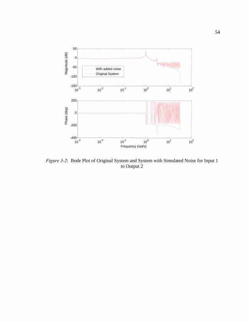
Figure 3-2: Bode Plot of Original System and System with Simulated Noise for Input 1 to Output 2 ........................................................................................................................ 54
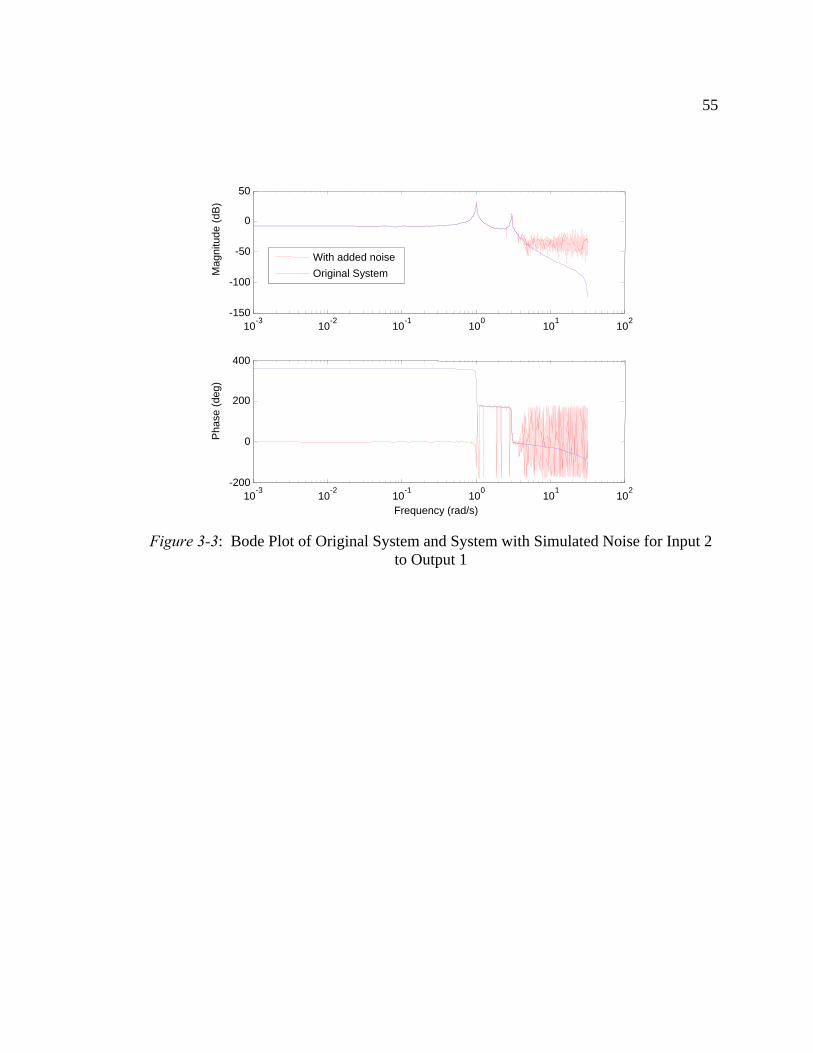
Figure 3-3: Bode Plot of Original System and System with Simulated Noise for Input 2 to Output 1 ........................................................................................................................ 55
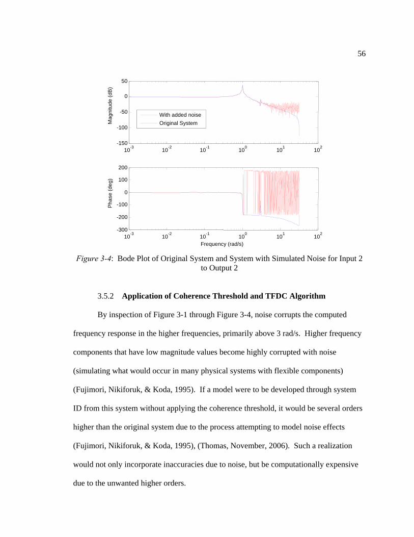
Figure 3-4: Bode Plot of Original System and System with Simulated Noise for Input 2 to Output 2 ........................................................................................................................ 56
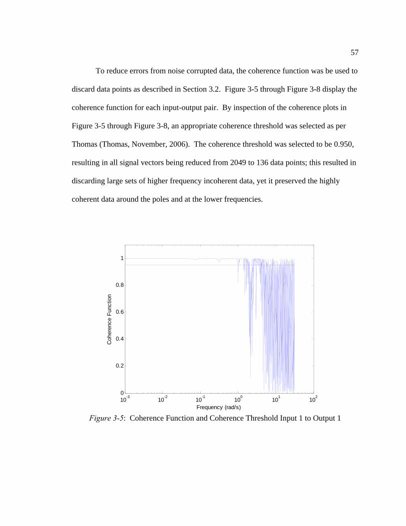
Figure 3-5: Coherence Function and Coherence Threshold Input 1 to Output 1 ............ 57
Figure 3-6: Coherence Function and Coherence Threshold Input 1 to Output 2 ............ 58
Figure 3-7: Coherence Function and Coherence Threshold Input 2 to Output 1 ............ 58
Figure 3-8: Coherence Function and Coherence Threshold Input 2 to Output 2 ............ 59
Figure 3-9: TFDC Estimated Bode Plot of Input 1 to Output 1 ...................................... 60
Figure 3-10: TFDC Estimated Bode Plot of Input 1 to Output 2 .................................... 61
Figure 3-11: TFDC Estimated Bode Plot of Input 2 to Output 1 .................................... 61
Figure 3-12: TFDC Estimated Bode Plot of Input 2 to Output 2 .................................... 62
Figure 3-13: Hybrid System Bode Plot of Input 1 to Output 1 ....................................... 64
Figure 3-14: Hybrid System Bode Plot of Input 1 to Output 2 ....................................... 64
Figure 3-15: Hybrid System Bode Plot of Input 2 to Output 1 ....................................... 65
Figure 3-16: Hybrid System Bode Plot of Input 2 to Output 2 ....................................... 65
Figure 3-17: Total Simulated Errors Input 1 to Output 1 ................................................ 67

9
Figure 3-18: Total Simulated Errors Input 1 to Output 2 ................................................ 68
Figure 3-19: Total Simulated Errors Input 2 to Output 1 ................................................ 69
Figure 3-20: Total Simulated Errors Input 2 to Output 2 ................................................ 70
Figure 4-1: Bode Plot of Flexlab for X-Axis Motor to X-Axis PSD .............................. 73
Figure 4-2: Bode Plot of Flexlab for X-Axis Motor to Y-Axis PSD .............................. 74
Figure 4-3: Bode Plot of Flexlab for Y-Axis Motor to X-Axis PSD .............................. 74
Figure 4-4: Bode Plot of Flexlab for Y-Axis Motor to Y-Axis PSD .............................. 75
Figure 4-5: Coherence Function and Coherence Threshold for Flexlab X-Axis Motor to X-Axis PSD with Applied Coherence Threshold of 0.3 ................................................... 76
Figure 4-6: Coherence Function and Coherence Threshold for Flexlab X-Axis Motor to Y-Axis PSD with Notional Coherence Threshold of 0.3 .................................................. 77
Figure 4-7: Coherence Function and Coherence Threshold for Flexlab Y-Axis Motor to X-Axis PSD with Notional Coherence Threshold of 0.3 .................................................. 77
Figure 4-8: Coherence Function and Coherence Threshold for Flexlab Y-Axis Motor to Y-Axis PSD with Applied Coherence Threshold of 0.3 ................................................... 78
Figure 4-9: TFDC Estimated Bode Plot for Flexlab X-Axis Motor to X-Axis PSD ...... 79
Figure 4-10: TFDC Estimated Bode Plot for Flexlab X-Axis Motor to Y-Axis PSD .... 80
Figure 4-11: TFDC Estimated Bode Plot for Flexlab Y-Axis Motor to X-Axis PSD .... 80
Figure 4-12: TFDC Estimated Bode Plot for Flexlab Y-Axis Motor to Y-Axis PSD .... 81
Figure 4-13: Flexlab Impulse Response Data X input X output ..................................... 82
Figure 4-14: Flexlab Impulse Response Data X input Y output ..................................... 82
Figure 4-15: Flexlab Impulse Response Data Y input X output ..................................... 83
Figure 4-16: Flexlab Impulse Response Data Y input Y output ..................................... 83
Figure 4-17: Hybrid System Estimated Bode Plot for Flexlab X-Axis Motor to X-Axis PSD ................................................................................................................................... 84
Figure 4-18: Hybrid System Estimated Bode Plot for Flexlab X-Axis Motor to Y-Axis PSD ................................................................................................................................... 85
10
Figure 4-19: Hybrid System Estimated Bode Plot for Flexlab Y-Axis Motor to X-Axis PSD ................................................................................................................................... 85
Figure 4-20: Hybrid System Estimated Bode Plot for Flexlab Y-Axis Motor to Y-Axis PSD ................................................................................................................................... 86
Figure 4-21: Hybrid Open Loop Bode Plot of Digital Low Pass Filter .......................... 87
Figure 4-22: Bode Plot of Flexlab for X-Axis Motor to X-Axis PSD ............................ 89
Figure 4-23: Bode Plot of Flexlab for X-Axis Motor to Y-Axis PSD ............................ 90
Figure 4-24: Bode Plot of Flexlab for Y-Axis Motor to X-Axis PSD ............................ 90
Figure 4-25: Bode Plot of Flexlab for Y-Axis Motor to Y-Axis PSD ............................ 91
Figure 4-26: LQG Estimated Impulse Response X-Axis Motor to X-Axis PSD ............ 92
Figure 4-27: LQG Estimated Impulse Response X-Axis Motor to Y-Axis PSD ............ 92
Figure 4-28: LQG Estimated Impulse Response Y-Axis Motor to X-Axis PSD ............ 93
Figure 4-29: LQG Estimated Impulse Response Y-Axis Motor to Y-Axis PSD ............ 93
Figure 4-30: Controller Simulation Using FRD Model ................................................... 94
Figure 4-31: Controller Simulation Using Flexlab Disturbance Data (Y-axis) .............. 96
Figure 4-32: Controller Simulation Using Flexlab Disturbance Data (X-axis) .............. 97
Figure 4-33: Flexlab Demonstration, Y-Axis PSD ......................................................... 99
Figure 4-34: Flexlab Demonstration, X-Axis PSD ....................................................... 100
Figure 4-35: Flexlab Demonstration, Y-Axis Using Thomas’ Settings ........................ 101
Figure 4-36: Flexlab Demonstration, X-Axis Using Thomas’ Settings ........................ 102
Figure 4-37: Flexlab Demonstration, Y-Axis Using More Conservative Settings ....... 102
Figure 4-38: Flexlab Demonstration, X-Axis Using More Conservative Settings ....... 103
Figure 4-39: Flexlab Demonstration, Y-Axis Using Balanced Settings ....................... 103
Figure 4-40: Flexlab Demonstration, X-Axis Using Balanced Settings ....................... 104

11
LIST OF TABLES
Page
Table 4-1: Controllers Attempted ................................................................................... 101

12
CHAPTER 1: INTRODUCTION
Large flexible structures are found in many applications such as space missions,
architectural design, and aircraft manufacturing. One issue when incorporating flexible
structures in such a system is the interaction between a control system and a structure’s
dynamics. This interaction can significantly degrade system performance due to
mismodeling, especially of flexible modes. To accommodate inaccurate models of
flexible modes, the control system bandwidth can be limited, but at the expense of
performance. To facilitate controller designs capable of desired performance, accurate
linear models that include troublesome modes are required. For large flexible structures,
system identification (ID), i.e. modeling a system from input/output data, is frequently
used to develop more accurate models. Associated with the growing interest in large
flexible structures, is the importance of improving methods in this field.
The underlying goal of this research is to produce and illustrate a system ID
technique for computing accurate models of the lowest order possible to facilitate
controller design using modern techniques to achieve system performance requirements.
To achieve this goal, a hybrid system ID method is developed that employs both a
frequency domain system ID method as well as state space system ID method.
1.1 Background
Applications in which a space vehicle has a deployment size larger than the
associated launch vehicle are often accomplished with deployable flexible space
structural components, such as solar panels, high accuracy sensor placement booms and
gravity gradient attitude control booms. Recent developments incorporating flexible
components include the United States Air Force Research Laboratory’s (AFRL)

13
Deployable Optical Telescope test bed (Schrader, Fetner, Griffin, & Erwin, 2002), the
AFRL Deployable Structures Experiment satellite concept (Adler, et al., April 19-22,
2004), and the deployable elastic composite shape memory alloy reinforced material
developed by AFRL and CSA Engineering (Pollard, Murphey, & Sanford, April 23-26,
2007). Understanding the characteristics of such components is therefore of primary
importance in advancing development and potential applications (Bihl, Pham, &
Murphey, May 3, 2007).
Additional space-based developments include developments by the National
Aeronautics and Space Administration (NASA) and the Jet Propulsion Laboratory. Both
organizations have a long history of incorporating flexible structures in their space
vehicle designs. These mission applications include using flexible deployable structures
to place instruments as far as possible from the radioisotope thermoelectric generators on
the Voyager probes of the 1970s to avoid interference (French & Griffin, 1991), and the
application for shuttle missions to test the structural and electrical performance of the
large flexible solar panel deployed from a Space Shuttle’s cargo bay (Pappa, Woods-
Vedeler, & Jones, December, 2001). NASA experiments into control-structure
interactions have also included experiments such as the Mini-MAST flexible structures
ground experiments (NASA Controls-Structures Interaction Program, PHASE I Guest
Investigator Program, 1991) and the middeck active control flight experiment (Miller, et
al., 1998).
Aerodynamic research involving control-structures interaction includes projects
such as the joint NASA, AFRL, and Boeing Phantom Works’ Active Aeroelastic Wing

14
research program, which integrates flexible structural behavior of aircraft components
and active control systems to replace the function of an aircraft’s control surfaces
(Pendleton, Flick, Paul, Voracek, Reichenbach, & Griffin, April 23-26, 2007). Other
applications of research in this field can include hypersonic vehicles, such as the X-43
Hypersonic Scramjet Vehicle, which requires detailed structural knowledge since the
engine and airframe are completely integrated where oscillations in the airframe can
directly impact engine performance (Adami, Zhu, Bolender, Doman, & Oppenheimer,
August 21-24, 2006).
Flexible structure analysis is not limited to aerospace applications. Structures such
as skyscrapers and cellular phone towers often pose many structural challenges such as
the effects of wind-induced vibrations, which in severe circumstances can damage or
destroy a structure (Wind Control in Building Design, February, 2004). Counteracting
these effects is possible with various active and passive damping methods (Wind Control
in Building Design, February, 2004). Properly handling these vibrations requires an
accurate model to design a controller that can damp vibrations. System ID takes into
account the inputs and outputs to a system and is therefore often the best viable means for
developing a sufficient model for a specific structure and its surrounding environment.
Technology testing for controller model development and design for flexible
structures is essential. In Ohio University’s School of Electrical Engineering and
Computer Science is Flexlab, a flexible structures test bed that was designed to allow for
research on flexible structure modeling and control system design methodologies (Blinn,
March, 1997). Primarily, this research has encompassed development and refinement of

15
system ID methods and the demonstration of controller designs using models from
system ID.
System ID methods use experimental data to develop mathematical models of
dynamical systems. Of primary interest herein is the development of control-oriented
system ID methods that produce models that include the dynamics of the system plus the
dynamics of the sensors and actuators. Such models can then be used for controller
development and refinement (Juang, 1994). Flexlab enables advancements in this field
by offering an easy to use, reconfigurable system that can demonstrate system ID and
vibration suppression using active controllers designed from models developed via
system ID.
1.2 Flexlab Testbed Description
Flexlab, Figure 1-1, was designed by Blinn (Blinn, March, 1997) to be a flexible
controls-structure interaction test bed. Flexlab consists of a central structure of a 12 foot
flexible aluminum rod 3/8 inches in diameter, suspended from the ceiling by a two-
degree of freedom gimbaled assembly with direct current (DC) motors orthogonal to each
axis (Blinn, March, 1997). The drive shafts are aligned orthogonally to each other
(Blinn, March, 1997). Therefore, two degree-of-freedom motion about the z-axis
(vertical axis) is permitted, as shown in Figure 1-1 (Blinn, March, 1997).
Flexlab’s motors are employed for both disturbance and control inputs; motion of
the structure is measured by sensors mounted on the rod at strategic locations and by an
optical position sensing device (PSD) (Blinn, March, 1997). The PSD is mounted on the
floor below the bottom of the rod (see Figure 1-1). Two types of sensors are used,
16
multiple Kistler K-Beam accelerometers and one Hamamatsu S1200 PSD with a wide-
angle lens. The floor mounted PSD is aligned to a Hamamatsu L2791 highly directive
infrared LED located on the bottom of the structure as shown in Figure 1-1. This device
measures the x and y axis deflection of the bottom of the structure. The accelerometers
are mounted at various points along the structure and aligned to measure accelerations in
both the x and y axes.
Figure 1-1: Current Configuration of Flexlab (Strahler, March, 2000)
Flexlab was designed to be reconfigurable for various types of experiments. To
achieve this, masses placed along the structure of Flexlab can be repositioned for various
17
experiments in order to modify the dynamics of the structure (Blinn, March, 1997). In
addition, Flexlab was designed with a mounting point for additional actuators placed at
the bottom of the structure. This permits control or disturbance actuators, such as cold gas
thrusters, to be mounted on the structure but have a minimum effect on its symmetry
(Blinn, March, 1997). Currently, Flexlab is configured for 5 control signal channels (2 of
which are for the DC motors) and 8 sensor channels (2 of which are for the PSD).
Figure 1-2: Operational View of Flexlab

18
The current configuration of Flexlab, graphically illustrated in Figure 1-1, is
pictured in Figure 1-2, and includes a steering mirror mounted along the y-axis. In
previous research this was implemented to demonstrate active optical systems (Strahler,
March, 2000). Although this research has been completed, these components remain on
the structure and as a consequence affect structural symmetry, introducing a torsional
mode in the x-z plan. This torsional mode is measurable through the use of
accelerometers at the end of the steering mirror assembly, which can record the motion of
that structure in the x-y plane (Strahler, March, 2000).
Flexlab is operated with a Pentium II 333Mhz computer that has National
Instruments data acquisition cards which handle all system inputs and outputs using
National Instruments’ LabVIEW software (Saunders, November, 2006). Operating
Flexlab is enabled through a LabVIEW based graphical user interface depicted in Figure
1-3. Data collected through the LabVIEW interface can be analyzed with MatLab or
similar analytical software (Saunders, November, 2006).
19
Figure 1-3: Screenshot of LabVIEW Based Flexlab Control Panel
The benefits of the LabVIEW interface is that the operation of Flexlab can be
done with a small learning curve, where previously Flexlab operation was reliant on
application specific C and Java programs (Saunders, November, 2006). LabVIEW
greatly facilitates the experimentation process with the ability to transfer data and
knowledge to novice operators.
1.3 System Identification
Typically there are three methods primarily used to develop linear mathematical
models of dynamical systems for controller development, (1) using kinematics and
dynamics methods for analysis, (2) finite element analysis, and (3) system ID. Dynamics
and kinematics methods are employed by modeling the known forces and moments
acting upon a structure, then using this model to predict the behavior of the actual system
20
(Fierro & Lewis, 1997), (Tarokh & McDermott, 2005). This is a well known method of
modeling a system and its study forms the basis of dynamics and kinematics theory;
however, it is susceptible to inaccuracies from mismodeling and unanticipated conditions
(Fierro & Lewis, 1997). Its use is typically found in anticipating behavior of a dynamical
system during preliminary design stages.
Finite element analysis is a numerical analysis method that models a structure by
assembling individual structural elements connected together at various points, called
nodes. The material properties of each element are considered and a system of nodes,
called a mesh, is used to simulate the structure (Juang, 1994), (Widas, 1997). However, a
model developed with finite element analysis typically experiences significant initial
inaccuracies (due to errors from approximations, mismodeling, and incorrect
assumptions) and typically incorporates refining the model using experimental data
(Juang, 1994). For these reasons finite element analysis methods have not been
considered in conjunction with Flexlab.
System ID develops a mathematical model of a system based upon input/output
data (Ljung, Perspectives on system identification, 2010), with a heavy burden typically
placed on proper sensor placement (Thomas, November, 2006), input signal design
(Pintelon & Schoukens, 2001), data collection that includes significant cycles of the
lowest mode (Medina, November, 1991) and appropriate/acceptable estimated model
order (Ljung, Perspectives on system identification, 2010) (Markovsky, Willems, van
Huffel, de Moor, & Pintelon, 2005), (Pati, Rezaiifar, Krishnaprasad, & Dayawansa,
1993), (Wahlberg, 1986), (Gallivan & Murray, 2003). Generic system ID processes can

21
be broken into creating an analytical model of a system, estimating the system’s modal
and excitation characteristics, determining sensor and actuator locations and
requirements, exciting the system to collect experimental data, using a system ID method
(such as mentioned above) on the data to create a model, and then refining the analytical
model based on experimental results (Juang, 1994).
Of interest here is developing models that represent the entire system in question,
including actuators and sensors, and herein this will be termed “system-ID for control-
system design” (Mitchell & Irwin, 2008). This approach is relevant to many situations
where ideal sensor and actuator locations are not known a priori or it would be
impossible or inefficient to strategically locate sensors and actuators on a given structure,
e.g. space vehicle applications where servicing is cost prohibitive or technically
impossible.
With experimentally obtained input and output data, system ID methodologies are
used to develop mathematical models of a dynamical system plants. Frequency domain
system ID methods typically apply various types of frequency domain least squares
transfer function analysis for a single-input, multiple-output (SIMO) systems (Juang,
1994), (Thomas, November, 2006). Time domain system ID methods typically also
extend least squares system ID (for single-input, single-output systems (SISO)) or state
space system ID methods, for SISO, SIMO or multiple-input, multiple-output (MIMO)
systems (Juang, 1994), (Thomas, November, 2006).
Understanding the characteristics of the sensors and actuators to be used is also
important in system ID. Certain systems can only accept a small range of input signals

22
due to the types of actuators being used; understanding the performance characteristics of
sensors being used is equally important or aliasing issues maybe unknowingly be present
in the results as a consequence of collecting data discretely (Holst, 1998). Despite the
best precautions and system isolation, sensor noise, measurement noise and external
interferences will be present in any physical system. System ID research has had to
routinely focus on additional considerations to accommodate the extraction of models
from noisy data (Juang, 1994), (Thomas, November, 2006), (Fujimori, Nikiforuk, &
Koda, 1995) with estimated model order reduction being an area of ongoing research
interest (Ljung, Perspectives on system identification, 2010), (Fujimori, Nikiforuk, &
Koda, 1995). Thomas (Thomas, November, 2006) extended a SISO frequency domain
system ID technique termed “Transfer Function Determination Code” (TFDC) using a
threshold of the coherence function to eliminate data that was highly corrupted by noise
or disturbance in order to improve the fidelity of the models developed using TFDC.
The work presented herein will create a hybrid system ID method extending
TFDC, Thomas’ Coherence Thresholding technique (Thomas, November, 2006), along
with a state space system ID method, the Eigensystem Realization Algorithm (ERA).
This thesis will apply the Coherence Threshold to discard noisy frequency domain points
from which TFDC will calculate SIMO transfer function models. These models will then
be used to produce the needed data to compute MIMO state space models through the
ERA approach from the impulse responses of the SIMO systems. This hybrid method
will be illustrated with a contrived example and then with laboratory data from Flexlab.

23
1.4 Organization
The following chapters are organized such that Chapter 2 is a literature review of
the fundamentals of presently employed System ID techniques. Chapter 3 provides an
explanation of the methodology of the hybrid System ID method developed herein, along
with a simulation example and subsequent results. System ID using the hybrid method is
applied to Flexlab to develop a MIMO model. In Chapter 4 the model is used to design a
controller to suppress vibrations and then the design is tested using Flexlab. Chapter 5
concludes this thesis with a discussion of the methods used, results and suggestions for
future research.

24
CHAPTER 2: SYSTEM IDENTIFICATION METHODS
System ID uses input and output data in conjunction with estimation algorithms to
compute a mathematical relationship between the two sets of data. There are several
techniques used to analyze experimental data for system ID, including time and
frequency domain approaches. In this thesis, a hybrid system ID method will be
developed to create a minimum-order state-space estimated model. To lay the
groundwork for these developments, the three major techniques for performing system ID
are described below. These methods are grouped under the two categories, least squares
and state space.
Least squares system ID extends from ordinary and weighted least squares curve
fitting. System ID methods based upon this approach include: 1) the time domain least
squares system ID technique and 2) the frequency domain least squares, specifically
TFDC. The state space method considered for system ID is the Eigensystem Realization
Algorithm (ERA). This method is an extension of the Ho-Kalman algorithm, which
created the first minimal state-space realization from noise-free impulse response data
(Ljung, System Identification Theory for the User, 1999), (Gevers, 2006). Similar to the
Ho-Kalman algorithm, ERA uses impulse response data to generate a state space system
model. An interesting aspect of this approach is the ability to develop models from noisy
data, making it an attractive method for modeling dynamical systems where noise-free
data is impossible to gather with physical sensors. Estimated impulse responses are
generated for use with experimental data, as actual impulse responses are impossible to
generate.
25
2.1 Ordinary Least Squares
Both time domain least squares system ID and the frequency domain TFDC
methods are built upon least squares curve fitting. A brief explanation of these
underlying principles follows for a better understanding of the proposed solution concept.
Least squares estimation is an estimation technique used in many applications, with one
of the most important being data or curve fitting. It is used to obtain a curve that fits a set
of data points in the best least squares or weighted least squares sense (Maybeck, 1979).
Ordinary least squares can simply be viewed as weighted least squares with unity
weighting. This is important to note, as some least squares based system ID techniques
permit selective weighting of data points to improve the fidelity of the fit by
deemphasizing certain data points, usually data known to be corrupted with noise.
A set of measurement models can be represented as,
, (1)
where ∈ represents a set of i measurements, ∈ is a vector representing
measurement noise, ∈ is a vector of j unknown parameters, and ∈ is a
coefficient matrix relating the measurements to the unknown parameters where to
ensure that a system is over determined (Maybeck, 1979).
To determine a least squares estimate of the vector of unknown parameters, , it is
necessary to find the minimum estimate of the unknown parameters, , with respect to
, the measurements and the estimate of the measurements (Maybeck, 1979).
An weighting matrix, W, can be used to weigh the measurements (Maybeck,
1979). Then the unknown parameters can be determined to minimize the cost function
26
1
2. (2)
Weighted least squares curve fitting is used in conditions where it is desired to
weigh individual measurements differently; this is accomplished by determining the
individual elements or values of the weighting matrix, W. For standard weighted least-
squares, W is a diagonal matrix whose elements are, , , … , (Maybeck, 1979). In
this case, the cost function in Equation 2 becomes
1
2‖ ‖ . (3)
In many least-squares applications no weighting matrix is used; therefore, in its
absence an identity matrix would be used, if not entirely omitted (Thomas, November,
2006), (Maybeck, 1979). Under these conditions, the cost function in (3) becomes
1
2‖ ‖ . (4)
Minimization by the estimated value, , is accomplished only if the necessary
condition,
⋯ 0, (5)
is satisfied. The sufficiency condition being that the Jacobian of the cost function, J, is
positive semidefinite, i.e.
0. (6)
Differentiating (3) in the manner described in equation (5), yields

27
0. (7)
Solving the above, (7), for the estimate of the unknown parameters, , yields
, (8)
which, for the non-weighted case (Maybeck, 1979), is
. (9)
Additional information on least squares can be found in Maybeck (Maybeck, 1979).
2.2 Total Least Squares
For dynamical systems, where knowledge of a system and error-free sensor data
cannot be assumed, total least squares may be applicable in modeling. Total least squares
is different from ordinary least squares in that it assumes that the coefficient matrix H,
presented earlier in (1), is not noise free. For the total least squares problem, the
overdetermined system in equation (10) will be considered. The form for a total least
squares problem can be expressed as
, (10)
where, ∈ is the vector of unknown parameters. The expression is written as being
approximate due to the assumption of noise being present in the coefficient matrix (van
Huffel & Vanderwalle, 1991). Similar to the ordinary least squares example above, total
least squares will also solve for the estimate, , of the unknown parameters plus an
estimate of the coefficient matrix and measurement vector .
To determine the total least squares estimate of the vector of unknown
parameters, , a singular value decomposition is used on the concatenation of the
coefficient and observation matrices, i.e.,
28
; Π #, (11)
where U is a square matrix the size of the rows of ; , Π is a diagonal matrix of non-
negative real numbers the size of ; , and V# is a square unitary matrix of the size of
the columns of ; (Kailath, 1980). Using (11), equation (10) can be converted to
; ; 1 0. (12)
A correction term is employed in total least squares; its relationship between the system
and the system’s estimated matrices ; is determined so that
; Π #, (13)
where Π is a diagonal matrix of correction terms ( , , ⋯ , (van Huffel &
Vanderwalle, 1991), the symbol # is used to denote the conjugate transpose of .
The minimum total least squares correction term, , is therefore found by
minimizing the estimate of the unknowns ; by minimizing
; ; , (14)
subject to the rank of ; (van Huffel & Vanderwalle, 1991). This is reached
when the difference between the actual quantities and the estimated ones are as close as
possible, i.e.
; ; #, (15)
where and # are column vectors from the n-th columns of and # matrices in
equation (13) (van Huffel & Vanderwalle, 1991). Equation (15) by definition has a rank
of one, therefore the estimated relationship of (12) can be set equal to zero as shown as
follows (van Huffel & Vanderwalle, 1991),
29
; ; 1 0. (16)
The solution for the total least squares solution is reached through scaling the
term until
; 1
1
,,
(17)
where , 0 (van Huffel & Vanderwalle, 1991). The solution for the estimate of x,
1
,, , , , ⋯ , , ,
(18)
is therefore satisfied and the total least squares solution for the estimate then becomes
1
,, , , , ⋯ , , .
(19)
Further information about total least squares, including mathematically rigorous
proofs of the basic total least squares algorithm and additional extensions of total least
squares, can be found in van Huffel and Vanderwalle (van Huffel & Vanderwalle, 1991).
2.3 Least Squares System Identification
Applying the principles developed above to the determination of models for
designing control system for dynamical systems requires a method of representation for a
system. Essentially all modern aerospace control systems utilize controllers realized with
a digital computer. To facilitate the design of these controllers, a discrete mathematical
model that accurately portrays the input-output relationships between actuator inputs to
sensor measurements is critical. System ID that develops models from data obtained by
exciting the system with the actuators and measuring data from the response of this
actuation is called “system-ID for control-system design" (Mitchell & Irwin, 2008). In

30
this case the models developed need to be z-transfer functions or difference equation
representations. These difference equations are also known as recursive models.
To illustrate both time and frequency domain least squares system ID techniques,
a generic system in the z-domain is considered. Therefore, system ID techniques applied
to a generic discretized system in the z-domain is considered to illustrate current time
domain system ID methods. A general transfer function of a linear, time-invariant
system in the z-domain can be expressed as
⋯
⋯, (20)
where Y(z) is the z-transform output of the system, U(z) is the z-transform of the input to
the system; the order of the denominator is n, the order of the numerator is n-l, with l
being an integer constant (Phillips & Nagle, 1995).
By multiplying each side of Equation 20 with the identity ⁄ the transfer
function becomes
⋯
1 ⋯, (21)
a form that can easily be converted to a difference equation (Phillips & Nagle, 1995). To
create a difference equation from a discrete time transfer function, the inverse z-
transformation of the discrete time system is used. Generally this is indicated through
notation such as,
(22)

31
where is the inverse z-transformation operator, is unit pulse response and G(z)
is the discrete-time transfer function from equation (21) (Phillips & Nagle, 1995). The
inverse -transformation operation is defined as
1
2
(23)
where j is the imaginary unit and ∮
is a z-plane line integral along a closed path
enclosing all finite poles, Γ (Phillips & Nagle, 1995).
For known z-transformations, derived transformation properties can be used as
described in Phillips and Nagle (Phillips & Nagle, 1995). For the form displayed in (21),
a known inverse z-transformation, , can be applied to the z-domain elements in such a
manner:
, (24)
to convert to a difference equation, where n is the power of each z-domain element
(Phillips & Nagle, 1995). By cross multiplying the denominators in equation (21),
followed by applying the inverse z-transform as per equation (24), the following
difference equation results:
1 2 ⋯1 2
⋯ , (25)
the time-domain equivalent to the system in equations (20) or (21) (Phillips & Nagle,
1995).
2.3.1 Time Domain Least Squares System Identification
For time domain least squares system ID, we are interested in determining the
input and output coefficients from time domain measurements of the inputs and outputs.
32
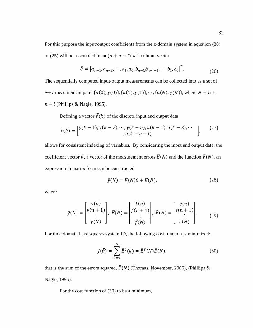
For this purpose the input/output coefficients from the z-domain system in equation (20)
or (25) will be assembled in an 1 column vector
, , ⋯ , , , , , ⋯ , , . (26)
The sequentially computed input-output measurements can be collected into as a set of
N+1 measurement pairs 0 , 0 , 1 , 1 ,⋯ , , , where
(Phillips & Nagle, 1995).
Defining a vector of the discrete input and output data
1 , 2 ,⋯ , , 1 , 2 ,⋯ ,
, (27)
allows for consistent indexing of variables. By considering the input and output data, the
coefficient vector , a vector of the measurement errors and the function , an
expression in matrix form can be constructed
, (28)
where
1
⋮,
1⋮
,1
⋮.
(29)
For time domain least squares system ID, the following cost function is minimized:
, (30)
that is the sum of the errors squared, (Thomas, November, 2006), (Phillips &
Nagle, 1995).
For the cost function of (30) to be a minimum,
33
2 2 0. (31)
Solving for produces the least squares solution
, (32)
which is the time domain system ID least-squares solution (analogous to the least-squares
solution in equation (9)).
Additionally, time domain least squares system ID permits error weighting. This
is analogous to the weighted least-squared solution in Equation (8). For its use, the
weighted cost function would be expressed as
, (33)
where is the weighting term. The weighted least squares solution is therefore
. (34)
Clearly this method of system ID can be seen as directly related to least squares.
Further information on this system ID method can be found in Phillips and Nagle
(Phillips & Nagle, 1995).
2.3.2 Frequency Domain Least Squares System Identification
The frequency domain least squares technique considered herein will be referred
to as the Transfer Function Determination Code (TFDC). TFDC is a system ID
technique concerned with identifying the coefficients of a z-domain transfer function
model from frequency response input-output data using least-squares techniques
34
(Medina, November, 1991). Revisiting the generic discretized system in Equation 20, the
frequency response of the system can be computed by letting , i.e.
X . (35)
Through Euler’s identity, cos sin , the representation of the system’s
frequency response can be aided by realizing that
cos sin (36)
where T is the sampling period or data rate of the digital controller, and i is the index of
frequency data points where, 1,2,⋯ , (Medina, November, 1991).
Substituting (36) into the system model of (20), the numerator and denominator
can be expressed as
cos sin (37)
and
cos sin ∑ cossin ,
(38)
respectively, with being the order of the numerator and 1 being one less than
the order of the denominator; the remaining denominator expression, , is expressed as
cos sin , which is not multiplied by a coefficient.
Similarly, solving (20) in such a way that and using Equation
(35), the real and imaginary parts of the system can be separated into two equations:
∑ cos ∑ cos
∑ sin cos sin , (39)

35
for the real parts, and
∑ cos ∑ sin
∑ cos cos sin , (40)
for the imaginary parts.
Equations (39) and (40) provide two simultaneous equations to solve for the
unknown transfer function coefficients of the system in (20), i.e., the unknown
denominator , , ⋯ , and numerator , , ⋯ , coefficients (Medina,
November, 1991). Combining these equations into a two row matrix with a 2n+1 vector
of input and output coefficients yields
cos 0 ⋯ cos cos cos 0 sin 0 ⋯
sin 0 ⋯ sin sin sin 0 cos 0 ⋯
cos sin
sin cos
⋮
⋮
cos sin
sin cos
(41)
with 0,1,⋯ , 1. For simplicity, Equation (41) can be expressed compactly as
,
(42)
where is the 2 2 1 matrix of real and imaginary equation pairs, is the
2 1 matrix of real and imaginary equation pairs, and is the 2 1 1 matrix of
unknown transfer function numerator and denominator coefficients (Medina, November,
1991), (Young, March, 1993).
Being a least squares derived technique, TFDC also permits weighting of
measurements. In this case the real and imaginary pairs of equation (42) would be

36
weighted, using a diagonal weighting matrix, W, which has two rows for each frequency
point (Medina, November, 1991),
. (43)
Additional methodologies of weighting are described by Medina (Medina, November,
1991); these include inverse magnitude weighting, coherence weighting, and logarithmic
frequency equilibration.
Solving equation (42) or (43) for the unknown transfer function coefficients is
accomplished through least squares techniques, including ordinary least-squares,
weighted least-squares or total least-squares. For example, to generate an ordinary least
squares solution for the unknown coefficients in , the method elaborated on in Section
2.1 would be applied; equation (42) would be solved in place of equation (1). Similarly a
weighted least-squares solution would use equation (43) in place of equation (1). A total
least squares solution for the unknown coefficients can be found using the total least-
squares technique described in Section 2.2, by using equation (42) or (43) in place of
equation (10). A similar process would be applied to solve for the unknown for any other
least squares technique.
2.4 State Space System Identification
A limitation to the above system ID techniques is that they cannot directly be
applied to a MIMO system. Combining multiple SISO or SIMO realizations may be used
for such cases, but a minimal realization is not straight-forward. State-space system ID
does not have this limitation. Ho and Kalman (Ho & Kalman, 1966) first developed a
state space system ID method through system realization techniques by constructing
37
minimum realizations of dynamical systems using impulse response data. Using the
underlying principles developed by Ho and Kalman, system ID methods, including the
Eigensystem Realization Algorithm (ERA), have evolved.
For the discussion herein, a generic description of a finite-dimensional, discrete-
time, linear time-invariant state-space system is,
1
, (44)
where it is assumed that is index of the sampling instant, is an n-dimensional state
vector, is an m-dimensional input vector, is a p-dimensional output vector,
is an state matrix, is an input coefficient matrix, is a output
coefficient matrix and is an feedthrough matrix. In physical, dynamical systems
the matrix D is equal to zero (Skelton, 1988). Due to the state-space nature of this system
description, system ID of SISO, SIMO and MIMO systems are permitted.
For control systems, the concepts of controllability and observability are
fundamentally important. For the system in equation (44), the observability and
controllability matrices are defined respectively as
⋮
(45)
and
⋯ (46)
38
respectively, with n being the dimension of the state transition matrix (Kailath, 1980).
For the state-space realization of the system to be minimal, the rank of both the
controllability and observability matrices needs to be equal to n (Kailath, 1980).
The impulse response is frequently used in control systems for determining
performance characteristics. The continuous time impulse response is defined as
0 ∀ 0, 1
(47)
which integrates to one, is zero everywhere except an interval around t equal to zero and
is infinite in magnitude when t is zero (Kailath, 1980), (Maybeck, 1979), (Norton, 1986).
However, in discrete-time systems, the discrete-time impulse function is defined as
follows:
1, 00, 0
, (48)
such a representation permits discrete time impulse responses to be easily calculated
(Kailath, 1980). For design purposes and to avoid saturating the motors operating
Flexlab an impulse signal was not applied to the structure itself; instead the digital
impulse was used during calculations. In order to measure the response of such a system
to an input, adequate excitation over a prolonged duration is normally required. Due to
this problem an approximated impulse response is usually calculated from the inverse
Fourier transform of the system’s frequency response that has been computed by
processing large amounts of data from random excitation (Juang, 1994).
The impulse response of a state space discrete-time system to a discrete impulse is

39
0, , , ⋯ , , 1, (49)
which is defined as the Markov parameters for a state-space system of the form shown in
equation (44), where k is the sample index and , ⋯ , are the calculated impulse
response values (Juang, 1994), (Kailath, 1980).
By observation of equations (45) through (49), it can be seen that the Markov
parameters in (49) could be easily calculated using observability and controllability
matrices. Exploiting this knowledge one can form a matrix comprised of the
observability and controllability matrices (equations (45) and (46)) with the state matrix
from (44),
⋮⋯ , (50)
which can be seen as a matrix of the Markov parameters,
1
⋯
⋯
⋮ ⋮ ⋱ ⋮⋯
, (51)
from equation (49) (Juang, 1994). Equation (51) is defined as the Hankel Matrix, a block
Toeplitz type of matrix whose elements along the block antidiagonals are identical (in
other words, an upside down Toeplitz matrix) (Kailath, 1980). In Medina (Medina,
November, 1991), it is shown that the minimum realization of any system would be the
Hankel Matrix for 1, i.e. 0 ,
40
0
⋯
⋯
⋮ ⋮ ⋱ ⋮⋯
(52)
Singular value decomposition of the rectangular 0 , allows the Hankel Matrix
to be decomposed into
0 Π #,
(53)
where Π is a diagonal matrix of nonnegative square roots of the eigenvalues
, , ⋯ of 0 0 , is an orthogonal matrix of the eigenvectors of
0 0 , and # is the conjugate transpose of , the orthogonal matrix of the
eigenvector of 0 0 (Kailath, 1980).
Since 1, it can be seen from equation (51) that
0 OP, (54)
therefore by equation (53) the observability and controllability matrices can be seen to be
represented as
Π (55)
and
Π #, (56)
respectively. The pseudo-inverse matrices of the observability and controllability
matrices can also be represented as # Π # and # Π , respectively.
From equation (51) it is known that for k=2, 1 (Juang, 1994). Using
this, one can combine the controllability and observability representations in equations
(55) and (56) (Juang, 1994). The Markov parameters can then be solved for
41
Π Π # 1 Π Π # , (57)
with output and input block companion matrices, 0 ⋯ 0 and
0 ⋯ 0 , respectively, where and 0 are identity and zero matrices of
order i, with i being either p or m, the lengths of the output and input vectors from
Equation (44) (Juang, 1994), (Ho & Kalman, 1966).
From Equation (57) a state coefficient matrix can be computed as
Π # H 1 Π # 1 #. (58)
Equation (58) also happens to be the minimum realization, this was rigorously shown by
Juang (Juang, 1994) and Medina (Medina, November, 1991). This means that the model
has the smallest state-space dimension as possible with a given input-output relationship,
assuming that noise free impulse response data is available (Juang, 1994). From Juang
(Juang, 1994), the values of the input and output coefficient matrices were determined to
be
Π # , C Π . (59)
Further analysis and information about the ERA family of methods can be found in
Juang (Juang, 1994), and Medina (Medina, November, 1991). Additional information on
the mathematical principles at use in this method can also be found in Kailath (Kailath,
1980).

42
CHAPTER 3: METHODOLOGY AND ANALYSIS WITH CONTRIVED EXAMPLE
3.1 Purpose
Noise in the input/output data introduces unwanted effects; because of this
uncertainty in the measurements, models generated through system ID may be of
significantly higher order than the actual system being modeled. If modern state space
techniques are used to design controllers to meet systems design specifications,
unnecessary complexity will result. It is therefore desirable to produce a model that
appropriately represents the system with an order as low as possible (Ljung, Perspectives
on system identification, 2010), (Wahlberg, 1986), (Gallivan & Murray, 2003)(Pati,
Rezaiifar, Krishnaprasad, & Dayawansa, 1993), (Markovsky, Willems, van Huffel, de
Moor, & Pintelon, 2005). Both time domain system ID and TFDC can produce
individual models between each input and output; however combining these into a
minimum order state space realization is not a straight-forward process. ERA produces
state space triplet (state, input and output coefficient matrices) realizations from impulse
response data. In practice, the impulse response data provided to ERA is generated from
noisy time-response data. Theoretically, the order of the system is the rank of the Hankel
matrix required by ERA. However, with noisy impulse response data, the rank of the
Hankel matrix is normally much higher than the order of the system. As a consequence,
ERA models are often many orders higher than necessary.
The approach presented in this thesis follows an alternative approach. The
impulse response data needed for ERA can be obtained from transfer function models
computed using the TFDC algorithm. By using TFDC and ERA system ID methods in a
tandem process, it is possible to create high fidelity and lesser, reasonable order state

43
space models using ERA, with the noise and disturbance effects reduced by processing
the noisy data with TFDC.
In discussing this method, the proper processing of the input/output data is
considered first. To accomplish this, TFDC is used to produce transfer function models
between each input and the outputs. Because TFDC uses frequency response data, it is
possible to take advantage of this capability to discard noisy frequency domain data
points in order to increase the fidelity of models. Time domain methods require the
processing of every data point, even though it is known that data which is small in
amplitude can be highly corrupted with noise; however, there is little theoretical basis
that allows these data points to be discarded in the system ID process. In a time domain
system ID method, one must process all data in sequence; by discarding time domain data
points, these data points are, in essence, set to zero, however; thus inserting zeros in the
data set used by the system ID algorithm. By operating in the frequency domain, each
frequency point to be processed independently. This approach was employed by
Thomas, in his Coherence Threshold technique, where the coherence function was used
to discard incoherent input/output data points (Thomas, November, 2006). This is
necessary to avoid the undesirably high orders typically introduced by system ID
processes attempting to model noise.
The ERA method directly computes a state space realization. However, it
requires impulse response data between each input and each output. To generate this
data, a linear difference equation between each input and output can be constructed from
input/output transfer functions that have been estimated through the frequency domain
44
technique, TFDC. Using difference equations, the impulse responses can be computed
and then input to ERA to produce a state space realization.
3.2 Applying the Coherence Threshold in SIMO Systems for Frequency Domain
Noise Reduction
The coherence function,
γS jω
S jω S jω (60)
provides a relative measure of how much an output signal is due to the input, where jω
refer to a variable being a function of frequency, S is the cross power spectral density
between the input x and output y, S is the power spectral density of the input x, and S
is the power spectral density of the output y (Thomas, November, 2006), (Mitchell &
Irwin, 2008). Thomas (Thomas, November, 2006) illustrated that by discarding all
frequency data points below a coherence threshold, the fidelity of transfer functions
estimated by TFDC could be significantly improved.
When applying a coherence threshold to discard data points for SIMO systems,
the coherence function of all outputs must be considered simultaneously. Discarding
more points below a certain coherence threshold for only one output would yields data
vectors of different lengths, resulting in frequency vectors of different lengths for a SIMO
system. This would preclude the consideration of a SIMO system and subsequently
multiple SISO systems would then have to be examined. However, this would fail to
ensure a consistent estimated transfer function denominator.

45
3.3 Extending TFDC to SIMO System Identification
To design controllers of flexible systems with multiple actuators and sensors,
models between each input and each output are required. This can be achieved by
sequentially exciting the system with each input and collecting all output data. There are
two methods of accomplishing this, creating separate SISO models for each output sensor
with respect to each input and then considering them collectively, or by creating SIMO
models between each input and the outputs. One drawback to creating multiple SISO
models is lack of assurance that the poles of all I/O relationships will be the same, as they
should since the same input is being used for all I/O data collections. Creating one SIMO
model prevents this situation; where the same denominator exists for all transfer
functions, but with different numerators for each input/output pair.
To apply least squares techniques to a SIMO data set, properly organizing the
structure of the realization method is important. To develop this process, the simplest
case, a one-input, two-output SIMO system, is assumed to extend the TFDC idea to
SIMO systems. The TFDC algorithm is modified so that the least squares process solves
for transfer function coefficients in such a way that the denominator is forced to be the
same for all numerators. Equation (61) shows a matrix setup that relates the numerator
and denominator coefficients for a SIMO discrete system and the frequency response
data,
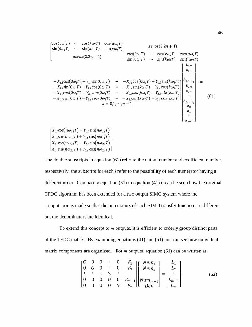
46
cos 0 ⋯ cos cos
sin 0 ⋯ sin sin2,2 1
2,2 1cos 0 ⋯
sin 0 ⋯
, cos 0 , sin 0 ⋯ , cos , sin
, sin 0 , cos 0 ⋯ , sin , cos
, 0 , 0 ⋯ , ,
, 0 , 0 ⋯ , ,
0,1,⋯ , 1
,
,
⋮
,
,
,
⋮
,
⋮
, cos , , sin ,
, sin , , cos ,
, cos , , sin ,
, sin , , cos ,
.
(61)
The double subscripts in equation (61) refer to the output number and coefficient number,
respectively; the subscript for each l refer to the possibility of each numerator having a
different order. Comparing equation (61) to equation (41) it can be seen how the original
TFDC algorithm has been extended for a two output SIMO system where the
computation is made so that the numerators of each SIMO transfer function are different
but the denominators are identical.
To extend this concept to m outputs, it is efficient to orderly group distinct parts
of the TFDC matrix. By examining equations (41) and (61) one can see how individual
matrix components are organized. For m outputs, equation (61) can be written as
0 0 ⋯ 00 0 ⋯ 0⋮ ⋮ ⋱ ⋱ ⋮ ⋮0 0 0 00 0 0 0
⋮ ⋮ . (62)
47
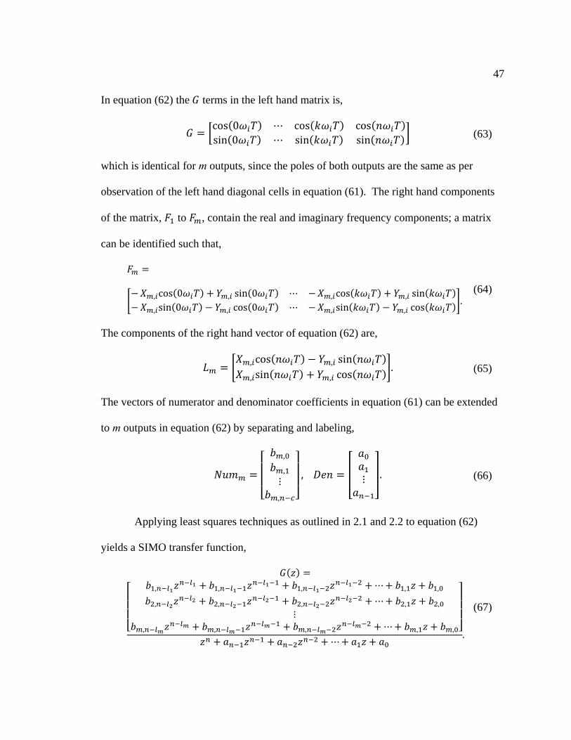
In equation (62) the terms in the left hand matrix is,
cos 0 ⋯ cos cos
sin 0 ⋯ sin sin (63)
which is identical for m outputs, since the poles of both outputs are the same as per
observation of the left hand diagonal cells in equation (61). The right hand components
of the matrix, to , contain the real and imaginary frequency components; a matrix
can be identified such that,
, cos 0 , sin 0 ⋯ , cos , sin
, sin 0 , cos 0 ⋯ , sin , cos.
(64)
The components of the right hand vector of equation (62) are,
, cos , sin
, sin , cos. (65)
The vectors of numerator and denominator coefficients in equation (61) can be extended
to m outputs in equation (62) by separating and labeling,
,
,
⋮
,
, ⋮ . (66)
Applying least squares techniques as outlined in 2.1 and 2.2 to equation (62)
yields a SIMO transfer function,
, , , ⋯ , ,
, , , ⋯ , ,
⋮
, , , ⋯ , ,
⋯.
(67)

48
3.4 Extending Frequency Domain System Identification to a State-Space
Realization
To calculate an impulse response (Markov parameters) from the z-domain
discrete-time transfer function estimated by TFDC in equation (62), the difference
equation must first be calculated. The impulse response can be computed using the
difference equation. The impulse response data is used in the ERA methodology to
generate a state space representation.
Section 2.3 discussed determining a difference equation from a z-domain transfer
function. By multiplying the SIMO transfer function calculated in equation (67) by the
identity ⁄ , a SIMO transfer function in the form
, , , ⋯ , ,
, , , ⋯ , ,
⋮
, , , ⋯ , ,
1 ⋯.
(68)
Applying the known derived z-transformation in equation (24) yields a SIMO difference
equation for a vector of outputs as follows:
1 2 ⋯
, , 1
, , 1
⋮
, , 1
, 2 ⋯ ,
, 2 ⋯ ,
⋮ ⋮ ⋮
, 2 ⋯ ,
(69)

49
The impulse response can then be computed from the difference equation in
equation (69) by letting the input, , be the discrete time impulse function, , in
equation (48). The output therefore becomes the impulse responses, which for each input
and output is defined as
, (70)
or the discrete time Markov parameters in equation (49), with 1 (Kailath, 1980).
The process to calculate an ERA representation described in Section 2.4 is then directly
followed for a MIMO system where each SIMO system ID step yields a column in each
Markov parameter to form the complete Markov parameter matrices.
3.5 Proof of Concept Testing
To verify the methods employed, a simple proof-of-concept test is employed
using a known generic system. The system is created in MATLAB, random noise is
added and the preceding methodology is applied; a comparison of the estimated system to
the known original system is then made to verify the methodology.
3.5.1 Simulation Setup
This system approximates a typical flexible structure with multiple low-frequency
modes (Medina, November, 1991). The MIMO transfer function for the continuous time
system for this example was chosen to be
G s
0.3s 0.70.45s 0.9
s 0.01s 1
0.4s 0.10.5s 0.04
s 0.033s 9 (71)
where there are two outputs and two inputs, symbolizing a system such as Flexlab, where
the user would excite both axes and analyze input/output (I/O) data from the floor
mounted, two-axis position sensor. This system has natural frequencies at 1.00 rad/s and

50
3.00 rad/s; damping ratios for this system are 0.005 and 0.0055. The continuous time
system Equation 71 is assumed to receive piece-wise continuous signals obtained from
discrete-time signals that have been processed with digital to analog (D/A) devices
operating at 10 Hz and the outputs are converted to digital signals with analog to digital
(A/D) devices operating at 10 Hz.
For a system such as Flexlab, the D/A and A/D components would be found on an
I/O interface board inside the computer or operating equipment. For the purposes of
simulation, a discretized version of this system incorporating the D/A and A/D parts is
required. This is created through the MATLAB function
Gz = c2d(Gs, T, method), (72)
where Gs is the continuous time system in question, T is the sampling period, 0.1
seconds, for this example, and method is the specific discretization method to be used
(the default method, a zero order hold, is the method employed herein) (Signal
Processing Toolbox For Use with MATLAB User's Guide, 2001). When processing
through MATLAB, the sampled-data transfer function matrix for Equation (71) becomes
G z0.003481z 0.003323z 0.003322z 0.0034720.0002312z 0.0004138z 0.0004029z 0.0002341
0.003z 0.002683z 0.002692z 0.0029890.004693z 0.004277z 0.004287z 0.004676
z 3.891z 5.379z 3.888z 0.9957.
(73)
To collect data for system ID, a known set of corresponding input-output data was
created. For the input, a series of 4096 pseudo-random normally distributed inputs, U,
were generated in MATLAB. The response of the system to this input set generates
outputs that are sampled at the same rate, creating output sequences of equal length.
51
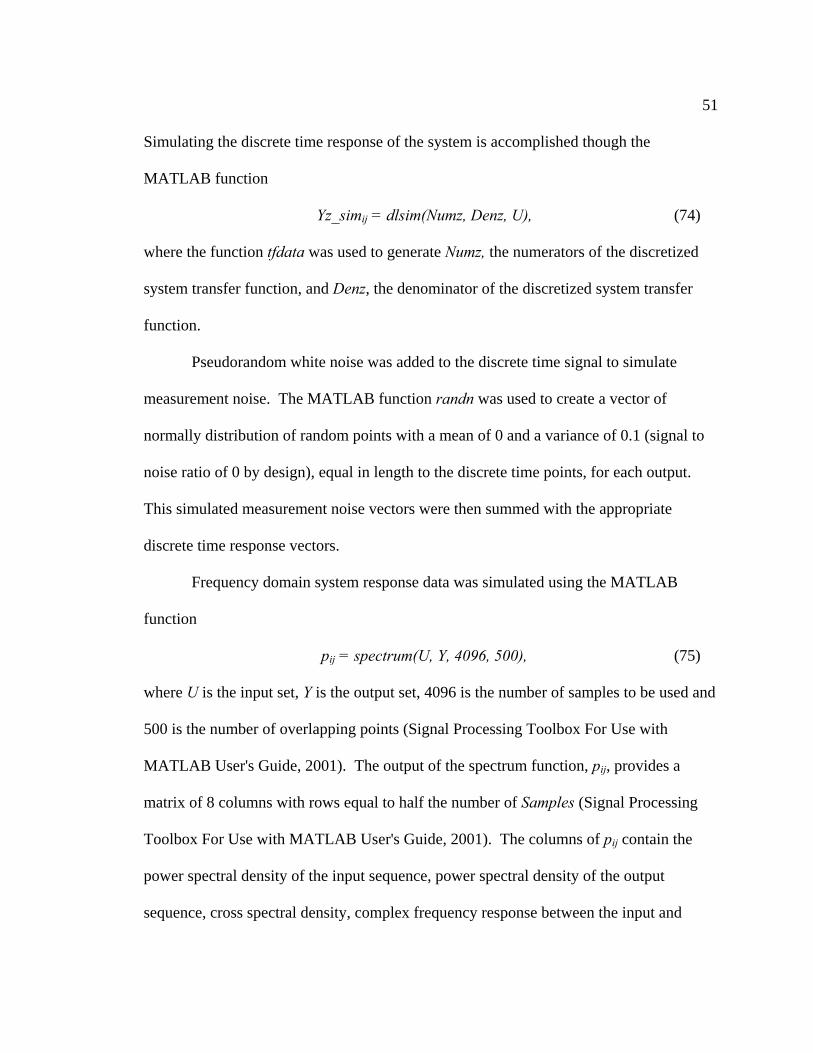
Simulating the discrete time response of the system is accomplished though the
MATLAB function
Yz_simij = dlsim(Numz, Denz, U), (74)
where the function tfdata was used to generate Numz, the numerators of the discretized
system transfer function, and Denz, the denominator of the discretized system transfer
function.
Pseudorandom white noise was added to the discrete time signal to simulate
measurement noise. The MATLAB function randn was used to create a vector of
normally distribution of random points with a mean of 0 and a variance of 0.1 (signal to
noise ratio of 0 by design), equal in length to the discrete time points, for each output.
This simulated measurement noise vectors were then summed with the appropriate
discrete time response vectors.
Frequency domain system response data was simulated using the MATLAB
function
pij = spectrum(U, Y, 4096, 500), (75)
where U is the input set, Y is the output set, 4096 is the number of samples to be used and
500 is the number of overlapping points (Signal Processing Toolbox For Use with
MATLAB User's Guide, 2001). The output of the spectrum function, pij, provides a
matrix of 8 columns with rows equal to half the number of Samples (Signal Processing
Toolbox For Use with MATLAB User's Guide, 2001). The columns of pij contain the
power spectral density of the input sequence, power spectral density of the output
sequence, cross spectral density, complex frequency response between the input and

52
output, coherence function between the input and the output, and confidence intervals for
the input, output and from the input to the output (Signal Processing Toolbox For Use
with MATLAB User's Guide, 2001).
A frequency vector was generated using the Matlab function
omega = linspace(0.001, π/T, 2049). (76)
The frequency vector created 2049 linearly spaced points from 0.001 to π/T (31.4149
radians per second). The first frequency datapoint was selected to be 0.001 rad/s so it
would be close to zero; the final datapoint was selected to be π/T, the half sample
frequency of the system also known as the Nyquist frequency (Medina, November,
1991).
The complex frequency response output of spectrum and the frequency vector
were used to calculate the bode plot of the simulated system. The system with simulated
noise can be compared against the bode plot of the original system in equation (71),
Figure 3-1 through Figure 3-4 to see noise effects. The bode plot of the original system
without noise will also be used to determine the performance of the system ID method
against the noise free case.
53
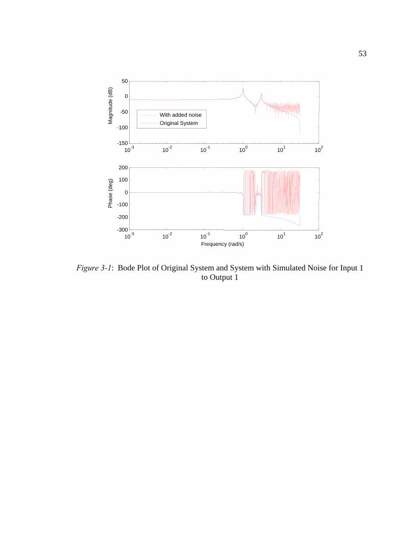
Figure 3-1: Bode Plot of Original System and System with Simulated Noise for Input 1 to Output 1
10 -3 10-2
10-1
100
101
102
-150
-100
-50
0
50
Mag
nitu
de (
dB)
10 -3 10-2
10-1
100
101
102
-300
-200
-100
0
100
200
Pha
se (
deg)
Frequency (rad/s)
With added noise
Original System
54
Figure 3-2: Bode Plot of Original System and System with Simulated Noise for Input 1 to Output 2
10 -3 10-2
10-1
100
101
102
-150
-100
-50
0
50
Mag
nitu
de (
dB)
10 -3 10-2
10-1
100
101
102
-400
-200
0
200
Pha
se (
deg)
Frequency (rad/s)
With added noise
Original System
55
Figure 3-3: Bode Plot of Original System and System with Simulated Noise for Input 2
to Output 1
10 -3 10-2
10-1
100
101
102
-150
-100
-50
0
50
Mag
nitu
de (
dB)
10 -3 10-2
10-1
100
101
102
-200
0
200
400
Pha
se (
deg)
Frequency (rad/s)
With added noise
Original System
56
Figure 3-4: Bode Plot of Original System and System with Simulated Noise for Input 2
to Output 2
3.5.2 Application of Coherence Threshold and TFDC Algorithm
By inspection of Figure 3-1 through Figure 3-4, noise corrupts the computed
frequency response in the higher frequencies, primarily above 3 rad/s. Higher frequency
components that have low magnitude values become highly corrupted with noise
(simulating what would occur in many physical systems with flexible components)
(Fujimori, Nikiforuk, & Koda, 1995). If a model were to be developed through system
ID from this system without applying the coherence threshold, it would be several orders
higher than the original system due to the process attempting to model noise effects
(Fujimori, Nikiforuk, & Koda, 1995), (Thomas, November, 2006). Such a realization
would not only incorporate inaccuracies due to noise, but be computationally expensive
due to the unwanted higher orders.
10 -3 10-2
10-1
100
101
102
-150
-100
-50
0
50
Mag
nitu
de (
dB)
10 -3 10-2
10-1
100
101
102
-300
-200
-100
0
100
200
Pha
se (
deg)
Frequency (rad/s)
With added noise
Original System
57
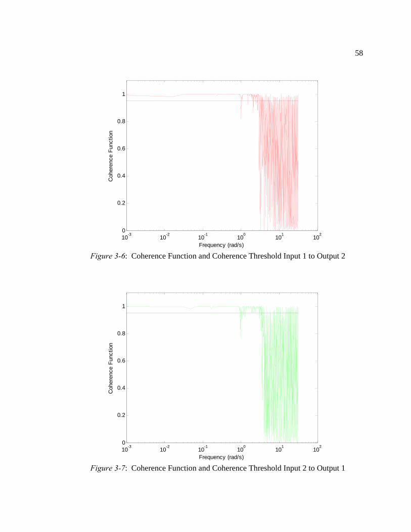
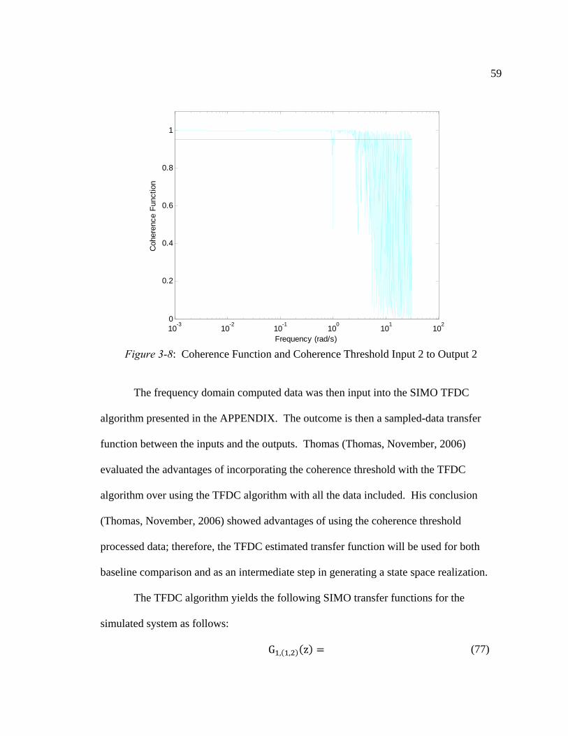
To reduce errors from noise corrupted data, the coherence function was be used to
discard data points as described in Section 3.2. Figure 3-5 through Figure 3-8 display the
coherence function for each input-output pair. By inspection of the coherence plots in
Figure 3-5 through Figure 3-8, an appropriate coherence threshold was selected as per
Thomas (Thomas, November, 2006). The coherence threshold was selected to be 0.950,
resulting in all signal vectors being reduced from 2049 to 136 data points; this resulted in
discarding large sets of higher frequency incoherent data, yet it preserved the highly
coherent data around the poles and at the lower frequencies.
Figure 3-5: Coherence Function and Coherence Threshold Input 1 to Output 1
10-3
10-2
10-1
100
101
102
0
0.2
0.4
0.6
0.8
1
Frequency (rad/s)
Coh
eren
ce F
unct
ion
58
Figure 3-6: Coherence Function and Coherence Threshold Input 1 to Output 2
Figure 3-7: Coherence Function and Coherence Threshold Input 2 to Output 1
10-3
10-2
10-1
100
101
102
0
0.2
0.4
0.6
0.8
1
Frequency (rad/s)
Coh
eren
ce F
unct
ion
10-3
10-2
10-1
100
101
102
0
0.2
0.4
0.6
0.8
1
Frequency (rad/s)
Coh
eren
ce F
unct
ion
59
Figure 3-8: Coherence Function and Coherence Threshold Input 2 to Output 2
The frequency domain computed data was then input into the SIMO TFDC
algorithm presented in the APPENDIX. The outcome is then a sampled-data transfer
function between the inputs and the outputs. Thomas (Thomas, November, 2006)
evaluated the advantages of incorporating the coherence threshold with the TFDC
algorithm over using the TFDC algorithm with all the data included. His conclusion
(Thomas, November, 2006) showed advantages of using the coherence threshold
processed data; therefore, the TFDC estimated transfer function will be used for both
baseline comparison and as an intermediate step in generating a state space realization.
The TFDC algorithm yields the following SIMO transfer functions for the
simulated system as follows:
G , , z (77)
10-3
10-2
10-1
100
101
102
0
0.2
0.4
0.6
0.8
1
Frequency (rad/s)
Coh
eren
ce F
unct
ion
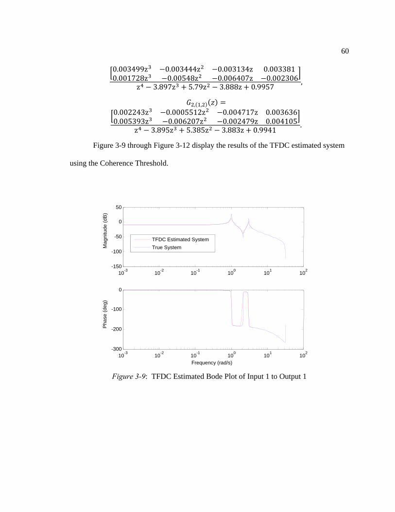
60
0.003499z 0.003444z 0.003134z 0.0033810.001728z 0.00548z 0.006407z 0.002306
z 3.897z 5.79z 3.888z 0.9957,
, ,
0.002243z 0.0005512z 0.004717z 0.0036360.005393z 0.006207z 0.002479z 0.004105
z 3.895z 5.385z 3.883z 0.9941.
Figure 3-9 through Figure 3-12 display the results of the TFDC estimated system
using the Coherence Threshold.
Figure 3-9: TFDC Estimated Bode Plot of Input 1 to Output 1
10 -3 10-2
10-1
100
101
102
-150
-100
-50
0
50
Mag
nitu
de (
dB)
10 -3 10-2
10-1
100
101
102
-300
-200
-100
0
Pha
se (
deg)
Frequency (rad/s)
TFDC Estimated System
True System
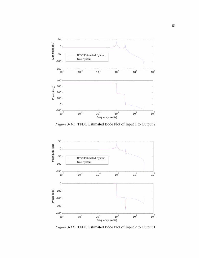
61
Figure 3-10: TFDC Estimated Bode Plot of Input 1 to Output 2
Figure 3-11: TFDC Estimated Bode Plot of Input 2 to Output 1
10-3
10-2
10-1
100
101
10 2-150
-100
-50
0
50
Mag
nitu
de (
dB)
10-3
10-2
10-1
100
101
102
-400
-300
-200
-100
0
Pha
se (
deg)
Frequency (rad/s)
TFDC Estimated System
True System
10 -3 10-2
10-1
100
101
102
-150
-100
-50
0
50
Mag
nitu
de (
dB)
10 -3 10-2
10-1
100
101
102
-100
0
100
200
300
400
Pha
se (
deg)
Frequency (rad/s)
TFDC Estimated System
True System
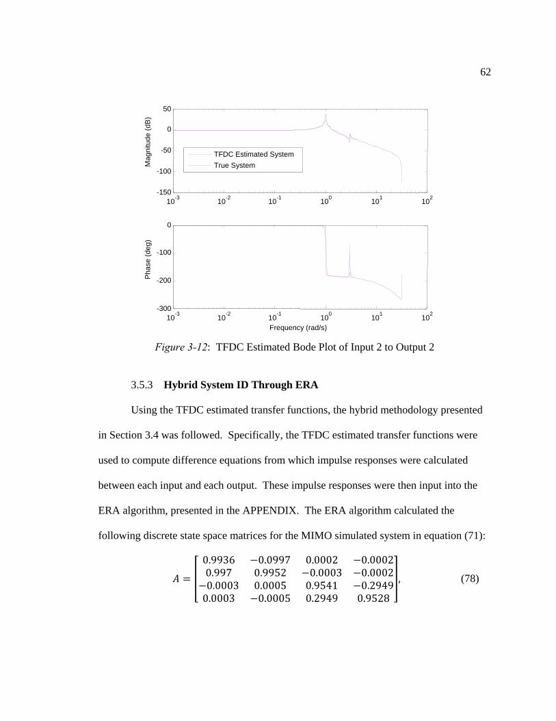
62
Figure 3-12: TFDC Estimated Bode Plot of Input 2 to Output 2
3.5.3 Hybrid System ID Through ERA
Using the TFDC estimated transfer functions, the hybrid methodology presented
in Section 3.4 was followed. Specifically, the TFDC estimated transfer functions were
used to compute difference equations from which impulse responses were calculated
between each input and each output. These impulse responses were then input into the
ERA algorithm, presented in the APPENDIX. The ERA algorithm calculated the
following discrete state space matrices for the MIMO simulated system in equation (71):
0.9936 0.0997 0.0002 0.00020.997 0.9952 0.0003 0.00020.0003 0.0005 0.9541 0.29490.0003 0.0005 0.2949 0.9528
, (78)
10 -3 10-2
10-1
100
101
102
-150
-100
-50
0
50
Mag
nitu
de (
dB)
10 -3 10-2
10-1
100
101
102
-300
-200
-100
0
Pha
se (
deg)
Frequency (rad/s)
TFDC Estimated System
True System

63
0.1105 0.22380.1030 0.22310.1081 0.02300.0962 0.0127
0.1587 0.1496 0.0727 0.06460.2042 0.1950 0.0827 0.0730
,
0.
The bode plot of the ERA realization were then calculated and plotted with the
bode plot of the original system, Figure 3-13 to Figure 3-16. By observation, the hybrid
method appears to effectively estimate the simulated system. By comparing Figure 3-13
to Figure 3-16 to the TFDC estimate, Figure 3-9 through Figure 3-12, it can be observed
that the TFDC estimate effectively models the original system, the estimated system
using ERA post-processing is shown to be equivalent; plus it provides a direct state space
representation.
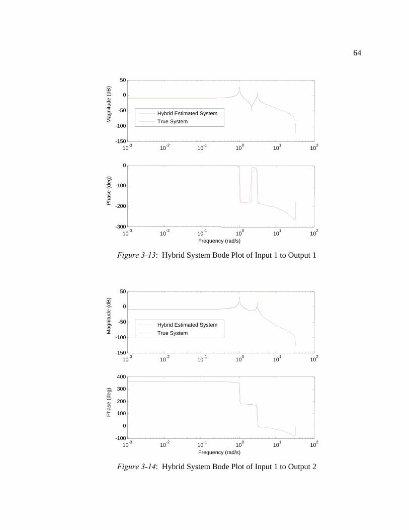
64
Figure 3-13: Hybrid System Bode Plot of Input 1 to Output 1
Figure 3-14: Hybrid System Bode Plot of Input 1 to Output 2
10 -3 10-2
10-1
100
101
102
-150
-100
-50
0
50
Mag
nitu
de (
dB)
10 -3 10-2
10-1
100
101
102
-100
0
100
200
300
400
Pha
se (
deg)
Frequency (rad/s)
Hybrid Estimated System
True System
10 -3 10-2
10-1
100
101
102
-150
-100
-50
0
50
Mag
nitu
de (
dB)
10 -3 10-2
10-1
100
101
102
-300
-200
-100
0
Pha
se (
deg)
Frequency (rad/s)
Hybrid Estimated System
True System

65
Figure 3-15: Hybrid System Bode Plot of Input 2 to Output 1
Figure 3-16: Hybrid System Bode Plot of Input 2 to Output 2
10 -3 10-2
10-1
100
101
102
-150
-100
-50
0
50
Mag
nitu
de (
dB)
10 -3 10-2
10-1
100
101
102
-300
-200
-100
0
Pha
se (
deg)
Frequency (rad/s)
Hybrid Estimated System
True System
10 -3 10-2
10-1
100
101
102
-150
-100
-50
0
50
Mag
nitu
de (
dB)
10 -3 10-2
10-1
100
101
102
-400
-300
-200
-100
0
Pha
se (
deg)
Frequency (rad/s)
Hybrid Estimated System
True System

66
3.5.4 Results Comparison
To quantify the results, an error analysis was made. This enabled comparison
between the TFDC estimated system using the Coherence Threshold to discriminate data
and the final hybrid estimated system from post-processing with ERA. To calculate
error, the bode magnitude of the original system, the TFDC estimated system and the
ERA realization were calculated. With the original simulated system being known,
relative errors are calculated by forming the absolute value of the differences of the
complex true values and the simulated values divided by the magnitude of the true
values. This is shown as follows:
E| |
. (79)
Figure 3-17 through Figure 3-20 display this comparison.
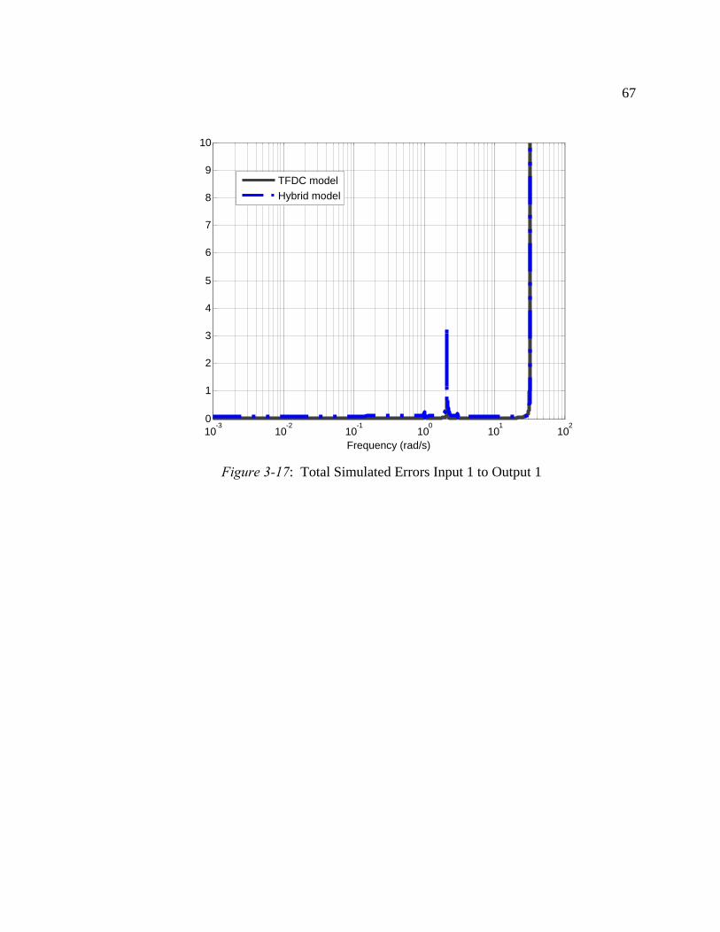
67
Figure 3-17: Total Simulated Errors Input 1 to Output 1
10-3
10 -2 10-1
100
101
102
0
1
2
3
4
5
6
7
8
9
10
Frequency (rad/s)
TFDC model
Hybrid model
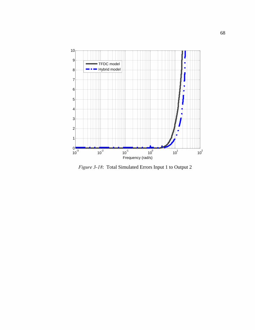
68
Figure 3-18: Total Simulated Errors Input 1 to Output 2
10-3
10 -2 10-1
100
101
102
0
1
2
3
4
5
6
7
8
9
10
Frequency (rad/s)
TFDC model
Hybrid model
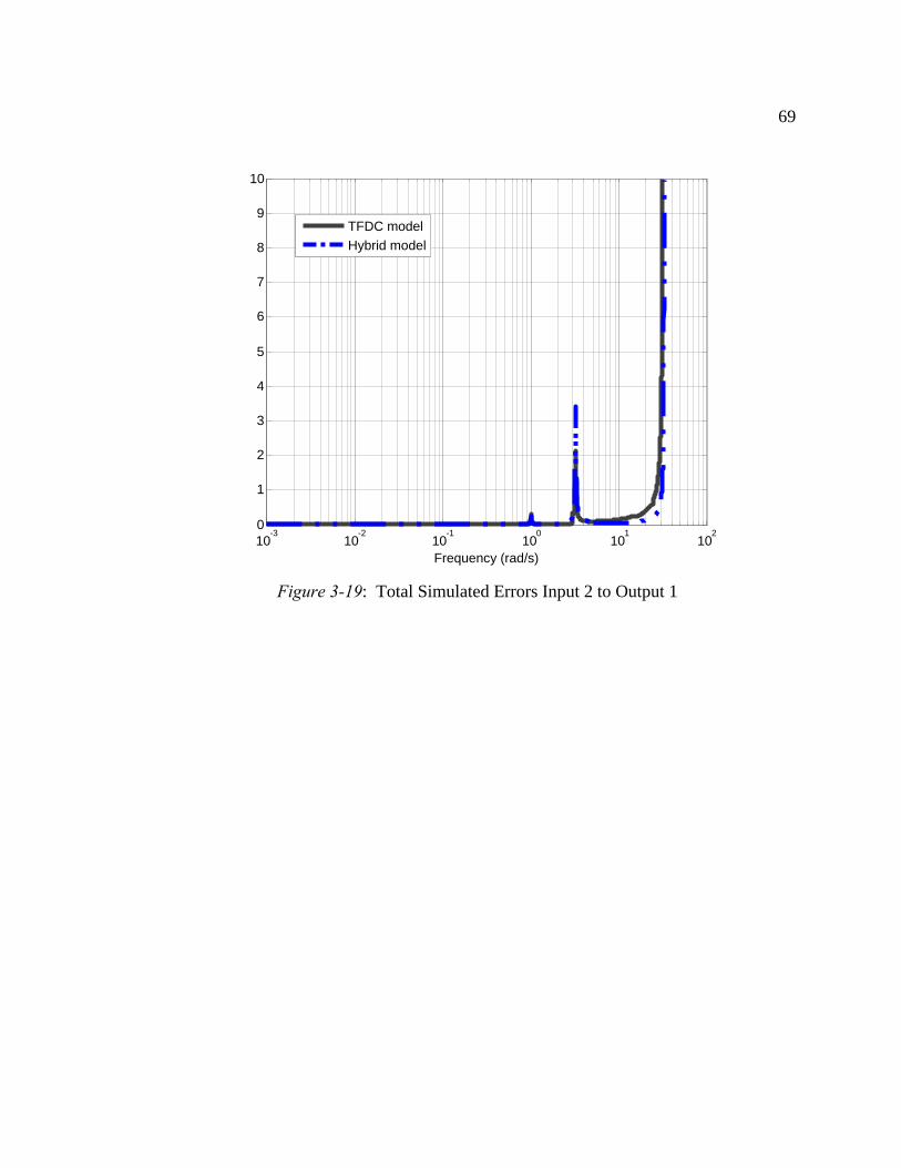
69
Figure 3-19: Total Simulated Errors Input 2 to Output 1
10-3
10 -2 10-1
100
101
102
0
1
2
3
4
5
6
7
8
9
10
Frequency (rad/s)
TFDC model
Hybrid model
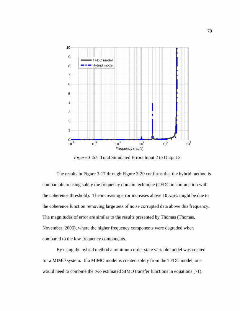
70
Figure 3-20: Total Simulated Errors Input 2 to Output 2
The results in Figure 3-17 through Figure 3-20 confirms that the hybrid method is
comparable to using solely the frequency domain technique (TFDC in conjunction with
the coherence threshold). The increasing error increases above 10 rad/s might be due to
the coherence function removing large sets of noise corrupted data above this frequency.
The magnitudes of error are similar to the results presented by Thomas (Thomas,
November, 2006), where the higher frequency components were degraded when
compared to the low frequency components.
By using the hybrid method a minimum order state variable model was created
for a MIMO system. If a MIMO model is created solely from the TFDC model, one
would need to combine the two estimated SIMO transfer functions in equations (71).
10-3
10-2
10-1
100
101
102
0
1
2
3
4
5
6
7
8
9
10
Frequency (rad/s)
TFDC model
Hybrid model
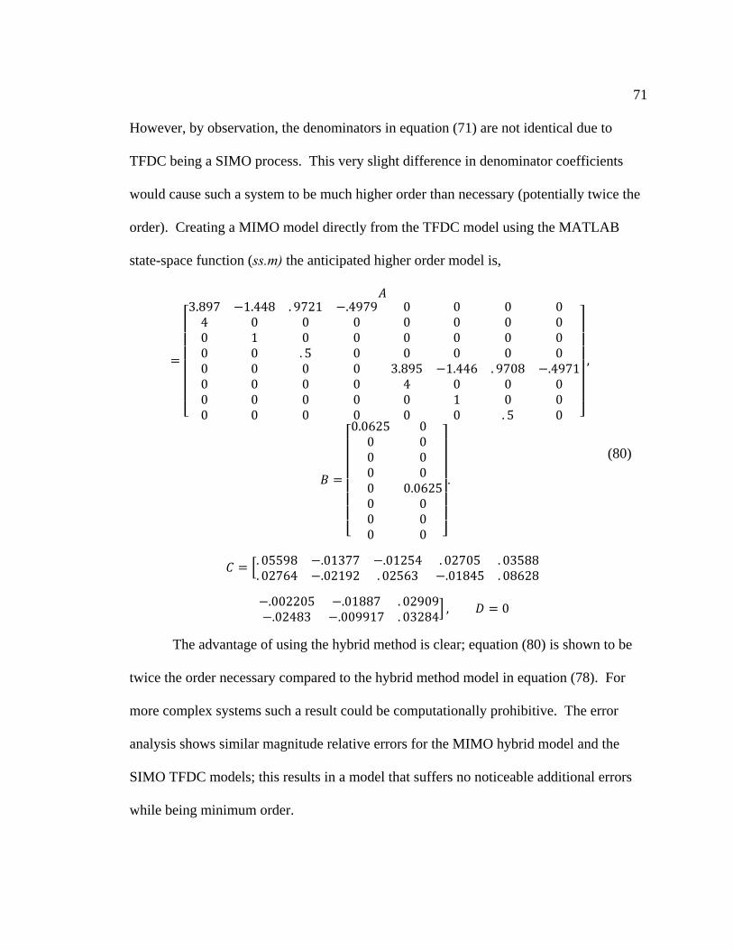
71
However, by observation, the denominators in equation (71) are not identical due to
TFDC being a SIMO process. This very slight difference in denominator coefficients
would cause such a system to be much higher order than necessary (potentially twice the
order). Creating a MIMO model directly from the TFDC model using the MATLAB
state-space function (ss.m) the anticipated higher order model is,
3.897 1.448 . 9721 .4979 0 0 0 04 0 0 0 0 0 0 00 1 0 0 0 0 0 00 0 . 5 0 0 0 0 00 0 0 0 3.895 1.446 . 9708 .49710 0 0 0 4 0 0 00 0 0 0 0 1 0 00 0 0 0 0 0 . 5 0
,
0.0625 00 00 00 00 0.06250 00 00 0
.
. 05598 .01377 .01254 . 02705 . 03588
. 02764 .02192 . 02563 .01845 . 08628
.002205 .01887 . 02909.02483 .009917 . 03284
, 0
(80)
The advantage of using the hybrid method is clear; equation (80) is shown to be
twice the order necessary compared to the hybrid method model in equation (78). For
more complex systems such a result could be computationally prohibitive. The error
analysis shows similar magnitude relative errors for the MIMO hybrid model and the
SIMO TFDC models; this results in a model that suffers no noticeable additional errors
while being minimum order.

72
CHAPTER 4: TEST BED DEMONSTRATION RESULTS USING FLEXLAB
Experimental demonstration of the hybrid system ID methodology on Flexlab was
the selected validation method. Flexlab has been proven effective multiple times for this
purpose, as it presents a platform that is difficult to model by traditional methods (Blinn,
March, 1997), (Strahler, March, 2000), (Saunders, November, 2006), (Thomas,
November, 2006). The validation method consists of collecting a set of MIMO
input/output data from Flexlab and generating a system realization through the hybrid
method outlined in Chapter 3. From the hybrid realization, a state space based controller
is developed and applied to an excited Flexlab with the goal of damping vibrations as
quickly as possible. X-axis and y-axis motors are used to excite Flexlab and x-axis and y-
axis PSD measurements are the outputs, creating a 2 input 2 output system.
4.1 System Excitation and Data Collection
To create a data set for Flexlab, the system was excited separately in both the x
and y axes for 340 seconds with discrete random disturbances. The random signals were
generated from the white noise generator in Flexlab’s LabVIEW interface. The
disturbance signals were input to the system for 340 seconds with a data rate of 100 Hz
giving 34,000 data points. The input signals’ amplitude range was [-4, 4] volts, as
specified by Thomas (Thomas, November, 2006). The input signals used herein have an
x-axis mean of 0.0017 and a y-axis mean of -0.0139. The variance for x-axis was 5.3472
and the variance for the y-axis was 5.3007, with standard deviations for the x-axis of
2.3124 and y-axis of 2.3023 (incidentally these values are comparable to those of Thomas
(Thomas, November, 2006)). The input signals have signal to noise ratios of 0.000735
and -0.006 for x-axis and y-axis respectively.
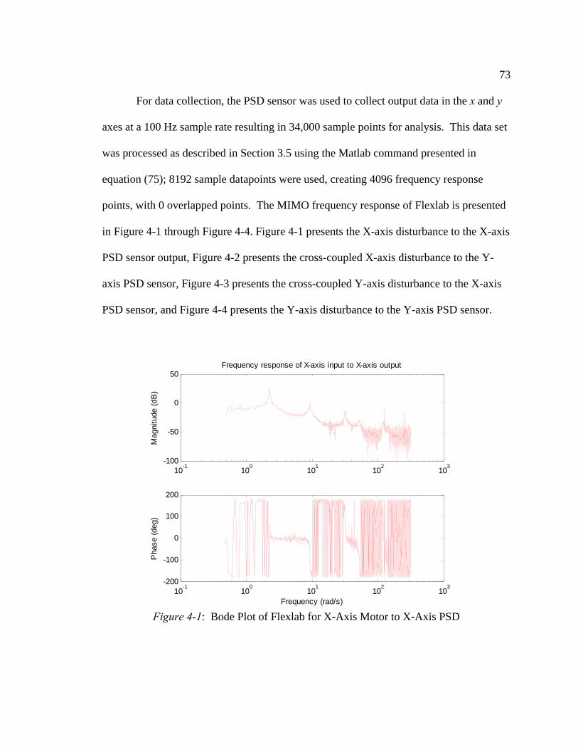
73
For data collection, the PSD sensor was used to collect output data in the x and y
axes at a 100 Hz sample rate resulting in 34,000 sample points for analysis. This data set
was processed as described in Section 3.5 using the Matlab command presented in
equation (75); 8192 sample datapoints were used, creating 4096 frequency response
points, with 0 overlapped points. The MIMO frequency response of Flexlab is presented
in Figure 4-1 through Figure 4-4. Figure 4-1 presents the X-axis disturbance to the X-axis
PSD sensor output, Figure 4-2 presents the cross-coupled X-axis disturbance to the Y-
axis PSD sensor, Figure 4-3 presents the cross-coupled Y-axis disturbance to the X-axis
PSD sensor, and Figure 4-4 presents the Y-axis disturbance to the Y-axis PSD sensor.
Figure 4-1: Bode Plot of Flexlab for X-Axis Motor to X-Axis PSD
10-1
100
101
102
103
-100
-50
0
50
Mag
nitu
de (
dB)
Frequency response of X-axis input to X-axis output
10-1
100
101
102
103
-200
-100
0
100
200
Pha
se (
deg)
Frequency (rad/s)
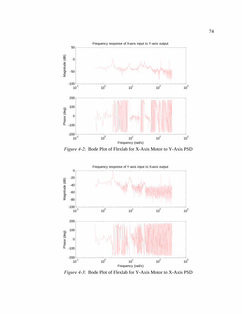
74
Figure 4-2: Bode Plot of Flexlab for X-Axis Motor to Y-Axis PSD
Figure 4-3: Bode Plot of Flexlab for Y-Axis Motor to X-Axis PSD
10-1
100
101
102
103
-100
-50
0
50
Mag
nitu
de (
dB)
Frequency response of X-axis input to Y-axis output
10-1
100
101
102
103
-200
-100
0
100
200
Pha
se (
deg)
Frequency (rad/s)
10-1
100
101
102
103
-100
-80
-60
-40
-20
0
Mag
nitu
de (
dB)
Frequency response of Y-axis input to X-axis output
10-1
100
101
102
103
-200
-100
0
100
200
Pha
se (
deg)
Frequency (rad/s)
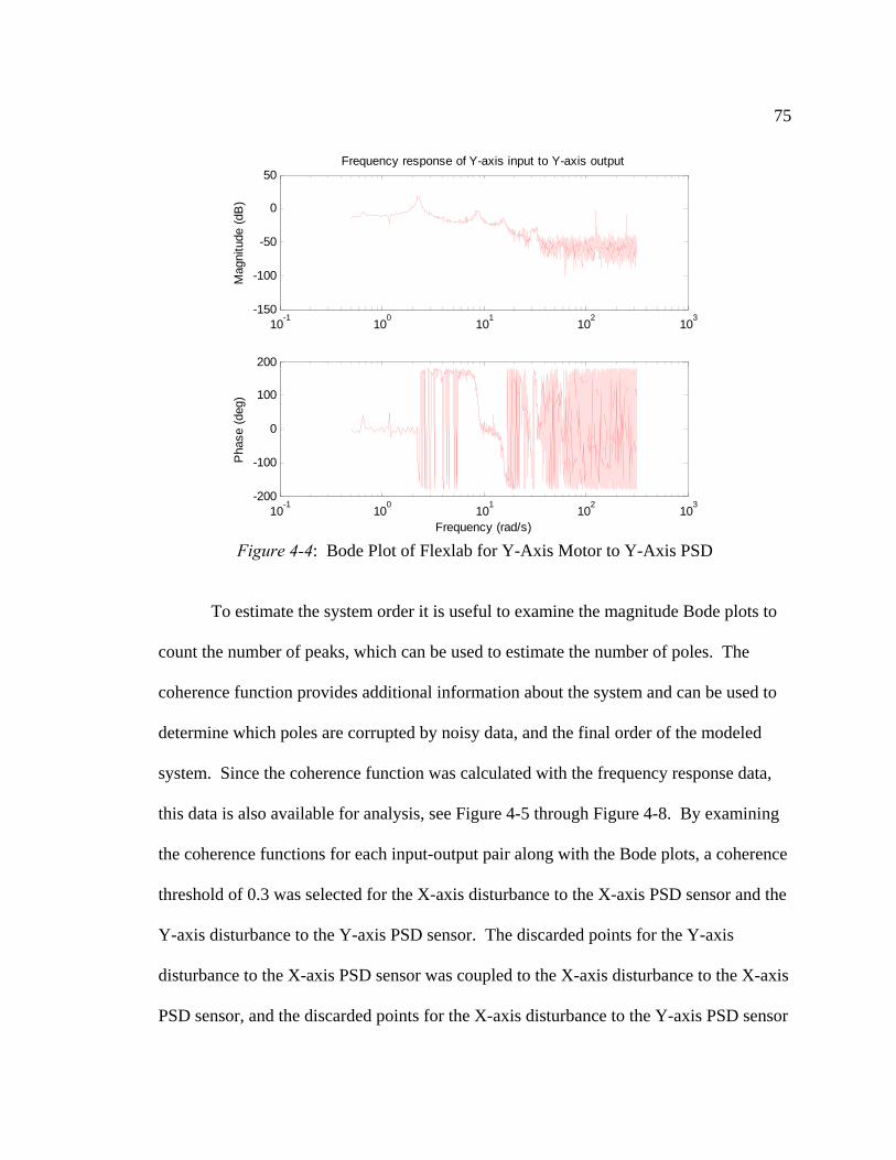
75
Figure 4-4: Bode Plot of Flexlab for Y-Axis Motor to Y-Axis PSD
To estimate the system order it is useful to examine the magnitude Bode plots to
count the number of peaks, which can be used to estimate the number of poles. The
coherence function provides additional information about the system and can be used to
determine which poles are corrupted by noisy data, and the final order of the modeled
system. Since the coherence function was calculated with the frequency response data,
this data is also available for analysis, see Figure 4-5 through Figure 4-8. By examining
the coherence functions for each input-output pair along with the Bode plots, a coherence
threshold of 0.3 was selected for the X-axis disturbance to the X-axis PSD sensor and the
Y-axis disturbance to the Y-axis PSD sensor. The discarded points for the Y-axis
disturbance to the X-axis PSD sensor was coupled to the X-axis disturbance to the X-axis
PSD sensor, and the discarded points for the X-axis disturbance to the Y-axis PSD sensor
10-1
100
101
102
103
-150
-100
-50
0
50
Mag
nitu
de (
dB)
Frequency response of Y-axis input to Y-axis output
10-1
100
101
102
103
-200
-100
0
100
200
Pha
se (
deg)
Frequency (rad/s)
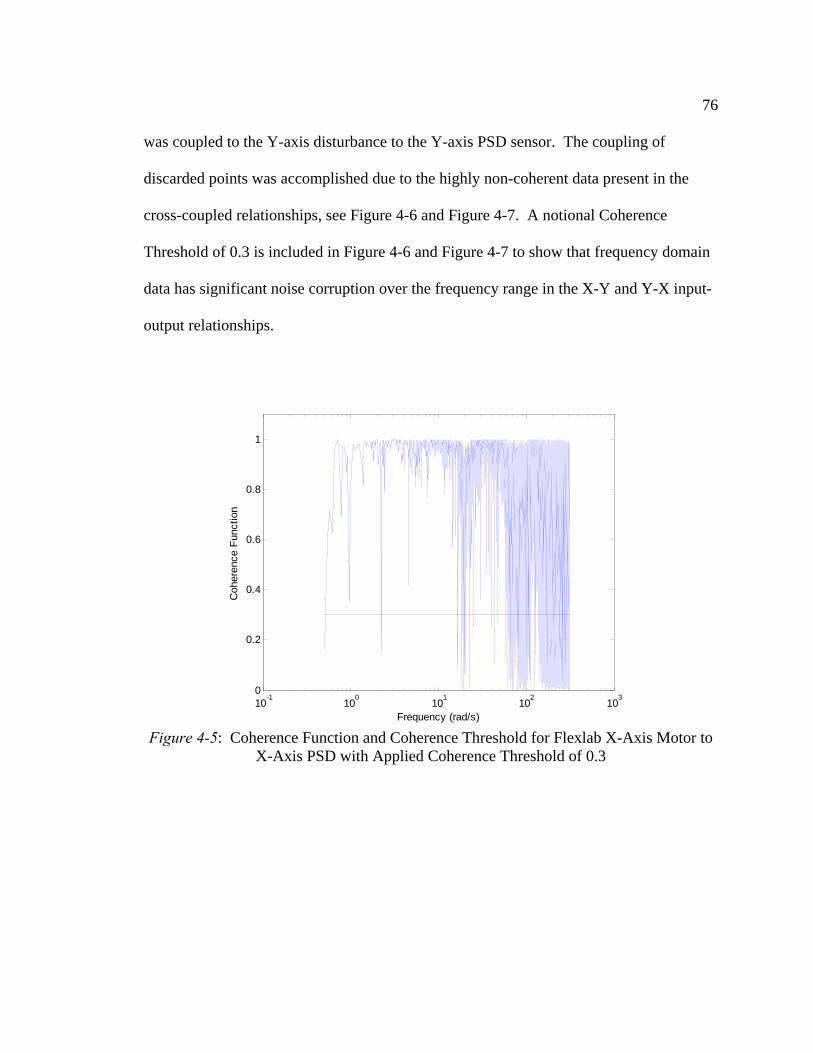
76
was coupled to the Y-axis disturbance to the Y-axis PSD sensor. The coupling of
discarded points was accomplished due to the highly non-coherent data present in the
cross-coupled relationships, see Figure 4-6 and Figure 4-7. A notional Coherence
Threshold of 0.3 is included in Figure 4-6 and Figure 4-7 to show that frequency domain
data has significant noise corruption over the frequency range in the X-Y and Y-X input-
output relationships.
Figure 4-5: Coherence Function and Coherence Threshold for Flexlab X-Axis Motor to
X-Axis PSD with Applied Coherence Threshold of 0.3
10-1
100
101
102
103
0
0.2
0.4
0.6
0.8
1
Frequency (rad/s)
Coh
eren
ce F
unct
ion
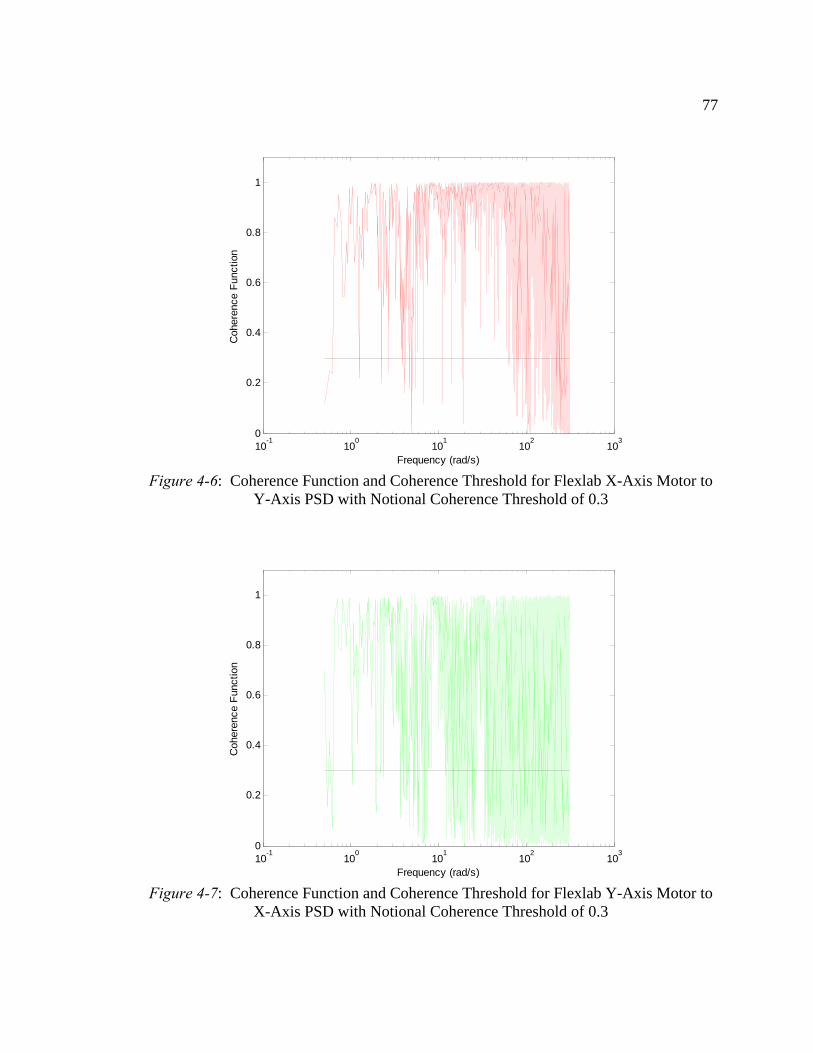
77
Figure 4-6: Coherence Function and Coherence Threshold for Flexlab X-Axis Motor to
Y-Axis PSD with Notional Coherence Threshold of 0.3
Figure 4-7: Coherence Function and Coherence Threshold for Flexlab Y-Axis Motor to
X-Axis PSD with Notional Coherence Threshold of 0.3
10-1
100
101
102
103
0
0.2
0.4
0.6
0.8
1
Frequency (rad/s)
Coh
eren
ce F
unct
ion
10-1
100
101
102
103
0
0.2
0.4
0.6
0.8
1
Frequency (rad/s)
Coh
eren
ce F
unct
ion
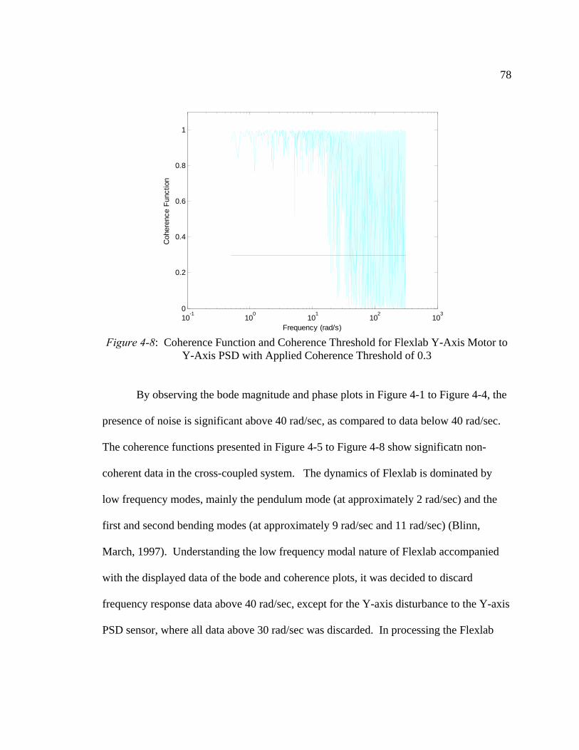
78
Figure 4-8: Coherence Function and Coherence Threshold for Flexlab Y-Axis Motor to
Y-Axis PSD with Applied Coherence Threshold of 0.3
By observing the bode magnitude and phase plots in Figure 4-1 to Figure 4-4, the
presence of noise is significant above 40 rad/sec, as compared to data below 40 rad/sec.
The coherence functions presented in Figure 4-5 to Figure 4-8 show significatn non-
coherent data in the cross-coupled system. The dynamics of Flexlab is dominated by
low frequency modes, mainly the pendulum mode (at approximately 2 rad/sec) and the
first and second bending modes (at approximately 9 rad/sec and 11 rad/sec) (Blinn,
March, 1997). Understanding the low frequency modal nature of Flexlab accompanied
with the displayed data of the bode and coherence plots, it was decided to discard
frequency response data above 40 rad/sec, except for the Y-axis disturbance to the Y-axis
PSD sensor, where all data above 30 rad/sec was discarded. In processing the Flexlab
10-1
100
101
102
103
0
0.2
0.4
0.6
0.8
1
Frequency (rad/s)
Coh
eren
ce F
unct
ion
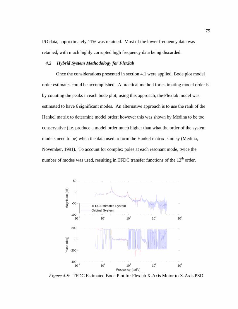
79
I/O data, approximately 11% was retained. Most of the lower frequency data was
retained, with much highly corrupted high frequency data being discarded.
4.2 Hybrid System Methodology for Flexlab
Once the considerations presented in section 4.1 were applied, Bode plot model
order estimates could be accomplished. A practical method for estimating model order is
by counting the peaks in each bode plot; using this approach, the Flexlab model was
estimated to have 6 significant modes. An alternative approach is to use the rank of the
Hankel matrix to determine model order; however this was shown by Medina to be too
conservative (i.e. produce a model order much higher than what the order of the system
models need to be) when the data used to form the Hankel matrix is noisy (Medina,
November, 1991). To account for complex poles at each resonant mode, twice the
number of modes was used, resulting in TFDC transfer functions of the 12th order.
Figure 4-9: TFDC Estimated Bode Plot for Flexlab X-Axis Motor to X-Axis PSD
10-1
100
101
102
103
-100
-50
0
50
Mag
nitu
de (
dB)
10-1
100
101
102
103
-400
-200
0
200
Pha
se (
deg)
Frequency (rad/s)
TFDC Estimated System
Original System

80
Figure 4-10: TFDC Estimated Bode Plot for Flexlab X-Axis Motor to Y-Axis PSD
Figure 4-11: TFDC Estimated Bode Plot for Flexlab Y-Axis Motor to X-Axis PSD
10-1
100
101
102
103
-100
-80
-60
-40
-20
0
Mag
nitu
de (
dB)
10-1
100
101
102
103
-1000
-500
0
500
Pha
se (
deg)
Frequency (rad/s)
TFDC Estimated System
Original System
10-1
100
101
102
103
-100
-50
0
50
Mag
nitu
de (
dB)
10-1
100
101
102
103
-1000
-500
0
500
Pha
se (
deg)
Frequency (rad/s)
TFDC Estimated System
Original System
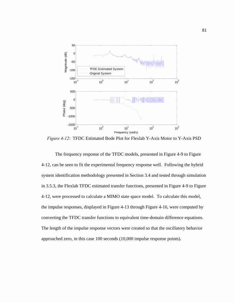
81
Figure 4-12: TFDC Estimated Bode Plot for Flexlab Y-Axis Motor to Y-Axis PSD
The frequency response of the TFDC models, presented in Figure 4-9 to Figure
4-12, can be seen to fit the experimental frequency response well. Following the hybrid
system identification methodology presented in Section 3.4 and tested through simulation
in 3.5.3, the Flexlab TFDC estimated transfer functions, presented in Figure 4-9 to Figure
4-12, were processed to calculate a MIMO state space model. To calculate this model,
the impulse responses, displayed in Figure 4-13 through Figure 4-16, were computed by
converting the TFDC transfer functions to equivalent time-domain difference equations.
The length of the impulse response vectors were created so that the oscillatory behavior
approached zero, in this case 100 seconds (10,000 impulse response points).
10-1
100
101
102
103
-150
-100
-50
0
50
Mag
nitu
de (
dB)
10-1
100
101
102
103
-1500
-1000
-500
0
500
Pha
se (
deg)
Frequency (rad/s)
TFDC Estimated System
Original System
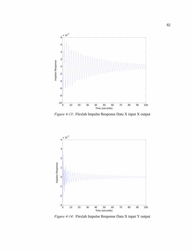
82
Figure 4-13: Flexlab Impulse Response Data X input X output
Figure 4-14: Flexlab Impulse Response Data X input Y output
0 10 20 30 40 50 60 70 80 90 100-10
-8
-6
-4
-2
0
2
4
6
8x 10
-3
Time (seconds)
Impu
lse
Res
pons
e
0 10 20 30 40 50 60 70 80 90 100-3
-2
-1
0
1
2
3
4x 10
-3
Time (seconds)
Impu
lse
Res
pons
e
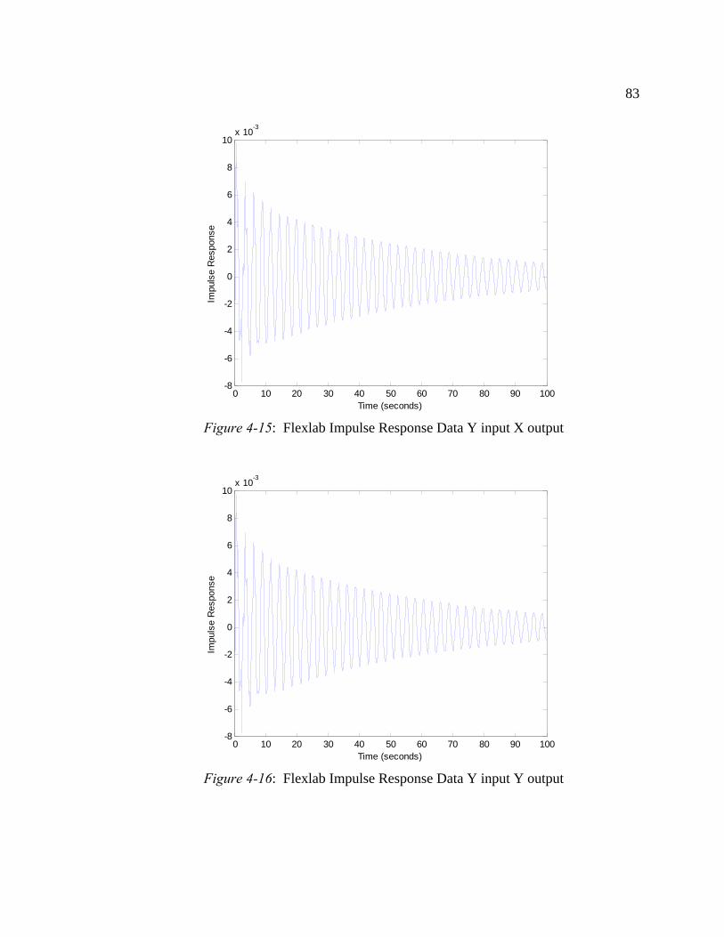
83
Figure 4-15: Flexlab Impulse Response Data Y input X output
Figure 4-16: Flexlab Impulse Response Data Y input Y output
0 10 20 30 40 50 60 70 80 90 100-8
-6
-4
-2
0
2
4
6
8
10x 10
-3
Time (seconds)
Impu
lse
Res
pons
e
0 10 20 30 40 50 60 70 80 90 100-8
-6
-4
-2
0
2
4
6
8
10x 10
-3
Time (seconds)
Impu
lse
Res
pons
e
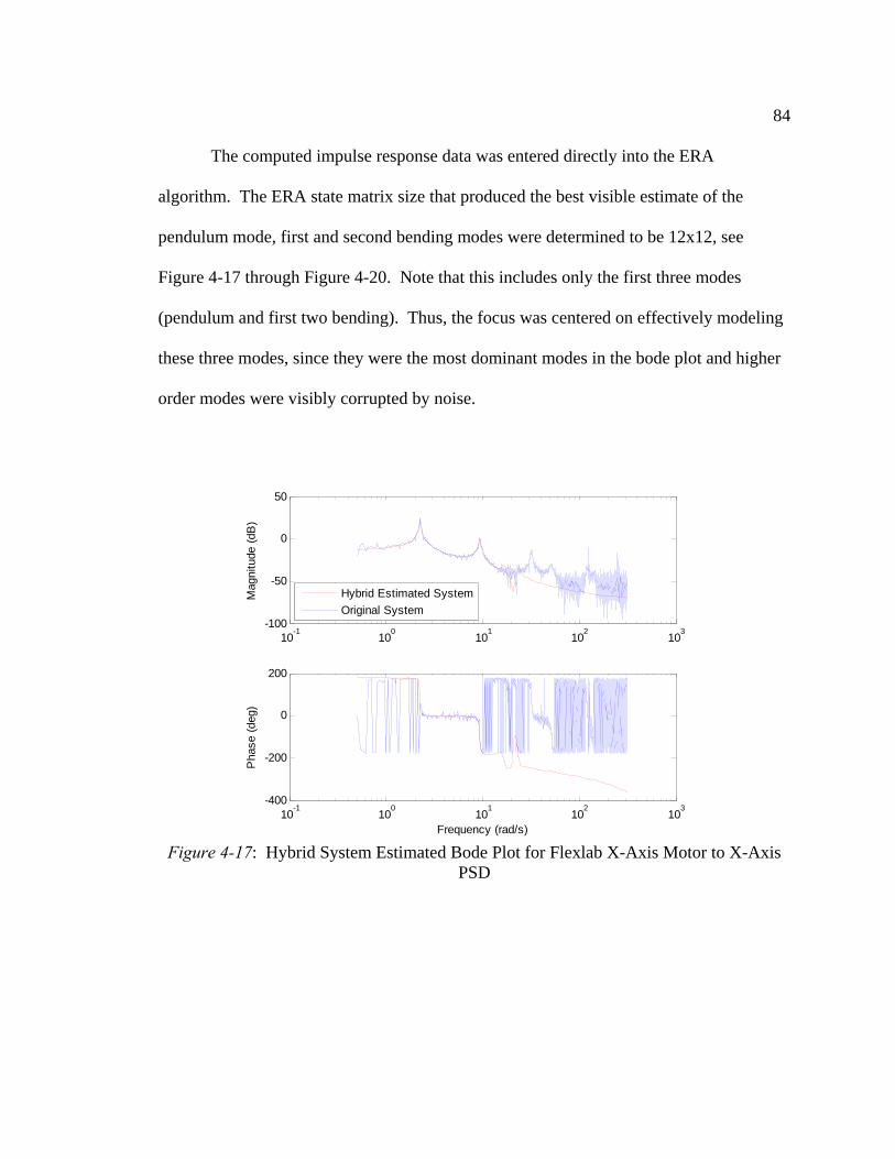
84
The computed impulse response data was entered directly into the ERA
algorithm. The ERA state matrix size that produced the best visible estimate of the
pendulum mode, first and second bending modes were determined to be 12x12, see
Figure 4-17 through Figure 4-20. Note that this includes only the first three modes
(pendulum and first two bending). Thus, the focus was centered on effectively modeling
these three modes, since they were the most dominant modes in the bode plot and higher
order modes were visibly corrupted by noise.
Figure 4-17: Hybrid System Estimated Bode Plot for Flexlab X-Axis Motor to X-Axis
PSD
10-1
100
101
102
103
-100
-50
0
50
Mag
nitu
de (
dB)
10-1
100
101
102
103
-400
-200
0
200
Pha
se (
deg)
Frequency (rad/s)
Hybrid Estimated System
Original System

85
Figure 4-18: Hybrid System Estimated Bode Plot for Flexlab X-Axis Motor to Y-Axis
PSD
Figure 4-19: Hybrid System Estimated Bode Plot for Flexlab Y-Axis Motor to X-Axis
PSD
10-1
100
101
102
103
-100
-50
0
50
Mag
nitu
de (
dB)
10-1
100
101
102
103
-800
-600
-400
-200
0
200
Pha
se (
deg)
Frequency (rad/s)
Hybrid Estimated System
Original System
10-1
100
101
102
103
-100
-50
0
50
Mag
nitu
de (
dB)
10-1
100
101
102
103
-800
-600
-400
-200
0
200
Pha
se (
deg)
Frequency (rad/s)
Hybrid Estimated System
Original System
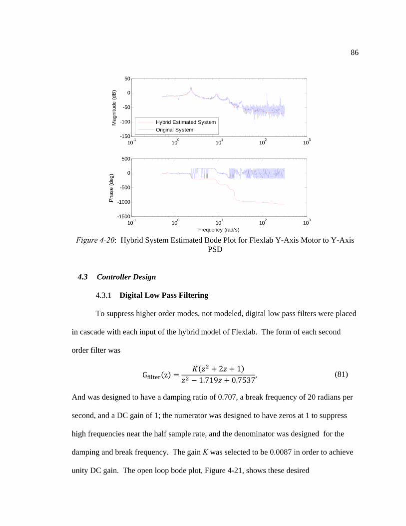
86
Figure 4-20: Hybrid System Estimated Bode Plot for Flexlab Y-Axis Motor to Y-Axis
PSD
4.3 Controller Design
4.3.1 Digital Low Pass Filtering
To suppress higher order modes, not modeled, digital low pass filters were placed
in cascade with each input of the hybrid model of Flexlab. The form of each second
order filter was
G z2 1
1.719 0.7537, (81)
And was designed to have a damping ratio of 0.707, a break frequency of 20 radians per
second, and a DC gain of 1; the numerator was designed to have zeros at 1 to suppress
high frequencies near the half sample rate, and the denominator was designed for the
damping and break frequency. The gain K was selected to be 0.0087 in order to achieve
unity DC gain. The open loop bode plot, Figure 4-21, shows these desired
10-1
100
101
102
103
-150
-100
-50
0
50
Mag
nitu
de (
dB)
10-1
100
101
102
103
-1500
-1000
-500
0
500
Pha
se (
deg)
Frequency (rad/s)
Hybrid Estimated System
Original System
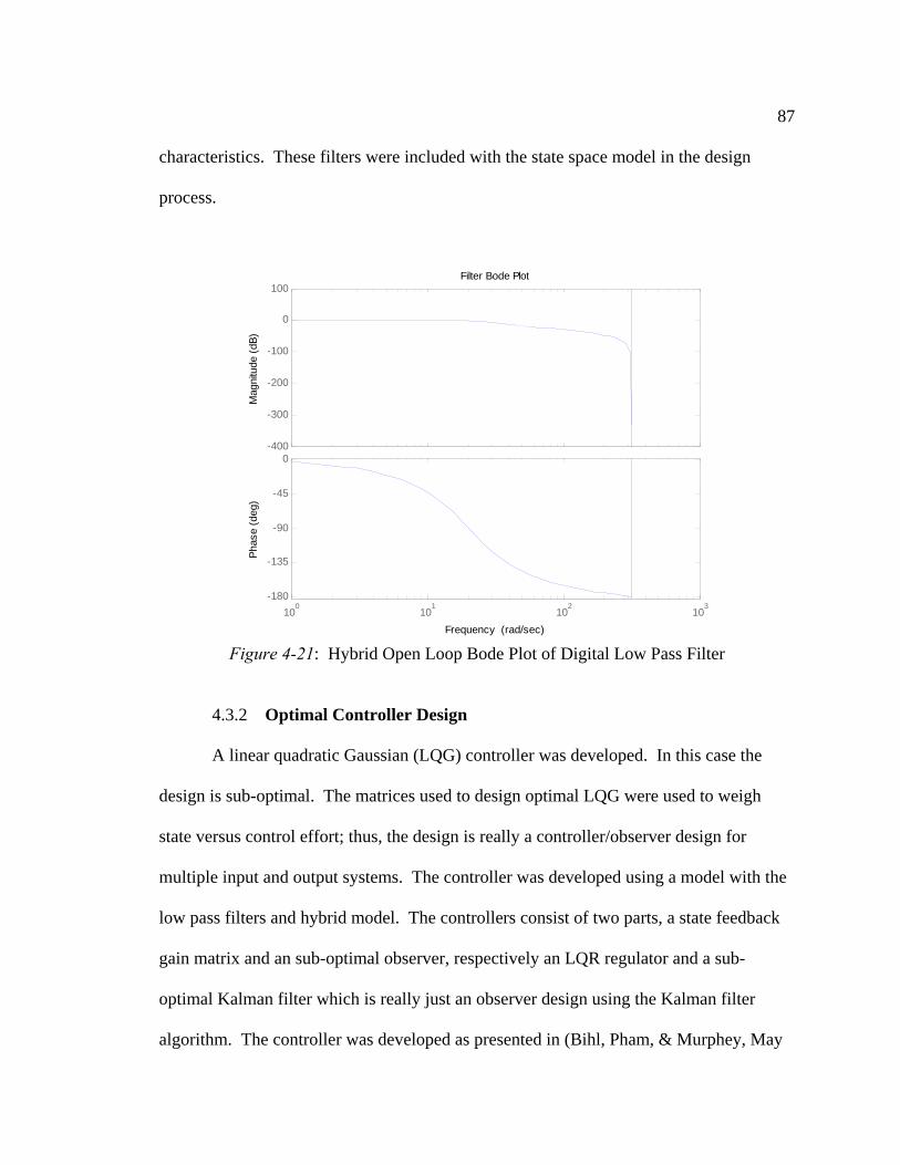
87
characteristics. These filters were included with the state space model in the design
process.
Figure 4-21: Hybrid Open Loop Bode Plot of Digital Low Pass Filter
4.3.2 Optimal Controller Design
A linear quadratic Gaussian (LQG) controller was developed. In this case the
design is sub-optimal. The matrices used to design optimal LQG were used to weigh
state versus control effort; thus, the design is really a controller/observer design for
multiple input and output systems. The controller was developed using a model with the
low pass filters and hybrid model. The controllers consist of two parts, a state feedback
gain matrix and an sub-optimal observer, respectively an LQR regulator and a sub-
optimal Kalman filter which is really just an observer design using the Kalman filter
algorithm. The controller was developed as presented in (Bihl, Pham, & Murphey, May
-400
-300
-200
-100
0
100
Mag
nitu
de (
dB)
100
101
102
103
-180
-135
-90
-45
0
Pha
se (
deg)
Filter Bode Plot
Frequency (rad/sec)
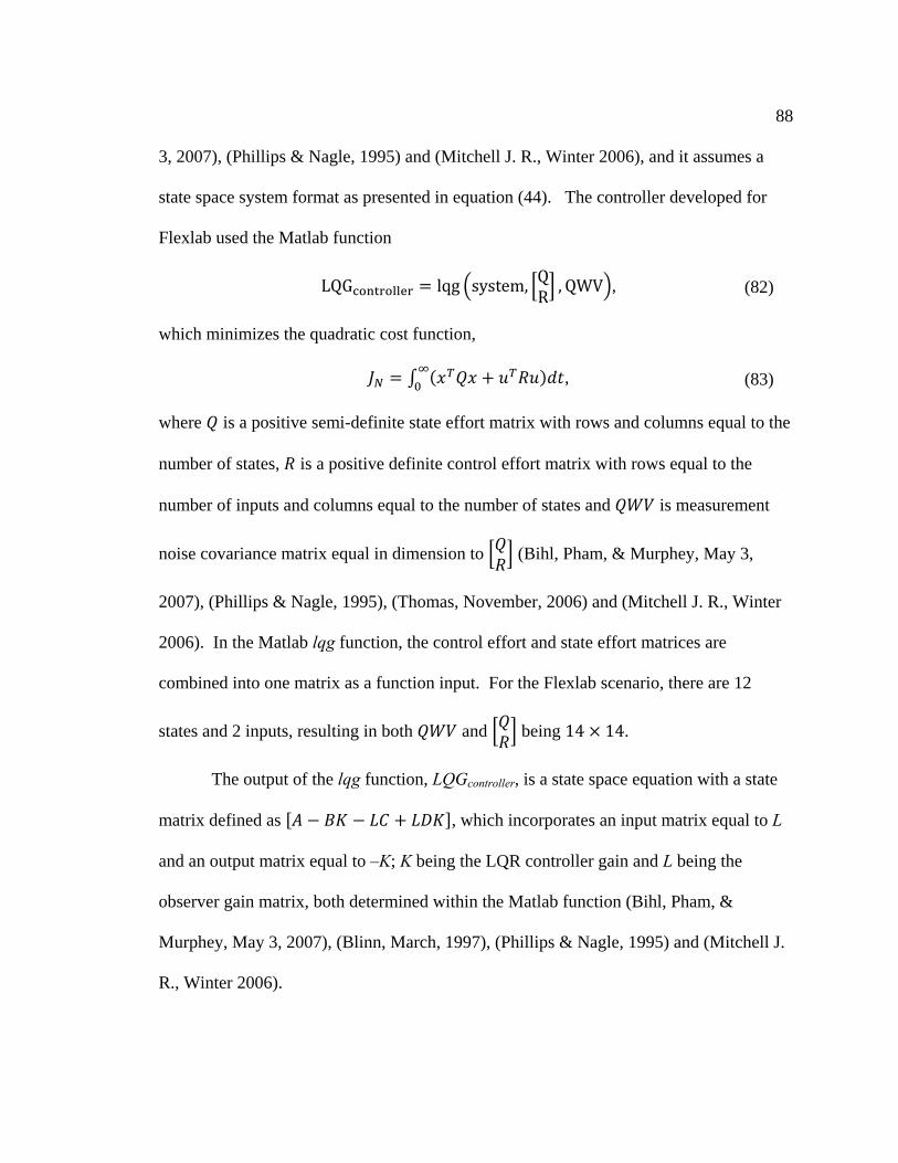
88
3, 2007), (Phillips & Nagle, 1995) and (Mitchell J. R., Winter 2006), and it assumes a
state space system format as presented in equation (44). The controller developed for
Flexlab used the Matlab function
LQG lqg system,QR, QWV , (82)
which minimizes the quadratic cost function,
, (83)
where is a positive semi-definite state effort matrix with rows and columns equal to the
number of states, is a positive definite control effort matrix with rows equal to the
number of inputs and columns equal to the number of states and is measurement
noise covariance matrix equal in dimension to (Bihl, Pham, & Murphey, May 3,
2007), (Phillips & Nagle, 1995), (Thomas, November, 2006) and (Mitchell J. R., Winter
2006). In the Matlab lqg function, the control effort and state effort matrices are
combined into one matrix as a function input. For the Flexlab scenario, there are 12
states and 2 inputs, resulting in both and being 14 14.
The output of the lqg function, LQGcontroller, is a state space equation with a state
matrix defined as , which incorporates an input matrix equal to L
and an output matrix equal to –K; K being the LQR controller gain and L being the
observer gain matrix, both determined within the Matlab function (Bihl, Pham, &
Murphey, May 3, 2007), (Blinn, March, 1997), (Phillips & Nagle, 1995) and (Mitchell J.
R., Winter 2006).
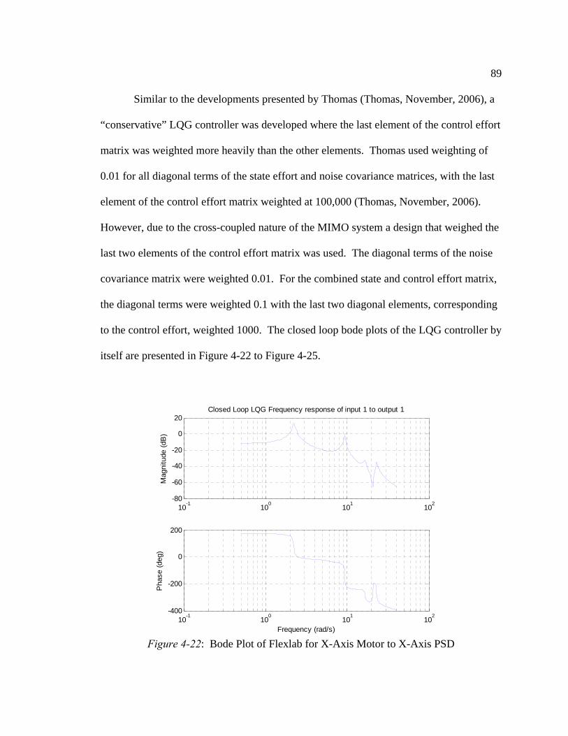
89
Similar to the developments presented by Thomas (Thomas, November, 2006), a
“conservative” LQG controller was developed where the last element of the control effort
matrix was weighted more heavily than the other elements. Thomas used weighting of
0.01 for all diagonal terms of the state effort and noise covariance matrices, with the last
element of the control effort matrix weighted at 100,000 (Thomas, November, 2006).
However, due to the cross-coupled nature of the MIMO system a design that weighed the
last two elements of the control effort matrix was used. The diagonal terms of the noise
covariance matrix were weighted 0.01. For the combined state and control effort matrix,
the diagonal terms were weighted 0.1 with the last two diagonal elements, corresponding
to the control effort, weighted 1000. The closed loop bode plots of the LQG controller by
itself are presented in Figure 4-22 to Figure 4-25.
Figure 4-22: Bode Plot of Flexlab for X-Axis Motor to X-Axis PSD
10-1
100
101
102
-80
-60
-40
-20
0
20
Mag
nitu
de (
dB)
Closed Loop LQG Frequency response of input 1 to output 1
10-1
100
101
102
-400
-200
0
200
Pha
se (
deg)
Frequency (rad/s)
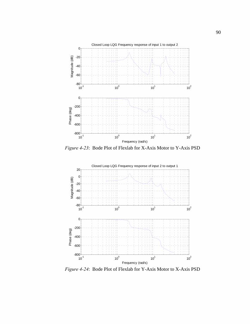
90
Figure 4-23: Bode Plot of Flexlab for X-Axis Motor to Y-Axis PSD
Figure 4-24: Bode Plot of Flexlab for Y-Axis Motor to X-Axis PSD
10-1
100
101
102
-80
-60
-40
-20
0
Mag
nitu
de (
dB)
Closed Loop LQG Frequency response of input 1 to output 2
10-1
100
101
102
-800
-600
-400
-200
0
Pha
se (
deg)
Frequency (rad/s)
10-1
100
101
102
-80
-60
-40
-20
0
20
Mag
nitu
de (
dB)
Closed Loop LQG Frequency response of input 2 to output 1
10-1
100
101
102
-800
-600
-400
-200
0
Pha
se (
deg)
Frequency (rad/s)
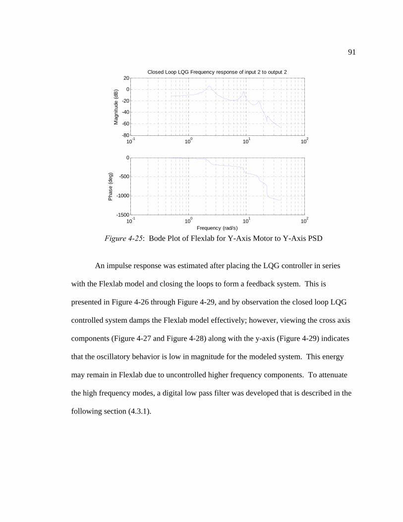
91
Figure 4-25: Bode Plot of Flexlab for Y-Axis Motor to Y-Axis PSD
An impulse response was estimated after placing the LQG controller in series
with the Flexlab model and closing the loops to form a feedback system. This is
presented in Figure 4-26 through Figure 4-29, and by observation the closed loop LQG
controlled system damps the Flexlab model effectively; however, viewing the cross axis
components (Figure 4-27 and Figure 4-28) along with the y-axis (Figure 4-29) indicates
that the oscillatory behavior is low in magnitude for the modeled system. This energy
may remain in Flexlab due to uncontrolled higher frequency components. To attenuate
the high frequency modes, a digital low pass filter was developed that is described in the
following section (4.3.1).
10-1
100
101
102
-80
-60
-40
-20
0
20
Mag
nitu
de (
dB)
Closed Loop LQG Frequency response of input 2 to output 2
10-1
100
101
102
-1500
-1000
-500
0
Pha
se (
deg)
Frequency (rad/s)
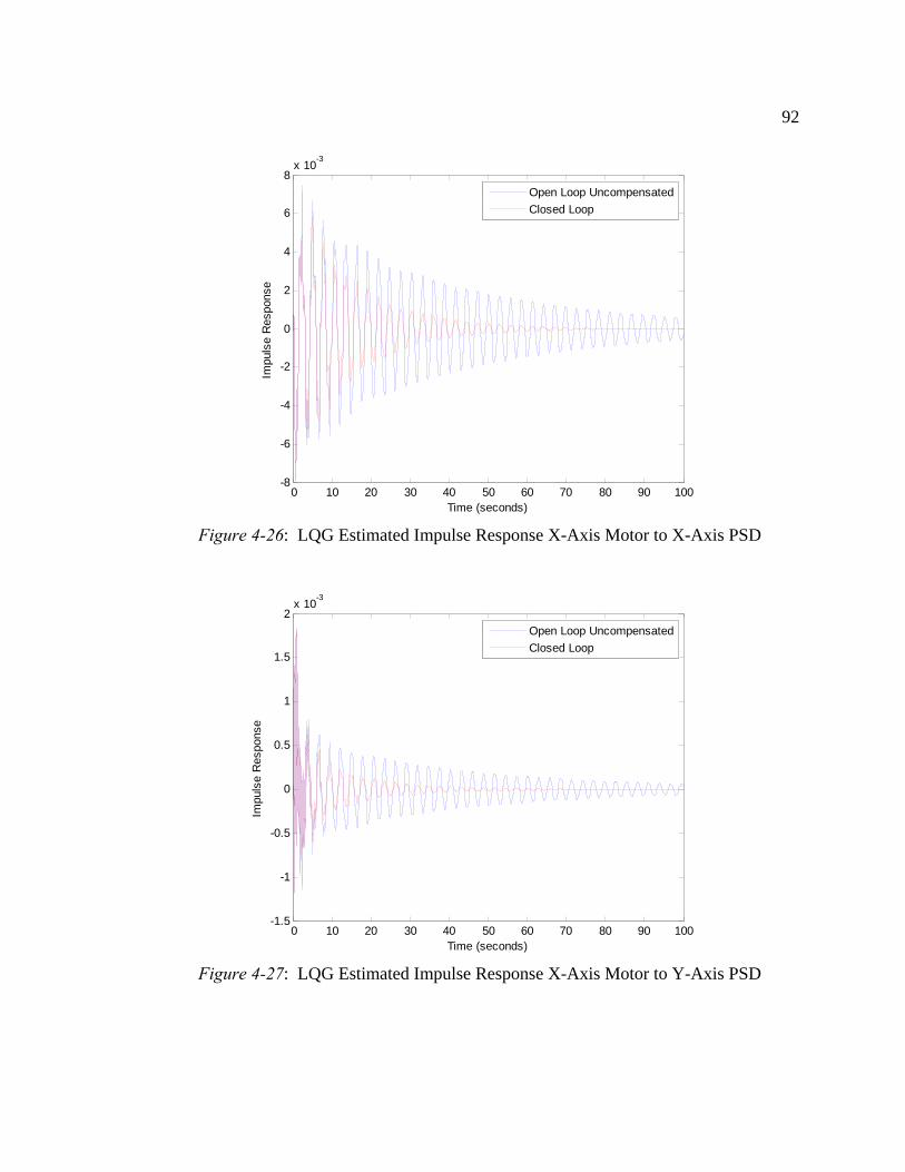
92
Figure 4-26: LQG Estimated Impulse Response X-Axis Motor to X-Axis PSD
Figure 4-27: LQG Estimated Impulse Response X-Axis Motor to Y-Axis PSD
0 10 20 30 40 50 60 70 80 90 100-8
-6
-4
-2
0
2
4
6
8x 10
-3
Time (seconds)
Impu
lse
Res
pons
e
Open Loop Uncompensated
Closed Loop
0 10 20 30 40 50 60 70 80 90 100-1.5
-1
-0.5
0
0.5
1
1.5
2x 10
-3
Time (seconds)
Impu
lse
Res
pons
e
Open Loop Uncompensated
Closed Loop
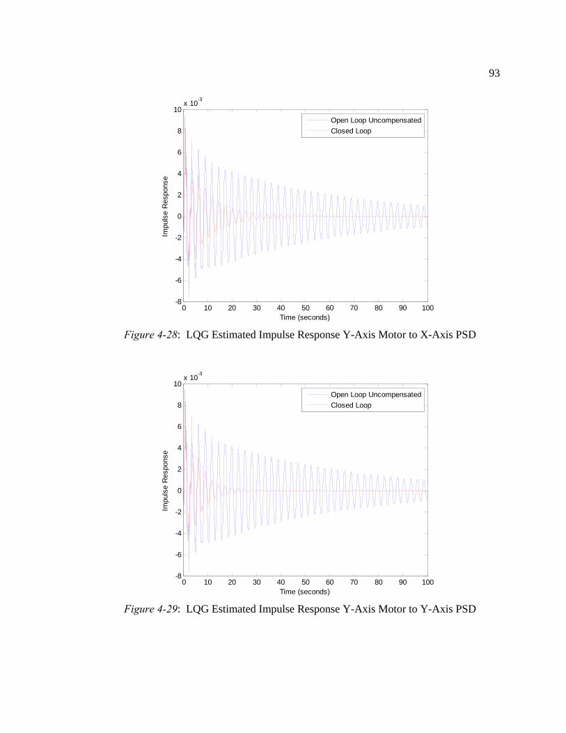
93
Figure 4-28: LQG Estimated Impulse Response Y-Axis Motor to X-Axis PSD
Figure 4-29: LQG Estimated Impulse Response Y-Axis Motor to Y-Axis PSD
0 10 20 30 40 50 60 70 80 90 100-8
-6
-4
-2
0
2
4
6
8
10x 10
-3
Time (seconds)
Impu
lse
Res
pons
e
Open Loop Uncompensated
Closed Loop
0 10 20 30 40 50 60 70 80 90 100-8
-6
-4
-2
0
2
4
6
8
10x 10
-3
Time (seconds)
Impu
lse
Res
pons
e
Open Loop Uncompensated
Closed Loop
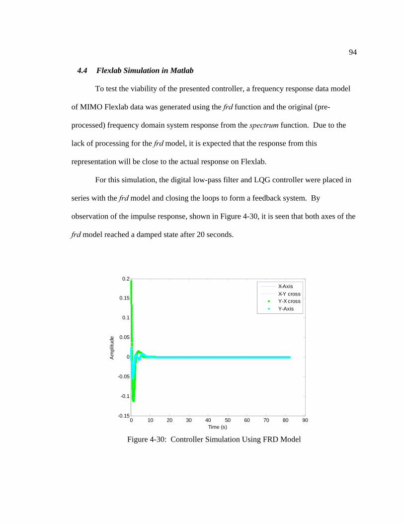
94
4.4 Flexlab Simulation in Matlab
To test the viability of the presented controller, a frequency response data model
of MIMO Flexlab data was generated using the frd function and the original (pre-
processed) frequency domain system response from the spectrum function. Due to the
lack of processing for the frd model, it is expected that the response from this
representation will be close to the actual response on Flexlab.
For this simulation, the digital low-pass filter and LQG controller were placed in
series with the frd model and closing the loops to form a feedback system. By
observation of the impulse response, shown in Figure 4-30, it is seen that both axes of the
frd model reached a damped state after 20 seconds.
Figure 4-30: Controller Simulation Using FRD Model
0 10 20 30 40 50 60 70 80 90-0.15
-0.1
-0.05
0
0.05
0.1
0.15
0.2
Time (s)
Am
plitu
de
X-Axis
X-Y crossY-X cross
Y-Axis

95
The response of the estimated system’s plant to being excited for 30 seconds by a
random input signal was simulated as an additional test of the controller viability. For
this experiment, the open loop system was excited using the lsim function in Matlab with
a matrix of x and y axis random disturbances generated by Flexlab corresponding to a 30
second signal at 100Hz. The final states of the open loop system model were input to the
closed loop model using lsim; however, now the random disturbance we turned off by
setting the input matrix to a matrix of zeros the same size of the disturbance signal. This
corresponds to the behavior of Flexlab of exciting a system and then applying a controller
to damp the vibration. A similar method was developed by Thomas (Thomas,
November, 2006) using Simulink.
For both the demonstration in Matlab and on Flexlab, a 30 second disturbance
signal at 100 Hz in both axes, with an amplitude range of [-4, 4] volts was used. The
disturbance signal was randomly created for the demonstration and differed from the
disturbance signal used to build the model, thereby avoiding any possibility of training
and testing on the same data. The input signals used for the demonstration has an x-axis
mean of -0.0404 and variance of 5.2351 and a y-axis mean of 0.0307 and variance of
5.3479; similar but not exact as the properties above.
The simulated x- and y-axis open and closed loop results in Figure 4-31 and
Figure 4-32 are overlaid with the actual open loop response of Flexlab to the same signal.
The y-axis in Figure 4-31 shows a damping time of over 30 seconds for the
undamped/open loop excitation of Flexlab and the simulated open loop; this compares to
an approximately 8 second damping time for the simulated closed loop.
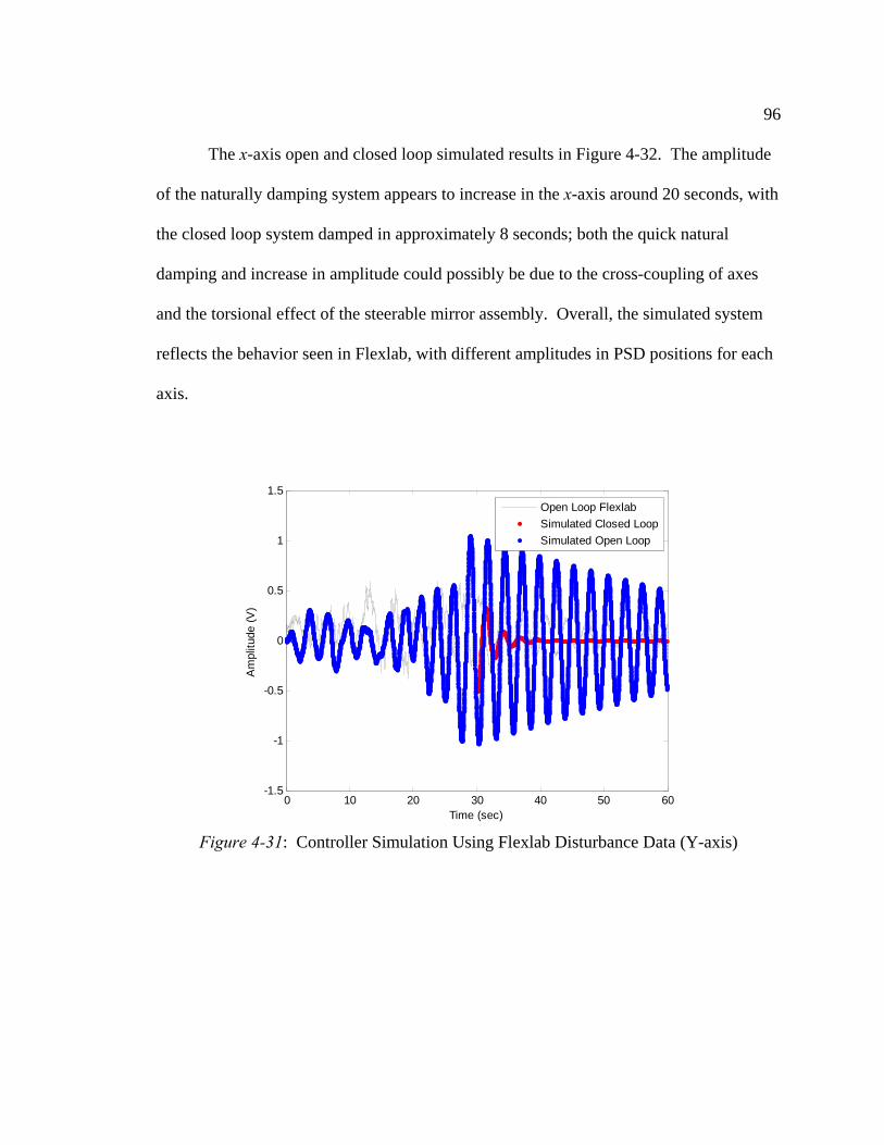
96
The x-axis open and closed loop simulated results in Figure 4-32. The amplitude
of the naturally damping system appears to increase in the x-axis around 20 seconds, with
the closed loop system damped in approximately 8 seconds; both the quick natural
damping and increase in amplitude could possibly be due to the cross-coupling of axes
and the torsional effect of the steerable mirror assembly. Overall, the simulated system
reflects the behavior seen in Flexlab, with different amplitudes in PSD positions for each
axis.
Figure 4-31: Controller Simulation Using Flexlab Disturbance Data (Y-axis)
0 10 20 30 40 50 60-1.5
-1
-0.5
0
0.5
1
1.5
Time (sec)
Am
plitu
de (
V)
Open Loop Flexlab
Simulated Closed Loop
Simulated Open Loop
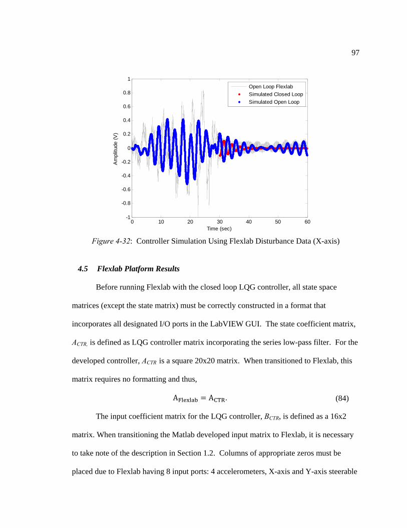
97
Figure 4-32: Controller Simulation Using Flexlab Disturbance Data (X-axis)
4.5 Flexlab Platform Results
Before running Flexlab with the closed loop LQG controller, all state space
matrices (except the state matrix) must be correctly constructed in a format that
incorporates all designated I/O ports in the LabVIEW GUI. The state coefficient matrix,
ACTR, is defined as LQG controller matrix incorporating the series low-pass filter. For the
developed controller, ACTR is a square 20x20 matrix. When transitioned to Flexlab, this
matrix requires no formatting and thus,
A A . (84)
The input coefficient matrix for the LQG controller, BCTR, is defined as a 16x2
matrix. When transitioning the Matlab developed input matrix to Flexlab, it is necessary
to take note of the description in Section 1.2. Columns of appropriate zeros must be
placed due to Flexlab having 8 input ports: 4 accelerometers, X-axis and Y-axis steerable
0 10 20 30 40 50 60-1
-0.8
-0.6
-0.4
-0.2
0
0.2
0.4
0.6
0.8
1
Time (sec)
Am
plitu
de (
V)
Open Loop Flexlab
Simulated Closed Loop
Simulated Open Loop

98
mirror PSD, and the floor mounted X-axis and Y-axis PSD. The accelerometer and
steerable mirror PSD channels were not considered in this study, therefore 6 columns of
zeros are appended to the controller input matrix,
B zeros rows A ,6 B . (85)
Similarly, the control matrix, CCTR, must be transitioned properly. To account for
Flexlab having 5 output ports, the X-axis and Y-axis motors in addition to a 3-axis
steerable mirror, the output matrix must include 3 rows of zeros and are appended to the
control matrix to ensure the control signals are sent to the correct output port,
CC
zeros 3, rows A. (86)
For the Flexlab demonstration, Flexlab was operated in closed loop mode using
the MIMO controller. In this operation, Flexlab was sent a random disturbance signal
and after a specified time period the controller was activated to damp the system.
Figure 4-33 and Figure 4-34 display the system performance of the controller
operating on Flexlab. The y-axis performance, displayed in Figure 4-33, indicates the
closed loop system is damped in approximately 12 seconds, versus over 30 seconds for
the open loop system using the same disturbance signal. The y-axis results are similar,
but less than anticipated by results simulated in Figure 4-31.
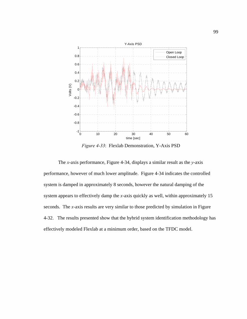
99
Figure 4-33: Flexlab Demonstration, Y-Axis PSD
The x-axis performance, Figure 4-34, displays a similar result as the y-axis
performance, however of much lower amplitude. Figure 4-34 indicates the controlled
system is damped in approximately 8 seconds, however the natural damping of the
system appears to effectively damp the x-axis quickly as well, within approximately 15
seconds. The x-axis results are very similar to those predicted by simulation in Figure
4-32. The results presented show that the hybrid system identification methodology has
effectively modeled Flexlab at a minimum order, based on the TFDC model.
0 10 20 30 40 50 60-1
-0.8
-0.6
-0.4
-0.2
0
0.2
0.4
0.6
0.8
1Y-Axis PSD
time [sec]
Vol
ts (
V)
Open Loop
Closed Loop
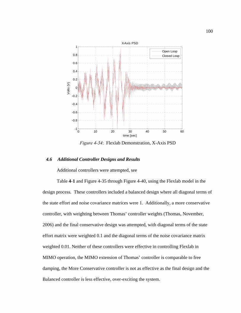
100
Figure 4-34: Flexlab Demonstration, X-Axis PSD
4.6 Additional Controller Designs and Results
Additional controllers were attempted, see
Table 4-1 and Figure 4-35 through Figure 4-40, using the Flexlab model in the
design process. These controllers included a balanced design where all diagonal terms of
the state effort and noise covariance matrices were 1. Additionally, a more conservative
controller, with weighting between Thomas’ controller weights (Thomas, November,
2006) and the final conservative design was attempted, with diagonal terms of the state
effort matrix were weighted 0.1 and the diagonal terms of the noise covariance matrix
weighted 0.01. Neither of these controllers were effective in controlling Flexlab in
MIMO operation, the MIMO extension of Thomas’ controller is comparable to free
damping, the More Conservative controller is not as effective as the final design and the
Balanced controller is less effective, over-exciting the system.
0 10 20 30 40 50 60-1
-0.8
-0.6
-0.4
-0.2
0
0.2
0.4
0.6
0.8
1X-Axis PSD
time [sec]
Vol
ts (
V)
Open Loop
Closed Loop
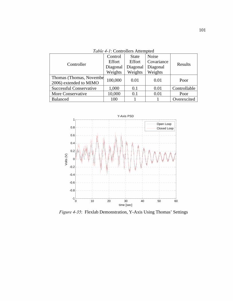
101
Table 4-1: Controllers Attempted
Controller
Control Effort
Diagonal Weights
State Effort
Diagonal Weights
Noise Covariance Diagonal Weights
Results
Thomas (Thomas, Novembe2006) extended to MIMO
100,000 0.01 0.01 Poor
Successful Conservative 1,000 0.1 0.01 ControllableMore Conservative 10,000 0.1 0.01 Poor Balanced 100 1 1 Overexcited
Figure 4-35: Flexlab Demonstration, Y-Axis Using Thomas’ Settings
0 10 20 30 40 50 60-1
-0.8
-0.6
-0.4
-0.2
0
0.2
0.4
0.6
0.8
1Y-Axis PSD
time [sec]
Vol
ts (
V)
Open Loop
Closed Loop
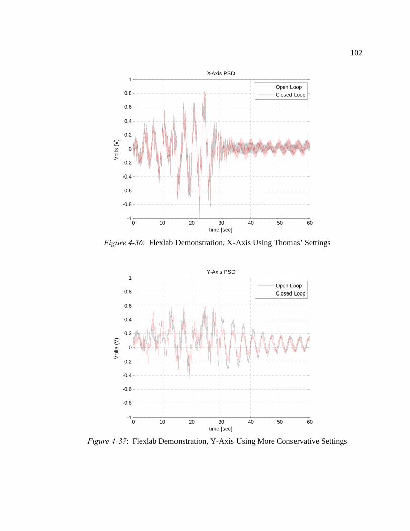
102
Figure 4-36: Flexlab Demonstration, X-Axis Using Thomas’ Settings
Figure 4-37: Flexlab Demonstration, Y-Axis Using More Conservative Settings
0 10 20 30 40 50 60-1
-0.8
-0.6
-0.4
-0.2
0
0.2
0.4
0.6
0.8
1X-Axis PSD
time [sec]
Vol
ts (
V)
Open Loop
Closed Loop
0 10 20 30 40 50 60-1
-0.8
-0.6
-0.4
-0.2
0
0.2
0.4
0.6
0.8
1Y-Axis PSD
time [sec]
Vol
ts (
V)
Open Loop
Closed Loop
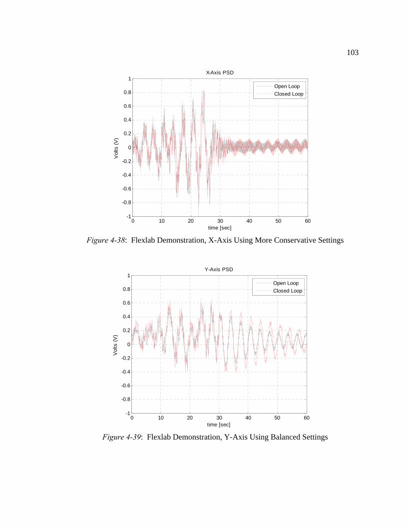
103
Figure 4-38: Flexlab Demonstration, X-Axis Using More Conservative Settings
Figure 4-39: Flexlab Demonstration, Y-Axis Using Balanced Settings
0 10 20 30 40 50 60-1
-0.8
-0.6
-0.4
-0.2
0
0.2
0.4
0.6
0.8
1X-Axis PSD
time [sec]
Vol
ts (
V)
Open Loop
Closed Loop
0 10 20 30 40 50 60-1
-0.8
-0.6
-0.4
-0.2
0
0.2
0.4
0.6
0.8
1Y-Axis PSD
time [sec]
Vol
ts (
V)
Open Loop
Closed Loop
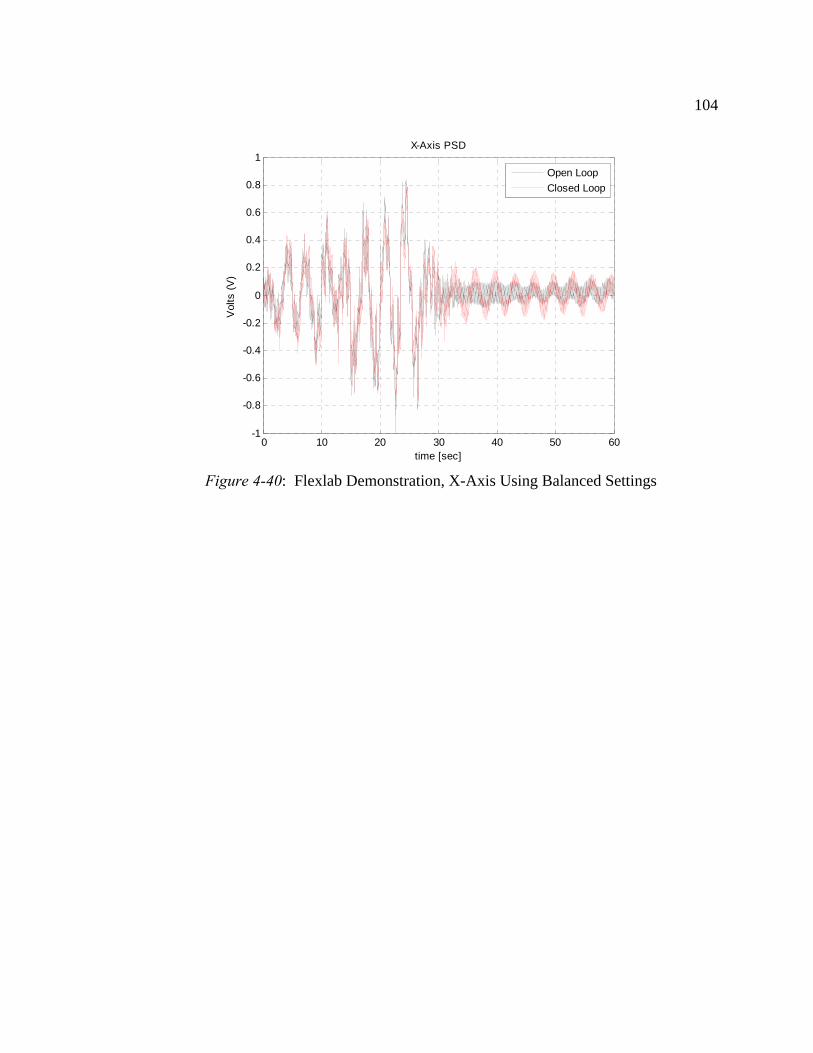
104
Figure 4-40: Flexlab Demonstration, X-Axis Using Balanced Settings
0 10 20 30 40 50 60-1
-0.8
-0.6
-0.4
-0.2
0
0.2
0.4
0.6
0.8
1X-Axis PSD
time [sec]
Vol
ts (
V)
Open Loop
Closed Loop

105
CHAPTER 5: CONCLUSIONS AND RECOMMENDATIONS
System ID is a viable approach for developing models for control system design.
Further applications of system ID are also possible due to the increasing development and
deployment of flexible structures that are difficult to model accurately by standard
methods, such as dynamics and kinematics elements. This thesis presented a hybrid
system ID method incorporating coherence thresholding, the TFDC frequency domain
system ID algorithm extended to SIMO, and the MIMO ERA state space system ID
approach. System ID through the hybrid method was shown to provide a minimum order
linear time-invariant MIMO model for both a simulated and a physical system by directly
computing the impulse responses from transfer functions obtained through TFDC
algorithms using frequency response data.
This thesis examined the advantages of system ID methods in detail, particularly
the advantages presented by the hybrid method. The TFDC approach to system ID was
extended to produce SIMO transfer function models. These models were then used to
produce the needed data to compute MIMO state space models through the ERA
approach from the impulse responses from the SIMO systems. This hybrid method was
illustrated with a contrived example and then with laboratory data from Flexlab.
Measurement noise present in Flexlab introduced additional challenges to the system ID
process, wherein the coherence function could not be used as effectively due to cross-
coupled effects. The hybrid system ID methodology in conjunction with the Coherence
Threshold and low pass filtering were shown to be applicable to Flexlab through the
development of a controller for damping the modes in an excited system.

106
Future research could apply statistical analysis methods, such as those described
by Montgomery (Montgomery, 2009) and applied by Mindrup et al.(Mindrup, Bihl, &
Bauer, 2010) for finding the optimal robust settings for image signal processing
algorithms. Such a robust approach would optimize all specified constants and variables
(e.g. excitation signal parameters, length of frequency response vector used, optimum
coherence threshold, optimal LQG weights, and/or optimum Matlab function
parameters), and this research could find an optimal operating point that does not require
a digital filter incorporated into the controller or one that damps the system faster than the
presented work.
Additional future research could introduce deterministic input signal design to
potentially improve the quality of the system realization; there are various documented
disadvantages associated with using pseudo-randomly generated signals for system ID (as
used in this thesis) (Pintelon & Schoukens, 2001). Examining characteristics in time-
domain system ID methodology that can be exploited for improvement or fusion with
other system ID methods could be explored. Employing a windowed coherence
threshold, where a different threshold is used for different parts of the signal, could also
improve model quality; in addition comparing this coherence threshold to Medina’s
coherence weighting scheme (Medina, November, 1991) and Thomas’ threshold
(Thomas, November, 2006) could be examined. Additionally, a windowed system
identifications technique that searches for local minimums and maximums
(corresponding to system poles) could be investigated. For example, the TFDC approach
could be used to accurately find the poles using windows of data. The known poles could

107
then be used to compute the denominator of the transfer function that could be used in a
modified TFDC that assumes the denominator of the transfer function is known. In a
similar fashion, if the poles are known, the state coefficient matrix in a state variable
model can be formed. This known information could be used in a modified ERA, along
with impulse response data generated from TFDC models, to compute the input and
output coefficient matrices for a state variable model of a system.
108
REFERENCES
Adami, T. A., Zhu, J. J., Bolender, M. A., Doman, D. B., & Oppenheimer, M. W. (August 21-24, 2006). Flight Control of Hypersonic Scramjet Vehicles Using a Differential Algebraic Approach. AIAA Guidance, Navigation, and Control Conference and Exhibit. Keystone, CO.
Adler, A. L., Easley, S., Spanjers, G. G., Winter, J. E., Cohen, D., Davis, L., et al. (April 19-22, 2004). Deployable Structures Space Science Experiment for Large Aperture, High Power Missions In MEO. 45th AIAA/ASME/ASCE/AHS/ASC Structures, Structural Dynamics & Materials Conference. Palm Springs, CA.
Bihl, T. J., Pham, K. D., & Murphey, T. W. (May 3, 2007). Modeling and control of active gravity off-loading for deployable space structures. Orlando, FL: SPIE Defense and Security Symposium.
Blinn, B. A. (March, 1997). FLEXLAB: A Flexible Structure Controls Test Platform. MS Thesis, Ohio University, School of Electrical Engineering and Computer Science, Athens, OH.
Fierro, R., & Lewis, F. L. (1997). Control of a nonholonomic mobile robot: backstepping kinematics into dynamics. Journal of Robotic Systems , 14 (3), 149-163.
French, J. R., & Griffin, M. D. (1991). Space Vehicle Design. Washington, DC: American Institute of Aeronautics and Astronautics, Inc.
Fujimori, A., Nikiforuk, P. N., & Koda, E. (1995). Modeling of a flexible arm using system identification and model reduction. Proceedings of the Institution of Mechanical Engineers 1847-1996 , 209 (I1), 13-20.
Gallivan, M. A., & Murray, R. M. (2003). Model reduction and system identification for master equation control systems. Proceedings of the American Control Conference , 3561-3566.
Gevers, M. (2006). System Identification without Lennart Ljung: what would have been different?". In T. Glad, & G. Hendeby, Forever Ljung in System Identification (pp. 61-85). Lund, Sweden: Studentlitteratur.
Ho, B. L., & Kalman, R. E. (1966). Effective construction of linear state-variable models from input/output functions. Regelungstechnik , 14, 545-548.
Holst, G. C. (1998). Sampling, Aliasing, and Data Fidelity. Winter Park, FL: JCD Publishing.
Juang, J. N. (1994). Applied System Identification. Englewood Cliffs, NJ: PTR Prentice Hall.
109
Kailath, T. (1980). Linear Systems. N.J.: Prentice-Hall.
Ljung, L. (2010). Perspectives on system identification. Annual Reviews in Control , 34, 1-12.
Ljung, L. (1999). System Identification Theory for the User. Upper Saddle River, NJ: Prentice Hall PTR.
Markovsky, I., Willems, J. C., van Huffel, S., de Moor, B., & Pintelon, R. (2005). Application of structured total least squares for system identification and model reduction. IEEE Transaction on Automatic Control , 50 (10), 1490-1500.
Maybeck, P. S. (1979). Stochastic Models, Estimation, and Control Volume 1. New York, NY: Academic Press.
Medina, E. A. (November, 1991). Multi-Input, Multi-Output System Identification from Frequency Response Samples with Applications to the Modeling of Large Space Structures. MS Thesis, Ohio University, School of Electrical Engineering and Computer Science, Athens, OH.
Miller, D. W., How, J. P., Campbell, M. E., Grocott, S., Liu, K., Glaese, R. M., et al. (1998). Flight Results from the Middeck Active Control Experiment (MACE). AIAA Journal , 36 (3), 432-440.
Mindrup, F., Bihl, T., & Bauer, K. (2010). Modeling Noise in a Framework to Optimize the Detection of Anomalies in Hyperspectral Imaging. Vol. 20, 517-524.
Mitchell, J. R. (Winter 2006). Lecture Notes for EE 791, Advanced Digital Control Systems.
Mitchell, J. R., & Irwin, R. D. (2008). System identification for control system design and demonstration by flexlab. 7th International ESA Conference on Guidance, Navigation & Control Systems. Tralee, Ireland.
Montgomery, D. C. (2009). Design and Analysis of Experiments (7th Ed ed.). John Wiley and Sons.
NASA Controls-Structures Interaction Program, PHASE I Guest Investigator Program. (1991, April 5).
Norton, J. P. (1986). An introduction to identification. London, UK: Academic Press.
Pappa, R. S., Woods-Vedeler, J. A., & Jones, T. W. (December, 2001). In-Space Structural Validation Plan for a Stretched-Lens Solar Array Flight Experiment. Hampton, VA: NASA Technical Report.
110
Pati, Y. C., Rezaiifar, R., Krishnaprasad, P. S., & Dayawansa, W. P. (1993). A fast recursive algorithm for system identification and model reduction using rational wavelets. Annual Asilomar Conference on Signals, Systems and Computers , 35-39.
Pendleton, E., Flick, P., Paul, D., Voracek, D., Reichenbach, E., & Griffin, K. (April 23-26, 2007). The X-53 A Summary of the Active Aeroelastic Wing Flight Program. 48th AIAA/ASME/ASCE/AHS/ASC Structures, Structural Dynamics, and Materials Conference. Honolulu, HI.
Phillips, C. L., & Nagle, H. T. (1995). Digital Control System Analysis and Design (third ed.). Prentice Hall, Inc.
Pintelon, R., & Schoukens, J. (2001). System Identification A Frequency Domain Approach. New York, NY: IEEE Press.
Pollard, E. L., Murphey, T. W., & Sanford, G. E. (April 23-26, 2007). Experimental and Numerical Analysis of a DECSMAR Structure’s Deployment and Deployed Performance. 48th AIAA/ASME/ASCE/AHS/ASC Structures, Structural Dynamics, and Materials Conference. Honolulu, HI.
Saunders, C. L. (November, 2006). Labview Software Development for Input and Output Measurement and Control of Flexlab. MS Thesis, Ohio University, School of Electrical Engineering and Computer Science, Athens, OH.
Schrader, K. N., Fetner, R. H., Griffin, S. F., & Erwin, R. S. (2002). Development of a sparse-aperture testbed for optomechanical control of space-deployable structures. Highly Innovative Space Telescope Concepts, Proceedings of SPIE , vol. 484, 3.
Schroeder, M. R. (1979). Integrated-impulse method measuring sound decay without using impulses. Journal of the Acoustical Society of America , 66 (2), 497-500.
Signal Processing Toolbox For Use with MATLAB User's Guide. (2001). Mathworks Inc.
Skelton, R. E. (1988). Dynamic systems control, linear system analysis and synthesis. New York: John Wiley & Sons.
Strahler, J. A. (March, 2000). Integration of an Active Optical System for Flexlab. MS Thesis, Ohio University, School of Electrical Engineering and Computer Science, Athens, OH.
Tarokh, M., & McDermott, G. J. (2005). Kinematics modeling and analyses of articulated rovers. IEEE Transactions on Robotics , 24 (4), 539-553.

111
Thomas, J. B. (November, 2006). Using the Coherence Function as a Means to Improve Frequency Domain Least Squares System Identification. MS Thesis, Ohio University, School of Electrical Engineering and Computer Science, Athens, OH.
van Huffel, S., & Vanderwalle, J. (1991). The Total Least Squares Problem Computational Aspects and Analysis. Philadelphia: Society for Industrial and Applied Mathematics.
Wahlberg, B. (1986). On model reduction in system identification. Proceedings of the American Control Conference , 1260-1266.
Widas, P. (1997, April 8). Introduction to Finite Element Analysis. (Virginia Tech Material Science and Engineering) Retrieved January 10, 2008, from http://www.sv.vt.edu/classes/MSE2094_NoteBook/97ClassProj/num/widas/history.html
Wind Control in Building Design. (February, 2004). Retrieved from http://go.rwdi.com/technotes/t10.pdf
Young, W. R. (March, 1993). Total Least Squares and Constrained Least Squares Applied to Frequency Domain System Identification. Athens, OH: Ohio University.
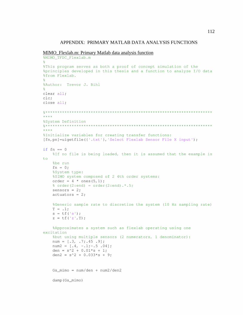
112
APPENDIX: PRIMARY MATLAB DATA ANALYSIS FUNCTIONS
MIMO_Flexlab.m: Primary Matlab data analysis function %MIMO_TFDC_Flexlab.m % %This program serves as both a proof of concept simulation of the %principles developed in this thesis and a function to analyze I/O data %from Flexlab. % %Author: Trevor J. Bihl % clear all; clc; close all; %************************************************************************** %System Definition %************************************************************************** %Initialize variables for creating transfer functions: [fn,pn]=uigetfile({'.txt'},'Select Flexlab Sensor File X input'); if fn == 0 %If no file is being loaded, then it is assumed that the example is to %be run fn = 0; %System type: %SIMO system composed of 2 4th order systems: order = 4 * ones(5,1); % order(2:end) = order(2:end).*.5; sensors = 2; actuators = 2; %Generic sample rate to discretize the system (10 Hz sampling rate) T = .1; s = tf('s'); z = tf('z',T); %Approximates a system such as flexlab operating using one excitation %but using multiple sensors (2 numerators, 1 denominator): num = [.3, .7;.45 .9]; num2 = [.4, -.1;-.5 .04]; den = s^2 + 0.01*s + 1; den2 = s^2 + 0.033*s + 9; Gs_mimo = num/den + num2/den2 damp(Gs_mimo)
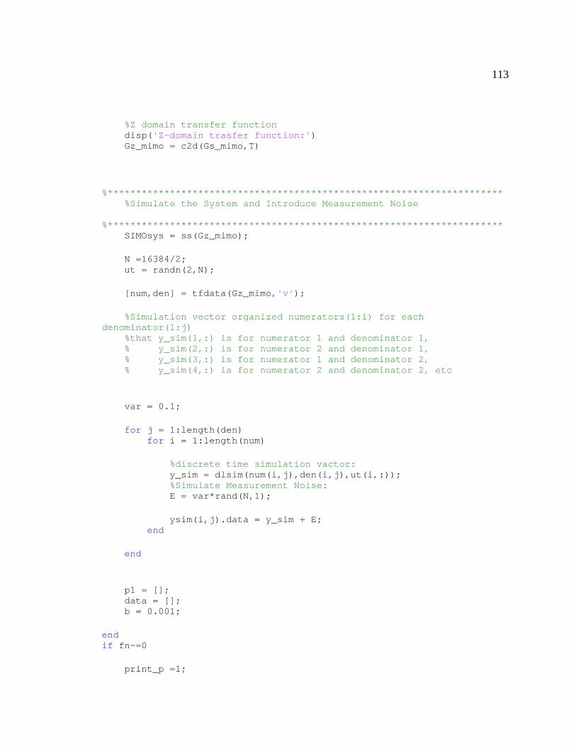
113
%Z domain transfer function disp('Z-domain trasfer function:') Gz_mimo = c2d(Gs_mimo,T) %********************************************************************** %Simulate the System and Introduce Measurement Noise %********************************************************************** SIMOsys = ss(Gz_mimo); N =16384/2; ut = randn(2,N); [num,den] = tfdata(Gz_mimo,'v'); %Simulation vector organized numerators(1:i) for each denominator(1:j) %that y_sim(1,:) is for numerator 1 and denominator 1, % y_sim(2,:) is for numerator 2 and denominator 1, % y_sim(3,:) is for numerator 1 and denominator 2, % y_sim(4,:) is for numerator 2 and denominator 2, etc var = 0.1; for j = 1:length(den) for i = 1:length(num) %discrete time simulation vactor: y_sim = dlsim(num(i,j),den(i,j),ut(i,:)); %Simulate Measurement Noise: E = var*rand(N,1); ysim(i,j).data = y_sim + E; end end p1 = []; data = []; b = 0.001; end if fn~=0 print_p =1;

114
save_p = 0; cd(pn); %set workspace as directory flexlab data is in sensor_data1 = load(strcat(pn,fn)); %%%%%%%%%%%%%%%%%%%%%%%%%%%%%%%%%%%%%%%%%%%%%%%%%%%%%%%%%%%%%%%%%%%%%%% %Uncomment if user file selection is desired %%%%%%%%%%%%%%%%%%%%%%%%%%%%%%%%%%%%%%%%%%%%%%%%%%%%%%%%%%%%%%%%%%%%%%% %[fn,pn]=uigetfile({'.txt'},'Select Flexlab Disturbance File x input'); %actuator_data1 = load(strcat(pn,fn)); actuator_data1 = load('dist_X_SIMO.txt'); %%%%%%%%%%%%%%%%%%%%%%%%%%%%%%%%%%%%%%%%%%%%%%%%%%%%%%%%%%%%%%%%%%%%%%% %Uncomment if user file selection is desired %%%%%%%%%%%%%%%%%%%%%%%%%%%%%%%%%%%%%%%%%%%%%%%%%%%%%%%%%%%%%%%%%%%%%%% %Initialize variables for creating transfer functions: %[fn,pn]=uigetfile({'.txt'},'Select Flexlab Sensor File y input '); %sensor_data2 = load(strcat(pn,fn)); sensor_data2 = load('input_open_Y_SIMO.txt'); %%%%%%%%%%%%%%%%%%%%%%%%%%%%%%%%%%%%%%%%%%%%%%%%%%%%%%%%%%%%%%%%%%%%%%% %Uncomment if user file selection is desired %%%%%%%%%%%%%%%%%%%%%%%%%%%%%%%%%%%%%%%%%%%%%%%%%%%%%%%%%%%%%%%%%%%%%%% %[fn,pn]=uigetfile({'.txt'},'Select Flexlab Disturbance File y input'); % actuator_data2 = load(strcat(pn,fn)); actuator_data2 = load('dist_Y_SIMO.txt'); %Ask user to input experiment data % sim_settings =inputdlg({'Sample Frequency:'}); sim_settings = {'100'}; T = 1/str2double(sim_settings{1}); N = length(actuator_data1); s = tf('s'); z = tf('z',T); %find closest lower power of 2 X = length(actuator_data1); pw2 = floor(log(X)/log(2)); pw2 = 2^pw2; %Flexlab data files organized so each column is a sensor input: %Columns 1-4 - Accelerometers %Columns 5,6 - Structure Mounted PSD (unknown Axes) %Column 7 - X Axis Ground PSD %Column 8 - Y Axis Ground PSD ysim(1,1).data = sensor_data1(1:pw2,7)'; ysim(1,2).data = sensor_data1(1:pw2,8)'; ysim(2,1).data = sensor_data2(1:pw2,7)'; ysim(2,2).data = sensor_data2(1:pw2,8)';
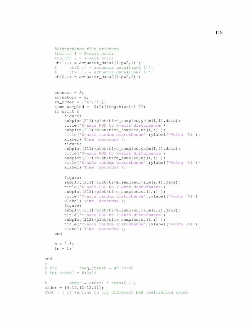
115
%Disturbance file oriented: %column 1 - X-axis motor %column 2 - Y-axis motor ut(1,:) = actuator_data1(1:pw2,1)'; % ut(2,:) = actuator_data(1:pw2,2)'; % ut(1,:) = actuator_data(1:pw2,1)'; ut(2,:) = actuator_data2(1:pw2,2)'; sensors = 2; actuators = 2; xy_order = {'X','Y'}; time_sampled = 0:T:(length(ut)-1)*T; if print_p figure; subplot(211);plot(time_sampled,ysim(1,1).data); title('X-axis PSD to X-axis disturbance') subplot(212);plot(time_sampled,ut(1,:) ); title('X-axis random disturbance');ylabel('Volts (V)'); xlabel('Time (seconds)'); figure; subplot(211);plot(time_sampled,ysim(1,2).data); title('Y-axis PSD to X-axis disturbance') subplot(212);plot(time_sampled,ut(1,:) ); title('X-axis random disturbance');ylabel('Volts (V)'); xlabel('Time (seconds)'); figure; subplot(211);plot(time_sampled,ysim(2,1).data); title('X-axis PSD to Y-axis disturbance') subplot(212);plot(time_sampled,ut(2,:) ); title('Y-axis random disturbance');ylabel('Volts (V)'); xlabel('Time (seconds)'); figure; subplot(211);plot(time_sampled,ysim(2,2).data); title('Y-axis PSD to Y-axis disturbance') subplot(212);plot(time_sampled,ut(2,:) ); title('Y-axis random disturbance');ylabel('Volts (V)'); xlabel('Time (seconds)'); end b = 0.5; fn = 1; end % % for freq_thresh = 40:10:60 % for order1 = 6:2:16 % order = order1 * ones(5,1); order = [4,12,12,12,12]; %Set = 1 if wanting to try different ERA realization sizes
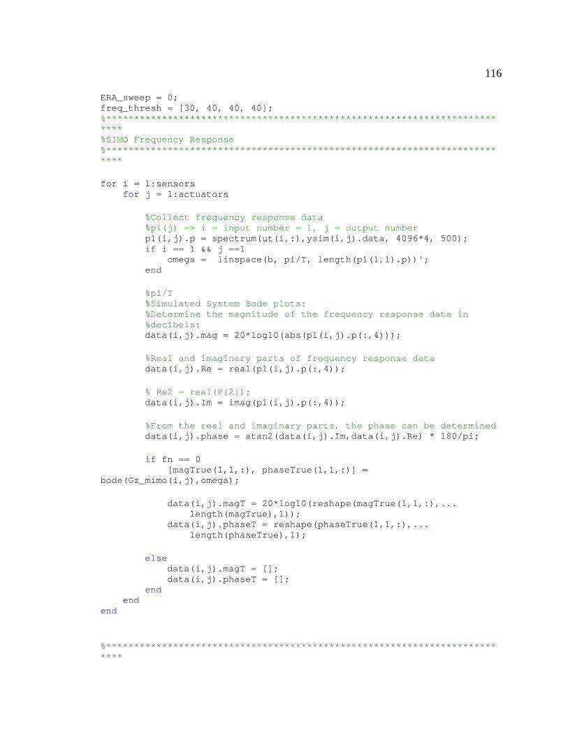
116
ERA_sweep = 0; freq_thresh = [30, 40, 40, 40]; %************************************************************************** %SIMO Frequency Response %************************************************************************** for i = 1:sensors for j = 1:actuators %Collect frequency response data %pi(j) => i = input number = 1, j = output number p1(i,j).p = spectrum(ut(i,:),ysim(i,j).data, 4096*4, 500); if i == 1 && j ==1 omega = linspace(b, pi/T, length(p1(1,1).p))'; end %pi/T %Simulated System Bode plots: %Determine the magnitude of the frequency response data in %decibels: data(i,j).mag = 20*log10(abs(p1(i,j).p(:,4))); %Real and imaginary parts of frequency response data data(i,j).Re = real(p1(i,j).p(:,4)); % Re2 = real(P{2}); data(i,j).Im = imag(p1(i,j).p(:,4)); %From the real and imaginary parts, the phase can be determined data(i,j).phase = atan2(data(i,j).Im,data(i,j).Re) * 180/pi; if fn == 0 [magTrue(1,1,:), phaseTrue(1,1,:)] = bode(Gz_mimo(i,j),omega); data(i,j).magT = 20*log10(reshape(magTrue(1,1,:),... length(magTrue),1)); data(i,j).phaseT = reshape(phaseTrue(1,1,:),... length(phaseTrue),1); else data(i,j).magT = []; data(i,j).phaseT = []; end end end %**************************************************************************

117
%Plot Bode and Coherence Function: %************************************************************************** if print_p for i = 1:sensors for j = 1:actuators figure;subplot(2,1,1); semilogx(omega,data(i,j).mag,'r'); hold on; if ~isempty(data(i,j).magT) semilogx(omega,data(i,j).magT,'b'); ylabel('Magnitude (dB)');... title(strcat({'Frequency response of input '},... num2str(i),{' to output '},num2str(j),... {', with noise'})); else ylabel('Magnitude (dB)');... title(strcat({'Frequency response of '},... xy_order{i},{'-axis input to '},xy_order{j},... {'-axis output'})); end subplot(2,1,2);... semilogx(omega,data(i,j).phase,'r');hold on; if ~isempty(data(i,j).magT) semilogx(omega,data(i,j).phaseT,'b'); ylabel('Phase (deg)');xlabel('Frequency (rad/s)'); legend('With added noise','Original System'); else ylabel('Phase (deg)');xlabel('Frequency (rad/s)'); legend('Flexlab Model'); end end end end CT1 = 0.3; CT2 = 0.3; CT3 = 0.3; CT4 = 0.3; %Coherence Function and Threshold of Discarded Data if print_p figure; x1 = semilogx(omega,p1(1,1).p(:,5),'b'); xlabel('Frequency (rad/s)'); ylabel('Coherence Function'); title('Coherence Functions for 1,1') ylim([0 1.1]); % [x,CT1] = ginput(1); hold on if CT1 > 1; CT1 = 1; end;
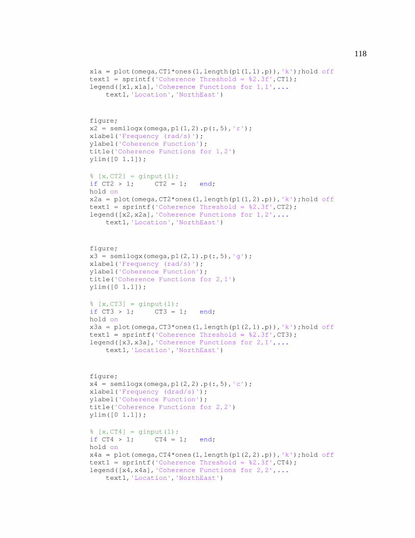
118
x1a = plot(omega,CT1*ones(1,length(p1(1,1).p)),'k');hold off text1 = sprintf('Coherence Threshold = %2.3f',CT1); legend([x1,x1a],'Coherence Functions for 1,1',... text1,'Location','NorthEast') figure; x2 = semilogx(omega,p1(1,2).p(:,5),'r'); xlabel('Frequency (rad/s)'); ylabel('Coherence Function'); title('Coherence Functions for 1,2') ylim([0 1.1]); % [x,CT2] = ginput(1); if CT2 > 1; CT2 = 1; end; hold on x2a = plot(omega,CT2*ones(1,length(p1(1,2).p)),'k');hold off text1 = sprintf('Coherence Threshold = %2.3f',CT2); legend([x2,x2a],'Coherence Functions for 1,2',... text1,'Location','NorthEast') figure; x3 = semilogx(omega,p1(2,1).p(:,5),'g'); xlabel('Frequency (rad/s)'); ylabel('Coherence Function'); title('Coherence Functions for 2,1') ylim([0 1.1]); % [x,CT3] = ginput(1); if CT3 > 1; CT3 = 1; end; hold on x3a = plot(omega,CT3*ones(1,length(p1(2,1).p)),'k');hold off text1 = sprintf('Coherence Threshold = %2.3f',CT3); legend([x3,x3a],'Coherence Functions for 2,1',... text1,'Location','NorthEast') figure; x4 = semilogx(omega,p1(2,2).p(:,5),'c'); xlabel('Frequency (drad/s)'); ylabel('Coherence Function'); title('Coherence Functions for 2,2') ylim([0 1.1]); % [x,CT4] = ginput(1); if CT4 > 1; CT4 = 1; end; hold on x4a = plot(omega,CT4*ones(1,length(p1(2,2).p)),'k');hold off text1 = sprintf('Coherence Threshold = %2.3f',CT4); legend([x4,x4a],'Coherence Functions for 2,2',... text1,'Location','NorthEast')
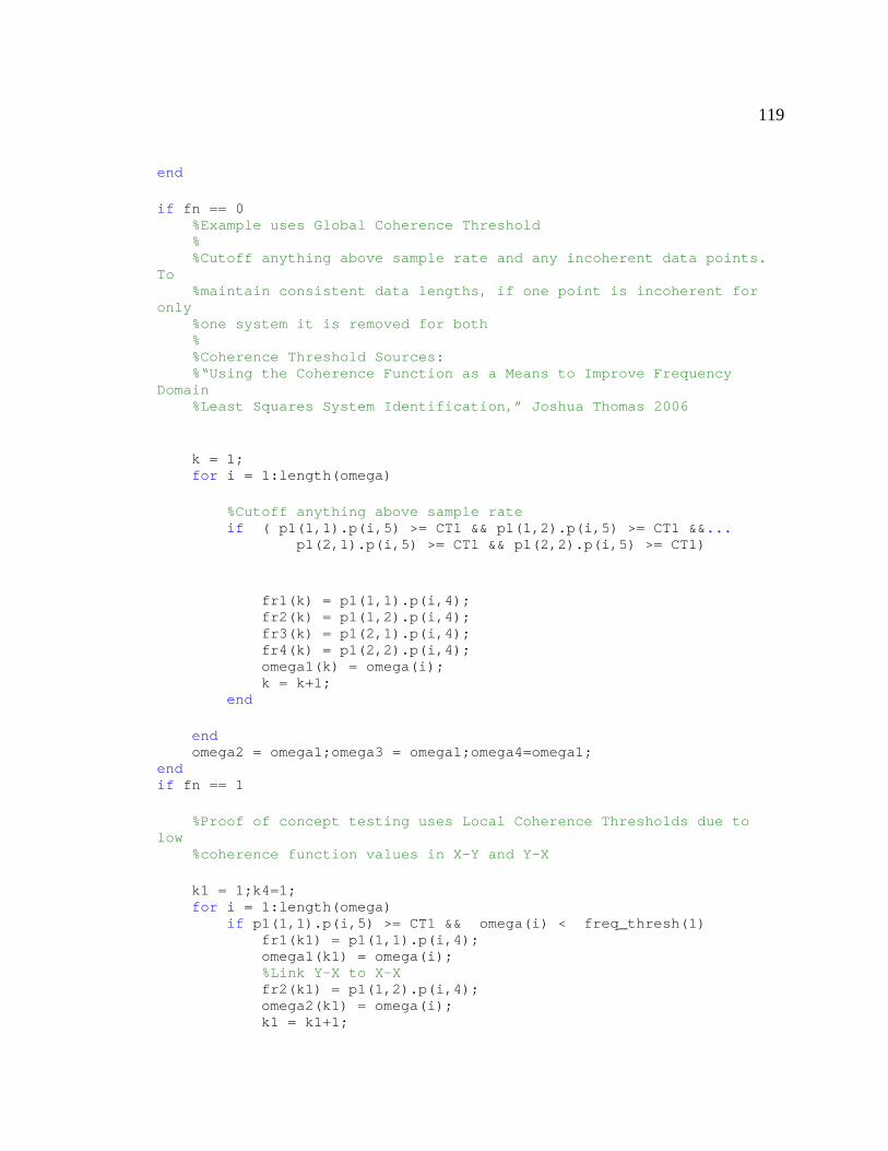
119
end if fn == 0 %Example uses Global Coherence Threshold % %Cutoff anything above sample rate and any incoherent data points. To %maintain consistent data lengths, if one point is incoherent for only %one system it is removed for both % %Coherence Threshold Sources: %“Using the Coherence Function as a Means to Improve Frequency Domain %Least Squares System Identification,” Joshua Thomas 2006 k = 1; for i = 1:length(omega) %Cutoff anything above sample rate if ( p1(1,1).p(i,5) >= CT1 && p1(1,2).p(i,5) >= CT1 &&... p1(2,1).p(i,5) >= CT1 && p1(2,2).p(i,5) >= CT1) fr1(k) = p1(1,1).p(i,4); fr2(k) = p1(1,2).p(i,4); fr3(k) = p1(2,1).p(i,4); fr4(k) = p1(2,2).p(i,4); omega1(k) = omega(i); k = k+1; end end omega2 = omega1;omega3 = omega1;omega4=omega1; end if fn == 1 %Proof of concept testing uses Local Coherence Thresholds due to low %coherence function values in X-Y and Y-X k1 = 1;k4=1; for i = 1:length(omega) if p1(1,1).p(i,5) >= CT1 && omega(i) < freq_thresh(1) fr1(k1) = p1(1,1).p(i,4); omega1(k1) = omega(i); %Link Y-X to X-X fr2(k1) = p1(1,2).p(i,4); omega2(k1) = omega(i); k1 = k1+1;
120
end if p1(2,2).p(i,5) >= CT4 && omega(i) < freq_thresh(4) fr4(k4) = p1(2,2).p(i,4); omega4(k4) = omega(i); %Link X-Y to Y-Y fr3(k4) = p1(2,1).p(i,4); omega3(k4) = omega(i); k4 = k4+1; end end end if fn == 2 k1 = 1;k4=1; for i = 1:length(omega) if data(1,1).mag(i) >= -20 fr1(k1) = p1(1,1).p(i,4); omega1(k1) = omega(i); %Link Y-X to X-X fr2(k1) = p1(1,2).p(i,4); omega2(k1) = omega(i); k1 = k1+1; end if data(2,2).mag(i) >= -20 fr4(k4) = p1(2,2).p(i,4); omega4(k4) = omega(i); %Link X-Y to Y-Y fr3(k4) = p1(2,1).p(i,4); omega3(k4) = omega(i); k4 = k4+1; end end end if fn == 3 k1 = 1;k4=1; for i = 1:length(omega) if data(1,1).mag(i) >= -20 && p1(1,1).p(i,5) >= CT1 fr1(k1) = p1(1,1).p(i,4); omega1(k1) = omega(i); %Link Y-X to X-X fr2(k1) = p1(1,2).p(i,4); omega2(k1) = omega(i); k1 = k1+1; end if data(2,2).mag(i) >= -20 && p1(2,2).p(i,5) >= CT4 fr4(k4) = p1(2,2).p(i,4); omega4(k4) = omega(i); %Link X-Y to Y-Y
121
fr3(k4) = p1(2,1).p(i,4); omega3(k4) = omega(i); k4 = k4+1; end end end if fn == 4 k1 = 1;k4=1; for i = 1:length(omega) if data(1,1).mag(i) >= -20 &&... p1(1,1).p(i,5) >= CT1 &&... omega(i) < freq_thresh(1) fr1(k1) = p1(1,1).p(i,4); omega1(k1) = omega(i); %Link Y-X to X-X fr2(k1) = p1(1,2).p(i,4); omega2(k1) = omega(i); k1 = k1+1; end if data(2,2).mag(i) >= -20 &&... p1(2,2).p(i,5) >= CT4 &&... omega(i) < freq_thresh(4) fr4(k4) = p1(2,2).p(i,4); omega4(k4) = omega(i); %Link X-Y to Y-Y fr3(k4) = p1(2,1).p(i,4); omega3(k4) = omega(i); k4 = k4+1; end end end if fn == 5 k1 = 1;k4=1; for i = 1:length(omega) if omega(i) < freq_thresh(1) fr1(k1) = p1(1,1).p(i,4); omega1(k1) = omega(i); %Link Y-X to X-X fr2(k1) = p1(1,2).p(i,4); omega2(k1) = omega(i); k1 = k1+1; end if omega(i) < freq_thresh(4) fr4(k4) = p1(2,2).p(i,4); omega4(k4) = omega(i); %Link X-Y to Y-Y fr3(k4) = p1(2,1).p(i,4);
122
omega3(k4) = omega(i); k4 = k4+1; end end end %************************************************************************** %TFDC: %************************************************************************** %Individually estimate tfdc: % T = 0.05; % z = tf('z',T); [num_tfdc_simo_In1,den_tfdc_simo_In1] = tfdc_simo2O(order(2),... [real(fr1);real(fr2)],[imag(fr1);imag(fr2)],omega1,T,2,'TLS'); [num_tfdc_simo_In4,den_tfdc_simo_In4] = tfdc_simo2O(order(5),... [real(fr3);real(fr4)],[imag(fr3);imag(fr4)],omega4,T,2,'TLS'); den11 = symZ_FromVector(den_tfdc_simo_In1,z); num11 = symZ_FromVector(num_tfdc_simo_In1(1,:),z); den12 = symZ_FromVector(den_tfdc_simo_In1,z); num12 = symZ_FromVector(num_tfdc_simo_In1(2,:),z); den21 = symZ_FromVector(den_tfdc_simo_In4,z); num21 = symZ_FromVector(num_tfdc_simo_In4(1,:),z); den22 = symZ_FromVector(den_tfdc_simo_In4,z); num22 = symZ_FromVector(num_tfdc_simo_In4(2,:),z); disp('TFDC est Z-domain trasfer function:') % Gz_coher = [num11;num22]/[den1;den2] Gz_coher11 = num11/den11 Gz_coher12 = num12/den12 Gz_coher21 = num21/den21 Gz_coher22 = num22/den22 [mag_SIM,phase_SIM, omega1] =... bode(Gz_coher11,omega1); tfdcdata(1).mag = 20*log10(reshape(mag_SIM(1,1,:),length(mag_SIM),1)); tfdcdata(1).phase = reshape(phase_SIM(1,1,:),length(phase_SIM),1); clear mag_SIM phase_SIM [mag_SIM,phase_SIM, omega2] =... bode(Gz_coher12,omega2); tfdcdata(2).mag = 20*log10(reshape(mag_SIM(1,1,:),length(mag_SIM),1)); tfdcdata(2).phase = reshape(phase_SIM(1,1,:),length(phase_SIM),1); clear mag_SIM phase_SIM [mag_SIM,phase_SIM, omega3] =...
123
bode(Gz_coher21,omega3); tfdcdata(3).mag = 20*log10(reshape(mag_SIM(1,1,:),length(mag_SIM),1)); tfdcdata(3).phase = reshape(phase_SIM(1,1,:),length(phase_SIM),1); clear mag_SIM phase_SIM [mag_SIM,phase_SIM, omega4] =... bode(Gz_coher22,omega4); tfdcdata(4).mag = 20*log10(reshape(mag_SIM(1,1,:),length(mag_SIM),1)); tfdcdata(4).phase = reshape(phase_SIM(1,1,:),length(phase_SIM),1); clear mag_SIM phase_SIM %TFDC Plots: if print_p figure;subplot(2,1,1); semilogx(omega1,tfdcdata(1).mag,'r-'); hold on; if fn == 0 semilogx(omega,data(1,1).magT,'b');... else semilogx(omega,data(1,1).mag,'b'); end ylabel('Magnitude (dB)'); title(strcat({'Frequency response of input '},... num2str(1),{' to output '},num2str(1),... {', using: freq thresh='},num2str(freq_thresh(1)),... {', with X-X order='},num2str(order(2)))); subplot(2,1,2);... semilogx(omega1,tfdcdata(1).phase,'r-'); hold on; if fn == 0 semilogx(omega,data(1,1).phaseT,'b'); else semilogx(omega,data(1,1).phase,'b'); end ylabel('Phase (deg)');xlabel('Frequency (rad/s)'); if fn == 0 legend('TFDC Estimated System','True System'); else legend('TFDC Estimated System','Original System'); end figure;subplot(2,1,1); semilogx(omega2,tfdcdata(2).mag,'r-'); hold on; if fn == 0 semilogx(omega,data(2,1).magT,'b'); else semilogx(omega,data(2,1).mag,'b'); end ylabel('Magnitude (dB)');... title(strcat({'Frequency response of input '},...
124
num2str(1),{' to output '},num2str(2),... {', using: freq thresh='},num2str(freq_thresh(2)),... {', with X-Y order='},num2str(order(3)))); subplot(2,1,2);... semilogx(omega2,tfdcdata(2).phase,'r-'); hold on; if fn == 0 semilogx(omega,data(2,1).phaseT,'b'); else semilogx(omega,data(2,1).phase,'b'); end ylabel('Phase (deg)');xlabel('Frequency (rad/s)'); if fn == 0 legend('TFDC Estimated System','True System'); else legend('TFDC Estimated System','Original System'); end figure;subplot(2,1,1); semilogx(omega3,tfdcdata(3).mag,'r-'); hold on; if fn == 0 semilogx(omega,data(1,2).magT,'b');... else semilogx(omega,data(1,2).mag,'b');... end ylabel('Magnitude (dB)');... title(strcat({'Frequency response of input '},... num2str(2),{' to output '},num2str(1),... {', using: freq thresh='},num2str(freq_thresh(3)),... {', with Y-X order='},num2str(order(4)))); subplot(2,1,2);... semilogx(omega3,tfdcdata(3).phase,'r-'); hold on; if fn == 0 semilogx(omega,data(1,2).phaseT,'b'); else semilogx(omega,data(1,2).phase,'b'); end ylabel('Phase (deg)');xlabel('Frequency (rad/s)'); if fn == 0 legend('TFDC Estimated System','True System'); else legend('TFDC Estimated System','Original System'); end figure;subplot(2,1,1); semilogx(omega4,tfdcdata(4).mag,'r-'); hold on; if fn == 0

125
semilogx(omega,data(2,2).magT,'b');... else semilogx(omega,data(2,2).mag,'b');... end ylabel('Magnitude (dB)');... title(strcat({'Frequency response of input '},... num2str(2),{' to output '},num2str(2),... {', using: freq thresh='},num2str(freq_thresh(4)),... {', with Y-Y order='},num2str(order(5)))); subplot(2,1,2);... semilogx(omega4,tfdcdata(4).phase,'r-'); hold on; if fn == 0 semilogx(omega,data(2,2).phaseT,'b'); else semilogx(omega,data(2,2).phase,'b'); end ylabel('Phase (deg)');xlabel('Frequency (rad/s)'); if fn == 0 legend('TFDC Estimated System','True System'); else legend('TFDC Estimated System','Original System'); end end %************************************************************************** %HYBRID SYSTEM %************************************************************************** length_max = max([length(omega1),length(omega2),length(omega3),... length(omega4)]); %Calculate discrete impulse from difference equation, not den_tfdc_simo is %negated as the difference equation is a sum (see Bihl 2.3) [c_imp_In1, c_time_In1] = dimpulse(num_tfdc_simo_In1,... den_tfdc_simo_In1,length_max); [c_imp_In4, c_time_In4] = dimpulse(num_tfdc_simo_In4,... den_tfdc_simo_In4,length_max); c_imp_In2 = c_imp_In1(:,2); c_imp_In1 = c_imp_In1(:,1); c_imp_In4 = c_imp_In4(:,2); c_imp_In3 = c_imp_In4(:,1); if print_p figure;plot(c_imp_In1); figure;plot(c_imp_In2); figure;plot(c_imp_In3); figure;plot(c_imp_In4); end
126
%************************************************************************** %EIGENSYSTEM REALIZATION ALGORITHM %************************************************************************** if ERA_sweep range = 4:2:16; else range = order(1); end for order1 = range order(1) = order1; order(1) = 4; [A,B,C,D] = era([c_imp_In1,c_imp_In3,... c_imp_In2,c_imp_In4 ],order(1),sensors,actuators,0,1,0); % [A,B,C,D] = era([c_imp_In1(:,1)],order,1,1,0,1,0); disp('Size of A:') size(A) disp('State Space System:') SS_sys = ss(A,B,C,0,T); %Matlab SS function organizes Outputs first then Inputs. Eg: A SIMO %system with 2 outputs would be organized MOSI [mag_SIM,phase_SIM, omega] =... bode(SS_sys(1,1),omega); simdata(1,1).mag = 20*log10(reshape(mag_SIM(1,1,:),length(mag_SIM),1)); simdata(1,1).phase = reshape(phase_SIM(1,1,:),length(phase_SIM),1); clear mag_SIM phase_SIM [mag_SIM,phase_SIM, omega] =... bode(SS_sys(2,1),omega); simdata(2,1).mag = 20*log10(reshape(mag_SIM(1,1,:),length(mag_SIM),1)); simdata(2,1).phase = reshape(phase_SIM(1,1,:),length(phase_SIM),1); clear mag_SIM phase_SIM [mag_SIM,phase_SIM, omega] =... bode(SS_sys(1,2),omega); simdata(1,2).mag = 20*log10(reshape(mag_SIM(1,1,:),length(mag_SIM),1)); simdata(1,2).phase = reshape(phase_SIM(1,1,:),length(phase_SIM),1); clear mag_SIM phase_SIM [mag_SIM,phase_SIM, omega] =... bode(SS_sys(2,2),omega); simdata(2,2).mag = 20*log10(reshape(mag_SIM(1,1,:),length(mag_SIM),1)); simdata(2,2).phase = reshape(phase_SIM(1,1,:),length(phase_SIM),1);
127
%Hybrid Plots: if print_p figure;subplot(2,1,1); semilogx(omega,simdata(1,1).mag,'r'); hold on; if fn == 0 semilogx(omega,data(1,1).magT,'b'); else semilogx(omega,data(1,1).mag,'b'); end ylabel('Magnitude (dB)');... title(strcat({'Frequency response of input '},... num2str(1),{' to output '},num2str(1),... {', with Hybrid order='},num2str(order(1)))); subplot(2,1,2);... semilogx(omega,simdata(1,1).phase,'r'); hold on; if fn == 0 semilogx(omega,data(1,1).phaseT,'b'); else semilogx(omega,data(1,1).phase,'b'); end ylabel('Phase (deg)');xlabel('Frequency (rad/s)'); if fn == 0 legend('Hybrid Estimated System','True System'); else legend('Hybrid Estimated System','Original System'); end figure;subplot(2,1,1); semilogx(omega,simdata(2,1).mag,'r'); hold on; if fn == 0 semilogx(omega,data(2,1).magT,'b'); else semilogx(omega,data(2,1).mag,'b'); end ylabel('Magnitude (dB)');... title(strcat({'Frequency response of input '},... num2str(1),{' to output '},num2str(2),... {', with Hybrid order='},num2str(order(1)))); subplot(2,1,2);... semilogx(omega,simdata(2,1).phase,'r'); hold on; if fn == 0 semilogx(omega,data(2,1).phaseT,'b'); else semilogx(omega,data(2,1).phase,'b');
128
end ylabel('Phase (deg)');xlabel('Frequency (rad/s)'); if fn == 0 legend('Hybrid Estimated System','True System'); else legend('Hybrid Estimated System','Original System'); end figure;subplot(2,1,1); semilogx(omega,simdata(1,2).mag,'r'); hold on; if fn == 0 semilogx(omega,data(1,2).magT,'b');... else semilogx(omega,data(1,2).mag,'b');... end ylabel('Magnitude (dB)');... title(strcat({'Frequency response of input '},... num2str(2),{' to output '},num2str(1),... {', with Hybrid order='},num2str(order(1)))); subplot(2,1,2);... semilogx(omega,simdata(1,2).phase,'r'); hold on; if fn == 0 semilogx(omega,data(1,2).phaseT,'b'); else semilogx(omega,data(1,2).phase,'b'); end ylabel('Phase (deg)');xlabel('Frequency (rad/s)'); if fn == 0 legend('Hybrid Estimated System','True System'); else legend('Hybrid Estimated System','Original System'); end figure;subplot(2,1,1); semilogx(omega,simdata(2,2).mag,'r'); hold on; if fn == 0 semilogx(omega,data(2,2).magT,'b');... else semilogx(omega,data(2,2).mag,'b');... end ylabel('Magnitude (dB)');... title(strcat({'Frequency response of input '},... num2str(2),{' to output '},num2str(2),... {', with Hybrid order='},num2str(order(1)))); subplot(2,1,2);... semilogx(omega,simdata(2,2).phase,'r'); hold on;
129
if fn == 0 semilogx(omega,data(2,2).phaseT,'b'); else semilogx(omega,data(2,2).phase,'b'); end ylabel('Phase (deg)');xlabel('Frequency (rad/s)'); if fn == 0 legend('Hybrid Estimated System','True System'); else legend('Hybrid Estimated System','Original System'); end end if ERA_sweep clear SS_sys A B C D end %%%%%%%%%%%%% %End of Plotting Loop %%%%%%%%%%%%% end %IF this is FLEXLAB calculate controller: if fn ~=0 % for qxu_end = [500,1000,5000,10000,100000] for qxu_end1 = [500,1000,5000,10000,100000] for QXU = 1:1:4 for QWV = 1:1:4 qxu_w1 = 1*10^(-QXU+1); qwv_w1 = 1*10^(-QWV+1); %Create weighting matrices equal size to State Matrix A %Bias last element to create a conservative controller: qxu = eye(size(SS_sys.a,1)+size(SS_sys.b,2),... size(SS_sys.a,2)+size(SS_sys.b,2))*qxu_w1; qxu(end,end) = qxu_end; qxu(end-1,end-1) = qxu_end1; qwv = eye(size(SS_sys.a,1)+size(SS_sys.b,2),... size(SS_sys.a,2)+size(SS_sys.b,2))*qwv_w1; LQG_cont = lqg(SS_sys,qxu,qwv); %Create a state space regulator at 1/2 the sample prd LQGregulator = ss(LQG_cont.a,-LQG_cont.b,... LQG_cont.c,LQG_cont.d,T); Gz_OpenLoop = series(LQGregulator,SS_sys); Gz_ClosedLoop = feedback(SS_sys,LQGregulator);
130
[Y_imp_uncomp,T_imp_uncomp]= impulse(SS_sys,20); [Y_imp_comp,T_imp_comp]= impulse(Gz_ClosedLoop,20); [mag_LQG,phase_LQG, omega_LQG] =... bode(Gz_ClosedLoop,omega3); for i = 1:size(mag_LQG,1) for j = 1:size(mag_LQG,2) LQGdata(i,j).mag =... 20*log10(reshape(mag_LQG(i,j,:),... length(mag_LQG),1)); LQGdata(i,j).phase =... reshape(phase_LQG(i,j,:),... length(phase_LQG),1); LQGdata(i,j).impulseOrig =... reshape(Y_imp_uncomp(:,i,j),... length(Y_imp_uncomp),1); LQGdata(i,j).impulseCL =... reshape(Y_imp_comp(:,i,j),... length(Y_imp_comp),1); if print_p figure else f = figure('visible','off'); end subplot(2,1,1) semilogx(omega_LQG,LQGdata(i,j).mag);grid on; ylabel('Magnitude (dB)');... title(strcat({'Closed Loop LQG Frequency response of input '},... num2str(i),{' to output '},num2str(j))); subplot(2,1,2) semilogx(omega_LQG,LQGdata(i,j).phase);grid on; ylabel('Phase (deg)'); xlabel('Frequency (rad/s)'); if print_p figure else f = figure('visible','off'); end plot(T_imp_uncomp,LQGdata(i,j).impulseOrig); hold on plot(T_imp_comp,LQGdata(i,j).impulseCL,'r'); legend('Open Loop Uncompensated',... 'Closed Loop'); ylabel('Impulse Response'); xlabel('Time (seconds)')
131
end end %Lowpass filter: %designed to roll of the high frequencies that are %unmodeled to focus the controller on the 1st few modes %(pendulum and first bending mode, etc). K = 0.0087 ; %Keep DC gain of filter near 1 % (solving G(1) = 1 for K) a = 20; %set to keep break frequency around 20 rad/s %with a damping ratio %near 0.707 b = .707; % Filt_den = (s^2 + 2*a*b*s + a^2); % Filt_z = c2d(Filt,T); Filt_z = K*(z^2+2*z+1)/ (z^2 - 1.719*z + 0.7537); if print_p figure; bode(Filt_z); title('Filter Bode Plot') end %DIsplay filter data: damp(Filt_z) %%%%%%Adding in Filter.... Gz_compen = series(Filt_z,SS_sys); % Gz_compen = SS_sys; % QXU = 3; % QWV = 2; % qxu_w = 1*10^(-QXU+1); % qwv_w = 1*10^(-QWV+1); qxu2 = eye(size(Gz_compen.a,1)+size(Gz_compen.b,2),... size(Gz_compen.a,2)+size(Gz_compen.b,2))*qxu_w1; qxu2(end,end) = qxu_end; qxu2(end-1,end-1) = qxu_end1; qwv2 = eye(size(Gz_compen.a,1)+size(Gz_compen.b,2),... size(Gz_compen.a,2)+size(Gz_compen.b,2))*qwv_w1; %Low Pass filtered LQG: LQG_LP = lqg(Gz_compen,qxu2,qwv2);
132
%Create a state space regulator at 1/2 the sample period LQG_LP_regulator = ss(LQG_LP.a,-LQG_LP.b,... LQG_LP.c,LQG_LP.d,T); LQG_LP_w_filter = series(Filt_z,LQG_LP_regulator); Gz_LP_OpenLoop = series(LQG_LP_regulator,SS_sys); Gz_LP_ClosedLoop = ... feedback(Gz_compen,LQG_LP_regulator); [Y_imp_uncomplp,T_imp_uncomplp]= impulse(Gz_compen,20); [Y_imp_complp,T_imp_complp]= ... impulse(Gz_LP_ClosedLoop,20); [mag_LP_LQG,phase_LP_LQG, omega_LP_LQG] =... bode(Gz_LP_ClosedLoop,omega3); for i = 1:size(mag_LP_LQG,1) for j = 1:size(mag_LP_LQG,2) LQGdataLP(i,j).mag =... 20*log10(reshape(mag_LP_LQG(i,j,:),... length(mag_LP_LQG),1)); LQGdataLP(i,j).phase =... reshape(phase_LP_LQG(i,j,:),... length(phase_LP_LQG),1); LQGdataLP(i,j).impulseOrig =... reshape(Y_imp_uncomplp(:,i,j),... length(Y_imp_uncomplp),1); LQGdataLP(i,j).impulseCL =... reshape(Y_imp_complp(:,i,j),... length(Y_imp_complp),1); if print_p figure else f = figure('visible','off'); end subplot(2,1,1) semilogx(omega_LP_LQG,LQGdataLP(i,j).mag); grid on; ylabel('Magnitude (dB)');... title(strcat({'Closed Loop LQG Frequency response of input '},... num2str(i),{' to output '},num2str(j))); subplot(2,1,2) semilogx(omega_LP_LQG,LQGdataLP(i,j).phase); grid on; ylabel('Phase (deg)'); xlabel('Frequency (rad/s)'); if print_p
133
elseif save_p print(f, '-r80', '-dtiff',... strcat('LQG_1mode_fig1',num2str(i),... num2str(j),... 'QXUw_',num2str(QXU),'QWVw_',... num2str(QWV),... 'QXUend_',num2str(qxu2(end,end)),... 'QXUend1_',num2str(qxu2(end-1,end-1)))); end if print_p figure else f = figure('visible','off'); end plot(T_imp_uncomplp,... LQGdataLP(i,j).impulseOrig);hold on plot(T_imp_complp,... LQGdataLP(i,j).impulseCL,'r'); title(strcat({'Closed Loop LQG response of input '},... num2str(i),{' to output '},num2str(j))); legend('Open Loop Uncompensated',... 'Closed Loop'); ylabel('Impulse Response'); xlabel('Time (seconds)') if print_p elseif save_p print(f, '-r80', '-dtiff',... strcat('LQG_1mode_fig2',num2str(i),... num2str(j),... 'QXUw_',num2str(QXU),'QWVw_',num2str(QWV),... 'QXUend_',num2str(qxu2(end,end)),... 'QXUend1_',... num2str(qxu2(end-1,end-1)))); end end end %%%%%%%%%%%%%%%%%%%%%%%%%%%%%%%%%%%%%%%%%%%%%%%%%%%%%%% %Look at frequency response model and IFT %%%%%%%%%%%%%%%%%%%%%%%%%%%%%%%%%%%%%%%%%%%%%%%%%%%%%%% % frd_model_uncompen = frd(SS_sys,omega3); % set(frd_LQG,'Name','Hybrid Estimated System') freq_dat(1,1,:) = p1(1,1).p(:,4); freq_dat(1,2,:) = p1(1,2).p(:,4);
134
freq_dat(2,1,:) = p1(2,1).p(:,4); freq_dat(2,2,:) = p1(2,2).p(:,4); frd_model_orig = frd(freq_dat,omega,T) frd_LQG = frd(LQG_LP_regulator,omega); frd_filter = frd(Filt_z,omega); frd_controller = series(frd_filter,frd_LQG); frd_closed_loop_sys = feedback(frd_controller,... frd_model_orig,T); temp = reshape(frd_model_orig.ResponseData,4,... size(frd_model_orig.ResponseData,3)); ift_frd_orig = ifft([temp, flipud(temp)]);clear temp temp1 = ift_frd_orig(1,1:length(omega)); temp2 = ift_frd_orig(2,1:length(omega)); temp3 = ift_frd_orig(3,1:length(omega)); temp4 = ift_frd_orig(4,1:length(omega)); time = 0:T:(length(omega)-1)*T; if print_p figure else f = figure('visible','off'); end plot(time,real(temp1),'b');hold on; plot(time,real(temp2),'r');hold on; plot(time,real(temp3),'g');hold on; plot(time,real(temp4),'c') xlabel('Time (s)'); ylabel('Amplitude'); title(strcat({'Closed loop Impulse Response'},... {'QXU_w = '},num2str(qxu_w1),{' QWV_w = '},... num2str(qwv_w1),... {'ERA Order = '},num2str(order(1)),... {'qxu2(end,end) = '},num2str(qxu2(end,end)),... {'qxu2(end-1,end-1) = '},... num2str(qxu2(end-1,end-1)))); legend('X-Axis','X-Y cross','Y-X cross','Y-Axis'); if print_p elseif save_p print(f, '-r80', '-dtiff',... strcat('LQG_1mode_fig3','QXUw_',... num2str(QXU),'QWVw_',num2str(QWV),... 'QXUend_',num2str(qxu2(end,end)),... 'QXUend1_',num2str(qxu2(end-1,end-1)))); end clear temp1 temp2 temp3 temp4 temp = reshape(frd_closed_loop_sys.ResponseData,4,... size(frd_closed_loop_sys.ResponseData,3));
135
ift_frd_CL = ifft([temp, flipud(temp)]);clear temp temp1 = ift_frd_CL(1,1:length(omega)); temp2 = ift_frd_CL(2,1:length(omega)); temp3 = ift_frd_CL(3,1:length(omega)); temp4 = ift_frd_CL(4,1:length(omega)); time = 0:T:(length(omega)-1)*T; if print_p figure else f = figure('visible','off'); end plot(time,real(temp1),'b-');hold on; plot(time,real(temp2),'r-');hold on; plot(time,real(temp3),'g.');hold on; plot(time,real(temp4),'c.') xlabel('Time (s)'); ylabel('Amplitude'); title(strcat({'Closed Loop Impulse Response'},... {'QXU_w = '},num2str(qxu_w1),{' QWV_w = '},... num2str(qwv_w1),... {'ERA Order = '},num2str(order(1)),... {'qxu2(end,end) = '},num2str(qxu2(end,end)),... {'qxu2(end-1,end-1) = '},... num2str(qxu2(end-1,end-1)))); legend('X-Axis','X-Y cross','Y-X cross','Y-Axis'); if print_p elseif save_p print(f, '-r80', '-dtiff',... strcat('LQG_1mode_fig4',... 'QXUw_',num2str(QXU),'QWVw_',num2str(QWV),... 'QXUend_',num2str(qxu2(end,end)),... 'QXUend1_',num2str(qxu2(end-1,end-1)))); end clear temp1 temp2 temp3 temp4 %%%%%%%%%%%%%%%%%%%%%%%%%%%%%%%%%%%%%%%%%%%%%%%%%%%%%%% %Uncomment if user file selection is desired %%%%%%%%%%%%%%%%%%%%%%%%%%%%%%%%%%%%%%%%%%%%%%%%%%%%%%% % [fn,pn]=uigetfile({'.txt'},... %'Select Flexlab 30 second File'); % % cd(pn); %set workspace as directory flexlab data %is in % dist_data = load(strcat(pn,fn)); dist_data = load('dist.txt'); %%%%%%%%%%%%%%%%%%%%%%%%%%%%%%%%%%%%%%%%%%%%%%%%%%%%%%%
136
%Uncomment if user file selection is desired %%%%%%%%%%%%%%%%%%%%%%%%%%%%%%%%%%%%%%%%%%%%%%%%%%%%%%% % [fn,pn]=uigetfile({'.txt'},... %'Select Flexlab Open Loop Sensor File'); % cd(pn); %set workspace as directory flexlab data %is in % OL_sensor_data = load(strcat(pn,fn)); OL_sensor_data = load('input_open.txt'); ysimOL(1,1).data = OL_sensor_data(:,8)'; ysimOL(2,2).data = OL_sensor_data(:,7)'; time = 0:T:(length(ysimOL(1,1).data)-1)*T; [sim_response1,a,x] = lsim(SS_sys,... [dist_data;zeros(size(dist_data))]); % figure;plot(time,ysimOL(1,1).data,'k-'); %hold on;plot(time,sim_response1(:,1),'r.'); % figure;plot(time,ysimOL(2,2).data,'k-');hold on; %plot(time,sim_response1(:,2),'r.'); sim_response2 = lsim(Gz_LP_ClosedLoop,... zeros(size(dist_data)),time(3001:end),... [x(end,:),zeros(1,12)]); f = figure('visible','off'); plot(time,ysimOL(1,1).data,'k-');hold on; plot(time(3001:end),sim_response2(:,1),'r.');hold on; plot(time,sim_response1(:,1),'b.'); xlabel('Time (sec)');ylabel('Amplitude (V)') legend('Open Loop Flexlab','Simulated Closed Loop',... 'Simulated Open Loop') title(strcat({'PSD X-Axis Estimated Disturbance Response'},... {'QXU_w = '},num2str(qxu_w1),{' QWV_w = '},... num2str(qwv_w1),... {'qxu2(end,end) = '},num2str(qxu2(end,end)),... {'qxu2(end-1,end-1) = '},... num2str(qxu2(end-1,end-1)))); print(f, '-r80', '-dtiff',... strcat('LQG_Xestimated','QXUw_',num2str(QXU),... 'QWVw_',num2str(QWV),... 'ERA Order_',num2str(order(1)),... 'QXUend_',num2str(qxu2(end,end)),... 'QXUend1_',num2str(qxu2(end-1,end-1)))); f = figure('visible','off'); plot(time,ysimOL(2,2).data,'k-');hold on; plot(time(3001:end),sim_response2(:,2),'r.');hold on; plot(time,sim_response1(:,2),'b.');
137
xlabel('Time (sec)');ylabel('Amplitude (V)') legend('Open Loop Flexlab',... 'Simulated Closed Loop','Simulated Open Loop') title(strcat({'PSD Y-Axis Estimated Disturbance Response'},... {'QXU_w = '},num2str(qxu_w1),{' QWV_w = '},... num2str(qwv_w1),... {'qxu2(end,end) = '},num2str(qxu2(end,end)),... {'qxu2(end-1,end-1) = '},... num2str(qxu2(end-1,end-1)))); print(f, '-r80', '-dtiff',... strcat('LQG_Yestimated','QXUw_',num2str(QXU),... 'QWVw_',num2str(QWV),... 'ERA Order_',num2str(order(1)),... 'QXUend_',num2str(qxu2(end,end)),... 'QXUend1_',num2str(qxu2(end-1,end-1)))); clear time ysimOL sim_response1 sim_response2 clear Gz_LP_ClosedLoop clear freq_dat frd_model_orig frd_LQG frd_filter clear frd_controller clear frd_closed_loop_sys LQGdata LQGdataLP dist_data clear ift_frd_orig clear Y_imp_uncomp T_imp_uncomp Y_imp_comp T_imp_comp %Save controller to XLS file for easy transference to %Flexlab xlswrite(strcat('LQG_2mode','QXUw_',num2str(QXU),... 'QWVw_',num2str(QWV),... 'QXUend_',num2str(qxu2(end,end)),... 'QXUend1_',num2str(qxu2(end-1,end-1)),'.xls'),... LQG_LP_w_filter.a,1); xlswrite(strcat('LQG_2mode','QXUw_',num2str(QXU),... 'QWVw_',num2str(QWV),... 'QXUend_',num2str(qxu2(end,end)),... 'QXUend1_',num2str(qxu2(end-1,end-1)),'.xls'),... LQG_LP_w_filter.b,2); xlswrite(strcat('LQG_2mode','QXUw_',num2str(QXU),... 'QWVw_',num2str(QWV),... 'QXUend_',num2str(qxu2(end,end)),...
138
'QXUend1_',num2str(qxu2(end-1,end-1)),'.xls'),... LQG_LP_w_filter.c,3); % end end end end %IF this is the proof of concept simulation then calculate errors: elseif fn == 0 %********************************************************************** %Calculate Errors: %********************************************************************** %Need an appropriately sized "True" vector: [Gz_true11] = reshape(freqresp(Gz_mimo(1,1),omega),length(omega),1); [Gz_true21] = reshape(freqresp(Gz_mimo(2,1),omega),length(omega),1); [Gz_true12] = reshape(freqresp(Gz_mimo(1,2),omega),length(omega),1); [Gz_true22] = reshape(freqresp(Gz_mimo(2,2),omega),length(omega),1); %Calculate Freq Resp of TFDC model [Gz_coher11] = reshape(freqresp(Gz_coher1(1),omega),length(omega),1); [Gz_coher21] = reshape(freqresp(Gz_coher1(2),omega),length(omega),1); [Gz_coher12] = reshape(freqresp(Gz_coher2(1),omega),length(omega),1); [Gz_coher22] = reshape(freqresp(Gz_coher2(2),omega),length(omega),1); %Calculate Freq Resp of Hybrid model [Gz_hybrid11] = reshape(freqresp(SS_sys(1,1),omega),length(omega),1); [Gz_hybrid21] = reshape(freqresp(SS_sys(2,1),omega),length(omega),1); [Gz_hybrid12] = reshape(freqresp(SS_sys(1,2),omega),length(omega),1); [Gz_hybrid22] = reshape(freqresp(SS_sys(2,2),omega),length(omega),1); %Calculate TFDC Errors: error_coherTFDC11 =(abs(Gz_true11 - Gz_coher11)./abs(Gz_true11)); error_coherTFDC21 = (abs(Gz_true21 - Gz_coher21)./abs(Gz_true21)); error_coherTFDC12 = (abs(Gz_true12 - Gz_coher12)./abs(Gz_true12));
139
error_coherTFDC22 = (abs(Gz_true22 - Gz_coher22)./abs(Gz_true22)); %Calculate Hybrid Errors error_hybrid11 = (abs(Gz_true11 - Gz_hybrid11)./abs(Gz_true11)); error_hybrid21 = (abs(Gz_true21 - Gz_hybrid21)./abs(Gz_true21)); error_hybrid12 = (abs(Gz_true12 - Gz_hybrid12)./abs(Gz_true12)); error_hybrid22 = (abs(Gz_true22 - Gz_hybrid22)./abs(Gz_true22)); figure; semilogx(omega,error_coherTFDC11,'r',omega,error_hybrid11,'b-.');... legend('TFDC model','Hybrid model'); title(strcat({'Relative error of input '},... num2str(1),{' to output '},num2str(1)));grid on; axis([10^-3 10^2 0 10]) ylabel('Relative Error Magnitude (db)');xlabel('Frequency (rad/s)'); figure; semilogx(omega,error_coherTFDC21,'r',omega,error_hybrid21,'b-.');... legend('TFDC model','Hybrid model'); title(strcat({'Relative error of input '},... num2str(1),{' to output '},num2str(2)));grid on; axis([10^-3 10^2 0 10]) ylabel('Relative Error Magnitude (db)');xlabel('Frequency (rad/s)'); figure; semilogx(omega,error_coherTFDC12,'r',omega,error_hybrid12,'b-.');... legend('TFDC model','Hybrid model'); title(strcat({'Relative error of input '},... num2str(2),{' to output '},num2str(1)));grid on; axis([10^-3 10^2 0 10]) ylabel('Relative Error Magnitude (db)');xlabel('Frequency (rad/s)'); figure; semilogx(omega,error_coherTFDC22,'r',omega,error_hybrid22,'b-.');... legend('TFDC model','Hybrid model'); title(strcat({'Relative error of input '},... num2str(2),{' to output '},num2str(2)));grid on; axis([10^-3 10^2 0 10]) ylabel('Relative Error Magnitude (db)');xlabel('Frequency (rad/s)'); end

140
141
tfdc_simo.m: TFDC Matlab function function [num_tfdc,den_tfdc, estimate] =... tfdc_simo2O(order,Re,Im,w,T,outputs,type) %%%%%%%%%%%%%%%%%%%%%%%%%%%%%%%%%%%%%%%%%%%%%%%%%%%%%%%%%%%%%%%%%%%%%%%%%%% %tfdc_simo2O.m % %This function applies the transfer function determination code (TFDC) to %create an estimate of a system from frequency using either Least Squares %or Total Least Squares response output data. This function calculates TFDC %points by numerator and denominator to ensure SIMO capability is supported % %Sources: %“Using the Coherence Function as a Means to Improve Frequency Domain Least %Squares System Identification,” Joshua Thomas 2006 %”MIMO System Identification from Frequency Response Samples with Application %To the Modeling of Large Space Structures,” Enrique Medina 1991 % % %Inputs: % order = estimated system order, assumes that the order of the % numerator is one less than the order of the denominator % Re = 2xn real frequency response data to be analyzed % Im = 2xn imaginary frequency response data to be analyzed % w_span = range of frequency response data % T = sampling period % outputs = number of outputs % type = least squares method to employ (least squares is default) % 'LS' - least squares % 'TLS' - total least squares % %Outputs: % num_tfdc = estimated numerators of discrete transfer function % den_tfdc = estimated denominators of discrete transfer function % estimate = Matrix of est. numerator and denominator coefficients % %Author: Trevor J. Bihl, Jun, 2008 %Modified: Trevor J. Bihl, Jan, 2009 (added SIMO capability) %%%%%%%%%%%%%%%%%%%%%%%%%%%%%%%%%%%%%%%%%%%%%%%%%%%%%%%%%%%%%%%%%%%%%%%%%%% %if Type is not specified, then Ordinary Least Squares is used by default: if nargin == 6 type = 'LS'; end
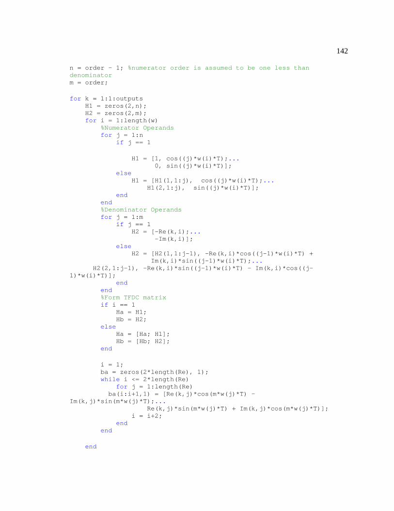
142
n = order - 1; %numerator order is assumed to be one less than denominator m = order; for k = 1:1:outputs H1 = zeros(2,n); H2 = zeros(2,m); for i = 1:length(w) %Numerator Operands for j = 1:n if j == 1 H1 = [1, cos((j)*w(i)*T);... 0, sin((j)*w(i)*T)]; else H1 = [H1(1,1:j), cos((j)*w(i)*T);... H1(2,1:j), sin((j)*w(i)*T)]; end end %Denominator Operands for j = 1:m if j == 1 H2 = [-Re(k,i);... -Im(k,i)]; else H2 = [H2(1,1:j-1), -Re(k,i)*cos((j-1)*w(i)*T) +
Im(k,i)*sin((j-1)*w(i)*T);... H2(2,1:j-1), -Re(k,i)*sin((j-1)*w(i)*T) - Im(k,i)*cos((j-1)*w(i)*T)]; end end %Form TFDC matrix if i == 1 Ha = H1; Hb = H2; else Ha = [Ha; H1]; Hb = [Hb; H2]; end i = 1; ba = zeros(2*length(Re), 1); while i <= 2*length(Re) for j = 1:length(Re) ba(i:i+1,1) = [Re(k,j)*cos(m*w(j)*T) - Im(k,j)*sin(m*w(j)*T);... Re(k,j)*sin(m*w(j)*T) + Im(k,j)*cos(m*w(j)*T)]; i = i+2; end end end

143
if outputs == 1 H = [Ha, Hb]; elseif k == 1 H = [Ha, zeros(size(Ha*outputs-1,1),size(Ha*outputs-1,2)), Hb]; elseif k < outputs H = [H;zeros(size(Ha,1),size(Ha,2)), Ha, Hb]; else H = [H;zeros(size(Ha,1),size(Ha,2)), Ha, Hb]; end if k == 1 b = ba; else b = [b;ba]; end end %Estimate numerator and denominator coefficients using specified least %squares method: switch type case 'LS' %Ordinary Least Squares Solution %Orthogonal-triangular decomposition of H: [Q,R] = qr(H); %Ordinary Least Squares Solution: estimate = pinv(R)*Q'*b; case 'TLS' %Total Least Squares Solution: [U, PHI, Vt] = svd([H,b]); s = size(PHI); estimate = -1/(Vt(s(2),s(2)))*Vt(1:s(2)-1,s(2)); otherwise %If something besides the above choices are entered then %Ordinary Least Squares will be used %Orthogonal-triangular decomposition of H: [Q,R] = qr(H); %Ordinary Least Squares Solution: estimate = pinv(R)*Q'*b; end %Gather numerator and denominator coefficients: if outputs == 1 num_tfdc = estimate(n+1:-1:1)'; den_tfdc = [1 estimate(length(estimate):-1:n+2)']; else for k = 1:1:outputs if k == 1 num_tfdc(k,:) = estimate(n+1:-1:1)'; else
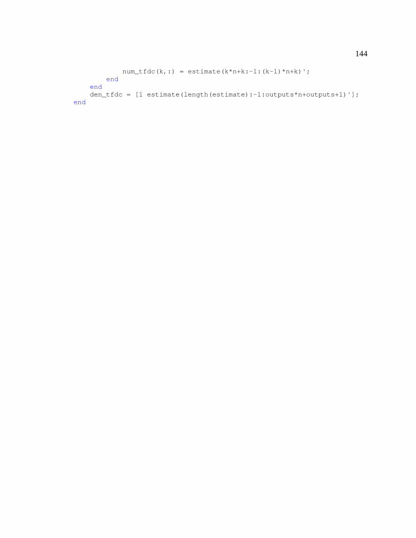
144
num_tfdc(k,:) = estimate(k*n+k:-1:(k-1)*n+k)'; end end den_tfdc = [1 estimate(length(estimate):-1:outputs*n+outputs+1)']; end
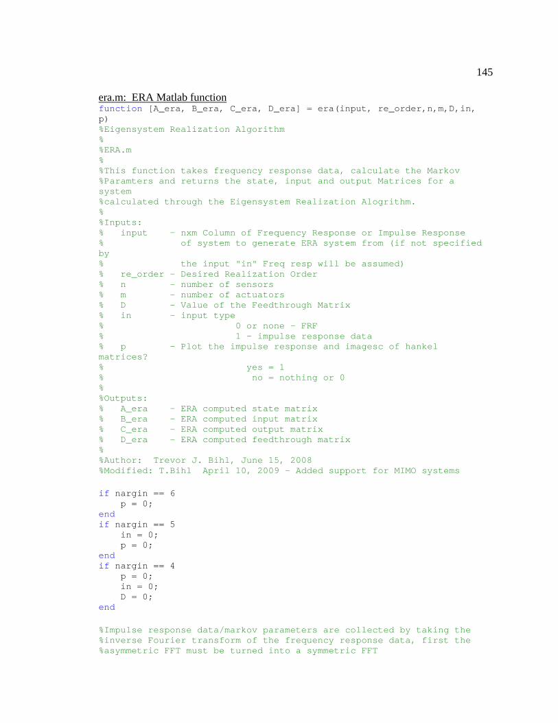
145
era.m: ERA Matlab function function [A_era, B_era, C_era, D_era] = era(input, re_order,n,m,D,in, p) %Eigensystem Realization Algorithm % %ERA.m % %This function takes frequency response data, calculate the Markov %Paramters and returns the state, input and output Matrices for a system %calculated through the Eigensystem Realization Alogrithm. % %Inputs: % input - nxm Column of Frequency Response or Impulse Response % of system to generate ERA system from (if not specified by % the input "in" Freq resp will be assumed) % re_order - Desired Realization Order % n - number of sensors % m - number of actuators % D - Value of the Feedthrough Matrix % in - input type % 0 or none - FRF % 1 - impulse response data % p - Plot the impulse response and imagesc of hankel matrices? % yes = 1 % no = nothing or 0 % %Outputs: % A_era - ERA computed state matrix % B_era - ERA computed input matrix % C_era - ERA computed output matrix % D_era - ERA computed feedthrough matrix % %Author: Trevor J. Bihl, June 15, 2008 %Modified: T.Bihl April 10, 2009 - Added support for MIMO systems if nargin == 6 p = 0; end if nargin == 5 in = 0; p = 0; end if nargin == 4 p = 0; in = 0; D = 0; end %Impulse response data/markov parameters are collected by taking the %inverse Fourier transform of the frequency response data, first the %asymmetric FFT must be turned into a symmetric FFT
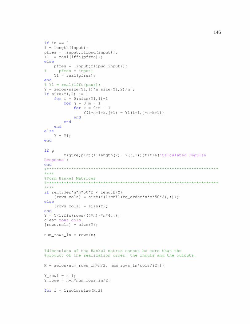
146
if in == 0 l = length(input); pfres = [input;flipud(input)]; Y1 = real(ifft(pfres)); else pfres = [input;flipud(input)]; % pfres = input; Y1 = real(pfres); end % Y1 = real(ifft(pxx)); Y = zeros(size(Y1,1)*n,size(Y1,2)/n); if size(Y1,2) ~= 1 for i = 0:size(Y1,1)-1 for j = 0:m - 1 for k = 0:n - 1 Y(i*n+1+k,j+1) = Y1(i+1,j*n+k+1); end end end else Y = Y1; end if p figure;plot(1:length(Y), Y(:,1));title('Calculated Impulse Response') end %************************************************************************** %Form Hankel Matrices %************************************************************************** if re_order*n*m*50*2 < length(Y) [rows,cols] = size(Y(1:ceil(re_order*n*m*50*2),:)); else [rows,cols] = size(Y); end Y = Y(1:fix(rows/(4*n))*n*4,:); clear rows cols [rows,cols] = size(Y); num_rows_in = rows/n; %dimensions of the Hankel matrix cannot be more than the %product of the realization order, the inputs and the outputs. H = zeros(num_rows_in*n/2, num_rows_in*cols/(2)); Y_rowi = n+1; Y_rowe = n+n*num_rows_in/2; for i = 1:cols:size(H,2)
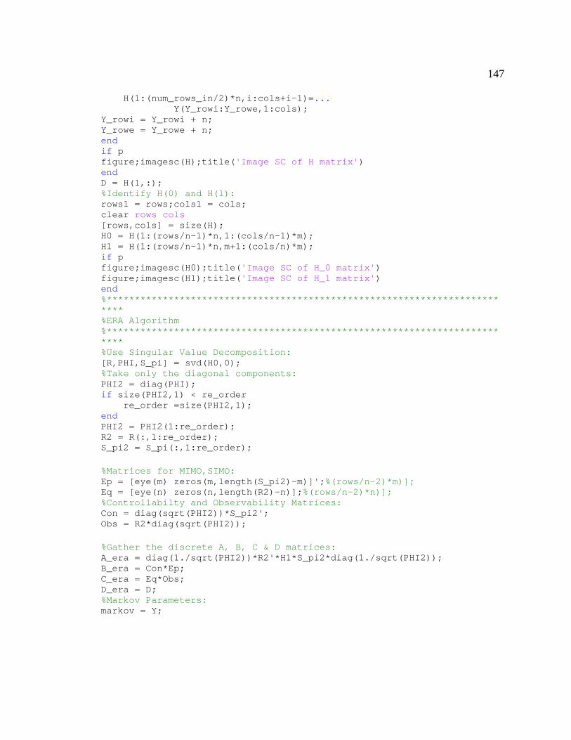
147
H(1:(num_rows_in/2)*n,i:cols+i-1)=... Y(Y_rowi:Y_rowe,1:cols); Y_rowi = Y_rowi + n; Y_rowe = Y_rowe + n; end if p figure;imagesc(H);title('Image SC of H matrix') end D = H(1,:); %Identify H(0) and H(1): rows1 = rows;cols1 = cols; clear rows cols [rows,cols] = size(H); H0 = H(1:(rows/n-1)*n,1:(cols/n-1)*m); H1 = H(1:(rows/n-1)*n,m+1:(cols/n)*m); if p figure;imagesc(H0);title('Image SC of H_0 matrix') figure;imagesc(H1);title('Image SC of H_1 matrix') end %************************************************************************** %ERA Algorithm %************************************************************************** %Use Singular Value Decomposition: [R,PHI,S_pi] = svd(H0,0); %Take only the diagonal components: PHI2 = diag(PHI); if size(PHI2,1) < re_order re_order =size(PHI2,1); end PHI2 = PHI2(1:re_order); R2 = R(:,1:re_order); S_pi2 = S_pi(:,1:re_order); %Matrices for MIMO,SIMO: Ep = [eye(m) zeros(m,length(S_pi2)-m)]';%(rows/n-2)*m)]; Eq = [eye(n) zeros(n,length(R2)-n)];%(rows/n-2)*n)]; %Controllabilty and Observability Matrices: Con = diag(sqrt(PHI2))*S_pi2'; Obs = R2*diag(sqrt(PHI2)); %Gather the discrete A, B, C & D matrices: A_era = diag(1./sqrt(PHI2))*R2'*H1*S_pi2*diag(1./sqrt(PHI2)); B_era = Con*Ep; C_era = Eq*Obs; D_era = D; %Markov Parameters: markov = Y;
148
symZ_FromVector.m: Function to place symbolic notation in transfer functions function [z_eqn] = symZ_FromVector(vector,z) %%%%%%%%%%%%%%%%%%%%%%%%%%%%%%%%%%%%%%%%%%%%%%%%%%%%%%%%%%%%%%%%%%%%%%%% %symZ_FromVector.m % %This function creates a z-domain equation in symbolic form from a vector %of z domain coefficients in reverse order (az^0 az^1 ... aZ^n) % %Inputs: % vector = vector of z-domain coefficients in order % (az^0 az^1 ... aZ^n) % z = symbolic z or z =tf('z',T) % %Outputs: % z_eqn = z-domain equation written in symbolic form %Author: Trevor J. Bihl, July 20, 2009 %%%%%%%%%%%%%%%%%%%%%%%%%%%%%%%%%%%%%%%%%%%%%%%%%%%%%%%%%%%%%%%%%%%%%%%% list = flipud(vector')'; n = length(list); z_ = list(1); for i = 2:n z_i = (z^(i-1))*list(i); z_ = z_i + z_; end z_eqn = z_;
149
Closed_Loop_Plotting.m: Function to plot Flexlab results %Closed_loop_plotting.m % %This program serves analyze I/O data from Flexlab while operating in %Closed Loop Mode % %Author: Trevor J. Bihl % %Initialize variables for creating transfer functions: [fn,pn]=uigetfile({'.txt'},'Select Flexlab Closed Loop Sensor File'); cd(pn); %set workspace as directory flexlab data is in sensor_data = load(strcat(pn,fn)); [fn,pn]=uigetfile({'.txt'},'Select Flexlab Disturbance File'); actuator_data = load(strcat(pn,fn)); [fn,pn]=uigetfile({'.txt'},'Select Flexlab Closed Loop Output File'); output_data = load(strcat(pn,fn)); [fn,pn]=uigetfile({'.txt'},'Select Flexlab Open Loop Sensor File'); % cd(pn); %set workspace as directory flexlab data is in OL_sensor_data = load(strcat(pn,fn)); %Ask user to input experiment data % sim_settings =inputdlg({'Sample Frequency:'}); sim_settings = {'100'}; T = 1/str2double(sim_settings{1}); N = length(actuator_data); ysim(1,1).data = sensor_data(:,8)'; ysim(2,2).data = sensor_data(:,7)'; ysimOL(1,1).data = OL_sensor_data(:,8)'; ysimOL(2,2).data = OL_sensor_data(:,7)'; time = 0:T:(length(ysim(1,1).data)-1)*T; figure; subplot(211);plot(time,ysim(1,1).data);hold on; plot(time,ysimOL(1,1).data,'k'); title('X-Axis PSD');grid on; xlabel('time [sec]');ylabel('Volts (V)') legend('Closed Loop','Open Loop') subplot(212);plot(time,[actuator_data(1:3000,1);output_data(:,1)]); title('X-Axis Motor Control Signal');grid on; xlabel('time [sec]');ylabel('Volts (V)') figure; subplot(211);plot(time,ysim(2,2).data);hold on; plot(time,ysimOL(2,2).data,'k'); title('Y-Axis PSD');grid on; xlabel('time [sec]');ylabel('Volts (V)') legend('Closed Loop','Open Loop') subplot(212);plot(time,[actuator_data(1:3000,2);output_data(:,2)]); title('Y-Axis Motor Control Signal');grid on; xlabel('time [sec]');ylabel('Volts (V)')