1

An ASABE Meeting Presentation Paper Number: 096372

Key Performance Indicators for Variable Rate Irrigation Implementation on Variable Soils

Carolyn Hedley New Zealand Centre for Precision Agriculture, Massey University and Landcare Research, Private Bag 11052, Manawatu Mail Centre, Palmerston North 4442, New Zealand. email: HedleyC@LandcareResearch.co.nz

Ian Yule New Zealand Centre for Precision Agriculture, Massey University, Palmerston North 4474, New Zealand.

Mike Tuohy New Zealand Centre for Precision Agriculture, Massey University, Palmerston North 4474, New Zealand.

Iris Vogeler AgResearch, Grasslands Research Centre, Tennent Drive, Private Bag 11008, Palmerston North 4442, New Zealand.

Written for presentation at the 2009 ASABE Annual International Meeting

Sponsored by ASABE Grand Sierra Resort and Casino

Reno, Nevada June 21 – June 24, 2009

Abstract. Decision support tools for precise irrigation scheduling are required to improve the efficiency of irrigation water use globally. This paper presents a method for mapping soil variability and relating it to soil hydraulic properties so that soil management zones for variable rate irrigation can be defined. A soil water balance is used to schedule hypothetical irrigation events based on (i) one blanket application of water to eliminate plant stress, which inevitably over-waters some zones where variable soils exist (uniform rate irrigation, URI) and compares this to (ii) variable rate irrigation (VRI), where irrigation is tailored to specific soil zone available water holding capacity (AWC) values. The key performance indicators: irrigation water use, drainage water loss, nitrogen leaching, energy use, irrigation water use efficiency (IWUE) and virtual water content are used to compare URI and VRI at three contrasting sites using four years climate data for a dairy pasture and maize crop and two

2

years climate data for a potato crop. Our research found that VRI saved 9 − 19 % irrigation water, with accompanying energy saving. Loss of water by drainage was also reduced by 20 − 29% using VRI, which reduced the risk of nitrogen leaching. Virtual water content of these three primary products further illustrates benefits of VRI and shows that virtual water content of potato production used least water per unit of dry matter production.

Keywords. Water use efficiency, nitrogen leaching, CO2 equivalent, drainage, virtual water.

Introduction

Variable rate irrigation (VRI) delivers different depths of irrigation water simultaneously to different parts of a field, preferably with high spatial resolution (<10m or better). Lateral and centre pivot sprinkler systems are well suited to VRI if modified with individual sprinkler control (King & Kincaid, 2004; Dukes & Perry, 2006; Pierce & Elliott, 2008; Bradbury, 2009), and other systems (e.g. surface and subsurface drip, towable spraylines, rain-guns) can also be employed but in general are less well suited with lower spatial resolution of application.

The benefits of VRI include increased flexibility for mixed cropping (with different irrigation requirements), ease of chemigation and fertigation (reduced fuel cost and soil compaction risk on wet soils; precision application), and the ability to shut-off water as the irrigator passes over farm tracks, ditches etc. In addition, where one irrigation system exists over an area of variable soils, VRI can maintain soil water status within the optimum range for maximum potential yields (Hedley & Yule, 2009), making best use of stored soil profile water, and minimizing run-off and deep percolation. VRI therefore enables strategic water use with improved water use efficiency.

Practitioner decisions to invest in VRI technologies will be driven by the perceived value of these benefits. Where water allocations are restricted (e.g. Kang et al., 2000: Kirda, 2004) and water charges exist (e.g. Burt, 2006) the economic benefits of improved water use efficiency (kg yield per amount of irrigation water applied) and reduced energy costs (less pumping) are easily quantified. Other potential benefits include less runoff and drainage with accompanying advantages of reduced risk of nutrient leaching, and protected biodiversity in waterways by reduced extraction. The “value” of this latter environmental benefit largely falls outside of traditional cost-benefit analysis, however it is now recognized that the traditional approach for assessing “value” is severely limited. “Value” should include not only direct benefits to the party who stands to gain from the product but also the wider ecological consequences of these decisions, and the social goals being served by the decision (Costanza, 2006). “Failure to think broadly enough about costs and benefits leads to decisions that serve only narrow special interest not the sustainable well-being of society as a whole” (Costanza, 2006).

An unprecedented demand by irrigation for freshwater in New Zealand in recent decades, to support increasing agricultural productivity, has led to decreased flows compared to long-term averages in some rivers. Irrigation demands 77% of all allocated freshwaters in New Zealand, slightly higher than the global average of 70%, (NZ Mfe, 2007). The Canterbury region of the South Island occupies 66% of total consented irrigated land, and river flows have dropped from long-term mean values at nearly all monitored sites, with drops of 10−25% at some sites (ECan, 2008). This example illustrates that freshwater extraction for irrigation has its limits which must be clearly defined. It exemplifies the reason why the New Zealand government formulated the “Sustainable Development Water Programme of Action” in 2003 (NZ MfE, 2007) focusing national policy on freshwater allocation with appropriate methods for setting ecological flows as well as setting standards for mandatory measurement of actual water takes. Where freshwater supply is limited (frequently due to high irrigation demand) then the full value of improved water use efficiency includes not only

3

profit margins of crop production but also societal impacts by addressing issues of reduced freshwater supply, reduced water quality, and insufficient environmental river flow (reduced biodiversity, culture and heritage). The direct economic value of irrigation for New Zealand is estimated to be NZ$920m from 475 700 ha of land (NZ MAF, 2004). This is estimated as net contribution to GDP at the farm-gate for the year 2002/03, and was estimated using the formula:

Farm-gate GDP due to irrigation = GDP with irrigation – GDP without irrigation (MAF, 2004)

Therefore the use of irrigation in New Zealand increases the dollar return per hectare of agricultural land by about NZ$1934.

The total ecosystem services value of New Zealand’s rivers and lakes has been defined and estimated by Patterson and Cole (1999). A full description of the methods used is beyond the scope of this paper, and readers are referred to Patterson and Cole (1999) and Costanza et al (1997) for more detail. Patterson and Cole (1999) assess the value of biodiversity (TEV) as:

TEV = DV + IV + PV (1)

where, TEV = total economic value; DV = direct value of goods and services derived from direct use of biodiversity (i.e. the agricultural production); IV = indirect value derived from supporting or protecting direct use activities, (i.e. nutrient cycling, biological refugia, waste treatment etc); PV = passive value, value not related to the actual use (i.e. existence and bequeath option).

Using the default methodology of values developed by Costanza et al (1997), Patterson and Cole (1999) derived a first approximation of the direct and indirect value of ecosystem services provided by New Zealand lake and river ecosystems as NZ$7871m. Using an estimate of 303 977 ha for the total surface area covered by lake ecosystems and 225 750 ha covered by river systems (calculated using first order rivers and assuming a mean width of 500 metre) this equates to a biodiversity value of New Zealand’s lakes and rivers of NZ$29 718 per hectare.

An increase in the productivity of irrigation water through changes in management and improvements in efficiency offer the greatest potential for global water savings, because irrigated agriculture is the dominant consumptive user of freshwater world-wide, (Jury and Vaux, 2007). This is where VRI plays its role.

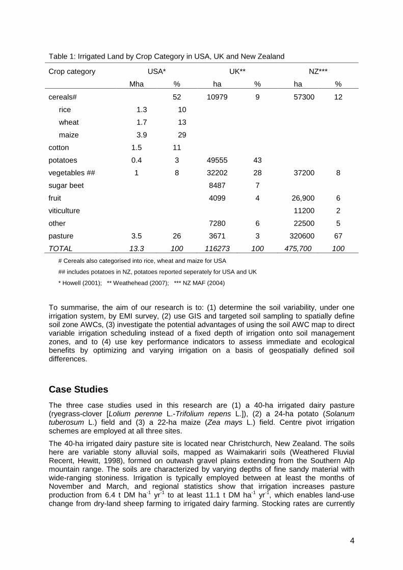
Case studies, for the research presented in this paper, to assess potential benefits of a VRI system compared to uniform rate irrigation (URI), were selected to represent two of the four major global irrigated crops (maize, potatoes) and pasture. Sustained productivity of the four major global crops: rice, wheat, maize and potatoes, is reliant on irrigation. In the USA, more than half of the irrigation is used for growing cereals, with maize (Zea mays L.) being the largest irrigated crop (Table 1). 71% of irrigation in the UK is used for vegetable growing, with potatoes being the largest irrigated crop. In New Zealand, two-thirds of our irrigation is used on pastoral soils (Table 1), and about 52% of this irrigated pastoral land is used for dairy farming (NZ Statistics, 2003).

Soil variability at each site was assessed by EMI (electromagnetic induction) survey. Maps of soil apparent electrical conductivity (ECa) define soil variability on a basis of texture and moisture (e.g. Sudduth et al., 2005), and these maps can be used to target soil zones for estimation of the range of soil AWC (available water holding capacity) present at one site (Hedley and Yule, 2009). Irrigation scheduling can then be optimized spatially using the soil zone AWC and a daily soil water balance.

4

Table 1: Irrigated Land by Crop Category in USA, UK and New Zealand

Crop category USA* UK** NZ***

Mha % ha % ha %

cereals# 52 10979 9 57300 12

rice 1.3 10

wheat 1.7 13

maize 3.9 29

cotton 1.5 11

potatoes 0.4 3 49555 43

vegetables ## 1 8 32202 28 37200 8

sugar beet 8487 7

fruit 4099 4 26,900 6

viticulture 11200 2

other 7280 6 22500 5

pasture 3.5 26 3671 3 320600 67

TOTAL 13.3 100 116273 100 475,700 100 # Cereals also categorised into rice, wheat and maize for USA

## includes potatoes in NZ, potatoes reported seperately for USA and UK

* Howell (2001); ** Weathehead (2007); *** NZ MAF (2004)

To summarise, the aim of our research is to: (1) determine the soil variability, under one irrigation system, by EMI survey, (2) use GIS and targeted soil sampling to spatially define soil zone AWCs, (3) investigate the potential advantages of using the soil AWC map to direct variable irrigation scheduling instead of a fixed depth of irrigation onto soil management zones, and to (4) use key performance indicators to assess immediate and ecological benefits by optimizing and varying irrigation on a basis of geospatially defined soil differences.

Case Studies The three case studies used in this research are (1) a 40-ha irrigated dairy pasture (ryegrass-clover [Lolium perenne L.-Trifolium repens L.]), (2) a 24-ha potato (Solanum tuberosum L.) field and (3) a 22-ha maize (Zea mays L.) field. Centre pivot irrigation schemes are employed at all three sites.

The 40-ha irrigated dairy pasture site is located near Christchurch, New Zealand. The soils here are variable stony alluvial soils, mapped as Waimakariri soils (Weathered Fluvial Recent, Hewitt, 1998), formed on outwash gravel plains extending from the Southern Alp mountain range. The soils are characterized by varying depths of fine sandy material with wide-ranging stoniness. Irrigation is typically employed between at least the months of November and March, and regional statistics show that irrigation increases pasture production from 6.4 t DM ha-1 yr-1 to at least 11.1 t DM ha-1 yr-1, which enables land-use change from dry-land sheep farming to irrigated dairy farming. Stocking rates are currently

5

3.3 cows ha-1 in this area; and nitrogen fertilizers are typically applied at a rate of 150−300 kg N ha-1 yr-1 which is used strategically to address expected feed deficits.

The 23-ha potato field near Ohakune, in the Central Volcanic Plateau region of the North Island of New Zealand. Here a 400 m centre pivot is employed for strategic irrigation of potatoes during the summer months of November to February. The variable soils at this site are formed on mixed volcanic parent materials: air-fall andesitic tephra, water-borne laharic material and air-fall rhyolitic pumice. The area is flat to easy rolling topography and a low-angle pumice ridge occurs in the south-east corner, against which laharic material has abutted. The pumice ridge has formed from tephra originating from a nuee ardent eruption from the Taupo area, ca. 1850 years ago. The soils have not been mapped but are likely to be Typic Orthic Pumice soils and Tephric Recent soils (Hewitt, 1998).

The 22-ha irrigated maize field occurs in the Sand Country Region of Manawatu Province, New Zealand. The topography is a sand plain-sand dune catena sequence. The soils are mapped as a Pukepuke-Foxton soil association (Cowie et al., 1967). The dune soils, Foxton dark grey sands (Typic Sandy Brown soils, Hewitt, 1998) are somewhat excessively drained sandy soils and they exist alongside low-lying poorly drained sandy soils, Pukepuke brown loamy sands (Typic Sandy Gley soils, Hewitt, 1998) where the water table rises close to the soil surface in low-lying areas during the winter months. Irrigation is normally employed during the summer months of November to March, when there is a significant seasonal soil moisture deficit. The use of irrigation at this site enables land-use change from dry-land sheep and beef production to productive cropping.

Methodology

Assessing soil variability by electromagnetic soil survey

An electromagnetic (EM) soil survey was employed to spatially define soil variability with respect to soil water supply characteristics at each site. A Geonics electromagnetic EM38 sensor (Geonics Ltd, Mississauga, Ontario, Canada) and real time kinematic-differential global positioning system (RTK-DGPS) with Trimble Ag170 field computer (Trimble Navigation Ltd, Sunnyvale, California, USA) on-board an all-terrain vehicle (ATV) were used for on-the-go soil EM mapping. The ATV was driven at 12 km h-1 at swath widths of 10 metres. Soil apparent electrical conductivity (ECa), measured by the EM sensor, was logged simultaneously with high resolution positional data at 1 Hz.

Soil apparent electrical conductivity map production

Soil ECa survey points were filtered to remove: (i) RTK-GPS data classified as low accuracy, in order to ensure precise elevation information, and (ii) outlying ECa values. Filtered data were then imported into ArcMap™ (Environmental Systems Research Institute, ESRI©1999) as latitude and longitude using a WGS84 projection, and subsequently converted to New Zealand Map Grid projection, using the (GD 1949) geodetic datum. The points were kriged using Geostatistical Analyst (ESRI©1999), using ordinary kriging and a spherical semivariogram model, to produce a map of soil ECa. Soil ECa values reflect soil texture and moisture changes in non-saline soils (e.g. Sudduth et al., 2005), so the soil ECa map could be used to target sites for soil description and sampling likely to reflect the widest range of soil water holding characteristics. Intact soil cores were collected in high, medium and low ECa zones, to assess the range of soil available water holding content (TAWC) at each site (Hedley & Yule, 2009).

Estimation of soil TAWC in ECa-defined management zones

The soil total available water-holding capacity (TAWC) of each ECa-defined management zone (high ECa zone, intermediate ECa zone, low ECa zone) was estimated by soil

6

sampling at three replicate sites within each zone. Intact cores were collected for laboratory estimation of soil water retention at 10kPa (Field Capacity) and 1500kPa (Wilting Point). TAWC is defined as the difference between the equivalent depths of water that the effective root zone (or a sampling depth within that root zone) contains at field capacity (FC) and at Permanent Wilting Point (WP).

The soils were sampled to 60 cm depth to include the majority of roots, which extract soil water for plant use. Soil samples (0–15 cm, 15–30 cm, 30–45 cm, 45–60 cm) were also collected for estimation of percent sand, silt, clay and stones.

Soil TAWC map production

The ECa map was interpreted on a basis of lab-estimated TAWC or EAWC (Effective AWC) for each soil management zone. EAWC is the sum of TAWC and Capillary Rise (CR) and was used where additional plant available water was supplied via capillary rise from a high water table.

Adding the daily time-step to soil TAWC maps using a water balance model

The amount of plant-available water held in each ECa-defined soil zone on any one day was calculated using a water balance model (Allen et al. 1998). This model determines soil water content in terms of root zone soil water depletion (S) relative to FC, and is expressed as a water depth in the root zone (mm).

S i = S i-1 – R i – I i – C i + Eti + Di (2)

where, Si is root zone soil water depletion at the end of day i (mm), Si-1 is the depletion at the end of the previous day, i-1 (mm), Ri is the rainfall on day i (mm), Ii is the irrigation applied on day i (mm), Ci is the capillary rise from groundwater (GW), assumed to be zero when GW>1 m, on day i, Eti is crop evapotranspiration on day i (mm) and Di is drainage (runoff plus root zone water loss due to deep percolation) on day i.

Root zone soil water depletion at FC is zero (S = 0), and as soil water is extracted by Et a critical soil moisture deficit (CSMD) is reached where Et is limited to less than potential values, and pasture or crop Et begins to decrease in proportion to the amount of water remaining in the root zone (Allen et al. 1998). The amount of water held in the soil between FC and CSMD is defined as the readily available water (RAW), which was determined using the specific pasture and maize depletion fractions (of TAWC) defined by Allen et al (1998). Site-specific R and I were measured, and Et was estimated from site-specific climate data and adjusted for crop stage at the irrigated maize and potato sites. Capillary rise, C, was assumed to be zero at two sites, but contributes additional plant available water at the maize site. At this site, retentivity and conductivity data were used to assess the contribution from capillary rise (Scotter, 1989). A value for D, which includes runoff and deep percolation below the root zone, was calculated as the excess water above FC by the soil water balance model.

The water balance, calculated for each soil zone AWC, assesses soil water status, i.e. mm of available water present in each soil zone on any one day, indicating the day when the CSMD is reached and irrigation should commence.

In addition the water balance was used to estimate the total amount of drainage and evapo-transpiration (Et) in any one season.

Variable-rate irrigation scheduling

The soil water balance was also used to compare hypothetical uniform-rate irrigation (URI) scheduling with variable-rate irrigation (VRI) schedules for each of four seasons (1/7/04−30/6/05; 1/7/05−30/6/06; 1/7/06−30/6/07; 1/7/07-30/6/08) at the pasture and maize site, and for two seasons (1/7/07-30/06/08; 1/7/08-1/4/09) in the potato field. URI scheduling

7

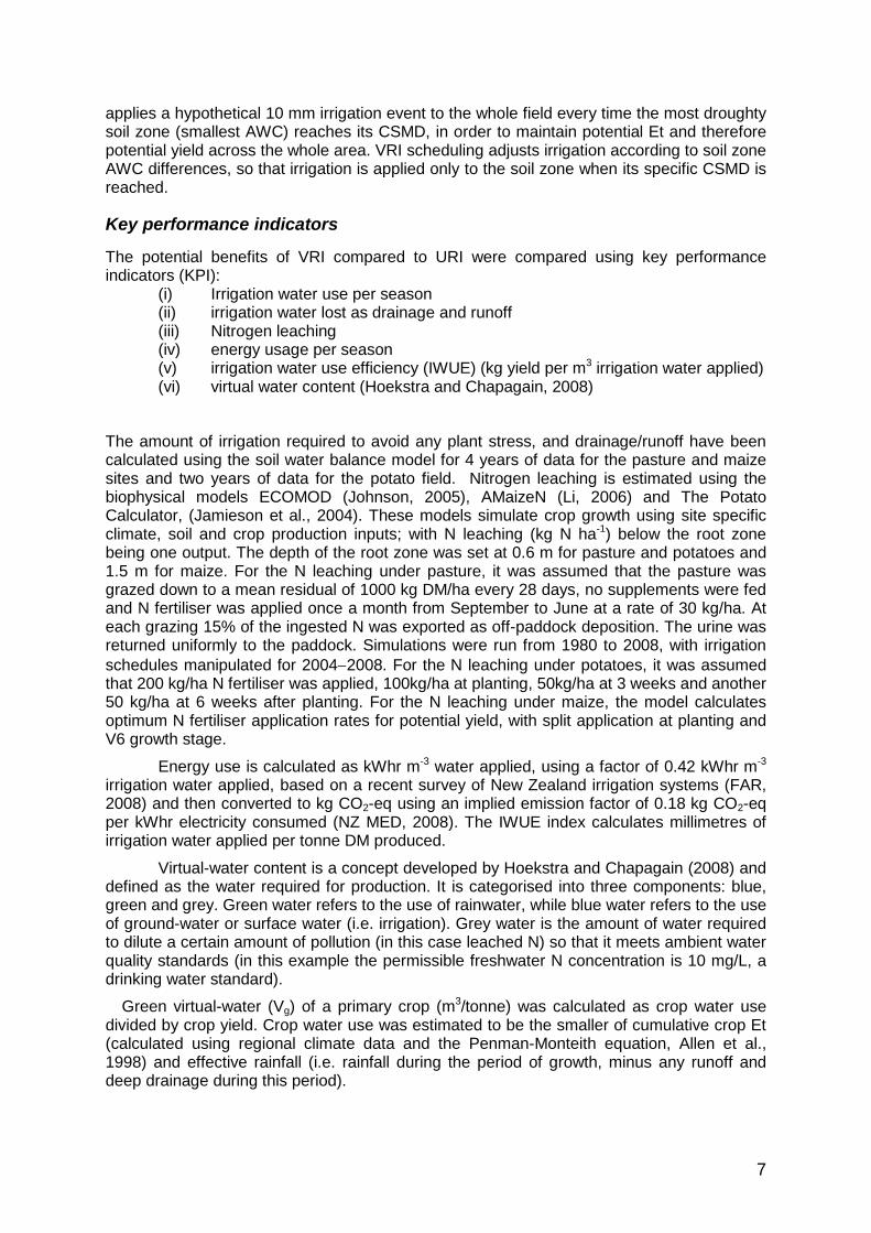
applies a hypothetical 10 mm irrigation event to the whole field every time the most droughty soil zone (smallest AWC) reaches its CSMD, in order to maintain potential Et and therefore potential yield across the whole area. VRI scheduling adjusts irrigation according to soil zone AWC differences, so that irrigation is applied only to the soil zone when its specific CSMD is reached.

Key performance indicators

The potential benefits of VRI compared to URI were compared using key performance indicators (KPI):

(i) Irrigation water use per season (ii) irrigation water lost as drainage and runoff (iii) Nitrogen leaching (iv) energy usage per season (v) irrigation water use efficiency (IWUE) (kg yield per m3 irrigation water applied) (vi) virtual water content (Hoekstra and Chapagain, 2008)

The amount of irrigation required to avoid any plant stress, and drainage/runoff have been calculated using the soil water balance model for 4 years of data for the pasture and maize sites and two years of data for the potato field. Nitrogen leaching is estimated using the biophysical models ECOMOD (Johnson, 2005), AMaizeN (Li, 2006) and The Potato Calculator, (Jamieson et al., 2004). These models simulate crop growth using site specific climate, soil and crop production inputs; with N leaching (kg N ha-1) below the root zone being one output. The depth of the root zone was set at 0.6 m for pasture and potatoes and 1.5 m for maize. For the N leaching under pasture, it was assumed that the pasture was grazed down to a mean residual of 1000 kg DM/ha every 28 days, no supplements were fed and N fertiliser was applied once a month from September to June at a rate of 30 kg/ha. At each grazing 15% of the ingested N was exported as off-paddock deposition. The urine was returned uniformly to the paddock. Simulations were run from 1980 to 2008, with irrigation schedules manipulated for 2004−2008. For the N leaching under potatoes, it was assumed that 200 kg/ha N fertiliser was applied, 100kg/ha at planting, 50kg/ha at 3 weeks and another 50 kg/ha at 6 weeks after planting. For the N leaching under maize, the model calculates optimum N fertiliser application rates for potential yield, with split application at planting and V6 growth stage.

Energy use is calculated as kWhr m-3 water applied, using a factor of 0.42 kWhr m-3 irrigation water applied, based on a recent survey of New Zealand irrigation systems (FAR, 2008) and then converted to kg CO2-eq using an implied emission factor of 0.18 kg CO2-eq per kWhr electricity consumed (NZ MED, 2008). The IWUE index calculates millimetres of irrigation water applied per tonne DM produced.

Virtual-water content is a concept developed by Hoekstra and Chapagain (2008) and defined as the water required for production. It is categorised into three components: blue, green and grey. Green water refers to the use of rainwater, while blue water refers to the use of ground-water or surface water (i.e. irrigation). Grey water is the amount of water required to dilute a certain amount of pollution (in this case leached N) so that it meets ambient water quality standards (in this example the permissible freshwater N concentration is 10 mg/L, a drinking water standard).

Green virtual-water (Vg) of a primary crop (m3/tonne) was calculated as crop water use divided by crop yield. Crop water use was estimated to be the smaller of cumulative crop Et (calculated using regional climate data and the Penman-Monteith equation, Allen et al., 1998) and effective rainfall (i.e. rainfall during the period of growth, minus any runoff and deep drainage during this period).

8

Blue virtual-water (Vb) of a primary crop (m3/tonne) was calculated as effective crop irrigation water use divided by crop yield. Effective irrigation water use was calculated as the irrigation requirement (estimated from the soil water balance model) minus any runoff and deep drainage during this period. Grey virtual-water (Vgr) is calculated as the load of pollutants that enters the water system (in this case leached nitrogen), divided by the maximum acceptable concentration for the pollutant and the crop production. The virtual water content on each primary product for any one year was then calculated in m3 t-1 (Hoeskstra and Chapagain, 2008):

V = Vg + Vb + Vgr (3)

Table 2 Explanation of Key Performance Indicators for assessing potential benefits of VRI

KPI Units Description

Water Use mm season-1 Total amount of irrigation water applied in one season (1 July 07 – 30 June 08)

Drainage/Runoff mm season-1 Drainage and runoff during one growing season (pasture: 1 July − 30 June), calculated as excess above FC by the soil water balance model; implications for nutrient leaching,

Nitrogen leaching kg ha-1 season-1 Amount of nitrogen leached below the root zone and therefore wasted to crop production

Energy usage kgCO2-eq kWhr-energy consumed-1

Energy usage (kWhr m-3) for operation of irrigation system (largely cost of pumping water) converted to equivalent CO2 emissions

Water Use Efficiency

mm tonne DM-1 Reports mm of irrigation water applied per tonne DM produced

Virtual-water m3 tonne DM-1 The water needed to produce a product

Results

Soil ECa maps

The soil ECa maps (Figure 1) were classified into three zones which were investigated for visible soil differences, and sampled to assess soil TAWC (Table 3). Soil ECa zones at the pasture site were characterised by percent stones difference. Increasing percent stones in a sandy loam matrix decreased soil ECa. There were significant differences in the soil water holding characteristics of each ECa-defined zone which could therefore be used as an irrigation management zone on a basis of its soil water holding properties. At this pasture site, TAWC increased linearly with soil ECa, reflecting this percent stone increase (Figure 2)

9

a)

b)

c)

Figure 1. Soil ECa maps delineate zones with contrasting TAWC (a = Pasture; b = Potato; c

= Maize site)

The low ECa soil management zone contains 70% stones which reduced its TAWC to 7% (44 mm in 60 cm of root zone) compared with the zone with no stones (TAWC = 17%) and the intermediate ECa zone with 39% stones (TAWC= 12%).

10

y = 38.4x - 450.8R2 = 0.9

0

20

40

60

80

100

120

12 13 14 15

ECa (mS m-1)

TAW

C (m

m in

root

zon

e)

Figure 2 Relation of soil ECa to TAWC for Waimakariri soils, at the pastoral site

At the potato site, visual soil inspections at the three ECa soil management zones, revealed three contrasting volcanic parent materials reflecting the frequent episodic nature of volcanic eruptions and lahar events which have contributed to soil forming processes at this site, which is adjacent to the active Central Volcanic Zone of the North Island of New Zealand. The low ECa value zone is characterized by deep, freely draining, pumiceous loamy silt soils, developed in the Taupo Pumice formation (1850 yrs BP). The soils in the intermediate ECa zone have developed in andesitic ash (with gravels) inter-bedded with some lahar material. Soils in the high ECa zone have developed on mixed andesitic and lahar parent materials, dominated by the more recent lahar material. The lahar deposit is possibly part of the Onetapu Formation, which has been described close to this site, and dated ca. 450 ± 55 years BP (Suryaningtyas, 1998). Each zone is characterized by significantly different soil AWCs (Table 3). The lower AWC in Zone 2 is likely due to the observed soil compaction and the welded nature of the andesitic ash, which suggests that drying and wetting patterns modelled using a soil water balance for this soil with impeded drainage are likely to over-estimate rate of drainage, because the soil water balance assumes a freely draining soil.

The maize site is characterized by sandy soils in an undulating topography where the water-table rises to, or close to, the surface in low-lying areas, during the winter months. These wet low-lying areas occupy the high ECa soil management zone, and the contribution of plant available water via capillary rise from the water table is an important contributor. Scotter (1989) showed that soil water retentivity and hydraulic conductivity data can be used to predict this contribution in these soils, and estimated that the equivalent depth of plant-available water increased substantially from 26 to 183 mm as the water table rises from 1.2 m to 0.4 m. Using this relationship, and our observations that the water table rises to within 0.8 m and 1.2 m of the root zone during the maize growing season in the high and medium ECa-zones, respectively, we estimated a contribution of 130 mm and 30 mm respectively to soil AWC at these two sites. The high, medium and low soil ECa management zones reflect decreasing TAWC and EAWC, respectively (Table 3).

At all three sites the range of AWC (mm available water in the root zone) under one irrigation system varied by more than a two-fold difference. Therefore the potential benefits of variable rate irrigation were assessed.

11

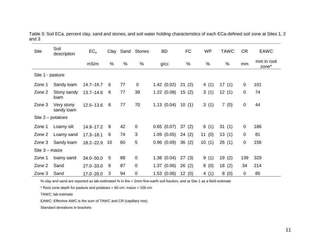
Table 3: Soil ECa, percent clay, sand and stones, and soil water holding characteristics of each ECa-defined soil zone at Sites 1, 2 and 3

% clay and sand are reported as lab-estimated % in the < 2mm fine-earth soil fraction, and at Site 1 as a field-estimate

* Root zone depth for pasture and potatoes = 60 cm; maize = 100 cm

TAWC: lab estimate

EAWC: Effective AWC is the sum of TAWC and CR (capillary rise)

Standard deviations in brackets

Site Soil description ECa Clay Sand Stones BD FC WP TAWC CR EAWC

mS/m % % % g/cc % % % mm mm in root zone*

Site 1 - pasture

Zone 1 Sandy loam 14.7−16.7 6 77 0 1.42 (0.02) 21 (2) 4 (1) 17 (1) 0 101

Zone 2 Stony sandy loam

13.7−14.6 6 77 39 1.22 (0.08) 15 (2) 3 (1) 12 (1) 0 74

Zone 3 Very stony sandy loam

12.5−13.6 6 77 70 1.13 (0.04) 10 (1) 3 (1) 7 (0) 0 44

Site 2 – potatoes

Zone 1 Loamy silt 14.9−17.2 8 42 0 0.65 (0.07) 37 (2) 6 (1) 31 (1) 0 186

Zone 2 Loamy sand 17.3−18.1 6 74 3 1.09 (0.05) 24 (2) 11 (0) 13 (1) 0 81

Zone 3 Sandy loam 18.2−22.9 10 60 5 0.96 (0.09) 36 (2) 10 (1) 26 (1) 0 156

Site 3 – maize

Zone 1 loamy sand 34.0−50.0 5 88 0 1.38 (0.04) 27 (3) 9 (1) 19 (2) 139 329

Zone 2 Sand 27.0−33.0 6 87 0 1.37 (0.06) 26 (2) 8 (0) 18 (2) 34 214

Zone 3 Sand 17.0−26.0 3 94 0 1.53 (0.06) 12 (0) 4 (1) 8 (0) 0 85

15

Estimation of daily soil water status in soil management zones using the soil water balance model

The soil water balance was used to estimate daily soil moisture deficit (SMD) and run-off/drainage events for each zone AWC. Figure 3 illustrates changes in SMD and runoff/drainage events for the period 1/7/07 to 1/7/08 for each of the high AWC zones at the three sites. It also shows the hypothetical 10 mm irrigation events, scheduled using the soil water balance, when each specific zone AWC reaches its Stress Point, the trigger point for irrigation (VRI). URI applies irrigation water to the whole site when the Stress Point for the soil with the smallest AWC is reached, and therefore applies water needlessly to other zones with larger available water storage capacity. Under VRI the number of irrigation events are reduced (Figure 3), because irrigation is tailored to each specific zone AWC, and irrigation is only applied to that zone when it’s specific Stress Point is reached. This soil water status information can be used to drive an automated variable rate irrigation system with irrigation scheduling optimized for each zone AWC.

Total volumes of irrigation water required, and total volumes of water lost through drainage and run-off were also calculated for each zone for a whole season, using 2−4 years of climate data (Table 4)

(a)

-120

-80

-40

0

40

80

120

1-Jul-0731-Aug-07

31-Oct-0731-Dec-07

1-Mar-081-May-08

1-Jul-08

SMD

m

m

RO

Past101URI_SMDPast101URI_ROPast101VRI_SMDPast101VRI_ROPast101NI_SMDPast101NI_RO

010

1/07/07 1/09/07 1/11/07 1/01/08 1/03/08 1/05/08 1/07/08

0

10 IE URI

IE VRI

16

(b)

-200.0

-150.0

-100.0

-50.0

0.0

50.0

100.0

1-Jul-0731-Aug-07

31-Oct-0731-Dec-07

1-Mar-081-May-08

1-Jul-08

SMD

m

m

RO Pot186URI_SMD

Pot186URI_ROPot186VRI_SMDPot186VRI_ROPot186NI_SMDPot186NI_RO

0.0

10.0

1/07/07 1/09/07 1/11/07 1/01/08 1/03/08 1/05/08 1/07/08

0.0

10.0IE URI

IE VRI

(c)

-340.0

-280.0

-220.0

-160.0

-100.0

-40.0

20.0

80.0

1-Jul-0731-Aug-07

31-Oct-0731-Dec-07

1-Mar-081-May-08

1-Jul-08

SMD

m

m

RO Mz329URI_SMD

Mz329URI_ROMz329VRI_SMDMz329VRI_ROMz329NI_SMDMz329NI_RO

0

10

0

10

1/07/07 1/09/07 1/11/07 1/01/08 1/03/08 1/05/08 1/07/08

IE URI

IE VRI

Figure 3. Soil moisture deficit, runoff and irrigation events for 1/7/07 − 1/7/08 at (a) pasture site, (b) potato field and (c) maize grain site, using URI, VRI and no irrigation (IE= 10 mm irrigation events)

17

Assessing the potential benefits of VRI using key performance indicators

Table 4 compares VRI and URI for (1) total volume of irrigation water required, (2) total volume of water lost during irrigation due to runoff and deep drainage, (3) the amount of nitrogen leached from the soil profile, (4) energy savings due to reduced pumping of reduced water, (5) irrigation water use efficiency (IWUE) expressed as mm/t (using one mean yield value). KPI were calculated for each zone and then these values were proportioned for the whole site, using size (ha) of each zone. Virtual water content for each production site is also reported in Table 5.

Table 4: A comparison of VRI and URI of pasture, potatoes and maize grain for total irrigation requirement, drainage, N leaching, energy use and IWUE

Site Site 1 Site 2 Site 3

Dairy pasture Potatoes Maize grain

Irrigation m3 ha-1

I uri 5100 2150 3850

I vri 4658 1879 3107

% saved 9 13 19

Drainage m3 ha-1

D uri 2183 500 595

D vri 1740 353 448

% saved 20 29 25

N leached kg ha-1

N uri 379 11.9 22.1

N vri 376 9.4 22.1

% saved 1 21 0

Energy used kg CO2-eq ha-1

E uri 386 163 291

E vri 352 142 235

% saved 9 13 19

Irrigation Water Use Efficiency mm t-1

IWUE uri 29 13 28

IWUE vri 26 11 22

18

Our results show that VRI scheduling to soil zones using a water balance approach saves 9 − 19 % of irrigation water at these three sites, with accompanying energy savings due to reduced pumping. This equates to an operating cost saving of NZ$35/ha (potatoes), NZ$88/ha (pasture) and NZ$149/ha (maize), based on an estimated operating cost for irrigation of NZ$2/mm/ha (FAR, 2008). Maximum water savings are at the maize site, where the contribution of plant available water via capillary rise in low-lying areas reduced the amount of irrigation water required by 743 m3 ha-1 yr-1 (mean of 4 years). 13% water saving at the potato field is a conservative estimate of potential water savings, because the water balance modelling approach assumes drainage is not impeded. However field observations showed significant compaction in the soil zone of smallest AWC suggesting that further water savings could be made using real-time soil moisture monitoring at this site.

A consequence of the over-watering that occurs under URI of variable soils is increased run-off and deep drainage, and our results show a 20 – 29 % reduction in drainage waters under VRI. Loss of irrigation water by drainage reduces IWUE (Table 4) and increases the likelihood of nitrogen leaching. Small decreases in nitrogen leaching were modelled for potatoes and pasture using VRI compared with URI, but no reduction was modelled at the maize site, perhaps reflecting the fact that the maize crop model is modelling N leaching below 1.5 m compared to the depth of 0.6 m used by the other two models. However the increased drainage implies that there is greater risk of N leaching below the root zone during the period of irrigation, e.g. during a large rainfall event.

Irrigation

Drainage

IWUE

Energy

pasture_vripasture_urimaize_vrimaize_uripotato_vripotato_uri

Figure 4 Radar chart comparing potential benefits of VRI under pasture, potatoes and maize

grain

The potential benefits of VRI of pasture, maize and potatoes is illustrated and compared in Figure 4, where each KPI index is expresses as a fraction of its largest value (in all cases URI of

19

pasture). This comparison of the three sites shows the potato crop to be most water and energy efficient per unit of dry matter production. IWUE was 13 mm t-1(URI) and 11 mm t-1(VRI) for potatoes, compared with 28 mm t-1(URI) and 22 mm t-1(VRI) for maize, and 29 mm t-1(URI) and 26 mm t-1(VRI) for pasture.

Figure 5 illustrates the relative proportions of virtual water contained in each product, produced under VRI and URI. Primary production of potatoes (VRI: 308 m3 t-1; URI: 325 m3 t-1) includes less virtual water than maize (VRI: 622 m3 t-1; URI 654 m3 t-1), which includes less virtual water than pasture production (VRI: 2651 m3 t-1; URI: 2667 m3 t-1). Virtual water content of maize (622−654 m3 t-1) compares with a world average value of 900 m3 t-1 (Hoekstra and Chapagain, 2008), reflecting differences in climate and technology. 81% of the total water requirement for pasture production is accounted for as grey water, significantly larger than for the other 2 sites, reflecting the level of nitrogen leaching which occurs from all-year grazed dairy pastures.

VRI increased the ratio of Vg to Vb at all sites and reduced Vgr at 2 of the 3 sites.

0

200

400

600

VRI URI VRI URI VRI URI

Pasture Pasture Maize Maize Potato Potato

Virt

ual w

ater

(m3

t-1)

greybluegreen

1000

2800

Figure 5 Virtual water content (m3 t-1) of pasture, maize and potato crop produced over one

season (pasture, maize = mean of 4 years; potato = mean of two years)

Conclusion An electromagnetic induction survey delineated and quantified soil variability on a basis of soil texture and moisture. The ECa map derived from the survey was used to target soil samples for characterization of each zone for its ability to supply plant available water. At each of the three sites (pasture, potatoes, maize grain) major differences (at least two-fold) were found between zone AWCs, necessitating variable rate irrigation. A soil water balance was used to schedule hypothetical irrigation events at each site, and a blanket depth of irrigation water applied to the whole site (URI) determined by the soil with smallest AWC was compared with irrigation depths

20

varied to each soil zone AWC, aiming to maintain each zone soil moisture between stress point and field capacity during the period of irrigation, to ensure maximum use efficiency.

A number of key performance indicators have been used to quantify potential benefits of VRI. Our research found that VRI gave 9 – 19 % water and energy savings, and reduced drainage (20 – 29 %), which in turn reduces likelihood of nitrogen leaching, and improves IWUE. The analysis of virtual water content of the three products provided a useful means of comparison, showing that per unit of dry matter the water efficiency of primary production increases from dairy pasture to maize to potato, with an increase in the ratio of Vg to Vb under VRI.

The direct value of water savings using VRI is therefore estimated to be NZ$35 − NZ$149/ha under these three contrasting primary productions, a significant saving to the producer. In addition VRI reduces the pollution risk and extraction demand on freshwaters, two of the suite of freshwater ecosystem services, which are valued at ~ NZ$30 000/ha.

Acknowledgements

We would like to thank Hew Dalrymple, Monty Spencer, and Gary McGregor for access to field sites; Todd White, Trevor Webb, Hugh Wilde and John Dando for assistance with site selection and soil analysis; Vicky Forgie for comment on ecological economics; and Sarah Sinton and Andrea Pearson for assistance with modelling.

References Allen, R.G., Periera, L.S., Raes, D. and Smith, M., 1998. Crop Evapotranspiration. Guidelines

for Computing Crop Water Requirements. FAO Irrigation and Drainage Paper 56, Food and Agriculture Organization of the United Nations, Rome.

Bradbury, S. 2009. Variable rate irrigation for centre pivot and linear move irrigators. Available at www.precisionirrigation.co.nz/index.php. Accessed 10th March 2009.

Burt, C.M. 2006. Volumetric Water Pricing. ITRC Report No. R 06-002. San Luis Obispo, CA: California Polytechnic State University.

Costanza R, dArge R, deGroot R, Farber S, Grasso M, Hannon B, Limburg K, Naeem S, Oneill RV, Paruelo J and others 1997. The value of the world's ecosystem services and natural capital. Nature 387(6630): 253-260.

Costanza, R., 2006. Thinking broadly about costs and benefits in ecological management. Integrated Environmental Assessment and Management 2: 166−173.

Cowie, J.D; Fitzgerald, P. and Owers, W. 1967. Soils of the Manawatu-Rangitikei Sand Country. Soil Bureau Bulletin 29. Published by Landcare Research. 58pp.

Dukes, M.D., Perry, C., 2006. Uniformity testing of variable-rate center pivot irrigation control systems. Precision Agric. 7, 205−218.

ECan Canterbury Regional Council, Canterbury Regional Environment Report 2008. ECan, Christchurch, New Zealand. Document available at www.ecan.govt.nz , 246 pp, 2008.

Foundation for Arable Research, 2008. Water. Cost of Irrigation. FAR brochure No. 73, February 2008. 2pp.

Hedley C and I Yule 2008 Soil water status mapping and two variable-rate irrigation scenarios. Submitted to Journal of Precison Agriculture, September 2008, Accepted March 2009.

21

Hewitt, A.E., 1998. New Zealand Soil Classification, 2nd Edition, Lincoln, New Zealand, Manaaki Whenua Press.

Hoekstra, A.Y., & Chapagain, A.K. (2008). Globalization of water: Sharing the planet’s freshwater resources. USA: Blackwell Publishing Ltd.

Howell, T. A., 2001. Enhancing water use efficiency in irrigated agriculture. Agronomy Journal 93: 281−289.

Jamieson, P.D., Stone, P.J., Zyskowski, R.F., Sinton, S. & R.J. Martin. (2004). Implementation and testing of the Potato Calculator, a decision support system for nitrogen and irrigation management. In Decision support systems in potato production. Eds (D.K.L. MacKerron & A.J. Haverkort) Wageningen Academic Publishers, Chapter 6: 85−99.

Johnson, I., 2005. Biophysical pasture simulation model documentation. Model documentation for the SGS Pasture Model, DairyMod and EcoMod, IMJ Consultants Pty Ltd.

Jury WA, Vaux HJ 2007. The emerging global water crisis: Managing scarcity and conflict between water users. Advances in Agronomy, 95. 1-76.

Kang, S., Shi, W., & Zhang, J. 2000. An improved water-use efficiency for maize grown under regulate deficit irrigation. Field Crops Research 67: 207−214.

King, B.A., & Kincaid, D.C. 2004. A variable flow rate sprinkler for site-specific irrigation management. Applied Engineering in Agriculture, 20(6), 765–770.

Kirda, C. 2002. Deficit irrigation scheduling based on plant growth stages showing water stress tolerance. In Deficit irrigation practices, FAO Water Reports No. 22, FAO, Rome, 3−10.

Li F.Y., Jamieson, P.D., Pearson, A & Arnold, N. 2007. Simulating soil mineral nitrogen dynamics during maize cropping under variable fertiliser management. In Designing sustainable farms: Critical aspects of soil and water management. (Eds. L.D.Currie and L.J Yates) Occasional Report No. 20, Fertiliser and Lime Research Centre, Massey University, Palmerston North, New Zealand, 448−458.

New Zealand Ministry of Economic Development. 2008. New Zealand greenhouse gas emissions 1990-2007. MED, Wellington, NZ. 39pp.

New Zealand Ministry of Agriculture and Forestry. 2004. The economic value of irrigation in New Zealand. MAF Technical Paper no: 04/01, April 2004, Wellington, NZ. 62pp.

New Zealand Ministry for the Environment. 2007. Environment New Zealand 2007. Published by the Ministry for the Environment, Wellington, New Zealand, Dec 2007. http://www.mfe.govt.nz Accessed 10th March 2009.

Patterson, M., & A. Cole., 1999. Assessing the value of New Zealand’s biodiversity. Massey University School of Resource and Envirnmental Planning Occasional Paper No. 1, Massey Univeristy, Palmerston North, 88pp.

Pierce, F.J., & T.V. Elliott., (2008). A modbus RTU, multidrop bus design for precision irrigation. In Proceeding 9th International Precision Agriculture Conference, 20−23 July 2008, Denver.

Scotter, D.R., 1989. An analysis of the effect of water table depth on plant-available soil water and its application to a yellow-brown sand. NZ Journal of Agricultural Research, 32: 71−76.

Statistics New Zealand, 2003. Agriculture Statistics 2002, Published December 2003, Catalogue Number 71.001, Statistics New Zealand, Wellington, New Zealand. Sudduth, K.A., Kitchen, N.R., Wiebold, W.J., Batchelor, W.D., Bollero, G.A., Bullock, D.G., Clay, D.E., Palm, H.L., Pierce, F.J., Schuler, R.T., & Thelen, K.D. (2005). Relating apparent

22

electrical conductivity to soil properties across the north-central USA. Computers and Electronics in Agriculture, 46, 263–283.

Suryaningtyas, D.T., 1998. Characterisation of volcanic ash soils of southern area of Mount Ruapehu, North Island, New Zealand. A thesis presented in partial fulfillment of the requirements for the degree of Master of Applied Science in Soil Science, Massey University, Palmerston North. 124pp.

Weatherhead, E.K., 2007. Survey of irrigation of outdoor crops in 2005 – England and Wales. Cranfield University, Silsoe, UK. 30pp.