Optimal irrigation planning model for an existingstorage based irrigation system in India

Annavarapu Srinivasa Prasad & N. V. Umamahesh &

G. K. Viswanath

Published online: 10 June 2011# Springer Science+Business Media B.V. 2011

Abstract Aweekly irrigation planning LP model is formulated for determining the optimalcropping pattern and reservoir water allocation for an existing storage based irrigationsystem in India. Objective of the model is maximization of net annual benefit from theproject. In an irrigation planning of a storage based irrigation system, initial storage of thereservoir at the beginning of the reservoir operation, expected inflows into the reservoirduring each intraseasonal period, capacity of channels, crop calendar and yield response towater deficit in each growth stage of crop play a vital role in deciding acreage and waterallocation to each crop. The planning model takes into account yield response to waterdeficit in each intraseasonal period of the crop, expected weekly inflows entering into thereservoir, storage continuity of reservoir, land and water availability, equity of waterallocation among sub areas and proportionate downstream river release. One yearcomprising of 52 weeks is considered as planning horizon. To account for uncertainty inwater resources availability, the model is solved for four levels of reliability of weekly inflowsentering into the reservoir (90%, 85%, 80% and 75%). Alternative optimal cropping patternsand weekly releases to crops grown in each sub area under each main canal are obtained forvarious states of initial storage at the beginning of reservoir operation and for various levels ofweekly inflows into the reservoir. Results reveal the importance of initial state of reservoirstorage for feasible solution and shows the impact on cropping pattern with the change in initialstorage of reservoir for different levels of reliability of weekly inflows.

Irrig Drainage Syst (2011) 25:19–38DOI 10.1007/s10795-011-9108-z

A. Srinivasa Prasad (*)Department of Civil Engineering, Vignan University, Vadlamudi, Guntur 522 213, Indiae-mail: annavarapu_sp@yahoo.com

N. V. UmamaheshWater and Environment Division, Department of Civil Engineering, National Institute of Technology,Warangal 506 004, Indiae-mail: uvnanduri@gmail.com

G. K. ViswanathDepartment of Civil Engineering, JNTU College of Engineering, Kukatpally, Hyderabad 500 872, Indiae-mail: gorti_gkv@yahoo.co.in

Keywords Allocation of resources . Irrigation planning . Linear programming .

Optimization model

Introduction

Water plays a critical role in the agricultural development. Recognizing the importanceof irrigation, huge investments are made expanding the irrigated area by buildingirrigation projects. With the growing demand for food due to increase in population, itis necessary to increase the food production by bringing more area under cultivation orby increasing the food production per unit area with the available limited resources.Due to the growing competition for the limited available water in different sectors, it ishigh time to review and improve the efficient use of irrigation water of existing projectsby implementing optimal irrigation planning and water management policies rather thaninvesting on new projects.

When irrigation water is insufficient, appropriate scheduling can increase crop yields. Adeficit occurring in certain stage of crop growth may cause a greater reduction in yield thanthe same amount of deficit occurring in some other growth stages. As the crop waterresponse to water deficit at different periods is not uniform, it is necessary to distributedeficits among intraseasonal periods optimally for a crop. Several factors are to beconsidered in irrigation planning, particularly when several crops are grown in the samecommand area in more than one season in a year. Two distinct decisions to be made arehow much water and land should be allocated to each crop. The strategy of allocationof land and irrigation for intraseasonal periods of a crop is to maximize net incomefrom the project.

Optimization models have been used extensively in water resources systems analysisand planning (Loucks et al. 1981). The problem of irrigation scheduling in case oflimited seasonal water supply has been studied extensively for single crop situation (Brasand Cordova 1981; Rao et al. 1988). Number of researchers addressed the problem ofallocation of a limited water supply for irrigation in multi-crop environment (Rao et al.1990; Sunantara and Ramirez 1997; Paul et al. 2000; Umamahesh and Sudarsan Raju2002; Teixeira and Marino 2002). Many researchers used Linear Programming models asan effective tool for optimal cropping pattern and water allocations as they can handlelarge number of constraints (Khepar and Chaturvedi 1982; Chavez-Morales et al. 1987;Mayya and Prasad 1989; Onta et al. 1995; Panda et al. 1996; Mainuddin et al. 1997;Singh et al. 2001; Sethi et al. 2002). In an irrigation planning of a storage based irrigationproject, initial storage of the reservoir at the beginning of the reservoir operation,expected inflows into the reservoir during each intraseasonal period, capacity of channels,crop calendar and yield response to water deficit in each growth stage of crop play a vitalrole in deciding acreage and water allocation to each crop. In the present study, an LPweekly planning model is formulated maximizing the annual net benefit from the projectto obtain optimal cropping pattern and weekly releases to crops grown in each sub areaunder each main canal. The planning model takes into account yield response to waterdeficit in each intraseasonal period of the crop, expected weekly inflows entering into thereservoir, storage continuity of reservoir, land and water availability, equity of waterallocation among sub areas and proportionate downstream river release. One yearcomprising of 52 weeks is considered as planning horizon. The model developed isdemonstrated by applying to Nagarjuna Sagar Project (NSP) in the state of AndhraPradesh in India.

20

The study area

The Nagarjuna Sagar Project (NSP) project is taken up for the present study and is locatedon the river Krishna in the state of Andhra Pradesh in India (Fig. 1). Two canals take offfrom the reservoir on either flanks, right main canal and left main canal. The length of rightmain canal is 203 km and that of left main canal is 295 km. The maximum area availablefor planting is 450,000 ha for sub area-1 under right canal and 386,812 ha for sub area-2under left canal. The designed head discharge of each main canal is 312 m3/s. The reservoiris located at latitude 16°–34′ N and longitude 79°–19′ E with a live storage capacity of5,733 million cubic meters (MCM). The command area under NSP project falls under semi-arid tropical region with an average annual rainfall of 938 mm, two thirds of which occursduring the period June to October. However, the area experiences prolonged dry spellsduring the same period, which are critical for the survival of crops. As per the KrishnaWater Dispute Tribunal (KWDT) award, water allocated to N S Project is 7,958 MCM inwhich 3,738 MCM is allocated to left canal, 3,738 MCM for right canal and 482 MCM

Fig. 1 Schematic representation of Nagarjuna Sagar Project Layout

21

towards evaporation losses in the N S Reservoir. 2,266 MCM of water is to be released tothe downstream river to augment the irrigation demands of Krishna delta ayacutconsidering the 75% dependable flows entering into the reservoir. The soils in the areaare dark grey-brown to black deep clay with fine to very fine texture. The study area ischaracterized by two distinct seasons Kharif (rainy) and Rabi (dry). The Kharif season isfrom July through October and the Rabi season from November through February. Majorcrops that are being grown are rice, groundnut, sorghum and grams in Kharif season,groundnut, sorghum, grams in Rabi season and chilli, cotton as two seasonal crops. In theinitial years when entire command area is not developed, farmers are encouraged tocultivate crops of their choice in the areas where irrigation water could reach. As a resultfarmers took to cultivation of rice in most of the area in Kharif season, as it is the staplefood of local people. The command area witnessed severe shortage of water due tocontinuous droughts in recent years in addition to the reduction in inflows into the reservoirof the project due to the development of upstream irrigation projects on Krishna River. Thisnecessitates the adoption of optimal irrigation planning.

Model formulation

The irrigation planning model is formulated to identify the acreage of each crop inmulticrop environment and weekly releases of reservoir maximizing the net economicreturns from the project. The decisions to be made depends on availability of land and waterresources, reliability of water supply, suitability of soil to crops, storage capacity ofreservoir, channel conveyance capacities and socio-economic factors. Depending upon theavailability of resources, two strategies can be applied i) Full irrigation: satisfying the fullirrigation requirements of crops when sufficient water supply is available. ii) Deficitirrigation: deliberately under irrigating the crops bringing more area under cultivation withlimited water supply. If water is the limiting resource, it is necessary to optimally distribute theamount of water through different intraseasonal periods considering the yield response to waterdeficit with the limited supply. In this way, optimized procedures for land and water allocationsare ensured to maximize annual net benefit of an irrigation scheme. The model is developed fordetermining optimal acreage and weekly irrigation releases from the reservoir for each cropgrown under each main canal, downstream river release and spill over the reservoir. Theproblem is solved by a linear programming model maximizing the net benefit from the projectsubjected to constraints of land and water availability, reservoir storage continuity, release-demand, equity of release among sub areas, channel capacity etc., leading to an optimal solution.

Development of objective function

The differential nature of crop yield response to different levels of soil moisture contents availableto it gives rise to the concept of water production functions of crops. The additive model of datedwater production function is considered in the present study (Doorenbos and Kassam 1979).

Yi;c

YMi;c¼ 1�

XNTi;c

t¼1

KYt 1� ETAt

ETMt

� �ð1Þ

where Yi,c is the actual yield with the available water, YMi,c is the maximum yield that can beobtained when there is no limitation of water. ETAt, ETMt and KYt are the actual

22

evapotranspiration, potential evapotranspiration and the yield response factor of intraseasonalperiod ‘t’ of the total crop period. NTi,c is total number of intraseasonal periods of crop. Oneweek is chosen as intraseasonal period and the duration of the physiological crop growth stageis adjusted as integral multiple of a week. Actual evapotranspriration ETA (mm) is estimated asthe sum of net irrigation applied and effective rainfall.

ETAi;c;t ¼Ri;c;tEFi;c

Ai;c� 1:0e05þ REt ð2Þ

where Ri,c,t is the release to crop c of sub area ‘i’ in time period ‘t’ in million cubic meters(MCM) and Ai,,c is the area of crop ‘c’ of subarea ‘i’ in hectares, EFi,c is the efficiency ofirrigation of crop ‘c’ of subarea ‘i’ and REt is effective rainfall (mm) in time period ‘t’.

Weekly potential evapotranspiration of crop is estimated as

ETMi;c;t ¼ KCi;c;tETOt ð3Þ

where KCi,c,t is crop coefficient of crop ‘c’ of sub area ‘i’ in time period ‘t’ and ETOt is thereference evapotranspiration in time period ‘t’. The net benefit for each crop can beestimated as

NBi;c ¼ PCi;cYi;cAi;c � CCi;cAi;c ð4Þ

where PCi,c is the market price per unit yield (Indian rupees), Yi,c is the yield per unit area(kg/hectare), CCi,c is the cost of cultivation per unit area (rupees/hectare) and Ai,c is area ofcrop ‘c’ of sub area ‘i’ (hectares). Total annual net benefit from all crops grown under thetwo main canals of the project is

TNB ¼X2i¼1

XNCi

c¼1

NBi;c ð5Þ

Combining the Eqs. 1, 2, 3, 4 and 5, objective function for total net benefit can beobtained as

TNB ¼X2i¼1

XNCi

c¼1

ai;cAi;c þXNTi;c

t¼1

bi;c;t Ri;c;t

!ð6Þ

where

ai;c ¼ PCi;cYMi;c 1�XNTi;c

t¼1

KYi;c;t þ KYi;c;tREt

ETMi;c;t

� � !� CCi;c ð7Þ

and

bi;c;t ¼ PCi;cYMi;cEFi;cKYi;c

ETMi;c;t

� �105 ð8Þ

23

To ensure sufficient carry over year storage and to minimize the reservoir spill SP(MCM), a penalty term is added to the simple objective function (6) as follows:

Maximize

X2i¼1

XNCi;

c¼1

ai;cAi;c þXNTi;c

t¼1

bi;c;tRi;c;t

!�M

X52t¼1

SPt ð9Þ

where M is sufficiently large number to minimize the spill SPtThe modified objective function (9) is maximized by linear programming subjected to

the following linear constraints.

Land resources availability

(i) Maximum total cropped area grown under each main canal ‘i’ in any season cannot begreater than total available land TAi

XNCi

c¼1

CIi;c;sAi;c � TAi 8i; s ð10Þ

where CIi,c,s is the index of crop ‘c’ in season ‘s’ and is equal to 1 if the crop is grownin season ‘s’ and is zero otherwise.

(ii) Maximum and minimum allowable crop areaConsidering the economical and social factors such as maintaining market price,

economic status of the farmers, food habits of the people etc., maximum and minimumbounds on crop area is to be imposed. A certain minimum area is to be occupied by foodcrops like rice to cater the local demands even though the benefit from those crops maynot be attractive when compared to commercial crops like cotton & Chilli. At the sametime, if more area is occupied by the commercial crops and production is more thanmarket demand, market price comes down. Therefore maximum and minimum boundsare to be imposed considering the local needs and market price.

For maximum area

Ai;c � AMAXi;c 8i; c ð11Þ

For minimum area

Ai;c � AMINi;c 8i; c ð12Þ

Water availability constraints

(i) Total annual allocation of water to each sub area should not exceed the maximumwater permitted for utilization TRi

XNCi

c¼1

X52t¼1

CIi;c;tRi;c;t � TRi 8i ð13Þ

where CIi,c,t = 1 if the crop ‘c’ of sub area ‘i’ is present in the field in time period ‘t’and is equal to zero if it is not present.

24

(ii) Total annual downstream river release should not exceed the maximum waterpermitted to the downstream projects TRR

X52t¼1

RRt � TRR ð14Þ

Equity in water allocation

(i) Total annual water allocated to each sub areas under left and right canals, should beequal as per the Krishna Water Dispute Tribunal (KWDT) award.

XNC1

c¼1

X52t¼1

CI1;c;tR1;c;t �XNC2

c¼1

X52t¼1

CI2;c;tR2;c;t ¼ 0 ð15Þ

(ii) To satisfy the irrigation demands of downstream irrigation projects, downstream riverreleases must be greater than or equal to a fraction of the total release allocated toproject sub areas in each time period.

RRt � kX2i¼1

XNCi

c¼1

CIi;c;tRi;c;t � 0 8t ð16Þ

where k is the fraction of the total release allocated to right and left main canals of theproject.

Maximum and minimum bounds on water allocation to each crop

(i) Maximum release to each crop is restiricted by its irrigation requirement IRRi,c,t (mm)in any time period.

Ri;c;t � IRRi;c;t

EFi;cx1:0e05Ai;c � 0 8i; c; t ð17Þ

(ii) Minimum limit on release to each crop in any time period is restricted to certainfraction (pi,c) of the irrigation requirement as yields decrease drastically if the level ofirrigation falls below it.

Ri;c;t �pi;cxIRRi;c;t

EFi;cx1:0e05Ai;c � 0 8i; c; t ð18Þ

Canal carrying capacity

The total water diverted into the main canal of each sub area in any time period ‘t’ shouldbe less than or equal to its designed carrying capacity during the same time period QMAXi

XNCi

c¼1

Ri;c;t � QMAXi 8i; t ð19Þ

25

Reservoir storage continuity

Water balance of reservoir is governed by reservoir storage continuity equation.

Stþ1 ¼ StþIt �X2i¼1

XNCi

c¼1

Ri;c;t � RRt � SPt � EVPt 8t ð20Þ

where St is live storage of the reservoir at the beginning of the time period ‘t’, It, SPt andEVPt are the inflow, spill and evaporation of the reservoir during time period ‘t’.Approximating the evaporation loss following Loucks et al. (1981), the equation ismodified as

1þ atð ÞStþ1 � 1�atð ÞSt þX2i¼1

XNCi

c¼1

Ri;c;tþRRtþSPt ¼ It � A0et 8t ð21Þ

where

at ¼ Aaet2

8t ð22Þ

and A0 is the water spread area corresponding to dead storage volume, Aa is the waterspread area per unit live storage volume above the dead storage level and et is theevaporation rate in period ‘t’.

Reservoir storage capacity

The live storage of the reservoir in any time period St should not exceed its storage capacitySmax.

St � Smax 8t ð23Þ

Carry over year storage

To ensure that there is ample water for next irrigation season, the carry over year storage(SCY) is specified to be greater than or equal to 1000 MCM and should be less thanmaximum storage capacity of the reservoir.

SCY � 1000 ð24Þ

SCY � Smax ð25Þ

Non-negativity

All the decision variables must be greater than or equal to zero.

Ai;c � 0 8i; c ð26Þ

Ri;c;t � 0 8i; c; t ð27Þ

26

RRt � 0 8t ð28Þ

SPt � 0 8t ð29Þ

Estimation of model inputs

Irrigation requirement of crops

The crop water requirement is computed following the guide lines given by Allen et al.(1998). A reference evapotranspiration ETO is first calculated from the weather data by thePenman-Monteith method. The growing period is divided into five general growth stagesviz., initial, crop development, flowering, grain formation and ripening stage. Duration ofcrop growth stages are adjusted to integral multiple of weeks. Crop coefficients during theinitial period (KCini), middle period (flowering and grain formation, KCmid) and at the endof the ripening period (KCend) are estimated. Crop coefficient curves are developed for allcrops considered in the present study. Weekly potential evapotranspiration for each crop isobtained using the KC values from the curves as

ETMc;t ¼ KCc;tETOt ð30Þ

Net irrigation requirement (NIR) is estimated as

NIRc;t ¼ ETMc;t � REt ð31Þ

where REt is the effective rainfall in time period ‘t’.

Weekly inflows into reservoir

From the historical record of daily inflows entering into the reservoir, weekly flows aredetermined. The obtained weekly flows are transformed by a mathematical function, suchthat the transformed series is normally distributed. This implies that the transformationfunction reduces the skewness to zero. Box-Cox transformation (Box and Cox 1964) isadopted in the present study.

Y ¼ Xl � 1

lif l 6¼ 0 ð32Þ

Y ¼ ln X if l ¼ 0 ð33Þin which X and Y are the observed and transformed data respectively. The value of l isarrived at by trial as that value which reduces the skewness of the transformed series tozero. Testing for goodness of fit is done through the chi-squared test and test is accepted thedeveloped distribution at 10% significance level. Expected weekly inflows into thereservoir at 90%, 85%, 80% and 75% probability of exceedence (PE) are estimated fromthe distribution fitted.

27

Assumptions

The following assumptions are made to reduce the complexity of the problem.

(i) Soil moisture dynamics in the root zone is neglected and total amount of waterapplied is assumed to be readily available to the plant and equal to the actualevapotranspiration.

(ii) Irrigation requirements are treated as deterministic and assumed to be uniform over theentire command area.

(iii) Market price of unit quantity of crop produced is assumed to be fixed.

A total of ten crops rice, delayed rice, groundnut, sorghum, grams in Kharif season andgroundnut, sorghum and grams in Rabi season including two seasonal crops chilli andcotton are considered in the present study for each sub area commanded by right and leftmain canals. Rice is transplanted as early rice (Rice-1) and delayed rice (Rice-2) with a lagof 2 weeks to reduce the peak demands. Data to compute ETo is obtained from a nearbyweather station, Rentachintala (30 years of data is available). Monthly mean daily ETo inmm/day is computed for the observed meteorological data and is shown in Table 1. Basiccrop data of all crops considered is obtained from the state department of irrigation and ispresented in Table 2. Estimated KC values and net seasonal irrigation requirement of cropsare presented in Table 3.

While applying optimal allocations of water and land, upper and lower bounds on areaand irrigation are imposed considering the local requirements and food habits of the people(Table 4.). As rice is the principal crop grown, a minimum area of 100,000 ha under eachsub area is fixed to satisfy the local food requirements. Rice is irrigated by flooding method

Table 1 Meteorological data and estimated reference evapotranspiration ETo

Month Dailytemperature (°C)

Daily relativehumidity (%)

Relativesunshineduration

Monthlyrainfall(mm)

No. ofrainydays

Windspeed(kmph)

ETo(mm/day)

Max. Min. Max. Min.

January 31.2 17.3 71 33 0.685 0.4 0.1 5.0 4.00

February 34.1 19.9 67 31 0.690 9.3 0.8 6.5 4.72

March 37.5 23.0 63 28 0.725 6.1 0.4 8.1 5.62

April 39.6 26.1 61 28 0.610 9.6 1.4 8.8 6.16

May 41.5 28.6 55 31 0.500 40.8 2.9 10.4 6.44

June 37.8 27.3 61 43 0.240 86.2 5.9 14.5 5.67

July 34.1 25.3 70 54 0.150 115.3 8.9 13.3 4.92

August 33.9 25.6 70 55 0.188 114.6 7.8 11.8 4.64

September 33.4 24.8 74 61 0.248 146.1 8.1 7.9 4.34

October 32.9 23.2 76 57 0.405 123.8 6.9 4.8 4.11

November 30.8 19.6 74 50 0.530 41.1 2.8 4.0 3.81

December 29.9 16.8 73 41 0.655 13.3 0.7 3.8 3.70

Station: Rentachintala Latitude: 16° 33′ Longitude: 79° 33′ Height above MSL: 106.0

28

and other crops are irrigated by furrow method. The irrigation efficiency is 56% in Kharifseason and 42% for Rabi season. In the net benefit calculation, cost of cultivation of cropwith out considering the cost of water is obtained from the near by agricultural researchstation and market prices of yield of crops prevailing in year 2004 are considered. Agroeconomic parameters adopted in the study and the maximum net benefit that can beobtained for each crop are tabulated in Table 5. The variation of relative yield with netseasonal depth of irrigation and variation of marginal net benefit per unit volume withdeficit irrigation is studied. The percentage of deficit irrigation at which the marginalbenefit per unit volume is maximum is found to be 5% for rice, 10% for groundnut (K),groundnut(R), and sorghum(R), and 15% for grams(R). For the cash crops chilli and cotton,the marginal benefit per unit volume is declining steeply when the deficit is above 10%.With the increase of percentage of deficit, the marginal net benefit per unit volume isincreasing for sorghum (K) and grams (K) as the crop yields are not very sensitive to waterdeficit (Srinivasa et al. 2006).

Table 2 Basic crop data

Crop (Season) Date of sowing(Standard week)

Duration of growth stages in weeks and yield response factors KY

Initial Crop development Flowering Grain formation Ripening

Rice(K) 1 July (27) 2, 1.10 5, 1.10 3, 2.40 3, 2.40 3, 0.33

Groundnut(K) 1 July (27) 3, 0.20 3, 0.20 2, 0.80 4, 0.60 3, 0.20

Sorghum(K) 16 July (29) 3, 0.20 3, 0.20 2, 0.55 4, 0.45 3, 0.20

Grams(K) 16 July (29) 3, 0.05 4, 0.05 2, 0.40 4, 0.35 2, 0.20

Cotton 16 July (29) 4, 0.20 5, 0.20 6, 0.50 6, 0.50 7, 0.25

Chilli 16 August (33) 4, 0.40 6, 0.40 4, 0.80 4, 0.80 3, 0.40

Groundnut(R) 1 November (44) 3, 0.20 3, 0.20 2, 0.80 4, 0.60 5, 0.20

Sorghum(R) 1 November (44) 3, 0.20 3, 0.20 2, 0.55 4, 0.45 3, 0.20

Grams(R) 1 November (44) 3, 0.05 4, 0.05 2, 0.40 4, 0.35 2, 0.20

Table 3 KC values and Irrigation requirement

Crop (Season) KCini KCmid KCend Net Irrigation requirement (mm)

Rice(K) 1.050 1.175 0.902 470

Groundnut(K) 0.831 1.137 0.562 260

Sorghum(K) 0.835 0.958 0.489 150

Grams(K) 0.835 1.016 0.559 160

Cotton(K) 0.814 1.105 0.702 325

Chilli(K) 0.863 0.967 0.708 520

Groundnut(R) 0.761 1.152 0.623 440

Sorghum(R) 0.761 1.002 0.582 345

Grams(R) 0.761 1.056 0.625 360

29

Daily inflows entering into the reservoir during the period 1967–2003 (37 years) areused for determining weekly water availability. The data is fitted into normal distribution byBox-Cox transformation. The expected values of weekly water available for probability ofexceedences of 90%, 85%, 80% and 75% are estimated from the fitted distribution and areshown in Table 6. Alternative states of initial storages of reservoir 250 MCM, 500 MCM,750 MCM, 1000 MCM and 1250 MCM are considered for planning purpose.

Results and discussion

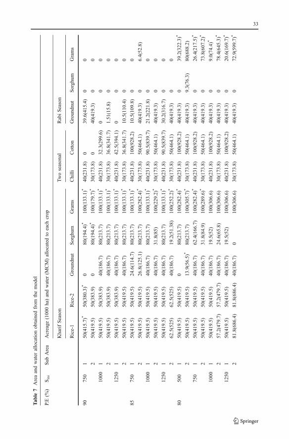
Optimal cropping patterns, water allocations and net annual benefits obtained from the LPmodel for various combinations of weekly water availability levels and initial storagesstates of reservoir considered, are presented in Table 7.

Table 4 Area and irrigation constraints

Crop (Season) Sub Area-1 (thousand ha) Sub Area-2 (thousand ha)

Max. Min. Max. Min.

Rice-1(K) 103.5 50 85 50

Rice-2(K) 103.5 50 85 50

Groundnut(K) 40 – 40 –

Sorghum(K) 80 – 80 –

Grams(K) 100 – 100 –

Cotton 100 – 100 –

Chilli 40 – 40 –

Groundnut (R) 40 – 40 –

Sorghum (R) 50 – 50 –

Grams (R) 80 – 80 –

Table 5 Agro economic parameters

Crop (Season) Max. yield (kg/ha) Market price (Rs.a/ kg) Cost of cultivation(Rs./ha)

Net benefit(Rs./ha)

Rice(K) 5400 5.65 10900 18045

Groundnut(K) 1500 14.00 7000 12987

Sorghum(K) 3000 5.00 5000 9657

Grams(K) 1300 14.10 5000 12630

Cotton(K) 3000 15.30 20520 24523

Chilli(K) 3200 22.00 42325 27389

Groundnut(R) 2500 14.00 7000 26743

Sorghum(R) 3000 5.00 5000 9200

Grams(R) 1300 14.10 5000 12187

a 1 US $=Rs.45 (Rupees of Indian currency)

30

Table 6 Expected weekly inflows into the reservoir

Standard week l Skewness Kurtosis Chi 75% PE(MCM)

80% PE(MCM)

85% PE(MCM)

90% PE(MCM)

1 0.10 0.06 2.48 2.67 94.2 84.0 73.3 61.7

2 0.25 -0.00 2.26 0.89 87.8 77.3 66.2 54.0

3 0.45 -0.01 2.70 3.10 80.8 68.4 55.4 41.1

4 0.50 0.06 2.99 1.78 94.5 80.5 65.5 48.8

5 0.15 -0.44 2.89 4.89 77.2 65.9 54.6 42.7

6 0.15 -0.31 2.69 3.56 78.5 67.6 56.5 44.8

7 0.20 -0.07 2.10 9.78 75.9 65.2 54.3 42.7

8 -0.15 -0.55 2.99 7.56 68.3 59.5 50.9 42.0

9 -0.05 -0.24 2.41 9.33 62.8 53.7 44.8 35.8

10 0.55 0.34 2.32 16.89 66.8 51.6 36.2 20.4

11 0.40 -0.03 2.71 9.33 55.0 43.1 31.3 19.5

12 0.35 -0.14 3.19 11.11 48.2 37.7 27.4 17.4

13 0.55 0.20 2.51 6.67 46.7 34.4 22.2 10.4

14 0.20 -0.05 3.12 4.00 38.8 31.0 23.5 16.2

15 -0.05 0.06 2.11 4.44 44.6 38.7 32.8 26.7

16 0.45 -0.03 3.38 3.11 22.6 16.5 10.7 5.3

17 0.40 0.48 4.36 3.56 20.2 15.4 10.8 6.4

18 0.40 -0.01 3.19 4.00 8.2 5.6 3.3 1.3

19 0.35 -0.00 3.27 8.44 4.0 2.2 0.9 0.2

20 0.35 0.81 4.74 6.22 4.3 1.9 0.5 0.0

21 0.35 0.07 3.66 1.33 9.5 6.2 3.4 1.3

22 0.40 0.50 2.71 1.78 5.3 2.5 0.7 0.0

23 0.30 -0.18 2.62 8.44 11.9 7.6 4.1 1.5

24 0.25 -0.14 3.44 4.00 11.1 6.1 2.7 0.7

25 0.30 -0.03 2.77 6.22 43.6 30.3 18.7 9.1

26 0.30 0.15 4.09 3.11 77.4 56.8 38.1 21.2

27 0.40 -0.00 3.53 4.00 164.2 124.3 85.9 49.1

28 0.30 0.07 3.80 5.33 260.2 191.0 127.9 71.3

29 0.35 0.43 3.94 8.44 315 234.9 159.7 90.1

30 0.30 0.16 3.63 2.67 466.0 365.7 269.0 174.8

31 0.40 -0.09 3.37 7.11 707.3 561.4 416.1 269.0

32 0.25 -1.17 5.77 9.78 580.0 442.1 314.1 195.2

33 0.35 -0.45 2.81 7.56 891.0 716.7 543.5 367.7

34 0.35 -0.02 2.82 4.44 842.7 675.6 510.0 342.5

35 0.45 -0.03 3.20 3.11 743.3 591.4 438.1 280.5

36 -0.20 -1.00 4.94 6.67 561.7 484.3 409.7 334.4

37 0.05 -0.44 2.72 9.33 595.9 514.0 432.1 346.6

38 0.20 0.05 3.49 7.11 431.2 347.4 266.7 187.3

39 -0.25 -0.85 4.44 6.67 412.3 351.5 294.2 237.7

40 0.15 -0.38 3.25 7.56 474.8 380.2 290.6 204.0

41 -0.05 -069 4.38 4.89 510.4 433.1 358.3 282.9

42 -0.10 -1.38 8.86 8.44 351.0 295.9 243.4 191.4

43 0.20 -0.00 6.03 8.89 271.9 219.3 168.6 118.6

31

From the results obtained, it is evident that the total annual benefit and totalallocated area is higher with water availability of PE 75% when compared with that ofPE 90% for all states of initial storage of reservoir. Variation of total benefit and totalcropped area with the initial storage of reservoir is shown in Fig. 2. and Fig. 3.respectively. From figures, it can be observed that feasible solution is possible only whenthe initial storage is 300 MCM, 500 MCM, 600 MCM and 750 MCM for 75% PE, 80%PE, 85% PE and 90% PE of expected weekly inflows respectively. Impact on croppingpattern with the change in initial storage of reservoir for 75% reliable weekly inflows intothe reservoir is shown in Fig. 4.

At a level of 75% water availability, area of crops chilli, cotton, grams(K) andgroundnut(R) are confined to their maximum limits for all states of initial storage ofreservoir considered. This is due to the fact that net benefit per hectare is high in caseof chilli, cotton, groundnut(R) and low water requirement in case of grams(K) eventhough net benefit is not attractive. When the initial storage is less than 300 MCM, nofeasible solution is obtained from the model as the water available is not sufficientenough to cultivate the minimum area imposed for rice. With the increase of initialstorage of reservoir from 500 MCM to 1000 MCM, acreage of rice and groundnut(K) isimproved and the net benefit is improved from 19,810 to 20,142 million rupees. Allcrops are irrigated with full irrigation except for grams(R) as it is more resistant towater deficit. Results indicate that there is no change in the area and water allocation,even if the initial storage of reservoir is greater than 1000 MCM. This is due to the factthat total annual water allocated to each sub area reaches the restriction imposed onmaximum water allowed to use. It is also observed from the results, with the increaseof availability of water at the beginning of the irrigation season, the acreage of rice andgroundnut(K) is increasing while that of sorghum(K&R) and grams(R) is decreasing asthey can be grown with low water requirement. Similar trend is observed at 85% and80% reliable weekly inflows.

At 90% reliable level of water availability, no feasible solution is found when the initialstorage is less than 750 MCM, as the available water could not satisfy the waterrequirement of rice for the minimum area imposed. Sorghum(R) and grams(R) do notappear in the irrigation plan and the area occupied by the rice is limited to its minimum areaimposed because it is more water consuming crop with respect to its net return. One can see

Table 6 (continued)

Standard week l Skewness Kurtosis Chi 75% PE(MCM)

80% PE(MCM)

85% PE(MCM)

90% PE(MCM)

44 0.05 -0.05 5.41 6.22 240.2 203.0 166.5 129.3

45 -0.20 -0.94 6.94 9.33 227.7 205.9 183.6 159.5

46 0.05 0.05 3.30 4.00 196.3 176.0 154.9 131.8

47 -0.10 0.01 4.53 4.44 166.2 150.1 133.4 115.3

48 0.15 0.42 7.86 9.78 140.1 121.6 102.7 82.5

49 -0.25 -018 3.01 5.78 131.7 118.8 105.6 91.5

50 0.80 0.08 1.97 3.56 133.5 115.6 95.4 71.2

51 0.35 -0.21 3.04 2.67 106.9 94.0 80.3 65.0

52 0.20 -0.02 2.60 1.33 111.7 99.1 85.9 71.2

32

Tab

le7

Areaandwater

allocatio

nobtained

from

themodel

P.E(%

)Sini

Sub

Area

Acreage

(1000ha)andwater

(MCM)allocatedto

each

crop

KharifSeason

Twoseason

alRabiSeason

Rice-1

Rice-2

Groundn

utSorgh

umGrams

Chilli

Cotton

Groundn

utSorgh

umGrams

9075

01

50(415

.7)*

50(380

.3)*

080

(194

.4)*

100(13

3.1)

*40

(231

.8)

039

.6(415

.4)

00

250

(419

.5)

50(383

.9)

080

(194

.4)*

100(17

9.7)

*30

(173

.8)

040

(419

.3)

00

1000

150

(419

.5)

50(383

.9)

40(186

.7)

80(213

.7)

100(13

3.1)

*40

(231

.8)

32.3(299.6)

00

0

250

(419

.5)

50(383

.9)

40(186

.7)

80(213

.7)

100(13

3.1)

*30

(173

.8)

36.8(341.7)

1.51(15.8)

00

1250

150

(419

.5)

50(383

.9)

40(186

.7)

80(213

.7)

100(13

3.1)

*40

(231

.8)

42.5(394.1)

00

0

250

(419

.5)

50(419

.5)

40(186

.7)

80(213

.7)

100(13

3.1)

*30

(173

.8)

36.8(341.7)

10.5(110

.4)

00

8575

01

50(419

.5)

50(419

.5)

24.6(114

.7)

80(213

.7)

100(13

3.1)

*40

(231

.8)

100(92

8.2)

10.5(109

.8)

00

250

(419

.5)

50(419

.5)

26.8(125.1)

80(213

.7)

100(28

2.4)

*30

(173

.8)

50(464

.1)

40(419

.3)

06.4(52

.8)

1000

150

(419

.5)

50(419

.5)

40(186

.7)

80(213

.7)

100(13

3.1)

*40

(231

.8)

90.5(839.7)

21.2(221

.8)

00

250

(419

.5)

50(419

.5)

40(186

.7)

31.8(85)

100(22

9.2)

*30

(173

.8)

50(464

.1)

40(419

.3)

00

1250

150

(419

.5)

50(419

.5)

40(186

.7)

80(213

.7)

100(13

3.1)

*40

(231

.8)

90.5(839.7)

30.2(316

.7)

00

262

.5(525)

62.5(525)

40(186

.7)

19.2(51.38

)10

0(25

2.2)

*30

(173

.8)

50(464

.1)

40(419

.3)

00

8050

01

50(419

.5)

50(419

.5)

080

(213

.7)

100(28

2.4)

*40

(231

.8)

100(92

8.2)

40(419

.3)

039

.2(322

.3)*

250

(419

.5)

50(419

.5)

13.9(56.5)

*80

(213

.7)

100(30

5.7)

*30

(173

.8)

50(464

.1)

40(419

.3)

9.3(76

.3)

80(688

.2)

750

150

(419

.5)

50(419

.5)

40(186

.7)

62.4(166

.7)

100(28

2.4)

*40

(231

.8)

100(92

8.2)

40(419

.3)

026

.4(217

.5)*

250

(419

.5)

50(419

.5)

40(186

.7)

31.8(84.9)

100(28

9.6)

*30

(173

.8)

50(464

.1)

40(419

.3)

073

.8(607

.2)*

1000

150

(419

.5)

50(419

.5)

40(186

.7)

19.5(52)

100(30

6.6)

40(231

.8)

100(92

8.2)

40(419

.3)

09.0(74

.4)*

257

.2(479.7)

57.2(479.7)

40(186

.7)

24.6(65.8)

100(30

6.6)

30(173

.8)

50(464

.1)

40(419

.3)

078

.4(645

.3)*

1250

150

(419

.5)

50(419

.5)

40(186

.7)

19.5(52)

100(30

6.6)

40(231

.8)

100(92

8.2)

40(419

.3)

020

.6(169

.7)*

281

.8(686.4)

81.8(686.4)

40(186

.7)

010

0(30

6.6)

30(173

.8)

50(464

.1)

40(419

.3)

072

.9(599

.7)*

33

Tab

le7

(contin

ued)

P.E(%

)Sini

Sub

Area

Acreage

(100

0ha)andwater

(MCM)allocatedto

each

crop

KharifSeason

Twoseason

alRabiSeason

Rice-1

Rice-2

Groundn

utSorgh

umGrams

Chilli

Cotton

Groundn

utSorgh

umGrams

7550

01

50(419

.5)

50(419

.5)

30.5(142

.2)

80(213

.7)

100(30

6.6)

40(231

.8)

100(92

8.2)

40(419

.3)

080

(665

.4)*

250

(419

.5)

50(419

.5)

40(186

.7)

50.6(135

.2)

100(30

6.6)

30(173

.8)

50(464

.1)

40(419

.3)

50(408

.8)

80(688

.2)

750

150

(419

.5)

50(419

.5)

40(186

.7)

21.4(57.2)

100(30

6.6)

40(231

.8)

100(92

8.2)

40(419

.3)

052

.1(428.4)*

250

(419

.5)

50(419

.5)

40(186

.7)

31.8(84.9)

100(30

6.6)

30(173

.8)

50(464

.1)

40(419

.3)

41.9(342

.3)

80(688

.2)

1000

150

(419

.5)

50(419

.5)

40(186

.7)

19.5(52)

100(30

6.6)

40(231

.8)

100(92

8.2)

40(419

.3)

050

.9(418.6)*

285

(713

.1)

85(713

.1)

36.8(171

.8)

010

0(30

6.6)

30(173

.8)

50(464

.1)

40(419

.3)

18.2(148

.5)

80(688

.2)

1250

150

(419

.5)

50(419

.5)

40(186

.7)

19.5(52)

100(30

6.6)

40(231

.8)

100(92

8.2)

40(419

.3)

050

.9(418.6)*

285

(713

.1)

85(713

.1)

36.8(171

.8)

010

0(30

6.6)

30(173

.8)

50(464

.1)

40(419

.3)

18.2(148

.5)

80(688

.2)

Note:

Sini–Initial

Storage

ofReservo

irin

MCM

andvalues

inparenthesisrepresentswater

allocatedin

MCM

*-DeficitIrrigatio

n

34

from the results obtained, that sorghum(K) and grams(K) are cultivated under deficitirrigation while chilli is cultivated under full irrigation occupying maximum areas imposed,as sorghum(K) and grams(K) are more resistant to water deficit while chilli is sensitive. Itcan also be observed that area occupied by groundnut(K) and cotton is increasing with theincrease of initial storage of reservoir.

From the results obtained, variation of reservoir storage for various levels of wateravailability is studied. Reservoir storage and release rule curves are prepared which areuseful to project authorities in guiding the reservoir release to be made or storage to bemaintained in the reservoir. Rule curves for storage and release from reservoir obtained

Fig. 2 Variation of total benefit with initial storage for different PE’s

Fig. 3 Variation of total area with initial storage for various levels of expected inflows

35

from the planning model is shown in Fig. 5 and Fig. 6 respectively. From Fig. 5, it can beobserved that the active storage is almost becoming zero at 30th week and is reachingmaximum at 44th week. Carry over year storage is found to be equal to imposed minimumlimit of 1000 MCM for 90%, 85% and 80% reliable inflows while it is 2,120 MCM for75% reliable flows. It is evident from Fig. 6 that releases in the early weeks of reservoiroperation are maximum as irrigation demand is peak and no releases are made from 9th

week to the end of the year as no crops are grown during the same period.

Fig. 4 Cropping pattern at 75% PE

Fig. 5 Variation of reservoir storage with standard weeks

36

Summary and conclusions

A model is developed for optimal irrigation planning and demonstrated through a casestudy. Crop water requirements are estimated by Penman-Monteith methodology. Optimalallocations of land and weekly releases are made for all crops grown in a year by runningLP allocation model maximizing the annual net benefit from the project at differentreliability levels of weekly water availability and initial storage states of reservoir. Theresults obtained are discussed. Following conclusions can be drawn for the study area basedon the results obtained from the model.

(i) Results reveal that initial storage of reservoir at the beginning of the season influencesin deciding the cropping pattern and water allocations. Model suggests a minimuminitial storage of 750 MCM, 600 MCM, 500 MCM and 300 MCM at 90%, 85%, 80%and 75% reliable weekly inflows into the reservoir respectively. It is also found that at75% PE, minimum initial storage of 1000 MCM is required to get maximum annualbenefit. Hence it seems appropriate to maintain a minimum carry over year storage of1000 MCM.

(ii) When the water available is low, planning model recommends deficit irrigation forsorghum(K) and grams(K) with maximum permitted area under cultivation whilekeeping the area occupied by rice at its minimum limit. Hence, irrigation managersand farmers are advised to adopt low water consuming crops with maximum areaunder deficit irrigation, when water availability is low.

The study indicates that model presented can be used to determine the optimal waterresources allocation and optimal planting of various crops grown in a year. As the problemis solved by linear programming, large number of variables and linear constraints can behandled efficiently. The model can be adopted as planning model of storage based irrigationsystem in arid and semi-arid areas for better water management. The uncertainty of inflowsentering into the reservoir is accounted in the model considering the probability ofexceedence of weekly flows. However, the randomness of rainfall occurrence, as well asamount and duration are not taken into account and irrigation requirements are treated asdeterministic in the model.

Fig. 6 Weekly releases from reservoir for various levels of expected inflows

37

Acknowledgements The authors wish to express their sincere thanks to All India Council of TechnicalEducation, New Delhi, for financial support provided to first author under R&D scheme (Project No. 8021/RID/NPROJ/R&D-62/2002-03).

References

Allen RG, Pereira LS, Smith M (1998) Crop evapotransipiration: guidelines for computing waterrequirements. FAO Irrigation and Drainage Paper 56, Food and Agriculture Organisation of the UnitedNations, Rome, Italy

Box GEP, Cox DR (1964) An analysis of transformations. J R Stat Soc, Ser B 26:211–252Bras RL, Cordova JR (1981) Intraseasonal water allocation in deficit irrigation. Water Resour Res 17(4):866–874Chavez-Morales J, Marino MA, Holzapfel EA (1987) Planning model of irrigation district. J Irrig Drain Eng

113(4):549–564Doorenbos J, Kassam AH (1979) Yield response to water. FAO Irrigation and Drainage Paper 33, Food and

Agricultural Organization of United Nations, Rome, ItalyKhepar SD, Chaturvedi MC (1982) Optimum cropping and groundwater management. Water Resour Bull 18

(4):655–660Loucks DP, Stedinger JR, Haith DA (1981) Water resources systems planning and management. Prentice-Hall,

Englewood CliffsMainuddin M, Gupta AD, Onta PR (1997) Optimal crop planning model for an existing groundwater

irrigation project in Thailand. Agric Water Manag 33:43–62Mayya SG, Prasad R (1989) System analysis of tank irrigation. I Crop staggering. J Irrig Drain Eng 115

(3):385–405Onta PR, Loof R, Banskota M (1995) Performance based irrigation planning under water shortage. Irrig

Drain Syst 9:143–162Panda SN, Khepar SD, Kaushal MP (1996) Interseasonal irrigation system planning for waterlogged sodic

soils. J Irrig Drain Eng 122(3):135–144Paul S, Panda SN, Kumar N (2000) Optimal irrigation allocation: a multilevel approach. J Irrig Drain Eng

126(3):149–156Rao NH, Sarma PBS, Chander S (1988) Irrigation Scheduling under limited water supply. Agric Water

Manag 15:165–175Rao NH, Sarma PBS, Chander S (1990) Optimal multi crop allocation of seasonal and intraseasonal

irrigation water. Water Resour Res 26(4):551–559Sethi L, Nagesh KD, Panda SN, Mal BC (2002) Optimal crop planning and conjunctive use of water

resources in coastal river basin. Water Resour Manag 16:145–169Singh DK, Jaiswal CS, Reddy KS, Singh RM, Bhandarkar DM (2001) Optimal cropping pattern in a canal

command area. Agric Water Manag 50:1–8Srinivasa PA, Umamahesh NV, Viswanath GK (2006) Optimal irrigation planning under water scarcity. J Irrig

Drain Eng 132(3):228–237Sunantara JD, Ramirez JA (1997) Optimal stochastic multi-crop seasonal and interseasonal irrigation control.

J Water Res Plan Manag 123(1):39–48Teixeira AS, Marino MA (2002) Coupled reservoir operation-irrigation scheduling by dynamic programming. J

Irrig Drain Eng 128(2):63–73Umamahesh NV, Sudarsan Raju S (2002) Two- phase DP-LP model for optimal irrigation planning under

deficit water supply. Proceedings of the international conference on Advances in Civil Engineering: IIT,Kharagpur, India

38