Stability of Systems with Stochastic Delays and Applications to Genetic Regulatory Networks

SIAM J. APPLIED DYNAMICAL SYSTEMS c© xxxx Society for Industrial and Applied MathematicsVol. xx, pp. x x–x

Stability of Systems with Stochastic Delays

and Applications to Genetic Regulatory Networks

Marcella M. Gomez∗, Mehdi Sadeghpour†, Matthew R. Bennett ‡, Gabor Orosz†, and

Richard M. Murray§

Abstract. The dynamics of systems with stochastically varying time delays are investigated in this paper. Itis shown that the mean dynamics can be used to derive necessary conditions for the stability ofequilibria of the stochastic system. Moreover, the second moment dynamics can be used to derivesufficient conditions for almost sure stability of equilibria. The results are summarized using stabilitycharts that are obtained via semi-discretization. The theoretical methods are applied to simple generegulatory networks where it is demonstrated that stochasticity in the delay can improve the stabilityof steady protein production.

Key words. stability, stochastic delay, systems biology, genetic networks

AMS subject classifications. 37H10, 92C42

1. Introduction. Time delays are a well known source of instability in dynamical systemsand can make control design a challenging task. When the delays are assumed to be constantor distributed, there are well established methods to analyze stability and bifurcations ofequilibria and periodic orbits [7, 9, 19, 24, 45, 46]. When the delays depend on time or on thestate of the system, stability analysis becomes more difficult and may require averaging ornumerical techniques [18, 20, 37]. However, in some cases delays vary stochastically in time,making it very challenging to characterize stability. In this paper, we target the problem ofstability analysis of systems with stochastically changing delays. Stochastic delays arise innetworked control systems [5], connected vehicles [43], and gene regulatory networks [15, 21].

When investigating dynamics under stochastic delay variations, key factors include thestochastic process describing the time evolution of the delay and the type of stability in-vestigated. In early works, random delays modeled by continuous-time Markov chains wereincorporated into delay differential equations [22, 29] and Lyapunov stability theorems wereused to obtain sufficient conditions of stability. This approach has been extended to nonlin-ear systems [25] and has also been applied to discrete-time systems where the correspondingmatrix inequalities again give sufficient stability conditions [12, 41, 55]. These conditions aretypically quite conservative, which makes it difficult to evaluate the effect of the delays on the

∗Electrical Engineering and Computer Science, University of California, Berkeley, CA 94720, USA([email protected]). The research of this author was supported by the TerraSwarm Research Center, oneof six centers supported by the STARnet phase of the Focus Center Research Program (FCRP) a SemiconductorResearch Corporation program sponsored by MARCO and DARPA.

†Department of Mechanical Engineering, University of Michigan, Ann Arbor, MI 48109, USA ([email protected],[email protected]). This research was supported by National Science Foundation (award # 1300319).

‡Department of BioSciences and Department of Bioengineering, Rice University, Houston, TX 77005, USA([email protected]). The research of this author was supported by the NIH, through the joint NSF/NIGMSMathematical Biology Program grant R01GM104974, and the Robert A. Welch Foundation grant C-1729

§Control and Dynamical Systems, California Institute of Technology, Pasadena, CA 91125, USA([email protected]).

1

mailto:[email protected]




2 Gomez, Sadeghpour, Bennett, Orosz, and Murray

dynamics. Similarly, taking the worst case scenario (e.g., largest delay) can lead to unneces-sary conservativeness or may simply give erroneous results. Even ensuring stability for eachvalue of the delay does not necessarily give the stability of the stochastic system [13].

Work has also been done comparing stability conditions for different types of stability(Lyapunov stability, moment stability, almost sure stability) for a continuous-time linear sys-tem under specific delay variations [51]. In this paper we expand these ideas to a broader classof delay processes, while focusing on moment stability, almost sure stability, and the relation-ship between these. We use a technique called semi-discretization [19] to classify differentstability losses and to derive stability charts.

To demonstrate the power of the developed mathematical tools, we apply them to simplegene regulatory networks where a protein represses its own production. Traditional mass-action kinetic models are based on instantaneous reactions and model the time evolutionof protein concentrations by ordinary differential equations (ODEs), which can be used tocharacterize the dynamics about equilibria and periodic solutions [6]. However, the proteinproduction process comprises of a sequence of biochemical reactions and, thus, a fully matureprotein only becomes available after some time delay. Consequently, a more accurate wayto describe the dynamics of genetic regulatory networks is to use delay differential equations(DDEs), which still allows one to investigate stability and bifurcations [28, 38]. For instance,it has been shown that delay may lead to oscillations in models with negative delayed feedbackin synthetic gene networks [35, 47, 49].

The intracellular environment is inherently noisy [36] and stochasticity is often incor-porated into modeling equations by simply adding Gaussian noise. Such studies have beenextended to gene networks modeled with delays [48]. However, the biochemical processes thatare lumped together by the delay are also stochastic in nature, which results in stochastic delayvariations [15, 21]. We analyze corresponding effects and produce stability charts for equi-libria on the plane of gain parameters for different distributions of the stochastic delay. Thestability results are also validated using numerical simulations of the linearized and nonlinearmodels.

2. Continuous-time Systems with Stochastic Delay. In this paper we consider systemsof the form

χ(t) = f(

χ(t), χ(t− τ(t)))

, (2.1)

where dot denotes the derivative with respect to time t, χ ∈ Rn, f : Rn × R

n → Rn, and the

delay τ ∈ R varies in time stochastically. More precisely we assume that the delay follows astationary stochastic process with probability distribution w(σ), σ ∈ [τmin, τmax]. Thus, theinitial condition is given by χ(t) = χ0(t), t ∈ [−τmax, 0]. Due to the stochasticity in thedelay, the vector χ(t) also follows a stochastic process.

Linearizing equation (2.1) about an equilibrium χ(t) ≡ χ∗ results in the system

x(t) = ax(t) + bx(t− τ(t)) , (2.2)

where x(t) = χ(t) − χ∗, a = ∂1f(χ∗, χ∗),b = ∂2f(χ∗, χ∗) ∈ Rn×n, and ∂1 and ∂2 represent

derivatives with respect to the first and second variables, respectively. In this paper, weanalyze the equations describing the first and second moments of the linear system (2.2).

Stochastic Delays and Genetic Networks 3

Note that equations describing the first and second moments of the nonlinear system (2.1)may differ from these in a general case.

We consider a class of delay processes where the delay trajectories are piece-wise constantfunctions of time. Namely, we assume that the delay τ(t) may only take J possible discretevalues from the set {τ1, τ2, . . . , τJ} with P[τ(t) = τj ] = wj , where P denotes probability.Without loss of generality we can consider τ1 < τ2 < · · · < τJ . In this case, the correspondingprobability density function (pdf) consists of Dirac deltas, that is,

w(σ) =

J∑

j=1

wj δ(σ − τj) , (2.3)

where∫ τmax

τminw(σ) dσ =

∑Jj=1wj = 1. From here on, we use the term pdf and delay distribution

interchangeably. Note that one can approximate continuous delay distributions by increasingthe density of the Dirac deltas. Also we assume that the delay stays constant for a holdingtime T before potentially taking on a new value, as demonstrated by the sample realizationin Fig. 2.1 for J = 3 different delay values. Since the probability distribution in (2.3) isnot changing with time, the delays assumed across the holding intervals are independent andidentically distributed (IID). In this paper, we focus on stability analysis of systems in theform of (2.2) with stated assumptions on the delay, while linear approximations and numericalsimulations are used to investigate nonlinear phenomena in nonlinear systems of type (2.1).

Taking the expected value, denoted by E, of system (2.2) we obtain

d

dtE[x(t)] = aE[x(t)] + b

J∑

j=1

P[τ(t) = τj ] E[x(t− τj)|τ(t) = τj] . (2.4)

If the holding time T is smaller than the minimum delay, i.e., T < τ1 then x(t − τj) isindependent of τ(t) due to the IID nature of the delay sequence. Thus, introducing thenotation x = E[x], we obtain

˙x(t) = a x(t) + b

J∑

j=1

wj x(t− τj) . (2.5)

Generalizing this for any stationary stochastic delay process where the autocorrelation of thedelay becomes zero after T and T < τmin yields the general form

˙x(t) = a x(t) + b

∫ τmax

τmin

w(σ) x(t− σ) dσ . (2.6)

The distributed delay systems (2.5) and (2.6) describe the dynamics of the mean and theycan be analyzed using standard stability and bifurcation analysis tools [9, 45, 46]. The meandynamics can provide some information about the effect of stochastic delays as they explicitlycontain the delay distribution. However, to characterize the stochastic dynamics one needs toanalyze higher moments.

In order to analyze the higher moments of the continuous-time system (2.2), we discretizeit by dividing the holding intervals of length T into ℓ ∈ N subintervals of length ∆t = T/ℓ;


τ

τ3

τ2

τ1

0 ∆t T 2T 3T 4T 5T 6T t

Figure 2.1. A sample realization of the time evolution of the delay with J = 3 possible delay values. Thedelay remains constant for a holding time T while ∆t denotes the discretization step.

see Fig. 2.1. Then, using a time discretization technique, called semi-discretization [19], weconstruct a discrete-time map as a discretization of (2.2) which allows us to obtain conditionsfor the stability of the mean and the second moment. Then, we demonstrate the convergenceof the corresponding spectra and stability charts when ∆t → 0.

To apply semi-discretization we assume that the delayed term in (2.2) stays constant inthe time interval t ∈ [i∆t, (i+ 1)∆t), that is,

˙x(t) = a x(t) + b x(i∆t− r(i)∆t), t ∈ [i∆t, (i+ 1)∆t), (2.7)

where r(i) ∈ Z+ takes the values {r1, . . . , rJ} with rj = ⌊ τj

∆t⌋, j = 1, . . . , J , for i = 0, 1, 2, . . ..In other words, the delay values are rounded off by the mesh size ∆t. Since equation (2.7)is a linear differential equation with constant forcing, it can be solved in the time intervalt ∈ [i∆t, (i+ 1)∆t) yielding

x(i+ 1) = α x(i) + β x(i− r(i)) , (2.8)

where

α = ea∆t , β =

(∫ ∆t

0ea(∆t−t)dt

)

b, (2.9)

and we have used the notation x(i) = x(i∆t). We remark that if a−1 exists, then the secondformula results in β =

(

ea∆t − I)

a−1b, where I is the n-dimensional identity matrix.

Let us define the augmented vector X(i) = [ xT(i) xT(i−1) · · · xT(i− rJ) ]T ∈ R

(rJ+1)n,where T denotes the transpose. Then equation (2.8) can be written in the compact form

X(i + 1) = G(i)X(i), (2.10)


where the matrix G(i) follows a stochastic process and takes the values

Gj =

α 0 · · · β · · · 0

I 0 0 · · · 0 0

0 I 0 · · · 0 0

0 0 I · · · 0 0...

......

. . ....

...0 0 0 · · · I 0

∈ R(rJ+1)n×(rJ+1)n , (2.11)

with probability wj for j = 1, . . . , J .The first block row in matrix Gj corresponds to the delay τj in (2.8) and therefore it

changes when the delay changes such that the block β is in the (rj + 1)-th block-column.Note that given that the delay holding time T = ℓ∆t, the matrix Gj is kept constant for ℓtime steps before changing. Thus defining Y (k) = X(kℓ), k = 0, 1, 2, . . . the system (2.10) canbe written as

Y (k + 1) = A(k)Y (k), (2.12)

where A(k) takes values

Aj =(

Gj

)ℓ ∈ R(rJ+1)n×(rJ+1)n , (2.13)

and P[A(k) = Aj ] is wj , j = 1, . . . , J . Since the delays of different holding intervals are IIDthe matrices A(k) are IID and A(k) is independent of Y (k).

3. Stability Conditions. In this section, we establish conditions for stability of the stochas-tic dynamical system (2.12), that is the discretization of system (2.2). We focus on almostsure stability, which is obtained by calculating second moment stability. Let us start withsome definitions.

Definition 3.1.A random sequence {X(k) ∈ Rn}+∞

k=0 converges to 0 almost surely ifP[

∀ ǫ > 0, ‖X(k)‖ > ǫ happens only finitely often]

= 1. If sequences generated by a stochasticdynamical system converge to 0 almost surely, then the trivial solution X(k) ≡ 0 is almost

surely asymptotically stable.Note that almost sure convergence is also called convergence with probability one.Definition 3.2. A random sequence {X(k) ∈ R

n}+∞k=0 converges to 0 in the mean if

limk→∞ E[

X(k)]

= 0 and converges to 0 in the second moment if limk→∞ E[

X(k)XT(k)]

=0. If sequences generated by a stochastic dynamical system converge to 0 in the mean or in thesecond moment, then the trivial solution X(k) ≡ 0 is asymptotically stable in the mean

or in the second moment, respectively.It can be shown that stability in the second moment implies stability in the mean, but in

general, there is no relationship between second moment stability and almost sure stability.However, in the special case described by system (2.12) where A(k) are IID, stability in thesecond moment does imply almost sure stability; see [26]. We also remark that for vectorvalued sequences, defining moments higher than 2 is not trivial and they are rarely used inthe literature; see [43].

We begin by characterizing the dynamics of the mean E[Y (k)] for (2.12). As explainedbelow, stability of the mean provides a necessary condition for the stability of the stochasticsystem, that is, if the mean is unstable then the system is unstable. Therefore, the stability


region for the mean in the parameter space contains the true stable region. We will thenderive the dynamics of the second moment E[Y (k)Y T(k)] to provide sufficient conditions foralmost sure stability.

Since A(k) is IID, it is independent of Y (k). Thus, taking the expected value of bothsides of (2.12), we obtain

E [Y (k + 1)] = E[

A(k)Y (k)]

= E[

A(k)]

E[Y (k)]

=

( J∑

j=1

P[

A(k) = Aj

]

Aj

)

E[Y (k)]

=

( J∑

j=1

wjAj

)

E[Y (k)].

(3.1)

Using the notationY (k) := E[Y (k)] ∈ R

(rJ+1)n , (3.2)

we can write the discretized mean dynamics (3.1) in the form

Y (k + 1) = A Y (k), (3.3)

where

A =

J∑

j=1

wj Aj =

J∑

j=1

wj (Gj)ℓ , (3.4)

and A ∈ R(rJ+1)n×(rJ+1)n, cf. (2.13). Thus, limk→∞ Y (k) = 0 if and only if ρ

(

A)

< 1, whereρ(.) denotes the spectral radius. This is in fact a necessary condition for the stability of thestochastic system (2.12), which is the discretization of the continuous-time system (2.2).

To analyze the second moment of (2.12), we proceed as follows

E[

Y (k + 1)Y T(k + 1)]

= E[

A(k)Y (k)Y T(k)AT(k)]

=

J∑

j=1

P[

A(k) = Aj

]

E[

A(k)Y (k)Y T(k)AT(k)|A(k) = Aj

]

=

J∑

j=1

wjAjE[

Y (k)Y T(k)|A(k) = Aj

]

ATj

=

J∑

j=1

wjAjE[

Y (k)Y T(k)]

ATj ,

(3.5)

where in the last step we used the independence of Y (k) and A(k). Now we rewrite (3.5) asthe time evolution of a vector. For a matrix H = [ h1 h2 · · · hm ] ∈ R

n×m, where hi ∈ Rn

denotes the i-th column vector, let us define the operator

vec(H) =

h1h2...

hm

∈ Rnm . (3.6)


Using (3.6), let us define the vector

¯Y (k) := vec(

E[

Y (k)Y T(k)])

∈ R(rJ+1)2n2

, (3.7)

and also note that for matrices A, B, and C for which the matrix product ABC is defined,the equality

vec(ABC) =(

CT ⊗A)

vec(B) (3.8)

holds, where ⊗ denotes the Kronecker product. Using (3.7) and (3.8), (3.5) can be rewrittenas

¯Y (k + 1) = ¯A ¯Y (k) , (3.9)

where

¯A =J∑

j=1

wjAj ⊗Aj =J∑

j=1

wj

(

Gj

)ℓ ⊗(

Gj

)ℓ, (3.10)

and ¯A ∈ R(rJ+1)2n2×(rJ+1)2n2

, cf. (2.13). Thus from (3.9), limk→∞¯Y (k) = 0 if and only

if ρ( ¯A

)

< 1. Moreover, condition ρ( ¯A

)

< 1 implies almost sure stability of the stochasticsystem (2.12), which is the discretization of the continuous-time system (2.2). We remark that,if J = 1, conditions ρ

(

A)

< 1 and ρ( ¯A

)

< 1 reduce to the asymptotic stability condition ofa deterministic system with one single delay.

Remark 1.We provided stability conditions for the mean and the second moment of themap (2.12) that is a discretization of the continuous-time system (2.2). For the case of adeterministic delay, the semi-discretization method preserves asymptotic stability, i.e., if theoriginal continuous-time system is stable, the discretized system is stable as well given thatthe time step ∆t is small enough. Moreover, when ∆t approaches zero, the stable parameterdomain of the discretized system approaches the stable parameter domain of the continuous-time system; see [16, 17]. In the case of stochastic delay, our conjecture is that the stableparameter domain of the discretized system (2.12) converges to that of the continuous-timesystem (2.2) as ∆t → 0. The convergence proof may be constructed based on the fact thatin the stochastic system the delay remains constant in each holding interval [kT, (k + 1)T ),k = 0, 1, 2, . . ., allowing one to apply the same arguments as in [16]. In this paper, we demon-strate the convergence through the spectral radius of matrices A in (3.4) and ¯A in (3.10) andcorresponding stability charts.

3.1. Convergence of Spectra and Stability Charts – An Illustrative Example. We con-sider a simple example in order to illustrate the stability analysis established in the previoussection. By calculating the spectra of matrices (3.4) and (3.10) we draw stability charts. Wealso show that the spectral radius and the stability charts converge to a limit as the dis-cretization step ∆t decreases. Consider the scalar example x ∈ R in which case system (2.2)simplifies to

x(t) = a x(t) + b x(t− τ(t)) , (3.11)

where a and b are scalars. Assume that the delay may take the values τ1 = 0.2, τ2 = 0.3, andτ3 = 0.4 (J = 3) with equal probability, i.e., w1 = w2 = w3 = 1/3, and set the holding time


to T = 0.1. We draw stability charts in the plane of parameters a and b for different valuesof ∆t. Note that here the matrix (2.11) simplifies to

Gj =

α 0 · · · β · · · 01 0 0 · · · 0 00 1 0 · · · 0 00 0 1 · · · 0 0...

......

. . ....

...0 0 0 · · · 1 0

∈ R(r3+1)×(r3+1), (3.12)

where r3 = ⌊τ3/∆t⌋ and

α = ea∆t , β =(

ea∆t − 1) b

a, (3.13)

cf. equation (2.9).For comparison, first we consider stability analysis of the continuous-time mean dynamics

˙x(t) = a x(t) + b3

∑

j=1

wj x(t− τj) , (3.14)

(cf. (2.5) that holds since T < τ1). When using the trial solution x(t) = kest, k, s ∈ C, weobtain the characteristic equation

s− a− b

3∑

j=1

wj e−sτj = 0 . (3.15)

Here, two different kinds of stability losses may occur: (i) a real eigenvalue crosses the imagi-nary axis at 0 (referred to as fold stability loss) corresponding to the boundary

b = −a , (3.16)

(ii) a pair of complex conjugate eigenvalues crosses the imaginary axis at ±iω (referred to asHopf stability loss) corresponding to the stability boundary

a =ω∑3

j=1wj cos(ωτj)∑3

j=1wj sin(ωτj),

b =−ω

∑3j=1wj sin(ωτj)

.

(3.17)

The boundaries (3.16) and (3.17) are obtained by substituting s = 0 and s = iω into thecharacteristic equation (3.15). The parameter ω is varied continuously to obtain the Hopfstability bound (3.17). The stability curves corresponding to (3.16) and (3.17) are plotted asdashed black curves in Fig. 3.1.

In order to evaluate the stability of the discretized mean dynamics, given by equations(3.3) and (3.4), we consider the characteristic equation

det(

zI− A)

= 0 , (3.18)


a

b

P

∆t=

0.1

−1 0 1

−1

0

1

Re z

Im z

spectrum of A

−1 0 1

−1

0

1

Re z

Im z

spectrum of ¯A

a

b

P

∆t=

0.05

−1 0 1

−1

0

1

Re z

Im z

−1 0 1

−1

0

1

Re z

Im z

a

b

P

∆t=

0.01

−1 0 1

−1

0

1

Re z

Im z

−1 0 1

−1

0

1

Re z

Im z

a

b

P

∆t=

0.005

−1 0 1

−1

0

1

Re z

Im z

−1 0 1

−1

0

1

Re z

Im z

A

Figure 3.1. Left column: Stability charts for system (3.11) with delay distribution w(σ) = 1

3δ(σ − 0.2) +

1

3δ(σ − 0.3) + 1

3δ(σ − 0.4) and the holding time T = 0.1 for different values of the discretization step ∆t

as indicated on the left. Blue curves are the stability boundaries for the mean while the red curves are thestability boundaries for the second moment. The dashed black curves are stability boundaries for the meanin the continuous limit. Light gray shading indicates mean stability and dark gray shading indicates secondmoment stability. Middle column: Eigenvalues for the discretized mean dynamics (matrix A) corresponding topoint P located at (a, b) = (−1,−6.5). Right column: Eigenvalues for the second moment dynamics (matrix ¯

A)at point P. Stable eigenvalues are plotted as green while unstable eigenvalues are plotted as red.


where I is the (r3 + 1)-dimensional identity matrix. This equation has r3 + 1 = ⌊τ3/∆t⌋ + 1solutions for the eigenvalues z. To investigate stability bounds in the (a, b) parameter space,we note that there can be three different kinds of stability losses defined by the movement ofeigenvalues across the unit circle: (i) A real eigenvalue crosses the unit circle at 1; (ii) a realeigenvalue crosses the unit circle at −1; (iii) a pair of complex conjugate eigenvalues crossesthe unit circle at e±iφ, φ ∈ (0, π). We refer to these as fold, flip, and Hopf stability losses,respectively, based on the nomenclature of the corresponding bifurcations of nonlinear systems.(A Hopf bifurcation for discrete-time systems is often called a Neimark-Sacker bifurcation.)To obtain the corresponding stability curves in cases (i) and (ii), we substitute z = 1 andz = −1 into the characteristic equation (3.18) and solve for b as a function of a. This maynot be obtained analytically so we use numerical continuation to obtain the solution; see [44].First we fix a, then consider an initial guess for b, and then correct it by using the Newton-Raphson method. Next we use this solution as an initial guess for a nearby value of a. Thisway we can continue the solution while varying a. In case (iii), we substitute z = eiφ into thecharacteristic equation (3.18), separate the real and imaginary parts, and solve the equationsfor a and b as a function of φ. Again, we use numerical continuation to trace the curves inthe (a, b)-plane while varying φ.

The corresponding curves are plotted on the (a, b) parameter plane in the left column ofFig. 3.1 for different values of ∆t as indicated. The dashed blue curve corresponds to fold sta-bility loss, the solid blue curve corresponds to Hopf stability loss, and the equilibrium is meanstable in all shaded domains. The corresponding angular frequency ω = φ/T increases alongthe Hopf curve when moving away from the dashed blue curve. Notice that as ∆t decreasesthe boundary moves but it converges to the dashed black curve. The convergence can befurther observed by looking at the eigenvalues in the second column of Fig. 3.1 correspondingto the point P located at (a, b) = (−1,−6.5). Indeed the number of eigenvalues increases butthe leading eigenvalues converge with decreasing ∆t while more and more eigenvalues appearin the vicinity of the origin. To better visualize the convergence of the leading eigenvalues weplot the spectral radius of A as a function of 1/∆t in Fig. 3.2(a). We also calculate the lead-ing eigenvalues of the continuous-time mean dynamics (3.14) from the characteristic equation(3.15) using the package DDEbiftool [8] for point P; these are s1,2 = −0.037102 ± i5.781085.Then the corresponding leading eigenvalues of A shall converge to z1,2 = es1,2T as ∆t → 0 andconsequently ρ(A) converges to |es1,2T | = 0.996297 that is shown in Fig. 3.2(a) as a dashedhorizontal red line. Note that while the parameters α and β depend on ∆t in matrix Gj

in (3.12), the size of the matrix Gj is also proportional to 1/∆t. Therefore, we see discon-tinuities in the spectral radius of A as ∆t changes. We also remark that no flip instabilitycan appear in the continuous-time system (3.14). If it were to appear in the correspondingdiscretized system, then the corresponding curve would have moved to infinity when takingthe limit ∆t → 0. We remark further that in the case T > τ1 we still observe that the leadingeigenvalues converge to a limit as ∆t → 0 but the mean dynamics are not anymore describedby system (3.14) in the continuous limit.

To evaluate the stability of the second moment, we use (3.9) and (3.10)) and study thecharacteristic equation

det(

z¯I− ¯A)

= 0 , (3.19)


0 50 100 150 2000.98

1

1.02

1.04(a)

1∆t

ρ(A)

0 50 100 150 2000.97

1

1.06

1.12(b)

1∆t

ρ( ¯A)

Figure 3.2. The spectral radii of the matrices A and ¯A as functions of 1/∆t shown in panels (a) and

(b), respectively. The horizontal dashed red line in (a) shows the value of |es1,2T | where s1,2 are the leadingcharacteristic roots of (3.15).

where ¯I is the (r3 +1)2-dimensional identity matrix. Here we have (r3 +1)2 = (⌊τ3/∆t⌋+1)2

solutions for the eigenvalues z. Again, one may investigate the three possible stability lossesbut it turns out that only fold type occurs in this case. The corresponding curves are plottedas red curves in the (a, b)-plane in the left column of Fig. 3.1 where the second moment stableregion is indicated by dark gray shading. The eigenvalues of matrix ¯A at point P are plottedin the right column, showing convergence of the leading eigenvalues with decreasing ∆t. Thecorresponding spectral radius is plotted in Fig. 3.2(b). Due to our hardware limitations, thesmallest value of ∆t for which we could compute ρ( ¯A) was 0.005, since the size of ¯A growswith 1/∆t2. More details about the computational limitations of the method are given inSection 4.1. In this case, while we do not have an equation to describe the continuous-timesecond moment dynamics, we still observe that the spectral radius of ¯A converges to a limit.

4. Stochastic delays in a gene regulatory network. To illustrate the methods above weanalyze the stability of genetic circuits where a protein regulates its own production. The twomajor processes involved are called transcription and translation [6]. During transcription,a gene (a section of the DNA) is copied into messenger RNA (mRNA) one nucleotide at atime by an enzyme called RNA polymerase. Then during translation, ribosomes “read” thegenetic code from the messenger RNA to sequentially assemble proteins from amino acids.That is, transcription and translation involve sequential biochemical reactions [2]. Althougheach individual reaction generally happens on a fast time-scale, the large number of reactionsrequired and their sequential nature can result in significant delays [52]. Further processes,such as protein folding and modification, can also impact the time it takes to produce a fullymature protein [39, 40]. Proteins can regulate (activate or repress) the production of otherproteins by binding to the promoter region of the corresponding genes. Here we study the casewhere a protein represses its own production as shown by the diagram in Fig. 4.1. It has beenshown that this single feedback system may produce oscillatory behavior and that time delaysplay a crucial role in the dynamics [47]. We construct two different models: a simpler modelwhere the mRNA dynamics are neglected and another one where they are included. Theseexamples allow us to highlight nontrivial dynamics caused by the stochastic delay variations.


RNA polymerase

LacIPLac

(promoter site)target gene

dimerized

proteins

Figure 4.1. An auto-regulatory gene network. The target gene codes for the protein LacI that represses itsown production by blocking the RNA polymerase from binding.

We begin by describing how delays arise in protein production. We model the sequentialbiochemical reactions involved in protein production by the chain of reactions

P0c1−→ P1 ,

P1c2−→ P2 ,

...

PN−1cN−→ PN ,

(4.1)

where Pi denotes the number of molecules in the i-th state of the process and N is the numberof reactions in the chain. For example, one may consider P0 as the transcription initiationstate and PN as the fully mature protein. The parameter ci is the reaction rate of the i-threaction and the probability of reaction i happening during the time interval [t, t + dt] isproportional to the firing rate ci and the number of proteins Pi−1 in the (i− 1)-th state.

In Appendix A we assume that the time elapsed between reactions are independent andexponentially distributed and we consider the simplification ci = c for i = 1, . . . , N and theinitial condition P0 = 1, Pi = 0, for i = 1, . . . , N . Then we show that the stochastic delay, i.e.,the total time elapsed between the first reaction and the last reaction in system (4.1) followsthe Erlang distribution

we(σ) =cNσN−1e−cσ

(N − 1)!; (4.2)

see also [11]. Numerically, we find that equation (4.2) still describes the delay distributionwell for different initial conditions. To demonstrate this we consider N = 50 reactions, c =5 reactions per second, the initial condition P0 = 10000, Pi = 0, for i = 1, . . . , N , andwe simulate the reactions using a Gillespie algorithm [14]. The corresponding normalizedhistogram of the delay is overlaid with the distribution (4.2) in Fig. 4.2(a). We remark thatin this case we still measure the delay as the time difference between the first reaction andthe N -th reaction rather than tracing individual molecules in the simulation.

To characterize the Erlang distribution (4.2) we calculate its mean

E :=

∫ ∞

0we(σ)σ dσ =

N

c, (4.3)


4 8 12 160

0.05

0.15

0.25

0.35

σ [s]

w (a)

4 8 12 160

0.05

0.15

0.25

0.35

σ [s]

wj(b)

∆t

Figure 4.2. (a) A normalized histogram of the delay obtained with running a Gillespie simulation forsystem (4.1) with N = 50 reactions and c = 5 reactions per second using the initial condition P0 = 10000,Pi = 0, for i = 1, . . . , N . The black curve shows the Erlang distribution (4.2) for the same parameters withmean E = N/c = 10 [s] and variance V = N/c2 = 2 [s2]. (b) Discretization of the Erlang distribution usingDirac deltas separated by ∆t = 1 [s].

and variance

V :=

∫ ∞

0we(σ) (σ − E)2dσ =

N

c2. (4.4)

Notice that the relative variance

R :=V

E2=

1

N, (4.5)

is inversely proportional to the number of reactions N but does not depend on the transcriptionrate c; see [1].

4.1. Single gene auto-regulatory network. After characterizing the stochastic delay aris-ing from sequential reactions we analyze the auto-repressor depicted in Fig. 4.1. Neglectingthe mRNA dynamics, we consider the one-dimensional model

p(t) = −γ p(t) +κ

1 +(

p (t− τ(t)) /ph)2 , (4.6)

where p denotes the concentration of fully matured proteins. The linear term on the righthand side accounts for the protein degradation while the nonlinear term represents the proteinproduction. Here, γ denotes the degradation rate, κ is the maximum production rate, andph is the protein concentration corresponding to half repression. The nonlinearity is in theform of a Hill function where the power 2 in the denominator represents repression strength.This model has been studied in the literature [6, 47] with constant delay τ(t) ≡ τ and canbe shown to admit one of two behaviors: asymptotic convergence to a positive equilibrium orconvergence to a limit cycle [33] depending on the parameters γ, κ, and ph. Here, we assumethat the delay follows a stationary stochastic process with Erlang distribution (4.2) and showthat this system demonstrates similar behavior in the stochastic sense. More details aboutthe reactions involved in system (4.6) can be found in Appendix B where the parameters γ, κ,and ph are related to reaction rates using mass action kinetics. For the stability charts shown


in the following section we set ph = 100 proteins per cell and vary γ and κ while assumingγ > 0 and κ > 0.

The model (4.6) has a unique equilibrium p(t) ≡ p∗ where p∗ is the real solution of thecubic equation

p3∗ + p2h p∗ −κp2hγ

= 0. (4.7)

To study the stability of this equilibrium, we define the perturbation x(t) = p(t) − p∗ andlinearize the system (4.6) about the equilibrium. This yields

x(t) = a x(t) + b x(t− τ(t)) , (4.8)

with

a = −γ ,

b =−2κp2h p∗(p2h + p2∗)

2.

(4.9)

Indeed, equation (4.8) has the same form as equation (3.11) but here the delay follows theErlang distribution (4.2) instead of the uniform distribution used in Sec. 3.1.

As mentioned above, if the autocorrelation of the delay becomes zero after T and T < τmin

then we can use equation (2.6) to obtain the continuous-time mean dynamics. While τmin = 0for the Erlang distribution, for the examples considered in this section the distribution isvery close to zero for σ ≤ E − 3

√V ; see Fig. 4.2(a) as an example and also Appendix A for

some quantitative details. Thus, we assume T < E − 3√V and we apply equation (2.6) with

continuous distribution (4.2). Using the trial solution x(t) = kest, k, s ∈ C, we obtain thecharacteristic equation

s− a− bcN

(s + c)N= 0 , (4.10)

which has finitely many (i.e., N+1) solutions for the eigenvalues s. It can be shown that whenthe Erlang distribution is perturbed with perturbation size ǫ, additional spectra appear in theneighborhood of these eigenvalues such that the size of the neighborhood is proportional toǫ. Additional eigenvalues may also appear to the left of a vertical line located at Res= −1/ǫ;see [10].

Again we check for two types of stability losses. Substituting s = 0 into equation (4.10)still results in b = −a but when using equations (4.7) and (4.9) no feasible solutions canbe found in the (γ, κ) parameter plane. On the other hand, when substituting s = iω intoequation (4.10) we obtain the stability boundary

a =ω cos(Nθ)

sin(Nθ),

b =−ω

sin(Nθ)

(

1 +ω2

c2

)N2

,

(4.11)

where

θ = tan−1

(

ω

c

)

. (4.12)


Now using equations (4.7) and (4.9) one may obtain

γ = −a ,

κ = −2pha2

b

(

b

2a− b

)3/2

,(4.13)

which do result in a stability curve in the positive quadrant in (γ, κ)-plane; see black dashedcurves in Fig. 4.3.

In order to apply the stability analysis developed in Section 3, the delay distribution musthave finite support. To achieve this we truncate and discretize the Erlang distribution we(σ)given in (4.2). Again, noticing that the distribution is close to zero when σ is more than threestandard deviations away from the mean, we set weights at σi = E − 3

√V + (i− 1)∆t to be

wi =

{

∆t we(σi) , if |σi − E| ≤ 3√V ,

0 , if |σi − E| > 3√V ,

(4.14)

for i = 1, 2, . . . such that wi 6= 0 only for i = q, . . . , Q. Finally, we normalize the distributionby

wj =wq+j−1∑Q

k=q wk

, (4.15)

for j = 1, . . . , J where J = Q − q + 1. Fig. 4.2(b) depicts the discretization of the Erlangdistribution shown in Fig. 4.2(a) with ∆t = 1 [s].

Once the delay distribution w is characterized for system (4.8),(4.9), we may constructthe discretized systems (3.3),(3.4) for the mean and (3.9),(3.10) for the second moment toanalyze their stability using the characteristic equations (3.18) and (3.19), respectively. Theresults are shown in Fig. 4.3 in the (γ, κ) parameter plane where the same notation is used asin the left column of Fig. 3.1. We vary the mean E and the relative variance R, as indicated,in order to understand the effects of changing the probability distribution of the delay. Notethat the delay distribution used in Fig. 4.3(g) corresponds to the case shown in Fig. 4.2(b).We kept ∆t constant for all the plots in Fig. 4.3 so that the effect of changing the delay valuesis reflected accurately. When we discretize the continuous delay distribution (4.2), we usethe same time step as the time discretization step ∆t. In all the panels in Fig. 4.3, we set∆t = 1[s] and also T = 1[s].

As explained above, the mean loses stability only via Hopf stability loss where the angularfrequency ω increases along the stability boundary from left to right (blue curves obtained bythe semi-discretization and the black dashed curves obtained through (4.10)-(4.13)). For thesecond moment, only fold stability loss occurs and the corresponding red curves are obtainedby the semi-discretization. In general, the stability regions shrink when increasing the meandelay E = N/c and when decreasing relative variance R = 1/N . Also, when decreasing Rthe difference between mean stability and second moment stability decreases as indicated bythe size of the light gray area. This corresponds to the fact that as the delay distributionis getting narrower, the dynamics get closer to the dynamics of a system with a single delayτ ≡ E. Moreover, notice that the size of the dark gray domain, where the second momentis stable, increases with R indicating that the stochasticity in the delay may stabilize the


A B C

γ [s−1]

κ[s−1]

R = 0.1

(a)

γ [s−1]

κ[s−1]

R = 0.05

(b)

γ [s−1]

κ[s−1]

R = 0.02

(c)

γ [s−1]

κ[s−1]

R = 0.01

(d)

E=

5[s]

γ [s−1]

κ[s−1]

(e)

γ [s−1]

κ[s−1]

(f)

γ [s−1]

κ[s−1]

(g)

γ [s−1]

κ[s−1]

(h)

E=

10[s]

A

Figure 4.3. Stability charts for system (4.8),(4.9) when the delay follows the Erlang distribution (4.2) fordifferent values of the mean delay E = N/c and relative variance R = 1/N . The holding time is set to T = 1 [s]and ∆t = 1 [s]. The same notation is used as in the left column of Fig. 3.1.

system. Similar results relating to noise induced stability have been shown in other works[3, 4, 27, 32].

We remark that our stability analysis may require large computational effort when calcu-lating the largest eigenvalues of the matrix ¯A in (3.10). This may cause problems especially ifboth large and small delays exist in the system. In particular, ∆t should be smaller than theminimum delay τmin in the system so that ⌊ τmin

∆t ⌋ ≥ 1. Otherwise all the delays that are smallerthan ∆t will be neglected in the analysis. On the other hand, if τmax ≫ τmin the size of ma-trix ¯A, that is proportional to (⌊ τmax

∆t ⌋)2, gets unmanageably large. In panels (b-d) and (f-h),∆t = 1[s] is small enough. Consequently, the blue curves obtained by the semi-discretizationapproximate well the black dashed curves obtained using the continuous-time mean dynamics(4.11)-(4.13). On the other hand for the wide distributions used in Fig. 4.3(a,e), ∆t = 1[s]is not small enough. In particular, in case (a), we have τmin = E − 3

√V ≈ 0.26. Therefore

ideally ∆t should be smaller than 0.26.

In order to demonstrate the time evolution of the linear system (4.8),(4.9) and the originalnonlinear system (4.6), we use numerical simulation that is based on semi-discretization, i.e.,we assume the delayed term stays constant in the time interval [i∆t, (i+1)∆t]. Since in (4.6),the delayed term is contained in the only nonlinearity, the resulting ODE can still be solvedanalytically in each interval. The Erlang distribution is also discretized as in (4.14)-(4.15).We set E = 10 [s] and R = 0.02 and choose three points marked with A (γ = 1.5, κ = 600),B (γ = 2.5, κ = 600), and C (γ = 3.5, κ = 600) in different regions in Fig. 4.3(g). The initialcondition is set to x(t) ≡ 0.1p∗ in the linear system (4.8) (that corresponds to p(t) ≡ 1.1p∗in the nonlinear system (4.6)) along the time domain t ∈ [−τJ , 0] where p∗ is the equilibriumobtained from (4.7).


case A case B case C

0 1000 2000 3000−8

−4

0

4

8×1024

0 200−1000

1000

✞

✝

☎

✆

��✒

0 1000 2000 3000−8000

−4000

0

4000

8000

0 250 500−12

−6

0

6

12

t [s]

x(a)

t [s]

x(b)

t [s]

x(c)

0 5000 100000

100

200

300

400

0 5000 100000

100

200

300

400

0 250 50080.44

86.44

92.44

98.44

104.44

t [s]

p(d)

t [s]

p(e)

t [s]

p(f)

Linearsystem

Non

linearsystem

A

Figure 4.4. (a–c) Numerical simulations of the linear model (4.8),(4.9) for points A (γ, κ) = (1.5, 600), B(γ, κ) = (2.5, 600), and C (γ, κ) = (3.5, 600) marked in Fig. 4.3(g). (d–f) Corresponding simulation results ofthe nonlinear model (4.6). In each panel (a–f), the black trajectory indicates the mean while the red trajectoriesenclose mean ± standard deviation for 1000 runs and the gray curve shows a sample realization.

The results are summarized in Fig. 4.4 where the black curve indicates the mean andthe red curves bound the mean plus and minus the standard deviation computed from 1000simulations. A sample realization is shown by a gray curve in each panel. Fig. 4.4(a–c)show the results for the linear system (4.8),(4.9). In case A, the equilibrium is unstableand both the mean and the standard deviation diverge. In case B, the mean converges tozero while the standard deviation diverges. In case C, both the mean and the standarddeviation converge to zero corresponding to almost sure stability of the equilibrium. Thecorresponding simulation results for the nonlinear system (4.6) are displayed in Fig. 4.4(d–f). The results are qualitatively similar to the linear ones except that in cases A and B thestandard deviation does not go to infinity but saturates due to the saturating nonlinear terms.The corresponding nonlinear oscillations shown by the gray sample trajectories resemble thosefound for a deterministic system with distributed delay in [33]. For example, by doing FastFourier Transform (FFT) analysis, the main frequency of the nonlinear oscillations is foundto be close to the Hopf frequency at which the continuous-time mean dynamics lose stability.Note that in case C, almost sure stability of the equilibrium is ensured by our analysis at thelinear level only, but the nonlinear system also demonstrates almost sure stability.

4.2. A single gene auto-regulatory network with mRNA dynamics and dual delayed

feedback. We now consider a model where we incorporate mRNA dynamics, resulting in a


non-scalar example. Additionally, we assume that the system has two distinct regulatorypathways with distinct signaling delays [31, 50].

In particular, we consider the model

˙m(t) = −γm m(t) +αm

1 + (p(t− τ(t))/ph)2

p(t) = −γp p(t) + αp m(t),(4.16)

where m is the concentration of mRNA in the transcriptional initiation phase, p is the con-centration of fully matured protein, and γm and γp are mRNA and protein degradation rates,respectively. The nonlinear term in the first equation in (4.16) incorporates the feedback dueto self-repression where the delay τ(t) still represents the total delay in the feedback loop andαm is the maximum mRNA production rate. According to the second equation in (4.16), theprotein production is assumed to be proportional to the mRNA concentration with rate αp.Assuming that mRNA dynamics are fast relative to the protein dynamics, i.e., assuming thatthe first equation in (4.16) approaches steady state quickly, the model (4.16) can be reducedto (4.6) with κ = αpαm/γm as shown in Appendix B.

As mentioned above, we assume two distinct signaling pathways. Thus, the delay τ(t) willhave a bimodal distribution where each mode resembles an Erlang distribution. To simplifythe model we consider a bimodal distribution with two distinct delay values τ1 and τ2, thatis, the probability density function

w(σ) = u δ(σ − τ1) + (1− u) δ(σ − τ2), (4.17)

where 0 ≤ u ≤ 1 represents the likelihood of the protein being produced through pathway1 and it can be tuned through a combination of relative plasmid copy numbers, promoterstrengths, and ribosome binding strengths. The steady state protein concentration is the realsolution of the cubic equation

p3∗ + p2hp∗ −αmαpp

2h

γmγp= 0, (4.18)

that is the equilibrium point of (4.16) is the same as that of (4.6) since κ = αmαp/γm.The steady state mRNA concentration is m∗ = (γp/αp)p∗. Defining the perturbation x =[m − m∗ p − p∗], we linearize (4.16) around the steady state obtaining the form (2.2) withmatrices

a =

[

−γm 0αp −γp

]

, b =

[

0−2κp2

hp∗

(p2h+p2∗)

2

0 0

]

. (4.19)

Figure 4.5(a–c) show stability plots for different values of the parameter u of the distribu-tion (4.17). The delay holding time is assumed to be T = 5 [s] and a time step of ∆ t = 1 [s]is used for the semi-discretization. Figure 4.5(a) and (b) show the second moment stableregion (the dark grey shaded area) for u = 1 and u = 0, respectively. The values u = 1 andu = 0 correspond to the deterministic systems with delays τ = 10 and τ = 20, respectively.Figure 4.5(c) shows the stable region for the stochastic system with u = 0.75.


αm

[s−1]

αm

[s−1]

αm

[s−1]

γp [s−1] γp [s−1] γp [s−1]

(a) (b) (c)Q Q Q

0 250 500 750 0

200

400

600

0 250 500 750 0

200

400

600

0 250 500 750 0

200

400

600

p p p

t [s] t [s] t [s]

(d) (e) (f)

A

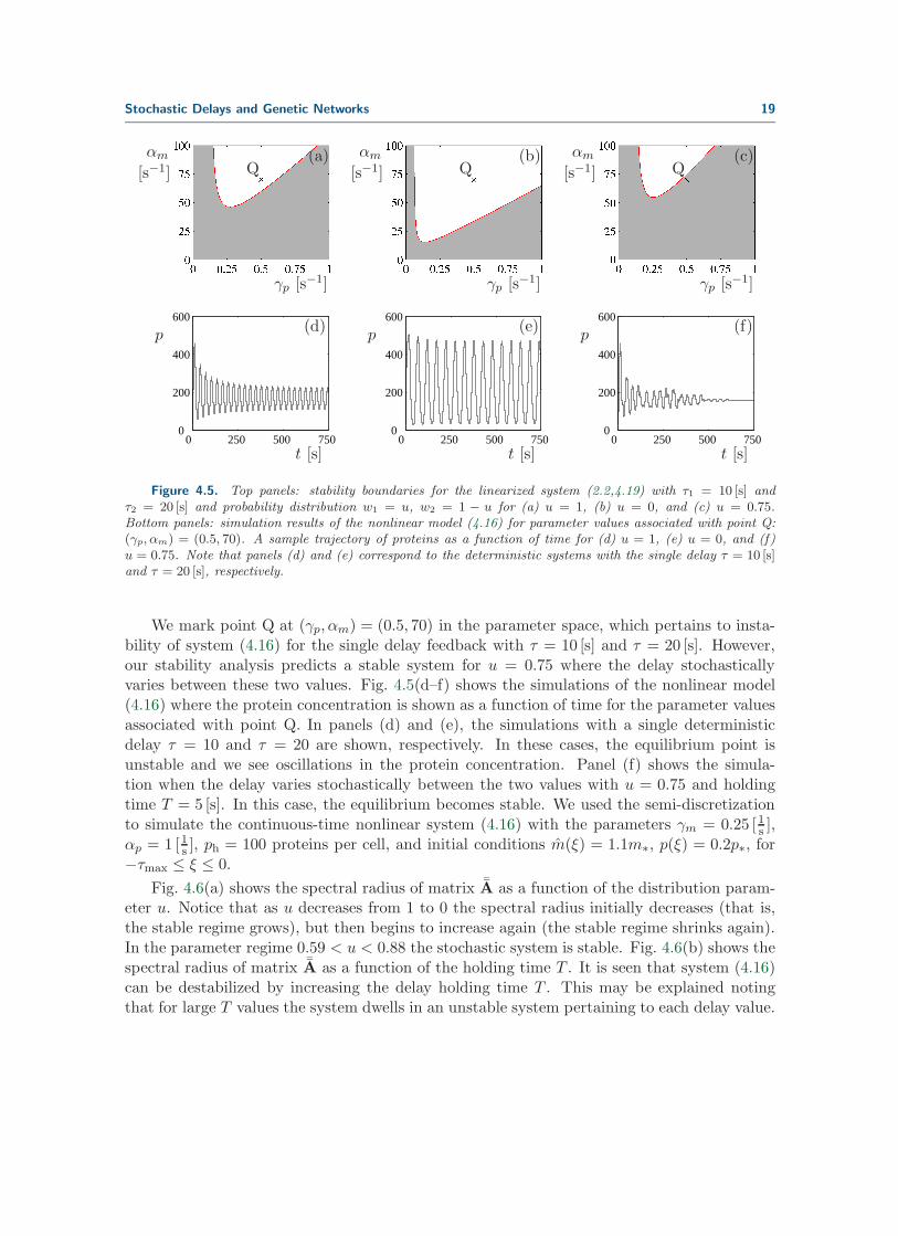
Figure 4.5. Top panels: stability boundaries for the linearized system (2.2,4.19) with τ1 = 10 [s] andτ2 = 20 [s] and probability distribution w1 = u, w2 = 1 − u for (a) u = 1, (b) u = 0, and (c) u = 0.75.Bottom panels: simulation results of the nonlinear model (4.16) for parameter values associated with point Q:(γp, αm) = (0.5, 70). A sample trajectory of proteins as a function of time for (d) u = 1, (e) u = 0, and (f)u = 0.75. Note that panels (d) and (e) correspond to the deterministic systems with the single delay τ = 10 [s]and τ = 20 [s], respectively.

We mark point Q at (γp, αm) = (0.5, 70) in the parameter space, which pertains to insta-bility of system (4.16) for the single delay feedback with τ = 10 [s] and τ = 20 [s]. However,our stability analysis predicts a stable system for u = 0.75 where the delay stochasticallyvaries between these two values. Fig. 4.5(d–f) shows the simulations of the nonlinear model(4.16) where the protein concentration is shown as a function of time for the parameter valuesassociated with point Q. In panels (d) and (e), the simulations with a single deterministicdelay τ = 10 and τ = 20 are shown, respectively. In these cases, the equilibrium point isunstable and we see oscillations in the protein concentration. Panel (f) shows the simula-tion when the delay varies stochastically between the two values with u = 0.75 and holdingtime T = 5 [s]. In this case, the equilibrium becomes stable. We used the semi-discretizationto simulate the continuous-time nonlinear system (4.16) with the parameters γm = 0.25 [1s ],αp = 1 [1s ], ph = 100 proteins per cell, and initial conditions m(ξ) = 1.1m∗, p(ξ) = 0.2p∗, for−τmax ≤ ξ ≤ 0.

Fig. 4.6(a) shows the spectral radius of matrix ¯A as a function of the distribution param-eter u. Notice that as u decreases from 1 to 0 the spectral radius initially decreases (that is,the stable regime grows), but then begins to increase again (the stable regime shrinks again).In the parameter regime 0.59 < u < 0.88 the stochastic system is stable. Fig. 4.6(b) shows thespectral radius of matrix ¯A as a function of the holding time T . It is seen that system (4.16)can be destabilized by increasing the delay holding time T . This may be explained notingthat for large T values the system dwells in an unstable system pertaining to each delay value.


0 0.25 0.5 0.75 10.95

1

1.05

1.1

1.15(a)

u

ρ( ¯A)

1 5 10 15 20 25 300.95

1

1.1

1.2

1.3(b)

T

ρ( ¯A)

Figure 4.6. (a) The spectral radius of ¯A versus the probability distribution u. (b) The spectral radius of ¯

A

versus the holding time T .

The dynamics are only stabilized by the switching events between the two unstable systems.

5. Conclusion and Discussion. Delay differential equations with stochastic delay wereinvestigated in this paper. In particular, we derived stability conditions for equilibria byanalyzing the mean and the second moment dynamics. We showed that if the delay followsa stationary stochastic process with autocorrelation becoming zero fast enough, then themean dynamics are described by a distributed delay system that can be analyzed to obtainnecessary conditions for the stability of the stochastic system. We also used the notion ofsecond moment stability to ensure almost sure stability. We applied the semi-discretizationtechnique and demonstrated convergence of spectra and stability charts when decreasing thesize of the discretization time step.

The theoretical tools were applied to simple auto-regulatory gene networks where stochas-tic delays appear due to sequential biochemical reactions. We showed that the resultant delaydistribution is well approximated by an Erlang distribution. We first investigated an auto-regulatory gene circuit described by a scalar model. We found that increasing the stochasticityin the delay (characterized by the relative variance of the distribution) increased the size ofthe almost sure stable region indicating that stochasticity in the delay may stabilize unstableequilibria. Our findings were justified using numerical simulations of the linearized and fullnonlinear system. We also investigated the auto-regulatory circuit taking into account mRNAdynamics which yielded a model with a higher dimension where we included a bimodal delaydistribution. We found that even if both the regulatory delays are individually destabilizing,the stochastic combination of these two delays can make the system stable. Furthermore, wefound that the longer the dwelling times, the more unstable the network became. We plan touse the developed tools to analyze the dynamics of more complicated synthetic and naturalgene regulatory networks.

While we were able to derive mean dynamics in the continuous limit (when the autocor-relation of the delay became zero faster than the shortest delay), such limit was not foundfor the second moment dynamics analytically but left for future research. Moreover, we re-mark that the stochastic delay system studied in this paper can also be viewed as a hybridsystem where switching between various delayed-differential equations happen in a stochasticfashion. Work has been done on the stability analysis of hybrid systems with constant time


delays [30, 34, 53, 54] or with deterministically time-varying delays [42]; however, modelingstochastic delay systems such as ours is less explored in the hybrid systems literature.


Appendix A. Erlang distribution.

In this appendix we provide some details about the derivation and properties of the Erlangdistribution used in the main part of the paper. Consider the chain of reactions shown inequation (4.1), assuming that c1 = c2 = . . . = cN = c. That is,

P0c−→ P1 ,

P1c−→ P2 ,

...

PN−1c−→ PN ,

(A.1)

where Pi represents the number of molecules of species i and we define the time delay τ as thetime it takes for a molecule to go through this chain of reactions. Let us assume the initialconditions to be such that at time t = 0 we have P0 = 1 and Pi = 0, i = 1, . . . , N − 1. Thereactions are assumed to happen sequentially such that the first reaction happens at time t1,the second reaction happens at time t1 + t2, and so forth. The last reaction happens at time∑N

k=1 tk that is equal to the delay τ . Then, the state vector changes as

0 t1 t1 + t2 · · · ∑Nk=1 tk = τ

P0

P1

P2...

PN

100...0

010...0

001...0

· · ·

000...1

(A.2)

In chemical reaction networks, a fundamental assumption is to model reaction occurrencetimes as arrivals of a Poisson process [6]. Therefore, the time elapsed between reactions isan exponential random variable. The rate at which reaction i occurs is determined by thepropensity cPi−1 and thus ti is an exponential random variable with rate cPi−1. Based on thestate vectors shown in (A.2), the times ti, i = 1, . . . , N are exponential random variables withidentical rate c. Furthermore, we assume that they are independent. That is, the time delayτ =

∑Nk=1 tk is the sum of N independent, exponentially-distributed random variables. To

find the probability density function of τ we start with introducing the notation t :=∑N

k=2 tk.Thus the cumulative distribution function becomes

FN (t) = P[τ < t] = P[t1 + t < t] =

∫ ∞

0P[

t1 + t < t | t1 = u]

c e−cudu , (A.3)

Moreover,

P[

t1 + t < t | t1 = u]

=

{

0 , if u ≥ t ,

P[

t < t− u | t1 = u]

= P[t < t− u] , if u < t ,(A.4)

where we used independence of t1 and t. Also, FN−1(t−u) = P[t < t−u] since t is the sum ofN − 1 independent, exponentially-distributed random variables. Substituting this into (A.3)


and (A.4) we obtain the recursive rule

FN (t) =

∫ t

0c e−cuFN−1(t− u) du . (A.5)

Taking the derivative of both sides with respect to time t, we obtain a similar relationshipbetween the probability density functions

wN (t) =

∫ t

0c e−cuwN−1(t− u) du , (A.6)

where wk(t) =ddtFk(t), k = 1, . . . , N .

Now we show by induction that the probability density function wN (t) follows the Erlangdistribution (4.2). For N = 1 we have

F1(t) = P[t1 < t] =

∫ t

0c e−cudu = 1− e−ct ⇒ w1(t) =

d

dtF1(t) = c e−ct . (A.7)

Assume wN−1(t) is Erlang. Thus using (A.6), we have

wN (t) =

∫ t

0c e−cu c

N−1(t− u)N−2e−c(t−u)

(N − 2)!du =

cN tN−1e−ct

(N − 1)!, (A.8)

that completes the proof.In the method proposed in the paper, we discretize the Erlang distribution such that we

neglect the delays less than E − n√V and larger than E + n

√V where E denotes the mean,

V denotes the variance. We choose n = 3 for the examples shown in the paper. Here, wediscuss this approximation and investigate other values of n.

The cumulative distribution function of the Erlang distribution (4.2) is

Fe(τ) =

∫ τ

0we(σ) dσ = 1− e−cτ

N−1∑

k=0

(cτ)k

k!. (A.9)

Therefore, the probability of the delay falling between E − n√V and E + n

√V is

P[

|τ − E| < n√V]

= Fe

(

E + n√V)

− Fe

(

E − n√V)

. (A.10)

Substituting E = N/c (cf. (4.3)) and√V =

√N/c (cf. (4.4)) into A.10 and assuming E −

n√V > 0, we can show by some algebraic manipulations that

P[

|τ−E| < n√V]

= −e−(N+n√N)

N−1∑

k=0

(N + n√N)k

k!+e−(N−n

√N)

N−1∑

k=0

(N − n√N)k

k!. (A.11)

If E − n√V ≤ 0, we have

P[

|τ − E| < n√V]

= Fe

(

E + n√V)

− Fe(0) = 1− e−(N+n√N)

N−1∑

k=0

(N + n√N)k

k!. (A.12)


n = 1 n = 2 n = 3 n = 4 n = 5

N = 10 0.69120 0.95851 0.99328 0.99899 0.99987N = 20 0.68683 0.95688 0.99506 0.99946 0.99995N = 50 0.68432 0.95553 0.99635 0.99974 0.99999N = 100 0.68350 0.95503 0.99682 0.99984 0.99999

Table A.1

P[

|τ − E| < n√V]

for different n and N values.

Note (A.11) or (A.12) only depend on N and n and Table A.1 shows the correspondingnumerical values for different values of N and n. This shows that the probability of fallingoutside the domain [E − n

√V ,E + n

√V ] is less than 1% for n = 3.

Appendix B. Mass-action kinetics of the auto-regulatory network.

Here, we use mass-action kinetics to provide some details regarding the origin of theparameters such as degradation and production rates that appear in the auto-regulatorynetwork models (4.6) and (4.16). We first consider mRNA dynamics into account to derivemodel (4.16). Then we show how one can simplify (4.16) to (4.6) using quasi steady stateapproximations (QSSA). We assume that the proteins produced through transcription andtranslation form dimers which bind to the promoter site of the gene and repress their owntranscription by blocking the RNA polymerase from binding.

The set of reactions we consider are

P + Pk+⇋

k−D ,

G+Dr+⇋r−

Gd ,

Gν−→ G+M0 ,

M0c−→ M1 ,

...

MNc−→ M , (B.1)

Mγm−→ ∅ ,

Mν−→ M + P0 ,

P0c−→ P1 ,

...

PNc−→ P ,

Pγp−→ ∅ ,

where P represents the number of the fully mature proteins (often called transcription factors),M represents the number of mRNA transcripts, D is the number of dimers, G is the numberof genes without dimers bound to them, and Gd is the number of genes with dimers bound.


Finally, the symbols Mi, i = 0, . . . , N , and Pi, i = 0, . . . , N are the numbers of molecules ofmRNA and protein in the intermediate stages of synthesis in the transcription and translationprocesses, respectively. The variables k+ and k− are the associative and dissociative rateconstants for dimerization, while r+ and r− are the reaction rates for binding and unbindingof a dimer to the promoter site. The initiation of the transcription that occurs when an RNApolymerase binds to a gene with an unoccupied promoter site occurs with reaction rate ν.For each reaction in the following sequence the reaction rate is set to c (transcription rate).The initiation of the translation occurs at rate ν and each reaction in the following sequencehappens with rate c. The symbols γm and γp represent the mRNA and protein degradationrates, respectively. We remark that further details may be considered regarding the bindingof the RNA polymerase [23] that are omitted here for simplicity.

Using the generalized mass-action kinetics for (B.1), we arrive at the following set of ODEs

dd

dt= k+ p2 − k− d− r+ g d+ r− gd ,

dg

dt= −r+ g d+ r− gd ,

dm0

dt= νg − cm0 ,

dmi

dt= cmi−1 − cmi , for i = 1, . . . , N ,

dm

dt= −γmm+ cmN ,

dp0dt

= νm− c p0 ,

dpidt

= c pi−1 − c pi , for i = 1, . . . , N ,

dp

dt= −γp p+ c pN − 2k+ p2 + 2k− d ,

(B.2)

where the lower case letters denote the corresponding concentrations and the plasmid copynumber g + gd is assumed to be constant. Notice that the set of linear equations for mi,i = 1, . . . , N and pi, i = 1, . . . , N can be solved analytically to obtain mN (t) and pN (t) as afunction of m0(t) and p0(t), respectively. In particular, considering zero initial conditions wehave

mi(t) =

∫ t

0c e−c(t−u)mi−1(u) du , (B.3)

for i = 1, . . . , N . Substituting the solution

m1(t) =

∫ t

0c e−c(t−u)m0(u) du , (B.4)

into the formula of m2(t) gives

m2(t) =

∫ t

0c e−c(t−v)m1(v) dv =

∫ t

0

∫ v

0c2 e−c(t−u)m0(u) dudv =

∫ t

0c2 σe−cσm0(t− σ) dσ ,

(B.5)


where we changed the order of integration and defined the new variable σ = t− u to obtainthe result. Similarly, we can obtain

m3(t) =

∫ t

0

c3σ2e−cσ

2!m0(t− σ) dσ. (B.6)

Repeating the integration in the same manner we arrive at

mN (t) =

∫ ∞

0

cNσN−1e−cσ

(N − 1)!m0(t− σ) dσ =

∫ ∞

0we(σ)m0(t− σ) dσ , (B.7)

where we(σ) is the Erlang distribution (4.2) and we extended the integration limit to infinitysince we consider m0(t) ≡ 0 for t ≤ 0. Similarly, for pN (t) we have

pN (t) =

∫ ∞

0

cNσN−1e−cσ

(N − 1)!p0(t− σ) dσ =

∫ ∞

0we(σ) p0(t− σ) dσ , (B.8)

where we(σ) is the Erlang distribution with order N and rate c. Using (B.7) and (B.8), wecan reduce (B.2) to

dd

dt= k+ p2 − k− d− r+ g d+ r− gd ,

dg

dt= −r+ g d+ r− gd ,

dm0

dt= ν g − cm0 ,

dm

dt= γmm+ c

∫ ∞

0we(σ)m0(t− σ) dσ ,

dp0dt

= ν m− c p0 ,

dp

dt= −γp p+ c

∫ ∞

0we(σ) p0(t− σ) dσ − 2k+ p2 + 2k− d .

(B.9)

This may be further reduced by using quasi-steady state approximations and singular pertur-bation methods. In particular, assuming that the kinetics of dimerization, promoter binding,transcription initiation, and translation initiation happen on a fast time-scale, the correspond-ing equations can be assumed to reach equilibrium quickly, allowing us to replace d(t), g(t),m0(t), and p0(t) with their respective steady-state values yielding

m(t) = −γmm(t) +

∫ ∞

0we(σ)

αm

1 +(

p(t− σ)/ph)2 dσ ,

p(t) = −γp p(t) +

∫ ∞

0we(σ)αp m(t− σ) dσ ,

(B.10)

with constants αm = ν(g + gd), ph =√

r−k−r+k+

, and αp = ν.


Note that equations (B.10) are the mean dynamics of the auto-regulatory network as theyare obtained through mass-action kinetics. Thus we may assume a single delay σ for thetranscription and a single delay ¯σ for the translation to obtain

m(t) = −γmm(t) +αm

1 +(

p(t− σ)/ph)2 ,

p(t) = −γp p(t) + αpm(t− ¯σ) .

(B.11)

We can further simplify (B.11) by using the change of variables m(t) = m(t− ¯σ). This allowsus to absorb the two delays into one single delay τ = σ + ¯σ and change (B.11) to

˙m(t) = −γm m(t) +αm

1 +(

p(t− τ)/ph)2 ,

p(t) = −γp p(t) + αp m(t),

(B.12)

which is the same as (4.16).

Finally assuming that the mRNA dynamics are fast and replacing m(t) in the secondequation in (B.12) with its steady-state value we arrive at

p(t) = −γp p(t) +κ

1 +(

p(t− τ)/ph)2 , (B.13)

where κ = αmαp/γm that is the same as (4.6).

We remark that one may also obtain (B.13) by neglecting the mRNA dynamics in (B.1)and following the steps above yielding

p(t) = −γp p(t) +

∫ ∞

0we(σ)

κ

1 +(

p(t− σ)/ph)2 dσ (B.14)

for the mean protein dynamics.

Acknowledgments:. The authors would like to thank Mark J. Balas for helpful discussion.

REFERENCES

[1] R. F. V. Anderson. The relative variance criterion for stability of delay systems. Journal of Dynamicsand Differential Equations, 5(1):105–128, 1993.

[2] A. Arkin, J. Ross, and H. H. McAdams. Stochastic kinetic analysis of developmental pathway bifurcationin Phage λ-infected Escherichia coli cells. Genetics, 149(4):1633–1648, 1998.

[3] L. Arnold, H. Crauel, and V. Wihstutz. Stabilization of linear systems by noise. SIAM Journal on Controland Optimization, 21(3):451–461, 1983.

[4] G. K. Basak. Stabilization of dynamical systems by adding a colored noise. IEEE Transactions onAutomatic Control, 46(7):1107–1111, 2001.

[5] M. B. G. Cloosterman, N. van de Wouw, W. P. M. H. Heemels, and H. Nijmeijer. Stability of net-worked control systems with uncertain time-varying delays. IEEE Transactions on Automatic Control,54(7):1575–1580, 2009.

[6] D. Del Vecchio and R. M. Murray. Biomolecular Feedback Systems. Princeton University Press, 2014.


[7] O. Diekmann, S. A. van Gils, S. M. Verduyn Lunel, and H. O. Walther. Delay Equations: Functional-,Complex-, and Nonlinear Analysis, volume 110 of Applied Mathematical Sciences. Springer, 1995.

[8] K. Engelborghs, T. Luzyanina, and D. Roose. Numerical bifurcation analysis of delay differential equationsusing dde-biftool. ACM Transactions on Mathematical Software, 28(1):1–21, 2002.

[9] T. Erneux. Applied Delay Differential Equations, volume 3 of Surveys and Tutorials in the AppliedMathematical Sciences. Springer, 2009.

[10] M. Farkas and G. Stepan. On perturbation of the kernel in infinite delay systems. Zeitschrift fur Ange-wandte Mathematik und Mechanik, 72(2):153–156, 1992.

[11] R. M. Feldman and C. V. Flores. Applied Probability and Stochastic Processes. Springer, 2010.[12] H. Gao and T. Chen. New results on stability of discrete-time systems with time-varying state delay.

IEEE Transactions on Automatic Control, 52(2):328–334, 2007.[13] M. Ghasemi, S. Zhao, T. Insperger, and T. Kalmar-Nagy. Act-and-wait control of discrete systems with

random delays. In Proceedings of the American Control Conference, pages 5440–5443, 2012.[14] D. T. Gillespie. Exact stochastic simulation of coupled chemical reactions. The Journal of Physical

Chemistry, 81:2340–2361, 1977.[15] C. Gupta, J. M. Lopez, R. Azencott, M. R. Bennett, K. Josic, and W. Ott. Modeling delay in genetic

networks: From delay birth-death processes to delay stochastic differential equations. The Journalof Chemical Physics, 140(20):204108, 2014.

[16] F. Hartung, T. Insperger, G. Stepan, and J. Turi. Approximate stability charts for milling processes usingsemi-discretization. Applied Mathematics and Computation, 174(1):51–73, 2006.

[17] T. Insperger and G. Stepan. Semi-discretization method for delayed systems. International Journal forNumerical Methods in Engineering, 55(5):503518, 2002.

[18] T. Insperger and G. Stepan. Stability analysis of turning with periodic spindle speed modulation viasemidiscretization. Journal of Vibration and Control, 10(12):1835–1855, 2004.

[19] T. Insperger and G. Stepan. Semi-discretization for Time-delay Systems: Stability and EngineeringApplications, volume 178 of Applied Mathematical Sciences. Springer, 2011.

[20] T. Insperger, G. Stepan, and Turi. State-dependent delay in regenerative turning processes. NonlinearDynamics, 47(1-3):275–283, 2007.

[21] K. Josic, J. M. Lopez, W. Ott, L. Shiau, and M. R. Bennett. Stochastic delay accelerates signaling ingene networks. PLoS Computational Biology, 7(11):e1002264, 2011.

[22] I. Kats. On the stability of systems with random delay in the first approximation. Prikladnaya Matematikai Mekhanika (P. M. M.), translated as Journal of Applied Mathematics and Mechanics, 31(3):447–452,1967.

[23] S. Klumpp. A superresolution census of RNA polymerase. Biophysical Journal, 105(12):2613–2614, 2013.[24] V. B. Kolmanovskii and V. R. Nosov. Stability of Functional Differential Equations, volume 180 of

Mathematics in Science and Engineering. Academic Press Inc., 1986.[25] I. Kolmanovsky and T.L. Maizenberg. Stochastic stability of a class of nonlinear systems with randomly

varying time-delay. In Proceedings of the American Control Conference, pages 4304–4308, 2000.[26] H. J. Kushner. Introduction to Stochastic Control. Holt, Rinehart and Winston, 1971.[27] A. A. Kwiecinska. Stabilization of partial differential equations by noise. Stochastic Processes and their

Applications, 79(2):179–184, 1999.[28] J. Lewis. Autoinhibition with transcriptional delay: a simple mechanism for the zebrafish somitogenesis

oscillator. Current Biology, 13(16):1398–1408, 2003.[29] E. A. Lidskii. On stability of motion of a system with random delays. Differentialnye Uravnenia, translated

as Differential Equations, 1(1):96–101, 1965.[30] X. Liu and J. Shen. Stability Theory of Hybrid Dynamical Systems With Time Delay. IEEE Transactions

on Automatic Control, 51(4):620–625, 2006.[31] D. M. Longo, J. Selimkhanov, J. D. Kearns, J. Hasty, A. Hoffmann, and L. S. Tsimring. Dual delayed

feedback provides sensitivity and robustness to the nf-κb signaling module. PLoS ComputationalBiology, 9(6), 2013.

[32] M. C. Mackey, A. Longtin, and A. Lasota. Noise-induced global asymptotic stability. Journal of StatisticalPhysics, 60(5-6):735–751, 1990.

[33] J. Mallet-Paret and H. L. Smith. The Poincare-Bendixson theorem for monotone cyclic feedback systems.Journal of Dynamics and Differential Equations, 2(4), 1990.


[34] X. Mao. Exponential stability of stochastic delay interval systems with Markovian switching. IEEETransactions on Automatic Control, 47(10):1604–1612, 2002.

[35] W. Mather, M. R. Bennett, J. Hasty, and L. S. Tsimring. Delay-induced degrade-and-fire oscillations insmall genetic circuits. Physical Review Letters, 102(6):068105, 2009.

[36] H. H. McAdams and A. Arkin. It’s a noisy business! genetic regulation at the nanomolar scale. Trendsin Genetics, 15(2):65–69, 1999.

[37] W. Michiels, V. Van Assche, and S.-I. Niculescu. Stabilization of time-delay systems with a controlledtime-varying delay. IEEE Transactions on Automatic Control, 50(4):493–504, 2005.

[38] N. A. Monk. Oscillatory expression of Hes1, p53, and NF-κb driven by transcriptional time delays.Current Biology, 13(16):1409–1413, 2003.

[39] A. N. Naganathan and V. Munoz. Scaling of folding times with protein size. Journal of the AmericanChemical Society, 127(2):480–481, 2005.

[40] G. Orosz, J. Moehlis, and R. M. Murray. Controlling biological networks by time-delayed signals. PhilTrans of R Soc A, 368(1911):439–454, 2010.

[41] P. G. Park. A delay-dependent stability criterion for systems with uncertain time-invariant delays. IEEETransactions on Automatic Control, 4(4):876–877, 1999.

[42] X. Pu and H. Zhao. Stability of a kind of hybrid systems with time delay. Advances in ElectronicEngineering, Communication and Management, 139:159–165, 2012.

[43] W. B. Qin, M. M. Gomez, and G. Orosz. Stability and frequency response under stochastic communi-cation delays with applications to connected cruise control design. IEEE Transactions on IntelligentTransportation Systems, submitted, 2015.

[44] D. Roose and R. Szalai. Continuation and bifurcation analysis of delay differential equations. InB. Krauskopf, H. M. Osinga, and J. Galan-Vioque, editors, Numerical Continuation Methods forDynamical Systems, Understanding Complex Systems, pages 359–399. Springer, 2007.

[45] H. Smith. An Introduction to Delay Differential Equations with Sciences Applications to the Life, vol-ume 57 of Texts in Applied Mathematics. Springer, 2011.

[46] G. Stepan. Retarded Dynamical Systems: Stability and Characteristic Functions, volume 210 of PitmanResearch Notes in Mathematics. Longman, 1989.

[47] J. Stricker, S. Cookson, M. R. Bennett, W. H. Mather, L. S. Tsimring, and J. Hasty. A fast, robust andtunable synthetic gene oscillator. Nature, 456:516–519, 2008.

[48] T. Tian, K. Burrage, P. M. Burrage, and M. Carletti. Stochastic delay differential equations for geneticregulatory networks. Journal of Computational and Applied Mathematics, 205(2):696–707, 2007.

[49] M. Tigges, T. T. Marquez-Lago, J. Stelling, and M. Fussenegger. A tunable synthetic mammalian oscil-lator. Nature, 457:309–312, 2009.

[50] O. S. Venturelli, H. El-Samad, and R. M. Murray. Synergistic dual positive feedback loops establishedby molecular sequestration generate robust bimodal response. Proceedings of the National Academyof Sciences of the United States of America, 109(48):E3324–33, 2012.

[51] E. I. Verriest and W. Michiels. Stability analysis of systems with stochastically varying delays. Systemsand Control Letters, 58(10-11):783–791, 2009.

[52] U. Vogel and K. F. Jensen. The RNA chain elongation rate in Escherichia coli depends on the growthrate. Journal of Bacteriology, 176(10):2807–2813, 1994.

[53] P. Xing-Cheng and Y. Wei. Stability of hybrid stochastic systems with time-delay. ISRN MathematicalAnalysis, 2014. Article ID.

[54] C. Yuan and X. Mao. Stability of stochastic delay hybrid systems with jumps. Eur. J. Control, 16:595–608,2010.

[55] D. Yue, Y. Zhang, E. Tian, and C. Peng. Delay-distribution-dependent exponential stability criteria fordiscrete-time recurrent neural networks with stochastic delay. IEEE Transactions on Neural Networks,19(7):1299–1306, 2008.

Stability of Systems with Stochastic Delays and Applications to Genetic Regulatory Networks

Documents

Transcript of Stability of Systems with Stochastic Delays and Applications to Genetic Regulatory Networks