http://www.jclinpharm.org

PharmacologyThe Journal of Clinical

1997; 37; 486 J. Clin. Pharmacol.EI Ette

Stability and performance of a population pharmacokinetic model

http://www.jclinpharm.org/cgi/content/abstract/37/6/486 The online version of this article can be found at:

Published by:

http://www.sagepublications.com

On behalf of: American College of Clinical Pharmacology

can be found at:The Journal of Clinical PharmacologyAdditional services and information for

http://www.jclinpharm.org/cgi/alerts Email Alerts:

http://www.jclinpharm.org/subscriptions Subscriptions:

http://www.sagepub.com/journalsReprints.navReprints:

http://www.sagepub.com/journalsPermissions.navPermissions:

at ACCP Member on November 25, 2009 http://www.jclinpharm.orgDownloaded from

486 #{149}J ClinPharmacol 1997;37:486-495

Stability and Performance of a PopulationPharmacokinetic Model

Ene I. Ette, PhD, FCP, FCCP

This study aimed to determine the stability (in terms of covariate selection) of a popula-tion pharmacokinetic model and evaluate its performance in the absence of a test data

set. Data from 88 full-term infants, 11 of whom were human immunodeficiency virus(HIV)-seropositive, taking an antiinfective agent were analyzed using exploratory data

analysis methods and the nonlinear mixed-effects modeling (NONMEM) program toobtain the final population pharmacokinetic model. The stability of the populationpharmacokinetic model was tested using the non parametric bootstrap approach in four

steps: 1) with the base pharmacokinetic model, 100 bootstrap replicates of the originaldata were generated by sampling with replacement; 2) ascertainment that each bootstrap

data replicate was described by the basic structural model using the NONMEM objective

function; 3) generalized additive modeling (CAM) applied to empiric Bayesian estimates

for covariate selection at a = 0.05 and a frequency (f) cutoff value of 0.50; and 4)NONMEM population model building using covariates selected in the third step witha = 0.005. Performance of the population pharmacokinetic model was evaluated using

200 additional bootstrap replicates of the data by fitting the model obtained in step 4

to them. Parameters obtained were compared with those obtained in the model stability

step, and improved prediction error, a measure of predictive accuracy as an index ofinternal validation, was computed. The reciprocal of serum creatinine (RSC; f = . 73)and HIV (f = 0.70) were selected by CAM as predictors of clearance (Cl). The population

pharmacokinetic model obtained without the determination of model stability included

RSC as a predictor of Cl, but the final model from the model stability step includedboth HIV and RSC as predictors of Cl. Final population pharmacokinetic parameters

were obtained with this model fitted to the original data; however, the 95% confidence

interval on the HIV status regression coefficient included zero, indicating no signifi-

cance. The mean parameter estimates obtained with the additional 200 bootstrap repli-cates of data were within 15% of those obtained with the final model at the regressionstability step. Bootstrap resampling procedure is useful for evaluating the stability and

performance of a population model by repeatedly fitting it to the bootstrap sampleswhen there is no test data set.

W ithout considering the stability of a populationpharmacokinetic model in an independent

sample, it is possible to be unaware that some factorsrepresent spurious associations with the outcome be-cause of “noise” in the data or multiple comparisons.

From the Office of Clinical Pharmacology & Biopharmaceutics, Food andDrug Administration, Rockville, Maryland. The views expressed are thoseof the author and not of the U.S. Food and Drug Administration. Submit-

ted for publication September 25, 1996; accepted in revised form March25, 1997. Address for reprints: Ene I. Ette, PhD, Pharmacometrics Staff,

HFD-855, Office of Clinical Pharmacology & Biopharmaceutics, CDER,

FDA, 5600 Fishers Lane, Rockville, MD 20857.

Further, minor changes in the data set may result inthe selection of different covariates. This might leaveone in a quandary regarding which covariates actu-ally are of predictive importance. When statisticalsignificance is the sole criterion for including a co-variate in the model, the number of covariates se-lected is a function of the sample size.

Because a population pharmacokinetic model isused for predictions, a key issue is its predictive ac-curacy; therefore, the stability of the populationpharmacokinetic model (in terms of the covariates)and good predictive performance are essential. Inthis context, “stability” refers to replication stabilityfor inclusion of covariates in a model.1 Sample sizes

PHARMACOKINETIC MODEL STABILITY AND PERFORMANCE

PHARMACOKINETICS SERIES 487

are usually too small (especially in pediatric studies)to apply the well-known and often recommendedmethod of data splitting.2 With better computer facil-ities, computer-intensive methods, such as jackknifeand the related bootstrap method, may provide apracticable alternative.3 “In a world in which theprice of calculation continues to decrease rapidly,but the price of theorem proving continues to holdsteady or increase, elementary economics indicatesthat we ought to spend a larger and larger fractionof our time on calculation” (p. 74)6 The bootstrapreplaces difficult mathematics with an increase ofseveral orders of magnitude in the computing neededfor statistical analysis.

The bootstrap resampling technique can be ap-plied to complicated problems for which one cannotassess analytical accuracy of a statistical procedure.By resampling the original data with replacement,artificial samples are generated on which the infer-ence of interest can be made as for the original sam-ple. A combination of the bootstrap technique andother methods are used to investigate the stabilityand performance of a population pharmacokineticmodel for a test drug in pediatrics.

PATIENTS AND METHODS

Data from 88 full-term infants and children from fivepharmacokinetic studies were pooled for populationpharmacokinetic analysis. There were 48 boys and40 girls; of these 60 were white, 15 were black, 9were Hispanic, and 4 of other races. Thirteen patientswere human immuno deficiency virus (HIV) -sero-positive. The patients’ mean weight was 22.15 ±

18.27 kg, mean age was 6.78 ± 4.3 years, and theaverage serum creatinine value was 0.8 ± 0.31 mg/dL.The reciprocal of serum creatinine (RSC) was usedfor population pharmacokinetic modeling. Ninehundred seventy-four plasma concentrations of thedrug were provided by these patients. An average of11.1 (range, 1-21) concentrations were measured perparticipant. The patients received either a singledose or multiple doses of the drug. The number ofdoses ranged from 1 to 21. Some studies lasted for 21days. Participants received either oral or intravenousformulations of the drug.

POPULATION MODEL BUILDING WITHOUTREPLICATION STABILITY

A structured approach to population pharmacoki-netic modeling was used. Using nonlinear mixed-effects modeling (NONMEM) program (version 4.0;NONMEM Project Group, University of California atSan Francisco, San Francisco, CA), the two-compart-

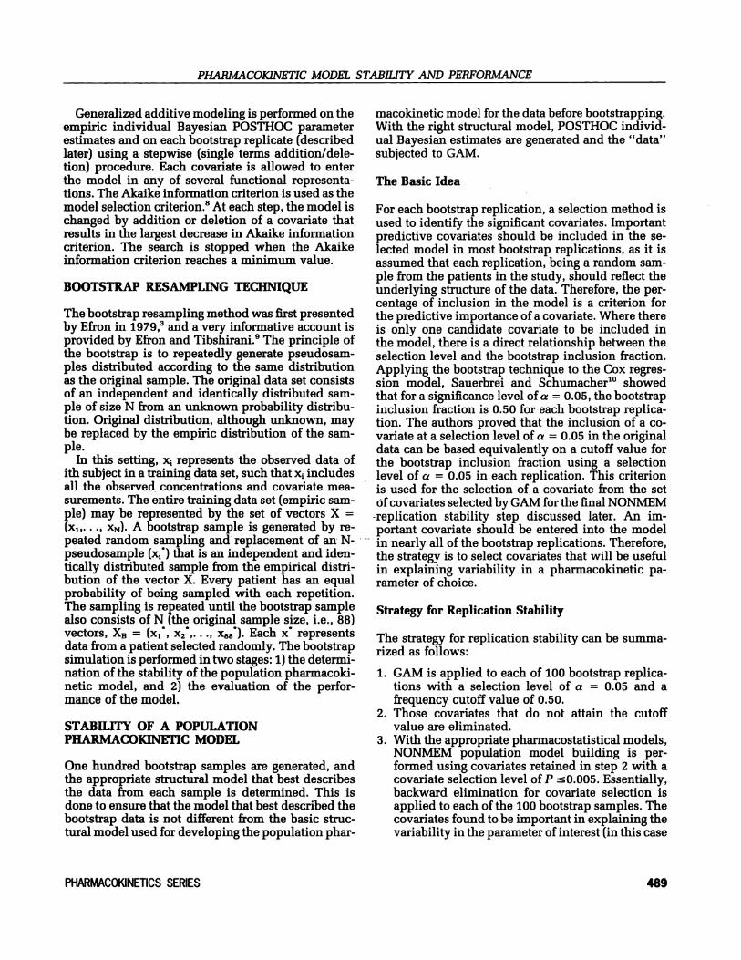
ment pharmacokinetic open model with first-orderinput and elimination (parameters: clearance [Cl],volume of central compartment [Vi], volume of pe-ripheral compartment [V2], intercompartmental Cl[OJ, absorption rate constant [Ka], and absolute bio-availability [F]) was found to fit the data better thana one-compartment open model. Because of the na-ture of the concentration-time data (Figure 1), Clwas modeled as a step function with a break pointtime of 180 hours. This provided a significantly bet-ter fit of the data than modeling Cl without the stepfunction. The 180-hour break point was found to bethe best break point time among a series of time val-ues tested. The choice was based on monitoring theobjective function. Incorporating the break pointtime in the model became necessary to account fora change in renal function in infants during the 3weeks of study. All structural model parameters ex-cept Ka and F were normalized for weight.

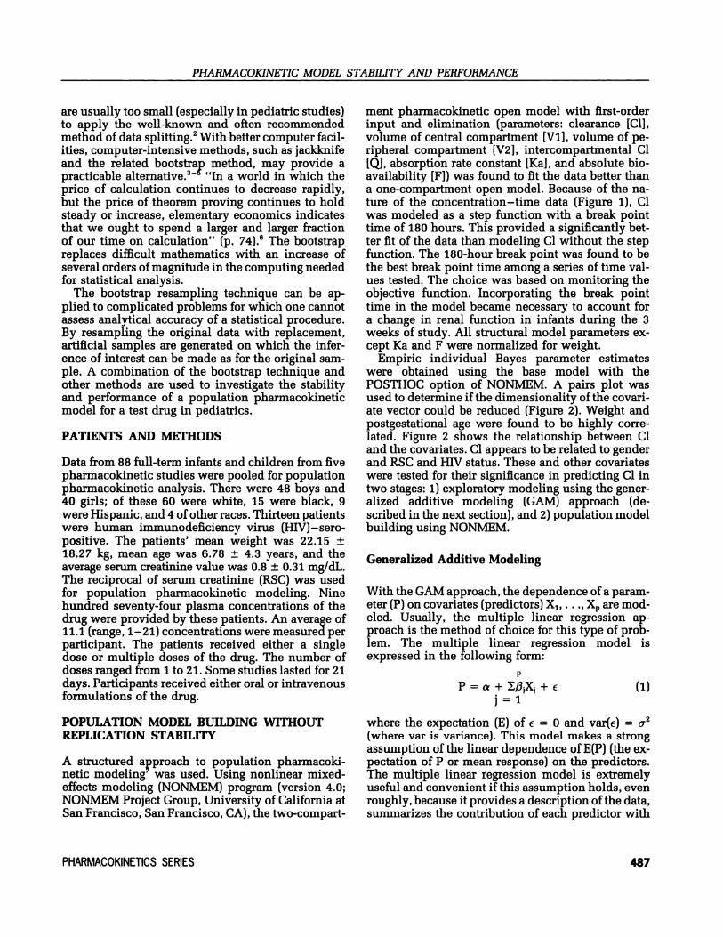
Empiric individual Bayes parameter estimateswere obtained using the base model with thePOSTHOC option of NONMEM. A pairs plot wasused to determine if the dimensionality of the covari-ate vector could be reduced (Figure 2). Weight andpostgestational age were found to be highly corre-lated. Figure 2 shows the relationship between Cland the covariates. Cl appears to be related to genderand RSC and HIV status. These and other covariateswere tested for their significance in predicting Cl intwo stages: 1) exploratory modeling using the gener-alized additive modeling (GAM) approach (de-scribed in the next section), and 2) population modelbuilding using NONMEM.

Generalized Additive Modeling

With the GAM approach, the dependence of a param-eter (P) on covariates (predictors) X1 X, are mod-eled. Usually, the multiple linear regression ap-proach is the method of choice for this type of prob-lem. The multiple linear regression model isexpressed in the following form:

p

P = a ++ #{128}

j=1(1)

where the expectation (E) of #{128}= 0 and var(#{128})= a2

(where var is variance). This model makes a strongassumption of the linear dependence of E(P) (the ex-pectation of P or mean response) on the predictors.The multiple linear regression model is extremelyuseful and convenient if this assumption holds, evenroughly, because it provides a description of the data,summarizes the contribution of each predictor with

A

U)

12

U)

0’

+

+

+A

+ +

A

A

A A

*

+ * * A

+ A

#{149} A +

+i+ ‘.S *

+

+

+A

AA + LAA + +

+A A

A AL#{224}+*

+

+

1. ++

A A

0 100 200 300 400 500 600

Time (h)

rSEX

Figure 2. Pairs plot showing the relationship between covariateson one hand, and covariates and clearance (CL) on the other.WT, weight; RSC, reciprocal of serum creatinine; HIV, humanimmunodeficiency virus.

ETTE

488 #{149}J ClinPharmacol 1997;37:486-495

Figure 1. Concentration-time plot

for boys (+) and girls (tx).

a single coefficient, and provides a simple methodfor predicting new observations.

The assumption of linear dependence of the re-sponse variable on each of the predictors may not

always hold. For many types of data, a change in themean of the response variable is accompanied by achange in its variance. The GAM approach presentsa general perspective for the handling of covariatesin a multiple regression setting. The linear form ofa + JflJXJ is replaced with the additive form a +

j(X), that is,p

P = a + f,(X) + #{128}

j=1(2)

where f(X) is an arbitrary univariate function that iseither a linear function or a smoothing spline. Be-cause each covariate is represented separately inequation 2, GAM retains the important interpretivefeature of the linear model: The variation of the fittedresponse surface holding all but one predictor fixeddoes not depend on the values of the other pre-dictors. In practice, this means that once the additivemodel is fitted to the data, one can plot the p coordi-nate functions separately to examine the roles of pre-dictors in modeling the response. The estimatedfunction forms of GAM are analogs of the coefficientsin multiple linear regression. Therefore, separatefunctions are introduced to allow nonlinearity andheterogenous variances. This is closer to a reformula-tion of the model than to a reexpression of the re-sponse.

PHARMACOKINETIC MODEL STABILITY AND PERFORMANCE

PHARMACOKINETICS SERIES 489

Generalized additive modeling is performed on theempiric individual Bayesian POSTHOC parameterestimates and on each bootstrap replicate (describedlater) using a stepwise (single terms addition/dele-tion) procedure. Each covariate is allowed to enterthe model in any of several functional representa-tions. The Akaike information criterion is used as themodel selection criterion.8 At each step, the model ischanged by addition or deletion of a covariate thatresults in the largest decrease in Akaike informationcriterion. The search is stopped when the Akaikeinformation criterion reaches a minimum value.

BOOTSTRAP RESAMPLING TEChNIQUE

The bootstrap resampling method was first presentedby Efron in 1979, and a very informative account isprovided by Efron and Tibshirani.9 The principle ofthe bootstrap is to repeatedly generate pseudosam-ples distributed according to the same distributionas the original sample. The original data set consistsof an independent and identically distributed sam-ple of size N from an unknown probability distribu-tion. Original distribution, although unknown, maybe replaced by the empiric distribution of the sam-ple.

In this setting, x, represents the observed data ofith subject in a training data set, such that x, includesall the observed concentrations and covariate mea-surements. The entire training data set (empiric sam-

ple) may be represented by the set of vectors X =

(x1,..., xN). A bootstrap sample is generated by re-peated random sampling and replacement of an N-pseudosainple (x1*) that is an independent and iden-tically distributed sample from the empirical distri-bution of the vector X. Every patient has an equalprobability of being sampled with each repetition.The sampling is repeated until the bootstrap samplealso consists of N (the original sample size, i.e., 88)vectors, X8 = (x1’, x2,..., x88’). Each x representsdata from a patient selected randomly. The bootstrapsimulation is performed in two stages: 1) the determi-nation of the stability of the population pharmacoki-netic model, and 2) the evaluation of the perfor-mance of the model.

STABILITY OF A POPULATIONPHARMACOKINETIC MODEL

One hundred bootstrap samples are generated, andthe appropriate structural model that best describesthe data from each sample is determined. This isdone to ensure that the model that best described thebootstrap data is not different from the basic struc-tural model used for developing the population phar-

macokinetic model for the data before bootstrapping.With the right structural model, POSTHOC individ-ual Bayesian estimates are generated and the “data”subjected to GAM.

The Basic Idea

For each bootstrap replication, a selection method isused to identify the significant covariates. Importantpredictive covariates should be included in the se-lected model in most bootstrap replications, as it isassumed that each replication, being a random sam-ple from the patients in the study, should reflect theunderlying structure of the data. Therefore, the per-centage of inclusion in the model is a criterion forthe predictive importance of a covariate. Where thereis only one candidate covariate to be included inthe model, there is a direct relationship between theselection level and the bootstrap inclusion fraction.Applying the bootstrap technique to the Cox regres-sion model, Sauerbrei and Schumacher1#{176} showedthat for a significance level of a = 0.05, the bootstrapinclusion fraction is 0.50 for each bootstrap replica-tion. The authors proved that the inclusion of a co-variate at a selection level of a = 0.05 in the originaldata can be based equivalently on a cutoff value forthe bootstrap inclusion fraction using a selectionlevel of a = 0.05 in each replication. This criterionis used for the selection of a covariate from the setOf covariates selected by GAM for the final NONMEM

.replication stability step discussed later. An im-

portant covariate should be entered into the modelin nearly all of the bootstrap replications. Therefore,the strategy is to select covariates that will be usefulin explaining variability in a pharmacokinetic pa-rameter of choice.

Strategy for Replication Stability

The strategy for replication stability can be summa-rized as follows:

1. GAM is applied to each of 100 bootstrap replica-tions with a selection level of a = 0.05 and afrequency cutoff value of 0.50.

2. Those covariates that do not attain the cutoffvalue are eliminated.

3. With the appropriate pharmacostatistical models,NONMEM population model building is per-formed using covariates retained in step 2 with acovariate selection level of P �0.005. Essentially,

backward elimination for covariate selection isapplied to each of the 100 bootstrap samples. Thecovariates found to be important in explaining thevariability in the parameter of interest (in this case

ETTE

490 #{149}J Clin Pharmacol 1997;37:486-495

Cl) are used to build the final population pharma-cokinetic model.

4. The population model is then applied to the origi-nal data to obtain parameter estimates for thedrug.

Application

After performing this procedure, 100 bootstrap repli-cates of the data were generated and analyzed withNONMEM. For each bootstrap replicate the modelthat best described the data was determined usingthe log likelihood ratio test. Each of the bootstrapdata sets was best described with the two-compart-ment model incorporating a step function. POST-HOC individual empiric Bayesian estimates weregenerated from each replicate data set and the esti-mates with the covariates formed a new “data” set,which was subjected to GAM. The criterionfor the selection of covariates outlined previouslywas applied, and the covariates selected were usedfor subsequent population model building withNONMEM using backward elimination. The popula-tion model was then applied to the original data toobtain pharmacokinetic parameter estimates for thedrug.

EVALUATION OF MODEL PERFORMANCE

The most stringent test of a model is external valida-tion-the application of the “frozen” model to a newpopulation. Often, the failure of a model to be vali-dated externally could have been predicted from anunbiased internal validation. It is likely that manypopulation pharmacokinetic models that failed to bevalidated could have been found to fail with anotherseries of subjects from the original source. The majormethods of obtaining nearly unbiased internal as-sessments of accuracy are data splitting, cross valida-tion, and bootstrapping.114 A random portion of thedata, for example, two thirds of the data, is used formodel development when the data splitting ap-proach for model validation (predictive perfor-mance) is used. The model is later frozen and appliedto the remaining sample for computing measures ofpredictive performance, such as mean prediction er-ror and its standard deviation. Usually the size of thevalidation sample must be such that the relationshipbetween predicted and observed outcomes can beestimated with good accuracy and the remainingdata used as the model development data set. Datasplitting has the advantage of simplicity because allthe modeling steps are only done once; however,data splitting may not validate the final model if one

desires to recombine the training and test data set toderive a model for others to use, which, in mostcases, is the reason for population pharmacokineticmodeling.

Repeated data splitting is cross validation. Thebenefits of cross validation over data splitting are 1)the size of the model development database can bemuch larger so that less data are discarded from theestimation process, and 2) cross validation reducesvariability by not relying on a single sample split. Itis has been shown that cross validation is inefficientbecause of high variation of accuracy estimates whenthe entire validation process is repeated.12 Data split-ting is worse; the indices of accuracy vary greatlywith different splits. An alternative method of inter-nal validation is bootstrapping. It provides nearlyunbiased estimates of predictive accuracy that are ofrelatively low variance. Bootstrapping has the addi-tional advantage that the entire data set is used formodel development. Others have shown that dataare too precious to waste,15’16 and sample size is evenmore critical in the pediatric setting in which ethicaland medical concerns limit recruitment into studies.

Two hundred bootstrap samples are generated andused for the evaluation of the model performance.The model obtained in step 3 in the section “Strategy

for Replication Stability” is fitted repeatedly to the200 additional bootstrap samples. From each fit, theprediction error is calculated, and this is termed theapparent error (AEbooJ.12 Prediction error (PE) refersto the expected squared difference between a futureresponse and its prediction from the model:

PE = E(C - (3)

where C and C are observed and predicted responses(concentrations) and E (the expectation) refers to re-peated sampling from the true population.

Next, each of the 200 fitted models is applied tothe original sample to give bootstrap estimates of PE(i.e.. PEorig). The overall estimate of PEorig is the aver-age of these bootstrap estimates. The amount bywhich the AEb00t (or average residual squared error)underestimates the true prediction error is the “opti-mism” (opt).12 This is defined as follows:

opt = PE08 - AEboot. (4)

The overall estimate of optimism is the average ofthe differences. The estimate of optimism obtainedis added to the average of residual squared error(RSE/n, where n is number of observations) obtainedfrom fitting the final model obtained from the replica-tion stability step to the original data to get an im-proved estimate of prediction error (PEimp),’2 that is,

PEimp = opt + RSE/n. (5)

4

S

-

0

0 :T: S

t 4 8 I I‘Iv

PHARMACOKINETICS SERIES 491

PI-JARMACOKINETIC MODEL STABILITY AND PERFORMANCE

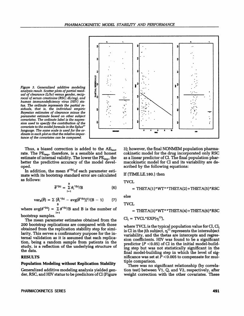
Figure 3. Generalized additive modelinganalysis result. Scatter plots of partial resid-ual of clearance (L/hr) versus gender, recip-rocal of serum creatinine (RSC; dLlmg), andhuman immunodeficiency virus (HIV) sta-tus. The ordinate represents the partial re-siduals, that is, the individual empiricBayesian estimates of clearance minus theparameter estimate based on other subjectcovariates. The ordinate label is the expres-sion used to specify the contribution of thecovariate to the modelformula in the Splus’7language. The same scale is used for the or-dinate in each plot so that the relative impor-tance of the covariates can be compared.

Thus, a biased correction is added to the AEb00trate. The PEimp, therefore, is a sensible and honestestimate of internal validity. The lower the PEimp, thebetter the predictive accuracy of the model devel-oped.

In addition, the mean 9of each parameter esti-mate with its bootstrap standard error are calculatedas follows:

B=

11

var8(8) = [*ft) - avg(*)]2/(B - 1)B

(6)

(7)

where avg(O*) = O*(b)/B and B is the number of

bootstrap samples.The mean parameter estimates obtained from the

200 bootstrap replications are compared with thoseobtained from the replication stability step for simi-larity. This serves a confirmatory purpose for the in-ternal validation as it is assumed that each replica-tion, being a random sample from patients in thestudy, is a reflection of the underlying structure ofthe data.

RESULTS

Population Modeling without Replication Stability

Generalized additive modeling analysis yielded gen-der, RSC, and HIV status to be predictors of Cl (Figure

3); however, the final NONMEM population pharma-cokinetic model for the drug incorporated only RSCas a linear predictor of Cl. The final population phar-macokinetic model for Cl and its variability are de-scribed by the following equations:

If (TIME.LE.180.) then

TVCL

else

= THETA(i)*WT**THETA(2)+THETA(5)*RSC

TVCL

= THETA(3)*WT* *TpETA(4)+THETA(6)*RSc

Cl = TVCL*EXP(),

where TVCL is the typical population value for Cl, Clis Cl in the jth subject, mC represents the intersubjectvariability, and the thetas are intercepts and regres-sion coefficients. HIV was found to be a significantpredictor (P <0.05) of Cl in the initial model-build-ing step but was not statistically significant in thefinal model-building step in which the level of sig-nificance was set at P <0.005 to compensate for mul-tiple comparison.

There was no significant relationship (by correla-tion test) between Vi, Q, and V2, respectively, afterweight correction with the other covariates. These

CI, clearance; VI, volume of central compartment; V2, volume of peripheralcompartment; Ka, absorption rate constant.

Cl, clearance, WT, weight; RSC, reciprocal of serum creatinine; VI, volume ofcentral compartment; V2, volume of peripheral compartment; Ka, absorption rateconstant; F, absolute bioavailability; Q, intercompartmental Cl.

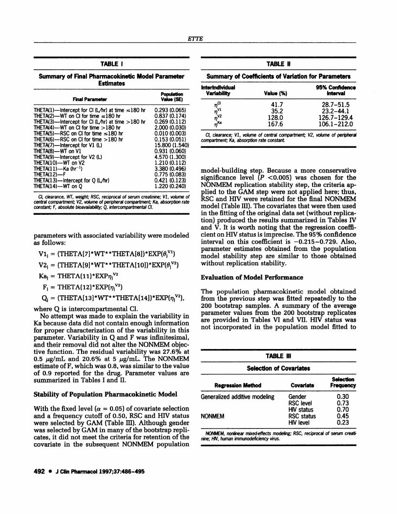
TABLE Ill

Selection of Covariates

NONMEM, nonlinear mixed-effects modeling; RSC, reciprocal of serum creati-nine; HIV, human immunodeficiency virus.

ETTE

492 #{149}J Clin Pharmacol 1997;37:486-495

TABLE I

Summary of Final Pharmacokinetic Model ParameterEstimates

PopulationFinal Parameter Value (SE)

THETA(l)-Intercept for Cl (Lfiir) at time l8O hr 0.293 (0.065)THETA(2)-WT on CI for time �180 hr 0.837 (0.174)THETA(3)-lntercept for Cl (LAir) at time >180 hr 0.269 (0.112)THETA(4)-WT on CI for time >180 hr 2.000 (0.030)THETA(5)-RSC on CI for time l80 hr 0.010 (0.003)THETA(6)-RSC on CI for time >180 hr 0.153 (0.051)

THETA(7)-Intercept for Vi (L) 15.800 (1.540)

THETA(8)-WT on Vi 0.931 (0.060)THETA(9)-lntercept for V2 (L) 4.570 (1.300)THETA(10)-WT on V2 1.210 (0.112)THETA(1 1)-Ka (hr’) 3.380 (0.496)THETA(12)-F 0.775 (0.083)

THETA(13)-lntercept for Q (LAir) 0.421 (0.123)THETA(14)-WT on Q 1.220 (0.240)

parameters with associated variability were modeled

as follows:

Vi, = (THETA[7] *WT* *TFIfTA[8]) *EXp(OVl)

V2, = (THETA[9]*WT**THETA[i0])*EXP(O’2)

Ka, = THETA(1i)*EXP2

F, = THETA(12)*EXP(7’2)

= (THETA[13] *WT* *pET[4])*E)(p(.V2)

where Q is intercompartmental Cl.No attempt was made to explain the variability in

Ka because data did not contain enough informationfor proper characterization of the variability in thisparameter. Variability in Q and F was infinitesimal,and their removal did not alter the NONMEM objec-tive function. The residual variability was 27.6% at0.5 ,ag/mL and 20.6% at 5 g/mL. The NONMEMestimate ofF, which was 0.8, was similar to the valueof 0.9 reported for the drug. Parameter values aresummarized in Tables I and II.

Stability of Population Pharmacokinetic Model

With the fixed level (a = 0.05) of covariate selectionand a frequency cutoff of 0.50, RSC and HIV statuswere selected by GAM (Table HI). Although genderwas selected by GAM in many of the bootstrap repli-cates, it did not meet the criteria for retention of thecovariate in the subsequent NONMEM population

TABLE II

Summary of Coefficients of Variation for Parameters

lnterindMdualVariability Value (%)

95% ConfidenceInterval

CI

V1

V2

Ka

41.735.2

128.0167.6

28.7-51.523.2-44.1

126.7-129.4106.1-212.0

model-building step. Because a more conservativesignificance level (P <0.005) was chosen for theNONMEM replication stability step, the criteria ap-plied to the GAM step were not applied here; thus,RSC and HIV were retained for the final NONMEMmodel (Table Ill). The covariates that were then usedin the fitting of the original data set (without replica-tion) produced the results summarized in Tables IVand V. It is worth noting that the regression coeffi-cient on HIV status is imprecise. The 95% confidenceinterval on this coefficient is -0.215-0.729. Also,parameter estimates obtained from the populationmodel stability step are similar to those obtainedwithout replication stability.

Evaluation of Model Performance

The population pharmacokinetic model obtainedfrom the previous step was fitted repeatedly to the200 bootstrap samples. A summary of the averageparameter values from the 200 bootstrap replicatesare provided in Tables VI and VII. HIV status wasnot incorporated in the population model fitted to

SelectionRegression Method Covariate Frequency

Generalized additive modeling GenderRSC levelHIV status

0.300.730.70

NONMEM RSC statusHIV level

0.450.23

PHARMACOKINETIC MODEL STABILITY AND PERFORMANCE

PHARMACOKINETICS SERIES 493

TABLE N

Replication Stability: Summary of Final PopulationPharmacokinetic Model Parameter Estimates*

PopulationParameter Value (SE)

ThETA(1)-lntercept for CI (1/lir) at time s180 hr 0.297 (0.055)THETA(2)-WT on Cl for time �180 hr 0.832 (0.137)THETA(3)-lntercept for CI (1/lw) at time >180 hr 0.262 (0.086)THETA(4)-WT on Cl for time >180 hr 2.070 (0.223)ThETA(5)-RSC on Cl for time 180 hr 0.010 (0.001)THETA(6)-RSC on CI for time >180 hr 0.141 (0.045)ThETA(7)-lntercept for Vi (L) 15.900 (1.240)THETA(8)-WT on Vi 0.928 (0.050)TFIETA(9)-Intercept for V2 (L) 4.940 (1.070)THETA(i0)-WT on V2 1.190 (0.128)THETA(1i)-Ka (hr’) 3.390 (0.499)THETA(12)-F 0.790 (0.079)THETA(13)-Intercept for Q 0.431 (0.127)THETA(14)-WT on Q 1.180 (0.215)THETA(i5)-HIV on Cl for time 180 hr 0.257 (0.236)

* Cl model revised to include the effect of HIV.

Cl, clearance; W, weight; RSC, reciprocal of serum creatinine; VI, volume ofcentral compartment; V2, volume of peripheral compartment; Ka, absorption rateconstant; F, absolute bioavailability; Q, intercompartrnental Cl; HIV, human immuno-deficiency virus.

TABLE VI

Model Performance Evaluation: Summary of PopulationPharmacokinetic Model Parameter Estimates*

PopulationParameter Value (SE)

THETA(1)-Intercept for CI (L/hr) at time 180 hr 0.245 (0.064)THETA(2)-WT on CI for time �i80 hr 0.881 (0.042)THETA(3)-Intercept for CI (L/hr) at time >180 hr 0.330 (0.019)THETA(4)-WT on Cl for time >180 hr 2.230 (0.051)THETA(5)-RSC on CI for time �180 hr 0.023 (0.004)THETA(6)-RSC on Cl for time >180 hr 0.252 (0.014)THETA(7)-Intercept for Vi (L) 15.287 (0.162)TFIETA(8)-WT on Vi 0.934 (0.011)THETA(9)-Intercept for V2 (L) 8.384 (0.344)THEIA(i0)-WT on V2 0.934 (0.035)ThETA(1 i)-Ka (hr) 3.522 (0.847)THETA(i2)-F 0.788 (0.095)THETA(13)-Intercept for Q 0.551 (0.042)THETA(i4)-WT on Q 1.146 (0.482)

200 NONMEM runs used.

Cl, clearance; Wf, weight; RSC, reciprocal of serum creatinine; VI, volume ofcentral compartment; V2, volume of peripheral compartment; Ka, absorption rateconstant; F, absolute bioavailability; Q, intercompartmental Cl.

these data sets. Also, the average RSE/n, AEbO0t, PEorig,

and optimism values obtained were 0.78, 0.63, 0.90,and 0.12, respectively, and the improved predictionerror was 0.90.

DISCUSSION

A structured approach for developing populationpharmacokinetic models7 was used in developingthe population pharmacokinetic model. Of the covar-

TABLE V

iates selected by CAM, only RSC was retained inthe final NONMEM population model. This is notsurprising, as GAM is an exploratory modeling toolused for the reduction in the number of covariatesused in the NONMEM population model-buildingstep and for understanding the nature of the relationbetween a parameter and predictive covariates.7’17H1V status was found by NONMEM to be marginallyinsignificant as a predictor of Cl. This prompted theinvestigation of the stability of the population phar-macokinetic model developed.

TABLE VII

Replication Stability: Summary of Coefficients ofVariation for Parameters*

lnterindividualVariability

Value(%)

95% ConfidenceInterval

CI

1V1

V2

Ka

F

43.434.5167.0126.08.9

32.1-52.222.8-43.2103.3-212.467.5-165.70.0-58.6

Cl model revised to include HIV.

Cl, clearance; VI, volume of central compartment; V2, volume of peripheralcompartment; Ka, absorption rate constant; F, absolute bioavailabilily.

Model Performance Evaluation: Summary of Coefficientsof Variation for Parameters*

InterindividualVariability

Value(%)

95% ConfidenceInterval

CI

97V1

V2Ka

F

41.347.5127.9i0i.928.6

51.5-74.941.7-88.090.i-i56.842.3-138.10.0-51.2

#{149}200 NONMEM runs used.Cl, clearance; Vi, volume of central compartment; V2, volume of peripheral

compartment; Ka, absorption rate constant; F, absolute bioavailability.

ETTE

494 #{149}J Clin Pharmacol 1997;37:486-495

The bootstrap technique is useful for the estima-tion of parameters and their variability in a givenmodel. In this article, it is used for the investigationof the population pharmacokinetic model stability,that is, the selection of covariates for building anappropriate population pharmacokinetic model. Theresult of a stepwise selection procedure is usuallyjust a single model without any information aboutits stability. Stepwise selection depends very muchon covariates selected in the early steps and on in-fluential data points. With the bootstrap approachand a fixed selection level, an attempt is made toestimate the whole distribution of importance for thecovariates under consideration. By so doing, it is pos-sible to see whether there are some important covari-ates to be included in the model, and some idea aboutthe importance of each of the other covariates condi-tioned on the whole set of covariates is obtained.Moreover, one may feel more confident about theimportance of a covariate when it has been selectedin nearly all the bootstrap replications. Although anestimator may be influenced by a single data point,an influential data point cannot result in a covariatebeing selected in nearly all of the bootstrap replica-tions. Instability of a selected model can be deducedwhen different models are identified (i.e., a differentselection of covariates) in nearly all bootstrap repli-cations.

The results of GAM on the bootstrap replicatesshowed that RSC and HIV were important predictorsof Cl. The fixed selection level of a = 0.05 and afrequency cutoff of 50% enabled a reduction of thecovariates to be tested in the subsequent NONMEManalysis of the bootstrap sample. These two covari-ates also were selected from the NONMEM runs,with HIV status selected approximately half as oftenas RSC. Using HIV status in the population modelyielded regression coefficients on this parameterwith a 95% confidence interval incorporating zero.This indicates that the final population model ob-tained before using the bootstrap technique was sta-ble. It is important to note that although HIV statusis not included in the final model, its selection, andin fact selection of a covariate from a stability stepof model building (although not in a final model), isa strong indication for further investigation of thecovariate in explaining variability in the pharmaco-kinetics of the drug studied. The similarity of theparameter estimates obtained with or without repli-cation stability is a further confirmation that the finalpopulation model obtained without bootstrap repli-cation was optimal for this data set.

In modeling, model simplicity is usually balancedagainst incremental improvement in prediction. Inpopulation pharinacokinetic modeling, it is not only

important to develop a model that is stable but thepredictive ability of such a model is of great signifi-cance.

In the absence of a new test data set, internal vali-dation of a population pharmacokinetic model is es-sential if such a model is to be used confidently foroptimization of dosage in the clinical setting. It ispreferable to test a population model on a new dataset for predictive accuracy (external validation). Datasplitting is an effective method of model validation(internal validation) when it is not practical to collect

a new data set to test the model. This method, how-

ever, has the disadvantage that the predictive accu-racy of the model is a function of the sample size

resulting from the data splitting.15 To maximize pre-dictive accuracy while retaining a reliable estimateof the accuracy, it has been recommended that the

entire sample usually be used for model develop-ment and assessment.15 Thus, the bootstrap resam-pling technique for assessing the predictive accuracyof a population pharmacokinetic model has beenproposed and applied to a data set from a test drug.The mean parameter estimates obtained with the ad-ditional 200 bootstrap replicates of the data werewithin 15% of those obtained with the final modelof the replication stability step. Also, the estimate ofthe improved prediction error that corrects for thebias in the apparent error rate was very small. Thisindicates that the population model developed isreasonably accurate. PEimp is a better estimate of thelikely accuracy of external validation than is PE08given that all other aspects of the study design re-

main constant.This article addresses the issue of stability and

performance of a population pharmacokineticmodel. The amount of covariate selection undoubt-edly influences the predictive value of the final pop-ulation model. Determining the stability of a popula-tion pharmacokinetic model is important for rulingout covariates that represent spurious associationswith the outcome measure because of “noise” in the

data or multiple comparisons. As population phar-macokinetic modeling is often undertaken for subse-quent use of the model developed in a clinical set-ting, the bootstrap resampling procedure is useful forevaluating the performance of the final populationpharmacokinetic model by repeatedly fitting it to thebootstrap samples when there is no new data set.

REFERENCES

1. Gifi J: Nonlinear Multivariate Analysis. Chichester: Wiley,

1990.

2. Cox DR: A note on data-splitting for the evaluation of signifi-

cance levels. Biometrika 1975; 62:441-444.

PHARMACOKINETIC MODEL STABILITY AND PERFORMANCE

PHARMACOKINETICS SERIES 495

3. Efron B: Bootstrap methods: another look at the jackknife. AnnStat 1979;7:1-26.

4. Efron B: Censored data and the bootstrap. J Am Stat Assoc1981; 76:312-319.

5. Efron B: Nonparametric standard errors and confidence inter-

vals (with discussion). Can J Stat 1981;9:139-172.

6. Tukey JW: Sunset salvo. Am Stat 1986;40:72-76.

7. Ette El, Ludden TM: Population pharmacokinetic modeling:

the importance of informatic graphics. Pharm Res 1995; 12:1845-

1855.

8. Hastie TJ: Generalized additive models. In: Chambers JM, Has-

tie TJ., eds. Statistical Models in S. Pacific Grove, CA: Wadsw-orth & Brooks/Cole Advanced Books & Software, 1992;249-307.

9. Efron B, Tibshirani R: Bootstrap methods for standard errors,

confidence intervals, and other measures of statistical accuracy.

Stat Sci 1986;1:54-77.

10. Sauerbrei W, Schumacher M: A bootstrap resampling proce-

dure for model building: application to the cox regression model.

Stat Med 1992;11:2093-2109.

11. Picard RR, Berk KN: Data splitting. Am Stat 1990;44:140-147.

12. Efron B: Estimating the error rate of a prediction rule: im-

provement on cross-validation. / Am’ Stat Assoc 1983;78:316-

331.

13. Efron B: How biased is the apparent error rate of a prediction

rule? JAm Stat Assoc 1986;81:461-470.

14. Efron B, Gong G: A leisurely look at the bootstrap, the jack-

knife, and cross-validation. Am Stat 1983;37:36-48.

15. Roecker EB: Prediction error and its estimation for subset-

selected models. Technometrics 1991; 33; 459-468.

16. Breiman L: The little bootstrap and other methods for dimen-

sionality selection in regression: X-fixed prediction error. I AmStat Assoc 1992;87:738-754.

17. Splus (version 3.3) User’s Manual. Seattle: Statistical Sci-ences, 1995.