Physiologically Based Pharmacokinetic and Toxicokinetic Models

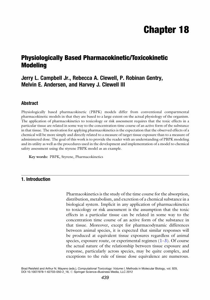
Chapter 18

Physiologically Based Pharmacokinetic/ToxicokineticModeling

Jerry L. Campbell Jr., Rebecca A. Clewell, P. Robinan Gentry,Melvin E. Andersen, and Harvey J. Clewell III

Abstract

Physiologically based pharmacokinetic (PBPK) models differ from conventional compartmentalpharmacokinetic models in that they are based to a large extent on the actual physiology of the organism.The application of pharmacokinetics to toxicology or risk assessment requires that the toxic effects in aparticular tissue are related in some way to the concentration time course of an active form of the substancein that tissue. The motivation for applying pharmacokinetics is the expectation that the observed effects of achemical will be more simply and directly related to a measure of target tissue exposure than to a measure ofadministered dose. The goal of this work is to provide the reader with an understanding of PBPK modelingand its utility as well as the procedures used in the development and implementation of a model to chemicalsafety assessment using the styrene PBPK model as an example.

Key words: PBPK, Styrene, Pharmacokinetics

1. Introduction

Pharmacokinetics is the study of the time course for the absorption,distribution, metabolism, and excretion of a chemical substance in abiological system. Implicit in any application of pharmacokineticsto toxicology or risk assessment is the assumption that the toxiceffects in a particular tissue can be related in some way to theconcentration time course of an active form of the substance inthat tissue. Moreover, except for pharmacodynamic differencesbetween animal species, it is expected that similar responses willbe produced at equivalent tissue exposures regardless of animalspecies, exposure route, or experimental regimen (1–3). Of coursethe actual nature of the relationship between tissue exposure andresponse, particularly across species, may be quite complex, andexceptions to the rule of tissue dose equivalence are numerous.

Brad Reisfeld and Arthur N. Mayeno (eds.), Computational Toxicology: Volume I, Methods in Molecular Biology, vol. 929,DOI 10.1007/978-1-62703-050-2_18, # Springer Science+Business Media, LLC 2012

439

Nevertheless, the motivation for applying pharmacokinetics is theexpectation that the observed effects of a chemical will be moresimply and directly related to a measure of target tissue exposurethan to a measure of administered dose.

1.1. Compartmental

Modeling

One of the first general descriptions of pharmacokinetic modelingwas presented by Teorell (4, 5). The model consisted of a number ofcompartments representing specific tissues. The concentration ofchemical in each compartment was described by a mass balance equa-tion in which the rate of change of the amount of chemical in acompartment was determined from the rates at which the chemicalentered and left the compartment in the blood as well as, whenappropriate, the rate of clearance of the chemical in that compartment.Unfortunately, in order to obtain an analytical solutionof the resultingsystem of differential equations, Teorell found it necessary to make anumber of simplifying assumptions. These assumptions led to a solu-tion in the formof a sumof exponential terms, and thus the “classical”compartmental modeling approach still used today was born.

Over the years, Teorell’s association of the model compartmentswith specific tissues has to a large extent been lost, and compartmen-tal modeling as currently practiced is largely an empirical exercise. Inthis empirical approach, data on the time course of the chemical ofinterest in blood (and perhaps other tissues, urine, etc.) are collected.Based on the behavior of the data, a mathematical model is selectedwhich possesses a sufficient number of compartments (and thereforeparameters) to describe the data. The compartments do not in gen-eral correspond to identifiable physiological entities but rather aredescribed in abstract terms. An example of a simple two-compartment mathematical model of this type is shown in Fig. 1.This particularmodel consists of a “central” compartment, character-ized by concentrations measured in the blood (but not considered toactually represent only the blood), and a “deep” compartment repre-senting unspecified tissues communicating with the central compart-ment as described by kinetic parameters, k12 and k21, whichthemselves have no obvious physiological or biochemical interpreta-tion. Similarly, the volume of the central compartment and the uptakeand clearance parameters (ka and ke) are empirically determined by theanalysis or fitting of experimental data sets.

CENTRALclearance

ke

uptake

ka

k21k12

DEEP

Fig. 1. Simple compartmental pharmacokinetic model.

440 J.L. Campbell Jr. et al.

The advantage of this modeling approach is that there is nolimitation to fitting the model to the experimental data. If a partic-ular model is unable to describe the behavior of a particular data set,additional compartments can be added until a successful fit isobtained. Since the model parameters do not possess any intrinsicmeaning, they can be freely varied to obtain the best possible fit,and different parameter values can be used for each data set in arelated series of experiments. Statistical tests can then be employedto compare the values of the parameters used, for example at twoadministered dose levels, in order to determine whether any appar-ent differences are statistically significant (6). Once developed,these models are useful for interpolation and limited extrapolationof the concentration profiles which can be expected as experimentalconditions are varied. If the model parameters vary with dose, thisinformation can provide evidence for the presence of nonlinearitiesin the animal system, such as saturable metabolism or binding. Atthis point, however, one of the serious disadvantages of the empiri-cal approach becomes evident. Since the compartmental modeldoes not possess a physiological structure, it is often not possibleto incorporate a description of these nonlinear biochemical pro-cesses in a biologically appropriate context. For example, in the caseof inhalation of chemicals subject to high-affinity, low-capacitymetabolism in the liver, an important determinant of metabolicclearance at low inhaled concentrations is the fact that only thefraction of the chemical in the blood reaching the liver is availablefor metabolism (1). Without a physiological structure it is notpossible to correctly describe the interaction between blood-transport of the chemical to the metabolizing organ and the intrin-sic clearance of the chemical by the organ.

1.2. Physiologically

Based Modeling

Physiologically based pharmacokinetic (PBPK) models differ fromconventional compartmental pharmacokinetic models in that theyare based to a large extent on the actual physiology of the organism.Instead of compartments defined solely by the experimental data,actual organ and tissue groups are described using weights andblood flows obtained from the literature. Moreover, instead ofcomposite rate constants determined solely by fitting data,measured physical–chemical and biochemical constants of the com-pound can often be used. To the extent that the structure of themodel reflects the important determinants of the kinetics of thechemical, PBPK models can predict the qualitative behavior of anexperimental time course data set without having been baseddirectly on it. Refinement of the model to incorporate additionalinsights gained from comparison with experimental data yields amodel which can be used for quantitative extrapolation well beyondthe range of experimental conditions on which it was based. Inparticular, a properly validated PBPKmodel can be used to perform

18 Physiologically Based Pharmacokinetic/Toxicokinetic Modeling 441

the high-to-low dose, dose-route, and interspecies extrapolationsnecessary for estimating human risk on the basis of animal toxicol-ogy studies (7–15).

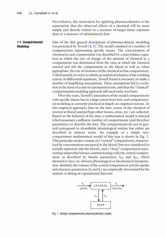
A number of excellent reviews have beenwritten on the subject ofPBPK modeling (16–20). The basic approach is illustrated in Fig. 2.The process of model development begins with the definition of thechemical exposure and toxic effect of concern, as well as the speciesand target tissue inwhich it is observed. Literature evaluation involvesthe integration of available information about the mechanism oftoxicity, the pathways of chemical metabolism, the nature of thetoxic chemical species (i.e., whether the parent chemical, a stablemetabolite, or a reactive intermediate produced during metabolismis responsible for the toxicity), the processes involved in absorption,transport and excretion, the tissue partitioning and binding charac-teristics of the chemical and its metabolites, and the physiologicalparameters (e.g., tissue weights and blood flow rates) for the speciesof concern (i.e., the experimental species and the human). Using thisinformation, the investigator develops a PBPKmodelwhich expressesmathematically a conception of the animal–chemical system. In themodel, the various time-dependent biological processes are describedas a system of simultaneous differential equations. A mathematicalmodel of this form can easily be written and exercised using

Design /ConductCritical Experiments

Compare toKinetic Data

Simulation

Model Formulation

BiochemicalConstants

LiteratureEvaluation

ProblemIdentification

Mechanismsof Toxicity

BiochemicalConstants

Refine Model Validate Model

Extrapolationto Humans

Fig. 2. Flowchart of the biologically motivated PBPK modeling approach to chemical riskassessment.


commonly available computer software (21). The specific structureof the model is driven by the need to estimate the appropriatemeasure of tissue dose under the various exposure conditions ofconcern in both the experimental animal and the human. Beforethe model can be used in human risk assessment it has to bevalidated against kinetic, metabolic, and toxicity information and,in many cases, refined based on comparison with the experimentalresults. The model itself can frequently be used to help designcritical experiments to collect data needed for its own validation.

The chief advantage of a PBPK model over an empiricalcompartmental description is its greater predictive power. Sincefundamental biochemical processes are described, dose extrapola-tion over ranges where saturation of metabolism occurs is possible(22). Since known physiological parameters are used, a differentspecies can be modeled by simply replacing the appropriate con-stants with those for the species of interest, or by allometric scaling(23–25). Similarly, the behavior for a different route of administra-tion can be determined by adding equations which describe thenature of the new input function (21, 26). The extrapolation fromone exposure scenario, say a single 6 h exposure, to another, e.g., arepetitive 6 h exposure, 5 days a week for the life of the animal, isrelatively easy and only requires a little ingenuity in writing theequations for the dosing regimen in the kinetic model (27, 28).

Since measured physical–chemical and biochemical parametersare used, the behavior for a different chemical can quickly be esti-mated by determining the appropriate constants. An important resultis the ability to reduce the need for extensive experiments with newchemicals (12). The process of selecting the most informative experi-mental data is also facilitated by the availability of a predictive phar-macokinetic model (29). Perhaps the most desirable feature of aphysiologically based model is that it provides a conceptual frame-work for employing the scientificmethod in which hypotheses can bedescribed in terms of biological processes, predictions can bemadeonthe basis of the description, and the hypothesis can be revised on thebasis of comparison with experimental data.

The trade-off against the greater predictive capability ofphysiologically based models is the requirement for an increasednumber of parameters and equations. However, values for manyof the parameters, particularly the physiological ones, are alreadyavailable in the literature (30–35), and in vitro techniques havebeen developed for rapidly determining the compound-specificparameters (36–39). An important advantage of PBPK models isthat they provide a biologically meaningful quantitative frame-work within which in vitro data can be more effectively utilized(40). There is even a prospect that predictive PBPK models cansomeday be developed based almost entirely on data obtainedfrom in vitro studies.


Some of the best examples of successful PBPKmodeling effortswere performed to support the clinical use of chemotherapeuticdrugs, e.g., methotrexate (41) and cisplatin (42) (see (43) for areview). There are also a large number of good examples of PBPKmodels which describe the kinetics of important environmentalcontaminants, including methylene chloride (8, 44, 45), trichloro-ethylene (46–48), chloroform (49, 50), 2-butoxyethanol (51),kepone (52), polybrominated biphenyls (53), polychlorinatedbiphenyls (54) and dibenzofurans (55), dioxins (56, 57), lead(58–62), arsenic (63, 64), methylmercury (65), atrazine (66, 67),acrylonitrile (68–70), perchlorate (71–76), and BTEX components(77–81). The U.S. EPA is currently compiling a compendium ofPBPK models including source code. This should be availableonline within the next year.

2. Materials

Currently there exists a very diverse group of modeling softwarepackages that vary in both complexity and range of application.Because of this diversity, there is a software package suitable forevery level of user from the expert to the first-timemodeler.However,not all modeling packages are created equal, and some of the moreuser-friendly software can lack the capabilities of the more complexprograms. Consequently, no single software package available canmeet all needs of all users, and the diversity and complexity of theprograms can often make converting a model from one package toanother rather difficult. Table 1 provides a list of some of the availablesoftware packages that may be useful for PBPKmodeling (82).

An additional list of pharmacokinetic software is located athttp://boomer.org/pkin/soft.html. However, not all of the soft-ware listed on this website is suitable for PBPK modeling.

The most commonly used software packages for PBPK model-ing have included Advanced Continuous Modeling Language(ACSL) (now acslX), Berkeley Madonna, MATLAB, MATLAB/Simulink, ModelMaker, and SCoP. Table 2 provides a summary ofthe features of each of these followed by further information.

acslX is an updated version of the widely used ACSL software.It has graphical as well as text interface with automatic linkage tothe integration algorithm. In particular, a Pharmacokinetic Toolkitin the graphic code interface makes it possible to build PBPKmodels by connecting predefined tissue code blocks. The softwareallows for the use of discrete blocks and script files and automati-cally sorts equations in the derivative block. The model may becompiled into either C/C++ or Fortran, although C++ is nowthe preferred compiler, and may be debugged interactively.


http://boomer.org/pkin/soft.html

http://boomer.org/pkin/soft.html

Table 1Representative list of available software packages

Package Source Website

General-purpose high-level scientific computing software. These high-level programming languagepackages are very general modeling tools that are not specifically designed for PBPK modeling, butoffer more complexity

acslX AEgis TechnologiesGroup, Inc.

http://www.acslX.com

Berkeley Madonna University of Californiaat Berkeley

http://www.berkeleymadonna.com

GNU octave University of Wisconsin http://www.octave.orgMATLAB/Simulink The MathWorks, Inc. http://www.mathworks.comMLAB Civilized Software, Inc. http://www.civilized.com

Biomathematical modeling software. Packages that were specifically designed for modeling biologicalsystems and some are user-friendly. Their usefulness in PBPK modeling is determined by theirgraphical interfaces, computational speed, and language flexibility and may provide mixed-effects(population) capabilities allowing for the analysis of sparse data sets

ADAPT II Biomedical SimulationsResource,USC

http://bmsr.usc.edu

MCSim INERIS http://toxi.ineris.fr/activites/toxicologie_quantitative/mcsim/mcsim.php

ModelMaker ModelKinetix http://www.modelkinetix.comNONMEM University of California

at SanFrancisco andGlobomax ServiceGroup

http://www.globomaxservice.com

SAAM II SAAM Institute, Inc. http://www.saam.comSCoP Simulation Resources,

Inc.http://www.simresinc.com

Stella High PerformanceSystems, Inc.

http://www.hps-inc.com

WinNonlin Pharsight Corp. http://www.pharsight.comWinNonMix Pharsight Corp. http://www.pharsight.com

Toxicokinetic software. These packages were designed specifically for PBPK and PBTK modeling andare extremely flexible. They are based on modeling languages developed in the aerospace industryfor modeling complex systems

SimuSolv Dow chemical Not maintained or subject to furtherdevelopment

Physiologically based custom-designed software. Custom-designed proprietary software programsspecifically for biomedical systems or applications that provide a high level of biological detail butare not easily customized

GastroPlus Simulations Plus, Inc. http://www.simulations-plus.comPathway prism Physiome Sciences, Inc. http://www.physiome.comPhysiolab Entelos, Inc. http://www.entelos.comSimCYP Simcyp, Ltd. http://www.simcyp.com






http://www.octave.org

http://www.octave.org

http://www.mathworks.com

http://www.mathworks.com

http://www.civilized.com

http://www.civilized.com

http://bmsr.usc.edu

http://bmsr.usc.edu

http://toxi.ineris.fr/activites/toxicologie_quantitative/mcsim/mcsim.php




http://www.modelkinetix.com

http://www.modelkinetix.com



http://www.saam.com

http://www.saam.com

http://www.simresinc.com

http://www.simresinc.com



http://www.pharsight.com




http://www.simulations-plus.com

http://www.simulations-plus.com

http://www.physiome.com

http://www.physiome.com

http://www.entelos.com

http://www.entelos.com

http://www.simcyp.com

http://www.simcyp.com

An optimization program is also included. Sensitivity analysis andMonte Carlo analysis can currently be conducted with script filesand there is some capability built into the package that allows theseanalyses to be conducted with the aid of a using a gui.

Berkeley Madonna has many of the same features as acslX;however, it does not allow for the use of discrete blocks or scriptfiles. It does currently have both an optimization and sensitivityanalysis feature, but does not have a built-inMonte Carlo capability.

MATLAB has a text interface, but not a graphical interface. Itdoes allow for the use of script files but not discrete blocks. It doesnot sort the code in the model so the user must be careful regarding

Table 2Comparison of modeling software features

Feature acslXc, dBerkeleyMadonnac, d MATLABc, d

MATLAB/Simulinkc, d

Modelmakerc, d SCoPd

Graphical interface Y Y N Y Y N

Text interface Y Y Y N Y Y

Automatic linkage tointegration algorithm

Y Y N Y Y Y

Discrete blocks Y N N Y Y N

Scripting Y N Y Y N N

Code sorting Y Y N Y Y N

Choice of target language Y N N N N N

Interactive modeldebugging

Y Y N Y N N

Optimization Y Y Ya Y Y Y

Sensitivity analysis Yb Y Yb Yb Y Y

Monte Carlo Yb Yb Yb Yb Y N

Units checking N N N N N Y

Database of physiologicalvalues

N N N N N N

Compiled (faster) Y Y Ya, e N N Y

Interpreted(more convenient)

N N Y Y Y N

aExtra costbCan perform through the use of user-developed model code or script filescMust contact vendor for price. Price may depend upon the type of licensedStudent and/or academic licenses are availableeWith separate compiler


the order of statements in the code. This statement order problemcan be problematic in the case of PBPK models, which requiresimultaneous solution of multiple differential equations, and cancomplicate conversion from a software package that automaticallysorts the model equations. An optimization package is availablethrough an add-on toolbox, but sensitivity analysis and MonteCarlo analysis must be performed through the use of script files.A large variety of user-built model code blocks are available at theMATLAB web site. The model code may be compiled through thepurchase and use of a MATLAB Compiler, but the user has nochoice of the target language used.

Simulink is an add-on to MATLAB that offers a graphic inter-face but no text interface. The use of discrete blocks is also addedwith the use of Simulink. Since Simulink uses only a graphicalinterface, there is no code to be viewed. Simulink adds a graphicaldebugger to MATLAB and an optimizer.

ModelMaker has many of the same features as acslXtreme andBerkeley Madonna. It has both a graphical and a text interface withautomatic linkage to the integration algorithm and allows for theuse of discrete blocks but not the use of script files. ModelMakeralso provides the capabilities for optimization, sensitivity analysis,and Monte Carlo analysis.

SCoP has only a text interface with automatic linkage to theintegration algorithm. It does not allow for the use of discreteblocks or script files and it does not automatically sort the code.Optimization and sensitivity analysis capabilities are included, butnot Monte Carlo analysis capabilities.

An additional modeling software package, not included inTable 2, is designed specifically to support Markov Chain MonteCarlo (MCMC) simulation. This program, MCSim, has been usedto reestimate parameter distributions for PBPKmodels on the basisof the agreement between model predictions and measured datafrom kinetic studies. MCSim is available for free download from thewebsite listed in Table 1. Its proper use requires expertise in pro-gramming and statistics.

Each of the software packages described above provides differ-ent features that would recommend them for a particular user.From the viewpoint of a risk assessor wanting to apply an existingPBPK model, as well as for a model developer seeking to have hismodel used in a risk assessment, the key requirement is the ability toreadily evaluate (verify) the model, reproduce (validate) the capa-bility of the model to simulate key data sets, and document itsapplication for the risk assessment. The necessary documentationincludes a model definition (preferably code-based) that can bereviewed to verify the mathematical correctness of the model, adescription of the parameters that should be used to run the modelfor comparison with validation data, and a description of the


parameters used to calculate the dose metrics for the risk assess-ment. The most important characteristics of a language for modelevaluation are verifiable code, self-documentation, and ease of use.The feature that is most important with regard to self-documentation is scripting, which allow the model developer tocreate procedures consisting of sequences of commands that, forexample, set model parameters, run the model, and plot the modelpredictions against the appropriate data set. Other features whichcontribute to ease of model evaluation include viewable modeldefinition code, code sorting, and automatic linkage to integrationalgorithms.

The modeling language that has seen the most widespread usein PBPKmodeling is the ACSL, which is currently implemented asacslX. The ACSL language has also served as the basis for a varietyof older packages, including SimuSolv (from Dow Chemical,no longer supported), ACSL/Tox (from Pharsight, no longersupported), and ERDM (currently used by the USEPA). Theautomatic code sorting provided by ACSL allows code to begrouped functionally (liver, lung, fat, etc.) rather than in programorder, greatly simplifying model development and improvingreadability of the code. The graphic code block capability inacslX is particularly attractive for PBPK modeling because it pro-vides the ability to create a model by connecting functional units(e.g., tissues) in a graphic environment, while at the same timecreating a model definition in ACSL code that can be reviewed formodel verification. The scripting capability, which permits bothMATLAB-like m-files, greatly expedites the comparison of themodel with multiple data sets that is generally required forPBPK modeling of data from multiple species and routes of expo-sure. The scripting capability also makes it possible to documentthe use of a model in a risk assessment, since m-scripts or com-mand file procedures can be written that set the model parametersand run the model for each of the dose metrics required for therisk assessment, as well as for each of the data sets used for modelevaluation/validation.

Berkeley Madonna provides a particularly intuitive, flexibleplatform for model development, and has been very popular inacademic settings. The software provides automatic code sorting,the ability to automatically convert between code and graphicmodel descriptions, and automatic compilation, greatly simplifyingand expediting model development, debugging, and verification.Conversion of models between ACSL and Berkeley Madonna isrelatively straightforward. However, the lack of a scripting capabil-ity makes comparison of the model with data fairly cumbersome,particularly in situations where a large number of data sets are beingmodeled. The lack of scripting also makes it more difficult todocument the actual use of a model in a risk assessment and greatlycomplicates model evaluation.


MATLAB is a very powerful and flexible software package thatis particularly attractive in research activities. Its main drawback isthat its use requires significant expertise in programming.MATLAB/Simulink avoids this drawback by providing a graphicalinterface, and is very popular with engineers in the automotive andelectronic industries. However, verification of a Simulink model bya nonengineer is hampered by the lack of any model definitioncode. That is, the model is specified only by a “wiring diagram”that shows the connections between blocks built up from basicmathematical functions (adders, multipliers, integrators, etc.).Conversion of a model between MATLAB and Simulink, orbetween one of these programs and another software package,can be very difficult.

ModelMaker, which is popular in Europe, provides surprisinglybroad functionality at a relatively low price. Its only serious draw-back is the lack of a scripting capability.

SCoP, which along with ACSL was one of the first languages tobe used for PBPK modeling, continues to be used due to itsfamiliarity and low cost. However, its lack of scripting or codesorting, and its DOS-based, menu-driven run-time interface canmake model evaluation more difficult.

3. Methods

3.1. General Concepts The methods will begin with a description of the seminal PBPKmodel published by Ramsey and Andersen in 1984 and lead intothe elements necessary for successful model development, refine-ment and validation. The experience of Ramsey and Andersenserves as a useful example of the advantages of the PBPK modelingapproach. In this case, blood and tissue time-course curves ofstyrene had been obtained for rats exposed to four different con-centrations of 80, 200, 600, and 1,200 ppm (83). Data wereobtained during a 6 h exposure period and for 18 h after cessationof the exposure. The initial analysis of these data had been based ona simple compartmental model, similar to the model shown inFig. 1, which had a zero-order input related to the amount ofstyrene inhaled, a two-compartment description of the rat, andlinear metabolism in the central compartment. The compartmentalmodel was successful with lower concentrations but was unable toaccount for the more complex behavior at higher concentrations(note the different behavior of the data at the two concentrationsshown in Fig. 3).

In an attempt to provide a more successful description, a PBPKmodel was developed with a realistic equilibration process for pul-monary uptake and Michaelis–Menten saturable metabolism in the


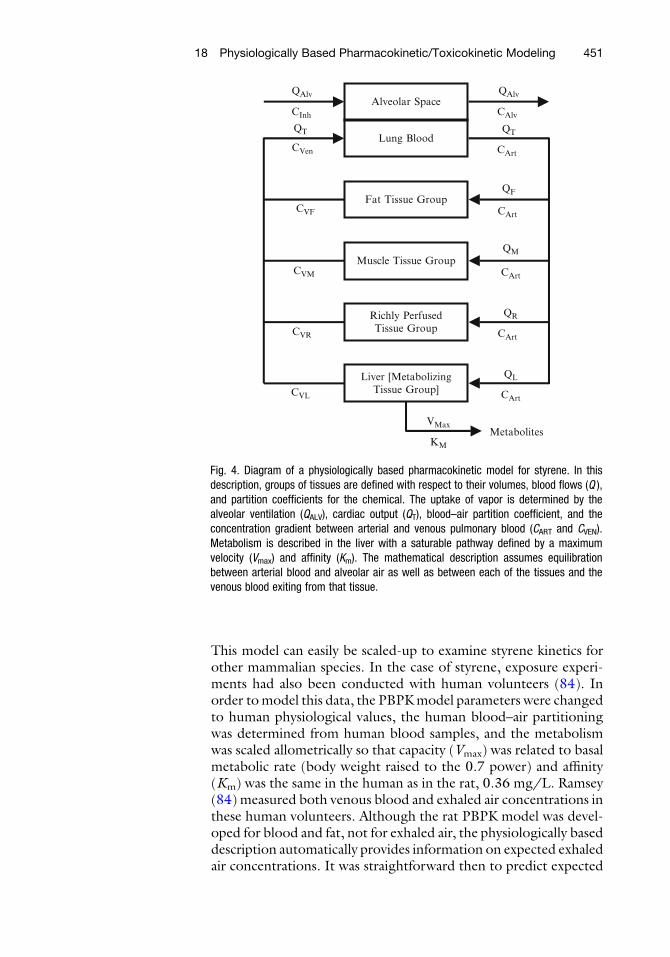
liver. A diagram of the PBPK model that was used by Ramsey andAndersen (1984) (22) to describe styrene inhalation in both ratsand humans is shown in Fig. 4. In this diagram, the boxes representtissue compartments and the lines connecting them representblood flows. The model contained several “lumped” tissue com-partments: fat tissues, poorly perfused tissues (muscle, skin, etc.),richly perfused tissues (viscera), and metabolizing tissues (liver).The fat tissues were described separately from the other poorlyperfused tissues due to their much higher partition coefficient forstyrene, which leads to different kinetic properties, while the liverwas described separately from the other richly perfused tissues dueto its key role in the metabolism of styrene. Each of these tissuegroups was defined with respect to their blood flow, tissue volume,and their ability to store (partition) the chemical of interest.Although the model diagram in Fig. 4 shows a lung compartment,a steady-state approximation for the equilibration of lung bloodwith alveolar air was used in the mathematical formulation of themodel to eliminate the need for an actual lung tissue compartment.This simple model structure, with realistic constants for the physi-ological, partitioning, and metabolic parameters, very accuratelypredicted the behavior of styrene in both fat and blood of the ratat all concentrations. Fig. 3 compares the model-predicted timecourse in the blood with the experimental data for the highest andlowest exposure concentrations in the rat studies.

The structure of the PBPK model for styrene reflects thegeneric mammalian architecture. Organs are arranged in a parallelsystem of blood flows with total blood flow through the lungs.

Rat600 ppm

80 ppm

Hours

Styr

ene

Con

cent

ration

(m

g/L

)

Fig. 3. Model predictions (solid lines) and experimental blood styrene concentrations inrats during and after 6 h exposures to 80 and 600 ppm styrene. The thick bars representthe chamber air concentrations of styrene and are shown to highlight the nonlinearity ofthe relationship between administered and internal concentrations. The model (Fig. 1.3)contains sufficient biological realism to predict the very different behaviors observed atthe two concentrations.


This model can easily be scaled-up to examine styrene kinetics forother mammalian species. In the case of styrene, exposure experi-ments had also been conducted with human volunteers (84). Inorder tomodel this data, the PBPKmodel parameters were changedto human physiological values, the human blood–air partitioningwas determined from human blood samples, and the metabolismwas scaled allometrically so that capacity (Vmax) was related to basalmetabolic rate (body weight raised to the 0.7 power) and affinity(Km) was the same in the human as in the rat, 0.36 mg/L. Ramsey(84) measured both venous blood and exhaled air concentrations inthese human volunteers. Although the rat PBPK model was devel-oped for blood and fat, not for exhaled air, the physiologically baseddescription automatically provides information on expected exhaledair concentrations. It was straightforward then to predict expected

Alveolar Space

Lung BloodQT

Fat Tissue GroupQF

Muscle Tissue GroupQM

Richly PerfusedTissue Group

QR

Liver [MetabolizingTissue Group]

QL

CArt

CArt

CArt

CArt

CArt

QAlv

CAlv

QAlv

CInh

QT

CVen

CVF

CVM

CVR

CVL

VMax

KM

Metabolites

Fig. 4. Diagram of a physiologically based pharmacokinetic model for styrene. In thisdescription, groups of tissues are defined with respect to their volumes, blood flows (Q ),and partition coefficients for the chemical. The uptake of vapor is determined by thealveolar ventilation (QALV), cardiac output (QT), blood–air partition coefficient, and theconcentration gradient between arterial and venous pulmonary blood (CART and CVEN).Metabolism is described in the liver with a saturable pathway defined by a maximumvelocity (Vmax) and affinity (Km). The mathematical description assumes equilibrationbetween arterial blood and alveolar air as well as between each of the tissues and thevenous blood exiting from that tissue.


exhaled air concentrations in humans and compare the predictionswith the concentrations measured during the experiments (Fig. 5).A similar comparison of the model’s predictions with anotherhuman data set from (85) also demonstrated the ability of thePBPK structure to support extrapolation of styrene kinetics fromthe rat to the human (Fig. 6).

80 ppm

Blood

Exhaled Air

Hours

Styr

ene

Con

cent

ration

(m

g/L

)

Fig. 5. Model predictions and experimental blood and exhaled air concentrations in humanvolunteers during and after 6 h exposures to 80 ppm styrene. The model is identical tothat used for rats (Fig. 1.4). The model parameters have been changed to valuesappropriate for humans on the basis of physiological and biochemical information, andhave not been adjusted to improve the fit to the experimental data.

376

21651

Hours

Styr

ene

Con

cent

ration

(m

g/L

)

Fig. 6. Model predictions and experimental exhaled air concentrations in human volun-teers following 1 h exposures to 51, 216, and 376 ppm styrene. The model is the same asFig. 1.5.


3.2. Modeling

Philosophy

This basic PBPK model for styrene has several tissue groups whichwere lumped according to their perfusion and partitioning character-istics. In the mathematical formulation, each of these several com-partments is described by a single mass-balance differential equation.It would be possible to describe individual tissues in each of thelumped compartments, if necessary. This detail is usually unnecessaryunless some particular tissue in a lumped compartment is the targettissue. One might, for example, want to separate brain from otherrichly perfused tissues if themodelwere for a chemical that had a toxiceffect on the central nervous system (86–88). Other examples ofadditional compartments include the addition of placental andmam-mary compartments to model pregnancy and lactation (89–91). Theinteractions of chemical mixtures can even be described by includingcompartments for more than one chemical in the model (92–94).Increasing the number of compartments does increase the number ofdifferential equations required to define the model. However, thenumber of equations does not pose any problem due to the power ofmodern desktop computers.

On the other hand, as the number of compartments in thePBPK model increases, the number of input parameters increasescorrespondingly. Each of these parameters must be estimated fromexperimental data of some kind. Fortunately, the values of many ofthese can be set within narrow limits from nonkinetic experiments.The PBPK model can also help to define those experiments whichare needed to improve parameter estimates by identifying condi-tions where the sensitivity of the model to the parameter is thegreatest (95). The demand that the PBPK fit a variety of data alsorestricts the parameter values that will give a satisfactory fit toexperimental data. For example, the styrene model (describedabove) was required to reproduce both the high and low concen-tration behaviors, which appeared qualitatively different, using thesame parameter values. If one were independently fitting singlecurves with a model, the different parameter values obtainedunder different conditions would be relatively uninformative forextrapolation.

As the renowned statistician George Box has said, “All modelsare wrong, and some are useful.” Even a relatively complex descrip-tion such as a PBPK model will sometimes fail to fit reliable experi-mental data. When this occurs, the investigator needs to think howthe model might be changed, i.e., what extra biological aspectsmust be added to the physiological description to bring the predic-tions in line with experimental observation? In the case of the workwith styrene cited above, continuous 24 h styrene exposures couldnot be modeled with a time-independent maximum rate of metab-olism, and induction of enzyme activity had to be included to yielda satisfactory representation of the observed kinetic behavior (96).

When a PBPK model is unable to adequately describe kineticdata, the nature of the discrepancy can provide the investigator with


additional insight into time dependencies in the system. Thisinsight can then be utilized to reformulate the biological basis ofthe model and improve its fidelity to the data. The resulting modelmay be more complicated, but it will still be useful if the pertinentkinetic constants can be estimated for human tissues. Indeed, aslong as the model maintains its biological basis the additionalparameters can often be determined directly from separate experi-ment, rather than estimated by fitting the model to kinetic data. Asthe models become more complex, they necessarily contain largernumbers of physiological, biochemical, and biological constants.The crucial task during model development is to keep the descrip-tion as simple as possible and to ensure the identifiability of newparameters that are added to the model; every attempt should bemade to obtain or verify model parameters from experimentalstudies separate from the modeling exercises themselves (97).

The following section explores some of the key issues associatedwith the development of PBPK models. It is meant to provide ageneral understanding of the basic design concepts and mathemat-ical forms underlying the PBPKmodeling process, and is not meantto be a complete exposition of the PBPK modeling approach for allpossible cases. It must be understood that the specifics of theapproach can vary greatly for different types of chemicals, e.g.,volatiles, nonvolatiles, and metals, and for different applications.

Model building is an art, and is best understood as an iterativeprocess in the spirit of the scientific method (97). The literaturearticles cited in the introductory section include examples of suc-cessful PBPK models for a wide variety of chemicals and provide awealth of insight into various aspects of the PBPK modeling pro-cess. They should be consulted for further detail on the approachfor applying the PBPK methodology in specific cases.

3.3. Tissue Grouping The first aspect of PBPKmodel development that will be discussed isdetermining the extent to which the various tissues in the body maybe grouped together. Although tissue grouping is really just oneaspect of model design, which is discussed in the next section, itprovides a simple context for introducing the two alternativeapproaches to PBPK model development: “lumping” and“splitting” (Fig. 7). In the context of tissue grouping, the guidingphilosophy in the lumping approach can be stated as follows:“Tissues which are pharmacokinetically and toxicologically indistin-guishable may be grouped together.” In this approach, modeldevelopment begins with information at the greatest level of detailthat is practical, and decisions are made to combine physiologicalelements (tissues and blood flows) to the extent justified by theirsimilarity. The common grouping of tissues into richly (or rapidly)perfused and poorly (or slowly) perfused on the basis of theirperfusion rate (ratio of blood flow to tissue volume) is an exampleof the lumping approach. The contrasting philosophy of splitting is


as follows: “Tissues which are pharmacokinetically or toxicologicallydistinct must be separated.” This approach starts with the simplestreasonable model structure and increases the model’s complexityonly to the extent required to reproduce data on the chemical ofconcern for the application of interest. Splitting requires the greaterinitial investment in data collection and, if taken to the extreme,could paralyze model development. Lumping, on the other hand, ismore efficient but runs a greater risk of overlooking chemical-specific determinants of chemical disposition.

The description of fat tissue in the PBPK model of styrenedescribed in the previous section can be used to provide an exampleof the different approach associated with the two philosophies. Inthe splitting approach, which is the approach used by Ramsey andAndersen (22), a single fat compartment was used initially withvolume, blood flow and partitioning parameters selected to repre-sent all adipose tissues in the body. Clearly, there are actually anumber of distinguishable adipose tissues, including inguinal, peri-renal, and brown fat, among others, which may have differentpartitioning and kinetic characteristics for styrene. However, sincethis single-compartment treatment provided an adequate descrip-tion of the available data on the kinetics of styrene in the fat andblood, no attempt was made to split the fat tissue group intomultiple compartments. For a more lipophilic chemical, polychlor-otrifluoroethylene oligomer, on the other hand, it was not possibleto adequately reproduce fat and blood kinetic data using a single fatcompartment (98); therefore, the fat compartment was split intotwo parts: “perirenal fat” and “other fat tissues,” resulting in anacceptable simulation of the observed kinetic behavior.

The splitting process just described can be contrasted with alumping approach, in which the PBPK model would initially bedesigned to include separate compartments for all physiologicallydistinguishable fat tissues. Partition coefficients for each of the fat

All Tissues and Organs Separate

Only a Few Tissues Grouped

Rapid / Slow / Liver / Fat

Rapid / Slow / Liver

Body / Liver

Body

SplittingLumping

Fig. 7. The role of lumping and splitting processes in PBPK model development.


tissues would be determined experimentally, and the volume andblood flow for each fat tissue would be estimated. If it were thendetermined that the kinetic characteristics of the various fat tissueswere not sufficiently different to justify retaining separate compart-ments, they would be lumped together by appropriately combiningthe individual parameter values (adding the volumes and bloodflows and averaging the partition coefficients).

3.3.1. Criteria for Grouping

Tissues

There are two alternative approaches for determining whethertissues are kinetically distinct or should be lumped together. Inthe first approach, the tissue rate-constants are compared. Therate-constant (kT) for a tissue is similar to the perfusion rate exceptthat the partitioning characteristics of the tissue are also considered:

kT ¼ Q T= PT � V Tð Þ;whereQT ¼ thebloodflowto the tissue (L/h),PT ¼ the tissue–bloodpartition coefficient for the chemical, VT ¼ the volume of thetissue (L).

Thus the units of the tissue rate-constant are the same as for theperfusion rate, h�1, but the rate-constant more accurately reflectsthe kinetic characteristics of a tissue for a particular chemical. It wasthe much smaller rate-constant for fat in the case of a lipophilicchemical such as styrene that required the separation of the fatcompartment from the other poorly perfused tissues (muscle,skin, etc.) in the PBPK model for styrene (22).

The second, less rigorous, approach for determining whethertissues should be lumped together is simply to compare the perfor-mance of the model with the tissues combined and separated. Thisapproach is essentially the reverse of the example given above forsplitting of the fat compartment. The reliability of this approachdepends on the availability of data under conditions where thetissues being evaluated would be expected to have an observableimpact on the kinetics of the chemical. Sensitivity analysis cansometimes be used to determine the appropriate conditions forsuch a comparison (95).

3.4. Model Design

Principles

There is no easy rule for determining the structure and level ofcomplexity needed in a particular modeling application. The widevariability of PBPKmodel design for different chemicals can be seenby comparing the diagram of the PBPK model for methotrexate(41), shown in Fig. 8, with the diagram for the styrene PBPKmodel shown in Fig. 3. Model elements which are important for avolatile, lipophilic chemical such as styrene (lung, fat) do not needto be considered in the case of a nonvolatile, water soluble com-pound such as methotrexate. Similarly, while kidney excretion andenterohepatic recirculation are important determinants of thekinetics of methotrexate, only metabolism and exhalation are


significant for styrene. The decision of which elements to include inthe model structure for a specific chemical and application draws onall of the modeler’s experience and knowledge of the animal–chemical system.

The alternative approaches to tissue groupingdiscussed above areactually just reflections of the two competing criteria which must bebalanced during model design: parsimony and plausibility. The prin-ciple of parsimony simply states that a model should be as simple aspossible for the intended application (but no simpler). This“splitting” philosophy is related to that of Occam’s Razor: “Entitiesshould not be multiplied unnecessarily.” That is, structures and para-meters should not be included in themodel unless they are needed tosupport the application for which the model is being designed. Forexample, if a model is developed to describe inhalation exposure to achemical over periods fromhours to years, as in the case of the styrenemodel discussed earlier, it is not necessary to describe transient,breath-by-breath behavior of chemical uptake and exhalation in thelung. On the other hand, if the model is being developed to predictinitial inhalation uptake of the chemical at times on the order ofminutes, this level of detail clearly might be justified (98, 99).

The desire for parsimony in model development is driven notonly by the desire to minimize the number of parameters whosevalues must be identified, but also by the recognition that as thenumber of parameters increases, the potential for unintended inter-actions between parameters increases disproportionately. A gener-ally accepted rule of software engineering warns that it is relativelyeasy to design a computer program which is too complicated to be

Plasma

G.I. TractLiver

τ τ τ

Kidney

Muscle

C1 C2 C3 C4

r

r1 r2 r3

Biliary Secretion

Gut Lumen

Feces

Gut Absorption

QG

QL - QG

QK

QM

Urine

Fig. 8. PBPK model for methotrexate (Bischoff et al. 1971).


completely comprehended by the human mind. As a modelbecomes more complex, it becomes increasingly difficult to vali-date, even as the level of concern for the trustworthiness of themodel should increase.

Countering the desire for model parsimony is the need forplausibility of the model structure. As discussed in the introduc-tion, it is the physiological and biochemical realism of PBPK mod-els that gives them an advantage for extrapolation. The credibilityof a PBPKmodel’s predictions of kinetic behavior under conditionsdifferent from those under which the model was validated rests to alarge extent on the correspondence of the model design to knownphysiological and biochemical structures. In general, the ability of amodel to adequately simulate the behavior of a physical systemdepends on the extent to which the model structure is homomor-phic (having a one-to-one correspondence) with the essential fea-tures determining the behavior of that system. For example, if themodel of styrene had not included a description of saturable metab-olism, it would not have been able to adequately simulate thekinetics of styrene at both low and high doses using a singleparameterization.

3.4.1. Model Identification The process ofmodel identification begins with the selection of thosemodel elements which the modeler considers to be minimum essen-tial determinants of the behavior of the particular animal–chemicalsystemunder study, from the viewpoint of the intended application ofthe model. Comparison with appropriate data, relevant to theintended purpose of themodel, then can provide insights into defectsin themodel whichmust be corrected either by reparameterization orby changes to the model structure. Unfortunately, it is not alwayspossible to separate these two elements. In models of biologicalsystems, estimates of the values of model parameters will always beuncertain, due both to biological variation and experimental error. Atthe same time, the need for biological realism unavoidably results inmodels that are “overparameterized”; that is, they contain moreparameters than can be identified from the kinetic data the model isused to describe.

As an example of the interaction between model structure andparameter identification, the two metabolic parameters, Vmax andKm, in the model for styrene discussed earlier could both be identi-fied relatively unambiguously in the case of the rat. Indeed, aspointed out previously, the inclusion of capacity-limitedmetabolismin the model was necessary in order to reproduce the available dataat both low and high exposure concentrations. In the case of thehuman, however, data was not available at sufficiently high concen-trations to saturate metabolism. Therefore, only the ratio, Vmax/Km, would actually be identifiable. The use of the same modelstructure, including a two-parameter description of metabolism, inthe human as in the rat was justified by the knowledge that similar


enzymatic systems are responsible for the metabolism of chemicalssuch as styrene in both species. However, if the model were to beused to extrapolate to higher concentrations in the human, thepotential impact of the uncertainty in the values of the individualmetabolic parameters would have to be carefully considered.

Model identification is the selection of a specific model struc-ture from several alternatives, based on conformity of the models’predictions to experimental observations. The practical reality ofmodel identification in the case of biological systems is that regard-less of the complexity of the model there will always be some levelof “model error” (lack of homomorphism) which will result insystematic discrepancies between the model and experimentaldata. This model structural deficiency interacts with deficiencies inthe identifiability of the model parameters, potentially leading tomisidentification of the parameters or misspecification of struc-tures. This most dangerous aspect of model identification is exacer-bated by the fact that, in general, adding equations and parametersto a model increases the model’s degrees of freedom, improving itsability to reproduce data, regardless of the validity of the underlyingstructure. Therefore, when a particular model structure improvesthe agreement of the model with kinetic data, it can only be saidthat the model structure is “consistent” with the kinetic data; itcannot be said that the model structure has been “proved” by itsconsistency with the data. In such circumstances, it is imperativethat the physiological or biochemical hypothesis underlying themodel structure is tested using nonkinetic data.

3.5. Elements of Model

Structure

The process of selecting a model structure can be broken down intoa number of elements associated with the different aspects ofuptake, distribution, metabolism, and elimination. In addition,there are several general model structure issues that must beaddressed, including mass balance and allometric scaling. The fol-lowing section treats each of these elements in turn.

3.5.1. Storage

Compartments

Naturally, any tissues which are expected to accumulate significantquantities of the chemical or its metabolites need to be included inthe model structure. As discussed earlier, these storage tissues canbe grouped together to the extent that they have similar timeconstants. Three storage compartments were included in the sty-rene model described above: fat tissues, richly perfused tissues, andpoorly perfused tissues. The generic mass balance equation forstorage compartments such as these is (Fig. 9):

TissueQT

CVT

QT

CA

Fig. 9. Blood flow through a storage compartment.


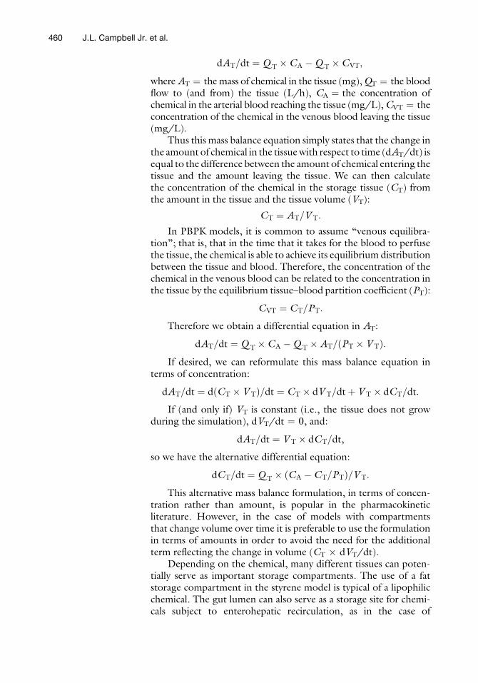
dAT=dt ¼ Q T � CA �Q T � CVT;

whereAT ¼ themass of chemical in the tissue (mg),QT ¼ the bloodflow to (and from) the tissue (L/h), CA ¼ the concentration ofchemical in the arterial blood reaching the tissue (mg/L),CVT ¼ theconcentration of the chemical in the venous blood leaving the tissue(mg/L).

Thus this mass balance equation simply states that the change inthe amount of chemical in the tissuewith respect to time (dAT/dt) isequal to the difference between the amount of chemical entering thetissue and the amount leaving the tissue. We can then calculatethe concentration of the chemical in the storage tissue (CT) fromthe amount in the tissue and the tissue volume (VT):

CT ¼ AT=V T:

In PBPK models, it is common to assume “venous equilibra-tion”; that is, that in the time that it takes for the blood to perfusethe tissue, the chemical is able to achieve its equilibrium distributionbetween the tissue and blood. Therefore, the concentration of thechemical in the venous blood can be related to the concentration inthe tissue by the equilibrium tissue–blood partition coefficient (PT):

CVT ¼ CT=PT:

Therefore we obtain a differential equation in AT:

dAT=dt ¼ Q T � CA �Q T �AT= PT � V Tð Þ:If desired, we can reformulate this mass balance equation in

terms of concentration:

dAT=dt ¼ d CT � V Tð Þ=dt ¼ CT � dV T=dtþ V T � dCT=dt:

If (and only if) VT is constant (i.e., the tissue does not growduring the simulation), dVT/dt ¼ 0, and:

dAT=dt ¼ V T � dCT=dt,

so we have the alternative differential equation:

dCT=dt ¼ Q T � CA � CT=PTð Þ=V T:

This alternative mass balance formulation, in terms of concen-tration rather than amount, is popular in the pharmacokineticliterature. However, in the case of models with compartmentsthat change volume over time it is preferable to use the formulationin terms of amounts in order to avoid the need for the additionalterm reflecting the change in volume (CT � dVT/dt).

Depending on the chemical, many different tissues can poten-tially serve as important storage compartments. The use of a fatstorage compartment in the styrene model is typical of a lipophilicchemical. The gut lumen can also serve as a storage site for chemi-cals subject to enterohepatic recirculation, as in the case of


methotrexate. Important storage sites for metals, on the otherhand, can include the kidney, red blood cells, intestinal epithelialcells, skin, bone, and hair. Transport to and from a storage com-partment does not always occur via the blood, as described above;for example, in some cases the storage is an intermediate step in anexcretion process (e.g., hair, intestinal epithelial cells). As withmethotrexate, it may also be necessary to use multiple compart-ments in series, or other mathematical devices, to model plug flow(i.e., a time delay between entry and exit from storage).

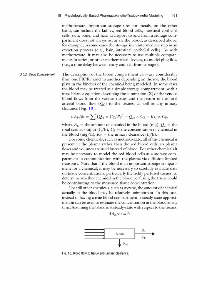
3.5.2. Blood Compartment The description of the blood compartment can vary considerablyfrom one PBPK model to another depending on the role the bloodplays in the kinetics of the chemical being modeled. In some casesthe blood may be treated as a simple storage compartment, with amass balance equation describing the summation (S) of the venousblood flows from the various tissues and the return of the totalarterial blood flow (QC) to the tissues, as well as any urinaryclearance (Fig. 10):

dAB=dt ¼X

Q T � CT=PT

� ��Q C � CB �KU � CB;

where AB ¼ the amount of chemical in the blood (mg), QC ¼ thetotal cardiac output (L/h), CB ¼ the concentration of chemical inthe blood (mg/L), KU ¼ the urinary clearance (L/h).

For some chemicals, such as methotrexate, all of the chemical ispresent in the plasma rather than the red blood cells, so plasmaflows and volumes are used instead of blood. For other chemicals itmay be necessary to model the red blood cells as a storage com-partment in communication with the plasma via diffusion-limitedtransport. Note that if the blood is an important storage compart-ment for a chemical, it may be necessary to carefully evaluate dataon tissue concentrations, particularly the richly perfused tissues, todetermine whether chemical in the blood perfusing the tissue couldbe contributing to the measured tissue concentration.

For still other chemicals, such as styrene, the amount of chemicalactually in the blood may be relatively unimportant. In this case,instead of having a true blood compartment, a steady-state approxi-mation can be used to estimate the concentration in the blood at anytime. Assuming the blood is at steady-state with respect to the tissues:

dAB=dt ¼ 0:

BloodQC

CB

KU

Fig. 10. Blood flow to tissue and urinary clearance.


Therefore, solving the blood equation for the concentration:

CB ¼X Q T � CT=PT

� �

Q C

:

3.5.3. Metabolism/

Elimination

The liver is frequently the primary site of metabolism for a chemi-cal. The following equation is an example of the mass balanceequation for the liver in the case of a chemical which is metabolizedby two pathways (Fig. 11):

dAL=dt ¼ Q L � CA � CL=PLð Þ � kF � CL � V L=PL � Vmax

� CL=PL= Km þ CL=PLð Þ:In this case, the first term on the right-hand side of the equa-

tion represents the mass flux associated with transport in the bloodand is identical to the case of the storage compartment describedpreviously. The second term describes metabolism by a linear (first-order) pathway with rate constant kF (h�1) and the third termrepresents metabolism by a saturable (Michaelis–Menten) pathwaywith capacity Vmax (mg/h) and affinity Km (mg/L). If it weredesired to model a water soluble metabolite produced by thesaturable pathway, an equation for its formation and eliminationcould be added to the model (Fig. 12):

dAM=dt ¼ Rstoch � Vmax � CL=PL= Km þ CL=PLð Þ � ke �AM

CM ¼ AM=V D;

where AM ¼ the amount of metabolite in the body (mg), Rstoch ¼the stoichiometric yield of the metabolite times the ratio of itsmolecular, Weight to that of the parent chemical, ke ¼ the rate

Metabolite

ke

VMax, KM

Fig. 12. Metabolite formation and elimination compartment.

LiverQL

CVL

QL

CA

kF

VMax, KM

Fig. 11. Liver compartment metabolizing a chemical by two pathways.


constant for the clearance of the metabolite from the body (h�1),CM ¼ the concentration of the metabolite in the plasma (mg/L),VD ¼ the apparent volume of distribution for the metabolite (L).

3.5.4. Metabolite

Compartments

In principle, the same considerations which drive decisions regardingthe level of complexity of the PBPK model for the parent chemicalmust also be applied for each of its metabolites, and their metabolites,and so on. As in the case of the parent chemical, the first and mostimportant consideration is the purpose of themodel. If the concern isdirect parent chemical toxicity and the chemical is detoxified bymetabolism, then there is no need for a description of metabolismbeyond its role in the clearance of the parent chemical. Themodels forstyrene and methotrexate discussed above are examples of parentchemical models. Similarly, if reactive intermediates produced duringthe metabolism of a chemical are responsible for its toxicity, as in thecase ofmethylene chloride, a very simple description of themetabolicpathwaysmightbeadequate (8).The cancer risk assessmentmodel formethylene chloride described the rate of metabolism for two path-ways: the glutathione conjugation pathway, which was consideredresponsible for the carcinogenic effects, and the competing P450oxidation pathway, which was considered protective.

On the other hand, if one or more of the metabolites areconsidered to be responsible for the toxicity of a chemical, it maybe necessary to provide a more complete description of the kineticsof the metabolites themselves. For example, in the case of teratoge-nicity from all-trans-retinoic acid, both the parent chemical andseveral of its metabolites are considered to be toxicologically active;therefore, in developing the PBPK model for this chemical it wasnecessary to include a fairly complete description of the metabolicpathways (100). Fortunately, the metabolism of xenobiotic com-pounds often produces metabolites which are relatively water solu-ble, simplifying the description needed. In many cases, such as theproduction of trichloroacetic acid from trichloroethylene (46–48),a classical one-compartment description may be adequate fordescribing the metabolite kinetics. An example of such a descriptionwas provided earlier. In other cases, however, the description of themetabolite (or metabolites) may have to be as complex as that of theparent chemical. An example of such a case is the PBPK model forparathion (88), in which the model for the active metabolite, para-oxon, is actually more complex than that of the parent chemical.

3.5.5. Target Tissues Typically, a PBPK model used in toxicology or risk assessmentapplications will include compartments for any target tissues forthe toxic action of the chemical. The target tissue description mayin some cases need to be fairly complicated, including such featuresas in situ metabolism, binding, and pharmacodynamic processes inorder to provide a realistic measure of biologically effective tissueexposure (57). For example, whereas the lung compartment in the


styrene model was represented only by a steady-state description ofalveolar vapor exchange, the PBPK model for methylene chloridethat was applied to perform a cancer risk assessment (8) included atwo-part lung description in which alveolar vapor exchange wasfollowed by a lung tissue compartment with in situ metabolism.This more complex lung compartment was required to describe thedose–response for methylene chloride induced lung cancer, whichwas assumed to result from the metabolism of methylene chloridein lung clara cells.

In other cases, describing a separate compartment for thetarget tissue may be unnecessary. For example, the styrene modeldescribed above could be used to relate acute exposures associatedwith neurological effects without the necessity of separating out abrain compartment. Instead, the concentration or AUC of styrenein the blood could be used as a metric, on the assumption that therelationship between brain concentration and blood concentrationwould be the same under all exposure conditions, routes, andspecies, namely, that the concentrations would be related by thebrain–blood partition coefficient. In fact, this is probably a reason-able assumption across different exposure conditions in a givenspecies. However, while tissue–air partition coefficients for volatilelipophilic chemicals appear to be similar in dog, monkey, and man(101), human blood–air partition coefficients appear to be roughlyhalf of those in rodents (102). Therefore, the human brain–bloodpartition would probably be about twice that in the rodent. Never-theless, if the model were to be used for extrapolation from rodentsto humans, this difference could easily be factored into the analysisas an adjustment to the blood metric, without the need to actuallyadd a brain compartment to the model.

A fundamental issue in determining the nature of the target tissuedescription required is the need to identify the toxicologically activeform of the chemical. In some cases, a chemical may produce a toxiceffect directly, either through its reactionwith tissue constituents (e.g.,ethylene oxide) or through its binding to cellular control elements(e.g., dioxin).Often, however, it is themetabolismof the chemical thatleads to its toxicity. In this case, toxicity may result primarily fromreactive intermediates produced during the process of metabolism(e.g., chlorovinyl epoxide produced from the metabolism of vinylchloride) or from the toxic effects of stable metabolites (e.g., trichlor-oacetic acid produced from the metabolism of trichloroethylene).

The specific nature of the relationship between tissue exposureand response depends on the mechanism of toxicity, or mode ofaction, involved. Some toxic effects, such as acute irritation or acuteneurological effects, may result primarily from the current concen-tration of the chemical in the tissue. Other toxic effects, such astissue necrosis and cancer, may depend on both the concentrationand duration of the exposure. For developmental effects, the chem-ical time course may also have to be convoluted with the window of


susceptibility for a particular gestational event. The selection of thedose metric, that is, the active chemical form for which tissueexposure should be determined and the nature of the measureto be used—e.g., peak concentration (Cmax) or area under theconcentration (AUC)–time profile—is the most important step ina pharmacokinetic analysis and a principal determinant of the struc-ture and level of detail that will be required in the PBPK model.

3.5.6. Uptake Routes Each of the relevant uptake routes for the chemical must bedescribed in the model. Often there are a number of possibleways to describe a particular uptake process, ranging from simpleto complex. As with all other aspects of model design, the compet-ing goals of parsimony and realism must be balanced in the selec-tion of the level of complexity to be used. The following examplesare meant to provide an idea of the variety of model code which canbe required to describe the various possible uptake processes.

Intravenous Administration AB0 ¼ Dose� BW,

whereAB0 ¼ the amount of chemical in the blood at the beginningof the simulation (t ¼ 0), Dose ¼ administered dose (mg/kg),BW ¼ animal body weight (kg).

or, in the case where a steady-state approximation has beenused to eliminate the blood compartment:

CB ¼ Q L � CVL þ � � � þQ F � CVF þ kIV� �

=QC,

where

kIV ¼ Dose � BW=t IV ; ðt<t IVÞ¼ 0 ðt>t IVÞ

tIV ¼ the duration of time over which the injection takes place (h).In the latter case, the model code must be written with a

“switch” to change the value of kIV to zero at t ¼ tIV.

Drinking Water (Fig. 13) k0 ¼ Dose� BW=24

dAL=dt ¼ Q L � CA � CL=PLð Þ � kF � CL � V L=PL þ k0;

where Dose ¼ the daily ingestion rate of chemical in drinking water(mg/kg/day) and the liver compartment as shown includes onlyfirst-order metabolism

Liver

kF

k0

QL

CVL

QL

CA

Fig. 13. Ingestion of chemical through drinking water.


Oral Gavage For a chemical which is not excreted in the feces (Fig. 14):

AST0 ¼ Dose� BW

dAST=dt ¼ �kA �AST

dAL=dt ¼ Q L � CA � CL=PLð Þ � kF � CL � V L=PL þ kA �AST;

where Dose ¼ the gavage dose (mg/kg), BW ¼ the animal bodyweight (kg), AST0 ¼ the amount of chemical in the stomach at thebeginning of the simulation, AST ¼ the amount of chemical in thestomach at any given time, kA ¼ the oral absorption rate (h�1).

For a chemical which is excreted in the feces (Fig. 15):

AST0 ¼ Dose� BW

dAST=dt ¼ �kA �AST

dAI=dt ¼ kA �Ast � kI �AI �KF �AI=V I

dAL=dt ¼ Q L � CA � CL=PLð Þ � kF � CL � V L=PL þ kI �AI;

where AI ¼ the amount of chemical in the intestinal lumen (mg),kI ¼ the rate constant for intestinal absorption (h�1), KF ¼ thefecal clearance (L/h), VI ¼ the volume of the intestinal lumen (L).

The rate of fecal excretion of the chemical is then:

dAF=dt ¼ KF �AI=V I:

Liver

kF

kA

QL

CVL

QL

CA

Stomach

Fig. 14. Chemical ingested through oral gavage and not excreted in the feces.

Intestinal Lumen

kI

kA

KF

Stomach

Liver

kF

QL

CVL

QL

CA

Fig. 15. Chemical being excreted through feces.


Note, however, that this simple formulation does not considerthe plug flow of the intestinal contents and will not reproduce thedelay which actually occurs in the appearance of the chemical in thefeces. Such a delay could be added using a delay function availablein common simulation software, or multiple compartments couldbe used to simulate plug flow, as shown in the diagram of themethotrexate model (Fig. 8).

Inhalation (Fig. 16) dAAB=dt ¼ Q C � CV � CAð Þ þQ P � C I � CXð Þ;where AAB ¼ the amount of chemical in the alveolar blood (mg),QC ¼ the total arterial blood flow (L/h), CV ¼ the concentrationof chemical in the pooled venous blood (mg/L), CA ¼ the con-centration of chemical in the alveolar (arterial) blood (mg/L), QP

¼ the alveolar (not total pulmonary) ventilation rate (L/h), CI ¼the concentration of chemical in the inhaled air (mg/L), CX ¼ theconcentration of chemical in the exhaled air (mg/L).

Assuming the alveolar blood is at steady-state with respect tothe other compartments:

dAAB=dt ¼ 0:

Also, assuming lung equilibration (i.e., that the blood in thealveolar region has reached equilibriumwith the alveolar air prior toexhalation):

CX ¼ CA=PB:

Substituting into the equation for the alveolar blood, andsolving for CA:

CA ¼ Q C � CV þQ P � C I

� �

Q C þQ P=PB

� � :

This steady-state approximation is used in the styrene modeldescribed earlier. Note that the rate of elimination of the chemicalby exhalation is just QP � CX. The alveolar ventilation rate, QP,does not include the “deadspace” volume (the portion of theinhaled air which does not reach the alveolar region), and is there-fore roughly 70% of the total respiratory rate. The concentrationCX represents the “end-alveolar” air concentration; in order to

Alveolar BloodQC

CA

QC

CV

QP CX

Alveolar Air

CI

Fig. 16. Inhalation of chemical through the lung compartment.


estimate the average exhaled concentration (CEX), the dead-spacecontribution must be included:

CEX ¼ 0:3� C I þ 0:7� CX:

Dermal (Fig. 17) dASK dt ¼ KP �ASFC � CSFC � CSK=PSKVð Þ== 1;000þQ SK

� CA � CSK=PSKBð Þ;whereASK ¼ the amount of chemical in the skin (mg),KP ¼ the skinpermeability coefficient (cm/h),ASFC ¼ the skin surface area (cm2),CSFC ¼ the concentration of chemical on the surface of the skin(mg/L), CSK ¼ the concentration of the chemical in the skin (mg/L), PSK ¼ the skin–vehicle partition coefficient (i.e., the vehicle con-taining the chemical on the surface of the skin), QSK ¼ the bloodflow to the skin region (L/h),CA ¼ the arterial concentration of thechemical (mg/L), PSKV ¼ the skin–blood partition coefficient.

Note that due to adding this compartment, the equation forthe blood in the model must also be modified to add a term for thevenous blood returning from the skin (+Q SK � CSK/PSKB), theblood flow and volume parameters for the slowly perfused tissuecompartment must be reduced by the amount of blood flow andvolume for the skin.

3.5.7. Experimental

Apparatus

In some cases, in addition to compartments describing theanimal–chemical system, it may also be necessary to includemodel compartments that describe the experimental apparatus inwhich measurements were obtained. An example of such a case ismodeling a closed-chamber gas uptake experiment. In a gas uptakeexperiment, several animals are maintained in a small, enclosedchamber while the air in the chamber is recirculated, with replen-ishment of oxygen and scrubbing of carbon dioxide. A smallamount of a volatile chemical is then allowed to vaporize into thechamber, and the concentration of the chemical in the chamber airis monitored over time. In this design, any loss of the chemical fromthe chamber air reflects uptake into the animals (103). In order tosimulate the change in the concentration in the chamber air as thechemical is taken up into the animals, an equation is required forthe chamber itself (Fig. 18):

Skin

KP, ASkC

QSk

CSkV

QSk

CA

Surface

Fig. 17. Diffusion of chemical through the skin.


dACH=dt ¼ N �Q P � CX � C Ið ÞCI ¼ ACH=V CH;

whereACH ¼ the amount of chemical in the chamber (mg),N ¼ thenumber of animals in the chamber,CX ¼ the concentration of chem-ical in the air exhaled by the animals (mg/L), QP ¼ the alveolarventilation rate for a single animal (L/h), CI ¼ the chamber airconcentration (mg/L),VCH ¼ the volume of air in the chamber (L).

3.5.8. Distribution/Transport There are a number of issues associated with the description of thetransport and distribution of the chemical that must be consideredin the process of model design. Examples of a few of the morecommon ones are included here.

Binding When there is evidence that saturable binding is an importantdeterminant of the distribution of a chemical (such as an apparentdose-dependence of the tissue partitioning), a description of bind-ing can be added to the model. For example, in the case of saturablebinding in the kidney (Fig. 19):

dAKT=dt ¼ V KdCKT=dt¼ Q K � CA � CKF=PKFð Þ � ke � CKF=PKF;

where AKT ¼ the total amount of chemical in the kidney (mg),VK ¼ the volume of the kidney (L), CKT ¼ the total concentrationof chemical in the kidney (mg/L), QK ¼ the blood flow to thekidney, CKF ¼ the concentration of free (unbound) chemical in thekidney (mg/L), PKF ¼ the kidney–blood partition coefficient forfree chemical, ke ¼ the urinary excretion rate constant (h�1).

The apparent complication in adding this equation to themodel is that the total movement of chemical is needed for themass balance, but the determinants of the kinetics are in terms of

Alveoli

N * QP

Chamber

CXCI

Fig. 18. The change in concentration in the chamber air as the chemical is absorbed.

Kidney

ke

QK

CKV

QK

CA

Fig. 19. Saturable binding in the kidney.


the free concentration. To solve for free in terms of total, we notethat:

CKT ¼ CKF þ CKB;

where CKB ¼ the concentration of bound chemical.We can describe the saturable binding with an equation similar

to that for saturable metabolism:

CKB ¼ B � CKF= KB þ CKFð Þ;where B ¼ the binding capacity (mg/L),KB ¼ the binding affinity(mg/L).

Substituting this equation in the previous one:

CKT ¼ CKF þ B � CKF

KB þ CKFð Þ :

Rewriting this equation to solve for the free concentration interms of only the total concentration would result in a quadraticequation, the solution of which could be obtained with the qua-dratic formula. However, taking advantage of the iterative algo-rithm by which these PBPK models are exercised (as will bediscussed later), it is not necessary to go to this effort. Instead, amuch simpler implicit equation can be written for the free concen-tration (i.e., an equation in which the free concentration appears onboth sides):

CKF ¼ CKT= 1þ B= KB þ CKFð Þð Þ:In an iterative algorithm, this equation can be solved at each

time step using the previous value ofCKF to obtain the new value! Anew value of CKT is then obtained from the mass balance equationfor the kidney and the process is repeated.

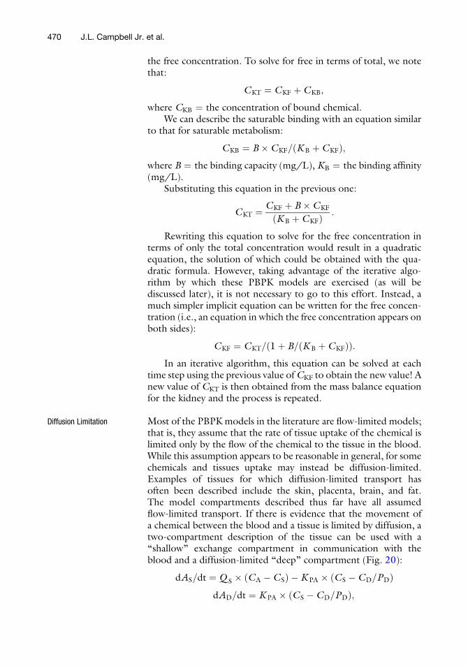
Diffusion Limitation Most of the PBPK models in the literature are flow-limited models;that is, they assume that the rate of tissue uptake of the chemical islimited only by the flow of the chemical to the tissue in the blood.While this assumption appears to be reasonable in general, for somechemicals and tissues uptake may instead be diffusion-limited.Examples of tissues for which diffusion-limited transport hasoften been described include the skin, placenta, brain, and fat.The model compartments described thus far have all assumedflow-limited transport. If there is evidence that the movement ofa chemical between the blood and a tissue is limited by diffusion, atwo-compartment description of the tissue can be used with a“shallow” exchange compartment in communication with theblood and a diffusion-limited “deep” compartment (Fig. 20):

dAS=dt ¼ Q S � CA � CSð Þ �KPA � CS � CD=PDð ÞdAD=dt ¼ KPA � CS � CD=PDð Þ;


where AS ¼ the amount of chemical in the shallow compartment(mg), QS ¼ the blood flow to the shallow compartment (L/h),CS ¼ the concentration of chemical in the shallow compartment(mg/L),KPA ¼ the permeability-area product for diffusion-limitedtransport (L/h), CD ¼ the concentration of chemical in the deepcompartment (mg/L), PD ¼ the tissue–blood partition coefficient,AD ¼ the amount of chemical in the deep compartment (mg).

3.6. Model

Parameterization

Once the model structure has been determined, it still remains toidentify the values of the input parameters in the model.

3.6.1. Physiological

Parameters

Estimates of the various physiological parameters needed in PBPKmodels are available from a number of sources in the literature,particularly for the human, monkey, dog, rat, and mouse (30–35).Estimates for the same parameter often vary widely, however, dueboth to experimental differences and to differences in the animalsexamined (age, strain, activity). Ventilation rates and blood flowrates are particularly sensitive to the level of activity (31, 33). Dataon some important tissues is relatively poor, particularly in the caseof fat tissue. Table 3 shows typical values of a number of physiolog-ical parameters in several species.

3.6.2. Biochemical

Parameters

For volatile liquids, the type of chemicals which are common envi-ronmental contaminants, tissue partition coefficients can be deter-mined by a simple in vitro technique called vial equilibration (36, 38)and tissue metabolic constants by a modification of the same tech-nique (37) or other in vitro methods (105). Alternatively, rapidin vivo approaches for determining metabolic constants can be usedeither based on steady-state (96) or gas uptake experiments(102–104, 106, 107).Determinationof the total amount of chemicalmetabolized in a particular exposure situation can also be used toestimate metabolic parameters (109). In addition, determination ofstable end-product metabolites after exposure can be a particularlyattractive technique in some cases (108, 110). Similar approaches canbe used with nonvolatile chemicals (39, 111) and metals (112).

ShallowQS

CS

QS

CA

KPA

Deep

Fig. 20. A two-compartment model describing the movement of a chemical between the“shallow” and diffusion-limited “deep” compartment.


3.6.3. Allometry The different types of physiological and biochemical parameters in aPBPK model are known to vary with body weight in different ways(23). Typically, the parameterization of PBPK models is simplifiedby assuming standard allometric scaling (33, 113), as shown inTable 4, where the scaling factors, b, can be used in the followingequation:

Y ¼ aXb ;

where Y ¼ the value of the parameter at a given body weight, X(kg), a ¼ the scaled parameter value for a 1 kg animal.

While standard allometric scaling provides a useful startingpoint, or hypothesis, for cross-species scaling, it is not sufficientlyaccurate for some applications, such as risk assessment. In the caseof the physiological parameters, the species-specific parametervalues are generally available in the literature (30–35), and can beused directly in place of the allometric estimates. This is often notthe case for the other model parameters, however. The use of theallometric scaling convention provides a useful way to estimatereasonable initial values for parameters across species. It also pro-vides a reasonable method for intraspecies scaling.

Table 3(II-1) Typical physiological parameters for PBPK models

Species Mouse Rat Monkey Human

VentilationAlveolar (L/(h - 1 kg)) 29.0 15.0 15.0 15.0

Blood flowsTotal (L/(h - 1 kg)) 16.5 15.0 15.0 15.0Muscle (Fraction) 0.18 0.18 0.18 0.18Skin (Fraction) 0.07 0.08 0.06 0.06Fat (Fraction) 0.03 0.06 0.05 0.05Liver (arterial) (Fraction) 0.035 0.03 0.065 0.07Gut (portal) (Fraction) 0.165 0.18 0.185 0.19Other organs (Fraction) 0.52 0.47 0.46 0.45

Tissue volumesBody weight (kg) 0.02 0.3 4.0 80.0Body water (Fraction) 0.65 0.65 0.65 0.65Plasma (Fraction) 0.04 0.04 0.04 0.04RBCs (Fraction) 0.03 0.03 0.03 0.03Muscle (Fraction) 0.34 0.36 0.048 0.33Skin (Fraction) 0.17 0.195 0.11 0.11Fat (Fraction) 0.10 0.07 0.05 0.21Liver (Fraction) 0.046 0.037 0.027 0.023Gut tissue (Fraction) 0.031 0.033 0.045 0.045Other organs (Fraction) 0.049 0.031 0.039 0.039


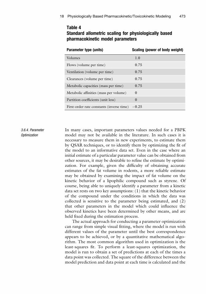
3.6.4. Parameter

Optimization

In many cases, important parameters values needed for a PBPKmodel may not be available in the literature. In such cases it isnecessary to measure them in new experiments, to estimate themby QSAR techniques, or to identify them by optimizing the fit ofthe model to an informative data set. Even in the case where aninitial estimate of a particular parameter value can be obtained fromother sources, it may be desirable to refine the estimate by optimi-zation. For example, given the difficulty of obtaining accurateestimates of the fat volume in rodents, a more reliable estimatemay be obtained by examining the impact of fat volume on thekinetic behavior of a lipophilic compound such as styrene. Ofcourse, being able to uniquely identify a parameter from a kineticdata set rests on two key assumptions: (1) that the kinetic behaviorof the compound under the conditions in which the data wascollected is sensitive to the parameter being estimated, and (2)that other parameters in the model which could influence theobserved kinetics have been determined by other means, and areheld fixed during the estimation process.

The actual approach for conducting a parameter optimizationcan range from simple visual fitting, where the model is run withdifferent values of the parameter until the best correspondenceappears to be achieved, or by a quantitative mathematical algo-rithm. The most common algorithm used in optimization is theleast-squares fit. To perform a least-squares optimization, themodel is run to obtain a set of predictions at each of the times adata point was collected. The square of the difference between themodel prediction and data point at each time is calculated and the

Table 4Standard allometric scaling for physiologically basedpharmacokinetic model parameters

Parameter type (units) Scaling (power of body weight)

Volumes 1.0

Flows (volume per time) 0.75

Ventilation (volume per time) 0.75

Clearances (volume per time) 0.75

Metabolic capacities (mass per time) 0.75

Metabolic affinities (mass per volume) 0

Partition coefficients (unit less) 0

First-order rate constants (inverse time) �0.25


results for all of the data points are summed. The parameter beingestimated is then modified, and the sum of squares is recalculated.This process is repeated until the smallest possible sum of squaresis obtained, representing the best possible fit of the model tothe data.

In a variation on this approach, the square of the difference ateach point is divided by the square of the prediction. This variation,known as relative least squares, is preferable in the case of data withan error structure which can be described by a constant coefficientof variation (that is, a constant ratio of the standard deviation to themean). The former method, known as absolute least squares, ispreferable in the case of data with a constant variance. From apractical viewpoint, the absolute least squares method tends togive greater weight to the data at higher concentrations and resultsin fits that look best when plotted on a linear scale, while the relativeleast squares method gives greater weight to the data at lowerconcentrations and results in fits that look best when plotted on alogarithmic scale.

A generalization of this weighting concept is provided by theextended least squares method, available in a number of optimiza-tion packages including ACSL/Opt (MGA Software, Concord,MA). In the extended least squares algorithm, the heteroscedasti-city parameter can be varied from 0 (for absolute weighting) to2 (for relative weighting), or can be estimated from the data. Ingeneral, setting the heteroscedasticity parameter from knowledgeof the error structure of the data is preferable to estimating it from adata set.

A common example of identifying PBPK model parameters byfitting kinetic data is the estimation of tissue partition coefficientsfrom experiments in which the concentration of chemical in theblood and tissues is reported at various time points. Using anoptimization approach, the predictions of the model for the timecourse in the blood and tissues could be optimized with respect tothe data by varying the model’s partition coefficients. There is reallylittle difference in the strength of the justification for estimating thepartition coefficients in this way as opposed to estimating themdirectly from the data (by dividing the tissue concentrations bythe simultaneous blood concentration). In fact, the direct estimateswould probably be used as initial estimates in the model when theoptimization was started.

A major difficulty in performing parameter optimization resultsfrom correlations between the parameters. When it is necessary toestimate parameters which are highly correlated, it is best to gener-ate a contour plot of the objective function (sum of squares) orconfidence region over a reasonable range of values of the twoparameters. Generation of a contour plot with ACSL/Opt is rela-tively straightforward. An example of a contour plot for two of themetabolic parameters in the PBPK model for methylene chloride is


shown in Fig. 21. The contours in the figure outline the jointconfidence region for the values of the two parameters, and thefact that the confidence region is aligned diagonally reflects thecorrelation between the two parameters.

3.7. Mass Balance

Requirements

One of the most important mathematical considerations duringmodel design is the maintenance of mass balance. Simply put, themodel should neither create nor destroy mass. This seeminglyobvious principle is often violated unintentionally during the pro-cess of model development and parameterization. A common vio-lation of mass balance, which typically leads to catastrophic results,involves failure to exactly match the arterial and venous blood flowsin the model. As described above, the movement of chemical in theblood (in units of mass per time) is described as the product of theconcentration of chemical in the blood (in units of mass per vol-ume) times the flow rate of the blood (in units of volume per time).Therefore, to maintain mass balance, the sum of the blood flowsleaving any particular tissue compartment must equal the sum ofthe blood flows entering the compartment. In particular, to main-tain mass balance in the blood compartment (regardless of whetherit is actually a compartment or just a steady-state equation), thesum of the venous flows from the individual tissue compartmentsmust equal the total arterial blood flow leaving the heart:

XQ T ¼ Q C:

Another obvious but occasionally overlooked aspect of main-taining mass balance during model development is that if a model ismodified by splitting a tissue out of a lumped compartment, the

Fig. 21. Contour plot for correlated metabolic parameters in the PBPK model for methylenechloride.


blood flow to the separated tissue (and its volume) must be sub-tracted from that for the lumped compartment. Moreover, eventhough a model may initially be designed with parameters that meetthe above requirements, mass balance may unintentionally be vio-lated later if the parameters are altered during model execution. Forexample, if the parameter for the blood flow to one compartment isincreased, the parameter for the overall blood flow must beincreased accordingly or an equivalent reduction must be made inthe parameter for the blood flow to another compartment. Partic-ular care must be taken in this regard when the model is subjectedto sensitivity or uncertainty analysis; inadvertent violation of massbalance during Monte Carlo sampling has lead in the past to thepublication of erroneous sensitivity results (95).

A similar mass balance requirement must be met for transportother than blood flow. For example, if the chemical is cleared bybiliary excretion, the elimination of chemical from the liver in thebile must exactly match the appearance of chemical in the gutlumen in the bile. Put mathematically, the same term for thetransport must appear in the equations for the two compartments,but with opposite signs (positive vs. negative). For example, if thefollowing equation were used to describe a liver compartment withfirst-order metabolism and biliary clearance.

dAL=dt ¼ Q L � CA � CL=PLð Þ � kF � CL � V L=PL �KB � CL;

where KB ¼ the biliary clearance rate (L/h).The equation for the intestinal lumen would then need to

include the term: +KB � CL.As amodel grows in complexity, it becomes increasingly difficult

to assure its mass balance by inspection. Therefore, it is a worthwhilepractice to check for mass balance by including an equation in themodel that adds up the total amount of chemical in each of themodel compartments, including metabolized and excreted chemi-cal, for comparison with the administered or inhaled dose.

3.8. Model Diagram As described in the previous sections, the process of developing aPBPK model begins by determining the essential structure of themodel based on the information available on the chemical’s toxicity,mechanism of action, and pharmacokinetic properties. The resultsof this step can usually be summarized by an initial model diagram,such as those depicted in Figs. 3 and 8. In fact, in many cases awell-constructed model diagram, together with a table of the inputparameter values and their definitions, is all that an accomplishedmodeler should need in order to create the mathematical equationsdefining a PBPK model. In general, there should be a one-to-onecorrespondence of the boxes in the diagram to the mass balanceequations (or steady-state approximations) in the model. Similarly,the arrows in the diagram correspond to the transport or


metabolism processes in the model. Each of the arrows connectingthe boxes in the diagram should correspond to one of the terms inthe mass balance equations for both of the compartments it con-nects, with the direction of the arrow pointing from the compart-ment in which the term is negative to the compartment in which itis positive. Arrows only connected to a single compartment, whichrepresent uptake and excretion processes, are interpreted similarly.The model diagram should be labeled with the names of the keyvariables associated with the compartment or process representedby each box and arrow. Interpretation of the model diagram is alsoaided by the definition of the model input parameters in thecorresponding table. The definition and units of the parameterscan indicate the nature of the process being modeled (e.g.,diffusion-limited vs. flow-limited transport, binding vs. partition-ing, saturable vs. first-order metabolism, etc.).

3.9. Elements of Model

Evaluation

One of the key advantages of PBPK models is their ability toperform extrapolations across species, routes of exposure, andexposure conditions. The reliability of a particular PBPK modelfor the purpose of extrapolation depends not only on the adequacyof its structure, but also on the correctness of its parameterization.The following section discusses some of the key issues associatedwith evaluating the adequacy of a model to predict chemical kinet-ics under conditions different from those for which experimentaldata are available.

3.9.1. Model Documentation In cases where a model previously developed by one investigator isbeing evaluated for use in a different application by another inves-tigator, adequate model documentation is critical for evaluation ofthe model. The documentation for a PBPK model should includesufficient information about the model so that an experiencedmodeler could accurately reproduce its structure and parameteri-zation. Usually the suitable documentation of a model will requirea combination of one or more “box and arrow” model diagramstogether with any equations which cannot be unequivocallyderived from the diagrams. Model diagrams should clearly differ-entiate blood flow from other transport (e.g., biliary excretion) ormetabolism, and arrows should be used where the direction oftransport could be ambiguous. All tissue compartments, metabo-lismpathways, routes of exposure, and routes of elimination shouldbe clearly and accurately presented. All equations should be dimen-sionally consistent and in standardmathematical notation. Genericequations (e.g., for tissue “i”) can help to keep the description briefbut complete. The values used for all model parameters should beprovided, with units. If any of the listed parameter values are basedon allometric scaling, a footnote should provide the body weightused to obtain the allometric constant as well as the power of bodyweight used in the scaling.


3.9.2. Model Validation Internal validation consists of the evaluation of the mathematicalcorrectness of themodel (114). It is best accomplished on the actualmodel code, but if necessary can be performed on appropriatedocumentation of the model structure and parameters, as describedabove (Assuming, of course, that the actual model code accuratelyreflects the model documentation). A more important issue regardsthe provision of evidence for external validation (sometimes referredto as verification). The level of detail incorporated into a model isnecessarily a compromise between biological accuracy and parsi-mony. The process of evaluating the sufficiency of the model for itsintended purpose, termedmodel verification, requires a demonstra-tion of the ability of the model to predict the behavior of experi-mental data different from that on which it was based.

Whereas a simulation is intended simply to reproduce thebehavior of a system, a model is intended to confirm a hypothesisconcerning the nature of the system (115). Therefore, model vali-dation should demonstrate the ability of the model to predict thebehavior of the system under conditions which test the principalaspects of the underlying hypothetical structure. While quantitativetests of goodness of fit may often be a useful aspect of the verifica-tion process, the more important consideration may be the abilityof the model to provide an accurate prediction of the generalbehavior of the data in the intended application.

Where only some aspects of the model can be verified, it isparticularly important to assess the uncertainty associated with theaspects which are untested. For example, a model of a chemicaland its metabolites which is intended for use in cross-speciesextrapolation to humans would preferably be verified using datain different species, including humans, for both the parent chemi-cal and the metabolites. If only parent chemical data is available inthe human, the correspondence of metabolite predictions withdata in several animal species could be used as a surrogate, but thisdeficiency should be carefully considered when applying themodel to predict human metabolism. One of the values of biolog-ically based modeling is the identification of specific data whichwould improve the quantitative prediction of toxicity in humansfrom animal experiments.

In some cases it is necessary to use all of the available data tosupport model development and parameterization. Unfortunately,this type of modeling can easily become a form of self-fulfillingprophecy: models are logically strongest when they fail, butpsychologically most appealing when they succeed (116). Underthese conditions, model verification can particularly difficult, puttingan additional burden on the investigators to substantiate the trustwor-thiness of the model for its intended purpose. Nevertheless, a com-bined model development and verification can often be successfullyperformed, particularly formodels intended for interpolation, integra-tion, and comparison of data rather than for true extrapolation.


3.9.3. Parameter Verification In addition to verifying the performance of the model againstexperimental data, the model should be evaluated in terms of theplausibility of its parameters. This is particularly important in thecase of PBPK models, where the parameters generally possessbiological significance, and can therefore be evaluated for plausibil-ity independent of the context of the model. The source of eachmodel input parameter value should be identified, whether it wasobtained from prior literature, determined directly by experiment,or estimated by fitting a model output to experimental data. Param-eter estimates derived independently of tissue time course or dose-response data are preferred. To the extent feasible, the degree ofuncertainty regarding the parameter values should also be evalu-ated. The empirically derived “Law of Reciprocal Certainty” statesthat the more important the model parameter, the less certain willbe its value. In accordance with this principle, the most difficult,and typically most important, parameter determination for PBPKmodels is the characterization of the metabolism parameters.

When parameter estimation has been performed by optimizingmodel output to experimental data, the investigator must assurethat the parameter is adequately identifiable from the data (114).Due to the confounding effects of model error, overparameteriza-tion, and parameter correlation, it is quite possible for an optimiza-tion algorithm to obtain a better fit to a particular data set bymodifying a parameter which in fact should not be identified onthe basis of that data set. Also, when an automatic optimizationroutine is employed it should be restarted with a variety of initialparameter values to assure that the routine has not stopped at alocal optimum. These precautions are particularly important whenmore than one parameter is being estimated simultaneously, sincethe parameters in biologically based models are often highly corre-lated, making independent estimation difficult. Estimates of param-eter variance obtained from automatic optimization routinesshould be viewed as lower bound estimates of true parameteruncertainty since only a local, linearized variance is typically calcu-lated. In characterizing parameter uncertainty, it is probably moreinstructive to determine what ranges of parameter values are clearlyinconsistent with the data than to accept a local, linearized varianceestimate provided by the optimization algorithm.

It is usually necessary for the investigator to repeatedly vary themodel parameters manually to obtain a sense of their identifiabilityand correlation under various experimental conditions, althoughsome simulation languages include routines for calculating param-eter sensitivity and covariance or for plotting confidence regioncontours. Sensitivity analysis and Monte Carlo uncertainty analysistechniques can serve as useful methods to estimate the impact ofinput parameter uncertainty on the uncertainty of model outputs(95, 117). However, care should be taken to avoid violation of mass


balance when parameters are varied by sensitivity or Monte Carloalgorithms (95, 114), particularly where blood flows are affected.

3.9.4. Sensitivity Analysis To the extent that a particular PBPK model correctly reflects thephysiological and biochemical processes underlying the pharmaco-kinetics of a chemical, exercising the model can provide a means foridentifying the most important physiological and biochemical para-meters determining the pharmacokinetic behavior of the chemicalunder different conditions (95). The technique for obtaining thisinformation is known as sensitivity analysis and can be performed bytwo different methods. Analytical sensitivity coefficients are definedas the ratio of the change in amodel output to the change in amodelparameter that produced it. To obtain a sensitivity coefficient by thismethod, the model is run for the exposure scenario of interest usingthe preferred values of the input parameters, and the resultingoutput (e.g., hair concentration) is recorded. The model is thenrun again with the value of one of the input parameters variedslightly. Typically, a 1% change is appropriate. The ratio of theresulting incremental change in the output to the change in theinput represents the sensitivity coefficient. For example, if a 1%increase in an input parameter resulted in a 0.5% decrease in theoutput, the sensitivity coefficient would be �0.5. Sensitivity coeffi-cients >1.0 in absolute value represent amplification of input errorand would be a cause for concern. An alternative approach is toconduct a Monte Carlo analysis, as described below, and then toperform a simple correlation analysis of themodel outputs and inputparameters. Both methods have specific advantages. The analyticalsensitivity coefficient most accurately represents the functional rela-tionship of the output to the specific input under the conditionsbeing modeled. The advantage of the correlation coefficients is thatthey also reflect the impact of interactions between the parametersduring the Monte Carlo analysis.

3.9.5. Uncertainty Analysis There are a number of examples in the literature of evaluations ofthe uncertainty associated with the predictions of a PBPK modelusing the Monte Carlo simulation approach (10, 117, 118). In aMonte Carlo simulation, a probability distribution for each of thePBPKmodel parameters is randomly sampled, and the model is runusing the chosen set of parameter values. This process is repeated alarge number of times until the probability distribution for thedesired model output has been created. Generally speaking, 1,000iterations or more may be required to ensure the reproducibility ofthe mean and standard deviation of the output distributions as wellas the 1st through 99th percentiles. To the extent that the inputparameter distributions adequately characterize the uncertainty inthe inputs, and assuming that the parameters are reasonably inde-pendent, the resulting output distribution will provide a usefulestimate of the uncertainty associated with the model outputs.


In performing a Monte Carlo analysis it is important to distin-guish uncertainty from variability. As it relates to the impact ofpharmacokinetics in risk assessment, uncertainty can be defined asthe possible error in estimating the “true” value of a parameter for arepresentative (“average”) person. Variability, on the other hand,should only be considered to represent true interindividual differ-ences. Understood in these terms, uncertainty is a defect (lack ofcertainty) which can typically be reduced by experimentation, andvariability is a fact of life which must be considered regardless of therisk assessment methodology used. An elegant approach for sepa-rately documenting the impact of uncertainty and variability is“two-dimensional” Monte Carlo, in which distributions for bothuncertainty and variability are developed and multiple Monte Carloruns are used to convolute the two aspects of overall uncertainty.Unfortunately, in practice it is often difficult to differentiate thecontribution of variability and uncertainty to the observed variationin the reported measurements of a particular parameter (118).

Due to its physiological structure, many of the parameters in aPBPK model are interdependent. For example, the blood flowsmust add up to the total cardiac output and the tissue volumes(including those not included in the model) must add up tothe body weight. Failure to account for the impact of MonteCarlo sampling on these mass balances can produce erroneousresults (95, 117). In addition, some physiological parameters arenaturally correlated, such as cardiac output and respiratory ventila-tion rate, and these correlations should be taken into accountduring the Monte Carlo analysis (118).

3.9.6. Collection

of Critical Data

As with model development, the best approach to model evaluationis within the context of the scientific method. The most effectiveway to evaluate a PBPKmodel is to exercise the model to generate aquantitative hypothesis; that is, to predict the behavior of thesystem of interest under conditions “outside the envelope” of thedata used to develop the model (at shorter/longer durations,higher/lower concentrations, different routes, different species,etc.). In particular, if there is an element of the model whichremains in question, the model can be exercised to determine theexperimental design under which the specific model element canbest be tested. For example, if there is uncertainty regardingwhether uptake into a particular tissue is flow or diffusion limited,alternative forms of the model can be used to compare predictedtissue concentration time courses under each of the limitingassumptions under various experimental conditions. The experi-mental design and sampling time which maximizes the differencebetween the predicted tissue concentrations under the two assump-tions can then serve as the basis for the actual experimental datacollection. Once the critical data has been collected, the samemodel can also be used to support a more quantitative experimental


inference. In the case of the tissue uptake question just described,not only can the a priori model predictions be compared with theobserved data to test the alternative hypotheses, but the model canalso be used a posteriori to estimate the quantitative extent of anyobserved diffusion limitation (i.e., to estimate the relevant modelparameter by fitting the data). If, on the other hand, the model isunable to reproduce the experimental data under either assump-tion, it may be necessary to reevaluate other aspects of the modelstructure. The key difference between research and analysis is theiterative nature of the former. It has wisely been said, “If we knewwhen we started what we had to do to finish, they’d call it search,not research.”

4. Example

The previous sections have focused on the process of designing thePBPK model structure needed for a particular application. At thispoint the model consists of a number of mathematical equations:differential equations describing the mass balance for each of thecompartments and algebraic equations describing other relation-ships betweenmodel variables. The next step inmodel developmentis the coding of the mathematical form of the model into a formwhich can be executed on a computer. The discussion in this sectionwill be couched in terms of a particular software package, acslX.

4.1. Mathematical

Formulation

Mathematically, a PBPK model is represented by a system of simul-taneous linear differential equations. The model compartments arerepresented by the differential equations that describe the massbalance for each one of the “state variables” in the model. Theremay also be additional differential equations to calculate othernecessary model outputs, such as the area under the AUC in aparticular compartment, which is simply the integral of the concen-tration over time. The resulting system of equations is referred to assimultaneous because the time courses of the chemical in the vari-ous compartments are so interdependent that solving the equationsfor any one of the compartments requires information on thecurrent status of all the other compartments; that is, the equationsfor all of the compartments must be solved at the same time. Theequations are considered to be linear in the sense that they includeonly first-order derivatives, not due to any pharmacokinetic con-siderations. This kind of mathematical problem, in which a systemis defined by the conditions at time zero together with differentialequations describing how it evolves over time, is known as an initialvalue problem, and matrix decomposition methods are used toobtain the simultaneous solution.


A number of numerical algorithms are available for solving suchproblems. They all have in common that they are step-wise approx-imations; that is, they begin with the conditions at time zero anduse the differential equations to predict how the system will changeover a small time step, resulting in an estimate of the conditions at aslightly later time, which serves as the starting point for the nexttime step. This iterative process is repeated as long as necessary tosimulate the experimental scenario.

The more sophisticated methods, such as the Gear algorithm(named after the mathematician, David Gear, who developed it)use a predictor–corrector approach, in which the corrector stepessentially amounts to “predicting backwards” after each step for-ward, in order to check how closely the algorithm is able to repro-duce the conditions at the previous time step. This allows the timestep to be increased automatically when the algorithm isperforming well, and to be shortened when it is having difficulty,such as when conditions are changing rapidly. However, due to thewide variation of the time constants (response times) for the variousphysiological compartments (e.g., fat vs. richly perfused), PBPKmodels often represent “stiff” systems. Stiff systems are character-ized by state variables (compartments) with widely different timeconstants, which cause difficulty for predictor–corrector algo-rithms. The Gear algorithm was specifically designed to overcomethis difficulty. It is therefore generally recommended that the Gearalgorithm be used for executing PBPK models. An implementationof the Gear algorithm is available in most of the advanced softwarepackages.

Regardless of the specific algorithm selected, the essentialnature of the solution, as stated above, will be a step-wise approxi-mation. However, all of the algorithms made available in computersoftware are convergent; that is, they can stay arbitrarily close to thetrue solution, given a small enough time step. On modern personalcomputers, even large PBPK models can be run to more thanadequate accuracy in a reasonable timeframe.

4.2. Model Coding

in ACSL

The following sections contain typical elements of the ACSL codefor a PBPK model, interspersed with comments, which will bewritten in italics to differentiate them from the actual modelcode. The first section describes the model definition file, whichby convention in ACSL is given a filename with the extension CSL.

The model used as an example in the following sections is asimple, multiroute model for volatile chemicals, similar to thestyrene model discussed earlier, except that is also has the abilityto simulate closed-chamber gas uptake experiments.

4.3. Typical Elements

in a Model File

An acslX source file follows the structure defined in the Standard forContinuous Simulation Languages (just like there is a standard forC++). Thus, for example, there will generally be an INITIAL block


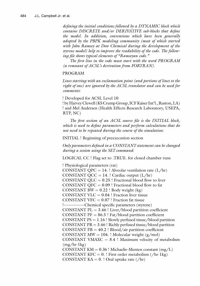
defining the initial conditions followed by a DYNAMIC block whichcontains DISCRETE and/or DERIVATIVE sub-blocks that definethe model. In addition, conventions which have been generallyadopted by the PBPK modeling community (most of which startedwith John Ramsey at Dow Chemical during the development of thestyrene model) help to improve the readability of the code. The follow-ing file shows typical elements of “Ramseyan code.”

The first line in the code must start with the word PROGRAM(a remnant of ACSL’s derivation from FORTRAN).

PROGRAM

Lines starting with an exclamation point (and portions of lines to theright of one) are ignored by the ACSL translator and can be used forcomments:

! Developed for ACSL Level 10! byHarveyClewell (KSCrumpGroup, ICFKaiser Int’l.,Ruston,LA)! and Mel Andersen (Health Effects Research Laboratory, USEPA,RTP, NC)

The first section of an ACSL source file is the INITIAL block,which is used to define parameters and perform calculations that donot need to be repeated during the course of the simulation:

INITIAL ! Beginning of preexecution section

Only parameters defined in a CONSTANT statement can be changedduring a session using the SET command:

LOGICAL CC ! Flag set to .TRUE. for closed chamber runs

! Physiological parameters (rat)CONSTANT QPC ¼ 14. ! Alveolar ventilation rate (L/hr)CONSTANT QCC ¼ 14. ! Cardiac output (L/hr)CONSTANT QLC ¼ 0.25 ! Fractional blood flow to liverCONSTANT QFC ¼ 0.09 ! Fractional blood flow to fatCONSTANT BW ¼ 0.22 ! Body weight (kg)CONSTANT VLC ¼ 0.04 ! Fraction liver tissueCONSTANT VFC ¼ 0.07 ! Fraction fat tissue!—————Chemical specific parameters (styrene)CONSTANT PL ¼ 3.46 ! Liver/blood partition coefficientCONSTANT PF ¼ 86.5 ! Fat/blood partition coefficientCONSTANT PS ¼ 1.16 ! Slowly perfused tissue/blood partitionCONSTANT PR¼ 3.46 ! Richly perfused tissue/blood partitionCONSTANT PB ¼ 40.2 ! Blood/air partition coefficientCONSTANT MW ¼ 104. ! Molecular weight (g/mol)CONSTANT VMAXC ¼ 8.4 ! Maximum velocity of metabolism(mg/hr-1kg)CONSTANT KM¼ 0.36 ! Michaelis–Menten constant (mg/L)CONSTANT KFC ¼ 0. ! First order metabolism (/hr-1kg)CONSTANT KA ¼ 0. ! Oral uptake rate (/hr)


!—————Experimental parametersCONSTANT PDOSE ¼ 0. ! Oral dose (mg/kg)CONSTANT IVDOSE ¼ 0. ! IV dose (mg/kg)CONSTANT CONC ¼ 1000. ! Inhaled concentration (ppm)CONSTANT CC ¼ .FALSE.! Default to open chamberCONSTANTNRATS¼ 3. ! Number of rats (for closed chamber)CONSTANTKLC¼ 0. ! First order loss from closed chamber (/hr)CONSTANT VCHC ¼ 9.1 ! Volume of closed chamber (L)CONSTANT TINF ¼ .01 ! Length of IV infusion (hr)

It is an understandable requirement in ACSL to define when tostop and how often to report. The parameter for the reporting fre-quency (“communication interval”) is assumed by the ACSL transla-tor to be called CINT unless you tell it otherwise using theCINTERVAL statement. The parameter for when to stop can becalled anything you want, as long as you use the same name in theTERMT statement (see below), but the Ramseyan convention isTSTOP:

CONSTANT TSTOP ¼ 24. ! Length of experiment (hr)

The following parameter name is generally used to define the length ofinhalation exposures (the name LENGTH is also used by some):

CONSTANT TCHNG ¼ 6. ! Length of inhalation exposure (hr)

The INITIAL block is a useful place to perform logical switching fordifferent model applications, in this case between the simulation ofclosed-chamber gas uptake experiments and normal inhalation stud-ies. It is also sometimes necessary to calculate initial conditions for oneof the integrals (“state variables”) in the model (the initial amount inthe closed chamber in this case):

IF (CC) RATS ¼ NRATS ! Closed chamber simulationIF (CC) KL ¼ KLC

IF (.NOT.CC) RATS ¼ 0. ! Open chamber simulationIF (.NOT.CC) KL ¼ 0.! (Turn off chamber losses so concentration in chamber remainsconstant)

IF (PDOSE.EQ.0.0) KA ¼ 0. ! If not oral dosing, turn off oraluptake

VCH ¼ VCHC-RATS*BW ! Net chamber air volume (L)AI0 ¼ CONC*VCH*MW/24450. ! Initial amount in cham-ber (mg)

After all the constants have been defined, calculations using themcan be performed. In contrast to the DERIVATIVE block (of whichmore later), the calculations in the INITIAL block are performed in


the order written, just like in FORTRAN, so a variable must bedefined before it can be used.

Note how allometric scaling is used for flows (QC, QP) andmetabolism (VMAX, KFC). Also note how the mass balance for theblood flows and tissue volumes is maintained by the model code. Run-time changes in the parameters for fat and liver are automaticallybalanced by changes in the slowly and richly perfused compartments,respectively. The fractional blood flows add to one, but the fractionaltissue volumes add up to only 0.91, allowing 9% of the body weight toreflect nonperfused tissues:

!————Scaled parameters

QC ¼ QCC*BW**0.74 ! Cardiac outputQP ¼ QPC*BW**0.74 ! Alveolar ventilationQL ¼ QLC*QC ! Liver blood flowQF ¼ QFC*QC ! Fat blood flowQS ¼ 0.24*QC-QF ! Slowly perfused tissue blood flowQR ¼ 0.76*QC-QL ! Richly perfused tissue blood flowVL ¼ VLC*BW ! Liver volumeVF ¼ VFC*BW ! Fat tissue volumeVS ¼ 0.82*BW-VF ! Slowly perfused tissue volumeVR ¼ 0.09*BW-VL ! Richly perfused tissue volumeVMAX ¼ VMAXC*BW**0.7 ! Maximum rate of metabolismKF ¼ KFC/BW**0.3 ! First-order metabolic rate constantDOSE ¼ PDOSE*BW ! Oral doseIVR ¼ IVDOSE*BW/TINF ! Intravenous infusion rate

An END statement is required to delineate the end of the initialblock:

END ! End of initial se-ction

The next (and often last) section of an ACSL source file is theDYNAMIC block, which contains all of the code defining what is tohappen during the course of the simulation:

DYNAMIC ! Beginning of execution section

ACSL possesses a number of different algorithms for performingthe simulation, which mathematically speaking consists of solving aninitial value problem for a system of simultaneous linear differentialequations. (Although it is easier to just refer to it as integrating.)Available methods include the Euler, Runga-Kutta, and Adams-Moulton, but the tried and true choice of most PBPK modelers is theGear predictor–corrector, variable step-size algorithm for stiff systems,which PBPK models often are. (Stiff, that is):

ALGORITHM IALG¼ 2 ! Use Gear integration algorithm

NSTEPS NSTP ¼ 10 ! Number of integration steps incommunication interval


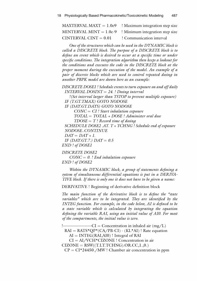
MAXTERVAL MAXT ¼ 1.0e9 ! Maximum integration step size

MINTERVAL MINT ¼ 1.0e-9 ! Minimum integration step size

CINTERVAL CINT ¼ 0.01 ! Communication interval

One of the structures which can be used in the DYNAMIC block iscalled a DISCRETE block. The purpose of a DISCRETE block is todefine an event which is desired to occur at a specific time or underspecific conditions. The integration algorithm then keeps a lookout forthe conditions and executes the code in the DISCRETE block at theproper moment during the execution of the model. An example of apair of discrete blocks which are used to control repeated dosing inanother PBPK model are shown here as an example:

DISCRETEDOSE1 ! Schedule events to turn exposure on and off dailyINTERVAL DOSINT ¼ 24. ! Dosing interval

!(Set interval larger than TSTOP to prevent multiple exposure)IF (T.GT.TMAX) GOTO NODOSEIF (DAY.GT.DAYS) GOTO NODOSE

CONC ¼ CI ! Start inhalation exposureTOTAL ¼ TOTAL + DOSE ! Administer oral doseTDOSE ¼ T ! Record time of dosing

SCHEDULE DOSE2 .AT. T + TCHNG ! Schedule end of exposureNODOSE..CONTINUEDAY ¼ DAY + 1.IF (DAY.GT.7.) DAY ¼ 0.5

END ! of DOSE1

DISCRETE DOSE2CONC ¼ 0. ! End inhalation exposure

END ! of DOSE2

Within the DYNAMIC block, a group of statements defining asystem of simultaneous differential equations is put in a DERIVA-TIVE block. If there is only one it does not have to be given a name:

DERIVATIVE ! Beginning of derivative definition block

The main function of the derivative block is to define the “statevariables” which are to be integrated. They are identified by theINTEG function. For example, in the code below, AI is defined to bea state variable which is calculated by integrating the equationdefining the variable RAI, using an initial value of AI0. For mostof the compartments, the initial value is zero.

!———————CI ¼ Concentration in inhaled air (mg/L)RAI ¼ RATS*QP*(CA/PB-CI) - (KL*AI) ! Rate equation

AI ¼ INTEG(RAI,AI0) ! Integral of RAICI ¼ AI/VCH*CIZONE ! Concentration in air

CIZONE ¼ RSW((T.LT.TCHNG).OR.CC,1.,0.)CP ¼ CI*24450./MW ! Chamber air concentration in ppm


Any experienced programmer would shudder at the code shownabove, because several variables appear to be used before they have beencalculated (for example, CIZONE is used to calculate CI and CI isused to calculate RAI. However, within the derivative block, writingcode is almost too easy because the translator will automatically sortthe statements into the proper order for execution. That is, there is noneed to be sure that a variable is calculated before it is used.

The down side of the sorting is that you cannot be sure that twostatements will be calculated in the order you want just because youplace them one after the other. Also, because of the sorting (as well asthe way the predictor–corrector integration algorithm hops forwardand backward in time), IF statements will not work right. The RSWfunction above works like an IF statement, setting CIZONE to 1.whenever T (the default name for the time variable in ACSL) is LessThan TCHNG, and setting CIZONE to 0. (and thus turning off theexposure) whenever T is greater than or equal to TCHNG.

The following blocks of statements each define one of the compart-ments in the model. These statements can be compared with themathematical equations described in the previous sections of the man-ual. One of the advantages of models written in ACSL following theRamseyan convention is that they are easier to comprehend andreasonably self-documenting.

!——MR ¼ Amount remaining in stomach (mg)RMR ¼ -KA*MRMR ¼ DOSE*EXP(-KA*T)

Note that the stomach could have been defined as one of the statevariables:

MR ¼ INTEG(RMR,DOSE)

But instead the exact solution for the simple integral has been useddirectly.

Similarly, instead of defining the blood as a state variable, thesteady-state approximation is used:

!——CA ¼ Concentration in arterial blood (mg/L)CA ¼ (QC*CV + QP*CI)/(QC + (QP/PB))AUCB ¼ INTEG(CA,0.)

!——AX ¼ Amount exhaled (mg)CX ¼ CA/PB ! End-alveolar air concentration (mg/L)CXPPM ¼ (0.7*CX+0.3*CI)*24450./MW ! Average exhaledair concentration (ppm)RAX ¼ QP*CXAX ¼ INTEG(RAX,0.)

!——AS ¼ Amount in slowly perfused tissues (mg)RAS ¼ QS*(CA-CVS)AS ¼ INTEG(RAS,0.)CVS ¼ AS/(VS*PS)


CS ¼ AS/VS

!——AR ¼ Amount in rapidly perfused tissues (mg)RAR ¼ QR*(CA-CVR)AR ¼ INTEG(RAR,0.)CVR ¼ AR/(VR*PR)CR ¼ AR/VR

!——AF ¼ Amount in fat tissue (mg)RAF ¼ QF*(CA-CVF)AF ¼ INTEG(RAF,0.)CVF ¼ AF/(VF*PF)CF ¼ AF/VF

!——AL ¼ Amount in liver tissue (mg)RAL ¼ QL*(CA-CVL)-RAM + RAOAL ¼ INTEG(RAL,0.)CVL ¼ AL/(VL*PL)CL ¼ AL/VLAUCL ¼ INTEG(CL,0.)

!——AM ¼ Amount metabolized (mg)RAM ¼ (VMAX*CVL)/(KM + CVL) + KF*CVL*VLAM ¼ INTEG(RAM,0.)

!——AO ¼ Total mass input from stomach (mg)RAO ¼ KA*MRAO ¼ DOSE-MR

!——IV ¼ Intravenous infusion rate (mg/h)IVZONE ¼ RSW(T.GE.TINF,0.,1.)IV ¼ IVR*IVZONE

!——CV ¼ Mixed venous blood concentration (mg/L)CV ¼ (QF*CVF + QL*CVL + QS*CVS + QR*CVR + IV)/QC

!——TMASS ¼ mass balance (mg)TMASS ¼ AF + AL + AS + AR + AM + AX + MR

!——DOSEX ¼ Net amount absorbed (mg)DOSEX ¼ AI + AO + IVR*TINF-AX

Last, but definitely not least, you have to tell ACSL when to stop:

TERMT(T.GE.TSTOP) ! Condition for terminating simulation

END ! End of derivative blockEND ! End of dynamic section

Another kind of code section, the TERMINAL block, can also beused here to execute statements that should only be calculated at theend of the run.

END ! End of program


4.4. Model Evaluation The following section discusses various issues associated with theevaluation of a PBPK model. Once an initial model has beendeveloped, it must be evaluated on the basis of its conformancewith experimental data. In some cases, the model may be exercisedto predict conditions under which experimental data should becollected in order to verify or improve model performance. Com-parison of the resulting data with the model predictions may sug-gest that revision of the model will be required. Similarly, a PBPKmodel designed for one chemical or application may be adapted toanother chemical or application, requiring modification of themodel structure and parameters. It is imperative that revision ormodification of a model is conducted with the same level of rigorapplied during initial model development, and that structures arenot added to the model with no other justification than that theyimprove the agreement of the model with a particular data set.

In addition to comparing model predictions to experimentaldata, model evaluation includes assessing the plausibility of themodel input parameters, and the confidence which can be placedin extrapolations performed by the model. This aspect of modelevaluation is particularly important in the case of applications in riskassessment, where it is necessary to assess the uncertainty associatedwith risk estimates calculated with the model.

4.5. Model Revision An attempt to model the metabolism of allyl chloride (119) servesas an excellent example of the process of model refinement andvalidation. As mentioned earlier, in a gas uptake experiment severalanimals are maintained in a small, enclosed chamber while the air inthe chamber is recirculated, with replenishment of oxygen andscrubbing of carbon dioxide. A small amount of a volatile chemicalis then allowed to vaporize into the chamber, and the concentrationof the chemical in the chamber air is monitored over time. In thisdesign, any loss of the chemical from the chamber air reflects uptakeinto the animals. After a short period of time during which thechemical achieves equilibration with the animals’ tissues, any fur-ther uptake represents the replacement of chemical removed fromthe animals by metabolism. Analysis of gas uptake data with a PBPKmodel has been used successfully to determine the metabolic para-meters for a number of chemicals (103).

In an example of a successful gas uptake analysis, (108)described the closed chamber kinetics of methylene chloride usinga PBPK model which included two metabolic pathways: one satu-rable, representing oxidation by Cytochrome P450 enzymes, andone linear, representing conjugation with glutathione (Fig. 22).As can be seen in this figure, there is a marked concentrationdependence of the observed rate of loss of this chemical from thechamber. The initial decrease in chamber concentration in all of theexperiments results from the uptake of chemical into the animal


tissues. Subsequent uptake is a function of the metabolic clearancein the animals, and the complex behavior reflects the transitionfrom partially saturated metabolism at higher concentrations tolinearity in the low concentration regime. The PBPK model isable to reproduce this complex behavior with a single set of para-meters because the model structure appropriately captures theconcentration dependence of the rate of metabolism.

A similar analysis of gas uptake experiments with allyl chlorideusing the same model structure was less successful. The smoothcurves shown in Fig. 23 are the best fit that could be obtained tothe observed allyl chloride chamber concentration data assuming asaturable pathway and a first-order pathway with parameters thatwere independent of concentration. Using this model structurethere were large systematic errors associated with the predictedcurves. The model predictions for the highest initial concentrationwere uniformly lower than the data, while the predictions for theintermediate initial concentrations were uniformly higher than thedata. A much better fit could be obtained by setting the first-orderrate constant to a lower value at the higher concentration; thisapproach would provide a better correspondence between thedata and the model predictions, but would not provide a basis forextrapolating to different exposure conditions.

The nature of the discrepancy between the PBPK model andthe data for allyl chloride suggested the presence of a dose-dependent limitation on metabolism not included in the modelstructure. This indication was consistent with other experimentalevidence indicating that the conjugative metabolism of allyl chlo-ride depletes glutathione, a necessary cofactor for the linear

Fig. 22. Gas uptake experiment. Concentration (ppm) of methylene chloride in a closed,recirculated chamber containing three Fischer 344 rats. Initial chamber concentrationswere (top to bottom) 3,000, 1,000, 500, and 100 ppm. Solid lines show the predictions ofthe model for a Vmax of 4.0 mg/h/kg, a Km of 0.3 mg/L, and a first-order rate constant of2.0/h/kg, while symbols represent the measured chamber atmosphere concentrations.


conjugation pathway. The conjugation pathway for reaction ofmethylene chloride and glutathione regenerates glutathione, butin the case of allyl chloride glutathione is consumed by the conju-gation reaction. Therefore, to adequately reflect the biological basisof the kinetic behavior, it was necessary to model the time depen-dence of hepatic glutathione. To accomplish this, the mathematicalmodel of the closed chamber experiment was expanded to include amore complete description of the glutathione-dependent pathway.The expanded model structure used for this description (120)included a zero-order production of glutathione and a first-orderconsumption rate that was increased by reaction of the glutathionewith allyl chloride; glutathione resynthesis was inversely related tothe instantaneous glutathione concentration. This descriptionprovided a much improved correspondence between the data andpredicted behavior (Fig. 24). Of course, the improvement in fit wasobtained at the expense of adding several new glutathione-relatedparameters to the model. To ensure that the improved fit is not justa consequence of the additional parameters providing more free-dom to the model for fitting the uptake data, a separate test of thehypothesis underlying the added model structure (depletion ofglutathione) was necessary. Therefore the expanded model wasalso used to predict both allyl chloride and hepatic glutathioneconcentrations following constant concentration inhalation expo-sures. Model predictions for end-exposure hepatic glutathione con-centrations compared very favorably with actual data obtained inseparate experiments (Table 5).

Fig. 23. Model failure. Concentration (ppm) of allyl chloride in a closed, recirculatedchamber containing three Fischer 344 rats. Initial chamber concentrations were (top tobottom) 5,000, 2,000, 1,000, and 500 ppm. Symbols represent the measured chamberatmosphere concentrations. The curves represent the best result that could be obtainedfrom an attempt to fit all of the data with a single set of metabolic constants using thesame closed chamber model structure as in Fig. 4.1.


Fig. 24. Cofactor depletion. Symbols represent the same experimental data as in Fig. 23.The curves show the predictions of the expanded model, which not only includeddepletion of glutathione by reaction with allyl chloride, but also provided for regulationof glutathione biosynthesis on the basis of the instantaneous glutathione concentration, asdescribed in the text.

Table 5Predicted glutathione depletion caused by inhalationexposure to allyl chloride

Depletion (mM)

Concentration (ppm) Observed Predicted

0 7,080 � 120 7,088

10 7,290 � 130 6,998a

0 7,230 � 80 7,238a

100 5,660 � 90 5,939

0 7,340 � 180 7,341a

1,000 970 � 10 839

0 6,890 � 710 6,890a

2,000 464 � 60 399

Note: Glutathione depletion data were graciously supplied by John Waechter,Dow Chemical Co., Midland, MichiganaFor the purpose of this comparison, the basal glutathione consumption rate inthe model was adjusted to obtain rough agreement with the controls in eachexperiment. This basal consumption rate was then used to simulate the asso-ciated exposure


To reiterate the key points of this example:

1. A PBPK model which had successfully described experimentalresults for a number of chemicals was unable to reproducesimilar kinetic data on another chemical.

2. A hypothesis was developed that depletion of a necessarycofactor was affecting metabolism. This hypothesis wasbased on:

(a) The nature of the discrepancy between the model predic-tions and the kinetic data.

(b) Other available information about the nature of the che-mical’s biochemical interactions.

3. The code for the PBPKmodel was altered to include additionalmass balance equations describing the depletion of this cofac-tor, and its resynthesis, as well as the resulting impact onmetabolism.

4. The modification to the model was then tested in two ways:

(a) By testing the ability of the newmodel structure to simulatethe kinetic data that the original model was unable toreproduce.

(b) By testing the underlying hypothesis regarding cofactordepletion against experimental data on glutathione deple-tion from a separate experiment.

Both elements of testing themodel, kinetic validation andmech-anistic validation, are necessary to provide confidence in the model.Unfortunately, there is a temptation to accept kinetic validationalone, particularly when data for mechanistic validation are unavail-able. It shouldbe remembered, however, that the simple act of addingequations and parameters to a model will, in itself, increase theflexibility of the model to fit data. Therefore, every attempt shouldbe made to obtain additional experimental data to provide supportfor the mechanistic hypothesis underlying the model structure.

References

1. Andersen ME (1981) Saturable metabolismand its relation to toxicity. Crit Rev Toxicol9:105–150

2. Monro A (1992) What is an appropriate mea-sure of exposure when testing drugs for carci-nogenicity in rodents? Toxicol ApplPharmacol 112:171–181

3. Andersen ME, Clewell HJ, Krishnan K(1995) Tissue dosimetry, pharmacokineticmodeling, and interspecies scaling factors.Risk Anal 15:533–537

4. Teorell T (1937) Kinetics of distribution ofsubstances administered to the body. I. The

extravascular mode of administration. ArchInt Pharmacodyn 57:205–225

5. Teorell T (1937) Kinetics of distribution ofsubstances administered to the body.I. The intravascular mode of administration.Arch Int Pharmacodyn 57:226–240

6. O’Flaherty EJ (1987) Modeling: an introduc-tion. National Research Council. In: Pharma-cokinetics in risk assessment. Drinking waterand health, vol 8. National Academy Press,Washington DC, pp. 27–35

7. Clewell HJ, Andersen ME (1985) Risk assess-ment extrapolations and physiological model-ing. Toxicol Ind Health 1(4):111–131


https://www.researchgate.net/publication/21616882_What_is_an_appropriate_measure_of_exposure_when_testing_drugs_for_carcinogenicity_in_rodents?el=1_x_8&enrichId=rgreq-b8a4c963-a6b0-46ff-a4ff-f8980739a250&enrichSource=Y292ZXJQYWdlOzI4MTI5NzUwMTtBUzoyNzc2NzMwNTUxNDYwMDJAMTQ0MzIxMzgyMzc1MQ==




https://www.researchgate.net/publication/15718054_Tissue_Dosimetry_Pharmacokinetic_Modeling_and_Interspecies_Scaling_Factors?el=1_x_8&enrichId=rgreq-b8a4c963-a6b0-46ff-a4ff-f8980739a250&enrichSource=Y292ZXJQYWdlOzI4MTI5NzUwMTtBUzoyNzc2NzMwNTUxNDYwMDJAMTQ0MzIxMzgyMzc1MQ==




8. Andersen ME, Clewell HJ, Gargas ML, SmithFA, Reitz RH (1987) Physiologically basedpharmacokinetics and the risk assessment formethylene chloride. Toxicol Appl Pharmacol87:185–205

9. Gerrity TR, Henry CJ (1990) Principles ofroute-to-route extrapolation for risk assess-ment. Elsevier, New York

10. Clewell HJ, Jarnot BM (1994) Incorporationof pharmacokinetics in non-carcinogenic riskassessment: Example with chloropentafluoro-benzene. Risk Anal 14:265–276

11. Clewell HJ (1995) Incorporating biologicalinformation in quantitative risk assessment:an example with methylene chloride. Toxicol-ogy 102:83–94

12. Clewell HJ (1995) The application of physio-logically based pharmacokinetic modeling inhuman health risk assessment of hazardoussubstances. Toxicol Lett 79:207–217

13. ClewellHJ,Gentry PR,Gearhart JM,AllenBC,AndersenME(1995)Consideringpharmacoki-netic andmechanistic information in cancer riskassessments for environmental contaminants:examples with vinyl chloride and trichloroethy-lene. Chemosphere 31:2561–2578

14. Clewell HJ, Andersen ME (1996) Use ofphysiologically-based pharmacokinetic mod-eling to investigate individual versus popula-tion risk. Toxicology 111:315–329

15. Clewell HJ III, Gentry PR, Gearhart JM(1997) Investigation of the potential impactof benchmark dose and pharmacokineticmodeling in noncancer risk assessment. J Tox-icol Environ Health 52:475–515

16. Himmelstein KJ, Lutz RJ (1979) A review ofthe application of physiologically based phar-macokinetic modeling. J Pharmacokinet Bio-pharm 7:127–145

17. Gerlowski LE, Jain RK (1983) Physiologicallybased pharmacokinetic modeling: principlesand applications. J Pharm Sci 72:1103–1126

18. Fiserova-Bergerova V (1983) Modeling ofinhalation exposure to vapors: uptake distri-bution and elimination, vol 1 and 2. CRC,Boca Raton

19. Bischoff KB (1987) Physiologically basedpharmacokinetic modeling. NationalResearch Council. In: Pharmacokinetics inRisk Assessment. Drinking water and health,vol 8. National Academy Press, Washington,DC, pp. 36–61

20. Leung HW (1991) Development andutilization of physiologically based pharmaco-kinetic models for toxicological applications.J Toxicol Environ Health 32:247–267

21. Clewell HJ, Andersen ME (1986) A multipledose-route physiological pharmacokineticmodel for volatile chemicals using ACSL/PC.In: Cellier FD (ed) Languages for continuoussystem simulation. Society for ComputerSimulation, San Diego, pp 95–101

22. Ramsey JC, Andersen ME (1984) A physio-logical model for the inhalation pharmacoki-netics of inhaled styrene monomer in rats andhumans. Toxicol Appl Pharmacol73:159–175

23. Adolph EF (1949) Quantitative relations inthe physiological constitutions of mammals.Science 109:579–585

24. Dedrick RL (1973) Animal scale-up. J Phar-macokinet Biopharm 1:435–461

25. Dedrick RL, Bischoff KB (1980) Speciessimilarities in pharmacokinetics. Fed Proc39:54–59

26. McDougal JN, Jepson GW, Clewell HJ, Mac-Naughton MG, Andersen ME (1986) A phys-iological pharmacokinetic model for dermalabsorption of vapors in the rat. Toxicol ApplPharmacol 85:286–294

27. Paustenbach DJ, Clewell HJ, Gargas ML,Andersen ME (1988) A physiologically basedpharmacokinetic model for inhaled carbontetrachloride. Toxicol Appl Pharmacol96:191–211

28. Vinegar A, Seckel CS, Pollard DL, KinkeadER, Conolly RB, Andersen ME (1992) Poly-chlorotrifluoroethylene (PCTFE) oligomerpharmacokinetics in Fischer 344 rats: devel-opment of a physiologically based model.Fundam Appl Toxicol 18:504–514

29. Clewell HJ, Andersen ME (1989) Improvingtoxicology testing protocols using computersimulations. Toxicol Lett 49:139–158

30. Bischoff KB, Brown RG (1966) Drug distri-bution in mammals. ChemEng Prog Symp 62(66):33–45

31. Astrand P, Rodahl K (1970) Textbook ofwork physiology. McGraw-Hill, New York

32. International Commission on RadiologicalProtection (ICRP) (1975) Report of the taskgroup on reference man. ICRP Publication 23

33. Environmental Protection Agency (EPA)(1988) Reference physiological parameters inpharmacokinetic modeling. EPA/600/6-88/004. Office of Health and EnvironmentalAssessment, Washington, DC

34. Davies B, Morris T (1993) Physiological para-meters in laboratory animals and humans.Pharm Res 10:1093–1095

35. Brown RP, Delp MD, Lindstedt SL,Rhomberg LR, Beliles RP (1997) Physiologi-cal parameter values for physiologically based


https://www.researchgate.net/publication/223075676_A_Physiologically_Based_Pharmacokinetic_Model_for_Inhaled_Carbon_Tetrachloride?el=1_x_8&enrichId=rgreq-b8a4c963-a6b0-46ff-a4ff-f8980739a250&enrichSource=Y292ZXJQYWdlOzI4MTI5NzUwMTtBUzoyNzc2NzMwNTUxNDYwMDJAMTQ0MzIxMzgyMzc1MQ==





https://www.researchgate.net/publication/21630086_Polychlorotrifluoroethylene_PCTFE_Oligomer_Pharmacokinetics_in_Fischer_344_Rats_Development_of_a_Physiologically_Based_Model?el=1_x_8&enrichId=rgreq-b8a4c963-a6b0-46ff-a4ff-f8980739a250&enrichSource=Y292ZXJQYWdlOzI4MTI5NzUwMTtBUzoyNzc2NzMwNTUxNDYwMDJAMTQ0MzIxMzgyMzc1MQ==






https://www.researchgate.net/publication/222993214_A_physiological_pharmacokinetic_model_for_dermal_absorption_of_vapors_in_the_rat?el=1_x_8&enrichId=rgreq-b8a4c963-a6b0-46ff-a4ff-f8980739a250&enrichSource=Y292ZXJQYWdlOzI4MTI5NzUwMTtBUzoyNzc2NzMwNTUxNDYwMDJAMTQ0MzIxMzgyMzc1MQ==





https://www.researchgate.net/publication/6006010_Quantitative_Relations_in_the_Physiological_Constitutions_of_Mammals?el=1_x_8&enrichId=rgreq-b8a4c963-a6b0-46ff-a4ff-f8980739a250&enrichSource=Y292ZXJQYWdlOzI4MTI5NzUwMTtBUzoyNzc2NzMwNTUxNDYwMDJAMTQ0MzIxMzgyMzc1MQ==



https://www.researchgate.net/publication/16433122_Species_Similarites_in_Pharmacokinetics?el=1_x_8&enrichId=rgreq-b8a4c963-a6b0-46ff-a4ff-f8980739a250&enrichSource=Y292ZXJQYWdlOzI4MTI5NzUwMTtBUzoyNzc2NzMwNTUxNDYwMDJAMTQ0MzIxMzgyMzc1MQ==



https://www.researchgate.net/publication/222794028_Improving_Toxicology_Testing_Protocols_Using_Computer_Simulations?el=1_x_8&enrichId=rgreq-b8a4c963-a6b0-46ff-a4ff-f8980739a250&enrichSource=Y292ZXJQYWdlOzI4MTI5NzUwMTtBUzoyNzc2NzMwNTUxNDYwMDJAMTQ0MzIxMzgyMzc1MQ==



https://www.researchgate.net/publication/284152603_Drug_distribution_in_mammals?el=1_x_8&enrichId=rgreq-b8a4c963-a6b0-46ff-a4ff-f8980739a250&enrichSource=Y292ZXJQYWdlOzI4MTI5NzUwMTtBUzoyNzc2NzMwNTUxNDYwMDJAMTQ0MzIxMzgyMzc1MQ==



https://www.researchgate.net/publication/283996271_Textbook_of'Work_Physiology?el=1_x_8&enrichId=rgreq-b8a4c963-a6b0-46ff-a4ff-f8980739a250&enrichSource=Y292ZXJQYWdlOzI4MTI5NzUwMTtBUzoyNzc2NzMwNTUxNDYwMDJAMTQ0MzIxMzgyMzc1MQ==





pharmacokinetic models. Toxicol Ind Health13(4):407–484

36. Sato A, Nakajima T (1979) Partition coeffi-cients of some aromatic hydrocarbons andketones in water, blood and oil. Br J IndMed 36:231–234

37. Sato A, Nakajima T (1979) A vial equilibra-tion method to evaluate the drug metaboliz-ing enzyme activity for volatile hydrocarbons.Toxicol Appl Pharmacol 47:41–46

38. Gargas ML, Burgess RJ, Voisard DE, CasonGH, Andersen ME (1989) Partition coeffi-cients of low-molecular-weight volatile che-micals in various liquids and tissues. ToxicolAppl Pharmacol 98:87–99

39. Jepson GW, Hoover DK, Black RK, McCaff-erty JD, Mahle DA, Gearhart JM (1994) Apartition coefficient determination methodfor nonvolatile chemicals in biological tissues.Fundam Appl Toxicol 22:519–524

40. Clewell HJ (1993) Coupling of computermodeling with in vitro methodologies toreduce animal usage in toxicity testing.Toxicol Lett 68:101–117

41. Bischoff KB, Dedrick RL, Zaharko DS, Long-streth JA (1971) Methotrexate pharmacoki-netics. J Pharm Sci 60:1128–1133

42. Farris FF, Dedrick RL, King FG (1988) Cis-platin pharmacokinetics: application of a phys-iological model. Toxicol Lett 43:117–137

43. Edginton AN, Theil FP, Schmitt W, WillmannS (2008) Whole body physiologically-basedpharmacokinetic models: their use in clinicaldrug development. Expert Opin Drug MetabToxicol 4:1143–1152

44. Andersen ME, Clewell HJ III, Gargas ML,MacNaughton MG, Reitz RH, Nolan R,McKenna M (1991) Physiologically basedpharmacokinetic modeling with dichloro-methane, its metabolite carbon monoxide,and blood carboxyhemoglobin in rats andhumans. Toxicol Appl Pharmacol 108:14–27

45. Andersen ME, Clewell HJ, Mahle DA, Gear-hart JM (1994) Gas uptake studies of deute-rium isotope effects on dichloromethanemetabolism in female B6C3F1 mice in vivo.Toxicol Appl Pharmacol 128:158–165

46. Fisher J, Gargas M, Allen B, Andersen M(1991) Physiologically based pharmacokineticmodeling with trichloroethylene and itsmetab-olite, trichloroacetic acid, in the rat and mouse.Toxicol Appl Pharmacol 109:183–195

47. Fisher JW, Allen BC (1993) Evaluating therisk of liver cancer in humans exposed to tri-chloroethylene using physiological models.Risk Anal 13:87–95

48. Allen BC, Fisher J (1993) Pharmacokineticmodeling of trichloroethylene and trichloroa-cetic acid in humans. Risk Anal 13:71–86

49. CorleyRA,MendralaAL, Smith FA, StaatsDA,Gargas ML, Conolly RB, Andersen ME, ReitzRH (1990) Development of a physiologicallybased pharmacokinetic model for chloroform.Toxicol Appl Pharmacol 103:512–527

50. Reitz RH, Mendrala AL, Corley RA, QuastJF, Gargas ML, Andersen ME, Staats DA,Conolly RB (1990) Estimating the risk ofliver cancer associated with human exposuresto chloroform using physiologically basedpharmacokinetic modeling. Toxicol ApplPharmacol 105:443–459

51. Johanson G (1986) Physiologically basedpharmacokinetic modeling of inhaled 2-butoxyethanol in man. Toxicol Lett 34:23–31

52. Bungay PM, Dedrick RL, Matthews HB(1981) Enteric transport of chlordecone(Kepone) in the rat. J Pharmacokinet Bio-pharm 9:309–341

53. Tuey DB, Matthews HB (1980) Distributionand excretion of 2,20,4,40,5,50-hexabromobi-phenyl in rats and man: pharmacokineticmodel predictions. Toxicol Appl Pharmacol53:420–431

54. Lutz RJ, Dedrick RL, Tuey D, Sipes IG,Anderson MW, Matthews HB (1984) Com-parison of the pharmacokinetics of severalpolychlorinated biphenyls in mouse, rat,dog, and monkey by means of a physiologicalpharmacokinetic model. Drug Metab Dispos12(5):527–535

55. King FG, Dedrick RL, Collins JM, MatthewsHB, Birnbaum LS (1983) Physiologicalmodel for the pharmacokinetics of 2,3,7,8-tetrachlorodibenzofuran in several species.Toxicol Appl Pharmacol 67:390–400

56. Leung HW, Ku RH, Paustenbach DJ, Ander-sen ME (1988) A physiologically based phar-macokinetic model for 2,3,7,8-tetrachlorodibenzo-p-dioxin in C57BL/6Jand DBA/2J mice. Toxicol Lett 42:15–28

57. Andersen ME, Mills JJ, Gargas ML, KedderisL, Birnbaum LS, Norbert D, Greenlee WF(1993) Modeling receptor-mediated pro-cesses with dioxin: implications for pharmaco-kinetics and risk assessment. Risk Anal 13(1):25–36

58. O’Flaherty EJ (1991) Physiologically basedmodels for bone seeking elements. I. Rat skel-etal and bone growth. Toxicol Appl Pharma-col 111:299–312

59. O’Flaherty EJ (1991) Physiologically basedmodels for bone seeking elements. II. Kinetics


https://www.researchgate.net/publication/22641064_Partition_Coefficients_of_Some_Aromatic_Hydrocarbons_and_Ketones_in_Water_Blood_and_Oil?el=1_x_8&enrichId=rgreq-b8a4c963-a6b0-46ff-a4ff-f8980739a250&enrichSource=Y292ZXJQYWdlOzI4MTI5NzUwMTtBUzoyNzc2NzMwNTUxNDYwMDJAMTQ0MzIxMzgyMzc1MQ==




https://www.researchgate.net/publication/23100024_A_vial-equilibration_method_to_evaluate_the_drug-metabolizing_enzyme_activity_for_volatile_hydrocarbons?el=1_x_8&enrichId=rgreq-b8a4c963-a6b0-46ff-a4ff-f8980739a250&enrichSource=Y292ZXJQYWdlOzI4MTI5NzUwMTtBUzoyNzc2NzMwNTUxNDYwMDJAMTQ0MzIxMzgyMzc1MQ==




https://www.researchgate.net/publication/20227282_Partition_Coefficients_of_Low_Molecular_Weight_Volatile_Chemicals_in_Various_Liquids_and_Tissues?el=1_x_8&enrichId=rgreq-b8a4c963-a6b0-46ff-a4ff-f8980739a250&enrichSource=Y292ZXJQYWdlOzI4MTI5NzUwMTtBUzoyNzc2NzMwNTUxNDYwMDJAMTQ0MzIxMzgyMzc1MQ==





https://www.researchgate.net/publication/15679117_A_Partition_Coefficient_Determination_Method_for_Nonvolatile_Chemicals_in_Biological_Tissues?el=1_x_8&enrichId=rgreq-b8a4c963-a6b0-46ff-a4ff-f8980739a250&enrichSource=Y292ZXJQYWdlOzI4MTI5NzUwMTtBUzoyNzc2NzMwNTUxNDYwMDJAMTQ0MzIxMzgyMzc1MQ==





https://www.researchgate.net/publication/18041919_Methotrexate_pharmacokinetics_J_Pharm_Sci?el=1_x_8&enrichId=rgreq-b8a4c963-a6b0-46ff-a4ff-f8980739a250&enrichSource=Y292ZXJQYWdlOzI4MTI5NzUwMTtBUzoyNzc2NzMwNTUxNDYwMDJAMTQ0MzIxMzgyMzc1MQ==



https://www.researchgate.net/publication/20103804_Cisplatin_pharmacokinetics_Applications_of_a_physiological_model?el=1_x_8&enrichId=rgreq-b8a4c963-a6b0-46ff-a4ff-f8980739a250&enrichSource=Y292ZXJQYWdlOzI4MTI5NzUwMTtBUzoyNzc2NzMwNTUxNDYwMDJAMTQ0MzIxMzgyMzc1MQ==



https://www.researchgate.net/publication/223262159_Physiologically_based_toxicokinetic_modeling_with_dichloromethane_its_metabolite_carbon_monoxide_and_blood_carboxyhemoglobin_in_rats_and_humans?el=1_x_8&enrichId=rgreq-b8a4c963-a6b0-46ff-a4ff-f8980739a250&enrichSource=Y292ZXJQYWdlOzI4MTI5NzUwMTtBUzoyNzc2NzMwNTUxNDYwMDJAMTQ0MzIxMzgyMzc1MQ==







https://www.researchgate.net/publication/15120598_Gas_Uptake_Studies_of_Deuterium_Isotope_Effects_on_Dichloromethane_Metabolism_in_Female_B6C3F1_Mice_in_Vivo?el=1_x_8&enrichId=rgreq-b8a4c963-a6b0-46ff-a4ff-f8980739a250&enrichSource=Y292ZXJQYWdlOzI4MTI5NzUwMTtBUzoyNzc2NzMwNTUxNDYwMDJAMTQ0MzIxMzgyMzc1MQ==





https://www.researchgate.net/publication/223585344_Physiologically_Based_Pharmacokinetic_Modeling_with_Trichloroethylene_and_Its_Metabolite_Trichloroacetic_Acid_In_the_Rat_and_Mouse?el=1_x_8&enrichId=rgreq-b8a4c963-a6b0-46ff-a4ff-f8980739a250&enrichSource=Y292ZXJQYWdlOzI4MTI5NzUwMTtBUzoyNzc2NzMwNTUxNDYwMDJAMTQ0MzIxMzgyMzc1MQ==





https://www.researchgate.net/publication/14746774_Evaluating_the_Risk_of_Liver_Cancer_in_Humans_Exposed_to_Trichloroethylene_Using_Physiological_Models?el=1_x_8&enrichId=rgreq-b8a4c963-a6b0-46ff-a4ff-f8980739a250&enrichSource=Y292ZXJQYWdlOzI4MTI5NzUwMTtBUzoyNzc2NzMwNTUxNDYwMDJAMTQ0MzIxMzgyMzc1MQ==




https://www.researchgate.net/publication/14746773_Pharmacokinetic_modeling_of_trichloroethylene_and_trichloroacetic_acid_in_humans?el=1_x_8&enrichId=rgreq-b8a4c963-a6b0-46ff-a4ff-f8980739a250&enrichSource=Y292ZXJQYWdlOzI4MTI5NzUwMTtBUzoyNzc2NzMwNTUxNDYwMDJAMTQ0MzIxMzgyMzc1MQ==



https://www.researchgate.net/publication/20817511_Development_of_a_Physiologically_Based_Pharmacokinetic_Model_for_Chloroform?el=1_x_8&enrichId=rgreq-b8a4c963-a6b0-46ff-a4ff-f8980739a250&enrichSource=Y292ZXJQYWdlOzI4MTI5NzUwMTtBUzoyNzc2NzMwNTUxNDYwMDJAMTQ0MzIxMzgyMzc1MQ==





https://www.researchgate.net/publication/20917990_Estimating_the_Risk_of_Liver_Cancer_Associated_with_Human_Exposures_to_Chloroform_Using_Physiologically_Based_Pharmacokinetic_Modeling?el=1_x_8&enrichId=rgreq-b8a4c963-a6b0-46ff-a4ff-f8980739a250&enrichSource=Y292ZXJQYWdlOzI4MTI5NzUwMTtBUzoyNzc2NzMwNTUxNDYwMDJAMTQ0MzIxMzgyMzc1MQ==







https://www.researchgate.net/publication/17016163_Enteric_transport_of_chlordecone_KeponeR_in_the_rat?el=1_x_8&enrichId=rgreq-b8a4c963-a6b0-46ff-a4ff-f8980739a250&enrichSource=Y292ZXJQYWdlOzI4MTI5NzUwMTtBUzoyNzc2NzMwNTUxNDYwMDJAMTQ0MzIxMzgyMzc1MQ==




https://www.researchgate.net/publication/16948061_Distribution_and_excretion_of_22'44'55'-hexabromobiphenyl_in_rats_and_man_Pharmacokinetic_model_predictions?el=1_x_8&enrichId=rgreq-b8a4c963-a6b0-46ff-a4ff-f8980739a250&enrichSource=Y292ZXJQYWdlOzI4MTI5NzUwMTtBUzoyNzc2NzMwNTUxNDYwMDJAMTQ0MzIxMzgyMzc1MQ==





https://www.researchgate.net/publication/17036219_Comparison_of_the_pharmacokinetics_of_several_polychlorinated_biphenyls_in_mouse_rat_dog_and_monkey_by_means_of_a_physiological_pharmacokinetic_model?el=1_x_8&enrichId=rgreq-b8a4c963-a6b0-46ff-a4ff-f8980739a250&enrichSource=Y292ZXJQYWdlOzI4MTI5NzUwMTtBUzoyNzc2NzMwNTUxNDYwMDJAMTQ0MzIxMzgyMzc1MQ==







https://www.researchgate.net/publication/16789810_A_Physiological_Model_for_the_Pharmacokinetics_of_2378-Te-trachlorodibenzofuran_in_Several_Species?el=1_x_8&enrichId=rgreq-b8a4c963-a6b0-46ff-a4ff-f8980739a250&enrichSource=Y292ZXJQYWdlOzI4MTI5NzUwMTtBUzoyNzc2NzMwNTUxNDYwMDJAMTQ0MzIxMzgyMzc1MQ==





https://www.researchgate.net/publication/14815175_Modeling_receptor-mediated_processes_with_dioxin_Implications_for_pharmacokinetics_and_risk_assessment?el=1_x_8&enrichId=rgreq-b8a4c963-a6b0-46ff-a4ff-f8980739a250&enrichSource=Y292ZXJQYWdlOzI4MTI5NzUwMTtBUzoyNzc2NzMwNTUxNDYwMDJAMTQ0MzIxMzgyMzc1MQ==






https://www.researchgate.net/publication/297212710_A_PHYSIOLOGICALLY_BASED_PHARMACOKINETIC_MODEL_FOR_2378-TETRACHLORODIBENZO-PARA-DIOXIN_IN_C57BL6J_AND_DBA2J_MICE?el=1_x_8&enrichId=rgreq-b8a4c963-a6b0-46ff-a4ff-f8980739a250&enrichSource=Y292ZXJQYWdlOzI4MTI5NzUwMTtBUzoyNzc2NzMwNTUxNDYwMDJAMTQ0MzIxMzgyMzc1MQ==








https://www.researchgate.net/publication/298519534_Whole_body_physiologically-based_pharmacokinetic_models_their_use_in_clinical_drug_development?el=1_x_8&enrichId=rgreq-b8a4c963-a6b0-46ff-a4ff-f8980739a250&enrichSource=Y292ZXJQYWdlOzI4MTI5NzUwMTtBUzoyNzc2NzMwNTUxNDYwMDJAMTQ0MzIxMzgyMzc1MQ==





of lead disposition in rats. Toxicol Appl Phar-macol 111:313–331

60. O’Flaherty EJ (1991) Physiologically basedmodels for bone seeking elements. III.Human skeletal and bone growth. ToxicolAppl Pharmacol 111:332–341

61. O’Flaherty EJ (1993) Physiologically basedmodels for bone seeking elements. IV. Kinet-ics of lead disposition in humans. ToxicolAppl Pharmacol 118:16–29

62. O’Flaherty EJ (1995) Physiologically basedmodels for bone seeking elements. V. Leadabsorption and disposition in childhood.Toxicol Appl Pharmacol 131:297–308

63. Mann S, Droz PO, Vahter M (1996) A physi-ologically based pharmacokinetic model forarsenic exposure. I. Development in hamstersand rabbits. Toxicol Appl Pharmacol137:8–22

64. Mann S, Droz PO, Vahter M (1996) A physi-ologically based pharmacokinetic model forarsenic exposure. II. Validation and applica-tion in humans. Toxicol Appl Pharmacol140:471–486

65. Farris FF, Dedrick RL, Allen PV, Smith JC(1993) Physiological model for the pharma-cokinetics of methyl mercury in the growingrat. Toxicol Appl Pharmacol 119:74–90

66. McMullin TS, Hanneman WH, Cranmer BK,Tessari JD, AndersenME (2007) Oral absorp-tion and oxidative metabolism of atrazine inrats evaluated by physiological modelingapproaches. Toxicology 240:1–14

67. Lin Z, Fisher JW, Ross MK, Filipov NM(2011) A physiologically based pharmacoki-netic model for atrazine and its main metabo-lites in the adult male C57BL/6 mouse.Toxicol Appl Pharmacol 251:16–31

68. Kirman CR, Hays SM, Kedderis GL, GargasML, Strother DE (2000) Improving cancerdose-response characterization by using phys-iologically based pharmacokinetic modeling:an analysis of pooled data for acrylonitrile-induced brain tumors to assess cancer potencyin the rat. Risk Anal 20:135–151

69. Sweeney LM, Gargas ML, Strother DE, Ked-deris GL (2003) Physiologically based pharma-cokinetic model parameter estimation andsensitivity and variability analyses for acryloni-trile disposition in humans. Toxicol Sci71:27–40

70. Takano R, Murayama N, Horiuchi K,Kitajima M, Kumamoto M, Shono F, Yama-zaki H (2010) Blood concentrations of acry-lonitrile in humans after oral administrationextrapolated from in vivo rat pharmacokinet-ics, in vitro human metabolism, and physio-

logically based pharmacokinetic modeling.Regul Toxicol Pharmacol 58:252–258

71. Clewell RA, Merrill EA, Robinson PJ (2001)The use of physiologically based models tointegrate diverse data sets and reduce uncer-tainty in the prediction of perchlorate andiodide kinetics across life stages and species.Toxicol Ind Health 17:210–222

72. Clewell RA, Merrill EA, Yu KO, Mahle DA,Sterner TR, Mattie DR, Robinson PJ, FisherJW, Gearhart JM (2003) Predicting fetal per-chlorate dose and inhibition of iodide kineticsduring gestation: a physiologically-basedpharmacokinetic analysis of perchlorate andiodide kinetics in the rat. Toxicol Sci73:235–255

73. Clewell RA, Merrill EA, Yu KO, Mahle DA,Sterner TR, Fisher JW, Gearhart JM (2003)Predicting neonatal perchlorate dose andinhibition of iodide uptake in the rat duringlactation using physiologically-based pharma-cokinetic modeling. Toxicol Sci 74:416–436

74. Merrill EA, Clewell RA, Gearhart JM, Robin-son PJ, Sterner TR, Yu KO,Mattie DR, FisherJW (2003) PBPK predictions of perchloratedistribution and its effect on thyroid uptake ofradioiodide in the male rat. Toxicol Sci73:256–269

75. Merrill EA, Clewell RA, Robinson PJ, JarabekAM, Gearhart JM, Sterner TR, Fisher JW(2005) PBPK model for radioactive iodideand perchlorate kinetics and perchlorate-induced inhibition of iodide uptake inhumans. Toxicol Sci 83:25–43

76. McLanahan ED, Andersen ME, Campbell JL,Fisher JW (2009) Competitive inhibition ofthyroidal uptake of dietary iodide by perchlo-rate does not describe perturbations in ratserum total T4 and TSH. Environ HealthPerspect 117:731–738

77. Haddad S, Charest-Tardif G, Tardif R, Krish-nan K (2000) Validation of a physiologicalmodeling framework for simulating the toxi-cokinetics of chemicals in mixtures. ToxicolAppl Pharmacol 167:199–209

78. Haddad S, Beliveau M, Tardif R, Krishnan K(2001) A PBPK modeling-based approach toaccount for interactions in the health riskassessment of chemical mixtures. Toxicol Sci63:125–131

79. Dennison JE, Andersen ME, Yang RS (2003)Characterization of the pharmacokinetics ofgasoline using PBPK modeling with acomplex mixtures chemical lumpingapproach. Inhal Toxicol 15:961–986

80. Dennison JE, Andersen ME, Clewell HJ,Yang RSH (2004) Development of a


https://www.researchgate.net/publication/11835147_A_PBPK_modeling-based_approach_to_account_for_interactions_in_the_health_risk_assessment_of_chemical_mixtures?el=1_x_8&enrichId=rgreq-b8a4c963-a6b0-46ff-a4ff-f8980739a250&enrichSource=Y292ZXJQYWdlOzI4MTI5NzUwMTtBUzoyNzc2NzMwNTUxNDYwMDJAMTQ0MzIxMzgyMzc1MQ==





https://www.researchgate.net/publication/10939885_The_use_of_physiologically_based_models_to_integrate_diverse_data_sets_and_reduce_uncertainty_in_the_prediction_of_perchlorate_and_iodide_kinetics_across_life_stages_and_species?el=1_x_8&enrichId=rgreq-b8a4c963-a6b0-46ff-a4ff-f8980739a250&enrichSource=Y292ZXJQYWdlOzI4MTI5NzUwMTtBUzoyNzc2NzMwNTUxNDYwMDJAMTQ0MzIxMzgyMzc1MQ==






https://www.researchgate.net/publication/12336332_Validation_of_a_Physiological_Modeling_Framework_for_Simulating_the_Toxicokinetics_of_Chemicals_in_Mixtures?el=1_x_8&enrichId=rgreq-b8a4c963-a6b0-46ff-a4ff-f8980739a250&enrichSource=Y292ZXJQYWdlOzI4MTI5NzUwMTtBUzoyNzc2NzMwNTUxNDYwMDJAMTQ0MzIxMzgyMzc1MQ==





https://www.researchgate.net/publication/10800997_Predicting_Fetal_Perchlorate_Dose_and_Inhibition_of_Iodide_Kinetics_during_Gestation_A_Physiologically-Based_Pharmacokinetic_Analysis_of_Perchlorate_and_Iodide_Kinetics_in_the_Rat?el=1_x_8&enrichId=rgreq-b8a4c963-a6b0-46ff-a4ff-f8980739a250&enrichSource=Y292ZXJQYWdlOzI4MTI5NzUwMTtBUzoyNzc2NzMwNTUxNDYwMDJAMTQ0MzIxMzgyMzc1MQ==








https://www.researchgate.net/publication/10800996_PBPK_predictions_of_perchlorate_distribution_and_its_effect_on_thyroid_uptake_of_radioiodide_in_the_male_rat?el=1_x_8&enrichId=rgreq-b8a4c963-a6b0-46ff-a4ff-f8980739a250&enrichSource=Y292ZXJQYWdlOzI4MTI5NzUwMTtBUzoyNzc2NzMwNTUxNDYwMDJAMTQ0MzIxMzgyMzc1MQ==






https://www.researchgate.net/publication/10708636_Predicting_Neonatal_Perchlorate_Dose_and_Inhibition_of_Iodide_Uptake_in_the_Rat_during_Lactation_Using_Physiologically-Based_Pharmacokinetic_Modeling?el=1_x_8&enrichId=rgreq-b8a4c963-a6b0-46ff-a4ff-f8980739a250&enrichSource=Y292ZXJQYWdlOzI4MTI5NzUwMTtBUzoyNzc2NzMwNTUxNDYwMDJAMTQ0MzIxMzgyMzc1MQ==






https://www.researchgate.net/publication/5608631_Physiologically_based_pharmacokinetic_model_parameter_estimation_and_sensitivity_and_variability_analyses_for_acrylonitrile_disposition_in_humans?el=1_x_8&enrichId=rgreq-b8a4c963-a6b0-46ff-a4ff-f8980739a250&enrichSource=Y292ZXJQYWdlOzI4MTI5NzUwMTtBUzoyNzc2NzMwNTUxNDYwMDJAMTQ0MzIxMzgyMzc1MQ==






https://www.researchgate.net/publication/12522736_Improving_Cancer_Dose-Response_Characterization_by_Using_Physiologically_Based_Pharmacokinetic_Modeling_An_Analysis_of_Pooled_Data_for_Acrylonitrile-Induced_Brain_Tumors_to_Assess_Cancer_Potency_in_th?el=1_x_8&enrichId=rgreq-b8a4c963-a6b0-46ff-a4ff-f8980739a250&enrichSource=Y292ZXJQYWdlOzI4MTI5NzUwMTtBUzoyNzc2NzMwNTUxNDYwMDJAMTQ0MzIxMzgyMzc1MQ==







https://www.researchgate.net/publication/14729439_Physiological_Model_for_the_Pharmacokinetics_of_Methyl_Mercury_in_the_Growing_Rat?el=1_x_8&enrichId=rgreq-b8a4c963-a6b0-46ff-a4ff-f8980739a250&enrichSource=Y292ZXJQYWdlOzI4MTI5NzUwMTtBUzoyNzc2NzMwNTUxNDYwMDJAMTQ0MzIxMzgyMzc1MQ==




https://www.researchgate.net/publication/6072524_Oral_absorption_and_oxidative_metabolism_of_atrazine_in_rats_evaluated_by_physiological_modeling_approaches?el=1_x_8&enrichId=rgreq-b8a4c963-a6b0-46ff-a4ff-f8980739a250&enrichSource=Y292ZXJQYWdlOzI4MTI5NzUwMTtBUzoyNzc2NzMwNTUxNDYwMDJAMTQ0MzIxMzgyMzc1MQ==





physiologically based pharmacokinetic modelfor volatile fractions of gasoline using chemi-cal lumping analysis. Environ Sci Technol38:5674–5681

81. Campbell JL, Fisher JW (2007) A PBPKmodeling assessment of the competitive met-abolic interactions of JP-8 vapor with twoconstituents, m-xylene and ethylbenzene.Inhal Toxicol 19:265–273

82. Rowland M, Balant L, Peck C (2004) Physio-logically based pharmacokinetics in drugdevelopment and regulatory science: a work-shop report (Georgetown University,Washington, DC, May 29-30, 2002). AAPSPharmSci 6:56–67

83. Ramsey JC, Young JD (1978) Pharmacoki-netics of inhaled styrene in rats and humans.Scand J Work Environ Health 4:84–91

84. Ramsey JC, Young JD, Karbowski R, Cheno-weth MB, Mc Carty LP, Braun WH (1980)Pharmacokinetics of inhaled styrene in humanvolunteers. Toxicol Appl Pharmacol53:54–63

85. Stewart RD, Dodd HC, Baretta ED, SchafferAW (1968) Human exposure to styrenevapors. Arch Environ Health 16:656–662

86. Gearhart JM, Clewell HJ, Crump KS, ShippAM, Silvers A (1995) Pharmacokinetic doseestimates of mercury in children and dose-response curves of performance tests in alarge epidemiological study. Water Air SoilPollut 80:49–58

87. Gearhart JM, Jepson GW, Clewell HJ,Andersen ME, Conolly RB (1990) Physiolog-ically based pharmacokinetic and pharmaco-dynamic model for the inhibition ofacetylcholinesterase by diisopropylfluoropho-sphate. Toxicol Appl Pharmacol106:295–310

88. Gearhart JM, Jepson GW, Clewell HJ, Ander-sen ME, Connoly RB (1995) A physiologi-cally based pharmacokinetic model for theinhibition of acetylcholinesterase by organo-phosphate esters. Environ Health Perspect102(11):51–60

89. Fisher JW, Whittaker TA, Taylor DH, ClewellHJ, AndersenME (1989) Physiologically basedpharmacokineticmodelingof thepregnant rat: amultiroute exposure model for trichlorethyleneand its metabolite, trichloroacetic acid. ToxicolAppl Pharmacol 99:395–414

90. Fisher JW, Whittaker TA, Taylor DH, ClewellHJ, Andersen ME (1990) Physiologicallybased pharmacokinetic modeling of the lactat-ing rat and nursing pup: a multiroute expo-sure model for trichlorethylene and its

metabolite, trichloroacetic acid. Toxicol ApplPharmacol 102:497–513

91. Luecke RH, Wosilait WD, Pearce BA, YoungJF (1994) A physiologically based pharmaco-kinetic computer model for human preg-nancy. Teratology 49:90–103

92. Andersen ME, Gargas ML, Clewell HJ,Severyn KM (1987) Quantitative evaluationof the metabolic interactions between trichlo-roethylene and 1,1-dichloroethylene by gasuptake methods. Toxicol Appl Pharmacol89:149–157

93. Mumtaz MM, Sipes IG, Clewell HJ, YangRSH (1993) Risk assessment of chemical mix-tures: biological and toxicologic issues. Fun-dam Appl Toxicol 21:258–269

94. Barton HA, Creech JR, Godin CS, RandallGM, Seckel CS (1995) Chloroethylene mix-tures: pharmacokinetic modeling and in vitrometabolism of vinyl chloride, trichloroethy-lene, and trans-1,2-dichloroethylene in rat.Toxicol Appl Pharmacol 130:237–247

95. Clewell HJ, Lee T, Carpenter RL (1994) Sen-sitivity of physiologically based pharmacoki-netic models to variation in modelparameters: methylene chloride. Risk Anal14:521–531

96. AndersenME, GargasML, Ramsey JC (1984)Inhalation pharmacokinetics: evaluating sys-temic extraction, total in vivo metabolismand the time course of enzyme induction forinhaled styrene in rats based on arterial blood:inhaled air concentration ratios. Toxicol ApplPharmacol 73:176–187

97. Andersen ME, Clewell HJ, Frederick CB(1995) Applying simulation modeling to pro-blems in toxicology and risk assessment—ashort perspective. Toxicol Appl Pharmacol133:181–187

98. Vinegar A, Winsett DW, Andersen ME,Conolly RB (1990) Use of a physiologicallybased pharmacokinetic model and computersimulation for retrospective assessment ofexposure to volatile toxicants. Inhal Toxicol2:119–128

99. Vinegar A, Jepson GW (1996) Cardiac sensiti-zation thresholds of halon replacement chemi-cals predicted in humans by physiologically-based pharmacokinetic modeling. Risk Anal16:571–579

100. Clewell HJ, Andersen ME, Wills RJ, LatrianoL (1997) A physiologically based pharmaco-kinetic model for retinoic acid and its meta-bolites. J Am Acad Dermatol 36:S77–S85

101. Fiserova-Bergerova V (1975) Biological—mathematical modeling of chronic toxicity.


https://www.researchgate.net/publication/15814340_Pharmacokinetics_of_inhaled_styrene_in_human_volunteers?el=1_x_8&enrichId=rgreq-b8a4c963-a6b0-46ff-a4ff-f8980739a250&enrichSource=Y292ZXJQYWdlOzI4MTI5NzUwMTtBUzoyNzc2NzMwNTUxNDYwMDJAMTQ0MzIxMzgyMzc1MQ==





https://www.researchgate.net/publication/14386679_Cardiac_sensitization_thresholds_of_halon_replacement_chemicals_predicted_in_humans_by_physiologically-based_pharmacokinetic_modeling?el=1_x_8&enrichId=rgreq-b8a4c963-a6b0-46ff-a4ff-f8980739a250&enrichSource=Y292ZXJQYWdlOzI4MTI5NzUwMTtBUzoyNzc2NzMwNTUxNDYwMDJAMTQ0MzIxMzgyMzc1MQ==





https://www.researchgate.net/publication/15462231_Physiologically_based_pharmacokinetic_model_for_the_inhibition_of_acetylcholinesterase_by_organophosphate_esters?el=1_x_8&enrichId=rgreq-b8a4c963-a6b0-46ff-a4ff-f8980739a250&enrichSource=Y292ZXJQYWdlOzI4MTI5NzUwMTtBUzoyNzc2NzMwNTUxNDYwMDJAMTQ0MzIxMzgyMzc1MQ==






https://www.researchgate.net/publication/16484856_Inhalation_pharmacokinetics_Evaluating_systemic_extraction_total_in_vivo_metabolism_and_the_time_course_of_enzyme_induction_for_inhaled_styrene_in_rats_based_on_arterial_bloodInhaled_air_concentration?el=1_x_8&enrichId=rgreq-b8a4c963-a6b0-46ff-a4ff-f8980739a250&enrichSource=Y292ZXJQYWdlOzI4MTI5NzUwMTtBUzoyNzc2NzMwNTUxNDYwMDJAMTQ0MzIxMzgyMzc1MQ==







https://www.researchgate.net/publication/20900190_Physiologically_based_pharmacokinetic_and_pharmacodynamic_model_for_the_inhibition_of_acetylcholinesterase_by_diisopropyfluorophosphate?el=1_x_8&enrichId=rgreq-b8a4c963-a6b0-46ff-a4ff-f8980739a250&enrichSource=Y292ZXJQYWdlOzI4MTI5NzUwMTtBUzoyNzc2NzMwNTUxNDYwMDJAMTQ0MzIxMzgyMzc1MQ==










https://www.researchgate.net/publication/15226196_Sensitivity_of_Physiologically_Based_Pharmacokinetic_Models_to_Variation_in_Model_Parameters_Methylene_Chloride?el=1_x_8&enrichId=rgreq-b8a4c963-a6b0-46ff-a4ff-f8980739a250&enrichSource=Y292ZXJQYWdlOzI4MTI5NzUwMTtBUzoyNzc2NzMwNTUxNDYwMDJAMTQ0MzIxMzgyMzc1MQ==





https://www.researchgate.net/publication/17534419_Human_Exposure_to_Styrene_Vapor?el=1_x_8&enrichId=rgreq-b8a4c963-a6b0-46ff-a4ff-f8980739a250&enrichSource=Y292ZXJQYWdlOzI4MTI5NzUwMTtBUzoyNzc2NzMwNTUxNDYwMDJAMTQ0MzIxMzgyMzc1MQ==



https://www.researchgate.net/publication/15181995_A_physiologically_based_pharmacokinetic_computer_model_for_human_pregnancy?el=1_x_8&enrichId=rgreq-b8a4c963-a6b0-46ff-a4ff-f8980739a250&enrichSource=Y292ZXJQYWdlOzI4MTI5NzUwMTtBUzoyNzc2NzMwNTUxNDYwMDJAMTQ0MzIxMzgyMzc1MQ==




https://www.researchgate.net/publication/15326765_Chloroethylene_Mixtures_Pharmacokinetic_Modeling_and_in_Vitro_Metabolism_of_Vinyl_Chloride_Trichloroethylene_and_trans-12-Dichloroethylene_in_Rat?el=1_x_8&enrichId=rgreq-b8a4c963-a6b0-46ff-a4ff-f8980739a250&enrichSource=Y292ZXJQYWdlOzI4MTI5NzUwMTtBUzoyNzc2NzMwNTUxNDYwMDJAMTQ0MzIxMzgyMzc1MQ==






https://www.researchgate.net/publication/22408737_Pharmacokinetics_of_inhaled_styrene_in_rats_and_humans?el=1_x_8&enrichId=rgreq-b8a4c963-a6b0-46ff-a4ff-f8980739a250&enrichSource=Y292ZXJQYWdlOzI4MTI5NzUwMTtBUzoyNzc2NzMwNTUxNDYwMDJAMTQ0MzIxMzgyMzc1MQ==

https://www.researchgate.net/publication/22408737_Pharmacokinetics_of_inhaled_styrene_in_rats_and_humans?el=1_x_8&enrichId=rgreq-b8a4c963-a6b0-46ff-a4ff-f8980739a250&enrichSource=Y292ZXJQYWdlOzI4MTI5NzUwMTtBUzoyNzc2NzMwNTUxNDYwMDJAMTQ0MzIxMzgyMzc1MQ==

https://www.researchgate.net/publication/15554169_Applying_Simulation_Modeling_to_Problems_in_Toxicology_and_Risk_Assessment_A_Short_Perspective?el=1_x_8&enrichId=rgreq-b8a4c963-a6b0-46ff-a4ff-f8980739a250&enrichSource=Y292ZXJQYWdlOzI4MTI5NzUwMTtBUzoyNzc2NzMwNTUxNDYwMDJAMTQ0MzIxMzgyMzc1MQ==





https://www.researchgate.net/publication/223523475_Quantitative_Evaluation_of_the_Metabolic_Interactions_Between_Trichloroethylene_and_11-Dichloroethylene_in_vivo_Using_Gas_Uptake_Methods?el=1_x_8&enrichId=rgreq-b8a4c963-a6b0-46ff-a4ff-f8980739a250&enrichSource=Y292ZXJQYWdlOzI4MTI5NzUwMTtBUzoyNzc2NzMwNTUxNDYwMDJAMTQ0MzIxMzgyMzc1MQ==






https://www.researchgate.net/publication/6442334_A_PBPK_Modeling_Assessment_of_the_Competitive_Metabolic_Interactions_of_JP-8_Vapor_with_Two_Constituents_m_-Xylene_and_Ethylbenzene?el=1_x_8&enrichId=rgreq-b8a4c963-a6b0-46ff-a4ff-f8980739a250&enrichSource=Y292ZXJQYWdlOzI4MTI5NzUwMTtBUzoyNzc2NzMwNTUxNDYwMDJAMTQ0MzIxMzgyMzc1MQ==





https://www.researchgate.net/publication/14123848_A_physiologically_based_pharmacokinetic_model_for_retinoic_acid_and_its_metabolites?el=1_x_8&enrichId=rgreq-b8a4c963-a6b0-46ff-a4ff-f8980739a250&enrichSource=Y292ZXJQYWdlOzI4MTI5NzUwMTtBUzoyNzc2NzMwNTUxNDYwMDJAMTQ0MzIxMzgyMzc1MQ==




AMRL-TR-75-5. Aerospace MedicalResearch Laboratory, Wright-Patterson AirForce Base

102. GargasML,AndersenME(1989)Determiningkinetic constants of chlorinated ethanemetabo-lism in the rat from rates of exhalation. ToxicolAppl Pharmacol 97:230–246

103. Gargas ML, Andersen ME, Clewell HJ(1986) A physiologically-based simulationapproach for determining metabolic con-stants from gas uptake data. Toxicol ApplPharmacol 86:341–352

104. Gargas ML, Clewell HJ, Andersen ME(1990) Gas uptake techniques and the ratesof metabolism of chloromethanes, chlor-oethanes, and chloroethylenes in the rat.Inhal Toxicol 2:295–319

105. Reitz RH, Mendrala AL, Guengerich FP(1989) In vitro metabolism of methylenechloride in human and animal tissues: use inphysiologically-based pharmacokinetic mod-els. Toxicol Appl Pharmacol 97:230–246

106. Filser JG, Bolt HM (1979) Pharmacokineticsof halogenated ethylenes in rats. Arch Toxicol42:123–136

107. Andersen ME, Gargas ML, Jones RA, JenkinsLH Jr (1980) Determination of the kineticconstants of metabolism of inhaled toxicantin vivo based on gas uptake measurements.Toxicol Appl Pharmacol 54:100–116

108. Gargas ML, Clewell HJ, Andersen ME(1986) Metabolism of inhaled dihalo-methanes in vivo: differentiation of kineticconstants for two independent pathways.Toxicol Appl Pharmacol 82:211–223

109. Watanabe P, Mc Gown G, Gehring P (1976)Fate of [14] vinyl chloride after single oraladministration in rats. Toxicol Appl Pharma-col 36:339–352

110. Gargas ML, Andersen ME (1982) Metabo-lism of inhaled brominated hydrocarbons:validation of gas uptake results by determina-tion of a stable metabolite. Toxicol Appl Phar-macol 66:55–68

111. Lam G, ChenM, ChiouWL (1981) Determi-nation of tissue to blood partition coefficientsin physiologically-based pharmacokineticstudies. J Pharm Sci 71(4):454–456

112. O’Flaherty EJ (1995) PBPK modeling formetals. Examples with lead, uranium, andchromium. Toxicol Lett 82–83:367–372

113. Environmental Protection Agency (EPA)(1992) EPA request for comments on draftreport of cross-species scaling factor for can-cer risk assessment. Fed Reg 57:24152

114. Carson ER, Cobelli C, Finkelstein L (1983)The mathematical modeling of metabolic andendocrine systems model formulation, identi-fication, and validation. Wiley, New York

115. Rescigno A, Beck JS (1987) The use andabuse of models. J Pharmacokinet Biopharm15:327–340

116. Yates FE (1978) Good manners in goodmodeling: mathematical models and com-puter simulations of physiological systems.Am J Physiol 234:R159–R160

117. Clewell HJ (1995) The use of physiologicallybased pharmacokinetic modeling in riskassessment: a case study with methylene chlo-ride. In: Olin S, Farland W, Park C, Rhom-berg L, Scheuplein R, Starr T, Wilson J (eds)Low-dose extrapolation of cancer risks: issuesand perspectives. ILSI, Washington, DC

118. Allen BC, Covington TR, Clewell HJ (1996)Investigation of the impact of pharmacoki-netic variability and uncertainty on risks pre-dicted with a pharmacokinetic model forchloroform. Toxicology 111:289–303

119. Clewell HJ, Andersen ME (1994)Physiologically-based pharmacokinetic mod-eling and bioactivation of xenobiotics. Toxi-col Ind Health 10:1–24

120. D’Souza RW, Francis WR, Andersen ME(1988) Physiological model for tissue gluta-thione depletion and increased resynthesisafter ethylene dichloride exposure. J Pharma-col Exp Ther 245:563–568


https://www.researchgate.net/publication/20421031_Determining_kinetic_constants_of_chlorinated_ethane_metabolism_in_the_rat_from_rates_of_exhalation?el=1_x_8&enrichId=rgreq-b8a4c963-a6b0-46ff-a4ff-f8980739a250&enrichSource=Y292ZXJQYWdlOzI4MTI5NzUwMTtBUzoyNzc2NzMwNTUxNDYwMDJAMTQ0MzIxMzgyMzc1MQ==








https://www.researchgate.net/publication/222132549_A_Physiologically_Based_Simulation_Approach_for_Determining_Metabolic_Constants_from_Gas_Uptake_Data?el=1_x_8&enrichId=rgreq-b8a4c963-a6b0-46ff-a4ff-f8980739a250&enrichSource=Y292ZXJQYWdlOzI4MTI5NzUwMTtBUzoyNzc2NzMwNTUxNDYwMDJAMTQ0MzIxMzgyMzc1MQ==





https://www.researchgate.net/publication/236658673_Gas_Uptake_Inhalation_Techniques_and_the_Rates_of_Metabolism_of_Chloromethanes_Chloroethanes_and_Chloroethylenes_in_the_Rat?el=1_x_8&enrichId=rgreq-b8a4c963-a6b0-46ff-a4ff-f8980739a250&enrichSource=Y292ZXJQYWdlOzI4MTI5NzUwMTtBUzoyNzc2NzMwNTUxNDYwMDJAMTQ0MzIxMzgyMzc1MQ==





https://www.researchgate.net/publication/20233015_In_Vitro_Metabolism_of_Methylene_Chloride_in_Human_and_Animal_Tissues_Use_in_Physiologically_Based_Pharmacokinetic_Models?el=1_x_8&enrichId=rgreq-b8a4c963-a6b0-46ff-a4ff-f8980739a250&enrichSource=Y292ZXJQYWdlOzI4MTI5NzUwMTtBUzoyNzc2NzMwNTUxNDYwMDJAMTQ0MzIxMzgyMzc1MQ==





https://www.researchgate.net/publication/15803880_Determination_of_the_Kinetic_Constants_for_Metabolism_of_Inhaled_Toxicants_In_Vivo_Using_Gas_Uptake_Measurements?el=1_x_8&enrichId=rgreq-b8a4c963-a6b0-46ff-a4ff-f8980739a250&enrichSource=Y292ZXJQYWdlOzI4MTI5NzUwMTtBUzoyNzc2NzMwNTUxNDYwMDJAMTQ0MzIxMzgyMzc1MQ==





https://www.researchgate.net/publication/223546190_Metabolism_of_Inhaled_Diholomethanes_In_Vivo_Differentiation_of_Kinetic_Constants_for_Two_Independent_Pathways?el=1_x_8&enrichId=rgreq-b8a4c963-a6b0-46ff-a4ff-f8980739a250&enrichSource=Y292ZXJQYWdlOzI4MTI5NzUwMTtBUzoyNzc2NzMwNTUxNDYwMDJAMTQ0MzIxMzgyMzc1MQ==





https://www.researchgate.net/publication/21881555_Fate_of_14Cvinyl_chloride_after_single_oral_administration_in_rats?el=1_x_8&enrichId=rgreq-b8a4c963-a6b0-46ff-a4ff-f8980739a250&enrichSource=Y292ZXJQYWdlOzI4MTI5NzUwMTtBUzoyNzc2NzMwNTUxNDYwMDJAMTQ0MzIxMzgyMzc1MQ==






https://www.researchgate.net/publication/16042463_Metabolism_of_inhaled_brominated_hydrocarbons_Validation_of_gas_uptake_results_by_determination_of_a_stable_metabolite?el=1_x_8&enrichId=rgreq-b8a4c963-a6b0-46ff-a4ff-f8980739a250&enrichSource=Y292ZXJQYWdlOzI4MTI5NzUwMTtBUzoyNzc2NzMwNTUxNDYwMDJAMTQ0MzIxMzgyMzc1MQ==





https://www.researchgate.net/publication/16111709_Determination_of_tissue_to_blood_partition_coefficients_in_physiologically-based_pharmacokinetic_studies?el=1_x_8&enrichId=rgreq-b8a4c963-a6b0-46ff-a4ff-f8980739a250&enrichSource=Y292ZXJQYWdlOzI4MTI5NzUwMTtBUzoyNzc2NzMwNTUxNDYwMDJAMTQ0MzIxMzgyMzc1MQ==




https://www.researchgate.net/publication/22496240_Good_manners_in_good_modeling_Mathematical_models_and_computer_simulations_of_physiological_systems?el=1_x_8&enrichId=rgreq-b8a4c963-a6b0-46ff-a4ff-f8980739a250&enrichSource=Y292ZXJQYWdlOzI4MTI5NzUwMTtBUzoyNzc2NzMwNTUxNDYwMDJAMTQ0MzIxMzgyMzc1MQ==



https://www.researchgate.net/publication/223948202_Investigation_of_the_Impact_of_Pharmacokinetic_Variability_and_Uncertainty_on_Risks_Predicted_with_a_Pharmacokinetic_Model_for_Chloroform?el=1_x_8&enrichId=rgreq-b8a4c963-a6b0-46ff-a4ff-f8980739a250&enrichSource=Y292ZXJQYWdlOzI4MTI5NzUwMTtBUzoyNzc2NzMwNTUxNDYwMDJAMTQ0MzIxMzgyMzc1MQ==





https://www.researchgate.net/publication/15627728_Physiologically-Based_Pharmacokinetic_Modeling_and_Bioactivation_of_Xenobiotics?el=1_x_8&enrichId=rgreq-b8a4c963-a6b0-46ff-a4ff-f8980739a250&enrichSource=Y292ZXJQYWdlOzI4MTI5NzUwMTtBUzoyNzc2NzMwNTUxNDYwMDJAMTQ0MzIxMzgyMzc1MQ==




https://www.researchgate.net/publication/302041086_Pharmacokinetics_of_Halogenated_Ethylenes?el=1_x_8&enrichId=rgreq-b8a4c963-a6b0-46ff-a4ff-f8980739a250&enrichSource=Y292ZXJQYWdlOzI4MTI5NzUwMTtBUzoyNzc2NzMwNTUxNDYwMDJAMTQ0MzIxMzgyMzc1MQ==



Physiologically Based Pharmacokinetic and Toxicokinetic Models

Documents

Transcript of Physiologically Based Pharmacokinetic and Toxicokinetic Models