Spectral studies of extra-terrestrial materials - Open Research ...

Open Research OnlineThe Open University’s repository of research publicationsand other research outputs

Spectral studies of extra-terrestrial materialsThesisHow to cite:

Fernandes, Catarina (2013). Spectral studies of extra-terrestrial materials. PhD thesis The Open University.

For guidance on citations see FAQs.

c© 2012 The Author

https://creativecommons.org/licenses/by-nc-nd/4.0/

Version: Version of Record

Link(s) to article on publisher’s website:http://dx.doi.org/doi:10.21954/ou.ro.0000d5a6

Copyright and Moral Rights for the articles on this site are retained by the individual authors and/or other copyrightowners. For more information on Open Research Online’s data policy on reuse of materials please consult the policiespage.

oro.open.ac.uk

http://oro.open.ac.uk/help/helpfaq.html

https://creativecommons.org/licenses/by-nc-nd/4.0/

http://dx.doi.org/doi:10.21954/ou.ro.0000d5a6

http://oro.open.ac.uk/policies.html

31 0342793 5

""" II UNf\ES 1 (zI (1 E-D

>....., --'" ~ OJ > --c: => c: OJ C-O OJ .c: .....

Spectral Studies of Extra-Terrestrial Materials

Catarina Fernandes

Licenciatura em Geologia Applicada e do Ambiente, Universidade de Lisboa

Submitted for the degree of Doctor of Philosophy

Faculty of Science, The Open University

Submitted March 2012

Date. OJ- Subm~S5 \on~ 2G Marc.h 20lL

Dote.. oJ ~\[a (}..; Co FQbvua~ 20\3

YOUR ACCEPTANCE

1

2

Student details

Authorisation statement

Your full name: Catarina Dolores Aires Fernandes

Personal identifier (PI): X7636619

Affiliated Research Centre (ARC) (if applicable) :

Department: Department of Physical Sciences

Thesis title : Spectral Studies of Extra-Terrestrial Materials

I confirm that I am willing for my thesis to be made available to readers by The Open University Library, and that it may be photocopied , subject to the discretion of the Librarian

Signed: ... (]o..:TY.1.0..IA9-.. r.e.~~w!l.n .. ..................... .. Print name: Catarina Fernandes

Date: 07/03/13 DD/MMlYY

http://www.open .ac.uk/research/research·degreesioffer·packs.php 2

3 British Library Authorisation (PhD and EdD candidates only)

The Open University has agreed that a copy of your thesis can be made available on loan to the British Library Thesis Service on a voluntary basis. The British Library may make the thesis available online. Please indicate your preference below:

t:8J I am willing for The Open University to loan the British Library a copy of my thesis

OR

o I do not wish The Open University to loan the British Library a copy of my thesis

Abstract

Experiments were made using a state-of-the-art UV-Vis microspectrophotometer

(MSP) in order to assess if the instrument is suitable for use on spectroscopy of

terrestrial and extra-terrestrial materials. This new instrument brings advantages

that cannot be found in instruments currently in use: it requires only extremely small

samples (min of -2 J..lm) and it is very quick to use (little sample preparation and

spectra taken in less than 2 min).

If suitable, the instrument could help to show the relationship between meteorites

and their parent bodies and in the study of very small fragile samples, such as

cometary samples and Interplanetary Dust Particles (lOPs).

Using samples of minerals commonly found in meteorites, it was concluded that the

instrument is suitable for the study of these materials, however it has some

limitations and certain conditions need to be met.

The method was then applied on two grains from comet 81PIWild 2 returned by the

space mission Stardust. Further limitations were found with these samples caused

by the fact that they are covered in aerogel and embedded in gold foil. Results

indicate however, that the samples seem to be composed of a mixture of different

materials.

Results from the study of HEO (howardites, eucrites and diogenites) type meteorites

proved that if the conditions are met, the technique is suitable and comparable to

other instruments and can be used to match the spectra of meteorites to that of their

possible asteroidal parent bodies.

A complementary investigation studied the effects of impact by shock on the spectra

of rocks using a Light Gas Gun and Near Infrared spectroscopy with the goal of

investigating the effects of weathering on the spectra of asteroids. It was found that

there is a change in the spectra of the samples and a relationship with a change in

composition of the impacted area.

ii

Acknowledgements

I would like to thank my supervisors Monica Grady, Simon Green and Stephen

Wolters for all their support, advice and expertise throughout the PhD. I would also

like to thank John Bridges for his support during the months he was my supervisor.

I would also like to acknowledge all of the au staff for their help in particular Chris

Hall for his help with the Light Gas Gun; Mabs Guilmore for her help with samples

and all lab related questions, Diane Johnson for the SEM support and my fellow

students who helped with what they could (even if only by taking me for a coffee!).

At the University of Oxford, I would like to thank Dr Neil Bowles and Ian Thomas for

their support using the FTIR.

I would mostly like to thank my husband Russ and my daughter Kaia. Your support

has been immeasurable and your sacrifices made this PhD possible.

iii

Table of contents

Abstract ..................................................................................................................... ii

Acknowledgements ................................................................................................. iii Table of contents ..................................................................................................... Iv

List of figures ........................................................................................................... vi

List of tables .......................................•.......•.•....•.•...•••................•....•...•.•.••..•.•..•..•... xi

List of equations .•...............•......................••....•••.•.•...................•....••..••.•.•••..••....••.. xii

1 Small Solar System Bodies .............................................................................. 1

1.1 Introduction .................................................................................................. 1

1.2 Interstellar Dust ............................................................................................ 5

1.3 Comets ......................................................................................................... 6

1.3.1 Cometary Missions ............................................................................. 10

1.4 Meteorites and Interplanetary Dust Particles (IDP) .................................... 12

1.5 Asteroids .................................................................................................... 16

1.5.1 Classification of Asteroids ................................................................... 18

1.5.2 Difficulties in correlation between meteorites and asteroids ............... 23

1.6 Summary .................................................................................................... 25

2 Spectroscopy .................................................................................................. 28

2.1 Introduction ................................................................................................ 28

2.2 UV-Vis Spectroscopy ................................................................................. 31

2.2.1 Other factors that influence the spectra of minerals at UVNis wavelengths ...................................................................................................... 34

2.3 IR spectroscopy ......................................................................................... 36 2.3.1 Other factors that influence the spectra of minerals in the IR wavelengths ...................................................................................................... 39

2.4 The FTIR Spectrometer ............................................................................. 42

3 Microspectrophotometer operation .............................................................. 45

3.1 Performance analysis of the instrument.. .................................................. .49

3. 1. 1 Characterisation of dark scan ............................................................. 50

3. 1.2 Characterisation of reference scan and reference standard ............... 56

3.1.3 Investigation of time shift .................................................................... 62

3.1.4 Investigation of out-of-focus reference standard ................................ 63

3.1.5 Conclusions ........................................................................................ 67

3.2 Application to minerals ............................................................................... 72

3.2. 1 Rhodonite ........................................................................................... 77

3.2.2 Apatite ................................................................................................. 82

3.2.3 Grain size ............................................................................................ 84

3.3 Conclusions ............................................................................................... 85

3.4 Further work ............................................................................................... 88

4 Stardust ............................................................................................................ 90

iv

4.1 Introduction ................................................................................................ 90

4.2 Results on Stardust grains from other investigations ................................. 94

4.3 Samples ..................................................................................................... 95

4.4 Aerogel and gold foil tests .......................................................................... 99

4.5 Sample data collection and analysis ........................................................ 102

4.6 Comparison with previous data ................................................................ 112

4.6.1 Comparison with IDP ........................................................................ 112

4.6.2 Comparison with CVand CM chondrites .......................................... 11 4

4.7 Conclusions ............................................................................................. 116

5 HED meteorites and their parent bodies ..................................................... 118

5.1 Introduction .............................................................................................. 118

5.2 HEDs and Vesta ...................................................................................... 118

5.2.1 UV-Vis Microspectroscopy of two Eucrites and one Diogenite ......... 122

5.3 Conclusions ............................................................................................. 127

6 The effects of high velocity impacts on the IR spectrum of basalts ........ 129

6.1 Introduction .............................................................................................. 129

6.1.1 Laboratory simulations ...................................................................... 130

6.2 The Light Gas Gun ................................................................................... 132

6.3 Shots and samples .................................................................................. 138

6.4 Spectroscopy results for the samples in the Mid Infrared ........................ 139

6.5 SEM analysis results from cratered and non-impacted area ................... 153

6.6 Conclusions ............................................................................................. 155

7 Conclusions and Further work .................................................................... 157

7.1 Operation of the MSP .............................................................................. 157

7.2 Application of the technique to minerals commonly found in meteorites .159

7.3 Application to Stardust samples and meteorites ...................................... 160

7.4 Investigation of the effect of impacts by shock in the spectra of basalt...162

7.5 Future work .............................................................................................. 163

References ............................................................................................................ 164

v

List of figures

Figure 1.1: Cartoon to illustrate the chain of events from the Big Bang through to the formation of the Solar System and the origin of life on Earth ..................................... 2

Figure 1.2: A panorama of the Southern Skies in the direction of the centre of the Galaxy ........................................................................................................................ 3

Figure 1.3: The protoplanetary disc HH-30 ............................................................... .4

Figure 1.4: Schematic of the profile of the Solar System showing the Kuiper belt and the Oort cloud ............................................................................................................. 8

Figure 1.5: The Dust and Ion Tales of Comet West ................................................... 9

Figure 1.6: Comet Halley in a composite of images taken by the Giotto probe ....... 10

Figure 1.7: Asteroid 951 Gaspra .............................................................................. 17

Figure 1.8: Examples of the spectra and albedo of some asteroid types ................. 19

Figure 1.9: Most common types of asteroids and their distribution according to distance from the Sun .............................................................................................. 19

Figure 1.10: Examples of asteroid spectra and their similarities to the spectra of some meteorites indicating a possible link ............................................................... 25

Figure 2.1: Relationship between molecular and atomic effects and wavelength .... 31

Figure 2.2: Bidirectional reflectance spectra of minerals found in the lunar surface 33

Figure 2.3: Schematic showing specular reflection surface scattering and volume scattering .................................................................................................................. 34

Figure 2.4: Water vibrational modes ........................................................................ 37

Figure 2.5: Example of a spectrum showing the different identification features ..... 39

Figure 2.6: Scheme showing the light path through the Fourier Transform Spectrometer ............................................................................................................ 42

Figure 2.7: Interferogram showing the differences in signal with the distances between mirrors ........................................................................................................ 44

Figure 3.1: The Microspectrophotometer and the light path .................................... .46

Figure 3.2: Light path inside the Spectrometer ....................................................... .47

Figure 3.3: The software - display of a processed spectrum .................................... 50

Figure 3.4: Typical dark scan from the instrument ................................................... 51

Figure 3.5: Dark scans normalised to the median of the first scan taken ................. 52

Figure 3.6: Ratio of each dark scan to dark scan 10 ................................................ 53

Figure 3.7: Scans normalised to their own mean and divided by the mean of all scans at each wavelength ........................................................................................ 54

Figure 3.8: Standard deviation ofthe normalised scans on figure 3.7 ..................... 55

Figure 3.9: Reference scan, dark scan and the difference between them giving us an idea of the sensitivity of the CCD ........................................................................ 56

Figure 3.10: White Reflectance Standard calibration ............................................... 58

Figure 3.11: Ratio of all the reference scans to reference scan 1 ............................ 59

vi

Figure 3.12: Ratio of all the reference scans, taken at different times and the same location, to reference scan 5 .................................................................................... 61

Figure 3.13: Ratio of all the reference scans taken on the same location, at different times, to reference scan 10 ...................................................................................... 63

Figure 3.14: Ratio of all the out of focus reference scans, taken at different times, to reference scan 1 ....................................................................................................... 65

Figure 3.15: Ratio of all the out of focus scans to focussed scan, taken on white reflectance standard ................................................................................................. 66

Figure 3.16: Ratio of all the out of focus scans to focussed scan, taken on sample67


Figure 3.18: Standard deviation of the normalised scans on figure 3.17 ................. 69





Figure 3.23: Images taken by the MSP of grains of rhodonite ................................. 78

Figure 3.24: Spectra from five individual grains of rhodonite, and the average of the five spectra, taken on the MSP ................................................................................ 80

Figure 3.25: Spectrum of rhodonite 1 taken on the MSP, compared with results of the same mineral (Px044) taken by the RELAB and UNIWIN systems ................... 81

Figure 3.26: Images taken by the MSP of five separate grains of apatite ................ 82

Figure 3.27: Spectra taken on the MSP of five different apatite grains compared with results from a similar mineral taken by RELAB ........................................................ 83

Figure 3.28: Spectra of the mineral orthoclase with a range of grain sizes taken by the MSP """ .............................................................................................................. 84

Figure 4.1: Aerogel cells and collector grid of the Stardust sample collector ........... 91

Figure 4.2: (a) path taken by Stardust on its journey to encounter comet Wild 2; (b) the nucleus of comet Wild 2 at closest approach .. · .... · ............................................. 93

Figure 4.3: Tracks of the different types of tracks produced by laboratory experiments and by impacts from the comet.. .......................................................... 94

Figure 4.4: SEM images of Stardust grain ............................................................... 97

Figure 4.5: SEM analysis results on grain A (top) and grain B (bottom) .................. 98

Figure 4.6: Reflectance spectra of gold foil and of gold foil covered with several pieces of aerogel with different thicknesses ........................................................... 1 00

Figure 4.7: Reflectance spectrum of a sheet of green paper (black curve) and from th~ same green paper covered with several pieces of aerogel with different thicknesses ............................................................................................................. 1 01

Figure 4.8: Images taken by the microspectrophotometer of both the samples ..... 1 03

Figure 4.9: Reference spectra taken on samples A and B at the locations shown on Figure 4.8 ............................................ " ................................................................. 1 04

vii

Figure 4.10: Reflectance spectra from a) Grain A; b) Grain B ............................... 105

Figure 4.11: Reflectance spectra of a) Grain A and b) Grain B divided by the spectrum of gold foil. .............................................................................................. 1 07

Figure 4.12: Reflectance spectra of three samples of aerogel with slightly different thicknesses on gold foil (black), and an average of these spectra (purple) .......... .1 08

Figure 4.13: Corrected spectra from Stardust grain A, taken at the locations shown in Figure 4.8 ........................................................................................................... 11 0

Figure 4.14: Corrected spectra from Stardust grain B, taken at the locations shown in Figure 4.8 ........................................................................................................... 111

Figure 4.15: Reflectance spectra from four 20-40 mm diameter fragments of matrix from Allende CV3 chondrite ................................................................................... 113

Figure 4.16: Reflectance spectra from nine IDPs ................................................... 114

Figure 4.17: Image taken by the MSP of a) Murchison and b) Allende .................. 115

Figure 4.18: Visible spectra of the meteorites Allende and Murchison .................. 116

Figure 5.1: Laboratory measurements of the spectral reflectivity of the Nuevo Laredo meteorite (eucrite) and telescope data from Vesta .................................... 119

Figure 5.2: Subclasses of eucrites, howardites and diogenites ............................. 120

Figure 5.3: A model of a layered crust of the HED parent body with four hypothetical impacts ................................................................................................................... 120

Figure 5.4: NASA's Dawn spacecraft obtained this image of the giant asteroid Vesta ............................................................................................................................... 121

Figure 5.5: Images taken by the MSP of grains of HED meteorites ....................... 123

Figure 5.6: Visible spectra of the HED meteorites taken by the MSP .................... 123

Figure 5.7: Spectra of a) the eucrite Juvinas taken by the MSP and in the RELAB facilities; b) the diogenite Johnstown taken by the MSP and the RELAB facilities.125

Figure 5.8: Spectra of Juvinas, EETA 79006 and Johnstown taken by the MSP and the asteroid 4 Vesta taken by the SMASSII survey ................................................ 126

Figure 6.1: a) The Open University Light Gas gun with a medium sized chamber attached .................................................................................................................. 133

Figure 6.2: A schematic of the LGG ....................................................................... 134

Figure 6.3: (a) A detail schematic and (b) an image. of the launcher on the LGG .134

Figure 6.4: A four piece sabot (a) filled with basalt powder and introduced in the LGG rifle barrel (b) ................................................................................................. 135

Figure 6.5: The sabot stop plate ............................................................................. 136

Figure 6.6: The LGG target chamber ..................................................................... 137

Figure 6.7: The target chamber locked on the steel door (the remaining components of the LGG are behind the steel door) (a) and the remote firing trigger (b) ............ 137

Figure 6.8: Results of LGG impacts onto basalt slabs ........................................... 138

Figure 6.9: MIR spectra of the meteorites Juvinas and Allende and the mineral orthoclase taken on the Oxford FTIR ..................................................................... 140

Figure 6.10: M I R spectra of basalt powder with different grain sizes and non-impacted basalt, taken on the Oxford FTIR ............................................................ 142

viii

Figure 6.11: MIR spectra of Slab 1 (powder impact). Slab 2 (cratered) and a non-impacted area of the basalt taken on the Oxford FTIR .......................................... 144

Figure 6.12: MIR spectra of Slab 1 (powder impacted). Slab 2 (cratered). scratched basalt. non-impacted basalt. and powdered mix basalt taken on the Oxford FTIR 146

Figure 6.13: MIR spectra of Slab 1. Slab 2. non-impacted basalt. scratched basalt in two different directions powdered basalt and basalt grains between 125 jJm and 0.4 mm. all normalized to 7 jJm .................................................................................... 147

Figure 6.14: MIR spectra of non-impacted basalt. scratched basalt (in two directions) and 125jJm to 0.4 mm .......................................................................... 151

Figure 6.15: FIBSEM results inside and outside the crater for Fe and Ca ............. 154

Figure A1: Image taken by the MSP of an agglomerate of grains of FoO. The black square in the middle is the aperture of the spectrometer and is 1 Ox1 0 jJm in size A-3

Figure A2: Visible spectra of synthetic olivines of known composition ................... A-4

Figure A3: Visible spectra of synthetic olivines Foo• F03o• F050 F070 and F0100 taken on the MSP compared with data from the same samples taken by RELAB .......... A-5

Figure A4: Visible spectra of synthetic olivines Foo• F03o• Foso F070 and F0100 taken on the MSP compared with data from the same samples taken at UNIWIN .......... A-6

Figure A5: Reflectance spectra of a series of natural olivine grains. comparing data taken by the RELAB system with those acquired at UNIWIN ................................ A-7

Figure A6: Images taken by the MSP of grains of pyroxenes ................................ A-8

Figure A7: Visible spectra of pyroxenes ................................................................. A-9

Figure A8: Spectra of a) the pyroxene augite taken by the MSP and the spectra of augite of different grain sizes taken in the RELAB facilities; b) the pyroxene enstatite taken by the MSP and the spectra of augite of different grain sizes taken in the RELAB facilities .................................................................................................... A-10

Figure A9: Images taken by the MSP of four grains of diopside .......................... A-11

Figure A 10: Spectra taken on the MSP of four grains of diopside with the same composition .......................................................................................................... A-12

Figure A 11: Spectrum from diopside 2. and the average of spectra from all four diopside grains (shades of red) shown on the same scale as five clinopyroxene grains analysed by UNIWIN ................................................................................. A-12

Figure A12: Data for a suite of high-calcium pyroxenes analysed by both RELAB (lines in green) and UNIWIN ................................................................................ A-13

Figure A 13: Spectrum of wollastonite taken on the MSP (in black) compared with that acquired by the RELAB system ..................................................................... A-14

Figure A 14: Images taken by the MSP of grains of feldspars .............................. A-15

Figure A 15: Visible spectra of feldspars ............................................................... A-16

Figure A16: Spectra of the feldspars (a) anorthite (bytownite An78.7) and (b) albite (An1.9) taken by the MSP compared with data from the RELAB and UNIWIN facilities ................................................................................................................. A-17

Figure A 17: Images taken with the MSP of oxides and sulphides ....................... A-18

Figure A 18: Visible spectra of oxides ................................................................... A-20

Figure A19: Spectra of oxides and a sulphide taken by the MSP and in the RELAB facilities ................................................................................................................. A-22

ix

Figure A20: Images taken by the MSP of grains of hibonite ................................ A-23

Figure A21: Spectra taken on the MSP of different grains (images in Figure A20) of hibonite compared with results of the same mineral taken by RELAB ................. A-23

Figure A22: Images taken with the MSP of grains of carbonates ........................ A-24

Figure A23: Visible spectra of carbonates ............................................................ A-26

Figure A24: Spectra of the carbonates aragonite, dolomite, magnesite and siderite taken by the MSP and in the RELAB facilities ...................................................... A-27

Figure A25: Images taken with the MSP of grains of clays .................................. A-28

Figure A26: Visible spectra of clays ..................................................................... A-29

Figure A27: Spectra of montmorillonite and saponite taken by the MSP and in the RELAB facilities .................................................................................................... A-30

x

List of tables

Table 1.1: Asteroid missions, asteroid target and types ........................................... 17

Table 3.1: Times at which the series of dark scans were taken and description of the figures ....................................................................................................................... 52

Table 3.2: Information on figure 3.11 scans ............................................................. 59


Table 3.4: Information on figure 3.13 ....................................................................... 62


Table 3.6: Distance of objective from focussed position and information on figure 3.15 scans taken on the white standard and figure 3.16 scans taken on a sample .66

Table 3.7: Expected metal-O charge transfer absorption bands ............................. 74

Table 3.8: Expected absorption bands in pyroxenes ............................................... 74

Table 3.9: Composition of the rhodonite analysed. The composition analysis was performed using a Scanning Electron Microscope ................................................... 77

Table 3.10: Composition of the apatite analysed. The composition analysis was performed using a Scanning Electron Microscope ................................................... 82

Table 4.1: Summary of features seen in Stardust Sample A ................................. 110

Table 6.1: LGG shot settings for the two targets used (1 Torr = 1 mmHg = 133.322 Pa) .......................................................................................................................... 138

Table 6.2: Comparison of the position of the CF and the TF between rock and powdered samples of basalt and the same results from the sample Basalt 1 from Cooper et al (2002) ................................................................................................ 144

Table 6.3: Description and position of the main features of the spectra of the samples shown in Figure 6.19 ................................................................................ 148

Table 6.4: Classes of shocked basalt and summary of petrography ...................... 152

Table A 1: Minerals studied by UV-Vis Microspectroscopy ..................................... A-1

Table A2: Summary of UV-Vis results from analysis of minerals by the OU MSP .A-2

Table A.3: Composition of the pyroxenes analysed ............................................... A-7

Table A4: Composition of the feldspars analysed in this chapter. The composition analysis was performed using a Scanning Electron Microscope ......................... A-14

Table A5: Composition of the oxides and sulphide analysed in this chapter. The composition analysis was performed using a Scanning Electron Microscope ..... A-18

Table A6: Composition of the carbonates analysed ............................................. A-24

Table A7: Composition of the clays analysed ...................................................... A-27

xi

List of equations

Equation 2.1 ............................................................................................................. 28

Equation 2.2 ............................................................................................................. 28

Equation 2.3 ............................................................................................................. 29

Equation 2.4 ............................................................................................................. 35

Equation 3.1 ............................................................................................................. 48

xii

1 Small Solar System Bodies

1.1 Introduction

Understanding the origin and evolution of the Solar System is one of the most

important topics studied by the scientific community, as without knowledge of how

the Sun and planets formed, it is difficult to understand how life originated, and

whether it might be present on bodies other than Earth. The purpose of the work

described by this thesis is to study and analyse extra-terrestrial materials, in

particular materials which originated from small bodies, such as asteroids and

comets, in order to comprehend some of the processes that the material

experienced during its history. It is important to outline the mechanisms of formation

of the Solar System in order to understand better the origins and compositions of

extra-terrestrial material. Paradoxically, it is the study of these materials that leads

back to theories of formation of the Solar System. The method selected to carry out

this study was laboratory-based UV-Vis spectroscopy of grains derived from

asteroids and comets. In this chapter, a brief introduction to the small Solar System

bodies investigated is given, and a rationalisation of why the spectroscopic

technique was selected, and what specific questions are hoped to be answered.

Since the Big Bang, circa 13.7 Ga (billion years) ago, stars have formed and died in

a continuous cycle during which elements (and their isotopes) heavier than

hydrogen are produced (Figure 1.1). The death of stars and the consequential

spread of material feed the interstellar medium with heavier elements that are

incorporated in molecular clouds. These clouds become unstable, collapse and

contract, and start forming other stars. The Solar System is, therefore, composed of

remains of previous stars.

1

The most accepted theory for the formation of planetary systems describes this

process as beginning in a dense cloud (Figure 1.2) with higher concentrations of

gas and dust than its surrounding medium. A region of slight over-density causes

this gas and dust to contract when the cloud reaches a certain size, mass and

temperature. As particles collide, other effects start to influence the collapse of the

cloud, such as magnetic fields, rotation, and effects external to the cloud.

Temperature and pressure rise and one, or a cluster, of protostars start to emerge

(e.g. Larson 2003 and references therein; Cole and Woolfson 2002).

Figure 1.1: Cartoon to illustrate the chain of events from the Big Bang through to the formation of the Solar System and the origin of life on Earth (credit: NASNJPL-Caltech)

2

· ( .

Figure 1.2: A panorama of the Southern Skies in the direction of the centre of the Galaxy. The dark region at centre right is known as the Coal Sack. It is not a star-free tunnel but a cool dense cloud, the dust in it obscuring the light from the stars behind (credit: NASA images)

When the temperature and pressure reach the stage where fusion reactions take

place, the protostar becomes a star - the Sun in the case of the Solar System. As

this occurs, the remaining dust, guided by angular momentum, flattens out, forming

a disc of debris around the star - the protoplanetary disc (Figure 1.3) (e.g.

Greaves 2005; Connolly 2005 and references therein). Within the disc, particles

continue to grow by condensation, collisional accretion and coagulation and

increase in size, leading to bodies of 0.1 to 10 km across - planetesimals. When it

reaches approximately 10 km in diameter, a planetesimal has gained sufficient

mass for its own gravitational field to attract more and more material, growing, and

affecting other passing planetesimals. Collisions become more common, leading to

fragmentation of planetesimals and then larger bodies from the accretion of these

fragments - planetary embryos. In the Solar System, as planetary embryos

continued to grow, the terrestrial planets formed in the hotter inner Solar System

and cooler, gaseous giants are formed further from the Sun. The Sun's T-Tauri

phase, in which stellar winds removed a great quantity of material from the disk,

removed most of the remaining material which had not been incorporated in the

terrestrial and giant planets. This and further information can be found in several

publications such as Cyr et al. 1998; Ehrenfreund and Charnley 2000; Alexander et

3

al. 2001; Cole and Woolfson 2002; Larson 2003; Greaves 2005; Montmerle et al.

2006.

Figure 1.3: The protoplanetary disc HH-30 (credit: NASA images)

The gravitational perturbation of Jupiter and other giant planets prevented the

accretion of some of the material into a planet, forming the asteroid belt, and flung

icy bodies towards the edge of the Solar System, forming the Oort cloud (Figure

1.4).

Some of the knowledge about the processes of formation of the Solar System is

derived from astronomical images of these processes occurring in other proto

planetary systems, assumed to be analogous to the early Solar System. Most of it,

however, has been acquired from the study of meteorites which contain remnants of

the various phases of the formation of the planetary system. From meteorites, we

can also derive information of conditions and timescales of the events which took

place as the Solar System formed. Furthermore, the development of new

techniques and missions, which allow us access to other bodies (e.g. dust from

pristine comets and interstellar space), takes the study of formation and evolution of

ours, and other planetary systems one step further. A description of the objects from

which the materials that were studied for this thesis were derived is presented in this

chapter.

4

1.2 Interstellar Dust

Interstellar Dust Grains (ISO) constitute -0.1 % of the solid matter in the Galaxy, but

they are a major constituent of diffuse and dense clouds in the interstellar medium

(Freund and Freund, 2006). They are the building blocks for the formation of stars

and planets, asteroids, comets and Kuiper Belt objects. The interstellar medium

consists mainly of hydrogen gas, -10% He atoms and -0.1 % dust particles of C, N

and 0 (Ehrenfreund and Charnley 2000 and references therein). These are present

in the molecular cloud from where, in the case of the Solar System, the protostar

and a protoplanetary disc evolved. Li and Greenberg (1997) developed models

based on astronomical observations and laboratory measurements to develop

theories of core and mantle components of ISO. They concluded that most particles

have silicate cores with a mantle of complex organic molecules. There are also

small carbonaceous particles and ices. These particles have different rates of

accretion and different abundances depending on the surrounding environment.

Results from Li and Greenberg (1997) are accepted by other authors. Mann et al.

(2005) confirmed that, at the early stages of the formation of the Solar System, the

particles which are colliding with each other consist either of a silicate core and an

organic refractory mantle, a few tenths of micrometres in size, or are very small

carbonaceous particles with an outer mantle of volatile ices. Cold gas-phase

chemistry can form simple species and short carbon chains, but the production of

organic molecules can be enriched by thermal and energetic processes such as UV

and cosmic ray irradiation. The organic refractory material started out as ices of

simple chemical compounds (e.g. CO, N2, O2). After millions of years of UV photo

processing in Interstellar space, the icy mixture changes into a carbon-rich and

oxygen poor refractory material containing very different organic molecules such as

carbon chains, aromatic compounds and Polycyclic Aromatic Hydrocarbons (PAH)

5

(e.g. Greenberg and Hage 1991; Ehrenfreund and Charnley 2000) which might

have played an important role in the origin of life.

1.3 Comets

Comets are small bodies (a few km in diameter) that orbit the Sun and that, at some

point in their orbit, as they come closer to the Sun (approximately between the orbits

of Jupiter and Saturn), their ices and dust begin to sublimate, and produce a coma

and a tail. Comets formed approximately 4.57 Ga ago from the presolar nebula in

the same processes that led ultimately to the formation of the Sun and planets. The

composition of comets is dominated by ice (water, carbon monoxide and dioxide,

methane and others), making it implicit that they formed at a distance from the Sun

where ice could condense. Comets and asteroids differ in their volatile content (high

abundances of volatiles in comets) and orbits (comets have more eccentric orbits

with higher inclinations) which are linked to the different locations where they were

formed. Asteroids were formed at a distance from the Sun at which significant

quantities of water-ice are unlikely to be present. However, 'old' comets, which have

lost most of their volatile composition, may come to resemble asteroids.

The Kuiper belt and the Oort cloud are the major reservoirs of comets in the Solar

System (Figure 1.4). Long period comets (with orbital period of more than 200

years) constitute the largest population. They inhabit the outermost fringes of the

Solar System, where they compose the Oort cloud. The Oort cloud, approximately

10,000 to 50,000 AU from the Sun, has never been viewed directly, but its existence

is inferred from observations of the orbits of long period comets (Oort 1950). These

comets are believed to have formed in the outer Solar System at the same time as

the other bodies and were then scattered outwards by the gas giants, forming the

Oort cloud (e.g. Fernandez and Brunini 2000). Objects in the outer Oort cloud can

be gravitationally perturbed by paSSing stars, causing some comets to be thrown

6

inwards, close enough to the giant planets to be affected by their gravity, and

become short period comets. Others may be thrown out of the Solar System and

are lost. Some single-apparition comets have parabolic and hyperbolic orbits, which

cause them to permanently exit the Solar System after one pass by the Sun (Oort,

1950).

Much closer to the Sun than the Oort Cloud is the KUiper Belt, stretching beyond

Neptune, from - 30 to 60 AU, a reservoir of comets with shorter orbital periods -

less than 200 years (e.g. Duncan et al. 1988; Weissman 1995; Jewitt 2004 and

references therein). The orbits of the comets from the Kuiper Belt and the Oort

cloud are distorted by gravitational interaction with the gas giants, extra-Solar

System influences, and collisions and close encounters with other bodies, causing

their orbits to become shorter and closer to the Sun. Eventually, the comets are

scattered out of the Solar System or collide with the Sun. Short period comets can

be further divided into families according to the position and characteristics of their

orbits (Jewitt 2004). Halley family comets are comets with short periods but various

inclinations including retrograde orbits. They are thought to have come from the

inner Oort cloud and captured by gravitational processes of the gas giants (Bailey

and Emel'Yanenko 1996). Jupiter-family comets have small orbits and small

inclinations and eccentricities and are believed to originate from the Kuiper Belt,

which has a similar inclination and distribution (Duncan et al. 1988). They are

possibly a result of the fragmentation of Kuiper belt objects. Centaurs are

dynamically intermediate between the Kuiper belt and the Jupiter-family comets.

Most of them appear asteroidal as they have lost most of their volatile content or

because their surfaces consist of non-volatiles, but some have been observed to

have a coma. They are strongly affected by the gravitational fields of the gas giants

and most are ejected from the Solar System. The remaining Centaurs become

Jupiter-family comets (Jewitt 2004).

7

Figure 1.4: Schematic of the profile of the Solar System showing the KUiper belt and the Oort cloud

(creditNASAlJPL)

Because comets formed and remain most of their 'lives' on the outer fringes of the

Solar System. they are thought to be relatively pristine in composition (Weissman

1985). This means that they have not been greatly altered by thermal or fluid

processing. They spend most of their 'lives' far from the Sun where temperatures

are low and therefore they are not affected by heating and solar radiation. Also.

because of their small sizes (usually less than 50 km diameter). gravity does not

play an important role and consequently internal heating is not significant. It is

generally accepted (e.g. Weissman 1985; Feldman 1987; Greenberg and Hage

1991; Greenberg and Li 1998) that their composition must be different from the

remaining bodies of the Solar System and they may have preserved the

composition and isotopiC ratios of the early Solar System.

As a comet draws closer to the Sun. solar radiation causes sublimation of the

material near the surface of the nucleus of the comet. forming a coma. Although the

8

comets are small (generally less that 50 km in diameter) the coma can be larger

than the Sun. A gas tail is formed and ionised by UV radiation and solar wind,

forming a straight plasma tail. This tail follows the direction of the Sun's magnetic

field. The force of the Sun's radiation pressure also forms a dust tail. Because the

dust particles are of different sizes and travel at different velocities, this is a curved

tail , which follows the path of the orbit of the comet and can stretch many thousands

of kilometres (e.g. Mendis and Ip 1977) (Figure 1.5).

Each time a comet approaches the Sun, and tail formation takes place, additional

material is lost, gradually resulting in a decrease in size of the nucleus. This

evolutionary sequence, however, is not believed to process material within the

nucleus, as material is constantly removed rather than being altered in situ - the

cometary nucleus remains almost pristine (some thermal processing of the near

surface takes place). Unlike planets and many asteroids, the composition of comets

has not changed to a great extent since their formation, and they are believed to be

the most primitive bodies in the Solar System. Comets can thus provide information

on the original material from which the Solar System formed (e.g. Feldman 1987;

Rotundi et al. 2002; Brownlee et al. 2003; Green et al. 2004).

Figure 1.5: The Dust and Ion Tales of Comet West. Credit: Observatoire de Haute, Provence, France

9

1.3.1 Cometary Missions

There have been several missions to comets over the past twenty five years. One of

the first, following Vega 1, was ESA's Giotto mission, which flew by Halley's comet

in 1986, took the first close up image of a cometary nucleus (Figure 1.6), and, for

the first time, directly measured the size of the nucleus (Reinhard 1986). Results

show an elongate, non-spherical nucleus - 15 km by 7-10 km in size. Irregular and

spherical structures, similar to impact craters, were seen. The comet has very low

albedo and most of the cometary activity seems to come from a few locations on the

illuminated surface (e.g. Keller et al. 1986; Reinhard 1986).

Figure 1.6: Comet Halley in a composite of images taken by the Giotto probe on 14 March 1986 from 1,500 km away. The nucleus of Halley's Comet, 16 km long, is visible. The image shows gaseous jets from sublimating ices spewing from the surface of the nucleus (Credit: ESA)

Results from the mass spectrometers PIA, PUMA 1 and PUMA2 on Giotto, Vega 1

and Vega 2, respectively (Kissel et al. 1986; Reinhard and Battrick 1986), show that

H20 is the dominant parent molecule in the coma followed by CO2, NH3 and CH4•

Daughter species, present in different abundances, include C+, CO+, S+, H+, He+,

0·, OH+, and H30·. There is a striking richness in C+, which cannot be accounted

for by photodissociation of CO, CH4, or CO2 (Greenberg and Li 1998). There is the

possibility that carbon atoms are released from the comet's surface directly, or the

source may be the dust grains. In the dust, H, C, N, 0, Na, Mg, Si, K, Ca, and Fe

were detected (Reinhard 1986). Results from the Vega missions show similar

10

compositions of the dust grains which match the composition of CI chondrites more

closely (Kissel et aI., 1986). However, mass spectra taken on some of the particles

of the comet indicate that the CI chondrite model for cometary particles cannot be

the sole model. as the particles are richer in carbon and nitrogen than expected

(Kissel et al. 1986; Reinhard 1986). Other dust grains are rich in H. C. Nand 0

(CHON) supporting models that describe comets containing radiation-processed

ices (e.g. Schutte et al. 1992). Ratios of silicate. CHONs and mixed particles show a

heterogeneity that is consistent with different origin location of the particles within

comet Halley (Clark et al. 1987). Composition of other particles may support the

idea that comets are aggregates of interstellar dust particles. consisting of a silicate

core embedded into a non-volatile organic mantle produced from ices by ultraviolet

radiation before solar nebula condensation (Kissel et al. 1986).

ESA followed up the success of the Giotto mission with the Rosetta mission (e.g.

Schulz. 2009). This is the first mission planned to rendezvous with and land on a

comet; the spacecraft. launched in March 2004. will deliver a lander (Philae) to the

nucleus of comet 67P/Churyumov-Gerasimenko in 2014 and make in situ

measurements of the nucleus.

NASA has also had two successful cometary missions. Deep Impact. launched in

January 2005. fired a 360 kg copper-rich projectile into the path of comet 9PITempei

1 in July 2005. When the projectile hit the comet. a crater was formed that liberated

vast amounts of ice. gas and dust in the process (A'Hearn et al. 2005). Results from

cameras and the spectrometer on board the spacecraft show that water and carbon

dioxide gases had asymmetric surface distributions. suggesting a non-uniform

composition of the nucleus (Sunshine et al. 2006). It was also the first time that

water ice had been observed on the surface of a comet (Sunshine et al. 2006;

Sunshine et al. 2007). However the amount of ice detected was insufficient to

produce the amount of water and by-products measured following the impact. so

11

there may be sources beneath the surface that supply the coma (Sunshine et aI.,

2006). The spectrometer on telescope Keck 2 in Hawaii detected eight gases in the

ejecta coming from the impact of the projectile: water, ethane, hydrogen cyanide,

carbon monoxide, methanol, formaldehyde, acetylene and methane (Mumma et al.

2005). The Deep Impact mission has been recently extended to the EPOXI mission

which flew by comet 03P/Hartley in 2010 (A'Hearn et al. 2008).

NASA's other successful cometary mission was Stardust, launched on February ih

1999 to comet 81 PlWild 2. This mission collected samples of the comet's coma and

it has recently been extended to the NEXT mission which will study the effects of

the copper projectile from Deep Impact on comet 9PITempie 1. The Stardust

mission, and results from analysis of the samples returned from comet 81 PlWild 2

are presented in Chapter 5.

1.4 Meteorites and Interplanetary Dust Particles (lOP)

Thorough reviews of the classification and properties of meteorites can be found in

Papike 1998; McSween Jr. 1999; Hutchison 2004, from which much of the

information in this section is taken. Meteorites are mostly fragments from asteroids,

although there are separate populations from the Moon and Mars. They fall at

random over the Earth's surface. Meteorites can be sub-divided into two large

divisions: differentiated and undifferentiated materials. The former come from parent

bodies that have been subject to planetary processes of melting and segregation,

leading to fractionation of elements and minerals at a variety of scales, from

macroscopic to sub-micron. Differentiated meteorites include irons (composed of

nickel-rich iron metal), stony-irons (sub-equal mixtures of nickel-rich iron and

silicates) and achondrites (silicate-rich meteorites). Undifferentiated meteorites,

mainly chondrites, are of specific relevance to this study. They are silicate-rich

meteorites that emanate from parental sources that have not suffered episodes of

12

major melting and fractionation. A short definition is found in Hutchison (2004):

·Chondrites are agglomerate rocks of silicate, sulphide and, usually, metal, whose

chemical composition closely approach the composition of the Sun, less its

hydrogen, helium and other highly volatile elements". The grains from which

meteorites initially aggregated were interstellar silicates, processed through a

molecular cloud prior to accretion in the protoplanetary disk. Although chondrites

have experienced varying degrees of thermal and hydrothermal processing since

accretion, the most primitive of chondrites still retain a record of the original

primordial cloud. See Appendix 1 for classification of a meteorite.

Chondrites can be further sub-divided into carbonaceous, ordinary and enstatite

classes. Enstatite chondrites are rare meteorites with a very high abundance of the

Fe-poor silicate mineral enstatite, iron occurs mainly as metal or sulphide. This

indicates a very reducing environment of formation. Ordinary chondrites, as the

name suggests, are the most common chondrites in the meteorite samples

available. They are further subdivided according to their iron content into H (High

iron), L (Low-iron) and LL (Low-iron, Low-metal). Carbonaceous chondrites are rich

in magnesium-rich minerals and organic compounds, including amino acids. They

are the most primitive of the chondrites and have the same composition as the solar

nebula when the Solar System was formed (without the volatiles). They are sub

divided into seven groups, CI, CM, CO, CV, CK, CR, CH. The first six groups are

named after the first meteorite described of that type (Ivuna, Mighei, Ornans,

Vigarano, Karoonda and Renazzo, respectively); CH chondrites have very high iron

contents. CMs and Cis contain large quantities of water and volatiles and are

thought to be the most primitive of the carbonaceous chondrites. Most have been

altered by aqueous processes but have not undergone heating. Possible parent

bodies for these meteorites are discussed in the next section.

13

The main constituents of almost all chondrites are chondrules, which are near

spherical, sub-mm, silicate assemblages, composed of olivine and/or pyroxene set

in a feldspathic mesostasis. All chondrites, (apart from the Cl group) contain

calcium-aluminium-rich inclusions (CAls), which carry isotopic anomalies that date

them back to the birth of the Solar System. CAls are highly irregular objects, some

of which are surrounded by layered rims composed of Al-, Ti-, Ca-rich, Fe-poor

oxides and silicates that are stable at high temperatures (Hutchison 2004).

Chondrites also contain minor components that have distinct origins: over the past

30 years, interstellar and circum stellar grains have been separated from meteorites.

These grains were originally identified by the unusual isotopic composition of the

noble gases that they carried (Anders 1991). Subsequently, the isotopic

composition of the grains themselves were found to be very different from Solar

System material (Hoppe and Zinner 2000). Presolar grains identified so far, and that

provided information about their stellar sources, are diamonds, silicon carbide

(mainstream and type X), graphite, silicon nitride, corundum and spinel.

Dust grains from comets (and asteroids) have been captured from Earth's

atmosphere through collection on plates carried on U2 planes flying through the

stratosphere (Brownlee 1985). These interplanetary dust particles (lOPs) are

divided in three classes all of which have broadly chondritic composition. Two of the

classes are anhydrous with a mineralogy dominated by pyroxene and olivine; the

third class has hydrous silicates similar to terrestrial smectites. Pyroxene- and

olivine-dominated lOPs appear to come from comets because of their fragile

microstructures, high carbon abundance, high content of Mg-rich silicates and

inferred high atmospheric entrance speeds (Sandford and Bradley 1989). Hydrous

lOPs are more likely to be from asteroids (Sandford and Bradley 1989; Bradley et al.

1999). GEMS (glass with ~mbedded metal and .§.ulphides) are major components of

the chondritic porous anhydrous lOPs. GEMS are glassy spheroids, 0.1 to 0.5 IJm in

14

diameter, with nanometre-sized opaque (metal and sulphide) inclusions embedded

in nonstoichiometric Mg-silicate glass, and chondritic bulk compositions (Bradley et

aI., 1999). Their physical and chemical composition and inferred exposure ages

lead to the belief that they have an interstellar origin (Bradley 1994). The spectrum

of GEMS matches the spectrum of interstellar molecular cloud dust, young stellar

objects, and the M-type supergiant. The isotopic compositions of some lOPs rich in

GEMS link them to a molecular cloud environment (Bradley et al. 1999). Visible

reflectance spectroscopy has been applied to lOPs, in order to compare them with

primitive meteorites and with astronomical data. The preliminary results show that

chondritic lOPs are spectrally dark like carbonaceous chondrites; hydrated lOPs

show reflectance characteristics similar to CM and CI meteorites and main belt C

asteroids; some anhydrous chondritic porous lOPs have reflectance similar to outer

P and 0 asteroids (Bradley et al. 1996).

Micrometeorites are an additional class of extra-terrestrial materials that provide

information about the Solar System (Grady and Wright 2006; Genge et al. 2008)

and are the most abundant sources of lOPs available for study (e.g. Genge, 1997

and references therein). Antarctic micrometeorites show a composition similar to

that of eM (unmelted) and CR and CI (hydrous) carbonaceous chondrites and are

relatively free of terrestrial contamination, although subject to atmospheric entry

heating alteration (Genge and Grady 1998; Genge et al. 2008). Micrometeorites can

be more representative of a wider range of parent bodies than meteorites because

of the dynamic associated with their orbits (Genge, 1997) but, also because of their

small size, might not be representative of the whole parent body (Genge et al.

2008).

15

1.5 Asteroids

Asteroids are thought to be the parent bodies of most of the meteorites that fall on

Earth. Most asteroids occupy the main asteroid belt. the area between the orbits of

Mars and Jupiter (2-4 AU from the Sun). and it is widely accepted in the scientific

community that they are remnants of many small planetary bodies which. unlike the

planets. were never able to accrete into a single body. The cause for this inability to

form a planet was the strong gravitational influence of the newly formed gas giant.

Jupiter. which perturbed these small bodies. causing too many collisions for them to

be able to complete the accretion process to form a planet (e.g. O'Brien and Sykes

2011). Asteroids are still affected by this gravitational force: there are gaps in the

asteroid belt - Kirkwood gaps - which coincide with orbits in resonance to Jupiter's

orbit. If a body occupies an orbit in resonance with Jupiter it will be accelerated or

decelerated and. eventually. its orbit is altered sufficiently. removing the body from

that area. Mars can also have an effect on the asteroids of the inner asteroid belt.

Together with Jupiter. it changes the orbit of some asteroids throwing them in the

direction of the Sun. These asteroids may acquire an orbit which is close to or even

crosses the orbit of the Earth. making them potentially hazardous. These asteroids

are known as Near Earth Objects (NEO).

Several missions have had 'close encounters' with asteroids. The first was Galileo

which flew by asteroid 951 Gaspra. obtaining the first high resolution image of an

asteroid (Figure 1.7) and 243 Ida (Belton et al. 1992).

16

Figure 1.7: Asteroid 951 Gaspra. Image taken by Galileo spacecraft on a flyby in 1991 (Belton et al. 1992)

Other missions are shown in Table 1.1. The Hayabusa mission (JAXA) landed on

comet 25143 Itokawa, collected samples and returned them to Earth (e.g.

Tsuchiyama et al. 2011).

Table 1.1: Asteroid missions, asteroid target and types

Mission Name Encounter Date Target Type Asteroid

Galileo Oct 1991 951 Gaspra Flyby

Aug 1993 243 Ida

NEAR Jun 1997 253 Mathilde Flyby

Feb 2000 - Feb 2001 433 Eros Orbiter

Deep Space 1 Jul2001 9969 Braille Flyby

Hayabusa Sept 2005 251431tokawa Orbiter-lander

Rosetta Sept 2008 2867 Steins Flyby

Jul2010 21 Lutetia

Dawn Jun 2011 4 Vesta Orbiter

Feb 2015 (planned) 1 Ceres

Asteroids were formed at the same time as the Sun, planets and comets. Being

relatively small bodies (1 Ceres, the largest, is -1000 km in diameter), they have not

undergone much alteration since the formation of the Solar System (with the

exceptions described in the following section), and many are considered to have a

primitive composition. Asteroids could be considered the counterpart of comets in

17

the inner Solar System with regards to the importance they have for the study of the

processes of its formation. Asteroids are also studied for economic reasons - for

future resources, and, on another level, for protection in the event of a collision with

the Earth (Burbine et al. 2002).

1.5.1 Classification of Asteroids

Information about the composition of the asteroids derives from spectroscopic

measurements, both ground and space based, mainly in the ultraviolet, visible and

near-infrared wavelengths (UVNis/NIRlMIR). Their classification into different types

is based on albedo, depth of absorption bands and slope of the spectral continuum

(Clark et al. 2002). Asteroids were first classified according to their visible

wavelength reflectance spectra (Chapman et al. 1975) (see example in Figure 1.8),

and there are now several different taxonomic schemes followed (see examples in

Figure 1.10). Three characteristics are essential for this classification: the first one

discriminates the presence of a UV absorption feature caused by Fe2+ charge

transfer (see next chapter); the second characteristic is the slope of the spectrum

above 550 nm - which depends on alteration products and the presence of Fe-Ni

metal; the third characteristic is the presence or absence of silicate absorption

features beyond 700 nm (Pieters and McFadden 1994). A short description of the

asteroidal classes of most relevance to this thesis work follows, detailing major

features in their spectra and possible meteorite associations. For a more exhaustive

description see Chapman et al. 1975; Barucci 1991; Pieters and McFadden 1994;

Burbine et al. 2002; Bus and Binzel 2002; Cellino et al. 2002; Gaffey et al. 2002 and

references therein. Figure 1.9 shows the distribution of the different types of

asteroids and their distances from the Sun.

18

~ r-~~ __ rF~lu~r.~lL, __ ~-r~A~"~~~~~r~. __ r-~~A~ur.~l~b __ r-~~ __ r-~-' .. 0.4 o.s 0.6 0.7 0.8 0.9 1.0 1.1 G.4 o.s 0.6 0.7 o.a 0.9 1.0 1.1 .., wav.Iongth (microns! wav.Iongth (_, .. ... ...

om

Goornotrkal N_ G.4

o..z

0.1

o.oa 0.07 0.06 0.05

0.04

0.03

0.02

230 __ • /

~~ ~

Oola ""'" (hapmIn.M_ one! ~ 1,"",,25.104-130.1975.

o..z

0.1

0.08

0.06

0.04

0.02

Figure 1.8: Examples of the spectra and albedo of some asteroid types. 4 Vesta is a type V; 16 Psyche is a type M; 1 Ceres, 324 Bamberga and 2 Pallas are type C; 3 Juno and 230 Athamantis are type S. Image retrieved from http://www.observeasteroids.org/spectra.php. Data are from (Chapman et al. 1975)

c E

(\

2 3 4 5

Mean distance, AU

Figure 6.7 The uneven distribution of various spectral classes of asteroids in the asteroid belt. E asteroids may be the source of enstatite chondrites (Table 6.1); S asteroids, ordinary chondrites andlor stony-iron meteorites; M asteroids, iron meteorites; and C asteroids, carbonaceous chondrites. D and P asteroids are dark, carbon-rich objects that may not be represented in meteorite collections. (Abstracted with permission from J. Gradie and E. Tedesco, "Compositional Structure of the Asteroid Belt," Science 216,1982,1405-1407. Copyright 1982 American Association for the Advancement of Science)

Figure 1.9: Most common types of asteroids and their distribution according to distance from the Sun

19

S-type related asteroids

S-type asteroids

Mainly present in the inner asteroid belt, S-type asteroids have a moderate to high

albedo (0.10-0.22) and spectral features attributed to the presence of the silicate

minerals olivine and pyroxene (weak absorption feature at 1 and 2 ~m) (e.g.

Burbine et ai, 2002). Their spectra are similar to the spectra of ordinary chondrites

(OC) but they are redder and the features are not as strong. This may be because

of a slightly different mineralogy or it may be related to the effects of space

weathering (Wetherill and Chapman 1988). These effects will be considered further

in Section 1.5.2 and in Chapter 7. The asteroids of this class have two minor

features at 600 and 670 nm associated with the spinel group and oxidised Fe-Ni

metal (Hiroi et aI., 1996). They have a steep slope below 700 nm. S-type asteroids

have recently been divided into subsets with slightly different spectral characteristics

(Gaffey et al. 1993 and references therein). Of these, only sub-type S (IV) seems to

have similarities to the spectra of OC (Burbine et ai, 2002 and references therein).

K-tvpe asteroids

K-type asteroids are included in S-types on the Tholen classification. They have

spectra with characteristics between Sand C-types. They appear to be composed

of mainly olivine and pyroxene, with carbonaceous matter and are compatible with

CV and CO meteorites.

Q-type asteroids

Q-type asteroids are quite uncommon. Their spectra are somewhere between Sand

V-type asteroids. They have a strong absorption feature at 1 ~m indicating the

presence of olivine and pyroxene and features just below and above 1.7 ~m. The

slope of their spectra seems to indicate the presence of metal. There is a very

strong similarity to the spectra of ordinary chondrites. These asteroids are common

20

among Near Earth Objects (NEOs); they are much smaller bodies and their

surfaces are interpreted to be younger in terms of exposure to space weathering

and, therefore, are not as altered as the asteroids in the main belt. This explains

their stronger similarity with OC than with S and V-types.

C-type related asteroids

C-type asteroids

C-type asteroids populate most of the outer asteroid belt. They are thought to be

composed of carbon/organic/opaque rich rocks with hydrated silicates. C-types

have low visible albedo (0.03-0.10) and an essentially flat, albeit slightly reddish,

spectrum. There are some weak features between 600 and 900 nm from the

alteration of Fe oxides and a strong drop-off below 400 nm. Some asteroids of this

type show a water feature at 3 !-1m, leading to the belief that they have been the

subject of thermal aqueous metamorphism. A broad absorption at 700 nm, which is

also present in carbonaceous chondrites, is related to the presence of Fe3+ formed

by alteration of phyllosilicates. These similarities indicate that C-Type asteroids are

the parent bodies of carbonaceous chondrites. Some weakening of the features in

the asteroids spectra may be caused by space weathering (see e.g. Burbine et ai,

2002, section 1.5.2 in this chapter and Chapter 7).

B-type asteroids

The spectra of B-type asteroids are very similar to the spectra of C-types. The

differences between these two types reside on a slightly higher albedo, bluish

spectra and absence of a strong drop-off in the UV wavelengths on the B-type

asteroids. They are also mainly found in the outer asteroid belt. B-types appear to

be composed of hydrated silicates, carbon-rich/opaque/organic rich minerals with a

high degree of metamorphism. Their spectra characteristics indicate that they could

be the parent bodies of altered carbonaceous chondrites.

21

G-type asteroids

G-type asteroids have also quite similar spectra to C-types. They have a strong UV

feature below 500 nm and some spectra show a feature at 700 nm, which can be

caused by the presence of phyllosilicates such as clays and micas. Similarly to the

previous 3 types, they might also be composed of hydrated silicates and carbon

rich/organic/opaque matter, which makes them suitable candidates for thermally

metamorphosed, aqueous altered carbonaceous chondrites.

P-type asteroids

The letter P comes from Pseudo M-type because both these types have very similar

spectra, albeit with quite different albedos. P-types have very low albedo (0.1) and

featureless, reddish spectra. With the exception of these last two characteristics,

their spectra are also similar to S-types and they are believed to be composed of

silica/organic/carbon-rich and hydrated materials. They are found essentially in the

outer asteroid belt seeming to form the tail of C-types.

D-type asteroids

O-type asteroids have dark, featureless and reddish spectra. Their spectra are

similar to the spectra of S-types but they lack the strong drop-off in the UV

wavelengths. The orbits of O-type asteroids are located further away from the Sun

and most of them are in fact Trojans. Trojans are asteroids that share the same

orbit as Jupiter. They appear to be composed of silicates and organic/carbon rich

material and possibly clays. There are some theories that they might have an icy

interior. They have no apparent link to any type of known meteorite but they might

be the parent body of some lOPs.

V-type asteroids

Vesta is the most referred to asteroid of the V-type. There are several smaller

asteroids on the same 'orbit' as Vesta (vestoids) which seem to have a similar

22

composition. They have a moderate to high albedo and a very strong feature just

above 700 nm. The spectra are similar to S-type indicating the presence of olivine,

pyroxene and feldspars. Vesta appears to be the only relatively large body with an

almost intact basaltic surface. Its spectra have been linked to howardite, eucrite and

diogenite meteorites (HED). Eucrites seem to originate from the upper layers of the

asteroid and diogenites from the interior. Howardites look like a mixture of both

maybe a result of some impact/geological event. Vesta's major feature is at 506 nm,

consistent with the presence of augite.

1.5.2 Difficulties in correlation between meteorites and

asteroids

There are several factors that make the characterisation of asteroids through their

spectra a difficult task. The phase angle of the observation (angle between the light

source-Sun and the detector-telescope), space weathering, particle size and even

temperature change the spectra in different ways. Differences in mineralogy within

the same body, such as a slightly more metallic region caused by a collision may

also cause reddening and darkening of the spectra. The abundance of spectrally

dark minerals on a meteorite or asteroid may produce a featureless spectrum, even

though there are minerals present with strong absorption bands (e.g. Pieters et al.

1993; Noble et al. 2001). This is true especially for carbonaceous chondrites in

which, even though the mineral olivine is predominant, the presence of opaque

minerals that are very fine grained, dispersed and very effective absorbers,

transforms the spectra of these meteorites into almost featureless spectra (Clark

1983). The effects of opaque phases are a darkening and reddening of the spectra

and also a change in position of the silicate absorption feature at 1 IJm towards

shorter wavelengths (Gaffey et al. 2002).

23

Space weathering is one of the major factors thought to be the cause of

discrepancies between the reflectance spectra of meteorites and asteroids. Space

weathering of asteroids is discussed in greater detail in Chapter 7.

Other than telescope observations and space missions, meteorites are the main

source of information we have about asteroids. It is, however, essential to identify

the meteorite's parent body. It is thought that, in general, different groups of

meteorites derive from different parent bodies, with the exception of some cases

where the same parent body seemed to be the origin of different meteorite groups.

But the meteorite collection available is greatly reduced, compared to the number of

asteroids, and this collection may be biased. Examples of more fragile compositions

may not be common because they are more easily destroyed, and more resistant

compositions may be more common even though they may not be predominant in

the asteroid belt (Burbine et al. 2002). Furthermore, the dynamics of their orbits

might prevent some populations from reaching the Earth.

The spectra of asteroids can be compared to the spectra of meteorites taken in

laboratories. Gaffey (1976) showed that different meteorite types appear to produce

different spectra in Vis and NIR. Features and slopes are dependent on mineralogy,

particle size and temperature. Examples of comparison of spectra of meteorites and

asteroids can be seen in Figure 1.10.

24

a)

b)

A ..

0_

t a It I.A ---:':,....." .. .,...-,,':"~ -""=' .. -:':, .. ---:':t.,,.....,, •• o.-J ~I .. Ie. II II .. tt .... W.-...(jIIII

Figure 1.10: Examples of asteroid spectra and their similarities to the spectra of some meteorites indicating a possible link. a) John L. Remo, "Classifying and Modeling NEO Material Properties and Interactions" in Hazards, p. 561 . b) Comparison of reflectance spectra of the Tagish Lake meteorite with individual reflectance spectra of the T-, P-, and D-type asteroids. Each of the reflectance spectra of the asteroids (open squares) and that of the Tagish Lake meteorite (solid line) are scaled for the best fit with each other for spectral shape comparison

1.6 Summary

In this Chapter, the basic features of small bodies in the Solar System were

outlined. Much of this information has been acquired through remote observations

by ground- and space-based telescopes and by space missions. The purpose of

this thesis is to describe the work carried out on meteorites and cometary dust to

25

complement the remote observations. UV-Vis reflectance spectroscopy is used

because it is widely used in remote sensing of distant objects (as seen above) and

classification of asteroids. Furthermore, the instrument used in this work, the

microspectrophotometer (MSP) is an instrument of high definition, non-destructive

and quick (see Chapter 3 for more information on the instrument).

We know from results from the recent Dawn mission that the surface of Vesta is

heterogeneous. By analysing a variety of HED meteorites, possibly including some

with anomalous composition, I hope to identify which types of meteorites are

represented on Vesta's surface. This, in turn, will yield an idea of the extent of

overlay by impact bombardment, projecting fresh material from deeper down onto

the surface of Vesta. The ultimate goal will be to help understand the formation and

processes occurring in differentiated asteroids.

Despite the fact that ordinary chondrites are the most abundant in the collection of

meteorites falling onto the Earth's surface, no specific asteroid class has been

identified as the source of OC, although S type asteroids come closest. It has been

suggested that space weathering, which produces a regolith on the surface of the

asteroids, is responsible for modifying the OC signal. This hypothesis has been

tested by laser irradiation of OC and measuring of the resulting spectra (Yamada et

al. 1999 and Sasaki et al. 2001). I will take a different approach and analyse the

effect of impacts by shock in the spectra of basalts. If effective, this technique can

be applied to OC and possibly establish a better link between OC and S-type

asteroids.

In summary, the specific goals of the research project were to:

• Determine whether the technique used in this work, UV-Vis

microspectrophotometry, could be applied to the study of terrestrial and

extra-terrestrial samples

26

• Produce a database of spectra from minerals most commonly found in

meteorites and cometary materials; compare these data with data collected

using other instruments (specifically NASA's RELAB Facility at Brown

University, which provides data for most Solar System missions)

• Perform the first UV-Vis analysis of cometary grains and compare with

results by other authors and using other techniques

• Determine the UV-Vis spectral characteristics of meteorites from Vesta, and

compare with results from other instrument systems (see below).

• Simulate space weathering of asteroids by impact processes, and record

any changes in the spectrum of the samples. Assess whether results from

the simulations can be applied to assist in interpretation of the effects of

space weathering on asteroids, and how this might influence their links to

meteorites.

In Chapter 2, some of the background theory behind spectroscopy is given. In

Chapter 3 the MSP will be described together with a series of tests performed in

order to better understand the capabilities and limitations of this technique.

In Chapter 4, the technique will be applied to the study of two grains from the comet

Wild 2, collected by the Stardust spacecraft. This chapter will also include some

analysis of the limitations of the technique on certain samples. Chapter 5 will

describe and compare the spectra of HED meteorites with data from other

techniques and results will be compared to the spectrum of the asteroid Vesta.

Chapter 6 is a tentative approach to the effects of space weathering on the parent

bodies of meteorites. Samples were impacted at hypervelocities and their UV-IR

spectra were acquired. The final chapter brings together all the conclusions derived

in each chapter and suggests further work.

27

2 Spectroscopy

2.1 Introduction

This work focuses on the study of solids using ultraviolet (UV), visible (Vis) and near

infrared (NIR) techniques. In this chapter a summary of the theory behind each of

the techniques will be given as well as a brief description of the instruments used.

For more detailed explanations of spectroscopy theory, see, e.g. Hapke 1993; Clark

1995; Beran and Libowitzky 2004.

Spectroscopy studies the effects of the interaction between radiation and matter.

Electromagnetic radiation is the propagation of energy as a wave. It consists of

oscillating magnetic and electrical fields which are perpendicular to each other and

perpendicular to the direction of propagation. Electromagnetic radiation (EMR) is

classified according to its wavelength from gamma-rays to long radio waves.

Different atomic or molecular processes are associated with each wavelength

region (Figure 2.1). The wavelength ()..) of the radiation is coupled to its frequency (f

or u) by the relation:

c=IA Equation 2.1

where c is the speed of light in a vacuum (3 x 108 ms-1).

EMR also has particle-like characteristics, referred to as photons, which are

transporters of energy. The energy per photon can be related to the frequency via

the Planck-Einstein equation:

E= hI Equation 2.2

where h is Planck's constant and fis frequency.

28

Combining equations 2.1 and 2.2:

E = ch/l Equation 2.3

Equation 2.3 relates the energy of a photon to the wavelength of radiation. The

incidence of electromagnetic radiation, or photons, into or onto matter causes

changes in energy at the atomic and molecular level. Objects can emit, absorb, or

reflect EMR, and the different energy transfer mechanisms result in different effects.

For example:

Rotational Spectroscopy - Molecules with an electric dipole moment (Le.,

molecules made from charged particles e.g., H+Cr) change their orientation by

rotating when exposed to electromagnetic radiation (Figure 2.1). The ability for the

molecule to rotate in a solid depends on their shape and type of bonds. Rotation

bands occur in the far infra-red and microwave regions of the spectrum, are beyond

the scope of this study and, for that reason, will not be discussed further.

Vibration Spectroscopy - Molecules with an electric dipole can change their

configuration by vibration around their equilibrium position in a crystal lattice (Figure

2.1). Absorption of electromagnetic radiation interferes with the frequency of lattice

vibration, causing the lattice to jump from one vibrational state to one of higher

energy. It can then return to a lower energy state, releasing photons and heat

(Hapke 1993). Vibration bands occur in the infrared region of the spectrum. Specific

structural or functional groups within a molecule give rise to features at

characteristic wavelengths, and so vibrational (or infrared, IR) spectroscopy is a

valuable method for the identification of materials. Vibrational mechanisms are the

basis of IR spectroscopy and will be discussed further in Section 2.3.

Electron transitions - Absorption or emission of electromagnetic radiation can

change a previously stable system. Photons that are introduced into the system

29

may alter the configuration of electron shells or orbitals 1, causing electrons to

experience transitions between energy states and change the energy level of the

system (Figure 2.1). If an electron travels from a lower energy orbital to a higher

energy one, then the system has absorbed energy and the electron is said to be in

an excited state. If an electron moves from a higher energy shell to a lower energy

one, the system emits energy. This is the mechanism that produces absorption in

the NUV, Vis and NIR and will be described in Section 2.2.

1 Very simply, atoms can be regarded as a system in which electrons orbit a central nucleus

comprised of protons and neutrons. The electrons have a higher probability of being found in

specific regions around the nucleus; these are known as shells or orbitals, have different

shapes and energies, and each may be occupied by up to two electrons. The innermost

orbital is the single s orbital. Next are the three p orbitals, then five d orbitals and seven f

orbitals. The letters s, p, d and f stand for sharp, principal, diffuse and fundamental, from the

characteristics of spectral lines. Electrons in the outermost orbital are the bonding electrons.

30

Decreasing wavelength

Increasing frequency

Microwave

(; •• _-.0.-0 ---<+ c:J

Rotation - change of

orientation

Wavelensth 1 cm

frequency (Hz) 3x10'u

Infra-red

+ •• ~-----O ~ ~

or

Vibration - change

of configuration

lOOlim

3xl0"

Visible-UV

Change of electron

distribution (within

molecular orbitals)

3x10"

X-ray

Change of electron

distribution (within

atomic energy

levels)

lOnm

Figure 2.1: Relationship between molecular and atomic effects and wavelength. Adapted from Banwell (1966)

2.2 UV-Vis Spectroscopy

Near UV-Vis spectroscopy concerns the excitation of valence electrons within an

atom. where transitions between energy levels result in absorption (or emission) of

energy at wavelengths below - 1 ~m. The electron transitions taking place are from

movement of electrons between orbitals. In inorganic compounds, the subject of this

work, electron transitions are dominated by one of two effects: crystal field effects

and charge transfer effects. These transitions occur between (or within) atoms or

ions.

Crystal field effects result from changes in the distribution of electrons in the outer

shells of an individual ion (especially the transition metals, where electrons are

31

arranged in the d orbitals). Co-ordinating anions (or ligands) create an electric field

about a central transition metal ion - crystal field - with a specific symmetry and

shape, depending on the number of anions, their distance from the central cation

and their electronic charge. The interaction between anions and central cation force

the outer d and f orbitals of the cation to split into different energy levels, allowing

electron transitions between different orbitals to occur within the cation. These

transitions are dependent on the cation, so each element will result in a different

spectrum. Crystal field transitions are more common in minerals with partially filled

3d orbitals. Each absorption band corresponds to the transition of an electron from

the ground state to one of the possible excited states. The transitions occur in the

visible to NIR region of the spectrum, and are the cause of the characteristic colours

of transition metal compounds and minerals. There are several rules for these

transitions to occur. The spin-multiplicity selection rule states that, in a free ion,

there cannot be a change in the number of unpaired electrons, i.e., A change in the

spin of the electron. These Spin-forbidden transitions have very low probability of

occurring and have very weak features. The Laporte selection rule states that

transitions within the same quantum shell (between the same type of orbitals) for

example between d and another d which involves a change in configuration of the

orbital are strictly forbidden. If there is a lack of a centre of symmetry (such as in

tetrahedral coordination), however, these transitions may occur or, in case of

octahedral coordination, there are moments when molecular vibration causes the

metal ion to leave its symmetrical central position e.g. (Burns 1970).

The main Charge Transfer effect gives rise to features in the visible part of the

spectrum, and is known as the Inter-Valence Charge Transfer effect (IVCT). It

occurs between neighbouring ions with different oxidation states in a lattice (Gaffey

1976). These transitions occur in minerals when valence electrons transfer back

and forth between adjacent ions· the electrons are in shared molecular orbitals.

32

E.g., in Fe2+ _ Fe3+ an electron is transferred from Fe2+ to Fe3+ (they switch). The

same also happens between Fe2+ and Ti4+. The IVCT effect is much stronger than

crystal field effects and is particularly significant in mineral species, where the

'cages' of SiO/- are held together by arrays of metal ions (Mg2+; Ca2+, etc.). These

ions are present in mafic minerals such as olivine. pyroxene and Fe phyllosilicates.

Different mineral compositions will have a different 'signature' shown by the depth,

width and wavelength position of the absorption bands created by the charge

transfer effect (Gaffey et al. 2002). An example of a very characteristic feature is the

strong Fe2+ band at 260 nm, which is shown as a significant drop-off in the spectrum

(e.g. Loeffler and Burns 1974). If Ti4+ is present in a mineral (e.g., in the pyroxene

augite) it interacts with Fe2+. An electron in Fe2+ becomes excited into a higher state,

changing Fe2+ to Fe3+ and Ti4+ as Ti3+. This is seen in a charge transfer band at 340

and at 430 nm (Cohen 1972; Hapke 2001 b). The 260 nm drop-off in anorthite and

the charge transfer effects in augite can be seen in Figure 2.2.

0.7

0.6 -----anorthite

0.5

I 0."

0.3

0.2

0.1 ilmenite

0 0.2 0." 0.6 0.8 1 1.2 1." 1.6 1.8

W8Y81ength (~)

Figure 2.2: Bidirectional reflectance spectra of minerals found in the lunar surface. The spectrum of anorthite show the 260 nm drop-off caused by Fe2+. The spectrum of augite shows the charge transfer bands at 340 and 430 nm caused by the presence of Ti4+. From Hapke (2001) using data from (Wagner et a!. 1987)

33

2.2.1 Other factors that influence the spectra of minerals at

UV jVis wavelengths

Two important definitions in spectroscopy are those of specular and diffuse

reflectance. Specular reflection occurs when the light is reflected from a smooth

surface. In this case the reflection has one direction only depending on the angle of

incidence of the incident radiation. In diffuse reflection, the radiation is reflected

back in various different directions. This happens when the surface of the material is

not smooth.

Scattering (when the path of radiation is changed in any way by a change in

medium) can be divided into surface scattering, in which light is reflected from the

surface of a mineral, and volume scattering, in which light is absorbed to some

extent by the mineral and then reflected back to the detector (Figure 2.3). The

difference between reflected and scattered light as a function of wavelength is

dependent on the composition and internal structure of the material and is used to

derive information about its chemistry and internal structure.

~ ~ , \ , \ , \

\ \

\ \ \ \ \ \ \

\ \ \ \ ,

Figure 2.3: Schematic showing specular reflection surface scattering and volume scattering. Incident rays (full lines in black) can be specularly reflected - surface scattering (dotted lines in red) or scattered into the particle - volume scattering (dashed lines in blue)

34

In opaque minerals at UV-Vis wavelengths, the spectrum is dominated by surface

scattering, showing a reflectance maximum within a low reflectance spectrum.

Volume scattering dominates in the NUV-NIR range. The relative contribution of

surface and volume scattering to the final spectrum is not, however, proportional to

the quantity of a mineral present. If an opaque mineral (e.g. carbon, with a

featureless spectrum) is present, it can significantly diminish the features of a

silicate, turning the spectra flat even with just a small quantity (Wagner et al. 1987).

The scattering process, or transmission into the medium, is dependent on the

absorption coefficient of the medium according to the Beer-Lambert law:

T = e-ta Equation 2.4

where T is the transmission of electromagnetic radiation, a is the absorption

coefficient which varies with wavelength of the incident radiation and t is the

thickness of the medium.

Particle size also influences spectra, even within minerals of the same composition.

In a large (or thick) grain, there is a greater internal path for the light to travel before

it is reflected back, resulting in a spectrum with a lower overall reflectance. As

particle grain size decreases, incident light experiences a greater number of internal

reflections as it travels through the material, which decreases the magnitude of

surface reflectance and increases volume reflectance (Aronson et al. 1966).

Materials with low absorption coefficients become brighter as particle size

decreases: incident radiation hits more surfaces, or interfaces, after having passed

a shorter distance through the absorbing medium, and so less light will absorbed

before it is reflected back out of the medium. Several studies have been made on

the effects of particle size on a spectrum including (Cloutis et al. 1986; Hapke 1993;

Pieters et al. 1993; Pieters et al. 2000; Hapke 2001a; Hapke 2001b; Noble et al.

2001; Noble et al. 2007).

35

2.3 IR spectroscopy

Infrared spectroscopy results from the excitation of vibrational motions of atoms

within a molecule. There are several ways a molecule can vibrate (vibrational

modes) and this is related to the linearity of the molecules of the compound and the

Cartesian coordinates it can move towards. Linear molecules have 3N-5 vibrational

modes (3 are the Cartesian coordinates x, y and z) and non-linear molecules have

3N-6, where N is the number of atoms. The frequencies at which the vibrations

occur are the fundamental frequencies (assigned as U1, U2, etc - e.g. water

molecule in Figure 2.4.

When the vibration produces a dipole in the molecule, there will be an absorption

band in the spectrum and the vibration is said to be active in the IR. If no dipole is

produced, the vibration is inactive in the IR, and there is no absorption band. The

frequency at which a vibration occurs is dependent on the strength of the bond and

the mass of the atoms and is, therefore, specific to the molecule.

36

o.

b.

c. V3

(001)

Figure 2.4: Water vibrational modes. The three normal (or fundamental) modes are: (a) the symmetrical stretch ('U1). (b) the symmetrical bend ('U2). and (c) the anti-symmetrical bend ('U3). Image from http://www.webexhibits.org/causesofcolor/5B.html( 12/09/2012)

Overtones occur at multiples of the fundamental frequency: at 2U1, 3U1, 2U2, etc.;

each overtone is usually 30 to 100 times weaker than the previous. Combinations

(U1+U2, U2+U3, etc.) occur when two (or more) fundamental vibrations are excited

simultaneously. Vibrations of different modes can also occur at the same frequency,

in which case they are known as degenerate.

Several other features and characteristics, which can be seen in Figure 2.5, can be

identified in the IR in order to determine the composition of the sample:

The Christiansen Feature (CF) was first recognised as a mineral composition

indicator by (Conel 1969). It is an emissivity maximum, or a reflectivity minimum

(see Figure 2.5), resulting from similarity in refractive index between the sample and

the surrounding material (Conel 1969; Cooper et al. 2002). The similarity between

the refractive indices results in little backscatter and low absorption. This results in

the IR radiation passing freely through the sample (Conel 1969; Cooper et ai, 2002)

37

and reflectance values are at a minimum. Volume scattering dominates at

wavelengths below the CF and surface scattering dominates above the CF

(Salisbury et al. 1991: Hapke 1993). The wavelength at which the CF occurs

(typically between 7.5 to 9 IJm for silicates in air) may change with grain size, but it

is fixed if the grain size is smaller than the wavelength. For rock samples, analysis is

more complex than for a single mineral, because the various minerals in a rock

have different CF, some of which may overlap (Cone I 1969). If the CFs are close to

each other they average, if they are separate they are shown as different features

(Salisbury et al. 1991: Cooper et al. 2002 and references therein). The Reststrahlen

Bands (see below) of minerals at a shorter wavelength may also mask the different

CF (Cooper et al. 2002).

Reststrahlen bands (RB) are the fundamental molecular vibration bands located in

the surface scattering dominated part of the spectrum, i.e., immediately above the

CF. This results in high peaks in a reflectance spectrum. The RBs are much

stronger than other absorption bands and can be easily seen in the spectra of

silicates (Figure 2.5). Because silicates have such high absorption coefficients in the

Reststrahlen bands they behave as if they were opaque, producing a mirror-like

reflection (high reflectivity peaks). RB are affected by the particle size of the sample

(Lyon 1964) and become quite weak in fine powder of some minerals. If the surface

is roughened and the grain size diminished, multiple scattering starts occurring and

the reflectance decreases - the Reststrahlen bands become weaker and weaker

(Salisbury et al. 1991).

Absorption bands occur in the region between 4 and 7 IJm where volume

scattering prevails (see below). For this reason, the absorption bands are seen as

troughs or minima. These are also characteristic of the composition of the sample

and have the advantage of increasing in definition with decreasing grain size.

38

Transparency Features (TF) appear in the normally transparent part of the

spectrum (between the Si-O fundamental vibration bands at around 4 and 8 !-1m). It

is only at small grain sizes that particles become optically thin at this wavelength

and where volume scattering begins to dominate. TF are generally present in

particles with grain sizes < 75 !-1m. The reason for this is that sizes of the particles

that pass through this sieve size are predominantly much lower than 75 !-1m «5 !-1m)

and, which tend to be optically thin (Hunt and Logan, 1972; Salisbury et aI., 1991).

In addition, (Salisbury and Wald 1992) have shown that larger particles are coated

by finer particles, hence the finer particles influence the spectra to a greater extent.

TFs are a broad peak in reflectance and. Like CF and RB, they change in

wavelength with composition. For this reason they can be used as an identification

tool, together with the CF I of finely powdered samples (Salisbury et al. 1991;

Cooper et al. 2002).

0-75 I'm

TF

!.5 3.5 4.5 5.5 6.5 7.5 8.5 9.5 105 11.5 12.5 13 WAVELENGTH (I'm)

Figure 2.5: Example of a spectrum showing the different identification features. Spectrum of < 75 IJm powder of olivine. Spectral features include: C, Christiansen feature; R residual Reststrahlen features; TF, transparency feature (from Salisbury, et al 1991)

2.3.1 Other factors that influence the spectra of minerals in the

IR wavelengths

There are several additional factors that influence the IR spectrum of a sample. The

orientation of the crystals relative to the polarised beam changes the intensities of

39

the bands. If the orientation is parallel to the beam, the features are stronger. In

order to obtain a representative spectrum, random crystal orientations and non

cleavage surfaces should be chosen. Different areas of solids have different

absorbances because of the variation of shape, size and distribution of the particles

- this is the mosaic effect. To minimize the mosaic effect, the particles should be

smaller than the wavelength of the incident radiation. This will, however, cause the

RB to decrease.

Particle size - Rocks and particles with a large grain size are dominated by surface

scattering - higher spectral contrast in the RBs. As roughness increases and

particle size decreases, there is multiple surface scattering (cavity effect) and

volume scattering starts to dominate, resulting in shallower bands. At particle sizes

< 5 IJm, close to the wavelength of the incident light, the particles become optically

thin even in the RB area, resulting in TF (see above). The CF of rocks also

changes, becoming enhanced and shifting to longer wavelengths. The amount of

shift depends on the type of rock (Cooper et al. 2002). Below the CF, where volume

scattering dominates, bands behave in the opposite fashion. As particle size

decreases, volume scattering increases, resulting in a greater spectral contrast.

Vincent and Hunt (1968) first described three different particle size effects, later also

explained by Salisbury and Wald (1992):

Type 1: present in the RB of silicates, and is a reduction in spectral contrast with

decreasing particle size. The strength of the RB in silicates however, are sufficiently

high that they never completely disappear.

Type 2: present in calcite at 11.47 IJm, where a switch between the influence of

volume and surface scattering changes a shallow reflectance maximum into a

minimum as particle size decreases.

40

Type 3: weaker reflectance features are also exhibited as troughs rather than

maxima.

Surface scattering gives reflectance peaks from the very strong molecular vibration

bands, and is dominant in particles down to 5 ~m in size, where type 1 behaviour is

shown. If the particles become optically thin, at intermediate particle sizes, then

volume scattering will become more significant and type 2 behaviour dominates. If

type 3 behaviour is shown, it implies that all particles are optically thin and that that

volume scattering is dominant (Salisbury and Wald, 1992). When the volume

scattering starts to dominate, the shape of the RB is changed and the wavelength

shifts (Vincent and Hunt 1968).

Porosity is a complex function of grain shapes and sizes and it may be higher in

samples made of finer grains, because electrostatic forces cause adhesion and the

particles form bridges and branches with large cavities between them (Salisbury

and Wald, 1992). These cavities will act as a 'photon trap', altering the spectrum of

a sample by reducing the spectral contrast of the RB (Salisbury and Wald 1992).

Smaller particles cling to larger ones influencing the spectrum as described above

(TF description) strongly changing the shape and wavelength positions of the RB

(Salisbury and Wald 1992). Even in a sample where larger particles are dominant,

smaller grains stick to the surface of the larger grains, covering them and the

resulting spectrum will strongly reflect the influence of the smaller particles as

described above. In packed samples, the porosity of fine particulate samples is

reduced, and they become optically thicker, hence reducing volume scattering.

However, packing may orientate the grains which leads to other alterations in the

spectrum explained above.

Temperature and pressure also interfere with the spectra: Low temperatures cause

higher reflectances and low pressure changes the eF, shifting it - 0.5 jJm to shorter

wavelengths, and deletes TF.

41

2.4 The FTIR Spectrometer

For the measurement of NIR to MIR spectra of our samples, we used a Fourier

Transform Spectrometer (FTS). The main components of the instrument are:

• A polychromatic (multiple wavelengths) globar source - a silicon carbide rod

which emits radiation from -4 to -15 jJm, approximate to a black body

radiator.

A potassium bromide (KBr) beam splitter

• One movable mirror and one fixed mirror

The sample chamber

DTGS detector - deuterated triglycine sulphate detector.

Source emits

the light

Fixed mirror

x. · . · . · . · . · . · . · . · . · . · . · . · . · . · . · . · . · . · . · . · . · . · .

50% is reflected to the fixed mirror,

50% is transmitted to the movable

mirror. Both reflect back from the

mirrors to the beam splitter.

••••...•.•.•.....

The beam splitter

separates the light once

again. 50% is reflected to

the sample chamber and

50% back to the source

Sample chamber and

detector

Movable

mirror

Figure 2.6: Scheme showing the light path through the Fourier Transform Spectrometer

42

Figure 2.6 shows the light path through the spectrometer. A parallel beam of

monochromatic radiation is emitted by the source hits the beam splitter, half is

reflected to the fixed mirror and half to the movable mirror. They are both reflected

back from the mirrors to the beam splitter where they are again divided and ideally

50% will reach the sample and 50% the detector. If the distances between the beam

splitter and the mirrors (retardation) are the same or differ by an integral number of

wavelengths, the beams leaving the beam splitter are in phase and interfere

constructively, creating a very strong signal (peaks in Figure 2.7). As the difference

in distance between the mirrors increases, different wavelengths will produce peaks

at different positions and the signal diminishes (Figure 2.7), cancelling it if the

difference is half integer wavelength number. As the movable mirror is moved away

or closer to the fixed mirror, the detector sees radiation alternating in intensity. Fig

2.6 shows the interferogram that is produced by the detector with alternating

intensities dependent on the distances between mirrors. If the source is

polychromatic, however, as it is in this case, the interference pattern of the different

frequencies of emitted colours will overlay and the beam will see a more

complicated intensity fluctuation. A Fourier Transformation is applied by the

computer software and it becomes possible to calculate the original frequencies of

the light emitted by the source and remove it from the interferogram. Different 'sets'

of wavelengths interfere differently (destructively or constructively) at each position

of the mirror and at each position a data point is taken. The result is a sum of data

points, each with information on how light at all wavelengths behaved at that mirror

configuration. The spectrum of a sample is dependent on how that sample absorbs

or emits light which is, in turn, dependent on the composition of the sample. The

sample is positioned in the sample chamber, just before the detector. After the light

passes through the sample, when the Fourier transformation is applied, the result is

a normal absorption spectrum: by moving the fixed mirror over a period of time and

43

applying the transformation to detector signal at small intervals resulting in a

spectrum of the sample at all frequencies.

1:: 0.9 C')

....J 4 5 6 Mirror position (mm)

Figure 2.7: Interferogram showing the differences in signal with the distances between mirrors

The application of IR spectroscopy to minerals and meteorites will be discussed

further in Chapter 6.

44

3 Microspectrophotometer operation

The instrument used for this work was an optical microspectrophotometer system

supplied by Craic Technologies (San Dimas, Ca). The system is based on a Leica

DMR microscope, with the regular objective lenses removed and fitted with

Cassegrain reflecting mirrors (Figure 3.1). The light source is a 75W xenon lamp.

The square aperture through which light was focussed varied in size with selected

magnification, from 10 x 1 0 ~m to 2 x 2 ~m. The microspectrophotometer combines

a microscope and a UVNis range (200-800 nm wavelength) spectrometer allowing

viewing and magnification of a sample at very small scales (the samples can be as

small as 2 ~m) and measuring of the intensity of light in the UVNis region. This

allows the distribution of organics or mineral types within small clumps of materials

to be determined simply by selecting the specific area from which to gather the

spectral data. This technique is non-destructive and quick as it needs almost no

sample preparation. The microspectrophotometer also has a spectral resolution of >

2 nm (the Full Width at Half Maximum of the smallest resolvable spectral

feature. This is the ideal spectrophotometer resolution but other factors in the

microscope, sample and even the software can affect this number). The instrument

also allows measurement of spectra by transmittance and reflectance in various

types of samples. For this work we used only reflectance spectroscopy.

In reflectance mode, the light is focused onto the sample by the objective. The light

reflected by the sample is then collected by the objective and the magnified image is

projected into the spectrometer aperture (Figure 3.1). There is also a camera fitted

which allows us to take photographs of the samples.

45

UY-v I>le-NIR bophotometet

WvisNlR Reflectance light source

UVvisNIR transmittance light source

Figure 3.1: The Microspectrophotometer and the light path (adapted from Craic Technologies)

Inside the spectrometer (Figure 3.2) the light is reflected by a concave mirror (1)

which then focuses the light onto the diffraction grating (2) . The diffraction grating or

monochromator separates the light into different wavelengths. The different

wavelengths are then reflected by another concave mirror (3) onto the CCD

(Charged Couple Device) (4) so that they can be read individually. This CCD array

is positioned at the focal plane of the monochromator so that the entire spectrum

can be detected.

46

1

~~

Entrance slit

3

cco

Figure 3.2: Light path inside the Spectrometer (courtesy of Craic Technologies)

4

Because the light has been separated into different wavelengths the intensity of the

separated wavelengths will be lower. Sometimes it is too low to be detected. eeos

are integrating detectors. This means that if the signal we are receiving is too low to

be detected, we can increase the exposure time of the detector to the incoming light

to improve the signal-to-noise. The eeo is a device which responds to incoming

photons of light using light sensitive elements (pixels) and produces a voltage .

When a photon hits the pixel it generates an electron-hole pair. This electron is

called the photoelectron. This information is accumulated, transferred and converted

into a digital signal that can be stored and displayed.

There are several corrections that must be applied to the measured spectrum in

order to obtain a true spectrum. The spectrum must be corrected for dark current

and the varying sensitivity of the detector at different wavelengths.

A dark current occurs when some signal is still generated on the detector even if

there is no light. This dark current results from the production of electrons that

originate not from the light, but from thermal electrons and this increases with

temperature. The way to correct this effect is to take a dark scan, i.e. a background

exposure with no light. This dark spectrum is then subtracted from the sample and

47

reference spectrum (explained below) so that the effects of temperature are not

shown in the final spectrum.

The Sensitivity varies with wavelength because neither the detector nor the light

source have a flat spectral response. This problem is solved with a reference scan.

The reference scan reflects the source effects and the reference imperfections. The

sample scan is divided by this reference scan which eliminates the variation in

detector sensitivity. Therefore the final spectrum will be a relative spectrum: the

spectrum of the sample relative to the reference material. The ratio will be different if

the standard used is different, but the features of the sample spectrum will be there

and will be related to the instrument sensitivity. The instrument sensitivity can still be

a problem if the Signal is too low. This problem will be further analysed and

discussed in the following section.

In summary the final spectrum (corrected) C will be:

S-D c=-R-D Equation 3.1

where S is the sample spectrum, 0 is the dark scan and R is the reference scan.

C will eliminate the system spectral response to give a corrected spectrum of the

sample relative to the reference, which is a standard material with a known

spectrum.

The spectrum is wavelength calibrated by exposing the spectrograph to a standard

emission light source whose spectral lines are at well determined wavelengths. The

pixel values of the signal are compared to the lines of the known source and

wavelengths are attributed.

The software (see Figure 3.3) supplied with the instrument is equipped with several

tools which Include a calibration check. This calibration is done every day at the

beginning of the session, after the lamp has stabilized. It ensures that the

48

wavelength conversion is calibrated and that all parts are aligned correctly. For this

calibration check Holmium Oxide and Fluorilon TM diffuse white reflectance

standards are used.

3.1 Performance analysis of the instrument

The microspectrophotometer is a state-of-the-art instrument which makes taking

spectra of samples very easy and quick. The final output is a spectrum that is

corrected with reference and dark scans.

The software (Figure 3.3) works in the following way: the scan duration and number

of counts are first defined. A dark scan and a reference scan (the reference we used

is a NIST traceable Fluoriion™ white reflectance standard) are then taken, followed

by the sample. The final result has the correction for dark scan subtraction and the

ratio with the reference standard; however, dark scans and reference scans are

saved separately in the specified folder, allowing data to be retrieved for any off-line

processing.

49

n · I ... ......,·IO:OtJt~/2OOIt:n:eI ..... ,

• Figure 3.3: The software - display of a processed spectrum

TECHNOLOGIES

......... -

In order to understand fully the performance of the microscope, and to characterise

the accuracy of the dark and reference scans, some tests were made.

3.1.1 Characterisation of dark scan

The spectrometer measures the way light is reflected off a sample. This is caused

by the energy transitions that occur between the atoms when they are hit by the

light, i.e., transition of electrons between energy levels. If there is no light in the

system, there should be no transition and therefore a featureless spectrum.

However, even without a light source, some signal can be detected: the dark

current (discussed previously).

50

Figure 3.4 shows a typical dark scan from this instrument. The spectrum has a

noticeable gradient, as well as fine scaled structure. It is necessary to know if these

features and this gradient are reproducible and can be quantified.

2550

2500

n c ::l 2450 o U

2400

2350

200 300 500 600

Wavelength (nm)

Figure 3.4: Typical dark scan from the instrument

--Dark.can

700 800 900

For this purpose, a series of dark scans were taken throughout the day. The lamp

was switched on and left for 1.5 hours (time assumed it would take to stabilize the

lamp; the supplier advised only half an hour; this issue is discussed later). One dark

scan was taken every half hour so that not only the reproducibility of the features

and the gradient were analysed but also changes in time (Table 3.1). The results

were plotted in different ways to illustrate the results.

51

Table 3.1: Times at which the series of dark scans were taken and description of the figures

Dar!< Scan FiQ.3.5 ~I!I . dj ~3.7

NLrnb ... Time of scan SpectrLrn Spectrum

Desaiption Spectrum

Descriptia1 number

Descrip tion Numb ... Number

1 To=1h30m 1 1 1

2 T,=To+30m 2 2 2

3 T.=To+1hOOm 3 3 3

4 T3=To+1h30m 4 4 4

All the spectra are

5 T.=To+2hOOm 5 5 Ratio of respective dark

5 normalised t> their own Respective dark scans scans to dar!< scan 10 mean and then divided

norma lised t> the at each point by the median of dar!< scan 1 mean of all the other

6 T.=To+2h30m 6 6 6 normalised spectra at that same point.

7 T.=To+3hOOm 7 7 7

8 T,=To+3h30m 8 8 8

9 T.=To+4hOOm 9 9 9

10 T.=To+4h30m 10 ~j/\ 1« L{ 10

~: : : ~

1.06

--1

1.04 --2

--4 --5 --6

1.02 --8 --9 --10

1

0.98

200 300 400 500 600 700 800 900

Wavelength (nm)

Figure 3.5: Dark scans normalised to the median of the first scan taken

After the spectra were taken , they were normalised to the median of the first

spectrum so that variations became easier to analyse (Table 3.1, Figure 3.5). It

shows that the features are reproducible and so is the gradient; however there is a

52

shift in the scan over time. This shift reaches values of 1 % which is quite a

significant value. All the features, gradients and shifts are present when there is no

light source so they represent the instability of the instrument itself.

The fine scale features result from the pixel to pixel sensitivity variation; the cause of

the gradient is unknown. Since features and gradient are reproducible over the

entire wavelength range, they are not considered to be problems; the shift in the

value of the dark current must be caused by temperature stabil ization . If the shift

decreases with time, then the spectra must be taken after the instrument stabilizes.

If not, a dark scan must be taken before every spectrum taken from the sample -

whilst this is not difficult, it is time consuming. In order to verify if the shift decreases

with time, the scans were plotted as a ratio of each scan to the last scan taken

(Table 3.1, Figure 3.6).

1.002

1

0.998

--1 0 0.996 --2 += IV

0::: 0.994 --4 --5 --6

0.992 --8

0.99 --9

0.988 200 300 400 500 600 700 800 900

Wavelength (nm)

Figure 3.6: Ratio of each dark scan to dark scan 10

Figure 3.6 shows that after 4 hours, the shift decreases to -0.1 %/half hour which is

acceptable. This means that if we allow 4 hours for the lamp to stabilise we only

need to take one dark scan and the error will be sufficiently low.

53

An alternative solution for this problem is to calculate the uncertainty associated

with the shift in dark current during the time of the experiment. This would mean that

any fine-scaled structures in a spectrum smaller than that error should be discarded

as artefacts (Figure 3.7). To calculate that error several steps were made. The first

step was to normalise each scan by dividing each one by its own mean. Then find

the mean of the ten scans at each wavelength. The last step was to divide each of

the previously normalised scan at each wavelength by the mean found in step two

(Figure 3.7).

The purpose of these steps is to find how much each feature varies during the time

of the experiment, and find the standard deviation (Figure 3.8) which will give us the

uncertainty of the scans.

1.0015 .--.---y--,...----,----,-..,--r--.---y--,...----,----.-..,----.

1.001

1.0005

1 --1 --2

0.9995 --4

0.999 --5 --6

0.9985 --8 --9

0.998 --10

0.9975 L----1_-'-_..L---.JI.....---L._....L..._.L....--1_-'-_...l....---...JL---L_...l.-----l

200 300 400 500 600 700 800 900 Wavelength (nm)

Figure 3.7: Scans normalised to their own mean and divided by the mean of all scans at each wavelength

54

0.0014

0.0012

0.001

0.0008

0.0006

200 300 400 500 600

--Standard Deviation

700

Wavelength (nm)

Figure 3.8: Standard deviation of the normalised scans on figure 3.7

800 900

The highest value for the standard deviation is -0.12% at one place, but the typical

values are 0.05%, which means that any feature smaller than this error should be

ignored. However, this value is taken from data from the full time of the experiment

including the spectra at the time at which the lamp is not stabilised. This will give us

a highest error than waiting 4 hours for the lamp to stabilise. This value is negligible

compared to other effects which will be discussed in the next sections.

For samples which require results with high precision, the best method is to wait for

the lamp to stabilise. If this is not possible then the best method is to take a dark

scan immediately before each of the samples. This way the drift will not be too

significant.

55

3.1.2 Characterisation of reference scan and reference

standard

As explained above, part of the calibration procedure is to take a spectrum of a

reference material. This reference scan removes the variation in detector and

source sensitivity.

The reference scan that is saved as a file by the automated software is not

corrected for dark current (i.e., it does not have the dark scan subtracted). This

calculation is not made until the time the sample spectrum is taken. In order to

analyse any spectrum taken by using the reference scan on the software, the dark

scan must be subtracted manually. In the plots presented in the rest of this chapter,

all the spectra have the dark scan subtracted. The reference scan minus the dark

scan also gives us an idea of the sensitivity of the CCD at each wavelength (Figure

3.9)

20000

15000

~ c :::s 10000 o o

5000

200 300

--Dark Scan --Reference scan --Refe ·ence-Da

400 500 600 700 800 900

Wavelength (nm)

Figure 3.9: Reference scan, dark scan and the difference between them giving us an idea of the sensitivity of the CCD

The results show that for a typical integration time of -2000 milliseconds, between

200-300nm the signal is very poor. Results over this wavelength range then, are

56

likely to be more subject to error. This problem may be overcome if a spectrum is

acquired over a longer integration time. It will increase the number of counts and

show more reliable results. However, this may result in saturation of the features at

longer wavelengths, but the problem is overcome by acquiring a separate spectrum

across a shorter wavelength range.

Another factor to take into consideration is the calibration of the white standard

itself. The reference standard used in this work is the NIST traceable Fluorilon FW-

99-01 c Diffuse White Reflectance Standard which is suitable for wavelengths

between 250 and 850 nm. The supplier provided the data for the calibration of this

standard. The data provided refer to wavelength intervals of 25 nm so data were

interpolated to 1 nm intervals. The results show that, although the reflectance should

be flat, there are some variations in response throughout the spectrum and a severe

drop off in reflectance at wavelengths below -350nm (Figure 3.10). This means that

all the data that we obtain have to be corrected for this factor. All data presented

from now onwards will be corrected for the white reference calibration factor.

Together with the low signal of the instrument at these wavelengths, the uncertainty

in calibration of any data under 250nm is too large for any confidence to be attached

to the results.

57

1

0.99

0.98

0.97

0.96

0.95

0.94

0.93

0.92 1.-......1 __ -"'_ ...... _-1..._-'-_-'--_"'--_'--......11....--"'_--'-_-'-_ .....

250 350 450 550 650 750 850

Wavelength (nm)

Figure 3.10: White Reflectance Standard calibration (data courtesy of Craic Technologies)

Because the white reference standard has a relatively rough surface and the

precision of the microscope is so high, we needed to ensure that a reference scan

taken in different places on the reference would not be too different from each other

and therefore interfere with the results. If that was not possible then a precision

error should be estimated.

Another test that was needed, after the above experiments with the dark scan, was

to analyse if the reference spectrum shifted with time, how much it did shift when a

light source is included, and if after some time this shift decreases.

The first test to be done was to take a series of scans at different locations on the

reference standard. In total 5 scans were made one after the other. One single dark

scan was taken before this series.

Figure 3.11 shows the ratio of each scan with the first one taken (Table 3.2), so that

the differences are made clearer.

58

Table 3.2: Information on figure 3.11 scans. Spectra was taken on different place on the reference and

at consecutive times

Reference Scan Time of scan

Number

To=1h30m

2 T 1=To+3m

3 T ?To+7m

4 T :r=To+10m

5 T4=To+13m

1.01

1.005

1

0.995

Fig . 3.11

Spectrum number

Description

..... .. .. . .... . .......... · . . . . . . . .. . ............ . .. .. . . . . ................ . · . . ...... , .............. . .. ... ... ... . ....... ... .. . · , ............. ..... .... , . .. ... . .. ... . . . .......... . · ...... . .. , ............. .

2

3

4

5

. . . ..... . .. . ....... .

ratio of respective reference scans to reference scan 1

--2 --3

--5

0.99 L...1._.L.....1_'--_'--_'--_'--_'--_'--_'--_'--_'--_'--_'--_'-----I

200 300 400 soo 600 700 800 900

Wavelength (nm)

Figure 3.11 : Ratio of all the reference scans to reference scan 1. Spectra was taken on different place on the reference and at consecutive times

We can see that there are some differences related to the spot from where the

spectrum is taken; the surface of the standard is not uniform at the scale of the

aperture of the instrument (10 IJm for a magnification of 15x). This means that,

because the final spectrum is relative to the reference, the results will be different

59

each time we measure them as going back to the exact same spot on the reference

at different occasions will be almost impossible. These differences however are

lower than 0.5% at wavelengths longer than 300 nm. Further tests may give us

more information on the significance of this scatter and how to best correct these

effects.

The second test to be made is related to the variations over time. A number of

scans were made keeping the focus on the exact same location of the reference

and taking spectra at different intervals of time (Figure 3.12, Table 3.3). One dark

scan was taken before this set of experiments.

Table 3.3: Information on figure 3.12 scans. Scans were taken at the same location at the times referred

Reference Fig.3.12 Scan Time of scan Spec rum

Number number Description

To=01h30m

2 T1=To+5m 2 Ratio of respective reference scans to

3 T2"To+15m 3 reference scan 5

4 Tj=To+35m 4

5 T4=To+75m

60

1.02

1

0.98

0 ~ 0.96 ~ 0:::

--1 0.94 --2

--4 0.92

0.9 200 300 400 500 600 700 800 900

Wavelength (nm)

Figure 3.12: Ratio of all the reference scans, taken at different times and the same location, to reference scan 5

Figure 3.12 shows that there are systematic drifts of up to about 3%. These drifts,

however, seem to decrease after about one hour after the start of the experiment. It

is important to check if the drift stops or diminishes after a certain time, define that

time and check if greater precision «1 %) can be achieved. At this point, the drift

observed in the first hour is too significant for results to be useful. More tests need

to be done at longer intervals of time to see if it is repeatable . The drift may be

dependent on the stabilization time of the lamp or to external factors .

At this point there are two problems of accuracy presented to us: A drift of the

spectra in time and the roughness of the surface of the reference standard. The

following sections are dedicated to the tests made in order to overcome these

problems.

61

3.1.3 Investigation of time shift

It is clear from previous experiments that there is a drift of the spectra in time. This

drift, however, seemed to diminish after a certain amount of time which leads to

believe that it is related to stabilization of the instrument.

It is necessary to find out how long it takes the system to stabilize enough so that

the error is at least as low as 1 % instead of the 3% shown until the 3rd hour.

A series of reference scans were taken every 30 minutes for a total of 4.5 hours,

after the lamp has been on for 1.5 hours (Table 3.4). One dark scan was taken

before each scan so that the drift also seen in the dark scan (Figure 3.5-3.8) is not a

problem. The light was focused on the surface of the reference standard and the

spectra were taken always in the same spot so that the roughness of the standard

does not interfere with the results.

Table 3.4: Information on figure 3.13. Scans were taken always at the same location, at the times

referred

Reference Fig.3.13 Scan Time of scan Speclrum Description Number Number

1 To=1h30m 1

2 T1=To+30m 2

3 T2=To+1hOOm 3

4 T3=To+1h30m 4

Ratio c:l the respective

5 T.=To+2hOOm 5 reference scan to reference scan 10

6 T5=To+2h30m 6

7 T6=To+3h00m 7

8 T7=To+3h30m 8

9 Ta=To+4hOOm 9

.. '" . . .. .. . . ... .... . . .... · . . . . ... . .... . ..... 10 Tg=To+4h30m

... . . .... .... . . .... · . . ... " . . . . ..... .. . . ... .... . . .... · . . ... .... . . ..... .. . . ... .... . . .... · . . . '" . . ....

62

In order to better analyse after how long and how much this drift start to be reduced

the data was plotted as a ratio of all the spectra with the last one taken (after 6

hours from the moment the lamp was on) on Figure 3.13, Table 3.4.

1.04

1.02

0 +: CG D::

--1 --6

0.98 --2 --8

--4 --9 0.96 --5

200 300 400 500 600 700 800 900

Wavelength (nm)

Figure 3.13: Ratio of all the reference scans taken on the same location, at different times, to reference scan 10

The plot shows that the drift strongly decreases after 3.5 hours. Above 300 nm there

is a drift of -1 % after 2 hours and that drift is reduced to -0.2% after 3.5 hours

similar to what happened with the dark scan (Figure 3.5-3.8).

3.1.4 Investigation of out-of-focus reference standard

A possible solution for the roughness of the surface of the Fluorilon White

Reflectance Standard could be defocusing the beam of light so that a larger area of

the standard was scanned. If proved, this could also be a system used to overcome

the fact that the aperture of the spectrometer is so small . One of the major

advantages of this Microspectrophotometer is that the spectra are taken from very

small areas, from 2 to 10 nm. Although being excellent if the sample is very small

and for single composition samples, this also means that when samples of rock are

63

analysed, each spectra taken will most likely be of a simple grain and not

representative of the whole sample.

There may be two solutions for the problem of the roughness of the white reference

standard: Put the instrument out of focus so that a large region of the surface is

observed giving an average of the area, or take a series of in focus scan at various

places, average them and calculate the standard deviation to find the error.

A small test was made in order to see if defocusing the light spot on the reference

standard was viable and accurate enough. For this experiment one single dark scan

was taken and then a series of scans at different times. The time lapses were the

same as the previous experiments. The reference scans were made on one single

place on the standard surface but defocused so that the area analysed was larger.

The results were plotted as a ratio of all the scans to the first one taken (Table 3.5).

Table 3.5: Information on figure 3.14 scans. Scans were taken with the reference out of focus

Reference Scan Time of scan

Number

1 To=01h30m

2

Spectrum number

Fig.3.14

Description

......................... .. '" ... , ............. " .. ......................... .. ... .. . .. ... ... . .... ... . . ..... ... ................ . .. '" .................... . ................. , ...... . .. '" ................... "

2

64

1.01

1.008 --2 --3

1.006 --5

0 += 1.004 "' 0::

1.002

1

0.998 200 300 400 500 600 700 800 900

Wavelength (nm)

Figure 3.14: Ratio of all the out of focus reference scans, taken at different times, to reference scan 1

It is obvious that a drift is still present. Even at wavelengths where the signal is quite

high (Figure 3.9), the spectrum drifts about 0.1 %. Any feature smaller than -0.2%

should not be trusted . They don't seem to be larger than the previous experiments

with focussed standard so it looks like an out of focus scan may be a solution for the

roughness problem. However the results are not conclusive as the time drifting may

disguise the results. Further tests must be made in order to prove the accuracy of

using an out of focus beam.

To analyse the effects of defocusing the reference measurement, data were

obtained using a rock sample calibrated with reference spectra, taken with a range

of defocusing (Table 3.6, Figure 3.16, Figure 3.17).

The process of this experiment was to take a spectrum with the beam focussed on

the sample and on the white standard and increasingly defocusing it by decreasing

the distance of the objective to the sample in steps of known distances.

All these spectra were taken after the lamp has been on for 4 hours.

65

Table 3.6: Distance of objective from focussed position and information on figure 3.15 scans taken on the white standard and figure 3.16 scans taken on a sample

Reference Distance from Fig. 3.15 Fig. 3.16

Scan focussed Spectrum Description

Spectrum Description

Number position (jJm) number Number

1 4514 1 1

2 9028 2 2

3 13514 3 3

4 18056 4 4

5 22570 5 5

6 31598 6 6

Ratio of respective Ratio of res pective 7 40626 7 scan to the focussed 7 scan to the focussed

scan scan

8 58682 8 8

9 103822 9 9

10 148962 10 10

11 194102 11 11

12 284382 12 12

13 464942 13 13

1.2

1 --1 --2

0.8 0 +=

--4 --5

"' 0::: --6

0.6 --8 --9 --10

0.4 --11

--13

0.2 200 300 400 500 600 700 800

Wavelength (nm)

Figure 3.15: Ratio of all the out of focus scans to focussed scan, taken on white reflectance standard

66

1.3

1.2

o 1.1 :.;:

"' 0:: 1

0.9

0.8

--1 --2

--4

~~;;;;;~~~~ -5 ~ --6

--9 --8 -- 10 -11

~-~

- 13 0.7 L--_1....-_.L.-_..L.--_...L.-_....L..._....L..._--'-_--'-_--'-_--'-_--'-_--'

200 300 400 500 600 700 800

Wavelength (nm)

Figure 3.16: Ratio of all the out of focus scans to focussed scan , taken on sample

These results indicate that there seems to be an illumination issue; the less focused

the sample is, the less light it has as a result of the same amount of light being

spread over a larger area.

There is also a larger difference in the wavelength dependence as a function of

focus . This might be explained by scattering. The surface of the sample is rougher

and the scattering from the different grains may compensate the lack of light. The

shape of the spectra can also be influenced by the size of the grains in comparison

with the wavelength. All these effects mean that defocusing the light beam is not a

solution to compensate for the roughness of the reference materials.

3.1.5 Conclusions

When using an instrument for the first time, it is important to evaluate all the

characteristics , potential and limitations of that instrument. For that reason, a series

of tests were conducted on the microspectrophotometer. These tests included the

stability of the CCO, by testing the dark scan; the stability of the source and the

sensitivity of the system at all wavelengths, by testing the reference scan; and the

homogeneity of the diffuse white reflectance standard used. The results show that

67

there are a few limitations and that a certain method is necessary in order to obtain

an acceptable degree of uncertainty. There are several steps that can be made and

these depend on the level of uncertainty necessary for the work which will be

discussed at the end of this section.

One of the problems encountered was the fact that the reference standard was not

homogenous at the micron scale (aperture of the spectrometer). The solution found

was to take a series of reference scans, in order to have a representation of the

whole standard, average them, and find the uncertainty associated with it.

The same steps were made as in Figure 3.7 and Figure 3.8: each scan was

normalised by dividing them by their own mean. Then the mean of the ten scans at

each wavelength was found and each of the previously normalised scans were

divided by this mean at each wavelength. This procedure was made on the three

different magnifications (15x-aperture of 1 0 ~m; 36x-aperture of 4 ~m; 52x-aperture

of 2 ~m) of the microspectrophotometer (Figures 3.17-3.22).

1.1 --1 --2

1.05 --4 --5 --6

--8 1 --9

--10 -11

0.95 - 13

-15

--17 0.9 1....----IL..-----I_---1_---L_--l._-L_---'-_---'-_--L_--L_-L------1

200 300 400 500 600

Wavelength (nm) 700 800 -19

- 20

Figure 3.17: Scans normalised to their own mean and divided by the mean of all scans at each wavelength. The scans were taken on a 15x magnification - 10 IJm

68

0.04

0.035

0.03 --1 --2

0.025

0.02

0.015

0.01

0.005

0 200 300 400 500 600

Wavelength (nm)


1.15

1.1

1.05

0.95

0.9 200 300 400 500 600 700

Wavelength (nm)

700 800

--1 --2

--4 --5 --6

--8 --9 -- 10 -11

- 13

-15

- 17

-19 800 -20

Figure 3.19: Scans normalised to their own mean and divided by the mean of all scans at each wavelength . The scans were taken on a 36x magnification - 4 f..Im

69

0.05

0.04 --1 --2

0.03

0.02

0.01

0 200 300 400 500 600 700 800

Wavelength (nm)


1.15 ,--,---,---,-----,----r---,--r--,---,---,-----,----, --1

1.1

1.05

0.95

0.9

0.85 200 300 400 500 600

Wavelength (nm) 700

--2

--4 --5 --6

--B --9 --10 - 11

--13

--15

- 17

-19 800 -20

Figure 3.21 : Scans normalised to their own mean and divided by the mean of all scans at each wavelength. The scans were taken on a 52x magnification - 2 11m

70

0.07

0.06 --1 --2

0.05

0.04

0.03

0.02

0.01

oL-~~--~-L~~~~~~~--L-~~ 200 300 400 500 600 700 800

Wavelength (nm)


The plots show that the uncertainty increases with the magnification; however, th is

uncertainty is a fraction of the wavelength and always lower than 7%. This is the

uncertainty if we only take one reference scan of the reference standard. The line in

red on the plot is the uncertainty divided by -../20. This is the uncertainty we take 20

reference scans and average them every day. This is less than 0.5% at a 15x

magnification.

As a result, different steps can be taken according to the level of resolution and

uncertainty necessary for the work in progress:

For a quick measurement with no need for a high resolution results, then the

method is to just wait for -1 hour after the lamp is on, take one dark scan, one

reference scan before each sample scan and let the system do the automatic

corrections. This will give us an uncertainty of -3-4%.

71

If the accuracy of the results needs to be higher, there are several steps that must

be taken:

• Wait 4 hours for the system to stabilise;

• Take one dark scan and one reference scan after the instrument is

stabilised;

• Take the spectrum of the sample as if it were a reference so that all

correction may be done manually;

• Do all the correction (subtract the dark scan and divide the reference scan)

and include the white standard correction given by the supplier (Figure 3.10)

This will give us an uncertainty of -2-3%

For samples which require very high accuracy, then at least 20 reference scans

must be taken from the reference standard as shown above. This will lower the

uncertainty to <1 %.

3.2 Application to minerals

UV-VIS reflectance microspectrophotometry is a non-destructive and rapid

technique which requires very small amounts of material. This makes it an

invaluable tool for the study of meteorites and other fragile and rare samples. The

UV-Vis microspectrophotometer (MSP) is, however, an instrument which has only

recently been used in planetary sciences (Bradley et al. 1996) although it has

extensive applications in ore mineralogy (Criddle and Stanley 1993). Because there

is a lack of high (spatial) resolution reflectance data for silicate minerals, the

technique was tested on various samples, to build up a spectral library. We first

analysed single grains of different minerals, followed by analyses of meteorites and

their components, to aid in the process of matching meteorites with potential parent

bodies. As described in Chapter 1, asteroids are the parent bodies of most of the

meteorites we have sampled and they are classified according to their visible

72

reflectance spectra. The spectra taken in laboratories of meteorites are compared

with the spectra of asteroids in an attempt to find the parent body of each type of

meteorite (e.g. Pieters and McFadden 1994; Binzel et al. 1996; Hiroi et al. 2001;

Burbine et al. 2002; Pieters et al. 2005b; Hiroi et al. 2007; Hiroi et al. 2008 and

references therein.) By extending the wavelength range down towards the UV, I

hoped to find additional spectral features that could be matched between meteorites

and asteroids. Further to this aim, there is also the case of the presence of organic

matter within carbonaceous chondrites which may hold clues to the origin of life. To

have a non-destructive technique which may, at a preliminary stage, identify the

presence of specific minerals and organics in extra-terrestrial samples, as well as

aid in the task of identifying meteorite parent bodies, using very small samples, was

the reason for the study described in this section.

The minerals used in this study were chosen because of their abundance and/or

significance in meteorites. In this chapter, only the results of two minerals are shown

as example of the quality of the spectra obtained. analysis of the artefacts and

errors that can be generated by the instruments and provide an overall assessment

of its performance. Results from other minerals can be seen in Appendix 1.

As outlined in Chapter 2, UV-Vis spectra arise from the movement of electrons

between energy levels in an atom, or between two separate atoms. Previous work

(e.g., Burns, 1970, Gaffey, 1976, Hapke 1993) has shown that features in the UV

Vis spectra of minerals are caused by two main processes:

(1) Charge transfer, which may be either the transfer of charge (electrons) between

metal and oxygen in a crystal lattice (e.g., 0 2- - Fe2+), or the transfer of charge

between two metal ions in the lattice (e.g., Fe2+ - Ti4+). The wavelength at which the

feature occurs is related to the site symmetry of the ions involved in the transition,

and not necessarily to mineral species (olivine, pyroxene, etc). Table 3.7 lists the

73

wavelengths at which some of the most prominent features occur, and the metal-

oxide charge transfer with which they are associated.

Table 3.7: Expected metal-O charge transfer absorption bands, after (Cloutis et al. 2008)

Metal Site Symmetry Wavelength (nm)

Fe3; Octahedral 234,280,340,395

Fe3+ Non-octahedral 217

Fe2+ Tetrahedral 343 F 2+ e. Octahedral 250,267,380 Till; Octahedral 259,296

Ti3; Octahedral 216,242

Cr3+ Octahedral 169 V'J; Octahedral 253,303,322

Co'J+ Octahedral - 330

Mn3+ Octahedral <200

Ni2+ Octahedral <200

(2) Crystal field transitions are the second process by which features in UV-Vis

spectra are produced. These are transitions in which an electron moves between

energy levels in an individual ion. The wavelengths at which features associated

with such transitions occur are related to site symmetry and to mineral species.

Table 3.8 lists some of the main absorbance features for both low (LCP) and high

(HCP) calcium pyroxene.

Table 3.8: Expected absorption bands In pyroxenes (Cloutis 2002)

Cation Ind Site Occllrancy

Cr'· in M I octahedral lite in IiCP C,,· in !loll octahedral lite in LCP Ti4+ in M I ocllhedral site in tlCP V" in M I ~ site in tlCP Mn'> in !loll octahedral lite in LCP Mn'· in ;\11 octahedral lite in IICP Zr Li 1\1 C.

~I«hanism

Cryslil field transitions C~'slll field transitions Fe > -Tio• charge trans~ Cryllil field transitions Cryslll field transitions Crystal field transitions

Fe1• in :>.12 octahedral site in LCP Srin-forhidden crystal field transitions Fe'· in octahedral .ites in lCP Fe1> • Fe'> charge transfer Fe'· in OCIIhedral sites in IICP Fe1 •• Fe'· charge transfer

• The IIncr Ih~ bands may only Irrear as In unresolved broad absorption fNture.

Locarion of Associated Ab50l1'tion Bands. I'm

0.455. 0.64,0.66, 0.69" 0.45,0.60.0.67 0.46 0.445, 0.6110 0.345, 0.360, 0.410, 0.540, 1.5 0.420, 0.440 1\0 diagnostic absorrtion bands No diagnostic "'50l1'lion bands No diagnostic amorplion bandl No diagnostic: absorption band. 0.425, 0.445, 0.480, 0.505, 0.545 0.69 0.73

74

Spin-forbidden transitions produce weaker features in spectra than either metal

oxide transfer or crystal field transition. Spin-forbidden transitions occur when an

unpaired electron in one orbital pairs with an unpaired electron in a second orbital,

changing its spin direction in the process. Such transitions are associated with ions

in which all the outer electrons are unpaired, and so have the same spin, e.g., Fe3+

and Mn2+.

If not already provided in powder form, minerals were ground in an agate pestle and

mortar. With the exception of the minerals used for grain size analysis, samples

were not sieved and a variety of grain sizes were used. It is possible to observe the

size of the grains relative to the aperture of the spectrometer in the images

provided.

Further sample preparation was minimal: grains were simply placed on to a quartz

slide, which was laid on the MSP stage. Analyses were taken with the 15x

magnification. The reason why a quartz slide was used was to minimise effects of

the medium surrounding the grain as those observed on the scans taken on

Stardust samples which were pressed into gold foil (see Chapter 4 for more

information). Unlike glass, quartz is transparent to UV wavelengths and is used in

UV studies in transmission for this reason. The purpose was to use as little sample

and sample preparation as possible. For all samples, the same number of counts

(50) and Integration Time (1000 ms) was used in order to compare results between

samples. Previous sections of this chapter contain a description of the MSP

instrument and the data reduction procedures.

In some cases (where data were available) the results from the MSP were

compared to those from the Reflectance Experiment LABoratory (RELAB)

instrument at Brown University, and also with those from the spectroscopy

laboratory at the University of Winnipeg (UNIWIN; Cloutis et al.. 2008). The purpose

is to infer if the MSP can be used in this field where data are often shared and

75

compared for validity. Further to this, the results from RELAB and UNIWIN are the

ones used for comparison to asteroid spectra and their link to meteorites. If the

results from this study are not comparable with RELAB or UNIWIN data, then the

MSP might not be an appropriate instrument for the analysis of minerals and extra

terrestrial samples.

It must be pointed out that the geometry and sample sizes used by both the RELAB

and UNIWIN instruments are completely different from each other and from the au

MSP and, therefore, some differences in results are expected. The RELAB

instrument is a bi-directional reflectance spectrometer for visible to near-infrared

wavelengths (range of 0.3 to 2.6 !Am) with a spot size > 1 mm (Pieters and Hiroi

2004), http://www.planetary.brown.edu/relabdocs/RelabManuaI2006a.pdO. At least

20 mg, with an optimum sample size of - 500 mg, of powdered sample is required,

and each sample takes -2 hours to run. The phase angle (angle of incidence of the

source + angle of detector to the vertical) must be at least 10 degrees. The UNIWIN

instrument Ocean optics S-2000 covers from 200 to 859 nm and the phase angle is

o degrees http://psf.uwinnipeg.ca/SampleDatabase.html. The sample size is not

described by Cloutis et al (2008) but a reference to a sample holder 20 mm wide

and 10 mm deep was used for the BaS04 standard to avoid light interactions with

the sample holder. In contrast, the OU MSP can acquire a spectrum from 0.25 to

0.8 Ilm from a single grain < 20 Ilm across, in less than 2 minutes; the incident and

reflected beams are normal to the sample. However, since the RELAB, UNIWIN and

au instruments are reflectance spectrometers operating across similar wavelength

ranges, any features characteristic of the minerals should be present in spectra from

both instruments at the same wavelengths, even if not with the same signal/noise

ratio.

76

Rhodonite and apatite are used in this section as examples that show the

capabilities and limitations of the instrument. A test of the influence of the grain size

in the spectra of minerals is also shown.

3.2.1 Rhodonite

Rhodonite is a pyroxenoid. with Mn2+ replacing Ca2+ as the major cation. Fe2+ and

Zn2+ may also substitute for Ca2+ (Klein and Hurlbut Jr. 1993). Figure 3.23 shows

images of five rhodonite grains for which spectra were acquired; the associated

spectra. and the average of the five spectra, are in Figure 3.24. The composition of

this sample can be found in Table 3.9.

Table 3.9: Composition of the rhodonite analysed. The composition analysis was performed using a Scanning Electron Microscope

Rhodonite

F (wt%)

1.2

Mg (wt%)

0.3

51 (wt%)

21.6

Ca (wt%)

5.9

Mn (wt%)

23.6

Fe (wt%)

10.3

o (wt%)

37

77

a) b)

c) d)

e)

Figure 3.23: Images taken by the MSP of grains of rhodonite indicating the position where the spectra in Fig. 3.24 were acquired a) rhodonite 1, b) rhodonite 2, c) rhodonite 3, d) rhodonite 4, e) rhodonite 5. The black square in the middle is the aperture of the spectrometer and is 10 x 10 !-1m in size

A characteristic of the spectra taken from our samples is a series of very weak

features occurring at wavelengths above 450 nm, which we infer to be some type of

analytical artefact. Cloutis et al. (2008) noted a similar effect in many of their

spectra, where "spectral artifacts in the form of narrow (- 3 nm wide) peaks and

valleys appeared in the 200-212 nm and 390-400 nm regions" (Cloutis et al. 2008).

They concluded: "Our interpretation of this is that the light path is effectively different

for BaS04 versus a mirror or directly through air because some of the light will

scatter within the BaS04 before reaching the spectrometer, thereby effectively

78

increasing its path length versus the standard mirror surface measurement." [Note:

Cloutis et al. employed BaS04 as the standard against which their samples were

compared, whereas a Spectralon standard was used in this study]. The specific

wavelengths noted by Cloutis et al. were regions where the deuterium light source

was known to have strong emission features. It is unlikely that completely the same

explanation holds for the data acquired herein: we are using a xenon light source

which has strong emission features around 475 nm and above 800 nm (see Figure

3.9), whilst the multiple narrow peaks and valleys occur in most spectra above -

450 nm.

Rhodonite was selected as a mineral to study because, whilst it is not a mineral

known to be common in meteorites, it does possess a combination of transition

metals (Mn, Fe and Zn) present in the M1 and M2 sites which should give a

spectrum with additional features to those seen in pyroxenes. This seems to be the

case. There is a very strong absorbance at around 300 nm, along with weaker, but

still distinct, absorbances at - 410 and 550 nm, and a broad minimum around 700

nm (seen most clearly in rhodonite 2).

79

0.9

--Rho1 0.85 --Rho2

--Rho4

0.8 --Rho5 -RhoAv

0.75 Q) u c:

"' 0.7 -u Q) I;: Q)

0:: 0.65

0.6

0.55

0.5 300 400 500 600 700 800

Wavelength (nm)

Figure 3.24: Spectra from five individual grains of rhodonite , and the average of the five spectra, taken

on the MSP

All five of the spectra are very similar in shape, but there are differences in

brightness, redness and definition of the spectra which seems to be related to the

shape and size of a sample. The spectrum of Rhodonite 1 is redder and with more

features than the other spectra taken by the MSP. It is also the largest of the grains,

and one that completely fills the field of view of the MSP. It was assumed that as

long as the aperture of the MSP covered the sample, then we would be acquiring a

representative spectrum of the material. Results from different grains indicate that

this assumption may not be true, and that the entire field of view had to be filled with

grains. Generally, the samples were mounted on a quartz slide, transparent to UV-

Vis light. However, it is possible that the 'signal' from a small sample surrounded by

what is, in effect, 'no signal', may be 'diluted', preventing the instrument from

detecting a distinctive spectrum, or that the slide is causing specular reflection. This

problem is considered again in Chapter 4, where it is clear that the area surrounding

the sample can influence the final spectrum.

80

The data can be compared with results from a mineral with similar composition

(Px044) analysed by both the UNIWIN and RELAB systems (Figure 3.25). The

spectrum of Rhodonite 1 and Px044 show the same deep feature at 300 nm,

possibly from charge transfer between Mn3+ and oxygen (Langer and Abu-Eid

1977). The feature at - 410 nm is from Mn3+ in octahedral coordination in the M 1

site, whilst that at - 550 nm, seen in the RELAB spectrum but only very indistinctly

in the UNIWIN spectrum, is possibly a spin-forbidden transition associated with Fe2+

in the M1 octahedral site (Cloutis 2002).

The spectrum with the strongest similarity to the results from UNIWIN and RELAB is

the one taken on a grain that fills the field of view which supports the statement that

there might be some influence from stray light scattered into the instrument.

90

80

70

II) 60 u c ns -u II)

50 I;: II)

0:: ~ 0

40 --Px44 UNIWIN

30 -- Px044 Relab

-Rho1

20 300 400 500 600 700 800

Wavelength (nm)

Figure 3.25: Spectrum of rhodonite 1 taken on the MSP. compared with results of the same mineral (Px044) taken by the RELAB and UNIWIN systems. Sample Px044 is 45-90 ~m powder. UNIWIN and RELAB data from http://psf.uwinnipeg.ca/Sample_Database.html and http://www.planetary.brown.edu/relab/ respectively

81

3.2.2 Apatite

Apatite is a group of phosphate minerals. Five separate grains of apatite were

analysed; their images are shown in Figure 3.26 and their composition can be found

in Table 3.10. The spectra of all five grains and of one of similar composition take by

RELAB can be seen in Figure 3.27.

Table 3.10: Composition of the apatite analysed. The composition analysis was performed using a Scanning Electron Microscope

F P AI Ca 0 (wt%) (wt%) (wt%) (wt%) (wt%)

Apatite 8.6 16.6 3.0 38.2 36.7

Figure 3.26: Images taken by the MSP of five separate grains of apatite ; associated spectra are given in Figure 3.27. (a) apatite 1, (b) apatite 2, (c) apatite 3, (d) apatite 4, (e) apatite 5. The black square in the middle is the aperture of the spectrometer and is 10 x 10 11m in size

82

0.8

0.7

0.6

Q) 0.5 (.) c::

"' -0.4 (.) Q)

= Q)

~ 0.3 --Apatite 1

0.2 --Apatite 2

--Apatite 5 0.1 --Apatite 4

- Apatite RELAB

0 300 400 500 600 700 800

Wavelength (nm)

Figure 3.27: Spectra taken on the MSP of five different apatite grains compared with results from a similar mineral taken by RELAB . The RELAB sample is a 125-180 IJm powder

Three of the five grains (1, 3 and 5) have very similar spectra: a steep drop in

reflectance up to - 400 nm, then becoming flat and almost featureless. In contrast,

grains 2 and 4 show several pronounced features: there is a deep absorbance at

350 nm and a broader and shallower feature at 520 nm, centred at 490 nm. The

overall spectrum reddens towards the highest wavelengths measured. The apatite

spectrum measured by the RELAB system also has a reddish slope with a deep

absorbance at 340 nm. There are also minor features at 580 nm and 700 - 750 nm;

if these features occur in the OU spectra, they are hidden by 'noise'. It is possible

that the 340 - 350 nm absorbance is from either Mn5+ or Cr5

+ substituted into the

P043

- anion (Grisafe and Hummel 1970). The longer wavelength absorptions might

result from Mn7+ in the P04

3- anion (Grisafe and Hummel 1970).

The clearer and flatter grains (grains 2 and 4) yield much better spectra than the

other three grains which have rougher, and therefore, more poorly-focussed

83

surfaces (Figure 3.26). Grains 2 and 4 also have spectra that are the most

comparable with data from RELAB. This result indicates that the flatter the grain, the

better focussed is the microscope and the more detailed and complete is the final

spectrum.

3.2.3 Grain size

As referred to above, the grain size of the sample influences the spectrum of the

sample. Because the MSP has such a small aperture, a series of spectra were

taken of the mineral orthoclase at a range of grain sizes, in order to assess the

extent of grain size effect. Results are shown in Figure 3.28. Orthoclase mix is a

mixture of all the grain sizes (before the sample was sieved).

0.9

0.85

0.8 Q)

~ 0.75 !! ~ 0.7 ;::: Q)

0:: 0.65

0.6

0.55

--Orthoclase <30 11m

--Orthoclase 75-125 11m --O.lhoclase >125 11m --OrthOC

300 400 500 600

Wavelength (nm) 700 800

Figure 3.28: Spectra of the mineral orthoclase with a range of grain sizes taken by the MSP. Spectra

taken on the MSP were averages of spectra taken in at least 5 separate locations on the sample

The results show that grain size influences the spectra and are consistent with

previous work by other authors (e .g. Cloutis et al. 1986; Hapke 1993; Pieters et al.

1993; Hapke 2001 b; Noble et al. 2001). Reflectivity and redness of the spectra

decreases with increasing grain size as expected , with the smallest size fraction «

84

30 IJm) having the brightest and redder spectrum and that with grain size> 125 IJm

the lowest reflectance and less red spectrum. Pieters et aL (1993) also showed that

the finest fraction of a suite of minerals had the highest reflectance when the

samples were ground. The mixed sample had a very high and red spectrum, almost

as much as the finest sample, probably because the finest grain size makes up a

large percentage by volume of the mix and tend to 'cling' to the largest particles,

covering them (Pieters et aL, 1993; Noble et aL, 2001)

It is reasonable to question why there should be a grain size effect with the MSP,

given that the size of the aperture (10 x 10 IJm) is below that of the smallest grain

size fraction. However, there is an effect, and it is interpreted to be caused, in the

same way as Pieters et al (1993), by light not being able to be transmitted through

the grain and scattered back to the detector in larger particles. We also need to

consider the fact that all grains within the field of view are going to have an influence

on the final spectrum.

3.3 Conclusions

Previous work (summarised in Table 3.7 and Table 3.8) has shown that specific

absorption bands are associated with the presence of certain cations (see e.g.,

Gaffey 1976; Wagner et al. 1987; Cloutis 2002; Cloutis et al. 2008). Despite the fact

that an MSP has rarely been used for silicate mineralogy, results should have some

similarity with results from other instruments in order to be of use to the field. The

capacity of the instrument may affect the definition of absorption or reflectance

bands, however features related to the composition and crystal structure of minerals

should show at the same wavelengths independently of the instrument used.

There is a variety of results from the different minerals, with some having spectra

that show few identifiable characteristics, whilst others produce spectra that display

85

features very similar to those of the RELAB or UNIWIN instruments, which are

widely used by the scientific community for the study of minerals and meteorites.

From the results described in this chapter, several conclusions can be drawn from

the discrepancies between the spectra from the MSP and the RELAB and UNIWIN

instruments:

Instrument Geometry:

There are differences between the three instruments. The light path in the MSP has

an angle of incidence on the sample of 0° and at the detector of 0° (Le., phase

angle of 0°). The RELAB instrument is bidirectional, with an angle of incidence of 10

- 30° degrees (usually set at 30°) and an angle of detection of 0° (a phase angle of

10 - 30°). A phase angle of 0° may cause some interference from specular reflection

from both the sample (if we have a cleavage or straight surface) and the sample

holder (discussed further down). UNIWIN has a phase angle of 0°, but the aperture

of the instrument and the size of the sample are not known. It is assumed that the

spectrometer is not attached to a microscope for small samples. Nevertheless,

some results from the MSP are very similar to those from RELAB and UNIWIN,

which might mean that the phase angle has a smaller influence on the results than

other effects.

Sample size:

In the case of olivine (see appendix A), the grains are smaller than the aperture of

the spectrometer and they may, in some cases, be smaller than the wavelength of

the incident light. This may lead to light not being reflected from the sample. It can

also be easily seen with the naked eye that they are very dark, possibly because of

their size, and the results are dark, featureless spectra.

86

Surface Roughness:

The area surrounding the sample being analysed can influence the results. The

quartz slide where the scans were taken for this chapter is transparent to these

wavelengths and should emit no signal. If the beam does not hit the sample only or

if the spot size is larger than expected, then the results might be diluted or, given

that the slide is flat, there might be some specular reflection from the slide. Any

features might then be too small to be discernible. Grains that have high relief and

surface roughness are very difficult to focus on. This shouldn't influence the results,

however there are consistencies on the results that show that badly focused

samples produce 'bad' spectra and well-focussed samples produce spectra

comparable to other instruments. The reason for this is unknown but it might be

related to the configuration of the instrument or scattering effect. The same problem

with focus was analysed in section 3.1.4. The beam might be focussing on

something else or the light path might be altered in some way.

At this small scale with an aperture in the order of micron scale, cleavage at the

surface of the grains may cause unusual visual effects caused by surface

scattering, which may not have enough information on the composition of the grain.

On the RELAB instrument the spot size is much larger (>1mm) so back scattering

and irregularities of the grains are averaged out. It can be seen on the MSP results

that different grains produce different spectra, some comparable to RELAB and

UNIWIN results (when the grains are well focussed, occupying the majority of the

field of view, bright enough but not with a flat surface) and others have featureless

or darker spectra. Furthermore, results from the study of the reference standard in

previous sections also show that the very small aperture and high magnification of

the MSP lead to significant differences in spectra even when the sample is

considered smooth and even to the naked eye (and other instruments).

87

All instruments may produce artefacts in the spectra that might cause its

interpretation very difficult or even misleading. One of the artefacts visible in every

spectrum, and first identified in the spectra of olivines, is that of low amplitude

variations. These are reproducible so they are not caused by noise, which would be

different in every spectrum. Even Fixed Pattern Noise, which has a constant pattern,

should have been removed by the corrections applied. Calibration and corrections

should reduce any influences outside the actual spectrum of the sample but it might

be that there is some error with the corrections or the calibration or another factor

related to the geometry of the instrument that causes these artefacts. One of the

reasons might be because the calibration and reference material is not uniform at

this scale. Another possible explanation is the much higher spatial resolution of the

MSP «2 nm) which is not achieved by most instruments, resulting in smoother

spectra. The artefact seen close to UV wavelengths might also be caused by the

reference material which is not suitable for NUV and also by the fact that signal from

the instrument at these wavelengths is very poor.

3.4 Further work

This instrument seems to have many limitations when used in the field of

mineralogy and planetary sciences. A number of conditions must be met in order to

obtain similar results to those of other instruments used in the field but there is no

exact formula as to how to obtain reliable results. More tests need to be made to

assure the utility of this instrument. It is recommended that the following work is

carried out.

• Scan a higher diversity of minerals some with little variation in composition

• The same mineral must be analysed in a variety of grain sizes

• Different sample holder must be used in order to access its influel')ce on the

final spectra

88

• Different amounts of samples must be scanned in order to find how this will

affect the results.

Other suggestions will be presented in the following chapters. Chapter 4 describes

an attempt to apply this technique to the study of micron-sized samples returned

from the Stardust spacecraft from comet 81 PlWild 2. In Chapter 5, spectra taken

from meteorites that have been ground to powders are presented. It is expected that

mixtures of powders of different compositions might show more promising results.

Meteorites are rare and their study would have much to gain in a technique that is

non-destructive and requires only small amount of samples.

89

4 Stardust

4.1 Introduction

Comets are thought to have remained mostly unaltered since their formation in the

early Solar System (see Chapter 1). Analysing material from comets can provide

valuable insight into, and further our understanding of, the processes that formed

the Solar System and which occurred prior to the formation of the Sun. For that

reason, several missions have been sent to comets, mostly for imagery and

analysis of the coma e.g. ESA's Giotto mission (Reinhard 1986; Reinhard and

Battrick 1986) or investigation of surface and subsurface composition, e.g., NASA's

Deep Impact mission (Mumma et al. 2005; Sunshine et al. 2006; Sunshine et aJ.

2007). However, one key mission had a fundamentally different approach: it would

retrieve samples from the comet and return them to Earth, where state-of-the-art

laboratory techniques could be used to analyse them. This mission was known as

Stardust and provided the opportunity to study cometary samples using techniques

that cannot be utilised in-situ.

The Stardust spacecraft (Brownlee et al. 2003) aimed to collect two sample sets;

material from the coma of comet 81 PIWild 2 and the stream of interstellar dust

entering the Solar System. Comet Wild 2, with a 5 km diameter nucleus, was

chosen because up until 1974, it had an elongated orbit, with aphelion at 25 AU,

perihelion - 5 AU and a period of 57 years (Sekanina 2003), so had not come close

in to the Sun. In 1974, comet Wild 2 experienced a close encounter with Jupiter,

giving it a new period of 6.4 years (with an aphelion of -5.3 AU and perihelion of

-1.5 AU). The change in orbit meant that comet Wild 2 had not completed many

orbits around the Sun since its encounter with Jupiter, and so would be relatively

unaltered. At the same time, the Ulysses spacecraft detected a stream of 'fresh'

90

interstellar dust entering the Solar System (Grun et al. 1993) making the Stardust

mission the perfect opportunity to collect both cometary and interstellar samples.

The Stardust spacecraft was equipped with an aerogel collector grid which collected

samples from the comet on one side and interstellar dust on the other side (Figure

4.1). Aerogel. a very low density material (it is made of 99.8% air and has a density

of 3 mg/cm3) derived from silica gel by supercritical drying. is extremely thermally

resistant and can also support 4000 times its weight. As a result. it is ideally suited

to the retardation and capture of particles travelling at high velocity from the comet

and within the interstellar dust stream.

Figure 4.1: Aerogel cells and collector grid of the Stardust sample collector (images courtesy NASAlJPL). The collector assembly is about 50 cm across and the cells are 1 to 3 cm thick

The Stardust spacecraft was launched in February 1999. and made three orbits

around the Sun before encountering Comet Wild 2 on January 2nd 2004. During

91

transit the spacecraft passed through the interstellar dust stream, collecting samples

on two occasions (Figure 4.2) during the journey to the comet and while the

spacecraft was moving away from the dust stream direction (reducing the impact

speeds encountered). On encounter, the spacecraft passed in front of comet Wild 2,

collecting samples from the coma. The collected grains were then returned to Earth,

a capsule containing the collector assembly landing in the Utah desert on January

15th 2006. Figure 4.2a shows the path taken by the Stardust mission. An image

taken by the Stardust spacecraft (Figure 4.2b) shows the cometary nucleus to have

an irregular surface that is cratered in appearance.

a}

Encounter 02 Jan 04

Heliocentric loops

.Ian 0 I - .lUI v Jul 03 - Jan 06

A

IIIIIIII II Interstellar Particle Stream

Interstellar particle collection A: Mar-May 2000 B: Jul-Dec 2002

92

b)

Figure 4.2: (a) path taken by Stardust on its journey to encounter comet Wild 2; (b) the nucleus of comet Wild 2 at closest approach (image courtesy NASAlJPL). The nucleus is about 5 km across

On impact with the aerogel, captured particles form tracks (Burchell et al. 2008).

Three different track morphologies (A, B and C) have been identified (Harz et al.

2006). A-type tracks are typically single, long, narrow, carrot-shaped tracks with the

impacting particle found at the track termination point. The particles that form these

tracks are thought to be strong consolidated grains, whilst the particles that form the

remaining tracks are thought to be less coherent or more volatile (Harz et al. 2006).

B-type tracks (Figure 4.3) are bulbous and are formed when the particle heats and

explodes, losing its gases resulting in the widening of the track at one end (Harz et

al. 2006). The remaining sample can be collected at the end, and occasionally on

the walls of, the track. C-type tracks are similar to type B but exhibit the wider

feature only (Harz et al. 2006).

93

J! c IU E 'C IU CI. >< W A o

2mm B -2mm c -2mm

Figure 4.3: Tracks of the different types of tracks produced by laboratory experiments and by impacts from the comet (Horz et al 2006)

4.2 Results on Stardust grains from other

investigations

Preliminary results published in a Science special issue (Keller et al. 2006;

McKeegan et al. 2006; Sandford et al. 2006a; Sandford et al. 2006b; Zolensky et al.

2006a) show a range of compositions and possible sources for the material

recovered from both the aerogel and the aluminium foil craters. The material

collected is rich in amorphous silicates and with some crystalline silicates such as

olivine and pyroxene. These silicates are formed at high temperatures, indicating

that they were formed closer to the sun and then transported to the Kuiper belt

before the aggregation of the comet. (McKeegan et al. 2006). The composition of

this material is consistent with theories indicating a mixing of solar system and

interstellar matter within the protoplanetary disc. Most material, however, seems to

originate from the Solar System and not presolar materials (McKeegan et al. 2006).

94

Samples collected from comet Wild 2 show similarities in chemical, mineralogical

and isotopic composition with IDPs, micrometeorites and carbonaceous chondrites

suggesting a continuum between asteroidal matter and comets. Together with

analysis of refractory material (Chi et al. 2009) they seem to confirm the idea that

they are composed of material formed in different locations, through different

processes and were then subject to radial mixing in the early solar nebula (Dobrica

et al. 2009).

The absence of hydrous phases is indicative of no or very mild aqueous alteration

(Zolensky et al. 2006 and Keller et al. 2006). However results on a TEM and EMPA

analysis of sulphides from comet Wild 2 (Berger et al. 2011) reveal that they have

been formed via low temperature aqueous processes. The authors suggest that

sulphides such as troilite formed in the inner Solar System and have been

transported to the Kuiper belt region by radial mixing and were then subject to

aqueous alteration. The liquid that led to the formation of these sulphides formed by

aqueous alteration would have been formed by micro-impacts or short-lived

radionuclides.

4.3 Samples

Initial studies of the returned samples were undertaken by Preliminary Examination

Teams (PETs) from various institutions across the globe. The PETs, along with the

techniques to be used, were established before sample return. As many non

destructive techniques as possible were chosen for preliminary examination, to

minimize sample loss. Our team was selected to measure the spectrum of the

grains between 250 nm (in the near ultra violet; UV) to 800 nm (near infrared; IR)

with a non-destructive, state-of-the-art instrument. UVNis spectroscopy was to be

used to characterise the grains, and is complementary to other spectroscopic

techniques. UVNis spectroscopy should be able to produce results that could be

95

matched directly with spectra acquired remotely (telescope or spacecraft

instrumentation). Together with other analysis techniques, UVNis spectroscopy can

give a deeper insight to the materials, environments and processes that occurred

from the central to the outer region of the Solar System and around other stars by

comparing the returned Stardust samples from comet Wild 2 to primitive meteorites,

lOPs, and spectra acquired remotely.

The team received two grains, extracted from two different tracks. The sample

reference numbers (C2054,O,35,1,O and C2054,O,35,28,O) refer to the aerogel cell

from which they were removed and their position relative to the track on the aerogel

grid. Here, we will refer to them as grain A and grain B respectively.

The grains were extracted from aerogel and pressed into one gold foil by Lindsay

Keller from the NASA Johnson Space Center (JSC). Images of grains A and B

(Figure 4.4) on the gold foil were taken at the au using a high spatial resolution

FEG-SEM (Zeiss Supra 55 field emission gun scanning electron microscope).

96

Figure 4.4: SEM images of Stardust grain A (top and middle) and B (bottom). In the middle image, the aerogel coating is clearly visible

97

Figure 4.5: SEM analysis results on grain A (top) and grain B (bottom). Only the Si and 0 of the aerogel was detected, the Au peak is from the gold foil substrate on which the particle is supported

The samples are approximately 10 IJm (grain A) and 8 IJm (grain B) across. A

preliminary analysis of the samples noted that they seemed to be grain aggregates,

possibly melted together. Both grains were surrounded by aerogel, which probably

melted on impact and fused with the sample (Figure 4.4). Figure 4.5 shows the SEM

98

analysis of the grains where only the SI and 0 of the aerogel can be detected.

Because of the non-destructive nature of this investigation (as required by the

Stardust Preliminary Examination Team), the samples could not be removed from

the melted aerogel. As a result, spectra had to be obtained through the aerogel.

Being primarily composed of silica, aerogel should be transparent at UVNis

wavelengths. However, impurities or other aspects of the aerogel may affect the

ability to obtain UVNis spectra of the samples. For this reason, calibration tests

were carried out in order to evaluate the effects of the aerogel on the final spectra.

Samples of flight-spare aerogel from the Stardust mission were made available for

analysis.

4.4 Aerogel and gold foil tests

As a preliminary test, and because the samples were pressed into gold foil (see

previous chapter for influences of the background on spectra), a spectrum was

taken of a gold foil and then of gold foil through several pieces of aerogel of different

thicknesses. Unfortunately, because of their transparency and difficulty in handling,

it was not easy to measure the exact thickness of the aerogel pieces, but they were

all slightly more than 2 mm thick. The results of the tests on aerogel and gold foil

are showed in Figure 4.6.

99

7

6 --Gold --Aerogel on Gold

5 Q) 0

--Aerogel on Gold2 -- Aerogel on Gold3

c 4 ns --Aerogel on Gold4 -0 Q) I;: 3 Q)

~

2

1

0 300 400 500 600 700 800

Wavelength (nm)

Figure 4.6: Reflectance spectra of gold foil and of gold foil covered with several pieces of aerogel with different thicknesses. Because of the brittle and transparent nature of the aerogel, it is not possible to determine the relative thicknesses of the samples of aerogel

The spectrum of gold foil itself is shown as the black curve in Figure 4.6. It is

characterized by a single broad minimum between 300 and 500 nm, followed by a

rapid rise to - 575 nm (the yellow region of the spectrum), then a more gentle

increase up to 800 nm. It is clear from Figure 4.6 that the aerogel produces a

difference in the gold spectrum, particularly by reducing the intensity of the reflected

light. The figure shows that all the spectra taken through aerogel are darker than the

spectrum of gold foil. This difference was not unexpected, because to look at,

aerogel is not completely transparent, so some scattering of light must occur. Most

of the features in the gold spectrum are still present, but reduced in intensity - the

features are wider and not as deep. This effect will be referred to as smoothed from

this point on. There are very few differences between the individual aerogel spectra;

where there is a difference, it occurs above 700 nm. The 700 nm occurrence might

be because of impurities and faults in the gold foil and/or the aerogel. Despite the

100

fact that the gold foil is clean and of extreme purity, at these magnifications several

flaws and faults are visible.

Because gold has such a high reflectance, particularly above 500 nm, and is, apart

from that, almost featureless, it was considered that this test would be more

successful if made on a coloured surface. The experiment was repeated on a piece

of green paper. Again the aerogel thickness was similar but could not be

determined. The results are shown in Figure 4.7.

1.2 --Green --Aerogel on Green

1 --Aerogel on Green2

0.4

0.2

300 400 500 600 700 800

Wavelength (nm)

Figure 4.7: Reflectance spectrum of a sheet of green paper (black curve) and from the same green paper covered with several pieces of aerogel with different th icknesses. Because of the brittle and transparent nature of the aerogel, it is not possible to determine the relative thicknesses of the samples of aerogel

As was observed for aerogel on gold foil , the results show a darkening and

smoothing of the spectrum. There is only a small change in the aerogel on green

spectrum at 300 nm, but this may also be because of some impurity on the paper

and/or the aerogel. As described before, at these magnifications, gold, paper and

aerogel are very heterogeneous.

101

On the basis of these results, it seems that aerogel will not introduce a significant

difference to the spectra of the Stardust samples, except to reduce their reflectance,

which would make it very difficult, if not impossible, to discern any weak features. It

must also be considered that the flight aerogel may contain impurities, even though

it was made in an extremely clean environment.

4.5 Sample data collection and analysis

The next step was to take spectra of the two cometary samples we received.

Because of the small size of the particles, the only magnification available for use

was 52x, giving an aperture of 2 x 2 IJm. Several spectra were taken from different

areas of the samples, in order to determine if they are homogeneous. Pictures of

the samples and where the aperture was placed are shown in Figure 4.8 and Figure

4.9 shows all the spectra taken on the samples.

102

Grain A ~------------------~

Grain A1

Grain A2 Grain A3

Grain B1 ~------------------~.

Grain B ~--~--------------~

Grain B2

Figure 4.8: Images taken by the microspectrophotometer of both the samples. Within the circles is where the aperture was placed onthe scans shown in Fig. 4.9 (black square).

103

2.8

2.4

Q) 2 o c CIS o 1.6 Q) rt:: Q)

0::: 1.2

0.8

0.4

--Grain A

--GrainA1

--GrainA3

--GrainB

G'OIi B2

300 400 500 600 700 Wavelength (nm)

Figure 4.9: Reference spectra taken on samples A and B at the locations shown on Figure 4.8

800

By analysing the spectra of the two particles a few facts can be deduced. The

spectra seem to be flat, featureless and very similar to each other below 500 nm.

There is a common, sharp rise in reflectivity at 500 nm and then a gradual increase

in reflectance up to 800 nm. The reddening and the features are different for each

spectrum which leads us to believe that there are differences in composition

between grains and even within the same grain. In order to analyse the results more

thoroughly, and compare the samples with each other, the results of the two grains

were plotted separately (Figure 4.10a) and b)).

104

a)

3

2.5 --Grain A --GrainA1

~ 2

0 --GrainA3 c "' tH.s ~ ;:: ~

0::: 1

0.5

0 300 400 500 600 700 800

Wavelength (nm)

b)

3

2.5

--GrainS

~ 2

--GrainS2 0 c "' '01.5 ~ ;:: ~

0::: 1

0.5

0 300 400 500 600 700 800

Wavelength (nm) Figure 4.10: Reflectance spectra from a) Grain A; b) Grain B

It seems clear that there are differences between the samples and within the same

sample. Some spectra present the same features but they seem smoothed. The

most striking characteristic of the spectra that we can observe is how similar they

are to the spectrum of gold. They are flat, featureless and very similar at

wavelengths below 500 nm, above which there is a pronounced reddening of the

105

spectra. This is a concern, because if the spectra are so similar to the gold

spectrum, it presumably means that the gold foil is influencing the results. This

should not happen, as the aperture of the spectrometer is smaller than the grains

(as can be seen in Figure 4.8), and the spectra are not taken on the gold. It is

however possible that light is reflected and scattered in different directions by the

gold foil and that some of this light reaches the aperture of the spectrometer. If this

is true, then spectra taken closer to the border of the grains should have a higher

reflectance than spectra taken in the middle of the grains. Examination of Figure 4.8

and Figure 4.9 shows that this is, indeed the case, and there is a relationship

between the position of the aperture and the brightness of the spectrum. When the

aperture is closer to the border of the sample, the spectrum becomes much brighter.

So, for sample A, spectra A and A2 are brighter than A 1 and A3, and were taken

closer to the margins of the sample. The same is true for sample B, where spectrum

B is brighter than B2 or 83, and was taken from the edge of the grain. It seems that

reflectance from the gold foil does influence the measured spectra. These results

confirm the observations in chapter 4 where it was noted that the area surrounding

the sample had an influence on spectra, possibly caused by the scattering of light

from that area into the aperture of the instrument. Unfortunately the sample cannot

be removed from the gold foil, but we can attempt to correct for the presence of the

gold. In an attempt to analyse better the characteristics of the spectra of the grains

without the influence of gold, the spectra of the former were divided by the spectrum

of the latter. The results are shown in Figure 4.11.

106

a)

0.5

0.45

0.4

Q) 0.35 u c ca - 0.3 u Q) I;: Q) 0.25 0::

--Grain A

0.2 --GrainA1

0.15 --GrainA3

0.1 300 400 500 600 700 800

Wavelength (nm)

b)

0.6

0.55 --GrainS

0.5 --GraInS2

Q) 0.45 u c:::: ca ... 0.4 u Q) I;: Q)

0.35 0::

0.3

0.25

0.2 300 400 500 600 700 800

Wavelength (nm)

Figure 4.11: Reflectance spectra of a) Grain A and b) Grain S divided by the spectrum of gold foil.

Once the spectrum of the gold foil is removed, more pronounced features can be

observed in the spectra of the grains. It is obvious that there are differences

between grains and within the same grain as stated previously. There is one further

step that has to be taken before we can attempt to interpret the Stardust spectra,

and that is to remove any effects resulting from the presence of aerogel. The results

107

shown in Figure 4.6 allow a spectrum of aerogel to be calculated, by taking the

spectra in Figure 4.6, and dividing them by the spectrum of gold foil. The results of

this procedure are shown in Figure 4.12 .

1

0.9

0.8

Q) 0.7 u c::: co -u 0.6 Q) I;: Q)

0:: 0.5

0.4

0.3 --Aerogel on gold foil - Average spectrum of aerogel on gold fOil

0.2 300 400 500 600 700 800

Wavelength (nm)

Figure 4.12: Reflectance spectra of three samples of aerogel with sl ightly different thicknesses on gold foil (black), and an average of these spectra (purple). All spectra have been corrected for the presence of gold foil by dividing the (aerogel + gold) spectrum

The final spectra for Stardust Grain A and Grain B are shown in Figure 4.13 and

Figure 4.14. The measured spectra have been corrected for contributions from gold

foil and from aerogel. It must be noted that it is impossible to determine how much

the spectrum of gold and aerogel will influence the sample, because these depend

on the proximity to the border of the grain (for the gold) and the thickness of the

aerogel. It is however expected that the main features should still be observable and

accurate, considering the transparency of aerogel and the flatness of the spectrum

of the gold foil below 500 nm.

The corrected spectra for the two grains are similar, but there are differences

between and within them.

108

Sample A: The four scans taken from sample A are quite similar to each other; their

differences reside mainly in the brightness and relative intensity of features, which

may result from sma" differences in composition. A" the scans show a sma"

minimum at - 330 nm. This feature is present in minerals like diopside (Gaffey

1976), where the cause is Fe3+, and in augite and ilmenite, where the cause is Fe2

+ •

Ti4+ charge transfer (Gaffey 1976 and Wagner 1987). Additional minima also occur

at 380 • 400 nm, 440 nm, 550 nm, 640 - 660 nm, 730 nm and 760 - 770 nm. Table

5.1 summarises possible assignations for these features, based on comparison of

data from other studies. The first of these may be caused by Fe2+·0 or Fe3+·0

charge transfer in minerals like enstatite, as may the feature at 550 nm. A sma"

shoulder at 730 nm occurs in magnetite (Gaffey 1976). A weak minimum at 760 nm

is present in phy"osilicates and is caused by Fe charge transfer. In hedenbergite,

the feature is caused by Fe2+ • Fe3

+ charge transfer (Cloutis 2002). It is clear that

Sample A is not a single grain, but is an assemblage of different minerals. A very

tentative conclusion, given the uncertainty in the corrections that have been applied

to the data, is that Sample A seems to be of at least two different types of pyroxene,

plus magnetite and a phy"osilicate.

109

0.9

--A

0.8 --A1

--A3

0.7 Q) 0 C IV 0.6 -0 Q) ;::: Q)

0:: 0.5

0.4

0.3

0.2 300 400 500 600 700 800

Wavelength (nm)

Figure 4.13: Corrected spectra from Stardust grain A, taken at the locations shown in Figure 4.8

Table 4.1 : Summary of features seen in Stardust Sample A

Wavelength Species Transition Mineral Phase Reference (nm) 330 Fe3+; Fe2+;

Fe2+_Ti4+ Charge transfer Diopside, augite 1, 2

380 - 400 Fe3+; Mn3+ Charge transfer Enstatite 3, 4 440 Mn3+ Crystal field transition Diopside, augite 3

540 - 550 Fe2+; Spin-forbidden CFT Enstatite 3 Mn3+ Crystal field transition Enstatite 3

640 - 660 Cr3+ Crystal field transition Diopside, augite 3 730 Fe3+ Charge transfer Diopside, magnetite 1

760 - 770 Fe2+ Charge transfer Olivine 5

References: (1) Gaffey, 1976; (2) Wagner, 1987; (3) Cloutis, 2002; (4) Cloutis et aI. , 2008; (5) (Hunt 1977)

Sam Ie B: The scans taken from sample B are also quite similar to each other and

to the scans taken from sample A. They seem to be slightly brighter, but this might

be caused by a stronger influence of the gold foil spectrum, because the sample is

smaller and the percentage of gold foil in the field of view is higher. Other

differences might be caused by small changes in composition . Sample B exhibits a

110

strong absorbance at 360 - 380 nm, and broad features at 400 nm and 520 - 560

nm, as well as weak absorbance features at 320, 330, 450, 620 and 710 - 720 nm.

Again, these are all features that can be assigned to silicate minerals and

magnetite. Sample B, like Sample A, is an assemblage of different mineral grains

and not a single grain.

1

0.9

0.8 --B --B1

CII u 0.7 c --B3

"' -(.) CII 0.6 c;: CII a:

0.5

0.4

0.3 200 300 400 500 600 700 800

Wavelength (nm)

Figure 4.14: Corrected spectra from Stardust grain B, taken at the locations shown in Figure 4.8

In summary, after correction for gold and aerogel , the spectra analysed here are

consistent with the presence of silicate minerals such as both high- and low-calcium

pyroxenes and olivines, and opaque minerals such as magnetite. These minerals

have been found in Stardust grains by other authors. These analyses were

performed on the craters that some grains left on the aluminium foil (Zolensky et al.

2006b), or, when conducted on the grains collected on the aerogel, using more

invasive techniques that required the slicing and embedding of the grains in other

material (Zolensky et al. 2006b; Leroux et al. 2008).

111

4.6 Comparison with previous data

4.6.1 Comparison with IDP

There has only been one other attempt to determine the reflectance spectra of

interplanetary dust particles using a microspectrophotometer (Bradley et al. 1996).

The authors used a microspectrophotometer to measure the visible spectrum of 5

chondritic smooth IDP and 4 chondritic porous IDP collected from the stratosphere

(Figure 4.15). They also measured the spectra, at the same wavelengths, of the

carbonaceous chondrite Allende (Figure 4.16).

A strong fall off below 400 nm is visible in all the spectra collected by Bradley et al.

(1996) (Figure 4.15). The reason for this is not certain but the authors attribute it to

two possibilities. One is the change from diffuse to specular scattering conditions

and another is the positioning of diaphragm apertures close to the edge of minerals

that may cause diffraction effects in the UV. This fall-off does not happen with the

spectra taken by the MSP at 400 nm but in some spectra there is a strong artefact

below 350 nm. There is not, however, a direct connection to the positioning of the

aperture.

Sample results in Bradley et al. (1996) show that anhydrous IDPs, even with

different ~ompositions, show similar, slightly flat to reddened slopes. Their

composition varies from single grain to chondritic element assemblies. The spectra

of single grains are, in general, brighter and the C-rich compositions are usually the

darkest. Samples rich in C and aromatic compounds show a distinctive red slope,

especially above 500 nm, e.g., particle D in the top plot in Figure 4.15. The spectra

of the Stardust particles analysed in this work (Figure 4.13 and Figure 4.14) also

have a reddened slope at wavelengths above 500 nm, but it is not certain that the

cause is the presence of aromatic compounds. Bradley et al. (1996) conclude that

the presence of magnetite formed by heating during atmospheric entry of the lOPs

112

can be identified by a darkening of the spectrum at UV-Vis wavelengths, but no

other conclusions are drawn regarding mineralogy. The spectra of Stardust particles

taken by the MSP show more detail, with various features visible (described above).

This might be caused by the fact that the MSP has greater sensitivity and resolution,

but the influence of the gold foil and the aerogel cannot be discarded. Because of

the strong drop-off below 400 nm, no detail can be seen in the spectra taken by

Bradley et al (1996). The lack of C in the Stardust samples may also account for the

more detailed, less flat spectra compared with the ones in their work. Both works

seem to indicate that some lOPs and Stardust samples are aggregates of different

minerals with Fe silicates such as olivine and pyroxene and other Fe bearing

minerals.

12------------------------------------, 10 ~ _____ .."",.,..,....,..,.r. ,,--

-?fl. 8 .' ;,::t=;: -

2

II . -fill. -. . --• • Allende matrix fragments

oL-----~----~----~----~----------~ 300 400 500 600 700 800 900 Wavelength (nm)

Figure 4.15: Reflectance spectra from four 20-40 mm diameter fragments of matrix from Allende CV3 chondrite. Fragments B, C and 0 are shifted upwards from A by 1, 2 and 3 reflectance units, respectively. The figure and caption are Figure 3 from Bradley et al. 1996

113

15 Chondritic-smooth

- 1 ~ 10 -41)

I 2 g ,I

«I • U • 3 41) ;;:

4 Q) 5 a:

5

o~--~------~--------------------~ 300 400 500 600 700 800 900 Wavelength (nm)

15~--------------------------------------~

~10 -j ~ 5 a:

Chondritic-porous

2

3

4

o~--~------~--~~------------------~ 300 400 500 600 700 800 900 Wavelength (nm)

Figure 4.16: Reflectance spectra from nine IDPs: upper diagram - chondritic smooth particles; lower diagram - chondritic porous particles. This is Figure 4 from Bradley et al. (1996)

4.6.2 Comparison with CV and CM chondrites

IDPs are thought to be of cometary or asteroidal origin with chondritic composition

(see Chapter 1). Hydrated IDPs have similar spectra to CM carbonaceous

chondrites. For this reason, spectra were acquired from the CM2 meteorite

Murchison and the CV3 chondrite Allende.

114

Murchison is a carbonaceous chondrite rich in organic materials and has been

subjected to aqueous alteration (e.g. Hutchison 2004). Murchison has been

extensively studied particularly because of its amino acid content (e.g Kvenvolden

et al. 1970). Amino acids such as purines and pyrimidines are building blocks of

DNA and the connection between their presence in meteorites and the existence of

life on Earth is being studied (e.g. Martins et al. 2008). Allende is a CV3 meteorite,

rich in refractory materials (Calcium- and Aluminium-rich Inclusions (CAls) (see

Chapter 1 for more details). Figure 4.17 shows images taken by the MSP of

Murchison (left) and Allende (right) showing the aperture of the spectrometer (black

square). Figure 4.18 shows the spectra of both meteorites for comparison.

Figure 4.17: Image taken by the MSP of a) Murchison and b) Allende. The black square in the middle is the aperture of the spectrometer and is 10x10 ~m in size

Samples were prepared in the same way as the mineral samples in Chapter 3 -

powdered samples placed on a quartz slide, but in this case there was sufficient

material to fill the field of view of the MSP.

115

0.6

0.55

0.5 cu 0 c CG

0.45 -0 cu ;;: cu ~ 0.4

0.35

0.3 300 400

--Allende

500 600

Wavelength (nm)

--Murchinson

700 800

Figure 4.18: Visible spectra of the meteorites Allende and Murchison. Spectra were averaged from spectra taken in different locations on the sample

The Allende spectrum shares the low reflectivity seen in Bradley et al (1996) as

does Murchison. Both spectra are flat, dark and featureless, possibly as a result of

being rich in carbon. Both spectra are featureless with a slight reddening of the

spectra above - 620 nm, with Murchison darker and redder than Allende.

4.7 Conclusions

Analysis of two particles from Comet Wild 2 demonstrated the utility of the

microspectrophotometer for non-destructive characterisation of small samples.

There were analytical problems because the particles were embedded in aerogel

and pressed into gold foil, but careful acquisition of spectra from gold foil and from

aerogel supported on gold foil allowed a qualitative correction for these materials,

and deduction of the UV-Vis spectra of the cometary particles.

Results from the spectral measurements showed that the two particles (Grain A and

Grain B) had very similar spectra, implying similar compositions. Comparison of the

spectra with mineral data suggested that the particles were a mixture of silicates

116

(e.g. pyroxene and olivine), with opaque minerals (such as magnetite). These

results are in keeping with the findings from analyses of Wild 2 particles by other

techniques, which show that comet Wild 2 is composed of a large variety of material

(e.g. Keller 2006). These include silicates and refractory minerals, which were

formed at very high temperatures, suggesting a mixing of material from the inner to

the outer protoplanetary disc, and organics and other material which have not been

heavily processed since their accretion in the comet (e.g. Weissman 1985; Feldman

1987; Greenberg and Hage 1991; Greenberg and Li 1998). Silicates present in the

interstellar medium are amorphous whereas a major fraction of the grains found in

Stardust samples are crystalline, indicating that they were produced in the Solar

System (Brownlee et al. 2006). The suggestion that they might have formed by

annealing of amorphous pre-solar grains is countered by their isotopic compositions

which indicate Solar System origin (McKeegan et al. 2006). The varied range of

olivine and low-Ca pyroxene indicates a varied range of formation conditions and

the presence of Ca-rich pyroxenes further supports this hypothesis since they are

indicative of processed Solar System materials (Zolensky et al. 2006b)

These observations contradict the previous belief that comets were dominated by

pristine pre-solar grains or interstellar material. Instead, they are a collection of a

variety of material - pristine and processed - of pre-solar and solar origin. The main

aspect of these results is that the study of comets provides not only valuable

insights into the processes and conditions of formation of the Solar System but also

clues to the question: "Has the origin of life on Earth been triggered by the impacts

of cometary material?"

Analysis of carbonaceous chondrites by UV-Vis spectroscopy has revealed little

about their composition except for the fact that they have high abundance of carbon

in their composition which turns the spectra flat and dark (e.g. Wagner et al. 1987;

Clark 1983).

117

5 HED meteorites and their parent bodies

5.1 Introduction

As described in Chapter 1. one of the purposes of this work is to identify if the

microspectrophotometer (MSP) can be an aid in the study of meteorites and their

parent bodies. This means. not only tentatively identifying aspects of the

composition of meteorites and IDPs. but also helping to establish links between

these and their parent bodies whether they are asteroids. comets or Mars.

Chapter 5 contained a description of the application of the instrument to the study of

cometary grains and carbonaceous chondrites and their possible parent bodies. In

this chapter. result from HED meteorites (definitions to follow) and links to possible

parent bodies are presented. If successful. this technique can also be applied to the

study of recently discovered basaltic micrometeorites (Gounelle et al. 2009) and

contribute to the investigation of their parent body.

5.2 HEDs and Vesta

Howardites. eucrites and diogenites (HED) are differentiated meteorites. i.e .• their

parent body has experienced some melting and processing. Diogenites are

generally spinel-bearing orthopyroxenites (Hutchison 2004). Eucrites are composed

mainly of calcic plagioclase and Ca-poor pyroxene and have textures similar to

those of terrestrial basalts and gabbros and may include breccias (Duke and Silver

1967). Howardites are all breccias. and are composed of eucrite and diogenite

debris plus some chondrite fragments (Hutchison 2004). They contain solar wind

gases. implying that they come from the surface of the HED body. The chemistry.

and particularly the oxygen isotopic composition of the three groups of meteorites

suggests that they originate from the same parent body (Mittlefehldt 1994;

Mittlefehldt and Lindstrom 2003; Greenwood et a!. 2005). Pb-Pb age dating of HED

118

show that they have a crystallization age of at least 4.51 Ga, making them amongst

the oldest basalts in the Solar System (Tera et al. 1997) and references therein.

,:-~,,:-~l' ,. 0.3 G.4 0.5 0.6 0.7 0.' 0. t 1.0 1.i

, , I

WI"'1enP (jI)

Figure 5.1: Laboratory measurements of the spectral reflectivity of the Nuevo Laredo meteorite (eucrite) and telescope data from Vesta taken from McCord (1970)

The first link between HEDs and Vesta was made by McCord et al. (1970) using

Vis-NIR spectroscopy data collected by two telescopes (Figure 5.1). They identified

a 900 nm feature associated with Fe2+ in the M2 site of magnesium-rich pyroxene,

and a shallow band between 500 and 600 nm, possibly from Ti3+ in pigeonite, and

suggested that basaltic achondrites (a eucrite) were the closest match to the

spectrum of Vesta. Since then, it has been generally accepted that Vesta is the

parent body of the HED meteorites (see for example McSween Jr. 1999; Burbine et

al. 2002; Keil 2002; Pieters et al. 2005a; McSween et al. 2011 and references

therein) with different sides of Vesta with more similar spectra to either howardites,

diogenites or eucrites. In his paper, Takeda (1997) further classifies HED meteorites

into more specific categories, such as eucrites originating at different depths in the

crust (Figure 5.2 and Figure 5.3), and links the different types to areas and

geological features of the asteroid observed by telescopes, such as large craters.

119

TABLE I. ExplllIation for subclasses of the howardilC. eucrile, diogcnite echondrites.

I. Diogeniles Monomict or unbrccdalcd echondritcs with major onhopyroxene

2. Eucritcs Pyroxene-plagioclae echondrilCS

A. NorK:umulate Euc:ritcs a. Ordinary (Q-) eucritcs (monomict or unbn:cciated)

basaltic rocks with homogeneous host pigeonilC Ind fine exsolulion lamellae (i) Main group eucritcs (Juvinas-type) (ii) Stannern Ind Nuevo Laredo-typcs

b. Surface (S-) eucritcs (plSIlIIOnlC-type or lava-like eucrite) 8. Cumulate (C·) cucritcs

(i) Binda-type (ii) Moore Co.-type (Serra de Mag~)

C. Polymict eucritcs Polymict brecc:ias of various types of eucritcs with <10% (modal) orthopyroxene

3.lIowardites Polymict brecc:las of diogenitcs IlId eucritcs >10% (modal) orthopyroxene

Figure 5.2: Subclasses of eucrites, howardites and diogenites by Takeda, 1997

Surface Ncrit.

Ordinary IUCrite

Cumulate eucrit.

Oioglnite

Figure 5.3: A model of a layered crust of the HED parent body with four hypothetical impacts, producing various polymict breccias, polymict eucrite (top two), howardites (bottom) and polymict eucrites with <10% orthopyroxene

In summary, eucrites are basaltic rocks that seem to originate from the crust of 4

Vesta, Diogenites are similar to plutoniC rocks composed mainly of Mg-rich

pyroxene with some plagioclase and olivine, possibly from deeper within the

asteroid and howardites are surface breccias mainly composed of pieces of

diogenites and eucrites with clasts of carbonaceous chondrite.

120

Dawn Mission

Vesta and Ceres are the largest bodies in the asteroid belt and their study is

essential in order to understand better the processes of melting and planetary

evolution of the Solar System. For this reason, the Dawn mission was designed with

the purpose of orbiting and studying first the asteroid 4 Vesta (Figure 5.4) and then

the asteroid 1 Ceres. Ceres does not have any recognised associated meteorites;

the study of HEDs does not tell us all the information about Vesta that we could get

from a purposely built mission. A good review of the mission, its scientific

justification and payload of the Dawn mission can be found in Russell and Raymond

(2011 ).

Figure 5.4: NASA's Dawn spacecraft obtained this image of the giant asteroid Vesta with its framing camera on July 24, 2011. It was taken from a distance of about 3,200 miles (5,200 kilometers). Credit: NASAlJPL-Caltech/UCLNMPS/DLRlIDA. Image and caption from http://dawn.jpl.nasa.gov/multimedia/dawn vesta image full 072411.asp

Preliminary results show that dark material found on the walls of craters on 4 Vesta

could be shocked eucrite/impact melt, possibly with clasts of carbonaceous

chondrites (Reddy et al. 2012a). The link between the HEDs and the asteroid are

also strengthened by VIR maps from the spacecraft, which show mostly howardites-

121

like spectra at the surface, with diogenites-like material inside craters and eucrite

enriched howardites at shallow depths (McSween et al. 2012).

5.2.1 UV-Vis Microspectroscopy of two Eucrites and one

Diogenite

Spectra of the meteorites EETA 79006 (eucrite), Johnstown (diogenite) and Juvinas

(eucrite) were taken by the MSP. The sampling and data collection is the same as

described in Chapter 3: a few grains of each meteorite were placed on a quartz

slide and analysed on the MSP. In this case the samples of the eucrites are

powdered and the diogenites are small grains of - 50 !-1m diameter. Following from

the results described in Chapter 3, care was taken to ensure that there was

sufficient material to fill the field of view of the MSP. This meant that all light entering

the MSP came from the sample. Figure 5.5 shows an image of one of the site

where the spectra were taken in all three meteorites. Figure 5.6 shows the average

spectra of the same meteorites. Spectra presented is an average of at least 5

spectra taken at different sites on the sample.

122

a) b)

c)

Figure 5.5: Images taken by the MSP of grains of HED meteorites. a) Juvinas, b) EETA 79006, c) Johnstown. The black square in the middle is the aperture of the spectrometer and is 10 x 10 IJm in

size

QI U c: "'

0.7

0.65

0.6

~ 0.55 ;:

~ 0.5

0.45

0.4

-- EETA79006 --Johnstown

300 400 500 600 700

Wavelength (nm)

Figure 5.6: Visible spectra of the HED meteorites taken by the MSP

800

123

The spectra seen in Figure 5.6 seem to be consistent with the spectra of the same

meteorites taken by other authors (such as McCord et al. 1970; Gaffey 1976). The

same shallow band between 450 and 600 nm is visible. Gaffey (1976) attributes the

similarity of the spectra of the three meteorites with the fact that their composition is

dominated by the same mineral: the Ca-poor pyroxene, hypersthene, mixed with

varying amounts of plagioclase. Because of the lower resolution and longer

wavelength range of the spectra given by Gaffey (1976), the shallow band centred

at - 500 nm is visible as a narrow, weak absorption features. Another shallow band

just before 700 nm and a peak above this wavelength is also visible both in the work

of Gaffey (1976) and the au data (Figure 5.7).

The most prominent feature seen in Figure 5.6 is that of the deep absorbance

centred between 300 and 400 nm. This is not recorded by Gaffey (1976), as his

wavelength range did not reach down to that value. The feature reaches a minimum

at 340 nm in the eucrites, and 320 nm in the Johnstown diogenite. By analogy with

the results from single minerals documented in Chapter 3, and results by Reddy et

al. (2012b) it is likely that this absorbance results from Charge transfer effects. From

Figure 5.6, it can be seen that above 400 nm, the two eucrites, EETA 79006 and

Juvinas, have a similar reflectivity, albeit Juvinas has a redder spectrum and the

features seem to be sharper. Johnstown has a higher reflectivity and sharper

features than the eucrites. The reason for the difference between the eucrites and

diogenites is probably because the diogenite is almost all orthopyroxene, whilst the

eucrites are mixed with plagioclase.

As with the data taken from minerals in chapter 3, the spectra from meteorites were

also compared, when possible, to the ones taken at the RELAB facility. Figure 5.7

a) and b) show the spectra of Juvinas and Johnstown (respectively).

124

a)

QI u C tel -u QI

10: QI

a:::

b)

0.65

0.6

0.55

0.5

0.45

0.4

0.35

• u C

~u • ~ • a:::

300

0.75

0.7

0.65

0.6

0.55

0.5

400 SOO 600 700 800

Wavelength (nm)

--Johnstown

- Johnstown Re -:"

400 500 600 700 800

Wavelength (nm)

Figure 5.7: Spectra of a) the eucrite Juvinas taken by the MSP and in the RELAB facilities; b) the diogenite Johnstown taken by the MSP and the RELAB facilities. RELAB results have been offset by +0.4 to aid the comparison

125

The spectrum of Juvinas taken by the MSP is quite similar to the one taken at the

RELAB facilities but slightly redder. It also seem to present more detail in some

areas such as more visible peak at -580 nm and the broad absorption at -600-700

nm is also more clear.

The opposite occurs with the spectra of Johnstown. The RELAB spectrum shows a

much clearer and sharp peak in reflectivity at -500 nm than the MSP and the peak

at -700 nm is also more evident. However, the band at -420 nm is clearer on the

MSP spectrum and the shallow band between 500 and 700 nm is also deeper.

Overall the spectrum from the MSP is less red than the one taken by RELAB.

In order to understand the contribution the MSP technique might make to the link of

meteorites to their parent bodies, the spectra taken by the MSP was compared to

that of asteroid 4 Vesta taken by the SMASSII survey (Xu 1994; Xu et al. 1995)

(Figure 5.8).

-- EETA79006 -- Johnstown

-Vesta

400 450 500 550 600 650 700 750 800

Wavelength (nm)

Figure 5.8: Spectra of Juvinas, EETA 79006 and Johnstown taken by the MSP and the asteroid 4 Vesta taken by the SMASSII survey (Xu, 1994 and Xu et al. 1995). The spectrum from Vesta has been offset by +0.4 for better comparison

126

Even though all spectra share some similarities, it is the spectra of Juvinas that is

more similar to the spectra of 4 Vesta especially in terms of redness. The spectrum

of the asteroid is very noisy and this prevents the smaller and shallower feature

from being observable, if they are, at all, present. Just like the initial results from

McCord (1970), the HED meteorites seem to be a very good match to the asteroid 4

Vesta. This similarity together with the comparison with the RELAB spectra shows

that the MSP is a suitable technique to use in the field of meteorites and their links

to parent bodies if the conditions noted in chapter 4 are followed.

~pplications to the study of micrometeorites

A new type of micrometeorite has been reported by Gounelle et al. (2009). It is the

first basaltic micrometeorite found and analysis shows that its parent body is not the

same as for other extra-terrestrial basaltic samples available: Mars, the Moon and

Vesta. It seems to originate from a non - Vestoid asteroid and it provides, therefore,

a new opportunity to study planetary crusts in the Solar System. Given its small size

(140x100 j.lm) it is an ideal candidate for study with the microspectrophotometer in

order to attempt to identify its parent body. It is the perfect example of how this

technique can aid in the study of parent bodies, when the sample available is too

small for other spectrometer and too unique for destructive techniques

5.3 Conclusions

By analysing the spectra of the HED meteorites EETA79006 (eucrite), Juvinas

(eucrite) and Johnstown (diogenite), it is clear that the MSP is a suitable technique

for the study of the spectra of meteorites and a tentative approach to relate and link

their spectra to the spectra of possible parent bodies.

It can be seen in Figure 5.5 that the parameters identified in Chapter 3 and 4 for the

good collection of suitable spectra - clear and focused image, samples covering the

entirety of the field of view. When compared with spectra taken by other authors

127

such as McCord (1970) and Gaffey (1976) and spectra taken from the RELAB

instrument, the results are very similar and the same features are present.

Furthermore, when compared with the spectrum of the asteroid 4 Vesta, as it would

be expected, considering the above is true, the spectra of the HED meteorites taken

by the MSP show a visible resemblance to that of the asteroid.

The conclusions of this chapter are consistent with the conclusions from Chapter 3

and 4. For future work, some care must be applied in finding suitable samples and a

database of spectra of different types of meteorites must be taken for comparison

with the spectra taken from asteroids either by telescope of by space missions such

as Dawn. There is no doubt that Dawn will bring many answers, and possibly even

more questions, relating to the formation of the asteroids 1 Ceres and 4 Vesta and,

consequently, the formation of the solar system. The study of meteorites will also

aid in the understanding of results from the spacecraft.

128

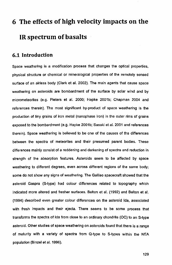
6 The effects of high velocity impacts on the

IR spectrum of basalts

6.1 Introduction

Space weathering is a modification process that changes the optical properties,

physical structure or chemical or mineralogical properties of the remotely sensed

surface of an airless body (Clark et al. 2002). The main agents that cause space

weathering on asteroids are bombardment of the surface by solar wind and by

micrometeorites (e.g. Pieters et al. 2000; Hapke 2001 b; Chapman 2004 and

references therein). The most significant by-product of space weathering is the

production of tiny grains of iron metal (nanophase iron) in the outer rims of grains

exposed to the bombardment (e.g. Hapke 2001 b; Sasaki et al. 2001 and references

therein). Space weathering is believed to be one of the causes of the differences

between the spectra of meteorites and their presumed parent bodies. These

differences mainly consist of a reddening and darkening of spectra and reduction in

strength of the absorption features. Asteroids seem to be affected by space

weathering to different degrees, even across different regions of the same body;

some do not show any signs of weathering. The Galileo spacecraft showed that the

asteroid Gaspra (S-type) had colour differences related to topography which

indicated more altered and fresher surfaces. Belton et al. (1992) and Belton et al.

(1994) described even greater colour differences on the asteroid Ida, associated

with fresh impacts and their ejecta. There seems to be some process that

transforms the spectra of Ida from close to an ordinary chondrite (OC) to an S-type

asteroid. Other studies of space weathering on asteroids found that there is a range

of maturity with a variety of spectra from Q-type to S-types within the NEA

population (Binzel et al. 1996).

129

Many experiments have been made in order to determine the cause of space

weathering. Because no samples of asteroidal soil were available (until the return of

small amounts of material from the Hayabusa mission in 2011), lunar samples have

been used in laboratory experiments as an analogue of asteroid regolith. There are,

however several factors that must be taken into consideration when applying lunar

soil studies to the study of asteroid weathering. Firstly is the fact that asteroids are

much further away from the Sun than the Moon. For this reason they will not be as

affected by solar wind as the Moon. Secondly, the speed of the impactors in the

asteroid belt is lower (Clark et aI., 2002). Mineralogical differences are also an

important factor: on asteroids, the most common mineral is olivine, whilst on the

Moon, the predominant mineral is feldspar (Clark et al. 2002). This fact affects the

quantity of Fe available for the formation of nanophase metallic iron particles (or

submicroscopical reduced iron; SMFe). The main outcome of experiments on lunar

soil is the detection of SMFe particles on the upper surface of grains (Hapke

2001b). This metallic iron, produced by vapour deposition, causes the reddening

and the darkening of the spectra and also the decrease in strength of the spectral

features.

6.1.1 Laboratory simulations

In 1993, Pieters and Fincher studied the influence of the finest fraction of particles

on spectra. They concluded that weathering is surface-related and not volume

related, adding to the idea that the alteration of spectra is caused by coating of

particles with SMFe. The optical effects of submicroscopical reduced iron are non

linear and related to particle size. Because opaque and packed grains inhibit

multiple scattering, carbonaceous materials and bare rock surfaces are less readily

space weathered.

Yamada et al. (1999) and Sasaki et al. (2001) used pulsed laser irradiation of OC in

order to simulate micrometeorite impacts. The results show that both olivine and

130

pyroxene (olivine more than pyroxene) spectra are altered (darkened and reddened)

which leads to an increased similarity between the spectra of the altered OC and of

S-type asteroids. They also observed that the grains in the sample were coated with

SMFe which may have been the cause of the alteration of the spectra. Brunetto and

Strazzulla (2005) and Brunetto et al. (2007) simulated micrometeorite bombardment

and solar wind by laser ablation of silicates and irradiation with different ions at

different energies. The irradiation produced reddening and darkening of the spectra

of the samples. The authors state that solar irradiation must be a very strong effect

closer to the Sun. whilst at further distances micrometeorite bombardment seems to

be the dominant agent of weathering.

Hapke (2001 b) described several previous experiments to investigate space

weathering of lunar samples and analysed the causes of formation of SMFe.

Meteorite impact vitrification (meteorite impact effect). in which impact melts and

vitrifies material. is one of the processes thought to be responsible production of

SMFe. However, the results obtained by other authors do not reproduce lunar

conditions (Pieters et al. 2000; Noble et al. 2001). Hapke was also unable to mimic

space weathering. even using experimental conditions closer to those of the lunar

environment (Hapke 2001a).

The source of ion irradiation (solar wind effects) is plasma of solar composition

coming from the Sun at speeds of 500 km S·1 with a flux of ions of mainly hydrogen

and helium and some heavier ions (Brandt 1970). Experiments with irradiation of

solid surfaces irradiated with H ions do not show any darkening or reddening of the

spectra (Hapke 2001 and references therein). On the other hand, after irradiation of

hydrogen on loose powders there was a strong darkening and reddening with

temperatures too low to allow melting of the minerals (Hapke 2001 and references

therein). The only samples that did not darken were those without Fe in their

composition. which shows that Fe must be present in the first place (Hapke 2001

131

and references therein). Irradiation with helium also produces darkening in powders

containing Fe, so inert gas sputtering also causes darkening (Hapke 2001 and

references therein). The samples have to have a rough surface and porous texture

in order for them to be darkened by sputtering. On experiments with alumina, the

surfaces darkened were the sides and under the samples, not on the irradiated

surface - samples must be of loose powders. Compacted powders will not show

these results (Hapke 2001 and references therein).

The purpose of the work presented here was to simulate the alteration effects of

micrometeorite impacts on asteroids, not by irradiation or by laser pulsed heating,

but by shock. The first part of the study was to undertake impact experiments on

terrestrial basalt to see whether any measurable effects were produced. If so, the

procedure could be applied to meteorite samples, in the first instance, to those with

identified parent bodies, in order to observe whether the impacts would change the

spectra of the meteorites to spectra more similar to the assumed parent body.

Because of the few features present in the measured spectra of individual minerals

by the MSP in Chapter 4, it was decided that a search for any effects of impact

would be undertaken in the Mid Infrared (MIR), a region of spectrum known to

contain features from the main minerals present in basalt. As described in Chapter

3, the instrument used was a FTIR spectrometer in the department of Atmospheric

Physics at the University of Oxford.

6.2 The Light Gas Gun

One option for producing impact shock would be to use a Van de Graaff (VdG) to

shoot particle into a rock. The particles must, however, be conductive and sub

micron sized in order to obtain hypervelocities, and the only instrument available at

the time was one that shot a fine iron metal powder. Because it would be difficult to

distinguish SMFe produced by shock reduction of silicates from fine-grained iron

132

from the projectile embedded in the sample, use of the VdG was ruled out. .The

instrument used for the impact experiment was a Light Gas Gun (LGG), available

at the Hypervelocity Impact laboratory (HVI) at the Open University. The LGG was

the preferred instrument because it produces hypervelocity impacts into targets by

firing any type of particle with a wide range of sizes - for micron-sized powders to

millimetre size particles.

The LGG used in these experiments is shown in Figure 6.1 a) and b). This gun is

one of only two in the world that can shoot into targets from different inclinations,

allowing impact into liquids. The figures show one of the possible sample chambers

at the end of the gun and the gun in a vertical position (Figure 6.1 b). The sample

chamber shown in the picture also allows a high speed camera to be attached at

various angles.

a) b)

Figure 6.1: a) The Open University Light Gas gun with a medium sized chamber attached. The empty ports are connections for cameras or other detectors b) The LGG in a vertical position (images courtesy of Chris Hall)

A schematic of the different sections of the LGG is shown in Figure 6.2 and Figure

6.3.

133

GimblllledPan<:1ary Chamber (GPC)

Tara et S«ondary £xil Aper1ure

Time of Flight

PrimM)' Blast Tank

Lascrligbl curtains

Blast Tank EK(t Aper1ure

Launcher

AdjusI8ble baffie

Figure 6.2: A schematic of the LGG showing the different components and chambers (courtesy of

Chris Hall)

a)

Firing Mechanism

Powder Chamber

Lar~O..nng Powder Breech

Pump Tube

Large O-ring

Centl"1t1 Breech Collar

Rear Certral Breech Collar Central Breech

Front Central Breech Collar SIUiII O-ring

Launch Tute

Muzzle.

b)

Figure 6.3: (a) A detail schematic and (b) an image. of the launcher on the LGG (courtesy of Chris

Hall)

The firing mechanism is a 12 G (gauge) shotgun cartridge, specially loaded with up

to 10 g of rifle powder. A variety of powders can be used which will influence the

speed of the projectile. After the firing mechanism there is a piston with 2 '0' - rings

134

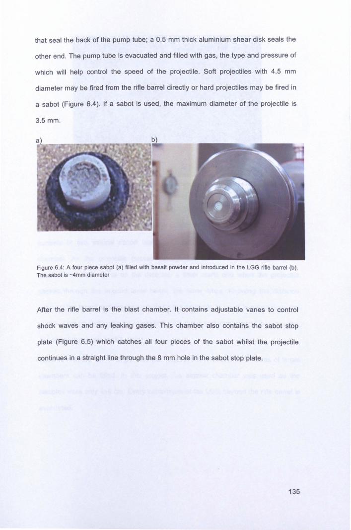
that seal the back of the pump tube; a 0.5 mm thick aluminium shear disk seals the

other end. The pump tube is evacuated and filled with gas, the type and pressure of

which will help control the speed of the projectile. Soft projectiles with 4.5 mm

diameter may be fired from the rifle barrel directly or hard projectiles may be fired in

a sabot (Figure 6.4). If a sabot is used, the maximum diameter of the projectile is

3.5mm.

Figure 6.4: A four piece sabot (a) filled with basalt powder and introduced in the LGG rifle barrel (b). The sabot is -4mm diameter

After the rifle barrel is the blast chamber. It contains adjustable vanes to control

shock waves and any leaking gases. This chamber also contains the sabot stop

plate (Figure 6.5) which catches all four pieces of the sabot whilst the projectile

continues in a straight line through the 8 mm hole in the sabot stop plate.

135

Figure 6.5: The sabot stop plate showing the impact craters from the four pieces of the sabot and the Bmm hole through which the projectile carries

Following the blast chamber in the range assembly is the time-of-flight chamber. It

consists of two vertical ribbon lasers with detectors on opposite sides of the

chamber. As the projectile passes through the first laser beam, causing an

interruption of the signal on the detector, a timer starts and when the projectile

passes through the second laser beam, the timer stops. Knowing the distance

between the lasers and the time it took for the projectile to travel between them the

speed of the projectile can be calculated. With the speed and mass of the impactor,

the impact force can be determined.

The last chamber is the target chamber (Figure 6.6). Three different sizes of target

chambers can be fitled. In this project, the smaller chamber was used as the

samples were only 4x4 cm. Every component of the LGG beyond the rifle barrel is

evacuated.

136

Figure 6.6: The LGG target chamber. The target is attached to a plate at the end of the chamber

As mentioned above, different powder types and different gases at different

pressures result in different velocities. It these experiments rifle powder of the type

R19 was used with hydrogen gas. The pressure is 45 bar giving a speed of -5 km s'

1. Because of the high pressure and velocities involved in this procedure, the LGG is

locked within a steel door, the lab is evacuated and a remote trigger is used from

outside the lab to fire the LGG (Figure 6.7).

Figure 6.7: The target chamber locked on the steel door (the remaining components of the LGG are behind the steel door) (a) and the remote firing trigger (b)

137

6.3 Shots and samples

Two different types of shots were attempted on the LGG: one with micron-sized

basalt powder to simulate micrometeorite impact and the second with mm-sized

grains to simulate the effects of larger impacts. Several shots were made, some

with no success either because the gun did not fire or because the projectiles did

not hit the target. Two slabs of impacted basalt were eventually available for

spectroscopic analysis. The sample names and the LGG shot settings are given in

Table 6.1 and their images in Figure 6.8.

Table 6.1: LGG shot settings for the two targets used (1 Torr = 1 mmHg = 133.322 Pa)

Propellant Gas Type Vacuum In

Pump Shot

Sample Projectile Type and and Stop Disk Range Tube Gas Velocity Load Pre.sure Pre.sure

Slab1 lmm diameter 7!>-1251lm

R1910g Hydrogen 45

0.5 em Hard Aluminium 8.510 ' torr 45 bar 3.68 kmls Basalt Powder bar

Slab 2 1 mm diameter basalt grain R1910g Hydrogen 45

0.5 em Hard Aluminium 8.0 10~ torr 45 bar 1.39 kmls bar

Figure 6.8: Results of LGG impacts onto basalt slabs: Slab 1 (a) hit by 75-125 101m powder and Slab 2 (b) hit by a 1 mm basalt grain. The crater formed by the basalt grain impact can be seen at the top left. Each slab is - 4 x 4 cm

Because there was the possibility of the single grain projectiles not hitting the target,

six 1 mm grains were fired into 4 slabs (sections of slab 2). As can be seen in the

picture, two projectiles hit the target but one of them hit between the slabs. For the

analysis, the crater on the top left (see Figure 6.8b) was chosen. This crater had an

approximate diameter of 1 cm. The impact with the basalt powder formed a series of

138

mm-sized craters across an area of approximately 3 cm in diameter. An additional

slab of basalt was prepared by scratching the surface with a second piece of basalt.

The objective of this experiment was to roughen the surface of the slab, in order to

determine whether changes in the spectra of the impacted basalts were caused by

an increase in roughness, rather than other physical changes to the sample. This

final sample will be referred to as 'scratched basalt'.

6.4 Spectroscopy results for the samples in the Mid

Infrared

In this section, several results acquired with the FTIR spectrometer with the

instrument described in Chapter 2, are presented. The positions of the identified

features were found by hovering the cursor over the spectrum and noting where the

first minimum was for the absorbance and Christiansen Features (CF), and the

maxima for the Reststrahlen Bands (RB) and Transparency Features (TF) (see

Chapter 2 for a description of CF, RB and TF).

Spectra of the meteorites Juvinas and Allende and the mineral orthoclase were

taken to visualise some of the characteristics of their spectra and to help with the

interpretation of data from the analysis of the basalt slabs. Allende is a

carbonaceous chondrite, Juvinas is a eucrite, which has a basaltic origin, and

orthoclase is a potassium feldspar, not often present in these meteorites. Results

are plotted in Figure 6.9.

139

5

--Orthoclase --Juvlnas

4

CI) TF 0 3 CF c cu ... 0 CI)

~ CI) 2 0::

1

2 4 6 8 10 12 14

Wavelength (JIm)

Figure 6.9: MIR spectra of the meteorites Juvinas and Allende and the mineral orthoclase taken on the Oxford FTIR. CF is the Christiansen feature in all the samples and TF the transparency feature in orthoclase

The MIR spectra of these samples have clear features that differ between the

materials. Orthoclase, a terrestrial mineral sample, has a clear absorbance from

water at 2.8 \-1m and overtone and combination bands (see Chapter 2) at around 6

\-1m . Above 6 \-1m, there is a sharp drop in reflectivity in the spectrum, forming the

Christiansen Feature (CF) with a minimum at 7.5 \-1m. This sample of orthoclase has

been ground to a grain size of < 125 \-1m. For this reason, and as explained in

Chapter 2, the Reststrahlen Bands (RB) are weak and a broad transparency feature

appears. It is difficult to determine the exact position of the TF because it is a broad

feature but its maximum is at 11.4 \-1m.

The spectrum of the meteorite Juvinas (a eucrite) seems to have a small H20

feature at 3 \-1m, but this might be caused by terrestrial contamination. There is a

combination of other features between at -5.5 and 7 \-1m which may be a mixture of

water contamination and features from minerals such as pyroxene. The CF of the

meteorite Juvinas is somewhat broad and difficult to measure, but its minimum

140

appears at 8.2 IJm. This might be caused by the CF of different minerals that are

present in the meteorites being far apart and broadening the CF of the meteorite.

Another reason might be the fact that this sample is also a powder, causing the RB

to become much weaker reducing the sharpness of the CF. The TF of Juvinas is at

12 IJm.

Allende is a CV3 carbonaceous chondrite, and is known to have experienced slight

amounts of aqueous alteration (e.g. Hutchison 2004); however, water bands cannot

be distinguished in the spectrum. The fact that the sample is a fine powder should

have increased the depth of any water bands relative to the continuum. The lack of

water bands may be explained by the presence of organic (opaque) matter in

Allende, which suppresses the water bands (Clark, 1983). c=o and C=C bands

normally appear near 6.13 IJm. A series of small bands can be seen in this area of

the spectrum of Allende, but because there is interference from water bands and

other minerals such as olivine and pyroxene in this region of the spectrum, the

bands cannot be attributed to the presence of carbon (Salisbury et al. 1991). The

CF of Allende is quite difficult to discern because the RB are almost

undistinguishable (sample is a very fine powder < 50 IJm). Its minimum is at 9 IJm.

The TF of Allende peaks at 12.4 IJm.

The most obvious difference between the spectra of the meteorites and the mineral

is the lack of water bands (which are present at - 3 and 6 IJm in the orthoclase) in

the meteorite samples. Even when they are present, they are small and are likely to

be the result of terrestrial contamination. Orthoclase is a mineral with a degree of

transparency which is reflected in the higher features in both the volume and

surface part of the spectrum (refer to Chapter 2 for definitions). Allende is also the

finer powder. Because the samples are powdered, RB are strongly reduced and the

TF can be seen at wavelengths around 12 IJm.

141

For comparison purposes, the different sizes of basalt powder (from the same

sample as the impacted slabs) and a non-impacted area of a basalt slab

(representing basalt as a solid rock) were also analysed on the FTIR at MIR

wavelengths. The reasoning behind this was that differences in spectra following

impact might have been caused by breaking the rock to powder, rather than

changing the chemistry or structure of the minerals. The basalt was taken from the

same piece as the target slabs, ground and sieved. Five different samples size-

fractions were produced: 30 - 63 IJm; 63 - 75 IJm; 75 - 125 IJm; 125 IJm - 0.4 mm

and a powder mix of grain sizes < 125 IJm. Results can be seen in Figure 6.10.

3

2.5 -- 125 J.lm to 0 4 mm

--75 J.lm to 125 J.lm

2 --30 IJmt063 J.lm

Q) -- Powder mix (..)

--Non-impacted c "' -1.5 (..) II)

= Q)

~ 1

0.5

o 2 4 6 8 10 12 14

Wavelength (pm)

Figure 6.10: MIR spectra of basalt powder with different grain sizes and non-impacted basalt, taken on the Oxford FTIR

The results are as expected, according to the effect of grain size (see Chapter 3 for

explanation and references). The only samples with RB present are the coarser 125

IJm to 0.4 mm and the solid rock sample . In the spectra from the finer grain sizes,

the RB disappear and a TF appears at 12.1 IJm, which is not present in the rock

142

sample or the coarser 125 !-1m to 0.4 mm fraction. The CF on the powdered samples

remains at the same wavelength (7.9 !-1m) with different grain size which is also to

be expected with grain sizes smaller than the wavelength. The exception is the

sample with basalt grain from 125 !-1m to 0.4 mm. In this case. the CF is found at

shorter wavelength (7.8 !-1m). an intermediate position between the CF of the

powdered samples and the rock sample with a CF at 7.6 !-1m. In the volume

dominated part of the spectrum (wavelengths < 8 !-1m). as particle size decreases.

the reflectance increases resulting in higher peaks - the rock sample has the lowest

reflection under the CF and the smaller powders the highest. All sample show water

bands at 2.7 and 6 !-1m. although the latter might have the influence of some

minerals such as olivine and pyroxene. present in basaltic rocks. At 4 - 7 ~m.

volume scattering dominates and the absorption bands are troughs instead of

peaks. These increase with decreased particle size becoming diagnostic features

(Salisbury et al. 1997). This can be seen in Figure 6.10 where the absorption bands

of smaller sized fractions are more sharp and deeper relative to the continuum than

the coarse samples or the rock sample. In the mixed powder. the results

substantiate the fact that small particle sizes cling to larger ones influencing the

spectrum. This can be seen by the fact that the mixed powder. even though it has

particles of all sizes. behaves like a smaller particle sized sample.

The results presented here were compared with the results from Cooper et al.

(2002) for validation. One of the samples of basalt was chosen (Basalt 1) and the

positions of the CF and TF in his rock and powdered samples are shown in Table

6.2. Because of the slightly different results for the fraction 125 !-1m - 0.4 mm. those

are also shown in the table. Different positions of the CF and TF between the

samples of Cooper et al. (2002) are caused by the fact that the sample may have

different compositions. The table shows that the difference between the CF of rock

and powder in Cooper et al (2002) and the results of this work are approximate 0.24

143

!-1m for Cooper et al. (2002) and 0.3 !-1m for this work. The slight discrepancy might

be, again, cause by difference in composition (in his work, Cooper et al (2002) finds

that the changes in the positions of CF in powders and rocks vary according to the

composition of the sample), but also because the method for finding the position of

features of this work is different and less accurate.

Table 6.2: Comparison of the position of the CF and the TF between rock and powdered samples of basalt and the same results from the sample Basalt 1 from Cooper et al (2002)

Cooper (2002) Difference

Our CF sample Difference

Cooper (2002) Cooper (2002) between solid betw .. n solid CFPowder CFrock ea.alt

and powdered Our CF powder 125 ~m-4 .4 OurCFRock

and powdered TFpowder Our TF powder

easalt1 1 basalt

mm basalt

Ba.alt 1

8.18 ~m 7.89 ~m 024 ~m 7.9 ~m 7.8 ~m 7.6 ~m 0.3 ~m 12~m 12.1 ~m

The purpose of this work is to analyse the effects of impact shock on the IR spectra

of basalt samples. Spectra of SIab1 (impacted and non-impacted area) and the

crater on Slab 2 are given in Figure 6.11.

1.5

G> 1 o c :! o G> I;: G>

Q: 0.5

--Non-impacted --Impacted --Cratered

o ~ __ ~ __ ~ __ ~ __ ~ __ L-__ L-__ L-__ L-__ L-__ L-__ L-__ L-__ L-~

2 4 6 8 10 12 14 16

Wavelength (Jim)

Figure 6.11 : MIR spectra of Slab 1 (powder impact). Slab 2 (cratered) and a non-impacted area of the basalt taken on the Oxford FTIR

144

There is a noticeable difference between the impacted area on Slab 1 and the non

impacted basalt. The CF has changed from 7.4 to 7.9 ~m and a much broader

feature from the non-impacted to the impacted spectrum. The water feature at -2.8

~m was enhanced with the impact. the RB were suppressed and the peak was

slightly shifted to longer wavelengths. This may be caused by 3 reasons:

• An alteration in composition resulting from the impacts. In this case the

purpose of the experiment was accomplished. as the impact changed the

composition of the basalt as it would do to an asteroid with a surface

impacted by micrometeorites;

• A change in texture caused by the craters formed by the impacts. giving it a

more porous surface more similar to a powder. As the surface is roughened

surface scattering increases and the intensity of the RB diminishes

(Salisbury et al. 1991);

• An alteration in composition cause by contamination deriving from the LGG.

If the alteration of the spectra is caused by the change in texture. then the scratched

basalt should show a similar spectrum to the impacted basalt. The powdered basalt

was also analysed to determine if the results are caused by the formation of a

powdered. roughened surface on the impact area. To determine if the cause was

contamination. a spectrum of the crater on Slab 2 was also taken - a larger

projectile would have sufficient energy to vaporise the contaminants. and the

alteration should not be present. Figure 6.12 shows the spectra of the non-impacted

basalt. Slab 1. Slab 2. scratched basalt and powdered basalt for texture

comparison.

145

1.5

--Non-Impacted --Impacted --Cratered

Scr :1

1

0.5

o 2 4 6 8 10 12 14 16

Wavelength (~m)

Figure 6.12: MIR spectra of Slab 1 (powder impacted). Slab 2 (cratered). scratched basalt. nonimpacted basalt. and powdered mix basalt taken on the Oxford FTIR

The more apparent differences between spectra are as follows: TF are only present

in powders. It makes sense that only the basalt powder shows this feature at around

12 !-1m. The RB were suppressed in the basalt powder and completely disappear,

giving rise to the TF. The non-impacted basalt, Slab 1 and scratched basalt were

averaged from two different scans in order to eliminate any crystal direction effect

on the spectra. On a first approach to analysing the results, the scratched basalt

seems very different from the impacted basalt but that may be related to the fact

that both the scratched scans that were averaged were very different in the first

place, possibly because of a direction effect and the fact that the slab was tilted.

They should be analysed independently. In the impacted basalt, the RB are

suppressed, as would be expected for a surface altered by impact, and also from a

smaller grain size effect. In the spectrum for the cratered sample, the RB are also

very small; this was not expected . A small roughness effect was expected but not

such a great difference. Maybe there is scattering against the walls of the crater and

146

insufficient signal reached the detector, or maybe there is a deposition of smaller

particles on the bottom of the crater.

In order to better understand the differences between the samples, all the spectra

were normalized at 7 J..lm and the two scratched basalt spectra were plotted

separately (Figure 6.13). Table 6.3 contains a description and positions of the main

features present in the spectra from Figure 6.12 and Figure 6.13.

5

--Non-impacted --Impacted --Cratered

4 --Scratched direction B

Q) --Powder mix u c: 125 IJm to 0.4 mm

"' - 3 u Q)

= ~ Q)

> +:: 2

"' Q; 0::

1

o 2 4 6 8 10 12 14

Wavelength (IJm)

Figure 6.13: MIR spectra of Slab 1, Slab 2, non-impacted basalt, scratched basalt in two different directions powdered basalt and basalt grains between 125 IJm and 0.4 mm, all normalized to 7 IJm

147

Table 6.3: Description and position of the main features of the spectra of the samples shown in Figure 6.19

Water feature I Ranectance between

Water feature n Sample

(2.7 .... , water featur ••

(S .... , CF RB TF

(2.7-8 .... '

Weakest In aU the Very weak

Broad at -7.5 Hgh refleclNiIy w til

Non-lmpacted built u""",a

Low est of al the sa"1'las Iogetherwith spectra definition. Atake at Jl¥A cratered IJIT1 8.1.8.9.9.7. 10.2. 11 ....

Hgh reflectance but low er Hgh reflectivity and

Scratched built Deep

than pow dar, 12511"'1"0.4 Deep -7.6 .... enhanced peake deacribed Jl¥A

dIrectIon" Inn and scratched d~8Ction B and non l"1'acted

above

Hgh reflecbvily and Scratche d bu alt

Very deep Hghest reflectance aftar

Deep -7.5 .... very enhanced peake deacribed

dIrectIon B 125 ~m-O.4 Inn broad above (leas than direction Jl¥A

A) RaflecWity decreases,

Impactld Deep Hghest reflectance aftar

Deep Broad at paake are not

the pow dered aa"1'ie -7.9"", distinguishable, paak at 11 Jl¥A

.... becomos domnant

Very broad at MJch weakar and broader

Crate rid Deep Simlar to non-irrpactad Deep RB. Rlake not Jl¥A -7.5 ....

distinguishable

Very deep Very deep at Very hogh (hoghest)

125,.., toO.4mm (deepast)

Very high (highest) Very deep 7.5 ....

reflectivity but paaks are Jl¥A not distinguishable

Powder Very deep HIgher reflecWl1y of the

Very deep 7.9 .... None 12 .... 8a"1'198

From the normalised data, it can be seen that H20 bands increase in depth from the

non-impacted basalt, impacted, cratered, powder and 125 IJm to 0.4 mm. It is

expected that smaller grain sizes increase the depth of the water bands and in this

case this seems to happen perhaps because of the roughening of the surfaces with

the impacts. The scratched basalt shows very different behaviour from one scan to

the other, and, again, this may be cause by the different scratching direction and

because the slab was not horizontal. It has an inclination on the surface, which

caused a difference in reflectance. The 125 IJm to 0.4 mm powder behaviour

remains unexplained. The grains were quite coarse, shiny and loose so the porosity

effect seems to be stronger showing a much higher reflectance at the wavelengths

where scattering domains. It almost behaves like a metal. The CF on this sample is

also the strongest and has similar shape spectrum to the scratched spectra.

The reflectance in the volume scattering wavelengths between the water bands at

2.7 and 6.1 IJm decreases in the order 125 IJm - 0.4 mm powder> scratched basalt

direction B > powdered> scratched basalt direction A> cratered> impacted> non-

148

impacted. This behaviour is consistent with the behaviour of the water absorption

bands described above.

CF of all the samples do not vary much from the non-impacted basalt. The

exceptions are the impacted basalt and the powder. Powdered samples of the same

composition have CF at longer wavelengths as powders than as solid rocks (e.g.

Cooper 2002 and Salisbury et al. 1997). Once again there is the possibility that the

surface of the slab has been roughened by the impact and behaves similarly to a

powder. An increase in the ratio between the amount of pyroxene and olivine and

plagioclase would also shifts the CF to longer wavelengths. It is possible that with

the impact. the less resistant plagioclase was removed - the ratio between Fe and

(AI plus K) would also be higher - resulting in a change in composition to more Fe

rich. Another explanation might be the effect of shock pressure inducing changes in

the structure of the minerals. rather than composition. This possibility is discussed

below.

The presence of nanophase Fe would have the same effects on the spectra.

however. according to some authors. e.g .. Pieters (2000) and Hapke (2001 b). for

the formation of nanophase Fe. reduction through sputtering by irradiation or H+

ions from the solar wind is also needed and this experiment does not include a

simulation of that effect. It is. therefore. unlikely that the change in spectra is caused

by the formation of nanophase Fe. The next section will include SEM results on the

composition of the cratered and non-impacted areas in an attempt to investigate if

there are indeed changes in composition with the impacts

The scratched slabs look quite similar to each other at the RB area. only with a

difference in brightness. The positions of the RB are the same between them. They

are. however. slightly different from the remaining basalt slabs. impacted or not.

Most RB are in the same position but their intensities are different depending on

wavelength. They seem to decrease equally between the scratched basalt but are

149

higher at shorter wavelengths compared to longer wavelengths. The changes from

the non-impacted basalt to the impacted and cratered are not only a reduction in

intensities, but at shorter wavelengths, closer to 8 \.1m, the decrease is more

noticeable. The RB become asymmetric with a higher peak at 11.5 \.1m.

In the powdered samples, there seems to be the formation of a TF at 12 \.1m as

described above. This is consistent with the presence of feldspar dominating the

spectrum as it normally exhibits a TF at this wavelength. The cause of this might be

that harder minerals resist the grinding process better, being retained on the sieves

with a larger mesh, and the less hard like feldspars are broken and accumulated in

the smaller fractions (Salisbury et al. 1997). This selection process will also be

discussed in the next section.

Because they seem to be quite similar, the spectra of non-impacted basalt,

scratched basalt and grain size 125 \.1m to 0.4 mm were plotted on Figure 6.14 for

better comparison. The results were normalised at 7 \.1m.

150

5

--Non-impacted

4 --Scratched direction B

G> U c --125Ilm to 0.4 mm

"' ... 3 u

G> ;0= G> ~

G> .~

2 ... "' 'ii a::

1

o 2 4 6 8 10 12 14

Wavelength (~m)

Figure 6.14: MIR spectra of non-impacted basalt, scratched basalt (in two directions) and 125 Ilm to 0.4 mm

The sample with grain size 125 IJm to 0.4 mm is very similar to the scratched basalt.

This is expected as it represents an increase in roughness of the surface. There are

no other major changes, other that the intensity of the RB, which indicates that there

are no differences in composition.

The effects of shock on basalts , including the resulting changes in their spectra,

have been studied by several authors. Kieffer et at. (1976) studied the effects of

impact shock on basalts from an impact crater and compared them with samples

shocked in laboratory conditions using a high velocity gun under vacuum conditions.

Wright et at. (2011) further studied the effects effect of impact shock on the Thermal

Infrared Spectra (TIR) of basalts and summarised the different classes of effects

described in Kieffer et at. (1976) into a table (Table 6.4) The following discussion is

151

based on the work of Kieffer et al. (1976), Johnson et al. (2007), Wright et al. (2011)

and references therein:

Table 6.4: Classes of shocked basalt and summary of petrography (Wright et aI., 2011 adapted from Keiffer et aI., 1976).

Sho.l<:k Pn.'S.u!e Cb!ll (Gra) Dri.:r P~""'llf3I'hic o.."".,iptitlll

I <;!O Gillins an fractun:d 2 2(}..40 Plagioclase tramfonncd to nwkc:lynitc 3 4660 Plaglodase tramfonncd to IIIaJa of

plal!ioclase compositlOll 4 60~ Plal!iodase con\'crtcd to , .... ,it'"loI .. J IIlasl;

pyroxClle mc:hcd on crystal cdges and'or hc.t~ily fflll.1un:d

5 >!IO Plagiodase and PYTU"mc compkkly melted

The spectra of un-shocked basalt taken by Johnson et al (2007) and Wright et al

(2011) show similarities with the spectrum from this work, with main features at 9

and 11 j.Jm, resulting from Si-O vibrations in Ca-rich plagioclase, plus contributions

from olivine and pyroxene. Their results show a shift in the CF to longer

wavelengths with increasing pressure, which also happens here (in particular with

the impacted basalt, see Table 6.3). Wright et al. (2011) compared the Thermal

Infrared spectra of class 2 shocked (20 - 40 GPa) and un-shocked basalts, with

particular attention to the features of labradorite (a type of plagioclase), which turns

to maskelynite (a glass of plagioclase chemistry, but not crystallography). In type 2

shocked basalt, the features of labradorite (CF at 8.1 j..Im, followed by a sharp slope,

absorption at 9 j..Im and emission at 10 j.Jm) seem to disappear.

In the results from our work, the CF seems to be influenced by the presence of

other minerals, however a shift to longer wavelength is especially clear in the

impacted basalt sample (Figure 6.19 and Table 6.3). The slope after the CF also

appears flatter and the sharp feature at 9 j..Im is reduced, as is the broader feature

above 10 j..Im. The entire spectrum is moving closer in appearance to that of the

basalt powder - as discussed earlier, this may be because the surface has taken on

the more porous texture of a powder. The 10 j..Im 'hump' is also reduced in intensity

152

in the cratered basalt; if this feature is, in part, caused by the presence of

plagioclase, then it may be that we are seeing the effect of the plagioclase to

maskelynite transition in the impacted and cratered samples. At this stage, it is not

possible to confirm the definite presence of maskelynite without further tests,

although it appears that melting has not occurred because of the absence of a

sharp 9.5 ~m Si-O feature that occurs in glasses.

6.5 SEM analysis results from cratered and non

impacted area

To complement the investigation of the effect of impacts by shock on the mineralogy

of a sample, composition maps were taken by the FIBSEM, in the Department of

Physical Sciences of the OU, from an area inside the crater on Slab 2 and a non

impacted area outside but close to the crater. The reason why the cratered sample

rather than the impacted sample was chosen resides in the characteristics of the

SEM. It required a relatively flat area for the mapping and the impacted area was

too rough. Instead, a flattened area inside the crater was use in this investigation.

Figure 6.15 shows the composition maps of an area outside the crater and one

inside the crater of Slab 2. Because there is great interest in ascertaining if there are

differences in the quantities of Fe after impact, this was one of the elements for

which data were acquired. One of the hypotheses for a change in compositions

might also be that the impact, in the same way as grinding, destroys the less

resistant minerals. The less resistant mineral that is present in sufficient quantities

for a clear result is plagioclase. For this reason, data for concentration of Ca were

also taken.

153

Inside the Crater

Fe-red

Ca-green ; Ti-red

Outside the crater

Fe-red

Ca-green; Ti-red

Figure 6.15: FIBSEM results inside and outside the crater for Fe and Ca

It can be seen in Figure 6.15 that there is a major increase in the amount of Fe

inside the crater at the same time as there is a decrease in Ca. Evidence for the

possibility of contamination from the LGG is not seen. If the contaminant is for Fe it

would not affect the results of Fe and Ca and if it was Fe, it would be visible in areas

outside the crater as well .

154

These results are consistent with the possibility that, with a high speed impact, even

when the impactor is small, generates enough energy to vaporise less resistant

minerals. Besides the presence of SMFe, an alteration in the ratios of certain

minerals at the surface of an asteroid cause by an impact as seen in this chapter,

would modify the spectrum of that asteroid in variable amounts which would make

the identification of this asteroid as a parent body of a meteorite more difficult.

6.6 Conclusions

The purpose of this work was to test an impact technique that would help analyse

the effects of impact shock on basalt samples. If successful, meteorite samples

could be used with the purpose of aiding the establishment of links between

meteorites and asteroid parent bodies.

There is some (tentative) evidence provided by spectroscopy that supports the

possibility that impact changes the sample composition, either the alteration of

plagioclase to maskelynite, or by vaporization of less resistant materials. The results

for the FIBSEM further sustain this possibility. However there are other effects that

may have given rise to the differences between impacted and non-impacted

samples, such as surface roughness or contamination. In order to draw more firm

conclusions about whether impact experiments provide a useful analogue for space

weathering processes on asteroids, additional experiments need to be carried out.

Only a limited number of samples was examined in these experiments, and results

should be regarded carefully. Additional tests with basalts and other terrestrial rocks

should be done, as well as with other types of meteorite.

The light gas gun is a good technique for the tests although it is vulnerable to

contamination and it requires relatively large sample which might not be possible

with meteorites. Another option for the study of the effects of impact shock is to use

a Van de Graaff (VdG). The VdG has the advantage of requiring very small samples

155

as a target and it has the possibility of bombarding the target continuously for quite

a long time (days or even weeks), as opposed to the LGG which shoots one

projectile at a time. On the other hand, the VdG does not reach velocities as high as

the LGG- It does not generally reach velocities above 3 kms·1 and it requires the

projectiles to be conductive. Fe particles are generally used but these would

strongly interfere with the amount of Fe found in the target, which is one of the

results of high speed impacts (nanophase iron). Copper would also affect the results

in the same way. Some work has been done by Hillier et al. (2001) to develop

conducting silicate particles that can be accelerated in the VdG and therefore can

provide more reliable results.

156

7 Conclusions and Further work

The technique of UV-Vis microspectroscopy (MSP) is one that has many

applications in pharmaceutical and forensic investigations, where samples are

mostly analysed using transmission mode, i.e., spectral signatures are

characterised following transmission of radiation through a sample. UV-Vis

reflectance spectroscopy, where a powdered samples is analysed in bulk, using a

target of around 1 mm in diameter, is also a commonly-found technique, and has

special application for comparison with remotely-obtained spectra from asteroids.

The aim of this study was to apply the micro technique in reflectance mode, to

establish whether the MSP was a suitable technique for UV-Vis spectroscopy of

extra-terrestrial materials, specifically samples that are too small for analysis by the

bulk technique, i.e., cometary grains. If the technique was found to be appropriate,

by analysis of minerals and meteorites, and comparison of results with those

obtained from conventional spectroscopy, it would then be applied to study of

cometary samples from comet 81 PIWild2 collected by the Stardust spacecraft. Part

of the investigation process involved study of grains from HED meteorites,

comparing spectra with those from their potential parent body, Vesta. In addition, a

study of the effects of shock impact was carried out, using a light gas gun (LGG) on

basalts, as a starting pOint to the determination of whether or not this was a useful

analogue for space weathering of asteroid surfaces.

7.1 Operation of the MSP

In the first chapter of the thesis, I describe the type of extra-terrestrial materials

available for study, and the formation processes that they have experienced. In

Chapter 2, I give a broad introduction to spectroscopy, particularly electronic

spectroscopy, without entering into a detailed discussion of the atomic processes

that cause the spectra (which was thought to be beyond the scope of the thesis).

157

Chapter 3 is an extensive analysis of the performance and operation of the MSP.

The tests performed included the characterization of the dark current, the stability of

the light source, the sensitivity of the instrument at all wavelengths and homogeneity

of the diffuse white reflectance standard provided by the manufacturer. I found

several problems with the system, all of which would impact on collection and

interpretation of data:

lighUQu~~:

I found by investigating the drift of the dark scan and reference scans with time that

the system only stabilised after the light source ( a xenon lamp) had been switched

on for - 4 hours. This finding had a significant effect on the way in which I then had

to carry out my experiments. Figure 3.9 also shows that there are emission lines

between 450 and 500 nm and above 700 nm that might be related to the light

source, and which might influence interpretation of the results if data were

improperly corrected.

Reference homogeneity:

The reference standard is only suitable for wavelengths above - 250 - 350 nm

(Figure 3.10) and, even at the lowest of magnifications, is very heterogeneous,

which causes great variation in the reference scan used for the corrections of the

spectra. For this reason, it is advised that 20 reference scans should be taken in

order to minimise the effects of heterogeneity in the results. For this to be possible,

the spectrum of a sample has to be taken as a reference scan and the corrections

have to be carried out in a spreadsheet, rather than using the software supplied by

the manufacturer.

Focussing:

The optics of the microscope rely on mirrors, rather than lenses, and so the optical

image of a sample is very poor. This led to problems with the correct focussing of

158

samples, even over the small area of the aperture (generally 10 x 10 J,tm, but 2 x 2

J,tm for the Stardust grains). Results of tests made on the reference scan show that

there is a change in spectra with different focussing, which might be related to an

illumination problem, or to the geometry of the instrument which might be capturing

reflected light from sources other than the sample.

7.2 Application of the technique to minerals commonly

found in meteorites

A series of scans was taken on minerals commonly found in meteorites in order to

ascertain, in the first instance, if the instrument were suitable for the study of

minerals, rocks and meteorites (Chapter 3). The results were also compared, when

possible, with results from other authors, either taken by the RELAB spectrometer

or the UNIWIN instrument (Cloutis et al. 2008).

Results varied greatly with the samples studied, even from grain to grain. It was

found that the ability to focus the MSP correctly on the sample significantly

influenced the spectra. If the surface of a grain was rough, such that it was not

possible to bring to a single focus within the area of the aperture, the resulting

spectrum was essentially featureless and flat, which might be evidence for an

illumination issue.

Another concern was the size of the sample relative to the field of view. At the 10x

magnification that was used for most of the observations, the aperture of the

spectrometer was 10 x 10 IJm. It had been assumed that as long as the grains being

analysed were larger than the aperture, there would be no influence on the spectra

from the surrounding area, and that results would be valid. What was found,

however, was that if the sample under consideration did not fill the whole field of

view of the spectrometer, then light scattered into the detector from the substrate

supporting the sample could have a significant effect on the resulting spectrum. In

159

the samples analysed in Chapter 3, the influence is from the quartz slide on which

the mineral grains were supported. Quartz is transparent to UV light, so it was

assumed that any reflection from the slide would be minimal and would not interfere

with the sample analysis. What was found, though, was that the spectrometer did

pick up a signal from the quartz, possibly from specular reflection from the flat

surface of the slide. This had an effect of 'diluting' the signal from the sample, giving

a lower signal to noise ratio.

It was also observed that, when the grains are very dark, the spectrum is flat and

featureless. This occurs even when, with the naked eye, the sample is almost white.

This was evident in the case of olivine (see Appendix A). It seems like a

combination of the fact that the grains are extremely small with the inability to

correctly focus the microscope on the sample and the influence of the quartz slide

are the cause for the featureless, very dark spectra

When comparing data from different instruments, it was noticeable that results

varied from instrument to instrument. The geometry of the instrument was less

significant in influencing the final spectrum than the size and shape of the sample. It

was apparent that if the grains were flat (and so bright and well-focussed) and

covered most of the field of view, data from the MSP were comparable to those

taken at the RELAB facilities and UNIWIN.

7.3 Application to Stardust samples and meteorites

Once the MSP had been characterised, and the most appropriate experimental

conditions had been determined, the technique could be applied to meteorites and

cometary dust. Chapter 5 gives the results from analysis by the MSP of the UV-Vis

spectra of two grains collected from comet Wild 2 by the Stardust mission.

Unfortunately the grains were covered in aerogel which made the analysis difficult.

Furthermore, as predicted by the results from Chapter 4, the gold foil into which the

160

grains were pressed, greatly influenced the spectra: even at the highest

magnification of the MSP, the grains did not fill the field of view of the microscope,

and so the signal observed was dominated by reflectance from the gold foil.

Corrections were made in an attempt to minimise the effect of the aerogel and the

gold foil, but these are only qualitative, since we could not measure the thickness of

the aerogel, and could not be sure how much light was scattered into the MSP from

the gold foil. Despite this, results indicated that the two samples analysed were

assemblages of low- and high-calcium pyroxene and olivine, possibly with some

magnetite, and were not single mineral grains.

There has only been one previously published analysis of extra-terrestrial materials

by MSP, and that was a study which compared spectra from the Allende

carbonaceous chondrite with spectra from lOPs (Bradley et al. 1996). This

comparison was also included in Chapter 4: spectra from the Murchison and

Allende carbonaceous chondrites were recorded and compared with the published

data, and also with the Stardust grains. The chondrites were very dark to look at,

and produced dark, flat and featureless spectra, similar to those recorded by

Bradley et al. 1996), who concluded that the spectra were influenced by the

presence of carbonaceous material in the samples.

Chapter 5 however shows that the technique, when the conditions described above

are met, can be applied in the field of planetary sciences. Spectra from three HED

meteorites are compared with results from RELAB and also spectra taken of their

possible parent body (asteroid 4 Vesta). The spectra show a great similarity

between results from other laboratories, and also from the asteroid, confirming the

utility of the MSP under the correct circumstances.

161

7.4 Investigation of the effect of impacts by shock in the

spectra of basalt

Space weathering is a possible cause for the discrepancies between the spectra of

meteorites and their possible parent bodies (asteroids) (e.g. Clark et ai, 2002) and

one of the main factors of space weathering is the impact of micrometeorites on the

surface of the asteroid. Previous work attempted to duplicate the effects of space

weathering by laser irradiation (Yamada et al. 1999 and Sasaky et al. 2001) and

ablation (Brunetto and Strazzulla 2005 and Brunetto et al. 2007). In this work, the

effects of impacts by shock were investigated, using a Light Gas Gun (LGG) to

shoot powders or grain of basalt onto basalt. Because, at the time, it looked as if it

would be difficult to obtain useful information from spectra recorded by the MSP for

comparison of impacted and non-impacted materials, spectra were recorded at a

longer wavelength, using an FTIR system at the University of Oxford (Chapter 6).

Results show that there is a difference between the spectra of impacted and non

impacted areas, although the reasons are not clear. Reasons for this difference

include the effect of roughening of the surface by the impact, where the impacted

surface behaved as a fine-grained sample; contamination by residue in the LGG;

the formation of SMFe by the impact observed by other authors (e.g. Pieters et al.

1993); or a change In the mineralogy within the impacted area. SEM results support

the last-mentioned effect, with a high increase in the concentration of Fe inside the

impacted area and a depletion of Ca. These results are consistent with the

hypothesis that the impact vaporised the minerals that are less resistant, such as

plagioclase, compared with ferromagnesian minerals. This effect may also occur at

the surface of the asteroids, causing a change in the spectra of the body. Only a few

samples were used In this study, not enough to reach any definite conclusions.

Further experiments must be conducted.

162

7.5 Future work

Results from the study of minerals and meteorites have shown that the MSP can be

used to record spectra from individual mineral grains and from very small amounts

of powdered meteorite, but that the experimental conditions under which valid data

can be acquired are very specific. Currently, results can only be interpreted by

comparison of the data with results from similar samples that have been measured

on other instruments. If the MSP is to be a useful analytical tool, then a more

systematic study of minerals and mixtures of minerals must be carried out. It would

also be very useful if experiments were made using mixtures of different minerals

with different ratios to determine the influence of composition on the results and

complement the investigation with the analysis of the spectra of powders and slabs

of rocks. The analysis of spectra from the HED meteorites was encouraging,

however, other meteorite types should also be analysed and their spectra compared

to those of asteroids considered possible parent bodies.

The effect of impact shock on the spectra of basalt slabs as described in Chapter 6

revealed some interesting results with some form of composition change on the

impacted areas. Nevertheless only two samples were analysed, which is insufficient

for more concrete conclusions. More impacts using the LGG should be made using

different types of targets but, ideally, a VDG should also be used on the same

samples and for varied periods of time if non-metal projectiles can be used.

In summary, the investigations described in this work are of value for planetary

sciences and set a solid stepping stone on the use of new techniques in the field,

especially for the analysis of samples that are too small to be analysed by more

conventional techniques. However, further investigations should be made and the

method should be applied to a greater range of samples.

163

References

A'Hearn, M. F., M. J. S. Belton, W. A. Delamere, J. Kissel, K. P. Klaasen, L. A. McFadden, K. J. Meech, H. J. Melosh, P. H. Schultz, J. M. Sunshine, P. C. Thomas, J. Veverka, D. K. Yeomans, M. W. Baca, I. Busko, C. J. Crockett, S. M. Collins, M. Desnoyer, C. A. Eberhardy, C. M. Ernst, T. L. Farnham, L. Feaga, O. Groussin, D. Hampton, S. I. Ipatov, J.-Y. Li, D. Lindler, C. M. Lisse, N. Mastrodemos, W. M. Owen, J. E. Richardson, D. D. Wellnitz and R. L. White (2005). "Deep Impact: Excavating Comet Tempel 1." Science 310(5746): 258-264.

A'Hearn, M. F., J. M. Sunshine, L. A. McFadden, D. D. Wellnitz, L. Feaga, T. L. Farnham, J.-Y. Li, M. J. S. Belton, P. C. Thomas, J. Veverka and K. P. Klaasen (2008). Epoxi's Mission to Comet 103p/Hartley 2. Asteroids, Comets, Meteors, Baltimore.

Alexander, C. M., A. P. Boss and R. W. Carlson (2001). The Early Evolution of the Inner Solar System: A Meteoritic Perspective. Science. 293: 64-68.

Anders, E. (1991). "Organic Matter in Meteorites and Comets: Possible Origins." Space Science Reviews 56: 157-166.

Aronson, J. R., A. G. Emslie and H. G. Mclinden (1966). Infrared Spectra from Fine Particulate Surfaces. Science. 152: 345-346.

Bailey, M. E. and V. V. Emel'Yanenko (1996). "Dynamical Evolution of Halley-Type Comets." Monthly Notices of the Royal Astronomical Society 278(4): 1087-

1110. Banwell, C. N. (1966). Fundamentals of Molecular Spectroscopy, McGraw-Hili. Baruccl, M. A. (1991). "Asteroid Taxonomy Types .. Advances Space Research

11(12): 183-191. Belton, M. J. S., C. Chapman, J. Veverka, K. P. Klaasen, A. Harch, R. Greeley, R.

Greenberg, J. W. Head III, A. McEwen, D. Morrison, P. Thomas, M. E. Davies, M. Carr, G. Neukum, F. Fanale, D. R. Davis, C. Anger, P. J. Gierasch, A. P. Ingersol and C. Pilcher (1994). First Images of Asteroid 243 Ida. Science. 265 1543 - 1547.

Belton, M. J. S .• J. Veverka, P. Thomas, P. Helfenstein, D. Simonelli, C. Chapman, M. E. Davies, R. Greeley, R. Greenberg, J. Head, S. Murchie, K. Klaasen, T. V. Johnson. A. McEwen, D. Morrison, G. Neukum, F. Fanale, C. Anger, M. Carr and C. Pilcher (1992a). "Galileo Encounter with 951 Gaspra: First Pictures of an Asteroid" Science 257(5077): 1647-1652.

Beran, A. and E. Libowitzky, Eds. (2004). Spectroscopic Methods in Mineralogy. European Mineralogical Union Notes in Mineralogy. Budapest.

Berger, E. L., T. J. Zega, L. P. Keller and D. S. Lauretta (2011). "Evidence for Aqueous Activity on Comet 81p/WiJd 2 from Sulfide Mineral Assemblages in Stardust Samples and CI Chondrites .. Geochimica et Cosmochimica Acta 75(12): 3501-3513.

Bermanec, V., D. Holtstam, D. Sturman, A. J. Criddle, M. E. Back and S. Scavnicar (1996). "Nezilovite. a New Member of the Magnetoplumbite Group, and the Crystal Chemistry of Magnetoplumbite and Hibonite. II The Canadian ~inera!Qglst 34(6): 1287-1297.

164

Binzel, R. P., S. J. Bus, T. H. Burbine and J. M. Sunshine (1996). Spectral Properties of near-Earth Asteroids: Evidence for Sources of Ordinary Chondrite Meteorites. Science. 273: 1647-1652.

Bradley, J. P. (1994). Chemically Anomalous, Preaccretionally Irradiated Grains in Interplanetary Dust from Comets. Science. 265: 925-929.

Bradley, J. P., L. P. Keller, D. E. Brownlee and K. L. Thomas (1996). "Reflectance Spectroscopy of Interplanetary Dust Particles" Meteoritics and Planetary Science 31 : 394-402.

Bradley, J. P., L. P. Keller, T. P. Snow, M. S. Hanner, G. J. Flynn, J. C. Gezo, S. J. Clemett, D. E. Brownlee and J. E. Bowey (1999). An Infrared Spectral Match between Gems and Interstellar Grains. Science. 285: 1716-1718.

Brandt, J. C. (1970). Introduction to the Solar Wind. San Francisco, W. H. Freeman. Brownlee, D. (1985). "Cosmic Dust: Collection and Research." Annual Reviews

Earth and Planetary Science 13: 147-173. Brownlee, D. E., P. Tsou, J. D. Anderson, M. S. Hanner, R. L. Newburn, Z.

Sekanina, B. C. Clark, F. Horz, M. E. Zolensky, J. Kissel, J. A. M. McDonnell, S. Sandford and A. J. Tuzzolino (2003). "Stardust: Comet and Interstellar Dust Sample Return Mission." Journal of Geophysical Research 108 (E10)(8111).

Brunetto, R., T. L. Roush, A. C. Marra and V. Orofino (2007). "Optical Characterization of Laser Ablated Silicates." Icarus 191: 381-393.

Brunetto, R. and G. Strazzulla (2005). "Elastic Collisions in Ion Irradiating Experiments: A Mechanism Fpr Space Weathering of Silicates." Icarus(179): 265-273.

Brunetto, R., P. Vernazza, S. Marchi, M. Birlan, M. Fulchignoni, V. Orofino and G. Stazzulla (2006). "Modelling Asteroid Surfaces from Observations and Irradiation Experiments: The Case of 832 Karin." Icarus 184: 327-337.

Burbine, T. H., T. J. McCoy, A. Meibom, B. Galdman and K. Keil (2002). Meteoritic Parent Bodies: Their Number and Identification. Asteroids III. A. C. W. F. Bottke Jr., P. Paolicchi, and R. P. Binzel. Tucson, Arizona Press.

Burchell, M. J., S. A. J. Fairey, P. Wozniakiewicz, D. E. Brownlee, F. Harz, A. T. Kearsley, T. H. See, P. Tsou, A. Westphal, S. F. Green, J. M. TrigoRodrfguez and G. Dominguez (2008). "Characteristics of Cometary Dust Tracks in Stardust Aerogel and Laboratory Calibrations." Meteoritics & Planetary Science 43(1-2): 23-40.

Burns, R. G. (1970). Mineralogical Applicaions of Crystal Field Theory. London, Cambridge University Press.

Bus, S. J. and R. P. Binzel (2002). "Phase Iii of the Small Main-Belt Asteroid Spectroscopic Survey. A Feature-Based Taxonomy." Icarus 158: 146-177.

Celli no, A., S. J. Bus, A. Doressoundiram and D. Lazzaro (2002). Spectroscopic Properties of Asteroid Families. Asteroids III. A. C. W. F. Bottke Jr., P. Paolicchi, and R. P. Binzel. Tucson, Arizona Press.

Chapman, C. R. (2004). "Space Weathering on Asteroid Surfaces." Annual Review Earth and Planetary Science(32): 539-537.

Chapman, C. R., D. Morrison and B. Zellner (1975). "Surface Properties of Asteroids: A Synthsis of Polarimetry, Radiometry, an Spectrometry." Icarus 25: 104-130.

165

Chi, M., H. A. Ishii, S. B. Simon, J. Bradley, Z. Dai, D. Joswiak, N. D. Browning and G. Matrajt (2009). "The Origin of Refractory Minerals in Comet 81pIWild 2." Geochimica et Cosmochimica Acta 73(23): 7150-7161.

Clark, B. E., B. Hapke, C. Pieters and D. Britt (2002). Asteroid Space Weathering and Regolith Evolution. Asteroids Iii. A. C. W. F. Bottke Jr., P. Paolicchi, and R. P. Binzel. Tucson, Arizona Press.

Clark, R. N. (1983). "Spectral Properties of Mixtures of Montmorillonite and Dark Carbon Grains: Implications for Remote Sensing Minerals Containing Chemically and Physically Adsorbed Water." J. Geophys. Res. 88(B12): 10635-10644.

Clark, R. N. (1995). Reflectance Spectra. AGU Reference Shelf 3. Rock Physics and Phase relations. A Handbook of Physical Constants: 178-188.

Cloutis, E. A. (2002). "Pyroxene Reflectance Spectra: Minor Absorption Bands and Effects of Elemental Substitutions." Journal of Geophysical Research 1 07(E6, 5039).

Cloutis, E. A., M. J. Gaffey, T. L. Jackowski and K. L. Reed (1986). "Calibrations of Phase Abundance, Composition and Particle Size Distibution for OlivineOrthopyroxene Mixtures from Reflectance Spectra." Journal of Geophysical Research 91 (B11): 11641-11653.

Cloutis, E. A., K. A. McCormack, J. F. Bell Iii, A. R. Hendrix, D. T. Bailey, M. A. Craig, S. A. Mertzman, M. S. Robinson and M. A. Riner (2008). "Ultraviolet Spectral Reflectance Properties of Common Planetary Minerals." Icarus 197(1): 321-347.

Cohen, A. J. (1972). "Trace Ferric Ion in Lunar and Meteoritic Titanaugites." The Moon 4(1-2): 141-154.

Cole, G. H. A. and M. M. Woolfson (2002). Planetary Science: The Science of Planets around Stars, lOP Publishing, Ltd.

Comodi, P., Y. Liu, P. F. Zanazzi and M. Montagnoli (2001). "Structural and Vibrational Behaviour of Fluorapatite with Pressure. Part I: In Situ SingleCrystal X-Ray Diffraction Investigation." Physics and Chemistry of Minerals 28(4): 219-224.

Conel, J. E. (1969). "Infrared Emissivities of Silicates:Experimental Results and a Cloudy Atmosphere Model of Spectral Emission from Condensed Particulate Mediums." JOUfoaLQf Geophysical Research 74(6): 1614-1634.

Connolly, H. C. (2005). "From Stars to Dust: Looking into a Circumstellar Disk through Chondritic Meteorites." Science 307(5706): 75-76.

Cooper, B. L., J. W. Salisbury, R. M. Killen and A. E. Potter (2002). "Midinfrared Spectral Features of Rocks and Their Powders." Journal of Geophysical Research 107(E4).

Criddle, A. J. and C. J. Stanley (1993). Quantitative Data File for Ore Minerals, Springer.

Cyr, K. E., W. D. Sears and J. I. Lunine (1998). "Distribution and Evolution of Water Ice In the Solar Nebula: Implications for Solar System Body Formation." Icarus 135: 537-548.

Dobrica, E.,-C. Engrand, J. Duprat, M. Gounelle, H. Leroux, E. Quirico and J.-N. Rouzaud (2009). "Connection between Micrometeorites and Wild 2 Particles:

166

From Antartic Snow to Cometary Ices." Meteoritics and Planetary Science 44(10): 1643-1661.

Dollase, W. A. (1970). "Least-Squares Refinement of the Structure of a Plutonic Nepheline .. Zeitschrift fur Kristallographie 132: 27-44.

Duke, M. B. and l. T. Silver (1967). "Petrology of Eucrites, Howardites and Mesosiderites" Geochimica et Cosmochimica Acta 31 (10): 1637-1665.

Duncan, M., T. Quinn and S. Tremaine (1988). "The Origin of Short Period Comets." The Astrophysical Journal 328: L69-L73.

Dyar, M. D., E. C. Sklute, O. N. Menzies, P. A. Bland, D. lindsley, T. Glotch, M. D. Lane, M. W. Schaefer, B. Wopenka, R. Klima, J. l. Bishop, T. Hiroi, C. Pieters and J. Sunshine (2009). "Spectroscopic Characteristics of Synthetic Olivine: An Integrated Multi-Wavelength and Multi-Technique Approach." ~erica~i!l_~~aI9gist 94(7): 883-898.

Ehrenfreund, P. and S. B. Charnley (2000). "Organic Molecules in the Interstellar Medium, Comets, and Meteorites: A Voyage from Dark Clouds to the Early Earth" Annual Reviews Astronomy and Astrophysics 38: 427-483.

Feldman, P. D. (1987). Observations of Molecules in Comets. IAU Symposium, Goa. India, D. Reidel Publishing Co.

Fernandez, J. A. and A. Brunini (2000). "The Buildup of a Tightly Bound Comet Cloud around an Early Sun Immersed in a Dense Galactic Environment: Numerical Experiments." Icarus 145(580-590).

Freund, M. M. and F. T. Freund (2006). "Solid Solution Model for Interstellar Dust Grains and Their Organics" The Astrophysical Journal 639: 210-226.

Gaffey, M. J. (1976). "Spectral Reflectance Characteristics of the Meteorite Classes." Journal of Geophysical Research 81 (5): 905-920.

Gaffey, M. J., J. F. Bell, R. H. Brown, T. H. Burbine, J. l. Piatek, K. l. Reed and D. A. Chakl (1993). "Mineralogical Variations within the S-Type Asteroid Class." Icaru~(106): 573-602.

Gaffey, M. J., E. A. Cloutis, M. S. Kelley and K. l. Reed (2002). Mineralogy of Asteroids. Asteroids III. A. C. W. F. Bottke Jr., P. Paolicchi, and R. P. Binze!. Tucson, Arizona Press.

Genge, M. J., C. Engrand, M. Gounelle and S. Taylor (2008). "The Classification of Micrometeorites .. M~l~Q!ltics & Planetary Science 43(3): 497-515.

Genge, M. J. and M. M. Grady (1998). "Melted Micrometeorites from Antarctic Ice with Evidence for the Separation of Immiscible Fe-Ni-S liquids During Entry Heating" Meteoritics & Planetary Science 33(3): 425-434.

Gounelle, M., M. Chaussidon, A. Morbidelli, J.-A. Barrat, C. Engrand, M. E. Zolensky and K. D. McKeegan (2009). "A Unique Basaltic Micrometeorite Expands the Inventory of Solar System Planetary Crusts." Proceedings of the National Academy of Sciences.

Grady, M. M. and I. Wright (2006). Types of Extra-Terrestrial Material Available for Study. Meteorites and the Early Solar System II. D. S. Lauretta and H. McSween. Tucson, Arizona Press: 3-18.

Greaves, J. S. (2005). Disks around Stars and the Growth of Planetary Systems. ScJ~J)_ce. 307: 68-71.

Green, S. F., J. A. M. McDonnell, N. McBride, M. T. S. H. Colwell, A. J. Tuzzolino, T. E. Economou, P. Tsou, B. C. Clark and D. E. Brownlee (2004). "The Dust

167

Mass Distribution of Comet 81pIWild 2." J. Geophys. Res. 109(E12): E12S04.

Greenberg, J. M. and J. Hage (1991). "The Interstellar Connection to Solar System Bodies." Space Science Reviews 56: 75-82.

Greenberg, J. M. and A. Li (1998). "From Interstellar Dust to Comets: The Extended Co Source in Comet Halley." Astronomy and Astrophysics 332: 374-384.

Greenwood, R. C., I. A. Franchi, A. Jambon and P. C. Buchanan (2005). "Widespread Magma Oceans on Asteroidal Bodies in the Early Solar System." Nature 435(7044): 916-918.

Grisafe, D. A. and F. A. Hummel (1970). "Pentavalent Ion Substitutions in the Apatite Structure Part B. Color." Journal of Solid State Chemistry 2(2): 167-175.

Grun, E., H. A. Zook, M. Baguhl, A. Balogh, S. J. Bame, H. Fechtig, R. Forsyth, M. S. Hanner, M. Horanyi, J. Kissel, B.-A. Lindblad, D. Linkert, G. Linkert, I. Mann, J. A. M. McDonnell, G. E. Morfill, J. L. Phillips, C. Polanskey, G. Schwehm, N. Siddique, P. Staubach, J. Svestka and A. Taylor (1993). "Discovery of Jovian Dust Streams and Interstellar Grains by the Ulysses Spacecraft." Nature 362: 428-430.

Hapke, B. (1993). Theory of Reflectance and Emittance Spectroscopy, Cambridge University Press.

Hapke, B. W. (2001a). Progress in Theoretical Modeling of Space Weathering in lunar and Asteroid Regoliths. lunar and Planetary Science XXXII, Houston, Texas.

Hapke, B. W. (2001 b). "Space Weathering from Mercury to the Asteroid Belt." Journal of Geophysical Research 106(ES): 10039-10073.

Hillier, J. K., A. Mocker, S. F. Green, S. Kempf, F. Postberg, S. Sestak, R. Srama, Z. Sternovsky and M. Trieloff (2001). Impact Ionisation Mass Spectra of ~ineral Microparticles. EPSC.

Hirol, T., M. Abe, K. Kitazato, S. Abe, S. Sasaki, M. Ishiguro, Y. Takagi, B. E. Clark, O. S. Bardouin-Jha and T. Nimura (2007). Meteorite Analogs on Asteroid 25143 Itokawa: Seeing Beyond the Effects of Grain Size and Space Weathering. Lunar and Planetary Science XXXVIII. Houston.

Hirol, T., T. Nimura, Y. Ueda, S. Sasaki and C. Pieters (2008). Deriving the Distribution of Ordinary Chondrite (H, l, LJ)-Like Materials in Asteroids from Their Visible and near-Infrared Reflectance Spectroscopy. Lunar and Phmeta~cience XXXIX.

Hirol, T., M. E. Zolensky and C. M. Pieters (2001). "The Tagish Lake Meteorite: A Possible Sample from a D-Type Asteroid." Science 293(5538): 2234-2236.

Hoppe, P. and E. Zinner (2000). "Presolar Dust Grains from Meteorites and Their Stellar Sources." Journal of Geophysical Research 105(AS): 10,371-310,385.

Harz, F., R. Bastien, J. Borg, J. P. Bradley, J. C. Bridges, D. E. Brownlee, M. J. Burchell, M. Chi, M. J. Cintala, Z. R. Dai, Z. Djouadi, G. Dominguez, T. E. Economou, S. A. J. Fairey, C. Floss, I. A. Franchi, G. A. Graham, S. F. Green, P. Heck, P. Hoppe, J. Huth, H. Ishii, A. T. Kearsley, J. Kissel, J. leitner, H. leroux, K. Marhas, K. Messenger, C. S. Schwandt, T. H. See, C. Snead, F. J. Stadermann, T. Stephan, R. Stroud, N. Teslich, J. M. Trigo-

168

Rodriguez, A. J. Tuzzolino, D. Troadec, P. Tsou, J. Warren, A. Westphal, P. Wozniakiewicz, I. Wright and E. Zinner (2006). "Impact Features on Stardust: Implications for Comet 81 plWild 2 Dust." Science 314(5806): 1716-1719.

Hunt, G. R. (1977). "Spectral Signatures of Particulate Minerals in the Visible and near Infrared: Geophysics 42(3): 501-513.

Hunt, G. R. and L. M. Logan (1972). "Variation of Single Particle Mid-Infrared Emission Spectrum with Particle Size." Appl. Opt. 11 (1): 142-147.

Hutchison, R. (2004). Meteorites - a Petrologic, Chemical and Isotopic Synthesis. Cambridge, Cambridge University Press.

Jewitt, D. (2004). From Cradle to Grave: The Rise and Demise of the Comets. Comets II. H. U. K. M. C. Festou, and H. A. Weaver. Houston, Tucson : University of Arizona Press; Houston: Lunar and Planetary Institute.

Johnson, J. R., Staid, M. I. and Kraft, M. D. (2007). "Thermal Infrared Spectroscopy and Modelling of Experimentally Shocked Basalts." American Mineralogist 92: 1148-1157.

Keil, K. (2002). Geological Hstory of Asteroid 4 Vesta: "The Smallest Terrestrial Planet". Asteroids III. A. C. W. F. Bottke Jr., P. Paolicchi, and R. P. Binzel. Tucson, Arizona Press: 573-584.

Keller, H. U., C. Arpigny, C. Barbieri, R. M. Bonnet, S. Cazes, M. Coradini, C. B. Cosmovicl, W. A. Delamere, W. F. Huebner, D. W. Hughes, C. Jamar, D. Malaise, H. J. Reitsema, H. U. Schmidt, W. K. H. Schmidt, P. Seige, F. L. Whipple and K. Wilhelm (1986). "First Halley Multicolour Camera Imaging Results from Giotto." Nature 321 (6067s): 320-326.

Keller, L. P., S. Bajt, G. A. Baratta, J. Borg and e. al (2006). Infrared Spectroscopy of Comet 81pIWild 2 Samples Returned by Stardust. Science. 314: 1728-

1731. Kieffer, S. W., Schaal, R. B., Gibbons, R., Horz, R., Milton, D. J. and Dube, A.

(1976). Shocked Basalt from Lonar Impact Crater, India, and Experimental AnCil()9l!es. Lunar Science Conference, Houston, Pergamon Press.

King, T. V. V. and R. N. Clark (1989). "Spectral Characteristics of Chlorites and MgSerpentines Using High-Resolution Reflectance Spectroscopy." J. Geophys. Res~ 94(B10): 13997-14008.

Kissel, J., R. Z. Sagdeev, J. E. Bertaux, V. N. Angarov, J. Audouze, J. E. Blamont, K. Buchler, E. N. Evlanov, H. Fechtig, V. N. Fomenkova, H. Hoerner, N. A. Inogamov, V. N. Khromov, W. Knabe, F. R. Krueger, Y. Langevin, V. B. Leonas, A. C. Levasseur-Regourd, G. G. Managadze, S. N. Podkolzin, V. D. Shapiro, S. R. Tabaldyev and B. V. Zubkov (1986). Composition of Comet Halley Dust Particles from Vega Observations. Nature. 321: 280-282.

Klein, C. and C. S. Hurlbut Jr., Eds. (1993). Manual of Mineralogy (after James D. Qana}. New York, John Wiley & Sons Ltd.

Kvenvolden, K., J. Lawless, K. Pering, E. Peterson, J. Flores, C. Ponnamperuma, I. R. Kaplan and C. Moore (1970). "Evidence for Extraterrestrial Amino-Acids and Hydrocarbons In the Murchison Meteorite." Nature 228(5275): 923-926.

Langer, K. and R. M. Abu-Eid (1977). "Measurement of the Polarized Absorption Spectra of SynthetiC Transition Metal-Bearing Silicate Microcrystals in the

169

Spectral Range 44,000-4,000 Cm&Lt;Sup&Gt;-1&Lt;/Sup&Gt." Physics and Chemistry of Minerals 1 (3): 273-299.

Larson, R. B. (2003). "The Physics of Star Formation." Reports on Progress in Physics 66(10): 1651.

Leroux, H., F. J. M. Rietmeijer, M. A. Velbel, A. J. Brearley, D. Jacob, F. Langenhorst, J. C. Bridges, T. J. Zega, R. M. Stroud, P. Cordier, R. P. Harvey, M. Lee, M. Gounelle and M. E. Zolensky (2008). "A Tem Strudy of Thermally Modified Comet 81 pIWild2 Dust Particles by Interactions with the Aerogel Matrix During the Stardust Capture Process." Meteoritics & Planetary Science 43(1/2): 97-120.

Li, A. and J. M. Greenberg (1997). "A Unified Model of Interstellar Dust." Astronomy and Astrophysics 323: 566-584.

Loeffler, B. M. and R. G. Burns (1974). Charge Transfer in Lunar Materials: Interpretation of Ultraviolet-Visible Spectral Properties of the Moon. Fifth Lunar conference. G. a. C. Acta.

Lyon, R. J. P. (1964). "Analysis of Rocks by Spectral Infrared Emission (8 to 25 Microns)." Economic Geology 60: 717-736.

Mann, I., A. Czechowski, H. Kimura, M. Kohler, T. Minato and T. Yamamoto (2005). Physical Properties of the Dust in the Solar System and Its Interrelation with Small Bodies. Asteroids, Comets, Meteors, Rio de Janeiro, Brazil, Cambridge University Press.

Martins, Z., O. Botta, M. L. Fogel, M. A. Sephton, D. P. Glavin, J. S. Watson, J. P. Dworkin, A. W. Schwartz and P. Ehrenfreund (2008). "Extraterrestrial Nucleobases in the Murchison Meteorite." Earth and Planetary Science Letters 270(1,Ai2): 130-136.

McCord, T. B., J. B. Adams and T. V. Johnson (1970). "Asteroid Vesta: Spectral Reflectivity and Compositional Implications." Science 168(3938): 1445-1447.

McKeegan, K. D., J. Aleon, J. Bradley, D. Brownlee and e. all (2006). Isotopic Compositions of Cometary Matter Returned by Stardust. Science. 314: 1724-1728.

McSween, H., D. Mittlefehldt, A. Beck, R. Mayne and T. McCoy (2011). "Hed Meteorites and Their Relationship to the Geology of Vesta and the Dawn Mission." Space Science Reviews 163(1): 141-174.

McSween, H., D. W. Mittlefehldt, A. Beck, T. McCoy, S. Marchi, M. C. DeSanctis, E. Ammanito, C. Raymond and C. Russell (2012). Dawn and the Vesta - Hed Connection. 43rd Lunar and Planetary SCience, Texas.

McSween Jr., H. Y. (1999). Meteorites and Their Parent Planets. Cambridge, Cambridge University Press.

Mellini, M. (1982). "The Crystal Structure of Lizardite 1t; Hydrogen Bonds and Polytypism: American Mineralogist 67(5-6): 587-598.

Mendis, D. A. and W.-H. Ip (1977). "The Ionospheres and Plasma Tails of Comets." Space Science Reviews 20: 145-190.

Mittlefehldt, D. W. (1994). "The Genesis of Diogenites and Hed Parent Body Petrogenesis." Geochimica et Cosmochimica Acta 58(5): 1537-1552.

170

Mittlefehldt, D. W. and M. M. Lindstrom (2003). "Geochemistry of Eucrites: Genesis of Basaltic Eucrites, and Hf and Ta as Petrogenetic Indicators for Altered Antarctic Eucrites." Geochimica et Cosmochimica Acta 67(10): 1911-1934.

Montmerle, T., J.-C. Augereau, M. Chaussidon, M. Gounelle, B. Marty and A. Morbidelli (2006). "3. Solar System Formation and Early Evolution: The First 100 Million years." Earth, Moon, and Planets 98(1): 39-95.

Mumma, M. J., M. A. DiSanti, K. Magee-Sauer, B. P. Bonev, G. L. Villanueva, H. Kawakita, N. D. Russo, E. L. Gibb, G. A. Blake, J. E. Lyke, R. D. Campbell, J. Aycock, A. Conrad and G. M. Hill (2005). Parent Volatiles in Comet 9 pIT empel 1: Before and after Impact. Science. 31 0: 270-274.

Noble, S. K., C. Pieters, L. A. Taylor, M. R. V., C. C. Allen, D. S. McKay and L. P. Keller (2001). "The Optical Properties of the Finest Fraction of Lunar Soil: Implications for Space Weathering." Meteoritics & Planetary Science(36): 31-42.

Noble, S. K., C. M. Pieters and L. P. Keller (2007). "An Experimental Approach to Understanding the Optical Effects of Space Weathering." Icarus In Press.

O'Brien, D. and M. Sykes (2011). "The Origin and Evolution of the Asteroid BeltImplications for Vesta and Ceres." Space Science Reviews 163(1): 41-61.

Oort, J. H. (1950). "The Structure of the Cloud of Comets Surrounding the Solar System, and a Hypothesis Concerning Its Origin." Bulletin of the Astronomical Institutes of the Netherlands XI(408): 91-110.

Papike, J. J., Ed. (1998). Planetary Materials. Reviews in Mineralogy. Washington, D. C., Mineralogical Society of America.

Peterson, R. C., G. A. Lager and R. L. Hitterman (1991). "A Time-of-Flight Neutron Powder Diffraction Study of Mg-AI 2 0 4 at Temperatures up to 1273 K." American Mineralogist 76 (9-1 0): 1455-1458.

Pieters, C., R. P. Binzel, D. Bogard, T. Hiroi, D. W. Mittlefehldt, L. Nyquist, A. Rivkin and T. H. (2005a). Asteroid-Meteorite Links: The Vesta Conundrum(S). Asteroids, Comets, Meteors.

Pieters, C., E. M. Fischer, O. Rode and A. Basu (1993). "Optical Effects of Space Weathering: The Role of the Finest Franction." Journal of Geophysical Research 98(E11): 20817-20824.

Pieters, C. M., R. P. Binzel, D. Bogard, T. Hiroi, D. W. Mittlefehldt, L. Nyquist, A. Rivkin and H. Takeda (2005b). "Asteroid-Meteorite Links: The Vesta Conundrum(S)." Proceedings of the International Astronomical Union 1 (Symposium S229): 273-288.

Pieters, C. M. and T. Hiroi (2004). Relab (Reflectance Experiment Laboratory): A Nasa Multiuser Spectroscopy Facility. Lunar and Planetary Science XXXV.

Pieters, C. M. and L. A. McFadden (1994). "Meteorite and Asteroid Reflectance Spectroscopy: Clues to Early Solar System Processes." Annual Reviews Earth and Planetary Science 22: 457-497.

Pieters, C. M., L. A. Taylor, S. K. Noble, L. P. Keller, B. W. Hapke, R. V. Morris, C. C. Allen, D. S. McKay and S. Wentworth (2000). "Space Weathering on Airless Bodies: Resolving a Mistery with Lunar Samples." Meteoritics and Planetary Science 35: 1101-1107.

Reddy, V., L. Corre, A. Nathues, E. A. Cloutis, M. J. Gaffey, K. J. Becker, T. B. McCord, J. Combe, E. Palomba, D. T. Blewett, H. McSween, C. Raymond

171

and D. Williams (2012a). Investigating the Origin of Dark Material on Vesta Using Dawn Framing Camera. 43rd Lunar and Planetary Science, Texas.

Reddy, V., J. A. Sanchez, A. Nathues, N. A. Moskovitz, J.-Y. Li, E. A. Cloutis, K. Archer, R. A. Tucker, M. J. Gaffey, J. Paul Mann, H. Sierks and U. Schade (2012b). "Photometric, Spectral Phase and Temperature Effects on 4 Vesta and Hed Meteorites: Implications for the Dawn Mission." Icarus 217(1): 153-168.

Reinhard, R. (1986). The Giotto Encounter with Comet Halley. Nature. 321: 313-318.

Reinhard, R. and B. Battrick (1986). The Giotto Mission - Its Scientific Investigations. Esa Special Publication. 1077.

Rotundi, A., J. R. Brucato, L. Colangeli, G. Ferrini, V. Mennela, E. Palomba and P. Palumbo (2002). "Production, Processing and Characterization Techniques for Cosmic Dust Analoges. n Meteoritics and Planetary Science 37: 1623-1635.

Russell, C. and C. Raymond (2011). "The Dawn Mission to Vesta and Ceres." Space Science Reviews 163(1): 3-23.

Salisbury, J. W., A. Basu and E. M. Fischer (1997). "Thermal Infrared Spectra of Lunar Soils." Icarus 130: 125-139.

Salisbury, J. W., D. M. D'Aria and E. Jarosewich (1991). "Midinfrared (2.5-13.5 J.lM) Reflectance Spectra of Powdered Stony Meteorites." Icarus(92): 280-297.

Salisbury, J. W. and J. W. Eastes (1985). "The Effect of Particle Size and Porosity on Spectral Contrast in the Mid-Infrared." Icarus(64): 586-588.

Salisbury, J. W. and A. Wald (1992). "The Role of Volume Scattering in Reducing Spectral Contrast of Reststrahlen Bands in Spectra of Powdered Minerals." Icarus(96): 121-128.

Sandford, S. and J. P. Bradley (1989). "Interplanetary Dust Particles Collected in the Stratosphere: Observations of Atmospheric Heating and Constraints on Their Interrelationships and Sources." Icarus 82: 146-166.

Sandford, S. A., J. Aleon, C. M. O. D. Alexander, T. Araki, S. a. Bajt, G. A. Baratta, J. Borg, J. P. Bradley, D. E. Brownlee, J. R. Brucato, M. J. Burchell, H. Busemann, A. Butterworth, S. J. Clemett, G. Cody, L. Colangeli, G. Cooper, L. D'Hendecourt, Z. Djouadi, J. P. Dworkin, G. Ferrini, H. Fleckenstein, G. J. Flynn, J. A. Franchi, M. Fries, M. K. Gilles, D. P. Glavin, M. Gounelle, F. Grossemy, C. Jacobsen, L. P. Keller, A. L. D. Kilcoyne, J. Leitner, G. Matrajt, A. Meibom, V. Mennella, S. Mostefaoui, L. RO. Nittler, M. E. Palumbo, D. A. Papanastassiou, F. Robert, A. Rotundi, C. J. Snead, M. K. Spencer, F. J. Stadermann, A. Steele, T. Stephan, P. Tsou, T. Tyliszczak, A. J. Westphal, S. Wirick, B. Wopenka, H. Yabuta, R. N. Zare and M. E. Zolensky (2006a). "Organics Captured from Comet 81pIWild 2 by the Stardust Spacecraft." Science 314(5806): 1720-1724.

Sasaki, S., K. Nakamura, Y. Hamabe, E. Kurahashi and T. Hiroi (2001). Production of Iron Nanoparticles by Laser Irradiation in a Silmulation of Lunar-Like Space Weathering. Nature. 410: 555-557.

Sasaki, S., T. Nimura, T. Hiroi, M. Ishiguro, N. Hirata, M. Abe, Y. Ueda, A. Yamamoto and B. E. Clark (2006). Space Weathering of Rock Surface

172

without Regolith: Laboratory Simulation. Lunar and Planetary Science XXXVII, Huston, Texas.

Schulz, R. (2009). "The Rosetta Mission: Comet and Asteroid Exploration." Proceedings of the International Astronomical Union 5 (Symposium S263): 312-316.

Schutte, W. A., L. J. Allamandola and S. A. Sandford (1992). "Laboratory Simulation of the Photoprocessing and Warm-up of Cometary and Pre-Cometary Ices: Production and Analysis of Complex Organic Molecules." Advances in Space Research 12(4): 47-51.

Sekanina, Z. (2003). "A Model for Comet 81pIWild 2." Journal of Geophysical Research (Planets) 108J.

Sunshine, J. M., M. F. A'Hearn, O. Groussin, J.-Y. Li, M. J. S. Belton, W. A. Delamere, J. Kissel, K. P. Klaasen, L. A. McFadden, K. J. Meech, H. J. Melosh, P. H. Schultz, P. C. Thomas, J. Veverka, D. K. Yeomans, J. C. Busko, M. Desnoyer, T. L. Farnham, L. M. Feaga, D. L. Hampton, D. J. Lindler, C. M. Lisse and D. D. Wellnitz (2006). Exposed Water Ice Deposits on the Surface of Comet 9p/TempeI1. Science. 311: 1453-1455.

Sunshine, J. M., O. Groussin, P. H. Schultz, M. P. A'Hearn, L. M. Feaga, T. L. Farnham and K. P. Klaasen (2007). "The Distribution of Water Ice in the Interior of Comet Temple '." Icarus 190: 284-294.

Takeda, H. (1997). "Mineralogical Records of Early Planetary Processes on the Howardite, Eucrite, Diogenite Parent Body with Reference to Vesta." Meteoritics & Planetary Science 32(6): 841-853.

Tera, F., R. W. Carlson and N. Z. Boctor (1997). "Radiometric Ages of Basaltic Achondrites and Their Relation to the Early History of the Solar System." Geochimica et Cosmochimica Acta 61 (8): 1713-1731.

Tokonami, M., K. Nishigushi and N. Morimoto (1972). "Crystal Structure of a Monoclinic Pyrrhotite." American Mineralogist 57: 1066-1080.

Tomeoka, K., K. Nomura and H. Takeda (1992). "Na-Bearing Ca-AI-Rich Inclusions in the Yamato-791717 Co Carbonaceous Chondrite." Meteoritics & Planetary Science 27: 136-143.

Tossell, J. A., D. J. Vaughan, R. G. Burns, B. M. Loeffler and K. H. Johnson (1974). Charge Transfer in Lunar Materials: Interpretation of Uv-Visible Spectral Properties of the Moon. Lunar and Planetary Conference: 804.

Tsuchiyama, A., M. Uesugi, T. Matsushima, T. Michikami, T. Kadono, T. Nakamura, K. Uesugi, T. Nakano, S. A. Sandford, R. Noguchi, T. Matsumoto, J. Matsuno, T. Nagano, Y. Imai, A. Takeuchi, Y. Suzuki, T. Ogami, J. Katagiri, M. Ebihara, T. R. Ireland, F. Kitajima, K. Nagao, H. Naraoka, T. Noguchi, R. Okazaki, H. Yurimoto, M. E. Zolensky, T. Mukai, M. Abe, T. Yada, A. Fujimura, M. Yoshikawa and J. Kawaguchi (2011). "Three-Dimensional Structure of Hayabusa Samples: Origin and Evolution of Itokawa Regolith." Science 333(6046): 1125-1128.

Viani, A., A. F. Gualtieri and G. Artioli (2002). "The Nature of Disorder in Montmorillonite by Simulation of X-Ray Powder Patterns." American Mineralogist 87(7): 966-975.

173

Vincent, R. K. and G. R. Hunt (1968). "Infrared Reflectance from Mat Surfaces." Applied Optics 7: 53-58

Wagner, J. K., B. W. Hapke and E. N. Wells (1987). "Atlas of Reflectance Spectra of Terrestrial, lunar, and Meteoritic Powders and Frosts from 92 to 1800 Nm." Icarus 69: 14-18.

Weissman, P. R. (1985). "Cometary Dynamics." Space Science Reviews 41: 299-349.

Weissman, P. R. (1995). "Source of Comets." Science 269(5227): 1120. Wetherill, G. W. and C. Chapman (1988). Asteroids and Meteorites. Meteorites and

the Early Solar System. J. F. K. a. M. S. Matthews. Tucson: 35-67. Wright, S. P., P. R. Christensen and T. G. Sharp (2011). "laboratory Thermal

Emission Spectroscopy of Shocked Basalt from lonar Crater, India, and Implications for Mars Orbital and Sample Data." J. Geophys. Res. 116(E9): E09006.

Xu, S. (1994). Ccd Photometry and Spectroscopy of Small Main-Belt Asteroids. PhD, Massachusetts Institute of Technology.

Xu, S., R. P. Binzel, T. H. Burbine and S. J. Bus (1995). "Small Main-Belt Asteroid Spectroscopic Survey: Initial Results." Icarus 115: 1-35.

Yamada, M., S. Sasaki, A. Fujiwara, T. Hiroi, S. Hasegawa, H. Nagahara, H. Ohashi, H. Ohtake and H. Yano (1999). Simulation of Space Weathering by Nanosecond Pulse laser Heating and Proton Implatation: Difference of Olivine and Pyroxene Samples. lunar and Planetary Science XXX. Houston, Texas.

Zolensky, M. E., T. J. Zega, H. Yano, S. Wirick, A. J. Westphal, M. K. Weisberg, I. Weber, J. l. Warren, M. A. Velbel, A. Tsuchiyama, P. Tsou, A. Toppani, N. Tomioka, K. Tomeoka, N. Teslich, M. Taheri, J. Susini, R. Stroud, T. Stephan, F. J. Stadermann, C. J. Snead, S. B. Simon, A. Simionovici, T. H. See, F. Robert, F. J. M. Rietmeijer, W. Rao, M. C. Perronnet, D. A. Papanastassiou, K. Okudaira, K. Ohsumi, I. Ohnishi, K. NakamuraMessenger, T. Nakamura, S. Mostefaoui, T. Mikouchi, A. Meibom, G. Matrajt, M. A. Marcus, H. leroux, l. lemelle, l. le, A. lanzirotti, F. langenhorst, A. N. Krot, l. P. Keller, A. T. Kearsley, D. Joswiak, D. Jacob, H. Ishii, R. Harvey, K. Hagiya, l. Grossman, J. N. Grossman, G. A. Graham, M. Gounelle, P. Gillet, M. J. Genge, G. Flynn, T. Ferroir, S. Fallon, D. S. Ebel, Z. R. Dai, P. Cordier, B. Clark, M. Chi, A. l. Butterworth, D. E. Brownlee, J. C. Bridges, S. Brennan, A. Brearley, J. P. Bradley, P. Bleuet, P. A. Bland and R. Bastien (2006a). "Mineralogy and Petrology of Comet 81p/wild 2 Nucleus Samples." Science 314(5806): 1735-1739.

Zolensky, M. E., T. J. Zega, H. Yano, S. Wirik and e. all (2006b). Mineralogy and Petrology of Comet 81 p/wild 2 Nucleus Samples. Science. 314: 1735-1739.

174

Appendix A - Database of Mineral

Compositions and UV-Vis Spectra

A selection of the most common minerals in meteorites was collected and used in

this work. Table A 1 lists the minerals studied; their compositions, as measured by

SEM, are given In the relevant SUb-sections of the results section.

Table A1: Minerals studied by UV-Vis Microspectroscopy

Minerai Group Silicates: Olivine

Pyroxene

Feldspar

Phosphates Sulphates Oxides: Spinel group

Carbonates

Phyllosilicates

Name

Foo (Fayalite) Fo30

Foso Fo70

Fo,oo (Forsterite) Rhodonite Wollastonite Diopside Enstatite Augite Albite Nepheline (feldspathoid) Anorthite Orthoclase Apatite Pyrrhotite

Spinel Magnetite Hibonite Dolomite Aragonite Siderite Magnesite Montmorillonite Saponite Llzardite

Table A2 Is a compilation of the most obvious spectral features present in the

minerals analysed in this study, with the transitions that they have been assigned to

be based on crystal field theory (e.g. Burns 1970).

A-1

Table A2: Summary of UV-Vis results from analysis of minerals by the OU MSP

Mineral Ollvlnes

Pyroxenes Enstatite Augite

Diopside

Wollastonite

Rhodonite

Feldspars Nepheline Anorthite

Albite Oxides Spinel

Magnetite

Hibonite

Pyrrotite Apatite

Carbonates Aragonite Dolomite

Magnesite, Siderite Phyllosilicates

Llzardite Montmorrilonlte

Saponlte

Feature 320nm

300-340 nm 270, 295, 300 nm 520, 620, 680 nm

330 nm 600-700 nm

300nm 670, 720, 780 nm

300 nm 410 nm 550nm 700nm

280nm 270nm

400-500, 700 nm

270 nm 320,550-700 nm

270nm 305, 350, 620-640 nm

270nm 340nm 270 nm 350nm 490nm

270,490 nm 270, 300, 340 nm 270, 300, 340 nm

270nm 350nm 260nm 300nm

500,620 nm

Possible Assignation unknown

Fe-O charge transfer (CT) Fe2+

Unknown Fe-O charge transfer (CT)

Unknown Ti4+ or Fe-O

Unknown (s~stem artefact?) Mn +-0 CT

Mn3+ Oct Coord. M1 site

Spin Forb. Fe2+ M1 site

unknown

Fe2+-0 CT Fe2+-0 CT unknown

unknown unknown

Fe2+-0 CT unknown

Fe2+-0 CT Ti4+/Fe2+-0 CT

Fe2+_0 CT Mn5+ or Cr5+

unknown

unknown Ti4+/Fe2+-0 CT

Tetrah Fe2+'Octah Fe3+ CT

unknown unknown

Fe2+

Octah Fe Fe3+/Fe2

+ CT

A-2

Silicates

Olivines . (Ca, Mg, FehSi04

Figure A 1: Image taken by the MSP of an agglomerate of grains of FoO. The black square in the middle is the aperture of the spectrometer and is 10x10 IJm in size

a) 0.65

0.6

--FoO

0.55 --Fo30

QI 0.5 --Fo70 u c::

"' --Fol00 ... u QI ;: 0.45 QI It:

0.4

0.35

0.3

300 400 500 600 700 800

Wavelength (nm)

A·3

b)

0.64

--FoO

0.6 --Fo30

0.56 --Fo70

--Fo100 Q) 0.52 u c III -u

0.48 Q) ;0: Q) Q:

0.44

0.4

0.36

0.32

250 300 350 400 450 500

Wavelength (nm)

c)

0.38 --FoO

--Fo30

--Fo70 0.36

--Fo100 Q) u C III -U Q)

;0: 0.34 Q)

a:

500 550 600 650 700 750 800

Wavelength (nm)

Figure A2: Visible spectra of synthetic olivines of known composition a) spectra from 250 to 800 nm; b) same spectra from 250 to 500 nm; c) same spectra from 500 to 800 nm. Spectra were averaged from spectra taken in different locations on the sample

A-4

0.8

0.7

0.6

4) 0.5 u c "' t) 0.4 4) ;: 4)

0:: 0.3

0.2

0.1

o 300

-FoO

--FoO --Fo30

--Fo70 --Fo90

400 500 600 700 800

Wavelength (nm)

Figure A3: Visible spectra of synthetic olivines Foo, F03o, Foso Fo7o and Fo1oo taken on the MSP compared with data from the same samples taken by RELAB (note, though, for the most magnesian samples, the au data are for F01oo, whilst those for RELAB are for FOgo). The au spectra (thicker lines) were averaged from spectra taken in different locations on the sample

A-5

80

- ",LJ Fa3.1

70 --OI002Fa144

60

II U50 c .. .. ~ (0 ~ .. ~ .,e 30 ..

20

10

o 300

--Ol022

400

- FoD - Fo50 - Fo70 _ 1:,.,"1

500 600 700 800

Wavelength (nm)

Figure A4: Visible spectra of synthetic olivines FOQ. F030. Foso F070 and F0100 taken on the MSP compared with data from the same samples taken at UNIWIN by Cloutis (2008) (note. though . UNIWIN samples are labelled 01 x(sample number) Fa.y(composition). The compositions are not exactly the same between the two sets of data because no equivalent to the OU compositions was found on the UNIWIN database. Data downloaded from http://psf.uwinnipeg.ca/Sample Database.html

A-6

80

70

60

Q) 50 u --OLOO7 --0l:A..3

c "' -u 40 Q)

--OL022

~ Q)

0::: 30

~ 0

20 -OLOO7 Fa3.1 - 0 4:>a96

10 - OL022 Fa42 4 - OL011 ·a':l9

0 300 400 500 600 700 800

Wavelength (nm)

Figure AS: Reflectance spectra of a series of natural olivine grains, comparing data taken by the RELAB system with those acquired at UNIWIN (Cloutis et aI., 2008). Data downloaded from http://psf.uwinnie .ca/SampleDatabase.html

Table A.3: Composition of the pyroxenes analysed in this chapter. The composition analysis was performed using a Scanning Electron Microscope

F Na Mg AI Si Ca Mn Fe 0 Ti Cr B (wt (wt (wt (wt (wt (wt (wt (wt (wt (wt (Wt (wt %) %) %) %) %) %) %) %) %) %) %) %)r

Wollasto 24 34 .8 41.2 nite

Diopside 0.4 7.2 0.3 24.7 17.1 trac 7.9 42.4 e

Enstatite 18.4 0.3 26.2 0.2 9.5 45 0.4

Augite 0.6 10 3 20.1 8.3 2.8 54 .0 0.45 0.21 3 8

A-7

a) b)

c) d)

Figure A6: Images taken by the MSP of grains of pyroxenes. a) diopside, b) enstatite, c) augite, d) rhodonite. The black square in the middle is the aperture of the spectrometer and is 10 x 10 IJm in size

a)

CiI u c:

"' U CiI ;::: CiI 0:::

0.9

0.8

0.7

0.6

0.5

0.4

0.3

0.2

250

--Diopside -- Enstatite

--Rhodonite --Wollastonite

300 350 400

Wavelength (nm)

450 500

A-8

b) 0.9

0.8

0.7

Q) u 0.6 c: ns -u Q) ;;::: Q) 0.5 0:::

--Diopside -- Enstatite

0." --Rhodonite --Wollastonite

0.3

0.2

300 400 500 600 700 800 Wavelength (nm)

c) 0.9

0.8

Q) 0.7 CJ c: ns -CJ Q)

;;::: Q)

0::: 0.6 --Diopside --Enstatite

--Rhodonite --Wollastonite

0.5

0.4

500 550 600 650 700 750 800

Wavelength (nm) Figure A7: Visible spectra of pyroxenes a) from 250 to 800 nm; b) from 250 to 500 nm; c) from 500 to 800 Spectra were averaged from spectra taken in different locations on the sample

A-9

a) 0.5

0.4

~ 0.3 c

b)

ns -o Q)

== Q)

0::

0.45

0.4

0.35

0.3

0.25

0.2

0.15

0.1

005

0.2

0.1

0

--Augite RELAB slab UH ,J

--Augite RELAB 250-500 IJm --Augite

400 500 600

Wavelength (nm)

--Enstatite RELAB Slab

700

J

-- Enstatite RELAB 250-500 IJm

400 500

--Enstallte

600

Wavelength (nm)

700

800

800

Figure A8: Spectra of a) the pyroxene augite taken by the MSP and the spectra of augite of different grain sizes taken in the RELAB facilities; b) the pyroxene enstatite taken by the MSP and the spectra of augite of different grain sizes taken in the RELAB facilities. Spectra of enstatite are offset for clarity. Exact composition of the minerals used by RELAB is unknown. Spectra taken on the MSP were averaged from spectra taken in different locations on the sample

A-10

Pyroxenes - (Ca, Mg, Fe)Si03

a) ~_~ __ ~ b)

c) d)

Figure A9: Images taken by the MSP of four grains of diopside a) diopside 1, b) diopside 2, c) diopside3, d) diopside 4. The black square in the middle is the aperture of the spectrometer and is 10 x10 I-Im in size. The corresponding spectra are in Fig. A 10

A-11

0.65

0.8

0.55 G> u c: .., - 0.5 u Ct ;:: Ct

0::: 0.45

O~

0.35

FJgure A 10: S FIg A9)

70

60

50 G> U c: .., 40 -u Ct c: Ct 30 0::: .,.

20

10

0

--011 -0

300 400 500 600 700 800

Wavelength (nm)

en on the MSP of (our grains of diopside with the same composition (images in

300

--Px018 --Px009 -P039 --P 038 -P021

400 500 600 700 800 Wavelength (nm)

nd the average of spectra from all four diopside grains five clinopyroxene grains analysed by UNIWIN (shades of

Px018 En478Fs38Wo484; Px009 - En39.sFs97Woso.s; WOS3S: Px021 - En. 2Fs4u WOS21

A-12

80

- Px018 - Px009

70

60

50 QI u c: "' - 40 u QI ~ QI

0::: 30 '$.

20

10

0 300 400 500 600 700 800

Wavelength (nm)

Figure A12: Data for a suite of high-calcium pyroxenes analysed by both RELAB (lines in green) and UNIWIN (lines in blue). The composition of the grains is given in the legend to Fig A 11 . Data from (UNIWIN public database; http://psf.uwinnipeg.ca/SampleDatabase.html) and RELAB database

A-13

P roxenoids

0.9

0.8

Q)

gO.7 .!! u Q)

;::: Q)

0:: 0.6

0.5

0.4 300

--wollastonite

I-PX182 1

400 500 600 700 800

Wavelength (nm)

Figure A 13: Spectrum of wollastonite taken on the MSP (in black) compared with that acquired by the RELAB system (RELAB sample-id PP-EAC-006-PYX011; in blue). The steep drop-off below 350 nm in the RELAB data is possibly a system artefact

Table A4: Composition of the feldspars analysed in this chapter. The composition analysis was performed using a Scanning Electron Microscope

Composition Na AI Si Ca 0 K Fe

(wt. %) (wt. %) (wt. %) (wt. %) (wt. %) (wt.%) (wt. %)

Albite An, Q.Abge , 8.8 10.4 31 .8 0.3 48.7

Anorthite An7e 7Ab2' ,3 1.8 17.4 22.4 12 46.4

(bytownite)

Orthoclase Ab,e90re, , 1.7 9.8 30.6 46.5 11 .1

Nepheline 12.4 16.9 21 .3 44.6 4 .2 Trace

A-14

(a) (b) (c)

Figure A14: Images taken by the MSP of grains of feldspars. a) albite, b) anorthite, c) nepheline. The black square in the middle is the aperture of the spectrometer and is 10 x1 0 j.Jm in size

a) 1.1

0.9

IV --Albite

u 0.8 --Anorthite c:

"' U IV r;: --Orthoclase IV 0.7 D::

0.6

0.5

0.4

300 400 500 600 700 800

Wavelength (nm)

A-15

b) 1.1

1 --Albite

--Anorthite

0.9 --Orthoclase

<II to) c: "' U 0.8 <II IC <II a:

0.7

0.6

250 300 350 400 450 500

Wavelength (nm)

c) 1.1

0.9 --Albite

<II --Anorthite to)

0.8 c:

~ --Orthoclase

" IC <II 0.7 a:

0.6

0.5

0 .•

600 600 650 700 750 800 Wavelength (nm)

Figure A15 Visible pectra of feldspars a) from 250 to 800 nm; b) from 250 to 500 nm; c) from 500 to 800 nm Spectra t ken on the MSP were averaged from spectra taken in different locations on the

sample

A-16

a)

b)

1

0.8

~ 0.6 c:: S U QI

~ 0.4 ~

0.2

o

0.9

0.8

QI u 0.7 c "' ti QI c;:

0.6 QI ~

0.5

0.4

300

300

-Anorthite OU

--Anorthite (RELAB)

--Anorthite (UNIWIN)

400 500 600 700 800

wavelength (nm)

--Albite (UNIWIN) -AlbiteOU --Albite (RELAB)

400 500 600 700 800

wavelength (nm)

Figure A16: Spectra of the feldspars (a) anorthite (bytownite An78.7) and (b) albite (An1.9) taken by the MSP compared with data from the RELAB and UNIWIN facilities. The same plagioclase samples were measured by both RELAB and UNIWIN: Albite - PLG103 (AnO); Anorthite (bytownite) - PLG111 (An79). Spectra taken on the MSP were an average of spectra taken in 5 separate locations on a single

grain

A-17

Oxides and Sulphides

Table AS: Composition of the oxides and sulphide analysed in this chapter. The composition analysis was performed using a Scanning Electron Microscope

Mg AI 5i Ca Ti Fe Ce 0 Cr (wt%) (wt%) (wt%) (wt%) (wt%) (wt%) (wt%) (wt%) (wt%)

Spinel 17.3 37.1 44.8 0.7

Magnetite 0.4 0.8 0.4 75.5 22.9

Hibonite 1.2 42.8 0.2 4.6 1.5 3.4 2 43 .3

(a) (b)

(c) (d)

Figure A17: Images taken with the MSP of oxides and sulphides (a) spinel, (b) magnetite, (c) hibonite, (d) pyrrhotite . The black square in the middle is the aperture of the spectrometer and is 10 x10 ~m in size

A-18

a) 0.7

0.6

~ 0.5 c:

~ GI

co: GI IX 0.4

0.3

--Hibonite

--Spinel

--Pyrrhotite

300 500 600 700 800 Wavelength (nm)

A-19

b) 0.7

0.65

--Hibonite

0.6 --SpInel

0.55 Q) -- Pyrrhotite 0 c: IV

~ ~ 0.5 r;: Q)

~ 0:: 0.45

0.4

0.35

0.3

250 300 350 400 450 500

Wavelength (nm)

c) 0.55

--Hibonite

0.5 --Spinel

0.35

0.3

500 550 600 650 700 750 800

Wavelength (nm)

Figure A18: Visible spectra of oxides a) from 250 to 800 nm; b) from 250 to 500 nm; c) from 500 to 800 nm. Spectra taken on the MSP were averaged from spectra taken in different locations on the sample

A-20

a) 0.7

- SpAy

0.65 --Sp122r

0.6

C» CJ c 0.55 ftS .... CJ C» Ii: C» 0.5 0::

0.45

0.4 300 400 500 600 700 800

wavelength (nm)

b) 0.7

0.6

0.5

C» CJ 0.4 c ftS .... CJ C» 0.3 Ii: C» 0::

0.2

0.1

0 300 400 500 600 700 800

wavelength (nm)

A-21

c) 0.6

0.5

Q) 0.4 u c n:s ...

0.3 u Q) ro: Q)

0: 0.2

0.1 - HibAv

--Hib101r

0 300 400 500 600 700 800

wavelength (nm)

d) 0.6

-PyrrhAv 0.5 --Pyrrh101r

0.4 Q) u c n:s 0.3 ... u Q)

ro: Q)

0: 0.2

0.1

0 300 400 500 600 700 800

wavelength (nm)

Figure A 19: Spectra of oxides and a sulphide taken by the MSP and in the RELAB facilities : (a) spinel . (b) magnetite. (c) hibonite and (d) pyrrhotite. Spectra taken on the MSP were averaged from spectra taken in at least 5 different locations on a single mineral grain

A-22

Figure A20: Images taken by the MSP of grains of hibonite ; the associated spectra are shown in Fig. A21: a) hibonite 1, b) hibonite 2, c) hibonite 3, d) hibonite 4, e) hibonite 5. The black square in the middle is the aperture of the spectrometer and is 10 x 10 IJm in size

--Hibonite 1 --Hibonite 2

--Hibonite 4 -- Hibonite 5 - Hibonite RELAB

300 400 500 800 700 800

Wavelength (nm)

Figure A21 : Spectra taken on the MSP of different grains (images in Figure A20) of hibonite compared with results of the same mineral taken by RELAB . Sample hibonite RELAB 1 is 0-45 IJm particulate

A-23

Carbonates

Table A6: Composition of the carbonates analysed in this chapter. The composition analysis was performed using a Scanning Electron Microscope

Cr C Mg Ti Ca Fe 0 Sr Mn (wt%) (wt%) (wt%) (wt%) (wt%) (wt%) (wt%) (wt%) (wt%)

Siderite 13.4 0.9 10.3 25 .3 48 .3

Magnesite 12.9 2.6 33.8 0.5 49 .8 trace

Dolomite 0.3 11.3 8.8 8.5 12.4 9.6 49 .3

Aragonite 13.8 34.8 50.8 0.6

(a) (b)

(c) (d)

Figure A22: Images taken with the MSP of grains of carbonates. a) siderite, b) magnesite, c) dolomite , d) aragonite. The black square in the middle is the aperture of the spectrometer and is 10 x1 0 ~m in size

A-24

1.7

0.5

a) 1

--Aragonite

0.9 --Dolomite

--Siderite

0.8

0.4 L...L..--L..--L..--L..--L..--L..--L......L..-,--,--,--,-....L..--,---,---'---'-....L..--'--'--'--'---'--'--'--'--'-...J

300 400 500 600 700 800

Wavelength (nm)

A-25

b)

c)

Q) u c:: :!

0.9

0.8

~ 0.7

~ 0.6

0.5

250

0.8

~ 0.7 c::

"' U Q)

li 0:: 0.6

0.5

0.4

500

--Aragonite

--Dolomite

--Siderite

300 350 400 450 500

Wavelength (nm)

--Aragonite

--Dolomite

--Siderite

550 600 650 700 750 800

Wavelength (nm)

Figure A23: Visible spectra of carbonates a) from 250 to 800 nm; b) from 250 to 500 nm; c) from 500 to 800 nm. Spectra taken on the MSP were averages of spectra taken from at least five different locations on single mineral grains

A-26

1

0.8

8 0.6 c

"' '0 Q)

z;:: Q) 0.4 a::

0.2

o 300 400

--- Aragonite RELAB -Aragonite --- Dolomite RELAB ---- Siderite RELAB -Sidente

500 600 700 800 Wavelength (nm)

Figure A24: Spectra of the carbonates aragonite, dolomite, magnesite and siderite taken by the MSP and in the RELAB facilities. Exact composition of the minerals used by RELAB is unknown. Spectra taken on the different sample by the MSP were averages of spectra taken from at least 5 different locations on a single mineral grain

Phyllosilicates

Table A7: Composition of the clays analysed in this chapter. The composition analysis was performed using a Scanning Electron Microscope

Na Mg AI Si K Ca Ti Fe 0 CI (wt%) (wt%) (wt%) (wt%) (wt%) (wt%) (wt%) (wt%) (wt%) (wt%)

Lizardite 25.6 0.3 21 .8 41 .9 0.2

Montmorillonite 1.1 1.9 9.3 24.9 0.3 0.3 4.7 40.3

Saponite 0.6 11 .5 3.2 19.9 1.3 8.4 36.2

A-27

Figure A25: Images taken with the MSP of grains of clays. (a) lizardite, b) montmorillonite, c) saponite . The black square in the middle is the aperture of the spectrometer and is 10 x1 0 iJm in size

a)

0.9

0.8 --Montmorillonite

-- Lizardite

0.6

0.5

0.4

300 400 500 600 700 800

Wavelength (nm)

A-28

b)

c)

0.9

0.8

~ c: "' ~ 0.7

~ 0.6

0.5

0.4

250

(II u c: .l!

0.9

0.8

:rl 0.7

~ ~

0.6

0.5

0.4

500

300

550

--Montmorillonite

-- Lizardite

350 400

Wavelength (nm)

450

--Montmorillonite

--Uzardlte

800 650 700 750

Wavelength (nm)

500

800

Figure A26: Visible spectra of clays a) from 250 to 800 nm; b) from 250 to 500 nm; c) from 500 to 800 nm. Spectra taken on the MSP were averages of spectra taken in at least 5 different locations on the sample

A-29

1

0.8

0.6

0.4

0.2

o 300 400 500

---.,---. ~:1111';-::-~~ -

--- Montmorillonite RELAB

- Montmorillonite

- Liz (dite

600 700

Wavelength {nm}

800

Figure A27: Spectra of montmorillonite and saponite taken by the MSP and in the RELAB facilities. Exact composition of the minerals used by RELAB is unknown. Spectra taken on the MSP were averages of spectra taken in at least 5 separate locations on the sample

A-30

Spectral studies of extra-terrestrial materials - Open Research ...

Documents

Transcript of Spectral studies of extra-terrestrial materials - Open Research ...