
Herschel observations of EXtra-Ordinary Sources: Analysis of the HIFI 1.2 THz Wide Spectral Survey...
35
The Astrophysical Journal, 787:112 (35pp), 2014 June 1 doi:10.1088/0004-637X/787/2/112 C 2014. The American Astronomical Society. All rights reserved. Printed in the U.S.A. HERSCHEL OBSERVATIONS OF EXTRAORDINARY SOURCES: ANALYSIS OF THEHIFI 1.2THz WIDE SPECTRAL SURVEY TOWARD ORION KL. I. METHODS * Nathan R. Crockett 1 ,13 , Edwin A. Bergin 1 , Justin L. Neill 1 , C´ ecile Favre 1 , Peter Schilke 2 , Dariusz C. Lis 3 , Tom A. Bell 4 , Geoffrey Blake 5 ,6 , Jos´ e Cernicharo 4 , Martin Emprechtinger 3 , Gisela B. Esplugues 4 , Harshal Gupta 7 , Maria Kleshcheva 5 , Steven Lord 8 , Nuria Marcelino 9 , Brett A. McGuire 6 , John Pearson 7 , Thomas G. Phillips 3 , Rene Plume 10 , Floris van der Tak 11 ,12 , Bel´ en Tercero 4 , and Shanshan Yu 7 1 Department of Astronomy, University of Michigan, 500 Church Street, Ann Arbor, MI 48109, USA 2 Physikalisches Institut, Universit¨ at zu K ¨ oln, Z¨ ulpicher Str. 77, D-50937 K¨ oln, Germany 3 Cahill Center for Astronomy and Astrophysics 301-17, California Institute of Technology, Pasadena, CA 91125, USA 4 Centro de Astrobiolog´ ıa (CSIC/INTA), Laboratiorio de Astrof´ ısica Molecular, Ctra. de Torrej´ on a Ajalvir, km 4, E-28850 Torrej´ on de Ardoz, Madrid, Spain 5 Division of Geological and Planetary Sciences, California Institute of Technology, MS 150-21, Pasadena, CA 91125, USA 6 Division of Chemistry and Chemical Engineering, California Institute of Technology Pasadena, CA 91125, USA 7 Jet Propulsion Laboratory, California Institute of Technology, 4800 Oak Grove Drive, Pasadena, CA 91109, USA 8 Infrared Processing and Analysis Center, California Institute of Technology, MS 100-22, Pasadena, CA 91125, USA 9 National Radio Astronomy Observatory, 520 Edgemont Road, Charlottesville, VA 22903, USA 10 Department of Physics and Astronomy, University of Calgary, 2500 University Drive NW, Calgary, AB T2N 1N4, Canada 11 SRON Netherlands Institute for Space Research, P.O. Box 800, 9700 AV Groningen, The Netherlands 12 Kapteyn Astronomical Institute, University of Groningen, P.O. Box 800, 9700 AV Groningen, The Netherlands Received 2013 September 25; accepted 2014 March 24; published 2014 May 9 ABSTRACT We present a comprehensive analysis of a broadband spectral line survey of the Orion Kleinmann–Low nebula (Orion KL), one of the most chemically rich regions in the Galaxy, using the HIFI instrument on board the Herschel Space Observatory. This survey spans a frequency range from 480 to 1907 GHz at a resolution of 1.1 MHz. These observations thus encompass the largest spectral coverage ever obtained toward this high-mass star-forming region in the submillimeter with high spectral resolution and include frequencies >1 THz, where the Earth’s atmosphere prevents observations from the ground. In all, we detect emission from 39 molecules (79 isotopologues). Combining this data set with ground-based millimeter spectroscopy obtained with the IRAM 30 m telescope, we model the molecular emission from the millimeter to the far-IR using the XCLASS program, which assumes local thermodynamic equilibrium (LTE). Several molecules are also modeled with the MADEX non-LTE code. Because of the wide frequency coverage, our models are constrained by transitions over an unprecedented range in excitation energy. A reduced χ 2 analysis indicates that models for most species reproduce the observed emission well. In particular, most complex organics are well fit by LTE implying gas densities are high (>10 6 cm -3 ) and excitation temperatures and column densities are well constrained. Molecular abundances are computed using H 2 column densities also derived from the HIFI survey. The distribution of rotation temperatures, T rot , for molecules detected toward the hot core is significantly wider than the compact ridge, plateau, and extended ridge T rot distributions, indicating the hot core has the most complex thermal structure. Key words: ISM: abundances – ISM: individual objects (Orion KL) – ISM: molecules Online-only material: color figures, figure sets 1. INTRODUCTION The origin of chemical complexity in the interstellar medium (ISM) is still not well understood. Approximately 175 molecules, not counting isotopologues, have been detected in the ISM (Menten & Wyrowski 2011). The majority of com- plex molecules are thought to originate on grain surfaces, al- though it is possible that gas-phase processes play a significant but, as of yet, unknown role (Herbst & van Dishoeck 2009). One of the best ways to probe the chemistry that is occurring within the ISM is via unbiased spectral line surveys of star-forming re- gions in the millimeter and submillimeter, where molecular line emission is strong. High-mass star-forming regions are among the most prolific emitters of complex organic molecules, which are produced primarily by energetic protostars that heat the sur- * Herschel is an ESA space observatory with science instruments provided by European-led Principal Investigator consortia and with important participation from NASA. 13 Current address: Division of Geological and Planetary Sciences, California Institute of Technology, MS 150-21, Pasadena, CA 91125, USA. rounding material liberating molecules from dust grains and driving chemical reactions that cannot occur at lower tempera- tures (see, e.g., Herbst & van Dishoeck 2009; Garrod & Herbst 2006; Garrod et al. 2008 and references therein). Unbiased spec- tral line surveys offer a unique avenue to explore the full chem- ical inventory and active molecular pathways in the dense ISM. Molecular rotational emissions are, for the most part, concen- trated at millimeter and submillimeter wavelengths but the in- terference of atmospheric absorption has left broad wavelength regimes unexplored, which has hampered our ability to obtain a complete view of the molecular content in these regions. In this study, we present a comprehensive full band analy- sis of the HIFI 1.2 THz wide spectral survey toward the Orion Kleinmann–Low nebula (Orion KL), one of the archetypal mas- sive star-forming regions in our Galaxy. Specifically, we model the emission in order to obtain reliable molecular abundances. Because of its close distance (420 pc; Menten et al. 2007; Hirota et al. 2007) and high luminosity (∼10 5 L ; Wynn-Williams et al. 1984), Orion KL has been exhaustively studied not only in the (sub)millimeter but throughout the electromagnetic spectrum 1
-
Upload
univ-grenoble-alpes -
Category
Documents
-
view
0 -
download
0
Transcript of Herschel observations of EXtra-Ordinary Sources: Analysis of the HIFI 1.2 THz Wide Spectral Survey...

The Astrophysical Journal, 787:112 (35pp), 2014 June 1 doi:10.1088/0004-637X/787/2/112C! 2014. The American Astronomical Society. All rights reserved. Printed in the U.S.A.
HERSCHEL OBSERVATIONS OF EXTRAORDINARY SOURCES: ANALYSIS OF THE HIFI 1.2 THz WIDESPECTRAL SURVEY TOWARD ORION KL. I. METHODS"
Nathan R. Crockett1,13, Edwin A. Bergin1, Justin L. Neill1, Cecile Favre1, Peter Schilke2, Dariusz C. Lis3,Tom A. Bell4, Geoffrey Blake5,6, Jose Cernicharo4, Martin Emprechtinger3, Gisela B. Esplugues4, Harshal Gupta7,
Maria Kleshcheva5, Steven Lord8, Nuria Marcelino9, Brett A. McGuire6, John Pearson7, Thomas G. Phillips3,Rene Plume10, Floris van der Tak11,12, Belen Tercero4, and Shanshan Yu7
1 Department of Astronomy, University of Michigan, 500 Church Street, Ann Arbor, MI 48109, USA2 Physikalisches Institut, Universitat zu Koln, Zulpicher Str. 77, D-50937 Koln, Germany
3 Cahill Center for Astronomy and Astrophysics 301-17, California Institute of Technology, Pasadena, CA 91125, USA4 Centro de Astrobiologıa (CSIC/INTA), Laboratiorio de Astrofısica Molecular,
Ctra. de Torrejon a Ajalvir, km 4, E-28850 Torrejon de Ardoz, Madrid, Spain5 Division of Geological and Planetary Sciences, California Institute of Technology, MS 150-21, Pasadena, CA 91125, USA
6 Division of Chemistry and Chemical Engineering, California Institute of Technology Pasadena, CA 91125, USA7 Jet Propulsion Laboratory, California Institute of Technology, 4800 Oak Grove Drive, Pasadena, CA 91109, USA
8 Infrared Processing and Analysis Center, California Institute of Technology, MS 100-22, Pasadena, CA 91125, USA9 National Radio Astronomy Observatory, 520 Edgemont Road, Charlottesville, VA 22903, USA
10 Department of Physics and Astronomy, University of Calgary, 2500 University Drive NW, Calgary, AB T2N 1N4, Canada11 SRON Netherlands Institute for Space Research, P.O. Box 800, 9700 AV Groningen, The Netherlands
12 Kapteyn Astronomical Institute, University of Groningen, P.O. Box 800, 9700 AV Groningen, The NetherlandsReceived 2013 September 25; accepted 2014 March 24; published 2014 May 9
ABSTRACT
We present a comprehensive analysis of a broadband spectral line survey of the Orion Kleinmann–Low nebula(Orion KL), one of the most chemically rich regions in the Galaxy, using the HIFI instrument on board the HerschelSpace Observatory. This survey spans a frequency range from 480 to 1907 GHz at a resolution of 1.1 MHz.These observations thus encompass the largest spectral coverage ever obtained toward this high-mass star-formingregion in the submillimeter with high spectral resolution and include frequencies >1 THz, where the Earth’satmosphere prevents observations from the ground. In all, we detect emission from 39 molecules (79 isotopologues).Combining this data set with ground-based millimeter spectroscopy obtained with the IRAM 30 m telescope, wemodel the molecular emission from the millimeter to the far-IR using the XCLASS program, which assumeslocal thermodynamic equilibrium (LTE). Several molecules are also modeled with the MADEX non-LTE code.Because of the wide frequency coverage, our models are constrained by transitions over an unprecedented range inexcitation energy. A reduced !2 analysis indicates that models for most species reproduce the observed emissionwell. In particular, most complex organics are well fit by LTE implying gas densities are high (>106 cm#3) andexcitation temperatures and column densities are well constrained. Molecular abundances are computed using H2column densities also derived from the HIFI survey. The distribution of rotation temperatures, Trot, for moleculesdetected toward the hot core is significantly wider than the compact ridge, plateau, and extended ridge Trotdistributions, indicating the hot core has the most complex thermal structure.
Key words: ISM: abundances – ISM: individual objects (Orion KL) – ISM: molecules
Online-only material: color figures, figure sets
1. INTRODUCTION
The origin of chemical complexity in the interstellarmedium (ISM) is still not well understood. Approximately175 molecules, not counting isotopologues, have been detectedin the ISM (Menten & Wyrowski 2011). The majority of com-plex molecules are thought to originate on grain surfaces, al-though it is possible that gas-phase processes play a significantbut, as of yet, unknown role (Herbst & van Dishoeck 2009). Oneof the best ways to probe the chemistry that is occurring withinthe ISM is via unbiased spectral line surveys of star-forming re-gions in the millimeter and submillimeter, where molecular lineemission is strong. High-mass star-forming regions are amongthe most prolific emitters of complex organic molecules, whichare produced primarily by energetic protostars that heat the sur-
" Herschel is an ESA space observatory with science instruments provided byEuropean-led Principal Investigator consortia and with important participationfrom NASA.13 Current address: Division of Geological and Planetary Sciences, CaliforniaInstitute of Technology, MS 150-21, Pasadena, CA 91125, USA.
rounding material liberating molecules from dust grains anddriving chemical reactions that cannot occur at lower tempera-tures (see, e.g., Herbst & van Dishoeck 2009; Garrod & Herbst2006; Garrod et al. 2008 and references therein). Unbiased spec-tral line surveys offer a unique avenue to explore the full chem-ical inventory and active molecular pathways in the dense ISM.Molecular rotational emissions are, for the most part, concen-trated at millimeter and submillimeter wavelengths but the in-terference of atmospheric absorption has left broad wavelengthregimes unexplored, which has hampered our ability to obtaina complete view of the molecular content in these regions.
In this study, we present a comprehensive full band analy-sis of the HIFI 1.2 THz wide spectral survey toward the OrionKleinmann–Low nebula (Orion KL), one of the archetypal mas-sive star-forming regions in our Galaxy. Specifically, we modelthe emission in order to obtain reliable molecular abundances.Because of its close distance (420 pc; Menten et al. 2007; Hirotaet al. 2007) and high luminosity ($105 L%; Wynn-Williams et al.1984), Orion KL has been exhaustively studied not only in the(sub)millimeter but throughout the electromagnetic spectrum
1

The Astrophysical Journal, 787:112 (35pp), 2014 June 1 Crockett et al.
(Genzel & Stutzki 1989; O’dell 2001). As such, numerous highspectral resolution single dish line surveys have been carriedout toward Orion KL in the millimeter (Johansson et al. 1984;Sutton et al. 1985; Blake et al. 1987; Turner 1989; Greaves &White 1991; Ziurys & McGonagle 1993; Lee et al. 2001; Lee& Cho 2002; Goddi et al. 2009b; Tercero et al. 2010, 2011),submillimeter (Jewell et al. 1989; Schilke et al. 1997, 2001;White et al. 2003; Comito et al. 2005; Olofsson et al. 2007;Persson et al. 2007), and far-IR (Lerate et al. 2006), though thefar-IR survey was obtained at a much lower spectral resolution("/!" < 104) than the (sub)millimeter surveys ("/!" > 105).These studies show that Orion KL is one of the most chemicallyrich sources in the Milky Way and that the molecular line emis-sion originates from several spatial/velocity components repre-senting a diverse set of environments within Orion KL. Althoughnot spatially resolved by single dish observations, these compo-nents can be differentiated using high-resolution spectroscopybecause they have significantly different line widths and cen-tral velocities. Furthermore, interferometric observations havemapped the spatial distributions of these components using dif-ferent molecular tracers revealing a complex morphology (see,e.g., Blake et al. 1996; Wright et al. 1996; Beuther et al. 2005,2006; Friedel & Snyder 2008; Wang et al. 2010; Goddi et al.2011; Favre et al. 2011; Peng et al. 2012; Brouillet et al. 2013).A more detailed description of these components is given inSection 3.1.
The observations presented in this study were obtained aspart of the Herschel Observations of EXtraOrdinary Sources(HEXOS) guaranteed time key program and span a frequencyrange from 480 to 1907 GHz, providing extraordinary frequencycoverage in the submillimeter and far-IR. This data set alone pro-vides a factor of 2.5 larger frequency coverage than all previoushigh-resolution (sub)millimeter spectral surveys combined. Asa result, we are able to robustly constrain the emission of bothcomplex organics, using hundreds to thousands of lines, andlighter species with more widely spaced transitions over an un-precedented range in excitation energy. Molecular abundancesderived in this study thus span the entire range of ISM chemistry,from simple molecules to complex organics. The HIFI spectrumat " ! 1 THz, furthermore, represents the first high spectral res-olution observation of Orion KL in this spectral region, whichis not accessible from the ground, giving access to transitions oflight hydrides, such as H2O and H2S. We emphasize that thesedata were obtained with the same instrument and near uniformefficiency, meaning that relative line intensities across the entireband are tremendously reliable.
This paper is organized in the following way. In Section 2, wepresent the observations and outline our data reduction proce-dure. Our modeling methodology using two different computercodes is described in Section 3. Our results are presented inSection 4. This includes line statistics and reduced !2 calcula-tions for our models (Section 4.1), our derived molecular abun-dances (Section 4.2), calculated vibration temperatures for HCNand CH3CN (Section 4.3), and unidentified (U) line statistics(Section 4.4). Descriptions of individual molecular fits are givenin Section 5. We give a discussion of our results in Section 6.Finally, our conclusions are summarized in Section 7.
2. OBSERVATIONS AND DATA REDUCTION
2.1. The HIFI Survey
The data presented in this work were obtained using the HIFIinstrument (de Graauw et al. 2010) on board the Herschel Space
Table 1HIFI Observations
Banda Observation Date OD ObsID Frequency Range rms(GHz) (mK)
1a 2010 Mar 1 291 1342191504 479.5–561.5 201b 2010 Mar 2 292 1342191592 554.5–636.5 202a 2010 Apr 12 333 1342194540 626.0–726.0 202b 2010 Mar 7 297 1342191755 714.1–801.3 303a 2010 Sep 29 504 1342205334 799.0–860.0 403b 2010 Mar 19 309 1342192329 858.1–961.0 404a 2010 Mar 2 293 1342191601 949.1–1061.0 504b 2010 Mar 3 294 1342191649 1049.9–1122.0 805a 2010 Mar 6 296 1342191725 1108.1–1242.8 1005b 2011 Mar 19 674 1342216387 1227.1–1280.0 1006a (HC) 2010 Mar 6 296 1342191727 1425.9–1535.0 7006b (HC) 2010 Mar 22 312 1342192562 1573.3–1702.8 8007a (HC) 2010 Apr 15 336 1342194732 1697.2–1797.8 8007b (HC) 2010 Mar 23 313 1342192673 1788.4–1906.5 8006a (CR) 2010 Mar 6 296 1342191728 1425.9–1535.0 7006b (CR) 2010 Mar 22 312 1342192563 1573.3–1702.8 8007a (CR) 2010 Apr 15 336 1342194733 1697.2–1797.8 8007b (CR) 2010 Mar 23 313 1342192674 1788.4–1906.5 800
Note. a For bands 6 and 7, “HC” and “CR” indicate hot core and compact ridgepointings, respectively.
Observatory (Pilbratt et al. 2010). The full HIFI spectral surveytoward Orion KL is composed of 18 observations, each of whichis an independent spectral scan obtained using the wide bandspectrometer (WBS) covering the entire frequency range of theband in which the observation was taken. All available HIFIbands (1a–7b) are represented in this data set, meaning totalfrequency coverage between 480 and 1900 GHz with two gaps at1280–1430 GHz and 1540–1570 GHz. The WBS has a spectralresolution of 1.1 MHz (corresponding to 0.2–0.7 km s#1 acrossthe HIFI scan) and provides separate observations for horizontal(H) and vertical (V) polarizations. The scans were taken suchthat any given frequency was covered by six subsequent localoscillator (LO) settings for bands 1–5, or four LO settings forbands 6–7. Additional details concerning HIFI spectral surveyscan be found in Bergin et al. (2010).
The telescope was pointed toward #J2000 = 5h35m14.s3,$J2000 = #5&22'33.''7 in bands 1–5, where the beam size, %b,was large enough ($44''–17'') to include emission from allspatial/velocity components. For bands 6 and 7, however,the beam size was small enough ($15''–11'') that individualpointings toward the hot core (#J2000 = 5h35m14.s5, $J2000 =#5&22'30.''9) and compact ridge (#J2000 = 5h35m14.s1, $J2000 =#5&22'36.''5) were obtained. We assume the nominal Herschelpointing uncertainty of 2'' (Pilbratt et al. 2010). All data weretaken using dual beam switch (DBS) mode with the referencebeam 3' east or west of the target position.
The method we used to reduce the data is described inCrockett et al. (2014). This procedure begins with standardHIPE (Ott 2010) pipeline processing (version 5.0, build 1648) toproduce calibrated “Level 2” double sideband (DSB) spectra atindividual LO settings. Spurious spectral features (“spurs”) andbaselines were also removed from each scan before they weredeconvolved into a single sideband (SSB) spectrum (Comito& Schilke 2002). The finished product of this procedure isa deconvolved, H/V polarization-averaged, SSB spectrum foreach band with the continuum emission removed. We note thateven though the continuum emission was removed from the DSBdata prior to deconvolution, baseline offsets as large as ± 0.1 Kin the SSB spectra are present. Table 1 lists the date, operational
2

The Astrophysical Journal, 787:112 (35pp), 2014 June 1 Crockett et al.
Figure 1. Orion KL HIFI spectral survey is plotted after baseline subtraction.For bands 6 and 7, the hot core pointing is plotted. The data are resampleduniformly to a velocity resolution of $10 km s#1 to improve the appearance atthis scale.
day (OD), observation ID (ObsID), frequency coverage, and rmson an antenna temperature intensity scale for each observation.We note that the rms level can vary by as much as a factorof $two across a given band. Values reported in Table 1 are,therefore, merely the most representative rms estimates.
All scans were corrected for aperture efficiency usingEquations (1) and (2) from Roelfsema et al. (2012). In bands1–5, we applied the aperture efficiency, which is linked to apoint source, because the Herschel beam is large relative to thesize of the hot core and compact ridge ($10''). For bands 6and 7, on the other hand, we applied the main beam efficiencybecause the beam size is comparable to the size of the hot coreand compact ridge, and the main beam efficiency is coupled toan extended source. We, however, refer to all line intensitiesas main beam temperatures, Tmb, in this work for the sake ofsimplicity. Figure 1 plots the entire HIFI spectral survey towardOrion KL. From the figure, the high submillimeter line density,characteristic of Orion KL, is readily apparent. Figures 2–6 ploteach band individually so that more details of the spectrum canbe seen. In particular, these figures show a marked decrease inthe observed line density as a function of frequency, which ismainly due to a drop off in the number of emissive transitionsfrom complex organics (Crockett et al. 2010).
In addition to these data products, we also provide SSBspectra with the continuum present. These data were pro-duced by deconvolving DSB spectra after spur removal butbefore baseline subtraction. The resulting SSB spectra thuscontained the continuum but had higher noise levels due tobaseline offsets between scans. We next fit a second-orderpolynomial to the continuum in each band. We then addedthese polynomial fits to the baseline-subtracted SSB scans,thus yielding a spectrum which includes the continuum butdoes not contain the extra noise brought about by base-line offsets. All reduced data products are available online athttp://herschel.esac.esa.int/UserProvidedDataProducts.shtml inASCII, CLASS, and HIPE readable FITS formats. Model fitsof individual molecular species (Section 3) are also availablethere.
2.2. The IRAM Survey
In order to constrain the molecular emission at millimeterwavelengths, we include a spectral survey obtained with the
IRAM 30 m telescope in our analysis. This data set is de-scribed in Tercero et al. (2010) and covers frequency ranges200–280 GHz, 130–180 GHz, and 80–116 GHz, correspondingto spectral windows at 1.3, 2, and 3 mm, respectively, at a spec-tral resolution of 1.25 MHz corresponding to 1.3–4.7 km s#1
across the IRAM survey. These observations were pointed to-ward IRc2 at #2000.0 = 5h45m14.s5 and $2000 = #5&22'30.''0.Because the beam size varies between 29'' and 9'', these obser-vations are most strongly coupled to the hot core, especially athigh frequencies where the beam size is smallest. As a result,our models often overpredict emission toward the compact ridgerelative to the data in the 1.3 mm band.
2.3. The ALMA Survey
We take advantage of the publicly available ALMA band sixline survey to investigate the spatial distribution of a subsetof molecules detected toward the hot core. This survey wasobserved as part of ALMA’s science verification (SV) phaseand covers a frequency range of 214–247 GHz at a spectralresolution of 0.488 MHz ($0.6 km s#1 at 231 GHz). Theobservations were obtained with an array of 16 antennas on2012 January 20. All antennas had a diameter of 12 m, andprojected baselines had lengths between 13 and 202 k&. Thephase center was pointed at coordinates #J2000 = 5h35m14.s35and $J2000 = #05&22'35''. At 231 GHz, ALMA’s primarybeam size (field of view) is $27'', similar to Herschel at HIFIfrequencies. Callisto and the quasar J0607-085 were used as theabsolute flux and phase calibrators, respectively. The CommonAstronomy Software Applications package, CASA, was usedto produce the maps presented in this work using the samemethodology as Neill et al. (2013b). We also employ the publiclyavailable continuum map of Orion KL, derived from 30 line freechannels near 230.9 GHz. Both the line survey and continuummap can be downloaded from the ALMA-SV Web site athttps://almascience.nrao.edu/alma-data/science-verification.
3. MODELING METHODOLOGY
We modeled the emission of each detected molecule, includ-ing isotopologues, one at a time. Summing all of the individualfits, thus, yielded the total molecular emission, i.e., the “full bandmodel.” This procedure was carried out by multiple individualssimultaneously, each person modeling several molecules andincorporating the best-fit results for other species as determinedby other participants, thereby allowing for blended lines to bemore quickly identified. The molecular emission was fit usingtwo programs: XCLASS14 and MADEX (Cernicharo 2012). Wenote that two species, CO and H2O (main isotopologues only),were too optically thick to model with either program as de-scribed below. Consequently, we fit Gaussian profiles to thesespecies and include those fits in the full band model.
We use both the HIFI and IRAM surveys to constrain ourmolecular fits. By combining these data sets, we are essentiallymodeling the entire spectrum of a given molecule includinglow-energy states, i.e., ground state transitions or close to it, upto energy levels where emission is no longer detected. This istrue even for lighter molecules with widely spaced transitions.Because of the extremely large number of observed lines inthe HIFI survey ($13,000; see Section 4.1), we do not compileline lists for detected molecules. Rather, we provide a modelspectrum for each detected species, from which line intensitiesfor individual transitions can be obtained.14 http://www.astro.uni-koeln.de/projects/schilke/XCLASS
3

The Astrophysical Journal, 787:112 (35pp), 2014 June 1 Crockett et al.
Figure 2. Bands 1a, 1b, and 2a of the HIFI spectral survey toward Orion KL. The data are resampled to a velocity resolution of $10 km s#1 to improve the appearanceat this scale. Each band is labeled in the upper left corner of each panel.
Figure 3. Same as Figure 2, but for bands 2b, 3a, and 3b.
4
The Astrophysical Journal, 787:112 (35pp), 2014 June 1 Crockett et al.
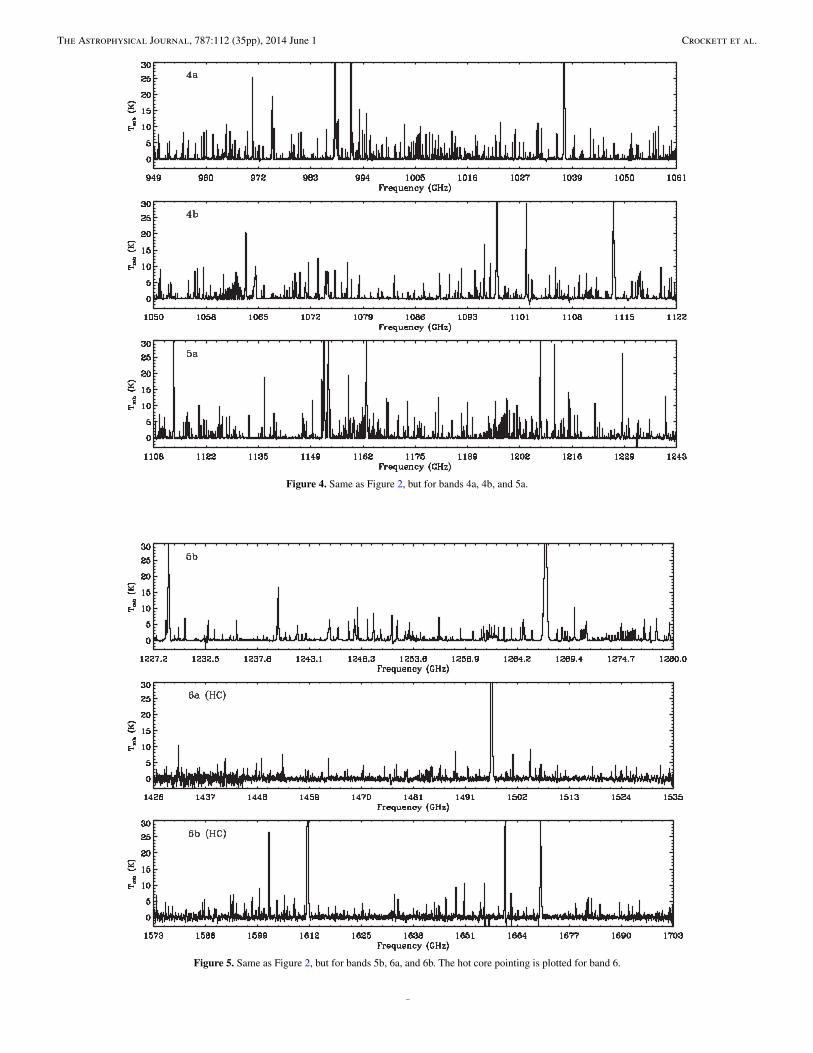
Figure 4. Same as Figure 2, but for bands 4a, 4b, and 5a.
Figure 5. Same as Figure 2, but for bands 5b, 6a, and 6b. The hot core pointing is plotted for band 6.
5
The Astrophysical Journal, 787:112 (35pp), 2014 June 1 Crockett et al.
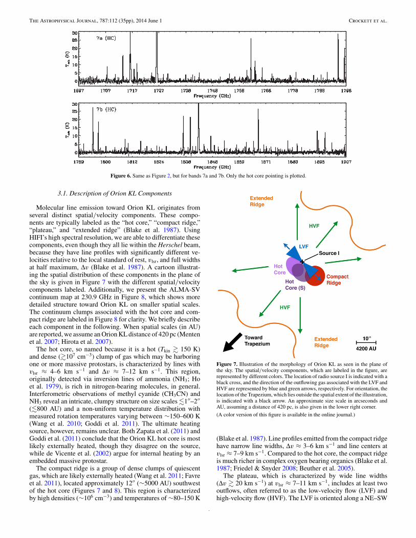
Figure 6. Same as Figure 2, but for bands 7a and 7b. Only the hot core pointing is plotted.
3.1. Description of Orion KL Components
Molecular line emission toward Orion KL originates fromseveral distinct spatial/velocity components. These compo-nents are typically labeled as the “hot core,” “compact ridge,”“plateau,” and “extended ridge” (Blake et al. 1987). UsingHIFI’s high spectral resolution, we are able to differentiate thesecomponents, even though they all lie within the Herschel beam,because they have line profiles with significantly different ve-locities relative to the local standard of rest, vlsr, and full widthsat half maximum, !v (Blake et al. 1987). A cartoon illustrat-ing the spatial distribution of these components in the plane ofthe sky is given in Figure 7 with the different spatial/velocitycomponents labeled. Additionally, we present the ALMA-SVcontinuum map at 230.9 GHz in Figure 8, which shows moredetailed structure toward Orion KL on smaller spatial scales.The continuum clumps associated with the hot core and com-pact ridge are labeled in Figure 8 for clarity. We briefly describeeach component in the following. When spatial scales (in AU)are reported, we assume an Orion KL distance of 420 pc (Mentenet al. 2007; Hirota et al. 2007).
The hot core, so named because it is a hot (Tkin ! 150 K)and dense (!107 cm#3) clump of gas which may be harboringone or more massive protostars, is characterized by lines withvlsr ( 4–6 km s#1 and !v ( 7–12 km s#1. This region,originally detected via inversion lines of ammonia (NH3; Hoet al. 1979), is rich in nitrogen-bearing molecules, in general.Interferometric observations of methyl cyanide (CH3CN) andNH3 reveal an intricate, clumpy structure on size scales "1''–2''
("800 AU) and a non-uniform temperature distribution withmeasured rotation temperatures varying between $150–600 K(Wang et al. 2010; Goddi et al. 2011). The ultimate heatingsource, however, remains unclear. Both Zapata et al. (2011) andGoddi et al. (2011) conclude that the Orion KL hot core is mostlikely externally heated, though they disagree on the source,while de Vicente et al. (2002) argue for internal heating by anembedded massive protostar.
The compact ridge is a group of dense clumps of quiescentgas, which are likely externally heated (Wang et al. 2011; Favreet al. 2011), located approximately 12'' ($5000 AU) southwestof the hot core (Figures 7 and 8). This region is characterizedby high densities ($106 cm#3) and temperatures of $80–150 K
Figure 7. Illustration of the morphology of Orion KL as seen in the plane ofthe sky. The spatial/velocity components, which are labeled in the figure, arerepresented by different colors. The location of radio source I is indicated with ablack cross, and the direction of the outflowing gas associated with the LVF andHVF are represented by blue and green arrows, respectively. For orientation, thelocation of the Trapezium, which lies outside the spatial extent of the illustration,is indicated with a black arrow. An approximate size scale in arcseconds andAU, assuming a distance of 420 pc, is also given in the lower right corner.(A color version of this figure is available in the online journal.)
(Blake et al. 1987). Line profiles emitted from the compact ridgehave narrow line widths, !v ( 3–6 km s#1 and line centers atvlsr ( 7–9 km s#1. Compared to the hot core, the compact ridgeis much richer in complex oxygen bearing organics (Blake et al.1987; Friedel & Snyder 2008; Beuther et al. 2005).
The plateau, which is characterized by wide line widths(!v ! 20 km s#1) at vlsr ( 7–11 km s#1, includes at least twooutflows, often referred to as the low-velocity flow (LVF) andhigh-velocity flow (HVF). The LVF is oriented along a NE–SW
6

The Astrophysical Journal, 787:112 (35pp), 2014 June 1 Crockett et al.
Figure 8. Continuum map of Orion KL at 230.9 GHz taken from theALMA-SV survey. The continuum clumps associated with the hot core andcompact ridge are labeled for clarity. Locations of various sources, which arelabeled in the plot, are indicated by red crosses (see the text in Section 3.1for details concerning these sources). The position of BN is also representedwith a red square. The contour levels correspond to (0.1, 0.2, 0.4, 0.5, 0.75) )1.334 Jy beam#1. A size scale in AU, assuming a distance of 420 pc, is givenin the upper left corner and the size of the synthesized beam is indicted by anoval in the lower left corner.(A color version of this figure is available in the online journal.)
axis (Genzel & Stutzki 1989; Blake et al. 1996; Stolovy et al.1998; Greenhill et al. 1998; Nissen et al. 2007; Plambeck et al.2009; Goddi et al. 2009a) and is thought to be driven by radiosource I, an embedded massive protostar with no submillimeteror IR counterpart (Menten & Reid 1995; Plambeck et al. 2009).The HVF, on the other hand, is more spatially extended (>30'')than the LVF and is oriented along a NW–SE axis, perpendicularto the LVF (Allen & Burton 1993; Chernin & Wright 1996;Schultz et al. 1999; O’dell 2001; Doi et al. 2002; Nissen et al.2012). Figure 7 illustrates the relative orientation of these twooutflows. The most compact part of the LVF, as traced byinterferometric observations of SiO (Plambeck et al. 2009), isindicated by a blue hourglass, though we note the full spatialextent of the LVF is somewhat larger ($30'', see Section 3.3).There have been several suggestions as to the ultimate powersource behind the HVF. Vibrationally excited transitions ofmethanol (CH3OH), cyanoacetylene (HC3N), and sulfur dioxide(SO2) have been detected toward the submillimeter sourceSMA1 (Beuther et al. 2004), possibly indicating the presence ofan embedded protostar, which Beuther & Nissen (2008) suggestmay be driving the HVF. Plambeck et al. (2009), on the otherhand, argue that the HVF is merely a continuation of the LVF. Yetanother possibility is that the HVF is powered by the dynamicaldecay of a multi-star system possibly involving radio source I,IR source n, and BN (Rodrıguez et al. 2005; Gomez et al. 2005,2008; Zapata et al. 2009; Bally et al. 2011; Nissen et al. 2012).Both source n and BN are themselves strong IR continuumemitters, which likely harbor embedded self-luminous sources(Becklin & Neugebauer 1967; Lonsdale et al. 1982; Menten& Reid 1995; Gezari et al. 1998; De Buizer et al. 2012). Fororientation, we indicate the positions of radio source I, SMA1,IR source n, and BN in Figure 8. We also indicate the locationsof two “infrared clumps,” IRc2 and IRc7, which are adjacent tothe hot core (Rieke et al. 1973; Gezari et al. 1998).
The extended ridge represents the most widespread, quiescentgas toward Orion KL (Figure 7). Measured rotation temperatures
are typically " 60 K, and the line profiles are narrow, !v (2–4 km s#1, with line centers at vlsr ( 8–10 km s#1 (Blake et al.1987). The extended ridge is rich in unsaturated carbon-richspecies, indicating the dominance of exothermic ion-moleculereactions that do not require activation energies (Herbst &Klemperer 1973; Watson 1973; Smith 1992; Ungerechts et al.1997).
3.2. Hot Core South
In the course of modeling the data, we noticed that sev-eral molecules contained a spectral component with !v $5–10 km s#1 and vlsr $ 6.5–8 km s#1, in between line param-eters typically associated with the hot core and compact ridge.The presence of this type of component was noted previouslyby Neill et al. (2013b), who present a detailed analysis of waterand HDO emission in the Orion KL HIFI survey. Specifically,HD18O lines detected in the HIFI scan have an average vlsr =6.7 km s#1 and !v = 5.4 km s#1, consistent with this “in be-tween” component. Using HDO interferometric maps obtainedfrom the ALMA-SV line survey of Orion KL (Section 2.3), theNeill et al. (2013b) study showed that this emission likely orig-inates from a high water column density clump approximately1'' south of the hot core submillimeter continuum peak.
We employ the ALMA-SV data set here to map, in additionto HDO, 13CH3OH, another species which contains an “inbetween” component in the HIFI scan (vlsr = 7.5 km s#1,!v = 6.5 km s#1), 13CH3CN, a hot core tracer with typical lineparameters for that region (vlsr ( 5.5 km s#1, !v ( 8 km s#1),and methyl formate (CH3OCHO), a prominent compact ridgetracer also with typical line parameters (vlsr ( 8 km s#1, !v (3 km s#1). Figure 9 contains four panels each plotting anintegrated intensity map (color scale) of a transition from oneof these molecules. The continuum at 230.9 GHz is overlaidas white contours in each panel. White crosses indicate thelocations of IRc7, and methyl formate peaks MF1, MF4, andMF5 in the notation of Favre et al. (2011). The submillimeterclump associated with the hot core is also labeled. We used thesame data product presented in Neill et al. (2013b) to makeFigure 9.
From Figure 9, we see that 13CH3CN traces the hot corecontinuum closely, while HDO, as first pointed out by Neillet al. (2013b), traces a clump $1'' south of the continuum peak.The 13CH3OH map in Figure 9 is integrated in the velocityrange 3–5 km s#1 to avoid emission from the compact ridge,which methanol also traces. As such, Figure 9 shows that13CH3OH emission from the “in between” component does notoriginate from the compact ridge as traced by methyl formate.Rather, this emission is strongest just south of where 13CH3CNpeaks. Because the difference is more subtle than with HDO,Figure 10 plots the 13CH3OH/13CH3CN integrated intensityratio, which shows a clear gradient in 13CH3OH emissionrelative to 13CH3CN from north to south. Given that HDOand 13CH3OH both trace regions south of the 13CH3CN peak,we assume other molecules displaying emission from this “inbetween” component originate from a similar region. We thuslabel this component “hot core south” or hot core (S), which werepresent schematically in the cartoon presented in Figure 7.
3.3. XCLASS Modeling
All molecular species are modeled using XCLASS.This program uses both the CDMS (Muller et al. 2001,2005; http://www.cdms.de) and JPL (Pickett et al. 1998;
7

The Astrophysical Journal, 787:112 (35pp), 2014 June 1 Crockett et al.
Figure 9. Integrated intensity maps obtained from lines in the ALMA-SV data set plotted as a color scale. The velocity range over which the intensity is integratedis given in each panel. The transitions plotted are 13CH3CN 132–122 (upper left), 13CH3OH-E 52–42 (lower left), HDO 31,2–22,1 (lower right), and CH3OCHO196,13–186,12 (upper right). We only show integrated emission in the range 3–5km s#1 for 13CH3OH because we wanted to avoid contamination from the compactridge. The continuum at 230.9 GHz is overlaid in each panel as white contours. The contour levels correspond to (0.1, 0.2, 0.4, 0.5, 0.75) ) 1.334 Jy beam#1. Thesynthesized beam size is indicated by an oval in the lower left corner of each panel.(A color version of this figure is available in the online journal.)
Figure 10. Integrated intensity ratio of the 13CH3OH-E map to 13CH3CN givenin Figure 9 showing the increase in methanol emission relative to methyl cyanidefrom north to south. The synthesized beam size is indicated by an oval in thelower left corner.(A color version of this figure is available in the online journal.)
http://spec.jpl.nasa.gov) databases to produce model spectraassuming local thermodynamic equilibrium (LTE). Input pa-rameters are the telescope diameter, Dtel, source size, %s , rota-tion temperature, Trot, total column density, Ntot, line velocity
relative to the local standard of rest, vlsr, and line full width athalf maximum, !v. In order to account for dust extinction, thedust optical depth, 'd , is parameterized by a power law,
'd = 2mH(!dust)NH2(1.3 mm
! "
230 GHz
")
, (1)
where NH2 is the H2 column density, (1.3 mm is the dust opacityat 1.3 mm (230 GHz), ) is the spectral index, mH is the massof a hydrogen atom, and !dust is the dust to gas mass ratio.As outlined below, we hold NH2 and %s fixed for a givenspatial/velocity component but note that there are severalexceptions in which we varied %s to obtain better agreementbetween the models and data. These instances are explained inSection 5. We also set Dtel = 3.5 m and 30 m when comparingour models to the HIFI and IRAM surveys, respectively. Wevaried Trot, Ntot, vlsr, and !v as free parameters. Additionalinformation regarding XCLASS, e.g., specific equations usedin the code, can be found in Comito et al. (2005) and Zernickelet al. (2012).
We assume that all molecules emitting from the same spatial/velocity component have the same source size, which is asimplifying assumption. The aim of this study, however, isnot a detailed analysis of any single molecule. It is a holisticanalysis of the entire spectrum. This is therefore a reasonableapproximation and is in line with previous spectral survey papersof Orion KL (see, e.g., Tercero et al. 2010, 2011). Adoptedsource sizes for each spatial/velocity component are given in
8

The Astrophysical Journal, 787:112 (35pp), 2014 June 1 Crockett et al.
Table 2Adopted Values for Source Size and H2 Column Density
Component %s NH2
('') (cm#2)
Hot core 10 3.1 ) 1023
Compact ridge 10 3.9 ) 1023
Plateau 30 2.8 ) 1023
Extended ridge 180 7.1 ) 1022
Note. Values for %s and NH2 , including references, areexplained in Section 3.3.
Table 2. We estimate %s for the hot core and compact ridge usinginterferometric observations from Beuther & Nissen (2008) andFavre et al. (2011), respectively. The plateau source size wasobtained from Herschel/HIFI water maps taken as part of theHEXOS program (G. J. Melnick et al. 2014, in preparation).Finally, we assume a source size of 180'' for the extended ridgeto reflect the fact that the extended ridge completely fills theHerschel beam at all frequencies. For several molecules, wewere forced to use %s values that differed from those givenin Table 2. These deviations are explained in the descriptionsof individual molecular fits presented in Section 5. Estimatesof NH2 for each spatial/velocity component are also given inTable 2. We obtained these values from Plume et al. (2012), whouse C18O lines within the Orion KL HIFI scan to derive totalC18O column densities, which they convert to NH2 estimates byassuming a CO abundance of 1.0 ) 10#4 and 16O/18O = 500.We modified the H2 column densities for the compact ridgeand plateau because the Plume study assumed source sizes forthese components that are different from what we adopt here.Consequently, we recalculated the C18O upper state columnsassuming the source sizes used in this study and applied thesame correction factors reported by Plume et al. (2012).
For the dust extinction power law, we assume (1.3 mm =0.42 cm2 g#1, corresponding to the midpoint between baregrains and grains with thin ice mantles (Ossenkopf & Henning1994). We also set ) = 2 and !dust = 0.01. In the course ofmodeling the data, we found that the NH2 values given in Table 2tended to underestimate the extinction necessary to reproducethe emission in the highest frequency bands where the dustoptical depth is highest. In other words, molecules fit well atfrequencies below $1 THz always tended to be overpredictedat higher frequencies. As a result, we use a higher NH2 estimateto compute the dust optical depth. We adopt a value of NH2 =2.5 ) 1024 cm#2 for the hot core, compact ridge, and plateau.Because the extended ridge represents lower density gas thatis not as heavily embedded, we retain the NH2 value given inTable 2 for this spatial/velocity component. Figure 11 plots eighttransitions of dimethyl ether (CH3OCH3), a prominent compactridge tracer. The panels are organized so that both columnsspan a range in upper state energy, Eup, from $200 to 600 K,with Eup increasing from bottom to top. Lines in the left andright columns occur at frequencies below and above 800 GHz,respectively. Transitions in the left column are therefore lessaffected by dust extinction than the right with both columnscovering similar ranges in Eup. The red line corresponds to anXCLASS fit which sets NH2 = 2.5 ) 1024 cm#2, while the blueline represents a similar model that assumes the H2 columndensity given in Table 2. Dimethyl ether column densities forthe higher and lower extinction fits are 6.5 ) 1016 cm#2 and5.9 ) 1016 cm#2, respectively. Both models set Trot = 110 Kand %s = 10''. From the plot, we see that the model with greater
dust extinction fits the data better than the lower extinctionmodel over all frequencies. Because similar ranges in Eup arecovered at low and high frequencies, it is not possible to improvethe fit at lower extinction by changing either Trot or %s . Weobserved the same trend for molecules detected toward the hotcore and plateau. Figure 12 plots a sample of eight transitions of34SO2, a molecule with strong hot core and plateau components,organized in the same way as Figure 11, with red and bluelines representing an analogous set of XCLASS models. Weagain see better agreement for the higher extinction model. TheNH2 we adopt to compute 'd is between six and nine timeslarger than the H2 column densities derived toward the hot core,compact ridge, and plateau using C18O line emission but iscommensurate with other NH2 estimates derived from millimeterand submillimeter observations, which report NH2 ! 1024 cm#2
(Favre et al. 2011; Mundy et al. 1986; Genzel & Stutzki 1989).This difference could be resolved by assuming a higher dustopacity, i.e., increasing (1.3 mm by the same factor NH2 is reduced(see Equation (1)). However, because this adjustment wouldresult in the same 'd , we use the higher NH2 and conclude a dustoptical depth which obeys the relation
'd = 3.5 ) 10#2! "
230 GHz
"2, (2)
which produces the required dust extinction to accurately fit thedata across the entire HIFI band.
We fit an XCLASS model to the emission of each molecule byfirst selecting a sample of transitions with varying line strengthsthat covered the entire range in excitation energy over whichemission was detected. For simple species, with relatively fewlines, this was straightforward. For more complex organics,however, we had many lines, thousands in some cases, fromwhich to choose. Care was taken to select lines that were notblended with any other species. This was done by overlayingthe full band model and observed spectrum while we selectedtransitions on which to base our fit. Because the full band modelis the sum of all molecular fits, it evolved as the individualmolecular fits changed. Once a sample of lines was selected,each transition was plotted simultaneously in a different panelwith the panels arranged so that the upper state energy increasedfrom the lower left panel to the upper right. The emission wasthen fit by varying the free parameters (i.e., Trot, Ntot, vlsr, and!v) by hand until good agreement, as assessed by eye, wasachieved between the data and models at all excitation energies.At this point, we computed a reduced !2 metric (described inthe Appendix) for each model across the entire HIFI band inorder to determine how well the models reproduced the datarelative to one another and to identify those fits which could beimproved. Model fits were then revised iteratively.
We found that automated fitting algorithms had diffi-culty reaching reasonable solutions, especially when multiplespatial/velocity components and/or temperature gradients wererequired. Weaker species (Tpeak " 1 K) that had observed lineintensities close to the noise, combined with the prevalence ofline blends, presented additional difficulties in assessing thegoodness of fit with these algorithms. As a result, we derivedmost models by hand. However, in some instances, when a sam-ple of strong unblended transitions was available, we employedthe MAGIX program (Moller et al. 2013), which optimizesthe output of other numerical codes (XCLASS in this case), toautomate the fitting process using a Levenberg–Marquardt algo-rithm. MAGIX utilizes a subset of observed transitions suppliedby the user to assess the goodness of fit for a given molecule.
9

The Astrophysical Journal, 787:112 (35pp), 2014 June 1 Crockett et al.
Figure 11. Sample of eight CH3OCH3 lines from the HIFI scan. The data are plotted in black and the quantum numbers, rest frequency, and Eup for each transitionare labeled from top to bottom in each panel. We use the quantum numbers from the EA spin isomer but note that transitions from AA, EE, AE, and EA-CH3OCH3are blended together at HIFI frequencies. The red and blue lines represent XCLASS models which assume NH2 = 2.5 ) 1024 cm#2 and 3.9 ) 1023 cm#2 and setNtot = 6.5 ) 1016 cm#2 and 5.9 ) 1016 cm#2, respectively. Both models set Trot = 110 K and %s = 10''. Dimethyl ether is also detected toward the hot core but thiscomponent is not emissive for the transitions plotted here.(A color version of this figure is available in the online journal.)
Consequently, we carried out by hand alterations to these fitsonce reduced !2 calculations were performed over the entireHIFI band as described above.
When we observed more than one isotopologue for a givenmolecule, effort was made to produce models which usedconsistent values for Trot, !v, and vlsr for all isotopic species.We, however, sometimes made small adjustments to theseparameters to get the optimum fit. The major difference betweenthe models is thus the column density, the ratio of whichshould be equal to the isotopic abundance ratio. Among rarerisotopologues, isotopic ratios inferred from our models arecommensurate with those derived previously toward Orion KL(Tercero et al. 2010; Blake et al. 1987), indicating opticallythin emission. Our models, however, also indicate that many ofthe most abundant isotopologues are optically thick, meaningour models likely underestimate Ntot. Furthermore, we oftenhad to fit very optically thick isotopologues with higher rotationtemperatures than their more optically thin counterparts in orderto reproduce the observed line intensities over all energies.
Emission from these species therefore is too optically thick fromwhich to derive reliable Trot and Ntot values using XCLASS. As aresult, these models serve mainly as templates for the molecularemission. Species that fall into this category are marked with an“X” in Table 3. This table is broken down by spatial/velocitycomponent because a particular molecule may not be opticallythick in all of its components.
While modeling the hot core and plateau with XCLASS, wefound that, for some molecules, a single temperature fit failed toreproduce the observed emission, which suggests the presenceof temperature gradients in these components. This was mostapparent when trying to simultaneously fit both the IRAM andHIFI data. Because the IRAM data, in general, probed lowerenergy transitions compared to HIFI, the IRAM spectra some-times required additional cooler subcomponents in order for asingle model to fit both data sets well. We, therefore, includedadditional subcomponents when necessary to simulate temper-ature gradients. For the hot core, the subcomponent responsiblefor most of the emission in the HIFI scan always had a source
10

The Astrophysical Journal, 787:112 (35pp), 2014 June 1 Crockett et al.
Figure 12. Sample of eight 34SO2 lines from the HIFI scan. The data are plotted in black and the quantum numbers, rest frequency, and Eup for each transition arelabeled from top to bottom in each panel. The red and blue lines represent XCLASS models which assume NH2 = 2.5 ) 1024 cm#2 and 3.9 ) 1023 cm#2, respectively.Each model has a hot core and plateau component. The model plotted in red sets Ntot = 5.0 ) 1015 and 4.7 ) 1015 cm#2, while the model plotted in blue sets Ntot =3.5 ) 1015 and 3.0 ) 1015 cm#2 for the hot core and plateau components, respectively. Both models set Trot = 240 K and 150 K and %s = 10'' and 30'' for the hotcore and plateau components, respectively. There are additional cooler subcomponents present in these models to fit the emission at lower excitation for both the hotcore and plateau. These subcomponents, however, are not significantly emissive for the plotted transitions.(A color version of this figure is available in the online journal.)
size of 10''. Hotter or cooler subcomponents were then addedsuch that the source size increased or decreased by successivefactors of two. Temperature gradients were organized such thatTrot increased as %s decreased (i.e., the more compact emission ishotter), corresponding to an internally heated clump. We chosethis convention based on more detailed non-LTE models pre-sented by Neill et al. (2013b) and Crockett et al. (2014) whichfit the H2O/HDO and H2S emission, respectively, within theHIFI scan. In order to reproduce the observed emission of thesespecies, their models require enhanced near and far-IR radiationfields relative to what is observed, suggesting the presence ofa self-luminous source or sources within the hot core. More-over, ethyl cyanide (C2H5CN) transitions observed within theALMA-SV survey show that more highly excited C2H5CN linesoriginate from a more compact region than lower lying transi-tions (C. Favre et al. 2014, in preparation). For the plateau, wekept a 30'' source size for all subcomponents to simulate thefact that the plateau fills most of the Herschel beam at HIFI
frequencies. We did not need temperature gradients to fit thecompact ridge or extended ridge in our XCLASS models.
Our final XCLASS models are plotted in Figure 13, availablein the online edition. In this set, each molecule is representedby a figure in which a sample of transitions is plotted coveringthe entire range in excitation energy over which that species isdetected. At least one transition is plotted in each panel, andthe panels are organized so that Eup increases from the lowerleft panel to the upper right. The lowest energy panels oftenshow transitions observed in the IRAM scan. The quantumnumbers corresponding to the transition at the center of eachpanel are labeled. The solid blue line represents the XCLASSmodel for the molecule being considered, the solid green linecorresponds to the model emission from all other molecules,and the dashed red line is the model for all detected species(the sum of the former two curves). Figures 13.13, 13.33,and 13.66 show examples from Figure 13, which plot themolecular fits for H13CN, a polyatomic linear rotor, H2CS,
11

The Astrophysical Journal, 787:112 (35pp), 2014 June 1 Crockett et al.
Figure 13. Observed transitions in the HIFI and IRAM surveys (black) with the XCLASS model for H13CN overlaid as a blue solid line. Modeled emission fromall other species (solid green) along with the total fit (dashed red) are also overlaid. Quantum numbers labeling each transition are given in each panel and excitationenergy increases from the lower left panel to the upper right. See Section 5 for a description of the quantum numbers.
(A color version and the complete figure set (91 images) of this figure are available in the online journal.)
an asymmetric rotor, and CH3OCHO, a complex organic,respectively. These figures illustrate the diversity in observedline profiles not only between molecules, which trace differentspatial/velocity components, but also from the same species atdifferent excitation energies. The latter arises because the hotcore, compact ridge, plateau, and extended ridge are emissiveover different ranges in excitation energy.
XCLASS model parameters for molecular fits from which weobtain robust Trot and Ntot information are given in Table 4 . Wedo not include models marked in Table 3 because they do notprovide any physical information. We estimate the uncertaintyin our derived Trot and Ntot values to be approximately 10% and25%, respectively. Our estimated error in vlsr is ±1 km s#1 forthe hot core, compact ridge, and extended ridge, and ±2 km s#1
for the plateau. We also estimate !v errors of ±0.5 km s#1,1.5 km s#1, and 5.0 km s#1, for the compact/extended ridge, hotcore, and plateau, respectively. These uncertainty calculationsare described in the Appendix.
3.4. MADEX Modeling
A subset of the molecules detected in the HIFI scan were alsomodeled using the MADEX code. When collisional excitationrates are available, this non-LTE program solves the equationsof statistical equilibrium assuming the large velocity gradientapproximation based on the formalism of Goldreich & Kwan(1974). MADEX computes transition frequencies and linestrengths for most molecules directly from an internal databaseof rotation constants and dipole moments. For a small fraction($6%) of molecules, however, frequencies and line strengthsare taken directly from the JPL and CDMS catalogs. If collisionrates do not exist for a given molecular species, model spectracan also be computed assuming LTE. Just as with XCLASS,model input parameters include: Dtel, %s , Ntot, vlsr, and !v.Because MADEX is a non-LTE code, the user must also setthe kinetic temperature, Tkin, and the H2 volume density, nH2 .We take %s , Tkin, nH2 , Ntot, vlsr, and !v to be free parameters.
12

The Astrophysical Journal, 787:112 (35pp), 2014 June 1 Crockett et al.
Table 3Optically Thick Molecules
Molecule Hot Core Compact Ridge Plateau Extended Ridge
CH3CN X X X · · ·CH3OH X X · · · · · ·13CO X X X XCS X X X XH2CO X X · · ·H2
18O X X X · · ·H2S X · · · XHCN X X X XHCN,"2 = 1 X · · · · · · · · ·H13CN X X XHCO+ X X X XHNC X X XHNCO X · · · X · · ·NH3 X · · · X XOH · · · · · · X · · ·SiO · · · · · · X · · ·SO X · · · XSO2 X X
Note. “X” indicates an optically thick model, “. . .” corresponds to a non-detection, and no mark indicates an optically thin model, which will have anentry in Table 4 and possibly Table 5.
However, as described in more detail below, we attempt touse consistent Tkin and nH2 values for a given spatial/velocitycomponent, especially when modeling a gradient, and apply %s
values that are similar to those used with XCLASS. We alsoset Dtel = 3.5 m and 30 m when modeling the HIFI and IRAMsurveys, respectively, consistent with XCLASS. Additionally,the user can also specify a spatial offset from the center pointingposition, !% , to account for differences in the telescope response.For the hot core and compact ridge, we adopt a !% value of 3'' anddo not apply any spatial offsets for the plateau or extended ridge.These values were obtained from a two-dimensional line surveyof Orion KL taken with the IRAM 30 m telescope (N. Marcelinoet al. 2014, in preparation).
Our modeling approach is similar to previous studies whichuse MADEX to model molecular emission within the IRAMsurvey (N. Marcelino et al. 2014, in preparation; Tercero et al.2010, 2011; Esplugues et al. 2013a, 2013b). The moleculeswe model using MADEX are: CH3CN, HCN, HNC, HCO+,SO, SO2, and their isotopologues. These molecules are chosenbecause they have existing collision rates for states probedby HIFI. This group also includes a complex organic aswell as simpler two and three atom molecules. In addition,these species are detected toward almost every spatial/velocitycomponent. (We do not detect CH3CN and SO toward theextended ridge and compact ridge, respectively.) Temperatureand density gradients surely exist within these components(see, e.g., Wang et al. 2011, 2010). As a result, we modelall but the extended ridge and, in some cases, the compactridge with multiple subcomponents which vary both Tkin andnH2 to simulate such gradients. Utilizing MADEX in this way,thus, allows us to compare the column densities, and ultimatelymolecular abundances, derived from our XCLASS LTE modelsto more advanced non-LTE calculations, which include bothtemperature and density gradients. In particular, we are ableto determine if including density gradients significantly affectsthe determination of molecular abundances toward the differentspatial velocity/components. Where possible, we have used thesame values for !v, vlsr, %s , Tkin, and nH2 for the subcomponents,
Table 4XCLASS Model Parameters
Molecule %s Trot Ntot vlsr !v
('') (K) (cm#2) (km s#1) (km s#1)
Hot core
C2H3CN 20 130 7.5 ) 1014 3.5 12.5C2H3CN 10 215 2.7 ) 1015 5.0 5.5C2H5CN 10 136 2.1 ) 1016 5.0 7.0C2H5CN 5 300 6.5 ) 1015 5.0 7.0CH2NH 10 130 1.3 ) 1015 6.0 8.0CH3CN,"8 = 1 10 260 3.7 ) 1015 6.0 6.013CH3CN 20 80 8.0 ) 1013 5.5 8.013CH3CN 10 260 1.3 ) 1014 5.5 8.0CH3
13CN 20 80 8.0 ) 1013 5.5 8.0CH3
13CN 10 260 1.3 ) 1014 5.5 8.0C18O 10 150 1.9 ) 1017 6.0 9.0C17O 10 150 6.3 ) 1016 6.0 9.0H2O,"2 5 270 1.7 ) 1019 5.5 7.0H2
17O 5 270 5.5 ) 1015 4.8 7.0HDO 5 270 3.0 ) 1016 5.0 7.0H2
34S 6 145 3.8 ) 1016 4.5 8.6H2
33S 6 145 1.1 ) 1016 4.5 8.6HC3N 20 10 1.0 ) 1015 5.5 6.5HC3N 10 210 1.5 ) 1015 5.5 6.5HC3N,"7 = 1 20 10 1.0 ) 1015 5.5 6.5HC3N,"7 = 1 10 210 1.5 ) 1015 5.5 6.5HCN,"2 = 2 10 217 4.7 ) 1017 6.0 7.0H13CN,"2 = 1 10 157 3.5 ) 1016 5.5 6.0HC15N 20 20 1.5 ) 1014 4.5 10.0HC15N 10 210 3.5 ) 1014 4.5 10.0DCN 20 20 9.0 ) 1013 6.0 8.0DCN 10 210 1.6 ) 1014 5.5 8.0H13CO+ 10 190 9.0 ) 1012 6.0 10.0HNC,"2 = 1 10 220 1.3 ) 1015 4.5 7.0HN13C 20 15 3.0 ) 1012 2.5 8.5HN13C 10 220 3.5 ) 1013 2.5 8.5HN13CO 20 30 4.5 ) 1013 6.3 6.2HN13CO 10 209 4.9 ) 1014 6.3 6.2o-NH2 10 130 1.3 ) 1015 6.0 12.0NH3,"2 10 250 1.3 ) 1017 6.0 5.515NH3 10 200 1.0 ) 1015 5.0 5.5NH2D 10 250 3.9 ) 1015 6.2 6.0NO 10 180 1.7 ) 1017 6.0 8.0NS 10 105 2.1 ) 1015 4.2 10.5OCS 10 190 3.2 ) 1016 6.0 8.034SO 20 70 4.5 ) 1014 4.5 7.034SO 10 258 1.8 ) 1015 4.5 7.033SO 20 70 2.3 ) 1014 4.5 7.033SO 10 258 5.0 ) 1014 4.5 7.0SO2,"2 = 1 10 240 9.0 ) 1016 6.0 7.034SO2 20 50 1.1 ) 1015 5.0 8.034SO2 10 240 5.0 ) 1015 5.0 8.033SO2 20 50 2.6 ) 1014 5.0 8.033SO2 10 240 1.3 ) 1015 5.0 8.0
Hot core (S)
CCH 10 53 2.3 ) 1015 7.0 13.5CH3OCH3 10 100 2.1 ) 1016 7.2 10.013CH3OH 10 128 1.5 ) 1016 7.5 6.5CH3OD-A 10 128 7.8 ) 1014 7.5 6.5CH3OD-E 10 128 7.8 ) 1014 7.5 6.5CH2DOH 10 128 1.3 ) 1015 7.5 6.513CS 10 100 9.7 ) 1014 6.5 10.5C34S 10 100 1.9 ) 1015 6.5 10.5C33S 10 100 6.4 ) 1014 6.5 10.5H2
13CO 10 135 8.5 ) 1014 6.5 13.0H2CS 10 120 4.6 ) 1015 7.5 7.5HD18O 3 100 1.3 ) 1015 6.5 6.0D2O 3 100 7.0 ) 1014 6.5 6.0
13

The Astrophysical Journal, 787:112 (35pp), 2014 June 1 Crockett et al.
Table 4(Continued)
Molecule %s Trot Ntot vlsr !v
('') (K) (cm#2) (km s#1) (km s#1)
Compact ridge
C2H5OH 10 110 6.5 ) 1015 7.8 2.5CH3CN,"8 = 1 10 230 3.5 ) 1015 7.5 4.013CH3CN 10 230 1.1 ) 1014 7.5 4.0CH3
13CN 10 230 1.1 ) 1014 7.5 4.0CH3OCH3 10 110 6.5 ) 1016 8.0 3.2CH3OCHO 10 110 1.3 ) 1017 8.0 2.813CH3OH 10 140 1.0 ) 1016 7.8 2.5CH3OD-A 10 140 1.7 ) 1015 7.8 2.5CH3OD-E 10 140 1.7 ) 1015 7.8 2.5CH2DOH 10 140 8.1 ) 1015 7.8 2.5C18O 10 125 1.3 ) 1017 8.0 4.0C17O 10 125 2.0 ) 1016 8.0 4.013C18O 10 125 2.5 ) 1015 8.0 4.013CS 10 225 2.0 ) 1014 7.2 4.0C34S 10 225 2.5 ) 1014 7.2 4.0C33S 10 225 1.3 ) 1014 7.2 4.0H2CCO 10 100 2.0 ) 1015 8.0 3.0H2
13CO 15 50 3.8 ) 1014 8.0 3.5HDCO 12 60 1.8 ) 1014 10.0 2.2HDCO 12 60 2.6 ) 1014 7.7 2.2H2CS 10 100 2.9 ) 1015 8.0 3.0H2
17O 5 150 9.0 ) 1014 8.0 3.0HDO 5 150 3.5 ) 1015 8.0 3.0H13CN 10 120 3.6 ) 1013 8.0 4.0DCN 10 120 1.7 ) 1013 8.0 4.0H13CO+ 20 100 3.0 ) 1012 9.0 5.5HCS+ 10 105 1.8 ) 1014 9.0 6.0HNC 10 80 6.5 ) 1013 9.0 3.0NH2CHO 10 190 7.5 ) 1014 7.2 4.8NO 10 70 3.2 ) 1016 7.2 2.5NS 10 200 6.1 ) 1014 7.7 5.5OCS 10 165 4.3 ) 1015 7.5 2.5OD 10 125 2.5 ) 1014 8.0 3.5SO2 10 100 1.8 ) 1015 8.2 3.0
Plateau
CH3CN,"8 = 1 30 120 1.0 ) 1016 6.0 18.013CH3CN 30 120 6.5 ) 1013 6.0 18.0CH3
13CN 30 120 6.5 ) 1013 6.0 18.0CN 30 43 6.3 ) 1014 8.0 20.0C18O 30 130 1.3 ) 1017 8.5 25.0C17O 30 130 3.7 ) 1016 8.5 25.013CS 30 30 6.1 ) 1013 8.7 26.713CS 30 155 2.8 ) 1013 8.7 26.7C34S 30 30 1.5 ) 1014 8.7 26.7C34S 30 155 6.4 ) 1013 8.7 26.7C33S 30 30 5.0 ) 1013 8.7 26.7C33S 30 155 1.7 ) 1013 8.7 26.7H2CO 30 20 1.1 ) 1015 8.0 32.0H2CO 30 88 3.5 ) 1015 8.0 23.0H2
17O 30 150 2.3 ) 1015 9.0 25.0HDO 30 150 1.5 ) 1015 9.0 25.0H2
34S 30 12 2.1 ) 1015 9.0 30.0H2
34S 30 115 2.5 ) 1015 9.0 30.0H2
33S 30 12 5.6 ) 1014 9.0 30.0H2
33S 30 115 7.5 ) 1014 9.0 30.0HC3N 30 115 1.3 ) 1015 5.5 23.0HC3N,"7 = 1 30 115 3.0 ) 1015 5.5 23.0HCl 50 73 1.4 ) 1015 11.5 25.0H37Cl 50 73 4.9 ) 1014 11.5 25.0HC15N 30 25 2.3 ) 1014 7.5 28.0HC15N 30 130 1.0 ) 1014 8.5 28.0DCN 30 25 3.5 ) 1013 5.5 20.0DCN 30 130 3.2 ) 1013 8.5 20.0
Table 4(Continued)
Molecule %s Trot Ntot vlsr !v
('') (K) (cm#2) (km s#1) (km s#1)
H13CO+ 30 25 1.5 ) 1013 9.0 50.0H13CO+ 30 135 1.7 ) 1012 8.5 30.0HN13C 30 20 1.0 ) 1013 7.5 28.0HN13C 30 115 4.3 ) 1012 7.5 25.0HN13CO 30 25 2.0 ) 1013 9.0 20.0HN13CO 30 168 4.3 ) 1013 9.0 20.015NH3 30 35 9.5 ) 1013 6.0 15.0NO 30 155 1.5 ) 1017 8.0 27.0OCS 30 110 1.2 ) 1016 5.0 21.029SiO 30 25 1.5 ) 1014 10.0 35.029SiO 30 120 4.8 ) 1013 10.0 35.029SiO 30 18 1.0 ) 1014 8.0 15.029SiO 30 270 5.2 ) 1013 7.0 15.030SiO 30 25 1.6 ) 1014 10.0 35.030SiO 30 120 3.0 ) 1013 10.0 35.030SiO 30 18 6.7 ) 1013 8.0 15.030SiO 30 270 4.1 ) 1013 7.0 15.0SiS 30 145 4.3 ) 1014 8.5 23.034SO 30 65 4.6 ) 1015 10.0 26.034SO 30 163 3.0 ) 1015 10.0 26.033SO 30 65 1.1 ) 1015 10.0 26.033SO 30 163 7.5 ) 1014 10.0 26.034SO2 30 20 3.0 ) 1014 9.5 30.034SO2 30 50 2.5 ) 1015 9.5 30.034SO2 30 150 4.7 ) 1015 9.5 23.033SO2 30 20 7.1 ) 1013 9.5 30.033SO2 30 50 5.9 ) 1014 9.5 30.033SO2 30 150 9.8 ) 1014 9.5 23.0
Extended ridge
CCH 180 37 4.5 ) 1014 8.8 3.5CH2NH 180 40 2.0 ) 1013 9.0 4.0CN 180 21 2.2 ) 1014 9.0 3.5C18O 180 40 1.4 ) 1016 9.0 3.0C17O 180 40 6.2 ) 1015 9.0 3.013C18O 180 40 2.3 ) 1014 9.0 3.013CS 180 35 2.5 ) 1013 8.0 4.0C34S 180 35 4.2 ) 1013 8.0 4.0C33S 180 35 8.5 ) 1012 8.0 4.0H2S 180 50 1.0 ) 1014 8.6 3.0HC15N 180 30 1.0 ) 1013 8.5 4.0DCN 180 30 9.5 ) 1012 8.5 4.0H13CO+ 180 27 5.3 ) 1012 9.0 4.5HN13C 180 20 1.2 ) 1012 8.0 3.0o-NH2 180 50 2.0 ) 1013 8.0 3.015NH3 180 23 5.3 ) 1012 8.2 3.0NO 180 60 7.5 ) 1015 10.0 5.0OCS 180 10 2.0 ) 1015 7.5 2.5SO 180 60 7.8 ) 1014 10.5 5.0SO2 180 50 3.0 ) 1014 8.2 3.0
Notes. We estimate the uncertainties of Trot and Ntot in our XCLASS modelsto be $10% and 25%, respectively. Errors in vlsr are ±1 km s#1 for the hotcore, compact ridge, and extended ridge, and ±2 km s#1 for the plateau. Errorsin !v are ±0.5 km s#1, 1.5 km s#1, and 5.0 km s#1 for the compact/extendedridge, hot core, and plateau, respectively. See the Appendix for more detailsconcerning error estimates.
allowing only the column density to vary. In order to obtainbetter agreement between the data and model, however, slightadjustments were needed in some cases. The need for theseadjustments likely indicates the sensitivity of these moleculesto the complex underlying physical structure of Orion KL. Justas with XCLASS, these parameters were varied by hand.
14
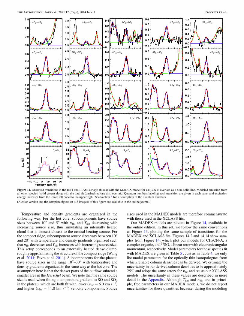
The Astrophysical Journal, 787:112 (35pp), 2014 June 1 Crockett et al.
Figure 14. Observed transitions in the HIFI and IRAM surveys (black) with the MADEX model for CH3CN-E overlaid as a blue solid line. Modeled emission fromall other species (solid green) along with the total fit (dashed red) are also overlaid. Quantum numbers labeling each transition are given in each panel and excitationenergy increases from the lower left panel to the upper right. See Section 5 for a description of the quantum numbers.
(A color version and the complete figure set (18 images) of this figure are available in the online journal.)
Temperature and density gradients are organized in thefollowing way. For the hot core, subcomponents have sourcesizes between 10'' and 5'' with nH2 and Tkin decreasing withincreasing source size, thus simulating an internally heatedcloud that is densest closest to the central heating source. Forthe compact ridge, subcomponent source sizes vary between 10''
and 20'' with temperature and density gradients organized suchthat nH2 decreases and Tkin increases with increasing source size.This setup corresponds to an externally heated dense clump,roughly approximating the structure of the compact ridge (Wanget al. 2011; Favre et al. 2011). Subcomponents for the plateauhave source sizes in the range 10''–30'' with temperature anddensity gradients organized in the same way as the hot core. Theassumption here is that the denser parts of the outflow subtend asmaller area in the Herschel beam. We note that the same sourcesize is used when fitting a temperature gradient to SO and SO2in the plateau, which are both fit with lower (vlsr = 6.0 km s#1)and higher (vlsr = 11.0 km s#1) velocity components. Source
sizes used in the MADEX models are therefore commensuratewith those used in the XCLASS fits.
Our MADEX models are plotted in Figure 14, available inthe online edition. In this set, we follow the same conventionsas Figure 13, plotting the same sample of transitions for theMADEX and XCLASS fits. Figures 14.2 and 14.14 show sam-ples from Figure 14, which plot our models for CH3CN-A, acomplex organic, and 34SO, a linear rotor with electronic angularmomentum, respectively. Model parameters for those species fitwith MADEX are given in Table 5 . Just as in Table 4, we onlylist model parameters for the optically thin isotopologues fromwhich reliable column densities can be derived. We estimate theuncertainty in our derived column densities to be approximately25% and adopt the same errors for vlsr and !v as our XCLASSmodels. The uncertainty in these values are described in moredetail in the Appendix. Although Tkin and nH2 are, in princi-ple, free parameters in our MADEX models, we do not reportuncertainties for these quantities because, during the modeling
15

The Astrophysical Journal, 787:112 (35pp), 2014 June 1 Crockett et al.
Table 5MADEX Model Parameters
Molecule %s Tkin nH2 Ntot vlsr !v
('') (K) (cm#3) (cm#2) (km s#1) (km s#1)
Hot core13CH3CN-A 10.0 250.0 1.5 ) 107 5.0 ) 1013 5.5 9.013CH3CN-A 7.0 300.0 5.0 ) 107 2.5 ) 1013 5.5 7.013CH3CN-A 5.0 400.0 1.0 ) 108 3.0 ) 1013 6.0 5.013CH3CN-E 10.0 250.0 1.5 ) 107 5.0 ) 1013 5.5 9.013CH3CN-E 7.0 300.0 5.0 ) 107 2.5 ) 1013 5.5 7.013CH3CN-E 5.0 400.0 1.0 ) 108 3.0 ) 1013 6.0 5.0CH3
13CN-A 10.0 250.0 1.5 ) 107 5.0 ) 1013 5.5 9.0CH3
13CN-A 7.0 300.0 5.0 ) 107 2.5 ) 1013 5.5 7.0CH3
13CN-A 5.0 400.0 1.0 ) 108 3.0 ) 1013 6.0 5.0CH3
13CN-E 10.0 250.0 1.5 ) 107 5.0 ) 1013 5.5 9.0CH3
13CN-E 7.0 300.0 5.0 ) 107 2.5 ) 1013 5.5 7.0CH3
13CN-E 5.0 400.0 1.0 ) 108 3.0 ) 1013 6.0 5.0HC15N 10.0 180.0 1.5 ) 107 2.5 ) 1014 5.5 10.0HC15N 7.0 250.0 5.0 ) 107 2.5 ) 1014 4.5 10.0HC15N 5.0 300.0 1.0 ) 108 3.5 ) 1014 4.5 10.0DCN 10.0 180.0 1.5 ) 107 1.8 ) 1014 5.5 10.0DCN 7.0 250.0 5.0 ) 107 1.2 ) 1014 4.5 8.0DCN 5.0 300.0 1.0 ) 108 1.2 ) 1014 6.5 5.0HN13C 10.0 180.0 1.5 ) 107 4.0 ) 1012 5.5 10.0HN13C 7.0 250.0 5.0 ) 107 1.0 ) 1012 4.5 10.0HN13C 5.0 300.0 1.0 ) 108 1.0 ) 1012 4.5 10.0H13CO+ 10.0 180.0 1.5 ) 107 3.0 ) 1012 5.5 10.0H13CO+ 7.0 250.0 5.0 ) 107 2.0 ) 1012 5.5 10.034SO2 10.0 220.0 · · · 8.0 ) 1015 5.5 10.033SO2 10.0 220.0 · · · 3.0 ) 1015 5.5 10.034SO 10.0 220.0 1.5 ) 107 2.2 ) 1015 5.5 10.033SO 10.0 220.0 1.5 ) 107 4.0 ) 1014 5.5 10.0
Compact ridge13CH3CN-A 10.0 300.0 5.0 ) 107 5.0 ) 1013 8.0 4.013CH3CN-E 10.0 300.0 5.0 ) 107 5.0 ) 1013 8.0 4.0CH3
13CN-A 10.0 300.0 5.0 ) 107 5.0 ) 1013 8.0 4.0CH3
13CN-E 10.0 300.0 5.0 ) 107 5.0 ) 1013 8.0 4.0H13CN 10.0 100.0 1.0 ) 107 1.0 ) 1014 9.0 4.0H13CN 15.0 150.0 5.0 ) 106 1.0 ) 1014 9.0 4.0DCN 10.0 100.0 1.0 ) 107 2.5 ) 1013 9.0 4.0DCN 15.0 150.0 5.0 ) 106 5.0 ) 1013 9.0 4.0HNC 10.0 100.0 1.0 ) 107 9.0 ) 1013 9.0 4.0HNC 15.0 150.0 5.0 ) 106 1.2 ) 1014 9.0 4.0HN13C 10.0 100.0 1.0 ) 107 3.0 ) 1012 9.0 4.0HN13C 15.0 150.0 5.0 ) 106 5.0 ) 1012 9.0 4.0H13CO+ 10.0 120.0 5.0 ) 107 1.0 ) 1012 8.0 6.0H13CO+ 15.0 150.0 1.5 ) 107 3.0 ) 1012 9.0 6.0H13CO+ 20.0 180.0 5.0 ) 106 3.5 ) 1012 9.0 4.034SO2 10.0 110.0 · · · 5.0 ) 1014 8.0 3.033SO2 10.0 110.0 · · · 7.0 ) 1013 8.0 3.0
Plateau13CH3CN-A 10.0 150.0 5.0 ) 107 5.8 ) 1013 8.0 25.013CH3CN-E 10.0 150.0 5.0 ) 107 5.8 ) 1013 8.0 25.0CH3
13CN-A 10.0 150.0 5.0 ) 107 5.8 ) 1013 8.0 25.0CH3
13CN-E 10.0 150.0 5.0 ) 107 5.8 ) 1013 8.0 25.0HC15N 30.0 80.0 1.0 ) 106 1.0 ) 1014 6.0 25.0HC15N 20.0 125.0 5.0 ) 106 1.0 ) 1014 8.0 25.0HC15N 10.0 150.0 5.0 ) 107 1.5 ) 1014 8.0 25.0DCN 30.0 80.0 1.0 ) 106 2.0 ) 1013 6.0 25.0DCN 20.0 125.0 5.0 ) 106 4.0 ) 1013 8.0 25.0DCN 10.0 150.0 5.0 ) 107 2.0 ) 1013 8.0 25.0HN13C 30.0 80.0 1.0 ) 106 1.5 ) 1012 4.0 25.0HN13C 20.0 125.0 5.0 ) 106 2.0 ) 1012 5.0 25.0HN13C 10.0 150.0 5.0 ) 107 2.0 ) 1012 7.0 25.0H13CO+ 30.0 80.0 1.0 ) 106 3.5 ) 1012 8.0 25.0H13CO+ 20.0 125.0 5.0 ) 106 1.0 ) 1012 9.0 25.0H13CO+ 10.0 150.0 5.0 ) 107 1.0 ) 1012 8.0 25.0
Table 5(Continued)
Molecule %s Tkin nH2 Ntot vlsr !v
('') (K) (cm#3) (cm#2) (km s#1) (km s#1)34SO2 30.0 100.0 · · · 3.5 ) 1015 11.0 30.034SO2 30.0 150.0 · · · 6.0 ) 1014 6.0 25.033SO2 30.0 100.0 · · · 1.5 ) 1015 11.0 30.033SO2 30.0 150.0 · · · 1.0 ) 1014 6.0 25.034SO 30.0 100.0 1.0 ) 106 8.5 ) 1015 11.0 30.034SO 30.0 150.0 5.0 ) 106 1.5 ) 1015 6.0 15.033SO 30.0 100.0 1.0 ) 106 5.3 ) 1014 11.0 30.033SO 30.0 150.0 5.0 ) 106 2.2 ) 1014 6.0 25.0
Extended ridge
HC15N 120.0 60.0 1.0 ) 105 3.0 ) 1013 9.0 4.0DCN 120.0 60.0 1.0 ) 105 5.5 ) 1013 9.0 4.0HN13C 120.0 60.0 1.0 ) 105 1.6 ) 1012 10.0 4.0H13CO+ 120.0 60.0 1.0 ) 105 2.4 ) 1012 10.0 4.0SO2 120.0 60.0 · · · 2.3 ) 1014 8.5 4.034SO2 120.0 60.0 · · · 5.0 ) 1013 8.5 4.033SO2 120.0 60.0 · · · 3.5 ) 1013 8.5 4.0SO 120.0 60.0 1.0 ) 105 2.8 ) 1014 8.5 4.034SO 120.0 60.0 1.0 ) 105 7.0 ) 1012 8.5 4.0
Notes. We estimate Ntot uncertainties in our MADEX models to be $25%. Errorsin vlsr are ± 1 km s#1 for the hot core, compact ridge, and extended ridge, and± 2 km s#1 for the plateau. Errors in !v are ± 0.5 km s#1, 1.5 km s#1, and5.0 km s#1 for the compact/extended ridge, hot core, and plateau, respectively.See the Appendix for more details concerning error estimates. There are no H2density entries for SO2 and its isotopologues because we assume LTE for thismolecule within MADEX (see Section 5.16).
process, these values were, for the most part, held fixed for agiven spatial/velocity component. That is, we a priori assumedthe temperature/density structure of a spatial/velocity compo-nent (via one or more temperature/density sub-components)and only changed these parameters when varying Ntot did notsignificantly improve the fit.
4. RESULTS
4.1. The Full Band Model and Line Statistics
In total, we detect 79 isotopologues of 39 molecules. Emissionfrom each species has been modeled simultaneously over theentire bandwidths of the HIFI and IRAM surveys. In general,we find excellent agreement between the data and models.Summing the molecular fits, we obtain the full band modelfor Orion KL. Figure 15 plots three sections from the HIFIspectrum with the full band model overlaid as a solid red line.Individual models for the five most emissive molecules in theseregions are also overlaid as different colors. Figure 15 focuseson frequencies less than 1280 GHz and intensity scales #5 K.The plot thus gives a flavor for how well the full band modelreproduces strong lines in bands 1a–5b. Figure 16, on the otherhand, plots three regions at the low frequency end of the surveyat Tmb levels less than 0.8 K, highlighting weak emission fit bythe full band model largely from complex organics. A similarsample of three spectral regions in bands 6 and 7, the highestfrequency bands in the HIFI survey, is plotted in Figure 17. Wesee from this plot that the high-frequency bands are dominatedby emission from lighter species, the exception being CH3OH,which is the only complex organic detected at these frequencies.
In order to quantify how well each molecular fit reproducesthe data, we compute a reduced chi-squared, !2
red, statistic for
16

The Astrophysical Journal, 787:112 (35pp), 2014 June 1 Crockett et al.
Figure 15. Three selected spectral regions from the HIFI survey. The data are plotted in black and the full band model is overlaid in red. Other colors correspond toindividual molecular fits which are labeled in a legend at the bottom of the plot. The overlaid individual fits include emission from all detected isotopologues andvibrationally excited states.(A color version of this figure is available in the online journal.)
Figure 16. Three selected spectral regions from the HIFI survey which highlight weak emission (Tmb < 1 K) originating principally from complex organics. The sameconventions as Figure 15 are followed here.(A color version of this figure is available in the online journal.)
17

The Astrophysical Journal, 787:112 (35pp), 2014 June 1 Crockett et al.
Figure 17. Three selected spectral regions from the HIFI survey displaying emission from bands 6 and 7, the highest frequency bands in the HIFI survey. The sameconventions as Figure 15 are followed here.(A color version of this figure is available in the online journal.)
each model. The !2red calculations are described in the Appendix
and reported in Table 6 in ascending order along with thedatabase from which we obtained each spectroscopic catalog.Because we are mainly focused on the analysis of the HIFIspectrum in this study, the !2
red statistic is computed only atHIFI frequencies. Our models make a number of simplifyingassumptions. First, the molecular fits approximate temperature,and in the case of MADEX, density gradients in a simple way(i.e., adding multiple sub-components). Second, the XCLASSmodels assume LTE level populations. Third, both XCLASSand MADEX do not include radiative excitation effects whichare likely important for some species, especially those withdetected vibrational modes. And fourth, we assume the emittingsource size does not change as a function of excitation energy,though we tried to mitigate this issue by changing the source sizetoward certain spatial/velocity components when temperaturegradients are invoked. As a result, we do not expect all of our fitsto have !2
red $ 1. These calculations, however, do convey whichmodels reproduce the data best. From Table 6, we see a range of!2
red values from 83 XCLASS models. The number of models islarger than 79, the number of detected isotopologues, because,in some instances, we fit vibrationally excited emission (seeSection 4.3) or different spin isomers with separate XCLASSmodels. We note that three XCLASS fits, which model weak orheavily blended emission (13C18O, OD, and HN13C), do not haveenough usable channels to compute reliable !2
red values. Table 6shows that over half, 47 out of 80, of the XCLASS models have!2
red $ 1.5, indicating excellent agreement between the data andmodels. Another group of 18 have !2
red = 1.6–3.0, which by eyefit quite well, but do not agree with the data as closely as thosemodels with !2
red $ 1.5. Finally, 15 models have !2red > 3.0,
which do not reproduce the data as well as the former twocategories.
There are several factors that contribute to high !2red values
in some of our XCLASS models. First, we are unable to getexcellent fits for some molecules partially because they areextremely optically thick. Species that fall into this category areo-NH3, H2CO, SO2, H2S, CH3OH-A, and CH3OH-E. Second,radiative pumping likely plays a significant role in the excitationof several molecules with high !2
red values producing deviationsfrom our LTE models. H2O, CH3OH, H2S, NH3, and NH2,most of which have detected vibrationally/torsionally excitedlines in the HIFI band, may, along with their isotopologues,represent such species. We also include in this category theCH3CN,"8 = 1 model, which has a !2
red = 4.0, but notethat the ground vibrational mode models fit the data well. Inaddition to pumping, some of these molecules may not be inLTE, possibly indicating they are tracing lower density gas.As a result, our LTE models may be ill suited to reproducethe observed emission. Finally, emission from OH, NH3, andHCl contain absorption components which we do not fit in thisstudy (see Section 5), thus increasing our calculated !2
red valuesfor these molecules. Table 6 also reports !2
red statistics for theMADEX models, most of which have values commensuratewith their XCLASS counterparts, though they tend to be highercompared to XCLASS. This is, in part, a result of how weperformed the MADEX modeling, which was less ad hoc thanour XCLASS approach. That is, using MADEX, we took aset of subcomponents with given Tkin and NH2 and adjustedonly the column densities to get the best fit, altering the kinetictemperatures and H2 densities only when Ntot adjustments didnot produce enough improvement in the fit. An additional
18

The Astrophysical Journal, 787:112 (35pp), 2014 June 1 Crockett et al.
Table 6Reduced !2 Calculations
Molecule %eff Nchan !2red Catalog
XCLASS13C18O 100 1 · · · CDMSOD 10 2 · · · JPLHN13C 20 22 · · · CDMSp-NH3 20 227 0.3 JPLH37Cl 50 109 0.3 JPLC17O 20 98 0.4 CDMSNO 20 1388 0.4 JPLC18O 20 286 0.4 CDMSH13CN,"2 = 1 10 151 0.4 CDMS15NH3 100 49 0.4 CDMSOCS 20 181 0.4 CDMS13CO 20 733 0.5 CDMSHNC,"2 = 1 10 94 0.5 CDMSH2CCO 10 23 0.5 CDMSCH3
13CN 20 15 0.6 CDMSHCN 20 871 0.6 CDMSHCO+ 20 722 0.6 CDMSD2O 3 13 0.6 CDMSHCS+ 10 28 0.6 CDMSC2H5OH 10 238 0.7 JPL29SiO 30 233 0.8 CDMSC2H5CN 10 1682 0.8 JPLSiO 30 1116 0.8 CDMSCN 100 252 0.8 CDMS33SO 20 793 0.9 CDMSNH2CHO 10 280 0.9 CDMSCH2NH 100 188 0.9 JPLCH3OD-E 10 342 0.9 JPLH2CS 10 467 0.9 CDMSCH3OD-A 10 243 1.0 JPLHC3N,"7 = 1 20 38 1.0 CDMS33SO2 20 651 1.0 CDMSNH3,"2 10 70 1.1 JPLSiS 30 123 1.1 CDMSCS 20 888 1.1 CDMS13CS 20 154 1.1 CDMSHC15N 20 211 1.1 CDMSCCH 100 136 1.2 CDMSHCN,"2 = 1 10 318 1.2 CDMSCH3CN-A 20 510 1.2 CDMSCH3OCHO 10 1367 1.2 JPLHC3N 20 112 1.2 CDMS30SiO 30 250 1.3 CDMSH13CO+ 20 57 1.4 CDMSCH3OCH3 10 2851 1.4 CDMSH2
33S 20 306 1.4 CDMSHNCO 20 1445 1.4 CDMS34SO 20 2029 1.5 CDMSDCN 20 308 1.5 CDMSC2H3CN 10 128 1.5 CDMSHNC 20 558 1.6 CDMSHDCO 12 56 1.6 CDMSNS 10 449 1.6 JPL13CH3CN 20 102 1.6 CDMSH2
13CO 12 417 1.6 CDMSCH3CN-E 20 860 1.7 CDMSSO2,"2 = 1 10 541 1.8 CDMS13CH3OH 10 2574 1.9 CDMSHCN,"2 = 2 10 72 1.9 CDMSC33S 20 171 2.0 CDMSH2
34S 20 655 2.0 CDMSNH2D 10 135 2.2 CDMSH13CN 20 607 2.4 CDMSSO 20 5786 2.6 CDMSHD18O 3 22 2.7 JPL
Table 6(Continued)
Molecule %eff Nchan !2red Catalog
HN13CO 20 68 2.9 JPLC34S 20 110 3.0 CDMS34SO2 20 5105 3.0 CDMSo-NH3 20 147 3.5 JPLSO2 20 23341 3.8 CDMSH2CO 20 4147 3.8 CDMSCH3CN,"8 = 1 20 1024 4.0 JPLCH3OH-E 10 15197 4.1 JPLH2S 20 1917 4.2 CDMSCH2DOH 10 1208 5.7 JPLHDO 20 1013 7.2 JPLH2O,"2 5 88 7.6 JPLHCl 50 201 24.8 JPLH2
17O 20 668 26.9 JPLo-NH2 100 287 65.8 CDMSH2
18O 20 870 69.5 JPLOH 30 354 94.2 JPLCH3OH-A 10 13336 326.5 JPL
MADEX13CH3CN-A/Ea 20 18 · · · MADEXCH3
13CN-A/Ea 20 18 · · · MADEXHN13C 20 0 · · · MADEXHCO+ 20 637 0.5 MADEXDCN 20 268 0.6 MADEXHCN 20 774 1.3 MADEXH13CN 20 521 1.4 MADEXHC15N 20 170 1.6 MADEX33SO 20 1009 1.9 MADEXCH3CN-A/E 20 2025 2.2 MADEXSO 20 5204 3.1 MADEXHNC 20 467 3.4 MADEX34SO 20 1543 3.5 MADEXH13CO+ 20 60 5.8 MADEX33SO2 20 2746 10.3 MADEX34SO2 20 6669 10.9 MADEXSO2 20 30855 38.5 MADEX
Notes. A “...” indicates there were not enough channels to compute a robust !2red
value.a Both 13C isotopologues of methyl cyanide were fit in the same model.
reason for the higher MADEX !2red values, especially for SO2
and its isotopologues, which have particularly discrepant !2red
values, is that the MADEX models do not include reddening.Consequently, the largest deviations between the data and fitsoccur at high frequencies (" ! 1 THz) where SO2 emission isstill strong, and the models tends to overpredict the observations.
Using our XCLASS models as a template for the data, wecompute, for each molecular species, the number of detectedlines, NL, and total integrated intensity,
#Tmbdv, within the
HIFI survey. Integrated intensities are computed separately foreach spatial/velocity component and are reported in Table 7with molecules organized such that the total integrated intensityfrom all components (last column) is in descending order.For these calculations, we consider a “line” to be any featurewith a discernible peak given the resolution of HIFI. Hence, adetected “line” which contains multiple unresolved hyperfinetransitions, for example, is only counted once. In order for aline to be considered detected, it had to have a peak intensity#3 times the local rms, where we used a single rms for eachband. From Table 7, we see that CH3OH (sum of A and E) is
19

The Astrophysical Journal, 787:112 (35pp), 2014 June 1 Crockett et al.
Table 7Integrated Intensity and Number of Lines Based on XCLASS Models
Molecule NL#
Tmbdv (K km s#1)
Hot Core Compact Ridge Plateau Extended Ridge Totala
CO 11 0.0 0.0 61790.8 0.0 61790.8SO2 704 10379.1 217.3 46389.5 205.1 57191.0CH3OH-E 1664 23313.7 16885.8 0.0 0.0 40199.5H2O 35 0.0 0.0 38797.5 0.0 38797.5CH3OH-A 1248 22328.1 15812.1 0.0 0.0 38140.2SO 66 1395.9 0.0 25307.2 244.6 26947.6H2CO 129 3520.4 2258.8 4311.1 0.0 10090.3HCN 13 587.9 297.9 7025.5 107.6 8018.913CO 11 1410.6 229.1 4994.3 385.2 7019.2H2S 64 2171.3 0.0 4112.5 75.0 6358.734SO2 338 1360.0 0.0 4097.4 0.0 5457.4H2
18O 18 609.5 67.5 4275.4 0.0 4952.4CH3OCH3 596 1011.1 2982.7 0.0 0.0 3993.8CS 17 869.4 121.8 1957.0 65.7 3013.934SO 57 428.9 0.0 2490.3 0.0 2919.3OH 2 0.0 0.0 2894.2 0.0 2894.2HDO 39 1218.3 191.7 1455.7 0.0 2865.713CH3OH 727 1656.5 1139.4 0.0 0.0 2795.9H2
17O 12 320.2 62.8 2044.5 0.0 2427.5SiO 18 0.0 0.0 2366.2 0.0 2366.2HCO+ 9 326.2 332.9 1515.9 183.9 2358.8NO 29 491.1 35.0 1677.6 98.6 2302.4HNCO 193 1143.8 0.0 844.7 0.0 1988.5CH2DOH 1257 234.9 1493.7 0.0 0.0 1728.6C2H5CN 827 1719.8 0.0 0.0 0.0 1719.8H2
34S 35 805.9 0.0 829.2 0.0 1635.2CH3CN-E 170 817.7 244.5 437.6 0.0 1499.8HCN,"2 = 1 22 1403.9 0.0 0.0 0.0 1403.9H13CN 10 453.8 0.0 920.0 15.8 1389.6CH3OCHO 1323 0.0 1279.8 0.0 0.0 1279.833SO2 120 356.5 0.0 880.9 0.0 1237.5HNC 9 317.8 28.5 657.5 7.8 1011.5C18O 7 213.6 120.6 623.6 50.2 1008.0CH3CN-A 102 548.7 151.7 281.3 0.0 981.7p-NH3 6 134.7 0.0 824.2 19.8 978.8SO2,"2 = 1 308 915.8 0.0 0.0 0.0 915.8CH3CN,"8 = 1 225 405.3 249.7 137.0 0.0 792.033SO 40 131.0 0.0 623.0 0.0 754.0HC15N 9 339.9 0.0 381.6 0.0 721.4o-NH3 3 86.7 0.0 586.9 45.2 718.8HCl 2 0.0 0.0 701.9 0.0 701.9H2
33S 23 310.4 0.0 226.4 0.0 536.8CH3OD-E 318 161.0 365.8 0.0 0.0 526.8CH3OD-A 279 158.3 360.4 0.0 0.0 518.8CH2NH 143 444.4 0.0 0.0 29.9 474.4o-NH2 33 391.1 0.0 0.0 77.3 468.4H2CS 99 323.6 137.7 0.0 0.0 461.3H2
13CO 69 363.6 69.7 0.0 0.0 433.3C2H5OH 440 0.0 407.8 0.0 0.0 407.8C34S 17 216.0 86.4 80.0 8.2 390.6NS 45 222.5 159.5 0.0 0.0 382.0C2H3CN 168 374.2 0.0 0.0 0.0 374.2NH2D 55 359.7 0.0 0.0 0.0 359.7C17O 7 81.6 23.1 187.0 22.6 314.2NH2CHO 249 0.0 311.5 0.0 0.0 311.529SiO 17 0.0 0.0 293.5 0.0 293.5H37Cl 2 0.0 0.0 285.6 0.0 285.6DCN 11 153.0 0.0 103.8 7.0 263.930SiO 16 0.0 0.0 220.7 0.0 220.713CS 17 104.3 66.0 31.3 3.0 204.7CN 8 0.0 0.0 156.9 24.7 181.6HN13CO 76 125.7 0.0 48.5 0.0 174.2H2O,"2 8 173.6 0.0 0.0 0.0 173.6OCS 26 121.3 10.9 40.7 0.0 172.913CH3CN 55 76.5 47.9 37.3 0.0 161.7
20

The Astrophysical Journal, 787:112 (35pp), 2014 June 1 Crockett et al.
Table 7(Continued)
Molecule NL#
Tmbdv (K km s#1)
Hot Core Compact Ridge Plateau Extended Ridge Totala
CH313CN 57 77.1 48.5 36.1 0.0 161.7
C33S 16 80.1 45.8 21.6 1.6 149.2HNC,"2 = 1 18 133.7 0.0 0.0 0.0 133.7HC3N 28 91.6 0.0 38.7 0.0 130.315NH3 5 86.7 0.0 38.3 5.2 130.2HCN,"2 = 2 27 112.7 0.0 0.0 0.0 112.7NH3,"2 24 92.7 0.0 0.0 0.0 92.7H13CN,"2 = 1 18 89.6 0.0 0.0 0.0 89.6CCH 10 35.1 0.0 0.0 52.5 87.5SiS 13 0.0 0.0 76.5 0.0 76.5HDCO 55 0.0 73.0 0.0 0.0 73.0HN13C 9 39.0 0.0 15.0 0.0 54.0HD18O 11 52.0 0.0 0.0 0.0 52.0HC3N,"7 = 1 36 40.0 0.0 10.8 0.0 50.8H13CO+ 7 15.4 8.9 15.4 7.1 46.8D2O 10 32.2 0.0 0.0 0.0 32.2H2CCO 32 0.0 20.5 0.0 0.0 20.5HCS+ 9 0.0 19.2 0.0 0.0 19.2OD 2 0.0 5.3 0.0 0.0 5.313C18O 2 0.0 3.0 0.0 0.9 3.9
Notes. We estimate a 25% error in the integrated intensity of individual spatial/velocity components. Details concerningthis uncertainty calculation are given in the Appendix.a Total integrated intensity from all spatial/velocity components.
the most emissive molecule, both in terms of total integratedintensity and number of detected lines. After methanol, thetotal integrated intensity is dominated by molecules with strongplateau components (e.g., CO, SO2, and H2O). Dimethyl etheris the second most emissive complex organic in terms oftotal integrated intensity, while methyl formate has the highestnumber of detected lines after methanol and its isotopologues.Summing NL from all modeled species, we obtain a total of$13,000 identified lines in the Orion KL HIFI survey at orabove 3* .
4.2. Abundances
We compute molecular abundances by dividing the columndensities in Tables 4 and 5 by NH2 values given in Table 2. Weemphasize each complex organic is typically constrained by over400 lines that, when combined with the mm data, encompassesan extremely broad range of excitation energies. The emissionfrom lighter molecules (e.g., HCN, CS, etc.), with more widelyspaced transitions, is also globally constrained in terms of Eupbecause of the wide bandwidth. For the rare isotopologue mod-els, we obtained molecular abundances by multiplying Ntot byan assumed isotopic ratio. When more than one isotopologueis observed for a given molecule, they are averaged together.The same isotopologues are used to compute abundances fromthe XCLASS and MADEX models. That is, we do not usecompact or extended ridge components which are invoked insome MADEX models but are not included in correspondingXCLASS fits (see Sections 5.5, 5.6, 5.15, and 5.16). We assumethe following isotopic ratios: 12C/13C = 45, 32S/33S = 75,32S/34S = 20, 16O/18O = 250, 14N/15N = 234, and35Cl/37Cl = 3. The C, S, and O ratios are taken fromTercero et al. (2010), who derive these values by modeling OCSand H2CS emission present in the IRAM 30 m line survey using
MADEX. The N isotopic ratio is taken from Adande & Ziurys(2012), who compute this value by analyzing CN hyperfine tran-sitions, from which reliable optical depths can be measured. Weassume a solar isotopic ratio for Cl (Asplund et al. 2009).
Molecular abundances, derived from our XCLASS models,are given in Table 8. For models with temperature gradients, weadd the column densities from the individual subcomponentstogether and take this sum as Ntot in our abundance calcula-tions. Table 8 also reports abundances derived from our moreadvanced MADEX models, which often employ temperatureand density gradients. We follow the same convention whencomputing abundances based on MADEX, summing columndensities from the individual subcomponents. We estimate theuncertainty in our derived abundances to be approximately 40%.This error estimate is described in the Appendix. Figure 18 is abar chart which plots abundance as a function of molecule. Eachspatial/velocity component is plotted in a different panel. Abun-dances computed by XCLASS and MADEX are plotted as solidblack and dashed red lines, respectively. Hot core models withvlsr # 6.5 km s#1 are identified as originating from hot core(S). XCLASS abundances for these models are plotted in blue.The molecules are labeled along the x-axis and are roughly or-ganized such that the cyanides are on the left side of the plot,the sulfur bearing species are in the middle, and the complexoxygen bearing organics are on the right. Comparing the overallabundance levels of the different spatial/velocity components,the richness of the hot core and compact ridge in complex or-ganics is readily apparent. We also observe the well-establishedchemical differentiation of O- and N-bearing organics betweenthe compact ridge and hot core (Blake et al. 1987), and note thatcomplex oxygen bearing organics observed toward the hot corehave vlsr values consistent with hot core (S), which is spatiallycloser to the compact ridge (see Section 3.2). From Table 8and Figure 18, we see that XCLASS and MADEX abundances
21

The Astrophysical Journal, 787:112 (35pp), 2014 June 1 Crockett et al.
Table 8Abundances: Ntot(X)/NH2
Molecule Hot Core Compact Ridge Plateau Extended Ridge
XCLASS
CH3CN 3.0 ) 10#8 1.3 ) 10#8 1.0 ) 10#8 · · ·C2H3CN 1.1 ) 10#8 · · · · · · · · ·C2H5CN 8.9 ) 10#8 · · · · · · · · ·HC3N 8.1 ) 10#9 · · · 4.6 ) 10#9 · · ·HCN 3.8 ) 10#7 4.1 ) 10#9 2.8 ) 10#7 3.3 ) 10#8
HNC 5.5 ) 10#9 1.7 ) 10#10 2.3 ) 10#9 7.6 ) 10#10
CN · · · · · · 2.3 ) 10#9 3.1 ) 10#9
HNCO 7.8 ) 10#8 · · · 1.0 ) 10#8 · · ·NH2 1.7 ) 10#8 · · · · · · 1.1 ) 10#9
HCO+ 6.5 ) 10#10 3.3 ) 10#10 2.4 ) 10#9 2.0 ) 10#9
CCH 7.4 ) 10#9 · · · · · · 6.3 ) 10#9
CS 1.4 ) 10#7 2.0 ) 10#8 1.6 ) 10#8 1.2 ) 10#8
H2Sa 3.1 ) 10#6 · · · 3.4 ) 10#7 1.4 ) 10#9
H2CS 1.5 ) 10#8 7.4 ) 10#9 · · · · · ·OCS 1.0 ) 10#7 1.1 ) 10#8 4.3 ) 10#8 2.8 ) 10#8
SO 1.6 ) 10#7 · · · 5.2 ) 10#7 1.1 ) 10#8
SO2 3.9 ) 10#7 4.6 ) 10#9 4.9 ) 10#7 4.2 ) 10#9
HCS+ · · · 4.6 ) 10#10 · · · · · ·SiS · · · · · · 1.5 ) 10#9 · · ·SiO · · · · · · 1.4 ) 10#8b · · ·HCl · · · · · · 5.2 ) 10#9 · · ·NS 6.8 ) 10#9 1.6 ) 10#9 · · · · · ·NO 5.5 ) 10#7 8.2 ) 10#8 5.4 ) 10#7 1.1 ) 10#7
H2CO 1.2 ) 10#7 4.4 ) 10#8 1.6 ) 10#8 · · ·H2CCO · · · 5.1 ) 10#9 · · · · · ·H2Oc 6.5 ) 10#4 4.5 ) 10#6 4.8 ) 10#6 · · ·CH2NH 4.2 ) 10#9 · · · · · · 2.8 ) 10#10
NH2CHO · · · 1.9 ) 10#9 · · · · · ·C2H5OH · · · 1.7 ) 10#8 · · · · · ·CH3OCH3 6.8 ) 10#8 1.7 ) 10#7 · · · · · ·CH3OCHO · · · 3.3 ) 10#7 · · · · · ·CH3OH 2.2 ) 10#6 1.2 ) 10#6 · · · · · ·COd 1.0 ) 10#4 1.0 ) 10#4 1.0 ) 10#4 1.0 ) 10#4
MADEX
CH3CN 3.0 ) 10#8 1.2 ) 10#8 1.9 ) 10#8 · · ·SO 1.2 ) 10#7 · · · 4.6 ) 10#7 3.9 ) 10#9
SO2 6.2 ) 10#7 2.0 ) 10#8 3.6 ) 10#7 3.2 ) 10#9
HCN 6.4 ) 10#7 2.3 ) 10#8 2.9 ) 10#7 9.9 ) 10#8
HNC 8.7 ) 10#10 5.4 ) 10#10 8.8 ) 10#10 1.0 ) 10#9
HCO+ 7.3 ) 10#10 8.7 ) 10#10 8.8 ) 10#10 1.5 ) 10#9
Notes. We estimate abundance uncertainties derived from both XCLASS andMADEX to be $40%. See the Appendix for more details concerning errorestimates.a Hot core abundance taken from Crockett et al. (2014).b Abundance computed by averaging the column densities from the low- andhigh-velocity plateau components (see Section 5.19).c All abundances taken from Neill et al. (2013b).d Assumed abundance.
typically agree quite well with one another (within a factor of$two to three). However, we report HCN and SO2 abundancestoward the compact ridge that are offset by factors of 5.6 and4.3, respectively, as well as an HNC hot core abundance thatis offset by a factor of 6.3. Such discrepancies for HCN andSO2 can be explained by the fact that the compact ridge com-ponent in the line profiles of these molecules is weak and thatthese species also have extended ridge components which blendwith the compact ridge, making derived Ntot values less certain.The discrepant HNC hot core abundance is likely brought aboutby many of the HN13C lines being blended with other species,leading to greater uncertainty in the derived column density.
4.3. Vibrationally Excited Emission
We detect vibrationally excited emission from severalmolecules within the HIFI scan. These species are HCN ("2 =1 and "2 = 2), H13CN ("2 = 1), HNC ("2 = 1), HC3N ("7 = 1),CH3CN ("8 = 1), NH3 ("2 = 1), SO2 ("2 = 1), and H2O ("2 =1). Emission from these vibrationally excited modes are fit inde-pendently of the ground vibrational mode in XCLASS becauseseparate JPL and CDMS catalogs exist for these states. We notethat torsionally excited emission from CH3OH and CH3OCHOis also detected in the HIFI scan. For these molecules, however,the ground and vibrationally excited modes are included in thesame catalog.
As with different isotopologues, we attempted to fit self-consistent models between vibrationally excited and " = 0models, i.e., the same Trot and Ntot, though adjustments to Trotin the vibrationally excited models were sometimes employedto improve the fit. For most of the molecules with detectedvibrationally excited modes, total column densities inferredfrom ground and vibrationally excited states agree to withina factor of three. We, however, required significantly highertotal column densities to fit vibrationally excited HCN (hotcore) and CH3CN (plateau only) emission relative to the groundvibrational state. The "2 = 1 H13CN and "2 = 2 HCN modelssuggest total HCN column densities toward the hot core thatare higher than that predicted by the HC15N ground vibrationalstate model by factors of approximately 14 and 4, respectively,once Ntot values are scaled according to appropriate isotopicratios (see Section 4.2). We note here that emission from HCN,"2 = 1 and H13CN, " = 0 is likely optically thick. Similarly, theCH3CN, "8 = 1 plateau model requires a total column densitythat is a factor of 3.4 times higher than that predicted by the13CH3CN and CH3
13CN isotopologues once Ntot is properlyscaled. Because we do not derive abundances for NH3 and H2Ousing XCLASS, we do not include them in the analysis below.
The need for higher total column densities in the HCNand CH3CN vibrationally excited models implies that theseenergetic modes are more heavily populated than predicted byour " = 0 models and is possibly the result of pumping bymid/far-IR photons. The ratio in column density between suchmodes yields a vibration temperature, Tvib, which may moreclosely reflect the local radiation temperature than the rotationtemperature in our " = 0 models. We estimate Tvib from our ownLTE (XCLASS) models by calculating the total column densitywithin individual vibrational modes, Ntot("). This is done bysumming individual upper state columns of all rotation levelswithin a vibrational mode. That is,
Ntot(") = Ntot
Q(T )
$
i
gie# Ei
kTrot , (3)
where the index i corresponds to a rotation level, Ntot is thetotal molecular column density, Q(T ) is the partition function,gi is the statistical weight, and Ei is the excitation energy. Thevibration temperature can then be calculated by solving fortemperature in the Boltzmann equation,
Tvib = #!E
kln
%gl
gu
Ntot("u)Ntot("l)

. (4)
Here, !E is the excitation energy between vibrational modes inthe ground rotation state, k is the Boltzmann constant, gl and guare the statistical weights of the lower and upper vibrationallyexcited modes, and Ntot("l) and Ntot("u) are the total column
22

The Astrophysical Journal, 787:112 (35pp), 2014 June 1 Crockett et al.
Figure 18. Derived abundances plotted as a function of molecule. Each panel corresponds to a different spatial/velocity component which is labeled in the upper leftcorner of each panel. Abundances derived using XCLASS and MADEX are plotted as solid black and dashed red lines, respectively. XCLASS abundances plotted inblue indicate an origin from hot core S.(A color version of this figure is available in the online journal.)
Table 9Computed Vibrational Temperatures
Molecule Modes Tvib (K)
Hot Core Plateau
HCN "2 = 1/" = 0 270 ± 20 · · ·HCN "2 = 2/"2 = 1 240 ± 20 · · ·CH3CN "8 = 1/" = 0 260a 170 ± 20
Notes. The method by which we compute uncertainties for Tvib isdescribed in the Appendix.a Because the hot core " = 0 model is consistent with "8 = 1, wereport Trot here.
densities of the lower and upper vibrationally excited modes,respectively. When calculating Tvib for "2 = 1/" = 0 (HCN),"2 = 2/"2 = 1 (HCN), and "8 = 1/" = 0 (CH3CN), we takegl/gu = 1/2, 2/3, and 1/2, respectively, because + splitting inthe vibrationally excited modes break each rotation level into 2("2 = 1 and "8 = 1) or 3 ("8 = 1) states.
Vibration temperature estimates are reported in Table 9. Tvib,as measured by HCN ("2 = 1/"2 = 0), toward the hot coreis markedly higher than our measured rotation temperature inthe ground vibrational state (Trot = 210 K). This suggests thatpumping plays a significant role in the excitation of the "2 = 1and "2 = 2 vibrationally excited modes. If this temperature doesindeed reflect the local continuum emitted by dust, it points toa radiation temperature !250 K. The "2 = 2/"2 = 1 HCN Tvibestimate is somewhat lower than the "2 = 1/"2 = 0 temperature,most likely because of the extremely high excitation energy of
the "2 = 2 mode ($2000 K). The local radiation field, therefore,may not be intense enough to populate this mode as efficiently as"2 = 1. The vibration temperature for CH3CN toward the plateauis also reported in Table 9. As with HCN, our derived Tvib isnotably higher than the Trot reported for the ground vibrationalstate (Trot = 130 K), indicating that CH3CN is possibly beingpumped by hot dust in the outflow.
4.4. Unidentified Lines
The residual between the observed spectrum and the fullband model allows us to estimate the number of unidentified,“U,” lines. We identified channels emitted from U lines byfirst uniformly smoothing the data to a velocity resolution of$1 km s#1 to increase the S/N. Residuals between the fullband model and data were then computed by stepping acrossthe spectrum in frequency intervals corresponding roughly to1000 km s#1. At each interval, we calculated the rms noise leveland subtracted a local baseline. A channel was then flagged asemitting from a U line if it was greater than three times thelocal rms and three times the intensity level predicted by the fullband model. Based on these criteria, we flag 8650 channels inemission. If we assume a line width of 5 km s#1, this correspondsto 1730 U lines. According to the full band model, we identify$13,000 molecular lines at or above the 3* noise level, leadingto a U line fraction of $12%. This calculation was checkedby visual inspection to make sure most flagged channels doindeed appear to be originating from U lines. We, however, notethat in some instances, our methodology does produce “falsepositives,” which are mostly the result of complex line shapes
23

The Astrophysical Journal, 787:112 (35pp), 2014 June 1 Crockett et al.
Figure 19. Histogram of the number of U lines as a function of frequency (top)and the fraction of U line channels as a function of frequency (bottom). Bothhistograms have a bin width of 181 GHz.
not modeled particularly well, especially in the wings, isolatedregions with relatively high noise, weak spurs not removedduring the data reduction process, and irregular baselines. Thisis especially true in bands 6 and 7 where more than half ofthe flagged channels may be “false positives.” We thereforeemphasize that this calculation should be viewed as a roughestimate.
Figure 19 (upper panel) is a histogram that plots the numberof U lines as a function of frequency. From the plot, we see thatthe number of U lines is highest at the low frequency end of thesurvey and quickly drops off at higher frequencies. The lowerpanel of Figure 19 plots the fraction of U line channels as afunction of frequency. That is, the number of U line channels,xul, divided by xul + xem, where xem is the number of emissionchannels (>3* ) according to the full band model. The plotshows that this fraction stays between 6% and 15% acrossthe entire HIFI band and suggests a possible trend in the Uline fraction that increases with frequency, though given theuncertainties in U line flagging (i.e., “false positives”) especiallyat higher frequencies, this trend may not be real. We, thus,conclude that there is not a large over density of U lines relativeto the total number of detected features at the low frequencyend of the HIFI band (" " 1200 GHz) where the line densityis highest. Nor is the U line fraction drastically larger (withina factor of two) at higher frequencies, with the exception ofthe highest frequency end of the HIFI survey (" ! 1740 GHz)where the U line fraction is largest.
5. DESCRIPTION OF INDIVIDUAL MOLECULAR FITS
We present details of individual XCLASS and MADEXmodels in this section. Figure numbers within Figures 13
and 14 corresponding to each XCLASS and MADEX model,respectively, are given below. Unless otherwise stated, wecompute critical densities using collision rates obtained fromthe LAMDA database (Schoier et al. 2005). In the followingdiscussion, the J quantum number corresponds to the totalangular momentum of the molecule, i.e., J = N + S + L,where N, S, and L are the rotation, electron spin, and electronorbital angular momentum quantum numbers, respectively. Forspecies without electronic angular momentum, J = N androtation transitions are referenced by !J . For molecules withelectronic angular momentum, we label the rotation levels asNJ . Energy levels for symmetric rotors are labeled as JK ,where K corresponds to the angular momentum along theaxis of symmetry. For asymmetric rotors, energy levels arelabeled as JKa,Kc, where Ka and Kc represent the angularmomentum along the axis of symmetry in the oblate andprolate symmetric top limits, respectively. In instances whenwe required a temperature gradient to fit the observed emissionusing XCLASS, we only report the rotation temperature of thesubcomponent which dominates the flux at HIFI frequencies.We focus our analysis on the molecular emission because itoverwhelmingly dominates the line flux within the HIFI survey.We thus do not model atomic species but note the detections ofC i and C ii and the non-detection of N ii in Section 5.40.
5.1. CH3CN
We observe methyl cyanide (CH3CN) toward the hot core,plateau, and compact ridge (Figures 13.1–13.5). In the HIFIband, we detect transitions over an approximate range inexcitation energy of 330–1800 K over K ladders spanning J = 27up to 49. In the IRAM survey, we detect transitions from Eup (18 K to 660 K (J = 5 to 13). We also detect emission from both13C isotopologues as well as the "8 = 1 vibrationally excitedmode from levels with excitation energies >2000 K. We deriveTrot = 260, 230, and 120 K for the hot core, compact ridge, andplateau, respectively. Only the hot core requires a temperaturegradient in XCLASS. We also model methyl cyanide alongwith its rarer isotopologues using MADEX (Figures 14.1–14.4).Collision rates are derived from the expressions and calculationsof Green (1986) for collisions with H2. For these models, weinvoke a temperature/density gradient for the hot core and usesingle temperature/density models for the plateau and compactridge. Total column densities for the 13C isotopologues derivedvia XCLASS and MADEX are equal to one another. Using atwo-dimensional line survey of Orion KL taken with the IRAM30 m telescope (N. Marcelino et al. 2014, in preparation), Bellet al. (2014) report several CH3CN Ntot values toward IRc2, theinfrared clump closest to the hot core, based on MADEX modelsof different K ladders most of which lie between 1 ) 1016 cm#2
and 2 ) 1016 cm#2. Our hot core column density thus agrees towithin a factor of $2 with theirs.
5.2. C2H3CN
We observe vinyl cyanide (C2H3CN) only toward the hotcore (Figure 13.6). In the HIFI and IRAM surveys, we detecttransitions over ranges in Eup of $600–750 K and 20–600 K,respectively. The HIFI scan is thus only sensitive to the mosthighly excited lines. A temperature gradient is required to fit theobserved emission. The cooler component, only visible in theIRAM survey, has a wider line width (!v = 12.5 km s#1) thanthe hotter component (!v = 5.5 km s#1), indicating the formeris possibly probing more turbulent material. We derive Trot =215 K toward the hot core.
24

The Astrophysical Journal, 787:112 (35pp), 2014 June 1 Crockett et al.
5.3. C2H5CN
We observe ethyl cyanide (C2H5CN) exclusively toward thehot core (Figure 13.7). In the HIFI scan, we detect transitionsover a range in Eup of $120–550 K, while in the IRAM survey,we detect transitions with excitation energies as low as $15 K.The line profiles observed in the IRAM scan have line widthsthat are approximately a factor of two wider than observed in theHIFI data, even for transitions with similar excitation energies.Given its intricate structure, it is possible the IRAM data ispointed toward a more turbulent region within the hot core. As aresult, our model fits the HIFI data well but tends to overpredicttransitions observed in the IRAM survey because of the widerline widths. We derive Trot = 136 K toward the hot core butnote that we require a compact 300 K component to fit themost highly excited emission. Daly et al. (2013) modeled theemission of ethyl cyanide in the IRAM survey using MADEXassuming LTE. They include three temperature subcomponentsin their hot core model (Trot = 275 K, 110 K, and 65 K) andderive a total column density that is a factor of 1.5 times higherthan our value.
5.4. HC3N
Cyanoacetylene (HC3N) is detected toward the hot core andthe plateau (Figures 13.8 and 13.9). In the HIFI and IRAM scans,we observe transitions from J = 53–52 to approximately 77–76(Eup ( 620–1300 K) and J = 9–8 to 30–29 (Eup ( 20–200 K),respectively. In addition, we observe the "7 = 1 vibrationallyexcited mode toward both spatial/velocity components upto excitation energies of $1320 K (J ( 67). We require atemperature gradient to fit the hot core component while theplateau is fit well by a single temperature model. We adopted aconsistent set of rotation temperatures for both the " = 0 and"7 = 1 models. Our derived rotation temperatures for the hotcore and plateau are 210 K and 115 K, respectively. Esplugueset al. (2013a) present a more detailed non-LTE analysis of HC3Nemission in the HIFI and IRAM surveys. Using MADEX andassuming two temperature/density subcomponents for both thehot core and plateau, they derive total column densities thatagree well (within a factor of 1.5 and 1.1 for the hot core andplateau, respectively) with the LTE Ntot values reported here.
5.5. HCN
We observe hydrogen cyanide (HCN) toward all spatialvelocity components (Figures 13.10–13.16). In addition to themain isotopologue, we also detect H13CN, HC15N, and DCN inthe ground vibrational state. Transitions from J = 6–5 to 21–20(Eup ( 90–980 K) are detected in the HIFI scan. The IRAMsurvey contains the 1–0 and 2–1 transitions. We also observeemission in the "2 = 1 (HCN and H13CN) and "2 = 2 (HCN)vibrationally excited states only toward the hot core. The "2 =1 HCN line profiles contain two velocity components, one wide(!v = 15 km s#1) and one more narrow (!v = 7 km s#1),both at vlsr = 5.0 km s#1, consistent with the hot core. Inthe "2 = 2 state, we detect emission at excitation energies ashigh as $2400 K. In XCLASS, we do not require temperaturegradients to fit the compact or extended ridge. Additional coolersubcomponents, however, are needed to reproduce the observedIRAM line intensities in the hot core and plateau. Our derivedTrot values are 210 K for the hot core, 120 K for the compactridge, 130 K for the plateau, and 30 K for the extended ridge.We also model all HCN isotopologues in the ground vibrationalstate with MADEX (Figures 14.5–14.8), using temperature/
density gradients for all spatial/velocity components except theextended ridge. The HC15N MADEX model has a compact ridgecomponent to fit emission at low excitation, which we do notinclude in the corresponding XCLASS model because includingjust an extended ridge component is sufficient to fit the lineprofiles with XCLASS. A more detailed analysis of emissionfrom HCN and its isotopologues in both the HIFI and IRAMsurveys using MADEX is presented in N. Marcelino et al. (2014,in preparation). Collision rates are taken from Dumouchel et al.(2010) for collisions with He scaled to H2.
5.6. HNC
Hydrogen isocyanide (HNC) is detected toward allspatial/velocity components in the main isotopologue(Figures 13.17–13.19). We also observe HN13C toward the hotcore and plateau. Between the HIFI and IRAM surveys, we de-tect the ground state line up to approximately the J = 16–15transition (Eup ( 590 K). The "2 = 1 vibrationally excited modeis observed toward the hot core in the main isotopologue up toexcitation energies of $1120 K (J $ 14). In XCLASS, we re-quire temperature gradients to fit both the hot core and plateau.The compact ridge and extended ridge are fit well by single tem-perature models. Our derived Trot values are 220 K for the hotcore, 80 K for the compact ridge, 115 K for the plateau, and 20 Kfor the extended ridge. We fit the "2 = 1 vibrationally excitedemission using the same Trot as the ground vibrational state.HNC and HN13C, in the ground vibrational state, are also fitwith MADEX (Figures 14.9 and 14.10). As with HCN, we usedtemperature/density gradients to fit all spatial/velocity compo-nents, except the extended ridge. The HN13C MADEX modelhas a compact ridge component to fit emission at low excita-tion, which we do not include in the corresponding XCLASSmodel because including just an extended ridge component issufficient to fit the line profiles with XCLASS. A more de-tailed analysis of emission from HNC and its isotopologues inboth the HIFI and IRAM surveys using MADEX is presentedin N. Marcelino et al. (2014, in preparation). Collision ratesare taken from Dumouchel et al. (2010) for collisions with Hescaled to H2.
5.7. CN
Cyanide radical (CN) emission is detected toward the plateauand extended ridge (Figure 13.20). We do not observe hyperfinestructure at HIFI frequencies but do detect the doublets broughtabout by the unpaired electron. Combining the IRAM and HIFIscans, we observe from the ground rotation transition to the N =8–7 doublet (Eup = 196 K). Both the plateau and extended ridgeare well fit by single temperature XCLASS models, althoughthe N = 1–0 lines (detected in the IRAM scan) are somewhatunderpredicted in the extended ridge by no more than a factorof $1.5. Our derived rotation temperatures are 43 K and 21 Kfor the plateau and extended ridge, respectively, indicating CNis probing cool material toward these regions.
5.8. HNCO
We observe isocyanic acid (HNCO) along with its rarerisotopologue HN13CO toward the hot core and plateau (Figures13.21 and 13.22). In the HIFI scan, we detect transitions overexcitation energies of $40–1050 K. In the IRAM survey, wedetect somewhat lower energy lines over an Eup range of$10–600 K. Temperature gradients are required to fit bothcomponents. We derive Trot values of 209 K and 168 K for the hot
25

The Astrophysical Journal, 787:112 (35pp), 2014 June 1 Crockett et al.
core and plateau, respectively. Non-LTE excitation effects arelikely important for this molecule because transitions betweenKa ladders are not collisionally excited. Rather, these states arepumped via the far-IR (Churchwell et al. 1986). Our derivedvalues for Trot thus more closely couple to the dust temperaturethan the kinetic temperature of the gas. As a result, our LTE fitsdo deviate somewhat from the observations. In particular, ourmodel tends to underpredict A-type transitions and overpredictB-type transitions. Nevertheless, our values for Trot and Ntotagree well with previous spectral survey studies who have alsonoted this effect (see, e.g., Comito et al. 2005; Schilke et al.2001, 1997).
5.9. HCO+
Formylium (HCO+) and its rarer isotopologue H13CO+ aredetected toward all spatial/velocity components (Figures 13.23and 13.24). Between the IRAM and HIFI scans, we observetransitions from the ground state line up to J = 17–16 (Eup =655 K). Using XCLASS, we require a temperature gradientonly for the plateau. The cooler subcomponent, most prominentin the IRAM survey, is significantly wider (!v = 50 km s#1)than the warmer subcomponent (!v = 30 km s#1), indicatingthe presence of higher velocity material. Our derived rotationtemperatures are 190 K for the hot core, 80 K for the compactridge, 135 K for the plateau, and 27 K for the extended ridge. Weuse a compact ridge source size of 25'' in our XCLASS modelbecause fits with %s = 10'', our standard value for the compactridge, underpredict the observed line intensities for the mainisotopologue. The reason for this is that the model emissionbecomes too optically thick before the observed peak intensityis reached. This may indicate that HCO+ is more spatiallyextended than other compact ridge tracers or that emissionwe are attributing to the compact ridge is indeed originatingfrom hotter than typically observed gas in the extended ridge.HCO+ maps, presented by Vogel et al. (1984), suggest the latterscenario is possible. They observe highly extended emission(%s # 45'') toward two peaks to the NE and SW of IRc2at vlsr $ 11.4 and 7.4 km s#1, respectively. Comparing theposition of these peaks with a similar map of SO, they argueHCO+ is tracing a region of the extended ridge that is impedingoutflowing gas. Peak line intensities toward the 7.4 km s#1 peaksuggest gas kinetic temperatures #78 K, which is similar tothe Trot we derive for our compact ridge component. We alsomodeled HCO+ and H13CO+ using MADEX (Figures 14.11and 14.12). Temperature/density gradients are invoked for allspatial/velocity components except the extended ridge. A moredetailed analysis of emission from HCO+ and its isotopologuesin both the HIFI and IRAM surveys using MADEX is presentedin N. Marcelino et al. (2014, in preparation). Collision rates forthe MADEX models are taken from Flower (1999) for collisionswith H2.
5.10. CCH
We observe ethynyl (CCH) emission toward the hot core S andextended ridge (Figure 13.25). In the HIFI survey, we detecttransitions from N = 6–5 to 10–9 (Eup = 90–230 K). In theIRAM scan, we detect the N = 1–0 and 2–1 transitions (Eup $13 K). Hyperfine components are resolved in the IRAM databut not in the HIFI scan. The doublets, however, brought aboutby the unpaired electron, are separated enough that they areresolved in both surveys. We did not need to invoke temperaturegradients to fit either the hot core (S), Trot = 53 K, or extended
ridge, Trot = 37 K. The hot core rotation temperature is verylow compared to other molecules detected toward this region,indicating CCH is probing very cool gas relative to other hotcore tracers.
5.11. CS
We observe carbon monosulfide (CS) along with the rarer13CS, C34S, and C33S isotopologues toward all spatial/velocitycomponents (Figures 13.26–13.29). In the HIFI and IRAMscans, we detect transitions from J = 10–9 to 26–25 (Eup (130–820 K) and 2–1 to 5–4 (Eup ( 10–40 K), respectively.We require a temperature gradient only for the plateau. Weadopted a consistent set of rotation temperatures for the rarerisotopologues. These Trot values are 100 K for the hot core(S), 225 K for the compact ridge, 155 K for the plateau, and35 K for the extended ridge. Using non-LTE MADEX models,Tercero et al. (2010) also analyze emission from CS and itsisotopologues within the IRAM survey. Their column densities,among the rarer isotopologues, agree with ours to within a factorof two toward all spatial/velocity components.
5.12. H2S
Hydrogen sulfide (H2S) is observed toward the hot core,plateau, and extended ridge (Figures 13.30–13.32). In additionto the main isotopologue, we also detect H2
34S and H233S. In
the HIFI scan, we observe emission over a range in excitationenergies of $50–1230 K. The IRAM data contains the 11,0–10,1transition (Eup = 28 K) for all three isotopologues, providingan additional constraint at low excitation. A detailed non-LTEstudy of H2S emission toward the hot core is presented byCrockett et al. (2014), and we use the abundance derived inthat study here. We use single temperature models for all but theplateau, which requires a gradient. A consistent set of rotationtemperatures is used for the rarer isotopologues. Our derivedTrot values are 145 K for the hot core, 115 K for the plateau, and50 K for the extended ridge. For the hot core, we use a sourcesize of 6'' to be consistent with Crockett et al. (2014).
5.13. H2CS
We observe thioformaldehyde (H2CS) emission toward thehot core (S) and compact ridge (Figure 13.33). In the HIFI scan,we detect emission over a range in Eup of $200–600 K, whilein the IRAM survey, we detect transitions at lower excitationover an Eup range of $10–200 K. Temperature gradients arenot required for either component in our XCLASS model. Wederive rotation temperatures of 120 K and 100 K for the hotcore and compact ridge, respectively. Tercero et al. (2010)present analysis of the H2CS emission in the IRAM survey.Despite the fact that they assume a different compact ridgesource size (15'') and a different temperature for the hot core(225 K) in their analysis, we derive column densities thatagree to within a factor of 2.5. They also derive an ortho/pararatio of $2.0 ± 0.7 for both the compact ridge and hot core(small variations exist between isotopologues), which, giventhe uncertainty, is consistent with the equilibrium value of 3.We used a spectroscopic catalog that did not separate the orthoand para species (CDMS catalog) and found that a single ortho+ para model fit the data well, which, for the temperaturesconsidered in our models, points to an ortho/para ratio of 3.
26

The Astrophysical Journal, 787:112 (35pp), 2014 June 1 Crockett et al.
5.14. OCS
We observe carbonyl sulfide (OCS) emission toward allspatial/velocity components (Figure 13.34). In the HIFI andIRAM scans, we detect transitions from J = 40–39 to approx-imately 61–60 (Eup ( 480–1100 K) and 7–6 to 23–22 (Eup (20–160 K), respectively. We do not detect vibrationally excitedemission in the HIFI data set but do in the IRAM scan ("2 = 1).Temperature gradients are not needed to fit any component us-ing XCLASS. Our derived rotation temperatures are 190 K forthe hot core, 165 K for the compact ridge, 110 K for the plateau,and 10 K for the extended ridge. The OCS emission within theIRAM survey, including the vibrationally excited emission, isanalyzed in detail by Tercero et al. (2010). As a result, we donot include a vibrationally excited OCS model here. Our derivedcolumn densities agree to within a factor of 2.5 with that derivedin the Tercero study.
5.15. SO
Sulfur monoxide (SO) is detected toward the hot core, plateau,and extended ridge (Figures 13.35–13.37). We also observe therarer isotopologues, 33SO and 34SO, toward the hot core andplateau. In the HIFI scan, we detect transitions over a rangein Eup of $10–1200 K. While in the IRAM survey, we detectadditional low-energy rotation transitions with Eup " 100 K.Using XCLASS, we require temperature gradients to fit both thehot core and plateau. A consistent set of rotation temperatures isadopted for the rarer species. We derive Trot values of 258 K forthe hot core, 163 K for the plateau, and 60 K for the extendedridge. Line profiles are dominated by the plateau, especiallyat low excitation. Hence, our reported extended ridge model isnot very well constrained because it manifests as a small bumpatop the strong plateau component. Our model reproduces theobserved line intensities of the !N = 1 and !J = 1 transitionswell, which are quite strong in the HIFI scan (Tpeak valuescan be as high as 25 K). We, however, note that our modelsystematically underpredicts the less emissive !N = 1 and !J =0 rotation transitions (observed Tpeak " 3 K) by approximatelya factor of five. We even detect several !N = 3 lines at the 1 Klevel, which our model also underpredicts. We also fit SO andits isotopologues using MADEX (Figures 14.13–14.15). Theplateau is modeled with a temperature/density gradient whilethe hot core and extended ridge are fit with single components.Our MADEX models also underpredict the !N = 1, !J = 0,and !N = 3 transitions. The 34SO MADEX model includes anextended ridge component to fit extremely weak emission in theIRAM survey, which we do not include in the correspondingXCLASS model. Collision rates are taken from Lique et al.(2006), who report rates for He, scaled to H2. Esplugues et al.(2013b) modeled the emission of SO and its isotopologueswithin the IRAM survey using MADEX in non-LTE mode.Their column densities, for the rarer isotopologues, agree towithin a factor of three with our LTE Ntot values.
5.16. SO2
The main isotopologue of sulfur dioxide (SO2) is observedtoward all spatial velocity components (Figures 13.38–13.41).The rarer isotopologues, 33SO2 and 34SO2, are also detected to-ward the hot core and plateau. Additionally, we observe the "2 =1 vibrationally excited mode toward the hot core. In the HIFIscan, we detect transitions with Eup from $70 K to $1100 K,the most highly excited lines originating from the "2 = 1 state.The IRAM survey probes excitation energies as low as $10 K.
Modeling the data with XCLASS, we adopt a single set of ro-tation temperatures for all isotopologues. We derive Trot valuesof 240 K for the hot core, 100 K for the compact ridge, 150 Kfor the plateau, and 50 K for the extended ridge. Temperaturegradients are required to fit the hot core and compact ridge. Wefit the "2 = 1 emission using the same Trot as the ground vibra-tional state. We also modeled SO2 and its isotopologues in theground vibrational state with MADEX (Figures 14.16–14.18).Unfortunately, collision rates do not exist at high enough exci-tation to produce reliable non-LTE models at HIFI frequencies.Attempts to use estimated collision rates, moreover, producedsuspicious level populations. As a result, the MADEX SO2 mod-els presented here are computed assuming LTE. Just as with theMADEX SO models, the plateau is fit with a temperature gra-dient. The hot core, extended ridge, and compact ridge are fitwith single temperature models. Our 33SO2 and 34SO2 MADEXfits include compact ridge and extended ridge components to fitextremely weak emission in the IRAM survey, which we do notinclude in the corresponding XCLASS models. Esplugues et al.(2013b) modeled the emission of SO2 and its isotopologueswithin the IRAM survey using MADEX assuming LTE. Theyderive column densities for the rarer isotopologues that agree towithin a factor of three with ours.
5.17. HCS+
We detect the main isotopologue of thioformylium (HCS+)exclusively toward the compact ridge (Figure 13.42). In the HIFIscan, we observe transitions from J = 12–11 (Eup = 160 K) toapproximately 20–19 (Eup = 430 K). The IRAM data containsthe J = 2–1, 4–3, and 5–4 transitions (Eup = 6–31 K). Allobserved HCS+ lines in both the IRAM and HIFI scans are weak(Tpeak " 1 K). A single temperature model with Trot = 105 Kfits the data well. As with the other sulfur carbon moleculesdetected in this survey, the HCS+ emission in the IRAM scanwas analyzed using MADEX by Tercero et al. (2010). Ourderived column density (Ntot = 1.8 ) 1014 cm#2) is a factorof $2 times higher than that reported by the Tercero study forthe compact ridge. Our results are thus in close agreement withtheirs, despite our assumption of LTE and the fact that Terceroet al. (2010) assume %s = 15'' for the compact ridge, which islikely the biggest reason our HCS+ column density is somewhathigher than theirs.
5.18. SiS
We detect the main isotopologue of silicon monosulfide (SiS)toward the plateau (Figure 13.43). We observe transitions fromJ = 27–26 to approximately 41–40 (Eup ( 330–750 K) in theHIFI scan, while the IRAM survey contains transitions fromJ = 5–4 to 15–14 (Eup ( 10–110 K). The observed emissionis fit well by a single temperature XCLASS model with Trot =145 K. Tercero et al. (2011) analyze the SiS emission withinthe IRAM data set. In that study, they model the SiS lines byincluding contributions from the hot core, plateau, and the socalled 15.5 km s#1 component. At HIFI frequencies, we onlyobserve SiS emission from the plateau. As a result, we do notinclude models for the other two components. The Tercero studyderives a column density of 3.5 ) 1014 cm#2 toward the plateauusing MADEX, not assuming LTE. Our derived column densityof 4.3 ) 1014 cm#2 thus agrees well with the Tercero result,despite our assumption of LTE.
27

The Astrophysical Journal, 787:112 (35pp), 2014 June 1 Crockett et al.
5.19. SiO
Silicon monoxide (SiO) emission is detected toward theplateau (Figures 13.44–13.46). In addition to the main isotopo-logue, we also detect emission from 29SiO and 30SiO. TheHIFI survey contains transitions from J = 12–11 to 29–28(Eup= 163–905 K) and the IRAM scan contains transitionsfrom J = 2–1 to 6–5 (Eup = 6–44 K). We fit the line emissionin XCLASS by splitting the model into high-velocity plateau(vlsr = 10.0 km s#1, !v = 35 km s#1) and low-velocity plateau(vlsr = 7–8.0 km s#1, !v = 15 km s#1) components. These twocomponents do not necessarily correspond to the LVF and HVFas defined in Section 3.1. Both components require temperaturegradients in order to fit both the HIFI and IRAM observations.We were able to adopt a consistent set of rotation temperaturesfor all isotopologues. We derive Trot values of 120 K and 270 Kfor the high- and low-velocity plateau components, respectively.Tercero et al. (2011) modeled the SiO emission in the IRAMsurvey using MADEX in a similar way. In addition to low- andhigh-velocity plateau components, they include hot core, com-pact ridge, and extended ridge components to fit the line pro-files. We do not detect compact or extended ridge componentsat HIFI frequencies and thus do not include models for thosecomponents here. It is, however, possible that the componentwe attribute to the low-velocity plateau may include emissionfrom the hot core. Nevertheless, we find a two component modelreproduces the data well. Furthermore, our 29SiO and 30SiO col-umn densities (the sum of all temperature sub-components) arecommensurate with those derived in the Tercero study.
5.20. HCl
We observe the J = 1–0, 2–1, and 3–2 transitionsof hydrochloric acid (HCl) and H37Cl in the HIFI scan(Figures 13.47–13.48). The line profiles are wide (!v =25 km s#1), indicating an origin in the plateau. Because ofthe wide line profiles, we do not resolve the hyperfine compo-nents. The J = 2–1 and 3–2 lines show blue-shifted absorptionin both the main and 37Cl isotopologues, while the ground statelines do not. The absorption component appears also to be wide(!v ! 15 km s#1), though it is difficult to constrain becauseof the blending between absorption and emission. The wideline width suggests the absorbing layer also originates from theplateau. We do not fit the absorption component in this work.A temperature gradient is not required to fit the emission andwe derive Trot = 73 K for both isotopologues. In order to repro-duce the observed peak line intensities, we needed to use a 50''
source size as opposed to 30'', indicating HCl is quite extendedtoward the plateau. It is also possible that emission from othercomponents (e.g., the hot core) may be contributing to the lineprofiles. However, given the dominance of the plateau and thepresence of blue-shifted absorption in the excited lines, addingsuch components would not be meaningfully constrained.
5.21. NS
We observe nitric sulfide (NS) emission toward the hot coreand compact ridge (Figure 13.49). In the HIFI scan, we detectNS transitions from J = 21/2–19/2 to approximately J =47/2–45/2 (Eup= 134–960 K). In the IRAM survey, we observeemission from the J = 5/2–3/2 and J = 7/2–5/2 transitions(Eup ( 10–340 K), the hyperfine structure being visible in theIRAM scan but not at HIFI frequencies. However, we do observethe splitting from the unpaired electron in the HIFI spectrum.We did not require temperature gradients for either component
in our XCLASS model and derive Trot = 105 and 200 K for thehot core and compact ridge, respectively. We note that our modelsystematically predicts line centers $10–20 MHz higher thanobserved for many transitions !1 THz. Such differences arecommensurate with the quoted uncertainties in the line catalog(JPL database) used to produce the model, which begin tonoticeably increase as a function of frequency for " ! 700 GHz.
5.22. NO
We observe nitric oxide (NO) emission toward all spatial/velocity components (Figure 13.50). In the HIFI scan, we detecttransitions from J = 11/2–9/2 to approximately J = 29/2–27/2 (Eup ( 80–540 K). In the IRAM survey, we detect hyperfinelines from the ground state rotation transition J = 3/2–1/2. Aswith the other nitrogen-bearing radicals in this survey, we donot detect hyperfine structure in the HIFI scan but do observethe doublets produced by the spin angular momentum of theunpaired electron. We do not need temperature gradients forany spatial/velocity component and derive Trot values of 180 Kfor the hot core, 70 K for the compact ridge, 155 K for theplateau, and 60 K for the extended ridge.
5.23. H2CO
We observe formaldehyde (H2CO) emission toward the hotcore (S), compact ridge, and plateau (Figures 13.51–13.53). Wealso detect the rarer isotopologue H2
13CO toward the hot core(S) and compact ridge, as well as the singly deuterated species,HDCO, only toward the compact ridge. In the HIFI and IRAMsurveys, we detect transitions over ranges in excitation energy of$100–1000 K and $10–90 K, respectively. Single temperaturemodels are used for all spatial/velocity components, except theplateau. For H2CO and H2
13CO, we use a source size of 15'' forthe compact ridge because models with %s = 10'', our standardsource size for the compact ridge, predict line intensities thatare too weak. We derive Trot values of 135 K for the hot core (S),50 K for the compact ridge, and 88 K for the plateau. A moredetailed analysis of formaldehyde emission in the HIFI scan ispresented by Neill et al. (2013a), who use the RADEX non-LTE code (van der Tak et al. 2007) to model the formaldehydeemission toward the compact ridge in order to obtain a robustD/H ratio. As discussed in the Neill et al. (2013a) study, theHDCO line profiles differ somewhat from other compact ridgetracers in that they contain two narrow components (both with!v = 2.2 km s#1): one at vlsr = 7.7 km s#1, near the canonicalvelocity of the compact ridge, and the other at vlsr = 10.0 km s#1.The detection of the higher velocity component points to thepresence of a highly deuterated clump, the origin of whichremains unclear. As a result, our HDCO model contains twovelocity components at 7.7 and 10.0 km s#1, both of whichassume a source size 12.''5 to remain consistent with Neill et al.(2013a).
5.24. H2CCO
We detect ketene (H2CCO) emission only toward the com-pact ridge (Figure 13.54). In the HIFI scan, the observedline intensities are quite weak (Tpeak < 0.5 K). Nevertheless,we detect transitions in the HIFI scan over an approximate rangein Eup of 300–500 K, while in the IRAM survey, we observetransitions with excitation energies from $20 K to 150 K. Theline profiles in the IRAM scan contain a wider component (vlsr (6 km s#1, !v ( 15 km s#1) that we attribute to the hot core.Because this component is only visible in the IRAM data, we
28

The Astrophysical Journal, 787:112 (35pp), 2014 June 1 Crockett et al.
do not include a hot core model in this work. We derive Trot =100 K with no temperature gradient.
5.25. H2O
We detect water (H2O) emission toward the hot core (S),compact ridge, and plateau (Figures 13.55–13.61). In additionto the main isotopologue, we also observe H2
18O, H217O, HDO,
HD18O, and D2O. Emission from the "2 = 1 vibrationally ex-cited mode is also detected from the main isotopologue. Inthe HIFI survey, we detect from the ground state transitionup to excitation energies !2500 K, the most highly excitedlines originating from "2 = 1. Absorption is also observedin low-energy lines (Eup " 200 K). We derive Trot values of270, 150, and 150 K for the hot core, compact ridge, andplateau, respectively. More detailed non-LTE analyses of thewater emission in the HIFI scan are presented by Melnick et al.(2010) and, more recently, by Neill et al. (2013b), in whichwater abundances as well as D/H ratios toward the differentspatial/velocity components are derived. We adopt the abun-dances derived in Neill et al. (2013b) here.
5.26. CH2NH
Methanimine (CH2NH) is detected toward the hot core andextended ridge (Figure 13.62). In the HIFI and IRAM scans, wedetect transitions over ranges in Eup of $15–370 K and 5–50 K,respectively. Temperature gradients are not required for eithercomponent. We derive Trot = 130 and 40 K toward the hot coreand extended ridge, respectively.
5.27. NH2CHO
We observe formamide (NH2CHO) emission only toward thecompact ridge (Figure 13.63). The HIFI and IRAM scans con-tain transitions over ranges in excitation energy of approxi-mately 280–660 K and 10–150 K, respectively. We detect onlythe more emissive a-type transitions, with the b-types havingover a factor of four lower dipole moment than the a-types.Even at low excitation, the lines are weak (Tpeak < 0.5 K) in theHIFI survey. There are hints of a wider component in the IRAMscan, possibly from the hot core (see Motiyenko et al. 2012),but we do not include a model for that component here. A singletemperature model with Trot = 190 K fits the observed emis-sion well. Motiyenko et al. (2012) model formamide emissionwithin the IRAM survey. They obtain a compact ridge columndensity that agrees closely (within 10%) with our value. Our de-rived Trot agrees well with that reported in Sutton et al. (1995),which we used as a starting point for our own fit. Our derivedNtot is roughly a factor of $3 higher than that reported in theSutton study, most likely because Sutton et al. (1995) report abeam-averaged column density for formamide.
5.28. C2H5OH
Ethanol (C2H5OH) emission is observed toward the compactridge (Figure 13.64). In the HIFI and IRAM surveys, we detecttransitions over approximate ranges in Eup of 100–470 K and30–210 K, respectively. We do not need a temperature gradientto fit the observed emission and derive Trot = 110 K. As withseveral other complex organics detected in this survey, theobserved line profiles are weak (Tpeak < 1 K).
5.29. CH3OCH3
Dimethyl ether (CH3OCH3) is detected toward the hot core(S) and compact ridge (Figure 13.65). In the HIFI and IRAM
scans, we observe transitions over ranges in excitation energyof $90–620 K and 5–510 K, respectively. Single temperaturemodels are sufficient to fit both components. We derive Trot =100 and 110 K for the hot core (S) and compact ridge,respectively.
5.30. CH3OCHO
We observe methyl formate (CH3OCHO) only toward thecompact ridge (Figure 13.66). Transitions in the HIFI andIRAM surveys are detected over Eup ranges of $160–740 K and10–300 K, respectively. A fraction of the detected lines are fromthe vt = 1 torsionally excited state. Favre et al. (2011) observemultiple transitions of CH3OCHO using the Plateau de BureInterferometer. In that study, they fit the observed line profilesusing two velocity components, one at vlsr = 7.5 km s#1 and theother at 9.2 km s#1, both of which have !v = 1.7 km s#1. We findthat a single compact ridge model with vlsr = 8.0 km s#1, !v =2.8 km s#1, and Trot = 110 K reproduces the HIFI observationswell, though some line profiles hint at the possibility for twocomponents. When both velocity components are combined, ourderived Trot agrees well with theirs toward MF1 (Trot = 100 K),the largest methyl formate clump observed toward the compactridge. Our derived column density is also commensurate withthat derived by Favre et al. (2011) toward MF1.
5.31. CH3OH
We observe methanol (CH3OH) emission toward the hot core(S) and compact ridge (Figures 13.67–13.72). In addition tothe main isotopologue, we also detect 13CH3OH as well as thesingly deuterated CH3OD and CH2DOH isotopologues towardthese same spatial/velocity components. In both the HIFI andIRAM surveys, we detect transitions over a range in excitationenergy of approximately 20–1200 K, the most highly excitedtransitions originating from the torsionally excited "t = 1 mode.We derive Trot = 128 and 140 K for the hot core (S) and compactridge, respectively. More detailed analysis of methanol emissionwithin the HIFI scan is presented by Wang et al. (2011) and Neillet al. (2013a).
5.32. HF
The J = 1–0 transition of hydrogen fluoride (HF) is detectedin the HIFI scan (Figure 13.73), but is heavily blended withtransitions of SO2 and CH3OH. After subtracting emissionfrom contaminating lines, Phillips et al. (2010) find the HF 1–0transition displays a strong blue-shifted absorption component,which extends over a vlsr range of $#9 to #45 km s#1, and aweaker red-shifted emission component which extends over avlsr range of $12–50 km s#1. The broad line profile indicates anorigin in the plateau. Phillips et al. (2010) estimate an HF columndensity in the absorption component, which they attribute to theLVF, of 2.9 ) 1013 cm#2. Because we only observe the groundstate and the line profile is dominated by absorption, we do notprovide an HF model.
5.33. CO
We observe CO, 13CO, C18O, and C17O toward all spatial/velocity components and 13C18O toward the extended ridgeand compact ridge (Figures 13.74–13.78). In the HIFI scan,we detect transitions from 5–4 up to 17–16 (Eup = 80–810 K),while the IRAM survey contains the 1–0 ground state transition.Our reported Trot values are the same as those used in Plumeet al. (2012), who analyze the C18O and C17O emission in the
29

The Astrophysical Journal, 787:112 (35pp), 2014 June 1 Crockett et al.
HIFI scan to obtain robust H2 column density measurementstoward the different spatial/velocity components within OrionKL, except for the plateau, toward which we use a higherTrot. These Trot values are 150 K for the hot core, 125 K forthe compact ridge, 130 K for the plateau, and 40 K for theextended ridge. As described in Section 3.3, we adopt these NH2
estimates in this study modulo small adjustments for the plateauand compact ridge. With this said, we note that our reportedplateau C18O column density is higher by a factor of 1.8 thanthe NH2 value given in Table 2 multiplied by 2.0 ) 10#7, ourassumed C18O abundance. The reason for this discrepancy isthat a somewhat wider plateau line width (!v = 25 km s#1)than used in the Plume study (!v = 20 km s#1) appears toproduce better agreement between the model and data. As aresult, we were forced to increase the C18O column density bya factor of 1.8 to properly fit the data.
5.34. NH2
Only the ortho species of amidogen (NH2) is detected towardthe hot core and extended ridge (Figure 13.79). In the HIFIscan, we detect from the ground state up to excitation energiesof $375 K. No transitions are detected in the IRAM survey. Wederive Trot = 130 and 50 K toward the hot core and extendedridge, respectively.
5.35. NH3
We observe ammonia (NH3) toward the hot core, plateau, andextended ridge (Figures 13.80–13.84). We also detect 15NH3and NH2D as well as the "2 = 1 vibrationally excited modefrom the main isotopologue. Emission from the "2 = 1 modeand NH2D are only detected toward the hot core. The mainand 15N isotopologues are observed via low-energy rotationtransitions, which include the ground state ortho and para linesup to the 30–20 ortho transition (Eup ( 170 K). Because thedeuterium atom breaks the symmetry of the ammonia molecule,we observe NH2D transitions within and across K ladders up toexcitation energies of $600 K. Vibrationally excited emissionis detected from energy levels as high as $2000 K. A detailedanalysis of the NH2D emission in the HIFI scan is presentedby Neill et al. (2013a) for the purpose of obtaining a robustammonia D/H ratio. The observed NH3 and 15NH3 transitionsdo not cover a large range in excitation energy. The lines fromthe main isotopologue, moreover, have a blue-shifted absorptioncomponent, which we do not fit here. Consequently, we derive aTrot = 250 K toward the hot core based on the "2 = 1 and NH2Demission. We also derive Trot = 23 and 35 K for the extendedridge and plateau, respectively, though these values are not aswell constrained because of the limited coverage in excitationenergy. Because of the limited coverage in Eup, we do not reportNH3 abundances in this work.
5.36. OH
We observe the hydroxyl radical (OH) toward the plateauand the deuterated isotopologue (OD) toward the compact ridge(Figures 13.85–13.86). For both species, we detect only the2"1/2 J = 3/2–1/2 doublet in the HIFI scan. We used Trot =125 K, characteristic of the compact ridge, to fit the OD lines.However, we note that this rotation temperature is not wellconstrained because only one Eup is sampled.
5.37. CH+
We detect the J = 2–1 transition of methyliumylidene (CH+)in absorption (Figure 13.87). The line profile has a vlsr (8 km s#1 and !v ( 5 km s#1 indicating a possible origin inthe extended ridge, though the measured !v is slightly widerthan typical for this spatial/velocity component. We possiblydetect the J = 1–0 transition with both emission and absorptioncomponents, although it is not clear because the baseline isirregular at this frequency. Because of the small Eup coverageand the fact that this species is detected in absorption, we do notinclude a model for CH+.
5.38. H2O+
We detect the ortho ground state rotation transition (11,1–00,0)of the water cation (H2O+) in absorption (Figure 13.88). Bothfine structure components, J = 3/2–1/2 and J = 1/2–1/2, aredetected but the latter is heavily blended with emission linesfrom other species. As discussed by Gupta et al. (2010), whoanalyze the H2O+ emission in detail, the J = 3/2–1/2 transitioncontains a narrow absorption component at vlsr $ 9 km s#1,consistent with the extended ridge. The J = 3/2–1/2 transitionalso displays a broad blue-shifted absorption component thatextends to vlsr $ #45 km s#1, similar to the J = 1–0 transitionof HF (see Phillips et al. 2010), which likely originates from theLVF. Gupta et al. (2010) derive column densities of 7 ± 2 )1012 cm#2 and 1.0 ± 0.3 ) 1013 cm#2 for the narrow and broadcomponents, respectively. Because of the small Eup coverageand the fact that this molecule is only detected in absorption,we do not provide an H2O+ model.
5.39. OH+
We detect the ground state rotation transition of the hydroxylcation (OH+) in absorption (Figure 13.89). The J = 1–1 and 2–1fine structure components are clearly detected, while the J =0–1 component is heavily blended. Gupta et al. (2010) analyzethe OH+ emission in detail. They find that the OH+ lines aresimilar to those of H2O+ and HF, and contain both a narrowcomponent at vlsr $ 9 km s#1, consistent with the extendedridge, and a wider blue-shifted component which originates inthe LVF. Gupta et al. (2010) derive column densities of 9 ± 3 )1012 cm#2 and 1.9 ± 0.7 ) 1013 cm#2 for the narrow and broadcomponents, respectively. Because of the small Eup coverageand the fact that this molecule is only detected in absorption,we do not provide an OH+ model.
5.40. Atomic Species
We detect the 3P1–3P0 and 3P2–3P1 transitions of neutralatomic carbon (C i, Figure 13.90) and the 2P3/2–2P1/2 transitionof singly ionized carbon (C ii, Figure 13.91). The C i and C ii lineprofiles contain emission and absorption components. There areat least two emission components in the C i profiles: one wide(vlsr $ 8.5 km s#1, !v $ 13 km s#1), suggesting an originin the plateau or hot core (S), and one more narrow (vlsr $7.5 km s#1, !v $ 3 km s#1), indicating emission from thecompact ridge. In the C i lines, the absorption component hasvlsr $ 11.5 km s#1 and !v $ 2 km s#1, suggesting absorptionfrom the extended ridge. The C ii line also contains at leasttwo emission components possibly originating from the plateau(vlsr $ 7.5 km s#1, !v $ 17 km s#1) and compact ridge (vlsr $8.0 km s#1, !v $ 4 km s#1). The absorption component inthe C ii line is more prominent than in the C i transitions, and is
30

The Astrophysical Journal, 787:112 (35pp), 2014 June 1 Crockett et al.
Figure 20. Rotation temperature histograms originating from the individual spatial/velocity components. Rotation temperatures from cyanides, sulfur-bearingmolecules, and complex oxygen bearing organics are plotted as solid green, dashed red, and dashed blue lines, respectively. Trot values from all molecules are plottedas a black solid line.(A color version of this figure is available in the online journal.)
wider (vlsr $ 8.0 km s#1, !v $ 6 km s#1) than what is typical forthe extended ridge. Atomic emission toward Orion KL is moreextended than the DBS mode 3' chopper throw (see, e.g., Werneret al. 1984; Genzel & Stutzki 1989; Herrmann et al. 1997; Ikedaet al. 1999, 2002). Emission in the off beam, therefore, likelycontributes to some of the perceived absorption observed in theC i and C ii lines. Lastly, we do not detect the 3P1 – 3P0 transitionof N ii at 1461.1 GHz. Because of the off beam contaminationand the fact that we are focused on molecular emission in thisstudy, we do not include models for C i and C ii.
6. DISCUSSION
The !2red values reported in Table 6, in general, indicate
excellent agreement between the data and models. Most of thecomplex organics, in particular, have low !2
red values ("1.5),indicating that LTE is a good approximation for these speciesand suggests an origin in high-density gas (>106 cm#3). Asa result, abundances of complex molecules derived from ourLTE fits should be robust estimates toward Orion KL. Thefact that CH3CN abundances derived from our XCLASS andmore advanced non-LTE models agree closely with one anothersupports this assertion. LTE models, therefore, may be sufficientto derive robust abundances for complex organics toward othermassive hot cores, where gas densities are high. The exceptionsto this are some isotopologues (including the main isotopologue)of methanol and the "8 = 1 CH3CN model, which have!2
red # 3.5. These high !2red values are likely due to a combination
of issues brought on by high optical depth, non-LTE excitation,and radiative pumping (see Section 4.1).
In addition to molecular abundances, our XCLASS modelsprovide rotation temperatures for each species, which, underthe assumption of LTE, estimates the local gas kinetic tem-perature. The distribution of rotation temperatures toward eachspatial/velocity component therefore yields insight into the ther-mal structure within each region. Figure 20 shows histograms ofrotation temperature in four panels, each representing a differentspatial/velocity component. For molecules fit with temperaturegradients, we only include the Trot which corresponds to thesubcomponent that dominates the emission in the HIFI survey.Species with multiple detected isotopologues are only countedonce. We exclude rotation temperatures derived for NH3 towardthe plateau and extended ridge, as well as OD toward the com-pact ridge, because they were fit using transitions over a smallrange in Eup (see Sections 5.35 and 5.36). Within each panel,the black solid curve corresponds to the Trot distribution of allmolecules detected toward that component. The solid green,dashed red, and dashed blue lines represent cyanides, sulfurbearing molecules, and complex oxygen bearing organics, re-spectively. More discussion on the chemical implications of ourresults will be given in a future work (N. R. Crockett et al. 2014,in preparation).
Examining Figure 20, we see the spread in rotation temper-ature is much larger toward the hot core relative to the otherspatial/velocity components, suggesting the hot core has themost heterogeneous thermal structure toward Orion KL. In par-ticular, there are a significant number of hot core molecules
31

The Astrophysical Journal, 787:112 (35pp), 2014 June 1 Crockett et al.
Figure 21. Integrated intensity maps of OCS 20–19 and CS 5–4 between vlsr = 7.6–8.3 km s#1 (blue contours) from the ALMA-SV survey. The first contourcorresponds to 1.32 Jy beam#1 km s#1 and higher contours increase in steps of 1.28 Jy beam#1 km s#1. The yellow contours in both panels correspond to a channelmap of CH3OCHO 187,11–177,10 at vlsr = 7.8 km s#1. The first contour is 337 mJy beam#1, which is also the contour step. The continuum at 230.9 GHz in Jy beam#1
is overlaid as a gray scale.(A color version of this figure is available in the online journal.)
with Trot > 175 K, which is where the other distributions (savea few species in the compact ridge) terminate. Interferometricstudies of molecular emission toward the hot core have certainlydemonstrated that this region is both chemically and physicallyintricate, having structure on scales "1''–2'' (Wang et al. 2010;Goddi et al. 2011). Examining which molecules have the highestTrot toward the hot core, we see that cyanides (green histogram)account for 5 of the 11 molecules with Trot > 200 K. We note thecyanide in the 125–150 K bin, C2H5CN with Trot = 136 K, re-quires an additional compact 300 K subcomponent to fit lines athigh excitation. In general, sulfur bearing molecules do not haveparticularly high rotation temperatures toward the hot core, al-though S-bearing species which also contain oxygen (i.e., OCS,SO, and SO2) all have rotation temperatures >175 K.
It is possible that the hot core Trot distribution is influenced byradiative pumping from the strong IR continuum characteristicof this region (Genzel & Stutzki 1989; De Buizer et al. 2012).Detailed non-LTE studies of emission from H2O (Neill et al.2013b) and H2S (Crockett et al. 2014) within the Orion KLHIFI scan require an enhanced far-IR continuum (& < 100 µm),compared to what is observed, to explain the emission of boththese light hydrides. Because much of the far-IR is opticallythick, this suggests a possible origin near a hidden self-luminoussource or sources. Other studies have also needed to invokestrong IR radiation fields to explain NH3 (Hermsen et al. 1988)and HDO (Jacq et al. 1990) emission toward the hot core.We note that all hot core tracers with detected vibrationalmodes, except CH3OH, have rotation temperatures >175 K.Most of these vibrationally excited modes are likely populatedvia pumping from the mid/far-IR. Thus, it is possible that thelocal radiation field is redistributing the population levels ofthese molecules to reflect a higher Trot than the actual kinetictemperature.
The compact ridge Trot distribution is much narrower than thatof the hot core with a little less than half of the distribution fallingin the 100–125 K bin, indicating a more quiescent, uniformenvironment. Most of the complex O-bearing molecules haverotation temperatures near the peak of this distribution, with
the exception of NH2CHO, which has Trot = 190 K. Thereare, however, several high-temperature outliers. Just as in thehot core, CH3CN and OCS are on the high end of the Trotdistribution. Unlike the hot core, HCN and HNC do not appearto be particularly warm (Trot = 120 K and 80 K, respectively).The other species populating the high-temperature part of thecompact ridge distribution are NS and CS, both of which do nothave particularly high Trot values toward the hot core (Trot (100 K).
To determine if these higher Trot molecules correspond toa spatially distinct region within the compact ridge, we onceagain employ the ALMA-SV line survey. Emission from twomolecules which have high Trot measurements toward thecompact ridge, OCS (Trot = 165 K) and CS (Trot = 225 K), arepresent in the ALMA scan. Figure 21 plots integrated emissionmaps of OCS 20–19 and CS 5–4 in the left and right panels asblue contours, respectively. The emission is integrated betweenvlsr = 7.6–8.3 km s#1 to avoid contributions from the hotcore and plateau. We also overlay emission from CH3OCHO187,11–177,10 in both panels as yellow contours. Methyl formateis a prominent compact ridge tracer with a derived Trot = 110 K,close to the peak of the compact ridge Trot distribution. TheCH3OCHO contours surround a cavity that is likely carved outby the LVF (Irvine et al. 1987; Plambeck et al. 2009; Favre et al.2011). The two southern methyl formate peaks, furthermore,correspond to MF1 and MF3 using the labeling conventions ofFavre et al. (2011). The continuum is also overlaid on both panelsas a gray scale, which mainly traces IRc2, the infrared sourceclosest to the hot core. From the plot, we see that both the OCSand CS peaks are offset from MF1 and MF3, occurring midwaybetween the two and closer to the edge of the CH3OCHO cavity.The higher rotation temperatures may therefore be a result ofthe interactions between the LVF and the compact ridge.
The plateau has a narrower Trot distribution than the hot core.Although not as centrally peaked as the compact ridge, theplateau does not have a conspicuous high-temperature (>175 K)tail in its distribution. Unlike the hot core, cyanides are notamong the hottest molecules detected toward this component,
32

The Astrophysical Journal, 787:112 (35pp), 2014 June 1 Crockett et al.
although we note torsionally excited CH3CN emission is ob-served toward the plateau, from which we compute a vibrationtemperature of 170 K (see Section 4.3). This indicates methylcyanide may be probing hotter material toward the plateau thanthe rotation temperature (Trot = 120 K) would suggest. As withthe hot core, sulfur bearing species are spread throughout the dis-tribution with the hottest being the O/S-bearing species SO andSO2. OCS, on the other hand, traces somewhat cooler gas. Wenote that the highest Trot molecule detected toward the plateauis HNCO (Trot = 168 K), which also displays one of the high-est rotation temperatures toward the hot core (Trot = 209 K).This is likely the result of pumping from the far-IR, whichChurchwell et al. (1986) have shown is significant for thismolecule (see Section 5.8).
Finally, the extended ridge displays the narrowest of all fourtemperature distributions centered at $40 K, exemplifying thecool, quiescent nature of this region. Although there is not muchvariation in Trot, sulfur-bearing molecules tend to be warmerthan average. Cyanides, on the other hand, are on the coolerside of the distribution.
7. CONCLUSIONS
We have presented a full band analysis of the HIFI spectralsurvey toward Orion KL, which spans a frequency rangefrom 480 to 1907 GHz. In all, we detect emission from 39molecules (79 isotopologues). Combining this data set with aground-based millimeter line survey, we modeled the molecularemission using the XCLASS program, which assumes LTE levelpopulations. A subset of the molecules detected in this surveywas also modeled using the MADEX non-LTE code. A !2
redanalysis demonstrates that there is excellent agreement betweenthe data and models for most molecules. In particular, complexorganics are well fit by our LTE models, which indicatesthat these species are emitting from high-density gas (nH2 >106 cm#3). According to our LTE fits, we detect $13,000 linesin the HIFI scan and estimate a U line fraction of 12%. Methanolis the most emissive molecule in the HIFI survey both in terms oftotal integrated intensity and number of detected lines. We detectvibrationally/torsionally excited emission from 10 species andfind evidence for radiative pumping of HCN in the hot coreand CH3CN in the plateau. We also isolate a spatial/velocitycomponent that has line parameters “in between” that expectedfrom the hot core and compact ridge (!v $ 5–10 km s#1, vlsr $6.5–8 km s#1), which likely peaks $1'' south of the hot coresubmillimeter continuum peak, consistent with the high watercolumn density clump discovered by Neill et al. (2013b).
Using column densities derived from our models, we com-puted molecular abundances toward the hot core, compact ridge,plateau, and extended ridge. Abundances derived from ourXCLASS and more advanced MADEX models typically agreeto within a factor of three, indicating our LTE abundances are re-liable. Plotting the distribution of rotation temperatures towardeach spatial/velocity component reveals the HIFI scan probesa diversity of environments toward Orion KL. The Trot distri-bution for the hot core is significantly wider than the others,suggesting that the hot core harbors a more complex thermalstructure than the other spatial/velocity components. Althoughthe compact ridge Trot distribution is quite narrow, it does havea high-temperature tail. Interferometric maps of OCS and CS,two molecules at the high-temperature end of the compact ridgedistribution, show these molecules peak closer to the LVF thanCH3OCHO, a species with a rotation temperature near the peakof the compact ridge Trot distribution. The higher temperature
tail thus may be the result of interactions between the LVF andcompact ridge. The relative and absolute abundances derived inthis study, along with the publicly available data and molecularfits, which extend from below 100 GHz to beyond 1.9 THz, rep-resent a legacy for comparison to other sources and chemicalmodels.
We thank the anonymous referee for giving comments thatgreatly improved the paper. HIFI has been designed and builtby a consortium of institutes and university departments fromacross Europe, Canada, and the United States under the leader-ship of SRON Netherlands Institute for Space Research, Gronin-gen, The Netherlands and with major contributions from Ger-many, France, and the US. Consortium members are: Canada:CSA, U.Waterloo; France: CESR, LAB, LERMA, IRAM; Ger-many: KOSMA, MPIfR, MPS; Ireland, NUI Maynooth; Italy:ASI, IFSI-INAF, Osservatorio Astrofisico di Arcetri-INAF;Netherlands: SRON, TUD; Poland: CAMK, CBK; Spain: Ob-servatorio Astronomico Nacional (IGN), Centro de Astrobi-ologıa (CSIC-INTA); Sweden: Chalmers University of Tech-nology—MC2, RSS & GARD; Onsala Space Observatory;Swedish National Space Board, Stockholm University—Stock-holm Observatory; Switzerland: ETH Zurich, FHNW; and USA:Caltech, JPL, NHSC. HIPE is a joint development by the Her-schel Science Ground Segment Consortium, consisting of ESA,the NASA Herschel Science Center, and the HIFI, PACS, andSPIRE consortia. The National Radio Astronomy Observatoryis a facility of the National Science Foundation operated undercooperative agreement by Associated Universities, Inc. Supportfor this work was provided by NASA through an award issuedby JPL/Caltech.
APPENDIX
REDUCED !2 CALCULATIONS ANDUNCERTAINTY ESTIMATES
We calculate reduced chi-squared, !2red, statistics for each
model, which are reported in Table 6. This calculation isperformed by first uniformly smoothing the data to a velocityresolution of $0.5 km s#1. Residuals between the molecular fitsand data are then computed by stepping across the spectrum infrequency intervals corresponding roughly to 1000 km s#1. Ateach interval, we calculate the rms noise level and subtracta local baseline. For a channel to be included in the !2
redcalculation of a given molecular fit, the model emission hasto be >3 times the local rms and responsible for 95% of thetotal flux when compared to the entire full band model. Thatis, the intensity ratio between the fit being considered and thefull band model has to be #0.95 in order to avoid channels thatcontain emission from more than one molecule (i.e., blendedlines). The uncertainty in each channel, *tot, is computed byadding in quadrature the contributions from several differentsources of error,
*tot ='
* 2bl + * 2
rms + * 2cal + * 2
pt + * 2bf + * 2
'd. (A1)
Here, *bl is a baseline offset uncertainty, *rms is the localrms noise level, *cal is the calibration uncertainty, *pt is thepointing error, *bf is the error in the beam filling factorbrought on by the source size uncertainty, and *'d
is theerror due to our uncertainty in the dust optical depth. Themethod used to compute each source of error is given below.All uncertainties are propagated using the “error propagation
33

The Astrophysical Journal, 787:112 (35pp), 2014 June 1 Crockett et al.
equation” of Bevington & Robinson (2003, their Equation(3.13)),
*bl. This represents offsets in the baseline that still existdespite having subtracted a baseline within each 1000 km s#1
interval. These offsets exist at approximately the 0.05 K level,we thus take *bl = 0.05 K.
*rms. This is the rms noise level in the baseline. Emissionline channels are rejected by excluding channels predicted to bein emission by the full band model. We also use a sigma clipalgorithm to remove any additional channels in emission fromU lines.
*cal. We assume a 10% calibration uncertainty for eachchannel (Roelfsema et al. 2012).
*pt. The pointing uncertainty is computed assuming a Gaus-sian beam and the nominal Herschel absolute pointing error(APE) of 2'' (Pilbratt et al. 2010). The percent error in the in-tensity of each channel brought on by the APE, $p, is thus
$p = 1 # exp%# APE2
2(%b/2.355)2
&, (A2)
where %b is the beam size.*bf . Because we do not vary the source size in our molecular
fits, we include a beam filling factor uncertainty. We take theerror in source size to be 20%. Assuming the shape of thetelescope beam and source are Gaussian, the beam filling factor,,bf , is
,bf = %2s
%2s + %2
b
. (A3)
The beam filling factor is directly proportional to the observedintensity. Propagating the uncertainty, we derive an expressionfor the percent error in the intensity of each channel due to ourassumed %s uncertainty, $ss ,
$ss = 2 ,bf(1 # ,bf)*s
%s
, (A4)
where *s is the error in the source size and *s/%s is the percenterror in the source size. In instances when more than onespatial/velocity component is detected for a given species, anintermediate “effective” source size, %eff , is used for the %s inEquation (A3). Adopted %eff values are given in Table 6.
*'d. We find that extinction due to dust significantly re-
duces the observed line profiles particularly at high frequencies(!800 GHz). We account for the uncertainty in 'd by assum-ing a 1* error of 30% in NH2 and propagating this uncertaintyusing Equation (1). This is the same error assumed by Crockettet al. (2014) and encompasses NH2 values reported in variousstudies (Plume et al. 2012; Favre et al. 2011; Mundy et al. 1986;Genzel & Stutzki 1989) at the 3* level when we set NH2 =2.5 ) 1024 cm#2 (see Section 3.3). The observed main beamtemperature goes as Tmb * e#'d , the percent error due to 'd isthus equal to *'d
.Our derived column densities are based on optically thin emis-
sion, which, in this limit, is directly proportional to the observedintensity. The uncertainty in Tmb is given by Equation (A1). Wenote that, in our XCLASS models, line intensity is also a func-tion of rotation temperature. However, for most molecules, weobserve transitions over a comprehensive range in excitation en-ergy. As a result, we are able to reasonably decouple Ntot and Trotfrom one another. We estimate an Ntot uncertainty of 25% forXCLASS, which we compute using Equation (A1) at 1 THz, as-suming the sources of error given above. This value is consistent
with Ntot uncertainties estimated in previous studies which useMADEX to model the Orion KL IRAM survey (N. Marcelinoet al. 2014, in preparation; Tercero et al. 2010, 2011; Esplugueset al. 2013a, 2013b). Because the modeling methodology issimilar here, we adopt the same Ntot 25% error for MADEX.Applying the same calculation (using Equation (A1) at 1 THz)to Table 7, we estimate a 25% error in the integrated intensitiesreported for individual spatial/velocity components. We notethat this uncertainty may be an underestimate for molecular fitswith high !2
red values (i.e., !2red > 3.0, see Section 4.1).
We estimate a 10% uncertainty for Trot in our XCLASSmodels. This uncertainty is commensurate with the Trot percenterror derived by Crockett et al. (2014) for H2S, who reportTrot = 141 ± 12 K, yielding a percent error of 9%. We take thisuncertainty as representative of all molecular species and notethat changes of 10% in Trot produce noticeable deviations byeye in models that fit the data well.
We adopt errors in the vlsr values reported in Tables 4 and 5of ±1 km s#1 for the hot core, compact ridge, and extendedridge, and ±2 km s#1 for the plateau. We also estimate !vuncertainties of ± 0.5 km s#1, 1.5 km s#1, and 5.0 km s#1, forthe compact/extended ridge, hot core, and plateau, respectively.These uncertainties are derived by visual comparison of themodels and data. Changing the vlsr or !v by incrementsequal to or greater than these uncertainties produce noticeabledifferences in model line profiles. The errors are smaller forspatial/velocity components with narrower line profiles becausevariations in !v and vlsr are more easily detected in these“sharper” components. We note that our uncertainty estimatesfor !v and vlsr toward each spatial/velocity component are alsocommensurate with the standard deviation of these quantitiesfor all molecules detected toward each component.
We estimate a 40% error in molecular abundance. We arriveat this value by assuming a 25% error in column density, a 30%error in NH2 , and propagating the uncertainty, which amounts toadding these quantities in quadrature with one another.
Tvib errors reported in Table 9 are computed assuming a 25%error in the column density of each vibrational mode and usingEquation (4) to propagate the uncertainties.
REFERENCES
Adande, G. R., & Ziurys, L. M. 2012, ApJ, 744, 194Allen, D. A., & Burton, M. G. 1993, Natur, 363, 54Asplund, M., Grevesse, N., Sauval, A. J., & Scott, P. 2009, ARA&A, 47, 481Bally, J., Cunningham, N. J., Moeckel, N., et al. 2011, ApJ, 727, 113Becklin, E. E., & Neugebauer, G. 1967, ApJ, 147, 799Bell, T. A., Cernicharo, J., Viti, S., et al. 2014, A&A, 564, A114Bergin, E. A., Phillips, T. G., Comito, C., et al. 2010, A&A, 521, L20Beuther, H., & Nissen, H. D. 2008, ApJL, 679, L121Beuther, H., Zhang, Q., Greenhill, L. J., et al. 2004, ApJL, 616, L31Beuther, H., Zhang, Q., Greenhill, L. J., et al. 2005, ApJ, 632, 355Beuther, H., Zhang, Q., Reid, M. J., et al. 2006, ApJ, 636, 323Bevington, P. R., & Robinson, D. K. 2003, Data Reduction and Error Analysis
for the Physical Sciences (New York: McGraw-Hill)Blake, G. A., Mundy, L. G., Carlstrom, J. E., et al. 1996, ApJL, 472, L49Blake, G. A., Sutton, E. C., Masson, C. R., & Phillips, T. G. 1987, ApJ,
315, 621Brouillet, N., Despois, D., Baudry, A., et al. 2013, A&A, 550, A46Cernicharo, J. 2012, in European Conference on Laboratory Astrophysics, ed.
C. Stehle, C. Jublin, & L. d’Hendecourt (EAS Publications Series, Vol. 58;New York: Cambridge Univ. Press), 251
Chernin, L. M., & Wright, M. C. H. 1996, ApJ, 467, 676Churchwell, E., Wood, D., Myers, P. C., & Myers, R. V. 1986, ApJ, 305, 405Comito, C., & Schilke, P. 2002, A&A, 395, 357Comito, C., Schilke, P., Phillips, T. G., et al. 2005, ApJS, 156, 127Crockett, N. R., Bergin, E. A., Neill, J. L., et al. 2014, ApJ, 781, 114Crockett, N. R., Bergin, E. A., Wang, S., et al. 2010, A&A, 521, L21
34

The Astrophysical Journal, 787:112 (35pp), 2014 June 1 Crockett et al.
Daly, A. M., Bermudez, C., Lopez, A., et al. 2013, ApJ, 768, 81De Buizer, J. M., Morris, M. R., Becklin, E. E., et al. 2012, ApJL, 749, L23de Graauw, T., Helmich, F. P., Phillips, T. G., et al. 2010, A&A, 518, L6de Vicente, P., Martın-Pintado, J., Neri, R., & Rodrıguez-Franco, A. 2002, ApJL,
574, L163Doi, T., O’Dell, C. R., & Hartigan, P. 2002, AJ, 124, 445Dumouchel, F., Faure, A., & Lique, F. 2010, MNRAS, 406, 2488Esplugues, G. B., Cernicharo, J., Viti, S., et al. 2013a, A&A, 559, A51Esplugues, G. B., Tercero, B., Cernicharo, J., et al. 2013b, A&A, 556, A143Favre, C., Despois, D., Brouillet, N., et al. 2011, A&A, 532, A32Flower, D. R. 1999, MNRAS, 305, 651Friedel, D. N., & Snyder, L. E. 2008, ApJ, 672, 962Garrod, R. T., & Herbst, E. 2006, A&A, 457, 927Garrod, R. T., Weaver, S. L. W., & Herbst, E. 2008, ApJ, 682, 283Genzel, R., & Stutzki, J. 1989, ARA&A, 27, 41Gezari, D. Y., Backman, D. E., & Werner, M. W. 1998, ApJ, 509, 283Goddi, C., Greenhill, L. J., Chandler, C. J., et al. 2009a, ApJ, 698, 1165Goddi, C., Greenhill, L. J., Humphreys, E. M. L., Chandler, C. J., & Matthews,
L. D. 2011, ApJL, 739, L13Goddi, C., Greenhill, L. J., Humphreys, E. M. L., et al. 2009b, ApJ, 691, 1254Goldreich, P., & Kwan, J. 1974, ApJ, 189, 441Gomez, L., Rodrıguez, L. F., Loinard, L., et al. 2005, ApJ, 635, 1166Gomez, L., Rodrıguez, L. F., Loinard, L., et al. 2008, ApJ, 685, 333Greaves, J. S., & White, G. J. 1991, A&AS, 91, 237Green, S. 1986, ApJ, 309, 331Greenhill, L. J., Gwinn, C. R., Schwartz, C., Moran, J. M., & Diamond, P. J.
1998, Natur, 396, 650Gupta, H., Rimmer, P., Pearson, J. C., et al. 2010, A&A, 521, L47Herbst, E., & Klemperer, W. 1973, ApJ, 185, 505Herbst, E., & van Dishoeck, E. F. 2009, ARA&A, 47, 427Hermsen, W., Wilson, T. L., Walmsley, C. M., & Henkel, C. 1988, A&A,
201, 285Herrmann, F., Madden, S. C., Nikola, T., et al. 1997, ApJ, 481, 343Hirota, T., Bushimata, T., Choi, Y. K., et al. 2007, PASJ, 59, 897Ho, P. T. P., Barrett, A. H., Myers, P. C., et al. 1979, ApJ, 234, 912Ikeda, M., Maezawa, H., Ito, T., et al. 1999, ApJL, 527, L59Ikeda, M., Oka, T., Tatematsu, K., Sekimoto, Y., & Yamamoto, S. 2002, ApJS,
139, 467Irvine, W. M., Goldsmith, P. F., & Hjalmarson, A. 1987, in Interstellar Processes,
ed. D. J. Hollenbach & H. A. Thronson, Jr. (Astrophysics and Space ScienceLibrary, Vol. 134; Dordrecht: Reidel), 561
Jacq, T., Walmsley, C. M., Henkel, C., et al. 1990, A&A, 228, 447Jewell, P. R., Hollis, J. M., Lovas, F. J., & Snyder, L. E. 1989, ApJS, 70, 833Johansson, L. E. B., Andersson, C., Ellder, J., et al. 1984, A&A, 130, 227Lee, C. W., & Cho, S.-H. 2002, JKAS, 35, 187Lee, C. W., Cho, S.-H., & Lee, S.-M. 2001, ApJ, 551, 333Lerate, M. R., Barlow, M. J., Swinyard, B. M., et al. 2006, MNRAS, 370, 597Lique, F., Spielfiedel, A., Dhont, G., & Feautrier, N. 2006, A&A, 458, 331Lonsdale, C. J., Becklin, E. E., Lee, T. J., & Stewart, J. M. 1982, AJ, 87, 1819Melnick, G. J., Tolls, V., Neufeld, D. A., et al. 2010, A&A, 521, L27Menten, K. M., & Reid, M. J. 1995, ApJL, 445, L157Menten, K. M., Reid, M. J., Forbrich, J., & Brunthaler, A. 2007, A&A,
474, 515Menten, K. M., & Wyrowski, F. 2011, STMP, 241, 27Moller, T., Bernst, I., Panoglou, D., et al. 2013, A&A, 549, A21Motiyenko, R. A., Tercero, B., Cernicharo, J., & Margules, L. 2012, A&A,
548, A71Muller, H. S. P., Schloder, F., Stutzki, J., & Winnewisser, G. 2005, JMoSt,
742, 215Muller, H. S. P., Thorwirth, S., Roth, D. A., & Winnewisser, G. 2001, A&A,
370, L49
Mundy, L. G., Scoville, N. Z., Baath, L. B., Masson, C. R., & Woody, D. P.1986, ApJL, 304, L51
Neill, J. L., Crockett, N. R., Bergin, E. A., Pearson, J. C., & Xu, L.-H. 2013a, ApJ,777, 85
Neill, J. L., Wang, S., Bergin, E. A., et al. 2013b, ApJ, 770, 142Nissen, H. D., Cunningham, N. J., Gustafsson, M., et al. 2012, A&A, 540, A119Nissen, H. D., Gustafsson, M., Lemaire, J. L., et al. 2007, A&A, 466, 949O’dell, C. R. 2001, ARA&A, 39, 99Olofsson, A. O. H., Persson, C. M., Koning, N., et al. 2007, A&A, 476, 791Ossenkopf, V., & Henning, T. 1994, A&A, 291, 943Ott, S. 2010, in ASP Conf. Ser. 434, Astronomical Data Analysis Software and
Systems XIX, ed. Y. Mizumoto, K.-I. Morita, & M. Ohishi (San Francisco,CA: ASP), 139
Peng, T.-C., Despois, D., Brouillet, N., Parise, B., & Baudry, A. 2012, A&A,543, A152
Persson, C. M., Olofsson, A. O. H., Koning, N., et al. 2007, A&A, 476, 807Phillips, T. G., Bergin, E. A., Lis, D. C., et al. 2010, A&A, 518, L109Pickett, H. M., Poynter, I. R. L., Cohen, E. A., et al. 1998, JQSRT, 60, 883Pilbratt, G. L., Riedinger, J. R., Passvogel, T., et al. 2010, A&A, 518, L1Plambeck, R. L., Wright, M. C. H., Friedel, D. N., et al. 2009, ApJL,
704, L25Plume, R., Bergin, E. A., Phillips, T. G., et al. 2012, ApJ, 744, 28Rieke, G. H., Low, F. J., & Kleinmann, D. E. 1973, ApJL, 186, L7Rodrıguez, L. F., Poveda, A., Lizano, S., & Allen, C. 2005, ApJL, 627, L65Roelfsema, P. R., Helmich, F. P., Teyssier, D., et al. 2012, A&A, 537, A17Schilke, P., Benford, D. J., Hunter, T. R., Lis, D. C., & Phillips, T. G. 2001, ApJS,
132, 281Schilke, P., Groesbeck, T. D., Blake, G. A., & Phillips, T. G. 1997, ApJS,
108, 301Schoier, F. L., van der Tak, F. F. S., van Dishoeck, E. F., & Black, J. H.
2005, A&A, 432, 369Schultz, A. S. B., Colgan, S. W. J., Erickson, E. F., et al. 1999, ApJ, 511, 282Smith, D. 1992, Chem. Rev., 92, 1473Stolovy, S. R., Burton, M. G., Erickson, E. F., et al. 1998, ApJL, 492, L151Sutton, E. C., Blake, G. A., Masson, C. R., & Phillips, T. G. 1985, ApJS,
58, 341Sutton, E. C., Peng, R., Danchi, W. C., et al. 1995, ApJS, 97, 455Tercero, B., Cernicharo, J., Pardo, J. R., & Goicoechea, J. R. 2010, A&A,
517, A96Tercero, B., Vincent, L., Cernicharo, J., Viti, S., & Marcelino, N. 2011, A&A,
528, A26Turner, B. E. 1989, ApJS, 70, 539Ungerechts, H., Bergin, E. A., Goldsmith, P. F., et al. 1997, ApJ, 482, 245van der Tak, F. F. S., Black, J. H., Schoier, F. L., Jansen, D. J., & van Dishoeck,
E. F. 2007, A&A, 468, 627Vogel, S. N., Wright, M. C. H., Plambeck, R. L., & Welch, W. J. 1984, ApJ,
283, 655Wang, K.-S., Kuan, Y.-J., Liu, S.-Y., & Charnley, S. B. 2010, ApJ, 713, 1192Wang, S., Bergin, E. A., Crockett, N. R., et al. 2011, A&A, 527, A95Watson, W. D. 1973, ApJL, 183, L17Werner, M. W., Hollenbach, D. J., Crawford, M. K., et al. 1984, ApJL, 282, L81White, G. J., Araki, M., Greaves, J. S., Ohishi, M., & Higginbottom, N. S.
2003, A&A, 407, 589Wright, M. C. H., Plambeck, R. L., & Wilner, D. J. 1996, ApJ, 469, 216Wynn-Williams, C. G., Genzel, R., Becklin, E. E., & Downes, D. 1984, ApJ,
281, 172Zapata, L. A., Schmid-Burgk, J., Ho, P. T. P., Rodrıguez, L. F., & Menten, K.
M. 2009, ApJL, 704, L45Zapata, L. A., Schmid-Burgk, J., & Menten, K. M. 2011, A&A, 529, A24Zernickel, A., Schilke, P., Schmiedeke, A., et al. 2012, A&A, 546, A87Ziurys, L. M., & McGonagle, D. 1993, ApJS, 89, 155
35