Spatio-Temporal Modelling of Bluetongue Virus Distribution in ...

Department of Spatial Sciences

Spatio-Temporal Modelling of Bluetongue Virus Distribution in Northern Australia Based on Remotely Sensed Bioclimatic Variables

Bernhard Johann Klingseisen

This thesis is presented for the Degree of Doctor of Philosophy

of Curtin University of Technology

December 2010

ii

Declaration

To the best of my knowledge and belief this thesis contains no material previously

published by any other person except where due acknowledgement has been made.

This thesis contains no material which has been accepted for the award of any other

degree or diploma in any university.

Signature: ……………………………………

Date: ………………………

i

ABSTRACT

The presence of Bluetongue virus (BTV) in Northern Australia poses an ongoing

threat for animal health and although clinical disease has not been detected in

livestock, it limits export of livestock from the infected areas. BTV presence is

governed by variable environmental conditions, which influence vector and host

habitats. The National Arbovirus Monitoring Program (NAMP) was established to

determine the extent of virus activity and control the risk of infection spread. Groups

of young cattle, previously unexposed to infection, are regularly tested to detect

evidence of transmission. This approach is labour and cost intensive and difficult to

operate in the remote areas of Northern Australia. The resulting data are therefore

characterised by spatial and temporal gaps. The aim of this research is to assess the

use of remotely sensed environmental and climatic data as a means of predicting the

distribution of BTV seroprevalence throughout Northern Australia to complement

conventional surveillance.

Environmental factors relating to the viruses’ host and vector habitats and the

transmission cycle of BTV have been identified based on the extensive review of

virus ecology. Different data sources have been assessed to provide sufficient spatial

and temporal coverage for the definition of spatio-temporal environmental variables

that can be used to explain and predict the distribution of BTV. Following this

assessment, satellite data products from the Moderate Resolution Imaging

Spectroradiometer (MODIS) and the Tropical Rainfall Measuring Mission (TRMM)

were acquired for the Pilbara in Western Australia, and the Northern Territory. These

were reprojected and processed into spatio-temporal variables for the period between

the years 2000 and 2009. Due to uncertainty in the precision of the geographic

location and timing of animals tested for seropositivity, summary statistics of

bioclimatic variables were generated at the station (i.e. property) level for each year.

Different combinations of these variables, including vegetation greenness and

phenology, land surface temperature and precipitation were screened for correlation

with BTV presence using a Generalised Additive Model approach. A final model

was developed to predict the presence or absence of BTV seropositivity on the basis

ii

of statistical significance of the remotely sensed predictor variables, and informed by

knowledge of virus ecological principles.

The model, based on the maximum seasonal Normalised Difference Vegetation

Index (NDVI), and mean and maximum land surface temperature variables provided

excellent discriminatory ability and the basis for the generation of prediction maps of

BTV seropositivity for the first eight years. Besides internal assessment, the model’s

predictive capabilities were validated using monitoring data from the season

2008/09.

It has been demonstrated that the predictions are useful in complementing

complement NAMP surveillance by identifying areas at higher risk for seropositivity

in cattle, which aids planning of livestock movement and further monitoring

activities. Uncertainty in the model was attributed to the spatio-temporal

inconsistency in the precision of the available serosurveillance data. The

discriminatory ability of models of this type could be further improved by ensuring

that exact location details and date of NAMP BTV test events are consistently

recorded.

iii

ACKNOWLEDGEMENTS

This research has been made possible through a number of institutions and individual

persons who not only motivated me to move to Australia but also provided assistance

throughout the more than three years I have worked on this project. For those I forgot

to mention here, please accept my gratitude for the role that you have played.

I am very grateful to Dr. Robert (Rob) Corner, for his tireless guidance,

encouragement and patience in supervising my research work and assistance during

the writing of my thesis. Besides our frequent eye to eye meetings, Rob was always

available for an informal discussion, particularly when crucial decisions had to be

made. His experience in remote sensing and spatial modelling proved invaluable in

exploring the different alleys to successfully achieve the set out objectives. Rob’s

critical eye on details was also very helpful in submitting a grammatically sound

thesis.

I also want to thank Serryn Eagleson, who provided mentorship during the difficult

early stages of identifying an interesting research area for a PhD thesis. Without her

encouragement, I would not have taken up the challenge and dipped into the

unknown waters of epidemiology.

A research project is hardly feasible without the necessary funding and there are of

number of institutions I want to thank for their support. I would not have come to

Australia without the generous Endeavour Europe Scholarship granted by the

Australian Government and the CIRTS Scholarship offered to me by Curtin

University through the efforts of Dr. Graciela Metternicht. I am also indebted to the

Australian Biosecurity CRC for Emerging Infectious Disease (AB-CRC), who

enabled me to do this research work on Bluetongue through the provision of a

postgraduate scholarship as part of Project P3.036RE. The AB-CRC has become like

a family, providing an environment for scientific exchange and meetings with fellow

students, in such exotic places as Bangkok, Darwin or Fraser Island. I want to

particularly thank Peta Edwards and Deb Gendle, representing the AB-CRC staff, for

their continuous support in the background to ensure my research could be done as

smoothly as possible.

iv

Through the AB-CRC I have also been able to spend four weeks at the EpiCentre of

Massey University in Palmerston North, New Zealand, to work with Mark Stevenson

on the statistical analyses. I want to thank him again for the hospitality in New

Zealand and his tireless effort to work with the challenging data in this project.

From the many friends I have made through the AB-CRC, I foremost would like to

mention Ivan Houisse, who has become a fellow fighter on the Bluetongue front and

provided great company during the field trips to our study area. I also enjoyed the

discussions with Debbie Eagles who is now investigating the introduction of BTV

into Australia from Southeast Asia. I wish the both of you the best for finishing your

theses.

I would also like to thank the Department of Agriculture and Food Western Australia

(DAFWA) for acting as a partner in this study and most notably Richard Norris for

the valuable information about the NAMP program in Western Australia and Damian

Shepherd for his assistance with spatial datasets. Andrew Longbottom and Matt

Bullard, both NAMP officers for DAFWA in the Pilbara and the Kimberley,

respectively ensured that the field trips were an unforgettable experience and

contributed much to the knowledge I gained about Bluetongue and pastoralism in

Australia. Lorna Melville who leads the team of BTV experts in the Northern

Territory Department of Regional Development, Primary Industry, Fisheries and

Resources, was very supportive by sharing her extensive knowledge on Bluetongue

and I want to thank her and her team very much for her contribution. Thanks are also

extended to the facilitators of NAMP for providing access to the serological and

entomological data and inviting me to two of their annual meetings to give me the

opportunity to present my research and get valuable feedback on the methodology

and the outcomes.

At Curtin I want to thank all staff and students for providing such an inspiring

environment. The regular research group meetings have provided an ideal panel to

discuss and present my work, while not loosing sight of the other spatial areas.

Extensive discussions with Grit Schuster, who was busily working on her part of the

AB-CRC project on arbovirus dynamics, and Tom Schut with his experience in

remote sensing have contributed many ideas and often helped me to see the light at

v

the end of the tunnel after digging through the vast amounts of remote sensing data.

Thank you to Lori Patterson and Meredith Mulcahy for their assistance with

formatting, editing and associated issues.

I want to thank Georgina Warren for the long-lasting friendship and the inspiration

and collegial advice that kept me going. Special thanks also go to Michael Filmer

and Sten Claessens and many others for their friendship that did not stop at the lab

door. The often very welcome distractions such as the rogaining and orienteering

events and barbecues will never be forgotten.

I also want to thank my family and friends back in Austria for the ongoing support

and friendship and the hearty welcome I received whenever I went to visit them.

Last but most importantly I want to say thank you to Doris for making such a big

step and leaving everything behind to follow me to Australia. Your encouragement to

continue the chosen way was never ending and you provided all possible support

particularly during the writing of this thesis to keep any distractions out of my way.

Bernhard Klingseisen

Perth, WA, December 2010

vi

TABLE OF CONTENTS

ABSTRACT.................................................................................................................. i

ACKNOWLEDGEMENTS ........................................................................................iii

TABLE OF CONTENTS............................................................................................ vi

LIST OF FIGURES ...................................................................................................xii

LIST OF TABLES ..................................................................................................... xv

TERMS AND ACRONYMS .................................................................................... xvi

CHAPTER 1

INTRODUCTION ....................................................................................................... 1

1. 1 Problem Formulation ............................................................................... 1

1. 2 Background .............................................................................................. 2

1.2.1 Bluetongue Virus ................................................................................. 2

1.2.2 Distribution and Control of BTV in Australia ..................................... 2

1.2.3 The Role of Remote Sensing and Geographic Information Science

in Epidemiology................................................................................... 3

1. 3 Research Objectives ................................................................................. 5

1.3.1 Aims of the Research ........................................................................... 5

1.3.2 Expected Outcomes.............................................................................. 6

1. 4 Significance and Benefits of the Research............................................... 6

1. 5 Research Methodology ............................................................................ 8

1. 6 Overview of Thesis .................................................................................. 9

CHAPTER 2

REVIEW OF BLUETONGUE VIRUS, ITS HOSTS AND VECTORS IN

AUSTRALIA ............................................................................................................. 12

2. 1 Arboviruses in Australia ........................................................................ 12

2. 2 Bluetongue Virus ................................................................................... 13

2.2.1 Epidemiology ..................................................................................... 13

2.2.2 Bluetongue Disease............................................................................ 15

2.2.3 Implications of Bluetongue for the Livestock Industry in Australia . 15

2. 3 Bluetongue Transmission Cycle ............................................................ 17

2.3.1 Culicoides Biting Midges................................................................... 18

vii

CHAPTER 2 continued

2.3.2 Culicoides Vectors of Bluetongue in Australia.................................. 18

2.3.3 Hosts................................................................................................... 21

2.3.4 Interepidemic Survival and Overwintering........................................ 21

2.3.5 Environmental Factors Influencing Vectors and Hosts ..................... 22

2. 4 Current Surveillance and Control .......................................................... 26

2.4.1 International Legislation .................................................................... 26

2.4.2 The National Arbovirus Monitoring Program ................................... 26

2.4.3 Resulting Data and Information ......................................................... 28

2.4.4 Limitations ......................................................................................... 29

2. 5 Summary ................................................................................................ 29

CHAPTER 3

DISEASE DISTRIBUTION MODELLING IN SPATIAL EPIDEMIOLOGY........ 31

3. 1 Spatial Epidemiology............................................................................. 31

3.1.1 History and Future of Spatial Epidemiology ..................................... 32

3.1.2 The Concept of Landscape Epidemiology ......................................... 33

3.1.3 Scale and Scope of Variations in Environmental Conditions ............ 34

3.1.4 Epidemiological Data......................................................................... 35

3. 2 A Framework for Disease and Species Distribution Models ................. 37

3. 3 Statistical Modelling Approaches for Vectors and Vector-Borne

Diseases ................................................................................................. 42

3.3.1 Logistic Regression Models............................................................... 42

3.3.2 Generalised Linear Models and Generalised Additive Models ......... 44

3.3.3 Discriminant Analysis........................................................................ 46

3.3.4 Environmental Envelopes and Ecological Niche Factor Analysis..... 47

3.3.5 Bayesian Methods .............................................................................. 49

3.3.6 Other Methods.................................................................................... 50

3. 4 Dealing with Spatial Effects .................................................................. 51

3.4.1 Spatial Heterogeneity and Dependence ............................................. 51

3.4.2 Measuring Spatial Autocorrelation .................................................... 52

3.4.3 Incorporating Spatial Dependence into Distribution Models............. 53

3. 5 Evaluating the Accuracy of Distribution Models .................................. 55

3. 6 Selection of Modelling Approach .......................................................... 57

viii

CHAPTER 3 continued

3. 7 Summary ................................................................................................ 58

CHAPTER 4

APPLICATIONS OF REMOTE SENSING IN SPATIAL EPIDEMIOLOGY........ 60

4. 1 Remote Sensing in Epidemiology.......................................................... 60

4.1.1 Principles of Remote Sensing ............................................................ 60

4.1.2 Satellite Remote Sensing Platforms and Sensors............................... 64

4. 2 Remotely Sensed Environmental Variables for Epidemiological

Applications ........................................................................................... 69

4.2.1 Rainfall............................................................................................... 70

4.2.2 Temperature ....................................................................................... 72

4.2.3 Atmospheric and Near-Surface Humidity.......................................... 74

4.2.4 Vegetation .......................................................................................... 76

4.2.5 Soil Moisture and Surface Wetness ................................................... 81

4.2.6 Surface Water..................................................................................... 82

4.2.7 Wind................................................................................................... 83

4.2.8 Density of Population at Risk ............................................................ 84

4.2.9 Topography ........................................................................................ 85

4. 3 Summary ................................................................................................ 86

CHAPTER 5

SELECTION OF STUDY AREA AND DATA........................................................ 88

5. 1 Study Areas ............................................................................................ 88

5.1.1 Pilbara and Gascoyne......................................................................... 89

5.1.2 Northern Territory.............................................................................. 94

5. 2 Conceptual Model and Spatio-temporal Data Requirements................. 99

5.2.1 Defining the Response Variable......................................................... 99

5.2.2 Environmental Factors Relevant to BTV......................................... 102

5.2.3 Spatial and Temporal Resolution Requirements for

Environmental Data ......................................................................... 103

5. 3 Selection of Remote Sensing Instruments and Data Products ............. 106

5.3.1 Selection of Remote Sensing Platforms........................................... 106

ix

5.3.2 MODIS Data Products ..................................................................... 107

CHAPTER 5 continued

5.3.3 Vegetation Indices and Vegetation Phenology from MODIS.......... 107

5.3.4 Land Surface Temperature from MODIS ........................................ 111

5.3.5 Satellite-based Precipitation Products.............................................. 112

5. 4 Land Information and Infrastructure Datasets ..................................... 116

5.4.1 Topographic Base Data .................................................................... 116

5.4.2 Pastoral Property and Infrastructure Datasets .................................. 116

5.4.3 Digital Elevation Data...................................................................... 117

5.4.4 Rangeland Land Systems ................................................................. 117

5. 5 Software ............................................................................................... 118

5.5.1 GIS, Remote Sensing and Data Processing Software ...................... 118

5.5.2 Statistical Software .......................................................................... 118

5. 6 Summary .............................................................................................. 118

CHAPTER 6

GENERATION OF BIOCLIMATIC VARIABLES ............................................... 121

6. 1 General Workflow and Processing Environment................................. 121

6. 2 Extraction of Bio- and Geophysical Parameters from

Remote Sensing Data........................................................................... 123

6.2.1 MODIS Data Preparation................................................................. 123

6.2.2 Extracting MODIS Vegetation Indices ............................................ 125

6.2.3 Extracting MODIS Land Surface Temperature ............................... 126

6.2.4 Extraction of Precipitation Rates from TRMM ............................... 126

6. 3 Development of Bioclimatic Variables................................................ 127

6.3.1 Selection of Seasonal Variables and Temporal Aggregation

Intervals............................................................................................ 127

6.3.2 Maximum Vegetation Indices .......................................................... 132

6.3.3 Vegetation Phenology ...................................................................... 132

6.3.4 Minimum, Maximum and Mean Land Surface Temperature .......... 137

6.3.5 Growing Degree Periods .................................................................. 138

6.3.6 Accumulated Rainfall....................................................................... 139

6. 4 Spatial Aggregation of Bioclimatic Variables at a Pastoral

Property Level...................................................................................... 140

x

CHAPTER 6 continued

6.4.1 Definition of Sampling Areas for Bioclimatic Variables................. 140

6.4.2 Station Averaging Approach............................................................ 141

6.4.3 Weighted Station Average Approach............................................... 142

6. 5 Summary .............................................................................................. 144

CHAPTER 7

DEVELOPING A PREDICTIVE MODEL OF BTV DISTRIBUTION

BASED ON BIOCLIMATIC VARIABLES ........................................................... 146

7. 1 Organising and Screening the Serological and Environmental Data ... 146

7. 2 Selection of Variables to be Used in Model Development .................. 148

7.2.1 Analyses of Associations between Bioclimatic Variables and

BTV Status ....................................................................................... 149

7.2.2 Assessment of Correlations Between Predictor Variables............... 155

7. 3 Developing the Distribution Model ..................................................... 157

7.3.1 Generalised Linear Models Versus Generalised Additive Models .. 157

7.3.2 Developing the Generalised Additive Model................................... 158

7.3.3 Spatial Effects .................................................................................. 161

7.3.4 Predicting the Probability of BTV Seropositivity............................ 162

7. 4 Model Validation ................................................................................. 167

7. 5 Discussion of Model Results................................................................ 172

7.5.1 Model and Prediction Results .......................................................... 172

7.5.2 Model Performance.......................................................................... 174

7. 6 Preliminary Tests of the Model’s Forecasting Capabilities ................. 175

7. 7 Summary .............................................................................................. 177

CHAPTER 8

CONCLUSIONS AND RECOMMENDATIONS .................................................. 179

8. 1 Conclusions.......................................................................................... 179

8.1.1 Review of Bluetongue Epidemiology in Australia to Identify the

Environmental Factors Relating to Host and Vector Dynamics ...... 179

8.1.2 Identify Relevant Spatial Data Suitable for the Definition of

Environmental Factors that relate to the Distribution of BTV......... 180

xi

CHAPTER 8 continued

8.1.3 Developing an Efficient and Cost-effective Methodology for the

Generation of Bioclimatic Variables................................................ 181

8.1.4 Assessing the Relationship Between BTV and the Environment .... 182

8.1.5 Developing a Spatio-temporal Model to Predict the Distribution

of BTV ............................................................................................. 183

8.1.6 Ability of the Model to Complement Ground Based Surveillance .. 184

8.1.7 Contribution to Knowledge about the Interaction Between the

Environment and the Presence of BTV in the North of Australia ... 185

8. 2 Recommendations ................................................................................ 186

8.2.1 Optimisation of Monitoring ............................................................. 186

8.2.2 Investigation of Alternative Variables and Data Sources ................ 187

8.2.3 Applicability of Methodology to Other Regions and Arboviruses .. 187

REFERENCES......................................................................................................... 189

APPENDICES ......................................................................................................... 222

A NAMP Test Results for BTV in the Pilbara from Samples Collected

Between 1 November 2000 and 31 October 2009............................... 223

B NAMP Test Results for BTV in the Northern Territory from Samples

Collected Between 1 November 2000 and 31 October 2009............... 227

C Summary of BTV Status and Average Environmental Conditions

of NAMP Sites in the Pilbara .............................................................. 243

D Summary of BTV Status and Weighted Average Environmental

Conditions of NAMP Sites in the Pilbara............................................ 252

E Summary of BTV Status and Average Environmental Conditions

of NAMP Sites in the Northern Territory............................................ 261

xii

LIST OF FIGURES

Figure 1.1 Research structure and relationship to the chapters of this thesis......... 10

Figure 2.1 Selected Bluetongue zone maps published between 2003 and 2010.... 14

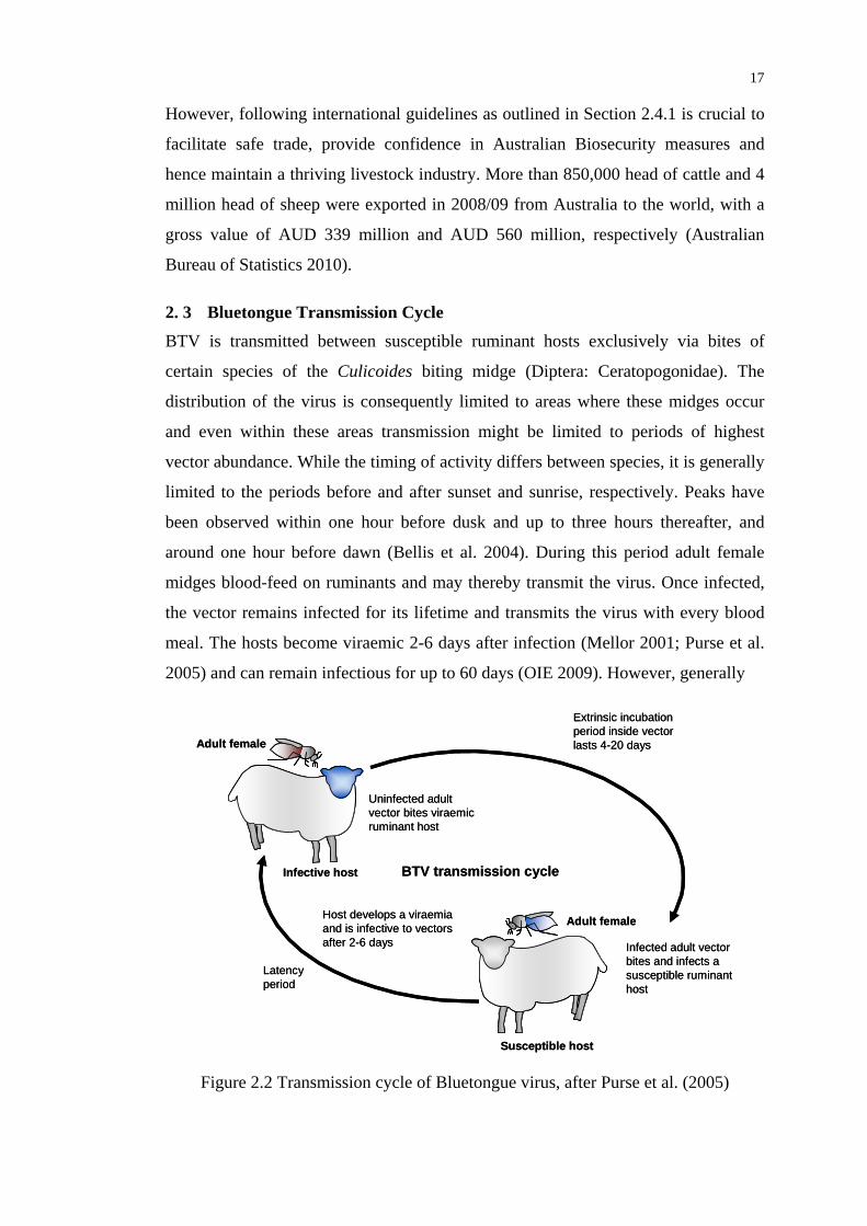
Figure 2.2 Transmission cycle of Bluetongue virus............................................... 17

Figure 2.3 Sheep and cattle numbers in the Pilbara from 1909 to 2006 ................ 25

Figure 2.4 Location of NAMP sites tested between November 2000 and

October 2009 in WA and the NT.......................................................... 27

Figure 3.1 Dr. John Snow’s map of deaths from cholera in the Broad Street

area of London ...................................................................................... 32

Figure 3.2 Conceptual nidus showing how competent vector, host and pathogen

populations intersect within a permissible environment to enable

pathogen transmission........................................................................... 33

Figure 3.3 Overview of the successive steps of the (generic) model building

process .................................................................................................. 39

Figure 3.4 Rectilinear environmental envelope for two climatic variables ........... 47

Figure 3.5 A simple Bayesian network .................................................................. 49

Figure 3.6 A confusion or error matrix that cross-tabulates observed presence/

absence patterns against those predicted .............................................. 56

Figure 4.1 The Electromagnetic Spectrum............................................................. 61

Figure 4.2 Spectral reflectance curves for clear water, green grass and bare

soil in the visible and near-to-mid infrared range................................. 62

Figure 4.3 Spatial and temporal resolution considerations for different

applications of remote sensing.............................................................. 64

Figure 4.4 Examples of seasonality parameters that can be computed from

NDVI time series .................................................................................. 80

Figure 5.1 Topography of the Pilbara-Gascoyne region ........................................ 90

Figure 5.2 Average daily temperature range and monthly rainfall from long-

term weather observations at Onslow, Wittenoom, and Carnarvon ..... 91

Figure 5.3 Extent of pastoral properties, conservation areas, aboriginal land

and crown land in the Pilbara-Gascoyne region ................................... 92

Figure 5.4 Overview of BTV activity on pastoral properties in the Pilbara -

Gascoyne region tested between November 2000 and October 2009 .. 93

Figure 5.5 Topographic overview of the Northern Territory ................................. 95

xiii

Figure 5.6 Average daily temperature range and monthly rainfall from long-

term weather observations at Darwin, Katherine, and Alice Springs... 96

Figure 5.7 Extent of pastoral properties, conservation areas, aboriginal land

and crown land in the Northern Territory............................................. 97

Figure 5.8 Overview of BTV activity on pastoral properties in the Northern

Territory tested between November 2000 and October 2009............... 98

Figure 5.9 Relationship between timing of serological survey and the peak of

seasonal vegetation greenup ............................................................... 101

Figure 5.10 Average monthly BTV seroprevalence at three sentinel herds in the

Northern Territory between November 2000 and October 2008........ 102

Figure 5.11 Simple conceptual model of factors related to BTV activity in

Northern Australia .............................................................................. 103

Figure 5.12 Missing pixels due to misplacement of the land water masked

used in the generation of the MOD13Q1 product............................... 109

Figure 5.13 Plotting BoM rain gauge locations over a TRMM accumulated

rainfall dataset clearly shows the advantage of satellite imagery ....... 114

Figure 6.1 Simplified workflow for the generation of bioclimatic variables

from remote sensing data products, and aggregation of annual

statistics on pastoral property level..................................................... 122

Figure 6.2 MODIS Sinusoidal GRID and tiles needed to cover WA and

the NT ................................................................................................. 124

Figure 6.3 Extent of areas covered during the successive processing steps,

using the NDVI as an example ........................................................... 125

Figure 6.4 Average percentage of valid pixels in quality filtered and gap

filled time series between November 2000 and October 2009........... 129

Figure 6.5 Average percentage of valid pixels in quality filtered and gap

filled time series between November 2000 and October 2009........... 130

Figure 6.6 Percentage of missing LST night images between November 2000

and October 2009................................................................................ 130

Figure 6.7 Comparison of smoothing techniques applied to NDVI time series

for a pixel at the Carnarvon Basin ...................................................... 135

Figure 6.8 Sample NDVI time series from the Pilbara and the Northern

Territory representing typical landscapes ........................................... 136

Figure 6.9 Glenflorrie Station and surrounding properties in the Pilbara ............ 141

xiv

Figure 6.10 Carrying capacity of Land Systems at Glenflorrie Station and the

weights used in the weighted station average calculation .................. 144

Figure 7.1 Relationship between selected Growing Degree Day variables

and BTV status.................................................................................... 150

Figure 7.2 Relationship between selected minimum and maximum

temperature variables and BTV status ................................................ 150

Figure 7.3 Relationship between selected mean temperature variables and

BTV status .......................................................................................... 151

Figure 7.4 Relationship between vegetation variables and BTV status ............... 151

Figure 7.5 Relationship between rainfall variables and BTV status .................... 152

Figure 7.6 Relationship between vegetation and rain variables and BTV

status for the area around the initial BTV outbreak in the Pilbara ..... 155

Figure 7.7 Smoothed fits to the variables maxndviss, maxlstdau, meanlstdau

and meanlstnpw used in the final BTV distribution model for the

Northern Territory............................................................................... 159

Figure 7.8 ROC plot of sensitivity versus 1-specificity for the final GAM

based on data from 2000/2001 to 2007/2008...................................... 161

Figure 7.9 Predicted BTV seropositivity in the NT for the seasons 2000/2001

and 2001/2002 in relation to the surveyed presence/absence data ..... 163






and 2007/2008 in relation to the surveyed presence/absence data. .... 166

Figure 7.13 Predicted BTV seropositivity in the NT for the season 2008/2009

in relation to the surveyed presence/absence data .............................. 168

Figure 7.14 ROC plot for the predictions of BTV presence in 2008/2009 ............ 169

Figure 7.15 Plot of sensitivity and specificity versus all possible cutoff points

to determine the optimum cut-off value for classification.................. 170

Figure 7.16 Binary prediction maps for the NT in 2008/2009, based on a cutoff

probability of 0.6................................................................................. 171

Figure 7.17 Preliminary predicted BTV seropositivity in the NT for the season

2009/2010 in relation to the surveyed presence/absence data ............ 176

xv

LIST OF TABLES

Table 2.1 Competent Bluetongue vectors in Australia ......................................... 19

Table 2.2 Incompetent Bluetongue vectors in Australia....................................... 20

Table 3.1 Overview of accuracy measures applicable in distribution

modelling .............................................................................................. 57

Table 5.1 Required temporal resolution for the remotely sensed climatic

and environmental datasets ................................................................. 105

Table 5.2 Remote sensing data products selected for this study......................... 119

Table 5.3 Land Information and Infrastructure datasets selected for this study. 119

Table 6.1 Aggregation periods used for the development of bioclimatic

variables .............................................................................................. 128

Table 6.2 Overview of bioclimatic variables...................................................... 131

Table 7.1 Extract of data compiled from NAMPInfo ......................................... 147

Table 7.2 Extract from the dataset developed for the analysis of correlations

between the predictor environmental variables and BTV .................. 148

Table 7.3 Number of tested properties and seroprevalence in the Pilbara

and the Northern Territory.................................................................. 148

Table 7.4 Test statistics for the Pilbara and Northern Territory study areas ...... 153

Table 7.5 Pearson correlation coefficients for rainfall and vegetation

variables .............................................................................................. 156

Table 7.6 Pearson correlation coefficients for temperature variables................. 156

Table 7.7 Significance of smooth and parametric model terms in the BTV

distribution model ............................................................................... 160

Table 7.8 Confusion matrix based on predictions from station average

variables .............................................................................................. 171

Table 7.9 Confusion matrix based on maximum predicted probability

per station............................................................................................ 172

Table 7.10 Accuracy measures for the classified presence/absence maps ........... 172

xvi

TERMS AND ACRONYMS

Below is a list of terms and acronyms used in the thesis:

AB-CRC Australian Biosecurity Cooperative Research Centre for Emerging

Infectious Disease

AMSR Advanced Microwave Scanning Radiometer

AMSU Advanced Microwave Sounding Unit

ASRIS Australian Soil Resource Information System

ASTER Advanced Spaceborne Thermal Emission and Reflection Radiometer

AVHRR Advanced Very High Resolution Radiometer

AIC Akaike Information Criterion

ANN Artificial Neural Network

AUC Area under the ROC curve (see ROC)

BoM Australian Bureau of Meteorology

BRDF Bidirectional Reflectance Distribution Function

CSIRO Commonwealth Scientific and Industrial Research Organisation

CMORPH NOAA Climate Prediction Center Morphing Technique

CU Cattle Unit

DAFWA Department of Agriculture and Food Western Australia

DEM Digital Elevation Model

DSE Dry Sheep Equivalent

ENFA Ecological Niche Factor Analysis

ENSO El Niño – Southern Oscilllation

ETM Enhanced Thematic Mapper

EVI Enhanced Vegetation Index

FAO Food and Agriculture Organisation of the United Nations

GAM Generalised Additive Model

GDD Growing Degree Days

GIS Geographic Information System or Science

GLM Generalised Linear Model

GLW Gridded Livestock of the World dataset

GPW Gridded Population of the World dataset

GMS Geostationary Meteorological Satellite

xvii

GOES Geostationary Operational Environmental Satellites

GWR Geographically Weighted Regression

HDF Hierarchical Data Format

IPWG International Precipitation Working Group

IR Infrared

JAXA Japan Aerospace Exploration Agency

LST Land Surface Temperature

MIR Mid Infrared

MODIS Moderate Resolution Imaging Spectroradiometer

NASA National Aeronautics and Space Administration

NAMP National Arbovirus Monitoring Program

NBAR Nadir BRDF-Adjusted Reflectance (also see BRDF)

NDVI Normalised Difference Vegetation Index

NIR Near Infrared

NOAA National Oceanic and Atmospheric Administration

NSW New South Wales

NT Northern Territory

NVIS National Vegetation Information System

OIE Office international des epizooties (World Organisation for Animal

Health)

PCA Principal Component Analysis

PMW Passive Microwave

PR TRMM Precipitation Radar (also see TRMM)

ROC Receiver Operating Characteristic

QLD Queensland

SAR Synthetic Aperture Radar

SDS Scientific Dataset

SG Savitzky-Golay Filter

SiNDVI Small integrated NDVI (also see NDVI)

SPOT Satellite Pour l'Observation de la Terre

SZA Solar Zenith Angle

TAIR Air Temperature

TIR Thermal Infrared

TM Thematic Mapper

xviii

TMI TRMM Microwave Imager (also see TRMM)

TMPA TRMM Multi-satellite Precipitation Analysis (also see TRMM)

TRMM Tropical Rainfall Measuring Mission

VI Vegetation Index

VPD Vapour Pressure Deficit

WA Western Australia

WHO World Health Organisation

WMO World Meteorological Organisation

List of Viruses and Diseases:

AKA Akabane Virus

BEF Bovine Ephemeral Fever Virus

BSE Bovine Spongiform Encephalopathy

BT/BTV Bluetongue / Bluetongue Virus

DEN/DENV Dengue Fever/ Dengue Virus

EHD Epizootic Haemorrhagic Disease Virus

JE/JEV Japanese Encephalitis Virus

KUN/KUNV Kunjin Virus

MVE/MVEV Murray Valley Encephalitis Virus

RR Ross River Virus

1

CHAPTER 1

INTRODUCTION

1. 1 Problem Formulation Arthropod transmitted viruses (arboviruses) such as Bluetongue virus (BTV) are

enzootic in the northern parts of Australia, where they pose a threat to human and

animal health. The ecology of arboviruses involves a transmission cycle between

competent insect vectors (e.g. mosquitoes or biting midges), who blood-feed on

vertebrate hosts (e.g. humans, livestock, feral animals) and thereby may transmit the

virus. Each component of the transmission cycle is influenced by the interplay of

underpinning environmental variables such as climatic conditions, vegetation, terrain

and soil properties, which characterise the vector and host habitat structure.

Current virus surveillance in Australia is based on antibody testing of sentinel

animals at regular time intervals, complemented by strategic serological surveys.

This approach is time consuming, expensive, and the resulting data are characterised

by an incomplete spatial coverage and a coarse temporal resolution. As a

consequence, it is impracticable to predict disease spread over space and time within

the timeframe necessary for early warning systems. As an alternative,

epidemiologists have used environmental data from earth observation satellites

combined with serological data to map vector habitats and hence estimate the

potential virus distribution over large areas (e.g. malaria in Africa). Such

epidemiological studies rely on low cost data available at wide areal coverage and

high temporal resolution over longer periods.

This research addresses the current lack of an efficient and cost-effective

methodology for the area-wide prediction of arbovirus occurrence in the North of

Australia, using BTV as the target virus. Different remote sensing instruments and

ancillary datasets are assessed for their capability to provide environmental and

climatic data to be used within a spatial distribution model that can predict BTV

presence accurately and hence complement traditional surveillance methods in areas,

where these are impractical.

2

1. 2 Background

1.2.1 Bluetongue Virus Bluetongue virus is an Orbivirus transmitted by biting midges that causes a non-

contagious, infectious disease of wild and domestic ruminants. The virus is spread

almost worldwide in the tropics and subtropics approximately between the latitudes

35°S and 40°N (Mellor 2001). In recent years, the effects of climate change have

contributed to an extension of its distribution area into higher latitudes and facilitated

major outbreaks in Europe (Mellor et al. 2009; Saegerman, Berkvens, and Mellor

2008). In the Mediterranean region, over one million sheep have died from both the

disease itself and elective culling since 1998 (Purse et al. 2005).

The virus is transmitted between its ruminant hosts almost exclusively via the bites

of Culicoides midges, which act as the predominant vectors. Hence, the global

distribution is limited to the areas where the biting midges can survive. In Australia,

currently five species of Culicoides have been identified by entomologists as

competent vectors for BTV, namely C. fulvus, C. wadai, C. actoni, C. dumdumi and

C. brevitarsis. Amongst them, C. brevitarsis is the most widely distributed species,

while other midges species are less expansively distributed and are confined to areas

within the limits of C. brevitarsis distribution (Kirkland 2004). In general, Culicoides

habitats are determined by environmental and climatic factors, including

temperature, moisture, geographic barriers, vegetation cover and health, the presence

of ruminants as blood reservoirs for feeding, as well as the availability of breeding

sites. Dispersal of Culicoides is not limited to their flight range of a few kilometres,

but can extend to hundreds of kilometres if midges are blown by prevailing winds as

aerial plankton (Mellor 2001).

1.2.2 Distribution and Control of BTV in Australia Although BTV is endemic in Australia, no signs of clinical disease have been

observed in the major sheep herds. The major reason is that from the presently

70 million sheep (Curtis 2009), only a few hundred graze in areas where the virus is

permanently present (Kirkland 2004). Nevertheless, BTV has a major impact on the

Australian livestock industry by restricting trade of sheep, cattle or goats. Even if

trade is not prevented, it becomes very expensive due to serological tests and other

measures necessary to reduce the perceived BTV risk (Oliver 2004). After the first

3

isolation of BTV in Australia near Darwin in the late 1970s, a sentinel herd system

for arbovirus surveillance was installed. The system was gradually expanded from

Northern Australia to the Eastern States and resulted in the establishment of the

National Arbovirus Monitoring Program (NAMP) in 1993. The locations of sentinel

herds are confined to the areas of commercial cattle operations (Melville 2004) and

are selected representatively to allow mapping of the distribution of infections.

Hence most herds are positioned along the border between expected infected and

uninfected areas, or where infection occurs irregularly. Herds within the affected

areas are also tested to assess the seasonal intensity of infection. Supplementary,

expected BTV-free areas are monitored to verify their free status (Animal Health

Australia 2006). Sentinel herds usually consist of 10 to 25 young cattle, which have

initially returned negative tests for Bluetongue antibodies. Cattle are replaced

annually or after seroconversion is determined. The herds are bled at regular

intervals, with the frequency being approximately proportional to the probability of

arbovirus activity. Opportunistic serological surveys complement the testing of

sentinel herds. The second corner post of surveillance is vector trapping and

quantification of Culicoides species at the sentinel herd sites and a number of other

strategic locations (Cameron 2004). The data sampled at the monitoring sites are

collected in a central database, which defines the main input for the definition of

three zones according to regulations of the World Organisation for Animal Health

(OIE): ‘free of BTV’, ‘infected’, an a “surveillance” buffer zone between those two.

The zone boundaries are defined and adjusted on the basis of monitoring results and

expert knowledge.

1.2.3 The Role of Remote Sensing and Geographic Information Science in Epidemiology

The field of spatial epidemiology aims to investigate and map the spatial distribution

of emerging diseases over time, based on the distribution of vectors, hosts and

incidences (Ostfeld, Glass, and Keesing 2005). The basic underlying concept

comprises three components as observed by Pavlovsky (1966). First, diseases tend to

be limited geographically; second, the spatial variation of diseases is influenced by

biological and physical variations that support the distribution of the pathogen, its

vectors and hosts; and third, if these biotic and abiotic environmental conditions can

4

be delineated on a map, then spatial and temporal patterns of disease risk should be

predictable.

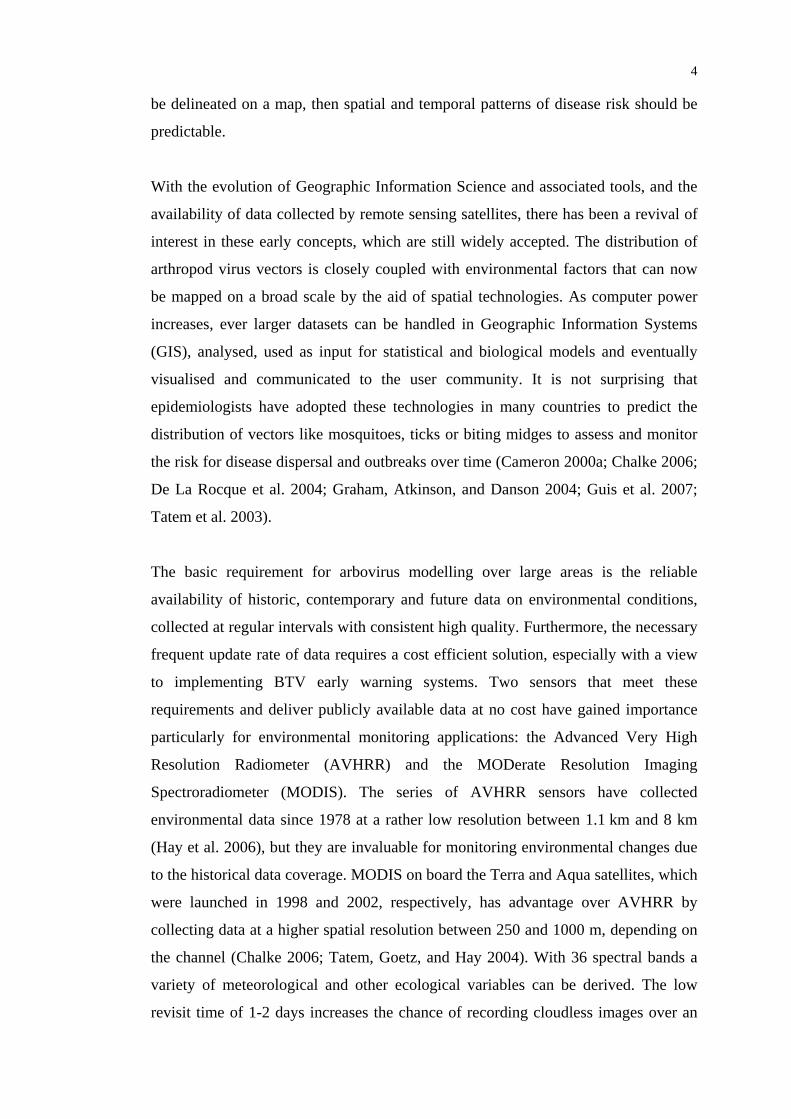
With the evolution of Geographic Information Science and associated tools, and the

availability of data collected by remote sensing satellites, there has been a revival of

interest in these early concepts, which are still widely accepted. The distribution of

arthropod virus vectors is closely coupled with environmental factors that can now

be mapped on a broad scale by the aid of spatial technologies. As computer power

increases, ever larger datasets can be handled in Geographic Information Systems

(GIS), analysed, used as input for statistical and biological models and eventually

visualised and communicated to the user community. It is not surprising that

epidemiologists have adopted these technologies in many countries to predict the

distribution of vectors like mosquitoes, ticks or biting midges to assess and monitor

the risk for disease dispersal and outbreaks over time (Cameron 2000a; Chalke 2006;

De La Rocque et al. 2004; Graham, Atkinson, and Danson 2004; Guis et al. 2007;

Tatem et al. 2003).

The basic requirement for arbovirus modelling over large areas is the reliable

availability of historic, contemporary and future data on environmental conditions,

collected at regular intervals with consistent high quality. Furthermore, the necessary

frequent update rate of data requires a cost efficient solution, especially with a view

to implementing BTV early warning systems. Two sensors that meet these

requirements and deliver publicly available data at no cost have gained importance

particularly for environmental monitoring applications: the Advanced Very High

Resolution Radiometer (AVHRR) and the MODerate Resolution Imaging

Spectroradiometer (MODIS). The series of AVHRR sensors have collected

environmental data since 1978 at a rather low resolution between 1.1 km and 8 km

(Hay et al. 2006), but they are invaluable for monitoring environmental changes due

to the historical data coverage. MODIS on board the Terra and Aqua satellites, which

were launched in 1998 and 2002, respectively, has advantage over AVHRR by

collecting data at a higher spatial resolution between 250 and 1000 m, depending on

the channel (Chalke 2006; Tatem, Goetz, and Hay 2004). With 36 spectral bands a

variety of meteorological and other ecological variables can be derived. The low

revisit time of 1-2 days increases the chance of recording cloudless images over an

5

area and hence facilitates the monitoring of dynamic spatial environmental processes.

With a scheduled operation period of 18 years, the MODIS data archive will

facilitate global long-term observations of disease related factors.

In the case of BTV, spatial epidemiologists successfully modelled its distribution in

Europe using remote sensing and GIS and so could predict the outbreak in the

1990’s. Besides meteorological parameters like temperature and rainfall, which are

most relevant for estimating vector survival rates (Purse et al. 2005), environmental

variables derived from satellites were used in modelling the occurrence of vector-

borne diseases. These included dynamic factors like vegetation indices, soil moisture

and surface water (e.g. Baylis and Rawlings 1998; Chalke 2006; Purse, Tatem, et al.

2004). By incorporating such remotely sensed variables, vector distribution could be

more accurately predicted on an area-wide basis.

1. 3 Research Objectives

1.3.1 Aims of the Research The overall aim of this research, which forms part of an Australian Biosecurity CRC

funded project on arboviral diseases, is to provide a better understanding of the

relationship between the spatio-temporal variability of climatic and environmental

conditions and the occurrence of Bluetongue virus. This understanding will

eventually facilitate the prediction of the future distribution and potential diffusion

scenarios of the virus. To achieve this ambitious goal, the primary objective of the

project is:

• To test the application of remotely sensed environmental variables for the

development of predictive models of BTV presence and absence in Northern

Australia across space and through time.

To address this primary objective encompasses the following secondary objectives:

• To identify relevant spatial data suitable for the definition of environmental

factors that relate to the distribution of BTV as the target virus. The

availability, spatial and temporal resolution of remote sensing imagery,

6

topographic, climatic, vegetation and other ancillary data will play a crucial

role in the capability to accurately model and predict BTV host and vector

dynamics; and

• To develop algorithms for timely delivery of multi-temporal spatial data to

model bioclimatic landscapes relating to BTV host and vector dynamics. The

reliability of these spatio-temporal data for estimating and mapping the

distribution of infected hosts in the study areas will be assessed using

arbovirus surveillance data from within and beyond the period under

investigation.

1.3.2 Expected Outcomes The expected outcomes of this research include:

• A summary of environmental biotic and abiotic factors and available data

sources, relevant to model habitats, dispersal and abundance of the main BTV

vectors Culicoides spp.;

• An effective, cost efficient and rapid methodology to derive those

environmental factors from satellite images, meteorological and ancillary

datasets of sufficient quality, and of appropriate spatial and temporal

resolution;

• A spatio-temporal model of virus distribution based on bioclimatic variables;

as well as

• A better understanding of Bluetongue host and vector dynamics in the spatio-

temporal domain.

1. 4 Significance and Benefits of the Research

Vector-borne diseases are an emerging threat for humans and livestock worldwide.

BTV is an arbovirus, which has killed a large number of sheep during major

outbreaks of the Bluetongue disease in Europe, Asia and Africa. Although no

evidence for severe clinical disease has been found in Australia, it has halted export

of cattle and even cattle products since then. International trade of livestock

according to OIE guidelines is restricted to cattle that were held in BTV-free zones

prior to export (Oliver 2004). The current zone definition within NAMP delivers

important information for planning live stock exports. However, this process is solely

7

based on ground based surveillance and expert knowledge, while neglecting

important environmental factors. There is currently no national capability to predict

disease spread consistently over space and time necessary for early warning systems.

The limitations of the approach were highlighted in 2000, when the diffusion of BTV

into the Pilbara region in Western Australia could not be predicted.

Rational control of the virus activity requires an understanding of the transmission

cycle of BTV, which is governed by complex spatial interactions between the vectors

(biting midges) and hosts (predominantly domestic and wild ruminants). Dynamic

environmental, biological, agricultural and socio-economic factors and their spatio-

temporal variations affect the habitats of hosts and vectors, and as such determine the

activity and movement patterns of the virus. Despite the ongoing intensive

monitoring in Australia, these factors and the ecology and epidemiology of BTV are

still poorly understood, as pointed out by Melville (2004) during an international

Bluetongue Symposium. While localised studies in the Eastern States of Australia

were quite successful in modelling the distribution of only one vector species, the

situation is different for Northern Australia. The presence of a variety of Culicoides

species as potential BTV vectors as well as the large observation area with complex

climatic and geographic interactions make the development of distribution models

difficult. Furthermore, the proximity to South East Asia bears the risk of further virus

incursions. Hence, there is a high research demand for investigations in this area to

get a better understanding of BTV activities on a regional scale and in case of new

incursions, to predict the possible distribution of the pathogen well ahead in time.

The advance of spatial epidemiology is very closely tied to the availability of data on

environmental and climate factors to describe to the occurrence of vector and host

species. Despite the ongoing development and the successful application of spatio-

temporal models to predict BTV outbreaks in the Mediterranean region, the lack of

suitable data has long been a limiting factor in research (Herbreteau et al. 2007).

However, with the increasing availability of remote sensing data, particularly from

the MODIS instrument, monitoring of environmental factors has become more

efficient on a regional to global scale with appropriate temporal and spatial

resolution. This research aims to investigate the potential of MODIS and other

8

satellite-borne sensors for epidemiological studies particularly for the Australian

conditions, by delivering area-wide environmental and climatic data at low cost.

Another issue discussed by Ostfeld, Glass & Keesing (2005) is the prediction of

disease risk or incidence only by distribution of host and vector species. While the

generation of presence/absence maps is relatively simple using existing GIS

methods, more dynamic models are necessary. To facilitate timely prediction of

arbovirus spread, varying environmental conditions affecting ecological processes

have to be incorporated, including plant and animal life cycles, soil moisture, as well

as vegetation type and condition. Although arboviruses are enzootic in some areas,

under certain environmental conditions, viruses migrate to distant areas, when

linkages between suitable habitats and breeding places are established. These spatial

processes have yet to be fully investigated and formalized. Eventually the research

aims to contribute to a better understanding of the relationship between dynamic

landscape, environmental and climate factors and the risk for vector-borne diseases.

1. 5 Research Methodology The study area covers parts of Northern Australia, where BTV is endemic and

extends to areas where BTV is not endemic, but which might be subject to further

spread of the virus. The regions investigated are the Pilbara-Gascoyne in Western

Australia (WA) as well as the entire Northern Territory (NT), both of which are

characterised by varying levels of virus activity and a great environmental diversity.

The study comprises two major stages which are carried out sequentially as outlined

below:

i) Timely delivery of multi-temporal spatial data relating to virus vector

and host dynamics, through:

a. Review of relevant literature on BTV transmission, host and vector

ecology, and the utilisation of Geographic Information Technology,

remotely sensed data, as well as ecological and statistical modelling

techniques to predict virus distribution;

b. Inventory of sources for environmental and climatic data relevant

to the ecology of BTV vectors and hosts. Data from remote sensing

9

satellites, weather stations, and government agencies are assessed

for their quality, spatial and temporal resolution required for

mapping at a regional scale; and

c. Development of algorithms for the generation and timely delivery

of spatio-temporal variables that relate to arbovirus host and vector

dynamics.

ii) Predicting the distribution of BTV using spatio-temporal modelling

techniques, incorporating the following steps:

a. Identifying the crucial bioclimatic variables associated with virus

dynamics in the study area;

b. Developing models for spatio-temporal mapping of BTV presence

and absence, based on the underpinning bioclimatic variables; and

b. Performing an evaluation process to assess the predictive

capabilities of the resulting distribution model.

The next section provides a brief overview of the chapters in this thesis. The main

stages of the study in relation to the thesis chapters are outlined in Figure 1.1 below.

1. 6 Overview of Thesis This thesis comprises eight chapters. Chapter 1 introduces the problem and provides

relevant background information on Bluetongue in Australia and its significance for

animal health and the livestock industry. Based on the stated objectives and the

proposed outcomes, a simplified structure of this research is outlined.

Chapter 2 reviews the historic and present distribution of BTV, its hosts and vectors

and investigates possible causal environmental and climatic factors that influence the

transmission cycle. An overview of the current surveillance system is provided, and

its limitations are discussed.

Chapter 3 introduces the field of spatial epidemiology and explains the basic concept

of disease presence being dependent on suitable habitat conditions for host and

vectors. Based on these ecological principles, modelling techniques used in

ecological and epidemiological applications are explored. Advantages and

disadvantages are highlighted in order to find the most appropriate and robust

10

technique for this study on landscape, environmental and climatic factors. The

chapter concludes with methods for model validation.

Chapter 4 provides a brief overview of the principles of remote sensing and its role

for mapping the distribution of vector-borne diseases. Current and future satellite

sensors delivering environmental data at low, medium and high spatial resolution are

reviewed. The applicability of the available environmental data from these sensors to

this study is discussed, considering factors like spatial and temporal resolution, cost

of data acquisition and processing. Also a variety of bioclimatic variables that can be

derived from remotely sensed data and have been previously used in comparable

studies are reviewed.

Figure 1.1 Research structure and relationship to the chapters of this thesis

11

Chapter 5 introduces the study areas in the Pilbara-Gascoyne region and the Northern

Territory in terms of climate, weather patterns, topography, pastoral potential and

virus activity. All data sources used in subsequent chapters are presented. The

software packages used to analyse, present and derive the various outputs of this

study are documented.

In Chapter 6, the methodology is described to transform the satellite data into a set of

meaningful bioclimatic variables. Processing of data from MODIS and the Tropical

Rainfall Measuring Mission (TRMM) is detailed, followed by a discussion of issues

with cloud cover and missing data in the tropical North of the country. Governed by

the underlying spatial and temporal resolution of the virus presence/absence data, the

variables were aggregated into seasonal variables on a pastoral property level,

utilising station average conditions and a novel weighting approach.

Chapter 7 continues with the spatial analyses of relationships between the seasonal

bioclimatic variables and BTV occurrence, upon which a spatial distribution model is

developed. Annual prediction maps derived from the best fitting model are presented

and the model results are validated and discussed.

The thesis is concluded in Chapter 8, with a summary of the outcomes in relation to

the stated objectives and recommendations for future research.

12

CHAPTER 2

REVIEW OF BLUETONGUE VIRUS, ITS HOSTS AND VECTORS IN AUSTRALIA

In order to model the distribution of an arbovirus like Bluetongue it is important to

understand the ecology of the virus, identify relevant vector and host species and

their preferred habitat, and understand the role of the surrounding environment in

each stage of the transmission cycle. The following chapter reviews the epidemiology

and ecology of Bluetongue virus, with a focus on the Australian continent, from the

first discovery of the virus to current surveillance and control mechanisms.

2. 1 Arboviruses in Australia Arboviruses, or arthropod-borne viruses, are generally defined by the World Health

Organisation (WHO) (1967) as a group of “viruses maintained in nature by a

biological transmission cycle between susceptible vertebrate hosts and

haematophagous (bloodsucking) arthropod vectors”. Vectors include mosquitoes,

ticks, sand flies and biting midges. For an arbovirus to be sustained and pose a risk

for human and animal health in an area, both hosts and vectors have to be present at

that location in sufficient numbers (Chalke 2006; Hanley and Weaver 2008). Suitable

environmental conditions particularly for the vectors, are therefore crucial for the

abundance and distribution of an arbovirus.

In Australia, more than 75 arboviruses have been reported, of which 12 are of

concern for human health, including Dengue (DEN), Kunjin (KUN), Japanese

Encephalitis (JE), Murray Valley Encephalitis (MVE) and Ross River (RR) (Russell

and Dwyer 2000). Arboviruses affecting animal health and causing economical

impact for the livestock industry include the Bovine Ephemeral Fever (BEF),

Epizootic Haemorrhagic Disease (EHD), Akabane (AKA) and Bluetongue (BT)

(Gard et al. 1988; St. George 1989). The latter is the subject of the following sections

in this chapter.

13

2. 2 Bluetongue Virus

2.2.1 Epidemiology

Bluetongue virus is of the genus Orbivirus and includes 24 known serotypes (Attoui

et al. 2009). It was first found in sheep in South Africa in the 19th century and first

described clinically as Malarial Catarrhal Fever by Hutcheon (1902). From an

African origin, which BTV is traditionally regarded as having, the virus spread out

almost worldwide in the tropics and subtropics approximately between the latitudes

35°S and 40°N (Mellor 2001). Major outbreaks in sheep occurred in Cyprus (1943),

Portugal and Spain (1956), Pakistan (1959) and India (1969) and raised concerns in

countries with large sheep populations, such as Australia (Erasmus and Potgieter

2009; Gibbs and Greiner 1994).

The first evidence of BTV in Australia was provided by the isolation of serotype 20

from Culicoides collected at Beatrice Hill, NT, in March 1975. Serotype 21 was

isolated, followed by serotypes 3, 9, 15, 16, 20 and 23 (St. George 1995; Ward

1994a). More recently, BT 7 was found for the first time in mid 2007 near Humpty

Doo (NT) (Animal Health Australia 2008; Melville et al. 2009; Murray 2008) and

BT 2 was isolated from sentinel cattle in the Northern NT in December 2008

(Animal Health Australia 2009a; Murray 2009). Except for serotypes 1 and 21,

which are widely distributed across northern and eastern coastal regions of Australia,

serotypes 2, 3, 7, 9, 15, 16, 20 and 23 occur in the northern region of Australia but do

not spread beyond (Kirkland 2004).

In recent years, the effects of global climate change have resulted in an extension of

the BTV distribution area into higher latitudes and facilitated major outbreaks in

Europe. In the Mediterranean region, over 1 million sheep died from both the disease

itself and elective culling between 1998 and 2004 (Purse et al. 2005). During 2006

and 2007, a major outbreak of Bluetongue 8, which reached parts of Northern

Europe, including France, Germany, Denmark and Great Britain halted livestock

movement from that region and caused still unknown costs (Mellor et al. 2009;

Saegerman, Berkvens, and Mellor 2008).

14

In Australia, BTV has been found in the northern parts of WA, the NT and

Queensland (QLD) as well as eastern Queensland and north eastern New South

Wales (NSW). Fluctuation of the viruses’ expansion have been observed over the

past years, which are mainly explained by weather patterns, extreme temperature

ranges, droughts or intensive wet seasons (Animal Health Australia 2001). In the

Pilbara region in WA, where BTV was present between 2000 and 2007, the virus

was not found the following two years but appeared again in August 2010. The

annual and quarterly reports of Animal Health Australia provide a general overview

of the current situation for Bluetongue and other livestock diseases in Australia (e.g.

Animal Health Australia 2009b). Figure 2.1 shows an overview of BTV zone

boundaries between 2003 and 2010.

November 2009 Bluetongue Zones

Positive

Surveillance

August 2010

November 2007 August 2008

Data Source:National Arbovirus Monitoring ProgramAnimal Health Australia

September 2005July 2003

October 2006

´Free

July 2004

Figure 2.1 Selected Bluetongue zone maps published by Animal Health Australia between 2003 and 2010

15

For areas that are declared free from disease, no viral activity must have been

detected for at least the past two years. These BTV free areas are separated from the

BTV positive zones by a 50 km wide surveillance buffer. The surveillance system

underlying the definition of these zones is described in Section 2.4 below. Although

these maps do not give an accurate representation of the actual occurrence of the

virus, as they include additional safety buffers, they do provide a general overview of

BTV susceptible regions.

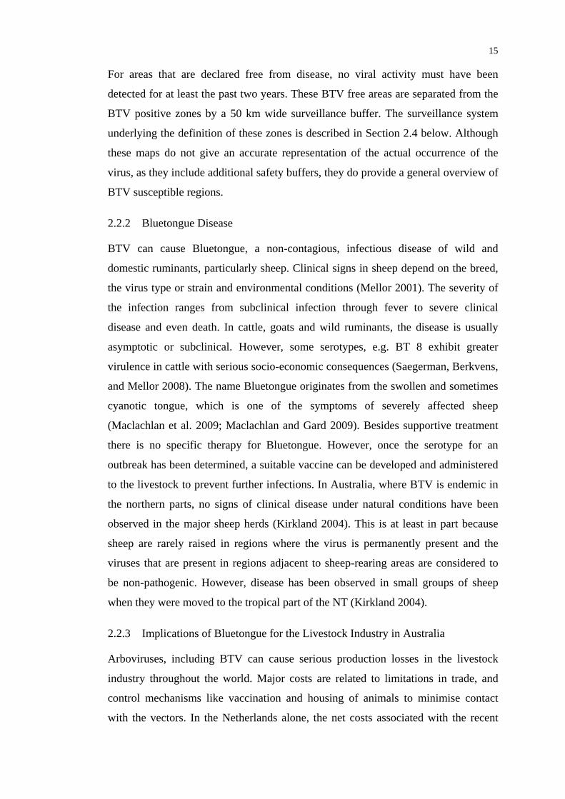
2.2.2 Bluetongue Disease

BTV can cause Bluetongue, a non-contagious, infectious disease of wild and

domestic ruminants, particularly sheep. Clinical signs in sheep depend on the breed,

the virus type or strain and environmental conditions (Mellor 2001). The severity of

the infection ranges from subclinical infection through fever to severe clinical

disease and even death. In cattle, goats and wild ruminants, the disease is usually

asymptotic or subclinical. However, some serotypes, e.g. BT 8 exhibit greater

virulence in cattle with serious socio-economic consequences (Saegerman, Berkvens,

and Mellor 2008). The name Bluetongue originates from the swollen and sometimes

cyanotic tongue, which is one of the symptoms of severely affected sheep

(Maclachlan et al. 2009; Maclachlan and Gard 2009). Besides supportive treatment

there is no specific therapy for Bluetongue. However, once the serotype for an

outbreak has been determined, a suitable vaccine can be developed and administered

to the livestock to prevent further infections. In Australia, where BTV is endemic in

the northern parts, no signs of clinical disease under natural conditions have been

observed in the major sheep herds (Kirkland 2004). This is at least in part because

sheep are rarely raised in regions where the virus is permanently present and the

viruses that are present in regions adjacent to sheep-rearing areas are considered to

be non-pathogenic. However, disease has been observed in small groups of sheep

when they were moved to the tropical part of the NT (Kirkland 2004).

2.2.3 Implications of Bluetongue for the Livestock Industry in Australia

Arboviruses, including BTV can cause serious production losses in the livestock

industry throughout the world. Major costs are related to limitations in trade, and

control mechanisms like vaccination and housing of animals to minimise contact

with the vectors. In the Netherlands alone, the net costs associated with the recent

16

BTV outbreak in 2006 and 2007 were estimated at € 200 million, particularly

affecting cattle farmers (Velthuis et al. 2010). In an earlier paper Tabachnick (1996)

estimated the annual loss in the US due to BTV induced export limitations at USD

125 million.

While currently in Australia pathogenic serotypes are confined to the far North of the

Northern Territory, far removed from susceptible commercial sheep populations,

BTV has been an important restriction to the export of livestock since its first

isolation (Doyle 1989; Kirkland 2004). Trade of livestock, semen and embryos, but

not animal products such as meat and milk from a declared BTV zone is subject to

strict regulations by the OIE. Even if trade is not prevented, it becomes very

expensive due to serological tests and other measures necessary to reduce the

perceived BTV risk (Oliver 2004). Australia has developed an internationally

recognised National Arbovirus Monitoring Program (NAMP) based on scientific

methods and international guidelines that helps to reduce the risk of undetected virus

incursions and movements and declare areas free from disease (see Section 2.4).

The introduction of rigorous monitoring and the accompanied definition of zones,

amongst other economic factors, lead to a significant change in livestock production.

Producers in regions where Bluetongue is endemic or the only economic export route

leads through the declared Bluetongue zone are now producing cattle for markets in

Southeast Asia, traditionally for Indonesia (Van Vreeswyk and Thomas 2008). These

countries host the same BTV serotypes as Australia and are therefore less sensitive to

the risk of importing infected livestock (Daniels et al. 2004). Cattle producers in

regions where BTV is rarely found, such as some areas in the Pilbara, are often

targeting high price export markets for livestock in the Near East, including Israel

(Department of Agriculture and Food Western Australia 2006). Although some BTV

serotypes are present in this part of the world (Mellor et al. 2008), fears of importing

new strains require strong evidence of disease freedom from trade partners.

Therefore, identifying BTV on a cattle station previously free from disease and hence

changing the status of that station and many others in the declared risk zone has not

only significant economic, but also socio-economic implications. This challenges the

management and operation of a monitoring system that relies heavily on the

collaboration of pastoralists who are willing to have their cattle tested for BTV.

17

However, following international guidelines as outlined in Section 2.4.1 is crucial to

facilitate safe trade, provide confidence in Australian Biosecurity measures and

hence maintain a thriving livestock industry. More than 850,000 head of cattle and 4

million head of sheep were exported in 2008/09 from Australia to the world, with a

gross value of AUD 339 million and AUD 560 million, respectively (Australian

Bureau of Statistics 2010).

2. 3 Bluetongue Transmission Cycle BTV is transmitted between susceptible ruminant hosts exclusively via bites of

certain species of the Culicoides biting midge (Diptera: Ceratopogonidae). The

distribution of the virus is consequently limited to areas where these midges occur

and even within these areas transmission might be limited to periods of highest

vector abundance. While the timing of activity differs between species, it is generally

limited to the periods before and after sunset and sunrise, respectively. Peaks have

been observed within one hour before dusk and up to three hours thereafter, and

around one hour before dawn (Bellis et al. 2004). During this period adult female

midges blood-feed on ruminants and may thereby transmit the virus. Once infected,

the vector remains infected for its lifetime and transmits the virus with every blood

meal. The hosts become viraemic 2-6 days after infection (Mellor 2001; Purse et al.

2005) and can remain infectious for up to 60 days (OIE 2009). However, generally

BTV transmission cycleInfective host

Susceptible host

Uninfected adultvector bites viraemicruminant host

Infected adult vector bites and infects a susceptible ruminant host

Adult female

Adult female

Extrinsic incubationperiod inside vectorlasts 4-20 days

Host develops a viraemiaand is infective to vectors after 2-6 days

Latency period

BTV transmission cycleInfective host

Susceptible host

Uninfected adultvector bites viraemicruminant host

Infected adult vector bites and infects a susceptible ruminant host

Adult female

Adult female

Extrinsic incubationperiod inside vectorlasts 4-20 days

Host develops a viraemiaand is infective to vectors after 2-6 days

Latency period

Figure 2.2 Transmission cycle of Bluetongue virus, after Purse et al. (2005)

18

infections last for 7-28 days in cattle and less then two weeks in sheep (Animal

Health Australia 2009a; Ward 1994a). Each stage is influenced by the surrounding

environment, with temperature and moisture levels determining activity, survival and

development rates of the vectors (Purse et al. 2005). Figure 2.2 summarises the

stages of the transmission cycle.

2.3.1 Culicoides Biting Midges

Worldwide, more than 1400 species of Culicoides have been named and they have

been found on all large inhabited land masses, excluding Hawaii, Iceland and New

Zealand. Their habitats range from sea level to an elevation of 4000 m (Mellor,

Boorman, and Baylis 2000). Culicoides are amongst the smallest blood feeding

insects and range in size from 1-3 mm. Different species are distinguishable mainly

by their unique wing pattern. The development stage requires some form of humidity

and eggs are accordingly laid in habitats that meet this criterion. The midges also

seek the proximity of hosts, so they tend to breed in sites like irrigation channels,

dams or even cattle dung. Culicoides have been found to transmit a wide range of

bacteria, protozoal and helminth parasites, but they are best known as virus vectors.

To date, more than 50 viruses have been isolated worldwide (Mellor, Carpenter, and

White 2009).

2.3.2 Culicoides Vectors of Bluetongue in Australia

In Southeast Asia, 168 different species of Culicoides are recorded (Wirth and

Hubert 1989), of which some occur on the Australian continent that are capable of

transmitting BTV. Out of the 16 species tested, seven supported virus growth, but

only C. fulvus, C. wadai, C. actoni and C. brevitarsis are considered competent

vectors (Standfast, Dyce, and Muller 1985). Amongst them, C. brevitarsis is the most

widely distributed species, while the others remain within the extent of C. brevitarsis

and are confined to the far North of Australia (Kirkland 2004). More recently, it has

been recognized that some of the insects previously identified in Northern Australia

as C. fulvus are in fact C. dumdumi, which has therefore been confirmed as another

competent vector (Bellis and Dyce 2005). The typical form of C. dumdumi has only

been found in North Queensland, while an atypical form was also identified in the

Northern Territory. Table 2.1 provides details on main vectors, their distribution,

preferred hosts and relevance for BTV.

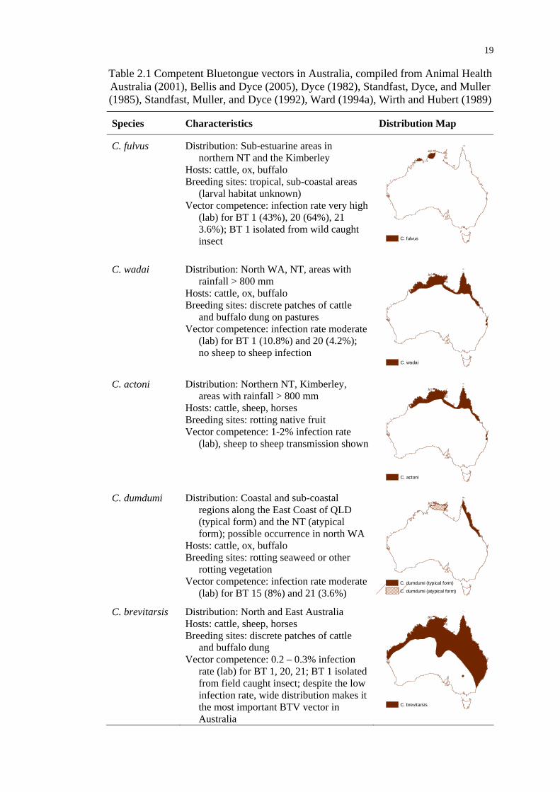
19

Table 2.1 Competent Bluetongue vectors in Australia, compiled from Animal Health Australia (2001), Bellis and Dyce (2005), Dyce (1982), Standfast, Dyce, and Muller (1985), Standfast, Muller, and Dyce (1992), Ward (1994a), Wirth and Hubert (1989)

Species Characteristics Distribution Map

C. fulvus Distribution: Sub-estuarine areas in northern NT and the Kimberley

Hosts: cattle, ox, buffalo Breeding sites: tropical, sub-coastal areas

(larval habitat unknown) Vector competence: infection rate very high

(lab) for BT 1 (43%), 20 (64%), 21 3.6%); BT 1 isolated from wild caught insect C. fulvus

C. wadai Distribution: North WA, NT, areas with rainfall > 800 mm

Hosts: cattle, ox, buffalo Breeding sites: discrete patches of cattle

and buffalo dung on pastures Vector competence: infection rate moderate

(lab) for BT 1 (10.8%) and 20 (4.2%); no sheep to sheep infection

C. wadai

C. actoni Distribution: Northern NT, Kimberley, areas with rainfall > 800 mm

Hosts: cattle, sheep, horses Breeding sites: rotting native fruit Vector competence: 1-2% infection rate

(lab), sheep to sheep transmission shown

C. actoni

C. dumdumi Distribution: Coastal and sub-coastal regions along the East Coast of QLD (typical form) and the NT (atypical form); possible occurrence in north WA

Hosts: cattle, ox, buffalo Breeding sites: rotting seaweed or other

rotting vegetation Vector competence: infection rate moderate

(lab) for BT 15 (8%) and 21 (3.6%) C. dumdumi (typical form)

C. dumdumi (atypical form)

C. brevitarsis Distribution: North and East Australia Hosts: cattle, sheep, horses Breeding sites: discrete patches of cattle

and buffalo dung Vector competence: 0.2 – 0.3% infection

rate (lab) for BT 1, 20, 21; BT 1 isolated from field caught insect; despite the low infection rate, wide distribution makes it the most important BTV vector in Australia

C. brevitarsis

20

Since C. brevipalpis, C. peregrinus and C. oxystoma have been infected with BTV in

the laboratory they are considered potential vectors, but no natural infection has been

recorded. Although they are not considered as functional BTV vectors, they are listed

here as potential vectors and their expansion has to be monitored (see Table 2.2).

Table 2.2 Incompetent Bluetongue vectors in Australia, from Animal Health Australia (2001), Bellis and Dyce (2005), Dyce (1982), Standfast, Dyce, and Muller (1985), Standfast, Muller, and Dyce (1992), Ward (1994a), Wirth and Hubert (1989)

Species Characteristics Distribution Map

C. brevipalpis Distribution: North NT, recently caught in the Western Kimberley (WA) around Broome

Hosts: cattle, sheep, horses Breeding sites: discrete patches of cattle

and buffalo dung Vector competence: 0.9% infection rate for

BT 1 (Lab), but population levels are never high and the species is facultatively autogenous for the first egg mass (autogenous mosquitoes do not require blood to mature an initial egg batch and, instead, acquire nutrients for egg provisioning as larvae) > no pressure for a first blood meal > very low vector capability

C. brevipalpis

C. peregrinus Distribution: Coastal floodplains of Northern NT

Hosts: cattle (preferred), ox, buffalo, horses Breeding sites: shaded and sunlit ground

waters Vector competence: Infection rate very low

(no virus isolated from insects that fed on viraemic sheep), but 2 sheep (of 4) developed antibodies after treated with midges suspension

C. peregrinus

C. oxystoma Distribution: North of NT and WA with rainfall > 800 mm

Hosts: bovids, like buffalo (preferred) or ox Breeding sites: variety of ground waters

(most exposed to direct sunlight and contaminated with bovid faeces and supporting algae growth)

Vector competence: Infection rate very low (no virus isolated from insects that fed on viraemic sheep), but 1 sheep developed antibodies after treated with midges suspension

C. oxystoma

21

Tables 2.1 and 2.2 were compiled from various publications that provide

comprehensive overviews of vector ecology (Animal Health Australia 2001; Bellis

and Dyce 2005; Dyce 1982; Standfast, Dyce, and Muller 1985; Standfast, Muller,

and Dyce 1992; Ward 1994a; Wirth and Hubert 1989). Although a number of

Culicoides have been tested for their vector potential, the studies are by no means

complete. Limited resources, and the difficulty of infecting vectors with the virus, are

only some of the obstacles to overcome (Mellor, Boorman, and Baylis 2000).

2.3.3 Hosts

Bluetongue virus has a wide variety of ruminant hosts. In Australia, the life cycle of

BTV is based on vectors and hosts species introduced with European settlement, as

originally no ruminant species were present on the continent. While sera from cattle,

buffaloes, deer, goats and sheep have been found to react with BTV, no reactions

have been found in sera collected from pigs, horses, camels, marsupials (kangaroos

and wallabies) or humans (St. George 1985).

The preference for any of the possible hosts depends much on the vector species, but

generally Culicoides orient towards the strongest olfactory and visual stimulus. If a

mixed herd of cattle and sheep is present, the midges tend to bite the cattle, which

have a more accessible skin for biting insects (Animal Health Australia 2001). Also

some of the Culicoides species emerge from cattle dung and will therefore encounter

cattle before sheep.

2.3.4 Interepidemic Survival and Overwintering

In the endemic regions of BTV in the far North of Australia, where temperature,

moisture, habitat and feeding conditions are consistently suitable for the survival,

growth and reproduction of vectors, virus activity has been determined year round.

Further south in endemic regions, suitable habitat conditions (e.g. temperature range,

humidity levels) are found only seasonally. Especially in the cooler regions of inland

NSW, Culicoides cannot survive during the winter months but reintroduction occurs

in years in which conditions become favourable. Virus distribution in those areas can

sometimes be accidental (e.g. through movement of infected hosts) but often occurs

as a result of the vectors’ independent or mechanical movement (e.g. through wind or

weather patterns, or transport) (Bishop et al. 2000).

22

The possibility of vertical transmission as a means for overwintering has been

subject of many studies. In the case of vectors, several barriers to infection and

transmission of arboviruses exist in Culicodes and no evidence has been found for

transovarian transmission to date (Mellor, Carpenter, and White 2009). However,

recent evidence was found in Europe for the possibility of vertical transmission of

BTV in dairy cattle (Menzies et al. 2008; Santman-Berends et al. 2010). Calves had

become infected with serotype 8 through transplacental and contact transmission.

This path of transmission might be less important in periods where vectors are

abundant, but in areas and/or times of low vector activity it may play a significant

role by the lack of other routes of transmission. No evidence has yet been found for

vertical transmission of other serotypes such as those present in Australia.

2.3.5 Environmental Factors Influencing Vectors and Hosts

Several climatic and environmental factors have a profound influence on vector and

host habitats and populations and similarly on the epidemiologies of related

arboviruses. Each of the factors and combinations thereof influence both a range of

lifecycle stages of Culicoides (activity or biting rate, dispersal, larval development,

adult survival, seasonality and abundance) and also livestock and, as a consequence,

virus transmission.

2.3.5.1 Climate and Weather

Three climatic factors particularly related to Culicoides abundance and spread, are

air temperature, humidity, wind speed and direction. Culicoides midges are

crepuscular and most active in dawn, when humidity levels rise and the risk of

desiccation decreases. With suitable light intensity, temperature and wind are the

influencing factors for vector activity. Increasing wind is negatively correlated to

vector activity for a wide variety of Culicoides (Mellor 2001) and at wind speeds of

greater than 2.2 m/s activity of C. brevitarsis is fully suppressed (Murray 1987).

Temperature on the other hand shows a positive correlation with activity rates.

Below 18°C, activity of C. brevitarsis is suppressed (Murray 1987), but upper limits

also exist at 35°C (Sellers 1992). In arid environments such as Australia, where

moisture levels are particularly important for Culicoides survival, activity occurs at

dawn, when the saturation deficit of the air is minimised, and higher humidity lowers

the risk of desiccation. However, direct precipitation, even light rainfall, inhibits

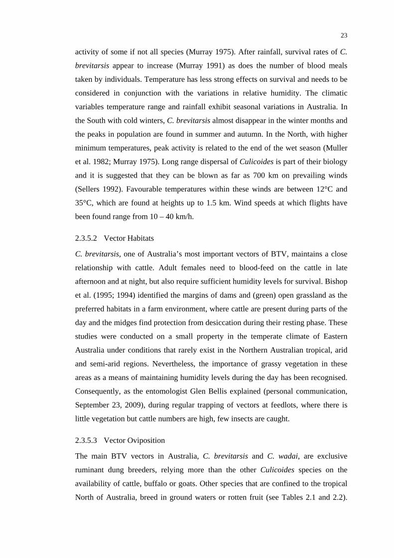
23

activity of some if not all species (Murray 1975). After rainfall, survival rates of C.

brevitarsis appear to increase (Murray 1991) as does the number of blood meals

taken by individuals. Temperature has less strong effects on survival and needs to be

considered in conjunction with the variations in relative humidity. The climatic

variables temperature range and rainfall exhibit seasonal variations in Australia. In

the South with cold winters, C. brevitarsis almost disappear in the winter months and

the peaks in population are found in summer and autumn. In the North, with higher

minimum temperatures, peak activity is related to the end of the wet season (Muller

et al. 1982; Murray 1975). Long range dispersal of Culicoides is part of their biology

and it is suggested that they can be blown as far as 700 km on prevailing winds

(Sellers 1992). Favourable temperatures within these winds are between 12°C and

35°C, which are found at heights up to 1.5 km. Wind speeds at which flights have

been found range from 10 – 40 km/h.

2.3.5.2 Vector Habitats

C. brevitarsis, one of Australia’s most important vectors of BTV, maintains a close

relationship with cattle. Adult females need to blood-feed on the cattle in late

afternoon and at night, but also require sufficient humidity levels for survival. Bishop

et al. (1995; 1994) identified the margins of dams and (green) open grassland as the

preferred habitats in a farm environment, where cattle are present during parts of the

day and the midges find protection from desiccation during their resting phase. These

studies were conducted on a small property in the temperate climate of Eastern

Australia under conditions that rarely exist in the Northern Australian tropical, arid

and semi-arid regions. Nevertheless, the importance of grassy vegetation in these

areas as a means of maintaining humidity levels during the day has been recognised.

Consequently, as the entomologist Glen Bellis explained (personal communication,

September 23, 2009), during regular trapping of vectors at feedlots, where there is

little vegetation but cattle numbers are high, few insects are caught.

2.3.5.3 Vector Oviposition

The main BTV vectors in Australia, C. brevitarsis and C. wadai, are exclusive

ruminant dung breeders, relying more than the other Culicoides species on the

availability of cattle, buffalo or goats. Other species that are confined to the tropical

North of Australia, breed in ground waters or rotten fruit (see Tables 2.1 and 2.2).

24

Adult female C. brevitarsis lay a batch of eggs in fresh dung pads, not older than 7

days, from where they hatch about one day after deposition. After the larvae have

gone through three stages, they pupate and emerge as adults in 7-10 days under

optimal conditions (Campbell and Kettle 1976).

2.3.5.4 Density, Fecundity, and Longevity of the Vector

Abundance is a function of several factors: high rates of activity, low rates of

dispersal, rapid larval development, low adult mortality, and year-round breeding

(Mellor, Boorman, and Baylis 2000). The influence of environmental factors varies

from place to place. The latitudinal limits are often determined by temperature, while

abundance is related to summer rainfall, as has been shown for C. brevitarsis in

NSW (Murray and Kirkland 1995). In regions further north, where temperature is

more suitable, both temperature and rainfall have been positively related to the risk

of BTV seroconversion of cattle during the wet season (Ward 1996). A major

response to adequate rain is good pasture growth that may well change the quantity

and quality of cow pads, increasing their availability for oviposition and suitability

for the immature stages of C. brevitarsis (Murray 1991). While vectors are active

year-round in the tropical North, the major period of activity is between November

and May, when temperatures are favourable on the East Coast of QLD and the

Northeast of NSW and tropical and monsoonal rainfall creates suitable breeding sites

in the otherwise arid regions of the North (Pilbara, Kimberley). Adult female

Culicoides start mating on the day of hatching and after having the first blood meal

they lay their eggs. Midges may then be ready for another blood meal within 1-2

days, but it takes 1-2 weeks after an infective blood meal (depending on the

temperature) before the midge becomes infected with the virus which may be

excreted through the saliva during subsequent blood meals (Animal Health Australia

2001). Once infected, Culicoides may transmit the virus for their lifetime of several

weeks.

2.3.5.5 Movement and Migration of Vectors and Hosts

Dispersal of Culicoides is not limited to their flight range of a few kilometres, but

can extend to 700 km if midges are blown by prevailing winds as aerial plankton

(Mellor, Boorman, and Baylis 2000). Movement of infected hosts (particularly

livestock) plays an important role in the spread of BTV and is discussed below.

25

2.3.5.6 Anthropogenic Influence

The most relevant anthropogenic influence on BTV abundance is the movement of

livestock around the pastoral regions of Australia. As most of the susceptible vectors

preferentially feed on cattle and some rely on cattle dung to breed, midges numbers

might rise and fall with the availability of suitable livestock. Moving cattle from

areas where BTV is endemic to epidemic areas could lead to outbreaks, if the

environmental conditions are favourable. As an example, the Pilbara region

experienced an outbreak of BTV in 2001, more than 20 years after the last recording

of BTV. According to the former NAMP coordinator for WA, R. Norris (personal

communication, March 14, 2008), it is assumed that infected cattle had been moved

from the Kimberley into an environment that supported BTV at least for several

years, before the virus temporarily disappeared in 2007. Another possible factor

supporting BTV emergence might be the significant rise in cattle numbers, changing

from a sheep industry almost solely to cattle stations (Animal Health Australia 2001).

Although no direct relationship can be proven between the first isolation of BTV and

the increase in cattle numbers since the late 1990’s, it is certainly an effect that needs

to be taken into consideration, when estimating vector numbers and BTV infections.

Figure 2.3 shows the historical development of total numbers of cattle and sheep held

in the Pilbara between 1909 and 2006, based on data from the Australian Bureau of

Statistics.

0

200,000

400,000

600,000

800,000

1,000,000

1,200,000

1,400,000

1,600,000

1,800,000

1910 1920 1930 1940 1950 1960 1970 1980 1990 2000 2010

cattlesheep

stoc

k nu

mbe

rs

year

Figure 2.3 Sheep and cattle numbers in the Pilbara from 1909 to 2006. Source: Australian Bureau of Statistics and the Pastoral Lease Information System

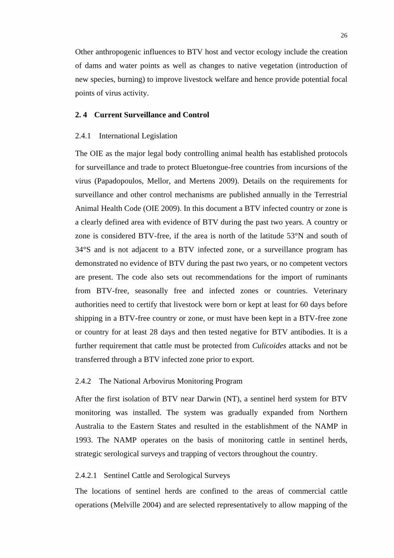
26

Other anthropogenic influences to BTV host and vector ecology include the creation

of dams and water points as well as changes to native vegetation (introduction of

new species, burning) to improve livestock welfare and hence provide potential focal

points of virus activity.

2. 4 Current Surveillance and Control

2.4.1 International Legislation

The OIE as the major legal body controlling animal health has established protocols

for surveillance and trade to protect Bluetongue-free countries from incursions of the

virus (Papadopoulos, Mellor, and Mertens 2009). Details on the requirements for

surveillance and other control mechanisms are published annually in the Terrestrial

Animal Health Code (OIE 2009). In this document a BTV infected country or zone is

a clearly defined area with evidence of BTV during the past two years. A country or

zone is considered BTV-free, if the area is north of the latitude 53°N and south of

34°S and is not adjacent to a BTV infected zone, or a surveillance program has

demonstrated no evidence of BTV during the past two years, or no competent vectors

are present. The code also sets out recommendations for the import of ruminants

from BTV-free, seasonally free and infected zones or countries. Veterinary

authorities need to certify that livestock were born or kept at least for 60 days before

shipping in a BTV-free country or zone, or must have been kept in a BTV-free zone

or country for at least 28 days and then tested negative for BTV antibodies. It is a

further requirement that cattle must be protected from Culicoides attacks and not be

transferred through a BTV infected zone prior to export.

2.4.2 The National Arbovirus Monitoring Program

After the first isolation of BTV near Darwin (NT), a sentinel herd system for BTV

monitoring was installed. The system was gradually expanded from Northern

Australia to the Eastern States and resulted in the establishment of the NAMP in

1993. The NAMP operates on the basis of monitoring cattle in sentinel herds,

strategic serological surveys and trapping of vectors throughout the country.

2.4.2.1 Sentinel Cattle and Serological Surveys

The locations of sentinel herds are confined to the areas of commercial cattle

operations (Melville 2004) and are selected representatively to allow mapping of the

27

distribution of infections. Hence most herds are positioned along the border between

expected infected and uninfected areas, or where infection occurs irregularly. Herds

within the affected areas are also tested to assess the seasonal intensity of infection.

Supplementary, areas which are expected to be BTV-free are monitored to verify

their free status (Animal Health Australia 2006). Figure 2.4 shows an overview of

NAMP sites in northwest Australia that were tested between November 2000 and

October 2009.

!

!

!

!

!

!

!(

(

(<

!

<

<

(

<

!

<<

(

(

!

((

(

<(

((

(

(

(

(

(

(

(

(

( (

(

(

(

<

(

(

<

(!

!

!

(

(

(

(

(

((

( (

(

(<

(

(

(

<

(

(

(

(

((

(

(

<

(

(

<

<

<

<

(

(

(

!

!

!

!

<

!

!

(

(

((

(

<<(

(

(

!

<

!

(

(

(

(( ((

!

(

!

(

<

(

(

(

(

(

( (

(

(

( (

<

<(

<

<

(

((<

(

(

(

<

!

(

(

(

(((

(

((

(

(

(

( ((

(

(

(

(

(

(

(

((

(

(

!

(

(

(

!

(

! Sentinel Herd

< Sentinel Herd / Serosurvey

( Serosurvey

Western Austral ia South Austra lia

Northern Terri tory

Figure 2.4 Location of NAMP sites (sentinel herds and serological surveys) tested between November 2000 and October 2009 in WA and the NT. Note: not all sites are

tested regularly. For a more detailed annual overviews see Figures 5.4 and 5.8 in Chapter 5

Sentinel herds usually consist of 10 to 25 young cattle, which have initially tested

negative for BTV antibodies. The animals are bled in intervals ranging from monthly

to at least twice a year (pre and post summer) and samples are tested for BTV

28

antibodies to determine seroconversion during the BTV activity season. Cattle are

replaced annually or after seroconversion has been determined. In addition to the

sentinel herd system, opportunistic serological surveys are conducted during the

mustering season. Random blood samples are taken from cattle not older than 12

months and born on the property, and tested for BTV. In contrast to sentinel animals,

the same animal is not necessarily sampled twice. The campaign usually starts at the

end of the wet season in May and may last until October, with most samples taken in

August and September.

2.4.2.2 Vector Trapping

The second corner stone of surveillance is vector trapping and quantification of

Culicoides species at the sentinel herd sites and numerous other strategic locations

(Cameron 2004). Light traps are usually positioned in trees near cattle during new

moon, up to ten times a year. After two consecutive nights, the specimens - caught in

a preserving solution - are sent an entomologist for identification.

2.4.2.3 Virus Isolation

In addition to serological tests, NAMP conducts virus isolation studies at two sites on

Cape York (QLD) and one site at Beatrice Hill Farm (BHF) Research Station, 60 km

north of Darwin. At BHF incursions of new BTV strains from overseas have been

detected for the first time in Australia. At BHF, sentinel animals are bled weekly for

virus isolation and monthly for serology (Melville 2004).

2.4.3 Resulting Data and Information

The data sampled at monitoring sites are entered into the NAMP database via a

secure web based interface, which has been in operation since 1998 (Cameron

2000b). This database defines the main input for the definition of three zones

according to OIE guidelines as mentioned earlier. The zones ‘free of BTV’,

‘infected’ and a ‘surveillance zone’ as buffer between those two are defined and

adjusted on the basis of monitoring results, property boundaries and expert

knowledge (Cameron 2004). Although a spatio-temporal distribution model of BTV

host and vectors has been developed by Cameron (2000a) using geographical and

environmental factors in addition to monitoring results, the model has never been

operationally used in the zone definition process (Angus Cameron, AusVet Animal

29

Health Services, personal communication, February 28, 2008). The current zoning

maps, automatically generated reports on BT status and vector numbers can be

access through the NAMPinfo web interface (Animal Health Australia 2010).

2.4.4 Limitations

The traditional monitoring described here is very time consuming and also

expensive. With limited resources available and large remote areas to observe, data

on arbovirus activity exhibit strong spatial and temporal limitations. Numbers and

locations of cattle herds and vector trapping sites vary from year to year, as sentinel

animals are moved within properties or operation is ceased. Hence, presence and

absence information for vectors and virus is often available for a certain period and

only at property level, which can include areas of some tens of thousands of hectares.

Even where the geographic location of sample sites is known, e.g. for trapped

vectors, and detection of vector activity is possible, this detection is limited to

specific locations, which are sparsely and unevenly distributed over Australia.

Furthermore, the time intervals between serological tests and vector trapping are

often irregular, due to varying accessibility of sites and size of the surveyed region.

Extending the surveillance program is costly and difficult to achieve under the

current policy that providing cattle for sentinel herds and serological surveys is

voluntary for pastoralists. Finding BTV on a property often means significant losses

not only on the positively tested station, but also on neighbouring properties in a

radius of 100 km. As a consequence of the limitations of traditional monitoring, the

spatio-temporal variations of virus ecology are still incompletely understood.

2. 5 Summary Australia hosts a wide range of arthropod transmitted viruses, some of which pose a

serious threat for human and animal health. Bluetongue virus is an Orbivirus

transmitted by Culicoides biting midges that can cause Bluetongue, a non-

contagious, infectious disease of wild and domestic ruminants, particularly sheep.

While there is no immediate risk of a BTV outbreak in the large sheep populations in

the South of Australia, the presence of the virus the North causes limitations to the

trade of livestock.

30

The distribution of BTV is limited to the tropic and sub-tropic regions in the North of

Australia and along the East Coast, where the environmental conditions are suitable

to sustain the transmission cycle of the virus. Currently, five Culicodes species are

known to be capable of transmitting the virus in Australia. Importantly, the presence,

emergence and survival of these vector species is closely related to environmental

factors, such as temperature, humidity, vegetation, as well as the availability of

ruminant hosts.

Current surveillance of BTV activity includes testing of sentinel animals for

antibodies, complemented by serological surveys and trapping of vectors. While this

system has been recognised for its ability to reliably monitor and report the disease

status to international trade partners, it is not the most efficient approach. Resulting

data from the remote pastoral areas in North Australia are sparse and characterised

by large spatial and temporal gaps.

31

CHAPTER 3

DISEASE DISTRIBUTION MODELLING IN SPATIAL EPIDEMIOLOGY

The ecology of Bluetongue virus has been explored in the previous chapter, with a

review of environmental factors relevant to the transmission cycle of the pathogen.

This chapter first introduces the field of spatial epidemiology, which is concerned

with the analysis of disease patterns and spatio-temporal linkages between disease

occurrence and environmental factors. The following section continues with a

description and comparison of potential modelling techniques that are frequently

applied in epidemiology to predict the spatial distribution of disease from a set of

explanatory variables. The strengths and weaknesses of each method are

highlighted. Recommendations are then given for the most appropriate method for

vector-borne disease modelling within the context of this research. The chapter

concludes with an overview of measures for model evaluation.

3. 1 Spatial Epidemiology The field of spatial epidemiology studies the distribution of diseases, as well as the

causes and consequences of spatial variation in disease risk (Clements and Pfeiffer

2009; Ostfeld, Glass, and Keesing 2005). When the location, and ideally also the

time of disease occurrence is known, e.g. through human cases or serological

surveys, spatial analytical methods can be used to address the following sequence of

questions: What is the distribution of the disease? Can any spatial or spatio-temporal

patterns be detected? What are the causal factors underpinning these patterns? Can

those factors be mapped to identify risk areas and ideally change the factors to

improve human and animal health? (Robinson 2000). A number of books provide

comprehensive overviews on the use of spatial statistical methods, GIS and remotely

sensed environmental risk factors in the field of epidemiology to answer these

questions (Durr and Gattrell 2004; Hay, Graham, and Rogers 2006; Hay, Randolph,

and Rogers 2000; Pfeiffer et al. 2008). The fundamental concepts and most relevant

methods and data for distribution modelling will be highlighted in Chapter 3 and 4.

32

3.1.1 History and Future of Spatial Epidemiology

The cholera outbreak map by Dr. John Snow (see Figure 3.1) is probably the best

known and earliest example of a spatial epidemiological application. The locations of

cholera incidents were plotted on a street map of London together with the locations

of public water pumps as the possible risk factors. This approach supposedly lead to

the identification of a contaminated pump in Broad Street as the cause of the

outbreak. Following the removal of the handle from the pump no further incidences

were reported. While today it is acknowledged that this well might not be the only

cause for the outbreak (McLeod 2000), the map published by Snow has made him a

hero in medical geography, spatial epidemiology and related disciplines. Snow not

only demonstrated the importance of maps for spatial reasoning, but also promoted

the benefits of maps for decision making and risk communication.

Figure 3.1 Dr. John Snow’s map of deaths from cholera in the area around Broad Street in London. Source: Gilbert (1958)

33

More than 150 years later, spatial epidemiology has developed into an innovative

field that is driven by advances in digital data processing, spatial statistical analysis

and modelling (Clements and Pfeiffer 2009). Environmental variables derived from

remote sensing satellites have become widely available to be used as risk factors in

epidemiological models (Hay et al. 2006). Geographic Information Science and

Systems and statistical analysis software provide means for efficient processing and

analysis of environmental and disease data to identify spatial and temporal patterns

and predict future occurrences (see Chapter 4).

3.1.2 The Concept of Landscape Epidemiology

In the 1930s the pioneering Russian parasitologist Pavlowsky (1966) first discovered

the importance of the landscape and the environment for the transmission of

infectious diseases, and coined the term Landscape Epidemiology. Pavlovsky made

three basic observations, which are still fundamental to epidemiology and underpin

the work presented in this thesis. Firstly, diseases tend to be limited geographically to

an area, which is also known as the focus or nidus of the disease. According to the

third edition of Webster’s New World Medical Dictionary, nidus is the latin word for

nest and is used in medicine to refer to any structure that resembles a nest in

appearance. In the context of this research, nidus refers to a breeding place where

bacteria, parasites and other agents of a disease lodge and develop. Secondly, the

spatial variation of the disease is influenced by biological and physical variations that

support the distribution of the pathogen, its vectors and hosts.

Figure 3.2 Conceptual nidus showing how competent vector, host and pathogen populations intersect within a permissible environment to enable pathogen

transmission. Adapted from Reisen (2010)

34

A natural nidus of disease exists under certain conditions of climate, vegetation, soil,

and microclimate at locations, where vectors, infected and uninfected hosts cluster

(see Figure 3.2). Thirdly, if these biotic and abiotic conditions can be delineated on a

map, then spatial and temporal patterns of disease risk should be predictable.

3.1.3 Scale and Scope of Variations in Environmental Conditions

The environmental conditions defining the nidus or focus of a disease are spatially

and temporally dynamic and variations are important at different spatial and temporal

scales. Changes in climate often occur on a regional to global scale, in contrast to the

local to regional scale variations in landscape.

Temporal variations in climate can be divided into seasonal (intraannual), annual

(interannual), and long-term (decadal or longer) change (Reisen 2010). Seasonal

changes in temperature, precipitation and day length are closely related to primary

productivity and food availability and therefore determine the favourable and hence

reproductive periods of vectors and hosts. Long term climate cycles such as the

El Niño - Southern Oscillation (ENSO) can influence the duration and intensity of

these favourable periods. The El Niño phase of the three to eight year ENSO cycle

may lead to drought in Australia and reduced risk for BTV infections (Ward and

Johnson 1996), while increasing rainfall and hence the risk for Rift Valley Fever in

East Africa (Linthicum et al. 1999). Above these long term climate patterns, a trend

of global warming has been observed in the last century with an increase in mean

annual surface air temperature in Australia by about 0.9°C (CSIRO and Bureau of

Meteorology 2007). One of the associated risks is the dispersal of vector-borne

diseases from their known distribution into areas that have previously been outside

the habitable range of the vectors, mainly due to low temperatures. There is evidence

that climate change was one of the main factors to allow the spread of BTV into

Northern Europe (Purse et al. 2005; Purse and Rogers 2009), but this relationship is

less obvious for other arboviruses and it is advisable to investigate alternative causal

factors (Gould and Higgs 2009; Rogers and Randolph 2006).

On a spatial scale, favourable climatic conditions may persist over large areas, such

as the tropics, where many pathogens are endemic, including Bluetongue, Dengue or

parasites such as Malaria. In times of adverse conditions, such as drought or low

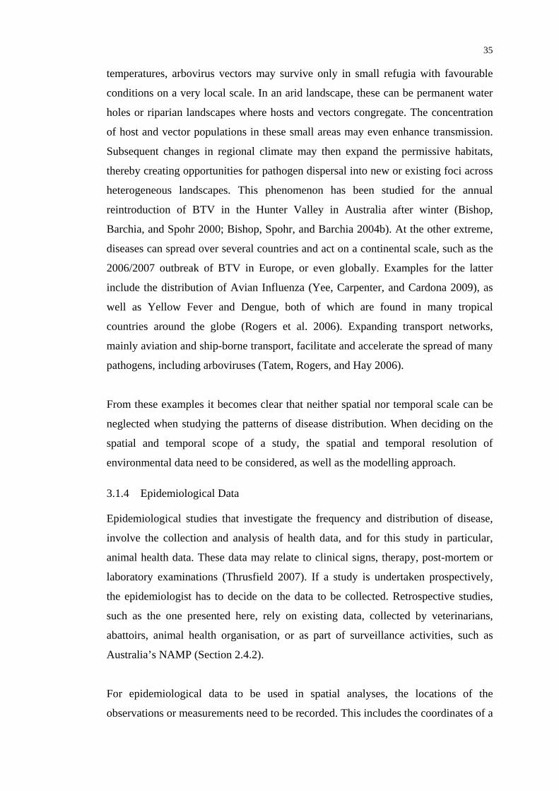
35

temperatures, arbovirus vectors may survive only in small refugia with favourable

conditions on a very local scale. In an arid landscape, these can be permanent water

holes or riparian landscapes where hosts and vectors congregate. The concentration

of host and vector populations in these small areas may even enhance transmission.

Subsequent changes in regional climate may then expand the permissive habitats,

thereby creating opportunities for pathogen dispersal into new or existing foci across

heterogeneous landscapes. This phenomenon has been studied for the annual

reintroduction of BTV in the Hunter Valley in Australia after winter (Bishop,

Barchia, and Spohr 2000; Bishop, Spohr, and Barchia 2004b). At the other extreme,

diseases can spread over several countries and act on a continental scale, such as the

2006/2007 outbreak of BTV in Europe, or even globally. Examples for the latter

include the distribution of Avian Influenza (Yee, Carpenter, and Cardona 2009), as

well as Yellow Fever and Dengue, both of which are found in many tropical

countries around the globe (Rogers et al. 2006). Expanding transport networks,

mainly aviation and ship-borne transport, facilitate and accelerate the spread of many

pathogens, including arboviruses (Tatem, Rogers, and Hay 2006).

From these examples it becomes clear that neither spatial nor temporal scale can be

neglected when studying the patterns of disease distribution. When deciding on the

spatial and temporal scope of a study, the spatial and temporal resolution of

environmental data need to be considered, as well as the modelling approach.

3.1.4 Epidemiological Data

Epidemiological studies that investigate the frequency and distribution of disease,

involve the collection and analysis of health data, and for this study in particular,

animal health data. These data may relate to clinical signs, therapy, post-mortem or

laboratory examinations (Thrusfield 2007). If a study is undertaken prospectively,

the epidemiologist has to decide on the data to be collected. Retrospective studies,

such as the one presented here, rely on existing data, collected by veterinarians,

abattoirs, animal health organisation, or as part of surveillance activities, such as

Australia’s NAMP (Section 2.4.2).

For epidemiological data to be used in spatial analyses, the locations of the

observations or measurements need to be recorded. This includes the coordinates of a

36

specific point location associated with a spatial reference system, such as latitude and

longitude. Mobile GPS-enabled devices are able to record location information at

accuracies in the range of 10 m horizontally (Hay 2000) and usually allow for

capture of associated attributes. Another form of registering point locations includes

the physical address of e.g. a farm or veterinary practice, although this approach may

introduce inaccuracies due to geocoding errors (Zinszer et al. 2010). Point based

information may be useful for some studies, especially at a local scale, when clusters

of disease shall be detected. However, point locations may be only representative,

when the target population is immobile, such as livestock held in enclosures. Often

the true location of an incidence is unknown, and the support, regarded as the

effective size of each sample (Isaaks and Srivastava 1989), is much wider. On large

farms, cattle could have been able to roam over a large area before a survey could be

conducted. In this case the support would expand over the whole property and areal

representation of the farm would be more appropriate (Pfeiffer et al. 2008). Due to

cost-efficiency considerations and complexity of analyses, point representations of

either the farm house or the farm centroid are still predominantly used, even though

this introduces spatial error (Durr and Froggatt 2002).

While it would be desirable to preserve the original location information, this may

often be against confidentiality policies, particularly when dealing with public health

data. Epidemiological data are therefore often provided in aggregated form as

summary statistics at a defined administrative level, such as a shire, state or country.

The most common form of aggregation is to count the total number of disease cases

in an area. These counts can then be expressed as prevalence or incidence rate

(Pfeiffer et al. 2008). In brief, prevalence is the number of instances of a disease (or

associated attributes, e.g. infection or presence of antibodies), divided by the number

of animals in the population at risk at a certain point in time. Incidence rate measures

the rapidity with which new cases of disease develop over time. The full definition of

these and other measures of disease occurrence is provided by Thrusfield (2007).

It is important that the choice of administrative unit matches with the spatial

resolution at which the epidemiological conclusions are drawn. If assessing the

occurrence of BTV on a continental level, district or shire data should be appropriate,

but if the relationship with local environmental conditions is to be investigated, data

37

on single farm locations are necessary. Also the influence of changing zone

boundaries on the observed spatial patterns, the so called Modifiable Areal Unit

Problem (MAUP) (Openshaw 1984) needs to be recognised. This is related to

ecological fallacy, which is a widely recognized error that occurs in data

interpretation, when conclusions for individuals are drawn from aggregate statistics

for a group, to which the individuals belong (Cressie 1993). Consequently, if a farm

has been declared BTV positive, this does not necessarily mean that all cattle are

infected.

Epidemiological data can be, and often are, replete with errors and uncertainty that

compromise location and attribute accuracy. These errors can include incorrect

georeferencing; confusion about the correct choice of spatial reference unit, e.g.

administrative unit; incorrect diagnosis of a disease, which may lead to false

presence or absence records; and confusion over the aggregation method, which may

lead to the use of incorrect location and data values. If the investigator has control

over data collection and analysis, much of the uncertainty can be controlled or at

least accounted for. However, if the data come from another source, it is important to

be aware of the quality and methods that have been used to produce the data

(Atkinson and Graham 2006).

The following sections within this chapter will review distribution modelling

approaches frequently used in ecology and epidemiology, as well as measures for

model evaluation.

3. 2 A Framework for Disease and Species Distribution Models The purpose of any model is to represent the complexity of a real world system.

Models can improve the understanding of a system and be used to predict or describe

an outcome within a system (O'Brien 2004). Distribution models used in ecology aim

to predict the geographic range of species based on known occurrences and

environmental factors. In epidemiology, and in particular when dealing with vector-

borne diseases, the distribution of vector and host species is of major interest to

predict the probability of pathogen transmission. In general, two major groups of

models are used for vector-borne diseases, namely mathematical biological (or

process based) models and statistical models.

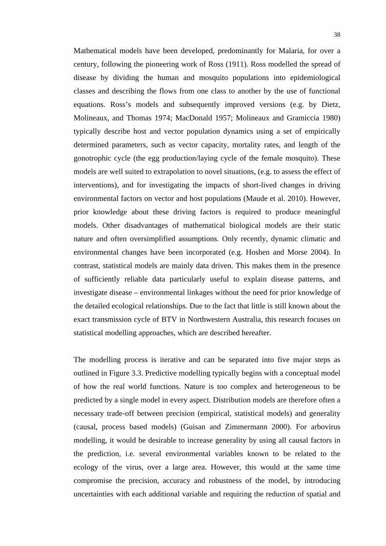
38

Mathematical models have been developed, predominantly for Malaria, for over a

century, following the pioneering work of Ross (1911). Ross modelled the spread of

disease by dividing the human and mosquito populations into epidemiological

classes and describing the flows from one class to another by the use of functional

equations. Ross’s models and subsequently improved versions (e.g. by Dietz,

Molineaux, and Thomas 1974; MacDonald 1957; Molineaux and Gramiccia 1980)

typically describe host and vector population dynamics using a set of empirically

determined parameters, such as vector capacity, mortality rates, and length of the

gonotrophic cycle (the egg production/laying cycle of the female mosquito). These

models are well suited to extrapolation to novel situations, (e.g. to assess the effect of

interventions), and for investigating the impacts of short-lived changes in driving

environmental factors on vector and host populations (Maude et al. 2010). However,

prior knowledge about these driving factors is required to produce meaningful

models. Other disadvantages of mathematical biological models are their static

nature and often oversimplified assumptions. Only recently, dynamic climatic and

environmental changes have been incorporated (e.g. Hoshen and Morse 2004). In

contrast, statistical models are mainly data driven. This makes them in the presence

of sufficiently reliable data particularly useful to explain disease patterns, and

investigate disease – environmental linkages without the need for prior knowledge of

the detailed ecological relationships. Due to the fact that little is still known about the

exact transmission cycle of BTV in Northwestern Australia, this research focuses on

statistical modelling approaches, which are described hereafter.

The modelling process is iterative and can be separated into five major steps as

outlined in Figure 3.3. Predictive modelling typically begins with a conceptual model

of how the real world functions. Nature is too complex and heterogeneous to be

predicted by a single model in every aspect. Distribution models are therefore often a

necessary trade-off between precision (empirical, statistical models) and generality

(causal, process based models) (Guisan and Zimmermann 2000). For arbovirus

modelling, it would be desirable to increase generality by using all causal factors in

the prediction, i.e. several environmental variables known to be related to the

ecology of the virus, over a large area. However, this would at the same time

compromise the precision, accuracy and robustness of the model, by introducing

uncertainties with each additional variable and requiring the reduction of spatial and

39

temporal resolution to be able to handle the model computationally. Also a model

that very accurately describes the suitable habitat conditions for a species in one area,

may not work for the same species in another area.

1.Conceptual Model

2.StatisticalFormulation

Descriptive data from literature,field knowledge

Laboratory experiments

Statistical literature,Existing models

Samplingdesign

3.Calibration

4.Predictions

Calibration dataset

Fitted values

Evaluation dataset

Predicted values

Diagnostic tests

Quality ofthe fit

Predictivepower

Evaluationtables

Model 5.Evaluation

1.Conceptual Model

2.StatisticalFormulation

Descriptive data from literature,field knowledge

Laboratory experiments

Statistical literature,Existing models

Samplingdesign

3.Calibration

4.Predictions

Calibration dataset

Fitted values

Evaluation dataset

Predicted values

Diagnostic tests

Quality ofthe fit

Predictivepower

Evaluationtables

Model 5.Evaluation

Figure 3.3 Overview of the successive steps (1-5) of the (generic) model building process, if two independent datasets are available – one for model calibration and

one for model evaluation. Adapted from Guisan and Zimmermann (2000)

The first step, the formulation of a conceptual model based on knowledge from

literature, field work and laboratory experiments will ideally lead to the choice of an

appropriate spatial and temporal scale and a set of conceptually meaningful

explanatory variables for the predictive model (see Chapter 5).

Also, an efficient sampling strategy needs to be developed, for the species or disease

under investigation as well as the explanatory bioclimatic variables. A number of

approaches have been reviewed in the literature (e.g. Thrusfield 2007) that can be

separated into probabilistic (e.g. random, systematic, stratified) and non-probabilistic

(e.g. convenience, purposive, haphazard) approaches. Surveillance programs, such as

NAMP apply a stratified random sampling strategy, where from the population at

risk (the strata), e.g. all cattle on a pastoral station, individuals are selected randomly

for bleeding. Cattle age has been included in NAMP as an additional selection

criteria within the population at risk, to ensure the tested animals are young enough

40

that they could have been exposed to the virus only during a single season. Ideally,

the choice of sampled cattle stations should be systematic rather than random to

provide an even spatial coverage, at least of at-risk areas (Curran et al. 2000). Often,

as in the case of NAMP, a convenience approach is followed due to practical and

strategic considerations, and the spatial variation of observations will necessarily be

biased. This needs to be considered when interpreting the model outcome. In many

cases, particularly when working with surveillance data retrospectively, the modeller

is not involved in sampling design.

Methods for the acquisition of environmental data for the entire study area at the

desired resolution will be discussed in Chapter 4. For the purpose of model

development and to establish a relationship between environment and disease, it is

crucial to decide on a support of the response variable, i.e. the effective sample size,

or space on which each observation is defined, that makes biological sense and is

constant across the region of interest (Curran and Atkinson 1999; Curran et al. 2000).

For example, when animals sampled at a specific location have been exposed to a

much wider environment that might have led to infection with the virus, then the

choice of support should reflect this.

The second step in model development comprises the choice of a suitable algorithm

for predicting a particular response variable and estimating the model coefficients, as

well as finding an optimal statistical approach with regards to the particular

modelling context (Guisan and Zimmermann 2000). In epidemiology, the response

variable may be a count of disease summarised by an area unit (e.g. county or state)

or more simply, as in the present project, disease presence (‘positive’) or absence

(‘negative’) at a given location (e.g. farm or household). Less frequently, compared

to other disciplines (e.g. ecology), the outcomes may be measured on a continuous or

ordinal scale (Pfeiffer et al. 2008). Hence, in Section 3.3, the focus will shift to

statistical modelling approaches dealing with binary presence/absence data.

Consideration will also be given to identifying a robust approach that may deal with

a small sample size, is easy to implement and, in view of a future operational

implementation, easy to operate and communicate. Section 3.4 will then discuss

spatial effects that may induce variations between the response at different location,

and present ways of expanding traditional models to deal with those effects.

41

The third step is model calibration, an iterative process that aims to enhance the

accuracy and predictive power of the model. This task involves the selection of

variables or combinations of variables to be included in the model. It can be either

arbitrarily (which is not recommended), automatically (e.g. by stepwise inclusion or

stepwise exclusion of variables used on regression models), by following

physiological principles, or by following shrinkage rules (Harrell, Lee, and Mark

1996). The main decisions to be made by the modeller are the starting set of

variables, the statistical or knowledge based criteria upon which to exclude or

include a variable, and when to stop adding or subtracting a variable. In many

instances, developing a parsimonious model that achieves a certain predictive

capability with as few parameters as possible is the preferred strategy. This strategy

is based on the principle known as Occam’s Razor, which suggests that the simplest

explanation is more likely the correct one. In the case of epidemiological modelling,

using fewer variables to explain virus distribution also limits the risk of propagating

errors present in the environmental data. As a rule of thumb, Harrell, Lee, and Mark

(1996) suggest that no more than m/10 predictors should be included in the final

model, where in the case of a binary response m is the number of observations in the

least represented category.

Variable selection may be based on strict statistical measures or upon the improved

fit of the model to the data with or without the variable. A number of measures that

are available to assess model fit will be discussed in Section 3.5 and have previously

been reviewed by Rogers (2006). There is some controversy, as to whether using as

many predictor variables as possible (also termed data mining) improves the fit of the

model, or leads to models that are neither parsimonious nor informative biologically.

Overfitting a model with too many parameters may produce a model that performs

well within the context of the data used for development, but may fail to be robust,

when used elsewhere (Rushton, Ormerod, and Kerby 2004). A more recent trend to

information theoretic approaches (Burnham and Anderson 2002) is based on the

definition of a set of candidate models with prior knowledge and uses the Akaike

Information Criterion (AIC) to select the best-performing one (Gibson et al. 2004).

Rushton, Ormerod, and Kerby (2004) suggest that these approaches will lead to more

ecologically sound and parsimonious models.

42

Once the response of a species or disease to multiple environmental variables has

been derived with any of the described modelling techniques, the possible

distribution within the modelled area can be predicted. GIS has often been used to

implement predictive models (Aspinall and Veitch 1993; Chalke 2006; Guisan,

Weiss, and Weiss 1999; O'Brien 2004) for a number of reasons. They have the

advantage of providing capabilities for exploratory analysis of disease patterns,

handling large predictive datasets that are spatial in nature very efficiently, and

rapidly turning the model outcome into a communicable map (for reviews see Durr

and Gattrell 2004; Kistemann, Dangendorf, and Schweikart 2002; Pfeiffer et al.

2008; Rinaldi et al. 2006). However, not all statistical models are easily implemented

in a GIS environment and some of the modelling steps (statistical formulation and

model calibration) may need to be conducted in a statistical package, such as R or

SPSS or specific ecological modelling programs (Guisan and Zimmermann 2000).

The last and most important step in model selection and development is model

validation or evaluation, as it is alternatively termed. Several methods have been

developed that analyse the predictive success of models based on measuring the

agreement between model predictions and field observations and those are further

described in Section 3.5. Generally, two approaches can be distinguished that either

use a single dataset to calibrate and then evaluate the model, or alternatively use two

separate datasets, one for calibration (the training dataset) and one for evaluation (the

evaluation dataset).

3. 3 Statistical Modelling Approaches for Vectors and Vector-Borne Diseases

3.3.1 Logistic Regression Models

Regression analysis has been widely used in ecology and epidemiology to establish

relationships between a single (simple regression) or a combination (multiple

regression) of predictor variables (independent variables) and the response

(dependant) variable. In studies where the response variable is interval or ratio, linear

regression may be appropriate (Baylis and Rawlings 1998; Hay, Snow, and Rogers

1998; McCann, Baylis, and Williams 2010). However, as Austin (2002) points out,

environmental functions tend to be rarely linear and therefore multiple linear

regression is not often used.

43

Logistic regression, however, is capable of predicting a binary response variable (e.g.

presence/absence) from either continuous or categorical predictor variables, and is

therefore very popular amongst epidemiologists. Logistic regression makes no

assumption about the distribution of the independent variables. They do not have to

be normally distributed, linearly related or of equal variance within each group.

The logistic regression function takes the form:

Logit )( p = mm xx βββ +++ ...110 (3.1)

where β0 is the intercept, β1… βm are the regression coefficients, and x1… xm are the

predictor variables. Logit(p) is the logarithm of the odds, written as:

Logit )( p = ⎥⎦

⎤⎢⎣

⎡− pp

1log

(3.2)

This transformation leads to the logistic model, where the probability of the outcome

p can be expressed as a function of m explanatory variables:

)...( 11011

mm xxep βββ +++−+=

(3.3)

This equation has the convenient property, that p is bounded between the logical

range of 0 and 1, where 1 represents the highest probability for the dependent

variable, e.g. the presence of BTV based on vegetation greenness and mean day

temperature.

As shown in the review by Rushton, Ormerod and Kerby (2004), logistic regression

has been applied by ecologists to map the distribution of a large variety of plant and

animal species and communities, including Rufous Bristlebird in Victoria (Gibson et

al. 2004) and aquatic invertebrates in the Himalaya (Manel, Ceri Williams, and

Ormerod 2001). In epidemiology, logistic regression has been applied to model the

distribution of Murray Valley Encephalitis in Western Australia (Chalke 2006),

Bluetongue in Corsica (Guis et al. 2007), the arbovirus vector Culicoides Imicola in

Italy (Conte et al. 2003), and Foot and Mouth Disease in Northern Thailand (Cleland

et al. 1996).

44

Some of the strengths of logistic regression, e.g. its statistical robustness, the fact that

it is a well defined method and various statistical measures exist for validation

(O'Brien 2004), have certainly contributed to its widespread application in species

distribution mapping (Rushton, Ormerod, and Kerby 2004). Nevertheless, it is

acknowledged that, despite the great accuracy of some logistic regression models, the

assumptions that have to be made are often not realistic (Rogers 2006). Logistic

regression only allows a single transition from 0 (absence) to 1 (presence) across the

entire range of a predictor variable in the situation where the response is an

increasing function of the predictor variable. However, in nature often more than one

transition between species presence and species absence may be found. As an

example, the increase of temperature from very low levels (species is absent) to

intermediate levels (species is present) to very high levels (species is absent again)

clearly shows two transitions on a single predictor variable. In such a case a logistic

regression model would only capture parts of the species’ distribution.

3.3.2 Generalised Linear Models and Generalised Additive Models

First developed in the 1960’s, Generalised Linear Models (GLM) have found

widespread application in ecology (Guisan, Edwards, and Hastie 2002). One of the

reasons is their ability to handle a multitude of probability distributions that describe

ecological data, including normal, binomial or Poisson distributions. GLMs are

mathematical extensions of linear models that allow for non-linearity and non-

constant variance structures in the data. Generalised Additive Models (GAM) (Hastie

and Tibshirani 1990) are a further semi-parametric extension of GLMs, where the

only assumption to be made is that the functions are additive and that the

components are smooth (Guisan, Edwards, and Hastie 2002). The strength of these

models is their ability to deal with highly non-linear and non-monotonic relationships

between the response and the explanatory variables.

In a GLM, the predictor variables xi are combined to produce a linear predictor LP,

which is related to the expected value E(Y) of the response variable Y through a link

function g() in the form:

ii

i xLPYEg ∑+== ββ0))(( (3.4)

45

where β0 is the intercept and βi are the regression coefficients. The distribution of Y

may be any of the distributions of the exponential family, and the link function may

be any monotonic differentiable function (e.g. logarithm or logit) (Guisan, Edwards,

and Hastie 2002). GLM where a binomial distribution is used for the link function

are equivalent to logistic regression.

GAMs are in contrast to GLMs data- rather than knowledge-driven. The relationship

between the response and the explanatory variables is determined directly from the

data rather that assuming some form of parametric relationship (Yee and Mitchell

1991). GAMs relate the expected response E(Y) to the predictor variables xi via:

)())(( 0 ii

i xfYEg ∑+= β (3.5)

where fi are the various functions. In practice, GAMs can be parameterised just like

GLM, with the exception that some predictors can be modelled non-parametrically

using smoothing functions, in addition to linear and polynomial terms (Guisan,

Edwards, and Hastie 2002).

GAMs have been increasingly used in ecological modelling (Austin 2007), and

application examples include studies of ecological factors related to the distribution

of vegetation in New Zealand (Yee and Mitchell 1991) and Switzerland (Lehmann

1998) or of breeding birds in Spain (Seoane, Bustamante, and Diaz-Delgado 2004).

In Australia, McLeod and Pople (2010), used a GAM to map the habitats of feral

camels in the NT. GAMs have also been applied to investigate the risk for cancer

(Kelsall and Diggle 1998), and study the effect of air pollution on public health

(Schwartz 1996). However, compared to logistic regression, fewer epidemiological

studies seem to exploit the potential of GAMs.

The advantage of using GAMs instead of GLMs (or similarly logistic regression) for

presence/absence modelling is the additional flexibility through the replacement of

linear functions with unknown smooth functions. Any response shape is possible,

which allows the estimate to follow the observations more closely (Austin and

Meyers 1996). This makes GAMs particularly attractive for ecological modelling

where linear relationships are seldomly found. A minor drawback is the lack of a

46

conventional mathematical function, which makes it difficult to communicate the

influence of each predictor variable on the response (Heegaard 2002).

3.3.3 Discriminant Analysis

An alternative to logistic regression is discriminant analysis, proposed by Rogers,

Hay and Packer (1996). In contrast to the regression methods presented previously,

which seek a least squares or error-minimizing description of epidemiological data,

discriminant analysis seeks to maximise the between-sample variance relative to the

within-sample variance or other measure of spread around the sample means

(Pfeiffer et al. 2008). The samples are considered categorical, such as presence or

absence of disease, and are defined by multivariate normal distributions of the same

set of predictor variables, but with different multivariate means or centroids and

(usually) different co-variances (Rogers 2006).

In classical linear discriminant analysis, the same co-variance matrix is used for

presence and absence data. Linear discriminant analysis has been used with varying

levels of accuracy for the prediction of tsetse flies in various regions of Africa (e.g.

Rogers, Hay, and Packer 1996) and, using a stepwise approach, to predict

Bluetongue infections in Queensland based on maximum temperature and rainfall

(Ward 1994b). However, as Robinson (2000) notes, the assumption of a common

covariance matrix for both presence and absence is unrealistic and violated by the

data. Instead, using non-linear discriminant analysis, which is equivalent to the

maximum likelihood classification known from remote sensing applications, a

discriminating function that produces more accurate classification results can be

defined (Robinson, Rogers, and Williams 1997a; Rogers 2000). Formulae for linear

and non-linear discriminant analysis are found in Pfeiffer (2008 pp. 103-107) or

Rogers, Hay and Packer (1996).

Essentially, discriminant analysis and logistic regression are very similar and often

produce a similar outcome (Press and Wilson 1978). Nevertheless, the strict

assumption of normally distributed explanatory variables can be seen as a major

limitation compared to the more flexible regression statistics. However, if the

predictors are normally distributed, discriminant analysis may be the more powerful

and efficient strategy (Tabachnick and Fidell 2007).

47

3.3.4 Environmental Envelopes and Ecological Niche Factor Analysis

Environmental envelopes define an envelope in multidimensional attribute space,

within which a species can be expected to be found and persist (O'Brien 2004). The

response variable tends to be presence/absence and responses are classified as

‘present’ if they fall within a given percentile for all variables. Additionally, a

‘marginal’ class may be added for responses that fall within that percentile for some

factors but outside for others (Figure 3.4).

suitablesuitable

unsuitablemarginal

climaticvariable 1

climaticvariable 2

90th

perc

entil

esu

itabl

e

100th

perc

entil

em

argi

nal

90th percentilesuitable

100th percentilemarginal

Figure 3.4 Rectilinear environmental envelope for two climatic variables, after Skidmore et al. (1996)

A number of different algorithms have been developed to define environmental

envelopes and those are often formalised in specialised software packages with GIS

functionality. The most basic environmental envelopes are rectilinear, such as the

technique implemented in the BIOCLIM software (Busby 1991). The BIOCLIM

model fits a species-specific minimal rectilinear envelope in a multidimensional

climatic space, an approach equivalent to the parallepiped or boxcar image

classification algorithms used in multispectral remote sensing applications.

BIOCLIM models have been developed to map a number of species, particularly in

Australia, for example the endangered snake Hoplocephalus bungaroides (Penman et

al. 2010) or kangaroos (Skidmore, Gauld, and Walker 1996), and also to assess the

effects of climate change (Hughes 2003).

More sophisticated approaches define environmental envelopes using bounding

polygons or fuzzy clouds. HABITAT (Walker and Cocks 1991) is an expansion of

48

the BIOCLIM concept that uses a convex polytope (multidimensional polygon)

envelope rather than rectilinear envelopes and also works with an expanded range of

environmental factors. Both models create continuous envelopes in multidimensional

attribute space, including all data points, or those within a given percentile. Any new

location will therefore be classified as ‘suitable’ if all its attribute values fall within

the given range (O'Brien 2004).

A slightly different concept to environmental envelopes is followed by climatic

mapping, which was designed to study the risk of introducing an invasive species

into a new area under the influence of climate change (Sutherst 2004), rather than

mapping natural distributions. As an example, the CLIMEX program (Sutherst and

Maywald 1985) determines a climatic envelope of favourable conditions that is

defined by growth (optimum climatic range) and stress indices (wet, dry, hot, cold)

from a global climatic database. Model parameters are determined using occurrence

and abundance of the target species from outside the area under risk of introduction.

Besides a number of applications in invasive plant and animal species mapping,

CLIMEX has been used to map the potential spread of the arbovirus vector C. Wadai

in Australia under a changing climate, based on known occurrences in Asia

(Standfast and Maywald 1992).

The Ecological Niche Factor Analysis (ENFA) method, developed by Hauser (1995)

and implemented in the BIOMAPPER software (Hirzel et al. 2002) is similar to the

environmental envelope approach in requiring presence-only data. ENFA is an

extension of Principal Component Analysis (PCA) that reduces the predictor

variables to a few uncorrelated factors, but retains their ecological meaning (Hirzel et

al. 2002). Having the advantage of working with presence-only data, ENFA has also

been used to generate pseudo absence data as a preparatory step for developing

GLMs (Calvete et al. 2009).

The major strength of environmental envelopes is that they can be easily interpreted

in biological terms. They also offer the opportunity to include expert knowledge,

where data are lacking (O'Brien 2004). However, compared to GLMs and GAMs

(Segurado and Araújo 2004), the predictive performance of environmental envelopes

is rather poor.

49

3.3.5 Bayesian Methods

Bayesian methods have become increasingly popular in epidemiological applications

over the past 20 years, in common with the development of fast computational

algorithms needed to solve the often complex models (Lawson 2008). Bayesian

models combine a priori probabilities of species or disease occurrence with the

probability (or likelihood) of occurrence conditional to the value of each

environmental predictor (Guisan and Zimmermann 2000).

The prior probability distribution is an initial assumption that may be based on

previous results, literature, or expert opinion. Conditional probability, denoted as

P(X/Y) is the probability of a response variable Y being in a given state, given that the

predictor variable X is in a particular state, and is usually derived from the data.

When the sample size is large, the conditional probabilities will dominate the

outcome, in studies that are data poor, the prior distributions will dominate. For a

comprehensive overview of Bayesian methods used in epidemiology, see Lawson

(2008), Lawson, Browne, and Vidal Rodeiro (2003), or Lawson and Cressie (2000).

In a hierarchical Bayesian model (or alternatively termed Bayesian network),

different parameters may be added to the model to improve the outcome. A Bayesian

network is represented through a Directed Acyclic Graph (DAG) with directed

(cause-effect) linkages between different nodes, each of which represents a predictor

or response variables (Figure 3.5).

Figure 3.5 A simple Bayesian network, after Stassopoulou, Petrou, and Kittler (1998)

For each node, prior and conditional probability distributions are defined. Using

combination rules, conditional probability distributions are propagated through the

network. Realistic models in disease mapping often have two or more hierarchy

50

levels and the resulting complexity of the posterior distribution makes it impossible

to determine its exact form. Various posterior sampling algorithms have been

developed (e.g. Gibbs Sampler, Markov Chain Monte Carlo) (see Lawson 2008). The

implementation of these methods in dedicated software packages, such as BUGS

(Bayesian inference Using Gibbs Sampling) and its Windows version WinBUGS

(Lawson, Browne, and Vidal Rodeiro 2003; Lunn et al. 2000) have had a huge effect

on the dissemination and acceptance of Bayesian modelling in epidemiology.

The study of Stevenson et al. (2005) exemplifies an approach, where a hierarchical

model was used to investigate the factors influencing the distribution of Bovine

Spongiform Encephalopathy (BSE) in Great Britain. Initially, a so called fixed

effects model, e.g. using GLM, is developed under the assumption that the influence

of the predictor variables on the response is independent of the location. However,

the assumption that the predictor variables alone explain the distribution of BSE may

be violated by the presence of spatial autocorrelation between sample sites (see

Section 3.4 for further details) or other random effects. Therefore, the authors

developed a Bayesian mixed effects model (or hierarchical model) that accounts for

the structured (spatially correlated) and unstructured heterogeneity in the data. The

prior probability was determined by the response from the fixed effects model.

Multilevel Bayesian models have been developed to investigate the distribution of a

number of infectious diseases, including BTV in Spain (Allepuz et al. 2010), BSE in

Great Britain (Stevenson et al. 2005), and Malaria in South Africa (Kleinschmidt et

al. 2002).

One of the major strengths of probability based methods like Bayesian approaches is

the flexibility to incorporate both data and expert knowledge. They are also able to

deal with uncertainties that may be included in the probability distributions and

propagated through the model. Dedicated software tools, such as WinBUGS are now

widely available and provide efficient means to even develop more complex models.

3.3.6 Other Methods

In the previous sections a number of modelling techniques based on presence and

absence data were reviewed, which help to increase the understanding of biological

51

and other processes that determine the distribution of species in space and time.

Alternative approaches have been applied to ecological and also disease modelling

(see reviews by Austin 2007), but as Rogers (2006) argues, they often simply

reproduce the distribution map or points drawn from the distribution map through a

“pattern-matching” approach. While the resulting prediction maps might be highly

statistically accurate, these approaches provide minimal biological insight (Rogers

2006). The use of artificial neural network models and k-nearest neighbour

techniques is therefore discouraged , as is that of tree-based classification methods,

and those hybrid systems such as the genetic algorithm for rule-set prediction

(GARP) (Stockwell and Peters 1999), that use genetic algorithms to improve on

initial approaches using more traditional methods.

3. 4 Dealing with Spatial Effects In most classical statistical methods, independence of observations is a fundamental

assumption. However, this assumption may be violated, if spatial dependence is

found in a dataset. In this case, data from spatially close samples contribute less

additional information than if they were further apart. As a consequence of ignoring

this effect in modelling, errors may be underestimated and the significance of some

predictor variables may be overestimated (Pfeiffer et al. 2008). It has therefore

become common practice to analyse the residuals in the model results for spatial

dependence (or spatial autocorrelation; see Section 3.4.2) and if present, to apply one

of the various methods that have been developed to deal with the problem of spatial

dependence and heterogeneity (see Section 3.4.3).

3.4.1 Spatial Heterogeneity and Dependence

The basic principle behind spatial dependence, following Tobler’s (1970) First Law

of Geography, is that attribute values measured at locations that are close together

are more similar than those taken from more distant locations (Pfeiffer et al. 2008). If

this dependence does not vary regardless of the location in a geographic area, the

underlying spatial process is called stationary. In contrast, if the dependence structure

varies throughout the area, the process is termed unstationary or heterogeneous. If

the dependence in a stationary process is the same in any direction, it is considered

isotropic, whereas if dependence changes with direction then it is considered to be

anisotropic.

52

First order effects describe large (macro-) scale variations in the mean of the

outcome of interest due to location or other explanatory variables. This effect

expresses itself as a trend across a geographical region. For example, the risk for

infectious disease transmission may decrease from North to South in a region due to

changes in temperature that affect the survival of an infectious vector. Second order

effects are small-scale variations due to interactions between neighbours, also called

spatial heterogeneity. These effects may be found, e.g. where disease cases cluster

around a saleyard, or disease vectors show some local habitat preference.

3.4.2 Measuring Spatial Autocorrelation

The measure of the degree of similarity between the attributes of neighbouring

samples is also termed spatial autocorrelation. Based on the fact that spatial

autocorrelation is very common, a number of techniques have been developed to

measure it. Moran’s I and Geary’s C, as well as a local Moran test are discussed here

as examples for methods working with aggregated data, such as disease status on a

farm or county level. Other autocorrelation measures can be found e.g. in Cliff and

Ord (1973, 1981). Metrics that identify clusters amongst point locations are

discussed elsewhere (e.g. Pfeiffer et al. 2008).

In order to derive any measurement of autocorrelation, the neighbourhood between

locations needs to be determined. Neighbourhood may be defined based on

adjacency or distance. Approaches using adjacency (also called contiguity), define

neighbourhood between polygons, e.g. by sharing a border (rook contiguity), corner

or border (queen contiguity), or through a second order neighbourhood (neighbours

of neighbours) (Pfeiffer et al. 2008). Approaches based on distance consider

polygons with their centroid located within a specific distance as being adjacent.

Moran’s I coefficient of correlation (Moran 1950) quantifies the similarity of an

outcome variable among areas that are defined as spatially related. It takes the form:

∑∑ ∑∑∑

−

−−=

i j i iij

i j jiij

yyw

yyyywnI

2)()(

))((

(3.6)

53

where n is the number of spatial units, yi is the attribute of an area (e.g. the residuals

of a model), and y the mean of the attributes. wij defines the closeness between areas

i and j through a weight matrix that assigns areas that are close in space a higher

weight than those that are more distant. A Moran’s I of 0 indicates no clustering,

while a positive value indicates positive spatial autocorrelation (i.e. clustering of

areas with similar attribute values) and a negative value indicates negative spatial

autocorrelation (i.e. contiguous areas tending to have dissimilar attribute values). A

disadvantage of Moran’s I is that it is based on the assumption that the correlation is

isotropic (i.e. the same in all directions) and that the attribute of interest is evenly

distributed within the study area. The lack of anisotropy can be overcome by changes

in the weight matrix to reflect directional indifferences. In epidemiology to account

for population differences between spatial units, the use of proportional measures

instead of e.g. disease counts is recommended (Pfeiffer et al. 2008).

Another weighted estimate of spatial autocorrelation is provided by Geary’s

contiguity ratio (abbreviated to Geary’s C). In contrast to Moran’s I it does not

consider similarities between regions, but between pairs of regions. Geary’s C ranges

from 0 to 2, where zero is an indicator for perfect positive autocorrelation and 2

indicates perfect negative autocorrelation. It can be calculated with the following

equation:

( )( )∑ ∑∑∑∑

−

−−=

i j iji i

i j jiij

wyy

yywnC

(2

)()1( 2

(3.7)

where n is the number of spatial units in the study area, wij are the weights in the

spatial proximity matrix, yi are the attributes under investigation and y is the mean of

all attributes.

3.4.3 Incorporating Spatial Dependence into Distribution Models

When the residuals of a model are plotted on a choropleth map as an initial step, they

may show some spatial pattern. If spatial autocorrelation can be found using the tests

discussed before, then the original models should be extended by including

additional parameters. A number of techniques have been developed, including those

54

that extend the regression models and the increasingly popular Bayesian mixed

effects models (described in Section 3.3.5).

Using so called frequentist approaches, regression models are extended with a

normally distributed random effect term with a covariance matrix. There are three

types of spatial covariance structures that can be used: conditional autoregressive,

simultaneous autoregressive and moving average models. For the mathematical

equations see Pfeiffer et al. (2008) and for a comparison of these models refer to

(Dormann et al. 2007). All these methods assume the same degree of autocorrelation

across the study area and few methods exist that allow for non-stationarity. One such

approach is Geographically Weighted Regression (GWR) by Brunsdon,

Fotheringham and Charlton (1996). According to Dormann et al. (2007), however,

this approach is not targeted at distribution modelling due to its limited use for

hypothesis testing, as the coefficient estimates depend on spatial position.

The Bayesian approaches described in Section 3.3.5 provide additional flexibility to

incorporate a mixture of terms for random effects that can be spatially structured

(spatially correlated), or unstructured (spatially random). Compared to the methods

described above, which provide a single (global) autocorrelation coefficient, spatially

correlated random-effect terms are calculated for each spatial unit. For a theoretical

background of Bayesian approaches see Lawson (2008), Lawson, Browne, and

Vidal Rodeiro (2003), Lawson and Cressie (2000), and Pfeiffer et al. (2008).

Bayesian methods can be used for area as well as point data, however when working

with point data the contiguity matrix may become very large and complex. An

alternative is to fit a logistic geostatistical model, implemented in the geoR and

geoRglm packages (Diggle and Ribeiro 2007). The difference to area-based

approaches can be found in the addition of a structured (spatially correlated)

heterogeneity term that is allowed to vary continuously through space rather than

discretely.

There has been a significant advance from considering spatial dependence as

annoyance in distribution models (Horne and Schneider 1995) to the increasing

development of spatially explicit distribution models, particularly using Bayesian

approaches. However, as noted by Pfeiffer et al. (2008) and Pfeiffer (2004),

55

incorporating spatial dependence in model building is only justified if significant

autocorrelation is found. Otherwise a fixed effects model should provide a

satisfactory description of the data. Also by choosing a resolution for the aggregation

area that is lower than the scale at which spatial dependence occurs, the development

of complex spatial models may be avoided.

3. 5 Evaluating the Accuracy of Distribution Models Evaluating or validating a model is the last task in the modelling exercise. While it

lies in the nature of a model that it cannot be tested for being true or false, it can be

assessed for providing good testable hypotheses relevant to important problems

(Levins 1966) and for the accurate prediction of biological patterns (Guisan and

Zimmermann 2000). Furthermore, model evaluation includes a measure of adequacy,

which depends on the purpose of the project and the domain to which the model is

supposed to be applicable (Fielding and Bell 1997).

Depending on the available sample size there are two main approaches for evaluating

the predictive power of a model. In the first approach, a single dataset is used to

calibrate and evaluate a dataset. Different methods exist to select samples for testing,

including leave-one-out or Jack-knife (n samples of 1 case are tested sequentially, the

remaining n - 1 cases comprise the training set), bootstrap sampling (sampling with

replacement) or cross validation (Fielding and Bell 1997; Guisan and Zimmermann

2000). In the second approach, if the data set is large enough to be split, two separate

datasets are used for model calibration and model evaluation.

There are two types of prediction errors that may result from a presence/absence

model: false negatives and false positives. To assess the performance of a

presence/absence model the observed and predicted presence/absence patterns are

usually cross tabulated in a confusion or error matrix that identifies true positive (a),

false positive (b), false negative (c) and true negative (d) cases predicted by each

model (Figure 3.6). A number of measures reviewed by Fielding and Bell (1997),

Pearce and Ferrier (2000) and Rogers (2006) can be derived from the count values in

the confusion matrix (a-d) and the total number of observations N (see Table 3.1).

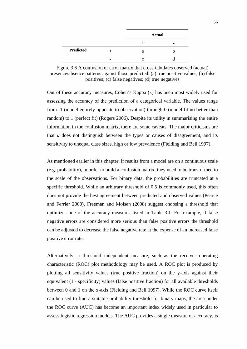
56

Actual

+ - + a b Predicted

- c d

Figure 3.6 A confusion or error matrix that cross-tabulates observed (actual) presence/absence patterns against those predicted: (a) true positive values; (b) false

positives; (c) false negatives; (d) true negatives

Out of these accuracy measures, Cohen’s Kappa (κ) has been most widely used for

assessing the accuracy of the prediction of a categorical variable. The values range

from -1 (model entirely opposite to observation) through 0 (model fit no better than

random) to 1 (perfect fit) (Rogers 2006). Despite its utility in summarising the entire

information in the confusion matrix, there are some caveats. The major criticisms are

that κ does not distinguish between the types or causes of disagreement, and its

sensitivity to unequal class sizes, high or low prevalence (Fielding and Bell 1997).

As mentioned earlier in this chapter, if results from a model are on a continuous scale

(e.g. probability), in order to build a confusion matrix, they need to be transformed to

the scale of the observations. For binary data, the probabilities are truncated at a

specific threshold. While an arbitrary threshold of 0.5 is commonly used, this often

does not provide the best agreement between predicted and observed values (Pearce

and Ferrier 2000). Freeman and Moisen (2008) suggest choosing a threshold that

optimizes one of the accuracy measures listed in Table 3.1. For example, if false

negative errors are considered more serious than false positive errors the threshold

can be adjusted to decrease the false negative rate at the expense of an increased false

positive error rate.

Alternatively, a threshold independent measure, such as the receiver operating

characteristic (ROC) plot methodology may be used. A ROC plot is produced by

plotting all sensitivity values (true positive fraction) on the y-axis against their

equivalent (1 - specificity) values (false positive fraction) for all available thresholds

between 0 and 1 on the x-axis (Fielding and Bell 1997). While the ROC curve itself

can be used to find a suitable probability threshold for binary maps, the area under

the ROC curve (AUC) has become an important index widely used in particular to

assess logistic regression models. The AUC provides a single measure of accuracy, is

57

independent of a specific threshold and less affected than κ by a high/low overall

prevalence (Rogers 2006). The AUC can assume values between 0.5 and 1, where

values of 0.5 – 0.7 indicate low accuracy, values of 0.7 – 0.9 indicate useful

applications and values of > 0.9 indicate high accuracy (Swets 1988).

Table 3.1 Overview of accuracy measures applicable in distribution modelling, compiled from Fielding and Bell (1997) and Rogers (2006)

Measure Description Calculation

Correct classification rate

Total fraction of the sample that is correctly predicted

Nda +

Sensitivity Ability to identify positives correctly ca

a+

Specificity Ability to identify negatives correctly db

d+

False positive rate

Proportion of wrongly predicted positives db

b+

False negative rate

Proportion of wrongly predicted negatives ca

c+

Positive predictive power (PPP)

Probability that a case is positive, if the algorithm classifies the case as positive

baa+

Negative predictive power (NPP)

Probability that a case is negative, if the algorithm classifies the case as negative

dcd+

Cohen’s Kappa (κ)

Index of agreement for positive and negative samples combined

Ndcdbbaca

N

Ndcdbbacada

))(())((

))(())(()(

+++++−

+++++−+

3. 6 Selection of Modelling Approach

The main models considered for distribution mapping in this chapter were logistic

regression, GLM, GAM, discriminant analysis, environmental envelopes and

Bayesian methods. Most of these models are empirical, data driven, while some can

be at least partly knowledge driven.

58

Currently, little is still known about the conditions related to the changing limits of

BTV distribution in the Northwest of Australia. In order to identify the driving

bioclimatic factors for Bluetongue occurrence from the presence and absence data in

the NAMP database, an empiric model will be the most appropriate choice. In

addition, some prior knowledge about the ecology of BTV vectors that is available

for the East Coast of Australia, can be incorporated in the model building process, by

developing and selecting the most appropriate bioclimatic variables. It is most likely,

that pure statistical measures alone would not necessarily lead to an ecologically

sound set of predictor variables.

It is therefore proposed to use a multiple regression model, such as a GLM or GAM

with a binomial distribution to build an initial model based on both statistically and

biologically significant environmental variables. GAMs and GLMs have been widely

applied in ecology due to their robustness and support of a multitude of probability

distributions that best describe ecological data. In particular the semi-parametric

GAM offers a flexible tool for exploratory analysis of predictor variables that do not

follow a standard response curve (see Section 7.3.1). This enables the modeller,

during the variable selection process, to maximise the model predictive capabilities,

while maintaining biological integrity. It can be expected that due to the small

sample size, a stable model would only allow for a small set of predictor variables

(see Harrell, Lee, and Mark 1996). However, this is in line with the plea for

parsimony in distribution models found throughout the literature. If warranted by

strong spatial autocorrelation, the initial non-spatial model may be extended by

spatial heterogeneity terms using a hierarchical Bayesian approach similar to

Stevenson et al. (2005).

3. 7 Summary The field of spatial epidemiology aims to investigate the causal factors for the spatial

variation of disease risk. Occurrence or focus of vector-borne disease is defined by

climatic and environmental factors that govern the interaction between vectors, hosts

and pathogens. Mapping these underlying factors enables epidemiologists to develop

models of disease distribution and risk. However, in order to establish the

relationship between environment and disease it is important to investigate the origin

of the disease data. Epidemiological data, including the location of disease incidents,

59

are often collected at different levels of aggregation, ranging from farms to shires or

whole countries. Considering this aggregation is crucial for determining the support,

i.e. the spatial and temporal range within which the environment influences each

case, and consequently choosing the required spatial and temporal resolution of the

environmental data which will de discussed in Chapter 4.

Following the introduction to spatial epidemiology, a typical workflow for the

development of a species distribution model was presented. The major steps of the

workflow are:

i) Development of a conceptual model;

ii) Statistical formulation;

iii) Model calibration;

iv) Prediction of species distribution; and

v) Model evaluation (validation).

The chapter continued with a review of modelling techniques that could deal with the

binomial presence/absence data as collected by NAMP to develop ecologically

meaningful models that are robust and easy to implement.

The brief discussion of spatial autocorrelation highlighted the importance of

accounting for spatial dependency in model development. A summary of accuracy

metrics was presented that can be used for internal and external model validation.

Finally, a recommendation was made to use GLM and GAM to develop a data driven

model, but still incorporate prior knowledge through the choice of ecologically

meaningful predictor variables.

The following chapter will review current meteorological and environmental earth

observation satellites and associated data products with applications in disease

distribution modelling. A variety of environmental and climatic variables, also

referred to as bioclimatic variables, will be presented as possible candidates for

model development.

60

CHAPTER 4

APPLICATIONS OF REMOTE SENSING IN SPATIAL EPIDEMIOLOGY

This chapter provides a brief overview of the principles of remote sensing, before

reviewing current and future remote sensing technology and data as well as derived

environmental variables commonly used to investigate vector-borne diseases.

4. 1 Remote Sensing in Epidemiology Remote sensing data have been widely adopted by epidemiologists to study a number

of vector-borne diseases, which have been summarised by Kalluri (2007), including

Malaria, Dengue fever, Rift Valley fever and Leishmaniasis. These studies dealt with

the mapping of disease, host and vector distribution and abundance, modelling of

disease risk, early prediction and also the forecasting of disease at a local (e.g. Brown

et al. 2008; Clennon et al. 2006), to regional (e.g. Baylis et al. 1998; Martin et al.

2008; Rizzoli et al. 2007) and global scale (e.g. Rogers et al. 2006). The basic

common principle behind these studies is the utilisation of relationships between

environmental factors derived from remote sensing data and the presence or absence

of the disease of interest (Curran et al. 2000; Schuster et al. 2009). Remote sensing

technology is not able to identify disease vectors directly, but it can be used to

characterise the landscape in which vectors thrive. Environmental parameters such as

land and sea surface temperature, vegetation type, amount and health can be

identified and measured from space. In contrast to other measurements, e.g. from

weather stations, remotely sensed data provide spatially regular information with

area-wide coverage, which makes them particularly useful in remote areas. They also

have the distinctive advantage of being captured automatically, repeatedly (Kalluri et

al. 2007) and unobstrusively when using passive sensors (Jensen 2007). Some

derived high level data products are available at no cost to the user (Tatem, Goetz,

and Hay 2004).

4.1.1 Principles of Remote Sensing

Remote sensing is defined by Lillesand et al. (2008) as the “science and art of

obtaining information about an object, area, or phenomenon through the analysis of

data acquired by a device that is not in contact with the object, area or phenomenon

under investigation”. Many scientific fields, including Geology, Ecology,

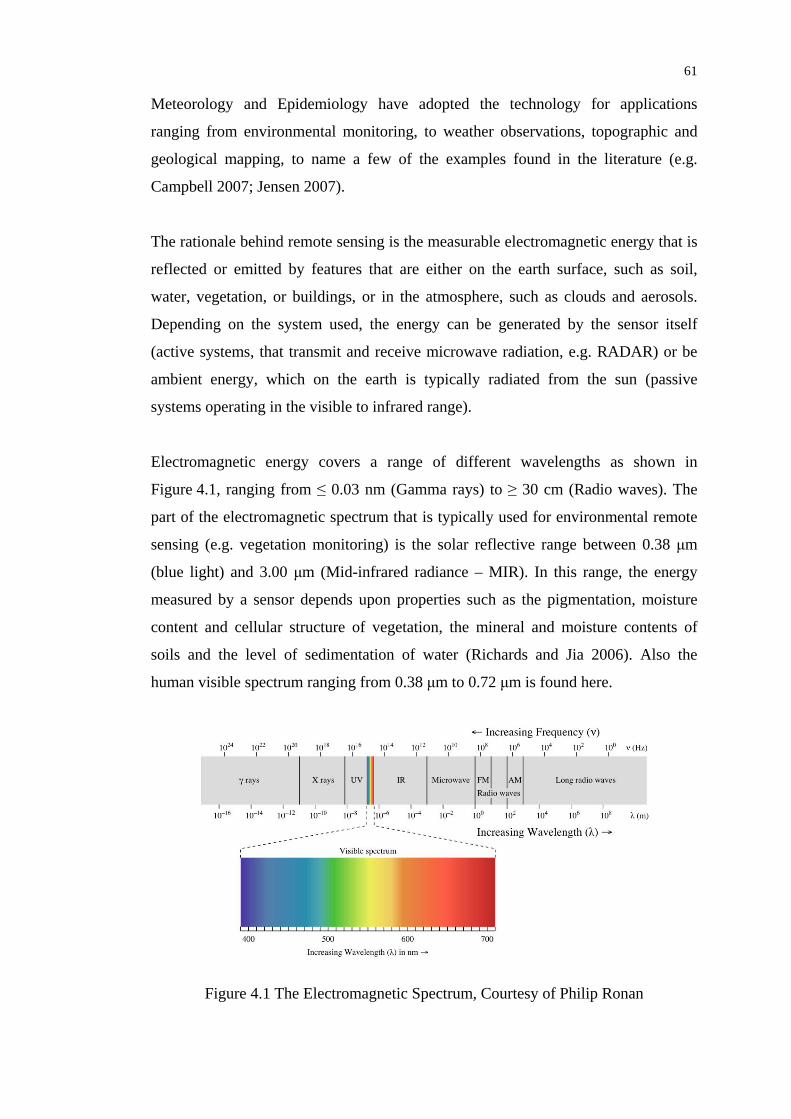
61

Meteorology and Epidemiology have adopted the technology for applications

ranging from environmental monitoring, to weather observations, topographic and

geological mapping, to name a few of the examples found in the literature (e.g.

Campbell 2007; Jensen 2007).

The rationale behind remote sensing is the measurable electromagnetic energy that is

reflected or emitted by features that are either on the earth surface, such as soil,

water, vegetation, or buildings, or in the atmosphere, such as clouds and aerosols.

Depending on the system used, the energy can be generated by the sensor itself

(active systems, that transmit and receive microwave radiation, e.g. RADAR) or be

ambient energy, which on the earth is typically radiated from the sun (passive

systems operating in the visible to infrared range).

Electromagnetic energy covers a range of different wavelengths as shown in

Figure 4.1, ranging from ≤ 0.03 nm (Gamma rays) to ≥ 30 cm (Radio waves). The

part of the electromagnetic spectrum that is typically used for environmental remote

sensing (e.g. vegetation monitoring) is the solar reflective range between 0.38 μm

(blue light) and 3.00 μm (Mid-infrared radiance – MIR). In this range, the energy

measured by a sensor depends upon properties such as the pigmentation, moisture

content and cellular structure of vegetation, the mineral and moisture contents of

soils and the level of sedimentation of water (Richards and Jia 2006). Also the

human visible spectrum ranging from 0.38 μm to 0.72 μm is found here.

Figure 4.1 The Electromagnetic Spectrum, Courtesy of Philip Ronan

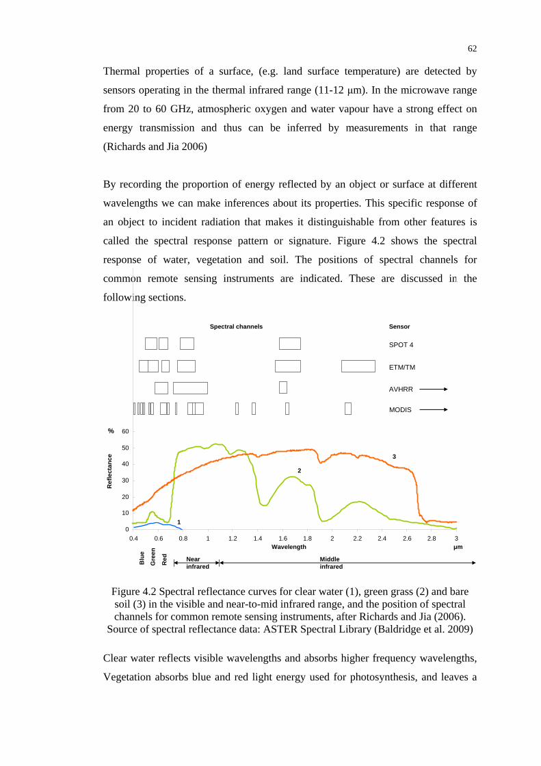
62

Thermal properties of a surface, (e.g. land surface temperature) are detected by

sensors operating in the thermal infrared range (11-12 μm). In the microwave range

from 20 to 60 GHz, atmospheric oxygen and water vapour have a strong effect on

energy transmission and thus can be inferred by measurements in that range

(Richards and Jia 2006)

By recording the proportion of energy reflected by an object or surface at different

wavelengths we can make inferences about its properties. This specific response of

an object to incident radiation that makes it distinguishable from other features is

called the spectral response pattern or signature. Figure 4.2 shows the spectral

response of water, vegetation and soil. The positions of spectral channels for

common remote sensing instruments are indicated. These are discussed in the

following sections.

μmWavelength

MODIS

AVHRR

ETM/TM

SPOT 4

Ref

lect

ance

%

0

10

20

30

40

50

60

0.4 0.6 0.8 1 1.2 1.4 1.6 1.8 2 2.2 2.4 2.6 2.8 3

1

2

3

Middle infrared

Near infraredB

lue

Gre

en

Red

SensorSpectral channels

Figure 4.2 Spectral reflectance curves for clear water (1), green grass (2) and bare soil (3) in the visible and near-to-mid infrared range, and the position of spectral channels for common remote sensing instruments, after Richards and Jia (2006).

Source of spectral reflectance data: ASTER Spectral Library (Baldridge et al. 2009)

Clear water reflects visible wavelengths and absorbs higher frequency wavelengths,

Vegetation absorbs blue and red light energy used for photosynthesis, and leaves a

63

small reflectance peak between that makes it appear green (Mather 2004). Vegetation

is reflective in near infrared and mid infrared wavelengths. For soils, reflectivity

generally increases with higher wavelength.

In some cases, the interaction between incident radiation and surface material varies

from time to time, depending on factors like orientation of the sun (solar azimuth),

height of the sun in the sky (solar elevation angle), the direction of the sensor in

relation to nadir (the look angle) and the state and structure of the vegetation if this is

the target (Mather 2004). The Bidirectional Reflectance Distribution Function

(BRDF) (Nicodemus 1965; Nicodemus et al. 1977) describes the response of a

surface at all possible view and illumination angles. It may be used to model the

reflectance as if viewed from nadir and as such, correct for the spatial variance in

directional remote sensing (Schaaf et al. 2002; Strahler 1997). Another factor to be

considered is the Earth’s atmosphere, which alters the radiation as it passes through,

and can compromise the quality of the received data. The effects can be scattering,

refraction and absorption of radiation. Only specific wavelengths, called atmospheric

windows are relatively easily transmitted through the atmosphere and these are used

in remote sensing.

Remote sensing instruments can be mounted on aircraft or satellite platforms.

Sensors or radiometers record the incoming radiation digitally for a discrete area on

the Earth surface. The size of the smallest recordable area determines the spatial

resolution of the sensor and depends on the height of the flight path or orbit, and

sensor characteristics. Most sensors operate in discreet wavelength bands or channels

in the visible, near infrared (NIR), mid infrared (MIR) or thermal infrared (TIR)

range of the spectrum. The bandwidth of each channel (spectral resolution) and the

number of bands (spectral dimensionality) determine the ability of a sensor to record

subtle differences in the spectral response of the sensed surface. The level of

different brightness values that can be recorded for each band is known as the

radiometric resolution. Another important characteristic is the temporal resolution or

repeat time, which is the time taken between viewing the same part of the Earth. It is

determined by orbital characteristics and may be constrained by the internal storage

capacity of the sensor. Remote sensing data therefore tend to have either a high

temporal, spectral or spatial resolution, but not all of them (Hay 2000).

64

Further details on the physical basics of remote sensing, the actual recording

mechanisms, issues of atmospheric absorption, terrain and surface effects, sensor

view angle, and specific sensor characteristics are discussed in numerous text books

(e.g. Campbell 2007; Lillesand, Kiefer, and Chipman 2008; Mather 2004; Richards

and Jia 2006), In the following sections space-borne sensors commonly used in

epidemiology, and the bio- and geophysical information (i.e. earth surface or

atmospheric properties, such as surface temperature, soil moisture, surface cover, air

humidity, or air temperature) that can be derived from the measured surface

reflectance are discussed.

4.1.2 Satellite Remote Sensing Platforms and Sensors

The selection of an appropriate sensor depends on the objectives of the study, the

ecology of hosts, vectors and pathogens and the temporal and spatial scales at which

transmission takes place (Kalluri et al. 2007). In most cases, it is a trade-off between

spatial resolution (< 1 m to several kilometres) and temporal resolution (half-hourly

to near-monthly). Figure 4.3 shows the requirements of epidemiology in relation to

remote sensing in other disciplines.

0.1 m 1 m 10 m 100 m 100 km10 km1 km

0.0001

0.001

0.01

0.1

1

10

100

Spatial and Temporal Resolution for Selected Applications

Tem

pora

l Res

olut

ion

(Yea

rs)

Nominal Spatial Resolution

Emergency Response

1 satellite: 16 day revisit

2 satellites: 8 day revisit


Dig

ital G

lobe

IKO

NO

S/Im

ages

atSP

OT

IKO

NO

S/D

G/O

V-3

IRS

IC

SPO

T

The

mat

ic M

appe

rA

STE

R

Lan

dsat

MSS

AST

ER

MO

DIS

AV

HR

R

GO

ES

GOES

Aer

ial P

hoto

grap

hy

Precision Agriculture

Utility, Trans-portation, Infrastructure

Topography

Land-UseLand-Cover

Forestry

Geology

Climate

Weather-Prediction

Epidemiology

Crop Type,Yield

0.1 m 1 m 10 m 100 m 100 km10 km1 km

0.0001

0.001

0.01

0.1

1

10

100

Spatial and Temporal Resolution for Selected Applications

Tem

pora

l Res

olut

ion

(Yea

rs)

Nominal Spatial Resolution

Emergency Response

1 satellite: 16 day revisit



Dig

ital G

lobe

IKO

NO

S/Im

ages

atSP

OT

IKO

NO

S/D

G/O

V-3

IRS

IC

SPO

T

The

mat

ic M

appe

rA

STE

R

Lan

dsat

MSS

AST

ER

MO

DIS

AV

HR

R

GO

ES

GOES

Aer

ial P

hoto

grap

hyA

eria

l Pho

togr

aphy

Precision Agriculture

Utility, Trans-portation, Infrastructure

Topography

Land-UseLand-Cover

Forestry

Geology

Climate

Weather-Prediction

Epidemiology

Crop Type,Yield

Figure 4.3 Spatial and temporal resolution considerations for different applications of remote sensing, after Jensen (2007)

65

Not all of the available sensors have proven useful for epidemiological studies and

some are constrained by image costs and availability. Extensive reviews of data from

past, present and future sensors applied in epidemiology are provided by Beck,

Lobitz, and Wood (2000), Dale et al. (1998), Hay (2000), Hay et al. (2006), Huh and

Malone (2001), Tran et al. (2010), and Washino and Wood (1994). The currently

operating weather and environmental satellites that are particularly useful in

arbovirus studies are discussed below and have been broadly categorised according

to their spatial resolution into low (≥ 1000 m), moderate (250 m to 1000 m) and high

resolution sensors (≤ 30 m).

4.1.2.1 Low Resolution Meteorological Satellites

Meteorological applications such as weather forecasts require near real-time weather

observations over large areas. Dedicated sensors generally operate at a coarse spatial

resolution and are capable of capturing surface and air temperature at different

altitudes, monitoring cloud cover and movement, as well as water vapour and

precipitation for an area at a high temporal frequency. The bands of major

importance are in the visible, near infrared, and thermal infrared range, sensors

measuring precipitation typically utilise the microwave spectrum.

Geostationary satellites operated by several countries under the umbrella of the

World Meteorological Organization (WMO), are positioned in orbits about

36,000 km above the Earth’s surface to constantly monitor a specific area on the

ground. The Meteosat Mission, operated by the European Organisation for the

Exploitation of Meteorological Satellites (Eumetsat), covers Europe and Africa, and

the western Indian Ocean. The first of the Meteosat Second Generation (MSG)

satellites was launched in 2002 and provides images every 15 minutes since going

fully operational in 2004 (Hay et al. 2006). The spatial resolution ranges from 1.4 km

in the visible bands to 3 km for all other bands (thermal infrared, water vapour)

(Schmetz et al. 2002). Satellites with equivalent capabilities for the American and

Pacific region are operated by the National Oceanic and Atmospheric Administration

(NOAA). NOAA’s Geostationary Operational Environmental Satellites (GOES),

capture images at a spatial resolution of 1 km in the visible and 4-8 km in the thermal

bands every 15 minutes for the continental United States and every 30 minutes for

the hemisphere between the North Poles and 20°S latitude (Jensen 2007). The

66

Australasian region is currently observed by the Japanese Advanced Meteorological

Imager (JAMI) aboard the geostationary Multi-functional Transport Satellite

(MTSAT)-2, following the former Japanese Geostationary Meteorological Satellite

(GMS) series (Kawamura et al. 2010). For Australia, hourly data are available at a

spatial resolution of 1 km for the two visible and at 4 km for the 4 infrared bands.

Half-hourly images are available for the northern half hemisphere, including

Japan.These optical and thermal sensors may be used indirectly to infer ground

precipitation based on measurements of cloud reflectivity or cloud top temperature,

which are related to probability and intensity of rainfall (Prigent 2010). Less frequent

but more direct measurements can be achieved with specifically designed microwave

instruments, such as the passive Advanced Microwave Scanning Radiometer-E

(AMSR-E) on board NASA’s Aqua satellite (Section 2.5.2.2) or the instruments on

board the TRMM. Ongoing research by the International Precipitation Working

Group (IPWG) (Turk and Bauer 2006) has shown that passive microwave

measurements deliver more accurate instantaneous measurements, while Infrared

(IR) techniques provide the best long term estimates (Ebert and Manton 1998) and it

is suggested that a combination of both techniques would be advantageous.

TRMM was jointly launched by NASA and the Japan Aerospace Exploration

Agency (JAXA) in 1997 to monitor and predict tropical cyclone tracks and intensity,

estimate rainfall, and monitor climate variability (precipitation and sea surface

temperature) between the latitudes 38°N and 38°S, at spatial resolutions from 2.1 to

45 km (TRMM - Tropical Rainfall Measuring Mission 2010). The satellite,

positioned in a low non-sunsynchronous orbit, carries three instruments: TRMM

Microwave Imager (TMI), the Visible/Infrared/Scanner (VIRS) and the first

operational space-borne Precipitation Radar (PR) (Jensen 2007). A number of

TRMM data products are readily available, such as the TRMM and other satellites

rainfall product (3B42) that exploit the advantages of several sensors on board.

Originally designed for an operation period of 3 years, TRMM is likely to remain

operative until 2012. With the Global Precipitation Mission (GPM) a follow up

project is currently in the implementation stage and anticipated to be launched in

2013 – 2014 (Global Precipitation Measurement 2010; Smith et al. 2007).

67

4.1.2.2 Moderate to Low Resolution Sensors

Two sensors delivering publicly available data at low cost that have gained

importance particularly for environmental monitoring applications are the Advanced

Very High Resolution Radiometer (AVHRR) and more recently the MODerate

Resolution Imaging Spectroradiometer (MODIS). The series of AVHRR sensors

carried on polar orbiting NOAA satellites have collected environmental data since

1978 at a low to moderate spatial resolution between 1.1 and 8 km. The very high

resolution (VHR) in the acronym relates to the improved radiometric resolution

compared to the earlier sensors. Daily coverage of the entire Earth and a large

historical data archive have made AVHRR invaluable for monitoring environmental

changes and for applications in large area epidemiology. Hay et al. (2006) provide

ample details about the sensor, data processing and epidemiological applications.

The MODIS instruments are on board NASA’s Earth Observation System (EOS)

Terra and Aqua satellites, which were launched into a sunsynchronous orbit in 1999

and 2002 respectively. Their advantage over AVHRR is due to their higher spatial

and spectral resolution. The MODIS sensors collect data every 12 to 24 hours

(depending on the use of one or both sensors) over a wide spectral range at spatial

resolutions of 250 m (Red, NIR), 500 m (MIR) and 1 km (TIR) (MODIS Web 2010).

This low revisit time increases the chance of recording cloudless images over an area

and hence facilitates the monitoring of dynamic spatial environmental processes.

With 36 spectral channels (from 0.62 to 14.385 μm) and 12-bit radiometric resolution

a large number of meteorological and other geophysical parameters and variables can

be derived, such as the Normalised Difference Vegetation Index (NDVI), Land

Surface Temperature (LST) and Landcover/Landcover change. Most of these data

are readily available as quality controlled MODIS products (discussed in the

following sections), which reduces the need for time consuming atmospheric

correction, georegistration, image composition and processing.

With a scheduled operation period of 18 years, the MODIS data archive facilitates

global long term observations of disease related factors (Tatem, Goetz, and Hay

2004). The timeline for planned follow up missions, the National Polar-orbiting

Operational Environmental Satellite System (NPOESS) and its predecessor, the

68

NPOESS Preparatory Project (NPP), expected to be launched as early as 2011, are

currently under review (NPOESS 2010). Once in operation, the Visible/Infrared

Imager/Radiometer Suite (VIIRS) on board will provide data continuity for

parameters currently recorded by AVHRR and MODIS. However, differences in data

acquired by those sensors due to varying overpass times need to be considered

(Townshend and Justice 2002).

4.1.2.3 High Resolution Sensors

Disease mapping projects conducted on a local scale generally aim to detect and

monitor potential disease foci, or more specifically for vector-borne diseases, the

vector habitats. This task includes monitoring of ground cover, permanent and

ephemeral bodies of open water and wetlands. Very often, these features, such as

narrow streams are to small to be detectable by moderate resolution sensors (Chalke

2006), and high resolution data are required instead.

Present polar orbiting satellites carrying high resolution sensors include Landsat 5

and 7 with the Thematic Mapper (TM) and Enhanced Thematic Mapper (ETM)

instruments, the Satellite Pour l'Observation de la Terre (SPOT) - 5 with the High

Resolution Geometric (HRG) camera on board and the EOS Terra platform with the

Advanced Spaceborne Thermal Emission and Reflection Radiometer (ASTER).

These have repeat cycles of 16, 26 and 16 days, and a spatial resolution of 15-30 m,

2.5-5 m and 15-90 m respectively, depending on the channel.

Various epidemiological studies have used high resolution satellite imagery,

particularly from Landsat satellites (Bogh et al. 2007; Brown et al. 2008; Kitron et al.

1996), which have collected invaluable data on land cover change that are now freely

available electronically (Cheng et al. 2009). Nevertheless, limited evidence for

widespread adoption of data from the other named sensors is found in literature due

to various limiting factors, including availability of cloud free images, temporal

resolution and processing requirements (Herbreteau et al. 2007). Moreover,

commercial very high resolution systems (sub-meter to 4 m horizontal resolution)

launched in recent years, including Ikonos, Quickbird, Rapid Eye and GeoEye, are

often operated to collect data ‘on demand’ rather than on a regular basis. This and

associated high costs of the collected data are not advantageous for monitoring larger

69

areas like Australia frequently under similar conditions (time of day, viewing angle,

etc). However, high resolution radiometer sensors like ASTER on multi-sensor

platforms may be used as a zoom-lens for the other (lower resolution) instruments on

board for validation and calibration purposes (ASTER Mission 2010).

4. 2 Remotely Sensed Environmental Variables for Epidemiological Applications

A wide range of environmental and climatic variables with relevance to arboviral

diseases can be derived from geostationary (GEO) and low Earth orbiting (LEO)

remote sensing platforms. These include rainfall, air and land surface temperature,

vegetation type and condition, or humidity. These variables often replicate ground

based climatic, soil or vegetation datasets that have been used in epidemiological

studies, e.g. by Conte et al. (2007), Dascălu, Ionescu, and Rizac (2007), Ward and

Thurmond (1995) or Wittmann, Mellor, and Baylis (2001). However, remote sensing

data are in many aspects advantageous as shown in the following sections, mainly

due to wider areal coverage and shorter update cycles, while retaining the overall

spatio-temporal patterns observed on the ground.

Which parameters can be extracted from remote sensing data primarily depends on

the spatial resolution of the instrument as well as the available spectral bands. High

resolution instruments are able to detect specific environmental attributes, including

soil type and plant species, while low and moderate resolution sensors such as

MODIS record average environmental conditions over the large areas covered by a

pixel, and are used for regional studies of vegetation condition or precipitation.

Converting the radiation measured by a sensor into environmental variables for

epidemiological applications involves a number of pre-processing steps. These are

explained in detail by Mather (2004) and Richards (2006), and include radiometric,

atmospheric and geometric corrections, image registration and reprojection to an

appropriate spatial reference system. The corrected images are then transformed into

either 1) climatic or geophysical parameters that are built on the relationship between

emitted radiation and ground based measurements, using physical and/or empirical

models (e.g. precipitation, land surface temperature), or 2) indices, which are defined

by different mathematical band combinations (e.g. vegetation or water indices)

70

(Lillesand, Kiefer, and Chipman 2008). For many sensors, data products at different

processing levels are provided to the scientific community, ranging from raw data to

multi-band images and quality controlled scientific datasets. While these products

offer scientists the opportunity to focus on the interpretation rather than the

processing of the data, it is crucial to assess data quality and its fitness for a

particular application. This is often neglected in epidemiological studies, either due

to time and cost constraints, or limited access to ground truth data in the same spatial

and temporal domain as the remotely sensed data (Goetz, Prince, and Small 2000).

Therefore, the supplied metadata and quality information, e.g. for the MODIS Land

datasets (Roy et al. 2002) or results from validation activities (Morisette, Privette,

and Justice 2002) are frequently the only source to assess fitness for use.

4.2.1 Rainfall

Rainfall is often related to an increase in abundance of arbovirus vectors, particularly

mosquitoes (Thomson et al. 1996). Also the short-term and long-term occurrence of

BTV in Australia has been linked to rainfall (Ward 1994a; Ward and Thurmond

1995). The distribution of competent Culicoides vectors is generally confined to

areas in excess of 800 mm annual precipitation (Standfast, Dyce, and Muller 1985).

However, this relationship is not necessarily immediate, as all but very light rainfall

initially suppresses vector activity and may even wipe out vector populations,

particularly if extensive flooding occurs. The associated increase in humidity, soil

moisture, availability of vegetation and the development of breeding grounds may

lead to a lagged abundance of vector populations and increased risk of virus

transmission (Ward and Thurmond 1995).

Before the launch of TRMM with the first precipitation radar in 1997, rainfall

intensity retrieval has been mostly based on passive sensors using the visible, IR and

passive microwave (PMW) wavelengths, which lack the ability to obtain a three

dimensional structure of clouds and precipitation (Michaelides et al. 2009). Thus,

combining data from active and passive sensors and ancillary data (e.g. wind and rain

gauge data) is the only feasible strategy to improve the accuracy of cloud and

precipitation retrievals from satellite imagery (Stephens and Kummerow 2007).

Michaelides et al. (2009) categorised methods for multisatellite precipitation retrieval

into 1) those that use ancillary products from sensors not in the PMW range to

71

actively adjust the PMW derived rainfall intensities (e.g. Huffman et al. 2007), and

2) those which use the ancillary data to temporally interpolate the rain maps from

one overpass of a PMW sensor to the next one (e.g. Joyce et al. 2004).

The TRMM Multisatellite Precipitation Analysis (TMPA), was developed by

Huffman et al. (2007). It provides a calibration-based sequential scheme for

combining precipitation estimates from multiple satellites, as well as gauge analyses

where feasible, at fine scales (0.25° x 0.25° and 3 hourly) for a global band extending

from 50 degrees South to 50 degrees North latitude. The estimates depend on the

input from different sets of LEO PMW sensors and GEO IR (~10.7μm) instruments.

TRMM combined instrument (TMI+PR) estimates as well as the Global Precipitation

Climatology Project (GPCP) and Climate Assessment and Monitoring (CAMS)

monthly rain gauge analysis are also incorporated in TMPA. The method performs

reasonably on a monthly scale and detects large scale rain events, but shows less

ability in correctly specifying moderate to light rain rates at short time intervals

(Michaelides et al. 2009).

The Climate Prediction Center morphing method (CMORPH) uses motion vectors

derived from half-hourly interval IR GEO satellite imagery to propagate the

relatively high quality precipitation estimates derived from PMW data for a global

product. Additionally, shape and intensity of the precipitation features are modified

(morphed) during the time between microwave sensor scans using a time-weighted

linear interpolation. A detailed description of the algorithm can be found in Joyce et

al. (2004). The process yields spatially and temporally complete PMW derived

precipitation estimates, with the performance depending on the used PMW retrieval

method. CMORPH has been available since December 2002 with different temporal

and spatial resolutions: 30 min/8 km, 3-hourly/~25 km, daily/~25 km. The higher

spatial resolutions are produced through interpolation of the individual satellite

estimates that have a coarser resolution of about 12 to 15 km.

Still, interpolated rainfall variables are often found in species distribution models

(e.g. Baylis et al. 1998; Baylis, Meiswinkel, and Venter 1999). A few studies have

used satellite derived cold cloud duration (CCD) as surrogate for precipitation

probability (e.g. Hay, Snow, and Rogers 1998; Thomson et al. 1996), but there is

72

little evidence for adoption of more advanced satellite based rainfall estimates like

TMPA and CMORPH in epidemiology. The usability of these methods and

associated data products for this study will be further explored in Chapter 5.

4.2.2 Temperature

Temperature regulates many land surface processes and is the single most important

factor for survival and replication rates of arbovirus vectors. More specifically,

higher temperatures are known to increase growth rates of vector populations,

decrease the length of the gonotrophic cycle and hence the interval between blood

meals, shorten the extrinsic incubation period of the virus in the vector and increase

the rate of virus evolution (Ruiz et al. 2010). Minimum and maximum daily

temperatures measured on or above ground, as well as temperature time series are

frequently used as variables in predicting Bluetongue (e.g. by Purse, Baylis, et al.

2004; Purse et al. 2007; Wittmann, Mellor, and Baylis 2001), and other insect-borne

diseases (Rizzoli et al. 2007; Rogers 2000).

4.2.2.1 Land Surface Temperature

Land Surface Temperature (LST) is here referred to as the radiometric (kinetic)

temperature related to the TIR radiation emitted from the ground (Norman and

Becker 1995). This can be top of canopy in vegetated areas or soil surface in bare

areas. LST plays an important role for the development and survival of the larval

stage of vectors, particular for the ground breeding species of Culicoides that

transmit BTV in Australia. Although previously the spatial and temporal variability

of LST has been used as an index of vector abundance (Malone et al. 1994; Rogers,

Hay, and Packer 1996), absolute temperatures may be better suited for studies of

vector survival and reproductive success (Goetz, Prince, and Small 2000).

Land surface temperature can be inferred from the thermal infrared bands of

moderate to coarse resolution instruments like AVHRR, MODIS or higher resolution

instruments like ASTER and ETM. Accurate determination of LST depends on the

knowledge of the emissivity of the surface and the availability of clear sky images

(Goetz, Prince, and Small 2000). The split-window approach is the most commonly

applied technique to reduce the error from atmospheric effects, based on the

differences in signal attenuation between two thermal bands (Hay and Lennon 1999).

73

There are two methods implemented for LST retrieval from MODIS. One is a

generalised split-window approach based on calibrated radiance data of bands 31 and

32 data (Wan and Dozier 1996) and the second one is the physics based day/night

algorithm (Wan and Li 1997) using a pair of day-time and night-time data in TIR

bands 20, 22, 23, 29, and 31–33. Daily or 8-daily data products are available for both

methods at 1 km and 5 km spatial resolutions, respectively. Validation attested the

MODIS LST products accuracy to be in the order of ± 1 K (Wan 2008; Wan et al.

2002; Wan et al. 2004) for lakes, snow/ice, and dense vegetated areas. However, in

arid and semi-arid regions, where surface emissivity may vary significantly with

location and time, the split-window algorithm tends to underestimate LST (Hulley

and Hook 2009; Wan et al. 2002). It remains unclear, though, if this is the case in the

savannahs of Northern Australia.

4.2.2.2 Air Temperature

Air temperature (TAIR) measured about 2 m above ground is a primary descriptor of

terrestrial environmental conditions (Prihodko and Goward 1997) and potentially

more useful for many applications than ground temperature, which bears little

relationship to the micro-environment in which an insect, animal, plant or human is

living (Cresswell et al. 1999; Goetz, Prince, and Small 2000).

Two major techniques have been developed for TAIR retrieval, mainly utilising the

LST derived from MODIS, AVHRR or meteorological satellites. One technique,

known as the temperature–vegetation index, is based on the hypothesis that the LST

over a thick vegetation canopy is close to ambient TAIR and utilizes the negative

correlation between LST and NDVI (Prihodko and Goward 1997; Stisen et al. 2007).

The achieved accuracies of TAIR estimates are in the range of 3 K (Stisen et al.

2007). The other approach, known as the statistical method, often combines

LST/brightness temperature and other parameters, such as geographic location and

altitude (Yan et al. 2009), solar zenith angle (SZA) (Cresswell et al. 1999), or

combinations thereof (Jang, Viau, and Anctil 2004), to derive TAIR through

regression analysis. Vancutsem et al. (2010) found generally good correlation

between LST from the MODIS night overpass and the observed minimum air

temperature, an important variable in epidemiology. However, estimates of

maximum day temperature based on MODIS LST, NDVI and SZA, respectively,

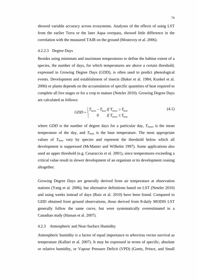
74

showed variable accuracy across ecosystems. Analyses of the effects of using LST

from the earlier Terra or the later Aqua overpass, showed little difference in the

correlation with the measured TAIR on the ground (Mostovoy et al. 2006).

4.2.2.3 Degree Days

Besides using minimum and maximum temperatures to define the habitat extent of a

species, the number of days, for which temperatures are above a certain threshold,

expressed in Growing Degree Days (GDD), is often used to predict phenological

events. Development and establishment of insects (Baker et al. 1984; Kunkel et al.

2006) or plants depends on the accumulation of specific quantities of heat required to

complete all live stages or for a crop to mature (Neteler 2010). Growing Degree Days

are calculated as follows:

basemean

basemeanbasemean

TTTT

ififTT

GDD≤>

⎩⎨⎧ −

=0

(4.1)

where GDD is the number of degree days for a particular day, Tmean is the mean

temperature of the day, and Tbase is the base temperature. The most appropriate

values of Tbase vary by species and represent the threshold below which all

development is suppressed (McMaster and Wilhelm 1997). Some applications also

used an upper threshold (e.g. Cesaraccio et al. 2001), since temperatures exceeding a

critical value result in slower development of an organism or its development ceasing

altogether.

Growing Degree Days are generally derived from air temperature at observation

stations (Yang et al. 2006), but alternative definitions based on LST (Neteler 2010)

and using weeks instead of days (Ruiz et al. 2010) have been found. Compared to

GDD obtained from ground observations, those derived from 8-daily MODIS LST

generally follow the same curve, but were systematically overestimated in a

Canadian study (Hassan et al. 2007).

4.2.3 Atmospheric and Near-Surface Humidity

Atmospheric humidity is a factor of equal importance to arbovirus vector survival as

temperature (Kalluri et al. 2007). It may be expressed in terms of specific, absolute

or relative humidity, or Vapour Pressure Deficit (VPD) (Goetz, Prince, and Small

75

2000). The latter is a measure of the lack of moisture equilibrium between an object

and the surrounding atmosphere and is a particularly useful index for the drying

power of air and hence the desiccation rate of vectors and their eggs (Green and Hay

2002).

Prince and Goward (1995) developed a method to derive VPD from AVHRR that is

based on the differences between the TIR channels 4 and 5, which has also been

employed in air temperature estimation. More recently, Hashimoto et al. (2008)

applied an empiric VPD model based on LST and long term air temperature (Granger

2000) to MODIS LST data. The VPD maps produced with those methods show

spatial and temporal patterns that are in general agreement with known climatic

patterns and interpolated meteorological observations (Goetz, Prince, and Small

2000). However, absolute errors in VPD tend to be large (Green and Hay 2002), and

Granger’s (2000) method performed poorly along the coast and over sparsely

vegetated areas (Hashimoto et al. 2008). This is in line with the problems associated

with LST derival over arid and semi-arid regions due to the large spatial and

temporal variability of surface emissivity.

An operational algorithm to derive water vapour from ratios of several MODIS

bands in the thermal range aims to remove the effects of the variation of surface

reflectance with wavelength for most land surfaces (Gao and Kaufman 2003). A

1 km resolution NIR water vapour product is generated during the day, and daily, 8-

daily, and monthly IR water vapour products are generated day and night at a spatial

resolution of 1°. The products, aimed at the study of seasonal and annual variations

of water vapour on regional and global scales, have typical errors in the derived

water vapour values ranging between 5% and 10% (Gao and Kaufman 2003).

However, an evaluation of the product by McAtee and Maier (2006) showed that

these algorithms perform poorly over continental Australia with an RMS error

of 44%.

Alternatively, microwave sensors capable of deriving atmospheric humidity

parameters can be found on the Terra and Aqua platforms, most notably the

Atmospheric Infrared Sounder (AIRS) and the Advanced Microwave Sounding Unit

(AMSU) (Tatem, Goetz, and Hay 2004). However, in addition to the lack of

76

validation studies, their low spatial resolution makes them less useful for

epidemiological studies that operate at local or regional scales using near surface

environmental conditions.

What is common to any of the higher level humidity estimators is that they are

typically derivatives of a combination of satellite products and ancillary data and are

as such prone to propagate errors and uncertainties from the input parameters.

Understandably, the epidemiological community has hardly adopted any of the

presented humidity variables in favour of more robust lower level variables, such as

LST or vegetation indices (see next section).

4.2.4 Vegetation

Information about vegetation is integral to the study of vector-borne diseases, which

are linked to the vegetated environment at least during some aspect of their

transmission cycle (Beck, Lobitz, and Wood 2000). Vegetation not only provides

shelter from desiccation during resting periods for some vector species (Bishop et al.

1995; Bishop et al. 1994), and nectar supply particularly for the male population of

blood sucking insects, it also strongly influences the distribution of hosts (e.g.

grazing livestock) and hence the focus of disease transmission. The spatial and

temporal variability of vegetation type and condition is governed by the combined

impact of rainfall, temperature, humidity, topographic effects, soil, water availability,

and human activities. Therefore, vegetation indices and type, which are described

hereafter, are also used as surrogates for many of these environmental variables.

4.2.4.1 Vegetation Type and Landscape Composition

Land cover maps that delineate vegetation type and landscape composition at varying

hierarchy levels are generally derived from high resolution imagery e.g. from

Landsat or SPOT. Image classification techniques are applied to automatically

categorise all pixels in an image into land cover classes. The two main approaches

are unsupervised and supervised classification, which differ in the definition of the

pixel categories. The supervised classification involves a training step, where an

image analyst defines the spectral characteristics of a class by selecting pixels

representative for a category in the image, whereas in unsupervised classification, the

image data are automatically aggregated into natural spectral groups or clusters.

77

General overviews of image classification methods are given e.g. by Lillesand,

Kiefer, and Chipman (2008) or Mather (2004), while Curran et al. (2000) specifically

addresses applications in disease mapping.

Global and regional land cover datasets are also available and useful for broad scale

studies where detailed information on particular plant species is not required.

Examples include the 300 m resolution GlobeCover product (Arino et al. 2008) and

the global annual MODIS Landcover product, which is produced at 500 m spatial

resolution (Friedl et al. 2010). For the Australian continent, a dedicated dynamic land

cover classification derived from satellite remote sensing data has been proposed

(Lymburner et al. 2008), but is currently not available. Instead, a number of regions

have been mapped as part of traditional vegetation surveys, which used aerial photo

mosaics to delineate vegetation communities at scales between 1:100,000 and

1:1 million (e.g. Beard 1975b). Other surveys have been conducted to assess the

condition of rangeland land systems (see Chapter 5 for details). Data on native

vegetation and soils on different aggregation levels have been homogenised across

Australia and are now available through the National Vegetation Information System

(NVIS) and Australian Soil Resource Information System (ASRIS), respectively.

However, these data are all static in nature and remote sensing approaches are

therefore increasingly used to monitor dynamic changes such as land cover, related

e.g. to pastoral management (Hamilton, Chilcott, and Savage 2008) or mosquito

vector habitats (Dale et al. 1998).

Specific vegetation type information offers opportunities to map species habitat and

range. Several studies have used vegetation type and structure to study vector

habitats (e.g. Hayes et al. 1985). More often than looking at specific plant species,

homogenous landscape units, defined by environmental variables, such as vegetation

or soil type, are used in health studies (e.g. Beck et al. 1994). Using a supervised

classification of SPOT imagery to create a mosaic of major landscape units, De La

Rocque (2004) found BT seroprevalence was highest in districts with a high

percentage of meadows.

To be able to utilise landscape units for disease cause and effect analysis requires

some method of quantification. So called Landscape Metrics have been developed by

78

McGarigal and Marks (1995) for this purpose to describe either the patch itself in

terms of e.g. mean patch size and shape, or to characterize the spatial relationship

between the patches, e.g. nearest neighbour, contagion and connectivity (McGarigal

and McComb 1995). In epidemiology, Landscape Metrics have been applied to study

the relationship between landscape composition and the presence of Bluetongue

virus (Guis et al. 2007), Murray Valley Encephalitis virus (Chalke 2006) and West

Nile virus in horses (Pradier, Leblond, and Durand 2008).

However, more frequently than plant species composition and landscape metrics, the

amount and density of vegetation cover is associated with disease and vector

abundance (Goetz, Prince, and Small 2000).

4.2.4.2 Vegetation Indices

A vegetation index (VI) is a dimensionless, radiometric measure that indicates

relative abundance and activity of green vegetation (Jensen 2007). Summaries of the

various vegetation indices that can be extracted from remotely sensed data are given

e.g. by Jackson and Huete (1991), Jensen (2007), Lyon et al. (1998), Running et al.

(1994), and Wiegand et al. (1991). VIs are generated using mathematical

combinations of several bands of remote sensing data that utilise the significant

differences in reflectance of vegetation in the blue, green, red and NIR bands

(previously shown in Figure 4.2). The index is typically a sum, difference, ratio or

other linear combination that reduces multi-band observations to a single numerical

index (Wiegand et al. 1991). Vegetation indices are simple tools for exploring or

quickly evaluating the state of vegetation over large areas. They enhance the spectral

contrast of vegetation and minimise effects like viewing and sun angles, topography

or soil variations to facilitate consistent spatial and temporal comparisons. The

usefulness of any VI for a specific application depends upon the relationship that

may be found between the index and the variable of interest, e.g. biomass, primary

productivity (Warren 2007).

The Normalized Difference Vegetation Index (NDVI), originally envisaged by

Rouse et al. (1973) is the most commonly used index in health studies. NDVI is

calculated as a normalised ratio from the RED and NIR bands and hence is less

affected by the absolute reflectance values:

79

REDNIRREDNIRNDVI

+−

=

(4.2)

The values can theoretically range from -1 to 1, with highly vegetated land producing

values close to 1, while NDVI over bare land will be close to zero and assume

negative values over water (Holben 1986; Tucker 1979). NDVI has been associated

with habitat suitability for disease vectors, such as ticks (Eisen, Eisen, and Lane

2006; Ogden et al. 2006), Anopheles spp. mosquitoes (Shililu et al. 2003) and

Culicoides biting midges (Purse, Tatem, et al. 2004).

Despite its usefulness as a robust vegetation index, NDVI has some disadvantages,

including saturation in high biomass areas, sensitivity to background soil brightness

and differential atmospheric effects (Huete, Jackson, and Post 1985; Huete et al.

1997). The Enhanced Vegetation Index (EVI) was developed to optimise the

vegetation signal with improved sensitivity in high biomass regions and improved

vegetation monitoring through a de-coupling of the canopy background signal and a

reduction in atmosphere influences (Huete et al. 2002). The equation takes the form,

)1(21

LLBLUECREDCNIR

REDNIRGEVI ++−+

−=

(4.3)

where G is a gain factor set to 2.5 and L is a soil adjustment factor empirically

determined as 1.0. C1 and C2 are coefficients that describe the use of the blue band in

correction of the red band for atmospheric aerosol scattering and have been

determined empirically as 6.0 and 7.5, respectively.

NDVI and EVI are produced as standard MODIS products at 500 m and 250 m using

8-day compositing periods.

4.2.4.3 Vegetation Phenology

In regions outside the endemic range of arboviruses, transmission may be suppressed

during certain periods of the year, be it through low temperatures or periods of low

precipitation or even drought. The underlying pattern can be attributed to seasonal

climatic differences, or shifts in the spatial distribution of bioclimatic zones, which

are also reflected in the growing periods of vegetation.

80

Vegetation phenology refers to the timing of different life-cycle events of the plants,

such as greenup and senescence (i.e., the start and end of growing season) (Zhang et

al. 2003). A number of methods have been developed to analyse long time series of

NDVI and extract phenological parameters, some of which are shown in Figure 4.4.

Figure 4.4 Examples of seasonality parameters that can be computed from NDVI time series: (a) beginning of season, (b) end of season, (c) left 90% level, (d) right

90% level, (e) peak, (f) amplitude, (g) length of season, (h) small integral over growing season giving area between fitted function and average of left and right

minimum values, (i) large integral over growing season giving area between fitted function and zero level. Source: Jönsson and Eklundh (2004)

Phenology extraction from NDVI time series typically involves as a first step

removal of noise that arises from varying atmospheric conditions and sun-sensor-

surface viewing geometries (Hird and McDermid 2009). In a second step,

phenological markers for the start and end point of one or more seasons is

determined. Several methods are available that either work with a fixed NDVI

threshold or a portion of the maximum seasonal greenup (Bradley et al. 2007;

Jönsson and Eklundh 2002), or by analysing the rate of change in curvature and slope

along the fitted curve (Zhang et al. 2003).

A number of smoothing techniques have been applied to NDVI time series, including

Fourier transform (Stöckli and Vidale 2004), wavelet transform (Martínez and

Gilabert 2009), function-fitting (Beck et al. 2006; Bradley et al. 2007; Jönsson and

81

Eklundh 2002; Zhang et al. 2003), and filtering methods (Chen et al. 2004). Hird and

McDermid (2009) assessed several of these techniques for their ability to preserve

the characteristics of the growing season and found that Asymmetric Gaussian

(Jönsson and Eklundh 2002) and Double-logistic (Beck et al. 2006) function fitting

techniques performed best. From the other tested filters, an adapted Savitzky-Golay

(1964) filter gave the best results and is also superior to the fast Fourier transforms

(e.g. Chen et al. 2004), which usually have problems to detect short seasons marked

by rapid increases in NDVI.

4.2.5 Soil Moisture and Surface Wetness

Wet soils indicate a suitable habitat for species of snails, mosquito larvae, ticks, and

worms (Beck, Lobitz, and Wood 2000). Consequently, sufficient moisture levels are

also an important requirement for the presence of some ground breeding arbovirus

vectors, such as some species of Culicoides (Foxi and Delrio 2010). However, none

of the Australian BTV vector species is known to lay their eggs in wet soil (see

Tables 2.1 and 2.2).

Several types of sensors that can detect near surface soil moisture are listed e.g. by

Beck, Lobitz, and Wood (2000), and include passive microwave sensors, microwave

Synthetic Aperture Radar (SAR), shortwave-infrared, and thermal-infrared sensors.

Passive microwave systems such as AMSR-E (Njoku et al. 2003) have the advantage

that they can penetrate cloud, have reduced sensitivity to land surface roughness and

vegetation, and the signal has a direct relationship with soil moisture through the soil

dielectric constant (Draper et al. 2009). Comparisons of different products have

shown that the algorithm used for soil moisture retrieval plays an equally important

role for the quality of a soil-moisture dataset as the technical specifications and

performance of the satellite system (Draper et al. 2009; Wagner et al. 2007). In

relation to this project the very low spatial resolution of most datasets, which

depends on the bands used in the algorithm, and might be as low as 56 km for the

standard AMSR-E product, is considered a major disadvantage. Alternatively, soil

moisture can be estimated from data in the visible and IR spectrum based on the

relationship between LST and NDVI, which is also utilised for air temperature and

evapotranspiration rate estimates (Goetz, Prince, and Small 2000). Brooker and

Michael (2000) also found that precipitation and vegetation amount may be useful

82

indicators for soil moisture, since rainfall increases humidity and soil moisture and

vegetation cover prevents evaporation and conserves soil moisture. In fact, NDVI has

therefore often been used in arbovirus studies as a surrogate for soil moisture (e.g. by

Calvete et al. 2009; Purse, Tatem, et al. 2004; Tatem et al. 2003).

4.2.6 Surface Water

Water is a requirement for many stages of disease cycles, particularly those involving

arthropod vectors. Different forms of surface water, ranging from lakes, water holes,

and streams to flooded grasslands and forests, salt lakes, wetlands and swamps

provide a breeding habitat for larvae of a number of mosquito and midge species.

While most Australian BTV vectors do not rely on surface water to breed, water that

acts as drinking supply for livestock potentially increases the risk of virus

transmission, by creating areas where high densities of virus amplifiers, hosts and

vector may be found together.

In contrast to rainfall that has often been used as a predictive variable for occurrence

of mosquito-borne viruses like Dengue, Japanese and Murray Valley Encephalitis,

Ross River and Malaria, remote sensing of surface water offers the opportunity of

mapping the direct link between water habitat and disease. As Chalke (2006) points

out, the correlation between rainfall and habitat is highly variable in both space and

time, and the area of resulting habitat, i.e. surface water that results from rainfall, is

influenced by the local geology, soil type, vegetation, watershed characteristics and

anthropogenic intervention. Local habitat development may also result from rainfall

events far from the area of flooding.

Surface water mapping can be conducted on local to regional scales, depending on

the purpose of the study and the size of the habitat to be mapped. The AVHRR and

MODIS instruments are able to monitor surface water daily, at spatial resolutions of

1 km and 250 m, respectively, which limits their application to regional studies

involving larger rivers, dams and lakes, and large scale flooding. However, the high

temporal resolution may aid in capturing highly dynamic flood events that are

frequent in the semi-arid and arid regions of Australia during the wet season. Higher

resolution instruments, such as ASTER, SPOT and TM/ETM facilitate identification

83

of smaller surface water features, such as small streams and tributaries, as well as

small flooded areas in forests and flood plains.

A number of water classification methods have been developed, including change

detection (e.g. Faruolo et al. 2009), spectral matching (e.g. Roshier and Rumbachs

2004), or simple threshold analysis (e.g. Lacaux et al. 2007) of the NIR, MIR or

thermal bands, or of ratios such as visible/NIR visible/MIR, or NDVI. Common to

these algorithms are difficulties in defining boundaries between land and turbid or

highly saline water bodies (Campbell 2007) or detecting flooded areas with high

vegetation cover (Townsend and Walsh 1998). Active systems such as SAR have

been successfully applied to identify water beneath vegetation cover, either

exclusively (Milne 1999) or in combination with optical sensors and Digital

Elevation Models (e.g. Li and Chen 2005). What makes SAR less practicable for

dynamic surface water monitoring over large areas is the relatively high cost, and

limited accessibility of recent and historical data covering Australia (Dale et al.

1998).

4.2.7 Wind

Wind may affect the flight of arbovirus vectors like Culicoides in two ways.

Unsupported flight for the purpose of finding hosts for blood meals, for mating and

egg-laying, and for seeking shelter, is limited to times of low wind speed (Murray

1987). During times where wind velocity exceeds the unaided flight speed, midges

may be transported from 5 to 700 km in heights of up to 1.5 km, where they can

survive in temperatures between 12 and 35°C (Sellers 1980; Sellers 1992).

In areas, where arboviruses are not endemic, infected vectors carried by wind are one

possible route of introduction of a pathogen, besides travel, trade and animal

movements. Ritchie and Rochester (2001) showed for example that Japanese

Encephalitis was introduced from New Guinea into Australia through wind blown

Culex spp.. Other examples include local (Bishop, Barchia, and Spohr 2000) and

long distance wind dispersal of Culicodes carrying Bluetongue or Akabane viruses,

which has been demonstrated around the globe (Ducheyne et al. 2007; Hendrickx et

al. 2008; Sellers 1992).

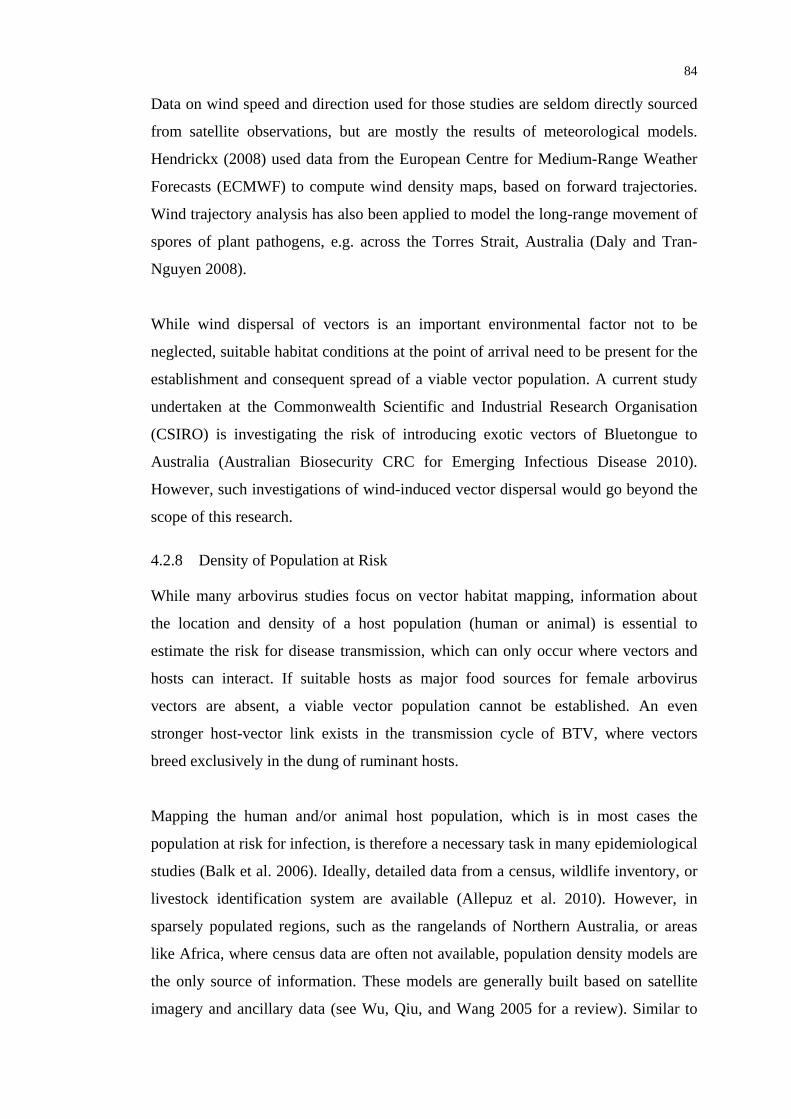
84

Data on wind speed and direction used for those studies are seldom directly sourced

from satellite observations, but are mostly the results of meteorological models.

Hendrickx (2008) used data from the European Centre for Medium-Range Weather

Forecasts (ECMWF) to compute wind density maps, based on forward trajectories.

Wind trajectory analysis has also been applied to model the long-range movement of

spores of plant pathogens, e.g. across the Torres Strait, Australia (Daly and Tran-

Nguyen 2008).

While wind dispersal of vectors is an important environmental factor not to be

neglected, suitable habitat conditions at the point of arrival need to be present for the

establishment and consequent spread of a viable vector population. A current study

undertaken at the Commonwealth Scientific and Industrial Research Organisation

(CSIRO) is investigating the risk of introducing exotic vectors of Bluetongue to

Australia (Australian Biosecurity CRC for Emerging Infectious Disease 2010).

However, such investigations of wind-induced vector dispersal would go beyond the

scope of this research.

4.2.8 Density of Population at Risk

While many arbovirus studies focus on vector habitat mapping, information about

the location and density of a host population (human or animal) is essential to

estimate the risk for disease transmission, which can only occur where vectors and

hosts can interact. If suitable hosts as major food sources for female arbovirus

vectors are absent, a viable vector population cannot be established. An even

stronger host-vector link exists in the transmission cycle of BTV, where vectors

breed exclusively in the dung of ruminant hosts.

Mapping the human and/or animal host population, which is in most cases the

population at risk for infection, is therefore a necessary task in many epidemiological

studies (Balk et al. 2006). Ideally, detailed data from a census, wildlife inventory, or

livestock identification system are available (Allepuz et al. 2010). However, in

sparsely populated regions, such as the rangelands of Northern Australia, or areas

like Africa, where census data are often not available, population density models are

the only source of information. These models are generally built based on satellite

imagery and ancillary data (see Wu, Qiu, and Wang 2005 for a review). Similar to

85

the Gridded Population of the World (GPW) dataset for humans (see Balk et al. 2006

for details and alternative approaches) a livestock density map has been produced by

the Food and Agriculture Organisation (FAO) for global applications. The freely

available Gridded Livestock of the World (GLW) dataset (Robinson, Franceschini,

and Wint 2007) has been produced to provide population density estimates for cattle,

buffalo, sheep, goats, pigs and poultry/chickens at a resolution of about 5 km at the

equator, using statistical data and environmental variables. Since the GLW dataset is

built on a model that uses similar bioclimatic variables as intended for this research,

it will not be further considered as an additional variable.

4.2.9 Topography

The last factor that is discussed in this chapter is static in nature, but influences many

of the other dynamic environmental factors. Topographic characteristics of a

landscape, including landforms, elevation, surface orientation and slope often

determine the boundaries of local habitats. This can be either directly by creating a

physical barrier to species movements (e.g. through steep slopes or cliffs), or by

influencing wind and temperature patterns. An increase in elevation is generally

coupled with a decrease in temperature and this relationship has been used for

example to model the distribution limits of tick-borne diseases (e.g. Altobelli et al.

2008), or Malaria (e.g. Mushinzimana et al. 2006; Shililu et al. 2003).

In the absence of climatic data, topographic attributes computed from Digital

Elevation Models (DEM) can be used to model long term climatological variables,

such as topographic radiation and temperature, wind exposure and even precipitation

(Böhner and Antonic 2009). Other topographic attributes that may be relevant to

vector habitats include modelled surface runoff, soil wetness and landforms

classified as low depressions that are subject to flooding (Hengl and Reuter 2009;

Wilson and Gallant 2000). Freely available elevation data for Australia that are

suitable for regional scale applications have been recently reviewed by Hirt, Filmer,

and Featherstone (2010) and include the Shuttle Radar Topography Mission (SRTM)

DEM with a horizontal resolution of 90 m and the ASTER-DEM with a nominal

resolution of 30 m.

86

4. 3 Summary As described in Chapter 3, mapping environmental factors that define the focus of a

disease enables epidemiologists to develop disease distribution models. Data from

environmental and meteorological remote sensing satellites have many

characteristics that make them particularly useful for this task, the most important of

which are the large spatial coverage, and the low cost of data acquisition. Choosing

the appropriate remote sensing instrument, which will be further explored in

Chapter 5, is a critical part in this study and in any application of remote sensing.

Following Chalke (2006), consideration should hereby be given to five major

criteria:

1. spectral dimensionality and resolution available from the sensor;

2. spatial resolution of the sensor;

3. temporal resolution of the sensor;

4. historic, current and future data availability from the sensor; and

5. costs involved in acquiring and processing data.

What variables can be derived from a sensor depends largely on its spectral

characteristics. Vegetation indices, such as NDVI for example require images from

sensors operating in the red and near infrared spectrum, while accurate rainfall

estimates will only be possible using a combination of active and passive radar

systems. The spatial resolution determines which features may be discerned from the

images and is therefore an important factor for analysis. For regional or continental

studies, low to moderate resolution sensors (e.g. AVHRR or MODIS) provide

sufficient detail to monitor larger scale environmental changes and climatic

conditions that govern epidemiological processes. The high temporal resolution

generally associated with these sensors (Thomson and Connor 2000) make them

particularly useful for studies of vector or disease processes that are influenced by

daily, weekly or monthly climatic and environmental trends. Higher spatial

resolution images are often utilised for local studies. They are less suited for regional

studies of dynamic processes over tropical regions, where it is unlikely that sensors

like SPOT, ASTER and Landsat will provide daily or monthly cloud-free images.

Besides the technical criteria, considerations of data availability from a sensor are

also necessary. Consistent historic data coverage is required to build distribution

87

models, and if these models are to be used to predict future disease distribution, then

a sensor with guaranteed data continuity should be selected. Finally, the availability

of quality controlled higher level products as well as cost aspects are important

considerations in health studies. The fact that often a multitude of potential causal

factors need to be investigated leaves little time to process each of the factors from

the raw images and conduct extensive validation.

The review of remotely sensed environmental variables used previously in arboviral

studies suggests that Vegetation Indices and Phenology, Land Surface Temperature

and Rainfall are also potentially useful for the development of spatio-temporal BTV

distribution models. These variables are freely available as ready to use data

products, e.g. from MODIS and TRMM, and are constantly being refined and

validated by a relatively large user community (discussed in Chapter 5). Other

climatic variables, such as air temperature, humidity or soil moisture are also

relevant for the survival of BTV vectors. However, these measures are generally

derived empirically from the other primary variables, a process which introduces an

additional layer of uncertainty, but does not necessarily create unique information.

This view is supported by the lack of literature found on widespread application in

disease modelling. Wind has been identified as important factor for studying

dispersal of arbovirus vectors, but this would go beyond the scope of this research.

More static land surface features, including topography, vegetation type and the built

environment (not discussed here) may be used to delineate the general habitat

boundaries of vectors and hosts. A final selection and computation of candidate

variables for this study will be presented in Chapter 5.

88

CHAPTER 5

SELECTION OF STUDY AREA AND DATA

The previous chapters provided background information on Bluetongue virus and

reviewed statistical approaches and remotely sensed variables used in

epidemiological studies to model the distribution of vector-borne diseases.

This chapter first introduces the study areas in the Pilbara-Gascoyne region and the

Northern Territory. It then identifies the required spatial and temporal resolution for

this study, based on an examination of the virus surveillance dataset. Thereafter, a

conceptual model is developed that includes the main hypothesised drivers for BTV

activity and forms the basis for the selection of suitable environmental and climatic

datasets. A number of remote sensing data products are assessed for their fitness to

identify regional variations in vegetation, land surface temperature and

precipitation. The chapter concludes with an overview of other ancillary datasets

and software employed in this research.

5. 1 Study Areas The analysis focused on two distinct regions of Australia, the Pilbara and Gascoyne

regions in the Northwest of WA (Figure 5.1), and the entire area of the Northern

Territory (Figure 5.5). This choice is mainly based on the relatively dense

surveillance network as previously shown in Section 2.4.2.1. Other factors that make

these areas ideal test cases to study the linkages between environmental factors and

the distribution of BTV include the varying levels of enzootic and epizootic virus

activity (see Figures 5.4 and 5.8), the incorporation of different climate regimes

(from tropical to semi-arid and arid), and the potential for a southwards expansion of

the virus that would pose a risk to the more productive livestock holdings in those

areas. While the latter aspect has been the focus of much of the research on BTV in

the eastern parts of Australia (Bishop, Barchia, and Spohr 2000; Bishop, Spohr, and

Barchia 2004a, 2004b), similar studies have not been undertaken in the North and

Northwest of the continent. Also, very few studies (e.g. Chalke 2006) have been

conducted in this part of the world or under similar conditions (in terms of

89

environmental, climatic and sample site characteristics) that assess the potential of

using remotely sensed bioclimatic variables to model the distribution of arboviruses.

5.1.1 Pilbara and Gascoyne

The study area comprising the Pilbara and Gascoyne regions, in the course of this

thesis simply referred to as the Pilbara, lies between longitudes 112° 55' and 121°

41'E and latitudes 18° 41' and 29° 51'S and covers an area of about 510,000 km2. The

Pilbara is best known for the prosperous resource industry and the beautiful rugged

landscape that is also home to the ecologically important Chichester-Millstream and

Karijini National Parks, the latter of which is the largest of its kind in WA. An

overview of the region showing major landscape elements, roads and regional

centres is provided in Figure 5.1.

5.1.1.1 Topography and Hydrology

The study area (Figure 5.1) is bounded by the Indian Ocean to the North and East,

the Murchison River Mouth to the South and the Great and Little Sandy Deserts to

the East. Rising from this ancient landscape, the most prominent features are the

mountainous plateaus of the Hamersley and Chichester Ranges, where relative relief

between the plains and some crests can reach 600 m, but is usually about 200 m

(Payne, Holman, and Mitchell 1988). Most water courses, including the large

Fortescue, Ashburton, Gascoyne and Murchison rivers, are ephemeral and are fed

principally by summer rain. After heavy rain events, the barren landscape is unable

to hold the water, which runs off rapidly from the large catchment areas and results

in extensive flooding of the vast and flat alluvial plains. While flooding is only

temporary, some permanent pools in the dry river beds as well as flooded clay pans

provide a source of water for livestock year-round. Along the northern coast,

extensive sandy plains with some longitudinal dunes characterise the landscape as

well as broad clay plains with numerous clay pans. In the eastern reaches of the

region, comprising the Canarvon Basin, slightly sloping sand plains are the

predominant landform (Payne, Curry, and Spencer 1987). The Great Sandy Desert to

the East of the region provides a natural barrier between the Pilbara and the

Kimberley, a region with higher levels of rainfall and arbovirus activity (Animal

Health Australia 2001). Means of introduction other than natural flight of vectors

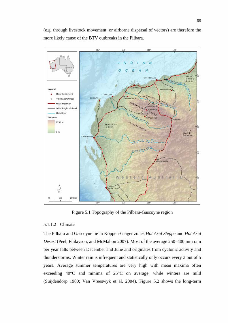
90

(e.g. through livestock movement, or airborne dispersal of vectors) are therefore the

more likely cause of the BTV outbreaks in the Pilbara.

NEWMAN

MEEKATHARRA

GERALDTON

PARABURDOO

TOM PRICE

MARBLE BAR

EXMOUTH

ONSLOW

PANNAWONICA

KARRATHA

PORT HEDLAND

(WITTENOOM)

CARNARVON

D E G R E Y R I V ER O A K

OVE

R R

I VE

R

F O R T E S C U E R I V E R

A SHB U R T O N R I V ER

G A S C O Y N E R I V E R

M U R C H I S O N R I V E R

120°

120°

118°

118°

116°

116°

114°

114°

20°

22°

24°

26°

28°

´0 200100 km

I N D I A N

O C E A N

H A M E R SL E Y

C H I C H E S T E R R A N G E

R A N G E

K E N N E T H R A N G E

C a r n a r v o nB a s i n

W e s t e r n A u s t r a l i aW e s t e r n A u s t r a l i a

L i t t l eS a n d yD e s e r t

G r e a tS a n d yD e s e r t

Legend

Elevation

1250 m

0 m

Major Settlement

Main River

(Town abandoned)

Major Highway

Other Regional Road

Figure 5.1 Topography of the Pilbara-Gascoyne region

5.1.1.2 Climate

The Pilbara and Gascoyne lie in Köppen-Geiger zones Hot Arid Steppe and Hot Arid

Desert (Peel, Finlayson, and McMahon 2007). Most of the average 250–400 mm rain

per year falls between December and June and originates from cyclonic activity and

thunderstorms. Winter rain is infrequent and statistically only occurs every 3 out of 5

years. Average summer temperatures are very high with mean maxima often

exceeding 40°C and minima of 25°C on average, while winters are mild

(Suijdendorp 1980; Van Vreeswyk et al. 2004). Figure 5.2 shows the long-term

91

averages of rainfall, minimum and maximum temperature for three locations in the

study area.

average daily temperature range average monthly rainfall

Onslow

0

5

10

15

20

25

30

35

40

J F M A M J J A S O N D

month

tem

pera

ture

(°C

)

0

100

200

300

400

500

600

700

800

rain

(mm

)

all readings from 1886 - 2010 Wittenoom

0

5

10

15

20

25

30

35

40


month

tem

pera

ture

(°C

)0

100

200

300

400

500

600

700

800

rain

(mm

)

all readings from 1951Carnarvon Airport

0

5

10

15

20

25

30

35

40


month

tem

pera

ture

(°C

)

0

100

200

300

400

500

600

700

800

rain

(mm

)

all readings from 1945 - 2010


Onslow

0

5

10

15

20

25

30

35

40


month

tem

pera

ture

(°C

)

0

100

200

300

400

500

600

700

800

rain

(mm

)

all readings from 1886 - 2010 Wittenoom

0

5

10

15

20

25

30

35

40


month

tem

pera

ture

(°C

)0

100

200

300

400

500

600

700

800

rain

(mm

)

all readings from 1951Carnarvon Airport

0

5

10

15

20

25

30

35

40


month

tem

pera

ture

(°C

)

0

100

200

300

400

500

600

700

800

rain

(mm

)


Figure 5.2 Average daily temperature range and monthly rainfall from long-term weather observations at Onslow, the now abandoned town of Wittenoom, and

Carnarvon

5.1.1.3 Soils, Vegetation and Land Use

The area inland from present day Karratha was first assessed for its pastoral potential

in 1861 by Frank T. Gregory (Van Vreeswyk et al. 2004), before state-wide

vegetation surveys were conducted by Gardner (1928) and Beard (1975a, 1975b) at

scales of 1:4,800,000, and 1:1,000,000, respectively. Later, a number of rangeland

surveys were commissioned by the Department of Agriculture to map topography,

soil and plant communities in different land systems (Tille 2006) at a scale of

1:250,000, e.g. for the Pilbara (Van Vreeswyk et al. 2004), the Ashburton (Payne,

Holman, and Mitchell 1988) and Gascoyne River (Wilcox and McKinnon 1970)

catchments, and the Carnarvon Basin (Payne, Curry, and Spencer 1987).

The type of vegetation predominating in an area depends on the landform and soil

type. As summarised by Suijdendorp (1980) and Tille (2006), most of the hilly

terrain and stony inland flats are dominated by hummock grasslands with different

types of spinifex grass and low mulga woodlands. Of the various types of spinifex,

some of the softer types are palatable to livestock. Denser perennial grasslands are

found on the flood plains along the major creeks and water courses, with native

grasses being increasingly replaced by Buffel and Birdwood grasses introduced from

India. The coastal alluvial plains have soft spinifex grasslands on the loamy soils

92

while clay soils support tussock grasslands. Hard and soft spinifex grasslands are

found on the coastal sandy plains. While about 65% of the resource rich study area

are pastoral properties, some areas, particularly in the Hamersley Ranges are too

rugged and the vegetation unsuitable for pastoral purposes (Payne, Holman, and

Mitchell 1988). Flood plains along the rivers as well as some of the coastal plains

bear the highest carrying capacity for livestock. Figure 5.3 provides an overview of

pastoral areas and other land uses in the study area.

NEWMAN

MEEKATHARRA

GERALDTON

PARABURDOO

TOM PRICE

MARBLE BAR

EXMOUTH

ONSLOW

PANNAWONICA

KARRATHA

PORT HEDLAND

(WITTENOOM)

CARNARVON

D E G R E Y R I V ER O A K

OVE

R R

I VE

R

F O R T E S C U E R I V E R

A SHB U R T O N R I V ER

G A S C O Y N E R I V E R

M U R C H I S O N R I V E R

120°

120°

118°

118°

116°

116°

114°

114°

20°

22°

24°

26°

28°

´0 200100 km

I N D I A N

O C E A N

H AM E R S L E Y

C H I C H E S T E R R A N G E

R A N G E

K E N N E T H R A N G E

C a r n a r v o nB a s i n

L i t t l eS a n d yD e s e r t

G r e a tS a n d yD e s e r t

Legend

Major Settlement

Main River

(Town abandoned)

Major Highway

Other Regional Road

Agricultural Land

Pastoral Station

Conservation Area

Military Area

Aboriginal Land

Crown Land /Other Use

Figure 5.3 Extent of pastoral properties, conservation areas, aboriginal land and crown land in the Pilbara-Gascoyne region. Note that pastoral properties managed by

aboriginal communities are mapped as pastoral stations

5.1.1.4 Host and Vector Activity

Bluetongue is epizootic in this area, and after an anecdotal outbreak in the late

1970’s no evidence of virus presence could be found for several years. However, the

93

large increase in cattle numbers in the region since the 1990’s (as earlier shown in

Figure 2.3), which provide reservoirs for dung breeding BTV vectors like

C. brevitarsis, has likely contributed to an outbreak in 2000. As shown in Figure 5.4,

the number of infected properties increased initially, but this might partly be

explained by an intensification of surveillance activities.

!

!

!

!

!

!

NEWMAN

KARRATHA

CARNARVON

GERALDTON

MEEKATHARRA

2000 / 2001!

!

!

!

!

!

NEWMAN

KARRATHA

CARNARVON

GERALDTON

MEEKATHARRA

2001 / 2002!

!

!

!

!

!

NEWMAN

KARRATHA

CARNARVON

GERALDTON

MEEKATHARRA

2002 / 2003

!

!

!

!

!

!

NEWMAN

KARRATHA

CARNARVON

GERALDTON

MEEKATHARRA

2003 / 2004!

!

!

!

!

!

NEWMAN

KARRATHA

CARNARVON

GERALDTON

MEEKATHARRA

2004 / 2005!

!

!

!

!

!

NEWMAN

KARRATHA

CARNARVON

GERALDTON

MEEKATHARRA

2005 / 2006

!

!

!

!

!

!

NEWMAN

KARRATHA

CARNARVON

GERALDTON

MEEKATHARRA

2006 / 2007!

!

!

!

!

!

NEWMAN

KARRATHA

CARNARVON

GERALDTON

MEEKATHARRA

2007 / 2008!

!

!

!

!

!

NEWMAN

KARRATHA

CARNARVON

GERALDTON

MEEKATHARRA

2008 / 2009

Bluetongue status of tested properties

Bluetongue Status of Pastoral Properties in the Pilbara - Gascoyne RegionBased on NAMP data collected between 1 November and 31 October each year

negativepositive

Figure 5.4 Overview of BTV activity on pastoral properties in the Pilbara - Gascoyne region tested between November 2000 and October 2009

94

A subsequent steady decline in virus antibody detections over the years from 2002 to

2006 resulted in the declaration of the Pilbara as BTV-free in 2009, two years after

the last detection. However, in August 2010, the detection of BTV antibodies in

cattle from a station near Onslow required the reintroduction of the BTV infected

zone in parts of the Pilbara. This is outside the period considered in the present

research and therefore not shown on the map in Figure 5.4. Also in 2010, a single

specimen of the competent vector C. wadai has been trapped near Karratha for the

first time. While this development is not as dramatic as the potential distribution of

the vector modelled by Standfast and Maywald (1992) under a climate change

scenario, it raised awareness for the risks that a southwards expansion of the species

might pose on the more productive livestock holdings in the state. It has therefore

become a major motivation for NAMP, besides fulfilling international OIE

requirements, to provide early warning of any expansion of the vector’s habitat

range.

5.1.2 Northern Territory

The whole Northern Territory covers about one sixth of the Australian landmass,

which equates to an area of 1.35 million km2. Pastoralism is the major land use

throughout much of the Northern Territory with beef cattle being the main enterprise.

Aboriginal land use and conservation areas are also significant, including the

Arnhem Land, Kata Tjuta, and the Kakadu and Litchfield National Parks.

5.1.2.1 Topography and Hydrology

As shown in Figure 5.5, the Northern Territory is a country of gentle to moderate

relief, consisting mostly of plains that rise from sea level at the North Coast to about

590 m near Alice Springs, before falling again towards Lake Eyre (Perry 1960). Most

of the more rugged hilly and mountainous landscape is found in the North. This

includes the rugged dissected plateaus ranging from Arnhem Land southeast into

QLD, as well as the area contiguous with the Kimberley region in WA. The large

catchments of the Victoria, Daly and Roper Rivers are found in this region. In the

South, the McDonnell Ranges, which extend in east-west direction over half of the

width of the NT at the same latitude as Alice Springs, are the only large mountain

mass. While the highest mountain of the Territory, Mt Zeil (1531 m above sea level)

is found here, the relative relief, at less than 600 m, is generally low.

95

##

#

ORD

RIVER

ROPER R IVER

VICTO

RIA

RIV

ER

SO

UTH ALLIG

ATOR RIVER

DALY

RI VER

138°

138°

136°

136°

134°

134°

132°

132°

130°

130°

12°

14°

16°

18°

20°

22°

24°

26°

´0 200100 km

Legend

Major Settlement

# Topographic Feature

Major Highway

Other Regional Road

Major River

State Boundary

Elevation

1530 m

0 m

A R A F U R A S E A

M A C D O N N E L R A N G E S

Ta n a m iD e s e r t

N o r t h e r n T e r r i t o r yN o r t h e r n T e r r i t o r y

B a r k l e yTa b l e l a n d

S i m p s o nD e s e r t

A r n h e m L a n d

G U L FO F

C A R P E N T A R I A

T I M O RS E A

TENNANT CREEK

ALICE SPRINGS

KATHERINE

JABIRU

DARWIN

P E T E R M A N N R A N G E S

T R E U E R

R A N G E

KataTjuta

Uluru(Ayers Rock)

Mt Zeil1531 m

L a k e A r g y l e

Figure 5.5 Topographic overview of the Northern Territory

5.1.2.2 Climate

The climate of the Northern Territory is under the influence of the north-west

monsoon with a summer wet season and a winter dry-season. From north to south the

climate changes from Köppen-Geiger zones Tropical Savannah to Hot Arid Steppe

and Hot Arid Desert (Peel, Finlayson, and McMahon 2007), with annual rainfall

ranging between 250-500 mm in the South and 1000-1700 mm in the North. Most

rain falls between November and April.

96

While it is warm in the North throughout the year, frost can occur in the arid interior

as far north as Alice Springs (Wilson et al. 1990). Long-term average conditions are

shown in Figure 5.6.

Darwin Airport

0

5

10

15

20

25

30

35

40


month

tem

pera

ture

(°C

)

0

100

200

300

400

500

600

700

800

rain

(mm

)

all readings from 1941 - 2010 Katherine Council

0

5

10

15

20

25

30

35

40


month

tem

pera

ture

(°C

)

0

100

200

300

400

500

600

700

800

rain

(mm

)

temperature from 1937 - 2010rain from 1873 - 2010

Alice Springs Airport

0

5

10

15

20

25

30

35

40


month

tem

pera

ture

(°C

)

0

100

200

300

400

500

600

700

800

rain

(mm

)



Darwin Airport

0

5

10

15

20

25

30

35

40


month

tem

pera

ture

(°C

)

0

100

200

300

400

500

600

700

800

rain

(mm

)

all readings from 1941 - 2010 Katherine Council

0

5

10

15

20

25

30

35

40


month

tem

pera

ture

(°C

)

0

100

200

300

400

500

600

700

800

rain

(mm

)

temperature from 1937 - 2010rain from 1873 - 2010

Alice Springs Airport

0

5

10

15

20

25

30

35

40


month

tem

pera

ture

(°C

)

0

100

200

300

400

500

600

700

800

rain

(mm

)



Figure 5.6 Average daily temperature range and monthly rainfall from long-term weather observations at Darwin, Katherine, and Alice Springs

5.1.2.3 Soils, Vegetation and Land Use

Vegetation in the Northern Territory ranges from tussock grasslands, shrublands and

low open woodlands in the South to tall woodland with patches of monsoon

rainforest in the North. A territory-wide vegetation map at a scale of 1:1 million has

been compiled by Wilson et al. (1990). More detailed land system maps are available

at a scale of 1:250,000 for the northern parts of the NT. A territory-wide vegetation

map at nominal scale of 1:100,000 has been proposed during a workshop in 2008

(Brocklehurst et al. 2008), but has not yet been completed.

Perry (1960) divides the NT ‘vegetationally’ into two halves: The northern half,

where rainfall exceeds 380 mm (15 inch) and Eucalyptus species are predominantly

found, and the southern half with less that 380 mm annual rainfall, where Eucalypts

are virtually absent. Treeless grasslands on heavy clay soils are found in both parts,

but they are more extensive in the North. Particularly the Barkley Tableland and the

Victoria River District are home to ephemeral grass species that provide nutritious

stock fodder during and after the wet season. Later in the dry season, cattle are forced

to feed on the less nutritious short perennial grasses. In the central and southern part,

vast areas are characterised by spinifex grasslands with scattered shrubs and low

trees that cover the sand plains, dune fields and stony hills. About 48% of the

97

Northern Territory is leased for pastoral purposes (Wilson et al. 1990), as also shown

in Figure 5.7. Only the drier regions covering the Tanami and Gibson deserts in the

South as well as the Arnhem Land and the National Parks in the North have been

considered unsuitable for pastoralism and returned to their traditional owners or

protected for conservation purposes. Some intensive horticulture occurs particularly

in the North in the regions around Darwin and Katherine.

##

#

ORD

RIVER

ROPER R IVER

VIC

TORI

A R

IVER

SO

UTH ALLIG

ATOR RIVER

DALY RI VER

138°

138°

136°

136°

134°

134°

132°

132°

130°

130°

12°

14°

16°

18°

20°

22°

24°

26°

´0 200100 km

A R A F U R A S E A

M A C D O N N E L R A N G E S

Ta n a m iD e s e r t

N o r t h e r n T e r r i t o r yN o r t h e r n T e r r i t o r y

B a r k l e yTa b l e l a n d

S i m p s o nD e s e r t

A r n h e m L a n d

G U L FO F

C A R P E N T A R I A

T I M O RS E A

TENNANT CREEK

ALICE SPRINGS

KATHERINE

JABIRU

DARWIN

P E T E R M A N N R A N G E S

T R E U E R

R A N G E

KataTjuta

Uluru(Ayers Rock)

Mt Zeil1531 m

L a k e A r g y l e

Legend

Major Settlement

Main River

(Town abandoned)

Major Highway

Other Regional Road

Pastoral Station

Conservation Area

Military Area

Aboriginal Land

Vacant Crown Land / Other Use

Figure 5.7 Extent of pastoral properties, conservation areas, aboriginal land and crown land in the Northern Territory. Note that pastoral properties managed by

aboriginal communities are mapped as pastoral stations

98

5.1.2.4 Host and Vector Activity

Bluetongue is endemic north of 13° latitude, and epidemic south of that line with

occurrences in Katherine and the Victoria River District in some years. The peak of

activity is typically between January and May, but late seroconversions have

occurred between August and September (Animal Health Australia 2001).

!

!

!

!

!

!!

!

!

DARWIN

KATHERINE

KUNUNURRA

ALICE SPRINGS

2000 /2001

!

!

!

!

!

!!

!

!

!

!

DARWIN

KATHERINE

KUNUNURRA

ALICE SPRINGS

!

!

!

!

!

!!

!

!

DARWIN

KATHERINE

KUNUNURRA

ALICE SPRINGS

!

!

!

!

!

!!

!

!

!

DARWIN

KATHERINE

KUNUNURRA

ALICE SPRINGS

!

!

!

!

!

!!

!

!

DARWIN

KATHERINE

KUNUNURRA

ALICE SPRINGS

!

!

!

!

!

!!

!

!

!

DARWIN

KATHERINE

KUNUNURRA

ALICE SPRINGS

!

!

!

!

!!

!

!

!

DARWIN

KATHERINE

KUNUNURRA

ALICE SPRINGS

!

!

!

!

!

!!

!

!

DARWIN

KATHERINE

KUNUNURRA

ALICE SPRINGS

!

!

!

!

!

!!

!

!

!

!

DARWIN

KATHERINE

KUNUNURRA

ALICE SPRINGS

Bluetongue status of tested properties (dots represent smaller stations)

Bluetongue Status of Pastoral Properties in the Northern TerritoryBased on NAMP data collected between 1 November and 31 October each year

2001 / 2002

2002 / 2003

2003 /2004

2004 /2005

2005 /2006

2006 /2007

2007 /2008

2008 /2009

/ negative/ positive !!

Figure 5.8 Overview of BTV activity on pastoral properties in the Northern Territory tested between November 2000 and October 2009

99

Surveillance activities focus on the detection of new strains of BTV and other viruses

as well as vector incursions from South East Asia on the prevailing winds. Several

BTV serotypes found in Australia have been isolated from sentinel cattle at the

Beatrice Hill research station north of Darwin. Figure 5.8 shows the varying levels of

BTV activity throughout the years 2000 to 2009.

5. 2 Conceptual Model and Spatio-temporal Data Requirements A conceptual model is the first stage in the development of a predictive distribution

model (Guisan and Zimmermann 2000). In this case the concept represents a

simplified view of the natural complexity of virus ecology. After defining the

characteristics of the response variable, i.e. answering the question What shall be

predicted?, all environmental factors that hypothetically influence the outcome of the

response (e.g. virus presence or absence) may be included in the concept. For

parsimony, and because the aim of this research is not to develop a complex disease

model, a set of the most promising environmental factors is being selected for the

development of predictor variables. Based on this conceptual model, an assessment

of suitable data products can then be conducted. Therefore, considerations need to be

given to the required minimum spatial and temporal resolution, which is governed by

the seasonality of virus activity and the characteristics of the virus dataset (sampling

frequency, spatial reference unit), both of which are discussed below.

5.2.1 Defining the Response Variable

Data on the primary phenomenon of interest (i.e. the response variable), whether it

be the vector or the disease, are required to build a statistical model of its relation to

the secondary (or explanatory) variable (e.g. temperature or rainfall) (Curran et al.

2000). These data may come in a variety of formats. Epidemiological models have

for example been developed based on disease prevalence (Kleinschmidt et al. 2000),

intensity of infection (Clements, Moyeed, and Brooker 2006), vector abundance

(Altobelli et al. 2008; Baylis et al. 1998), or presence and absence of a virus (e.g.

Boyer, Ward, and Singer 2010; Calvete et al. 2009; Chalke 2006). As part of the

surveillance activities under the NAMP, a series of data related to the presence of

arboviruses are recorded, such as serological status of cattle or number of potential

arbovirus vectors. These measures are potential response variables to be predicted for

either a certain location or aggregated over an area. Hence a decision needs to be

100

made based on the NAMP data on the type of response variable used in this study as

well as the most appropriate spatial and temporal support that influences the outcome

at each location similarly (Curran et al. 2000).

Vector trapping is conducted once every one to two months at selected sample sites,

where the number of specimens for each species is recorded. However, while

trapping methods are being constantly improved (Bishop et al. 2006), it has been

acknowledged by entomologists that the number of caught insects is not necessarily

representative for vector abundance, due to various factors reducing the efficiency of

the utilised light traps (Bishop et al. 2000). This, together with the fact that vector

sample sites are very widely dispersed over the study areas, excludes vector presence

and absence or abundance as response variables.

Seroconversion data from sentinel herds are usually collected at regular intervals

from once a month to twice annually. Complimentary serological surveys are

conducted less frequently on an ad-hoc basis. Cattle are often only accessible once a

year during mustering, when they are driven to the yards where they can be tested by

veterinary officers. Often, this rare opportunity for testing is missed due to limited

human resources and the inaccessibility of some properties. Both approaches deliver

information about the presence of antibodies in the blood of tested cattle and hence

about BT presence and absence. Only for particular sites, viruses are isolated to

determine the serotype (Melville 2004). It was therefore decided on using the

presence and absence of BTV as the response variable, regardless of the serotype and

without differentiating between data from sentinel herd and serological surveys.

Knowledge about the timing of infection is vital for the identification of

environmental risk factors, which may have contributed to the abundance of vectors

and hence the increased risk for transmission. At sites with sentinel herds that are

tested monthly, the range of possible infection dates is relatively narrow. However,

for the majority of sites, where serological surveys are conducted once a year, the

timing of infection can only be estimated with an accuracy of several months. BTV

antibodies can still be detected for several months post infection or even for the

host’s life time (Mertens et al. 2009), and as Figure 5.9 demonstrates, this may be

well after the annual peak of virus activity. The timing of serological surveys at

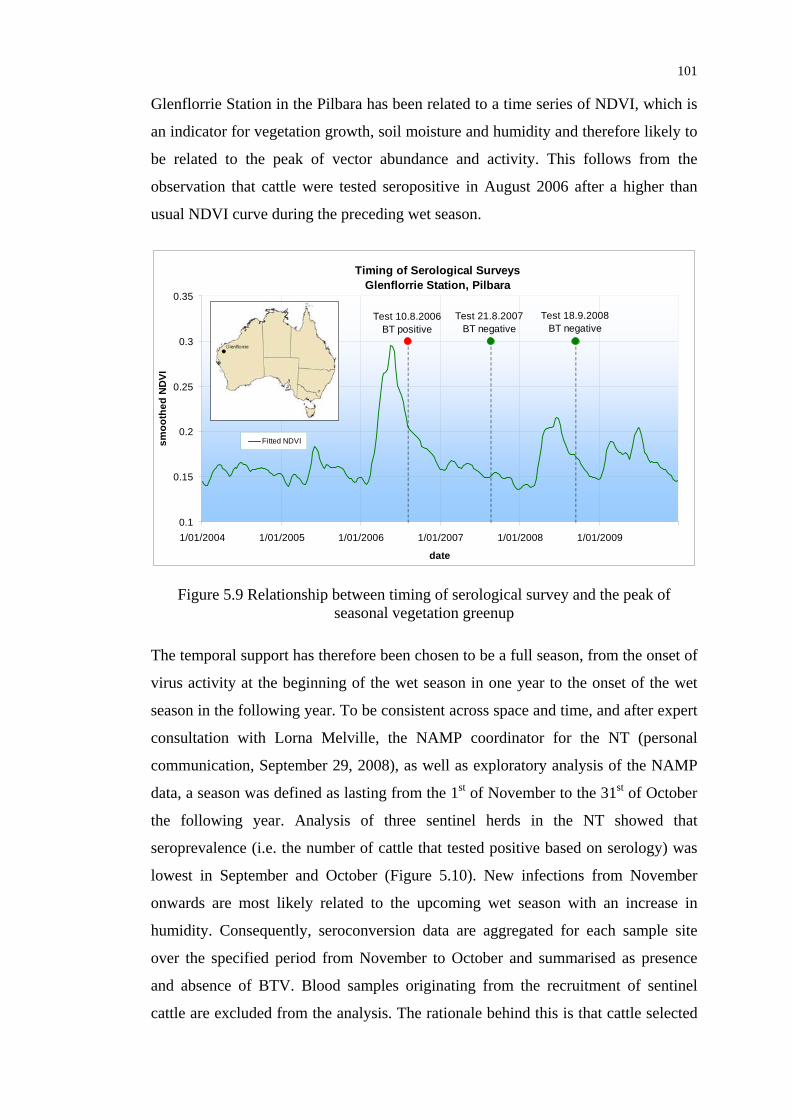
101

Glenflorrie Station in the Pilbara has been related to a time series of NDVI, which is

an indicator for vegetation growth, soil moisture and humidity and therefore likely to

be related to the peak of vector abundance and activity. This follows from the

observation that cattle were tested seropositive in August 2006 after a higher than

usual NDVI curve during the preceding wet season.

Timing of Serological SurveysGlenflorrie Station, Pilbara

Test 10.8.2006BT positive

Test 21.8.2007BT negative

Test 18.9.2008BT negative

0.1

0.15

0.2

0.25

0.3

0.35

1/01/2004 1/01/2005 1/01/2006 1/01/2007 1/01/2008 1/01/2009

date

smoo

thed

ND

VI

Fitted NDVI

Figure 5.9 Relationship between timing of serological survey and the peak of seasonal vegetation greenup

The temporal support has therefore been chosen to be a full season, from the onset of

virus activity at the beginning of the wet season in one year to the onset of the wet

season in the following year. To be consistent across space and time, and after expert

consultation with Lorna Melville, the NAMP coordinator for the NT (personal

communication, September 29, 2008), as well as exploratory analysis of the NAMP

data, a season was defined as lasting from the 1st of November to the 31st of October

the following year. Analysis of three sentinel herds in the NT showed that

seroprevalence (i.e. the number of cattle that tested positive based on serology) was

lowest in September and October (Figure 5.10). New infections from November

onwards are most likely related to the upcoming wet season with an increase in

humidity. Consequently, seroconversion data are aggregated for each sample site

over the specified period from November to October and summarised as presence

and absence of BTV. Blood samples originating from the recruitment of sentinel

cattle are excluded from the analysis. The rationale behind this is that cattle selected

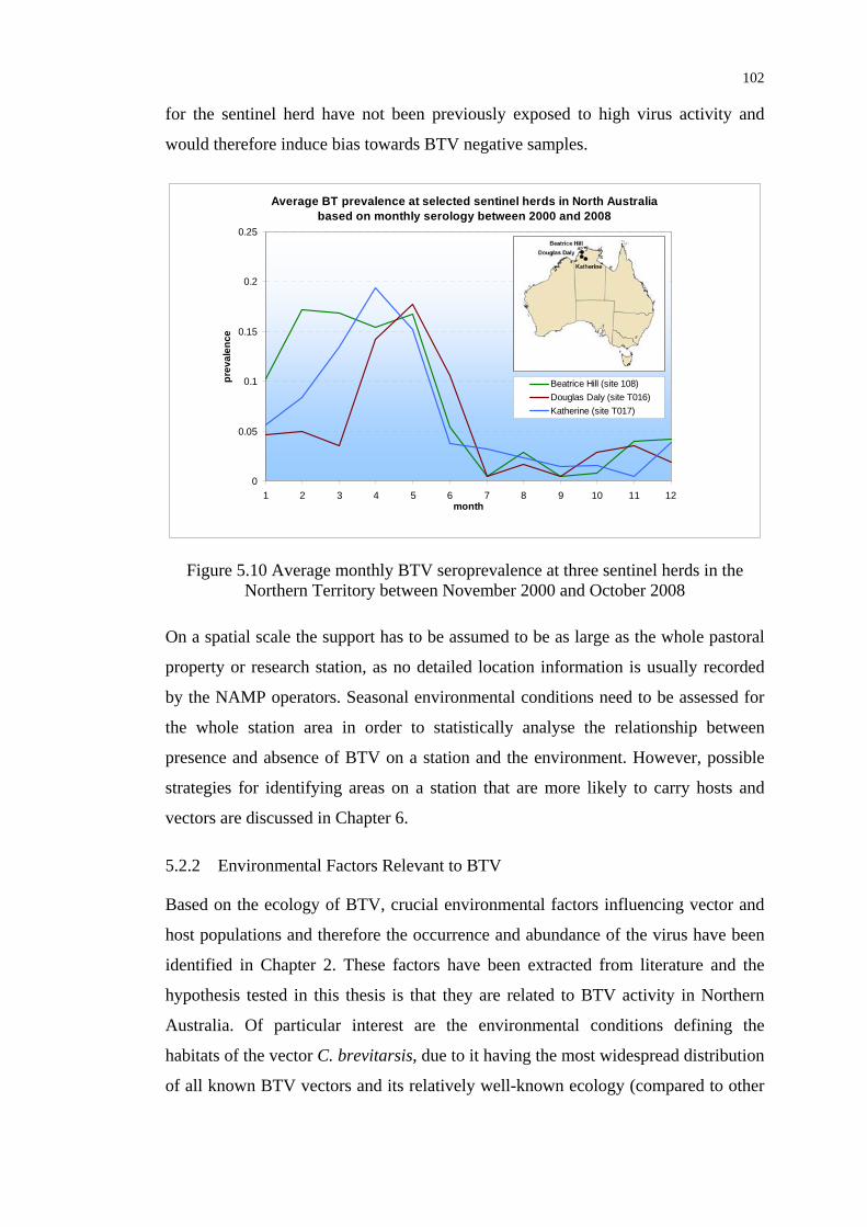
102

for the sentinel herd have not been previously exposed to high virus activity and

would therefore induce bias towards BTV negative samples.

Average BT prevalence at selected sentinel herds in North Australiabased on monthly serology between 2000 and 2008

0

0.05

0.1

0.15

0.2

0.25

1 2 3 4 5 6 7 8 9 10 11 12month

prev

alen

ce

Beatrice Hill (site 108)Douglas Daly (site T016)Katherine (site T017)

Figure 5.10 Average monthly BTV seroprevalence at three sentinel herds in the Northern Territory between November 2000 and October 2008

On a spatial scale the support has to be assumed to be as large as the whole pastoral

property or research station, as no detailed location information is usually recorded

by the NAMP operators. Seasonal environmental conditions need to be assessed for

the whole station area in order to statistically analyse the relationship between

presence and absence of BTV on a station and the environment. However, possible

strategies for identifying areas on a station that are more likely to carry hosts and

vectors are discussed in Chapter 6.

5.2.2 Environmental Factors Relevant to BTV

Based on the ecology of BTV, crucial environmental factors influencing vector and

host populations and therefore the occurrence and abundance of the virus have been

identified in Chapter 2. These factors have been extracted from literature and the

hypothesis tested in this thesis is that they are related to BTV activity in Northern

Australia. Of particular interest are the environmental conditions defining the

habitats of the vector C. brevitarsis, due to it having the most widespread distribution

of all known BTV vectors and its relatively well-known ecology (compared to other

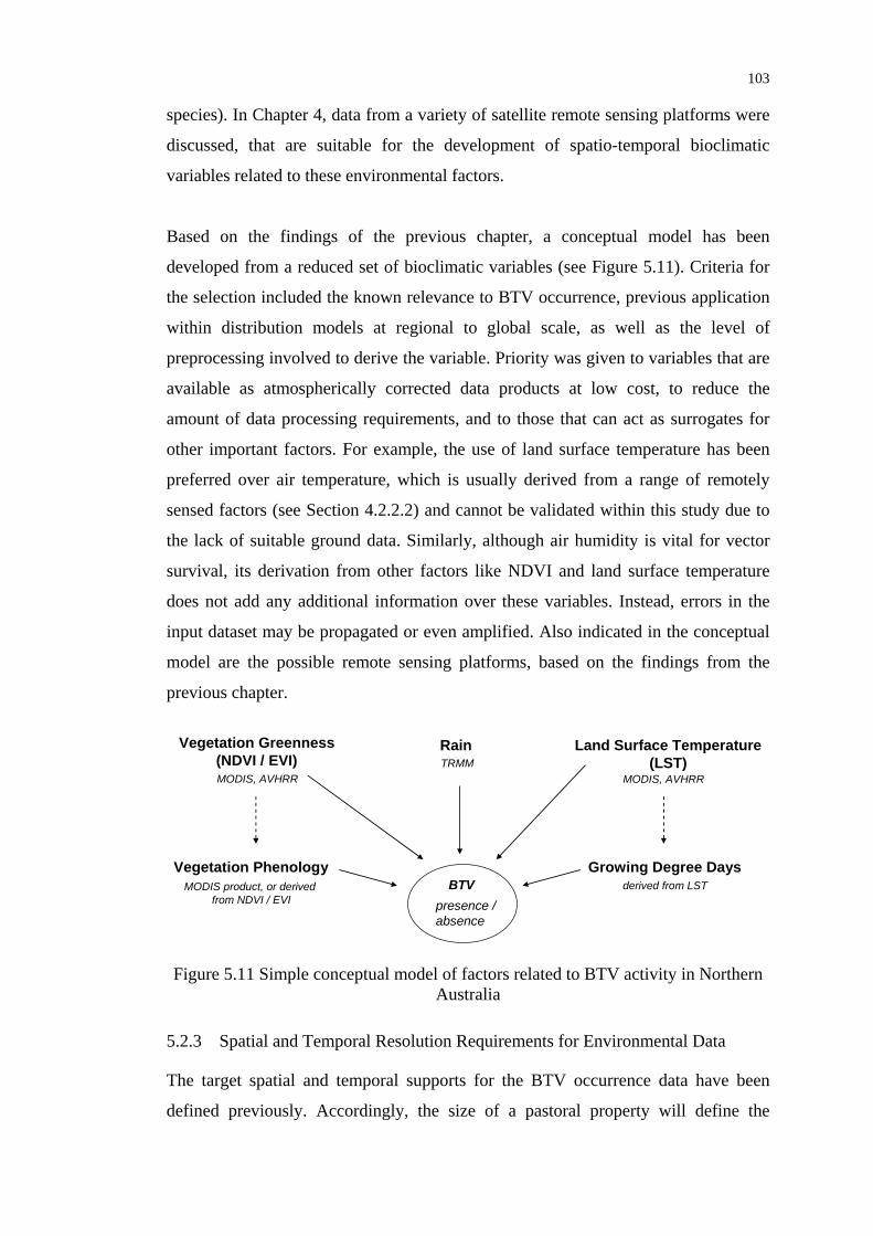
103

species). In Chapter 4, data from a variety of satellite remote sensing platforms were

discussed, that are suitable for the development of spatio-temporal bioclimatic

variables related to these environmental factors.

Based on the findings of the previous chapter, a conceptual model has been

developed from a reduced set of bioclimatic variables (see Figure 5.11). Criteria for

the selection included the known relevance to BTV occurrence, previous application

within distribution models at regional to global scale, as well as the level of

preprocessing involved to derive the variable. Priority was given to variables that are

available as atmospherically corrected data products at low cost, to reduce the

amount of data processing requirements, and to those that can act as surrogates for

other important factors. For example, the use of land surface temperature has been

preferred over air temperature, which is usually derived from a range of remotely

sensed factors (see Section 4.2.2.2) and cannot be validated within this study due to

the lack of suitable ground data. Similarly, although air humidity is vital for vector

survival, its derivation from other factors like NDVI and land surface temperature

does not add any additional information over these variables. Instead, errors in the

input dataset may be propagated or even amplified. Also indicated in the conceptual

model are the possible remote sensing platforms, based on the findings from the

previous chapter.

Vegetation Greenness(NDVI / EVI)

Land Surface Temperature(LST)

Vegetation Phenology

Rain

Growing Degree Days

MODIS, AVHRRTRMM

MODIS, AVHRR

MODIS product, or derived from NDVI / EVI

BTVpresence /absence

derived from LST

Figure 5.11 Simple conceptual model of factors related to BTV activity in Northern Australia

5.2.3 Spatial and Temporal Resolution Requirements for Environmental Data

The target spatial and temporal supports for the BTV occurrence data have been

defined previously. Accordingly, the size of a pastoral property will define the

104

minimum scale for the analysis and model building processes. The environmental

variables will necessarily have to be aggregated on a cattle station level. It is

however important to preserve regional features as well as the environmental

variability, which both have an effect on virus transmission cycles. The rationale

behind that is, once the model parameters have been determined, the aim is to predict

the probability of BTV presence as a continuous surface over the entire study area.

Annual prediction maps are to be produced, based on the environmental variables of

a particular year. In order for the prediction maps to be useful for decision making, a

pixel must be small enough to be associated with features on the ground, e.g. to

identify paddocks that might be a higher risk, or to delineate areas that are best suited

for vector trapping.

A regional scale is therefore considered adequate for this study, with resolutions

ranging from 500 m to 1000 m for vegetation and land surface temperature variables.

Remotely sensed area-wide rainfall measurements are generally available at lower

resolutions, e.g. 25 km from TRMM. While this is not ideal for depicting small scale

rainfall events, it provides information on regional rainfall patterns and a pixel would

still be smaller than the average size of a pastoral property (about 1,850 km2 in the

Pilbara – Gascoyne region, and 2,800 km2 in the Northern Territory.

Similar research that has been undertaken on a regional scale include the study by

Tatem et al. (2003), where the low spatial resolution AVHRR sensor was utilised for

monitoring of environmental variables which successfully predicted the distribution

of the BTV vector C. imicola. Hay et al. (1998) also demonstrated the capacity of

regional monitoring with AVHRR for predicting mosquito-borne malaria seasons.

The LST and VI products from MODIS at resolutions of 1000 m and 500 m

respectively, have been used by Altobelli et al. (2008) to predict the distribution of

ticks in Northern Italy. Chalke (2006) has similarly demonstrated the application of

MODIS derived NDVI variables for analysis of MVEV in Northwestern Australia.

As previously defined, the minimum temporal resolution of 12 months for

exploratory data analysis and model development is governed by the virus dataset.

Consequently, environmental conditions or changes to the environment over the

same period need to be captured and distilled into seasonal variables, while

105

preserving the characteristics of the season (see Chapter 6). Not all 12 months will be

equally important, however the period during and after the wet season, when the

highest levels of virus activity are recorded, is of particular interest, as are the winter

months where temperature is the crucial factor for vector survival.

Bioclimatic parameters associated with habitat dynamics have diverse temporal

characteristics. Some of them such as climatic factors or related changes of surface

conditions (e.g. flooding, or surface temperature) are highly dynamic in time, while

others such as vegetation might change more slowly. Different temporal resolutions

are therefore needed for each of the factors in order to accumulate or average

measurements accurately over time (see Table 5.1 below).

Table 5.1 Required temporal resolution for the remotely sensed climatic and environmental datasets

Factor Aggregation method Required temporal resolution of source data

Rainfall Accumulation of rainfall Hourly to daily

Land surface temperature

Average minimum, maximum and mean temperatures

Half-daily to capture day and night temperatures

Growing degree days

Accumulation of average daily temperature

Half-daily to capture day and night temperatures

NDVI/EVI Maximum NDVI/EVI Weekly to monthly

Vegetation phenology

Extraction of seasonal phenology measures from NDVI/EVI time series

Weekly

Particularly during the wet season, there is a reduced possibility of obtaining images

over tropical areas that are not significantly affected by atmospheric conditions such

as cloud cover. In order to gather high quality data at the required resolution for this

project, images need to be obtained at a higher frequency. However, if the target

variable is an average or accumulated value over a certain period, e.g. the mean

monthly night temperature, it might not be necessary to acquire daily images and

then determine the average temperature range. A number of data products exist, for

example for MODIS, that provide quality controlled 8-daily or monthly

environmental data, which reduce the resources required for data acquisition and

processing significantly.

106

5. 3 Selection of Remote Sensing Instruments and Data Products To facilitate the identification and analysis of spatio-temporal relationships between

BTV dynamics and earth surface and atmospheric conditions the data reflecting these

conditions need to meet specific requirements. Data must be continuously available

for the whole study area. Their spatial and temporal resolution must be appropriate to

this study as defined in the previous section.

5.3.1 Selection of Remote Sensing Platforms

Based upon the definition of the spatial and temporal resolution requirements of this

project, the range of possible platforms is reduced to AVHRR, MODIS, and for

rainfall variables, to TRMM and CMORPH precipitation estimates.

Before the availability of MODIS, many regional studies investigating correlations

between environment and BTV or Malaria have utilised data from AVHRR.

However, the big advantages of MODIS, such as the higher spatial resolution,

enhanced stability of both spectral and geolocational accuracy (Huete et al. 2002;

Wolfe et al. 2002), as well as the large variety of freely available atmospherically

corrected data products, make it the preferred instrument for this project. Although

the future supply of MODIS and MODIS-like data products through continuity

missions is a major strength, a limitation of MODIS is the smaller archive of

historical data. Imagery from the Terra platform only dates back to February 2000

and MODIS images from the Aqua satellite are available from August 2002 onwards.

BTV surveillance data for this project extends from before 2000 till present so the

availability of historic MODIS imagery limits the full use of available virus data for

developing and testing models. Nevertheless, the MODIS sensor on board the Terra

satellite meets all of the requirements for this project, and will therefore be utilised

for monitoring of vegetation and land surface temperature in Northern Australia

between 2000 and 2009.

A review of candidate data products from the MODIS sensor is provided in the

following section, followed by a comparison of rainfall estimates using the TMPA

and CMORPH methods, with rain gauge data.

107

5.3.2 MODIS Data Products

MODIS offers a range of daily, 8-daily, 16-daily and monthly standard data products

at native spatial resolutions of 250 m, 500 m and 1000 m, and different processing

levels (Justice et al. 2002). Level one (source data) and level two data (derived

geophysical variables) are geolocated to latitude and longitude. Level three products

deliver temporally and or spatially manipulated geophysical variables and level four

products are either model output or results from analyses of lower level data

products. Both are usually provided as integerised values in an equal-area Sinusoidal

projection in tiles measuring about 1113 km by 1113 km (Wolfe, Roy, and Vermote

1998). All data products are delivered in a hierarchical data format (HDF) and can be

obtained at no cost from the Land Processes Distributed Active Archive Centre (LP

DAAC). The current generation of MODIS products is termed Collection 5, which,

depending on the product, offers several advantages over previous collections

(Ganguly et al. 2010; Wan 2008) and is therefore used throughout this project.

Datasets of major interest for this project are those from which the vegetation indices

(NDVI and EVI) and subsequently, phenological parameters can be extracted, as

well as data on land surface temperature. In view of the need for a continuous time

series from which phenology and growing degree periods can be derived, 8 –16-daily

images composited from cloud-free daily images are preferable.

5.3.3 Vegetation Indices and Vegetation Phenology from MODIS

Vegetation monitoring with MODIS can be carried out in two ways, either using the

dedicated Vegetation Index and Vegetation Dynamics products or calculating these

two parameters from surface reflectance data. The following sections explore both

avenues in order to find the most appropriate solution for this project.

5.3.3.1 MODIS/Terra Vegetation Indices 16-Day L3 Global 250 m

The MODIS Vegetation Index product (MOD13Q1) provides 16-day composites of

the NDVI and EVI indices (see section 4.2.4.2) at a spatial resolution of 250 m. It is

produced from gridded level two daily surface reflectance data corrected for

molecular scattering, ozone absorption, and aerosols (Vermote, El Saleous, and

Justice 2002). While the red and NIR bands included in NDVI and EVI are natively

available at a 250 m spatial resolution, the 500 m blue band that is included in EVI

108

for aerosol resistance, needs to be resampled to the higher resolution (Huete et al.

2002). Prior to compositing the NDVI data, a filter selects higher quality, near-nadir

observations that show the least distortions, and are free from clouds and cloud

shadows, from the 16 days of observation. This overcomes the effect introduced by a

whiskbroom scanner like MODIS that the pixel size on the ground increases with the

viewing angle.

The goal of compositing methodologies is to select the best observation, on a per

pixel basis, from all the retained filtered data, to represent each pixel over the 16-day

compositing period. Depending on the number of good quality pixels after screening,

the compositing algorithm chooses between two approaches. If valid pixels are

available for at least two out of 16 days, the algorithm compares the two highest

NDVI values after filtering and selects the observation closest to nadir with the

highest observed NDVI value, using the constrained-view angle-maximum value

composite (CV-MVC) approach. In all other cases, i.e. when one or more pixels over

16 days showed cloud cover, mixed clouds or were adjacent to clouds, the largest

NDVI value over the 16-day period is selected, using an approach called maximum

value composite (MVC) (Didan and Huete 2006).

The VI values in the MOD13Q1 product are accompanied by auxiliary information

on different parameters, such as aerosol quantity and likelihood of snow cover, as

well as an overall indication of the usefulness of each data point. MODIS NDVI was

designed to be compatible with AVHRR NDVI products and therefore provides

continuity for time series used in historical applications. Thus it was initially

considered for this research. However, assessment of the data showed that the

land/water mask used to clip the dataset and exclude ocean pixels, was shifted

eastwards by up to 4 km. As a result, relatively large areas along north south oriented

coast lines were missing (Figure 5.12). This error which was not previously known to

the research community has been reported to the MODIS Land Science Team (K.

Didan, personal communication, November 13, 2008), and is now documented on

the MODIS Land Quality Assessment website (NASA Goodard Space Flight Centre

2009). However, it is not expected to be fixed before the next major update cycle of

MODIS products due in late 2010. For this reason, although the product was initially

the preferred option, an alternative dataset was chosen to derive the vegetation

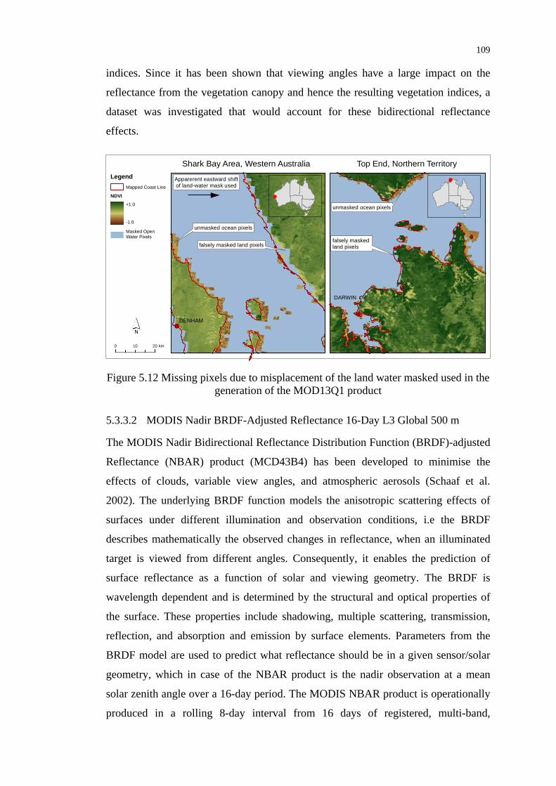
109

indices. Since it has been shown that viewing angles have a large impact on the

reflectance from the vegetation canopy and hence the resulting vegetation indices, a

dataset was investigated that would account for these bidirectional reflectance

effects.

!DENHAM

falsely masked land pixels

Apparerent eastward shiftof land-water mask used

0 2010 km

!

DARWIN

falsely masked land pixels

Shark Bay Area, Western Australia Top End, Northern Territory

unmasked ocean pixels

unmasked ocean pixels

LegendMapped Coast Line

NDVI+1.0

-1.0

Masked Open Water Pixels

´

Figure 5.12 Missing pixels due to misplacement of the land water masked used in the generation of the MOD13Q1 product

5.3.3.2 MODIS Nadir BRDF-Adjusted Reflectance 16-Day L3 Global 500 m

The MODIS Nadir Bidirectional Reflectance Distribution Function (BRDF)-adjusted

Reflectance (NBAR) product (MCD43B4) has been developed to minimise the

effects of clouds, variable view angles, and atmospheric aerosols (Schaaf et al.

2002). The underlying BRDF function models the anisotropic scattering effects of

surfaces under different illumination and observation conditions, i.e the BRDF

describes mathematically the observed changes in reflectance, when an illuminated

target is viewed from different angles. Consequently, it enables the prediction of

surface reflectance as a function of solar and viewing geometry. The BRDF is

wavelength dependent and is determined by the structural and optical properties of

the surface. These properties include shadowing, multiple scattering, transmission,

reflection, and absorption and emission by surface elements. Parameters from the

BRDF model are used to predict what reflectance should be in a given sensor/solar

geometry, which in case of the NBAR product is the nadir observation at a mean

solar zenith angle over a 16-day period. The MODIS NBAR product is operationally

produced in a rolling 8-day interval from 16 days of registered, multi-band,

110

atmospherically corrected surface reflectance data from the MODIS instrument on

both the Terra and Aqua platforms. In Collection 5, NBAR data are generated for

bands 1-7 at 500-m spatial resolution and distributed with accompanying data on

band quality.

Since view angle effects, as well as cloud and aerosol contamination, have been

removed, NBAR is ideal for applications such as time series analysis of NDVI,

which have traditionally had to depend on compositing methods to reduce these

effects. The product has therefore been increasingly used to investigate vegetation

dynamics from NBAR derived vegetation indices (see below), to map global land

cover (Friedl et al. 2010) and also to provide global bioclimatic variables for use in

epidemiology (Scharlemann et al. 2008).

5.3.3.3 MODIS Land Cover Dynamics Yearly L3 Global 1 km

The MODIS Land Cover Dynamics (MLCD) product (MCD12Q2) has been

developed to support studies of seasonal phenology and interannual variation in land

surface and ecosystem properties. MCD12Q2 is produced using the algorithm

presented in Zhang et al. (2003), which fits series of piecewise logistic functions to

vegetation index time series. The algorithm characterises vegetation growth cycles

using four transition dates estimated from time series of MODIS enhanced vegetation

index (EVI) data: (1) greenup: the date of onset of EVI increase; (2) maturity: the

date of onset of EVI maximum; (3) senescence: the date of onset of EVI decrease;

and (4) dormancy (Ganguly et al. 2010).

While the MCD12Q2 product could be potentially of interest for this project, at the

time of writing it has only been made available for the years 2000 – 2006.

Assessment of a test dataset further indicated that the amount of missing data in the

study areas makes in less useful for this project.

5.3.3.4 Selection of MODIS Product for Vegetation Monitoring

The investigation into products capable of either providing vegetation indices or the

bands to calculate those indices gave some clear indication on the most appropriate

dataset. The BRDF-Adjusted MCD43B4 product has ideal characteristics to derive

spatially coherent VI maps that are not biased by different viewing angles. Although

111

the spatial resolution of 500 m is not as high as for the Vegetation Index product, it

provides enough detail for regional studies. The MCD43B4 dataset has therefore

been selected for this study to generate NDVI and EVI time series that can be

analysed further for the extraction of phenological variables as described in

Chapter 6.

5.3.4 Land Surface Temperature from MODIS

5.3.4.1 MODIS Land Surface Temperature & Emissivity 8-Day L3 Global 1km

The MODIS Land Surface Temperature and Emissivity products (MOD11A2 from

Terra satellite and MYD11A2 from Aqua satellite) provide land surface temperature

and emissivity values averaged over a period of 2-8 days at a spatial resolution of

1 km (Wan 2009). The products are the result of the generalised split-window LST

algorithm (Wan and Dozier 1996), which is aimed at reaching an accuracy of better

than 1°K (+/− 0.7°K stddev.) for areas with known emissivities in the range −10°K

to 58°K (Wan 2008). Data are ideally generated under clear-sky conditions to avoid

mixing with cloud top temperature. Low quality pixels resulting from clouds and

other atmospheric disturbances, which constitute a significant obstacle for

continuous LST monitoring, are marked in an accompanying quality assessment

(QA) layer. LST is observed by the two MODIS sensors four times per day, at 10:30

and 22:30 local solar time by MODIS Terra, and at 01:30 and 13:30 by MODIS

Aqua. Data for the morning and afternoon/evening overpasses are encoded in the

dataset as LST night and LST day, respectively. The other layers included in the

MOD11A2 product are quality assessment, observation times, view angles, a record

of clear sky days and nights, and emissivities in Bands 31 and 32 estimated from

land cover types (Wan 2009).

Ecologically, using night and day temperatures from the Aqua overpass might seem

to be the preferred option, as they are captured closer to the daily temperature

minimum and maximum, respectively. However, Mostovoy et al. (2006) showed that

the strength of the correlation between observed and remotely sensed LST did not

significantly change with the overpass time. Therefore, if we are not interested in the

absolute minimum temperatures, but in the relative temperature patterns, the

additional 2 years of coverage from the Terra platform outweighs that disadvantage.

112

In an epidemiological context, the MOD11A2 product has been used by

Scharlemann et al. (2008) to generate a Fourier processed time series over 5 years.

Neteler (2010) produced gap filled LST maps for the prediction of tick-borne

encephalitis in Northern Italy, using the daily MOD11 LST dataset.

5.3.4.2 MODIS Land Surface Temperature & Emissivity 8-Day L3 Global 5km

An alternative product, MOD11B1, consists of 8-daily LST and emissivity data at

5 km spatial resolution. It is generated by the day/night LST algorithm (Wan & Li,

1997). However, this product has been disregarded due to the lower spatial

resolution.

5.3.5 Satellite-based Precipitation Products

The TRMM 3B42 or ‘TRMM and Other Satellite Precipitation Product’ (Huffman et

al. 2007) and CMORPH (Joyce et al. 2004) from NOAA’s Climate Prediction Center

provide global satellite derived precipitation data sets. These products have been

shortlisted for this project due to their quality, and their spatial and temporal

properties. As reviewed in Chapter 4, the strength of these methods is the

combination of high resolution optical and infrared sensors with the active and

passive microwave sensors that are able to penetrate cloud cover and provide three-

dimensional rainfall estimates. The two methods and related datasets are compared to

rain gauge measurements hereafter.

5.3.5.1 TRMM and Other Satellite Precipitation Product

TRMM data are acquired as part of a joint mission by the Japan Aerospace

Exploration Agency (JAXA, formerly NASDA) and the US National Aeronautics

and Space Administration (NASA). The TRMM science team developed the

algorithms for the processing of the rainfall data products, also known as TRMM

Multisatellite Precipitation Analysis (TMPA) (Huffman et al. 2007), that is carried

out by the TRMM Science Data and Information System (TSDIS) and the TRMM

office. The data are archived and distributed by the Goddard Earth Sciences (GES)

Data and Information Services Center (DISC) free of charge.

The TRMM and Other Satellites Rainfall Product (3B42) has been available since

1998. It provides 3-hourly rain rates (mm/hr) at a 0.25° by 0.25° spatial resolution,

113

which approximates to a 25 km resolution for Northern Australia. Precipitation

estimates are produced in four stages: 1) the microwave precipitation estimates from

the TMI and PR sensors on the TRMM satellite are calibrated and combined, 2)

infrared precipitation estimates are created using the calibrated microwave

precipitation, 3) the microwave and IR estimates are combined, and 4) rain gauge

data are incorporated (Huffman and Bolvin 2009; Huffman et al. 2007). In the

current version 6 of the product, the estimates depend on the input from different

PMW sensors from low earth orbit satellites (AMSR-E, AMSU-B) and infrared data

from geosynchronos satellites (GMS, GOES-East, GOES-West, Meteosat-7,

Meteosat-5, and NOAA-12.). The Global Precipitation Climatology Project (GPCP)

and Climate Assessment and Monitoring (CAMS) monthly precipitation gauge

analyses are used for calibration (Huffman et al. 2007). Depending on the availability

of these analyses, the 3B42 product is currently available within two weeks after the

end of each month (Huffman and Bolvin 2009).

5.3.5.2 Real-Time TRMM Product

The real-time TRMM product 3B42RT is computed in near real-time (i.e. within

about 6 hours), and constitutes the timeliest source of TMPA estimates. The

processing of the 3B42RT data set requires several simplifications compared to the

3B42 product, which is designed to maximise the quality of the estimates. In near

real-time it is for example not possible to apply rain gauge data. Huffman and Bolvin

(2009) therefore strongly recommend using the 3B42 instead of the 3B42RT data set

for any research that is not specifically focusing on near real-time applications.

5.3.5.3 CMORPH

The CMORPH (Joyce et al. 2004) morphing scheme to temporally interpolate

microwave patterns with IR-based motion vectors has been briefly described in

Section 3.2.1. CMORPH data have been available since December 2002 with

different spatial and temporal resolutions. Half-hourly precipitation estimates are

available at pixel sizes of 8 km, while 3-hourly and daily precipitation estimates are

provided at pixel sizes of 25 km. CMORPH estimates are processed and distributed

by the NOAA Climate Prediction Center (CPC) about 18 hours past real-time. More

timely estimates are provided by the QMORPH product, which is available within 3

hours of real-time (NOAA CPC Morphing Technique ("CMORPH") 2010).

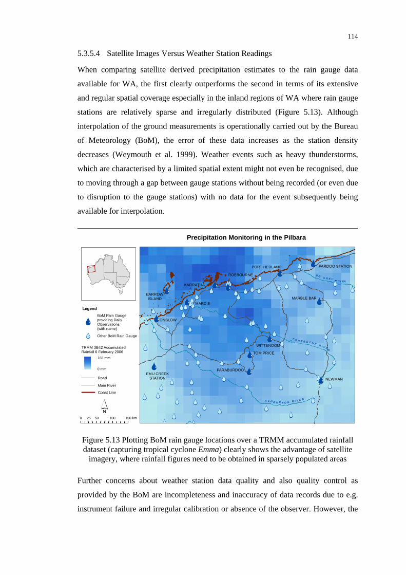
114

5.3.5.4 Satellite Images Versus Weather Station Readings

When comparing satellite derived precipitation estimates to the rain gauge data

available for WA, the first clearly outperforms the second in terms of its extensive

and regular spatial coverage especially in the inland regions of WA where rain gauge

stations are relatively sparse and irregularly distributed (Figure 5.13). Although

interpolation of the ground measurements is operationally carried out by the Bureau

of Meteorology (BoM), the error of these data increases as the station density

decreases (Weymouth et al. 1999). Weather events such as heavy thunderstorms,

which are characterised by a limited spatial extent might not even be recognised, due

to moving through a gap between gauge stations without being recorded (or even due

to disruption to the gauge stations) with no data for the event subsequently being

available for interpolation.

ÔÔ

ÔÔ

ÔÔÔÔÔÔ

ÔÔ

ÔÔ

ÔÔ

ÔÔ

ÔÔ

ÔÔ

ÔÔ

ÔÔÔÔ

ÔÔ

ÔÔ

ÔÔ

ÔÔ

ÔÔ

ÔÔ

ÔÔ

ÔÔ

ÔÔ

ÔÔÔÔ

ÔÔÔÔÔÔ

ÔÔ

ÔÔ

ÔÔ

ÔÔ

ÔÔÔÔÔÔ

ÔÔ

ÔÔ

ÔÔ

ÔÔ

ÔÔ

ÔÔ

ÔÔÔÔ

ÔÔÔÔ

ÔÔ

ÔÔ

ÔÔ

ÔÔ

ÔÔ

ÔÔ

ÔÔÔÔ

ÔÔ

ÔÔ ÔÔ

ÔÔ

ÔÔ

ÔÔ

ÔÔ

ÔÔ

ÔÔ

ÔÔ

ÔÔ

ÔÔ

ÔÔ

ÔÔ

ÔÔ ÔÔ

ÔÔ

ÔÔ

ÔÔ

ÔÔ

ÔÔ

ÔÔÔÔ

ÔÔ

ÔÔ

ÔÔ

ÔÔ ÔÔÔÔÔÔÔÔ

ÔÔ

ÔÔÔÔ

ÔÔ

ÔÔ

ÔÔ

ÔÔ

ÔÔ

ÔÔ

ÔÕ

ÔÕ

ÔÕ

ÔÕÔÕ

ÔÕ

ÔÕ

ÔÕ

ÔÕÔÕ

ÔÕ

ÔÕ

ÔÕ

NEWMAN

PARABURDOO

TOM PRICE

MARBLE BAR

ONSLOW

MARDIE

KARRATHA

PORT HEDLAND

ROEBOURNE

PARDOO STATION

WITTENOOM

EMU CREEKSTATION

BARROWISLAND

D E G R E Y R I V ER

F O R T E S C U E R I V ER

A S H B U R T O N R I V E R

´

Legend

Main River

Road

Precipitation Monitoring in the Pilbara

0 50 100 15025 km

ÔÕÔÔ

BoM Rain Gauge providing DailyObservations(with name)

Other BoM Rain Gauge

Coast Line

TRMM 3B42 AccumulatedRainfall 6 February 2006

165 mm

0 mm

Figure 5.13 Plotting BoM rain gauge locations over a TRMM accumulated rainfall dataset (capturing tropical cyclone Emma) clearly shows the advantage of satellite

imagery, where rainfall figures need to be obtained in sparsely populated areas

Further concerns about weather station data quality and also quality control as

provided by the BoM are incompleteness and inaccuracy of data records due to e.g.

instrument failure and irregular calibration or absence of the observer. However, the

115

alternative satellite precipitation products provide not direct measurements but

estimates depending on specific cloud properties (Yan et al. 2005). They are

operationally or semi-operationally processed by a variety of algorithms that have

been developed during the last few decades. Precipitation data products have

different spatial, temporal and quality features and their performance also strongly

depends on the observed precipitation regime. In general, satellite precipitation

estimates show a greater accuracy for tropical, convective, and summertime rainfall

than for mid-latitude, stratiform, and wintertime rainfall (Ebert 2004).

Before using satellite rainfall estimates it is necessary to understand their accuracy

and limitations. Validation and intercomparison of different satellite precipitation

products is done for several regions including Australia (Ebert, Janowiak, and Kidd

2007), Europe (Kidd 2004) and the US (Janowiak 2004) as a project of the

International Precipitation Working Group (IPWG). The results for Australia are

made available online (Ebert 2007). One of the key findings from ongoing research

of the IWG is that satellite estimates usually detect heavy rainfall events too

frequently while light rainfall is not estimated often enough (Ebert, Janowiak, and

Kidd 2007). Consequently, satellite based precipitation data are biased low during

winter by underestimating rainfall. Ebert, Janowiak, and Kidd (2007) further showed

that the CMORPH algorithm is less accurate, compared to the TRMM 3B42 data,

especially in the focus areas of this project. CMORPH data strongly overestimate

heavy rainfall as produced by tropical systems, the dominant weather systems during

the wet season in Northern Australia, which are hypothesised to be important drivers

of arbovirus dynamics. In contrast, TRMM shows slight underestimates of these

events.

5.3.5.5 Selection of Precipitation Product

Based on a comprehensive analysis and interpretation of the validation data provided

by the BoM Research Centre (see Schuster et al. 2009) TRMM 3B42 was finally

chosen as the basic rainfall data set for this study. Although these data do not deliver

high precision rainfall rates, which are not required by this project, they provide the

most accurate and coherent information for the entire study area. The verification

results pointed out that 3B42 data performed well for stronger rainfall events which

116

are associated with the dominant weather systems of the northern parts of WA during

the wet season. CMORPH was not chosen as a main data source, because it showed

pronounced overestimates e.g. in the Kimberley region and was not available before

December 2002.

5. 4 Land Information and Infrastructure Datasets

Data on more static parameters such as topography, hydrology, geology, soils, land

cover and infrastructure are produced by national (Geoscience Australia) and state

mapping agencies (Landgate) as well as the Department of Agriculture and Food

Western Australia (DAFWA) in scales ranging from 1:100,000 to 1:1 million. The

main purpose of these datasets within the project is not to use them as additional

predictor variables, but to inform the structuring of the bioclimatic data layers, i.e. to

decide which area to weight higher in the modelling process, or which to exempt

from the predictions. The key data sets considered for the project are described

below.

5.4.1 Topographic Base Data

Regional topographic base maps have been produced nation-wide at a scale of

1:250,000 as part of the GEODATA TOPO 250K Series 3 (Geoscience Australia

2006). This dataset, published digitally in the latest version in 2006 provides much of

the topographical base layers utilised in this project for reference mapping. Of major

interest are hydrological features (including watercourses, lakes, canals, flats, bores,

reservoirs etc.), transport infrastructure (roads railways), as well as reserves (natural

and aboriginal) and military areas.

5.4.2 Pastoral Property and Infrastructure Datasets

Data on pastoral properties and related infrastructures (i.e. water points, dams,

fences, yards and homesteads) are provided by the responsible state government

Departments. Property boundaries are a crucial dataset for this project as they define

the primary spatial reference unit for BTV presence/absence data. These data are

available as cadastre data from DAFWA for the Pilbara region and from the

Department of Planning and Infrastructure in the Northern Territory. Data on

infrastructure are captured either from topographic maps (e.g. the Geoscience

117

Australia 1:250,000 dataset mentioned before) or through field inspections as part of

the rangeland condition monitoring activities.

5.4.3 Digital Elevation Data

Terrain parameters such as slope and aspect derived from a DEM can be used to

model surface water runoff, soil moisture, radiant fluxes, or extract landforms. Such

information is of use in this project to exclude certain areas from the study, e.g. due

to their steep slope and inaccessibility for hosts and vectors. Several datasets suitable

for mapping at regional scale are available, of which data from the Shuttle Radar

Topography Mission (SRTM) with a spatial resolution of 90 m (JPL2008b) provide

the best spatial resolution for regional applications while providing higher accuracy

compared to the higher resolution ASTER DEM (Hirt, Filmer, and Featherstone

2010). The latest version of a national DEM for Australia with a spatial resolution of

9 arc seconds (250 m) has been generated using spot heights and terrain break lines

from the GEODATA TOPO 250K (Geoscience Australia 2006), trigonometric points

from the National Geodetic Database and as well as additional elevation, streamline

and sink point data digitised from 1:100,000 source material (Hutchinson et al.

2008). This dataset, provided by Geoscience Australia, is particularly useful for

overview mapping on a continental scale (as in Figure 5.1). Digital elevation data

with a very high spatial resolution only cover parts of coastal and metropolitan areas

and are therefore of limited use for this project.

5.4.4 Rangeland Land Systems

As a result of several survey campaigns the pastoral areas of WA have been mapped

and classified into land system units, comprising dominant geomorphology, soils,

vegetation and climate (Van Vreeswyk et al. 2004). Most mapping is at scale of

1:250,000, except for the Kimberley Region (1:1 million) and Wiluna-Meekatharra

(1:506,880). Similar maps have been produced for the Northern Territory, though

only 30% of the area is mapped at the scale of 1:250,000, while the remainder of the

Territory, particularly the South is only mapped at a 1:1 million scale. On a national

level, land systems maps have been homogenised in the Australian Soil Resource

Information System (ASRIS) (McKenzie et al. 2005). Although mapping is rather

coarse at the land system level, and extraction of information on landforms, soils and

vegetation groups within the units is impracticable, the data provide information on

118

the carrying capacity of the land and hence facilitate estimating the distribution of

livestock as arbovirus hosts.

5. 5 Software

5.5.1 GIS, Remote Sensing and Data Processing Software

The remote sensing package ERDAS Imagine (ERDAS Inc. 2008) was used initially

for data assessment. Most of the resource intensive data management and data

processing was implemented in ArcGIS 9.3 (ESRI Inc. 2008) using Python scripts

specifically developed for this project to automate the generation of the bioclimatic

variables. Other software used in this project includes the MODIS Reprojection Tool

MRT (Dwyer and Schmidt 2006) as well as the TIMESAT package (Eklundh and

Jönsson 2010), which will be discussed in the later sections where appropriate.

5.5.2 Statistical Software

The R programming language and environment for statistical computing and

graphics (R Development Core Team 2010) was used throughout the project for

exploratory analysis and development of the predictive models, described in

Chapter 7, and the preparation of graphs.

5. 6 Summary In this chapter, the study areas in the Pilbara-Gascoyne region and the Northern

Territory have been introduced in terms of virus activity, hydrology and topography,

climate as well as soils and vegetation. These regions span vast landscapes

influenced by several climatic zones, and are characterised by varying levels of virus

activity, all of which makes them an ideal test bed for the application of remote

sensing to study the distribution of BTV.

An analysis of the virus dataset concluded with the definition of the minimum

required spatial and temporal resolution for model building and prediction. The

heterogeneity of the dataset requires the aggregation of presence/absence data for the

period from November to October on a pastoral property level in order to build

spatial relationships with the environment. To preserve the seasonal characteristics of

the region, but limit the dependence on daily images that may be obscured by cloud

cover, a weekly to fortnightly temporal resolution was selected. The spatial

119

resolution for the environmental data has been chosen to detect host and vector

habitats on the ground and capture regional rainfall patterns. A set of bioclimatic

factors for predictor variable definition was chosen and included vegetation indices

(NDVI and EVI), LST, rainfall, as well as the derived factors vegetation phenology

and GDD. After the selection of MODIS and TRMM for the delivery of medium

spatial resolution and high temporal resolution satellite data, various data products

where assessed for their fitness. The final selection of satellite remote sensing data is

listed below (Table 5.2) together with topographic and land information datasets

employed for this study (Table 5.3).

Table 5.2 Remote sensing data products selected for this study

Remote sensing product

Spatial resolution

Spatial coverage

Temporal resolution

Temporal coverage

Source

MODIS Nadir BRDF-Adjusted Reflectance (MCD43B4)

500 m global 16-day 2000 – current

LP DAAC 1

MODIS Land Surface Temperature and Emissivity (MOD11A2)

1 km global 8-day 2000 – current

LP DAAC 1

TRMM and Other Satellite Precipitation Product (3B42)

25 km global 3–hourly – monthly

1998 – current

GES DISC DAAC 2

1) Land Processes Distributed Active Archive Center (LP DAAC); 2) Goddard Earth Sciences Data and Information Service Center Distributed Active Archive Center (GES DISC DAAC)

Table 5.3 Land Information and Infrastructure datasets selected for this study

Data set Scale, spatial resolution (for DEM data)

Spatial coverage

Creation time

Source

GEODATA TOPO 250K topographic base data

1: 250,000 Australia 2006 Geoscience Australia

Pastoral property and infrastructure data

1: 250,000 WA, NT DAFWA 1 NT DLP 2

Rangeland land systems

1:250,000 – 1:1,000,000 3 WA, NT 2006 (WA)

DAFWA 1 NRETA4

SRTM 5 DEM Version 4.1

90 m Global 2008 CGIAR- CSI 6

GEODATA 9 Second DEM Version 3

250 m Australia 2008 Geoscience Australia

1) Department of Agriculture and Food WA (DAFWA); 2) NT Department of Lands and Planning (DLP); 3) depending on the region; 4) NT Department of Natural Resources, Environment, The Arts and Sport (NRETA); 5) Shuttle Radar Topography Mission (SRTM); 6) Consultative Group for International Agriculture Research – Consortium for Spatial Information (CGIAR-CSI)

120

The chapter concluded with an overview of software products used in this research.

In the following chapter, the process of generating bioclimatic variables from the

remotely sensed data products is explained.

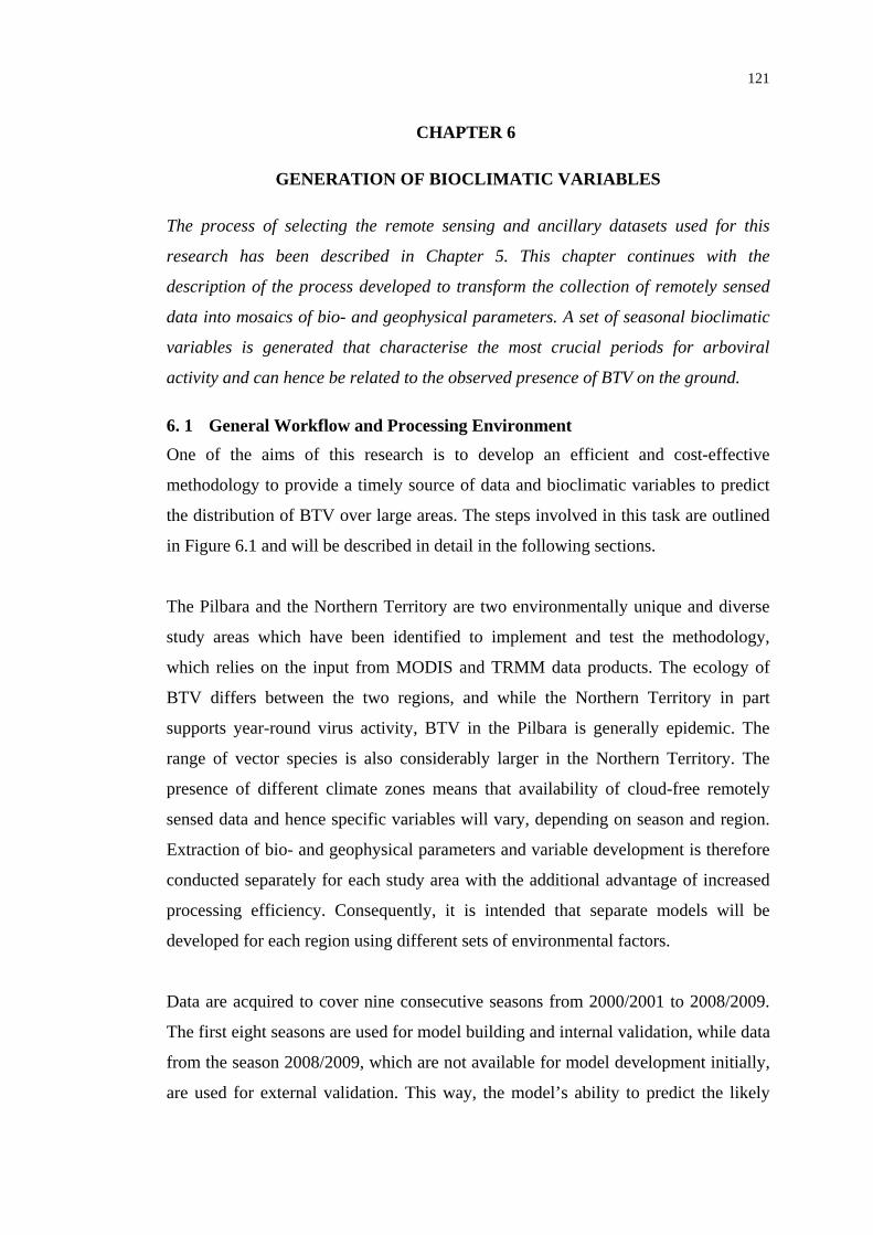
121

CHAPTER 6

GENERATION OF BIOCLIMATIC VARIABLES

The process of selecting the remote sensing and ancillary datasets used for this

research has been described in Chapter 5. This chapter continues with the

description of the process developed to transform the collection of remotely sensed

data into mosaics of bio- and geophysical parameters. A set of seasonal bioclimatic

variables is generated that characterise the most crucial periods for arboviral

activity and can hence be related to the observed presence of BTV on the ground.

6. 1 General Workflow and Processing Environment One of the aims of this research is to develop an efficient and cost-effective

methodology to provide a timely source of data and bioclimatic variables to predict

the distribution of BTV over large areas. The steps involved in this task are outlined

in Figure 6.1 and will be described in detail in the following sections.

The Pilbara and the Northern Territory are two environmentally unique and diverse

study areas which have been identified to implement and test the methodology,

which relies on the input from MODIS and TRMM data products. The ecology of

BTV differs between the two regions, and while the Northern Territory in part

supports year-round virus activity, BTV in the Pilbara is generally epidemic. The

range of vector species is also considerably larger in the Northern Territory. The

presence of different climate zones means that availability of cloud-free remotely

sensed data and hence specific variables will vary, depending on season and region.

Extraction of bio- and geophysical parameters and variable development is therefore

conducted separately for each study area with the additional advantage of increased

processing efficiency. Consequently, it is intended that separate models will be

developed for each region using different sets of environmental factors.

Data are acquired to cover nine consecutive seasons from 2000/2001 to 2008/2009.

The first eight seasons are used for model building and internal validation, while data

from the season 2008/2009, which are not available for model development initially,

are used for external validation. This way, the model’s ability to predict the likely

122

hood of virus transmission based on historic occurrences and recent climatic and

environmental conditions can be assessed.

Mosaic and reproject

Mask poor quality pixels

Mosaic and reproject

Fill small data gaps

Mask poor quality pixels

Compute vegetation indices

LST night Time

Series

Clean NBAR

Mosaics

Clean LST

Mosaics

Daily Precipitation Time Series

Determine maximum

value(per aggregation

period)

Smooth time series and extract phenology

parameters(per annual growing season)

Pheno-logical

Variables

Maximum Seasonal NDVI/EVI

Compute Growing

Degree Days (per aggregation

period)

Determine minimum, maximum

& mean values(per aggregation period)

LST night Time

Series

Growing Degree Days

Min, max & mean LST day & night

temperatures

Compute rainfall

accumulates (per aggregation

period)

Accumulated Rainfall

EVITime

Series

NDVI Time

Series

LST DayNDVI

MODIS Nadir BRDF Adjusted Reflectance (MCD43A4) - NBAR

MODIS Nadir BRDF Adjusted Reflectance (MCD43A4) - LST

469 NBAR

Mosaics469 LST Mosaics

TRMM and Other Satellite Precipitation Product (3B42)

Daily Rainfall

Exclude pixels of bare ground, sealed areas and

perennial water bodies

Pastoral Property

Boundaries

Property ID 2000/2001 2001/2002 2002/2003 …. 2008/2009W008 … … … … …W12 … … … … …T014 … … … … ……. … … … … …T022 … … … … …

Year

Property ID 2000/2001 2001/2002 2002/2003 …. 2008/2009W008 … … … … …W12 … … … … …T014 … … … … ……. … … … … …T022 … … … … …

Year

Summary statistics for each variable

Calculate mean variable values for each pastoral

property and year

Figure 6.1 Simplified workflow for the generation of bioclimatic variables from remote sensing data products, and aggregation of annual statistics on pastoral

property level

In contrast to other studies that compiled seasonality variables from remotely sensed

data over several years using Temporal Fourier Analysis (TFA) (Hay et al. 2006;

123

Scharlemann et al. 2008), this study will generate annual seasonal variables. This

approach facilitates the preservation of seasonal characteristics for individual years,

the generation of annual prediction maps, and analysis of the drivers for the inter-

annual variations in virus distribution. While TFA has been widely used in vector-

borne disease studies (e.g. Rogers 2000; Tatem et al. 2003), the resulting data are

best suited to identify factors related to general habitat suitability, as described by a

typical seasonal signal of environmental variables, such as land surface temperature

or NDVI over an annual, bi-annual or tri-annual cycle. This study however aims to

investigate the inter-annual variability of environmental variables and the associated

fluctuations in arbovirus activity.

The study uses a geographic coordinate system of latitude and longitude, due to the

larger area covered and because this is the most widespread reference system for

global climate and environmental datasets. For analyses involving area and distance

measurements, the datasets are reprojected to a Lambert Conformal Conic projection,

which shows the least distortions for Australia on a continental scale

(Intergovernmental Committee on Surveying & Mapping 2009).

The processing environment, comprising the MODIS Reprojection Tool (described

below), ArcGIS with the Spatial Analyst Extension, and the scripting language

Python facilitated the development of an efficient automated processing chain. Data

processing was performed on a standard PC (Intel Core 2, 3 GHz, 4 GB RAM) with

the data held on two 1 TB external hard drives. The scripts are reusable for future

processing as new data become available.

6. 2 Extraction of Bio- and Geophysical Parameters from Remote Sensing Data

6.2.1 MODIS Data Preparation

The MODIS data products Nadir BRDF-Adjusted Reflectance (MCD43A4),

including the related quality information data (MCD43A2), as well as Land Surface

Temperature and Emissivity (MOD11A2) were acquired from the Land Processes

Distributed Active Archive Center (LP DAAC) through the NASA Warehouse

Inventory Search Tool (WIST) for the period between February 2000 and May 2010.

The data are provided on a Sinusoidal projection as 460 tiles for the entire Earth

124

(Figure 6.2). Each tile consists of 2400 x 2400 pixels, for the 500 m spatial resolution

MCD43A2 data set and 1200 x 1200 pixels for the 1000 m spatial resolution

MOD11A2 dataset. To cover the area of WA and the NT requires 11 of these tiles

(H27V11, H27V12, H28V10, H28V11, H28V12, H29V10, H29V11, H29V12,

H30V10, H30V11, H31V10), which equates to more than three quarters of the

Australian landmass (see Figure 6.3). In total, satellite images were acquired for 469

8-day periods (also referred to as epochs), which amounts to 170 GB of raw data.

The MRT software (Dwyer and Schmidt 2006) was used to reproject from the

original Sinusoidal projection to a geographic coordinate system of latitude and

longitude and create a seamless mosaic for each epoch.

0 1 2 3 4 5 6 7 8 9 10 11 12 13 14 15 16 17 18 19 20 21 22 23 24 25 26 27 28 29 30 31 32 33 34 350123456789

1011121314151617

H

V

MODIS Sinusoidal Tile Grid

11 Tiles needed to cover WA and the NT

Figure 6.2 MODIS Sinusoidal GRID and tiles needed to cover WA and the NT. Image Source: Stöckli et al. (2006)

Amongst other formats, MRT offers export to GeoTiff, which is a standard format

that can be read by most GIS packages and was therefore selected for this study. The

geographic subsetting ability of MRT was utilised to extract the area between

longitudes 112.0459° and 138.0901°E and latitudes 10.5012° and 35.5022°S as

shown in Figure 6.3.

The MRT software supports nearest neighbour, bilinear, and cubic convolution

resampling. For this work, nearest neighbour resampling was chosen as it is able to

maintain the original values in each of the layers during resampling, particularly the

bit-pattern encoded structure of the quality maps, as it does not interpolate between

125

existing bit values. To provide a consistent spatial resolution across the MODIS

datasets, the MOD11A2 data with a nominal resolution of 1000 m were resampled to

500 m resolution, which is equivalent to 0.0046° at the equator in the geographic

reference system. Subsequently, several datasets were clipped with a coastline

dataset to cover only the mainland of Australia.

Footprint of mosaicprocessed with MRT

Extent of areas for whichvariables are generated

No MODIS data acquired

NDVI

1.0

- 1.0

´

Coverage of Processed MODIS Satellite Data Products

0 500 1,000 1,500250 Kilometers

Figure 6.3 Extent of areas covered during the successive processing steps, using the NDVI as an example

6.2.2 Extracting MODIS Vegetation Indices

The MODIS NBAR product MCD43A4 comprises seven nadir reflectance data

layers (termed scientific datasets - SDS), that have been computed for MODIS bands

1-7 at the mean solar zenith angle of a 16-day period). Out of these, only bands 1

(red), 2 (NIR) and 3 (blue) are required for the extraction of NDVI and EVI.

Natively, values are encoded as integers, using a scaling factor of 10,000. The

previously generated GeoTiff mosaics were imported to ArcGIS, masked for pixels

that contain no data due to the presence of water, cloud cover or other effects, and

transformed into NDVI and EVI images using the equations given in Section 4.2.4.2.

To account for the scaling factor, the results were multiplied by 0.0001.

The presence of surface water or bare land such as mine sites, industrial areas or

densely populated areas would bias the regional statistics of land surface temperature

126

and vegetation dynamics. An NDVI threshold of 0.1 was determined empirically to

delineate these areas and create a dynamic low NDVI mask for each 8-day period.

6.2.3 Extracting MODIS Land Surface Temperature

The MODIS Land Surface Temperature product MOD11A2 comprises 12 SDSs

(Wan 2009), of which the layers “Daily daytime 1km grid Land Surface Temperature

(LST_Day_1km)”, “Quality control for daytime LST and emissivity (QC_Day)”,

“Daily nighttime 1km grid Land Surface Temperature (LST_Night_1km)”, and

“Quality control for nighttime LST and emissivity (QC_Night)” were used for this

study.

LST is only produced for pixels that are on land or inland water, and are in clear-sky

conditions at a confidence of >=95% over land <= 2000 m above sea level, and at a

confidence of >= 66% over lakes (Wan 2009). Information on the quality of the

retrieved LST and Emissivity values for each pixel is found in the Quality Control

(QC_day and QC_night) layers. Pixels with limited quality, denoted by the following

flags were masked out: “not produced due to cloud effects”, “not produced due to

reasons other than cloud”, “average emissivity error >= 0.02”, “average LST error >

2K”. The remaining pixels were corrected for the scaling factor by multiplying with

0.02 and stored as GeoTiff images for LST night and LST day.

In a subsequent step, data gaps resulting from the removal of poor quality pixels

were filled in a two stage process. Using the low NDVI mask, small spatial gaps that

are not water or bare ground, with a width of less than five pixels were replaced by

the mean LST value within a radius of six pixels. Interpolation of land surface

temperature across wider gaps is not advisable due to the large spatial variation in

land cover. Therefore, in a second step, temporal gaps not wider than two

consecutive epochs were linearly interpolated on a pixel basis. The approach to fill

only small gaps enures that no data are artificially generated where there aren’t

enough valid data initially.

6.2.4 Extraction of Precipitation Rates from TRMM

The post real-time TRMM 3B42 product provides instantaneous precipitation rates at

a 0.25° (about 25 km) grid resolution time-stamped at 3-hourly intervals. The data

127

used within this project are daily (9.00 am to 9.00 am) rainfall accumulates for the

Australian continent that were processed within an intercomparison study of

precipitation time series of TRMM and interpolated surfaces from BoM rain gauge

observations (Renzullo 2008). These data covering the period between 1999 and

2009 were originally obtained from the NASA Goddard Space Flight Center

Distributed Data Archive Center (GSFC DAAC). The area covered by these data

extends between longitudes 109.625° and 154.125°E, and latitudes 9.625° and

44.125°S. To be compatible with the already processed datasets, the TRMM data

were converted from a floating point file format to the GeoTiff format and clipped to

the extent of the Australian mainland.

6. 3 Development of Bioclimatic Variables

6.3.1 Selection of Seasonal Variables and Temporal Aggregation Intervals

As defined in the previous chapter, virus data are summarised over 12 months, which

include the period of highest vector activity before and after the wet season. The

environmental and climatic conditions over that period, which lasts approximately

from December to May, will determine virus activity and need to be aggregated into

seasonal variables for later use in model building. This step is necessary to reduce the

data layers collected for each year to a manageable number before analysis, whilst

retaining as much information as possible (Robinson, Rogers, and Williams 1997b).

In this section the types of variables as well as the aggregation periods are defined,

considering ecological principles as well as the availability of remotely sensed data.

A series of environmental variables that are relevant to epidemiological studies can

be derived from MODIS LST, NDVI, EVI, and TRMM precipitation time series, by

time series aggregation. In particular, daily/monthly/annual mean value maps of

minimum/mean/maximum temperature or accumulated rainfall have been previously

identified as relevant ecological indicators (Hay et al. 1996). Other ecologically

important variables for insect or plant development are annual or monthly growing

degree days, or vegetation phenological parameters such as length of growing season

or amplitude of seasonal green-up, which are determined annually.

128

Seasonal variables may either describe climatic and environmental conditions in

absolute terms (e.g. maximum seasonal NDVI or minimum winter temperature), or

in relation to long term trends to identify unusually dry, wet, cold or hot seasons. For

example, Chalke (2006) used unusual change in early or maximum greenness in

comparison with a five-year average. Previous studies developing BTV models for

Africa and Europe have also used seasonal change, or rates of change as predictor

variables (Purse, Tatem, et al. 2004; Tatem et al. 2003). However, for this study

using MODIS data alone, the time series is considered too short to deliver reasonable

multi-annual statistics. Moreover, the continuing acquisition of data in future will

result in the instability of the long-term average, which needs constant adjustment.

Variables are therefore defined independently for each year, using absolute values

subsumed over specific aggregation periods. The simplicity of this method also

facilitates biological interpretation of the results (Robinson, Rogers, and Williams

1997b).

The aggregation periods identified as most suitable for this study follow the observed

and documented peak of virus activity, as well as the meteorological seasons (Table

6.1). Also the months of the previous winter with cold nights in some areas, are

important determinants for vector survival and the southern distribution limit of the

virus (Bishop, Spohr, and Barchia 2004b).

Table 6.1 Aggregation periods used for the development of bioclimatic variables. Note that the start and end dates for MODIS composites need to be shifted one day

forward between March and December in leap years (2000, 2004, 2008)

Aggregation period Calendar Months MODIS compositing period Start date – End date

Annual November - October 1.11. – 31.10.

Bluetongue Season November - May 1.11. – 1.6.

Summer December - February 3.12. – 25.2.

Autumn March – May 26.2. – 1.6.

Previous winter June - August 2.6. - 28.8.

The compositing periods of MODIS LST and NBAR products, which slightly differ

from calendar months have been additionally defined. Because the NBAR product is

generated every 8-days like the LST product, but is composited over 16 days, one

epoch less than for LST will be taken into account to cover the same period. The

availability of data from visible and infrared bands is limited particularly during the

129

wet season in the northernmost parts of Australia. The processed time series have

therefore been analysed for the proportion of missing data after quality filtering and

gap filling (Figure 6.4), in order to determine which factors can be derived for each

aggregation period and region. Extraction of precipitation rates and accumulates

from TRMM are not affected, because the microwave sensors that are predominantly

used in the generation of the 3B42 precipitation product are not affected by cloud

cover.

As Figure 6.4 shows, particularly during the summer months, up to about 40% of

data are missing in the Northern Territory. The highest proportion of missing data is

found in the night LST data. This effect has also been found by Neteler (2010), who

analysed LST time series in north Italy. It can be explained by the different algorithm

used to detect cloud contamination during the night overpass, which produces a less

accurate cloud mask (Ackerman et al. 1998). Pixels which have been assigned a

clear-sky flag with low confidence are automatically removed during the production

of the LST product.

MODIS data coverage in the Northern Territory (November 2000 - October 2009)

50556065707580859095

100

1 5 9 13 17 21 25 29 33 37 41 458-day period

Ave

rage

cov

erag

e [%

]

Nov

Dec

Jan

Feb

Mar

Apr

May

Jun

Jul

Aug

Sep

Oct

Month

NDVI, quality filtered

LST day, gap filled

LST night, gap filled

LST day, quality filtered


Figure 6.4 Average percentage of valid pixels in quality filtered and gap filled (for LST) time series between November 2000 and October 2009

As illustrated in Figure 6.5, the availability of data is generally very high in the

semiarid Pilbara region, except for a small outlier at epoch 19, which is caused by

cyclone activity in February 2002 over that area.

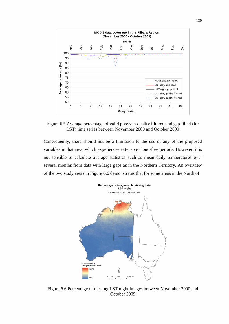
130

MODIS data coverage in the Pilbara Region (November 2000 - October 2009)

50556065707580859095

100

1 5 9 13 17 21 25 29 33 37 41 458-day period

Ave

rage

cov

erag

e [%

]

Nov

Dec

Jan

Feb

Mar

Apr

May

Jun

Jul

Aug

Sep

Oct

Month

NDVI, quality filteredLST day, gap filled

LST night, gap filledLST day, quality filtered


Figure 6.5 Average percentage of valid pixels in quality filtered and gap filled (for LST) time series between November 2000 and October 2009

Consequently, there should not be a limitation to the use of any of the proposed

variables in that area, which experiences extensive cloud-free periods. However, it is

not sensible to calculate average statistics such as mean daily temperatures over

several months from data with large gaps as in the Northern Territory. An overview

of the two study areas in Figure 6.6 demonstrates that for some areas in the North of

Percentage of images with missing dataLST night

November 2000 - October 2009

Percentage ofimages with no data

30 %

0 %

´0 500 1,000250 km

Figure 6.6 Percentage of missing LST night images between November 2000 and October 2009

131

Australia, valid unprocessed data on night LST are missing for as many as 30% of

the 8-day periods. Therefore, variables based on accumulation, such as Growing

Degree Days, cannot be determined for these areas. As a consequence, instead of

using mean variables for night temperatures, only maximum and minimum values

from the 8-daily MODIS datasets are determined for the NT. Also average daily

temperatures that involve night temperature data been excluded as well as any

derived variables like Growing Degree Days.

Table 6.2 Overview of bioclimatic variables (x = variable produced)

Variable Short Name Pilbara NT

Vegetation / Phenology

Maximum NDVI, season maxndviss X X

Maximum EVI, season maxeviss X X

Small Integral under seasonal NDVI curve, annual smint X X

Temperature

Mean day temperature of warmest 8-day period, season maxlstdss x X

Mean day temperature of warmest 8-day period, summer maxlstdsu x X

Mean day temperature of warmest 8-day period, autumn maxlstdau x X

Mean day temperature of warmest 8-day period, previous winter maxlstdpw x X

Minimum night temperature of coldest 8-day period, season minlstnss x

Minimum night temperature of coldest 8-day period, summer minlstnsu x

Minimum night temperature of coldest 8-day period, autumn minlstnau x

Minimum night temperature of coldest 8-day period, previous winter minlstnpw x X

Mean day temperature, season meanlstdss x X

Mean day temperature, summer meanlstdsu x X

Mean day temperature, autumn meanlstdau x X

Mean day temperature, previous winter meanlstdpw x X

Mean night temperature, season meanlstnss x

Mean night temperature, summer meanlstnsu x

Mean night temperature, autumn meanlstnau x

Mean night temperature, previous winter meanlstnpw x X

Mean daily temperature (day and night), season meanlstss x

Mean daily temperature (day and night), summer meanlstsu x

Mean daily temperature (day and night), autumn meanlstau x

Mean daily temperature (day and night), previous winter meanlstpw x X

Growing Degree Days, annual gdda x

Growing Degree Days, season gddss x

Growing Degree Days, summer gddsu x

Growing Degree Days, autumn gddau x

Precipitation

Accumulated rain, summer rsu x X

Accumulated rain, autumn rau x X

Accumulated rain, season rss x X

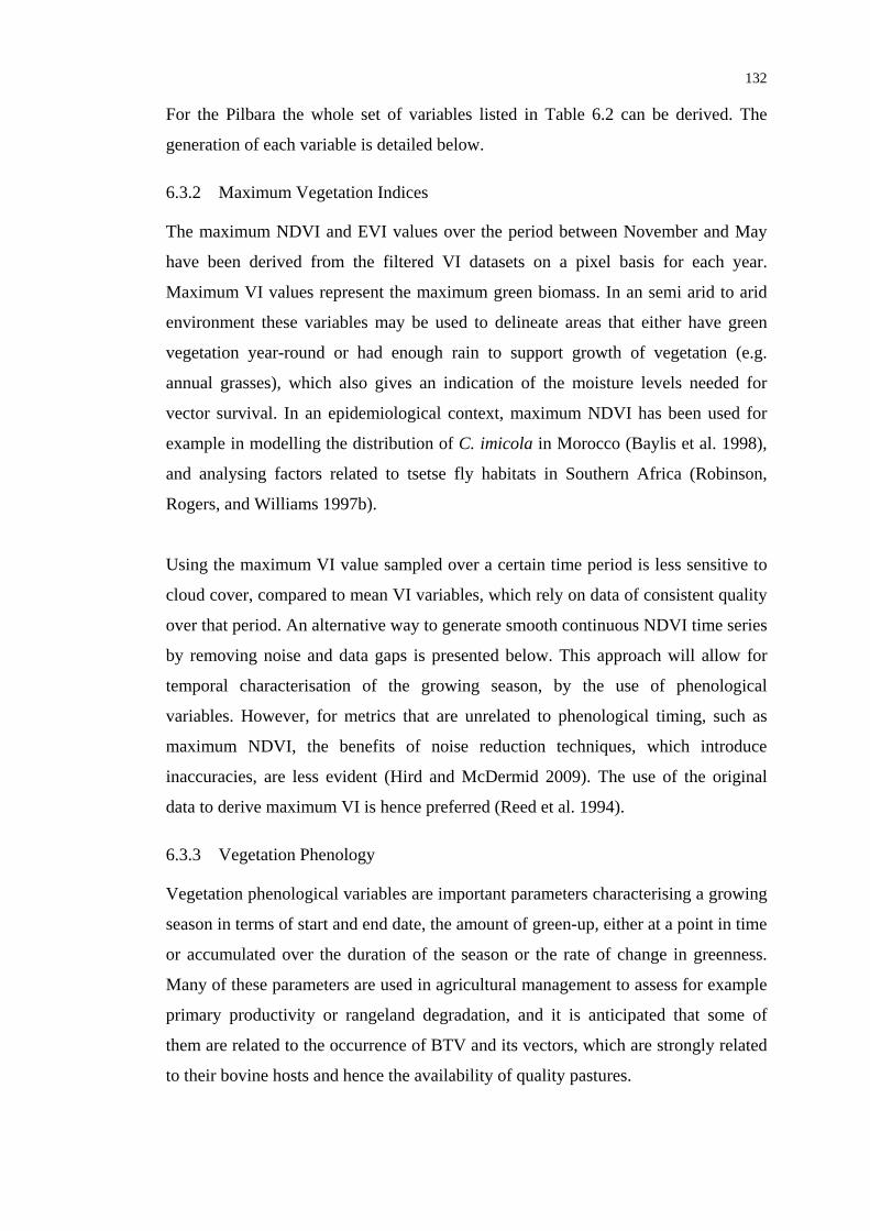
132

For the Pilbara the whole set of variables listed in Table 6.2 can be derived. The

generation of each variable is detailed below.

6.3.2 Maximum Vegetation Indices

The maximum NDVI and EVI values over the period between November and May

have been derived from the filtered VI datasets on a pixel basis for each year.

Maximum VI values represent the maximum green biomass. In an semi arid to arid

environment these variables may be used to delineate areas that either have green

vegetation year-round or had enough rain to support growth of vegetation (e.g.

annual grasses), which also gives an indication of the moisture levels needed for

vector survival. In an epidemiological context, maximum NDVI has been used for

example in modelling the distribution of C. imicola in Morocco (Baylis et al. 1998),

and analysing factors related to tsetse fly habitats in Southern Africa (Robinson,

Rogers, and Williams 1997b).

Using the maximum VI value sampled over a certain time period is less sensitive to

cloud cover, compared to mean VI variables, which rely on data of consistent quality

over that period. An alternative way to generate smooth continuous NDVI time series

by removing noise and data gaps is presented below. This approach will allow for

temporal characterisation of the growing season, by the use of phenological

variables. However, for metrics that are unrelated to phenological timing, such as

maximum NDVI, the benefits of noise reduction techniques, which introduce

inaccuracies, are less evident (Hird and McDermid 2009). The use of the original

data to derive maximum VI is hence preferred (Reed et al. 1994).

6.3.3 Vegetation Phenology

Vegetation phenological variables are important parameters characterising a growing

season in terms of start and end date, the amount of green-up, either at a point in time

or accumulated over the duration of the season or the rate of change in greenness.

Many of these parameters are used in agricultural management to assess for example

primary productivity or rangeland degradation, and it is anticipated that some of

them are related to the occurrence of BTV and its vectors, which are strongly related

to their bovine hosts and hence the availability of quality pastures.

133

A number of methods exist that derive phenology from time series of NDVI or EVI,

and most of them follow a two-step approach as explained in Section 4.2.4.3. In the

first step, the often noisy vegetation index time series are smoothed, either by

applying a filter or fitting a function. The fitted curve is then analysed for points that

exceed a certain VI threshold, or for changes in curvature that are relevant for the

growing cycle. The TIMESAT program developed by Jönsson and Eklundh (2002,

2004) fits a smooth continuous curve to time series of VI data using Savitzky–Golay

filtering (SG), asymmetric Gaussian (AG), or double logistic (DL) functions, and an

adaptive upper envelope to account for negatively biased noise such as cloud. The

software has mainly been used to extract phenological parameters from AVHRR and

MODIS NDVI time series, e.g. in the Italian rice growing areas (Boschetti et al.

2009), the African Sahel Zone (Heumann et al. 2007), as well as the Rangelands of

the Northern Territory (Graham, Trueman, and Yates 2008).

TIMESAT has been selected for this study, because it not only provides an efficient

processing environment for large datasets, but also offers three smoothing

techniques, from which the best fitting can be chosen for a particular area. The

software is freely available for non-commercial academic research.

The first decision to be made is on the vegetation index to be used. As stated by

Huete et al. (2002), EVI shows some advantages over NDVI in high biomass

regions, where NDVI tends to saturate. It is also less sensitive to atmospheric effects

and soil background. It has therefore been used to derive global phenology products

(e.g. by Ganguly et al. 2010; Zhang et al. 2003). However, its future availability as

part of the MODIS continuity program is uncertain, due to the proposed changes to

the specifications of the blue band (Huete et al. 2006), which is crucial for the

calculation of EVI. NDVI on the other hand is the most widely used index and hence

a large archive of historical data from different sensors is available for retrospective

studies. Schnur, Xie, and Wang (2010) found that NDVI is stronger correlated to soil

moisture in a semi-arid setting, and the initial assessment of MODIS derived NDVI

by Huete et al. (2002) also demonstrated that NDVI has a higher dynamic range over

semi-arid regions. For those reasons it was decided to use NDVI instead of EVI time

series to derive phenological parameters for the Australian landscape which is

dominated by low biomass vegetation species (Gill et al. 2009).

134

TIMESAT is available as a tool within MATLAB® (The MathWorks 2008), as well

as a set of Fortran 2003 command line programs. While the MATLAB® GUI offers

tools for data exploration, selection and calibration of the smoothing function, large

datasets are most efficiently processed with the Fortran executables. TIMESAT

requires the input rasters to be in binary format and the NDVI rasters have therefore

been exported from ArcGIS as binary float files (*.flt). To ensure that a full growing

season is always covered, TIMESAT generates one less season than the number of

years of supplied data (Eklundh and Jönsson 2010). For this study to analyse the nine

years between November 2000 and October 2009, six months of additional data have

been added on either side. The function fitting is executed in steps. Firstly, the

number of seasons and their approximate timing is determined. Secondly, TIMESAT

filters the data (SG filter) or fits a smooth function to the data (a least-squares fitted

asymmetric Gaussian or Double Logistic smooth function). After the fitting has been

achieved, the seasonality parameters are computed and written to output files. For the

full description of the mathematical and methodological foundation of the process

see Jönsson and Eklundh (2002, 2004).

The time series of 460 epochs (equivalent to 10 years of data) for selected locations

have been analysed to select the appropriate smoothing technique and calibration

parameters. It was found that the adapted SG filter consistently achieved the closest

fit particular in areas with irregular growing seasons (see Figure 6.7).

The SG filter allows data smoothing without forcing a given mathematical function

(e.g. Gaussian or Logistic curves) to fit the data time series, and thus reducing

artefact creation (Boschetti et al. 2009; Chen et al. 2004; White and Nemani 2006).

As seen in the example in Figure 6.7 for a pixel in the Carnarvon Basin, the method

identified season start and end dates correctly, while preserving the characteristics of

original data.

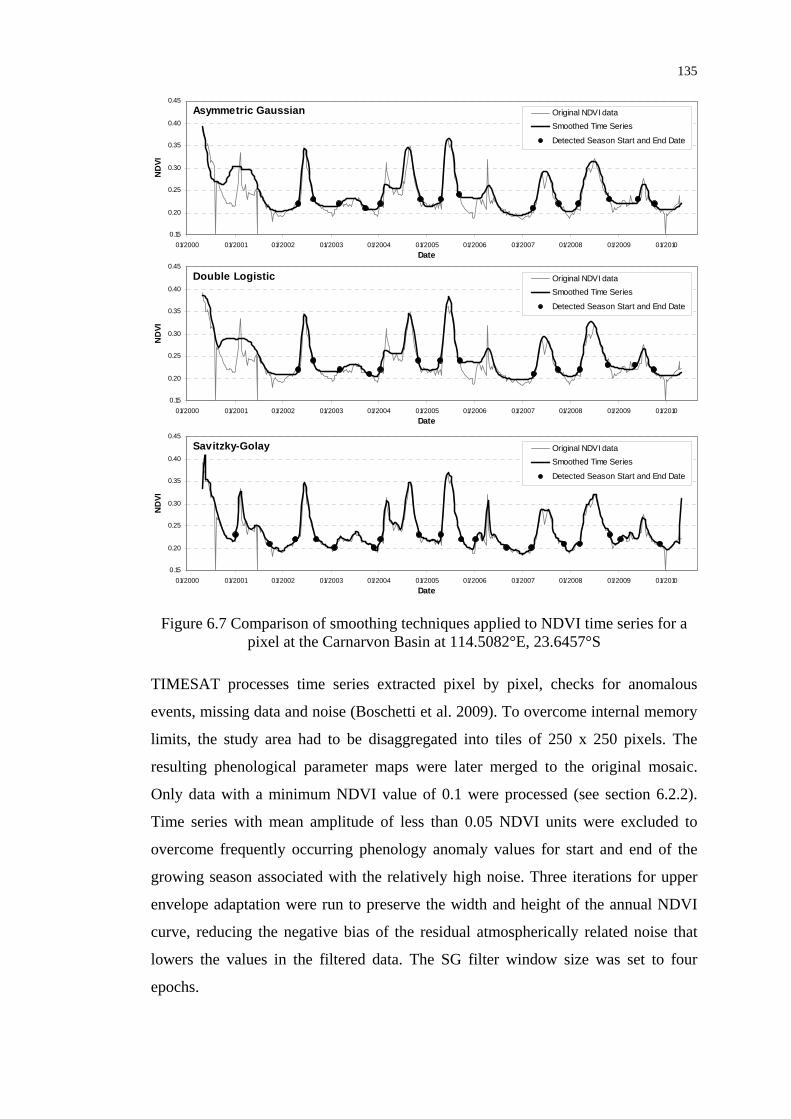
135

0.15

0.20

0.25

0.30

0.35

0.40

0.45

01/2000 01/2001 01/2002 01/2003 01/2004 01/2005 01/2006 01/2007 01/2008 01/2009 01/2010Date

ND

VI

Original NDVI dataSmoothed Time Series

Detected Season Start and End Date

Asymmetric Gaussian

0.15

0.20

0.25

0.30

0.35

0.40

0.45

01/2000 01/2001 01/2002 01/2003 01/2004 01/2005 01/2006 01/2007 01/2008 01/2009 01/2010Date

ND

VI



Double Logistic

0.15

0.20

0.25

0.30

0.35

0.40

0.45

01/2000 01/2001 01/2002 01/2003 01/2004 01/2005 01/2006 01/2007 01/2008 01/2009 01/2010Date

ND

VI



Savitzky-Golay

0.15

0.20

0.25

0.30

0.35

0.40

0.45

01/2000 01/2001 01/2002 01/2003 01/2004 01/2005 01/2006 01/2007 01/2008 01/2009 01/2010Date

ND

VI



Asymmetric Gaussian

0.15

0.20

0.25

0.30

0.35

0.40

0.45

01/2000 01/2001 01/2002 01/2003 01/2004 01/2005 01/2006 01/2007 01/2008 01/2009 01/2010Date

ND

VI



Double Logistic

0.15

0.20

0.25

0.30

0.35

0.40

0.45

01/2000 01/2001 01/2002 01/2003 01/2004 01/2005 01/2006 01/2007 01/2008 01/2009 01/2010Date

ND

VI



Savitzky-Golay

Figure 6.7 Comparison of smoothing techniques applied to NDVI time series for a pixel at the Carnarvon Basin at 114.5082°E, 23.6457°S

TIMESAT processes time series extracted pixel by pixel, checks for anomalous

events, missing data and noise (Boschetti et al. 2009). To overcome internal memory

limits, the study area had to be disaggregated into tiles of 250 x 250 pixels. The

resulting phenological parameter maps were later merged to the original mosaic.

Only data with a minimum NDVI value of 0.1 were processed (see section 6.2.2).

Time series with mean amplitude of less than 0.05 NDVI units were excluded to

overcome frequently occurring phenology anomaly values for start and end of the

growing season associated with the relatively high noise. Three iterations for upper

envelope adaptation were run to preserve the width and height of the annual NDVI

curve, reducing the negative bias of the residual atmospherically related noise that

lowers the values in the filtered data. The SG filter window size was set to four

epochs.

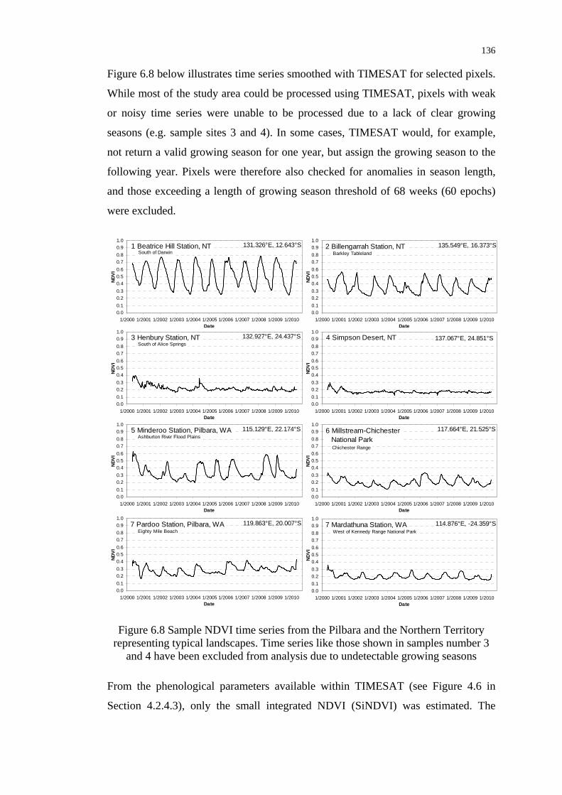
136

Figure 6.8 below illustrates time series smoothed with TIMESAT for selected pixels.

While most of the study area could be processed using TIMESAT, pixels with weak

or noisy time series were unable to be processed due to a lack of clear growing

seasons (e.g. sample sites 3 and 4). In some cases, TIMESAT would, for example,

not return a valid growing season for one year, but assign the growing season to the

following year. Pixels were therefore also checked for anomalies in season length,

and those exceeding a length of growing season threshold of 68 weeks (60 epochs)

were excluded.

0.00.10.20.30.40.50.60.70.80.91.0

1/2000 1/2001 1/2002 1/2003 1/2004 1/2005 1/2006 1/2007 1/2008 1/2009 1/2010Date

NDVI

1 Beatrice Hill Station, NT 131.326°E, 12.643°SSouth of Darwin

0.00.10.20.30.40.50.60.70.80.91.0

1/2000 1/2001 1/2002 1/2003 1/2004 1/2005 1/2006 1/2007 1/2008 1/2009 1/2010Date

NDVI

2 Billengarrah Station, NT 135.549°E, 16.373°SBarkley Tableland

0.00.10.20.30.40.50.60.70.80.91.0

1/2000 1/2001 1/2002 1/2003 1/2004 1/2005 1/2006 1/2007 1/2008 1/2009 1/2010Date

NDVI

3 Henbury Station, NT 132.927°E, 24.437°SSouth of Alice Springs

0.00.10.20.30.40.50.60.70.80.91.0

1/2000 1/2001 1/2002 1/2003 1/2004 1/2005 1/2006 1/2007 1/2008 1/2009 1/2010Date

NDVI

4 Simpson Desert, NT 137.067°E, 24.851°S

0.00.10.20.30.40.50.60.70.80.91.0

1/2000 1/2001 1/2002 1/2003 1/2004 1/2005 1/2006 1/2007 1/2008 1/2009 1/2010Date

NDVI

5 Minderoo Station, Pilbara, WA 115.129°E, 22.174°SAshburton River Flood Plains

0.00.10.20.30.40.50.60.70.80.91.0

1/2000 1/2001 1/2002 1/2003 1/2004 1/2005 1/2006 1/2007 1/2008 1/2009 1/2010Date

NDVI

6 Millstream-Chichester National Park

117.664°E, 21.525°S

Chichester Range

0.00.10.20.30.40.50.60.70.80.91.0

1/2000 1/2001 1/2002 1/2003 1/2004 1/2005 1/2006 1/2007 1/2008 1/2009 1/2010Date

NDVI

7 Pardoo Station, Pilbara, WA 119.863°E, 20.007°SEighty Mile Beach

0.00.10.20.30.40.50.60.70.80.91.0

1/2000 1/2001 1/2002 1/2003 1/2004 1/2005 1/2006 1/2007 1/2008 1/2009 1/2010Date

NDVI

7 Mardathuna Station, WA 114.876°E, -24.359°SWest of Kennedy Range National Park

Figure 6.8 Sample NDVI time series from the Pilbara and the Northern Territory representing typical landscapes. Time series like those shown in samples number 3

and 4 have been excluded from analysis due to undetectable growing seasons

From the phenological parameters available within TIMESAT (see Figure 4.6 in

Section 4.2.4.3), only the small integrated NDVI (SiNDVI) was estimated. The

137

SiNDVI metric was extracted from the smoothed NDVI time series for each of the

nine years between November 2000 and October 2009. It is defined as the area under

the vegetation curve during the growing season and above the mean of the base value

(i.e. the mean of the NDVI values measured before and after the season). The start

and end of the growing season were estimated as 15% of the annual amplitude from

the left (pre season) and right (post season) minimum levels, respectively. The small

integrated NDVI is strongly correlated with primary productivity and total

phytomass (Holm, Cridland, and Roderick 2003), particularly in semi-arid regions. It

thus provides an indication of the productivity of the area for pastoral purposes, i.e.

how many cattle can be sustained and therefore provide a reservoir for arbovirus

vectors. The SiNDVI tiles for each study area were extracted as binary raster files in

TIMESAT and converted to GeoTiff and remerged in ArcGIS.

6.3.4 Minimum, Maximum and Mean Land Surface Temperature

Most Culicoides vector species have been found to be active within a particular

temperature range (generally between 10° and 35°), where oviposition, feeding, and

flight occurs (Sellers 1992). Above or below these temperatures, adult Culicoides

midges are quiescent. Minimum and maximum temperatures are also considered the

most important factors for the survival of Culicoides vectors and have therefore often

been used as variables to analyse and model their distribution (e.g. Baylis,

Meiswinkel, and Venter 1999; Bishop, Barchia, and Harris 1995; Cameron 2000a;

Conte et al. 2003; Purse, Tatem, et al. 2004; Tatem et al. 2003; Ward and Thurmond

1995). While high daily maximum temperatures during summer may increase the

risk of desiccation, low temperatures at night, the time when vectors are typically

most active, will slow down vector activity. During the winter months when

temperatures fall below a certain threshold, the vectors will disappear from endemic

areas such as southeast Australia (Bishop, Barchia, and Harris 1995). Average

temperatures are also known to relate to levels of vector activity and hence the risk

for virus transmission.

Maximum day temperatures in summer and autumn and minimum night

temperatures in autumn and winter have therefore been identified as crucial variables

for the development of the BTV distribution model, together with average day, night

and daily temperatures, over periods for which enough data were available (see Table

138

6.2). Due to the nature of the MODIS product utilised, only 8-daily averages of day

and night time temperatures can be derived. Thus the maximum and minimum values

that have been extracted from the processed LST day and LST night data represent

the average day and average night temperature of the warmest and coldest eight days,

respectively, in any aggregation period. Due to the large amount of missing data on

night temperature in the NT, average daily temperature variables have been

generated for the Pilbara only. Several variables were generated for a pixel only if

data were available for more than 50% of the epochs in the aggregation period.

6.3.5 Growing Degree Periods

Besides the minimum and maximum temperature limits that determine vector

survival, the duration of favourable conditions are an important factor particularly for

the development stage of insects. For this reason, Growing Degree Days (GDD),

which is a temperature-based index used e.g. to predict flowering of plants, insect

molting (Pasotti et al. 2006), and the risk for West Nile virus transmission (Liu et al.

2009), were considered for this study. The GDD index estimates heat accumulation

from the daily mean temperature minus a base temperature, usually calculated year-

wise from the winter minimum to the end of a year (Neteler 2010).

Here, the traditional GDD calculation, which uses daily air temperature

measurements, has been adapted to the available MODIS LST data and the ecology

of the vectors (Equation 6.1).

⎪⎩

⎪⎨

⎧

≥≤

>>−=

maxmax

max

0TTifTTTif

TTTifTTGDD

mean

basemean

basemeanbasemean

LST (6.1)

where GDDLST is the average number of degree days per day in an 8-day MODIS

LST compositing period and Tmean is the mean temperature of the 8-day period. If the

mean temperature is below the base temperature Tbase, no GDDLST will be accrued,

because all insect development is expected to cease below that temperature. A

maximum cut-off temperature Tmax is also defined, acknowledging that no further

increase in the insect's growth rate is expected above that temperature. The

temperatures for Tbase and Tmax have been set to 17°C and 36°C, respectively,

informed by the findings of Bishop et al. (1996), who investigated development rates

139

of Culicoides in dung pads at different temperatures. Growing Degree Days were

accumulated for the Pilbara annually, seasonally, as well as over the summer and

autumn months (Table 6.2).

It is recognised that these quasi GDD measures are not directly comparable to the

index use in agriculture, due to differences in base and cut-off temperatures, the fact

that LST is used instead of air temperature and GDD have been calculated from

8-daily average temperatures. However, the variables generated here support the

analysis of spatial and temporal patterns in the temperature regime relevant to the

ecology of Culicoides vectors.

6.3.6 Accumulated Rainfall

Studies of the association between rainfall and the occurrence of BTV in cattle in

North Eastern Australia provide several findings of relevance for this research. Ward

and Thurmond (1995) identified correlations between BTV seroconversion and

rainfall two to three months previously, with the effect of rainfall on the risk for

seroconversion being highest in the preceding month. Considering that Bluetongue

seroconversion in Queensland cattle generally occurs in late autumn and early

winter, the authors suggest that autumn rainfall is likely to be important for the

detection of BTV in that area. Translated to the Northern Territory and Western

Australia, where virus activity outside the endemic region generally occurs between

January and June (see Figure 5.10 and Animal Health Australia (2001)), this

indicates that rainfall from early summer through to autumn may be important for

BTV occurrence.

Consequently, several seasonal rainfall accumulation totals were calculated from the

daily rainfall data for the periods covering the wet season (November to May),

summer (December to February) and autumn (March to May) months. While there is

an overlap between variable classes, they each contain distinct information on the

wet season pattern of rainfall.

140

6. 4 Spatial Aggregation of Bioclimatic Variables at a Pastoral Property Level The nature of the seroconversion dataset from NAMP with location information only

given at a property level demands the application of an aggregation approach for the

environmental variables to describe the conditions on the whole station.

6.4.1 Definition of Sampling Areas for Bioclimatic Variables

Since the environmental conditions will be analysed for their correlation with virus

occurrence, they should ideally be sampled from locations where BTV transmission

is most likely to occur. These areas, earlier referred to as the focus or nidus of the

disease are found where hosts and vector congregate. In regions with small farms, it

is relatively easy to delineate the origin of the tested cattle with an accuracy of a few

kilometres or less, if cattle are kept in an enclosure or paddock near the homestead or

farmhouse. In such cases bioclimatic variables may be sampled at a buffer around the

homestead (Guis et al. 2007), or, if that is the origin of an infected cattle, at a

particular paddock.

In the rangelands of Northern Australia, however, where the size of a typical

property is 1,850 km2 on average in the Pilbara and around 2,800 km2 in the

Northern Territory, such an approach is not practical. Figure 6.9 below demonstrates

the dimension of a Pilbara cattle station and the location of the homestead with

Glenflorrie Station as an example.

Except for some sentinel herds, the true location of infection cannot be determined

accurately, as cattle are mainly free roaming over large distances. The majority of

cattle spend most of the year far from the homestead and it is only during the muster

that they are driven to the yards where they can be bled for BTV and other arbovirus

antibodies. Although fenced paddocks exist and at the time of testing, pastoralists

might still be able to determine the paddock from which a cattle herd was driven to

the yards (as experienced by the author during a field trip), this information is not

recorded in the database. Moreover, spatial information about fence lines is

incomplete and is therefore of limited use for this study.

141

!Glenflorrie

NORTH WEST

COASTAL

HIGHWAY

ASHBURTON

RIVER

0 10 20 30 40 50 605 km´

Glenflorrie Station, Pilbara:Area: 1,970 km2

! Homestead

Waterway

Major Road

Property Boundary

Figure 6.9 Glenflorrie Station and surrounding properties in the Pilbara

Environmental variable sampling will therefore involve large areas and there are two

approaches that are tested and explained below:

1. Determine the station average for each of the variables;

2. Use ancillary information to determine the likely location of livestock to

weight those areas higher when calculating the station average of each

variable.

6.4.2 Station Averaging Approach

For the calculation of the station average, the whole station area was considered of

equal importance, regardless of any factors that favour or exclude the presence of

host and vector habitats. Only pixels with low NDVI values, as well as built-up

areas, mines, road reserves, perennial water courses and lakes, and swamps from the

GEODATA TOPO 250K Series 3 (Geoscience Australia 2006) have been excluded

from the analysis. Using the zonal statistics function in ArcGIS, the average of each

variable from Table 6.2 was determined for all pastoral properties in the NAMP

database and summarised in a table for each region for the seasons 2000/2001 to

2008/2009 (see Appendices A and C).

142

6.4.3 Weighted Station Average Approach

An alternative to the station average approach has been developed based on the basic

needs for cattle to survive, which are water and food. The availability and location of

these two resources can help identify areas where cattle are most likely to graze and

hence develop a habitat for vectors and a focus for BTV. Those areas are then

weighted higher in calculation of the station average of the bioclimatic variables as

described below. The approach was tested for the Pilbara initially due to the

availability of suitable data, and can be applied to other areas if it proves to be

superior to the simple station average.

Particularly in the warmer months of the year, cattle congregate around water points,

permanent or temporal water bodies to drink and seek shade during the heat of the

day. However, these areas are often heavily overgrazed and cattle are required to

walk further away from the water points towards the end the day. This is also the

time when humidity levels increase and Culicoides midges are most active. Cattle are

travelling up to 8 - 10 km (Hodder and Low 1978), depending on the quality of

pasture, terrain and other limiting factors like fence lines. Initially, it was intended to

weight areas around water points or other sources of permanent waters higher.

However, analyses of the distribution of watering points showed that 80% of station

properties are within 10 km from a water point. Hence, cattle are able to search for

the best pasture while still being in reach of a source of water.

For this reason, the availability of palatable vegetation that would attract cattle is

considered to be more important for the estimation of cattle density. The Rangeland

Land System dataset compiled by the Department of Agriculture Western Australia

(see Section 5.4.4) provided a very useful source of information not only about the

predominant vegetation type found in each land system, but also about the carrying

capacity of each land system, i.e. how many hectares of land are needed to sustain a

cattle unit (CU). CU is a standard measure equivalent to seven dry sheep equivalents

(DSE), which is a unit of stocking rate frequently used among graziers in Australia

that equates to an intake of ~7 MJ of metabolisable energy per day (Walcott and Zuo

2003). The data are static and do not reflect any changes in management that

influence the actual number of cattle (e.g. through destocking as a result of drought

143

stress or overgrazing). However, they give an indication about areas of different

pastoral potential and can be used to disaggregate a station as described below.

Unfortunately, an equivalent rangeland land system dataset is not currently available

for the NT to apply the disaggregation approach in that area.

Based on the carrying capacity data (given in CU / ha) and the area of a land system

within a property, the potential number of cattle for each land system was

determined. This number in relation to the potential total number of cattle on a

station determines the weight for each land system in the calculation of the weighted

average (Equation 6.2).

in i wyy ∑= (6.2)

where y is the weighted station average of an environmental variable, n is the

number of land systems comprising a property, y is the average of an environmental

variable for a land system i, and wi is the weight assigned to each land system based

on carrying capacity and area as follows:

∑=

n ii

iii areapacitycarryingca

areapacitycarryingcaw (6.3)

The average variable values for each land system have been determined with the

ArcGIS zonal statistics function and the weighted averages were summarized in

tables for the nine seasons from 2000/2001 to 2008/2009. As before, pixels with low

NDVI values, as well as built-up areas, mines, road reserves, perennial water courses

and lakes, and swamps from the topographic dataset have been excluded from the

analysis.

Figure 6.10 illustrates the land systems that comprise Glenflorrie Station in the

Pilbara and the weights that have been assigned to each Land System, considering

the potential number of cattle it can sustain. A summary of the weighted

environmental variables can be found in Appendix B.

144

!Glenflorrie

ASHBURTON RI VER0 10 20 30 40 50 605 km´

!Glenflorrie

ASHBURTON RIVER

0 10 20 30 40 50 605 km

Pastoral Potential of each Land System

´

Weights determined for each Land System

! Homestead

Waterway

Major Road

Property Boundary

Carrying Capacityha per CU

10 - 22

23 - 55

56 - 74

75 - 85

86 - 90

91 - 115

116 - 125

126 - 230

Weight0.111 - 0.198

0.032 - 0.110

0.019 - 0.031

0.012 - 0.018

0.008 - 0.011

0.005 - 0.007

0.003 - 0.004

0.000 - 0.002

Figure 6.10 Carrying capacity of Land Systems at Glenflorrie Station and the weights used in the weighted station average calculation

6. 5 Summary

In this chapter, the workflow for the generation of bioclimatic variables has been

described. The initial data processing steps, including data acquisition, reprojection,

merging and quality filtering were outlined, followed by the extraction of the various

environmental parameters from MODIS and TRMM data products.

After the definition of the aggregation periods (annual, seasonal, summer, winter and

autumn), the various variables (maximum NDVI, integrated NDVI, minimum,

maximum and mean land surface temperatures, Growing Degree Days and

accumulated rainfall) were derived for these periods, using the geoprocessing

environment of ArcGIS and custom Python scripts. Problems were highlighted in

areas where data are missing due to the effects of cloud cover during the wet season,

which resulted in a reduced set of useful variables in the Northern Territory.

Approaches were then presented to aggregate the environmental variable on a

145

pastoral property level, either using a simple averaging method or a weighted

average approach based on the potential cattle density of different land systems.

In the following chapter the station summaries of the environmental variables will be

analysed for their correlation with the occurrence of BTV. Distribution models will

then be built with the variables that show significant correlation and are most

important ecologically.

146

CHAPTER 7

DEVELOPING A PREDICTIVE MODEL OF BTV DISTRIBUTION BASED ON BIOCLIMATIC VARIABLES

In the previous chapter the process involved in the generation of remotely sensed

bioclimatic variables was described. This chapter continues with the spatial analyses

of relationships between these bioclimatic variables and BTV occurrence, upon

which a spatial distribution model can be developed. Following the structuring of the

predictor and response variables in a database, the development of a BTV

distribution model is carried out in four stages. After the predictor variables have

been analysed for correlation with BTV, the set of significant variables are used for

the development of models for the Pilbara and the Northern Territory. The best

fitting models are then used for the generation of annual prediction maps, which will

be assessed using external data from a season that have not been included in model

building. Issues of spatial autocorrelation are also addressed.

7. 1 Organising and Screening the Serological and Environmental Data The serological data collected by the NAMP collaborators are centrally stored in a

web based information system NAMPInfo (Cameron 2000b, 2004), where they can

be extracted for a particular time span and jurisdiction (i.e. state or territory). Besides

the bleeding date, the information recorded includes the unique ID, latitude and

longitude of each site, the total number of cattle tested and the number of infected

cattle. Data can either be viewed online or downloaded as Excel worksheets, as was

done for this project. In this way, serological data from both serological surveys and

sentinel herds were initially obtained for the whole area of Western Australia and the

Northern Territory from January 2000 to December 2009. From these data, which

contain information about Bluetongue, Akabane and EHD viruses, relevant

information was extracted only for Bluetongue virus for the study period from

November 2000 to October 2009. Samples obtained as part of the process of

recruiting new sentinel cattle were excluded as those cattle have not been at risk of

being infected. Also, data from all sites that are not fully inside the study area limits

as defined in Chapter 5 have been excluded. The location information for the NAMP

sites was also assessed for inconsistencies using the property boundary datasets

mentioned in Chapter 5. Generally, NAMP collaborators record the location of a

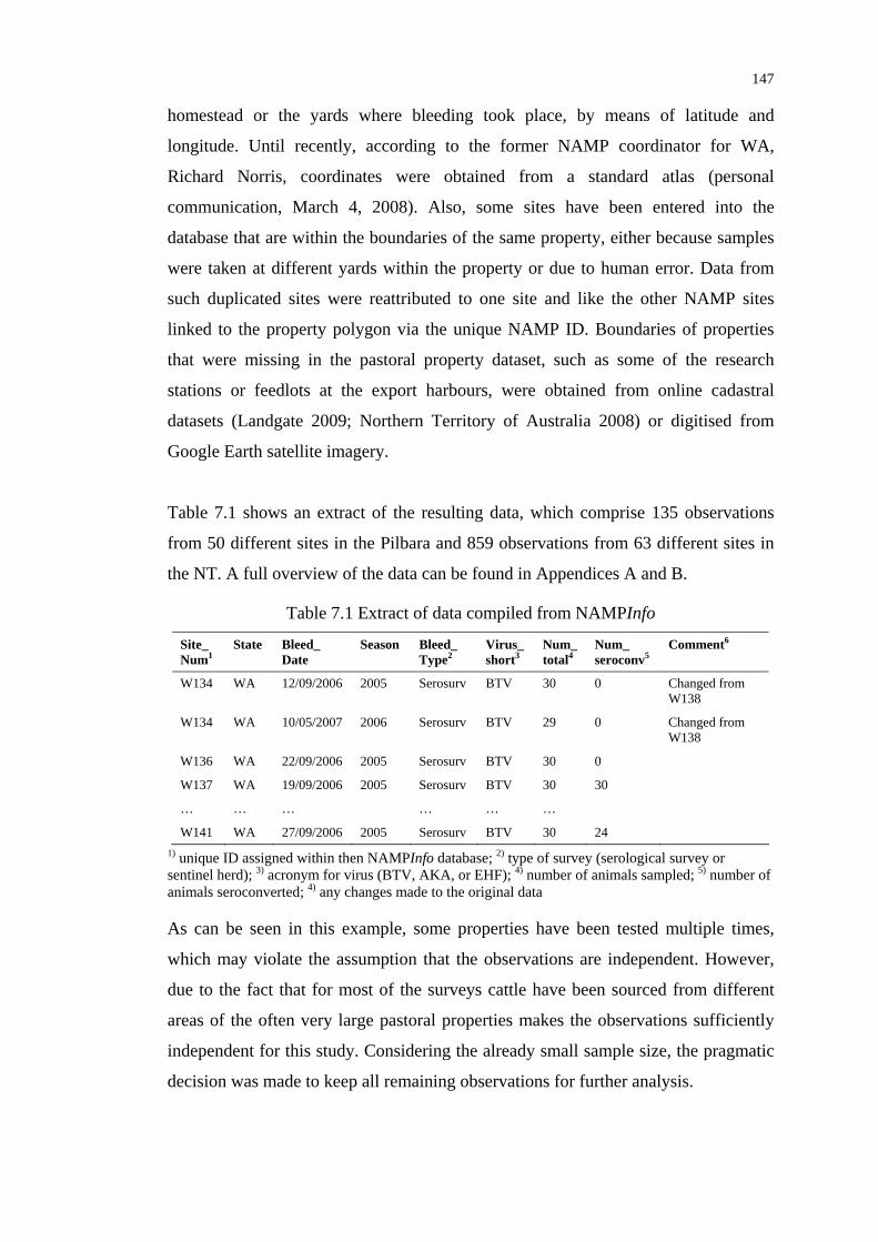
147

homestead or the yards where bleeding took place, by means of latitude and

longitude. Until recently, according to the former NAMP coordinator for WA,

Richard Norris, coordinates were obtained from a standard atlas (personal

communication, March 4, 2008). Also, some sites have been entered into the

database that are within the boundaries of the same property, either because samples

were taken at different yards within the property or due to human error. Data from

such duplicated sites were reattributed to one site and like the other NAMP sites

linked to the property polygon via the unique NAMP ID. Boundaries of properties

that were missing in the pastoral property dataset, such as some of the research

stations or feedlots at the export harbours, were obtained from online cadastral

datasets (Landgate 2009; Northern Territory of Australia 2008) or digitised from

Google Earth satellite imagery.

Table 7.1 shows an extract of the resulting data, which comprise 135 observations

from 50 different sites in the Pilbara and 859 observations from 63 different sites in

the NT. A full overview of the data can be found in Appendices A and B.

Table 7.1 Extract of data compiled from NAMPInfo

Site_ Num1

State Bleed_ Date

Season Bleed_ Type2

Virus_short3

Num_total4

Num_ seroconv5

Comment6

W134 WA 12/09/2006 2005 Serosurv BTV 30 0 Changed from W138

W134 WA 10/05/2007 2006 Serosurv BTV 29 0 Changed from W138

W136 WA 22/09/2006 2005 Serosurv BTV 30 0

W137 WA 19/09/2006 2005 Serosurv BTV 30 30

… … … … … …

W141 WA 27/09/2006 2005 Serosurv BTV 30 24 1) unique ID assigned within then NAMPInfo database; 2) type of survey (serological survey or sentinel herd); 3) acronym for virus (BTV, AKA, or EHF); 4) number of animals sampled; 5) number of animals seroconverted; 4) any changes made to the original data

As can be seen in this example, some properties have been tested multiple times,

which may violate the assumption that the observations are independent. However,

due to the fact that for most of the surveys cattle have been sourced from different

areas of the often very large pastoral properties makes the observations sufficiently

independent for this study. Considering the already small sample size, the pragmatic

decision was made to keep all remaining observations for further analysis.

148

Following the screening process, a file geodatabase was set up in ArcGIS, where all

tabular data of serology and the extracted bioclimatic variables are managed together

with the spatial property datasets. To create a suitable structure for the analysis of

virus - environment relationships the serological status of each of the tested

properties was summarized per year as a dichotomous variable (1: presence; 0:

absence) and merged with the bioclimatic variables for those years as illustrated in

Table 7.2 below. For the complete dataset see Appendices C to E.

Table 7.2 Extract from the dataset developed for the analysis of correlations between the predictor environmental variables and BTV occurrence response variable

NAMP ID Station_name Year BT_status maxndviss maxlstdsu … Rau

108 Crown 2001 1 0.726 35.848 243.06

108 Crown 2002 1 0.735 31.607 166.10

T029 Helen Springs 2000 0 0.503 42.249 177.98

… … … … … … … …

T075 Buchanan Downs 2004 1 0.527 47.208 … 38.172

Table 7.3 below provides a summary of the number of tested properties as well as the

farm level seroprevalence for both study areas. More detailed analyses, such as

seroprevalence standardised by the age of animals tested were not feasible due to the

lack of suitable data collected through the NAMP.

Table 7.3 Number of tested properties and seroprevalence in the Pilbara and the Northern Territory

Pilbara Northern Territory Year No. of tested

properties Prevalence (95% confidence interval)

No. of tested properties

Prevalence (95% confidence interval)

2000/2001 30 0.13 (0.03-0.31) 14 0.36 (0.13-037)

2001/2002 13 0.46 (0.19-0.75) 18 0.67 (0.41-0.87)

2002/2003 15 0.33 (0.12-0.62) 25 0.68 (0.46-0.85)

2003/2004 7 0.14 (0.00-0.58) 23 0.74 (0.52-0.90)

2004/2005 8 0.13 (0.00-0.53) 18 0.28 (0.10-0.53)

2005/2006 16 0.06 (0.00-0.30) 10 0.80 (0.44-0.97)

2006/2007 9 0.22 (0.03-0.60) 17 0.70 (0.44-0.90)

2007/2008 8 0.00 (0.00-0.48) 37 0.54 (0.37-0.71)

2008/2009 7 0.00 (0.00-0.53) 38 0.71 (0.54-0.85)

7. 2 Selection of Variables to be Used in Model Development

The initial set of environmental variables developed has been selected on

ecologically sound principles using knowledge about BTV ecology, but also

149

considering the availability of data of sufficiently high quality. This section

statistically analyses the relationship between BTV presence and each of the

explanatory variables in order to identify the significant predictor variables for model

building. The analyses are conducted for the station average and weighted station

average variables of the Pilbara region and the station averages of the Northern

Territory.

7.2.1 Analyses of Associations between Bioclimatic Variables and BTV Status

As a first step, univariate analyses were conducted using the statistical environment

R (R Development Core Team 2010) to identify those variables which are most able

to discriminate between BTV positive and negative properties. Using a non-

parametric Kruskal-Wallis test (Kruskal and Wallis 1952), variables showing

statistically significant differences between the two groups (BTV positive and BTV

negative properties) could be identified. The hypothesis to be tested is that the same

environmental conditions are present on cattle stations where BTV has been found as

on those where the virus is absent. The test is similar to the parametric one way

Anova, but has the advantage that it does not require the variables to be normally

distributed (Moore, McCabe, and Craig 2009). It is also better suited for small

sample sizes, which is another characteristic of the data used in this study. If the

number of different groups equals two as with presence/absence data, the Kruskal-

Wallis test is equal to the Mann-Whitney test. As with many other non-parametric

procedures these techniques do not work with the original measurements, but instead

with the ranks of the measurements, as described in detail by Zar (1999). Boxplots

were generated for all variables to visually investigate their correlation with BTV

positive and BTV negative sites (some of the key variables are shown in Figures 7.1

to 7.5). The entire test results are tabulated in Table 7.4 and discussed below.

150

0 135

0040

0045

0050

00

P = 0.012

gdda

Pilb

ara

(sta

tion

aver

age)

0 1

2600

3000

3400

P = 0

gdds

s

0 1

1300

1500

P = 0.002

gdds

u

0 1

600

800

1000

1400

P = 0.008

gdda

u

0 1

3500

4000

4500

5000

P = 0.005

gdda

Pilb

ara

(sta

tion

aver

age)

0 126

0030

0034

00

P = 0

gdds

s

0 1

1200

1400

1600

P = 0.002

gdds

u

0 1

600

800

1200

P = 0.005

gdda

u

Figure 7.1 Relationship between selected Growing Degree Day variables and BTV status (0 = negative, 1 = positive), with the p-value indicating the significance of the

group differences

0 1

4850

5254

56

P = 0.177

max

lstd

su

Pilb

ara

(sta

tion

aver

age)

0 1

3840

4244

4648

P = 0.01

max

lstd

au

0 1

1214

1618

P = 0.443

min

lstn

pw

0 1

4648

5052

5456

P = 0.015

max

lstd

su

Pilb

ara

(wei

ghte

d st

atio

n av

erag

e)

0 1

3842

4650

P = 0.002

max

lstd

au

0 1

1214

1618

P = 0.765

min

lstn

pw

0 1

3035

4045

5055

P = 0

max

lstd

su

Nor

ther

n Te

rrito

ry

(sta

tion

aver

age)

0 1

3035

4045

P = 0

max

lstd

au

0 1

05

1015

P = 0

min

lstn

pw

Figure 7.2 Relationship between selected minimum and maximum temperature variables and BTV status (0 = negative, 1 = positive), with the p-value indicating the

significance of the group differences

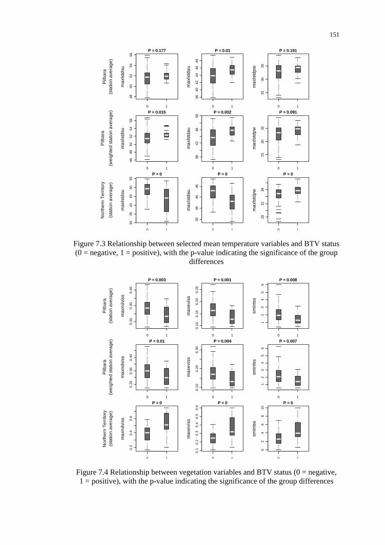
151

0 1

4850

5254

56

P = 0.177

max

lstd

su

Pilb

ara

(sta

tion

aver

age)

0 1

3840

4244

4648

P = 0.01

max

lstd

au

0 1

2530

35

P = 0.191

max

lstd

pw

0 1

4648

5052

5456

P = 0.015

max

lstd

su

Pilb

ara

(wei

ghte

d st

atio

n av

erag

e)

0 1

3842

4650

P = 0.002

max

lstd

au

0 1

2530

35

P = 0.091

max

lstd

pw

0 1

3035

4045

5055

P = 0

max

lstd

su

Nor

ther

n Te

rrito

ry

(sta

tion

aver

age)

0 1

3035

4045

P = 0

max

lstd

au

0 1

2832

36

P = 0

max

lstd

pw

Figure 7.3 Relationship between selected mean temperature variables and BTV status (0 = negative, 1 = positive), with the p-value indicating the significance of the group

differences

0 1

0.20

0.30

0.40

P = 0.003

max

ndvi

ss

Pilb

ara

(sta

tion

aver

age)

0 1

0.10

0.15

0.20

0.25

P = 0.001

max

evis

s

0 1

12

34

56

P = 0.008

smin

tss

0 1

0.20

0.30

0.40

P = 0.01

max

ndvi

ss

Pilb

ara

(wei

ghte

d st

atio

n av

erag

e)

0 1

0.10

0.20

0.30

P = 0.004

max

evis

s

0 1

12

34

56

P = 0.007

smin

tss

0 1

0.2

0.4

0.6

P = 0

max

ndvi

ss

Nor

ther

n Te

rrito

ry(s

tatio

n av

erag

e)

0 1

0.1

0.2

0.3

0.4

0.5

0.6

P = 0

max

evis

s

0 1

02

46

810

P = 0

smin

tss

Figure 7.4 Relationship between vegetation variables and BTV status (0 = negative, 1 = positive), with the p-value indicating the significance of the group differences

152

0 1

020

040

060

080

0

P = 0.018

rss

Pilb

ara

(sta

tion

aver

age)

0 1

010

030

050

0

P = 0.039

rsu

0 1

010

020

030

040

0

P = 0.37

rau

0 1

020

040

060

080

0

P = 0.016

rss

Pilb

ara

(wei

ghte

d st

atio

n av

erag

e)

0 1

010

030

050

0

P = 0.036

rsu

0 1

010

020

030

040

0

P = 0.357

rau

0 1

050

015

00

P = 0

rss

Nor

ther

n Te

rrito

ry

(sta

tion

aver

age)

0 1

040

080

012

00

P = 0

rsu

0 1

020

060

010

00

P = 0

rau

Figure 7.5 Relationship between rainfall variables and BTV status (0 = negative, 1 = positive), with the Kruskal-Wallis p-value given

The scatterplots reveal some notable differences between the effects of

environmental conditions on the BTV status at the two study areas. Results from the

Northern Territory show that the association between BTV presence/absence and

NDVI, temperature and rain fits well with what is currently known about the ecology

of the virus. Higher vegetation index values, rainfall accumulates and winter

temperatures are found at BTV positive sites, while higher temperatures during the

warmer months are associated with virus absence. The latter effect can be explained

by the cessation of vector activity at higher temperatures due to desiccation,

particularly in central Australia.

All variables are significantly different between positive and negative sites (Table

7.4) and are therefore equally capable of explaining differences between positive and

negative sites, which is needed to develop a robust model. Although only observable

at the least significant digits of the p-value and therefore not shown in Table 7.4, the

strongest difference was found between the vegetation and rainfall variables.

153

Table 7.4 Test statistics for the Pilbara and Northern Territory study areas

Region (aggregation level)

Pilbara (station average)

n = 76

Pilbara (weighted station average)

n = 76

Northern Territory (station average)

n = 162

Variable (see Table 6.2) Chi-square p-value chi-square p-value chi-square p-value

maxndviss 9.1204 0.0025** 6.7186 0.0095** 39.1673 <0.0001**

maxeviss 11.8884 0.0006** 8.3101 0.0039** 37.8558 <0.0001**

smint 7.0148 0.0081** 7.2738 0.0070** 27.1438 <0.0001**

maxlstdss 1.4867 0.2227 5.4082 0.0200* 14.8629 0.0001**

maxlstdsu 1.8185 0.1775 5.9468 0.0147* 25.2792 <0.0001**

maxlstdau 6.5936 0.0102* 9.1692 0.0025** 35.8284 <0.0001**

maxlstdpw 1.7112 0.1908 2.8481 0.0915 12.7371 0.0004**

minlstnss 12.2257 0.0005** 8.3345 0.0039**

minlstnsu 11.7228 0.0006** 10.4855 0.0012**

minlstnau 4.5444 0.0330* 3.6934 0.0546

minlstnpw 0.5885 0.4430 0.0893 0.7651 32.1725 <0.0001**

meanlstdss 4.4761 0.0344* 7.4496 0.0063** 24.5983 <0.0001**

meanlstdsu 1.5066 0.2197 2.6083 0.1063 32.8723 <0.0001**

meanlstdau 1.5565 0.2122 3.4945 0.0616 14.4972 0.0001**

meanlstdpw 1.1276 0.2883 2.1244 0.1450 24.1942 <0.0001**

meanlstnss 4.8419 0.0278* 5.7324 0.0167*

meanlstnsu 9.3172 0.0023** 8.7828 0.0030**

meanlstnau 0.8850 0.3468 0.6199 0.4311

meanlstnpw 1.1796 0.2774 0.2308 0.6309 24.9716 <0.0001**

meanlstss 14.2811 0.0002** 16.6944 <0.0001**

meanlstsu 0.4823 0.4874 0.3105 0.5774

meanlstau 2.4668 0.1163 2.2924 0.1300

meanlstpw 1.0767 0.2994 1.2508 0.2634 25.86522 <0.0001**

gdda 6.2660 0.0123* 7.8511 0.0051**

gddss 12.6233 0.0004** 14.1593 0.0002**

gddsu 9.2673 0.0023** 10.0706 0.0015**

gddau 7.0577 0.0079** 7.8964 0.0050**

rsu 5.5976 0.0180* 5.8292 0.0158* 34.61466 <0.0001**

rau 4.2732 0.0387* 4.4077 0.0358* 33.69828 <0.0001**

rss 0.8034 0.3701 0.8474 0.3573 17.95233 <0.0001**

**: The difference between groups is statistically significant (p ≤ 0.01) *: The difference between groups is statistically significant (p ≤ 0.05) n: Number of records

The differences between the positive and negative sites are generally less significant

for the Pilbara. The most significant differences between presence and absence sites

were found for the variables summarising vegetation indices, night land surface

temperature, mean seasonal temperatures, and growing degrees days (Table 7.4). The

154

effects vary slightly between variables generated using the station average approach

and variables based on the weighted station average, the later of which shows higher

significance in group differences for smintss, and the various maxlst, gdd and rain

variables.

Unexpectedly, the box plots show a negative relationship between BTV presence and

the usually important variables related to rainfall, humidity and vegetation.

According to the data, the higher NDVI values are related to BTV absence, as are

higher rainfall figures. If these variables were included in the model, a higher

probability for BTV presence would be predicted for drier regions, such as the Great

Sandy Desert. This is contradictory to the ecology of the BTV vectors, which are

unlikely to occur in those regions due to the lack of both humidity and cattle.

The effects are mainly related to a bias towards negatively tested properties (out of

76 samples, only 16 are BTV positive), which may provide suitable habitats for

Culicoides vectors, but where BTV has not been detected for several reasons. In

contrast to the Northern Territory, the Pilbara has been declared BTV infected very

recently and BTV is still not considered endemic to the area. Therefore, in years

where BTV was not present in the Pilbara there is a natural bias towards negative test

results. Factors other than environment and climate may be driving virus occurrence

(see the maps in Figure 5.4), particularly during the first year of BTV introduction.

The outbreak that was detected at the Kooline and Mt Stuart stations in the central

Pilbara only infected neighbouring stations, while more distant properties tested BTV

negative during an extensive surveillance campaign. The following season

(2001/2002), BTV seemed to have spread further, infecting properties to the east and

south of the original detection. This trend continued in 2002/2001. However, the

following years, surveillance activities were gradually reduced, and therefore so was

the detection of BTV. For this reason it is not known, if virus activity was lower due

to changes in the environment or due to reduced surveillance activities. As indicated

in Section 2.2.3, the economic impacts of declaring an area as BTV infected are

nowhere else in Australia as large as they are in the Pilbara. This also needs to be

considered in the analysis of the data, since NAMP surveillance depends on the

collaboration of pastoralists. Further analyses were conducted to investigate the

effect of study area boundaries and include only data from sites closer to the original

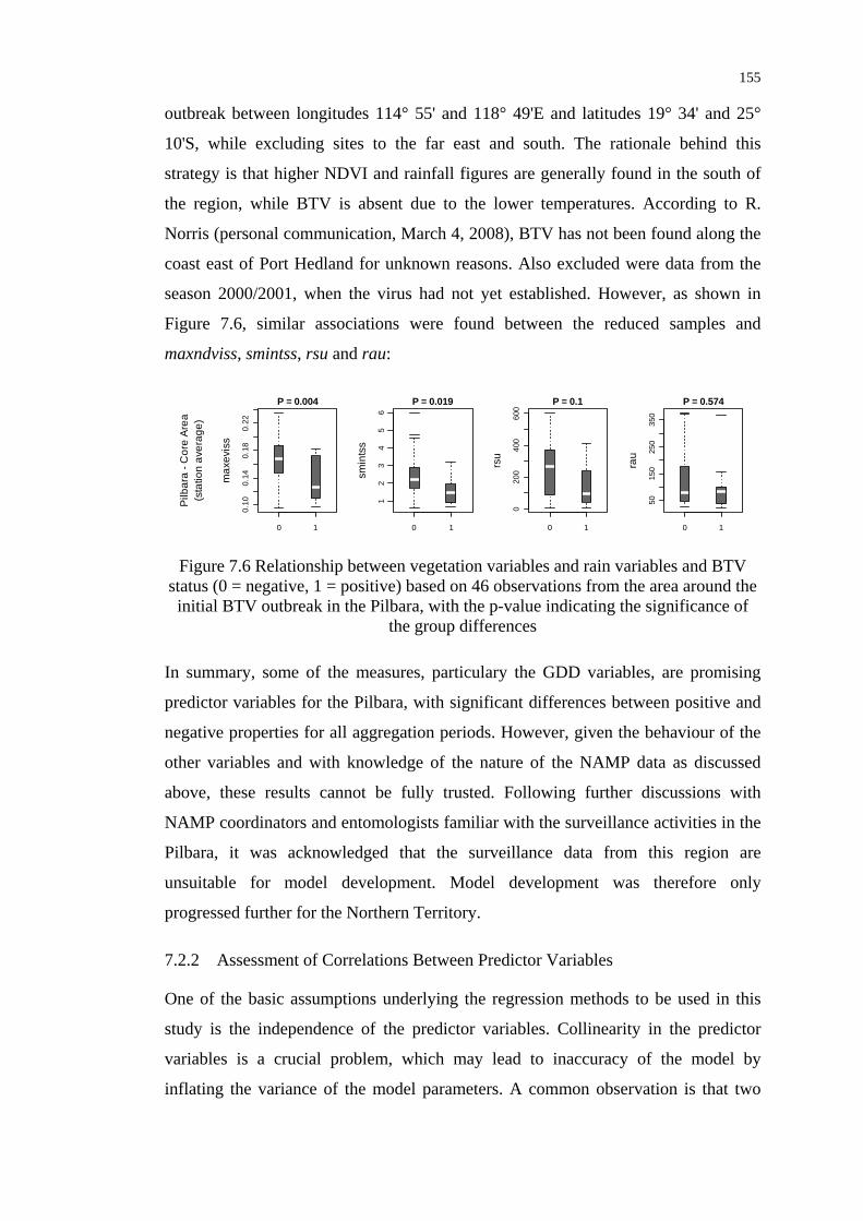
155

outbreak between longitudes 114° 55' and 118° 49'E and latitudes 19° 34' and 25°

10'S, while excluding sites to the far east and south. The rationale behind this

strategy is that higher NDVI and rainfall figures are generally found in the south of

the region, while BTV is absent due to the lower temperatures. According to R.

Norris (personal communication, March 4, 2008), BTV has not been found along the

coast east of Port Hedland for unknown reasons. Also excluded were data from the

season 2000/2001, when the virus had not yet established. However, as shown in

Figure 7.6, similar associations were found between the reduced samples and

maxndviss, smintss, rsu and rau:

0 1

0.10

0.14

0.18

0.22

P = 0.004

max

evis

s

Pilb

ara

- Cor

e Ar

ea(s

tatio

n av

erag

e)

0 1

12

34

56

P = 0.019

smin

tss

0 10

200

400

600

P = 0.1

rsu

0 1

5015

025

035

0

P = 0.574

rau

Figure 7.6 Relationship between vegetation variables and rain variables and BTV status (0 = negative, 1 = positive) based on 46 observations from the area around the initial BTV outbreak in the Pilbara, with the p-value indicating the significance of

the group differences

In summary, some of the measures, particulary the GDD variables, are promising

predictor variables for the Pilbara, with significant differences between positive and

negative properties for all aggregation periods. However, given the behaviour of the

other variables and with knowledge of the nature of the NAMP data as discussed

above, these results cannot be fully trusted. Following further discussions with

NAMP coordinators and entomologists familiar with the surveillance activities in the

Pilbara, it was acknowledged that the surveillance data from this region are

unsuitable for model development. Model development was therefore only

progressed further for the Northern Territory.

7.2.2 Assessment of Correlations Between Predictor Variables

One of the basic assumptions underlying the regression methods to be used in this

study is the independence of the predictor variables. Collinearity in the predictor

variables is a crucial problem, which may lead to inaccuracy of the model by

inflating the variance of the model parameters. A common observation is that two

156

highly correlated predictors can both appear non-significant even though each would

explain a significant proportion of the deviance if considered individually (Guisan,

Edwards, and Hastie 2002). Although it is less of a problem for predictive models, if

the model parameters are to be interpreted, it may become difficult to assess the

individual importance of each collinear predictor variable. Careful selection of the

variables during the model building process is therefore required.

In order to identify possible collinearity between variables they have been analysed

pair-wise for correlations. The data divide naturally into two groups, namely

temperature variables, and rainfall and vegetation variables. They were therefore

analysed in those groups (Tables 7.5 and 7.6). The results will be considered when

building the model and deciding which predictor variables to include or exclude.

Table 7.5 Pearson correlation coefficients for rainfall and vegetation variables

maxndviss maxeviss smintss rss rsu Rau

maxndviss 1 0.978 0.666 0.839 0.815 0.658 maxeviss 0.978 1 0.602 0.849 0.796 0.703 rmintss 0.666 0.602 1 0.531 0.539 0.401 rss 0.839 0.849 0.531 1 0.942 0.842 rsu 0.815 0.796 0.539 0.942 1 0.627 rau 0.658 0.703 0.401 0.842 0.627 1

Table 7.6 Pearson correlation coefficients for temperature variables

max

lstd

ss

max

lstd

su

max

lstd

au

max

lstd

pw

min

lstn

pw

mea

nlst

dss

mea

nlst

dsu

mea

nlst

dau

mea

nlst

dpw

mea

nlst

npw

Mea

nlst

pw

maxlstdss 1 0.685 0.664 -0.257 -0.423 0.886 0.843 0.727 -0.175 -0.315 -0.255 maxlstdsu 0.685 1 0.832 -0.331 -0.642 0.646 0.733 0.382 -0.581 -0.691 -0.666 maxlstdau 0.664 0.832 1 -0.401 -0.591 0.737 0.744 0.608 -0.569 -0.645 -0.636 maxlstdpw -0.257 -0.331 -0.401 1 0.621 -0.345 -0.423 -0.268 0.543 0.645 0.62 minlstnpw -0.423 -0.642 -0.591 0.621 1 -0.396 -0.526 -0.157 0.709 0.889 0.836 meanlstdss 0.886 0.646 0.737 -0.345 -0.396 1 0.96 0.913 -0.212 -0.341 -0.288 meanlstdsu 0.843 0.733 0.744 -0.423 -0.526 0.96 1 0.783 -0.34 -0.48 -0.428 meanlstdau 0.727 0.382 0.608 -0.268 -0.157 0.913 0.783 1 -0.018 -0.124 -0.072 meanlstdpw -0.175 -0.581 -0.569 0.543 0.709 -0.212 -0.34 -0.018 1 0.812 0.956 meanlstnpw -0.315 -0.691 -0.645 0.645 0.889 -0.341 -0.48 -0.124 0.812 1 0.947 meanlstpw -0.255 -0.666 -0.636 0.62 0.836 -0.288 -0.428 -0.072 0.956 0.947 1

As can be seen in Table 7.6, there is considerable correlation observable between

vegetation and rainfall. Strong correlation was found between rss (seasonal rain) and

rsu (summer rain), indicating that most rainfall occurs during the summer months.

157

The strongest correlation was present between maxndvi and maxevi, which suggest

using only one of the two in a model. In relation to temperature (Table 7.5), the

highest correlation has been found between the two variables meanlstdsu and

meanlstdau and the derivative seasonal mean day temperature meanlstdss, and

similarly between the two variables meanlstdpw and meanlstnpw and the derived

mean temperature in winter, meanlstpw.

7. 3 Developing the Distribution Model

7.3.1 Generalised Linear Models Versus Generalised Additive Models

Based on the comparison of different modelling techniques in Section 3.3, GLM and

GAM approaches were both considered for this study. To be able to decide which

method is the most appropriate, the nature of the relationship between predictor

variables and BTV occurrence needs to be analysed. Some variables might be

characterised by a linear response, which can be sufficiently accurately modelled

using a GLM. However, non-linear responses to changes in environmental variables

are often found in ecological and epidemiological modelling, e.g. rising temperature

might initially increase vector activity, but after reaching an optimum temperature

range, an additional increase in temperature might have an adverse effect. In such

cases, one approach would be to categorise the variables (e.g. define specific

temperature ranges for which the response is linear) as demonstrated by Austin,

Nicholls and Margules (1990). Nevertheless, even after the transformation of

variables and the addition of higher order terms, GLMs can still be an inadequate

modelling procedure (Yee and Mitchell 1991). Early exploratory analyses using

GLMs were abandoned due to their low explanatory power, compared to GAMs.

In contrast to a GLM, the response curve of a GAM is determined by the data and

can take any shape. In a GAM, linear functions of the variables are replaced by so

called smoothers, which gives additional flexibility for the modelling process.

According to Hastie and Tibshirani (1990) a smoother is a non-parametric tool for

summarising the trend of a response measurement as a function of one or more

predictor measurements. The name refers to the characteristic that an estimate of the

trend is produced that is less variable than the response itself. Examples of smoothers

include running means, kernel smoothers, regression splines and natural splines. The

158

non-parametric nature of GAMs also makes them very useful analytical tools for

investigating the shape of the response curve for each variable. Some software

implementations of the GAM approach, such as in R (Wood 2006) allow for the

combination of variables with linear and non linear responses. Hence the question is

no longer, if a GLM or a GAM should be used, but which variables show a linear

response and can be parameterised in the model and which variables require a non-

parametric curve due to their non-linearity. An example is shown in Figure 7.7,

where one of the variables in a GAM can be described by a linear function. Full

details about the modelling process are given below.

7.3.2 Developing the Generalised Additive Model

Generalised additive models were fitted using the gam() function from the R ‘mgcv’

package (version 1.7–1) (Wood 2010), starting with a model that includes all

predictor variables with a Kruskal Wallis p < 0.2. A stepwise exclusion approach was

then employed, removing the least significant variables during each iteration, until all

variables were significant (p < 0.05). The p-value given for each smooth term is

approximate and based on the test statistic motivated by Nychka’s (1988) analysis of

the frequentist properties of Bayesian confidence intervals for smoothers (Wood

2010). Where variables had the same or a similar p-value, those variables that are

known to be important for the BTV cycle were retained in the model. Hence, the

model was developed utilising expert knowledge as well as statistics. This minimises

the risk of potentially using relationships which may be statistically significant but

have no grounding in the ecological process being modelled. Several models were

developed using this hybrid approach and the best model was chosen by maximising

the discriminatory ability, given by the area under the receiver operator characteristic

(ROC) curve (Pearce and Ferrier 2000). As described in Section 3.5 the area under

the ROC curve (AUC) is a measure of the model’s ability to correctly distinguish

between presence and absence and can be interpreted in a straightforward manner. A

value of 1 indicates perfect discrimination, whereas a value of 0.5 indicates that the

model performs no better than a random guess (Fawcett 2006). Hosmer and

Lemeshow (2000) considered values above 0.7 to provide reasonable discrimination

and the larger the AUC the better the model at predicting group membership.

159

0.2 0.3 0.4 0.5 0.6 0.7

-10

-50

510

maxndviss

s(m

axnd

viss

,3)

30 35 40 45

-10

-50

510

maxlstdau

s(m

axls

tdau

,3.2

5)

25 30 35 40 45 50

-10

-50

510

meanlstdsu

s(m

eanl

stds

u,1)

6 8 10 12 14

-10

-50

510

meanlstnpw

s(m

eanl

stnp

w,2

.71)

Figure 7.7 Smoothed fits to the variables maxndviss, maxlstdau, meanlstdau and meanlstnpw used in the final BTV distribution model for the Northern Territory

(solid line). Dashed lines give ~95% confidence intervals

As summarised in Table 7.7 the four predictor variables that gave the best fit are

maximum seasonal NDVI (maxndviss), mean day temperature of the warmest 8-day

period in autumn (maxlstdau), mean day temperature in summer (meanlstdsu) and

mean night temperature of the previous winter months (meanlstnpw). The GAM plot

(Figure 7.7) shows the smoothers for these four covariates and the 95% confidence

interval. The x-axis on the plots of covariate effects on the presence of Bluetongue

illustrates the density of samples used for each covariate in the model. The plots

show that the effect of one of the four variables on the outcome can be expressed by

a linear function, while the other three variables were best described by an unimodal

smoothing function (Figure 7.7).

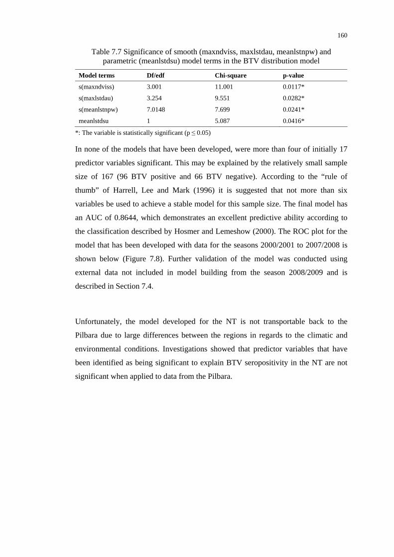
160

Table 7.7 Significance of smooth (maxndviss, maxlstdau, meanlstnpw) and parametric (meanlstdsu) model terms in the BTV distribution model

Model terms Df/edf Chi-square p-value

s(maxndviss) 3.001 11.001 0.0117*

s(maxlstdau) 3.254 9.551 0.0282*

s(meanlstnpw) 7.0148 7.699 0.0241*

meanlstdsu 1 5.087 0.0416*

*: The variable is statistically significant (p ≤ 0.05)

In none of the models that have been developed, were more than four of initially 17

predictor variables significant. This may be explained by the relatively small sample

size of 167 (96 BTV positive and 66 BTV negative). According to the “rule of

thumb” of Harrell, Lee and Mark (1996) it is suggested that not more than six

variables be used to achieve a stable model for this sample size. The final model has

an AUC of 0.8644, which demonstrates an excellent predictive ability according to

the classification described by Hosmer and Lemeshow (2000). The ROC plot for the

model that has been developed with data for the seasons 2000/2001 to 2007/2008 is

shown below (Figure 7.8). Further validation of the model was conducted using

external data not included in model building from the season 2008/2009 and is

described in Section 7.4.

Unfortunately, the model developed for the NT is not transportable back to the

Pilbara due to large differences between the regions in regards to the climatic and

environmental conditions. Investigations showed that predictor variables that have

been identified as being significant to explain BTV seropositivity in the NT are not

significant when applied to data from the Pilbara.

161

AUC 0.8644

False positive rate

True

pos

itive

rate

0.0 0.2 0.4 0.6 0.8 1.0

0.0

0.2

0.4

0.6

0.8

1.0

Figure 7.8 ROC plot of sensitivity (true positive rate) versus 1-specificity (false positive rate) for the final GAM based on data from 2000/2001 to 2007/2008

7.3.3 Spatial Effects

So far the effects of spatial autocorrelation (reviewed in Section 3.4) have not been

considered when building the so called fixed effects GAM. Looking at the

distribution of virus occurrence in Figure 5.8 suggests that the observed

seropositivity may not be related to environmental factors alone (first order effects),

but also may depend on the presence or absence of the virus on neighbouring

stations. To identify such unaccounted for second-order effects, a typical approach is

to examine the model residuals for evidence of spatial autocorrelation (see Pfeiffer et

al. 2008). This involves the definition of “neighbourhood” between pastoral

properties, either by distance or by adjacency, e.g. through sharing a common

boundary. If there is evidence for spatial autocorrelation, the model can be extended

to account for the spatial dependence between sites.

The peculiarities of the data that are dealt with in this study and the resulting model

however exacerbate the situation. The samples that have been used for model

building describe the BTV status over several years and some stations have multiple

162

representations. Consequently, residuals would have to be analysed for each year

separately. In the case of evidence for autocorrelation and considering that the effects

will vary between years, distribution models would be needed to be developed on an

annual basis. Given that the fixed effects model has originally been built from eight

years of data comprising only 162 samples, reducing the sample size to between ten

(season 2005/2006) and 25 samples annually (season 2002/2003) would lead to

instability in the model. It was therefore concluded that, although spatial

autocorrelation may be present between the dependant variables, the data in this

study do not support further investigations. The previously developed stable and

ecologically meaningful model is used to generate annual prediction maps as

described below.

7.3.4 Predicting the Probability of BTV Seropositivity

Based on the final fixed effects GAM, annual prediction maps were generated using

R. In contrast to the station average variables used for model development, the

predictions were performed on a pixel basis, using the GeoTiff rasters of the

bioclimatic variables. In order to be able to process the whole study area, the nominal

spatial resolution had to be reduced to 1 km to avoid computer memory limitations.

The results are illustrated in Figures 7.9 to 7.12, showing the probability that cattle

tested in an area are BTV seropositive. Standard error maps indicate spatial

variations in the accuracy of the predictions.

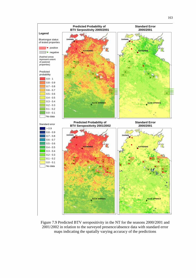
163

!

!

!

!(

!(

!(

!(

!(

!(

!(!(

!(

!(

!(

!(

!(

!(

DARWIN

KATHERINE

ALICE SPRINGS

!

!

!

!(

!(

!(

!(

!(

!(

!(!(

!(

!(

!(

!(

!(

!(

DARWIN

KATHERINE

ALICE SPRINGS

!

!

!

!(

!(

!(

!(

!(

!(

!(

!(!(

!(!(

!(!(

!(

!(

!(

!(

!(

DARWIN

KATHERINE

ALICE SPRINGS

!

!

!

!(

!(

!(

!(

!(

!(

!(

!(!(

!(!(

!(!(

!(

!(

!(

!(

!(

DARWIN

KATHERINE

ALICE SPRINGS

Predicted Probability of BTV Serpositivity 2000/2001

Standard Error2000/2001

Predicted Probability of BTV Seropositivity 2001/2002


Bluetongue statusof tested properties

/ negative

/ positive

!(

!(

(hashed areasrepresent extentof pastoralproperties)

Legend

0.8 - 0.90.7 - 0.80.6 - 0.70.5 - 0.60.4 - 0.50.3 - 0.40.2 - 0.30.1 - 0.20.0 - 0.1

Predictedprobability

Standard error

0.9 - 1

> 0.90.8 - 0.90.7 - 0.80.6 - 0.70.5 - 0.60.4 - 0.50.3 - 0.40.2 - 0.30.1 - 0.2

No data

0.0 - 0.1No data

Figure 7.9 Predicted BTV seropositivity in the NT for the seasons 2000/2001 and 2001/2002 in relation to the surveyed presence/absence data with standard error

maps indicating the spatially varying accuracy of the predictions

164

!

!

!

!(

!(

!(

!(

!(

!(

!(

!(

!(

!(

!(!(

!(!(

!(

!(

!(

!(

!(

!(

!(

!(

!(

!(

!(

DARWIN

KATHERINE

ALICE SPRINGS

!

!

!

!(

!(

!(

!(

!(

!(

!(

!(

!(

!(

!(!(

!(!(

!(

!(

!(

!(

!(

!(

!(

!(

!(

!(

!(

DARWIN

KATHERINE

ALICE SPRINGS

!

!

!

!(

!(

!(

!(!(

!(

!( !(

!(

!(!(

!(!(

!(

!(

!(

!(

!(

!(

!(

!(

!(

!(

DARWIN

KATHERINE

ALICE SPRINGS

!

!

!

!(

!(

!(

!(!(

!(

!( !(

!(

!(!(

!(!(

!(

!(

!(

!(

!(

!(

!(

!(

!(

!(

DARWIN

KATHERINE

ALICE SPRINGS






/ negative

/ positive

!(

!(


Legend

0.8 - 0.90.7 - 0.80.6 - 0.70.5 - 0.60.4 - 0.50.3 - 0.40.2 - 0.30.1 - 0.20.0 - 0.1


Standard error

0.9 - 1

> 0.90.8 - 0.90.7 - 0.80.6 - 0.70.5 - 0.60.4 - 0.50.3 - 0.40.2 - 0.30.1 - 0.2

No data

0.0 - 0.1No data


maps indicating the spatially varying accuracy of the predictions

165

!

!

!

!(

!(!(

!(

!(

!(

!(

!(

!(!(

!(

!(

!(

!(

!(

!(

!(

!(

DARWIN

KATHERINE

ALICE SPRINGS

!

!

!

!(

!(!(

!(

!(

!(

!(

!(

!(!(

!(

!(

!(

!(

!(

!(

!(

!(

DARWIN

KATHERINE

ALICE SPRINGS

!

!

!

!(

!(

!(

!(

!(!(

!(

!(

!(

!(

DARWIN

KATHERINE

ALICE SPRINGS

!

!

!

!(

!(

!(

!(

!(!(

!(

!(

!(

!(

DARWIN

KATHERINE

ALICE SPRINGS






/ negative

/ positive

!(

!(


Legend

0.8 - 0.90.7 - 0.80.6 - 0.70.5 - 0.60.4 - 0.50.3 - 0.40.2 - 0.30.1 - 0.20.0 - 0.1


Standard error

0.9 - 1

> 0.90.8 - 0.90.7 - 0.80.6 - 0.70.5 - 0.60.4 - 0.50.3 - 0.40.2 - 0.30.1 - 0.2

No data

0.0 - 0.1No data


maps indicating the spatially varying accuracy of the predictions.

166

!

!

!

!(

!(

!(

!(

!(

!(

!(

!(

!(!(

!(

!(

!(

!(

!(

!(

!(

DARWIN

KATHERINE

ALICE SPRINGS

!

!

!

!(

!(

!(

!(

!(

!(

!(

!(

!(!(

!(

!(

!(

!(

!(

!(

!(

DARWIN

KATHERINE

ALICE SPRINGS

!

!

!

!(

!(

!(

!(

!(

!(

!(

!(

!(

!(

!(

!(

!(

!(

!(

!(

!(

!(

!(!(

!(!(

!(

!(

!(

!(

!(

!(

!(!(

!(

!(

!(

!(

!(

!(

!(

!(

DARWIN

KATHERINE

ALICE SPRINGS

!

!

!

!(

!(

!(

!(

!(

!(

!(

!(

!(

!(

!(

!(

!(

!(

!(

!(

!(

!(

!(!(

!(!(

!(

!(

!(

!(

!(

!(

!(!(

!(

!(

!(

!(

!(

!(

!(

!(

DARWIN

KATHERINE

ALICE SPRINGS






/ negative

/ positive

!(

!(


Legend

0.8 - 0.90.7 - 0.80.6 - 0.70.5 - 0.60.4 - 0.50.3 - 0.40.2 - 0.30.1 - 0.20.0 - 0.1


Standard error

0.9 - 1

> 0.90.8 - 0.90.7 - 0.80.6 - 0.70.5 - 0.60.4 - 0.50.3 - 0.40.2 - 0.30.1 - 0.2

No data

0.0 - 0.1No data


maps indicating the spatially varying accuracy of the predictions.

167

The predictions are based on data from serological tests conducted on pastoral

properties and hence the resulting probability correctly indicates the likelihood that

cattle tested in an area will return seropositive status. It needs to be noted that areas

outside the bounds of pastoral properties are unlikely to support virus survival due to

the lack of cattle as the major group of hosts. Nevertheless, area-wide prediction

maps have been generated to delineate areas where the environmental conditions

might in principal provide suitable host and vector habitats. Although, there is no

evidence that native animals are involved in BTV transmission, recent laboratory

experiments in Morocco (Batten et al. in press) have demonstrated that camels,

which are plentiful in central Australia, may act as hosts for BTV. Knowing about

areas with a higher probability for virus transmission also aids in logistic planning of

livestock movement and if necessary, precautionary measures can be taken to avoid

contact between hosts and potentially infected vectors.

7. 4 Model Validation Besides the internal validation as part of model development, external validation of

the model was conducted with data from the season 2008/2009, which were not used

for model development. This way it can be determined if the model built from

previous years has the capability to predict the probability of detecting BTV

seropositivity in the following season. Model validation was performed in two ways:

i) Predict the probability for detecting BTV in 2008/2009 based on station

average variables, which haven’t been included in model development

and assess the results against the serological test results from that season.

ii) Determine the maximum probability for seropositivity for each cattle

station from the 2008/2009 prediction map. Based on a cut-off

probability, a station is flagged BTV positive or negative and then

compared to the test data from that season.

For the first approach, station average environmental variables were generated for

2008/2009 as described in Chapter 6. A prediction map was then computed using the

existing GAM model (Figure 7.13). The discriminatory ability of the model in

regards to the new season has been assessed using the area under the ROC curve.

168

!

!

!

!(

!(!(

!(

!(

!(

!(

!(

!(

!(

!(

!(

!(

!(

!(

!(

!(

!(

!(

!(!(

!(

!(

!(

!(

!(

!(

!(

!(

!(

!(

!(

!(

!(

!(

!(

!(

!(

!(

DARWIN

KATHERINE

ALICE SPRINGS

!

!

!

!(

!(!(

!(

!(

!(

!(

!(

!(

!(

!(

!(

!(

!(

!(

!(

!(

!(

!(

!(!(

!(

!(

!(

!(

!(

!(

!(

!(

!(

!(

!(

!(

!(

!(

!(

!(

!(

!(

DARWIN

KATHERINE

ALICE SPRINGS



Legend Bluetongue statusof tested properties

/ negative

/ positive

!(

!(


0.8 - 0.90.7 - 0.80.6 - 0.70.5 - 0.60.4 - 0.50.3 - 0.40.2 - 0.30.1 - 0.20.0 - 0.1

Predicted probability0.9 - 1

No Data

Standard error> 0.90.8 - 0.90.7 - 0.80.6 - 0.70.5 - 0.60.4 - 0.50.3 - 0.40.2 - 0.30.1 - 0.20.0 - 0.1No Data

Figure 7.13 Predicted BTV seropositivity in the NT for the season 2008/2009 in relation to the surveyed presence/absence data with standard error map indicating the

spatially varying accuracy of the prediction

169

AUC 0.8215

False positive rate

True

pos

itive

rate

0.0 0.2 0.4 0.6 0.8 1.0

0.0

0.2

0.4

0.6

0.8

1.0

Figure 7.14 ROC plot for the predictions of BTV presence in 2008/2009

With an AUC of 0.8215 (see Figure 7.14) it can again be demonstrated that the

model has excellent discriminatory capabilities based on the classification by

Hosmer and Lemeshow (2000). This assessment is based on the data from 38 stations

tested between November 2008 and October 2009.

While probability maps are advantageous as they retain the original information,

there are many application areas where it is desirable to translate the probability

maps into binary presence/absence maps. This is particularly important in decision

making processes, e.g. when the boundary around an infected zone needs to be

redrawn based on the predicted presence of a disease. To derive a binary

(dichotomous) map, a cut-off point must be defined and compared to each

probability to assign value of 1 to pixels with a probability above the threshold and a

value of 0 otherwise. However, defining an appropriate probability threshold is no

simple task and the wrong choice can heavily influence the perceived accuracy of the

predictions. Although often a cut-off point of 0.5 is chosen for convenience, here a

cut-off point has been selected that maximises both specificity and specificity

(Hosmer and Lemeshow 2000). This choice is facilitated by the graph in Figure 7.15

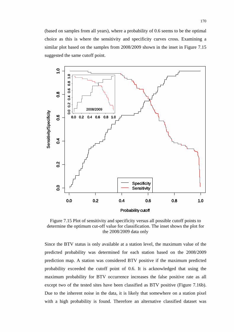
170

(based on samples from all years), where a probability of 0.6 seems to be the optimal

choice as this is where the sensitivity and specificity curves cross. Examining a

similar plot based on the samples from 2008/2009 shown in the inset in Figure 7.15

suggested the same cutoff point.

Probability cutoff

Sen

sitiv

ity/S

peci

ficity

0.0 0.2 0.4 0.6 0.8 1.0

0.0

0.2

0.4

0.6

0.8

1.0

0.0 0.2 0.4 0.6 0.8 1.0

0.0

0.2

0.4

0.6

0.8

1.0

SpecificitySensitivity

0.0 0.2 0.4 0.6 0.8 1.0

0.0

0.2

0.4

0.6

0.8

1.0

2008/2009

Probability cutoff

Sen

sitiv

ity/S

peci

ficity

0.0 0.2 0.4 0.6 0.8 1.0

0.0

0.2

0.4

0.6

0.8

1.0

0.0 0.2 0.4 0.6 0.8 1.0

0.0

0.2

0.4

0.6

0.8

1.0


0.0 0.2 0.4 0.6 0.8 1.0

0.0

0.2

0.4

0.6

0.8

1.0

Probability cutoff

Sen

sitiv

ity/S

peci

ficity

0.0 0.2 0.4 0.6 0.8 1.0

0.0

0.2

0.4

0.6

0.8

1.0

0.0 0.2 0.4 0.6 0.8 1.0

0.0

0.2

0.4

0.6

0.8

1.0


0.0 0.2 0.4 0.6 0.8 1.00.0 0.2 0.4 0.6 0.8 1.0

0.0

0.2

0.4

0.6

0.8

1.0

0.0

0.2

0.4

0.6

0.8

1.0

2008/2009

Figure 7.15 Plot of sensitivity and specificity versus all possible cutoff points to determine the optimum cut-off value for classification. The inset shows the plot for

the 2008/2009 data only

Since the BTV status is only available at a station level, the maximum value of the

predicted probability was determined for each station based on the 2008/2009

prediction map. A station was considered BTV positive if the maximum predicted

probability exceeded the cutoff point of 0.6. It is acknowledged that using the

maximum probability for BTV occurrence increases the false positive rate as all

except two of the tested sites have been classified as BTV positive (Figure 7.16b).

Due to the inherent noise in the data, it is likely that somewhere on a station pixel

with a high probability is found. Therefore an alternative classified dataset was

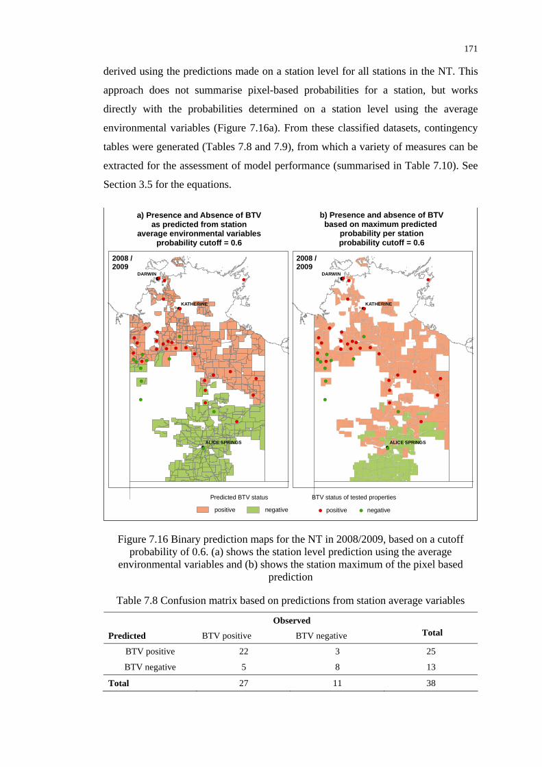
171

derived using the predictions made on a station level for all stations in the NT. This

approach does not summarise pixel-based probabilities for a station, but works

directly with the probabilities determined on a station level using the average

environmental variables (Figure 7.16a). From these classified datasets, contingency

tables were generated (Tables 7.8 and 7.9), from which a variety of measures can be

extracted for the assessment of model performance (summarised in Table 7.10). See

Section 3.5 for the equations.

!

!

!

!(

!( !(

!(

!(

!(

!(

!(

!(

!(

!(

!(

!(

!(

!(

!(

!(

!(

!(

!(!(

!(

!(

!(

!(

!(

!(

!(!(

!(

!(

!(

!(

!(

!(

!(

!(

!(

!(

DARWIN

KATHERINE

ALICE SPRINGS

2008 /2009

a) Presence and Absence of BTVas predicted from station

average environmental variablesprobability cutoff = 0.6

negativepositive !(!(positive

Predicted BTV status

negative

BTV status of tested properties

!

!

!

!(

!( !(

!(

!(

!(

!(

!(

!(

!(

!(

!(

!(

!(

!(

!(

!(

!(

!(

!(!(

!(

!(

!(

!(

!(

!(

!(!(

!(

!(

!(

!(

!(

!(

!(

!(

!(

!(

DARWIN

KATHERINE

ALICE SPRINGS

b) Presence and absence of BTVbased on maximum predicted

probability per stationprobability cutoff = 0.6

2008 /2009

Figure 7.16 Binary prediction maps for the NT in 2008/2009, based on a cutoff probability of 0.6. (a) shows the station level prediction using the average

environmental variables and (b) shows the station maximum of the pixel based prediction

Table 7.8 Confusion matrix based on predictions from station average variables

Observed

Predicted BTV positive BTV negative Total

BTV positive 22 3 25

BTV negative 5 8 13

Total 27 11 38

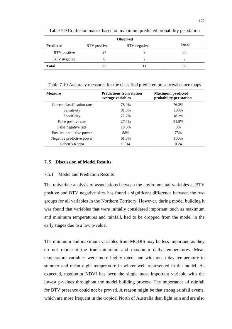
172

Table 7.9 Confusion matrix based on maximum predicted probability per station

Observed

Predicted BTV positive BTV negative Total

BTV positive 27 9 36

BTV negative 0 2 2

Total 27 11 38

Table 7.10 Accuracy measures for the classified predicted presence/absence maps

Measure Predictions from station average variables

Maximum predicted probability per station

Correct classification rate 78.9% 76.3% Sensitivity 81.5% 100% Specificity 72.7% 18.2%

False positive rate 27.3% 81.8% False negative rate 18.5% 0%

Positive predictive power 88% 75% Negative predictive power 61.5% 100%

Cohen’s Kappa 0.514 0.24

7. 5 Discussion of Model Results

7.5.1 Model and Prediction Results

The univariate analysis of associations between the environmental variables at BTV

positive and BTV negative sites has found a significant difference between the two

groups for all variables in the Northern Territory. However, during model building it

was found that variables that were initially considered important, such as maximum

and minimum temperatures and rainfall, had to be dropped from the model in the

early stages due to a low p-value.

The minimum and maximum variables from MODIS may be less important, as they

do not represent the true minimum and maximum daily temperatures. Mean

temperature variables were more highly rated, and with mean day temperature in

summer and mean night temperature in winter well represented in the model. As

expected, maximum NDVI has been the single most important variable with the

lowest p-values throughout the model building process. The importance of rainfall

for BTV presence could not be proved. A reason might be that strong rainfall events,

which are more frequent in the tropical North of Australia than light rain and are also

173

better detectable by TRMM, can limit vector activity. NDVI on the other hand has

been related to the effects of rainfall on the ground (increased humidity, soil

moisture, increased plant growth) which more directly influence vector habitat

conditions. EVI, which contains similar information, was excluded from the model

due to collinearity with NDVI and the disadvantages discussed earlier. The small

NDVI integral which was the only phenological variable used for model

development was not included in the final model. However, its strong relationship

with maximum seasonal NDVI suggests that no information is lost by excluding it

from the model. In addition, generating phenological variables requires data for six

more months after the season ends, whereas all of the variables that are currently

present in the model describe the conditions of the most crucial period in the BTV

cycle early in the year and are available by the end of June. Considering processing

time, the model results may be available in early July. This means that the latest

predictions would be available to NAMP coordinators for their annual meeting in

August each year, where decisions are made on zone boundary changes and the focus

of future surveillance activities.

Model coefficients and the shape of the smooth functions in Figure 7.7 indicate that

the probability of BTV presence is generally higher in areas with high NDVI,

although this relationship is not linear. High average summer day temperatures on

the other hand decrease the probability of BTV presence, which can be explained by

the risk of desiccation, particularly in the southern arid part of the Northern Territory.

Maximum autumn day temperatures, or more precisely the average day temperature

of the warmest 8-day period in autumn has a positive effect on BTV presence up to

about 40°C, but higher temperatures seem to reduce the likelihood of finding the

virus. Higher mean day temperatures in winter positively contribute to the

probability of BTV detection.

As illustrated in Figures 7.9 to 7.11 the predictions from the GAM model

consistently spatially replicate the distribution of BTV in cattle tested between 2000

and 2009. In particular the season 2004/2005, for which dry and hot conditions were

experienced throughout the study area with associated low virus activity,

demonstrates the predictive capabilities of the model. The general pattern of

decreasing BTV presence probability from North to South is present throughout the

174

years analysed, but the divide between high and low probability varies between the

years and largely follows the observed BTV presence. Also, smaller patches of high

and low probability are depicted well (e.g. season 2003/2004) and are confirmed by

the test results.

Comparison of predicted and observed BTV occurrence also reveals that some

positive test results are found in areas of low predicted probability. However, often

there is a small area within a cattle station with a high probability. Without the

knowledge of the true geographical origin of the tested animals, one can assume that

they could have come from these areas. It is therefore recommended that the

maximum observed probability be used as a guideline, when deciding if a property is

to be declared BTV positive or negative.

7.5.2 Model Performance

Assessment of the models predictive and discriminatory ability has been performed

as described in the previous section. The area under the ROC curve has been used as

a measure for the discriminatory ability of the model, which according to the

classification by Hosmer and Lemeshow (2000) is excellent for both internal and

external validation. For the season 2008/2009, from which data have not been

included in model building, the AUC is only slightly lower.

The predicted probability maps have also been classified into presence/absence maps

using a cutoff value of 0.6 to maximise both sensitivity and specificity. It was found

that using the station average variables for predictions on a station level resulted in

the highest overall accuracy (Cohen’s Kappa). However, using the maximum

predicted probability per station decreased the likelihood of false negative

classifications, which is a crucial factor in epidemiology. While economically it

might not seem appropriate to declare a station BTV infected if only a small area has

a high probability of representing a focus for the virus, for Biosecurity reasons, it

might be the less risky approach.

In summary, the necessity to develop and assess a model using station aggregates is

certainly one of the limitations of the study. While it is still possible to identify areas

of higher BTV probability on the prediction maps, one must be aware that the

175

variables used for model development are not directly related to those areas, but

represent the station average conditions. Nevertheless, validation results are

promising and are well suited to complement present surveillance. Particularly in

areas that are less accessible on the ground the remote sensing based prediction

model is advantageous by providing estimates of infection probability for almost the

entire study area.

7. 6 Preliminary Tests of the Model’s Forecasting Capabilities The NAMP technical group holds its annual meeting each August, when a review of

recent BTV activity is provided by the state coordinators. Upon their

recommendations and based on the latest test results, proposed zone changes are

finalised. Additionally, any changes to the location of monitoring sites are decided

upon. Currently, the only underlying data base for these decisions is a web-based

map showing the serological status of the tested properties. An area-wide estimate of

the probability for BTV serpopositivity based on bioclimatic factors is not available

to support the planning of monitoring activities and the definition of zone

boundaries.

To demonstrate that the approach developed in this study is useful for the timely

delivery of model results to decision makers, a preliminary prediction map was

generated from bioclimatic variables derived for the season 2009/2010 (Figure 7.17).

This map is based on the previously described model developed from data collected

between 2000/2001 and 2007/2008. Due to time limitation and the fact that not all

test results had been entered into the NAMP database, no detailed validation was

conducted, but the ground surveillance results available as of November 25, 2010,

have been plotted on the prediction map for illustration. The aggregation periods of

the variables that have been selected for the final model enabled the predictions to be

available by the end of June. While this is not to be considered as “Forecasting” in a

sense that the probability of BTV seropositivity could be predicted before the

beginning of the BTV activity season, the prediction results are available area-wide

before all ground surveillance data are accessible through the NAMP database.

176

!

!

!

DARWIN

KATHERINE

ALICE SPRINGS

!

!

!

DARWIN

KATHERINE

ALICE SPRINGS



Legend

0.8 - 0.90.7 - 0.80.6 - 0.70.5 - 0.60.4 - 0.50.3 - 0.40.2 - 0.30.1 - 0.20.0 - 0.1

Predicted probability0.9 - 1

No Data

Standard error> 0.90.8 - 0.90.7 - 0.80.6 - 0.70.5 - 0.60.4 - 0.50.3 - 0.40.2 - 0.30.1 - 0.20.0 - 0.1No Data

Bluetongue statusof properties testeduntil 30 June 2010

negativepositive

Bluetongue statusof properties testedafter 30 June 2010

negativepositive

(all samples available in the NAMP database by 25 November 2010 have been considered)

Figure 7.17 Preliminary predicted BTV seropositivity in the NT for the season 2009/2010 in relation to the surveyed presence/absence data with the standard error

map indicating the spatially varying accuracy of the prediction

As can be seen in Figure 7.17, particularly in areas where test results became

available after the production of the prediction map, the model has correctly

identified stations at increased risk for seropositivity. It is expected that model

performance can be further improved through recalibration by including data from

the season preceding the forecast period, which in this case 2008/2009.

177

As a consequence of presenting the results for 2009/2010 to NAMP facilitators

during the meeting held in Geelong in August 2010, previously unmonitored possible

risk area have been identified, where vector trapping is likely to be intensified in

future. Also stakeholders from the federal and state government Departments of

Agriculture and Primary Industries were interested in seeing the predictive

capabilities of the model, which can aid in demonstrating Australia’s Biosecurity

efforts to trade partners.

7. 7 Summary Following an initial selection of variables based on their ability to discriminate

between BTV positive and negative sites, variables were also assessed for the

ecological meaning of their associations with BTV. All variables showed significant

differences in the Northern Territory, and most showed significant differences in the

Pilbara, although at a lower magnitude. Differences in effects between the station

average variables and the weighted station average based on carrying capacity were

small and not uniform across variables. Unfortunately, further analyses of the

environment virus relationships unveiled discrepancies in the effects caused by some

of the key variables in the Pilbara. Therefore, model development was progressed

only for the Northern Territory.

A Generalised Additive Model was developed using a stepwise exclusion approach

informed by both statistical significance and the ecological meaning of each variable.

The best performing model according to the area under the ROC curve of 0.8644 is

based on maximum seasonal NDVI (maxndviss), mean day temperature of the

warmest 8-day period in autumn (maxlstdau), the mean day temperature in summer

(meanlstdsu) and the mean night temperature during the previous winter

(meanlstnpw) as the predictor variables. Possible implications of spatial

autocorrelation that might be present between the dependant variables have been

discussed. However, considering the small annual sample size of the multi-annual

dataset used to develop the model further investigations into approaches to account

for spatial effects were not conducted.

The spatial patterns in the annual predicted probability maps generated from the

model corresponded well with the serological status of the tested properties. External

178

model validation was performed with data from the season 2008/2009. The very

good discriminatory ability was again confirmed with an AUC of 0.8215.

Assessment of model performance was also conducted using binary

presence/absence maps. Depending on the classification method a correct

classification rate between 76.3 and 78.9% could be achieved, while importantly the

false negative rate was very low.

It was also demonstrated in Section 7.5 that the model’s capability to generate timely

area-wide prediction maps may provide useful information for decision making

within the management of the NAMP.

179

CHAPTER 8

CONCLUSIONS AND RECOMMENDATIONS

The presence of Bluetongue Virus and other infectious diseases in Australia requires

an efficient and effective surveillance mechanism to control and minimise the risk for

animal health and facilitate safe trade of livestock. Both aspects are important from

a Biosecurity perspective and also for the livestock industries, which are a major

contributor to the Australian economy.

This study demonstrated feasible alternatives to the current labour and cost intensive

surveillance approaches that produce data with large temporal and spatial gaps and

may compromise the integrity of the system in the future. Spatial sciences and remote

sensing technology provide efficient means of gaining information about

environmental conditions on the ground that can be related to the presence of BTV

hosts and vectors and hence define a risk area for transmission. This research has

investigated a number of data sources of environmental and climatic data and

developed a robust and cost-effective methodology to generate environmental

variables to model the distribution of BTV.

This chapter summarises the achievements of the project and gives recommendations

for improvements and future research.

8. 1 Conclusions

A methodology for the spatial and temporal prediction of BTV has been

implemented as a number of successive steps that have been defined to meet the aims

set out in Chapter 1. These steps are reiterated and dealt with individually below.

8.1.1 Review of Bluetongue Epidemiology in Australia to Identify the

Environmental Factors Relating to Host and Vector Dynamics

An extensive review of Bluetongue ecology in Australia has provided an up to date

compilation of what is currently known about competent and in principle vectors,

susceptible hosts and their habitats. It was found that except for C. brevitarsis, little

is still known about the breeding habitats of other Culicoides vectors in the

Australasian region. The environmental factors that are hypothesised to be related to

180

the presence of BTV have therefore been based on the ecology of C. brevitarsis,

which has the most widespread distribution of all vectors found in Australia. The

factors relating to vector survival and activity include rainfall, atmospheric humidity,

air and surface temperature, while vegetation structure and condition are more

important to sustain a critical mass of ruminant hosts. Furthermore, wind has been

associated with long range dispersal, but was not considered in this research which

has concentrated on mapping the general habitat suitability.

This study also compiled valuable information about Bluetongue epidemiology for

areas that have so far received little attention, such as the Pilbara in WA and the

Northern Territory. Within the period under investigation, the Pilbara has

experienced its first outbreak of BTV, followed by varying levels of activity

characteristic for an epidemic area. More recently, the discovery of the competent

vector C. wadai has been documented for the Pilbara. It is anticipated that this thesis

will provide a valuable reference for future research in the area, particularly with the

consideration that the pool of entomologists with knowledge about the ecology of

Culicoides midges in Australia is small.

8.1.2 Identify Relevant Spatial Data Suitable for the Definition of Environmental

Factors that relate to the Distribution of BTV

A variety of data sources have been assessed for their capability to provided relevant

environmental data on the factors previously identified at the spatial and temporal

resolution appropriate for this study. These resolution requirements were mainly

governed by the underlying serological data and the spatial and temporal scope of the

study. Operating in an area with a tropical climate and therefore extensive cloud

cover particularly in the months during and after the wet season demanded a high

temporal resolution in order to obtain sufficient data coverage at least on a

fortnightly to monthly basis. The spatial resolution on the other hand was chosen to

be comparatively low to account for the large area to be analysed on a regional scale

and to minimise processing time. Also, the predominantly climatic factors chosen for

this study act on a regional scale. Other criteria defined for data selection included

the cost of data acquisition, the level of pre-processing and data quality

documentation.

181

Satellite data products from MODIS and TRMM were selected for this research

based on the above criteria and the successful applications of MODIS data in

previous epidemiological studies. The application of TRMM precipitation estimates

for arboviral studies is original to this study and a related project on MVEV

(Schuster et al. 2009).

Although ground-based meteorological datasets have been considered initially, the

complete spatial coverage provided by the remote sensing products utilised is a

distinct advantage while preserving the same patterns as observed by weather

stations. For land surface temperature the spatial coverage is limited to areas with

clear sky conditions.

Due to time constraints, limited human resources, and the lack of suitable data, a

comprehensive assessment of the satellite data products with ground truth data could

not be conducted. The selection of data products is therefore mainly based on

published validation studies and metadata, complemented by exploratory data

analysis to detect larger error in the datasets. These analyses led to the discovery of a

problem in the MODIS vegetation index product due to a shifted cloud mask, which

was not previously known to the research community.

8.1.3 Developing an Efficient and Cost-effective Methodology for the Generation

of Bioclimatic Variables

The multi-stage process of turning the satellite data from MODIS and TRMM into

meaningful bioclimatic variables (describing vegetation condition, land surface

temperature and precipitation) as input for model development has been largely

implemented in a professional GIS environment. Satellite data covering almost 10

years between April 2000 and November 2009 were merged, reprojected and quality

filtered using automated scripts driving the MODIS Reprojection Tool and the

geoprocessing environment of ArcGIS. The entire collection of raster datasets was

stored in the standard GIS compatible GeoTiff format. The resulting time series of

environmental and climatic raster datasets were accumulated into seasonal variables,

and as demanded by the locational precision of the virus data, aggregated on a

pastoral property level using an areal mean.

182

The whole process of generating bioclimatic variables has been implemented in an

efficient manner and the scripts developed can be reused in future, to

semiautomatically process new data as they become available. However, should the

prediction of BTV become operational, it is recommended that a more powerful

dedicated processing environment be set up to replace the standard commercial off

the shelf hardware used in this study.

8.1.4 Assessing the Relationship Between BTV and the Environment

A number of bioclimatic factors have been summarised over four aggregation

periods: annual (November to October), seasonal (November to May), summer

(December to February), autumn (March to May) and the previous winter (June to

August). The hypothesis is that these variables relate to the serological status of a

pastoral property in a particular year (per definition from 1 November to 31

October). The choice of aggregation period was informed by the observed annual

cycle of virus activity.

Univariate analyses were initially conduced to identify those variables that showed

the most significant difference between BTV positive and negative sites and were

therefore most suitable for model development due to their discriminatory qualities.

While investigations showed that all of the candidate variables were significantly

different for the Northern Territory, the effect was less obvious in the Pilbara.

Moreover, some of the variable groups (vegetation indices and rainfall) showed an

unexpected response in virus presence. Following further investigations and

discussions with NAMP coordinators and entomologists it was concluded that the

sampling strategy currently employed in the Pilbara does not provide sufficiently

reliable data for the development of an ecologically sound model.

The final set of variables contributing most to explaining the distribution of BTV in

the Northern Territory was identified during model building and comprises the

following four variables:

• maximum seasonal NDVI (maxndviss);

• mean day temperature of the warmest 8-day period in autumn (meanlstdau);

• mean day temperature in summer (meanlstdsu); and

• mean night temperature during the previous winter (meanlstdnpw).

183

The model building process also identified some of the minimum and maximum

temperature variables and also rainfall as least significant. These observations in the

first case may be explained by the fact that the 8-daily MODIS composite data do not

provide the true minimum and maximum temperatures. The reason for excluding

precipitation from the model indicates that individual rainfall events are less

important for vector ecology than for example the resulting increase of NDVI, which

has been identified as most significant variable.

The necessity to summarise both virus and environmental data spatially (on a

property level) and temporally (on an annual or seasonal basis) can be seen as one of

the major limitations of this study. Much of the information about direct linkages

between environmental variability and the occurrence of BTV is lost through this

process. Since it is not known where tested cattle might have been infected with the

virus, the environmental conditions preceding the infection cannot be accurately

determined. An alternatively weighted average approach has been implemented in

the Pilbara where suitable data on carrying capacity are available. This method

provided better means for discrimination between BTV positive and negative sites

for some variable groups (e.g. small integrated NDVI, maximum day temperatures,

growing degree days, rain), while for others (e.g. maximum NDVI, minimum night

temperatures) it did not provide an advantage over the simpler station average

approach. This suggests that the application of the station average in areas where

suitable carrying capacity data do not exist, which is the case in the Northern

Territory, does not create a disadvantage.

8.1.5 Developing a Spatio-temporal Model to Predict the Distribution of BTV

For the development of a virus distribution model as described in Chapter 7, a GAM

approach was chosen. This is a non-parametric extension of the generalised linear

and logistic regression models frequently used in ecological and epidemiological

modelling. The major advantage of GAMs is their support of response curves not

bound to linear or higher order functions, which rarely describe ecological processes

appropriately.

Amongst the candidate models that have been developed using a stepwise exclusion

approach, the best fitting model has been selected based on the maximisation of the

184

area under the ROC curve (AUC) metric. The final model has been confirmed to

possess excellent discriminatory abilities with an AUC of 0.8644.

Although the model did not account for possible spatial dependencies between

response variables due to the multi-annual data used for model development (see

Section 7.3.3) it can be considered a spatio-temporal model. The spatial component

is given by reference to the environmental conditions at a particular location or

sampled over a particular spatial reference unit. The temporal component is given by

including data that have been sourced over several years and the annual estimates of

BTV seropositivity that have been facilitated by the model.

Annual prediction maps have been produced, which resemble the spatial patterns of

serological status as determined by conventional surveillance, with the additional

advantage of providing an area-wide estimate of potential virus activity based on

suitable environmental conditions. Classified prediction maps have been generated to

aid decision makers in officially declaring the serological status of a pastoral

property and defining boundaries of the BTV infected zone. Additionally, the pixel

based probability maps help to identify areas that principally provide suitable

conditions for virus transmission and should therefore be primarily targeted when

planning strategic sampling locations.

Model validation with external data from the season 2008/2009 has demonstrated

that the model is capable of describing the spatial extent of potential seropositivity in

the current season with a relatively high accuracy, with the degree of success

depending on the measure used for assessment. The AUC of 0.8215 has again shown

that the model has excellent discriminatory abilities in relation to predicting BTV

seropositivity on the basis of station average bioclimatic variables.

8.1.6 Ability of the Model to Complement Ground Based Surveillance

Ample evidence has been given so far that the presented environmental data and the

modelling approach are well suited to reproduce what can be observed on the

ground. However, there is no doubt that the model can only be as good as the input

data and as such, the results of this study are seen as complimentary to the data

produced by conventional surveillance. What this study has demonstrated well, is

185

that the spatial gaps between the sampled pastoral properties may be filled to provide

a more complete image of the actual extent of potential virus activity.

The model can also be used to provide early predictions of seropositivity risk in the

current season. This has been demonstrated at a meeting of the NAMP technical

committee in Geelong in August 2010, where a prediction map for the season

2009/2010 was presented. This map was compiled by the model built with data from

2000/2001 to 2007/2008, but using the most recent bioclimatic variables. The fact

that the model uses data collected during the previous winter as well as the summer

and autumn months means that after data acquisition and processing a prediction can

be generated at the end of June each year. Depending on the timing of the annual

muster, most data collected as part of serological surveys are not available in the

NAMP database much earlier than the predictions. The model therefore has the

capability of acting as an early indicator for potential virus activity hotspots, where

monitoring should be intensified.

As mentioned before, the strength of a model is determined by the data it is built

upon. It is therefore suggested that the increasing archive of virus and environmental

data be used to gradually recalibrate the model, if the major aim is to provide an

early prediction of virus presence before the annual NAMP meeting to be held in

August. By providing such a prediction and identifying pastoral properties which

might host the virus, the risk of undesired events such as BTV infected cattle being

exported can be minimised. Stakeholders from the state and federal Departments of

agriculture therefore indicated strong interest in the results of this research at the

latest NAMP meeting.

8.1.7 Contribution to Knowledge about the Interaction Between the Environment

and the Presence of BTV in the North of Australia

In conclusion, while this study was predominantly dedicated to the investigation of

options for the application of spatial data and technology in the area of

epidemiology, it has also provided new insights into the role of environment factors

in the distribution of an important livestock pathogen. From a set of environmental

variables, those which in combination may best describe the presence of the virus

have been highlighted. The initially hypothesised importance of NDVI was

186

confirmed, as well as the role of temperature. In contrast, accumulated rainfall

variables were excluded from the model due to their low statistical significance. As

discussed previously this may be explained through the relative importance of other

more indirect measures of rainfall effects on the ground.

8. 2 Recommendations

During the implementation of this research some limitations have been identified, but

also opportunities for strengthening and expanding the current approach.

Recommendations and directions for future research are given below.

8.2.1 Optimisation of Monitoring

This research has clearly demonstrated the limitations of using data from an

operational surveillance system such as NAMP, which has been designed

predominantly for fulfilling international Biosecurity requirements. In order to

facilitate more in-depth spatio-temporal studies of virus environmental relationships

based on NAMP data, the following improvements are recommended from the

viewpoint of a spatial scientist:

• Recording spatial information more accurately, including the location of

vector traps, bleeding sites and if known the approximate location where the

tested cattle have been held prior to bleeding;

• Maintain a core network of sentinel herds in strategic locations which are

tested at regular intervals to provide a continuous record of virus activity data

and facilitate comparison of inter-annual variations. The Northern Territory

provides a good example for such a network, which is based on governmental

research stations; and

• Where possible, select the sites for serological surveys based on the perceived

risk (e.g. informed by previous survey results and modelled probability).

It has been acknowledged that any additional monitoring sites cause additional

operational costs, but the costs of losing the good reputation that Australian BTV

surveillance currently enjoys as evident in various publications (e.g. Gibbs and

Greiner 1994; Racloz, Griot, and Stärk 2006) may be much higher.

187

8.2.2 Investigation of Alternative Variables and Data Sources

One of the major aims of this research is to identify factors that are important for the

ecology of BTV and they have been extensively discussed in Chapters 2 and 3.

However, time constraints demanded the use of largely pre-processed and validated

datasets, which have not been available for all factors. Further research is therefore

necessary to investigate the association of other factors with the virus. Of particular

interest are the effects of humidity, air temperature, landscape structure, and cattle

density. Potential data sources need to be identified and assessed.

Potential for future research has also been identified in the 2.5 decades of data from

AVHRR, which could be analysed to make full use of the long records of

epidemiological data from more than 30 years of arbovirus surveillance on Australia.

Also the definition of alternative aggregation periods for the bioclimatic variables is

worth investigating, perhaps using the well known BIOCLIM set of variables (Busby

1991) as a guideline.

In the case of future continuation of this research, the Collection 6 MODIS data

products (to be made available in early 2011) will need to be investigated for

changes from the current Collection 5 data used in this study. It is likely that

Collection 5 processing will be phased out in the foreseeable future and the effects of

using alternative Collection 6 datasets on the model outcome requires further

research.

8.2.3 Applicability of Methodology to Other Regions and Arboviruses

The present approach of using environmental and climate data from remote sensing

satellites to model virus distribution is not limited to BTV. As reviewed in Chapters

3 and 4, similar approaches have been applied to a variety of other viruses and

emerging diseases. Within Australia there exist a number of arboviruses that may

provide an ideal test bed for the methodology. These include Akabane virus, which

like BTV is predominantly transmitted by Culicoides brevitarsis and may therefore

provide additional explanation for observed presence of BTV in an area.

188

It has further been suggested by the members of the NAMP technical committee that

research should be expanded to the eastern states of Australia. Not only have these

parts of the country a longer tradition in Bluetongue epidemiological research, also

the typical size of a farm / pastoral station is smaller than in northern Australia,

allowing for a more accurate determination of environmental factors related to BTV.

189

REFERENCES

Ackerman, S. A., K. I. Strabala, W. P. Menzel, R. A. Frey, C. C. Moeller, and L. E. Gumley. 1998. Discriminating clear sky from clouds with MODIS. Journal of Geophysical Research D: Atmospheres 103 (D24): 32141-32157.

Allepuz, A., I. García-Bocanegra, S. Napp, J. Casal, A. Arenas, M. Saez, and M. A. González. 2010. Monitoring bluetongue disease (BTV-1) epidemic in southern Spain during 2007. Preventive Veterinary Medicine 96 (3-4): 263-271.

Altobelli, A., B. Boemo, K. Mignozzi, M. Bandi, R. Floris, G. Menardi, and M. Cinco. 2008. Spatial Lyme borreliosis risk assessment in north-eastern Italy. International Journal of Medical Microbiology 298 (Supplement 1): 125-128.

Animal Health Australia. 2001. The history of bluetongue, Akabane and ephemeral fever viruses and their vectors in Australia. Deakin, ACT, Australia: Animal Health Australia.

--------. 2006. National Arbovirus Monitoring Program - Report 2005-2006. Australian Animal Health Council.

--------. 2008. National Arbovirus Monitoring Program - 2007-2008 Report. Australian Animal Health Council.

--------. 2009a. Animal Health Surveillance. Quarterly Report. 1 October to 31 December 2008. Animal Health Australia. http://www.animalhealthaustralia.com.au/fms/Animal%20Health%20Australia/ADSP/AHSQ/AHSQ-2009-00-13-(23Mar09)_FINAL(online).pdf (accessed November 22, 2010).

--------. 2009b. National Arbovirus Monitoring Program - 2008-2009 Report. Australian Animal Health Council.

--------. 2010. National Arbovirus Monitoring Program (NAMP). http://www.animalhealthaustralia.com.au/nahis/public.php?page=pub_home&aha_program=2 (accessed November 22, 2010).

Arino, O., P. Bicheron, F. Achard, J. Latham, R. Witt, and J. L. Weber. 2008. GLOBCOVER - The most detailed portrait of Earth. ESA Bulletin 136, November 2008, 24-31.

Aspinall, R., and N. Veitch. 1993. Habitat mapping from satellite imagery and wildlife survey data using a Bayesian modeling procedure in a GIS. Photogrammetric Engineering & Remote Sensing 59 (4): 537-543.

ASTER Mission. 2010. http://asterweb.jpl.nasa.gov/mission.asp (accessed November 22, 2010).

190

Atkinson, P. M., and A. J. Graham. 2006. Issues of Scale and Uncertainty in the Global Remote Sensing of Disease. In Advances in Parasitology, ed. A. G. Simon I. Hay and J. R. David, 79-118. Academic Press.

Attoui, H., S. Maan, S. J. Anthony, and P. P. C. Mertens. 2009. Bluetongue virus, other orbiviruses and other reoviruses: Their relationships and taxonomy. In Bluetongue, 23-52. London: Academic Press.

Austin, M. 2007. Species distribution models and ecological theory: A critical assessment and some possible new approaches. Ecological Modelling 200 (1-2): 1-19.

Austin, M. P. 2002. Spatial prediction of species distribution: An interface between ecological theory and statistical modelling. Ecological Modelling 157 (2-3): 101-118.

Austin, M. P., and J. A. Meyers. 1996. Current approaches to modelling the environmental niche of eucalypts: Implication for management of forest biodiversity. Forest Ecology and Management 85 (1-3): 95-106.

Austin, M. P., A. O. Nicholls, and C. R. Margules. 1990. Measurement of the realized qualitative niche: Environmental niches of five Eucalyptus species. Ecological Monographs 60 (2): 161-177.

Australian Biosecurity CRC for Emerging Infectious Disease. 2010. P3.129EI Post-graduate project: Debbie Eagles: The risk of bluetongue virus introduction into Northern Australia via the airborne spread of Culicoides midges from Indonesia. http://www.abcrc.org.au/pages/project.aspx?projectid=209 (accessed August 16, 2010).

Australian Bureau of Statistics. 2010. Year Book Australia, 2009-10. Canberra. Australian Bureau of Statistics.

Baker, D. G., B. S. Sharratt, H. C. Chiang, J. A. Zandlo, and D. L. Ruschy. 1984. Base temperature selection for the prediction of european corn borer instars by the growing degree day method. Agricultural and Forest Meteorology 32 (1): 55-60.

Baldridge, A. M., S. J. Hook, C. I. Grove, and G. Rivera. 2009. The ASTER spectral library version 2.0. Remote Sensing of Environment 113 (4): 711-715.

Balk, D. L., U. Deichmann, G. Yetman, F. Pozzi, S. I. Hay, and A. Nelson. 2006. Determining Global Population Distribution: Methods, Applications and Data. In Global Mapping of Infectious Diseases: Methods, Examples and Emerging Applications, Advances in Parasitology 62, ed. A. G. Simon I. Hay and J. R. David, 119-156. London: Academic Press.

Batten, C. A., B. Harif, M. R. Henstock, S. Ghizlane, L. Edwards, C. Loutfi, C. A. L. Oura, and M. El Harrak. in press. Experimental infection of camels with bluetongue virus. Research in Veterinary Science:

191

Baylis, Bouayoune, Touti, and E. H. Hasnaoui. 1998. Use of climatic data and satellite imagery to model the abundance of Culicoides imicola, the vector of African horse sickness virus, in Morocco. Medical and Veterinary Entomology 12 (3): 255-266.

Baylis, M., R. Meiswinkel, and G. J. Venter. 1999. A preliminary attempt to use climate data and satellite imagery to model the abundance and distribution of Culicoides imicola (Diptera: Ceratopogonidae) in southern Africa. Journal of the South African Veterinary Association 70 (2): 80-9.

Baylis, M., and P. Rawlings. 1998. Modelling the distribution and abundance of Culicoides imicola in Morocco and Iberia using climatic data and satellite imagery. Archives of Virology, Supplement 1998 (SUPPL. 14): 137-153.

Beard, J. S. 1975a. The vegetation survey of Western Australia. Plant Ecology 30 (3): 179-187.

--------. 1975b. Vegetation Survey of Western Australia. 1:1.000,000 Vegetation Series: Pilbara. Explanatory Notes to Sheet 5. Nedlands, WA: University of Western Australia Press.

Beck, L. R., B. M. Lobitz, and B. L. Wood. 2000. Remote sensing and human health: new sensors and new opportunities. Emerging infectious diseases 6 (3): 217-27.

Beck, L. R., M. H. Rodriguez, S. W. Dister, A. D. Rodriguez, E. Rejmankova, A. Ulloa, R. A. Meza, D. R. Roberts, J. F. Paris, M. A. Spanner, R. K. Washino, C. Hacker, and L. J. Legters. 1994. Remote Sensing as a Landscape Epidemiologic Tool to Identify Villages at High Risk for Malaria Transmission. Am J Trop Med Hyg 51 (3): 271-280.

Beck, P. S. A., C. Atzberger, K. A. Høgda, B. Johansen, and A. K. Skidmore. 2006. Improved monitoring of vegetation dynamics at very high latitudes: A new method using MODIS NDVI. Remote Sensing of Environment 100 (3): 321-334.

Bellis, G. A., and A. L. Dyce. 2005. Intraspecific variation in three species of Culicoides in the Orientalis complex of the subgenus Avaritia within the Australasian zoogeographic region. In Arbovirus research in Australia 9, ed. P. A. Ryan, J. G. Aaskov, T. D. St. George and P. E. R. Dale, 33-36. Brisbane: Queensland Institute of Medical Research.

Bellis, G. A., L. F. Melville, N. T. Hunt, and M. N. Hearnden. 2004. Temporal activity of biting midges (Diptera: Ceratopogonidae) on cattle near Darwin, Northern Territory, Australia. Veterinaria Italiana 40 (3): 324-328.

Bishop, A., H. McKenzie, I. Barchia, and L. Spohr. 2000. Moon phase and other factors affecting light-trap catches of Culicoides brevitarsis Kieffer (Diptera: Ceratopogonidae). Australian Journal of Entomology 39 (1): 29-32.

192

Bishop, A. L., I. M. Barchia, and A. M. Harris. 1995. Last occurrence and survival during winter of the arbovirus vector Culicoides brevitarsis at the southern limits of its distribution. Australian Veterinary Journal 72 (2): 53-55.

Bishop, A. L., I. M. Barchia, and L. J. Spohr. 2000. Models for the dispersal in Australia of the arbovirus vector, Culicoides brevitarsis Kieffer (Diptera: Ceratopogonidae). Preventive Veterinary Medicine 47 (4): 243-254.

Bishop, A. L., G. A. Bellis, H. J. McKenzie, L. J. Spohr, R. J. Worrall, A. M. Harris, and L. Melville. 2006. Light trapping of biting midges Culicoides spp. (Diptera: Ceratopogonidae) with green light-emitting diodes. Australian Journal of Entomology 45 (3): 202-205.

Bishop, A. L., H. J. McKenzie, I. M. Barchia, and A. M. Harris. 1995. The Effects of Habitat on the Distribution of Culicoides Brevitarsis Kieffer (Diptera, Ceratopogonidae) During Its Resting Phase. Australian Journal of Zoology 43 (5): 531-539.

--------. 1996. Effect of Temperature Regimes on the Development, Survival and Emergence of Culicoides brevitarsis Kieffer (Diptera: Ceratopogonidae) in Bovine Dung. Australian Journal of Entomology 35 (4): 361-368.

Bishop, A. L., H. J. McKenzie, L. J. Spohr, and I. M. Barchia. 1994. Cilicoides Brevitarsis Kieffer (Diptera, Ceratopogonidae) in Different Farm Habitats. Australian Journal of Zoology 42 (3): 379-384.

Bishop, A. L., L. J. Spohr, and I. M. Barchia. 2004a. Effects of altitude, distance and waves of movement on the dispersal in Australia of the arbovirus vector, Culicoides brevitarsis Kieffer (Diptera: Ceratopogonidae). Preventive Veterinary Medicine 65 (3-4): 135-145.

--------. 2004b. Factors affecting the spread of Culicoides brevitarsis at the southern limit of distribution in eastern Australia. Veterinaria Italiana 40 (3): 316-319.

Bogh, C., S. W. Lindsay, S. E. Clarke, A. Dean, M. Jawara, M. Pinder, and C. J. Thomas. 2007. High spatial resolution mapping of malaria transmission risk in the Gambia, West Africa, using Landsat TM satellite imagery. American Journal of Tropical Medicine and Hygiene 76 (5): 875-881.

Böhner, J., and O. Antonic. 2009. Land-Surface Parameters Specific to Topo-Climatology. In Developments in Soil Science, ed. H. Tomislav and I. R. Hannes, 195-226. Elsevier.

Boschetti, M., D. Stroppiana, P. A. Brivio, and S. Bocchi. 2009. Multi-year monitoring of rice crop phenology through time series analysis of MODIS images. International Journal of Remote Sensing 30 (18): 4643-4662.

Boyer, T. C., M. P. Ward, and R. S. Singer. 2010. Climate, Landscape, and the Risk of Orbivirus Exposure in Cattle in Illinois and Western Indiana. Am J Trop Med Hyg 83 (4): 789-794.

193

Bradley, B. A., R. W. Jacob, J. F. Hermance, and J. F. Mustard. 2007. A curve fitting procedure to derive inter-annual phenologies from time series of noisy satellite NDVI data. Remote Sensing of Environment 106 (2): 137-145.

Brocklehurst, P., B. Sparrow, B. Wilson, and M. Clark. 2008. A Finer Scale Vegetation Map for the Northern Territory. Technical Report No. 23/2008D. Palmerston, NT: Department of Natural Resources, Environment, The Arts and Sport.

Brooker, S., and E. Michael. 2000. The potential of geographical information systems and remote sensing in the epidemiology and control of human helminth infections. In Remote Sensing and Geographical Information Systems in Epidemiology, Advances in Epidemiology 47, ed. S. I. Hay, S. E. Randolph and D. J. Rogers, 245-270. London: Academic Press.

Brown, H. E., M. A. Diuk-Wasser, Y. Guan, S. Caskey, and D. Fish. 2008. Comparison of three satellite sensors at three spatial scales to predict larval mosquito presence in Connecticut wetlands. Remote Sensing of Environment 112 (5): 2301-2308.

Brunsdon, C., A. S. Fotheringham, and M. E. Charlton. 1996. Geographically weighted regression: A method for exploring spatial nonstationarity. Geographical Analysis 28 (4): 281-298.

Burnham, K. P., and D. R. Anderson. 2002. Model selection and multimodel inference: a practical information-theoretic approach. 2nd ed. New York: Springer.

Busby, J. R. 1991. BIOCLIM - a bioclimate analysis and prediction system. In Nature conservation: cost effective biological surveys and data analysis, ed. C. R. Margules and M. P. Austin, 64-68. Canberra: CSIRO.

Calvete, C., R. Estrada, M. A. Miranda, D. Borrás, J. H. Calvo, and J. Lucientes. 2009. Ecological correlates of bluetongue virus in Spain: Predicted spatial occurrence and its relationship with the observed abundance of the potential Culicoides spp. vector. The Veterinary Journal 182 (2): 235-243.

Cameron, A. R. 2000a. Development of a tempero-spatial disease distribution model for arboviruses and their vectors in Australia. Proceedings of the IXth Symposium of the International Society for Veterinary Epidemiology and Economics (ISVEE), Breckenridge, Colorado, USA, 6-11 August, 2000.

--------. 2000b. Development of an internet-based information system for monitoring veterinary arboviruses and their vectors Proceedings of the IXth Symposium of the International Society for Veterinary Epidemiology and Economics (ISVEE), Breckenridge, Colorado, USA, 6-11 August 2000.

--------. 2004. Data management and analysis systems for bluetongue virus zoning in Australia. Veterinaria Italiana 40 (3): 365-368.

Campbell, J. B. 2007. Introduction to Remote Sensing. 4th ed. New York: Guilford Press.

194

Campbell, M. M., and D. S. Kettle. 1976. Number of Adult Culicoides Brevitarsis Kieffer (Diptera: Ceratopogonidae) Emerging From Bovine Dung Exposed Under Different Conditions in the Field. Australian Journal of Zoology 24 (1): 75-85.

Cesaraccio, C., D. Spano, P. Duce, and R. L. Snyder. 2001. An improved model for determining degree-day values from daily temperature data. International Journal of Biometeorology 45 (4): 161-169.

Chalke, T. 2006. The Utilisation of Remote Sensing and Spatial Analysis for Prediction of Murray Valley Encephalitis Activity in Western Australia. Thesis (MSc), Department of Spatial Sciences, Curtin University of Technology, Perth, Western Australia

Chen, J., P. Jönsson, M. Tamura, Z. Gu, B. Matsushita, and L. Eklundh. 2004. A simple method for reconstructing a high-quality NDVI time-series data set based on the Savitzky-Golay filter. Remote Sensing of Environment 91 (3-4): 332-344.

Cheng, X., Y. Bai, L. Di, and D. Nebert. 2009. Providing public standardized data access function: Lessons learned from accessing USGS Landsat archive. Proceedings of the 17th International Conference on Geoinformatics, Fairfax, VA, August 12-14, 2009.

Cleland, P. C., F. C. Baldock, P. Chamnanpood, and L. J. Gleeson. 1996. Village level risk factors for foot-and-mouth disease in Northern Thailand. Preventive Veterinary Medicine 26 (3-4): 253-261.

Clements, A. C. A., R. Moyeed, and S. Brooker. 2006. Bayesian geostatistical prediction of the intensity of infection with Schistosoma mansoni in East Africa. Parasitology 133 (06): 711-719.

Clements, A. C. A., and D. U. Pfeiffer. 2009. Emerging viral zoonoses: Frameworks for spatial and spatiotemporal risk assessment and resource planning. The Veterinary Journal 182 (1): 21-30.

Clennon, J. A., P. L. Mungai, E. M. Muchiri, C. H. King, and U. Kitron. 2006. Spatial and Temporal Variations in Local Transmission of Schistosoma Haematobium in Msambweni, Kenya. American Journal of Tropical Medicine and Hygiene 75 (6): 1034-1041.

Cliff, A. D., and J. K. Ord. 1973. Spatial autocorrelation. London: Pion.

--------. 1981. Spatial processes : models & applications. London: Pion.

Conte, A., A. Giovannini, L. Savini, M. Goffredo, P. Calistri, and R. Meiswinkel. 2003. The Effect of Climate on the Presence of Culicoides imicola in Italy. Journal of Veterinary Medicine Series B 50 (3): 139-147.

195

Conte, A., C. Ippoliti, L. Savini, M. Goffredo, and R. Meiswinkel. 2007. Novel environmental factors influencing the distribution and abundance of Culicoides imicola and the Obsoletus Complex in Italy. Veterinaria Italiana 43 (3): 571-580.

Cressie, N. A. C. 1993. Statistics for spatial data. Rev. ed, Wiley series in probability and mathematical statistics. Applied probability and statistics. New York: Wiley.

Cresswell, M. P., A. P. Morse, M. C. Thomson, and S. J. Connor. 1999. Estimating surface air temperatures, from Meteosat land surface temperatures, using an empirical solar zenith angle model. International Journal of Remote Sensing 20 (6): 1125-1132.

CSIRO and Bureau of Meteorology. 2007. Climate Change in Australia. Australia Greenhouse Office. www.climatechangeinaustralia.gov.au (accessed November 23, 2010).

Curran, P., and P. Atkinson. 1999. Issues of scale and optimal pixel size. In Spatial Statistics for Remote Sensing, ed. A. Stein, F. Van der Meer and B. Gorte, 115-133. Dordrecht: Kluwer Academic Publishers.

Curran, P. J., P. M. Atkinson, G. M. Foody, and E. J. Milton. 2000. Linking remote sensing, land cover and disease. In Remote Sensing and Geographical Information Systems in Epidemiology, Advances in Epidemiology 47, ed. S. I. Hay, S. E. Randolph and D. J. Rogers, 37-78. London: Academic Press.

Dale, P. E. R., S. A. Ritchie, B. M. Territo, C. D. Morris, A. Muhar, and B. H. Kay. 1998. An Overview of Remote Sensing and GIS for Surveillance of Mosquito Vector Habitats and Risk Assessment. Journal of Vector Ecology 23 (1): 54-61.

Daly, A., and L. Tran-Nguyen. 2008. Grapevine Leaf Rust - Incursion Risk Analysis and Improvement of PCR Diagnostics (Project 1D). Final Report to Grape and Wine Research & Development Corporation. Darwin, NT

Daniels, P. W., I. Sendow, L. I. Pritchard, Sukarsih, and B. T. Eaton. 2004. Regional overview of bluetongue viruses in South-East Asia: viruses, vectors and surveillance. Veterinaria Italiana 40 (3): 94-100.

Dascălu, L., A. Ionescu, and V. Rizac. 2007. Weather stations and the data reports from Romania as part of the East-BTNet project. Veterinaria Italiana 43 (3): 519-526.

De La Rocque, S., V. Michel, D. Plazanet, and R. Pin. 2004. Remote sensing and epidemiology: examples of applications for two vector-borne diseases. Comparative Immunology, Microbiology and Infectious Diseases 27 (5): 331-341.

196

Department of Agriculture and Food Western Australia. 2006. Annual Pastoral Land Condition Report 2005/2006 Financial Year. South Perth, WA: Department of Agriculture and Food Western Australia. http://lands.rdl.wa.gov.au/mediaFiles/WA_Pastoral_Land_Condition_Report_2005-06.pdf (accessed November 22, 2010).

Didan, K., and A. Huete. 2006. MODIS Vegetation Index Product Series Collection 5 Change Summary. TBRS Lab, The University of Arizona. http://landweb.nascom.nasa.gov/QA_WWW/forPage/MOD13_VI_C5_Changes_Document_06_28_06.pdf (accessed 13 October 2010).

Dietz, K., L. Molineaux, and A. Thomas. 1974. A malaria model tested in the African Savannah. Bulletin of the World Health Organization 50 (3-4): 347-357.

Diggle, P. J., and P. J. Ribeiro. 2007. Model-based Geostatistics, Springer Series in Statistics S. Dordrecht: Springer.

Dormann, C. F., J. M. McPherson, M. B. Araújo, R. Bivand, J. Bolliger, G. Carl, R. G. Davies, A. Hirzel, W. Jetz, W. D. Kissling, I. Kühn, R. Ohlemüller, P. R. Peres-Neto, B. Reineking, B. Schröder, F. M. Schurr, and R. Wilson. 2007. Methods to account for spatial autocorrelation in the analysis of species distributional data: A review. Ecography 30 (5): 609-628.

Doyle, K. A. 1989. Arboviruses as they relate to export and imports of livestock and genetic material. In Arbovirus research in Australia 5, ed. M. F. Uren, J. Blok and L. H. Manderson, 347-350. Brisbane: CSIRO. Division of Tropical Animal Science and Queensland Institute of Medical Research.

Draper, C. S., J. P. Walker, P. J. Steinle, R. A. M. de Jeu, and T. R. H. Holmes. 2009. An evaluation of AMSR-E derived soil moisture over Australia. Remote Sensing of Environment 113 (4): 703-710.

Ducheyne, E., R. De Deken, S. Bécu, B. Codina, K. Nomikou, O. Mangana-Vougiaki, G. Georgiev, B. V. Purse, and G. Hendickx. 2007. Quantifying the wind dispersal of Culicoides species in Greece and Bulgaria. Geospatial Health 1 (2): 177-189.

Durr, P. A., and A. E. A. Froggatt. 2002. How best to geo-reference farms?: A case study from Cornwall, England. Preventive Veterinary Medicine 56 (1): 51-62.

Durr, P. A., and A. C. Gattrell. 2004. GIS and spatial analysis in veterinary science. Wallingford, Oxon, UK: CABI Publishing.

Dwyer, J., and G. Schmidt. 2006. The MODIS Reprojection Tool. In Earth Science Satellite Remote Sensing, ed. J. J. Qu, W. Gao, M. Kafatos, R. E. Murphy and V. V. Salomonson, 162-177. Springer Berlin Heidelberg.

Dyce, A. L. 1982. Distribution of Culicoides (Avaritia) spp. (Diptera: Ceratopogonidae) west of the Pacific Ocean. In Arbovirus Research in Australia 3, ed. T. D. St. George and B. H. Kay, 35-43. Brisbane: CSIRO and Queensland Institute of Medical Research.

197

Ebert, E. E. 2004. International Precipitation Working Group (IPWG) Workshop, 25-28 October 2004: Monitoring the quality of operational and semi-operational satellite precipitation estimates – the IPWG validation/intercomparison study. Monterey, California, USA:

--------. 2007. Validation / intercomparison of satellite precipitation estimates over Australia. http://www.bom.gov.au/bmrc/SatRainVal/sat_val_aus.html (accessed November 2, 2010).

Ebert, E. E., J. E. Janowiak, and C. Kidd. 2007. Comparison of near-real-time precipitation estimates from satellite observations and numerical models. Bulletin of the American Meteorological Society 88 (1): 47-64.

Ebert, E. E., and M. J. Manton. 1998. Performance of Satellite Rainfall Estimation Algorithms during TOGA COARE. Journal of the Atmospheric Sciences 55 (9): 1537-1557.

Eisen, R. J., L. Eisen, and R. S. Lane. 2006. Predicting density of Ixodes pacificus nymphs in dense woodlands in Mendocino County, California, based on geographic information systems and remote sensing versus field-derived data. The American journal of tropical medicine and hygiene 74 (4): 632-40.

Eklundh, L., and P. Jönsson. 2010. Timesat 3.0 Software Manual. Lund, Sweden: Lund University.

Erasmus, B. J., and A. C. Potgieter. 2009. The history of bluetongue. In Bluetongue, 7-21. London: Academic Press.

ERDAS Inc. 2008. ERDAS Imagine, version 9.2 (program).

ESRI Inc. 2008. ArcGIS, version 9.3 (program).

Faruolo, M., I. Coviello, T. Lacava, N. Pergola, and V. Tramutoli. 2009. Geoscience and Remote Sensing Symposium,2009 IEEE International,IGARSS 2009, 12-17 July 2009: Real time monitoring of flooded areas by a multi-temporal analysis of optical satellite data. 10.1109/IGARSS.2009.5417339 (accessed

Fawcett, T. 2006. An introduction to ROC analysis. Pattern Recognition Letters 27 (8): 861-874.

Fielding, A. H., and J. F. Bell. 1997. A review of methods for the assessment of prediction errors in conservation presence/absence models. Environmental Conservation 24 (01): 38-49.

Foxi, C., and G. Delrio. 2010. Larval habitats and seasonal abundance of Culicoides biting midges found in association with sheep in northern Sardinia, Italy. Medical and Veterinary Entomology 24 (2): 199-209.

Freeman, E. A., and G. G. Moisen. 2008. A comparison of the performance of threshold criteria for binary classification in terms of predicted prevalence and kappa. Ecological Modelling 217 (1-2): 48-58.

198

Friedl, M. A., D. Sulla-Menashe, B. Tan, A. Schneider, N. Ramankutty, A. Sibley, and X. Huang. 2010. MODIS Collection 5 global land cover: Algorithm refinements and characterization of new datasets. Remote Sensing of Environment 114 (1): 168-182.

Ganguly, S., M. A. Friedl, B. Tan, X. Zhang, and M. Verma. 2010. Land surface phenology from MODIS: Characterization of the Collection 5 global land cover dynamics product. Remote Sensing of Environment 114 (8): 1805-1816.

Gao, B. C., and Y. J. Kaufman. 2003. Water vapor retrievals using moderate resolution Imaging spectroradiometer (MODIS) near-infrared channels. Journal of Geophysical Research-Atmospheres 108 (D13): ACH 4-1 - ACH 4-10.

Gard, G. P., J. E. Shorthose, R. P. Weir, S. J. Walsh, and L. F. Melville. 1988. Arboviruses recovered from sentinel livestock in Northern Australia. Veterinary Microbiology 18 (2): 109-118.

Gardner, C. A. 1928. Vegetation map of Western Australia, edited by S. l. Kessell, Conservator of Forests. Perth, WA. Forests Department Western Australia.

Geoscience Australia. 2006. GEODATA TOPO 250K Series 3 User Guide. Canberra: Geoscience Australia.

Gibbs, E. P. J., and E. C. Greiner. 1994. The epidemiology of bluetongue. Comparative Immunology, Microbiology and Infectious Diseases 17 (3-4): 207-220.

Gibson, L. A., B. A. Wilson, D. M. Cahill, and J. Hill. 2004. Spatial prediction of rufous bristlebird habitat in a coastal heathland: a GIS-based approach. Journal of Applied Ecology 41 (2): 213-223.

Gilbert, E. W. 1958. Pioneer Maps of Health and Disease in England. The Geographical Journal 124 (2): 172-183.

Gill, T. K., S. R. Phinn, J. D. Armston, and B. A. Pailthorpe. 2009. Estimating tree-cover change in Australia: Challenges of using the MODIS vegetation index product. International Journal of Remote Sensing 30 (6): 1547-1565.

Global Precipitation Measurement. 2010. http://gpm.gsfc.nasa.gov/ (accessed November 22, 2010).

Goetz, S. J., S. D. Prince, and J. Small. 2000. Advances in satellite remote sensing of environmental variables for epidemiological applications. In Advances in Parasitology 47, ed. S. I. Hay, S. E. Randolph and D. J. Rogers, 289-307. London, UK: Academic Press.

Gould, E. A., and S. Higgs. 2009. Impact of climate change and other factors on emerging arbovirus diseases. Transactions of the Royal Society of Tropical Medicine and Hygiene 103 (2): 109-121.

199

Graham, A. J., P. M. Atkinson, and F. M. Danson. 2004. Spatial analysis for epidemiology. Acta Tropica 91 (3): 219-225.

Graham, K., M. Trueman, and C. Yates. 2008. Monitoring Land Condition in Tropical Savannah Rangelands Using MODIS Imagery in the Northern Territory. Proceedings of the 14th Australasian Remote Sensing and Photogrammetry Conference, Darwin, Northern Territory, Australia, 29 September - 3 October 2008.

Granger, R. J. 2000. Satellite-derived estimates of evapotranspiration in the Gediz basin. Journal of Hydrology 229 (1-2): 70-76.

Green, R. M., and S. I. Hay. 2002. The potential of Pathfinder AVHRR data for providing surrogate climatic variables across Africa and Europe for epidemiological applications. Remote Sensing of Environment 79 (2-3): 166-175.

Guis, H., A. Tran, S. de La Rocque, T. Baldet, G. Gerbier, B. Barragué, F. Biteau-Coroller, F. Roger, J.-F. Viela, and F. Maunya. 2007. Use of high spatial resolution satellite imagery to characterize landscapes at risk for bluetongue. Veterinary Research 38: 669-683.

Guisan, A., T. C. Edwards, and T. Hastie. 2002. Generalized linear and generalized additive models in studies of species distributions: setting the scene. Ecological Modelling 157 (2-3): 89-100.

Guisan, A., S. B. Weiss, and A. D. Weiss. 1999. GLM versus CCA spatial modeling of plant species distribution. Plant Ecology 143 (1): 107-122.

Guisan, A., and N. E. Zimmermann. 2000. Predictive habitat distribution models in ecology. Ecological Modelling 135 (2-3): 147-186.

Hamilton, J. S., C. R. Chilcott, and D. B. Savage. 2008. Contemporary livestock carrying capacities for pastoral properties in Northern Australia: A methodology for integrating objective data on pasture growth and condition. Australian Journal of Experimental Agriculture 48 (7): 735-740.

Hanley, K. A., and S. C. Weaver. 2008. Arbovirus evolution. In Origin and Evolution of Viruses (Second Edition), ed. D. Esteban, R. P. Colin and J. H. John, 351-391. London: Academic Press.

Harrell, F. E., K. L. Lee, and D. B. Mark. 1996. Multivariate prognostic models: issues in developing models, evaluating assumptions and adequacy, and measuring and reducing errors. Statistics in Medicine 15 (4): 361-387.

Hashimoto, H., J. L. Dungan, M. A. White, F. Yang, A. R. Michaelis, S. W. Running, and R. R. Nemani. 2008. Satellite-based estimation of surface vapor pressure deficits using MODIS land surface temperature data. Remote Sensing of Environment 112 (1): 142-155.

200

Hassan, Q. K., C. P. Bourque, F.-R. Meng, and W. Richards. 2007. Spatial mapping of growing degree days: an application of MODIS-based surface temperatures and enhanced vegetation index. Journal of Applied Remote Sensing 1: 1-12.

Hastie, T. J., and R. J. Tibshirani. 1990. Generalized additive models. London: Chapman and Hall.

Hay, S. I. 2000. An overview of remote sensing and geodesy for epidemiology and public health application. In Remote Sensing and Geographical Information Systems in Epidemiology, Advances in Epidemiology 47, ed. S. I. Hay, S. E. Randolph and D. J. Rogers, 1-35. London: Academic Press.

Hay, S. I., A. Graham, and D. Rogers, J., eds. 2006. Global Mapping of Infectious Diseases: Methods, Examples and Emerging Applications, Advances in Parasitology 62. London: Academic Press.

Hay, S. I., and J. J. Lennon. 1999. Deriving meteorological variables across Africa for the study and control of vector-borne disease: a comparison of remote sensing and spatial interpolation of climate. Tropical Medicine & International Health 4 (1): 58-71.

Hay, S. I., S. E. Randolph, and D. J. Rogers, eds. 2000. Remote Sensing and Geographical Information Systems in Epidemiology, Advances in Parasitology 47. London: Academic Press.

Hay, S. I., R. W. Snow, and D. J. Rogers. 1998. Predicting malaria seasons in Kenya using multitemporal meteorological satellite sensor data. Transactions of the Royal Society of Tropical Medicine and Hygiene 92 (1): 12-20.

Hay, S. I., A. J. Tatem, A. J. Graham, S. J. Goetz, and D. J. Rogers. 2006. Global Environmental Data for Mapping Infectious Disease Distribution. In Global Mapping of Infectious Diseases: Methods, Examples and Emerging Applications, Advances in Parasitology 62, ed. S. I. Hay, A. J. Graham and D. J. Rogers, 37-77. London: Academic Press.

Hay, S. I., C. J. Tucker, D. J. Rogers, and M. J. Packer. 1996. Remotely sensed surrogates of meteorological data for the study of the distribution and abundance of arthropod vectors of disease. Annals of tropical medicine and parasitology 90 (1): 1-19.

Hayes, R. O., E. L. Maxwell, C. J. Mitchell, and T. L. Woodzick. 1985. Detection, identification, and classification of mosquito larval habitats using remote sensing scanners in earth-orbiting satellites. Bulletin of the World Health Organization 63 (2): 361-74.

Heegaard, E. 2002. The outer border and central border for species-environmental relationships estimated by non-parametric generalised additive models. Ecological Modelling 157 (2-3): 131-139.

201

Hendrickx, G., M. Gilbert, C. Staubach, A. Elbers, K. Mintiens, G. Gerbier, and E. Ducheyne. 2008. A wind density model to quantify the airborne spread of Culicoides species during north-western Europe bluetongue epidemic, 2006. Preventive Veterinary Medicine 87 (1-2): 162-181.

Hengl, T., and H. I. Reuter. 2009. Geomorphometry: Concepts, Software, Applications, Developments in Soil Science 33. Amsterdam: Elsevier.

Herbreteau, V., G. Salem, M. Souris, J.-P. Hugot, and J.-P. Gonzalez. 2007. Thirty years of use and improvement of remote sensing, applied to epidemiology: From early promises to lasting frustration. Health & Place 13 (2): 400-403.

Heumann, B. W., J. W. Seaquist, L. Eklundh, and P. Jönsson. 2007. AVHRR derived phenological change in the Sahel and Soudan, Africa, 1982-2005. Remote Sensing of Environment 108 (4): 385-392.

Hird, J. N., and G. J. McDermid. 2009. Noise reduction of NDVI time series: An empirical comparison of selected techniques. Remote Sensing of Environment 113 (1): 248-258.

Hirt, C., M. S. Filmer, and W. E. Featherstone. 2010. Comparison and validation of the recent freely available ASTER-GDEM ver1, SRTM ver4.1 and GEODATA DEM-9S ver3 digital elevation models over Australia. Australian Journal of Earth Sciences: An International Geoscience Journal of the Geological Society of Australia 57 (3): 337 - 347.

Hirzel, A. H., J. Hausser, D. Chessel, and N. Perrin. 2002. Ecological-niche factor analysis: How to compute habitat-suitability maps without absence data? Ecology 83 (7): 2027-2036.

Hodder, R. M., and W. A. Low. 1978. Grazing distribution of free-ranging cattle at three sites in the Alice Springs district, central Australia. Australian Rangeland Journal 1 (2): 95-105.

Holben, B. N. 1986. Characteristics of maximum-value composite images from temporal AVHRR data. International Journal of Remote Sensing 7 (11): 1417 - 1434.

Holm, A. M., S. W. Cridland, and M. L. Roderick. 2003. The use of time-integrated NOAA NDVI data and rainfall to assess landscape degradation in the arid shrubland of Western Australia. Remote Sensing of Environment 85 (2): 145-158.

Horne, J. K., and D. C. Schneider. 1995. Spatial variance in ecology. Oikos 74 (1): 18-26.

Hoshen, M. B., and A. P. Morse. 2004. A weather-driven model of malaria transmission. Malaria journal 3 (32):

Hosmer, D. W., and S. Lemeshow. 2000. Applied logistic regression. 2nd ed, Wiley series in probability and statistics Texts and references section. New York: Wiley.

202

Huete, A., K. Didan, T. Miura, E. P. Rodriguez, X. Gao, and L. G. Ferreira. 2002. Overview of the radiometric and biophysical performance of the MODIS vegetation indices. Remote Sensing of Environment 83 (1-2): 195-213.

Huete, A. R., R. D. Jackson, and D. F. Post. 1985. Spectral response of a plant canopy with different soil backgrounds. Remote Sensing of Environment 17 (1): 37-53.

Huete, A. R., H. Q. Liu, K. Batchily, and W. van Leeuwen. 1997. A comparison of vegetation indices over a global set of TM images for EOS-MODIS. Remote Sensing of Environment 59 (3): 440-451.

Huete, A. R., T. Miura, Y. Kim, K. Didan, and J. Privette. 2006. Assessments of multisensor vegetation index dependencies with hyperspectral and tower flux data. Proceedings of the SPIE 2006 - Remote Sensing and Modeling of Ecosystems for Sustainability III Conference, San Diego, 13-17 August, 2006.

Huffman, G. J., and D. T. Bolvin. 2009. TRMM and Other Data Precipitation Data Set Documentation. Laboratory for Atmospheres, NASA Goddard Space Flight Center and Science Systems and Applications, Inc. ftp://precip.gsfc.nasa.gov/pub/trmmdocs/3B42_3B43_doc.pdf (accessed October 11, 2010).

Huffman, G. J., D. T. Bolvin, E. J. Nelkin, D. B. Wolff, R. F. Adler, G. Gu, Y. Hong, K. P. Bowman, and E. F. Stocker. 2007. The TRMM Multisatellite Precipitation Analysis (TMPA): Quasi-Global, Multiyear, Combined-Sensor Precipitation Estimates at Fine Scales. Journal of Hydrometeorology 8 (1): 38-55.

Hughes, L. 2003. Climate change and Australia: Trends, projections and impacts. Austral Ecology 28 (4): 423-443.

Huh, O. K., and J. B. Malone. 2001. New tools: potential medical applications of data from new and old environmental satellites. Acta Tropica 79 (1): 35-47.

Hulley, G. C., and S. J. Hook. 2009. Intercomparison of versions 4, 4.1 and 5 of the MODIS Land Surface Temperature and Emissivity products and validation with laboratory measurements of sand samples from the Namib desert, Namibia. Remote Sensing of Environment 113 (6): 1313-1318.

Hutcheon, D. 1902. Malarial catarrhal fever of sheep. Veterinary Record 14: 629–633.

Hutchinson, M., J. Stein, J. Stein, H. Anderson, and P. Tickle. 2008. GEODATA 9 Second DEM and D8. Digital Elevation Model Version 3 and Flow Direction Grid. Canberra, Australia: Geoscience Australia and the Fenner School of Environment and Society, The Australian National University.

203

Intergovernmental Committee on Surveying & Mapping. 2009. Some Commonly Used Map Projections. http://www.icsm.gov.au/mapping/map_projections.html (accessed November 16, 2010).

Isaaks, E. H., and R. M. Srivastava. 1989. An Introduction to Applied Geostatistics. Oxford University Press.

Jackson, R. D., and A. R. Huete. 1991. Interpreting vegetation indices. Preventive Veterinary Medicine 11 (3-4): 185-200.

Jang, J.-D., A. A. Viau, and F. Anctil. 2004. Neural network estimation of air temperatures from AVHRR data. International Journal of Remote Sensing 25 (21): 4541 - 4554.

Janowiak, J. E. 2004. International Precipitation Working Group (IPWG) Workshop, 25-28 October 2004: Validation of satellite-derived rainfall estimates and numerical model forecasts of precipitation over the US. Monterey, California, USA:

Jensen, J. R. 2007. Remote Sensing of the Environment : An Earth Resource Perspective. 2nd ed, Prentice Hall Series in Geographic Information Science. Upper Saddle River, NJ: Pearson Prentice Hall.

Jönsson, P., and L. Eklundh. 2002. Seasonality extraction by function fitting to time-series of satellite sensor data. Geoscience and Remote Sensing, IEEE Transactions on 40 (8): 1824-1832.

--------. 2004. TIMESAT--a program for analyzing time-series of satellite sensor data. Computers & Geosciences 30 (8): 833-845.

Joyce, R. J., J. E. Janowiak, P. A. Arkin, and P. Xie. 2004. CMORPH: A Method that Produces Global Precipitation Estimates from Passive Microwave and Infrared Data at High Spatial and Temporal Resolution. Journal of Hydrometeorology 5 (3): 487-503.

Justice, C. O., J. R. G. Townshend, E. F. Vermote, E. Masuoka, R. E. Wolfe, N. Saleous, D. P. Roy, and J. T. Morisette. 2002. An overview of MODIS Land data processing and product status. Remote Sensing of Environment 83 (1-2): 3-15.

Kalluri, S., P. Gilruth, D. J. Rogers, and M. Szczur. 2007. Surveillance of arthropod vector-borne infectious diseases using remote sensing techniques: a review. PLoS Pathog 3 (10): 1361-71.

Kawamura, H., H. Qin, F. Sakaida, and R. Y. Setiawan. 2010. Hourly sea surface temperature retrieval using the Japanese geostationary satellite, Multi-functional Transport Satellite (MTSAT). Journal of Oceanography 66 (1): 61-70.

204

Kelsall, J. E., and P. J. Diggle. 1998. Spatial variation in risk of disease: a nonparametric binary regression approach. Journal of the Royal Statistical Society: Series C (Applied Statistics) 47 (4): 559-573.

Kidd, C. 2004. International Precipitation Working Group (IPWG) Workshop, 25-28 October 2004: Validation of Satellite Rainfall Estimates over the Mid-latitudes. Monterey, California, USA:

Kirkland, P. D. 2004. Bluetongue viruses, vectors and surveillance in Australia – the current situation and unique features. Veterinaria Italiana 40 (3): 47-50.

Kistemann, T., F. Dangendorf, and J. Schweikart. 2002. New perspectives on the use of Geographical Information Systems (GIS) in environmental health sciences. International Journal of Hygiene and Environmental Health 205 (3): 169-181.

Kitron, U., L. H. Otieno, L. L. Hungerford, A. Odulaja, W. U. Brigham, O. O. Okello, M. Joselyn, M. M. Mohamed-Ahmed, and E. Cook. 1996. Spatial Analysis of the Distribution of Tsetse Flies in the Lambwe Valley, Kenya, Using Landsat TM Satellite Imagery and GIS. Journal of Animal Ecology 65 (3): 371-380.

Kleinschmidt, I., M. Bagayoko, G. Clarke, M. Craig, and D. Le Sueur. 2000. A spatial statistical approach to malaria mapping. International Journal of Epidemiology 29 (2): 355-361.

Kleinschmidt, I., B. Sharp, I. Mueller, and P. Vounatsou. 2002. Rise in malaria incidence rates in south africa: A small-area spatial analysis of variation in time trends. American Journal of Epidemiology 155 (3): 257-264.

Kruskal, W., and A. Wallis. 1952. Use of Ranks in One-Criterion Variance Analysis. Journal of the American Statistical Association 47 (260): 583-621.

Kunkel, K. E., R. J. Novak, R. L. Lampman, and W. Gu. 2006. Modeling the Impact of Variable Climatic Factors On The Crossover of Culex Restauns and Culex Pipiens (Diptera: Culicidae), Vectors of West Nile Virus in Illinois. American Journal of Tropical Medicine and Hygiene 74 (1): 168-173.

Lacaux, J. P., Y. M. Tourre, C. Vignolles, J. A. Ndione, and M. Lafaye. 2007. Classification of ponds from high-spatial resolution remote sensing: Application to Rift Valley Fever epidemics in Senegal. Remote Sensing of Environment 106 (1): 66-74.

Landgate. 2009. SLIP Enabler. https://www2.landgate.wa.gov.au/web/guest/home (accessed November 12, 2010).

Lawson, A. 2008. Bayesian disease mapping hierarchical modeling in spatial epidemiology, Chapman & Hall/CRC interdisciplinary statistics series. Boca Raton: Taylor & Francis.

205

Lawson, A., W. J. Browne, and C. L. Vidal Rodeiro. 2003. Disease mapping with WinBUGS and MLwiN, Statistics in practice. Chichester, West Sussex ; Hoboken, N.J.: Wiley.

Lawson, A. B., and N. Cressie. 2000. Spatial Statistical Methods for Environmental Epidemiology. In Handbook of Statistics, ed. P. K. Sen and C. R. Rao, 357-396. Elsevier.

Lehmann, A. 1998. GIS modeling of submerged macrophyte distribution using Generalized Additive Models. Plant Ecology 139 (1): 113-124.

Levins, R. 1966. The strategy of model building in population biology. American Scientist 54 (4): 421-431.

Li, J., and W. Chen. 2005. A rule-based method for mapping Canada's wetlands using optical, radar and DEM data. International Journal of Remote Sensing 26 (22): 5051-5069.

Lillesand, T. M., R. W. Kiefer, and J. W. Chipman. 2008. Remote Sensing and Image Interpretation. 6th ed. New York: Wiley.

Linthicum, K. J., A. Anyamba, C. J. Tucker, P. W. Kelley, M. F. Myers, and C. J. Peters. 1999. Climate and Satellite Indicators to Forecast Rift Valley Fever Epidemics in Kenya. Science 285 (5426): 397-400.

Liu, A., V. Lee, D. Galusha, M. D. Slade, M. Diuk-Wasser, T. Andreadis, M. Scotch, and P. M. Rabinowitz. 2009. Risk factors for human infection with West Nile Virus in Connecticut: A multi-year analysis. International Journal of Health Geographics 8: art. no. 67.

Lunn, D. J., A. Thomas, N. Best, and D. Spiegelhalter. 2000. WinBUGS - A Bayesian modelling framework: Concepts, structure, and extensibility. Statistics and Computing 10 (4): 325-337.

Lymburner, L., F. Li, P. Tan, N. Mueller, and S. Reddy. 2008. Dynamic land cover mapping from space. AusGeo News.

Lyon, J. G., D. Yuan, R. S. Lunetta, and C. D. Elvidge. 1998. A change detection experiment using vegetation indices. Photogrammetric Engineering and Remote Sensing 64 (2): 143-150.

MacDonald, G. 1957. The epidemiology and control of malaria. London: Oxford University Press.

Maclachlan, N. J., C. P. Drew, K. E. Darpel, and G. Worwa. 2009. The Pathology and Pathogenesis of Bluetongue. Journal of Comparative Pathology 141 (1): 1-16.

Maclachlan, N. J., and G. Gard. 2009. Clinical signs and pathology. In Bluetongue, 285-293. London: Academic Press.

206

Malone, J. B., O. K. Huh, D. P. Fehler, P. A. Wilson, D. E. Wilensky, R. A. Holmes, and A. I. Elmagdoub. 1994. Temperature data from satellite imagery and the distribution of schistosomiasis in Egypt. The American journal of tropical medicine and hygiene 50 (6): 714-22.

Manel, S., H. Ceri Williams, and S. J. Ormerod. 2001. Evaluating presence-absence models in ecology: The need to account for prevalence. Journal of Applied Ecology 38 (5): 921-931.

Martin, V., L. De Simone, J. Lubroth, P. Ceccato, and V. Chevalier. 2008. Perspectives on using remotely-sensed imagery in predictive veterinary epidemiology and global early warning systems. Geospatial Health 2 (1): 3-14.

Martínez, B., and M. A. Gilabert. 2009. Vegetation dynamics from NDVI time series analysis using the wavelet transform. Remote Sensing of Environment 113 (9): 1823-1842.

Mather, P. M. 2004. Computer Processing of Remotely-Sensed Images : An Introduction. 3rd ed. Chichester, West Sussex, England: John Wiley & Sons.

Maude, R. J., Y. Lubell, D. Socheat, S. Yeung, S. Saralamba, W. Pongtavornpinyo, B. S. Cooper, A. M. Dondorp, N. J. White, and L. J. White. 2010. The role of mathematical modelling in guiding the science and economics of malaria elimination. International Health 2 (4): 239-246.

McAtee, B. K., and S. W. Maier. 2006. A comparison of algorithms for Near-Real Time water vapour retrieval from MODIS. International Journal of Remote Sensing 27 (23): 5145-5163.

McCann, C. M., M. Baylis, and D. J. L. Williams. 2010. The development of linear regression models using environmental variables to explain the spatial distribution of Fasciola hepatica infection in dairy herds in England and Wales. International Journal for Parasitology 40 (9): 1021-1028.

McGarigal, K., and B. J. Marks. 1995. FRAGSTATS: spatial pattern analysis program for quantifying landscape structure. General Technical Report - US Department of Agriculture, Forest Service (PNW-GTR-351):

McGarigal, K., and W. C. McComb. 1995. Relationships Between Landscape Structure and Breeding Birds in the Oregon Coast Range. Ecological Monographs 65 (3): 235-260.

McKenzie, N. J., D. W. Jacquier, D. J. Maschmedt, E. A. Griffin, and D. M. Brough. 2005. The Australian Soil Resource Information System. Technical specifications. Australian Collaborative Land Evaluation Program. http://www.asris.csiro.au/downloads/ASRIS%20Tech%20Specs%201.5.pdf (accessed November 2, 2010).

McLeod, K. S. 2000. Our sense of Snow: the myth of John Snow in medical geography. Social Science & Medicine 50 (7-8): 923-935.

207

McLeod, S. R., and A. R. Pople. 2010. Modelling the distribution and relative abundance of feral camels in the Northern Territory using count data. The Rangeland Journal 32 (1): 21-32.

McMaster, G. S., and W. W. Wilhelm. 1997. Growing degree-days: one equation, two interpretations. Agricultural and Forest Meteorology 87 (4): 291-300.

Mellor, P. S. 2001. Bluetongue Virus. In The Encyclopedia of Arthropod-transmitted Infections, ed. M. W. Service, 78-83. Oxon, UK: CABI Publishing.

Mellor, P. S., J. Boorman, and M. Baylis. 2000. Culicoides Biting Midges: Their Role as Arbovirus Vectors. Annual Review of Entomology 45 (1): 307-340.

Mellor, P. S., S. Carpenter, L. Harrup, M. Baylis, and P. P. C. Mertens. 2008. Bluetongue in Europe and the Mediterranean Basin: History of occurrence prior to 2006. Preventive Veterinary Medicine 87 (1-2): 4-20.

Mellor, P. S., S. Carpenter, L. Harrup, M. Baylis, A. Wilson, and P. P. C. Mertens. 2009. Bluetongue in Europe and the Mediterranean Basin. In Bluetongue, 235-264. London: Academic Press.

Mellor, P. S., S. Carpenter, and D. M. White. 2009. Bluetongue virus in the insect host. In Bluetongue, 295-320. London: Academic Press.

Melville, L. F. 2004. Bluetongue surveillance methods in an endemic area: Australia. Veterinaria Italiana 40 (3): 184-187.

Melville, L. F., S. Davis, N. T. Hunt, R. P. Weir, M. Harmsen, and S. J. Walsh. 2009. Isolation of bluetongue serotype 7 from sentinel cattle in the Northern Territory. In Arbovirus research in Australia 10, ed. P. A. Ryan, J. G. Aaskov and R. C. Russell, 99-101. Brisbane: Queensland Institute of Medical Research.

Menzies, F. D., S. J. McCullough, I. M. McKeown, J. L. Forster, S. Jess, C. Batten, A. K. Murchie, J. Gloster, J. G. Fallows, W. Pelgrim, P. S. Mellor, and C. A. L. Oura. 2008. Evidence for transplacental and contact transmission of bluetongue virus in cattle. Veterinary Record 163 (7): 203-209.

Mertens, P. P. C., S. Maan, C. Batten, K. E. Darpel, A. Shaw, N. S. Maan, K. Nomikou, S. J. Anthony, E. Veronesi, C. A. L. Oura, S. Carpenter, and P. S. Mellor. 2009. Bluetongue virus diagnosis. In Bluetongue, 365-395. London: Academic Press.

Michaelides, S., V. Levizzani, E. Anagnostou, P. Bauer, T. Kasparis, and J. E. Lane. 2009. Precipitation: Measurement, remote sensing, climatology and modeling. Atmospheric Research 94 (4): 512-533.

Milne, A. K. 1999. A comparative evaluation of multiband radar for detecting and mapping wetland inundation. Proceedings of the IGARSS '99, Geoscience and Remote Sensing Symposium, Hamburg, Germany, 28 June - 2 July 1999, 1883-1885.

208

MODIS Web. 2010. http://modis.gsfc.nasa.gov/ (accessed November 23, 2010).

Molineaux, L., and G. Gramiccia. 1980. The Garki project: research on the epidemiology and control of malaria in the Sudan savanna of West Africa. Geneva: World Health Organization.

Moore, D. S., G. P. McCabe, and B. A. Craig. 2009. Introduction to the practice of statistics

Moran, P. A. 1950. Notes on continuous stochastic phenomena. Biometrika 37 (1-2): 17-23.

Morisette, J. T., J. L. Privette, and C. O. Justice. 2002. A framework for the validation of MODIS Land products. Remote Sensing of Environment 83 (1-2): 77-96.

Mostovoy, G. V., R. L. King, K. R. Reddy, V. G. Kakani, and M. G. Filippova. 2006. Statistical estimation of daily maximum and minimum air temperatures from MODIS LST data over the State of Mississippi. GIScience and Remote Sensing 43 (1): 78-110.

Muller, M. J., H. A. Standfast, T. D. St. George, and D. H. Cybinski. 1982. Culicoides brevitarsis (Diptera: Ceratopogonidae) as a vector of arboviruses in Australia. In Arbovirus Research in Australia 3, ed. T. D. St. George and B. H. Kay, 43-49. Brisbane: CSIRO and Queensland Institute of Medical Research.

Murray, G. J. 2008. Immediate notification report. OIE Ref 6964. Paris: Office International des Epizootics (OIE). http://www.oie.int/wahis/reports/en_imm_0000006964_20080415_200102.pdf (accessed November 23, 2010).

--------. 2009. Immediate notification report. OIE Ref 7685. Paris: Office International des Epizootics (OIE). http://www.oie.int/wahis/reports/en_imm_0000007685_20090116_143931.pdf (accessed November 23, 2010).

Murray, M. D. 1975. Potential vectors of bluetongue in Australia. Australian Veterinary Journal 51: 216-220.

--------. 1987. Local Dispersal of the Biting-Midge Culicoides-Brevitarsis Kieffer (Diptera, Ceratopogonidae) in Southeastern Australia. Australian Journal of Zoology 35 (6): 559-573.

--------. 1991. The Seasonal Abundance of Female Biting-Midges, Culicoides-Brevitarsis Kieffer (Diptera, Ceratopogonidae), in Coastal South-Eastern Australia. Australian Journal of Zoology 39 (3): 333-342.

Murray, M. D., and P. D. Kirkland. 1995. Bluetongue and Douglas virus activity in New South Wales in 1989: further evidence for long-distance dispersal of the biting midge Culicoides brevitarsis. Australian Veterinary Journal 72 (2): 56-57.

209

Mushinzimana, E., S. Munga, N. Minakawa, L. Li, C. C. Feng, L. Bian, U. Kitron, C. Schmidt, L. Beck, G. Zhou, A. K. Githeko, and G. Yan. 2006. Landscape determinants and remote sensing of anopheline mosquito larval habitats in the western Kenya highlands. Malaria journal 5: 13.

NASA Goodard Space Flight Centre. 2009. Known issues in MOD13 product (Vegetation indices) - Case No SD_MOD13_08324 (NDVI not retrieved for pixels adjacent to coastline in VI suite of products ). http://landweb.nascom.nasa.gov/cgi-bin/QA_WWW/getSummary.cgi?esdt=MOD13 (accessed November 26, 2010).

Neteler, M. 2010. Estimating Daily Land Surface Temperatures in Mountainous Environments by Reconstructed MODIS LST Data. Remote Sensing 2 (1): 333-351.

Nicodemus, F. E. 1965. Directional Reflectance and Emissivity of an Opaque Surface. Appl. Opt. 4 (7): 767-773.

Nicodemus, F. E., J. C. Richmond, J. J. Hsia, I. W. Ginsberg, and T. Limperis. 1977. Geometrical considerations and nomenclature for reflectance. National Bureau of Standards (US) Monograph (160): 1-52.

Njoku, E. G., T. J. Jackson, V. Lakshmi, T. K. Chan, and S. V. Nghiem. 2003. Soil moisture retrieval from AMSR-E. Geoscience and Remote Sensing, IEEE Transactions on 41 (2): 215-229.

NOAA CPC Morphing Technique ("CMORPH") 2010. http://asterweb.jpl.nasa.gov/data.asp (accessed 10 October 2010).

Norman, J. M., and F. Becker. 1995. Terminology in thermal infrared remote sensing of natural surfaces. Agricultural and Forest Meteorology 77 (3-4): 153-166.

Northern Territory of Australia. 2008. Northern Territory Land Information System (NTLIS). http://www.nt.gov.au/ntlis/ (accessed November 13, 2010).

NPOESS. 2010. http://npoess.noaa.gov/index.php (accessed November 23, 2010).

Nychka, D. 1988. Bayesian confidence intervals for smoothing splines. Journal of the American Statistical Association 83: 1134-1143.

O'Brien, R. A. 2004. Spatial decision support for selecting tropical crops and forages in uncertain environments. Thesis (Ph D), Curtin University of Technology. http://adt.curtin.edu.au/theses/available/adt-WCU20050526.144234/

Ogden, N. H., I. K. Barker, G. Beauchamp, S. Brazeau, D. F. Charron, A. Maarouf, M. G. Morshed, C. J. O'Callaghan, R. A. Thompson, D. Waltner-Toews, M. Waltner-Toews, and L. R. Lindsay. 2006. Investigation of ground level and remote-sensed data for habitat classification and prediction of survival of Ixodes scapularis in habitats of southeastern Canada. Journal of medical entomology 43 (2): 403-14.

210

OIE. 2009. Bluetongue. Terrestrial Animal Health Code 2009. International Organisation for Animal Health. http://www.oie.int/eng/normes/Mcode/en_chapitre_1.8.3.htm (accessed November 23, 2010).

Oliver, G. R. 2004. Bluetongue trade issues – an Australian perspective. Veterinaria Italiana 40 (4): 688-690.

Openshaw, S. 1984. The Modifiable Areal Unit Problem, Concepts and Techniques in Modern Geography 38. Norwich: Geo Books.

Ostfeld, R. S., G. E. Glass, and F. Keesing. 2005. Spatial epidemiology: an emerging (or re-emerging) discipline. Trends in Ecology & Evolution 20 (6): 328-336.

Papadopoulos, O., P. S. Mellor, and P. P. C. Mertens. 2009. Bluetongue control strategies. In Bluetongue, 429-452. London: Academic Press.

Pasotti, L., M. Maroli, S. Giannetto, and E. Brianti. 2006. Agrometeorology and models for the parasite cycle forecast. Parassitologia 48 (1-2): 81-83.

Pavlovsky, E. N. 1966. Natural nidality of transmissible diseases: with special reference to the landscape epidemiology of zooanthroponoses. Urbana: Illinois U.P.

Payne, A. L., P. J. Curry, and G. F. Spencer. 1987. An inventory and condition survey of rangelands in the Carnarvon Basin, Western Australia. Technical Bulletin No. 73. South Perth: Dept. of Agriculture Western Australia.

Payne, A. L., W. F. Holman, and A. A. Mitchell. 1988. An inventory and condition survey of rangelands in the Ashburton River catchment, Western Australia. South Perth: Dept. of Agriculture Western Australia.

Pearce, J., and S. Ferrier. 2000. Evaluating the predictive performance of habitat models developed using logistic regression. Ecological Modelling 133 (3): 225-245.

Peel, M. C., B. L. Finlayson, and T. A. McMahon. 2007. Updated world map of the Köppen-Geiger climate classification. Hydrology and Earth System Sciences 11 (5): 1633-1644.

Penman, T. D., D. A. Pike, J. K. Webb, and R. Shine. 2010. Predicting the impact of climate change on Australia's most endangered snake, Hoplocephalus bungaroides. Diversity and Distributions 16 (1): 109-118.

Perry, R. A. 1960. Pasture lands of the Northern Territory, Australia, Land research series no. 5. Melbourne: Commonwealth Scientific and Industrial Research Organization.

Pfeiffer, D., T. P. Robinson, M. Stevenson, K. B. Stevens, D. J. Rogers, and A. C. A. Clements. 2008. Spatial Analysis in Epidemiology. New York: Oxford University Press.

211

Pfeiffer, D. U. 2004. Geographical Information Science and Spatial Analysis in Animal Health. In GIS and Spatial Analysis in Veterinary Science, ed. P. A. Durr and A. C. Gattrell, 205-222. Wallingford, Oxon, UK: CABI Publishing.

Pradier, S., A. Leblond, and B. Durand. 2008. Land cover, landscape structure, and West Nile virus circulation in southern France. Vector-Borne and Zoonotic Diseases 8 (2): 253-263.

Press, S. J., and S. Wilson. 1978. Choosing Between Logistic Regression and Discriminant Analysis. Journal of the American Statistical Association 73 (364): 699-705.

Prigent, C. 2010. Precipitation retrieval from space: An overview. Comptes Rendus Geoscience 342 (4-5): 380-389.

Prihodko, L., and S. N. Goward. 1997. Estimation of air temperature from remotely sensed surface observations. Remote Sensing of Environment 60 (3): 335-346.

Prince, S. D., and S. N. Goward. 1995. Global Primary Production: A Remote Sensing Approach. Journal of Biogeography 22 (4/5): 815-835.

Purse, B. V., M. Baylis, A. J. Tatem, D. J. Rogers, P. S. Mellor, M. Van Ham, A. Chizov-Ginzburg, and Y. Braverman. 2004. Predicting the risk of bluetongue through time: climate models of temporal patterns of outbreaks in Israel. Revue Scientifique et technique de l'office international des epizooties 23 (3): 761-775.

Purse, B. V., B. J. J. McCormick, P. S. Mellor, M. Baylis, J. P. T. Boorman, D. Borras, I. Burgu, R. Capela, S. Caracappa, F. Collantes, C. De Liberato, J. A. Delgado, E. Denison, G. Georgiev, M. E. Harak, S. De La Rocque, Y. Lhor, J. Lucientes, O. Mangana, M. A. Miranda, N. Nedelchev, K. Nomikou, A. Ozkul, M. Patakakis, I. Pena, P. Scaramozzino, A. Torina, and D. J. Rogers. 2007. Incriminating bluetongue virus vectors with climate envelope models. Journal of Applied Ecology 44 (6): 1231-1242.

Purse, B. V., P. S. Mellor, D. J. Rogers, A. R. Samuel, M. P. P. C., and M. Baylis. 2005. Climate change and the recent emergence of bluetongue in Europe. Nature Reviews. Microbiology 3 (2): 171-181.

Purse, B. V., and D. J. Rogers. 2009. Bluetongue virus and climate change. In Bluetongue, 343-364. London: Academic Press.

Purse, B. V., A. J. Tatem, S. Caracappa, D. J. Rogers, P. S. Mellor, M. Baylis, and A. Torina. 2004. Modelling the distributions of Culicoides bluetongue virus vectors in Sicily in relation to satellite-derived climate variables. Medical and Veterinary Entomology 18 (2): 90-101.

R Development Core Team. 2010. R: A Language and Environment for Statistical Computing. Vienna, Austria.

212

Racloz, V., C. Griot, and K. D. Stärk. 2006. Sentinel surveillance systems with special focus on vector-borne diseases. Animal health research reviews / Conference of Research Workers in Animal Diseases 7 (1-2): 71-79.

Reed, B. C., J. F. Brown, D. VanderZee, T. R. Loveland, J. W. Merchant, and D. O. Ohlen. 1994. Measuring phenological variability from satellite imagery. Journal of Vegetation Science 5 (5): 703-714.

Reisen, W. K. 2010. Landscape Epidemiology of Vector-Borne Diseases. Annual Review of Entomology 55 (1): 461-483.

Renzullo, L. 2008. Considerations for the blending of multiple precipitation data sets for hydrological applications. Proceedings of the 4th International Precipitation Working Group Workshop, Beijing, China, 13-17 October 2008.

Richards, J. A., and X. Jia. 2006. Remote Sensing Digital Image Analysis An Introduction. Berlin, Heidelberg: Springer-Verlag Berlin Heidelberg. http://dx.doi.org/10.1007/3-540-29711-1 (accessed August 20, 2010).

Rinaldi, L., V. Musella, A. Biggeri, and G. Cringoli. 2006. New insights into the application of geographical information systems and remote sensing in veterinary parasitology. Geospatial Health 1 (1): 33-47.

Ritchie, S. S. A., and W. W. Rochester. 2001. Wind-blown mosquitoes and introduction of Japanese encephalitis into Australia. Emerging infectious diseases 7 (5): 900-903.

Rizzoli, A., M. Neteler, R. Rosà, W. Versini, A. Cristofolini, M. Bregoli, A. Buckley, and E. A. Gould. 2007. Early detection of tick-borne encephalitis virus spatial distribution and activity in the province of Trento, northern Italy. Geospatial Health 1 (2): 169-176.

Robinson, T., D. Rogers, and B. Williams. 1997a. Mapping tsetse habitat suitability in the common fly belt of Southern Africa using multivariate analysis of climate and remotely sensed vegetation data. Medical and Veterinary Entomology 11 (3): 235-245.

--------. 1997b. Univariate analysis of tsetse habitat in the common fly belt of Southern Africa using climate and remotely sensed vegetation data. Medical and Veterinary Entomology 11 (3): 223-234.

Robinson, T. P. 2000. Spatial statistics and geographical information systems in epidemiology and public health. In Remote Sensing and Geographical Information Systems in Epidemiology, Advances in Parasitology 47, ed. S. I. Hay, S. E. Randolph and D. J. Rogers, 81-128. London: Academic Press.

Robinson, T. P., G. Franceschini, and W. Wint. 2007. The Food and Agriculture Organization's Gridded Livestock of the World. Vet Ital 43 (3): 745-51.

213

Rogers, D. J. 2000. Satellites, space, time and the African trypanosomiases. In Remote Sensing and Geographical Information Systems in Epidemiology, Advances in Parasitology 47, ed. S. I. Hay, S. E. Randolph and D. J. Rogers, 129-171. Academic Press.

--------. 2006. Models for Vectors and Vector-Borne Diseases. In Global Mapping of Infectious Diseases: Methods, Examples and Emerging Applications, ed. S. I. Hay, A. J. Graham and D. J. Rogers, 1-35. London, UK: Academic Press.

Rogers, D. J., S. I. Hay, and M. J. Packer. 1996. Predicting the distribution of tsetse flies in West Africa using temporal Fourier processed meteorological satellite data. Annals of tropical medicine and parasitology 90 (3): 225-41.

Rogers, D. J., and S. E. Randolph. 2006. Climate Change and Vector-Borne Diseases. In Global Mapping of Infectious Diseases: Methods, Examples and Emerging Applications, Advances in Parasitology 62, ed. S. I. Hay, A. J. Graham and D. J. Rogers, 345-381. London: Academic Press.

Rogers, D. J., A. J. Wilson, S. I. Hay, and A. J. Graham. 2006. The Global Distribution of Yellow Fever and Dengue. In Global Mapping of Infectious Diseases: Methods, Examples and Emerging Applications, Advances in Parasitology 62, ed. S. I. Hay, A. J. Graham and D. J. Rogers, 181-220. London: Academic Press.

Roshier, D. A., and R. M. Rumbachs. 2004. Broad-scale mapping of temporary wetlands in arid Australia. Journal of Arid Environments 56 (2): 249-263.

Ross, R. 1911. The prevention of Malaria. 2nd ed. London: Murray.

Rouse, J. W., R. H. Haas, J. A. Schell, and D. W. Deering. 1973. Monitoring vegetation systems in the Great Plains with ERTS. Proceedings of the Third ERTS Symposium, Washington DC, 10 - 14 December, 1973, 309-317.

Roy, D. P., J. S. Borak, S. Devadiga, R. E. Wolfe, M. Zheng, and J. Descloitres. 2002. The MODIS Land product quality assessment approach. Remote Sensing of Environment 83 (1-2): 62-76.

Ruiz, M., L. Chaves, G. Hamer, T. Sun, W. Brown, E. Walker, L. Haramis, T. Goldberg, and U. Kitron. 2010. Local impact of temperature and precipitation on West Nile virus infection in Culex species mosquitoes in northeast Illinois, USA. Parasites & Vectors 3 (1): 19.

Running, S. W., C. O. Justice, V. Salomonson, D. Hall, J. Barker, Y. J. Kaufmann, A. H. Strahler, A. R. Huete, J.-P. Muller, V. Vanderbilt, Z. M. Wan, P. Teillet, and D. Carneggie. 1994. Terrestrial remote sensing science and algorithms planned for EOS/MODIS. International Journal of Remote Sensing 15 (17): 3587 - 3620.

Rushton, S. P., S. J. Ormerod, and G. Kerby. 2004. New paradigms for modelling species distributions? Journal of Applied Ecology 41 (2): 193-200.

214

Russell, R. C., and D. E. Dwyer. 2000. Arboviruses associated with human disease in Australia. Microbes and Infection 2 (14): 1693-1704.

Saegerman, C., D. Berkvens, and P. S. Mellor. 2008. Bluetongue epidemiology in the European Union. Emerging Infectious Diseases 14 (4): 539-544.

Santman-Berends, I. M. G. A., L. van Wuijckhuise, P. Vellema, and P. A. van Rijn. 2010. Vertical transmission of bluetongue virus serotype 8 virus in Dutch dairy herds in 2007. Veterinary Microbiology 141 (1-2): 31-35.

Savitzky, A., and M. J. E. Golay. 1964. Smoothing and Differentiation of Data by Simplified Least Squares Procedures. Analytical Chemistry 36 (8): 1627–1639.

Schaaf, C. B., F. Gao, A. H. Strahler, W. Lucht, X. Li, T. Tsang, N. C. Strugnell, X. Zhang, Y. Jin, J.-P. Muller, P. Lewis, M. Barnsley, P. Hobson, M. Disney, G. Roberts, M. Dunderdale, C. Doll, R. P. d'Entremont, B. Hu, S. Liang, J. L. Privette, and D. Roy. 2002. First operational BRDF, albedo nadir reflectance products from MODIS. Remote Sensing of Environment 83 (1-2): 135-148.

Scharlemann, J. P. W., D. Benz, S. I. Hay, B. V. Purse, A. J. Tatem, G. R. W. Wint, and D. J. Rogers. 2008. Global Data for Ecology and Epidemiology: A Novel Algorithm for Temporal Fourier Processing MODIS Data. PLoS ONE 3 (1): e1408.

Schmetz, J., P. Pili, S. Tjemkes, D. Just, J. Kerkmann, S. Rota, and A. Ratier. 2002. An Introduction to Meteosat Second Generation (MSG). Bulletin of the American Meteorological Society 83 (7): 977-992.

Schnur, M. T., H. Xie, and X. Wang. 2010. Estimating root zone soil moisture at distant sites using MODIS NDVI and EVI in a semi-arid region of southwestern USA. Ecological Informatics In Press, Corrected Proof:

Schuster, G., B. Klingseisen, R. Corner, C. Johansen, and B. Veenendaal. 2009. Remote Sensing - Based Analysis and Modelling of Spatio-Temporal Arbovirus Activity Using Climatic and Other Environmental Variables. Arbovirus Research in Australia 10: 151-158.

Schwartz, J. 1996. Air pollution and hospital admissions for respiratory disease. Epidemiology 7 (1): 20-28.

Segurado, P., and M. B. Araújo. 2004. An evaluation of methods for modelling species distributions. Journal of Biogeography 31 (10): 1555-1568.

Sellers, R. F. 1980. Weather, host and vector--their interplay in the spread of insect-borne animal virus diseases. J Hyg (Lond) 85 (1): 65-102.

--------. 1992. Weather, Culicoides, and the distribution and spread of Bluetongue and African Horse Sickness Viruses. In Bluetongue, African Horse Sickness and Related Orbiviruses. Proceedings of the Second International Symposium, Paris, 17-21 June 1991 ed. T. E. Walton and B. I. Osburn, 284-290. Boca Raton: CRC Press.

215

Seoane, J., J. Bustamante, and R. Diaz-Delgado. 2004. Competing roles for landscape, vegetation, topography and climate in predictive models of bird distribution. Ecological Modelling 171 (3): 209-222.

Shililu, J., T. Ghebremeskel, S. Mengistu, H. Fekadu, M. Zerom, C. Mbogo, J. Githure, W. Gu, R. Novak, and J. C. Beier. 2003. Distribution of anopheline mosquitoes in Eritrea. The American journal of tropical medicine and hygiene 69 (3): 295-302.

Skidmore, A. K., A. Gauld, and P. Walker. 1996. Classification of kangaroo habitat distribution using three GIS models. International Journal of Geographical Information Systems 10 (4): 441-454.

Smith, E., G. Asrar, Y. Furuhama, A. Ginati, A. Mugnai, K. Nakamura, R. Adler, M.-D. Chou, M. Desbois, J. Durning, J. Entin, F. Einaudi, R. Ferraro, R. Guzzi, P. Houser, P. Hwang, T. Iguchi, P. Joe, R. Kakar, J. Kaye, M. Kojima, C. Kummerow, K.-S. Kuo, D. Lettenmaier, V. Levizzani, N. Lu, A. Mehta, C. Morales, P. Morel, T. Nakazawa, S. Neeck, K. i. Okamoto, R. Oki, G. Raju, J. Shepherd, J. Simpson, B. Sohn, E. Stocker, W.-K. Tao, J. Testud, G. Tripoli, E. Wood, S. Yang, and W. Zhang. 2007. International Global Precipitation Measurement (GPM) Program and Mission: An Overview. In Measuring Precipitation From Space: EURAINSAT and the Future, ed. V. Levizzani, P. Bauer and F. J. Turk, 611-653. Springer.

St. George, T. D. 1985. Epidemiology of Bluetongue in Australia: The Vertebrate Hosts. In Bluetongue and related Orbiviruses, ed. T. L. Barber and M. M. Jochim, 519-525. New York: Alan R. Liss.

--------. 1989. An overview of arboviruses affecting domestic animals in Australia. Australian Veterinary Journal 66 (12): 393-395.

--------. 1995. The History of Bluetongue in Australia and the Pacific Islands. In Bluetongue Disease in Southeast Asia and the Pacific, ed. T. D. St. George and P. Kegao, 33-40. Canberra: ACIAR.

Standfast, H. A., A. L. Dyce, and M. J. Muller. 1985. Vectors of Bluetongue Virus in Australia. In Bluetongue and related Orbiviruses, ed. T. L. Barber and M. M. Jochim, 177-186. New York: Alan R. Liss.

Standfast, H. A., and G. F. Maywald. 1992. Modelling for Global Changes Affecting Arboviruses. In Bluetongue, African Horse Sickness and Related Orbiviruses. Proceedings of the Second International Symposium, Paris, 17-21 June 1991 ed. T. E. Walton and B. I. Osburn, 16-20. Boca Raton: CRC Press.

Standfast, H. A., M. J. Muller, and A. L. Dyce. 1992. An overview of bluetongue virus vector biology and ecology in the Oriental and Australasian regions of the Western Pacific. In Bluetongue, African Horse Sickness and Related Orbiviruses. Proceedings of the Second International Symposium, Paris, 17-21 June 1991 ed. T. E. Walton and B. I. Osburn, 253-261. Boca Raton: CRC Press.

216

Stassopoulou, A., M. Petrou, and J. Kittler. 1998. Application of a Bayesian network in a GIS based decision making system. International Journal of Geographical Information Science 12 (1): 23-46.

Stephens, G. L., and C. D. Kummerow. 2007. The Remote Sensing of Clouds and Precipitation from Space: A Review. Journal of the Atmospheric Sciences 64 (11): 3742-3765.

Stevenson, M. A., R. S. Morris, A. B. Lawson, J. W. Wilesmith, J. B. M. Ryan, and R. Jackson. 2005. Area-level risks for BSE in British cattle before and after the July 1988 meat and bone meal feed ban. Preventive Veterinary Medicine 69 (1-2): 129-144.

Stisen, S., I. Sandholt, A. Nørgaard, R. Fensholt, and L. Eklundh. 2007. Estimation of diurnal air temperature using MSG SEVIRI data in West Africa. Remote Sensing of Environment 110 (2): 262-274.

Stöckli, R., E. Vermote, N. Saleous, R. Simmon, and D. Herring. 2006. True color earth data set includes seasonal dynamics. EOS 87 (5): 49-55.

Stöckli, R., and P. L. Vidale. 2004. European plant phenology and climate as seen in a 20-year AVHRR land-surface parameter dataset. International Journal of Remote Sensing 25 (17): 3303-3330.

Stockwell, D., and D. Peters. 1999. The GARP modelling system: Problems and solutions to automated spatial prediction. International Journal of Geographical Information Science 13 (2): 143-158.

Strahler, A. H. 1997. Vegetation canopy reflectance modeling—recent developments and remote sensing perspectives. Remote Sensing Reviews 15 (1): 179 - 194.

Suijdendorp, H. 1980. Pastoral Development and Research in the Pilbara Region of Western Australia. The Rangeland Journal 2 (1): 115-123.

Sutherst, R. W. 2004. Global Change and Human Vulnerability to Vector-Borne Diseases. Clinical Microbiology Reviews 17 (1): 136-173.

Sutherst, R. W., and G. F. Maywald. 1985. A computerised system for matching climates in ecology. Agriculture, Ecosystems & Environment 13 (3-4): 281-299.

Swets, J. A. 1988. Measuring the accuracy of diagnostic systems. Science 240 (4857): 1285-1293.

Tabachnick, B. G., and L. S. Fidell. 2007. Using multivariate statistics. 5th ed. Boston: Pearson/Allyn & Bacon.

Tabachnick, W. J. 1996. Culicoides Variipennis and Bluetongue-Virus Epidemiology in the United States. Annual Review of Entomology 41 (1): 23-43.

217

Tatem, A. J., M. Baylis, P. S. Mellor, B. V. Purse, R. Capela, I. Pena, and D. J. Rogers. 2003. Prediction of bluetongue vector distribution in Europe and north Africa using satellite imagery. Veterinary Microbiology 97 (1-2): 13-29.

Tatem, A. J., S. J. Goetz, and S. I. Hay. 2004. Terra and Aqua: new data for epidemiology and public health. International Journal of Applied Earth Observation and Geoinformation 6 (1): 33-46.

Tatem, A. J., D. J. Rogers, and S. I. Hay. 2006. Global Transport Networks and Infectious Disease Spread. In Global Mapping of Infectious Diseases: Methods, Examples and Emerging Applications, Advances in Parasitology 62, ed. S. I. Hay, A. J. Graham and D. J. Rogers, 293-343. London: Academic Press.

The MathWorks. 2008. MATLAB, version R2008 (program).

Thomson, M. C., and S. J. Connor. 2000. Environmental information systems for the control of arthropod vectors of disease. Medical and Veterinary Entomology 14 (3): 227-244.

Thomson, M. C., S. J. Connor, P. J. Milligan, and S. P. Flasse. 1996. The ecology of malaria - as seen from Earth-observation satellites. Annals of Tropical Medicine and Parasitology 90 (3): 243-64.

Thrusfield, M. V. 2007. Veterinary epidemiology. 3rd ed. Oxford: Blackwell.

Tille, P. 2006. Soil-landscapes of Western Australia’s Rangelands and Arid Interior. Resource Management Technical Report 313. South Perth, WA: Department of Agriculture and Food Western Australia.

Tobler, W. R. 1970. A Computer Movie Simulating Urban Growth in the Detroit Region. Economic Geography 46: 234-240.

Townsend, P. A., and S. J. Walsh. 1998. Modeling floodplain inundation using an integrated GIS with radar and optical remote sensing. Geomorphology 21 (3-4): 295-312.

Townshend, J. R. G., and C. O. Justice. 2002. Towards operational monitoring of terrestrial systems by moderate-resolution remote sensing. Remote Sensing of Environment 83 (1-2): 351-359.

Tran, A., F. Goutard, L. Chamaillé, N. Baghdadi, and D. Lo Seen. 2010. Remote sensing and avian influenza: A review of image processing methods for extracting key variables affecting avian influenza virus survival in water from Earth Observation satellites. International Journal of Applied Earth Observation and Geoinformation 12 (1): 1-8.

TRMM - Tropical Rainfall Measuring Mission. 2010. http://trmm.gsfc.nasa.gov/index.html (accessed November 23, 2010).

218

Tucker, C. J. 1979. Red and photographic infrared linear combinations for monitoring vegetation. Remote Sensing of Environment 8 (2): 127-150.

Turk, J., and P. Bauer. 2006. The International Precipitation Working Group and Its Role in the Improvement of Quantitative Precipitation Measurements. Bulletin of the American Meteorological Society 87 (5): 643-647.

Van Vreeswyk, A. M. E., A. L. Payne, K. A. Leighton, and P. Hennig. 2004. An inventory and condition survey of the Pilbara region, Western Australia. Technical Bulletin No. 92. South Perth, WA: Dept. of Agriculture Western Australia.

Van Vreeswyk, S., and P. Thomas. 2008. Annual Pastoral Land Condition Report 2006/2007 Financial Year. South Perth, WA: Department of Agriculture and Food Western Australia. http://lands.rdl.wa.gov.au/mediaFiles/WA_Pastoral_Land_Condition_Report_2006-07.pdf (accessed November 23, 2010).

Vancutsem, C., P. Ceccato, T. Dinku, and S. J. Connor. 2010. Evaluation of MODIS land surface temperature data to estimate air temperature in different ecosystems over Africa. Remote Sensing of Environment 114 (2): 449-465.

Velthuis, A. G. J., H. W. Saatkamp, M. C. M. Mourits, A. A. de Koeijer, and A. R. W. Elbers. 2010. Financial consequences of the Dutch bluetongue serotype 8 epidemics of 2006 and 2007. Preventive Veterinary Medicine 93 (4): 294-304.

Vermote, E. F., N. Z. El Saleous, and C. O. Justice. 2002. Atmospheric correction of MODIS data in the visible to middle infrared: First results. Remote Sensing of Environment 83 (1-2): 97-111.

Wagner, W., V. Naeimi, K. Scipal, R. de Jeu, and J. Martínez-Fernández. 2007. Soil moisture from operational meteorological satellites. Hydrogeology Journal 15 (1): 121-131.

Walcott, J., and H. Zuo. 2003. Spatial patterns and temporal trends in productivity of Australian agriculture. Proceedings of the 11th Australian Agronomy Conference, Geelong, VIC, Australia, 2 - 6 February 2003.

Walker, P. A., and K. D. Cocks. 1991. HABITAT: a procedure for modelling a disjoint environmental envelope for a plant or animal species. Global Ecology & Biogeography Letters 1 (4): 108-118.

Wan, Z. 2008. New refinements and validation of the MODIS Land-Surface Temperature/Emissivity products. Remote Sensing of Environment 112 (1): 59-74.

--------. 2009. Collection-5 MODIS Land Surface Temperature Products User's Guide. Santa Barbara: ICESS, University of California. http://modis.datamirror.csdb.cn/resource/doc/MOD11_UserGuide.pdf (accessed October 11, 2010).

219

Wan, Z., and J. Dozier. 1996. A generalized split-window algorithm for retrieving land-surface temperature from space. IEEE Transactions on Geoscience and Remote Sensing 34 (4): 892-905.

Wan, Z., and Z.-L. Li. 1997. A physics-based algorithm for retrieving land-surface emissivity and temperature from EOS/MODIS data. IEEE Transactions on Geoscience and Remote Sensing 35 (4): 980-996.

Wan, Z., Y. Zhang, Q. Zhang, and Z.-l. Li. 2002. Validation of the land-surface temperature products retrieved from Terra Moderate Resolution Imaging Spectroradiometer data. Remote Sensing of Environment 83 (1-2): 163-180.

Wan, Z., Y. Zhang, Q. Zhang, and Z.-L. Li. 2004. Quality assessment and validation of the MODIS global land surface temperature. International Journal of Remote Sensing 25 (1): 261 - 274.

Ward, M. P. 1994a. The epidemiology of bluetongue virus in Australia - a review. Australian Veterinary Journal 71 (1): 3-7.

--------. 1994b. The use of discriminant analysis in predicting the distribution of bluetongue virus in Queensland, Australia. Veterinary Research Communications 18 (1): 63-72.

--------. 1996. Seasonality of infection of cattle with bluetongue viruses. Preventive Veterinary Medicine 26 (2): 133-141.

Ward, M. P., and S. J. Johnson. 1996. Bluetongue virus and the southern oscillation index: evidence of an association. Preventive Veterinary Medicine 28 (1): 57-68.

Ward, M. P., and M. C. Thurmond. 1995. Climatic factors associated with risk of seroconversion of cattle to bluetongue viruses in Queensland. Preventive Veterinary Medicine 24 (2): 129-136.

Warren, G. M. R. 2007. Developing land management units using geospatial technologies: an agricultural application. Thesis (PhD), Dept. of Spatial Sciences, Curtin University of Technology, Perth, Western Australia

Washino, R. K., and B. L. Wood. 1994. Application of Remote Sensing to Arthropod Vector Surveillance and Control. American Journal of Tropical Medicine and Hygiene 50 (6): 134-144.

Weymouth, G., G. A. Mills, D. A. Jones, E. E. Ebert, and M. J. Manton. 1999. A continental-scale daily rainfall analysis system. Australian Meteorological Magazine 48 (3): 169-179.

White, M. A., and R. R. Nemani. 2006. Real-time monitoring and short-term forecasting of land surface phenology. Remote Sensing of Environment 104 (1): 43-49.

WHO. 1967. Report of a WHO Scientific Group, Arboviruses and Human Disease. WHO Technical Report Series 369. Geneva: World Health Organisation.

220

Wiegand, C. L., A. J. Richardson, D. E. Escobar, and A. H. Gerbermann. 1991. Vegetation indices in crop assessments. Remote Sensing of Environment 35 (2-3): 105-119.

Wilcox, D. G., and E. A. McKinnon. 1970. A report on the condition of the Gascoyne catchment. Perth: Dept. of Agriculture and Dept. of Lands & Surveys.

Wilson, B. A., P. A. Brocklehurst, M. J. Clark, and K. J. M. Dickinson. 1990. Vegetation survey of the Northern Territory, Australia : explanatory notes to accompany 1:1 000 000 map sheets, Technical report,. [Palmerston, N.T.]: Conservation Commission of the Northern Territory.

Wilson, J. P., and J. C. Gallant. 2000. Terrain analysis: Principles and Applications. New York: Wiley.

Wirth, W. W., and A. A. Hubert. 1989. The Culicoides of southeast Asia (Diptera: Ceratopogonidae), Memoirs of the American Entomological Institute. Gainesville, Florida: American Entomological Institute.

Wittmann, E. J., P. S. Mellor, and M. Baylis. 2001. Using climate data to map the potential distribution of Culicoides imicola (Diptera: Ceratopogonidae) in Europe. OIE Revue Scientifique et Technique 20 (3): 731-740.

Wolfe, R. E., M. Nishihama, A. J. Fleig, J. A. Kuyper, D. P. Roy, J. C. Storey, and F. S. Patt. 2002. Achieving sub-pixel geolocation accuracy in support of MODIS land science. Remote Sensing of Environment 83 (1-2): 31-49.

Wolfe, R. E., D. P. Roy, and E. Vermote. 1998. MODIS land data storage, gridding, and compositing methodology: Level 2 grid. IEEE Transactions on Geoscience and Remote Sensing 36 (4): 1324-1338.

Wood, S. N. 2006. Generalized additive models : an introduction with R, Texts in statistical science. Boca Raton: Chapman & Hall/CRC.

--------. 2010. Package ‘mgcv’. http://cran.r-project.org/web/packages/mgcv/mgcv.pdf (accessed November 9, 2010).

Wu, S. S., X. Qiu, and L. Wang. 2005. Population estimation methods in GIS and remote sensing: A review. GIScience and Remote Sensing 42 (1): 80-96.

Yan, H., J. Wang, M. Wu, and W. Zhou. 2005. A comparison of Modis infrared technique and AMSR-E microwave technique for overland rainfall estimates in midlatitude. Proceedings of the IGARSS '05, Geoscience and Remote Sensing Symposium, 2005, Seoul, Korea, 25 - 29 July, 2005, 5116-5118.

Yan, H., J. Zhang, Y. Hou, and Y. He. 2009. Estimation of air temperature from MODIS data in east China. International Journal of Remote Sensing 30 (23): 6261-6275.

221

Yang, G.-J., A. Gemperli, P. Vounatsou, M. Tanner, X.-N. Zhou, and J. Utzinger. 2006. A growing degree-days based time-series analysis for prediction of Schistosoma japonicum transmission in Jiangsu province, China. American Journal of Tropical Medicine and Hygiene 75 (3): 549-555.

Yee, K. S., T. E. Carpenter, and C. J. Cardona. 2009. Epidemiology of H5N1 avian influenza. Comparative Immunology, Microbiology and Infectious Diseases 32 (4): 325-340.

Yee, T. W., and N. D. Mitchell. 1991. Generalized additive models in plant ecology. Journal of Vegetation Science 2 (5): 587-602.

Zar, J. H. 1999. Biostatistical analysis. 4th ed. Upper Saddle River, N.J.: Prentice Hall.

Zhang, X., M. A. Friedl, C. B. Schaaf, A. H. Strahler, J. C. F. Hodges, F. Gao, B. C. Reed, and A. Huete. 2003. Monitoring vegetation phenology using MODIS. Remote Sensing of Environment 84 (3): 471-475.

Zinszer, K., C. Jauvin, A. Verma, L. Bedard, R. Allard, K. Schwartzman, L. de Montigny, K. Charland, and D. L. Buckeridge. 2010. Residential address errors in public health surveillance data: A description and analysis of the impact on geocoding. Spatial and Spatio-temporal Epidemiology 1 (2-3): 163-168.

Every reasonable effort has been made to acknowledge the owners of copyrighted

material. I would be pleased to hear from any copyright owner who has been omitted

or incorrectly acknowledged.

222

APPENDICES

223

APPENDIX A

NAMP TEST RESULTS FOR BTV IN THE PILBARA FROM SAMPLES COLLECTED BETWEEN 1 NOVEMBER 2000 AND 31 OCTOBER 2009

224

Site_ num State

Bleed_ date Season

Virus_short

Bleed_ type

Num_total

Num_ seroconv Comment

F60 WA 21/06/2002 2001 BT Sentinel 17 0 F60 WA 15/05/2003 2002 BT Sentinel 17 2 F60 WA 27/09/2006 2005 BT Sentinel 10 0 F60 WA 9/10/2009 2008 BT Sentinel 10 0 W006 WA 14/08/2001 2000 BT Serosurv 12 0 W014 WA 12/09/2001 2000 BT Serosurv 25 0 W014 WA 9/09/2003 2002 BT Serosurv 20 0 W015 WA 12/09/2001 2000 BT Serosurv 19 0 W015 WA 19/06/2006 2005 BT Serosurv 30 0 W015 WA 21/08/2007 2006 BT Serosurv 27 0 W023 WA 14/08/2001 2000 BT Serosurv 13 0 W023 WA 24/09/2001 2000 BT Serosurv 16 0 W023 WA 14/06/2006 2005 BT Serosurv 30 0 W023 WA 10/06/2009 2008 BT Serosurv 30 0 W024 WA 30/07/2001 2000 BT Serosurv 20 0 W026 WA 14/08/2001 2000 BT Serosurv 15 0 W034 WA 23/08/2001 2000 BT Serosurv 15 0 W034 WA 20/09/2001 2000 BT Serosurv 9 0 W034 WA 9/09/2003 2002 BT Serosurv 23 0 changed from W109 W039 WA 6/12/2002 2002 BT Serosurv 55 4 W039 WA 30/08/2005 2004 BT Serosurv 30 0 W047 WA 12/12/2000 2000 BT Sentinel 20 0 W047 WA 31/07/2001 2000 BT Sentinel 18 0 W048 WA 14/08/2001 2000 BT Serosurv 12 0 W064 WA 23/05/2001 2000 BT Sentinel 8 1 W065 WA 12/09/2001 2000 BT Serosurv 15 0 W065 WA 9/09/2003 2002 BT Serosurv 22 0 W066 WA 15/08/2001 2000 BT Serosurv 20 1 W066 WA 24/09/2001 2000 BT Serosurv 21 0 W067 WA 14/08/2001 2000 BT Serosurv 12 0 W069 WA 14/08/2001 2000 BT Serosurv 4 0 W069 WA 13/01/2004 2003 BT Serosurv 37 0 W070 WA 15/06/2001 2000 BT Serosurv 10 1 W071 WA 3/09/2001 2000 BT Serosurv 15 0 W072 WA 3/09/2001 2000 BT Serosurv 16 0 W072 WA 31/07/2002 2001 BT Serosurv 11 0 W072 WA 7/08/2002 2001 BT Serosurv 9 0 W072 WA 29/06/2006 2005 BT Serosurv 29 0 W073 WA 14/08/2001 2000 BT Serosurv 14 1 W073 WA 15/06/2001 2000 BT Serosurv 20 1 W073 WA 7/08/2002 2001 BT Serosurv 20 16 W074 WA 14/08/2001 2000 BT Serosurv 12 0 W075 WA 20/09/2001 2000 BT Serosurv 20 0 W075 WA 27/09/2002 2001 BT Serosurv 52 8 W075 WA 14/09/2005 2004 BT Serosurv 30 0 W076 WA 14/08/2001 2000 BT Serosurv 11 0 W076 WA 9/09/2003 2002 BT Serosurv 20 0 W076 WA 31/07/2007 2006 BT Serosurv 40 0 W076 WA 20/08/2002 2001 BT Sentinel 25 0 W076 WA 11/08/2004 2003 BT Sentinel 12 0 W076 WA 31/07/2007 2006 BT Sentinel 22 0

225

Site_ num State

Bleed_ date Season

Virus_short

Bleed_ type

Num_total


W076 WA 18/06/2009 2008 BT Sentinel 24 0 W077 WA 14/08/2001 2000 BT Serosurv 11 0 W078 WA 14/08/2001 2000 BT Serosurv 15 0 W078 WA 31/05/2002 2001 BT Serosurv 20 0 W079 WA 14/08/2001 2000 BT Serosurv 12 0 W080 WA 20/09/2001 2000 BT Serosurv 20 0 W080 WA 24/06/2008 2007 BT Serosurv 30 0 changed from W150 W081 WA 24/09/2001 2000 BT Serosurv 21 0 W081 WA 26/07/2007 2006 BT Serosurv 30 0 W082 WA 14/08/2001 2000 BT Serosurv 13 0 W082 WA 30/07/2001 2000 BT Serosurv 20 0 W082 WA 21/06/2002 2001 BT Serosurv 20 4 W082 WA 14/09/2005 2004 BT Serosurv 27 2 W082 WA 10/07/2007 2006 BT Serosurv 30 1 W082 WA 24/06/2008 2007 BT Serosurv 30 0 W084 WA 28/09/2001 2000 BT Serosurv 21 0 W084 WA 31/10/2003 2002 BT Serosurv 21 1 W084 WA 30/05/2003 2002 BT Sentinel 13 0 W084 WA 3/06/2004 2003 BT Sentinel 16 0 W085 WA 26/06/2008 2007 BT Serosurv 30 0 W085 WA 26/06/2008 2007 BT Serosurv 30 0 W085 WA 19/04/2002 2001 BT Sentinel 24 0 W085 WA 19/04/2002 2001 BT Sentinel 24 0 W085 WA 8/04/2003 2002 BT Sentinel 20 0 W085 WA 8/04/2003 2002 BT Sentinel 20 0 W085 WA 30/08/2004 2003 BT Sentinel 9 0 W085 WA 30/08/2004 2003 BT Sentinel 9 0 W085 WA 30/08/2005 2004 BT Sentinel 15 0 W085 WA 30/08/2005 2004 BT Sentinel 15 0 W086 WA 11/06/2002 2001 BT Sentinel 20 1 W087 WA 9/10/2001 2000 BT Serosurv 22 0 W087 WA 3/05/2006 2005 BT Serosurv 31 0 W088 WA 4/06/2002 2001 BT Serosurv 20 17 W088 WA 23/09/2003 2002 BT Serosurv 18 16 changed from W111 W088 WA 30/03/2004 2003 BT Sentinel 24 1 changed from W111 W088 WA 10/09/2004 2003 BT Sentinel 19 0 changed from W111 W089 WA 14/06/2002 2001 BT Serosurv 14 0 W089 WA 4/12/2002 2002 BT Serosurv 47 0 W089 WA 19/06/2006 2005 BT Serosurv 25 0 W089 WA 11/06/2002 2001 BT Sentinel 14 0 W089 WA 16/06/2003 2002 BT Sentinel 14 0 W093 WA 7/08/2002 2001 BT Serosurv 20 18 W094 WA 23/08/2002 2001 BT Serosurv 20 0 W094 WA 5/11/2005 2005 BT Serosurv 20 4 W094 WA 17/08/2006 2005 BT Serosurv 30 0 W094 WA 24/07/2007 2006 BT Serosurv 30 0 W095 WA 19/11/2002 2002 BT Serosurv 55 9 W095 WA 30/08/2005 2004 BT Serosurv 32 0 W096 WA 28/08/2007 2006 BT Serosurv 31 0 W096 WA 8/04/2003 2002 BT Sentinel 18 0 W096 WA 9/08/2006 2005 BT Sentinel 11 0

226

Site_ num State

Bleed_ date Season

Virus_short

Bleed_ type

Num_total


W098 WA 14/08/2007 2006 BT Serosurv 21 0 W098 WA 22/12/2003 2003 BT Sentinel 29 0 W098 WA 21/05/2004 2003 BT Sentinel 23 0 W098 WA 3/09/2004 2003 BT Sentinel 19 0 W098 WA 8/02/2005 2004 BT Sentinel 18 0 W098 WA 31/05/2005 2004 BT Sentinel 18 0 W098 WA 25/07/2006 2005 BT Sentinel 23 0 W098 WA 13/08/2008 2007 BT Sentinel 9 0 W098 WA 15/06/2009 2008 BT Sentinel 10 0 W099 WA 1/12/2003 2003 BT Serosurv 28 0 W099 WA 8/01/2008 2007 BT Serosurv 21 0 W099 WA 14/05/2004 2003 BT Sentinel 28 0 W099 WA 8/09/2005 2004 BT Sentinel 21 0 W099 WA 1/11/2006 2006 BT Sentinel 27 0 W100 WA 23/11/2004 2004 BT Serosurv 50 0 W100 WA 1/09/2005 2004 BT Sentinel 16 0 W100 WA 22/06/2006 2005 BT Sentinel 16 0 W101 WA 14/08/2003 2002 BT Serosurv 20 0 W101 WA 8/11/2005 2005 BT Serosurv 30 0 W110 WA 9/09/2003 2002 BT Serosurv 22 0 W112 WA 23/09/2003 2002 BT Serosurv 17 0 W126 WA 8/11/2005 2005 BT Serosurv 30 0 W127 WA 8/11/2005 2005 BT Serosurv 30 0 W127 WA 26/05/2009 2008 BT Serosurv 30 0 W128 WA 3/05/2006 2005 BT Serosurv 30 0 W128 WA 25/06/2008 2007 BT Serosurv 30 0 W129 WA 3/05/2006 2005 BT Serosurv 30 0 W129 WA 25/06/2008 2007 BT Serosurv 29 0 W133 WA 8/08/2001 2000 BT Serosurv 8 0 changed from W068 W133 WA 10/08/2006 2005 BT Serosurv 30 0 W133 WA 21/08/2007 2006 BT Serosurv 30 1 W133 WA 18/09/2008 2007 BT Serosurv 30 0 W133 WA 30/09/2009 2008 BT Sentinel 11 0

227

APPENDIX B

NAMP TEST RESULTS FOR BTV IN THE NORTHERN TERRITORY FROM SAMPLES COLLECTED BETWEEN 1 NOVEMBER 2000 AND 31 OCTOBER 2009

228

Site_ num

State Bleed_ date

Season Virus_short

Bleed_ type

Num_total

Num_ seroconv

Comment

108 NT 9/11/2000 2000 BT Sentinel 24 2 changed from T027 108 NT 14/12/2000 2000 BT Sentinel 24 0 changed from T027 108 NT 11/01/2001 2000 BT Sentinel 24 3 changed from T027 108 NT 15/02/2001 2000 BT Sentinel 24 9 changed from T027 108 NT 15/03/2001 2000 BT Sentinel 24 4 changed from T027 108 NT 12/04/2001 2000 BT Sentinel 24 0 changed from T027 108 NT 24/05/2001 2000 BT Sentinel 24 0 changed from T027 108 NT 14/06/2001 2000 BT Sentinel 24 0 changed from T027 108 NT 23/08/2001 2000 BT Sentinel 14 3 changed from T027 108 NT 6/09/2001 2000 BT Sentinel 14 0 changed from T027 108 NT 11/10/2001 2000 BT Sentinel 14 1 changed from T027 108 NT 15/11/2001 2001 BT Sentinel 14 1 changed from T027 108 NT 13/12/2001 2001 BT Sentinel 24 0 changed from T027 108 NT 10/01/2002 2001 BT Sentinel 24 0 changed from T027 108 NT 7/02/2002 2001 BT Sentinel 24 0 changed from T027 108 NT 7/03/2002 2001 BT Sentinel 24 1 changed from T027 108 NT 11/04/2002 2001 BT Sentinel 24 16 changed from T027 108 NT 10/05/2002 2001 BT Sentinel 24 6 changed from T027 108 NT 13/06/2002 2001 BT Sentinel 24 1 changed from T027 108 NT 5/07/2002 2001 BT Sentinel 24 0 changed from T027 108 NT 15/08/2002 2001 BT Sentinel 24 0 changed from T027 108 NT 4/10/2002 2001 BT Sentinel 24 0 changed from T027 108 NT 7/11/2002 2002 BT Sentinel 24 4 changed from T027 108 NT 5/12/2002 2002 BT Sentinel 24 5 changed from T027 108 NT 2/01/2003 2002 BT Sentinel 24 10 changed from T027 108 NT 13/02/2003 2002 BT Sentinel 24 1 changed from T027 108 NT 13/03/2003 2002 BT Sentinel 24 0 changed from T027 108 NT 10/04/2003 2002 BT Sentinel 24 2 changed from T027 108 NT 8/05/2003 2002 BT Sentinel 24 9 changed from T027 108 NT 6/06/2003 2002 BT Sentinel 24 3 changed from T027 108 NT 30/06/2003 2002 BT Sentinel 24 3 changed from T027 108 NT 10/07/2003 2002 BT Sentinel 24 0 changed from T027 108 NT 7/08/2003 2002 BT Sentinel 24 0 changed from T027 108 NT 4/09/2003 2002 BT Sentinel 24 1 changed from T027 108 NT 16/10/2003 2002 BT Sentinel 24 0 changed from T027 108 NT 6/11/2003 2003 BT Sentinel 24 1 changed from T027 108 NT 4/12/2003 2003 BT Sentinel 23 0 changed from T027 108 NT 8/01/2004 2003 BT Sentinel 24 5 changed from T027 108 NT 5/02/2004 2003 BT Sentinel 24 4 changed from T027 108 NT 11/03/2004 2003 BT Sentinel 24 8 changed from T027 108 NT 8/04/2004 2003 BT Sentinel 23 1 changed from T027 108 NT 7/05/2004 2003 BT Sentinel 23 0 changed from T027 108 NT 8/07/2004 2003 BT Sentinel 24 0 changed from T027 108 NT 12/08/2004 2003 BT Sentinel 24 1 changed from T027 108 NT 9/09/2004 2003 BT Sentinel 23 0 changed from T027 108 NT 7/10/2004 2003 BT Sentinel 23 0 changed from T027 108 NT 4/11/2004 2004 BT Sentinel 23 0 changed from T027 108 NT 2/12/2004 2004 BT Sentinel 23 0 changed from T027 108 NT 6/01/2005 2004 BT Sentinel 23 0 changed from T027 108 NT 3/02/2005 2004 BT Sentinel 23 1 changed from T027 108 NT 3/03/2005 2004 BT Sentinel 23 2 changed from T027 108 NT 7/04/2005 2004 BT Sentinel 23 8 changed from T027 108 NT 5/05/2005 2004 BT Sentinel 23 8 changed from T027 108 NT 2/06/2005 2004 BT Sentinel 11 0 changed from T027 108 NT 7/07/2005 2004 BT Sentinel 24 0 changed from T027 108 NT 4/08/2005 2004 BT Sentinel 24 0 changed from T027 108 NT 1/09/2005 2004 BT Sentinel 24 0 changed from T027 108 NT 6/10/2005 2004 BT Sentinel 23 0 changed from T027 108 NT 3/11/2005 2005 BT Sentinel 23 0 changed from T027

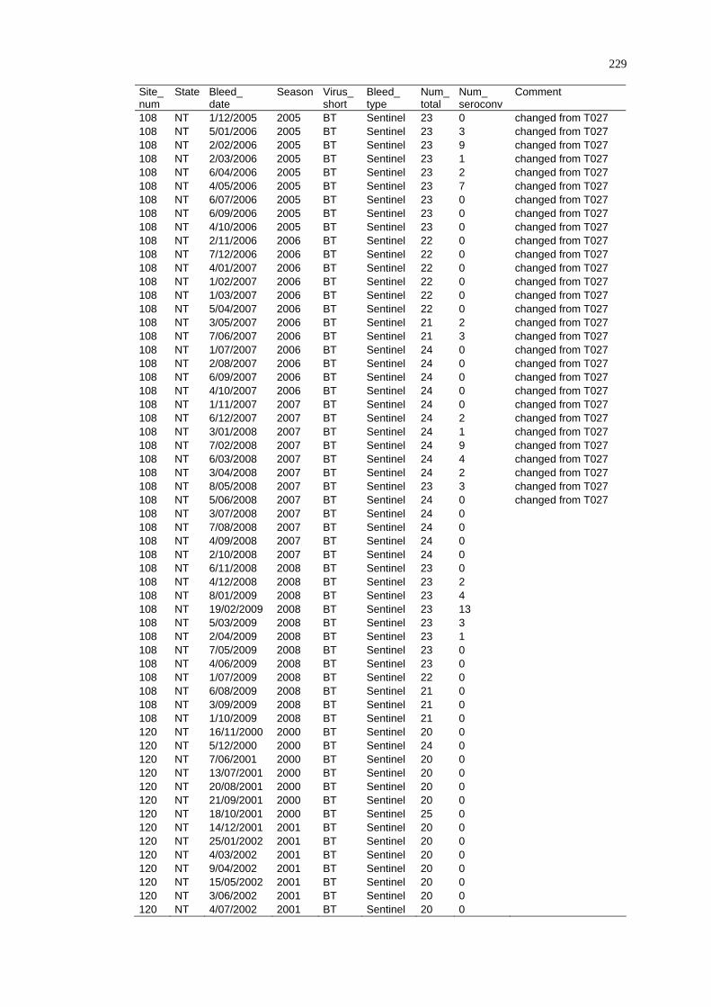
229

Site_ num

State Bleed_ date

Season Virus_short

Bleed_ type

Num_total

Num_ seroconv

Comment

108 NT 1/12/2005 2005 BT Sentinel 23 0 changed from T027 108 NT 5/01/2006 2005 BT Sentinel 23 3 changed from T027 108 NT 2/02/2006 2005 BT Sentinel 23 9 changed from T027 108 NT 2/03/2006 2005 BT Sentinel 23 1 changed from T027 108 NT 6/04/2006 2005 BT Sentinel 23 2 changed from T027 108 NT 4/05/2006 2005 BT Sentinel 23 7 changed from T027 108 NT 6/07/2006 2005 BT Sentinel 23 0 changed from T027 108 NT 6/09/2006 2005 BT Sentinel 23 0 changed from T027 108 NT 4/10/2006 2005 BT Sentinel 23 0 changed from T027 108 NT 2/11/2006 2006 BT Sentinel 22 0 changed from T027 108 NT 7/12/2006 2006 BT Sentinel 22 0 changed from T027 108 NT 4/01/2007 2006 BT Sentinel 22 0 changed from T027 108 NT 1/02/2007 2006 BT Sentinel 22 0 changed from T027 108 NT 1/03/2007 2006 BT Sentinel 22 0 changed from T027 108 NT 5/04/2007 2006 BT Sentinel 22 0 changed from T027 108 NT 3/05/2007 2006 BT Sentinel 21 2 changed from T027 108 NT 7/06/2007 2006 BT Sentinel 21 3 changed from T027 108 NT 1/07/2007 2006 BT Sentinel 24 0 changed from T027 108 NT 2/08/2007 2006 BT Sentinel 24 0 changed from T027 108 NT 6/09/2007 2006 BT Sentinel 24 0 changed from T027 108 NT 4/10/2007 2006 BT Sentinel 24 0 changed from T027 108 NT 1/11/2007 2007 BT Sentinel 24 0 changed from T027 108 NT 6/12/2007 2007 BT Sentinel 24 2 changed from T027 108 NT 3/01/2008 2007 BT Sentinel 24 1 changed from T027 108 NT 7/02/2008 2007 BT Sentinel 24 9 changed from T027 108 NT 6/03/2008 2007 BT Sentinel 24 4 changed from T027 108 NT 3/04/2008 2007 BT Sentinel 24 2 changed from T027 108 NT 8/05/2008 2007 BT Sentinel 23 3 changed from T027 108 NT 5/06/2008 2007 BT Sentinel 24 0 changed from T027 108 NT 3/07/2008 2007 BT Sentinel 24 0 108 NT 7/08/2008 2007 BT Sentinel 24 0 108 NT 4/09/2008 2007 BT Sentinel 24 0 108 NT 2/10/2008 2007 BT Sentinel 24 0 108 NT 6/11/2008 2008 BT Sentinel 23 0 108 NT 4/12/2008 2008 BT Sentinel 23 2 108 NT 8/01/2009 2008 BT Sentinel 23 4 108 NT 19/02/2009 2008 BT Sentinel 23 13 108 NT 5/03/2009 2008 BT Sentinel 23 3 108 NT 2/04/2009 2008 BT Sentinel 23 1 108 NT 7/05/2009 2008 BT Sentinel 23 0 108 NT 4/06/2009 2008 BT Sentinel 23 0 108 NT 1/07/2009 2008 BT Sentinel 22 0 108 NT 6/08/2009 2008 BT Sentinel 21 0 108 NT 3/09/2009 2008 BT Sentinel 21 0 108 NT 1/10/2009 2008 BT Sentinel 21 0 120 NT 16/11/2000 2000 BT Sentinel 20 0 120 NT 5/12/2000 2000 BT Sentinel 24 0 120 NT 7/06/2001 2000 BT Sentinel 20 0 120 NT 13/07/2001 2000 BT Sentinel 20 0 120 NT 20/08/2001 2000 BT Sentinel 20 0 120 NT 21/09/2001 2000 BT Sentinel 20 0 120 NT 18/10/2001 2000 BT Sentinel 25 0 120 NT 14/12/2001 2001 BT Sentinel 20 0 120 NT 25/01/2002 2001 BT Sentinel 20 0 120 NT 4/03/2002 2001 BT Sentinel 20 0 120 NT 9/04/2002 2001 BT Sentinel 20 0 120 NT 15/05/2002 2001 BT Sentinel 20 0 120 NT 3/06/2002 2001 BT Sentinel 20 0 120 NT 4/07/2002 2001 BT Sentinel 20 0

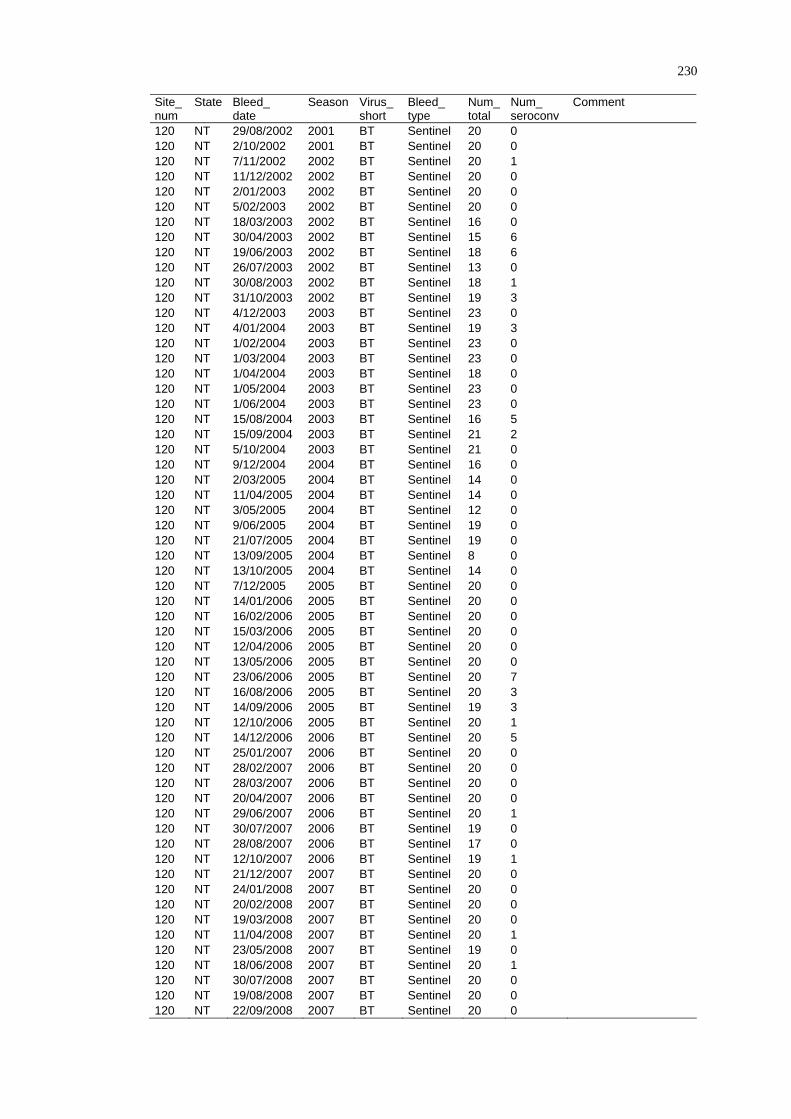
230

Site_ num

State Bleed_ date

Season Virus_short

Bleed_ type

Num_total

Num_ seroconv

Comment

120 NT 29/08/2002 2001 BT Sentinel 20 0 120 NT 2/10/2002 2001 BT Sentinel 20 0 120 NT 7/11/2002 2002 BT Sentinel 20 1 120 NT 11/12/2002 2002 BT Sentinel 20 0 120 NT 2/01/2003 2002 BT Sentinel 20 0 120 NT 5/02/2003 2002 BT Sentinel 20 0 120 NT 18/03/2003 2002 BT Sentinel 16 0 120 NT 30/04/2003 2002 BT Sentinel 15 6 120 NT 19/06/2003 2002 BT Sentinel 18 6 120 NT 26/07/2003 2002 BT Sentinel 13 0 120 NT 30/08/2003 2002 BT Sentinel 18 1 120 NT 31/10/2003 2002 BT Sentinel 19 3 120 NT 4/12/2003 2003 BT Sentinel 23 0 120 NT 4/01/2004 2003 BT Sentinel 19 3 120 NT 1/02/2004 2003 BT Sentinel 23 0 120 NT 1/03/2004 2003 BT Sentinel 23 0 120 NT 1/04/2004 2003 BT Sentinel 18 0 120 NT 1/05/2004 2003 BT Sentinel 23 0 120 NT 1/06/2004 2003 BT Sentinel 23 0 120 NT 15/08/2004 2003 BT Sentinel 16 5 120 NT 15/09/2004 2003 BT Sentinel 21 2 120 NT 5/10/2004 2003 BT Sentinel 21 0 120 NT 9/12/2004 2004 BT Sentinel 16 0 120 NT 2/03/2005 2004 BT Sentinel 14 0 120 NT 11/04/2005 2004 BT Sentinel 14 0 120 NT 3/05/2005 2004 BT Sentinel 12 0 120 NT 9/06/2005 2004 BT Sentinel 19 0 120 NT 21/07/2005 2004 BT Sentinel 19 0 120 NT 13/09/2005 2004 BT Sentinel 8 0 120 NT 13/10/2005 2004 BT Sentinel 14 0 120 NT 7/12/2005 2005 BT Sentinel 20 0 120 NT 14/01/2006 2005 BT Sentinel 20 0 120 NT 16/02/2006 2005 BT Sentinel 20 0 120 NT 15/03/2006 2005 BT Sentinel 20 0 120 NT 12/04/2006 2005 BT Sentinel 20 0 120 NT 13/05/2006 2005 BT Sentinel 20 0 120 NT 23/06/2006 2005 BT Sentinel 20 7 120 NT 16/08/2006 2005 BT Sentinel 20 3 120 NT 14/09/2006 2005 BT Sentinel 19 3 120 NT 12/10/2006 2005 BT Sentinel 20 1 120 NT 14/12/2006 2006 BT Sentinel 20 5 120 NT 25/01/2007 2006 BT Sentinel 20 0 120 NT 28/02/2007 2006 BT Sentinel 20 0 120 NT 28/03/2007 2006 BT Sentinel 20 0 120 NT 20/04/2007 2006 BT Sentinel 20 0 120 NT 29/06/2007 2006 BT Sentinel 20 1 120 NT 30/07/2007 2006 BT Sentinel 19 0 120 NT 28/08/2007 2006 BT Sentinel 17 0 120 NT 12/10/2007 2006 BT Sentinel 19 1 120 NT 21/12/2007 2007 BT Sentinel 20 0 120 NT 24/01/2008 2007 BT Sentinel 20 0 120 NT 20/02/2008 2007 BT Sentinel 20 0 120 NT 19/03/2008 2007 BT Sentinel 20 0 120 NT 11/04/2008 2007 BT Sentinel 20 1 120 NT 23/05/2008 2007 BT Sentinel 19 0 120 NT 18/06/2008 2007 BT Sentinel 20 1 120 NT 30/07/2008 2007 BT Sentinel 20 0 120 NT 19/08/2008 2007 BT Sentinel 20 0 120 NT 22/09/2008 2007 BT Sentinel 20 0

231

Site_ num

State Bleed_ date

Season Virus_short

Bleed_ type

Num_total

Num_ seroconv

Comment

120 NT 22/10/2008 2007 BT Sentinel 19 0 120 NT 16/12/2008 2008 BT Sentinel 20 0 120 NT 20/01/2009 2008 BT Sentinel 19 0 120 NT 10/02/2009 2008 BT Sentinel 19 0 120 NT 25/03/2009 2008 BT Sentinel 19 1 120 NT 16/04/2009 2008 BT Sentinel 18 4 120 NT 29/05/2009 2008 BT Sentinel 19 2 120 NT 17/06/2009 2008 BT Sentinel 20 0 120 NT 15/07/2009 2008 BT Sentinel 19 0 120 NT 24/08/2009 2008 BT Sentinel 19 2 120 NT 20/09/2009 2008 BT Sentinel 17 1 165 NT 14/04/2004 2003 BT Serosurv 21 2 165 NT 29/11/2006 2006 BT Serosurv 20 1 165 NT 3/08/2004 2003 BT Sentinel 15 0 165 NT 12/04/2005 2004 BT Sentinel 15 0 165 NT 28/07/2005 2004 BT Sentinel 15 0 165 NT 18/05/2006 2005 BT Sentinel 9 1 165 NT 4/04/2007 2006 BT Sentinel 19 0 165 NT 15/08/2007 2006 BT Sentinel 18 0 165 NT 11/06/2008 2007 BT Sentinel 18 0 165 NT 21/04/2009 2008 BT Serosurv 60 9 165 NT 21/04/2009 2008 BT Sentinel 13 5 179 NT 24/11/2000 2000 BT Sentinel 20 0 179 NT 31/01/2001 2000 BT Sentinel 20 0 179 NT 28/02/2001 2000 BT Sentinel 20 0 179 NT 11/04/2001 2000 BT Sentinel 20 0 179 NT 9/05/2001 2000 BT Sentinel 20 0 179 NT 20/06/2001 2000 BT Sentinel 20 0 179 NT 11/07/2001 2000 BT Sentinel 20 0 179 NT 15/08/2001 2000 BT Sentinel 20 0 179 NT 13/09/2001 2000 BT Sentinel 20 0 179 NT 12/10/2001 2000 BT Sentinel 20 0 179 NT 14/11/2001 2001 BT Sentinel 20 0 179 NT 12/12/2001 2001 BT Sentinel 20 0 179 NT 7/02/2002 2001 BT Sentinel 20 0 179 NT 7/03/2002 2001 BT Sentinel 20 0 179 NT 10/04/2002 2001 BT Sentinel 20 0 179 NT 9/05/2002 2001 BT Sentinel 20 0 179 NT 5/06/2002 2001 BT Sentinel 20 0 179 NT 9/07/2002 2001 BT Sentinel 20 0 179 NT 7/08/2002 2001 BT Sentinel 20 0 179 NT 10/09/2002 2001 BT Sentinel 20 0 179 NT 30/10/2002 2001 BT Sentinel 20 0 179 NT 30/11/2002 2002 BT Sentinel 20 0 179 NT 24/12/2002 2002 BT Sentinel 20 0 179 NT 30/01/2003 2002 BT Sentinel 20 0 179 NT 28/02/2003 2002 BT Sentinel 20 0 179 NT 30/03/2003 2002 BT Sentinel 20 0 179 NT 29/04/2003 2002 BT Sentinel 20 0 179 NT 30/05/2003 2002 BT Sentinel 20 0 179 NT 30/06/2003 2002 BT Sentinel 21 0 179 NT 7/08/2003 2002 BT Sentinel 20 0 179 NT 3/09/2003 2002 BT Sentinel 20 0 179 NT 2/10/2003 2002 BT Sentinel 20 0 179 NT 11/11/2003 2003 BT Sentinel 20 0 179 NT 3/12/2003 2003 BT Sentinel 20 0 179 NT 10/02/2004 2003 BT Sentinel 20 0 179 NT 2/03/2004 2003 BT Sentinel 20 0 179 NT 18/05/2004 2003 BT Sentinel 20 0

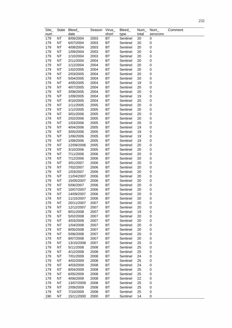
232

Site_ num

State Bleed_ date

Season Virus_short

Bleed_ type

Num_total

Num_ seroconv

Comment

179 NT 8/06/2004 2003 BT Sentinel 20 0 179 NT 6/07/2004 2003 BT Sentinel 20 0 179 NT 4/08/2004 2003 BT Sentinel 20 0 179 NT 1/09/2004 2003 BT Sentinel 20 0 179 NT 1/10/2004 2003 BT Sentinel 20 0 179 NT 2/11/2004 2004 BT Sentinel 20 0 179 NT 1/12/2004 2004 BT Sentinel 20 0 179 NT 1/02/2005 2004 BT Sentinel 20 0 179 NT 2/03/2005 2004 BT Sentinel 20 0 179 NT 5/04/2005 2004 BT Sentinel 20 0 179 NT 4/05/2005 2004 BT Sentinel 19 0 179 NT 4/07/2005 2004 BT Sentinel 20 0 179 NT 3/08/2005 2004 BT Sentinel 20 0 179 NT 1/09/2005 2004 BT Sentinel 19 0 179 NT 4/10/2005 2004 BT Sentinel 20 0 179 NT 1/11/2005 2005 BT Sentinel 20 0 179 NT 1/12/2005 2005 BT Sentinel 20 0 179 NT 3/01/2006 2005 BT Sentinel 20 0 179 NT 2/02/2006 2005 BT Sentinel 20 0 179 NT 1/03/2006 2005 BT Sentinel 20 0 179 NT 4/04/2006 2005 BT Sentinel 19 0 179 NT 3/05/2006 2005 BT Sentinel 19 0 179 NT 1/06/2006 2005 BT Sentinel 19 0 179 NT 1/08/2006 2005 BT Sentinel 19 0 179 NT 12/09/2006 2005 BT Sentinel 20 0 179 NT 3/10/2006 2005 BT Sentinel 20 0 179 NT 7/11/2006 2006 BT Sentinel 20 0 179 NT 7/12/2006 2006 BT Sentinel 20 0 179 NT 3/01/2007 2006 BT Sentinel 20 0 179 NT 7/02/2007 2006 BT Sentinel 20 0 179 NT 1/03/2007 2006 BT Sentinel 20 0 179 NT 11/04/2007 2006 BT Sentinel 20 0 179 NT 15/05/2007 2006 BT Sentinel 20 0 179 NT 5/06/2007 2006 BT Sentinel 20 0 179 NT 10/07/2007 2006 BT Sentinel 20 0 179 NT 14/09/2007 2006 BT Sentinel 20 0 179 NT 11/10/2007 2006 BT Sentinel 20 0 179 NT 20/11/2007 2007 BT Sentinel 20 0 179 NT 12/12/2007 2007 BT Sentinel 20 0 179 NT 8/01/2008 2007 BT Sentinel 19 0 179 NT 5/02/2008 2007 BT Sentinel 20 0 179 NT 4/03/2008 2007 BT Sentinel 20 0 179 NT 1/04/2008 2007 BT Sentinel 20 0 179 NT 8/05/2008 2007 BT Sentinel 20 0 179 NT 5/06/2008 2007 BT Sentinel 20 0 179 NT 8/07/2008 2007 BT Sentinel 20 0 179 NT 13/10/2008 2007 BT Sentinel 25 0 179 NT 5/11/2008 2008 BT Sentinel 25 0 179 NT 4/12/2008 2008 BT Sentinel 25 0 179 NT 7/01/2009 2008 BT Sentinel 24 0 179 NT 4/02/2009 2008 BT Sentinel 25 0 179 NT 4/03/2009 2008 BT Sentinel 24 0 179 NT 8/04/2009 2008 BT Sentinel 25 0 179 NT 6/05/2009 2008 BT Sentinel 25 0 179 NT 4/06/2009 2008 BT Sentinel 22 0 179 NT 13/07/2009 2008 BT Sentinel 25 0 179 NT 2/09/2009 2008 BT Sentinel 25 0 179 NT 7/10/2009 2008 BT Sentinel 25 0 190 NT 15/11/2000 2000 BT Sentinel 14 0

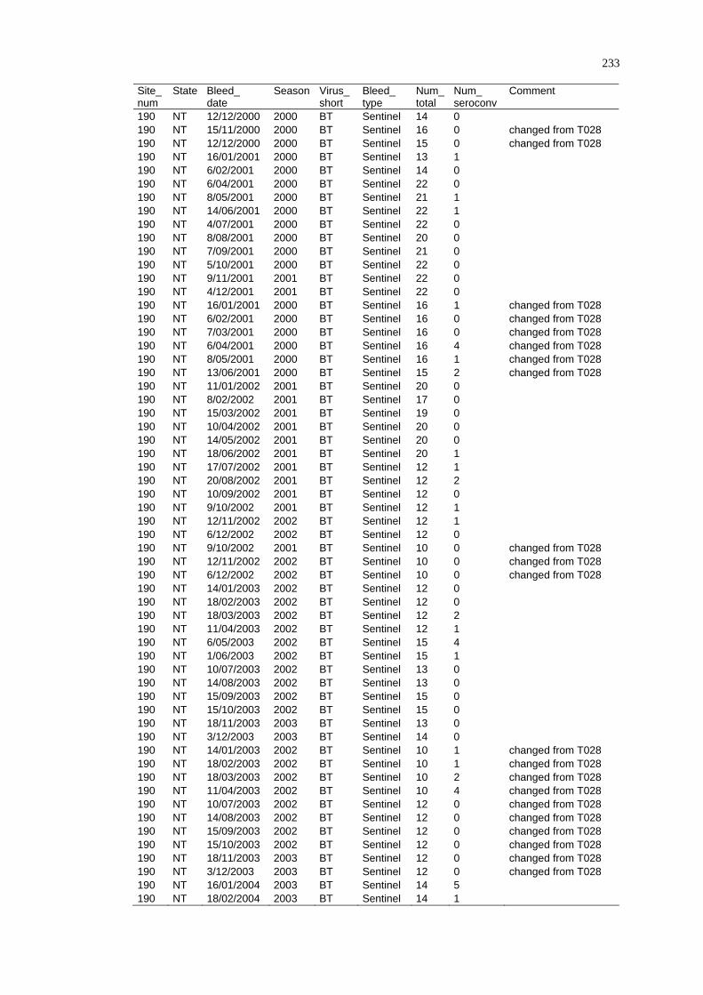
233

Site_ num

State Bleed_ date

Season Virus_short

Bleed_ type

Num_total

Num_ seroconv

Comment

190 NT 12/12/2000 2000 BT Sentinel 14 0 190 NT 15/11/2000 2000 BT Sentinel 16 0 changed from T028 190 NT 12/12/2000 2000 BT Sentinel 15 0 changed from T028 190 NT 16/01/2001 2000 BT Sentinel 13 1 190 NT 6/02/2001 2000 BT Sentinel 14 0 190 NT 6/04/2001 2000 BT Sentinel 22 0 190 NT 8/05/2001 2000 BT Sentinel 21 1 190 NT 14/06/2001 2000 BT Sentinel 22 1 190 NT 4/07/2001 2000 BT Sentinel 22 0 190 NT 8/08/2001 2000 BT Sentinel 20 0 190 NT 7/09/2001 2000 BT Sentinel 21 0 190 NT 5/10/2001 2000 BT Sentinel 22 0 190 NT 9/11/2001 2001 BT Sentinel 22 0 190 NT 4/12/2001 2001 BT Sentinel 22 0 190 NT 16/01/2001 2000 BT Sentinel 16 1 changed from T028 190 NT 6/02/2001 2000 BT Sentinel 16 0 changed from T028 190 NT 7/03/2001 2000 BT Sentinel 16 0 changed from T028 190 NT 6/04/2001 2000 BT Sentinel 16 4 changed from T028 190 NT 8/05/2001 2000 BT Sentinel 16 1 changed from T028 190 NT 13/06/2001 2000 BT Sentinel 15 2 changed from T028 190 NT 11/01/2002 2001 BT Sentinel 20 0 190 NT 8/02/2002 2001 BT Sentinel 17 0 190 NT 15/03/2002 2001 BT Sentinel 19 0 190 NT 10/04/2002 2001 BT Sentinel 20 0 190 NT 14/05/2002 2001 BT Sentinel 20 0 190 NT 18/06/2002 2001 BT Sentinel 20 1 190 NT 17/07/2002 2001 BT Sentinel 12 1 190 NT 20/08/2002 2001 BT Sentinel 12 2 190 NT 10/09/2002 2001 BT Sentinel 12 0 190 NT 9/10/2002 2001 BT Sentinel 12 1 190 NT 12/11/2002 2002 BT Sentinel 12 1 190 NT 6/12/2002 2002 BT Sentinel 12 0 190 NT 9/10/2002 2001 BT Sentinel 10 0 changed from T028 190 NT 12/11/2002 2002 BT Sentinel 10 0 changed from T028 190 NT 6/12/2002 2002 BT Sentinel 10 0 changed from T028 190 NT 14/01/2003 2002 BT Sentinel 12 0 190 NT 18/02/2003 2002 BT Sentinel 12 0 190 NT 18/03/2003 2002 BT Sentinel 12 2 190 NT 11/04/2003 2002 BT Sentinel 12 1 190 NT 6/05/2003 2002 BT Sentinel 15 4 190 NT 1/06/2003 2002 BT Sentinel 15 1 190 NT 10/07/2003 2002 BT Sentinel 13 0 190 NT 14/08/2003 2002 BT Sentinel 13 0 190 NT 15/09/2003 2002 BT Sentinel 15 0 190 NT 15/10/2003 2002 BT Sentinel 15 0 190 NT 18/11/2003 2003 BT Sentinel 13 0 190 NT 3/12/2003 2003 BT Sentinel 14 0 190 NT 14/01/2003 2002 BT Sentinel 10 1 changed from T028 190 NT 18/02/2003 2002 BT Sentinel 10 1 changed from T028 190 NT 18/03/2003 2002 BT Sentinel 10 2 changed from T028 190 NT 11/04/2003 2002 BT Sentinel 10 4 changed from T028 190 NT 10/07/2003 2002 BT Sentinel 12 0 changed from T028 190 NT 14/08/2003 2002 BT Sentinel 12 0 changed from T028 190 NT 15/09/2003 2002 BT Sentinel 12 0 changed from T028 190 NT 15/10/2003 2002 BT Sentinel 12 0 changed from T028 190 NT 18/11/2003 2003 BT Sentinel 12 0 changed from T028 190 NT 3/12/2003 2003 BT Sentinel 12 0 changed from T028 190 NT 16/01/2004 2003 BT Sentinel 14 5 190 NT 18/02/2004 2003 BT Sentinel 14 1

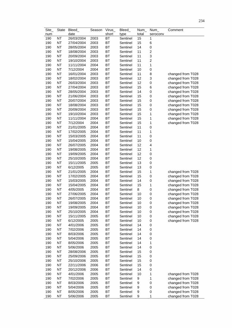
234

Site_ num

State Bleed_ date

Season Virus_short

Bleed_ type

Num_total

Num_ seroconv

Comment

190 NT 26/03/2004 2003 BT Sentinel 15 1 190 NT 27/04/2004 2003 BT Sentinel 15 6 190 NT 28/05/2004 2003 BT Sentinel 14 0 190 NT 18/08/2004 2003 BT Sentinel 11 2 190 NT 20/09/2004 2003 BT Sentinel 11 3 190 NT 19/10/2004 2003 BT Sentinel 11 2 190 NT 11/11/2004 2004 BT Sentinel 11 1 190 NT 7/12/2004 2004 BT Sentinel 10 0 190 NT 16/01/2004 2003 BT Sentinel 11 8 changed from T028 190 NT 18/02/2004 2003 BT Sentinel 12 3 changed from T028 190 NT 26/03/2004 2003 BT Sentinel 12 0 changed from T028 190 NT 27/04/2004 2003 BT Sentinel 15 6 changed from T028 190 NT 28/05/2004 2003 BT Sentinel 14 0 changed from T028 190 NT 21/06/2004 2003 BT Sentinel 15 0 changed from T028 190 NT 20/07/2004 2003 BT Sentinel 15 0 changed from T028 190 NT 18/08/2004 2003 BT Sentinel 15 0 changed from T028 190 NT 20/09/2004 2003 BT Sentinel 15 0 changed from T028 190 NT 19/10/2004 2003 BT Sentinel 15 1 changed from T028 190 NT 11/11/2004 2004 BT Sentinel 15 1 changed from T028 190 NT 7/12/2004 2004 BT Sentinel 15 1 changed from T028 190 NT 21/01/2005 2004 BT Sentinel 11 0 190 NT 17/02/2005 2004 BT Sentinel 11 1 190 NT 15/03/2005 2004 BT Sentinel 11 0 190 NT 15/04/2005 2004 BT Sentinel 10 0 190 NT 26/07/2005 2004 BT Sentinel 12 4 190 NT 19/08/2005 2004 BT Sentinel 12 1 190 NT 19/09/2005 2004 BT Sentinel 12 0 190 NT 25/10/2005 2004 BT Sentinel 12 0 190 NT 15/11/2005 2005 BT Sentinel 13 0 190 NT 6/12/2005 2005 BT Sentinel 13 0 190 NT 21/01/2005 2004 BT Sentinel 15 1 changed from T028 190 NT 17/02/2005 2004 BT Sentinel 15 0 changed from T028 190 NT 15/03/2005 2004 BT Sentinel 14 0 changed from T028 190 NT 15/04/2005 2004 BT Sentinel 15 1 changed from T028 190 NT 4/05/2005 2004 BT Sentinel 8 0 changed from T028 190 NT 27/06/2005 2004 BT Sentinel 10 0 changed from T028 190 NT 26/07/2005 2004 BT Sentinel 10 0 changed from T028 190 NT 19/08/2005 2004 BT Sentinel 10 0 changed from T028 190 NT 19/09/2005 2004 BT Sentinel 10 0 changed from T028 190 NT 25/10/2005 2004 BT Sentinel 10 0 changed from T028 190 NT 15/11/2005 2005 BT Sentinel 10 0 changed from T028 190 NT 6/12/2005 2005 BT Sentinel 10 0 changed from T028 190 NT 4/01/2006 2005 BT Sentinel 14 0 190 NT 7/02/2006 2005 BT Sentinel 14 0 190 NT 8/03/2006 2005 BT Sentinel 14 0 190 NT 5/04/2006 2005 BT Sentinel 14 0 190 NT 8/05/2006 2005 BT Sentinel 14 1 190 NT 5/06/2006 2005 BT Sentinel 14 0 190 NT 28/08/2006 2005 BT Sentinel 15 0 190 NT 25/09/2006 2005 BT Sentinel 15 0 190 NT 25/10/2006 2005 BT Sentinel 15 0 190 NT 22/11/2006 2006 BT Sentinel 15 0 190 NT 20/12/2006 2006 BT Sentinel 14 0 190 NT 4/01/2006 2005 BT Sentinel 10 1 changed from T028 190 NT 7/02/2006 2005 BT Sentinel 9 1 changed from T028 190 NT 8/03/2006 2005 BT Sentinel 9 0 changed from T028 190 NT 5/04/2006 2005 BT Sentinel 9 0 changed from T028 190 NT 8/05/2006 2005 BT Sentinel 9 0 changed from T028 190 NT 5/06/2006 2005 BT Sentinel 9 1 changed from T028

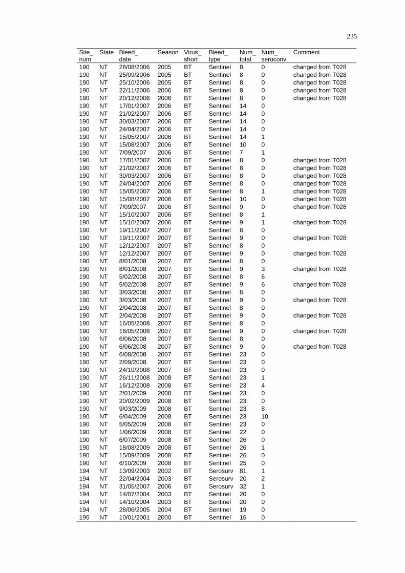
235

Site_ num

State Bleed_ date

Season Virus_short

Bleed_ type

Num_total

Num_ seroconv

Comment

190 NT 28/08/2006 2005 BT Sentinel 8 0 changed from T028 190 NT 25/09/2006 2005 BT Sentinel 8 0 changed from T028 190 NT 25/10/2006 2005 BT Sentinel 8 0 changed from T028 190 NT 22/11/2006 2006 BT Sentinel 8 0 changed from T028 190 NT 20/12/2006 2006 BT Sentinel 8 0 changed from T028 190 NT 17/01/2007 2006 BT Sentinel 14 0 190 NT 21/02/2007 2006 BT Sentinel 14 0 190 NT 30/03/2007 2006 BT Sentinel 14 0 190 NT 24/04/2007 2006 BT Sentinel 14 0 190 NT 15/05/2007 2006 BT Sentinel 14 1 190 NT 15/08/2007 2006 BT Sentinel 10 0 190 NT 7/09/2007 2006 BT Sentinel 7 1 190 NT 17/01/2007 2006 BT Sentinel 8 0 changed from T028 190 NT 21/02/2007 2006 BT Sentinel 8 0 changed from T028 190 NT 30/03/2007 2006 BT Sentinel 8 0 changed from T028 190 NT 24/04/2007 2006 BT Sentinel 8 0 changed from T028 190 NT 15/05/2007 2006 BT Sentinel 8 1 changed from T028 190 NT 15/08/2007 2006 BT Sentinel 10 0 changed from T028 190 NT 7/09/2007 2006 BT Sentinel 9 0 changed from T028 190 NT 15/10/2007 2006 BT Sentinel 8 1 190 NT 15/10/2007 2006 BT Sentinel 9 1 changed from T028 190 NT 19/11/2007 2007 BT Sentinel 8 0 190 NT 19/11/2007 2007 BT Sentinel 9 0 changed from T028 190 NT 12/12/2007 2007 BT Sentinel 8 0 190 NT 12/12/2007 2007 BT Sentinel 9 0 changed from T028 190 NT 8/01/2008 2007 BT Sentinel 8 0 190 NT 8/01/2008 2007 BT Sentinel 9 3 changed from T028 190 NT 5/02/2008 2007 BT Sentinel 8 6 190 NT 5/02/2008 2007 BT Sentinel 9 6 changed from T028 190 NT 3/03/2008 2007 BT Sentinel 8 0 190 NT 3/03/2008 2007 BT Sentinel 9 0 changed from T028 190 NT 2/04/2008 2007 BT Sentinel 8 0 190 NT 2/04/2008 2007 BT Sentinel 9 0 changed from T028 190 NT 16/05/2008 2007 BT Sentinel 8 0 190 NT 16/05/2008 2007 BT Sentinel 9 0 changed from T028 190 NT 6/06/2008 2007 BT Sentinel 8 0 190 NT 6/06/2008 2007 BT Sentinel 9 0 changed from T028 190 NT 6/08/2008 2007 BT Sentinel 23 0 190 NT 2/09/2008 2007 BT Sentinel 23 0 190 NT 24/10/2008 2007 BT Sentinel 23 0 190 NT 26/11/2008 2008 BT Sentinel 23 1 190 NT 16/12/2008 2008 BT Sentinel 23 4 190 NT 2/01/2009 2008 BT Sentinel 23 0 190 NT 20/02/2009 2008 BT Sentinel 23 0 190 NT 9/03/2009 2008 BT Sentinel 23 8 190 NT 6/04/2009 2008 BT Sentinel 23 10 190 NT 5/05/2009 2008 BT Sentinel 23 0 190 NT 1/06/2009 2008 BT Sentinel 22 0 190 NT 6/07/2009 2008 BT Sentinel 26 0 190 NT 18/08/2009 2008 BT Sentinel 26 1 190 NT 15/09/2009 2008 BT Sentinel 26 0 190 NT 6/10/2009 2008 BT Sentinel 25 0 194 NT 13/09/2003 2002 BT Serosurv 81 1 194 NT 22/04/2004 2003 BT Serosurv 20 2 194 NT 31/05/2007 2006 BT Serosurv 32 1 194 NT 14/07/2004 2003 BT Sentinel 20 0 194 NT 14/10/2004 2003 BT Sentinel 20 0 194 NT 28/06/2005 2004 BT Sentinel 19 0 195 NT 10/01/2001 2000 BT Sentinel 16 0

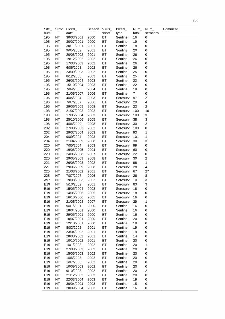
236

Site_ num

State Bleed_ date

Season Virus_short

Bleed_ type

Num_total

Num_ seroconv

Comment

195 NT 30/03/2001 2000 BT Sentinel 16 0 195 NT 30/07/2001 2000 BT Sentinel 19 0 195 NT 30/11/2001 2001 BT Sentinel 18 0 195 NT 9/05/2002 2001 BT Sentinel 20 0 195 NT 20/08/2002 2001 BT Sentinel 26 0 195 NT 19/12/2002 2002 BT Sentinel 26 0 195 NT 17/03/2003 2002 BT Sentinel 26 0 195 NT 6/06/2003 2002 BT Sentinel 26 0 195 NT 23/09/2003 2002 BT Sentinel 25 0 195 NT 8/12/2003 2003 BT Sentinel 25 0 195 NT 26/03/2004 2003 BT Sentinel 22 0 195 NT 15/10/2004 2003 BT Sentinel 22 0 195 NT 7/04/2005 2004 BT Sentinel 18 0 195 NT 21/05/2007 2006 BT Sentinel 7 0 196 NT 4/05/2004 2003 BT Serosurv 97 2 196 NT 7/07/2007 2006 BT Serosurv 29 4 196 NT 29/06/2009 2008 BT Serosurv 23 2 198 NT 21/07/2003 2002 BT Serosurv 100 10 198 NT 17/05/2004 2003 BT Serosurv 100 3 198 NT 25/10/2006 2005 BT Serosurv 38 3 198 NT 4/06/2009 2008 BT Serosurv 30 2 202 NT 27/08/2003 2002 BT Serosurv 100 0 202 NT 29/07/2004 2003 BT Serosurv 93 1 204 NT 9/09/2004 2003 BT Serosurv 101 1 204 NT 21/04/2009 2008 BT Serosurv 30 3 220 NT 7/05/2004 2003 BT Serosurv 99 0 220 NT 19/08/2005 2004 BT Serosurv 60 0 220 NT 24/06/2008 2007 BT Serosurv 22 0 220 NT 29/05/2009 2008 BT Serosurv 30 2 221 NT 26/08/2003 2002 BT Serosurv 98 1 221 NT 29/06/2009 2008 BT Serosurv 28 4 225 NT 21/08/2002 2001 BT Serosurv 67 27 225 NT 7/07/2007 2006 BT Serosurv 26 8 A97 NT 19/08/2003 2002 BT Serosurv 101 3 E19 NT 5/10/2002 2001 BT Serosurv 83 3 E19 NT 15/05/2004 2003 BT Serosurv 18 0 E19 NT 14/05/2006 2005 BT Serosurv 18 0 E19 NT 16/10/2006 2005 BT Serosurv 16 0 E19 NT 21/05/2008 2007 BT Serosurv 39 1 E19 NT 9/01/2001 2000 BT Sentinel 16 0 E19 NT 18/04/2001 2000 BT Sentinel 16 0 E19 NT 29/05/2001 2000 BT Sentinel 16 0 E19 NT 10/07/2001 2000 BT Sentinel 20 0 E19 NT 12/10/2001 2000 BT Sentinel 19 0 E19 NT 8/02/2002 2001 BT Sentinel 19 0 E19 NT 23/04/2002 2001 BT Sentinel 19 0 E19 NT 28/08/2002 2001 BT Sentinel 14 0 E19 NT 10/10/2002 2001 BT Sentinel 20 0 E19 NT 1/01/2003 2002 BT Sentinel 20 1 E19 NT 27/03/2003 2002 BT Sentinel 20 0 E19 NT 15/05/2003 2002 BT Sentinel 20 0 E19 NT 1/06/2003 2002 BT Sentinel 20 0 E19 NT 1/07/2003 2002 BT Sentinel 20 0 E19 NT 10/09/2003 2002 BT Sentinel 20 0 E19 NT 9/10/2003 2002 BT Sentinel 20 2 E19 NT 21/12/2003 2003 BT Sentinel 20 0 E19 NT 22/03/2004 2003 BT Sentinel 19 0 E19 NT 30/04/2004 2003 BT Sentinel 15 0 E19 NT 20/09/2004 2003 BT Sentinel 16 0

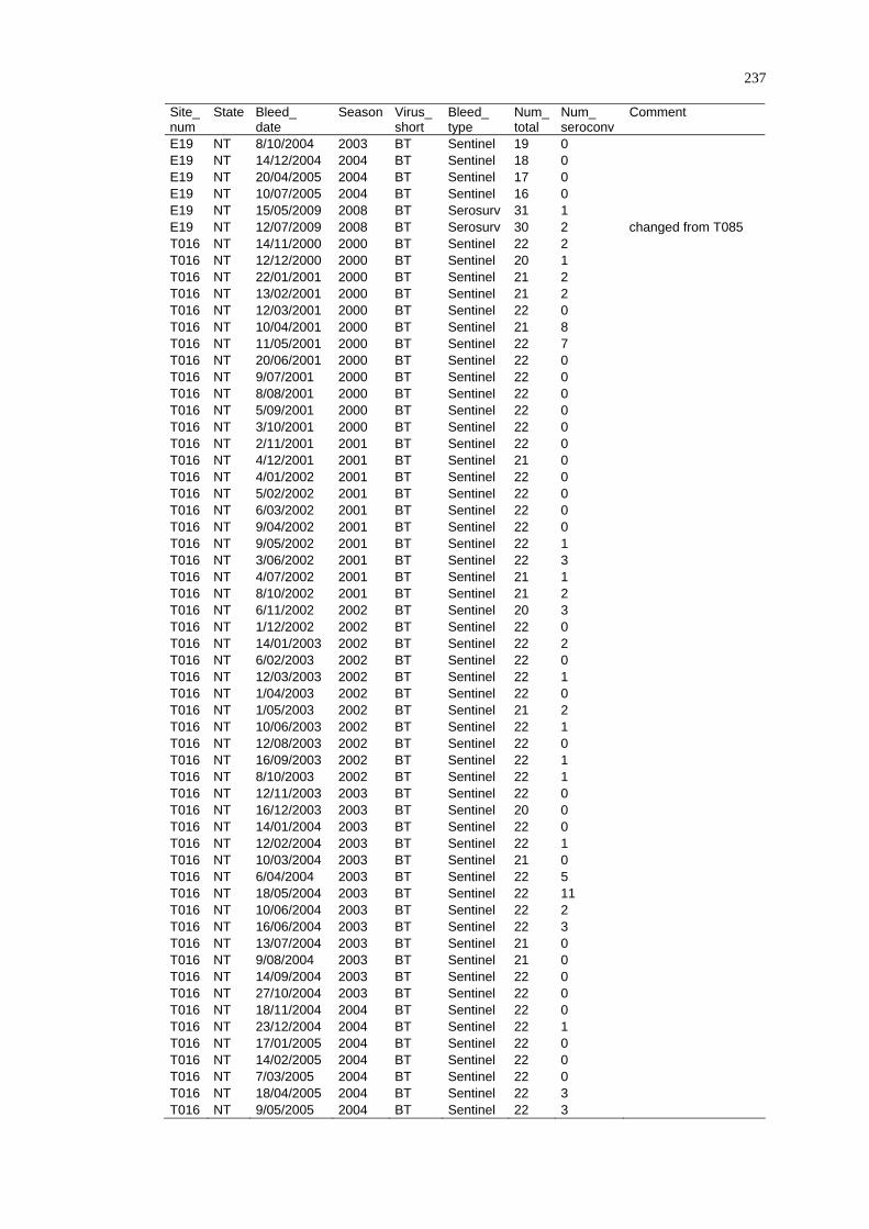
237

Site_ num

State Bleed_ date

Season Virus_short

Bleed_ type

Num_total

Num_ seroconv

Comment

E19 NT 8/10/2004 2003 BT Sentinel 19 0 E19 NT 14/12/2004 2004 BT Sentinel 18 0 E19 NT 20/04/2005 2004 BT Sentinel 17 0 E19 NT 10/07/2005 2004 BT Sentinel 16 0 E19 NT 15/05/2009 2008 BT Serosurv 31 1 E19 NT 12/07/2009 2008 BT Serosurv 30 2 changed from T085 T016 NT 14/11/2000 2000 BT Sentinel 22 2 T016 NT 12/12/2000 2000 BT Sentinel 20 1 T016 NT 22/01/2001 2000 BT Sentinel 21 2 T016 NT 13/02/2001 2000 BT Sentinel 21 2 T016 NT 12/03/2001 2000 BT Sentinel 22 0 T016 NT 10/04/2001 2000 BT Sentinel 21 8 T016 NT 11/05/2001 2000 BT Sentinel 22 7 T016 NT 20/06/2001 2000 BT Sentinel 22 0 T016 NT 9/07/2001 2000 BT Sentinel 22 0 T016 NT 8/08/2001 2000 BT Sentinel 22 0 T016 NT 5/09/2001 2000 BT Sentinel 22 0 T016 NT 3/10/2001 2000 BT Sentinel 22 0 T016 NT 2/11/2001 2001 BT Sentinel 22 0 T016 NT 4/12/2001 2001 BT Sentinel 21 0 T016 NT 4/01/2002 2001 BT Sentinel 22 0 T016 NT 5/02/2002 2001 BT Sentinel 22 0 T016 NT 6/03/2002 2001 BT Sentinel 22 0 T016 NT 9/04/2002 2001 BT Sentinel 22 0 T016 NT 9/05/2002 2001 BT Sentinel 22 1 T016 NT 3/06/2002 2001 BT Sentinel 22 3 T016 NT 4/07/2002 2001 BT Sentinel 21 1 T016 NT 8/10/2002 2001 BT Sentinel 21 2 T016 NT 6/11/2002 2002 BT Sentinel 20 3 T016 NT 1/12/2002 2002 BT Sentinel 22 0 T016 NT 14/01/2003 2002 BT Sentinel 22 2 T016 NT 6/02/2003 2002 BT Sentinel 22 0 T016 NT 12/03/2003 2002 BT Sentinel 22 1 T016 NT 1/04/2003 2002 BT Sentinel 22 0 T016 NT 1/05/2003 2002 BT Sentinel 21 2 T016 NT 10/06/2003 2002 BT Sentinel 22 1 T016 NT 12/08/2003 2002 BT Sentinel 22 0 T016 NT 16/09/2003 2002 BT Sentinel 22 1 T016 NT 8/10/2003 2002 BT Sentinel 22 1 T016 NT 12/11/2003 2003 BT Sentinel 22 0 T016 NT 16/12/2003 2003 BT Sentinel 20 0 T016 NT 14/01/2004 2003 BT Sentinel 22 0 T016 NT 12/02/2004 2003 BT Sentinel 22 1 T016 NT 10/03/2004 2003 BT Sentinel 21 0 T016 NT 6/04/2004 2003 BT Sentinel 22 5 T016 NT 18/05/2004 2003 BT Sentinel 22 11 T016 NT 10/06/2004 2003 BT Sentinel 22 2 T016 NT 16/06/2004 2003 BT Sentinel 22 3 T016 NT 13/07/2004 2003 BT Sentinel 21 0 T016 NT 9/08/2004 2003 BT Sentinel 21 0 T016 NT 14/09/2004 2003 BT Sentinel 22 0 T016 NT 27/10/2004 2003 BT Sentinel 22 0 T016 NT 18/11/2004 2004 BT Sentinel 22 0 T016 NT 23/12/2004 2004 BT Sentinel 22 1 T016 NT 17/01/2005 2004 BT Sentinel 22 0 T016 NT 14/02/2005 2004 BT Sentinel 22 0 T016 NT 7/03/2005 2004 BT Sentinel 22 0 T016 NT 18/04/2005 2004 BT Sentinel 22 3 T016 NT 9/05/2005 2004 BT Sentinel 22 3

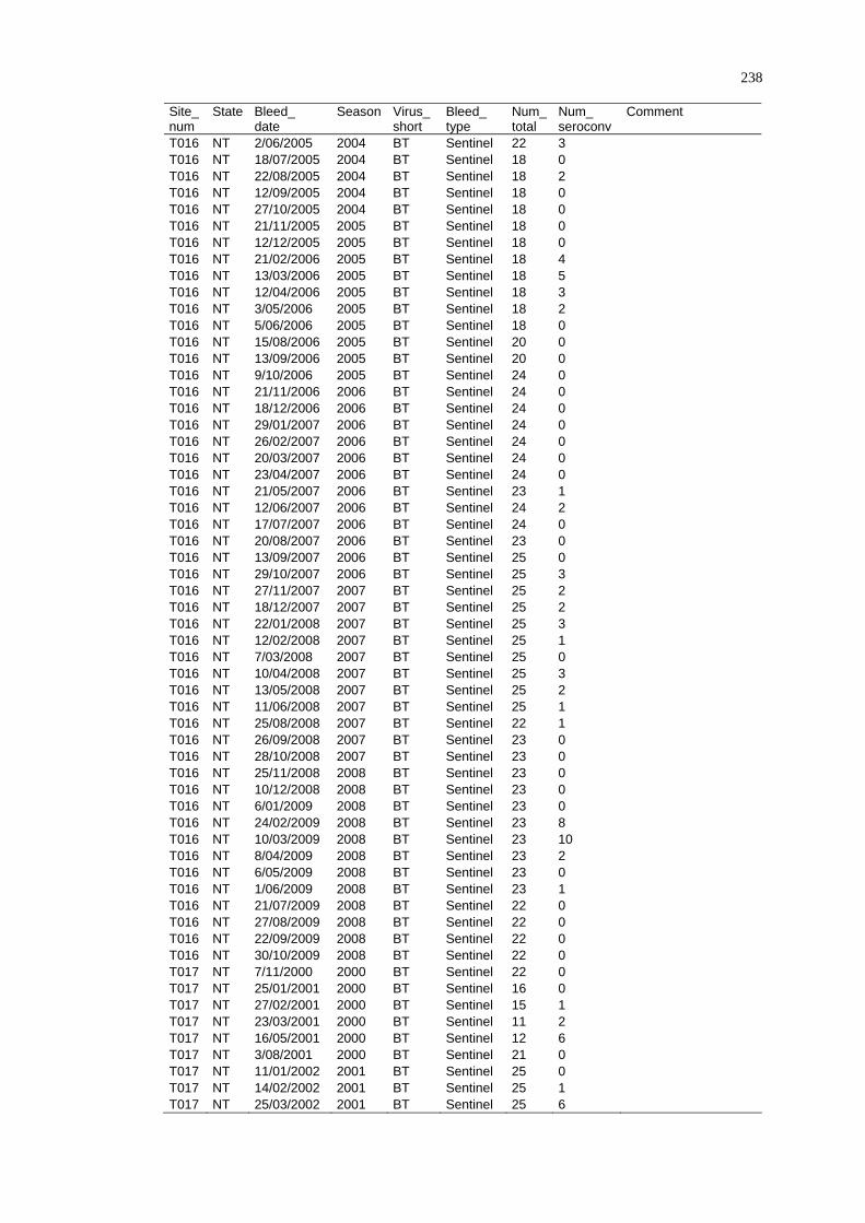
238

Site_ num

State Bleed_ date

Season Virus_short

Bleed_ type

Num_total

Num_ seroconv

Comment

T016 NT 2/06/2005 2004 BT Sentinel 22 3 T016 NT 18/07/2005 2004 BT Sentinel 18 0 T016 NT 22/08/2005 2004 BT Sentinel 18 2 T016 NT 12/09/2005 2004 BT Sentinel 18 0 T016 NT 27/10/2005 2004 BT Sentinel 18 0 T016 NT 21/11/2005 2005 BT Sentinel 18 0 T016 NT 12/12/2005 2005 BT Sentinel 18 0 T016 NT 21/02/2006 2005 BT Sentinel 18 4 T016 NT 13/03/2006 2005 BT Sentinel 18 5 T016 NT 12/04/2006 2005 BT Sentinel 18 3 T016 NT 3/05/2006 2005 BT Sentinel 18 2 T016 NT 5/06/2006 2005 BT Sentinel 18 0 T016 NT 15/08/2006 2005 BT Sentinel 20 0 T016 NT 13/09/2006 2005 BT Sentinel 20 0 T016 NT 9/10/2006 2005 BT Sentinel 24 0 T016 NT 21/11/2006 2006 BT Sentinel 24 0 T016 NT 18/12/2006 2006 BT Sentinel 24 0 T016 NT 29/01/2007 2006 BT Sentinel 24 0 T016 NT 26/02/2007 2006 BT Sentinel 24 0 T016 NT 20/03/2007 2006 BT Sentinel 24 0 T016 NT 23/04/2007 2006 BT Sentinel 24 0 T016 NT 21/05/2007 2006 BT Sentinel 23 1 T016 NT 12/06/2007 2006 BT Sentinel 24 2 T016 NT 17/07/2007 2006 BT Sentinel 24 0 T016 NT 20/08/2007 2006 BT Sentinel 23 0 T016 NT 13/09/2007 2006 BT Sentinel 25 0 T016 NT 29/10/2007 2006 BT Sentinel 25 3 T016 NT 27/11/2007 2007 BT Sentinel 25 2 T016 NT 18/12/2007 2007 BT Sentinel 25 2 T016 NT 22/01/2008 2007 BT Sentinel 25 3 T016 NT 12/02/2008 2007 BT Sentinel 25 1 T016 NT 7/03/2008 2007 BT Sentinel 25 0 T016 NT 10/04/2008 2007 BT Sentinel 25 3 T016 NT 13/05/2008 2007 BT Sentinel 25 2 T016 NT 11/06/2008 2007 BT Sentinel 25 1 T016 NT 25/08/2008 2007 BT Sentinel 22 1 T016 NT 26/09/2008 2007 BT Sentinel 23 0 T016 NT 28/10/2008 2007 BT Sentinel 23 0 T016 NT 25/11/2008 2008 BT Sentinel 23 0 T016 NT 10/12/2008 2008 BT Sentinel 23 0 T016 NT 6/01/2009 2008 BT Sentinel 23 0 T016 NT 24/02/2009 2008 BT Sentinel 23 8 T016 NT 10/03/2009 2008 BT Sentinel 23 10 T016 NT 8/04/2009 2008 BT Sentinel 23 2 T016 NT 6/05/2009 2008 BT Sentinel 23 0 T016 NT 1/06/2009 2008 BT Sentinel 23 1 T016 NT 21/07/2009 2008 BT Sentinel 22 0 T016 NT 27/08/2009 2008 BT Sentinel 22 0 T016 NT 22/09/2009 2008 BT Sentinel 22 0 T016 NT 30/10/2009 2008 BT Sentinel 22 0 T017 NT 7/11/2000 2000 BT Sentinel 22 0 T017 NT 25/01/2001 2000 BT Sentinel 16 0 T017 NT 27/02/2001 2000 BT Sentinel 15 1 T017 NT 23/03/2001 2000 BT Sentinel 11 2 T017 NT 16/05/2001 2000 BT Sentinel 12 6 T017 NT 3/08/2001 2000 BT Sentinel 21 0 T017 NT 11/01/2002 2001 BT Sentinel 25 0 T017 NT 14/02/2002 2001 BT Sentinel 25 1 T017 NT 25/03/2002 2001 BT Sentinel 25 6

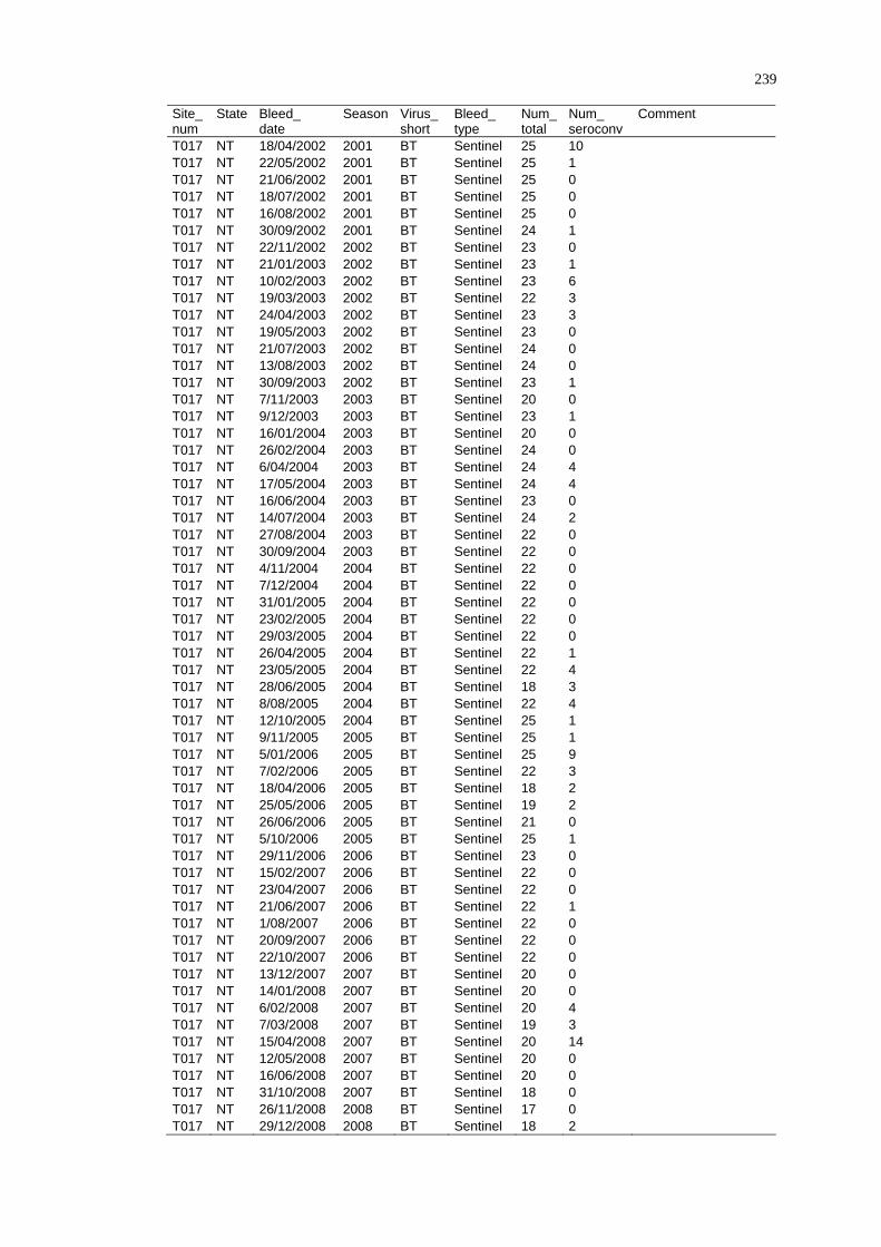
239

Site_ num

State Bleed_ date

Season Virus_short

Bleed_ type

Num_total

Num_ seroconv

Comment

T017 NT 18/04/2002 2001 BT Sentinel 25 10 T017 NT 22/05/2002 2001 BT Sentinel 25 1 T017 NT 21/06/2002 2001 BT Sentinel 25 0 T017 NT 18/07/2002 2001 BT Sentinel 25 0 T017 NT 16/08/2002 2001 BT Sentinel 25 0 T017 NT 30/09/2002 2001 BT Sentinel 24 1 T017 NT 22/11/2002 2002 BT Sentinel 23 0 T017 NT 21/01/2003 2002 BT Sentinel 23 1 T017 NT 10/02/2003 2002 BT Sentinel 23 6 T017 NT 19/03/2003 2002 BT Sentinel 22 3 T017 NT 24/04/2003 2002 BT Sentinel 23 3 T017 NT 19/05/2003 2002 BT Sentinel 23 0 T017 NT 21/07/2003 2002 BT Sentinel 24 0 T017 NT 13/08/2003 2002 BT Sentinel 24 0 T017 NT 30/09/2003 2002 BT Sentinel 23 1 T017 NT 7/11/2003 2003 BT Sentinel 20 0 T017 NT 9/12/2003 2003 BT Sentinel 23 1 T017 NT 16/01/2004 2003 BT Sentinel 20 0 T017 NT 26/02/2004 2003 BT Sentinel 24 0 T017 NT 6/04/2004 2003 BT Sentinel 24 4 T017 NT 17/05/2004 2003 BT Sentinel 24 4 T017 NT 16/06/2004 2003 BT Sentinel 23 0 T017 NT 14/07/2004 2003 BT Sentinel 24 2 T017 NT 27/08/2004 2003 BT Sentinel 22 0 T017 NT 30/09/2004 2003 BT Sentinel 22 0 T017 NT 4/11/2004 2004 BT Sentinel 22 0 T017 NT 7/12/2004 2004 BT Sentinel 22 0 T017 NT 31/01/2005 2004 BT Sentinel 22 0 T017 NT 23/02/2005 2004 BT Sentinel 22 0 T017 NT 29/03/2005 2004 BT Sentinel 22 0 T017 NT 26/04/2005 2004 BT Sentinel 22 1 T017 NT 23/05/2005 2004 BT Sentinel 22 4 T017 NT 28/06/2005 2004 BT Sentinel 18 3 T017 NT 8/08/2005 2004 BT Sentinel 22 4 T017 NT 12/10/2005 2004 BT Sentinel 25 1 T017 NT 9/11/2005 2005 BT Sentinel 25 1 T017 NT 5/01/2006 2005 BT Sentinel 25 9 T017 NT 7/02/2006 2005 BT Sentinel 22 3 T017 NT 18/04/2006 2005 BT Sentinel 18 2 T017 NT 25/05/2006 2005 BT Sentinel 19 2 T017 NT 26/06/2006 2005 BT Sentinel 21 0 T017 NT 5/10/2006 2005 BT Sentinel 25 1 T017 NT 29/11/2006 2006 BT Sentinel 23 0 T017 NT 15/02/2007 2006 BT Sentinel 22 0 T017 NT 23/04/2007 2006 BT Sentinel 22 0 T017 NT 21/06/2007 2006 BT Sentinel 22 1 T017 NT 1/08/2007 2006 BT Sentinel 22 0 T017 NT 20/09/2007 2006 BT Sentinel 22 0 T017 NT 22/10/2007 2006 BT Sentinel 22 0 T017 NT 13/12/2007 2007 BT Sentinel 20 0 T017 NT 14/01/2008 2007 BT Sentinel 20 0 T017 NT 6/02/2008 2007 BT Sentinel 20 4 T017 NT 7/03/2008 2007 BT Sentinel 19 3 T017 NT 15/04/2008 2007 BT Sentinel 20 14 T017 NT 12/05/2008 2007 BT Sentinel 20 0 T017 NT 16/06/2008 2007 BT Sentinel 20 0 T017 NT 31/10/2008 2007 BT Sentinel 18 0 T017 NT 26/11/2008 2008 BT Sentinel 17 0 T017 NT 29/12/2008 2008 BT Sentinel 18 2

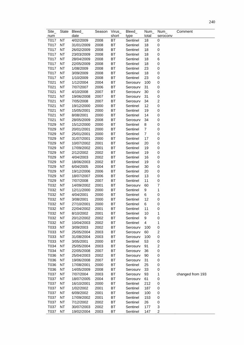
240

Site_ num

State Bleed_ date

Season Virus_short

Bleed_ type

Num_total

Num_ seroconv

Comment

T017 NT 4/02/2009 2008 BT Sentinel 18 0 T017 NT 31/01/2009 2008 BT Sentinel 18 0 T017 NT 26/02/2009 2008 BT Sentinel 18 0 T017 NT 23/03/2009 2008 BT Sentinel 18 0 T017 NT 28/04/2009 2008 BT Sentinel 18 6 T017 NT 22/05/2009 2008 BT Sentinel 18 0 T017 NT 1/08/2009 2008 BT Sentinel 23 0 T017 NT 3/09/2009 2008 BT Sentinel 18 0 T017 NT 1/10/2009 2008 BT Sentinel 23 0 T021 NT 1/12/2004 2004 BT Serosurv 100 0 T021 NT 7/07/2007 2006 BT Serosurv 31 0 T021 NT 4/10/2008 2007 BT Serosurv 30 0 T021 NT 19/06/2008 2007 BT Serosurv 31 0 T021 NT 7/05/2008 2007 BT Serosurv 34 2 T021 NT 19/12/2000 2000 BT Sentinel 12 0 T021 NT 15/05/2001 2000 BT Sentinel 19 0 T021 NT 8/08/2001 2000 BT Sentinel 14 0 T021 NT 28/05/2009 2008 BT Serosurv 34 0 T029 NT 15/12/2000 2000 BT Sentinel 8 0 T029 NT 20/01/2001 2000 BT Sentinel 7 0 T029 NT 25/01/2001 2000 BT Sentinel 7 0 T029 NT 31/07/2001 2000 BT Sentinel 17 0 T029 NT 10/07/2002 2001 BT Sentinel 20 0 T029 NT 17/09/2002 2001 BT Sentinel 19 0 T029 NT 2/12/2002 2002 BT Sentinel 19 0 T029 NT 4/04/2003 2002 BT Sentinel 16 0 T029 NT 18/06/2003 2002 BT Sentinel 19 0 T029 NT 6/04/2005 2004 BT Sentinel 30 0 T029 NT 19/12/2006 2006 BT Sentinel 20 0 T029 NT 18/07/2007 2006 BT Sentinel 13 0 T029 NT 7/07/2008 2007 BT Sentinel 11 0 T032 NT 14/09/2002 2001 BT Serosurv 60 7 T032 NT 12/11/2000 2000 BT Sentinel 9 1 T032 NT 4/04/2001 2000 BT Sentinel 6 0 T032 NT 3/08/2001 2000 BT Sentinel 12 0 T032 NT 27/10/2001 2000 BT Sentinel 6 0 T032 NT 22/04/2002 2001 BT Sentinel 11 0 T032 NT 8/10/2002 2001 BT Sentinel 10 1 T032 NT 20/12/2002 2002 BT Sentinel 9 0 T032 NT 10/04/2003 2002 BT Sentinel 4 1 T033 NT 3/09/2003 2002 BT Serosurv 100 0 T033 NT 25/05/2004 2003 BT Serosurv 60 2 T033 NT 31/08/2004 2003 BT Serosurv 100 0 T033 NT 3/05/2001 2000 BT Sentinel 53 0 T034 NT 25/05/2004 2003 BT Serosurv 91 2 T034 NT 22/05/2008 2007 BT Serosurv 36 0 T036 NT 25/04/2003 2002 BT Serosurv 90 0 T036 NT 19/06/2008 2007 BT Serosurv 31 0 T036 NT 17/08/2001 2000 BT Sentinel 25 0 T036 NT 14/05/2009 2008 BT Serosurv 33 0 T037 NT 7/07/2004 2003 BT Serosurv 93 1 changed from 193 T037 NT 18/07/2005 2004 BT Serosurv 61 0 T037 NT 16/10/2001 2000 BT Sentinel 212 0 T037 NT 1/02/2002 2001 BT Sentinel 187 0 T037 NT 6/09/2002 2001 BT Sentinel 100 0 T037 NT 17/09/2002 2001 BT Sentinel 153 0 T037 NT 7/12/2002 2002 BT Sentinel 26 0 T037 NT 30/07/2003 2002 BT Sentinel 177 3 T037 NT 19/02/2004 2003 BT Sentinel 147 2

241

Site_ num

State Bleed_ date

Season Virus_short

Bleed_ type

Num_total

Num_ seroconv

Comment

T037 NT 7/07/2009 2008 BT Serosurv 30 1 changed from 193 T038 NT 22/07/2002 2001 BT Serosurv 81 4 T039 NT 24/07/2002 2001 BT Serosurv 87 20 T040 NT 25/07/2002 2001 BT Serosurv 80 8 T040 NT 11/11/2004 2004 BT Serosurv 54 14 changed from T056 T041 NT 1/08/2002 2001 BT Serosurv 80 27 T042 NT 5/09/2002 2001 BT Serosurv 60 3 T042 NT 27/06/2008 2007 BT Serosurv 37 0 changed from T69 T042 NT 15/05/2009 2008 BT Serosurv 31 1 T043 NT 11/10/2002 2001 BT Serosurv 66 0 T043 NT 26/04/2008 2007 BT Serosurv 40 5 changed from T061 T043 NT 1/07/2009 2008 BT Serosurv 32 9 changed from T061 T043 NT 1/07/2009 2008 BT Serosurv 32 9 T044 NT 17/04/2003 2002 BT Serosurv 89 0 T044 NT 17/04/2003 2002 BT Sentinel 25 0 T044 NT 15/05/2003 2002 BT Sentinel 22 0 T044 NT 11/06/2003 2002 BT Sentinel 22 0 T044 NT 14/07/2003 2002 BT Sentinel 25 0 T044 NT 29/08/2003 2002 BT Sentinel 25 0 T044 NT 24/09/2003 2002 BT Sentinel 25 0 T044 NT 14/11/2003 2003 BT Sentinel 25 0 T044 NT 18/12/2003 2003 BT Sentinel 25 0 T044 NT 6/01/2004 2003 BT Sentinel 22 0 T044 NT 21/03/2004 2003 BT Sentinel 23 0 T044 NT 28/04/2004 2003 BT Sentinel 22 0 T044 NT 6/05/2005 2004 BT Sentinel 15 0 T044 NT 12/08/2005 2004 BT Sentinel 15 0 T044 NT 8/09/2009 2008 BT Serosurv 31 1 T045 NT 7/07/2007 2006 BT Serosurv 26 10 T046 NT 14/07/2003 2002 BT Serosurv 100 0 T046 NT 19/10/2007 2006 BT Serosurv 33 0 T046 NT 18/06/2008 2007 BT Serosurv 30 0 T046 NT 16/05/2009 2008 BT Serosurv 32 0 T046 NT 25/08/2009 2008 BT Serosurv 33 0 T047 NT 14/07/2003 2002 BT Serosurv 100 2 T047 NT 20/05/2004 2003 BT Serosurv 92 0 T047 NT 16/07/2005 2004 BT Serosurv 65 0 T047 NT 21/08/2008 2007 BT Serosurv 32 0 changed from T079 T047 NT 28/05/2009 2008 BT Serosurv 33 0 changed from T079 T048 NT 1/04/2003 2002 BT Serosurv 93 2 T048 NT 3/06/2009 2008 BT Serosurv 36 0 changed from T084 T049 NT 5/06/2003 2002 BT Serosurv 98 2 T049 NT 3/06/2004 2003 BT Serosurv 100 2 T050 NT 15/04/2003 2002 BT Serosurv 103 4 T051 NT 29/05/2003 2002 BT Serosurv 92 3 T051 NT 4/06/2004 2003 BT Serosurv 96 8 T051 NT 2/06/2005 2004 BT Serosurv 62 0 T051 NT 11/04/2008 2007 BT Serosurv 50 0 T054 NT 27/08/2004 2003 BT Serosurv 100 1 T054 NT 17/07/2008 2007 BT Serosurv 23 0 changed from T077 T057 NT 25/05/2006 2005 BT Serosurv 20 6 T057 NT 8/06/2008 2007 BT Serosurv 36 2 T058 NT 7/07/2007 2006 BT Serosurv 28 5 T058 NT 5/06/2008 2007 BT Serosurv 30 9 T059 NT 19/07/2007 2006 BT Serosurv 22 17 T059 NT 22/05/2008 2007 BT Serosurv 29 27 T060 NT 6/04/2008 2007 BT Serosurv 34 0 T060 NT 6/04/2008 2007 BT Serosurv 34 0 T060 NT 2/09/2009 2008 BT Serosurv 35 0

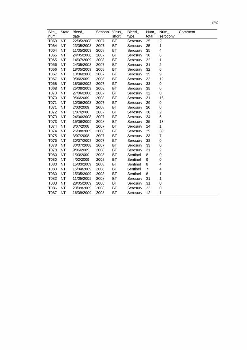
242

Site_ num

State Bleed_ date

Season Virus_short

Bleed_ type

Num_total

Num_ seroconv

Comment

T063 NT 22/05/2008 2007 BT Serosurv 35 2 T064 NT 23/05/2008 2007 BT Serosurv 35 1 T064 NT 11/05/2009 2008 BT Serosurv 35 4 T065 NT 24/05/2008 2007 BT Serosurv 30 6 T065 NT 14/07/2009 2008 BT Serosurv 32 1 T066 NT 24/05/2008 2007 BT Serosurv 31 2 T066 NT 18/05/2009 2008 BT Serosurv 32 6 T067 NT 10/06/2008 2007 BT Serosurv 35 9 T067 NT 9/06/2009 2008 BT Serosurv 32 12 T068 NT 18/06/2008 2007 BT Serosurv 33 0 T068 NT 25/08/2009 2008 BT Serosurv 35 0 T070 NT 27/06/2008 2007 BT Serosurv 32 0 T070 NT 9/06/2009 2008 BT Serosurv 31 16 T071 NT 30/06/2008 2007 BT Serosurv 29 0 T071 NT 2/03/2009 2008 BT Serosurv 20 0 T072 NT 1/07/2008 2007 BT Serosurv 30 2 T073 NT 24/06/2008 2007 BT Serosurv 34 6 T073 NT 15/06/2009 2008 BT Serosurv 35 13 T074 NT 8/07/2008 2007 BT Serosurv 24 1 T074 NT 26/08/2009 2008 BT Serosurv 35 30 T075 NT 3/07/2008 2007 BT Serosurv 23 7 T076 NT 30/07/2008 2007 BT Serosurv 38 0 T078 NT 30/07/2008 2007 BT Serosurv 33 0 T078 NT 9/06/2009 2008 BT Serosurv 31 2 T080 NT 1/03/2009 2008 BT Sentinel 8 0 T080 NT 4/02/2009 2008 BT Sentinel 9 0 T080 NT 15/03/2009 2008 BT Sentinel 8 4 T080 NT 15/04/2009 2008 BT Sentinel 7 4 T080 NT 15/05/2009 2008 BT Sentinel 8 1 T082 NT 11/05/2009 2008 BT Serosurv 31 1 T083 NT 28/05/2009 2008 BT Serosurv 31 0 T086 NT 23/09/2009 2008 BT Serosurv 32 0 T087 NT 16/09/2009 2008 BT Serosurv 12 1

243

APPENDIX C

SUMMARY OF BTV STATUS AND AVERAGE ENVIRONMENTAL CONDITIONS OF NAMP SITES IN THE PILBARA

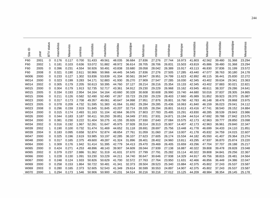
244

Site

ID

year

BTV

sta

tus

max

ndvi

ss

Max

evis

s

smin

tss

max

lstd

ss

max

lstd

su

max

lstd

au

Max

lstd

pw

Min

lstn

ss

min

lstn

su

min

lstn

au

Min

lstn

pw

mea

nlst

dss

Mea

nlst

dsu

mea

nlst

dau

mea

nlst

dpw

Mea

nlst

nss

F60 2001 0 0.176 0.117 0.700 51.433 49.561 48.035 36.684 27.836 27.276 27.744 16.973 41.803 42.562 39.480 31.368 23.294 F60 2002 1 0.181 0.103 0.636 53.072 51.882 48.972 36.614 28.705 28.706 26.831 15.503 43.819 45.886 39.480 31.368 23.294 F60 2005 0 0.396 0.231 4.554 50.926 50.491 43.838 33.680 28.058 28.042 26.389 15.917 43.113 46.830 37.836 31.199 23.572 F60 2008 0 0.321 0.190 2.611 50.966 50.966 44.445 34.545 27.836 27.276 27.505 17.285 43.440 47.077 38.763 30.180 24.178 W006 2000 0 0.233 0.127 1.302 53.836 53.839 41.334 30.561 28.947 28.951 24.799 11.623 42.892 48.115 36.441 25.830 22.272 W014 2000 0 0.323 0.199 3.283 54.171 52.883 41.930 35.270 27.909 27.547 27.285 16.030 42.345 43.402 39.634 29.341 23.363 W014 2002 0 0.305 0.179 2.205 50.613 50.395 44.760 37.127 28.214 28.216 25.354 15.133 42.345 43.402 37.883 30.021 22.821 W015 2000 0 0.304 0.179 1.913 52.735 52.717 43.361 34.912 29.230 29.229 26.968 15.162 43.945 48.611 38.337 29.286 24.641 W015 2005 0 0.334 0.193 2.954 54.164 54.164 43.660 30.328 30.608 30.608 26.990 15.740 44.680 50.016 37.837 28.305 24.865 W015 2006 0 0.211 0.126 0.582 52.490 52.490 47.267 33.723 29.230 29.229 28.403 17.660 45.989 51.852 39.923 28.370 25.987 W023 2000 0 0.317 0.173 2.708 49.357 49.061 40.647 34.998 27.951 27.876 26.801 16.790 42.783 46.148 38.476 28.868 23.975 W023 2005 0 0.378 0.209 4.732 51.595 51.383 41.064 31.692 29.284 29.285 25.436 16.063 41.840 46.159 36.023 29.041 24.112 W023 2008 0 0.296 0.159 2.919 51.845 51.845 43.207 32.714 28.335 28.294 26.801 16.613 43.416 47.741 38.540 28.152 24.884 W024 2000 0 0.315 0.174 2.493 51.163 51.104 42.664 36.076 27.803 27.783 25.495 15.291 43.830 48.285 38.539 29.843 23.986 W026 2000 0 0.344 0.183 3.187 50.411 50.293 39.851 34.049 27.931 27.931 24.871 15.194 44.514 47.692 39.788 27.842 23.575 W034 2000 0 0.381 0.230 3.222 51.404 50.275 41.155 35.926 27.930 27.640 27.084 15.575 42.173 42.963 39.777 28.850 23.098 W034 2002 0 0.316 0.192 1.967 52.261 51.647 45.975 37.928 28.314 28.313 25.907 14.407 42.173 42.963 36.961 29.840 22.347 W039 2002 1 0.190 0.100 0.732 51.474 51.469 44.652 31.118 28.691 28.697 25.756 13.448 41.778 46.699 34.433 24.110 21.851 W039 2004 0 0.183 0.095 0.658 52.874 52.874 48.654 27.761 31.059 31.060 27.164 13.007 41.178 45.832 34.759 24.015 22.607 W047 2000 0 0.325 0.196 2.619 53.985 53.197 42.285 36.107 27.623 27.605 26.174 15.534 44.182 45.550 41.407 29.364 23.274 W048 2000 0 0.317 0.165 2.375 49.600 49.287 41.324 31.896 28.401 28.402 24.960 13.811 43.295 47.937 36.870 25.874 23.220 W064 2000 1 0.309 0.176 1.942 51.414 51.395 42.779 34.413 29.470 29.469 26.405 15.659 43.296 47.704 37.707 28.188 25.217 W065 2000 0 0.424 0.271 4.253 48.896 48.143 39.907 34.609 28.044 27.939 27.138 16.887 40.322 39.808 39.478 28.828 23.048 W065 2002 0 0.379 0.237 2.886 51.362 51.319 41.631 37.670 27.799 27.791 25.282 15.114 40.322 39.808 34.841 29.256 22.367 W066 2000 1 0.228 0.130 1.091 53.230 53.229 44.211 34.740 30.647 30.646 27.938 14.329 44.917 49.756 38.815 28.481 24.564 W067 2000 0 0.248 0.124 1.933 50.826 50.629 41.700 32.572 27.763 27.764 23.950 11.631 42.466 46.856 36.449 24.386 22.047 W069 2000 0 0.258 0.153 1.864 50.722 50.481 41.341 32.373 28.504 28.523 25.340 15.884 42.375 45.802 37.243 26.537 23.587 W069 2003 0 0.280 0.165 2.373 52.605 52.543 41.349 29.614 30.599 30.553 24.897 14.907 42.375 45.802 37.243 26.537 23.587 W070 2000 1 0.294 0.173 1.546 50.906 50.900 43.231 34.514 30.216 30.216 27.012 15.125 44.209 48.984 38.354 28.145 25.178

245

Site

ID

year

BTV

sta

tus

max

ndvi

ss

max

evis

s

smin

tss

max

lstd

ss

max

lstd

su

max

lstd

au

max

lstd

pw

min

lstn

ss

Min

lstn

su

min

lstn

au

min

lstn

pw

mea

nlst

dss

mea

nlst

dsu

mea

nlst

dau

mea

nlst

dpw

mea

nlst

nss

W071 2000 0 0.313 0.177 2.113 50.859 50.658 43.703 38.770 28.049 27.698 27.508 16.585 44.420 46.878 41.116 31.823 23.425 W072 2000 0 0.323 0.191 1.706 50.044 49.851 43.583 35.660 27.398 27.394 25.977 14.967 43.478 47.754 38.528 29.885 23.234 W072 2001 0 0.280 0.152 2.107 50.526 50.507 44.497 35.839 27.467 27.438 26.278 16.050 41.687 43.254 38.545 29.227 22.727 W072 2005 0 0.376 0.210 3.499 52.504 52.505 41.282 30.639 28.866 28.827 26.858 16.237 45.019 49.912 38.672 29.772 23.414 W073 2000 1 0.319 0.175 2.446 50.606 50.579 41.986 34.325 28.917 28.905 26.353 15.212 43.042 47.542 37.529 27.997 24.413 W073 2001 1 0.289 0.159 2.247 51.569 51.577 43.198 34.367 29.988 29.995 26.821 16.356 40.906 42.545 37.293 28.817 23.333 W074 2000 0 0.297 0.163 2.485 50.016 49.824 39.361 30.785 27.543 27.543 23.756 12.359 41.477 45.626 35.455 23.591 22.134 W075 2000 0 0.288 0.170 1.812 50.223 49.957 43.749 34.033 28.634 28.634 26.592 15.114 43.980 48.368 39.079 29.141 23.910 W075 2001 1 0.247 0.137 1.227 51.355 51.355 46.507 34.639 28.725 28.715 27.544 15.994 41.905 43.891 38.311 28.060 23.053 W075 2004 0 0.223 0.126 1.151 52.960 52.960 49.291 30.582 31.187 31.181 28.930 15.762 44.271 47.963 39.295 28.245 23.956 W076 2000 0 0.329 0.208 3.796 51.776 51.298 41.812 35.617 27.969 27.851 27.246 16.286 41.485 41.836 39.994 28.868 23.435 W076 2001 0 0.305 0.193 1.851 49.009 47.832 44.617 34.152 27.559 27.556 25.750 16.494 40.100 41.547 36.695 30.070 22.783 W076 2002 0 0.300 0.183 2.294 51.856 51.840 44.259 36.738 28.392 28.394 25.324 15.665 41.485 41.836 36.695 30.070 22.783 W076 2003 0 0.317 0.192 2.707 50.390 50.129 42.210 32.882 27.438 27.440 25.311 17.864 41.485 41.836 39.994 28.868 23.435 W076 2006 0 0.292 0.177 1.915 52.050 51.871 49.429 36.614 27.969 27.851 27.521 15.795 43.965 45.885 41.330 30.548 24.644 W076 2008 0 0.296 0.180 2.136 50.456 50.455 43.848 34.889 27.559 27.556 27.246 16.753 43.436 48.258 37.121 30.095 24.132 W077 2000 0 0.280 0.168 2.120 51.122 51.080 41.160 34.949 28.360 28.360 25.855 16.950 43.180 44.758 39.977 28.033 23.949 W078 2000 0 0.280 0.170 1.838 52.341 52.127 42.179 34.061 28.608 28.599 26.619 16.038 41.682 43.641 37.831 26.490 24.457 W078 2001 0 0.303 0.186 2.093 51.798 48.867 42.578 32.884 29.830 29.829 26.064 15.387 40.873 42.315 37.177 28.353 23.062 W079 2000 0 0.241 0.153 1.048 51.171 51.171 44.195 31.838 27.778 27.738 26.980 15.637 42.740 47.261 37.764 27.385 23.226 W080 2000 0 0.274 0.168 1.354 49.905 49.901 43.824 33.716 26.982 26.980 25.643 15.618 43.901 48.020 39.447 29.546 22.864 W080 2007 0 0.256 0.150 1.405 54.153 54.076 44.556 34.395 26.982 26.980 27.906 16.824 41.702 44.852 37.143 25.561 22.322 W081 2000 0 0.302 0.179 1.632 49.766 49.759 43.791 34.736 28.147 28.144 25.921 14.736 43.976 47.944 39.407 29.527 23.525 W081 2006 0 0.218 0.126 0.536 53.346 53.346 48.507 34.627 28.147 28.144 26.922 16.452 46.246 51.380 41.073 28.533 24.698 W082 2000 0 0.300 0.162 1.929 52.195 52.189 44.315 37.169 27.638 27.416 27.135 16.062 44.908 48.921 39.895 31.641 23.686 W082 2001 1 0.244 0.125 1.752 52.669 52.512 45.946 36.907 27.837 27.656 27.171 15.925 43.315 45.287 39.801 30.873 23.165 W082 2004 1 0.296 0.145 2.319 53.959 53.960 48.840 35.051 29.116 29.025 27.905 17.115 46.616 49.730 41.993 30.970 24.143 W082 2006 1 0.242 0.130 0.896 52.450 52.446 46.848 35.378 27.638 27.416 27.541 16.514 46.117 51.126 40.745 31.168 24.778 W082 2007 0 0.319 0.158 2.955 55.926 55.857 44.154 38.625 27.638 27.416 27.135 15.609 40.433 43.651 34.414 28.385 23.172

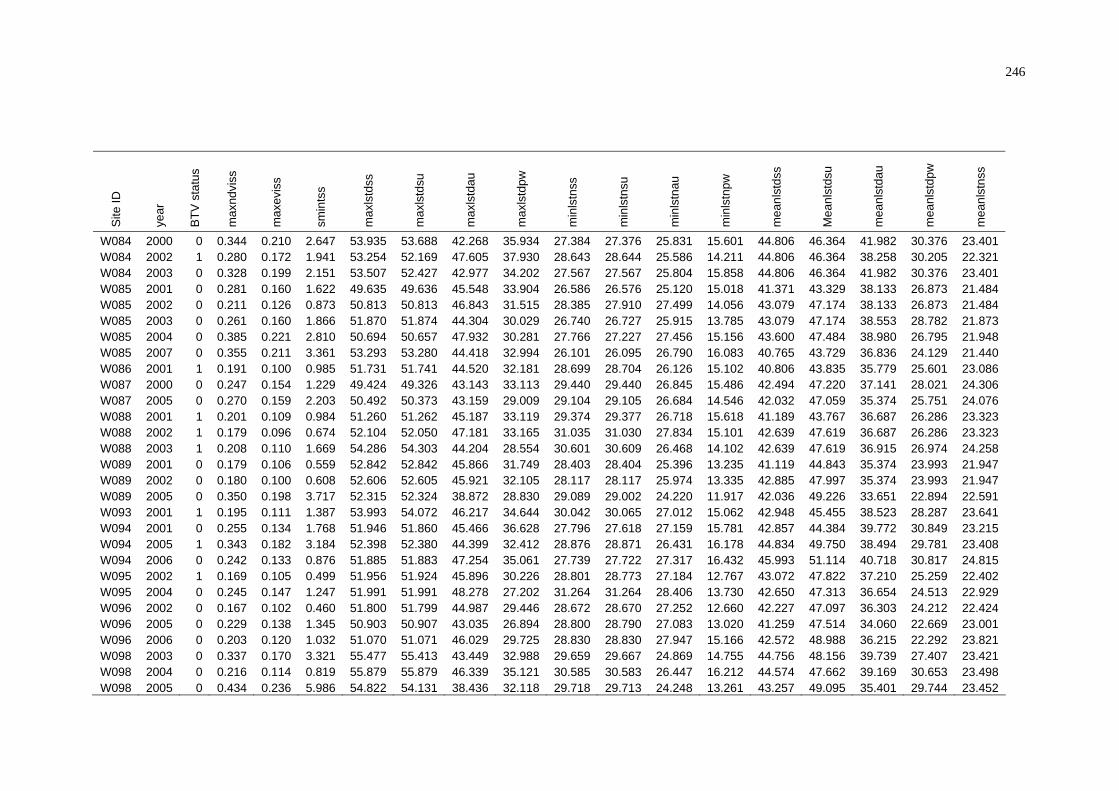
246

Site

ID

year

BTV

sta

tus

max

ndvi

ss

max

evis

s

smin

tss

max

lstd

ss

max

lstd

su

max

lstd

au

max

lstd

pw

min

lstn

ss

min

lstn

su

min

lstn

au

min

lstn

pw

mea

nlst

dss

Mea

nlst

dsu

mea

nlst

dau

mea

nlst

dpw

mea

nlst

nss


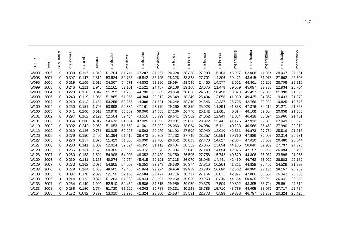
247

Site

ID

year

BTV

sta

tus

max

ndvi

ss

max

evis

s

smin

tss

max

lstd

ss

max

lstd

su

max

lstd

au

max

lstd

pw

min

lstn

ss

min

lstn

su

min

lstn

au

min

lstn

pw

mea

nlst

dss

mea

nlst

dsu

mea

nlst

dau

mea

nlst

dpw

mea

nlst

nss

W098 2006 0 0.338 0.167 1.843 51.754 51.744 47.287 34.567 28.328 28.328 27.283 16.153 46.997 52.008 41.354 28.947 24.561 W098 2007 0 0.307 0.147 2.311 53.624 52.768 46.842 36.125 28.328 28.328 27.701 14.306 39.471 43.615 31.075 27.662 22.303 W098 2008 0 0.319 0.168 2.518 54.567 54.571 44.652 32.130 29.594 29.598 24.435 14.577 42.651 48.361 36.268 26.798 23.316 W099 2003 0 0.246 0.121 1.945 52.161 52.161 42.522 24.487 29.108 29.108 23.676 11.478 39.579 45.097 32.738 22.934 20.704 W099 2004 0 0.220 0.110 0.842 51.753 51.753 44.730 25.309 28.850 28.850 24.531 10.498 39.829 45.497 32.391 21.998 21.222 W099 2006 0 0.240 0.119 1.056 51.865 51.865 44.384 28.812 28.349 28.349 25.404 13.056 41.939 49.435 34.867 19.433 21.878 W099 2007 0 0.219 0.112 1.151 53.258 53.257 44.388 31.521 28.349 28.349 24.646 12.337 36.795 42.766 28.283 19.825 19.676 W100 2004 0 0.260 0.151 1.795 50.898 50.884 47.161 23.179 29.360 29.359 25.928 11.394 41.358 47.376 34.212 21.271 21.758 W100 2005 0 0.341 0.200 3.312 50.978 50.689 39.006 24.063 27.136 26.770 25.142 11.681 40.894 48.108 32.584 20.658 21.383 W101 2002 0 0.297 0.162 2.122 52.504 52.484 43.516 33.299 29.641 29.582 24.362 12.949 41.884 46.418 35.094 25.966 21.461 W101 2005 0 0.364 0.200 4.017 54.672 54.334 37.825 31.392 29.901 29.893 23.872 12.441 41.125 47.912 32.325 27.049 22.876 W110 2002 0 0.392 0.242 2.953 51.653 51.659 41.061 36.992 28.063 28.064 24.984 15.111 40.233 40.566 35.453 27.990 22.219 W112 2002 0 0.212 0.126 0.766 50.925 50.925 46.503 30.089 28.192 27.508 27.949 13.010 42.681 46.873 37.751 25.516 21.317 W126 2005 0 0.279 0.150 2.492 51.394 51.416 38.473 26.863 27.733 27.749 23.257 10.554 39.790 47.986 30.003 22.314 20.931 W127 2005 0 0.270 0.157 1.870 51.429 51.386 45.890 29.788 28.852 28.835 27.473 14.627 42.854 47.616 36.507 26.486 23.544 W127 2008 0 0.233 0.141 1.009 52.824 52.824 45.355 31.112 28.434 28.332 26.866 13.894 44.105 50.040 37.939 27.797 24.270 W128 2005 0 0.255 0.151 1.576 50.365 50.365 45.372 29.375 27.304 27.042 27.140 14.054 42.325 47.157 36.281 26.094 22.499 W128 2007 0 0.260 0.153 1.691 54.908 54.908 46.053 32.439 26.750 26.505 27.756 15.742 40.620 44.806 35.032 23.898 21.966 W129 2005 0 0.239 0.141 1.135 49.974 49.974 45.415 30.121 27.215 26.979 26.948 14.441 42.469 46.762 36.920 26.883 22.182 W129 2007 0 0.273 0.162 2.071 54.605 54.603 46.052 32.943 26.530 26.374 27.316 16.264 41.211 44.828 36.406 24.529 21.893 W133 2000 0 0.278 0.164 1.667 49.501 49.455 41.844 33.924 29.959 29.959 26.786 16.080 42.502 46.890 37.181 28.157 25.353 W133 2005 0 0.307 0.176 2.829 52.150 52.152 42.684 29.477 30.716 30.717 27.164 16.031 42.927 47.866 36.551 26.943 25.255 W133 2006 1 0.214 0.122 0.871 51.263 51.262 45.844 32.597 29.959 29.959 29.258 18.340 44.584 50.025 39.260 26.941 26.555 W133 2007 0 0.264 0.149 1.990 52.510 52.450 45.586 34.715 29.959 29.959 29.376 17.509 39.892 43.895 33.724 25.691 24.312 W133 2008 0 0.255 0.150 1.774 51.720 51.720 44.362 30.788 30.231 30.228 26.786 15.710 43.765 48.995 38.071 27.717 26.434 W154 2008 0 0.172 0.092 0.799 53.010 52.995 41.324 23.860 25.587 25.591 22.778 8.598 39.388 46.797 31.759 20.324 20.425

248

site

ID

year

BTV

sta

tus

mea

nlst

nsu

mea

nlst

nau

mea

nlst

npw

mea

nlst

ss

mea

nlst

su

mea

nlst

au

mea

nlst

pw

gdda

gdds

s

gdds

u

gdda

u

rss

rsu

rau

F60 2001 0 25.932 21.008 13.720 33.766 13.951 13.451 22.544 4963.271 3548.542 1582.713 1352.435 33.097 9.914 23.183 F60 2002 1 24.938 21.008 13.720 34.705 34.247 13.451 22.544 4997.325 3629.545 1637.185 1394.169 86.434 51.202 35.232 F60 2005 0 25.359 22.044 13.925 31.457 37.090 31.773 22.562 4541.748 3051.749 1445.339 1016.893 573.491 373.569 199.848 F60 2008 0 26.313 22.010 13.034 32.549 34.051 27.590 21.607 4606.327 3249.335 1488.479 1215.751 312.660 268.115 43.543 W006 2000 0 25.368 19.462 9.930 31.718 36.282 26.205 17.880 3723.478 2963.297 1493.700 883.846 355.749 272.130 61.969 W014 2000 0 25.207 21.709 13.768 32.321 34.413 29.171 21.555 4367.755 3154.825 1406.428 1169.062 593.518 545.357 48.112 W014 2002 0 25.207 20.459 13.164 33.016 34.413 12.966 21.593 4714.922 3355.858 1588.116 1166.819 482.430 327.773 152.412 W015 2000 0 27.129 22.631 13.713 33.186 35.721 29.882 21.500 4476.958 3306.879 1486.846 1235.686 327.082 301.248 25.036 W015 2005 0 27.962 22.006 13.797 32.563 38.524 31.403 21.051 4598.128 3166.478 1550.413 1028.530 423.056 225.627 197.411 W015 2006 0 29.554 23.517 14.020 35.742 38.989 29.922 21.195 4964.612 3664.778 1671.908 1397.310 109.977 27.546 78.255 W023 2000 0 25.740 22.472 14.945 31.670 33.747 28.699 21.907 4270.659 3091.791 1402.934 1123.035 423.781 367.020 42.513 W023 2005 0 26.679 21.791 14.836 31.021 36.876 30.863 21.939 4287.512 2906.966 1376.236 934.266 922.845 544.600 378.243 W023 2008 0 26.993 22.656 13.445 31.670 33.699 26.726 20.798 4428.767 3186.635 1475.758 1160.044 423.781 367.020 42.513 W024 2000 0 26.240 22.120 13.707 32.397 34.749 29.263 21.775 4405.826 3206.188 1451.897 1177.200 447.227 389.054 47.410 W026 2000 0 25.939 21.296 12.855 30.864 33.350 27.317 20.348 3979.905 2909.807 1363.149 990.453 567.380 488.819 54.436 W034 2000 0 25.011 21.462 13.049 30.998 32.750 28.223 20.949 4050.379 2925.698 1303.259 1078.088 530.323 491.164 39.159 W034 2002 0 25.011 19.486 12.317 33.448 32.750 12.521 21.078 4765.496 3383.688 1571.433 1211.762 421.406 279.937 140.602 W039 2002 1 25.673 18.073 10.108 31.892 35.260 11.671 17.109 3791.141 3093.341 1569.647 937.916 206.441 148.009 56.584 W039 2004 0 26.409 18.787 10.007 33.873 36.186 27.836 17.011 3956.585 3302.826 1631.330 1146.637 106.814 17.744 74.934 W047 2000 0 24.989 21.936 13.352 32.253 34.855 28.903 21.358 4318.108 3147.465 1442.588 1142.673 661.488 607.750 49.390 W048 2000 0 26.603 19.736 11.333 30.920 33.719 26.917 18.603 3880.763 2920.472 1393.802 956.201 491.624 412.450 43.394 W064 2000 1 27.968 22.800 14.213 32.666 35.105 29.377 21.200 4395.695 3239.747 1466.089 1188.200 444.457 413.647 26.539 W065 2000 0 24.665 21.665 13.683 30.056 32.154 27.232 21.255 3886.699 2762.082 1273.317 984.957 583.760 482.626 101.036 W065 2002 0 24.665 19.620 13.397 32.307 32.154 12.098 21.326 4612.780 3215.688 1493.141 1133.227 564.845 423.631 139.734 W066 2000 1 27.823 21.579 12.855 33.405 36.114 29.634 20.668 4418.664 3299.461 1482.413 1211.226 375.778 349.719 25.600 W067 2000 0 25.502 18.723 9.532 30.890 34.365 26.001 16.959 3676.165 2889.972 1434.127 864.476 512.776 424.315 59.259 W069 2000 0 26.160 20.818 12.231 31.529 33.993 28.075 19.384 4036.820 3039.986 1402.890 1069.609 569.734 496.894 34.209 W069 2003 0 26.160 20.818 12.231 32.147 33.993 28.075 19.384 4174.932 3081.046 1575.794 914.818 545.278 348.028 190.163 W070 2000 1 28.161 22.508 13.488 32.747 35.131 29.306 20.817 4356.282 3235.711 1455.345 1181.309 413.488 393.378 20.073

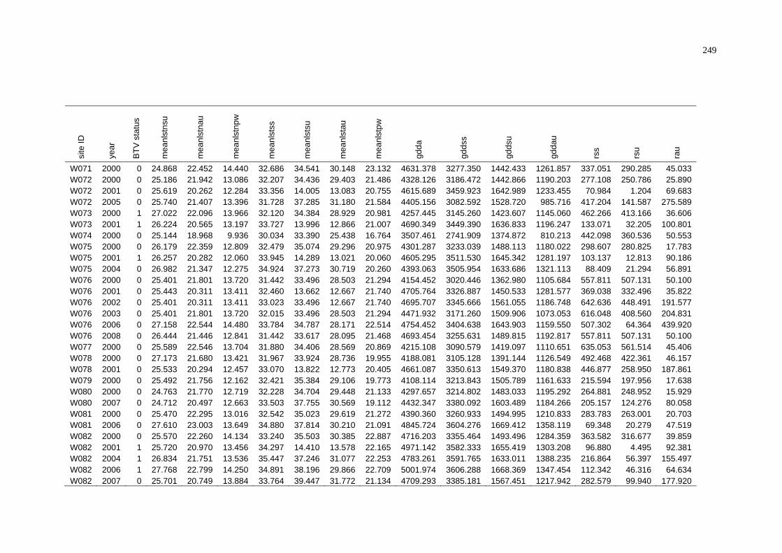
249

site

ID

year

BTV

sta

tus

mea

nlst

nsu

mea

nlst

nau

mea

nlst

npw

mea

nlst

ss

mea

nlst

su

mea

nlst

au

mea

nlst

pw

gdda

gdds

s

gdds

u

gdda

u

rss

rsu

rau

W071 2000 0 24.868 22.452 14.440 32.686 34.541 30.148 23.132 4631.378 3277.350 1442.433 1261.857 337.051 290.285 45.033 W072 2000 0 25.186 21.942 13.086 32.207 34.436 29.403 21.486 4328.126 3186.472 1442.866 1190.203 277.108 250.786 25.890 W072 2001 0 25.619 20.262 12.284 33.356 14.005 13.083 20.755 4615.689 3459.923 1642.989 1233.455 70.984 1.204 69.683 W072 2005 0 25.740 21.407 13.396 31.728 37.285 31.180 21.584 4405.156 3082.592 1528.720 985.716 417.204 141.587 275.589 W073 2000 1 27.022 22.096 13.966 32.120 34.384 28.929 20.981 4257.445 3145.260 1423.607 1145.060 462.266 413.166 36.606 W073 2001 1 26.224 20.565 13.197 33.727 13.996 12.866 21.007 4690.349 3449.390 1636.833 1196.247 133.071 32.205 100.801 W074 2000 0 25.144 18.968 9.936 30.034 33.390 25.438 16.764 3507.461 2741.909 1374.872 810.213 442.098 360.536 50.553 W075 2000 0 26.179 22.359 12.809 32.479 35.074 29.296 20.975 4301.287 3233.039 1488.113 1180.022 298.607 280.825 17.783 W075 2001 1 26.257 20.282 12.060 33.945 14.289 13.021 20.060 4605.295 3511.530 1645.342 1281.197 103.137 12.813 90.186 W075 2004 0 26.982 21.347 12.275 34.924 37.273 30.719 20.260 4393.063 3505.954 1633.686 1321.113 88.409 21.294 56.891 W076 2000 0 25.401 21.801 13.720 31.442 33.496 28.503 21.294 4154.452 3020.446 1362.980 1105.684 557.811 507.131 50.100 W076 2001 0 25.443 20.311 13.411 32.460 13.662 12.667 21.740 4705.764 3326.887 1450.533 1281.577 369.038 332.496 35.822 W076 2002 0 25.401 20.311 13.411 33.023 33.496 12.667 21.740 4695.707 3345.666 1561.055 1186.748 642.636 448.491 191.577 W076 2003 0 25.401 21.801 13.720 32.015 33.496 28.503 21.294 4471.932 3171.260 1509.906 1073.053 616.048 408.560 204.831 W076 2006 0 27.158 22.544 14.480 33.784 34.787 28.171 22.514 4754.452 3404.638 1643.903 1159.550 507.302 64.364 439.920 W076 2008 0 26.444 21.446 12.841 31.442 33.617 28.095 21.468 4693.454 3255.631 1489.815 1192.817 557.811 507.131 50.100 W077 2000 0 25.589 22.546 13.704 31.880 34.406 28.569 20.869 4215.108 3090.579 1419.097 1110.651 635.053 561.514 45.406 W078 2000 0 27.173 21.680 13.421 31.967 33.924 28.736 19.955 4188.081 3105.128 1391.144 1126.549 492.468 422.361 46.157 W078 2001 0 25.533 20.294 12.457 33.070 13.822 12.773 20.405 4661.087 3350.613 1549.370 1180.838 446.877 258.950 187.861 W079 2000 0 25.492 21.756 12.162 32.421 35.384 29.106 19.773 4108.114 3213.843 1505.789 1161.633 215.594 197.956 17.638 W080 2000 0 24.763 21.770 12.719 32.228 34.704 29.448 21.133 4297.657 3214.802 1483.033 1195.292 264.881 248.952 15.929 W080 2007 0 24.712 20.497 12.663 33.503 37.755 30.569 19.112 4432.347 3380.092 1603.489 1184.266 205.157 124.276 80.058 W081 2000 0 25.470 22.295 13.016 32.542 35.023 29.619 21.272 4390.360 3260.933 1494.995 1210.833 283.783 263.001 20.703 W081 2006 0 27.610 23.003 13.649 34.880 37.814 30.210 21.091 4845.724 3604.276 1669.412 1358.119 69.348 20.279 47.519 W082 2000 0 25.570 22.260 14.134 33.240 35.503 30.385 22.887 4716.203 3355.464 1493.496 1284.359 363.582 316.677 39.859 W082 2001 1 25.720 20.970 13.456 34.297 14.410 13.578 22.165 4971.142 3582.333 1655.419 1303.208 96.880 4.495 92.381 W082 2004 1 26.834 21.751 13.536 35.447 37.246 31.077 22.253 4783.261 3591.765 1633.011 1388.235 216.864 56.397 155.497 W082 2006 1 27.768 22.799 14.250 34.891 38.196 29.866 22.709 5001.974 3606.288 1668.369 1347.454 112.342 46.316 64.634 W082 2007 0 25.701 20.749 13.884 33.764 39.447 31.772 21.134 4709.293 3385.181 1567.451 1217.942 282.579 99.940 177.920

250

site

ID

year

BTV

sta

tus

mea

nlst

nsu

mea

nlst

nau

mea

nlst

npw

mea

nlst

ss

mea

nlst

su

mea

nlst

au

mea

nlst

pw

gdda

gdds

s

gdds

u

gdda

u

rss

rsu

rau


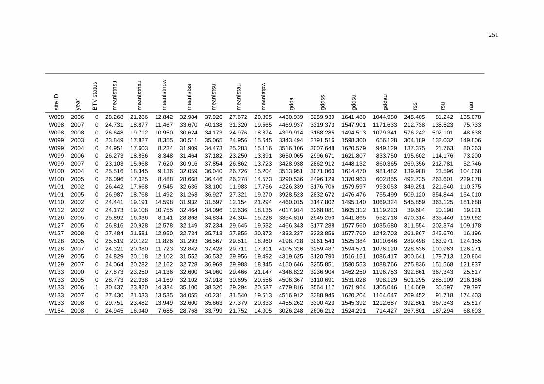
251

site

ID

year

BTV

sta

tus

mea

nlst

nsu

mea

nlst

nau

mea

nlst

npw

mea

nlst

ss

mea

nlst

su

mea

nlst

au

mea

nlst

pw

gdda

gdds

s

gdds

u

gdda

u

rss

rsu

rau

W098 2006 0 28.268 21.286 12.842 32.984 37.926 27.672 20.895 4430.939 3259.939 1641.480 1044.980 245.405 81.242 135.078 W098 2007 0 24.731 18.877 11.467 33.670 40.138 31.320 19.565 4469.937 3319.373 1547.901 1171.633 212.738 135.523 75.733 W098 2008 0 26.648 19.712 10.950 30.624 34.173 24.976 18.874 4399.914 3168.285 1494.513 1079.341 576.242 502.101 48.838 W099 2003 0 23.849 17.827 8.355 30.511 35.065 24.956 15.645 3343.494 2791.516 1598.300 656.128 304.189 132.032 149.806 W099 2004 0 24.951 17.603 8.234 31.909 34.473 25.283 15.116 3516.106 3007.648 1620.579 949.129 137.375 21.763 80.363 W099 2006 0 26.273 18.856 8.348 31.464 37.182 23.250 13.891 3650.065 2996.671 1621.807 833.750 195.602 114.176 73.200 W099 2007 0 23.103 15.968 7.620 30.916 37.854 26.862 13.723 3428.938 2862.912 1448.132 860.365 269.356 212.781 52.746 W100 2004 0 25.516 18.345 9.136 32.059 36.040 26.726 15.204 3513.951 3071.060 1614.470 981.482 139.988 23.596 104.068 W100 2005 0 26.096 17.025 8.488 28.668 36.446 26.278 14.573 3290.536 2496.129 1370.963 602.855 492.735 263.601 229.078 W101 2002 0 26.442 17.668 9.545 32.636 33.100 11.983 17.756 4226.339 3176.706 1579.597 993.053 349.251 221.540 110.375 W101 2005 0 26.987 18.768 11.492 31.263 36.927 27.321 19.270 3928.523 2832.672 1476.476 755.499 509.120 354.844 154.010 W110 2002 0 24.441 19.191 14.598 31.932 31.597 12.154 21.294 4460.015 3147.802 1495.140 1069.324 545.859 363.125 181.688 W112 2002 0 24.173 19.108 10.755 32.464 34.096 12.636 18.135 4017.914 3268.081 1605.312 1119.223 39.604 20.190 19.021 W126 2005 0 25.892 16.036 8.141 28.868 34.834 24.304 15.228 3354.816 2545.250 1441.865 552.718 470.314 335.446 119.692 W127 2005 0 26.816 20.928 12.578 32.149 37.234 29.645 19.532 4466.343 3177.288 1577.560 1035.680 311.554 202.374 109.178 W127 2008 0 27.484 21.581 12.950 32.734 35.713 27.855 20.373 4333.237 3333.856 1577.760 1242.703 261.867 245.670 16.196 W128 2005 0 25.519 20.122 11.826 31.293 36.567 29.511 18.960 4198.728 3061.543 1525.384 1010.646 289.498 163.971 124.155 W128 2007 0 24.321 20.080 11.723 32.842 37.428 29.711 17.811 4105.326 3259.487 1594.571 1076.120 228.636 100.963 126.271 W129 2005 0 24.829 20.118 12.102 31.552 36.532 29.956 19.492 4319.625 3120.790 1516.151 1086.417 300.641 179.713 120.864 W129 2007 0 24.064 20.282 12.162 32.728 36.969 29.988 18.345 4150.646 3255.851 1580.553 1088.766 275.836 151.568 121.937 W133 2000 0 27.873 23.250 14.136 32.600 34.960 29.466 21.147 4346.822 3236.904 1462.250 1196.753 392.861 367.343 25.517 W133 2005 0 28.773 22.038 14.169 32.102 37.918 30.695 20.556 4506.367 3110.691 1531.028 998.129 501.295 285.109 216.186 W133 2006 1 30.437 23.820 14.334 35.100 38.320 29.294 20.637 4779.816 3564.117 1671.964 1305.046 114.669 30.597 79.797 W133 2007 0 27.430 21.033 13.535 34.055 40.231 31.540 19.613 4516.912 3388.945 1620.204 1164.647 269.452 91.718 174.403 W133 2008 0 29.751 23.482 13.949 32.600 35.663 27.379 20.833 4455.262 3300.423 1545.392 1212.687 392.861 367.343 25.517 W154 2008 0 24.945 16.040 7.685 28.768 33.799 21.752 14.005 3026.248 2606.212 1524.291 714.427 267.801 187.294 68.603

252

APPENDIX D

SUMMARY OF BTV STATUS AND WEIGHTED AVERAGE ENVIRONMENTAL CONDITIONS OF NAMP SITES IN THE PILBARA

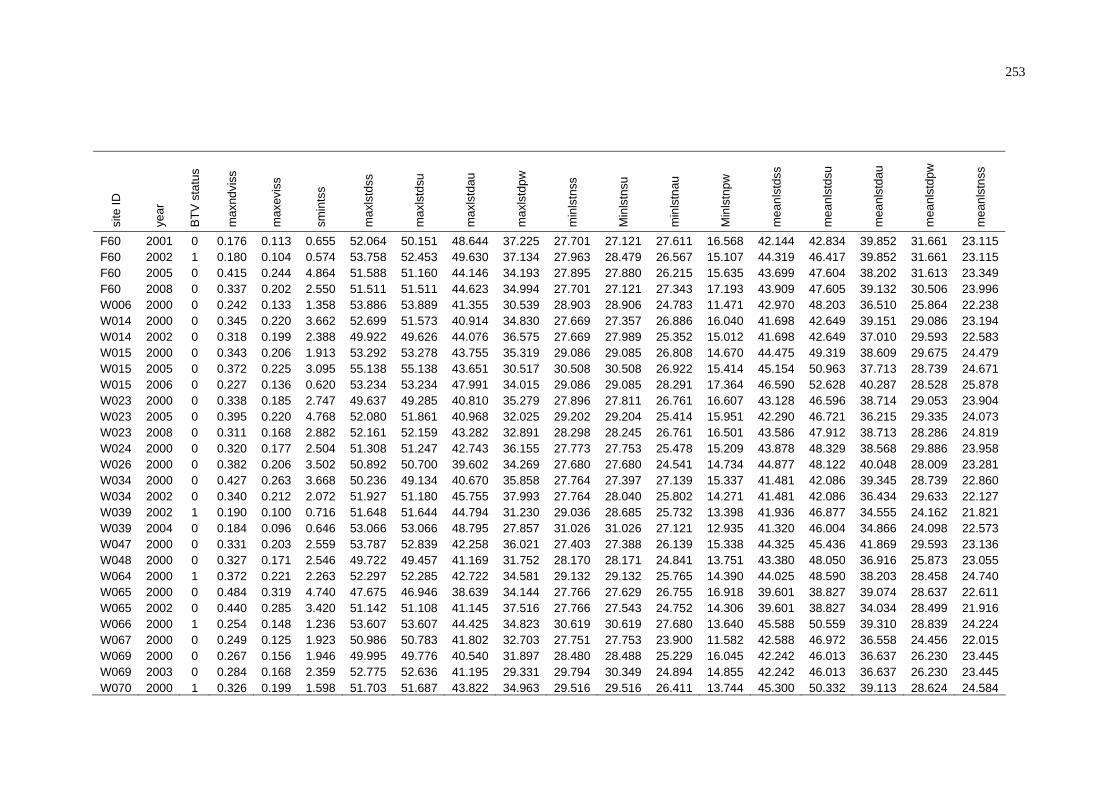
253

site

ID

year

BTV

sta

tus

max

ndvi

ss

max

evis

s

smin

tss

max

lstd

ss

max

lstd

su

max

lstd

au

max

lstd

pw

min

lstn

ss

Min

lstn

su

min

lstn

au

Min

lstn

pw

mea

nlst

dss

mea

nlst

dsu

mea

nlst

dau

mea

nlst

dpw

mea

nlst

nss

F60 2001 0 0.176 0.113 0.655 52.064 50.151 48.644 37.225 27.701 27.121 27.611 16.568 42.144 42.834 39.852 31.661 23.115 F60 2002 1 0.180 0.104 0.574 53.758 52.453 49.630 37.134 27.963 28.479 26.567 15.107 44.319 46.417 39.852 31.661 23.115 F60 2005 0 0.415 0.244 4.864 51.588 51.160 44.146 34.193 27.895 27.880 26.215 15.635 43.699 47.604 38.202 31.613 23.349 F60 2008 0 0.337 0.202 2.550 51.511 51.511 44.623 34.994 27.701 27.121 27.343 17.193 43.909 47.605 39.132 30.506 23.996 W006 2000 0 0.242 0.133 1.358 53.886 53.889 41.355 30.539 28.903 28.906 24.783 11.471 42.970 48.203 36.510 25.864 22.238 W014 2000 0 0.345 0.220 3.662 52.699 51.573 40.914 34.830 27.669 27.357 26.886 16.040 41.698 42.649 39.151 29.086 23.194 W014 2002 0 0.318 0.199 2.388 49.922 49.626 44.076 36.575 27.669 27.989 25.352 15.012 41.698 42.649 37.010 29.593 22.583 W015 2000 0 0.343 0.206 1.913 53.292 53.278 43.755 35.319 29.086 29.085 26.808 14.670 44.475 49.319 38.609 29.675 24.479 W015 2005 0 0.372 0.225 3.095 55.138 55.138 43.651 30.517 30.508 30.508 26.922 15.414 45.154 50.963 37.713 28.739 24.671 W015 2006 0 0.227 0.136 0.620 53.234 53.234 47.991 34.015 29.086 29.085 28.291 17.364 46.590 52.628 40.287 28.528 25.878 W023 2000 0 0.338 0.185 2.747 49.637 49.285 40.810 35.279 27.896 27.811 26.761 16.607 43.128 46.596 38.714 29.053 23.904 W023 2005 0 0.395 0.220 4.768 52.080 51.861 40.968 32.025 29.202 29.204 25.414 15.951 42.290 46.721 36.215 29.335 24.073 W023 2008 0 0.311 0.168 2.882 52.161 52.159 43.282 32.891 28.298 28.245 26.761 16.501 43.586 47.912 38.713 28.286 24.819 W024 2000 0 0.320 0.177 2.504 51.308 51.247 42.743 36.155 27.773 27.753 25.478 15.209 43.878 48.329 38.568 29.886 23.958 W026 2000 0 0.382 0.206 3.502 50.892 50.700 39.602 34.269 27.680 27.680 24.541 14.734 44.877 48.122 40.048 28.009 23.281 W034 2000 0 0.427 0.263 3.668 50.236 49.134 40.670 35.858 27.764 27.397 27.139 15.337 41.481 42.086 39.345 28.739 22.860 W034 2002 0 0.340 0.212 2.072 51.927 51.180 45.755 37.993 27.764 28.040 25.802 14.271 41.481 42.086 36.434 29.633 22.127 W039 2002 1 0.190 0.100 0.716 51.648 51.644 44.794 31.230 29.036 28.685 25.732 13.398 41.936 46.877 34.555 24.162 21.821 W039 2004 0 0.184 0.096 0.646 53.066 53.066 48.795 27.857 31.026 31.026 27.121 12.935 41.320 46.004 34.866 24.098 22.573 W047 2000 0 0.331 0.203 2.559 53.787 52.839 42.258 36.021 27.403 27.388 26.139 15.338 44.325 45.436 41.869 29.593 23.136 W048 2000 0 0.327 0.171 2.546 49.722 49.457 41.169 31.752 28.170 28.171 24.841 13.751 43.380 48.050 36.916 25.873 23.055 W064 2000 1 0.372 0.221 2.263 52.297 52.285 42.722 34.581 29.132 29.132 25.765 14.390 44.025 48.590 38.203 28.458 24.740 W065 2000 0 0.484 0.319 4.740 47.675 46.946 38.639 34.144 27.766 27.629 26.755 16.918 39.601 38.827 39.074 28.637 22.611 W065 2002 0 0.440 0.285 3.420 51.142 51.108 41.145 37.516 27.766 27.543 24.752 14.306 39.601 38.827 34.034 28.499 21.916 W066 2000 1 0.254 0.148 1.236 53.607 53.607 44.425 34.823 30.619 30.619 27.680 13.640 45.588 50.559 39.310 28.839 24.224 W067 2000 0 0.249 0.125 1.923 50.986 50.783 41.802 32.703 27.751 27.753 23.900 11.582 42.588 46.972 36.558 24.456 22.015 W069 2000 0 0.267 0.156 1.946 49.995 49.776 40.540 31.897 28.480 28.488 25.229 16.045 42.242 46.013 36.637 26.230 23.445 W069 2003 0 0.284 0.168 2.359 52.775 52.636 41.195 29.331 29.794 30.349 24.894 14.855 42.242 46.013 36.637 26.230 23.445 W070 2000 1 0.326 0.199 1.598 51.703 51.687 43.822 34.963 29.516 29.516 26.411 13.744 45.300 50.332 39.113 28.624 24.584

254

site

ID

year

BTV

sta

tus

max

ndvi

ss

max

evis

s

smin

tss

max

lstd

ss

max

lstd

su

max

lstd

au

max

lstd

pw

min

lstn

ss

min

lstn

su

min

lstn

au

min

lstn

pw

mea

nlst

dss

mea

nlst

dsu

mea

nlst

dau

mea

nlst

dpw

mea

nlst

nss


255

site

ID

year

BTV

sta

tus

max

ndvi

ss

max

evis

s

smin

tss

max

lstd

ss

max

lstd

su

max

lstd

au

max

lstd

pw

min

lstn

ss

min

lstn

su

min

lstn

au

min

lstn

pw

mea

nlst

dss

mea

nlst

dsu

mea

nlst

dau

mea

nlst

dpw

mea

nlst

nss


256

site

ID

year

BTV

sta

tus

max

ndvi

ss

max

evis

s

smin

tss

max

lstd

ss

max

lstd

su

max

lstd

au

max

lstd

pw

min

lstn

ss

min

lstn

su

min

lstn

au

min

lstn

pw

mea

nlst

dss

mea

nlst

dsu

mea

nlst

dau

mea

nlst

dpw

mea

nlst

nss

W098 2006 0 0.369 0.184 1.872 51.970 51.967 48.027 34.811 28.062 28.062 27.041 15.408 47.829 52.947 42.051 29.357 24.111 W098 2007 0 0.328 0.158 2.303 54.548 53.706 47.630 36.660 28.062 28.062 27.575 13.604 39.649 44.037 30.660 28.097 22.042 W098 2008 0 0.347 0.185 2.544 55.470 55.471 44.882 32.811 29.622 29.623 24.060 14.282 42.933 48.726 36.472 26.900 22.864 W099 2003 0 0.244 0.121 1.915 52.266 52.266 42.657 24.575 26.281 29.112 23.707 11.495 39.743 45.265 32.885 23.091 20.729 W099 2004 0 0.215 0.109 0.787 51.855 51.855 44.859 25.377 28.860 28.860 24.540 10.495 39.958 45.641 32.491 22.091 21.230 W099 2006 0 0.235 0.118 1.012 51.992 51.991 44.541 28.896 28.404 28.404 25.441 13.083 42.046 49.553 34.955 19.466 21.890 W099 2007 0 0.217 0.112 1.115 53.338 53.337 44.428 31.633 28.404 28.404 24.661 12.350 36.816 42.792 28.276 19.880 19.676 W100 2004 0 0.263 0.153 1.830 51.007 50.991 47.212 23.197 29.404 29.403 25.957 11.364 41.408 47.442 34.228 21.310 21.777 W100 2005 0 0.347 0.204 3.428 51.027 50.738 38.745 24.016 27.118 26.744 25.056 11.627 40.954 48.205 32.601 20.674 21.413 W101 2002 0 0.319 0.178 2.181 52.716 52.702 42.887 33.356 28.461 29.370 24.207 12.748 41.793 46.501 34.659 25.857 21.329 W101 2005 0 0.390 0.222 4.247 55.214 54.848 37.251 31.678 29.786 29.773 23.796 12.260 41.128 48.139 32.014 27.104 22.756 W110 2002 0 0.461 0.291 3.733 51.393 51.403 39.313 37.000 27.705 27.722 24.391 14.031 39.195 39.211 33.857 25.142 21.652 W112 2002 0 0.214 0.127 0.777 51.061 51.060 46.645 30.231 26.608 27.533 27.974 13.011 42.811 47.024 37.786 25.610 21.329 W126 2005 0 0.275 0.150 2.398 51.509 51.531 38.540 27.004 27.717 27.733 23.315 10.489 39.845 48.038 30.020 22.433 20.935 W127 2005 0 0.274 0.161 1.879 51.539 51.502 46.188 29.807 28.785 28.765 27.488 14.594 42.945 47.712 36.598 26.527 23.478 W127 2008 0 0.237 0.144 1.028 52.891 52.891 45.428 31.122 28.351 28.235 26.849 13.765 44.181 50.127 38.009 27.803 24.164 W128 2005 0 0.260 0.154 1.629 50.385 50.384 45.412 29.380 27.299 27.045 27.126 14.005 42.395 47.235 36.334 26.148 22.508 W128 2007 0 0.264 0.155 1.712 54.968 54.968 46.155 32.489 26.748 26.511 27.760 15.682 40.647 44.839 35.046 23.918 21.961 W129 2005 0 0.244 0.144 1.173 50.027 50.027 45.357 30.133 27.213 27.025 26.899 14.499 42.468 46.779 36.891 26.890 22.199 W129 2007 0 0.281 0.167 2.189 54.622 54.620 45.928 32.927 26.515 26.382 27.267 16.319 41.218 44.848 36.404 24.520 21.884 W133 2000 0 0.302 0.177 1.884 50.235 50.191 42.082 34.337 29.876 29.876 26.742 15.798 42.973 47.419 37.534 28.296 25.262 W133 2005 0 0.329 0.188 3.111 53.012 53.010 42.962 29.756 30.615 30.616 27.108 15.874 43.490 48.655 36.837 27.231 25.153 W133 2006 1 0.224 0.128 0.876 51.879 51.879 46.420 32.840 29.876 29.876 29.216 18.209 45.168 50.724 39.655 27.191 26.428 W133 2007 0 0.281 0.159 2.168 53.167 53.098 46.311 35.156 29.876 29.876 29.278 17.206 40.319 44.484 33.846 25.897 24.203 W133 2008 0 0.276 0.162 1.940 52.390 52.390 44.671 31.116 30.154 30.143 26.742 15.510 44.300 49.631 38.495 27.831 26.333 W154 2008 0 0.172 0.094 0.771 53.057 53.038 41.330 23.877 25.543 25.548 22.726 8.580 39.432 46.877 31.811 20.324 20.324

257

site

ID

year

BTV

sta

tus

mea

nlst

nsu

mea

nlst

nau

mea

nlst

npw

mea

nlst

ss

mea

nlst

su

mea

nlst

au

mea

nlst

pw

gdda

gdds

s

gdds

u

gdda

u

rss

rsu

rau

F60 2001 0 25.842 20.736 13.303 33.920 13.986 13.472 22.482 4986.619 3571.195 1594.801 1360.400 33.191 9.891 23.300 F60 2002 1 24.811 20.736 13.303 34.867 34.338 13.472 22.482 5016.990 3645.612 1644.652 1400.786 85.935 51.031 34.904 F60 2005 0 25.191 21.807 13.451 31.562 37.308 31.882 22.532 4555.137 3063.536 1458.156 1013.560 574.482 373.674 200.735 F60 2008 0 26.156 21.801 12.604 32.629 34.271 27.555 21.555 4629.884 3267.546 1496.967 1217.695 312.939 268.306 43.635 W006 2000 0 25.349 19.405 9.823 31.720 36.289 26.198 17.843 3719.728 2962.878 1493.731 883.382 354.804 271.912 60.314 W014 2000 0 25.025 21.560 13.786 31.587 33.607 28.571 21.436 4199.080 3027.241 1355.964 1112.052 613.113 559.400 53.634 W014 2002 0 25.025 20.131 12.994 32.596 33.607 12.699 21.294 4620.777 3292.828 1561.746 1141.650 494.059 339.527 151.789 W015 2000 0 27.032 22.376 13.365 33.210 35.762 29.845 21.520 4492.348 3305.100 1483.643 1231.996 332.823 306.463 25.531 W015 2005 0 27.825 21.708 13.482 32.632 38.843 31.532 21.110 4585.231 3159.947 1545.238 1023.163 423.700 227.493 196.192 W015 2006 0 29.516 23.312 13.701 35.940 39.394 29.710 21.114 4997.396 3676.317 1671.906 1405.868 108.755 27.605 76.849 W023 2000 0 25.713 22.355 14.770 31.699 33.783 28.677 21.912 4281.052 3094.769 1404.141 1121.009 423.880 367.057 42.574 W023 2005 0 26.614 21.738 14.642 31.075 37.064 30.994 21.989 4291.994 2908.142 1377.090 932.849 919.850 541.667 378.180 W023 2008 0 26.966 22.556 13.291 31.699 33.783 26.713 20.789 4430.566 3186.854 1476.419 1155.873 423.880 367.057 42.574 W024 2000 0 26.232 22.073 13.593 32.402 34.767 29.244 21.740 4406.114 3206.954 1452.520 1175.410 444.954 387.224 47.139 W026 2000 0 25.762 20.887 12.364 30.697 33.351 26.943 20.186 3930.976 2874.097 1361.893 954.581 567.912 489.460 54.073 W034 2000 0 24.889 21.133 12.718 30.446 32.177 27.784 20.729 3900.193 2825.205 1266.767 1035.509 534.673 496.739 37.934 W034 2002 0 24.889 19.133 12.104 33.136 32.177 12.316 20.869 4706.918 3342.286 1552.410 1194.750 427.438 290.676 136.134 W039 2002 1 25.670 18.020 10.036 31.947 35.324 11.687 17.099 3800.572 3099.041 1572.021 940.456 205.607 147.737 56.099 W039 2004 0 26.395 18.737 9.922 33.927 36.274 27.886 17.010 3964.897 3307.410 1631.569 1148.740 106.527 17.646 74.782 W047 2000 0 24.886 21.749 13.241 32.059 34.519 28.876 21.417 4291.071 3118.669 1424.531 1140.101 672.710 618.300 49.006 W048 2000 0 26.492 19.478 11.146 30.843 33.774 26.728 18.510 3863.275 2909.763 1400.008 941.931 487.040 410.356 40.823 W064 2000 1 27.724 22.086 13.187 32.359 34.928 28.849 20.823 4298.151 3172.142 1449.793 1137.521 446.511 415.018 27.080 W065 2000 0 24.405 21.030 13.069 29.321 31.351 26.514 20.853 3659.731 2611.171 1212.616 915.077 610.556 505.127 105.329 W065 2002 0 24.405 18.994 13.139 31.870 31.351 11.781 20.819 4483.104 3132.914 1463.040 1093.612 570.922 420.193 149.457 W066 2000 1 27.625 21.082 12.251 33.299 36.097 29.410 20.545 4393.885 3274.265 1478.780 1190.119 375.557 350.682 24.288 W067 2000 0 25.476 18.683 9.481 30.911 34.394 26.006 16.969 3684.968 2893.844 1435.236 865.460 511.695 423.724 58.865 W069 2000 0 26.026 20.700 12.160 31.223 33.792 27.645 19.195 3980.609 2999.326 1394.359 1036.856 567.026 494.842 33.266 W069 2003 0 26.026 20.700 12.160 32.059 33.792 27.645 19.195 4147.555 3063.131 1572.976 901.661 541.148 345.962 188.023 W070 2000 1 27.775 21.710 12.416 32.569 35.068 28.960 20.520 4306.497 3197.962 1449.894 1148.187 414.440 394.360 19.993

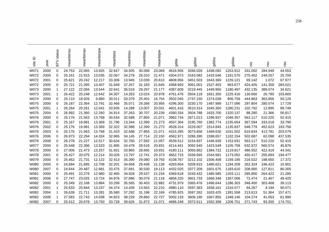
258

site

ID

year

BTV

sta

tus

mea

nlst

nsu

mea

nlst

nau

mea

nlst

npw

mea

nlst

ss

mea

nlst

su

mea

nlst

au

mea

nlst

pw

gdda

gdds

s

gdds

u

gdda

u

rss

rsu

rau


259

site

ID

year

BTV

sta

tus

mea

nlst

nsu

mea

nlst

nau

mea

nlst

npw

mea

nlst

ss

mea

nlst

su

mea

nlst

au

mea

nlst

pw

gdda

gdds

s

gdds

u

gdda

u

rss

rsu

rau


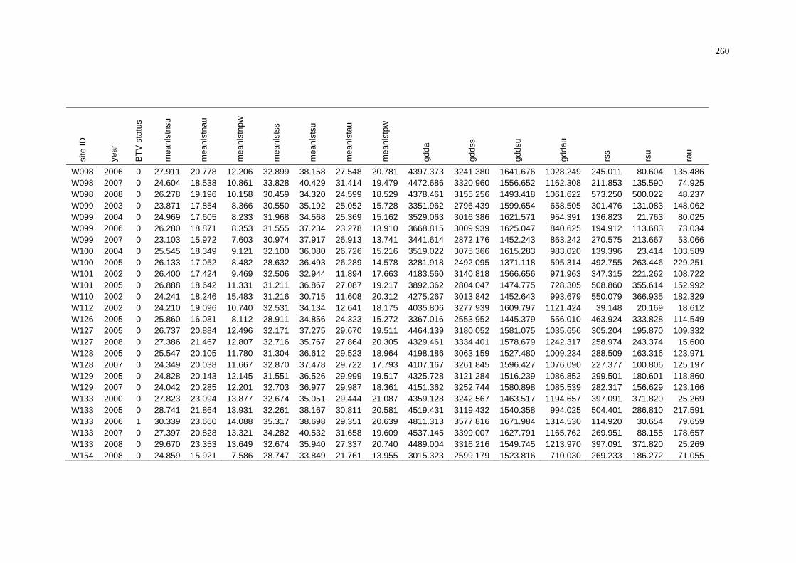
260

site

ID

year

BTV

sta

tus

mea

nlst

nsu

mea

nlst

nau

mea

nlst

npw

mea

nlst

ss

mea

nlst

su

mea

nlst

au

mea

nlst

pw

gdda

gdds

s

gdds

u

gdda

u

rss

rsu

rau

W098 2006 0 27.911 20.778 12.206 32.899 38.158 27.548 20.781 4397.373 3241.380 1641.676 1028.249 245.011 80.604 135.486 W098 2007 0 24.604 18.538 10.861 33.828 40.429 31.414 19.479 4472.686 3320.960 1556.652 1162.308 211.853 135.590 74.925 W098 2008 0 26.278 19.196 10.158 30.459 34.320 24.599 18.529 4378.461 3155.256 1493.418 1061.622 573.250 500.022 48.237 W099 2003 0 23.871 17.854 8.366 30.550 35.192 25.052 15.728 3351.962 2796.439 1599.654 658.505 301.476 131.083 148.062 W099 2004 0 24.969 17.605 8.233 31.968 34.568 25.369 15.162 3529.063 3016.386 1621.571 954.391 136.823 21.763 80.025 W099 2006 0 26.280 18.871 8.353 31.555 37.234 23.278 13.910 3668.815 3009.939 1625.047 840.625 194.912 113.683 73.034 W099 2007 0 23.103 15.972 7.603 30.974 37.917 26.913 13.741 3441.614 2872.176 1452.243 863.242 270.575 213.667 53.066 W100 2004 0 25.545 18.349 9.121 32.100 36.080 26.726 15.216 3519.022 3075.366 1615.283 983.020 139.396 23.414 103.589 W100 2005 0 26.133 17.052 8.482 28.632 36.493 26.289 14.578 3281.918 2492.095 1371.118 595.314 492.755 263.446 229.251 W101 2002 0 26.400 17.424 9.469 32.506 32.944 11.894 17.663 4183.560 3140.818 1566.656 971.963 347.315 221.262 108.722 W101 2005 0 26.888 18.642 11.331 31.211 36.867 27.087 19.217 3892.362 2804.047 1474.775 728.305 508.860 355.614 152.992 W110 2002 0 24.241 18.246 15.483 31.216 30.715 11.608 20.312 4275.267 3013.842 1452.643 993.679 550.079 366.935 182.329 W112 2002 0 24.210 19.096 10.740 32.531 34.134 12.641 18.175 4035.806 3277.939 1609.797 1121.424 39.148 20.169 18.612 W126 2005 0 25.860 16.081 8.112 28.911 34.856 24.323 15.272 3367.016 2553.952 1445.379 556.010 463.924 333.828 114.549 W127 2005 0 26.737 20.884 12.496 32.171 37.275 29.670 19.511 4464.139 3180.052 1581.075 1035.656 305.204 195.870 109.332 W127 2008 0 27.386 21.467 12.807 32.716 35.767 27.864 20.305 4329.461 3334.401 1578.679 1242.317 258.974 243.374 15.600 W128 2005 0 25.547 20.105 11.780 31.304 36.612 29.523 18.964 4198.186 3063.159 1527.480 1009.234 288.509 163.316 123.971 W128 2007 0 24.349 20.038 11.667 32.870 37.478 29.722 17.793 4107.167 3261.845 1596.427 1076.090 227.377 100.806 125.197 W129 2005 0 24.828 20.143 12.145 31.551 36.526 29.999 19.517 4325.728 3121.284 1516.239 1086.852 299.501 180.601 118.860 W129 2007 0 24.042 20.285 12.201 32.703 36.977 29.987 18.361 4151.362 3252.744 1580.898 1085.539 282.317 156.629 123.166 W133 2000 0 27.823 23.094 13.877 32.674 35.051 29.444 21.087 4359.128 3242.567 1463.517 1194.657 397.091 371.820 25.269 W133 2005 0 28.741 21.864 13.931 32.261 38.167 30.811 20.581 4519.431 3119.432 1540.358 994.025 504.401 286.810 217.591 W133 2006 1 30.339 23.660 14.088 35.317 38.698 29.351 20.639 4811.313 3577.816 1671.984 1314.530 114.920 30.654 79.659 W133 2007 0 27.397 20.828 13.321 34.282 40.532 31.658 19.609 4537.145 3399.007 1627.791 1165.762 269.951 88.155 178.657 W133 2008 0 29.670 23.353 13.649 32.674 35.940 27.337 20.740 4489.004 3316.216 1549.745 1213.970 397.091 371.820 25.269 W154 2008 0 24.859 15.921 7.586 28.747 33.849 21.761 13.955 3015.323 2599.179 1523.816 710.030 269.233 186.272 71.055

261

APPENDIX E

SUMMARY OF BTV STATUS AND AVERAGE ENVIRONMENTAL CONDITIONS OF NAMP SITES IN THE NORTHERN TERRITORY

262

site

ID

year

BTV

sta

tus

max

ndvi

ssal

l

max

evis

sall

smin

tss

max

lstd

ss

max

lstd

su

max

lstd

au

max

lstd

pw

min

lstn

pw

mea

nlst

dss

Mea

nlst

dsu

mea

nlst

dau

mea

nlst

dpw

mea

nlst

npw

mea

nlst

pw

rss

rsu

rau

108 2000 1 0.718 0.505 6.630 38.222 34.519 30.651 36.237 12.413 29.116 28.435 28.274 30.560 15.555 23.057 1914.786 1292.955 493.966 108 2001 1 0.726 0.522 7.590 37.498 35.848 33.293 34.247 11.328 30.238 28.880 30.761 30.863 17.022 23.942 1348.896 922.204 243.064 108 2002 1 0.735 0.532 6.542 37.343 31.607 33.471 36.104 12.617 30.635 28.653 31.119 32.416 14.849 23.633 1389.148 1071.307 166.099 108 2003 1 0.747 0.579 7.034 41.303 37.438 31.341 35.718 14.755 28.841 27.632 28.256 33.265 17.199 25.232 1931.793 1164.826 625.092 108 2004 1 0.692 0.531 4.963 35.828 35.320 33.437 34.942 12.099 30.883 30.067 30.655 30.473 15.470 22.971 1229.827 864.744 253.924 108 2005 1 0.734 0.599 8.871 39.691 33.745 29.122 37.433 12.465 27.511 26.405 26.525 33.347 17.106 25.227 2394.810 1103.649 992.777 108 2006 1 0.724 0.529 6.566 35.337 30.832 31.362 35.294 11.757 28.688 27.323 28.288 28.638 14.986 21.812 2356.750 1361.961 927.409 108 2007 1 0.703 0.490 6.456 35.000 34.287 32.365 35.623 10.392 28.921 27.235 29.677 29.767 15.352 22.559 1869.711 1253.317 480.831 108 2008 1 0.716 0.528 7.330 35.387 33.114 32.011 33.122 12.966 29.520 28.899 29.174 31.373 15.847 23.610 1914.786 1292.955 493.966 120 2000 0 0.511 0.315 4.833 41.943 37.601 34.758 34.495 13.060 33.498 33.660 31.186 30.560 16.283 23.422 1067.733 826.484 181.950 120 2001 0 0.506 0.321 4.517 43.071 41.109 38.830 34.562 13.867 35.164 33.818 35.285 31.992 17.582 24.787 949.013 763.153 52.080 120 2002 1 0.458 0.275 2.990 46.143 46.254 38.594 35.258 12.506 38.126 40.289 34.717 30.947 14.695 22.821 979.315 679.797 238.702 120 2003 1 0.511 0.315 4.995 46.327 39.936 35.747 35.939 14.290 33.532 32.228 31.662 31.894 17.138 24.516 1267.427 1017.407 211.246 120 2004 0 0.476 0.332 3.439 44.772 45.062 39.007 35.601 11.931 37.186 37.567 35.176 30.436 15.791 23.113 814.456 571.349 171.949 120 2005 1 0.492 0.316 4.977 44.304 41.090 35.984 37.130 13.392 33.172 34.733 28.879 32.076 17.197 24.637 1238.218 584.440 558.969 120 2006 1 0.453 0.285 3.050 47.140 47.280 39.434 36.152 13.537 35.826 37.206 32.324 28.838 15.575 22.206 526.139 258.323 224.023 120 2007 1 0.444 0.280 3.115 47.176 41.453 38.369 35.563 11.235 35.647 34.347 33.967 29.384 15.278 22.331 916.416 845.369 22.211 120 2008 1 0.511 0.324 4.745 44.179 40.707 37.903 34.250 14.154 33.397 30.377 33.964 30.848 16.420 23.634 1067.733 826.484 181.950 165 2003 1 0.465 0.318 2.937 49.238 48.681 42.158 37.069 9.717 36.233 34.340 34.439 31.731 13.084 22.407 582.026 480.616 69.924 165 2004 0 0.342 0.238 2.275 47.354 51.866 44.837 36.199 8.079 37.114 36.908 35.084 30.700 11.913 21.307 362.199 320.439 14.597 165 2005 1 0.480 0.328 5.638 45.992 52.118 39.427 34.566 9.842 32.450 36.234 25.766 30.687 13.658 22.172 658.379 273.582 325.499 165 2006 1 0.417 0.287 2.484 42.819 49.290 43.293 36.159 9.121 34.031 34.439 31.365 27.243 11.324 19.283 217.761 119.996 93.066 165 2007 0 0.268 0.189 1.349 54.463 51.673 44.087 34.436 6.708 42.761 45.279 38.560 26.933 10.520 18.727 243.188 216.866 4.247 165 2008 1 0.548 0.392 4.419 52.900 51.935 39.598 34.666 9.796 37.043 36.020 34.141 30.444 12.725 21.584 996.418 777.243 130.895 179 2000 0 0.468 0.294 3.283 50.228 50.228 42.877 27.497 1.412 36.603 42.065 30.107 22.907 5.353 14.130 512.298 312.957 156.203 179 2001 0 0.391 0.249 2.707 45.494 45.494 40.196 26.821 4.502 36.233 37.959 34.019 21.481 6.323 13.902 416.340 304.319 7.290 179 2002 0 0.324 0.223 1.352 48.942 48.942 41.250 30.164 -0.556 39.442 43.904 34.393 24.659 3.161 13.910 347.994 111.088 16.861 179 2003 0 0.258 0.160 2.058 54.770 54.770 46.467 29.221 1.693 41.829 46.657 35.886 24.657 5.551 15.104 320.989 118.280 182.617 179 2004 0 0.180 0.109 0.551 53.783 52.121 47.012 33.017 2.823 44.373 49.522 38.196 23.393 6.912 15.152 42.847 36.849 0.332 179 2005 0 0.251 0.158 0.000 52.340 52.340 45.353 29.289 2.465 41.719 47.498 34.874 22.625 6.314 14.469 149.411 84.332 38.437 179 2006 0 0.269 0.183 1.465 55.649 52.150 48.163 34.792 1.743 42.534 46.674 36.068 24.052 4.555 14.303 149.981 78.949 55.538

263

site

ID

year

BTV

sta

tus

max

ndvi

ssal

l

max

evis

sall

smin

tss

max

lstd

ss

max

lstd

su

max

lstd

au

max

lstd

pw

min

lstn

pw

mea

nlst

dss

mea

nlst

dsu

mea

nlst

dau

mea

nlst

dpw

mea

nlst

npw

mea

nlst

pw

rss

rsu

rau

179 2007 0 0.180 0.114 0.240 53.199 53.052 45.700 31.541 0.944 42.432 48.130 36.710 23.729 4.611 14.170 60.884 48.359 0.000 179 2008 0 0.311 0.219 1.620 50.869 49.172 46.019 28.182 2.603 40.518 44.230 36.245 23.416 4.749 14.082 512.298 312.957 156.203 190 2000 1 0.671 0.485 0.000 40.849 32.046 34.082 37.438 14.516 30.555 29.603 29.691 32.348 17.467 24.907 1860.855 1250.943 492.642 190 2001 1 0.692 0.514 0.000 39.189 33.525 34.225 34.094 15.613 30.534 29.087 30.946 32.138 18.474 25.306 1361.753 852.163 259.731 190 2002 1 0.697 0.525 0.000 37.326 33.638 34.609 36.887 14.252 31.255 28.559 32.565 32.652 16.840 24.746 1583.739 1189.864 221.738 190 2003 1 0.703 0.536 0.000 39.859 32.696 33.804 36.588 16.316 29.910 28.644 29.839 34.195 19.178 26.686 1990.178 1264.732 581.404 190 2004 1 0.677 0.518 0.000 40.442 32.889 34.387 35.691 13.734 30.679 28.467 31.523 31.549 17.408 24.479 1374.235 907.622 350.094 190 2005 1 0.713 0.550 0.000 38.332 33.960 31.640 37.842 14.704 29.089 28.604 27.673 32.892 19.061 25.977 2273.058 1027.450 885.539 190 2006 1 0.684 0.524 0.000 36.645 32.804 34.879 36.439 13.513 30.713 30.041 30.208 30.603 16.184 23.394 1932.067 1012.638 852.109 190 2007 1 0.668 0.492 0.000 35.034 32.079 34.526 37.055 13.856 30.497 28.881 31.250 31.478 17.517 24.497 1890.273 1323.720 428.018 190 2008 1 0.680 0.495 0.000 34.663 34.309 34.488 35.404 15.682 25.799 18.496 31.425 33.102 17.616 25.359 1860.855 1250.943 492.642 194 2002 1 0.339 0.206 2.830 51.525 51.569 40.607 35.728 9.338 39.935 42.171 35.511 30.924 11.920 21.422 703.320 595.468 84.178 194 2003 1 0.374 0.228 4.771 48.423 42.648 39.921 34.339 10.128 37.189 35.219 35.810 30.069 13.650 21.860 730.048 605.793 114.203 194 2004 0 0.230 0.140 0.612 54.024 54.202 48.048 34.314 8.309 44.943 47.452 40.984 28.900 12.760 20.830 320.284 227.674 45.791 194 2006 1 0.332 0.205 2.596 47.580 47.716 42.487 35.441 10.085 39.288 41.109 35.377 27.503 12.226 19.865 367.075 145.775 194.160 195 2000 0 0.587 0.402 6.905 42.049 43.104 34.841 32.835 7.701 30.425 31.519 28.243 27.897 10.761 19.329 761.622 584.304 99.146 195 2001 0 0.484 0.327 2.403 40.485 47.513 42.023 32.447 8.275 33.656 35.804 31.212 29.794 12.740 21.267 286.350 247.478 11.727 195 2002 0 0.539 0.371 3.423 44.183 53.744 39.489 34.925 7.185 32.926 35.277 28.254 30.433 9.854 20.144 520.364 458.918 49.844 195 2003 0 0.487 0.327 4.360 41.771 46.772 39.983 34.971 8.671 30.847 29.895 28.741 30.442 12.534 21.488 576.695 481.008 73.568 195 2004 0 0.342 0.238 1.518 41.226 51.181 45.015 35.521 7.406 33.311 33.868 31.304 29.572 11.739 20.655 355.891 292.731 26.798 195 2006 0 0.414 0.273 2.620 38.321 48.179 42.795 36.224 8.943 31.153 31.921 28.609 26.833 10.882 18.858 237.394 121.444 108.926 196 2003 1 0.337 0.202 3.156 48.266 46.109 42.285 34.878 10.368 38.477 37.253 36.733 29.561 13.605 21.583 508.775 394.934 100.465 196 2006 1 0.309 0.185 2.031 49.293 48.803 42.042 35.237 10.419 40.004 41.967 36.076 27.133 12.410 19.772 196.049 93.802 84.324 196 2008 1 0.293 0.182 2.719 51.295 50.948 43.731 33.696 10.350 40.497 41.533 36.927 28.915 12.658 20.786 854.063 539.149 224.367 198 2002 1 0.546 0.384 3.266 42.742 53.191 41.431 36.069 8.192 32.208 33.346 28.652 31.151 10.687 20.919 497.744 416.542 69.444 198 2003 1 0.548 0.381 5.243 41.244 47.777 39.068 36.490 9.553 28.942 27.692 26.526 31.748 13.510 22.629 646.967 544.277 75.390 198 2005 1 0.546 0.384 6.579 40.026 52.340 36.734 35.649 10.197 27.648 30.872 21.972 31.670 14.019 22.845 658.430 337.553 279.060 198 2008 1 0.515 0.377 4.744 53.364 52.535 39.180 35.065 9.748 35.926 34.952 33.907 31.054 12.747 21.900 904.935 705.079 117.616 202 2002 0 0.342 0.238 1.701 50.850 54.330 44.292 34.573 6.068 39.433 41.657 34.706 30.409 9.212 19.810 337.135 295.543 14.503 202 2003 1 0.385 0.278 2.163 50.320 52.698 43.858 36.863 7.234 27.283 25.997 21.870 31.112 11.393 21.252 468.854 400.640 37.056 204 2003 1 0.332 0.225 1.916 47.892 48.343 43.726 34.998 9.327 33.871 32.752 30.903 29.271 12.731 21.001 471.139 404.208 43.699

264

site

ID

year

BTV

sta

tus

max

ndvi

ssal

l

max

evis

sall

smin

tss

max

lstd

ss

max

lstd

su

max

lstd

au

max

lstd

pw

min

lstn

pw

mea

nlst

dss

mea

nlst

dsu

mea

nlst

dau

mea

nlst

dpw

mea

nlst

npw

mea

nlst

pw

rss

rsu

rau

204 2008 1 0.440 0.317 3.827 52.509 52.096 41.835 33.220 9.090 38.320 37.798 35.473 28.733 11.928 20.331 799.419 571.660 139.596 220 2003 0 0.305 0.185 2.428 49.773 48.159 43.123 34.633 8.970 40.005 39.586 37.537 29.617 12.575 21.096 477.333 375.883 89.070 220 2004 0 0.207 0.126 0.077 52.554 52.805 47.261 34.881 8.613 44.138 47.020 40.124 28.676 12.458 20.567 272.441 160.280 61.743 220 2007 0 0.233 0.144 0.558 51.701 50.447 45.815 33.667 8.584 42.330 44.388 39.201 26.326 11.011 18.668 189.916 167.728 9.684 220 2008 1 0.279 0.171 2.077 51.224 50.597 44.617 33.442 9.779 41.318 43.027 37.603 28.118 12.070 20.094 763.631 450.441 228.382 221 2002 1 0.476 0.292 4.226 49.866 50.943 36.296 35.863 10.299 36.878 38.870 32.294 30.818 12.873 21.846 843.657 662.705 159.027 221 2008 1 0.484 0.299 4.948 47.838 45.915 37.546 33.521 11.566 35.182 34.352 32.946 29.589 14.210 21.899 1107.934 804.284 209.650 225 2001 1 0.465 0.290 3.861 44.961 44.140 39.422 35.130 12.955 36.399 36.315 35.207 32.014 16.589 24.302 669.297 581.708 63.117 225 2006 1 0.480 0.308 4.118 46.745 44.399 36.426 35.916 13.507 35.620 36.731 31.750 28.918 15.538 22.228 733.228 486.086 227.639

A97 2002 1 0.489 0.335 2.966 47.922 53.209 41.115 34.840 8.059 36.353 38.732 31.468 30.123 10.525 20.324 446.940 389.090 42.493 E19 2000 0 0.527 0.336 5.932 44.061 38.809 36.700 36.601 11.407 34.559 34.722 32.304 31.718 14.841 23.280 1135.096 848.951 221.827 E19 2001 1 0.545 0.354 5.349 45.774 41.652 40.599 35.601 12.714 36.338 34.426 36.472 32.487 17.049 24.768 851.128 695.446 24.100 E19 2002 1 0.465 0.281 3.132 49.372 49.801 39.352 36.407 11.031 39.270 41.819 35.146 31.902 13.403 22.652 891.124 624.598 222.738 E19 2003 0 0.548 0.355 5.564 48.737 42.665 36.776 36.932 12.959 34.499 32.572 32.492 33.098 16.149 24.624 1182.996 989.136 162.604 E19 2004 0 0.469 0.292 3.551 49.058 49.583 41.280 36.650 10.269 39.232 40.691 36.172 31.628 14.994 23.311 700.681 459.259 195.511 E19 2005 0 0.532 0.346 5.938 46.630 44.071 35.382 37.372 11.836 34.263 35.926 29.572 32.520 16.427 24.474 1058.635 552.914 420.595 E19 2007 1 0.493 0.308 3.859 50.495 45.778 39.159 35.947 10.078 37.801 37.541 35.030 30.243 13.780 22.011 790.953 710.933 33.206 E19 2008 1 0.538 0.350 4.875 47.577 45.077 38.874 35.556 12.772 35.988 33.719 35.054 31.790 15.058 23.424 1135.096 848.951 221.827 T016 2000 1 0.676 0.472 7.250 40.585 32.792 33.795 36.797 11.771 29.926 28.364 29.047 32.356 14.372 23.364 1679.193 1200.797 391.275 T016 2001 1 0.682 0.467 7.389 41.051 33.706 36.823 36.207 11.369 31.611 29.221 32.976 32.994 15.790 24.392 1210.663 946.612 90.984 T016 2002 1 0.700 0.504 6.462 42.533 40.446 34.886 39.076 10.903 33.090 32.138 32.457 34.033 13.351 23.692 1105.043 767.286 228.507 T016 2003 1 0.718 0.535 8.001 45.396 34.357 33.577 37.318 13.161 31.348 29.050 30.088 33.368 16.465 24.916 1774.483 1314.536 385.799 T016 2004 1 0.701 0.507 6.775 41.677 41.677 35.427 35.808 10.720 33.412 33.641 32.595 31.754 14.225 22.989 1203.970 860.647 215.116 T016 2005 1 0.714 0.542 9.998 33.871 31.588 29.176 37.320 11.527 27.475 27.296 26.314 33.276 16.473 24.874 1936.883 1045.712 686.629 T016 2006 1 0.707 0.528 7.211 41.762 33.477 32.929 36.760 10.532 30.685 29.601 28.906 30.150 13.587 21.869 1267.827 615.690 585.094 T016 2007 1 0.695 0.515 7.347 38.894 36.505 32.999 35.617 9.252 31.293 30.438 30.866 30.535 13.077 21.806 1943.150 1376.173 467.076 T016 2008 1 0.713 0.522 7.742 39.191 31.827 34.352 34.885 11.736 30.413 27.479 31.250 31.747 14.578 23.163 1679.193 1200.797 391.275 T017 2000 1 0.646 0.437 7.381 41.484 33.634 33.519 37.160 10.344 31.098 29.652 29.814 31.542 14.534 23.038 1483.928 1014.791 408.130 T017 2001 1 0.656 0.467 6.422 41.935 36.109 37.654 35.619 11.514 32.923 30.981 33.969 32.742 16.485 24.613 1226.243 860.645 76.260 T017 2002 1 0.684 0.484 6.040 44.413 40.324 36.383 36.966 10.915 35.066 34.383 33.398 32.548 13.328 22.938 1216.580 805.427 275.403 T017 2003 1 0.645 0.416 6.356 46.273 36.082 33.902 36.093 13.431 32.710 30.246 31.025 32.833 16.434 24.633 1928.084 1438.182 438.080

265

site

ID

year

BTV

sta

tus

max

ndvi

ssal

l

max

evis

sall

smin

tss

max

lstd

ss

max

lstd

su

max

lstd

au

max

lstd

pw

min

lstn

pw

mea

nlst

dss

mea

nlst

dsu

mea

nlst

dau

mea

nlst

dpw

mea

nlst

npw

mea

nlst

pw

rss

rsu

rau

T017 2004 1 0.642 0.439 6.107 41.464 40.112 36.210 35.591 11.421 33.968 32.826 33.372 31.114 14.594 22.854 988.763 642.599 235.639 T017 2005 1 0.689 0.510 8.511 39.107 34.898 33.050 37.622 12.464 30.066 30.353 27.909 33.368 16.605 24.987 1627.014 860.172 618.268 T017 2006 1 0.681 0.493 6.598 44.767 38.182 35.037 36.974 11.413 33.265 32.316 30.839 29.824 14.098 21.961 792.063 411.178 351.906 T017 2007 1 0.658 0.458 6.572 43.676 36.697 36.457 34.527 8.428 33.523 32.174 32.540 31.015 13.632 22.323 1081.684 886.600 140.599 T017 2008 1 0.641 0.454 5.663 44.273 42.539 36.402 35.188 11.002 33.206 30.194 33.367 31.814 14.881 23.347 1483.928 1014.791 408.130 T021 2000 0 0.446 0.257 4.284 46.864 43.724 35.180 35.113 10.009 35.834 37.312 32.038 29.692 12.904 21.298 1324.398 887.665 365.435 T021 2004 0 0.343 0.192 1.791 52.668 52.950 44.874 35.762 9.150 41.769 44.309 38.086 30.234 13.749 21.992 456.392 266.920 175.894 T021 2006 0 0.384 0.219 3.161 50.967 49.908 42.944 37.338 10.150 39.863 42.463 34.597 28.478 12.170 20.324 269.041 124.785 140.319 T021 2007 1 0.380 0.221 2.195 52.099 47.954 42.438 34.035 7.492 40.201 40.535 38.141 27.795 12.292 20.043 385.485 300.474 17.230 T021 2008 0 0.396 0.239 3.493 49.678 48.143 43.015 34.937 11.075 39.329 38.944 37.400 30.041 13.442 21.741 1324.398 887.665 365.435 T029 2000 0 0.503 0.333 6.259 42.182 42.249 33.279 33.936 8.690 32.035 34.471 28.039 28.960 12.209 20.584 1019.658 735.775 177.982 T029 2001 0 0.421 0.272 1.918 43.054 47.990 45.012 31.750 9.602 36.497 37.661 34.861 29.027 14.109 21.568 338.557 302.448 1.895 T029 2002 0 0.501 0.344 3.807 47.586 53.755 37.965 36.165 8.471 35.244 37.915 30.009 31.164 11.022 21.093 714.500 640.341 56.330 T029 2004 0 0.271 0.178 0.619 45.866 52.731 46.428 34.443 7.671 37.597 39.262 34.964 28.730 12.408 20.569 363.368 268.125 46.145 T029 2006 0 0.449 0.295 3.529 40.595 47.635 40.612 36.149 9.554 32.845 34.062 29.516 27.283 11.812 19.547 355.560 160.365 179.740 T029 2007 0 0.261 0.177 0.878 52.496 50.483 45.163 34.875 8.008 42.603 44.764 39.202 27.477 11.829 19.653 397.576 302.462 67.836 T032 2000 1 0.553 0.319 7.158 40.206 37.620 33.131 35.126 9.543 31.535 32.237 28.659 29.946 14.081 22.014 1146.101 879.081 174.839 T032 2001 1 0.514 0.300 3.739 45.949 44.327 41.835 33.123 11.634 37.298 37.182 36.144 29.791 15.904 22.847 530.966 431.818 23.577 T032 2002 1 0.559 0.327 5.043 50.595 50.916 35.540 35.906 10.469 37.258 40.068 32.431 31.193 13.042 22.118 887.193 718.459 149.271 T033 2000 0 0.459 0.309 4.521 45.362 46.717 43.199 33.403 7.228 35.323 36.063 33.432 29.003 10.570 19.787 611.822 443.349 62.954 T033 2002 0 0.367 0.243 1.908 50.831 53.072 43.074 33.301 7.453 40.188 43.525 34.612 28.428 9.930 19.179 289.948 249.208 13.889 T033 2003 1 0.202 0.135 0.651 50.281 52.101 46.208 34.385 7.930 39.380 41.296 35.005 28.872 11.722 20.297 351.545 312.735 17.839 T034 2003 1 0.423 0.261 4.523 50.087 48.104 39.681 36.870 10.802 36.746 35.034 34.907 32.403 14.013 23.208 913.350 780.165 98.533 T034 2007 0 0.342 0.211 1.802 52.429 49.300 44.808 35.402 9.560 41.947 42.561 39.577 28.965 12.547 20.756 343.856 254.180 40.815 T036 2000 0 0.437 0.247 4.105 47.345 45.798 34.330 35.469 8.302 34.903 37.792 29.302 29.415 11.499 20.457 1144.245 774.676 281.930 T036 2002 0 0.377 0.217 2.588 49.385 52.916 43.460 36.142 8.299 38.855 41.968 34.272 30.653 10.771 20.712 427.960 315.886 78.070 T036 2007 0 0.333 0.199 1.696 52.510 49.799 43.649 34.273 9.501 41.331 41.855 39.198 27.456 12.027 19.742 252.521 193.620 10.168 T036 2008 0 0.339 0.205 2.542 49.909 49.179 45.147 34.496 9.605 40.643 40.322 38.732 29.257 12.121 20.689 1144.245 774.676 281.930 T037 2000 0 0.535 0.355 5.987 44.454 44.371 35.094 32.800 8.259 33.074 34.854 29.759 27.977 11.324 19.651 851.409 595.638 155.469 T037 2001 0 0.436 0.278 2.263 44.721 47.334 43.677 31.835 8.838 37.550 39.086 35.645 29.215 13.160 21.188 347.104 299.265 9.473 T037 2002 1 0.505 0.337 3.748 49.187 53.034 38.216 34.891 7.623 36.945 39.864 31.472 30.544 10.305 20.425 586.016 530.217 37.374

266

site

ID

year

BTV

sta

tus

max

ndvi

ssal

l

max

evis

sall

smin

tss

max

lstd

ss

max

lstd

su

max

lstd

au

max

lstd

pw

min

lstn

pw

mea

nlst

dss

mea

nlst

dsu

mea

nlst

dau

mea

nlst

dpw

mea

nlst

npw

mea

nlst

pw

rss

rsu

rau


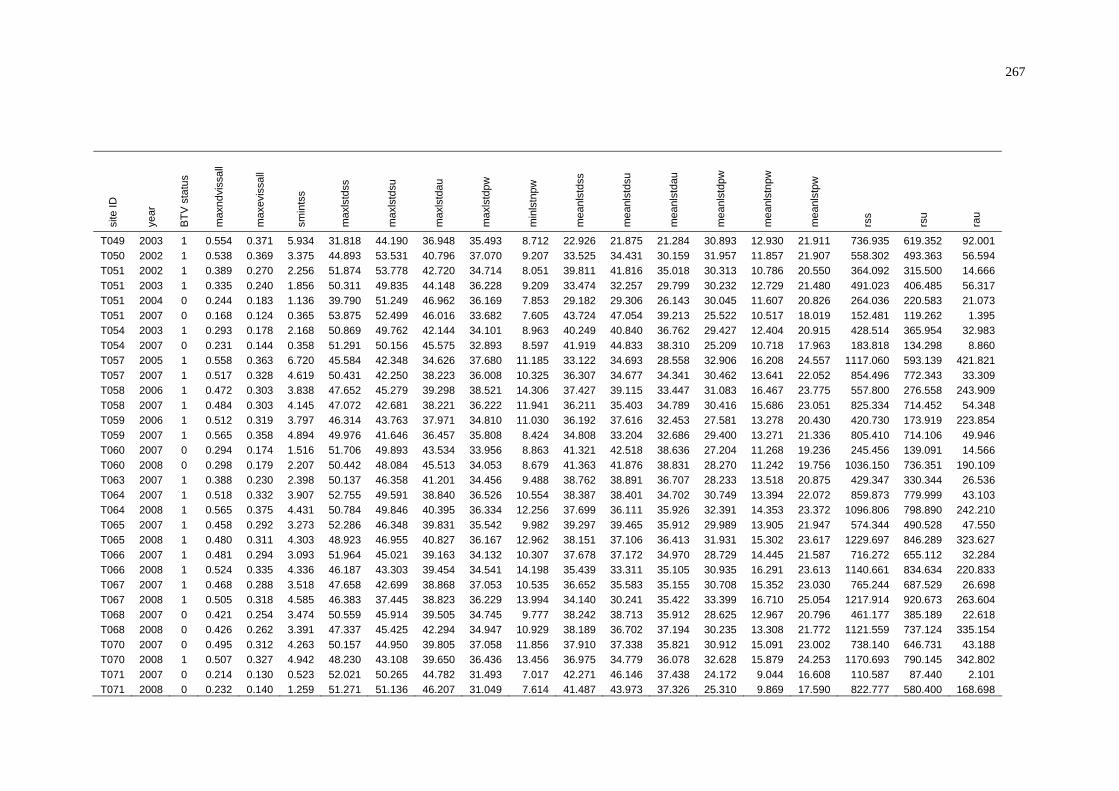
267

site

ID

year

BTV

sta

tus

max

ndvi

ssal

l

max

evis

sall

smin

tss

max

lstd

ss

max

lstd

su

max

lstd

au

max

lstd

pw

min

lstn

pw

mea

nlst

dss

mea

nlst

dsu

mea

nlst

dau

mea

nlst

dpw

mea

nlst

npw

mea

nlst

pw

rss

rsu

rau


268

site

ID

year

BTV

sta

tus

max

ndvi

ssal

l

max

evis

sall

smin

tss

max

lstd

ss

max

lstd

su

max

lstd

au

max

lstd

pw

min

lstn

pw

mea

nlst

dss

mea

nlst

dsu

mea

nlst

dau

mea

nlst

dpw

mea

nlst

npw

mea

nlst

pw

rss

rsu

rau

T072 2007 1 0.238 0.144 0.932 52.164 51.444 45.770 33.519 8.269 42.773 44.910 39.411 26.593 10.537 18.565 186.808 166.848 12.305 T073 2007 1 0.484 0.293 3.760 50.816 44.199 38.102 33.916 10.135 37.052 36.991 34.195 28.006 13.386 20.696 584.077 495.009 61.152 T073 2008 1 0.510 0.319 5.218 46.649 44.647 38.518 33.768 12.111 35.537 34.645 34.016 29.855 14.511 22.183 1220.799 861.244 276.743 T074 2007 1 0.468 0.284 4.212 49.945 43.159 37.937 34.148 8.251 36.397 35.856 34.021 28.124 12.915 20.520 668.793 547.317 79.252 T074 2008 1 0.474 0.298 5.128 48.520 47.487 38.993 32.606 11.261 35.949 35.474 33.919 28.954 13.947 21.451 1133.852 810.350 230.973 T075 2007 1 0.527 0.317 5.021 52.756 47.208 37.162 34.313 7.187 36.225 35.489 33.430 28.264 12.850 20.557 742.835 673.838 38.172 T076 2007 0 0.390 0.245 2.918 48.858 43.809 39.738 36.412 9.984 37.143 35.859 35.704 30.439 15.882 23.160 808.498 740.273 28.280 T078 2007 0 0.427 0.259 3.479 50.013 47.163 39.727 36.804 11.753 38.706 38.815 36.391 30.495 15.820 23.158 720.064 637.243 35.901 T078 2008 1 0.460 0.291 4.337 47.737 42.988 40.105 36.045 14.381 37.121 34.945 36.347 32.290 16.769 24.529 1163.803 794.957 328.286 T080 2008 1 0.745 0.512 10.806 39.199 30.712 31.687 30.026 16.571 27.757 26.018 26.839 25.817 18.833 22.325 1694.567 903.100 692.240 T082 2008 1 0.254 0.154 1.386 49.304 48.925 45.069 31.546 8.673 40.267 42.062 36.816 25.751 11.041 18.396 848.884 568.147 197.289 T083 2008 0 0.584 0.368 5.716 44.611 41.163 36.297 32.627 12.669 32.664 29.899 32.560 29.269 15.115 22.192 1198.832 860.888 249.907 T086 2008 0 0.240 0.134 1.635 51.178 50.763 47.074 32.992 7.122 43.418 45.988 39.536 27.928 9.952 18.940 849.545 503.389 235.560 T087 2008 1 0.242 0.154 1.170 53.883 53.877 46.616 29.679 6.629 42.114 45.386 37.928 25.211 9.058 17.135 631.167 420.357 135.344

Spatio-Temporal Modelling of Bluetongue Virus Distribution in ...

Documents

Transcript of Spatio-Temporal Modelling of Bluetongue Virus Distribution in ...