ST-Hadoop: A MapReduce Frameworkfor Spatio-Temporal Data

Louai Alarabi(B), Mohamed F. Mokbel(B), and Mashaal Musleh

Department of Computer Science and Engineering,University of Minnesota, Minneapolis, MN, USA

{louai,mokbel,musle005}@cs.umn.edu

Abstract. This paper presents ST-Hadoop; the first full-fledged open-source MapReduce framework with a native support for spatio-temporaldata. ST-Hadoop is a comprehensive extension to Hadoop and Spatial-Hadoop that injects spatio-temporal data awareness inside each of theirlayers, mainly, language, indexing, and operations layers. In the languagelayer, ST-Hadoop provides built in spatio-temporal data types and oper-ations. In the indexing layer, ST-Hadoop spatiotemporally loads anddivides data across computation nodes in Hadoop Distributed File Sys-tem in a way that mimics spatio-temporal index structures, which resultin achieving orders of magnitude better performance than Hadoop andSpatialHadoop when dealing with spatio-temporal data and queries. Inthe operations layer, ST-Hadoop shipped with support for two funda-mental spatio-temporal queries, namely, spatio-temporal range and joinqueries. Extensibility of ST-Hadoop allows others to expand features andoperations easily using similar approach described in the paper. Extensiveexperiments conducted on large-scale dataset of size 10 TB that containsover 1 Billion spatio-temporal records, to show that ST-Hadoop achievesorders of magnitude better performance than Hadoop and SpaitalHadoopwhen dealing with spatio-temporal data and operations. The key ideabehind the performance gained in ST-Hadoop is its ability in indexingspatio-temporal data within Hadoop Distributed File System.

1 Introduction

The importance of processing spatio-temporal data has gained much interest inthe last few years, especially with the emergence and popularity of applicationsthat create them in large-scale. For example, Taxi trajectory of New York cityarchive over 1.1 Billion trajectories [1], social network data (e.g., Twitter hasover 500 Million new tweets every day) [2], NASA Satellite daily produces 4 TBof data [3,4], and European X-Ray Free-Electron Laser Facility produce largecollection of spatio-temporal series at a rate of 40 GB per second, that collectively

This work is partially supported by the National Science Foundation, USA, underGrants IIS-1525953, CNS-1512877, IIS-1218168, and by a scholarship from the Col-lege of Computers & Information Systems, Umm Al-Qura University, Makkah, SaudiArabia.

c© Springer International Publishing AG 2017M. Gertz et al. (Eds.): SSTD 2017, LNCS 10411, pp. 84–104, 2017.DOI: 10.1007/978-3-319-64367-0 5

ST-Hadoop: A MapReduce Framework for Spatio-Temporal Data 85

Objects = LOAD ‘points’ AS (id:int, Location:POINT, Time:t);Result = FILTER Objects BY

Overlaps (Location, Rectangle(x1, y1, x2, y2))AND t < t2 AND t > t1;

(a) Range query in SpatialHadoop

Objects = LOAD ‘points’ AS (id:int, STPoint:(Location,Time));Result = FILTER Objects BY

Overlaps (STPoint, Rectangle(x1, y1, x2, y2), Interval (t1, t2) );

(b) Range query in ST-Hadoop

Fig. 1. Range query in SpatialHadoop vs. ST-Hadoop

form 50 PB of data yearly [5]. Beside the huge achieved volume of the data,space and time are two fundamental characteristics that raise the demand forprocessing spatio-temporal data.

The current efforts to process big spatio-temporal data on MapReduce environ-ment either use: (a) General purpose distributed frameworks such as Hadoop [6]or Spark [7], or (b) Big spatial data systems such as ESRI tools on Hadoop [8],Parallel-Secondo [9], MD-HBase [10], Hadoop-GIS [11], GeoTrellis [12],GeoSpark [13], or SpatialHadoop [14]. The former has been acceptable for typi-cal analysis tasks as they organize data as non-indexed heap files. However, usingthese systems as-is will result in sub-performance for spatio-temporal applicationsthat need indexing [15–17]. The latter reveal their inefficiency for supporting time-varying of spatial objects because their indexes are mainly geared toward process-ing spatial queries, e.g., SHAHED system [18] is built on top of SpatialHadoop [14].

Even though existing big spatial systems are efficient for spatial operations,nonetheless, they suffer when they are processing spatio-temporal queries, e.g.,find geo-tagged news in California area during the last three months. Adoptingany big spatial systems to execute common types of spatio-temporal queries, e.g.,range query, will suffer from the following: (1) The spatial index is still ill-suitedto efficiently support time-varying of spatial objects, mainly because the indexare geared toward supporting spatial queries, in which result in scanning throughirrelevant data to the query answer. (2) The system internal is unaware of thespatio-temporal properties of the objects, especially when they are routinelyachieved in large-scale. Such aspect enforces the spatial index to be reconstructedfrom scratch with every batch update to accommodate new data, and thus thespace division of regions in the spatial-index will be jammed, in which requiremore processing time for spatio-temporal queries. One possible way to recognizespatio-temporal data is to add one more dimension to the spatial index. Yet, suchchoice is incapable of accommodating new batch update without reconstruction.

This paper introduces ST-Hadoop; the first full-fledged open-source MapRe-duce framework with a native support for spatio-temporal data, available todownload from [19]. ST-Hadoop is a comprehensive extension to Hadoop and

86 L. Alarabi et al.

SpatialHadoop that injects spatio-temporal data awareness inside each of theirlayers, mainly, indexing, operations, and language layers. ST-Hadoop is compat-ible with SpatialHadoop and Hadoop, where programs are coded as map andreduce functions. However, running a program that deals with spatio-temporaldata using ST-Hadoop will have orders of magnitude better performance thanHadoop and SpatialHadoop. Figures 1(a) and (b) show how to express a spatio-temporal range query in SpatialHadoop and ST-Hadoop, respectively. The queryfinds all points within a certain rectangular area represented by two corner points〈x1, y1〉, 〈x2, y2〉, and a within a time interval 〈t1, t2〉. Running this query ona dataset of 10 TB and a cluster of 24 nodes takes 200 s on SpatialHadoopas opposed to only one second on ST-Hadoop. The main reason of the sub-performance of SpatialHadoop is that it needs to scan all the entries in its spa-tial index that overlap with the spatial predicate, and then check the temporalpredicate of each entry individually. Meanwhile, ST-Hadoop exploits its built-inspatio-temporal index to only retrieve the data entries that overlap with boththe spatial and temporal predicates, and hence achieves two orders of magnitudeimprovement over SpatialHadoop.

ST-Hadoop is a comprehensive extension of Hadoop that injects spatio-temporal awareness inside each layers of SpatialHadoop, mainly, language, index-ing, MapReduce, and operations layers. In the language layer, ST-Hadoop extendsPigeon language [20] to supports spatio-temporal data types and operations.The indexing layer, ST-Hadoop spatiotemporally loads and divides data acrosscomputation nodes in the Hadoop distributed file system. In this layer ST-Hadoop scans a random sample obtained from the whole dataset, bulk loadsits spatio-temporal index in-memory, and then uses the spatio-temporal bound-aries of its index structure to assign data records with its overlap partitions.ST-Hadoop sacrifices storage to achieve more efficient performance in support-ing spatio-temporal operations, by replicating its index into temporal hierarchyindex structure that consists of two-layer indexing of temporal and then spa-tial. The MapReduce layer introduces two new components of SpatioTemporal-FileSplitter, and SpatioTemporalRecordReader, that exploit the spatio-temporalindex structures to speed up spatio-temporal operations. Finally, the operationslayer encapsulates the spatio-temporal operations that take advantage of theST-Hadoop temporal hierarchy index structure in the indexing layer, such asspatio-temporal range and join queries.

The key idea behind the performance gain of ST-Hadoop is its ability to loadthe data in Hadoop Distributed File System (HDFS) in a way that mimics spatio-temporal index structures. Hence, incoming spatio-temporal queries can haveminimal data access to retrieve the query answer. ST-Hadoop is shipped withsupport for two fundamental spatio-temporal queries, namely, spatio-temporalrange and join queries. However, ST-Hadoop is extensible to support a myriadof other spatio-temporal operations. We envision that ST-Hadoop will act as aresearch vehicle where developers, practitioners, and researchers worldwide, caneither use it directly or enrich the system by contributing their operations andanalysis techniques.

ST-Hadoop: A MapReduce Framework for Spatio-Temporal Data 87

The rest of this paper is organized as follows: Sect. 2 highlights related work.Section 3 gives the architecture of ST-Hadoop. Details of the language, spatio-temporal indexing, and operations are given in Sects. 4, 5 and 6, followed byextensive experiments conducted in Sect. 7. Section 8 concludes the paper.

2 Related Work

Triggered by the needs to process large-scale spatio-temporal data, there is anincreasing recent interest in using Hadoop to support spatio-temporal operations.The existing work in this area can be classified and described briefly as following:

On-Top of MapReduce Framework. Existing work in this category hasmainly focused on addressing a specific spatio-temporal operation. The ideais to develop map and reduce functions for the required operation, which willbe executed on-top of existing Hadoop cluster. Examples of these operationsincludes spatio-temporal range query [15–17], spatio-temporal join [21–23]. How-ever, using Hadoop as-is results in a poor performance for spatio-temporal appli-cations that need indexing.

Ad-hoc on Big Spatial System. Several big spatial systems in this categoryare still ill-suited to perform spatio-temporal operations, mainly because theirindexes are only geared toward processing spatial operations, and their inter-nals are unaware of the spatio-temporal data properties [8–11,13,14,24–27]. Forexample, SHAHED runs spatio-temporal operations as an ad-hoc using Spatial-Hadoop [14].

Spatio-Temporal System. Existing works in this category has mainly focusedon combining the three spatio-temporal dimensions (i.e., x, y, and time)into a single-dimensional lexicographic key. For example, GeoMesa [28] andGeoWave [29] both are built upon Accumulo platform [30] and implementeda space filling curve to combine the three dimensions of geometry and time. Yet,these systems do not attempt to enhance the spatial locality of data; insteadthey rely on time load balancing inherited by Accumulo. Hence, they will havea sup-performance for spatio-temporal operations on highly skewed data.

ST-Hadoop is designed as a generic MapReduce system to support spatio-temporal queries, and assist developers in implementing a wide selection ofspatio-temporal operations. In particular, ST-Hadoop leverages the design ofHadoop and SpatialHadoop to loads and partitions data records according totheir time and spatial dimension across computations nodes, which allow theparallelism of processing spatio-temporal queries when accessing its index. Inthis paper, we present two case study of operations that utilize the ST-Hadoopindexing, namely, spatio-temporal range and join queries. ST-Hadoop operationsachieve two or more orders of magnitude better performance, mainly becauseST-Hadoop is sufficiently aware of both temporal and spatial locality of datarecords.

88 L. Alarabi et al.

3 ST-Hadoop Architecture

Figure 2 gives the high level architecture of our ST-Hadoop system; as thefirst full-fledged open-source MapReduce framework with a built-in support forspatio-temporal data. ST-Hadoop cluster contains one master node that breaksa map-reduce job into smaller tasks, carried out by slave nodes. Three typesof users interact with ST-Hadoop: (1) Casual users who access ST-Hadoopthrough its spatio-temporal language to process their datasets. (2) Developers,who have a deeper understanding of the system internals and can implement newspatio-temporal operations, and (3) Administrators, who can tune up the systemthrough adjusting system parameters in the configuration files provided with theST-Hadoop installation. ST-Hadoop adopts a layered design of four main layers,namely, language, Indexing, MapReduce, and operations layers, described brieflybelow:

Language Layer: This layer extends Pigeon language [20] to supports spatio-temporal data types (i.e., STPoint, time and interval) and spatio-temporaloperations (e.g., overlap, and join). Details are given in Sect. 4.

Indexing Layer: ST-Hadoop spatiotemporally loads and partitions data acrosscomputation nodes. In this layer ST-Hadoop scans a random sample obtainedfrom the input dataset, bulk-loads its spatio-temporal index that consists oftwo-layer indexing of temporal and then spatial. Finally ST-Hadoop repli-cates its index into temporal hierarchy index structure to achieve more efficient

Fig. 2. ST-Hadoop system architecture

ST-Hadoop: A MapReduce Framework for Spatio-Temporal Data 89

performance for processing spatio-temporal queries. Details of the index layerare given in Sect. 5.

MapReduce Layer: In this layer, new implementations added inside Spatial-Hadoop MapReduce layer to enables ST-Hadoop to exploits its spatio-temporalindexes and realizes spatio-temporal predicates. We are not going to discuss thislayer any further, mainly because few changes were made to inject time aware-ness in this layer. The implementation of MapReduce layer was already discussedin great details [14].

Operations Layer: This layer encapsulates the implementation of two commonspatio-temporal operations, namely, spatio-temporal range, and spatio-temporaljoin queries. More operations can be added to this layer by ST-Hadoop develop-ers. Details of the operations layer are discussed in Sect. 6.

4 Language Layer

ST-Hadoop does not provide a completely new language. Instead, it extendsPigeon language [20] by adding spatio-temporal data types, functions, and oper-ations. Spatio-temporal data types (STPoint, Time and Interval) are used todefine the schema of input files upon their loading process. In particular, ST-Hadoop adds the following:

Data types. ST-Hadoop extends STPoint, TIME, and INTERVAL. The TIMEinstance is used to identify the temporal dimension of the data, while the timeINTERVAL mainly provided to equip the query predicates. The following codesnippet loads NYC taxi trajectories from ‘NYC’ file with a column of typeSTPoint.

trajectory = LOAD ‘NYC’ as(id:int, STPoint(loc:point, time:timestamp));

NYC and trajectory are the paths to the non-indexed heap file and thedestination indexed file, respectively. loc and time are the columns that specifyboth spatial and temporal attributes.

Functions and Operations. Pigeon already equipped with several basic spa-tial predicates. ST-Hadoop changes the overlap function to support spatio-temporal operations. The other predicates and their possible variation for sup-porting spatio-temporal data are discussed in great details in [31]. ST-Hadoopencapsulates the implementation of two commonly used spatio-temporal opera-tions, i.e., range and Join queries, that take the advantages of the spatio-temporalindex. The following example “retrieves all cars in State Fair area representedby its minimum boundary rectangle during the time interval of August 25th andSeptember 6th” from trajectory indexed file.

cars = FILTER trajectoryBY overlap( STPoint,

RECTANGLE(x1,y1,x2,y2),INTERVAL(08-25-2016, 09-6-2016));

90 L. Alarabi et al.

ST-Hadoop extended the JOIN to take two spatio-temporal indexes as an input.The processing of the join invokes the corresponding spatio-temporal procedure.For example, one might need to understand the relationship between the birdsdeath and the existence of humans around them, which can be described as “findevery pairs from birds and human trajectories that are close to each other withina distance of 1 mile during the last year”.

human_bird_pairs = JOIN human_trajectory, bird_trajectoryPREDICATE = overlap( RECTANGLE(x1,y1,x2,y2),

INTERVAL(01-01-2016, 12-31-2016),WITHIN_DISTANCE(1) );

5 Indexing Layer

Input files in Hadoop Distributed File System (HDFS) are organized as a heapstructure, where the input is partitioned into chunks, each of size 64 MB. Givena file, the first 64 MB is loaded to one partition, then the second 64 MB is loadedin a second partition, and so on. While that was acceptable for typical Hadoopapplications (e.g., analysis tasks), it will not support spatio-temporal applica-tions where there is always a need to filter input data with spatial and temporalpredicates. Meanwhile, spatially indexed HDFSs, as in SpatialHadoop [14] andScalaGiST [27], are geared towards queries with spatial predicates only. Thismeans that a temporal query to these systems will need to scan the wholedataset. Also, a spatio-temporal query with a small temporal predicate mayend up scanning large amounts of data. For example, consider an input file thatincludes all social media contents in the whole world for the last five years or so.A query that asks about contents in the USA in a certain hour may end up inscanning all the five years contents of USA to find out the answer.

ST-Hadoop HDFS organizes input files as spatio-temporal partitions thatsatisfy one main goal of supporting spatio-temporal queries. ST-Hadoop imposestemporal slicing, where input files are spatiotemporally loaded into intervalsof a specific time granularity, e.g., days, weeks, or months. Each granularityis represented as a level in ST-Hadoop index. Data records in each level arespatiotemporally partitioned, such that the boundary of a partition is definedby a spatial region and time interval.

Figures 3(a) and (b) show the HDFS organization in SpatialHadoop and ST-Hadoop frameworks, respectively. Rectangular shapes represent boundaries ofthe HDFS partitions within their framework, where each partition maintains a64 MB of nearby objects. The dotted square is an example of a spatio-temporalrange query. For simplicity, let’s consider a one year of spatio-temporal recordsloaded to both frameworks. As shown in Fig. 3(a), SpatialHadoop is unaware ofthe temporal locality of the data, and thus, all records will be loaded once andpartitioned according to their existence in the space. Meanwhile in Fig. 3(b), ST-Hadoop loads and partitions data records for each day of the year individually,such that each partition maintains a 64 MB of objects that are close to each other

ST-Hadoop: A MapReduce Framework for Spatio-Temporal Data 91

Fig. 3. HDFSs in ST-Hadoop vs. SpatialHadoop

in both space and time. Note that HDFS partitions in both frameworks vary intheir boundaries, mainly because spatial and temporal locality of objects are notthe same over time. Let’s assume the spatio-temporal query in the dotted square“find objects in a certain spatial region during a specific month” in Figs. 3(a), and(b). SpatialHadoop needs to access all partitions overlapped with query region,and hence SpatialHadoop is required to scan one year of records to get the finalanswer. In the meantime, ST-Hadoop reports the query answer by accessing fewpartitions from its daily level without the need to scan a huge number of records.

5.1 Concept of Hierarchy

ST-Hadoop imposes a replication of data to support spatio-temporal queries withdifferent granularities. The data replication is reasonable as the storage in ST-Hadoop cluster is inexpensive, and thus, sacrificing storage to gain more efficientperformance is not a drawback. Updates are not a problem with replication,mainly because ST-Hadoop extends MapReduce framework that is essentiallydesigned for batch processing, thereby ST-Hadoop utilizes incremental batchaccommodation for new updates.

The key idea behind the performance gain of ST-Hadoop is its ability to loadthe data in Hadoop Distributed File System (HDFS) in a way that mimics spatio-temporal index structures. To support all spatio-temporal operations includingmore sophisticated queries over time, ST-Hadoop replicates spatio-temporal datainto a Temporal Hierarchy Index. Figures 3(b) and (c) depict two levels of daysand months in ST-Hadoop index structure. The same data is replicated on bothlevels, but with different spatio-temporal granularities. For example, a spatio-temporal query asks for objects in one month could be reported from any levelin ST-Hadoop index. However, rather than hitting 30 days’ partitions from thedaily-level, it will be much faster to access less number of partitions by obtainingthe answer from one month in the monthly-level.

92 L. Alarabi et al.

Fig. 4. Indexing in ST-Hadoop

A system parameter can be tuned by ST-Hadoop administrator to choose thenumber of levels in the Temporal Hierarchy index. By default, ST-Hadoop setits index structure to four levels of days, weeks, months and years granularities.However, ST-Hadoop users can easily change the granularity of any level. Forexample, the following code loads taxi trajectory dataset from “NYC” file usingone-hour granularity, Where the Level and Granularity are two parametersthat indicate which level and the desired granularity, respectively.

trajectory = LOAD ‘NYC’ as(id:int, STPoint(loc:point, time:timestamp))Level:1 Granularity:1-hour;

5.2 Index Construction

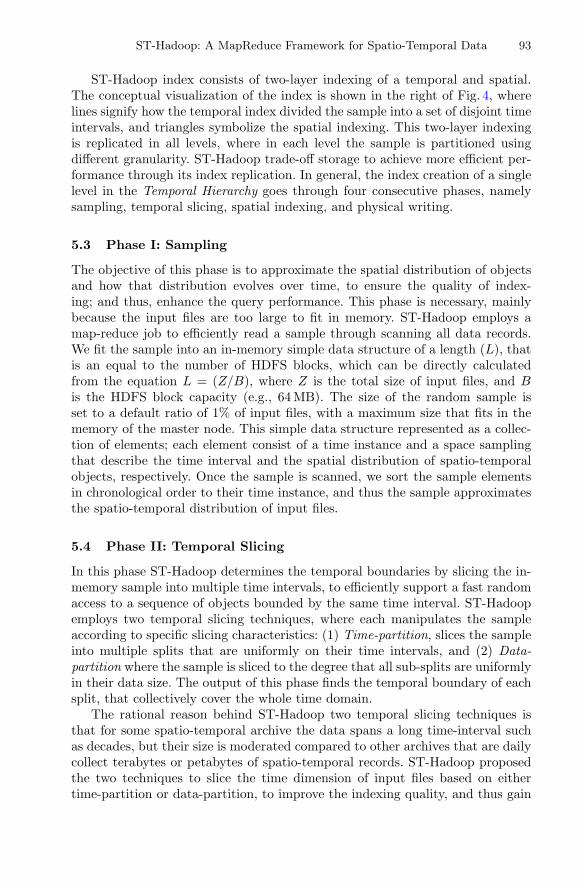
Figure 4 illustrates the indexing construction in ST-Hadoop, which involves twoscanning processes. The first process starts by scanning input files to get a ran-dom sample, and this is essential because the size of input files is beyond memorycapacity, and thus, ST-Hadoop obtains a set of records to a sample that can fitin memory. Next, ST-Hadoop processes the sample n times, where n is thenumber of levels in ST-Hadoop index structure. The temporal slicing in eachlevel splits the sample into m number of slice (e.g., slice1.m). ST-Hadoop findsthe spatio-temporal boundaries by applying a spatial indexing on each temporalslice individually. As a result, outputs from temporal slicing and spatial indexingcollectively represent the spatio-temporal boundaries of ST-Hadoop index struc-ture. These boundaries will be stored as meta-data on the master node to guidethe next process. The second scanning process physically assigns data records inthe input files with its overlapping spatio-temporal boundaries. Note that eachrecord in the dataset will be assigned n times, according to the number of levels.

ST-Hadoop: A MapReduce Framework for Spatio-Temporal Data 93

ST-Hadoop index consists of two-layer indexing of a temporal and spatial.The conceptual visualization of the index is shown in the right of Fig. 4, wherelines signify how the temporal index divided the sample into a set of disjoint timeintervals, and triangles symbolize the spatial indexing. This two-layer indexingis replicated in all levels, where in each level the sample is partitioned usingdifferent granularity. ST-Hadoop trade-off storage to achieve more efficient per-formance through its index replication. In general, the index creation of a singlelevel in the Temporal Hierarchy goes through four consecutive phases, namelysampling, temporal slicing, spatial indexing, and physical writing.

5.3 Phase I: Sampling

The objective of this phase is to approximate the spatial distribution of objectsand how that distribution evolves over time, to ensure the quality of index-ing; and thus, enhance the query performance. This phase is necessary, mainlybecause the input files are too large to fit in memory. ST-Hadoop employs amap-reduce job to efficiently read a sample through scanning all data records.We fit the sample into an in-memory simple data structure of a length (L), thatis an equal to the number of HDFS blocks, which can be directly calculatedfrom the equation L = (Z/B), where Z is the total size of input files, and Bis the HDFS block capacity (e.g., 64 MB). The size of the random sample isset to a default ratio of 1% of input files, with a maximum size that fits in thememory of the master node. This simple data structure represented as a collec-tion of elements; each element consist of a time instance and a space samplingthat describe the time interval and the spatial distribution of spatio-temporalobjects, respectively. Once the sample is scanned, we sort the sample elementsin chronological order to their time instance, and thus the sample approximatesthe spatio-temporal distribution of input files.

5.4 Phase II: Temporal Slicing

In this phase ST-Hadoop determines the temporal boundaries by slicing the in-memory sample into multiple time intervals, to efficiently support a fast randomaccess to a sequence of objects bounded by the same time interval. ST-Hadoopemploys two temporal slicing techniques, where each manipulates the sampleaccording to specific slicing characteristics: (1) Time-partition, slices the sampleinto multiple splits that are uniformly on their time intervals, and (2) Data-partition where the sample is sliced to the degree that all sub-splits are uniformlyin their data size. The output of this phase finds the temporal boundary of eachsplit, that collectively cover the whole time domain.

The rational reason behind ST-Hadoop two temporal slicing techniques isthat for some spatio-temporal archive the data spans a long time-interval suchas decades, but their size is moderated compared to other archives that are dailycollect terabytes or petabytes of spatio-temporal records. ST-Hadoop proposedthe two techniques to slice the time dimension of input files based on eithertime-partition or data-partition, to improve the indexing quality, and thus gain

94 L. Alarabi et al.

Fig. 5. Data-Slice Fig. 6. Time-Slice

efficient query performance. The time-partition slicing technique serves best in asituation where data records are uniformly distributed in time. Meanwhile, data-partition slicing best suited with data that are sparse in their time dimension.

• Data-partition Slicing. The goal of this approach is to slice the sample to thedegree that all sub-splits are equally in their size. Figure 5 depicts the keyconcept of this slicing technique, such that a slice1 and slicen are equallyin size, while they differ in their interval coverage. In particular, the temporalboundary of slice1 spans more time interval than slicen. For example,consider 128 MB as the size of HDFS block and input files of 1 TB. Typically,the data will be loaded into 8 thousand blocks. To load these blocks intoten equally balanced slices, ST-Hadoop first reads a sample, then sort thesample, and apply Data-partition technique that slices data into multiplesplits. Each split contains around 800 blocks, which hold roughly a 100 GBof spatio-temporal records. There might be a small variance in size betweenslices, which is expectable. Similarly, another level in ST-Hadoop temporalhierarchy index could loads the 1 TB into 20 equally balanced slices, whereeach slice contains around 400 HDFS blocks. ST-Hadoop users are allowedto specify the granularity of data slicing by tuning α parameter. By defaultfour ratios of α is set to 1%, 10%, 25%, and 50% that create the four levelsin ST-Hadoop index structure.

• Time-partition Slicing. The ultimate goal of this approach is to slices the inputfiles into multiple HDFS chunks with a specified interval. Figure 6 shows thegeneral idea, where ST-Hadoop splits the input files into an interval of one-month granularity. While the time interval of the slices is fixed, the size ofdata within slices might vary. For example, as shown in Fig. 6 Jan slice hasmore HDFS blocks than April.

ST-Hadoop users are allowed to specify the granularity of this slicing tech-nique, which specified the time boundaries of all splits. By default, ST-Hadoopfiner granularity level is set to one-day. Since the granularity of the slicing isknown, then a straightforward solution is to find the minimum and maximumtime instance of the sample, and then based on the intervals between the bothtimes ST-Hadoop hashes elements in the sample to the desired granularity.

ST-Hadoop: A MapReduce Framework for Spatio-Temporal Data 95

The number of slices generated by the time-partition technique will highlydepend on the intervals between the minimum and the maximum times obtainedfrom the sample. By default, ST-Hadoop set its index structure to four levels ofdays, weeks, months and years granularities.

5.5 Phase III: Spatial Indexing

This phase ST-Hadoop determines the spatial boundaries of the data recordswithin each temporal slice. ST-Hadoop spatially index each temporal slice inde-pendently; such decision handles a case where there is a significant disparity inthe spatial distribution between slices, and also to preserve the spatial localityof data records. Using the same sample from the previous phase, ST-Hadooptakes the advantages of applying different types of spatial bulk loading tech-niques in HDFS that are already implemented in SpatialHadoop such as Grid,R-tree, Quad-tree, and Kd-tree. The output of this phase is the spatio-temporalboundaries of each temporal slice. These boundaries stored as a meta-data in afile on the master node of ST-Hadoop cluster. Each entry in the meta-data rep-resents a partition, such as <id,MBR, interval, level>. Where id is a uniqueidentifier number of a partition on the HDFS, MBR is the spatial minimumboundary rectangle, interval is the time boundary, and the level is the numberthat indicates which level in ST-Hadoop temporal hierarchy index.

5.6 Phase IV: Physical Writing

Given the spatio-temporal boundaries that represent all HDFS partitions, weinitiate a map-reduce job that scans through the input files and physically parti-tions HDFS block, by assign data records to overlapping partitions according tothe spatio-temporal boundaries in the meta-data stored on the master node ofST-Hadoop cluster. For each record r assigned to a partition p, the map functionwrites an intermediate pair 〈p, r〉 Such pairs are then grouped by p and sent tothe reduce function to write the physical partition to the HDFS. Note that for arecord r will be assigned n times, depends on the number of levels in ST-Hadoopindex.

6 Operations Layer

The combination of the spatiotemporally load balancing with the temporal hier-archy index structure gives the core of ST-Hadoop, that enables the possibility ofefficient and practical realization of spatio-temporal operations, and hence pro-vides orders of magnitude better performance over Hadoop and SpatialHadoop.In this section, we only focus on two fundamental spatio-temporal operations,namely, range (Sect. 6.1) and join queries (Sects. 6.2), as case studies of how toexploit the spatio-temporal indexing in ST-Hadoop. Other operations can alsobe realized following a similar approach.

96 L. Alarabi et al.

6.1 Spatio-Temporal Range Query

A range query is specified by two predicates of a spatial area and a temporalinterval, A and T , respectively. The query finds a set of records R that overlapwith both a region A and a time interval T , such as “finding geotagged news inCalifornia area during the last three months”. ST-Hadoop employs its spatio-temporal index described in Sect. 5 to provide an efficient algorithm that runsin three steps, temporal filtering, spatial search, and spatio-temporal refinement,described below.

In the temporal filtering step, the hierarchy index is examined to selecta subset of partitions that cover the temporal interval T . The main challengein this step is that the partitions in each granularity cover the whole time andspace, which means the query can be answered from any level individually orwe can mix and match partitions from different level to cover the query intervalT . Depending on which granularities are used to cover T , there is a tradeoffbetween the number of matched partitions and the amount of processing neededto process each partition. To decide whether a partition P is selected or not, thealgorithm computes its coverage ratio r, which is defined as the ratio of the timeinterval of P that overlaps T . A partition is selected only if its coverage ratiois above a specific threshold M. To balance this tradeoff, ST-Hadoop employsa top-down approach that starts with the top level and selects partitions thatcovers query interval T , If the query interval T is not covered at that granularity,then the algorithm continues to the next level. If the bottom level is reached,then all partitions overlap with T will be selected.

In the spatial search step, Once the temporal partitions are selected, thespatial search step applies the spatial range query against each matched partitionto select records that spatially match the query range A. Keep in mind that eachpartition is spatiotemporally indexed which makes queries run very efficiently.Since these partitions are indexed independently, they can all be processed simul-taneously across computation nodes in ST-Hadoop, and thus maximizes thecomputing utilization of the machines.

Finally in the spatio-temporal refinement step, compares individualrecords returned by the spatial search step against the query interval T , to selectthe exact matching records. This step is required as some of the selected tem-poral partitions might partially overlap the query interval T and they need tobe refined to remove records that are outside T . Similarly, there is a chancethat selected partitions might partially overlap with the query area A, and thusrecords outside the A need to be excluded from the final answer.

6.2 Spatio-Temporal Join

Given two indexed dataset R and S of spatio-temporal records, and a spatio-temporal predicate θ. The join operation retrieves all pairs of records 〈r, s〉 thatare similar to each other based on θ. For example, one might need to understandthe relationship between the birds death and the existence of humans around

ST-Hadoop: A MapReduce Framework for Spatio-Temporal Data 97

Fig. 7. Spatio-temporal join

them, which can be described as “find every pairs from bird and human trajec-tories that are close to each other within a distance of 1 mile during the lastweek”. The join algorithm runs in two steps as shown in Fig. 7, hash and join.

In the hashing step, the map function scans the two input files and hasheseach record to candidate buckets. The buckets are defined by partitioning thespatio-temporal space using the two-layer indexing of temporal and spatial,respectively. The granularity of the partitioning controls the tradeoff betweenpartitioning overhead and load balance, where a more granular-partitioningincreases the replication overhead, but improves the load balance due to the hugenumber of partitions, while a less granular-partitioning minimizes the replicationoverhead, but can result in a huge imbalance especially with highly skewed data.The hash function assigns each point in the left dataset, r ∈ R, to all bucketswithin an Euclidean distance d and temporal distance t, and assigns each pointin the right dataset, s ∈ S, to the one bucket which encloses the point s. Thisensures that a pair of matching records 〈r, s〉 are assigned to at least one com-mon bucket. Replication of only one dataset (R) along with the use of singleassignment, ensure that the answer contains no replicas.

In the joining step, each bucket is assigned to one reducer that performs atraditional in-memory spatio-temporal join of the two assigned sets of recordsfrom R and S. We use the plane-sweep algorithm which can be generalized tomultidimensional space. The set S is not replicated, as each pair is generated byexactly one reducer, and thus no duplicate avoidance step is necessary.

7 Experiments

This section provides an extensive experimental performance study of ST-Hadoop compared to SpatialHadoop and Hadoop. We decided to compare with

98 L. Alarabi et al.

this two frameworks and not other spatio-temporal DBMSs for two reasons.First, as our contributions are all about spatio-temporal data support in Hadoop.Second, the different architectures of spatio-temporal DBMSs have great influ-ence on their respective performance, which is out of the scope of this paper.Interested readers can refer to a previous study [32] which has been establishedto compare different large-scale data analysis architectures. In other words, ST-Hadoop is targeted for Hadoop users who would like to process large-scale spatio-temporal data but are not satisfied with its performance. The experiments aredesigned to show the effect of ST-Hadoop indexing and the overhead imposedby its new features compared to SpatialHadoop. However, ST-Hadoop achievestwo orders of magnitude improvement over SpatialHadoop and Hadoop.

Experimental Settings. All experiments are conducted on a dedicated inter-nal cluster of 24 nodes. Each has 64 GB memory, 2 TB storage, and Intel(R)Xeon(R) CPU 3 GHz of 8 core processor. We use Hadoop 2.7.2 running on Java1.7 and Ubuntu 14.04.5 LTS. Figure 8(b) summarizes the configuration para-meters used in our experiments. Default parameters (in parentheses) are usedunless mentioned.

Datasets. To test the performance of ST-Hadoop we use the Twitter archiveddataset [2]. The dataset collected using the public Twitter API for more thanthree years, which contains over 1 Billion spatio-temporal records with a totalsize of 10 TB. To scale out time in our experiments we divided the datasetinto different time intervals and sizes, respectively as shown in Fig. 8(a). Thedefault size used is 1 TB which is big enough for our extensive experimentsunless mentioned.

In our experiments, we compare the performance of a ST-Hadoop spatio-temporal range and join query proposed in Sect. 6 to their spatial-temporalimplementations on-top of SpatialHadoop and Hadoop. For range query, we usesystem throughput as the performance metric, which indicates the number ofMapReduce jobs finished per minute. To calculate the throughput, a batch of 20

Twitter Data Size Num-Records Time windowLarge 10TB > 1 Billion > 3 yearsAverage–Large 6.7TB 692 Million 1 yearsMedium–Large 3TB 152 Million 9 monthsModerate–Large (1TB) 115 Million 3 months

(a) DatasetsParameter Values (default)HDFS block capacity (B) 32, 64, (128), 256 MBCluster size (N ) 5, 10, 15, 20, (23)Selection ratio (ρ) (0.01), 0.02, 0.05, 0.1, 0.2, 0.5, 1.0Data-pratition slicing ratio(α) 0.01, 0.02, 0.025, 0.05, (0.1), 1Time-partition Slicing granularity(σ) (days), weeks, months, years

(b) Parameters

Fig. 8. Experimental settings and Dataset

ST-Hadoop: A MapReduce Framework for Spatio-Temporal Data 99

queries is submitted to the system, and the throughput is calculated by dividing20 by the total time of all queries. The 20 queries are randomly selected with aspatial area ratio of 0.001% and a temporal window of 24 h unless stated. Thisexperimental design ensures that all machines get busy and the cluster stays fullyutilized. For spatio-temporal join, we use the processing time of one query as theperformance metric as one query is usually enough to keep all machines busy.The experimental results for range and join queries are reported in Sects. 7.1,and 7.3, respectively. Meanwhile, Sect. 7.2 analyzes ST-Hadoop indexing.

7.1 Spatiotemporal Range Query

In Fig. 9(a), we increase the size of input from 1 TB to 10 TB, while measuringthe job throughput. ST-Hadoop achieves more than two orders of magnitudehigher throughput, due to the temporal load balancing of its spatio-temporalindex. As for SpatialHadoop, it needs to scan more partitions, which explain whythe throughput of SpatialHadoop decreases with the increase of data records inspatial space. Meanwhile, ST-Hadoop throughput remains stable as it processesonly partition(s) that intersect with both space and time. Note that it is alwaysthe case that Hadoop needs to scan all HDFS blocks, which gives the worstthroughput compared to SpatialHadoop and ST-Hadoop.

Figure 9(b) shows the effect of configuring the HDFS block size on the jobthroughput. ST-Hadoop manages to keep its performance within orders of mag-nitude higher throughput even with different block sizes. Extensive experimentsare shown in Fig. 9(c), analyzed how slicing ratio (α) can affect the performanceof range queries. ST-Hadoop keeps its higher throughput around the defaultHDFS block size, as it maintains the load balance of data records in its two-layerindexing. As expected expanding the block size from its default value will reducethe performance on SpatialHadoop and ST-Hadoop, mainly because blocks willcarry more data records.

Experiments in Fig. 10 examines the performance of the temporal hierarchyindex in ST-Hadoop using both slicing techniques. We evaluate different gran-ularities of time-partition slicing (e.g., daily, weekly, and monthly) with variousdata-partition slicing ratio. In these two figures, we fix the spatial query range

0

10

20

30

40

50

60

70

80

90

1 3 6.7 10

Th

ro

ug

hp

ut

(Jo

b/m

in)

Input Size (TB)

SpatialHadoopST-Hadoop

Hadoop

(a) Input files (TB)

0

10

20

30

40

50

60

70

80

32 64 128 256

Th

ro

ug

hp

ut

(Jo

b/m

in)

HDFS Block Size (MB)

Data-partitionTime-partition

Hadoop

(b) Block size (MB)

0

10

20

30

40

50

60

70

32 64 128 256

Th

rou

gh

pu

t (J

ob

/min

)

HDFS Block Size (MB)

α = 0.1α = 0.05

α = 0.025α = 0.0125

α = 0.01

(c) Block size VS Slicing ratio (α)

Fig. 9. Spatio-temporal range query

100 L. Alarabi et al.

0

2

4

6

8

10

5 10 15 20 25 30

Tim

e (s

ec)

Temporal Interval (Days)

α = 0.5α = 0.2α = 0.1

α = 0.025α = 0.01

Non Temporal Index

(a) Data-partition Slicing

0

2

4

6

8

10

5 10 15 20 25 30

Tim

e (s

ec)

Temporal Interval (Days)

DailyWeekly

Monthly ≡ ST-Hadoop(M=0.0)ST-Hadoop(M=0.2)ST-Hadoop(M=0.4)ST-Hadoop(M=0.7)ST-Hadoop(M=1.0)

Non Temporal Index

(b) Time-partition Slicing

Fig. 10. Spatio-temporal range query interval window

and increase the temporal range from 1 day to 31 days, while measuring the totalrunning time. As shown in the Figs. 10(a) and (b), ST-Hadoop utilizes its tem-poral hierarchy index to achieve the best performance as it mixes and matchesthe partitions from different levels to minimize the running time, as described inSect. 6.1. ST-Hadoop provides good performance for both small and large queryintervals as it selects partitions from any level. When the query interval is verynarrow, it uses only the lowest level (e.g., daily level), but as the query inter-val expand it starts to process the above level. The value of the parameter Mcontrols when it starts to process the next level. At M = 0, it always selectsthe up level, e.g., monthly. If M increases, it starts to match with lower levelsin the hierarchy index to achieve better performance. At the extreme value ofM = 1, the algorithm only matches partitions that are completely containedin the query interval, e.g., at 18 days it matches two weeks and four days whileat 30 days it matches the whole month. The optimal value in this experiment isM = 0.4 which means it only selects partitions that are at least 40% covered bythe query temporal interval.

In Fig. 11 we study the effect of the spatio-temporal query range (σ) on thechoice of M. To measure the quality of M, we define an optimal running timefor a query Q as the minimum of all running times for all values of M ∈ [0, 1].Then, we determine the quality of a specific value of M on a query workloadas the mean squared error (MSE) between the running time at this value of Mand the optimal running time. This means, if a value of M always provides theoptimal value, it will yield a quality measure of zero. As this value increases,it indicates a poor quality as the running times deviates from the optimal. InFig. 11(a), We repeat the experiment with three values of spatial query rangesσ ∈ {1E − 6, 1E − 4, 0.1}. As shown in the figure, M = 0.4 provides the bestperformance for all the experimented spatial ranges. This is expected as M isonly used to select temporal partitions while the spatial range (σ) is used toperform the spatial query inside each of the selected partitions. Figure 11(b),shows the quality measures with a workload of 71 queries with time intervals

ST-Hadoop: A MapReduce Framework for Spatio-Temporal Data 101

0

20

40

60

80

100

0 0.2 0.4 0.6 0.8 1

MSE

σ=1E-6σ=1E-4

σ=0.1

M(a) Tuning of M for query intervals from 1 to 30 days

0

2

4

6

8

10

12

0 0.1 0.2 0.3 0.4 0.5 0.6

MSE

σ=1E-6σ=1E-4σ=0.01

M(b) Tuning of M for query intervals from 1 to 400 days

Fig. 11. The effect of the spatio-temporal query ranges on the optimal value of M

that range from 1 day to 421 days. This experiment also provides a very similarresult where the optimal value of M is around 0.4.

7.2 Index Construction

Figure 12 gives the total time for building the spatio-temporal index in ST-Hadoop. This is a one time job done for input files. In general, the figure showsexcellent scalability of the index creation algorithm, where it builds its indexusing data-partition slicing for a 1 TB file with more than 115 Million recordsin less than 15 min. The data-partition technique turns out to be the fastest asit contains fewer slices than time-partition. Meanwhile, the time-partition tech-nique takes more time, mainly because the number of partitions are increased,and thus increases the time in physical writing phase.

In Fig. 13, we configure the temporal hierarchy indexing in ST-Hadoop toconstruct five levels of the two-layer indexing. The temporal indexing usesData-partition slicing technique with different slicing ratio α. We evaluate theindexing time of each level individually. Because the input files are sliced intosplits according to the slicing ratio, which directly effects on the number of par-titions. In general with stretching the slicing ratio, the indexing time decreases,mainly because the number of partitions will be much less. However, note thatin some cases the spatial distribution of the slice might produce more partitionsas in shown with 0.25% ratio.

7.3 Spatiotemporal Join

Figure 14 gives the results of the spatio-temporal join experiments, where wecompare our join algorithm for ST-Hadoop with MapReduce implementation ofthe spatial hash join algorithm [33]. Typically, in this join algorithm we performthe following query, “find every pairs that are close within an Euclidean distanceof 1mile and a temporal distance of 2 days”, this join query is executed on bothST-Hadoop and Hadoop and the response times are compared. The y-axis in the

102 L. Alarabi et al.

0

200

400

600

800

1000

1200

1 3 6.7 10

Tim

e (m

in)

Input Size (TB)

Data-partitionTime-partition

Fig. 12. Input files

15 20 25 30 35 40 45 50 55

0.01 0.0125 0.025 0.05 0.1

Tim

e (m

in)

Slicing Ratio α

Fig. 13. Data-partition

0

100

200

300

400

500

2x2 3x3 5x5 30x30 2x2

Tim

e (m

in)

Number of Days

ST-HadoopHadoop

Fig. 14. Spatio-temporal join

figure represents the total processing time, while the x-axis represents the joinquery on numbers of days× days in ascending order. With the increase of join-ing number of days, the performance of ST-Hadoops join increases, because itneeds to join more indexes from the temporal hierarchy. In general, ST-Hadoopgives the best results as ST-Hadoop index replicates data in several layers, andthus ST-Hadoop significantly decreases the processing of non-overlapping parti-tions, as only partitions that overlap with both space and time are consideredin the join algorithm. Meanwhile, the same joining algorithm without usingST-Hadoop index gives the worst performance for joining spatio-temporal data,mainly because the algorithm takes into its consideration all data records fromone dataset. However, ST-Hadoop only joins the indexes that are within thetemporal range, which significantly outperforms the join algorithm with doubleto triple performance.

8 Conclusion

In this paper, we introduced ST-Hadoop [19] as a novel system that acknowledgesthe fact that space and time play a crucial role in query processing. ST-Hadoopis an extension of a Hadoop framework that injects spatio-temporal awarenessinside SpatialHadoop layers. The key idea behind the performance gain of ST-Hadoop is its ability to load the data in Hadoop Distributed File System (HDFS)in a way that mimics spatio-temporal index structures. Hence, incoming spatio-temporal queries can have minimal data access to retrieve the query answer. ST-Hadoop is shipped with support for two fundamental spatio-temporal queries,namely, spatio-temporal range and join queries. However, ST-Hadoop is exten-sible to support a myriad of other spatio-temporal operations. We envision thatST-Hadoop will act as a research vehicle where developers, practitioners, andresearchers worldwide, can either use directly or enrich the system by contribut-ing their operations and analysis techniques.

ST-Hadoop: A MapReduce Framework for Spatio-Temporal Data 103

References

1. NYC Taxi and Limousine Commission (2017). http://www.nyc.gov/html/tlc/html/about/trip record data.shtml

2. (2017). https://about.twitter.com/company3. Land Process Distributed Active Archive Center, March 2017. https://lpdaac.usgs.

gov/about4. Data from NASA’s Missions, Research, and Activities (2017). http://www.nasa.

gov/open/data.html5. European XFEL: The Data Challenge, September 2012. http://www.xfel.eu/news/

2012/the data challenge6. Apache. Hadoop. http://hadoop.apache.org/7. Apache. Spark. http://spark.apache.org/8. Whitman, R.T., Park, M.B., Ambrose, S.A., Hoel, E.G.: Spatial indexing and

analytics on hadoop. In: SIGSPATIAL (2014)9. Lu, J., Guting, R.H.: Parallel secondo: boosting database engines with hadoop. In:

ICPADS (2012)10. Nishimura, S., Das, S., Agrawal, D., El Abbadi, A.: MD-HBase: design and imple-

mentation of an elastic data infrastructure for cloud-scale location services. DAPD31, 289–319 (2013)

11. Aji, A., Wang, F., Vo, H., Lee, R., Liu, Q., Zhang, X., Saltz, J.: Hadoop-GIS:a high performance spatial data warehousing system over mapreduce. In: VLDB(2013)

12. Kini, A., Emanuele, R.: Geotrellis: adding geospatial capabilities to spark (2014).http://spark-summit.org/2014/talk/geotrellis-adding-geospatial-capabilities-to-spark

13. Yu, J., Wu, J., Sarwat, M.: GeoSpark: a cluster computing framework for processinglarge-scale spatial data. In: SIGSPATIAL (2015)

14. Eldawy, A., Mokbel, M.F.: SpatialHadoop: a MapReduce framework for spatialdata. In: ICDE (2015)

15. Ma, Q., Yang, B., Qian, W., Zhou, A.: Query processing of massive trajectory databased on MapReduce. In: CLOUDDB (2009)

16. Tan, H., Luo, W., Ni, L.M.: Clost: a hadoop-based storage system for big spatio-temporal data analytics. In: CIKM (2012)

17. Li, Z., Hu, F., Schnase, J.L., Duffy, D.Q., Lee, T., Bowen, M.K., Yang, C.: Aspatiotemporal indexing approach for efficient processing of big array-based climatedata with mapreduce. Int. J. Geograph. Inf. Sci. IJGIS 31, 17–35 (2017)

18. Eldawy, A., Mokbel, M.F., Alharthi, S., Alzaidy, A., Tarek, K., Ghani, S.: SHAHED:a MapReduce-based system for querying and visualizing Spatio-temporal satellitedata. In: ICDE (2015)

19. ST-Hadoop website. http://st-hadoop.cs.umn.edu/20. Eldawy, A., Mokbel, M.F.: Pigeon: a spatial mapreduce language. In: ICDE (2014)21. Han, W., Kim, J., Lee, B.S., Tao, Y., Rantzau, R., Markl, V.: Cost-based predictive

spatiotemporal join. TKDE 21, 220–233 (2009)22. Al-Naami, K.M., Seker, S.E., Khan, L.: GISQF: an efficient spatial query processing

system. In: CLOUDCOM (2014)23. Fries, S., Boden, B., Stepien, G., Seidl, T.: PHiDJ: parallel similarity self-join for

high-dimensional vector data with mapreduce. In: ICDE (2014)24. Stonebraker, M., Brown, P., Zhang, D., Becla, J.: SciDB: a database management

system for applications with complex analytics. Comput. Sci. Eng. 15, 54–62 (2013)

104 L. Alarabi et al.

25. Zhang, X., Ai, J., Wang, Z., Lu, J., Meng, X.: An efficient multi-dimensional indexfor cloud data management. In: CIKM (2009)

26. Wang, G., Salles, M., Sowell, B., Wang, X., Cao, T., Demers, A., Gehrke, J., White,W.: Behavioral simulations in MapReduce. PVLDB 3, 952–963 (2010)

27. Lu, P., Chen, G., Ooi, B.C., Vo, H.T., Wu, S.: ScalaGiST: scalable generalizedsearch trees for MapReduce systems. PVLDB 7, 1797–1808 (2014)

28. Fox, A.D., Eichelberger, C.N., Hughes, J.N., Lyon, S.: Spatio-temporal indexingin non-relational distributed databases. In: BIGDATA (2013)

29. GeoWave. https://ngageoint.github.io/geowave/30. Accumulo. https://accumulo.apache.org/31. Erwig, M., Schneider, M.: Spatio-temporal predicates. In: TKDE (2002)32. Pavlo, A., Paulson, E., Rasin, A., Abadi, D., DeWitt, D., Madden, S., Stonebraker,

M.: A comparison of approaches to large-scale data analysis. In: SIGMOD (2009)33. Lo, M.L., Ravishankar, C.V.: Spatial hash-joins. In: SIGMODR (1996)