Characterization of the spatio-temporal patterns in the osmosedimentation process

Journal of Biogeography, 27, 57–69

Characterization of the spatio-temporal patternsof global fire activity using satellite imagery forthe period April 1992 to March 1993Edward Dwyer1∗, Jose M. C. Pereira2, Jean-Marie Gregoire1 and Carlos C. DaCamara3

1Global Vegetation Monitoring Unit, TP 440, Space Applications Institute, Joint Research

Centre, European Commission, 21020 Ispra, Italy, 2Departamento de Engenharia Florestal,

Instituto Superior de Agronomia, Universidade Tecnica de Lisboa, Tapada da Ajuda, 1399

Lisboa Codex, Portugal, 3Departamento de Fisica, Universidade de Lisboa, Campo Grande,

Ed. C1, Piso 4, P-1700 Lisboa, Portugal

AbstractAim This paper describes the characteristics of the spatio-temporal distribution of

vegetation fires as detected from satellite data for the 12 months April 1992 to March 1993.

Location Fires are detected daily at a spatial resolution of 1 km for all land areas of the

globe.

Methods From the fire location information a daily gridded product at 0.5° by 0.5° has been

constructed. Two methods of characterizing the spatio-temporal pattern of vegetation fires are

discussed. The first applies empirical orthogonal function analysis to the monthly series of

gridded data. The second approach defines and extracts a number of spatial and temporal

parameters from the gridded product. The descriptive parameters extracted are used in a cluster

analysis in order to group cells with similar characteristics into a small number of classes.

Results Using daily global satellite observations, it is possible to characterize the spatial

and temporal variability in fire activity. Most of this variability is within the tropical belt,

where the majority of fire activity is concentrated, nonetheless fire was also detected in

temperate and boreal regions. The period in which fire occurred varied from region to

region. Parameterization provided a very synthetic view of this variability facilitating

regional intercomparison. Clustering identifies five classes of fire activity, each of which

can be associated with particular climatic conditions, vegetation types and land-use.

Main conclusions Global monitoring of vegetation fire from satellite is possible. The

analysis provides a coherent, consistent and synoptic view of global fire activty with one

data set. The type of information extracted can be of use in global atmospheric chemistry

modelling and for studying the role of fire in relation to global change issues.

KeywordsVegetation fire, global fire patterns, remote sensing of fire, empirical orthogonal functions

INTRODUCTION whole regions of Southeast Asia engulfed in smog. Fires caused

by lightning in boreal regions of North America and Russia areFire has been very much in the public eye recently with images

responsible for up to 80% of the area burned (Stocks, 1992).of out of control forest burning in Indonesia and Brazil, fires

However, from a global perspective, the majority of fires arethreatening cities in the United States, Europe and Australia and

man-made. They are used for many reasons such as grassland

management, burning of crop residues, elimination of disease

bearing insects and snakes, hunting and land clearance (Andreae,Correspondence: J.-M. Gregoire, Global Vegetation Monitoring

1992). Fires are also caused by negligence and their ability to getUnit, TP 440, Space Applications Institute, Joint Research Centre,

out of control can be aided by climatic conditions.European Commission, 21020 Ispra, Italy∗Now at SARMAP S.A. 6980 Croglio, Ticino, Switzerland Irrespective of the causes of fire, burning leads to the emission

1999 Blackwell Science Ltd

58 Edward Dwyer, Jose M. C. Pereira, Jean-Marie Gregoire and Carlos C. DaCamara

of vast amounts of gaseous and particulate matter (Crutzen & using one data source for a relatively extended period of time,

processed using a single methodology based on an algorithmAndreae, 1990). It is estimated that up to 40% of CO2

production due to human activities may be due to biomass accepted by the international community of experts in remote

sensing of vegetation fire (IGBP, 1997; Stroppiana et al., 1999)burning (Levine, 1996). The emissions of CO2 in addition to a

range of other gases such as CO, CH4 and NOx are of interest Global, time-series data sets are large and complex by their

nature. The information must be summarized in a quantitativein atmospheric chemistry modelling to determine the

contribution of vegetation fire to climate change through forcing and objective manner which goes beyond simply displaying

large quantities of data. Analysis methods are only now beingof the earth’s radiation budget. Fire is an ecosystem disturbance.

It partially or completely removes the vegetation layer. This developed. Davis et al. (1991) pointed to the lack of quantitative

analysis techniques for multitemporal imagery while Piwowarcan be very dramatic as in the burning of forest or more subtle

as in the burning of bush and grasslands. Timing and severity et al. (1998) called attention to the fact that little development

had occurred on exploring methods to highlight space-timeof fire can affect succession, favouring those species which have

developed an adaptation to fire. It can affect plant nutrition in relations in data.

The objective of this paper is to describe the characteristicsa variety of ways. The ash can provide a sudden pulse of

nutrients to the soil but conversely the burned surface is more of the spatio-temporal distribution of vegetation fires as

detected from satellite data for the 12 months from April 1992sensitive to nutrient leaching, soil erosion and changes in the

hydrological cycle than the vegetated surface (Menaut et al., to March 1993. This is achieved by using analysis techniques

which highlight the spatial and temporal variability and present1993).

To improve understanding of the role of vegetation fire it in a small number of new variables. The patterns of fire

distribution identified, using two different techniques, areemissions in atmospheric chemistry and fire itself as an

ecosystem disturbance there has been a request for information described and their significance in relation to climate and

vegetation distributions are discussed.on fire from the international science community. This has been

focused through a number of core projects of the International

Geosphere Biosphere Programme (IGBP) such as theDATA AND METHODS

International Global Atmospheric Chemistry Project (IGAC)

and the Global Change and Terrestrial Ecosystems (GCTE)The global satellite fire data set

project (IGBP, 1994). Their information requirements include

global fire distribution, timing, extent, severity and return The geographical positions of those pixels in which fires were

detected (fire pixels) were determined from a global 1 kmfrequency. Other groups which require fire related data include

international organizations involved in environmental policy Advanced Very High Resolution Radiometer (AVHRR) data

set for each day in the 21-month period from April 1992 toand management and national organizations with land

management mandates. December 1993 (Stroppiana et al., 1999). This data set is the

first of its kind to give a global picture of vegetation fire, usingThe term fire regime is used to describe a collection of

attributes pertinent to fires in a given ecosystem or region. a single data source and a single fire detection algorithm, which

leads to an internally consistent data product (Dwyer et al.,Usually included are fire frequency (1/n years), intensity, date

of occurrence and fuels involved. Some aspects of fire regimes 1998). However, as with any remotely sensed data product

there are limitations. The product represents a sample of theare known and have been documented for many global

ecosystems (Stocks, 1992; Goldammer, 1993; Trabaud et al., total fire activity which took place during the period as only

those fires which were active during the time of satellite1993). However, their characterization is rather generalized

and is usually described in terms of probability of occurrence overpass, in the early afternoon, were recorded. For some

regions of the tropics this coincides with the time of peak fireor fire frequency (Malingreau & Gregoire, 1996). We are still

unable to answer the simple question: where and when do fires activity (Eva & Lambin, 1998). False detection can occur due

to the algorithm considering certain ground features, such asoccur? We have lacked the spatial and temporal detail needed

to help meet the requirements for global change studies. Since hot soil or sun-glint from water as fire events. An evaluation

of various fire detection algorithms for global applications isthe early 1980s satellite data have been used to determine the

spatial and temporal location of fires. A wide range of optical given in Giglio et al. (1999) and the one used to produce the

data set discussed here is described in detail in Flasse & Ceccatoand infra-red sensors have been employed to detect active fires

and burned surfaces at different spatial resolutions, for different (1996).

Each fire pixel detected represents a point event, at a spatialtimes of the day, at local, regional and continental scale

and for different time periods. Good reviews of the different resolution of 1 km, in space and time. In order to characterize

spatial patterns for the globe it was first necessary to aggregateapproaches are given in Robinson (1991) and Eva & Lambin

(1998). fire counts for larger spatial units. We chose to work with only

the first 12 months of data as this represents one complete fireAlthough these data sets are valuable, they are not

appropriate for building a global database of fire occurrence cycle or season for the whole globe. The fire pixels were

aggregated into cells of fire pixel counts for each day at adue to the heterogeneity of the source data and processing

methods. This lack of coherent, consistent and systematic resolution of 0.5° by 0.5° for the whole globe. The gridding

procedure produces a pseudo-continuous surface and a datainformation on vegetation fire led the IGBP to propose and

support the development of a satellite based, global fire product set of reasonable dimensions for further processing and analysis.

Blackwell Science Ltd 1999, Journal of Biogeography, 27, 57–69

Spatio-temporal patterns of global fire activity 59

Choosing the cell size is a nontrivial problem. Surface processes bulk of the variability can be represented through a limited

number of new variables or components.tend to be scale dependent. A phenomenon may appear

homogenous at one spatial scale but heterogeneous at another The analysis involves creating a new set of variables which

are a linear transformation of the input variables. The new(Davis et al., 1991). The cell size used here was considered

appropriate for a global scale analysis as it retains major spatial variables or components are mutually orthogonal and therefore

uncorrelated with each other. In the analysis of thevariation. It is also compatible with other global scale data

sets of climate parameters and vegetation type and the cell size multitemporal data considered here, each input variable is a

two dimensional grid of fire counts accumulated over a 1-of models used in the study of emissions and carbon cycling,

thus facilitating integrated analysis. month period, therefore only variability at a monthly time

scale is considered. The components are calculated by firstA geographical or latitude/longitude representation does not

preserve area, therefore the ground area of each aggregated constructing the covariance or correlation matrix of the input

variables. Then the eigenvectors and corresponding eigenvaluesgrid cell (0.5° by 0.5°) decreases as a function (cosine) of

latitude, with increasing distance from the Equator. This means of this matrix are extracted. The EOFs are calculated by

multiplying the matrix of input variables by the transpose ofthat cell counts should not be compared without considering

area. The National Oceanic Atmospheric Administration the eigenvector matrix. A full mathematical treatment of the

method is found in many texts (Johnston, 1978; Gonzalez &(NOAA) satellite series are polar orbiting and make

approximately fourteen orbits per day. As each ground swath Wintz, 1987; Richards, 1993).

In the analysis of time series data of a single environmentalis a constant width of nominally 2700 km, there is increasing

swath overlap as the satellite moves from the Equator towards variable, it has been observed that the first EOF indicates the

characteristic value or ‘typical’ condition of that variable; thethe poles. For the purpose of this analysis, we consider the

effect of reduced cell ground area to be offset by the cell being second identifies the main seasonal evolution in the variable,

while the higher components represent increasingly localobserved a number of times, therefore no area correction is

made (i.e. at 60° North or South, a cell is half the area of one variations and anomalies (Eastman & Fulk, 1993; Piwowar &

LeDrew, 1996). This is not an intrinsic property of EOF analysis.at the Equator, however, it is viewed twice in consecutive

satellite orbits). The same fire pixel was rarely counted twice The distribution of the variability in that order could be

considered coincidental. By definition, the first EOF containsin subsequent orbits, at high latitudes. Detection depends not

only on fire size and temperature, but also on satellite viewing most of the variation found in the original data set, subsequent

components contain progressively decreasing amounts ofangle (Giglio et al., 1999).

variance. There are three outputs from the analysis which are

of interest. The component loadings show the strength of theAnalysis techniques

relationship between each input variable and the corresponding

component. The component scores are the values for eachIn order to characterize global spatio-temporal fire patterns,

two methods were explored. Empirical Orthogonal Function observation on the new variables or components, thus if an

observation has high values for the variables with large loadings(EOF) analysis is useful to study phenomena which vary

spatially over time as it can identify seasonal elements of change on the component, then it should have a high score on the

component. The eigenvalue is the sum of the squared loadingsand isolated change events. It captures all modes of variability

in the data, however, it can be difficult to interpret the patterns, for each input variable and indicates the total variance

accounted for by that component.especially in areas which contribute marginally to the

variability. An alternative technique involves the extraction of If there is significant correlation between the input variables,

then in general only the first few components are retained frompredefined spatial and temporal metrics from the data set.

These metrics are then used to group fire patterns in a small the analysis, as they contain most of the variance in the data

set. The higher order components contain progressively lessnumber of classes. It is easier than EOF analysis to interpret

the fire distributions at the individual grid cell level, however, information from the source data and in certain circumstances

they can be considered as noise. The decision as to the number ofthe modes of variability are restricted to only those captured

by the preselected parameters. components to keep is somewhat subjective. Although statistical

tests can be used to determine a cut-off point, these are

considered of limited use in practice (Davis, 1973). It is moreEmpirical Orthogonal Function analysis

appropriate to keep those components which can be interpreted

in relation to the phenomenon being studied (Piwowar &Empirical Orthogonal Function (EOF)) analysis is a popular

technique used in remote sensing studies for image enhancement LeDrew, 1996). There has been some debate as to whether

standardized or nonstandardized components should beand to reduce the dimensionality of multispectral data sets

(Richards, 1993). It is commonly used by climatologists for the calculated when using multitemporal data (Singh & Harrison,

1985; Fung & LeDrew, 1987; Piwowar & LeDrew, 1996). In astudy of atmospheric circulation (Yarnal, 1993). Studies have

been done using EOF analysis of multitemporal satellite imagery nonstandardized analysis the eigenvectors and hence the

loadings are calculated from the covariance matrix of the inputfor land cover classification (Townshend et al., 1985; Tucker

et al., 1985) and to detect change in time series data (Eastman variables. Here, each input variable corresponds to the matrix

of monthly fire pixel counts. Those which have a higher& Fulk, 1993; Piwowar & LeDrew, 1996; Keiner & Yan, 1997).

The method can be used to reduce the size of a data set as the variance will have a greater influence on the generated EOFs



in a nonstandardized analysis. In a standardized analysis the of the season have been extracted for each grid cell and are

defined as follows.components are calculated from the correlation matrix. This

has the effect of giving each input variable a mean of zero and Season start: this was defined as the time when 10% of all fire

pixels in the year were detected. This threshold was chosen ina standard deviation of one. Hence, all variables are of equal

importance in the analysis. In this data set the standard order to reduce the effect of occasional or very low levels of

fire activity which may take place throughout the year;deviation of the fire counts varies by a factor of 2 over the

12 months, therefore in order to minimize the effect of those Season end: this was defined as the time when 90% of all fire

pixels were detected. Again this threshold was imposed in ordermonths showing a large variability we have calculated the

standardized components. to filter out very low levels of fire activity;

Mid season: this was defined as the time when 50% of all fire

pixels were detected. This is not the same as the time of peakSpatial and temporal descriptors

fire occurrence, which can be at any time within the fire season;

Season duration: time between the start and end of the season.Another approach to capturing space-time variability relies on

the explicit extraction of spatial and temporal variables or Although the concept of season may not be appropriate for

cells containing only one fire pixel or those in which burningmetrics from the data being studied. These variables can

then be integrated into a single classification scheme which continues all year, the above definitions allow a value to be

assigned to each cell. In order to calculate the descriptors forcharacterizes variability in a number of groups or classes.

Clustering and classification is a powerful method for capturing all grid cells, fire occurrence was considered to be identical for

the year preceding and the year subsequent to that analysed.and simplifying the heterogeneity in a data set and expressing

it as a small umber of classes, which are often easier to interpret This is not the case in reality, but was a necessary assumption

given the lack of a multiannual data set.than the original data. These techniques have been used to

determine different land cover types for global mapping by Of the six parameters extracted, both spatial descriptors

and one temporal descriptor (season duration) were chosen forusing remotely sensed satellite data (Lloyd, 1990; DeFries et

al., 1995). Several approaches to characterizing fire patterns in input to a clustering algorithm. The other temporal descriptors

were not used in the classification as they are dependent onterms of their spatial and temporal aspects have been proposed.

Goldammer (1993) defined seven different regimes for tropical northern/southern hemisphere seasonal effects. The resulting

classification should therefore be more easy to compare acrossand subtropical regions based on fire frequency or return

interval, fire intensity (e.g. surface v. crown fire) and impact geographical regions.

Agglomeration sizes can and do change over the durationon soil. Christensen (1993) defines the components of a fire

regime as intensity, frequency, spatial extent, seasonality and of the fire season, but to simplify the classification one period

was selected for all grid cells. This was the averagepredictability, while Gregoire (1993) defines regime for tropical

regions in terms of the temporal distribution of fire events in agglomeration size during 10 days centred on the mid season.

An average over the complete fire season resulted in all cellsa given geographical area throughout the dry season.

The parameters which can be extracted from the data set having a small agglomeration size. The three parameters, which

are not significantly spatially correlated, were standardized anddescribed earlier incorporate many of these concepts.

input to the ISODATA clustering algorithm which produced a

series of classes that group cells exhibiting similar spatial andSpatial descriptors

temporal attributes. By examining the cluster signatures andFire number: for each 0.5° by 0.5° grid cell the total number

merging similar cluster groupings, five distinct classes wereof fire pixels detected in the year was calculated;

selected.Fire agglomeration size: this is a measure of the degree to

which fire pixels are clustered within each grid cell. During the

fire detection process fire pixels are geolocated on a latitude/ RESULTSlongitude grid at 0.01° resolution, but adjacent image pixels

may not be projected to adjacent positions in the latitude/ Empirical Orthogonal Function analysislongitude frame. This is due to the variable pixel size in both

Table 1 shows the eigenvalues and the percentage of the totalalong track and across track directions (Frulla et al., 1995). By

variance explained by each of the components extracted. Hereaccumulating the projected data into cells of 0.02° by 0.02°

we present the first four components which account for 73%this effect can be mitigated to some extent. Many fire pixels

of the variability and can be readily interpreted. Using thesethat were adjacent in the image frame are now adjacent in the

four components the original twelve monthly fire count maps0.02° by 0.02° lat/lon gridded data. Then for each day within

were reconstructed. A visual interpretation indicated that alleach half degree cell, the average agglomeration size was

major spatial and temporal features were retained, althoughcalculated using simple neighbourhood analysis as shown in

some local variability was lost. For each component the loadingsFig. 1.

plot is given (Fig. 2) with the corresponding scores for all cells

presented as an image (Fig. 3). A month which shows a strongTemporal descriptors

positive or negative loading or correlation on a given component

indicates that the month contains a spatial pattern which hasThe period of the year in which burning occurs in a given

region is often referred to as the fire season. Four descriptors close similarities with the one shown in the component. The



Figure 1 (a) Within each 0.5° by 0.5° cell, the fire pixels are accumulated in 0.02° by 0.02° cells. The agglomeration size is calculated as the

total number of fire pixels in this smaller cell and its immediate eight neighbours (a 0.06° by 0.06° area). This procedure is repeated for each fire

pixel in the 0.5° by 0.5° cell. To calculate the agglomeration size for 0.5° by 0.5° cell edge pixels the neighbouring cells’ pixels are included. The

average agglomeration size is then calculated from these individual values for each 0.5° by 0.5° grid cell for each day. (b) Example of the average

fire agglomeration size in cells of 0.5° by 0.5° during the mid fire season 10 day period. Large savanna fires in the sparsely populated areas on

the border between CAR and Sudan are often set by hunters and left to burn uncontrolled, while in the west of CAR fires are used for

agricultural purposes and are therefore controlled and smaller. The three classes indicate the number of fire pixels detected in each 0.06° by 0.06°area averaged for the whole 0.5° by 0.5° cell.

Table 1 The eigenvalues and the percentage of the total variation

explained by each of the twelve components of the empirical

orthogonal function analysis.

Component Eigenvalue % variance % Accumulated variance

1 3.4 28.3 28.3

2 2.4 20.0 48.3

3 1.8 15.0 63.3

4 1.2 10.0 73.3

5 0.9 7.5 80.8

6 0.6 5.0 85.8

7 0.5 4.2 90.0

8 0.3 2.5 92.5

9 0.3 2.5 95.0

10 0.2 1.7 96.7

11 0.2 1.7 98.4

12 0.2 1.6 100.0

sign of the loadings and hence of the score images allows the

geographical location of the patterns to be identified.

EOF 1, by definition, accounts for the largest proportion of

the variance in the data set. The loadings plot (Fig. 2(a)) is

almost flat, which indicates that, by and large, the spatial

pattern of EOF 1 is representative of fire activity during the

whole year. This spatial pattern, shown in Fig. 3(a), indicates

that the highest score values coincide with the areas of highest

fire number, the location of which is almost completely within

the tropical belt. This component accounts for slightly less Figure 2 The eigenvector loadings for the first four empiricalthan 30% of the total variability in the data set, hence further orthogonal functions derived from the global active fire distributionscomponents must be interpreted in order to explain more fully for the period April 1992 to March 1993. EOF 1, characteristic firethe fire distributions. activity; EOF 2, timing of northern/southern hemisphere tropical fire

season; EOF 3, spring/autumn fire season; EOF 4, semi-annual cycle.The second component or EOF exhibits an accentuated



seasonal variability (as can be seen in the loadings plot, Fig. 2 High positive correlations in October and November, Fig. 2

(b), are associated with fire activity at the beginning of the dry(a)). The high positive correlations from June to September

correspond to fire activity in the tropical belt of the southern season in Africa, north of the Equator and with the end of the

fire season in south-east Africa, Brazil and northern Australia,hemisphere as can be seen in the scores image, Fig. 3(b). The

cross over point in November, Fig. 2(a), is when minimum Fig. 3(c). The negative correlation values correspond to high

fire activity in Southeast Asia and India as well as parts ofglobal fire activity occurs and the strong negative correlation

values in January and February are associated with high fire Central America and South America, north of the Equator,

in April and May. An interesting detail highlighted in thisactivity in the northern tropics, mainly in Africa. The bimodal

nature of the loadings plot corresponds, to some extent, to the component is the high negative scores seen in Africa in the

west of the Republic of Guinea and in southern Sudan,yearly change of seasons.

Component 3 also shows a strong annual cycle, but it compared with the positive values for the rest of the region.

In contrast to surrounding areas, rainfall amounts were lesshighlights fire activity occurring during the Spring and Autumn.



Figure 3 The scores for the first four empirical orthogonal functions derived from the twelve months of active fire position data. To enhance

visualization, the top (and bottom for components 2, 3 and 4) 5% of values have been saturated, i.e. the highest 5% of data cells take on the

most positive correlation colour, while the lowest 5% take on the most negative correlation colour.

(a) Characteristic fire activity, (b) timing of northern/southern hemisphere tropical fire season, (c) spring/autumn fire season,

(d) semi-annual cycle.

than normal in western Guinea in April and May 1992, which in component 2, while the negative values from June to August

coincide with high fire activity in south-west Africa. The peakmay have resulted in an extended fire season. The area in

southern Sudan is centred on the Jonglie marsh and it is known in the loadings plot in October corresponds to an area of

burning in north-east Brazil, south-east Africa and part ofthat fishermen burn off reeds and grasses in the late dry season to

improve accessibility (Mr M. Lock, personal communication). the Northern Territory in Australia. The negative values in

December and January correspond to a high level of burningComponent 4 shows a semiannual cycle in the loadings,

Fig. 2 (b). Examination of the scores image, Fig. 3 (d), indicates in subsaharan Africa, north of the Equator.

The higher components account for progressively decreasingthat the positive values seen in April and May correspond to

high fire activity in mainland Southeast Asia, as already noted amounts of variation, representing local variations in fire



Figure 4 The average agglomeration size in each 0.5° by 0.5° cell during the 10 day period centred on the mid fire season, for the year April

1992 to March 1993. (Small, 1–2 fire pixels; medium, 3–4; large Ζ4).

activity and significant regional patterns are difficult to increases from the start to the middle of the season and then

decreases again towards the end of the season. The size of firedetermine.

The EOF analysis has been an effective method for agglomerations is an indicator of land-use and fire practices.

Large fire agglomerations were consistently found on the borderconcentrating the majority of global and regional variability

in fire distributions in just four new variables. In addition, between Sudan and the Central African Republic, Fig. 1(b).

This is a sparsely populated savanna region where many firesthe modes of variability described are not correllated. The

component score plots display and highlight the spatial pattern are set by hunters and then left to burn uncontrolled (Eva

et al., 1998). On the contrary, in the west of the Central Africanof fire activity. Not only is the well documented shift of burning

with the dry season in the Tropics from the northern to the Republic, fire agglomerations get smaller from the middle to

the end of the season. Mid season fires are associated withsouthern hemispheres revealed (EOF 2), but the difference in

the timing of the fire season between the northern tropical belt grassland management, while late season fires are used in

preparation of croplands before the first rains and are generallyof Africa and that of peninsular Southeast Asia, India and

Central America is also clearly evident (EOF 3). A drawback smaller. One notable exception to this pattern is seen in India

and Southeast Asia where the number of bigger agglomerationsof the technique is that it is difficult to interpret, in a geophysical

sense, all patterns unambiguously. In addition, little information continues to increase towards the end of the fire season. At

least in Southeast Asia, the increase may be due to shiftingon the temporal dynamics of the fire season is gained for those

regions which make a small contribution to overall variability. cultivation within fragmented forest. The most efficient burns

are achieved towards the end of the dry season after prolongedAn alternative method is used to address these shortcomings.

drying of felled vegetation (Jones, 1997). In eastern Siberia

and parts of Ontario and Manitoba in Canada many largeParameter extraction

agglomerations are seen. Here many of the biggest fires occur

in sparsely populated regions and are often allowed to burnA total of six parameters were extracted from the 0.5° by 0.5°gridded data set, two based on the spatial and four on the out naturally (Stocks et al., 1996).

Figure 5 shows the month corresponding to the middle oftemporal distributions of the fire pixels.

The spatial pattern of the accumulated number of fire pixels the fire season for every grid cell containing one or more fire

pixels. Equivalent plots can be constructed for the start andfor the 12-month period is very similar to the first EOF, which

showed fires in almost all regions of the world but with a high end of season. Although the EOF analysis revealed the temporal

trends in burning, in particular for tropical areas where thereconcentration of events in the tropics.

Figure 4 shows the average fire agglomeration size for the was a high number of fires, little information was available

for those cells with few fires. The figure shows that the middlewhole globe during the 10-day period centred on the mid

season. A comparison of the spatial distribution of average fire of the burning season runs from May to August in most regions

of the northern hemisphere’s temperate and boreal biomes,agglomeration sizes during the months representing the start,

mid and end of season shows that, in general, in tropical while in the temperate regions of the southern hemisphere, the

mid season is from December to March. The timing andregions the number of cells containing larger agglomerations



Figure 5 For each 0.5° by 0.5° cell the month of the mid fire season is shown. This is independent of the number of fire pixels detected in a

cell.

Table 2 The mean value of the three input

variables is shown for the five classes defined

in the cluster analysis using a-priori defined

parameters. Also shown in the percentage of

cells in each class.

Class Number of fire pixels Duration (months) Agglomeration size (pixels) % in class

(mean) (mean) (mean)

1 31 1.4 1.2 32

2 101 3.4 1.2 24

3 94 6.1 1.4 23

4 220 3.0 3.7 15

5 1211 3.5 2.6 6

duration of the fire season are important parameters used in in a cell. The fire season is short and the fire agglomerations

are very small.determining the amount of trace gases and aerosol particles

emitted from burning biomass. Fire season duration, which is Class 2: Moderate level of fire activity with a moderate fire

season duration, the fire agglomerations are small.calculated from the time of observation of the first and last

fire events during the year, should not be confused with the Class 3: Moderate level of fire activity, very long fire season

duration. Fire agglomerations are small.period of fire risk. For example in northern Siberia, most fire

cells show a fire season duration of one month. However, on Class 4: Moderate to high level of fire activity with a

moderate fire season duration. Fire agglomerations are large.average, there is a high fire risk for three to four months in

this region (Stocks et al., 1996). In temperate and tropical Class 5: Very high level of fire activity, moderate to long

fire season duration and moderate to large fire agglomerations.regions the fire season duration was three to four months while

in more arid regions, such as the horn of Africa, interior Although class 1 accounts for 32% of the cells, it only

represents 6% of the total fire pixels detected. On the otherAustralia and central India the fire season was seen to last six

months or more. hand, the 6% of cells in class 5 account for 45% of the total

fire pixels detected, showing how very intense fire activity is

restricted to a relatively small area.Classification

The ability of a clustering algorithm to separate groups can

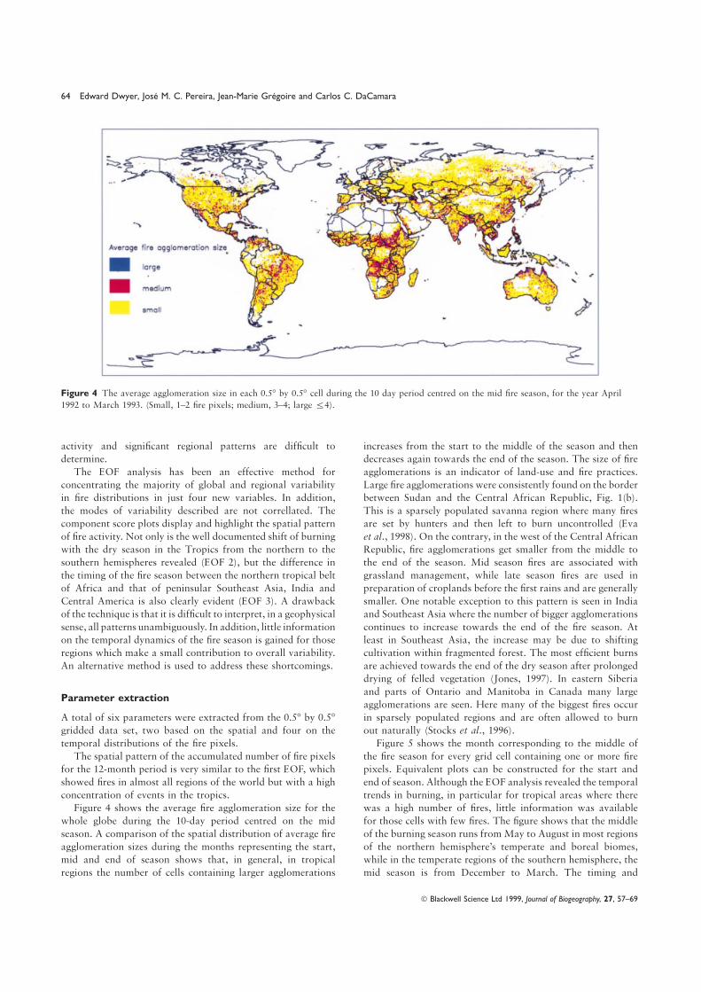
be evaluated with a number of measures. One widely usedAn automatic clustering algorithm (ISODATA) was used to

extract five classes based on the three global grids of fire method is the Jeffries-Matusita distance measure. The JM

distance receives an exponentially decreasing weight withnumber, seasonal duration and agglomeration size. Table 2

shows the mean values and the standard deviations of the three increasing separation between classes and is asymptotic towards

two which indicates complete separability, while zero representsinput parameters for each class, as well as the percentage of

cells belonging to each class. The class characteristics can be no separability (Richards, 1993). The values for all class

combinations are presented in Table 3. The best separabilitydescribed as follows.

Class 1: Low level of fire activity, there are few fire pixels is between classes 1 and 3, while the poorest is between classes



Table 3 The Jeffries-Matusita distance for each of the ten class Southeast Asia and eastern India are dominated by high densitycombinations shows the separability between the classes constructed burning (class 5) and a strikingly seasonal pattern of vegetationusing the three parameters: fire count, agglomeration size and fire fire (class 2), while in western India and in southern China fireseason duration. Zero represents no separability, two, complete is of a more moderate nature, with an extended fire seasonseparability.

(class 3). Australia and insular Southeast Asia show moderate

burning levels (class 2 & 3). In the Northern Territory ofClasses JM Classes JM Classes JM

Australia which is dominated by shrub land, there is a region

of very high density burning and fires of large agglomeration1:2 1.8 2:3 1.7 3:4 1.8sizes (classes 4 and 5). Other years may show different patterns1:3 2.0 2:4 1.6 3:5 1.9

1:4 1.8 2:5 1.8 4:5 1.5 of burning. In the year analysed, a low level of fire occurrence1:5 1.9 was detected in insular Southeast Asia. This would certainly

not have been the case if the analysis had covered 1998.

4 and 5. This indicates that the clustering algorithm has DISCUSSIONbeen quite successful in identifying groups which have distinct

characteristics. This study has characterized global patterns of vegetation fire

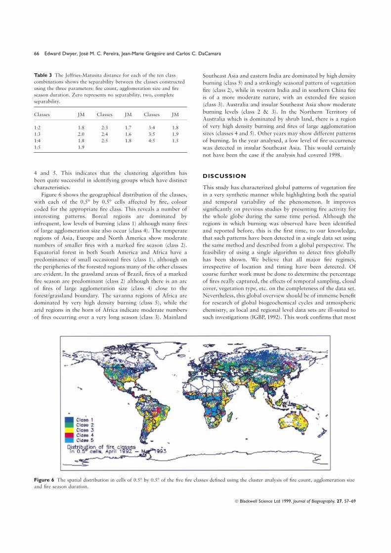
in a very synthetic manner while highlighting both the spatialFigure 6 shows the geographical distribution of the classes,

with each of the 0.5° by 0.5° cells affected by fire, colour and temporal variability of the phenomenon. It improves

significantly on previous studies by presenting fire activity forcoded for the appropriate fire class. This reveals a number of

interesting patterns. Boreal regions are dominated by the whole globe during the same time period. Although the

regions in which burning was observed have been identifiedinfrequent, low levels of burning (class 1) although many fires

of large agglomeration size also occur (class 4). The temperate and reported before, this is the first time, to our knowledge,

that such patterns have been detected in a single data set usingregions of Asia, Europe and North America show moderate

numbers of smaller fires with a marked fire season (class 2). the same method and described from a global perspective. The

feasibility of using a single algorithm to detect fires globallyEquatorial forest in both South America and Africa have a

predominance of small occasional fires (class 1), although on has been shown. We believe that all major fire regimes,

irrespective of location and timing have been detected. Ofthe peripheries of the forested regions many of the other classes

are evident. In the grassland areas of Brazil, fires of a marked course further work must be done to determine the percentage

of fires really captured, the effects of temporal sampling, cloudfire season are predominant (class 2) although there is an arc

of fires of large agglomeration size (class 4) close to the cover, vegetation type, etc. on the completeness of the data set.

Nevertheless, this global overview should be of immense benefitforest/grassland boundary. The savanna regions of Africa are

dominated by very high density burning (class 5), while the for research of global biogeochemical cycles and atmospheric

chemistry, as local and regional level data sets are ill-suited toarid regions in the horn of Africa indicate moderate numbers

of fires occurring over a very long season (class 3). Mainland such investigations (IGBP, 1992). This work confirms that most

Figure 6 The spatial distribution in cells of 0.5° by 0.5° of the five fire classes defined using the cluster analysis of fire count, agglomeration size

and fire season duration.



fire activity occurs in the tropics (Crutzen & Andreae, 1990; certain sun-target-sensor angles, there is specular reflection into

the sensor optics. The values recorded are then interpreted byAndreae, 1992), and identifies the most significant spatial and

temporal variability across this belt. the fire detection algorithm as ‘hot spots’ which leads to false

fire detection. Although burning of crop residues in the field isBoth the EOF approach and the extraction of temporal

parameters summarize temporal variability very effectively. common in south-eastern China, and the spatial location of the

fire activity coincides with that of estimated residue emissionsThe strongest temporal variability in biomass burning is that

associated with the movement of the dry season in the tropics (Zhuang et al., 1996) we believe that some of the very large

fire agglomerations seen here are associated with sun glint fromfrom the northern to the southern hemisphere, as evidenced in

the second EOF. In addition, there is a very clear separation flooded paddies.

The EOF analysis is ideal for capturing and separating allin time between burning in Africa and that in Central America

and southern Asia, the latter occurring most intensely in April modes of variability within a data set and here it has been

particularly effective in highlighting the variation in timing ofand May, when in Africa it is a transition period between

burning in the northern and southern hemispheres. The timing the fire season across the tropical belt. Conversely, the

parameter extraction and classification technique limits theof the burning season conflicts to some extent with those

studies which have used the concentration of surface ozone as range of variability described to those metrics chosen, however,

the spatial and temporal patterns are easier to interpreta proxy for the presence of biomass burning. For Africa, during

the year studied here, most fires were observed a couple of geophysically. The classification method will be considered in

the following discussion.months earlier than those reported by Hao & Liu (1994) for

the northern hemisphere and also earlier than those reported Figure 6 shows the spatial distribution of the five fire classes.

The class characteristics have been presented already. Class 1by Delmas et al. (1992) and Hao & Liu (1994) for the southern

hemisphere. The timing of the fire season here is more in fires are found predominantly at high latitudes (both North

and South) and in temperate maritime regions. In boreal regionsline with that determined from previous satellite observations

(Cahoon et al., 1992; Koffi et al., 1996). Kim & Newchurch many fires are caused by lightning (Stocks, 1992), however, the

density of fire activity is low. Much of this region is forested(1998) associate high levels of lower-tropospheric ozone, in the

period July to September, averaged over the period 1979–93, and given the very low population densities, fire is not used to

any appreciable extent in land management. In temperatein western New Guinea, with biomass burning in the western

part of the island. This conflicts, to some extent, with our maritime regions fire activity is restricted by unfavourable

weather conditions, with no extended dry period in which firesobservations, where the peak fire season was from September

to November with most activity concentrated in the southern can occur. The other regions in which class 1 fire activity is

seen are in the forested areas of Brazil and Africa. Tropicalpart of the island. It is possible that the dry season was later

or longer than usual in 1992, however, the use of satellite forest does not support any significant burning; the few fires

seen are in openings or degraded forest or are used for burningobservations of fire activity can certainly improve on the use

of measurements of other variables to infer burning. already felled timber.

Class 2 fire activity occurs in the mid-latitudes, where theIn addition to highlighting the spatial and temporal

distributions in tropical burning, the burning patterns in climate is warmer and there is a dry period sufficiently long to

allow vegetation to dry. Much of the western United States istemperate and boreal regions are also captured. Monitoring of

fire in boreal regions is important due to the significant role characterized by this fire class. During the Spring and Summer

fire is used in forest management, but many fires can also bethat boreal forest plays in global carbon cycling. Fire in such

ecosystems has huge direct and indirect impacts on the carbon started unintentionally. An extensive fire belt stretches from

the Black sea to lake Baikal in Eurasia. Burning is used forpool (French et al., 1996). The temperate and boreal regions

contribute significantly to the number of fires observed in the grassland management in this area but fires can also get out

of control and spread into forested areas (Associated Pressperiod May to August, which coincides with the northern

hemisphere’s summer. The classification (Fig. 6) shows fire news report 1996).

Class 3 fire activity is seen in arid and semiarid areas, suchactivity in many parts of the United States. In Eurasia a band

of fire activity stretches from the Black sea to Lake Baikal, as the horn of Africa, western India and the Australian interior.

Here there is little vegetation and there are very long drywhile in the more northern regions of Siberia and North

America, large fire agglomerations can be seen. periods, therefore fire activity is low and those fires that take

place are not necessarily restricted to a particular period of theSome problems remain with the automatic fire detection

algorithm (Stroppiana et al., 1999). Many false fires were year. Class 3 also occurs in subtropical maritime areas, such

as the south-eastern United States and southern China. Heredetected in the north-western part of Argentina on the border

with Chile. In semidesert areas of the Arabian peninsula, there is not a very well developed dry season, however,

temperatures are high enough to dry vegetation relativelysouthern Africa and Australia, we also observe unexpected fire

activity. These detections are most likely associated with areas quickly, therefore allowing fire activity during short dry spells.

Class 4 fires are not restricted to any particular geographicalof hot soil or bright surfaces. The radiative response from the

sensor’s perspective is the same as that of a fire and the or climatic zone. They are seen in boreal regions, where it is

not uncommon to have extremely large fire events. In tropicalalgorithm used is not sufficiently sophisticated to distinguish

between this and actual fire events. Another problem is areas, such large agglomerations of fire are associated with

savanna burning, particularly in sparsely populated areas,associated with sun glint from temporary water bodies. At



K. P. (1992) Seasonal distribution of African savanna fire. Nature,where fires are not highly controlled (e.g. Northern Australia,359, 812–815.Southern Sudan, Angola). Quite an extensive band of fire

Christensen, N.L. (1993) Fire regimes and ecosystem dynamics. Fire inactivity is seen in Brazil to the east of the Amazonian forest.the environment (ed. by P. J. Crutzen and J. G. Goldammer), pp.Large fires are known to occur in the cerrado and in grazing233–244. Wiley and Sons, Chichester.

lands in this region (Hlavka et al., 1996).Crutzen, P.J. & Andreae, M.O. (1990) Biomass burning in the tropics:

Class 5, which is characterized by a very high number ofimpact on atmospheric chemistry and biogeochemical cycles. Science,

fires, is essentially confined to tropical regions, with most of 250, 1669–1788.the savanna in Africa dominated by this class. It is also seen Davis, J.C. (1973) Statistics and data analysis in geology. Wiley &in parts of southern Asia, north-east Brazil and the ‘Top End’ Sons, New York.of Australia. In these areas the climate is characterized by high Davis, F. W., Quattrochi, D. A., Kidd, M. K., Lam, N. S.-N., Walsh,

temperatures, large quantities of rainfall and a dry season from S. J., Michaelsen, J. C., Franklin, J., Stow, D. A., Johannsen, C. J.

& Johnston, C. A. (1991) Environmental analysis using integratedthree to six months. These conditions are ideal for vegetationGIS and remotely sensed data: some research needs and priorities.growth and its subsequent desiccation. Fire is used for a myriadPhotogramm. Engng Remote Sensing, 57, 689–697.of purposes in these ecosystems, e.g. grassland management,

DeFries, R., Hansen, M. & Townshend, J. (1995) Global discriminationhunting, crop residue burning and land clearance (Andreae,of land cover types from metrics derived from AVHRR pathfinder

1992).data. Remote Sensing Environ. 54, 209–222.

The Kyoto protocol on climate change (UNEP/IUC, 1998)Delmas, R. A., Loudjani, P., Podaire, A. & Menaut, J.-C. (1992) Biomass

makes specific reference to vegetation fire as a source ofburning in Africa: an assessment of annually burned biomass. Global

greenhouse gases. It furthermore requires signatories to the biomass burning (ed. by J. Levine), pp. 126–132. MIT Press, Cam-protocol to develop systematic observation systems and work bridge, Mass.to improve the quality of the data and methodologies used for Dwyer, E., Gregoire, J.-M. & Malingreau, J. P. (1998) A global

estimating the emissions (Article 10). This study has shown analysis of vegetation fires using satellite images: spatial and temporal

dynamics. Ambio,. 27, 175–181.the feasibility of providing objective and globally consistentEastman, J.R. & Fulk, M. (1993) Long sequence time series evaluationinformation on vegetation fire using satellite observations and

using standardized principal components. Photogramm. Engng Re-could potentially be used to help in making a first estimate ofmote Sensing, 59, 1307–1312.global greenhouse gas emissions due to vegetation fire very

Eva, H. & Lambin, H.&. (1998) Remote sensing of biomass burning innear in time to the baseline year of 1990.tropical regions: sampling issues and multisensor approach. Remote

In the tropics, especially in savanna, the fire return intervalSensing Environ. 64, 292–315.

is very short, with the same area being burned year after year.Eva, H. D., Malingreau, J. P., Gregoire, J.-M., Belward, A. S. &

The number of fires and the fire characteristics change in Mutlow, C. T. (1998) The advance of burnt areas in central Africarelation to climatic factors, however, regional patterns remain as detected by ERS-1 ATSR-1. Int J. Remote Sensing, 19, 1635–1637.quite constant as has been observed in multiyear satellite data Flasse, S. & Ceccato, P. (1996) A contextual algorithm for AVHRRsets (Miranda et al., 1994; Koffi et al., 1996). In temperate and fire detection. Int J. Remote Sensing, 17, 419–424.

in boreal regions, although the number of fires may not vary French, N. H. F., Kasischke, E. S., Johnson, R. D., Bourgeau-Chavez,

L. L., Frick, A. L. & Ustin, S. (1996) Estimating fire-related carbongreatly from year to year there is a very large interannualflux in Alaskan boreal forests using multisensor remote-sensing data.variation in the area burned (Stocks, 1992). Long-termBiomass burning and global change, Vol. 2 (ed. by J. Levine), pp.monitoring of global fire occurrence with satellite data will808–826. MIT Press, Cambridge, Mass.allow us to improve characterization of fire regimes and aid

Frulla, L. A., Milovich, J. A. & Gagliardini, D. A. (1995) Illuminationour understanding of the complex relationship between climate,and observation geometry for NOAA-AVHRR images. Int J. Remote

vegetation, land-use and fire. Although the analysis describedSensing, 16, 2233–2253.

here was restricted to a 12-month period, by lack of suitableFung, T. & LeDrew, E. (1987) Application of principal components

long-term data sets, the results have demonstrated the feasibility analysis to change detection. Photogramm. Engng Remote Sensing,of extracting useful information from such global data sets. 53, 1649–1658.

Giglio, L., Kendall, J. D. & Justice, C. O. (1999) Evaluation of global

fire detection algorithms using simulated AVHRR infrared data. Int

J. Remote Sensing, 20, 1947–1985.ACKNOWLEDGMENTSGoldammer, J.G. (1993) Historical biogeography of fire: tropical and

E. Dwyer was funded by the TMR doctoral programme of the subtropical. Fire in the environment (ed. by P. J. Crutzen and J. G.

European Commission. Thanks to Michel Verstraete for his Goldammer), pp. 297–314. Wiley and Sons, Chichester.

Gonzalez, R.C. & Wintz, P. (1987) Digital image processing, 2nd edn,comments on the manuscript.503 pp. Addison-Wesley, Mass.

Gregoire, J.-M. (1993) Description quantitative des regimes de feu en

zone soudanienne d’Afrique de l’Ouest. Secheresse, 4, 37–45.REFERENCESHao, W. & Liu, M. (1994) Spatial and temporal distribution of tropical

biomass burning. Global Biochem. Cycles, 8, 495–503.Andreae, M.O. (1992) Biomass burning: its history, use, and distribution

Hlavka, C. A., Ambrosia, V. G., Brass, J. A., Rezendez, A. R. & Guild,and its impact on environmental quality and global climate. Global

L. S. (1996) Mapping fire scars in the Brazilian cerrado using AVHRRbiomass burning, atmospheric, climatic, and biospheric implications

imagery. Biomass burning and global change, Vol. 2 (ed. by J.(ed. by J. Levine), pp. 3–21. MIT Press, Cambridge, Mass.

Cahoon, D. R., Stocks, B. J., Levine, J. S., Cofer, W. R. & O’Neill, Levine), pp. 555–560. MIT Press, Cambridge, Mass.



IGBP (1992) Improved global data for land applications, IGBP Global Stocks, B. J., Cahoon, D. R., Cofer, W. R. III & Levine, J. S. (1996)

Monitoring large-scale forest-fire behavior in northeastern SiberiaChange Report No. 20 (ed. by R. G. Townshend). IGBP, Stockholm

using NOAA-AVHRR satellite imagery. Biomass burning and globaland Toulouse.

change, Vol. 2 (ed. by J. Levine), pp. 802–807. MIT Press, Cambridge,IGBP (1994) IGBP-DIS satellite fire detection algorithm workshop

Mass.technical report Working Paper 9. IGBP, Toulouse.Stroppiana, D., Pinnock, S. & Gregoire, J.-M. (1999) The global fireIGBP. (1997) Definition and implementation of a global fire product

product: daily fire occurrence, from April 1992 to December 1993,derived from AVHRR data. Working Paper 17. IGBP, Toulouse.derived from NOAA-AVHRR data. Int J. Remote Sensing, in press.Johnston, R.J. (1978) Multivariate statistical analysis in geography,

Townshend, J. R. G., Goff, T. E. & Tucker, C. J. (1985) Multi-temporal280 pp. Longman, London.dimensionality of images of normalized difference vegetation indexJones, S.H. (1997) Vegetation fire in mainland Southeat Asia: spatio-at continental scales. IEEE Trans. Geosci. Remote Sensing, GE-23temporal analysis of AVHRR 1 km data for the 1992/93 dry season.888–895.Report no. EUR 17282 EN. European Commission, Luxembourg.

Trabaud, L. V., Christensen, N. L. & Gill, A. M. (1993) HistoricalKeiner, L.E. & Yan, X.-H. (1997) Empirical orthogonal functionbiogeography of fire in temperate and mediterranean ecosystems.analysis of sea surface temperature patterns in Delaware bay. IEEEFire in the environment (ed. by P. J. Crutzen and J. G. Goldammer),Trans. Geosci. Remote Sensing, 35, 13199–13206.pp. 277–296. Wiley and Sons, Chichester.Kim, J.H. & Newchurch, M.J. (1998) Biomass-burning influence on

Tucker, C. J., Townshend, J. R. G. & Goff, T. E. (1985) African land-tropospheric ozone over New Guinea and South America. J. geophyscover classification using satellite data. Science, 227, 369–375.Res. 103, 1455–1461.

UNEP/I. U. C. (1998) The Kyoto Protocol to the Convention on ClimateKoffi, B., Gregoire, J.-M. & Eva, H. D. (1996) Satellite monitoring ofChange, 34 pp. Climate Change Secretariat, Bonn and UNEP/IUC,vegetation fires on a multiannual basis at continental scale in Africa.Geneva.Biomass burning and global change, Vol. 1 (ed. by J. Levine), pp.

Yarnal, B. (1993) Synoptic climatology in environmental analysis.225–235. MIT Press, Cambridge, Mass.Belhaven Press, London.Levine, J.S. (1996) Introduction. Biomass burning and global change,

Zhuang, Y.-H., Cao, M., Wang, X. & Yao, H. (1996) Spatial distributionVol. 1 (ed. by J. Levine), pp. xxxv-xliii. MIT Press, Cambridge,of trace-gas emissions from burning crop residue in China. BiomassMass.burning and global change, Vol. 2 (ed. by J. Levine), pp. 764–770.Lloyd, D. (1990) A phenological classification of terrestrial vegetationMIT Press, Cambridge, Mass.

cover using shortwave vegetation index imagery. Int J. Remote

Sensing, 11, 2269–2279.

Malingreau, J.-P. & Gregoire, J.-M. (1996) Developing a global vegeta- BIOSKETCHEStion fire monitoring system for global change studies: a framework.

Biomass burning and global change, Vol. 1 (ed. by J. Levine), pp.

14–24. MIT Press, Cambridge, Mass. Edward Dwyer received an MSc in remote sensing from theMenaut, J.-C., Abbadie, L. & Vitousek, P. M. (1993) Nutrient and University of Edinburgh. He is currently carrying out his

organic matter dynamics in tropical ecosystems. Fire in the en- PhD research using remotely sensed data to characterizevironment: the ecological, atmospheric, and climatic importance of global vegetation fire distributions and investigate the linksvegetation fires (ed. by P. J. Crutzen and J. G. Goldammer), pp. between fire, climate and vegetation215–231. Wiley and Sons, Chichester.

distributions.de Miranda, E. E., Setzer, A. W. & Takeda, A. M. (1994) Moni-

Jose Miguel Pereira is an associate Professor. He obtained atoramento Orbital das Queimadas No Brasil (Remote sensing ofPhD from the University of Arizona, in 1989. His mainfires in Brazil), 149 pp. ECOFORCA, Campinas.research interests are in the remote sensing of vegetationPiwowar, J.M. & LeDrew, E.F. (1996) Principal components analysisand fire activity, including burnt area mapping andof Arctic ice conditions between 1978 and 1987 as observed fromestimation of atmospheric emissions from biomass burning.the SMMR data record. Can J. Remote Sensing, 22, 390–403.

Piwowar, J. M., Peddle, D. R. & LeDrew, E. F. (1998) Temporal Jean-Marie Gregoire obtained a PhD in 1980 from the

mixture analysis of arctic sea ice imagery: a new approach for Louis Pasteur University, Strasbourg on the use of remotemonitoring environmental change. Remote Sensing Environ. 63, sensing in the field of modelling of water and energy195–207. transfer in the soil-plant-atmosphere system. He is currently

Richards, J.A. (1993) Remote sensing digital image analysis. Springer- a project leader and his research interests are in developingVerlag, Berlin. remote sensing approaches to environmental monitoring

Robinson, J. (1991) Fire from space: global fire evaluation using infrared and in particular fire.remote sensing. Int J. Remote Sensing, 12, 3–24.

Carlos C. DaCamara received a PhD degree in AtmosphericSingh, A. & Harrison, A. (1985) Standardized principal components.

Sciences from the University of Missouri-Columbia (USA)Int J. Remote Sensing, 6, 883–896.

in 1991. He is currently an Assistant Professor. His researchStocks, B.J. (1992) The extent and impact of forest fires in northern

has been partly devoted to exploring relationships betweencircumpolar countries. Global biomass burning, atmospheric, cli-

Atmospheric Circulation Types and wildfire activity.matic, and biospheric implications (ed. by J. Levine), pp. 197–202.

MIT Press, Cambridge, Mass.


Characterization of the spatio-temporal patterns in the osmosedimentation process

Documents

Transcript of Characterization of the spatio-temporal patterns in the osmosedimentation process