Environ Monit AssessDOI 10.1007/s10661-008-0582-1

Spatial variability of depth and salinity of groundwaterunder irrigated ustifluvents in the Middle Black SeaRegion of Turkey

Yusuf Demir · Sabit Ersahin · Mustafa Güler ·Bilal Cemek · Hikmet Günal · Hakan Arslan

Received: 22 September 2007 / Accepted: 29 September 2008© Springer Science + Business Media B.V. 2008

Abstract Information on the potential risk for soilsalinity buildup can be very helpful for soil salinitymanagement in irrigated areas. We evaluated thespatial and temporal variability of groundwatersalinity (GWS) and groundwater depth (GWD),which are two of the most important indicatorsof soil salinity, by indicator kriging technique ina large irrigated area in northern Turkey. GWSand GWD were measured on a monthly basis

Y. DemirDepartment of Agricultural Structures and Irrigation,Ondokuz Mayıs University, 55139 Samsun, Turkey

S. Ersahin (B)Department of Soil Science Agricultural Faculty,Ordu University, Ordu, Turkeye-mail: acapsu@gmail.com

M. GülerAgricultural Research Institute,Gelemen, Samsun, Turkey

B. CemekDepartment of Agricultural Structures and Irrigation,Gaziomanpasa University, Tokat, Turkey

H. GünalDepartment of Soil Science Agricultural Faculty,Gaziomanpasa University, Tokat, Turkey

H. ArslanVIIth Region, State Hydraulic Works,Bafra, Samsun, Turkey

from irrigation season (August 2003) to rainy sea-son (April 2004) at 60 observation wells in the8,187-ha irrigated area. Five indicator thresholdswere used for GWS and GWD. The semivario-gram for each of the thresholds for both variableswas analyzed then used together with experimen-tal data to interpolate and map the correspond-ing conditional cumulative distribution functions(CCDF). Risk for soil salinity buildup was greaterin the irrigation season compared to that in therainy season. The greatest risk for soil salinitybuildup occurred in the eastern part of the studyarea, suffering from poor drainage problem dueto malfunctioning drainage infrastructure, as indi-cated by the CCDF of GWS and GWD obtainedin both seasons. It was concluded that a combina-tion of mechanical and cultural measures shouldbe taken in high-risk locations to avoid furthersalinity problems.

Keywords Evapotranspiration ·Groundwater depth · Groundwater salinity ·Indicator kriging · Irrigation

Introduction

In many irrigated areas, crop yields are reduceddue to salinization and alkalinization of the soils.The rapid irrigation development of the early-and mid-decades of the twentieth century, mostly

Environ Monit Assess

implemented without providing proper irrigationwater management and drainage, has left a globallegacy of risen water tables and large-scale salini-zation of irrigated lands (Smedema et al. 2000).Bafra Plain’s right-land-irrigated area is one ofthe largest irrigation and drainage projects inTurkey. Excessive irrigation water use, seepagefrom canals, poor irrigation efficiencies, and in-adequate drainage systems have resulted in localareas with elevated saline groundwater, increas-ing the risk of soil salinity. Cemek et al. (2006)indicated that cauliflower, radish, and leek pro-duction in Bafra plain increased and beans andcorn production considerably decreased due tothe increased groundwater salinity (GWS) in irri-gation season. Arslan et al. (2007) also reported10% yield loss in the Bafra Plain due to the highelectrical conductivity (EC) of groundwater.

Salinity buildup in the root zone depends onseveral factors such as GWS, quality of irrigationwater, irrigation strategy, crops being grown, soiltype, and groundwater depth (GWD) (Prathaparand Qureshi 1999; Ali et al. 2000). The irriga-tion strategy is an important factor affecting thedepth and elevation of the groundwater as wellas salinity buildup in the root zone. Ali et al.(2000) simulated the effect of irrigation intervaland amount of irrigation water used on the soilsalinity buildup at different conditions of GWSand GWD. They found that average soil salinitywas considerably affected by the amount of irri-gation water and interval of the irrigation events,especially under a combination of low GWD andhigh GWS. They stressed that the effect of irriga-tion strategy was pronounced at the greater EC ofgroundwater. Therefore, spatial relation betweensoil and groundwater properties should be consid-ered in the management of irrigation water.

Soils spatially vary in the vertical and horizon-tal directions as a response to the variation inthe interaction between parent material and soil-forming factors such as climate, topography, andvegetation (Heuvelink and Webster 2001). Thepattern of the variation is controlled by manyfactors such as combined action of soil-formingfactors and processes on parent material, spa-tial distribution of parent material, and soil man-agement. Geostatistical analysis has been widelyused to analyze the systematic variation of soil

and water variables in space and time (Vieiraet al. 1981; Yates and Warrick 1987; Isaaksand Srivastava 1989; Goovaerts 1997; Ersahin2001, 2003; Ersahin and Brohi 2006; and manyothers). Geostatistical application has two mainstages: characterizing spatial dependency by semi-variograms and predicting the variable at theunvisited locations by various forms of krigingprocedure. The latter procedure requires the re-sults from the former.

Kriging techniques have been widely used topredict soil properties from a limited number ofsamples. However, linear kriging has not beenproved suitable to assess the likelihood of ex-ceeding a given threshold. For many practicalproblems of land management, information onsoil properties, relative to soil threshold valuesthat may have limits of a practical importance isneeded at unsampled sites (Lark and Ferguson2004). The risk of overriding a given thresholdconcentration of an agent can be analyzed suc-cessfully by indicator kriging (Goovaerts 1997).Indicator kriging is an approach for estimatingthe proportion of values that fall within classifiedclass intervals (Mulla and Mc Bratney 2001), byincorporating the uncertainty of the value of thevariable at the unsampled locations. This tech-nique provides a nonparametric solution to theproblems via estimation of a local cumulative dis-tribution function of the variable at an unsampledlocation using values of neighboring locations.When a land manager wants to interpret a kriggedmap of a soil property with respect to the somecritical thresholds, then the uncertainty of theseestimates becomes important (Lark and Ferguson2004). This problem is critical for delineating theareas for remedial treatments, delineating thecontaminated areas, and determining the landsuitability for specific crops (Emery 2006).

Goovaerts (1997) applied indicator kriging toassess the rock type and land management in-fluence on the short- and long-range variabilityof heavy metals in a contrasting area. Hu et al.(2005) concluded from their study that the mapgenerated by ordinary kriging method could notcorrectly reflect the groundwater pollution statusof nitrate. However, they further reported thatindicator kriging method satisfactorily helped inassessing the risk of nitrate pollutions. Hu et al.

Environ Monit Assess

(2005) stressed that the sources of nitrate could bedistinguishable in the maps generated by indicatorkriging. Smith et al. (1993) analyzed soil qualityindicators in a shrub–steppe ecosystem, and Liuet al. (2004) evaluated arsenic contamination po-tential by indicator kriging in Yun-Lin aquifer,Taiwan. Lark and Ferguson (2004) applied indi-cator kriging to map the risk of soil nutrient defi-ciency or excess.

The characterization of spatial dependency ofGWD and GWS is vital in evaluating their likelycombined contribution to soil salinity buildup.The indicator kriging technique can be satis-factorily applied to estimate the likelihood forthese variables to exceed a specified value. Oncedetected, the high-risk salinity areas can be site-specifically managed to avoid further deteriora-tion in these localities. The objectives of this studywere (1) to map the likelihood for GWD andGWS as related to irrigation practices, soils, andtopographic properties, (2) to delineate the areaswith high salinity risk as posed by GWD and GWS,and (3) to suggest the management practices tomitigate management-related soil salinity risk.

Materials and methods

Description of the study area

The study area is a part of Kizilirmak Delta thatis located in the central Black Sea coastal region(41◦30′–41◦45′ latitude and 35◦30′–36◦15′ longi-tude) in Northern Turkey (Fig. 1).

The soils of the study area formed from al-luvial materials on different elevations. Table 1presents some properties of the soils in the studyarea. The sediments in the area consists of UpperPleistocene and Holocene alluviums and variesfrom fine sand, silt, and clay in varying thicknessand extents. The thickness of Quaternary depositsincreases through the north (Akkan 1970). Major-ity of the soil are deeper than 1.5 m. The soilsare fine-textured with moderate hydraulic con-ductivity. The pH of soils is around 8.2, whichis considered high. Depending on the drainageand soil aeration, some of the soils located belowthe elevation of 2 m, were high in organic matter

content (Ozesmi 1999). Sublayers of these soilswere massive in structure.

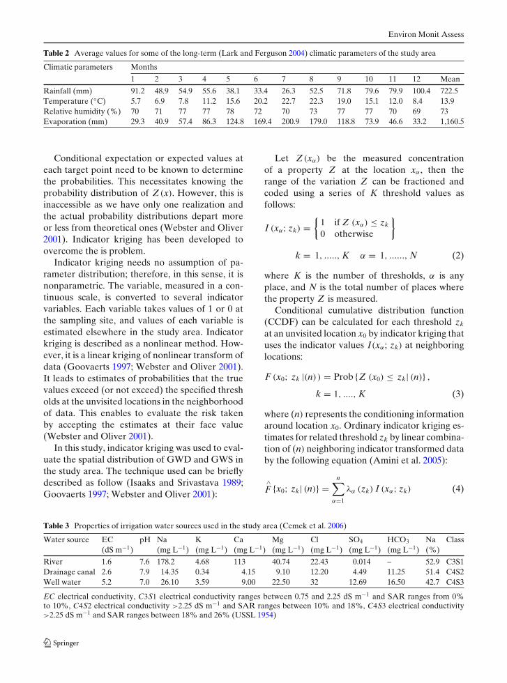
The current climate in the region is semihu-mid. Seasonal variations of temperature, class Apan evaporation, and rainfall are presented inTable 2. Temperature and evaporation values arehigh in the irrigation season compared to those inthe rainy season. The summers are warmer thanwinters (the average temperature in July is 22.2◦Cand in January is 6.9◦C). The annual averagetemperature is 13.9◦C. The annual precipitationis 722.5 mm, most of which precipitates betweenSeptember and April (Anonymous 2004). Soil wa-ter and temperature regimes are ustic and mesic,respectively (Soil Survey Staff 1999) (Table 2).

Groundwater level and drainage differ consid-erably within the study area due to the differencesin elevation, which slightly increases from the sea-side and reaches to 10 m within an approximately6 km distance. The study area has been underconventional tillage including moldboard plough(about 20 cm depth) in fall, cultivator (about15 cm depths), and disc harrow (about 10 cmdepths) subsequent to threshold soil tillage.

The Kizilirmak River is the major irrigationwater source in Bafra Plain. Water from drainagecanals and from groundwater is used in the areaswhere canal water is scarce. Some characteristicsof all three irrigation water sources are presentedin Table 3.

Classical canal irrigation system is predomi-nant in the area. Border and furrow irrigation arethe main irrigation types although many types ofirrigation are practiced depending on the need ofcrops grown. Sprinkler irrigation is also used, butrarely. However, no drip irrigation is practiced.Approximately 75% of the area was irrigatedwith surface water and the rest was irrigated withgroundwater (Arslan et al. 2007).

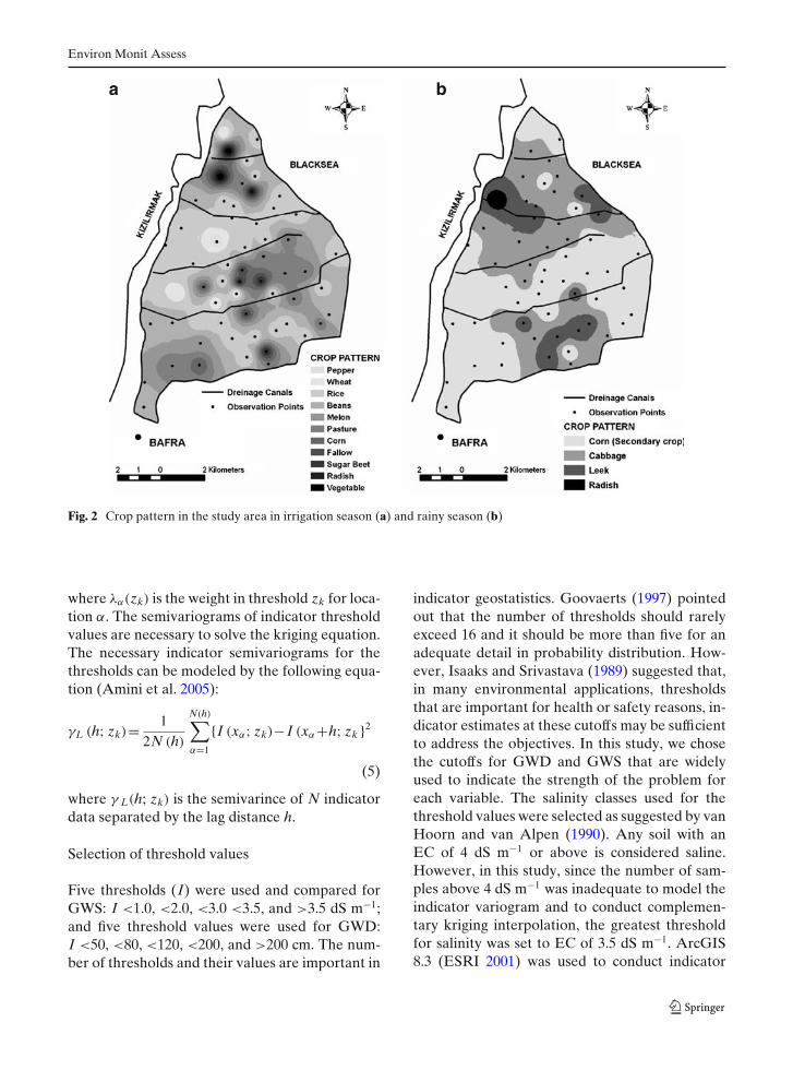
Crop pattern considerably differs in the studyarea (Fig. 2). Wheat, tomatoes, pepper, water-melon, beet, and sweet melon are predominantlygrown in the irrigation season (Fig. 2a); and cab-bage, and leek are grown in rainy season (Fig. 2b).Corn is also grown as a primary and secondarycrop. Recently, a considerable increase occurredin the rice production as more irrigation waterbecame available by newly completed irrigationprojects.

Environ Monit Assess

Fig. 1 Location andlayout of the study area

Methods

Measurements of GWD and GWS were made ona monthly basis at 60 observation wells during theperiod between 2003 and 2004. Both spatial andtemporal variations in GWD and GWS were ana-lyzed and compared. The elevations and locationsof 60 observation wells, shown in the Fig. 1 weredetermined using topographic maps with a scale of1/5,000 and a Global Positioning System. Salinity

and GWD were measured at each sampling site.The wells, where water was sampled based on themethod described by de Ritter (1994), were case-typed.

The data were grouped into two classes basedon meteorological conditions to determine thetemporal and spatial changes in GWS and GWD.The period from May to September was consid-ered as irrigation season and from October toApril was considered as rainy season.

Environ Monit Assess

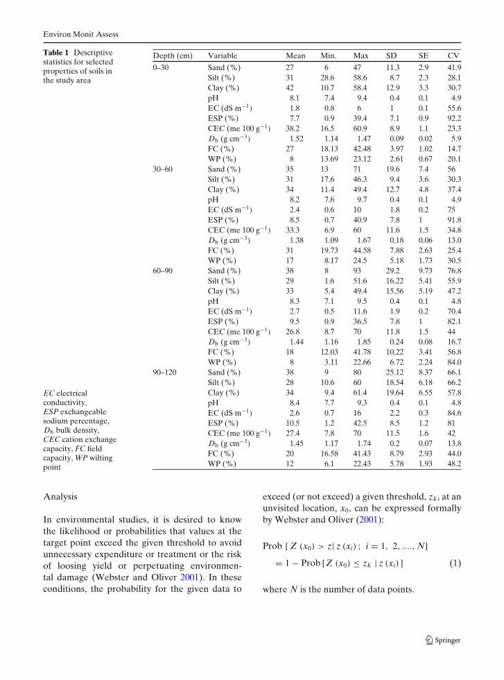
Table 1 Descriptivestatistics for selectedproperties of soils inthe study area

EC electricalconductivity,ESP exchangeablesodium percentage,Db bulk density,CEC cation exchangecapacity, FC fieldcapacity, WP wiltingpoint

Depth (cm) Variable Mean Min. Max SD SE CV

0–30 Sand (%) 27 6 47 11.3 2.9 41.9Silt (%) 31 28.6 58.6 8.7 2.3 28.1Clay (%) 42 10.7 58.4 12.9 3.3 30.7pH 8.1 7.4 9.4 0.4 0.1 4.9EC (dS m−1) 1.8 0.8 6 1 0.1 55.6ESP (%) 7.7 0.9 39.4 7.1 0.9 92.2CEC (me 100 g−1) 38.2 16.5 60.9 8.9 1.1 23.3Db (g cm−3) 1.52 1.14 1.47 0.09 0.02 5.9FC (%) 27 18.13 42.48 3.97 1.02 14.7WP (%) 8 13.69 23.12 2.61 0.67 20.1

30–60 Sand (%) 35 13 71 19.6 7.4 56Silt (%) 31 17.6 46.3 9.4 3.6 30.3Clay (%) 34 11.4 49.4 12.7 4.8 37.4pH 8.2 7.6 9.7 0.4 0.1 4.9EC (dS m−1) 2.4 0.6 10 1.8 0.2 75ESP (%) 8.5 0.7 40.9 7.8 1 91.8CEC (me 100 g−1) 33.3 6.9 60 11.6 1.5 34.8Db (g cm−3) 1.38 1.09 1.67 0.18 0.06 13.0FC (%) 31 19.73 44.58 7.88 2.63 25.4WP (%) 17 8.17 24.5 5.18 1.73 30.5

60–90 Sand (%) 38 8 93 29.2 9.73 76.8Silt (%) 29 1.6 51.6 16.22 5.41 55.9Clay (%) 33 5.4 49.4 15.56 5.19 47.2pH 8.3 7.1 9.5 0.4 0.1 4.8EC (dS m−1) 2.7 0.5 11.6 1.9 0.2 70.4ESP (%) 9.5 0.9 36.5 7.8 1 82.1CEC (me 100 g−1) 26.8 8.7 70 11.8 1.5 44Db (g cm−3) 1.44 1.16 1.85 0.24 0.08 16.7FC (%) 18 12.03 41.78 10.22 3.41 56.8WP (%) 8 3.11 22.66 6.72 2.24 84.0

90–120 Sand (%) 38 9 80 25.12 8.37 66.1Silt (%) 28 10.6 60 18.54 6.18 66.2Clay (%) 34 9.4 61.4 19.64 6.55 57.8pH 8.4 7.7 9.3 0.4 0.1 4.8EC (dS m−1) 2.6 0.7 16 2.2 0.3 84.6ESP (%) 10.5 1.2 42.5 8.5 1.2 81CEC (me 100 g−1) 27.4 7.8 70 11.5 1.6 42Db (g cm−3) 1.45 1.17 1.74 0.2 0.07 13.8FC (%) 20 16.58 41.43 8.79 2.93 44.0WP (%) 12 6.1 22.43 5.78 1.93 48.2

Analysis

In environmental studies, it is desired to knowthe likelihood or probabilities that values at thetarget point exceed the given threshold to avoidunnecessary expenditure or treatment or the riskof loosing yield or perpetuating environmen-tal damage (Webster and Oliver 2001). In theseconditions, the probability for the given data to

exceed (or not exceed) a given threshold, zk, at anunvisited location, x0, can be expressed formallyby Webster and Oliver (2001):

Prob [ Z (x0) > z| z (xi) ; i = 1, 2, ...., N]

= 1 − Prob [Z (x0) ≤ zk | z (xi) ] (1)

where N is the number of data points.

Environ Monit Assess

Table 2 Average values for some of the long-term (Lark and Ferguson 2004) climatic parameters of the study area

Climatic parameters Months

1 2 3 4 5 6 7 8 9 10 11 12 Mean

Rainfall (mm) 91.2 48.9 54.9 55.6 38.1 33.4 26.3 52.5 71.8 79.6 79.9 100.4 722.5Temperature (◦C) 5.7 6.9 7.8 11.2 15.6 20.2 22.7 22.3 19.0 15.1 12.0 8.4 13.9Relative humidity (%) 70 71 77 77 78 72 70 73 77 77 70 69 73Evaporation (mm) 29.3 40.9 57.4 86.3 124.8 169.4 200.9 179.0 118.8 73.9 46.6 33.2 1,160.5

Conditional expectation or expected values ateach target point need to be known to determinethe probabilities. This necessitates knowing theprobability distribution of Z (x). However, this isinaccessible as we have only one realization andthe actual probability distributions depart moreor less from theoretical ones (Webster and Oliver2001). Indicator kriging has been developed toovercome the is problem.

Indicator kriging needs no assumption of pa-rameter distribution; therefore, in this sense, it isnonparametric. The variable, measured in a con-tinuous scale, is converted to several indicatorvariables. Each variable takes values of 1 or 0 atthe sampling site, and values of each variable isestimated elsewhere in the study area. Indicatorkriging is described as a nonlinear method. How-ever, it is a linear kriging of nonlinear transform ofdata (Goovaerts 1997; Webster and Oliver 2001).It leads to estimates of probabilities that the truevalues exceed (or not exceed) the specified thresholds at the unvisited locations in the neighborhoodof data. This enables to evaluate the risk takenby accepting the estimates at their face value(Webster and Oliver 2001).

In this study, indicator kriging was used to eval-uate the spatial distribution of GWD and GWS inthe study area. The technique used can be brieflydescribed as follow (Isaaks and Srivastava 1989;Goovaerts 1997; Webster and Oliver 2001):

Let Z (xα) be the measured concentrationof a property Z at the location xα , then therange of the variation Z can be fractioned andcoded using a series of K threshold values asfollows:

I (xα; zk) ={

1 if Z (xα) ≤ zk

0 otherwise

}

k = 1, ....., K α = 1, ......, N (2)

where K is the number of thresholds, α is anyplace, and N is the total number of places wherethe property Z is measured.

Conditional cumulative distribution function(CCDF) can be calculated for each threshold zk

at an unvisited location x0 by indicator kriging thatuses the indicator values I(xα ; zk) at neighboringlocations:

F (x0; zk |(n) ) = Prob {Z (x0) ≤ zk| (n)} ,

k = 1, ...., K (3)

where (n) represents the conditioning informationaround location x0. Ordinary indicator kriging es-timates for related threshold zk by linear combina-tion of (n) neighboring indicator transformed databy the following equation (Amini et al. 2005):

∧F {x0; zk| (n)} =

n∑α=1

λα (zk) I (xα; zk) (4)

Table 3 Properties of irrigation water sources used in the study area (Cemek et al. 2006)

Water source EC pH Na K Ca Mg Cl SO4 HCO3 Na Class(dS m−1) (mg L−1) (mg L−1) (mg L−1) (mg L−1) (mg L−1) (mg L−1) (mg L−1) (%)

River 1.6 7.6 178.2 4.68 113 40.74 22.43 0.014 – 52.9 C3S1Drainage canal 2.6 7.9 14.35 0.34 4.15 9.10 12.20 4.49 11.25 51.4 C4S2Well water 5.2 7.0 26.10 3.59 9.00 22.50 32 12.69 16.50 42.7 C4S3

EC electrical conductivity, C3S1 electrical conductivity ranges between 0.75 and 2.25 dS m−1 and SAR ranges from 0%to 10%, C4S2 electrical conductivity >2.25 dS m−1 and SAR ranges between 10% and 18%, C4S3 electrical conductivity>2.25 dS m−1 and SAR ranges between 18% and 26% (USSL 1954)

Environ Monit Assess

a b

Fig. 2 Crop pattern in the study area in irrigation season (a) and rainy season (b)

where λα(zk) is the weight in threshold zk for loca-tion α. The semivariograms of indicator thresholdvalues are necessary to solve the kriging equation.The necessary indicator semivariograms for thethresholds can be modeled by the following equa-tion (Amini et al. 2005):

γL (h; zk)= 1

2N (h)

N(h)∑α=1

{I (xα; zk)− I (xα+h; zk }2

(5)

where γ L(h; zk) is the semivarince of N indicatordata separated by the lag distance h.

Selection of threshold values

Five thresholds (I) were used and compared forGWS: I <1.0, <2.0, <3.0 <3.5, and >3.5 dS m−1;and five threshold values were used for GWD:I <50, <80, <120, <200, and >200 cm. The num-ber of thresholds and their values are important in

indicator geostatistics. Goovaerts (1997) pointedout that the number of thresholds should rarelyexceed 16 and it should be more than five for anadequate detail in probability distribution. How-ever, Isaaks and Srivastava (1989) suggested that,in many environmental applications, thresholdsthat are important for health or safety reasons, in-dicator estimates at these cutoffs may be sufficientto address the objectives. In this study, we chosethe cutoffs for GWD and GWS that are widelyused to indicate the strength of the problem foreach variable. The salinity classes used for thethreshold values were selected as suggested by vanHoorn and van Alpen (1990). Any soil with anEC of 4 dS m−1 or above is considered saline.However, in this study, since the number of sam-ples above 4 dS m−1 was inadequate to model theindicator variogram and to conduct complemen-tary kriging interpolation, the greatest thresholdfor salinity was set to EC of 3.5 dS m−1. ArcGIS8.3 (ESRI 2001) was used to conduct indicator

Environ Monit Assess

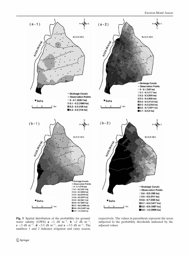
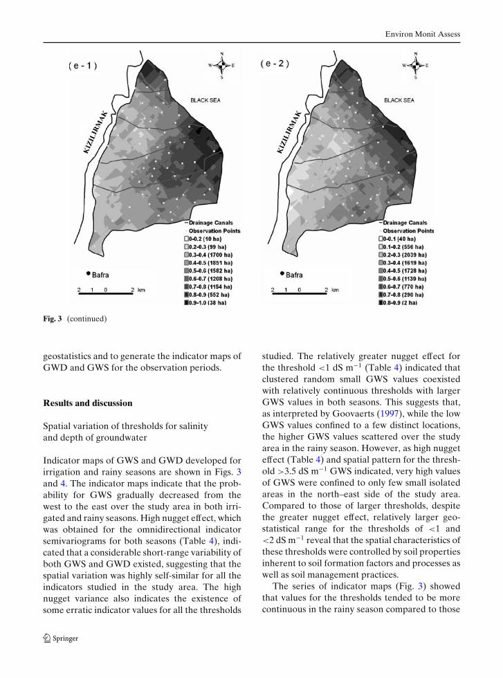
Fig. 3 Spatial distribution of the probability for ground-water salinity (GWS) a <1 dS m−1, b <2 dS m−1,c <3 dS m−1, d <3.5 dS m−1, and e >3.5 dS m−1. Thenumbers 1 and 2 indicates irrigation and rainy season,

respectively. The values in parenthesis represent the areassubjected to the probability thresholds indicated by theadjacent values

Environ Monit Assess

Fig. 3 (continued)

Environ Monit Assess

Fig. 3 (continued)

geostatistics and to generate the indicator maps ofGWD and GWS for the observation periods.

Results and discussion

Spatial variation of thresholds for salinityand depth of groundwater

Indicator maps of GWS and GWD developed forirrigation and rainy seasons are shown in Figs. 3and 4. The indicator maps indicate that the prob-ability for GWS gradually decreased from thewest to the east over the study area in both irri-gated and rainy seasons. High nugget effect, whichwas obtained for the omnidirectional indicatorsemivariograms for both seasons (Table 4), indi-cated that a considerable short-range variability ofboth GWS and GWD existed, suggesting that thespatial variation was highly self-similar for all theindicators studied in the study area. The highnugget variance also indicates the existence ofsome erratic indicator values for all the thresholds

studied. The relatively greater nugget effect forthe threshold <1 dS m−1 (Table 4) indicated thatclustered random small GWS values coexistedwith relatively continuous thresholds with largerGWS values in both seasons. This suggests that,as interpreted by Goovaerts (1997), while the lowGWS values confined to a few distinct locations,the higher GWS values scattered over the studyarea in the rainy season. However, as high nuggeteffect (Table 4) and spatial pattern for the thresh-old >3.5 dS m−1 GWS indicated, very high valuesof GWS were confined to only few small isolatedareas in the north–east side of the study area.Compared to those of larger thresholds, despitethe greater nugget effect, relatively larger geo-statistical range for the thresholds of <1 and<2 dS m−1 reveal that the spatial characteristics ofthese thresholds were controlled by soil propertiesinherent to soil formation factors and processes aswell as soil management practices.

The series of indicator maps (Fig. 3) showedthat values for the thresholds tended to be morecontinuous in the rainy season compared to those

Environ Monit Assess

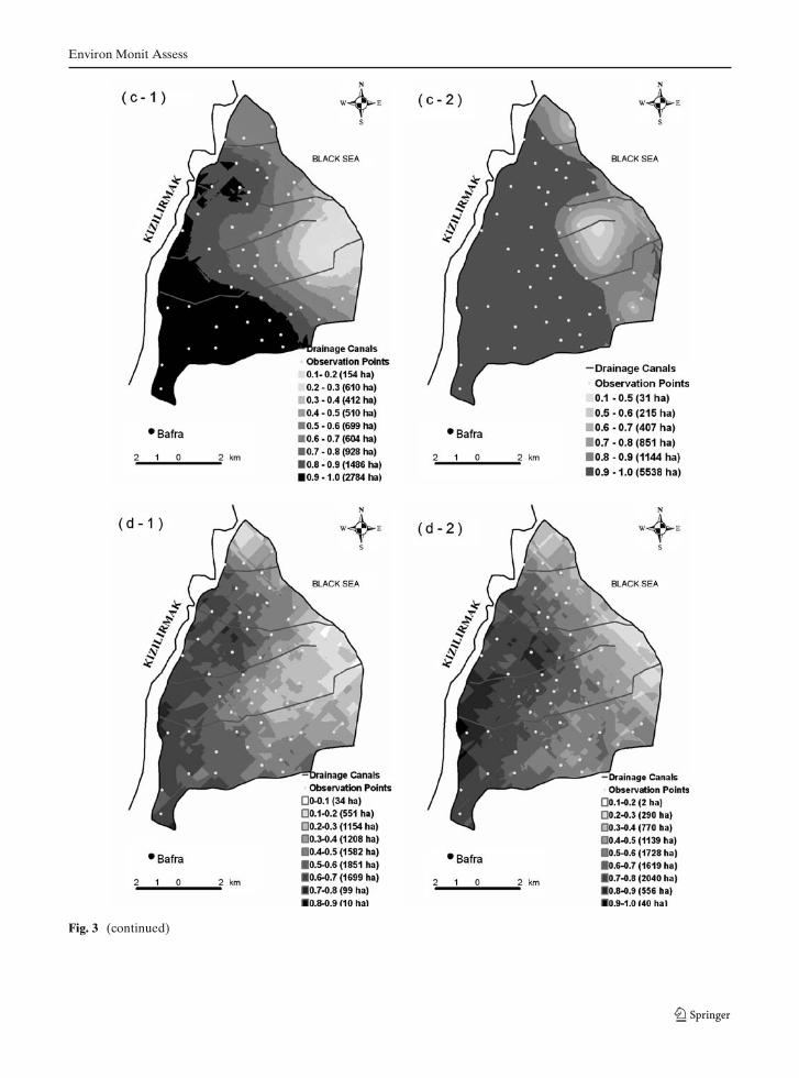
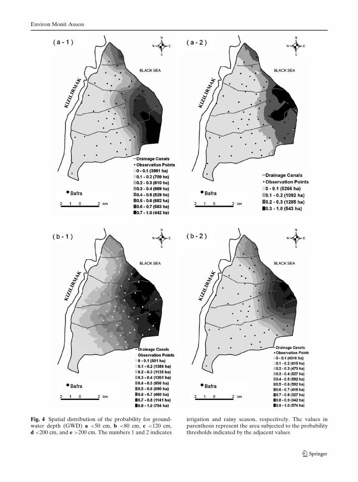
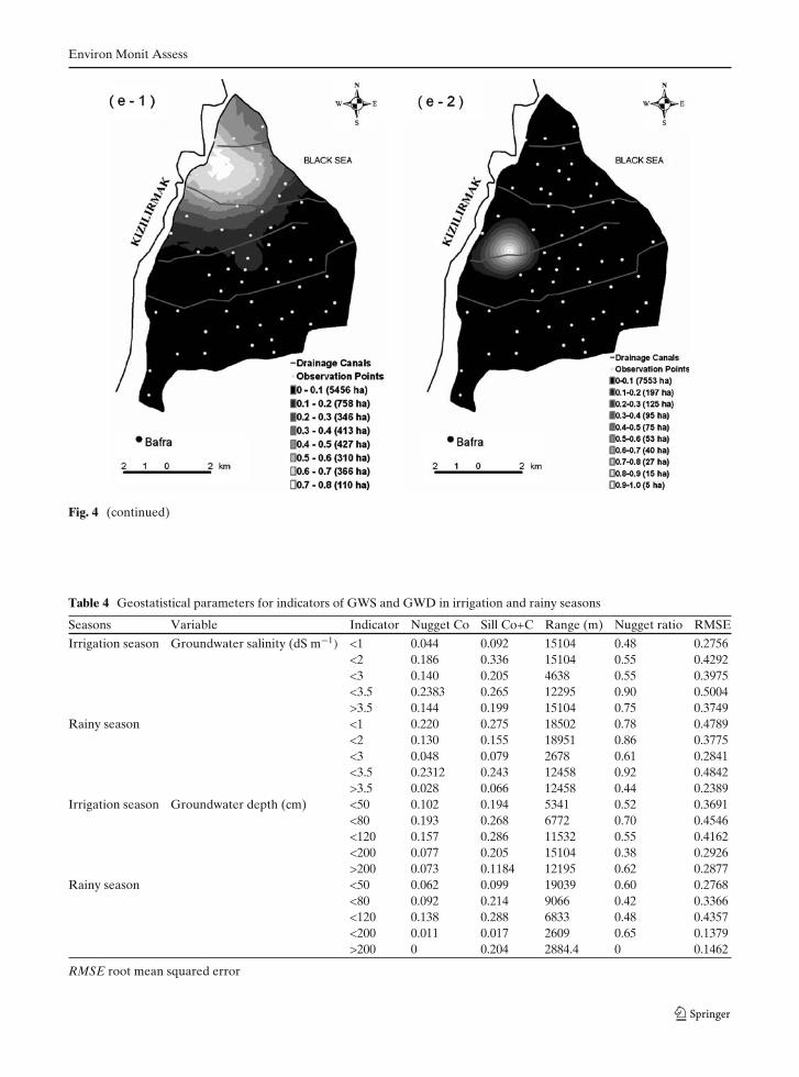
Fig. 4 Spatial distribution of the probability for ground-water depth (GWD) a <50 cm, b <80 cm, c <120 cm,d <200 cm, and e >200 cm. The numbers 1 and 2 indicates

irrigation and rainy season, respectively. The values inparenthesis represent the area subjected to the probabilitythresholds indicated by the adjacent values

Environ Monit Assess

Fig. 4 (continued)

Environ Monit Assess

Fig. 4 (continued)

Table 4 Geostatistical parameters for indicators of GWS and GWD in irrigation and rainy seasons

Seasons Variable Indicator Nugget Co Sill Co+C Range (m) Nugget ratio RMSE

Irrigation season Groundwater salinity (dS m−1) <1 0.044 0.092 15104 0.48 0.2756<2 0.186 0.336 15104 0.55 0.4292<3 0.140 0.205 4638 0.55 0.3975<3.5 0.2383 0.265 12295 0.90 0.5004>3.5 0.144 0.199 15104 0.75 0.3749

Rainy season <1 0.220 0.275 18502 0.78 0.4789<2 0.130 0.155 18951 0.86 0.3775<3 0.048 0.079 2678 0.61 0.2841<3.5 0.2312 0.243 12458 0.92 0.4842>3.5 0.028 0.066 12458 0.44 0.2389

Irrigation season Groundwater depth (cm) <50 0.102 0.194 5341 0.52 0.3691<80 0.193 0.268 6772 0.70 0.4546<120 0.157 0.286 11532 0.55 0.4162<200 0.077 0.205 15104 0.38 0.2926>200 0.073 0.1184 12195 0.62 0.2877

Rainy season <50 0.062 0.099 19039 0.60 0.2768<80 0.092 0.214 9066 0.42 0.3366<120 0.138 0.288 6833 0.48 0.4357<200 0.011 0.017 2609 0.65 0.1379>200 0 0.204 2884.4 0 0.1462

RMSE root mean squared error

Environ Monit Assess

in the irrigation season due to probably that thesalt distribution became more uniform in thestudy area during the rainy season. In general,except for the very high thresholds, this was alsoconfirmed by greater nugget effect observed forthresholds in the irrigated season. The indicatormaps further revealed that the indicator valueswere more continuous in the north–south direc-tion for all the cutoffs studied. This is expecteddue to the greater variability in the soil particlesize distribution that exists perpendicular to RiverKizilirmak.

Irrigation increased the likelihood of greaterGWS as indicated by highly different patterns inthe probability distribution for thresholds in theirrigated season compared to those in the rainyseason. The probability for GWS to exceed anygiven threshold was higher in the irrigated season.For instance, the area where the probability forthe GWS to exceed 3.5 dS m−1 was 38 ha in theirrigated season, while it was only 2 ha in therainy season. The same is also true for the otherthresholds of GWS.

Irrigation highly decreased the spatial variabil-ity of the water table for the threshold <50 cmcontrary to the threshold <200 cm as indicated byboth comparable geostatistical range and nuggeteffect values. The indicator maps (Fig. 4) showedthat the shallow groundwater tables were confinedto a few distinct locations in the east side of thestudy area.

Implications of water and soil management

Depth of groundwater was highly affected byirrigation as indicated by the difference betweenthe indicator maps for the irrigation season andthose for the rainy season (Fig. 4). Contrary toGWS, GWD gradually decreased from west toeast of the study area (Figs. 3 and 4). This partof the study area is located in the proximity ofthe seaside where the slope is quite low, obscuringdrainage from the drains. The high risk for salinitybuildup in these locations can be decreased bytaking several measures. Controlling evaporationof groundwater might be one of the measuresneeded to be considered.

In the east side of the study area, due to highwater table, significant amount of total ET may

be replenished by groundwater depending on theEC of groundwater. This should be consideredin the planning of the amount of irrigation waterand intervals of the irrigation. High water tableand EC of groundwater requires the use of irri-gation water in limited amounts and intervalsdepending on stress of crops. Leaving the light-colored residue on the soil surface may increasethe soil surface reflectivity, which decreases theamount of evaporating water and aids more waterto infiltrate into the soil, leaching the surface-accumulated salts to the deeper zones of thesoil profile.

In contrast, in the western part of the studyarea where probability for GWD to elevate is low,irrigation water may be used to replenish greateramount of total ET as crops cannot sufficientlyuse the water from deep groundwater. Appli-cation of irrigation water in greater amount mayleach salts from the soil profile to maintain salinityat a reasonable level in these locations. Stablemulching may be a good practice to decrease ETand increase the water infiltration into the soilprofile as indicated by Brady (1990).

The soils in the study area formed over allu-vial materials deposited by Kizilirmak River thatwould result in existence of entities with claytexture, necessitating particular care to be takento these fine-textured localities. In these areas,hydraulic conductivity of capillary ascent maybe restricted by several means (Prathapar andQureshi 1999). Hydraulic properties of the surfacesoils can be modified by mechanical cultivation.This also increases the mulchability of the sur-face soils, which is also effective in decreasing theevaporation of groundwater. Since plowing thesurface soil breaks the capillarity of pores fromthe water table to the soil surface and increasesthe roughness and porosity of the surface, evapo-ration decreases and infiltration increases.

Prathapar and Qureshi (1999) simulated theeffect of plowing 30 cm surface layer to decreasethe groundwater evaporation under varying GWDconditions in Pakistan. They concluded that thereclamation by plowing was inadequate if thewater table is at 50 cm or shallower. Therefore,in our case, the water table should be lowered atleast below 100 cm to effectively control ET bymechanical means in the high-risk shallow GWD.

Environ Monit Assess

The sites with GWD greater than 100 cm aremainly located in the west part of the study area.In these localities, plowing surface soil before arainy season can be a proper practice to decreaseevaporation and increase leaching of salts fromthe surface layer. Since tillage results in a moreuniform water flow in a soil profile, plowing mayresult in a uniform transport of salts through asoil profile.

The transpiration efficiency of the crops highlyaffects the portion of evaporation in evapotran-spiration. Figure 2 shows the crop patterns forrainy season and irrigation season growing peri-ods in the study area. In general, with the ex-ception of the rice plantation in the eastern partof the study site, the grower’s discretion is themain determinant of cropping pattern, regardlessof the conditions of the soil and groundwater.The locations with high GWD and GWS aremostly occupied by wheat, rice, leak, cabbage,pepper, and bean. Crops with high leaf areaindex and transpiration efficiency should be pre-ferred in these locations to restrict the evapo-ration of the water from the soil. Except ricegrowing conditions, the surface of soil should bekept as dry as possible by proper planning ofirrigation. The irrigation water can be concen-trated to the root zone, by subsurface drip irriga-tion, without wetting the surface of the soil, andthe soil between the rows in the case of row plantsare grown.

Conclusions and recommendations

The patterns of spatial continuity for GWS andGWD were evaluated by indicator kriging to ana-lyze the spatial characteristics of GWS and GWDas indicators of soil salinization. The results wereinterpreted in regard to soil salinity buildup andsoil management. The geostatistical parametersnugget effect and range and series of indicatormaps were highly helpful to interpret the effectof irrigation on the likelihood of groundwater ele-vation and changes in GWS. Spatial distributionsof the highest threshold in the GWS and lowestthreshold in GWD in irrigated season were highlysimilar as both were influenced considerably byirrigation. The likely combined effect of GWD

and GWS on the soil salinization risk was greatestin the eastern part of the study area where theslope of groundwater flow direction is the lowest.

Indicator kriging proved helpful in the evalu-ation of irrigation effect on the GWD and GWSacross various thresholds over the study area. Incontrast to the rainy season, spatial continuityfor GWD gradually decreased across the thresh-olds in the irrigation season as revealed by thegeostatistical ranges predicted. High nugget effectobtained in both seasons indicated that smallerGWS values were less connected in space. Theseries of surface maps showed that the likelihoodof greater GWS increased in the irrigation seasonacross all the thresholds. The eastern side of thestudy area appeared to be more prone to soil salin-ization as the indicator maps for GWD and GWSwere compared. Soil and irrigation water shouldbe managed carefully in the localities prone tosoil salinity to avoid further deterioration. Theresults of this study should be considered by theauthorities and growers in the region to promoteor, at least, maintain the current sustainability ofthe soils in the study area.

References

Akkan, E. (1970). The geomorphology of the KizilirmakValley between Bafra peninsula and Delice joint (Vol.191, pp. 8–38). Ankara: Ankara University, School ofLanguage and History—Geography Publ.

Ali, R., Elliot, R. L., Ayars, J. E., & Stevens, E. W.(2000). Soil salinity modeling over shallow watertables. II: Applications of LEACHC. Journal ofIrrigation and Drainage Engineering, 126, 234–242.doi:10.1061/(ASCE)0733-9437(2000)126:4(234).

Amini, M., Afyuni, M., Khademi, H., Abbaspour, K. C.,& Schulin, R. (2005). Mapping risk of cadmium andlead contamination to human health in soils of CentralIran. The Science of the Total Environment, 347, 64–77.doi:10.1016/j.scitotenv.2004.12.015.

Anonymous. (2004). Samsun climatic data. State Meteoro-logical Services (DMI): Ankara, Turkey.

Arslan, H., Guler, M., Cemek, B., & Demir, Y. (2007).Assessment of groundwater quality in Bafra plain forirrigation. Journal of Tekirdag Agricultural Faculty,4(2), 219–226.

Brady, N. C. (1990). The nature and properties of soils (10thed.). New York, NY: MacMillan.

Cemek, B., Guler, M., & Arslan, H. (2006). Determinationof salinity distribution using GIS in Bafra plain rightland irrigated area. Ataturk University Journal of Agri-cultural Faculty, 37(1), 63–72.

Environ Monit Assess

de Ritter, N. A. (1994). Groundwater investigation. InH. P. Ritzema (Ed.), Drainage principles and ap-plications (2nd ed.). Wageningen, The Netherlands:International Institute for Land Reclamation andImprovement.

Emery, X. (2006). Ordinary multigaussian kriging formapping conditional probabilities of soil properties.Geoderma, 132(1–2), 75–88. doi:10.1016/j.geoderma.2005.04.019.

Ersahin, S. (2001). Assessment of spatial variability in ni-trate leaching to reduce nitrogen fertilizers impact onwater quality. Agricultural Water Management, 48(3),179–189. doi:10.1016/S0378-3774(00)00138-4.

Ersahin, S. (2003). Comparing ordinary kriging and cokrig-ing to estimate infiltration rate. Soil Science Society ofAmerica Journal, 67, 1848–1855.

Ersahin, S., & Brohi, A. R. (2006). Spatial variation ofsoil water content in topsoil and subsoil of a TypicUsitfluvent. Agricultural Water Management, 83, 79–86. doi:10.1016/j.agwat.2005.09.002.

ESRI. (2001). Using Arcview GIS. Redlands, CA: Environ-mental System Research Institute.

Goovaerts, P. (1997). Geostatistics for natural resourceevaluation. New York: Oxford University Press.

Heuvelink, G. B. M., & Webster, R. (2001). Modeling soilvariation: Past, present, and future. Geoderma, 100,269–301. doi:10.1016/S0016-7061(01)00025-8.

Hu, K., Huang, Y., Li, H., Li, B., Chen, D., & White,R. E. (2005). Spatial variability of shallow groundwa-ter level, electrical conductivity and nitrate concen-tration, and risk assessment of nitrate contaminationin North China Plain. Environment International, 31,896–903. doi:10.1016/j.envint.2005.05.028.

Isaaks, H. E., & Srivastava, R. M. (1989). An introductionto applied geostatistics. New York: Oxford UniversityPress.

Lark, R. M., & Ferguson, R. B. (2004). Mapping risk ofnutrient deficiency or excess by disjunctive and indica-tor kriging. Geoderma, 118, 39–53. doi:10.1016/S0016-7061(03)00168-X.

Liu, C. W., Jang, C. S., & Liao, C. M. (2004). Evalu-ation of arsenic contamination potential using indi-

cator kriging in the Yun-Lin aquifer (Taiwan). TheScience of the Total Environment, 321, 174–188.doi:10.1016/j.scitotenv.2003.09.002.

Mulla, D. J., & Mc Bratney, A. B. (2001). Soil spatial vari-ability, handbook of soil science (pp. 321–352). BocaRaton, FL: CRC.

Ozesmi, U. (1999). Conservation strategies for sustainableresource use in the Kizilirmak Delta, Turkey. Ph.D.Dissertation, University of Minnesota.

Prathapar, S. A., & Qureshi, A. S. (1999). Mechanicallyreclaiming abandoned saline soils: A numerical evalu-ation. Research report 30 (p. 20). Colombo, Sri Lanka:International Water Management Institute.

Smith, J. L., Halvorson, J. J., & Papendick, R. I. (1993). Us-ing multiple-variable indicator Kriking for evaluatingsoil quality. Soil Science Society of America Journal,57, 743–749.

Smedema, L. K., Abdel-Dayem, S., & Ochs, W. J.(2000). Drainage and agricultural development. Irri-gation and Drainage Systems, 14, 223–235. doi:10.1023/A:1026570823692.

Soil Survey Staff. (1999). Soil taxonomy, a basic sys-tem of soil classification for making and interpret-ing soil surveys. Agriculture handbook number 436(2nd ed., p. 870). Washington, DC: U.S. Depart-ment of Agriculture, Natural Resources ConservationService.

USSL. (1954). Diagnosis and improvement of saline alka-line soils. In L. A. Richard (Ed.), Agriculture hand-book no. 60. Washington, DC: USSL.

Van Hoorn, J. W., & Van Alpen, J. G. (1990). Salin-ity control, salt balance and leaching requirement ofirrigation soils. In 29th International course on landdrainage, Lecture Notes, Wageningen.

Vieira, S. R., Nielsen, D. R., & Biggar, J. W. (1981). Spa-tial variability of field measured infiltration rate. SoilScience Society of America Journal, 45, 1040–1048.

Webster, R., & Oliver, M. A. (2001). Geostatistics for envi-ronmental scientists. Chichester: Wiley.

Yates, S. R., & Warrick, A. W. (1987). Estimating soilwater content using cokriging. Soil Science Society ofAmerica Journal, 51, 23–30.