PLEASE SCROLL DOWN FOR ARTICLE

This article was downloaded by: [Joseph, Shijo]On: 24 November 2010Access details: Access Details: [subscription number 930113869]Publisher Taylor & FrancisInforma Ltd Registered in England and Wales Registered Number: 1072954 Registered office: Mortimer House, 37-41 Mortimer Street, London W1T 3JH, UK

International Journal of Sustainable Development & World EcologyPublication details, including instructions for authors and subscription information:http://www.informaworld.com/smpp/title~content=t908394088

Spatial interpolation of carbon stock: a case study from the Western Ghatsbiodiversity hotspot, IndiaShijo Josephab; Ch. Sudhakar Reddyc; A. P. Thomasa; S. K. Srivastavad; V. K. Srivastavae

a School of Environmental Sciences, Mahatma Gandhi University, Kottayam, Kerala, India b

Department of Natural Resources, International Institute for Geo-Information Science and EarthObservation (ITC), Enschede, The Netherlands c Forestry and Ecology Division, National RemoteSensing Centre, Indian Space Research Organization, Hyderabad, Andhra Pradesh, India d Tamil NaduForest Department, Geomatics Centre, Chennai, Tamil Nadu, India e Land Resources Group, NationalRemote Sensing Centre, Indian Space Research Organization, Hyderabad, Andhra Pradesh, India

Online publication date: 24 November 2010

To cite this Article Joseph, Shijo , Sudhakar Reddy, Ch. , Thomas, A. P. , Srivastava, S. K. and Srivastava, V. K.(2010)'Spatial interpolation of carbon stock: a case study from the Western Ghats biodiversity hotspot, India', InternationalJournal of Sustainable Development & World Ecology, 17: 6, 481 — 486To link to this Article: DOI: 10.1080/13504509.2010.516107URL: http://dx.doi.org/10.1080/13504509.2010.516107

Full terms and conditions of use: http://www.informaworld.com/terms-and-conditions-of-access.pdf

This article may be used for research, teaching and private study purposes. Any substantial orsystematic reproduction, re-distribution, re-selling, loan or sub-licensing, systematic supply ordistribution in any form to anyone is expressly forbidden.

The publisher does not give any warranty express or implied or make any representation that the contentswill be complete or accurate or up to date. The accuracy of any instructions, formulae and drug dosesshould be independently verified with primary sources. The publisher shall not be liable for any loss,actions, claims, proceedings, demand or costs or damages whatsoever or howsoever caused arising directlyor indirectly in connection with or arising out of the use of this material.

International Journal of Sustainable Development & World EcologyVol. 17, No. 6, December 2010, 481–486

Spatial interpolation of carbon stock: a case study from the Western Ghats biodiversityhotspot, India

Shijo Josepha,b∗, Ch. Sudhakar Reddyc, A.P. Thomasa, S.K. Srivastavad and V.K. Srivastavae

aSchool of Environmental Sciences, Mahatma Gandhi University, Kottayam, Kerala, India; bDepartment of Natural Resources,International Institute for Geo-Information Science and Earth Observation (ITC), Enschede, The Netherlands; cForestry and EcologyDivision, National Remote Sensing Centre, Indian Space Research Organization, Hyderabad, Andhra Pradesh, India; dTamil Nadu ForestDepartment, Geomatics Centre, Chennai, Tamil Nadu, India; eLand Resources Group, National Remote Sensing Centre, Indian SpaceResearch Organization, Hyderabad, Andhra Pradesh, India

Carbon stock distribution in different tropical forest types in India is rarely studied although India is a country withmega-diversity. The present study estimates the biomass and carbon stock of major tropical forest types in India, andattempts to identify suitable interpolation techniques for mapping carbon stock. Empirically derived allometric equationsand carbon conversion coefficients were used to estimate the aboveground biomass and carbon stock, respectively. The pointestimates were interpolated to spatial surface using different interpolation techniques. Two main modelling approaches wereimplemented: deterministic modelling and stochastic modelling. Deterministic modelling was to interpolate point informa-tion using similarities between measured points (inverse distance weighted (IDW) interpolation), and fitting a smoothingcurve along the measured points (polynomial interpolation). In stochastic modelling, ordinary kriging (OK) was employedusing parameters derived from semivariograms. The results showed that the average carbon stock in the study area was84 t/ha. The highest carbon stock was in evergreen forest and the lowest in thorny scrub forest. Validation of the modelusing the mean and RMS errors indicated that ordinary kriging performs better than IDW and polynomial interpolations.

Keywords: aboveground biomass; carbon stock; geostatistics; Anamalai; India

Introduction

Forest ecosystems are the major biological ‘scrubbers’of atmospheric carbon dioxide among terrestrial biomes.They remove nearly 3 billion tons of anthropogenic carbonevery year (3 Pg C/year) through net growth, absorb-ing about 30% of all emissions from fossil fuel burningand net deforestation (Canadell et al. 2007; Canadell andRaupach 2008). The main carbon pools in tropical forestecosystems are the living biomass of trees, understoreyvegetation, dead mass of litter, woody debris and soilorganic matter. The carbon stored in the aboveground liv-ing biomass of trees is typically the largest pool, more thandouble the amount of carbon in the atmosphere (Sabineet al. 2004; FAO 2006), and the most directly impactedby degradation and deforestation. Thus, estimating above-ground forest biomass carbon is a critical step in the globalcarbon cycle.

The most direct way to quantify the carbon stored inaboveground living forest biomass is to harvest all treesin a known area, weigh the biomass and then multiplyby a standard value of carbon concentration to producean estimate of carbon stock (Kauppi et al. 1992; Goodaleet al. 2002). While this method is accurate for a particu-lar location, it is prohibitively time-consuming, expensiveand destructive. Tropical forests often contain 300 or morespecies, and research has shown that species-specific allo-metric relationships are not needed to generate reliable

∗Corresponding author. Email: shijonrsa@gmail.com

estimates of forest carbon stocks. Instead, generalised allo-metric equations, stratified by broad forest types are foundto be highly effective for the tropics because the DBH(diameter at breast height) alone explains more than 95%of the variation in aboveground tropical forest carbon stock(Brown 2002). A remaining problem with this approach isthat stock is measured at single sites, and is not readilyscaled up.

The methods used for scaling up forest biomass canbe classified into two groups: estimating biomass fromremote sensing data (Foody et al. 2003; Broadbent et al.2008; Anaya et al. 2009; Fuchs et al. 2009), and interpo-lation of biomass estimates obtained in the field (Chenget al. 2007; Sales et al. 2007; Lufafa et al. 2008). Althoughthere are several studies in the second category, very few ofthem have compared the relative advantages of the variousinterpolation techniques.

India has a geographical area of 328 Mha, of which51 Mha (million hectare) are under tropical forest (FSI2003). Based on a limited number of studies, it is esti-mated that carbon storage capacity of tropical forests isbetween 1.9 and 4.1 Gt C. Two main approaches have beentaken to reach this conclusion. Using phytomass carbondensities based on ecological studies and remote sensingof forest areas, estimates forest phytomass C pool is 2.5 to4.1 Gt C (Ravindranath et al. 1997). Using field inventoryof growing stock volume and biomass expansion factors

ISSN 1350-4509 print/ISSN 1745-2627 online© 2010 Taylor & FrancisDOI: 10.1080/13504509.2010.516107http://www.informaworld.com

Downloaded By: [Joseph, Shijo] At: 04:41 24 November 2010

482 S. Joseph et al.

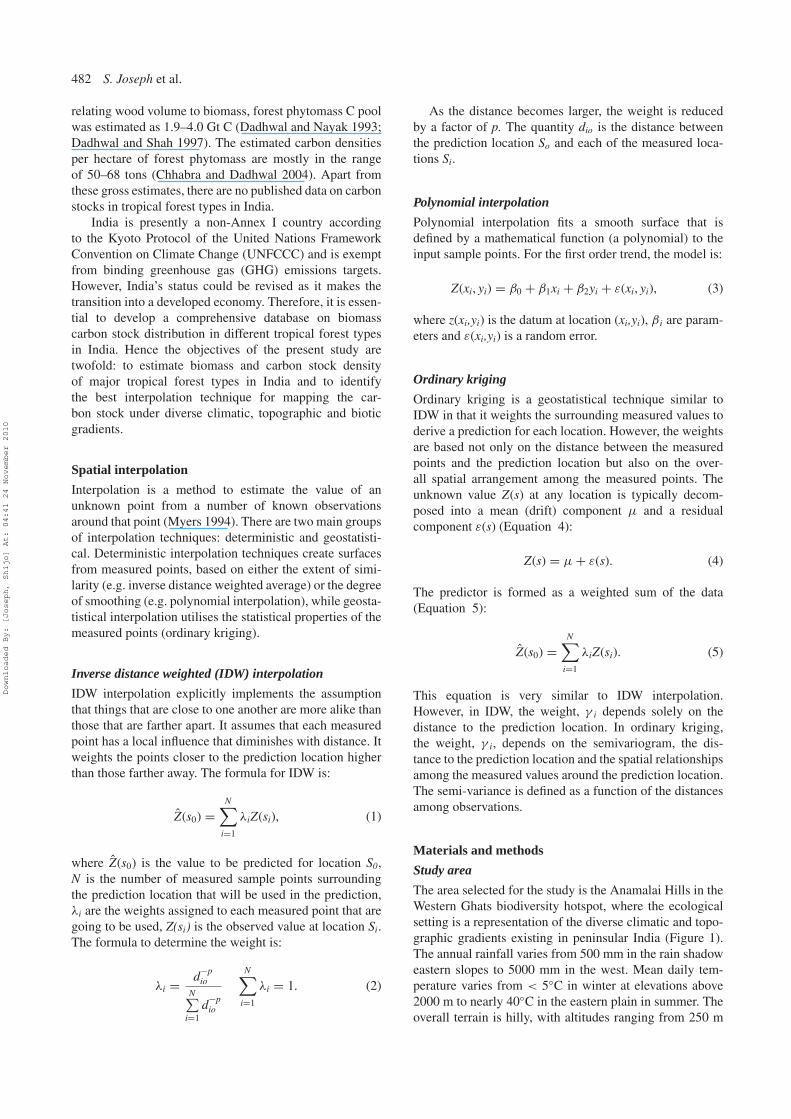
relating wood volume to biomass, forest phytomass C poolwas estimated as 1.9–4.0 Gt C (Dadhwal and Nayak 1993;Dadhwal and Shah 1997). The estimated carbon densitiesper hectare of forest phytomass are mostly in the rangeof 50–68 tons (Chhabra and Dadhwal 2004). Apart fromthese gross estimates, there are no published data on carbonstocks in tropical forest types in India.

India is presently a non-Annex I country accordingto the Kyoto Protocol of the United Nations FrameworkConvention on Climate Change (UNFCCC) and is exemptfrom binding greenhouse gas (GHG) emissions targets.However, India’s status could be revised as it makes thetransition into a developed economy. Therefore, it is essen-tial to develop a comprehensive database on biomasscarbon stock distribution in different tropical forest typesin India. Hence the objectives of the present study aretwofold: to estimate biomass and carbon stock densityof major tropical forest types in India and to identifythe best interpolation technique for mapping the car-bon stock under diverse climatic, topographic and bioticgradients.

Spatial interpolation

Interpolation is a method to estimate the value of anunknown point from a number of known observationsaround that point (Myers 1994). There are two main groupsof interpolation techniques: deterministic and geostatisti-cal. Deterministic interpolation techniques create surfacesfrom measured points, based on either the extent of simi-larity (e.g. inverse distance weighted average) or the degreeof smoothing (e.g. polynomial interpolation), while geosta-tistical interpolation utilises the statistical properties of themeasured points (ordinary kriging).

Inverse distance weighted (IDW) interpolation

IDW interpolation explicitly implements the assumptionthat things that are close to one another are more alike thanthose that are farther apart. It assumes that each measuredpoint has a local influence that diminishes with distance. Itweights the points closer to the prediction location higherthan those farther away. The formula for IDW is:

Z(s0) =N∑

i=1

λiZ(si), (1)

where Z(s0) is the value to be predicted for location S0,N is the number of measured sample points surroundingthe prediction location that will be used in the prediction,λi are the weights assigned to each measured point that aregoing to be used, Z(si) is the observed value at location Si.The formula to determine the weight is:

λi = d−pio

N∑i=1

d−pio

N∑i=1

λi = 1. (2)

As the distance becomes larger, the weight is reducedby a factor of p. The quantity dio is the distance betweenthe prediction location So and each of the measured loca-tions Si.

Polynomial interpolation

Polynomial interpolation fits a smooth surface that isdefined by a mathematical function (a polynomial) to theinput sample points. For the first order trend, the model is:

Z(xi, yi) = β0 + β1xi + β2yi + ε(xi, yi), (3)

where z(xi,yi) is the datum at location (xi,yi), β i are param-eters and ε(xi,yi) is a random error.

Ordinary kriging

Ordinary kriging is a geostatistical technique similar toIDW in that it weights the surrounding measured values toderive a prediction for each location. However, the weightsare based not only on the distance between the measuredpoints and the prediction location but also on the over-all spatial arrangement among the measured points. Theunknown value Z(s) at any location is typically decom-posed into a mean (drift) component μ and a residualcomponent ε(s) (Equation 4):

Z(s) = μ + ε(s). (4)

The predictor is formed as a weighted sum of the data(Equation 5):

Z(s0) =N∑

i=1

λiZ(si). (5)

This equation is very similar to IDW interpolation.However, in IDW, the weight, γ i depends solely on thedistance to the prediction location. In ordinary kriging,the weight, γ i, depends on the semivariogram, the dis-tance to the prediction location and the spatial relationshipsamong the measured values around the prediction location.The semi-variance is defined as a function of the distancesamong observations.

Materials and methods

Study area

The area selected for the study is the Anamalai Hills in theWestern Ghats biodiversity hotspot, where the ecologicalsetting is a representation of the diverse climatic and topo-graphic gradients existing in peninsular India (Figure 1).The annual rainfall varies from 500 mm in the rain shadoweastern slopes to 5000 mm in the west. Mean daily tem-perature varies from < 5◦C in winter at elevations above2000 m to nearly 40◦C in the eastern plain in summer. Theoverall terrain is hilly, with altitudes ranging from 250 m

Downloaded By: [Joseph, Shijo] At: 04:41 24 November 2010

International Journal of Sustainable Development & World Ecology 483

10°35′0′′N

76°50′0′′E 76°55′0′′E 77°0′0′′E 77°5′0′′E 77°10′0′′E 77°15′0′′E 77°20′0′′E

76°50′0′′E

0 3 6 12 Km

76°55′0′′E 77°0′0′′E 77°5′0′′E 77°10′0′′E 77°15′0′′E 77°20′0′′E

W

N

E

S

10°30′0′′N

10°25′0′′N

10°20′0′′N

10°15′0′′N

10°35′0′′N

10°30′0′′N

10°25′0′′N

10°20′0′′N

10°15′0′′N

Anamalai Wildlife Sanctuary

Figure 1. Location map of Anamalai Wildlife Sanctuary in Western Ghats, India.

in the foothills of the northeast to 2500 m in the GrassHills area in the southwest. Due to varied topography andmicroclimatic regimes, this area is considered as one of 25microcentres of diversity in the Indian subcontinent (Nayar1996). Floristically, the western side of the hills is occupiedby luxuriant rain forest (humid forest), while the easternside is dominated by dry forests.

Methods

A stratified transect survey was conducted in the AnamalaiHills during 2005–2006. The strata were delineated tak-ing into consideration long-term climatic observations andaltitudinal variation within the study area. Circular plots of10-m radius (plot size – 314 m2) were laid every 200 malong transects. Care was taken to include all vegetationtypes in the sampling. In each plot, all woody plants with≥ 10 cm DBH were identified to species level, individ-uals counted and DBH measured with a tape. Biomasswas calculated using allometric equations developed forthe Western Ghats (Murali et al. 2005). Two allometricequations were used: one for evergreen forests (Equation 6)and the other was for deciduous forests (Equation 7). Thebasal area required for these equations was calculated fromDBH using Equation (8). Carbon conversion coefficientsdiffer, considering species, age, formation and commu-nity structure of vegetation types, and range from 0.45 to0.55 (Kauppi et al. 1992; Goodale et al. 2002; Xia et al.2005; Ramachandran et al. 2008). Since such coefficientswere not available for the study area, a carbon conversion

coefficient of 0.5 was used in the present study. Forestcarbon storage of each vegetation type was estimated bymultiplying the forest carbon density per hectare by theextent of forest area.

Forest area statistics are derived from the supervisedclassification of IRS P6 LISS III satellite data (Indianremote sensing satellite). Based on knowledge of the dataand ground truth information, nine different land-coverclasses were identified. Parametric signatures were used totrain a statistically based (e.g. mean and covariance matrix)classifier to define the classes. Maximum likelihood para-metric rule were implemented for classifying the data.An accuracy assessment was performed by comparing theclassified image with the ground truth reference data.

Biomass evergreen

= (−2.81 + 6.78 ∗ Basal area) (r2 = 0.53)

Biomass deciduous

= (−73.55 + 10.73 ∗ Basal area) (r2 = 0.82)

Basal area = (DBH)2

4π. (6)

Spatial interpolation was conducted on the data toquantify the patterns of spatial variation in carbon stock.From the total sample points (206 sample points), a sub-set of 155 sample points (75%) was taken randomly formodel generation (training datasets) and the remaining

Downloaded By: [Joseph, Shijo] At: 04:41 24 November 2010

484 S. Joseph et al.

51 sample points (25%) were used for model valida-tion (testing datasets). Three interpolation techniques wereapplied. Inverse distance weighting was the first techniqueimplemented. The power value for IDW is optimised byconsidering the root mean square (RMS) error. At least10 neighbouring points were included in the prediction ofan unknown point. The second method involved fitting afirst order polynomial equation (local polynomial interpo-lation) to the sample points. The selection of the first orderequation was based on the least RMS error. At least 10neighbouring points were included, as in the case of IDW.

Ordinary kriging was the third method implemented forinterpolation of training datasets. The changes in semivari-ance with distance was analysed using different models,such as circular, spherical, exponential and Gaussian, andthe spherical model was found to be the best choice sinceit gave the lowest RMS error. The other inputs (nugget,sill and range) were derived from this semivariogram. Thenugget represents measurement/independent error and isthe deviation from zero on the y-axis. The sill is the heightthat the semivariogram reaches when it levels off, locatedon the y-axis, and the range is the distance where the modelfirst flattens out on the x-axis. The interpolated surfaceand error surface were derived from the analysis. The testdata taken from the total sample plots was used for valida-tion. The selection of best interpolation method was basedon the mean prediction error (Equation 9) and root meansquare prediction error (Equation 10).

Mean error (ME) =

n∑i=1

(Z(si) − z(si))

n

Root mean square error (RMSE)

=√√√√ n∑

i=1

[Z(si) − z(si)]2

n, (7)

where Z(si) is the predicted value and Z(si) is the observedvalue.

Results

The average values of the aboveground biomass and car-bon stock in the whole of Anamalai Wildlife Sanctuary are167 t/ha and 84 t/ha, respectively. Vegetation and land-cover type mapping using the IRS P6 LISS III data showed

Table 1. Area statistics of major land-cover types and theirclassification accuracy in Indira Gandhi Wildlife Sanctuary, India(area statistics derived from the IRS P6 LISS III data of 28 March2006).

Sl.No. Land-cover type

Area(km2)

Area(%)

Produceraccuracy

(%)

Useraccuracy

(%)

1 Tropical evergreenforest

230.2 23.8 87.5 89.4

2 Montane wettemperate forest

21.8 2.2 66.7 83.3

3 Tropical deciduousforest

487.6 50.3 90.0 75.9

4 Thorn scrub forest 34.3 3.5 58.8 76.95 Grassland 85.8 8.9 70.0 95.56 Teak plantation 31.3 3.2 75.0 69.27 Tea plantation 30.2 3.1 100.0 84.68 Agriculture and

fallow lands36.5 3.8 84.6 91.7

9 Water bodies 10.9 1.1 100.0 90.0Total area 968.6 100.0

the area is dominated by deciduous forest (487.6 km2)and evergreen forest (230.2 km2). The nine land-coverclasses, their area statistics and estimated classificationaccuracy are given in Table 1. Pristine grasslands, a par-ticular feature of the hills, covered 86 km2. In additionto natural vegetation types, the other land-cover types inthe area are plantations, agriculture areas and reservoirs,which together contribute 108.9 km2 (11.2%). Overallclassification accuracy was 83% and the Kappa statisticwas 0.79. The lowest producer accuracy is observed fortropical thorny scrub forest (58.8%), followed by montanewet temperate forest (66.7%). In the case of user accu-racy, the lowest is reported for teak plantations (69.2%),followed by tropical deciduous forest (75.9%).

Distribution of aboveground biomass and carbon stockin different forest types is given in Table 2. Evergreen for-est had a high amount of biomass (236.8 t/ha) whereasthorny scrub had a low biomass (32.23 t/ha). Summationof carbon stock in different forest types yielded 6.44 Mt ofcarbon. These forest types covered 80% of the total sanc-tuary area. The remaining area is not considered in theestimation of carbon stock due to the absence of samplepoints in those land-cover types.

Kriging was found to be the best method for spatialinterpolation of carbon stock, in comparison with IDW andpolynomial interpolation. The lowest mean error and root

Table 2. Distribution of aboveground biomass (AGB) and carbon stock in different forest types in Anamalai Hills,Western Ghats, India.

Forest typeAverage

AGB (t/ha)

Averageabovegroundcarbon stock

Area(ha)

Total AGB(Mt)

Total abovegroundcarbon stock (Mt)

Tropical evergreen forest 236.80 118.4 23020 5.45 2.73Montane wet temperate forest 187.78 93.89 2180 0.41 0.20Tropical deciduous forest 141.69 70.85 48760 6.91 3.45Thorn scrub forest 32.23 16.12 3430 0.11 0.06

Downloaded By: [Joseph, Shijo] At: 04:41 24 November 2010

International Journal of Sustainable Development & World Ecology 485

Table 3. Mean error and root mean square error of interpola-tions methods.

Validation

Interpolation method Mean error RMS error

IDW −0.194 1.31Local polynomial −0.184 1.33Kriging −0.144 1.29

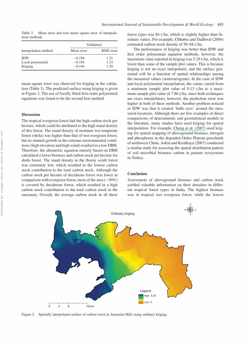
mean square error was observed for kriging in the valida-tion (Table 3). The predicted surface using kriging is givenin Figure 2. The use of locally fitted first-order polynomialequations was found to be the second best method.

Discussion

The tropical evergreen forest had the high carbon stock perhectare, which could be attributed to the high stand densityof this forest. The stand density of montane wet temperateforest (shola) was higher than that of wet evergreen forest,but its stunted growth in the extreme environmental condi-tions (high elevation and high wind) resulted in a low DBH.Therefore, the allometric equation entirely based on DBHcalculated a lower biomass and carbon stock per hectare forshola forest. The stand density in the thorny scrub forestwas extremely low, which resulted in the lowest carbonstock contribution to the total carbon stock. Although thecarbon stock per hectare of deciduous forest was lower incomparison with evergreen forest, most of the area (∼50%)is covered by deciduous forest, which resulted in a highcarbon stock contribution to the total carbon stock in thesanctuary. Overall, the average carbon stock in all these

forest types was 84 t/ha, which is slightly higher than lit-erature values. For example, Chhabra and Dadhwal (2004)estimated carbon stock density of 50–68 t/ha.

The performance of kriging was better than IDW andfirst order polynomial equation methods, however, themaximum value reported in kriging was 5.29 t/ha, which islower than some of the sample plot values. This is becausekriging is not an exact interpolator, and the surface gen-erated will be a function of spatial relationships amongthe measured values (semivariogram). In the case of IDWand local polynomial interpolation, the values varied froma minimum sample plot value of 0.13 t/ha to a maxi-mum sample plot value of 7.86 t/ha, since both techniquesare exact interpolators; however, the prediction error washigher in both of these methods. Another problem noticedin IDW was that it created ‘bulls eyes’ around the mea-sured locations. Although there are few examples of directcomparisons of deterministic and geostatistical models inthe literature, many studies have used kriging for spatialinterpolation. For example, Cheng et al. (2007) used krig-ing for spatial mapping of aboveground biomass, nitrogenand phosphorus in the degraded Ordos Plateau grasslandsof northwest China. Askin and Kizilkaya (2007) conducteda similar study for assessing the spatial distribution patternof soil microbial biomass carbon in pasture ecosystemsin Turkey.

Conclusion

Assessment of aboveground biomass and carbon stockyielded valuable information on their densities in differ-ent tropical forest types in India. The highest biomasswas in tropical wet evergreen forest, while the lowest

0 4 8 16 Km

Legend

Ordinary krigingW E

N

S

High : 5.29

Low : 0

Figure 2. Spatially interpolated surface of carbon stock in Anamalai Hills using ordinary kriging.

Downloaded By: [Joseph, Shijo] At: 04:41 24 November 2010

486 S. Joseph et al.

was in thorny scrub forest. The spatial interpolation ofpoint estimates using different techniques showed thatordinary kriging performed better than polynomial andinverse distance weighted interpolations. The error anal-ysis using the test data showed that mean and root meansquare errors are lower for kriging interpolation. Sphericalsearch model in ordinary kriging was found to be moresuitable to the varied climatic and topographic gradientsthan models such as circular, spherical, exponential andGaussian.

AcknowledgementsThe authors sincerely thank M.S.R. Murthy, Head of the Forestryand Ecology Division; R.S. Dwivedi, Group Head of the LandResources Group; P.S. Roy, Deputy Director (RS&GIS-AA)and Director of the National Remote Sensing Centre; andV.B. Mathur, Dean and Principal Investigator of the WII-NNRMSProject, Wildlife Institute of India for their encouragement;and the Ministry of Environment and Forests, Government ofIndia, for funding support. Tamil Nadu Forest Department kindlygranted permission to carry out fieldwork.

ReferencesAnaya JA, Chuvieco E, Palacios-Orueta A. 2009. Aboveground

biomass assessment in Colombia: A remote sensingapproach. For Ecol Manage. 257:1237–1246.

Askin T, Kizilkaya R. 2007. Spatial distribution patterns of soilmicrobial biomass carbon within pasture. Agri Conspec Sci.72:75–79.

Broadbent EN, Asner GP, Peña-Claros M, Palace M, Soriano M.2008. Spatial partitioning of biomass and diversity in alowland Bolivian forest: linking field and remote sensingmeasurements. For Ecol Manage. 255:2602–2616.

Brown S. 2002. Measuring carbon in forests: current status andfuture challenges. Environ Pollut. 116:363–372.

Canadell JG, Le QC, Raupach MR, Field CB, BuitenhuisET, Ciais P, Conway TJ, Gillett NP, Houghton RA,Marland G. 2007. Contributions to accelerating atmosphericCO2 growth from economic activity, carbon intensity, andefficiency of natural sinks. Proc Natl Acad Sci USA.104:18866–18870.

Canadell JG, Raupach MR. 2008. Managing forests for climatechange mitigation. Science. 320:1456–1457.

Cheng X, An S, Chen J, Li B, Liu Y, Liu S. 2007. Spatial rela-tionships among species, above-ground biomass, N, and P indegraded grasslands in Ordos Plateau, northwestern China. JArid Environ. 68:652–667.

Chhabra A, Dadhwal VK. 2004. Assessment of major poolsand fluxes of carbon in Indian forests. Clim Change. 64:341–360.

Dadhwal VK, Nayak SR. 1993. A preliminary estimate of thebiogeochemical cycle of carbon for India. Sci Cult. 59:9–13.

Dadhwal VK, Shah AK. 1997. Recent changes (1982–1991) inforest phytomass carbon pool in India, estimated using grow-ing stock and remote sensing-based forest inventories. J TropFor. 13:182–188.

Food and Agriculture Organization. 2006. Global forest resourceassessment 2005. Rome: Food and Agriculture Organizationof the United Nations.

Foody, GM, Boyd DS, Cutler MEJ. 2003. Predictive relationsof tropical forest biomass from Landsat TM data andtheir transferability between regions. Remote Sens Environ.85:463–474.

Forest Survey of India. 2003. State of forests report 2003. Forestsurvey of India. Dehradun, India: Government of India.

Fuchs H, Magdon P, Kleinn C, Flessa H. 2009. Estimating above-ground carbon in a catchment of the Siberian forest tundra:combining satellite imagery and field inventory. Remote SensEnviron. 113:518–531.

Goodale CL, Apps MJ, Birdsey RA, Field CB, Heath LS,Houghton RA, Jenkins JC, Kohlmaier GH, Kurz W, Liu S,et al. 2002. Forest carbon sinks in the northern hemisphere.Ecol Appl. 12:891–899.

Kauppi PE, Mielikainen K, Kuusela K. 1992. Biomass and carbonbudget of European forests, 1971–1990. Science. 256:70–74.

Lufafa A, Diedhiou I, Samba SAN, Sene M, Khouma M,Kizito F, Dick RP, Dossa E, Noller JS. 2008. Carbon stocksand patterns in native shrub communities of Senegal’s PeanutBasin. Geoderma. 146:75–82.

Murali KS, Bhat DM, Ravindranath NH. 2005. Biomass estima-tion equations for tropical deciduous and evergreen forests.Int J Agric Res Governance Ecol. 4:81–92.

Myers DE. 1994. Spatial interpolation: an overview. Geoderma.62:17–28.

Nayar MP. 1996. Hotspots of endemic plants of India. India:Tropical Botanic Garden Research Institute.

Ramachandran A, Jayakumar S, Haroon RM, Bhaskaran A,Arockiasamy DI. 2007. Carbon sequestration: estimation ofcarbon stock in natural forests using geospatial technol-ogy in the Eastern Ghats of Tamil Nadu, India. Curr Sci.92:323–331.

Ravindranath NH, Somashekhar BS, Gadgil M. 1997. Carbonflow in Indian forests. Clim Change. 35:297–320.

Sabine CL, Heiman M, Artaxo P, Bakker DCE, Chen CTA, FieldCB, Gruber N, LeQuéré C, Prinn RG, Richey JE, et al. 2004.Current status and past trends of the carbon cycle. In: FieldCB, Raupach MR, editors. The global carbon cycle: inte-grating humans, climate, and the natural world. Washington(DC): Island Press. p. 17–44.

Sales MH, Souza CM, Kyriakidis PC, Roberts DA, Vidal E. 2007.Improving spatial distribution estimation of forest biomasswith geostatistics: a case study for Rondonia, Brazil. EcolModell. 205:221–230.

Xia C, Guosheng H, Aihui H. 2005. MODIS-based estimation ofbiomass and carbon stock of forest ecosystems in NortheastChina. Geoscience and Remote Sensing Symposium, 2005.IGARSS ’05. Proceedings. 2005 IEEE Int. 4:3016–3019.

Downloaded By: [Joseph, Shijo] At: 04:41 24 November 2010