Spatial HARDI: Improved Visualization of Complex White MatterArchitecture with Bayesian Spatial Regularization

Ashish Raj1, Christopher Hess2, and Pratik Mukherjee21 Department of Radiology, Weill Medical College of Cornell University, New York, NY2 Department of Radiology and Bioengineering, University of California, San Francisco, CA

AbstractImaging of water diffusion using magnetic resonance imaging has become an important noninvasivemethod for probing the white matter connectivity of the human brain for scientific and clinical studies.Current methods such as diffusion tensor imaging (DTI), high angular resolution diffusion imaging(HARDI) such as q-ball imaging, and diffusion spectrum imaging (DSI), are limited by low spatialresolution, long scan times, and low signal-to-noise ratio (SNR). These methods fundamentallyperform reconstruction on a voxel-by-voxel level, effectively discarding the natural coherence of thedata at different points in space. This paper attempts to overcome these tradeoffs by using spatialinformation to constrain the reconstruction from raw diffusion MRI data, and thereby improveangular resolution and noise tolerance. Spatial constraints are specified in terms of a prior probabilitydistribution, which is then incorporated in a Bayesian reconstruction formulation. By taking the logof the resulting posterior distribution, optimal Bayesian reconstruction is reduced to a costminimization problem. The minimization is solved using a new iterative algorithm based onsuccessive least squares quadratic descent. Simulation studies and in vivo results are presented whichindicate significant gains in terms of higher angular resolution of diffusion orientation distributionfunctions, better separation of crossing fibers, and improved reconstruction SNR over the sameHARDI method, spherical harmonic q-ball imaging, without spatial regularization. Preliminary dataalso indicate that the proposed method might be better at maintaining accurate ODFs for smallernumbers of diffusion-weighted acquisition directions (hence faster scans) compared to conventionalmethods. Possible impacts of this work include improved evaluation of white matter microstructuralintegrity in regions of crossing fibers and higher spatial and angular resolution for more accuratetractography.

INTRODUCTIONDiffusion MRI has rapidly become an important noninvasive tool for characterization of whitematter structure because it enables the visualization and evaluation of fiber tracts connectingcortical regions. Clinical uses range from the evaluation of white matter fiber microstructuralintegrity due to neurodegeneration, traumatic injury, or primary demyelinating white matterdiseases such as multiple sclerosis to 3D tractography for neurosurgical planning. The mostcommonly used technique, diffusion tensor imaging (DTI), resolves water diffusion in termsof cardinal ellipsoidal shapes, ranging from purely spherical in the absence of oriented fibers

Corresponding author: Ashish Raj, Department of Radiology, Weill Medical College of Cornell University, 1300 York Avenue, NewYork, NY 10044, Phone: 212-746-9406, asr2004@med.cornell.edu.Publisher's Disclaimer: This is a PDF file of an unedited manuscript that has been accepted for publication. As a service to our customerswe are providing this early version of the manuscript. The manuscript will undergo copyediting, typesetting, and review of the resultingproof before it is published in its final citable form. Please note that during the production process errors may be discovered which couldaffect the content, and all legal disclaimers that apply to the journal pertain.

NIH Public AccessAuthor ManuscriptNeuroimage. Author manuscript; available in PMC 2012 January 1.

Published in final edited form as:Neuroimage. 2011 January 1; 54(1): 396–409. doi:10.1016/j.neuroimage.2010.07.040.

NIH

-PA Author Manuscript

NIH

-PA Author Manuscript

NIH

-PA Author Manuscript

to prolate ellipsoids in the presence of healthy fibers predominantly oriented along a singledirection (Beaulieu, 2002).

While the diffusion tensor can be estimated from as few as 6 different diffusion directions, itsuffers from the important limitation that it cannot resolve individual orientations within voxelsthat contain fibers with more than one orientation. As a result, it is difficult to resolve crossingfibers and to accurately perform tractography in these areas of complex fiber architecture. Highangular resolution diffusion imaging (HARDI) techniques overcome this limitation of DTI bymeasuring diffusion attenuation in many more angular directions, typically dozens or evenhundreds, in order to resolve the orientations of multiple fiber populations co-existing in thesame voxel. Compared to DTI, HARDI can faithfully reproduce underlying complex fibergeometries by better resolving the angular dependence of intravoxel diffusion. DTI is a limitedSNR and low spatial resolution modality compared to routine clinical T1- and T2-weightedMR imaging. Because it employs higher diffusion-weighting factors (b-values), HARDI yieldseven lower SNR than DTI. Furthermore, it requires longer experiment times to acquire manydiffusion directions, thus reducing practical feasibility for routine clinical neuroimaging.Further reduction in scan time is possible in HARDI only at the cost of lower SNR and/orangular resolution.

The goal in HARDI is to construct the fiber orientation distribution function (ODF) F(u)(Tuch, 2002), a spherical function that characterizes the relative likelihood of water diffusionalong any given angular direction u. Several approaches have been proposed to recover F(u)from raw diffusion-weighted data, including spherical harmonic modeling of the apparentdiffusion coefficient (ADC) profile (Frank, 2002; Alexander et al., 2002), multitensor modeling(Tuch, et al., 2002), generalized tensor representations (Ozarslan et al., 2003; Liu et al.,2004), circular spectrum mapping (Zhan et al., 2004), q-ball imaging (QBI) (Tuch, 2004; Tuch,2005; Hess et al., 2006; Mukherjee et al., 2007), persistent angular structure (Jansons et al.,2003), spherical deconvolution (Tournier et al., 2004), and diffusion orientation transform(DOT) (Ozarslan et al, 2006). In this paper, we focus on QBI due to its linearity, modelindependence and sensitivity to multimodal diffusion; in fact the correspondence between QBIODF peaks and multimodal fiber orientations has been established using phantom models(Perrin et al., 2005). Recently, improved results have been reported using a spherical harmonicrepresentation (Groemer, 1996) for QBI (shQBI) (Anderson, 2005; Hess et al., 2006;Descoteaux et al., 2007). The use of a spherical harmonic basis is parsimonious for typical b-values, which enables the ODF to be synthesized from a relatively small number of noisymeasurements and thus brings the technique closer to clinical feasibility from the standpointof total imaging time. The presented work is based upon this parsimonious shQBI approach.

Proposed MethodWe aim to improve the shQBI reconstruction from diffusion MRI data by exploiting a prioriknowledge about the smoothly varying orientation structure of white matter tracts over 3Dspace and incorporating this knowledge as a constraint in the reconstruction. This approach,which we call spatially coherent HARDI, or “spatial HARDI” for short, improves noisetolerance, spatial resolution, and fiber orientation accuracy compared to conventional methods.It is important to note that, although the presented work applies to shQBI, it can be equallywell applied to other QBI reconstruction methods. As DTI can be considered as a special caseof HARDI at lower angular resolution, this new technique would also be applicable to bothconventional DTI and more recently developed HARDI methods including sphericaldeconvolution and DOT.

With the proposed method, spatial smoothness constraints are determined from theneighborhood of each voxel and incorporated into the HARDI reconstruction algorithm. Themotivation for this approach is that the angular variability of the diffusion function in HARDI

Raj et al. Page 2

Neuroimage. Author manuscript; available in PMC 2012 January 1.

NIH

-PA Author Manuscript

NIH

-PA Author Manuscript

NIH

-PA Author Manuscript

is expected to be spatially coherent within any given white matter tract. In other words, theorientation and anisotropy of any single fiber population are expected to change smoothly fromone voxel to the next, particularly along the dominant fiber orientation, except at the boundariesbetween tracts and interfaces with gray matter structures and cerebrospinal fluid (CSF) spaces.This a priori assumption constitutes a very important and powerful constraint that can beexploited to improve the conditioning and therefore the noise tolerance of the reconstructionstep. Current techniques do not make use of this spatial constraint because they perform thereconstruction independently for each voxel. In this paper, we develop the mathematicalframework necessary to incorporate spatial smoothness as a constraint and jointly estimate theHARDI reconstruction parameters for each voxel in the entire volume simultaneously. Weexplore spatial prior models incorporating global and directional smoothness constraints,described in the Theory section. Spatial constraints are specified in terms of a prior probabilitydistribution, which is then incorporated in a Bayesian formulation of the reconstructionproblem. By taking the log of the resulting posterior distribution, the reconstruction problemis reduced to a cost minimization. The minimization is solved using a new iterative algorithmbased on least squares Q-R (LSQR) iterations (Paige et al., 1982), which accommodates non-convex and data-dependent terms in the cost function. We show that, by incorporating non-linear weight updates in our proposed algorithm within the LSQR iteration, execution time ofour approach can be made linear in the number of voxels. Testing and validation of thetechnique using simulations as well as in vivo HARDI data are reported in the Results section.

Related WorkResolving ODFs from available diffusion directions under noise and scan time limitations isa well-studied subject in the field of diffusion MR; here we review only recent work mostrelevant to our study. Deterministic (Tuch, 2002; Hess et al., 2006; Tournier et al., 2004;Descoteaux et al., 2007; Sakaie et al., 2006) as well as probabilistic (Jian et al., 2007; Tristan-Vega et al., 2009) approaches have been proposed.

Tournier et al. (2004) proposed a spherical deconvolution approach to obtaining the ODFsfrom raw diffusion data. Tristan-Vega et al. (2009) proposed a probabilistic method forcomputing the orientation probability density function, and demonstrated improved resultsover traditional Q-ball reconstruction using spherical harmonics. Estimation of sphericalharmonic coefficients in a manner very similar to the work of Hess et al., (2006), butincorporating a different regularization term using Laplace-Beltrami operators, was proposedin (Sakaie et al., 2006, Descoteaux et al. 2007). This regularization method was shown toperform better than the traditional Tikhonov regularization proposed by Hess et al.

Although our work uses spherical harmonic functions as the ODF model, many other modelshave been proposed and fruitfully employed in the field. The “persistent angular structure”, orPASMRI, method was proposed by Jansons et al., (2003) as a nonlinear parametric techniquefor orientation estimation. A multi-tensor model proposed (Hosey et al., 2005; Tuch, 2002)appears to reliably capture mixed fiber populations; this model was solved by Hosey et al.(2005) in a probabilistic Bayesian manner and produced estimates of the number of fibers ineach voxel. A tensor distribution model was employed by Jian et al., (2007) where the mixturedistribution was modeled as a Wishart distribution. Other models include the original radialbasis function q-ball model of Tuch (2004). The present work differs from existing methodsin that our focus is not on the particular ODF reconstruction method, but rather on a powerfulframework for spatially-constrained joint ODF estimation; our approach can be equally wellemployed on any of these other ODF models.

Our method is also related to the literature on denoising of HARDI ODFs, for which severalmethods have been proposed (Kim et al., 2009; Goh et al., 2009). Kim et al. (2009) proposeda variational approach, and Goh et al. (2009) proposed denoising in the framework of

Raj et al. Page 3

Neuroimage. Author manuscript; available in PMC 2012 January 1.

NIH

-PA Author Manuscript

NIH

-PA Author Manuscript

NIH

-PA Author Manuscript

convolution operations on a derived Riemannian manifold. Especially the latter work is inmany ways the correct one for diffusion ODFs, and would appear the right model for denoisingand other post-processing operations. Denoising the raw diffusion images first, followed byreconstruction has also been proposed (Descoteaux et al., 2008). These denoising methods arenot directly comparable to our work, because we wish to both reconstruct and denoise the ODFsat the same time, instead of first reconstructing and then denoising, or denoising thenreconstructing.

To summarize, existing methods have either focused on developing new models for singlevoxel ODFs using various basis functions, or on statistically optimal estimation of modelparameters under constraints on single voxel ODFs. To our knowledge, the proposed approachis the first one advocating the joint estimation of ODFs across the image, using spatialconstraints to simultaneously regularize and denoise the problem. Spatial regularization haspreviously been performed for smoothing or denoising as a post-processing step, but not as anintegral part of the ODF reconstruction process itself.

THEORY AND BACKGROUNDQ-Ball Imaging Using Spherical Harmonic Reconstruction

According to the q-space formalism, the wavevector that describes diffusion encoding in apulsed-gradient spin-echo experiment is defined as q = (2π)−1γδg, where γ represents thegyromagnetic ratio, δ is the diffusion gradient duration, and g is the diffusion gradient vector.HARDI acquisition schemes measure samples from an underlying diffusion-attenuated signalE(q) at a finite set of points on the sphere that are relatively uniform in their angular distribution.The choice of the spherical sampling radius in q-space, q0, depends on the desired angularresolution, the available SNR, and the gradient performance specifications. In practice, b-values of 3000 s/mm2 or greater are typically required in order to distinguish among differentintravoxel fiber populations at high angular resolution (Hess et al., 2006).

To simplify the numerical solution, both q and u are discretized to reflect finite sampling ofm measurements and reconstruction over a fixed number of points n. Because both the ODFand the diffusion signal are defined on the domain of the sphere, it is convenient to normalizespherical points to unit magnitude and adopt a spherical coordinate system q = q(θ,φ) and u =u(θ,φ), where θ and φ denote elevation and azimuth, respectively.

Linear HARDI reconstruction algorithms such as QBI and spherical deconvolution have incommon that each point of the reconstruction is computed as a linear combination of thediffusion measurements. Enumerating points on the sphere to construct a vector representation,this relationship can be expressed as

where f and e denote n × 1 and m × 1 column vectors composed of the estimated values of theODF and the diffusion measurements, respectively. Here ZQ is the matrix of sphericalharmonics evaluated at measurement points Q, and ZU is the matrix of spherical harmonicsevaluated at reconstruction points U. Diagonal matrix P = diag[p0, p2,…, pL] contains theLegendre polynomials of order l = 0, 2,…, L. Details of notation and formulation are containedin Hess et al., (2006). The conventional way of obtaining an estimate of f given e is thepseudoinverse, which happens to be the maximum likelihood estimator in the presence ofGaussian additive noise:

Raj et al. Page 4

Neuroimage. Author manuscript; available in PMC 2012 January 1.

NIH

-PA Author Manuscript

NIH

-PA Author Manuscript

NIH

-PA Author Manuscript

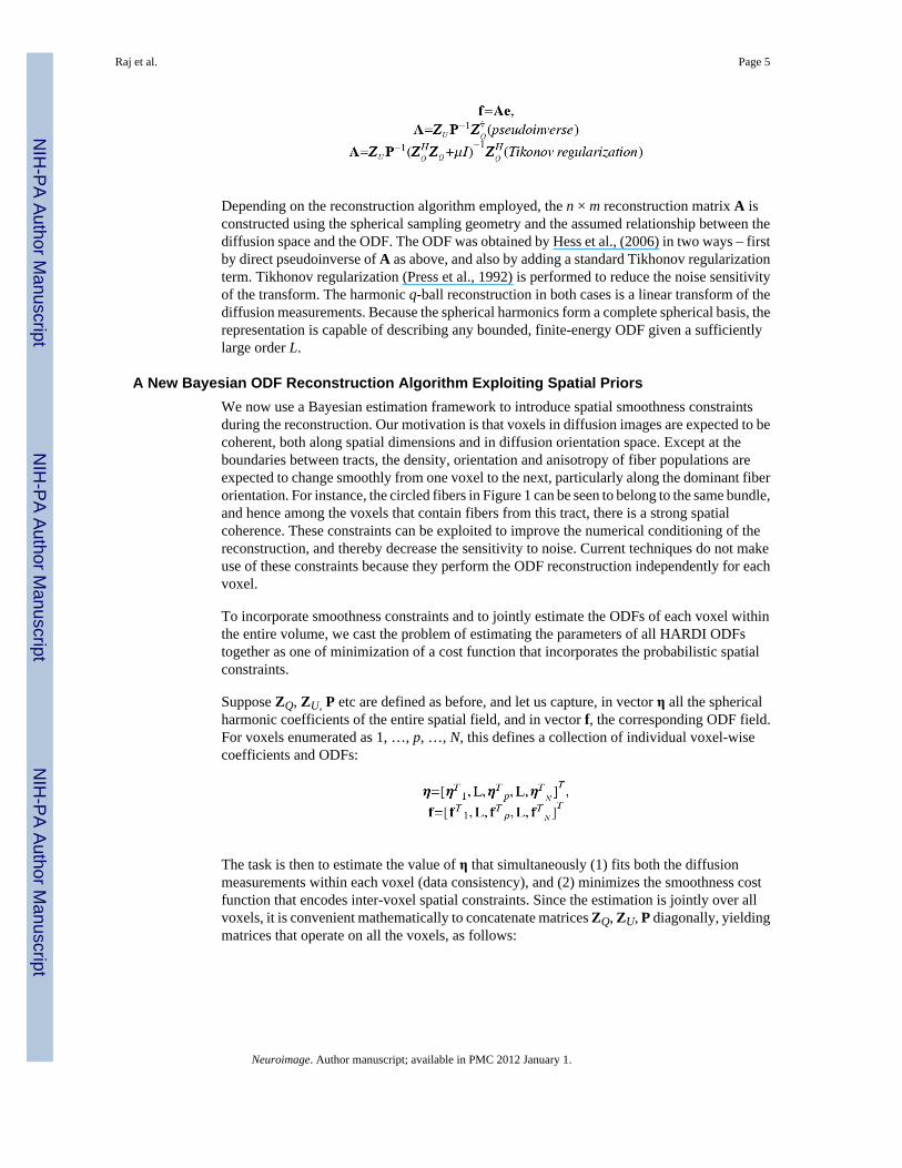
Depending on the reconstruction algorithm employed, the n × m reconstruction matrix A isconstructed using the spherical sampling geometry and the assumed relationship between thediffusion space and the ODF. The ODF was obtained by Hess et al., (2006) in two ways – firstby direct pseudoinverse of A as above, and also by adding a standard Tikhonov regularizationterm. Tikhonov regularization (Press et al., 1992) is performed to reduce the noise sensitivityof the transform. The harmonic q-ball reconstruction in both cases is a linear transform of thediffusion measurements. Because the spherical harmonics form a complete spherical basis, therepresentation is capable of describing any bounded, finite-energy ODF given a sufficientlylarge order L.

A New Bayesian ODF Reconstruction Algorithm Exploiting Spatial PriorsWe now use a Bayesian estimation framework to introduce spatial smoothness constraintsduring the reconstruction. Our motivation is that voxels in diffusion images are expected to becoherent, both along spatial dimensions and in diffusion orientation space. Except at theboundaries between tracts, the density, orientation and anisotropy of fiber populations areexpected to change smoothly from one voxel to the next, particularly along the dominant fiberorientation. For instance, the circled fibers in Figure 1 can be seen to belong to the same bundle,and hence among the voxels that contain fibers from this tract, there is a strong spatialcoherence. These constraints can be exploited to improve the numerical conditioning of thereconstruction, and thereby decrease the sensitivity to noise. Current techniques do not makeuse of these constraints because they perform the ODF reconstruction independently for eachvoxel.

To incorporate smoothness constraints and to jointly estimate the ODFs of each voxel withinthe entire volume, we cast the problem of estimating the parameters of all HARDI ODFstogether as one of minimization of a cost function that incorporates the probabilistic spatialconstraints.

Suppose ZQ, ZU, P etc are defined as before, and let us capture, in vector η all the sphericalharmonic coefficients of the entire spatial field, and in vector f, the corresponding ODF field.For voxels enumerated as 1, …, p, …, N, this defines a collection of individual voxel-wisecoefficients and ODFs:

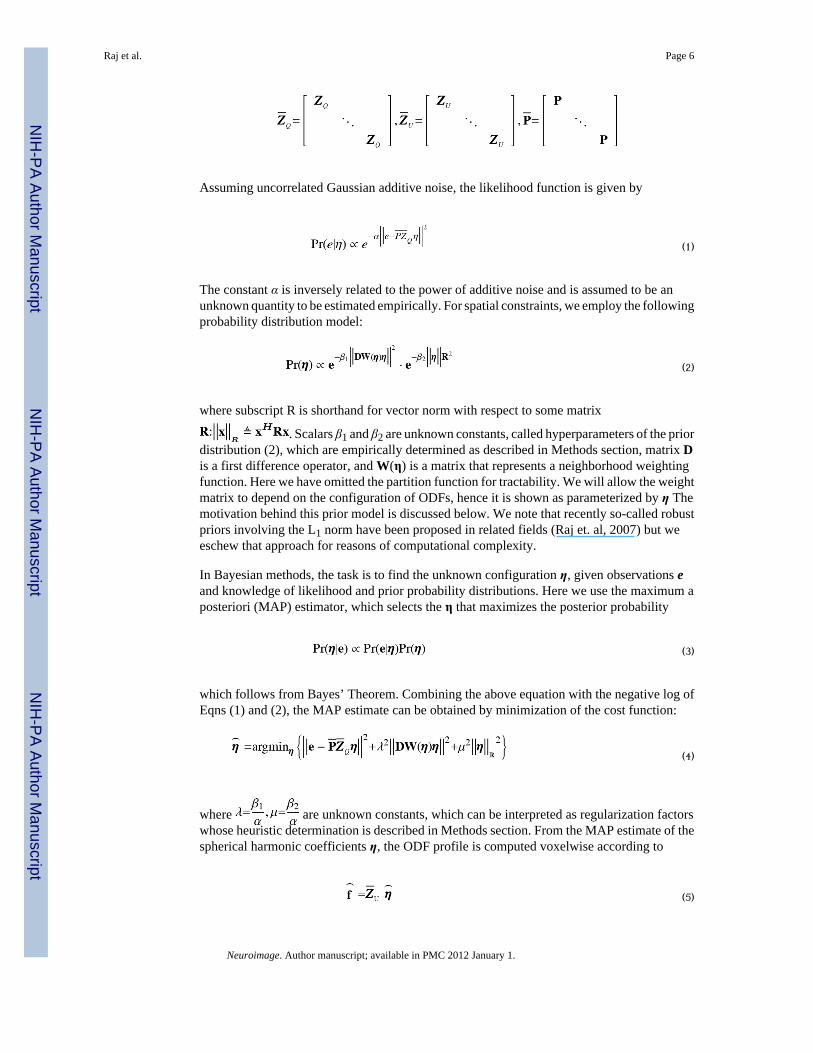
The task is then to estimate the value of η that simultaneously (1) fits both the diffusionmeasurements within each voxel (data consistency), and (2) minimizes the smoothness costfunction that encodes inter-voxel spatial constraints. Since the estimation is jointly over allvoxels, it is convenient mathematically to concatenate matrices ZQ, ZU, P diagonally, yieldingmatrices that operate on all the voxels, as follows:

Raj et al. Page 5

Neuroimage. Author manuscript; available in PMC 2012 January 1.

NIH

-PA Author Manuscript

NIH

-PA Author Manuscript

NIH

-PA Author Manuscript

Assuming uncorrelated Gaussian additive noise, the likelihood function is given by

(1)

The constant α is inversely related to the power of additive noise and is assumed to be anunknown quantity to be estimated empirically. For spatial constraints, we employ the followingprobability distribution model:

(2)

where subscript R is shorthand for vector norm with respect to some matrix

. Scalars β1 and β2 are unknown constants, called hyperparameters of the priordistribution (2), which are empirically determined as described in Methods section, matrix Dis a first difference operator, and W(η) is a matrix that represents a neighborhood weightingfunction. Here we have omitted the partition function for tractability. We will allow the weightmatrix to depend on the configuration of ODFs, hence it is shown as parameterized by η Themotivation behind this prior model is discussed below. We note that recently so-called robustpriors involving the L1 norm have been proposed in related fields (Raj et. al, 2007) but weeschew that approach for reasons of computational complexity.

In Bayesian methods, the task is to find the unknown configuration η, given observations eand knowledge of likelihood and prior probability distributions. Here we use the maximum aposteriori (MAP) estimator, which selects the η that maximizes the posterior probability

(3)

which follows from Bayes’ Theorem. Combining the above equation with the negative log ofEqns (1) and (2), the MAP estimate can be obtained by minimization of the cost function:

(4)

where are unknown constants, which can be interpreted as regularization factorswhose heuristic determination is described in Methods section. From the MAP estimate of thespherical harmonic coefficients η, the ODF profile is computed voxelwise according to

(5)

Raj et al. Page 6

Neuroimage. Author manuscript; available in PMC 2012 January 1.

NIH

-PA Author Manuscript

NIH

-PA Author Manuscript

NIH

-PA Author Manuscript

This Bayesian formulation of ODF reconstruction has similarities with regularizedreconstruction methods proposed earlier, especially Tikhonov regularization. The first term inEq. (4) can be understood to enforce data consistency and exactly reproduces the least squaresfitting approach. The last term enforces Tikhonov regularization (when R=I) by adding astabilizing term to the least squares fitting and favors solutions which have a low L2 norm. Asmentioned above, there exists an explicit formula for computing this estimate using the Moore-Penrose pseudoinverse. Although we show the Tikhonov regularization term, our work isindependent of which regularization scheme is used – whether Tikhonov, Laplace-Beltrami orotherwise. For brevity these other terms are not shown, but we assume that they can be capturedby an appropriate norm induced by matrix R. The middle term is new, and introduces the spatialsmoothness cost discussed above. When W(η) = I, the solution that results is maximally smoothunder the data consistency constraint, because other potential non-smooth solutions will havea large first derivative norm and cause the smoothness cost to increase.

While global smoothness is frequently used in multi-dimensional imaging applications, itsutility is limited in situations where global smoothness may not apply. For instance, the ODFfield in typical MR data displays smoothness along the orientations of individual fiber bundlesbut may not display smoothness perpendicular to the fiber, or around voxels with crossingfibers. Global smoothness in these situations may lead to an indiscriminate blurring of theODFs. To prevent this from occurring, we use a spatial weight matrix W(η). This matrixdetermines the strength of the constraint to place on the similarity of the spherical harmonicsbetween neighboring voxels. Because the weight between two neighboring voxels shouldgenerally depend on their ODFs and hence on the joint configuration η, we denote an explicitdependence on η. Computationally, the nonlinearity that the spatial weighting matrixintroduces into the function renders the optimization sensitive to starting estimates and pronegetting stuck in local minima. Ideally the estimation of η should reflect the non-linear presenceof W; however the resulting estimation problem would then become intractable and difficultto minimize.

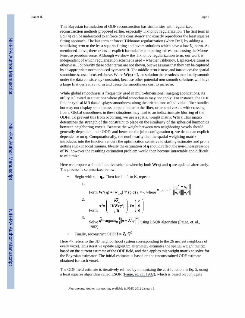
Here we propose a simple iterative scheme whereby both W(η) and η are updated alternately.The process is summarized below:

• Begin with η = η0. Then for k = 1 to K, repeat:

1.

Form Wk(η) = [wp,q] ∀ (p,q) ε , where

2.

Form

3.Solve using LSQR algorithm (Paige, et. al.,1982)

• Finally, reconstruct ODF: f̂ = Z̄Uη̄K ̄

Here refers to the 3D neighborhood system corresponding to the 26 nearest neighbors ofevery voxel. This iterative update algorithm alternately estimates the spatial weight matrixbased on the current estimate of the ODF field, and then applies this weight matrix to solve forthe Bayesian estimator. The initial estimate is based on the unconstrained ODF estimateobtained for each voxel.

The ODF field estimate is iteratively refined by minimizing the cost function in Eq. 5, usinga least squares algorithm called LSQR (Paige, et. al., 1982), which is based on conjugate

Raj et al. Page 7

Neuroimage. Author manuscript; available in PMC 2012 January 1.

NIH

-PA Author Manuscript

NIH

-PA Author Manuscript

NIH

-PA Author Manuscript

gradient descent. Because the cost function passed to LSQR is a quadratic function, it can beeasily calculated. We employed the LSQR implementation in MATLAB version 7.8.0. LSQRwas chosen for this purpose for several reasons. First, in each iteration, step 3 above is a linearleast squares problem, which is preferable to solving an unconstrained general optimizationproblem. Second, LSQR does not involve computing the normal equations (Press et al.,1992) which are known to have much worse conditioning than LSQR, which is based onconjugate gradients (Paige, et. al., 1982). The MATLAB implementation of LSQR isparticularly attractive because it does not require explicit computation or storage of , whichis a very large matrix. Instead, a user-defined function can be passed which simply returns theproduct , which is easily computed in 0(N P1P2) time, where N is the number of voxels inthe brain volume, and P1 is the number of diffusion directions and P2 is the number of ODFdirections. In order to speed up processing, we update the weight matrix at each iteration, whichmeans that the outer loop involving weight updates can be dispensed with. Therefore thecomputational complexity of the algorithm is Q(KLSQRNP1P2), where KLSQR is the number ofLSQR iterations, which in practice is between 10 and 20 till full convergence. Note that thecost is linear in N, just like traditional ODF methods.

The iterative approach above has a well-tested pedigree in both alternate projections ontoconvex sets (Gerchberg et al., 1972) and in Expectation Maximization (EM) theory (Zhang etal., 2001). Several theoretical and practical results from these fields point to guaranteedconvergence of these methods. The form of W(η) above was chosen based on computationaland tractability considerations. Intuitively, this iterative scheme weighs neighboring voxels ininverse proportion to the similarity of their coefficients, as shown in Figure 2. This avoidsincluding voxels with vastly different fiber profiles in the difference operator, and limits thesmoothness constraint to voxels with similar fiber populations. This prevents blurring thatwould otherwise result from enforcing the global smoothness constraint.

MATERIALS AND METHODSSimulation Studies

A software suite capable of simulating random 3D or user-generated 2D fiber configurationswas developed, tested and exercised under a variety of imaging conditions. To investigate theaccuracy of the proposed technique and compare it with conventional shQBI reconstructionwithout spatial constraints, we performed Monte Carlo simulations similar to those previouslyreported (Jones, 2004; Hess et al., 2006). Multiple fiber populations (varying from 2 to 100fibers) distributed in 3D within a 20 × 20 × 20 voxel volume, in slow Gaussian exchange, withorientations separated by a prescribed angle, were modeled as the sum of prolate Gaussianfunctions with varying volume fractions and fractional anisotropies (FAs) of 0.75. Thesimulated MR signal was generated as the corresponding sum of multiple exponential decays.Non-zero volume fraction of water (with spherical ODF, FA of 0) was also added in order torealistically model fiber populations in the brain. A feature of our simulation software is thatit allows the user to draw any number of linear fibers within the above 3D space, with user-selected FA and fiber width. This is particularly useful for modeling the effect of the spatialdistribution of fibers on the ODF reconstruction, and to visualize possible performanceimprovements using spatial priors.

For the fiber population within each voxel, samples of the corresponding synthetic diffusionsignal were obtained along non-collinear diffusion gradient orientations derived from theelectrostatic repulsion algorithm (Jones 2004) and used to reconstruct the ODF. Complex-valued independent Gaussian noise was added to each sample in order to evaluate thedependence of the reconstruction on SNR, and the magnitude of the resulting data was used tocalculate the ODF. SNR was defined as the ratio of the maximum signal intensity with no

Raj et al. Page 8

Neuroimage. Author manuscript; available in PMC 2012 January 1.

NIH

-PA Author Manuscript

NIH

-PA Author Manuscript

NIH

-PA Author Manuscript

diffusion weighting to the standard deviation (SD) of the noise, corresponding to the SNR ofthe b = 0 s · mm−2 images that were obtained experimentally. SNR values for the b = 0 s ·mm−2 non-DW data range from 1/10 to 10. This SNR range for the simulations was chosen tooverlap the typical SNR range of the experimental HARDI data both in our experience andpreviously reported by other authors.

Large-scale Monte Carlo simulations were executed to evaluate the performance of theproposed spatial HARDI technique against the existing algorithm described in Hess et al.,(2006) – “shQBI”, and its regularized version. Regularization in the latter case was performedusing the Laplace-Beltrami operator described in (Sakaie et al., 2006; Descoteaux et al.2007). Tikhonov regularization was also tested but was found to produce results eithercomparable to or worse than Laplace-Beltrami regularization, and was therefore dropped fromfurther analysis. In addition, smoothed shQBI results were obtained by applying an isotropicsmoothing operation with a 3×3×3 box filter as a post-processing step after standard shQBIreconstruction. The central element of the box filter is assigned a value of 5, and all otherelements are assigned a value of 1. For each reconstructed ODF direction, the corresponding3D volume was convolved with this box filter, giving a spatially smoothed version of the ODFs.This last method was implemented in order to address the important question of whether similarresults to our proposed method can be obtained by simply smoothing the shQBI output.

All three reconstructions were evaluated with respect to various metrics including root meansquare error (RMSE) of the ODF, error of generalized fractional anisotropy (GFA) (Hess etal., 2006; Tuch et al., 2004), fiber orientation accuracy, and smallest crossing fiber angleresolvable. These performance measures are well-known from previous reports, exceptorientation accuracy and angular resolution. The computation of the latter two is now brieflydescribed.

Angular resolution refers to the smallest angle at which crossing fibers are resolvable by agiven technique (Hess et al., 2006). Unfortunately it is difficult to automate the decision-making involved in resolving crossing fibers in the presence of significant noise and/orsmoothing – this is usually done visually by an experienced user. Ultimately, the ability toresolve crossing fibers can be evaluated by the performance of subsequent fiber tractographysteps. However, this does not provide an intrinsic angular resolution measure, being dependenton the properties of a separate tractography algorithm

To assess angular resolution, we implemented an unsupervised fiber detection module in lieuof tractography. This module infers the number of fibers present in a given voxel by detectingregional peaks in the 2D (azimuth and elevation) plot of ODF after Gaussian smoothing, in amanner similar to what has been described in other reports, e.g. (Tristan-Vega et al., 2009;Descoteaux et al., 2007). In order to reduce sensitivity to spurious peaks introduced by noise,the traditional approach was made more robust as described below. Significant peaks weredefined as peaks with a minimum area of 10 degrees (azimuth) × 10 degrees (elevation) in the2D plane, and minimum height of at least 40% of maximum peak height. A morphologicalerosion operation was also performed in order to remove irregularly-shaped (and henceerroneous) peaks. This fiber detection module was tested thoroughly, and its output was usedto measure angular resolution, as follows. Two crossing fibers were deemed resolvable if themean error in detecting the correct number of fibers, over a large number of repeated trials,was found to be less than 10%. There exist more advanced Bayesian fiber detection techniques(Hosey et al., 2005) which might improve on our basic detection module, but the time andcomplexity involved in implementing such a technique was not justified in the scope of thiswork.

Raj et al. Page 9

Neuroimage. Author manuscript; available in PMC 2012 January 1.

NIH

-PA Author Manuscript

NIH

-PA Author Manuscript

NIH

-PA Author Manuscript

Orientation accuracy was evaluated by taking single-fiber voxel populations and measuringthe direction of the peak closest to the true fiber orientation. The angular difference betweenthese two directions was defined as orientation accuracy. The closest peak was detected bystarting at the given true peak orientation, and applying a brute force search within a specifiedneighborhood (22 degrees in elevation and azimuth) for the location of the maximum ODF.The maximum location is then iteratively refined by searching over successively smallerneighborhoods around the detected peak.

We note that the number of crossing fibers in our simulations can be two or more. RMSE andGFA-RMS are evaluated in every voxel whether having mixed fiber population or not.Orientation accuracy was evaluated in single fiber voxels only in order to preclude the effectof other fibers from contaminating the orientation accuracy value of the main fiber. Angularresolution was calculated at voxels with two fiber populations oriented at various angles. Threeor more fiber voxels were precluded from this calculation because it is difficult to interpret theeffect of the third fiber on the angular resolution between the first two fibers. Even if we could,the result would not necessarily increase our understanding of the proposed method.

Performance of the 3 or 4 competing algorithms (unregularized and/or regularized shQBI,smoothed shQBI and spatial HARDI) was evaluated using four criteria: root mean square error(RMSE) of the ODF, root mean square of the generalized fractional anisotropy (RMS-GFA),orientation accuracy and angular resolution.

In order to evaluate the sensitivity of all three or four methods to parameter choice, it may notbe sufficient to evaluate these methods at fixed parameter settings, because the relativeperformance of different methods varies with parameter choice. An alternate way is nowpresented to capture these parameter-dependent performance differences and to evaluate eachmethod over a wide range of parameter choice, through a joint investigation of two performancemeasures simultaneously with changing parameter choice. We believe this to be an importantfeature, because no single performance measure, whether RMSE, orientation accuracy orangular resolution, is by itself an adequate measure of overall performance of the method.Correct reconstruction of ODF, measured by RMSE, is probably more important forquantitative diffusion measurements, whereas angular resolution and orientation accuracymight be more relevant for subsequent tractography. In addition, these measures are somewhatconflicting in nature, meaning that it is sometimes possible to improve one at the cost of theother. For example, increasing regularization using any method can easily improve theorientation accuracy of a single-fiber ODF, but at the cost of higher RMSE. Unless parameteroptimization was performed very carefully for each algorithm separately, it is difficult to statecategorically how the competing methods compare. Therefore, the value of a method mustnecessarily depend on its performance jointly on a number of measures.

We plotted RMSE and orientation accuracy for each method as a curve parameterized by thealgorithmic parameter under consideration – in this case the regularization factor. Algorithmicparameters specific to spatial HARDI (μ) was fixed at 0.1, and the regularization parameter λwas varied over the range [0.05, 0.3] in 12 increments for all three methods. Two SNR levelswere used, and were plotted separately. In some ways this analysis technique is similar to theso-called L-curve analysis (Lin et al., 2004) which is useful in ascertaining optimal parameterchoice, especially the regularization parameter.

In Vivo Experimental StudiesWhole-brain HARDI was performed on two adult male volunteers (23–34 years old) using a3T Signa EXCITE scanner (GE Healthcare, Waukesha, WI) equipped with an eight-channelphased-array head coil. The imaging protocol was approved by the institutional review boardat our medical center, and written informed consent was obtained from the participants. On

Raj et al. Page 10

Neuroimage. Author manuscript; available in PMC 2012 January 1.

NIH

-PA Author Manuscript

NIH

-PA Author Manuscript

NIH

-PA Author Manuscript

one subject, a multislice single-shot echo-planar spin-echo pulse sequence was employed toobtain measurements at a diffusion weighting of b = 3000 s · mm−2, where the diffusion-encoding directions were distributed uniformly over the surface of a sphere using electrostaticrepulsion (Jones, 2004). Conventional Stejskal-Tanner diffusion encoding was applied withδ = 31.8 ms, Δ = 37.1 ms and grnax= 40 mT.m−1, yielding a q-space radius of 534.7 cm−1. Anadditional acquisition without diffusion weighting at b = 0 s · mm−2 was also obtained. Thetotal scan time for whole-brain acquisition of 131 diffusion-encoding directions was 39.6 minwith TR/TE = 18 s/84 ms, NEX = 1, and isotropic 2-mm voxel resolution (FOV = 260 × 260mm, matrix = 128 × 128, 68 interleaved slices with 2-mm slice thickness and no gap). Onanother subject, whole-brain HARDI was performed at 2.2-mm isotropic spatial resolution(FOV = 280 × 280 mm, matrix = 128 × 128, 60 interleaved slices with 2.2 mm slice thicknessand no gap) using 55 diffusion encoding directions with TR/TE = 16.4 s/82 ms, for a total scantime of 15.3 min. Axial slices in both cases were oriented along the plane passing through theanterior and posterior commissures. Parallel acquisition of the DW data using the eight-channeltransmit-receive EXCITE head coil was accomplished using the array spatial sensitivityencoding technique (GE Healthcare, Waukesha, WI, USA) with an acceleration factor of 2.

Reconstruction using all three methods was performed on these in vivo HARDI data sets.Reconstruction parameters were identical to the optimal parameters found during simulationstudies: Regularization parameter and spatial prior weights were both set at 0.2. Sphericalharmonics up to order four and order six were estimated.

Reconstruction and VisualizationFor all three methods, ODF values were computed at locations corresponding to the verticesof a fourfold tessellated icosahedron, giving 642 directions. For ease of visualization of theresults, ODFs were min-max normalized and plotted as a 3D surface. Points on the surface ofthe ODF were color-coded by direction according to the standard red (left–right), blue(superoinferior), and green (anteroposterior) convention used to represent the direction of theprincipal eigenvector in DTI. The ODF surfaces are overlaid onto a grayscale backgroundcorresponding to the generalized fractional anisotropy (GFA) within each voxel forvisualization of the human subject data (Hagmann et al., 2007). The more anisotropic ODFsthus appear superimposed on brighter backgrounds, and the background appears dark in voxelswith low GFA. All q-ball computations were performed using custom software written inMATLAB version 7.6 (MathWorks, Natick, MA, USA).

RESULTSUnits

RMSE and RMS-GFA are shown in arbitrary units, given by the error norm between(normalized) true and reconstructed ODFs – smaller is better. Orientation accuracy and angularresolution are in degrees – smaller is better.

Simulation studiesPerformance of the 3 competing algorithms (Laplace-Beltrami regularized shQBI, smoothedshQBI and spatial HARDI) was evaluated. As the results in Figures 3 and 4 show, for harmonicorder 4, neither the original spherical harmonic method nor post-processing by applying adirectional smoothing filter is able to achieve the level of performance of the proposed spatially-constrained technique. A slight worsening of orientation accuracy and angular resolution isseen in spatial HARDI compared to smoothed shQBI; this points to our approach sacrificingmodest amounts of angular resolution for significant gains in noise performance. The ODFpeaks from all algorithms appear slightly misaligned with the fibers. We believe this to result

Raj et al. Page 11

Neuroimage. Author manuscript; available in PMC 2012 January 1.

NIH

-PA Author Manuscript

NIH

-PA Author Manuscript

NIH

-PA Author Manuscript

from the (parsimonious) spherical harmonic basis, which is not rotation-invariant, and thereforedoes not guarantee perfect alignment.

In order to evaluate sensitivity of all three methods to parameter choice, Figure 5 shows RMSEand orientation accuracy versus SNR for two different parameter settings. Harmonic order waschosen as 6 for both. Relative performance of the three methods varies with parameter choice.Note the difference in performance from Figure 4, which is for a different model order andwhose parameters were selected very carefully after an exhaustive search. This example servesto illustrate the difficulty in ascertaining performance of ODF reconstruction algorithms atuser-selected, fixed values of algorithmic parameters.

Results of joint analysis of two performance measures with harmonic order 6, RMSE andorientation accuracy, are shown in Figure 6. The figure indicates that over a large range ofregularization parameter, spatial HARDI is better at minimizing both RMS error andorientation error than the other two methods. Clearly, shQBI and its smoothed version bothexceed the performance of spatial HARDI occasionally on a single performance measure, butnot on both measures simultaneously. We chose RMSE and orientation accuracy in thisinvestigation because of the known conflicting nature of these two measures. Unfortunately,this approach is not easily extendable to more than two measures simultaneously. RMS of GFAand angular resolution were not investigated in this work, but we expect similar results to Figure6.

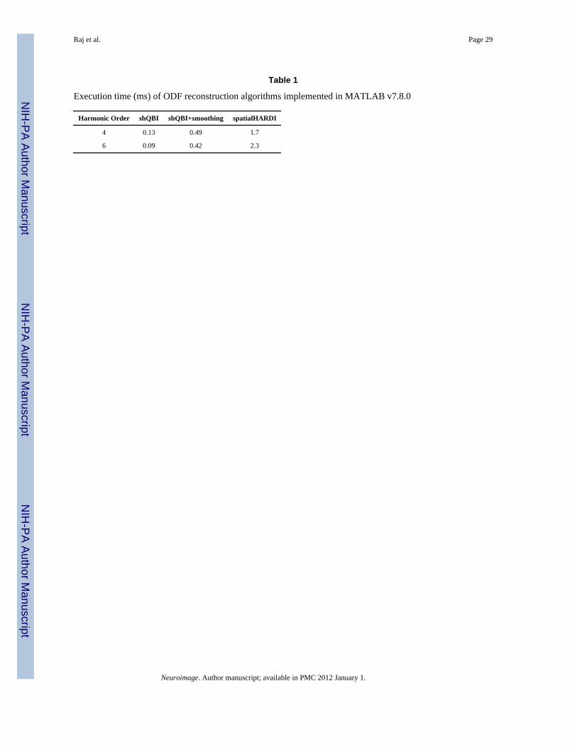
Execution time—As per Table 1, Spatial HARDI takes about 3–5× more time than sqQBIwith smoothing. However, these numbers do not reflect the overhead associated with file input/output and preprocessing, which are shared by all algorithms but vary with image size andresolution. In realistic in vivo imaging situations we have found about 2× increase in overallexecution time of spatialHARDI compared to sqQBI+smoothing.

In vivo studiesFigure 7 shows the three reconstructions for a region of interest (ROI) where fibers within theoptic radiation, oriented in the anterior-posterior direction, co-exist with cortical fibers of theposterior temporal lobe, oriented left-right as shown in figure 7(a-b). Spherical harmonics upto order four were used, which were reconstructed from raw diffusion data in 36 directions andb-value of 3000. Figure 7(c) is the standard shQBI reconstruction with no regularization. Part(d) shows shQBI at regularization factor of 0.2, and (e) shows the result of a post-processingstep involving spatial smoothing of (c). This was done in order to assess the utility of spatialsmoothing as a post-reconstruction step with respect to both shQBI and spatial HARDI, whichis shown in (f). Note that post-reconstruction spatial smoothing gives different ODF shapesthan spatially constrained Bayesian reconstruction. Clearly spatial smoothing did not result inappreciable improvement over shQBI or regularized shQBI; consequently it has been droppedfrom subsequent examples.

It is interesting that the same diffusion data can produce sharp differences in reconstructionunder various assumptions. The shQBI reconstructions all appear to show an abrupt boundarybetween the two fiber populations at the interface between second and third columns in Fig.7. Note especially the voxels denoted by the white arrowhead in Fig. 7(f). In shQBI recons (c-e), these ODFs do not seem to give contiguous fiber bundles. It appears to us unlikely thatneighboring voxels could have such divergent orientations without other voxels in the sameneighborhood showing signs of mixed fiber populations due to partial volume averaging. Thelast row of shQBI shows incoherently oriented ODFs, particularly the fourth and fifth voxelsimply existence of an A-P oriented fiber, but this is not supported by any of their neighbors.Spatial HARDI in contrast produces a jointly consistent but different configuration. Althoughthe true configuration is difficult to determine in this case, at this level of prior weight (0.2), it

Raj et al. Page 12

Neuroimage. Author manuscript; available in PMC 2012 January 1.

NIH

-PA Author Manuscript

NIH

-PA Author Manuscript

NIH

-PA Author Manuscript

is quite unlikely that spatial HARDI would have artifactually introduced a fiber configuration,unless there was support for it in the observed data itself. Note also that neighboring supportcomes not just from the slice shown but also its adjacent slices which are not shown. Fig. 7(f)depicts a mixed population of fibers in column 3, with medial-lateral fibers (in red) fanningout in the Anterior-Posterior (A-P, green) and Superior-Inferior (S-I, blue) directions. Finally,as shown in the center voxel (3rd row and 3rd column) of Fig. 7(f), spatial HARDI managedto capture some ML-oriented fibers en route to/from the cortex within the A-P fibers -- theseare definitely present anatomically but not depicted by any of the other methods.

Figure 8 shows the three reconstructions for an ROI in the anterior limb of the internal capsule,which is a well-known region of mainly cortico-thalamic fibers oriented in the anterior-posterior direction, along with some other fibers of mixed orientation. This region is shownby the red rectangle drawn in (a) and (b), which contain the T2-weighted image slice and thecolor FA maps respectively. Figs. (c-e) were reconstructed from a maximum sphericalharmonic order of 4, and Figs. (f-h) from maximum order 6. In the 4-harmonic case, both shQBIand spatial HARDI reconstructions are able to resolve ODFs originating from the main A-Pfiber population quire well. At this level of noise, an order-4 harmonic fit is sufficient to getgood results in all cases. Imposition of spatial prior in (e) did not lead to any degradation ofODF profiles in the region denoted by the red rectangle in (e). This demonstrates that ourmethod does not indiscriminately blur ODFs across neighboring voxels. Row 3 (f-h) show thata higher harmonic order of 6 caused overfitting of the data, leading to noise in the reconstructedshQBI. At a higher regularization factor, this noise was removed, but at the cost of appreciableblurring. The spatial HARDI reconstruction (h) overcomes the noise problem without leadingto ODF blurring. For instance, compare the voxels indicated by the arrowheads for all threereconstructions.

Figure 9 shows the three reconstructions for a ROI in a region shown in (a) and (b) whereMedial-Lateral (M-L, red, 3 left columns) oriented fibers to cortical areas coexist with A-Poriented fibers within the superior longitudinal fascicle (green, middle 3 columns) and S-Ioriented projections of the corona radiata (blue, rightmost 2 columns). ODFs werereconstructed from order 6 spherical harmonics. These crossing fibers can be resolved in allreconstructions, but the main problem with shQBI in this case appears to be noise, which hasled in some cases to spurious ODF peaks – some examples are indicated by arrowheads.Although regularization of shQBI succeeds in removing these spurious peaks, it does so at thecost of much poorer angular resolution, which might become an important limitation in thisregion of several coexisting fiber tracts. Imposition of the spatial prior in (d) removes spuriousODF peaks without degradation of ODF profiles, while at the same time faithfully resolvingthe extant crossing fiber configuration. Notice how easily each fiber population can be tracedright through the ROI without encountering spurious ODF peaks, which might mislead atractography algorithm, or ambiguity due to crossing fibers, which might cause computedtracks to end abruptly.

Figure 10 shows the effect of different numbers of gradient directions. We chose a ROI at theinterface of M-L and S-I fibers within the right occipital white matter, shown in (a) and (b).This data was acquired at b=6000 and 131 directions and reconstructed with 6-order harmonics.A single voxel from the calcarine projections oriented in the diagonal direction was selectedfor detailed viewing; this voxel is adjacent to a fiber bundle oriented in the S-I direction. Theoriginal data, acquired at 131 directions, was subsampled to fewer directions (55, 33 and 25),as follows. The original data in (θ,φ) space was uniformly subsampled to the nearest regulartiling in (θ,φ) space; however this may or may not give the exact number we want, so fromhere we randomly throw away some directions until the desired number is reached. At theoriginal 131 directions, all methods perform similarly. Due to decreasing SNR and lowerangular resolution as the number of directions is decreased, shQBI reconstruction suffers from

Raj et al. Page 13

Neuroimage. Author manuscript; available in PMC 2012 January 1.

NIH

-PA Author Manuscript

NIH

-PA Author Manuscript

NIH

-PA Author Manuscript

significant noise and spurious peaks, and is clearly unusable at 33 and 25 directions.Regularized shQBI is able to remove spurious peaks but at the cost of reduced angularresolution; finally it too fails at 25 directions because the dominant direction is simply incorrect.In clear contrast, spatial HARDI is able to maintain both orientation accuracy and angularresolution at all levels.

DISCUSSION AND CONCLUSIONAlthough presented results pertain to the shQBI method, we note that it is easily applicable toany linear HARDI reconstruction technique. In addition to shQBI, other popular reconstructionmethods that use radial basis functions – RBF-QBI (Tuch, 2004) and PASMRI (Jansons et al.,2003) - could have been used for this work. Spatial HARDI can also be used in conjunctionwith different regularization techniques, like Tikhonov regularization or the graduatedLaplace-Beltrami regularization. Our approach can also be used within proposed model-basedreconstructions like multi-tensor mixture models (Hosey et al., 2005; Tuch, 2002) or tensordistribution models (Jian et al., 2007). In all cases, we can write ODF reconstruction as a costminimization problem similar to Eq. (1), where the use of spatial information adds an additionalterm to the minimization function.

Although not the focus of the present work, the proposed method can also be used to obtainconventional DTI reconstruction (“spatial DTI”), because diffusion tensors are estimated viaa linear estimator, just like shQBI, PASMRI or RBF-QBI. Our experimentation with DTIreconstruction using spatial HARDI indicates performance similar to conventional DTI, witha small improvement in extremely noisy cases. This data is not shown in this paper, becauseour focus is on high angular resolution. For standard DTI reconstruction, there is really no needto acquire at high b-values and large number of directions. One potential use for spatial DTIwould be to enable very high spatial resolution DTI by more faithfully reconstructing the tensoreven at very low SNR.

The inclusion of spatially smoothed shQBI in our comparative results might appearunconventional – it is certainly not a standard technique reported anywhere that we are awareof – but we believe it serves an important purpose: it answers the question of whether spatialHARDI, which after all imposes spatial smoothness constraints, could be reproduced simplyby spatially smoothing the conventional shQBI output. Presented results confirm that the twomethods are very different, and that post-reconstruction smoothing is a suboptimal approachfor imposing spatial smoothness constraints. Instead, spatial constraints should be imposed atthe time of reconstruction, where it can usefully disambiguate noisy or incomplete observeddata by supplying additional information. If one waits until after the reconstruction hascompleted, the noise or inadequate data quality have already propagated and cannot be easilyremoved at this stage. Our comparative results corroborate this fact, which is a well-knownfeature whenever Bayesian methods employing spatial priors were used for image estimationin various contexts – image segmentation (Zhang et al., 2001), parallel imaging reconstruction(Raj et al., 2007), etc.

Finally, our use of weighted norms via the neighborhood weights wi,j has previously appearedin anatomically-constrained prior models for MR image reconstruction (e.g. Haldar et al.,2008 and references therein), where the weights are estimated from a set of prior referenceimages. In contrast we do not have access to appropriate reference images, since no otherimaging modality exhibits directionally-variant diffusion-weighted tissue contrast.Consequently our optimization problem is harder, since the weights must also be jointlyestimated along with the ODFs.

Raj et al. Page 14

Neuroimage. Author manuscript; available in PMC 2012 January 1.

NIH

-PA Author Manuscript

NIH

-PA Author Manuscript

NIH

-PA Author Manuscript

The proposed work serves as more robust and tolerant to measurement noise and time-limitedacquisitions than current voxelwise methods of reconstructing ODFs. Our method can lead tomore accurate and sensitive tractography outcomes, which in turn could lead to more preciseand reliable surgical planning. Tractography is also being proposed as an input to advancednetwork-level analysis of brain neuronal connectivity (Hagmann et al., 2007). Again, theoutcome of these tasks is crucially dependent on the accuracy and resolution, both spatial andangular, of reconstructed ODFs.

Limitations and Future WorkOne limitation of the proposed method is its assumption of uncorrelated Gaussian noise.Although raw complex diffusion data does in fact have additive Gaussian noise, the samecannot be said for the observations e, which are obtained from the raw data in a highly non-linear fashion, especially with the use of parallel imaging. Many proposed noise models forHARDI are known (Kim et al., 2009; Jones et al., 2004), and it has been shown that the Gaussianassumption fails especially at very low signal levels. However, the Gaussian assumption in ourmethod follows much of the literature, and has been shown to produce reasonable results. Ofcourse, any given noise model can be incorporated in the formulation presented in Eqs. (1) –(4) by suitably altering the likelihood term; unfortunately the resulting cost minimizationproblem quickly becomes intractable in such cases. This is because the first term in Eq. (4) isno longer quadratic or even convex, characterized by multiple local minima that renderoptimization untenable. In this work our focus is to introduce spatial prior models rather thana detailed noise model. Our future work will involve extending our method to other noisemodels and obtaining efficient minimization algorithms to solve them.

Some very recent work (Canales-Rodríguez, et al., 2009; Barnett, A,. 2009) suggests that theq-ball model employed in our work, although widely used, might not be optimal or even a goodapproximation to Tuch’s original ODF model. Present work does not attempt to address thisissue; however it should prove tractable to modify our approach to incorporate the latestapproach advocated by Canales-Rodríguez, Barnett and co-workers. In any case, the presentwork is more concerned with how to exploit spatial constraints rather than with a specific q-ball model.

The prior penalty terms in Eq. (4) introduce some prior bias, which might be detrimental toaccuracy. Fortunately, it is generally known in Bayesian literature (Raj et al., 2007;Lin et al.,2004) that a very small amount of bias can improve the conditioning of extremely badly-posedinverse problems. Still, there is always a trade-off between prior bias and conditioning of theproblem, and the optimal point of this tradeoff must ultimately be determined by the user. Forinstance in Bayesian MR image reconstruction, too much regularization causes excessivesmoothing and too little gives noise amplification due to poor matrix conditioning (Raj et al.,2007). Several techniques exist to evaluate this trade-off, including generalized cross validation(Golub et al., 1979) and L-curve analysis (Lin et al., 2004). In this paper we do not performthese analyses, because our experience has been that the result of such an analysis are specificto the experimental situation and cannot easily be transferred. Instead we chose a trial and errorapproach where the regularization parameters are varied in small increments within a feasiblerange, and the parameters that produce the best results (RMSE, angular resolution, etc) werechosen. This paper employs global, spatially invariant regularization parameters. Spatiallyvarying parameters are in general much harder to validate due to a vastly greater parameterspace, and there appears little justification in doing so since the essential local variability isalready being captured in the weight matrix. The optimal parameters might change for differentsubjects and scans because they depend on SNR and image resolution. It might be possiblethat some sort of scaling law for λ and μ as a function of image resolution and SNR mightaccommodate inter-scan and inter-subject variability; these issues will form part of our future

Raj et al. Page 15

Neuroimage. Author manuscript; available in PMC 2012 January 1.

NIH

-PA Author Manuscript

NIH

-PA Author Manuscript

NIH

-PA Author Manuscript

work. We also plan a visual evaluation by experts in neurology of whole brain tractographybased on proposed ODFs.

The exact form of W(η) is an open question at this time, and most likely will depend oncomputational and tractability considerations. Since the weights should generally depend onthe ODF configuration η, we denote an explicit dependence on η. This is a tricky issue froma statistical as well as computational standpoint, because it makes the minimization task non-linear and the cost function non-quadratic and/or non-convex. Here we have examined aninteresting form of W(η), and proposed a simple iterative scheme whereby both W(η.) and ηitself are updated alternately. Future work will look into the optimal choice of W(η).

ConclusionIn conclusion, we proposed a novel Bayesian approach to DTI and HARDI reconstruction,called Spatial HARDI, by exploiting the spatial coherence of the diffusion profiles of watermolecules in vivo. Careful algorithm design enables the added Bayesian technology to beemployed without impractical increase in overall execution time compared to standard shQBIreconstruction. Presented simulation and in vivo evidence suggests that Spatial HARDI canjointly improve RMSE and orientation accuracy of ODF reconstruction. Results from in vivohuman brain data also indicates that the proposed method might be better at maintainingaccurate ODFs for smaller numbers of acquisition directions (hence faster scans) compared tospatial smoothing or single-voxel ODF regularization.

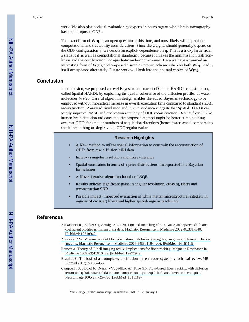
Research Highlights

• A New method to utilize spatial information to constrain the reconstruction ofODFs from raw diffusion MRI data

• Improves angular resolution and noise tolerance

• Spatial constraints in terms of a prior distributions, incorporated in a Bayesianformulation

• A Novel iterative algorithm based on LSQR

• Results indicate significant gains in angular resolution, crossing fibers andreconstruction SNR

• Possible impact: improved evaluation of white matter microstructural integrity inregions of crossing fibers and higher spatial/angular resolution.

ReferencesAlexander DC, Barker GJ, Arridge SR. Detection and modeling of non-Gaussian apparent diffusion

coefficient profiles in human brain data. Magnetic Resonance in Medicine 2002;48:331–340.[PubMed: 12210942]

Anderson AW. Measurement of fiber orientation distributions using high angular resolution diffusionimaging. Magnetic Resonance in Medicine 2005;54(5):1194–206. [PubMed: 16161109]

Barnett A. Theory of Q-ball imaging redux: Implications for fiber tracking. Magnetic Resonance inMedicine 2009;62(4):910–23. [PubMed: 19672943]

Beaulieu C. The basis of anisotropic water diffusion in the nervous system—a technical review. MRBiomed 2002;15:438–455.

Campbell JS, Siddiqi K, Rymar VV, Sadikot AF, Pike GB. Flow-based fiber tracking with diffusiontensor and q-ball data: validation and comparison to principal diffusion direction techniques.NeuroImage 2005;27:725–736. [PubMed: 16111897]

Raj et al. Page 16

Neuroimage. Author manuscript; available in PMC 2012 January 1.

NIH

-PA Author Manuscript

NIH

-PA Author Manuscript

NIH

-PA Author Manuscript

Canales-Rodríguez EJ, Melie-García L, Iturria-Medina Y. Mathematical description of q-space inspherical coordinates: exact q-ball imaging. Magnetic Resonance in Medicine 2009;61(6):1350–67.[PubMed: 19319889]

Descoteaux M, Angelino E, Fitzgibbons S, Deriche R. Regularized, Fast, and Robust Analytical Q-BallImaging. Magnetic Resonance in Medicine 2007;58:497–510. [PubMed: 17763358]

Descoteaux M, Wiest-Daesslé N, Prima S, Barillot C, Deriche R. Impact of Rician adapted Non-LocalMeans filtering on HARDI. International Conference on Medical Image Computing and Computer-Assisted Intervention 2008;11(2):122–130.

Frank LR. Characterization of anisotropy in high angular resolution diffusion weighted MRI. MagneticResonance in Medicine 2002;47:1083–1099. [PubMed: 12111955]

Gerchberg RW, Saxton WO. Practical algorithm for the determination of phase from image anddiffraction plane pictures. Optik 1972;35(2):237–250.

Golub GH, Heath M, Wahba G. Generalized cross-validation as a method for choosing a good ridgeparameter. Technometrics. 1979

Goh, A.; Lenglet, C.; Thompson, PM.; Vidal, R. A Nonparametric Riemannian Framework for ProcessingHigh Angular Resolution Diffusion Images (HARDI). Proceedings of Computer Vision and PatternRecognition Conference; 2009; 2009.

Groemer, H. Geometric applications of Fourier series and spherical harmonics. Cambridge UniversityPress; 1996.

Hagmann P, Kurant M, Gigandet X, Thiran P, Wedeen VJ, Meuli R, Thiran JP. Mapping human whole-brain structural networks with diffusion MRI. PLoS ONE 2007;2(7):597.

Haldar JP, Hernando D, Song SK, Liang ZP. Anatomically constrained reconstruction from noisy data.Magnetic Resonance in Medicine 2008;59(4):810–818. [PubMed: 18383297]

Hess CP, Mukherjee P, Han ET, Xu D, Vigneron DB. Q-ball reconstruction of multimodal fiberorientations using the spherical harmonic basis. Magnetic Resonance in Medicine 2006;56:104–117.[PubMed: 16755539]

Hosey T, Williams G, Ansorge R. Inference of Multiple Fiber Orientations in High Angular ResolutionDiffusion Imaging. Magnetic Resonance in Medicine 2005;54:1480–1489. [PubMed: 16265642]

Jansons KM, Alexander DC. Persistent angular structure: new insights from diffusion magnetic resonanceimaging data. Inverse Problems 2003;19:1031–1046.

Jian B, Vemuri BC, özarslan E, Carney PR, Mareci TH. A novel tensor distribution model for thediffusion-weighted MR signal. NeuroImage 2007;37(1):164–176. [PubMed: 17570683]

Jones DK. The effect of gradient sampling schemes on measures derived from diffusion tensor MRI: aMonte Carlo study. Magnetic Resonance in Medicine 2004;51:807–815. [PubMed: 15065255]

Kim, Y.; Thompson, PM.; Toga, AW.; Vese, L.; Zhan, L. HARDI Denoising: Variational Regularizationof the Spherical Apparent Diffusion Coefficient sADC. IPMI; 2009.

Lin F, Kwang K, Belliveau J, Wald L. Parallel imaging reconstruction using automatic regularization.Magnetic Resonance in Medicine 2004;51:559–567. [PubMed: 15004798]

Liu C, Bammer R, Acar B, Moseley ME. Characterizing non-Gaussian diffusion by using generalizeddiffusion tensors. Magnetic Resonance in Medicine 2004;51:924–937. [PubMed: 15122674]

Mori S, Crain BJ, Chacko VP, Van Zijl PM. Three-dimensional tracking of axonal projections in thebrain by magnetic resonance imaging. Ann Neurol 1999;45:265–269. [PubMed: 9989633]

Mukherjee P, Hess CP, Xu D, Han ET, Kelley DA, Vigneron DB. Development and initial evaluation of7-T q-ball imaging of the human brain. Magn Reson Imaging. 200710.1016/j.mri

Ozarslan E, Mareci TH. Generalized diffusion tensor imaging and analytical relationships betweendiffusion tensor imaging and high angular resolution diffusion imaging. Magnetic Resonance inMedicine 2003;50:955–965. [PubMed: 14587006]

Ozarslan E, Shepherd TM, Vemuri BC, Blackband SJ, Mareci TH. Resolution of complex tissuemicroarchitecture using the diffusion orientation transform (DOT). Neuroimage 2006;31(3):1086–103. [PubMed: 16546404]

Paige CC, Saunders MA. LSQR: An Algorithm for Sparse Linear Equations And Sparse Least Squares.ACM Trans Math Soft 1982;8:43–71.

Raj et al. Page 17

Neuroimage. Author manuscript; available in PMC 2012 January 1.

NIH

-PA Author Manuscript

NIH

-PA Author Manuscript

NIH

-PA Author Manuscript

Perrin M, Poupon C, Rieul B, Leroux P, Constantinesco A, Mangin JF, Lebihan D. Validation of q-ballimaging with a diffusion fibre-crossing phantom on a clinical scanner. Phil Trans R Soc Lond B BiolSci 2005;360:881–891. [PubMed: 16087433]

Press, W.; Teukolsky, S.; Vetterling, W.; Flannery, B. Numerical recipes in C. 2. Cambridge UniversityPress; 1992.

Pruessmann KP, Weiger M, Scheidegger MB, Boesiger P. SENSE: sensitivity encoding for fast MRI.Magnetic Resonance in Medicine 1999;42:952–962. [PubMed: 10542355]

Raj A, Singh G, Zabih R, Kressler B, Wang Y, Schuff N, Weiner M. Bayesian Parallel Imaging withEdge-Preserving Priors. Magnetic Resonance in Medicine 2007;57(1):8–21. [PubMed: 17195165]

Sakaie KE, Lowe MJ. An objective method for regularization of fiber orientation distributions derivedfrom diffusion-weighted MRI. NeuroImage. 200610.1016/j.neuroimage.2006.08.034

Tournier JD, Calamante F, Gadian DG, Connelly A. Direct estimation of the fiber orientation densityfunction from diffusion-weighted MRI data using spherical deconvolution. Neuroimage2004;23:1176–1185. [PubMed: 15528117]

Tristán-Vega A, Westin CF, Aja-Fernández S. Estimation of fiber Orientation Probability DensityFunctions in High Angular Resolution Diffusion Imaging. NeuroImage 2009;47:638–650. [PubMed:19393321]

Tuch DS. Q-ball imaging. Magnetic Resonance in Medicine 2004;52:1358–72. [PubMed: 15562495]Tuch DS. Q-ball imaging of macaque white matter architecture. Phil Trans R Soc B Biol Sci

2005;360:869–879.Tuch DS, Reese TG, Wiegell MR, Makris N, Belliveau JW, Wedeen VJ. High angular resolution diffusion

imaging reveals intravoxel white matter fiber heterogeneity. Magnetic Resonance in Medicine2002;48:577–82. [PubMed: 12353272]

Zhan W, Stein EA, Yang Y. Mapping the orientation of intravoxel crossing fibers based on the phaseinformation of diffusion circular spectrum. Neuroimage 2004;23:1358–1369. [PubMed: 15589100]

Zhang Y, Brady M, Smith S. Segmentation of Brain MR Images through hidden markov random fieldmodel and the expectation maximization algorithm. IEEE Transactions on Medical Imaging2001;20:45–57. [PubMed: 11293691]

Raj et al. Page 18

Neuroimage. Author manuscript; available in PMC 2012 January 1.

NIH

-PA Author Manuscript

NIH

-PA Author Manuscript

NIH

-PA Author Manuscript

Figure 1.Spatial and angular coherence in HARDI. Except at the boundaries between separate tracts,fiber orientation in neighboring voxels varies smoothly, and as a result adjacent voxels arelikely to have similar ODFs. By imposing spatial constraints among individual fiber tracts, itis possible to mitigate noise and other limitations.

Raj et al. Page 19

Neuroimage. Author manuscript; available in PMC 2012 January 1.

NIH

-PA Author Manuscript

NIH

-PA Author Manuscript

NIH

-PA Author Manuscript

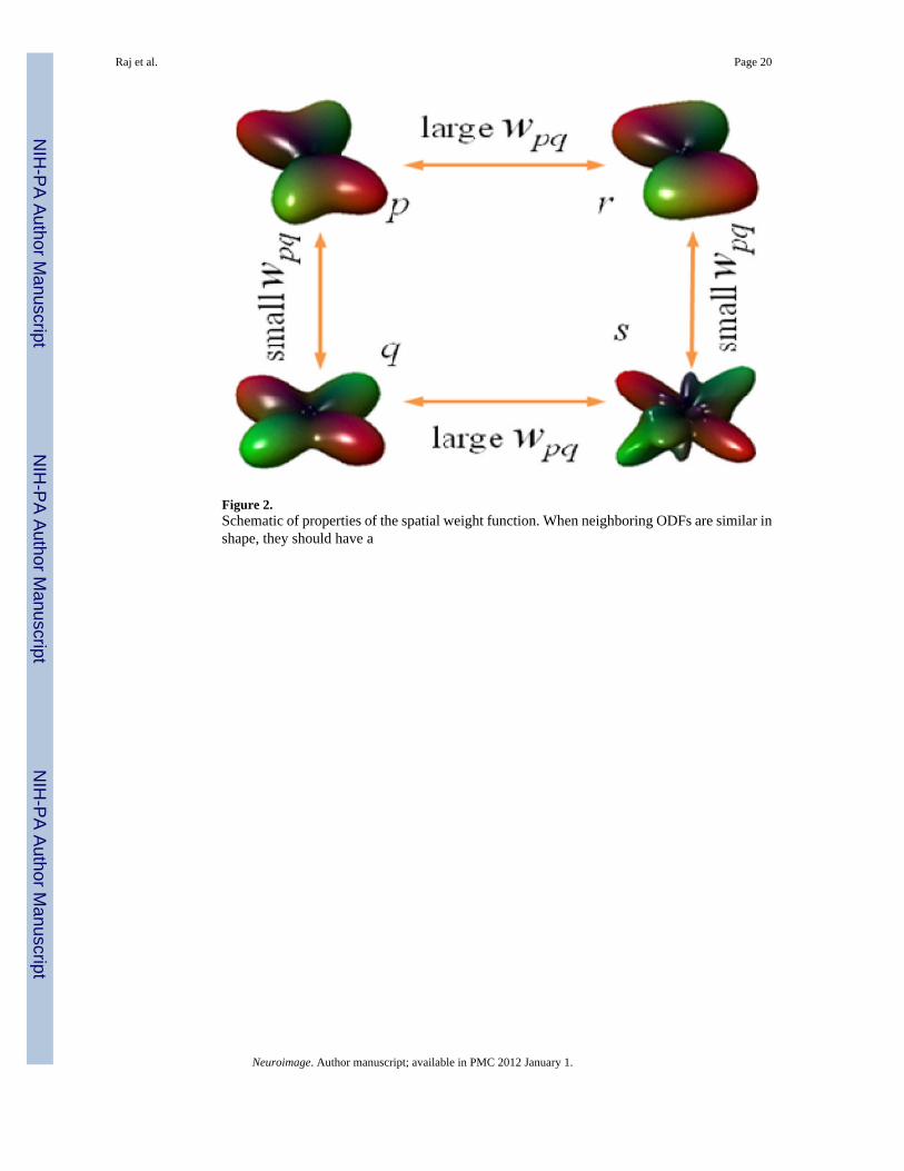
Figure 2.Schematic of properties of the spatial weight function. When neighboring ODFs are similar inshape, they should have a

Raj et al. Page 20

Neuroimage. Author manuscript; available in PMC 2012 January 1.

NIH

-PA Author Manuscript

NIH

-PA Author Manuscript

NIH

-PA Author Manuscript

Figure 3.Simulated ODFs with crossing fibers, at SNR of 1.0, and harmonic order 4. Note the distortioncaused in shQBI due to noise. Spatial HARDI exhibits sharper profiles compared to others,and is able to recover the crossing fiber profile in the center. Voxels with no fibers are notshown.

Raj et al. Page 21

Neuroimage. Author manuscript; available in PMC 2012 January 1.

NIH

-PA Author Manuscript

NIH

-PA Author Manuscript

NIH

-PA Author Manuscript

Figure 4.Performance versus SNR, harmonic order 4, λ = 0.2, μ = 0.2. RMSE captures the overallmismatch between actual and noisy ODFs, GFA captures the mismatch in generalizedfractional anisotropy, and orientation accuracy captures the mean mismatch in the estimatedangle of the fibers.

Raj et al. Page 22

Neuroimage. Author manuscript; available in PMC 2012 January 1.

NIH

-PA Author Manuscript

NIH

-PA Author Manuscript

NIH

-PA Author Manuscript

Figure 5.RMSE and orientation accuracy versus SNR for two different parameter settings. Harmonicorder was chosen as 6 for both. (a) λ = 0.1, μ = 0.05 and (b) (a) λ = 0.05, μ = 0.25. Both (a)and (b) are special cases of curves similar to those shown in Figure 4.

Raj et al. Page 23

Neuroimage. Author manuscript; available in PMC 2012 January 1.

NIH

-PA Author Manuscript

NIH

-PA Author Manuscript

NIH

-PA Author Manuscript

Figure 6.Joint performance curves of reconstruction methods for various SNR levels. In each case theregularization parameter λ was varied in the range [0.05, 0.3] in 12 increments. Spatial HARDIreconstruction was performed at μ equal to λ in order to reduce possible degrees of freedom.The first three plots are shown on the same axes, and the last one on a different one for easeof viewing.

Raj et al. Page 24

Neuroimage. Author manuscript; available in PMC 2012 January 1.

NIH

-PA Author Manuscript

NIH

-PA Author Manuscript

NIH

-PA Author Manuscript

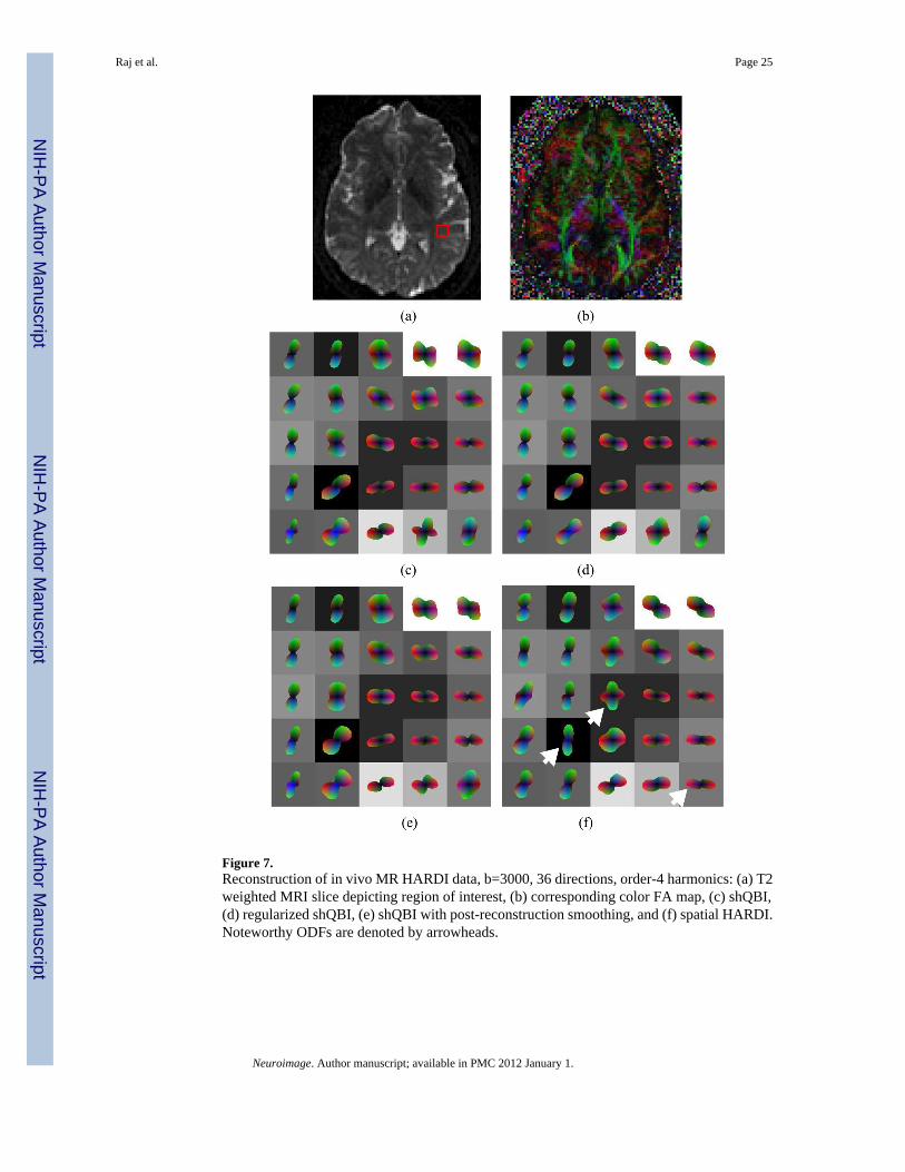
Figure 7.Reconstruction of in vivo MR HARDI data, b=3000, 36 directions, order-4 harmonics: (a) T2weighted MRI slice depicting region of interest, (b) corresponding color FA map, (c) shQBI,(d) regularized shQBI, (e) shQBI with post-reconstruction smoothing, and (f) spatial HARDI.Noteworthy ODFs are denoted by arrowheads.

Raj et al. Page 25

Neuroimage. Author manuscript; available in PMC 2012 January 1.

NIH

-PA Author Manuscript

NIH

-PA Author Manuscript

NIH

-PA Author Manuscript

Figure 8.Reconstruction of in vivo MR HARDI data in the anterior limb of the internal capsule, b=3000,36 directions: (a) T2 weighted MRI slice depicting region of interest, (b) corresponding FAmap. Second row shows results with 4-order harmonics and third row shows results with 6-order harmonics. (c, f) shQBI, (d, g) regularized shQBI, (e, h) spatial HARDI. Note improveddefinition of the ODFs and better resolution of crossing fibers. Instances of crossing fiberresolution in spatial HARDI are denoted by yellow arrowheads in the right panel. Red box in(e) shows ODFs which are unaffected by differing inference in neighboring voxels.

Raj et al. Page 26

Neuroimage. Author manuscript; available in PMC 2012 January 1.

NIH

-PA Author Manuscript

NIH

-PA Author Manuscript

NIH

-PA Author Manuscript

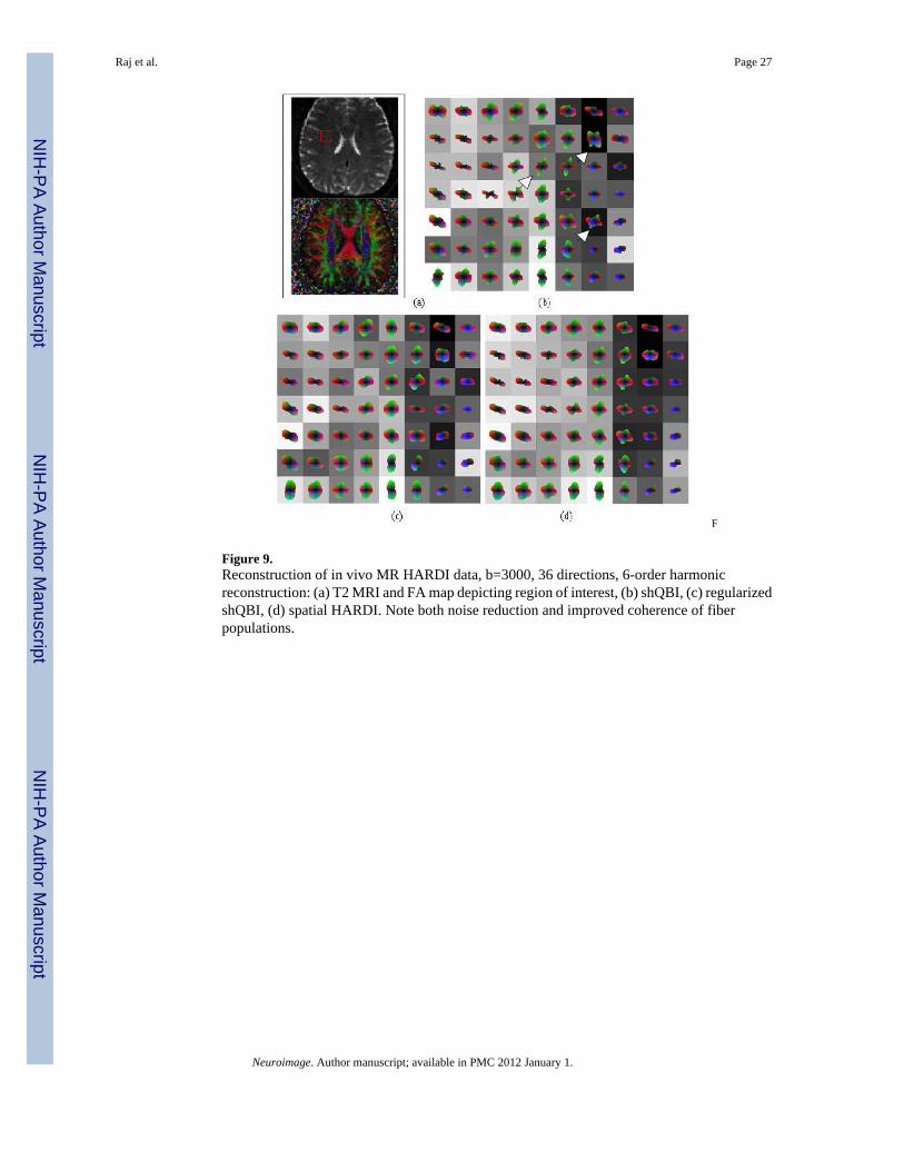
Figure 9.Reconstruction of in vivo MR HARDI data, b=3000, 36 directions, 6-order harmonicreconstruction: (a) T2 MRI and FA map depicting region of interest, (b) shQBI, (c) regularizedshQBI, (d) spatial HARDI. Note both noise reduction and improved coherence of fiberpopulations.

Raj et al. Page 27

Neuroimage. Author manuscript; available in PMC 2012 January 1.

NIH

-PA Author Manuscript

NIH

-PA Author Manuscript

NIH

-PA Author Manuscript

Figure 10.Reconstruction of in vivo data, b=6000, at various number of directions, 6-order harmonicreconstruction: (a) T2 MRI and (b) zoomed-in FA map depicting region of interest, (c) singlevoxel reconstruction with shQBI, regularized shQBI, and spatial HARDI. Our result maintainsthe orientation and angular resolution of the ODF in all cases.

Raj et al. Page 28

Neuroimage. Author manuscript; available in PMC 2012 January 1.

NIH

-PA Author Manuscript

NIH

-PA Author Manuscript

NIH

-PA Author Manuscript

NIH

-PA Author Manuscript

NIH

-PA Author Manuscript

NIH

-PA Author Manuscript

Raj et al. Page 29

Table 1

Execution time (ms) of ODF reconstruction algorithms implemented in MATLAB v7.8.0

Harmonic Order shQBI shQBI+smoothing spatialHARDI

4 0.13 0.49 1.7

6 0.09 0.42 2.3

Neuroimage. Author manuscript; available in PMC 2012 January 1.