A 3D particle visualization system for temperaturemanagement

Lange B.a, Rodriguez N.a, Puech W.a, Rey H.b and Vasques X.b

aLIRMM, 141 rue ADA, Montpellier, France;bIBM, Rue de la vieille poste, Montpellier, France

ABSTRACT

This paper deals with a 3D visualization technique proposed to analyze and manage energy efficiency from a datacenter. Data are extracted from sensors located in the IBM Green Data Center in Montpellier France. Thesesensors measure different information such as hygrometry, pressure and temperature. We want to visualize inreal-time the large among of data produced by these sensors. A visualization engine has been designed, basedon particles system and a client server paradigm. In order to solve performance problems, a Level Of Detailsolution has been developed. These methods are based on the earlier work introduced by J. Clark in 19761 . Inthis paper we introduce a particle method used for this work and subsequently we explain different simplificationmethods applied to improve our solution.

Keywords: 3D Visualization, Sensors, Particles, Client/Server, Level Of Details

1. INTRODUCTION

In this paper, we present a method to produce a 3D visualization for analyzing and managing temperature. Dataare extracted from sensors located in the IBM Green Data Center in Montpellier, which provides many differenttypes of information like temperature, pressure or hygrometry. In our system, sensors are placed in a virtualroom and the internal space is modeled using particles. The main constraint here is to produce a real-timerendering. However, latency appears du to the number of vertices. In this paper, we use a solution called LOD(Level Of Detail) to produce multi resolution 3D objects. This solution has been introduced in 1976 by J. Clark1

. In this paper, J. Clark introduces the use of several mesh resolutions to simplify the 3D scene complexity.In our work, we use various simplification methods to provide interactive rendering and allows rendering themost important part of data extracted from sensors. In this paper, we describe how we create a room, and themethods used to produce different resolution visualization.In Section 2, we introduce related work on particles systems and LOD. In Section 3, we expose our solution tosimplify particles system. In Section 4 we give some results and finally, in Section 5 we present our conclusionsand future work.

2. RELATED WORK

In this section we present several previous works concerning data visualization, particle systems and level ofdetail methods.Some previous work present solutions to visualize large data flow extracted from mantle convection. M. Damon etal.2 and K. E. Jordan et al.3 present interactive viewers for this kind of data. These data are computed by usingHight Performance Computing (HPC) and visualized on a large display. The rendering is calculated by usinganother HPC. The data flow is very important and a real-time 3D simulation is hard to obtain. W. Kapfer and

Further author information:Lange B.: E-mail: benoit.lange@lirmm.frRodriguez N.: E-mail: nancy.rodriguez@lirmm.frPuech W.: E-mail: william.puech@lirmm.frRey H.: E-mail:REYHERVE@fr.ibm.comVasques X.: E-mail: xavier.vasques@fr.ibm.com

lirm

m-0

0808

114,

ver

sion

1 -

4 Ap

r 201

3Author manuscript, published in "SPIE Electronic Imaging 2011, Parallel Processing for Imaging Applications 7872, California : United

States (2011)"

T. Riser6 introduce how to use particle system to visualize astronomic simulation, particles representing spaceobjects. The number of particles is extremely important for computing motion in real-time. GPU computing ispreferred to render instead of a common HPC solution. To display their data, they have developed their own 3Dgraphical engine. The space objects are represented by point sprite instead of sphere. Lights are used to givea spherical aspect to the point sprite. This solution allows to render more stars than spherical object method.The 3D engine provides different rendering methods to group space objects: cell simplification or extraction ofisosurface. The use of GPU seems quite well for a particle solution, parallel processing allows to render largedata; the astrological data seems to be well suited.In 1976, J. Clark introduces Level Of Detail (LOD) concept1 . LOD consists to produce several resolution meshesfor using them at different distance from the camera. Firstly, designer produces these meshes. First algorithms,in 1992 Schroeder et al. developed a method by decimation for simplify the mesh7 . It analyses mesh geometryand evaluates the complexity of triangles. Vertices are removed if only constraints set by the user are respected.Vertices are removed and gaps are filled using triangulation. These algorithms of simplification are not enoughto simplify mesh efficiently because shape is not always totally respected. D. Luebke, in 1997, has proposed ataxonomy of mesh simplification8 . He presented the most used algorithms. He extracted different ways to useeach algorithm. But in this paper, only one solution works with volumetric mesh9 . T. He et al. propose amethod based on voxel simplification by using a grid for clustering voxels. A marching cube10 algorithm wasapplied to produce a surface mesh. But this simplification algorithm did not preserve the shape of the mesh. Inour work, we look for point cloud simplification. Indeed, previous methods which deal with simplification forsurface point cloud like11–13 are not adapted to our case. All of these methods produce LOD for surface meshand point cloud is extracted from scanner.

3. PROPOSED APPROACH

This section presents the different methods that are used to visualize a kind of data from Green Data Center(GDC). The main goal is to be able to visualize in real-time the evolution of temperature in the data center. Forthis, we use a special particle method. Particles are located using a segmentation algorithm based on Voronoıcell extraction and Delaunay triangulation. The latency due to the large flow of particles is avoided by using aclient server paradigm. We improve our solution by using LOD methods to simplify rendering.

3.1 Particle systems

Rooms are the bases of our study. For modeling a room, we extract the shape of the space representation which iscomposed by a box with three measures: length (l ∈ R), width (w ∈ R), height (h ∈ R). Sensors are representedby S = {S1, ..., SM}, where M is the number of sensors. Sensors Si (i ∈ {1, ..., M}) are placed on the space ona layer L ∈ N and have a location represented by: {Xi, Yi, Lj} with Xi ∈ R, Yi ∈ R and j is the layer used.For modeling the space inside a room, we use a particle system instead of 2D map representations which havesome lacks.14 Actually 2D map does not allow having a real visualization of space. A particle visualization givesa better efficiency for modeling space. We use a large number of particle to represent the entire space. N ∈ Nrepresents the number of particles in the room. It can be calculated using:

N =((l + 1)× (h+ 1)× (w + 1))

δ3, (1)

where δ ∈ R is the space between particles. The particle grid is regular. In this model, three layers oftemperature sensors compose rooms. They are defined according to their real locations in the data center.Figure ?? presents the different layers of sensors in the data center.Particles carry information, and flow motion can be simulated if needed by changing the value of particles andthe computational cost is inferior.

lirm

m-0

0808

114,

ver

sion

1 -

4 Ap

r 201

3

3.2 Segmentation algorithms

In our solution, each sensors has an influence on surrounding particules. To calculate the set of particles in thesensor range, we use two methods: Voronoı cells extraction and Delaunay triangulation.Voronoı cells is a method to extract a partition of space15 . This method is available for φ dimensions whereφ ∈ [1,+∞], but most of implementations are done in 2D. Tools for extracting 3D Voronoı diagrams exist:Voro++16 and QHull17 but particles are discrete and these solutions are not suitable because they extractVoronoı diagram in a continuous way. Then we designed our own method based on sphere expansion. We searchnearest sensors for each particle. This part allows to weight particles outside the sensors mesh. A second methodto weight the interior of the sensors mesh is used. We extract the mesh tetrahedron of sensors using the Delaunaytriangulation implemented in QHull17 . This method was used to analyze the location of particle. We computethe exact location using ray tracing18 on the soup of tetrahedron. First, we search the nearest particles insidethe hull of each tetrahedron. We extract the normal of each face of tetrahedron and we apply these normals oneach particle. If the ray cuts three faces or more, the particle is inside the tetrahedron. This method is costexpensive and done in preprocessing. Moreover, particles are static and position didn’t need to be update.

3.3 Client server paradigm

To improve computation, a client server paradigm is used. We define a low cost communication protocol totransfer data from a server to a client. Server computes the modification of particles and the client displaysthe results. This protocol works in five steps. These steps are: sending header, sending sensor data, sendingparticle data, sending footer and receiving acknowledgment/command from client. At each step, the server waitsthe acknowledgment from the client. We develop two ways to send data. The first sends the entire point cloud(sensors and particles). The biggest problem of this method is the transmission of data. Sensors are sent withtheir coordinates and their value. We encode these data in bit words. For the particles data, the same methodwas used. The footer was sent for closing the communication. The second method is used to reduce efficientlythe communication cost. We only send modified sensors and particles. The id and the new value is sent insteadof coordinates. The last step is the command sent by the client. It allows the user to interact with the server.We use it to modify the camera viewpoint.

3.4 Level of detail for particles

Level of detail (LOD) is one of the most important methods in computer graphics. It allows to solve renderingproblems or performance problems. This method consists by producing several resolution of a 3D object. In ourworks, we use some features to define the object resolution: hardware and viewpoint. Hardware and viewpointdo not need the same data structure and we need to recompute it for each modification of the viewpoint or whenhardware changes. LOD was defined by two problems statement. The first one uses a sample of original points,the second one uses a new point data set. In this part, we define six methods to produce LOD. The four firstmethods are for the client, the other are for the server.

Problems statement:For this two approaches, we have a set ω of Vertices V, V = {V1, ..., Vω}. Each vertex is defined in R3. Simplifya mesh using a sample vertex means ω > ω2, where ω2 is the size of the second data set. For approach 1, weobtain a new object V2 = {V21, ... , V2ω} with fewer point than V but V2 is a subset of V. For approach 2, weobtain a new object V3 = {V31, ... , V3ω} with fewer point than V but each point in V3 is a new vertex.

In Section 2 we have presented methods to produce simplification. A few were designed for volumetricsimplification. In this section, we propose several methods to produce different volumetric simplifications on ourclient. We develop four approaches to simplify 3D objects: clustering, neighbor simplification and two approachesbased on server.Clustering method was based on He et al.9 works, it consists of clustering particles using a 3D grid. Cellssizes of grid are set depending to the viewpoint of the camera. Clusters were being weight with the average ofthe different values of particles. The position is the barycenter of these particles. Figures 1(a)-1(e) give someexamples of simplification using clustering solution. Figure 1(a) present the original point of cloud mesh. Figure

lirm

m-0

0808

114,

ver

sion

1 -

4 Ap

r 201

3

1(b) and 1(d) give two different methods for clustering. And finally, Figure 1(c) and 1(e) give the results ofclustering methods.

(a) Original pointcloud.

(b) First simplifica-tion cluster.

(c) First new pointcloud.

(d) Second simplifica-tion cluster.

(e) Second new pointcloud.

Figure 1. Clustering method for simplification point cloud.

The second solution used is based on neighborhood extraction. Before runtime, we extract all neighbors of aparticle. We measure the distance between each particle. Some optimization can help to decrease complexity:we can estimate easily in our structure which particle is closer to another one (using the fact that particle gridis regular). After this, we extract the main value of particles. We explore each neighbor of particles and wekeep the most important. In some cases, the most important can be the high values, in other the low valuesand in other both of them. This solution is able to produce a low resolution model with the most importantinformation structure. Several low resolution models are created by exploring deeper in neighborhood. Figures2(a)-2(c) illustrate a neighbor, and two simplifications of this mesh.

(a) Neighborhood of pointcloud.

(b) Simplification using aneighborhood of 1.

(c) Simplification using aneighborhood of 2.

Figure 2. Neighbor method for simplification.

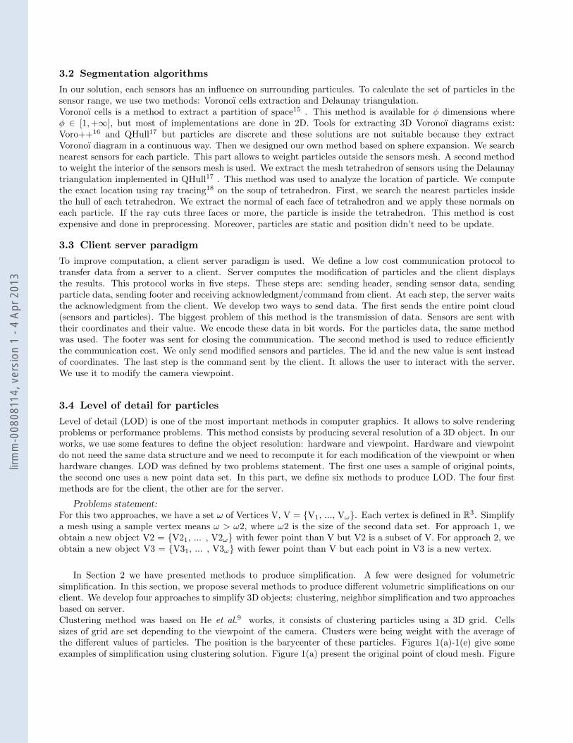
Other methods were based on server instead of client. Client sent via TCP connection his viewpoint. Theserver recomputes the particles structure and recreates the entire structure. With this solution, it is possible toproduce a point cloud resolution depending on hardware. Figure 3(a) presents particles rendering with a distanceof 2 from the camera. Figure 3(b) is the decimation produced with a distance of 3 and Figure 3(c) is a distanceof 1.

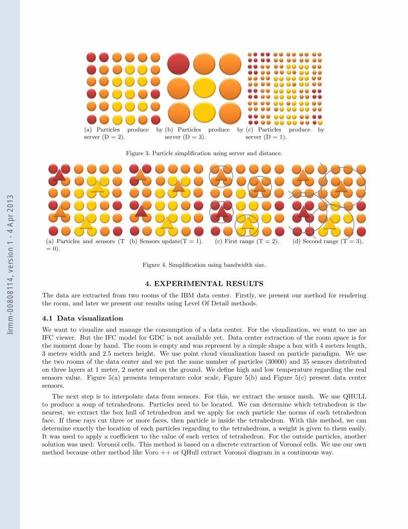
Another method was based on Voronoı diffusion of temperature. The bandwidth for transmitting data islimited. We developed Voronoı temperature diffusion to solve this communication. In this approach, we updatedata using sphere expansion. Each time, we update particles depending on their distance from sensors. The moreparticles are distant from sensors the later they will be refreshed. This method sends only modified particles.The bandwidth is saved and the visualization gives a flow effect. Figure 4(a) represents values at time 0. At time1, values of sensors change, 4(b). After time 2, we update a first range of particles 4(c) and finally the secondrange 4(d).

lirm

m-0

0808

114,

ver

sion

1 -

4 Ap

r 201

3

(a) Particles produce byserver (D = 2).

(b) Particles produce byserver (D = 3).

(c) Particles produce byserver (D = 1).

Figure 3. Particle simplification using server and distance.

(a) Particles and sensors (T= 0).

(b) Sensors update(T = 1). (c) First range (T = 2). (d) Second range (T = 3).

Figure 4. Simplification using bandwidth size.

4. EXPERIMENTAL RESULTS

The data are extracted from two rooms of the IBM data center. Firstly, we present our method for renderingthe room, and later we present our results using Level Of Detail methods.

4.1 Data visualization

We want to visualize and manage the consumption of a data center. For the visualization, we want to use anIFC viewer. But the IFC model for GDC is not available yet. Data center extraction of the room space is forthe moment done by hand. The room is empty and was represent by a simple shape a box with 4 meters length,3 meters width and 2.5 meters height. We use point cloud visualization based on particle paradigm. We usethe two rooms of the data center and we put the same number of particles (30000) and 35 sensors distributedon three layers at 1 meter, 2 meter and on the ground. We define high and low temperature regarding the realsensors value. Figure 5(a) presents temperature color scale, Figure 5(b) and Figure 5(c) present data centersensors.

The next step is to interpolate data from sensors. For this, we extract the sensor mesh. We use QHULLto produce a soup of tetrahedrons. Particles need to be located. We can determine which tetrahedron is thenearest, we extract the box hull of tetrahedron and we apply for each particle the norms of each tetrahedronface. If these rays cut three or more faces, then particle is inside the tetrahedron. With this method, we candetermine exactly the location of each particles regarding to the tetrahedrons, a weight is given to them easily.It was used to apply a coefficient to the value of each vertex of tetrahedron. For the outside particles, anothersolution was used: Voronoı cells. This method is based on a discrete extraction of Voronoı cells. We use our ownmethod because other method like Voro ++ or QHull extract Voronoı diagram in a continuous way.

lirm

m-0

0808

114,

ver

sion

1 -

4 Ap

r 201

3

(a) Temperature Color. (b) Room one. (c) Room two.

Figure 5. Data use to model the system.

4.2 Level of details

In the earlier days of this project, first solution proposed gives a low frame rates, about 15 FPS (Frame PerSecond): visualization was not in real-time (real-time is about 24 FPS). For solving this problem, we define aclient server paradigm. This solution allows to produce a real-time rendering on the client. Figure ?? gives anexample of LOD for particles. We use Openscenegraph20 as a 3D engine. It owns several features useful in LOD.A special object is defined to manage multi-resolution model. It calculates the distance of the object from thecamera. For our experimentation we use five resolutions of mesh. The first mesh was the original mesh, it is setat 0 to 500. The next mesh was set at 500 to 1000, the next at 1000 to 1500 and the other at 1500 to 2000.These three meshes were constructed by specific LOD methods: clustering and significant vertices. Clusteringdefines a 3D grid inside the room. The size of each cell depends on the viewpoint location. The size of the clusterdepends on the visibility of the clustered particles. First results are given Figure 6(a) and 6(b). Value of clusteris an average of clustered value. The number of points of the final mesh depends on the grid size. Table 1 showsthe results at several distances.

D = 0 to 500 D = 500 to 1000 D = 1000 to 1500 D = 1500 to 2000C = X 30 000 3 900 240 36

Table 1. Results of clustering simplification.

(a) D = 500 to 1000. (b) D = 1000 to 1500.

Figure 6. Clustering visualization algorithms.

Significant points method extracts the neighbors for each particle. We extract the highest and lowest tem-peratures, by exploring the neighborhood of a particle, in order to have significant vertices of the model. For thefirst step of simplified model we explore neighbor. For the second model, we explore neighbor and neighbor ofneighbor, etc. This solution simplifies drastically the model. First results are given Figure ??-??. Table 2 showsthe number of vertices at several distance.

lirm

m-0

0808

114,

ver

sion

1 -

4 Ap

r 201

3

D = 0 to 500 D = 500 to 1000 D = 1000 to 1500 D = 1500 to 2000C = X 30 000 22 950 4 554 3 524

Table 2. Results of neighbor simplification.

(a) Neighborhood 1. (b) Neighborhood 2.

Figure 7. Clustering visualization algorithms using neighbor.

The first server solution receives orders from client as presented Section 3.4. We calculate the viewpointdistance and we send data according to it. A new structure is recalculated if the camera is too far from theobject. After the recomputing, we send the new data. This solution allows the user to receive more or less dataaccording to its distance to the object. Table 3 shows some different resolutions produced with this method.

D = 0 to 500 D = 500 to 1000 D = 1000 to 1500 D = 1500 to 2000C = X 120 000 30 000 7 500 1 875

Table 3. Several resolution of model.

Another solution is to use bandwidth latency. We send data at several times, we do not send the entire setof data but only modified particles. We send at first time the sensors data, and subsequently we send a rangeof data (the nearest). After few minutes, all data are sent. This solution gives good results, and simulates athermal diffusion in the whole structure of particles. Figure 8(a)-8(c) illustrate this method.

(a) T = 0. (b) T = 1. (c) T = 4.

Figure 8. Bandwidth simplification.

5. CONCLUSION

In this paper, we have presented a method to visualize sensors data extracted from a Green Data Center. Thisapproach produces interpolation visualization for managing and visualizing data. This interpolation used a De-launay triangulation and a cell extraction based on Voronoı . An unusual way of use particles helps to processdata. First results present the solution proposed to visualize the inside of a GDC space. The second results

lirm

m-0

0808

114,

ver

sion

1 -

4 Ap

r 201

3

proposed in this paper aim to improve the rendering.For this, first step introduces a client/server protocol a second step illustrates methods to simplify the model.With these different approaches we improve the rendering time, preserving most important data are kept. Infuture works, we will work on data ”dressing”. We want to find a way to improve rendering of the scene usingmeatballs or marching cube algorithms. A main constraint of this work is real-time computation. Future workalso concern to add rooms to the visualization. At present, we only visualize a single room. We want to visualizebuilding, and complex form, by using an IFC loader.

ACKNOWLEDGMENTS

We want to thanks the PSSC (Products and Solutions Support Center) team of IBM Montpellier for havingprovided the necessary equipment and data need for this experimentation. And we thank the FUI (FondsUnique Interministriel) for their financial support.

REFERENCES

[1] Clark, J. H., “Hierarchical geometric models for visible surface algorithms,” Communications of theACM 19(10), 547–554 (1976).

[2] Damon, M., Kameyama, M., Knox, M., Porter, D., Yuen, D., and Sevre, E., “Interactive visualization of 3dmantle convection,” Visual Geosciences (2008).

[3] Jordan, K. E., Yuen, D. A., Reuteler, D. M., Zhang, S., and Haimes, R., “Parallel interactive visualizationof 3d mantle convection,” IEEE Comput. Sci. Eng. 3(4), 29–37 (1996).

[4] Reeves, W. T., “Particle systems - a technique for modeling a class of fuzzy objects,” ACM Transactionson Graphics 2, 359–376 (1983).

[5] Latta, L., “Building a million particle system,” (2004).

[6] Kapferer, W. and Riser, T., “Visualization needs and techniques for astrophysical simulations,” New Journalof Physics 10(12), 125008 (15pp) (2008).

[7] Schroeder, W. J., Zarge, J. A., and Lorensen, W. E., “Decimation of triangle meshes,” 65–70 (1992).

[8] Luebke, D., “A survey of polygonal simplification algorithms,” (1997).

[9] He, T., Hong, L., Kaufman, A., Varshney, A., and Wang, S., “Voxel based object simplification,” in [Proc.SIGGRAPH Symposium on Interactive 3D Graphics ], 296–303 (1995).

[10] Lorensen, W. E. and Cline, H. E., “Marching cubes: A high resolution 3d surface construction algorithm,”SIGGRAPH Comput. Graph. 21(4), 163–169 (1987).

[11] Pauly, M., Gross, M., and Kobbelt, L. P., “Efficient simplification of point-sampled surfaces,” (2002).

[12] Moenning, C., , Moenning, C., and Dodgson, N. A., “Intrinsic point cloud simplification,” (2004).

[13] Song, H. and Feng, H.-Y., “A progressive point cloud simplification algorithm with preserved sharp edgedata,” The International Journal of Advanced Manufacturing Technology 45, 583–592 (November 2009).

[14] Buschmann, C., Pfisterer, D., Fischer, S., Fekete, S. P., and Kroller, A., “Spyglass: a wireless sensor networkvisualizer,” SIGBED Rev. 2(1), 1–6 (2005).

[15] Avis, D. and Bhattacharya, B., “Algorithms for computing d-dimensional voronoi diagrams and their duals,”1, 159–180 (1983).

[16] Rycroft, C. H., “Voro++: a three-dimensional voronoi cell library in c++,” Chaos 19 (2009). LawrenceBerkeley National Laboratory.

[17] Barber, C. B., Dobkin, D. P., and Huhdanpaa, H., “The quickhull algorithm for convex hulls,” ACM Trans.Math. Softw. 22(4), 469–483 (1996).

[18] Snyder, J. M. and Barr, A. H., “Ray tracing complex models containing surface tessellations,” SIGGRAPHComput. Graph. 21(4), 119–128 (1987).

[19] Hoppe, H., “Progressive meshes. computer graphics,” SIGGRAPH96 Proceedings , 99108 (1996).

[20] Burns, D. and Osfield, R., “Open scene graph a: Introduction, b: Examples and applications,” 265 (2004).

lirm

m-0

0808

114,

ver

sion

1 -

4 Ap

r 201

3