Sparse and compositionally robust inference of microbialecological networks

Zachary D. Kurtz∗ †1, Christian L. Mueller∗ ‡2,3, Emily R. Miraldi∗ §1,2,4, Dan R.Littman¶1, Martin J. Blaser‖1 and Richard A. Bonneau∀2,3,4

1Departments of Microbiology and Medicine, New York University School of Medicine, New York, NY 100162Department of Biology, Center for Genomics and Systems Biology, New York University, New York, NY 10003

3Courant Institute of Mathematical Sciences, New York University, New York, NY 100124Simons Center for Data Analysis, Simons Foundation, New York, NY 10010

August 20, 2014

Abstract16S-ribosomal sequencing and other metagonomic techniques provide snapshots of microbial com-

munities, revealing phylogeny and the abundances of microbial populations across diverse ecosystems.While changes in microbial community structure are demonstrably associated with certain environmen-tal conditions (from metabolic and immunological health in mammals to ecological stability in soils andoceans), identification of underlying mechanisms requires new statistical tools, as these datasets presentseveral technical challenges. First, the abundances of microbial operational taxonomic units (OTUs)from 16S datasets are compositional. That is, counts are normalized to the total number of counts inthe sample. Thus, microbial abundances are not independent, and traditional statistical metrics (e.g.,correlation) for the detection of OTU-OTU relationships can lead to spurious results. Secondly, micro-bial sequencing-based studies typically measure hundreds of OTUs on only tens to hundreds of samples;thus, inference of OTU-OTU interaction networks is severely under-powered, and additional information(or assumptions) are required for accurate inference. Here, we present SPIEC-EASI (SParse InversECovariance Estimation for Ecological Association Inference), a statistical method for the inference ofmicrobial ecological interactions from metagenomic datasets that addresses both of these issues. SPIEC-EASI combines data transformations developed for compositional data analysis with a graphical modelinference framework that assumes the underlying ecological interaction network is sparse. To reconstructthe interaction network, SPIEC-EASI relies on algorithms for sparse neighborhood and inverse covari-ance selection. Because no large-scale microbial ecological networks have been experimentally validated,SPIEC-EASI is accompanied by a set of computational tools to generate realistic OTU count data froma set of diverse underlying network topologies. SPIEC-EASI outperforms state-of-the-art methods interms of edge recovery and network properties on realistic synthetic data under a variety of scenarios.SPIEC-EASI also reproducibly predicts previously unknown microbial interactions using data from theAmerican Gut project.

1 IntroductionLow-cost metagenomic sequencing promises to make the resolution of complex interactions between microbialpopulations and their surrounding environment a routine component of observational ecology and experimen-tal biology. Indeed, large-scale data collection efforts (such as Earth Microbiome Project [23], the Human∗These authors contributed equally to this work†Zachary.Kurtz@med.nyu.edu‡cm192@nyu.edu§emiraldi@nyu.edu¶Dan.Littman@med.nyu.edu‖Martin.Blaser@med.nyu.edu∀rb133@nyu.edu

1

arX

iv:1

408.

4158

v1 [

stat

.AP]

18

Aug

201

4

Microbiome Project [54], and the American Gut Project [3]) bring an ever-increasing number of samplesfrom soil, marine and animal-associated microbiota to the public domain. Recent research efforts in ecol-ogy, statistics, and computational biology have been aimed at reliably inferring novel biological insights andtestable hypotheses from population abundances and phylogenies. Classic objectives in community ecologyinclude, (i) the accurate estimation of the number of taxa (observed and unobserved) from microbial studies[9] and, related to that, (ii) the estimation of community diversity within and across different habitats fromthe modeled population counts [18]. Moreover, some microbial compositions appear to form distinct clusters,leading to the concept of enterotypes, or ecological steady states in the gut [4], but their existence has notbeen established with certainty [28]. Another aim of recent studies is the elucidation of connections betweenmicrobes and environmental or host covariates. Examples include a novel statistical regression frameworkfor relating microbiome compositions and covariates in the context of nutrient intake [11], observations thatmicrobiome compositions strongly correlate with disease status in new-onset Crohn’s disease [22], and theconnections between helminth infection and the microbiome diversity [34].

One goal of microbiome studies is the accurate inference of microbial ecological interactions from pop-ulation count data [17], generated by profiling 16S-rDNA sequences, a variable region from the bacterial16S gene. These regions are amplified, sequenced, and the resulting reads are then grouped into commonOperational Taxonomic Units (OTUs) and quantified, with OTU counts serving as a proxy to the underlyingmicrobial populations’ abundances. Knowledge of interaction networks provides a foundation to predictivelymodel the interplay between environment and microbial populations, the basis for by a recent study to builda dynamic differential equation model to describe the primary succession of intestinal microbiota in mice[42]. A commonly used tool to infer species interactions is correlation network analysis, computing Pearson’scorrelation coefficient among all pairs of OTU samples, and an interaction between microbes is assumedwhen the absolute value of the correlation coefficient is sufficiently high [15].

However, applying traditional correlation analysis to metagenomic surveys of microbial population datais likely to yield spurious results [20, 22]. To limit experimental biases due to sampling depth, OTU countdata is typically transformed by normalizing each OTU count to the total sum of counts in the sample. Thus,communities of microbial relative abundances, termed compositions, are not independent, and classical cor-relation analysis may fail [1]. Recent methods such as Sparse Correlations for Compositional data (SparCC)[20] and Compositionally Corrected by REnormalization and PErmutation (CCREPE) [22] are designed toaccount for these compositional biases and represent the state of the art in the field. Dimensionality posesanother challenge to statistical analysis of microbiome studies, as the number of measured OTUs p is on theorder of hundreds to thousands whereas the number of samples n generally ranges from tens to hundreds.This implies that any meaningful interaction inference scheme must operate in the underdetermined dataregime (p > n), which is viable only if additional assumptions about the interaction network can be made.As technological developments lead to greater sequencing depths, new computational methods that addressthe (p > n) challenge will become increasingly important.

In the present work, we present a novel strategy to infer networks from (potentially high-dimensional)community composition data. We introduce the SPIEC-EASI (SParse InversE Covariance Estimationfor Ecological ASsociation Inference, pronounced speakeasy) pipeline, a new statistical method for theinference of microbial ecological interactions and generation of realistic synthetic data. SPIEC-EASI inferencecomprises two steps: First, a transformation from the field of compositional data analysis is applied to theOTU data. Second, SPIEC-EASI estimates the interaction graph from the transformed data using one oftwo methods: (i) neighborhood selection [44, 8] and (ii) sparse inverse covariance selection [19, 5]. Unlikeempirical correlation or covariance estimation, these methods seek to infer an underlying graphical modelusing the concept of conditional independence. A link between any two nodes (OTUs) in the graphical modelimplies that there is a (linear) relationship between them, even when conditioned on all the other speciesin the data. The resulting microbial network is an undirected graph where links between OTUs representsigned associations between OTUs. The use of graphical models has gained considerable popularity innetwork biology [56, 21, 7] and, more recently, in structural biology [26]. To the best of our knowledge, thisstudy includes the first application of this methodology in the microbiome context.

To properly benchmark our inference scheme and compare its performance with other state-of-the-artschemes [20, 22], SPIEC-EASI is accompanied by a synthetic data generation routine, which generatesrealistic synthetic OTU data from interaction networks with diverse topologies. This is significant because,to date, (i) no experimentally verified set of “gold-standard" microbial interactions exists, (ii) previous

2

synthetic benchmark data do not accurately reflect the actual properties of microbiome data [20], and (iii)theoretical and empirical work from high-dimensional statistics [49, 52, 38] strongly suggests that networktopology can have an strong impact on network recovery performance and thus must be considered in thedesign of synthetic datasets.

We show that SPIEC-EASI is a scalable inference engine that (i) yields superior performance with respectto state-of-the-art methods in terms of interaction recovery and network features in a diverse set of realisticsynthetic benchmark scenarios, (ii) provides the most stable and reproducible network when applied to realdata, and (iii) reliably estimates an invertible covariance matrix which can be used for additional downstreamstatistical analysis. In agreement with statistical theory [49], inference on the synthetic datasets demonstratesthat the degree distribution of the underlying network has the largest effect on performance, and this effect isobserved across all methods tested. SPIEC-EASI network inference applied to actual data from the AmericanGut Project (AGP) shows (i) that clusters of strongly connected components are likely to contain OTUs withcommon family membership and (ii) that actual gut microbial networks are likely composites of archetypicalnetwork topologies. In Section 2, we present all statistical and computational aspects of SPIEC-EASI. InSection 3, we benchmark SPIEC-EASI, comparing it to current inference schemes using synthetic data. Wethen apply SPIEC-EASI to measurements available from the AGP database. The SPIEC-EASI pipeline isimplemented in the R package [SpiecEasi] freely available at https://github.com/zdk123/SpiecEasi. Allpresented numerical data will be made available at http://bonneaulab.bio.nyu.edu/.

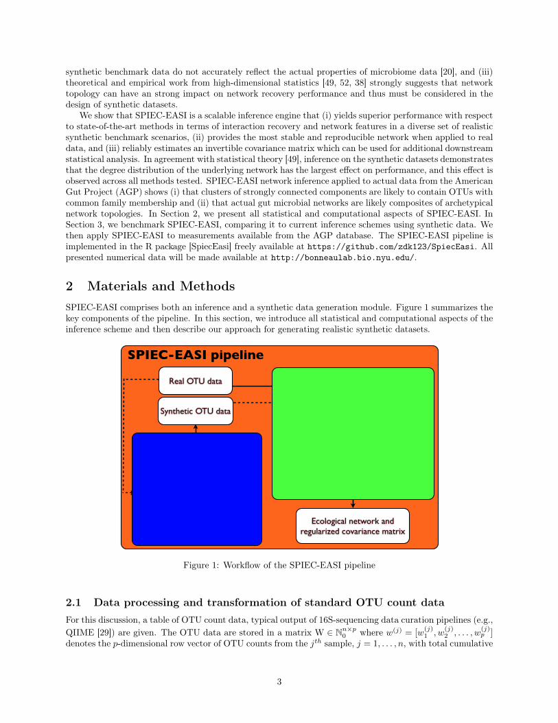
2 Materials and MethodsSPIEC-EASI comprises both an inference and a synthetic data generation module. Figure 1 summarizes thekey components of the pipeline. In this section, we introduce all statistical and computational aspects of theinference scheme and then describe our approach for generating realistic synthetic datasets.

Real OTU data

Graphical model generator

Synthetic OTU data

Marginal fitting

Data processing and CLR transformation

Neighborhood selection

Inverse Covariance Selection

Stability-based model selection

Ecological network and regularized covariance matrix

Synthetic data generation

Network inference

SPIEC-EASI pipeline

NORmal To Anything

Figure 1: Workflow of the SPIEC-EASI pipeline

2.1 Data processing and transformation of standard OTU count dataFor this discussion, a table of OTU count data, typical output of 16S-sequencing data curation pipelines (e.g.,QIIME [29]) are given. The OTU data are stored in a matrix W ∈ Nn×p0 where w(j) = [w

(j)1 , w

(j)2 , . . . , w

(j)p ]

denotes the p-dimensional row vector of OTU counts from the jth sample, j = 1, . . . , n, with total cumulative

3

count m(j) =p∑i=1

w(j)i ; N0 denotes the set of natural numbers 0, 1, 2, ... As described above, to account

for sampling biases, microbiome data is typically transformed by normalizing the raw count data w(j) withrespect to the total count m(j) of the sample [34]. We thus arrive at vectors of relative abundances or

compositions, which we notate for sample j as x(j) = [w

(j)1

m(j) ,w

(j)2

m(j) , . . . ,w(j)

p

m(j) ]. Due to this normalizationOTU abundances are no longer independent, and the sample space of this p-part composition x(j) is notunconstrained Euclidean space but rather the p-dimensional unit simplex Sp .

= x |xi > 0,∑pi=1 xi = 1.

Thus, the OTU sample compositions from n samples are constrained to lie in the unit simplex, X ∈ Sn×p. Thisrestriction of the data to the simplex prohibits the application of standard statistical analysis techniques,such as linear regression or empirical covariance estimation. Covariance matrices of compositional dataexhibit, for instance, a negative bias due to closure effects.

Major advances in the statistical analysis of compositional data were achieved by Aitchison in the 1980’s[1, 2]. Rather than considering compositions in the simplex, Aitchison proposed log-ratios, log[ xi

xj], as a

basis for studying compositional data. The simple equivalence log[ xi

xj] = log[wi/m

wj/m] = log[wi

wj] implies that

statistical inferences drawn from analysis of log-ratios of compositions are equivalent to those that could bedrawn from the log-ratios of the unobserved absolute measurements, also termed the basis.

Aitchison also proposed several statistically equivalent log-ratio transformations to remove the unit-sumconstraint of compositional data [1]. Here we apply the centered log-ratio (clr) transform:

z.= clr(x) = [log(x1/g(x)), ..., log(xp/g(x)] = [log(w1/g(w)), ..., log(wp/g(w))] (1)

where g(x) =

[p∏i=1

xi

]1/p

is the geometric mean of the composition vector. The clr transform is symmetric

and isometric with respect to the component parts. The resulting vector z is constrained to a zero sum.The clr transform maps the data from the unit simplex to a p − 1-dimensional Euclidean space, and thecorresponding population covariance matrix Γ = Cov [clr(X)] ∈ Rp×p is also singular [1]. The covariancematrix Γ is related to the population covariance of the log-transformed absolute abundances Ω = Cov [logW]via the relationship [2]:

Γ = GΩG (2)

where G = Ip − 1pJ, Ip is the p-dimensional identity matrix, and J = [j1, j2, . . . , ji, jp], ji = [1, 1, . . . , 1] the

p-dimensional all-ones vector. In the present high-dimensional data, p >> 0, the matrix G is close to theidentity matrix, and thus we can assume that a finite sample estimator Γ of Γ serves as a good approximationof Ω. This approximation serves as the basis of our network inference scheme. Finally, becasue real-worldOTU data often contain samples with a zero count for low-abundance OTUs, we add a unit pseudocount tothe original count data to avoid numerical problems with the clr transform.

2.2 Inference of microbial interactions from microbial abundance datasetsOur key objective is to learn a network of pairwise taxon-taxon interactions from clr-transformed microbiomecompositions Z ∈ Rn×p. We represent the interaction network as an an undirected, weighted graph G =(V,E), where the vertex set V = v1, . . . , vp represents the p taxa (e.g., OTUs) and the edge set E ⊂ V ×Vthe possible interactions among them. Our formal approach is to learn a probabilistic graphical model [27] (i)that is consistent with the observed data and (ii) for which the (unknown) graph G encodes the conditionaldependence structure between the random variables (in our case, the observed taxa). Graphical modelsover undirected graphs (also known as Markov networks or Markov Random Fields) have a straightforwarddistributional interpretation when the data are drawn from a probability distribution π(x) that belongsto an exponential family [32, 55]. For example, when the data are drawn from a multivariate normaldistribution π(x) = N (x|µ,Σ) with mean µ and covariance Σ, the non-zero elements of the off-diagonalentries of the inverse covariance matrix Θ = Σ−1, also termed the precision matrix, defines the adjacencymatrix of the graph G and thus describes the factorization of the normal distribution into conditionallydependent components [27]. Conversely, if and only if an entry in Θ: Θi,j = 0, then the two variables areconditionally independent, and there is no edge between vi and vj in G. Inferring the exact underlyinggraph structure in the presence of a finite amount of samples is, in general, intractable. However, two

4

types of statistical inference procedures have been useful in high-dimensional statistics due to their provableperformance guarantees under assumptions about the sample size n, dimensionality p, underlying graphproperties, and the generating distribution[48, 49]. The first approach, neighborhood selection [44, 48], aimsat reconstructing the interaction graph on a node-by-node basis where, for each node, a penalized regressionproblem is solved. The second approach is the penalized maximum likelihood method [5, 19], where theentire graph is reconstructed by solving a global optimization problem, the so-called covariance selectionproblem [14]. The key advantages of these approaches are that (i) their underlying inference procedurescan be formulated as convex (and hence tractable) optimization problems, and (ii) they are applicable evenin the underdetermined regime (p > n), provided that certain structural assumptions about the underlyinggraph hold. One assumption is that the true underlying graph is reasonably sparse, i.e., that the numberof edges e = O(p), or, particularly, the number of taxon-taxon interactions only scale linearly with only thenumber of measured taxa.

Graphical model inference. The SPIEC-EASI pipeline comprises two types of inference schemes, neigh-borhood and covariance selection. The neighborhood selection framework, introduced by Meinshausen andBühlmann [44] and thus often referred as the MB method, tackles graph inference by solving p regularizedlinear regression problems, leading to local conditional independence structure predictions for each node.Let us denote the ith column of the data matrix Z by Zi ∈ Rn and the remaining columns by Z¬i ∈ Rn×p−1.For each node vi, we solve the following convex problem:

βi,λ = arg minβ∈Rp−1

(1

n‖Zi − Z¬iβ‖2 + λ‖β‖1

), (3)

where ‖a‖1 =∑p−1i=1 |ai| denotes the L1 norm, and λ ≥ 0 is a scalar tuning parameter. This so-called

LASSO problem [53] aims at balancing the least-square fit and the number of necessary predictors (thenon-zero components βj of β) by tuning the λ parameter. We define the local neighborhood of a node vias Nλ

i = j ⊂ 1, . . . p \ i : βi,λj 6= 0. The final edge set E of G can be defined via the intersection or theunion operation of the local neighborhoods. An edge ei,j between node vi and vj exists if j ∈ Nλ

i ∩ i ∈ Nλj or

j ∈ Nλi ∪i ∈ Nλ

j . For edges in the set j ∈ Nλi ∩i ∈ Nλ

j , the edge weights, ei,j and ej,i, are estimated using theaverage of the two corresponding β entries. From a theoretical point of view, both edge selection choices areasymptotically consistent under certain technical assumptions [44]. The choice of the λ parameter controlsthe sparsity of the local neighborhood selection, which requires tuning [33]. We present our parameterselection strategy at the end of this section.

The second inference approach, (inverse) covariance selection, relies on the following penalized maximumlikelihood approach. In the standard Gaussian setting, the related convex optimization problem reads:

Θ = arg minΘ∈PD

(− log det(Θ) + tr(ΘΣ) + λ ‖Θ‖1

), (4)

where PD denotes the set of symmetric positive definite matrices A : xTAx > 0, ∀x ∈ Rp, Σ the empiricalcovariance estimate, ‖ · ‖1 the element-wise L1 norm, and λ ≥ 0 a scalar tuning parameter. For λ = 0, theexpression is identical to the maximum likelihood estimate of a normal distribution N (x|0,Σ). For non-zeroλ, the objective function (also referred as the graphical Lasso [19]) encourages sparsity in the underlyingprecision matrix Θ. The non-zero, off-diagonal entries in Θ define the adjacency matrix of the interactiongraph G which, similar to MB, depends on the proper choice of the penalty parameter λ. Originally,this estimator was shown to have theoretical guarantees on consistency and recovery only under normalityassumptions [31]. However, recent theoretical [49, 39] work shows that distributional assumptions can beconsiderably relaxed, and the estimator is applicable to a larger class of problems, including inference ondiscrete (count) data. In addition, nonparametric approaches, such as sparse additive models, can be used to“gaussianize" the data prior to network inference [36]. We thus propose the following estimator for inferringmicrobial ecological interactions. Given clr-transformed OTU data Z ∈ Rn×p, we propose the modifiedoptimization problem:

Ω−1 = arg minΩ−1∈PD

(− log det(Ω−1) + tr(Ω−1Γ) + λ

∥∥Ω−1∥∥

1

), (5)

5

where Γ is the empirical covariance estimate of Z, and Ω−1 is the inverse covariance (or precision matrix) ofthe underlying (unknown) basis. As stated above, Γ will be a good approximation for the basis covariancematrix Ω because p >> 0. The resulting solution is constrained to the set of PD matrices, ensuring that thepenalized estimator has full rank p. The non-zero off-diagonal entries of the estimated matrix Ω−1 definethe inferred network G, and their values are the signed edge weights of the graph. To reduce the variance ofthe estimate, the covariance matrix Γ also can be replaced by the empirical correlation matrix R = DΓD,where D is a diagonal matrix that contains the inverse of the estimated element-wise standard deviations γi.

The covariance selection approach has two advantages over the neighborhood selection framework. First,we obtain unique weights associated with each edge in the network. No averaging or subsequent edgeselection is necessary. Second, the covariance selection framework provides invertible precision and covariancematrix estimates that can be used in further downstream microbiome analysis tasks, such as regression anddiscriminant analysis [34].

Model selection. For both neighborhood and covariance selection, the tuning parameter λ ∈ [0, λmax]controls the sparsity of the final model. Rather than inferring a single graphical model, both methods producea λ-dependent solution path with the complete and the empty graph as extreme networks. A number ofmodel selection criteria, such as Bayesian Information Criteria [59] and resampling schemes [25], have beenused. Here we use a popular model selection scheme known as the Stability Approach to RegularizationSelection (StARS) [37]. This method repeatedly takes random subsamples (80% in the standard setting) ofthe data and estimates the entire graph solution path based on this subsample. For each subsample, theλ-dependent incidence frequencies of individual edges are retained, and a measure of overall edge stabilityis calculated. StARS selects the λ value at which subsampled non-empty graphs are the least variable(most stable) in terms of edge incidences. For the selected graph, the observed edge frequencies indicate thereproducibility of the inferred edges, implying an edge is predicted from unseen data, and be used to rankedges according to confidence.

Theoretical and computational aspects. Learning microbial graphical models with neighborhood orinverse covariance selection schemes has important theoretical and practical advantages over current methods.A wealth of theoretical results are available that characterize conditions for asymptotic and finite sampleguarantees for the estimated networks [44, 31, 59, 48, 49]. Under certain model assumptions, the numberof samples n necessary to infer the true topology of the graph in the neighborhood selection framework isknown to scale as n = O(d3 log(p)), where d is the maximum vertex (or node) degree of the underlyinggraph (i.e. the maximum size of any local neighborhood). Additional assumptions on the sample covariancematrices reduce the scaling to n = O(d2 log(p)) [48]. This implies that graph recovery and precision matrixestimation is indeed possible even in the p >> n regime, and that the underlying graph topology stronglyimpacts edge recovery. The latter observation means that, even if the number of interactions e is constant,graphs with large hub nodes, perhaps representing keystone species in microbial networks, or, more generally,scale-free graphs with a few highly connected nodes will be more difficult to recover than networks withmore evenly distributed neighborhoods (we provide an in-depth analysis of this effect in an independentcontribution [45]). In addition to these theoretical results, a second advantage is that well-established,efficient, and scalable implementations are available to infer microbial interaction networks from OTU datain practice. Thus, SPIEC-EASI methods will efficiently scale as microbiome dataset dimensions grow (e.g.,due to technological advances that increase the number of OTUs detected per sample). The SPIEC-EASIinference engine relies on the R package huge [60], which includes algorithms to solve neighborhood andcovariance selection problems [44, 19], as well as the StARS model selection.

2.3 Generation of synthetic microbial abundance datasetsEstimating the absolute and comparative performance of network inference schemes from biological dataremains a fundamental challenge in biology. In the context of gene regulatory network inference, recentcommunity-wide efforts, such as the DREAM (Dialogue for Reverse Engineering Assessments and Methods)Challenges (http://www.the-dream-project.org/), have considerably advanced our understanding aboutfeasibility, accuracy, and applicability of a large number of developed methods. In the DREAM challenges,both real data from “gold standard" regulatory networks (e.g., networks where the true topology is known

6

from independent experimental evidence) and realistic in-silico data (using, e.g., the GeneNetWeaver pipeline[50]) are included. In the context of 16S microbiome data and microbial interaction networks, neither a goldstandard nor a realistic synthetic data generator exist. SPIEC-EASI is accompanied by a set of computationaltools that allow the generation of realistic synthetic OTU data. As outlined in Figure 1, real taxa countdata serve as input to SPIEC-EASI’s synthetic data generation pipeline. The pipeline enables one to: (i) fitthe marginal distributions of the count data to a parametric statistical model and (ii) specify the underlyinggraphical model architecture (e.g., scale-free).

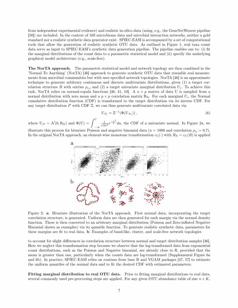
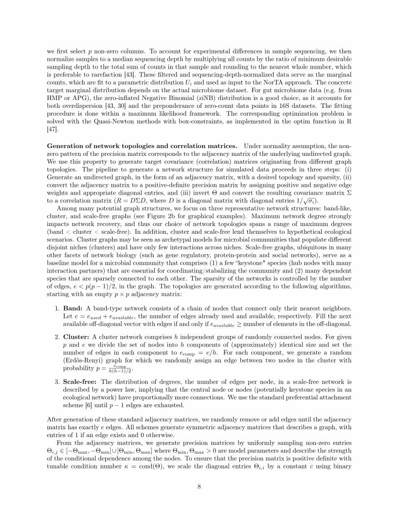
The NorTA approach. The parametric statistical model and network topology are then combined in the’Normal To Anything’ (NorTA) [46] approach to generate synthetic OTU data that resemble real measure-ments from microbial communities but with user-specified network topologies. NorTA [46] is an approximatetechnique to generate arbitrary continuous and discrete multivariate distributions, given (1) a target cor-relation structure R with entries ρi,j and (2) a target univariate marginal distribution Ui. To achieve thistask, NorTA relies on normal-copula functions [46, 41, 10]. A n × p matrix of data U is sampled from anormal distribution with zero mean and a p × p correlation matrix RN. For each marginal Ui, the Normalcumulative distribution function (CDF) is transformed to the target distribution via its inverse CDF. Forany target distribution P with CDF Ξ, we can thus generate multivariate correlated data via

UPi= Ξ−1(Φ(UNi

)) , (6)

where UN ∼ N (0,RN) and Φ(U) =

ˆ U

−∞

1√2σ2

e−u2

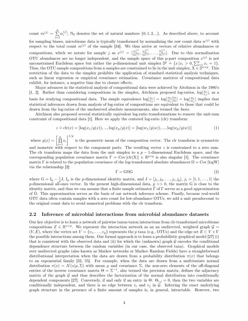
2 du, the CDF of a univariate normal. In Figure 2a, we

illustrate this process for bivariate Poisson and negative binomial data (n = 1000 and correlation ρij = 0.7).In the original NorTA approach, an element-wise monotone transformation cU(·) with RN = cU(R) is applied

a

b

Figure 2: a: Bivariate illustration of the NorTA approach. First normal data, incorporating the targetcorrelation structure, is generated. Uniform data are then generated for each margin via the normal densityfunction. These is then converted to an arbitrary marginal distribution (Poisson and Zero-inflated NegativeBinomial shown as examples) via its quantile function. To generate realistic synthetic data, parameters forthese margins are fit to real data. b: Examples of band-like, cluster, and scale-free network topologies

to account for slight differences in correlation structure between normal and target distribution samples [46].Here we neglect this transformation step because we observe that the log-transformed data from exponentialcount distributions, such as the Poisson and Negative binomial, are already close to R, provided that themean is greater than one, particularly when the counts data are log-transformed (Supplemental Figure 6aand 6b). In practice, SPIEC-EASI relies on routines from base R and VGAM packages [47, 57] to estimatethe uniform quantiles of the normal data and to fit the desired CDF with estimated parameters.

Fitting marginal distribution to real OTU data. Prior to fitting marginal distributions to real data,several commonly used pre-proccesing steps are applied. For any given OTU abundance table of size n×K,

7

we first select p non-zero columns. To account for experimental differences in sample sequencing, we thennormalize samples to a median sequencing depth by multiplying all counts by the ratio of minimum desirablesampling depth to the total sum of counts in that sample and rounding to the nearest whole number, whichis preferable to rarefaction [43]. These filtered and sequencing-depth-normalized data serve as the marginalcounts, which are fit to a parametric distribution Ui and used as input to the NorTA approach. The concretetarget marginal distribution depends on the actual microbiome dataset. For gut microbiome data (e.g. fromHMP or APG), the zero-inflated Negative Binomial (ziNB) distribution is a good choice, as it accounts forboth overdispersion [43, 30] and the preponderance of zero-count data points in 16S datasets. The fittingprocedure is done within a maximum likelihood framework. The corresponding optimization problem issolved with the Quasi-Newton methods with box-constraints, as implemented in the optim function in R[47].

Generation of network topologies and correlation matrices. Under normality assumption, the non-zero pattern of the precision matrix corresponds to the adjacency matrix of the underlying undirected graph.We use this property to generate target covariance (correlation) matrices originating from different graphtopologies. The pipeline to generate a network structure for simulated data proceeds in three steps: (i)Generate an undirected graph, in the form of an adjacency matrix, with a desired topology and sparsity, (ii)convert the adjacency matrix to a positive-definite precision matrix by assigning positive and negative edgeweights and appropriate diagonal entries, and (iii) invert Θ and convert the resulting covariance matrix Σto a correlation matrix (R = DΣD, where D is a diagonal matrix with diagonal entries 1/

√σi).

Among many potential graph structures, we focus on three representative network structures: band-like,cluster, and scale-free graphs (see Figure 2b for graphical examples). Maximum network degree stronglyimpacts network recovery, and thus our choice of network topologies spans a range of maximum degrees(band < cluster < scale-free). In addition, cluster and scale-free lend themselves to hypothetical ecologicalscenarios. Cluster graphs may be seen as archetypal models for microbial communities that populate differentdisjoint niches (clusters) and have only few interactions across niches. Scale-free graphs, ubiquitous in manyother facets of network biology (such as gene regulatory, protein-protein and social networks), serve as abaseline model for a microbial community that comprises (1) a few “keystone" species (hub nodes with manyinteraction partners) that are essential for coordinating/stabalizing the community and (2) many dependentspecies that are sparsely connected to each other. The sparsity of the networks is controlled by the numberof edges, e < p(p− 1)/2, in the graph. The topologies are generated according to the following algorithms,starting with an empty p× p adjacency matrix:

1. Band: A band-type network consists of a chain of nodes that connect only their nearest neighbors.Let e = eused + eavailable, the number of edges already used and available, respectively. Fill the nextavailable off-diagonal vector with edges if and only if eavailable ≥ number of elements in the off-diagonal.

2. Cluster: A cluster network comprises h independent groups of randomly connected nodes. For givenp and e we divide the set of nodes into h components of (approximately) identical size and set thenumber of edges in each component to ecomp = e/h. For each component, we generate a random(Erdös-Renyi) graph for which we randomly assign an edge between two nodes in the cluster withprobability p =

ecomph(h−1)/2 .

3. Scale-free: The distribution of degrees, the number of edges per node, in a scale-free network isdescribed by a power law, implying that the central node or nodes (potentially keystone species in anecological network) have proportionally more connections. We use the standard preferential attachmentscheme [6] until p− 1 edges are exhausted.

After generation of these standard adjacency matrices, we randomly remove or add edges until the adjacencymatrix has exactly e edges. All schemes generate symmetric adjacency matrices that describes a graph, withentries of 1 if an edge exists and 0 otherwise.

From the adjacency matrices, we generate precision matrices by uniformly sampling non-zero entriesΘi,j ∈ [−Θmax,−Θmin]∪ [Θmin,Θmax] where Θmin,Θmax > 0 are model parameters and describe the strengthof the conditional dependence among the nodes. To ensure that the precision matrix is positive definite withtunable condition number κ = cond(Θ), we scale the diagonal entries Θi,i by a constant c using binary

8

search. The precision matrix Θ is then converted to a correlation matrix R to be used as input to the NorTAapproach.

3 Network inference on synthetic microbiome dataGiven that no large-scale experimentally validated microbial ecological network exists, we use SPIEC-EASI’sdata generator capabilities to synthesize data whose OTU count distributions faithfully resemble micro-biome 16s data. By varying parameters known to influence network recovery (network topology, interactionstrength, sample number) and quantifying performance on resulting networks, we rigorously assess SPIEC-EASI inference relative to state-of-the-art inference methods, SparCC [20] and CCREPE [22], as well asstandard Pearson correlation.

3.1 Benchmark setupWe modeled the synthetic datasets on American Gut Project data using SPIEC-EASI’s data generationmodule. The count data, accessed February, 2014 at www.microbio.me/qiime, come from two samplingrounds and comprise several thousand OTUs. Round 1 data contains n1 = 304, and Round 2 data containsn2 = 254 samples. As filtering steps, OTUs were removed from the input data if present in fewer than 37% ofthe samples, while samples were removed if total sequencing depth fell below the 1st quartile (10,800 sequencereads). Thus, we arrived at a total of p = 205 distinct OTUs. We also generated smaller-dimensional datasets(p = 68) with fewer zero counts by requiring that OTUs be present in > 60% of the samples. We used Round1 data and fit the n1 count histograms to a ziNB distribution. The empirical effective number neff is 13.5for p = 205 and 7.5 for p = 68 data. The resulting parametrized marginal distributions served as input toNorTA.

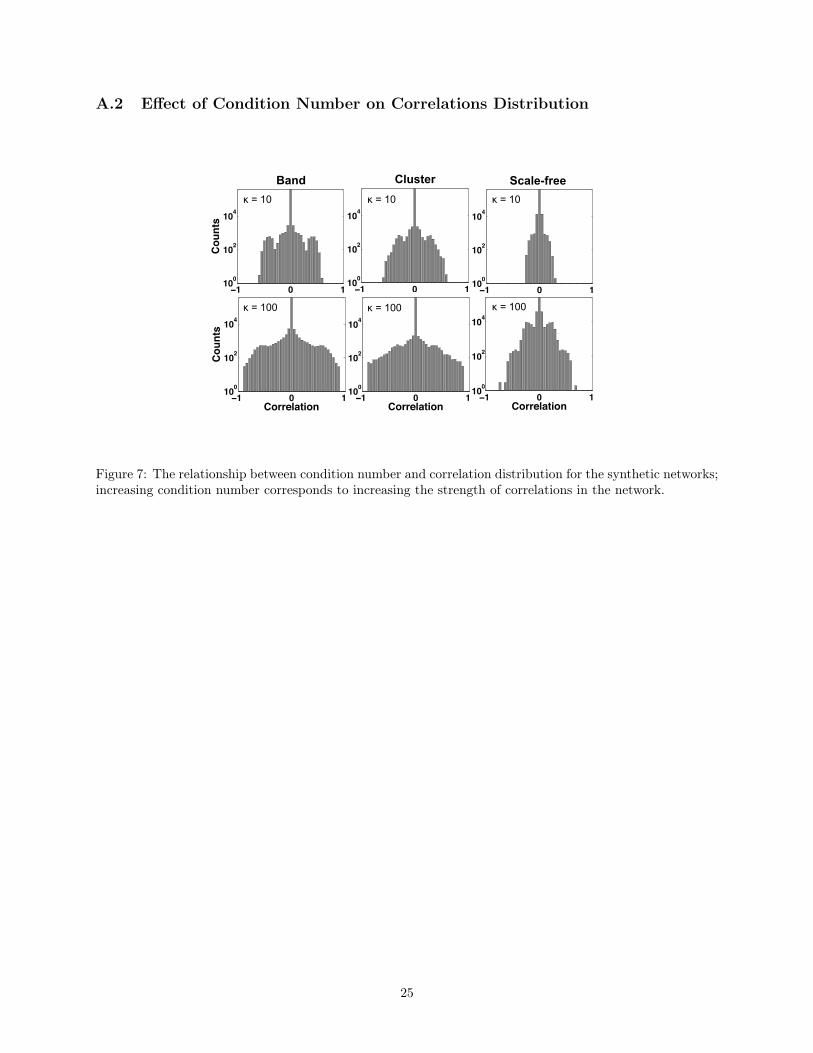
As described above, network topology is expected to influence network recovery; thus, we consider thethree previously described topologies (band-like, cluster, and scale-free) as representative microbial interac-tion networks. We hypothesize that any method that successfully infers the sets of interactions underlyingthese archetypal networks from synthetic datasets is likely to also perform well in the context of true micro-biomes, whose underlying network architecture is unknown but expected to be a mixture of these networktypes. For all networks, we fix the total number of edges e to the respective number of OTUs p, and weanalyze a medium (p = 68) and a high-dimensional scenario (p = 205). Microbial interaction strength iscontrolled by the range of values in off-diagonal entries in the precision matrices Θ and the condition numberκ = cond(Θ). We use Θmin = 2 and Θmax = 3 with either condition number κ = 10 or 100. In this set-ting, κ controls the spread of the absolute correlation values (and thus the strength of indirect interactions)present in the synthetic data. The relationship between condition number and distribution of correlation isillustrated in Supplemental Figure 7. For each network type and size, we generate 20 distinct instances. Foreach instance, we then use the NorTA approach to generate a maximum of n = 1360 synthetic microbialcount data samples. To assess the effect of sample size on network recovery, we test methods on a range ofsample sizes: n = 34, 68, 102, 1360.

We compare SPIEC-EASI’s covariance selection method (referred to as S-E(glasso)) and neighborhoodselection method (referred to as S-E(MB)) to SparCC and CCREPE, methods which were also designedto be robust to compositional artifacts. As a baseline reference, we also compared all methods to Pearsoncorrelation, which is neither compositionally robust nor appropriate for estimating correlation in the under-determined regime. Both of these methods, however, infer interactions from correlations and do not considerthe concept of conditional independence. We improved the runtime of the original SparCC implementation(available at https://bitbucket.org/yonatanf/sparcc) and include the updated code in our SPIEC-EASIpackage. The CCREPE implementation is downloaded from http://www.bioconductor.org/packages/release/bioc/html/ccrepe.html.

3.2 Recovery of microbial interactionsTo quantify each method’s ability to recover the true underlying interaction network, we evaluated per-formance in terms of precision-recall (P-R) curves and area under P-R curves (AUPR). For each method,we ranked edge predictions according to confidence. For SparCC, CCREPE and Pearson correlation, edge

9

predictions were ranked according to p-value. SPIEC-EASI edge pedictions were ranked according to edgestability, inferred by StARS model selection step at the most stable tuning parameter λStARS. Figure 3summarizes methods’ performance on 960 independent synthetic datasets for a total of 48 conditions (4samples sizes × 2 conditions numbers × 3 network topologies × 2 dimensions).

We observe the following key trends. First, the performance of all methods improves with increasingsample size. Under certain scenarios, even near-perfect recovery (AUPR ≈ 1) is possible in the large samplelimit (n = 1360). Second, all methods show a clear dependence on the network topology. Best performanceis achieved for band graphs, followed by cluster and scale-free graphs. These results are consistent withtheoretical results [49], which show that the maximum node degree d reduces the probability of correctlyinferring network edges for fixed sample size (scale-free networks have highest maximum degree, followed bycluster and then band.) Third, for most scenarios, the SPIEC-EASI methods, particularly S-E(MB), performas well or significantly better than all control methods. Standard Pearson correlation is outperformed byall methods that take the compositional nature of the data into account. Forth, in the large sample limit(n = 1360), S-E(MB) is the only method that recovers a significant portion of edges under all tested scenarios(particularly scale-free networks). The present results suggest that complete interaction recovery is likelyan unrealistic goal for microbiome studies, given that most studies have at most hundreds of samples. Inaddition, the P-R curves are based on ranking predicted edges. To generate a final network, confidence-basedcriteria must be applied to select a final set of edges for network inclusion, and, to date, no optimal selectionprocess exists. Nonetheless, if we focus on the set of high-confidence interactions (i.e. the top-ranked entriesin the edge list), we see that S-E methods, particularly S-E(MB), can achieve very high precision for allnetwork types (see lower panel in Figure 3 for a representative P-R curve).

10

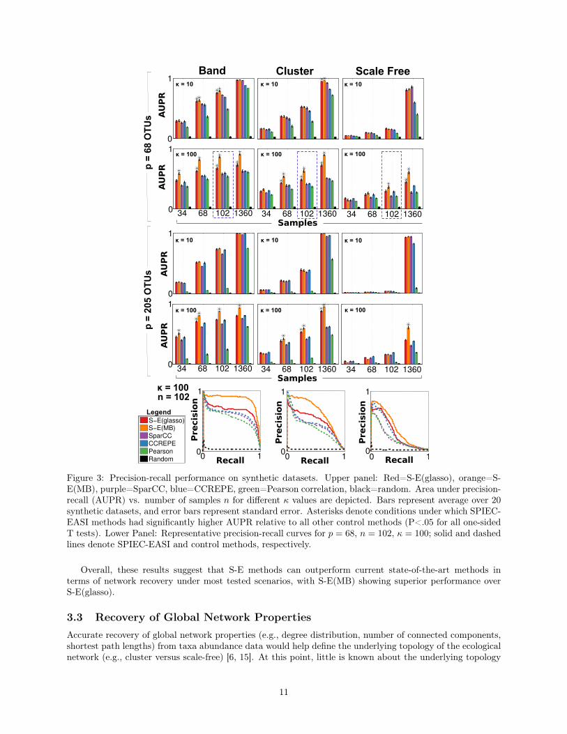
Figure 3: Precision-recall performance on synthetic datasets. Upper panel: Red=S-E(glasso), orange=S-E(MB), purple=SparCC, blue=CCREPE, green=Pearson correlation, black=random. Area under precision-recall (AUPR) vs. number of samples n for different κ values are depicted. Bars represent average over 20synthetic datasets, and error bars represent standard error. Asterisks denote conditions under which SPIEC-EASI methods had significantly higher AUPR relative to all other control methods (P<.05 for all one-sidedT tests). Lower Panel: Representative precision-recall curves for p = 68, n = 102, κ = 100; solid and dashedlines denote SPIEC-EASI and control methods, respectively.

Overall, these results suggest that S-E methods can outperform current state-of-the-art methods interms of network recovery under most tested scenarios, with S-E(MB) showing superior performance overS-E(glasso).

3.3 Recovery of Global Network PropertiesAccurate recovery of global network properties (e.g., degree distribution, number of connected components,shortest path lengths) from taxa abundance data would help define the underlying topology of the ecologicalnetwork (e.g., cluster versus scale-free) [6, 15]. At this point, little is known about the underlying topology

11

of microbial ecological networks, but, as elaborated in Section 5, such information could be incorporated asa constraint into SPIEC-EASI’s inference methods, thereby further improving prediction. Thus, we testedhow well SPIEC-EASI and other methods recover global network properties from the synthetic datasets andevaluate whether these methods might be able to provide insight into global network architecture, perhapseven in the underdetermined regime, where the prediction of individual edges is less accurate. To controlfor the disparate means by which individual methods ranked edge confidences (e.g., stability for the SPIEC-EASI methods, estimation of p-values for SparCC, Pearson and CCREPE), for each synthetic dataset andmethod, final networks were generated by selecting the top 205 predicted edges and comparing to the truesynthetic network topologies for p = 205 OTUs.

We first consider (node) degree distributions, where node degree is defined as the number of edges eachnode has. In Figure 4, we show the empirical degree distribution and the underlying ground truth for allmethods and networks types, n = 1360 and κ = 100. Scale-free networks are characterized by exponentialdegree distributions, in which few nodes (e.g., hubs and, in our context, potential keystone taxa) have veryhigh degree (e.g., interact with other taxa), while most nodes/taxa have few interactions. In contrast, nodes incluster networks have relatively even degree, which depends on cluster size. In the ecological context, clusternetworks would be consistent with niche communities that share few interactions with microbiota outsideof one’s niche community; this structure is also be reflected in degree distributions. Using Kullback-Leibler(KL) divergence to measure the dissimilarity between methods’ predicted degree distributions and the truedegree distribution we see that S-E(MB) outperforms all other methods in recovering degree distributions(Figure 4). This performance improvement also holds for smaller samples sizes.

12

0

0.5

1

1.5

2

2.5

3

3.5

*********

KL−

Div

erge

nce

Degree: Band (1360, 100)

S−E(

glas

so)

S−E(

MB

)

Spar

CC

CC

REP

E

Pear

son

0

0.2

0.4

0.6

0.8

1

******

******

******

Degree: Cluster (1360, 100)

S−E(

glas

so)

S−E(

MB

)

Spar

CC

CC

REP

E

Pear

son

0

1

2

3

4

5

6

7 **** ** *****

Degree: Scale−free (1360, 100)

S−E(

glas

so)

S−E(

MB

)

Spar

CC

CC

REP

E

Pear

son

Ban

d C

lust

er

Scal

e-fr

ee

Degree Degree Degree Degree Degree

Figure 4: Upper panels: Predicted degree distributions (colored) are overlaid with the true degree distri-bution (white) for n = 1360 samples, p = 205 OTUs, κ = 100. Lighter shades correspond to regions ofoverlap between predicted and true distributions. Dissimilarity between the distributions is measured by KLdivergence, DKL. Lower panels: Bars represent the average DKL over three independent sets of syntheticdatasets (7 datasets per set); error bars represent standard error. Divergences were compared between S-Eand control methods using one-sided T-tests; ***,**,* correspond to P<.001,.01, and .05.

Another common topological feature is betweenness centrality, which, similar to degree, betweennesscentrality can be used to gauge the relative importance of a node (e.g., taxon) to the (ecological) network.

13

Betweenness centrality, as the fraction of shortest paths between all other nodes in the network that containthe given node, highlights central nodes. The distribution of nodes’ betweenness centrality provides informa-tion about the network architecture (Supplemental Figure 8). Specifically, scale-free networks are expectedto have a few nodes with very high betweenness centrality that connect most other nodes to each other; inscale-free networks, betweenness centrality can near unity. For cluster networks, the maximum betweennesscentrality is limited by the total number of independent clusters. In band networks, similar to scale-free, allnodes are connected; however, the degree is fixed and so the betweenness centrality distribution is roughlyuniform from zero to one. For smaller sample sizes n < 1360, no method dominates. However, for thelargest sample size, n = 1360, S-E(MB) is again significantly better than all other methods for five out of sixconditions with the exception of scale-free networks κ = 10, where SparCC recovery is best (SupplementalFigure 9).

We next consider distributions over graph geodesic distances. The geodesic distance is the length ofthe shortest path between two nodes. Given the existence of highly connected hubs in scale-free networks,geodesic distances for scale-free networks tend to be short, a feature that is described as the "small-world"property. Thus, the geodesic distributions in the scale-free network are a lot smaller than for the bandand cluster networks (Supplemental Figure 10). In recovery of geodesic distance distributions, S-E(MB)performs equivalently or significantly better than all other methods for scale-free networks as well as bandgraphs across all conditions. For cluster networks, the other methods generally outperform SPIEC-EASImethods for smaller sample sizes (n < 1360). In the large sample limit n = 1360, S-E(MB) has significantlybetter recovery of geodesic distance distributions relative to all control methods, even for cluster graphs(Supplemental Figure 11).

Finally, we analyzed the number and size of connected components in the inferred graphs. While allsynthetic band and scale-free synthetic networks form a single connected component containing all nodes,cluster networks have a variable number of connected components. In terms of cluster number recovery, allmethods predicted too many connected components. Overall, S-E methods had lower error rates for bandand scale-free networks over all sample sizes. For high sample number (n = 1360), S-E(MB) had significantlybetter recover of cluster size across all network types (Supplemental Figure 12), with nearly perfect recoveryfor cluster graphs (DKL = 0, Supplemental Figure 13).

4 Inference of American Gut interactionsThus far we have used the n1 = 304 first-round AGP samples as a means to construct realistic syntheticmicrobiome data sets with SPIEC-EASI’s data generation module. In this section, we apply SPIEC-EASIinference methods to construct ecological interaction networks from the AGP data directly. Although thereis no independent means to assess the accuracy of these hypothetical networks, we can assess their repro-ducibility and consistency. For each method, we first infer a single representative network of taxon-taxoninteractions from Round 1 AGP abundance data. For SPIEC-EASI, the StARS model selection approach isused to select the final model network. For SparCC, we use a threshold ρt = 0.35 to construct a relevancenetwork from the SparCC-inferred correlation matrix; i.e. an edge between nodes vi, vj is present in theSparCC network if |ρi,j | > ρt [20]. Similarly, we use a q-value cut-off of 10−24 to create an interaction net-work from CCREPE-corrected significance scores of Pearson’s correlation coefficient [22]. For each method,we thus arrive at a reference network that can be considered the hypothetical gold standard. We then usethe n2 = 254 Round 2 AGP samples as an independent test set and learn a new model network from thesedata alone. We measure consistency between the two network models by computing the Hamming distancebetween the reference and new network models, i.e., the difference between the upper triangular part of thetwo adjacency matrices. For the present data, the Hamming distance can vary between p(p− 1)/2 = 20910(no edges in common) and a minimum of 0 for identical networks. Confidence intervals for hamming dis-tances can be obtained by combining Round 1 and 2 samples into a unified dataset, repeatedly subsamplingthese data into two disjoint groups of size n1 and n2, and repeating the entire inference procedure.

The upper left panel in Figure 5 shows network reproducibility for SPIEC-EASI methods, SparCC,and CCREPE. The S-E(MB) has smallest the Hamming distance, followed by S-E(glasso), SparCC, andCCREPE. In S-E(MB), the edge disagreement is roughly 50 with very small error bars. At the otherextreme, CCREPE edge disagreement is 250 edges and highly variable. These numerical experiments clearly

14

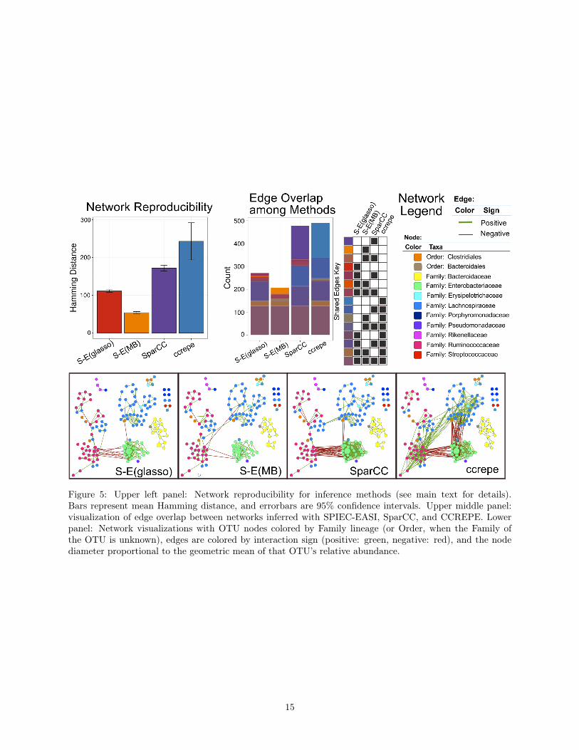
Figure 5: Upper left panel: Network reproducibility for inference methods (see main text for details).Bars represent mean Hamming distance, and errorbars are 95% confidence intervals. Upper middle panel:visualization of edge overlap between networks inferred with SPIEC-EASI, SparCC, and CCREPE. Lowerpanel: Network visualizations with OTU nodes colored by Family lineage (or Order, when the Family ofthe OTU is unknown), edges are colored by interaction sign (positive: green, negative: red), and the nodediameter proportional to the geometric mean of that OTU’s relative abundance.

15

demonstrate that SPIEC-EASI methods are more consistent in their network construction procedures thanother current methods.

Finally, we use each inference method to construct a candidate American Gut microbiome interactionnetwork from the unified dataset of size n1 + n2 = 558 (Figure 5, lower panel). We analyze the differencesbetween the reconstructed networks by quantifying the number of unique and shared predicted edges (Fig-ure 5, middle upper panel). All four methods agree on a core network that consists of 127 edges. Theseedges are mostly found within OTUs of the same taxonomic group. This phenomenon, termed assortativ-ity, has also been observed in other microbial network studies [17] Assortativity is one of the most salientfeatures of the AGP-derived networks, and, for all networks, the assortativity coefficients for each networkare close to unity (e.g., maximum assortativity, Supplemental Figure 14). The SparCC network comprisesabout twice as many edges as the SPIEC-EASI networks. SparCC infers 147 distinct edges; these additionaledges correspond to negative associations between OTUs of Ruminococcaceae (genus Faecalibacterium) andEnterobacteriacae families (various genera) and a dense web of correlations within Enterobacteriacae OTUs.Similarly, CCREPE identified 152 edges uniquely, with many negative edges between Enterobacteriaceaeand Lachnospiraceae (genera: Blautia, Roseburia and unknown); additionally, CCREPE uniquely predictedpositive edges between the Lachnospiraceae and Ruminococcaceae (genus: Faecalibacterium). Both SPIEC-EASI methods produce relatively sparse networks by comparison. S-E(glasso) infers a total of 271 total edges(with one unique edge), and S-E(MB) infers 206 edges with 25 unique edges. In scale with edge predictions,both CCREPE and SparCC infer interaction networks with large maximum degree (33 and 30, respectively),while the S-E(MB) and S-E(glasso) networks have max degree of sixteen and eight, respectively (Supple-mental Figure 14). However, even though CCREPE and SparCC predict a similar number of total edges,the global network properties are distinct. CCREPE predicts a higher maximum betweenness centrality, alarger number of nodes in the largest connected component (100), and a lower mean geodesic distance thanSparCC (data not shown).

In summary, analysis of the AGP networks suggests that the SPIEC-EASI inference schemes produce morereproducible taxon-taxon interactions than SparCC and CCREPE and infer considerably sparser model net-works than the other two methods. These observations may be explained as follows: SparCC and CCREPEaim to recover correlation networks, which contain both direct edges as well as indirect (e.g., spurious) edges(due to correlation alone). SparCC and CCREPE may recover indirect edges less robustly than direct edges,an explanation that would be consistent with the Hamming distance reproducibility analysis. In addition, allmethods’ resulting networks suggest that the topology of the American Gut interaction network cannot beattributed to a specific network class. Instead, these networks are a mixture of band, scale-free, and clusternetwork type, and they exhibit high phylogenetic assortativity within highly connected components.

5 Discussion and conclusionInferring interactions among different microbial species within a community and understanding their influenceon the environment is of central importance in ecology and medicine [16, 40]. An ever increasing numberof recent metagenomic sequencing studies have uncovered strong correlations between microbial communitycomposition and environment in diverse and highly relevant domains of life [23, 12, 13, 22, 34, 51]. Thesestudies alone underscore the need to understand how the microbial communities adapt, develop, and interactwith the environment [18]. Elucidation of species interactions in microbial communities across differentenvironments remains, however, a formidable challenge. Foremost, available high-throughput experimentaldata are compositional in nature, overdispersed, and usually underdetermined with respect to statisticalinference. In addition, for most microbes few to no ecological interactions are known, thus the ecologicalinteraction network must be constructed de novo, in the absence of guiding assumptions and a set of "goldstandard" interactions for validation.

To overcome both challenges, we present SPIEC-EASI (Sparse InversE Covariance Estimation forEcological Association Inference), a computational pipeline that includes statistical methods for the inferenceof microbial ecological interactions from 16S sequencing datasets and a sophisticated synthetic microbiomedata generator with controllable underlying species interaction topology. SPIEC-EASI’s inference engine in-cludes two well-known graphical model estimators, neighborhood selection [44] and sparse inverse covarianceselection [59, 5, 19] that are extended by compositionally robust data transformations for application to the

16

specific context of microbial abundance data.The synthetic data pipeline was used to generate realistic-looking gut microbiome datasets for a controlled

benchmark of SPIEC-EASI’s inference performance relative to two state-of-the-art methods, SparCC [20]and CCREPE [22]. We showed that neighborhood selection (S-E(MB)) outperforms SparCC and CCREPEin terms of recovery of taxon-taxon interactions and global network topology features under almost all testedbenchmark scenarios, while covariance selection (S-E(glasso)) performs competitively with and sometimesbetter than SparCC and CCREPE.

Through our simulation study, we demonstrate that several other factors, in addition to total number ofsamples, affect network recovery. Foremost and in agreement with theoretical results from high-dimensionalstatistics [48, 49, 52], network topology has a significant impact, as network recovery performance is nearlydoubled from scale-free to cluster to band (Figure 3) for fixed sample size, number of taxa, and conditionnumber. We also demonstrated dependence to strength of direct interactions (and thus strength of corre-lations) within a given network. Our simulation study provides the community with rough guidelines forrequisite sample sizes, given state-of-the-art network inference and basic assumptions about the underlyingnetwork. This is of obvious importance to experimental design and the estimation of statistical power [45].Here, we used the synthetic data pipeline to generate datasets characteristic of the gut microbiome. However,the SPIEC-EASI data generator is generic and therefore enables researchers to generate synthetic datasetsthat resemble microbiome samples in terms of taxa dispersion and marginal distributions from their field ofresearch, such as soil or sea water ecosystems [23].

Our application study on real American Gut Project (AGP) data revealed that inference with SPIEC-EASI produced more consistent and sparser interaction networks than SparCC and CCREPE. In addition,our AGP network analysis revealed several biologically relevant observations. Specifically, we observedthat OTUs were more likely to interact with phylogenetically related OTUs (Lower panel in Figure 5 andSupplementary Figure 14). In addition, our gut microbial interaction networks appear to be a composite ofnetwork types, as we find evidence for scale-free, band-like, and cluster subnetworks.

An important advantage of neighborhood and covariance selection as underlying inference frameworks istheir ability to include prior knowledge about the underlying data or network structure from independentscientific studies in a principled manner. For example, in the neighborhood selection scheme, the standardLASSO approach can be augmented by a group penalty [58] that takes into account a priori known groupstructure. The assortativity observed in our gut microbial interaction networks suggests that such a groupingof OTUs based on phylogenetic relationship might improve inference. Moreover, if verified species interactionsare available for a certain microbial contexts, this knowledge can be included in covariance and neighborhoodselection by relaxing the penalty term on these interactions. This strategy has already been fruitfully appliedto inference of similarly high-dimensional transcriptional regulatory networks [24]. Finally, in agreement withtheoretical and empirical work in high-dimensional statistics, our synthetic benchmark results confirmed thatnetworks with scale-free structures elude accurate inference even if the underlying network is globally sparse.Recent modified neighborhood [52] and covariance selection [38] schemes improve recovery of scale-freenetworks and can be conveniently included into SPIEC-EASI.

Finally, although the main focus of this work is inference of microbial interaction networks, estimationof the regularized inverse covariance matrix with S-E(glasso) will be key to addressing several other impor-tant questions arising from microbiome studies. For example, statistical methods to infer which taxa areresponsive to design factors in 16S-based studies is an active area of research. Most methods test each taxonindependently one-at-a-time (see [43] and references therein) even though taxa are actually highly correlatedand thought to ecologically interact. Inference of taxa responses from 16S sequencing datasets could beimproved by modeling this correlation structure through incorporation of the inverse covariance matrix intothe statistical model [35].

Other, more complex questions are motivated by a desire to understand why and how ecosystems evolvewith time. In the dynamic modeling setting, interaction networks have already been successfully used asan underlying structure to fit a differential-equation-based model of gut microbiome development in mice[42]. Thus, interaction networks provide the underlying topology for dynamic models, which can be used todevelop hypotheses about how the ecosystems might respond to specific perturbations [18].

In conclusion, SPIEC-EASI is an improvement over state-of-the-art methods for inference of microbialecological interaction networks from 16S sequencing datasets. We demonstrate this through rigorous bench-marking with synthetic networks and also through application to a true biological dataset. In addition, the

17

LASSO underpinnings of the SPIEC-EASI inference methods provide a flexible and principled mathematicalframework to incorporate additional information about microbial ecological interaction networks as it be-comes available, thereby improving prediction. We anticipate that SPIEC-EASI network inference will serveas a backbone for more sophisticated modeling endeavors, engendering new hypotheses and predictions ofrelevance to environmental ecology and medicine.

18

References[1] John Aitchison. A new approach to null correlations of proportions. Mathematical Geology, 13(2):175–

189, 1981.

[2] John Aitchison. The statistical analysis of compositional data. Chapman and Hall, London; New York,1986.

[3] AmGut. The american gut project. http://humanfoodproject.com/americangut/. Accessed: 2014-01-30.

[4] Manimozhiyan Arumugam, Jeroen Raes, Eric Pelletier, Denis Le Paslier, Takuji Yamada, Daniel R.Mende, Gabriel R. Fernandes, Julien Tap, Thomas Bruls, Jean-Michel Batto, Marcelo Bertalan, NataliaBorruel, Francesc Casellas, Leyden Fernandez, Laurent Gautier, Torben Hansen, Masahira Hattori,Tetsuya Hayashi, Michiel Kleerebezem, Ken Kurokawa, Marion Leclerc, Florence Levenez, ChaysavanhManichanh, H. Bjorn Nielsen, Trine Nielsen, Nicolas Pons, Julie Poulain, Junjie Qin, Thomas Sicheritz-Ponten, Sebastian Tims, David Torrents, Edgardo Ugarte, Erwin G. Zoetendal, Jun Wang, FranciscoGuarner, Oluf Pedersen, Willem M. de Vos, Soren Brunak, Joel Dore, Jean Weissenbach, S. DuskoEhrlich, and Peer Bork. Enterotypes of the human gut microbiome. Nature, 473(7346):174–180, 052011.

[5] Onureena Banerjee, Laurent El Ghaoui, and Alexandre d’Aspremont. Model selection through sparsemaximum likelihood estimation for multivariate gaussian or binary data. The Journal of Machine . . . ,9:485–516, 2008.

[6] Albert-László Barabási and Réka Albert. Emergence of Scaling in Random Networks. Science,286(5439):509–512, October 1999.

[7] Richard Bonneau. Learning biological networks: from modules to dynamics. Nature chemical biology,4(11):658–64, November 2008.

[8] Richard Bonneau, David Reiss, Paul Shannon, Marc Facciotti, Leroy Hood, Nitin Baliga, and VesteinnThorsson. The inferelator: an algorithm for learning parsimonious regulatory networks from systems-biology data sets de novo. Genome Biology, 7(5):R36, 2006.

[9] John Bunge, Amy Willis, and Fiona Walsh. Estimating the number of species in microbial diversitystudies. Annual Review of Statistics and Its Application, 1(1):427–445, 2014.

[10] Marne C. Cario and Barry L. Nelson. Modeling and generating random vectors with arbitrary marginaldistributions and correlation matrix. Industrial Engineering, pages 1–19, 1997.

[11] Jun Chen and Hongzhe Li. Variable selection for sparse dirichlet-multinomial regression with an appli-cation to microbiome data analysis. The Annals of Applied Statistics, 7(1):418–442, 03 2013.

[12] The Human Microbiome Project Consortium. Structure, function and diversity of the healthy humanmicrobiome. Nature, 486(7402):207–214, 06 2012.

[13] Willem M de Vos and Elisabeth AJ de Vos. Role of the intestinal microbiome in health and disease:from correlation to causation. Nutrition Reviews, 70:S45–S56, 2012.

[14] Arthur P Dempster. Covariance selection. Biometrics, pages 157–175, 1972.

[15] Ye Deng, Yi-Huei Jiang, Yunfeng Yang, Zhili He, Feng Luo, and Jizhong Zhou. Molecular ecologicalnetwork analyses. BMC Bioinformatics, 13(1):113, 2012.

[16] Karoline Faust and Jeroen Raes. Microbial interactions: from networks to models. Nat Rev Micro,10(8):538–550, 08 2012.

[17] Karoline Faust, J. Fah Sathirapongsasuti, Jacques Izard, Nicola Segata, Dirk Gevers, Jeroen Raes,and Curtis Huttenhower. Microbial Co-occurence Relationships in the Human Microbiome. PLoSComputational Biology, 8:e1002606, 2012.

19

[18] James A Foster, Stephen M Krone, and Larry J Forney. Application of ecological network theory to thehuman microbiome. Interdisciplinary perspectives on infectious diseases, 2008:839501, January 2008.

[19] Jerome Friedman, Trevor Hastie, and Robert Tibshirani. Sparse inverse covariance estimation with thegraphical lasso. Biostatistics (Oxford, England), 9(3):432–441, 2008.

[20] Jonathan Friedman and Eric J Alm. Inferring correlation networks from genomic survey data. PLoScomputational biology, 8(9):e1002687, September 2012.

[21] Nir Friedman. Inferring Cellular Networks Using Probabilistic Graphical Models. Science,303(5659):799–805, 2004.

[22] Dirk Gevers, Subra Kugathasan, Lee A. Denson, Yoshiki Vázquez-Baeza, Will Van Treuren, Boyu Ren,Emma Schwager, Dan Knights, Se Jin Song, Moran Yassour, Xochitl C. Morgan, Aleksandar D. Kostic,Chengwei Luo, Antonio González, Daniel McDonald, Yael Haberman, Thomas Walters, Susan Baker,Joel Rosh, Michael Stephens, Melvin Heyman, James Markowitz, Robert Baldassano, Anne Griffiths,Francisco Sylvester, David Mack, Sandra Kim, Wallace Crandall, Jeffrey Hyams, Curtis Huttenhower,Rob Knight, and Ramnik J. Xavier. The treatment-naive microbiome in new-onset crohn’s disease. CellHost & Microbe, 15(3):382–392, June 2014.

[23] Jack Gilbert, Folker Meyer, Janet Jansson, Jeff Gordon, Norman Pace, James Tiedje, Ruth Ley, NoahFierer, Dawn Field, Nikos Kyrpides, Frank Glöckner, Hans-Peter Klenk, K. Wommack, Elizabeth Glass,Kathryn Docherty, Rachel Gallery, Rick Stevens, and Rob Knight. The earth microbiome project: Meet-ing report of the “1st emp meeting on sample selection and acquisition” at argonne national laboratoryoctober 6th 2010. Standards in Genomic Sciences, 3(3), 2010.

[24] Alex Greenfield, Christoph Hafemeister, and Richard Bonneau. Robust data-driven incorporation ofprior knowledge into the inference of dynamic regulatory networks. Bioinformatics, 29(8):1060–1067,2013.

[25] Trevor Hastie, Robert Tibshirani, Jerome Friedman, T Hastie, J Friedman, and R Tibshirani.The Elements of Statistical Learning. Springer, 2009.

[26] David T. Jones, Daniel W. A. Buchan, Domenico Cozzetto, and Massimiliano Pontil. Psicov: Precisestructural contact prediction using sparse inverse covariance estimation on large multiple sequencealignments. Bioinformatics, 2011.

[27] Daphne Koller and Nir Friedman. Probabilistic graphical models: principles and techniques. MIT press,2009.

[28] Omry Koren, Dan Knights, Antonio Gonzalez, Levi Waldron, Nicola Segata, Rob Knight, Curtis Hut-tenhower, and Ruth E Ley. A guide to enterotypes across the human body: meta-analysis of microbialcommunity structures in human microbiome datasets. PLoS computational biology, 9(1):e1002863,2013.

[29] Patricio S La Rosa, J Paul Brooks, Elena Deych, Edward L Boone, David J Edwards, Qin Wang, EricaSodergren, George Weinstock, and William D Shannon. Hypothesis testing and power calculations fortaxonomic-based human microbiome data. PloS one, 7(12):e52078, 2012.

[30] Patricio S La Rosa, J Paul Brooks, Elena Deych, Edward L Boone, David J Edwards, Qin Wang, EricaSodergren, George Weinstock, and William D Shannon. Hypothesis testing and power calculations fortaxonomic-based human microbiome data. PloS one, 7(12):e52078, 2012.

[31] Clifford Lam and Jianqing Fan. Sparsistency and rates of convergence in large covariance matrixestimation. The Annals of Statistics, 37(6B):4254–4278, 12 2009.

[32] Steffen L Lauritzen. Graphical models. Oxford University Press, 1996.

[33] Johannes Lederer and Christian Müller. Don’t fall for tuning parameters: Tuning-free variable selectionin high dimensions with the trex. arXiv preprint arXiv:1404.0541, 2014.

20

[34] Soo Ching Lee, Mei San Tang, Yvonne A. L. Lim, Seow Huey Choy, Zachary D. Kurtz, Laura M. Cox,Uma Mahesh Gundra, Ilseung Cho, Richard Bonneau, Martin J. Blaser, Kek Heng Chua, and P’ngLoke. Helminth colonization is associated with increased diversity of the gut microbiota. PLoS NeglTrop Dis, 8(5):e2880, 05 2014.

[35] Wei Lin, Pixu Shi, Rui Feng, and Hongzhe Li. Variable selection in regression with compositionalcovariates. Biometrika, accepted, 2014.

[36] Han Liu, John Lafferty, and Larry Wasserman. The nonparanormal: Semiparametric estimation of highdimensional undirected graphs. J. Mach. Learn. Res., 10:2295–2328, December 2009.

[37] Han Liu, Kathryn Roeder, and Larry Wasserman. Stability approach to regularization selection (stars)for high dimensional graphical models. Proceedings of the Twenty-Third Annual Conference on NeuralInformation Processing Systems (NIPS), pages 1–14, 2010.

[38] Qiang Liu and Alexander T. Ihler. Learning scale free networks by reweighted l1 regularization. InAISTATS, pages 40–48, 2011.

[39] Po-Ling Loh and Martin J. Wainwright. Structure estimation for discrete graphical models: Generalizedcovariance matrices and their inverses. The Annals of Statistics, 41(6):3022–3049, 12 2013.

[40] Randy S Longman, Yi Yang, Gretchen E Diehl, Sangwon V Kim, and Dan R Littman. Microbiota:Host interactions in mucosal homeostasis and systemic autoimmunity. In Cold Spring Harbor symposiaon quantitative biology, volume 78, pages 193–201. Cold Spring Harbor Laboratory Press, 2013.

[41] Lisa Madsen and Dan Dalthorp. Simulating correlated count data. Environmental and EcologicalStatistics, 14(2):129–148, March 2007.

[42] Simeone Marino, Nielson T Baxter, Gary B Huffnagle, Joseph F Petrosino, and Patrick D Schloss. Math-ematical modeling of primary succession of murine intestinal microbiota. Proceedings of the NationalAcademy of Sciences of the United States of America, 111(1):439–44, January 2014.

[43] Paul J. McMurdie and Susan Holmes. Waste Not, Want Not: Why Rarefying Microbiome Data IsInadmissible. PLoS Computational Biology, 10(4):e1003531, April 2014.

[44] Nicolai Meinshausen and Peter Bühlmann. High Dimensional Graphs and Variable Selection with theLasso. The Annals of Statistics, 34(3):1436–1462, 2006.

[45] Emily R. Miraldi, Christian L. Müller, Zachary D. Kurtz, and Richard A. Bonneau. Network topologyimpacts recovery of microbial networks from 16s sequencing data. in preparation, 2014.

[46] Roger B Nelsen. An introduction to copulas. Springer Series in Statistics. Springer, 1999.

[47] R Development Core Team. R: A Language and Environment for Statistical Computing, 2011.

[48] Pradeep Ravikumar, Martin JWainwright, John D Lafferty, et al. High-dimensional ising model selectionusing l1-regularized logistic regression. The Annals of Statistics, 38(3):1287–1319, 2010.

[49] Pradeep Ravikumar, Martin J. Wainwright, Garvesh Raskutti, and Bin Yu. High-dimensional covarianceestimation by minimizing L1 -penalized log-determinant divergence. Electronic Journal of Statistics,5(January 2010):935–980, 2011.

[50] Thomas Schaffter, Daniel Marbach, and Dario Floreano. GeneNetWeaver: in silico benchmark gen-eration and performance profiling of network inference methods. Bioinformatics (Oxford, England),27(16):2263–2270, 2011.

[51] Jose U Scher, Andrew Sczesnak, Randy S Longman, Nicola Segata, Carles Ubeda, Craig Bielski, TimRostron, Vincenzo Cerundolo, Eric G Pamer, Steven B Abramson, et al. Expansion of intestinal pre-votella copri correlates with enhanced susceptibility to arthritis. eLife, 2, 2013.

21

[52] Rashish Tandon and Pradeep Ravikumar. Learning Graphs with a Few Hubs. In Proceedings of The31st International Conference on Machine Learning, pages 602–610, 2014.

[53] Robert Tibshirani. Regression shrinkage and selection via the lasso. Journal of the Royal StatisticalSociety. Series B (Methodological), 58(1):267–288, 1996.

[54] Peter J Turnbaugh, Ruth E Ley, Micah Hamady, Claire Fraser-Liggett, Rob Knight, and Jeffrey IGordon. The human microbiome project: exploring the microbial part of ourselves in a changing world.Nature, 449(7164):804, 2007.

[55] Martin J Wainwright and Michael I Jordan. Graphical models, exponential families, and variationalinference. Foundations and Trends in Machine Learning, 1(1-2):1–305, 2008.

[56] Anja Wille, Philip Zimmermann, Eva Vranová, Andreas Fürholz, Oliver Laule, Stefan Bleuler, LarsHennig, et al. Sparse graphical Gaussian modeling of the isoprenoid gene network in Arabidopsisthaliana. Genome Biol, 5(11):R92, 2004.

[57] Thomas W. Yee. The VGAM Package for Categorical Data Analysis. Journal of Statistical Software,32(10):1–34, 2007.

[58] Ming Yuan and Yi Lin. Model selection and estimation in regression with grouped variables. Journalof the Royal Statistical Society: Series B (Statistical Methodology), 68(1):49–67, 2006.

[59] Ming Yuan and Yi Lin. Model selection and estimation in the Gaussian graphical model. Biometrika,94(1):19–35, 2007.

[60] Tuo Zhao, H Liu, and Kathryn Roeder. The huge package for high-dimensional undirected graphestimation in R. The Journal of Machine Learning Research, 13:1059–1062, 2012.

22

23

A Appendix

A.1 Relationship between target and empirical correlation after NorTA trans-formation

(a)

(b)

Figure 6: The recovery of empirical Pearson correlations generated from the NORTA process, using zero-inflated Negative Binomial as a model (x-axis) verses the input multivariate Normal empirical correlations(upper panels) or inverse correlations (lower panels) on untransformed counts (6a) or log-transformed counts(6b). Simulated data are with p=205 OTUs, n=20,000 samples with 10 replicates on each plot.

24

A.2 Effect of Condition Number on Correlations Distribution

Cluster Scale-free Band

−1 0 1100

102

104

Correlation

Coun

ts

Cond = 100, Graph = band, #OTUs = 205, 205 Edges −1 0 1100

102

104

Correlation

Coun

ts

Cond = 10, Graph = scale free, #OTUs = 205, 205 Edges

−1 0 1100

102

104

Correlation

Coun

ts

Cond = 10, Graph = cluster, #OTUs = 205, 205 Edges

−1 0 1100

102

104

Correlation

Coun

ts

Cond = 10, Graph = band, #OTUs = 205, 205 Edges

−1 0 1100

102

104

Correlation

Coun

ts

Cond = 100, Graph = scale free, #OTUs = 205, 205 Edges

−1 0 1100

102

104

Correlation

Coun

ts

Cond = 100, Graph = cluster, #OTUs = 205, 205 Edges

κ = 10 κ = 10 κ = 10

κ = 100 κ = 100 κ = 100

Figure 7: The relationship between condition number and correlation distribution for the synthetic networks;increasing condition number corresponds to increasing the strength of correlations in the network.

25

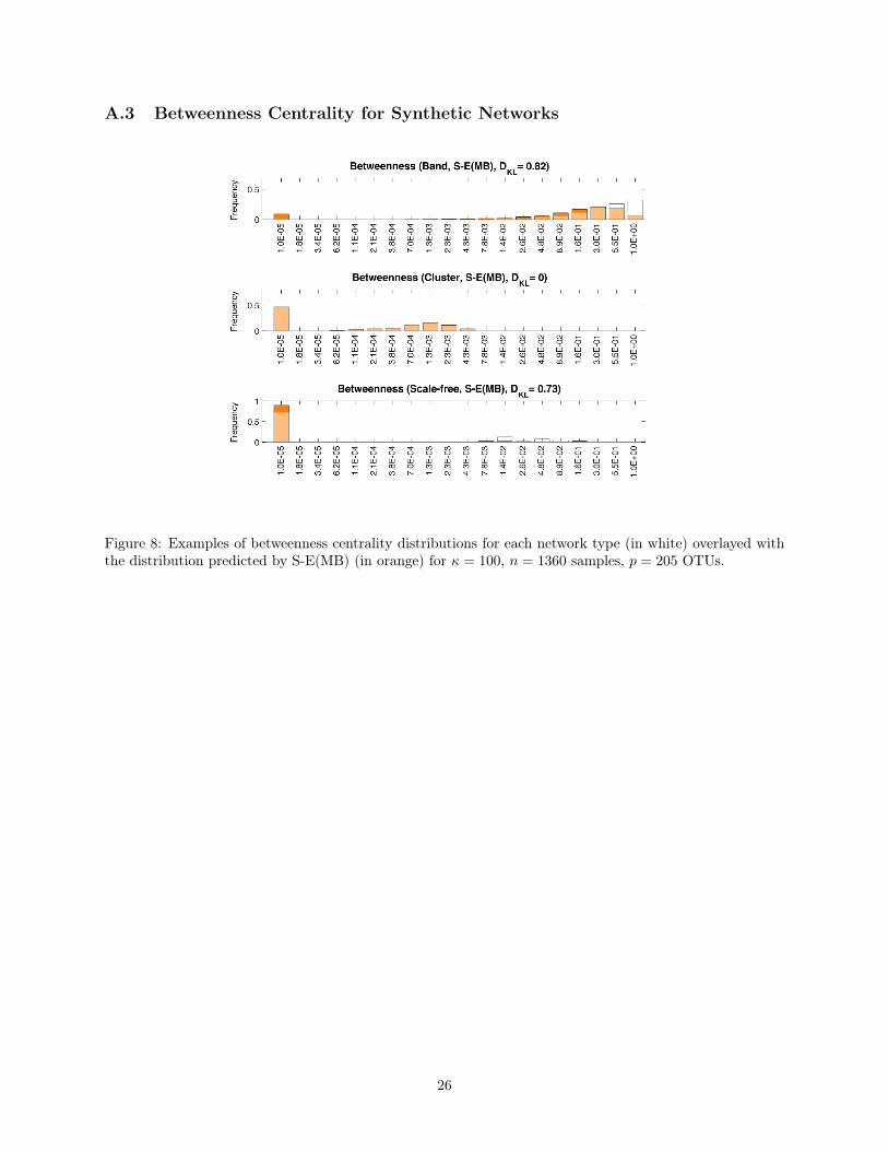
A.3 Betweenness Centrality for Synthetic Networks

Figure 8: Examples of betweenness centrality distributions for each network type (in white) overlayed withthe distribution predicted by S-E(MB) (in orange) for κ = 100, n = 1360 samples, p = 205 OTUs.

26

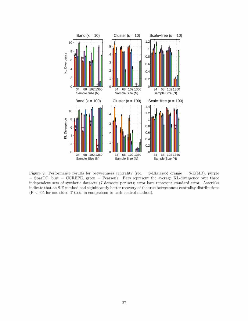
34 68 102 13600

2

4

6

8

10

Sample Size (N)

KL

Div

erge

nce

Band (κ = 10)

34 68 102 13600

1

2

3

4

5

Sample Size (N)

Cluster (κ = 10)

34 68 102 13600

0.2

0.4

0.6

0.8

1

1.2

Sample Size (N)

Scale−free (κ = 10)

34 68 102 13600

2

4

6

8

10

Sample Size (N)

KL

Div

erge

nce

Band (κ = 100)

34 68 102 13600

1

2

3

4

Sample Size (N)

Cluster (κ = 100)

34 68 102 13600

0.2

0.4

0.6

0.8

1

1.2

1.4

Sample Size (N)

Scale−free (κ = 100)

Figure 9: Performance results for betweenness centrality (red = S-E(glasso) orange = S-E(MB), purple= SparCC, blue = CCREPE, green = Pearson). Bars represent the average KL-divergence over threeindependent sets of synthetic datasets (7 datasets per set); error bars represent standard error. Asterisksindicate that an S-E method had siginificantly better recovery of the true betweenness centrality distributions(P < .05 for one-sided T tests in comparison to each control method).

27

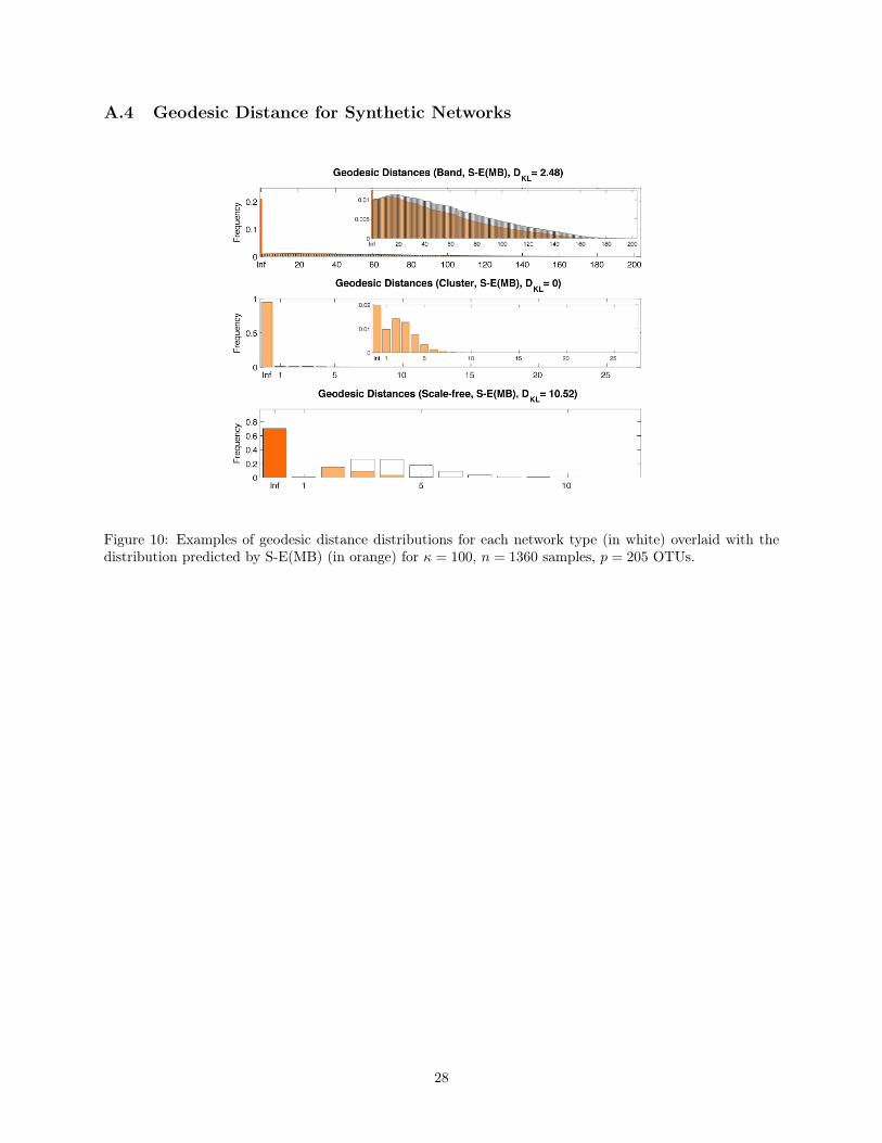
A.4 Geodesic Distance for Synthetic Networks

Figure 10: Examples of geodesic distance distributions for each network type (in white) overlaid with thedistribution predicted by S-E(MB) (in orange) for κ = 100, n = 1360 samples, p = 205 OTUs.

28

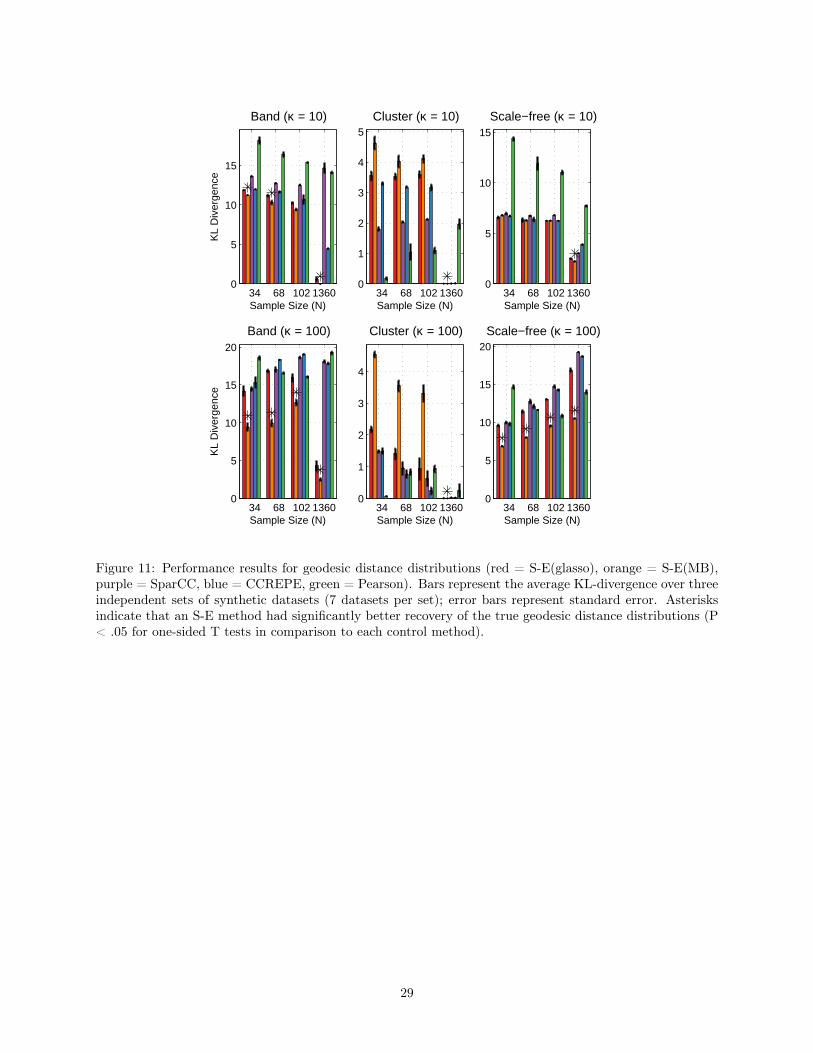
34 68 102 13600

5

10

15

Sample Size (N)

KL

Div

erge

nce

Band (κ = 10)

34 68 102 13600

1

2

3

4

5

Sample Size (N)

Cluster (κ = 10)

34 68 102 13600

5

10

15

Sample Size (N)

Scale−free (κ = 10)

34 68 102 13600

5

10

15

20

Sample Size (N)

KL

Div

erge

nce

Band (κ = 100)

34 68 102 13600

1

2

3

4

Sample Size (N)

Cluster (κ = 100)

34 68 102 13600

5

10

15

20

Sample Size (N)

Scale−free (κ = 100)

Figure 11: Performance results for geodesic distance distributions (red = S-E(glasso), orange = S-E(MB),purple = SparCC, blue = CCREPE, green = Pearson). Bars represent the average KL-divergence over threeindependent sets of synthetic datasets (7 datasets per set); error bars represent standard error. Asterisksindicate that an S-E method had significantly better recovery of the true geodesic distance distributions (P< .05 for one-sided T tests in comparison to each control method).

29

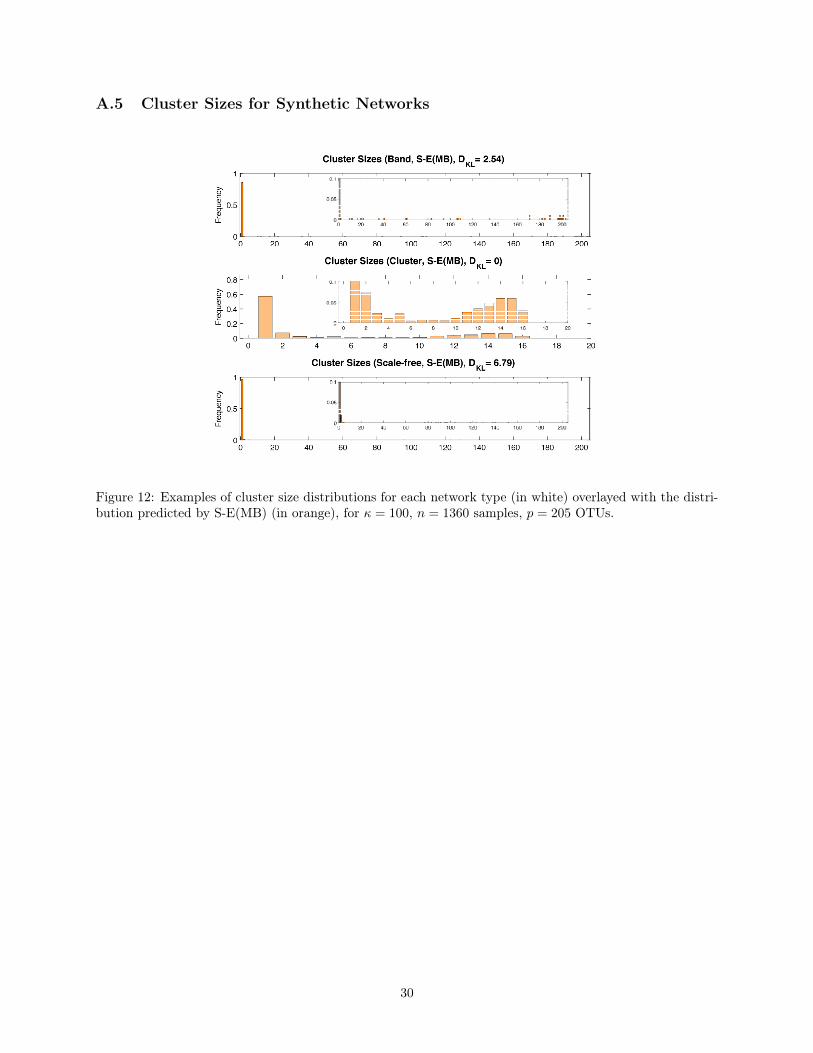
A.5 Cluster Sizes for Synthetic Networks

Figure 12: Examples of cluster size distributions for each network type (in white) overlayed with the distri-bution predicted by S-E(MB) (in orange), for κ = 100, n = 1360 samples, p = 205 OTUs.

30

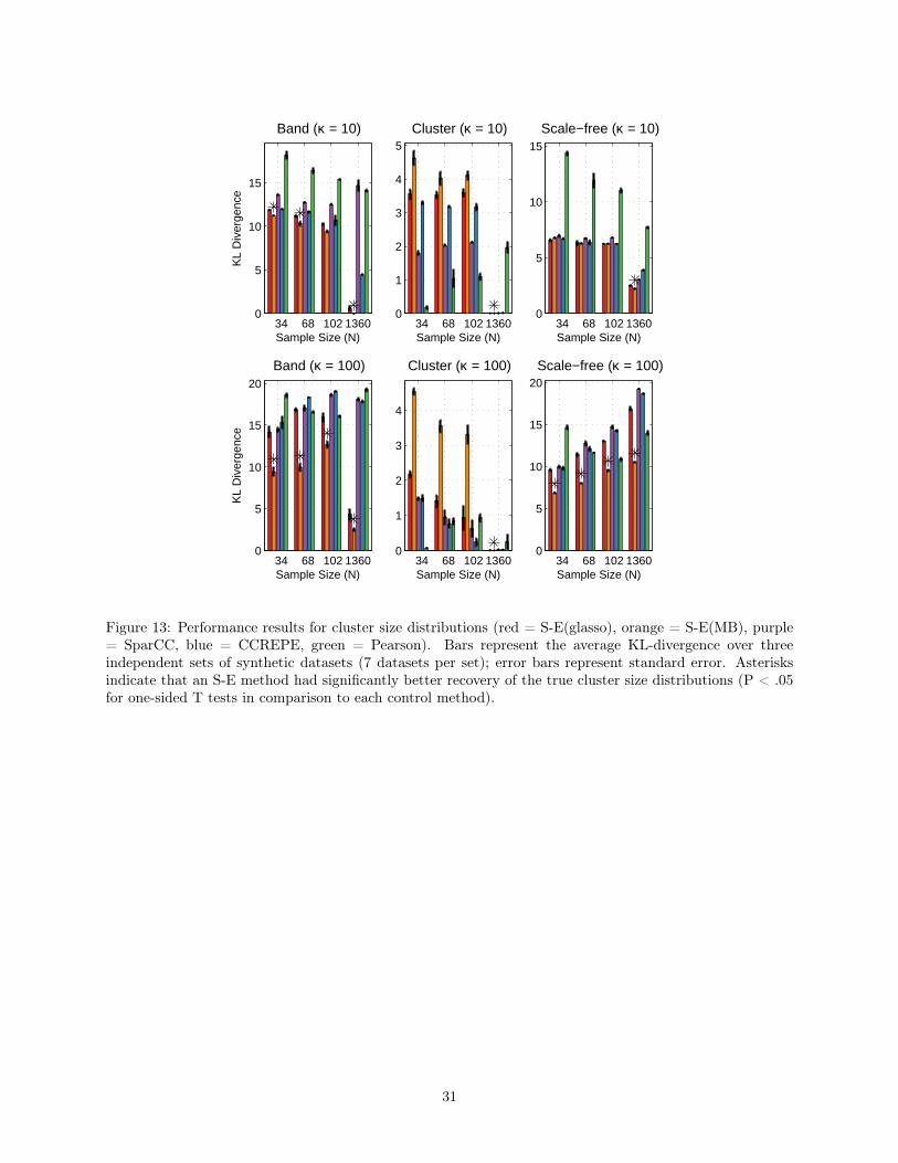
34 68 102 13600

5

10

15

Sample Size (N)

KL

Div

erge

nce

Band (κ = 10)

34 68 102 13600

1

2

3

4

5

Sample Size (N)

Cluster (κ = 10)

34 68 102 13600

5

10

15

Sample Size (N)

Scale−free (κ = 10)

34 68 102 13600

5

10

15

20

Sample Size (N)

KL

Div

erge

nce

Band (κ = 100)

34 68 102 13600

1

2

3

4

Sample Size (N)

Cluster (κ = 100)

34 68 102 13600

5

10

15

20

Sample Size (N)

Scale−free (κ = 100)

Figure 13: Performance results for cluster size distributions (red = S-E(glasso), orange = S-E(MB), purple= SparCC, blue = CCREPE, green = Pearson). Bars represent the average KL-divergence over threeindependent sets of synthetic datasets (7 datasets per set); error bars represent standard error. Asterisksindicate that an S-E method had significantly better recovery of the true cluster size distributions (P < .05for one-sided T tests in comparison to each control method).

31

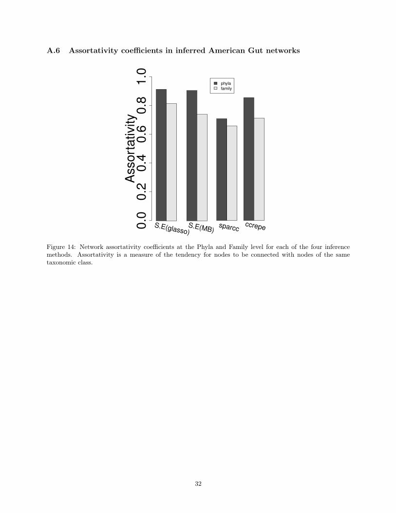
A.6 Assortativity coefficients in inferred American Gut networks

Figure 14: Network assortativity coefficients at the Phyla and Family level for each of the four inferencemethods. Assortativity is a measure of the tendency for nodes to be connected with nodes of the sametaxonomic class.

32