i

Source localization using particle filtering on FPGAfor robotic navigation with imprecise binary

measurementAdithya Krishna, André van Schaik, Fellow, IEEE, and Chetan Singh Thakur, Senior Member, IEEE

Abstract—Particle filtering is a recursive Bayesian estimationtechnique that has gained popularity recently for tracking andlocalization applications. It uses Monte Carlo simulation and hasproven to be a very reliable technique to model non-Gaussianand non-linear elements of physical systems. Particle filtersoutperform various other traditional filters like Kalman filters innon-Gaussian and non-linear settings due to their non-analyticaland non-parametric nature. However, a significant drawback ofparticle filters is their computational complexity, which inhibitstheir use in real-time applications with conventional CPU or DSPbased implementation schemes. This paper proposes a modifica-tion to the existing particle filter algorithm and presents a high-speed and dedicated hardware architecture. The architectureincorporates pipelining and parallelization in the design to reduceexecution time considerably. The design is validated for a sourcelocalization problem wherein we estimate the position of a sourcein real-time using the particle filter algorithm implemented onhardware. The validation setup relies on an Unmanned GroundVehicle (UGV) with a photodiode housing on top to sense andlocalize a light source. We have prototyped the design usingArtix-7 field-programmable gate array (FPGA), and resourceutilization for the proposed system is presented. Further, we showthe execution time and estimation accuracy of the high-speedarchitecture and observe a significant reduction in computationaltime. Our implementation of particle filters on FPGA is scalableand modular, with a low execution time of about 5.62 µs forprocessing 1024 particles and can be deployed for real-timeapplications.

Keywords—Particle filters, Field programmable gate array,Bearings-only tracking, Bayesian filtering, Unmanned groundvehicle, Hardware architectures, Real-time processing.

I. INTRODUCTION

Emergency response operations such as disaster relief andmilitary applications often require localization of a contam-inant chemical or biological source in an unknown envi-ronment. Unmanned vehicles are gaining popularity in suchapplications in recent times due to reduced human involvementand ability to carry out the task remotely. These autonomoussystems can eventually supplement human intervention invarious safety-critical and hazardous missions. Nevertheless,conditions in which these missions are conducted vary drasti-cally depending on the environmental factors, that result in thesensor receiving noise-corrupted measurements. This poses a

A. Krishna and C. S. Thakur are with the Department of Electronic SystemsEngineering, Indian Institute of Science, Bangalore - 560012, India (Email:{adithyaik,csthakur}@iisc.ac.in); A. van Schaik is with the InternationalCentre for Neuromorphic Systems, The MARCS Institute, Western SydneyUniversity, Australia. (Email: A.VanSchaik@westernsydney.edu.au);

significant challenge to the unmanned vehicles to navigate andlocate a target in an unknown environment autonomously.

In our study, we demonstrate autonomous source localiza-tion using a UGV (robot) utilizing the Bearings-only tracking(BOT) model [1] for light source localization with noise-corrupted input measurements as a proof-of-concept. TheBOT model utilized here uses a particle filter algorithm [2]to increase the robustness to false detections, and noise-corrupted measurements. In recent times, there is growingpopularity of particle filters (PFs) in signal processing andcommunication applications to solve various state estimationproblems like tracking [3], localization, navigation [4], andfault diagnosis [5]. PFs have been applied to achieve filteringfor models described using a dynamic state-space approachcomprising a system model describing the state evolution anda measurement model describing the noisy measurements ofthe state [6]. In most real-time scenarios, these models arenon-linear and non-Gaussian. Traditional filters like Kalmanfilters prove to be less reliable for such applications, and ithas been shown that PFs outperform conventional filters insuch scenarios [7].

PFs are inherently Bayesian in nature, intending to constructa posterior density of the state (e.g., location of a target orsource) from observed noisy measurements. In PFs, posteriorof the state is represented by a set of weighted randomsamples known as particles. A weighted average of the samplesgives the state estimate (location of the source). PFs usethree major steps: Sampling, Importance, and Re-samplingfor state estimation, thus deriving the name SIR filter. Inthe sampling step, particles from the prior distribution aredrawn. The importance step is used to update the weightsof particles based on input measurements. The re-samplingstep prevents any weight degeneracy by discarding particleswith lower weights and replicating particles having higherweights. Since PFs apply a recursive Bayesian calculation,all particles must be processed for sampling, importance,and re-sampling steps. Then, the process is repeated for thenext input measurement, resulting in enormous computationalcomplexity. Further, execution time of PFs is proportionalto the number of particles, which inhibits the use of PFsin various real-time applications wherein a large number ofparticles need to be processed to obtain a good performance.Various implementation strategies (discussed below) have beensuggested in the literature to alleviate this problem and makethe PFs feasible in real-time applications.

arX

iv:2

010.

1191

1v1

[cs

.RO

] 2

2 O

ct 2

020

ii

A. State-of-the-art

The first hardware prototype for PFs was proposed byAthalye et al. [8] by implementing a standard SIR filter onan FPGA. They provided a generic hardware framework forrealizing SIR filters and implemented traditional PFs withoutparallelization on FPGA. As an extension to [8], Bolic et al.[9] suggested a theoretical framework for parallelizing there-sampling step by proposing distributed algorithms calledRe-sampling with Proportional Allocation (RPA) and Re-sampling with Non-proportional Allocation (RNA) of particlesto minimize execution time. The design complexity of RPA issignificantly higher than that of RNA due to non-deterministicrouting and complex routing protocol. Though the RNA so-lution is preferred over RPA for high-speed implementationswith low design time, the RNA algorithm trades performancefor speed improvement. Miao et al. [10] proposed a parallelimplementation scheme for PFs using multiple processingelements (PEs) to reduce execution time. However, the com-munication overhead between the PEs increases linearly withthe number of PEs, making the architecture not scalable toprocess a large number of particles. Agrawal et al. [11] pro-posed an FPGA implementation of a PF algorithm for objecttracking in video. Ye and Zhang [12] implemented an SIRfilter on the Xilinx Virtex-5 FPGA for bearings-only trackingapplications. Sileshi et al. [13]–[15] suggested two methodsfor implementation of PFs on an FPGA: the first methodis a hardware/software co-design approach for implementingPFs using MicroBlaze soft-core processor, and the secondapproach is a full hardware design to reduce execution time.Velmurugan [16] proposed an FPGA implementation of a PFalgorithm for tracking applications without any parallelizationusing the Xilinx system generator tool.

Further, several real-time software-based implementationschemes have been proposed with an intent to reduce compu-tational time. Hendeby et al. [17] proposed the first GraphicalProcessing Unit (GPU) based PFs and showed that a GPU-based implementation outperforms a CPU implementation interms of processing speed. Murray et al. [18] provided an anal-ysis of two alternative schemes for the re-sampling step basedon Metropolis and Rejection samplers to reduce the overallexecution time. They compared it with a standard Systematicresamplers [19] over GPU and CPU platforms. Chitchian etal. [20] devised an algorithm for implementing a distributedcomputation PF on GPU for fast real-time control applications.Zhang et al. [21] proposed an architecture for implementingPFs on a DSP efficiently for tracking applications in wirelessnetworks. However, these software-based methods have theirown drawbacks when it comes to hardware implementationowing to their high computational complexity. Therefore, itis essential to develop a high-speed and dedicated hardwaredesign with the capacity to process a large number of particlesin a specified time to meet the speed demands of real-timeapplications. This paper addresses this issue by proposing ahigh-speed architecture that is massively parallel and easilyscalable to handle a large number of particles. The benefitsof the proposed architecture are explained in the followingsubsection.

B. Our contributions

The contributions of this paper are on the algorithmic andhardware fronts:

1) Algorithmic Contribution: We present an experimentalframework and a measurement model to solve the sourcelocalization problem using the bearing-only tracking modelin real-time. In our experiment, we employ a light sourceas the target/source to be localized and a UGV carrying anarray of photodiodes to sense and localize the source. Thephotodiode measurements and the UGV position are processedto estimate the bearing of the light source relative to theUGV. Based on the bearing of the light source, we try tolocalize the source using the PF algorithm. Reflective objectsand other stray light sources are also picked by the sensor(photodiodes), leading to false detections. In this study, wehave successfully demonstrated that our PF system is robustto noise and can localize the source even when the environ-ment is noisy. However, the PFs are computationally veryexpensive, and the execution time often becomes unrealisticusing a traditional CPU based platform. The primary issuefaced during the design of high-speed PF architecture is theparallelization of the re-sampling step. The re-sampling stepis inherently not parallelizable as it needs the informationof all particles. To overcome this problem, we propose amodification to the standard SIR filter (cf. Algorithm 1)to make a parallel and high-speed implementation possible.The modified algorithm proposed (cf. Algorithm 2) uses anetwork of smaller filters termed as sub-filters, each doing theprocessing independently and concurrently. The processing oftotal N particles is partitioned into K sub-filters so that atmost N/K particles are processed within a sub-filter. Thismethod reduces the overall computation time by a factor of K.The modified algorithm also introduces an additional particlerouting step (cf. Algorithm 2), which distributes the particlesamong the sub-filters and makes the parallel implementationof re-sampling possible. The particle routing step is integratedwith the sampling step in the architecture proposed and doesnot require any additional time for computation. We alsocompare the estimation accuracy of the standard algorithmwith the modified algorithm in Section VII-C and concludethat there is no significant difference in estimation errorbetween the modified and the standard approach. Additionally,the modified algorithm achieves a very low execution time ofabout 5.62 µs when implemented on FPGA, compared to 64ms on Intel Core i7-7700 CPU with eight cores clocking at3.60 GHz for processing 1024 particles and outperforms otherstate-of-the-art FPGA implementation techniques.

2) Hardware Contribution: We implemented the proposedmodified SIR algorithm on an FPGA, and key features of thearchitecture are:

• Modularity: We divide the overall computation into multiplesub-filters, which process a fixed number of particles inparallel, and the processing of the particles is local to thesub-filter. This modular approach makes the design simpleand adaptable as it allows us to customize the number ofsub-filters in the design depending on the sampling rateof the input measurement and the amount of parallelism

iii

needed.• Scalability: Our architecture can be scaled easily to process

a large number of particles without increasing the executiontime, by using additional sub-filters.

• Design complexity: The proposed architecture relies on theexchange of particles between sub-filters. However, commu-nication and design complexity increase proportionally withthe number of sub-filters used in the design. In our architec-ture, we employ a simple ring topology to exchange particlesbetween sub-filters to reduce complexity and design time.

• Memory utilization: The sampling step uses particles fromthe previous time instant to compute the particles of thecurrent time instant. This requires the sampled and re-sampled particles to be stored in two separate memories.The straightforward implementation of the modified SIRalgorithm needs 2 × K memory elements each of depthM for storing the sampled and re-sampled particles forK sub-filters. Here, M is the number of particles in asub-filter (M = N/K). However, applications involvingnon-linear models require a large number of particles [22].This would make the total memory requirement 2 × Ksignificant for large K or M . The proposed architecturereduces this memory requirement to K memory elementseach of depth M using a dual-port ram, as explained inSection VI-A1. Therefore, the proposed architecture reducesmemory utilization and is more energy-efficient due toreduced memory accesses.

• Real-time: Since all sub-filters operate in parallel, the execu-tion time is significantly reduced compared to that of othertraditional implementation schemes that use just one filterblock [8]. Our implementation has a very low executiontime of about 5.62 µs (i.e., a sampling rate of 178 kHz)for processing 1024 particles and outperforms other state-of-the-art implementations, thus making it possible to bedeployed in real-time scenarios.

• Flexibility: The proposed architecture is not limited to asingle application, and the design can be easily modifiedby making slight changes to the architecture for other PFapplications.

The architecture was successfully implemented on an Artix-7 FPGA. Our experimental results demonstrate the effective-ness of the proposed architecture for source localization usingthe PF algorithm with noise-corrupted input measurements.

The rest of the paper is organized as follows: We providethe theory behind Bayesian filtering and PFs in Section II andIII, respectively. The experimental setup for source localizationusing a Bearings-only tracking (BOT) model is presented insection IV. In this model, input to the filter is a time-varyingangle (bearing) of the source, and each input is processed bythe PF algorithm implemented on hardware to estimate thesource location. Further, in section V, we propose algorithmicmodifications to the existing PF algorithm that make the high-speed implementation possible. The architecture for imple-menting PFs on hardware is provided in Section VI. Evaluationof resource utilization on the Artix-7 FPGA, performanceanalysis in terms of execution time, estimation accuracy, andthe experimental results are provided in Section VII.

II. BAYESIAN FRAMEWORK

In a dynamic state space model, the evolution of the statesequence xt is defined by:

xt = ft(xt−1, wt) (1)

where, ft is a nonlinear function of the state xt−1, and wt

represents the process noise. The objective is to recursivelyestimate the state xt based on a measurement defined by:

zt = gt(xt, vt) (2)

where, gt is a nonlinear function describing the measurementmodel, and zt is the observation vector of the system corruptedby measurement noise vt at time instant t.

From a Bayesian standpoint, the objective is to constructthe posterior p(xt|z1:t) of the state xt from the measurementdata z1:t up to time t. By definition, constructing the posterioris done in two stages namely, prediction and update.

The prediction stage involves using the system model (cf.Eq. 1) to obtain a prediction probability density function (PDF)of the state at time instant t, using the Chapman-Kolmogorovequation:

p(xt|z1:t−1) =∑xt−1

p(xt|xt−1)p(xt−1|z1:t−1) (3)

where, the transition probability p(xt|xt−1) is defined bysystem model (cf. Eq. 1).

In the update stage, the measurement data zt at time step tis used to update the PDF obtained from the prediction stageusing Bayes rule, to construct the posterior:

p(xt|z1:t) =p(zt|xt)p(xt|z1:t−1)∑xtp(zt|xt)p(xt|z1:t−1)

(4)

where, p(zt|xt) is a likelihood function defined by themeasurement model (cf. Eq. 2).

The process of prediction (cf. Eq. 3) and update (cf.Eq. 4) are done recursively for every new measurement zt.Constructing the posterior based on Bayes rule is a conceptualsolution and is analytically estimated using traditional Kalmanfilters. However, in a non-Gaussian and non-linear setting,the analytic solution is intractable, and approximation-basedmethods such as PFs are employed to find an approximateBayesian solution. A detailed illustration of the Bayesianframework and its implementation for estimating the state ofa system is provided by Thakur et al. [23].

III. PARTICLE FILTERS BACKGROUND

The key idea of PFs is to represent the required posteriordensity by a set of random samples termed as particles, withassociated weights, and to compute the state estimate based onthese particles and weights. The particles and their associatedweights are denoted by {xit, wi

t}Ni=1, where N is the totalnumber of particles. xit denotes the ith particle at time instantt. wi

t represents the weight corresponding to the particle xit.The most commonly used PF named the sampling, importance,and re-sampling filter (SIRF) is presented in Algorithm 1.

In the sampling step, particles are drawn from the priordensity p(xt|xit−1) to generate particles at time instant t.

iv

Algorithm 1 : SIR Algorithm

Initialization: Set the particle weights of previous time stepto 1/N, {wi

t−1}Ni=1 = 1/N .Input: Particles from previous time step {xit−1}Ni=1 andmeasurement zt.Output: Particles of current time step {xit}Ni=1.Method:

1: Sampling and Importance:2: for i = 1 to N do3: Sample xit ∼ p(xt|xit−1)4: Calculate wi

t = wit−1p(zt|xit)

5: end for6: Re-sampling: Deduce the re-sampled particles {xit}Ni=1

from {xit, wit}Ni=1.

p(xt|xit−1) is deduced from (1). Intuitively, it can be thought aspropagating the particles from time step t−1 to t. The sampledset of particles at time instant t is denoted by {xit}Ni=1. Attime instant 0, particles are initialized with prior distributionto start the iteration. These particles are then propagated intime successively.

The importance step assigns weights to every particle xitbased on the measurement zt. By definition, the weights aregiven by:

wit = wi

t−1p(zt|xit) (5)

However, weights of the previous time step are initialized to1/N i.e wi

t−1 = 1/N . Thus, we have:

wit ∝ p(zt|xit) (6)

The re-sampling step is used to deal with the degeneracyproblem in PFs. In the re-sampling step, particles with lowerweights are eliminated, and particles with higher weights arereplicated to compensate for the discarded particles dependingon the weight wi

t associated with the particle xit. The re-sampled set of particles is denoted by {xit}Ni=1.

IV. BEARINGS-ONLY TRACKING MODEL

This section briefly describes an experimental setup anda measurement model to solve the Bearings-Only Tracking(BOT) problem using the PF algorithm. As a real-worldapplication, we consider a source localization problem whereinwe try to estimate the source position based on the receivedsensor measurements in a noisy environment.

A. Overview of the experimental setup

In our experiment, an omnidirectional light source servesas a source to be localized. A photodiode housing mountedon top of a UGV (cf. Fig. 1(a)) constitutes a sensor tomeasure the relative intensity of light in a horizontal plane.The space around the UGV is divided into 8 sectors with 45°angular separation, as shown in Fig. 1(b), and an array of 8photodiodes are placed inside the circular housing to sense thelight source in all directions. The housing confines the angleof exposure of the photodiode to 45°. Depending on the light

incident on each photodiode, we consider the output of thephotodiode to be either 0 or 1.

The PF algorithm applied to the BOT model requires dy-namic motion between the sensor and source [24]. We considera stationary source, and a moving sensor mounted on a UGV,in our experimental setup. The UGV is made to traverse inthe direction of the source and eventually converges to thesource. Reflective sources and other stray light sources arepotential sources of noise picked up by the sensor, producingfalse detections. A target-originated measurement, along withnoise, is sensed by the photodiodes and processed in additionto the UGV position data, to estimate a bearing of the lightsource relative to the UGV. Based on the bearing of the lightsource, we try to estimate its position using the PF algorithm.

B. Measurement model

The position of UGV (xUGVt ) at time instant t is defined

by the Cartesian co-ordinate system:

xUGVt = [XUGV

t , Y UGVt ]

The orientation of the longitudinal axis of UGV is representedby φUGV

t which gives its true bearing.The source is considered to be stationary, and its co-

ordinates in the 2-dimensional setting is given by:

xt = [Xt, Yt] (7)

At time instant t, a set of 8 photodiode measurements arecaptured zt = {z1t , z2t · · · z8t }, which comprise of the target-associated measurement and clutter noise. Then, based on themeasurement model (2), the source-associated measurementcan be modelled as:

zt = g(xt) + vt (8)

Since the measurement gives the bearing information of thesource, we have:

g(xt) = tan−1

(Yt − Y UGV

t

Xt −XUGVt

)(9)

The four-quadrant inverse tangent function evaluated from[0, 2π) gives the true bearing of the source.

The relevant probabilities needed to model the sensor im-perfections and clutter noise are as follows:

(i) The probability of clutter noise (nt) produced by a strayor reflective light source is: p(nt) = β.

(ii) The probability of the jth photodiode output being 1 i.e.,(zjt = 1) either due to light source or clutter noise is:p(zjt |xt, nt) = α.

(iii) If there is a light source in the sector j, then jth

photodiode output will be 1 with a probability of αirrespective of noise. The likelihood of photodiode outputbeing 1 or 0 in the presence of the source is:

p(zjt |xt) =

{α, for zjt = 1.

1− α, for zjt = 0.(10)

v

Axis of UGV

Photodiode

PhotodiodeHousing

ElectronicsHousing

MountingPlate

(a)

1

23

4

5

6 7

8

45∘

45∘

45∘

45∘

45∘

45∘

45∘

45∘

(b)

Fig. 1: UGV Design. (a) Schematic of the UGV with a photodiode housing mounted on top. (b) The region around the UGVis divided into 8 sectors with 45° angular separation.

(iv) If there is no source in sector j, then there is a noisesource with probability β. The likelihood of photodiodeoutput being 1 or 0 in the absence of source is:

p(zjt |xt) =

{αβ, for zjt = 1.

1− αβ, for zjt = 0.(11)

These two likelihoods are used in our system to model thesensor imperfections and noise, and even with high noiseprobability β, the PF algorithm is robust enough to localizethe source.

V. ALGORITHMIC MODIFICATION OF SIRF FOR REALIZINGHIGH-SPEED ARCHITECTURE

In this section, we suggest modifications to the standard SIRalgorithm to make it parallelizable. The key idea of the high-speed architecture is to utilize multiple parallel filters, termedas sub-filters, working simultaneously, and performing sam-pling, importance and re-sampling operations independentlyon particles. The architecture utilizes K sub-filters in parallelto process a total of N particles. Thus, the number of particlesprocessed within each sub-filter is M = N/K. In this way, thenumber of particles processed within each sub-filter is reducedby a factor K, compared to conventional filters.

The sampling and importance steps are inherently par-allelizable since there is no data dependency for particlegeneration and weight calculation. However, the re-samplingstep cannot be parallelized as it needs to have the informationof all particles. This creates a major bottleneck in the parallelimplementation scheme. Thus, in addition to the SIR stage,we introduce a particle routing step, as shown in Algorithm 2,to route particles between sub-filters. The particle routing stepenables the distribution of particles among sub-filters, and there-sampling step can be effectively parallelized.

The particles and their associated weights in sub-filterk at time step t are represented by {x(k,i)t , w

(k,i)t }Mi=1, for

k = 1, · · ·K. The particle x(k,i)t represents the position in

the Cartesian co-ordinate system.

Algorithm 2 : High-level description of each sub-filter kperforming SIR and particle routing operations.

Initialization: Set the particle weights of previous time stepto 1/M, {w(k,i)

t−1 }Mi=1 = 1/M .Input: Particles from previous time step {x(k,i)t−1 }Mi=1 andmeasurement ztOutput: Particles of current time step {x(k,i)t }Mi=1

Method:

1: Particle Routing: Exchange Q particles with neighbour-ing sub-filters.

2: {x(k,q)t−1 }Qq=1 ← {x

(k−1,q)t−1 }Qq=1 for k = 2, · · ·K, and

3: {x(k,q)t−1 }Qq=1 ← {x

(K,q)t−1 }

Qq=1 for k=1.

4: Sampling and Importance:5: for i = 1 to M do6: Sample x(k,i)t ∼ p(xt|x(k,i)t−1 )

7: Calculate w(k,i)t = w

(k,i)t−1 p(zt|x

(k,i)t )

8: end for9: Re-sampling: Compute the re-sampled particles{x(k,i)t }Mi=1 from {x(k,i)t , w

(k,i)t }Mi=1.

VI. ARCHITECTURE OVERVIEW

In this section, we present a high-speed architecture for PFs,based on the modified SIRF algorithm presented in Section V.

The top-level architecture shown in Fig. 2 utilizes a filterbank consisting of K sub-filters working in parallel. Sampling,importance, and re-sampling operations are carried out withina sub-filter. In addition to the SIR step, a fixed number ofparticles are routed between sub-filters after the completionof every iteration as part of a particle routing operation. Thesub-filters are connected based on ring-topology inside thefilter bank. M particles are time-multiplexed and processedwithin each sub-filter, and Q = M/2 particles are exchangedwith neighbouring sub-filters. Since the number of particlesexchanged and the routing topology are fixed, the proposedarchitecture has very low design complexity. The design can

vi

Sub-Filter 1

Sub-Filter 2

Sub-Filter K

SEED

Filter Bank

����

Random Number Generator

Sector Check Block

Mean EstimationBlock

PRN(1)

PRN(�)

CLK

�(1,�)�−1

�(2,�)�−1

�(�−1,�)�−1

�(�,�)�−1

�(1,�)�

�(�,�)�

�(1)Count Ind

�(�)Count Ind

Ind �

��

����

�

�����

Fig. 2: Top-level architecture of the realized particle filter algorithm.

be easily scaled up to process a large number of particles(N) by replicating sub-filters. The binary measurements ofthe eight photodiodes (zt) are fed as an input to the filterbank along with the true bearing (φUGV

t ) and the positionof the UGV (xUGV

t ). Random number generation neededfor the sampling and re-sampling steps is provided by arandom number generator block. We use a parallel multipleoutput LFSR architecture presented by Milovanovic et al. [25]for random number generation. As our internal variables are16 bits in size, a 16 bit LFSR is used. Further, a detaileddescription of the sub-filter architecture is provided in SectionVI-A. The sector check block, described in Section VI-B,computes the particle population in each of the eight sectorsand outputs a sector index that has the maximum particlepopulation. This information is used by the UGV to traversein the direction of the source. The mean computational blockused to calculate the global mean of all N particles from Ksub-filters to estimate the source location (post), is explainedin Section VI-C.

A. Sub-filter architecture

The sub-filter is the main computational block responsiblefor particle generation, processing, and filtering. It consistsof three main sub-modules, namely, sampling, importanceand re-sampling, as shown in Fig. 3. The sampling andimportance blocks are pipelined in operation. The re-samplingstep cannot be pipelined with the former steps as it requiresweight information of all particles. Thus, it is started afterthe completion of the importance step. Since sampling andimportance stages are pipelined, together they take M clockcycles to iterate for M particles, as shown in Algorithm 2 fromline 5 to line 8. The particle routing between the sub-filtersis done along with the sampling step and does not requireany additional cycles. The re-sampling step takes 3M clockcycles, as discussed in Section VI-A3.

1) Sampling and routing: The sampling step involves gen-erating new sampled particles {x(k,i)t }Mi=1 by propagating there-sampled particles {x(k,i)t−1 }Mi=1 from the previous time stepusing the dynamic state space model:

x(k,i)t ∼ p(xt|x(k,i)t−1 ) (12)

Conventionally, particles {x(k,i)t }Mi=1 are used to generatethe weights {w(k,i)

t }Mi=1 in the importance unit, and using theseweights we determine the re-sampled particles {x(k,i)t }Mi=1.Further, {x(k,i)t }Mi=1 is utilized to obtain particles {x(k,i)t+1 }Mi=1

of the next time step. Thus, with the straightforward approach,we would need two memories each of depth M to store{x(k,i)t }Mi=1 and {x(k,i)t }Mi=1 within a sub-filter. Similarly, forK sub-filters we would require 2×K memory elements, eachof depth M . This increases memory usage for higher K or M .In this paper, we propose a novel scheme to store the particlesusing a single dual-port memory instead of two memoryblocks, which brings down the total memory requirement forstoring particles to K memory elements, each of depth M .

In this scheme, since the re-sampled particles are actuallythe subset of sampled particles (i.e.,{x(k,i)t }Mi=1 ⊂ {x

(k,i)t }Mi=1)

instead of storing {x(k,i)t }Mi=1 in a different memory, we canuse the same memory as {x(k,i)t }Mi=1 and use suitable pointersor indices to read {x(k,i)t }Mi=1.

The re-sampling unit in our case is modified such thatinstead of returning re-sampled particles x(k,i)t−1 , it returns theindices of replicated (Ind R(k,i)) and discarded (Ind D(k,i))particles (cf. Fig. 3). Ind R(k,i) is used as a read address ofthe dual-port particle memory shown in Fig. 4 to point to there-sampled particles x(k,i)t−1 . The dual-port memory enables usto perform read and write operations simultaneously; however,this might result in data overwriting. For example, considersix particles, after re-sampling particle 2 (x(k,2)t−1 ) is replicatedfour times; particle 5 (x(k,5)t−1 ) is replicated two times and

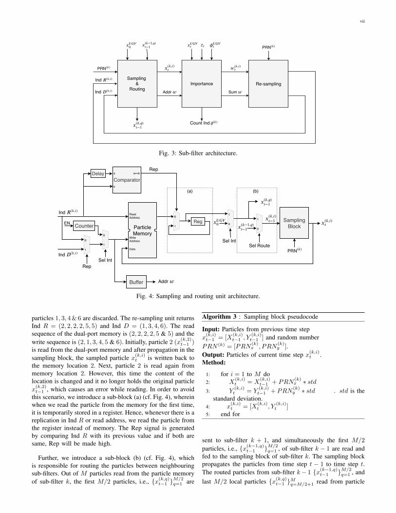
vii

Sampling &

RoutingImportance Re-sampling

PRN(�)

Ind �(�,�)

Ind �(�,�)

�(�,�)�

�(�−1,�)

�−1

�(�,�)

�−1

����0

����� �� ����

�

Count Ind �(�)

Addr �

 �(�,�)�

Sum �

PRN(�)

Fig. 3: Sub-filter architecture.

ParticleMemory

0

1

0

1

Counter

0

1Reg Sampling

Block

ReadAddress

WriteAddress

Ind �(�,�)

Ind �(�,�)

EN

Data

Sel IntRep

����0

�(�,�)

�−1

�(�,�)�

1

0

Sel IntSel Route

DelayRep

Comparatora

b

a==b

Buffer

PRN(�)

Addr �

1

0�(�−1,�)

�−1

(b)(a)

�(�,�)

�−1

Fig. 4: Sampling and routing unit architecture.

particles 1, 3, 4&6 are discarded. The re-sampling unit returnsInd R = (2, 2, 2, 2, 5, 5) and Ind D = (1, 3, 4, 6). The readsequence of the dual-port memory is (2, 2, 2, 2, 5 & 5) and thewrite sequence is (2, 1, 3, 4, 5 & 6). Initially, particle 2 (x

(k,2)t−1 )

is read from the dual-port memory and after propagation in thesampling block, the sampled particle x(k,i)t is written back tothe memory location 2. Next, particle 2 is read again frommemory location 2. However, this time the content of thelocation is changed and it no longer holds the original particlex(k,2)t−1 , which causes an error while reading. In order to avoid

this scenario, we introduce a sub-block (a) (cf. Fig. 4), whereinwhen we read the particle from the memory for the first time,it is temporarily stored in a register. Hence, whenever there is areplication in Ind R or read address, we read the particle fromthe register instead of memory. The Rep signal is generatedby comparing Ind R with its previous value and if both aresame, Rep will be made high.

Further, we introduce a sub-block (b) (cf. Fig. 4), whichis responsible for routing the particles between neighbouringsub-filters. Out of M particles read from the particle memoryof sub-filter k, the first M/2 particles, i.e., {x(k,q)t−1 }

M/2q=1 are

Algorithm 3 : Sampling block pseudocode

Input: Particles from previous time stepx(k,i)t−1 = [X

(k,i)t−1 , Y

(k,i)t−1 ] and random number

PRN (k) = [PRN(k)x , PRN

(k)y ].

Output: Particles of current time step x(k,i)t .Method:

1: for i = 1 to M do2: X

(k,i)t = X

(k,i)t−1 + PRN

(k)x ∗ std

3: Y(k,i)t = Y

(k,i)t−1 + PRN

(k)y ∗ std . std is the

standard deviation.4: x

(k,i)t = [X

(k,i)t , Y

(k,i)t ]

5: end for

sent to sub-filter k + 1, and simultaneously the first M/2

particles, i.e., {x(k−1,q)t−1 }M/2

q=1 , of sub-filter k − 1 are read andfed to the sampling block of sub-filter k. The sampling blockpropagates the particles from time step t − 1 to time step t.The routed particles from sub-filter k− 1 {x(k−1,q)

t−1 }M/2q=1 , and

last M/2 local particles {x(k,q)t−1 }Mq=M/2+1 read from particle

viii

WeightMemory

WeightComputation

Block

Cordic IP

(tan-1)_

_ x

y

�

IndexGenerator

�(�,�)�

0

1

CounterEN

����

�

�(�,�)�

����

�

Addr �

Accumulator

ParticlePopulationBlock

��

Ind �(�,�)�

Sum �

 �(�,�)�

Count Ind �(�)

�(�,�)�

����

�

����

�

Data

Read/WriteAddress

 �

Angle Computation Block

�(�,�)

�

Read/Write

Fig. 5: Importance unit architecture.

memory of sub-filter k are propagated by the sampling blockand written back to the memory. The input to the samplingblock are particles of time step t−1 (x

(k,i)t−1 ) and the output are

particles of current time step t (x(k,i)t ). The sampling block

pseudocode is provided by Algorithm 3. The random numberPRN (K) needed for random sampling of particles as shownin Algorithm 3, line 2 and line 3 is provided by a randomnumber generator block (cf. Fig. 2). The Sel Route signal isused to control the switching between the local and routedparticles by making it low for the first M/2 cycles and thenmaking it high for the next M/2 cycles. Further, at time instant0, we feed the UGV position xUGV

0 as a prior to the samplingblock to distribute the particles around the UGV. The Sel Intcontrol signal is made low in the first iteration, i.e., at timeinstant 0, and then made high for the subsequent iterations.

2) Importance: The importance unit computes the weightsof the particles based on the photodiode measurements ztgiven by:

w(k,i)t = w

(k,i)t−1 p(zt|x

(k,i)t ) (13)

w(k,i)t−1 is initialized to 1/M. Estimation of p(zt|x(k,i)t ) in-

volves determining the angle of each particle (θ(k,i)t ), which

is computed using an inverse tangent function based on theposition of UGV (xUGV

t ) and position of the particle (x(k,i)t ),

as follows:

θ(k,i)t = tan−1

(Y

(k,i)t − Y UGV

t

X(k,i)t −XUGV

t

)

where, X(k,i)t and Y

(k,i)t represents the co-ordinates of the

particle x(k,i)t in two-dimensional Cartesian co-ordinate sys-tem.

The inverse tangent function is implemented using a CordicIP block provided by Xilinx [26]. The architecture of theimportance unit is shown in Fig. 5. The index generatorblock estimates the angle of the particles with respect to the

longitudinal axis of the UGV based on the bearing of theUGV (φUGV

t ). In addition to this, the index generator blockis used for determining the sector indices (Ind θ

(k,i)t ) of the

particles based on the angle information. The sector indicesof the particle can be defined as follows:

Ind θ(k,i)t = d4/π ∗ (θ(k,i)t − φUGV

t )e

zt is 8 bit wide data consisting of 8 binary photodiodemeasurements {z1t , z2t · · · z8t }. Based on the measurement ztand the sector indices of the particles, weights are generatedby the weight computation block. These weights are stored inthe weight memory using the address provided by the samplingunit, to store weights in the same order as the sampled particlesx(k,i)t . The sum of all the weights required by the re-sampling

unit is obtained by an accumulator. The particle populationblock is used to estimate the number of particles presentin each of the eight sectors, using the sector indices of theparticles for a given sub-filter. The particle count in each ofthe eight sectors of sub-filter k is concatenated and given asthe output Count Ind θ(k). For example, if sector 1 has 15particles, sector 3 has 14 particles, and sector 5 has 3 particles,then Count Ind θ(k) = {15, 0, 14, 0, 3, 0, 0, 0}.

3) Re-sampling: The re-sampling step replicates particleswith higher weights and discards particles with lower weights.This is accomplished by utilizing a Systematic re-samplingalgorithm shown in Algorithm 4. A detailed description ofthe systematic re-sampling algorithm is provided in [8], [19].The weights and sum of all weights are obtained from theimportance unit. The random number (U0) needed to computethe parameter U_scale in line 2 of Algorithm 4 is providedby the Random number generator block shown in Fig. 2.The algorithm presented works with un-normalized weights,which will avoid M division operations on all particles toimplement normalization. The division required to computeAw in line 1 of Algorithm 4 is implemented using theright shift operation. This approach consumes fewer resources

ix

EN d

EN r

ReplicatedIndex Memory

DiscardedIndex Memory

Systematic re-sampling

Block

Counter R

Counter D

Data

Read/WriteAddress

PRN(�)

�(�,�)�

Sum �

Ind �(�,�)

Ind �(�,�)

Data

Read/WriteAddress

Ind �

Ind �

Fig. 6: Re-sampling unit architecture.

and area on hardware. The replicated and discarded indicesgenerated by the systematic re-sampling block are stored intheir respective memories, as shown in Fig. 6. In the worst-casescenario, the inner loop of Algorithm 4 takes 2M cycles forexecution in hardware as it involves fetching M weights fromweight memory and doing M comparison operations. Further,line 13 and line 14 take M cycles to obtain M replicatedindices. Thus, in total, the execution of the re-sampling steprequires 2M +M = 3M cycles.

Algorithm 4 : Systematic Re-sampling.

Input: Un-normalized weights ({w(k,i)t }Mi=1) of M particles,

summation of all the weights in a sub-filter (Sum w) and theuniform random number (U0) between [0, 1]Output: Replicated index (Ind R) and Discarded index (IndD).Method:

1: Compute Aw =Sumw

M2: Initialize : U_scale = U0 ×Aw3: s = 0, p = 0,m = 04: for i=1 to M do5: while s < U_scale do6: p = p+ 17: s = s+ w(k,p)

8: if s < U_scale then9: m = m+ 1

10: Ind D(k,m) = p11: end if12: end while13: U_scale = U_scale+Aw

14: Ind R(k,i) = p15: end for

B. Sector check block

The direction/orientation of the UGV is decided by thepopulation of particles in different sectors and is used to movetowards the source. This is achieved by the sector check block,which estimates the particle population in each of the eightsectors and gives the sector index with maximum particlecount. The block diagram shown in Fig. 7 utilizes eight paralleladders to count the number of particles in each sector. Theparticle count in a given sector of K sub-filters is fed as an

input to the adder. Count Ind θ(k)n in Fig. 7 denotes the particlecount in sector n of sub-filter k. The output of an adder givesthe total particle population in a particular sector. Furthermore,the sector index (Ind θ) having maximum particle count isestimated using a max computation block. The UGV uses thisinformation to traverse in the direction of the source.

Max ComputationBlock

Count Ind �1

Count Ind �2

Count Ind �8

Ind �

Count Ind �(1)

2

Count Ind �(�)

2

∑

Count Ind �(1)

1

Count Ind �(�)

1

∑

Count Ind �(1)

8

Count Ind �(�)

8

∑

Fig. 7: Sector check block architecture.

C. Mean estimation block

The mean of total N particle positions is estimated usingthe mean estimation block. Particle positions from K sub-filters are fed in parallel and accumulated over M cycles togenerate the sum, which is further divided by N , by rightshifting log2(N) times to get the mean. In our implementation,we consider N as a power of 2. The mean gives an estimateof the position of the source post.

VII. RESULTS

In this section, we present resource utilization of the pro-posed design on an FPGA. We also evaluate the executiontime of the proposed architecture as a function of number ofsub-filters and inspect the estimation accuracy by scaling thenumber of particles. We then compare our design with state-of-the-art implementations. Furthermore, we present experimentalresults for the source localization problem implemented on anFPGA using the proposed architecture.

A. Resource utilization

The architecture presented was implemented on an Artix-7 FPGA. Resource utilization of the implemented design

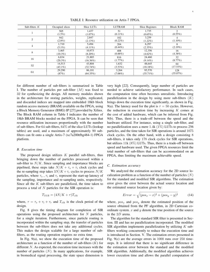
x

TABLE I: Resource utilization on Artix-7 FPGA.

Sub-filters K Occupied slices Slice LUTs LUTRAM Slice Registers Block RAM

1505

(1.5%)1,437

(1.07%)51

(0.11%)1,735

(0.65%)2

(0.55%)

2942

(2.8%)2,847

(2.13%)102

(0.22%)3,259

(1.22%)4

(1.10%)

41,710(5.1%)

5,494(4.11%)

204(0.44%)

6,297(2.35%)

8(2.19%)

83,465

(10.3%)10,973(8.20%)

408(0.88%)

12,356(4.62%)

16(4.38%)

166,834

(20.3%)21,885

(16.36%)816

(1.77%)24,460(9.14%)

32(8.77%)

3214,513(43.1%)

43,804(32.74%)

1,632(3.53%)

48,645(18.18%)

64(17.53%)

6429,290(87%)

86,101(64.35%)

3,264(7.06%)

95,570(35.71%)

128(35.07%)

for different number of sub-filters is summarized in TableI. The number of particles per sub-filter (M) was fixed to32 for synthesizing the design. All memory modules shownin the architecture for storing particles, weights, replicated,and discarded indices are mapped into embedded 18kb blockrandom access memory (BRAM) available on the FPGA, usinga Block Memory Generator (BMG) IP [27] provided by Xilinx.The Block RAM column in Table I indicates the number of18kb BRAM blocks needed on the FPGA. It can be seen thatresource utilization increases proportionally with the numberof sub-filters. For 64 sub-filters, 64% of the slice LUTs (lookuptables) are used, and a maximum of approximately 90 sub-filters can fit onto a single Artix-7 (xc7a200tfbg484-1) FPGAplatform.

B. Execution time

The proposed design utilizes K parallel sub-filters, thusbringing down the number of particles processed within asub-filter to N/K. Since sampling and importance blocks arepipelined, these steps take N/K + τs + τi clock cycles andthe re-sampling step takes 3N/K+τr cycles to process N/Kparticles, where τs , τi and τr represent the start-up latency ofthe sampling, importance and re-sampling units, respectively.Since all the K sub-filters are parallelized, the time taken toprocess a total of N particles for the SIR operation is:

TSIR = (4N/K + τ)Tclk

where, τ = τs + τi + τr and Tclk is the clock period of thedesign.

Fig. 8 gives the timing diagram for completion of SIRoperations using the proposed architecture for N particles,for a single iteration. Furthermore, since particle routing isincorporated within the sampling step, the transfer of particlesbetween the sub-filters does not take any additional cycles.This makes the design scalable for a large number of sub-filters, as the routing operation requires no extra time.

In Fig. 9(a), we show the execution time of the proposedarchitecture as a function of the number of sub-filters (K) fordifferent N . As expected, the execution time increases with thenumber of particles (N). In many applications, for example,in biomedical signal processing, the state space dimension is

very high [22]. Consequently, large number of particles areneeded to achieve satisfactory performance. In such cases,the computation time often becomes unrealistic. Introducingparallelization in the design by using more sub-filters (K)brings down the execution time significantly, as shown in Fig.9(a). The latency used for the plot is τ = 50 cycles. However,the reduction in execution time by increasing K comes atthe cost of added hardware, which can be inferred from Fig.9(b). Thus, there is a trade-off between the speed and thehardware utilized. For instance, using a single sub-filter, andno parallelization uses a mere 1.4k (1%) LUTs to process 256particles, and the time taken for SIR operations is around 1075clock cycles. On the other hand, with a design consisting 8sub-filters, it takes only 178 clock cycles for SIR operations,but utilizes 11k (8%) LUTs. Thus, there is a trade-off betweenspeed and hardware used. The given FPGA resources limit thetotal number of sub-filters that can be accommodated on anFPGA, thus limiting the maximum achievable speed.

C. Estimation accuracy

We analyzed the estimation accuracy for the 2D source lo-calization problem as a function of the number of particles (N)for the standard and modified SIR algorithms. The estimationerror gives the error between the actual source location andthe estimated source location given by:

Error =√

(posx − x)2 + (posy − y)2 (14)

where, posx and posy denote the estimated position of thesource obtained from the PF algorithm, in 2D Cartesian co-ordinate system. x and y denote the true position of the sourcein the 2D arena.

The algorithm for the standard SIR filter is presented in Sec-tion. III and has no parallelization incorporated. The modifiedSIR algorithm implements parallelization by utilizing K sub-filters working concurrently to reduce the execution time andis introduced in Section. V. The estimation errors presented inFig. 9(c) are the average errors in 1000 runs over 250 time-steps. It is inferred that there is no significant difference inthe estimation error between the standard and the modifiedSIR algorithm. Additionally, the modified algorithm achieveslower execution time and allows the parallel computation of

xi

Re-sampling

Sampling & Routing

Importance

�� �/� + �� 3�/� + ��

����

Fig. 8: Timing diagram for SIR operations of the proposed design.

0 1 2 3 4 5 60

50

100

150

200N=128N=256N=512N=1024N=2048N=4096

�� ��2

Exec

utio

n Ti

me

(us)

(a)

0 1 2 3 4 5 60

20

40

60

80

100

�� ��2

Slic

e LU

Ts U

tiliz

ed (k

LU

Ts)

(b)

2 4 6 8 10 12 14 16-10

0

10

20

30

40

50

4 6 8 10 12 14 16

0

5

10

15

Standard SIR algorithm

Estim

atio

n er

ror

Standard SIR algorithmModified SIR algorithm

(c)

Fig. 9: Performance analysis of the proposed design. (a) Execution time of the proposed design as a function of the number ofsub-filters (K), for different number of particles (N). (b) Resource utilization in terms of the number of slice LUTs used asa function of the number of sub-filters (K). (c) Estimation error as a function of the number of particles (N) for the standardSIR filter without any parallelization using Algorithm 1 and the modified SIR filter with parallelization using Algorithm 2.

PFs. Further, it is noted that by scaling the number of particles,the estimation accuracy improves as the error decreases.

D. Choice of number of sub-filters K

Choice of the number of sub-filters (K) used in the designdepends on several factors, such as the number of particles(N), the clock frequency of the design (fclk), and the obser-vation sampling rate (fs) of the measurement samples. Thesampling rate gives the rate at which new input measurementscan be processed. N is chosen depending on the application forwhich the particle filter is applied. fclk is selected based on the

maximum frequency supported by the design. The samplingrate is related to the execution time (TSIR) of the filter as:

fs = 1/TSIR =fclk

(4N/K + τ)

where, fclk = 1/Tclk. Thus, for a specified measurementsampling rate (fs), clock frequency of the design (fclk), andthe number of particles (N), we can determine the number ofsub-filters (K) needed from the above equation. For instance,in our application, we use 256 particles because the errorcurve levels off at N = 256 (cf. Fig. 9(c)), and there is noimprovement in the estimation error by further increasing N .

xii

Thus, to achieve a sampling rate of fs = 562 kHz, with 256particles and clock frequency fclk = 100 Mhz, we utilizeK = 8 sub-filters. The maximum number of sub-filters thatcan be used in the design depends on the resources of thegiven FPGA.

E. Comparison with state-of-the-art FPGA implementations

A comparison of our design with state-of-the-art FPGAimplementation schemes is provided in Table II. To obtaina valid assessment with other works, we have used N =1, 024 particles (although 256 particles are sufficient for ourapplication as error curve levels off at N = 256 (cf. Fig.9(c)) and K = 8 sub-filters for the comparison. Most ofthe existing implementation schemes in literature implementthe standard SIR algorithm (cf. Algorithm 1), which lacksparallelization. Moreover, their architectures are not scalableto process a large number of particles at a high samplingrate, as the execution time is proportional to the number ofparticles. Also, the re-sampling step is a major computationalbottleneck, as it is inherently not parallelizable. In this work,we propose a modification to the existing algorithm that over-comes this computation bottleneck of the PF algorithm andmakes the high-speed implementation possible. We introducean additional particle routing step (cf. Algorithm 2) allowingfor parallel re-sampling. We develop a PF architecture basedon the modified algorithm incorporating parallelization andpipelining design strategies to reduce the execution time. Ourdesign achieves very high input sampling rates, even for alarge number of particles, by scaling the number of sub-filtersK.

The first hardware architecture for implementing PFs onan FPGA was provided by Athalye et al. [8], applied toa tracking problem. Their architecture is generic and doesnot incorporate any parallelization in the design. Thus, theirarchitecture suffers from a low sampling rate of about 16kHz for 2048 particles, which is approximately 11 timeslower than the sampling rate of our design. However, owingto the non-parallel architecture, the resource consumption oftheir design (4.3k registers and 3.8k LUTs) is relatively low.Another state-of-the-art system was presented in [12]. Theauthors implemented an SIR filter on the Xilinx Virtex-5FPGA platform for bearings-only tracking application andachieved a sampling rate of 46 kHz for 1024 particles. Re-garding its hardware utilization, it uses 13.6k registers and7.3k LUTs, which are comparable to those of our design;however, their sampling rate is four times lower than thatof our system. Sileshi et al. [13] proposed two methodsfor implementing PFs on hardware. The first method was ahardware/software (HW/SW) co-design approach, where thesoftware components were implemented using an embeddedprocessor (MicroBlaze). The hardware part was based on a PFhardware acceleration module on an FPGA. This HW/SW co-design approach has a low sampling rate of about 1 kHz dueto communication overhead between the MicroBlaze soft pro-cessor and the hardware acceleration module. Further, speedupof the design by utilizing a large number of parallel particleprocessors is limited by the number of bus interfaces available

in the soft-core processor (MicroBlaze). Thus, to improve thesampling rate, they proposed a second approach which is en-tirely a hardware design. However, their architecture does notsupport parallel processing and achieves a low sampling rateof about 18 kHz, whereas our system can sample at 178 kHzfor processing the same 1024 particles. Their full hardwaresystem utilizes 1.4k registers and 19k LUTs. Velmurugan [16]proposed a fully digital PF FPGA implementation for trackingapplication, without any parallelization in the design. Theyused a high-level Xilinx system generator tool to generate theVHDL code for deployment on a Xilinx FPGA from Simulinkmodels or MATLAB code. Their design is not optimizedin terms of hardware utilization as they use a high-levelabstraction tool and lack flexibility to fine-tune the design. Onthe other hand, our design is completely hand-coded in Verilogand provides granular control to tweak the design parametersand provides flexibility for easy integration of the design innumerous PF applications. They achieve a sampling rate ofabout 30 kHz for 1000 particles, which is six times lowerthan that of our design. Further, their resource consumption isrelatively high (17.4k registers and 30.9k LUTs) as they usehigh-level abstraction tools for implementation.

Our system has a comparable resource utilization (12.3kregisters and 10.9k LUTs for 8 sub-filters) with a low execu-tion time of about 5.62 µs and can achieve a very high inputsampling rate of about 178 kHz compared to other designs.Our design can be used in real-time applications due to the lowexecution time. Further, to achieve a high sampling rate evenwith a large number of particles, more sub-filters can be used,as shown in Fig. 9(a). However, this comes at the cost of addedhardware. On the other hand, the resource utilization of oursystem can go as low as 1.7k registers and 1.4k LUTs using asingle sub-filter (cf. Table I) for applications that have stringentresource constraints, but at the cost of increased execution time(cf. Fig. 9(a)).

F. Experimental results

The experimental result for the 2-dimensional source lo-calization is shown in Fig. 10. State in this 2D model is 2-dimensional and incorporates position in x and y directions.The input to the design is binary measurements from a setof 8 photodiodes and the instantaneous position of the UGV.The inputs are sampled and processed by the PF system over250 time-steps on an FPGA to estimate the source location.We consider the probabilities α and β to be 0.8 and 0.6,respectively. It can be seen that the algorithm is robust enoughto localize the source even with a noise probability of 0.6.However, with an increase in noise probability (β), the numberof time-steps or iterations required to localize the source alsoincreases, as shown in Fig. 11. The source is considered to belocalized if the estimation error is less than the predeterminedthreshold, which is 2.5 in our case. The time-steps shown inFig. 11 are the average time required to localize the sourceover 500 runs. The entire design was coded in Verilog HDL,and the design was implemented on an FPGA.

We converted all variables from a floating-point to a fixedpoint representation for the implementation on an FPGA. We

xiii

TABLE II: Performance summary and comparison with state-of-the-art particle filter FPGA implementation schemes.

Reference Athalye et al. [8] Ye and Zhang [12] Sileshi et al. [13] Velmurugan [16] This WorkApplication Tracking Tracking Localization Tracking Localization

FPGA Device Xilinx Virtex II pro Xilinx Virtex-5 Xilinx Kintex-7 Xilinx Virtex II pro Xilinx Artix-7Number of particles (N) 2, 048 1, 024 1, 024 1, 000 1, 024

Slice Registers 4, 392 13, 692 1, 462 17, 418 12, 356

Slice LUTs 3, 848 7, 379 19, 116 30, 900 10, 973

Clock Frequency 100 MHz 100 MHz 100 MHz 100 MHz 100 MHzExecution Time (µs) 60.24 21.74 55.37 33.33 5.62∗

Sampling Rate (kHz) 16 46 18 30 178∗

∗K = 8 sub-filters are used for the calculation.

Fig. 10: 2D source localization experimental result. The source is positioned at [6, 22] marked by a ’red’ circular dot. Atthe start, the UGV is positioned at [38,−4]. The model is run over 250 time-steps for 256 particles, and the UGV traversestowards the source based on sensor measurements. The final source estimate (post) obtained by the PF algorithm is markedby a ’yellow’ circular dot and has an estimation error of 0.5.

�

Tim

e St

eps

Fig. 11: Variation in the number of time-steps required to localize the source as a function of α and β.

have used a 16-bit fixed-point representation for particles andtheir associated weights. All bearing-related information, suchas the angle of the UGV and the angle of particles usedin the importance block, is represented by a 12-bit fixed-point representation. Further, the indices of the replicated andthe discarded particles are integers and are represented usinglog2(M) = 5 bits. The output estimate of the source location(post) is represented using a 16-bit representation. N = 256particles were used for processing. K = 8 sub-filters wereused in the design with M = 32 particles processed withineach sub-filter. M/2 = 16 particles were exchanged between

the sub-filters after the completion of every iteration as a partof particle routing operation. The time taken to complete SIRoperations for N = 256 and K = 8 is 178 clock cycles. Usinga clock frequency of 100 MHz, the speed at which we canprocess new samples is around 562 kHz, and the executiontime for SIR operation is 1.78 µs. This high sampling rateenables us to use the proposed hardware architecture in variousreal-time applications.

Further, we show that the 2D source localization problemcan be extended to 3D, and we have modelled it in softwareusing MATLAB. This 3D model incorporates position along

xiv

Fig. 12: 3D source localization experimental result. The source is positioned at [40, 30, 20], and the initial position of the UGVis [10, 0,−20]. The model runs over 350 time-steps for 512 particles. Here, the UAV traverses in three dimensions to movetowards the source. The error between the source and the estimated location is 2.2.

the x, y, and z directions. Here, an Unmanned Aerial Vehicle(UAV) can be utilized to localize the source. As compared to8 sensors used in 2D localization, here we utilize 16 sensorsfor scanning the entire 3D space. We consider α = 0.8 andβ = 0.4, and the model was run over 350 time-steps for 512particles to localize the source. The result is presented in Fig.12. The estimation error between the actual source locationand the estimated source location in the 3D arena is given by:

Error =√

(posx − x)2 + (posy − y)2 + (posz − z)2 (15)

where, posx, posy and posz denote the estimated position ofthe source obtained from PF algorithm, in 3D Cartesian co-ordinate system. x, y and z represent the true position of thesource in 3D arena.

VIII. CONCLUSIONS AND OUTLOOK

In this paper, we presented an architecture for hardwarerealization of PFs, particularly sampling, importance, and re-sampling filters, on an FPGA. PFs perform better than tradi-tional Kalman filters in non-linear and non-Gaussian settings.Interesting insights into the advantages of PFs, performancecomparison, and trade-offs of PFs over other non-PF solutionsare provided by [28], [29]. However, PFs are computationallyvery demanding and take a significant amount of time toprocess a large number of particles; hence, PFs are seldomused for real-time applications. In our architecture, we try toaddress this issue by exploiting parallelization and pipeliningdesign techniques to reduce the overall execution time, thusmaking the real-time implementation of PFs feasible. How-ever, a major bottleneck in high-speed parallel implementationof the SIR filter is the re-sampling step, as it is inherently notparallelizable and cannot be pipelined with other operations.In this regard, we modified the standard SIR filter to makeit parallelizable. The modified algorithm has an additional

particle routing step and utilizes several sub-filters workingconcurrently and performing SIR operations independently onparticles to reduce the overall execution time. The architecturepresented is massively parallel and scalable to process a largenumber of particles and has low design complexity.

A performance assessment in terms of the resources utilizedon an FPGA, execution time, and estimation accuracy is pre-sented. We also compared the estimation error of the modifiedSIR algorithm with that of the standard SIR algorithm andnoted that there is no significant difference in the estimationerror. The proposed architecture has a total execution timeof about 5.62 µs (i.e., a sampling rate of 178 kHz) byutilizing 8 sub-filters for processing N = 1024 particles.We compared our design with state-of-the-art FPGA imple-mentation schemes and found that our design outperformsother implementation schemes in terms of execution time. Thelow execution time (i.e., high input sampling rate) makes ourarchitecture ideal for real-time applications.

The proposed PF architecture is not limited to a particularapplication and can be used for other applications by modify-ing the importance block of the sub-filter. The sampling andre-sampling block designs are generic and can be used for anyapplication. In this work, we validated our PF architecturefor the source localization problem to estimate the positionof a source based on received sensor measurements. Our PFimplementation is robust to noise and can predict the sourceposition even with a high noise probability. Experimentalresults show the estimated source location with respect to theactual location for 2D and 3D settings and demonstrate theeffectiveness of the proposed algorithm.

In recent times, there has been an increase in the utilizationof UGVs in several instances, such as disaster relief andmilitary applications, due to reduced human involvement andthe ability to carry out the task remotely. The proposed sourcelocalization framework using PFs can autonomously navigate

xv

and localize the source of interest without any human interven-tion, which would be very helpful in missions wherein thereis an imminent threat involved, such as locating chemical,biological or radiative sources in an unknown environment.Further, the proposed PF framework and its hardware real-ization would be useful for the signal processing communityfor solving various state estimation problems such as tracking,navigation, and positioning in real-time.

REFERENCES

[1] A. Farina, “Target tracking with bearings only measurements,” SignalProcessing, vol. 78, no. 1, pp. 61 – 78, 1999. [Online]. Available:http://www.sciencedirect.com/science/article/pii/S016516849900047X

[2] N. J. Gordon, D. J. Salmond, and A. F. M. Smith, “Novel approach tononlinear/non-Gaussian Bayesian state estimation,” IEEE ProceedingsF - Radar and Signal Processing, vol. 140, no. 2, pp. 107–113, Apr.1993.

[3] M. Tian, Y. Bo, Z. Chen, P. Wu, and C. Yue, “Multi-target trackingmethod based on improved firefly algorithm optimized particle filter,”Neurocomputing, vol. 359, pp. 438 – 448, 2019. [Online]. Available:http://www.sciencedirect.com/science/article/pii/S0925231219308240

[4] N. Merlinge, K. Dahia, and H. Piet-Lahanier, “A Box Regularized Par-ticle Filter for terrain navigation with highly non-linear measurements,”IFAC-Papers, vol. 49, no. 17, pp. 361 – 366, 2016.

[5] Z. Zhang and J. Chen, “Fault detection and diagnosis based onparticle filters combined with interactive multiple-model estimation indynamic process systems,” ISA Transactions, vol. 85, pp. 247 – 261,2019. [Online]. Available: http://www.sciencedirect.com/science/article/pii/S001905781830394X

[6] A. Doucet, S. Godsill, and C. Andrieu, “On sequential Monte Carlosampling methods for Bayesian filtering,” Statistics and Computing,vol. 10, no. 3, pp. 197–208, July 2000. [Online]. Available:https://doi.org/10.1023/A:1008935410038

[7] M. S. Arulampalam, S. Maskell, N. Gordon, and T. Clapp, “A tutorialon particle filters for online nonlinear/non-Gaussian Bayesian tracking,”IEEE Transactions on Signal Processing, vol. 50, no. 2, pp. 174–188,Feb. 2002.

[8] A. Athalye, M. Bolic, S. Hong, and P. M. Djuric, “Generic hardwarearchitectures for sampling and resampling in particle filters,” EURASIPJournal on Advances in Signal Processing, vol. 2005, no. 17, p. 476167,Oct. 2005. [Online]. Available: https://doi.org/10.1155/ASP.2005.2888

[9] M. Bolic, P. M. Djuric, and S. Hong, “Resampling algorithms andarchitectures for distributed particle filters,” IEEE Transactions on SignalProcessing, vol. 53, no. 7, pp. 2442–2450, July 2005.

[10] L. Miao, J. J. Zhang, C. Chakrabarti, and A. Papandreou-Suppappola,“Algorithm and parallel implementation of particle filtering andits use in waveform-agile sensing,” Journal of Signal ProcessingSystems, vol. 65, no. 2, p. 211, July 2011. [Online]. Available:https://doi.org/10.1007/s11265-011-0601-2

[11] S. Agrawal, P. Engineer, R. Velmurugan, and S. Patkar, “FPGA im-plementation of particle filter based object tracking in video,” in 2012International Symposium on Electronic System Design (ISED), Dec.2012, pp. 82–86.

[12] B. Ye and Y. Zhang, “Improved FPGA implementation of particle filterfor radar tracking applications,” in 2009 2nd Asian-Pacific Conferenceon Synthetic Aperture Radar, 2009, pp. 943–946.

[13] B. G. Sileshi, J. Oliver, and C. Ferrer, “Accelerating particle filter onFPGA,” in 2016 IEEE Computer Society Annual Symposium on VLSI(ISVLSI), July 2016, pp. 591–594.

[14] B. Sileshi, C. Ferrer, and J. Oliver, “Chapter 2 - AcceleratingTechniques for Particle Filter Implementations on FPGA,” in EmergingTrends in Computational Biology, Bioinformatics, and Systems Biology,2015, pp. 19 – 37. [Online]. Available: http://www.sciencedirect.com/science/article/pii/B9780128025086000028

[15] B. Sileshi, J. Oliver, R. Toledo, J. Gonçalves, and P. Costa, “On thebehaviour of low cost laser scanners in HW/SW particle filter SLAMapplications,” Robotics and Autonomous Systems, vol. 80, pp. 11 – 23,2016. [Online]. Available: http://www.sciencedirect.com/science/article/pii/S0921889015303201

[16] R. Velmurugan, “Implementation strategies for particle filter based targettracking,” Ph.D thesis, School of Electrical and Computer Engineering,Georgia Institute of Technology, May 2007.

[17] G. Hendeby, J. D. Hol, R. Karlsson, and F. Gustafsson, “A graphicsprocessing unit implementation of the particle filter,” in 2007 15thEuropean Signal Processing Conference, Sep. 2007, pp. 1639–1643.

[18] L. M. Murray, A. Lee, and P. E. Jacob, “Parallel resampling inthe particle filter,” Journal of Computational and Graphical Statistics,vol. 25, no. 3, pp. 789–805, 2016. [Online]. Available: https://doi.org/10.1080/10618600.2015.1062015

[19] M. Bolic, A. Athalye, P. M. Djuric, and S. Hong, “Algorithmic modi-fication of Particle Filters for hardware implementation,” in 2004 12thEuropean Signal Processing Conference, Sep. 2004, pp. 1641–1644.

[20] M. Chitchian, A. Simonetto, A. S. van Amesfoort, and T. Keviczky,“Distributed computation particle filters on GPU architectures for real-time control applications,” IEEE Transactions on Control Systems Tech-nology, vol. 21, no. 6, pp. 2224–2238, Nov. 2013.

[21] Y. Q. Zhang, T. Sathyan, M. Hedley, P. H. W. Leong, and A. Pasha,“Hardware efficient parallel particle filter for tracking in wirelessnetworks,” in 2012 IEEE 23rd International Symposium on Personal,Indoor and Mobile Radio Communications - (PIMRC), Sept. 2012, pp.1734–1739.

[22] L. Miao, J. J. Zhang, C. Chakrabarti, and A. Papandreou-Suppappola,“Multiple sensor sequential tracking of neural activity: Algorithm andFPGA implementation,” in 2010 Conference Record of the Forty FourthAsilomar Conference on Signals, Systems and Computers, 2010, pp.369–373.

[23] C. S. Thakur, S. Afshar, R. M. Wang, T. J. Hamilton, J. Tapson, andA. van Schaik, “Bayesian Estimation and Inference Using StochasticElectronics,” Frontiers in Neuroscience, vol. 10, p. 104, 2016. [Online].Available: https://www.frontiersin.org/article/10.3389/fnins.2016.00104

[24] J. L. Palmer, R. Cannizzaro, B. Ristic, T. Cheah, C. V. D. Nagahawatte,J. L. Gilbert, and S. Arulampalam, “Source localisation with a Bernoulliparticle-filter-based bearings-only tracking algorithm,” 2015.

[25] E. Milovanovic, M. Stojcev, I. Milovanovic, T. Nikolic, and Z. Sta-menkovic, “Concurrent generation of pseudo random numbers withLFSR of Fibonacci and Galois type,” Computing and Informatics,vol. 34, Aug. 2015.

[26] “CORDIC v6.0 LogiCORE IP Product Guide,” Xilinx, Product Guide,pp. 1–66, 2017.

[27] “Block Memory Generator v8.4,” Xilinx, LogiCORE IP Product Guide,pp. 1–129, 2017.

[28] F. Ababsa, M. Mallem, and D. Roussel, “Comparison between particlefilter approach and Kalman filter-based technique for head trackingin augmented reality systems,” in IEEE International Conference onRobotics and Automation, 2004. Proceedings. ICRA ’04. 2004, vol. 1,2004, pp. 1021–1026.

[29] N. Y. Ko and T. G. Kim, “Comparison of Kalman filter and particle filterused for localization of an underwater vehicle,” in 2012 9th InternationalConference on Ubiquitous Robots and Ambient Intelligence (URAI),2012, pp. 350–352.