arX

iv:c

ond-

mat

/021

2105

v2 [

cond

-mat

.sta

t-m

ech]

12

Dec

200

2

November 29, 2002

Solvation Effects and Driving Forces for Protein

Thermodynamic And Kinetic Cooperativity: How

Adequate Is Native-Centric Topological Modeling?

Huseyin KAYA and Hue Sun CHAN†

Protein Engineering Network of Centres of Excellence (PENCE),

Department of Biochemistry, and Department of Medical Genetics & Microbiology,

Faculty of Medicine, University of Toronto, Toronto, Ontario M5S 1A8, Canada

Running title: Continuum Go Model Chevron Plots

Key words: calorimetric cooperativity / single-exponential kinetics / unfolding /

chevron plot / desolvation barrier / continuum Go models / heat capacity

† Corresponding author.

E-mail address of Hue Sun CHAN: chan@arrhenius.med.toronto.edu

Tel: (416)978-2697; Fax: (416)978-8548

Mailing address: Department of Biochemistry, University of Toronto, Medical Sciences

Building – 5th Fl., 1 King’s College Circle, Toronto, Ontario M5S 1A8, Canada.

1

Summary

What energetic and solvation effects underlie the remarkable two-state thermodynamics

and folding/unfolding kinetics of small single-domain proteins? To address this question,

we investigate the folding and unfolding of a hierarchy of continuum Langevin dynamics

models of chymotrypsin inhibitor 2. We find that residue-based additive Go-like contact

energies, although native-centric, are by themselves insufficient for proteinlike calorimet-

ric two-state cooperativity. Further native biases by local conformational preferences

are necessary for proteinlike thermodynamics. Kinetically, however, even models with

both contact and local native-centric energies do not produce simple two-state chevron

plots. Thus a model protein’s thermodynamic cooperativity is not sufficient for sim-

ple two-state kinetics. The models tested appear to have increasing internal friction

with increasing native stability, leading to chevron rollovers that typify kinetics that are

commonly referred to as non-two-state. The free energy profiles of these models are

found to be sensitive to the choice of native contacts and the presumed spatial ranges of

the contact interactions. Motivated by explicit-water considerations, we explore recent

treatments of solvent granularity that incorporate desolvation free energy barriers into

effective implicit-solvent intraprotein interactions. This additional feature reduces both

folding and unfolding rates vis-a-vis that of the corresponding models without desolva-

tion barriers, but the kinetics remain non-two-state. Taken together, our observations

suggest that interaction mechanisms more intricate than simple Go-like constructs and

pairwise additive solvation-like contributions are needed to rationalize some of the most

basic generic protein properties. Therefore, as experimental constraints on protein chain

models, requiring a consistent account of proteinlike thermodynamic and kinetic cooper-

ativity can be more stringent and productive for some applications than simply requiring

a model heteropolymer to fold to a target structure.

2

INTRODUCTION

A fundamental unresolved question in molecular biology is how solvent-mediated in-

teractions conspire to produce the highly specific structures and dynamics of proteins.

Recent experiments on highly cooperative “two-state” folding/unfolding kinetics of small

single-domain proteins1−4 have, however, revealed an intriguing phenomenological sim-

plicity. Most notably, the folding rates of these proteins are found to be well correlated

with a simple contact order parameter deducible entirely from the native contact pat-

tern, often referred to as a protein’s “topology.”1,5−7

From a reductionist viewpoint, protein behavior is ultimately determined by the large

collection of atoms of the protein and those that constitute the solvent. Indeed, com-

putational studies of protein folding by all-atom simulations have led to many useful

insights.8−10 As well, recent developments in Monte Carlo conformational sampling tech-

niques are promising (see, e.g., ref. 10). However, currently even the most extensive

all-atom explicit-solvent simulations of proteins8,9 do not appear to provide sufficient

conformational coverage to tackle many equilibrium and long-timescale kinetic proper-

ties under ambient conditions. Thus, a long-standing11−13 complementary approach is

to adopt simplified lattice14−19 or continuum19−21 representations of polypeptide geome-

tries and interactions, trading high structural resolution for the extensive conformational

sampling that is often necessary for conceptual advances.15−21

Considerable progress has been made using simplified representations. But still it has

been exceedingly difficult to fold a heteropolymer chain to the native structure of a real

protein by a potential function determined solely by the chain’s one-dimensional amino

acid sequence. In this context, the recent discovery of certain predictive powers of native

topology5 has inspired intense interests in native-centric modeling.22−46 These models are

often called Go or Go-like since they make no explicit reference to a protein’s sequence.

Instead, teleological47,48 interaction schemes are postulated to bias conformations toward

a given native structure, in a manner similar to the original lattice constructs of Go and

coworkers.12,49

Remarkably, despite their apparent simplicity and artificiality, tremendous advance

3

has been made by recent innovations in native-centric modeling. This investigative ap-

proach has proven to be a very effective tool to gain understanding in the face of difficul-

ties encountered by more reductionist approaches.50 Through the questions they posed,

critical physical insights have been gained into the thermodynamics,27,28,30,32,37−41,45 fold-

ing kinetics,30−35,38−46 folding rates,22−25,35,43 and transition states and folding interme-

diates26,31,32,36,40,42,43,46 of proteins. For example, physical rationalizations of the observed

relationship between contact order and folding rate have been provided by Ising-type

native-centric models without an explicit chain representation23−25 as well as explicit

Go-like chain models.35 In separate efforts, using a protein’s database native structure

as starting point, Gaussian elastic network51,52 and graph theoretic53 models have been

notably successful in deciphering the flexibility and vibrational modes of real proteins

without explicitly considering the myriad intraprotein interactions involved. These mod-

els of near-native dynamics do not originally tackle protein folding/unfolding kinetics.

But in a recent generalization of the Gaussian elastic network model that took into

account chain connectivity, a significant correlation between experimental folding rates

and the relaxation rates of the slowest vibrational modes was discovered,44 suggesting

an intimate connection between near-native vibrations and folding/unfolding kinetics.

Some of the successes of native-centric approaches have been attributed to the stipu-

lation28,32 that Go-like potentials are proteinlike to a certain degree because they serve to

eliminate “to first order”28 or to minimize32 the “energetic frustration” that is presumed

to be minimized in real proteins.54−56 According to this view, native-centric models are

thus left free to account for “topological frustration”28,32 alone — i.e., to capture the

physics arising solely from chain connectivity, excluded volume, and the favorability of

the native fold.

While we cherish the successes of the native-centric paradigm, it is also important

to not lose sight of its limitations. In short, native-centric modeling entails: (i) Admit-

ting our ignorance of the basic physics of protein folding, at least for the time being.

(ii) Recognizing that a protein sequence’s known native structure may contain signif-

icant information about its actual energetics. (iii) Assuming that a Go-like potential

inferred from the known native structure is in some sense an approximate description of

the underlying physical energetics. (iv) Working out the logical consequences of these

4

assumptions to gain insight into various aspects of the folding process. In this perspec-

tive, native-centric modeling should be taken as a tentative means to capture collective

atomic/molecular effects that we don’t yet understand. As such, its application may

be physically more meaningful at a coarse-grained level (perhaps as a “renormalized”

description). Although all-atom Go-like models36,46 are obviously superior in accounting

for the important effects of sidechain packing (see, e.g., insightful discussion in ref. 46),

physically it is even harder to justify why the interaction between a pair of atoms in gen-

eral would depend on whether they are in close spatial proximity in a particular protein’s

native structure. Historically speaking, the renewed popularity of Go-like models in pro-

tein folding studies since the late 1990s may arguably represent a partial backtracking

— albeit a very productive and well justified one — in modeling philosophy. This is so

because the desire to supersede these earlier ad hoc interaction schemes appeared to be

an impetus for the emergence since the late 1980s of simplified lattice protein folding

models with general sequence-dependent potentials.57−62

Here we endeavor to better delineate the utility and limitation of several common

native-centric approaches to protein folding. In identifying their strengths as well as

weaknesses, our goal is to pave the way for improved native-centric modeling and better

reductionist approaches. It goes without saying that Go-like models are intrinsically in-

complete, because (i) possible nonnative interactions are in large measure neglected,63,64

and (ii) interaction (energetic) heterogeneities can be present in proteins with essen-

tially identical topologies.65 Practically speaking, even if a general usefulness of native-

centric modeling is presumed, robustness of the predictions has to be ascertained. Many

native-centric interaction schemes can be postulated; not all of them have the same pre-

dictions. Some discrepancies are puzzling. For example, the combination of a Go-like

potential with an explicit chain representation should, in principle, be a more adequate

model of topological frustration28,32 than models without an explicit chain representa-

tion. Yet so far native-centric constructs with geometrically less realistic (non-explicit)

chain representations23−25,43 appear to be more successful in reproducing experimental

folding rates than direct folding kinetics simulations of Go-like models with explicit chain

representations.35

Specifically, the present work addresses two basic questions of robustness in native-

5

centric modeling: (i) How much do the model predictions depend on the choice of native

contacts for a given protein? (ii) To what extent would these predictions be modi-

fied when the effects of the protein’s aqueous solvent are taken into account with more

sophistication?40,66 Pursuing a line of inquiry we have recently developed in the context

of lattice models,18,47,48,67,68 we focus here on whether continuum coarse-grained Go-like

energetics with an explicit chain representation can reproduce certain generic thermody-

namic and kinetic cooperativities that have been experimentally observed across many

real proteins. These statistical mechanics tests are stringent. For instance, the mere

existence of a qualitatively sharp folding transition in a chain model does not necessar-

ily imply that its underlying thermodynamics is proteinlike.18,47,48,67 Homopolymers can

have very sharp coil-globule transitions that are not calorimetrically two-state.69 Com-

parisons between simulated and experimental chevron plots70 show that even for chain

models that satisfy the experimental thermodynamic two-state criteria, it is nontrivial68

to reproduce the highly cooperative nonglassy two-state folding kinetics71 of many small

single-domain proteins. Therefore, applying these tests would, in due course, facilitate

the improvement of existing models, suggest yet unexplored avenues of native-centric

topological modeling, and ultimately help decipher the energetics of real proteins.

COMPARING DIFFERENT NATIVE CONTACT SETS FOR CI2

We consider the 64-residue truncated form of chymotrypsin inhibitor 2 (CI2)72 using

coarse-grained Cα representations with sidechain interactions accounted for by contacts

between pairs of Cα positions separated by at least three Cαs along the chain sequence

(contact order ≥ 4). CI2 is a widely studied small single-domain protein with no disulfide

bond. It folds and unfolds as an apparent simple two-state system. CI2 is an ideal test

case because a large body of experimental, all-atom molecular dynamics, and native-

centric modeling data is available (see, e.g., refs. 32, 36, 73, 74). To investigate how

coarse-grained native-centric model predictions may be sensitive to the definition of na-

tive contacts, here we examine two native contact sets, which we refer to as NCS1 and

NCS2.

NCS1 is determined by the distance criterion of Shea et al:28 Two amino acid residues

6

i and j of a given protein are in contact if, in its native structure from the Protein Data

Bank (PDB), either their Cα atoms are less than 8A apart, or any two heavy atoms one

from each of their two sidechains are less than 4A apart, or both. Using this definition,

there are 137 NCS1 contacts. NCS2 is borrowed from Clementi et al.’s native contact

map for CI2 (Figure 2 of ref. 32). NCS2 has 142 contacts. It was based upon the CSU

software75 which takes into account more detailed structural information∗ such as con-

tact surface area and solvent accessibility. There are considerable variations in native

Cα–Cα distances among contacts in both NCS1 and NCS2. The minimum native contact

distance is 4.325 A for both sets, but the maximum are 12.255 A and 15.558 A for

NCS1 and NCS2 respectively. The average native distance of NCS1 (6.528 A) is smaller

than that of NCS2 (7.288 A). However, the average sequence separations of NCS1 (23.1)

and NCS2 (22.6) are almost identical.

Figure 1 compares the two native contact sets. They have 108 contacts in common

(blue lines in Figure 1b). Among the native contacts that are not common to both

sets, those belonging to NCS1 but not NCS2 (green lines in Figure 1c) tend to be be-

tween two ends of the chain or involve the β1 strand (residues 27–34).73 In contrast,

contacts belonging to NCS2 but not NCS1 (red lines in Figure 1d) appear to be more

uniformly distributed, involving more the α-helix (residues 13–23) and the region span-

ning residues 35–44. Specific examples of these differences are provided in Figure 2,

showing that NCS1 identifies an hydrophobic-polar (alanine-arginine) contact but not

an hydrophobic-hydrophobic (valine-phenylalanine) contact.

MODELS AND METHODS

Coarse-grained Potentials Without Solvation/Desolvation Barriers

The basic construct of our native-centric potentials follows that of Clementi et al.32

For a given model protein conformation specified by the positions of all its Cα atoms,

∗For CI2, the current version of the CSU software available from the Internet also produces a set of

142 native contacts, all except 8 of which are identical to the contacts in NCS2. For the computational

tests we have conducted (detailed data not shown), differences in results for this particular CSU native

contact set and that for NCS2 are negligible.

7

the total Go-like potential energy

Vtotal = Vstretching + Vbending + Vtorsion + Vnon−bonded

=N−1∑

bonds

Kr(r − r0)2 +

N−2∑

angles

Kθ(θ − θ0)2

+N−3∑

dihedrals

{

K(1)φ [1 − cos(φ − φ0)] + K

(3)φ [1 − cos 3(φ − φ0)]

}

+native∑

i<j−3

ǫ[

5(r′ij

rij

)12

− 6(r′ij

rij

)10]

+non−native

∑

i<j−3

ǫ(

rrep

rij

)12

, (0.1)

where N is the total number of particles. This functional form has also been used by

Koga and Takada.35 Here the first three summations are for local interactions, where r, θ,

and φ are, respectively, the Cα–Cα virtual bond length between successive residues along

the chain sequence, Cα–Cα virtual bond angles, and Cα–Cα virtual torsion angles; r0, θ0,

and φ0 are the corresponding native values in the PDB structure. These terms account

for chain connectivity and presumed local conformational preferences for the native fold.

The last two summations are for nonlocal interactions; rij is the spatial distance between

two Cαs that have at least three residues between them along the chain sequence. In the

summation over native contacts (as defined above for either NCS1 or NCS2), a 10–12

Lennard Jones (LJ) form is used, where r′ij is the Cα–Cα distance between the contacting

residue i and residue j in the PDB structure. In the summation over non-native contacts,

rrep parametrizes the excluded volume repulsion between residue pairs that do not belong

to the given native contact set. As in refs. 32 and 35, we use rrep = 4 A (whereas ref. 28

uses rrep = 7.8 A). The ratios between interaction parameters are Kr = 100ǫ, Kθ = 20ǫ,

K(1)φ = ǫ, and K

(3)φ = 0.5ǫ, as in ref. 32. The interaction strength is thus controlled by a

single parameter ǫ. We refer to the potential just described as the “without-solvation”

model because it does not have a solvation/desolvation barrier (see below), although the

terms in equation 1 may be interpreted as part of an implicit-solvent scheme that takes

into account other aspects of solvent-mediated interactions.

Equation 1 assumes that native-centric favorable interactions have relatively long

spatial ranges. In alternate square-well Go models,41 however, favorable contact inter-

actions have sharp cutoffs. Moreover, in many lattice models, contact interactions may

be viewed as having infinitesimal spatial ranges. Thus, to investigate how the presumed

spatial ranges of contact interactions may affect model predictions, we study a variation

8

of the above model that restricts each of the pairwise 10–12 LJ native contact terms in

equation 1 to rij ≤ 1.2r′ij and sets the interaction to zero for rij > 1.2r′ij, but all other

aspects of the model stay the same. We call this the “without-solvation-SSR” (short

spatial range) model.

An Approximate Account of Solvation/Desolvation Barriers

We consider also coarse-grained “with-solvation” models designed to semi-quantitatively

account for the solvation/desolvation free energy barriers encountered by a protein’s

constituent groups as they cluster together in aqueous solvents (Figure 3). We refer

to these barriers simply as “desolvation barriers” below. Desolvation barriers are a ro-

bust consequence of granularity or the particulate nature of the solvent.76 They have

long been predicted by theory77 and atomic simulations.78,79 However, aside from an ear-

lier study that used a square-well/square-shoulder form of desolvation barriers,66 until

very recently40,80,81 this salient physical feature was not taken into account in continuum

coarse-grained protein models. While explicit-solvent molecular dynamics account for

solvation effects directly, these simulations do not yet provide a definitive answer as to

whether they can or cannot reproduce the experimentally observed thermodynamic and

kinetic cooperativities in protein folding. Therefore, complementary “implicit-solvent”82

treatments40,66,79,80 like the present approach are needed. Indeed, the experimentally

based cooperative tests conducted here should also be applied to all-atom models once

their computational efficiency has improved to make it possible.

The scope of the present work is limited. In particular, the study of structural details

— such as connections to the powerful experimental Φ-value analysis of transition-state

structures,4,72,74 is deferred to future applications of our investigative framework. We first

tackle a little-explored but fundamental question: How deeply are protein folding ther-

modynamic and kinetic cooperativities affected by the introduction of generic desolvation

barriers? To this end, we employ the general implicit-solvent functional form introduced

recently by Cheung et al.40 (Figure 3). The repulsive part of this potential (for r < r′) is

similar, though not identical, to the repulsive part of the 10–12 LJ term in the without-

solvation model above (equation 1). The key difference is that now a free energy barrier

is present at the midpoint (r′ + r′′)/2 between the contact (r′) and water-separated (r′′)

free energy minima of a given pairwise interaction; r′′ − r′ = 3.0 A is the approximate

9

diameter of a single water molecule. Shown in Figure 3b(i) is a potential with relative

magnitudes of the barrier and minima similar to that in ref. 40. This form has a rel-

atively high desolvation barrier.† The U(r) function in the present study has a lower

barrier (Figure 3a). As our goal is only to elucidate the generic implications of having a

significant desolvation barrier, provided that the barrier is not negligible, a lower barrier

is advantageous because it allows for faster kinetics and thus broader conformational

sampling. Not the least, our choice is not inconsistent with recent explicit-water atomic

simulations that predicted a lower pairwise desolvation barrier83 [Figure 3b(ii)]. Now, for

the with-solvation model, we simply replace the pairwise 10–12 LJ terms of the second

last summation over native contacts in the Vtotal equation 1 above with U(r)s (Figure 3a)

for the corresponding native pairs. Other terms in equation 1 remain the same. We call

the resulting potential function V(S)total. Again, the interaction strength of a given model

is controlled by one single parameter ǫ. In principle, terms in both the without-solvation

and with-solvation potentials representing solvent-mediated interactions can depend on

temperature.84−86 To simplify the formulation, however, and especially since most of the

results in this report entail comparing kinetic trajectories under a constant given temper-

ature, here Vtotal and U(r) are taken to be temperature independent, as in refs. 32 and 40.

Langevin Dynamics

Folding and unfolding kinetics are simulated by Langevin dynamics,‡ using a formu-

lation similar to Thirumalai and coworkers’.88,89 For each of the 3N degrees of freedom

of the model protein (x, y or z coordinates of the Cαs), the equation of motion is:

mv(t) = Fconf(t) − mγv(t) + η(t) , (0.2)

where m, v, v, Fconf , γ and η are, respectively, mass, velocity, acceleration, conformational

force, friction (viscosity) constant and random force. The conformational force is equal

to the negative gradient of the total potential energy of the given model (Vtotal or V(S)total).

For the without-solvation-SSR models, conformational force from the pairwise 10–12 LJ

native contact term in Vtotal between residues i and j is applied only if rij ≤ 1.2r′ij. The

†In order not to have a negative ǫ′′/ǫ ratio, it appears that the relation (ǫ′′ − ǫ′)/(ǫ′ − ǫ) = 1.33 in

the legend for Figure 1 in Cheung et al.40 should read (ǫ′′ + ǫ′)/(ǫ′ − ǫ) = 1.33.‡Alternately, Newtonian dynamics in conjunction with the Berendsen et al. algorithm87 for coupling

to a heat bath was used by several previous investigations32,35 of similar Go-like coarse-grained protein

models.

10

random force has the autocorrelation function

〈η(t)η(t′)〉 = 2mγ kBT δ(t − t′) , (0.3)

where kBT is Boltzmann constant times absolute temperature. Every Cα is subject to

a random force at each integration time step. The components of the random force

are independently generated by setting ηi = (2mγkBT/δt)1/2ξi. Here i denotes the

uncorrelated random force components in the x, y or z directions, ξi is a random value

taken from a Gaussian distribution with zero mean and unit variance (obtained from

a random number generator by standard techniques90), and δt is the integration time

step. At the commencement of a simulation at temperature T , the initial velocities are

assigned random values by setting vi = (kBT/m)1/2ξi.

We use the velocity-verlet algorithm88−91 (equations 12 and 13 in ref. 89) to integrate

equation 2. Independent of simulation conditions such as variations in ǫ and T , the time

scale of the model systems here is always controlled by the quantity τ =√

ma2/ǫ0, with

the length scale a = 4 A and a reference energy scale ǫ0 = 1. We further set γ = 0.05τ−1

and use a molecular dynamics time step δt = 0.005τ in the numerical integration. Con-

formational sampling is performed by averaging over snapshots taken at every 400 time

steps. Simulation times in this study are presented in units of δt. The energy param-

eter ǫ and temperature T are given respectively in units of ǫ0 and ǫ0/kB, and length is

measured in units of A. To simplify notation, other units are chosen such that m = 1

and kB = 1 in the present simulations, as in Veitshans et al.89 An approximate corre-

spondence between model time and real protein kinetic time scales can be found in ref. 89.

THERMODYNAMIC COOPERATIVITY

Free Energy Profiles in Different Native-Centric Schemes

Using the progress variable Q (native contact fraction), Figure 4 shows that confor-

mational distribution is significantly sensitive to the choice of native contact set and the

presumed spatial ranges of native contact interactions. Consistent with the expectation

for a two-state protein such as CI2 and a previous without-solvation study,32 the free

energy profiles for NCS2 (solid curves) exhibit a single peak at intermediate Q sepa-

rating the native (high Q) and denatured (low Q) minima. In contrast, the NCS1 free

energy profile has a plateau-like transition region in the without-solvation formulation

11

(Figure 4a, dashed curve). More remarkably, for the without-solvation-SSR and with-

solvation models (Figure 4b, c), the NCS1 profiles develop a shallow minimum flanked

by two peaks in the intermediate Q region (dashed curves), similar to certain postulated

free energy profiles discussed previously, for example, by Fersht92 and Chu and Bai,93 in

the context of folding kinetics that apparently involves intermediates. Also notable is

the progressive movement of the native minimum position from Q ≈ 0.9 for the without-

solvation models toward Q = 1 for the with-solvation models. The incorporation of

desolvation barriers dramatically raises the overall folding/unfolding free energy barrier

for NCS2, but only has a relatively subdued effect for NCS1 (c.f. Figure 4b, c), sug-

gesting that there is an intricate interplay between desolvation barrier effects and other

aspects of solvent-mediated interactions in protein folding.

Calorimetric Cooperativity: Local Conformational Preferences are Cru-

cial

Figure 5 assesses the calorimetric cooperativity47,48,67,68 of seven different native-

centric models of CI2 by comparing their simulated van’t Hoff over calorimetric enthalpy

ratios ∆HvH/∆Hcal to the experimental two-state requirement that ∆HvH/∆Hcal ≈ 1.

Model intraprotein interactions are taken to be temperature independent in this evalua-

tion. Since vibrations along the bonds (equation 1) contribute to heat capacity in these

models outside the folding/unfolding transition region, and there is experimental evi-

dence for heat capacity contributions from bond vector motion in real proteins,94 the sim-

ulated ∆HvH/∆Hcal ratio without baseline subtractions does not correspond physically to

the experimental ∆HvH/∆Hcal ratio obtained by empirical baseline subtractions.47,48,67,68

Thus, only the baseline-subtracted ∆HvH/∆Hcal ratio κ(s)2 from the models are judged

against the experimental calorimetric two-state criterion.47,48,68 Figure 5 shows that

∆HvH/∆Hcal = κ(s)2 ≈ 1 is satisfied by all six models described in the last section.

Apparently, similar Go-like models in refs. 32 and 40 also exhibit calorimetric cooper-

ativity. This is evident from their reported heat capacity scans although ∆HvH/∆Hcal

ratios were not computed in these works.

The role of local interactions is addressed by a different coarse-grained model with

Go-like (through-space) contact interactions but very little local (through-bond) prefer-

ence for the CI2 native structure. The setup of this “contact-dominant” model is similar

12

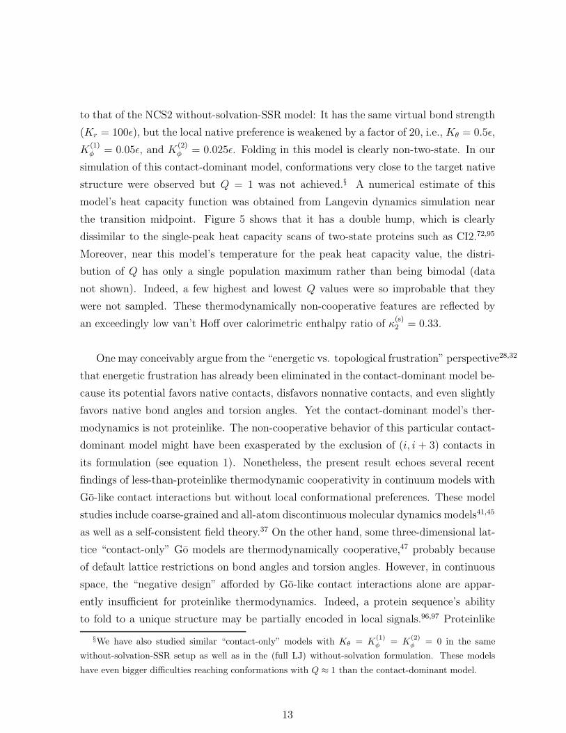
to that of the NCS2 without-solvation-SSR model: It has the same virtual bond strength

(Kr = 100ǫ), but the local native preference is weakened by a factor of 20, i.e., Kθ = 0.5ǫ,

K(1)φ = 0.05ǫ, and K

(2)φ = 0.025ǫ. Folding in this model is clearly non-two-state. In our

simulation of this contact-dominant model, conformations very close to the target native

structure were observed but Q = 1 was not achieved.§ A numerical estimate of this

model’s heat capacity function was obtained from Langevin dynamics simulation near

the transition midpoint. Figure 5 shows that it has a double hump, which is clearly

dissimilar to the single-peak heat capacity scans of two-state proteins such as CI2.72,95

Moreover, near this model’s temperature for the peak heat capacity value, the distri-

bution of Q has only a single population maximum rather than being bimodal (data

not shown). Indeed, a few highest and lowest Q values were so improbable that they

were not sampled. These thermodynamically non-cooperative features are reflected by

an exceedingly low van’t Hoff over calorimetric enthalpy ratio of κ(s)2 = 0.33.

One may conceivably argue from the “energetic vs. topological frustration” perspective28,32

that energetic frustration has already been eliminated in the contact-dominant model be-

cause its potential favors native contacts, disfavors nonnative contacts, and even slightly

favors native bond angles and torsion angles. Yet the contact-dominant model’s ther-

modynamics is not proteinlike. The non-cooperative behavior of this particular contact-

dominant model might have been exasperated by the exclusion of (i, i + 3) contacts in

its formulation (see equation 1). Nonetheless, the present result echoes several recent

findings of less-than-proteinlike thermodynamic cooperativity in continuum models with

Go-like contact interactions but without local conformational preferences. These model

studies include coarse-grained and all-atom discontinuous molecular dynamics models41,45

as well as a self-consistent field theory.37 On the other hand, some three-dimensional lat-

tice “contact-only” Go models are thermodynamically cooperative,47 probably because

of default lattice restrictions on bond angles and torsion angles. However, in continuous

space, the “negative design” afforded by Go-like contact interactions alone are appar-

ently insufficient for proteinlike thermodynamics. Indeed, a protein sequence’s ability

to fold to a unique structure may be partially encoded in local signals.96,97 Proteinlike

§We have also studied similar “contact-only” models with Kθ = K(1)φ = K

(2)φ = 0 in the same

without-solvation-SSR setup as well as in the (full LJ) without-solvation formulation. These models

have even bigger difficulties reaching conformations with Q ≈ 1 than the contact-dominant model.

13

behavior requires minimization of energetic frustration of the target native structure as

well as enhanced frustration in the competing nonnative conformations.98 A comparison

between the contact-dominant model and the other models with local native propen-

sities in Figure 5 suggests that an interplay between local conformational preference

and nonlocal compactification forces47,48,67,68,99,100 are necessary for proteinlike thermo-

dynamic cooperativity. For this conclusion to be properly interpreted, we hasten to add

that structural details of sidechain packing, hydrogen bonding, as well as general non-

native-centric physical restrictions on bond angles and torsion angles (as in standard

non-Go-like force fields) have not been taken into account in the present coarse-grained

(residue-based) contact-dominant model. But these effects are operative in real proteins.

Clearly, these interactions must be part of the physical basis of any local propensity101

for the native fold in a more complete all-atom description.

KINETIC COOPERATIVITY

Sharp Kinetic Transitions Between Two Thermodynamic States

Folding kinetics in explicit-chain Go-like models have been investigated using equilib-

rium sampling in conjunction with free energy profile analyses32 as well as direct dynam-

ics simulations.35 Here, around their respective transition midpoints, all six native-centric

CI2 models — NCS1 or NCS2, with or without solvation — have kinetic characteristics

consistent with their thermodynamic two-state cooperativity. Figure 6a and b show

that the kinetic transitions between the native and denatured ensembles are sudden and

sharp. Figure 6c and d show that the distributions of potential energy and Q are bi-

modally well separated into native and denatured regions, and the correlation between

potential energy and Q is generally linear. A consistency check has also been made using

Figure 6c, which provided an average kinetic energy of 78.9. Equating this with 3NT/2

for N = 64 (equipartition theorem) yields T = 0.8219, which is essentially identical to

the input simulation temperature of T = 0.82, as it should. Figure 6c and d further indi-

cate that after the initiation of folding around the transition midpoint, pre-equilibration

of the denatured ensemble is rapid relative to the folding time scale.

Chevron Plots: Matching Kinetics with Thermodynamics?

14

Bearing in mind that protein thermodynamic cooperativity is necessary but not suf-

ficient for simple two-state folding/unfolding kinetics,68 we proceed to evaluate model

predictions against experimental stability curves and chevron plots. To do so, we deter-

mine model folding and unfolding rates using direct dynamics simulations over extensive

ranges of native stability by varying the interaction parameter ǫ at constant temperature.

Since the simulated kinetics are essentially single-exponential (see below), the folding or

unfolding rate may be taken to be approximately the reciprocal of the corresponding

mean first passage time (MFPT). The natural logarithms of the rates are plotted as

functions of ǫ in Figures 7 – 9. Inasmuch as it was computationally feasible, first passage

times (FPTs) of a large number of trajectories were used to provide reliable estimates

of MFPTs (Tables 1 – 3). As one of us has argued,98,102 the variation of ǫ may serve

as a tentative model for varying denaturant concentration, though the detailed physics

of how the effects of chemical denaturants should be incorporated into coarse-grained

protein models is a subject of ongoing research.103−106 Here we view the upper panels of

Figures 7 – 9 as model equivalences of chevron plots.

Native stability curves of the models as functions of ǫ are plotted in the lower panels of

Figures 7 – 9. They show that the free energy of unfolding between the native minimum

and low-Q open conformations are approximately linear in ǫ (upper solid and dashed

curves). These quasi-linear stability curves estimated from simulation data around the

transition midpoint correspond to those obtained experimentally by empirical linear ex-

trapolation from directly measured data around the transition region.107 In contrast,

the free energy difference between the native minimum and a denatured-state ensemble

encompassing low-Q as well as intermediate-Q conformations (lower solid and dashed

curves) is nonlinear in ǫ, similar to that observed in previously lattice model studies.67,68

This is an expected feature67,68 intimately connected to the multiple-conformation na-

ture of the native state,47,68 and is consistent with recent native-state hydrogen exchange

experiments.107−110 These characteristics of native stability underscore the fact that the

operational definition of calorimetric two-state behavior (see above) does not67 necessar-

ily imply that all denatured conformations have the same stability. Even for calorimetri-

cally two-state proteins under native conditions well below the global folding/unfolding

transition midpoint, the population of partially unfolded conformations67,68,107,111 can

sometimes be non-negligible as long as it does not exceed a certain threshold.67,68

15

Figures 7 – 9 show that the transition midpoints determined by thermodynamics

and kinetics are quite close, with only minor discrepancies. The discrepancies for NCS1

models appear to be slightly larger in Figures 8 and 9. This is probably related to the

high-free-energy minima in the transition regions of the corresponding NCS1 free energy

profiles (Figure 4b, c). More surprisingly, however, is that even with their native-centric

potentials, all six models fail to produce the type of simple two-state folding/unfolding

kinetics observed experimentally for CI295 and many other small single-domain proteins.7

The operational definition95,112 for simple two-state folding/unfolding kinetics requires

that the logarithmic folding and unfolding rates under constant temperature be approxi-

mately linear in native stability, and that the natural logarithm of the directly measured

and linearly extrapolated (folding rate)/(unfolding rate) ratio as a function of denaturant

concentration matches the directly measured and linearly extrapolated95,107 equilibrium

free energy of unfolding in units of kBT . Here, the dashed-dotted V-shapes in the upper

panels of Figures 7 – 9 show that as −ǫ/kBT is changed at constant T from the transi-

tion midpoint towards either more native or more denaturing conditions, the respective

trends of increase in simulated folding or unfolding rate fall short of this requirement

for the kinetics to be simple two-state. Instead, our models’ behavior is more akin to

proteins that exhibit chevron rollovers, such as ribonuclease A113 and barnase,114 whose

kinetics are operationally referred to as non-two-state.68,95,113,114 Comparisons with ex-

perimental chevron plots have not been made in other studies of continuum Go models,

but the reported results indicate that they also do not predict simple two-state chevron

behavior (see, e.g., Figure 2 of ref. 34).

The four without-solvation and without-solvation-SSR models in Figures 7 and 8

show a clear rollover in both the folding and unfolding arms of their chevron plots. Re-

flecting the lower barriers along their free energy profiles (Figure 4), kinetics are generally

faster for the without-solvation and without-solvation-SSR than the corresponding with-

solvation models (Figure 9). For the with-solvation models, the rate at a given −ǫ/kBT

is substantially slower for NCS2 than that for NCS1. This trend is consistent with

NCS2’s much higher free energy barrier in the transition region (Figure 4c). Most re-

markably, comparing Figures 7, 8 against Figure 9 demonstrates a dramatic impact of

desolvation barriers on the folding/unfolding kinetics. In contrast to the chevron plots

16

with significant curvatures for the without-solvation and without-solvation-SSR models,

both the folding and unfolding arms of the chevron plots are quasi-linear for the with-

solvation models. It is reassuring that the with-solvation models are more proteinlike in

this respect.113,114 Nevertheless, their deviations from simple two-state kinetics are huge:

The slopes of the simulated chevron plots are only approximately 1/5 that required for

simple two-state kinetics (c.f. the V-shape in the upper panel of Figure 9). Therefore,

the conclusion that these models’ kinetics correspond to those operationally referred to

as non-two-state should be reliable. This is because possible numerical uncertainties in

the estimation of stability curves by histogram techniques (lower panels of Figure 9) are

not likely to cause a factor-of-five discrepancy. Interestingly, similar mismatches between

extrapolated chevron plots and direct native stability measurements, albeit to a lesser

degree, have also been observed for real proteins.93

Single-Exponential Relaxation

Experimentally, kinetic relaxation of many small single-domain proteins7 such as

CI272,95 and some apparently non-two-state proteins with chevron rollovers113,114 are

found to be essentially single-exponential. Therefore, it is of interest to ascertain whether

the present models embody this hallmark, even though they are not kinetically simple

two-state. For this purpose, we examine the distributions of first passage times (FPTs,

as defined in Figures 7 – 9). Let P (t)dt be the probability for the FPT of a given kinetic

process to lie within a range dt around time t. If the relaxation is single-exponential,∫ t

t0dt′ P (t′) = 1 − e−k(t−t0) , (0.4)

where k is the kinetic rate, and t0 ≥ 0 is a minimum FPT to take into consideration the

finite time needed for pre-equilibration after initiation of the kinetic process at t = 0. It

follows that

MFPT =∫ t

t0dt′ t′P (t′) = t0 +

1

k. (0.5)

To assess whether a given FPT distribution conforms to this description, a quantity

P (t)∆t is computed by binning FPTs into time slots115 of size ∆t. If the kinetic process

is single-exponential,

ln[P (t)∆t] ={

ln(

∆t

MFPT − t0

)

+t0

MFPT − t0

}

−t

MFPT − t0, (0.6)

i.e., ln[P (t)∆t] versus t should be a straight line with slope = −(MFPT − t0)−1.

17

Figure 10a shows that even under strongly native conditions concomitant with a

significant chevron rollover, the NCS2 without-solvation-SSR model has approximately

single-exponential relaxation. This behavior echoes that of a recent four-helix-bundle

lattice model68 (Figure 10b). Consistent with equation 6, a comparison between the

filled and open circles in Figure 10a indicates that while changing the bin size ∆t natu-

rally changes the ln[P (t)∆t] values, reasonable variations in ∆t do not affect the slope

of the ln[P (t)∆t] distribution. Figure 11 applies similar analyses to folding and unfold-

ing in other models in the present study under representative native and denaturing

conditions.¶ Owing to computational limitations, the sample sizes for the FPT dis-

tributions are not very large, especially for the with-solvation models in Figure 11c.

Consequently, a certain level of statistical uncertainties ensued. Nonetheless, Figure 11

shows that for all cases tested, our data is consistent with single-exponential relax-

ation. As pointed out by Fersht,92 the high-free-energy minima along the NCS1 free

energy profiles (Figure 4b, c) do not preclude apparent single-exponential kinetics. The

viability of equation 6 for our models is further buttressed by the relatively small dif-

ferences between the slopes of the least-square-fitted lines in Figure 11 and the quantity

−(MFPT − t0)−1, where t0 is taken to be the minimum FPT encountered in the sim-

ulated trajectories of a given model: For the models and their simulation conditions

listed in the legend of Figure 11, and in the same order, {[106× (MFPT− t0)−1], [−106 ×

slope]} = {10.0, 10.6}, {6.13, 6.71}, {6.11, 6.53}, {7.28, 7.56}, {28.6, 36.1}, {6.41, 7.02},

{19.5, 26.4}, {8.53, 9.36}, {2.05, 2.08}, {0.504, 0.431}, {0.242, 0.189}, and {0.199, 0.161}.

The native-centric formulations in the present Go-like models lead to folding rates

that are at least four orders of magnitdue faster than the experimental CI2 folding rates.

At 25◦C and pH 6.3, the experimental CI2 folding rates at zero denaturant (native sta-

bility ∆G = 12.0kBT ) and the transition midpoint (in 3.92 M GdnHCl, native stability

∆G = 0) are, respectively, 47.8 sec−1 and 0.035 sec−1 (ref. 95). If we use the physical

argument of Veitshans et al.89 to identify the Langevin time unit δt with a real time

scale of ∼ 10−14 sec, the folding rate of the NCS2 with-solvation model in Figure 9 is

∼ 106 sec−1 at ∆G = 12.0kBT and ∼ 105 sec−1 at ∆G = 0. Corresponding folding

¶Rates in the chevron plots in Figures 7 – 9 are computed by taking t0 = 0. Our calculations

indicate that using finite t0s instead of t0 = 0 to determine the rates k via equation 5 only leads to

minimal modifications on the chevron plots (data not shown). The conclusions regarding rollovers and

non-two-state kinetics remain unchanged.

18

rates of other models in Figures 7 – 9 are even faster by approximately two orders of

magnitude. Despite these discrepancies, native-centric constructs do capture part of real

protein energetics. This is evident from studies of extensive sets of real proteins using

explicit-chain Go models, wherein theoretically predicted folding35 and relaxation44 rates

were found to correlate reasonably well with the experimental folding rates. However, it

is noteworthy that the spread of these model-predicted rates among the set of proteins

tested is apparently at least 1.5 – 2 orders of magnitude narrower than the diversity of

experimental folding rates.35 (c.f. Figure 5 of ref. 44). This suggests that certain basic

aspects of protein energetics are yet to be taken into account by common Go-like models.

In a similar vein, the chevron rollovers in Figures 7 –9 represent a failure to account for

the high degree of diversity in folding rates of a given protein under different native con-

ditions. For real CI2, the folding rates at zero denaturant and at the transition midpoint

differ by three orders of magnitude. But the Go-like models in Figures 7 –9 predict only

one order of magnitude difference.

Chevron Rollover: Stability-Dependent Front Factor?

To better understand the chevron rollovers, Figure 12 applies a protocol we recently

developed68 to assess the models’ conformity to the commonly employed transition state

picture in interpreting protein folding experiments. Model data is now fitted to the

expression

rate = F (ǫ, T ) exp[

−∆G‡(ǫ, T )

kBT

]

(0.7)

for folding or unfolding rate, taken as (MFPT)−1 from the direct dynamics simulations.

On the other side of the above equation, ∆G‡ is an activation free energy determined

soley by thermodynamic Boltzmann weights68 using the method of Nymeyer et al.,32,116

F is the corresponding front factor.2,38,39,68,98,117 Figure 12 shows that, in contrast to the

usual stipulation118 that the front factors of small single-domain proteins such as CI2

are essentially independent of intraprotein interaction strength and native stability, the

F factors deduced from the present analysis are highly sensitive to ǫ. This implies that

thermodynamic analyses of free energy profiles alone cannot predict the ǫ-dependencies of

the kinetic rates,38,39,68,117 and the chevron rollovers are underpinned by native-stability-

dependent front factors in these models.68 This hypothesis regarding the physical origin

of chevron rollover may soon be testable by single-molecule techniques.119 In addition

to the definitions for unfolded, transition, and folded regions in Figure 12, we analyzed

19

several other physically reasonable alternate Q-based definitions for these states (data

not shown). Whereas the absolute value of F varies somewhat, the overall trend of de-

pendence on ǫ remains essentially unchanged. This resilience is similar to that observed

in our previous analysis of the folding front factor of a 55mer lattice model (Figure 5 of

ref. 68).

Thus, for this key aspect of chevron behavior, the present native-centric models’

kinetics clearly do not resemble the simple two-state kinetics of CI2.72,95 The ramifica-

tion of this finding is far reaching, as it bears on the basic energetics of protein folding

(see Discussion below). As they stand, the apparently non-two-state kinetics of these

physical self-contained polymer models18 also shed light on the folding of other pro-

teins that exhibit similar chevron rollovers as well.93,113,114 To date, rationalizations of

chevron rollovers include deadtime intermediates,120 specific kinetic traps,98,102,121 peak-

shifting on complex free energy profiles,93,122 burst phase continuum,123 and internal

friction as manifested by front factors that depend on native stability (ref. 68 and dis-

cussion therein). These perspectives are not necessarily mutually exclusive. For exam-

ple, internal friction may arise from kinetic trapping mechanisms (H. K. & H. S. C., in

preparation). In any event, chevron rollover is an unequivocal prediction of the present

models, irrespective of whether Q or other folding reaction coordinates are used for the

transition state analysis (see, e.g., ref. 124). Figure 12d shows that the folding front fac-

tor decreases with more native conditions, and the unfolding front factor also decreases

with more denaturing conditions. In short, there appears to be an aversion to speed in

these models’ energetics. We tentatively attribute the slowing down in these models to a

possible combination of effects of internal friction (conformational search problems com-

pounded by more native conditions)68 and external friction (implicit solvent viscosity).

The origins of these effects remain to be better elucidated. For example, in some model-

ing situations,68 folding-arm rollovers are related to the onset of downhill folding.125,126

The chevron rollovers in the folding and unfolding arms of the NCS2 without-solvation

model may be similarly related to downhill scenarios (see, e.g., the ǫ = 0.90 and ǫ = 0.70

profiles in Figure 12a). At least for the NCS2 with-solvation model in Figure 6, the fact

that no deadtime intermediate was observed during our simulation suggests that such a

mechanism is not necessary for chevron rollovers.68,93 In this example, chevron rollover

emerges as a kinetic front-factor effect.

20

DISCUSSION

We have compared two different native contact sets, and three different formulations

of Go-like interactions with and without desolvation barriers. The predictions of these

native-centric models were evaluated against generic thermodynamic and kinetic prop-

erties of small single-domain proteins that these models were designed to mimic in the

first place. We learnt several lessons. First, proteinlike thermodynamic cooperativity

requires nonlocal contact-like interactions acting in concert with local conformational

favorabilities for the native fold47,48,67,68 (Figure 5). Second, some basic predictions of

native-centric models, such as the free energy profiles in Figure 4, are significantly de-

pendent on the native contact set and interaction scheme used, even if the choice is

made among physically reasonable definitions. A recent study38,39 shows also that free

energy profiles of native-centric models are sensitive to the chain’s presumed persistence

length and energetic barriers to bond rotations.98,102 Third, we found that pairwise des-

olvation barriers in native-centric models could lead to some proteinlike properties such

as a higher free energy barrier separating the native and denatured states (c.f. Fig-

ure 4a, b and c) as well as more linear chevron plots (c.f. Figures 7, 8 and 9). These

predictions are encouraging as they provide insight into corresponding features in real

proteins. Fundamentally, however, the kinetics of all present native-centric models for

CI2 do not resemble that of real CI2. The models with pairwise desolvation barriers,

like those without, are kinetically non-two-state in the operational sense that they have

large chevron rollovers.

Fourth, the significant differences between the predictions of with- and without-

solvation models underscore the importance of proper accounting for the energetic cost

of water expulsion in protein folding models, and that caution should be used when inter-

preting results obtained from effective potentials that do not have desolvation barriers.83,127

The barrier height in the present with-solvation models simulated at T = 0.82 is 0.24 ǫ kBT .

For real proteins, the desolvation barrier heights encountered by the polypeptide chain

as a part of the potential of mean force are expected to be sensitive to temperature.

Thus, the present results should also bear on explicit-solvent unfolding simulations at

21

high temperatures and the degree of dependencies of protein folding mechanisms on

temperature.128 Of relevance here is the model system of a pair of methanes in water.

Recent Monte Carlo simulations in the TIP4P water model indicate that their desolva-

tion barrier is reduced from approximately 0.16 to 0.12 kcal/mol (0.27kBT to 0.16kBT )

when temperature is increased from 298K to 368K under atmospheric pressure.84 Un-

der typical high-temperature unfolding conditions of 498K and a water density of 0.829

gm/ml,128 the desolvation barrier height is further reduced to ≈ 0.05 kcal/mol or 0.05kBT

(Figure 16.3 in ref. 18; S. Shimizu and H. S. C., personal communication).

In a broader perspective, solvent-mediated interactions are known to be intrinsi-

cally pairwise nonadditive,76,83 and the collapse of a hydrophobic chain may involve

large length-scale dynamic effects.129 In this light, that the pairwise desolvation barri-

ers here fail to produce simple two-state chevron plots is not too surprising. Indeed,

recent explicit-water simulations show that the sign of heat capacity of the free energy

barrier against folding is opposite to that against the association of a pair of methane

molecules.84,85,106 Considerations of a three-methane model system further indicate that

the height of desolvation barrier is clearly nonadditive, and the sign and magnitude of

this nonadditivty is dependent upon the configuration of the nonpolar solutes involved.83

Hence, solvation effects beyond the pairwise formulation considered here are likely needed

to account for simple two-state protein folding/unfolding kinetics.

In summary, the present findings imply that the actual solvent-mediated interactions

in real proteins are much more specific and well-designed than one would otherwise posit.

In short, real proteins are more cooperative than common Go-like models with pairwise

additive interactions. Nonetheless, recent innovations in native-centric modeling have

been immensely valuable. As discussed above, they do capture part of the essential

physics. Many deep insight would not have been gained without them (see, e.g., refs. 1,

29, 33). But, at the same time, the limitations of common Go-like chain models67,68 may

be more basic than previously appreciated. The present analysis implies that more pro-

teinlike interaction schemes are yet to be discovered. Every model considered here except

the contact-dominant variety can fold to the CI2 native structure. Qualitatively, the free

energy profiles of the NCS2 models fit the expectation for that of small single-domain

proteins as well. Yet their kinetics are fundamentally different from that of CI2. Thus, a

22

protein model’s ability to fold to one single target structure does not guarantee the ade-

quacy of its energetics; and the microscopic origin of simple two-state folding/unfolding

kinetics remains to be elucidated. Our effort to address some of these questions is un-

derway. Apparently, chevron rollovers can be essentially eliminated in more cooperative

chain models with added energetic favorabilities for the ground-state and near-ground-

state structures beyond that provided by the additive schemes in common Go models.

These results will be presented in a subsequent report (H. K. & H. S. C., in prepara-

tion). In the ongoing quest for a better understanding of protein energetics through

the design and interpretation of novel physical models, proteinlike statistical mechanics

properties such as calorimetric two-state cooperativity41,47,48,67,68,130,131 and simple two-

state chevron behavior68 should be useful as stringent but necessary modeling constraints.

AcknowledgmentsWe thank Yawen Bai, Margaret Cheung, Cecilia Clementi, Ken Dill, Angel Garcıa,

Chinlin Guo, Carol Hall, Anders Irback, Sophie Jackson, John Karanicolas, Bob Matthews,

Cristian Micheletti, Hugh Nymeyer, Mikael Oliveberg, Jose Onuchic, Kevin Plaxco, John

Portman, Eugene Shakhnovich, Joan-Emma Shea, Seishi Shimizu, Kim Sneppen, Dev

Thirumalai, Michele Vendruscolo, Peter Wolynes, and Yaoqi Zhou for helpful discus-

sions during the period in which these ideas were developed. This work was partially

supported by the Canadian Institutes of Health Research (CIHR grant no. MOP-15323),

a Premier’s Research Excellence Award from the Province of Ontario, and the Ontario

Centre for Genomic Computing at the Hospital for Sick Children in Toronto. H. S. C.

is a Canada Research Chair in Biochemistry.

23

References

[1] Baker, D. (2000). A surprising simplicity to protein folding. Nature 405, 39–42.

[2] Bilsel, O. & Matthews, C. R. (2000). Barriers in protein folding reactions. Adv.

Protein Chem. 53, 153–207.

[3] Eaton, W. A., Munoz, V., Hagen, S. J., Jas, G. S., Lapidus, L. J., Henry, E. R. &

Hofrichter, J. (2000). Fast kinetics and mechanisms in protein folding. Annu. Rev.

Biophys. Biomolec. Struct. 29, 321–359.

[4] Fersht, A. R. (2000). Transition-state structure as a unifying basis in protein-folding

mechanisms: Contact order, chain topology, stability, and the extended nucleus

mechanism. Proc. Natl. Acad. Sci. USA 97, 1525–1529.

[5] Plaxco, K. W., Simons, K. T. & Baker, D. (1998). Contact order, transition state

placement and the refolding rates of single domain proteins. J. Mol. Biol. 277,

985–994.

[6] Chan, H. S. (1998). Matching speed and locality. Nature 392, 761–763.

[7] Plaxco, K. W., Simons, K. T., Ruczinski, I. & Baker, D. (2000). Topology, stabil-

ity, sequence, and length: Defining the determinants of two-state protein folding

kinetics. Biochemistry 39, 11177–11183.

[8] Duan, Y. & Kollman, P. A. (1998). Pathways to a protein folding intermediate

observed in a 1-microsecond simulation in aqueous solution. Science 282, 740–744.

[9] Daggett V. (2002). Molecular dynamics simulations of the protein unfolding/folding

reaction. Acc. Chem. Res. 35, 422–429.

[10] Sanbonmatsu, K. Y. & Garcıa, A. E. (2002). Structure of Met-enkephalin in ex-

plicit aqueous solution using replica exchange molecular dynamics. Proteins Struct.

Funct. Genet. 46, 225–234.

[11] Levitt, M. & Warshel, A. (1975). Computer simulation of protein folding. Nature

253, 694–698.

24

[12] Taketomi, H., Ueda, Y. & Go, N. (1975). Studies on protein folding, unfolding and

fluctuations by computer simulation. 1. The effect of specific amino acid sequence

represented by specific inter-unit interactions. Int. J. Pept. Protein Res. 7, 445–459.

[13] Hagler, A. T. & Honig, B. (1978). On the formation of protein tertiary structure

on a computer. Proc. Natl. Acad. Sci. USA 75, 554–558.

[14] Godzik, A., Kolinski, A. & Skolnick, J. (1993). Lattice representations of globular

proteins: How good are they? J. Comp. Chem. 14, 1194–1202.

[15] Bryngelson, J. D., Onuchic, J. N., Socci, N. D. & Wolynes, P. G. (1995). Funnels,

pathways, and the energy landscape of protein folding: A synthesis. Proteins Struct.

Funct. Genet. 21, 167–195.

[16] Dill, K. A., Bromberg, S., Yue, K., Fiebig, K. M., Yee, D. P., Thomas, P. D. &

Chan, H. S. (1995). Principles of protein folding — A perspective from simple exact

models. Protein Sci. 4, 561–602.

[17] Thirumalai, D. & Woodson S. A. (1996). Kinetics of folding of proteins and RNA.

Acc. Chem. Res. 29, 433–439.

[18] Chan, H. S., Kaya, H. & Shimizu, S. (2002). Computational methods for protein

folding: Scaling a hierarchy of complexities. In Current Topics in Computational

Molecular Biology, eds. Jiang, T., Xu, Y. & Zhang, M. Q. (The MIT Press, Cam-

bridge, MA), pp. 403–447.

[19] Mirny, L. & Shakhnovich, E. (2001). Protein folding theory: From lattice to all-

atom models. Annu. Rev. Biophys. Biomol. Struct. 30, 361–396.

[20] Thirumalai, D. & Klimov, D. K. (1999). Deciphering the timescales and mechanisms

of protein folding using minimal off-lattice models. Curr. Opin. Struct. Biol. 9,

197—207.

[21] Onuchic, J. N., Nymeyer, H., Garcıa, A. E., Chahine, J. & Socci, N. D. (2000). The

energy landscape theory of protein folding: Insights into folding mechanisms and

scenarios. Adv. Protein Chem. 53, 87–152.

[22] Burton, R. E., Myers, J. K. & Oas, T. G. (1998). Protein folding dynamics: Quan-

titative comparison between theory and experiment. Biochemistry, 37, 5337–5343.

25

[23] Alm, E. & Baker, D. (1999). Prediction of protein-folding mechanisms from free-

energy landscapes derived from native structures. Proc. Natl. Acad. Sci. USA 96,

11305–11310.

[24] Debe, D. A. & Goddard, W. A. (1999). First principles prediction of protein folding

rates. J. Mol. Biol. 294, 619–625.

[25] Munoz, V. & Eaton, W. A. (1999). A simple model for calculating the kinetics of

protein folding from three-dimensional structures. Proc. Natl. Acad. Sci. USA 96,

11311–11316.

[26] Galzitskaya, O. V. & Finkelstein, A. V. (1999). A theoretical search for fold-

ing/unfolding nuclei in three-dimensional protein structures. Proc. Natl. Acad. Sci.

USA 96, 11299–11304.

[27] Micheletti, C., Banavar, J. R., Maritan, A. & Seno, F. (1999). Protein structures

and optimal folding from a geometrical variational principle. Phys. Rev. Lett. 82,

3372–3375.

[28] Shea, J.-E., Onuchic, J. N. & Brooks, C. L. III. (1999). Exploring the origins of

topological frustration: Design of a minimally frustrated model of fragment B of

protein A. Proc. Natl. Acad. Sci. USA 96, 12512–12517.

[29] Takada, S. (1999). Go-ing for the prediction of protein folding mechanisms. Proc.

Natl. Acad. Sci. USA 96, 11698–11700.

[30] Zhou, Y. & Karplus M. (1999). Interpreting the folding kinetics of helical proteins.

Nature 401, 400–403.

[31] Clementi, C., Jennings, P. A. & Onuchic, J. N. (2000). How native-state topology

affects the folding of dihydrofolate reductase and interleukin-1β. Proc. Natl. Acad.

Sci. USA 97, 5871–5876.

[32] Clementi, C., Nymeyer, H. & Onuchic, J. N. (2000). Topological and energetic

factors: What determines the structural details of the transition state ensemble and

“en-route” intermediates for protein folding? An investigation for small globular

proteins. J. Mol. Biol. 298, 937–953.

26

[33] Banavar, J. R. & Maritan, A. (2001). Computational approach to the protein-

folding problem. Proteins Struct. Funct. Genet. 42, 433–435.

[34] Cieplak, M. & Hoang, T. X. (2001). Kinetic nonoptimality and vibrational stability

of proteins. Proteins Struct. Funct. Genet. 44, 20–25.

[35] Koga, N. & Takada, S. (2001). Roles of native topology and chain-length scaling

in protein folding: A simulation study with a Go-like model. J. Mol. Biol. 313,

171–180.

[36] Li, L. & Shakhnovich, E. I. (2001). Constructing, verifying, and dissecting the

folding transition state of chymotrypsin inhibitor 2 with all-atom simulations. Proc.

Natl. Acad. Sci. USA 98, 13014–13018.

[37] Micheletti, C., Banavar, J. R. & Maritan, A. (2001). Conformations of proteins in

equilibrium. Phys. Rev. Lett. 87, Art. No. 088102.

[38] Portman, J. J., Takada, S. & Wolynes, P. G. (2001). Microscopic theory of protein

folding rates. I. Fine structure of the free energy profile and folding routes from a

variational approach. J. Chem. Phys. 114, 5069–5081.

[39] Portman, J. J., Takada, S. & Wolynes, P. G. (2001). Microscopic theory of protein

folding rates. II. Local reaction coordinates and chain dynamics. J. Chem. Phys.

114, 5082–5096.

[40] Cheung, M. S., Garcıa, A. E. & Onuchic, J. N. (2002). Protein folding mediated by

solvation: Water expulsion and formation of the hydrophobic core occur after the

structural collapse. Proc. Natl. Acad. Sci. USA 99, 685-690.

[41] Jang, H., Hall, C. K. & Zhou, Y. (2002). Folding thermodynamics of model four-

strand antiparallel β-sheet proteins. Biophys. J. 82, 646–659.

[42] Klimov, D. K. & Thirumalai, D. (2002). Stiffness of the distal loop restricts the

structural heterogeneity of the transition state ensemble in SH3 domains. J. Mol.

Biol. 317, 721–737.

[43] Makarov, D. E., Keller, C. A., Plaxco, K. W. & Metiu, H. (2002). How the folding

rate constant of simple, single-domain proteins depends on the number of native

contacts. Proc. Natl. Acad. Sci. USA 99, 3535–3539.

27

[44] Micheletti, C., Lattanzi, G. & Maritan, A. (2002). Elastic properties of proteins:

Insight on the folding process and evolutionary selection of native structures. J.

Mol. Biol. 321, 909–921.

[45] Zhou, Y. & Linhananta, A. (2002). Thermodynamics of an all-atom off-lattice model

of the fragment B of Staphylococcal protein A: Implication for the origin of the

cooperativity of protein folding. J. Phys. Chem. B 106, 1481–1485.

[46] Linhananta, A. & Zhou, Y. (2002). The role of sidechain packing and native contact

interactions in folding: Discontinuous molecular dynamics folding simulations of an

all-atom Go model of fragment B of Staphylococcal protein A. J. Chem. Phys. 117,

8983–8995.

[47] Kaya, H. & Chan, H. S. (2000). Polymer principles of protein calorimetric two-

state cooperativity. Proteins Struct. Funct. Genet. 40, 637–661 [Erratum: 43, 523

(2001)].

[48] Kaya, H. & Chan, H. S. (2000). Energetic components of cooperative protein fold-

ing. Phys. Rev. Lett. 85, 4823–4826.

[49] Go, N. (1999). The consistency principle revisited. In Old and New Views of Protein

Folding, eds. Kuwajima, K. & Arai, M. (Elsevier, Amsterdam, The Netherlands),

pp. 97–105.

[50] Laughlin, R. B. & Pines, D. (2000). The theory of everything. Proc. Natl. Acad.

Sci. USA 97, 28–31.

[51] Isin, B., Doruker, P. & Bahar, I. (2002). Functional motions of influenza virus

hemagglutinin: A structure-based analytical approach. Biophys. J. 82, 569–581.

[52] Keskin, O., Bahar, I., Flatow, D., Covell, D. G. & Jernigan, R. L. (2002). Molecular

mechanisms of chaperonin GroEL-GroES function. Biochemistry 41, 491–501.

[53] Jacobs, D. J., Rader, A. J., Kuhn, L. A. & Thorpe, M. F. (2001). Protein flexibility

prediction using graph theory. Proteins: Struct. Funct. Genet. 44, 150–165.

[54] Go, N. (1983). Theoretical studies of protein folding. Annu. Rev. Biophys. Bioeng.

12, 183–210.

28

[55] Bryngelson, J. D. & Wolynes, P. G. (1987). Spin glasses and the statistical mechan-

ics of protein folding. Proc. Natl. Acad. Sci. USA 84, 7524–7528.

[56] Panchenko, A. R., Luthey-Schulten, Z., Cole, R. & Wolynes, P. G. (1997). The

foldon universe: A survey of structural similarity and self-recognition of indepen-

dently folding units. J. Mol. Biol. 272, 95–105.

[57] Lau, K. F. & Dill, K. A. (1989). A lattice statistical mechanics model of the con-

formational and sequence spaces of proteins. Macromolecules 22, 3986–3997.

[58] Chan, H. S. & Dill, K. A. (1991). Sequence space soup of proteins and copolymers.

J. Chem. Phys. 95, 3775–3787.

[59] Shakhnovich, E., Farztdinov, G., Gutin, A. M. & Karplus, M. (1991). Protein

folding bottlenecks — a lattice Monte-Carlo simulation. Phys. Rev. Lett. 67, 1665–

1668.

[60] Leopold, P. E., Montal, M. & Onuchic, J. N. (1992). Protein folding funnels — a

kinetic approach to the sequence structure relationship. Proc. Natl. Acad. Sci. USA

89, 8721–8725.

[61] Camacho, C. J. & Thirumalai, D. (1993). Kinetics and thermodynamics of folding

in model proteins. Proc. Natl. Acad. Sci. USA 90, 6369–6372.

[62] Shrivastava, I., Vishveshwara, S., Cieplak, M., Maritan, A. & Banavar, J. R. (1995).

Lattice model for rapidly folding protein-like heteropolymers. Proc. Natl. Acad. Sci.

USA 92, 9206–9209.

[63] Plotkin, S. S. (2001). Speeding protein folding beyond the Go model: How a little

frustration sometimes helps. Proteins Struct. Funct. Genet. 45, 337–345.

[64] Paci, E., Vendruscolo, M. & Karplus, M. (2002). Native and non-native interactions

along protein folding and unfolding pathways. Proteins Struct. Funct. Genet. 47,

379–392.

[65] McCallister, E. L., Alm, E. & Baker, D. (2000). Critical role of β-hairpin formation

in protein G folding. Nature Struct. Biol. 7, 669–673.

29

[66] Hillson, N., Onuchic, J. N. & Garcıa, A. E. (1999). Pressure-induced protein-

folding/unfolding kinetics. Proc. Natl. Acad. Sci. USA 96, 14848–14853.

[67] Chan, H. S. (2000). Modeling protein density of states: Additive hydrophobic ef-

fects are insufficient for calorimetric two-state cooperativity. Proteins Struct. Funct.

Genet. 40, 543–571.

[68] Kaya, H. & Chan, H. S. (2002). Towards a consistent modeling of protein thermo-

dynamic and kinetic cooperativity: How applicable is the transition state picture

to folding and unfolding? J. Mol. Biol. 315, 899–909.

[69] Tiktopulo, E. I., Bychkova, V. E., Ricka, J. & Ptitsyn, O. B. (1994). Cooperativ-

ity of the coil-globule transition in a homopolymer — Microcalorimetric study of

poly(N -isopropylacrylamide). Macromolecules 27, 2879–2882.

[70] Matthews, C. R. (1987). Effect of point mutations on the folding of globular pro-

teins. Methods Enzymol. 154, 498–511.

[71] Gillespie, B. & Plaxco, K. W. (2000). Nonglassy kinetics in the folding of a simple

single-domain protein. Proc. Natl. Acad. Sci. USA 97, 12014–12019.

[72] Jackson, S. E., Moracci, M., elMasry, N., Johnson, C. M. & Fersht, A. R. (1993). Ef-

fect of cavity-creating mutations in the hydrophobic core of chymotrypsin inhibitor

2. Biochemistry 32, 11259–11269.

[73] De Jong, D., Riley, R., Alonso, D. O. V. & Daggett, V. (2002). Probing the energy

landscape of protein folding/unfolding transition states. J. Mol. Biol. 319, 229–242.

[74] Fersht, A. R. & Daggett, V. (2002) Protein folding and unfolding at atomic resolu-

tion. Cell 108, (4): 573–582.

[75] Sobolev, V., Sorokine, A., Prilusky, J., Abola, E. E. & Edelman, M. (1999). Auto-

mated analysis of interatomic contacts in proteins. Bioinformatics 15, 327–332.

[76] Vaiana, S. M., Manno, M., Emanuele, A., Palma-Vittorelli, M. B. & Palma, M. U.

(2001). The role of solvent in protein folding and in aggregation. J. Biol. Phys. 27,

133–145.

30

[77] Pratt L. R. & Chandler, D. (1977). Theory of the hydrophobic effect. J. Chem.

Phys. 67, 3683–3704.

[78] Geiger, A., Rahman, A. & Stillinger, F. H. (1979). Molecular dynamics study of

the hydration of Lennard-Jones solutes. J. Chem. Phys. 70, 263–276.

[79] Pangali, C., Rao, M. & Berne, B. J. (1979). A Monte Carlo simulation of the

hydrophobic interaction. J. Chem. Phys. 71, 2975–2981.

[80] Guo, C., Cheung, M. S., Levine, H. & Kessler, D. A. (2002). Mechanisms of coop-

erativity underlying sequence-independent β-sheet formation. J. Chem. Phys. 116,

4353–4365.

[81] Karanicolas, J. & Brooks, C. L. (2002). The origins of asymmetry in the folding

transition states of protein L and protein G. Protein Sci. 11, 2351–2361.

[82] Roux, B. & Simonson, T. (1999). Implicit solvent models. Biophys. Chem. 78, 1–20.

[83] Shimizu, S. & Chan, H. S. (2002). Anti-cooperativity and cooperativity in hy-

drophobic interactions: Three-body free energy landscapes and comparison with

implicit-solvent potential functions for proteins. Proteins Struct. Funct. Genet. 48,

15–30. [Erratum: 49, 294 (2002)].

[84] Shimizu, S. & Chan, H. S. (2000). Temperature dependence of hydrophobic inter-

actions: A mean force perspective, effects of water density, and non-additivity of

thermodynamic signatures. J. Chem. Phys. 113, 4683–4700. [Erratum: 116, 8636

(2002)].

[85] Shimizu, S. & Chan, H. S. (2001). Configuration-dependent heat capacity of pair-

wise hydrophobic interactions. J. Am. Chem. Soc. 123, 2083–2084.

[86] Ghosh, T., Garcıa, A. E. & Garde, S. (2002). Enthalpy and entropy contributions

to the pressure dependence of hydrophobic interactions. J. Chem. Phys. 116, 2480–

2486.

[87] Berendsen, H. J. C., Postma, J. P. M., van Gunsteren, W. F., DiNola, A. & Haak,

J. R. (1984). Molecular dynamics with coupling to an external bath. J. Chem. Phys.

81, 3684–3690.

31

[88] Guo, Z. & Thirumalai, D. (1995). Kinetics of protein folding: Nucleation mecha-

nism, time scales, and pathways. Biopolymers 36, 83–102.

[89] Veitshans, T., Klimov, D. & Thirumalai, D. (1997). Protein folding kinetics:

Timescales, pathways and energy landscapes in terms of sequence-dependent prop-

erties. Fold. Des. 2, 1–22.

[90] Allen, M. P. & Tildesley, D. J. (1987). Computer Simulation of Liquids. Oxford

University Press, Oxford, UK.

[91] Swope, W. C., Andersen, H. C., Berens, P. H. & Wilson, K. R. (1982). A computer

simulation method for the calculation of equilibrium constants for the formation of

physical clusters of molecules: Application to small water clusters. J. Chem. Phys.

76, 637–649.

[92] Fersht, A. R. (1997). Nucleation mechanisms in protein folding. Curr. Opin. Struct.

Biol. 7, 3–9.

[93] Chu, R.-A. & Bai, Y. (2002). Lack of definable nucleation sites in the rate-limiting

transition state of barnase under native conditions. J. Mol. Biol. 315, 759–770.

[94] Yang, D., Mok, Y. K., Forman-Kay, J. D., Farrow, N. A. & Kay, L. E. (1997). Con-

tributions to protein entropy and heat capacity from bond vector motions measured

by NMR spin relaxation. J. Mol. Biol. 272, 790–804.

[95] Jackson, S. A. & Fersht, A. R. (1991). Folding of chymotrypsin inhibitor 2. 1.

Evidence for a two-state transition. Biochemistry 30, 10428–10435.

[96] Cui, Y., Wong, W. H., Bornberg-Bauer, E. & Chan, H. S. (2002). Recombinatoric

exploration of novel folded structures: A heteropolymer-based model of protein

evolutionary landscapes. Proc. Natl. Acad. Sci. USA 99, 809–814.

[97] Chan, H. S. & Bornberg-Bauer, E. (2002). Perspectives on protein evolution from

simple exact models. Applied Bioinformatics, in press.

[98] Chan, H. S. & Dill, K. A. (1998). Protein folding in the landscape perspective:

Chevron plots and non-Arrhenius kinetics. Proteins Struct. Funct. Genet. 30, 2–

33.

32

[99] Bakk, A., Høye, J. S., Hansen, A., Sneppen, K. & Jensen, M. H. (2000). Pathways

in two-state protein folding. Biophys. J. 79, 2722–2727.

[100] Uversky, V. N. & Fink, A. L. (2002). The chicken-egg scenario of protein folding

revisited. FEBS Lett. 515, 79–83.

[101] Creamer, T. P. & Rose, G. D. (1994). α-Helix-forming propensities in peptides and

proteins. Proteins Struct. Funct. Genet. 19, 85–97.

[102] Chan, H.S. (1998). Modelling protein folding by Monte Carlo dynamics: Chevron

plots, chevron rollover, and non-Arrhenius kinetics. In Monte Carlo Approach to

Biopolymers and Protein Folding (Grassberger, P., Barkema, G.T. & Nadler, W.,

eds) pp. 29–44, World Scientific, Singapore.

[103] Wallqvist, A., Covell, D. G., Thirumalai, D. (1998). Hydrophobic interactions in

aqueous urea solutions with implications for the mechanism of protein denaturation.

J. Am. Chem. Soc. 120, 427–428.

[104] Crippen, G. M. (2001). A Gaussian statistical mechanical model for the equilibrium

thermodynamics of barnase folding. J. Mol. Biol. 306, 565–573.

[105] Ikeguchi, M., Nakamura S, Shimizu, K. (2001). Molecular dynamics study on hy-

drophobic effects in aqueous urea solutions. J. Am. Chem. Soc. 123, 677–682.

[106] Shimizu, S. & Chan, H. S. (2002). Origins of protein denatured states compactness

and hydrophobic clustering in aqueous urea: Inferences from nonpolar potentials of

mean force. Proteins Struct. Funct. Genet. 49, 560–566.

[107] Englander, S. W., Mayne, L., Bai, Y. & Sosnick, T. R. (1997). Hydrogen exchange:

The modern legacy of Linderstrøm-Lang. Protein Sci. 6, 1101–1109.

[108] Kim, K. S. & Woodward, C. (1993). Protein internal flexibility and global stability:

Effect of urea on hydrogen-exchange rates of bovine pancreatic trypsin inhibitor.

Biochemistry 32, 9609–9613.

[109] Bai, Y., Sosnick, T. R., Mayne, L. & Englander, S. W. (1995). Protein folding

intermediates: Native-state hydrogen exchange. Science 269, 192–197.

33

[110] Llinas, M., Gillespie, B., Dahlquist, F. W. & Marqusee, S. (1999). The energetics of

T4 lysozyme reveal a hierarchy of conformations. Nature Struct. Biol. 6, 1072–1078.

[111] Klimov, D. K. & Thirumalai, D. (2002). Is there a unique melting temperature for

two-state proteins? J. Comput. Chem. 23, 161–165.

[112] Kuhlman, B., Luisi, D. L., Evans, P. A. & Raleigh, D. P. (1998). Global analysis

of the effects of temperature and denaturant on the folding and unfolding kinetics

of the N-terminal domain of the protein L9. J. Mol. Biol. 284, 1661–1670.

[113] Houry, W. A., Rothwarf, D. M. & Scheraga, H. A. (1995). The nature of the

initial step in the conformational folding of disulphide-intact ribonuclease A. Nature

Struct. Biol. 2, 495–503.

[114] Oliveberg, M., Tan, Y. J. & Fersht, A. R. (1995). Negative activation enthalpies

in the kinetics of protein folding. Proc. Natl. Acad. Sci. USA 92, 8926–8929.

[115] Abkevich, V. I., Gutin, A. M. & Shakhnovich, E. I. (1994). Free energy landscape

for protein folding kinetics: Intermediates, traps, and multiple pathways in theory

and lattice model simulations. J. Chem. Phys. 101, 6052–6062.

[116] Nymeyer, H., Socci, N. D. & Onuchic, J. N. (2000). Landscape approaches for

determining the ensemble of folding transition states: Success and failure hinge on

the degree of frustration. Proc. Natl. Acad. Sci. USA 97, 634–639.

[117] Socci, N. D., Onuchic, J. N. & Wolynes, P. G. (1996). Diffusive dynamics of the

reaction coordinate for protein folding funnels. J. Chem. Phys. 104, 5860–5868.

[118] Fersht, A. R., Matouschek, A. & Serrano, L. (1992). The folding of an enzyme. I.

Theory of protein engineering analysis of stability and pathway of protein folding.

J. Mol. Biol. 224, 771–782.

[119] Schuler, B., Lipman, E. A. & Eaton, W. A. (2002). Probing the free-energy surface

for protein folding with single-molecule fluorescence spectroscopy. Nature 419, 743–

747.

[120] Matouschek, A., Kellis, J. T., Serrano, L., Bycroft, M. & Fersht, A. R. (1990).

Characterizing transient folding intermediates by protein engineering. Nature 346,

440-445.

34

[121] Li, R., Battiste, J. L. & Woodward, C. (2002). Native-like interactions favored

in the unfolded bovine pancreatic trypsin inhibitor have different roles in folding.

Biochemistry 41, 2246–2253.

[122] Oliveberg, M. (1998). Alternative explanations for “multistate” kinetics in protein

folding: Transient aggregation and changing transition-state ensembles. Acc. Chem.

Res. 31, 765–772.

[123] Parker, M. J. & Marqusee, S. (1999). The cooperativity of burst phase reactions

explored. J. Mol. Biol. 293, 1195–1210.

[124] Du, R., Pande, V. S., Grosberg, A. Yu., Tanaka, T. & Shakhnovich, E. I. (1998).

On the transition coordinate for protein folding. J. Chem. Phys. 108, 334–350.

[125] Sabelko, J., Ervin, J. & Gruebele, M. (1999). Observation of strange kinetics in

protein folding. Proc. Natl. Acad. Sci. USA 96, 6031–6036.

[126] Eaton, W. A. (1999). Searching for “downhill scenarios” in protein folding. Proc.

Natl. Acad. Sci. USA 96, 5897–5899.

[127] Lazaridis, T. & Karplus, M. (1999). Effective energy functions for proteins in so-

lution. Proteins Struct. Funct. Genet. 35, 133–152.

[128] Day, R., Bennion, B. J., Ham, S. & Daggett, V. (2002). Increasing temperature

accelerates protein unfolding without changing the pathway of unfolding. J. Mol.

Biol. 322, 189–203.

[129] ten Wolde, P. R. & Chandler, D. (2002). Drying-induced hydrophobic polymer

collapse. Proc. Natl. Acad. Sci. USA 99, 6539–6543.

[130] Fan, K., Wang, J. & Wang, W. (2001). Modeling two-state cooperativity in protein

folding. Phys. Rev. E 64, Art. No. 041907.

[131] Crippen, G. M. & Chhajer, M. (2002). Lattice models of protein folding permitting

disordered native states. J. Chem. Phys. 116, 2261–2268.

35

Table 1

unfolding folding

NCS1 NCS2 NCS1 NCS2

ǫ MFPT/105 Nt MFPT/105 Nt ǫ MFPT/105 Nt MFPT/105 Nt

0.60 0.1734 100 0.1763 100 1.00 0.6905 100 0.9250 100

0.65 0.2472 100 0.2547 100 0.95 0.9534 100 1.1668 100

0.70 0.3825 100 0.4212 100 0.90 1.4646 100 1.3102 100

0.75 0.7807 100 0.8950 100 0.89 1.5062 100 1.3865 100

0.77 1.2540 1100 1.9052 1100 0.88 1.8175 1100 1.5577 1100

0.78 1.7684 100 2.8292 100 0.87 2.1760 100 2.0039 100

0.79 2.4983 100 4.7346 100 0.86 2.2865 100 2.3725 100

0.80 2.3120 100 8.0901 100 0.85 3.0018 100 2.7999 100

0.82 3.4755 100 42.737 100 0.84 4.2971 100 4.0108 100

— — — — — 0.83 4.6969 100 5.1892 100

— — — — — 0.82 7.9260 100 7.3979 100

— — — — — 0.80 20.278 100 17.844 100

Table 1. Number of trajectories Nt used in the present study to determine the MFPT

of folding and unfolding for the NCS1 and NCS2 without-solvation models (T = 0.82,

Figure 7). Each MFPT listed is the average (arithmetic mean) over Nt first passage

times for the given interaction strength ǫ. Time is measured from the start of a given

simulation at t = 0 in units of δt (see text).

36

Table 2

unfolding folding

NCS1 NCS2 NCS1 NCS2

ǫ MFPT/105 Nt MFPT/105 Nt ǫ MFPT/105 Nt MFPT/105 Nt

0.70 0.1804 100 0.1856 100 1.30 1.0080 100 0.9121 100

0.75 0.2450 100 0.2730 100 1.25 1.1324 100 1.0924 100

0.80 0.3362 100 0.3759 100 1.20 1.4063 100 1.0754 100

0.83 0.4489 100 0.5304 100 1.18 1.4840 100 1.2380 100

0.85 0.5653 1100 0.6950 1940 1.15 1.7905 1100 1.6733 1097

0.88 0.9161 100 1.2724 100 1.13 2.3409 100 1.6971 100

0.90 1.3364 100 2.3473 100 1.10 2.8513 100 2.2875 100

0.93 2.3120 100 6.5846 100 1.08 4.0404 100 3.0059 100

0.95 4.7098 100 15.767 100 1.05 6.8365 100 4.8426 100

0.97 9.4389 75 40.261 45 1.03 10.385 100 9.6890 100

0.98 16.268 91 42.673 20 1.00 43.174 52 25.440 60

0.99 — — 71.042 15 0.98 — — 110.78 24

1.00 51.148 18 262.14 7 0.97 — — 349.46 14

Table 2. Same as Table 1, but for the without-solvation-SSR models (T = 0.64,

Figure 8).

37

Table 3

unfolding folding

NCS1 NCS2 NCS1 NCS2

ǫ MFPT/105 Nt MFPT/105 Nt ǫ MFPT/105 Nt MFPT/105 Nt

0.40 0.5559 600 0.6549 500 1.50 1.2196 100 2.1393 150

0.50 0.8419 126 1.5782 137 1.40 2.4237 108 3.5297 176

0.60 1.6697 111 7.2719 121 1.30 3.9479 117 5.5725 176

0.65 2.7900 103 17.122 50 1.25 5.4452 107 8.7000 85

0.70 5.4940 1100 44.590 205 1.20 6.8649 112 11.766 50

0.75 8.4002 120 104.18 34 1.18 8.7936 119 — —

0.80 15.463 91 293.56 26 1.15 10.823 52 30.141 42

0.83 26.101 51 — — 1.10 19.633 427 48.000 205

0.85 42.512 74 722.32 15 1.08 20.336 36 — —

0.90 119.01 32 1224.2 6 1.05 41.682 63 143.75 24

0.92 — — 1922.0 4 1.03 43.365 56 166.15 20

0.93 168.05 24 — — 1.00 75.048 52 330.35 28

0.95 216.32 37 — — 0.97 93.742 40 444.98 7

0.95 132.12 37 783.56 6

0.90 — — 1519.4 3

Table 3. Same as Table 1, but for the with-solvation models (T = 0.82, Figure 9).

38

Figure Captions

Figure 1. Native contact maps of the 64-residue truncated form of chymotrypsin

inhibitor 2 (2ci2) used in the present investigation. (a) Contact maps for the native

contact sets NCS1 (green dots) and NCS2 (red dots) as defined in the text. Numbering

of amino acids in these maps is initialized at residue 20 of the full-length 83-residue

CI2; i.e., residue 1 in (a) corresponds to Leu 20 in the untruncated protein. (b, c, d)

Similarities and differences between native contact maps. Contact pairs are indicated by

color lines joining Cα positions along the backbone (black trace). (b) Contacts shared

by NCS1 and NCS2. (c) Contacts in NCS1 but not in NCS2. (d) Contacts in NCS2 but

not in NCS1.

Figure 2. Different native contact definitions. Amino acid numbering here corre-

sponds to that of the full-length CI2, i.e., numbering in this figure equals to that in

Fig. 1a plus 19. The red contact belongs to NCS2 but not NCS1. This pair of residues

has a Cα–Cα distance of 11.24 A, with closest atomic separation between the residues

equals 4.3 A. The green contact belongs to NCS1 but not NCS2. The Cα–Cα distance

between this pair of residue is 5.36 A.

Figure 3. (a) Model with-solvation interactions between two amino acid residues

belonging to a given native contact pair in the present study (defined by either NCS1

or NCS2); r is their Cα–Cα separation. The potential energy U(r), shown here and in

part (b) in units of ǫ, depends also on the native Cα–Cα distance r′ of a given contact in

the PDB structure. The r′ values shown in this figure are only for illustrative purposes.

They do not correspond to actual contacts in the present NCS1 or NCS2 models (see

text). U(r) here is defined by the functional form of Cheung et al.40 with k = 6, n = 2,

m = 3, ǫ′ = 0.2ǫ, and ǫ′′ = 0.1ǫ, where k, n, and m parametrize the functional form

for r < r′, r′ ≤ r < r† and r ≥ r†, respectively (e.g., the excluded volume repulsion

∼ r−2k, see equation on page 689 of ref. 40 for details), ǫ′ is the depth of water-separated

minimum, and ǫ′′ is the height of the desolvation peak. The two potential functions

shown in (a) are for r′ = 4.0 A (left) and r′ = 6.5 A (right). The cartoons (for

r′ = 6.5 A) illustrate contact and water-separated minima configurations,40,83 where a

water molecule is depicted as a solid circle of diameter ≈ 3 A. (b) With-solvation na-

tive potential for r′ = 3.8 A in the present study (as labeled) is compared with: (i)

The r′ = 3.8 A functional form of Cheung et al. with the same values for k, n, m,

39

and ǫ as in (a), but with ǫ′ = ǫ/3 and ǫ′′ = 5ǫ/9. (ii) The explict-water simulated

methane-methane PMF at 25◦ C under atmospheric pressure obtained by Shimizu and

Chan,83 in a unit such that the free energy at contact equals −ǫ = −1. (LJ) The 10–12

Lennard-Jones without-solvation potential ǫ[5(r′/r)12−6(r′/r)10] (as in equation 1) with

r′ = 3.8 A. (SSR) The corresponding LJ cutoff at 1.2r′ in without-solvation-SSR models.

Figure 4. Free energy profiles for NCS1 (dashed curves) and NCS2 (solid curves),

using native contact potentials without (a, b) and with (c) desolvation barriers. (a) is

for without-solvation models that use the full spatial range of the LJ terms whereas (b)

is for without-solvation-SSR models with LJ cutoffs. The variable Q is the number of

native contacts in a conformation divided by the number of contacts in the native con-

formation of the given model. P (Q) is the normalized population distribution over Q.

The − ln P (Q) profiles are computed at each model’s approximate transition midpoint:

(a) at ǫ/kBT = 0.988 and 0.988 for the NCS1 and NCS2 without-solvation models, (b)

at ǫ/kBT = 1.563 and 1.547 for the NCS1 and NCS2 without-solvation-SSR models, and

(c) at ǫ/kBT = 1.165 and 1.098 for the NCS1 and NCS2 with-solvation models. For

without-solvation models in (a) and (b), the condition for contact is r ≤ 1.2r′, as in

ref. 32. For with-solvation models in (c), a pair of residues is defined to be in contact

when r ≤ r† = (r′ + r′′)/2, i.e., when the Cα–Cα distance r is within the contact basin

(r not larger than that of the desolvation peak), as in ref. 40.

Figure 5. Thermodynamic cooperativity. Heat capacity as a function of tempera-

ture is shown for seven models: (i) the contact-dominant model described in the text,

(ii) NCS1 and (iii) NCS2 without-solvation-SSR models, (iv) NCS1 and (v) NCS2 with-

solvation models, and (vi) NCS1 and (vii) NCS2 without-solvation models. Vertical

dotted lines correspond to the transition midpoints marked in Figures 7–9. The com-

puted van’t Hoff to calorimetric enthalpy ratios (defined in ref. 47) for these models with

no baseline subtractions are, respectively, κ2 = 0.30, 0.57, 0.61, 0.56, 0.63, 0.46, and

0.50. The corresponding ratios after subtracting the empirical baselines (shown in the

figure) are κ(s)2 = 0.33, 0.98, 1.00, 1.00, 1.01, 0.97, and 0.99. The unit of every heat

capacity scan plotted is for interaction strength ǫ = 1. Each scan was calculated from

the density of states estimated by histogram techniques.32,47 The sampling simulations

were conducted at temperature T and ǫ values chosen around each model’s transition

40

midpoint to efficiently cover both the folded and unfolded regions of the conformational

space. For (i) – (vii), T = 0.32, 0.64, 0.64, 0.82, 0.82, 0.82, and 0.82, respectively, and

ǫ = 1.0, 1.0, 1.0, 0.955, 0.90, 0.81, and 0.81 were used.

Figure 6. Signatures of two-state thermodynamics and sharp kinetic transitions

between states in the with-solvation NCS2 model at T = 0.82. Time evolution is moni-

tored by snapshots taken at every 400δt during the simulations. (a) A folding/unfolding

trajectory near the transition midpoint of this model at ǫ = 0.90 (−ǫ/kBT = −1.098,

∆Gu/kBT = 0.68). (b) A trajectory showing transient unfolding under moderately na-

tive conditions at ǫ = 0.92 (−ǫ/kBT = −1.122, ∆Gu/kBT = 2.70). (c) Scatter plot of

potential energy V(S)total versus kinetic energy of the model protein (sum of mv2/2 over

all Cα positions) for the trajectory in (a). Each dot represents a snapshot. The first

11 snapshots are connected by line segments to highlight the initial pre-equilibration

process. The average kinetic energy is equal to 78.9. (d) is the corresponding scatter

plot of potential energy versus Q for the trajectory in (a) and (c).

Figure 7. Folding/unfolding kinetics and thermodynamics of the without-solvation

NCS1 (squares, dashed curves) and NCS2 (circles, solid curves) models at T = 0.82. Up-

per panel: Chevron plots of negative natural logarithm of folding (filled symbols) and

unfolding (open symbols) MFPT data from Table 1. The curves are guides for the eye.

Unfolding simulations start with the native conformation; FPT is defined by the chain

having ≤ 25 native contacts. Folding simulations start with randomly generated open

conformations with Q ≈ 10%, FPT is defined by the chain achieving a Q value larger

than or equal to that of the native free energy minima on the free energy profiles in Fig-

ure 4A, i.e., Q ≥ 112/137 for NCS1 and Q ≥ 120/142 for NCS2. Lower panel: The free

energy of unfolding ∆Gu in units of kBT for each of the two models (dashed lines: NCS1,

solid lines: NCS2) is the natural logarithm of the Boltzmann weight (population) of the

folded state minus that of the denatured chain population with ≤ 35 native contacts

(upper curves) or that with ≤ 70 native contacts (lower curves). Conformations with

≥ 100 out of 137, and ≥ 105 out of 142 native contacts (corresponding approximately

to Q ≥ 0.73 around the native minima in Figure 4A) are taken to be the folded states,

respectively, of the NCS1 and NCS2 models. Stability curves shown are obtained by

histogram techniques from simulations at ǫ = 0.80 and 0.81 for NCS1, and at ǫ = 0.80,

41

0.81, and 0.82 for NCS2. The vertical dotted line marks the midpoint −ǫ/kBT values at

which ∆Gu = 0 for the two models. The V-shaped dashed-dot lines in the upper panel is

an hypothetical simple two-state chevron plot that would be consistent with the models’

approximately linear thermodynamic stability curves in the lower panel. Note that the

qusai-linear stability curves of the two models have approximately the same slope.

Figure 8. Same as Figure 7 but for the without-solvation-SSR models at T = 0.64.

Simulation details not identical to that in Figure 7 are as follows. Upper panel: MFPTs

are from Table 2. Here folding FPT is defined by the chain achieving Q = 1. Lower

panel: Stability curves are given by the natural logarithm of the Boltzmann weight

(population) of the folded state minus that of the denatured chain population with ≤ 35

native contacts (upper curves) or that with ≤ 80 native contacts (lower curves). Confor-

mations with 132 out of 137, and 137 out of 142 native contacts (corresponding to the

native minima on the free energy profiles in Figure 4B) are taken to be the folded states,

respectively, of the NCS1 and NCS2 models. The ∆Gu/kBT stability curves remain es-

sentially unchanged if the thermodynamic definitions for the folded states of these models

are extended to Q ≥ 132/137 for NCS1 and Q ≥ 137/142 for NCS2. Stability curves

shown are obtained by histogram techniques from simulations at ǫ = 0.97, 0.98, 0.99,

and 1.00 for NCS1, and at ǫ = 0.99, 1.00, and 1.01 as well as confirmed by simulations

at several temperatures other than T = 0.64 for NCS2.

Figure 9. Same as Figure 8 but for the with-solvation models at T = 0.82. Simula-

tion details not identical to that in Figure 8 are as follows. Upper panel: MFPTs are

from the 0.6 ≤ ǫ ≤ 1.30 entries in Table 3. Otherwise the kinetic definitions of folding

and unfolding are the same as that in Figure 8. Lower panel: Stability curves are given

by the natural logarithm of the Boltzmann weight of the folded state minus that of the

denatured chain population with ≤ 30 native contacts (upper curves) or that with ≤ 80

(lower curves). The folded state is defined here by conformations with exactly Q = 1 (c.f.

Figure 4C). The stability curves are obtained by histogram techniques from simulations

at ǫ = 0.955 and 0.96 for NCS1, and at ǫ = 0.90 for NCS2.

Figure 10. Approximate single exponential folding kinetics indicated by first pas-

sage time (FPT) distributions. P (t)∆t is the fraction of trajectories with t − ∆t/2 <

42

FPT ≤ t + ∆t/2. (a) The FPT distribution among the 1,097 folding trajectories un-

der strongly native conditions at −ǫ/kBT = −1.80 in the NCS2 without-solvation-SSR

model (ǫ = 1.15 entry in Table 2) is shown for bin sizes ∆t = 105 (filled circles) and

∆t = 2 × 104 (open circles). The solid line is the least-square fit through the ∆t = 105

data points. (b) Included for comparison is the FPT distribution among the 1,080 folding

trajectories of the three-dimensional lattice model described on page 903 of Kaya and

Chan68 with ǫ/kBT = −1.72 and ∆t = 106; t is the number of Monte Carlo time steps.

The solid line is the least-square fit (correlation coefficient r = 0.95) through the data

points shown in the main figure; 20 trajectories that give rise to a long-FPT tail in the

full distribution (inset) are excluded from this fit. The dashed line is equation 6 with

ln(MFPT) = 16.25 from ref. 68; t0 was taken to be zero for this lattice case.

Figure 11. Approximate single-exponential folding and unfolding kinetics. FPT

distributions are presented as in Figure 10A. Solid lines are least-square fits through the

data points shown. Numbers of trajectories in the distributions are given in Tables 1–3.

Unfolding and folding data using NCS1 (or NCS2) are plotted, respectively, by open

and filled squares (or circles). (a) Without-solvation models. (b) Without-solvation-SSR

models. The NCS2 folding plot here is identical to the ∆t = 105 case in Figure 10A.

(c) With-solvation models. The ǫ values for NCS1 unfolding, folding, NCS2 unfolding,

folding, and the corresponding ∆t bin sizes for these different models are, respectively,

(a) ǫ = 0.77, 0.88, 0.77, 0.88, ∆t/105 = 0.84, 1.4, 1.5, 1.2; (b) ǫ = 0.85, 1.15, 0.85, 1.15,

∆t/105 = 0.21, 1.3, 0.4, 1.0; (c) ǫ = 0.70, 1.10, 0.70, 1.10, ∆t/106 = 0.45, 2.0, 4.6, 5.5.

Figure 12. Front factor analyses. (a – c): Free energy profiles for the NCS2 without-

solvation (a), without-solvation-SSR (b) and with-solvation (c) models at the ǫ values in-

dicated (c.f. Figure 4). These plots are obtained from Boltzmann distributions computed

by histogram techniques. Where appropriate, different line styles are used for profiles

at different ǫ values for clarity. Shaded areas are examples of unfolded, transition, and

folded state regions considered (see text). (d) Correlations between rates and activation

free energies deduced from free energy profiles are analyzed as in ref. 68. The vertical

variable is given by lnF = − ln(MFPT) + ∆G‡/kBT (equation 7). In the present analy-

sis, ∆G‡(ǫ, T )/kBT = − ln[P (60/142 ≤ Q ≤ 80/142)/P (Q ≥ 105/142)] (open triangles,

without-solvation unfolding), − ln[P (60/142 ≤ Q ≤ 80/142)/P (Q ≤ 35/142)] (filled

43

triangles, without-solvation folding), − ln[P (75/142 ≤ Q ≤ 95/142)/P (Q = 137/142)]

(open squares, without-solvation-SSR unfolding), − ln[P (75/142 ≤ Q ≤ 95/142)/P (Q ≤

25/142)] (filled squares, without-solvation-SSR folding), − ln[P (70/142 ≤ Q ≤ 95/142)/P (Q =

1)] (open circles, with-solvation unfolding), and − ln[P (70/142 ≤ Q ≤ 95/142)/P (Q ≤

25/142)] (filled circles, with-solvation folding). The middle shaded regions in (a – c)

correspond to the transition-state regions used in the analysis in (d). NCS1 models have

similar trends (data not shown).

44

0

0

10

10

20

20

30

30

40

40

50

50

60

60

0 0

10 10

20 20

30 30

40 40

50 50

60 60

(a) (b)

( ) (d)

Fig.1

VAL 57PHE 69

ARG 65ALA 46

3 4 5 6 7 8 9 10 11 12r/angstrom

−1.5

−1

−0.5

0

0.5

1

1.5

U(r

)

(b)Present study

LJ (10−12)

(i)

(ii)

SSR

−1.5

−1

−0.5

0

0.5

1

1.5

U(r

)Fig.3

(a)

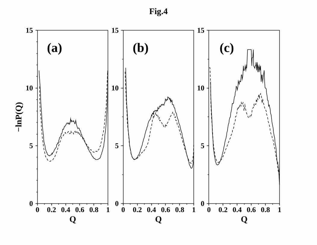
0 0.2 0.4 0.6 0.8 1Q

0

5

10

15

−ln

P(Q

)

(a)

0 0.2 0.4 0.6 0.8 1Q

0

5

10

15

Fig.4

(b)

0 0.2 0.4 0.6 0.8 1Q

0

5

10

15

(c)

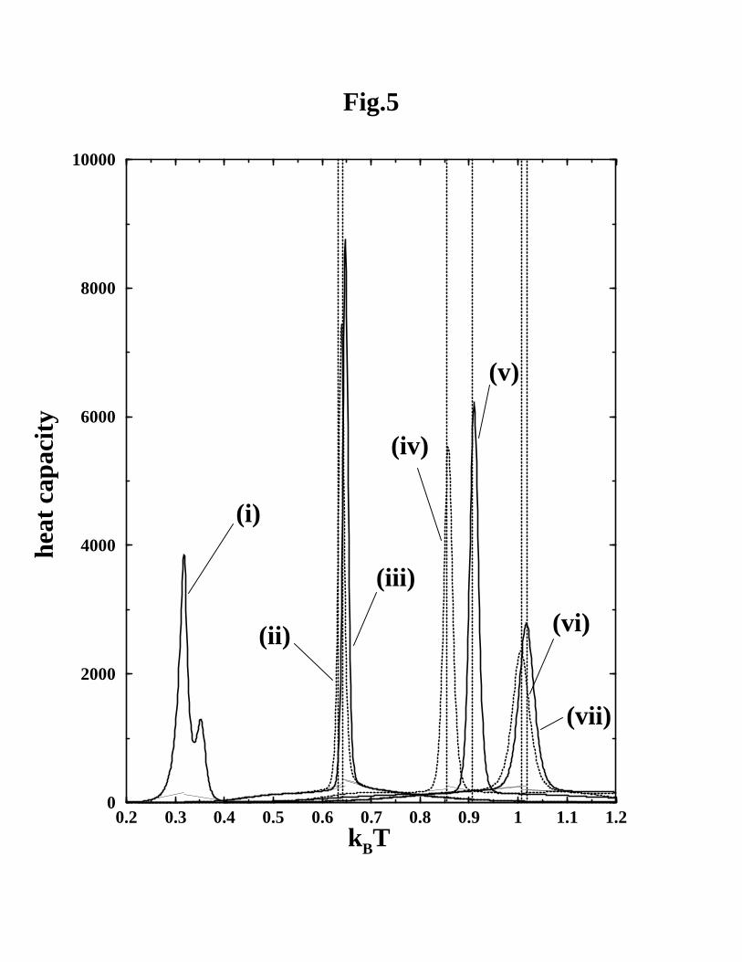
0.2 0.3 0.4 0.5 0.6 0.7 0.8 0.9 1 1.1 1.2kBT

0

2000

4000

6000

8000

10000

heat

cap

acity

Fig.5

(i)

(ii)

(iii)

(iv)

(v)

(vi)

(vii)

0 50 100 150kinetic energy

−100

−50

0

50

100

150

pote

ntia

l ene

rgy

0

0.2

0.4

0.6

0.8

1

Q

0 0.2 0.4 0.6 0.8 1Q

0 6e+07 1.2e+08 1.8e+08 2.4e+08time

0

0.2

0.4

0.6

0.8

1

Q

(a)

(b)

(c) (d)

Fig.6

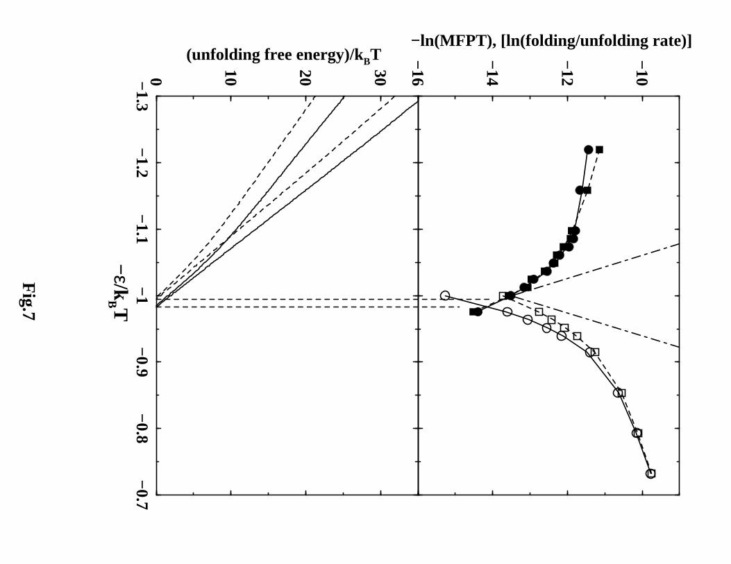
−1.3

−1.2

−1.1

−1

−0.9

−0.8

−0.7

−ε/kB T

0 10 20 30

(unfolding free energy)/kBT

Fig.7

−16

−14

−12

−10

−ln(MFPT), [ln(folding/unfolding rate)]

−2.1

−1.9

−1.7

−1.5

−1.3

−1.1

−ε/kB T

0 20 40 60

(unfolding free energy)/kBT

Fig.8

−17

−15

−13

−11

−9

−ln(MFPT), [ln(folding/unfolding rate)]

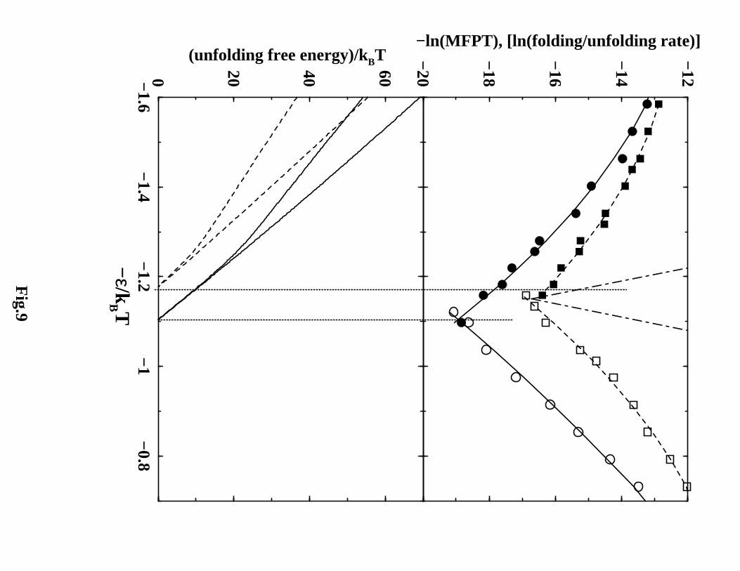
−1.6

−1.4

−1.2

−1

−0.8

−ε/kB T

0 20 40 60

(unfolding free energy)/kBT

Fig.9

−20

−18

−16

−14

−12

−ln(MFPT), [ln(folding/unfolding rate)]

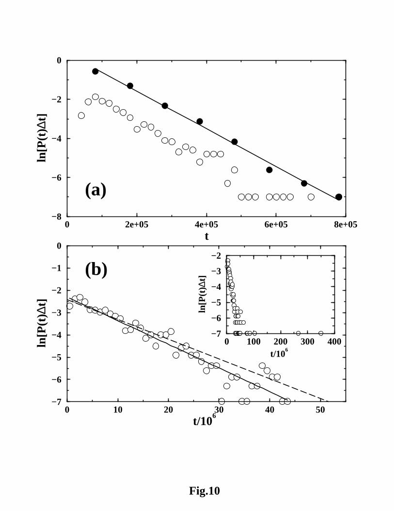
0 10 20 30 40 50t/10

6

−7

−6

−5

−4

−3

−2

−1

0

ln[P

(t)∆

t]

(a)

(b)

0 100 200 300 400t/10

6

−7

−6

−5

−4

−3

−2

ln[P

(t)∆

t]

0 2e+05 4e+05 6e+05 8e+05t

−8

−6

−4

−2

0

ln[P

(t)∆

t]

Fig.10

0 5e+05 1e+06t

−8

−6

−4

−2

0ln

[P(t

)∆t]

(a)

0 5e+05 1e+06t

Fig.11

(b)

0 2e+07 4e+07t

(c)

0 0.2 0.4 0.6 0.8 1Q

0

10

20

30

40

−ln

P(Q

)

0.90

0 0.2 0.4 0.6 0.8 1Q

0

10

20

30

40−

ln P

(Q)

0.90

1.00

0.95

0.80

0.90

0.70

0.85

0.81

0.90

−2.2 −1.8 −1.4 −1 −0.6 −0.2−ε/kBT

−55

−45

−35

−25

−15

−5

ln (

fron

t fac

tor)

0 0.2 0.4 0.6 0.8 1Q

0

10

20

30

40

−ln

P(Q

)

(a) (b)

(c)

1.03

0.99

(d)

1.10

Fig.12