421

AAS 14-229

SOLUTIONS OF MULTIVARIATE POLYNOMIAL SYSTEMS

USING MACAULAY RESULTANT EXPRESSIONS

Keith A. LeGrand,* Kyle J. DeMars† and Jacob E. Darling‡

Finding zeros of algebraic sets is a fundamental problem in aerospace engi-neering computation. Geometrically, this problem can often be represented bythe intersection of multiple conic or quadric surfaces. A common example isGPS trilateration, which is geometrically given by the intersection of threespheres. In this work, Macaulay resultant expressions are used to compute thesolutions of a set of multivariate polynomial expressions. Both two- andthree-dimensional algebraic sets are considered, and examples of two geomet-ric systems and their solutions are provided.

INTRODUCTION

Finding zeros of algebraic sets is a fundamental problem in aerospace engineering computation. Two com-

mon examples are computing the intersection of two or more conics (the graph of a degree-2 polynomial in

two dimensions) and computing the intersection of three or more quadrics (the graph of a degree-2 polynomial

in three dimensions). One example of intersecting quadrics is the intersection of three spheres, as shown in

Figure 1. Existing techniques for solving sets of multivariate polynomials include “guess and check” iterative

techniques such as Newton’s method and least squares, and other non-iterative techniques such as Grobner

bases.1 Iterative techniques are subject to their initialization, and many times require numerous iterations or

diverge completely if a poor initial guess is provided. Grobner bases, on the other hand, are non-iterative, but

become extremely computationally expensive for sets containing three or more polynomials. Over the past

two decades, resultant-based approaches have gained some popularity, especially in the computer graphics

industry. The resultant of a set of multivariate polynomials is a single univariate polynomial obtained by

eliminating all of the other variables. For example, if the equations that are to be solved are functions of

x1, x2, . . . , xn, then by eliminating the variables x2, . . . , xn, the resultant is given by Rpx1q. If the resul-

tant has a root, then there exists at least one solution that satisfies the algebraic set. The most versatile form

of the resultant, known as the Macaulay resultant, expresses the resultant as a ratio of the determinants of two

matrices whose entries are the set’s coefficients.2

The Macaulay resultant itself can be further categorized into numerous formulations, not all of which are

equal. A discussion of the applications of some of these variations is included in this work. Finally, a unique

method motivated by the works of References 3 and 4 is presented and applied to a set of two degree-2

bivariate polynomials (conics) as well as a set of three degree-2 trivariate polynomials (quadrics).

˚Undergraduate Research Assistant, Department of Mechanical and Aerospace Engineering, Missouri University of Science and Tech-

nology, 400 W. 13th St, Rolla MO, 65409-0050:Assistant Professor, Department of Mechanical and Aerospace Engineering, Missouri University of Science and Technology, 400 W.

13th St, Rolla MO, 65409-0050;Graduate Research Assistant, Department of Mechanical and Aerospace Engineering, Missouri University of Science and Technology,

400 W. 13th St, Rolla MO, 65409-0050

422

Figure 1. Intersection of three spheres.

RESULTANT EXPRESSIONS

Most forms of the resultant are expressed as a ratio of two determinants. Macaulay was the first to use this

determinant formulation in 1902, expressing the resultant as

R px1q “ det pMqdet pDq (1)

The existing methods today follow this same principle, but diverge in the ways that they construct the matrices

M and D. Macaulay’s method for constructing M involved first forming some non-square matrix with the

coefficients of the original algebraic set. In order to make M square, Macaulay provided a set of rules to

choose which rows to drop, but it proved to be unstable in many cases.5

Macaulay also provided a special form of the resultant for problems where there are as many inhomo-

geneous polynomials as variables. The homogenization of polynomials, which is discussed in detail later

in this work, introduces an additional variable to the system. This results in n homogeneous equations in

n ` 1 variables, and thus, an additional equation must be included. This equation is linear with coeffi-

cients u0, u1, . . . , un and is commonly referred to as the ‘U-equation.’ The resultant that follows as a con-

sequence of introducing the U-equation is known as the U-resultant and serves as the basis of References 3,4

and 5.

In Reference 5, the U-resultant is formed for n inhomogeneous equations in n variables. The U-equation

is formed with parameterized coefficients, that is, ui “ αi ´ λβi. The coefficients αi and βi are chosen

stochastically, and as the parameter λ is varied, the line defined by the U-equation ‘sweeps’ through the

solution space. The efficacy of this method is sensitive to the choice of coefficients αi and βi, as some

choices may create a sweepline that passes through several solutions simultaneously.5 Because the efficacy

of this method is dependent on a stochastic selection of coefficients, a more repeatable deterministic method

is sought.

Reference 4 presents a deterministic root-finding method using the U-resultant. In this approach, M is

expressed as a matrix polynomial. The matrix polynomial coefficient matrices are used to form a general

companion matrix, of which the eigenvalues correspond directly to the roots of the original polynomial sys-

tem. In this work, a similar root-finding method is presented which does not require an additional U-equation.

This omission of the U-equation significantly reduces the size of M , which greatly simplifies the algorithm

and mitigates computational issues caused by the matrix size and sparsity.

423

Consider a system of n polynomial equations in n unknowns given by

f1 px1, x2, ..., xnq “0

f2 px1, x2, ..., xnq “0 (2)

...

fn px1, x2, ..., xnq “0

with degrees d1, d2, . . . , dn. Multipolynomial resultants can be used to eliminate the variables x2, x3, . . . , xn

from these equations by projecting the algebraic set in a lower dimension.3 A resultant is, by definition, a

polynomial in the coefficients of the original system. Nearly all methods of computing resultants represent the

resultant in terms of matrices and determinants. One of these formulations, known as the Macaulay resultant,

expresses the resultant Rpx1q as a ratio of determinants of two matrices M and D as6

R px1q “ det pMqdet pDq . (3)

The entries of M and D are polynomials in x1, and if D is non-singular, the roots of the polynomial given

by det pMq correspond exactly to the roots of x1 in the original system.7 Reference 4 shows how resultant

expressions can be expressed as matrix polynomials. In this formulation, the root-finding reduces to an

eigenvalue problem.

This work presents the construction of multipolynomial resultants for the common problem of n polyno-

mial equations with n unknowns. Given the multivariate polynomials f1, f2, . . . , fn, the resultant transforms

the original nonlinear system of equations into a new system of linear equations such that3

Mpx1q ` 1 x2 . . . xn . . . xd2 xd

3 . . . xdn

˘T “

¨˚˝

00...

0

˛‹‹‹‚ . (4)

If f1, f2, . . . , fn simultaneously vanish at some point in the projective space, then the kernel of Mpx1qcontains some nontrivial vector.8 Recall that a resultant is simply a polynomial in the coefficients of the

original system. Therefore, as shown in Equation (4), if x1 is known, the remaining roots x2, x3, . . . , xn

simply correspond to the kernel of Mpx1q. With this, the root finding process consists of three main steps:

constructing M , computing x1, and solving for the remaining roots. M is constructed using the coefficients

of the original set of polynomials. Once M is formed, it is expanded into a matrix polynomial. The matrix

polynomial’s coefficient matrices are used in a generalized eigenvalue problem to compute all of the possible

roots in x1. Once x1 is found, the remaining roots are found by computing the kernel of Mpx1q. This entire

process, including the construction of M , the formation of the matrix polynomial, the computation of x1

using eigendecomposition, and the computation of the remaining coordinates’ roots is discussed in greater

detail in the following sections.

CONSTRUCTION OF M

This section is intended to serve as a reference for constructing the M matrix for a general set of homoge-

neous polynomials. The reader is strongly encouraged to reference the two examples presented later in this

work while reading this section.

As shown in Equation (4), M is expressed as a function of one of the system variables. Therefore, the sys-

tem must be reformulated, treating one variable as if it were a constant. For example, consider the following

system:

f1px1, x2q “ a1x21 ` a2x1x2 ` a3x

22 ` a4 “ 0 (5a)

f2px1, x2q “ b1x21 ` b2x1x2 ` b3x

22 ` b4 “ 0 (5b)

424

Regrouping f1 and f2 as if x1 was constant yields

f1px2q “ a3x22 ` pa2x1qx2 ` pa4 ` a1x

21q “ 0 (6a)

f2px2q “ b3x22 ` pb2x1qx2 ` pb4 ` b1x

21q “ 0 (6b)

Homogenization

In order to form the Macaulay resultant expression, f1, f2, . . . , fn must be homogeneous,6 that is, the

degree of every monomial in fi must be equal. Homogenization is achieved via the inclusion of an addi-

tional variable w. For example, consider the inhomogenous polynomials in Equations (6). Equations (6) are

inhomogenous because the first term is degree-2, whereas the second and third terms are of degree 1 and 0,

respectively. To homogenize, the homogenization variable w is added to produce

f1px2, wq “ a3x22 ` pa2x1qx2w ` pa4 ` a1x

21qw2 “ 0 (7a)

f2px2, wq “ b3x22 ` pb2x1qx2w ` pb4 ` b1x

21qw2 “ 0 (7b)

Matrix Size

To construct the resultant matrix M for the system of polynomials f1, f2, . . . , fn, the total degree of the

system must be determined. The total degree, d, of a given set of polynomials is computed as

d “ 1 `mÿi“1

pdi ´ 1q , (8)

where m is the number of equations, and di is the degree of the ith equation. The size of M is directly related

to the system’s total degree and can be computed as

sizepMq “ˆ

n ` dn

˙, (9)

where n is the number of variables in the set before homogenization. For example, for the previously men-

tioned polynomials (Eqs. 5), n “ 1, as there is only one variable (x2) before homogenization. Both polyno-

mials are of degree 2, so the total degree is calculated as

d “ 1 ` pd1 ´ 1q ` pd2 ´ 1q “ 3 .

It follows that the size of M is calculated as

sizepMq “ˆ

1 ` 31

˙“ 4 .

Therefore, M is a 4 ˆ 4 matrix for this example.

Column Labels

The columns of M correspond to all possible degree-d monomials, arranged in lexicographical order from

left to right. Consider the system with variables x2 and w and total degree d “ 3. The columns of M then

correspond (in order) to the monomials x32, x

22w, x2w

2, w3.

M “

x32 x2

2w x2w2 w3

425

Row Labels

Before presenting the algorithm for constructing the row labels of M , the concept of exponent “bigness”

must be understood. This concept is introduced in Reference 7 and is a useful definition when constructing

the rows of M . To determine whether a particular exponent is big, first associate each variable with a poly-

nomial. For example, associate x2 with f1 and w with f2. A variable’s exponent is considered big if it is

greater than or equal to its associated polynomial’s degree. For example, consider the monomial x22w. The

exponent of x2 is 2. Therefore, it is considered big because d1 ď 2. Similarly, consider the monomial w3.

The exponent of w is big because d2 ď 3.

With this definition, the rows of M can be constructed by following the following steps taken from Ref-

erence 7.

For each column label:

1. Search the monomial labeling that column from left to right for the first variable with a big exponent.

Such a variable must exist. Call it a marker variable.

2. Form a new polynomial from the polynomial associated with this marker variable by multiplying the

associated polynomial by the monomial and dividing by the marker variable raised to the degree of the

associated polynomial.

M “

x32 x2

2w x2w2 w3

x2f1wf1x2f2wf2

3. The coefficients of the new polynomial are the elements of the row. Each coefficient goes in the column

labeled by the monomial it multiplies. All the other elements of that row are zero.

M “

x32 x2

2w x2w2 w3

x2f1 a3 a2x1 pa4 ` a1x21q 0

wf1 0 a3 a2x1 pa4 ` a1x21q

x2f2 b3 b2x1 pb4 ` b1x21q 0

wf2 0 b3 b2x1 pb4 ` b1x21q

(10)

CONSTRUCTION OF D

In Macaulay’s original formulation, the determinant of the denominator matrix D was used to remove

extraneous factors from the resultant Rpx1q. However, if D is non-singular, the roots of the polynomial

given by detpMq correspond exactly to the roots of x1 in the original system. If, however, D is singular, Mmust be replaced with its largest non-vanishing minor.4 Therefore, the determinant of D must be computed

in order to determine whether M requires further reduction. An interesting property of D is that it is simply

a minor of M .2 More specifically, the entries of D are the entries of M whose row and column labels are

non-reduced monomials. Reference 7 defines a non-reduced monomial as a monomial comprised of more

than one variable with a big exponent. For the current example, M has no non-reduced column labels (see

Eq. 10), so D is simply 1.

426

MATRIX POLYNOMIALS

M can be written as a matrix polynomial in x1, that is3

Mpx1q “ M0 ` M1x1 ` M2x21 ` ... ` M�x

�1 (11)

For example, Equation (10) can be rewritten as

Mpx1q “

¨˚ a3 0 a4 0

0 a3 0 a4b3 0 b4 00 b3 0 b4

˛‹‹‚`

¨˚ 0 a2 0 0

0 0 a2 00 b2 0 00 0 b2 0

˛‹‹‚x1 `

¨˚ 0 0 a1 0

0 0 0 a10 0 b1 00 0 0 b1

˛‹‹‚x2

1 (12)

The matrix polynomial given in Equation (11) is univariate, and its roots can be easily computed by forming

its associated Frobenius companion matrix.4 The roots of the determinant of Mpx1q directly correspond to

the eigenvalues of the companion transpose matrix

CT “

¨˚˚

0 Im 0 . . . 00 0 Im . . . 0...

... . . ....

...0 0 0 . . . Im

´M0 ´M1 ´M2 . . . ´M �´1

˛‹‹‹‹‹‚ (13)

where M i “ M´1� Mi. Due to the high condition number of M�, it is often singular or close to singular,

thus preventing the computation of M i. Fortunately, matrix inversion can be avoided by reformulating

Equation (13) as the generalized eigenvalue problem, Ax1 ´ B, where

A “

¨˚˚

Im 0 0 . . . 00 Im 0 . . . 0...

... . . ....

...0 0 . . . Im 0

0 0 . . . 0 M�

˛‹‹‹‹‹‚ (14)

B “

¨˚˚

0 Im 0 . . . 00 0 Im . . . 0...

... . . ....

...0 0 0 . . . Im

´M0 ´M1 ´M2 . . . ´M�´1

˛‹‹‹‹‹‚ (15)

The eigenvalues of Ax1 ´ B are the roots that satisfy the original system of equations. Many software

packages include routines for solving generalized eigenvalue problems, including MATLAB’s eig function.

In most situations, only the real and finite solutions are of interest. If an eigenvalue x1 “ α1 is finite and

simple, the roots in the remaining coordinates x2, x3, . . . , xn can be computed algebraically.

COMPUTING ROOTS IN REMAINING COORDINATES

If α1 is a simple and finite eigenvalue, the remaining roots α2, α3, . . . , αn can be computed easily. As

suggested by Equation (4), the remaining solutions correspond to a kernel vector of Mpα1q; that is, the

nontrivial vector v which satisfies Mpα1qv “ 0. Several software routines are readily available that can

compute a matrix kernel, including MATLAB’s null function. Depending on the linear algebra routines

used, the kernel vector v may be a scalar multiple of the solution. In that case, the relationship of Equation (4)

can be used to back out the scale factor β:3

427

`1 x2 . . . xn . . . xd

2 xd3 . . . xd

n

˘T “ β`v1 v2 . . . vm

˘(16)

If α1 is not simple, that is, if it has a multiplicity greater than one, the kernel of Mpα1q will have more

than one vector. Consequently, it is difficult to compute α2, α3, . . . , αn from them. To solve the problem,

x1 “ α1 can be substituted back into the original set of polynomials, and the root finding process is repeated

recursively. In other words, after making the substitution x1 “ α1, a new resultant expression, Rpx2q is

formed by eliminating x3, . . . , xn from n ´ 1 equations, and the solutions in x2 are computed.

EXAMPLE: PLANAR ORBIT INTERSECTION

To demonstrate the applications of Macaulay resultant expressions for root-finding, the simplest case of

two degree-2 inhomogeneous equations in two unknowns is considered. Geometrically, this problem can be

represented as the intersection of two conics, as shown by the examples in Figure 2.

(a) Ellipse-parabola intersection. (b) Parabola-hyperbola intersection.

(c) Ellipse-hyperbola intersection.

Figure 2. Intersections of various conic sections.

For example, consider the planar, two-body motion of a spacecraft returning to orbit about Earth from an

interplanetary trajectory. The spacecraft is on a hyperbolic trajectory with respect to the Earth upon return,

with semi-major axis and eccentricity vector of

ah “ ´10000 km and eh “ “1.7 0

‰T.

It is desired to place the spacecraft in an elliptical orbit about the Earth with semi-major axis and eccentricity

vector of

ae “ 13000 km and ee “”

0.45?2

0.45?2

ıT.

In general, the intersection of an ellipse and a hyperbola can result in 0, 1, 2, 3, or 4 intersections; however, for

the orbit problem, only one branch of the hyperbola is of interest and so only 0, 1, or 2 intersections can exist

428

between an ellipse and the hyperbola branch of interest. These intersection points represent the candidate

locations at which an impulsive ΔV can be performed to inject the spacecraft from its original interplanetary

trajectory to its desired elliptical orbit. These orbits, as well as their intersections, are plotted in Figure 3. It

IntersectionElliptical OrbitHyperbolic Orbit

y EC

I[k

m]

xECI [km] ×104−2 −1.5 −1 −0.5 0 0.5 1

×104

−1.5

−1

−0.5

0

0.5

1

1.5

Figure 3. Hyperbolic and elliptical trajectories around Earth.

is shown in the Appendix that the hyperbolic and elliptic orbits can be expressed in Earth Centered Inertial

Cartesian coordinates respectively as

f1px, yq “ a1x2 ` a2xy ` a3y

2 ` a4x ` a5y ` a6 “ 0 (17a)

f2px, yq “ b1x2 ` b2xy ` b3y

2 ` b4x ` b5y ` b6 “ 0 (17b)

where

a1 “ 1

a2h, a2 “ 0 , a3 “ ´ 1

a2h pe2h ´ 1q , a4 “ 2eha

, a5 “ 0 , and a6 “ e2h ´ 1

and

b1 “ cos θe2

a2e` sin θe

2

a2e p1 ´ e2eq , b2 “ 2 sin θe cos θe

ˆ1

a2e´ 1

a2e p1 ´ e2eq˙

,

b3 “ sin θe2

a2e` cos θe

2

a2e p1 ´ e2eq , b4 “ 2ee cos θeae

, b5 “ 2ee sin θeae

, and b6 “ e2e ´ 1

and θe is the angle of the eccentricity vector of the elliptical orbit in the Cartesian coordinates, which is 45˝in this example.

Solution to Orbit Intersection

To compute the candidate orbit injection locations, Macaulay resultant expressions can be used to find

the roots of Equations (17). First, the matrix M is constructed from the coefficients of Equations (17).

429

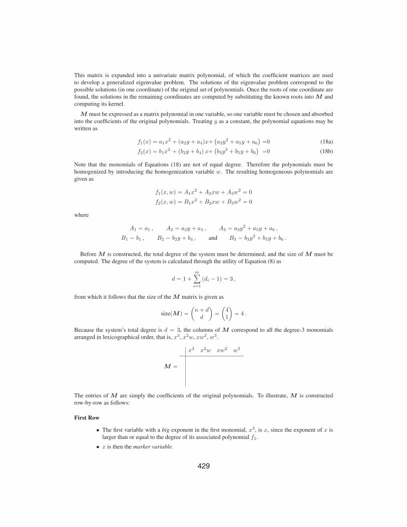
This matrix is expanded into a univariate matrix polynomial, of which the coefficient matrices are used

to develop a generalized eigenvalue problem. The solutions of the eigenvalue problem correspond to the

possible solutions (in one coordinate) of the original set of polynomials. Once the roots of one coordinate are

found, the solutions in the remaining coordinates are computed by substituting the known roots into M and

computing its kernel.

M must be expressed as a matrix polynomial in one variable, so one variable must be chosen and absorbed

into the coefficients of the original polynomials. Treating y as a constant, the polynomial equations may be

written as

f1pxq “ a1x2 ` pa2y ` a4qx` `

a3y2 ` a5y ` a6

˘ “0 (18a)

f2pxq “ b1x2 ` pb2y ` b4q x` `

b3y2 ` b5y ` b6

˘ “0 (18b)

Note that the monomials of Equations (18) are not of equal degree. Therefore the polynomials must be

homogenized by introducing the homogenization variable w. The resulting homogeneous polynomials are

given as

f1px,wq “ A1x2 ` A2xw ` A3w

2 “ 0

f2px,wq “ B1x2 ` B2xw ` B3w

2 “ 0

where

A1 “ a1 , A2 “ a2y ` a4 , A3 “ a3y2 ` a5y ` a6 ,

B1 “ b1 , B2 “ b2y ` b4 , and B3 “ b3y2 ` b5y ` b6 .

Before M is constructed, the total degree of the system must be determined, and the size of M must be

computed. The degree of the system is calculated through the utility of Equation (8) as

d “ 1 `mÿi“1

pdi ´ 1q “ 3 ,

from which it follows that the size of the M matrix is given as

sizepMq “ˆn ` dd

˙“

ˆ41

˙“ 4 .

Because the system’s total degree is d “ 3, the columns of M correspond to all the degree-3 monomials

arranged in lexicographical order, that is, x3, x2w, xw2, w3.

M “

x3 x2w xw2 w3

The entries of M are simply the coefficients of the original polynomials. To illustrate, M is constructed

row-by-row as follows:

First Row

• The first variable with a big exponent in the first monomial, x3, is x, since the exponent of x is

larger than or equal to the degree of its associated polynomial f1.

• x is then the marker variable.

430

• The polynomial associated with the first row of M is given by multiplying f1 (the associated

polynomial of the marker variable x) by x3 (the associated monomial of the first column) divided

by x2 (the marker variable x raised to the degree of its associated polynomial f1).

x3f1x2

“ xf1 “ A1x3 ` A2x

2w ` A3xw2 (19)

Second Row

• The first variable with a big exponent in the second monomial, x2w, is x, since the exponent of xis larger than or equal to the degree of its associated polynomial f1.

• x is then the marker variable.

• The polynomial associated with the second row of M is given by multiplying f1 (the associated

polynomial of the marker variable x) by x2w (the associated monomial of the second column)

divided by x2 (the marker variable x raised to the degree of its associated polynomial f1).

x2wf1x2

“ wf1 “ A1x2w ` A2xw

2 ` A3w3 (20)

Third Row

• The first variable with a big exponent in the third monomial, xw2, is w, since the exponent of wis larger than or equal to the degree of its associated polynomial f2.

• w is then the marker variable.

• The polynomial associated with the third row of M is given by multiplying f2 (the associated

polynomial of the marker variable w) by xw2 (the associated monomial of the third column)

divided by w2 (the marker variable w raised to the degree of its associated polynomial f2).

xw2f2w2

“ xf2 “ B1x3 ` B2x

2w ` B3xw2 (21)

Fourth Row

• The first variable with a big exponent in the fourth monomial, w3, is w, since the exponent of wis larger than or equal to the degree of its associated polynomial f2.

• w is then the marker variable.

• The polynomial associated with the fourth row of M is given by multiplying f2 (the associated

polynomial of the marker variable w) by w3 (the associated monomial of the fourth column)

divided by w2 (the marker variable w raised to the degree of its associated polynomial f2).

w3f2w2

“ wf2 “ B1x2w ` B2xw

2 ` B3w3 (22)

The M matrix is then assembled using the coefficients of Equations (19)-(22) as

M “

x3 x2w xw2 w3

xf1 A1 A2 A3

wf1 A1 A2 A3

xf2 B1 B2 B3

wf2 B1 B2 B3

431

Recall that the denominator matrix, D, must also be constructed to check its singularity. By examining the

column labels of M , it is apparent that none of the monomials are non-reduced, so it follows that detpDq “ 1.

M is now written as a polynomial in y as

Mpyq “ M0 ` M1y ` M2y2

where

M0 “

¨˚a1 a4 a6 0

0 a1 a4 a6b1 b4 b6 00 b1 b4 b6

˛‹‹‚ , M1 “

¨˚0 a2 a5 00 0 a2 a50 b2 b5 00 0 b2 b5

˛‹‹‚ , and M2 “

¨˚0 0 a3 00 0 0 a30 0 b3 00 0 0 b3

˛‹‹‚ (23)

The possible solutions for y are the finite, real eigenvalues of the generalized system

Ay “ B , (24)

where

A “ˆI4 00 M2

˙and B “

ˆ0 I4

´M0 ´M1

˙. (25)

Two possible solutions for y are found to be

y1 “ 2733.155 [km] and y2 “ ´13205.404 [km] . (26)

Recall that these solutions correspond to the roots of resultant, Rpyq, as shown in Figure 4. To compute

y = 2733.155y = −13205.404

R(y)(×

1016)

y [km]−15000 −10000 −5000 0 5000−2

−1

0

1

2

Figure 4. The solutions in y correspond exactly to the roots of the resultant, Rpyq.

the solutions in the x coordinate, the computed y solutions are substituted back into M . The remaining

coordinate solutions, x1 and x2, are found by computing the kernel of Mpy1q and Mpy2q, respectively. In

other words, for each solution yi, the vector v is found which satisfies

Mpyiqv “ 0 .

Depending on the numerical method used to compute the kernel, the vector v may be scaled from the solution.

In this case, the scaling factor β is computed using the relation shown in Equation (16). For this problem, the

scaling factor is given as β “ 1{v4. It follows that the x solutions are computed as

xi “ˆv3v4

˙i

. (27)

432

With this, the x solutions are computed as

x1 “ 6804.292 [km] and x2 “ 3133.999 [km] . (28)

It is observed in Figure 3 that these are the correct intersections for the hyperbolic and elliptical orbits.

EXAMPLE: INTERSECTION OF THREE SPHERES

Many astrodynamics problems can be formulated as computing the intersections of quadric surfaces.

Quadrics, by definition, are degree-2 trivariate polynomials. For example, GPS trilateration can be formulated

as finding the intersections of three spheres. The equations of three spheres can be written as

f1px, y, zq “ px ´ xc1q2 ` py ´ yc1q2 ` pz ´ zc1q2 ´ r21 “ 0 (29a)

f2px, y, zq “ px ´ xc2q2 ` py ´ yc2q2 ` pz ´ zc2q2 ´ r22 “ 0 (29b)

f3px, y, zq “ px ´ xc3q2 ` py ´ yc3q2 ` pz ´ zc3q2 ´ r23 “ 0 (29c)

The “cn” subscript denotes the center coordinate of the nth sphere, and rn is the radius of the nth sphere.

Equations (29) can be rewritten as polynomials in standard form as

f1px, y, zq “ a1x2`a2x ` a3y

2`a4y ` a5z2`a6z ` a7 “ 0 (30a)

f2px, y, zq “ b1x2 `b2x ` b3y

2 `b4y ` b5z2 `b6z ` b7 “ 0 (30b)

f3px, y, zq “ c1x2 `c2x ` c3y

2 `c4y ` c5z2 `c6z ` c7 “ 0 (30c)

where

a1 “ a3 “ a5 “ 1 a2 “ ´2xc1 a4 “ ´2yc1 a6 “ ´2zc1 a7 “ xc21 ` yc

21 ` zc

21 ´ r21

b1 “ b3 “ b5 “ 1 b2 “ ´2xc2 b4 “ ´2yc2 b6 “ ´2zc2 b7 “ xc22 ` yc

22 ` zc

22 ´ r22

c1 “ c3 “ c5 “ 1 c2 “ ´2xc3 c4 “ ´2yc3 c6 “ ´2zc3 c7 “ xc23 ` yc

23 ` zc

23 ´ r23

One variable must be chosen as the resultant variable, and the remaining variables are eliminated. For this

problem, all of the three variables are equally good choices, as the the total degree of the resulting system is

the same for any choice. Choosing z as the resultant variable, Equations (30) are rewritten, absorbing z into

the polynomial coefficients:

f1px, yq “ a1x2`a2x ` a3y

2`a4y` `a5z

2 ` a6z ` a7˘“ 0 (31a)

f2px, yq “ b1x2 `b2x ` b3y

2 `b4y` `b5z

2 ` b6z ` b7˘ “ 0 (31b)

f3px, yq “ c1x2 `c2x ` c3y

2 `c4y` `c5z

2 ` c6z ` c7˘ “ 0 (31c)

Homogenization

In order to form the Macaulay resultant expression, Equations (31) must be homogeneous,6 that is, the

degree of every monomial in fi must be equal. Thus, an extra variable w must be added. Homogenization

yields

f1px, y, wq “ A1x2 ` A2xw ` A3y

2 ` A4yw ` A5w2 “ 0 (32a)

f2px, y, wq “ B1x2 ` B2xw ` B3y

2 ` B4yw ` B5w2 “ 0 (32b)

f3px, y, wq “ C1x2 ` C2xw ` C3y

2 ` C4yw ` C5w2 “ 0 (32c)

where

A1 “ a1 A2 “ a2 A3 “ a3 A4 “ a4 A5 “ a5z2 ` a6z ` a7

B1 “ b1 B2 “ b2 B3 “ b3 B4 “ b4 B5 “ b5z2 ` b6z ` b7

C1 “ c1 C2 “ c2 C3 “ c3 C4 “ c4 C5 “ c5z2 ` c6z ` c7

433

Construction of M

The first step in constructing the M matrix requires computing the total degree of the algebraic set. The

total degree, d, of the system is computed using Equation (8) as

d “ 1 ` p2 ´ 1q ` p2 ´ 1q ` p2 ´ 1q “ 4 . (33)

The size of M is computed using Equation (9) as

sizepMq “ˆ

2 ` 42

˙“ 15 . (34)

Thus, M is a 15 ˆ 15 matrix as shown in Equation (35). The columns of M correspond to all possible

degree-d monomials, arranged in lexicographical order from left to right. The rows are constructed in the

same fashion as the two-dimensional example above.

M “

¨˚˚˚˚˚˚˚˚˚˚˚

x4 x3y x3w x2y2 x2yw x2w2 xy3 xy2w xyw2 xw3 y4 y3w y2w2 yw3 w4

x2f1 A1 ¨ A2 A3 A4 A5 ¨ ¨ ¨ ¨ ¨ ¨ ¨ ¨ ¨xyf1 ¨ A1 ¨ ¨ A2 ¨ A3 A4 A5 ¨ ¨ ¨ ¨ ¨ ¨xwf1 ¨ ¨ A1 ¨ ¨ A2 ¨ A3 A4 A5 ¨ ¨ ¨ ¨ ¨y2f1 ¨ ¨ ¨ A1 ¨ ¨ ¨ A2 ¨ ¨ A3 A4 A5 ¨ ¨ywf1 ¨ ¨ ¨ ¨ A1 ¨ ¨ ¨ A2 ¨ ¨ A3 A4 A5 ¨w2f1 ¨ ¨ ¨ ¨ ¨ A1 ¨ ¨ ¨ A2 ¨ ¨ A3 A4 A5

xyf2 ¨ B1 ¨ ¨ B2 ¨ B3 B4 B5 ¨ ¨ ¨ ¨ ¨ ¨xwf2 ¨ ¨ B1 ¨ ¨ B2 ¨ B3 B4 B5 ¨ ¨ ¨ ¨ ¨xyf3 ¨ C1 ¨ ¨ C2 ¨ C3 C4 C5 ¨ ¨ ¨ ¨ ¨ ¨xwf3 ¨ ¨ C1 ¨ ¨ C2 ¨ C3 C4 C5 ¨ ¨ ¨ ¨ ¨y2f2 ¨ ¨ ¨ B1 ¨ ¨ ¨ B2 ¨ ¨ B3 B4 B5 ¨ ¨ywf2 ¨ ¨ ¨ ¨ B1 ¨ ¨ ¨ B2 ¨ ¨ B3 B4 B5 ¨w2f2 ¨ ¨ ¨ ¨ ¨ B1 ¨ ¨ ¨ B2 ¨ ¨ B3 B4 B5

ywf3 ¨ ¨ ¨ ¨ C1 ¨ ¨ ¨ C2 ¨ ¨ C3 C4 C5 ¨w2f3 ¨ ¨ ¨ ¨ ¨ C1 ¨ ¨ ¨ C2 ¨ ¨ C3 C4 C5

˛‹‹‹‹‹‹‹‹‹‹‹‹‹‹‹‹‹‹‹‹‹‹‹‹‹‹‹‹‹‹‹‚

(35)

Construction of D

The denominator matrix D must be constructed to ensure that its determinant is non-zero. The entries

of D are simply the entries of M whose row and column labels are non-reduced monomials. Recall that

monomials are considered non-reduced if they contain more than one with big exponents. With this, D is

constructed as

D “¨˚

x2y2 x2w2 y2w2

y2f1 A1 ¨ A5

w2f1 ¨ A1 A3

w2f2 ¨ B1 B3

˛‹‚ (36)

It is easy to see that detpDq “ A1pA1B3 ´ A3B1q “ 0. Because D is vanishing, M must be replaced with

its largest non-vanishing minor.4 Analysis shows that at minimum, three rows and columns must be dropped.

434

Therefore, we drop the second, third, and fourth rows and columns of M :

M “

¨˚˚˚˚˚˚˚˚˝

x4 x2yw x2w2 xy3 xy2w xyw2 xw3 y4 y3w y2w2 yw3 w4

x2f1 A1 A4 A5 ¨ ¨ ¨ ¨ ¨ ¨ ¨ ¨ ¨ywf1 ¨ A1 ¨ ¨ ¨ A2 ¨ ¨ A3 A4 A5 ¨w2f1 ¨ ¨ A1 ¨ ¨ ¨ A2 ¨ ¨ A3 A4 A5

xyf2 ¨ B2 ¨ B3 B4 B5 ¨ ¨ ¨ ¨ ¨ ¨xwf2 ¨ ¨ B2 ¨ B3 B4 B5 ¨ ¨ ¨ ¨ ¨xyf3 ¨ C2 ¨ C3 C4 C5 ¨ ¨ ¨ ¨ ¨ ¨xwf3 ¨ ¨ C2 ¨ C3 C4 C5 ¨ ¨ ¨ ¨ ¨y2f2 ¨ ¨ ¨ ¨ B2 ¨ ¨ B3 B4 B5 ¨ ¨ywf2 ¨ B1 ¨ ¨ ¨ B2 ¨ ¨ B3 B4 B5 ¨w2f2 ¨ ¨ B1 ¨ ¨ ¨ B2 ¨ ¨ B3 B4 B5

ywf3 ¨ C1 ¨ ¨ ¨ C2 ¨ ¨ C3 C4 C5 ¨w2f3 ¨ ¨ C1 ¨ ¨ ¨ C2 ¨ ¨ C3 C4 C5

˛‹‹‹‹‹‹‹‹‹‹‹‹‹‹‹‹‹‹‹‹‹‹‹‹‚

(37)

Matrix Polynomial

M can be written as a matrix polynomial in z as

Mpzq “ M0 ` M1z ` M2z2 (38)

where

M0 “

¨˚˚˚˚˚˚

a1 a4 a7 ¨ ¨ ¨ ¨ ¨ ¨ ¨ ¨ ¨¨ a1 ¨ ¨ ¨ a2 ¨ ¨ a3 a4 a7 ¨¨ ¨ a1 ¨ ¨ ¨ a2 ¨ ¨ a3 a4 a7¨ b2 ¨ b3 b4 b7 ¨ ¨ ¨ ¨ ¨ ¨¨ ¨ b2 ¨ b3 b4 b7 ¨ ¨ ¨ ¨ ¨¨ c2 ¨ c2 c4 c7 ¨ ¨ ¨ ¨ ¨ ¨¨ ¨ c2 ¨ c2 c4 c7 ¨ ¨ ¨ ¨ ¨¨ ¨ ¨ ¨ b2 ¨ ¨ b3 b4 b7 ¨ ¨¨ b1 ¨ ¨ ¨ b2 ¨ ¨ b3 b4 b7 ¨¨ ¨ b1 ¨ ¨ ¨ b2 ¨ ¨ b3 b4 b7¨ c1 ¨ ¨ ¨ c2 ¨ ¨ c2 c4 c7 ¨¨ ¨ c1 ¨ ¨ ¨ c2 ¨ ¨ c2 c4 c7

˛‹‹‹‹‹‹‹‹‹‹‹‹‹‹‹‹‚

(39)

M1 “

¨˚˚˚˚˚˚

¨ ¨ a6 ¨ ¨ ¨ ¨ ¨ ¨ ¨ ¨ ¨¨ ¨ ¨ ¨ ¨ ¨ ¨ ¨ ¨ ¨ a6 ¨¨ ¨ ¨ ¨ ¨ ¨ ¨ ¨ ¨ ¨ ¨ a6¨ ¨ ¨ ¨ ¨ b6 ¨ ¨ ¨ ¨ ¨ ¨¨ ¨ ¨ ¨ ¨ ¨ b6 ¨ ¨ ¨ ¨ ¨¨ ¨ ¨ ¨ ¨ c6 ¨ ¨ ¨ ¨ ¨ ¨¨ ¨ ¨ ¨ ¨ ¨ c6 ¨ ¨ ¨ ¨ ¨¨ ¨ ¨ ¨ ¨ ¨ ¨ ¨ ¨ b6 ¨ ¨¨ ¨ ¨ ¨ ¨ ¨ ¨ ¨ ¨ ¨ b6 ¨¨ ¨ ¨ ¨ ¨ ¨ ¨ ¨ ¨ ¨ ¨ b6¨ ¨ ¨ ¨ ¨ ¨ ¨ ¨ ¨ ¨ c6 ¨¨ ¨ ¨ ¨ ¨ ¨ ¨ ¨ ¨ ¨ ¨ c6

˛‹‹‹‹‹‹‹‹‹‹‹‹‹‹‹‹‚

(40)

435

M2 “

¨˚˚˚˚˚˚

¨ ¨ a5 ¨ ¨ ¨ ¨ ¨ ¨ ¨ ¨ ¨¨ ¨ ¨ ¨ ¨ ¨ ¨ ¨ ¨ ¨ a5 ¨¨ ¨ ¨ ¨ ¨ ¨ ¨ ¨ ¨ ¨ ¨ a5¨ ¨ ¨ ¨ ¨ b5 ¨ ¨ ¨ ¨ ¨ ¨¨ ¨ ¨ ¨ ¨ ¨ b5 ¨ ¨ ¨ ¨ ¨¨ ¨ ¨ ¨ ¨ c5 ¨ ¨ ¨ ¨ ¨ ¨¨ ¨ ¨ ¨ ¨ ¨ c5 ¨ ¨ ¨ ¨ ¨¨ ¨ ¨ ¨ ¨ ¨ ¨ ¨ ¨ b5 ¨ ¨¨ ¨ ¨ ¨ ¨ ¨ ¨ ¨ ¨ ¨ b5 ¨¨ ¨ ¨ ¨ ¨ ¨ ¨ ¨ ¨ ¨ ¨ b5¨ ¨ ¨ ¨ ¨ ¨ ¨ ¨ ¨ ¨ c5 ¨¨ ¨ ¨ ¨ ¨ ¨ ¨ ¨ ¨ ¨ ¨ c5

˛‹‹‹‹‹‹‹‹‹‹‹‹‹‹‹‹‚

(41)

The roots in z can then be found by solving the generalized eigenvalue problem Az ´ B, where

A “ˆ

Im 00 M2

˙and B “

ˆ0 Im

´M0 ´M1

˙. (42)

Because the physical intersection of three spheres is sought, only the real and finite eigenvalues are of interest.

Let α12 “ z be a finite and real solution. The remaining coordinate solutions (x and y) are found by

computing the kernel of Mpα12q. Recall that the kernel vector v is scaled by some scalar value β. The scale

factor can be computed using the relationship shown in Equation. (16) as

β “ 1

v11. (43)

With this, the remaining coordinate solutions can be computed:

x “ α7 “ v7v12

and y “ α11 “ v11v12

. (44)

Numerical Example

Consider three spheres described by the data in Table 1. First, the coefficients a1, . . . , a7, b1, . . . , b7, c1, . . . , c7are calculated from the sphere center coordinates and radius information. Next, M is constructed using the

procedure described above. By expanding M into a matrix polynomial, the resulting coefficient matrices are

used to form the generalized eigenvalue problem given by Equation (42). The real and finite eigenvalues are

found to be

α12,1 “ 1.56731 rRCs and α12,2 “ 2.11845 rRCs.

Table 1. Sphere properties.

Sphere Center Coordinates [RC] Radius [RC]

1 p0.00, 0.50, 0.25q 1.902 p1.00, 1.00, 0.20q 2.303 p2.00, 1.00, 1.00q 2.40

Recall that the eigenvalues correspond exactly to the roots of Rpzq and therefore the polynomial solutions

in z, as shown in Figure 5. Each valid solution, z “ α12, is then substituted in Mpzq, of which the kernel is

then computed. Recall that the kernel is the set of vectors v which satisfies Mpα12qv “ 0. Remember that

the x and y solutions correspond to the seventh and eleventh kernel vector elements (Eq. 44). With this, the

full solutions are computed and are provided in Table 2.

These solutions satisfy the original set of polynomials given in Equations (29), and represent the intersec-

tions of the three spheres, as shown in Figure 6.

436

z “ 2.1184z “ 1.5673Rpzq

z rRCs0.5 1 1.5 2 2.5

´50

0

50

100

150

Figure 5. The solutions in z correspond exactly to the roots of the resultant, Rpzq.

Table 2. Numerical example solutions.

Solution x rRCs y rRCs z rRCs1 0.4911 -0.7781 1.5673

2 0.0502 0.1589 2.1184

-1 0 1 2 3 5-10123

-2

-1.5

-1

-0.5

0

0.5

1

1.5

2

2.5

3

x rRCsy rRCs

zrR

Cs

Figure 6. Solutions of numerical example.

437

CONCLUSIONS

A method of solving systems of multivariate inhomogeneous polynomials using Macaulay resultant ex-

pressions and matrix polynomials is presented. The presented method is non-iterative and deterministic. The

algorithm’s application is demonstrated through worked examples, including a planar orbit insertion prob-

lem, which is represented by two degree-2 bivariate polynomials, and a GPS trilateration problem, which is

represented by three degree-2 trivariate polynomials.

REFERENCES

[1] S. E. Allgeier, Determination of motion extrema in multi-satellite systems. PhD thesis, 2011.[2] F. Macaulay, “Some Formulæ in Elimination,” Proceedings of the London Mathematical Society, Vol. 1,

No. 1, 1902, pp. 3–27.[3] D. Manocha and S. Krishnan, “Solving Algebraic Systems Using Matrix Computations,” ACM SIGSAM

Bulletin, Vol. 30, No. 4, 1996, pp. 4–21.[4] D. Manocha, “Computing Selected Solutions of Polynomial Equations,” Proceedings of the International

Symposium on Symbolic and Algebraic Computation, ACM, 1994, pp. 1–8.[5] G. Jonsson and S. Vavasis, “Accurate Solution of Polynomial Equations Using Macaulay Resultant Ma-

trices,” Mathematics of computation, Vol. 74, No. 249, 2005, pp. 221–262.[6] F. S. Macaulay, The Algebraic Theory of Modular Systems. Cambridge University Press, 1916.[7] P. Stiller, “An Introduction to the Theory of Resultants,” tech. rep., Technical Report ISC-96-02-MATH,

Texas A & M University, Institute for Scientific Computation, 1996.[8] C. Bajaj, T. Garrity, and J. Warren, “On the Applications of Multi-equational Resultants,” 1988.

APPENDIX

Herein, it is shown that hyperbolic and elliptic orbits can be expressed in Earth Centered Inertial Cartesian

coordinates respectively as general equations of the second degree in rectangular coordinates of the form

fpx, yq “ a1x2 ` a2xy ` a3y

2 ` a4x ` a5y ` a6 (45)

Consider a general ellipse and a hyperbola, represented by the following equations respectively in their local

coordinate systems as

x2e

a2e` y2e

b2e“ 1

x2h

a2h´ y2h

b2h“ 1 (46)

where xe, ye, xh, yh represent the principal Cartesian coordinates of the ellipse and hyperbola, ae and ahrepresent the semi-major axes, and be and bh represent the semi-minor axis.

In order to ensure that the ellipse and hyperbola have a common focus, the hyperbola’s left focus is shifted

to lie at the origin of the Earth Centered Inertial Cartesian axes. This shift can be accomplished by the

following transformation

xh “ xh `ba2h ` b2h

yh “ yh

where x and y are the global axes in which both conic sections are desired to be expressed. Substituting this

result into the hyperbola equation of Equation (46) yields´xh ` a

a2h ` b2h

¯2

a2h´ y2h

b2h“ 1

Expanding and grouping terms, it follows that the hyperbola is given by

1

a2hx2 ` 2

aa2h ` b2ha2h

x ´ 1

b2hy2 `

`a2h ` b2h

˘a2h

´ 1 “ 0

438

Finally, by noting that

b2h “ a2h`e2h ´ 1

˘where e2h is the eccentricity of the hyperbola, it can be shown that the hyperbola with its left focus shifted to

the origin of the global axes is given in terms of semi-major axis and eccentricity as

1

a2hx2 ` 2eh

ahx ` ´1

a2h pe2h ´ 1q y2 ` pe2h ´ 1q “ 0 (47)

Similar to the hyperbola, the ellipse’s right focus is shifted to the left so that it lies at the origin of the Earth

Centered Inertial Cartesian axes, such that it is coincident with the hyperbola’s left focus. This shift can be

accomplished by the following transformation

xe “ x ´ aa2e ´ b2e

ye “ y

It is also desired to rotate the ellipse by angle θ about the origin of the shifted axes, which gives

x “ x cos θ ` y sin θ

y “ ´x sin θ ` y cos θ

where x and y are the global axes in which the ellipse is desired to be expressed. For ease of notation, Cθ

will be used to denote cos θ and Sθ will be used to denote sin θ. Combining the shift and the rotation yields

xe “ xCθ ` ySθ ´ aa2e ´ b2e

ye “ ´xSθ ` yCθ

Substituting this this result into the ellipse equation of Equation (46) yields´xCθ ` ySθ ´ a

a2e ´ b2e

¯2

a2e` p´xSθ ` yCθq2

b2e“ 1

Expanding and grouping terms yieldsˆC2

θ

a2e` S2

θ

b2e

˙x2 `

ˆ2CθSθ

a2e´ 2SθCθ

b2e

˙xy `

ˆS2θ

a2e` C2

θ

b2e

˙y2

´ 2Cθ

aa2e ´ b2ea2e

x ´ 2Sθ

aa2e ´ b2ea2e

y `˜`

a2e ´ b2e˘

a2e´ 1

¸“ 0

Noting that

b2e “ a2e`1 ´ e2e

˘where e2e is the eccentricity of the ellipse, the following coefficients for the ellipse with its right focus shifted

to the origin of the global axes and rotated by θ are given in terms of semi-major axis, eccentricity, and θ asˆC2

θ

a2e` S2

θ

a2e p1 ´ e2eq˙x2 `

ˆ2SθCθ

ˆ1

a2e´ 1

a2e p1 ´ e2eq˙˙

xy (48)

`ˆS2θ

a2e` C2

θ

a2e p1 ´ e2eq˙y2 ` 2eeCθ

aex ` 2eeSθ

aey ` `

e2e ´ 1˘ “ 0

By comparing terms in Equations (47) and (48) to the form of the general equation of the second degree

in rectangular coordinates that is given in Equation (45), it can be seen that both the hyperbolic and elliptical

orbits can be written in the form of Equation (45) through appropriate substitution for the coefficients.