Solution of the flow over a non-uniform heavily loaded ducted actuator disk
35
J Fluid Mech. (2013), vol 728, pp 163-195, doi:10.1017/jfm.2013.257 1 Solution of the flow over a non-uniform heavily loaded ducted actuator disk R. BONTEMPO, M. MANNA † Dipartimento di Meccanica ed Energetica, Universit` a degli Studi di Napoli Federico II, Via Claudio 21, 80125 Naples, Italy. (Received Received 12 December 2012; revised 7 May 2013; accepted 19 May 2013) The paper presents an extension to ducted rotors of the nonlinear actuator disk theory of Conway (J. Fluid Mech., vol. 365, 1998, pp.235-267) and it is exact for incompressible, axisymmetric and inviscid flows. The solution for the velocities and the Stokes stream function results from the superposition of ring vortices properly arranged along the duct surface and the wake region. Using a general analytical procedure the flow fields are given as a combination of one-dimensional integrals of expressions involving complete as well as incomplete elliptic integrals. The solution being exact, the proper shape of the slipstream whether converging or diverging is naturally accounted for, even for heavy loads. A semi-analytical method has been developed that enables the flow induced by an actuator disk housed in a contoured duct to be solved duly accounting for the nonlinear mutual interaction between the duct and the rotor. Non-uniform load distributions, rotor wake rotation and ducts of general shapes and thickness distribution can be dealt with. Thanks to its reduced numerical cost, the method is well suited for the design and/or analysis of ducted rotors for marine, wind and aeronautical applications. Key words: aerodynamics, general fluid mechanics, mathematical foundations 1. Introduction The concept of inserting a rotor into a duct is already very old, and it is currently used in the fields of propulsion and energy conversion systems for marine, wind and aeronautical applications. On general grounds, the duct enhances the performance of the coupled system by increasing either the efficiency of a heavily loaded propeller or the energy output of a turbine. Other applications aim at improving the cavitation behaviour of marine propellers. Most of the theoretical investigations on ducted rotors are based on the combined use of several representations of the velocity field induced by the duct with that generated by the rotor, typically modelled by the lifting line, the lifting surface or the boundary element methods. Remarkable applications are due to Ryan & Glover (1972), Kerwin et al. (1987), Baltazar & Falc˜ ao de Campos (2009) and C ¸ elik et al. (2010), but this list should not be regarded as exhaustive. A more thorough literature review can be found in the textbooks of Carlton (2007) and Breslin & Andersen (1994). Not disregarding the computationally intensive 3D unsteady computational fluid dynamics (CFD) based methods, in many applications the rotor is still modelled as a linearised actuator disk (Horlock 1978; Conway 1995) with spanwise variable load or its nonlinear generalized variant (Wu 1962; Greenberg & Powers 1970; Conway 1998). Dickmann & Weissinger † Email address for correspondence: [email protected]
Transcript of Solution of the flow over a non-uniform heavily loaded ducted actuator disk

J Fluid Mech. (2013), vol 728, pp 163-195, doi:10.1017/jfm.2013.257 1
Solution of the flow over a non-uniformheavily loaded ducted actuator disk
R. B O N T E M P O, M. M A N N A †Dipartimento di Meccanica ed Energetica, Universita degli Studi di Napoli Federico II,
Via Claudio 21, 80125 Naples, Italy.
(Received Received 12 December 2012; revised 7 May 2013; accepted 19 May 2013)
The paper presents an extension to ducted rotors of the nonlinear actuator disk theoryof Conway (J. Fluid Mech., vol. 365, 1998, pp.235-267) and it is exact for incompressible,axisymmetric and inviscid flows. The solution for the velocities and the Stokes streamfunction results from the superposition of ring vortices properly arranged along the ductsurface and the wake region. Using a general analytical procedure the flow fields aregiven as a combination of one-dimensional integrals of expressions involving complete aswell as incomplete elliptic integrals. The solution being exact, the proper shape of theslipstream whether converging or diverging is naturally accounted for, even for heavyloads. A semi-analytical method has been developed that enables the flow induced by anactuator disk housed in a contoured duct to be solved duly accounting for the nonlinearmutual interaction between the duct and the rotor. Non-uniform load distributions, rotorwake rotation and ducts of general shapes and thickness distribution can be dealt with.Thanks to its reduced numerical cost, the method is well suited for the design and/oranalysis of ducted rotors for marine, wind and aeronautical applications.
Key words: aerodynamics, general fluid mechanics, mathematical foundations
1. Introduction
The concept of inserting a rotor into a duct is already very old, and it is currentlyused in the fields of propulsion and energy conversion systems for marine, wind andaeronautical applications. On general grounds, the duct enhances the performance ofthe coupled system by increasing either the efficiency of a heavily loaded propeller or theenergy output of a turbine. Other applications aim at improving the cavitation behaviourof marine propellers.
Most of the theoretical investigations on ducted rotors are based on the combined useof several representations of the velocity field induced by the duct with that generatedby the rotor, typically modelled by the lifting line, the lifting surface or the boundaryelement methods. Remarkable applications are due to Ryan & Glover (1972), Kerwinet al. (1987), Baltazar & Falcao de Campos (2009) and Celik et al. (2010), but this listshould not be regarded as exhaustive. A more thorough literature review can be foundin the textbooks of Carlton (2007) and Breslin & Andersen (1994). Not disregardingthe computationally intensive 3D unsteady computational fluid dynamics (CFD) basedmethods, in many applications the rotor is still modelled as a linearised actuator disk(Horlock 1978; Conway 1995) with spanwise variable load or its nonlinear generalizedvariant (Wu 1962; Greenberg & Powers 1970; Conway 1998). Dickmann & Weissinger
† Email address for correspondence: [email protected]

2 R. Bontempo and M. Manna
(1955) modelled a ducted propeller representing the duct with an elliptical distributionof ring vortices lying on a cylinder of constant radius and the propeller by an actuator diskof constant load. Chaplin (1964) and van Gunsteren (1973) investigated the effects of theslipstream contraction on the duct performance using simplified actuator disk models.Gibson & Lewis (1973) modelled a ducted propeller by coupling an actuator disk witha surface vorticity method. Although the rotation effects and the slipstream contractionwere neglected, the duct was more closely represented by the localized surface vorticitydistribution, compared to the thin airfoil theory. Falcao de Campos (1983) calculatedthe axisymmetric flow through a ducted actuator disk in a wake using a discrete vortexsheet method.
The purpose of this paper is to extend the nonlinear actuator disk theory of Con-way (1998) to ducted rotors in order to better fulfil the design and analysis needs formarine, wind and aeronautical applications. In more detail, an exact solution of the in-viscid axisymmetric flow generated by a heavily loaded ducted rotor accounting for theproper shape of the slipstream, whether converging or diverging, is sought. Ideally, thesolution procedure should be cost-effective, and capable of handling arbitrary load radialdistributions, rotor wake rotation and ducts of general shape and thickness distribution.
This paper has been organized as follows. After this short introduction, in §2 and §3the models and the associated solutions for the open rotor and the duct-alone flows aredetailed. In §4 the differential problem governing the coupled flow is described; finally in§5 and §6 the solution procedure and the results are presented.
2. The open rotor flow model
In order to simulate an open rotor and its vortical wake, consider the incompressible,steady and axisymmetric flow of an effectively inviscid fluid with vorticity through anactuator disk with center at the origin of a cylindrical coordinate system (ζ, σ, θ), radiusσad and immersed in a free-stream with velocity U∞ in the positive ζ-axis direction.
Preliminarily, focus on the characteristics of a general axisymmetric flow. As is cus-tomary when dealing with this class of problems, it is convenient to introduce the Stokesstream function Ψ, so that the mass–conservation equation is automatically satisfied.For the above flows, the velocity vector field u = (u, v, w) can be expressed in terms ofa vector potential B through u = ∇ × B, with Bθ = Ψ/σ. If ∇ (∇ ·B) = 0 then Bsatisfies the equation (Batchelor 1967)
∇2B = −ω, (2.1)
with ω the vorticity vector
ω = (ωζ , ωσ, ωθ) =
(1
σ
∂ (σw)
∂σ,−∂w
∂ζ,∂v
∂ζ− ∂u
∂σ
). (2.2)
The θ component of (2.1) is equivalent to (Wu 1962; Batchelor 1967)
L(σ,ζ)
(Ψ
σ
)= σ
(∂2
∂σ2+
1
σ
∂
∂σ− 1
σ2+
∂2
∂ζ2
)Ψ
σ=∂2Ψ
∂σ2− 1
σ
∂Ψ
∂σ+∂2Ψ
∂ζ2= −ωθσ. (2.3)
Actually, since ∇ (∇ ·B) · iθ = 0 for axisymmetric flow, equation (2.3) is always validin this case. Alternatively, equation (2.3) can be found simply by substituting the axialand radial velocity expressions in terms of the Stokes stream function in the definitionof ωθ.
Denoting H = p/ρ+ 12
(u2 + v2 + w2
), the momentum equation for steady incompress-
Solution of the flow over a ducted actuator disk 3
ible inviscid flows, neglecting body forces, can be written as
u× ω =∇H (2.4)
and used to manipulate the vorticity field appearing on the right-hand side of (2.1)or (2.3). From (2.4) it follows that u · ∇H = 0, and therefore H is constant along astreamline and it is a function of Ψ alone, i.e. H = H(Ψ). Thus using the chain rule:
∇H =∇(Ψ)H JΨ =dH
dΨ∇Ψ, (2.5)
where∇(Ψ)H and JΨ are the gradient of H in the direction of Ψ and the Jacobian matrixof Ψ, respectively. Therefore equation (2.4) becomes
u× ω =dH
dΨ∇Ψ. (2.6)
Furthermore, the flow being axisymmetric, the θ component of equation (2.4) implies,with some lengthy, though straightforward, algebra, that the product σw is a functionof Ψ alone too (Wu 1962). Therefore, to compute the vorticity field needed on the right-hand side of (2.3), it suffices to evaluate the cross-product between u and equation (2.6).The result, obtained with some remarkable algebra, reads
ω = (ωζ , ωσ, ωθ) =
(u
d (σw)
dΨ, v
d (σw)
dΨ, w
d (σw)
dΨ− σdH
dΨ
). (2.7)
Recalling that the main objective is to simulate the axisymmetric flow induced by anopen rotor and its vortical wake through an actuator disk, and keeping in mind that(2.3) is the governing equation to be solved, it is necessary to express the azimuthalcomponent of the vorticity field ωθ(ζ, σ) as a function of the load radial distributionH(Ψ) = ∆Hacross the disk = H(Ψ)|(ζ>0,σ<σs) −H∞ at the disk. In the previous relation,the quantity σs denotes the outer edge of the wake. Since outside the slipstream H = H∞,and inside it, H(Ψ)|(ζ>0,σ<σs) 6= H∞, in the foregoing the subscript (ζ > 0, σ < σs) will
be omitted when referring to H(Ψ). Because H(Ψ) is a single-valued composite functionof Ψ, although defined at the disk, it can be used everywhere in the slipstream. With thehelp of the angular momentum equation, H(Ψ) can be written as
H(Ψ) = H(Ψ)−H∞ = Ωσw, (2.8)
where Ω is the angular velocity of the rotor. Finally, using (2.8) in (2.7), the θ–componentof the vorticity can be expressed as
−ωθσ =
Ω2σ2 −H
Ω2
dHdΨ
inside the slipstream,
0 outside the slipstream.(2.9)
Thus substituting (2.9) into (2.3) yields the following nonlinear partial differentialequation with the associated conditions at infinity (Wu 1962):
L(σ,ζ)
(Ψ
σ
)=
Ω2σ2 −H
Ω2
dHdΨ
inside the slipstream,
0 outside the slipstream,(2.10)
1
σ
∂Ψ
∂σ→ U∞,
∂Ψ
∂ζ→ 0 as ζ → −∞ or σ → ±∞, (2.11a)
∂Ψ
∂ζ→ 0 as ζ → +∞, (2.11b)
4 R. Bontempo and M. Manna
valid outside the disk. To complete the problem formulation (2.10)-(2.11), the load distri-bution at the disk H(Ψ) and the angular velocity Ω have to be prescribed. However, theslipstream location σs(ζ), defining the domain region inside which the right-hand side of(2.10) does not vanish, is not known in advance and must be determined as part of thesolution. For flows without swirl, that is, whenever the azimuthal velocity componentw(ζ, σ) is zero in the wake region, the through-flow velocities u(ζ, σ) and v(ζ, σ) can becomputed by solving problem (2.10)-(2.11) in terms of the Stokes stream function Ψ.Conversely, for swirled flows, the azimuthal velocity has to be computed using equation(2.8). It is worth noting that, for prescribed H(Ψ) and Ω, problem (2.10)-(2.11) is fullydecoupled from (2.8), and w(ζ, σ) can be evaluated from the field values of Ψ(ζ, σ).
Since L(ζ,σ) is a linear operator, the differential equation (2.10) can be converted intothe following nonlinear integral equation:
Ψ(ζ, σ)
σ=
∫ ∞0
∫ σs(z)
0
G(σ, r, ζ − z)ωθ(z, r)r dr dz + q(ζ, σ), (2.12)
where q(ζ, σ) is a solution of L(ζ,σ)q(ζ, σ) = 0. In (2.12), G(σ, r, ζ − z) is the Greenfunction of the operator L(ζ,σ) and satisfies
L(ζ,σ) G(σ, r, ζ − z) = −δ(σ − r)δ(ζ − z), (2.13)
where δ is the Dirac delta function. From the conditions (2.11), it follows that q(ζ, σ) =U∞σ/2 and G(σ, r, ζ − z) vanishes at infinity. A solution can be obtained by applying to(2.13) the Hankel transform with respect to σ (Wu 1962; Breslin & Andersen 1994):
G(σ, r, ζ − z) =1
2
∫ ∞0
e−s|ζ−z|J1(s r)J1(s σ) ds, (2.14)
where J1 is the Bessel function of the first kind. Finally, substituting (2.14) in (2.12), thesolution of the problem (2.10)-(2.11) reduces to
Ψ(ζ, σ)
σ=
1
2
∫ ∞0
∫ σs(z)
0
∫ ∞0
e−s|ζ−z|ωθ(z, r)rJ1(s r)J1(s σ) dsdr dz +U∞σ
2. (2.15)
Since the only non–zero component of the vorticity of the axisymmetric field (u, v, 0)is ωθ (see (2.2)), an alternative solution strategy for the problem (2.10)-(2.11) is basedon the description of the wake by a continuous distribution of ring vortices with axisparallel to the ζ–axis. To show the above, consider the stream function and velocity fieldinduced by a single ring vortex of radius r, strength κ and located at ζ = z and σ = 0,given by (Basset 1888; Lamb 1932)
Ψ′(ζ, σ)
σ=κr
2
∫ ∞0
e−s|ζ−z|J1(s r)J1(s σ) ds, (2.16)
u′(ζ, σ) =κr
2
∫ ∞0
e−s|ζ−z|sJ1(s r)J0(s σ) ds, (2.17)
v′(ζ, σ) = ±κr2
∫ ∞0
e−s|ζ−z|sJ1(s r)J1(s σ) ds, (2.18)
where the positive sign is for ζ − z > 0 and vice versa. This simple flow solution can beused to reproduce a vortical region, like the wake. To this aim, it is necessary to introducea continuum surface singularity distribution covering the space region bounded by thedisk and the slipstream σs(ζ). Defining γad(ζ, σ) as the ring vortex density strengthand integrating equations (2.16),(2.17) and (2.18) over the wake leads to the following

Solution of the flow over a ducted actuator disk 5
expressions:
Ψ(ζ, σ)
σ=
1
2
∫ ∞0
∫ σs(z)
0
∫ ∞0
e−s|ζ−z|γad(z, r)rJ1(s r)J1(s σ) dsdr dz +U∞σ
2, (2.19)
uad(ζ, σ) =1
2
∫ ∞0
∫ σs(z)
0
∫ ∞0
e−s|ζ−z|γad(z, r)srJ1(s r)J0(s σ) dsdr dz, (2.20)
vad(ζ, σ) = ±1
2
∫ ∞0
∫ σs(z)
0
∫ ∞0
e−s|ζ−z|γad(z, r)srJ1(s r)J1(s σ) dsdr dz. (2.21)
The density function γad(ζ, σ) has to be capable of reproducing the vorticity field ωθ(ζ, σ)imposed by the disk load distribution H(Ψ). Comparing equation (2.15) and (2.19), it isreadily understood that equation (2.19) satisfies problem (2.10)-(2.11) whenever (Conway1998)
γad(ζ, σ) = ωθ(ζ, σ). (2.22)
In conclusion, once the load distribution H(Ψ) and the angular velocity Ω have beenchosen, the through–flow can be described by a ring vortex distribution of strengthγad(ζ, σ) = ωθ(ζ, σ), while the tangential velocity is given by (2.8).
3. The duct alone flow model
As anticipated in §1, the main task of the duct is to enhance the performance of therotor whether it operates as a propeller or as a turbine. It is generally a slender liftingelement defining a contoured axisymmetric channel inside which the rotor is installed.
Following the classical approach of Martensen (1959), later elaborated by Jacob &Riegels (1963), Wilkinson (1967a,b) and Nyiri & Baranyi (1983), the inviscid flow aroundan axisymmetric duct of general shape is assumed to be described by a sheet of ring vor-ticity whose density strength γd makes the duct boundary a stream surface. An extensivedescription of the method and many related applications can be found in Lewis (1991)and references therein. Only the key elements of the procedure are summarized hereafter.
Since the flow at zero incidence around an annular body with contour C is axisym-metric, it is again convenient to introduce a cylindrical coordinate system (ζ, σ, θ). Theobjective is to determine the density strength γd that satisfies the appropriate velocityboundary condition along solid walls, i.e. u ·n = 0, with n the outward unit normal. Inturn, the γp distribution is related to the circulation around the duct by
Γ =
∮C
γd(c) dc. (3.1)
which controls the amount of lift around the duct cross-section. In (3.1), c is the curvi-linear abscissa measured clockwise from the leading edge.
It can be shown (see e.g. Lewis (1991); Anderson (2001)) that γd is also the jump inthe tangential velocity across the vortex sheet
γd(c) = (ua(c)− ub(c)) · t, (3.2)
where t is the unit vector tangent to the duct surface, and ua and ub are the velocities justabove and beneath the vorticity sheet, respectively. Moreover, it can be further shown(Martensen 1959; Lewis 1991) that the no-penetration requirement along the solid wallis satisfied by the homogeneous Dirichlet boundary condition on the tangent to the wallvelocity just beneath the vorticity sheet ub(c), provided there are no vortex or sourcedistributions within the profile. Using the homogeneous Dirichlet boundary condition in

6 R. Bontempo and M. Manna
equation (3.2), it follows that the solution γd equals the velocity parallel to the annularsurface just above the sheet.
In more detail, the γd(c) distribution can be computed by solving the following Fred-holm integral equation of the second kind (Lewis 1991):
−1
2γd(c) +
∮C
k(c, c)γd(c) dc+ U∞ cosβ(c) = 0. (3.3)
In the above equation, β(c) is the local profile slope and k(c, c) is the velocity parallel tothe surface, at c, induced by a ring vortex of unit strength located at c. The first termin (3.3) is precisely half the velocity jump across the sheet, the second is the velocityinduced in c by all the duct vortices, and the third is the contribution of U∞ in thetangent to the wall direction.
A classical result of the potential flow theory is that for a given body there is aninfinite number of valid theoretical solutions, one for each value of the total circulation Γ.Therefore, the method discussed above for the description of the flow around an annularwing must be complemented by an additional condition fixing Γ. In order to mimic thelifting behaviour induced by the viscosity in the inviscid formulation, the circulation Γhas to make the flow leave the duct smoothly at the trailing edge, according to the well-known Kutta condition. In conclusion, the γd(c) distribution has to satisfy (3.3) and theKutta condition at the trailing edge as well.
It is worth noting that an equivalent formulation of the present problem in terms of thestream function Ψd induced by the duct ring vortex sheet is obtained by associating theconditions at infinity and the no-penetration requirement along the solid wall contour Cto the elliptic equation (2.3) having set its rhs to zero:
L(σ,ζ)
(Ψd
σ
)= 0, (3.4)
1
σ
∂Ψd
∂σ→ U∞,
∂Ψd
∂ζ→ 0 at infinity, (3.5a)
Ψd = Ψ0 = const. on C. (3.5b)
Owing to the linearity of problem (3.4)-(3.5), its solution can be expressed as the super-position of an infinite number of ring vortices (eq. 2.16) forming a sheet:
Ψd(ζ, σ)
σ=
1
2
∮C
∫ ∞0
γd(c)r(c)e−s|ζ−z|J1(s r(c))J1(s σ) dsdc+
U∞σ
2, (3.6)
Clearly, in the above equation, the γd(c) distribution has to satisfy the boundary condi-tion (3.3) and the Kutta condition.
4. The coupled flow model
With the assumptions adopted in §2 and §3, the differential problem (2.10)-(2.11)applies as well to the case of a ducted rotor, provided the appropriate no-penetrationboundary condition on the profile is enforced:
L(ζ,σ)
(Ψ
σ
)=
Ω2σ2 −H
Ω2
dHdΨ
inside the slipstream,
0 outside the slipstream,(4.1)

Solution of the flow over a ducted actuator disk 7
1
σ
∂Ψ
∂σ→ U∞,
∂Ψ
∂ζ→ 0 as ζ → −∞ or σ → ±∞, (4.2a)
∂Ψ
∂ζ→ 0 as ζ → +∞, (4.2b)
Ψ = Ψ0 = const. on C. (4.2c)
Comparing (4.1)-(4.2) with (2.10)-(2.11), an additional difficulty arises, in that a newboundary condition has to be satisfied. Similarly to the slipstream position σs(ζ), theunknown value Ψ0 has also to be evaluated as part of the solution. The solution of (4.1)-(4.2) in terms of stream function can again be expressed in the form (2.12), with anappropriate value of q(ζ, σ) according to the new boundary condition (4.2c). As alreadystated, Ψd satisfies L(ζ,σ)Ψp(ζ, σ)/σ = 0 and the associated conditions at infinity.Therefore, q(ζ, σ) coincides with Ψd(ζ, σ)/σ, provided the density strength vortex distri-bution γd is computed by enforcing on the duct boundary the no-penetration condition.Owing to the presence of the actuator disk, the latter condition can be expressed as
−1
2γd(c) +
∮C
k(c, c)γd(c) dc+ (U∞ + uad(c)) cosβ(c) + vad(c) sinβ(c) = 0. (4.3)
Equation (4.3) is equivalent to (3.3) except for the presence of the uad(c) and vad(c) termsrepresenting the velocities induced by the actuator disk at c on the profile, evaluatedthrough (2.20)-(2.21). Finally, the coupled flow solution corresponding to (2.19), using(3.6), reads
Ψ(ζ, σ)
σ=
1
2
∫ ∞0
∫ σs(z)
0
∫ ∞0
e−s|ζ−z|γad(z, r)rJ1(s r)J1(s σ) dsdr dz +
1
2
∮C
∫ ∞0
γd(c)r(c)e−s|ζ−z|J1(s r(c))J1(s σ) dsdc+
U∞σ
2︸ ︷︷ ︸Ψd(ζ, σ)
σ
. (4.4)
Comparing (2.19) and (4.4) it turns out that, in addition to the terms associated with thewake ring vortex distribution and to the free stream, a new contribution to the streamfunction, provided by the duct ring vortex sheet, appears. Similarly to (2.19), equation(4.4) represents the exact flow solution of the coupled problem.
5. Solution strategy
In §4 it has been shown that (4.4) is the exact coupled flow solution in the whole field.However, the direct evaluation of Ψ via (4.4) is prevented due to the implicitness of thesolution. The implicitness is three-fold. Firstly, the slipstream location σs(ζ) dependsupon the stream function field Ψ and moreover it is unknown. Secondly, the unknowndensity strength γad, or else the angular component of the vorticity (see equation (2.22)),is also a function of the disk load H(Ψ) and thus of Ψ. Thirdly, differently from the openrotor formulation, the new term Ψd itself depends upon Ψ through uad,m and vad,m.
One way to approach the problem consists in specifying a priori the load distribution atthe disk in terms of Ψ, since by so doing the γad or else ωθ in (4.4) can also be expressedas a function of Ψ through (2.9). Assuming now that the load is a continuous function,
8 R. Bontempo and M. Manna
a suitable polynomial approximation to arbitrary accuracy is (Conway 1998)
H(Ψ) =
M∑m=0
am
(Ψ
Ψσad
)m, (5.1)
where Ψσadis the stream function evaluated at (ζ = 0, σ = σad). It can be simply proved
that H(0) = a0 and, if the load distribution falls to zero at the slipstream edge, i.e.
H(Ψσad) = 0, then
∑Mm=0 am = 0. Obviously, if H(0) = 0, then
∑Mm=1 am = 0. Using
(5.1) and further assuming the load H(Ψ) to be C1 continuous, the θ component of thevorticity inside the slipstream (eq. (2.9)) becomes
ωθ(ζ, σ)
σ=
[J2
π2U2∞
(σadσ
)2 M∑m=0
am
(Ψ
Ψσad
)m− 1
]M∑m=1
mamΨσad
(Ψ
Ψσad
)m−1
. (5.2)
In the above equation, the advance coefficient J is defined as J = U∞/nD, where D isthe rotor diameter and n is the rotational speed. The advance coefficient J is typicallyused in the propeller field, while the tip speed ratio λ = Ωσad/U∞ is the typical turbinerotation parameter. The previous and the following equations can be expressed in termsof λ simply by substituting J = π/λ. In view of the exact integration of (4.4), it isconvenient to express the tangential vorticity as a function of σ and ζ, a task that canbe accomplished using the following polynomial expansion (Conway 1998):
ωθ(ζ, σ)
σ=
N∑n=0
An(ζ)
[1−
(σ
σs(ζ)
)2]n. (5.3)
Evaluating (5.2) and (5.3) along the slipstream edge, it can be readily shown that the
value of the first coefficient in (5.2) is A0 = −∑Mm=1mam/Ψσad
. Applying the change ofvariable x = r/σs(z) to (4.4), the radial integral can be cast in the form∫ 1
0
xν+1(1− x2)µJν(b x) dx = 2µΓ(µ+ 1)b−(µ+1)Jν+µ+1(b), (5.4)
whose exact solution, appearing on the righ-hand side of (5.4), is due to Sonine (1880).With the help of (5.4) and (2.22), equations (4.4), (2.20) and (2.21) become
Ψ(ζ, σ) = σ
∫ ∞0
N∑n=0
An(z)2n−1n!σ2−ns (z)I(−(n+1),n+2,1)(σs(z), σ, ζ−z) dz+Ψd(ζ, σ), (5.5)
uad(ζ, σ) =
∫ ∞0
N∑n=0
An(z)2n−1n!σ2−ns (z)I(−n,n+2,0)(σs(z), σ, ζ−z) dz, (5.6)
vad(ζ, σ) = ±∫ ∞
0
N∑n=0
An(z)2n−1n!σ2−ns (z)I(−n,n+2,1)(σs(z), σ, ζ−z) dz. (5.7)
The integrals I(ξ,µ,ν) appearing in (5.5)-(5.7), with ξ, µ and ν integers, are of the type:
I(ξ,µ,ν) =
∫ ∞0
e−s|ζ−z|sξJµ(s r)Jν(s σ) ds
and can be expressed in terms of complete elliptic integrals and the Heuman Lambdafunction through the recursive scheme detailed in Conway (2000).
Furthermore, equation (5.5) requires the evaluation of the duct contribution Ψd(ζ, σ)through (3.6). As anticipated, the density strength γd(c) appearing in (3.6) has to be

Solution of the flow over a ducted actuator disk 9
computed by making the duct boundary a stream surface. In the coupled flow case, thisis obtained by satisfying (4.3), as explained in §4. For a body of arbitrary shape thereis no closed-form analytical solution for γd(c); rather, the solution must be obtainednumerically. Following the classical panel method approach, the discrete counterpart of(4.3) is obtained by approximating the curvilinear integral with a quadrature rule, thusdividing the profile into Mp panels with length ∆cn. The panels are spaced such thatpivotal points on the upper and lower surface lie directly opposite to one another inpairs. Using the trapezium rule yields the following system of Mp ×Mp linear algebraicequations:
∑Mp
n=1 K (c1, cn)γd(cn) =−(U∞ + uad,1) cosβ1 − vad,1 sinβ1∑Mp
n=1 K (c2, cn)γd(cn) =−(U∞ + uad,2) cosβ2 − vad,2 sinβ2
...∑Mp
n=1 K (cm, cn)γd(cn) =−(U∞ + uad,m) cosβm − vad,m sinβm...∑Mp
n=1 K (cMp , cn)γd(cn) =−(U∞ + uad,Mp) cosβMp − vad,Mp sinβMp
, (5.8)
In the above equations, uad,m and vad,m have to be evaluated through (5.6)-(5.7), whilethe entries of matrix K are equal to k(cm, cn)∆cn when n 6= m and k(cm, cm)∆cm −12γd(cm) for n = m. Therefore, the coefficients K (cm, cn) may be interpreted as thetangent to the wall velocity induced at cm by the ring vortex of unit strength located atcn. Thus, denoting by umn and vmn the axial and radial velocities due to the unit-strengthring vortex, the K (cm, cn) coefficients are (Gibson 1972)
K (cm, cn) = (umn cosβm + vmn sinβm)∆cn,
with
umn = − 1
2πσn
√ζ∗2 + (σ∗ + 1)2
K(k)−
[1 +
2(σ∗ − 1)
ζ∗2 + (σ∗ − 1)2
]E(k)
,
vmn =ζ∗/σ∗
2πσn
√ζ∗2 + (σ∗ + 1)2
K(k)−
[1 +
2σ∗
ζ∗2 + (σ∗ − 1)2
]E(k)
.
In the above equations, K(k) and E(k) are complete elliptic integrals of the first and
second kind, k =√
4σ∗/[ζ∗2 + (σ∗ + 1)2], σ∗ = σm/σn and ζ∗ = (ζm − ζn)/σn.
As proven in Martensen (1959) the matrix K is nearly singular. Moreover, the trape-zoidal integration in the mth equation is reasonably accurate except for those elementpairs formed with the subset of points lying on the opposite surface in closest proximityto point m (see Wilkinson (1967a) for details). There the integrand has a high and nar-row peak, the area of which is typically overestimated by the trapezium rule method. Toovercome this problem, the so-called back-diagonal correction, first proposed by Jacob& Riegels (1963), is used (see also Wilkinson (1967a) and Lewis (1991)). The techniqueoperates on the back-diagonal of the matrix K , i.e. on the coefficients K (ci, cMp+1−i)with i = 1, . . . ,Mp, to account for the quadrature errors. Specifically, it requires that thecoupling coefficients opposite to point cm with m = 1, . . . ,Mp, i.e. K (cMp+1−m, cm), arereplaced by a mean value derived by the condition of irrotationality in the inner of the
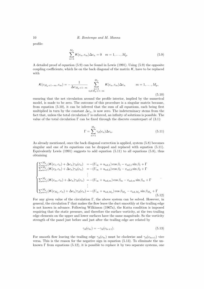
10 R. Bontempo and M. Manna
profile:
Mp∑n=1
K (cn, cm)∆cn = 0 m = 1, . . . ,Mp. (5.9)
A detailed proof of equation (5.9) can be found in Lewis (1991). Using (5.9) the oppositecoupling coefficients, which lie on the back diagonal of the matrix K , have to be replacedwith
K (cMp+1−m, cm) = − 1
∆cMp+1−m
Mp∑n=1
n 6=Mp+1−m
K (cn, cm)∆cn m = 1, . . . ,Mp,
(5.10)ensuring that the net circulation around the profile interior, implied by the numericalmodel, is made to be zero. The outcome of this procedure is a singular matrix because,from equation (5.10), it can be inferred that the sum of all equations, each being firstmultiplied in turn by the constant ∆cn, is now zero. The indeterminacy stems from thefact that, unless the total circulation Γ is enforced, an infinity of solutions is possible. Thevalue of the total circulation Γ can be fixed through the discrete counterpart of (3.1):
Γ =
Mp∑n=1
γd(cn)∆cn. (5.11)
As already mentioned, once the back diagonal correction is applied, system (5.8) becomessingular and one of its equations can be dropped and replaced with equation (5.11).Equivalently Lewis (1991) suggests to add equation (5.11) to all equations (5.8), thusobtaining
∑Mp
n=1(K (c1, cn) + ∆cn)γd(cn) =−(U∞ + uad,1) cosβ1 − vad,1 sinβ1 + Γ∑Mp
n=1(K (c2, cn) + ∆cn)γd(cn) =−(U∞ + uad,2) cosβ2 − vad,2 sinβ2 + Γ...∑Mp
n=1(K (cm, cn) + ∆cn)γd(cn) =−(U∞ + uad,m) cosβm − vad,m sinβm + Γ...∑Mp
n=1(K (cMp, cn) + ∆cn)γd(cn) =−(U∞ + uad,Mp
) cosβMp− vad,Mp
sinβMp+ Γ
.
(5.12)For any given value of the circulation Γ, the above system can be solved. However, ingeneral, the circulation Γ that makes the flow leave the duct smoothly at the trailing edgeis not known in advance. Following Wilkinson (1967a), the Kutta condition is imposedrequiring that the static pressure, and therefore the surface vorticity, at the two trailingedge elements on the upper and lower surfaces have the same magnitude. So the vorticitystrength of the panel just before and just after the trailing edge are related by
γd(cte) = −γd(cte+1). (5.13)
For smooth flow leaving the trailing edge γd(cte) must be clockwise and γd(cte+1) viceversa. This is the reason for the negative sign in equation (5.13). To eliminate the un-known Γ from equations (5.12), it is possible to replace it by two separate systems, one
Solution of the flow over a ducted actuator disk 11
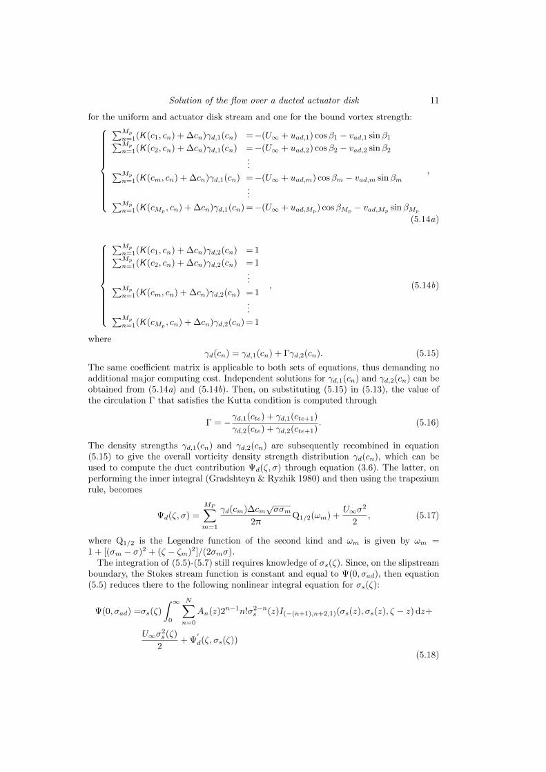
for the uniform and actuator disk stream and one for the bound vortex strength:
∑Mp
n=1(K (c1, cn) + ∆cn)γd,1(cn) =−(U∞ + uad,1) cosβ1 − vad,1 sinβ1∑Mp
n=1(K (c2, cn) + ∆cn)γd,1(cn) =−(U∞ + uad,2) cosβ2 − vad,2 sinβ2
...∑Mp
n=1(K (cm, cn) + ∆cn)γd,1(cn) =−(U∞ + uad,m) cosβm − vad,m sinβm...∑Mp
n=1(K (cMp, cn) + ∆cn)γd,1(cn) =−(U∞ + uad,Mp
) cosβMp− vad,Mp
sinβMp
,
(5.14a)
∑Mp
n=1(K (c1, cn) + ∆cn)γd,2(cn) = 1∑Mp
n=1(K (c2, cn) + ∆cn)γd,2(cn) = 1...∑Mp
n=1(K (cm, cn) + ∆cn)γd,2(cn) = 1...∑Mp
n=1(K (cMp , cn) + ∆cn)γd,2(cn) = 1
, (5.14b)
where
γd(cn) = γd,1(cn) + Γγd,2(cn). (5.15)
The same coefficient matrix is applicable to both sets of equations, thus demanding noadditional major computing cost. Independent solutions for γd,1(cn) and γd,2(cn) can beobtained from (5.14a) and (5.14b). Then, on substituting (5.15) in (5.13), the value ofthe circulation Γ that satisfies the Kutta condition is computed through
Γ = −γd,1(cte) + γd,1(cte+1)
γd,2(cte) + γd,2(cte+1). (5.16)
The density strengths γd,1(cn) and γd,2(cn) are subsequently recombined in equation(5.15) to give the overall vorticity density strength distribution γd(cn), which can beused to compute the duct contribution Ψd(ζ, σ) through equation (3.6). The latter, onperforming the inner integral (Gradshteyn & Ryzhik 1980) and then using the trapeziumrule, becomes
Ψd(ζ, σ) =
MP∑m=1
γd(cm)∆cm√σσm
2πQ1/2(ωm) +
U∞σ2
2, (5.17)
where Q1/2 is the Legendre function of the second kind and ωm is given by ωm =1 + [(σm − σ)2 + (ζ − ζm)2]/(2σmσ).
The integration of (5.5)-(5.7) still requires knowledge of σs(ζ). Since, on the slipstreamboundary, the Stokes stream function is constant and equal to Ψ(0, σad), then equation(5.5) reduces there to the following nonlinear integral equation for σs(ζ):
Ψ(0, σad) =σs(ζ)
∫ ∞0
N∑n=0
An(z)2n−1n!σ2−ns (z)I(−(n+1),n+2,1)(σs(z), σs(z), ζ − z) dz+
U∞σ2s(ζ)
2+ Ψ
′
d(ζ, σs(ζ))
(5.18)

12 R. Bontempo and M. Manna
with Ψ′
d = Ψd − 12U∞σ
2, to be solved iteratively. The solution procedure begins bycomputing and storing in a pre-processing stage the LU decomposition of the coeffi-cient matrix K that appears in (5.14), which merely depends upon the duct geometry.Subsequently, the γd,2(cm) distribution is evaluated once by (5.14b). Assume now thatprovisional values of σs(ζ) and Ann=0,N are available within the wake, for instancefrom the previous iteration. Likewise, assume provisional values of γd(cm) on the profileare available. Then the Stokes stream function in the wake can be evaluated through(5.5) by performing the integration in the axial direction numerically. Next, the tangen-tial vorticity field can be computed with (5.2) and parametrized with (5.3) through anew set of Ann=0,N , selected with the help of a least-squares minimization procedure.Then from (5.6) and (5.7) the axial and radial velocities induced by the actuator disk onthe profile are evaluated, and the rhs of (5.14a) and consequently γd,1(cm) are updated.After that, the Kutta condition is enforced through (5.16) and a new value of γd(cm)results from (5.15). Finally, from (5.18), the new σs(ζ) is
σs(ζ)=
√(Ψ
′d(ζ, σs(ζ))
σs(ζ)U∞+I(ζ, σs(ζ))
U∞
)2
+2Ψ(0, σad)
U∞−Ψ
′
d(ζ, σs(ζ))
σs(ζ)U∞− I(ζ, σs(ζ))
U∞,
where
I(ζ, σs(ζ)) =
∫ ∞0
N∑n=0
An(z)2n−1n!σ2−ns (z)I(−(n+1),n+2,1)(σs(z), σs(z), ζ − z) dz.
At the first iteration γd(cm), σs(ζ) and Ψ are calculated ignoring the presence of thedisk.
From an engineering point of view, it would definitely be preferable to specify theradial distribution of the disk load H(σ). However, on physical grounds, the existence ofa one-to-one correspondence between H(σ) and H(Ψ) is conjectured, and therefore it isalways possible to prescribe H(σ) and then to evaluate the associated H(Ψ); for example,it is possible to prescribe H(σ) at the disk and then to update the coefficient am in (5.1)to match H(σ) at each iteration (Conway 1998).
6. Results and applications
The method described in the previous sections provides the values of all physical quan-tities needed to evaluate the performance parameters of the device, namely the thrustcoefficient CT and the power coefficient CP . Moreover another very important perfor-mance coefficient, typically employed in the propeller field, is the propulsive efficiencyη = CT /CP . In particular, integrating the static pressure jump ∆pad(σ) across the actu-ator disk and the power over the rotor plane yields
CT,rot =Trot
12πρU
2∞σ
2ad
=1
12πρU
2∞σ
2ad
∫ σad
0
∆pad(σ)2πσ dσ, (6.1)
CP =P
12πρU
3∞σ
2ad
=1
12πρU
3∞σ
2ad
∫ σad
0
H(σ)ρu(0, σ)2πσ dσ, (6.2)
where Trot and P are the axial force and the power experienced by the rotor. In thefollowing, quantities denoted with a hat ( · ) are made dimensionless using the referencelength σad and reference velocity U∞. Therefore, (6.1) and (6.2) can be expressed in

Solution of the flow over a ducted actuator disk 13
terms of dimensionless variables, leading to
CT,rot = 2
∫ 1
0
∆pad(σ)σ dσ, (6.3)
CP = 2
∫ 1
0
u(0, σ)H(0, σ)σ dσ, (6.4)
where ∆pad = 2∆pad/ρU2∞ and H = 2H/U2
∞. The thrust coefficient of the duct, com-puted by integrating over its surface the axial force due to the pressure, reads
CT,duct =1
12πρU
2∞σ
2ad
∮C
p(c)n2πσ(c) dc · iζ = −2
∮C
σ(c)Cp,w(c) sinβ(c) dc, (6.5)
where Cp,w = 2(p − p∞)/ρU2∞ is the wall pressure coefficient and c = c/σad is the
dimensionless curvilinear abscissa. Finally, the overall thrust coefficient reads
CT = CT,rot + CT,duct. (6.6)
In the following subsections a few relevant applications of the present method are de-scribed. More precisely the global and local flow characteristics are detailed both for aducted propeller and a ducted turbine. While the results of the former configuration arepresented with and without slipstream rotation, those pertaining to the turbine are onlygiven in the general case of wake rotation, for the sake of brevity. Moreover, a validationprocedure of the method is carried out with the help of asymptotic solutions. A fewconvergence and stability results are also provided.
6.1. Ducted rotor without slipstream rotation
In the special case of a contra-rotating rotor pair or of a turbomachinery stage both withw(ζ, σ) = 0 in the wake, (5.2) returns
ωθ(ζ, σ)
σ= −
M∑m=1
mamΨσad
(Ψ
Ψσad
)m−1
, (6.7)
to be used in the iterative procedure instead of (5.2). In the downstream limit
ωθ(ζ→+∞, σ) = −du
dσ
∣∣∣∣(ζ→+∞,σ)
. (6.8)
Therefore, from equation (6.7) and from the definition of the Stokes stream function, thefollowing second order variable coefficients ordinary differential equation can be obtained(Conway 1998):
1
σ
d
dσ
(1
σ
dΨ
dσ
)=
M∑m=1
mamΨσad
(Ψ
Ψσad
)m−1
, (6.9)
with the associated boundary conditions
Ψ(ζ→+∞, σ=0) = 0Ψ(ζ→+∞, σ=σs(ζ→+∞)) = Ψσad
. (6.10)
To validate the method described in §5, equation (6.9) can be integrated, numericallyor in some special cases analytically, obtaining accurate values of Ψ and u at infinity.Furthermore, a different formulation of the performance coefficients of the device canbe obtained through the distribution of axial velocity at infinity. In fact, as a classicalresult of actuator disk theory, these coefficients can be related to the axial velocity at
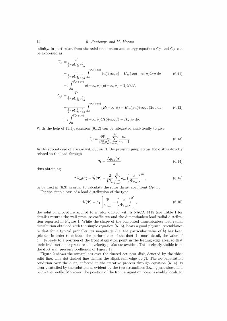
14 R. Bontempo and M. Manna
infinity. In particular, from the axial momentum and energy equations CT and CP canbe expressed as
CT =T
12πρU
2∞σ
2ad
=1
12πρU
2∞σ
2ad
∫ σs(+∞)
0
(u(+∞, σ)− U∞) ρu(+∞, σ)2πσ dσ
=4
∫ σs(+∞)
0
u(+∞, σ) (u(+∞, σ)− 1) σ dσ,
(6.11)
CP =P
12πρU
3∞σ
2ad
=1
12πρU
3∞σ
2ad
∫ σs(+∞)
0
(H(+∞, σ)−H∞)ρu(+∞, σ)2πσ dσ
=2
∫ σs(+∞)
0
u(+∞, σ)(H(+∞, σ)− H∞)σ dσ.
(6.12)
With the help of (5.1), equation (6.12) can be integrated analytically to give
CP =4Ψσad
U3∞σ
2ad
M∑m=0
amm+ 1
. (6.13)
In the special case of a wake without swirl, the pressure jump across the disk is directlyrelated to the load through
H =∆pad(σ)
ρ(6.14)
thus obtaining
∆pad(σ) = H(Ψ) =2
U2∞
M∑m=0
am
(Ψ
Ψσad
)m, (6.15)
to be used in (6.3) in order to calculate the rotor thrust coefficient CT,rot.For the simple case of a load distribution of the type
H(Ψ) = a1
[Ψ
Ψσad
−(
Ψ
Ψσad
)2], (6.16)
the solution procedure applied to a rotor ducted with a NACA 4415 (see Table 1 fordetails) returns the wall pressure coefficient and the dimensionless load radial distribu-tion reported in Figure 1. While the shape of the computed dimensionless load radialdistribution obtained with the simple equation (6.16), bears a good physical resemblance
to that for a typical propeller, its magnitude (i.e. the particular value of b) has beenselected in order to enhance the performance of the duct. In more detail, the value ofb = 15 leads to a position of the front stagnation point in the leading edge area, so thatundesired suction or pressure side velocity peaks are avoided. This is clearly visible fromthe duct wall pressure coefficient of Figure 1a.
Figure 2 shows the streamlines over the ducted actuator disk, denoted by the thicksolid line. The dot-dashed line defines the slipstream edge σs(ζ). The no-penetrationcondition over the duct, enforced in the iterative process through equation (5.14), isclearly satisfied by the solution, as evident by the two streamlines flowing just above andbelow the profile. Moreover, the position of the front stagnation point is readily localized

Solution of the flow over a ducted actuator disk 15
Chord/rotor diameter chord/D 1/2.76Angle between the profile chord and the ζ axis α 12.7
Tip gap/rotor diameter ε/D 1.244 %Leading edge radial position/rotor diameter σle/D 0.580Leading edge axial position/rotor diameter ζle/D -0.111
Load magnitude parameter b = σ2ada1/U∞Ψσad 15
Advance coefficient (only with wake rotation) J 0.5
Table 1: Propeller ducted with a NACA 4415 profile: geometry and operating conditions.
−0.4 −0.2 0 0.2 0.4 0.6 0.8−3
−2
−1
0
1
ζ/chord
Cp,w
(a)
0 0.2 0.4 0.6 0.8 10
2
4
6
8
σ/σad
H
(b)
Figure 1: Propeller ducted with a NACA 4415 profile with b = 15: (a) duct wall pressurecoefficient; (b) radial distribution of load.
by the dividing streamline. Finally, the flow leaves the profile smoothly at the trailingedge according to the Kutta condition requirement.
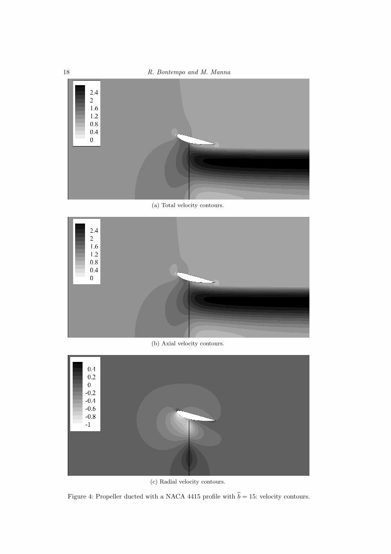
Figure 3 shows the radial distributions of axial and radial dimensionless velocity atdifferent axial stations (see also Figure 2 as a graphical aid to locate them). As a firstremark, both distributions highlight the typical propeller slipstream contraction whosemagnitude is largely dictated by the disk load. In fact the radial velocity is essentiallynegative in the outer part of the slipstream. Moreover, the axial velocity excess increasesin the streamwise direction, while the radial velocity simultaneously approaches zero.The above features further prove the contraction of the slipstream and the establishmentof the wake contraction in the downstream limit, respectively. Finally, the total, axialand radial velocity contours are shown in Figure 4.
The slipstream σs(ζ) at different iterations and the convergence history are given inFigures 5a and 5b, respectively. In the latter, the residue is defined as the absolute value ofthe difference between two successive slipstream radii evaluated at ζ = 5σad, normalizedwith σad. The number of iterations needed to reach convergence with different values of bis detailed in Table 2. The convergence of the iterative process is very rapid for moderateloads and worsens for higher loads, so that under-relaxation is typically needed in order

16 R. Bontempo and M. Manna
−2.5 −2 −1.5 −1 −0.5 0 0.5 1 1.5 2 2.50
0.5
1
1.5
2
2.5
ζ/σad
σ/σad
actuator disk
σs(ζ)
Figure 2: Propeller ducted with a NACA 4415 profile with b = 15: streamlines.
b ωrf = 1 ωrf = 1/3 ωrf = 1/65 12 27 4710 32 32 6415 178 39 7320 not converged 39 78
Table 2: Propeller ducted with a NACA 4415 profile with b = 15: Number of iterationsneeded to reach convergence with different loads and relaxation factors ωrf .
to preserve stability. In particular, the value of the slipstream radius at each iteration isupdated through the relation:
σs(ζ) = σs(ζ)|old + [σs(ζ)|new − σs(ζ)|old]ωrf (6.17)
where ωrf is the relaxation factor. The latter should be fixed minimizing the number ofiterations needed to reach convergence; Table 2 shows typical values.
In the special case of a parabolic load distribution, like the one in (6.16), equation(6.9) reduces to
1
σ
d
dσ
(1
σ
dΨ
dσ
)=U∞b
σ2ad
[1− 2
(Ψ
Ψσad
)]. (6.18)
The analytical solution of the above equation, with the associated boundary conditions(6.10), is detailed in Conway (1998). Figure 6 compares the dimensionless axial velocitydistribution computed by the iterative scheme described in §5 with the analytical oneobtained solving (6.18). It is worth noting that at four propeller radii downstream ofthe disk the axial velocity field has almost reached the theoretical profile at infinity. Theabove result provides a validation of the method and gives evidence of an appropriatecontrol of the related numerical issues. Finally, the global performance coefficients forthe NACA 4415 case are listed in Table 3.
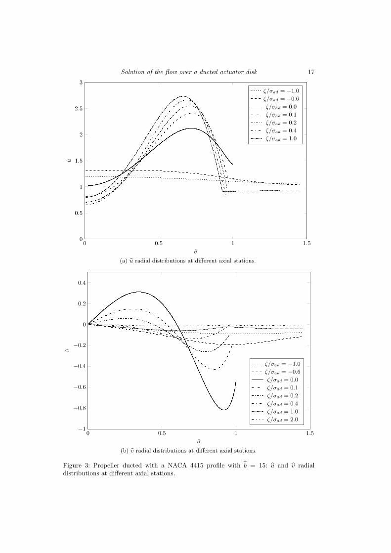
Solution of the flow over a ducted actuator disk 17
0 0.5 1 1.50
0.5
1
1.5
2
2.5
3
σ
u
ζ/σad = −1.0
ζ/σad = −0.6
ζ/σad = 0.0
ζ/σad = 0.1
ζ/σad = 0.2
ζ/σad = 0.4
ζ/σad = 1.0
(a) u radial distributions at different axial stations.
0 0.5 1 1.5−1
−0.8
−0.6
−0.4
−0.2
0
0.2
0.4
σ
v
ζ/σad = −1.0
ζ/σad = −0.6
ζ/σad = 0.0
ζ/σad = 0.1
ζ/σad = 0.2
ζ/σad = 0.4
ζ/σad = 1.0
ζ/σad = 2.0
(b) v radial distributions at different axial stations.
Figure 3: Propeller ducted with a NACA 4415 profile with b = 15: u and v radialdistributions at different axial stations.
18 R. Bontempo and M. Manna
(a) Total velocity contours.
(b) Axial velocity contours.
(c) Radial velocity contours.
Figure 4: Propeller ducted with a NACA 4415 profile with b = 15: velocity contours.

Solution of the flow over a ducted actuator disk 19
0 1 2 3 4 50.9
0.92
0.94
0.96
0.98
1
ζ/σad
σ
iteration number=1
iteration number=5
iteration number=10
iteration number=15
iteration number=20
iteration number=39
(a) Slipstream at different iterations.
0 10 20 30 4010−7
10−6
10−5
10−4
10−3
10−2
10−1
iteration number
residue
(b) Residue.
Figure 5: Propeller ducted with a NACA 4415 profile with b = 15: convergence analysis.

20 R. Bontempo and M. Manna
0 0.5 1 1.50
0.5
1
1.5
2
2.5
3
σ
u
ζ/σad = 0.6
ζ/σad = 1.0
ζ/σad = 1.5
ζ/σad = 2.0
ζ/σad = 4.0
ζ/σad = +∞
Figure 6: Propeller ducted with a NACA 4415 profile with b = 15: approach of the uradial distribution to the asymptotic one.
CT CT,rot CT,duct CP η4.62 4.14 0.48 8.01 0.58
Table 3: Propeller ducted with a NACA 4415 profile with b = 15: performance coeffi-cients.
6.2. Ducted rotor with slipstream rotation
In the case with swirl, the tangential velocity w(ζ, σ) is computed through the angularmomentum equation (2.8), which, using (5.1), yields
w(ζ, σ) =w(ζ, σ)
U∞=J
π
σadσ
1
U2∞
M∑m=0
am
(Ψ
Ψad
)m. (6.19)
Recalling the expression for the θ component of vorticity (5.2) and replacing in (5.2)its asymptotic value ωθ(ζ → +∞, σ) given by (6.8), the following second order variablecoefficients ordinary differential equation is obtained:
1
σ
d
dσ
(1
σ
dΨ
dσ
)=
[J2
π2
(σadσ
)2 1
U2∞
M∑m=0
am
(Ψ
Ψσad
)m− 1
]M∑m=1
mamΨσad
(Ψ
Ψσad
)m−1
(6.20)with the associated boundary conditions (6.10). Like in the case without slipstream

Solution of the flow over a ducted actuator disk 21
Chord/rotor diameter chord/D 0.513Angle between the profile chord and the ζ axis α −5.0
Tip gap/rotor diameter ε/D 1.039 %Leading edge radial position/rotor diameter σle/D 0.559Leading edge axial position/rotor diameter ζle/D -0.15
Load magnitude parameter b = σ2ada1/U∞Ψσad -2
Tip speed ratio λ 2π
Table 4: Turbine ducted with a NACA 5415 profile: geometry and operating conditions.
rotation, the above equation can be integrated to give an accurate solution for Ψ atdownstream infinity and furthermore this result can be used to compute the performancecoefficients of the device. In particular, the equivalent formula to (6.11) is
CT = 2
∫ σs(+∞)
0
[2π
Jσw(+∞, σ) + (u(+∞, σ)− 1)
2 − w2(+∞, σ)
]σ dσ (6.21)
while equations (6.12)-(6.13) are still valid.The pressure jump across the disk is related to the load radial distribution through
H = ∆pad(σ)/ρ + w2(0+, σ)/2. The latter equation, elaborated with the help of (5.1)and (2.8), yields
∆pad(σ) =1
U2∞
M∑m=0
am
(Ψ
Ψσad
)m [2− J2
π2
σ2ad
σ2
1
U2∞
M∑m=0
am
(Ψ
Ψσad
)m], (6.22)
to be used in (6.3) in order to calculate the rotor thrust coefficient CT,rot.With reference to the geometry and operating conditions detailed in Tables 1 and 4,
Figures 7 and 8 show the wall pressure coefficient and the dimensionless load radialdistribution for a propeller ducted with a NACA 4415 and a turbine ducted with aNACA 5415, respectively. The particular value of b = 15 (b = −2 in the turbine case)leads again to a position of the front stagnation point lying in the leading edge area(see Figures 7a and 8a). This latter feature of the flow, the streamline pattern and theconverging–diverging shape of the wake are shown in Figures 9 and 10. As for the casewithout swirl, the no-penetration and Kutta condition compliance can also be appre-ciated. Figures 11-14 present the radial distributions of dimensionless axial, radial andtangential velocities at different axial stations. Concerning the through-flow velocity dis-tributions, the same features as pointed out when discussing Figures 3 are also detectablein Figures 11 and 13. The tangential velocity falls to zero at the ζ axis and at the slip-stream edge, since the load is prescribed to vanish there. The dimensionless radii wherew = 0 in Figure 12 (14) locate the slipstream edge contraction (divergence) movingdownstream. Using the angular momentum conservation law (2.8), the variation of thew profile as ζ increases, can be easily explained. In fact, with reference to the propellercase, the tangential velocity along a streamline increases as ζ increases, a consequenceof the load H invariance along the streamline while the latter is converging. Finally, thecontours of total, axial and radial velocity are shown in Figures 15 and 16.
The slipstream σs(ζ) at different iterations and the convergence history are given inFigures 17a and 17b, respectively. There are no considerable effects of the slipstreamrotation on the convergence and stability of the iterative process.
Equation (6.20) can be numerically integrated to obtain an accurate solution for Ψat infinity; then u(+∞, σ) and w(+∞, σ) can be computed through the definition of

22 R. Bontempo and M. Manna
−0.4 −0.2 0 0.2 0.4 0.6 0.8−3
−2
−1
0
1
ζ/chord
Cp,w
(a)
0 0.2 0.4 0.6 0.8 10
2
4
6
8
σ/σad
H
(b)
Figure 7: Propeller ducted with a NACA 4415 profile with b = 15 and J = 0.5: (a) ductwall pressure coefficient; (b) radial distribution of load.
−0.4 −0.2 0 0.2 0.4 0.6 0.8−3
−2
−1
0
1
ζ/chord
Cp,w
(a)
0 0.2 0.4 0.6 0.8 1−1
−0.8
−0.6
−0.4
−0.2
0
σ/σad
H
(b)
Figure 8: Turbine ducted with a NACA 5415 profile with b = −2 and λ = 2π: (a) ductwall pressure coefficient; (b) radial distribution of load.
the Stokes stream function and equation (6.19), respectively. To validate the slipstreamrotation implementation, a sequence of u and w profiles, as ζ increases, are shown to-gether with the theoretical distribution at infinity in Figures 12, 14 and 18. At four–sixdisk diameters downstream, the velocity distributions have nearly attained their cor-responding asymptotic values. Finally, the global performance coefficients are listed inTables 5 and 6.

Solution of the flow over a ducted actuator disk 23
−2.5 −2 −1.5 −1 −0.5 0 0.5 1 1.5 2 2.50
0.5
1
1.5
2
2.5
ζ/σad
σ/σad
actuator disk
σs(ζ)
Figure 9: Propeller ducted with a NACA 4415 profile with b = 15 and J = 0.5: stream-lines.
−3 −2.5 −2 −1.5 −1 −0.5 0 0.5 1 1.5 2 2.5 30
1
2
3
ζ/σad
σ/σad
actuator disk
σs(ζ)
Figure 10: Turbine ducted with a NACA 5415 profile with b = 2 and λ = 2π: streamlines.
CT CT,rot CT,duct CP η4.57 4.02 0.55 8.60 0.53
Table 5: Propeller ducted with a NACA 4415 profile with b = 15 and J = 0.5: perfor-mance coefficients.
6.3. Comparison between open and ducted rotor
As mentioned in the introduction, the task of the duct is to improve the performance ofthe device. In particular, for a turbine with radius σad and immersed in a uniform flowwith free stream velocity U∞, the effect of the duct is to increase the power output or

24 R. Bontempo and M. Manna
0 0.5 1 1.50
0.5
1
1.5
2
2.5
3
σ
u
ζ/σad = −1.0
ζ/σad = −0.6
ζ/σad = 0.0
ζ/σad = 0.1
ζ/σad = 0.2
ζ/σad = 0.4
ζ/σad = 1.0
(a) u radial distributions at different axial stations.
0 0.5 1 1.5−1
−0.8
−0.6
−0.4
−0.2
0
0.2
0.4
σ
v
ζ/σad = −1.0
ζ/σad = −0.6
ζ/σad = 0.0
ζ/σad = 0.1
ζ/σad = 0.2
ζ/σad = 0.4
ζ/σad = 1.0
ζ/σad = 2.0
(b) v radial distributions at different axial stations.
Figure 11: Propeller ducted with a NACA 4415 profile with b = 15 and J = 0.5: u andv radial distributions at different axial stations.

Solution of the flow over a ducted actuator disk 25
0 0.5 10
0.2
0.4
0.6
0.8
1
σ
w
ζ/σad = 0.0
ζ/σad = 0.2
ζ/σad = 0.4
ζ/σad = 1.0
ζ/σad = 2.0
ζ/σad = 4.0
ζ/σad = +∞
Figure 12: Propeller ducted with a NACA 4415 profile with b = 15 and J = 0.5: w radialdistribution at different axial stations.
CT CT,rot CT,duct CP-0.64 -0.43 -0.21 -0.54
Table 6: Turbine ducted with a NACA 5415 profile with b = −2 and λ = 2π: performancecoefficients.
in dimensionless form the power coefficient CP , that is, the ratio between the extractedand the available power. In more detail, for a turbine without slipstream rotation, theload at the disk can be expressed through equation (6.14). Consequently, the thrust andthe power associated with the rotor infinitesimal surface element of area dArot = 2πσdσare dTrot = ∆pad(σ)dArot = ρH(σ)dArot and dP = H(σ)dm = (u(0, σ) + U∞)dTrot,respectively. Finally, the local power coefficient is
dCP = (u(0, σ) + 1)dCT,rot. (6.23)
The last equation shows that the power coefficient is the product of two terms related tothe mass flow and the load, respectively. Hansen et al. (2000) and de Vries (1979) analysedthe effects of placing a duct around a turbine without slipstream rotation through a 1Dtheoretical analysis and CFD results. In these works it is found that, for a ducted andopen turbine with the same load, the presence of the duct can increase the mass flowpassing through the disk, thus increasing the power coefficient (see equation (6.23)).
In the following, the previous issue is analysed through the method described in this

26 R. Bontempo and M. Manna
0 0.5 1 1.50.6
0.8
1
1.2
1.4
1.6
σ
u
ζ/σad = −1.0
ζ/σad = −0.6
ζ/σad = 0.0
ζ/σad = 0.5
ζ/σad = 0.7
ζ/σad = 1.0
ζ/σad = 2.0
(a) u radial distributions at different axial stations.
0 0.5 1 1.5−0.2
−0.1
0
0.1
0.2
0.3
0.4
0.5
σ
v
ζ/σad = −1.0
ζ/σad = −0.6
ζ/σad = 0.0
ζ/σad = 0.5
ζ/σad = 0.7
ζ/σad = 1.0
ζ/σad = 2.0
(b) v radial distributions at different axial stations.
Figure 13: Turbine ducted with a NACA 5415 profile with b = −2 and λ = 2π: u and vradial distributions at different axial stations.

Solution of the flow over a ducted actuator disk 27
0 0.5 1
0
-0.02
-0.04
-0.06
-0.08
-0.1
σ
w
ζ/σad = 0.0
ζ/σad = 0.5
ζ/σad = 1.0
ζ/σad = 2.0
ζ/σad = 4.0
ζ/σad = +∞
Figure 14: Turbine ducted with a NACA 5415 profile with b = −2 and λ = 2π: w radialdistributions at different axial stations.
Open turbine Ducted turbine ∆CP /CP,open
CT,rot -0.62 -0.62CT -0.62 -0.82CT,duct - -0.20CP -0.46 -0.61 32.61%
Table 7: Comparison of the open and ducted turbine performance coefficients.
paper. Consider a turbine ducted with a NACA 5415 (see Table 4 for geometrical details)without swirl and an open turbine with the same load radial distribution (see Figure19a). The results for this last configuration are obtained through the standard actuatordisk method of Conway (1998). Because the radial loads H(σ) of the two turbines arethe same, they also have the same dCT,rot and CT,rot. However, since the presence ofthe duct increases the mass flow through the ducted rotor (see Figure 20), the powercoefficient value of the ducted turbine is greater than that of the open turbine (see Table7). Moreover the CP value of the ducted turbine is also greater than 16/27 ' 0.593,which is the well-known maximum theoretical CP value achievable by an open turbine(Betz limit).
Figure 20 also shows that, in order to obtain an increase of the mass flow, the ductslipstream σs(ζ) has to be more divergent for ζ > 0 and more convergent for ζ < 0 incomparison with the open rotor configuration. So in the special case of a ducted turbine,

28 R. Bontempo and M. Manna
(a) Total velocity contours.
(b) Axial velocity contours.
(c) Radial velocity contours.
Figure 15: Propeller ducted with a NACA 4415 profile with b = 15 and J = 0.5: velocitycontours.

Solution of the flow over a ducted actuator disk 29
(a) Total velocity contours.
(b) Axial velocity contours.
(c) Radial velocity contours.
Figure 16: Turbine ducted with a NACA 5415 profile with b = −2 and λ = 2π: velocitycontours.

30 R. Bontempo and M. Manna
0 1 2 3 4 50.9
0.92
0.94
0.96
0.98
1
ζ/σad
σ
iteration number=1
iteration number=5
iteration number=10
iteration number=15
iteration number=20
iteration number=38
(a) Slipstream at different iterations.
0 10 20 30 4010−7
10−6
10−5
10−4
10−3
10−2
10−1
iteration number
residue
(b) Residue.
Figure 17: Propeller ducted with a NACA 4415 profile with b = 15 and J = 0.5: conver-gence analysis.

Solution of the flow over a ducted actuator disk 31
0 0.5 1 1.50
0.5
1
1.5
2
2.5
3
σ
u
ζ/σad = 0.6
ζ/σad = 1.0
ζ/σad = 1.5
ζ/σad = 2.0
ζ/σad = 6.0
ζ/σad = +∞
(a) Propeller ducted with a NACA 4415 profile with b = 15 and J = 0.5.
0 0.5 1 1.50.5
0.6
0.7
0.8
0.9
1
1.1
1.2
σ
u
ζ/σad = 2.0
ζ/σad = 3.0
ζ/σad = 4.0
ζ/σad = 6.0
ζ/σad = +∞
(b) Turbine ducted with a NACA 5415 profile with b = −2 and λ = 2π.
Figure 18: Rotors with slipstream rotation: u distribution at different axial stations.

32 R. Bontempo and M. Manna
0 0.2 0.4 0.6 0.8 1−1
−0.8
−0.6
−0.4
−0.2
0
σ
H
(a)
0 0.2 0.4 0.6 0.8 10
2
4
6
8
σ
H
open
ducted
(b)
Figure 19: Load radial distribution for open and ducted rotors. Left: turbines. Right:propellers.
−3 −2.5 −2 −1.5 −1 −0.5 0 0.5 1 1.5 2 2.5 30
1
2
3
ζ/σad
σ/σad
open turbine
ducted turbine
Figure 20: Comparison of the open and the ducted turbine slipstream edge.
the latter result points out the features of the method (which naturally takes into accountthe shape of the slipstream) in comparison with the 1D theory where the effects of theslipstream divergence is neglected.
For a propeller the main task of the duct is to increase the efficiency, notwithstandingthe propulsive thrust required by the carrier. Hence, the efficiency being η = CT /CP , awell-designed duct enables the propeller to achieve a lower value of CP without alter-ing the total thrust coefficient CT . Consider, then, an open propeller without slipstreamrotation and with a parabolic load radial distribution. The performance coefficients ob-tained when setting b = 22.025 are detailed in Table 8. These results are obtained usingthe standard actuator disk method of Conway (1998).
Consider now a propeller ducted with a NACA 5415 (see Table 9 for geometrical

Solution of the flow over a ducted actuator disk 33
Open propeller Ducted propeller ∆η/ηopen
CT 5.22 5.22CT,rot 5.22 4.31CT,duct - 0.91CP 9.90 9.14η 0.53 0.57 7.55%
Table 8: Comparison of the open and ducted propeller performance coefficients
axial chord/rotor diameter chordζ/D 0.5angle between the profile chord and the ζ axis α 12.7
tip gap/rotor diameter ε/D 1.019 %leading edge radius/rotor diameter σle/D 0.625
load magnitude parameter b = σ2ada1/U∞Ψσad 14
Table 9: Propeller ducted with a NACA 5415 profile: geometry and operating condition
−3 −2.5 −2 −1.5 −1 −0.5 0 0.5 1 1.5 2 2.5 30
1
2
3
ζ/σad
σ/σad
open propeller
ducted propeller
Figure 21: Comparison of the open and the duct propeller slipstream edge.
details) with the same radius σad and radial load distribution (b = 14.0) as the openpropeller. Such a propeller achieves the same CT value as the open one (see Table 8), butnow the thrust is split up between the duct and the rotor. In turn, the power coefficientCP is lower than that of the open propeller alone and this results in a higher efficiency.Figures 21 and 19b show the slipstream edge and the load radial distribution for the openand the ducted propeller. From Figure 21, it is easily inferred that the ducted propellerswallows a greater mass flow. Despite this latter feature, its overall power, or rather itspower coefficient CP , is lower than the open propeller one, because of the rotor loadreduction (see Figure 19b).

34 R. Bontempo and M. Manna
7. Conclusions
An extension to ducted rotors of the nonlinear actuator disk theory of Conway (1998)has been presented. In particular, an exact solution of the inviscid axisymmetric flowgenerated by a heavily loaded ducted rotor and a cost-effective semi-analytical solutionprocedure of the resulting equation are detailed. The solution being exact, the propershape of the slipstream, whether converging or diverging, is naturally accounted for,even for heavy loads. The solution procedure can handle rotor wake rotation, radial loaddistributions and ducts of general shape. Furthermore, the method preserves the fullycoupled nature of the solution, duly taking into account the non-linear mutual interactionbetween the duct and the rotor. The solution is expressed as a triple integral over theradial and axial coordinates and over the allowed values of the separation constant of theeigensolutions of the Laplace equation in cylindrical coordinates. Two of these integralsare exactly evaluated, while the integration in the axial direction is performed throughnumerical quadrature, with an extremely reduced computational cost. Therefore, themethod is well suited for the design and/or analysis of ducted rotors for marine, windand aeronautical applications.
The computer code is freely available on contacting the authors.
The authors would like to thank prof. Andrea Vacca, prof. Renato Tognaccini, prof.John T. Conway and prof. Salvatore Miranda for their helpful suggestions.
REFERENCES
Anderson, J. D. 2001 Fundamentals of Aerodynamics, 3rd edn. McGraw-Hill.
Baltazar, J. & Falcao de Campos, J. A. C. 2009 On the modelling of the flow in ductedpropellers with a panel method. In Proceedings of the 1st International Symposium onMarine Propulsors.
Basset, A. B. 1888 A treatise on hydrodynamics. vol. II. Deighton Bell.
Batchelor, G. K. 1967 An intoduction to fluid dynamics. Cambridge University Press.
Breslin, J. P. & Andersen, P. 1994 Hydrodynamics of ship propellers. Cambridge UniversityPress.
Falcao de Campos, J. A. C. 1983 On the calculation of ducted propeller performance inaxisymmetric flows. PhD thesis, Delft University of Technology.
Carlton, J. 2007 Marine propellers and propulsion. Butterworth-Heinemann.
Celik, F., Guner, M. & Ekinci, S. 2010 An approach to the design of ducted propeller.Transaction B: Mechanical Engineering, Scientia Iranica 17 (5), 406–417.
Chaplin, H.R. 1964 A method for numerical calculation of slipstream contraction of a shroudedimpulse disk in the static case with application to other axisymmetric potential flow prob-lems. Tech. Rep. 1857. David Taylor Model Basin.
Conway, J. T. 1995 Analytical solutions for the actuator disk with variable radial distributionof load. J. Fluid Mech. 297, 327–355.
Conway, J. T. 1998 Exact actuator disk solutions for non-uniform heavy loading and slipstreamcontraction. J. Fluid Mech. 365, 235–267.
Conway, J. T. 2000 Analytical solutions for the newtonian gravitational field induced by mat-ter within axisymmetric boundaries. Monthly Notices of the Royal Astronomical Society316 (3), 540–554.
Dickmann, H. E. & Weissinger, J. 1955 Beitrag zur theorie optimaler dusenchrauben (kort-dusen). Schiffbautrchn 49, 452–486.
Gibson, I. S. 1972 Application of vortex singularities to ducted propellers. PhD thesis, Univer-sity of Newcastle upon Tyne.
Gibson, I. S. & Lewis, R. I. 1973 Ducted propeller analysis by surface vorticity and actuator

Solution of the flow over a ducted actuator disk 35
disk theory. In Proceedings of the Symposium on Ducted Propeller . Royal Institute of NavalArchitects.
Gradshteyn, I. S. & Ryzhik, I. M. 1980 Tables of integrals, series and products. Academicpress.
Greenberg, M. D. & Powers, S. R. 1970 Nonlinear actuator disk theory and flow fieldcalculations, including nonuniform loading. Tech. Rep. CR-1672. NASA.
van Gunsteren, L. A. 1973 A contribution to the solution of some specific ship propulsionproblems. PhD thesis, Delft University of Technology.
Hansen, M. O. L., Sorensen, N. N. & Flay, R. G. 2000 Effect of placing a diffuser arounda wind turbine. Wind Energy 3, 207–213.
Horlock, J. H. 1978 Actuator disc theory . McGraw-Hill.Jacob, K. & Riegels, F. W. 1963 The calculation of the pressure distributions over aerofoil
sections of finite thickness with and without flaps and slats. Z. Flugwiss 11 (9), 357–367.Kerwin, J. E., Kinnas, S. A., Lee, J. T. & Shih, W. 1987 A surface panel method for the
hydrodynamic analysis of ducted propellers. Trans. SNAME 95.Lamb, H. 1932 Hydrodynamics. Cambridge University Press.Lewis, R. I. 1991 Vortex element methods for fluid dynamic analysis of engineering systems.
Cambridge University Press.Martensen, E. 1959 Berechnung der druckverteilung an gitterprofilen in ebener potentialstro-
mung mit einer fredholmschen integralgleichung. Arch. Rat. Mech. 3, 235 – 270.Nyiri, A. & Baranyi, L. 1983 Numerical method for calculating the flow around a cascade
of aerofoils. In Proceedings of VII international J.S.M.E. symposium fluid machinery andfluidics. vol. 2.
Ryan, P. G. & Glover, E. J. 1972 A ducted propeller design method: a new approach usingsurface vorticity distribution techniques and lifting line theory. Trans. R.I.N.A. 114, 545– 563.
Sonine, N. J. 1880 Recherches sur les fonction cylindriques et le developpement des fonctionscontinues en series. Math. Ann. 16 (1), 1 – 80.
de Vries, O. 1979 Fluid dynamic aspects of wind energy conversion. AGARDograph No.243.Wilkinson, D. H. 1967a A numerical solution of the analysis and design problems for the flow
past one or more aerofoils or cascades. Tech. Rep. 3545. A.R.C.Wilkinson, D. H. 1967b The calculation of rotational, non-solenoidal flows past two-
dimensional aerofoils and cascades. Tech. Rep. W/M(6C). English Electric, M.E.L.Wu, T. Y. 1962 Flow through a heavily loaded actuator disc. Schiffstechnik 9, 134 – 138.