Solubility and Surface Adsorption Characteristics of Metal Oxides to High Temperature

Chapter 14

Solubility and surface adsorptioncharacteristics of metal oxides

David J. Wesolowski,a,* Stephen E. Ziemniak,b Lawrence M. Anovitz,a

Michael L. Machesky,c Pascale Benezetha and Donald A. Palmera

a Chemical Sciences Division, Oak Ridge National Laboratory, Building 4500S, P.O. Box 2008,

Oak Ridge, TN 37831-6110, USAb Lockheed Martin Corporation, P.O. Box 1072, Schenectady, NY 12301-1072, USAc Illinois State Water Survey, 2204 Griffith Drive, Champaign, IL 61820-7495, USA

14.1. Introduction

This chapter provides an overview of the recent developments in our under-

standing of the interaction of metal oxide and hydroxide minerals with

hydrothermal solutions. It is not intended as an exhaustive review of this vast

subject, but rather to identify the major questions and to demonstrate how some of

them are addressed. An emphasis is placed on the equilibrium solubilities of metal

oxides encountered in steam generators and other industrial processes, but other

systems for which experimental data are available will also be addressed. Selected

silicon-bearing phases are included, though Si is not generally considered a metal,

senso stricto, because of their extreme importance in geologic and industrial

systems. The surface charging and ion adsorption characteristics of metal oxides

under hydrothermal conditions, a much less mature subject, will also be reviewed.

In addition to controlling colloidal particle and dissolved trace element transport

and deposition in hydrothermal systems, surface chemistry affects the rates and

mechanisms of metal oxide dissolution/precipitation reactions. However,

heterogeneous reaction kinetics will not be discussed. Recent books devoted

to these subjects provide a great deal of useful background information on

equilibrium solubility and speciation (Stumm and Morgan, 1981; Baes and

Mesmer, 1976; Cohen, 1989; Barnes, 1997; Tremaine et al., 2000; Byrappa and

Yoshimura, 2001), surface adsorption (Adamson and Gast, 1997; Halley, 2001;

*Corresponding author. E-mail: [email protected]

Aqueous Systems at Elevated Temperatures and Pressures:Physical Chemistry in Water, Steam and Hydrothermal SolutionsD.A. Palmer, R. Fernandez-Prini and A.H. Harvey (editors)q 2004 Elsevier Ltd. All rights reserved

Hunter, 2001, 2002; Wingrave, 2001; Kosmulski, 2001) and heterogeneous

kinetics (Blesa et al., 1994; Lasaga, 1998; Jolivet, 2000; Markov, 2003).

The hydrothermal regime will be considered as spanning temperatures from

about 100 to 350 8C, above the boiling point of pure water at 1 atm, but below the

near-critical region (the critical point of water is at 373.946 8C and 22.064 MPa).

Reactions in liquid water will only be considered (i.e., pressures at or above the

saturated vapor pressure, psat), since vapor-phase transport is addressed in Chapter

12. Over this region, pressure vessels, non-commercial probes and other

specialized facilities are needed in order to contain, exploit or study heterogeneous

reactions. The lower temperature limit is thus, not surprisingly, a boundary

between conditions under which experimental data are abundant and accurate, and

the hydrothermal regime where such data are typically sparse, conflicting, or

entirely lacking. The upper temperature limit separates the hydrothermal regime

from the near-critical region where the solvent, dielectric constant and hydrogen

bonding network change rapidly with temperature and are highly dependent upon

solvent density, thus imparting a strong pressure dependence to heterogeneous

reactions.

The term ‘oxide’ will be used loosely to represent any oxygen-bearing, solid

phase of a metal, Me, in the system Me–O–H, which also includes oxyhydroxides

and hydroxides. Some simple mixed oxides will be considered, but not the

solubilities of largely ionic phases formed by metals co-precipitating with the

oxyanions of carbonate, phosphate, sulfate, nitrate, borate, etc. although these

materials are of great interest to earth scientists as well as in industrial

applications. Such minerals and their impact on power plant operations are

discussed in Chapter 17. Nevertheless, the concepts and techniques reviewed

below are readily transferable to these systems.

14.2. Stability of Metal Oxides

Before discussing the solubilities of metal oxides, it is appropriate to first consider

the stabilities of these phases relative to one another and the metals from which

they form. With a few exceptions (Au, Pt, Cu under mildly reducing conditions,

etc.), metals exposed to aqueous solutions generally form an oxide surface film,

which may or may not passivate the surface toward further oxidation (Macdonald

and Cragnolio, 1989; Blesa et al., 1994). This phenomenon is driven by the

relative Gibbs energies of the solid phases and the redox state of the system.

Whether an anhydrous oxide, a mixed oxyhydroxide, or a hydroxide phase of a

particular metal is stable under a given set of pressure–temperature ðp–TÞ

conditions is also dependent on the relative Gibbs energies of these phases and the

prevailing water vapor pressure. Furthermore, oxides of the same composition can

occur in more than one crystalline structure, although this often has more to do

with the mechanisms and kinetics of formation than with thermodynamic stability.

D.J. Wesolowski et al.494

14.2.1. Oxidation

Oxidation reactions can be written with consumption of 1 mole of oxygen, as

for example the formation of zincite (ZnO) and corundum (a-Al2O3) from their

metals and the oxidation of magnetite (Fe3O4) to hematite (a-Fe2O3):

2ZnðsÞ þ O2ðgÞO 2ZnOðsÞ ð14:1Þ

ð4=3ÞAlðsÞ þ O2ðgÞO ð2=3ÞAl2O3ðsÞ ð14:2Þ

4Fe3O4ðsÞ þ O2ðgÞO 6Fe2O3ðsÞ ð14:3Þ

Since the Gibbs energies of formation of gaseous molecular oxygen and the

pure metals are by convention zero, the equilibrium Gibbs energy change for each

such oxidation reaction at any given temperature and pressure is related only to the

Gibbs energies of formation of the oxide phases involved in the reaction:

DrGo14:1 ¼ 2Df;zinciteGo ð14:4Þ

DrGo14:2 ¼ ð2=3ÞDf;corundumGo ð14:5Þ

DrGo14:3 ¼ 6Df;hematiteGo 2 4Df;magnetiteGo ð14:6Þ

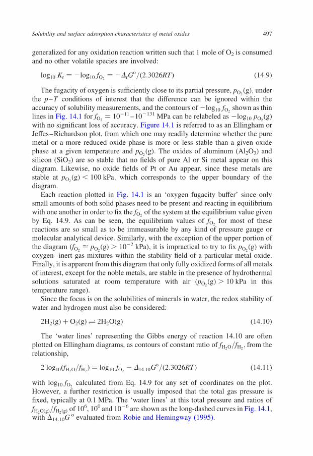
Figure 14.1 shows the Gibbs energies of a number of such oxidation reactions

versus temperature in the 100–350 8C range, with Gibbs energies of formation of

the solid oxides taken from Robie et al. (1978), Robie and Hemingway (1995) and

for Cr2O3, Anovitz et al. (2004). The calculations were performed at 0.1 MPa total

pressure, but the curves are nearly independent of pressure up to several hundred

MPa. The ‘curves’ are also essentially linear in this p–T range. The solid lines

represent reactions involving the most thermodynamically stable phases, and the

dotted lines show three metastable redox equilibria (Ti metal to the rutile

polymorph of TiO2 and reactions involving metallic iron to wustite, Fe0.947O, and

wustite to magnetite), which are of interest in some applications.

The thermodynamic equilibrium constant ðKÞ for any reaction at p and T is

related to its equilibrium Gibbs energy, enthalpy and entropy changes by:

22:3026RT log10 Kr ¼ DrGo ¼ DrH

o 2 TDrSo ð14:7Þ

where R is the gas constant (8.3145 J·K21·mol21) and T the temperature (K). The

equilibrium constant is defined as the activity ratio (fugacity for gases). For

reaction 14.3 as an example,

K14:3 ¼ a6hematitea24

magnetite f21O2

ð14:8Þ

The activities, a; of pure crystalline phases are taken as unity on the rational

activity coefficient scale, and so Eqs. 14.7 and 14.8 can be rearranged and

Solubility and surface adsorption characteristics of metal oxides 495

Fig. 14.1. Gibbs energies of anhydrous oxidation reactions versus temperature. Solid lines are stable

reaction boundaries, short-dashed lines are metastable reaction boundaries, thin contours are labeled

with 2log10 fO2ðgÞcalculated at 0.1 MPa total pressure. Long-dashed lines are contours at 0.1 MPa

total pressure of the ratio fH2OðgÞ=fH2ðgÞof, from top to bottom 106, 100 and 1026.


generalized for any oxidation reaction written such that 1 mole of O2 is consumed

and no other volatile species are involved:

log10 Kr ¼ 2log10 fO2¼ 2DrG

o=ð2:3026RTÞ ð14:9Þ

The fugacity of oxygen is sufficiently close to its partial pressure, pO2ðgÞ; under

the p–T conditions of interest that the difference can be ignored within the

accuracy of solubility measurements, and the contours of 2log10 fO2shown as thin

lines in Fig. 14.1 for fO2¼ 10211 –102131 MPa can be relabeled as 2log10 pO2

ðgÞ

with no significant loss of accuracy. Figure 14.1 is referred to as an Ellingham or

Jeffes–Richardson plot, from which one may readily determine whether the pure

metal or a more reduced oxide phase is more or less stable than a given oxide

phase at a given temperature and pO2ðgÞ: The oxides of aluminum (Al2O3) and

silicon (SiO2) are so stable that no fields of pure Al or Si metal appear on this

diagram. Likewise, no oxide fields of Pt or Au appear, since these metals are

stable at pO2ðgÞ , 100 kPa; which corresponds to the upper boundary of the

diagram.

Each reaction plotted in Fig. 14.1 is an ‘oxygen fugacity buffer’ since only

small amounts of both solid phases need to be present and reacting in equilibrium

with one another in order to fix the fO2of the system at the equilibrium value given

by Eq. 14.9. As can be seen, the equilibrium values of fO2for most of these

reactions are so small as to be immeasurable by any kind of pressure gauge or

molecular analytical device. Similarly, with the exception of the upper portion of

the diagram ðfO2ø pO2

ðgÞ . 1022 kPaÞ; it is impractical to try to fix pO2ðgÞ with

oxygen–inert gas mixtures within the stability field of a particular metal oxide.

Finally, it is apparent from this diagram that only fully oxidized forms of all metals

of interest, except for the noble metals, are stable in the presence of hydrothermal

solutions saturated at room temperature with air (pO2ðgÞ . 10 kPa in this

temperature range).

Since the focus is on the solubilities of minerals in water, the redox stability of

water and hydrogen must also be considered:

2H2ðgÞ þ O2ðgÞO 2H2OðgÞ ð14:10Þ

The ‘water lines’ representing the Gibbs energy of reaction 14.10 are often

plotted on Ellingham diagrams, as contours of constant ratio of fH2O=fH2; from the

relationship,

2 log10ðfH2O=fH2Þ ¼ log10 fO2

2 D14:10Go=ð2:3026RTÞ ð14:11Þ

with log10 fO2calculated from Eq. 14.9 for any set of coordinates on the plot.

However, a further restriction is usually imposed that the total gas pressure is

fixed, typically at 0.1 MPa. The ‘water lines’ at this total pressure and ratios of

fH2OðgÞ=fH2ðgÞof 106, 100 and 1026 are shown as the long-dashed curves in Fig. 14.1,

with D14.10G o evaluated from Robie and Hemingway (1995).


A more practical approach for hydrothermal systems is to plot contours of

hydrogen fugacity in liquid water, which is a well-defined quantity, at the

temperature and pressure of interest, since the fugacities of all components in

coexisting phases at equilibrium must be the same. This requires knowledge of the

Henry’s Law constant (Chapter 3):

kH ¼ fH2ðgÞ=mH2

ð14:12Þ

where mH2is the molal concentration of dissolved H2 in liquid water in equilibrium

with a gas phase having the indicated pH2ðgÞ ø fH2

(in MPa). Values of kH in units of

MPa per mole fraction of dissolved H2 can be calculated from Eq. 3.21 in Chapter 3

and Eq. 1.4 in Chapter 1, and converted to units of MPa·kg·mol21 by dividing

by 55.51 (the number of moles in 1 kg of pure water). Equation 14.12 is strictly

valid only in the limit of infinite dilution of the dissolved gas, but deviations from

this limit are small in the water–O2–H2 system over the p–T range of interest.

However, caution must be exercised in applying this and other formulations for

the Henry’s Law constant at total pressures significantly above psat, since these

formulations assume that kH is independent of total pressure at a given temperature.

To understand how the Henry’s Law constant is applied in this context,

consider a typical pressurized water reactor (PWR), where coolants are saturated

with 1 atm (0.1013 MPa) of hydrogen gas at approximately 25 8C. Assuming that

the resulting dissolved hydrogen concentration (7.92 £ 1024 molal at 25 8C)

remains essentially constant as the water circulates through the steam generator,

Eq. 14.12 can be used to calculate fH2in the water with increasing temperature (for

instance 17.6 kPa at 300 8C). The fugacity of pure water at any temperature and

pressure can be obtained from the IAPWS Standard (Wagner and Pruß, 2002)

using a NIST software package (Harvey et al., 2000), and these quantities are used

in Eq. 14.10 to calculate fO2; which is then used in Eq. 14.9 to calculate coordinates

to plot on the Ellingham diagram.

Figure 14.2 is an expanded section of Fig. 14.1 with the same metal/metal oxide

reaction lines shown, and including contours of the redox condition imposed by

water containing dissolved hydrogen fixed at the concentration established by

saturation at 25 8C with gas having pH2ðgÞranging from 1027 to 101 MPa.

This diagram demonstrates that solutions saturated with 0.1 MPa of H2(g) at

25 8C, that do not lose a significant amount of their dissolved hydrogen content

upon heating into the hydrothermal regime, are in equilibrium with magnetite

(Fe3O4) and cassiterite (SnO2), rather than iron or tin metal, but are compatible with

metallic Cd, Co, Ni, Cu and Pb. The diagram also demonstrates that the oxidation

state of a solution could be effectively manipulated by pre-saturation with hydrogen

gas or gas mixtures in order to maintain equilibrium with a particular metal or metal

oxide phase of interest in this range. However, caution must be used in practice,

since: (a) high hydrogen concentrations induce embrittlement and cracking of

metal parts; (b) hydrogen readily diffuses through metals and thin oxide films, and

thus may be lost from the system; (c) all of the curves shown in Figs. 14.1 and 14.2


are subject to uncertainty; (d) kinetic barriers may hinder hydrogen or oxygen

reaction with solid phases and even aqueous species; and (e) individual metals will

have lower activities (and therefore expanded stability fields), when alloyed with

other metals, and the same applies for oxide components in solid solutions.

14.2.2. Hydration

Figures 14.1 and 14.2 involve solid phases containing no hydrogen. However, in

liquid water or steam, hydration of solid oxides can occur, and more importantly,

Fig. 14.2. Expansion of Fig. 14.1 excluding the contours of fO2ðgÞand fH2ðgÞ

=fH2OðgÞ; but including

contours labeled with the redox state imposed at high temperature by liquid water saturated at 25 8C

with a gas having the log10 pH2ðgÞindicated (p in MPa).


metal oxides formed in the presence of water are often hydrated regardless of

whether the hydrous phase is thermodynamically stable relative to the pure oxide

or a less hydrated phase, e.g., the aluminum system with hydration reactions

relating corundum, a-Al2O3, boehmite, g-AlOOH, and gibbsite, g-Al(OH)3, or

their polymorphs:

Al2O3ðsÞ þ H2OðlÞO 2AlOOHðsÞ ð14:13Þ

Al2O3ðsÞ þ 3H2OðlÞO 2AlðOHÞ3ðsÞ ð14:14Þ

AlOOHðsÞ þ H2OðlÞO AlðOHÞ3ðsÞ ð14:15Þ

Figure 14.3 shows the thermodynamically predicted p–T conditions at which

these and a number of other hydrated/dehydrated oxide couples can coexist when

the total system pressure is determined by liquid water or vapor. The water

liquid–vapor coexistence curve ( psat, T) is also shown (Eq. 1.4 of Chapter 1).

Thermodynamic data for the hydroxides were taken from Robie et al. (1978),

Robie and Hemingway (1995), Pertlik (1999), Ziemniak (2001) and Anovitz et al.

(2004). For a given reaction in Fig. 14.3, the less hydrated phase is stable relative

to the more hydrated phase on the high-temperature, low-pressure side of the

curve. In the aluminum system, Figure 14.3 demonstrates that, except at low

temperatures and high pressures, the only stable phases are diaspore (a-AlOOH)

and corundum. Nonetheless, the other, hydroxide and oxyhydroxide phases

commonly occur in natural and industrial hydrothermal systems, and thus it is also

important to consider their relative stabilities.

Most of the reactions shown in Fig. 14.3 are simple dehydration reactions

like those in Eqs. 14.13–14.15, and the reaction boundaries were calculated

using the relationship:

DrGoðp2; T2Þ2 DrG

oðp1;T1Þ ¼ 2ðT2

T1

DrS dT þðp2

p1

DrVs dp þ RT ln fH2O

ð14:16Þ

where the subscripts ‘1’ and ‘2’ refer to different p–T conditions, with 0.1 MPa

and 298.15 K usually taken as reference conditions. At any given p–T; either the

pressure or temperature is fixed, and the equation is evaluated iteratively to find the

value of the other state variable that gives DrGo ¼ 0: The fugacity of water was

taken from Wagner and Pruß (2002), and the second term on the right, which

explicitly treats the volume change of the solids only, was ignored, since this

quantity varies insignificantly over the p–T range of interest.

The dehydration of Fe(OH)2 to Fe3O4 depends upon both fH2and fH2O; as shown

in Fig. 14.3, with reaction boundaries shown for water saturated at 25 8C with

pH2ðgÞ¼ 0:03; 0.1 and 1.0 MPa, using the Henry’s Law constant given above.

The relative stabilities of these phases were based on the solubility studies of

Ziemniak et al. (1995). Figure 14.3 indicates that magnetite is not stable relative to


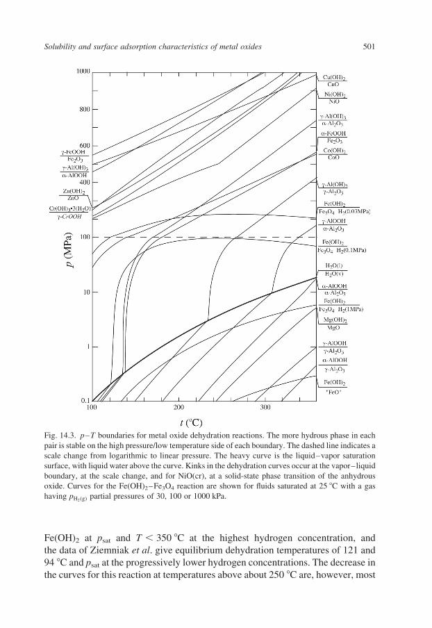
Fe(OH)2 at psat and T , 350 8C at the highest hydrogen concentration, and

the data of Ziemniak et al. give equilibrium dehydration temperatures of 121 and

94 8C and psat at the progressively lower hydrogen concentrations. The decrease in

the curves for this reaction at temperatures above about 250 8C are, however, most

Fig. 14.3. p–T boundaries for metal oxide dehydration reactions. The more hydrous phase in each

pair is stable on the high pressure/low temperature side of each boundary. The dashed line indicates a

scale change from logarithmic to linear pressure. The heavy curve is the liquid–vapor saturation

surface, with liquid water above the curve. Kinks in the dehydration curves occur at the vapor–liquid

boundary, at the scale change, and for NiO(cr), at a solid-state phase transition of the anhydrous

oxide. Curves for the Fe(OH)2–Fe3O4 reaction are shown for fluids saturated at 25 8C with a gas

having pH2ðgÞpartial pressures of 30, 100 or 1000 kPa.


likely an artifact of the constant heat capacity model used by Ziemniak et al. to fit

their data.

Figure 14.3 is shown with two scales, log10 p from 0.1 to 100 MPa, and linear

from 0.1 to 1 GPa, in order to show the effect of increasing water pressure on the

stabilization of hydrated phases, even at 350 8C. The discontinuity in some of the

curves is a result of solid-state phase transitions, such as a-NiO (bunsenite) to b-

NiO at 245 8C, and in each curve at the phase boundary between water and steam.

These predicted dehydration temperatures and pressures have limited practical

utility, however, as it is quite common for dehydrated phases to maintain

metastable equilibrium with aqueous solutions to lower temperatures and/or

higher pressures. The converse is also true for the more hydrated phases with

increasing temperature or decreasing pressure. It is common for a hydrated phase

to precipitate from a super-saturated solution, or to form by oxidation of a metal

surface in contact with water, even if the hydrated phase is metastable relative to a

less-hydrated or anhydrous phase, due to kinetic barriers to nucleation of the more

stable phase. Moreover, metastable dehydrated phases often form a poorly

crystalline, hydrated surface layer when exposed to hydrothermal solutions, which

may or may not affect their solubilities, e.g., corundum, a-Al2O3, which rapidly

form a series of AlOOH and Al(OH)3 surface layers upon exposure even to low-

pressure water vapor at room temperature (Brown et al., 1999).

Experimentally observed dehydration reactions for individual metal oxide

systems will be discussed in more detail below. In liquid water, the addition of

high concentrations of solutes, such as salts, ethylene glycol, alcohol, etc. can also

induce dehydration by lowering the activity (and therefore the fugacity) of water at

constant p–T: For instance, the water activity in 6 mol·kg21 NaCl ranges from

0.77 at 100 8C to 0.85 at 300 8C (Liu and Lindsay, 1972), whereas in mixtures with

completely miscible solvents such as alcohol and ethylene glycol, the water

activity will be approximately equal to its mole fraction and can range from near

zero to near unity.

14.2.3. Polymorphs and Nanoparticles

Many metal oxides and hydroxides occur as two or more polymorphs of identical

composition but different crystalline structure. Kosmulski (2001, Chapter 2)

provides an excellent summary of the common names, chemical formulas,

structures and standard state thermodynamic properties of hundreds of metal oxide

polymorphs, and Blesa et al. (1994) discuss metal oxide structure types in detail.

Quartz (a-SiO2) is the most stable form of silica under hydrothermal conditions,

but will transform to the tridymite, cristobalite, coesite and stishovite polymorphs

with increasing temperature and pressure. The transitions between these

polymorphs are not always rapid and reversible, and hysteresis is common.

TiO2 is found as rutile, anatase or brookite in natural environments, but the latter

two rather rapidly convert to the most stable polymorph, rutile (a-TiO2), under


hydrothermal conditions. Macro-crystalline corundum, a-Al2O3, is more stable

than g-Al2O3, but the latter is readily synthesized by dehydration of Al(III)

hydroxides at modest temperatures, and converts to corundum only with aging at

high temperature (in excess of 500 8C). Polymorphs of Me(III)OOH are common,

with goethite (a-FeOOH), diaspore (a-AlOOH) and grimaldiite (a-CrOOH) being

structurally similar. Lepidocrocite (g-FeOOH) and guyanaite (b-CrOOH) are also

observed in natural and industrial systems, and the less thermodynamically stable

polymorphs, boehmite (g-AlOOH) and g-CrOOH (no mineral name), which are

structurally related to lepidocrocite, are typically observed as the solubility-

controlling phases of Al(III) and Cr(III) under hydrothermal conditions (Palmer

et al., 2001; Ziemniak, 2001).

Metastable polymorphs form and persist because the activation barriers for

nucleation and/or growth of polymorphs in water vary considerably, and the rates

of solid-state transformation of one polymorph to another also vary widely for a

given p–T condition. Thus, it is important to establish which polymorph of a given

oxide phase is controlling the solubility of the metal of interest in hydrothermal

solutions, typically by X-ray diffraction analysis of the solid phase. However, it is

not uncommon for a metastable polymorph, which is structurally different from

the bulk substrate, to form on the surfaces of minerals reacting with hydrothermal

solutions. In this case, high-resolution transmission electron microscopy (TEM),

X-ray photoelectron spectroscopy (XPS), low energy electron diffraction (LEED)

and other surface diffraction and spectroscopic techniques may be needed in order

to determine the solubility-controlling phase (see Brown et al. (1999), Gibson and

LaFemina (1996) for summaries and applications of surface analysis methods). In

some cases, the solubility-controlling phase can only be inferred from observed

solubilities at a well-defined condition. Strictly, no thermodynamic data can be

obtained from solubility studies of amorphous phases and the terms ‘fresh’ and

‘aged’ are often used to describe the solubility trend always to lower values as the

particles crystallize or ‘ripen’.

For any reaction involving polymorphs (solubility, redox, dehydration, etc.),

the change in the equilibrium constant of the reaction upon substitution of one

polymorph for another can be calculated from the known difference in Gibbs

energies (Eq. 14.8). For example, the Gibbs energy change for reaction 14.13 at

250 8C and 50 MPa is 25.06 kJ·mol21 for conversion of a-Al2O3 to g-AlOOH,

and 211.56 kJ·mol21 for conversion of a-Al2O3 to a-AlOOH, giving a difference

of 6.50 kJ·mol21, which translates to a difference in log10 Kr of reaction 14.13

(or any reaction in which diaspore is substituted for boehmite) of 0.65 log10 units

at this p and T (Robie and Hemingway, 1995). However, the uncertainty in the

Gibbs energies, even at 25 8C and 0.1 MPa, is on the order of 2 kJ·mol21 for both

boehmite and diaspore and 1.3 kJ·mol21 for corundum (the uncertainty for water is

much smaller). Thus, the issue of which polymorph is stable, metastably persistent,

or likely to form under a given set of conditions, is often difficult to predict reliably

from thermodynamic compilations.


Recently, Navrotsky (2001) has demonstrated that a number of metal

oxyhydroxide systems, such as Al(III) (corundum–diaspore–boehmite–gibbsite),

Fe(III) (hematite–goethite–lepidocrocite), Ti(IV) (rutile–anatase–brookite), etc.

should exhibit crossovers in the relative thermodynamic stabilities of the oxides

versus hydroxides. These crossovers, even amongst polymorphs and amorphous

phases of a particular metal oxide, occur as a function of particle size, due to

differences in their surface energies, which become a significant portion of the total

energies of the particles below about 10 nm in average diameter. The calorimetric

studies of Navrotsky and co-workers indicate that for oxide phases with low surface

energies, small particle size is favored and the Gibbs energy difference between

more stable and less stable phases shrinks with decreasing particle size. Zhang and

Banfield (1998) predict that anatase should become more stable than rutile below a

particle size of a few nanometers, even at temperatures of 400–500 8C under dry

conditions, and Navrotsky’s group has presented calorimetric and molecular

dynamics simulation results supporting a similar crossover in relative stabilities of

corundum and g-Al2O3. However, in the nanoscale particle size range, the total

energies of all crystalline phases are higher than their macrocrystalline

counterparts, on a per-mole basis, due to the additional surface energy term, and

thus nanoparticles are thermodynamically driven to coarsen. Since hydrothermal

solutions are known to act as a flux for such recrystallization reactions, it remains to

be determined whether particle size effects will be significant in determining the

phases controlling mineral solubilities under hydrothermal conditions.

14.3. Equilibrium Solubility of Metal Oxides: General Considerations

With regard to heterogeneous systems involving metal oxide solids, it has often

been said that ‘thermodynamics do not necessarily apply in this situation’, and

some have questioned the validity of defining ‘solubility’ as a thermodynamically

rigorous concept. Neither of these statements has any basis in fact, but rather they

relate to the rates of solid-state and heterogeneous reactions relative to the time

frame of a specific observation or process. Given infinite time, all closed systems

will approach a state of stable equilibrium, defined as the lowest possible energy

configuration of the system for a given set of conditions (temperature, pressure,

volume, composition, external fields, etc.). In this state, less stable solid phases

and nanoparticles will have either dissolved or transformed to their most stable

macrocrystalline forms and compositions, and the liquid and vapor phases

coexisting with them will have achieved compositions such that the chemical

potentials of all thermodynamic components are equal in all coexisting phases. In

this state, dissolution, precipitation and vapor–liquid exchange processes still

proceed at finite (and sometimes rapid) rates, but forward and reverse reaction

rates are exactly balanced, such that individual phase compositions and structures

remain observationally unchanging at the macroscale.


However, equilibrium thermodynamic descriptions apply equally well to

systems containing metastable phases and species that otherwise maintain

reversible thermodynamic equilibria with other phases and components in the

system. Aluminum hydroxides have already been mentioned in this context, but

even metastable aqueous components can control reactions, such as the influence

of HSO24 (aq) and CO2(g) on solution pH under reducing conditions where the

stable species might be HS2(aq) and CH4(g) (Dickson et al., 1990; Patterson et al.,

1982). Chapter 16 of this volume discusses the metastable persistence of dissolved

organic species within this context. Typically, an activation barrier of some type,

or in the case of an electrochemical cell, an externally imposed potential, prevents

conversion of the metastable phase or species to lower-energy forms, at least

within the time frame of the observation. A brief and cogent discussion of

metastable equilibrium is presented by Anderson (2002).

One of the complicating factors of the hydrothermal regime is that solid phases

which exhibit reversible metastable equilibrium interactions with aqueous

solutions at low temperature are often observed to convert to more stable forms

over time scales similar to the length of an industrial or natural process or

experimental study, due to temperature-enhanced reaction rates. Alternatively, a

process may be controlled by an oxide formed at high temperature, but that phase

may remain in metastable equilibrium when the system temperature decreases,

rather than converting to a more stable hydrous phase. Even amorphous solids may

persist and establish metastable equilibrium with a coexisting solution, e.g.,

amorphous silica (Gunnarsson and Arnorsson, 2000). One of the greatest

challenges in interpreting the results of hydrothermal experiments and applying

thermodynamic and kinetic data and theories in the modeling of natural and

industrial processes is determining the nature of the solid phases and aqueous

species which are actually controlling, or which form as a result of, the observed

solution composition and prevalent environmental variables.

14.3.1. The Solubility Product

For ‘ionic’ minerals the solubility is usually expressed in terms of dissolution to

the constituent cations and anions, such as for calcite,

CaCO3ðcrÞO Ca2þðaqÞ þ CO223 ðaqÞ ð14:17Þ

with the ‘solubility product’ defined as (braces denote activities):

KspðcalciteÞ ¼ {Ca2þðaqÞ}{CO223 ðaqÞ}={CaCO3ðcrÞ} ð14:18Þ

However, this is not a particularly useful way of expressing the solubility of

an oxide such as MeO, since O22 is virtually non-existent in aqueous solutions.


Representative solubility reactions for the dissolution of anhydrous, single-metal

oxides to the ‘free’ metal ion in an aqueous solution at low pH are:

ZnOðzinciteÞ þ 2HþðaqÞO Zn2þðaqÞ þ H2OðlÞ ð14:19Þ

AlOOHðboehmiteÞ þ 3HþðaqÞO Al3þðaqÞ þ 2H2OðlÞ ð14:20Þ

Fe2O3ðhematiteÞ þ 6HþðaqÞO 2Fe3þðaqÞ þ 3H2OðlÞ ð14:21Þ

For a general, redox-independent dissolution reaction of a single-metal oxide,

1=xMexOaðOHÞxz22aðcrÞ þ ðzÞHþðaqÞO MezþðaqÞ þ ðz 2 a=xÞH2OðlÞ ð14:22Þ

the equilibrium constant, which will be defined as the solubility product, is

Ks0 ¼ {MezþðaqÞ}{H2O}ðz2a=xÞ{MexOaðOHÞxz22aðcrÞ}21=x{HþðaqÞ}2z ð14:23Þ

The subscript ‘aq’ indicates that the ions are understood to exist in solution as

hydrated species, typically with well-defined numbers and configurations of

nearest-neighbor water molecules bound to the central metal ion. The activity of

pure crystalline phases is taken as unity on the rational activity scale and the

activity of liquid water is typically very close to unity, except in mixed solvents or

very concentrated electrolyte solutions. Thus, in dilute solutions, the solubility

product can be expressed as

Ks0 ¼ {MezþðaqÞ}={HþðaqÞ}z ð14:24Þ

which can be rearranged to

log10{MezþðaqÞ} ¼ log10 Ks0 2 z pH ð14:25Þ

In solutions sufficiently acidic to suppress hydrolysis of the dissolved cation, a

plot of the logarithm of the total metal content in solution in equilibrium with its

oxide versus solution pH at constant temperature and pressure is therefore a

straight line with a slope of 2z; as shown for ZnO (slope ¼ 22) in Fig. 14.4. This

clearly demonstrates the importance of pH in determining the solubility of a metal

oxide. Under acidic conditions, the solubilities of oxides of divalent metal ions

increase with the square of the hydrogen ion activity, the cube for trivalent metals,

and so on!

The equilibrium state is precisely the condition at which the ion activity product

(IAP), which is defined as the right hand side of Eq. 14.23, is exactly equal to Ks0.

The saturation index (SI)

SI ; IAP=Ks0 ð14:26Þ


is unity in this case (SI is often given different names in various publications, but

the concept is the same). Since the dissolved metal species generally maintain

equilibrium with one another under hydrothermal conditions, defining SI in terms

of Ks0 is completely general, regardless of pH, although the concentrations of both

Hþ and Mezþ might be exceedingly low in neutral and basic solutions. The SI can

deviate significantly from unity, by orders of magnitude in some cases. Values less

than unity indicate a state of ‘under-saturation’ of the solution with respect to the

solubility reaction that defines K; whereas SI values greater than unity indicate a

state of ‘super-saturation’. Even if the SI of the solution is unity with respect to a

metastable oxide phase, the solution will be super-saturated (SI . 1) with respect

to the thermodynamically stable solid.

This is an important concept and misuse can lead to significant errors in the

interpretation of solubility data. The ideal method of defining a solubility product

is to demonstrate that the reaction is ‘reversible’, i.e., to show that the solution

achieves the same IAP ¼ K by approaching the equilibrium condition from under-

and super-saturation. Reversal can be achieved by manipulating any or all of the

variables in Eq. 14.23, such as pH in the example shown in Fig. 14.4. Reversal can

also be demonstrated if the same IAP is achieved at temperature T or pressure p;after allowing the solution to establish a new equilibrium at Tðor pÞ þ x and

Tðor pÞ2 x; since these variables change the value of K; as discussed for

homogeneous equilibria in Chapter 13.

Solutions under-saturated with respect to a solid phase approach the equili-

brium state by dissolving that phase until SI reaches unity. This is a well-defined

chemical system and most kinetic studies of metal oxide/water interactions in

Fig. 14.4. Molality of total zinc versus pHm for ZnO(cr) in 0.1 mol·kg21 sodium trifluoromethane-

sulfonate (NaTr) at 200 8C obtained in a HECC. Open triangles represent approach to equilibrium

from under-saturation, and filled, inverse triangles approach from super-saturation (Wesolowski

et al., 1998). The solid line, defining log10 Qs0, has a slope of exactly 22.0.


the literature focus on dissolution rates. Furthermore, solutions can be initially

infinitely under-saturated with respect to any given phase, providing a well-

defined boundary condition. The approach to equilibrium from super-saturation is

very different. It is impossible to generate a solution that is infinitely super-

saturated with respect to a solid, and it is even difficult to achieve high states

of super-saturation (i.e., SI . 10 or so), especially at elevated temperatures, due

to spontaneous formation of solid phases within the solution (homogeneous

nucleation) or on any surface with which it is in contact (heterogeneous

nucleation). Furthermore, it is very likely that a metastable solid phase will

precipitate initially, and then slowly convert to the more stable bulk phase,

following Ostwald’s Step Rule (Markov, 2003). Finally, if the solution is ‘seeded’

with a particular oxide phase, it is very likely that these seeds will cause further

precipitation of the same phase, even if a different phase of the same metal is more

stable. This is in fact the basis of the Bayer process for beneficiation of aluminum

ores. The ore is dissolved in a concentrated NaOH solution at high temperature,

and then cooled to super-saturation with respect to the stable phase, boehmite.

However, boehmite is difficult to nucleate homogeneously, and its precipitation

rate is rather slow, so the liquor is seeded with the desired form, gibbsite, which

precipitates rapidly in a highly pure form, leaving Fe, Si and organic contaminants

in solution.

Because of sluggish precipitation kinetics, the overall rates of dissolution and

precipitation are likely to be unsymmetrical with respect to the equilibrium

condition. Therefore, if a gap is observed between IAP values obtained from

under- and super-saturation in experiments which must be terminated before the

two values converge, it is by no means ‘reasonable’ to argue that the value of K

lies halfway between these values. It is a general rule of thumb that non-reversed

solubility products obtained from mineral dissolution studies are more reliable

than solubility products obtained by precipitation from super-saturated solutions

(Wesolowski and Palmer, 1994). However, it is desirable to demonstrate true

reversibility whenever possible.

14.3.2. Aqueous Speciation

The solubilities of metal oxides cannot be described without a detailed

understanding of the hydrolysis and complexation of the aqueous reactants and

products at elevated temperatures. An exhaustive review of this vast subject is

clearly beyond the scope of this chapter, and readers are referred to compilations

and reviews (Sillen and Martell, 1971; Stumm and Morgan, 1981; Brown et al.,

1985; Brown, 1989; Cobble and Lin, 1989; Ohtaki and Radnai, 1993; Martell

and Hancock, 1996; Marcus, 1997; Richens, 1997; Rimstidt, 1997a,b; Seward

and Barnes, 1997; Wood and Samson, 1998; Rustad et al., 1999; Martell et al.,

2001). Baes and Mesmer (1976) provide a detailed overview up to 1976 of

the pH dependence of metal hydrolysis speciation as well as metal oxide solubility


data under hydrothermal conditions, and this book remains one of the most widely

cited sources of hydrothermal hydrolysis and solubility data. Chapter 13 of this

volume also offers a comprehensive discussion of aqueous acid/base dissociation

equilibria, of which metal ion hydrolysis is a special subset. A number of published

studies of metal ion hydrolysis at high temperature (excluding heterogeneous

studies) are summarized in Table 14.1. Complexation of metals by ligands other

than Hþ and OH2 will not be addressed in this chapter, but they can have a

profound effect on the total solubility of oxides at high temperature (Cobble and

Lin, 1989; Benezeth et al., 1994; Wood and Samson, 1998; Tagirov et al., 2002).

14.3.2.1. Dilute Aqueous Solutions

Recent papers by Everett L. Shock and his collaborators (Shock et al., 1992,

1997a,b; Sverjensky et al., 1997; Murphy and Shock, 1999; Sassani and Shock,

1998; Haas et al., 1995; Oelkers et al., 1995; Shock and Koretsky, 1993, 1995;

Table 14.1. Representative cation hydrolysis data obtained from homogeneous solution methods

over wide ranges of temperature and salinity

Aqueous species Determined (x,y) Medium t (8C) References

ðAlÞxðOHÞð3x2yÞy

(2,2) (3,4)

(14,34) (1,1)

1.0 mol·kg21 KCl

0–5 mol·kg21 NaCl

62–150

25–125

Mesmer and Baes (1971),

Macdonald et al. (1973),

Palmer and Wesolowski (1993)

ðBÞxðOHÞð3xþyÞy

(1,1) (2,1)

(3,1) (4,2)

0–1 mol·kg21 KCl 60–290 Mesmer et al. (1972)

ðBeÞxðOHÞð2x2yÞy

(2,1) (3,3) (5,7) 1.0 mol·kg21 NaCl 0–60 Mesmer and Baes (1967)

CoðOHÞþ (1,1) 0–1 mol·kg21 KCl 25–200 Giasson and Tewari (1978)

CrðOHÞð32yÞy

(1,1) (1,2)

(1,3), (1,4)

Dilute NaClO4 25–200 Hiroishi et al. (1998)

ðHÞyðCrO4Þðy22xÞx

(1,1) (1,2) (2,2) 0–5 mol·kg21 NaCl 25–175 Palmer et al. (1987)

ðFeÞxðOHÞð32xÞ (1,1) (1,2)

(1,1)

0–6 mol·kg21 NaClO4

0–2 mol·kg21 NaClO4

5–56

80–200

Byrne et al. (2000),

Zotov and Kotova (1980)

Mg(OH)þ (1,1) 0–5 mol·kg21 NaCl 0–250 Palmer and Wesolowski (1997)

ðSiÞxðOHÞð4xþyÞy

(1,1) (1,2) (3,1),

(4,2) (5,2) (6,3)

1 mol·kg21 NaCl 60–290 Busey and Mesmer (1977)

ðThÞxðOHÞð4x2yÞy

(1,1) (1,2) (2,2),

(4,8) (6,15)

1.0 mol·kg21 NaCl 0–95 Baes et al. (1965)

ðUO2ÞxðOHÞð2x2yÞy

(1,0) (1,1) (2,2)

(2,3) (2,4) (3,5)

(3,7) (3,8)

0.5 mol·kg21 KCl

0.1 mol·kg21 TMATr

25–94.4

25–225

Baes and Meyer (1962),

Nguyen-Trung et al.

(1993, 2000)

(3,10) (3,11)

HyðWO4Þðy22xÞx

(1,1) (1,2) (6,7),

(6,10) (10,32),

(12,18)

0–5 mol·kg21 NaCl 95–295 Wesolowski et al. (1984),

Bilal et al. (1986)

ZnðOHÞð22yÞy

(1,1) (1,2) (1,3) Dilute NaClO4 25–225 Hanzawa et al. (1997)


Prapaipong et al., 1999; Prapaipong and Shock, 2001) provide exhaustive

references and critical evaluations of most of the available experimental data on

oxide solubility, metal ion hydrolysis and complexation by organic and inorganic

ligands under hydrothermal conditions. These papers also provide parameter

estimates for the revised Helgeson–Kirkham–Flowers (HKF) equation of state

model (Tanger and Helgeson, 1988) of aqueous species (also discussed in

Chapters 4 and 13 of this volume), including correlation algorithms that permit

estimation of parameters for many species not studied experimentally. The

SUPCRT92 computer program (Johnson et al., 1992) facilitates calculation of

equilibrium constants for homogeneous and heterogeneous reactions to very high

p and T using the revised-HKF model, although only at infinite dilution. Updates

of the input database for use with SUPCRT92 are available at the GEOPIG

website at Arizona State University (E. Shock). A word of caution relates to the

method of aqueous component identification used in this treatment. Metal

hydrolysis species are expressed as ‘minimized’ thermodynamic components,

rather than as they actually exist in solution. For instance, the well-characterized

tetrahedral species Al(OH)42(aq) is identified as AlO2

2 in the database, which is

rendered equivalent to the actual solution species by the addition of two H2O

molecules. The Geochemist’s Workbench (Rockware Inc. (www.rockware.com)),

is a highly flexible and user-friendly software package that utilizes the SUPCRT92

database and offers several activity coefficient models for generating solubility

and speciation diagrams at temperatures up to 300 8C (Bethke, 1998). EQ3NR

(Wolery, 1992) is a widely used computer code that also employs the SUPCRT

database.

In addition to the revised-HKF approach, several other schemes have been

developed for estimation or extrapolation of speciation at high temperature and

pressure, including simplifications of the HKF model (Sue et al., 2002), the

corresponding states principle (Criss and Cobble, 1964a,b), the density model

(Marshall and Franck, 1981; Anderson et al., 1991) and the isocoulombic

extrapolation method (Mesmer and Baes, 1974; Gu et al., 1994). Some of these

approaches are also discussed in Chapter 13. All these models rely on empirical

calibration, and thus in many cases produce reasonably good estimates and high

p–T extrapolations when based upon reliable experimental data at a minimum of

one p–T condition. When such data are unavailable, however, model predictions

can be very unreliable. An example is the solubility of zincite, for which Benezeth

et al. (1999, 2002) have demonstrated that predicted solubilities using the revised-

HKF model (Shock et al., 1997b) at near-neutral pH in the 100–350 8C range are

up to three orders of magnitude higher than reversed solubility measurements

obtained using new experimental methods which will be described below. In this

case, the discrepancy arose from a poorly defined equilibrium constant for the

formation of Zn(OH)þ(aq) from previously published solubility studies, rather

than a general failure of the revised-HKF model. However, Ziemniak (2001)

points out that the estimation procedures employed by Shock et al. (1997b) for the


http://www.rockware.com

entropies of transition metal hydrolysis species may be inadequate, due to the lack

of consideration of ligand-field stabilization, Jahn–Teller distortion, and structure

making/breaking effects associated with coordination changes.

Figure 14.5 shows the logarithm of the total dissolved aluminum concentration

(heavy curves) in equilibrium with boehmite (g-AlOOH) versus pH at 100 and

300 8C (Palmer et al., 2001; Benezeth et al., 2001). As can be seen, the curves at

100 8C and low pH approach straight lines with slopes of 23, as predicted for

reaction 14.20 by Eq. 14.25. However, with increasing pH and temperature, the

total solubility curves deviate drastically from this relationship, and the effect of

increasing the ionic strength of the background electrolyte (NaCl in this case) is

also significant. The first of these effects is due to the hydrolysis of Al3þ. Most di-,

tri- and quadri-valent metal cations in low-pH water are surrounded by 4–8

Fig. 14.5. Solubility of total aluminum in equilibrium with boehmite as a function of pHm at 100 and

300 8C (Palmer et al., 2001; Benezeth et al., 2001). Heavy curves indicate the total solubility in

‘pure’ water (solid curve), 0.3 mol·kg21 NaCl (dotted curve) and 5.0 mol·kg21 NaCl (dashed curve).

Thin lines show the solubilities of each stepwise hydrolysis species ð1; yÞ for AlðOHÞ32yy (aq) in ‘pure’

water.


strongly associated water molecules, and this solvation ‘sphere’ takes the form of a

semi-rigid octahedron, bipyrimid, tetrahedron, square-plane, etc. (Richens, 1997;

Crerar et al., 1985; Ziemniak, 2001), depending upon the charge, radius and

electronic configuration of the metal ion. The oxygen atoms of these nearest-

neighbor water molecules share valence electrons to greater or lesser degrees with

the central metal cation, weakening the H–O bonds in the solvation sphere. As a

result, the coordinated water molecules undergo stepwise acid dissociations

MeðH2OÞzþb ðaqÞO MeðOHÞyðH2OÞz2yb2yðaqÞ þ yHþðaqÞ ð14:27Þ

or by recasting in the more commonly used form for hydrolysis reactions (Baes

and Mesmer, 1986),

MezþðaqÞ þ yH2OðlÞO MeðOHÞz2yy ðaqÞ þ yHþðlÞ ð14:28Þ

Khy ¼ ð{MeðOHÞz2yy }{Hþ}yÞ=ðay

w{Mezþ}Þ ð14:29Þ

Thus, in addition to reaction 14.20, at progressively higher pH and temperature,

the solubility of boehmite is controlled by reactions involving the stepwise

hydrolysis species

AlOOHðsÞ þ 2HþðaqÞO AlðOHÞ2þðaqÞ þ H2OðlÞ ð14:30Þ

AlOOHðsÞ þ HþðaqÞO AlðOHÞþ2 ðaqÞ ð14:31Þ

AlOOHðsÞ þ H2OðlÞO AlðOHÞ03ðaqÞ ð14:32Þ

AlOOHðsÞ þ 2H2OðlÞO AlðOHÞ24 ðaqÞ þ HþðaqÞ ð14:33Þ

The equilibrium constants for each of these reactions (including Eq. 14.20) are

Ks0 ¼ a2w{Al3þ}={Hþ}3 ð14:34Þ

Ks1 ¼ aw{AlðOHÞ2þ}={Hþ}2 ð14:35Þ

Ks2 ¼ {AlðOHÞþ2 }={Hþ} ð14:36Þ

Ks3 ¼ {AlðOHÞ03}=aw ð14:37Þ

Ks4 ¼ {AlðOHÞ24 }{Hþ}=a2w ð14:38Þ

wherein the subscripts in Ksy correspond to the number of water molecules ðyÞ in

the solvation sphere of the dissolved metal cation that have deprotonated. These

subscripts are linked with the common method of designating metal ion hydrolysis

products, namely ðx; yÞ for the species MexðOHÞxz2yy : From Eqs. 14.29, 14.34–

14.38 it follows that:

Khy ¼ Ksy=Ks0 ð14:39Þ

All of the cationic Al(III) species ðy , 3Þ are octahedrally coordinated by H2O

and OH2, but the stepwise hydrolysis scheme terminates with the aluminate anion,


Al(OH)42(aq), which contains four hydroxides in tetrahedral configuration around

the central metal ion with no undissociated water molecules in the nearest-

neighbor shell. The configuration of the neutral species, AlðOHÞ03; is a matter of

current debate, but ab initio cluster calculations by Kubicki (2001) indicate that

the actual species in solution may be pentacoordinated AlðOHÞ3ðH2OÞ02: Kubicki’s

calculations indicate a similar coordination scheme for the equivalent Fe(III)

aqueous species. The tetrahedral anionic complex is highly stable, and many di-

and tri-valent metal ion hydrolysis schemes terminate with this species, even for

some Me(IV) species. It is convenient to write reactions without showing the

undissociated hydration waters, since under hydrothermal conditions the hydration

numbers and coordination geometries of aqueous metal ions can vary (Susak and

Crerar, 1985; Seward and Henderson, 2000; Fulton et al., 2000a,b; Anderson et al.,

2002), and this practice will be followed here.

High valence-state metal cations often form very stable tetrahedral oxyanions,

MeðOÞz284 ; analogous to sulfate and phosphate, over wide ranges of pH, due to the

strong attraction of the cation for the electrons of the bonding oxygen ligands.

Thus, for þVI and þV metals such as Cr, W, Mo, As, etc., the hydrolysis scheme

is normally depicted as an acid association process (Wesolowski et al., 1984;

Palmer et al., 1987):

WO224 ðaqÞ þ yHþðaqÞO HyðWO4Þ

y22ðaqÞ ð14:40Þ

with y ¼ 1 or 2.

Uranium(VI), neptunium(V), and other actinides of high valence may form

stable MeðOÞz242 oxycations, which then hydrolyze according to the scheme in

reaction 14.28, forming species such as ðUO2Þ2ðOHÞ2þ2 ; etc. (Murphy and Shock,

1999; Nguyen-Trung et al., 2000). A thermodynamic description of the solubility

of metal oxides does not depend on the molecular structure of the dissolved

species, although insight is gained regarding the observed solubility trends by

keeping the actual structures of these species in mind (Ziemniak, 2001). Moreover,

an appreciation of the variability of these structures can help guide the

experimentalist in the choice of aqueous species to be considered in fitting

solubility results for complex, multicomponent systems. Independent evidence

from more direct observations, such as spectroscopy, is also highly desirable in

making this choice.

It is apparent from Eqs. 14.34–14.38 that at constant ionic strength, the

logarithm of the molal concentration of each of the hydrolysis species ð1; yÞ in

equilibrium with boehmite will vary linearly with the solution pH (except for the

concentration of the AlðOHÞ03(aq) species, which is independent of pH), and the

slope of each of these lines (shown in Fig. 14.5) will be dictated by the hydrogen

ion stoichiometry in each solubility reaction. The total solubility of aluminum in

equilibrium with boehmite at any given pH is just the sum of the molalities of all

the stepwise hydrolysis species, all of which are present in solution, albeit at


negligible concentrations for some species, at any given pH:XAl ¼ ½Al3þ�þ ½AlðOHÞ2þ�þ ½AlðOHÞþ2 �þ ½AlðOHÞ03�þ ½AlðOHÞ24 � ð14:41Þ

The total solubility profile is thus generally not a series of linear segments that

intersect sharply, but rather a smooth curve, the shape of which is dictated by the

relative stabilities of the various hydrolysis species as a function of pH. Figure

14.6 shows the relative percentages of the various aluminum monomeric species

present in solution as a function of pH and ionic strength at 100 and 300 8C.

14.3.2.2. Ionic Strength Effects

Figures 14.5 and 14.6 show the solubility profile and distribution of aluminum

hydrolysis species at ‘infinite dilution’ (a hypothetical condition of zero ionic

strength that nevertheless reflects the behavior of very dilute real solutions) and in

Fig. 14.6. Distribution of aluminum monomeric hydrolysis species in ‘pure’ water (heavy solid

curves) and 5.0 mol·kg21 NaCl (dashed curves) at 100 and 300 8C from the model of Palmer et al.

(2001) and Benezeth et al. (2001) at 100 and 300 8C as a function of pHm.


0.3 and 5.0 mol·kg21 NaCl solutions. Boehmite is one of the few metal oxide

phases, the solubility of which has been studied over a wide range of temperature,

pH and ionic strength (quartz and amorphous silica (SiO2·x H2O) are the

most thoroughly studied minerals (Rimstidt, 1997a,b; Fournier and Marshall,

1983; Fleming and Crerar, 1982)). The horizontal axis of these plots is pHm ;2log10 [Hþ], where square brackets denote the ‘stoichiometric molal’ concen-

tration of Hþ in the aqueous phase (see Chapter 11). This definition of pH is useful

for experimental studies of mineral solubilities in strong electrolyte solutions

(NaCl, KCl, etc.). The difference between pHm and pH (the latter being pH defined

on the normal ‘NIST’ activity scale) is the activity coefficient of Hþ,

pHm 2 pH ¼ log10 gHþ ð14:42Þ

which approaches unity ðlog10 gHþ ! 0Þ as ionic strength approaches zero.

Stoichiometric molal activity coefficients are implicitly assumed to incorporate

specific ion interactions with the dominant electrolyte species, obviating the need

to define and quantify ion pair formation constants for such species as HCl0(aq),

NaCl0(aq), NaOH0(aq), as well as ion pairs of the medium ions with the metal ions

of interest (e.g., AlðOHÞyCl32y2aa ðaqÞ; NaAlðOHÞ04ðaqÞ; etc.), and the ionic strength

of solutions on this scale is computed from the stoichiometric molal

concentrations of the salts used to make up the solutions

Im ¼1

2

Xmiz

2i ð14:43Þ

where mi and zi are the stoichiometric molality and ionic charge of the ith cation and

anion, assuming complete dissociation of strong electrolyte salts. An approxi-

mation for converting these pH scales, at ionic strengths up to several molal, is to

assume that

gHþ ¼ ðgHþgOH2Þ1=2 ¼ ðawKw=QwÞ1=2 ð14:44Þ

where aw is the activity of water in the electrolyte solution, Kw is the dissociation

constant of water ðH2O O Hþ þ OH2Þ; and Qw (; [Hþ][OH2]) is the stoichio-

metric molal dissociation quotient of water in the electrolyte of interest. The value

of Kw can be calculated from the expression by Marshall and Franck (1981) that is

believed to be valid to 1000 8C and densities $0.4 g·cm23. The values of Qw have

been evaluated to temperatures #300 8C (tabulated in Chapter 13) over a wide

range of ionic strengths in KCl (Hitch and Mesmer, 1976), NaCl (Busey and

Mesmer, 1978) and NaTr media (sodium trifluoromethanesulfonate (Palmer and

Drummond, 1988)). The activity of water in NaCl solutions to 6 mol·kg21 is

available from Pitzer et al. (1984) and Archer (1992). In general, if the ionic strength

is derived principally by an excess of a 1:1 strong electrolyte and is#0.5 mol·kg21,

it is reasonable to assume thatgHþ and aw are equal to the values calculated for NaCl

solutions of the same ionic strength, temperature and pressure. However, unusually

strong binding of electrolyte ions with the metal species of interest, such as chloride


complexes with transition metal cations, must be treated explicitly, with

equilibrium constants determined using the same stoichiometric molal activity

coefficient and ionic strength model for all other ions in solution. In order to avoid

this complication, studies of metal oxide solubility should be conducted in an ‘inert’

ionic medium whenever practical, e.g., the solubility of ZnO and NiO were

investigated with NaTr as the supporting electrolyte rather than NaCl (Wesolowski

et al., 1998; Benezeth et al., 1999, 2002; Palmer et al., 2002). Note that if

complexation of a metal ion is sufficiently weak so that high concentrations of

ligand must be employed relative to that of the supporting electrolyte in order to

detect a measurable increase in total metal concentration then the resulting

uncertainties in activity–coefficient calculations will render these results

ambiguous. Spectroscopy, if applicable, then becomes the method of choice for

determining the stabilities of complexes.

Another stoichiometric molal activity coefficient approximation that is useful

over wide ranges of conditions (see Chapter 13) is to assume that the activity

coefficient of any ion Cn; regardless of the sign or magnitude of the charge ðnÞ or

the molecular structure of the species ðCÞ is to assume that

log10 gC ¼ n2 log10g^NaCl ð14:45Þ

where g^NaCl is the mean stoichiometric molal activity coefficient of NaCl, which

has been determined accurately over wide ranges of temperature, pressure and

concentration (Pitzer et al., 1984; Archer, 1992). This ‘model substance’ approach

(Meissner and Kusik, 1972; Lindsay, 1989) is effectively an assumption that long-

range electrostatic interactions dominate the activity coefficients of aqueous

species. However, this approximation should be used with caution, especially for

multi-atomic or highly charged species, as well as for very small, highly charged

‘free’ cations such as Al3þ and Mg2þ, which are so strongly hydrated that their

effective ionic radii in solution are much larger than those of the bare cations

(Palmer and Wesolowski, 1992, 1997).

Several other ‘stoichiometric molal’ activity coefficient approaches, including

Meissner’s equations and the Pitzer ion interaction treatment are discussed and

compared by Lindsay (1989) and Bethke (1996), and briefly reviewed in Chapter

13. The ion interaction treatment (Pitzer, 1979; Pabalan and Pitzer, 1987; Harvie

et al., 1984) usually cannot be applied successfully to high-temperature metal

oxide solubilities at present, due to a lack of reliable specific ion interaction

parameters as a function of temperature, especially for intermediate hydrolysis

species and transition metal ions, necessitating approximations that are little better

than those of the model substance approaches. The specific ion interaction

treatment (SIT), or Brønsted–Guggenheim–Scatchard model, (Grenthe and

Puigdomenech, 1997) is used widely for modeling the thermodynamics of

radionuclides and requires fewer parameters than the more elegant Pitzer

treatment. It is an empirical treatment that works well for complex aqueous


systems to ca. 3 mol·kg21 as it ignores mixing terms of the latter approach.

However, it also suffers from a lack of reliable high-temperature data from which

to establish the binary interaction coefficients.

The alternative to the stoichiometric molal treatment of activity coefficients in

high-temperature aqueous solutions is to employ simple extensions of the Debye–

Huckel equation, such as the ‘B-dot’ formulation (Helgeson, 1969) commonly

used together with ion pair formation constants derived from the revised-HKF

treatment. Various extended Debye–Huckel equations are discussed by Stumm

and Morgan (1981) and Bethke (1996). It is critical to recognize that the absolute

values of ion pair formation constants are highly dependent upon the activity

coefficient model used to extract these constants from experimental data at finite

ionic strengths. Furthermore, failure to adequately account for ion pairing via

mass-action equilibria, and iterative calculation of the ‘real’ ionic strength (after

accounting for these mass action equilibria and adjusting the activity coefficients

of the various species accordingly) compromises this approach. For metal ions,

which exhibit complex speciation due to extensive hydrolysis and binding with

other ligands in solution, adequate treatment of ion pairing, which justifies the use

of simple extended Debye–Huckel activity coefficient approximations, becomes a

formidable, and often haphazardly performed, task. Nevertheless, when dealing

with relatively dilute solutions, good agreement can be achieved between

‘stoichiometric molal’ and ‘ion-pairing’ approaches (cf. Chapter 13 and

comparisons of equilibrium constants at infinite dilution for the solubility of

boehmite and zincite discussed by Benezeth et al. (2001, 2002)).

Figure 14.5 illustrates that with increasing temperature, the minimum solubility

of boehmite shifts from about pHm 5 to 3–4, depending on ionic strength, whereas

with increasing ionic strength, the total solubility in acidic solutions increases

dramatically at 100 8C and also in basic solutions at 300 8C. This can be seen in

Fig. 14.6 as being a result of the changes in relative stabilities of the individual

aluminum hydrolysis species with increasing temperature and ionic strength. At

100 8C, the end-members of the hydrolysis scheme, Al3þ(aq) and AlðOHÞ24 ðaqÞ;are the dominant aluminum species in solution over wide ranges of pH, and are the

only species that exceed ca. 60% of the total aluminum content in solutions of

finite ionic strength. Furthermore, the regions of dominance of Al3þ(aq) and

Al(OH)2þ(aq) expand substantially with increasing ionic strength due to their high

charge. However, because the dielectric constant of water decreases rapidly with

increasing temperature, such highly charged species become destabilized, relative

to singly charged ions and especially the uncharged AlðOHÞ03ðaqÞ species. This

effect is typical of most metal oxides (i.e., the solubility minimum shifts to lower

pH and broadens with increasing temperature).

For the generalized hydrolysis reaction (Eq. 14.28), the ‘stoichiometric molal’

formation quotient is defined as

Qhy ; ½MeðOHÞz2yy �½Hþ�y=½Mezþ� ¼ KhyRhy ð14:46Þ


with the activity–coefficient ratio defined as:

Rhy ; aywgMezþ=ðgMeðOHÞ

z2yyg

y

HþÞ ð14:47Þ

Similarly, for the example of boehmite dissolution, the stoichiometric molal

solubility quotients are:

Qsy ; ½AlðOHÞ32yy �=½Hþ�32y ¼ KsyRsy ð14:48Þ

Rsy ; g32y

Hþ =ðgAlðOHÞ

32yy

a22yw Þ ð14:49Þ

However, the same relationship holds between Qhy and Qsy as for the

corresponding K values, viz.,

Qhy ¼ Qsy=Qs0 ð14:50Þ

Using these relationships, the solubility of boehmite at any given temperature

and ionic strength can be recast from Eq. 14.41:

XAl ¼ Qs0½H

þ�3 þ Qs1½Hþ�2 þ Qs2½H

þ� þ Qs3 þ Qs4=½Hþ� ð14:51Þ

Thus, the individual solubility constants at a fixed ionic strength and

temperature can be extracted by applying linear least squares regression to the

observed molal concentration of dissolved metal as a function of pHm, with the

hydrogen ion stoichiometry of each individual solubility reaction properly taken

into account. It is often possible to ‘anchor’ the hydrolysis scheme by establishing

Qs0 over a range of low pH, and the terminal hydrolysis species, such as Qs4

for AlðOHÞ24 ðaqÞ in the case of boehmite, over a range of high pH. In both

cases, pHm can often be calculated directly, or determined accurately from

the ‘quenched or 25 8C’ pHm (Palmer et al., 2001; Benezeth et al., 2002). The

remaining Qsy values are then readily extracted from Eq. 14.51 by fitting

the observed total solubility curve at intermediate pHm values. In solutions

containing other ligands, which form significant concentrations of complexes

with any of the metal hydrolysis species, additional terms describing these

reactions must be added to Eq. 14.51, or extracted by regression along with the

hydrolysis speciation, if possible without introducing massive covariance of

parameters. Alternatively, if any of the equilibrium quotients can be quantified

by independent experiments (as for example the first hydrolysis constant of Al3þ

by homogeneous pH titration experiments in 0.1–5.0 mol·kg21 NaCl solutions

(Palmer and Wesolowski, 1993)), these can be introduced into Eq. 14.51 as fixed

constants prior to regression analysis of the solubility data.

To describe oxide solubilities over a range of ionic strengths, an extended

Debye–Huckel formulation recommended by Pitzer (1977) for use with the

stoichiometric molal ionic strength, Im, defined in Eq. 14.43 can be utilized with


the activity coefficient ratio of, for example, reaction 14.20:

log10ðgAl3þ=g3HþÞ ¼ ðDz2Þf g=2:3026 þ n1Im þ n2FðImÞ þ n3I2

m ð14:52Þ

f g ¼ 2Af½q=ð1 þ 1:2qÞ þ ð2=1:2Þlnð1 þ 1:2qÞ� ð14:53Þ

FðImÞ ¼ 1 2 e22qð1 þ 2qÞ ð14:54Þ

where q ¼ I1=2m ; and the ni coefficients are arbitrary functions of temperature,

which mimic the b0; b1 and Cf parameters of the Pitzer ion interaction model.

Note that the constants 2 and 1.2 in Eq. 14.53 can be replaced by different values

for more highly charged ions (Pitzer, 1979). The minimum number of additional

terms beyond the first term on the right side of Eq. 14.52 is extracted as needed in

order to fit experimental solubility or hydrolysis data as a function of temperature

and ionic strength by least-squares regression. In this treatment, f g is a generic

activity coefficient assumed to apply to any singly charged cation or anion, and to

multicharged ions as well, when multiplied by the charge of the ion squared. The

parameter Af is the Debye–Huckel osmotic coefficient limiting law slope.

Dickson et al. (1990) give a polynomial function that adequately describes this

quantity at psat over the temperature range of interest.

The multiplier for f g in Eq. 14.52, Dz2; is the difference between the sum of the

squares of the charges of all product ions, each multiplied by their reaction

coefficient, minus the corresponding sum for reactants. For instance, Dz2 ¼

ðþ3Þ2 2 3ðþ1Þ2 ¼ 6 for reaction 14.20, 2ðþ3Þ2 2 6ðþ1Þ2 ¼ 12 for reaction 14.21,

ð21Þ2 þ ðþ1Þ2 2 0 ¼ 2 for reaction 14.33, and so on. The value of Dz2 can also be

negative, as in the case of the hydrolysis reaction

Al3þðaqÞ þ H2OðlÞO AlðOHÞ2þðaqÞ þ HþðaqÞ ð14:55Þ

wherein Dz2 ¼ ðþ2Þ2 þ ðþ1Þ2 2 ðþ3Þ2 ¼ 24; or Dz2 can be zero for reactions,

such as Eqs. 14.31 and 14.32.

14.3.2.3. Isocoulombic Reactions

Homogeneous and heterogeneous reactions for which Dz2 ¼ 0 are referred to as

‘isocoulombic’ because in the expression for the activity coefficient ratio, the

long-range coulombic attractive and repulsive forces, described by the first term in

Eq. 14.52, exactly cancel. For such reactions, the Ri values are typically very close

to unity (i.e., Qi < Ki), except in very concentrated salt solutions, and are often

found to be weak, nearly linear functions of ionic strength up to at least

1 mol·kg21. The properties of homogeneous isocoulombic reactions are also

discussed in Chapter 13.

It is often advantageous to combine the reaction of interest with that of another

reaction with very well-known thermodynamic properties in order to obtain an

isocoulombic reaction for interpolation or extrapolation purposes, or for fitting


experimental equilibrium constants at discrete conditions to functions of

temperature, pressure and ionic strength. For instance, reaction 14.33 can be

recast into an isocoulombic form by adding the reverse of the water dissociation

reaction to yield

AlOOHðsÞ þ OH2ðaqÞ þ H2OðlÞO AlðOHÞ24 ðaqÞ ð14:56Þ

Qsb4 ¼ Qs4=Qw < Ksb4 ð14:57Þ

where the subscript ‘sb4’ is used to designate the ‘base form’ of the dissolution

reaction. The ionic strength dependencies of log10 Qsb4 and log10 Qs4 for boehmite

at 100 and 300 8C are compared in Fig. 14.7 below. Clearly, log10 Qsb4 is nearly

linear across the entire ionic strength range, with a total variation of less than

0:3 log10 units at each temperature, whereas the corresponding log10 Qs4 values

are complex functions of ionic strength, particularly in very dilute solutions, and

exhibit an overall variation of about 0.4 log10 units at 100 8C and nearly two log10

units at 300 8C.

Another useful approach is to assume that the ionic strength dependence of a

given solubility or hydrolysis reaction is similar to that of an experimentally

well-studied reaction with an equivalent Dz2 and similar aqueous species involved

in the reaction. For example, the Qs0=Ks0 ¼ Rs0 values for ZnO (Wesolowski et al.,

1998) and Mg(OH)2(cr) (Brown et al., 1996), for which Dz2 ¼ 4; are approxi-

mately the same up to 1 mol·kg21 ionic strength, as shown in Fig. 14.8 below,

Fig. 14.7. Ionic strength dependencies of the log10 Qi values for boehmite dissolution in NaCl

solutions as a function of stoichiometric molal ionic strength, according to the solubility reactions

specified in the text.


and the same is true for the solubility of boehmite compared with Nd(OH)3(cr)

(Wood et al., 2002) in acidic solutions ðDz2 ¼ 6Þ for I # 0:2 mol·kg21, although

their Rs0 ratios deviate significantly at higher ionic strength. Equilibrium constants

for a large number of homogeneous acid and base dissociation reactions, useful for

charge balancing, have been studied over wide ranges of temperature and ionic

strength, and these are summarized in Chapter 13. A number of homogeneous

metal ion hydrolysis and complexation reactions have also been studied in

concentrated hydrothermal brines, including the hydrolysis constants given in the

references in Table 14.1, and their ionic strength dependencies can also be used to

approximate those of solubility reactions with identical Dz2 values.

14.3.2.4. Polynuclear Metal Hydrolysis Species

Many high-valence metal ions form complex polynuclear hydrolysis species in

aqueous solutions

xMezþðaqÞ þ yH2OðlÞO MexðOHÞxz2yy ðaqÞ þ yHþðaqÞ ð14:58Þ

Khxy ¼ {MexðOHÞxz2yy }{Hþ}y{Mezþ}2xa2y

w ð14:59Þ

Fig. 14.8. Comparison of the log10(Qs0/Ks0) ratios for the dissolution of boehmite, AlOOH(cr), in

NaCl solutions (Palmer et al., 2001), Nd(OH)3(cr) in NaTr (Wood et al., 2002), Mg(OH)2(cr) in

NaCl solutions (Brown et al., 1996) and ZnO(cr) in NaTr (Wesolowski et al., 1998) as a function of

stoichiometric molal ionic strength.


as described by Baes and Mesmer (1976). Most of the hydrolysis studies listed in

Table 14.1 also include information on polynuclear species. These species are

typically stable at near-neutral pH, but are generally subordinate to the free metal

cation at low pH, and to anionic monomers at high pH. Furthermore, in nearly all

cases, such species have been studied under conditions that are highly super-

saturated with respect to solid oxide phases, because the stabilities of the

polynuclear species depend on the concentration of the monomeric metal species

raised to the xth power (Eq. 14.58) and thus high concentrations of the monomeric

species are required to prevent decomposition via the reverse of reaction 14.58. In

some cases, it is impossible to maintain levels of super-saturation sufficient to

permit such species to be present at significant concentrations under hydrothermal

conditions for more than a few minutes. Furthermore, the formation constants of

polynuclear species generally decrease strongly with increasing temperature. This

has been explained for cationic species, such as Al13ðOHÞ7þ32 and ðUO2Þ4ðOHÞþ7 ; as

being a result of destabilization of charge as the dielectric constant of the solvent

decreases (Plyasunov and Grenthe, 1994). Decreased stability of polymers relative

to monomers with increasing temperature has also been demonstrated exper-

imentally for anionic species such as H18ðWO4Þ6212 and Cr2O22

7 (Wesolowski et al.,

1984; Palmer et al., 1987; Hoffmann et al., 2000, 2001). The combination of these

effects dictates that polynuclear metal species are not usually important in deriving

the equilibrium solubilities of most metal oxides under hydrothermal conditions

(actinides may be an exception). Whether or not they are important in precipita-

tion and nucleation processes under hydrothermal conditions, analogous to the

oligomerization–precipitation process postulated for low-temperature crystal

growth (Jolivet, 2000), is not clear at this time.

14.4. Equilibrium Solubility: Experimental Methods

The IUPAC Subcommittee on Solubility and Equilibrium Data is preparing a

publication on experimental solubility methods, which is as yet unavailable.

A wide range of experimental techniques suitable for studies of the solubilities of

metal oxides under hydrothermal conditions have been summarized by Ulmer and

Barnes (1987) and Byrappa and Yoshimura (2001), and all necessarily involve

maintaining elevated pressures to prevent boiling of the liquid phase. Furthermore,

many materials are readily attacked by acidic, basic or highly saline solutions at

elevated temperatures, and even the coexisting vapor phase can be corrosive, due

to the preferential partitioning of acidic or basic volatiles (such as HCl(g), NH3(g),

etc.) into the vapor with increasing temperature, as discussed in Chapter 11.

Therefore, the materials that come in contact with the experimental solutions are

necessarily selected for strength and corrosion resistance. There are three broad

categories of techniques: (a) direct observation of mineral growth and dissolution

at experimental conditions; (b) batch sampling experiments which involve


addition and removal of only small amounts of solution; and (c) flow-through

techniques that involve continuous pumping of a solution at high pressure through

a reactor or column.

14.4.1. Direct Observation Methods

Of the direct observation methods, the hydrothermal atomic force microscope

technique has been most recently developed (Higgins et al., 1998a,b, 2002) and

is currently applicable only at temperatures up to 150 8C and pressures up to

1.2 MPa. The method involves observation of the advance or retreat of atomic

layers (steps) on a crystal surface while changing the composition of an aqueous

solution flowing continuously over the surface from a condition of super- to under-

saturation, or vice versa. Because the method relies on the observation of advance

or retreat of a surface feature, it is confined to minerals with dissolution/

precipitation rates on the order of 1026–1029 mol·m22·s21. The approach has

been applied to studies of several carbonates, sulfates and silicates, as well as

hematite.

Another direct observational approach is the use of heated diamond-anvil

cells in which the size of an appreciably soluble crystal is determined optically

as a function of pressure and temperature (van Valkenburg et al., 1987). Fulton

et al. (2001) have used this method in conjunction with X-ray absorption fine

structure (XAFS, see Chapter 5) and X-ray diffraction (XRD) measurements to

observe changes in the structures and oxidation states of dissolved Cu(I) and

Cu(II) species in contact with Cu0(cr) and CuO(cr) at temperatures of 100

and 325 8C, and Schmidt and Rickers (2003) have employed this approach

to determine the solubility of AgCl(cr) at 1.1 GPa and 800 8C. This technique

is particularly suitable for extremely high-pressure studies, and has been of

great use in investigating the p–T dependence of metal ion hydration and

complexation (Bassett et al., 2000; Mayanovic et al., 2003; Anderson et al.,

2002). A number of researchers have employed sealed quartz capillary tubes or

windowed pressure vessels for spectroscopic studies of homogeneous metal

speciation to 350 8C (Seward et al., 1996; Sherman et al., 2000a,b), and these

could in principle be adapted for solubility studies, although detection limits

are high for this technique. Pokrovski et al. (1996) have been able to determine

qualitatively the relative concentrations of monomeric and polynuclear As(III)

hydrolysis species in equilibrium with highly soluble cubic and monoclinic

As2O3 using Raman spectroscopy at temperatures to 275 8C. Optical interfero-

metric mapping of mineral surfaces before and after dissolution experiments is

currently being applied to oxide, silicate and carbonate phases (Luttge et al.,

1999, 2003; Arvidson et al., 2003) and shows promise for investigating

dissolution/precipitation kinetics and equilibrium solubilities under hydrothermal

conditions.


14.4.2. Batch Methods

The simplest type of batch hydrothermal experiment is a weight-loss study,

wherein a single crystal of the oxide of interest is carefully weighed, exposed to a

solution, which partially dissolves the crystal, and then re-weighed after

quenching (Becker et al., 1983 and references therein). Obviously, this technique

is more accurate for minerals and aqueous conditions where a significant amount

of material is removed (at least 1 mg for the most accurate analytical balances

commonly available). Furthermore, the method is subject to many errors,

including re-precipitation of material on the crystal surface during quenching,

inadequate rinsing and drying either before or after the experiment, dehydration

during drying, etc. A variant of this approach is to attempt to recover all of

the dissolved material by carefully rinsing the single crystal, or crystalline

agglomerate, and the container walls with an acidic solution that can dissolve the

typically amorphous quench products. This approach is also subject to large

uncertainties, due to losses or incomplete dissolution of quench products,

additional dissolution of the crystalline experimental charge, etc.

Others have employed pressure vessels containing a screen or platform such

that the vessel can be inverted at the end of the experiment, leaving the solid

suspended in the vapor phase, which results in efficient separation of the solid

phase and dissolution products during quenching (Byrappa and Yoshimura, 2001).

Var’yash (1985, 1989) suspended a cup containing the dry metal oxide of interest

above the room temperature liquid level in their pressure vessel, which became

filled with the experimental solution as the solution expanded upon heating at psat.

Upon quenching of the experiment, the solid phase was thus isolated from the bulk

of the solution during most of the quenching process, and any precipitate could be

recovered without further dissolution of the experimental charge. Walther and

Orville (1983) developed an extraction–quench method that has been applied

extensively by Walther and his co-workers in a number of oxide and silicate

solubility studies, mainly in supercritical solutions. In their system, samples of the

solution in contact with a solid charge can be drawn into a length of capillary

tubing at the experimental p and T ; then valved off, quenched and flushed with an

acidic solution to extract all of the dissolved metal. A variety of cold-seal methods,

in which the solid and solution are sealed in a noble metal capsule within a

pressure vessel, have also been employed, including ‘rapid-quench’ and ‘double-

capsule’ approaches that facilitate control of solution acidity and redox state

(Eugster et al., 1987; Chou, 1987; Kerrick, 1987).

Large-volume, direct-sampling batch experimental systems provide a more

reliable approach for solubility studies in the subcritical region. Such systems

include a ‘dip-tube’ extending into the experimental solution and attached to a

valve at room temperature, through which multiple solution samples can be taken,

and the experimental solution can be replenished or chemically modified using a

high-pressure injection pump. Fixed-volume pressure vessels permit experiments


at psat, and chemically inert liners of various types can be employed to minimize

corrosion and the associated, undesirable changes in solution composition.

Bourcier and Barnes (1987) describe fixed volume ‘rocking-autoclave’ systems in

which the entire furnace/pressure vessel assembly oscillates continuously through

nearly 1808 of arc in order to maintain a well-mixed system. Seyfried et al. (1987)

describe a ‘flexible reaction cell’ rocking-autoclave method that involves a

chemically inert bladder contained within a fluid-filled pressure vessel. System

pressure is maintained by pumping fluid (pure water, gas, etc.) into the annular

space outside the bladder, while a sample of the solution within the bladder is

withdrawn through a filtered capillary tube attached directly to the bladder. This

type of system is ideal for experiments at pressures above psat, and is particularly

suited to highly corrosive solutions, since the solution comes in contact only with

the gold (or Teflon) and titanium (and/or platinum) bladder. In both the fixed-

volume and flexible-bladder rocking-autoclave systems, all fluid phases and the

pressure vessel are approximately isothermal. An alternative to rocking autoclave

systems is batch cells of the bolted-closure type with metal sealing gaskets. These

can also be heated isothermally in a tube-type furnace, and can be stirred using a

large rotating magnet mounted below the hot zone of the furnace.

Other fixed-volume, commercial-reaction vessels, whose tops protrude from

the furnace, have large temperature gradients between the main reactor body and

the vessel lid and sealing surface. Such systems are relatively inexpensive, and are

easily fitted with overhead stirring, sampling and probe connections, but the

temperature gradient results in continuous distillation of the experimental solution.

Since most mineral acids will partition significantly into the vapor phase, the

condensate can be highly corrosive and may attack the lid and gasket materials,

creating the possibility for pH changes and contamination of the experimental

solution. High-temperature bellows valves are available for operation up to about

250 8C at pressures near psat, but most direct sampling systems utilize titanium,

custom-made platinum or PEEK sampling valves near room temperature.

14.4.3. Flow-through Systems

Plug-flow and mixed-flow reactor systems offer several advantages over batch

systems, particularly for kinetic studies of mineral dissolution/precipitation

reactions (Posey-Dowty et al., 1986; Rimstidt and Dove, 1986). A plug-flow reactor

is simply a thick-walled pipe packed with grains of the solid of interest, through

which the experimental solution is pumped continuously, either in a one-pass, or

re-circulating configuration. Mixed-flow reactors are similar to stirred, fixed-

volume batch reactors, but solution is continuously pumped in and removed at the

same rate, maintaining a constant fluid volume in the cell. Dove and Crerar (1990)

developed a titanium mixed-flow reactor based on the Parr design, and Dove and

co-workers have used this technique for pioneering studies of the rates of quartz

and amorphous silica solubility (e.g., Icenhower and Dove, 2000; Dove, 1999).


Plug-flow reactors have been used extensively for kinetic studies at ambient

temperatures (Mogollon et al., 1996). Adschiri et al. (1992) describe a supercritical

water reactor system for the rapid and continuous production of metal oxide

nanoparticles (see also numerous references in Byrappa and Yoshimura (2001),

and Chapter 18 of this book).

The plug-flow approach has been extensively applied to equilibrium solubility

studies of metal oxides at temperatures to 300 8C (Sweeton and Baes, 1970;

Tremaine and LeBlanc, 1980a,b; Tremaine et al., 1981; Ziemniak et al., 1989,

1992a,b, 1993, 1995, 1998, 1999). Major advantages of these packed-column flow

systems are: (a) very high solid/liquid ratios shorten equilibration times and the

flow rate can be varied to verify equilibrium; (b) the system can be flushed at

temperature and pressure with large volumes of solution to remove contaminants

and ultra fine particles; (c) large samples can be accumulated for concentration

by evaporation, ion exchange, etc.; (d) two-fluid phase or single-fluid phase

p–T conditions can be maintained and p; T and flow rate can be varied indepen-

dently during a single experiment; and (e) on-line analysis methods such as

chemiluminescence can be configured into the flow path. Figure 14.9 is a

schematic of such a flow system currently in use at Oak Ridge National Labora-

tory. Pressure vessels and end caps are fabricated from pure titanium or zircalloy

and sealed with gold gaskets, and all high-temperature capillary tubing is made

from a platinum–rhodium alloy. Gold frits keep the powder charge in place

and PEEK tubing is used in the low-temperature segments. The experimental

solution is stored in a polyethylene carboy pressurized (ca. 0.15 MPa) with inert

gas or H2 as needed, and delivered to the heat exchanger and packed column by a

chromatography pump (70 MPa titanium/sapphire/fluoropolymer pump head,

flow rates 0.01–5.0 cm3·min21). The outlet solution is diluted at the experimental

p and T to avoid precipitation during quenching, via a platinum mixing-tee down-

stream from the packed column, into which an acidic or basic solution is pumped

using an identical fluid delivery system. Pressure is maintained by continuously

delivering all or a portion of the outlet stream to a gas-filled reservoir, the pressure

of which is controlled by tandem 70 MPa pressure relief valves. The furnace

temperature (50–400 8C) can be controlled to ^0.2 8C using a secondary

controller operating a heater wrapped around an aluminum block inside the tube

furnace. Samples can be taken by shunting a portion of the fluid flow through

titanium outlet valves. If necessary, the sampling area can be housed within a

Class 100 clean hood to avoid air-borne contamination. Results obtained with this

system will be discussed below. Sue et al. (1999) used a similar cell design for

preliminary studies of PbO and CuO solubility studies from 250 to 500 8C.

14.4.4. Control and Measurement of pH at Experimental p–T Conditions

As discussed above, and illustrated in Figs. 14.5 and 14.6, pH is one of the master

variables controlling the solubility of metal oxides. Many researchers have


employed pH buffers, such as phosphate, ammonia, etc. and calculated the pH at

the experimental conditions from the known (hopefully) solution composition.

Chapter 13 provides equilibrium constants for several aqueous buffers suitable

for pH control in hydrothermal solubility studies. However, interaction of the

buffer species with the dissolved metal species creates a difficult problem, often

involving simultaneous regression of hydrolysis constants as well as buffer–metal

complex formation constants (Ziemniak et al., 1992a,b, 1995, 1998) in order to

calculate both the pH and the buffer-free hydrolysis speciation. Furthermore, it is

often difficult to predict the affinities of buffer ligands for metal hydrolysis species.

For instance, in studies of the solubility of gibbsite, g-Al(OH)3, in NaCl brines at

25–50 8C, Wesolowski et al. (1990) discovered that the uncharged Bis–Tris, 2,2-

Bis(hydroxymethyl)-2,20,200-nitrilotriethanol, buffer forms a significant complex

with the aluminate anion, but the structurally related Tris, Tris(hydroxymethyl)-

aminomethane, buffer does not. Furthermore, while complexes between

Fig. 14.9. Schematic of plug-flow solubility apparatus currently in use at Oak Ridge National

Laboratory: (1) aluminum block within electrical resistance furnace; (2) Au–Pt outlet filter; (3) Pt-

capillary heat exchanger; (4) titanium or zircalloy pressure vessel; (5) Pt-capillary inlet–outlet

tubing; (6) titanium flow control and sampling valves; (7) pressure transducer; (8) Pt mixing tee at

experimental p and T; (9) strong acid or base reservoir; (10) HPLC pump with titanium pressure

head; (11) feed solution reservoir; (12) top-loading balance to calibrate fluid delivery rate; (13) He,

H2, O2, N2, etc. pre-saturating gas; (14) sample container; (15) outlet solution reservoir; (16) high

pressure N2 tank to provide backpressure; (17) backpressure regulators.


oppositely charged buffer and metal hydrolysis species typically increase in

stability with increasing temperature and decreasing pressure, the opposite is

generally true for neutral ligands, such as the well-known interaction of NH3(aq)

with transition metal cations (Mironov et al., 1994; Trevani et al., 2001).

The most reliable approach when using buffering agents to control pH in

solubility experiments is to make several solubility determinations at a given

set of p; T ; pH and ionic strength conditions, using several different total buffer

concentrations. Ideally, this should be done at several widely spaced pH values,

since the relative concentrations of the acidic and basic buffer species, and the

charges and stoichiometries of the metal hydrolysis species change with pH, and

buffer–metal interactions are likely to be species-specific. In addition, it is often

possible to overlap buffer-controlled experiments with experiments at the same pH

in which known concentrations of non-complexing acids or bases (e.g., HF3CSO3,

NaOH, etc.) are used to control the pH. If the same total solubility is achieved in

the presence or absence of the buffer, or at several different total buffer concen-

trations, lack of significant buffer–metal interaction is established, although

independent spectroscopic or NMR evidence is desirable. Alternatively, solubility

experiments provide data for quantifying the buffer–metal complex formation

constants, if these interactions are strong enough to be interpreted unambiguously

(Wesolowski et al., 1998).

In the absence of buffering agents, the solution pH, even at near-neutral pH,

can be calculated by solving a set of linear simultaneous equations including mass

and charge balances, and the equilibrium constants for all relevant reactions that

can affect solution composition. Measurement of ‘quench pH’, total metal and

electrolyte concentrations, etc. and any other reaction variables that can be used to

constrain the solution composition at p and T reduce the number of unknowns (and

therefore equations) needed to specify the system. Techniques for performing such

calculations have become highly developed within the geochemical community

and are discussed in detail by Anderson and Crerar (1993), Bethke (1996), and

Wood and Samson (1998). The calculation of pH in heterogeneous systems is

understandably more complex, since the solution cannot be treated as a system

closed to mass transfer. Occasionally, solubility measurements are reported of

metal oxide, metal hydroxide and mineral phases in ‘pure’ water at elevated

temperature and pressure. However, because of possible trace contamination of

‘pure’ water, side reactions with pressure vessel components, leaching of acidic

or basic contaminants from the solid phase, and the often unknown extent of

hydrolysis of the dissolving metals, it is very difficult to calculate pH reliably from

such experiments. Such studies (some of which will be mentioned below) give

useful information on the magnitude of total dissolved metal in equilibrium with a

selected oxide, but use of such data to derive equilibrium constants for solubility

reactions and hydrolysis constants is not recommended. Only solids that dissolve

independently of pH can be studied effectively by this method. Examples are

quartz and amorphous silica (SiO2), GeO2, rutile (TiO2) and, under reducing


conditions, uraninite (UO2), since the neutral species of these þIV metals—

MeðOHÞ04ðaqÞ—are dominant over a wide pH range encompassing the neutral pH

region at elevated temperatures.

The direct measurement of pH in hydrothermal systems is discussed in detail in

Chapter 11. Glass electrodes have recently been developed for use to 200 8C at

psat, in combination with a suitable reference electrode (Ragnarsdottir et al., 2001;

Zotov et al., 2002) and yttria-stablized cubic zirconia (YSZ) pH sensors have been

investigated for many years, even for use in the supercritical regime (Bourcier

et al., 1987; Macdonald et al., 1992; Ding and Seyfried, 1996; Lvov et al., 2003).

However, to our knowledge, such electrodes, which require frequent calibration

due to drifting and/or non-Nernstian response, have never been used in

hydrothermal solubility studies. The most widely used pH measurement method

for hydrothermal systems (see Chapters 11 and 13) is the hydrogen-electrode

concentration cell (HECC), first described by Mesmer et al. (1970). A schematic

of a large-volume HECC developed at ORNL specifically for mineral solubility

studies (Palmer et al., 2001) is given in Chapter 11. Cells of this type have been

used at ORNL to measure the solubility of Mg(OH)2 (Brown et al., 1996), ZnO

(Wesolowski et al., 1998; Benezeth et al., 1999, 2002), Fe3O4 (Wesolowski et al.,

2000a), g-AlOOH (Palmer et al., 2001; Benezeth et al., 2001), Nd(OH)3 (Wood

et al., 2002) and NiO (Palmer et al., 2002) from room temperature to 290 8C, as

will be discussed below.

For solubility measurements, the HECC is fitted with a platinum dip-tube

terminated by a submicron, porous platinum frit extending into the experimental

solution, which permits removal of solution samples for determination of total

dissolved metal content. A suitable in situ filter may also be fabricated by tamping

annealed gold filings into a short length of platinum tubing, which is then gold-

welded to the end of the capillary tube. The dip-tube extends out of the hot zone of

the furnace or oil bath, where it is connected to a PEEK drain valve suitable for

careful metering of solution flow. A syringe filter is typically fitted to the sampling

valve and samples are dispensed directly into a syringe, which contains a pre-

weighed aliquot of an acidic solution to preserve the dissolved metal content.

Some metals tend to precipitate over a certain pH range in the sample line during

quenching (Benezeth et al., 2001). In some cases, this can be circumvented by

addition of a suitable, non-complexing pH buffer, the dissociation constant of

which has a temperature dependence such that the solution remains under-

saturated in metal concentration during quenching. This HECC approach offers

tremendous advantages for oxide solubility studies. In addition to the ability to

demonstrate reversible equilibrium by shifting the solution pH from a condition of

under- to super-saturation, and vice versa (Fig. 14.4), the ability to monitor

solution pH continuously and highly precisely (^0.001 pH units relative to the

reference solution pH) makes this a promising approach for kinetic studies.

Of profound importance, however, is the ability to determine pHm with accuracy

on the order of ^0.01 pH units over virtually the entire pH region. This technique


has enabled much greater resolution of the shape and absolute magnitude of the

solubility curve near the solubility minimum, thereby improving the ability to

extract the stepwise hydrolysis speciation from the measured total solubility.

The HECC has been successfully employed for measurements of metal oxide

solubilities and surface adsorption characteristics in solutions saturated with 0.1–

3 MPa of pure H2 at room temperature, and in Ar–H2 mixtures containing as little

as 0.1 wt% H2. However, this approach cannot be used under more oxidizing

conditions, or in the presence of species that poison the electrode response (e.g.,

reduced sulfur species, and dissolved metal ions which are readily reduced,

Mo(VI), Fe(III), U(VI), etc.). Therefore, the system is limited to those oxide

phases and aqueous species which are stable or persist metastably under these

conditions. It is anticipated that further development of YSZ and high-temperature

glass electrodes (Lvov et al., 2003) might enable their use in solubility measure-

ments under oxidizing conditions in the near future. Lvov et al. (1999, 2000) have

also perfected a flow-through cell design, which employs a platinum–hydrogen

electrode in conjunction with an external (AglAgCl) pressure-balanced reference

electrode for pH and/or hydrogen fugacity measurements at sub- and super-critical

conditions (see Chapter 11). It should not be difficult to design a packed-column

flow-through solubility system, such as that shown in Fig. 14.9, which incor-

porates direct pH measurement using such flow-through pH=fH2sensors. This is

a very promising area for future advances in metal oxide solubility studies.

14.5. Equilibrium Solubility: Individual Metal Oxide Systems

As discussed above, the concentration of dissolved metal at the solubility

minimum of a single-metal, single-valence state oxide that dissolves to solution

species of the same valence state is closely approximated by the equilibrium

constant of the isocoulombic, pH-independent reaction:

ð1=xÞMexOyðOHÞxz22yðcrÞ þ ðy=xÞH2OðlÞO MeðOHÞ0z ðaqÞ ð14:60Þ

For isocoulombic reactions of this type, log10 Ksz ¼ {MeðOHÞ0z }a2y=xw <

log10½MeðOHÞ0z � ¼ log10 Qsz is expected to apply over a wide range of solution

ionic strength. This quantity is plotted for a number of metal oxides in Fig. 14.10

as a function of temperature and pressure near psat. This figure is intended to be

illustrative, rather than inclusive, but all of the reactions plotted, with the excep-

tion of those for ZrO2 and MnO, are based on experimental data over the range of

temperature indicated. The solid curves are largely from recently published

experimental studies, as will be discussed below, and the dashed curves are

calculated using SUPCRT92 and the revised-HKF parameters of Shock et al.

(1997a,b). The reaction for WO3 is calculated for dissolution to H2WO04ðaqÞ; as

discussed above, Eq. 14.40. These reactions are plotted without regard to the

redox state of the solution, which can affect both the stabilities of the solids


(Figs. 14.1 and 14.2) and the valence state of the predominant aqueous metal

species. Also shown in Fig. 14.10 is the solubility of magnetite (a mixed Fe(II),

Fe(III) oxide) to FeðOHÞ02ðaqÞ in water saturated with 0.1 MPa of H2(g) at 25 8C. It

is easy to see from Fig. 14.10 why zirconium (i.e., zircalloy), titanium, and alloys

high in Ni, Cr and Fe (stainless steel, Hastelloy and Monel) are the preferred

construction materials for corrosion-resistant hydrothermal equipment, since their

passivating oxide surface films are extremely insoluble at near-neutral pH.

Fig. 14.10. Temperature dependence of log10½MeðOHÞ0z� < log10 Ksz for the reactions listed in

Table 14.3 and discussed in the text.


If the heat capacity change of a solubility or metal ion hydrolysis reaction is

constant with temperature over the range of interest, and ignoring pressure effects

for reactions taking place at or near psat, then DrGoT can be calculated from

thermodynamic properties known at a single temperature and pressure, usually

298.15 K and 0.1 MPa:

DrGoT ¼ A 2 BT 2 CT ln T ð14:61Þ

where A ¼ DrHo298:15 2 298:15DrC

op; B ¼ DrS

o298:15 2 ð1 þ ln 298:15ÞDrC

op;

C ¼ DrCop and T is the temperature in kelvin. The equilibrium constant of the

reaction then becomes a simple function of temperature:

log10 Kr ¼ a þ b=T þ c ln T ð14:62Þ

where the a; b and c coefficients can be related to the reaction thermodynamic

properties at 298.15 K and 0.1 MPa. It is common, though not universal, to express

equilibrium constants in log10 units, but to use the natural logarithm (ln) of

temperature (and density) in functions used to fit and describe log10 Kr.

Ziemniak (2001) has developed an internally consistent set of 298.15 K,

0.1 MPa enthalpies, entropies and heat capacities for solids and aqueous hydro-

lysis species, listed with some revisions in Table 14.2, based on regression

of experimental oxide solubility data for the systems Ti(IV), Cr(III), Fe(II,III),

Co(II), Ni(II), Cu(II) and Zn(II) using Eqs. 14.61 and 14.62, as well as literature

data on the thermodynamic properties of individual phases and species. Note that

the heat capacities for a number of aqueous species are not known with sufficient

accuracy at the reference condition to be included in Table 14.2, and it is not valid

to assume that missing quantities are equal to zero. However, if the heat capacity

change of the reaction is zero, and again, ignoring pressure effects at or near psat,

Eqs. 14.61 and 14.62 reduce to:

DrGoT ¼ DrH

o298:15 2 TDrS

o298:15 ð14:63Þ

log10 Kr ¼ a þ b=T ð14:64Þ

As discussed by Gu et al. (1994), many isocoulombic aqueous reactions

have heat capacity changes near zero and are also often found to be insensitive

to pressure changes at constant temperature, ca. ,250 8C, because both these

reaction properties are highly dependent upon changes in the total number of

hydration waters associated with the aqueous species and this change is minimized

for truly isocoulombic reactions. Thus, Eq. 14.64 is often adequate to describe

homogeneous isocoulombic reactions over wide ranges of temperature and

pressure and most of the curves in Fig. 14.10 approach a linear dependence on

1=T ; although they are plotted here versus t (8C) for clarity.

Figure 14.11 is a plot of log10 Ks0 versus 1000=T for the oxide systems

discussed below. Since this is the equilibrium constant for the dissolution reaction


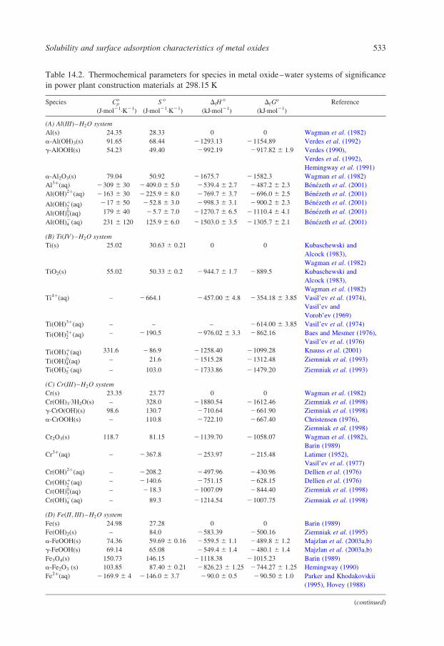
Table 14.2. Thermochemical parameters for species in metal oxide–water systems of significance

in power plant construction materials at 298.15 K

Species Cpo

(J·mol21·K21)

S o

(J·mol21·K21)

DfHo

(kJ·mol21)

DfGo

(kJ·mol21)

Reference

(A) AlðIIIÞ–H2O system

Al(s) 24.35 28.33 0 0 Wagman et al. (1982)

a-Al(OH)3(s) 91.65 68.44 21293.13 21154.89 Verdes et al. (1992)

g-AlOOH(s) 54.23 49.40 2992.19 2917.82 ^ 1.9 Verdes (1990),

Verdes et al. (1992),

Hemingway et al. (1991)

a-Al2O3(s) 79.04 50.92 21675.7 21582.3 Wagman et al. (1982)

Al3þ(aq) 2309 ^ 30 2409.0 ^ 5.0 2539.4 ^ 2.7 2487.2 ^ 2.3 Benezeth et al. (2001)

Al(OH)2þ(aq) 2163 ^ 30 2225.9 ^ 8.0 2769.7 ^ 3.7 2696.0 ^ 2.5 Benezeth et al. (2001)

AlðOHÞþ2 (aq) 217 ^ 50 252.8 ^ 3.0 2998.3 ^ 3.1 2900.2 ^ 2.3 Benezeth et al. (2001)

AlðOHÞ03(aq) 179 ^ 40 25.7 ^ 7.0 21270.7 ^ 6.5 21110.4 ^ 4.1 Benezeth et al. (2001)

AlðOHÞ24 (aq) 231 ^ 120 125.9 ^ 6.0 21503.0 ^ 3.5 21305.7 ^ 2.1 Benezeth et al. (2001)

(B) TiðIVÞ–H2O system

Ti(s) 25.02 30.63 ^ 0.21 0 0 Kubaschewski and

Alcock (1983),

Wagman et al. (1982)

TiO2(s) 55.02 50.33 ^ 0.2 2944.7 ^ 1.7 2889.5 Kubaschewski and

Alcock (1983),

Wagman et al. (1982)

Ti4þ(aq) – 2664.1 2457.00 ^ 4.8 2354.18 ^ 3.85 Vasil’ev et al. (1974),

Vasil’ev and

Vorob’ev (1969)

Ti(OH)3þ(aq) – – – 2614.00 ^ 3.85 Vasil’ev et al. (1974)

TiðOHÞ2þ2 (aq) – 2190.5 2976.02 ^ 3.3 2862.16 Baes and Mesmer (1976),

Vasil’ev et al. (1976)

TiðOHÞþ3 (aq) 331.6 286.9 21258.40 21099.28 Knauss et al. (2001)

TiðOHÞ04(aq) – 21.6 21515.28 21312.48 Ziemniak et al. (1993)

TiðOHÞ25 (aq) – 103.0 21733.86 21479.20 Ziemniak et al. (1993)

(C) CrðIIIÞ–H2O system

Cr(s) 23.35 23.77 0 0 Wagman et al. (1982)

Cr(OH)3·3H2O(s) – 328.0 21880.54 21612.46 Ziemniak et al. (1998)

g-CrO(OH)(s) 98.6 130.7 2710.64 2661.90 Ziemniak et al. (1998)

a-CrOOH(s) – 110.8 2722.10 2667.40 Christensen (1976),

Ziemniak et al. (1998)

Cr2O3(s) 118.7 81.15 21139.70 21058.07 Wagman et al. (1982),

Barin (1989)

Cr3þ(aq) – 2367.8 2253.97 2215.48 Latimer (1952),

Vasil’ev et al. (1977)

Cr(OH)2þ(aq) – 2208.2 2497.96 2430.96 Dellien et al. (1976)

CrðOHÞþ2 (aq) – 2140.6 2751.15 2628.15 Dellien et al. (1976)

CrðOHÞ03(aq) – 218.3 21007.09 2844.40 Ziemniak et al. (1998)

CrðOHÞ24 (aq) – 89.3 21214.54 21007.75 Ziemniak et al. (1998)

(D) FeðII; IIIÞ–H2O system

Fe(s) 24.98 27.28 0 0 Barin (1989)

Fe(OH)2(s) – 84.0 2583.39 2500.16 Ziemniak et al. (1995)

a-FeOOH(s) 74.36 59.69 ^ 0.16 2559.5 ^ 1.1 2489.8 ^ 1.2 Majzlan et al. (2003a,b)

g-FeOOH(s) 69.14 65.08 2549.4 ^ 1.4 2480.1 ^ 1.4 Majzlan et al. (2003a,b)

Fe3O4(s) 150.73 146.15 21118.38 21015.23 Barin (1989)

a-Fe2O3 (s) 103.85 87.40 ^ 0.21 2826.23 ^ 1.25 2744.27 ^ 1.25 Hemingway (1990)

Fe2þ(aq) 2169.9 ^ 4 2146.0 ^ 3.7 290.0 ^ 0.5 290.50 ^ 1.0 Parker and Khodakovskii

(1995), Hovey (1988)

(continued)


Table 14.2. continued

Species Cpo

(J·mol21·K21)

S o

(J·mol21·K21)

DfHo

(kJ·mol21)

DfGo

(kJ·mol21)

Reference

Fe(OH)þ(aq) – 2162.9 2354.83 2274.18 Ziemniak et al. (1995)

FeðOHÞ02(aq) – 229.2 2563.08 2446.13 Ziemniak et al. (1995)

FeðOHÞ23 (aq) – 228.7 2806.40 2613.42 Ziemniak et al. (1995)

Fe3þ(aq) 2317.4 ^ 15 2345.0 ^ 7.7 249.0 ^ 1.5 216.23 ^ 1.1 Parker and Khodakovskii

(1995), Hovey (1988)

Fe(OH)2þ(aq) – 2147.42 2290.69 2240.74 Zotov and Kotova (1980)

FeðOHÞþ2 (aq) – – – 2458.82 Baes and Mesmer (1976)

FeðOHÞ03(aq) – 38.1 2804.81 2657.86 Ziemniak et al. (1995)

FeðOHÞ24 (aq) – 10.9 21071.46 2840.22 Ziemniak et al. (1995)

FeðOHÞ24 (aq) 87.4 163.8 21028.32 2842.67 Ziemniak (2001)

(E) CoðIIÞ–H2O system

Co(s) 24.81 30.04 0 0 Barin (1989)

b-Co(OH)2(s) 97.1 97.2 2534.17 2454.07 Ziemniak et al. (1999),

Barin (1989)

CoO(s) 55.06 52.97 2237.94 2214.20 Barin (1989)

Co2þ(aq) 2169 2149.9 256.67 255.23 Ziemniak et al. (1999),

Abraham and Marcus (1986)

Co(OH)þ(aq) 223 278.4 2291.77 2235.49 Ziemniak et al. (1999)

CoðOHÞ02(aq) 124 23.6 2520.91 2410.76 Ziemniak et al. (1999)

CoðOHÞ23 (aq) – – – 2581.21 Ziemniak et al. (1999),

Gayer and Garrett (1950)

CoðOHÞ224 (aq) – – – 2739.49 Gordon and Schreyer (1955),

Ezhov and Kamnev (1983)

(F) NiðIIÞ–H2O system

Ni(s) 26.07 29.87 0 0 Wagman et al. (1982)

b-Ni(OH)2(s) – 79.3 2536.16 2450.77 Ziemniak and Goyette (2003)

NiO(s) 44.49 37.99 2239.3 2211.1 Hemingway (1990)

Ni2þ(aq) 2191.6 2176.6 253.6 243.9 Larson et al. (1968), Pan

and Campbell (1997)

Ni(OH)þ(aq) – 2140.8 2302.00 2227.15 Ziemniak and Goyette (2003)

NiðOHÞ02(aq) – 250.3 2512.80 2388.77 Ziemniak and Goyette (2003)

NiðOHÞ23 (aq) – 2100.6 2793.47 2578.28 Ziemniak et al. (1989)

(G) CuðIIÞ–H2O system

Cu(s) 24.43 33.14 ^ 0.21 0 0 Kubaschewski and

Alcock (1983)

Cu(OH)2(s) 87.85 87.03 2444.09 2359.02 Barin (1989)

CuO(s) 42.25 42.59 ^ 0.4 2156.06 ^ 2.1 2128.29 Chase et al. (1985)

Cu2þ(aq) 2162 2142.4 ^ 4.0 64.9 ^ 1.0 65.04 Larson et al. (1968),

Abraham and Marcus (1986)

Cu(OH)þ(aq) 282.1 113.9 2115.87 2116.00 Ziemniak et al. (1992a,b),

Hearn et al. (1969)

CuðOHÞ02(aq) – 59.3 2408.32 2315.98 Ziemniak (2001)

CuðOHÞ23 (aq) 213 86.1 2659.28 2498.98 Ziemniak et al. (1992a,b)

CuðOHÞ224 (aq) – 8.5 2917.96 2658.35 Ziemniak et al. (1992a,b)

(H) ZnðIIÞ–H2O system

Zn(s) 25.40 41.63 ^ 0.21 0 0 Kubaschewski and

Alcock (1983)

1-Zn(OH)2(s) 72.4 76.99 ^ 0.21 2645.47 2555.93 ^ 0.21 Khodakovskii and

Yelkin (1975)

(continued)


to the unhydrolyzed metal cation, Dz2 for this reaction is always non-zero for

multivalent metal ions, ranging from þ 2 for divalent to þ12 for quadrivalent

cations. In fact, these are typically the most ‘non-isocoulombic’ solubility

reactions exhibited by each metal oxide system. However, Fig. 14.11 clearly

demonstrates that many of these reactions are also closely approximated by Eq.

14.64, indicating a near-zero heat capacity of reaction, although the scale, which

spans 36 orders of magnitude, somewhat obscures significant deviations from

linearity. This observation suggests that perhaps too much emphasis is being

placed in the literature on the merits of isocoulombic extrapolation of hetero-

geneous equilibrium constants to higher temperatures. Limited experimental data

indicates that these reactions are also fairly insensitive to pressure changes at

temperatures ,250 8C, but certainly log10 Qs0 is not a simple or minor function

of ionic strength, as shown in Fig. 14.8. Another clear trend in Fig. 14.11 is that

log10 Ks0 uniformly decreases with increasing temperature, which as suggested

above, is related to the destabilization of highly charged solution species as the

dielectric constant of the solvent decreases.

To handle pressure effects, especially for temperatures in excess of 250 8C and

at pressures far above psat, Marshall and Franck (1981) originally proposed the

following function for homogeneous reactions (to describe the dissociation

constant of water):

log10 Kw ¼ a þ b=T þ c=T2 þ d=T3 þ ðe þ f=T þ g=T2Þln rw ð14:65Þ

where rw is the density of pure water (g·cm23) at the temperature and pressure of

interest. Subsequently, this relationship was thought to be valid at least for


Species Cpo

(J·mol21·K21)

S o

(J·mol21·K21)

DfHo

(kJ·mol21)

DfGo

(kJ·mol21)

Reference

ZnO(s) 40.25 43.64 ^ 0.42 2350.83 ^ 0.21 2320.91 ^ 0.25 Kubaschewski and

Alcock (1983)

Zn2þ(aq) 2167.8 ^ 0.6 2154.8 ^ 1.3 2153.64 ^ 0.42 2147.23 Pan and Tremaine (1994),

Khodakovskii and

Yelkin (1975)

Zn(OH)þ(aq) 10.25 258.06 2388.35 2334.65 Benezeth et al. (2002)

ZnðOHÞ02(aq) 23.8 67.7 2611.95 2519.67 Ziemniak et al. (1992a,b)

ZnðOHÞ23 (aq) – 52.4 2871.97 2699.02 Ziemniak et al. (1992a,b)

ZnðOHÞ224 (aq) – 7.9 21125.64 2863.30 Ziemniak et al. (1992a,b)

(I) Key parameters

H2(g) 28.84 130.68 0 0 Barin (1989)

O2(g) 29.38 205.15 0 0 Barin (1989)

H2O(aq) 75.29 69.95 2285.83 2237.14 Barin (1989)

Hþ(aq) 271 222.2 0 0 Abraham and Marcus (1986),

Criss and Cobble (1964a,b)


rw $ 0:4 g·cm23. Anderson et al. (1991) have shown that functions of this general

form (the ‘Density Model’) can be applied to a wide range of homogeneous

aqueous reactions, with the density terms related to the molar volume change of

the reaction. The revised-HKF approach also provides a reliable pressure

extrapolation, since the Born solvation model for individual aqueous species

used in this treatment depends heavily on the solvent dielectric constant, which is a

function of density. Whenever solubility data are available over a significant range

Fig. 14.11. Dependence of log10 Ks0 for the reactions listed in Table 14.3 on inverse

temperature (K).


of solvent densities, it is advantageous to introduce ln rw as a fitting parameter

and this generally decreases the temperature functionality needed to fit the data

precisely.

In Table 14.3, equations are presented for the temperature dependence of the

equilibrium constants ðKsyÞ of a large number of metal oxides that are derived from

published experimental data or estimates discussed below. In many cases, the

functions will be seen to resemble Eqs. 14.62, 14.64 and 14.65, but it must be

stressed that they are often purely empirical functions optimized to fit the available

data as simply as possible. Equations requiring greater temperature functionality

than are allowed by Eqs. 14.62 and 14.64 imply a temperature-dependent DrCop

and will thus not be entirely consistent with the standard-state thermodynamic

properties presented in Table 14.2. Within the specified temperature ranges, the

equations in Table 14.3 can be used to calculate the aqueous hydrolysis constants,

according to the discussion associated with Eq. 14.39, and in fact many of the

tabulated Ksy values were derived by coupling solubility and hydrolysis data. As

elsewhere in this chapter, the following summary is not exhaustive, but rather

representative of the best data currently thought to be available on hydrothermal

oxide solubilities.

14.5.1. Single Metal Oxides

Al(III): In addition to its importance in construction and packaging, aluminum is

the second most abundant metal in the Earth’s crust, and the solubility of its oxides

and hydroxides have received a great deal of attention by experimentalists (an

exhaustive list of the historic literature is presented by Pokrovskii and Helgeson,

1995). Aqueous aluminum is found only as Al3þ(aq) and its hydrolysis and

complexed species. The metal is not stable in the presence of water. The

Al(OH)3(s) polymorphs are neither stable above about 80 8C, nor are the Al2O3

polymorphs stable below about 380 8C in water at pressures at or above psat. While

diaspore (a-AlOOH) is predicted to be the stable aluminum phase under the

conditions of interest here, Gout and Verdes (1993) have demonstrated that it is

very difficult to synthesize in pure crystalline form under laboratory conditions

and is generally not observed in industrial environments. The formation of

boehmite (g-AlOOH), or pseudoboehmite, is kinetically favored, both on oxidized

metal surfaces and as a hydrated surface layer on Al2O3 exposed to sub-critical

hydrothermal solutions and boehmite persists metastably for long periods of time

in hydrothermal systems.

The most extensive investigations of boehmite solubility, covering wide ranges

of pH and temperature, have been conducted by Kuyunko et al. (1983), Bourcier

et al. (1993), Castet et al. (1993), Benezeth et al. (2001) and Palmer et al. (2001),

with the latter study extending to concentrated NaCl solutions (Fig. 14.5).

Boehmite, diaspore and corundum solubility studies at sub- and super-critical


Table 14.3. Coefficients for the equation log10 Ksy ¼ n1 þ n2ðTÞ21 þ n3 ln T þ n4T þ n5 ln rw þ n6ðTÞ

2 þ n7ðTÞ22

Oxide Reactiona y n1 n2 n3 n4 £ 103 n5 n6 £ 106 n7 £ 1026 Range (8C)

g-AlOOH 14.66 0 213.177 6207.36 25–300

14.66 1 28.417 3311.44 25–300

14.66 2 24.159 319.230 25–300

14.66 3 29.105 4.332 25–300

14.66 4 662.731 217457.2 2125.010 364.788 2177.964 25–300

As2O3 14.67 3 210.307 2263.43 1.8386 25–250

Ca(OH)2 14.68 0 0.070 6756.71 100–350

14.68 1 20.829 3333.7 100–350

CoO 14.69 0 22.255 5355.95 20.3536 79–300

14.69 1 23.232 2701.7 20.3688 79–300

14.69 2 24.387 2248.27 20.3317 79–300

g-CrOOH 14.70 3 222.645 1054.1 1.6730 55–300

14.70 4 56.452 26524.8 210.0171 55–300

CuO 14.71 0 28.251 3591.3 0.6811 25–300

14.71 1 23.546 22929.6 22.7866 25–300

14.71 2 22.781 21753.42 25–300

14.71 3 11.501 24320.64 22.6419 25–300

14.71 4 2.469 25690.69 22.6419 25–300

Fe(OH)2 14.72 0 22.575 4021.9 0–150

Fe3O4·Fe(II) 14.73 0 251.381 7114.02 6.8581 25–300

14.73 1 256.881 6085.05 6.8581 25–300

14.73 2 254.713 2031.8 6.8581 25–300

14.73 3 259.498 2188.03 6.8581 25–300

Fe3O4·Fe(III) 14.74 3 251.438 2271.6 6.8581 25–300

14.74 4 257.675 21274.5 6.8581 25–300

a-Fe2O3 14.75 0 3.302 2905.3 22.264 0–250

14.75 1 8.822 599.7 22.264 0–250

14.75 3 21.817 22847.0 100–300

14.75 4 28.054 23849.94 100–300

D.J.

Weso

low

skiet

al.

53

8

a-GaOOH 14.76 0 25.780 573.22 24.6035 0–350

14.76 1 6.926 551.91 21.7815 0–350

14.76 2 0.074 21749.15 0–350

14.76 3 21.448 24274.15 23.0820 0–350

14.76 4 44.382 25516.78 27.0332 0–250

GeO2 14.77 4 255.619 1014.1 8.2910 1.848 25–350

14.77 5 54.380 25819.2 28.637 25–300

Nd(OH)3 14.78 0 26.662 7330.0 25–300

La(OH)3 14.78 0 23.937 7029.81 25–150

Gd(OH)3 14.78 0 26.477 7127.61 25–150

Mg(OH)2 14.79 0 22.49 5847.0 0–350

14.79 1 21.892 2186.2 25–350

MnO 14.80 0 8.729 5735.1 21.6843 25–350

14.80 1 7.848 2681.5 21.5964 25–350

14.80 2 15.486 2864.40 22.8839 25–350

14.80 3 81.241 26602.3 213.2560 25–350

b-Ni(OH)2b 14.81b 0 23.800 4654.12 21–149

(22.829) (4320.17) (0–200)

14.81b 1 26.684 2699.14 21–149

14.81b 2 26.774 21220.11 (24.24534) 21–149

(20.881) (22128.33) (0–200)

NiOb 14.82b 0 25.016 5168.41 149–247

218.591 5432.60 2.0893 (4.24534) (247–315)

(29.833) (6255.01) (0–350)

14.82b 1 27.900 3213.43 149–247

221.475 3477.62 2.0893 247–315

14.82b 2 27.985 2705.83 149–247

221.559 2441.63 2.0893 247–315

(27.885) (2193.49) (0–350)

a-PbO 14.83 1 2.005 1242.9 100–300

(continued)

So

lub

ilitya

nd

surfa

cea

dso

rptio

nch

ara

cteristicso

fm

etal

oxid

es5

39


Oxide Reactiona y n1 n2 n3 n4 £ 103 n5 n6 £ 106 n7 £ 1026 Range (8C)

14.83 2 5.345 22164.7 28.066 100–300

14.83 3 18.129 27037.9 233.102 100–300

SiO2, amorphous 14.84 4 28.476 2485.24 1.3324 22.268 0–350

14.84 5 2633.399 33147.5 98.8856 297.611 22.268 22.17087 50–300

SiO2,quartz 14.84 4 234.188 197.47 5.31794 25.851 0–350

14.84 5 2659.111 33830.2 102.8711 297.611 25.851 22.17087 50–300

a-TiO2 14.88 3 2104.89 5694.2 14.2162 100–300

14.88 4 28.809 258.50 25–300

14.88 5 29.368 23572.16 25–300

UO2 14.89 2 34.798 21805.3 26.2501 25–325

14.89 3 23.440 22418.8 24.4188 25–325

14.89 4 29.536 39.0 25–325

14.89 5 2293.591 7326.27 46.5664 259.330 25–325

WO3c 14.90c 0 21673.99 72515.2 263.748 2245.44 300–600

14.90c 1 21232.91 53160.29 193.759 2169.66 300–600

14.90c 2 20.313 22107.3 300–600

ZnOd 14.91d 0 24.0168 4527.66 25–350

14.91d 1 26.3065 2278.86 3.5909 25–350

14.91d 2 5.6431 23139.58 29.9397 25–350

14.91d 3 22.5192 23640.69 27.4119 2.8327 25–350

ZrO2 14.92 0 2227.854 11648.23 35.2298 246.409 25–350

14.92 1 218.996 3688.95 0.87431 25–350

14.92 2 27.669 1534.62 23.8240 25–350

D.J.

Weso

low

skiet

al.

54

0

14.92 3 2144.062 6710.25 20.9074 215.30 25–350

14.92 4 252.236 1895.80 6.01403 25–350

14.92 5 2271.338 6614.92 43.6606 258.685 25–350

b-PbTiO3 14.94 1 2.0 ^ 0.5 150–300

14.94 2 220.68 2.4410 150–300

14.94 3 215.1 ^ 0.2 150–300

FeCr2O4 14.95 0 23.144 1726.79 23.3460 25–300

ZnCr2O4 14.95 0 64.168 21767.95 29.3417 150–300

CoCr2O4 14.95 0 64.539 2820.36 29.4681 150–300

KAlSi3O8,micr 14.96 – 278.594 26068.38 13.1626 227.776 0.31197 0–350

NaAlSi3O8,low 14.96 – 296.267 23985.50 15.5434 228.588 0.305542 0–350

CaAl2Si2O8 14.97 – 288.591 22720.61 13.5361 240.100 0.326546 0–350

(Fe,Mg)2SiO4 14.98 – 215.228 10502.86 16.3905 216.787 0–350

FeSiO3 14.99 – 228.641 10101.60 41.6322 228.281 20.636803 0–350

Fe2TiO4 14.100 – 212.763 7765.42 28.8254 0.376298 0–350

FeTiO3 14.101 – 244.807 5768.04 4.92488 27.0298 0–350

T is the absolute temperature (K) and rw is the density of pure water (g·cm23). The equations are valid over the temperature range specified and at pressures

near psat unless otherwise stated in the text.a Reaction number corresponds to equilibrium reaction discussed in the text for log10 Ksy, with y listed in the next column.b Coefficients are taken from both Ziemniak and Goyette (2003) and Palmer et al. (2002), with the latter set shown in parentheses.c The solubility of WO3 was measured at 1 kilobar and 300–600 8C, but extrapolated to 200 8C and assumed constant with temperature for plotting in

Fig. (14.11).d Benezeth et al. (2002) extracted the value log10 Ks0 ¼ 2:358 at 350 8C, rather than the value predicted by the tabulated equation from Wesolowski et al.

(1998).

So

lub

ilitya

nd

surfa

cea

dso

rptio

nch

ara

cteristicso

fm

etal

oxid

es5

41

conditions in fairly concentrated alkali-hydroxide-chloride solutions (references

in Pokrovskii and Helgeson, 1995; Palmer et al., 2001; Walther, 2001), as well as

recent potentiometric titrations with a high temperature, sodium-sensitive

electrode (Diakonov et al., 1996) have sparked a debate in the current literature

as to the stability of ion pairs between alkali metal cations (Naþ, Kþ) and

AlðOHÞ24 (aq) (Wesolowski and Palmer, 1994; Anderson, 1995a,b; Pokrovskii and

Helgeson, 1995, 1997; Walther, 1997; Palmer et al., 2001). Interestingly, although

there have been a large number of studies of the complexation of aluminum with

organic ligands, sulfate, etc. there is general consensus that inorganic, monovalent

anions do not significantly interact with Al3þ(aq) or its hydrolytic cations (Palmer

and Wesolowski, 1993; Wesolowski and Palmer, 1994; Palmer et al., 2001),

presumably due to the strong affinity of the small, highly charged cation for water

and hydroxyl oxygens.

Whether the effect of ionic strength is expressed by stoichiometric molal

activity coefficients or ion pair formation constants, there is general agreement that

the solubility of boehmite is well established at the conditions of interest here and

agreement is good among several independent research groups (Benezeth et al.,

2001; Tagirov and Schott, 2001). The principal remaining discrepancies are

confined essentially to the solubility minimum and are exacerbated by the facts

that (a) each of the intermediate hydrolysis species has significant fields of

stability, but only over narrow pH ranges (Fig. 14.6); and (b) the solubility

minimum is low and difficult to reverse. These problems are endemic to metal

oxide solubility studies, but no other sparingly soluble oxides have been studied as

intensively by as many different research groups. The equations for log10 Ksy

presented in Table 14.3 for the reaction ðy ¼ 0–4Þ

g-AlOOHðcrÞ þ ð3 2 yÞHþðaqÞO AlðOHÞ32yy ðaqÞ þ ð2 2 yÞH2OðlÞ ð14:66Þ

were taken from Palmer et al. (2001) and Benezeth et al. (2001), because these

were obtained using the HECC, in which reversal was repeatedly demonstrated on

both sides of the solubility minimum. In most cases no buffers were needed to

poise the solution pH, and pHm was measured precisely in situ. Furthermore, these

studies were augmented by independent measurement of the first hydrolysis

constant of Al3þ in NaCl brines to 125 8C using the same type of apparatus

(Palmer and Wesolowski, 1993).

Because data on the solubility of gibbsite at lower temperatures were

incorporated in these fitting equations, their range of validity is 25–300 8C at

psat. For extrapolation to higher pressures, and particularly higher temperatures,

the revised-HKF equation of state parameters given by Tagirov and Schott (2001)

are recommended. As stated previously, values of Qs0, Qs1 and Qs4 are also

known in 0–5 mol·kg21 NaCl solutions and the equilibrium constants for the

isocoulombic reactions ðy ¼ 2; 3Þ can be assumed to be independent of ionic

strength in dilute solutions.


As(III): Arsenic may occur in the þIII, þIV and þV valence states in aqueous

solutions, but few experimental studies have been conducted on the oxides of this

element. Pokrovski et al. (1996) reported experimental studies on As2O3(cr) at

temperatures to 250 8C and psat, in fixed-volume titanium reactors and

demonstrated that As(III) is likely to be the dominant form of this element in

moderately to strongly reducing hydrothermal solutions, with the predominant

hydrolysis species being AsðOHÞ03(aq) over wide ranges of pH and temperature,

even in the presence of reduced sulfur. They give revised-HKF equation of state

parameters for this species as well as the thermodynamic properties of monoclinic

As2O3 (claudetite). Using their tabulated 25 8C thermodynamic properties and Eq.

14.61, an equation was re-derived here describing log10 Ks3 (Table 14.3) for the

reaction

ð1=2ÞAs2O3ðclaudetiteÞ þ ð3=2ÞH2OðlÞO AsðOHÞ03ðaqÞ ð14:67Þ

in good agreement with their predicted values and giving solubilities in the molal

range, off the scale of Fig. 14.10, but with a temperature trend similar to that of

WO3(cr).

Ca(II): Calcium is stable only in the þII valence state under hydrothermal

conditions and the only stable oxide is portlandite, Ca(OH)2. The solubility of

portlandite has been studied by Seewald and Seyfried (1991) in water and dilute

acetate buffer solutions from 100–350 8C at 50 MPa using a flexible gold-bladder

rocking autoclave system. For the reaction

CaðOHÞ2ðportlanditeÞ þ ð2 2 yÞHþðaqÞO CaðOHÞ22yy ðaqÞ þ ð2 2 yÞH2OðlÞ

ð14:68Þ

their results for log10 Ks0 and log10 Ks1 were fitted within experimental error to the

equations given in Table 14.3, the latter being derived from a fit to their results for

the first hydrolysis constant of Ca2þ(aq), log10 Kh1 ¼ 20:899 2 3423:0=T: This

indicates that Ca(OH)þ(aq) is the dominant species in solution at pH above 10.07,

8.13, 6.87 and 6.39 at 100, 200, 300 and 350 8C, respectively (and 50 MPa).

A neutral CaðOHÞ02(aq) species was not identified in this study, but the authors

report an equilibrium constant for the formation of a Ca2þ–acetate complex.

Solubility data for the rarely observed alkaline earth hydroxides (i.e., Sr, Ba, etc.)

are summarized by Lambert and Clever (1992).

Co(II): Co(III) aqueous species may be stable under extremely oxidizing

conditions, but most crustal fluids and power-plant waters will contain only Co(II)

aqueous species. Dinov et al. (1993) report batch solubility measurements of CoO

in ‘pure’ water and dilute HCl solutions, but their results are difficult to interpret,

since pH was not controlled. Ziemniak et al. (1999) conducted a detailed study of

the solubility of cubic CoO in dilute ammonia and NaOH solutions from 22–

288 8C at pressures near psat using a packed-column, platinum-lined, flow-through

reactor system. However, in experiments involving solutions pre-saturated with


pure nitrogen gas at 25 8C, 0.1 MPa, b-Co(OH)2 formed on the surface of the

experimental charge at low temperature and persisted beyond the thermodyna-

mically predicted dehydration temperature (approximately 80 8C at psat). This

phase apparently gave reversible and reproducible solubilities up to 260 8C,

beyond which irreproducible results indicated incomplete dehydration. In a

separate sequence of experiments using solutions pre-saturated with 0.1 MPa of

hydrogen gas at 25 8C, they observed the formation of metallic Co on the oxide

surfaces, which controlled the solubility behavior. However, again due to sluggish

redox kinetics, these experiments gave irreproducible results at all temperatures

below 218 8C. Regression analysis of the b-Co(OH)2 and metallic Co solubility

data from these experiments permitted Ziemniak et al. (1999) to extract the

solubility products for these phases, as well as the formation constants of the

hydrolytic aqueous species Co(OH)þ(aq) and CoðOHÞ02(aq). Combining these

results with the thermodynamic properties of cubic CoO and b-Co(OH)2 given in

Table 14.2, equations are derived here describing log10 Ksy (Table 14.3) for the

reaction ðy ¼ 0–2Þ

CoOðcrÞ þ ð2 2 yÞHþðaqÞO CoðOHÞ22yy ðaqÞ þ ð1 2 yÞH2OðlÞ ð14:69Þ

The first hydrolysis constant derived from this study agrees well with the

homogeneous potentiometric titration results at room temperature reported by

Giasson and Tewari (1978), but their values are progressively higher with

increasing temperature, differing by 0.57 log10 units at 200 8C from the values

calculated from the hydrolysis equation given by Ziemniak et al. (1999). The

source of this discrepancy is not clear at this time.

Cr(III): Chromium (VI) occurs under oxidizing conditions as the CrO224 (aq)

anion and its hydrolysis products (Hoffmann et al., 2001; Palmer et al., 1987), but

it is highly soluble and of little interest here, other than the fact that it is highly

toxic and is a known carcinogen. Under moderately to strongly reducing

conditions, Cr(III) solids and solution species dominate. Ziemniak et al. (1998)

used a platinum-lined, flow-through cell to investigate the solubility of Cr2O3(cr)

from 21 to 288 8C at pressures near psat in dilute ammonia–NaOH–phosphate

buffer solutions pre-saturated at 25 8C with 0.1 MPa of either N2(g) or H2(g). XPS

analysis of the run products indicated that g-CrOOH was the solubility-controlling

phase at temperatures above 51 8C, and that CrðOHÞ03(aq) and CrðOHÞ24 (aq) were

the dominant species in neutral to basic solutions, in the absence of phosphate. For

the reaction

g-CrOOHðsÞ þ ð3 2 yÞHþðaqÞO CrðOHÞ32yy ðaqÞ þ ð2 2 yÞH2OðlÞ ð14:70Þ

equilibrium constants ðlog10 KsyÞ were reported for ðy ¼ 3; 4Þ and are listed in

Table 14.3. Hiroishi et al. (1998) reported the solubility of Cr2O3(s) in ‘pure’

water at 200 8C (quench pH 4.29) as 2.24 £ 1028 mol·kg21. They also conducted

experiments at 25, 50, 75 and 200 8C in which acidic Cr3þ(aq) solutions were


titrated to higher pH, with accompanying precipitation of an amorphous phase.

The pH was monitored using a glass electrode at the lower temperatures and a

yttria-stablized zirconia pH sensor at 200 8C. From the measured total dissolved

Cr and measured pH, they extracted formation constants for CrðOHÞ32yy (aq)

( y ¼ 1–4). No experimental data are given in the paper and there is no

indication that the solid phase precipitated was in thermodynamic equilibrium

with the solution. The equilibrium constant for the stepwise formation of

CrðOHÞ24 (aq) reported in this study does not agree well with that reported by

Ziemniak et al. (1998).

Cu(I,II): Copper(I) and (II) solid phases and aqueous species are important in

hydrothermal solutions, and copper metal is stable under mildly to strongly

reducing conditions, but solubility and speciation data at elevated temperatures are

sparse and conflicting. The solubility of CuO (tenorite) has been studied in ‘pure’

water using flow-cell methods by Hearn et al. (1969) at 50–550 8C, 24–40 MPa,

and 250–500 8C and 26–34 MPa, and by Sue et al. (1999) at 300–450 8C and

28 MPa. These two studies are in good agreement, but neither group attempted to

estimate pH or aqueous copper solution speciation at their experimental

conditions. Ziemniak et al. (1992a) conducted a detailed study of the solubility

of CuO(cr) in dilute phosphate buffers from 19 to 262 8C at pressures near psat

using a platinum-lined, flow-through cell, with the solutions deoxygenated by

sparging with pure N2(g) at 25 8C, 0.1 MPa. For the reaction

CuOðcrÞ þ ð2 2 yÞHþðaqÞO CuðOHÞ22yy ðaqÞ þ ð1 2 yÞH2OðlÞ ð14:71Þ

Ziemniak et al. (1992a) reported solubility and hydrolysis equilibria, giving the

log10 Ksy equations ðy ¼ 3; 4Þ listed in Table 14.3. Calculation of the same

equilibrium constants using SUPCRT92 and the revised-HKF parameters of Shock

et al. (1997b) gave much lower values for these constants. The thermodynamic

properties of Cu2þ(aq) and Cu(OH)þ(aq) listed in Table 14.2 were constrained by

the data of Hearn et al. and used together with those of CuO(s) in Eq. 14.61 to give

the equations for log10 Ks0 and log10 Ks1 listed in Table 14.3. The equilibrium

constant for log10 Ks2 (Table 14.3) was estimated from the thermodynamic data

given in Table 14.2, assuming that the heat capacity change of the reaction is zero

at all temperatures.

Var’yash (1985) also investigated the solubility of tenorite, using a batch-

quench approach at temperatures of 200–450 8C, apparently at psat for

temperatures below the critical point, and reported values for log10 Ks2 within

0.3–0.4 log10 units of those predicted from the equation in Table 14.3 at 200–

350 8C. However, there is much poorer agreement between the values for log10 Ks1

and log10 Ks4 in Table 14.3 compared to those reported by Var’yash in this

temperature range. The equation given in Table 14.3 for log10 Ks2 also agrees with

the predictions of Shock et al. (1997b) at 150–250 8C, but the latter predict higher

values at lower temperatures, and lower values at higher temperature. The total


solubilities in ‘pure’ water reported by Hearn et al. (1969) and Sue et al. (1999) are

much higher than the log10 Ks2 values given in Table 14.3 at all temperatures. The

T –rw function given by Sue et al. (1999) for a reaction constant approximately

similar to Ks2 appears to be in error. Ziemniak et al. (1992a) also demonstrated that

the measurements of Hearn et al. (1969) were consistent with the dominance of

Cu(OH)þ(aq), rather than with the formation of CuðOHÞ02(aq) as the main

copper(II) species in solution. Unpublished results for the solubility of tenorite

measured at ORNL from 25 to 350 8C, support the premise of Ziemniak et al.

(1992a) that at pH conditions varing from mildly acidic to moderately basic,

Cu(OH)þ(aq) and CuðOHÞ23 (aq) dominate from 100 to 350 8C. Moreover, this new

study indictates that the phase studied by Hearn et al. (1969) was Cu2O and not

CuO, noting that these investigators did not characterize the oxides recovered

from their experiments. Therefore, all reported values of log10KS2 should be

viewed with suspicion.

Very little experimental information is available on Cu(I) oxide at elevated

temperatures (Dirkse, 1986) and Shock et al. (1997b) did not treat this system.

Var’yash and Rekharskiy (1981a,b) report values of 20.22 ^ 0.14, 25.57 ^ 0.14

and 213.99 ^ 0.16, for log10 Ksy; y ¼ 0; 1 and 2, respectively, for the reaction

0:5Cu2OðcrÞ þ ð1 2 yÞHþðaqÞO CuðOHÞ12yy ðaqÞ þ ð0:5 2 yÞH2OðlÞ at 250 8C,

but few details of the experiments are provided. A major effort was recently

completed at ORNL to investigate the speciation and solubility of solutions in

equilibrium with Cu2O(cr) from 25 to 350 8C and pressures near psat. These results

indicate the above-mentioned solubilities for Cu2O(cr) in particular are orders of

magnitude too high at high temperature and that only the species Cuþ(aq) and

Cu(OH)22(aq) are important above 100 8C over a wide pH range.

Fe(II,III): Iron is the third most abundant metal in the Earth’s crust and the

principal component of steel alloys, and therefore the Fe–O–H system has

received a great deal of attention by geochemists and industrial chemists. Metallic

iron as well as oxide phases and aqueous species of Fe(II) and Fe(III) are common

in hydrothermal systems. As discussed above, several polymorphs of FeOOH are

abundant in near-surface geological environments and as low-temperature

corrosion products of iron-based materials. However, only a-FeOOH (goethite)

and Fe(OH)2 persist into the hydrothermal regime (Fig. 14.3). The decomposition

reaction of goethite to hematite (a-Fe2O3) occurs in the 80–120 8C range at

pressures near psat, depending on the thermodynamic data used, and also on the

particle size, as discussed in the previous section, although the differential

solubility studies conducted by Berner (1969) appear to indicate that well-

crystallized goethite is definitely more soluble (less stable) than hematite at 85 8C,

and possibly at lower temperatures. Although the thermodynamic properties of

lepidocrocite (g-FeOOH) and maghemite (g-Fe2O3) have been determined (Table

14.2), they are considered to be metastable phases.

Under moderately to strongly reducing conditions, Fe2þ(aq) and its hydrolysis

and complexation products dominate the aqueous speciation of iron; Fe(OH)2 and


magnetite (Fe3O4) are the important oxide phases. Three major studies of

the solubilities of these phases over wide ranges of temperature and pH have been

conducted (Sweeton and Baes, 1970; Tremaine and LeBlanc, 1980b; Ziemniak

et al., 1995), all of which employed flow-through cells. Ziemniak et al. conducted

their studies in alkaline ammonium hydroxide and phosphate buffers, while

the earlier two studies were performed in solutions ranging from 0.001 mol·kg21

HCl to 0.04 mol·kg21 NaOH. All three studies are in good agreement regarding

magnetite solubility in acidic solutions, but the two more recent studies considered

Fe(III) species, namely FeðOHÞ03(aq) and FeðOHÞ24 (aq), as becoming important

solution components in equilibrium with magnetite at high pH and temperature,

even in solutions pre-saturated with hydrogen gas at room temperature. Sweeton

and Baes interpreted their solubilities in terms of only Fe(II) hydrolysis species.

Shock et al. (1997b) extracted revised-HKF equation of state parameters for

the iron system using both the Sweeton and Baes (1970) speciation and the

Ziemniak–Tremaine model, but they favored the Sweeton and Baes scheme

because the stepwise FeðOHÞ22yy (aq) formation constants reported by these authors

conformed better to their correlation algorithms for such species. This is further

illustrated by Palmer and Hyde (1993) who show that the Tremaine and LeBlanc

(1980b) model predicts that Fe(OH)þ(aq) is always a subordinate species relative

to Fe2þ(aq) and FeðOHÞ02(aq), at 100–300 8C. However, Wesolowski et al.

(2000a) used a HECC to study the solubility of magnetite under strongly reducing

conditions ( fH2ðgÞ ¼ 1–3 MPa at temperature) in the 150–250 8C range and

reported quantitative agreement with the magnetite solubilities predicted by

the Ziemniak–Tremaine model in mildly basic solutions, whereas the Shock

speciation scheme predicted solubilities as much as three orders of magnitude

higher. Therefore, the preponderance of experimental evidence at this time favors

the Ziemniak–Tremaine model for magnetite solubility and Fe(II) aqueous

speciation.

Ziemniak et al. (1995) conducted their studies using a column initially packed

with magnetite, at pressures near psat from 21 to 288 8C in solutions pre-saturated

with a 30.5 vol% H2(g) (the balance was N2(g)) mixture at 25 8C and atmospheric

pressure. They observed a small degree of hysteresis and a distinct change in the

shape of the solubility profile around 121 8C, indicating the relatively rapid and

reversible formation of a surface coating of Fe(OH)2(s) at lower temperatures. In

addition to temperature, the stability of Fe(OH)2(s) relative to magnetite depends

on both the water vapor pressure and hydrogen fugacity, as shown in Fig. 14.3,

because magnetite is a mixed Fe(II,III) phase. Fe(OH)2(s) was neither reported

in the earlier studies of Sweeton and Baes (1970) (50–300 8C) nor by Tremaine

and LeBlanc (100–300 8C). Ziemniak et al. (1995) constrained the fit to their

solubility data by incorporating magnetite solubility results at lower pH from

Tremaine and LeBlanc (1980b), reporting for the reactions,

FeðOHÞ2ðcrÞ þ ð2 2 yÞHþðaqÞO FeðOHÞ22yy ðaqÞ þ ð2 2 yÞH2OðlÞ ð14:72Þ


ð1=3ÞFe3O4ðcrÞ þ ð2 2 yÞHþðaqÞ þ ð1=3ÞH2ðgÞ

O FeðOHÞ22yy ðaqÞ þ ð4=3 2 yÞH2OðlÞ ð14:73Þ

the values of log10 Ks0 listed in Table 14.3. They also reported temperature

functions describing the log10 Khy for the formation of FeðOHÞ22yy (aq), y ¼ 1–3;

from which log10 Ksy; y ¼ 1–3; were derived for both reactions (Table 14.3).

The effect of varying the hydrogen concentration of the saturating gas at

room temperature on the solubility of magnetite (including the results of Tremaine

and LeBlanc (1980b)) and Fe(OH)2 allowed Ziemniak et al. (1995) to extract

equilibrium constants for the aqueous redox reaction, FeðOHÞ03ðaqÞ þ 0:5H2ðgÞO

FeðOHÞ02ðaqÞ þ H2OðlÞ; reporting log10 KFeðOHÞ3=FeðOHÞ2¼ 23:275 þ 2303:4=T ; as

well as the equilibrium constant relating FeðOHÞ03(aq) and FeðOHÞ24 (aq), which

enable evaluation (Table 14.3) of log10 Ksy; y ¼ 3; 4; for the oxidative dissolution

of magnetite according to the reaction:

1=3Fe3O4ðcrÞ þ ð3 2 yÞHþðaqÞO FeðOHÞ32yy ðaqÞ þ ð1=6ÞH2ðgÞ

þ ð4=3 2 yÞH2OðlÞ ð14:74Þ

Under more oxidizing conditions, Tagirov et al. (2000) used an electrochemical

method from 5–90 8C at 0.1 MPa to study the aqueous reaction, Fe3þðaqÞ þ

0:5H2ðgÞO Fe2þðaqÞ þ HþðaqÞ; giving the expression, log10 KFe3þ=Fe2þ ¼

215:599 þ 3021:2=T þ 3:2431 ln T; from which they derived new standard-

state thermodynamic properties for Fe3þ(aq). Combining these values with the

equivalent properties for hematite (Hemingway, 1990) and water (SUPCRT92,

Johnson et al., 1992) in Eq. 14.61, the equation for log10 Ks0 listed in Table 14.3 is

derived here for the reaction,

0:5Fe2O3ðcrÞ þ ð3 2 yÞHþðaqÞO FeðOHÞ32yy ðaqÞ þ ð1:5 2 yÞH2OðlÞ ð14:75Þ

which is in quantitative agreement with the solubility of hematite in acidic

solutions determined at 25–200 8C and psat by Sergeeva et al. (1999) from their

own measurements at 200 8C ðlog10 Ks0 ¼ 24:54 ^ 0:36Þ and literature data at

other temperatures. Zotov and Kotova (1979, 1980) measured the first hydrolysis

constant of Fe(III), Fe3þðaqÞ þ H2OðlÞO FeðOHÞ2þðaqÞ þ HþðaqÞ; using a

spectrophotometric method and their data are represented exactly by the

function, log10 Kh1;FeðIIIÞ ¼ 5:520 2 2305:6=T; which gives a value of 22.21 at

25 8C, as compared with the value 22.18 ^ 0.04 determined by Byrne et al.

(2000) from potentiometric titrations in 0.01–6.0 mol·kg21 NaClO4 solutions.

This relationship was used here to derive a function describing log10 Ks1 for

hematite (Table 14.3) which gives 23.86 at 200 8C, in excellent agreement with

the value 23.88 ^ 0.36 at 200 8C reported by Sergeeva et al. (1999).

In basic solutions, Sergeeva et al. determined the value of log10 Ks4 for hematite

at 200 8C (215.86 ^ 0.36), which is in reasonable agreement with the value of

216.26 ^ 0.04 at 200 8C and psat obtained by Diakonov et al. (1999) from


an extensive solubility study in NaOH–NaCl solutions from 60 to 300 8C.

Diakonov et al. provide revised-HKF equation of state parameters for

FeðOHÞ24 (aq) consistent with their results. Their tabulated equilibrium constants

are described within experimental uncertainty by the expression for log10 Ks4

given in Table 14.3, as well as values of log10 Ks4 at 20, 25 and 300 8C derived by

them from previously published studies for hematite and goethite solubility in

strongly basic solutions, including the result obtained by Yishan et al. (1986) at

300 8C, 10 MPa. Thus, the equilibrium constants for reaction 14.75 are well

established for y ¼ 0; 1 and 4.

Byrne et al. (2000) demonstrate that the stabilities of FeðOHÞþ2 (aq) and

FeðOHÞ03(aq), as well as the solubility of Fe(III) oxides in near-neutral solutions,

are poorly defined at low temperature. Unfortunately, this is also true under

hydrothermal conditions. There are no reliable estimates of log10 Ks2 for hematite

at this time, but by analogy with the Al(III) system, FeðOHÞþ2 (aq) is likely to be a

minor contributor to the total solubility. In regard to Ks3; Yishan et al. (1986)

reported a minimum solubility of hematite of 1026.04 ^ 0.3 mol·kg21at 300 8C,

10 MPa, which was relatively constant over a wide pH range. However, this may

represent either an artifact of the analytical detection limit for iron, or a minimum

level of contamination, or a redox effect, since such a high value is inconsistent

with power plant operational experience in once-through boilers. Such units

operate with an oxygenated treatment, which is essentially pure water having

small additions of oxygen, in order to minimize iron transport. A redox effect is

possible because hydrolysis promotes stability of the Fe(III) oxidation state, as

discussed above, such that Fe(II) and Fe(III) species must be considered when

determining the total iron solubility of hematite or magnetite in alkaline

hydrothermal environments.

The equation listed in Table 14.3 describing log10 Ks3;hematite (Table 14.3) was

derived by combining the equation for log10 Ks4;hematite (Table 14.3) with the

equation describing the equilibrium constant for the reaction, FeðOHÞ03ðaqÞþ

H2Oð1ÞO FeðOHÞ24 ðaqÞ þ HþðaqÞ; given by Ziemniak et al. (1995). This

approach introduces a minor inconsistency because the FeðOHÞ24 (aq) Gibbs

energies determined from the magnetite and hematite solubility studies deviate

at elevated temperatures. Since the cause of the deviation may be an artifact of

the overly constrained regression analysis applied by Ziemniak et al. to extract

Gibbs energies for Fe(III) species, the inconsistency may be removed in future

by refitting the existing magnetite solubility database, while constraining the

FeðOHÞ24 (aq) Gibbs energy to that determined from hematite solubility studies by

Diakonov et al. (1999).

Ga(III): The aqueous and crystal chemistries of Ga(III) are similar to those of

Al(III) and this is the only valence state of importance in aqueous environments.

The solubility of a-GaOOH, which is isostructural with diaspore, has been

investigated in dilute acetic acid, ammonia and NaCl–NaOH solutions (pH 5–

12.5) from 25 to 250 8C by Diakonov et al. (1997) and in dilute HCl–NaCl


solutions (pH 1.6–4.1) from 150 to 250 8C by the same research group (Benezeth

et al., 1997). Experiments were conducted in a variety of batch reactors at low

temperature and in fixed-volume, titanium, rocking autoclaves at elevated

temperatures. These authors combined their results with the thermodynamic

properties for a-GaOOH(cr) of Pokrovskii et al. (1997) and presented revised-

HKF equation of state parameters describing the solubility of this phase to 350 8C

according to the reaction:

GaOOHðcrÞ þ ð3 2 yÞHþðaqÞO GaðOHÞ32yy ðaqÞ þ ð2 2 yÞH2OðlÞ ð14:76Þ

From their tabulated log10 Ksy ðy ¼ 0–4Þ the temperature functions listed in

Table 14.3 were derived here, within the reported experimental uncertainties.

Caution should be used in extrapolating the equation for log10 Ks4 beyond 250 8C,

whereas the other equations are valid to 350 8C. For extrapolation to higher

pressures and temperatures, the revised-HKF parameters reported by these authors

should be used in conjunction with SUPCRT92 (Johnson et al., 1992). It would be

reasonable to assume that the ionic strength dependencies of these reactions are

similar to the equivalent reactions for boehmite discussed above.

Ge(IV): GeO2 occurs as the hexagonal polymorph similar to quartz (a-SiO2)

at temperatures above 997 8C (O’Neill, 1986), but at sub-critical conditions

the tetragonal polymorph, similar to rutile (a-TiO2), is the stable phase. High-

temperature solubility studies of tetragonal GeO2(cr) have been reported by

Kosova et al. (1987), who employed a ‘saturated solution quench’ method in a

silver-lined, stainless steel autoclave at 25–300 8C and 140 MPa. Pokrovski and

Schott (1998) also measured the solubility of this phase over the pH range 1.5–

10 in dilute solutions of perchloric and hydrochloric acids, sodium hydroxide,

acetate and borate buffers from 25 to 350 8C and psat in a variety of agitated

batch reactors, including a titanium fixed-volume rocking autoclave for temper-

atures above 100 8C. Both groups found that, analogous to Si(IV), the tetra-

hedrally coordinated GeðOHÞ04(aq) and GeOðOHÞ23 (aq) species are predominant

over the entire pH–temperature–concentration (SGe) range investigated. For

the reaction,

GeO2ðcrÞ þ ð4 2 yÞHþðaqÞO GeðOHÞ42yy ðaqÞ þ ð2 2 yÞH2OðlÞ ð14:77Þ

the tabulated equilibrium constants reported by Pokrovski and Schott were fitted

here within experimental error to The temperature function for log10 Ks4 given

in Table 14.3. This equation gives values within 0.5 log10 units of the equation

reported by Kosova et al. (1987).

Pokrovski and Schott (1998) also conducted hydrolysis measurements to

200 8C in homogeneous GeðOHÞ04 þ KOHðaqÞ solutions using a high-temperature

glass electrode system, from which they extracted equilibrium constants for the

reaction GeðOHÞ04ðaqÞO GeOðOHÞ23 ðaqÞ þ HþðaqÞ: By combining their reported

equilibrium constants for this reaction with the dissociation constant of water,


the equilibrium constant for the reaction, GeðOHÞ04ðaqÞ þ OH2ðaqÞO

GeOðOHÞ23 ðaqÞ þ H2OðlÞ was evaluated to 200 8C and extrapolated to higher

temperatures, assuming a zero heat capacity for this isocoulombic reaction. This

was combined with the expression for log10 Ks4 listed in Table 14.3 and the water

dissociation constant to give the tabulated expression for log10 Ks5: Note that the

actual species in solution at high pH is believed to be GeOðOHÞ23 (aq), rather than

GeðOHÞ25 (aq), but this does not affect the derived value of log10 Ks5: Pokrovski

and Schott (1998) give revised-HKF equation of state parameters for GeðOHÞ04(aq)

and GeOðOHÞ23 (aq), as well as self-consistent thermodynamic properties for

GeO2(tetr) and GeO2(hex), which should be more reliable for extrapolation to

higher temperatures and pressures.

Ln(III): The lanthanides (or rare earth elements) are typically found in the þIII

valence state under hydrothermal conditions, although the þ II and þ IV valence

states are known for some elements under strongly reducing or oxidizing

conditions (e.g., Eu2þ and Ce4þ (Bilal, 1991; Bilal and Mueller, 1992)). Using

a HECC, Wood et al. (2002) determined the solubility of Nd(OH)3(cr), which is

the only stable oxide of neodymium under hydrothermal conditions, in 0.03–

1.0 mol·kg21 sodium trifluoromethanesulfonate (NaTr) solutions from 30 to

290 8C at psat. For the reaction,

LnðOHÞ3ðcrÞ þ ð3 2 yÞHþðaqÞO LnðOHÞ32yy ðaqÞ þ ð3 2 yÞH2OðlÞ ð14:78Þ

only the value of log10 Ks0;Nd (Table 14.3) was determined over the entire

experimental range. Note that there is a typographical error in the equation

describing this reaction as presented by Wood et al. (2002). The ionic strength

dependence of log10 Qs0;Nd is shown in Fig. 14.8. Deberdt et al. (1998) determined

the solubility of La(OH)3(cr) and Gd(OH)3(cr) in dilute ammonia and NaOH

solutions from 40 to 150 8C and the temperature functions for log10 Ks0,La and

log10 Ks0,Gd reported by these authors and listed in Table 14.3 closely parallel

log10 Ks0,Nd values of Wood et al.

Wood et al. (2002) also extracted log10 Qs3 values for Nd(OH)3(cr) in

0.03 mol·kg21 NaTr, reporting values of 26.5 ^ 0.2, 28.3 ^ 0.4, 29.1 ^ 0.1

and27.5 ^ 0.1 at 30, 50, 100 and 290 8C, respectively, which can be assumed to be

independent of ionic strength ðQs3 < Ks3Þ: However, the temperature dependence

indicated for this isocoulombic reaction, with a sharp minimum in the 100–200 8C

range, is unlike that of any other solid shown in Fig. 14.10. Wood et al. (2002) also

reported values for Qs1 and Qs2, but only at 250 and 290 8C. At lower temperatures,

it appears that the pH range of stability of the intermediate hydrolysis species is

extremely narrow and no species with y . 3 could be detected.

Mg(II): Magnesium is stable only in the þ II valence state and brucite,

Mg(OH)2, is the only stable solid under the conditions of interest, analogous to the

Ca(II) system. Using a HECC, Brown et al. (1996) determined the solubility of

brucite by observing the pH at which the potential of the cell containing dilute


MgCl2(aq) and HCl(aq) in NaCl solutions (stoichiometric molal ionic strength 0.1

and 1.0) became virtually insensitive to the addition of titrant (NaOH(aq) in

NaCl(aq) at matching ionic strengths), signaling precipitation of a solid, which

was later confirmed to be crystalline brucite. These results, which were obtained

at 60–200 8C, were combined with the low temperature results of McGee and

Hostetler (1977), and the high p–T results of Walther (1986) for the reaction:

MgðOHÞ2ðbruciteÞ þ ð2 2 yÞHþðaqÞO MgðOHÞ22yy ðaqÞ þ ð2 2 yÞH2OðlÞ

ð14:79Þ

The expression for log10 Ks0 is given in Table 14.3 and is valid at psat from

0 to 350 8C. The ionic strength dependence of this reaction at 200 8C is shown in

Fig. 14.8. Palmer and Wesolowski (1997) report values for the first hydrolysis

constant of Mg2þ(aq) in 0–5 mol·kg21 NaCl brines to 250 8C obtained from

homogeneous potentiometric titrations in a HECC. Using these results, an

expression for log10 Ks1 was derived here and is listed in Table 14.3. Solubilities at

higher ionic strengths can be estimated from the data given by Brown et al. (1996)

and Palmer and Wesolowski (1997). Solubility data for less common alkaline

earth hydroxides are summarized by Lambert and Clever (1992).

Mn(II): Very few solubility studies of manganese oxides at elevated

temperature have been reported, presumably due to the many valence states

(II–VII) and solid oxide phases prevalent in this system. Ampelogova et al. (1989)

report the solubility of Mn2O3(s) in oxygenated water from 20 to 300 8C, but they

made no attempt to determine the speciation. Macdonald (1976) presented Eh–pH

(Pourbaix) diagrams from 25 to 300 8C using tabulated standard-state thermo-

dynamic properties for a variety of solids and aqueous species in the system, which

indicate that MnO (manganosite) is the only oxide stable in hydrothermal

solutions under reducing conditions, and that Mn2þ(aq) and its hydrolysis products

are likely to be the only important solution species. Likewise, Shock et al. (1997b)

provide revised-HKF equation-of-state parameters only for the Mn(II) hydrolysis

species as a function of temperature. For the reaction,

MnOðcrÞ þ ð2 2 yÞHþðaqÞO MnðOHÞ22yy ðaqÞ þ ð1 2 yÞH2OðlÞ ð14:80Þ

the values of log10 Ksy ðy ¼ 0–3Þ predicted by Shock et al. (1997b) in the range

0–350 8C at psat were fitted here to the expressions given in Table 14.3. These

values agree with the corresponding values calculated from the Gibbs energies of

reaction given by Macdonald (1976) within an order of magnitude at all

temperatures.

Ni(II): Nickel alloys are the main structural materials used in the high

temperature portions of commercial nuclear power plants, and the solubilities of

nickel oxide corrosion products are thus of great interest. Although Ni2þ(aq) and

its hydrolysis and complexation products are the only aqueous nickel species in

hydrothermal solutions, interpretation of solubility behavior is complicated by


the sluggish kinetics of hydration/dehydration reactions between theophrastite,

b-Ni(OH)2(s), and bunsenite, NiO (Yasuda et al., 1988; Kritzer et al., 1999), a

magnetic ordering transition in NiO at 247 8C, and the stabilization of nickel metal

relative to the oxides at modest hydrogen fugacities. Two extensive hydrothermal

solubility studies of NiO were performed in the 1980s, both employing packed-

column, flow-through cells (Tremaine and LeBlanc, 1980a; Ziemniak et al.,

1989). Tremaine and LeBlanc used HCl and NaOH to control pH over a wide

range of values, while Ziemniak et al. conducted studies in alkaline phosphate

solutions. Recent advances in analytical capabilities (graphite-furnace atomic

absorption and inductively coupled plasma mass spectrometry) enabled Ziemniak

and Goyette (2004) to improve upon their earlier studies, and they report the

results of new experiments in near-neutral to alkaline, nitrogen-sparged ammonia

and NaOH solutions from 21 to 315 8C. In this new study, the observed solubilities

were interpreted in terms of dissolution of theophrastite at temperatures below

149 8C, and NiO at higher temperatures, according to the reactions

NiðOHÞ2ðcrÞ þ ð2 2 yÞHþðaqÞO NiðOHÞ22yy ðaqÞ þ ð2 2 yÞH2OðlÞ ð14:81Þ

NiOðcrÞ þ ð2 2 yÞHþðaqÞO NiðOHÞ22yy ðaqÞ þ ð1 2 yÞH2OðlÞ ð14:82Þ

Ziemniak and Goyette found that three aqueous hydrolysis species, Ni2þ(aq),

Ni(OH)þ(aq) and NiðOHÞ02(aq) were sufficient to explain their results, in addition

to several ammonia complexes. Significantly, they found no evidence for the

formation of NiðOHÞ23 (aq), even in 0.004 molal NaOH solutions, and observed

much lower solubility minima than were reported in their earlier study, which they

attribute to improvements in experimental and analytical capabilities, and possible

failure to account for additional nickel phosphate complexes in the earlier study.

Equations for log10 Ksy ðy ¼ 0; 1; 2Þ for both phases given by Ziemniak and

Goyette are listed in Table 14.3. The cubic-to-rhombohedral transformation in

bunsenite was approximated by imposing a step change in the heat capacity

(40 J·K21·mol21) at 247 8C.

Palmer et al. (2002) have employed flow-through cells with in situ sample

acidification, and the HECC with in situ pH monitoring, in separate experimental

studies of coarse-crystalline theophrastite and NiO ranging from 0 to 350 8C in

He-sparged solutions buffered over a wide range of pH by HTr, NH3–HTr

mixtures and NaOH. They report metastable persistence of the hydroxide at high

temperature (to 200 8C) and the kinetic hindrance of formation of the hydroxide on

NiO(cr) surfaces at low temperature (to 0 8C) in experiments lasting several days.

They also note that the efficient stirring in the HECC permitted equilibrium to be

established for these phases that otherwise dissolve sluggishly at low

temperatures, and they indicate that equilibrium solubilities of the oxides could

not be obtained by flow techniques below 30 8C. Similar accelerated rates of

dissolution in the HECC have been observed for other phases (Benezeth et al.,

2001; Palmer et al., 2001). Palmer et al. found that only two aqueous nickel


species, Ni2þ(aq) and NiðOHÞ02(aq), were necessary to reconcile all of their

experimental results for both phases in reactions 14.81 and 14.82, and their

equations for log10 Ksy ðy ¼ 0; 2Þ are also listed in Table 14.3. This study included

solutions with up to 0.04 molal NaOH and temperatures to 350 8C, but no evidence

for the formation of NiðOHÞ23 (aq) was observed, in agreement with Ziemniak and

Goyette. In their modeling, Palmer et al. did not specifically treat the magnetic

ordering transition in NiO, but allowed this to be accommodated by the fit

parameters.

Values of log10 Ks0 for theophrastite from the studies of Ziemniak and Goyette,

and Palmer et al. (Table 14.3) are in quantitative agreement and these are also in

good agreement with the value reported by Mattigod et al. (1997) at 25 8C.

However, the recent results of Gamsjager et al. (2002) at 35–80 8C give

consistently lower values of log10 Ks0 for theophrastite, by about 0.6 log10 units.

The latter study was conducted in concentrated sodium perchlorate solutions, and

differing activity coefficient models as well as pH calibration methodologies may

have contributed to this offset. An equilibrium dehydration temperature for b-

Ni(OH)2(cr) (in water at 0.1 MPa pressure) of 77 8C is predicted by Palmer et al.

from their solubility results, as well as from the best available thermodynamic data

on the solid phases. Yasuda et al. (1988) identified theophrastite as a corrosion

product of nickel alloys in water at higher temperatures, but it is possible for

metastable species to form during dynamic corrosion of metals.

Values of log10 Ks0 for NiO(s) from the studies of Ziemniak and Goyette and

Palmer et al. are in good agreement at low temperature, but deviate

systematically with increasing temperature, with the value reported by Ziemniak

and Goyette being 0.6 log10 units higher at 300 8C. The latter study may not have

extended to low enough pH values to fully constrain this equilibrium. The earlier

results of log10 Ks0 for NiO(s) reported by Tremaine and LeBlanc (1980a), from

experiments, which extended to much lower pH values, agree within

experimental uncertainty with the values reported by Palmer et al. (2002),

from 25 to 300 8C. Palmer et al. did not extract values of log10 Ks1 for either

solid phase. The first hydrolysis constant of Ni2þ(aq) extracted by Ziemniak and

Goyette is in good agreement with values reported at 15–42 8C by Perrin (1964)

and with equivalent values reported by Tremaine and LeBlanc at 250–300 8C,

but differs from the latter study by about 1 log10 unit at 100 8C. Because

Ni(OH)þ(aq) is predicted from these studies to be predominant over a relatively

narrow pH range, and Palmer et al. (2002) have few data points in this pH range,

it is not surprising that they did not need to introduce this species in order to

model their experimental results. From this analysis, it appears that all of the

high-temperature solubility studies discussed above are in qualitative agreement

for both theophrastite and NiO in acidic and near-neutral hydrothermal solutions.

Dinov et al. (1993) conducted experimental studies of NiO in ‘pure’ water from

100 to 250 8C and report results qualitatively consistent with Tremaine and

LeBlanc.


Values of log10 Ks2 for NiO reported by Ziemniak and Goyette (29.1), Palmer

et al. (28.2) and Tremaine and LeBlanc (28.6) are in reasonable agreement at

300 8C, considering the rather large uncertainty in this constant (on the order of

0.3–0.5 log10 units in each study, due to the exceedingly low solubility), and

though Tremaine and LeBlanc report progressively larger uncertainties for this

constant with decreasing temperature, their constants remain in qualitative

agreement with the values for NiO reported by Palmer et al. from 25 to 300 8C.

The equivalent values for NiO reported by Ziemniak and Goyette become much

lower than these results with decreasing temperature, being about 1.4 log10 units

lower than the results of Palmer et al. at 150 8C. Agreement between Ziemniak and

Goyette and Palmer et al. on the log10 Ks2 values for theophrastite is poor at all

temperatures, with the latter study reporting values that are lower by 1.5–1.8 log10

units from 25–150 8C. The much lower solubilities of both theophrastite and NiO

observed by Ziemniak and Goyette in basic solutions at temperatures below about

250 8C could possibly represent an experimental artifact, since this study (a) did

not employ in situ acidification to prevent precipitation in the sample lines, and (b)

employed flow rates and residence times of the solutions in contact with the solid

phase that were more than an order of magnitude faster and shorter, respectively,

than were employed in the study of Palmer et al., which may have prevented

complete equilibration of the initially undersaturated input solutions. For these

reasons, we have chosen to plot the equilibrium values for log10 Ks2 reported by

Palmer et al. in Fig. 14.10. However, because of the very low solubilities observed

in both the studies, and because of ambiguities associated with the hydration state

of the solid phases, it must be concluded that further experimentation is needed in

order to fully resolve the discrepancies between the two recent studies in near-

neutral and alkaline solutions, and to confirm the new finding that NiðOHÞ23 (aq) is

an insignificant species in the same pH range in which this was reported to be a

major species in the earlier studies of Tremaine and LeBlanc (1980a) and

Ziemniak et al. (1989).

Pb(II): Although lead(II) oxide exists in two forms, a-PbO (tetragonal,

litharge) and b-PbO (orthorhombic, massicot), the transformation between the

two occurs at about 593 8C (Schoonover et al., 1989), so only litharge is stable in

sub-critical solutions. The solubility of a-PbO (red oxide) in water and NaOH

solutions (1025–0.6 mol kg21) from 100 to 300 8C was reported by Tugarinov

et al. (1975). For the reaction,

PbOðsÞ þ ð2 2 yÞHþðaqÞO PbðOHÞ22yy ðaqÞ þ ð1 2 yÞH2OðlÞ ð14:83Þ

the functions for log10 Ksy; y ¼ 1–3; listed in Table 14.3 were fitted here to their

tabulated solubility values. The value of log10 Ks1 has an experimental uncertainty

of at least ^0.5 log10 units. Shock et al. (1997b) used results from Tugarinov et al.

(1975) to extract revised-HKF equation-of-state parameters for this system and

gave similar predictions for log10 Ksy: Sue et al. (1999) determined the solubility


of PbO(s) in pure water from 250 to 500 8C and pressures from 25.9 to 34.3 MPa.

They assumed that the species in solution is ‘PbO·n H2O’, but did not attempt to

estimate solution pH. Regression of their measured solubilities in the 250–350 8C

range gives log10½PbO·nH2O� ¼ 27:383 þ 0:78175 ln T (molal units), which is

about 0.5 log10 units higher than the value estimated here for log10 Ks2 in this

range. Since Tugarinov et al. (1975) predict that the PbOHþ(aq)–Pb(OH)20(aq)

stability boundary is within an order of magnitude of neutrality at these conditions,

the charged species may have contributed to the total solubility measured by

Sue et al.

Si(IV): Because silica is the most abundant element other than oxygen in the

Earth’s crust and quartz (a-SiO2) is one of the most abundant naturally occurring

minerals, an enormous number of experimental studies of this mineral, as well as

that of amorphous silica (SiO2·x H2O), have been reported over wide ranges of

temperature, pH and ionic strength. Rimstidt (1997a) and Gunnarsson and

Arnorsson (2000) reviewed much of this literature and the latter authors gave for

the reaction (applicable to both quartz and amorphous silica),

SiO2ðsÞ þ ð4 2 yÞHþðaqÞO SiðOHÞ42yy ðaqÞ þ ð2 2 yÞH2OðlÞ ð14:84Þ

the equations for log10 Ks4 listed in Table 14.3, valid from 0 to 350 8C at psat

(0.1 MPa below 100 8C). Von Damm et al. (1991) used the following equation to

fit their experimental quartz solubility results in synthetic seawater

(,0.5 mol·kg21 NaCl) along with a critically evaluated set of quartz solubility

data in dilute aqueous solutions, from 45 to 900 8C and pressures from ,0.1 to

986 MPa:

log10 Ks4ðquartzÞ ¼ 21:011 2 983:078=T þ 0:00176910T

þ 0:77976 ln rs þ 0:017320p=T ð14:85Þ

where rs is the solution density (g·cm23). This equation agrees well with the

equation given in Table 14.3 and also with the data of Rimstidt (1997b) indicating

that quartz solubility increases less than 0.1 log10 units from psat to 50 MPa at

temperatures below 325 8C. Fournier and Marshall (1983) propose that the

solubility of amorphous silica changes similarly with pressure at temperatures to

350 8C.

The effect of salinity on the solubility of quartz and amorphous silica is

reviewed by Marshall and Chen (1982), Fournier (1983), Fournier and Marshall

(1983), Von Damm et al. (1991) and Xie and Walther (1993). Similar to Von

Damm et al., Fournier and Marshall showed that a density term incorporating

salinity (in their case the ‘effective’ density of the solvent, rather than the solution

density) largely accounted for the changes in quartz solubility with increasing

salinity, even in concentrated solutions. However, these effects only become

greater than a factor of two (0.3 log10 units) at temperatures above 350 8C.


For lower temperatures, Xie and Walther (1993) showed that the small salinity

effect on quartz solubility could be described by a ‘Setchenow’ coefficient:

log10 gSiðOHÞ04¼ bSiðOHÞ0

4Im ð14:86Þ

with bSiðOHÞ04

values of þ0.05 at 200 8C, 100 MPa, and 20.03 and þ 0.028 at

300 8C and pressures of 50 and 100 MPa, respectively, in NaCl solutions with Im

defined as in Eq. 14.43. Thus, both ‘salting in’ and ‘salting out’ of dissolved silica

are observed, depending on the temperature and pressure. Marshall and Chen

(1982) present a similar relationship for amorphous silica solubility at psat from 25

to 300 8C,

log10{Ks4ðamorphousÞ=Qs4ðamorphousÞ} ¼ log10 gSiðOHÞ04¼X

iðDimiÞ ð14:87Þ

where the Setchenow coefficients, Di; are temperature-dependent constants

specific for each strong electrolyte (NaCl, KCl, NaNO3, KNO3, MgCl2, MgSO4,

Na2SO4) in solution and the overall effect in mixed salts is additive.

Except for sulfate salts at high temperature, Marshall and Chen (1982) found

that all added salts decrease amorphous silica solubility, at least at psat and

temperatures to 300 8C, although the magnitudes of their Setchenow coefficients

are similar to those reported for quartz solubility in NaCl solutions by Xie and

Walther (1993). One would assume that both amorphous silica and quartz

solubilities would respond to changes in salinity by exactly the same amount at a

given temperature, pressure and salt concentration, since Eq. 14.84 governs both

reactions. However, the effects are small at temperatures less than 350 8C and at

modest salinities, and are therefore highly subject to systematic errors related

to experimental design and the procedures used to synthesize and pre-treat

the solid phases. Furthermore, it has been suggested that polynuclear silica

species contribute to the solubility, particularly at lower temperatures, and since

amorphous silica is more soluble than quartz (Fig. 14.10), such species would be

more abundant in solutions equilibrated with this solid (Crerar and Anderson,

1971). It also seems conceivable that the activity coefficients of polynuclear silica

species might be affected by their ionic environment differently from those for

SiðOHÞ04(aq).

Busey and Mesmer (1977) determined the hydrolysis constant for the reaction,

SiðOHÞ04ðaqÞ þ OH2ðaqÞO SiOðOHÞ23 ðaqÞ þ H2OðlÞ; in 0 – 5 mol·kg21 NaCl

solutions from 50 to 300 8C based on potentiometric titrations in a HECC

and gave an expression for the hydrolysis constant, log10 Qbh1 ¼ 218:4014 þ

2346:69=T þ 2:57979 ln T þ f ðmNaCl; TÞ; where the last term describing the

temperature-dependent salt effect equals 0.50, 0.36, 0.18 log10 units at 100, 200

and 300 8C, respectively, in 5 mol·kg21 NaCl, with corresponding values of 0.12,

0.11 and 0.09 in 0.5 mol·kg21 NaCl. This expression can be combined with the

dissociation constant of water and the expressions for log10 Ks4 for both quartz and

amorphous silica given in Table 14.3 to obtain the equations listed for log10 Ks5.


Note that the species in high pH solutions is believed to be SiOðOHÞ23 (aq), rather

than SiðOHÞ25 (aq) implied by Eq. 14.84, but addition or subtraction of a water

molecule in the reaction has no effect on the value of log10 Ks5. These expressions

indicate that the dominant silica species in dilute aqueous solutions will change

from SiðOHÞ04(aq) to SiOðOHÞ23 (aq) at pHm values of 9.10, 8.90, 8.85, 8.96 and

9.22 at psat and temperatures of 100, 150, 200, 250 and 300 8C, respectively.

Estimates of log10 Qs5 can be obtained by similar combinations of the corres-

ponding Q values for the solubility and hydrolysis reactions.

Sn(II,IV): Cassiterite, SnO2(s), is the stable tin oxide under hydrothermal

conditions, but the aqueous speciation is dominated by Sn(IV) hydrolysis species

under oxidizing conditions and Sn(II) species under moderately to strongly

reducing conditions. Pabalan (1986) reviewed the literature on cassiterite

solubility and concluded that essentially all of the previous studies reporting

solubility or hydrolysis constants at hydrothermal conditions are suspect, due to

failure to control the redox state of the system. Pabalan conducted a number of

solubility measurements under reducing conditions in 0.1–5.0 mol·kg21 NaCl

solutions from 200–350 8C at psat, but found that the aqueous speciation of Sn(II)

was entirely dominated by chloride complexes. Under oxidizing conditions, he

found a constant value of 214.7 ^ 0.6 for log10 Ks5 for the reaction, SnO2ðcrÞ þ

3H2OðlÞO SnðOHÞ25 ðaqÞ þ HþðaqÞ; at 300 and 350 8C. Over most of the pH and

temperature range studied, he also identified a series of mixed Sn(IV) hydroxo-

chloro complexes. For Sn(II) hydrolysis species, Shock et al. (1997b) provide

revised-HKF equation of state parameters, which can be used with SUPCRT92 to

calculate solubility products for reductive dissolution of cassiterite, but these do

not appear to be calibrated experimentally at elevated temperatures.

Ti(IV): Rutile (a-TiO2) is the stable oxide over the temperature range of

interest and is the phase that forms on oxidizing titanium metal under all but the

most reducing conditions, where a series of lower valence-state oxides appear.

Two extensive solubility studies were performed as a function of pH and T :Ziemniak et al. (1993) used a platinum-lined, packed-column, flow-cell to study

rutile solubility in solutions with the pH buffered by sodium phosphates, ammonia,

and dilute NaOH at temperatures from 20 to 290 8C and pressures modestly above

psat. For the reaction,

TiO2ðcrÞ þ ð4 2 yÞHþðaqÞO TiðOHÞ42yy ðaqÞ þ ð2 2 yÞH2OðlÞ ð14:88Þ

they reported the functions for log10 Ksy; y ¼ 4 and 5, given in Table 14.3. By

analogy with the Ge(IV) and Si(IV) systems, the actual species in solution at high

pH is likely to be TiOðOHÞ23 (aq), rather than TiðOHÞ25 (aq), but this would not

affect the value of log10 Ks5.

Knauss et al. (2001) studied rutile solubility using a flexible-bladder (titanium–

gold–iridium) rocking autoclave system with borate, acetate and phosphate

buffers, as well as dilute HNO3 and NaOH, all in 0.1 mol·kg21 NaNO3, at pH


values ranging from 2 to 10, and temperatures from 100 to 300 8C at 20 MPa. They

reported values of log10 Ksy for y ¼ 3–5; and found these species sufficient to

explain all of their data, with the exception of results at the highest pH, where they

speculate that the Naþ-TiðOHÞ25 ðaqÞ species may have enhanced the solubility

modestly. Their values of log10 Ks4 are more than an order of magnitude higher

than the values reported by Ziemniak et al. (1993) at all temperatures. Knauss et al.

(2001) argue that this may be due, in part, to the relatively rapid flow rates used in

the former study, which may have prevented achievement of equilibrium.

However, Ziemniak et al. reported that their flow-cell results were compatible

with comparable batch cell measurements conducted over a much longer time-

period and the solution/solid ratio in their experiments was very high. On the other

hand, Knauss et al. reversed their solubility measurements by approaching

equilibrium at each temperature after prior equilibration at either a lower or higher

temperature. Since batch experiments are plagued by contamination problems at

very low solubilities, the flow-cell results are preferred at this time. Values of

log10 Ks5 from the two studies are within 0.2 log10 units at 300 8C, but diverge with

decreasing temperature, differing by more than 1 log10 unit at 100 8C. In Table

14.3 the equation for log10 Ks3 reported by Knauss et al. (2001) is listed, but note

that this may introduce an internal inconsistency. Additional experiments will be

required to further refine this system.

U(IV): There are no available experimental data on the solubilities of

U(V) oxides at hydrothermal conditions and very limited data on U(VI) oxides,

except for the measurement of UO3 solubility in pure water and dilute

calcium hydroxide solutions at 300 and 350 8C at 50 MPa (Valsami-Jones and

Ragnarsdottir, 1997), which gave total dissolved uranium concentrations in

the 1025.9–1026.3 mol·kg21 range, with no systematic change with pH (neutral

to alkaline) or temperature. Neither the pH nor the oxygen fugacity was buffered

in these experiments. UO2 (uraninite) solubility has been investigated at hydro-

thermal conditions by a number of researchers, as summarized by Tremaine et al.

(1981) and Parks and Pohl (1988). The latter study was performed in a flexible

gold-bladder rocking autoclave system, using dilute HCl, NaOH and LiOH

solutions saturated at temperature with 50 MPa of H2 gas from 100 to 300 8C and

in the pH range from 1 to 10. These authors observed much lower solubilities in

neutral to alkaline solutions than previous results. Shock et al. (1997a) performed

a detailed evaluation of all available experimental data and developed a self-

consistent set of revised-HKF equation of state parameters for U (III, IV, V and

VI) aqueous species and indicated that UO2(s) is likely to be the stable oxide

under moderately to strongly reducing hydrothermal conditions typical of deep

crustal fluids and industrial environments. This evaluation is based on their

analysis of U(IV) speciation from the solubility data of Parks and Pohl (1988).

For the reaction,

UO2ðsÞ þ ðy 2 4ÞHþðaqÞO UðOHÞ42yy ðaqÞ þ ð2 2 yÞH2OðlÞ ð14:89Þ


temperature functions were fitted here (25–325 8C, psat) to the log10 Ksy;y ¼ 2–5; predicted by Shock et al. (Table 14.3). The function for log10 Ks4

(Fig. 14.10) is in excellent agreement with the constant value of 29.47 ^ 0.3 at

50 MPa, 100–300 8C proposed by Parks and Pohl, as well as the uraninite

solubility of 1029.0 ^ 0.5 mol·kg21 reported at near-neutral pH from 300–600 8C

and 100 MPa by Redkin et al. (1989). Note, however, that although the thermo-

dynamic parameters proposed by Shock et al. (1997a) are generally compatible

with those preferred by the previous NEA OECD review of uranium thermo-

dynamics (Grenthe et al., 1992), a recent update by Guillaumont et al. (2003)

recommends significantly different values that would modify the results for

U(IV) in Table 14.3 and Fig. 14.10 significantly.

W(VI): Very few experimental data are available on pure tungsten oxides other

than WO3 under hydrothermal conditions as determined by Wood (1992) in dilute

HCl solutions at 100 MPa and 300–600 8C. For the reaction,

WO3ðsÞ þ H2OðlÞO HyWOy224 ðaqÞ þ ð2 2 yÞHþðaqÞ ð14:90Þ

an expression was derived here for log10 Ks2 and is given in Table 14.3 and plotted

in Fig. 14.10. Shock et al. (1997b) extracted revised-HKF equation of state

parameters for the acid dissociation constant of HWO24 (aq) from the homo-

geneous potentiometric studies of Wesolowski et al. (1984) to 290 8C at psat.

Wood and Samson (1998) combined this information with their earlier solubility

studies of WO3(s) to extract constants for the acid dissociation equilibrium,

H2WO4ðaqÞO HþðaqÞ þ HWO24 ðaqÞ: These values were used here to extract the

expressions for log10 Ks0 and log10 Ks1 given in Table 14.3 and these may or may

not be reliable at lower pressures and temperatures.

Zn(II): Zincite (cubic ZnO) is the only important oxide of this metal under

hydrothermal conditions, and Zn2þ(aq) and its hydrolysis and complexation

products are the only significant aqueous species. In addition to the earlier works

of Khodakovskiy and Yelkin (1975), Bourcier and Barnes (1987) and Plyasunov

et al. (1988), the solubility of zincite has been studied by Ziemniak et al. (1992b)

using a platinum-lined flow-through cell in alkaline solutions to 300 8C, and by

Hanzawa et al. (1997), who coupled batch-solubility measurements to 250 8C with

studies of the homogeneous hydrolysis of Zn2þ(aq) to 225 8C using an in situ,

yttria–zirconia pH electrode cell. More recently, Wesolowski et al. (1998) and

Benezeth et al. (1999, 2002) measured the solubility of ZnO from 50 to 350 8C

over a wide range of pH, using the apparatus shown in Fig. 14.9 and the HECC

method. For the reaction,

ZnOðcrÞ þ ð2 2 yÞHþðaqÞO ZnðOHÞ22yy ðaqÞ þ ð1 2 yÞH2OðlÞ ð14:91Þ

Wesolowski et al. reported the expression for log10 Ks0 listed in Table 14.3, in

good agreement with values reported to 300 8C by Plyasunov et al. (1988) and to

200 8C by Khodakovskiy and Yelkin (1975). Wesolowski et al. also evaluated this


equilibrium in acidic solutions to 1 mol·kg21 ionic strength in the non-complexing

sodium trifluoromethanesulfonate (NaTr) medium (Fig. 14.8). Benezeth et al.

(2002) provide a comparison of all previous studies in more dilute solutions over a

wide range of pH. They adopted the equation of Wesolowski et al. for log10 Ks0

(except at 350 8C, where the value 2.358 was extracted from the flow-cell data,

in good agreement with the value 2.44 reported by Plyasunov et al., 1988) and

reported the expressions for log10 Ksy; y ¼ 1–3; listed in Table 14.3.

The corroborating zincite solubility measurements of Benezeth et al. (2002)

and Hanzawa et al. (1997) appear to have resolved the previously conflicting

values reported for log10 Ks1 associated with the stability of the Zn(OH)þ(aq)

species. Khodakovskiy and Yelkin (1975) and Plyasunov et al. (1988) proposed

much larger values for this equilibrium constant and these anomalously high

values were incorporated into the revised-HKF treatment of Shock et al. (1997b)

and resulted in estimated zincite solubilities in neutral to mildly acidic solutions

that are up to three orders of magnitude higher than the reversed solubilities

measured by Benezeth et al. (2002). The reason for this discrepancy appears to be

related to the rather narrow pH range of stability of Zn(OH)þ(aq) and the fact that

the previous studies were conducted at nearly neutral pH, but without the benefit of

in situ pH measurement. This example illustrates the difficulty of extracting

stepwise hydrolysis equilibria from solubility data when the concentration of the

dissolving species can affect the solution pH at temperature and the pH range, over

which this species is significant, is narrow.

In hydrothermal solutions of moderate alkalinity, values of log10 Ks2 and

log10 Ks3 reported by Benezeth et al. (2002) are in excellent agreement with those

reported by Ziemniak et al. (1992b). The two studies report log10 Ks2 values at

300 8C of 25.53 and 25.73, respectively, and this level of dissolved zinc is

consistent with operating experience in Light Water Reactors (LWRs), where

soluble Zn(II) can be injected into the reactor coolant to decrease material

concerns associated with stress corrosion cracking and build-up of 60Co

radioactivity in the passive corrosion layers that form on materials of construction.

Bergmann et al. (1996) have found that 250 ppb Zn (1025.42 mol·kg21 dissolved

zinc) is the maximum concentration that can be maintained in PWR coolants at

300 8C.

Zr(IV): Only the þ IV valence state of zirconium is observed in contact with

water. The stable oxide under hydrothermal conditions and the phase known to

form on the surfaces of oxidizing zirconium metal is monoclinic ZrO2, baddeleyite

(Adair et al., 1997). Despite the fact that zirconium alloys are used as the fuel

cladding in commercial nuclear power plants and zirconia is an important ceramic

material, the solubility and solution chemistry of this oxide are poorly understood.

This is due to the exceedingly low solubility of the oxide and the fact that

amorphous or poorly crystalline material with the approximate stoichiometry

Zr(OH)4(s) commonly forms on ZrO2(s) surfaces, particularly at low temperature.

The hydrous phase may persist metastably to higher temperatures and Adair et al.


(1997) provide estimates of log10 Ks0 for both baddeleyite and the hydrous phase

according to the reaction,

ZrO2ðsÞ þ ð4 2 yÞHþðaqÞO ZrðOHÞ42yy ðaqÞ þ ð2 2 yÞH2OðlÞ ð14:92Þ

at 25, 100 and 200 8C in water near psat, indicating that the latter is metastable

above 100 8C. These authors also provide estimates for the formation of the

hydrolysis species, ZrðOHÞ42yy (aq), y ¼ 1–5; based on several previous studies.

The baddeleyite solubility and hydrolysis constants given by Adair et al. (1997)

are generally within an order of magnitude of the revised-HKF model predictions

of Shock et al. (1997b). The functions listed in Table 14.3 were fitted to the

revised-HKF predictions for log10 Ksy; y ¼ 0–5: At 200 8C, these equations give

total solubilities of baddeleyite in good agreement with those predicted by Adair

et al. (1997), except at high pH, in which case Adair et al. predict a lower

solubility by somewhat more than one order of magnitude. The value given in

Table 14.3 for log10 Ks5 is in excellent agreement with independent estimates

based on the solubilities of several alkali–zirconium–silicates reported by Aja

et al. (1995, 1997). However, baddeleyite solubilities at low pH predicted by these

authors are many orders of magnitude higher than the Shock/Adair estimates and

would be difficult to reconcile with operational experience in nuclear power

plants. This is a system for which additional experimental studies at hydrothermal

conditions are badly needed.

14.5.2. Mixed-Metal Oxide Systems

14.5.2.1. Ferrites

Magnetite, Fe3O4, or ‘ferrous ferrite’, Fe(II)Fe(III)2O4, is representative of the

simplest type of mixed-metal oxide, in which different valence states of the same

metal are present. Manganese typically forms such phases as well, as do a few

other metals under extreme conditions. Actually, in the case of magnetite, the

valence state is somewhat ambiguous, since crystal chemical studies of this

‘inverse’ spinel indicate that Fe(III) ions occupy the eight tetrahedral sites, while

the 16 octahedral sites in the unit cell are occupied by equivalent ions with average

localized charge, Fe2.5þ. Magnetite is isostructural with maghemite (g-Fe2O3), a

fully oxidized defect spinel in which half the octahedral sites are empty.

Maghemite is black in color, weakly magnetic and its X-ray diffraction pattern is

nearly indistinguishable from that of magnetite, except for very weak defect

ordering peaks that may be observed at very high resolution. The most reliable

ways of distinguishing between these two phases is by Mossbauer spectroscopy,

magnetite saturation measurements and thermogravimetric analysis in air (there is

a substantial weight gain when a given amount of magnetite oxidizes to Fe2O3ðsÞ).

These methods are not, however, able to distinguish between physical mixtures

of the two phases and true solid solutions, which might form by oxidation of


magnetite under oxidizing conditions, or reduction of maghemite under reducing

conditions. At temperatures above about 100 8C, maghemite readily recrystallizes

to hematite (a-Fe2O3) and heating samples of magnetite under oxygen-free

conditions is another way of detecting the presence of maghemite, since the XRD

pattern, color and magnetic characteristics of hematite are distinct.

Several researchers (Swaddle and Oltmann, 1980; Jolivet and Tronc, 1988;

White et al., 1994) have noted that under acidic conditions the Fe(II) component

can be leached out of magnetite, leaving behind Fe2O3(s) via the redox-

independent reaction,

Fe3O4ðcrÞ þ 2HþðaqÞO Fe2þðaqÞ þ Fe2O3ðcrÞ þ H2OðlÞ ð14:93Þ

where the Fe2O3(s) phase is typically maghemite at low temperature. Wesolowski

et al. (2000a,b) demonstrated that this process could also occur at temperatures

above 100 8C, with well-crystallized hematite being the oxidized phase formed,

even under several MPa of hydrogen gas, where hematite is highly unstable

(Fig. 14.2). These preliminary studies also suggest that this metastable reaction

might be reversible, although there is some ambiguity associated with the possible

formation of Fe(OH)2(s) during some of the longer-duration experiments.

Nevertheless, it is clear that in acidic solutions, the forward reaction to produce

maghemite or hematite can and does occur, even under very reducing conditions.

Ohmoto (2003) addresses the implications of this phenomenon in interpreting

the redox state of geologic systems. This may also suggest that the common

observation of hematite formation on steam generator tubing surfaces during

cleaning operations might be associated with acid or chelate leaching of Fe(II)

from pre-existing magnetite, rather than incursion of oxygen.

The possibility that magnetite and hematite might coexist metastably raises

questions regarding the prediction of iron levels in the primary and secondary

cycle solutions of nuclear power plants operated under ‘oxygen treatment’ (with

solutions saturated at room temperature with oxygen gas, rather than hydrogen).

Figure 14.12 shows the concentration of FeðOHÞ03(aq) in equilibrium with

magnetite and hematite, representing the minimum possible solubilities of these

phases under weakly to strongly oxidizing conditions. Under such conditions,

Fe(II) aqueous species are unstable, and the solubility of hematite is independent

of redox state. However, because of the stoichiometry of reaction 14.74, the

magnetite solubility minimum is dependent on the partial pressure of hydrogen.

This figure shows that the iron levels in solutions saturated with air or with gas

mixtures having hydrogen partial pressures less than about 10210 MPa will be

controlled by hematite, but that under more reducing conditions, this phase would

have a tendency to dissolve and reprecipitate as magnetite.

A number of mixed-metal ferrite phases, Me(II)Fe(III)2O4, which crystallize as

either inverse spinels isostructural with magnetite (e.g., NiFe2O4, CoFe2O4), or as

normal spinels (e.g., ZnFe2O4) are known to occur in power plants and natural


settings. These phases typically form a partial or nearly complete solid solution

series with magnetite, and are rarely found as the pure phases, except under

laboratory conditions. Their stabilities are further complicated by the redox

transformation of the end member magnetite to hematite or Fe(OH)2, and the

stability of the Me metal (e.g., Ni, Co) versus the Me(II) ferrite under moderately

to strongly reducing conditions. The solubilities of a number of ferrites have been

studied under hydrothermal conditions, including nickel ferrite (Sandler and

Kunig, 1977; Ishigure et al., 1992; Dinov et al., 1994; Hanzawa et al., 1996), zinc

ferrite (Hanzawa et al., 1998), and cobalt ferrite (Lambert and Joyer, 1992). These

experiments were all conducted in ‘pure’ water, and the prevailing pH and

aqueous metal speciation are therefore ambiguous. Furthermore, in the studies

conducted under oxidizing conditions, hematite was typically observed as a

byproduct of the dissolution reaction. A detailed discussion of this literature is not

warranted within the context of this chapter, due to the number of assumptions

needed to interpret the reported solubilities.

14.5.2.2. Titanates

Reaction 14.93 and the mixed-metal ferrite studies mentioned above are

representative of an important class of solubility reactions, described by

‘incongruent dissolution’, in which the solid phase dissolves in such a way as to

Fig. 14.12. Plot of the concentration of FeðOHÞ03(aq) in equilibrium with hematite (solid curve) or

magnetite (dashed curves), for solutions saturated at room temperature with air or the indicated

log10 pH2ðgÞvalues (MPa), calculated using the solubility equations given in Table 14.3.


leave behind another solid phase with a different composition from that of

the starting material. Figure 14.10 demonstrates that a-PbO(s) is six orders of

magnitude more soluble than a-TiO2(s) at their solubility minima and it is clear

that if PbTiO3(s) were to dissolve ‘congruently’ (i.e., equal moles of Pb and Ti

entering the solution at the same rate) in a solution at near-neutral pH, the solution

would soon reach levels of total Pb that are far under-saturated with respect to

a-PbO(s), but total Ti levels would be super-saturated with respect to TiO2(s),

unless the lead titanate is so insoluble that the concentration of Ti in equilibrium

with this phase were less than that imposed by reaction 14.88. Of course, if

lead titanate turned out to be more soluble for a given pH than the assemblage

PbO(s) þ TiO2(s), it would simply dissolve and re-precipitate as the latter assem-

blage, given sufficient time. In fact, Tugarinov et al. (1975) demonstrated that

the solubility of b-PbTiO3(s) is indeed intermediate between that of a-PbO and

a-TiO2, and determined equilibrium constants for the reaction:

PbTiO3ðcrÞ þ ð2 2 yÞHþðaqÞO PbðOHÞ22yy ðaqÞ þ ð1 2 yÞH2OðlÞ þ TiO2ðsÞ

ð14:94Þ

This implies that lead titanate is not stable in aqueous solutions in the absence

of TiO2(s) and will spontaneously dissolve and nucleate TiO2(s); although the

actual titanium oxide phase formed may not be a well-crystallized rutile if this

phase is difficult to nucleate relative to an amorphous phase or another polymorph

of TiO2(s). Because such a process might result in unpredictable and varying total

titanium concentrations in solution that might in turn affect the equilibrium Pb

concentration in solution, Tugarinov et al. (1975) wisely added crystalline rutile to

their experimental charges in order to fix the titanium chemistry of the system via

reaction 14.88. They also demonstrated that the hydrolysis speciation of Pb2þ(aq)

obtained from studies of reaction 14.94 is entirely consistent with that of reaction

14.83. In other words, a plot of total lead concentration equilibrated with both

b-PbTiO3(cr) and a-TiO2(cr) versus pH at a given temperature and ionic strength

should exactly parallel that in equilibrium with just a-PbO(cr), but at a much

lower total Pb concentration, as the experimental results demonstrate (the ‘gap’ is

approximately three orders of magnitude at 150 8C). Tugarinov et al. (1975) report

log10 Ks1 ¼ 2:0 ^ 0:5 and log10 Ks3 ¼ 215:1 ^ 0:1 for reaction 14.94 from 150

to 300 8C. An equation derived from their reported values of log10 Ks2 is given in

Table 14.3.

Lencka and Riman (1993, 1994, 1995a,b,c; Lencka et al., 1997) have

demonstrated the utility of thermodynamic modeling in predicting optimal

conditions for the hydrothermal synthesis of a variety of Me(II) titanates and

zirconates, but under hydrothermal conditions there is surprisingly little experi-

mental data of the type discussed above to permit validation of such models. This

is an area that is ripe for further studies due to the importance of this class


of ceramics in industry and the potential application of highly insoluble perovskite

structures for the permanent storage of high-level nuclear waste.

14.5.2.3. Chromites

Figure 14.10 suggests that the Me(II)Cr(III)2O4 spinels, which form as corrosion

products of stainless steel, might also exhibit incongruent dissolution. Indeed

Ziemniak et al. (1998) found, using their platinum-lined flow-cell system, that

upon exposure of FeCr2O4(s) (the mineral chromite, senso stricto) to dilute

phosphate, ammonia and NaOH buffers at neutral to alkaline pH from 21 to

288 8C, dissolution occurred incongruently with much higher Fe(II) than Cr(III)

concentrations appearing in solution, leaving a Cr-rich phase behind as a surface

coating. The coating was identified as Cr(OH)3·3H2O(s) at low temperature

and g-CrOOH(s) at hydrothermal temperatures, just as was the case in their

solubility studies of Cr2O3(cr) discussed above. They could adequately model the

solubility of both metals using the equations in Table 14.3 for g-CrOOH(cr)

solubility, the Fe2þ(aq) hydrolysis constants given by Ziemniak et al. (1995) from

their magnetite solubility studies, and the equilibrium constant (log10 Ks0) for the

reaction,

MeðIIÞCr2O4ðcrÞ þ 2HþðaqÞO Me2þðaqÞ þ 2CrOOHðcrÞ ð14:95Þ

given in Table 14.3. In a collaboration between the ORNL and Lockheed Martin

research teams, an as-yet unpublished study was made of the solubility of

ZnCr2O4(cr) and CoCr2O4(cr) in dilute ammonia and NaOH solutions from 150 to

300 8C near psat, using the apparatus shown in Fig. 14.9. It was found that within

experimental uncertainty, the concentration of Cr(III) was in keeping with the

equations given in Table 14.3 for reaction 14.70 and the pH dependencies of the

Co(II) and Zn(II) concentrations were described adequately by the hydrolysis

constants reported by Ziemniak et al. (1999) and Benezeth et al. (2002),

respectively. Values of log10 Ks0 for zinc and cobalt chromite extracted from this

study according to reaction 14.95 are listed in Table 14.3.

14.5.2.4. Geologic Materials

Consideration of the solubilities of mixed-metal oxides is routine in the

geochemical literature, because of the abundance of complex aluminosilicate

minerals in natural environments, and incongruent dissolution is common.

Feldspars are the most abundant minerals in the earth’s crust, predominantly

composed of orthoclase, KAlSi3O8 (microcline and sanidine polymorphs) and

solid solutions between the plagioclase end members, NaAlSi3O8 (high and low

albite polymorphs), and CaAl2Si2O8 (anorthite). Arnorsson and Stefansson (1999)

have critically evaluated the available thermodynamic and solubility data for these

minerals and relevant related reactions, and developed equations describing


log10 K for the dissolution of these phases from 0 to 350 8C and psat (0.1 MPa

below 100 8C) according to the reactions:

ðK;NaÞAlSi3O8ðsÞþ 8H2OðlÞO ðK;NaÞþðaqÞþAlðOHÞ24 ðaqÞþ 3SiðOHÞ04ðaqÞ

ð14:96Þ

CaAl2Si2O8ðsÞþ 8H2OðlÞOCa2þðaqÞþ 2AlðOHÞ24 ðaqÞþ 2SiðOHÞ04ðaqÞ

ð14:97Þ

Equations for the dissolution of the common low-temperature end-members

microcline, low-albite and anorthite are included in Table 14.3. Because quartz is

ubiquitous in geologic environments containing feldspars, it is practical to

calculate the concentration of dissolved silica under hydrothermal conditions from

the equations given for reaction 14.84 and the pH dependence of Al(III) speciation

can be modeled from the equations given for reaction 14.66.

Feldspars and quartz, along with micas (hydrous sheet silicates), are the

most abundant minerals in continental crust, which is composed predominantly

of granite. The oceanic crust is lower in Si and Al, and richer in Mg, Ca, Fe and

Ti than the continental crust. Stefansson (2001) has applied the revised-HKF

equation of state model in an analysis of the solubilities of a large number of

naturally occurring basaltic minerals, including the feldspars, as well as the Ca–

Mg–Fe-rich pyroxenes and olivines, and the Fe–Ti oxides (ilmenites and spinels).

Here temperature functions (Table 14.3) were fitted to their tabulated solubility

products for some representative mineral dissolution reactions in this system that

may also be relevant in some industrial settings, including an iron-rich olivine,

ðMg0:43Fe0:57Þ2SiO4ðsÞ þ 4HþðaqÞO 0:86Mg2þðaqÞ þ 1:14Fe2þðaqÞ

þ SiðOHÞ04ðaqÞ ð14:98Þ

the ferrosilite end-member of the enstatite–ferrosilite pyroxene solid solution

series,

FeSiO3ðsÞ þ 2HþðaqÞ þ H2OðlÞO Fe2þðaqÞ þ SiðOHÞ04ðaqÞ ð14:99Þ

the pure ulvospinel end-member of the ulvospinel–magnetite solid solution series,

Fe2TiO4ðsÞ þ 4HþðaqÞO 2Fe2þðaqÞ þ TiðOHÞ04ðaqÞ ð14:100Þ

and the pure ilmenite end-member of the hematite–ilmenite solid solution:

FeTiO3ðsÞ þ H2OðlÞ þ 2HþðaqÞO Fe2þðaqÞ þ TiðOHÞ04ðaqÞ ð14:101Þ

Solid solutions are common in geologic environments and methods for

predicting the activities of components in metal oxide solid solutions have become

highly refined. Space does not permit a detailed discussion of current approaches

and the reader is referred to excellent summaries of regular solution theory and its

application to a variety of mineral types, including the ilmenite–hematite and


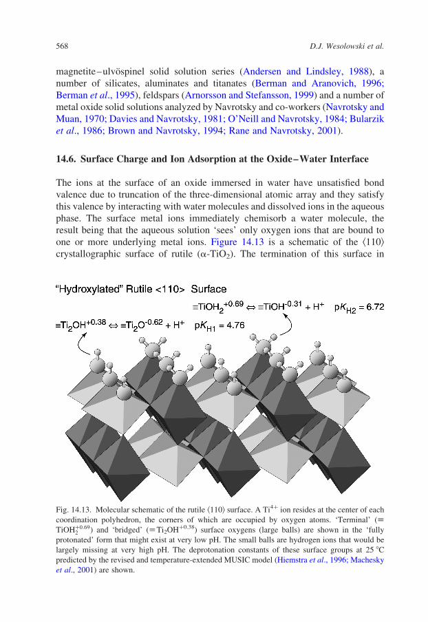
magnetite–ulvospinel solid solution series (Andersen and Lindsley, 1988), a

number of silicates, aluminates and titanates (Berman and Aranovich, 1996;

Berman et al., 1995), feldspars (Arnorsson and Stefansson, 1999) and a number of

metal oxide solid solutions analyzed by Navrotsky and co-workers (Navrotsky and

Muan, 1970; Davies and Navrotsky, 1981; O’Neill and Navrotsky, 1984; Bularzik

et al., 1986; Brown and Navrotsky, 1994; Rane and Navrotsky, 2001).

14.6. Surface Charge and Ion Adsorption at the Oxide–Water Interface

The ions at the surface of an oxide immersed in water have unsatisfied bond

valence due to truncation of the three-dimensional atomic array and they satisfy

this valence by interacting with water molecules and dissolved ions in the aqueous

phase. The surface metal ions immediately chemisorb a water molecule, the

result being that the aqueous solution ‘sees’ only oxygen ions that are bound to

one or more underlying metal ions. Figure 14.13 is a schematic of the k110lcrystallographic surface of rutile (a-TiO2). The termination of this surface in

Fig. 14.13. Molecular schematic of the rutile k110l surface. A Ti4þ ion resides at the center of each

coordination polyhedron, the corners of which are occupied by oxygen atoms. ‘Terminal’ ð;TiOHþ0:69

2 Þ and ‘bridged’ (;Ti2OHþ0.38) surface oxygens (large balls) are shown in the ‘fully

protonated’ form that might exist at very low pH. The small balls are hydrogen ions that would be

largely missing at very high pH. The deprotonation constants of these surface groups at 25 8C

predicted by the revised and temperature-extended MUSIC model (Hiemstra et al., 1996; Machesky

et al., 2001) are shown.


vacuum would consist of exposed Ti4þ ions coordinated with five oxygen ions in

the crystal (four on the surface and one below the Ti ion). In order to satisfy its

coordination, this metal ion chemisorbs a water molecule, forming the ‘terminal’

oxygen site shown in the figure, which is thus bonded to a single metal ion. The

vacuum-terminated surface also includes ‘bridged’ oxygens, which are bound to

two underlying Ti4þ ions and lie approximately one half of the k110l spacing

above the plane of Ti4þ ions. These terminal and bridged surface oxygens satisfy

their bond valence requirements by forming hydrogen bonds and exchanging

hydrogen ions with water molecules in solution via the same processes that give

rise to the structure of water and the water molecule self-dissociation, defined by

Kw. The vacuum-terminated surface also includes oxygen ions in the same plane

as the Ti4þ ions, which are bonded to three in-plane Ti4þ ions. However, these

oxygens are ‘buried’ by the bridged and terminal oxygens, and their bond

valence is largely satisfied, so they do not interact significantly with the adjacent

aqueous phase.

Rather than utilizing such surface structural information, metal oxide surface

protonation has been traditionally quantified by assuming a single, hypothetical,

uniformly distributed surface species, ;Me–O2, which can undergo one or two

protonation steps

;Me–O2 þ HþðsurÞO ;Me–OH0 ð14:102Þ

;Me–OH0 þ HþðsurÞ O ;Me–OHþ2 ð14:103Þ

in the ‘2-pK’ model, with equilibrium constants (KH1, KH2) quantifying these

reactions. Hþ(sur) is a hydrogen ion in solution adjacent to the surface, the activity

coefficient of which includes an additional electrostatic term to account for the

surface charge. In fact, molecular-level investigations suggest that these are the

actual species that exist on some oxide surfaces, such as quartz (a-SiO2).

Alternatively, the ‘1-pK’ model has been employed with a single equilibrium

constant (KH) for the reaction:

;Me–O20:5 þ HþðsurÞ O ;Me–OH0:5 ð14:104Þ

The surface oxygens and hydroxyl groups are able to ‘hydrate’ dissolved metal

ions, just as do water molecules in the bulk liquid. The primary difference between

the bulk aqueous phase and the oxide surface is that the pH-dependent exchange of

hydrogen ions with the bulk solution results in a fixed plane (approximately flat in

terms of long-range coulombic interactions) that is positively charged at low pH

and negatively charged at high pH. This charged surface then attracts dissolved

cations, anions and the dipolar water molecules, leading to the development of an

‘electrical double layer’ (EDL), which represents a separation of charge similar to

that of a parallel-plate capacitor, due to the finite radii of dissolved ions and water

molecules. This phenomenon is extremely important in a wide range of natural

and industrial processes, because (a) the transport, deposition and flocculation of


colloidal oxide particles depend critically on their surface charge; (b) surface

catalysis is directly related to sorption of the reactants; (c) oxide surfaces can

efficiently adsorb dissolved metal ions; and (d) for high mineral–surface/water–

mass systems, surface adsorption can significantly alter the solution chemistry.

It is evident from reactions 14.102–14.104, that there is a unique pH where the

surface will have no net positive or negative charge. If it is assumed that the

activity coefficient ratio of the surface sites is unity, this pH is exactly 1=2log10KH

for the 1-pK model or 1=2ðlog10KH1 þ log10KH2Þ for the 2-pK model. This pH is

termed the ‘point of zero charge’ or pHpzc. The hydrogen ion-induced surface

charge density at any pH is given by,

sH ¼ 2ðF=AÞðmoles of ‘excess’ or ‘missing’ Hþ in solutionÞ ð14:105Þ

where F is the Faraday constant (96 485 C per equivalent), A is the area (m2) of

oxide surface in contact with the solution, and the negative sign indicates that an

excess of Hþ in solution (calculated by taking the difference between the measured

pH and the pH calculated in the absence of the solid) corresponds to a deficit on

the surface. The effect of increasing ionic strength of an ‘indifferent’ supporting

electrolyte (i.e., one with weak and symmetrical absorption of its cation above and

anion below the pHpzc, e.g., KNO3, NaCl, etc.) is to increase lsHl for a given pH,

because the counter ions in solution are attracted to the plane of charge and reduce

the electrostatic repulsion between like charges at the surface. Thus, the principal

method of determining the pHpzc has traditionally been pH-titrations of oxide

powder suspensions at different ionic strengths, as shown in Fig. 14.14. The charge

density curves at different ionic strengths intersect at the pHpzc and in the absence of

contaminants and protolytic side reactions, this intersection falls close to sH ¼ 0:Ions and water molecules close to the charged surface are believed to be

immobile, or at least hindered in their motion, relative to species in the bulk

solution, due to electrostatic attraction. Both the ‘streaming potential’ of fluids

moving past a charged surface and the ‘electrophoretic mobility’ of charged

particles in an external field, can be related mathematically to the ‘zeta potential’,

z; which is defined as the electrical potential at the ‘plane of shear’ between bulk

solution and the ions and water molecules strongly bound to the charged surface.

The zeta potential also drops to zero at the pHpzc so that lzl increases at lower and

higher pH values, but unlike sH, the effect of increasing ionic strength is to

decrease the magnitude of z for a given pH, because the same counter ion

attraction that enhances the hydrogen-ion-induced charge build-up reduces the

magnitude of the electric field at the plane of shear generated by this surface

charge. The pH of zero potential is typically referred to as the ‘isoelectric pH’

(pHiep) and in indifferent electrolyte media, pHpzc and pHiep are generally found

experimentally to be nearly the same for equivalent materials.

Halley (2001), Hunter (2001, 2002) and Wingrave (2001) provide excellent

summaries of modern oxide–solution interaction theory and practical appli-

cations, and Kosmulski (2001, 2002) has compiled all the experimental data


published through 2001 on the pHpzc and pHiep of metal oxides. The reader is

encouraged to take advantage of these current and exhaustive reviews for

background information, including attempts to quantify the nature of the EDL at

metal oxide surfaces at ambient conditions. The following sections will focus

solely on recent progress in the hydrothermal regime. Almost no data are available

on the charging and adsorptive characteristics of metal oxide surfaces at

temperatures above 95 8C, with the exception of the recent studies by the authors

of this chapter and our collaborators, Moira K. Ridley at Texas Tech University

and Serguei N. Lvov at the Pennsylvania State University, in which we have

applied pH-titrations using the HECC apparatus described in Chapter 11, and lzlmeasurements in a newly designed microelectrophoresis apparatus, in studies of

the pHpzc and pHiep of several metal oxide powders to temperatures as high as

290 8C.

14.6.1. Temperature Dependence of the pHpzc

Berube and De Bruyn (1968) were the first investigators to study systematically

and rationalize the change in pHpzc with temperature. They noted that the pHpzc

of rutile decreased with temperature at about the same rate as that of 12

pKw over

Fig. 14.14. Surface charge density versus pH for rutile powders in 0.03 mol·kg21 (circles),

0.30 mol·kg21 (triangles) and 1.0 mol·kg21 NaCl (squares) solutions at 25 8C (open symbols) and

200 8C (filled symbols) obtained by Machesky et al. (1998) from pH titrations in a HECC. Common

intersection points correspond to pHpzc values of 5.4 ^ 0.2 and 4.3 ^ 0.2 at 25 and 200 8C,

respectively.


the 25–95 8C range, and this dependence was expressed as,

4:606R 12

pKw 2 pHpzc

h i¼ DHp=T 2 DSp ð14:106Þ

where R is the gas constant and DH p and DS p represent the enthalpy and entropy

difference of transferring Hþ and OH2 from bulk solution to the surface at the

pHpzc. These quantities can be determined from a plot of 12

pKw –pHpzc against

reciprocal temperature. They further postulated that the linearity of 12

pKw –pHpzc

with respect to inverse temperature would apply to all oxide systems.

Fokkink et al. (1989) studied the temperature dependence of the surface

charging of both rutile and hematite from 10 to 70 8C. They hypothesized that

while the pHpzc and its temperature dependence is a property specific to each

oxide, the increase of sH away from the pHpzc in the presence of inert electrolytes

is non-specific. They termed this phenomenon ‘temperature congruence’, which

means at a given ionic strength, surface charge curves are nearly identical when

plotted with respect to pHpzc–pH. Moreover, in the absence of specific ion

adsorption, they equated the isosteric heat of hydrogen ion adsorption (DadsH) with

the change in pHpzc with temperature,

2:303RðdpHpzc=dTÞ ¼ DadsHðTÞ22 ð14:107Þ

DadsH can be obtained from a plot of pHpzc against reciprocal temperature (K),

which proved to be highly linear for both their rutile and hematite data between

10 and 70 8C. They also found that the entropy gain accompanying hydrogen ion

adsorption on these oxide surfaces was nearly identical (42–46 J·K21·mol21),

independent of temperature and roughly equal to one half the entropy change of

the water association reaction.

Schoonen (1994) employed the ‘Balanced Like-Charge’ extrapolation

technique to estimate the pHpzc of several oxides to 350 8C. He used the water

dissociation reaction together with the 2-pK surface protonation model to give the

isocoulombic reaction,

;Me–O2 þ HþðsurÞ þ H2OðlÞO ;Me–OHþ2 þ OH2ðsurÞ ð14:108Þ

(where ‘sur’ refers to hydrogen and hydroxide ions on the oxide surface) for

which:

log10 Kp ¼ log10 KH1 þ log10 KH2 2 pKw ¼ 2pHpzc 2 pKw ð14:109Þ

Schoonen could apply this extrapolation technique to only five oxides (rutile,

magnetite, hematite, g-Al2O3 and Ni(OH)2), since these were the only solids for

which pHpzc data were available over a sufficient temperature range. He further

cautioned that pHpzc extrapolations above about 150 8C were probably very

unreliable, because data for the same mineral phase from different authors were

not in full agreement and were only available from room temperature to 95 8C at

most. Schoonen (1994) also provided an analogous isocoulombic equation for use

with the 1-pK model.


A slightly different isocoulombic representation of a 1-pK model for rutile

surface protonation was presented by Machesky et al. (1994),

;Me–OH20:5 þ 0:5HþðsurÞ þ 0:5H2OðlÞ O ;Me–OHþ0:52 þ 0:5OH2ðsurÞ

ð14:110Þ

log10 Kp ¼ log10 KH 2 12

pKw ð14:111Þ

This was the first study ever published that reported oxide powder pH-titration

results at temperatures above 95 8C and Machesky et al. (1994) suggested that the

approximately constant difference between the pHpzc of rutile and 12

pKw to 250 8C

might apply to higher temperatures and to other oxides as well.

Sverjensky and Sahai (1998) combined crystal chemical and Born solvation

theory to predict protonation enthalpies of oxides that were consistent with

the 2-pK model of surface protonation and the ‘triple layer’ representation of the

EDL, which includes the plane of oxygen protonation, an adjacent ‘Stern’ plane

containing cations and anions specifically adsorbed to the surface, and a ‘diffuse

layer’ in which ion concentrations decay in an approximate exponential manner to

the bulk solution composition. The predictive equations were derived from least-

squares regression of available oxide surface protonation data collected at various

temperatures, including the results of Machesky et al. (1994). For the overall 2-pK

model reaction,

;Me–O2 þ 2HþðaqÞ O ;Me–OHþ2 ð14:112Þ

pHpzc ¼12

log10 Kpzc ¼ 1=2log10ðKH1KH2Þ: The predictive enthalpy equation is,

DzpcH ¼ 257:614{1=1k þ ðT=12kÞð›1k=›TÞ} þ 76:578ðs=rMe–OHÞ2 23:043

ð14:113Þ

where 1k is the bulk dielectric constant of the solid, and s=rMe–OH is the Pauling

bond strength per angstrom. The temperature derivative of the solid dielectric

constant, ›1k=›T; was assumed to equal 1023 K21 for all solids. Similar equations

were given for the enthalpies associated with KH1 and KH2. Predictions for a wide

variety of oxide and silicate minerals revealed that DpzcHo ranged from about

217 to 2138 kJ·mol21. Combining this equation with one developed earlier

(Sverjensky and Sahai, 1996) for log10 Kpzc at 25 8C,

log10 Kpzc ¼ 42:2316ð1=1kÞ2 85:8296ðs=rMe–OHÞ þ 29:3732 ð14:114Þ

permits the corresponding entropy term to be determined by difference, so that the

pHpzc at temperatures other than 25 8C can be predicted. From these predictions

they also suggested that the temperature-parallelism between 12

pKw and the pHpzc

of rutile noted by Berube and De Bruyn (1968) and Machesky et al. (1994) was

fortuitous, and would not hold true for many solids. Finally, they noted that their


approach could be extended to include heat capacity terms when more data over an

extended temperature range become available.

In a refinement of their earlier study of rutile surface charge to 250 8C,

Machesky et al. (1998) found that careful pretreatment of the starting material

greatly improved the reversibility and reproducibility of surface charge density

curves and gave common intersection points for several ionic strengths at sH < 0

(Fig. 14.14). Kulick (2000) applied a Gibbs energy minimization approach to these

results to derive standard partial molal thermodynamic properties of surface

species within the context of the 2-pK, triple-layer model and proposed a general

relation for the change in pHpzc with temperature for simple oxides:

pHpzc;T ¼ 58:2682 {ðT298:15=TÞðpHpzc;298:15 þ 3:2385Þ}þ 4:545 ln T ð14:115Þ

This predictive relationship is based on the assumption that both DSo298:15 and

DCop;298:15 of protonation are constant at 25 and 87 J·K21·mol21, respectively, for

all oxide surfaces.

All of the approaches discussed above, and in fact most of the literature on

oxide surface charging, have assumed hypothetical 1- and 2-pK models of surface

protonation. Hiemstra et al. (1989) first proposed utilizing the known structures of

mineral surfaces and the Pauling bond-valence principle in order to estimate the

hydrogen ion binding affinities of surface oxygens, and Koretsky et al. (1998)

analyzed the likely surface densities and coordination numbers (with underlying

metal ions) of oxygen atoms exposed on cleavage surfaces of a large number of

oxides and silicates. In the revised MUtiSIte Complexation (MUSIC) model of

Hiemstra et al. (1996), surface protonation constants are estimated (at 25 8C) from

the empirical relationship,

log10 KH ¼ a V þX

SMe–O þ mðSHÞ þ nð1 2 SHÞ� �

ð14:116Þ

where a is a constant (the slope) obtained from a regression of log10 KH values of

homogeneous aqueous metal ion hydrolysis reactions versus the ‘under-saturation

of charge’ on the respective oxygen ligands (the summation of the terms in

parentheses), V the valence of oxygen (22) and SSMe–O the sum (over 1, 2 or 3 for

single, double or triple coordination, respectively, of oxygen(s) with coordinated

metal ions) of the bond valence values (z/CN, where z is the metal ion charge

and CN is its coordination number) for the metal–oxygen bonds of interest. The

remaining terms account for hydrogen bonding, where m is the number of

donating hydrogen bonds to the adsorbed water molecules (requires that an

hydrogen atom is present in the complex), n the number of accepting H-bonds

from the adsorbed water molecules, and SH (þ0.8) the assumed valence

contribution of a hydrogen bond. The under-saturation of charge of oxygen

atoms on crystal surfaces can be calculated in the same way with certain steric

restrictions imposed on the possible values of m and n. By applying the a value

obtained from homogeneous aqueous reactions, Hiemstra et al. (1996) predicted


the hydrogen ion binding constants for a large number of metal oxide surfaces

at 25 8C and demonstrated the ability of the MUSIC model to predict the

experimental charging curves of goethite and lepidocrocite.

Machesky et al. (2001) derived revised values of a in Eq. 14.116 at 25 8C and

extended this analysis to higher temperatures using a self-consistent set of

homogeneous aqueous metal ion hydrolysis reactions, the temperature depen-

dence of which are reasonably well known at 300 8C. The Pauling bond valence

values used by Hiemstra et al. (1996) were also replaced with values ofP

SMe–O ¼

z=AOCN; where z is the again the charge on the central metal ion, but AOCN is the

‘actual observed coordination number’ tabulated by Brown (1988). In deriving a

values for aqueous reactions at elevated temperatures, an adjustment to AOCN

was also made to take into account recent experimental studies which indicate that

the average ‘inner sphere’ hydration number of aqueous metal ions decreases

with increasing temperature. Assuming that only a varies with temperature in

Eq. 14.116, Machesky et al. (2001) applied this equation to rutile surface oxygen

sites, giving the 25 8C site charges and pKH values shown in Fig. 14.13. The rutile

powders used by Machesky et al. (1998) exhibited predominantly the k110l crystal

face with minor development of the k100l face, which exposes the same two

surface sites and Machesky et al. (2001) showed that the pHpzc of rutile could be

predicted with the temperature-extended MUSIC model within the experimental

uncertainty, as shown in Fig. 14.15.

Wesolowski et al. (2000b) conducted similar pH titrations of magnetite powders

from 25 to 290 8C in 0.03 and 0.3 mol·kg21 NaTr solutions. This solid exhibits five

distinct surface site types involving oxygen coordinated to 1, 2 or 3 underlying

Fe2.5þ and Fe3þ ions, which are distributed differently over the principal crystal

faces (k100l, k110l and k111l). They showed that the temperature-extended MUSIC

model also successfully predicted the temperature dependence of their exper-

imental pHpzc values for magnetite by assuming a face distribution consistent

with SEM images of the powder that gave a predicted pHpzc at 25 8C matching

the best available experimental data (57% k110l, 23% k100l and 20% k111l).The experimental and MUSIC model predictions for magnetite are compared in

Fig. 14.15, which also includes recently obtained data for NiFe2O4(cr) obtained

using the same HECC, pH-titration method. There is a much higher experimental

uncertainty associated with these results because the surface charging curves of

nickel ferrite were found to be much shallower than was the case for either

magnetite or rutile and the effects of dissolution of the solid phase and reduction of

Ni2þ(aq) to nickel metal were complicating factors. It is interesting to note,

however, that the MUSIC model protonation site types and charges predicted for

nickel ferrite are identical to those of magnetite (they are isostructural inverse

spinels) and the calculated pKH values are similar in magnitude, affected only by a

small difference in the average Ni2.5þ and Fe2.5þ bond lengths. However, whereas

the magnetite powders used by Wesolowski et al. (2000b) consisted of particles

with the k110l dodecahedron and k100l cube faces principally developed,


the nickel ferrite powder particles were principally octahedral (k111l) with the

cube face subordinate. The MUSIC model demonstrates that the primary cause of

the much higher pHpzc for nickel ferrite obtained in this study (Fig. 14.15) is this

difference in morphology, rather than an intrinsic difference in the charging

properties of the minerals. Temperature functions describing the pHpzc values

derived experimentally for rutile and magnetite (Machesky et al., 1998;

Wesolowski et al., 2000b) are listed in Table 14.4.

In principle, given information about the external morphology of a given

solid phase (i.e., the distribution of predominant crystal faces) and assuming

Fig. 14.15. Comparison of experimental pHpzc values for rutile (squares, Machesky et al., 1998),

magnetite (circles, Wesolowski et al., 2000b) and nickel ferrite (triangles, unpublished), with

estimates based on (a) the MUSIC Model (heavy curves, Machesky et al., 2001), Kulik (2000, thin

solid curves), and Schoonen (1994, dashed curves); and (b) Berube and De Bruyn (1968, solid

curves), Fokkink et al. (1989, dotted curves) and Sverjensky and Sahai (1998, dashed curves).


that surface ;Me–O bond lengths are equal to those in the bulk crystal (or

refined using ab initio cluster calculations), it is possible to calculate the pHpzc

as a function of temperature for any crystalline metal oxide using the MUSIC

model. Furthermore, this model predicts that different crystal faces on the same

particle can have quite different (and even opposite) charges at a given pH,

which has profound implications for particle transport, aggregation and adhe-

sion, and the sector-zoning of trace elements incorporated into growing crystals.

In current practice, however, the distribution of crystal faces and/or ;Me–O

bond lengths must be modified somewhat from ideal values in order that

predicted pHpzc values match those determined experimentally. This does not

imply that the MUSIC model is incorrect, but rather that: (a) surface relaxation

effects which may change ;Me–O bond lengths need to be quantified in situ, a

frontier area for surface science; (b) it is difficult to estimate actual surface

areas of individual crystal faces in a powder aggregate; and (c) undoubtedly,

defects and edge effects influence hydrogen ion uptake and release from real

oxide powders.

The MUSIC model predictions and experimental results for rutile and

magnetite are compared in Fig. 14.15 with the older temperature extrapolation

approaches discussed above. The most precise fits to the experimental data for

both solids are given by the isocoulombic extrapolation method of Schoonen

(1994) and the method advocated by Berube and De Bruyn (1968), which

represent least squares fits to the experimental pHpzc data, including either an

explicit (Schoonen) or implicit (Berube and Debruyn) heat capacity term. In fact,

these methods are very similar since they both rely on fitting pHpzc data that have

been normalized relative to 12

pKw (compare Eqs. 14.106, 14.109, and 14.111). The

extrapolation methods of Fokkink et al. (1989) and Sverjensky and Sahai (1998)

result in less satisfactory predictions, since neither of these methods include a

variable heat capacity term. However, the method of Sverjensky and Sahai (1998)

can be extended to include a heat capacity term and it is truly predictive like the

MUSIC model and can be used even when no experimental pHpzc data are

available. The extrapolation method of Kulick (2000) provides a very good fit to

the rutile data, which is not surprising since the constant entropy and heat capacity

terms in this model were derived from a fit to the experimental data for rutile.

Table 14.4. Coefficients for the equation pHpzc ¼ n1 þ n2ðTÞ21 þ n3 ln T of rutile (a-TiO2) and

magnetite (Fe3O4)

Oxide n1 n2 n3 Range (8C)

a-TiO2a 226.51 2450.8 4.158 25–250

Fe3O4b 243.44 3684.7 6.686 25–300

a Machesky et al. (1998).b Wesolowski et al. (2000).


However, the fit to the magnetite pHpzc data is less satisfactory, indicating that the

model cannot be generally applied to all oxide types.

14.6.2. Temperature Dependence of the pHiep

Alekhin et al. (1985), Jayaweera et al. (1992, 1994) and Lvov et al. (1999)

reported the first attempts to determine the zeta potential ðzÞ of metal oxides at

temperatures above 90 8C. Alekhin investigated g-Al2O3(s) and SiO2(s) at

temperatures of 20–250 8C using a streaming potential method, but these authors

did not report pHiep values, although for g-Al2O3 a reversal in the sign of z was

observed at all temperatures in 1023 mol·kg21 solutions at a room-temperature pH

of 6.7 (positive z) and 11.0 (negative z). Jayaweera et al. measured the streaming

potential across a column packed with the oxide powder of interest at 235 8C

reporting pHiep values of 3.4, 6.1–8.4, 7.2, 6.6, 6.3 and 6.6 for the solids a-Fe2O3,

Fe3O4, ZrO2, TiO2, Ta2O5 and Cr2O3, respectively. Few details regarding the

crystalline form of the starting materials were provided, but the authors indicate

that the hematite and magnetite commercial powders were too fine for the packed-

column technique and were coarsened by sintering at 962 8C. It is not known

whether the fO2was controlled within the stability fields of these oxides. The range

of pHiep values reported by Jayaweera et al. for magnetite (6.1–8.4) is much

higher than the experimental pHpzc value of 5.3 ^ 0.3 or the MUSIC model

estimate of 5.5 (Wesolowski et al., 2000b) for a predominantly dodecahedral

particle. The pHiep value reported for TiO2 (6.6) is also much higher than a pHpzc

of 4.2 ^ 0.2 obtained from the experimental measurements and MUSIC model

predictions of Machesky et al. (1998, 2001). Lvov et al. (1999) also obtained

preliminary z values from streaming potential measurements across ZrO2 capillary

tubes in aqueous solutions from 200–400 8C. They did not extract pHiep values

from their measurements in 0.01 mol·kg21 HCl in 0.1 mol·kg21 NaCl and

0.001 mol·kg21 HCl in 0.1 mol·kg21 NaCl solutions, but the reported z ¼ 0 values

for these solutions were observed at approximately 200 and 350 8C, respectively,

indicating much lower pHiep values than were reported by Jayaweera et al. (1994).

Zhou et al. (2003) have developed a high-temperature microelectrophoresis

apparatus and Fedkin et al. (2003) have applied this system to rutile powders

similar to those studied by Machesky et al. (1998). The pHiep values obtained for

rutile, 5.26 ^ 0.45, 5.13 ^ 0.37 and 4.50 ^ 0.55 at 25, 120 and 200 8C agree with

the pHpzc results (Machesky et al., 1998) within the combined experimental

uncertainty. This system is currently being applied in investigations of the

electrophoretic mobilities of rutile, ZrO2 (baddeleyite) and a-Al2O3 powders in

dilute aqueous solutions over a similar temperature range. This approach offers

great promise for future investigations of metal oxide surface chemistry,

particularly for applications to electrical power plant operations, since the zeta

potential is generally considered the ‘master variable’ in controlling the transport

and deposition of colloidal particles in circulating systems. It is possible to


calculate z indirectly from EDL models that are constrained by pH-titration and

ion adsorption results, as demonstrated for magnetite in dilute NaTr solutions by

Wesolowski et al. (2000b, 2002), but such estimates are highly model-dependent

and will benefit greatly from direct experimental calibration as further

developments in electrokinetic techniques progress.

14.6.3. Specific Ion Adsorption Studies at Elevated Temperatures

While there have been an enormous number of experimental studies of strongly

adsorbing cations, anions and organic compounds on metal oxide surfaces

(Kosmulski, 2001), almost none have been reported at temperatures above 50 8C

where the adsorption was monitored as a function of solution pH, with the

exception of Ca2þ adsorption on rutile powder surfaces from 25 to 250 8C reported

by Ridley et al. (1999) using the HECC method. Subsequent to that study, a

substantial body of new experimental data has been collected by the authors of

this chapter in collaboration with M.K. Ridley of Texas Tech University, for the

sorption of Y3þ, Nd3þ and Sr2þ on rutile powder surfaces in NaCl solutions, and

Zn2þ and Co2þ in NaTr solutions at ionic strengths of 0.03 and 0.3 mol·kg21,

using the HECC approach at temperatures of 25–250 8C. These recent studies

have focused on metal cation adsorption because: (a) due to electrostatic effects,

small multivalent ions are much more strongly adsorbed than monovalent ions or

large multivalent species (most multivalent anions are polyatomic); (b) the pH

range over which the surface is negatively charged expands (pHpzc decreases) with

increasing temperature for all oxides studied, indicating that cation adsorption

should become more important at elevated temperatures; and (c) cation adsorption

is generally of greater interest for contaminant migration in natural systems and

power plant operations at elevated temperatures.

Figure 14.16 is a plot of the right-hand side of Eq. 14.105 versus pH for rutile

titrations in 0.03 and 0.3 mol·kg21 NaCl or NaTr containing 0.001 mol·kg21 Mezþ

at temperatures of 25 and 200 8C. Each experiment involved about 40 g of starting

solution and 1–1.5 g of rutile powder with an average surface area of about

15 m2·g21. The Y3þ and Sr2þ results are not shown, but are similar to those of

Nd3þ and Ca2þ, respectively. The heights of the plateaus in these curves at high

pH result from essentially complete adsorption of Mezþ and are dependent upon

the initial (solution mass)/(surface area) ratio, but the position of the steep part of

each curve is characteristic of each individual cation. The vertical axes are not

labeled as sH; because it is not completely clear that the large increase in excess

Hþ(aq) in solution associated with adsorption of these cations is entirely related to

surface oxygen deprotonation. In fact, preliminary modeling suggests that surface-

enhanced hydrolysis of Zn2þ and Co2þ contributes to the solution hydrogen ion

balance. In addition to these ‘hydrogen ion release’ curves, nearly identical

experiments were conducted in which filtered samples of the solution were

removed at various points in the titrations and analyzed for their dissolved


Mezþ(aq) concentrations. The resulting ‘pH sorption edge’ curves are shown in

Fig. 14.17.

At the start of each titration or sampling experiment containing Mezþ(aq), the

ratio [Naþ]/[Mezþ] was either 30 or 300. Therefore, it is clear that the interaction

of these multivalent cations is much stronger than that of the ‘indifferent’

background electrolyte (NaCl or NaTr). It is also seen that the pH range over

which these cations cause enhanced hydrogen ion release into solution (Fig. 14.16)

approximately coincides with the pH range over which the percentage of the total

moles of Mezþ in the system that are adsorbed on the surface rises from near 0 to

near 100% (often termed the ‘sorption edge’) and is specific for each individual

Fig. 14.16. Plot of excess Hþ in solution per square meter of mineral surface as a function of pH at

25 and 150 8C for rutile powders in NaCl solutions with stoichiometric molal ionic strengths of 0.03

(open circles) and 0.30 mol·kg21 (filled circles), and in equivalent NaCl or NaTr solutions

containing 0.001 mol·kg21 Nd3þ, Zn2þ, Co2þ or Ca2þ. Dashed vertical lines indicate the pHpzc of

rutile (Machesky et al., 1998) and dashed horizontal lines indicate the condition of no excess Hþ in

solution (Ca2þ data from Ridley et al., 1999; NaCl data from Machesky et al., 1998).


cation. Finally, with increasing temperature, the sorption edges shift to lower pH,

both in absolute terms and with respect to the pHpzc. This indicates that, for

instance, Nd3þ is so strongly attracted to the surface that it adsorbs even at pH

where the overall surface is positively charged. Ridley et al. (2004) use the

MUSIC model of surface protonation, together with a ‘basic Stern’ model of the

EDL, with separate Stern planes and ion binding equilibrium constants for Naþ

and Ca2þ, to fit both types of data for Ca2þ adsorption on rutile surfaces. However,

the binding constants and Stern-plane capacitance terms are highly model-

specific, although constrained by recent synchrotron X-ray standing wave studies

of mono- and di-valent cation studies on the rutile surface (Fenter et al., 2000;

Zhang et al., 2002).

Fig. 14.17. Percent Nd3þ, Zn2þ, Co2þ and Ca2þ adsorbed as a function of pH and temperature.

Dashed vertical lines indicate the pHpzc of rutile (Machesky et al., 1998) at each temperature (Ca2þ

data from Ridley et al., 1999). Smooth curves are 4-parameter sigmoid functions which asymptote to

0 and 100%.


A model-independent method of comparing the effects of temperature and ion

type on the adsorption of cations on oxide surfaces would be desirable. The curves

shown in Fig. 14.17 are fits to the data using a four-parameter sigmoid function

(with the first two parameters both fixed at 100%),

%Mezþsorbed ¼ 100 2 100=½1 þ expðpH 2 aÞ=b� ð14:117Þ

which asymptomatically approaches to 0 and 100% at low and high pH,

respectively. The parameter b controls the steepness of the curve and the parameter

a is the model pH at which 50% of the total Mezþ in the system is adsorbed on the

surface. The latter value, pH50, is often used in comparing the sorption behavior of

various sorbates and sorbents in the literature (Kosmulski, 1997).

Specific adsorption of multivalent cations can be viewed simplistically as the

exchange reaction:

;Hþr þ Mezþ ðaqÞ O ;Mezþ þ rHþðaqÞ ð14:118Þ

If electrostatic effects and activity coefficients are ignored, and the

concentrations of surface sites are defined in the same units as those of surface

species (molality or molarity), as is often done in the literature, then for reaction

14.118:

pH50 ¼ ð1=rÞðpKads 2 log10½;Hþr �Þ ð14:119Þ

The surface area of the rutile powders used in the cation adsorption studies

presented here was always 16 ^ 2 m2·g21, the solid/solution mass ratio never

varied by more than a factor of 2 (0.3 log10 units) and the hydrogen ion release

factors (r) for all ions were observed to be between 1.5 and 2.5. Therefore, the

variation of pH50 with temperature and from one cation to another observed in

these studies is comparable to that of pKads for each species. The pH50 values

obtained for Nd3þ, Zn2þ, Co2þ and Ca2þ are compared with the pHpzc of rutile in

Fig. 14.18, which illustrates the very regular behavior of pH50 with increasing

temperature, the similarity in the temperature dependencies of the sorption of all

of these di- and tri-valent cations, and the insensitivity to ionic strength, except for

the most weakly bound species (Ca2þ). This figure also illustrates that pH50 and

therefore pKads for the hypothetical exchange reaction, decreases much more

rapidly than the value of pHpzc with increasing temperature. Since a decreasing

pKads indicates stronger adsorption, whereas a decreasing pHpzc means a wider

pH range over which the surface charge is negative; these trends both dictate

that cation adsorption on rutile surfaces becomes much more significant with

increasing temperature. Kosmulski (1997) has suggested that this trend is typical

of cation adsorption on metal oxide surfaces, but his conclusions were based on

observations over a very limited temperature range near ambient conditions.

Values of pH50 2 pKh1, where the latter is the first hydrolysis constant for each

cation (see the previous section), range from about 22 to 24 and are relatively

constant with temperature for each cation. This indicates that the adsorbing


species is Mezþ(aq), rather than a hydrolyzed species, although as mentioned

above, some hydrolysis of the adsorbed cation may occur, resulting in enhanced

hydrogen ion release from the EDL. There are no data or theoretical estimates

currently available that would permit prediction of the adsorption of these ions

on other metal oxides, or of other aqueous species on rutile surfaces. A great deal

of research is needed in order to quantify fully the interaction of metal oxide

surfaces with dissolved aqueous species under hydrothermal conditions, but the

results presented here indicate that the effect of temperature on this process is

profound.

14.7. Summary

This chapter has shown that many excellent experimental methods are currently

available or in the developmental stages for determining the equilibrium

solubilities of metal oxides in the subcritical hydrothermal regime. Several

Me–O–H systems are very well characterized (Al, Ca, Ga, Ge, Mg, Si, Zn) and

the solubilities and hydrolysis equilibria in these systems are not likely to change

significantly from the currently accepted values. Although experimentally deter-

mined solubilities and hydrolysis equilibria are available for other industrially

significant metal oxide systems, they are either controversial (Cr, Cu, Ni, Ti) or are

hardly constrained (Mn, U, Zr) at hydrothermal conditions. There is even a gap

Fig. 14.18. Variation of pH50 for Nd3þ, Zn2þ, Co2þ and Ca2þ on rutile powder surfaces in NaCl or

NaTr solutions at ionic strength 0.03 mol·kg21 (open circles) or 0.3 mol·kg21 (filled circles). Data

for Ca2þ from Ridley et al. (1999). Rutile pHpzc from Machesky et al. (1998).


in our understanding of the Fe–O–H system, concerning the stabilities of the

intermediate Fe(III) hydrolysis species, and this is the most important metal in

many geologic and industrial settings.

It is not a coincidence that the more poorly understood metal oxide systems are

characterized by multiple valence states and/or minimum solubilities in the parts-

per-billion range or lower. Rather, this serves to illustrate that further advances are

needed in (a) ultraclean experimental and sampling methods; (b) ultratrace and

in situ metal analysis methods; and (c) methods to control or monitor the oxidation

state of experimental systems. With the many well-characterized pH buffers

(Chapter 12) and new in situ pH measurement capabilities now available, there

does not appear to be strong justification for conducting new experimental studies

wherein the pH of the solution is unconstrained or poorly known. Such

information is likely to contribute only confusion to chemical systems that are

becoming clearer with time. The problem of determining what crystalline phase (if

any) is controlling the solubility of a given metal continues to present difficulties.

Increased emphasis on surface characterization relative to bulk solids character-

ization is required, since it is the surface phase that typically controls the solubility

equilibria. New methods are now being developed which might provide direct

information on the nature of the solid phase dissolving or precipitating, such as

hydrothermal atomic force microscopy (Higgins et al., 2002) and in situ, time-

resolved X-ray diffraction analysis (Cahill et al., 2000; Shaw et al., 2000a,b).

While there are a number of well-developed extrapolation and interpolation

schemes for predicting the temperature, pressure and ionic strength dependencies

of solubility reactions, these methods often result in exceedingly poor estimates

when they are applied to erroneous input data, or unconstrained by reliable

experimental data over a significant range of these variables. It appears that we are

far from being able to predict the thermodynamic properties of metal oxide

systems for which no experimental data are available, although progress is being

made in ab initio modeling and molecular dynamics simulations of metal

speciation in aqueous solutions (Fulton et al., 2000b; Kubicki, 2001; Rosso et al.,

2002; Chialvo and Simonson, 2002). However, these methods have yet to be

applied in the prediction of even the rates of metal oxide dissolution and

precipitation, and their applicability to equilibrium solubility predictions is a

matter of speculation at this time.

In contrast to speciation and solubility, the charging and ion adsorption

characteristics of metal oxide surfaces exposed to hydrothermal solutions is a

newly emerging subject area. While a number of methods have been developed

recently for extrapolating room-temperature properties into the hydrothermal

regime, very few systems have been investigated experimentally that serve to test

these methods. This is a frontier area for research and applications, and first-

principles calculation approaches are only now being attempted (Cygan and

Kubicki, 2001; Rustad et al., 2003). Because colloidal particle transport and

deposition and the migration of metal ions in the presence of oxide surfaces play


key roles in a wide range of industrial and geologic processes, this is an area ripe

for further research and development.

The kinetics of heterogeneous reactions have not been addressed in this

chapter, but many excellent texts exist on this subject (Connors, 1990; Lasaga,

1998). Within the geochemical community, it has long been recognized that

dissolution and precipitation reaction rates at elevated temperatures are pH

dependent, but in recent years a number of authors have attempted to make

quantitative links between the rates of these reactions and the surface charge and

ion adsorption properties of metal oxides (Casey and Sposito, 1992; Brady and

Walther, 1992; Dove, 1994, 1999; Walther, 1996; Chen and Brantley, 1997;

Pokrovsky and Schott, 1999). At this time, there are no systems for which both

dissolution/precipitation rate data and detailed information on the pH-dependent

charging and adsorptive characteristics of the solid phase are known at elevated

temperatures. However, the HECC and other emerging experimental techniques

make such studies feasible, and important targets for future research in

hydrothermal oxide–water interactions.

Acknowledgements

Wesolowski, Anovitz, Benezeth and Palmer wish to thank the US Department of

Energy and the Electric Power Research Institute for financial support of their

ongoing studies of metal oxide solubility, surface adsorption characteristics, and

aqueous speciation under hydrothermal conditions. In the case of the former

sponsor, specific acknowledgment is given to the Division of Chemical Sciences,

Geosciences and Biosciences, Office of Basic Energy Sciences, US Department of

Energy, under contract DE-AC05-00OR22725 with Oak Ridge National Labora-

tory, managed and operated by UT-Battelle, LLC. Machesky acknowledges the

support of the Illinois State Water Survey and the Illinois Department of Natural

Resources.

References

Abraham, M.H. and Marcus, Y., J. Chem. Soc. Faraday Trans., 82, 3255–3274 (1986).

Adair, J.H., Krarup, H.G., Venigalla, S. and Tsukada, T. In: Voigt, J.A., Wood, T.E., Bunker, B.C.,

Casey, W.H. and Crossey, L.J. (Eds.), Aqueous Chemistry and Geochemistry of Oxides,

Hydroxides, and Related Materials, Materials Research Society Symposium Proceedings, 1997,

Vol. 432, pp. 101–112.

Adamson, A.W. and Gast, A.P. (Ed.), Physical Chemistry of Surfaces, 6th edn. Wiley, New York,

1997.

Adschiri, T., Kanazawa, K. and Arai, K., J. Am. Ceram. Soc., 75, 1019–1022 (1992).

Aja, S.U., Wood, S.A. and Williams-Jones, A.E., Applied Geochem., 10, 603–620 (1995).


Aja, S.U., Wood, S.A. and Williams-Jones, A.E. In: Voigt, J.A., Wood, T.E., Bunker, B.C., Casey,

W.H. and Crossey, L.J. (Eds.), Aqueous Chemistry and Geochemistry of Oxides, Hydroxides,

and Related Materials, Materials Research Society Symposium Proceedings, 1997, Vol. 432,

pp. 69–74.

Alekhin, Y.V., Sidorova, M.P., Ivanova, L.I. and Lakshtanov, L.Z., Kolloidn. Zh., 46, 1195–2003

(1985).

Ampelogova, N.I., Bashilov, S.M. and Pentin, V.I., Radiokhimiya, 31(4), 160–165 (1989).

Anderson, G.M., Geochim. Cosmochim. Acta, 59, 2155–2161 (1995a).

Anderson, G.M., Geochim. Cosmochim. Acta, 59, 4103–4104 (1995b).

Anderson, G.M. In: Hellmann, R. and Wood, S.A. (Eds.), Water–Rock Interactions, Ore Deposits,

and Environmental Geochemistry: A Tribute to David A. Crerar, Special Publication No. 7. The

Geochemical Society, 2002, pp. 181–190.

Anderson, G.M. and Crerar, D.A., Thermodynamics in Geochemistry. The Equilibrium Model.

Oxford University Press, Oxford, 1993.

Andersen, D.J. and Lindsley, D.H., Am. Miner., 73, 714–726 (1988).

Anderson, G.M., Castet, S., Schott, J. and Mesmer, R.E., Geochim. Cosmochim. Acta, 55,

1769–1779 (1991).

Anderson, A.J., Jayanetti, S., Mayanovic, R.A., Bassett, W.A. and Chou, I.-M., Am. Miner., 87,

262–268 (2002).

Anovitz, L.M., Ziemniak, S., Wesolowski, D.J. and Simonson, J.M., Thermodynamics of Cr2O3,

FeCr2O4, ZnCr2O4 and CoCr2O4, 2004, manuscript in preparation.

Archer, D.G., J. Phys. Chem. Ref. Data, 21, 793–829 (1992).

Arnorsson, S. and Stefansson, A., Am. J. Sci., 299, 173–209 (1999).

Arvidson, R., Ertan, I.E., Amonette, J.E. and Luttge, A., Geochim. Cosmochim. Acta, 67, 1623–1634

(2003).

Baes, C.F. Jr. and Mesmer, R.E., The Hydrolysis of Cations, Wiley, New York, 1976 (reprint edn.

Krieger Publishing Co., Malabar, 1986).

Baes, C.F. Jr. and Meyer, N.J., Inorg. Chem., 1, 780–789 (1962).

Baes, C.F. Jr., Meyer, N.J. and Roberts, C.E., Inorg. Chem., 4, 518–527 (1965).

Barin, I., Thermochemical Data of Pure Substances. VCH Verlagsgesellschaft, Weinheim, 1989.

Barnes, H.L. (Ed.), Geochemistry of Hydrothermal Ore Deposits. Wiley, New York, 1997.

Bassett, W.A., Anderson, A.J., Mayanovic, R.A. and Chou, I.-M., Chem. Geol., 167, 3–10 (2000).

Becker, K.H., Cemic, L. and Langer, K.E.O.E., Geochim. Cosmochim. Acta, 47, 1573–1578 (1983).

Benezeth, P., Castet, S., Dandurand, J.-L., Gout, R. and Schott, J., Geochim. Cosmochim. Acta, 58,

4561–4571 (1994).

Benezeth, P., Diakonov, I.I., Pokrovski, G.S., Dandurand, J.-L., Schott, J. and Khodakovsky, I.L.,

Geochim. Cosmochim. Acta, 61, 1345–1357 (1997).

Benezeth, P., Palmer, D.A. and Wesolowski, D.J., Geochim. Cosmochim. Acta, 63, 1571–1586

(1999).

Benezeth, P., Palmer, D.A. and Wesolowski, D.J., Geochim. Cosmochim. Acta, 65, 2097–2111

(2001).

Benezeth, P., Palmer, D.A., Wesolowski, D.J. and Xiao, C., J. Solution Chem., 31, 947–973 (2002).

Bergmann, C.A., Gold, R.E., Sejvar, J., Perock, J.D., Dove, M. and Pathania, R.S., Water Chem.

Nucl. Reactor Sys., 7, 287–292 (1996).

Berman, R.G. and Aranovich, L.Y., Contrib. Miner. Petrol., 126, 1–24 (1996).

Berman, R.G., Aranovich, L.Y. and Pattison, D.R.M., Contrib. Miner. Petrol., 119, 30–42 (1995).

Berner, R.A., Geochim. Cosmochim. Acta, 33, 267–273 (1969).

Berube, Y.G. and De Bruyn, P.L., J. Colloid Interf. Sci., 27, 305–318 (1968).

Bethke, C.M., Geochemical Reaction Modeling. Oxford University Press, New York, 1996.

Bethke, C.M., The Geochemist’s Workbench, Release 3.0, (self-published by the author), 1998.


Bilal, B.A., Z. Naturforsch. A, 46, 1108–1116 (1991).

Bilal, B.A. and Mueller, E., Z. Naturforsch. A, 47, 974–984 (1992).

Bilal, B.A., Haufe, P. and Moeller, P., Physica B þ C, 139/140, 721–724 (1986).

Blesa, M.A., Morando, P.J. and Regazzoni, A.E., Chemical Dissolution of Metal Oxides. CRC Press,

Boca Raton, FL, 1994.

Bourcier, W.L. and Barnes, H.L. In: Ulmer, G.C. and Barnes, H.L. (Eds.), Hydrothermal

Experimental Techniques. Wiley, New York, 1987, pp. 189–215.

Bourcier, W.L., Ulmer, G.C. and Barnes, H.L. In: Ulmer, G.C. and Barnes, H.L. (Eds.),

Hydrothermal Experimental Techniques. Wiley, New York, 1987, pp. 157–188.

Bourcier, W.L., Knauss, K.G. and Jackson, K.J., Geochim. Cosmochim. Acta, 57, 747–762 (1993).

Brady, P.V. and Walther, J.V., Am. J. Sci., 292, 639–658 (1992).

Brown, I.D., Acta Crystallogr. B, 44, 545–553 (1988).

Brown, P.L., Talanta, 36, 351–355 (1989).

Brown, N.E. and Navrotsky, A., Am. Miner., 79, 485–496 (1994).

Brown, P.L., Sylva, R.N. and Ellis, J., J. Chem. Soc. Dalton Trans.: Inorg. Chem., 4, 723–730 (1985).

Brown, P.L., Drummond, S.E., Jr. and Palmer, D.A., J. Chem. Soc. Dalton Trans.: Inorg. Chem., 14,

3071–3075 (1996).

Brown, G.E., Jr., Henrich, V.E., Casey, W.H., Clark, D.L., Eggleston, C., Felmy, A., Goodman,

D.W., Gratzel, M., Maciel, G., McCarthy, M.I., Nealson, K.H., Sverjensky, D.A., Toney, M.F.

and Zachara, J.M., Chem. Rev., 99, 77–174 (1999).

Bularzik, J., Davies, P.K. and Navrotsky, A., J. Am. Ceram. Soc., 69, 453–457 (1986).

Busey, R.H. and Mesmer, R.E., Inorg. Chem., 16, 2444–2450 (1977).

Busey, R.H. and Mesmer, R.E., J. Chem. Eng. Data, 23, 175–176 (1978).

Byrappa, K. and Yoshimura, M., Handbook of Hydrothermal Technology: A Technology for Crystal

Growth and Materials Processing. Noyes Publications, Park Ridge, NJ, 2001.

Byrne, R.H., Luo, Y.-R. and Young, R.W., Marine Chem., 70, 23–35 (2000).

Cahill, C.L., Benning, L.G., Barnes, H.L. and Parise, J.B., Chem. Geol., 167, 53–63 (2000).

Casey, W.H. and Sposito, G., Geochim. Cosmochim. Acta, 56, 3825–3830 (1992).

Castet, S., Dandurand, J.-L., Schott, J. and Gout, R., Geochim. Cosmochim. Acta, 57, 4869–4884

(1993).

Chase, M.W., Davies, C.A., Downey, J.R., Frurip, D.J., McDonald, R.A. and Syverud, A.N., J. Phys.

Chem. Ref. Data, 14(Suppl. 2) (1985).

Chen, Y. and Brantley, S., Chem. Geol., 135, 275–290 (1997).

Chialvo, A.A. and Simonson, J.M., Mol. Phys., 100, 2307–2315 (2002).

Chou, I.-M. In: Ulmer, G.C. and Barnes, H.L. (Eds.), Hydrothermal Experimental Techniques.

Wiley, New York, 1987, pp. 61–99.

Christensen, A.N., Acta Chem. Scand. A, 30, 133–136 (1976).

Cobble, J.W. and Lin, S.W. In: Cohen, P. (Ed.), The ASME Handbook on Water Technology

for Thermal Power Systems. The American Society of Mechanical Engineers, New York, 1989,

pp. 545–658.

Cohen, P. (Ed.), The ASME Handbook on Water Technology for Thermal Power Systems. The

American Society of Mechanical Engineers, New York, 1989.

Connors, K.A., Chemical kinetics: the study of reaction rates in solution. VCH Publishers,

New York, 1990.

Crerar, D.A. and Anderson, G.M., Chem. Geol., 8, 107–122 (1971).

Crerar, D.A., Wood, S. and Brantley, S., Can. Miner., 23, 333–352 (1985).

Criss, C.M. and Cobble, J.W., J. Am. Chem. Soc., 86, 5385–5390 (1964).

Criss, C.M. and Cobble, J.W., J. Am. Chem. Soc., 86, 5390–5393 (1964).

Cygan, R.T. and Kubicki, J.D. (Ed.), Molecular Modeling Theory: Applications in the Geosciences,

Mineralogical Society of America, Washington, DC, 2001, Vol. 42.


Davies, P.K. and Navrotsky, A., J. Solid State Chem., 38, 264–276 (1981).

Deberdt, S., Castet, S., Dandurand, J.-L., Harrichoury, J.-C. and Louiset, I., Chem. Geol., 151,

349–372 (1998).

Dellien, L., Hall, F.M. and Hepler, L.G., Chem. Rev., 76, 283–310 (1976).

Diakonov, I.I., Pokrovski, G., Schott, J., Castet, S. and Gout, R., Geochim. Cosmochim. Acta, 60,

197–211 (1996).

Diakonov, I.I., Pokrovski, G.S., Benezeth, P., Schott, J., Dandurand, J.-L. and Escalier, J., Geochim.

Cosmochim. Acta, 61, 1333–1343 (1997).

Diakonov, I.I., Schott, J., Martin, F., Harrichourry, J.-C. and Escalier, J., Geochim. Cosmochim.

Acta, 63, 2247–2261 (1999).

Dickson, A.G., Wesolowski, D.J., Palmer, D.A. and Mesmer, R.E., J. Phys. Chem., 94, 7978–7985

(1990).

Ding, K. and Seyfried, W.E. Jr., Science, 272, 1634–1636 (1996).

Dinov, K., Matsuura, C., Hiroishi, D. and Ishigure, K., Nucl. Sci. Eng., 113, 207–216 (1993).

Dinov, K.A., Ishigure, K., Hiroishi, D. and Matsuura, C., Nucl. Tech., 106, 177–185 (1994).

Dirkse, T.P., Copper, Silver, Gold, and Zinc, Cadmium, Mercury Oxides and Hydroxides, IUPAC

Solubility Data Series, 1986, Vol. 23.

Dove, P.M., Am. J. Sci., 294, 665–712 (1994).

Dove, P.M., Geochim. Cosmochim. Acta, 63, 3715–3727 (1999).

Dove, P.M. and Crerar, D.A., Geochim. Cosmochim. Acta, 54, 955–969 (1990).

Eugster, H.P., Chou, I.-M. and Wilson, G.A. In: Ulmer, G.C. and Barnes, H.L. (Eds.), Hydrothermal


Ezhov, B.B. and Kamnev, A.A., Zh. Prikl. Khim., 54, 2346–2348 (1983).

Fedkin, M.V., Zhou, X.Y., Kubicki, J.D., Bandura, A.V. and Lvov, S.N., Langmuir, 19, 3797–3804

(2003).

Fenter, P., Cheng, L., Rihs, S., Machesky, M.L., Bedzyk, M.J. and Sturchio, N.C., J. Colloid Interf.

Sci., 225, 154–165 (2000).

Fleming, B.A. and Crerar, D.A., Geothermics, 11, 15–29 (1982).

Fokkink, L.G.J., De Keizer, A. and Lyklema, J., J. Colloid Interf. Sci., 127, 116–131 (1989).

Fournier, R.O., Geochim. Cosmochim. Acta, 47, 579–586 (1983).

Fournier, R.O. and Marshall, W.L., Geochim. Cosmochim. Acta, 47, 587–596 (1983).

Fulton, J.L., Darab, J.G. and Hoffmann, M.M. In: Tremaine, P.R., Hill, P.G., Irish, D.E. and

Balakrishnan, P.V. (Eds.), Steam, Water and Hydrothermal Systems: Physics and Chemistry

Meeting the Needs of Industry, Proceedings of the 13th International Conference on the

Properties of Water and Steam. NRC Research Press, Ottawa, 2000a, pp. 593–598.

Fulton, J.L., Hoffmann, M.M., Darab, J.G., Palmer, B. and Stern, E.A., J. Phys. Chem. A, 104,

11651–11663 (2000b).

Fulton, J.L., Darab, J.G. and Hoffmannn, M.M. Rev. Sci. Instrum., 72, 2117–2122 (2001).

Gamsjager, H., Wallner, H. and Preis, W., Monatshefte fur Chemie, 133, 225–229 (2002).

Gayer, K.H. and Garrett, A.B., J. Am. Chem. Soc., 72, 3921–3923 (1950).

Giasson, G. and Tewari, P.H., Can. J. Chem., 56, 435–440 (1978).

Gibson, A.S. and LaFemina, J.P. In: Brady, P.V. (Ed.), Physics and Chemistry of Mineral Surfaces.

CRC Press, Boca Raton, FL, 1996, pp. 1–62.

Gordon, S. and Schreyer, J.M., Chem. Anal., 44, 95–96 (1955).

Gout, R. and Verdes, G., Eur. J. Miner., 5, 215–217 (1993).

Grenthe, I. and Puigdomenech, I., Modelling in aquatic chemistry. OECD Nuclear Energy Agency,

Issy-les-Moulineaux, France, 1997.

Grenthe, I., Fuger, J., Konnings, R.J.M., Lemire, R.J., Muller, A.B., Nguyen-Trung, C. and Wanner,

H., Chemical thermodynamics of uranium. OECD Nuclear Energy Agency, Issy-les-Moulineaux,

France, 1992.


Gu, Y., Gammons, C.H. and Bloom, M.S., Geochim. Cosmochim. Acta, 58, 3545–3560 (1994).

Guillaumont, R., Fanghanel, T., Fuger, J., Grenthe, I., Neck, V., Palmer, D.A. and Rand, M.H. In:

Mompean, F.J., Illemassene, M., Domenech-Orti, C. and Ben Said, K. (Eds.), Update on the

Chemical Thermodynamics of Uranium, Neptunium, Plutonium, Americium and Technetium,

Nuclear Energy Agency, Organisation of Economic Development, Elsevier, Amsterdam, 2003,

Vol. 5, chapter 9.

Gunnarsson, I. and Arnorsson, S., Geochim. Cosmochim. Acta, 64, 2295–2307 (2000).

Haas, J.R., Shock, E.L. and Sassani, D.C., Geochim. Cosmochim. Acta, 59, 4329–4350 (1995).

Halley, J.W. (Ed.), Solid–Liquid Interface Theory. American Chemical Society, Washington, DC,

2001.

Hanzawa, Y., Hiroishi, D., Matsuura, C. and Ishigure, K., Nucl. Sci. Eng., 124, 211–218 (1996).

Hanzawa, Y., Hiroishi, D., Matsuura, C. and Ishigure, K., Nucl. Sci. Eng., 127, 292–299 (1997).

Hanzawa, Y., Hiroishi, D., Matsuura, C. and Ishigure, K., J. Nucl. Mater., 252, 209–215 (1998).

Harvey, A.H., Peskin, A.P. and Klein, S.A., NIST/ASME Steam Properties, NIST Standard

Reference Database 10, Version 2.2. National Institute of Standards and Technology,

Gaithersburg, MD, 2000.

Harvie, C.E., Møller, N. and Weare, J.H., Geochim. Cosmochim. Acta, 48, 723–751 (1984).

Hearn, B., Hunt, M.R. and Hayward, A., J. Chem. Eng. Data, 14, 442–447 (1969).

Helgeson, H.C., Am. J. Sci., 267, 729–804 (1969).

Hemingway, B.S., Am. Miner., 75, 781–790 (1990).

Hemingway, B.S., Robie, R.A. and Apps, J.A., Am. Miner., 76, 445–457 (1991).

Hiemstra, T., Van Riemsdijk, W.H. and Bolt, G.H., J. Colloid Interf. Sci., 133, 91–104 (1989).

Hiemstra, T., Venema, P. and Van Riemsdijk, W.H., J. Colloid Interf. Sci., 184, 680–692 (1996).

Higgins, S.R., Eggleston, C.M., Jordan, G., Knauss, K.G. and Boro, C.O., Min. Mag., 62A, 618–619

(1998a).

Higgins, S.R., Eggleston, C.M., Knauss, K.G. and Boro, C.O., Rev. Sci. Instrum., 69, 2994–2998

(1998b).

Higgins, S.R., Stack, A.G., Knauss, K.G., Eggleston, C.M. and Jordan, G. In: Hellmann, R. and

Wood, S.A. (Eds.), Water–Rock Interactions, Ore Deposits, and Environmental Geochemistry: A

Tribute to David A. Crerar, Special Publication 7. The Geochemical Society, St. Louis, MO,

2002, pp. 111–128.

Hiroishi, D., Matsuura, C. and Ishigure, K., Min. Mag., 62A, 626–627 (1998).

Hitch, B.F. and Mesmer, R.E., J. Solution Chem., 5, 667–680 (1976).

Hoffmann, M.M., Darab, J.G., Heald, S.M., Yonker, C.R. and Fulton, J.L., Chem. Geol., 167,

89–103 (2000).

Hoffmann, M.M., Darab, J.G. and Fulton, J.L., J. Phys. Chem. A, 105, 6876–6885 (2001).

Hovey, J.K., Thermodynamics of Aqueous Solutions. Ph.D. Dissertation, University of Alberta,

Canada, 1988.

Hunter, R.J., Foundations of Colloidal Science. Oxford University Press, Oxford, 2001.

Hunter, R.J., Introduction to Modern Colloid Science. Oxford University Press, Oxford, 2002.

Icenhower, J.P. and Dove, P.M., Geochim. Cosmochim. Acta, 64, 4193 (2000).

Ishigure, K., Dinov, K., Hiroishi, D. and Matsuura, C., Water Chem. Nucl. React. Sys., 6, 119–126

(1992).

Jayaweera, P., Hettiarachchi, S. and Pound, B.G., Identifying Prospective Antifouling Coatings for

Venturis: Zeta Potential Measurements of Oxides at Elevated Temperatures, EPRI Report, TR-

101256, Electric Power Research Institute, Palo Alto, CA, 1992.

Jayaweera, P., Hettiarachchi, S. and Ocken, H., Colloids Surf. A, 85, 19–27 (1994).

Johnson, J.W., Oelkers, E.H. and Helgeson, H.C., Computers Geosci., 18, 899–947 (1992).

Jolivet, J.-P., Metal Oxide Chemistry and Synthesis: From Solution to Solid State. Wiley, Chichester,

2000.


Jolivet, J.-P. and Tronc, E., J. Colloid Interf. Sci., 125, 688–701 (1988).

Kerrick, D.M. In: Ulmer, G.C. and Barnes, H.L. (Eds.), Hydrothermal Experimental Techniques.


Khodakovskiy, I.L. and Yelkin, A.Y., Geokhimiya, 10, 1490–1498 (1975).

Knauss, K.G., Dibley, M.J., Bourcier, W.L. and Shaw, H.F., Appl. Geochem., 16, 1115–1128

(2001).

Koretsky, C.M., Sverjensky, D.A. and Sahai, N., Am. J. Sci., 298, 349–438 (1998).

Kosmulski, M., J. Colloid Interf. Sci., 192, 215–227 (1997).

Kosmulski, M., Chemical Properties of Material Surfaces. Marcel Dekker, New York, 2001.

Kosmulski, M., J. Colloid Interf. Sci., 253, 77–87 (2002).

Kosova, T.B., Dem’yanets, L.N. and Uvarova, T.G., Russ. J. Inorg. Chem., 32, 430–432 (1987).

Kritzer, P., Boukis, N. and Dinjus, E., J. Supercrit. Fluids, 15, 205–227 (1999).

Kubaschewski, O. and Alcock, C.B., Metallurgical Thermochemistry. Pergamon Press, Oxford,

1983.

Kubicki, J.D., J. Phys. Chem. A, 105, 8756–8762 (2001).

Kulick, D.A., Geochim. Cosmochim. Acta, 64, 3161–3179 (2000).

Kuyunko, N.S., Malinin, S.D. and Khodakovsky, I.L., Geochem. Int., 20, 76–86 (1983).

Lambert, I. and Clever, L.H. (Eds.), Alkaline Earth Hydroxide in Water and Aqueous Solutions,

IUPAC Solubility Data Series, Vol. 52, Pergamon Press, Oxford, 1992.

Lambert, I. and Joyer, F., Water Chem. Nucl. React. Syst., 6, 196–197 (1992).

Larson, J.W., Cerutti, P., Garber, H.K. and Hepler, L.G., J. Phys. Chem., 72, 2902–2907 (1968).

Lasaga, A.C., Kinetic Theory in the Earth Sciences. Princeton University Press, Princeton, NJ, 1998.

Latimer, W.M., The Oxidation States of the Elements and Their Potentials in Aqueous Solutions.

Prentice-Hall, New York, 1952.

Lencka, M.M. and Riman, R.E., Chem. Mater., 5, 61–70 (1993).

Lencka, M.M. and Riman, R.E., Ferroelectrics, 151, 159–164 (1994).

Lencka, M.M. and Riman, R.E., Ceram. Trans., 54, 209–234 (1995).

Lencka, M.M. and Riman, R.E., Thermochim. Acta, 256, 193–203 (1995).

Lencka, M.M. and Riman, R.E., Chem. Mater., 7, 18–25 (1995).

Lencka, M.M., Nielsen, E., Anderko, A. and Riman, R.E., Chem. Mater., 9, 1116–1125 (1997).

Lindsay, W.T. Jr. In: Cohen, P. (Ed.), The ASME Handbook on Water Technology for Thermal

Power Systems. The American Society of Mechanical Engineers, New York, 1989, pp. 341–544.

Liu, C. and Lindsay, W.L., J. Solution Chem., 1, 45–69 (1972).

Luttge, A., Bolton, E.W. and Lasaga, A.C., Am. J. Sci., 299, 652–678 (1999).

Luttge, A., Winkler, U. and Lasaga, A.C., Geochim. Cosmochim. Acta, 67, 1099–1116

(2003).

Lvov, S.N., Zhou, X.Y. and Macdonald, D.D., J. Electroanal. Chem., 463, 146–156 (1999).

Lvov, S.N., Zhou, X.Y., Ulyanov, S.M. and Macdonald, D.D., PowerPlant Chem., 2, 5–8

(2000).

Lvov, S.N., Ulmer, G.C., Zhou, X.Y., Barnes, D.D., Ulyanov, S.M., Benning, L.G., Grandstaff, D.E.,

Manna, M. and Vicenzi, E., Chem. Geol., 198, 141–162 (2003).

Macdonald, D.D., Corrosion Sci., 16, 461–482 (1976).

Macdonald, D.D. and Cragnolio, G. In: Cohen, P. (Ed.), The ASME Handbook on Water Technology

for Thermal Power Systems. The American Society of Mechanical Engineers, New York, 1989,

pp. 659–1032.

Macdonald, D.D., Butler, P. and Owen, D., J. Phys. Chem., 77, 2474–2479 (1973).

Macdonald, D.D., Hettiarachchi, S., Song, H., Mekela, K., Emerson, R. and Benhaim, M., J. Solution

Chem., 21, 849–881 (1992).

Machesky, M.L., Palmer, D.A. and Wesolowski, D.J., Geochim. Cosmochim. Acta, 58, 5627–5632

(1994).


Machesky, M.L., Wesolowski, D.J., Palmer, D.A. and Hayashi, K.-I., J. Colloid Interf. Sci., 200,

298–309 (1998).

Machesky, M.L., Wesolowski, D.J., Palmer, D.A. and Ridley, M.K., J. Colloid Interf. Sci., 239,

314–327 (2001).

Majzlan, J., Lang, B.E., Stevens, R., Navrotsky, A., Woodfield, B.F. and Boerio-Goates, J., Am.

Miner., 88, 846–854 (2003).

Majzlan, J., Grevel, K.-D. and Navrotsky, A., Am. Miner. 88, 855–859 (2003).

Marcus, Y., Ion Properties. Marcel Dekker, New York, 1997.

Markov, I.V., Crystal Growth for Beginners: Fundamentals of Nucleation, Crystal Growth and

Epitaxy. World Scientific, Singapore, 2003.

Marshall, W.L. and Chen, C.-T.A., Geochim. Cosmochim. Acta, 46, 289–291 (1982).

Marshall, W.L. and Franck, E.U., J. Phys. Chem. Ref. Data, 10, 295–304 (1981).

Martell, A.E. and Hancock, R.D., Metal Complexes in Aqueous Solutions. Plenum Press, New York,

1996.

Martell, A.E., Smith, R.M. and Motekaitis, R.J., NIST Critically Selected Stability Constants of

Metal Complexes, NIST Standard Reference Database 46, Version 6.0 (computer program).

NIST, Gaithersburg, MD, 2001.

Mattigod, S.V., Rai, D., Felmy, A.R. and Rao, L., J. Solution Chem., 26, 391–403 (1997).

Mayanovic, R.A., Jayanetti, S., Anderson, A.J., Bassett, W.A. and Chou, I.-M., J. Chem. Phys., 118,

719–727 (2003).

McGee, K.A. and Hostetler, P.B., J. Res. US Geol. Survey, 5, 227–233 (1977).

Meissner, H.P. and Kusik, C.L., AIChE J., 18, 294–298 (1972).

Mesmer, R.E. and Baes, C.F. Jr., Inorg. Chem., 6, 1951–1960 (1967).

Mesmer, R.E. and Baes, C.F. Jr., Inorg. Chem., 10, 2290–2296 (1971).

Mesmer, R.E. and Baes, C.F. Jr., J. Solution Chem., 3, 307–321 (1974).

Mesmer, R.E., Baes, C.F. Jr. and Sweeton, F.H., J. Phys. Chem., 74, 1937–1942 (1970).

Mesmer, R.E., Baes, C.F. Jr. and Sweeton, F.H., Inorg. Chem., 11, 537–543 (1972).

Mironov, V.E., Pashkov, G.L., Stupko, T.V. and Pavlovskaya, Z.A., Russ. J. Inorg. Chem., 39,

1611–1614 (1994).

Mogollon, J.L., Ganor, J., Soler, J.M. and Lasaga, A.C., Am. J. Sci., 296, 729–765 (1996).

Murphy, W.M. and Shock, E.L. In: Burns, P.C. and Finch, R. (Eds.), Uranium: Mineralogy,

Geochemistry and the Environment, Reviews in Mineralogy. Mineralogical Society of America,

Washington, DC, 1999, Vol. 39, pp. 221–253.

Navrotsky, A. In: Banfield, J.F. and Navrotsky, A. (Eds.), Nanoparticles and the Environment,

Reviews in Mineralogy and Geochemistry, 2001, Mineralogical Society of America,

Washington, DC, Vol. 44, pp. 73–104.

Navrotsky, A. and Muan, A., J. Inorg. Nucl. Chem., 32, 3471–3484 (1970).

Nguyen-Trung, C., Begun, G.M. and Palmer, D.A., Inorg. Chem., 31, 5280–5287 (1993).

Nguyen-Trung, C., Palmer, D.A., Begun, G.M., Peiffert, C. and Mesmer, R.E., J. Solution Chem., 29,

101–129 (2000).

Oelkers, E.H., Helgeson, H.C., Shock, E.L., Sverjensky, D.A., Johnson, J.W. and Pokrovskii, V.A.,

J. Phys. Chem. Ref. Data, 24, 1401–1560 (1995).

Ohmoto, H., Econ. Geol., 98, 157–161 (2003).

Ohtaki, H. and Radnai, T., Chem. Rev., 93, 1157–1204 (1993).

O’Neill, H.St.C., J. Chem. Thermodyn., 18, 465–471 (1986).

O’Neill, H.St.C. and Navrotsky, A., Am. Miner., 69, 733–753 (1984).

Pabalan, R.T., Solubility of Cassiterite (SnO2) in NaCl Solutions from 200–350 8C, with geologic

implications, Ph.D. Dissertation, The Pennsylvania State University, University Park, PA, USA,

1986.

Pabalan, R.T. and Pitzer, K.S., Geochim. Cosmochim. Acta, 51, 2429–2443 (1987).


Palmer, D.A. and Drummond, S.E., J. Solution Chem., 17, 153–164 (1988).

Palmer, D.A. and Hyde, K.E., Geochim. Cosmochim. Acta, 57, 1393–1408 (1993).

Palmer, D.A. and Wesolowski, D.J., Geochim. Cosmochim. Acta, 56, 1093–1111 (1992).

Palmer, D.A. and Wesolowski, D.J., Geochim. Cosmochim. Acta, 57, 2929–2938 (1993).

Palmer, D.A. and Wesolowski, D.J., J. Solution Chem., 26, 217–232 (1997).

Palmer, D.A., Wesolowski, D. and Mesmer, R.E., J. Solution Chem., 16, 443–463 (1987).

Palmer, D.A., Benezeth, P. and Wesolowski, D.J., Geochim. Cosmochim. Acta, 65, 2081–2095

(2001).

Palmer, D.A., Benezeth, P., Wesolowski, D.J. and Anovitz, L.M., Impact of Nickel Oxide Solubility

on PWR Fuel Deposit Chemistry, EPRI Report 1003155, Electric Power Research Institute, Palo

Alto, CA, 2002.

Pan, P. and Campbell, A.B., J. Solution Chem., 26, 461–478 (1997).

Pan, P. and Tremaine, P.R., Geochim. Cosmochim. Acta, 58, 4867–4874 (1994).

Parker, V.B. and Khodakovskii, I.L., J. Phys. Chem. Ref. Data, 24, 1699–1745 (1995).

Parks, G.A. and Pohl, D.C., Geochim. Cosmochim. Acta, 52, 863–875 (1988).

Patterson, C.S., Slocum, G., Busey, R.H. and Mesmer, R.E., Geochim. Cosmochim. Acta, 44,

1653–1663 (1982).

Perrin, D.D., J. Chem. Soc., 3644–3648 (1964).

Pertlik, F., Monatsh. Chem., 130, 1083–1088 (1999).

Pitzer, K.S., Acc. Chem. Res., 10, 371–377 (1977).

Pitzer, K.S. In: Pytkowicz, R.M. (Ed.), Theory: Ion Interaction Approach, Activity Coefficients in

Electrolyte Solutions. CRC Press, Boca Raton, FL, 1979, Vol. 1, pp. 157–208.

Pitzer, K.S., Peiper, J.C. and Busey, R.H., J. Phys. Chem. Ref. Data, 13, 1–102 (1984).

Plyasunov, A.V. and Grenthe, I., Geochim. Cosmochim. Acta, 58, 3561–3582 (1994).

Plyasunov, A.V., Belonozhko, A.B., Ivanov, I.P. and Khodakovskiy, I.L., Geokhimiya, 3, 409–417

(1988).

Pokrovski, G. and Schott, J., Geochim. Cosmochim. Acta, 62, 1631–1642 (1998).

Pokrovski, G., Gout, R., Schott, J., Zotov, A. and Harrichoury, J.-C., Geochim. Cosmochim. Acta, 60,

737–749 (1996).

Pokrovski, G.S., Diakonov, I.I., Benezeth, P., Gurevich, V.M., Gavrichev, K.S., Gorbunov, V.E.,

Dandurand, J.-L., Schott, J. and Khodakovsky, I.L., Eur. J. Miner., 9, 941–951 (1997).

Pokrovskii, V.A. and Helgeson, H.C., Am. J. Sci., 295, 1255–1342 (1995).

Pokrovskii, V.A. and Helgeson, H.C., Chem. Geol., 137, 221–242 (1997).

Pokrovsky, O.S. and Schott, J., Wissenschaftliche Berichte-Forschungszentrum, 107–112 (1999).

Posey-Dowty, J., Crerar, D.A. and Hellmann, R., Am. Miner., 71, 85–94 (1986).

Prapaipong, P. and Shock, E.L., Geochim. Cosmochim. Acta, 65, 3931–3953 (2001).

Prapaipong, P., Shock, E.L. and Koretsky, C.M., Goechim. Cosmochim. Acta, 63, 2547–2577

(1999).

Ragnarsdottir, K.V., Fournier, P., Oelkers, E.H. and Harrichoury, J.-C., Geochim. Cosmochim. Acta,

65, 3955–3964 (2001).

Rane, M.V. and Navrotsky, A., J. Solid State Chem., 161, 402–409 (2001).

Redkin, A.F., Saveleva, N.I., Sergeeva, E.I., Omelyanenko, B.I., Ivanov, I.P. and Khodakovskii, I.L.,

Sci. Geologiques Bull., 42, 329–334 (1989).

Richens, D.T., The Chemistry of Aqua Ions. Wiley, Chichester, 1997.

Ridley, M.K., Machesky, M.L., Wesolowski, D.J. and Palmer, D.A., Geochim. Cosmochim. Acta, 63,

3087–3096 (1999).

Ridley, M.K., Machesky, M.L., Wesolowski, D.J. and Palmer, D.A., Geochim. Cosmochim. Acta, 68,

239–254 (2004).

Rimstidt, J.D. In: Barnes, H.L. (Ed.), Geochemistry of Hydrothermal Ore Deposits. Wiley, New

York, 1997a, pp. 487–516.


Rimstidt, J.D., Geochim. Cosmochim. Acta, 61, 2553–2558 (1997b).

Rimstidt, J.D. and Dove, P.M., Geochim. Cosmochim. Acta, 50, 2509–2516 (1986).

Robie, R.A. and Hemingway, B.S., Thermodynamic properties of minerals and related substances at

298.15 K and 1 Bar (105 Pascals) Pressure and at Higher Temperatures. US Geol. Survey Bull.,

2131, 461 (1995).

Robie, R.A., Hemingway, B.S. and Fisher, J.R., Thermodynamic properties of minerals and related

substances at 298.15 K and 1 bar (105 pascals) pressure and at higher temperatures. US Geol.

Survey Bull., 1452, 456 (1978).

Rosso, K.M., Rustad, J.R. and Gibbs, G.V., J. Phys. Chem. A, 106, 8133–8138 (2002).

Rustad, J.R., Dixon, D.A., Rosso, K.M. and Felmy, A.R., J. Am. Chem. Soc., 121, 3234–3235

(1999).

Rustad, J.R., Felmy, A.R. and Bylaska, E.J., Geochim. Cosmochim. Acta, 67, 1001–1016 (2003).

Sandler, Y.L. and Kunig, R.H., Nucl. Sci. Eng., 64, 866–874 (1977).

Sassani, D.C. and Shock, E.L., Geochim. Cosmochim. Acta, 62, 2643–2671 (1998).

Schmidt, C. and Rickers, K., Am. Miner., 88, 288–292 (2003).

Schoonen, M.A.A., Geochim. Cosmochim. Acta, 58, 2845–2851 (1994).

Schoonover, J.R., Groy, T.L. and Lin, S.H., J. Solid State Chem., 83, 207–213 (1989).

Seewald, J.S. and Seyfried, W.E. Jr., Geochim. Cosmochim. Acta, 55, 659–669 (1991).

Sergeeva, E.I., Suleimenov, O.M., Evstigneev, A.V. and Khodakovsky, I.L., Geochem. Int., 37,

1097–1107 (1999).

Seward, T.M. and Barnes, H.L. In: Barnes, H.L. (Ed.), Geochemistry of Hydrothermal Ore Deposits.


Seward, T.M. and Henderson, C.M.B. In: Tremaine, P.R., Hill, P.G., Irish, D.E. and Balakrishnan,

P.V. (Eds.), Steam, Water and Hydrothermal Systems: Physics and Chemistry Meeting the Needs

of Industry, Proceedings of the 13th International Conference Properties of Water and Steam.

NRC Research Press, Ottawa, 2000, pp. 579–584.

Seward, T.M., Henderson, C.M.B., Charnock, J.M. and Dobson, B.R., Geochim. Cosmochim. Acta,

60, 2273–2282 (1996).

Seyfried, W.E., Janecky, D.R. and Berndt, M.E. In: Ulmer, G.C. and Barnes, H.L. (Eds.),

Hydrothermal Experimental Techniques. Wiley, New York, 1987, pp. 216–239.

Shaw, S., Clark, S.M. and Henderson, C.M.B., Chem. Geol., 167, 129–140 (2000a).

Shaw, S., Henderson, C.M.B. and Komanschek, B.U., Chem. Geol., 167, 141–159 (2000b).

Sherman, D.M., Ragnarsdottir, K.V. and Oelkers, E.H., Chem. Geol., 167, 161–168 (2000a).

Sherman, D.M., Ragnarsdottir, K.V., Oelkers, E.H. and Collins, C.R., Chem. Geol., 167, 169–176

(2000b).

Shock, E.L. and Koretsky, C.M., Geochim. Cosmochim. Acta, 57, 4899–4922 (1993).

Shock, E.L. and Koretsky, C.M., Geochim. Cosmochim. Acta, 59, 1497–1532 (1995).

Shock, E.L., Oelkers, E.H., Johnson, J.W., Sverjensky, D.A. and Helgeson, H.C., J. Chem. Soc.

Faraday Trans., 88, 803–826 (1992).

Shock, E.L., Sassani, D.C. and Betz, H., Geochim. Cosmochim. Acta, 61, 4245–4266 (1997a).

Shock, E.L., Sassani, D.C., Willis, M. and Sverjensky, D.A., Geochim. Cosmochim. Acta, 61,

907–950 (1997b).

Sillen, L.G. and Martell, A.E., Stability Constants of Metal–Ion Complexes, Special Publication

No. 25. Chemical Society, London, 1971.

Stefansson, A., Chem. Geol., 172, 225–250 (2001).

Stumm, W. and Morgan, J.J., Aquatic Chemistry: An Introduction Emphasizing Chemical Equilibria

in Natural Waters. Wiley, New York, 1981.

Sue, K., Hakuta, Y., Smith, R.L. Jr., Adschiri, T. and Arai, K., J. Chem. Eng. Data, 44, 1422–1426

(1999).

Sue, K., Adschiri, T. and Arai, K., Ind. Eng. Chem. Res., 41, 3298–3306 (2002).


Susak, N.J. and Crerar, D.A., Geochim. Cosmochim. Acta, 49, 555–564 (1985).

Sverjensky, D.A. and Sahai, N., Geochim. Cosmochim. Acta, 60, 3773–3797 (1996).

Sverjensky, D.A. and Sahai, N., Geochim. Cosmochim. Acta, 62, 3703–3716 (1998).

Sverjensky, D.A., Shock, E.L. and Helgeson, H.C., Geochim. Cosmochim. Acta, 61, 1359–1412

(1997).

Swaddle, T.W. and Oltmann, P., Can. J. Chem., 58, 1763–1772 (1980).

Sweeton, F.H. and Baes, C.F. Jr., J. Chem. Thermodyn., 2, 479–500 (1970).

Tagirov, B. and Schott, J., Geochim. Cosmochim. Acta, 65, 3965–3992 (2001).

Tagirov, B.R., Diakonov, I.I., Devina, O.A. and Zotov, A.V., Chem. Geol., 162, 193–219 (2000).

Tagirov, B., Schott, J. and Harrichoury, J.-C., Chem. Geol., 184, 301–310 (2002).

Tanger, J.C. and Helgeson, H.C. IV, Am. J. Sci., 288, 19–98 (1988).

Tremaine, P.R. and LeBlanc, J.C., J. Chem. Thermodyn., 12, 521–538 (1980a).

Tremaine, P.R. and LeBlanc, J.C., J. Solution Chem., 9, 415–442 (1980b).

Tremaine, P.R., Chen, J.D., Wallace, G. and Boivin, W.A., J. Solution Chem., 10, 221–230 (1981).

Tremaine, P.R., Hill, P.G., Irish, D.E. and Balakrishnan, P.V. (Eds.), Steam, Water and Hydrothermal

Systems: Physics and Chemistry Meeting the Needs of Industry. Proceedings of the 13th

International Conference of the Properties of Water and Steam NRC Research Press, Ottawa,

2000.

Trevani, L.N., Roberts, J.C. and Tremaine, P.R., J. Solution Chem., 30, 585–622 (2001).

Tugarinov, I.A., Ganeyev, I.G. and Khodakovskiy, I.L. Geokhimiya, 9, 1345–1354 (1975).

Ulmer, G.C. and Barnes, H.L., Hydrothermal Experimental Techniques. Wiley, New York, 1987.

Valsami-Jones, E. and Ragnarsdottir, K.V., Radiochim. Acta, 79, 249–257 (1997).

van Valkenburg, A., Bell, P.R. and Mao, H. In: Ulmer, G.C. and Barnes, H.L. (Eds.), Hydrothermal


Var’yash, L.N., Geokhimiya, no. 3, 412–422 (1989).

Var’yash, L.N., Geokhimiya, no. 7, 1003–1013 (1985).

Var’yash, L.N. and Rekharskiy, V.I., Geokhimiya, no. 5, 683–690 (1981a).

Var’yash, L.N. and Rekharskiy, V.I., Geokhimiya, no. 7, 61–67 (1981b).

Vasil’ev, V.P. and Vorob’ev, P.N., Russ. J. Phys. Chem., 43, 1605–1610 (1969).

Vasil’ev, V.P., Vorob’ev, P.N. and Khodakovskii, I.L., Zh. Neorg. Khim., 19, 2712–2716 (1974).

Vasil’ev, V.P., Vasil’eva, V.N. and Ruskova, O.G., Zh. Neorg. Khim., 22, 2329–2332 (1977).

Vasil’ev, V.P., Vorob’ev, P.N. and Yashkova, V.I., Zh. Neorg. Khim., 31, 1869–1873 (1986).

Verdes, G., Solubilite des Hydroxides d’Aluminium Entre 20 and 300 8C. Proprietes Thermo-

dynamiques des Principales Especes Naturelles du Systeme Al2O3–H2O, These, Toulouse, 1990.

Verdes, G., Gout, R. and Castet, S., Eur. J. Miner., 4, 767–792 (1992).

Von Damm, K.L., Bischoff, J.L. and Rosenbauer, R.J., Am. J. Sci., 291, 977–1007 (1991).

Wagman, D.D., Evans, W.H., Parker, V.B., Schumm, R.H., Halow, L., Bailey, S.M., Churney, K.L.

and Nuttall, R.L., J. Phys. Chem. Ref. Data, 11(Suppl. 2) (1982).

Wagner, W. and Pruß, A., J. Phys. Chem. Ref. Data, 31, 387–535 (2002).

Walther, J.V., Geochim. Cosmochim. Acta, 50, 733–739 (1986).

Walther, J.V., Am. J. Sci., 296, 693–728 (1996).



Walther, J.V. and Orville, P.M., Am. Miner., 68, 731–741 (1983).

Wesolowski, D.J. and Palmer, D.A., Geochim. Cosmochim. Acta, 58, 2947–2969 (1994).

Wesolowski, D., Drummond, S.E., Mesmer, R.E. and Ohmoto, H., Inorg. Chem., 23, 1120–1132

(1984).

Wesolowski, D.J., Palmer, D.A. and Begun, G.M., J. Solution Chem., 19, 159–173 (1990).

Wesolowski, D.J., Benezeth, P. and Palmer, D.A., Geochim. Cosmochim. Acta, 62, 971–984

(1998).


Wesolowski, D.J., Palmer, D.A., Machesky, M.L., Anovitz, L.M., Hyde, K.E. and Hayashi, K.-I.

In: Tremaine, P.R., Hill, P.G., Irish, D.E. and Balakrishnan, P.V. (Eds.), Steam, Water and

Hydrothermal Systems: Physics and Chemistry Meeting the Needs of Industry, Proceedings of

the 13th International Conference Properties of Water and Steam. NRC Research Press, Ottawa,

2000a, pp. 754–763.

Wesolowski, D.J., Machesky, M.L., Palmer, D.A. and Anovitz, L.M., Chem. Geol., 167, 193–229

(2000b).

Wesolowski, D.J., Benezeth, P., Palmer, D.A. and Anovitz, L.M., Protonation Constants of

Morpholine, Dimethylamine and Ethanolamine to 290C and the Effect of Morpholine and

Dimethylamine on the Surface Charge of Magnetite at 150–250C, EPRI Report 1003179, 2002.

White, A.F., Peterson, M.L. and Hochella, M.F., Geochim. Cosmochim. Acta, 58, 1859–1876

(1994).

Wingrave, J.A. (Ed.), Oxide Surfaces. Marcel Dekker, New York, 2001.

Wolery, T., EQ3NR, A Computer Program for Geochemical Aqueous Speciation-Solubility

Calculations: User’s Guide and Related Documentation, UCRL-MA-110662 PT III. Lawrence

Livermore National Laboratory, Livermore, CA, 1992.

Wood, S.A., Geochim. Cosmochim. Acta, 56, 1827–1836 (1992).

Wood, S.A. and Samson, I.M. In: Richards, J. and Larson, P. (Eds.), Techniques in Hydrothermal

Ore Deposits Geology, Reviews in Economic Geology. Society of Economic Geologists, New

Haven, CT, 1998, Vol. 10, pp. 33–80.

Wood, S.A., Palmer, D.A., Wesolowski, D.J. and Benezeth, P. In: Hellmann, R. and Wood, S.A.

(Eds.), Water–Rock Interactions, Ore Deposits, and Environmental Geochemistry: A Tribute to

David A. Crerar, Special Publication 7. The Geochemical Society, 2002, pp. 229–256.

Xie, Z. and Walther, J.V., Geochim. Cosmochim. Acta, 57, 1947–1955 (1993).

Yasuda, M., Fukumoto, K., Ogata, Y. and Hine, F., J. Electrochem. Soc., 135, 2982–2987 (1988).

Yishan, Z., Ruiying, A. and Yuetuan, C., Sci. Sinica Ser. B, 29, 1221–1232 (1986).

Zhang, H. and Banfield, J.F., J. Mater. Chem., 8, 2073–2076 (1998).

Zhang, Z., Fenter, P., Cheng, L., Sturchio, N.C., Bedzyk, M.J., Machesky, M.L., Anovitz, L.M. and

Wesolowski, D.J., Abstracts of the 223rd ACS National Meeting, Orlando, FL, USA, GEOC-102,

2002.

Zhou, X.Y., Wei, X.J., Fedkin, M.V., Strass, K.H. and Lvov, S.N., Rev. Sci. Instrum., 74, 2501–2506

(2003).

Ziemniak, S.E., PowerPlant Chem., 3, 193–201 (2001).

Ziemniak, S.E. and Goyette, M.A., J. Solution Chem., (2004), in review.

Ziemniak, S.E., Jones, M.E. and Combs, K.E.S., J. Solution Chem., 18, 1133–1152 (1989).

Ziemniak, S.E., Jones, M.E. and Combs, K.E.S., J. Solution Chem., 21, 179–200 (1992a).

Ziemniak, S.E., Jones, M.E. and Combs, K.E.S., J. Solution Chem., 21, 1153–1176 (1992b).




Ziemniak, S.E., Goyette, M.A. and Combs, K.E.S., J. Solution Chem., 28, 809–836 (1999).

Zotov, A.V. and Kotova, Z.U., Geokhimiya, 2, 285–290 (1979).

Zotov, A.V. and Kotova, Z.U., Geokhimiya, 5, 768–773 (1980).

Zotov, A.V., Tagirov, B.R., Diakonov, I.I. and Ragnarsdottir, K.V., Geochim. Cosmochim. Acta, 66,

3599–3613 (2002).


Solubility and Surface Adsorption Characteristics of Metal Oxides to High Temperature

Documents

Transcript of Solubility and Surface Adsorption Characteristics of Metal Oxides to High Temperature