Social Security Programs and Retirement around the World: MicroEstimation
41
This PDF is a selection from a published volume from the National Bureau of Economic Research Volume Title: Social Security Programs and Retirement around the World: Micro-Estimation Volume Author/Editor: Jonathan Gruber and David A. Wise, editors Volume Publisher: University of Chicago Press Volume ISBN: 0-226-31018-3 Volume URL: http://www.nber.org/books/grub04-1 Publication Date: January 2004 Title: The Effect of Social Security on Retirement in the United States Author: Courtney Coile, Jonathan Gruber URL: http://www.nber.org/chapters/c10710
Transcript of Social Security Programs and Retirement around the World: MicroEstimation
This PDF is a selection from a published volume from theNational Bureau of Economic Research
Volume Title: Social Security Programs and Retirementaround the World: Micro-Estimation
Volume Author/Editor: Jonathan Gruber and David A. Wise,editors
Volume Publisher: University of Chicago Press
Volume ISBN: 0-226-31018-3
Volume URL: http://www.nber.org/books/grub04-1
Publication Date: January 2004
Title: The Effect of Social Security on Retirement in theUnited States
Author: Courtney Coile, Jonathan Gruber
URL: http://www.nber.org/chapters/c10710
691
12.1 Introduction
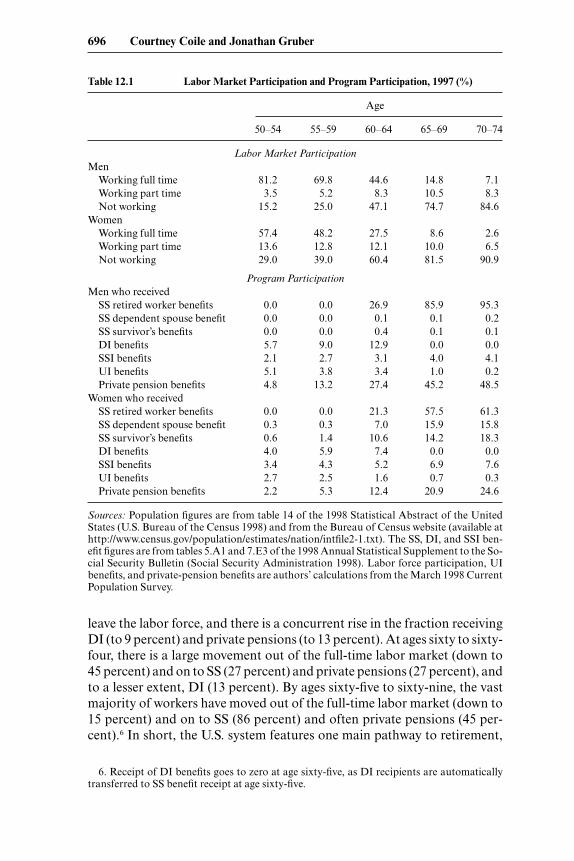
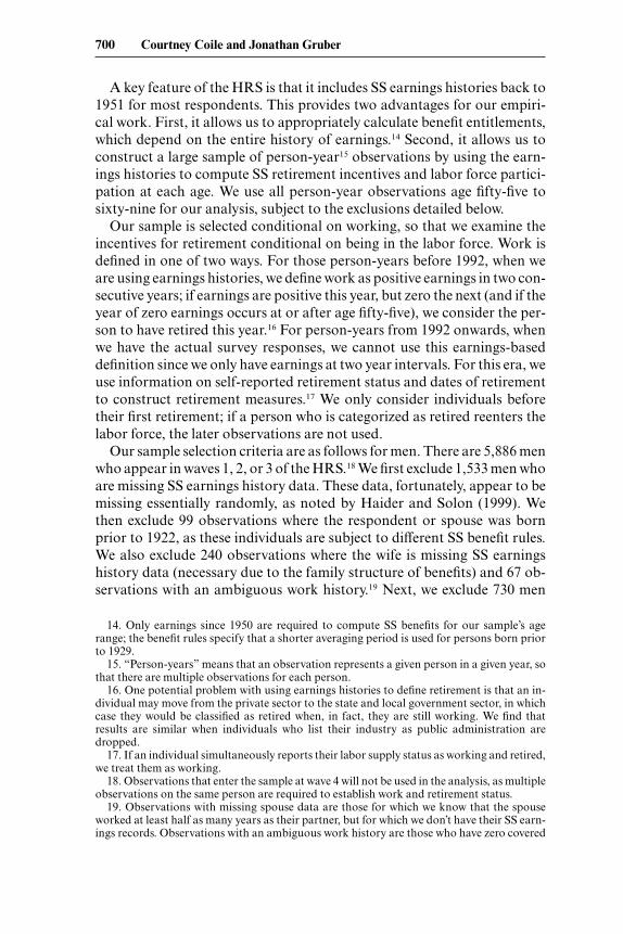
One of the most striking labor force phenomena of the second half of thetwentieth century in the United States has been the rapid decline in the la-bor force participation rate of older men. In 1950, for example, 81 percentof sixty-two-year-old men were in the labor force; by 1995, this figure hadfallen to 51 percent, although it has rebounded slightly in the past fewyears (Quinn 1999). Over the same period, the labor force participationrate of older women has risen dramatically, as shown in figure 12.1, due inlarge part to changing roles and opportunities for women during the pe-riod.
Much has been written about the proximate causes of the decline inolder men’s labor force participation and, in particular, about the role ofthe Social Security (SS) program. A large number of articles have docu-mented pronounced “spikes” in retirement at ages sixty-two and sixty-five,which correspond to the early and normal retirement ages for SS, respec-tively. While there are some other explanations for a spike at age sixty-five,such as entitlement for health insurance under the Medicare program orrounding error in surveys, there is little reason to see a spike at sixty-two as
12The Effect of Social Security onRetirement in the United States
Courtney Coile and Jonathan Gruber
Courtney Coile is assistant professor of economics at Wellesley College and a faculty re-search fellow of the National Bureau of Economic Research (NBER). Jonathan Gruber isprofessor of economics at MIT, director of the research program on children at NBER, andresearch associate of NBER.
We are grateful to Dean Karlan for research assistance and to Peter Diamond, Alan Gust-man, Jim Poterba, Andrew Samwick, and seminar participants at MIT, Harvard, NBER, andthe Social Security Administration for helpful comments, and especially to David Wise andother participants in the International Social Security Comparisons project for their insights.Coile gratefully acknowledges support from the National Institute on Aging through NBER.Gruber acknowledges support from the National Institute on Aging.
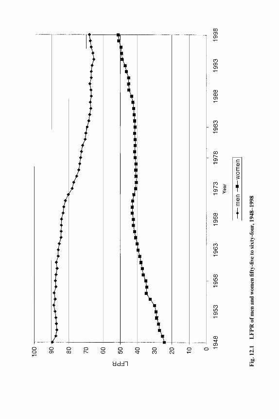
Fig
. 12.
1L
FP
R o
f men
and
wom
en fi
fty-
five
to s
ixty
-fou
r, 1
948–
1998
attributable to anything other than the SS program. Indeed, as Burtlessand Moffitt (1984) document, this spike at age sixty-two only emerged af-ter the early retirement eligibility age for men was introduced in 1961.
The presence of these strong patterns in retirement data suggest that theunderlying structure of SS plays a critical role in determining retirementdecisions, but the impact of increases in SS generosity on retirement deci-sions is less obvious. A large body of literature dating from the mid-1970shas investigated this relationship, and the broad conclusion of that litera-ture is that the level of SS benefits has a significant, but modest, effect onretirement dates. However, much of this literature either relies on data thatare now decades old or otherwise flawed or it suffers from methodologicalproblems.
The purpose of our paper is to revisit the impact of SS on retirement, tak-ing advantage of newly available data on retirement behavior and method-ological advances in retirement modeling over the past decade. Our dataset, the Health and Retirement Study (HRS), follows a sample of near-retirement-age individuals starting in 1992 and contains detailed informa-tion on demographic and job characteristics, labor force attachment, earn-ings histories, health, and private pensions.
Our empirical analysis relies on the important observation of Stock andWise (1990a,b) that it is not simply the level of retirement wealth or the in-crement with one additional year of work that matters, but the entire evo-lution of future wealth with further work. Their “option value” modelposited retirement decisions as a function of the difference between theutility of retirement at the current date and at the date that maximizes one’sutility. We use this model in a reduced-form context, as well as an alterna-tive forward-looking measure called “peak value,” introduced in Coile andGruber (2001) and described in more detail below.
We have two major findings. First, retirement appears to respond muchmore to SS incentive variables defined with reference to the entire futurestream of retirement incentives than to the accrual in retirement wealthover the next year alone, indicating that it is important to include forward-looking measures such as peak value or option value in retirement models.These forward-looking measures have a significant impact on retirementdecisions for men, although for women only the option value model gen-erates a significant result. Second, we conduct simulations of the effect oftwo possible policy changes—raising the early and normal retirement agesby three years or moving to a system with a flat benefit of 60 percent ofearnings—and find that these policy changes could have significant effectson retirement behavior.
Our paper proceeds as follows. In section 12.2, we briefly discuss the rel-evant institutional features of the SS system in the United States and pro-vide an overview of the previous literature in this area. In section 12.3, wedescribe our data and incentive variable calculations. In section 12.4, we
The Effect of Social Security on Retirement in the United States 693
describe the empirical framework for our regression analysis and presentthe results of our estimation. In section 12.5, we conduct a series of simu-lation exercises to assess the impact of SS reform using our model, and wepresent our conclusions in section 12.6.
12.2 Background
12.2.1 Institutional Features of Social Security
The SS system is financed by a payroll tax that is levied equally on work-ers and firms. The total payroll tax paid by each party is 7.65 percentagepoints; 5.3 percentage points are devoted to the Old Age and Survivors In-surance (OASI) program, with 0.9 percentage points funding the Disabil-ity Insurance (DI) system and 1.45 percentage points funding Medicare’sHospital Insurance (HI) program. The payroll tax that funds OASI and DIis levied on earnings up to the taxable maximum, $76,200 in 2000; the HItax is uncapped.
Individuals qualify for an OASI pension by working for forty quarters incovered employment, which now encompasses most sectors of the econ-omy. Benefits are determined in several steps. The first step is computationof the worker’s averaged indexed monthly earnings (AIME), which is one-twelfth of the average of the worker’s annual earnings in covered employ-ment, indexed by a national wage index. Importantly, additional higher-earnings years can replace earlier lower-earnings years, since only thehighest thirty-five years of earnings are used in the calculation.1
The next step is to convert the AIME into the primary insurance amount(PIA). This is done by applying a three-piece linear progressive scheduleto an individual’s average earnings, whereby 90 cents of the first dollar ofearnings is converted to benefits, while only 15 cents of the last dollar ofearnings (up to the taxable maximum) is so converted. As a result, the rateat which SS replaces past earnings (the “replacement rate”) falls with thelevel of lifetime earnings.
The final step is to adjust the PIA based on the age at which benefits arefirst claimed. For workers commencing benefit receipt at the normal re-tirement age (NRA; legislated to rise slowly from age sixty-five to sixty-seven over the next twenty years), the monthly benefit is the PIA. For work-ers claiming before the NRA, benefits are decreased by an actuarialreduction factor of five-ninths of one percent per month; thus, a worker
694 Courtney Coile and Jonathan Gruber
1. While earnings through age fifty-nine are converted to real dollars for averaging, earn-ings after age sixty are treated nominally. There is a two-year lag in availability of the wage in-dex, calling for a base in the year in which the worker turns sixty in order to be able to com-pute benefits for workers retiring at their sixty-second birthdays. This implies particularlylarge effects of this dropout-year provision for earnings near the age of retirement, particu-larly in high-inflation environments.
with an NRA of age sixty-five claiming on his sixty-second birthday re-ceives 80 percent of the PIA.2 Individuals can also delay the receipt of ben-efits beyond the NRA and receive a delayed retirement credit (DRC). Forworkers reaching age sixty-five in 2000, an additional 6 percent is paid foreach year of delay; this amount will steadily increase until it reaches 8 per-cent per year in 2008.
While a worker may claim as early as age sixty-two, receipt of SS bene-fits is conditioned on the earnings test until the worker reaches age sixty-five.3 A worker age sixty-two to sixty-five may earn up to $9,600 in 1999without the loss of benefits, then benefits are reduced $1 for each $2 ofearnings above this amount. Months of benefits lost through the earningstest are treated as delayed receipt, entitling the worker to a DRC on the lostbenefits when he resumes full-benefit receipt.
One of the most important features of SS is that it also provides benefitsto dependents of covered workers. Spouses receive a benefit equal to 50 per-cent of the worker’s PIA, which is available once the worker has claimedbenefits and the spouse has reached age sixty-two; however, the spouse onlyreceives the larger of this and their own entitlement as a worker.4 Depen-dent children are also each eligible for 50 percent of the PIA, but the totalfamily benefit cannot exceed a maximum that is roughly 175 percent of thePIA. Surviving spouses receive 100 percent of the PIA, beginning at agesixty, although there is an actuarial reduction for claiming benefits beforeage sixty-five or if the worker had an actuarial reduction. Finally, benefitpayments are adjusted for increases in the consumer price index (CPI) af-ter the worker has reached age sixty-two; thus, SS provides a real annuity.
12.2.2 Labor Market Participation and Program Participation
Table 12.1 documents the transition of men and women out of the laborforce and into receipt of SS and other benefits. At ages fifty to fifty-four, 81percent of men are working full time, 4 percent are working part time, and15 percent are not working. The fraction of men in this age group receivingsome type of benefit is about equal to the fraction not working and is di-vided roughly equally among those receiving DI benefits (6 percent), Un-employment Insurance (UI) benefits (5 percent), and private pensions (5percent).5 At ages fifty-five to fifty-nine, an additional 11 percent of men
The Effect of Social Security on Retirement in the United States 695
2. The reduction factor will be only five-twelfths of one percent for months beyond thirty-six months before the NRA, which is relevant for workers with an NRA past age sixty-five.
3. Until 2000, workers aged sixty-five to sixty-nine were subject to an earnings test with ahigher earnings floor and lower tax rate than that for workers aged sixty-two to sixty-five.However, the Senior Citizens’ Freedom to Work Act of 2000 eliminated the earnings test forpersons aged sixty-five to sixty-nine as of January 2000.
4. Spousal benefits can begin earlier if there is a dependent child in the household; spousalbenefits are also subject to actuarial reduction if receipt commences before the spouse’s NRA.
5. In addition, 2 percent of men are receiving supplemental security income (SSI), a means-tested benefit for people who are poor and either disabled or aged sixty-five or older.
leave the labor force, and there is a concurrent rise in the fraction receivingDI (to 9 percent) and private pensions (to 13 percent). At ages sixty to sixty-four, there is a large movement out of the full-time labor market (down to45 percent) and on to SS (27 percent) and private pensions (27 percent), andto a lesser extent, DI (13 percent). By ages sixty-five to sixty-nine, the vastmajority of workers have moved out of the full-time labor market (down to15 percent) and on to SS (86 percent) and often private pensions (45 per-cent).6 In short, the U.S. system features one main pathway to retirement,
696 Courtney Coile and Jonathan Gruber
Table 12.1 Labor Market Participation and Program Participation, 1997 (%)
Age
50–54 55–59 60–64 65–69 70–74
Labor Market ParticipationMen
Working full time 81.2 69.8 44.6 14.8 7.1Working part time 3.5 5.2 8.3 10.5 8.3Not working 15.2 25.0 47.1 74.7 84.6
WomenWorking full time 57.4 48.2 27.5 8.6 2.6Working part time 13.6 12.8 12.1 10.0 6.5Not working 29.0 39.0 60.4 81.5 90.9
Program ParticipationMen who received
SS retired worker benefits 0.0 0.0 26.9 85.9 95.3SS dependent spouse benefit 0.0 0.0 0.1 0.1 0.2SS survivor’s benefits 0.0 0.0 0.4 0.1 0.1DI benefits 5.7 9.0 12.9 0.0 0.0SSI benefits 2.1 2.7 3.1 4.0 4.1UI benefits 5.1 3.8 3.4 1.0 0.2Private pension benefits 4.8 13.2 27.4 45.2 48.5
Women who receivedSS retired worker benefits 0.0 0.0 21.3 57.5 61.3SS dependent spouse benefit 0.3 0.3 7.0 15.9 15.8SS survivor’s benefits 0.6 1.4 10.6 14.2 18.3DI benefits 4.0 5.9 7.4 0.0 0.0SSI benefits 3.4 4.3 5.2 6.9 7.6UI benefits 2.7 2.5 1.6 0.7 0.3Private pension benefits 2.2 5.3 12.4 20.9 24.6
Sources: Population figures are from table 14 of the 1998 Statistical Abstract of the UnitedStates (U.S. Bureau of the Census 1998) and from the Bureau of Census website (available athttp://www.census.gov/population/estimates/nation/intfile2-1.txt). The SS, DI, and SSI ben-efit figures are from tables 5.A1 and 7.E3 of the 1998 Annual Statistical Supplement to the So-cial Security Bulletin (Social Security Administration 1998). Labor force participation, UIbenefits, and private-pension benefits are authors’ calculations from the March 1998 CurrentPopulation Survey.
6. Receipt of DI benefits goes to zero at age sixty-five, as DI recipients are automaticallytransferred to SS benefit receipt at age sixty-five.
from full-time work to receipt of SS (and frequently private pension bene-fits), a move that typically occurs between ages sixty-two and sixty-five.This is in contrast to many other developed countries, where many peopleexit the labor force at earlier ages and receive UI or DI benefits prior to be-coming eligible for retirement benefits. As use of these other paths to retire-ment is minimal in the United States, they will not factor into our analysis.
For women, the patterns are similar but with a few notable differences.First, a lower fraction of women are initially working full time at ages fiftyto fifty-four (57 percent); this reflects both a higher fraction of women outof the labor force entirely (29 percent) and a higher fraction working parttime (14 percent). Second, while many women receive SS benefits based ontheir own work record (58 percent of women at ages sixty-five to sixty-nine), a significant fraction receive benefits only as a result of being a de-pendent spouse (16 percent) or widow (14 percent). Third, fewer womenreceive private pension benefits (21 percent at ages sixty-five to sixty-nine,versus 45 percent of men).
12.2.3 Previous Related Literature
A number of studies have used aggregate information on the labor forcebehavior of workers at different ages to infer the role played by SS. Hurd(1990) and Ruhm (1995) emphasize the spike in the age pattern of retire-ment at age sixty-two; as Hurd states, “there are no other institutional oreconomic reasons for the peak” (597). Using quarterly data, Blau (1994)finds that almost one-quarter of the men in the labor force at their sixty-fifth birthday retire in the next three months; this hazard rate is over 2.5times as large as the rate in surrounding quarters. Lumsdaine and Wise(1994) examine this excess retirement at sixty-five and conclude that it can-not be explained by the change in the actuarial adjustment at this age, bythe incentives in private pension plans, or by the availability of retirementhealth insurance through Medicare. However, SS may still play an impor-tant role by setting up the focal point of a normal retirement age.
The main body of the retirement incentives literature attempts to specif-ically model the role that potential SS benefits play in determining retire-ment. The earliest work in this area considered reduced-form models of theretirement decision as a function of SS wealth (SSW) and pension levels.Much of this literature is reviewed in Mitchell and Fields (1982); more re-cent cites include Diamond and Hausman (1984) and Blau (1994). Whilethese articles differ in the estimation strategies, with the more recent workusing richer models, such as nonlinear 2SLS or hazard modeling, their re-sults generally suggest that SS’s role is significant but small relative to thetime trends in retirement behavior.
A key limitation of these studies is that they consider SS effects at a pointin time, but not any impacts on the retirement decision arising from thetime pattern of SSW accruals. This was remedied in three different ways bysubsequent literatures. The first was to use structural models of retirement
The Effect of Social Security on Retirement in the United States 697
decisions by workers facing a lifetime budget constraint; for example, seeBurtless (1986), Burtless and Moffitt (1984), Gustman and Steinmeier(1985, 1986), and Rust and Phelan (1997). The second was to estimate re-duced-form models, but incorporate the accrual of SSW with a year of ad-ditional work; for example, see Fields and Mitchell (1984), Hausman andWise (1985), and Sueyoshi (1989). Both of these types of studies continuedto find an important, but modest, role for SS, and some indicated a largerrole for private pensions. The final type of literature is the option valuework of Stock and Wise noted previously.7
A final article that deserves particular mention is that of Krueger andPischke (1992). They note that the key regressor in many of these articles,SS benefits, is a nonlinear function of past earnings and that retirementpropensities are clearly correlated with past earnings. They solve this prob-lem by using a unique natural experiment provided by the end of double-indexing for the “notch generation” that retired in the late 1970s and early1980s. For this cohort, SS benefits were greatly reduced relative to whatthey would have expected, yet the dramatic fall in labor force participationcontinued unabated in this era. This raises important questions about theidentification of the cross-sectional literature. However, Krueger and Pis-chke still find significant and sizeable impacts of SS accruals on retirement,which highlights the value of the dynamic approach and suggest that theadditional nonlinearities that govern the evolution of SSW (as opposed toits level) may be a fruitful source of identification for retirement models.
Each of these dynamic literatures has important limitations. The firstsuffers from the perhaps untenable assumptions that are required to iden-tify these very complicated structural models.8 The second suffers from thelimited way in which dynamic retirement incentives are specified. Someof these problems are remedied by the option value literature, but this lit-erature has not separated the impact of SS incentives, as distinct from pen-sion incentives, on retirement.9 If all dollars of retirement wealth are notweighed equally by potential retirees, either because individuals under-stand their firm’s pension incentives better than SS incentives or becausethe real annuity provided by SS is valued differently than the nominal an-nuity provided by most defined-benefit pensions, then it is important toseparately estimate SS and private pension impacts.10
In addition, all of these studies suffer from important data deficiencies,as they use data from the 1970s (when the structure of the SS system wasfairly different), data from only a handful of firms, or data without com-
698 Courtney Coile and Jonathan Gruber
7. See also Samwick (1998), who uses the option value model in a reduced-form context.8. For a criticism of this type in the context of this type of estimation of general labor supply
responses, see MaCurdy (1981).9. Stock and Wise did not attempt this decomposition, and Samwick’s (1998) attempt to do
so with a reduced-form version of the option value model was unsuccessful, perhaps due tothe measurement error in SS incentives arising from a lack of earnings-history data.
10. The latter is suggested by Diamond and Hausman (1984), who find much smaller effectsof pensions on retirement than those of SS.
plete information on SS incentives. Finally, all of the literature suffer froma lack of careful attention to the sources of identification of the retirementincentive effects that they estimate. As highlighted by Krueger and Pischke(1992), SS benefits are a nonlinear function of earnings, making it difficultto disentangle their impact from the separate impact of earnings on thework decision. This problem is not necessarily surmounted and is poten-tially compounded, by the option value literature, as this measure is largelydetermined by wage differences across individuals and only secondarily in-fluenced by the structure of retirement incentives. In principle, this prob-lem can be surmounted by structural estimation of the option value model,which will identify the difference in the impacts of wages and retirement in-come on retirement decisions through the value of leisure parameter. But,in practice, this is only true if the particular utility structure is correct; forexample, if the additional leisure of utility enters the model only as a mul-tiplier on postretirement income and not in some other way.
To address these concerns, Coile and Gruber (2000, 2001) introduce anew measure, peak value, which incorporates the insights of the optionvalue measure but focuses solely on variation in SS incentives. This is com-parable to the accrual, but looks forward more than just one year: It cal-culates the difference between SSW at its maximum expected value andSSW at today’s value in order to measure the incentive to continued work.The peak value appropriately considers the trade-off between retiring to-day and working to a period with much higher SSW, thereby capturing theoption value of continued work even before SS entitlement ages arereached. Since wage is not included specifically into the peak value calcu-lation, there is much more variation from the structure of the SS entitle-ment.11 In the empirical analysis below, both peak value and option valueare used in a reduced-form context.
12.3 Data and Empirical Strategy
12.3.1 Data
Our data for this analysis comes from the HRS.12 The HRS is a survey of12,652 individuals aged fifty-one to sixty-one in 1992 with reinterviewsevery two years; the first four waves of the survey (1992, 1994, 1996, and1998) are used in this analysis.13 Spouses of respondents are also inter-viewed, so the total age range covered by the survey is much wider.
The Effect of Social Security on Retirement in the United States 699
11. In our sample, an earnings quartic and age dummies explain only 33 percent of the vari-ation in peak value versus 74 percent of the variation in option value.
12. The HRS is conducted by the Survey Research Center at the University of Michigan inAnn Arbor, Michigan. The data is available at http://www.umich.edu/~hrswww/. Most of thedata is publicly available, although the SS and firm-level private-pension data is restricted toapproved users.
13. The 1998 wave 4 data are preliminary.
A key feature of the HRS is that it includes SS earnings histories back to1951 for most respondents. This provides two advantages for our empiri-cal work. First, it allows us to appropriately calculate benefit entitlements,which depend on the entire history of earnings.14 Second, it allows us toconstruct a large sample of person-year15 observations by using the earn-ings histories to compute SS retirement incentives and labor force partici-pation at each age. We use all person-year observations age fifty-five tosixty-nine for our analysis, subject to the exclusions detailed below.
Our sample is selected conditional on working, so that we examine theincentives for retirement conditional on being in the labor force. Work isdefined in one of two ways. For those person-years before 1992, when weare using earnings histories, we define work as positive earnings in two con-secutive years; if earnings are positive this year, but zero the next (and if theyear of zero earnings occurs at or after age fifty-five), we consider the per-son to have retired this year.16 For person-years from 1992 onwards, whenwe have the actual survey responses, we cannot use this earnings-baseddefinition since we only have earnings at two year intervals. For this era, weuse information on self-reported retirement status and dates of retirementto construct retirement measures.17 We only consider individuals beforetheir first retirement; if a person who is categorized as retired reenters thelabor force, the later observations are not used.
Our sample selection criteria are as follows for men. There are 5,886 menwho appear in waves 1, 2, or 3 of the HRS.18 We first exclude 1,533 men whoare missing SS earnings history data. These data, fortunately, appear to bemissing essentially randomly, as noted by Haider and Solon (1999). Wethen exclude 99 observations where the respondent or spouse was bornprior to 1922, as these individuals are subject to different SS benefit rules.We also exclude 240 observations where the wife is missing SS earningshistory data (necessary due to the family structure of benefits) and 67 ob-servations with an ambiguous work history.19 Next, we exclude 730 men
700 Courtney Coile and Jonathan Gruber
14. Only earnings since 1950 are required to compute SS benefits for our sample’s agerange; the benefit rules specify that a shorter averaging period is used for persons born priorto 1929.
15. “Person-years” means that an observation represents a given person in a given year, sothat there are multiple observations for each person.
16. One potential problem with using earnings histories to define retirement is that an in-dividual may move from the private sector to the state and local government sector, in whichcase they would be classified as retired when, in fact, they are still working. We find thatresults are similar when individuals who list their industry as public administration aredropped.
17. If an individual simultaneously reports their labor supply status as working and retired,we treat them as working.
18. Observations that enter the sample at wave 4 will not be used in the analysis, as multipleobservations on the same person are required to establish work and retirement status.
19. Observations with missing spouse data are those for which we know that the spouseworked at least half as many years as their partner, but for which we don’t have their SS earn-ings records. Observations with an ambiguous work history are those who have zero covered
who retired prior to age fifty-five. The remaining 3,217 men are convertedinto 18,733 person-year observations by creating one observation for eachyear from 1980 through 1997 in which the individual is between the ages offifty-five and sixty-nine and working at the beginning of the year. Finally,we exclude 988 person-year observations that represent labor force reentryafter a previous retirement. The final sample size is 17,745 male observa-tions. A similar process generates a sample size of 11,419 female observa-tions.
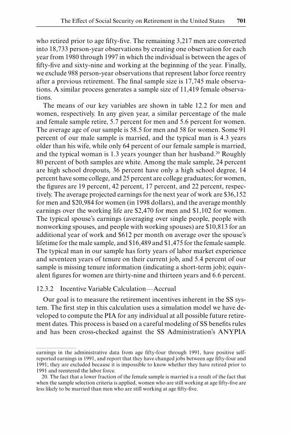
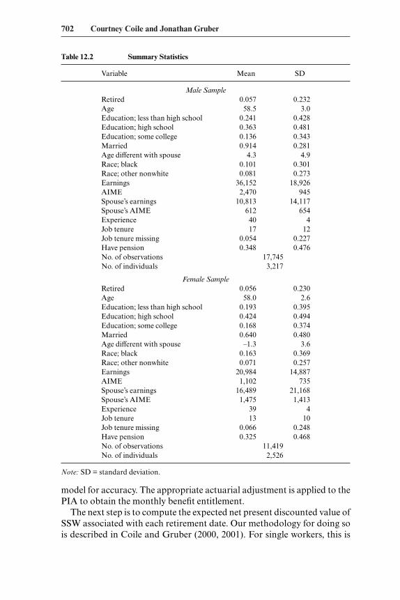
The means of our key variables are shown in table 12.2 for men andwomen, respectively. In any given year, a similar percentage of the maleand female sample retire, 5.7 percent for men and 5.6 percent for women.The average age of our sample is 58.5 for men and 58 for women. Some 91percent of our male sample is married, and the typical man is 4.3 yearsolder than his wife, while only 64 percent of our female sample is married,and the typical woman is 1.3 years younger than her husband.20 Roughly80 percent of both samples are white. Among the male sample, 24 percentare high school dropouts, 36 percent have only a high school degree, 14percent have some college, and 25 percent are college graduates; for women,the figures are 19 percent, 42 percent, 17 percent, and 22 percent, respec-tively. The average projected earnings for the next year of work are $36,152for men and $20,984 for women (in 1998 dollars), and the average monthlyearnings over the working life are $2,470 for men and $1,102 for women.The typical spouse’s earnings (averaging over single people, people withnonworking spouses, and people with working spouses) are $10,813 for anadditional year of work and $612 per month on average over the spouse’slifetime for the male sample, and $16,489 and $1,475 for the female sample.The typical man in our sample has forty years of labor market experienceand seventeen years of tenure on their current job, and 5.4 percent of oursample is missing tenure information (indicating a short-term job); equiv-alent figures for women are thirty-nine and thirteen years and 6.6 percent.
12.3.2 Incentive Variable Calculation—Accrual
Our goal is to measure the retirement incentives inherent in the SS sys-tem. The first step in this calculation uses a simulation model we have de-veloped to compute the PIA for any individual at all possible future retire-ment dates. This process is based on a careful modeling of SS benefits rulesand has been cross-checked against the SS Administration’s ANYPIA
The Effect of Social Security on Retirement in the United States 701
earnings in the administrative data from age fifty-four through 1991, have positive self-reported earnings in 1991, and report that they have changed jobs between age fifty-four and1991; they are excluded because it is impossible to know whether they have retired prior to1991 and reentered the labor force.
20. The fact that a lower fraction of the female sample is married is a result of the fact thatwhen the sample selection criteria is applied, women who are still working at age fifty-five areless likely to be married than men who are still working at age fifty-five.
702 Courtney Coile and Jonathan Gruber
Table 12.2 Summary Statistics
Variable Mean SD
Male SampleRetired 0.057 0.232Age 58.5 3.0Education; less than high school 0.241 0.428Education; high school 0.363 0.481Education; some college 0.136 0.343Married 0.914 0.281Age different with spouse 4.3 4.9Race; black 0.101 0.301Race; other nonwhite 0.081 0.273Earnings 36,152 18,926AIME 2,470 945Spouse’s earnings 10,813 14,117Spouse’s AIME 612 654Experience 40 4Job tenure 17 12Job tenure missing 0.054 0.227Have pension 0.348 0.476No. of observations 17,745No. of individuals 3,217
Female SampleRetired 0.056 0.230Age 58.0 2.6Education; less than high school 0.193 0.395Education; high school 0.424 0.494Education; some college 0.168 0.374Married 0.640 0.480Age different with spouse –1.3 3.6Race; black 0.163 0.369Race; other nonwhite 0.071 0.257Earnings 20,984 14,887AIME 1,102 735Spouse’s earnings 16,489 21,168Spouse’s AIME 1,475 1,413Experience 39 4Job tenure 13 10Job tenure missing 0.066 0.248Have pension 0.325 0.468No. of observations 11,419No. of individuals 2,526
Note: SD = standard deviation.
model for accuracy. The appropriate actuarial adjustment is applied to thePIA to obtain the monthly benefit entitlement.
The next step is to compute the expected net present discounted value ofSSW associated with each retirement date. Our methodology for doing sois described in Coile and Gruber (2000, 2001). For single workers, this is
simply a sum of future benefits discounted by time preference rates andsurvival probabilities. For married workers, it is more complicated since wemust include dependent spouse and survivor benefits and account for thejoint likelihood of survival of the worker and dependent. We use a real dis-count rate of 3 percent and survival probabilities from the age- and sex-specific U.S. life tables from the U.S. Department of Health and HumanServices (National Center for Health Statistics 1990, sec. 6).
We next compute the other SS incentive variables. We first calculate theaccrual, the change in SSW resulting from an additional year of work.There are two routes through which an additional year of work affectsSSW. First, the additional year of earnings will be used in the recomputa-tion of SS benefits. For workers who have not yet worked thirty-five years,this replaces a zero in the benefits computation; for workers who haveworked thirty-five years, it may replace a previous low-earnings year. Sothe recomputation raises SSW (or leaves it unchanged). Second, at agessixty-two and beyond, the additional year of work implies a delay in claim-ing; this raises future benefits through the actuarial adjustment, but re-duces the number of years of benefit receipt, so the net effect is uncertain.Both of these factors will affect workers differently, depending on their po-tential earnings next year, earnings history, mortality prospects (which willvary over time and cohort in our data), family structure, and spouse’s earn-ings. Thus, the net effect of an additional year of work on SSW is theoreti-cally ambiguous and will vary significantly across people.
Computing the accrual and other incentive variables requires projectingthe worker’s potential earnings next year (or in all future years). We con-sidered a number of different projection methodologies and found that thebest predictive performance was from a model which simply grew realearnings from the last observation by 1 percent per year, so we use this as-sumption in our simulations.21
Our SS incentive variables incorporate dependent spouse and survivorbenefits, since these are important components of SSW. For a worker witha nonworking spouse, these benefits are based solely on the worker’s earn-ings record. For a worker whose spouse is entitled to benefits on their own,the spouse’s benefits are based (partially or fully) on the spouse’s record,but are also included in SSW. Since a full modeling of the joint retirementdecision is beyond the scope of this paper, we simply assume that spouseswho are working will retire at age sixty-two; this seems reasonable, giventhat the median retirement age is sixty-two for women in the sample andsixty-three for men. For more evidence on joint retirement decisions, seeCoile (1999).
The Effect of Social Security on Retirement in the United States 703
21. Projected earnings always represent potential earnings for one full year. For example,in the case where an individual earns $2X in year t and $X in year t � 1 because they retirehalfway through the year, the year t � 1 observation has projected real earnings of $2X �(1.01) and there is no t � 2 observation (since the individual retires in year t � 1).
For the simulations below, we assume that workers claim SS benefits atretirement or when they become eligible (age sixty-two), if they have retiredbefore then. In fact, this is not necessarily true; retirement and claiming aretwo distinct events, and for certain values of mortality prospects and dis-count rates, it is optimal to delay claiming until some time after retirement,due to the actuarial adjustment of benefits. Coile et al. (2002) investigatethis issue in some detail, and they find that a relatively small share of thoseretiring before age sixty-two delay claiming until age sixty-three (about 10percent) and that virtually none of those retiring at age sixty-two or laterdelay claiming. Given these findings, we choose not to jointly model de-layed claiming here. Our incentive measures will therefore slightly over-state any subsidies to continued work, since part of this subsidy will comefrom delayed claiming that could be obtained without delaying retirement.
We do not incorporate private pension incentives into our analysis.Coile and Gruber (2000) estimate retirement models that include both SSand pension incentives, and they find that the results differ significantlyfrom those for SS alone. This suggests that changes in private pension pro-visions may have different impacts on retirement than changes in publicpensions, so that one should not extrapolate the effect of public pensionreform from private pension responses. Thus, since our primary goal is todiscuss the impacts of public pensions on retirement, we exclude privatepensions here.
Table 12.3 shows the medians of the retirement incentive variables forour male sample by age. The median present discounted value (PDV) risesfrom $179,316 at age fifty-five to a peak of $205,584 at age sixty-five, thenfalls to $194,555 at age sixty-nine.22 The age pattern of accruals demon-strates how the various effects of working an additional year enter in atdifferent ages. From ages fifty-five to sixty-one, accruals are positive, butsmall, reflecting the value of the dropout year provision. From ages sixty-two to sixty-four, accruals are two to three times larger; this is the delayed-claiming effect, whereby an additional year of work increases the actuarialadjustment and raises future benefits.23 After age sixty-five, accruals be-come negative and rise rapidly, as the delayed retirement credit is insuffi-cient to compensate for the value of lost benefits.
Most importantly for our analysis, there is enormous heterogeneity inaccruals, as is also shown in table 12.3. The standard deviation in accru-
704 Courtney Coile and Jonathan Gruber
22. The SSW median displayed in table 12.2 is the median SSW at age fifty-five increased ordecreased each year by the median accrual. The median SSW at each age in the sample risesmuch more rapidly with age due to a sample selection effect (those working at later ages havehigher SSW).
23. This large subsidy to work at age sixty-two is at odds with the common wisdom that theactuarial reduction at age sixty-two is approximately fair. This point is developed much fur-ther in Coile and Gruber (2000).
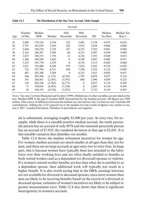
als is substantial, averaging roughly $3,000 per year. At sixty-two, for ex-ample, while there is a sizeable positive median accrual, the tenth percen-tile person has an accrual of only $978 and the ninetieth percentile personhas an accrual of $7,032; the standard deviation at that age is $2,691. It isthis sizeable variation that identifies our models.
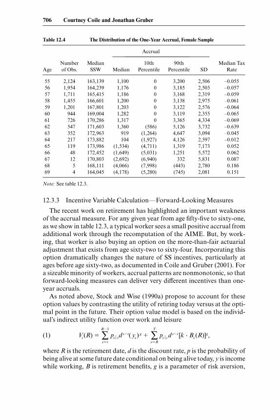
Table 12.4 shows the median retirement incentives for women by age.For women, median accruals are much smaller at all ages than they are formen, and there are no large accruals at ages sixty-two to sixty-four. In largepart, this is because women have typically been less attached to the laborforce over their working lives and are often dually entitled to benefits asboth retired workers and as a dependent (or divorced) spouses or widows.If a woman’s retired-worker benefits are less than what she is entitled to asa dependent spouse, then additional work will typically not result in ahigher benefit. It is also worth noting that in the HRS, earnings historiesare not available for divorced or deceased spouses; since more women thanmen are likely to be receiving benefits based on the record of a divorced ordeceased spouse, estimates of women’s incentives are likely to be subject togreater measurement error. Table 12.4 also shows that there is significantheterogeneity in women’s accruals.
The Effect of Social Security on Retirement in the United States 705
Table 12.3 The Distribution of the One-Year Accrual, Male Sample
Accrual
Number Median 10th 90th Median Median TaxAge of Obs. SSW Median Percentile Percentile SD Tax Rate Rate 2
55 2,809 179,316 2,554 322 5,492 2,334 –0.072 –0.02256 2,747 181,870 2,369 243 5,032 3,859 –0.066 0.04657 2,444 184,239 2,128 167 4,555 3,382 –0.061 0.06058 2,143 186,367 1,948 66 4,233 2,497 –0.054 0.06959 1,823 188,315 1,793 12 4,136 3,191 –0.048 0.07260 1,546 190,108 1,662 0 4,190 2,007 –0.042 0.07161 1,255 191,770 1,670 0 4,170 5,113 –0.043 0.06462 1,021 193,440 4,349 978 7,032 2,691 –0.118 –0.02863 716 197,789 4,511 430 7,394 3,532 –0.122 –0.00564 483 202,300 3,284 0 6,152 2,631 –0.093 0.03165 344 205,584 (1,123) (4,741) 1,785 4,470 0.027 0.11866 191 204,461 (2,301) (5,591) 600 2,996 0.059 0.22567 110 202,160 (3,302) (6,773) 0 8,027 0.114 0.26968 71 198,858 (4,303) (7,530) 0 2,693 0.134 0.43969 42 194,555 (4,758) (7,825) 0 2,735 0.119 0.455
Notes: Tax rate 2 is from Diamond and Gruber (1999). Definitions of other variables are provided in thetext. Median SSW is the age-55 median SSW incremented by the median accrual. All figures are 1998dollars. One source of difference between the median tax rate and tax rate 2 is that tax rate 2 includes SScontributions. Adding the 12.4% payroll tax to the median tax rate results in figures very similar to taxrate 2. SD = standard deviation. Numbers in parentheses are negative.
12.3.3 Incentive Variable Calculation—Forward-Looking Measures
The recent work on retirement has highlighted an important weaknessof the accrual measure. For any given year from age fifty-five to sixty-one,as we show in table 12.3, a typical worker sees a small positive accrual fromadditional work through the recomputation of the AIME. But, by work-ing, that worker is also buying an option on the more-than-fair actuarialadjustment that exists from age sixty-two to sixty-four. Incorporating thisoption dramatically changes the nature of SS incentives, particularly atages before age sixty-two, as documented in Coile and Gruber (2001). Fora sizeable minority of workers, accrual patterns are nonmonotonic, so thatforward-looking measures can deliver very different incentives than one-year accruals.
As noted above, Stock and Wise (1990a) propose to account for theseoption values by contrasting the utility of retiring today versus at the opti-mal point in the future. Their option value model is based on the individ-ual’s indirect utility function over work and leisure
(1) Vt (R) � ∑R�1
s�t
pstds�t( ys )
g � ∑T
s�R
pstds�t [k � Bs (R)]g,
where R is the retirement date, d is the discount rate, p is the probability ofbeing alive at some future date conditional on being alive today, y is incomewhile working, B is retirement benefits, g is a parameter of risk aversion,
706 Courtney Coile and Jonathan Gruber
Table 12.4 The Distribution of the One-Year Accrual, Female Sample
Accrual
Number Median 10th 90th Median TaxAge of Obs. SSW Median Percentile Percentile SD Rate
55 2,124 163,139 1,100 0 3,200 2,506 –0.05556 1,954 164,239 1,176 0 3,185 2,503 –0.05757 1,711 165,415 1,186 0 3,168 2,319 –0.05958 1,455 166,601 1,200 0 3,138 2,975 –0.06159 1,201 167,801 1,203 0 3,122 2,576 –0.06460 944 169,004 1,282 0 3,119 2,355 –0.06561 726 170,286 1,317 0 3,365 4,334 –0.06962 547 171,603 1,360 (586) 5,126 3,732 –0.63963 352 172,963 919 (1,264) 4,647 3,094 –0.04564 217 173,882 104 (1,927) 4,126 2,597 –0.01265 119 173,986 (1,534) (4,711) 1,319 7,173 0.05266 48 172,452 (1,649) (5,031) 1,251 5,572 0.06267 12 170,803 (2,692) (6,940) 332 5,831 0.08768 5 168,111 (4,066) (7,998) (443) 2,780 0.18669 4 164,045 (4,178) (5,280) (745) 2,081 0.151
Note: See table 12.3.
k is a parameter to account for disutility of labor (k � 1), and T is maxi-mum life length.
In this model, additional work has three effects. First, it raises total wageearnings, increasing utility. Second, it reduces the number of years overwhich benefits are received, lowering utility. Third, it may raise or lower thebenefit amount, depending on the shape of the benefit function, B(R). Thelatter two effects are weighted more heavily because of the disutility of la-bor, which acts as a devaluation of wage income relative to retirement in-come. The optimal date of retirement is the date at which the utility gainedfrom the increase in earnings resulting from additional work is outweighedby the utility lost from the decrease in retirement income. The option valueis the difference between the indirect utility from retirement at the optimaldate, R∗, and the indirect utility from retirement today. As a structural es-timation of the option value model is beyond the scope of this paper, we in-stead calculate the option value using reasonable utility parameters andinclude it as a regressor in a retirement model.24
As mentioned above, one possible weakness of the option value model isthat much of the variation in this measure arises from differences in wages,which may not be a legitimate source of identification of retirement effects.We take two approaches to addressing this potential shortcoming. First,we include rich controls for earnings in the retirement model to capture theheterogeneity that may bias these estimates. However, since wages enterhighly nonlinearly in the option value and the form of heterogeneity is un-known, even rich wage controls may not fully capture the underlying cor-respondence between option value and tastes for work.
Therefore, we also estimate retirement models utilizing the peak valuemeasure. As described above, peak value is the difference between SSW atits maximum expected value and SSW at today’s value.25 In this way, thepeak value incorporates the insights of the option value measure and ap-propriately considers the trade-off between retiring today and working toa period with much higher SSW, but focuses solely on variation in SS in-centives.
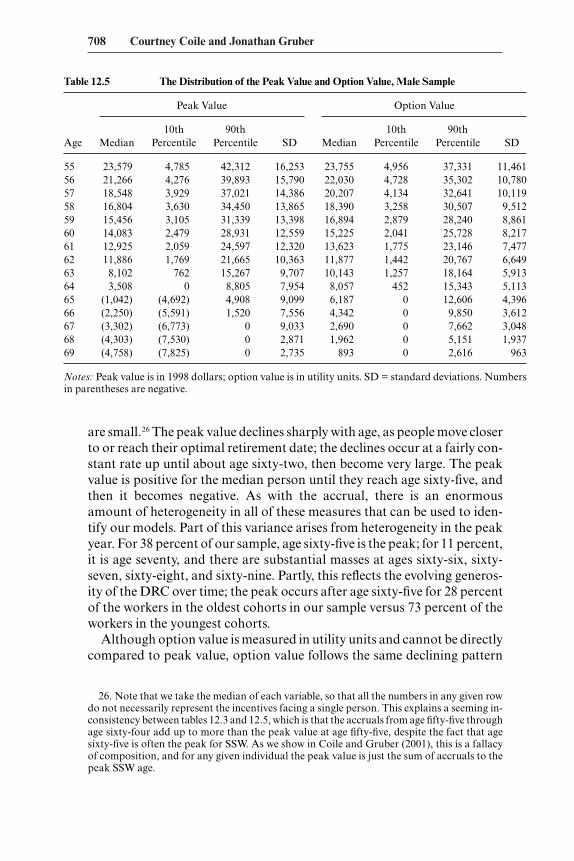
Table 12.5 shows the age pattern and heterogeneity for peak and optionvalue for the male sample. The important differences between peak valueand accrual, particularly at younger ages, are immediately apparent; peakvalues are quite large, at ages fifty-five to sixty-one, a range where accruals
The Effect of Social Security on Retirement in the United States 707
24. We follow Stock and Wise in assuming values of 1.5 and 0.75 for k and g, respectively,but we found that the fit of our model was much better with a more reasonable assumptionfor d of 0.97, relative to the very high discount rate of 0.75 obtained from their model. We alsotested the robustness of our model to the choice of k and g and the results are not sensitive tothis choice.
25. If the individual is at an age that is beyond the SSW optimum, then the peak value is thedifference between retirement this year and next year, which is exactly the accrual rate.
708 Courtney Coile and Jonathan Gruber
Table 12.5 The Distribution of the Peak Value and Option Value, Male Sample
Peak Value Option Value
10th 90th 10th 90thAge Median Percentile Percentile SD Median Percentile Percentile SD
55 23,579 4,785 42,312 16,253 23,755 4,956 37,331 11,46156 21,266 4,276 39,893 15,790 22,030 4,728 35,302 10,78057 18,548 3,929 37,021 14,386 20,207 4,134 32,641 10,11958 16,804 3,630 34,450 13,865 18,390 3,258 30,507 9,51259 15,456 3,105 31,339 13,398 16,894 2,879 28,240 8,86160 14,083 2,479 28,931 12,559 15,225 2,041 25,728 8,21761 12,925 2,059 24,597 12,320 13,623 1,775 23,146 7,47762 11,886 1,769 21,665 10,363 11,877 1,442 20,767 6,64963 8,102 762 15,267 9,707 10,143 1,257 18,164 5,91364 3,508 0 8,805 7,954 8,057 452 15,343 5,11365 (1,042) (4,692) 4,908 9,099 6,187 0 12,606 4,39666 (2,250) (5,591) 1,520 7,556 4,342 0 9,850 3,61267 (3,302) (6,773) 0 9,033 2,690 0 7,662 3,04868 (4,303) (7,530) 0 2,871 1,962 0 5,151 1,93769 (4,758) (7,825) 0 2,735 893 0 2,616 963
Notes: Peak value is in 1998 dollars; option value is in utility units. SD = standard deviations. Numbersin parentheses are negative.
are small.26 The peak value declines sharply with age, as people move closerto or reach their optimal retirement date; the declines occur at a fairly con-stant rate up until about age sixty-two, then become very large. The peakvalue is positive for the median person until they reach age sixty-five, andthen it becomes negative. As with the accrual, there is an enormousamount of heterogeneity in all of these measures that can be used to iden-tify our models. Part of this variance arises from heterogeneity in the peakyear. For 38 percent of our sample, age sixty-five is the peak; for 11 percent,it is age seventy, and there are substantial masses at ages sixty-six, sixty-seven, sixty-eight, and sixty-nine. Partly, this reflects the evolving generos-ity of the DRC over time; the peak occurs after age sixty-five for 28 percentof the workers in the oldest cohorts in our sample versus 73 percent of theworkers in the youngest cohorts.
Although option value is measured in utility units and cannot be directlycompared to peak value, option value follows the same declining pattern
26. Note that we take the median of each variable, so that all the numbers in any given rowdo not necessarily represent the incentives facing a single person. This explains a seeming in-consistency between tables 12.3 and 12.5, which is that the accruals from age fifty-five throughage sixty-four add up to more than the peak value at age fifty-five, despite the fact that agesixty-five is often the peak for SSW. As we show in Coile and Gruber (2001), this is a fallacyof composition, and for any given individual the peak value is just the sum of accruals to thepeak SSW age.
as peak value. The median option value falls monotonically with age, butremains positive even beyond age sixty-five, as additional earnings offsetlosses in SSW. There is also substantial heterogeneity in the option valuemeasure.
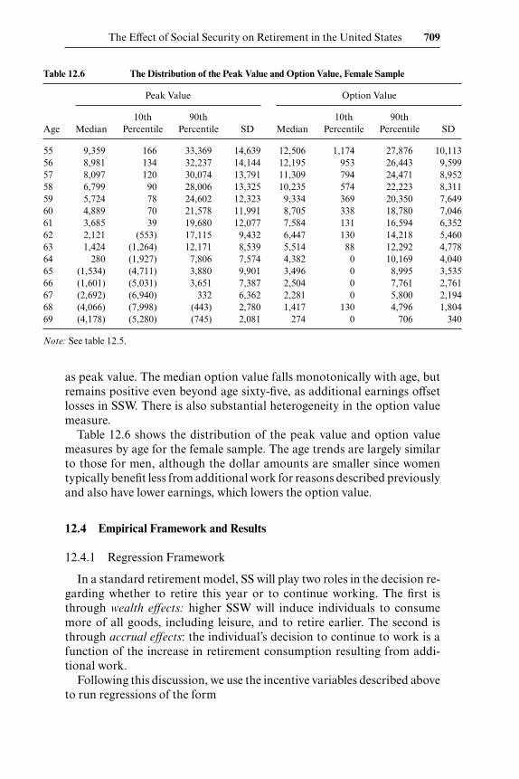
Table 12.6 shows the distribution of the peak value and option valuemeasures by age for the female sample. The age trends are largely similarto those for men, although the dollar amounts are smaller since womentypically benefit less from additional work for reasons described previouslyand also have lower earnings, which lowers the option value.
12.4 Empirical Framework and Results
12.4.1 Regression Framework
In a standard retirement model, SS will play two roles in the decision re-garding whether to retire this year or to continue working. The first isthrough wealth effects: higher SSW will induce individuals to consumemore of all goods, including leisure, and to retire earlier. The second isthrough accrual effects: the individual’s decision to continue to work is afunction of the increase in retirement consumption resulting from addi-tional work.
Following this discussion, we use the incentive variables described aboveto run regressions of the form
The Effect of Social Security on Retirement in the United States 709
Table 12.6 The Distribution of the Peak Value and Option Value, Female Sample
Peak Value Option Value
10th 90th 10th 90thAge Median Percentile Percentile SD Median Percentile Percentile SD
55 9,359 166 33,369 14,639 12,506 1,174 27,876 10,11356 8,981 134 32,237 14,144 12,195 953 26,443 9,59957 8,097 120 30,074 13,791 11,309 794 24,471 8,95258 6,799 90 28,006 13,325 10,235 574 22,223 8,31159 5,724 78 24,602 12,323 9,334 369 20,350 7,64960 4,889 70 21,578 11,991 8,705 338 18,780 7,04661 3,685 39 19,680 12,077 7,584 131 16,594 6,35262 2,121 (553) 17,115 9,432 6,447 130 14,218 5,46063 1,424 (1,264) 12,171 8,539 5,514 88 12,292 4,77864 280 (1,927) 7,806 7,574 4,382 0 10,169 4,04065 (1,534) (4,711) 3,880 9,901 3,496 0 8,995 3,53566 (1,601) (5,031) 3,651 7,387 2,504 0 7,761 2,76167 (2,692) (6,940) 332 6,362 2,281 0 5,800 2,19468 (4,066) (7,998) (443) 2,780 1,417 130 4,796 1,80469 (4,178) (5,280) (745) 2,081 274 0 706 340
Note: See table 12.5.
(2) Rit � b0 � b1SSWit � b2INCENTit � b3Xit � b4AGE it � b5EARNit
� b6AIMEit � b7MARit � b8AGEDIFFi � b9SPEARNit
� b10SPAIMEit � b11Yt � e,
where SSW is the expected PDV of SS benefits that is available to the per-son if he retires that year (t); INCENT is one of the incentive measuresnoted above (accrual, option value, and peak value); X is a vector of con-trol variables that may importantly influence the retirement decision, butdo not enter directly into the calculation of SSW (education, race, veteranstatus, born in the United States, region of residence, experience in the la-bor market and its square,27 tenure at the firm and its square, thirteen ma-jor industry dummies, and seventeen major occupation dummies); AGE iseither entered linearly or as a set of dummies for each age fifty-five to sixty-nine; EARN is a control for potential earnings in the next year; AIME is acontrol for average monthly lifetime earnings as of period t;28 MAR is adummy for marital status; AGEDIFF controls for the age difference withthe spouse; SPEARN and SPAIME are the spouse’s next year and averagelifetime earnings; and Y is a series of year dummies. Since our dependentvariable is dichotomous, we estimate the model as a probit. We have alsoestimated these models as Cox proportional hazard models and the resultswere very similar; this is not surprising, given that the models all include afull set of age dummies that pick up the same factors captured by the base-line in the hazard model.
This model parallels the types of models used in the first round of re-search on SS and retirement, with one important exception: the earningscontrols. Most articles in this literature did not control for earnings, and noarticles controlled for both earnings around time of retirement and averagelifetime earnings. Yet both of these variables are clearly important deter-minants of both SS incentives and retirement decisions, so excluding themfrom the model imparts a potential omitted variables bias. Moreover, thereis no reason to suspect that heterogeneity is a purely linear function ofearnings. Thus, for each of the earnings controls previously listed, we in-clude squared, cubed, and quartic terms as well. Moreover, it is possiblethat heterogeneity in retirement is also related to the relationship betweencurrent and average lifetime earnings; we therefore also include a full set ofinteractions between the EARN and AIME quartics in order to reflect this.
Finally, it is important to highlight that our work is focused on the im-
710 Courtney Coile and Jonathan Gruber
27. Experience is defined as age minus years of education minus six, since the HRS self-reported earnings histories may have gaps and administrative data do not include employ-ment in noncovered sectors.
28. Note that AIME is time varying because additional years of work change average life-time earnings through the dropout-year provision.
pact of SS on the labor force participation decision. A separate and inter-esting issue is the impact of SS on the marginal labor supply decisionamong those participating in the labor force. This is more complicated forthose around retirement age, since it involves incorporating the role of theearnings test, which we avoid with our analysis of participation. This, inturn, would involve modeling expectations about the earnings test, sinceindividuals appear not to understand that this is just a benefits delay in-stead of a benefits cut. This is clearly a fruitful avenue for further research.
12.4.2 Social Security Incentives and Retirement
Table 12.7 shows the results of estimating equation (2) for men for thethree incentive measures and the two possible sets of age controls. Peakvalue, accrual, and SSW are expressed in $100,000; option value is ex-pressed in units of 10,000. The magnitude of the coefficients is illustratedby the term in square brackets, which gives the implied percentage-pointimpact of a $1,000 increase in the accrual/peak value and a $10,000 in-crease in SSW.
In all the models, we estimate a positive impact of SSW levels, as ex-pected; however, the coefficient is significant at the 5 percent level in onlytwo of the six models. The coefficient implies that each $10,000 increase inSSW increases the probability of retirement by about 0.2 percent, or about3.5 percent of the sample average retirement rate; evaluated at the mean,this corresponds to an elasticity of nonparticipation with respect to bene-fits of 0.60. The coefficients are about 50 percent greater in the models withlinear age than in those with age dummies.
The coefficient on the accrual is the wrong sign (positive) and is highlyinsignificant once age dummies are included in the model. This suggeststhat there is little impact of one-year-forward incentives on retirement de-cisions. This could reflect the fact that individuals are not at all forward-looking in their decisions. Alternatively, given nonlinearities in future ac-cruals, it could represent the fact that individuals are not considering solelythe accrual to the next year but the entire future path of incentives.
This possibility is addressed in the next two sets of columns, which showthe estimates from the peak value and option value models. In both cases,we now estimate significant negative impacts of the forward-looking in-centive measures for retirement decisions. We find that each $1,000 in peakvalue lowers the odds of retirement by 0.05 percent, or about 1 percent ofthe sample average retirement rate; this corresponds to an elasticity of non-participation with respect to benefits of 0.15. For option value, it is notpossible to calculate the impact of a simple $1,000 increment since this is autility-based metric; we will return to comparisons of these two models inthe simulation section below.
The coefficients on peak value and option value are similar whether age
The Effect of Social Security on Retirement in the United States 711
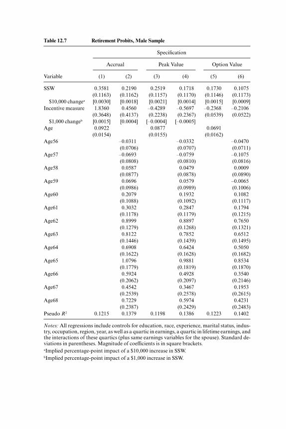
Table 12.7 Retirement Probits, Male Sample
Specification
Accrual Peak Value Option Value
Variable (1) (2) (3) (4) (5) (6)
SSW 0.3581 0.2190 0.2519 0.1718 0.1730 0.1075(0.1163) (0.1162) (0.1157) (0.1170) (0.1146) (0.1173)
$10,000 changea [0.0030] [0.0018] [0.0021] [0.0014] [0.0015] [0.0009]Incentive measure 1.8360 0.4560 –0.4289 –0.5697 –0.2368 –0.2106
(0.3648) (0.4137) (0.2238) (0.2367) (0.0539) (0.0522)$1,000 changeb [0.0015] [0.0004] [–0.0004] [–0.0005]
Age 0.0922 0.0877 0.0691(0.0154) (0.0155) (0.0162)
Age56 –0.0311 –0.0332 –0.0470(0.0706) (0.0707) (0.0711)
Age57 –0.0693 –0.0759 –0.1075(0.0808) (0.0810) (0.0816)
Age58 0.0587 0.0479 0.0009(0.0877) (0.0878) (0.0890)
Age59 0.0696 0.0579 –0.0065(0.0986) (0.0989) (0.1006)
Age60 0.2079 0.1932 0.1082(0.1088) (0.1092) (0.1117)
Age61 0.3032 0.2847 0.1794(0.1178) (0.1179) (0.1215)
Age62 0.8999 0.8897 0.7650(0.1279) (0.1268) (0.1321)
Age63 0.8122 0.7852 0.6512(0.1446) (0.1439) (0.1495)
Age64 0.6908 0.6424 0.5050(0.1622) (0.1628) (0.1682)
Age65 1.0796 0.9881 0.8534(0.1779) (0.1819) (0.1870)
Age66 0.5924 0.4928 0.3540(0.2062) (0.2097) (0.2146)
Age67 0.4542 0.3467 0.1953(0.2539) (0.2578) (0.2615)
Age68 0.7229 0.5974 0.4231(0.2387) (0.2429) (0.2483)
Pseudo R2 0.1215 0.1379 0.1198 0.1386 0.1223 0.1402
Notes: All regressions include controls for education, race, experience, marital status, indus-try, occupation, region, year, as well as a quartic in earnings, a quartic in lifetime earnings, andthe interactions of these quartics (plus same earnings variables for the spouse). Standard de-viations in parentheses. Magnitude of coefficients is in square brackets.aImplied percentage-point impact of a $10,000 increase in SSW.bImplied percentage-point impact of a $1,000 increase in SSW.
is controlled for using a linear variable or age dummies. The goodness of fitof all six models is similar, with a pseudo R2 of about 12 percent in modelswithout age dummies and 14 percent in models with age dummies. Thesefindings suggest that the forward-looking models of the type advocated byStock and Wise are very important for explaining retirement behavior. In-dividuals do appear to recognize the future path of SSW accumulation,and they take this into account in making their retirement decisions.
The other variables in the regression have their expected impacts.29
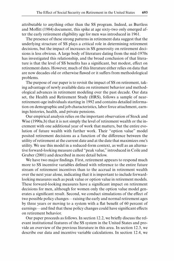
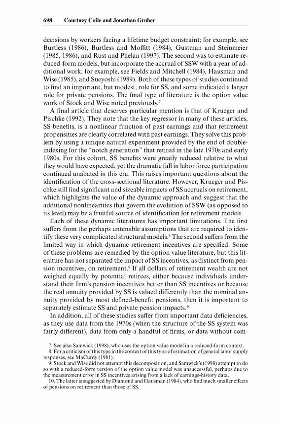
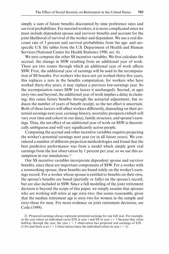
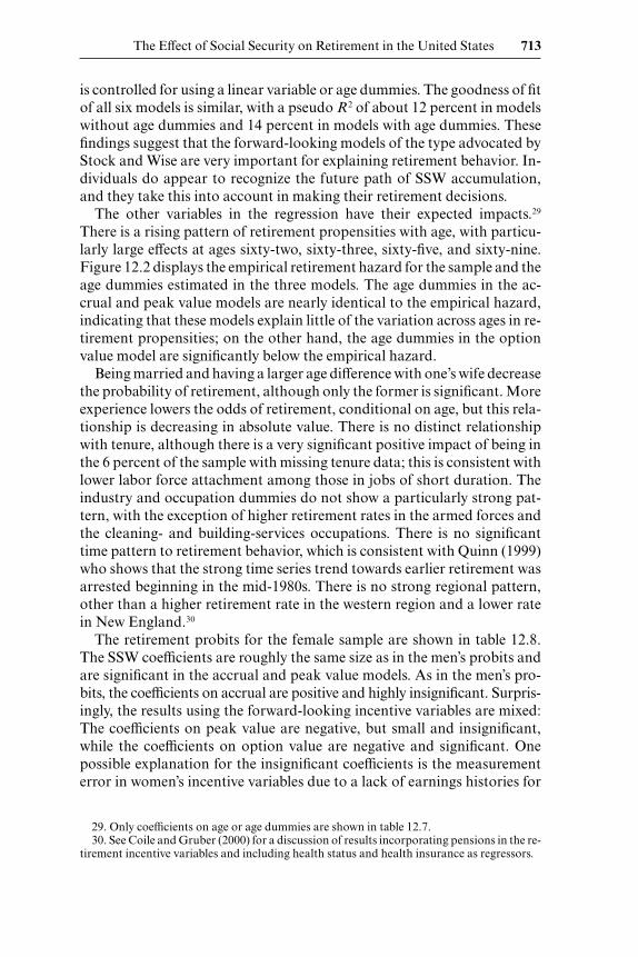
There is a rising pattern of retirement propensities with age, with particu-larly large effects at ages sixty-two, sixty-three, sixty-five, and sixty-nine.Figure 12.2 displays the empirical retirement hazard for the sample and theage dummies estimated in the three models. The age dummies in the ac-crual and peak value models are nearly identical to the empirical hazard,indicating that these models explain little of the variation across ages in re-tirement propensities; on the other hand, the age dummies in the optionvalue model are significantly below the empirical hazard.
Being married and having a larger age difference with one’s wife decreasethe probability of retirement, although only the former is significant. Moreexperience lowers the odds of retirement, conditional on age, but this rela-tionship is decreasing in absolute value. There is no distinct relationshipwith tenure, although there is a very significant positive impact of being inthe 6 percent of the sample with missing tenure data; this is consistent withlower labor force attachment among those in jobs of short duration. Theindustry and occupation dummies do not show a particularly strong pat-tern, with the exception of higher retirement rates in the armed forces andthe cleaning- and building-services occupations. There is no significanttime pattern to retirement behavior, which is consistent with Quinn (1999)who shows that the strong time series trend towards earlier retirement wasarrested beginning in the mid-1980s. There is no strong regional pattern,other than a higher retirement rate in the western region and a lower ratein New England.30
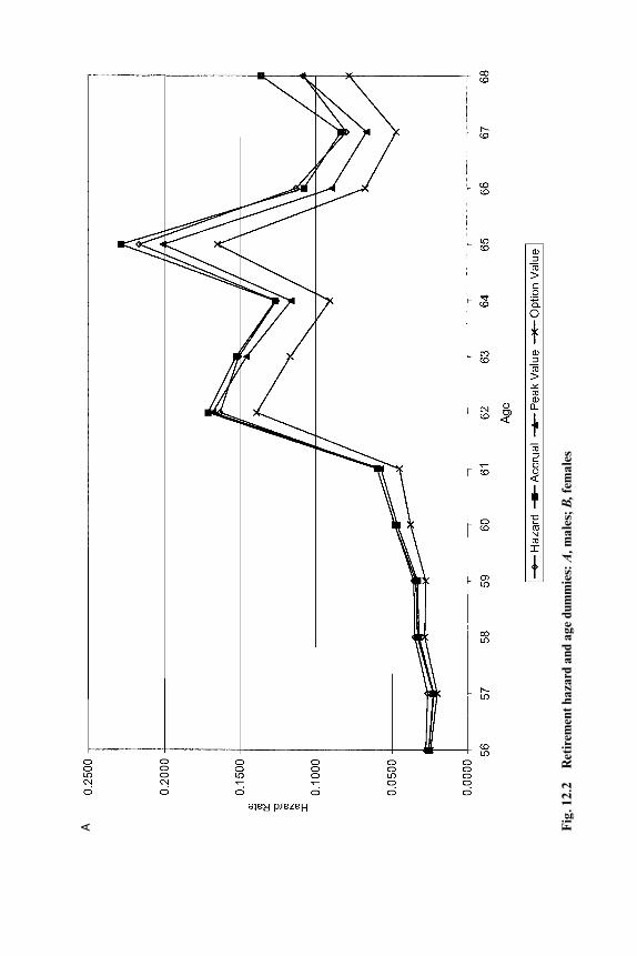
The retirement probits for the female sample are shown in table 12.8.The SSW coefficients are roughly the same size as in the men’s probits andare significant in the accrual and peak value models. As in the men’s pro-bits, the coefficients on accrual are positive and highly insignificant. Surpris-ingly, the results using the forward-looking incentive variables are mixed:The coefficients on peak value are negative, but small and insignificant,while the coefficients on option value are negative and significant. Onepossible explanation for the insignificant coefficients is the measurementerror in women’s incentive variables due to a lack of earnings histories for
The Effect of Social Security on Retirement in the United States 713
29. Only coefficients on age or age dummies are shown in table 12.7.30. See Coile and Gruber (2000) for a discussion of results incorporating pensions in the re-
tirement incentive variables and including health status and health insurance as regressors.
A Fig
. 12.
2R
etir
emen
t haz
ard
and
age
dum
mie
s: A
,mal
es; B
,fem
ales
B Fig
. 12.
2(c
ont.
)

716 Courtney Coile and Jonathan Gruber
Table 12.8 Retirement Probits, Female Sample
Specification
Accrual Peak Value Option Value
Variable (1) (2) (3) (4) (5) (6)
SSW 0.2619 0.2265 0.2430 0.2169 0.2080 0.1838(0.1132) (0.1130) (0.1132) (0.1129) (0.1142) (0.1135)
$10,000 changea [0.0020] [0.0017] [0.0019] [0.0017] [0.0016] [0.0014]Incentive measure 0.7727 0.4773 –0.0618 –0.0132 –0.2695 –0.2414
(0.7291) (0.8169) (0.0253) (0.2856) (0.0772) (0.0752)$1,000 changeb [0.0006] [0.0004] –[0.00005] [–0.00001]
Age 0.1219 0.1217 0.1040(0.0219) (0.0219) (0.0223)
Age56 0.0223 0.0217 0.0101(0.0825) (0.0824) (0.0826)
Age57 0.0474 0.0480 0.0312(0.0960) (0.0959) (0.0961)
Age58 0.1254 0.1268 0.0964(0.1104) (0.1103) (0.1104)
Age59 0.1186 0.1212 0.0784(0.1295) (0.1294) (0.1298)
Age60 0.4364 0.4389 0.3811(0.1415) (0.1414) (0.1422)
Age61 0.4587 0.4632 0.3928(0.1585) (0.1584) (0.1599)
Age62 1.0015 1.0075 0.9102(0.1702) (0.1699) (0.1720)
Age63 0.9872 0.9918 0.8721(0.1939) (0.1937) (0.1966)
Age64 0.8106 0.8119 0.6718(0.2229) (0.2223) (0.2262)
Age65 1.2619 1.2533 1.0901(0.2464) (0.2456) (0.2497)
Age66 0.8181 0.8086 0.6318(0.3377) (0.3371) (0.3406)
Age67 0.2807 0.2714 0.0774(0.5925) (0.5941) (0.6078)
Age68 0.8993 0.8815 0.6609(0.5079) (0.5084) (0.5215)
Pseudo R2 0.1418 0.1530 0.1416 0.1530 0.1441 0.1549
Note: See table 12.7.
divorced and deceased spouses; however, this would not explain why op-tion value is significant.31 The linear age variable and age dummies are sim-
31. Coile (2003) estimates similar models and finds that women respond to both peak valueand option value measures. Her sample differs in two ways from the female sample here: First,she looks only at married women (who may have less measurement error in their incentivevariables than unmarried women) and second, she conditions on working at age fifty or later(versus fifty-five here).
ilar to those in the men’s model, and again the age dummies from the op-tion value model are below the empirical hazard (figure 12.2, panel B). Thepseudo R2 is about 15 percent in all six models.
In summary, SSW has a positive and marginally significant effect on re-tirement behavior for both men and women. The one-year accrual has thewrong sign and an insignificant effect, while the forward-looking incen-tive measures, peak value and option value, have a significant negativeeffect (although peak value is not significant for women). However, theimplications of the estimates that we have presented thus far are difficultto interpret in a vacuum; are $1,000 changes in peak value consideredlarge or small? To provide some more context for the magnitudes of ourresults, we conduct simulations of changes to the SS system in the follow-ing section.
12.5 Policy Simulations
In this section, we consider two potential major reforms to the SS sys-tem. The first policy change examined is to raise both the early retirementage (ERA) and the normal retirement age (NRA) by three years, to sixty-five and sixty-eight, respectively. The second policy change is to move fromthe current SS system to a common system simulated by all chapters in thisvolume: an ERA of sixty and NRA of sixty-five, a replacement rate of 60percent of AIME at age sixty-five, and a 6 percent annual actuarial-adjustment factor between ages sixty and seventy.
Our basic procedure is to reestimate the incentive variables under thenew policy, then use the probit estimates discussed above to predictchanges in retirement behavior. But executing these simulations raises thedifficult question of how to translate the earlier models into policy re-sponses. In particular, we face the difficulty that our models are largely un-able to explain the age pattern of retirement, an age pattern that is cer-tainly at least partly due to SS incentives (in particular the spike at agesixty-two).
We therefore consider three possible simulation approaches. In the firstsimulation (S1), we use the model with linear age. This simulation does notallow for any age-specific deviations from a linear baseline, therefore in-creasing the explanatory power of our financial incentive variables. In thesecond simulation (S2), we use the model with age dummies, but we onlyconsider the impact of changing the financial incentive variables; that is,when retirement ages change, we only consider the impact that this hasthrough changing peak or option value, and not through any other struc-tural shifts. In contrast, the third simulated approach (S3) is also based onthe model in which age dummies are used, but imposes a shift in the spikesof the retirement hazard when the policy is changed; that is, when retire-ment ages change, we assume that there is a corresponding change in the
The Effect of Social Security on Retirement in the United States 717
underlying hazard of retirement by age.32 Simply put, S2 corresponds tothe assumption that any age pattern not captured by our financial mea-sures is not due to retirement programs; S3 assumes that the entire age pat-tern is driven by retirement programs. Since it is unknown whether or notthe policy changes would move the spikes in the retirement hazard, S2 andS3 can be thought of as bounding the true effect of the policy change, withS1 somewhere in between.
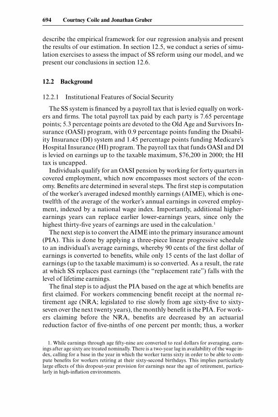
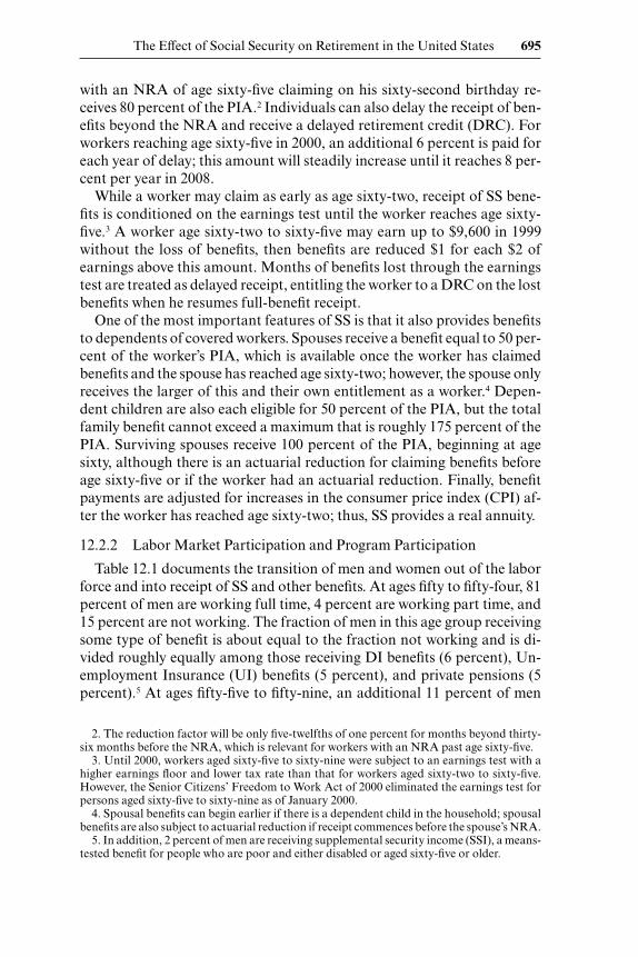
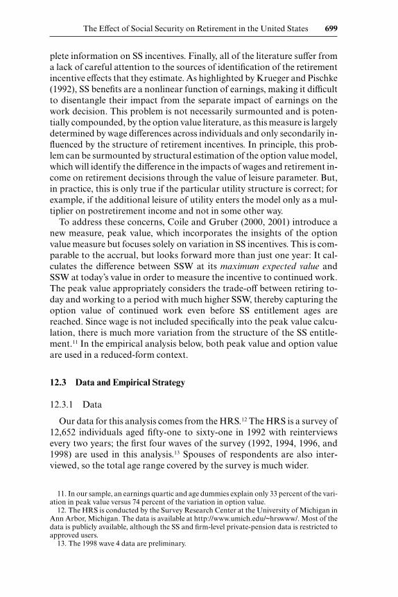
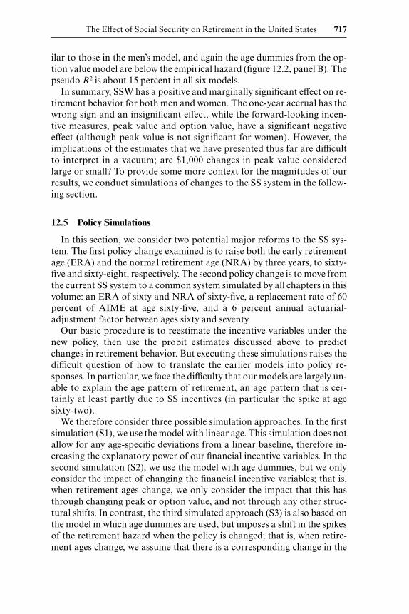
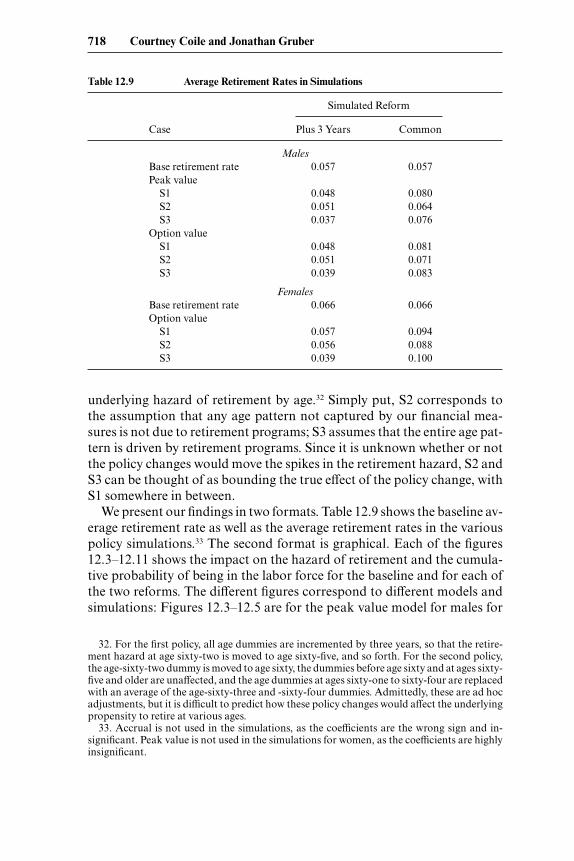
We present our findings in two formats. Table 12.9 shows the baseline av-erage retirement rate as well as the average retirement rates in the variouspolicy simulations.33 The second format is graphical. Each of the figures12.3–12.11 shows the impact on the hazard of retirement and the cumula-tive probability of being in the labor force for the baseline and for each ofthe two reforms. The different figures correspond to different models andsimulations: Figures 12.3–12.5 are for the peak value model for males for
718 Courtney Coile and Jonathan Gruber
32. For the first policy, all age dummies are incremented by three years, so that the retire-ment hazard at age sixty-two is moved to age sixty-five, and so forth. For the second policy,the age-sixty-two dummy is moved to age sixty, the dummies before age sixty and at ages sixty-five and older are unaffected, and the age dummies at ages sixty-one to sixty-four are replacedwith an average of the age-sixty-three and -sixty-four dummies. Admittedly, these are ad hocadjustments, but it is difficult to predict how these policy changes would affect the underlyingpropensity to retire at various ages.
33. Accrual is not used in the simulations, as the coefficients are the wrong sign and in-significant. Peak value is not used in the simulations for women, as the coefficients are highlyinsignificant.
Table 12.9 Average Retirement Rates in Simulations
Simulated Reform
Case Plus 3 Years Common
MalesBase retirement rate 0.057 0.057Peak value
S1 0.048 0.080S2 0.051 0.064S3 0.037 0.076
Option valueS1 0.048 0.081S2 0.051 0.071S3 0.039 0.083
FemalesBase retirement rate 0.066 0.066Option value
S1 0.057 0.094S2 0.056 0.088S3 0.039 0.100
simulations S1, S2, and S3; figures 12.6–12.8 are for the option value modelfor males; and figures 12.9–12.11 are for the option value model for fe-males.
12.5.1 Raising the ERA and NRA by Three Years
The first policy change, raising the ERA and NRA, would have the effectof lowering the average retirement rate for both men and women. The re-duction is 1 percentage point or less in S1 and S2, but 2–3 percentage
The Effect of Social Security on Retirement in the United States 719
A
B
Fig. 12.3 S1 for males, peak value model: A, simulated hazard; B, cumulativeprobability
points under S3. The larger reduction in average retirement rate under S3is not surprising, as this case moves the spikes in the retirement hazardback by three years.
We can assess the wealth and accrual effects underlying these results.This change will have a negative wealth effect on retirement, since thisamounts to a benefit cut for any retirement age, which will encourage work.The accrual effects are more complicated: For ages sixty-two to sixty-four,this change will decrease work incentives, as work in these years now onlybenefits the individual through the dropout year provision and no longer
720 Courtney Coile and Jonathan Gruber
A
B
Fig. 12.4 S2 for males, peak value model: A, simulated hazard; B, cumulativeprobability
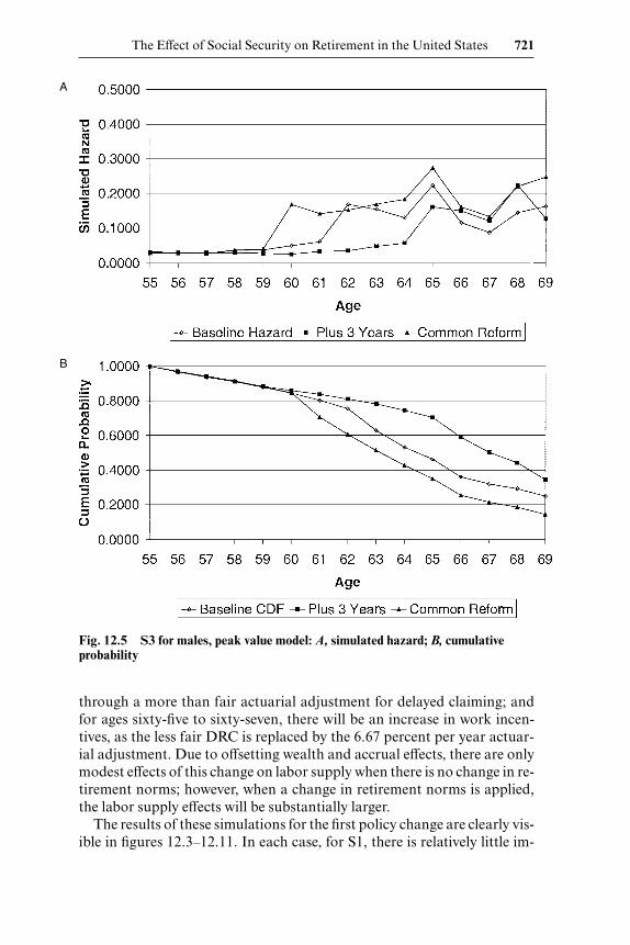
through a more than fair actuarial adjustment for delayed claiming; andfor ages sixty-five to sixty-seven, there will be an increase in work incen-tives, as the less fair DRC is replaced by the 6.67 percent per year actuar-ial adjustment. Due to offsetting wealth and accrual effects, there are onlymodest effects of this change on labor supply when there is no change in re-tirement norms; however, when a change in retirement norms is applied,the labor supply effects will be substantially larger.
The results of these simulations for the first policy change are clearly vis-ible in figures 12.3–12.11. In each case, for S1, there is relatively little im-
The Effect of Social Security on Retirement in the United States 721
A
B
Fig. 12.5 S3 for males, peak value model: A, simulated hazard; B, cumulativeprobability
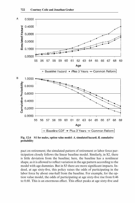
pact on retirement; the simulated pattern of retirement or labor force par-ticipation closely follows the linear baseline model. Similarly, in S2, thereis little deviation from the baseline; here, the baseline has a nonlinearshape, as it is allowed to reflect variation in the age pattern according to themodel with age dummies. But in S3 there are more significant impacts. In-deed, at age sixty-five, this policy raises the odds of participating in thelabor force by about one-half from the baseline. For example, for the op-tion value model, the odds of participating at age sixty-five rise from 0.46to 0.68. This is an enormous effect. This effect peaks at age sixty-five and
722 Courtney Coile and Jonathan Gruber
A
B
Fig. 12.6 S1 for males, option value model: A, simulated hazard; B, cumulativeprobability
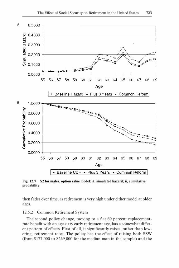
then fades over time, as retirement is very high under either model at olderages.
12.5.2 Common Retirement System
The second policy change, moving to a flat 60 percent replacement-rate benefit with an age sixty early retirement age, has a somewhat differ-ent pattern of effects. First of all, it significantly raises, rather than low-ering, retirement rates. The policy has the effect of raising both SSW(from $177,000 to $269,000 for the median man in the sample) and the
The Effect of Social Security on Retirement in the United States 723
A
B
Fig. 12.7 S2 for males, option value model: A, simulated hazard; B, cumulativeprobability
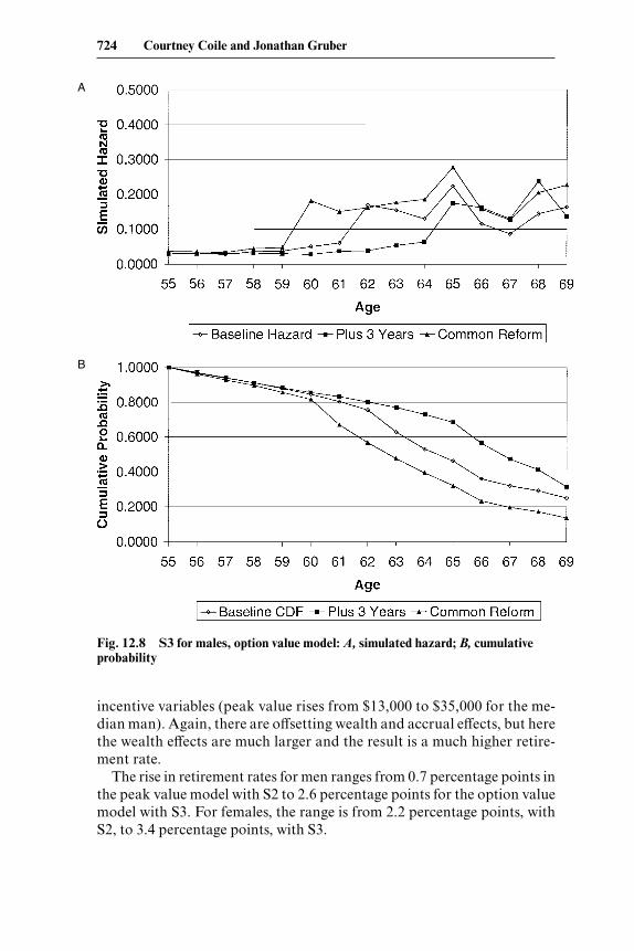
incentive variables (peak value rises from $13,000 to $35,000 for the me-dian man). Again, there are offsetting wealth and accrual effects, but herethe wealth effects are much larger and the result is a much higher retire-ment rate.
The rise in retirement rates for men ranges from 0.7 percentage points inthe peak value model with S2 to 2.6 percentage points for the option valuemodel with S3. For females, the range is from 2.2 percentage points, withS2, to 3.4 percentage points, with S3.
724 Courtney Coile and Jonathan Gruber
A
B
Fig. 12.8 S3 for males, option value model: A, simulated hazard; B, cumulativeprobability
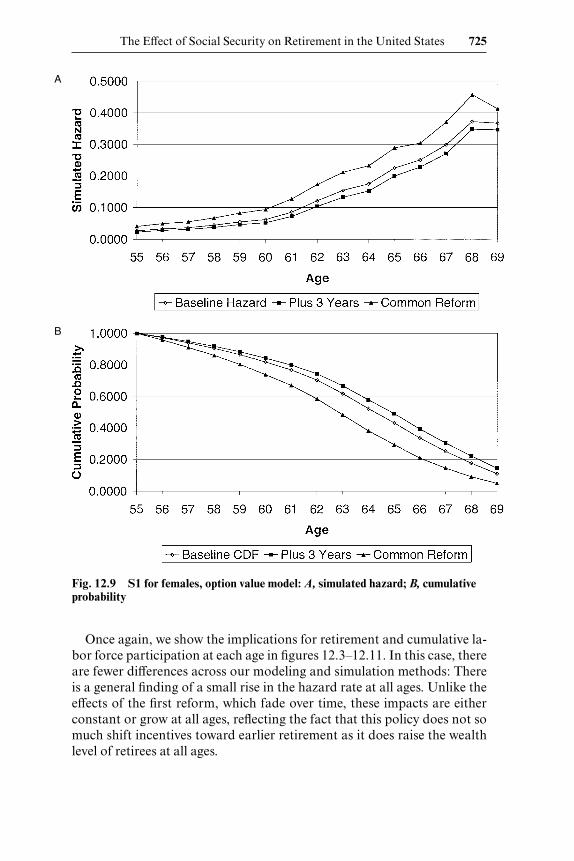
Once again, we show the implications for retirement and cumulative la-bor force participation at each age in figures 12.3–12.11. In this case, thereare fewer differences across our modeling and simulation methods: Thereis a general finding of a small rise in the hazard rate at all ages. Unlike theeffects of the first reform, which fade over time, these impacts are eitherconstant or grow at all ages, reflecting the fact that this policy does not somuch shift incentives toward earlier retirement as it does raise the wealthlevel of retirees at all ages.
The Effect of Social Security on Retirement in the United States 725
A
B
Fig. 12.9 S1 for females, option value model: A, simulated hazard; B, cumulativeprobability
12.6 Conclusion
The SS program is the most important source of retirement income sup-port for older Americans. As such, it is possible that the incentives em-bodied in this system for continued work or retirement at various ages area critical determinant of retirement decisions. Understanding the influ-ence that SS has on retirement decisions is particularly important now, asany reforms to the SS system will change the structure of the program in amanner that has important impacts on retirement incentives.
Our paper has used the richest available current data, the HRS, to pro-
A
B
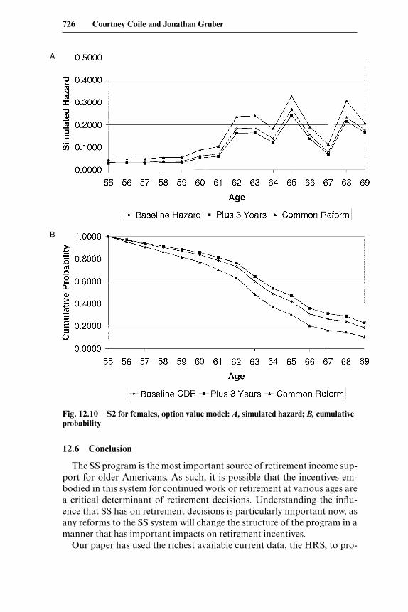
Fig. 12.10 S2 for females, option value model: A, simulated hazard; B, cumulativeprobability
726 Courtney Coile and Jonathan Gruber
The Effect of Social Security on Retirement in the United States 727
A
B
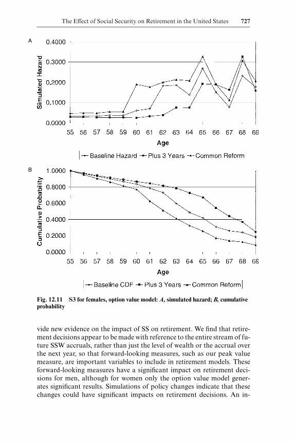
Fig. 12.11 S3 for females, option value model: A, simulated hazard; B, cumulativeprobability
vide new evidence on the impact of SS on retirement. We find that retire-ment decisions appear to be made with reference to the entire stream of fu-ture SSW accruals, rather than just the level of wealth or the accrual overthe next year, so that forward-looking measures, such as our peak valuemeasure, are important variables to include in retirement models. Theseforward-looking measures have a significant impact on retirement deci-sions for men, although for women only the option value model gener-ates significant results. Simulations of policy changes indicate that thesechanges could have significant impacts on retirement decisions. An in-

crease in the ERA and NRA could result in a 2 percentage point decreasein the average annual retirement rate if the increase has the effect of chang-ing retirement norms, although the effect would be much smaller if normsare unchanged, due to offsetting wealth and accrual effects. A move to apolicy with a 60 percent replacement rate at age sixty-five, a much moregenerous policy than the current SS system, would have very large wealtheffects, raising the average annual retirement rate by 2–3 percentage points.
References
Blau, David M. 1994. Labor force dynamics of older men. Econometrica 62 (1):117–56.
Burtless, Gary. 1986. Social security, unanticipated benefit increases, and the tim-ing of retirement. Review of Economic Studies 53 (5): 781–805.
Burtless, Gary, and Robert Moffitt. 1984. The effect of social security benefits onthe labor supply of the aged. In Retirement and economic behavior, ed. HenryAaron and Gary Burtless, 135–75. Washington, D.C.: Brookings Institution.
Coile, Courtney. 2003. Retirement incentives and couples’ retirement decisions.NBER Working Paper no. 9496. Cambridge, Mass.: National Bureau of Eco-nomic Research.
Coile, Courtney, Peter Diamond, Jonathan Gruber, and Alain Jousten. 2002.Delays in claiming social security benefits. Journal of Public Economics 84 (3):357–86.
———. 2000. Social security and retirement. NBER Working Paper no. 7830.Cambridge, Mass.: National Bureau of Economic Research, August.
Coile, Courtney, and Jonathan Gruber. 2001. Social security incentives for retire-ment. In Themes in the Economics of Aging, ed. David A. Wise. Chicago: Uni-versity of Chicago Press.
Diamond, Peter, and Jonathan Gruber. 1999. Social security and retirement in theUnited States. In Social Security and Retirement around the World, ed. JonathanGruber and David A. Wise, 437–73. Chicago: University of Chicago Press.
Diamond, Peter, and Jerry Hausman. 1984. Retirement and unemployment behav-ior of older men. In Retirement and economic behavior, ed. Henry Aaron andGary Burtless, 97–135. Washington, D.C.: Brookings Institution.
Fields, Gary S., and Olivia S. Mitchell. 1984. Economic determinants of the opti-mal retirement age: An empirical investigation. Journal of Human Resources 19(2): 245–62.
Gustman, Alan L., and Thomas L. Steinmeier. 1985. The 1983 social security re-forms and labor supply adjustments of older individuals in the long run. Journalof Labor Economics 3 (2): 237–53.
———. 1986. A structural retirement model. Econometrica 54 (3): 555–84.Haider, Steven, and Gary Solon. 1999. Nonrandom selection in the HRS social se-
curity earnings sample. University of Michigan, Department of Economics. Un-published Manuscript.
Hausman, Jerry A., and David A. Wise. 1985. Social security, health status, andretirement. In Pensions, labor, and individual choice, ed. David A. Wise, 159–91.Chicago: University of Chicago Press.
728 Courtney Coile and Jonathan Gruber
Hurd, Michael D. 1990. Research on the elderly: Economic status, retirement, andconsumption and saving. Journal of Economic Literature 28 (2): 565–637.
Krueger, Alan B., and Jorn-Steffan Pischke. 1992. The effect of social security onlabor supply: A cohort analysis of the notch generation. Journal of Labor Eco-nomics 10 (4): 412–37.
Lumsdaine, Robin, and David Wise. 1994. Aging and labor force participation: Areview of trends and explanations. In Aging in the United States and Japan: Eco-nomic trends, ed. Yukio Noguchi and David Wise, 7–42. Chicago: University ofChicago Press.
MaCurdy, Thomas E. 1981. An empirical model of labor supply in a life-cycle set-ting. Journal of Political Economy 89 (6): 1059–85.
Mitchell, Olivia S., and Gary S. Fields. 1982. The effects of pensions and earningson retirement. In Research in labor economics, Vol. 5, ed. Ronald Ehrenberg,115–55. Greenwich, Conn.: JAI Press.
National Center for Health Statistics. 1990. Vital statistics of the United States,1987. Vol. 2. Washington, D.C.: Washington Public Health Service.
Quinn, Joseph. 1999. Retirement patterns and bridge jobs in the 1990s. Policy brieffor the employee benefit research institute. Washington, D.C.: Employee BenefitResearch Institute (EBRI).
Ruhm, Christopher. 1995. Secular changes in the work and retirement patterns ofolder men. Journal of Human Resources 30 (2): 362–85.
Samwick, Andrew A. 1998. New evidence on pensions, social security, and the tim-ing of retirement. Journal of Public Economics 70 (2): 207–36.
Stock, James H., and David A. Wise. 1990a. Pensions, the option value of work,and retirement. Econometrica 58 (5): 1151–80.
———. 1990b. The pension inducement to retire: An option value analysis. In Is-sues in the economics of aging, ed. David A. Wise, 205–29. Chicago: University ofChicago Press.
Social Security Administration. 1998. Annual statistical supplement, 1998, to theSocial Security bulletin. Baltimore, Mary.: U.S. Department of Health and Hu-man Services.
Sueyoshi, Glenn T. 1989. Social security and the determinants of full and partialretirement: A competing risks analysis. NBER Working Paper no. 3113. Cam-bridge, Mass.: National Bureau of Economic Research, September.
U.S. Bureau of the Census. 1998. No. 1 population and area: 1790 to 1990. In Sta-tistical abstract of the United States. 118th ed. Washington, D.C.: Bureau of theCensus.
The Effect of Social Security on Retirement in the United States 729