
slides.pdf - Dynamics of Structures 2019-2020
111
An Introduction to Dynamics of Structures Giacomo Boffi February 26, 2019 http://intranet.dica.polimi.it/people/boffi-giacomo Dipartimento di Ingegneria Civile Ambientale e Territoriale Politecnico di Milano 1
-
Upload
khangminh22 -
Category
Documents
-
view
0 -
download
0
Transcript of slides.pdf - Dynamics of Structures 2019-2020

An Introduction to Dynamics of Structures
Giacomo BoffiFebruary 26, 2019
http://intranet.dica.polimi.it/people/boffi-giacomoDipartimento di Ingegneria Civile Ambientale e Territoriale
Politecnico di Milano
1
Outline
Part 1IntroductionCharacteristics of a Dynamical ProblemFormulation of a Dynamical ProblemFormulation of the equations of motion
Part 2
1 DOF System
Free vibrations of a SDOF system
Free vibrations of a damped system
2

Introduction

Definitions
Let’s start with some definitions
Dynamic adj., constantly changingDynamics noun, the branch of Mechanics concerned with
the motion of bodies under the action of forcesDynamic Loading a Loading that varies over time
Dynamic Response the Response (deflections and stresses) of asystem to a dynamic loading; DynamicResponses vary over time
Dynamics of Structures all of the above, applied to a structuralsystem, i.e., a system designed to stay inequilibrium
3
Definitions
Let’s start with some definitions
Dynamic adj., constantly changing
Dynamics noun, the branch of Mechanics concerned withthe motion of bodies under the action of forces
Dynamic Loading a Loading that varies over timeDynamic Response the Response (deflections and stresses) of a
system to a dynamic loading; DynamicResponses vary over time
Dynamics of Structures all of the above, applied to a structuralsystem, i.e., a system designed to stay inequilibrium
3
Definitions
Let’s start with some definitions
Dynamic adj., constantly changingDynamics noun, the branch of Mechanics concerned with
the motion of bodies under the action of forces
Dynamic Loading a Loading that varies over timeDynamic Response the Response (deflections and stresses) of a
system to a dynamic loading; DynamicResponses vary over time
Dynamics of Structures all of the above, applied to a structuralsystem, i.e., a system designed to stay inequilibrium
3
Definitions
Let’s start with some definitions
Dynamic adj., constantly changingDynamics noun, the branch of Mechanics concerned with
the motion of bodies under the action of forcesDynamic Loading a Loading that varies over time
Dynamic Response the Response (deflections and stresses) of asystem to a dynamic loading; DynamicResponses vary over time
Dynamics of Structures all of the above, applied to a structuralsystem, i.e., a system designed to stay inequilibrium
3
Definitions
Let’s start with some definitions
Dynamic adj., constantly changingDynamics noun, the branch of Mechanics concerned with
the motion of bodies under the action of forcesDynamic Loading a Loading that varies over time
Dynamic Response the Response (deflections and stresses) of asystem to a dynamic loading; DynamicResponses vary over time
Dynamics of Structures all of the above, applied to a structuralsystem, i.e., a system designed to stay inequilibrium
3
Dynamics of Structures
Our aim is to determine the stresses and deflections that a dynamicloading induces in a structure that remains in the neighborhood of apoint of equilibrium.
Methods of dynamic analysis are extensions of the methods ofstandard static analysis, or to say it better, static analysis is indeed aspecial case of dynamic analysis.
If we restrict ourselves to analysis of linear systems, it is so con-venient to use the principle of superposition to study the combinedeffects of static and dynamic loadings that different methods, ofdifferent character, are applied to these different loadings.
4
Characteristics of a DynamicalProblem
Types of Dynamic Analysis
Taking into account linear systems only, we must consider twodifferent definitions of the loading to define two types of dynamicanalysis
Deterministic Analysis applies when the time variation of the loading isfully known and we can determine the complete timevariation of all the required response quantities
Non-deterministic Analysis applies when the time variation of the loadingis essentially random and is known only in terms of somestatisticsIn a non-deterministic or stochastic analysis the structuralresponse can be known only in terms of statistics of theresponse quantities
Our focus will be on deterministic analysis
5
Types of Dynamic Analysis
Taking into account linear systems only, we must consider twodifferent definitions of the loading to define two types of dynamicanalysis
Deterministic Analysis applies when the time variation of the loading isfully known and we can determine the complete timevariation of all the required response quantities
Non-deterministic Analysis applies when the time variation of the loadingis essentially random and is known only in terms of somestatisticsIn a non-deterministic or stochastic analysis the structuralresponse can be known only in terms of statistics of theresponse quantities
Our focus will be on deterministic analysis5
Types of Dynamic Loading
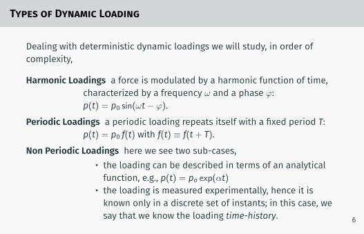
Dealing with deterministic dynamic loadings we will study, in order ofcomplexity,
Harmonic Loadings a force is modulated by a harmonic function of time,characterized by a frequency ω and a phase φ:p(t) = p0 sin(ωt− φ).
Periodic Loadings a periodic loading repeats itself with a fixed period T:p(t) = p0 f(t) with f(t) ≡ f(t+ T).
Non Periodic Loadings here we see two sub-cases,
• the loading can be described in terms of an analyticalfunction, e.g., p(t) = po exp(αt)
• the loading is measured experimentally, hence it isknown only in a discrete set of instants; in this case, wesay that we know the loading time-history.
6

Types of Dynamic Loading
Dealing with deterministic dynamic loadings we will study, in order ofcomplexity,
Harmonic Loadings a force is modulated by a harmonic function of time,characterized by a frequency ω and a phase φ:p(t) = p0 sin(ωt− φ).
Periodic Loadings a periodic loading repeats itself with a fixed period T:p(t) = p0 f(t) with f(t) ≡ f(t+ T).
Non Periodic Loadings here we see two sub-cases,
• the loading can be described in terms of an analyticalfunction, e.g., p(t) = po exp(αt)
• the loading is measured experimentally, hence it isknown only in a discrete set of instants; in this case, wesay that we know the loading time-history.
6
Types of Dynamic Loading
Dealing with deterministic dynamic loadings we will study, in order ofcomplexity,
Harmonic Loadings a force is modulated by a harmonic function of time,characterized by a frequency ω and a phase φ:p(t) = p0 sin(ωt− φ).
Periodic Loadings a periodic loading repeats itself with a fixed period T:p(t) = p0 f(t) with f(t) ≡ f(t+ T).
Non Periodic Loadings here we see two sub-cases,• the loading can be described in terms of an analyticalfunction, e.g., p(t) = po exp(αt)
• the loading is measured experimentally, hence it isknown only in a discrete set of instants; in this case, wesay that we know the loading time-history. 6
Characteristics of a Dynamical Problem
A dynamical problem is essentially characterized by the relevance ofinertial forces, arising from the accelerated motion of structural orserviced masses.
A dynamic analysis is required only when the inertial forces representa significant portion of the total load.
On the other hand, if the loads and the deflections are varyingslowly, a static analysis will provide an acceptable approximation.
We will define slowly
7

Formulation of a DynamicalProblem
Formulation of a Dynamical Problem
In a structural system the inertial forces depend on the timederivatives of displacements while the elastic forces, equilibratingthe inertial ones, depend on the spatial derivatives of thedisplacements. ... the natural statement of the problem is hence interms of partial differential equations.
In many cases it is however possible to simplify the formulation ofthe structural dynamic problem to ordinary differential equations.
8
Lumped Masses
In many structural problems we can say that the masses areconcentrated in a discrete set of lumped masses (e.g., in a multi-storeybuilding most of the masses is concentrated at the level of thestoreys’floors).
Under this assumption, the analytical problem is greatly simplified:
1. the inertial forces are applied only at the lumped masses,2. the only deflections that influence the inertial forces are thedeflections of the lumped masses,
3. using methods of static analysis we can determine those deflections,
thus consenting the formulation of the problem in terms of a set ofordinary differential equations, one for each relevant component ofthe inertial forces.
9
Dynamic Degrees of Freedom
The dynamic degrees of freedom (DDOF) in a lumped mass,discretized system are the displacements components of the lumpedmasses associated with the relevant components of the inertialforces.
10

Dynamic Degrees of Freedom
If a lumped mass can be regarded as a point mass then at most 3translational DDOFs will suffice to represent the associated inertialforce.
On the contrary, if a lumped mass has a discrete volume its inertialforce depends also on its rotations (inertial couples) and we need atmost 6 DDOFs to represent the mass deflections and the inertialforce.
Of course, a continuous system has an infinite number of degrees offreedom.
11
Generalized Displacements
The lumped mass procedure that we have outlined is effective if alarge proportion of the total mass is concentrated in a few points(e.g., in a multi-storey building one can consider a lumped mass foreach storey).
When the masses are distributed we can simplify our problemexpressing the deflections in terms of a linear combination ofassigned functions of position, the coefficients of the linearcombination being the generalized coordinates (e..g., the deflectionsof a rectilinear beam can be expressed in terms of a trigonometricseries).
12
Generalized Displacements, cont.
To fully describe a displacement field, we need to combine an infinityof linearly independent base functions, but in practice a goodapproximation can be achieved using just a small number offunctions and degrees of freedom.
Even if the method of generalized coordinates has itsbeauty, we must recognize that for each different problem wehave to derive an ad hoc formulation, with an evident loss ofgenerality.
13
Finite Element Method
The finite elements method (FEM) combines aspects of lumped massand generalized coordinates methods, providing a simple andreliable method of analysis, that can be easily programmed on adigital computer.
14
Finite Element Method
• In the FEM, the structure is subdivided in a number ofnon-overlapping pieces, called the finite elements, delimited bycommon nodes.
• The FEM uses piecewise approximations (i.e., local to eachelement) to the field of displacements.
• In each element the displacement field is derived from thedisplacements of the nodes that surround each particularelement, using interpolating functions.
• The displacement, deformation and stress fields in eachelement, as well as the inertial forces, can thus be expressed interms of the unknown nodal displacements.
• The nodal displacements are the dynamical DOFs of the FEMmodel.
15
Finite Element Method
Some of the most prominent advantages of the FEM method are
1. The desired level of approximation can be achieved by furthersubdividing the structure.
2. The resulting equations are only loosely coupled, leading to aneasier computer solution.
3. For a particular type of finite element (e.g., beam, solid, etc) theprocedure to derive the displacement field and the elementcharacteristics does not depend on the particular geometry ofthe elements, and can easily be implemented in a computerprogram.
16
Formulation of the equations ofmotion
Writing the equation of motion
In a deterministic dynamic analysis, given a prescribed load, we wantto evaluate the displacements in each instant of time.
In many cases a limited number of DDOFs gives a sufficient accuracy;further, the dynamic problem can be reduced to the determination ofthe time-histories of some selected component of the response.
The mathematical expressions, ordinary or partial differentialequations, that we are going to write express the dynamicequilibrium of the structural system and are known as the Equationsof Motion (EOM).
The solution of the EOM gives the requested displacements.
The formulation of the EOM is the most important, often the mostdifficult part of a dynamic analysis.
17
Writing the equation of motion
In a deterministic dynamic analysis, given a prescribed load, we wantto evaluate the displacements in each instant of time.
In many cases a limited number of DDOFs gives a sufficient accuracy;further, the dynamic problem can be reduced to the determination ofthe time-histories of some selected component of the response.
The mathematical expressions, ordinary or partial differentialequations, that we are going to write express the dynamicequilibrium of the structural system and are known as the Equationsof Motion (EOM).
The solution of the EOM gives the requested displacements.
The formulation of the EOM is the most important, often the mostdifficult part of a dynamic analysis. 17

Writing the EOM, cont.
We have a choice of techniques to help us in writing the EOM,namely:
• the D’Alembert Principle,• the Principle of Virtual Displacements,• the Variational Approach.
18
D’Alembert Principle
By Newton’s II law of motion, for any particle the rate of change ofmomentum is equal to the external force,
p(t) = ddt (m
dudt ),
where u(t) is the particle displacement.
In structural dynamics, we may regard the mass as a constant, and thuswrite
p(t) = m¨u,where each operation of differentiation with respect to time is denotedwith a dot.
When we interpret the term −m¨u as the inertial force that contrasts theacceleration of the particle, we can write an equation of equilibrium for theparticle, p(t) = m¨u.
19
D’Alembert principle, cont.
The concept that a mass develops an inertial force opposing itsacceleration is known as the D’Alembert principle, and using thisprinciple we can write the EOM as a simple equation of equilibrium.
The term p(t) must comprise each different force acting on theparticle, including the reactions of kinematic or elastic constraints,internal forces and external, autonomous forces.
In many simple problems, D’Alembert principle is the most direct andconvenient method for the formulation of the EOM.
20
Principle of virtual displacements
In a reasonably complex dynamic system, with e.g. articulated rigidbodies and external/internal constraints, the direct formulation ofthe EOM using D’Alembert principle may result difficult.
In these cases, application of the Principle of Virtual Displacements isvery convenient, because the reactive forces do not enter theequations of motion, that are directly written in terms of the motionscompatible with the restraints/constraints of the system.
21

Principle of Virtual Displacements, cont.
Considering, e.g., an assemblage of rigid bodies, the pvd states thatnecessary and sufficient condition for equilibrium is that, for every virtualdisplacement (i.e., any infinitesimal displacement compatible with therestraints) the total work done by all the external forces is zero.
For an assemblage of rigid bodies, writing the EOM requires
1. to identify all the external forces, comprising the inertial forces, and toexpress their values in terms of the ddof ;
2. to compute the work done by these forces for different virtualdisplacements, one for each ddof ;
3. to equate to zero all these work expressions.
The pvd is particularly convenient also because we have only scalarequations, even if the forces and displacements are of vectorial nature.
22
Variational approach
Variational approaches do not consider directly the forces acting onthe dynamic system, but are concerned with the variations of kineticand potential energy and lead, as well as the pvd, to a set of scalarequations.
For example, the equation of motion of a generical system can bederived in terms of the Lagrangian function, L = T− V where T and Vare, respectively, the kinetic and the potential energy of the systemexpressed in terms of a vector q of indipendent coordinates
ddt
(∂L∂qi
)=
∂L∂qi
, i = 1, . . . ,N.
The method to be used in a particular problem is mainly a matter ofconvenience (and, to some extent, of personal taste).
23
Variational approach
Variational approaches do not consider directly the forces acting onthe dynamic system, but are concerned with the variations of kineticand potential energy and lead, as well as the pvd, to a set of scalarequations.
For example, the equation of motion of a generical system can bederived in terms of the Lagrangian function, L = T− V where T and Vare, respectively, the kinetic and the potential energy of the systemexpressed in terms of a vector q of indipendent coordinates
ddt
(∂L∂qi
)=
∂L∂qi
, i = 1, . . . ,N.
The method to be used in a particular problem is mainly a matter ofconvenience (and, to some extent, of personal taste). 23

1 DOF System
1 DOF System
Structural dynamics is all about the motion of a system in theneighborhood of a point of equilibrium.
We’ll start by studying the most simple of systems, a single degree offreedom system, without external forces, subjected to a perturbation of theequilibrium.
If our system has a constant mass m and it’s subjected to a generical,non-linear, internal force F = F(y, y), where y is the displacement and y thevelocity of the particle, the equation of motion is
y = 1mF(y, y) = f(y, y).
It is difficult to integrate the above equation in the general case, but it’seasy when the motion occurs in a small neighborhood of the equilibriumposition.
24
1 DOF System, cont.
In a position of equilibrium, yeq., the velocity and the accelerationare zero, and hence f(yeq.,0) = 0.
The force can be linearized in a neighborhood of yeq., 0:
f(y, y) = f(yeq.,0) +∂f∂y(y− yeq.) +
∂f∂y(y− 0) + O(y, y).
Assuming that O(y, y) is small in a neighborhood of yeq., we can writethe equation of motion
x+ ax+ bx = 0
where x = y− yeq., a = − ∂f∂y
∣∣∣y=yeq,y=0
and b = − ∂f∂y
∣∣∣y=yeq,y=0
.
25
In an infinitesimal neighborhood of yeq. (yeq. being a position ofstatic equilibrium), the equation of motion can be studied in termsof a linear differential equation of second order with constantcoefficients.
26
1 DOF System, cont.
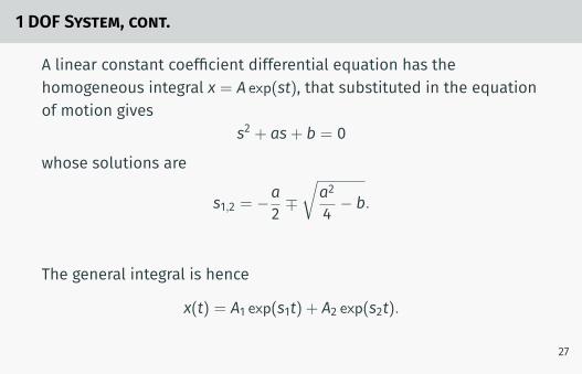
A linear constant coefficient differential equation has thehomogeneous integral x = A exp(st), that substituted in the equationof motion gives
s2 + as+ b = 0
whose solutions are
s1,2 = −a2 ∓√a24 − b.
The general integral is hence
x(t) = A1 exp(s1t) + A2 exp(s2t).
27
1 DOF System, cont.
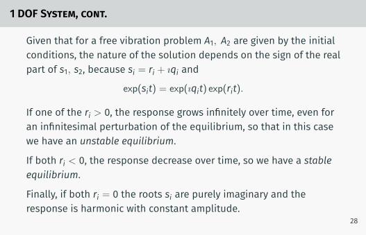
Given that for a free vibration problem A1, A2 are given by the initialconditions, the nature of the solution depends on the sign of the realpart of s1, s2, because si = ri + ıqi and
exp(sit) = exp(ıqit) exp(rit).
If one of the ri > 0, the response grows infinitely over time, even foran infinitesimal perturbation of the equilibrium, so that in this casewe have an unstable equilibrium.
If both ri < 0, the response decrease over time, so we have a stableequilibrium.
Finally, if both ri = 0 the roots si are purely imaginary and theresponse is harmonic with constant amplitude.
28
1 DOF System, cont.
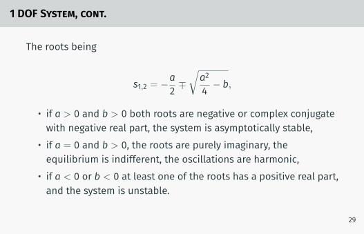
The roots being
s1,2 = −a2 ∓√a24 − b,
• if a > 0 and b > 0 both roots are negative or complex conjugatewith negative real part, the system is asymptotically stable,
• if a = 0 and b > 0, the roots are purely imaginary, theequilibrium is indifferent, the oscillations are harmonic,
• if a < 0 or b < 0 at least one of the roots has a positive real part,and the system is unstable.
29

The famous box car
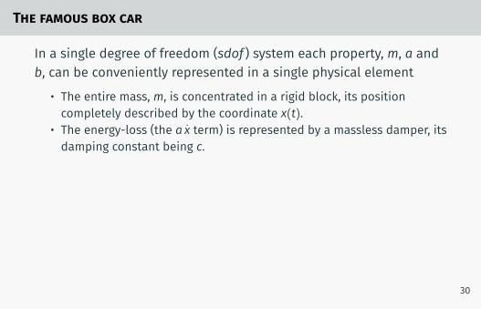
In a single degree of freedom (sdof ) system each property, m, a andb, can be conveniently represented in a single physical element
• The entire mass, m, is concentrated in a rigid block, its positioncompletely described by the coordinate x(t).
• The energy-loss (the a x term) is represented by a massless damper, itsdamping constant being c.
• The elastic resistance to displacement (b x) is provided by a masslessspring of stiffness k
• For completeness we consider also an external loading, thetime-varying force p(t).
(a)
m
c
k
p(t)
xx(t)
(b)
p(t)fD(t)fS(t)
fI(t)
30
The famous box car
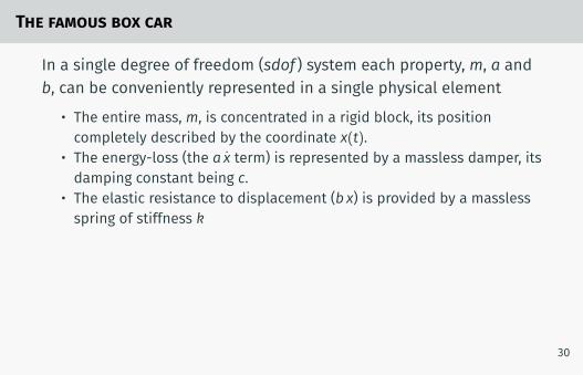
In a single degree of freedom (sdof ) system each property, m, a andb, can be conveniently represented in a single physical element
• The entire mass, m, is concentrated in a rigid block, its positioncompletely described by the coordinate x(t).
• The energy-loss (the a x term) is represented by a massless damper, itsdamping constant being c.
• The elastic resistance to displacement (b x) is provided by a masslessspring of stiffness k
• For completeness we consider also an external loading, thetime-varying force p(t).
(a)
m
c
k
p(t)
xx(t)
(b)
p(t)fD(t)fS(t)
fI(t)
30
The famous box car
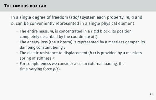
In a single degree of freedom (sdof ) system each property, m, a andb, can be conveniently represented in a single physical element
• The entire mass, m, is concentrated in a rigid block, its positioncompletely described by the coordinate x(t).
• The energy-loss (the a x term) is represented by a massless damper, itsdamping constant being c.
• The elastic resistance to displacement (b x) is provided by a masslessspring of stiffness k
• For completeness we consider also an external loading, thetime-varying force p(t).
(a)
m
c
k
p(t)
xx(t)
(b)
p(t)fD(t)fS(t)
fI(t)
30
The famous box car
In a single degree of freedom (sdof ) system each property, m, a andb, can be conveniently represented in a single physical element
• The entire mass, m, is concentrated in a rigid block, its positioncompletely described by the coordinate x(t).
• The energy-loss (the a x term) is represented by a massless damper, itsdamping constant being c.
• The elastic resistance to displacement (b x) is provided by a masslessspring of stiffness k
• For completeness we consider also an external loading, thetime-varying force p(t).
(a)
m
c
k
p(t)
xx(t)
(b)
p(t)fD(t)fS(t)
fI(t)
30

The famous box car
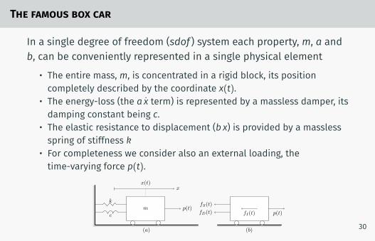
In a single degree of freedom (sdof ) system each property, m, a andb, can be conveniently represented in a single physical element
• The entire mass, m, is concentrated in a rigid block, its positioncompletely described by the coordinate x(t).
• The energy-loss (the a x term) is represented by a massless damper, itsdamping constant being c.
• The elastic resistance to displacement (b x) is provided by a masslessspring of stiffness k
• For completeness we consider also an external loading, thetime-varying force p(t).
(a)
m
c
k
p(t)
xx(t)
(b)
p(t)fD(t)fS(t)
fI(t)
30
The famous box car
In a single degree of freedom (sdof ) system each property, m, a andb, can be conveniently represented in a single physical element
• The entire mass, m, is concentrated in a rigid block, its positioncompletely described by the coordinate x(t).
• The energy-loss (the a x term) is represented by a massless damper, itsdamping constant being c.
• The elastic resistance to displacement (b x) is provided by a masslessspring of stiffness k
• For completeness we consider also an external loading, thetime-varying force p(t).
(a)
m
c
k
p(t)
xx(t)
(b)
p(t)fD(t)fS(t)
fI(t)
30
Equation of motion of the basic dynamic system
(a)
m
c
k
p(t)
xx(t)
(b)
p(t)fD(t)fS(t)
fI(t)
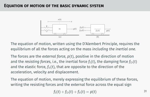
The equation of motion, written using the D’Alembert Principle, requires theequilibrium of all the forces acting on the mass including the inertial one.
The forces are the external force, p(t), positive in the direction of motionand the resisting forces, i.e., the inertial force fI(t), the damping force fD(t)and the elastic force, fS(t), that are opposite to the direction of theacceleration, velocity and displacement.
The equation of motion, merely expressing the equilibrium of these forces,writing the resisting forces and the external force across the equal sign
fI(t) + fD(t) + fS(t) = p(t) 31

EOM of the basic dynamic system, cont.
According to D’Alembert principle, the inertial force is the product ofthe mass and acceleration
fI(t) = m x(t).
Assuming a viscous damping mechanism, the damping force is theproduct of the damping constant c and the velocity,
fD(t) = c x(t).
Finally, the elastic force is the product of the elastic stiffness k andthe displacement,
fS(t) = k x(t).
32
EOM of the basic dynamic system, cont.
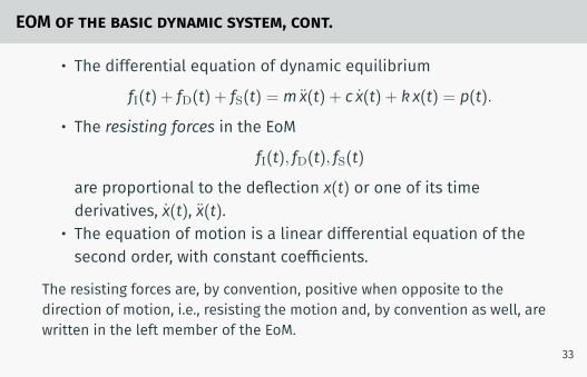
• The differential equation of dynamic equilibrium
fI(t) + fD(t) + fS(t) = m x(t) + c x(t) + k x(t) = p(t).
• The resisting forces in the EoM
fI(t), fD(t), fS(t)
are proportional to the deflection x(t) or one of its timederivatives, x(t), x(t).
• The equation of motion is a linear differential equation of thesecond order, with constant coefficients.
The resisting forces are, by convention, positive when opposite to thedirection of motion, i.e., resisting the motion and, by convention as well, arewritten in the left member of the EoM.
33
Influence of static forces
(a)
m
c
k
p(t)
x(t) x
∆st x(t)
(b)
p(t)
k∆st
fS(t)fD(t)
W
fI(t)
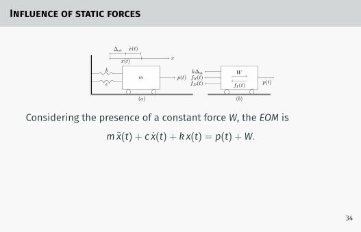
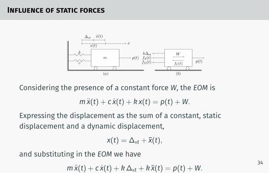
Considering the presence of a constant force W, the EOM is
m x(t) + c x(t) + k x(t) = p(t) +W.
Expressing the displacement as the sum of a constant, staticdisplacement and a dynamic displacement,
x(t) = ∆st + x(t),
and substituting in the EOM we have
m x(t) + c x(t) + k∆st + k x(t) = p(t) +W.
34
Influence of static forces
(a)
m
c
k
p(t)
x(t) x
∆st x(t)
(b)
p(t)
k∆st
fS(t)fD(t)
W
fI(t)
Considering the presence of a constant force W, the EOM is
m x(t) + c x(t) + k x(t) = p(t) +W.
Expressing the displacement as the sum of a constant, staticdisplacement and a dynamic displacement,
x(t) = ∆st + x(t),
and substituting in the EOM we have
m x(t) + c x(t) + k∆st + k x(t) = p(t) +W.34
Influence of static forces, cont.
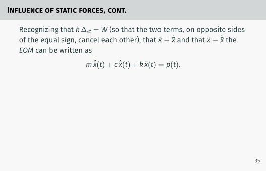
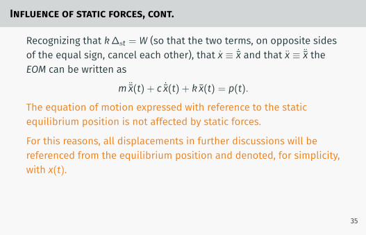
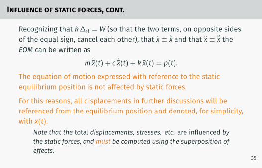
Recognizing that k∆st = W (so that the two terms, on opposite sidesof the equal sign, cancel each other), that x ≡ ˙x and that x ≡ ¨x theEOM can be written as
m ¨x(t) + c ˙x(t) + k x(t) = p(t).
The equation of motion expressed with reference to the staticequilibrium position is not affected by static forces.
For this reasons, all displacements in further discussions will bereferenced from the equilibrium position and denoted, for simplicity,with x(t).
Note that the total displacements, stresses. etc. are influenced bythe static forces, and must be computed using the superposition ofeffects.
35
Influence of static forces, cont.
Recognizing that k∆st = W (so that the two terms, on opposite sidesof the equal sign, cancel each other), that x ≡ ˙x and that x ≡ ¨x theEOM can be written as
m ¨x(t) + c ˙x(t) + k x(t) = p(t).
The equation of motion expressed with reference to the staticequilibrium position is not affected by static forces.
For this reasons, all displacements in further discussions will bereferenced from the equilibrium position and denoted, for simplicity,with x(t).
Note that the total displacements, stresses. etc. are influenced bythe static forces, and must be computed using the superposition ofeffects.
35

Influence of support motion
Fix
edre
fere
nce
axis
xtot(t)
xg(t) x(t)
k
2k
2
m
c
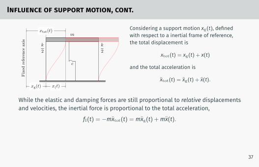
Displacements, deformations and stresses in a structure are induced alsoby a motion of its support.
Important examples of support motion are the motion of a buildingfoundation due to earthquake and the motion of the base of a piece ofequipment due to vibrations of the building in which it is housed. 36
Influence of support motion, cont.Fix
edre
fere
nce
axis
xtot(t)
xg(t) x(t)
k
2k
2
m
c
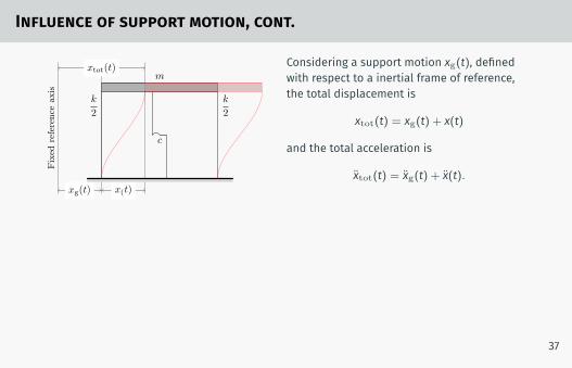
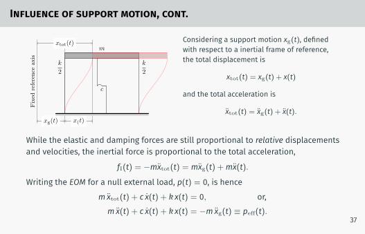
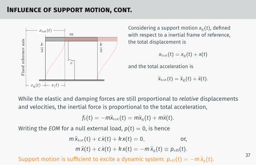
Considering a support motion xg(t), definedwith respect to a inertial frame of reference,the total displacement is
xtot(t) = xg(t) + x(t)
and the total acceleration is
xtot(t) = xg(t) + x(t).
While the elastic and damping forces are still proportional to relative displacementsand velocities, the inertial force is proportional to the total acceleration,
fI(t) = −mxtot(t) = mxg(t) +mx(t).
Writing the EOM for a null external load, p(t) = 0, is hencem xtot(t) + c x(t) + k x(t) = 0, or,m x(t) + c x(t) + k x(t) = −m xg(t) ≡ peff(t).
Support motion is sufficient to excite a dynamic system: peff(t) = −m xg(t).
37
Influence of support motion, cont.Fix
edre
fere
nce
axis
xtot(t)
xg(t) x(t)
k
2k
2
m
c
Considering a support motion xg(t), definedwith respect to a inertial frame of reference,the total displacement is
xtot(t) = xg(t) + x(t)
and the total acceleration is
xtot(t) = xg(t) + x(t).
While the elastic and damping forces are still proportional to relative displacementsand velocities, the inertial force is proportional to the total acceleration,
fI(t) = −mxtot(t) = mxg(t) +mx(t).
Writing the EOM for a null external load, p(t) = 0, is hencem xtot(t) + c x(t) + k x(t) = 0, or,m x(t) + c x(t) + k x(t) = −m xg(t) ≡ peff(t).
Support motion is sufficient to excite a dynamic system: peff(t) = −m xg(t).37

Free vibrations of a SDOF system
Free Vibrations
The equation of motion,
m x(t) + c x(t) + k x(t) = p(t)
is a linear differential equation of the second order, with constantcoefficients.
Its solution can be expressed in terms of a superposition of aparticular solution, depending on p(t), and a free vibration solution,that is the solution of the so called homogeneous problem, wherep(t) = 0.
In the following, we will study the solution of the homogeneousproblem, the so-called homogeneous or complementary solution,that is the free vibrations of the SDOF after a perturbation of theposition of equilibrium. 38
Free vibrations of an undamped system
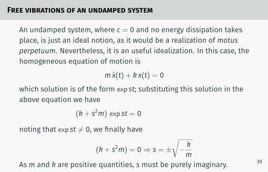
An undamped system, where c = 0 and no energy dissipation takesplace, is just an ideal notion, as it would be a realization of motusperpetuum. Nevertheless, it is an useful idealization. In this case, thehomogeneous equation of motion is
m x(t) + k x(t) = 0
which solution is of the form exp st; substituting this solution in theabove equation we have
(k+ s2m) exp st = 0
noting that exp st = 0, we finally have
(k+ s2m) = 0⇒ s = ±√− km
As m and k are positive quantities, s must be purely imaginary. 39
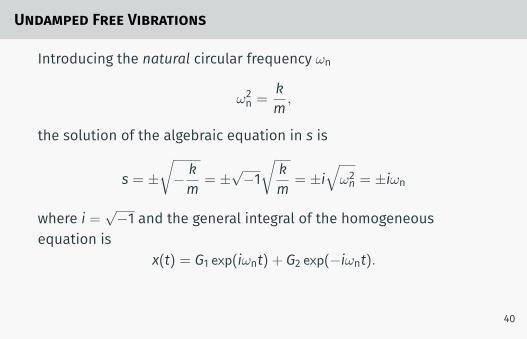
Undamped Free Vibrations
Introducing the natural circular frequency ωn
ω2n =km ,
the solution of the algebraic equation in s is
s = ±√− km = ±
√−1
√km = ±i
√ω2n = ±iωn
where i =√−1 and the general integral of the homogeneous
equation isx(t) = G1 exp(iωnt) + G2 exp(−iωnt).
The solution has an imaginary part?
40
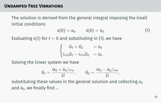
Undamped Free Vibrations
The solution is derived from the general integral imposing the (real)initial conditions
x(0) = x0, x(0) = x0 (1)Evaluating x(t) for t = 0 and substituting in (1), we have{
G1 + G2 = x0iωnG1 − iωnG2 = x0
Solving the linear system we have
G1 =ix0 + x0/ωn
2i , G2 =ix0 − x0/ωn
2i ,
substituting these values in the general solution and collecting x0and x0, we finally find ...
41
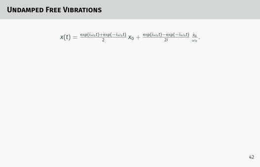
Undamped Free Vibrations
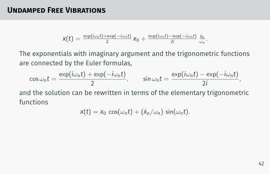
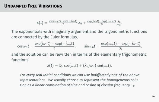
x(t) = exp(iωnt)+exp(−iωnt)2 x0 + exp(iωnt)−exp(−iωnt)
2ix0ωn.
The exponentials with imaginary argument and the trigonometric functionsare connected by the Euler formulas,
cosωnt =exp(iωnt) + exp(−iωnt)
2 , sinωnt =exp(iωnt)− exp(−iωnt)
2i ,
and the solution can be rewritten in terms of the elementary trigonometricfunctions
x(t) = x0 cos(ωnt) + (xo/ωn) sin(ωnt).
For every real initial conditions we can use indifferently one of the aboverepresentations. We usually choose to represent the homogeneous solu-tion as a linear combination of sine and cosine of circular frequency ωn
42
Undamped Free Vibrations
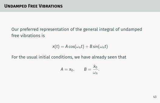
Our preferred representation of the general integral of undampedfree vibrations is
x(t) = A cos(ωnt) + B sin(ωnt)
For the usual initial conditions, we have already seen that
A = x0, B =x0ωn
.
43
Undamped Free Vibrations
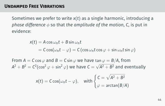
Sometimes we prefer to write x(t) as a single harmonic, introducing aphase difference ϕ so that the amplitude of the motion, C, is put inevidence:
x(t) = A cosωnt+ B sinωnt= C cos(ωnt− φ) = C (cosωnt cosφ+ sinωnt sinφ)
From A = C cosφ and B = C sinφ we have tanφ = B/A, fromA2 + B2 = C2(cos2 φ+ sin2 φ) we have C =
√A2 + B2 and eventually
x(t) = C cos(ωnt− φ), with{C =
√A2 + B2
φ = arctan(B/A)
44
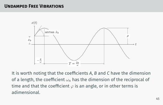
Undamped Free Vibrations
x(t)
t
x0
arctan x0
− θω
T = 2πω
ρ
It is worth noting that the coefficients A, B and C have the dimensionof a length, the coefficient ωn has the dimension of the reciprocal oftime and that the coefficient φ is an angle, or in other terms isadimensional.
45

Free vibrations of a damped system
Behavior of Damped Systems
The viscous damping modifies the response of a sdof systemintroducing a decay in the amplitude of the response. Depending onthe amount of damping, the response can be oscillatory or not. Theamount of damping that separates the two behaviors is denoted ascritical damping.
46
The solution of the EOM
The equation of motion for a free vibrating damped system is
m x(t) + c x(t) + k x(t) = 0,
substituting the solution exp st in the preceding equation andsimplifying, we have that the parameter s must satisfy the equation
ms2 + c s+ k = 0
or, after dividing both members by m,
s2 + cm s+ ω2n = 0
whose solutions are
s = − c2m ∓
√( c2m
)2− ω2n = ωn
− c2mωn
∓
√(c
2mωn
)2− 1
.
47
Critical Damping
The behavior of the solution of the free vibration problem dependsof course on the sign of the radicand ∆ =
(c
2mωn
)2− 1:
∆ < 0 the roots s are complex conjugate,∆ = 0 the roots are identical, double root,∆ > 0 the roots are real.
The value of c that make the radicand equal to zero is known as thecritical damping,
ccr = 2mωn = 2√mk.
48

Critical Damping
A single degree of freedom system is denoted as critically damped,under-critically damped or over-critically damped depending on thevalue of the damping coefficient with respect to the critical damping.
Typical building structures are undercritically damped.
49

Critical Damping
A single degree of freedom system is denoted as critically damped,under-critically damped or over-critically damped depending on thevalue of the damping coefficient with respect to the critical damping.
Typical building structures are undercritically damped.
49
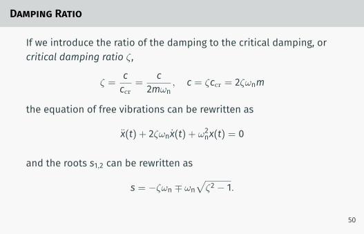
Damping Ratio
If we introduce the ratio of the damping to the critical damping, orcritical damping ratio ζ ,
ζ =cccr
=c
2mωn, c = ζccr = 2ζωnm
the equation of free vibrations can be rewritten as
x(t) + 2ζωnx(t) + ω2nx(t) = 0
and the roots s1,2 can be rewritten as
s = −ζωn ∓ ωn√
ζ2 − 1.
50
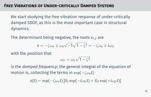
Free Vibrations of Under-critically Damped Systems
We start studying the free vibration response of under-criticallydamped SDOF, as this is the most important case in structuraldynamics.
The determinant being negative, the roots s1,2 are
s = −ζωn ∓ ωn√−1
√1− ζ2 = −ζωn ∓ iωD
with the position thatωD = ωn
√1− ζ2.
is the damped frequency; the general integral of the equation ofmotion is, collecting the terms in exp(−ζωnt)
x(t) = exp(−ζωnt) [G1 exp(−iωDt) + G2 exp(+iωDt)]
51
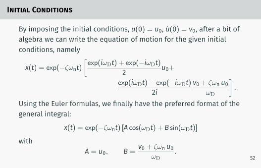
Initial Conditions
By imposing the initial conditions, u(0) = u0, u(0) = v0, after a bit ofalgebra we can write the equation of motion for the given initialconditions, namely
x(t) = exp(−ζωnt)[exp(iωDt) + exp(−iωDt)
2 u0+
exp(iωDt)− exp(−iωDt)2i
v0 + ζωn u0ωD
].
Using the Euler formulas, we finally have the preferred format of thegeneral integral:
x(t) = exp(−ζωnt) [A cos(ωDt) + B sin(ωDt)]
withA = u0, B =
v0 + ζωn u0ωD
.52
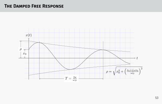
The Damped Free Response
x(t)
t
x0
ρ
T = 2πωD
ρ =
√x20 +
(x0+ζωx0
ωD
)2
53
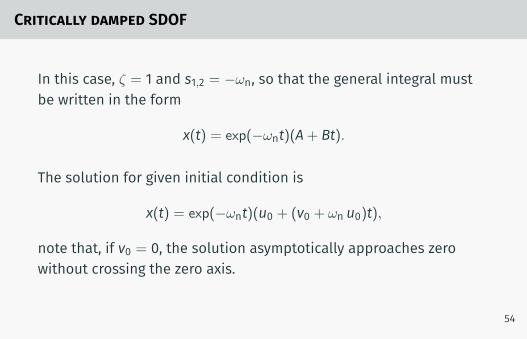
Critically damped SDOF
In this case, ζ = 1 and s1,2 = −ωn, so that the general integral mustbe written in the form
x(t) = exp(−ωnt)(A+ Bt).
The solution for given initial condition is
x(t) = exp(−ωnt)(u0 + (v0 + ωn u0)t),
note that, if v0 = 0, the solution asymptotically approaches zerowithout crossing the zero axis.
54
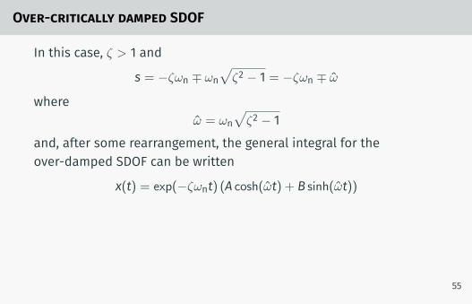
Over-critically damped SDOF
In this case, ζ > 1 and
s = −ζωn ∓ ωn√ζ2 − 1 = −ζωn ∓ ω
whereω = ωn
√ζ2 − 1
and, after some rearrangement, the general integral for theover-damped SDOF can be written
x(t) = exp(−ζωnt) (A cosh(ωt) + B sinh(ωt))
Note that:
• as ζωn > ω, for increasing t the general integral goes to zero, and that• as for increasing ζ we have that ω → ζωn, the velocity with which theresponse approaches zero slows down for increasing ζ .
55
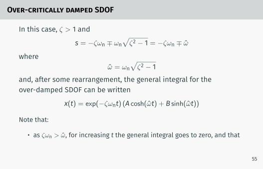
Over-critically damped SDOF
In this case, ζ > 1 and
s = −ζωn ∓ ωn√ζ2 − 1 = −ζωn ∓ ω
whereω = ωn
√ζ2 − 1
and, after some rearrangement, the general integral for theover-damped SDOF can be written
x(t) = exp(−ζωnt) (A cosh(ωt) + B sinh(ωt))
Note that:
• as ζωn > ω, for increasing t the general integral goes to zero, and that
• as for increasing ζ we have that ω → ζωn, the velocity with which theresponse approaches zero slows down for increasing ζ .
55
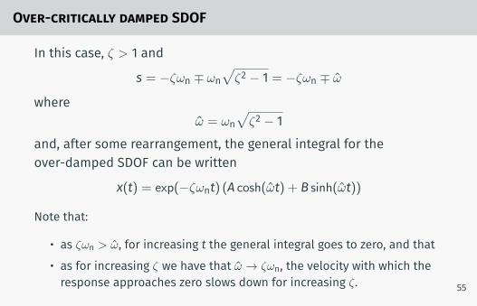
Over-critically damped SDOF
In this case, ζ > 1 and
s = −ζωn ∓ ωn√ζ2 − 1 = −ζωn ∓ ω
whereω = ωn
√ζ2 − 1
and, after some rearrangement, the general integral for theover-damped SDOF can be written
x(t) = exp(−ζωnt) (A cosh(ωt) + B sinh(ωt))
Note that:
• as ζωn > ω, for increasing t the general integral goes to zero, and that• as for increasing ζ we have that ω → ζωn, the velocity with which theresponse approaches zero slows down for increasing ζ . 55
Measuring damping
The real dissipative behavior of a structural system is complex andvery difficult to assess.
For convenience, it is customary to express the real dissipativebehavior in terms of an equivalent viscous damping.
In practice, we measure the response of a SDOF structural systemunder controlled testing conditions and find the value of the viscousdamping (or damping ratio) for which our simplified model bestmatches the measurements.
For example, we could require that, under free vibrations, the realstructure and the simplified model exhibit the same decay of thevibration amplitude.
56
Logarithmic Decrement
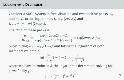
Consider a SDOF system in free vibration and two positive peaks, unand un+m, occurring at times tn = n (2π/ωD) andtn+m = (n+m) (2π/ωD).
The ratio of these peaks isunun+m
=exp(−ζωnn2π/ωD)
exp(−ζωn(n+m)2π/ωD)= exp(2mπζωn/ωD)
Substituting ωD = ωn√1− ζ2 and taking the logarithm of both
members we obtain
ln(unun+m
) = δ = 2mπζ√1− ζ2
where we have introduced δ, the logarithmic decrement; solving forζ , we finally get
ζ = δ((2mπ)2 + δ2
)− 12 . 57
Recursive Formula for ζ
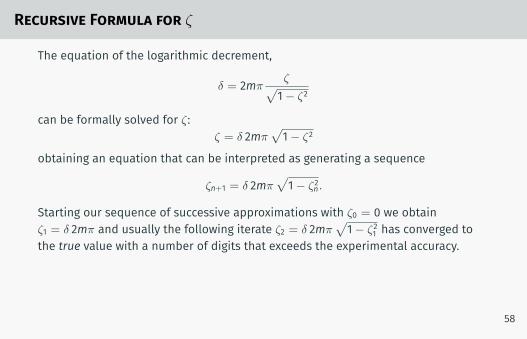
The equation of the logarithmic decrement,
δ = 2mπζ√1− ζ2
can be formally solved for ζ :ζ = δ 2mπ
√1− ζ2
obtaining an equation that can be interpreted as generating a sequence
ζn+1 = δ 2mπ√1− ζ2n.
Starting our sequence of successive approximations with ζ0 = 0 we obtainζ1 = δ 2mπ and usually the following iterate ζ2 = δ 2mπ
√1− ζ21 has converged to
the true value with a number of digits that exceeds the experimental accuracy.
While the recursive formula is useful in itself, it is also useful as a first example offinding better approximations of a system’s parameter using an iterative procedure.
58
Recursive Formula for ζ
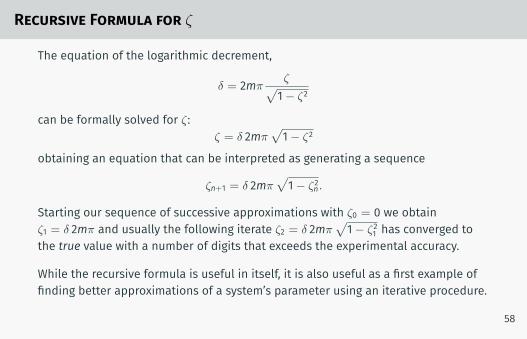
The equation of the logarithmic decrement,
δ = 2mπζ√1− ζ2
can be formally solved for ζ :ζ = δ 2mπ
√1− ζ2
obtaining an equation that can be interpreted as generating a sequence
ζn+1 = δ 2mπ√1− ζ2n.
Starting our sequence of successive approximations with ζ0 = 0 we obtainζ1 = δ 2mπ and usually the following iterate ζ2 = δ 2mπ
√1− ζ21 has converged to
the true value with a number of digits that exceeds the experimental accuracy.
While the recursive formula is useful in itself, it is also useful as a first example offinding better approximations of a system’s parameter using an iterative procedure.
58