Dynamics of Flow Structures and Transport Phenomena, 2. Relationship with Design Objectives and...

Dynamics of Flow Structures and Transport Phenomena, 1. Experimental andNumerical Techniques for Identification and Energy Content of Flow Structures

Jyeshtharaj B. Joshi,* Mandar V. Tabib, Sagar S. Deshpande, and Channamallikarjun S. Mathpati

Department of Chemical Engineering, Institute of Chemical Technology Matunga, Mumbai-400019, India

Most chemical engineering equipment is operated in the turbulent regime. The flow patterns in this equipmentare complex and are characterized by flow structures of wide range of length and time scales. The accuratequantification of these flow structures is very difficult and, hence, the present design practices are still empirical.Abundant literature is available on understanding of these flow structures, but in very few cases efforts havebeen made to improve the design procedures with this knowledge. There have been several approaches in theliterature to identify and characterize the flow structures qualitatively as well as quantitatively. In the last fewdecades, several numerical as well as experimental methods have been developed that are complementary toeach other with the onset of better computational and experimental facilities. In the present work, themethodologies and applications of various experimental fluid dynamics (EFD) techniques (namely, pointmeasurement techniques such as hot film anemometry, laser Doppler velocimetry, and planar measurementtechniques such as particle image velocimetry (PIV), high speed photography, Schlieren shadowgraphy, andthe recent volume measurement techniques such as holographic PIV, stereo PIV, etc.), and the computationalfluid dynamics (CFD) techniques (such as direct numerical simulation (DNS) and large eddy simulation (LES))have been discussed. Their chronological developments, relative merits, and demerits have been presented toenable readers to make a judgment as to which experimental/numerical technique to adopt. Also, severalnotable mathematical quantifiers are reviewed (such as quadrant technique, variable integral time averagetechnique, spectral analysis, proper orthogonal decomposition, discrete and continuous wavelet transform,eddy isolation methodology, hybrid POD-Wavelet technique, etc.). All three of these tools (computational,experimental, and mathematical) have evolved over the past 6-7 decades and have shed light on the physicsbehind the formation and dynamics of various flow structures. The work ends with addressing the presentissues, the existing knowledge gaps, and the path forward in this field.

1. Introduction

The present methodology of designing the process equipmentis based on empiricism, as well as knowledge accumulated fromprior experience. Because of inefficient design, the chemicalindustries have not been able to utilize the resources (rawmaterials, hardware, utilities, and energy) effectively, whichleads to a higher cost of production, a loss of product quality,and environmental pollution. The fundamental reason forempiricism is the complexity of the fluid dynamics in the processequipment. Hence, much work is ongoing for the understandingof the physics of turbulent flows. Because most of the industrialequipment is operated under the turbulent conditions, whereinthe motion of compendium of eddies (flow structures) ofdifferent length and time scales contribute toward mixing,momentum transfer, heat transfer, and mass transfer. Hence, aproper understanding of the mechanism related to the formationand the role of these turbulent flow structures in determiningthe transport phenomena can cause improvement in the scale-up and design procedures. The present work reviews someprominent methodologies and techniques devoted to identifying,characterizing, and studying the dynamics of these flowstructures, and their effect on transport phenomena.

Turbulence is generally defined as the fluctuations aroundthe mean flow. These fluctuations are the result of passage ofthe deterministic organized flow structures and the randomdisorganized irrotational motions, which, together, constitute theturbulent flows. The organized deterministic patterns are knownas eddies or turbulent flow structures. The flow structures areoften hidden among the incoherent turbulent motions. Some ofthese structures are shown in Figure 1. These organized flowstructures have been known from as early as the 15th century,as conceptualized by Leonardo Da Vinci. Brown and Roshko1

observed the roller structure in the mixing layer (Figure 1A).Richardson2 gave the first notion of a cascade process ofstructure breakup. He suggested that these structures are partof the turbulence (Figure 1B) and the energy is injected at largerlength scale structures, and the energy is transmitted to smallerand smaller length scale structures, until it reaches a size, whereviscosity is dominant, and the viscous dissipation results intodirect conversion to heat. To begin with, we review thehistorically much debated issue of categorizing flow structures,and make an effort toward rationalization. The coherent flowstructures have been defined in the following manners in theliterature.

(1) Hussain3,4 emphasized that coherent vorticity (i.e.,instantaneous phase-correlated and space-correlated vorticity)is a primary identifier for detecting characteristic structures (alsoknown as coherent structures) that possess a distinct boundary

* Author to whom correspondence should be addressed. Tel.: + 91-22-2414 0865. Fax: +91 -22-2414 5614. E-mail: [email protected].

Ind. Eng. Chem. Res. 2009, 48, 8244–82848244

10.1021/ie8012506 CCC: $40.75 2009 American Chemical SocietyPublished on Web 06/04/2009

and independent territory. He attempted to describe thesestructures as a turbulent fluid mass with instantaneously phase-correlated vorticity over its spatial extent, with spatial extentbeing comparable to transverse length scale of shear flow.Therefore, although length scales of the order of Kolmogorovscales are known to show intense coherent vorticity, they cannotbe called characteristic structures, because of the small spatialextent.

(2) While, according to McComb,5 coherent structures arediscernible patterns in the flow and occur with sufficientregularity, in space and/or time, to be recognizable as quasi-periodic or near-deterministic.

Although characteristic flow structures occur prominently inturbulent flows, their contribution to the total kinetic energy isonly a small fraction. Hence, to understand the effect of flowstructures on the transport phenomena, all the structures shouldbe taken into account. In the literature, more emphasis is givento study the characteristic flow structures, rather than all thestructures present in the flow. We have an opinion that, as faras possible, all the flow structures should be studied. Becauseall the flow structures, from large scale (of the order of reactorgeometry) to small scale (Kolmogorov scale), contribute tomixing and/or heat transfer by advecting the species and/orenthalpy from one place to another, at both the microlevel andthe macrolevel. For equipment such as ultrasound reactors, thetransient flow structures are very important and have significantimpact on the transport phenomena. Thus, the focus should beon characterizing each and every flow structure so that one canstudy their role in the overall transport phenomena, and perhapsnot into their classification/categorization categorizing it. In thisreview, the flow structures are characterized by their (a)mechanism of formation, and their location in space and time(how, when and where they are formed), (b) spatial and temporalcoherence (time and length scale), (c) their topological definition(size and shape), (d) their energy content (helps to determinestrength of the flow structure), (e) their properties (coherentvorticity value, second invariant gradient values), (f) theirdynamics (startup, merging, breakup, interaction with mean flowand other turbulent structures) as we change the operating andgeometric conditions, and, finally (g) the effect of these flowstructures on the transport phenomena and their relation withdesign parameters. The last point forms the basis for the secondpart of this review.

In the present review, fluid dynamics in the process equipment(Figure 2) has been classified as flows with stationary walls

(channel flow), flows with some rotating/moving walls (stirredtank, annular centrifugal extractors), flows with discontinuousmoving interfaces (bubble column), flows away from the walls(free shear turbulence, free jets, open channel flows), andultrasound reactor. These equipment are selected so that extremeflow conditions can be covered, e.g., in channel flow, majorturbulence generation is at the walls, where the no-slip conditionapplies and other extreme is free surface turbulence, wherepractically complete slip conditions prevail and the generationof flow structures is away from the interface. The other casesfall in these two extremes. The extreme flow conditions can becharacterized by the range of the energy dissipation rate (ε).For instance, the average value of ε in pipe flow is in the rangeof 4-10000 W/kg (for water flowing in a 2-in. pipe betweenRe ) 5600-100000) whereas it is in the range of 50-1000W/kg in annular centrifugal contactors.

The mechanism of formation of characteristic flow structuresis discussed in section 2 and literature pertaining to the studyof these structures using the experimental and computationaltools is presented in sections 3 and 4, respectively. Mathematicaltools for identification and characterization of flow structuresare reported in section 5. Structures identified using thesetechniques in the aforementioned equipment are discussed in section6. Finally, the effect of flow structures on energy spectra andestimation of turbulence parameters is reported in section 7.

2. Mechanism of Formation

Turbulent flow structures are described as the motions of fluidparcels that have a life cycle and undergo generation, develop-ment, and breakdown. Generally, the initial formation of a flowstructure is always the result of instability, i.e., on the relativecontribution of forces acting on the fluid element. For example,in pipe flow, the transition to turbulence occurs when the inertialforces are dominated over the viscous forces and structures formbecause of shear or velocity gradients in the flow. In some cases,it is the amplification of these instabilities that leads to theformation of flow structures with a definite pattern. Then, thevortex stretching mechanism is responsible for producing higher-intensity smaller vortices. The stretching of these vortices,because of velocity gradients, leads to a reduction in the sizesof the vortices, and a subsequent increase in their vorticity, toconserve the angular momentum. In this section, we discussthe mechanism of formation of flow structures at some distinctlocations: near the solid/fluid interface, near the free surface,behind bluff and blunt bodies, in free shear region (mixing layerand free jet region), and in the multiphase systems (dispersed-phase-induced turbulence).

2.1. Solid/Fluid Interface. Turbulent structures near the wallhave been studied comprehensively for the last four decades.5-9

Professor Kline’s group6-8 first discovered these structures usinga hydrogen bubble technique in the turbulent boundary layer,and called them “near-wall coherent structures”. They calledthe life cycle of these structures as a “burst”, and the ac-companying phenomena as the “bursting process”. They de-scribed “bursting” as a phenomenon comprised of regularejections (outward motion of fluid from the wall) and sweeps(inward motion of fluid toward the wall). They proposed thefollowing mechanism. The total process of bursting is acontinuous chain of events starting from a relatively quiescentwall flow and leading to the formation of relatively large andrelatively chaotic fluctuations. The first stage of bursting is thelifting of flow structures away from the wall. The fluid motionin the near-wall region is unsteady, and the flow structures alsomove in the streamwise and wall-normal directions (and they

Figure 1. Turbulence as depicted by (A) mixing layer flow structures(Roshko and Brown1), (B) Richardson2 cascade (notion of turbulence).

Ind. Eng. Chem. Res., Vol. 48, No. 17, 2009 8245

are also called “low speed streaks”). This movement is causedby the local instability in the flow. Once the low-speed streakreaches a critical distance from the wall (at x1

+ ≈ 12), it appearsto turn sharply outward, away from the wall. They then continueto move downstream (Kim et al.7). This more-rapid outwardmotion is called “low-speed-streak lifting” and is also character-ized by low secondary (streamwise) vorticity. Thus, therelatively rapid outward motion creates an inflectional point inthe instantaneous velocity profile as very rapid changes in theinstantaneous velocity profile10-12 (see Figure 3A). The instan-taneous inflectional profiles lead to the growth of an oscillatorydisturbance just downstream of the inflectional zone. Thedominant mode of this oscillation is the streamwise vortexmotion. This is also the reason for a peak in turbulent kineticenergy profile very close to the wall (x1

+ ) 10-20; see Figure3B). An increase in the total kinetic energy occurs during thebursting times, but most of this added energy is in the frequencyrange near the frequency of oscillatory growth. The oscillationis terminated by the start of a more-chaotic fluctuation called“breakup”. The beginning of the breakup phase indicates thereturn of the instantaneous velocity profile to a form qualitativelysimilar to that of the mean profile, including the vanishing ofthe inflectional zone. The ejection phase contributes to increasedinteraction with the bulk and, hence, mixing, whereas the sweepphase contributes to surface renewal and, hence, heat/masstransfer. This entire cycle repeats randomly in space and time.The maximum turbulence production is observed primarilyduring the ejection phase and somewhat less during the sweepphase of bursting. Systematic simulations of homogeneousturbulence with arbitrary shear at random locations in the bulkhave shown similar structures, proving that shear at the interfaceis a important for the formation of such structures.13

2.2. Free Surface Turbulence. The fluid/fluid interfacewhere the shear at the interface is negligibly small enough iscalled a free surface. The study of transport phenomena

governed by flow structures at free surfaces is of great interestto design contacting equipment (such as evaporators, condensers,and gas absorbers) and to study the interactions betweenatmosphere and sea/river for understanding the CO2 uptake.14

Mass transfer at these free interfaces (the relative velocitiesbetween two phases can be nonzero) plays a central role in manyindustrial and environmental processes. Generally, in the designof bubble columns, the contact time for surface renewal is takenapproximately as the bubble diameter divided by the bubblerise velocity. However, for the accurate estimation of mass-transfer rates, an understanding of the turbulence close to freesurfaces (a distance on the order of a few micrometers fromthe surface) is important. This area is still in a state ofdevelopment, because it is very difficult to measure and/orcompute the flow accurately in a region very close to theinterface. Many theories have been proposed in the literatureto qualitatively represent the free surface turbulence, namely,film theory, penetration theory, surface renewal models, surfacedivergence models, etc. Systematic measurements and computa-tions by the research groups of Komori and co-workers15-19

and Banerjee and co-workers20-23 have highlighted manyfeatures of free surface turbulence. These studies had beenmainly performed in open channel flows where at the topinterface slip boundary conditions could be manipulated fromcomplete slip (zero shear) to very close to no slip (very highshear). There are persistent large-scale flow structures at thefree surface (Figure 4A), comprised of the “upwellings” (causedeither by the impingement of bursts emanating from the bottomwall or by the vortices emanating from the bulk), the “down-drafts” (where the flow from adjacent upwellings meet), andthe “whirlpool like” attached vortices that form at the edge ofthe upwellings. In the case of a complete slip boundary, theupwellings are observed at the interface, apparently because ofthe bulk turbulence or turbulence at the bottom wall (Figure4B) (see Rashidi and Banerjee20). The upwellings cause the

Figure 2. Schematic diagram of all the equipments: (A) channel flow, (B) jet loop reactor, (C) stirred tank, (D) Taylor-Couette flow (annular contactor),(E) ultrasonic reactor, and (F) bubble column.

8246 Ind. Eng. Chem. Res., Vol. 48, No. 17, 2009

surface to diverge and surface renewal occurs. These upwellingvortices are energetic and play a significant role in redistributingheat and mass at the interfaces. The edge of the upwellings andthe region between the two upwellings are high-shear regionsthat cause instabilities, which lead to the formation of thesewhirlpool-like vortices. These attached vortices tend to pair ormerge with each other and dissipate very slowly, provided theyare not destroyed by other upwellings. These types of vorticesare unique to free surfaces and are not found at the solidinterface. With the incorporation of shear at the interface, low-speed and high-speed streaks start to appear at the gas/liquidinterface (see Figure 4C). In addition to upwellings, the streakingphenomena also help in heat and mass transfer at the interface.The mechanism of formation of these streaks is similar toturbulence at solid interfaces and the occurrence of thesestructures is very well-correlated with shear rate at the interface.There are several papers and reviews (Komori and co-workers15-19 and Nakagawa and Nezu24,25), either explicitlyor implicitly touching upon the subject of the present discussion.

2.3. Free Shear Flows. In some applications, a fluid isinjected through the nozzles in the pool of same fluid or acompletely miscible fluid. In this process, the ambient fluid gets

carried along with the jet by viscous drag at the outer layer ofthe jet. The rate at which fluid from the jet and from itssurroundings become mixed at the interface is given by theentrainment rate of the jet, which defines the rate of propagationof the interface between the chaotic and relatively stagnant fluid.This entrainment rate is controlled by the speed at which theinterface contortions with the largest scales move into thesurrounding fluid.26 As the jet emerges from an axisymmetricnozzle, a shear layer is formed between the jet stream and thesurroundings. In the regions nearer to the jet exit, there is anexponential growth of small perturbations, because of the earlylinear instability jet regime. In regions away from the jet regionand beyond the early development stage, the nonlinearKelvin-Helmholtz instability regime takes over, leading totransitional shear flow. In this regime, the large-scale vortexrings roll up and merge and demerge. Further downstream fromthe nozzle, the streamwise vorticity component and the three-dimensional azimuthal instabilities dominate, leading to thetransition to the turbulent jet regime. In the turbulent regime,the azimuthal instabilities cause the breakdown of the vortexrings. The vorticity dynamics witnessed in this regime causesself-induction, vortex stretching, and vortex reconnection, which

Figure 3. (A) Instantaneous velocity profiles close to wall using the hydrogen bubble technique (see Kim et al.7). (B) Turbulent kinetic energy profile inchannel flow in the wall-normal direction at different Reynolds numbers (data from Kawamura and co-workers10-12) (legend: line 1, Re ) 5600; line 2, Re) 14000; line 3, Re ) 24400; and line 4, Re ) 41400.


leads to an additional production of vorticity. The jet develop-ment is determined by the dynamics of large-scale vortex ringsand braid vortices, and by strong vortex interactions that resultin a more-disorganized flow regime characterized by smaller-scale elongated vortex tubes.27 The time-averaged and instan-taneous flow structures in jet loop reactor28 are shown in Figures5A and 5B, respectively. An instantaneous LES snapshot isshown in Figure 5B. The instantaneous flow shows the followingobservations:

(a) The flow showed major convective motion in the jetregion. The shear region shows the formation of small circula-tion cells in the shear region.

(b) The structures penetrate until the bottom wall and break.(c) The jet region shows fluctuations of the jet plume that

are due to the back pressure exerted by the bottom wall, whichis the result of the jet impact on the bottom. This causes the jetinstability (JI) in the flow.

(d) The bulk region shows the motion of eddies 0.04 m insize along the circulation path, and they disappear after a travellength of ∼0.1-0.15 m.

2.4. Flow Past Solid and Blunt Bodies. In the flow pastthe solid bodies, the two extremes are (i) parallel flow over astreamlined body29 (Figure 6A) and (ii) a circular or rectangular

disk normal to the flow29 (Figure 6B). The intermediate betweenthese extremes is flow past a cylinder29 (Figure 6C). Wheneverany such obstacle is placed in a free stream, at very lowReynolds number (Re < 0.01), flow just creeps on the surface.With an increase in Re, the flow gets separated from the surfaceat some point. The separation point is dependent on the shapeof the surface. Beyond this point, the flow structures get formedin the wake. At low to moderate Re values, the zone ofseparation contains a rather stable flow structure, in whichcirculatory motion is maintained through the transmission ofshear stress across the dividing streamline. Therefore, thevelocities within the flow structure are considerably below thoseof the surrounding flow. As the Reynolds number increasesfurther, essentially the same relative velocities are maintained,but the flow structure becomes more unstable. Eventually, apoint comes where these structures tend to grow and detachthemselves from the boundary and pass off into the wake, asnew flow structures form to take their place. At very high Revalues, this process is extremely rapid and complex. Becausethe separation occurs where the velocity of the surrounding flowis highest, the pressure at the rear of the blunt body is lowerthan that at the front. The separation produces a net force inthe direction of flow and, hence, increases resistance between

Figure 4. (A) Free surface turbulence (see Turney and Banerjee23). (B) Schematic of turbulence mechanism in open channel flow (see Rashidi and Banerjee20).(C) Instantaneous velocity profile using the hydrogen bubble technique in the presence of shear at the interface (from Rashidi and Banerjee20).


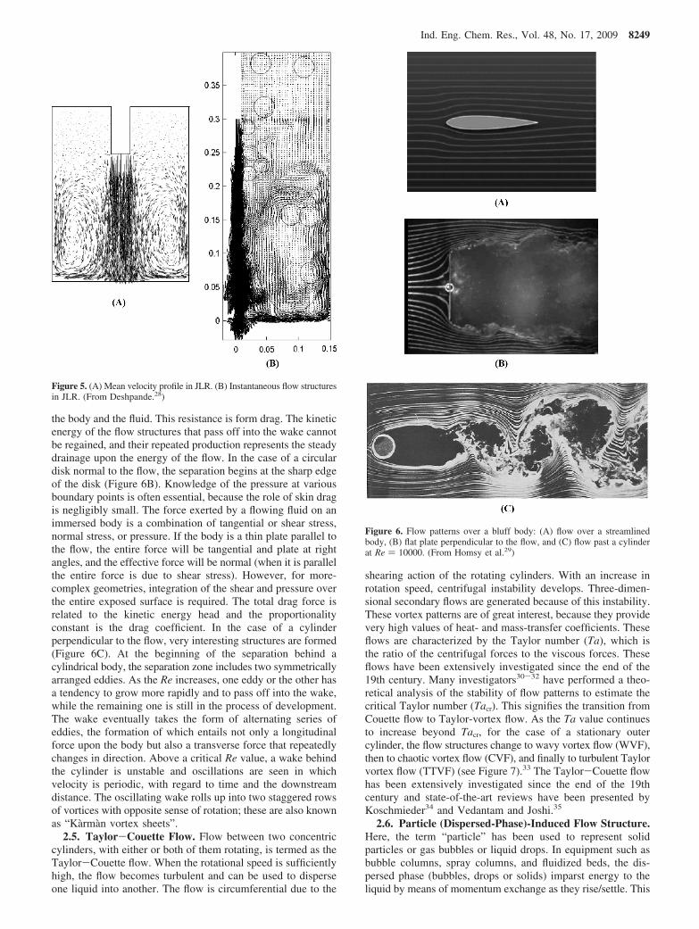
the body and the fluid. This resistance is form drag. The kineticenergy of the flow structures that pass off into the wake cannotbe regained, and their repeated production represents the steadydrainage upon the energy of the flow. In the case of a circulardisk normal to the flow, the separation begins at the sharp edgeof the disk (Figure 6B). Knowledge of the pressure at variousboundary points is often essential, because the role of skin dragis negligibly small. The force exerted by a flowing fluid on animmersed body is a combination of tangential or shear stress,normal stress, or pressure. If the body is a thin plate parallel tothe flow, the entire force will be tangential and plate at rightangles, and the effective force will be normal (when it is parallelthe entire force is due to shear stress). However, for more-complex geometries, integration of the shear and pressure overthe entire exposed surface is required. The total drag force isrelated to the kinetic energy head and the proportionalityconstant is the drag coefficient. In the case of a cylinderperpendicular to the flow, very interesting structures are formed(Figure 6C). At the beginning of the separation behind acylindrical body, the separation zone includes two symmetricallyarranged eddies. As the Re increases, one eddy or the other hasa tendency to grow more rapidly and to pass off into the wake,while the remaining one is still in the process of development.The wake eventually takes the form of alternating series ofeddies, the formation of which entails not only a longitudinalforce upon the body but also a transverse force that repeatedlychanges in direction. Above a critical Re value, a wake behindthe cylinder is unstable and oscillations are seen in whichvelocity is periodic, with regard to time and the downstreamdistance. The oscillating wake rolls up into two staggered rowsof vortices with opposite sense of rotation; these are also knownas “Karman vortex sheets”.

2.5. Taylor-Couette Flow. Flow between two concentriccylinders, with either or both of them rotating, is termed as theTaylor-Couette flow. When the rotational speed is sufficientlyhigh, the flow becomes turbulent and can be used to disperseone liquid into another. The flow is circumferential due to the

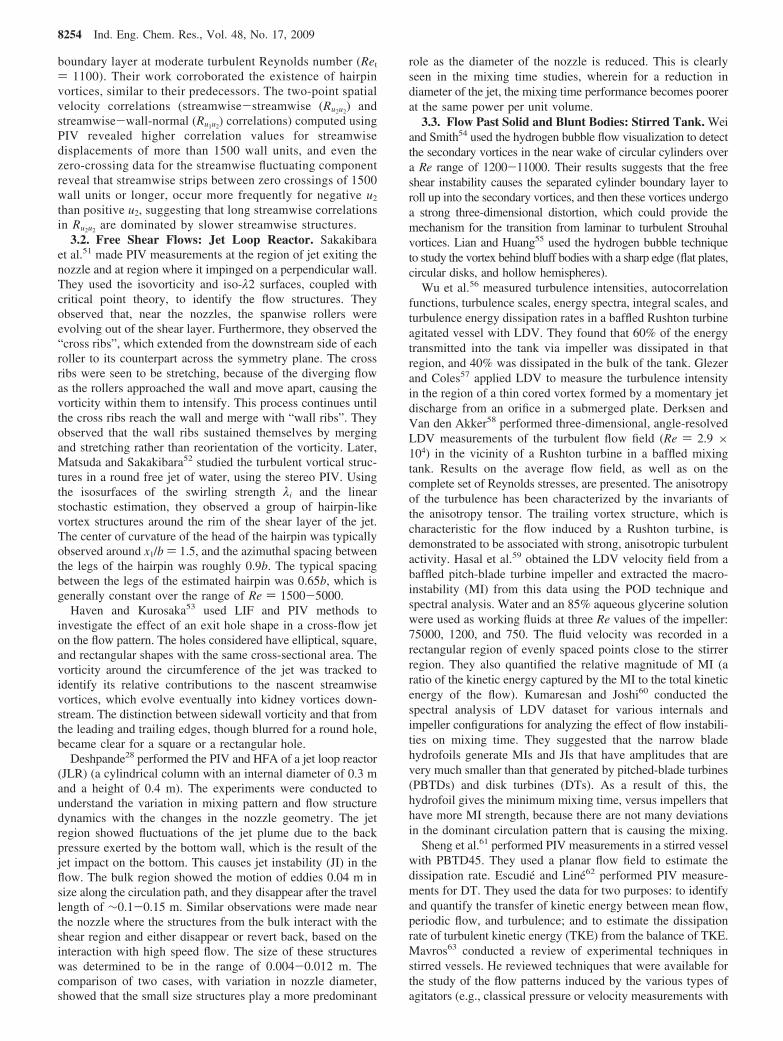
shearing action of the rotating cylinders. With an increase inrotation speed, centrifugal instability develops. Three-dimen-sional secondary flows are generated because of this instability.These vortex patterns are of great interest, because they providevery high values of heat- and mass-transfer coefficients. Theseflows are characterized by the Taylor number (Ta), which isthe ratio of the centrifugal forces to the viscous forces. Theseflows have been extensively investigated since the end of the19th century. Many investigators30-32 have performed a theo-retical analysis of the stability of flow patterns to estimate thecritical Taylor number (Tacr). This signifies the transition fromCouette flow to Taylor-vortex flow. As the Ta value continuesto increase beyond Tacr, for the case of a stationary outercylinder, the flow structures change to wavy vortex flow (WVF),then to chaotic vortex flow (CVF), and finally to turbulent Taylorvortex flow (TTVF) (see Figure 7).33 The Taylor-Couette flowhas been extensively investigated since the end of the 19thcentury and state-of-the-art reviews have been presented byKoschmieder34 and Vedantam and Joshi.35

2.6. Particle (Dispersed-Phase)-Induced Flow Structure.Here, the term “particle” has been used to represent solidparticles or gas bubbles or liquid drops. In equipment such asbubble columns, spray columns, and fluidized beds, the dis-persed phase (bubbles, drops or solids) imparst energy to theliquid by means of momentum exchange as they rise/settle. This

Figure 5. (A) Mean velocity profile in JLR. (B) Instantaneous flow structuresin JLR. (From Deshpande.28)

Figure 6. Flow patterns over a bluff body: (A) flow over a streamlinedbody, (B) flat plate perpendicular to the flow, and (C) flow past a cylinderat Re ) 10000. (From Homsy et al.29)


imparted energy ultimately sets the liquid into motion and canbe measured as the total kinetic energy of the liquid, which iscomprised of the kinetic energy due to mean velocity and theturbulent kinetic energy. Both of these quantities are important,because they dictate the performance of these reactors. Bulkmotion is mainly responsible for mixing/dispersion, whereasturbulent motion has a greater influence on interfacial heat andmass transfer. Understanding the sources of the fluctuatingvelocity components, in terms of frequency (time scale) andsize (length scale) of flow structures, is extremely important,because the energy imparted to cause these turbulent fluctuationsultimately dissipates into heat at the smallest scale throughviscous dissipation. Joshi et al.36 has discussed the chronologicaldevelopment in the understanding of bubble-induced coherentstructures in the bubble column. In the bubble column, themechanism for the onset of large-scale structures is related tothe reversal in the direction of the lift force that is acting onthe bubbles.37,38,121 The lift force is responsible for the radialhold-up profile (see Figure 8A) and the density gradients, whichcause the circulations within the bubble column (see Figure 8B).The magnitude and direction of lift force is dependent uponthe established velocity gradient in the liquid phase and thebubble diameter. The size of the bubble formed at the spargeris determined by the balance of four forces: the gas momentumand the buoyancy forces that push and expand the bubbles inopposition to the liquid drag force, liquid inertial force, andthe surface tension force. At lower superficial gas velocities,uniform bubbles are formed at the sparger (3-4 mm in diameter)and there is no further coalescence and breakup. The lift forceacts on the bubble toward the wall direction. This results in ahomogeneous regime having a flatter holdup profile and resultsin weaker circulation flow, because of a lower density gradient(the driving force for circulation). Thus, the large-scale structures

are absent and the flow structures are of the size of bubble-bubble spacing. As the superficial gas velocity is increased, thesize of bubble formed at the sparger increases, as a result of anincrease in liquid drag force and inertial force (see Joshi et al.39).The higher drag often results in increased bubble coalescenceand larger bubble sizes. These larger bubbles experience a liftforce in the direction of center of the column, resulting in thecreation of hold-up gradients and the density gradients that driveintense liquid circulation. At the top of the column, because ofthe reduction in hydrostatic pressure, the bubble sizes are largerthan that those at the bottom. This local bubble size distributioncauses the setup of local density gradients and local circulationpatterns (flow structures). These flow structures may, in turn,trap and disperse many small-sized bubbles. Depending on thelocal void fraction within the flow structure, they may have theirown local density. If this density is relatively higher than thatin other regions of the column, then they may move down;otherwise, they may move up in the column. Thus, at highersuperficial gas velocity, a heterogeneous regime exists that hasa wide bubble size distribution and several vortical structures.These vortical structures mostly lie in the midregion betweenthe central plume region and wall region, and they move upand down the column. To suggest the size, number, and locationsof circulation cells formed in the bubble column, Joshi andSharma40 and Joshi41 and Joshi et al.36 proposed two models:the multiple noninteracting circulation cells model and theinteracting cells with a considerable intercirculation model (seeFigures 8C and 8D). Similar to the bubble column, the fluidizedbed and spray columns may experience distributions in particleand bubble sizes, respectively, leading to local density gradientsand the formation of flow structures.

Figure 7. Flow structures in Taylor-Couette flow (from Deshmukh et al.33).


3. Experimental Tools

Experimental fluid dynamics (EFD) has played a veryimportant role in identification and characterization of flowstructures. These techniques can be classified as intrusive andnonintrusive techniques or as point measurement techniques,planar measurement techniques, and volumetric measurement

techniques. In the present work, a second methodology ofclassification has been adopted. Few techniques (such as smokeinjection, dye injection, hydrogen bubbles and photochromictracers, and fluorescent particle tracing) are widely used for flowvisualization and less for quantitative characterization. Thesetechniques are listed separately. Table 1 gives a brief accountof various techniques, as well as their principles, advantages,and limitations. The majority of the studies, to date, haveinvolved the use of point and planar techniques; however,recently, holographic and stereoscopic particle image velocim-etry (HPIV and SPIV, respectively) techniques are getting muchattention. The performance of different major measurementtechniques, in terms of qualitative and quantitative characteriza-tion of flow structures, is summarized in Table 2. The applicationof the aforementioned techniques for different flows underconsideration are discussed in this section.

3.1. Solid/Fluid Interface: Channel Flow. Because of theimportance of near-wall physics, in terms of understanding thetransport phenomena, a large number of efforts were presentedin the experimentation and conceptualization of near-wallturbulence. Experimental contributions of Fage and Townend,42

Einstein and Li,43 Popovich and Hummel,44 Kline et al.,6 andMeek and Baer45 are extensively referenced while developingthe theories of heat and mass transfer. Fage and Townend42

used ultramicroscopy to study the motion of dust particles inthe immediate vicinity of the wall on a turbulent fluid. The axialmovements of these particles were jerky, and sometimes theyalmost came to rest. The jerkiness of the axial motion due tothe large fluctuations in axial velocity was determined to beassociated with the combined effect of very small changes inwall-normal velocity and the large velocity gradient du2/dx1 atthe boundary. They noticed the existence of large lateraldisplacements of groups of these particles, and they mentionedthe fact that their motion can be regarded as practicallyrectilinear only during the interval between such displacements.These observations were contradictory to the Prandtl’s conceptof laminar sublayer with completely rectilinear motion of fluidelements without any lateral movements. Their work providedan experimental support for the renewal mechanism, which waslater popularized by Higbie46 and Danckwerts.47

Popovich and Hummel44 used a flash photolysis method tostudy viscous sublayers in nondisturbing turbulent flow. Theytook photographs of the near-wall region, introducing a pho-tosensitive fluid and focusing the light from a Xenon flash tube.The tracer was observed in two dimensions. They observedrectilinear motion in laminar sublayer for 38.1% of the measure-ments. An additional 7.5% of the photographs showed a viscousregion without turbulent motion, but with continually changingvelocity gradient, and the remaining 54.4% of the photographsindicated the presence of some turbulent motion or three-dimensional distortion. The authors also investigated thepenetration depth of eddies, because the rates of heat and masstransfer from the wall are greatly influenced by them. Theauthors found the closest distance to the wall reached by eddieswas x1

+ ) 2.09 ( 0.2. The observed average thickness of thelaminar sublayer corresponded to x1

+ ) 6.17, with a mostprobable thickness of x1

+ ) 4.3. Their results indicated that,adjacent to the wall, there is a layer of very small thickness(x1

+ ) 1.6 ( 0.4) in which a linear gradient occurs virtually atall times, but the slope of the gradient changes with time.Beyond x1

+ ) 34.6, essentially turbulent flow exists.The major breakthrough, in terms of understanding the

near-wall flow physics, emerged with the work of Klineet al.6 They used hot wire anemometry, dye injection, and

Figure 8. Flow structures in the bubble column (from Joshi et al.36): (A)hold-up profile in radial direction, (B) gross circulation cells in bubblecolumn, (C) multiple noninteracting cell model, and (D) multiple interactingcell model.


the hydrogen bubble technique for their study. Thesecombined visual and quantitative techniques, which wereemployed by the authors, revealed many significant featuresof turbulent boundary layers. They observed that the laminarsublayer was not two-dimensional and steady, as simple

models had previously perceived. It contained three-dimensional unsteady motions.

Nakagawa and Nezu25 computed the third-order conditionalprobability distribution of the Reynolds stress obtained fromHFA datasets to gain information on ejections, sweeps, and

Table 1. Experimental Tools for Structure Characterization

Sr. No. Technique Remarks

1 marker image tracking methods: (a)smoke injection (b) dye injection (c)hydrogen bubbles and photochromictracers and fluorescent particletracing

Principle: The principle underlying each technique is the measurement of the simultaneousdisplacements marked fluid particles in consecutive images

Advantages: very good (1) for flow visualization and (2) in correlating probe-type turbulentburst detection techniques with the corresponding visualization data

Limitations: (1) extracting accurate quantitative data is very difficult

Point Measurement Techniques

2 laser Doppler velocimetry, LDV(Figure 9A)

Principle: LDV provides the instantaneous velocity components at the point in the flow fieldwhere two or more mutually perpendicular laser beams (viz. blue, green and cyan) intersect toform a fringe pattern. As the seeding or entrained particle passes through this fringe pattern, itscatters the incident laser beam and induces a shift in the frequency of scattered beam (knownas Doppler shift). The Doppler shift depends on the fringe spacing and the velocity of theparticle normal to the fringes.

Advantages: (1) nonintrusive technique, (2) factory calibrated, and (3) micrometer-sizedseedings are traceable

Limitations: (a) unequispaced dataset, (b) Interpolation is needed for equispacing, and (c) highfrequency values of energy are anomalous

3 hot film anemometry, HFA(Figure 9B)

Principle: The HFA is based on convective heat transfer from a heated wire or film elementplaced in a fluid flow. Any change in the fluid flow condition that affects the heat transferfrom the heated element will be detected virtually instantaneously by a constant temperature/constant current HFA system. Therefore, HFA can be used to provide information related tofor example, the velocity and temperature of the flow, concentration changes in gas mixtures,and phase change in multiphase flows.

Advantages: (1) high data rate of ∼20 kHz, (2) equispaced data, and (3) evaluation of entireenergy spectrum possible

Limitations: (1) intrusive technique, (2) requires some prior knowledge to enable calibration, (3)HFA probe is very sensitive and very costly, (4) point datasets, and they cannot give usinformation on the spatial topology of flow structure, (5) voltage velocity calibration is critical,(6) limited response at high frequencies, (7) voltage stability is crucial, (8) variation intemperature is crucial, and (9) negative velocity cannot be measured and, therefore, the resultsof mean velocity cannot be reported

Planar Measurement Techniques

4 particle image velocimetry, PIV(Figure 9C)

Principle: The PIV technique is based on the following steps: seeding the fluid flow volumeunder investigation with a few micrometer-sized particles, which are assumed to follow thefluid flow closely, illuminating a slice of the flow field with a pulsing light sheet; recordingtwo images of the fluid flow with a short time interval between them, using a digital CCDcamera; processing these two successive images to get the instantaneous velocity field. Theentire image is then divided into interrogation areas. An intercorrelation technique is used toevaluate the most probable displacement of the seeding particles within each interrogation area.

Advantages: (a) Planar measurements, (b) two and three component measurements possible, (c)evaluation of spatial derivatives is possible, (d) velocity measurement over a wide range ispossible, (e) PIV gives much more space information on flow instabilities and aboutnoncoherent and coherent turbulent structures.

Limitations: (a) low data rate (∼7-10 Hz), (b) window size limits spatial resolution, (c) forstrong velocity gradients, accuracy is reduced

5 laser-induced fluorescence, LIF Principle: we seed the flow with fluorescent dye. Based on temperature and/or concentration, theintensity of the reflected light changes and local transient variations can be obtained. It is anadd-on to PIV.

Advantages: Quantification of scalar flux and cross-correlationsLimitations: same as those with PIV

Volumetric Measurement Techniques

6 stereoscopic particle imagevelocimetry, SPIV (Figure 9D)

Principle: The stereoscopic PIV (SPIV), which is commonly considered a 3D extension of PIV,provides three components of the flow velocities confined in a thin slice of moving fluidmedium. It employs the statistical average (correlation) of particles in two separate viewingangles before combining the averaged 2D vectors into 3D vectors, thereby losing informationabout individual particles. Even if one circumvents this problem by resorting to particletracking instead of correlation, the information attainable with PIV is only limited in the lasersheet thickness.

Advantages: shape estimation of flow structuresLimitations: (a) qualitative information, (b) very low data rate, and (c) still applicability is

limited to simple flows

7 defocusing particle image velocimetry,DPIV

Principle: three-dimensionality is achieved through defocusing principle

Advantages: Same as that for SPIVLimitations: qualitative information

8 holographic particle imagevelocimetry, HPIV

Principle: The HPIV records the 3D information of a large quantity of particles in a fluidvolume on a hologram instantaneously and then reconstructs the particle images in a 3D space.From the reconstructed image field, the 3D positions (as well as size and shape information) ofthese particles can be retrieved. Furthermore, by finding the 3D displacements of the particlesin the image volume between two exposures separated by a short time lapse, the instantaneous3D velocities of these particles in the volume can also be obtained.

Advantages: Same as those fot HPIVLimitations: (a) low laser light intensity, (b) low particle density, (c) low sampling rate, and (d)

qualitative information


interactions. Kreplin and Eckelmann48 computed the root-mean-square (rms) values, skewness and flatness factors, and prob-ability density functions in a fully developed turbulent channelflow at Re ) 7700 using hot-film probes. HFA probe measure-ments showed that the bursts are associated with a highReynolds shear stress. The wall layer is composed of elongatedregions of high-speed and low-speed streamwise velocity. Thelarge streamwise length of the streaks appears to be due to asequence of vortices following each other, pumping high-speedfluid toward the wall and low-speed fluid away from the wall.

Christensen and Adrian9 performed the PIV measurementsat the outer region of turbulent channel flow (x1

+ < 100) todetermine the average flow field associated with spanwisevortical motions. They observed that the mean structure consistsof a series of swirling motions ascending at an angle of 12°-13°from the wall. This is quite similar to the pattern followed by

hairpin vortices. The results proved that the instantaneousstructures occur with sufficient frequency, strength, and orderto leave an imprint on the mean statistics of the flow.

Similarly, Tomkins and Adrian49 investigated the spanwisestructure and the growth mechanisms in a turbulent boundary layer,by conducting the PIV measurements in the planar region betweenthe buffer layer and top of the logarithmic region, at Ret ) 1015and 7705. They observed the hairpin vortices at x1

+ < 60 and atregions of local minima of streamwise velocity, and also theorganized streamwise vortices as envisaged in the vortex parameterparadigm. The authors proposed that the additional scale growthoccurs by the merging of vortex packets on an eddy-by-eddy basisvia a vortex reconnection mechanism. Ganapathisubramani et al.50

performed a stereoscopic PIV measurements in streamwise-spanwise and inclined cross-stream planes (inclined at anglesof 45° and 135° to the principal flow direction) of a turbulent

Figure 9. Schematic of experimental techniques: (A) laser Doppler velocimetry (LDV), (B) hot film anemometry (HFA), (C) particle image velocimetry(PIV), and (D) stereoscopic PIV (SPIV). (Courtesy of Dantec Dynamics.)

Table 2. Relative Performance of Different Experimental Tools

Sr.No.

performanceparameter

marker imagetracking methods HFA LDV PIV

volumetricmeasurement

techniques

1 mean velocity cannot be estimated can be estimated,but without directionalinformation

accurately measured accurately measured accurately measured

2 turbulent kineticenergy

cannot be estimated gives good estimate gives good estimate gives good estimate gives good estimate

3 energy dissipationrate

cannot be estimated obtained usingenergy spectrum

can be estimatedusing EIM method anddimensional analysis

can be estimatedusing structurefunction approach


4 energy spectrum cannot be estimated 3D energy spectrumgives correct values

equispacing is required can be estimatedusing structurefunction approach


5 structure time scale can be estimated gives good estimate gives good estimate can be estimated, butreliability reduceswith increase in Re

can be estimated, butreliability reduceswith increase in Re

6 shape and size ofstructures

gives good estimate cannot be directly estimated cannot be directly estimated gives good estimate can be accuratelyestimated


boundary layer at moderate turbulent Reynolds number (Ret

) 1100). Their work corroborated the existence of hairpinvortices, similar to their predecessors. The two-point spatialvelocity correlations (streamwise-streamwise (Ru2u2

) andstreamwise-wall-normal (Ru1u2

) correlations) computed usingPIV revealed higher correlation values for streamwisedisplacements of more than 1500 wall units, and even thezero-crossing data for the streamwise fluctuating componentreveal that streamwise strips between zero crossings of 1500wall units or longer, occur more frequently for negative u2

than positive u2, suggesting that long streamwise correlationsin Ru2u2

are dominated by slower streamwise structures.3.2. Free Shear Flows: Jet Loop Reactor. Sakakibara

et al.51 made PIV measurements at the region of jet exiting thenozzle and at region where it impinged on a perpendicular wall.They used the isovorticity and iso-λ2 surfaces, coupled withcritical point theory, to identify the flow structures. Theyobserved that, near the nozzles, the spanwise rollers wereevolving out of the shear layer. Furthermore, they observed the“cross ribs”, which extended from the downstream side of eachroller to its counterpart across the symmetry plane. The crossribs were seen to be stretching, because of the diverging flowas the rollers approached the wall and move apart, causing thevorticity within them to intensify. This process continues untilthe cross ribs reach the wall and merge with “wall ribs”. Theyobserved that the wall ribs sustained themselves by mergingand stretching rather than reorientation of the vorticity. Later,Matsuda and Sakakibara52 studied the turbulent vortical struc-tures in a round free jet of water, using the stereo PIV. Usingthe isosurfaces of the swirling strength λi and the linearstochastic estimation, they observed a group of hairpin-likevortex structures around the rim of the shear layer of the jet.The center of curvature of the head of the hairpin was typicallyobserved around x1/b ) 1.5, and the azimuthal spacing betweenthe legs of the hairpin was roughly 0.9b. The typical spacingbetween the legs of the estimated hairpin was 0.65b, which isgenerally constant over the range of Re ) 1500-5000.

Haven and Kurosaka53 used LIF and PIV methods toinvestigate the effect of an exit hole shape in a cross-flow jeton the flow pattern. The holes considered have elliptical, square,and rectangular shapes with the same cross-sectional area. Thevorticity around the circumference of the jet was tracked toidentify its relative contributions to the nascent streamwisevortices, which evolve eventually into kidney vortices down-stream. The distinction between sidewall vorticity and that fromthe leading and trailing edges, though blurred for a round hole,became clear for a square or a rectangular hole.

Deshpande28 performed the PIV and HFA of a jet loop reactor(JLR) (a cylindrical column with an internal diameter of 0.3 mand a height of 0.4 m). The experiments were conducted tounderstand the variation in mixing pattern and flow structuredynamics with the changes in the nozzle geometry. The jetregion showed fluctuations of the jet plume due to the backpressure exerted by the bottom wall, which is the result of thejet impact on the bottom. This causes jet instability (JI) in theflow. The bulk region showed the motion of eddies 0.04 m insize along the circulation path, and they disappear after the travellength of ∼0.1-0.15 m. Similar observations were made nearthe nozzle where the structures from the bulk interact with theshear region and either disappear or revert back, based on theinteraction with high speed flow. The size of these structureswas determined to be in the range of 0.004-0.012 m. Thecomparison of two cases, with variation in nozzle diameter,showed that the small size structures play a more predominant

role as the diameter of the nozzle is reduced. This is clearlyseen in the mixing time studies, wherein for a reduction indiameter of the jet, the mixing time performance becomes poorerat the same power per unit volume.

3.3. Flow Past Solid and Blunt Bodies: Stirred Tank. Weiand Smith54 used the hydrogen bubble flow visualization to detectthe secondary vortices in the near wake of circular cylinders overa Re range of 1200-11000. Their results suggests that the freeshear instability causes the separated cylinder boundary layer toroll up into the secondary vortices, and then these vortices undergoa strong three-dimensional distortion, which could provide themechanism for the transition from laminar to turbulent Strouhalvortices. Lian and Huang55 used the hydrogen bubble techniqueto study the vortex behind bluff bodies with a sharp edge (flat plates,circular disks, and hollow hemispheres).

Wu et al.56 measured turbulence intensities, autocorrelationfunctions, turbulence scales, energy spectra, integral scales, andturbulence energy dissipation rates in a baffled Rushton turbineagitated vessel with LDV. They found that 60% of the energytransmitted into the tank via impeller was dissipated in thatregion, and 40% was dissipated in the bulk of the tank. Glezerand Coles57 applied LDV to measure the turbulence intensityin the region of a thin cored vortex formed by a momentary jetdischarge from an orifice in a submerged plate. Derksen andVan den Akker58 performed three-dimensional, angle-resolvedLDV measurements of the turbulent flow field (Re ) 2.9 ×104) in the vicinity of a Rushton turbine in a baffled mixingtank. Results on the average flow field, as well as on thecomplete set of Reynolds stresses, are presented. The anisotropyof the turbulence has been characterized by the invariants ofthe anisotropy tensor. The trailing vortex structure, which ischaracteristic for the flow induced by a Rushton turbine, isdemonstrated to be associated with strong, anisotropic turbulentactivity. Hasal et al.59 obtained the LDV velocity field from abaffled pitch-blade turbine impeller and extracted the macro-instability (MI) from this data using the POD technique andspectral analysis. Water and an 85% aqueous glycerine solutionwere used as working fluids at three Re values of the impeller:75000, 1200, and 750. The fluid velocity was recorded in arectangular region of evenly spaced points close to the stirrerregion. They also quantified the relative magnitude of MI (aratio of the kinetic energy captured by the MI to the total kineticenergy of the flow). Kumaresan and Joshi60 conducted thespectral analysis of LDV dataset for various internals andimpeller configurations for analyzing the effect of flow instabili-ties on mixing time. They suggested that the narrow bladehydrofoils generate MIs and JIs that have amplitudes that arevery much smaller than that generated by pitched-blade turbines(PBTDs) and disk turbines (DTs). As a result of this, thehydrofoil gives the minimum mixing time, versus impellers thathave more MI strength, because there are not many deviationsin the dominant circulation pattern that is causing the mixing.

Sheng et al.61 performed PIV measurements in a stirred vesselwith PBTD45. They used a planar flow field to estimate thedissipation rate. Escudie and Line62 performed PIV measure-ments for DT. They used the data for two purposes: to identifyand quantify the transfer of kinetic energy between mean flow,periodic flow, and turbulence; and to estimate the dissipationrate of turbulent kinetic energy (TKE) from the balance of TKE.Mavros63 conducted a review of experimental techniques instirred vessels. He reviewed techniques that were available forthe study of the flow patterns induced by the various types ofagitators (e.g., classical pressure or velocity measurements with


Pitot tubes or hot-wire anemometers, and novel ones such asLDV, laser-induced fluorescence (LIF), and PIV).

3.4. Taylor-Couette Flow: Annular Centrifugal Extrac-tor. The first set of experiments in Taylor-Couette flow systemswere reported by Couette64 and Mallock.65 During their dragmeasurement experiments, they reported instability at certainrotational speeds of the cylinders. Coles66 visualized wavyvortices by suspending aluminum particles in silicon oil andreported interesting observations. The wavy nature of the Taylorvortex was found to be dependent on the way in which therotational speed of the cylinders was varied. The numbers ofvortices were also found to be dependent on the methodologyof increasing or decreasing the speed. Smith and Townsend67

used HFA and Pitot tubes to measure the velocity and turbulenceintensity in turbulent Taylor-Couette flow. They introduced asmall amount of axial flow to push the toroidal vortices pastthe stationary probe. They concluded that the toroidal vorticeslose their regularity at very high rotation rates and cannot beclearly distinguished beyond a Ta value of (5 × 105)Tacr.Koschmeider68 reported the wavelength of turbulent Taylorvortices up to 40000Tacr, using visualization experiments.

Andereck et al.69 used flow visualization (laser light scatter-ing) to construct flow maps that showed the various regimesfrom Couette flow to Turbulent Taylor vortex flow. The timedependences of the flows have been studied by measuring theintensity of laser light scattered by polymeric flakes. Later,Lueptow et al.70 presented flow maps in the presence of axialflow. They also measured the wavelengths of vortices fordifferent flow regimes.

For highly turbulent regimes, Parker and Merati71 used LDVto measure three components of mean velocity and turbulentintensity at various circumferential planes. For the aspect ratioof 4 and 20, they studied the end effects on the vortices. Wereleyand Lueptow72 performed measurements of velocity fields withan imposed pressure-driven axial flow using PIV. For a radiusratio of 0.83 and an aspect ratio of 47, they determined thevelocity vector field for nonwavy toroidal vortices and helicalvortices. Racina and Kind73 measured the distribution of thelocal dissipation rate of turbulent kinetic energy in Taylor-Couette flow with the help of PIV. They observed that the valuesof dissipation rate are strongly affected by the spatial resolutionof PIV measurements. Fehrenbacher et al.74 used LDV tomeasure Reynolds stresses, integral and micro time scales, andpower spectra over a wide range of turbulence intensities.Measured integral and micro time scales and approximatedintegral length scales were all observed to decrease with theReynolds number, possibly associated with a confinement ofthe largest scales (of the order of the cylinder wall separationdistance). Power spectra for the independent directions ofvelocity fluctuation exhibited slopes of -5/3, which suggeststhat the flow also has some additional isotropic characteristicsand demonstrates the role of the Taylor-Couette apparatus asa novel means for generating turbulence.

Campero and Vigil75 studied the hydrodynamic structures andstudied the effects of various parameters, including density ratio,viscosity ratio, and feed composition in liquid-liquid Taylor-Couette flow, incorporating a weak axial flow. At least threedistinct structures were found, which included (1) a translatingbanded structure with alternating water and organic-rich vorticesat low organic-phase volume fractions or sufficiently largerotation rates, (2) a spatially homogeneous emulsion with phaseinversion at high organic-phase volume fraction and moderaterotation rates, and (3) an axially translating periodic variationbetween the banded and homogeneous states at low rotation

rates. From the photographic evidence, they found that thebanded flow pattern does not consist of separate aqueous andorganic-rich vortices. Instead, the banded appearance is causedby disperse phase droplet migration to vortex cores. A seriesof experiments with various fluid pairs suggested that densityand viscosity differences between fluid phases could not entirelyexplain the droplet migration to vortex cores.

3.5. Particle (Dispersed-Phase)-Induced Flow Struc-ture. 3.5.1. Flow Past Spheres/Drops. The behavior of thewake behind the sphere at varying Re values has been studiedby several researchers.76-86 The earlier flow visualizationexperiments have been performed by Taneda,76 using a stringmounted sphere, which has been constantly moved in a watertank with the help of a motor. He measured the size, theseparation angle, and the center of the steady axisymmetric wakebehind the sphere and reported that the size of the vortex ringis proportional to the logarithm of Re. He found that theReynolds number at which the axisymmetric toroidal vortex ringbegins to form in the rear end of a sphere is Re ) 24. He alsoobserved a faint periodic motion at the rare end of the vortexring beginning at Re ) 130. The wakes generated by the liquiddrops of carbon tetrachloride and chlorobenzene in water havebeen studied by Magarvey and Bishop,77 and they classifiedthe wakes, based on the nature of the tail of the vortex and theRe value. Up to Re ) 210, the wake was steady andaxisymmetric and was named as a single thread wake. For 210< Re < 270, the vortex became nonaxisymmetric and has beenclassified as a double-threaded wake. In the range of 270 < Re< 290, the double-threaded wake becomes unstable and wavynature of vortex tail has been reported. Above Re ) 290, vortexloops begin to release into the free stream. The formation andstructure of vortices due to accelerating liquid drops at differentintervals of time, at Re ) 340, has been shown experimentallyby Magarvey and MacLatchy.78 They observed that the liquiddrops follow a spiral path while settling. As noted by Winnikowand Chao79 and Natarajan and Acrivos,80 these experiments withfalling liquid drops in immiscible liquids were compared withthe standard solid rigid sphere wakes, because of the presenceof the surface active impurities at the liquid-liquid interface,which hold the drops in a spherical shape.

Masliyah81 has shown the recirculating wakes behind a sphereand three oblate spheroids, using flow visualization techniquesfor Re ) 15-100. He analyzed the variation of the wake lengthand angle of separation of the stable wake, with respect to Re.Achenbach87 studied the fixed sphere wakes for the range of400 < Re < 5 × 106. With a help of a sketch, he explained theperiodic formation and release of vortex loops in the free stream.He also determined the shedding frequencies at Re ) 3000 viathe timely release of 50 vortices. The characteristics of the steadywake behind liquid-filled spheres have been studied experimen-tally by Nakamura,82 using dyed water for flow visualizationexperiments. From these flow visualization experiments, heobserved that a stable and everlasting accumulation of dyedwater at the rare end of the sphere begins at Re ) 7.3 and theshape of the wake changes from concave to convex as Reincreases. He noted that the tracer, aluminum dust, that wasused by Taneda76 is not fine enough to drift along with the slowfluid stream when Re < 30. He reported that the maximumReynolds number at which the toroidal vortex is steady is ∼190,which is contrary to the observation of Magarvey and Bishop.77

This early instability in the wake at Re ) 190 can be attributedto the liquid-filled spheres, where the mass of fluid in thesespherical shells was free to move around and potentially affectthe sphere’s motion and the wake development. Sakamoto and


Haniu83 measured the vortex shedding frequencies of a fixedsphere for Re ) 300-40000, using hot wire anemometry andflow visualization experiments. They observed that the wavyinstability at Re ) 130, before the onset of shedding, corre-sponds to the periodic motion observed by Taneda,76 at the sameRe value, and the onset of the hairpin vortex shedding occursat Re ) 300. The wake behind a fixed sphere from Re ) 30 toRe ) 4000 has been visualized using tracers illuminated by alaser light sheet by Wu and Faeth.84 They also took laservelocimetry measurements for the streamwise velocities.

Ormieres and Provansal85 qualitatively showed that the double-threaded wake of a sphere held by a thin metallic pipe was formedat Re ) 220 and periodic vortex shedding occurred at Re ) 300.They also made quantitative measurements of the free streamvelocity in the wind tunnel, using LDV and HFA. Visualizationsof the vortex structures and measurements of streamwise velocityof a fixed sphere in the Re range of 270-500 in a uniform flowchannel have been made by Schouveiler and Provansal.88 Flowvisualization experiments that capture the wake structure behindthe rising and falling solid spheres in water have been shownquantitatively by Veldhuis et al.,89 using the Schlieren technique.From these experiments, they concluded that the wake generatedby a moving sphere is different from the wake generated by a fixedsphere. They have shown a pair of opposite signed vortices threads,subsequently resulting into the formation of kinks onto thesethreads. This phenomena eventually results in the hairpin vortices.

3.5.2. Bubble Column. The PIV method has been used tounderstand bubble wake dynamics and bubble-induced flowstructures, either for a single bubble train or in a bubble columnsetup. Initial work toward developing pulsed-laser imagevelocimetry-based digital data acquisition and analysis tech-niques, for measuring two component velocities of two-phasebubbly flow, was initiated by Hassan and Blanchat90 and Hassanet al.91 Joshi et al.36 reviewed the experimental observationson flow structures in the bubble column study. They havereviewed the works of Tzeng et al.,92 Reese and Fan,93 Chen etal.,94 and Lin et al.95 There have been several notable workssince then. Lin et al.95 used the PIV system in a two-dimensional(2D) bubble column set up to quantify the two-phase flowconditions (four- and three-region flows) with coherentflow structures. The columns operated in the four-region flowcondition comprise descending, vortical, fast bubble, and centralplume regions. The fast bubble flow region moves in a wavelikemanner and, hence, has been characterized macroscopically interms of wave properties. They observed that, for columns largerthan 0.2 m in width, the transition from the dispersed bubbleflow regime to the four-region flows, and then to three-regionflows in the coalesced bubble regime occur progressively withgas velocities at 1 and 3 cm/s, respectively.

Tokuhiro et al.96 investigated the flow around an oscillatingbubble and solid ellipsoid with a flat bottom. They measuredboth the flow field and the size of the bubble. The velocity ofthe flow field around the bubble was obtained using a CCDcamera digital particle image velocimetry (DPIV) systemenhanced by LIF. The shape of the bubble was simultaneouslyrecorded along with the velocity using a second CCD cameraand an infrared shadow technique (IST). They used the velocityvector plots of flow around and in the wake of a bubble/solid,supplemented by profiles and contours of the average and rmsvelocities, vorticity, Reynolds stress, and turbulent kineticenergy, to reveal the differences in the wake flow structurebehind a bubble and a solid. They observed that the inherent,oscillatory motion of the bubble leads to vorticity and itssubsequent stretching in the near-wake region. This vorticity

stretching was determined to be responsible for distributing theturbulent kinetic energy associated with this flow more uni-formly on its wake, in contrast to the wake for a solid.

Brooder and Sommerfeld97 studied a bubble column with adiameter of 140 mm and a height of 650 mm or 1400 mm (theinitial water level). The gas holdup was varied in the range of0.5%-19%. They used a two-phase pulsed-light velocimetry(PLV) system to evaluate instantaneous flow fields of both risingbubbles and the continuous phase. The measurement of theliquid velocities in the bubble swarm was achieved by addingfluorescing seed particles. Images of bubbles and fluorescingtracer particles were acquired by two CCD cameras. The opticalinterference filters with a bandwidth corresponding to theemitting wavelength of the fluorescing tracer particles and thewavelength of the applied Nd:YAG pulsed laser was used toseparate the images from tracers and bubbles. To improve thephase separation of the system, the CCD cameras wereadditionally placed in a nonperpendicular arrangement, withrespect to the light sheet. The acquired images were evaluatedwith the minimum-quadratic-difference algorithm. They ac-quired 1000 image pairs and recorded and evaluated data foreach phase. They were able to compute the turbulence propertiesand characterize the bubble-induced turbulence for variousbubble mean diameters and gas holdups, and they were able todetermine the average bubble slip velocity within the bubbleswarm.

Fujiwara et al.98 explored the flow structure in the vicinityof the single bubble (dB ≈ 2-6 mm) in one plane and itsdeformation in two planes by PIV/LIF and a projectiontechnique for two perpendicular planes, respectively. The secondand third CCD cameras were used to detect the bubble’s shapeand motion via backlighting from an array of infrared light-emitting diodes (LEDs). They studied the three-dimensional(3D) wake structure from measurements of the 2D vortexstructure and approximated 3D shape deformation arranged fromtwo perpendicular bubble images.

Liu et al.99 investigated the flow structure induced by a chainof gas bubbles in a rectangular bubble column using PIV. It isobserved that the bubble rising trajectory changes from onedimension to three dimensions as the liquid viscosity is reduced.Furthermore, they observed a free vortex, cross-flow, andirregular circular flow in the fluid flow.

Sathe et al.100 used the shadowgraphy technique and the PIV/LIF measurements in combination, along with the fluorescenttracer particles and the blue filter. This was done with thepurpose of obtaining the shape, size, velocity, and accelerationof gas bubbles, along with the flow structures and liquid velocityprofiles. The measurement was performed at a high local gasholdup (∼10%) with a wide variation of bubble sizes (0.1-15mm). The liquid velocity field was decomposed into sevenscales, using wavelet transform. Scales 5-7 were added togenerate the vector field showing small scale structures, whilescales 1-4 were added to generate the vector field showingthe large-scale structures. This separation was observed to behelpful in determining the slip velocities of bubbles in terms of“local” liquid velocity.

3.6. Recent Advances in Experimental Tools (Volumet-ric Measurement). Several extensions of the classical PIVsystem have been proposed to obtain volumetric 3D, three-component velocity information. The most common extensionis the application of the second CCD camera to acquire thestereoscopic view of the flow and, thus, achieve the out-of-plane component of the velocity on a plane (see Raffel et al.101).Some other well-known extensions of PIV toward three


dimensionality are multiple plane stereoscopic PIV (a combina-tion of two SPIV systems, i.e., two double-pulsed lasers, fourcameras, polarized light, and two planes, as proposed byKahler102), a defocusing PIV (three dimensionality is achievedthrough a defocusing principle, according to Willert andGharib103), and the HPIV (volume illumination and holographicrecording procedure). Many different variations of HPIV exist,such as light-in-flight, on-axis, off-axis, hybrid recording andreconstruction, etc. The stereoscopic PIV (SPIV), which iscommonly considered a 3D extension of PIV, provides threecomponents of the flow velocities confined in a thin slice ofmoving fluid medium (from Arroyo and Greated,104 Prasad andAdrian,105 and Lecerf et al.106). It uses the statistical average(correlation) of particles in two separate viewing angles beforecombining the averaged 2D vectors into 3D vectors, therebylosing information about individual particles. Even if onecircumvents this problem by resorting to particle tracking insteadof correlation, the information attainable with PIV is only limitedin the laser sheet thickness.

The HPIV method provides a solution to this limitation. HPIVrecords the 3D information of a large quantity of particles in afluid volume on a hologram instantaneously and then recon-structs the particle images in a 3D space. Recent works by Taoet al.107,108 have mostly focused on using the HPIV dataset ofa square duct facility to study the structure of the filtered, three-dimensional vorticity, strain-rate, sub-grid-scale (SGS) stresstensor distributions and 3D flow structures. They observed thatthe filtered high-vorticity isosurfaces obtained from HPIVshowed structures that are only slightly elongated, as opposedto the long and thin “worms” observed in DNS for unfilteredturbulence at much lower Re values. Furthermore, they calcu-lated a 3D geometric relationship between filtered vorticity,strain rate, and subgrid-scale stress tensors at high Re values.They are working on using such relationships to understand thefundamental complexities of turbulence generally, and for thedevelopment of turbulence models for large eddy simulationsin particular. Along the same lines, Van der Bos et al.109 usedHPIV to make better LES models. He studied the effects ofsmall-scale motions on the inertial range structure of turbulenceby considering the dynamics of the velocity gradient tensorfiltered at scale ∆. An attempt was made to optimize the mixedmodel.

Svizher and Cohen110 recently used an HPIV system to studythe evolution of coherent structures artificially generated in aplane Poiseuille air flow. Initially, they used the hot-wiretechnique and two-dimensional flow visualization technique(PIV) to determine the generation conditions and dimensionsof the coherent structures, their shedding frequency, trajectory,and convection velocity. The HPIV method then was used toobtain the instantaneous topology of the hairpin vortex and itsassociated 3D distribution of the two (streamwise and spanwise)velocity components, as well as the corresponding wall-normalvorticity. It was observed that the generation of hairpins undervarious base flow conditions was governed by the shear of thebase flow and an initial disturbance with large amplitude.

4. Computational Tools

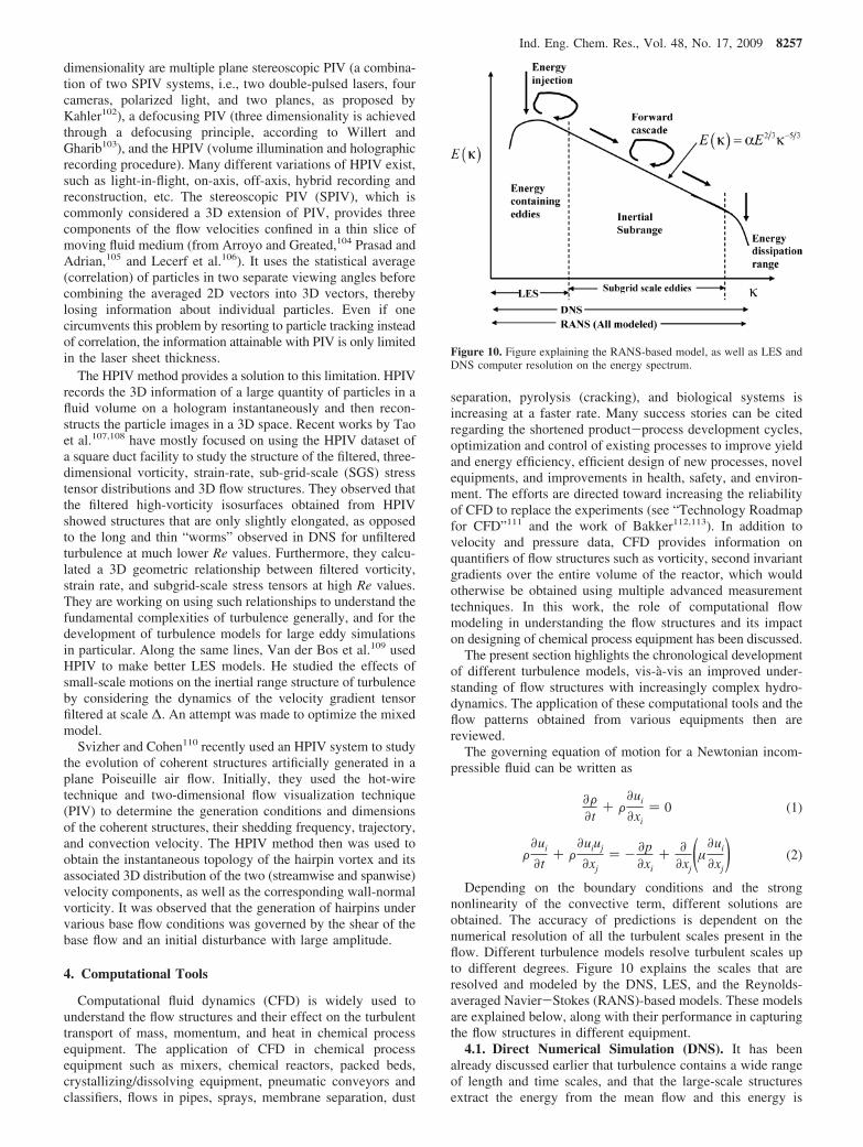
Computational fluid dynamics (CFD) is widely used tounderstand the flow structures and their effect on the turbulenttransport of mass, momentum, and heat in chemical processequipment. The application of CFD in chemical processequipment such as mixers, chemical reactors, packed beds,crystallizing/dissolving equipment, pneumatic conveyors andclassifiers, flows in pipes, sprays, membrane separation, dust

separation, pyrolysis (cracking), and biological systems isincreasing at a faster rate. Many success stories can be citedregarding the shortened product-process development cycles,optimization and control of existing processes to improve yieldand energy efficiency, efficient design of new processes, novelequipments, and improvements in health, safety, and environ-ment. The efforts are directed toward increasing the reliabilityof CFD to replace the experiments (see “Technology Roadmapfor CFD”111 and the work of Bakker112,113). In addition tovelocity and pressure data, CFD provides information onquantifiers of flow structures such as vorticity, second invariantgradients over the entire volume of the reactor, which wouldotherwise be obtained using multiple advanced measurementtechniques. In this work, the role of computational flowmodeling in understanding the flow structures and its impacton designing of chemical process equipment has been discussed.

The present section highlights the chronological developmentof different turbulence models, vis-a-vis an improved under-standing of flow structures with increasingly complex hydro-dynamics. The application of these computational tools and theflow patterns obtained from various equipments then arereviewed.

The governing equation of motion for a Newtonian incom-pressible fluid can be written as

∂F∂t

+ F∂ui

∂xi) 0 (1)

F∂ui

∂t+ F

∂uiuj

∂xj) - ∂p

∂xi+ ∂

∂xj(µ

∂ui

∂xj) (2)

Depending on the boundary conditions and the strongnonlinearity of the convective term, different solutions areobtained. The accuracy of predictions is dependent on thenumerical resolution of all the turbulent scales present in theflow. Different turbulence models resolve turbulent scales upto different degrees. Figure 10 explains the scales that areresolved and modeled by the DNS, LES, and the Reynolds-averaged Navier-Stokes (RANS)-based models. These modelsare explained below, along with their performance in capturingthe flow structures in different equipment.

4.1. Direct Numerical Simulation (DNS). It has beenalready discussed earlier that turbulence contains a wide rangeof length and time scales, and that the large-scale structuresextract the energy from the mean flow and this energy is

Figure 10. Figure explaining the RANS-based model, as well as LES andDNS computer resolution on the energy spectrum.


transferred down the cascade toward the smaller scales, until itreaches the smallest Kolmogorov scale, where viscous dissipa-tion directly converts the energy into heat. Now, it is theoreti-cally possible to resolve the entire spectrum of turbulent scalesdirectly and solve the Navier strokes equation (see eqs 1 and2) at a grid with a size less than that of the Kolmogorov scale.This approach is called as DNS, wherein only the instantaneousNavier-Stokes equations are solved and no turbulence modelsare used. However, this approach is limited by the speed ofcomputation, because, to resolve all the scales in three dimen-sions, the number of mesh elements required is proportional toRet

9/2Pr3 (from Mathpati et al.114). Hence, the limitation ofcomputational resources led to the development of turbulencemodels such as RANS equations and large-eddy simulation,which enabled the simulations to be performed at a coarser gridsize with reasonable accuracy concomitant with the assumptions.

4.2. Reynolds-Averaged Navier-Stokes (RANS)-BasedModels. The RANS approach involves solving the time-averaged Navier-Stokes governing equation to obtain the meanprofiles. The instantaneous components of velocities and pres-sure in the Navier-Stokes equation are split into its mean andfluctuating parts, and then the equation is time-averaged. Thisapproach reduces the computational demand. These equations,with time averaging, are reduced to the following form (eqs 3and 4):

∂F∂t

+ F∂⟨ui⟩∂xi

) 0 (3)

F∂⟨ui⟩∂t

+ F⟨uj⟩∂⟨ui⟩∂xj

) -∂⟨pi⟩∂xi

+ ∂

∂xj(µ

∂⟨ui⟩∂xj

- F⟨ui′uj′⟩) (4)

Time averaging of the equation of motion produces an additionalterm ( τij) that is given by τij ) -F⟨ui′uj′⟩. These stresses aremodeled using gradient diffusion hypothesis to close the systemof equations.

-F ⟨ui′uj′⟩ )23

kFδig - µt(∂⟨ui⟩∂xj

+∂⟨uj⟩∂xi

) (5)

To close the system of equations, µt has been formulated inmany ways in the literature, in terms of zero-, one-, and two-equation models. The most popular way is the two-equationmodel, where µt is estimated from turbulent length and timescales. In the case of the standard k-ε model, µt is estimatedusing turbulent kinetic energy (k) and rate of dissipation ofturbulent kinetic energy (ε).

µt ) CµF(k2

ε ) (6)

The values of k and ε are obtained by solving their transportequations (see Launder and Spalding115).

4.2.1. Standard k-ε Model. The equations for turbulentkinetic energy and dissipation rate are given below:

F∂k∂t

+ F⟨uk⟩∂k∂xk

) P - Fε + ∂

∂xk[(µ +

µt

σk) ∂k∂xk

] (7)

The transport equation for ε is rewritten as

F∂ε∂t

+ F⟨uj⟩∂ε∂xj

) FCε1(εk)P - Cε2F(ε2

k ) + ∂

∂xj[(µ +

µt

σε) ∂ε∂xj

](8)

where

P ) τij

∂⟨ui⟩∂xj

(9)

The aforementioned modeling of k and ε equations result intofive turbulence parameters: Cµ, Cε1, Cε2, σk, and σε. This modelhas been successfully applied in the literature for flow awayfrom walls and regions without sharp velocity gradients. As thewall is approached, the results deviate from the experimentalvalues. To model the effect of contribution of viscous stressesto turbulent stresses, wall functions and low Reynolds numbermodels have been developed in the literature. These aresemiempirical formulas and functions that link the solutionvariables at the near-wall cells and the corresponding quantitieson the wall. A critical review of low Reynolds number modelsis presented by Thakre and Joshi.116

4.2.2. Reynolds Stress Model (RSM). The standard k-εmodel inherently fails to predict the return to isotropy after theremoval of strain or the isotropization of grid-generatedturbulence properly.117 In the k-ε model, the production ofturbulence is modeled, whereas accurate prediction of turbulenceproduction can improve the overall flow patterns in anisotropicflows. Furthermore, the modeling of transport equations for kand ε clearly gives a glimpse of its inability to properly accountfor streamline curvature, rotational strains, and other body-forceeffects. RSM, in theory, will circumvent all the aforementioneddeficiencies and also gives it the ability to predict each individualstress more accurately. In RSM, six transport equations forReynolds stresses are solved to take into account anisotropicbehavior. The equation of turbulent stresses contains thefollowing terms: pressure rate of strain (which contains fluctuat-ing pressure velocity gradients) and the flux of Reynoldsstresses.

∂τij

∂t+ ⟨uk⟩

∂τij

∂xk) -(τik

∂⟨uj⟩∂xk

+ τjk

∂⟨ui⟩∂xk

) - ∂

∂xk(µt

σk

∂τij

∂xk) +

Πij - 2µ⟨∂ui′∂xk

∂uj′∂xk

⟩ + µ∇2τij (10)

Πij ) ⟨p′[∂uj′∂xi

+∂ui′∂xj

]⟩ ) Πij,slow + Πij,rapid + Πij,wall (11)

The pressure strain term is the most uncertain term in RSM.This term is responsible for making turbulence isotropic andredistribution of energy between components ⟨u1

′2⟩, ⟨u2′2⟩, and ⟨u3

′2⟩.The incompressibility condition guarantees that Π11 + Π22 +Π33 ) 0. If individual terms of Πii are nonzero, at least onemust be positive and one must be negative. The classicalapproach is to decompose the pressure strain term into a slowcomponent, a rapid component, and a wall reflection term.118

The RANS-based models (k-ε and RSM), because of timeaveraging, cannot resolve the flow structure, and they sufferfrom the following shortcomings: (a) the basic gradient diffusionassumption is questionable; (b) the eddy viscosity has isotropiccharacter; (c) there is inadequate incorporation of viscositydamping effects on the turbulence structure (low-Re models);and (d) there is an inability to mimic the preferentially orientedand geometry dependent effects of pressure reflection and eddy-flattening and squeezing mechanisms, because of the proximityof the solid or interphase surface.

4.3. Large Eddy Simulation (LES). In most of the chemicalprocess equipments, large flow structures govern the transportphenomena. If one could manage to resolve the large flowstructures and accurately model the small isotropic structures,then the computational demand can be significantly decreases,compared to the DNS. In large eddy simulations (LESs), the


instantaneous velocities are filtered in the spatial domain.119 Thefiltering induces a closure problem in which the dynamic effectsof the small-scale turbulence on the primary flow features mustbe represented by introducing a so-called subgrid scale (SGS)model. In LES, large scales are resolved numerically and smallsubgrid scales are modeled. The final results are dependent onthe accuracy of SGS models in transferring energy from largescales at cutoff to lower scales. Much of the LES research isdirected toward formulating accurate subgrid closures, evaluat-ing the numerical errors, and identifying and characterizinglarge-scale structures. The governing equations for LESs areas follows:

∂F∂t

+ F∂uji

∂xi) 0 (12)

F ∂

∂t(uji) + F ∂

∂xj(uiuj) ) - ∂pj

∂xi+ ∂

∂xj(µ

∂uji

∂xj- Fui,sgsuj,sgs)

(13)

The major difference between the RANS equations and theaforementioned equation is that the dependent variables arefiltered quantities rather than the mean quantities. The SGSstresses that result from the filtering operation are unknown andrequire modeling.

The LES can resolve the large scales, as a result, it can beuseful for simulating the flows undergoing transition and wakeregion, wherein large unsteady turbulent structures are resolved.The passage of flow structures are associated with high Reynoldsstress, as a result of strong rotational motions and acceleration/retardation motions that induces the gradients in flow.

4.4. Application of Turbulence Models for Flow StructureIdentification. 4.4.1. Solid/Fluid Interface: Channel Flow.In this section, a discussion on those flows where a majority ofturbulence production occurs at a stationary wall is presented.Solid/fluid interfaces offer very high shear rates, because of theflow structures that form near the solid wall, and a maxima ofturbulent kinetic energy production and dissipation is ob-served.120,122 Because of an increased contribution of viscousforces close to the wall, standard RANS models fail to reproduceindividual stresses, and even kinetic energy. To understand thetransient nature of wall dynamics, simulations must be per-formed using DNS and LES. The first DNS of wall-boundedflows was performed by Kim et al.123 Subsequent studies havemodified the channel configurations to examine the responseof wall-bounded turbulence to factors such as rotation,124 meanthree dimensionality,125 transverse curvature,126 and heat trans-fer.127 Some of the insights into the boundary layer structuregained from DNS are summarized below (also see the work ofMoin and Spalart128 and Robinson129). The DNS data suggeststhat the observed bursting event may simply be due to thepassage of streamwise vortices past the measuring station.Because of very high computational demand, the DNS couldnot be used at high Re values. In low-Re computations, near-wall streaks and horseshoe vortices have been observed.However, for better understanding, high-Re simulations areindispensable to remove the empiricism involved in the as-sumption of similarity between low-Re and high-Re near-wallstructures. Many times, the DNS were performed at lower Revalues, with the objective being to perform controlled studiesthat allow better insight, scaling laws, and turbulence modelsto be developed. To study the flow structures at higher Re values,LES has been used. LES of wall-bounded flows has beenconducted for different objectives, such as to understandturbulence,125 the development of SGS models,130-136 the effect

of filter shape,137 and wall treatment when coarse mesh isused,131,138 to study the scalar transport.139 Dong and Lee139

investigated passive heat transfer in turbulent channel flow atRe ) 10000 and Pr ) 0.1-200. They validated their LES resultsfor Pr ) 1 and 10 with the DNS data of Na et al.140 They foundthat the turbulent Prandtl number to be almost constant,independent of the molecular Pr within the range of study.Similar to the mean velocity profile, they observed a buffer layer,followed by a logarithmic region in the mean temperatureprofile. For their range of study, they confirmed a Pr1/3

dependency of the Nusselt number (Nu). The contours ofinstantaneous temperature fluctuations clearly indicated thatalmost all of the turbulent structures that exist in the viscoussublayer were efficient in the heat-transfer process at Pr ) 1,and only the smallest structures subsisting very close to the wallwere involved in the heat-transfer process at Pr ) 100. Thesesimulations accounted for the effect of flow structures on heattransfer indirectly. The instantaneous variation of temperaturewas averaged to get an accurate estimation of the meantemperature gradient and, hence, heat-transfer coefficient. Thistransfer coefficient then was related empirically to the rate ofsurface renewal.

4.4.2. Free Shear Flows: Jet Loop Reactor. Jet loopreactors (JLRs) are frequently used in the process industry, asan alternative to impeller mixers, because of the existence ofrelatively high convection currents, leading to an enhanced rateof macro-mixing at the same power consumption, compared tostirred tank reactors. The resulting high-speed jet entrains someof the surrounding liquid and creates a circulation pattern withinthe vessel. CFD has been used on numerous occasions tosimulate the flow patterns in the jet flows. A review onapplication of the k-ε model suggests that various researcherswere unable to get accurate results for the free jets; hence, theyhad to introduce modifications in the model constants of thestandard k-ε model to get accuracy.141-146

The LES of jet flow has been performed in the literature withthe following objective: to understand the initial developmentregion, vortex interaction in the jet region, the entrainment rate,and, subsequently, the mixing performance. Andersson et al.147

studied the effect of inflow conditions and SGS model on LESof mixing processes in turbulent jets. Grinstein and DeVore148

observed, through LESs, that the initial development of thesquare jet is characterized by the dynamics of vortex rings andbraid vortices. Further downstream, strong vortex interactionslead to the breakdown of the vortices, and to a more disorga-nized flow regime characterized by smaller scale elongatedvortices. Entrainment rates significantly larger than those forround jets are directly related to the enhanced fluid andmomentum transport between jet and surroundings determinedby the vortex dynamics underlying the axis-rotation of the jetcross-section. The first axis-rotation of the jet cross-section canbe directly correlated with self-induced vortex-ring deformation.Mathpati et al.149 performed JLR simulation using a hybrid k-εmodel and LES to assess the modeling assumption in RANS-based models. They also simulated scalar transport to study theeffect of nozzle diameter on mixing time. They found that, forvery small nozzle diameters, JLRs were inferior to stirred tankreactors for mixing applications.

4.4.3. Flow Past Solid and Blunt Bodies: Stirred Tank.The performance of the k-ε model in stirred vessels has beenreviewed extensively.150-154 The reviews suggest that the k-εmodel has been able to capture the gross circulation pattern quitewell, but not the macro-instability and rolloff of vortices behindthe impellers and other transient flow structures. The RSM


model has been used by Bakker and Van den Akker155 andOshinowo et al.156 They observed that the RSM model has betterprediction ability than the k-ε model. However, overall, theview that emerged from reviews was that the LES should beable to capture the instantaneous flow profile.

Bartels et al.157 conducted DNS of the flow around a six-bladed Rushton turbine with four baffles for Reynolds numbersranging from Re ) 0.1 to Re ) 106, and compared the resultswith those of the k-ε model. They observed that the flow fieldin a plane at an angle of 15° behind the blades is characterizedby two “tip” vortices that are created in a plane ∼5° behind theblades. The location of the vortices in the DNS results wasfurther away from the axis, compared to the RANS results(especially for the lower vortex). The two tip vortices were seento be dying out at an angle of ∼35° behind the blade. This resultis identically produced by the DNS and RANS simulations.

The very first study of LES for a stirred vessel was performedby Eggels,158 using a lattice-Boltzmann discretization schemefor filtered Navier-Stokes equations and the adaptive force fieldtechnique for the impeller rotation. This study presented theinstantaneous and mean flow field, which would help in theinitial understanding of the given system. However, there werediscrepancies in the quantitative predictions of the mean radialand mean axial velocities, especially in the near-impeller region.Revstedt et al.159 investigated both the mean flow and spectraldistribution of flow by power density function at variouslocations in a baffled stirred tank. In this study, the impellermotion was modeled by specifying the time-dependent momen-tum source term in a stationary grid. The LES could capturethe trailing vortices behind the blades and their detailedmovement away from the impeller with increasing distance fromthe blade. The acceleration of the fluid at the impeller tip,because of the fluid entrainment due to the trailing vortex pair,was well-simulated. Their instantaneous data from LES sup-ported the blade frequency and the existence of Kolmogorov’s-5/3 region in the energy spectrum. These observations werein close agreement with the expensive and time-consumingexperiment. They demonstrated that the LES could generate aninstantaneous flow field, such as sophisticated flow-measuringtechniques and sometimes even better, as far as the flow in theimpeller region and near-wall regions are concerned. The meanaxial velocity from LES was in good agreement with theexperimental data of Costes and Couderc161 at different loca-tions. Derksen and Van den Akker55 advanced the Eggels etal.158 study with a more-refined forcing algorithm. The realpotential of LES was explored as the simulations could identifya detailed local flow in the wakes behind each blade, whichwere determined to be significantly higher than the impeller tipspeed (2 × tip speed). Furthermore, the fluctuations becomeless coherent away from the impeller. The axial profiles ofrandom (turbulent), coherent (pseudo-turbulence), and totalkinetic energy are in good agreement with LDV phase-resolvedexperimental data. Derksen160 applied the previously developedlattice-Boltzmann-based solver for the flow generated by a4-PBTD45 impeller. He focused on the influence of the spatialresolution and SGS modeling on the flow predictions. It wasobserved that the spatial resolution has significant impact onthe overall average flow field results. No significant effect wasobserved in the overall and phase-averaged flow field results,because of changes in the SGS model. Only the formation andstrength of the tip vortex differed for the two SGS approaches(the vortex formed in the structure function simulations wasobserved to be weaker). Validation was made only within theimpeller region. For the PBTD45 impeller, Roussinova et al.162

performed LES simulations using sliding mesh methodology(SDM). The mean axial velocity in the impeller center planewas in agreement with the experimentally measured values. Thisextended for the identification of low-frequency macro-instabili-ties (MIs). Their predicted frequency value of the MI comparedwell with the LDV measurement. Furthermore, Hartmann andco-workers163,164 used LES to investigate the precessional vortexphenomenon with the help of LES. This study opted for thesame numerical techniques as those used by Derksen and Vanden Akker.58 Their LES model could capture the vorticalstructure moving around the tank centerline in the same directionas the impeller. Using LES, they also observed that the strengthof the vortex below the impeller was much stronger and morepronounced in size, compared to that prevailing above theimpeller, and both vortices move with a mutual phase difference,which was qualitatively in good agreement with the experimentaldata. It was found that the fluctuations in the impeller regionwere dominated by the blade passage frequency, whereas thefluctuation levels close to the tank centerline were dominatedby the low-frequency motion of a vertical structure. Their LESmodel could accurately predict the characteristic MI frequency.It could even predict a second frequency peak at f ) 0.092N atRe ) 12500. Using LES data, they observed that the flow wasdominated by the low-frequency processional vortex in the bulkflow region, and these were associated with a significant amountof kinetic energy. For the first time, Yeoh et al.165 performedLESs using the sliding deforming technique. The main objectivewas to assess the capability of the LES modeling technique,coupled with the sliding SDM and relative performance, withthe RANS approach. RANS calculations have been performedusing the standard k-ε model. The predicted mean radial,tangential, and axial velocities, and the turbulent kinetic energy,were compared with LDV data only in the impeller center plane.For all three velocity components, fairly good qualitative andquantitative agreement was obtained using both the RANS-basedand LES models. This work revealed that the equilibrium andisotropy hypotheses hold in most of the tank, except for theimpeller discharge stream. Hartmann and co-workers163,164 alsomade a detailed study to evaluate the predictive capabilities ofLES and RANS. The main difference was that this study usedthe lattice-Boltzmann solver and the RANS-based simulationshave been performed with the shear-stress-transport (SST)turbulence closure model. The RANS-based and LES predictionshave been compared and assessed with LDV-measured radial,tangential, and turbulent kinetic energy in the impeller zone.The radial velocities of both the models were in better agreementwith the experimental data. With regard to the predictions oftangential velocity, the overall performance of LES was quitegood, rather than RANS simulations. Their simulations revealedthat the Smagorinsky SGS model performed better than theVoke SGS model, especially when it comes to prediction ofthe trailing vortex pair. It was shown that LES predicted theturbulent kinetic energy better in the impeller discharge flow,whereas RANS invariably underperformed in this area. UsingLES data, they found almost-isotropic behavior in the circulationloops. However, in the impeller stream, the boundary layers,and at the separation points, turbulence was determined to bemore anisotropic, because of high shear rate. They did not seethe relative merits of using the Voke SGS model. Furthermore,they calculated the energy dissipation rate by assuming localequilibrium between production and dissipation at and belowthe SGS level and compared it with the RANS predictions inthe baffle midplane. It was observed that the RANS-based modelyielded higher values of the energy dissipation rate than LES


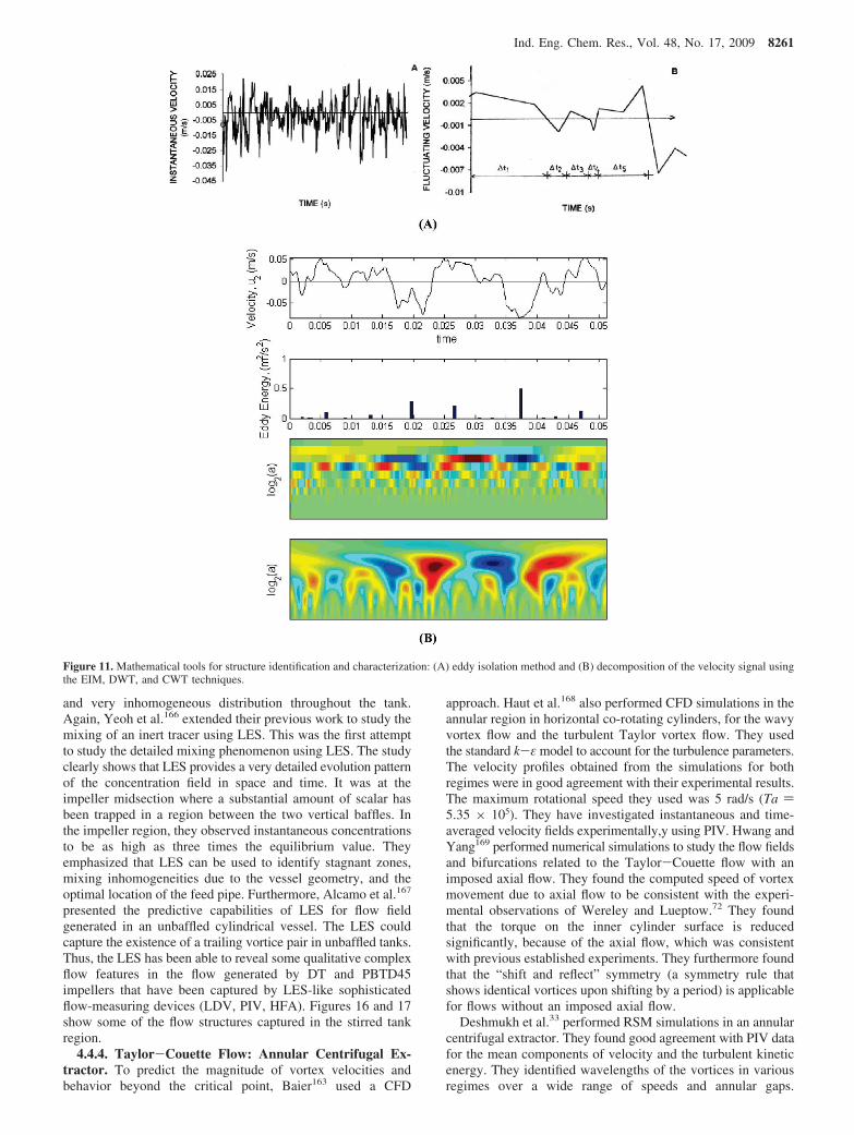
and very inhomogeneous distribution throughout the tank.Again, Yeoh et al.166 extended their previous work to study themixing of an inert tracer using LES. This was the first attemptto study the detailed mixing phenomenon using LES. The studyclearly shows that LES provides a very detailed evolution patternof the concentration field in space and time. It was at theimpeller midsection where a substantial amount of scalar hasbeen trapped in a region between the two vertical baffles. Inthe impeller region, they observed instantaneous concentrationsto be as high as three times the equilibrium value. Theyemphasized that LES can be used to identify stagnant zones,mixing inhomogeneities due to the vessel geometry, and theoptimal location of the feed pipe. Furthermore, Alcamo et al.167

presented the predictive capabilities of LES for flow fieldgenerated in an unbaffled cylindrical vessel. The LES couldcapture the existence of a trailing vortice pair in unbaffled tanks.Thus, the LES has been able to reveal some qualitative complexflow features in the flow generated by DT and PBTD45impellers that have been captured by LES-like sophisticatedflow-measuring devices (LDV, PIV, HFA). Figures 16 and 17show some of the flow structures captured in the stirred tankregion.

4.4.4. Taylor-Couette Flow: Annular Centrifugal Ex-tractor. To predict the magnitude of vortex velocities andbehavior beyond the critical point, Baier163 used a CFD

approach. Haut et al.168 also performed CFD simulations in theannular region in horizontal co-rotating cylinders, for the wavyvortex flow and the turbulent Taylor vortex flow. They usedthe standard k-ε model to account for the turbulence parameters.The velocity profiles obtained from the simulations for bothregimes were in good agreement with their experimental results.The maximum rotational speed they used was 5 rad/s (Ta )5.35 × 105). They have investigated instantaneous and time-averaged velocity fields experimentally,y using PIV. Hwang andYang169 performed numerical simulations to study the flow fieldsand bifurcations related to the Taylor-Couette flow with animposed axial flow. They found the computed speed of vortexmovement due to axial flow to be consistent with the experi-mental observations of Wereley and Lueptow.72 They foundthat the torque on the inner cylinder surface is reducedsignificantly, because of the axial flow, which was consistentwith previous established experiments. They furthermore foundthat the “shift and reflect” symmetry (a symmetry rule thatshows identical vortices upon shifting by a period) is applicablefor flows without an imposed axial flow.

Deshmukh et al.33 performed RSM simulations in an annularcentrifugal extractor. They found good agreement with PIV datafor the mean components of velocity and the turbulent kineticenergy. They identified wavelengths of the vortices in variousregimes over a wide range of speeds and annular gaps.

Figure 11. Mathematical tools for structure identification and characterization: (A) eddy isolation method and (B) decomposition of the velocity signal usingthe EIM, DWT, and CWT techniques.


Deshmukh et al.170 conducted RTD simulations in an annularcentrifugal extractor. They studied the effect of flow ratio,annular gap, and rotational speed on RTD. They observed thatthe flow in the ACE was similar to back-mixed behavior,because of the presence of counter-rotating vortices. The numberof vortices is dependent on the rotational speed and thegeometrical parameters of ACE.

4.4.5. Particle (Dispersed-Phase)-Induced Flow Struc-ture. 4.4.5.1. Flow Past Spheres/Drops. A very scant amountof literature is available regarding the direct numericalsimulation (DNS) of particles and drops at relatively low Refor a finite number of particles. The major focus was on theidentification of the point of bifurcation and the dragexperienced by the particles. Kim and Pearlstein171 performeda two-dimensional linear stability analysis by DNS, using apseudo-spectral method. They predicted that the primarybifurcation point occurs at Re ) 175, which was compara-tively lower than the experimental observations of Magarveyand Bishop.77 With the modified linear stability analysis,Natarajan and Acrivos80 performed two-dimensional simula-

tions of spheres and circular disks. They predicted that theprimary bifurcation of sphere occurs at Re ) 210, which wasin perfect agreement with the experimental observation, andthey reported that the secondary bifurcation and shedding ofvortices occurs at Re ) 278. Tomboulides172 have performedDNS of a fixed sphere from Re ) 20 to Re ) 1000. Theyobserved initial flow separation at Re ) 20 and steadynonaxisymmetric flow at Re ) 212. The vorticity of thenonaxisymmetric flow field resemble the double-thread wakeas observed by Magarvey and Bishop77 at Re ) 210. Bothnumerical and experimental analyses of the wake structure behinda fixed sphere in the Re range of 20-300 were also studied byJohnson and Patel.173 They reported that the flow separation andformation of a vortex behind the sphere begins at Re ) 20, andthey predicted the separation angle, the separation length, and theposition of the vortex. They observed that the axisymmetry wasbroken at Re ) 210 and explained this phenomenon by presentingthree-dimensional interactions of stream lines. They reported thevariations in the drag and lift forces, which arise after a breakageof symmetry. They reported that the periodic vortex shedding

Figure 12. Channel flow structures as captured by various methods: (A) DWT scales (Re ) 5600), (B) DWT scales (Re ) 18000), (C) POD modes (Re )5600), and (D) hybrid wavelet-POD scales.


begins at Re ) 270 and explained the same with the help ofvorticity diagrams.

DNS simulations of the flow past fixed oblate spheroidalbubbles at Re ) 100-1000 have been performed by Magnaudetand Mougin.174 At Re ) 180, they showed a nonaxisymmetricwake, with the help of 3D particle path. They also presentedthe vorticity isosurfaces at Re ) 180, 300, and 700. The wakeinstability of a fixed sphere has been studied by Ghidersa andDusek,175 using the spectral element method, and they reportedthat the primary bifurcation occur at Re ) 215. Vortex methodsfor DNS of flow past spheres have been developed by Ploum-hans et al.176 They presented the isosurfaces of streamwisevorticity at Re ) 300, 500, and 1000. Hydrodynamic forces

acting on the rigid fixed sphere for the Re range of 10-320have been simulated by Bouchet et al.,177 using the spectralelement method. They presented the vortex shedding frequenciesand oscillation amplitude of drag and lift forces from Re ) 280to Re ) 320.

DNS of the wake generated by freely falling particles, byReddy et al.,178 has shown that, at Re ) 1, the drag due to thepressure was 33% of the total drag and remainder was viscousdrag. As flow separation began (at Re ) 25), the pressurecontribution in the total drag increased and was equal to theviscous drag (CDP) at Re ≈ 180. They observed that, after Re >200, the pressure drag dominates over the viscous drag. At Re) 25, they observed a small and steady wake at the rear end of

Figure 13. JLR structures as captured by various methods: (A) DWT scales (Re ) 17000), (B) DWT scales (Re ) 26000), (C) POD modes (Re ) 17000),and (D) hybrid wavelet-POD scales.


the sphere. As the Re value increases from 25 to 200, the steadywake grew in size and stretched in the streamwise direction.At Re ) 200, it can be observed that the pressure distributionaround the sphere is symmetric. Whereas at Re ) 210, theasymmetry in the pressure distribution can be clearly observed.The reason for this nonaxisymmetry was attributed to theincrease in the centrifugal instability in the wake as the spherefalls freely, under the action of gravity. As the instantaneousReynolds number increases (velocity of the sphere increaseswith time up to its terminal settling velocity), the rotational orcentrifugal instability in the form of pressure gradient increases,because of the fluid rotation within the toroidal vortex. Forsteady axisymmetric flow, the pressure gradient inside the vortexwas balanced by the enforced viscous force of the flow.However, beyond Re ) 210, the viscous force is not sufficient

to maintain the balance, and as a result, the axisymmetric vortexbreaks. Because of the lift force, the pair of counter-rotatingvortices are formed after breakage of the axisymmetric vortex.

4.4.5.2. Bubble Column. In bubble column reactors andhorizontal sparged reactors (see Joshi and Sharma179), bubblesize is one of the most important parameters that determinesthe bubble rise velocity, the gas holdup, and the interfacial area,and, as a result, phenomena such as interphase heat and masstransfer. The bubble size is highly dependent on bubble breakupand coalescence, which are influenced by the interaction withturbulence. Although the fundamental equations governing thebehavior of gas and liquids, as well as the conditions at a fluidinterface are reasonably well-known, in most practical applica-tions, it is necessary to involve systems where the ratio between

Figure 14. Stirred tank structures as captured by various methods for disk turbine, PBTD45, and HF impellers: (A) DWT scales (DT), (B) DWT scales(PBTD45), (C) DWT scales (HF), (D) POD modes (DT), (E) POD modes (PBTD45), and (F) POD modes (HF).


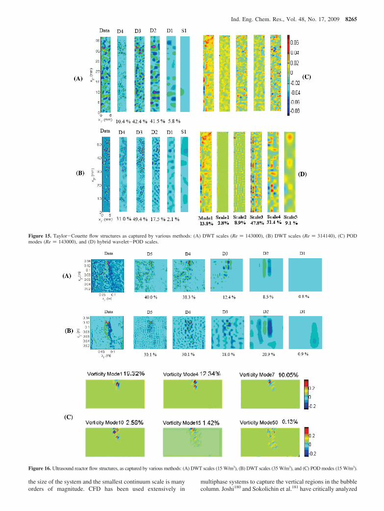
the size of the system and the smallest continuum scale is manyorders of magnitude. CFD has been used extensively in

multiphase systems to capture the vertical regions in the bubblecolumn. Joshi180 and Sokolichin et al.181 have critically analyzed

Figure 15. Taylor-Couette flow structures as captured by various methods: (A) DWT scales (Re ) 143000), (B) DWT scales (Re ) 314140), (C) PODmodes (Re ) 143000), and (D) hybrid wavelet-POD scales.

Figure 16. Ultrasound reactor flow structures, as captured by various methods: (A) DWT scales (15 W/m3), (B) DWT scales (35 W/m3), and (C) POD modes (15 W/m3).


the CFD literature in bubble columns. According to them, thecorrect modeling of interphase forces and turbulence is of primeimportance for capturing the physics correctly. A wide rangeof CFD studies on bubble column reactors have been conductedrecently. Mainly, two approachessnamely, Euler-Euler182-185

and Euler-Lagrange186-191shave been adopted to simulate agas-liquid system operating under different conditions. Thek-ε model has been used for both 2D181,183,186,192-199 and3D183,191,200-205 Euler-Euler CFD simulations. On most of theoccasions, the k-ε results gave good agreements with theexperimental results, but they could give no indication ofinstantaneous flow profile like the vertical spiral regime in sieveplate, or the plume dynamics of the bubble column. In this work,we cover some LES and DNS of the bubble column. Lakehalet al.206 were the first to employ the LES model for a bubblyflow. Their system involved a vertical bubbly shear flow at avery low void fraction (1.9%). From their study, they suggested

that, to obtain better results, the optimum cut-off filter shouldbe 1.5 times the bubble diameter. They observed that thedynamic approach of Germano et al.207 does not perform betterthan the Smagorinsky model, which they felt could be due tothe inadequate dimensions of their computational domain. Thisstudy suggested that the LES approach can be promising forpredicting the phase velocities and the void fraction, and itemphasized the need to perform more LES simulations oncomplex systems such as buoyancy-driven flow operating athigher void fractions. In this context, Deen et al.208 were thefirst to apply the LES model to simulate a bubble column, andthey reported observing a better resolved flow using LES ratherthan the k-ε model. Bombardelli et al.209 used the samegeometry as Deen et al.208 to study the influence of differentnumerical schemes, of different drag models, and of initial flowconditions on LES performance. They observed that the use ofa second-order FCT scheme for LES simulation enhanced its

Figure 17. Bubble column flow structures, as captured by various methods for single-hole, sieve-plate, and sintered-plate spargers: (A) DWT scales (single-hole sparger), (B) DWT scales (sieve-plate sparger), (C) DWT scales (sintered-plate sparger), (D) POD modes (single-hole sparger), (E) POD modes (sieve-plate sparger), and (F) POD modes (sintered-plate sparger).


performance. However, they suggested the need to conduct moretests on LES with higher-order schemes and finer grid resolu-tions before identifying the best numerical scheme for LESsimulations. It was observed that the LES results were verysensitive to the initial boundary conditions. This work alsosuggested that there is a need to pay attention toward the near-wall region, because the SGS models do not account for near-wall region processes, which can lead to the erroneous predictionof frictional stresses at the wall. Bombardelli et al.209 used afinite-element-based LES code to simulate and analyze thephenomena of wandering bubble plumes, as in the experimentsthat were conducted by Becker et al.210 They observed that LESwas been able to capture the instability associated withwandering more vividly, compared to k-ε simulation. Theyanalyzed the plume for coherent structures that arose from theinterplay of eddies and bubbles by studying the vorticitycontours. Their work showed the evolution of several eddiesand their inter-relation with the bubble plume. Zhang et al.211

advanced the work of Deen et al.208 by investigating the effectof the Smagorinsky constant and the interfacial closures for drag,lift, and virtual mass force in two columns that had differentaspect ratios (height/diameter ratios of H/DT ) 3 and 6). Theyobserved that, by increasing the value of the Smagorinskyconstant, the bubble plume dynamics dampens, and, conse-quently, a steep mean velocity profile is observed. They obtainedgood agreement with experimental results when the value ofthe Smagorinsky constant was used in the range of 0.08-0.10.They also suggested that, for taller columns (H/DT ) 6), theinterfacial force closures proposed by Tomiyama gave betteragreement with the experiments. As a future work, they havesuggested the need for simulating the dynamic free liquid surfaceat the top and observing its effect on the velocity profiles inthe top region. Tabib et al.212 used the LES to study theinstantaneous phenomena and flow structures in a cylindricalbubble column arising out of a change in the sparger design. Inthis work, the LES captured the flow structures and the flowregions of the vortical-spiral flow regime in the sieve platecolumn (as experimentally reported by Chen et al.94), and thebubble plume dynamics along with vortical structures forthe single-hole sparger. However, for sintered-plate columns,the LES showed almost-homogeneous flow conditions with anabsence of dynamic eddies. Thus, LES was very effective incapturing the dynamics in the continuous phase, as a result ofbubble-imparted turbulence. Compared to LES simulations, theDNS of multiphase flows has been limited to some finite numberof bubbles, but they have given some excellent information onbubble dynamics. The DNS of multiphase flows (see Tryggva-son et al.213) has been used both to (i) generate insight andunderstanding of the basic behavior of multiphase flow (suchas the forces on a single bubble or a drop), how bubbles anddrops affect the flow, and how many bubbles and drops interactin dense disperse flows, as well as (ii) provide data for thegeneration of closure models for engineering simulations of theaveraged flow field. The DNS of bubbly flows, where the flowaround each bubble is fully resolved and viscosity, inertia, andsurface tension are fully taken into account, have already beenused to study the behavior of systems that contain up to O(100)bubbles. As the number of bubbles in each period is increased,the bubbles generally rise unsteadily, repeatedly undergoingclose interactions with other bubbles. Figure 18 shows some ofthe flow structures captured in the stirred tank region.

5. Mathematical Tools

From DNS, LES, and advanced experimental techniques,much information has been obtained regarding flow structures.The datasets generated from numerous experimental andcomputational techniques carry a plethora of information withinthem. In this heap of information, many times, the most relevantinformation becomes indiscernible. To extract the informationpertinent to flow structures, many statistical and mathematicaltechniques have been proposed in the literature. These tech-niques help to identify, characterize, and quantify the flowstructures in terms of their size, shape, and energy content and,finally, their relationship with the design parameters. These

Figure 18. Energy spectra evaluation using various transform methods inchannel flow at x1

+ ) 20 using LES monitor points: (s) FFT, (0) EIM,(+) DWT, (O) CWT.


techniques have evolved in terms of accuracy and complexityfor last four decades, and they vary in terms of the amount ofinformation that they require to identify a flow structure. Thesetechniques make use of point data (only streamwise velocityand its time series), or a planar dataset or a complex 3D flowfield of velocity/strain rate/vorticity to extract the flow structures.However, the problem lies in the fact that different techniquesmay detect different flow structures. In this section, thesetechniques are described in brief, and their relative strength andlimitations are brought out. An attempt has been made to drawa correspondence between different techniques by obtaining thethreshold levels at which they strike some similarity in theiridentification of flow structures. In the present work, thesetechniques are used to extract flow structure information inchannel flow, where the top surface is subjected to differentlevels of shear boundary conditions with complete and no-slipas extreme cases. In the next section, we have covered the flowstructures that have been identified in different equipment, usingthese techniques.

5.1. Techniques Based on A Priori Known Features ofFlow Structures. These techniques are based on a central themethat the turbulent signal contains some key features, which formtheir footprints and they may be distinguished from the rawsignal by means of a criterion that uses some physics ofdevelopment of footprints. The raw data used to detect the flowstructures are either instantaneous or fluctuating velocity (orpressure, or temperature, or concentration of tracers, or vorticity,or velocity gradients) in space or in time, etc. The planar dataset(PIV) can provide us with the spatial patterns and length scalesof the structures; however, PIV datasets have a low data rate(up to 10 Hz), so we may not know the dynamics of these flowstructures. Although the methods based on the point dataset(HFA and LDV) are able to capture the age (or time scale) offlow structures, because of the high temporal resolution of thedataset, but they are not able to predict the shape of thestructures. These techniques were mainly developed to identifyflow structures in turbulent boundary layers. All these tech-niques214-225 have been summarized in Table 3. A criticalreview of most of these techniques has been conducted by Yuanand Mokhtarzadeh-Dehghan.216 In the present review, theirmethodology (with their own abbreviations) has been used tocompare various theories of heat and mass transfer.

5.2. Eddy Isolation Method. To identify the eddies, Lukand Lee226 developed an approach based on zero crossing inthe fluctuating velocity. This approach is briefly discussed here.As the eddy passes through the reference point, the velocityfluctuates about a mean value. Subtracting the mean value, onegets the fluctuating part of the velocity. The fluctuating velocityhas positive and negative values, and it crosses the time axis atmany locations (see Figure 11A). Thus, as the fluctuating partchanges from positive to negative or vice versa, it indicates thatall the fluid elements (moving in a radial or axial direction)that are taken into account during the measurement have thesame averaged kinetic properties. This can be considered todefine the existence of an eddy. Therefore, in the plot offluctuating velocity (u2′) versus time, as the velocity vectorcrosses the time axis, one eddy ends and the other enters thepoint of measurement. It has also been proposed that the timegap (tE) between the two successive crossings represents oneeddy. Thus, different eddies show different time gaps (tE,1, tE,2,tE,3, tE,4, and tE,5), which are taken as the eddy life. For any oneeddy, the velocity increases or decreases from zero, attainsmaxima (or minima), and then approaches zero. To estimatethe characteristic eddy energy, all the fluctuating velocities

within an eddy were squared and then added together. Luk andLee226 assumed that each eddy followed a sinusoidal shape. Thisapproach was modified by Kulkarni and Joshi227 by consideringthe shapes of the actual velocity-time diagram. The modifiedmethodology has been applied in the present work.

kE,i )∑ i

12

u2′2

∑ i

. (14)

The characteristic eddy velocity was then estimated from theeddy energy as

uE,i ) √2kE,i (15)

Eddy length scale (lE) was calculated from the eddy lifetime(tE) and the characteristic eddy velocity (uE). For the aforemen-tioned calculations, an in-house code was developed. All eddieswere sorted according to their age. An age distribution function(φ) was then estimated, where φ(t)∆t is the fraction of eddiesthat have a lifetime between t and t + ∆t.

5.3. Proper Orthogonal Decomposition (POD) Methodo-logy. Lumley228 defined the coherent structure as a representa-tion of the flow that has the largest projection onto the flow.Mathematically, this leads to the coherent structure being aneigenmode of a two-point correlation matrix built from adatabase of snapshots. These correlations can be built-up in twoways: either perform a spatial correlation or perform a temporalcorrelation. Lumley228 used the classical proper orthogonaldecomposition technique (POD) to obtain the most optimallycorrelated feature from the spatial correlation of a givenensemble of flow realization. In the present work, the POD hasbeen implemented using the temporal correlation because itreduces the computational efforts. This procedure is known asthe Sirovich229 method of snapshots. The variables that havebeen used in this study are the out-of-plane vorticity (ω3) planardatasets and the 2D velocity (u1, u2) planar datasets. The ω3

modes are more efficient than the corresponding velocity modesfor identification of the flow structures. A higher value ofenstrophy, which is the square of vorticity, indicates the presenceof organized vortices; however, the same may or may not beindicated by the presence of higher values of kinetic energy(square of velocity). Hence, enstrophy has been an importantquantifier in regard to identifying the flow structures. In thiswork, the enstrophy used is the pseudo-enstrophy, because onlyone component of the vorticity is considered. The velocitymodes have also been computed in this work to obtain thekinetic energy associated with the flow structures. Thesequantities are defined as

k ) (ui′, ui′) ) ui′2. (16)

� ) (ω3, ω3) ) ω32 (17)

The implementation of snapshot POD methodology is discussedbelow.

Given a database having M number of instantaneous spatialsnapshots (snapshot refers to the velocity or vorticity planardataset), with each snapshot having N data points (N ) Nx2

×Nx1

, where Nx1is the number of data points in the x1 direction

and Nx2is the number of data points in the x2 direction). The

application of the 2D snapshot POD method on these planardatasets enables the computation of spatial eigenmodes Ψn(x1)and accompanying temporal eigenmodes Ψn(t) that best fit themost energetic flow patterns contributing to the flow. The spatialeigenmodes represent a typical dynamical structure. The tem-


Table 3. Mathematical Tools for Structure Characterization


poral eigenmodes represents the variation in time of each spatialeigenmodes. The eigenvalue corresponding to a spatial moderepresents the fraction of turbulent kinetic energy (in the caseof the velocity dataset) or the fraction of enstrophy (in the caseof the vorticity dataset) associated with the mode.

5.4. Discrete Wavelet Transform (DWT). The DWT sepa-rates the information content in the data from a fine scale to acoarser scale systematically, by isolating the fine-scale vari-ability, in terms of wavelet coefficients that represent the detailsfrom the corresponding coarser-scale coefficients that depict thesmoothness. This procedure can be repeated iteratively oversmooth scales to obtain scale-wise detailed decomposition in amultiresolution framework. The wavelet coefficient matrixWa,b(x) may be obtained by the convolution of the 2D snapshotdata, say u(x1,x2), with a suitably chosen mother wavelet functionψa,b(x) as

W a,b(x) ) ∫ u(x)ψa,b(x) dx (18)

where

ψa,b(x) ) 2a / 2ψ(2a(x) - b) (19)

In this case, x represents the spatial domain of the 2D planardata, with a and b defining the scaling and translationparameters. When the wavelet functions ψa,b(x) are chosen tobe orthogonal to their dyadic dilations by 2-a and theirtranslations by discrete steps 2-ab (for b ) 1, ..., 2-a, it allowsa multiresolution analysis in wavelet scales a ) Ji-1, ..., 2, 1, 0that can be performed in the 2D domain. Here, Ji refers to thenumber of scales in the direction of x and is dependent on thedata resolution. For clarity in notation, we refer to the scale S1as representing the smooth scale for a ) 0 and D1, D2, ...representing the detailed scales for a ) 1, 2, ... etc., with thehigher scales studying the high wavenumber information in thedata. An analysis of the length scale distributions in the data isthen performed as follows:

(1) Obtain wavelet coefficients Wa,b(x), as shown in eq 18,from the two components of velocity ui(x), where i ) 1 and 2,representing the radial and axial components.

(2) Wa,b(x) may be used to obtain scalewise reconstructionsui

a, by performing the inverse wavelet transform (IWT). Thisis performed scalewise by choosing WT coefficients thatcorrespond to a particular scale for an IWT and setting thecoefficients at all other WT scales equal to zero. Note that thereconstructions ui

a lie in the spatial domain x and, therefore,this is assumed in the notation for u.

(3) A de-noising algorithm is then applied to uia by studying

the energy spectra at the WT scales. The procedure used issimilar to that used by Roy et al.,230 except that it has beenappropriately formulated here for application to 2D planar data,rather than for the 1D situation conducted in the work of Royet al.230 The de-noising method uses the derivative of thescalewise data ui

a for the WT with a chosen mother waveletfunction in eq 19. Thus, we obtain Wi′(a,b)(x) in the derivativedomain. By doing this, the deterministic component (true data)gets shifted to lower scales and the noise component to higherscales.230 An automatic threshold for identifying scales with anoise component can then be obtained by studying the powerspectra Pi′a vs a at different scales,

Pi′P(a) ) ∑

b

(Wi′(a,b)(x))2 (20)

and locating an inflection in the plot of Pi′a vs a. Scales higherthan the inflection scale have the noisy component. Thisthresholding scale may be identified in an automated fashion

for de-noising purposes. Therefore, de-noised 2D data may beobtained by performing an IWT after setting WT coefficientsin the scales higher than the threshold scale to zero. Integratingback from the derivative domain then gives noise-reduced dataui

d,(a) that advantageously retains the true dynamical features ofthe system that otherwise would have been obscured.

(4) De-noised uid,(a), obtained in the aforementioned manner,

are collated in matrices for i ) 1, 2 and are subjected to 1DWT, similar to the methodology suggested by Camussi,231 i.e.,u1 has been subjected to convolution in the x2 direction, whileu2 has been subjected to convolution in the x1 direction to obtainthe coefficient matrix Wi

d,(a,b)(x).(5) The structures can be identified by setting a threshold

cutoff to theWid,(a,b)(x), obtained in step 4, by analyzing the local

energy distribution in a scalewise fashion; this is defined as

E(x)a ) |[ W 1d,(a,b)(x)W 2

d,(a,b)(x)

maxa⟨W 1d,(a,b)(x)W 2

d,(a,b)(x)⟩b]| (21)

E(x)a > ⟨[E(x)a - ⟨E(x)a⟩]2⟩1/2 (22)

Here, E(x)a represents the local energy value at WT scale aand ⟨ · ⟩ is the spatial average. As shown in eq 21, energy E(x)a

has been normalized using the maximum of the average energyvalues obtained at all WT scales. The normalization suppressesthe effects of local high-frequency perturbations. The right-handside of eq 22 brings out the spatial energy dominance at everyscale and, therefore, is useful as a suitable criteria for identifica-tion of structures in a local region. This local energy measure(LEM) methodology is similar to evaluating the local intermit-tency measure (LIM).227,231-233 However, the present analysistakes care to contain the effects of LIM shooting to high valuesin the higher scales via improved normalization over all scalesrather than within scales.

(6) By studying the vorticity patterns in the data, it is possibleto obtain the length scale distribution of structures. For thispurpose, we show the advantage of using the scalewise vorticityωa(x), which is obtained by taking the curl of the velocitycomponents u1

d,(a) and u2d,(a) as

ωa(x) ) |u1d,(a) × u2

d,(a)| (23)

and evaluating LEM of this data (i.e., steps 4 and 5). Thescalewise LEM values from vorticity data (ωa(x)) may be usedto identify the location, magnitude, and shape of the structuresfrom contour maps. Noted that, although LEM of the velocitydata identifies structures, the LEM of vorticity data help toquantify the properties of these structures. The area of thecontours may be used as an indirect measure to evaluate theequivalent diameter and length scale distribution characteristicsof the structures in the data.

(7) The scalewise percentage energy content may be calcu-lated as

E(x)a )∑ x

uid,(a)2

∑ a ∑ x(ui

d,(a)2)× 100 (24)

The aforementioned methodology has been used for identifica-tion and length scale distribution of velocity and vorticityinformation for each of the equipment.

5.5. Continuous Wavelet Transform (CWT). In the caseof CWT, an appropriate wavelet basis function (ψ) is chosento decompose the 1D data u2(t) into elementary time-scalecomponents by means of translations b and dilations a.


T ia,b ) ∫ u2(t)ψ

a,b(t) dt

The wavelet function ψ can be selected as the nth derivative ofthe Gaussian (DoG) function:

ψ(n)(t) ≡ dn

dtnexp[-(1

2)t2] (25)

The organization of scales is made such that a ) Jt - 1, ...,2, 1, 0 and b ) It - 1, .., 2, 1, 0 for each scale index a. Thus,the resolution of the basis function may be made finer byincreasing the value of the index It at each scale 2-a. Using theGaussian function, the deterministic trends up to the (n - 1)thorder may be eliminated by a local polynomial fit, therebyextracting the masked singularity in the data. Furthermore, onlythe local maxima of |Ti

(a,b)| are chosen and grouped to obtainthe loci of maxima as a function of t across the scales a. Thesemaxima lines represent the locations of singularities. The lineshave been traced by starting at lower scales (low wavenumberregion) and then following the continuous trend of locus towardthe higher scales. The starting point of a singularity locus isdefined as the extreme point in the loci toward the lower scale.In other words, this point indicates an evolution of the eddy atthat scale which further breaks down the scale. The start-updistribution is obtained by finding all such points over a longdataset. The group is separated from the neighboring set of lociby fixing the maximum threshold limit, which is variedscalewise, i.e., at the lower scale, the limit for neighboring pointidentification is kept broader and it is reduced exponentiallytoward the higher scales. The end of the locus line is decidedeither by the highest scale location or by the nonavailability ofneighborhood tracer point within the threshold. The selectedgroups have been further studied by the symbolic analysis. Thesymbolic analysis involves the characterization of selectedgroups based on the various criteria, such as the start of thesingularity at the lowermost scale point, other singularities lyingwithin the bigger singularity, breakup occurring at intermediatescales, the energy and length scale distribution because ofbreakup, the time span of each singularity, the time span betweenthe two similar scale singularities (age distribution), etc. Thetime and scalewise singularity start-up points ts and as for eachgroup is extrapolated in time axis on both the sides. Theconsecutive singularity curves have been traced and the timecorresponding to them is stored as t< and t>, in the reverse andforward directions, respectively. The length scale fraction ofthe singularity breakup is obtained as

The fraction of time scale is obtained at each group of singularity,and the structure break-up distribution based on the time/lengthscales is obtained. Thus, a criteria for eddy passages is decidedand a corresponding surface renewal has been identified at variousscales. In view of studying the age distribution, span of thesesingularities have been evaluated. In addition, the phenomena ofan eddy within an eddy is also considered and additional possibleeffects have been evaluated. Figure 11B shows an analysis of theraw velocity data using EIM, DWT, and CWT.

5.6. Hybrid POD-Wavelet Technique. The snapshot PODand 2D wavelet transform techniques have been used extensivelyfor educting the flow structures; however, both of thesetechniques suffer from certain limitations. To reduce theintensity of limitations and gain the advantage of both techniques(namely, POD and wavelet transform), a hybrid technique hasbeen proposed by Tabib et al.234 In the hybrid POD and wavelettechnique, the 2D wavelet transform technique has been appliedon the spatial POD modes. This gave details of space scaleinformation captured by a POD mode, and its scale selectivity.Wavelet transform gives the advantage of local energy decomposi-tion. The wavelet coefficients span all the scales in the flow for aspecific time. The 2D snapshot POD method allows the computa-tion of spatial eigenmodes ψn(r) and the accompanying temporaleigenmodes φn(t) that best-fit the most-energetic flow patterns thatcontribute to the flow. Consider a database having M instantaneousspatial snapshots, and with each snapshot having N data points(Nx × Ny). This data is then reshaped into a data matrix A, whosecolumn represents the pixels of a given snapshot. Thus, if we areconsidering a POD of the vorticity field, then the column is stackedby the N data points of vorticity that are in a given snapshot, and,thus, the size of matrix A is then N × M. The time correlationmatrix C (of size M × M) is then obtained:

c(t, t′) ) ∫Σu(r, t)u(r, t′) dr (27)

where Σ represents the space domain. Now, applying singularvalue decomposition on the time correlation matrix C will giveus a set of temporal eigenmodes of size N × M and theircorresponding eigenvalues λn (having a size of M × 1). Thecorresponding eigenvalue represents the fraction of enstrophyassociated with it. The temporal eigenmodes, when projectedon the original dataset, gives us the transformed spatialeigenmodes as coefficients:

Ψn(r) ) 1µn

∫Tn(t)u(r, t) dt (28)

where T represents integration over the length of the acquisitionsequence. The spatial eigenmodes represents a typical dynamicalstructure or a flow event, depending on the type of flow. Thetemporal eigenmodes represent the variation in time of each ofthe spatial eigenmodes. A linear combination of the appropriateselected K number of spatial eigenmodes, with its associatedtemporal eigenmodes as coefficients, can help us study thedynamics of coherent structure.

u(r, t) ) ∑n)1

K

µnn(t)Ψn(r) (29)

where

λn ) (µn)2 (30)

Kostas et al.235 suggested that the vorticity modes have atendency to highlight vorticity structures more than the equiva-lent velocity modes. Hence, we use vorticity as a variable foridentification of coherent structures. To reveal the space scalestructure of POD spatial modes ψn(r), we subject them toscalewise decomposition through the application of DWT. TheDWT separates the information from a fine scale to a coarserscale by extracting information that describes the fine-scalevariability (detail coefficients or wavelet coefficients) and thecoarser-scale smoothness (the smooth coefficients or motherfunction coefficients). The resultant wavelet coefficient matrixcan be written as


Wa,b ) ∫ΣΨn(r)ψa,b(r) dr (31)

ψa,b ) 2a /2ψ(2a /2(r) - b) (32)

Here, ψa,b is the wavelet function. In this case, a and b arescaling and translation coefficients; a moves over the scale ina diadic manner, whereas b shifts the basis function in anorthogonal manner. The POD vorticity modes capture the flowevents based on their dominance over a period of time. Thefraction of total enstrophy captured by the POD vorticity mode(expressed as a percentage) represents the significance orcontribution of the flow event of the mode to the overall flowpattern over a period of time. The flow event may comprise offlow structures of different length scales. A scalewise decom-position of these vorticity modes then will give us the contribu-tion of these different length scales to the flow event capturedby the mode. This indicates which localized length scale isdominating the flow events captured by a mode, and it providesinformation about the scale selectivity of modes. Thus, we areable to relate the most-energetic flow events over a period oftime (as obtained in spatial modes of snapshot POD) with thelocalized dominant scales that are contributing to it.

6. Dynamics and Characterization of Flow Structures

Through the use of computational, experimental, and dataanalysis techniques, the characteristics of flow structures (suchas their topology (shape and size), their energy, and theirdynamics) have been uncovered. In this section, we summarizethe flow structures in various equipment, which again arecategorized into the following areas: near the boundary layerand walls (channel flow), flow structures observed in rotatingequipment (stirred tank, annular centrifugal contactor), dispersed-phase-induced flow structures (bubble column), and flows awayfrom the walls (free shear turbulence, free jets, open channelflows). The flow structures are classified according to theirenergy content as obtained by DWT, POD, and hybridwavelet-POD techniques.234,236,237

6.1. Solid/Fluid Interface: Channel Flow. DWT analysisof the channel flow at Re ) 5000 revealed scale D1 as the mostenergy-containing scale (50.7%) (see Figure 12A). The energycontent was determined to be reduced toward scale D5. On theother hand, for Re ) 18000, scale D1 showed 21.5% of theenergy, while scale D2 shows a maximum energy content thatcorresponds to 43.6% (see Figure 12B). From scale D2 onward,high vorticity regions were observed, even in the near vicinityof the wall. From DWT analysis, it can be concluded that asthe Re value increases, the velocity gradient increases and,hence, the possibility of structures penetrating into the filmregion also increases. Streaks of various length scales were seenascending away from wall. Most of the streaks followed eachother, and the interactions between structures are observed tobe minimal. The modewise decomposition using POD revealedthat many vortices are ascending away from the wall. At higherReynolds numbers (Re ≈ 18000), there was an increase in thefrequency of occurrence of streaking phenomena, and the sizesof structures were observed to be reduced, as shown by DWT.Streaking phenomena was observed in mode 2 (18% energy),which is a significant contribution to turbulence production (seeFigure 12C). Energy reconstruction with the first 10 modescontributed to 91% of the energy. An application of wavelettransform over the POD modes (i.e., hybrid wavelet-PODtechnique) revealed that the scalewise decomposition of Mode1 showed selectivity toward higher length scales (scales 3 and4). Wavelet transform of the intermediate modes (from mode 2

to mode 15) reveals their selectivity toward streaking phenom-ena, and these modes were selected to reconstruct the flow field,which is comprised of streaking and bursting events (see Figure12D).

6.2. Free Shear Flows: Jet Loop Reactor. In the jet loopreactor (JLR), measurements were made at two differentReynolds numbers (Re ) 17000 and 26000). At Re ) 17000,DWT analysis showed that scale D5 was the most energetic(42.6%) and the energy content was smaller at lower scales (seeFigure 13A). On the other hand, for Re ) 26000, scale D5captured 21.5% of the energy, whereas scale D4 showed themaximum energy content (i.e., 41.6%). The energy content wasreduced to 18.4% and 4.5% for scales D3 and D2, respectively(see Figure 13B). Thus, for a variation in flow rate and nozzlediameter, smaller-sized structures were observed to becomemore energetic. When the scalewise shapes of the structureswere compared, at scale D1, large vortex tubes were observedalong the periphery of the shear region with large circulationloops visible. At scale D2, leading edge vortices were observedin the shear region. The coexistence of smaller structures wasobserved in scales D2-D4. In POD analysis, Mode 1 (7.4%energy) captured large vortex tubes along the periphery (seeFigure 13C). Mode 2 showed leading-edge vortices that arepresent at the periphery of the vortex tube region. As the Revalue was increased from 17000 to 26000, the energeticcontributions of the jet vortex tube spatial pattern to the overallflow pattern increased. Reconstruction with the first 50 modescontributed to 90% of the energy. The scalewise decompositionof Mode 1 (hybrid technique) reconfirmed that Mode 1 wasindeed capturing the flow structure of the vortex tube. ScaleD4 contributed ∼82% of the energy (see Figure 13D). Similarly,all the modes were decomposed scalewise. Near Mode 20, theenergy of the modes was reduced and smaller vortices or someleading-edge vortices were captured that have a lesser contribu-tion to the overall flow.

6.3. Stirred Tank (Disk Turbine, PBTD45, and HF). Forthe analysis of flow structures in stirred tanks, two axial(downflow pitched blade turbine (PBTD 45°) and hydrofoil(HF)) and one radial flow impeller (disk turbine, DT) wereselected. In the case of DT, DWT analysis revealed that scalesD1 and D2 contained 24% and 14% energy, while scale D3has the maximum energy with 33% (see Figure 14A). ForPBTD45, scale D2 shows a maximum energy of 35% (seeFigure 14B). Similarly, for HF, energy was distributed promi-nently in scales D2 (30%) and D3 (25%) (see Figure 14C). Inthe case of DT, trailing vortices were observed at scales D1and D2. Also, the structures were seen to collapse toward theside wall in the impeller plane. These structures lost energyand moved upward and downward. At the shaft of the impeller,a small structure was seen at scales D2, D3, and D4. In thecase of PBTD45, a broad jet is formed inclined at an angle of35° from the vertical axis and in the lower part of the tank,because of the thrust from the impeller. The structures werecarried upward in the near-wall region and formed a largecirculation loop. In the case of HF, at scale D2, similar structureswere observed but with an angle of ∼25°. The energeticstructures were mainly observed in the portion below theimpeller, and these are carried upward in the near-wall region.Unlike DT and PBTD, no dominant structure was observed atthe top surface near the shaft in HF. For all three impellers,POD Mode 1 captured the respective dominant flow pattern (seeFigures 14D-F). The second mode (3% energy) representedthe vortices in the shear region along the periphery of therespective impeller discharge stream of three impellers. Higher


modes (>8% energy) showed vortices near the blade of theimpeller and fragments of these vortices, as a result of rolloff.

6.4. Annular Centrifugal Extractor (ACE). The annularcentrifugal extractor (ACE) was operated at two different Revalues (143000 and 314140). At Re ) 143000, DWT analysisshowed that scales D2 and D3 had most of the energy (42.4%and 41.5%, respectively; see Figure 15A). However, at Re )314140, scales D3 and D4 were the most dominant with energiesof 49.4% and 31%, respectively (see Figure 15B). The totalenergy content for the higher-Re case was ∼4 times higher.The lowest scale (i.e., smooth scale (S1)) showed circulationcells that had a width and height that were almost equal to theannular width. At scale D4, irregularly shaped, slender vorticesnear the wall and in the central region in the axial directionwere observed. Scales D2 and D3 were determined to have thedominant energy content with smaller vortices lying in theperiphery of larger structures identified in scale D1. PODanalysis revealed that Mode 1 (8.3% energy) had the mostirregular shape, and near the wall region, one can observe fewvertical, slender, high-intensity vorticity patches (see Figure15C). Using the hybrid technique, for Mode 1, the decomposi-tion showed that the length scales represented by scales 3 and4 are contributing more energy, and as the modes increase, theenergetic contribution of scale 4 reduces and scale 3 remainsdominant in most cases, while the energetic contribution of scale2 increases (Figure 15D).

6.5. Ultrasonic Reactor. An ultrasound reactor was operatedat a power input of 15 W/m3. DWT analysis revealed that scalesD4 and D5 contained 40% and 38% of the energy, respectively,and these correspond to a high energy content (see Figure 16A).On the other hand, scales D2 and D3 contribute only 12% and8%, respectively. At scale D2, two high-intensity counter-rotating vortices near the ultrasound source are observed. For ahigher power input (35 W/kg), the length of these vorticesbecame elongated (see Figure 16B). Similarly, at scale D3, theuse of higher power was seen to distribute the structures morein the bulk region. Sharp energy structures of small sizes wereobserved in scales D4 and D5 below the horn. The sharpgradients were observed in this region are due to high-frequencycontraction and rarefaction of energy packets. Mode 1 in PODanalysis had 20% of the energy and showed two high-intensitycounter-rotating vortices near the ultrasound source (see Figure16C). Higher modes showed very small vortices scattered nearthe source. In all the modes, the region away from the sourcedid not show any high-vorticity region.

6.6. Bubble Column. In bubble columns, the hydrodynamicsis significantly affected by the design of sparges. Hence, threedifferent spragers were selected for the study of flow structures,namely, single hole, sieve plate, and sintered plate, respectively.DWT analysis was performed for all three sparger designs. Inthe case of the single-hole sparger, scale D3 contained 44.2%of the energy, while scales D2 and D4 contained 17.8% and28.9% of the energy, respectively (see Figure 17A). For thesieve-plate and sintered-plate spargers, scale D4 showed amaximum (i.e., 43% of the energy) while scales D2 and D3contributed 12% and 31%, respectively (see Figures 17 and17C). Although the relative energy content was similar for sieve-plate and sintered-plate spargers, the spatial distribution ofdominant structures was determined to vary in each of the cases.For the single-hole sparger, elongated counter-rotating trailingvortices were observed in scales D1 and D2 just above thesparger, because of the plume formation at the gas entry. Inscales D3 and D4, plume-developing regions that correspondto the gas passage were observed in the snapshots. These

structures were determined to oscillate in time. In the case ofthe sieve-plate sparger, structures were observed over the entiretank in scales D2 and D3. The nature of these vortices wasdetermined to be elongated with irregularities in shape. Aninteraction of structures was observed at various locations andwas observed in a snapshot animation over time. Small structuresfound in scale D5 were mainly dominant near the wall. In thecase of the sintered-plate sparger, symmetric structures of largersize were observed at regular intervals in the axial direction.The structures were elongated and the dominant structures areobserved at the near-wall region for scale D3. This was mainlybecause of the unidirectional motion of bubbles of equal sizewhere significant gradients occur in the near-wall region. In PODanalysis, Mode 1 (23.36%) showed that two counter-rotatingvortex pairs were seen adjacent to the plume origin. Mode 2(9.03%) showed a high-energy vortex tubelike structure withinthe plume region (see Figure 17D). Reconstruction with the first50 modes contributed 88% of the energy. Compared to thesingle-hole sparger, there were no prominent dominant flowstructures in the sieve-plate columns. The first mode capturedfew large structures (contributing ∼18% of the energy), whilethe higher modes show a large number of small scale structures(see Figure 17E). In the case of a sintered-plate bubble column,no dominant vortices in any of the vorticity modes wereobserved. Also, the energy associated with the vorticity modeswas significantly smaller than those in the single-hole and sieve-plate case (see Figure 17F). The scalewise decomposition ofModes 1 and 2 (hybrid technique) showed that these modeswere selective toward scale 2, where plume-related oscillationsand vortices were observed. It did not capture any other flowpatterns such as vortices between the plume and the wall.Similarly, all the modes had been decomposed scalewise. Athigher modes, the vortices between the plume and the wall gotresolved. The wavelet transform at intermediate modes such asMode 20 reveals their selectivity toward scale 3, where vorticeswithin the plume and the wall are captured, and also showsselectivity for scale 2, where smaller vortices within the plumeregion are captured.

7. Energy Spectra and Flow Structures

The energy spectrum possesses a storehouse of relevantinformation related to three distinct regions: the low-frequencyflow structures region, an inertial region representing the cascadephenomena, and the high-frequency dissipation region. Itbecomes important that one should select the suitable technique(FFT, EIM, DWT, CWT, and POD) that can help in accuratelyevaluating the various regions of a spectra in a greater detail.Accurate information will lead to a better understanding of theturbulence cascade phenomena, and in regard to evaluating thelocal turbulence parameters (such as turbulent kinetic energy,rate of energy dissipation and tubulent viscosity, etc.). Thewavelet-based approaches show poorer frequency resolution,because it gives averaged energy density information within thefrequency scales considered, but it does offer the advantage ofkeeping the temporal information intact; thus, it can provideinformation in developing our understanding of the turbulencecascade by revealing the eddy breakup in time. The snapshotPOD gives an uneven wavenumber resolution, because thisenergy spectrum is based on the computation of length scaleand energy scale of the flow structures observed in the modes.

These techniques are compared based on (a) the frequencyresolution offered by the technique, (b) the phenomena andassumptions considered by the technique while evaluating the


spectra, and (c) the accuracy of the technique over a given range.These techniques are listed in Table 4, along with their relativemerits.

In the literature, there have been several attempts to accuratelymodel the irregular nature of energy dissipation in an energycascade (known as intermittency) by means of energy spectrumanalysis. An energy spectrum can give vital informationregarding the small scale dissipative range responsible for mostof the energy dissipation. The fundamental basis of these cascademodels is that the energy transfer occurring in the inertial rangemay be conceptualized as a cascade process, wherein each eddyof size l subdivides into nl pieces of size l/nl in such a way thatthe energy flux per unit mass is redistributed equally/unequallyamong the nl subeddies. The unequal split of the energy flux ismodeled as the source of intermittency. Most of these inter-mittency theories have developed on the seminal work ofKolmogorov’s theory of isotropic turbulence,238,239 whosehypothesis suggested a power-law relationship between thespectral density of energy in inertial range to its associatedwavenumber.

E(κ) ) Cε2 /3κ-5 /3 (33)

where κ is the wavenumber in the inertial range and C is auniversal constant with a value of 0.5. These theories assumethat the conservation of energy flux holds in one dimension, asit does in three dimensions. Later, a correction to this Kolmog-orov theory was proposed by Landau and Lifshitz, on the pretextthat instabilities do not allow the transfer process to be inertialand some amount of it is continuously dissipated. In view ofthe argument, Kolmogorov239,240 and Obukhov241 proposed arefinement on the basis of nonlinear interaction between eddyvelocity and vorticity by incorporating an addition term:

E(κ) ) Cε2 /3κ-5 /3 ln( κ

κ0)

(34)

where κ0 is the wavenumber at the beginning of the inertialrange. The revised relationship indicates that, at every scale,only a fraction of the energy of the earlier stage is transferredto the next scale. Various intermittency thoeries available inthe literature are listed in Table 5. Kulkarni et al.246 proposeda strategy based on the synergistic combination of energyspectrum and the intermittency theories for revealing differentstages in the turbulent cascades. They used these scales toestimate turbulent viscosity, and the estimates of viscosityobtained using different intermittency models were compared

with each other and with the estimates obtained using the k-εturbulence model. They found that the random model andthe P model gave good agreement of the turbulent viscositywith the k-ε turbulence model.

7.1. One-Dimensional Energy Spectrum. The FFT-basedenergy spectrum has been used more often in literature to depictthe -5/3 slope obtained in the inertial range of the Kolmogorovtheory. Kolmogorov238,239 suggested the equal breakup of energybased on the second-order structure function with a -5/3 lawover the energy spectrum. Although Kolmogorov’s K41 theorywas able to explain the experimentally observed slope in theinertial range, it is not a realistic model, because it does notconsider the intermittent behavior of energy dissipation. Justas K41 has limitations, the FFT method also has limitations, inthat it does not give information on temporal occurrence of afrequency; hence, it will not be able to provide information onbreak-up and eddy-size information on the basis of temporaldynamics. Whereas the CWT-based technique saves the tem-poral information and provides good frequency resolution. Theseintermittency theories involve some adjustable parameters tofit the cascade. The relative performance of various techniquesin channel flow is shown in Figure 18. As can be seen in thespectra (see Figure 18), the eddy isolation method (EIM) cannotfully capture the lower subeddies that comprise the higher-frequency dissipation region and the higher-length-scale low-frequency region. The EIM methodology has been able tocapture only the inertial region of the spectra. However, in thecase of FFT, the velocity signal is approximated by sinusoidalfunctions of varying frequency that have infinite length. Thepassage of a dominant eddy is represented by the frequencywith a high energetic contribution. Furthermore, the wavelet-based approaches approximate the eddies in terms of waveletsthat have localized time information. These methods help toimplicitly consider the effect of various eddies and subeddiesas being spread across various scales or frequencies. In the timeseries, the singularities are seen to be occurring at differenttimes, and the wavelet approach preserves the temporal infor-mation of their occurrences, along with their effect on variousscales. The resultant effect can be seen in the WT-based energyspectra (see Figure 18), where it captures all three ranges, unlikethe EIM procedure. The FFT-based energy spectra is probablythe most accurate, as far as the finer frequency resolution isconcerned; however, the method lacks the temporal informationrelated to eddy dynamics and, hence, does not provide muchinsight on when the eddy breaks up and how this break-up

Table 4. Methods Used for Estimation of Energy Spectra

Sr. No. technique expression for energy spectrum general remarksa

1 FFT E(κ) ) ∑κ12+κ2

2)κ2 ui(κ1,κ2)*ui(κ1,κ2) 1, 3, 4, 72 EIM kE,i ) ∑i

1/2u2′2/∑i

where uE,i ) (2kE,i)1/2 and κ ) 2π(∆tE)/uE

2

3 DWT Eii(κ) ) ∑b Wia,b(x)/nb

where κ2 ) κ12 + κ2

2 and κi ) 2π2a/∆xi

1, 3, 5, 7

4 CWT Eii(κ) ) ∑b Tia,b(x)/N(x)

where κ2 ) κ12 + κ2

2 and κi ) 2π2a/∆xi

1, 3, 5

5 POD Ψn(x) ) (1/µn) ∫Tφn(t)u(x,t) dt 66 SRLIM SRLIM(a,b) ) LIM(a,b)∑b W(a,b)2/(∑a∑b W(a,b)2) 8

a General remarks are identified as follows: (1) FFT offers the finest frequency resolution (0.0015 Hz) followed by CWT and DWT. (2) EIM, as itcannot identify an eddy within an eddy, cannot fully capture the lower subeddies comprising the higher-frequency-dissipation region, and thehigher-length-scale low-frequency region. But it captures inertial region of the spectra very well. (3) FFT, CWT and DWT implicitly consider the effectof various eddies and subeddies as being spread across various scales or frequencies. (4) The FFT-based energy spectrum is the most accurate, as aresult of its finer frequency resolution; however, the lack of temporal information is its major limitation to study eddy breakup. (5) Wavelet-basedapproaches (DWT and CWT) thus can provide information in developing our understanding of the turbulence cascade by revealing the eddy breakup intime. (6) The snapshot POD gives an uneven wavenumber resolution as this energy spectrum is based on the computation of length scale and energyscale of the flow structures observed in the modes. (7) The inertial range is captured nicely by DWT and FFT. (8) SRLIM involves multiplying the LIMof a wavelet coefficient of a given scale with the relative power of that scale (power of that scale/total power). Hence, it accounts for the relativestrength of the scales.


information finds its way into the energy spectra. However, thewavelet-based approaches show poorer frequency resolution,because it gives averaged energy density information within thefrequency scales considered, but it does offer the advantage ofkeeping the temporal information intact and, thus, can provideinformation in regard to developing our understanding of theturbulence cascade by revealing the eddy breakup in time.Among the wavelet-based approaches (DWT and CWT), theCWT offers finer frequency resolution, because of the frequencyscale overlap; however, this feature also results in the slightoverestimation of energy in the spectrum (see Figure 18). Inthis section, the flow structures in various equipments have beenidentified based on two concepts: (a) the frequencies with highenergies, whicha re observed as peaks in the spectral analysis,are considered as the flow structures, and (b) given theintermittency-based concept, the flow structure is viewed as anintermittent event with high energy.

7.1.1. Channel Flow. Figures 18A-C show energy spectraobtained in the near-wall regions of channel flow. Near the wall,a peak at a frequency of <0.2 Hz is observed, which is followed

by a steep slope. The first peak in the figure has been encircled,after which a sudden drop in energy levels of the frequenciesare observed. These frequency peaks may represent the burst.

7.1.2. Jet Loop Reactor (JLR). Figures 19A-F show thespectra at three locations within the jet loop reactor (JLR) usingvarious techniques. Figures 19A and 19D show the spectra at thenear-wall region of a jet system, and, here, no energetic peaks areobserved in the lower-frequency region. Figures 19B and 19E havebeen computed along the axis of the jet nozzle. Near the jet nozzle(Figures 19B and 19E), the peaks that correspond to the oscillatingvortex tube (3-10 Hz frequency dominant) have been observed.The peaks in the figure are encircled. However, away from thenozzle, the peak has been observed at frequencies of <1 Hz.

7.1.3. Stirred Vessels. Murthy and Joshi247 performedextensive simulation for extensive simulations for DT, PBTD30,PBTD45, PBTD60, and HF impellers using the standard k-ε,Reynolds stress model (RSM), and large eddy simulation (LES)models. They validated their results with in-house laser Dopplervelocimetry (LDV) experiments. In addition to providing a

Table 5. Various Intermittency Theories in the Literature

Sr.No. theory reference remarks

1 model Frisch242 The energy transferred at each cascade stage is only a fraction (1 - ) of the energy atthat stage. This clearly implies that at each stage, fraction is dissipated in a self-similarmanner.

2 random model

Benzi et al.243 This model considers varying values of at different stages in the cascade. Here, thevalue of changes continuously with a definite probability density characterized by thesystem under consideration. The suggested distribution appears as p() ) xδ( - 0.5) +(1 - x)δ( - 1) and the distribution of can be estimated for different x values and arange for .

3 P model Meneveau andSreenivasan244

In the P model, the energy distribution over the cascade occurred through a binarybreak-up mechanism, such that in the inertial range eddies break into two equal sizeswith a fixed proportion of eddy energy (P1:P2, such that P1 + P2 ) 1.0). Different setsof P yield a distinct intermittent nature. The authors suggested P1:P2 values of 0.7:0.3 fora more realistic turbulent flow.

4 L model Sreenivasan andStolovitzky245

In the L model approach, the breakup was assumed to follow an equal energy distribution,such that the length scales of daughter eddy maintain a fixed proportion (L1:L2) over thecascade.

5 PL model Sreenivasan andStolovitzky245

PL model envisages an unequal energetic and length wise distribution of eddy break up.This is the more realistic scenario. The PL model (with parameters P1 ) 0.7, P2 ) 0.3,L1 ) 0.7, L2 ) 0.3) are seen to be showing better performance in capturing the cascadeas compared to the and the log-normal model (Tabib et al.212).

Figure 19. Energy spectra evaluation using various transform methods in jet loop reactors (JLRs), using HFA at different locations: (A) near the wall (x1

) 0.13 m, x2 ) 0.28 m), using FFT; (B) away from the jet nozzle (x1 ) 0 m, x2 ) 0.05 m), using FFT; (C) near the jet nozzle (x1 ) 0 m, x2 ) 0.28 m);(D) near the wall; (E) away from the jet nozzle axis; and (F) near the jet nozzle. (Legend: (s) FFT, (O) DWT, and (×) CWT.)


comparison of various turbulence models, they analyzed theenergy spectrum obtained from the LES and LDV data, usingthe FFT technique. In their study, the Reynolds number of theflow was Re ) 45000 for all of the impeller designs underconsideration. To estimate the energy, time-resolved velocitymeasurements were made and the data obtained due to LDVare random in nature, with respect to time. For any type oftransformation, it is desirable that the time series should beexpressed in terms of the variable at equal time intervals. Here,this conversion of a random time series to a time series in terms

of discrete data at equal time intervals is called “equispacing”of the data. For this purpose, a linear interpolation techniquewas used. Furthermore, the signal obtained after equispacingwas again processed using FFT. The power spectrum wasobtained and the frequencies of instabilities were identified, andthe corresponding energy on the y-axis is associated with thatinstability.

Their analysis provided quantitative information regardingthe flow instabilities and associated energy with them, as wellas frequency, with respect to the impeller design. Figures

Figure 20. Energy spectra evaluation using various transform methods in a stirred tank for various impeller designs, (x2/H ) 0.27, x1/R ) 0.6): (A) DT, (B)PBTD60, (C) PBTD45, (D) PBTD30, and (E) HF. (Solid line represents FFT.)


20A-E show energy spectra obtained at a location (x2/H ) 0.27,x1/R ) 0.6) for DT, PBTD60, PBTD45, PBTD30, and HF,respectively. They found that the frequency of the precessingvortex instability was linearly related to the rotational speed((∼0.015-0.02)N Hz) of the impeller, and it was independentof the impeller design. For these observations, they proposedthat the precessing vortex instability stems from a precessionalmotion about the vessel axis, similar to the precession encoun-tered in most swirling flows. The energy of precessing vortexinstability for both DT and PBTD60 impellers near the vesselsurface was determined to be highest (∼9 m2/s2) and forPBTD45 and PBTD30 impellers, the energy was determinedto be 1.8 and 1.35 m2/s2, which is one-fifth of that for DT andPBTD60. However, for the HF impeller, the energy content is0.8 m2/s2, which is relatively less among the impeller designsthat have been considered in this study. Also, the macroinsta-bility (MI) was triggered by the complex interaction of theimpinging jet from the impeller discharge stream with eitherthe tank wall or bottom. The resulting oscillation in thecirculation pattern is called as jet instability (JI). The frequencyof JI was determined to be linearly related to the rotational speed((∼0.13-0.2)N Hz) of the impeller and to be essentiallyindependent of the impeller design for a given impellerclearance. The energies associated with JI for all the fiveimpellers (i.e., DT, PBTD60, PBTD45, PBTD30, and HF) have

been determined to be 42, 38, 0.64, 8, and 12 m2/s2, respectively.Figures 20A-E show the occurrence of some intermediateinstabilities in the frequency range of 0.2-0.3 (i.e., f/N ) 0.04-0.07) for all the impeller designs. The energy content of theseintermediate instabilities have been determined to be 8 m2/s2

(DT), 8 m2/s2 (PBTD60), 3 m2/s2 (PBTD45), 2 m2/s2 (PBTD30),and 1 m2/s2 (HF). These types of instabilities might be part ofthe cascading of the large scale instabilities.

7.1.4. Bubble Column. In the case of the bubble column(see Figures 21A-C), the passage of bubbles leads to theoccurrence of several frequency peaks (peaks are noted bytriangles in Figure 21). The presence of lower frequencies (of∼0.07 Hz) at different locations (near-wall region, vorticalregion, and central-plume region) indicates the presence of alarge scale gross circulation pattern that involves upflow in thecentral region and downflow in the near-wall region. Thisincludes the frequency scales that correspond to the vortices inthe vortical region. Approximately 3-5 vortice-related singu-larities have been observed within a time period of 3 s, whereasin the same time period, ∼6-8 bubble-passage-related singu-larities have been observed.

7.2. CWT-Based Structure Size Distribution. Figure 22shows the variation of break-up fraction for four radial locationsand three axial lines in a jet loop reactor (JLR) obtained usingthe CWT technique. The plots show a Gaussian profile in thehigh velocity region, whereas, in the bulk region, the nature ofthe curve is observed to be shifted to a parabolic nature. Thisbehavior clearly shows that the observation of break-up ratiowith a predefined length scale fraction, such as the L model, ishighly specific, whereas the break-up fraction generally isexperimentally verified to be distributed. Furthermore, the effectof the wavenumber range on break-up distribution takes onlythe inertial range wavenumbers into consideration. The distribu-tion at x1 ) 0 m showed a flatter profile, compared to thatobtained from all the scales. In contrast, in the dissipation region,the break-up distribution profile was determined to be steeper,which indicates a higher possibility of equal break-up profile.

8. Conclusion

Most of the chemical process equipment is operated underturbulent conditions, wherein a compendium of eddies (flowstructures) of different length and time scales contribute towardimproved/enhanced mixing, momentum transfer, heat transfer,and mass transfer (transport phenomena). Hence, a properunderstanding of the dynamics of these turbulent flow structures,and their role in the transport phenomena, can bring substantialimprovement in the scale-up and design procedures. This partof the review is devoted to identifying, characterizing, andstudying the dynamics of these flow structures, and their effecton transport phenomena is discussed in the next part.248

The future of chemical engineering lies in the design ofequipment on the basis of the understanding of the physics offlow structure. To achieve this, one must integrate the three toolsthat are used to identify the role of flow structures: thecomputational, experimental, and structure characterization tools.The methods used to extract the flow structure information inthis study (computational, experimental, and data analysis) havetheir own merits and demerits. They must be used synergisticallyand appropriately. For example, the rakes of hot wires haveexcellent time resolution and they can collect at a very highdata rate (>10 kHz). However, even with a huge number ofprobes, this method remains relatively poorly resolved in spaceand cannot be used in a nonintrusive environment. On the otherhand, the planar datasets obtained from particle image veloci-

Figure 21. Energy spectra evaluation using various transform methods ina bubble column: (A) near-wall region (x1 ) 0.074 m, x2 ) 0.76 m); (B)central-plume region (x1 ) 0 m, x2 ) 0.76 m), using FFT; and (C)midcolumn vorticity region (x1 ) 0.045 m, x2 ) 0.76 m). (Legend: (s)FFT, (O) DWT, and (×) CWT; triangles (4) are used to identify dominantpeaks.)


metry (PIV) can give a good idea of spatial topology of flowstructures. However, PIV gives a low data rate, which isinsufficient for the analysis of the dynamics of these flowstructures. The future is to understand the three-dimensional(3D) character of a flow structure using advanced in-develop-ment experimental tools such as holographic PIV (HPIV), andcomputational techniques such as direct numerical simulation(DNS), in conjunction with advanced mathematical tools thatwork on 3D volumetric datasets. Currently, HPIV gives a lowdata rate with a low signal-to-noise ratio, although it iscomputationally prohibitive to use DNS to simulate large-scaleequipment. Similarly, there are limitations with storing andprocessing the 3D datasets using the structure characterizationtechniques. These impediments have hampered the research inthe direction of flow structure analysis. However, the researchwith such an approach should persist and is the need of thehour. Currently, a combination of several advanced experimentalapproaches and large eddy simulation (LES)-type computationalfluid dynamics (CFD) comes across as a promising option, asshown in this work. In this part of the review, with thecombination of hot film anemometry (HFA), PIV, LES, properorthogonal decomposition (POD), and wavelet transform tech-niques, many features of flow structures in various equipments(such as channel flow, stirred tanks, annular centrifugal extrac-tors, bubble columns, and ultrasound reactors) are brought out.The analysis has been presented under various process condi-tions (Reynolds number in channel flow, free surface flows, jetloop reactors, Taylor number in annular centrifugal contactors),hardware designs (different impeller designs in stirred vessels,sparger designs in bubble columns). The results are presentedin a coherent way, based on the quality of flow instead of thetype of equipment. The energy spectra drawn using varioustechniques has shown that all the energetic scales of motion

are considered. The PL model was determined to be moresuitable to describe eddy break distribution.

9. Suggestions for Future Work

(1) To obtain flow structure information of industrial-scaleequipment, which are opaque in most cases, local pressure-timeseries can be used as a quantifier.

(2) A laser Doppler velocimetry (LDV) time series is morereliable, compared to hot film anemometry (HFA), because itis nonintrusive and does not require calibration. However, ithas a limitation of nonequispaced data. Hence, newer interpola-tion techniques should be developed for equispacing the LDVdata series.

(3) The three-dimensional (3D) information obtained fromdirect numerical simulation (DNS) and holographic particleimage velocimetry (HPIV) studies should be used for flowstructure identification. Most of the techniques used in this workare developed for point (one-dimensional, 1D) and planar (two-dimensional, 2D) datasets. The information from planar datasetsdoes not reveal the 3D shape of the flow structures. To get theaccurate information, the 3D dataset must be stored andprocessed at each time. Efforts also must be made to developnewer image processing algorithms for 3D studies that canextract the flow structure length scales and ages.

(4) The constant P or L fraction (according to intermittencytheories) is not a realistic model in practical systems, becauseof the inherent heterogeneity that is involved. Therefore, it isnecessary to take into account functional break-up formulation.More studies are required to ascertain, in terms of devising theformulation for the resulting spectral behavior.

Figure 22. Length-scale break-up distribution pattern for a jet loop reactor (JLR) at a flow rate of 0.287 kg/s at various locations.


Nomenclature

a ) dilations in wavelet functionb ) parameter in free jetsC ) constant in eq 34CS ) Smagorinsky constantCε1, Cε2, Cµ ) constants in the k-ε modeldB ) bubble diameter (m)DT ) vessel diameter (m)D1, D2,... ) scales in the discrete wavelet transformE ) energy (J)f ) frequency (1/s)H ) height of column (m)HN ) submergence height of nozzle (m)It ) maximum scale in the waveletJt ) maximum scale in the waveletk ) turbulent kinetic energy (m2/s2)kE,i ) kinetic energy of an eddy from the eddy isolation method

(m2/s2)lE ) eddy length scale (m)M ) number of snapshotsN ) rotational speed of impeller (rpm)Nx1

) number of points in a snapshot in the x1 directionNx2

) number of points in a snapshot in the x2 directionPi

′ ) power spectrap ) pressure (Pa)p′ ) fluctuating pressure (Pa)pj ) filtered pressure (Pa)⟨p⟩ ) time-averaged pressure (Pa)P ) turbulence production (m2/s3)Pr ) Prandtl numberRe ) Reynolds numberRet ) turbulent Reynolds numberRu2u2

) two-point spatial velocity correlation (streamwise-streamwise)Ru1u2

) two-point spatial velocity correlation (streamwise-wall-normal)

Sij ) rate of strain tensor (1/s)SRLIM ) scale relative local intermitency measureS1, S2,... ) smooth scales in DWTt ) time (s)tE ) eddy lifetime (s)T ) averaging time in VITA technique (see Table 3) (s)Ta ) Taylor numberTacr ) critical Taylor numberTi

a,b ) wavelet coefficient at translation a and dilation buE ) average velocity of an eddy (m/s)u1 ) radial component of velocity (m/s)u2 ) axial component of velocity (m/s)u3 ) tangential component of velocity (m/s)ui′ ) fluctuating velocity in the ith direction (m/s)ui,rms ) rms velocity in the ith direction (m/s)ui,sgs ) subgrid scale velocity in the ith direction (m/s)⟨ui⟩ ) time-averaged velocity in the ith direction (m/s)⟨ui′uj′⟩ ) time-averaged Reynolds stress (m2/s2)uτ,w ) wall shear velocity (m/s)VAR ) parameter in the VITA technique (see Table 3) (m2/s2)Wa,b ) wavelet coefficientWAG ) parameter in the windowed average gradients technique

(see Table 3)x1 ) distance from the wall/interface (m)x1+ ) dimensionless distance from wall/interface; x1

+ ) uτx1/υx2 ) streamwise or axial distance (m)

Greek Symbols

R ) threshold value

) parameter in intermittency theoriesδij ) Kronecker delta function∆ ) filter width in LES (m)ε ) energy dissipation rate (m2/s3)φ ) age distribution functionφ ) temporal eigenmodesη ) Kolmogorov scale (m) ) detection functionκ ) wavenumber (1/m)κ0 ) wavenumber at the beginning of inertial range (1/m)λ ) eigenvalues (represents kinetic energy within a mode) (m2/s2)µ ) molecular viscosity (Pa s)µt ) turbulent viscosity (Pa s)Πij ) pressure strain term (N/(m s))Πij,slow ) slow part in pressure strain term (N/(m s))Πij,rapid ) rapid part in pressure strain term (N/(m s))Πij,wall ) pressure strain term close to wall (N/(m s))F ) density (kg/m3)σε, σk ) constants in the k-ε modelτij ) Reynolds stress (N/m2)τsgs ) subgrid scale stress (N/m2)υSGS ) subgrid scale kinematic viscosity (m2/s)υt ) turbulent kinematic viscosity (m2/s)ωi ) vorticity in the ith direction (1/s)ω ) specific dissipation rate (1/s)ψ ) wavelet basis functionΨ ) spatial eigenmode� ) enstrophy

AbbreViations

ACE ) annular centrifugal extractorCFD ) computational fluid dynamicsCWT ) continuous wavelet transformDNS ) direct numerical simulationDPIV ) digital particle image velocimetryDT ) disk turbineDWT ) discrete wavelet transformEFD ) experimental fluid dynamicsEIM ) eddy isolation methodFFT ) fast Fourier transformHF ) hydrofoilHFA ) hot film anemometryHPIV ) holographic particle image velocimetryIWT ) inverse wavelet transformIST ) infrared shadow techniqueJI ) jet instabilityJLR ) jet loop reactorLDV ) laser Doppler velocimetryLEM ) local energy measureLES ) large eddy simulationLIF ) laser-induced fluorescenceLIM ) local intermittency measureLSE ) linear stochastic estimationMI ) macroinstabilityPBTD ) pitch blade turbinePIV ) particle image velocimetryPLV ) pulsed-light velocimetryPOD ) proper orthogonal decompositionRANS ) Reynolds-averaged Navier-StokesRSM ) Reynolds stress modelRTD ) residence time distributionSDM ) sliding deforming methodologySGS ) subgrid scale stressSPIV ) stereoscopic particle image velocimetrySST ) shear stress transport


VITA ) variable-interval time averagingWAG ) windowed average gradientWT ) wavelet transform

Literature Cited

(1) Brown, G.; Roshko, A. Density effect and large structure in turbulentmixing layers. J. Fluid Mech. 1974, 64, 775–816.

(2) Richardson, L. F. Weather Prediction by Numerical Process;Cambridge University Press.: Cambridge, U.K., 1922.

(3) Hussain, A. K. M. F. Coherent StructuressReality and Myth. Phys.Fluids 1983, 26, 2816–2850.

(4) Hussain, A. K. M. F. Coherent Structures and Turbulence. J. FluidMech. 1986, 173, 303–356.

(5) McComb, W. D. The Physics of Fluid Turbulence; Clarendon Press,Oxford, U.K., 1992.

(6) Kline, S. J.; Reynolds, W. C.; Schraub, F. A.; Runstadler, P. W.The Structure of Turbulent Boundary Layers. J. Fluid Mech. 1967, 30, 741–773.

(7) Kim, H. T.; Kline, S. J.; Reynolds, W. C. Turbulence Near a SmoothWall in a Turbulent Boundary Layer. J. Fluid Mech. 1971, 50, 133–160.

(8) Kim, J.; Moin, P. Flow Structures Responsible for the BurstingProcess. Bull. Am. Phys. Soc. 1986, 31, 1716.

(9) Christensen, K. T.; Adrian, R. J. Statistical Evidence of HairpinVortex Packets in Wall Turbulence. J. Fluid Mech. 2001, 431, 433–443.

(10) Abe, H.; Kawamura, H.; Matsuo, Y. Direct numerical simulationof a fully developed turbulent channel flow with respect to Reynolds numberdependence. ASME J. Fluids Eng 2001, 123, 382–393.

(11) Abe, H.; Kawamura, H. A study of turbulence thermal structure ina channel flow through DNS up to Reτ ) 640 with Pr ) 0.025 and 0.71.In Proceedings of the 9th European Turbulence Conference, 2002; pp 399-402.

(12) Abe, H.; Kawamura, H.; Matsuo, Y. Surface heat-flux fluctuationsin a turbulent channel flow up to Reτ ) 1020 with Pr ) 0.025 and 0.71.Int. J. Heat Fluid Flow 2004, 25, 404–419.

(13) Lee, M. J.; Kim, J.; Moin, P. Structure of turbulence at high shearrate. J. Fluid Mech. 1990, 216, 561–583.

(14) Banerjee, S. Turbulence Structure and Transport Mechanisms atInterface. In Proceedings of the 9th International Heat Transfer Conference,1990; Vol. 5, pp 395-418.

(15) Komori, S.; Ueda, H. Turbulence Structure and Transport Mech-anism at the Free Surface in an Open Channel Flow. Int. J. Heat MassTransfer 1982, 25, 513.

(16) Komori, S.; Murakami, Y.; Ueda, H. The Relationship BetweenSurface-Renewal and Bursting Motions in an Open-Channel Flow. J. FluidMech. 1989, 203, 103.

(17) Komori, S.; Nagaosa, R.; Murakami, Y.; Chiba, S.; Ishii, K.;Kuwahara, K. Direct Numerical Simulation of Three-Dimensional Open-Channel Flow with Zero-Shear Gas-Liquid Interface. Phys. Fluids A 1992,5 (1), 115–125.

(18) Komori, S.; Nagaosa, R.; Murakami, Y. Turbulence Structure andHeat and Mass Transfer Mechanism at a Gas-Liquid Interface in a Wind-Wave Tunnel. Appl. Sci. Res. 1993, 51 (1-2), 423–427.

(19) Komori, S.; Nagaosa, R.; Murakami, Y.; Chiba, S.; Ishii, K.;Kuwahara, K. Direct Numerical Simulation of Three-Dimensional Open-Channel Flow with Zero-Shear Gas-Liquid Interface. Phys. Fluids A 1993,5, 115.

(20) Rashidi, M.; Banerjee, S. Turbulence Structures in Free SurfaceChannel Flow. Phys. Fluids 1988, 31 (9), 2491–2503.

(21) Banerjee, S. Structure and Transport Processes in Free-SurfaceTurbulence in Two-Phase Flow Modelling and Experimentation; Celata,G. P., Shah, R. K., Eds.; Edizioni ETS: Pisa, Italy, 1995; pp 13-22 (PlenaryLecture).

(22) Banerjee, S.; MacIntyre, S. The Air-Water Interface: Turbulenceand Scalar Exchange. AdV. Ocean Coastal Eng. 2004, 9, 181–237.

(23) Turney, D.; Banerjee, S. Transport phenomena at interfaces betweenturbulent fluids. AIChE J. 2008, 54 (2), 344–349.

(24) Nakagawa, H.; Nezu, I. Prediction of the Contributions to theReynolds Stress from Bursting Events in Open-Channel Flows. J. FluidMech. 1977, 80 (1), 99–128.

(25) Nakagawa, H.; Nezu, I. Structure of Space-Time Correlations ofBursting Phenomena in an Open-Channel Flow. J. Fluid Mech. 1981, 104,1–43.

(26) Tennekes, H.; Lumley, J. L. A First Course in Turbulence; MITPress: Cambridge, MA, 1972.

(27) Grinstein, F. F.; DeVore, C. R. Dynamics of Coherent Structuresand Transition to Turbulence in Free Square Jets. Phys. Fluids 1996, 8 (5),1237–1251.

(28) Deshpande, S. S. Fluid Mechanics in Multiphase Systems, Ph.D.Thesis, UICT, University of Mumbai, Mumbai, India, 2008.

(29) Homsy, G. M.; Aref, H.; Breuer, K. S.; Hochgreb, S.; Koseff, J. R.;Munson, B. R.; Powell, K. G.; Robertson, C. R.; Thoroddsen, S. T.Multimedia Fluid Mechanics; Cambridge University Press: Cambridge,U.K., 2004.

(30) Rayleigh, L. On the Dynamics of Revolving Fluids. Proc. R. Soc.London A 1916, 93, 148.

(31) Taylor, G. I. Dispersion of Soluble Matter in Solvent FlowingSlowly Through a Tube. Proc. R. Soc. London A 1953, 219, 186–203.

(32) Chandrasekhar, S. The Stability of Viscous Flow Between Cylin-ders. Proc. R. Soc. London A 1958, 246, 301–311.

(33) Deshmukh, S.; Vedantam, S.; Joshi, J. B.; Koganti, S. B. Compu-tational Flow Modeling and Visualization in the Annular CentrifugalExtractor. Ind. Eng. Chem. Res. 2007, 46 (25), 8343–8354.

(34) Koschmieder, E. L. Turbulent Taylor Vortex Flow. J. Fluid Mech.1979, 93, 515–527.

(35) Vedantam, S.; Joshi, J. B. Annular Centrifugal ContactorssAReview. Chem. Eng. Res. Des. A 2006, 84 (7A), 522–542.

(36) Joshi, J. B.; Vitankar, V. S.; Kulkarni, A. A.; Dhotre, M. T.;Ekambara, K. Coherent Flow Structures in Bubble Column Reactors. Chem.Eng. Sci. 2002, 57, 3157–3183.

(37) Tomiyama, A.; Kataoka, I.; Zun, I.; Sakaguchi, T. Drag coefficientsof single bubbles under normal and micro gravity conditions. JSME Int. J.,Ser. B 1998, B41 (2), 472–479.

(38) Kulkarni, A. A. Lift Force on Bubbles in a Bubble Column Reactor:Experimental Analysis. Chem. Eng. Sci. 2008, 63 (6), 1710–1723.

(39) Joshi, J. B.; Parasu, U. V.; Prasad, C. V. S.; Phanikumar, D. V.;Deshpande, N. S.; Thorat, B. N. Gas Hold-Up Structures in Bubble ColumnReactors. PINSA-A: Proc. Indian Natl. Sci. Acad., Part A 1998, 64A, 441–567.

(40) Joshi, J. B.; Sharma, M. M. A Circulation Cell Model for BubbleColumns. Trans. Inst. Chem. Eng. 1979, 57, 244–251.

(41) Joshi, J. B. Gas Phase Dispersion in Bubble Columns. Chem. Eng.J. 1982, 24, 213–216.

(42) Fage, A.; Townend, H. C. H. An Examination of Turbulent Flowwith an Ultramicroscope. Proc. R. Soc. London 1932, 135, 656.

(43) Einstein, H. A.; Li, H. The Viscous Sublayer Along a SmoothBoundary. Trans. Am. Soc. CiV. Eng. 1956, 82, 293.

(44) Popovich, A. T.; Hummel, R. L. Experimental Study of the ViscousSublayer in Turbulent Pipe Flow. AIChE J. 1967, 13 (5), 854.

(45) Meek, R. L.; Baer, A. D. The Periodic Viscous Sublayer inTurbulent Flow. AIChE J. 1970, 16 (5), 841.

(46) Higbie, R. The Rate of Absorption of a Pure Gas in to a Still LiquidDuring Short Periods of Exposure. Trans. Am. Ind. Chem. Eng. 1935, 31,365.

(47) Danckwerts, P. V. Significance of Liquid Film Coefficient in GasAbsorption. Ind. Eng. Chem. 1951, 43, 1460.

(48) Kreplin, H. P.; Eckelmann, H. Behavior of the Three FluctuatingVelocity Components in the Wall Region of a Turbulent Channel Flow.Phys. Fluids 1979, 22 (7), 1233–1239.

(49) Tomkins, C. D.; Adrian, R. J. Spanwise Structure and Scale Growthin Turbulent Boundary Layers. J. Fluid Mech. 2003, 490, 37–74.

(50) Ganapathisubramani, B.; Hutchins, N.; Hambleton, W. T.; Long-mire, E. K.; Marusic, I. Investigation of Large-Scale Coherence in aTurbulent Boundary Layer Using Two-Point Correlations. J. Fluid Mech.2005, 524, 57–80.

(51) Sakakibara, J.; Hishida, K.; Phillips, W. R. C. On the VorticalStructure in a Plane Impinging Jet. J. Fluid Mech. 2001, 434, 273–300.

(52) Matsuda, T.; Sakakibara, J. On the Vortical Structure in a RoundJet. Phys. Fluids 2005, 17 (2), 1–11.

(53) Haven, B. A.; Kurosaka, M. Kidney and Anti-Kidney Vortices inCrossflow Jets. J. Fluid Mech. 1997, 352, 27–64.

(54) Wei, T.; Smith, C. R. Secondary Vortices in the Wake of CircularCylinders. J. Fluid Mech. 1986, 169, 513–533.

(55) Lian, Q.-X.; Huang, Z. Starting Flow and Structures of the StartingVortex Behind Bluff Bodies with Sharp Edges. Exp. Fluids 1989, 8 (1-2),95–103.

(56) Wu, H.; Patterson, G. K.; Van Doorn, M. Distribution of TurbulenceEnergy Dissipation Rates in a Rushton Turbine Stirred Mixer. Exp. Fluids1989, 8 (3-4), 153–160.

(57) Glezer, A.; Coles, D. Experimental Study of a Turbulent VortexRing. J. Fluid Mech. 1990, 211, 243–283.

(58) Derksen, J.; Van den Akker, H. E. A. Large Eddy Simulation onthe Flow Driven by a Rushton Turbine. AIChE J. 1999, 45, 209–221.

(59) Hasal, P.; Montes, J. L.; Boisson, H. C.; Fort, I. Macro-Instabilitiesof Velocity Field in Stirred Vessel: Detection and Analysis. Chem. Eng.Sci. 2000, 55, 391–401.


(60) Kumaresan, T.; Joshi, J. B. Spectral Analysis of IntermittentPhenomena in the Stirred Vessel Using Laser Doppler Anemometer. InProceedings of the IIChE and AIChE Joint Conference, 2004; pp 2-4(Presented in the Transport Process Session.).

(61) Sheng, J.; Meng, H.; Fox, R. O. A Large Eddy PIV Method forTurbulence Dissipation Rate Estimation. Chem. Eng. Sci. 2000, 55 (20),4423–4434.

(62) Escudie, R.; Line, A. Experimental Analysis of Hydrodynamics ina Radially Agitated Tank. AIChE J. 2003, 49 (3), 585–603.

(63) Mavros, P. Flow Visualization in Stirred Vessels: A Review ofExperimental Techniques. Chem. Eng. Res. Des. 2001, 79 (2), 113–127.

(64) Couette, M. Etudes Sur Le Frottement des Liquides. Ann. Chim.Phys. 1890, 6, 433–510.

(65) Mallock, A. Experiments on Fluid Viscosity. Philos. Trans. R. Soc.London 1896, 187A, 41–56.

(66) Coles, D. Transition in Circular Couette Flow. J. Fluid Mech. 1965,21, 385–425.

(67) Smith, G. P.; Townsend, A. A. Turbulent Couette Flow BetweenConcentric Cylinders at Large Taylor Numbers. J. Fluid Mech. 1982, 123,187–217.

(68) Koschmieder, E. L. Turbulent Taylor Vortex Flow. J. Fluid Mech.1979, 93, 515.

(69) Andereck, C. D.; Liu, S. S.; Swinney, H. L. Flow Regimes in aCircular Couette System with Independently Rotating Cylinders. J. FluidMech. 1986, 164, 155–183.

(70) Lueptow, R. M.; Docter, A.; Min, K. Stability of Axial Flow in anAnnulus with a Rotating Inner Cylinder. Phys. Fluids A 1992, 4, 2446–2455.

(71) Parker, J.; Merati, P. An Investigation of Turbulent Taylor-CouetteFlow Using Laser Doppler Velocimetry in a Refractive Index MatchedFacility. Trans. ASME 1996, 118, 810–818.

(72) Wereley, S. T.; Lueptow, R. M. Velocity Field for Taylor-CouetteFlow with an Axial Flow. Phys. Fluids 1999, 11 (12), 3637.

(73) Racina, A.; Kind, M. Specific Power Input and Local MicromixingTimes in Turbulent Taylor-Couette Flow. Exp. Fluids 2006, 41, 5130–522.

(74) Fehrenbacher, N.; Aldredge, R. C.; Morgan, J. T. TurbulenceStructure in a Taylor-Couette Apparatus. Exp. Therm. Fluid Sci. 2007, 32(1), 220–230.

(75) Campero, R. J.; Vigil, R. D. Axial Dispersion During Low ReynoldsNumber Taylor-Couette Flow: Intra Vortex Mixing Effect. Chem. Eng.Sci. 1997, 52 (19), 3305–3310.

(76) Taneda, S. Experimental investigation of the wake behind a sphereat low Reynolds numbers. J. Phys. Soc. Jpn. 1956, 11, 1104–1108.

(77) Magarvey, R. H.; Bishop, R. L. Transition ranges for three-dimensional wakes. Can. J. Phys. 1961, 39, 1418–1422.

(78) Magarvey, R. H.; MacLatchy, C. S. Vortices in sphere wakes. Can.J. Phys. 1965, 43, 1649–1656.

(79) Winnikow, S.; Chao, B. T. Droplet motion in purified systems. Phys.Fluids 1966, 9, 50–61.

(80) Natarajan, R.; Acrivos, A. The instability of the steady flow pastspheres and disks. J. Fluid Mech. 1993, 254, 323–344.

(81) Masliyah, J. H. Steady wakes behind oblate spheroids: Flowvisualization. Phys. Fluids 1972, 15, 6–8.

(82) Nakamura, I. Steady wake behind a sphere. Phys. Fluids 1976, 19,5–8.

(83) Sakamoto, H.; Haniu, H. A study on vortex shedding from spheresin a uniform flow. Trans. ASME J. Fluids Eng. 1990, 112, 386–392.

(84) Wu, J. S.; Faeth, G. M. Spheres wake in still surroundings atintermediate Reynolds numbers. AIAA J. 1993, 31 (8), 1447–1455.

(85) Ormieres, D.; Provansal, M. Transition to turbulence in the wakeof a sphere. Phys. ReV. Lett. 1999, 83, 80–83.

(86) Roos, F. W.; Willmarth, W. W. Some experimental results on sphereand disk drag. AIAA J. 1971, 9 (2), 285–291.

(87) Achenbach, E. Vortex shedding from spheres. J. Fluid Mech. 1974,62, 209–221.

(88) Schouveiler, L.; Provansal, M. Self-sustained oscillations in thewake of a sphere. Phys. Fluids 2002, 14, 3846–3854.

(89) Veldhuis, C.; Biesheuvel, A.; Wijngaarden, L.; Loshse, D. Motionand wake structure of spherical particles. Nonlinearity 2005, 18, C1–C8.

(90) Hassan, Y.; Blanchat, T. Full-Field Bubbly Flow Velocity Measure-ments By Digital Image Pulsed Laser Velocimetry. Exp. Fluids 1991, 11(5), 293–301.

(91) Hassan, Y. A.; Blanchat, T.; Seeley, C. H., Jr. Multiphase Flow1992, 18 (3), 371–395.

(92) Tzeng, J. W.; Chen, R. C.; Fan, L. S. Visualization of FlowCharacteristics in a 2-D Bubble Column and Three-Phase Fluidized Bed.AIChE J. 1993, 39, 733–744.

(93) Reese, J.; Fan, L. Transient Flow Structure in the Entrance Regionof a Bubble Column Using Particle Image Velocimetry. Chem. Eng. Sci.1994, 49, 5623–5636.

(94) Chen, R. C.; Reese, J.; Fan, L. S. Flow Structure in ThreeDimensional Bubble Column and Three Phase Fluidized Bed. AIChE J.1994, 40, 1093–1104.

(95) Lin, T. J.; Reese, J.; Hong, T.; Fan, L. S. Quantitative Analysisand Computation of Two-Dimensional Bubble Columns. AIChE J. 1996,42 (2), 301–318.

(96) Tokuhiro, A.; Maekawa, M.; Iizuka, K.; Hishida, K.; Maeda, M.Turbulent Flow Pasta Bubble and an Ellipsoid Using Shadow-Image andPIV Techniques. Int. J. Multiphase Flow 1998, 24 (8), 1383–1406.

(97) Broder, D.; Sommerfeld, M. An Advanced LIF-PLV System forAnalysing the Hydrodynamics in a Laboratory Bubble Column at HigherVoid Fractions. Exp. Fluids 2002, 33 (6), 826–837.

(98) Fujiwara, A.; Danmoto, Y.; Hishida, K.; Maeda, M. BubbleDeformation and Flow Structure Measured by Double Shadow Images andPIV/LIF. Exp. Fluids 2004, 36 (1), 157–165.

(99) Liu, Z.; Zheng, Y.; Jia, L.; Zhang, Q. Study of Bubble InducedFlow Structure Using PIV. Chem. Eng. Sci. 2005, 60 (13), 3537–3552.

(100) Sathe, M. J.; Thaker, I. H.; Strand, T. E.; Joshi, J. B. An AdvancedPIV/LIF and Shadowgraphy System to Visualize Flow Structures in Two-Phase Bubbly Flows. In Proceedings of 14th International Symposium onApplication of LASER Techniques to Fluid Mechanics, Lisbon, Portugal,2008.

(101) Raffel, M.; Seelhorst, U.; Willert, C. Vortical Flow Structures ata Helicopter Rotor Model Measured by LDV and PIV. Aeronaut. J. 1998,102, 221–227.

(102) Kahler, C. J. Investigation of the Spatio-Temporal Flow Structurein the Buffer Region of a Turbulent Boundary Layer by Means of MultiplaneStereo PIV. Exp. Fluids 2004, 36 (1), 114–130.

(103) Willert, C. E.; Gharib, M. Three-dimensional Particle Imagingwith a Single Camera. Expt. Fluids 1992, 12, 353–358.

(104) Arroyo, M. P.; Greated, C. A. Stereoscopic Particle ImageVelocimetry. Meas. Sci. Technol. 1991, 2, 1181–1186.

(105) Prasad, A. K.; Adrian, R. J. Stereoscopic Particle Image Veloci-metry Applied to Liquid Flows. Exp. Fluids 1993, 15 (1), 49–60.

(106) Lecerf, A.; Renou, B.; Allano, D.; Boukhalfa, A.; Trinite, M.Stereoscopic PIV: Validation and Application to an Isotropic TurbulentFlow. Exp. Fluids 1999, 26 (1-2), 107–115.

(107) Tao, B.; Katz, J.; Meneveau, C. Geometry and Scale Relationshipsin High Reynolds Number Turbulence Determined from Three-DimensionalHolographic Velocimetry. Phys. Fluids 2000, 12, 941.

(108) Tao, B.; Katz, J.; Meneveau, C. Holographic PIV Measurementsof the Structure of SGS Eigenvectors and their Alignment Relative toParameters Based on the Filtered Velocity Gradients. Submitted to J. FluidMech., 2001.

(109) Van der Bos, F.; Tao, B.; Meneveau, C.; Katz, J. Effects of Small-Scale Turbulent Motions on the Filtered Velocity Gradient Tensor asDeduced From Holographic Particle Image Velocimetry Measurements.Phys. Fluids 2002, 14 (7), 2456–2474.

(110) Svizher, A.; Cohen, J. Holographic Particle Image VelocimetryMeasurements of Hairpin Vortices in a Subcritical Air Channel Flow. Phys.Fluids 1996, 18, (1), art. no. 014105.

(111) Chemical industry of the future, “Technology roadmap for CFD”,1999. Available via the Internet at www.chemicalvision2020.org/pdfs/compfluid.pdf.

(112) Bakker, A. Realize Greater Benefits from CFD. Chem. Eng.Progress 2001, 45–53.

(113) Bakker, A. Design Reactors via CFD. Chem. Eng. Progress 2001,30–39.

(114) Mathpati, C. S.; Joshi, J. B. Insight into Theories of Heat andMass Transfer at the Solid-Fluid Interface Using Direct NumericalSimulation and Large Eddy Simulation. Ind. Eng. Chem. Res. 2007, 46(25), 8525–8557.

(115) Launder, B. E.; Spalding, D. B. The Numerical Computations ofTurbulent Flows. Comput. Meth. Appl. Mech. Eng. 1974, 3, 269–289.

(116) Thakre, S. S.; Joshi, J. B. Momentum, Mass and Heat Transfer inSingle-Phase Turbulent Flow. ReV. Chem. Eng. 2002, 18, 83–293.

(117) Reynolds, W. C. Fundamentals of Turbulence for TurbulenceModeling and Simulation, Lecture Notes for Von Karman Institute Agard,1987, Report No. 755.

(118) Launder, B. E. Second-moment closure and its use in modelingturbulent industrial flows. Int. J. Numer. Methods Fluids 1989, 9, 963–985.

(119) Leonard, A. Energy Cascade in Large-Eddy Simulations ofTurbulent Fluid Flow. AdV. Geophys. 1974, 18A, 237–248.


(120) Abe, H.; Kawamura, H.; Matsuo, Y. Direct numerical simulationof a fully developed turbulent channel flow with respect to Reynolds numberdependence. ASME J. Fluids Eng. 2001, 123, 382–393.

(121) Kulkarni, A. A. Transport Phenomenon and Non Linear Dynamics,Ph.D. Thesis, UICT, University of Mumbai, Mumbai, India, 2003.

(122) Abe, H.; Kawamura, H.; Matsuo, Y. Surface heat-flux fluctuationsin a turbulent channel flow up to Re_tau ) 1020 with Pr ) 0.025 and0.71. Int. J. Heat Fluid Flow 2004, 25, 404–419.

(123) Kim, J.; Moin, P.; Moser, R. Turbulence Statistics in a FullyDeveloped Channel Flow at Low Reynolds Number. J. Fluid Mech. 1987,177, 133–166.

(124) Kristoffersson, R.; Andersson, H. Direct Simulations of Low-Reynolds-Number Turbulent Flow in a Rotating Channel. J. Fluid Mech.1993, 256, 163–197.

(125) Moin, P.; Kim, J. Numerical Investigation of Turbulent ChannelFlow. J. Fluid Mech. 1982, 118, 341–377.

(126) Neves, J. C.; Moin, P.; Robert, D. Effects of Convex TransverseCurvature on Wall-Bounded Turbulence. Part 1. The Velocity and Vorticity.J. Fluid Mech. 1994, 272, 349–381.

(127) Kasagi, N.; Tomita, Y.; Kuroda, A. Direct Numerical Simulationof Passive Scalar Field in a Turbulent Channel Flow. J. Heat Trans. 1992,114 (3), 598–606.

(128) Moin, P.; Spalart, P. R. Contributions of Numerical SimulationDatabases to the Physics, Modeling and Measurement of Turbulence. NASA/TM 1987, 100022.

(129) Robinson, S. K. Coherent Motions in Turbulent Boundary Layer.Ann. ReV. Fluid Mech. 1991, 23, 601.

(130) Smagorinsky, J. General Circulation Experiments with the Primi-tive Equations: 1. The Basic Experiment. Mon. Weather ReV. 1963, 91,99–164.

(131) Schumann, U. Subgrid Scale Model for Finite Difference Simula-tions in Plane Channels and Annuli. J. Comput. Phys. 1975, 18, 376–404.

(132) Mason, P. J.; Callen, N. S. On the Magnitude of the Subgrid-Scale Eddy Coefficient in Large-Eddy Simulations of Turbulent ChannelFlow. J. Fluid Mech. 1986, 162, 439–462.

(133) Germano, M.; Piomelli, U.; Moin, P.; Cabot, W. H. A DynamicSubgrid-Scale Eddy Viscosity Model. Phys. Fluids 1992, A7, 1760–1765.

(134) Ghosal, S.; Lund, T. S.; Moin, P. A Dynamic Localization Modelfor Large-Eddy Simulation of Turbulent Flows. J. Fluid Mech. 1994, 286,229–255.

(135) Cabot, W.; Jimenez, J.; Baggett, J. S. On Wakes and Near WallBehavior in Coarse Large Eddy Simulation of Channel Flow with WallModels and Second Order Finite Difference Methods. Center for TurbineResearch, Annual Research Briefs, 1999, pp 343-354.

(136) Krajnovic, S.; Davidson, L. A Mixed One-Equation Subgrid Modelfor Large-Eddy Simulation. Int. J. Heat Mass Transfer 2002, 23, 413–425.

(137) Piomelli, U.; Moin, P.; Ferziger, J. H. Model Consistency in LargeEddy Simulation of Turbulent Channel Flows. Phys. Fluids 1988, 31, 1884–1891.

(138) Kobayashi, M. H.; Pereira, J. C. F.; Sousa, J. M. M. Comparisonof Several Open Boundary Numerical Treatments for Laminar RecirculatingFlows. Int. J. Numer. Methods Fluids 1993, 23, 971–979.

(139) Dong, H. H.; Lee, K. J. Single-Phase Heat Transfer and FlowCharacteristics of Micro-Fin Tubes. Appl. Therm. Eng. 2005, 25, 1657–1668.

(140) Na, Y.; Papavassiliou, D. V.; Hanratty, T. J. Use of DirectNumerical Simulation to Study the Effect of Prandtl Number on TemperatureFields. Int. J. Heat Fluid Flow 1999, 20, 187–195.

(141) Sadakata, M.; Kunii, D. Recirculation and Turbulence by Jet FlowConfined in Vessel. J. Chem. Eng. Jpn. 1972, 5, 355–360.

(142) Launder, B. E.; Morse, A. P.; Rodi, W.; Spalding, D. B. Theprediction of free shear flowssA comparison of six turbulence models,NASA Report SP-311, 1972.

(143) McGuick, J. J.; Rodi, W. The Calculation of Three DimensionalFree Jet. Presented at the Pennsylvania State University Symposium onTurbulent Shear Flows, 1977.

(144) Morse, A. P. Axisymmetric Turbulent Shear Flows with andwithout Swirl, Ph.D. Thesis, London University, England, 1977.

(145) Pope, S. B. An Explanation of Turbulent Round Jet/Plane JetAnomaly. AIAA J. 1978, 16, 279–281.

(146) Patwardhan, A. W. CFD Modeling of Jet Mixed Tanks. Chem.Eng. Sci. 2002, 57, 1307–1318.

(147) Andersson, N.; Eriksson, L. E.; Davidson, L. Effects of inflowconditions and subgrid model on LES for turbulent jets. Collect. Tech.Pap.s11th AIAA/CEAS Aeroacoustics Conf. 2005, 3, 556–1581.

(148) Grinstein, F. F.; DeVore, C. R. Dynamics of Coherent Structuresand Transition to Turbulence in Free Square Jets. Phys. Fluids 1996, 8 (5),1237–1251.

(149) Mathpati, C. S.; Deshpande, S. S.; Joshi, J. B. Computational andExperimental Fluid Dynamics of Jet Loop Reactor. AIChE J. in press.

(150) Jenne, M.; Reuss, M. A. Critical Assessment on the use of k-εTurbulence Models for Simulation of the Turbulent Liquid Flow Inducedby a Rushton-Turbine in Baffled Stirred-Tank Reactor. Chem. Eng. Sci.1999, 54, 3921–3941.

(151) Brucato, A.; Ciofalo, M.; Grisafi, F.; Michale, G. NumericalPrediction of Flow Fields in Baffled Stirred Vessels: A Comparison ofAlternative Modeling Approaches. Chem. Eng. Sci. 1998, 55, 291–302.

(152) Jaworski, Z.; Zakrzewska, B. Modeling of the Turbulence WallJet Generated by a Pitched Blade Turbine Impeller. The Effect of TurbulenceModel. Proc. 10th Eur. Conf. Mixing 2001, 11, 187–194.

(153) Patwardhan, A. W.; Joshi, J. B. Relation between Flow Patternand Blending in Stirred Tanks. Ind. Eng. Chem. Res. 1999, 38, 3131–3143.

(154) Sahu, A. K.; Kumar, P.; Patwardhan, A. W.; Joshi, J. B. CFDModelling and Mixing in Stirred Tanks. Chem. Eng. Sci. 1999, 54, 2285.

(155) Bakker, A.; Van den Akker, H. E. A. Single Phase Flow in StirredReactors. Chem. Eng. Res. Des. 1998, 72, 583–593.

(156) Oshinowo, L.; Jaworski, Z.; Dyster, K. N.; Marshall, E.; Nienow,A. W. Predicting the Tangential Velocity Field in Stirred Tanks using theMultiple Reference Frames (MRF) Model with Validation by LDAMeasurements. Proc. 10th Eur. Conf. Mixing, Delft, Netherlands 2000, 247–253.

(157) Bartels, C.; Breuer, M.; Wechsler, K.; Durst, F. ComputationalFluid Dynamics Applications on Parallel-Vector Computers: Computationsof Stirred Vessel Flows. Comput. Fluids 2001, 30 (1), 69–97.

(158) Eggels, J. G. M. Direct and Large-Eddy Simulation of TurbulentFluid Flow using the Lattice-Boltzmann Scheme. Int. J. Heat Fluid Flow1996, 17 (3), 307–323.

(159) Revstedt, J.; Fuchs, L.; Kovac, T.; Tragardh, C. Influence ofImpeller Type on the Flow Structure in a Stirred Reactor. AIChE J. 2000,46 (12), 2373–2382.

(160) Derksen, J. Assessment of Large Eddy Simulations for AgitatedFlows. Chem. Eng. Res. Des. 2001, 79, 824–830.

(161) Costes, J.; Couderc, D. Study by Laser Doppler Anemometry ofthe Turbulent Flow Induced by a Rushton Turbine in Stirred Tank: Influenceof the Size of the Unitss1. Mean Flow and Turbulence. Chem. Eng. Sci.1998, 43, 2751.

(162) Roussinova, V.; Kresta, S. M.; Weetman, R. Low frequencymacroinstabilities in a stirred tank: scale-up and prediction based on largeeddy simulations. Chem. Eng. Sci. 2003, 58, 2297–2311.

(163) Hartmann, H.; Derksen, J. J.; Montavo, C.; Pearson, J.; Hamill,I. S.; Van den Akkar, H. E. A. Assessment of Large Eddy and RANS StirredTank Simulations by Means of LDA. Chem. Eng. Sci. 2004, 59, 2419–2432.

(164) Hartmann, H.; Derksen, J. J.; Van den Akkar, H. E. A. Macro-Instabilities Uncovered in a Rushton Turbine Stirred Tank by Means ofLES. AIChE J. 2004, 60, 2383–2393.

(165) Yeoh, S. L.; Papadakis, G.; Yianneskis, M. Numerical Simulationof Turbulent Flow Characteristics in a Stirred Vessel using the LES andRANS Approaches with the Sliding/Deforming Mesh Methodology. Chem.Eng. Res. Des. 2004, 82, 834–848.

(166) Yeoh, S. L.; Papadakis, G.; Yianneskis, M. Determination ofMixing Time and Degree of Homogeneity in Stirred Vessels with LargeEddy Simulation. Chem. Eng. Sci. 2005, 60, 2293–2302.

(167) Alcamo, R.; Micale, G.; Grisafi, F.; Brucato, A.; Ciofalo, M. LargeEddy Simulation of Turbulent Flow in an Unbaffled Stirred Tank Drivenby a Rushton Turbine. Chem. Eng. Sci. 2005, 60, 2303–2316.

(168) Haut, B.; Ben, A. H.; Coulon, L.; Jacquet, A.; Halloin, V.Hydrodynamics and mass transfer in a Couette-Taylor bioreactor for theculture of animal cells. Chem. Eng. Sci. 2003, 58, 774–784.

(169) Hwang, J. Y.; Yang, K. S. Numerical study of Taylor-Couetteflow with an axial flow. Comput. Fluids 2004, 33, 97.

(170) Deshmukh, S. S.; Joshi, J. B.; Koganti, S. B. Flow Visualizationand Three-Dimensional CFD Simulation of the Annular Region of anAnnular Centrifugal Extractor. Ind. Eng. Chem. Res. 2008, 47 (10), 3677–3686.

(171) Kim, I.; Pearlstein, A. J. Stability of the flow past a sphere. J.Fluid Mech. 1990, 211, 73–93.

(172) Tomboulides, A. G. Direct and large-eddy simulation of wakeflows: flow pasta sphere, Ph.D. Thesis, Princeton University, Princeton, NJ,1993.

(173) Johnson, T. A.; Patel, V. C. Flow past a sphere up to a Reynoldsnumber of 300. J. Fluid Mech. 1999, 378, 19–70.

(174) Magnaudet, J.; Mougin, G. Wake instability of a fixed spheroidalbubble. J. Fluid Mech. 2007, 572, 311–337.

(175) Ghidersa, B.; Dusek, J. Breaking of axisymmetry and onset ofunsteadiness in the wake of a sphere. J. Fluid Mech. 2000, 423, 33–69.


(176) Ploumhans, P.; Winckelmans, G. S.; Salmon, J. K.; Leonard, A.;Warren, M. S. Vortex methods for Direct Numerical Simulation of Three-Dimensional bluff body flows: Application to the sphere at Re ) 300, 500,and 1000. J. Comput. Phys. 2002, 178, 427–463.

(177) Bouchet, G.; Mebarek, M.; Dusek, J. Hydrodynamic forces actingon a rigid fixed sphere in early transitional regimes. Eur. J. Mech. B: Fluids2006, 25, 321–336.

(178) Reddy, R. K.; Joshi, J. B.; Nandakumar, K.; Minev, P. D. Directnumerical simulations of wake generated by a freely falling sphere. To besubmitted to Chem. Eng. Sci., 2009.

(179) Joshi, J. B.; Sharma, M. M. Mass Transfer Characteristics ofHorizontal Sparged Contactors. Trans. Inst. Chem. Eng. 1976, 54, 42–53.

(180) Joshi, J. B. Computational Flow Modeling and Design of BubbleColumn Reactors. Chem. Eng. Sci. 2001, 56, 5893–5933.

(181) Sokolichin, A.; Eigenberger, G.; Lapin, A.; Lubbert, A. DynamicNumerical Simulation of Gas-Liquid Two-Phase Flows Euler-EulerVersus Euler-Lagrange. Chem. Eng. Sci. 1997, 52 (4), 611–626.

(182) Sokolichin, A.; Eigenberger, G. Applicability of the StandardTurbulence Model to the Dynamic Simulation of Bubble Columns: Part-I.Detailed Numerical Simulations. Chem. Eng. Sci. 1999, 54, 2273–2284.

(183) Mudde, R. F.; Simonin, O. Two and Three Dimensional Simulationof a Bubble Plume Using a Two Fluid Model. Chem. Eng. Sci. 1999, 54,5061–5071.

(184) Dhotre, M. T.; Ekambara, K.; Joshi, J. B. CFD Simulation ofSparger Design and Height to Diameter Ratio on Gas Hold-Up Profiles inBubble Column Reactors. Exp. Thermal Fluid Sci. 2004, 28, 407–421.

(185) Ekambara, K.; Dhotre, M. T.; Joshi, J. B. CFD Simulations ofBubble Column Reactors: 1D, 2D and 3D Approach. Chem. Eng. Sci. 2005,60, 6733–6746.

(186) Lapin, A.; Lubbert, A. Numerical Simulations of the Dynamicsof Two-Phase Gas-Liquid Flows in Bubble Columns. Chem. Eng. Sci. 1994,49, 3661–3674.

(187) Devanathan, N.; Dudukovic, M. P.; Lapin, A.; Lubbert, A. ChaoticFlow in Bubble Column Reactors. Chem. Eng. Sci. 1995, 50 (16), 2661–2667.

(188) Delnoij, E.; Lammers, F. A.; Kuipers, J. A. M.; Van Swaaij,W. P. M. Dynamic Simulation of Dispersed Gas-Liquid Two-Phase FlowUsing a Discrete Bubble Model. Chem. Eng. Sci. 1997, 52, 1429–1458.

(189) Delnoij, E.; Kuipers, J. A. M.; Van Swaaij, W. P. M. A Three-Dimensional CFD Model for Gas-Liquid Bubble Columns. Chem. Eng.Sci. 1999, 54 (13-14), 2217–2226.

(190) Lain, S.; Broder, D.; Sommerfeld, M. Experimental and NumericalStudies of the Hydrodynamics in a Bubble Column. Chem. Eng. Sci. 1999,54, 4913–4920.

(191) Buwa, V. V.; Ranade, V. V. Dynamics of Gas-Liquid Flows inRectangular Bubble Columns: Experiments and Single/Multi-Group Simula-tions. Chem. Eng. Sci. 2002, 57, 4715–4736.

(192) Sokolichin, A.; Eigenberger, G. Gas-Liquid Flow in BubbleColumns and Loop Reactors: Part I. Detailed Modeling and NumericalSimulation. Chem. Eng. Sci. 1994, 49, 5735–5746.

(193) Jakobsen, H. A.; Sannaes, B. H.; Grevskott, S.; Svendsen, H. F.Modeling of Vertical Bubble-Driven Flows. Ind. Eng. Chem. Res. 1997,36 (10), 4052–4074.

(194) Ranade, V. V. Modeling of Turbulent Flow in a Bubble ColumnReactor. Chem. Eng. Res. Des. 1997, 75, 14–23.

(195) Borchers, O.; Busch, C.; Sokolichin, A.; Eigenberger, G. Ap-plicability of the Standard k-ε Turbulence Model to the Dynamic Simulationof Bubble Columns. Part II: Comparison of Detailed Experiments and FlowSimulation. Chem. Eng. Sci. 1999, 54, 5927–5935.

(196) Pfleger, D.; Gomos, S.; Gilbert, N.; Wagner, H. G. HydrodynamicSimulation of Laboratory Scale Bubble Columns: Fundamental Studies ofEulerian-Eulerian Modeling Approach. Chem. Eng. Sci. 1999, 54, 5091–5099.

(197) Sanyal, J.; Vasquez, S.; Roy, S.; Dudukovic, M. P. NumericalSimulation of Gas--Liquid Dynamics in Cylindrical Bubble ColumnReactors. Chem. Eng. Sci. 1992, 54, 5071–5083.

(198) Pan, Y.; Dudukovic, M. P.; Chang, M. Dynamic Simulation ofBubble Flow in Bubble Columns. Chem. Eng. Sci. 1999, 54, 2481–2489.

(199) Dhotre, M. T.; Joshi, J. B. CFD simulation of heat transfer inturbulent pipe flow. Ind. Eng. Chem. Res. 2004, 43 (11), 2816–2829.

(200) Sokolichin, A.; Eigenberger, G. Simulation of Buoyancy DrivenBubbly Flow: Established Simplifications and Open Questions. AIChE J.2004, 50, 24–45.

(201) Pfleger, D.; Becker, S. 2001. Modeling and Simulation of theDynamic Flow Behaviour in a Bubble Column. Chem. Eng. Sci. 2001, 56,1737.

(202) Lapin, A.; Paaschen, T.; Junghans, K.; Lubbert, A. Bubble ColumnFluid Dynamics, Flow Structures in Slender Columns with Large-DiameterRing-Spargers. Chem. Eng. Sci. 2002, 57 (8), 1419–1424.

(203) Oey, R. S.; Mudde, R. F.; Van den Akker, H. E. A. SensitivityStudy on Interfacial Closure Laws in Two-Fluid Bubbly Flow Simulations.AIChE J. 2003, 49, 1621–1636.

(204) Monahan, S. M.; Vitankar, V. S.; Fox, R. O. CFD Predictions forFlow-Regime Transitions in Bubble Columns. AIChE J. 2005, 51, 1897–1923.

(205) Kulkarni, A. A.; Ekambara, K.; Joshi, J. B. On the Developmentof Flow Pattern in a Bubble Column Reactor: Experiments and CFD. Chem.Eng. Sci. 2007, 62, 1049–1072.

(206) Lakehal, D.; Smith, L. B.; Milelli, M. Large-Eddy Simulation ofBubbly Turbulent Shear Flows. J. Turbul. 2002, 3 (25), 1–21.

(207) Germano, M.; Piomelli, U.; Moin, P.; Cabot, W. H. A dynamicsubgrid-scale eddy viscosity model. Phys. Fluids 1992, A7, 1760–1765.

(208) Deen, N. G.; Solberg, T.; Hjertager, B. H. Large Eddy Simulationof Gas-Liquid Flow in a Square Cross-Sectioned Bubble Column. Chem.Eng. Sci. 2001, 56, 6341–6349.

(209) Bombardelli, F. A.; Buscaglia, G. C.; Garcıa, M. H.; Dari, E. A.Simulation of Bubble-Plume Wandering Phenomena in a Bubble PlumeUsing a k-ε Model and a Large-Eddy-Simulation (LES) Approach. Mecan.Comput. 2006, XXIII, 1969–1994.

(210) Becker, S.; Sokolichin, A.; Eigenberger, G. Gas-Liquid Flowin Bubble Columns and Loop Reactors: Part II. Comparison of DetailedExperiments and Flow Simulations. Chem. Eng. Sci. 1994, 49, 5747–5762.

(211) Zhang, D.; Deen, N. G.; Kuipers, J. A. M. Numerical Simulationof Dynamic Flow Behavior in a Bubble Column: A Study of Closuresfor Turbulence and Interface Forces. Chem. Eng. Sci. 2006, 61, 7593–7608.

(212) Tabib, M. V.; Roy, S.; Joshi, J. B. CFD Simulation of BubbleColumnsAn Analysis of Interphase Forces and Turbulence Models. Chem.Eng. J. 2008, 139 (3), 589–614.

(213) Tryggvason, G.; Esmaeeli, A.; Lu, J.; Biswas, S. Direct NumericalSimulations of Gas/Liquid Multiphase Flows. Fluid Dynam. Res. 2006, 38,660–681.

(214) Lu, S. S.; Willmarth, W. W. Measurements of the structure ofthe Reynolds stress in a turbulent boundary layer. J. Fluid Mech. 1973, 60,481.

(215) Wallace, J. W.; Eckelmann, H.; Brodkey, R. S. The wall regionin turbulent shear flow. J. Fluid Mech. 1972, 54, 49.

(216) Yuan, Y. M.; Mokhtarzadeh-Dehghan, M. R. A comparison studyof conditional-sampling methods used to detect coherent structures inturbulent boundary layers. Phys. Fluids 1994, 6 (6), 2038–2057.

(217) Willmarth, W. W.; Lu, S. S. Structure of the Reynolds stress nearthe wall. J. Fluid Mech. 1972, 54, 65–92.

(218) Wallace, J. M.; Brodkey, R. S.; Bockelmann, H. Pattern-recognizedstructures in bounded turbulent shear flows. J. Fluid Mech. 1977, 83, 673.

(219) Blackwelder, R. E.; Kaplan, R. E. On the bursting phenomenonnear the wall in bounded turbulent shear flows. J. Fluid Mech. 1976, 76,89.

(220) Chen, C. P.; Blackwelder, R. F. The large scale motion in aturbulent boundary layer. J. Fluid Mech. 1978, 89, 1.

(221) Brown, G. L.; Thomas, A. S. W. Large structure in a turbulentboundary layer. Phys. Fluids 1977, 20, S243.

(222) Liang, Z. C.; Yuan, Y. M. The coherent patterns of pressurefluctuations and their calculation. J. Hydraul. Eng. 1987, 11, 50.

(223) Yuan, Y. M. Coherent patterns of pressure fluctuations and theircalculation (in Chin.), M.S. Thesis, Wuhan Institute of Hydraulic andElectric Engineering, Wuhan, PRC, 1986.

(224) Bisset, D. K.; Antonia, R. A.; Browne, L. W. B. Spatialorganization of large structures in the turbulent far-wake of a cylinder. J.Fluid Mech. 1990, 218, 438–461.

(225) Bonnet, J. P.; Delville, J.; Glauser, M. N.; Antonia, R. A.; Bisset,D. K.; Cole, D. R.; Fiedler, H. E.; Garem, J. H.; Hilberg, D.; Jeong, J.;Kevlahan, N. K. R.; Ukeiley, L.; Vincendeau, E. Collaborative testing ofeddy structure identification methods in free turbulent shear flows. Exp.Fluids 1998, 25, 197–225.

(226) Luk, S.; Lee, Y. H. Mass Transfer in Eddies Close to Air-WaterInterface. AIChE J. 1986, 32, 1546–1555.

(227) Kulkarni, A. A.; Joshi, J. B. Simultaneous Measurement of FlowPattern and Mass Transfer Coefficient in Bubble Columns. Chem. Eng. Sci.2004, 59 (2), 271–281.

(228) Lumley, J. The Structure of Inhomogeneous Turbulent Flows. InProceedings of the International Colloquium on the Fine Scale Structureof The Atmosphere and its Influence on Radio WaVe Propagation; Yaglam,A. M., Tatarsky, V. I., Ed.; Nauka: Moscow, Russia, 1967; Vol. 16, pp6-178.

(229) Sirovich, L. Turbulence and the Dynamics of Coherent Structures.Part I: Coherent Structures. Q. Appl. Math. 1987, 45 (3), 561–571.


(230) Roy, M.; Kumar, V. R.; Kulkarni, B. D.; Sanderson, J.; Rhodes,M.; Stappen, M. V. Simple Denoising Algorithm using Wavelet Transform.AIChE J. 1999, 45, 2461–2466.

(231) Camussi, R. Coherent Structure Identification from WaveletAnalysis of Particle Image Velocimetry. Exp. Fluids 2002, 32, 76–86.

(232) Farge, M. Wavelet Transforms and Their Applications to Turbu-lence. Ann. ReV. Fluid Mech. 1992, 24, 395–457.

(233) Kulkarni, A. A.; Joshi, J. B.; Kumar, V. R.; Kulkarni, B. WaveletTransform of Velocity-Time Data for the Analysis of Turbulent Structuresin a Bubble Column. Chem. Eng. Sci. 2001, 56, 5305–5315.

(234) Tabib, M. V.; Sathe, M. J.; Deshpande, S. S.; Joshi, J. B. AHybridized Snapshot Proper Orthogonal Decomposition-Discrete WaveletTransform Technique for the Analysis of Flow Structures and TheirDynamics. Submitted to Chem. Eng. Sci., 2009.

(235) Kostas, J.; Soria, M. S.; Chong, L. A Comparison BetweenSnapshot Pod Analysis of PIV Velocity and Vorticity Data. Exp. Fluids2005, 38, 146–160.

(236) Deshpande, S. S.; Joshi, J. B.; Kumar, V. R.; Kulkarni, B. D.Identification and characterization of flow structures in chemical processequipment using multiresolution techniques. Chem. Eng. Sci. 2008, 63,5330–5346.

(237) Tabib, M. V.; Joshi, J. B. Analysis of Dominant Flow Structuresand Their Flow Dynamics in Chemical Process Equipment using SnapshotProper Orthogonal Decomposition Technique. Chem. Eng. Sci. 2008, 63(14), 3695–3715.

(238) Kolmogorov, A. N. On Logarithmically-Normal Law of Distribu-tion. Dokl. Akad. Nauk SSSR 1941, 31, 99–101.

(239) Kolmogorov, A. N. The Local Structure on Turbulence inIncompressible Fluid for Very Large Reynolds Numbers. Dokl. Akad. NaukSSSR 1941, 30 (4), 9–13.

(240) Kolmogorov, A. N. A Refinement of Previous HypothesisConcerning Local Structure of Turbulence in a Viscous Incompressible Fluidat High Reynolds Number. J. Fluid Mech. 1962, 13, 82–85.

(241) Obukhov, A. Some Specific Features of Atmospheric Turbulence.J. Fluid Mech. 1962, 13, 77–81.

(242) Frisch, U.; Sulem, P.; Nelkin, M. A Simple Dynamical Model ofIntermittent Fully Developed Turbulence. J. Fluid Mech. 1978, 87, 719–736.

(243) Benzi, R.; Paladin, G.; Parisi, G.; Vilpiani, A. On the MultifractalNature of Fully Developed Turbulence and Chaotic Systems. J. Phys. A:Math., Nucl. Gen. 1984, 62, 3521–3531.

(244) Meneveau, C.; Sreenivasan, K. Simple Multifractal Cascade Modelfor Fully Developed Turbulence. Phys. ReV. Lett. 1987, 59, 1424–1427.

(245) Sreenivasan, K.; Stolovitzky, G. Turbulent Cascades. J. Stat. Phys.1995, 78 (1/2), 311–333.

(246) Kulkarni, A. A.; Joshi, J. B. Measurement of Eddy Diffusivity inBubble Column and Validation Based on the Intermittency Models. Chem.Eng. Sci. 2005, 60, 6146–6159.

(247) Murthy, B. N.; Joshi, J. B. Assessment of standard k-ε, RSMand LES turbulence models in a baffled stirred vessel agitated by variousimpeller designs. Chem. Eng. Sci. 2008, 63, 5468–5495.

(248) Mathpati, C. S.; Tabib, M. V.; Deshpande, S. S.; Joshi, J. B.Dynamics of Flow Structures and Transport Phenomena, 2. Relationshipwith Design Objectives and Design Optimization. Ind. Eng. Chem. Res.2009, 48, DOI: 10.1021/iecr/ie900396k.

ReceiVed for reView August 15, 2008ReVised manuscript receiVed March 10, 2009

Accepted March 20, 2009

IE8012506


Dynamics of Flow Structures and Transport Phenomena, 2. Relationship with Design Objectives and...

Documents

Transcript of Dynamics of Flow Structures and Transport Phenomena, 2. Relationship with Design Objectives and...