Algorithms and data structures in molecular dynamics

Alexander Aprelkin

2009

1 Introduction

1.1 Numerical simulation of particle models

An important area of numerical simulation deals with so-called particle models. These are si-mulation models in which the representation of the physical system consists of discrete particlesand its interactions.

Particles carry properties of physical objects, i.e. mass, velocity, position. Particles can representatoms or molecules as well as stars or parts of galaxies.

The Schrodinger equation is often replaced by Newton’s law.Incrementally, approximations to the values at later points in time are computed from the

values of approximations at previous points in time.

There are N2 interactions between particles in a system which consists of N particles. If self-interactions are excluded, this number is reduced by N. If we consider that all other interactionsare counted twice we obtain in total N2−N

2actions between particles.

This is a naive approach with O(N2) operations for N particles in each time step.

1

1.2 Basic Algorithm

real t = t start;

for i = 1,..,N do

set initial conditions xi (positions) and vi (velocities);

while (t < t end) compute for i = 1,..,N the new positions xi and

velocities vi at time t + delta t by an integration

procedure from the positions xi, velocities vi and

forces Fi on the particle at earlier times;

t = t + delta t;

2 The Linked Cell Method for Short-Range Potentials

2.1 Domain of simulation and boundary conditions

We now consider a system which consists of N particles with masses m1, ...,mN characterized bythe positions x1, ..., xN and the associated velocities v1, ..., vN . xi and vi are functions of time t.

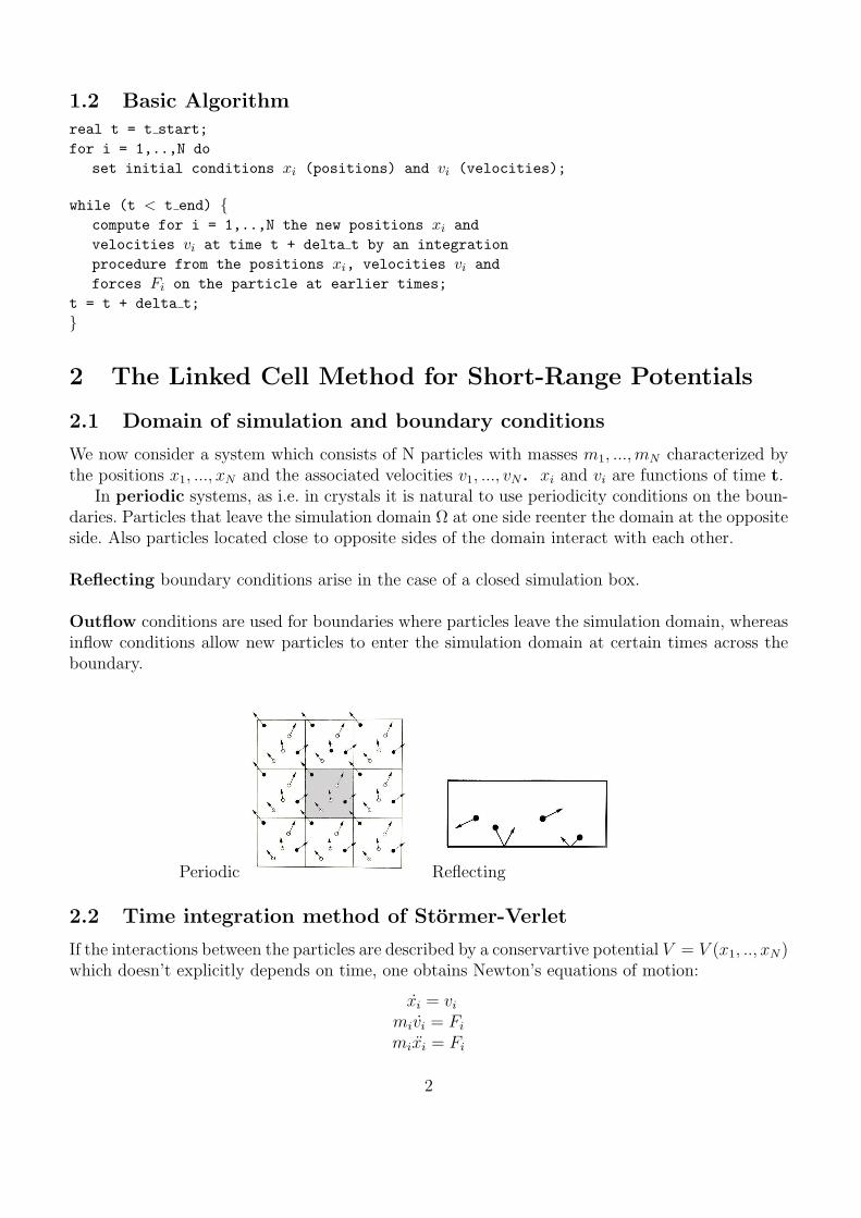
In periodic systems, as i.e. in crystals it is natural to use periodicity conditions on the boun-daries. Particles that leave the simulation domain Ω at one side reenter the domain at the oppositeside. Also particles located close to opposite sides of the domain interact with each other.

Reflecting boundary conditions arise in the case of a closed simulation box.

Outflow conditions are used for boundaries where particles leave the simulation domain, whereasinflow conditions allow new particles to enter the simulation domain at certain times across theboundary.

Periodic Reflecting

2.2 Time integration method of Stormer-Verlet

If the interactions between the particles are described by a conservartive potential V = V (x1, .., xN )which doesn’t explicitly depends on time, one obtains Newton’s equations of motion:

xi = vi

mivi = Fi

mixi = Fi

2

i = 1, ..., N , where the Forces Fi are given by

Fi = −∇xiV (x1, ..., xN )

We decompose the time interval [0, tend] ⊂ R, on which the system of differential equations isto be solved into l subintervals of the same size

δt := tend/l.

Instead of the first derivative

dxdt

:= limδt→0

x(t+δt)−x(t)δt

one can use the discrete difference operator:

[dxdt

]rn := x(tn+1)−x(tn)δt

or the central difference operator

[dxdt

]cn := x(tn+1)−x(tn−1)2δt

The second derivative at the grid point tn can be approximated by the difference operator

[d2xdt2

]n := 1δt2

(x(tn + δt) − 2x(tn) + x(tn − δt))

Using the Taylor-expansion we obtain that the discretization error for the approximation of thesecond derivative is of the order O(δt2)

The velocity as the derivative of the position can be approximated using the central difference:

vni =

xn+1

i−xn−1

i

2δt

The so-called Velocity-Stormer-Verlet method solves this equation for xn−1i , substitutes

the result into xn+1i = 2xn

i − xn−1i + δt2 · F n

i /mi and then solves for xn+1i .

One obtains:

xn+1i = xn

i + δt · vni +

F ni ·δt2

2mi

Furthermore, we have:

vni =

xn+1

i−xn−1

i

2δt=

xni

δt−

xn−1

i

δt+

F ni

2miδt,

and

vn+1i + vn

i =xn+1

i−xn−1

i

δt+

(F n+1

i+F n

i )δt

2mi,

and finally:

vn+1i = vn

i +(F n

i +F n+1

i)δt

2mi

These two equations are called the Velocity-Stormer-Verlet integration method.

xn+1i = xn

i + δtvni +

F ni ·δ2

2mi

vn+1i = vn

i +(F n

i +F n+1

i)δt

2mi

3

xn+1i = xn

i + δt · vni +

F ni ·δt2

2mi

compute forces F

vn+1i = vn

i +(F n

i +F n+1

i)δt

2mi

Velocity-Stormer-Verlet Method

// start with initial data x, v, t

// auxilary vector F old

compute forces F;

while (t < t end) t = t + delta t;

loop over all i xi = xi+ delta t ∗(vi + .5/mi ∗ Fi∗ delta t); // update x

F oldi = Fi

compute forces Fi

loop over all i

vi = vi+delta t∗.5/mi ∗ (Fi + F oldi ); // update v

compute derived quantities as for example kinetic energy;

print values of t, x, v as well as derived quantities;

Velocity-Stormer-Verlet Method is the most commonly used method for the integration ofNewton’s equations of motions.

2.3 Implementation of the Basic Algorithm

Data structure Particle:

typedef struct real m; // mass

x[DIM]; // position

v[DIM]; // velocity

F[DIM]; // force

Particle;

4

Velocity-Stormer-Verlet Method

void timeIntegration (real t, real delta t, real t end, Particle *p, int N) compF basis(p,N)

while (t<t end) t += delta t;

compX basis(p, N, delta t);

compF basis(p, N);

compV basis(p, N, delta t);

compoutStatistic basis (p, N, t); // computation of the kinetic energy

outputResults basis(p, N, t);

Computation of the forces with O(N2) operations

The force on the particle i:

Fi = −∇xiV (x1, ..., xN ) =

N∑

j=1,j 6=i

−∇xiU(rij) =

N∑

j=1,j 6=i

Fij

void compF basis(Particle *p, int N) for (int i=0; i<N; i++)

for (int d=0; d<DIM; d++)

p[i].F[d] = 0; // initialize F with 0 for all particles

for (int i=0; i<N; i++)

for (int j=0; d<N; j++)

if (i!=j) force(&p[i], &p[j]); // add the forces Fij to Fi

2.4 Cutoff radius

It doesn’t make sense to sum over all particles to compute the forces. It is enough to sum overonly those particles, which contribute to the potential and to the force. A function decays rapidlywith distance if it decays faster in r, than 1/rd, where d is the dimension of the problem

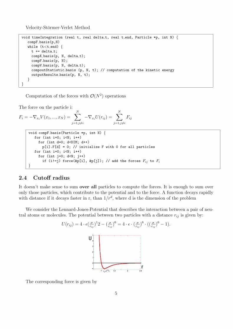
We consider the Lennard-Jones-Potential that describes the interaction between a pair of neu-tral atoms or molecules. The potential between two particles with a distance rij is given by:

U(rij) = 4 · ǫ( σrij

)12 − ( σrij

)6 = 4 · ǫ · ( σrij

)6 · (( σrij

)6 − 1).

The corresponding force is given by

5

Fi = −∇Vxi(x1, ..., xN )

= 24 · ǫ

N∑

j=1,j 6=i

1

r2ij

· (σ

rij

)6

· (1 − 2 · (σ

rij

)6

)rij

The force Fi =N

∑

j=1,j 6=i

Fij The potential decays very fast with the distance rij between the

particles.

The idea is to neglect all contributions in the Fi =∑

Fij , that are smaller than a certain

threshold.The Lennard-Jones potential is then approximated by

U(rij) ≈

4 · ǫ(( σrij

)12 − ( σrij

)6) rij ≤ rcut

0 rij > rcut

,

i.e. it is cutoff at a distance r = rcut.

We now assume that the particles are more or less uniformly distributed throughout thesimulation domain. Then rcut can be chosen so that the number of remaining terms in the trun-cated sum

Fi = −∇xiV (x1, ..., xN ) = 24 · ǫ

N∑

j=1,j 6=i,0<rij≤rcut

1

r2ij

· (σ

rij

)6

· (1 − 2 · (σ

rij

)6

)rij

is bounded independent of the number of particles N.

The complexity of the evaluation of the potential and the forces is then proportional to N, itis of the order O(N) only.

This is a substantial reduction of the computational cost compared to the compexity of theorder O(N2) for the basic approach.The only one question left is how to manage the data, so that for a given particle the neighbouringparticles it interacts with, can be found efficiently.

2.5 The Linked Cell Method

The idea of the linked cell method is to split the physical simulation domain Ω into uniformsubdomains (cells).

If the length of the sides of the cells is chosen larger or equal to the cutoff radius rcut, theninteractions in the truncated potentials are limited to particles within a cell and from adjacentcells.

6

For the force on particle i in cell ic one obtains a sum of the form

Fi =∑

cell kc, kc∈N(ic)

∑

j∈particles in cell kc, j 6=i

Fij

where N (ic) is the cell ic itself and the direct neighbours of ic.The question is now how to efficiently access the neighbouring cells and particles inside these

cells in an algorithm.The cells at the boundary of the domain have correspondingly fewer nighbouring cells except

for the case of the periodic boundary conditions.In two dimensions each cell can be described by two indices (ic1,ic2). Each cell in the grid

posseses eight neighbouring cells.

Computation of the force in the linked cell method

loop over all cells ic

loop over all particles i in cell ic i->F[d] = 0 for all d;

loop over all cells kc in N(ic)

loop over all particles j in cell kc

if (i!=j)

if (rij <= rcut)

force(&i,&j) // add Fij to Fi

The complexity of the computation of the forces on the particles amounts to C ·N operationsif the particles are distributed almost uniformly and thus the number of particles per cell isbounded from above.

Compared to the naive summation of the force over all pairs of particles, the complexity is reducedfrom originally O(N2) to now O(N).

2.6 Implementation

Implementation of the linked cell methodData structure Linked List:

typedef struct ParticleList Particle p;

struct ParticleList *next;

ParticleList;

A linked list is represented by a poin-

7

ter to the first element.

A complete loop over all elements of the list is given by:

ParticleList *l = root list;

while (NULL!=l) process element l->p;

l = l->next;

Repeatedly inserting elements into an initially empty list, we can fill that list with the appro-priate particles.

The insertion of an element into the list is easiest at the beginning of the list. To implementit we only have to change the values of two pointers (the root-pointer and the next-pointer of thenew element).

Inserting elements into a linked list

void insertList(ParticleList **root list, ParticleList *i)

i->next = *root list; *root list = i;

Removing an element in a singly linked list

void deleteList(ParticleList **q) *q->next = ((*q)->next) ->next;

If some particles leave the simulation domain, then the data structure associated to this particlehas to be removed from its list and its dynamical allocated memory should possibly be released.If new particles can enter the simulation domain, data structure for these particles have to be

8

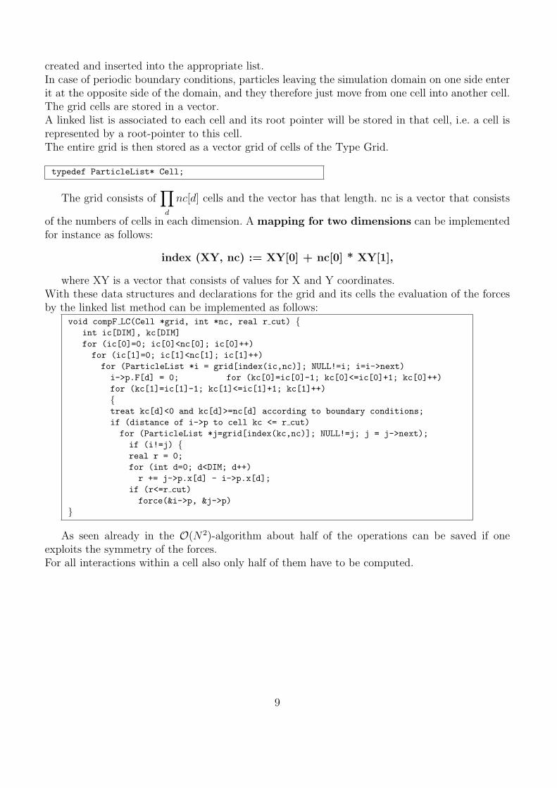
created and inserted into the appropriate list.In case of periodic boundary conditions, particles leaving the simulation domain on one side enterit at the opposite side of the domain, and they therefore just move from one cell into another cell.The grid cells are stored in a vector.A linked list is associated to each cell and its root pointer will be stored in that cell, i.e. a cell isrepresented by a root-pointer to this cell.The entire grid is then stored as a vector grid of cells of the Type Grid.

typedef ParticleList* Cell;

The grid consists of∏

d

nc[d] cells and the vector has that length. nc is a vector that consists

of the numbers of cells in each dimension. A mapping for two dimensions can be implementedfor instance as follows:

index (XY, nc) := XY[0] + nc[0] * XY[1],

where XY is a vector that consists of values for X and Y coordinates.With these data structures and declarations for the grid and its cells the evaluation of the forcesby the linked list method can be implemented as follows:

void compF LC(Cell *grid, int *nc, real r cut) int ic[DIM], kc[DIM]

for (ic[0]=0; ic[0]<nc[0]; ic[0]++)

for (ic[1]=0; ic[1]<nc[1]; ic[1]++)

for (ParticleList *i = grid[index(ic,nc)]; NULL!=i; i=i->next)

i->p.F[d] = 0; for (kc[0]=ic[0]-1; kc[0]<=ic[0]+1; kc[0]++)

for (kc[1]=ic[1]-1; kc[1]<=ic[1]+1; kc[1]++)

treat kc[d]<0 and kc[d]>=nc[d] according to boundary conditions;

if (distance of i->p to cell kc <= r cut)

for (ParticleList *j=grid[index(kc,nc)]; NULL!=j; j = j->next);

if (i!=j) real r = 0;

for (int d=0; d<DIM; d++)

r += j->p.x[d] - i->p.x[d];

if (r<=r cut)

force(&i->p, &j->p)

As seen already in the O(N2)-algorithm about half of the operations can be saved if oneexploits the symmetry of the forces.For all interactions within a cell also only half of them have to be computed.

9

3 Applications

Applications Collision of two bodies

Simulation of the Rayleigh-Taylor-instability.

and many many others.

4 Literature

M. Griebel, S. Knapek, G. Zumbusch - Numerical Simulation in Molecular Dynamics,Springer, 2007

10