
Algorithms and Data Structures Computer Science 226 Fall ...
1141
Algorithms and Data Structures Instructors: Bob Sedgewick Kevin Wayne Computer Science 226 Fall 2007 Copyright © 2007 by Robert Sedgewick and Kevin Wayne.
-
Upload
khangminh22 -
Category
Documents
-
view
0 -
download
0
Transcript of Algorithms and Data Structures Computer Science 226 Fall ...

Algorithms and Data Structures
Instructors:Bob SedgewickKevin Wayne
Computer Science 226
Fall 2007
Copyright © 2007 by Robert Sedgewick and Kevin Wayne.

outline
why study algorithms?
usual suspects
coursework
resources (web)
resources (books)
2
Course Overview

3
COS 226 course overview
What is COS 226?
• Intermediate-level survey course.
• Programming and problem solving with applications.
• Algorithm: method for solving a problem.
• Data structure: method to store information.
Topic Data Structures and Algorithms
data types stack, queue, list, union-find, priority queue
sorting quicksort, mergesort, heapsort, radix sorts
searching hash table, BST, red-black tree, B-tree
graphs BFS, DFS, Prim, Kruskal, Dijkstra
strings KMP, Rabin-Karp, TST, Huffman, LZW
geometry Graham scan, k-d tree, Voronoi diagram

4
Why study algorithms?
Their impact is broad and far-reaching
Internet. Web search, packet routing, distributed file sharing.
Biology. Human genome project, protein folding.
Computers. Circuit layout, file system, compilers.
Computer graphics. Movies, video games, virtual reality.
Security. Cell phones, e-commerce, voting machines.
Multimedia. CD player, DVD, MP3, JPG, DivX, HDTV.
Transportation. Airline crew scheduling, map routing.
Physics. N-body simulation, particle collision simulation.
…

Old roots, new opportunities
Study of algorithms dates at least to Euclid
Some important algorithms were discovered
by undergraduates!
5
Why study algorithms?
300 BC
1920s
1940s1950s1960s1970s1980s1990s2000s

6
Why study algorithms?
To be able solve problems that could not otherwise be addressed
Example: Network connectivity
[stay tuned]

7
Why study algorithms?
For intellectual stimulation

They may unlock the secrets of life and of the universe.
Computational models are replacing mathematical models
in scientific enquiry
8
Why study algorithms?
20th century science(formula based)
21st century science(algorithm based)
for (double t = 0.0; true; t = t + dt) for (int i = 0; i < N; i++) { bodies[i].resetForce(); for (int j = 0; j < N; j++) if (i != j) bodies[i].addForce(bodies[j]); }
E = mc2
F = ma F = Gm1m2
r2
h2
2m2
+ V (r)
(r) = E (r)

For fun and profit
9
Why study algorithms?

• Their impact is broad and far-reaching
• Old roots, new opportunities
• To be able to solve problems that could not otherwise be addressed
• For intellectual stimulation
• They may unlock the secrets of life and of the universe
• For fun and profit
10
Why study algorithms?

11
The Usual Suspects
Lectures: Bob Sedgewick
• TTh 11-12:20, Bowen 222
• Office hours T 3-5 at Cafe Viv in Frist
Course management (everything else): Kevin Wayne
Precepts: Kevin Wayne
• Thursdays.
1: 12:30 Friend 110
2: 3:30 Friend 109
• Discuss programming assignments, exercises, lecture material.
• First precept meets Thursday 9/20
• Kevin’s office hours TBA
Need a precept time? Need to change precepts?
• email Donna O’Leary (CS ugrad coordinator) [email protected]
Check course web page for up-to-date info

12
Coursework and Grading
7-8 programming assignments. 45%
• Due 11:55pm, starting Monday 9/24.
• Available via course website.
Weekly written exercises. 15%
• Due at beginning of Wednesday lecture, starting 9/24.
• Available via course website.
Exams.
• Closed-book with cheatsheet.
• Midterm. 15%
• Final. 25%
Staff discretion. Adjust borderline cases.
• Participation in lecture and precepts
• Everyone needs to meet us both at office hours!
Challenge for the bored. Determine importance of 45-15-15-25 weights
Final
Midterm
Programs
HW

Course content.
http://www.princeton.edu/~cos226
• syllabus
• exercises
• lecture slides
• programming assignments (description, code, test data, checklists)
Course administration.
https://moodle.cs.princeton.edu/course/view.php?id=24
• programming assignment submission.
• grades.
Booksites. http://www.cs.princeton.edu/IntroCS
http://www.cs.princeton.edu/IntroAlgsDS
• brief summary of content.
• code.
• links to web content.
13
Resources (web)

Algorithms in Java, 3rd edition
• Parts 1-4. [sorting, searching]
• Part 5. [graph algorithms]
Introduction to Programming in Java
• basic programming model
• elementary AofA and data structures
Algorithms in Pascal(!)/C/C++, 2nd edition
• strings
• elementary geometric algorithms
Algorithms, 4th edition
(in preparation)
Resources (books)
14

Union-Find
15

network connectivityquick findquick unionimprovementsapplications
1
Union-Find Algorithms

Subtext of today’s lecture (and this course)
Steps to developing a usable algorithm.
• Define the problem.
• Find an algorithm to solve it.
• Fast enough?
• If not, figure out why.
• Find a way to address the problem.
• Iterate until satisfied.
The scientific method
Mathematical models and computational complexity
READ Chapter One of Algs in Java
2

3
network connectivityquick findquick unionimprovementsapplications

Network connectivity
Basic abstractions
• set of objects
• union command: connect two objects
• find query: is there a path connecting one object to another?
4

Union-find applications involve manipulating objects of all types.
• Computers in a network.
• Web pages on the Internet.
• Transistors in a computer chip.
• Variable name aliases.
• Pixels in a digital photo.
• Metallic sites in a composite system.
When programming, convenient to name them 0 to N-1.
• Hide details not relevant to union-find.
• Integers allow quick access to object-related info.
• Could use symbol table to translate from object names
5
Objects
use as array index
0 7
2 3
8
4
6 5 91
stay tuned

6
Union-find abstractions
Simple model captures the essential nature of connectivity.
• Objects.
• Disjoint sets of objects.
• Find query: are objects 2 and 9 in the same set?
• Union command: merge sets containing 3 and 8.
0 1 { 2 3 9 } { 5 6 } 7 { 4 8 }
0 1 { 2 3 4 8 9 } { 5-6 } 7
0 1 { 2 3 9 } { 5-6 } 7 { 4-8 }
add a connection betweentwo grid points
subsets of connected grid points
are two grid points connected?
0 1 2 3 4 5 6 7 8 9 grid points

Connected components
Connected component: set of mutually connected vertices
Each union command reduces by 1 the number of components
7
in out
3 4 3 4
4 9 4 9
8 0 8 0
2 3 2 3
5 6 5 6
2 9
5 9 5 9
7 3 7 3
0
2 3
8
4
6 5 91
7 union commands
3 = 10-7 components
7

8
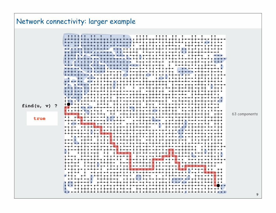
Network connectivity: larger example
find(u, v) ?
u
v
9
Network connectivity: larger example
63 components
find(u, v) ?
true

10
Union-find abstractions
• Objects.
• Disjoint sets of objects.
• Find queries: are two objects in the same set?
• Union commands: replace sets containing two items by their union
Goal. Design efficient data structure for union-find.
• Find queries and union commands may be intermixed.
• Number of operations M can be huge.
• Number of objects N can be huge.

11
network connectivityquick findquick unionimprovementsapplications
12
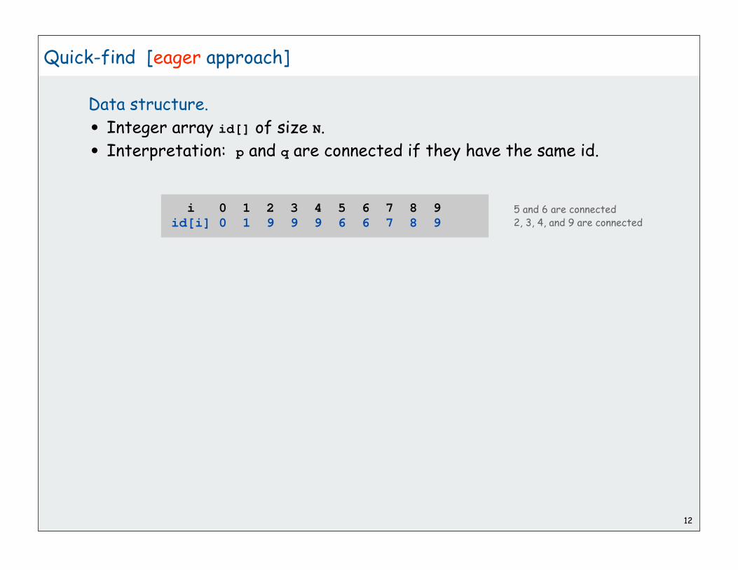
Quick-find [eager approach]
Data structure.
• Integer array id[] of size N.
• Interpretation: p and q are connected if they have the same id.
i 0 1 2 3 4 5 6 7 8 9id[i] 0 1 9 9 9 6 6 7 8 9
5 and 6 are connected2, 3, 4, and 9 are connected

13
Quick-find [eager approach]
Data structure.
• Integer array id[] of size N.
• Interpretation: p and q are connected if they have the same id.
Find. Check if p and q have the same id.
Union. To merge components containing p and q,
change all entries with id[p] to id[q].
i 0 1 2 3 4 5 6 7 8 9id[i] 0 1 9 9 9 6 6 7 8 9
5 and 6 are connected2, 3, 4, and 9 are connected
union of 3 and 62, 3, 4, 5, 6, and 9 are connected
i 0 1 2 3 4 5 6 7 8 9id[i] 0 1 6 6 6 6 6 7 8 6
id[3] = 9; id[6] = 63 and 6 not connected
problem: many values can change

14
Quick-find example
3-4 0 1 2 4 4 5 6 7 8 9
4-9 0 1 2 9 9 5 6 7 8 9
8-0 0 1 2 9 9 5 6 7 0 9
2-3 0 1 9 9 9 5 6 7 0 9
5-6 0 1 9 9 9 6 6 7 0 9
5-9 0 1 9 9 9 9 9 7 0 9
7-3 0 1 9 9 9 9 9 9 0 9
4-8 0 1 0 0 0 0 0 0 0 0
6-1 1 1 1 1 1 1 1 1 1 1
problem: many values can change

public class QuickFind{ private int[] id;
public QuickFind(int N) { id = new int[N]; for (int i = 0; i < N; i++) id[i] = i; }
public boolean find(int p, int q) { return id[p] == id[q]; }
public void unite(int p, int q) { int pid = id[p]; for (int i = 0; i < id.length; i++) if (id[i] == pid) id[i] = id[q]; }}
15
Quick-find: Java implementation
1 operation
N operations
set id of eachobject to itself

16
Quick-find is too slow
Quick-find algorithm may take ~MN steps
to process M union commands on N objects
Rough standard (for now).
• 109 operations per second.
• 109 words of main memory.
• Touch all words in approximately 1 second.
Ex. Huge problem for quick-find.
• 1010 edges connecting 109 nodes.
• Quick-find takes more than 1019 operations.
• 300+ years of computer time!
Paradoxically, quadratic algorithms get worse with newer equipment.
• New computer may be 10x as fast.
• But, has 10x as much memory so problem may be 10x bigger.
• With quadratic algorithm, takes 10x as long!
a truism (roughly) since 1950 !

17
network connectivityquick findquick unionimprovementsapplications

18
Quick-union [lazy approach]
Data structure.
• Integer array id[] of size N.
• Interpretation: id[i] is parent of i.
• Root of i is id[id[id[...id[i]...]]].
i 0 1 2 3 4 5 6 7 8 9id[i] 0 1 9 4 9 6 6 7 8 9
4
7
3
5
0 1 9 6 8
2
3's root is 9; 5's root is 6
keep going until it doesn’t change
19
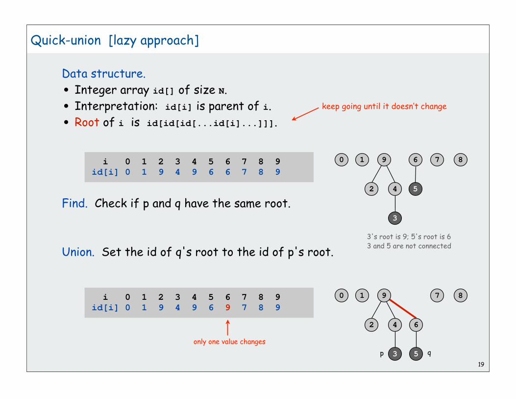
Quick-union [lazy approach]
Data structure.
• Integer array id[] of size N.
• Interpretation: id[i] is parent of i.
• Root of i is id[id[id[...id[i]...]]].
Find. Check if p and q have the same root.
Union. Set the id of q's root to the id of p's root.
i 0 1 2 3 4 5 6 7 8 9id[i] 0 1 9 4 9 6 6 7 8 9
4
7
3
5
0 1 9 6 8
2
3's root is 9; 5's root is 63 and 5 are not connected
i 0 1 2 3 4 5 6 7 8 9id[i] 0 1 9 4 9 6 9 7 8 9
4
7
3 5
0 1 9
6
8
2
only one value changes
p q
keep going until it doesn’t change

20
Quick-union example
3-4 0 1 2 4 4 5 6 7 8 9
4-9 0 1 2 4 9 5 6 7 8 9
8-0 0 1 2 4 9 5 6 7 0 9
2-3 0 1 9 4 9 5 6 7 0 9
5-6 0 1 9 4 9 6 6 7 0 9
5-9 0 1 9 4 9 6 9 7 0 9
7-3 0 1 9 4 9 6 9 9 0 9
4-8 0 1 9 4 9 6 9 9 0 0
6-1 1 1 9 4 9 6 9 9 0 0
problem: trees can get tall

21
Quick-union: Java implementation
time proportionalto depth of p and q
time proportionalto depth of p and q
time proportionalto depth of i
public class QuickUnion{ private int[] id;
public QuickUnion(int N) { id = new int[N]; for (int i = 0; i < N; i++) id[i] = i; }
private int root(int i) { while (i != id[i]) i = id[i]; return i; }
public boolean find(int p, int q) { return root(p) == root(q); }
public void unite(int p, int q) { int i = root(p); int j = root(q); id[i] = j; }}

22
Quick-union is also too slow
Quick-find defect.
• Union too expensive (N steps).
• Trees are flat, but too expensive to keep them flat.
Quick-union defect.
• Trees can get tall.
• Find too expensive (could be N steps)
• Need to do find to do union
algorithm union find
Quick-find N 1
Quick-union N* N worst case
* includes cost of find

23
network connectivityquick findquick unionimprovementsapplications

24
Improvement 1: Weighting
Weighted quick-union.
• Modify quick-union to avoid tall trees.
• Keep track of size of each component.
• Balance by linking small tree below large one.
Ex. Union of 5 and 3.
• Quick union: link 9 to 6.
• Weighted quick union: link 6 to 9.
4
7
3
5
0 1 9 6 8
2
p
q
4 211 1 1size

25
Weighted quick-union example
3-4 0 1 2 3 3 5 6 7 8 9
4-9 0 1 2 3 3 5 6 7 8 3
8-0 8 1 2 3 3 5 6 7 8 3
2-3 8 1 3 3 3 5 6 7 8 3
5-6 8 1 3 3 3 5 5 7 8 3
5-9 8 1 3 3 3 3 5 7 8 3
7-3 8 1 3 3 3 3 5 3 8 3
4-8 8 1 3 3 3 3 5 3 3 3
6-1 8 3 3 3 3 3 5 3 3 3
no problem: trees stay flat

26
Weighted quick-union: Java implementation
Java implementation.
• Almost identical to quick-union.
• Maintain extra array sz[] to count number of elements
in the tree rooted at i.
Find. Identical to quick-union.
Union. Modify quick-union to
• merge smaller tree into larger tree
• update the sz[] array.

27
Weighted quick-union analysis
Analysis.
• Find: takes time proportional to depth of p and q.
• Union: takes constant time, given roots.
• Fact: depth is at most lg N. [needs proof]
Stop at guaranteed acceptable performance? No, easy to improve further.
Data Structure Union Find
Quick-find N 1
Quick-union N * N
Weighted QU lg N * lg N
* includes cost of find

28
Path compression. Just after computing the root of i,
set the id of each examined node to root(i).
Improvement 2: Path compression
2
41110
2
54
7
8
1110
root(9)
0
1
0
3
6
9
9
78
136
5

Path compression.
• Standard implementation: add second loop to root() to set
the id of each examined node to the root.
• Simpler one-pass variant: make every other node in path
point to its grandparent.
In practice. No reason not to! Keeps tree almost completely flat.
29
Weighted quick-union with path compression
only one extra line of code !
public int root(int i){ while (i != id[i]) { id[i] = id[id[i]]; i = id[i]; } return i;}

30
Weighted quick-union with path compression
3-4 0 1 2 3 3 5 6 7 8 9
4-9 0 1 2 3 3 5 6 7 8 3
8-0 8 1 2 3 3 5 6 7 8 3
2-3 8 1 3 3 3 5 6 7 8 3
5-6 8 1 3 3 3 5 5 7 8 3
5-9 8 1 3 3 3 3 5 7 8 3
7-3 8 1 3 3 3 3 5 3 8 3
4-8 8 1 3 3 3 3 5 3 3 3
6-1 8 3 3 3 3 3 3 3 3 3
no problem: trees stay VERY flat

31
WQUPC performance
Theorem. Starting from an empty data structure, any sequence
of M union and find operations on N objects takes O(N + M lg* N) time.
• Proof is very difficult.
• But the algorithm is still simple!
Linear algorithm?
• Cost within constant factor of reading in the data.
• In theory, WQUPC is not quite linear.
• In practice, WQUPC is linear.
Amazing fact:
• In theory, no linear linking strategy exists
because lg* N is a constantin this universe
number of times needed to takethe lg of a number until reaching 1
N lg* N
1 0
2 1
4 2
16 3
65536 4
265536 5

32
Summary
Ex. Huge practical problem.
• 1010 edges connecting 109 nodes.
• WQUPC reduces time from 3,000 years to 1 minute.
• Supercomputer won't help much.
• Good algorithm makes solution possible.
Bottom line.
WQUPC makes it possible to solve problems
that could not otherwise be addressed
M union-find ops on a set of N objects
Algorithm Worst-case time
Quick-find M N
Quick-union M N
Weighted QU N + M log N
Path compression N + M log N
Weighted + path (M + N) lg* N
WQUPC on Java cell phone beats QF on supercomputer!

33
network connectivityquick findquick unionimprovementsapplications

34
Union-find applications
Network connectivity.
• Percolation.
• Image processing.
• Least common ancestor.
• Equivalence of finite state automata.
• Hinley-Milner polymorphic type inference.
• Kruskal's minimum spanning tree algorithm.
• Games (Go, Hex)
• Compiling equivalence statements in Fortran.

Percolation
A model for many physical systems
• N-by-N grid.
• Each square is vacant or occupied.
• Grid percolates if top and bottom are connected by vacant squares.
35
percolates does not percolate
model system vacant site occupied site percolates
electricity material conductor insulated conducts
fluid flow material empty blocked porous
social interaction population person empty communicates

Percolation phase transition
Likelihood of percolation depends on site vacancy probability p
Experiments show a threshold p*
• p > p*: almost certainly percolates
• p < p*: almost certainly does not percolate
36
Q. What is the value of p* ?
p high: percolatesp low: does not percolate
p*

37
• Initialize whole grid to be “not vacant”
• Implement “make site vacant” operation
that does union() with adjacent sites
• Make all sites on top and bottom rows vacant
• Make random sites vacant until find(top, bottom)
• Vacancy percentage estimates p*
UF solution to find percolation threshold
0 0 0 0 0 0 0 0
2 3 4 5 6 7 8 9
15 20 21
28 29 30 31 33
39 40 42 43 45
50 52 54 55 56 57
1 1 1 1 1 1 1 1
0 0 0 0
10 11 12 0
22 23 24 0
34 35 36 0
46 1 49
58 1
1 1 1 1 not vacant
vacant
top
bottom
14
14 14
14
32
32 1
1 11
1
1
16 16 16 16

38
Q. What is percolation threshold p* ?
A. about 0.592746 for large square lattices.
Q. Why is UF solution better than solution in IntroProgramming 2.4?
Percolation
percolation constant known only via simulation
percolates does not percolate

39
Hex
Hex. [Piet Hein 1942, John Nash 1948, Parker Brothers 1962]
• Two players alternate in picking a cell in a hex grid.
• Black: make a black path from upper left to lower right.
• White: make a white path from lower left to upper right.
Union-find application. Algorithm to detect when a player has won.
Reference: http://mathworld.wolfram.com/GameofHex.html

Subtext of today’s lecture (and this course)
Steps to developing an usable algorithm.
• Define the problem.
• Find an algorithm to solve it.
• Fast enough?
• If not, figure out why.
• Find a way to address the problem.
• Iterate until satisfied.
The scientific method
Mathematical models and computational complexity
READ Chapter One of Algs in Java
40

1
Collaboration policy
Exceptions
• Code from course materials OK [cite source]
• Coding with partner OK after first assignment [stay tuned]
Where to get help
• Email (but no code in email)
• Office hours
• Lab TAs in Friend 008/009
• Bounce ideas (but not code) off classmates
Note: Programming in groups except as above is a serious violation.
• working with classmates is encouraged
• checking solutions is OK
Programs: Do not use someone else’s code unless specifically authorized
Exercises: Write up your own solutions (no copying)

Stacks and Queues
stacksdynamic resizingqueuesgenericsapplications
2

3
Stacks and Queues
Fundamental data types.
• Values: sets of objects
• Operations: insert, remove, test if empty.
• Intent is clear when we insert.
• Which item do we remove?
Stack.
• Remove the item most recently added.
• Analogy: cafeteria trays, Web surfing.
Queue.
• Remove the item least recently added.
• Analogy: Registrar's line.
FIFO = "first in first out"
LIFO = "last in first out"
enqueue dequeue
pop
push
4
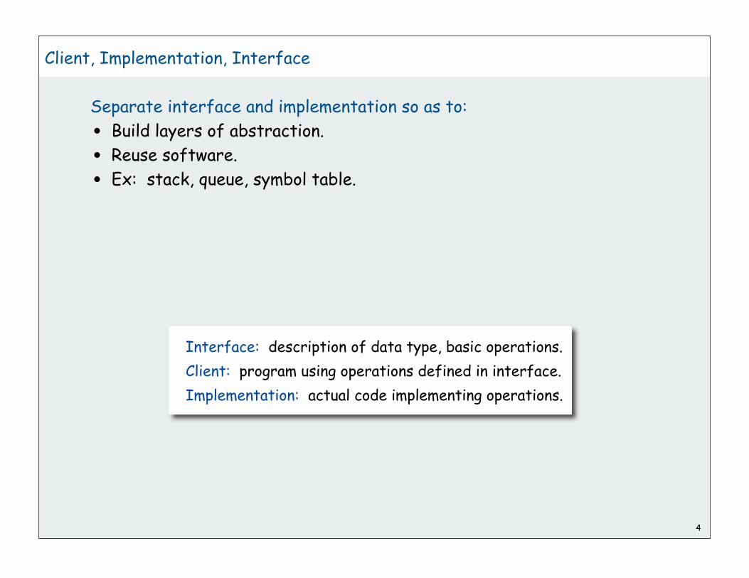
Client, Implementation, Interface
Separate interface and implementation so as to:
• Build layers of abstraction.
• Reuse software.
• Ex: stack, queue, symbol table.
Interface: description of data type, basic operations.
Client: program using operations defined in interface.
Implementation: actual code implementing operations.

5
Client, Implementation, Interface
Benefits.
• Client can't know details of implementation
client has many implementation from which to choose.
• Implementation can't know details of client needs
many clients can re-use the same implementation.
• Design: creates modular, re-usable libraries.
• Performance: use optimized implementation where it matters.
Interface: description of data type, basic operations.
Client: program using operations defined in interface.
Implementation: actual code implementing operations.

6
stacksdynamic resizingqueuesgenericsapplications
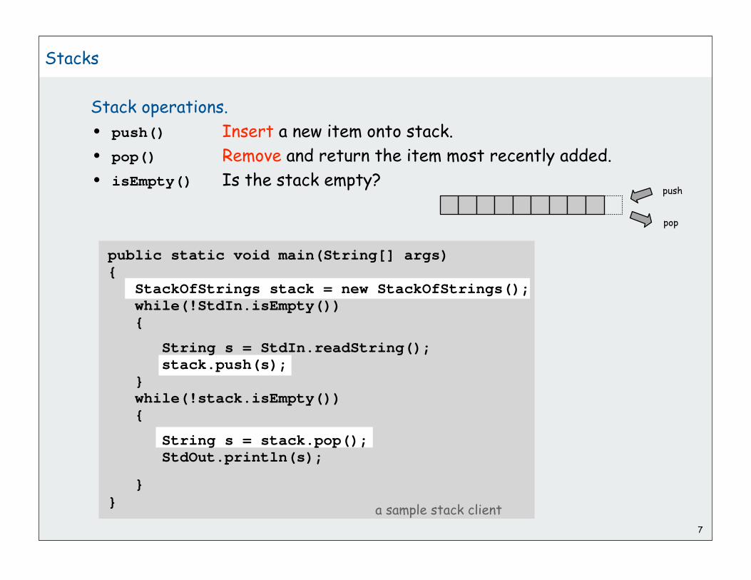
Stack operations.
• push() Insert a new item onto stack.
• pop() Remove and return the item most recently added.
• isEmpty() Is the stack empty?
7
Stacks
pop
push
a sample stack client
public static void main(String[] args){ StackOfStrings stack = new StackOfStrings(); while(!StdIn.isEmpty()) {
String s = StdIn.readString(); stack.push(s); } while(!stack.isEmpty()) {
String s = stack.pop(); StdOut.println(s);
}
}

8
Stack pop: Linked-list implementation
best the was it
best the was it first = first.next;
best the was it return item;
first
first
first
of item = first.item;
9
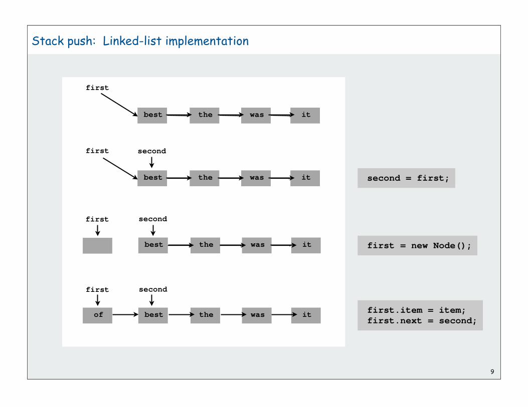
Stack push: Linked-list implementation
best the was it
second
best the was it
best the was it
first
of
second = first;
first.item = item;first.next = second;
best the was it
second
first = new Node();
first second
first
first

10
Stack: Linked-list implementation
"inner class"
public class StackOfStrings{ private Node first = null;
private class Node { String item; Node next; }
public boolean isEmpty() { return first == null; }
public void push(String item) { Node second = first; first = new Node(); first.item = item; first.next = second; }
public String pop() { String item = first.item; first = first.next; return item; }
}
Error conditions?Example: pop() an empty stack
COS 217: bulletproof the codeCOS 226: first find the code we want to use

11
Stack: Array implementation
Array implementation of a stack.
• Use array s[] to store N items on stack.
• push() add new item at s[N].
• pop() remove item from s[N-1].
it was the best
0 1 2 3 4 5 6 7 8 9
s[]
N

12
Stack: Array implementation
avoid loitering (garbage collector only reclaims memoryif no outstanding references)
public class StackOfStrings{ private String[] s; private int N = 0;
public StringStack(int capacity) { s = new String[capacity]; }
public boolean isEmpty() { return N == 0; }
public void push(String item) { s[N++] = item; }
public String pop() { String item = s[N-1]; s[N-1] = null; N--; return item; }
}

13
stacksdynamic resizingqueuesgenericsapplications

14
Stack array implementation: Dynamic resizing
Q. How to grow array when capacity reached?
Q. How to shrink array (else it stays big even when stack is small)?
First try:
• push(): increase size of s[] by 1
• pop() : decrease size of s[] by 1
Too expensive
• Need to copy all of the elements to a new array.
• Inserting N elements: time proportional to 1 + 2 + … + N N2/2.
Need to guarantee that array resizing happens infrequently
infeasible for large N

15
Q. How to grow array?
A. Use repeated doubling:
if array is full, create a new array of twice the size, and copy items
Consequence. Inserting N items takes time proportional to N (not N2).
public StackOfStrings() { this(8); }
public void push(String item) { if (N >= s.length) resize(); s[N++] = item; }
private void resize(int max) { String[] dup = new String[max]; for (int i = 0; i < N; i++) dup[i] = s[i]; s = dup; }
Stack array implementation: Dynamic resizing
no-argumentconstructor
create new arraycopy items to it
8 + 16 + … + N/4 + N/2 + N 2N

16
Q. How (and when) to shrink array?
How: create a new array of half the size, and copy items.
When (first try): array is half full?
No, causes thrashing
When (solution): array is 1/4 full (then new array is half full).
Consequences.
• any sequence of N ops takes time proportional to N
• array is always between 25% and 100% full
public String pop(String item) { String item = s[--N]; sa[N] = null; if (N == s.length/4) resize(s.length/2); return item; }
Stack array implementation: Dynamic resizing
Not a.length/2 to avoid thrashing
(push-pop-push-pop-... sequence: time proportional to N for each op)

17
Stack Implementations: Array vs. Linked List
Stack implementation tradeoffs. Can implement with either array or
linked list, and client can use interchangeably. Which is better?
Array.
• Most operations take constant time.
• Expensive doubling operation every once in a while.
• Any sequence of N operations (starting from empty stack)
takes time proportional to N.
Linked list.
• Grows and shrinks gracefully.
• Every operation takes constant time.
• Every operation uses extra space and time to deal with references.
Bottom line: tossup for stacks
but differences are significant when other operations are added
"amortized" bound

Stack implementations: Array vs. Linked list
Which implementation is more convenient?
18
array? linked list?
return count of elements in stack
remove the kth most recently added
sample a random element

19
stacksdynamic resizingqueuesgenericsapplications

Queue operations.
• enqueue() Insert a new item onto queue.
• dequeue() Delete and return the item least recently added.
• isEmpty() Is the queue empty?
20
Queues
public static void main(String[] args){ QueueOfStrings q = new QueueOfStrings(); q.enqueue("Vertigo"); q.enqueue("Just Lose It"); q.enqueue("Pieces of Me"); q.enqueue("Pieces of Me"); System.out.println(q.dequeue()); q.enqueue("Drop It Like It's Hot");
while(!q.isEmpty()
System.out.println(q.dequeue());
}

21
Dequeue: Linked List Implementation
was the best of
was the best of first = first.next;
was the best of return item;
first
first
first
it item = first.item;
last
last
last
Aside:dequeue (pronounced “DQ”) means “remove from a queue”deque (pronounced “deck”) is a data structure (see PA 1)

22
Enqueue: Linked List Implementation
x = new Node();x.item = item;x.next = null;
last = x;
last.next = x;
first
it was the best
x
of
last
first
it was the best
last
it was the best of
it was the best of
xfirst last
xfirst last

23
Queue: Linked List Implementation
public class QueueOfStrings{ private Node first; private Node last;
private class Node { String item; Node next; }
public boolean isEmpty()
{ return first == null; }
public void enqueue(String item) { Node x = new Node(); x.item = item; x.next = null; if (isEmpty()) { first = x; last = x; } else { last.next = x; last = x; } }
public String dequeue() { String item = first.item; first = first.next; return item; }}
24
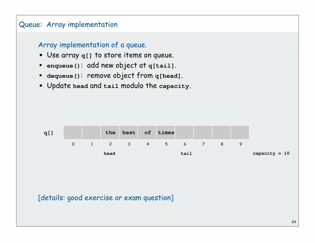
Queue: Array implementation
Array implementation of a queue.
• Use array q[] to store items on queue.
• enqueue(): add new object at q[tail].
• dequeue(): remove object from q[head].
• Update head and tail modulo the capacity.
[details: good exercise or exam question]
the best of times
0 1 2 3 4 5 6 7 8 9
q[]
head tail capacity = 10

25
stacksdynamic resizingqueuesgenericsapplications

26
Generics (parameterized data types)
We implemented: StackOfStrings, QueueOfStrings.
We also want: StackOfURLs, QueueOfCustomers, etc?
Attempt 1. Implement a separate stack class for each type.
• Rewriting code is tedious and error-prone.
• Maintaining cut-and-pasted code is tedious and error-prone.
@#$*! most reasonable approach until Java 1.5 [hence, used in AlgsJava]

27
Stack of Objects
We implemented: StackOfStrings, QueueOfStrings.
We also want: StackOfURLs, QueueOfCustomers, etc?
Attempt 2. Implement a stack with items of type Object.
• Casting is required in client.
• Casting is error-prone: run-time error if types mismatch.
Stack s = new Stack();Apple a = new Apple();Orange b = new Orange();s.push(a);s.push(b);a = (Apple) (s.pop());
run-time error

28
Generics
Generics. Parameterize stack by a single type.
• Avoid casting in both client and implementation.
• Discover type mismatch errors at compile-time instead of run-time.
Guiding principles.
• Welcome compile-time errors
• Avoid run-time errors
Why?
Stack<Apple> s = new Stack<Apple>();Apple a = new Apple();Orange b = new Orange();s.push(a);s.push(b);a = s.pop();
compile-time error
no cast needed in client
parameter

29
Generic Stack: Linked List Implementation
public class StackOfStrings{ private Node first = null;
private class Node { String item; Node next; }
public boolean isEmpty() { return first == null; }
public void push(String item) { Node second = first; first = new Node(); first.item = item; first.next = second; }
public String pop() { String item = first.item; first = first.next; return item; }
}
public class Stack<Item>{ private Node first = null;
private class Node { Item item; Node next; }
public boolean isEmpty() { return first == null; }
public void push(Item item) { Node second = first; first = new Node(); first.item = item; first.next = second; }
public Item pop() { Item item = first.item; first = first.next; return item; }
}
Generic type name

30
Generic stack: array implementation
public class Stack<Item>{ private Item[] s; private int N = 0;
public Stack(int cap) { s = new Item[cap]; }
public boolean isEmpty() { return N == 0; }
public void push(Item item) { s[N++] = item; }
public String pop() { Item item = s[N-1]; s[N-1] = null; N--; return item; }
}
The way it should be.
public class StackOfStrings{ private String[] s; private int N = 0;
public StackOfStrings(int cap) { s = new String[cap]; }
public boolean isEmpty() { return N == 0; }
public void push(String item) { s[N++] = item; }
public String pop() { String item = s[N-1]; s[N-1] = null; N--; return item; }
}
@#$*! generic array creation not allowed in Java
31
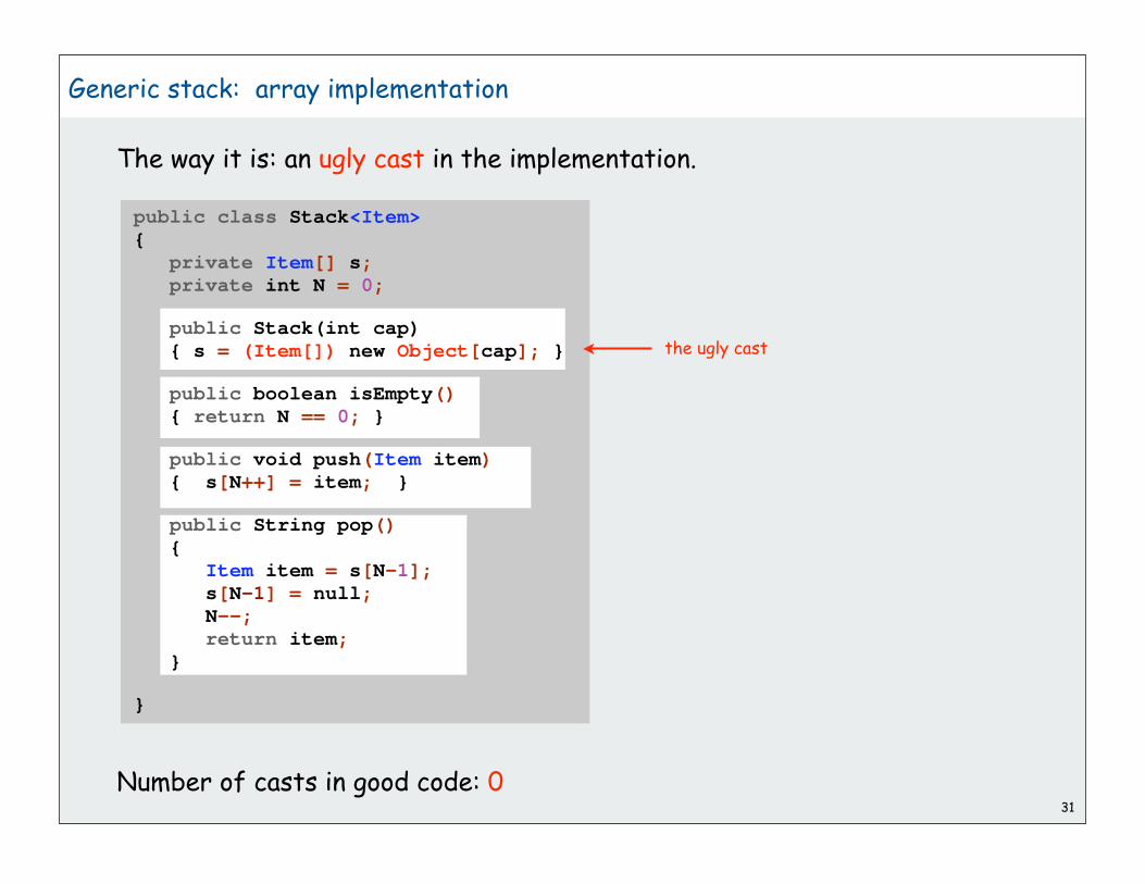
Generic stack: array implementation
public class Stack<Item>{ private Item[] s; private int N = 0;
public Stack(int cap) { s = (Item[]) new Object[cap]; }
public boolean isEmpty() { return N == 0; }
public void push(Item item) { s[N++] = item; }
public String pop() { Item item = s[N-1]; s[N-1] = null; N--; return item; }
}
The way it is: an ugly cast in the implementation.
the ugly cast
Number of casts in good code: 0

32
Generic data types: autoboxing
Generic stack implementation is object-based.
What to do about primitive types?
Wrapper type.
• Each primitive type has a wrapper object type.
• Ex: Integer is wrapper type for int.
Autoboxing. Automatic cast between a primitive type and its wrapper.
Syntactic sugar. Behind-the-scenes casting.
Bottom line: Client code can use generic stack for any type of data
Stack<Integer> s = new Stack<Integer>();s.push(17); // s.push(new Integer(17));int a = s.pop(); // int a = ((int) s.pop()).intValue();
33
stacksdynamic resizingqueuesgenericsapplications

34
Stack Applications
Real world applications.
• Parsing in a compiler.
• Java virtual machine.
• Undo in a word processor.
• Back button in a Web browser.
• PostScript language for printers.
• Implementing function calls in a compiler.

35
Function Calls
How a compiler implements functions.
• Function call: push local environment and return address.
• Return: pop return address and local environment.
Recursive function. Function that calls itself.
Note. Can always use an explicit stack to remove recursion.
static int gcd(int p, int q) {
if (q == 0) return p;
else return gcd(q, p % q);
}
gcd (216, 192)
static int gcd(int p, int q) {
if (q == 0) return p;
else return gcd(q, p % q);
}
gcd (192, 24)
static int gcd(int p, int q) {
if (q == 0) return p;
else return gcd(q, p % q);
}
gcd (24, 0)
p = 24, q = 0
p = 192, q = 24
p = 216, q = 192

36
Arithmetic Expression Evaluation
Goal. Evaluate infix expressions.
Two-stack algorithm. [E. W. Dijkstra]
• Value: push onto the value stack.
• Operator: push onto the operator stack.
• Left parens: ignore.
• Right parens: pop operator and two values;
push the result of applying that operator
to those values onto the operand stack.
Context. An interpreter!
operand operator
value stackoperator stack

37
Arithmetic Expression Evaluation
% java Evaluate( 1 + ( ( 2 + 3 ) * ( 4 * 5 ) ) )101.0
public class Evaluate {
public static void main(String[] args) {
Stack<String> ops = new Stack<String>();
Stack<Double> vals = new Stack<Double>();
while (!StdIn.isEmpty()) {
String s = StdIn.readString();
if (s.equals("(")) ;
else if (s.equals("+")) ops.push(s);
else if (s.equals("*")) ops.push(s);
else if (s.equals(")")) {
String op = ops.pop();
if (op.equals("+")) vals.push(vals.pop() + vals.pop());
else if (op.equals("*")) vals.push(vals.pop() * vals.pop());
}
else vals.push(Double.parseDouble(s));
}
StdOut.println(vals.pop());
}
}
Note: Old books have two-pass algorithm because generics were not available!

38
Correctness
Why correct?
When algorithm encounters an operator surrounded by two values
within parentheses, it leaves the result on the value stack.
as if the original input were:
Repeating the argument:
Extensions. More ops, precedence order, associativity.
1 + (2 - 3 - 4) * 5 * sqrt(6 + 7)
( 1 + ( ( 2 + 3 ) * ( 4 * 5 ) ) )
( 1 + ( 5 * ( 4 * 5 ) ) )
( 1 + ( 5 * 20 ) )
( 1 + 100 )
101

39
Stack-based programming languages
Observation 1.
Remarkably, the 2-stack algorithm computes the same value
if the operator occurs after the two values.
Observation 2.
All of the parentheses are redundant!
Bottom line. Postfix or "reverse Polish" notation.
Applications. Postscript, Forth, calculators, Java virtual machine, …
( 1 ( ( 2 3 + ) ( 4 5 * ) * ) + )
1 2 3 + 4 5 * * +
Jan Lukasiewicz

Stack-based programming languages: PostScript
Page description language
• explicit stack
• full computational model
• graphics engine
Basics
• %!: “I am a PostScript program”
• literal: “push me on the stack”
• function calls take args from stack
• turtle graphics built in
40
%!
72 72 moveto
0 72 rlineto
72 0 rlineto
0 -72 rlineto
-72 0 rlineto
2 setlinewidth
stroke
a PostScript program

Stack-based programming languages: PostScript
Data types
• basic: integer, floating point, boolean, ...
• graphics: font, path, ....
• full set of built-in operators
Text and strings
• full font support
• show (display a string, using current font)
• cvs (convert anything to a string)
41
%!
/Helvetica-Bold findfont 16 scalefont setfont
72 168 moveto
(Square root of 2:) show
72 144 moveto
2 sqrt 10 string cvs show
like System.out.print()
like toString()
Square root of 2:1.4142

Stack-based programming languages: PostScript
Variables (and functions)
• identifiers start with /
• def operator associates id with value
• braces
• args on stack
42
%!
/box{
/sz exch def
0 sz rlineto
sz 0 rlineto
0 sz neg rlineto
sz neg 0 rlineto
} def
72 144 moveto
72 box
288 288 moveto
144 box
2 setlinewidth
stroke
function definition
function calls
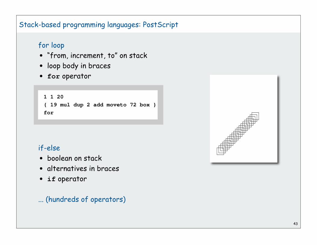
Stack-based programming languages: PostScript
for loop
• “from, increment, to” on stack
• loop body in braces
• for operator
if-else
• boolean on stack
• alternatives in braces
• if operator
... (hundreds of operators)
43
1 1 20
{ 19 mul dup 2 add moveto 72 box }
for

Stack-based programming languages: PostScript
An application: all figures in Algorithms in Java
44
%!
72 72 translate
/kochR
{
2 copy ge { dup 0 rlineto }
{
3 div
2 copy kochR 60 rotate
2 copy kochR -120 rotate
2 copy kochR 60 rotate
2 copy kochR
} ifelse
pop pop
} def
0 0 moveto 81 243 kochR
0 81 moveto 27 243 kochR
0 162 moveto 9 243 kochR
0 243 moveto 1 243 kochR
stroke
See page 218

45
Queue applications
Familiar applications.
• iTunes playlist.
• Data buffers (iPod, TiVo).
• Asynchronous data transfer (file IO, pipes, sockets).
• Dispensing requests on a shared resource (printer, processor).
Simulations of the real world.
• Traffic analysis.
• Waiting times of customers at call center.
• Determining number of cashiers to have at a supermarket.

46
M/D/1 queuing model
M/D/1 queue.
• Customers are serviced at fixed rate of μ per minute.
• Customers arrive according to Poisson process at rate of per minute.
Q. What is average wait time W of a customer?
Q. What is average number of customers L in system?
Arrival rate Departure rate μ
Infinite queue Server
Pr[X x] = 1 e x
inter-arrival time has exponential distribution

M/D/1 queuing model: example
47

M/D/1 queuing model: experiments and analysis
48
Observation.
As service rate μ approaches arrival rate , service goes to h***.
Queueing theory (see ORFE 309). W = 2μ (μ )
+ 1μ
, L = W
Little’s Law
wait time W and queue length L approach infinity as service rate approaches arrival rate

49
M/D/1 queuing model: event-based simulation
public class MD1Queue
{
public static void main(String[] args)
{
double lambda = Double.parseDouble(args[0]); // arrival rate
double mu = Double.parseDouble(args[1]); // service rate
Histogram hist = new Histogram(60);
Queue<Double> q = new Queue<Double>();
double nextArrival = StdRandom.exp(lambda);
double nextService = 1/mu;
while (true)
{
while (nextArrival < nextService)
{
q.enqueue(nextArrival);
nextArrival += StdRandom.exp(lambda);
}
double wait = nextService - q.dequeue();
hist.addDataPoint(Math.min(60, (int) (wait)));
if (!q.isEmpty())
nextService = nextArrival + 1/mu;
else
nextService = nextService + 1/mu;
}
}
}

Analysis of Algorithms
overviewexperimentsmodelscase studyhypotheses
1
Updated from:
Algorithms in Java, Chapter 2
Intro to Programming in Java, Section 4.1

2
Running time
Charles Babbage (1864)
As soon as an Analytic Engine exists, it will necessarily
guide the future course of the science. Whenever any
result is sought by its aid, the question will arise - By what
course of calculation can these results be arrived at by the
machine in the shortest time? - Charles Babbage
Analytic Engine
how many times do you have to turn the crank?

Reasons to analyze algorithms
Predict performance
Compare algorithms
Provide guarantees
Understand theoretical basis
Primary practical reason: avoid performance bugs
3
this course (COS 226)
theory of algorithms (COS 423)
Client gets poor performance because programmer did not understand performance characteristics

4
Overview
Scientific analysis of algorithms:
framework for predicting performance and comparing algorithms.
Scientific method.
• Observe some feature of the universe.
• Hypothesize a model that is consistent with observation.
• Predict events using the hypothesis.
• Verify the predictions by making further observations.
• Validate by repeating until the hypothesis and observations agree.
Principles.
• Experiments must be reproducible.
• Hypotheses must be falsifiable.
Universe = computer itself.

5
overviewexperimentsmodelscase studyhypotheses

Experimental algorithmics
Every time you run a program you are doing an experiment!
First step:
Debug your program!
Second step:
Decide on model for experiments on large inputs.
Third step:
Run the program for problems of increasing size.
6
?? Why is my program so slow ?

7
Experimental evidence: measuring time
• Manual:
• Automatic: Stopwatch.java
Stopwatch sw = new Stopwatch();// Run algorithmdouble time = sw.elapsedTime();StdOut.println("Running time: " + time + " seconds");
public class Stopwatch { private final long start;
public Stopwatch() { start = System.currentTimeMillis(); }
public double elapsedTime() { long now = System.currentTimeMillis(); return (now - start) / 1000.0; }}
client code
implementation

8
Experimental algorithmics
Many obvious factors affect running time.
• machine
• compiler
• algorithm
• input data
More factors (not so obvious):
• caching
• garbage collection
• just-in-time compilation
• CPU use by other applications
Bad news: it is often difficult to get precise measurements
Good news: we can run a huge number of experiments [stay tuned]
Approach 1: Settle for affordable approximate results
Approach 2: Count abstract operations (machine independent)

9
overviewexperimentsmodelscase studyhypotheses

10
Models for the analysis of algorithms
Total running time: sum of cost frequency for all operations.
• Need to analyze program to determine set of operations
• Cost depends on machine, compiler.
• Frequency depends on algorithm, input data.
In principle, accurate mathematical models are available
Donald Knuth1974 Turing Award

Developing models for algorithm performance
In principle, accurate mathematical models are available [Knuth]
In practice,
• formulas can be complicated
• advanced mathematics might be required
Ex.
Exact models best left for experts
Bottom line: We use approximate models in this course: TN ~ c N log N
11
TN = 24 AN + 11BN + 4CN + 3DN + 7N + 9SN
where
AN = 2(N+1) / 3
BN = (N + 1) (2HN+1 - 2H3 -1)/6 + 1/2
CN = (N + 1) (2HN+1 - 2H3 + 1)
DN = (N + 1)(1 - 2H3/3)
SN = (N + 1)/5 - 1
all constants rolled into one
frequencies (depend on algorithm, input)
costs (depend on machine, compiler)

Commonly used notations to model running time
notation provides example shorthand for used to
Big Theta growth rate (N2)N2
9000 N2
5 N2 + 22 N log N + 3N
classify
algorithms
Big Oh (N2) and smaller O(N2)N2
100 N 22 N log N + 3N
develop
upper bounds
Big Omega (N2) and larger (N2)9000 N2
N5
N3 + 22 N log N + 3N
develop
lower bounds
Tilde leading term ~ 10 N2
10 N2
10 N2 + 22 N log N10 N2 + 2 N +37
provide
approximate model
used in this course
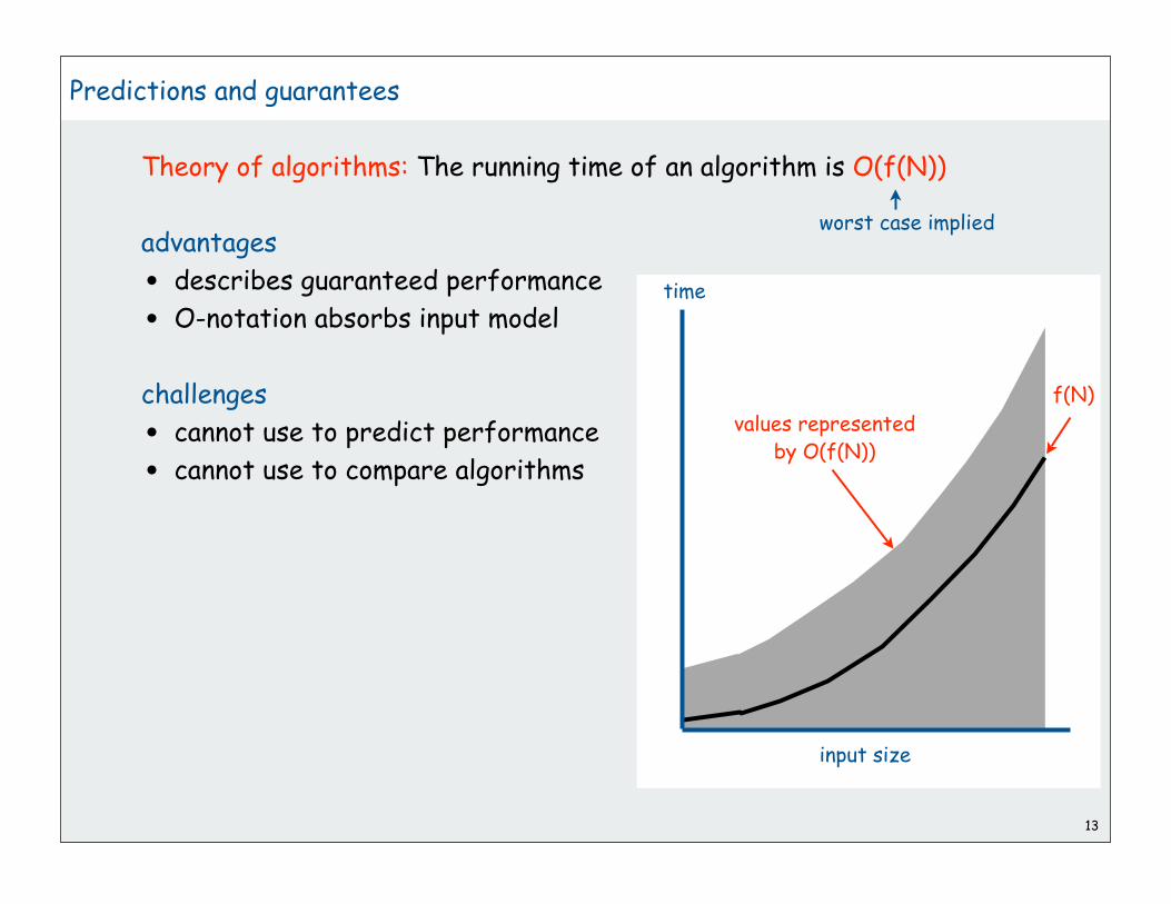
Predictions and guarantees
Theory of algorithms: The running time of an algorithm is O(f(N))
advantages
• describes guaranteed performance
• O-notation absorbs input model
challenges
• cannot use to predict performance
• cannot use to compare algorithms
13
worst case implied
time
input size
f(N)
values representedby O(f(N))

Predictions and guarantees (continued)
This course: The running time of an algorithm is ~ c f(N)
advantages
• can use to predict performance
• can use to compare algorithms
challenges
• need to develop accurate input model
• may not provide guarantees
14
time
input size
c f(N)
values representedby ~ c f(N)
understanding of alg’s dependence on input implied

15
overviewexperimentsmodelscase studyhypotheses

16
Case study [stay tuned for numerous algorithms and applications]
Sorting problem: rearrange N given items into ascending order
Hauser
Hong
Hsu
Hayes
Haskell
Hornet
...
...
Haskell
Hauser
Hayes
Hong
Hornet
Hsu
...
...
public static void less(double x, double y)
{ return x < y; }
public static void exch(double[] a, int i, int j)
{
double t = a[i];
a[i] = a[j];
a[j] = t;
}
Basic operations: compares and exchanges
compare
exchange

17
Selection sort: an elementary sorting algorithm
Algorithm invariants
• scans from left to right.
• Elements to the left of are fixed and in ascending order.
• No element to left of is larger than any element to its right.
in final order

18
Selection sort inner loop
• move the pointer to the right
• identify index of minimum item on right.
• Exchange into position.
Maintains algorithm invariants
int min = i;for (int j = i+1; j < N; j++) if (less(a[j], a[min])) min = j;
exch(a, i, min);
i++;

19
Selection sort: Java implementation
public static void sort(double[] a)
{
for (int i = 0; i < a.length; i++)
{
int min = i; for (int j = i+1; j < a.length; j++) if (less(a[j], a[min])) min = j; exch(a, i, min); }}
most frequent operation(“inner loop”)

20
Selection sort: initial observations
Observe, tabulate and plot operation counts for various values of N.
• study most frequently performed operation (compares)
• input model: N random numbers between 0 and 1
N compares
2,000 2.1 million
4,000 7.9 million
8,000 32.1 million
16,000 125.9 million
32,000 514.7 million
200M
100M
4K 8K 16K 32K2K
300M
400M
500M
600M
add counter to less()

21
Data analysis. Plot # compares vs. input size on log-log scale.
Regression. Fit straight line through data points a Nb.
Hypothesis. # compares is ~ N2/2
Selection sort: experimental hypothesis
slope
power law
2M
4M
8M
16M
32M
64M
2K 4K 8K 16K
lg C = lg a + b lg N
log-log scale
32K
C = a Nb
normal scale
128M
256M
512M
N compares
2,000 2.1 million
4,000 7.9 million
8,000 32.1 million
16,000 125.9 million
32,000 514.7 million
slope is 2

Selection sort: theoretical model
Hypothesis: number of compares is N + (N-1) + ... + 2 + 1 ~ N2/2
22
each black entry is 1 compare
a[i]
i min 0 1 2 3 4 5 6 7 8 9 10
S O R T E X A M P L E
0 6 S O R T E X A M P L E
1 4 A O R T E X S M P L E
2 10 A E R T O X S M P L E
3 9 A E E T O X S M P L R
4 7 A E E L O X S M P T R
5 7 A E E L M X S O P T R
6 8 A E E L M O S X P T R
7 10 A E E L M O P X S T R
8 8 A E E L M O P R S T X
9 9 A E E L M O P R S T X
10 10 A E E L M O P R S T X
A E E L M O P R S T X
= N(N + 1) / 2= N2/2 + N/2~ N2/2
circled entry ismin value found
gray entriesare untouched

23
Selection sort: Prediction and verification
Hypothesis (experimental and theoretical). # compares is ~ N2/2.
Prediction. 800 million compares for N = 40,000.
Observations.
Prediction. 20 billion compares for N = 200,000.
Observation.
19.997 billion200,000
comparesN
799.7 million40,000
801.6 million40,000
800.8 million40,000
comparesN
801.3 million40,000
Verifies.
Verifies.

Selection sort: validation
Implicit assumptions
• constant cost per compare
• cost of compares dominates running time
Hypothesis: Running time is ~ c N2
Validation: Observe actual running time.
Regression fit validates hypothesis.
24
N observed time .23x10-7 N2
2,000 0.1 seconds 0.1
4,000 0.4 seconds 0.4
8,000 1.5 seconds 1.5
16,000 5.6 seconds 5.9
32,000 23.2 seconds 23.5
A scientific connection between program and natural world.
.1 sec
.4 sec
1.6 sec
2K 4K 8K 16K 32K
6.4 sec
25.6 sec

25
Insertion sort: another elementary sorting algorithm
Algorithm invariants
• scans from left to right.
• Elements to the left of are in ascending order.
in order not yet seen
26
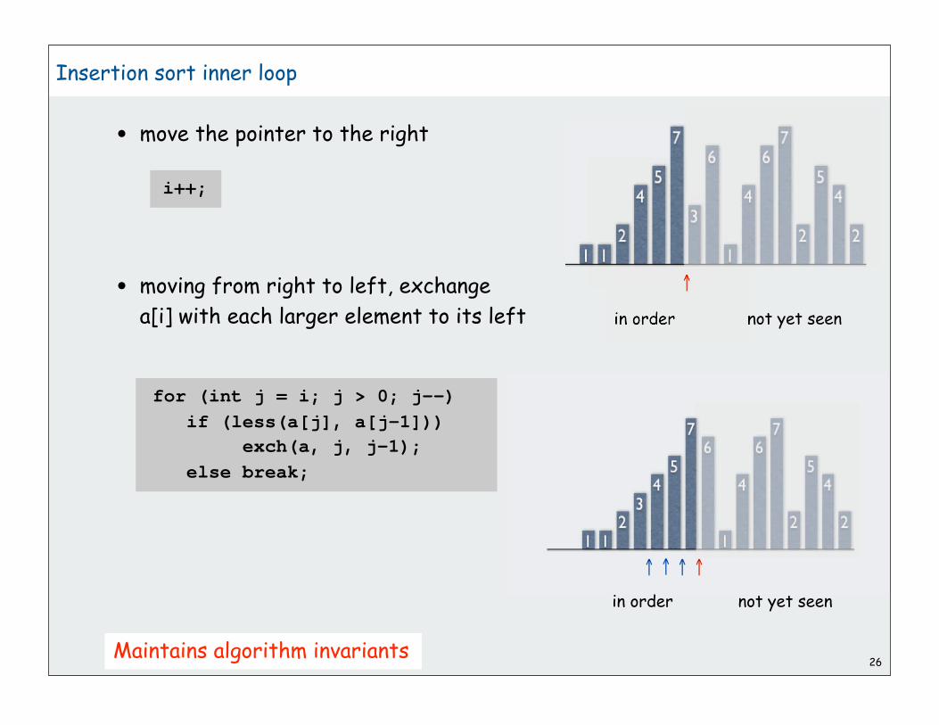
Insertion sort inner loop
• move the pointer to the right
• moving from right to left, exchange
a[i] with each larger element to its left
Maintains algorithm invariants
for (int j = i; j > 0; j--)
if (less(a[j], a[j-1]))
exch(a, j, j-1);
else break;
i++;
in order not yet seen
in order not yet seen

Insertion sort: Java implementation
27
public static void sort(Comparable[] a)
{
int N = a.length;
for (int i = 0; i < N; i++)
for (int j = i; j > 0; j--)
if (less(a[j], a[j-1]))
exch(a, j, j-1);
else break;
}
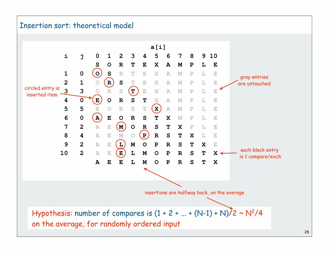
Insertion sort: theoretical model
28
each black entry is 1 compare/exch
a[i]
i j 0 1 2 3 4 5 6 7 8 9 10
S O R T E X A M P L E
1 0 O S R T E X A M P L E
2 1 O R S T E X A M P L E
3 3 O R S T E X A M P L E
4 0 E O R S T X A M P L E
5 5 E O R S T X A M P L E
6 0 A E O R S T X M P L E
7 2 A E M O R S T X P L E
8 4 A E M O P R S T X L E
9 2 A E L M O P R S T X E
10 2 A E E L M O P R S T X
A E E L M O P R S T X
Hypothesis: number of compares is (1 + 2 + ... + (N-1) + N)/2 ~ N2/4
on the average, for randomly ordered input
insertions are halfway back, on the average
circled entry isinserted item
gray entriesare untouched

Experimental comparison of insertion sort and selection sort
Plot both running times on log log scale
• slopes are the same (both 2)
• both are quadratic
Compute ratio of running times
Need detailed analysis
to prefer one over the other
Neither is useful for huge randomly-ordered files
29
.1 sec
.4 sec
1.6 sec
2K 4K 8K 16K 32K
6.4 sec
25.6 sec
% java SortCompare Insertion Selection 4000
For 4000 random double values
Insertion is 1.7 times faster than selection
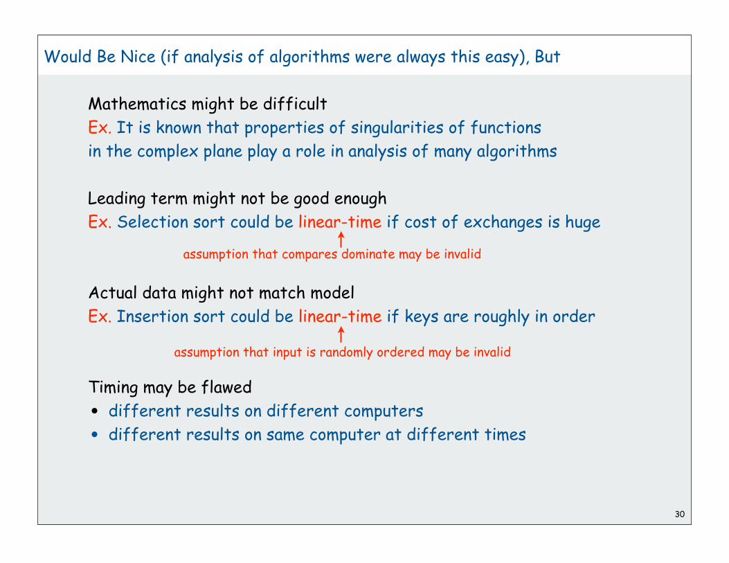
Would Be Nice (if analysis of algorithms were always this easy), But
Mathematics might be difficult
Ex. It is known that properties of singularities of functions
in the complex plane play a role in analysis of many algorithms
Leading term might not be good enough
Ex. Selection sort could be linear-time if cost of exchanges is huge
Actual data might not match model
Ex. Insertion sort could be linear-time if keys are roughly in order
Timing may be flawed
• different results on different computers
• different results on same computer at different times
30
assumption that compares dominate may be invalid
assumption that input is randomly ordered may be invalid

31
overviewexperimentsmodelscase studyhypotheses

Practical approach to developing hypotheses
First step: determine asymptotic growth rate for chosen model
• approach 1: run experiments, regression
• approach 2: do the math
• best: do both
Good news: the relatively small set of functions
1, log N, N, N log N, N2, N3, and 2N
suffices to describe asymptotic growth rate of typical algorithms
After determining growth rate
• use doubling hypothesis (to predict performance)
• use ratio hypothesis (to compare algorithms)
32
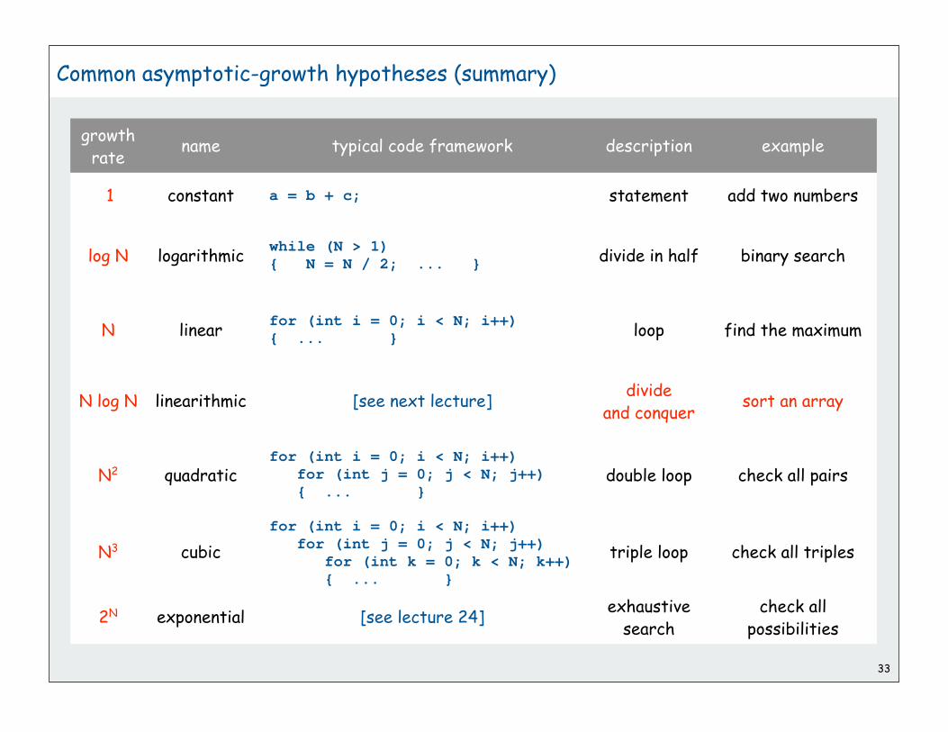
Common asymptotic-growth hypotheses (summary)
33
growthrate
name typical code framework description example
1 constant a = b + c; statement add two numbers
log N logarithmicwhile (N > 1)
{ N = N / 2; ... }divide in half binary search
N linearfor (int i = 0; i < N; i++)
{ ... }loop find the maximum
N log N linearithmic [see next lecture]divide
and conquersort an array
N2 quadraticfor (int i = 0; i < N; i++)
for (int j = 0; j < N; j++)
{ ... }double loop check all pairs
N3 cubic
for (int i = 0; i < N; i++)
for (int j = 0; j < N; j++)
for (int k = 0; k < N; k++)
{ ... }
triple loop check all triples
2N exponential [see lecture 24]exhaustive
searchcheck all
possibilities

Aside: practical implications of asymptotic growth
For back-of-envelope calculations, assume
How long to process millions of inputs?
How many inputs can be processed in minutes?
34
decadeprocessor
speed
instructions
per second
1970s 1M Hz
1980s 10M Hz
1990s 100M Hz
2000s 1G Hz
1
seconds
102
103
104
105
106
107
108
109
1010
1 second
equivalent
1.7 minutes
17 minutes
2.8 hours
1.1 days
1.6 weeks
3.8 months
3.1 years
3.1 decades
3.1 centuries
forever
1017 age ofuniverse
. . .
10 10 seconds106
107
108
109
Ex. Population of NYC was “millions” in 1970s; still is
Ex. Customers lost patience waiting “minutes” in 1970s; still do

Aside: practical implications of asymptotic growth
35
growthrate
problem size solvable in minutes time to process millions of inputs
1970s 1980s 1990s 2000s 1970s 1980s 1990s 2000s
1 any any any any instant instant instant instant
log N any any any any instant instant instant instant
N millionstens ofmillions
hundreds ofmillions
billions minutes seconds second instant
N log Nhundreds ofthousands
millions millionshundreds of
millionshour minutes
tens ofseconds
seconds
N2 hundreds thousand thousandstens of
thousandsdecades years months weeks
N3 hundred hundreds thousand thousands never never never millenia

Practical implications of asymptotic-growth: another view
36
growthrate
name description
effect on a program thatruns for a few seconds
time for 100xmore data
size for 100xfaster computer
1 constant independent of input size a few seconds same
log N logarithmic nearly independent of input size a few seconds same
N linear optimal for N inputs a few minutes 100x
N log N linearithmic nearly optimal for N inputs a few minutes 100x
N2 quadratic not practical for large problems several hours 10x
N3 cubic not practical for large problems several weeks 4-5x
2N exponential useful only for tiny problems forever 1x

Developing asymptotic order of growth hypotheses with doubling
To formulate hypothesis for asymptotic growth rate:
• compute T(2N)/T(N) as accurately (and for N as large) as is affordable
• use this table
37
ratio hypothesis reason
1constant
or logarithmic
c / c = 1
c log 2N / c log N ~ 1
2linear
orlinearithmic
c 2N / c N = 2
c 2 N log (2N) / c N log N ~ 2
4 quadratic c (2N)2 / c N2 = 4
9 cubic c (2N)2 / c N2 = 9
= 2 log(2N)/log N= 2 (log 2 + log N)/log N = 2 + 2 log 2/log N ~ 2
T
2T
4T
1K 2K 4K
cubic1024T
1024K
quad
rati
c
linea
r
linea
rithm
ic
constant
logarithmic
time
size

Example revisited: methods for timing sort algorithms
38
public static double time(String alg, Double[] a)
{
Stopwatch sw = new Stopwatch();
if (alg.equals("Insertion")) Insertion.sort(a);
if (alg.equals("Selection")) Selection.sort(a);
if (alg.equals("Shell")) Shell.sort(a);
if (alg.equals("Merge")) Merge.sort(a);
if (alg.equals("Quick")) Quick.sort(a);
return sw.elapsedTime();
}
public static double timetrials(String alg, int N, int trials)
{
double total = 0.0;
Double[] a = new Double[N];
for (int t = 0; t < trials; t++)
{
for (int i = 0; i < N; i++)
a[i] = StdRandom.uniform();
total += time(alg, a);
}
return total;
}
Compute time to sort a[] with alg
Compute total time to to sort trials arrays of N random doubles with alg

Developing asymptotic order of growth hypotheses with doubling
39
public class SortGrowth
{
public static void main(String[] args)
{
String alg = args[0];
int N = 1000;
if (args.length > 1)
N = Integer.parseInt(args[1]);
int trials = 100;
if (args.length > 2)
trials = Integer.parseInt(args[2]);
double ratio = timetrials(alg, 2*N, trials);
/ timetrials(alg, N, trials);
StdOut.printf("Ratio is %f\n", ratio);
if (ratio > 1.8 && ratio < 2.2)
StdOut.printf(" %s is linear or linearithmic\n", alg);
if (ratio > 3.8 && ratio < 4.2)
StdOut.printf(" %s is quadratic\n", alg);
}
}
THIS CODEMAY NOT
BE READYFOR THE
REAL WORLD
CAUTION
% java SortGrowth Selection
Ratio is 4.1
Selection is quadratic
% java SortGrowth Insertion
Ratio is 3.645756
% java SortGrowth Insertion 4000 1000
Ratio is 3.969934
Insertion is quadratic
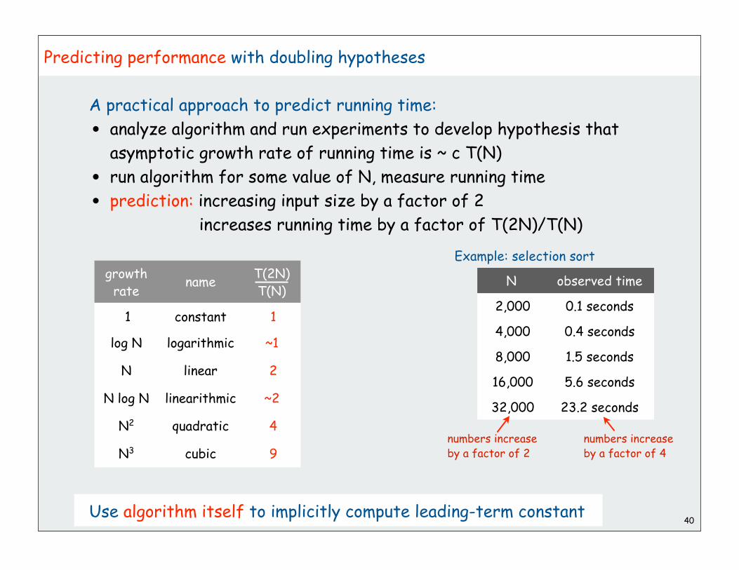
Predicting performance with doubling hypotheses
A practical approach to predict running time:
• analyze algorithm and run experiments to develop hypothesis that
asymptotic growth rate of running time is ~ c T(N)
• run algorithm for some value of N, measure running time
• prediction: increasing input size by a factor of 2
increases running time by a factor of T(2N)/T(N)
Use algorithm itself to implicitly compute leading-term constant40
N observed time
2,000 0.1 seconds
4,000 0.4 seconds
8,000 1.5 seconds
16,000 5.6 seconds
32,000 23.2 seconds
numbers increaseby a factor of 2
numbers increaseby a factor of 4
Example: selection sortgrowth
ratename
T(2N) T(N)
1 constant 1
log N logarithmic ~1
N linear 2
N log N linearithmic ~2
N2 quadratic 4
N3 cubic 9

Predicting performance with doubling hypotheses
41
public class SortPredict
{
public static void main(String[] args)
{
String alg = args[0];
int trials = 100;
if (args.length > 1) trials = Integer.parseInt(args[1]);
StdOut.printf("Seconds for %d trials\n", trials);
StdOut.printf(" predicted actual\n 1000 ");
double old = Double.POSITIVE_INFINITY;
for (int N = 1000; true; N = 2*N)
{
total = timeTrials(alg, N, trials);
double guess = (total/old)*total;
StdOut.printf(" %7.1f\n %5d %7.1f", total, 2*N, guess);
old = total;
}
}
}
THIS CODEMAY NOT
BE READYFOR THE
REAL WORLD
CAUTION
% java SortPredict Selection
Seconds for 100 trials
predicted actual
1000 0.9
2000 0.0 3.5
4000 13.9 14.4
8000 58.8 58.9
16000 240.9 239.2
32000 971.6
Note: SortGrowth is not needed!
[This code works for any power law.]
and deep math says that running time of typical algs must satisfy power law

Comparing algorithms with ratio hypotheses
A practical way to compare algorithms A and B with the same growth rate
• hypothesize that running times are ~ cA f(N) and ~ cB f(N)
• run algorithms for some value of N, measure running times
• Prediction: Algorithm A is a factor of cA/cB faster than Algorithm B
To compare algorithms with different growth rates
• hypothesize that the one with the smaller rate is faster
• validate hypothesis for inputs of interest
[values of constants may be significant]
To determine whether growth rates are the same or different
• compute ratios of running times as input size doubles
• [growth rates are the same if ratios do not change]
Use algorithms themselves to compute complex leading-term constants
42

Comparing algorithms with ratio hypothesis
43
public class SortCompare
{
public static void main(String[] args)
{
String alg1 = args[0];
String alg2 = args[1];
int N = Integer.parseInt(args[2]);
int trials = 100;
if (args.length > 3) trials = Integer.parseInt(args[3]);
double time1 = 0.0;
double time2 = 0.0;
Double[] a1 = new Double[N];
Double[] a2 = new Double[N];
for (int t = 0; t < trials; t++)
{
for (int i = 0; i < N; i++)
{ a1[i] = Math.random(); a2[i] = a1[i]; }
time1 += time(alg1, a1);
time2 += time(alg2, a2);
}
StdOut.printf("For %d random Double values\n %s is", N, alg1);
StdOut.printf(" %.1f times faster than %s\n", time2/time1, alg2);
}
}
THIS CODEMAY NOT
BE READYFOR THE
REAL WORLD
CAUTION
% java SortCompare Insertion Selection 4000
For 4000 random Double values
Insertion is 1.7 times faster than Selection
best to test algs on same input

Summary: turning the crank
Yes, analysis of algorithms might be challenging, BUT
Mathematics might be difficult?
• only a few functions seem to turn up
• doubling, ratio tests cancel complicated constants
Leading term might not be good enough?
• debugging tools are available to identify bottlenecks
• typical programs have short inner loops
Actual data might not match model?
• need to understand input to effectively process it
• approach 1: design for the worst case
• approach 2: randomize, depend on probabilistic guarantee
Timing may be flawed?
• limits on experiments insignificant compared to other sciences
• different computers are different!44

Sorting Algorithms
rules of the gameshellsortmergesortquicksortanimations
1
Reference:
Algorithms in Java, Chapters 6-8

2
Classic sorting algorithms
Critical components in the world’s computational infrastructure.
• Full scientific understanding of their properties has enabled us
to develop them into practical system sorts.
• Quicksort honored as one of top 10 algorithms of 20th century
in science and engineering.
Shellsort.
• Warmup: easy way to break the N2 barrier.
• Embedded systems.
Mergesort.
• Java sort for objects.
• Perl, Python stable sort.
Quicksort.
• Java sort for primitive types.
• C qsort, Unix, g++, Visual C++, Python.

3
rules of the gameshellsortmergesortquicksortanimations

4
Basic terms
Ex: student record in a University.
Sort: rearrange sequence of objects into ascending order.
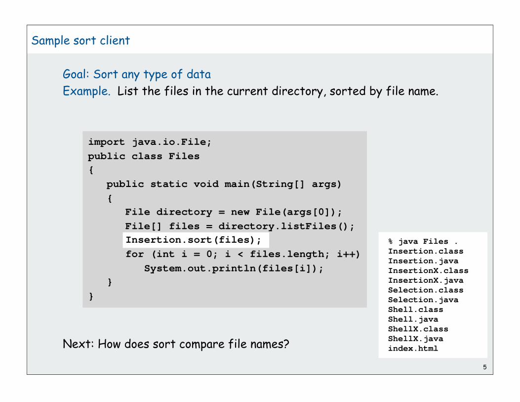
Goal: Sort any type of data
Example. List the files in the current directory, sorted by file name.
Next: How does sort compare file names?
5
% java Files .
Insertion.class
Insertion.java
InsertionX.class
InsertionX.java
Selection.class
Selection.java
Shell.class
Shell.java
ShellX.class
ShellX.java
index.html
Sample sort client
import java.io.File;
public class Files
{
public static void main(String[] args)
{
File directory = new File(args[0]);
File[] files = directory.listFiles();
Insertion.sort(files);
for (int i = 0; i < files.length; i++)
System.out.println(files[i]);
}
}

6
Callbacks
Goal. Write robust sorting library method that can sort
any type of data using the data type's natural order.
Callbacks.
• Client passes array of objects to sorting routine.
• Sorting routine calls back object's comparison function as needed.
Implementing callbacks.
• Java: interfaces.
•C: function pointers.
•C++: functors.

Callbacks
7
sort implementation
client
object implementationimport java.io.File;
public class SortFiles
{
public static void main(String[] args)
{
File directory = new File(args[0]);
File[] files = directory.listFiles();
Insertion.sort(files);
for (int i = 0; i < files.length; i++)
System.out.println(files[i]);
}
}
Key point: no reference to File
public static void sort(Comparable[] a)
{
int N = a.length;
for (int i = 0; i < N; i++)
for (int j = i; j > 0; j--)
if (a[j].compareTo(a[j-1]))
exch(a, j, j-1);
else break;
}
public class File
implements Comparable<File>
{
...
public int compareTo(File b)
{
...
return -1;
...
return +1;
...
return 0;
}
}
interface
interface Comparable <Item>
{
public int compareTo(Item);
}
built in to Java

8
Callbacks
Goal. Write robust sorting library that can sort any type of data
into sorted order using the data type's natural order.
Callbacks.
• Client passes array of objects to sorting routine.
• Sorting routine calls back object's comparison function as needed.
Implementing callbacks.
• Java: interfaces.
•C: function pointers.
•C++: functors.
Plus: Code reuse for all types of data
Minus: Significant overhead in inner loop
This course:
• enables focus on algorithm implementation
• use same code for experiments, real-world data

9
Interface specification for sorting
Comparable interface.
Must implement method compareTo() so that v.compareTo(w)returns:
• a negative integer if v is less than w
• a positive integer if v is greater than w
• zero if v is equal to w
Consistency.
Implementation must ensure a total order.
• if (a < b) and (b < c), then (a < c).
• either (a < b) or (b < a) or (a = b).
Built-in comparable types. String, Double, Integer, Date, File.
User-defined comparable types. Implement the Comparable interface.

10
Implementing the Comparable interface: example 1
only compare datesto other dates
public class Date implements Comparable<Date>{ private int month, day, year;
public Date(int m, int d, int y) { month = m; day = d; year = y; }
public int compareTo(Date b) { Date a = this; if (a.year < b.year ) return -1; if (a.year > b.year ) return +1; if (a.month < b.month) return -1; if (a.month > b.month) return +1; if (a.day < b.day ) return -1; if (a.day > b.day ) return +1; return 0; }}
Date data type (simplified version of built-in Java code)

11
Implementing the Comparable interface: example 2
Domain names
• Subdomain: bolle.cs.princeton.edu.
• Reverse subdomain: edu.princeton.cs.bolle.
• Sort by reverse subdomain to group by category. unsorted
sorted
public class Domain implements Comparable<Domain>{ private String[] fields; private int N; public Domain(String name) { fields = name.split("\\."); N = fields.length; } public int compareTo(Domain b) { Domain a = this; for (int i = 0; i < Math.min(a.N, b.N); i++) { int c = a.fields[i].compareTo(b.fields[i]); if (c < 0) return -1; else if (c > 0) return +1; } return a.N - b.N; }} details included for the bored...
ee.princeton.edu
cs.princeton.edu
princeton.edu
cnn.com
google.com
apple.com
www.cs.princeton.edu
bolle.cs.princeton.edu
com.apple
com.cnn
com.google
edu.princeton
edu.princeton.cs
edu.princeton.cs.bolle
edu.princeton.cs.www
edu.princeton.ee

Several Java library data types implement Comparable
You can implement Comparable for your own types12
% java Files .
Insertion.class
Insertion.java
InsertionX.class
InsertionX.java
Selection.class
Selection.java
Shell.class
Shell.java
Sample sort clients
import java.io.File;
public class Files
{
public static void main(String[] args)
{
File directory = new File(args[0]);
File[] files = directory.listFiles()
Insertion.sort(files);
for (int i = 0; i < files.length; i++)
System.out.println(files[i]);
}
}% java Experiment 10
0.08614716385210452
0.09054270895414829
0.10708746304898642
0.21166190071646818
0.363292849257276
0.460954145685913
0.5340026311350087
0.7216129793703496
0.9003500354411443
0.9293994908845686
public class Experiment
{
public static void main(String[] args)
{
int N = Integer.parseInt(args[0]);
Double[] a = new Double[N];
for (int i = 0; i < N; i++)
a[i] = Math.random();
Selection.sort(a);
for (int i = 0; i < N; i++)
System.out.println(a[i]);
}
}
File names Random numbers

Helper functions. Refer to data only through two operations.
• less. Is v less than w ?
• exchange. Swap object in array at index i with the one at index j.
13
Two useful abstractions
private static boolean less(Comparable v, Comparable w){ return (v.compareTo(w) < 0);}
private static void exch(Comparable[] a, int i, int j){ Comparable t = a[i]; a[i] = a[j]; a[j] = t;}

14
Sample sort implementations
public class Selection{ public static void sort(Comparable[] a) { int N = a.length; for (int i = 0; i < N; i++) { int min = i; for (int j = i+1; j < N; j++) if (less(a, j, min)) min = j; exch(a, i, min); } } ...}
public class Insertion{ public static void sort(Comparable[] a) { int N = a.length; for (int i = 1; i < N; i++) for (int j = i; j > 0; j--) if (less(a[j], a[j-1])) exch(a, j, j-1); else break; } ...}
selection sort
insertion sort

Why use less() and exch() ?
Switch to faster implementation for primitive types
Instrument for experimentation and animation
Translate to other languages
15
private static boolean less(double v, double w)
{
cnt++;
return v < w;
...
for (int i = 1; i < a.length; i++)
if (less(a[i], a[i-1]))
return false;
return true;}
Good code in C, C++, JavaScript, Ruby....
private static boolean less(double v, double w)
{
return v < w;
}

Properties of elementary sorts (review)
Selection sort
Running time: Quadratic (~c N2)
Exception: expensive exchanges
(could be linear)
16
Bottom line: both are quadratic (too slow) for large randomly ordered files
Insertion sort
Running time: Quadratic (~c N2)
Exception: input nearly in order
(could be linear)
a[i]
i j 0 1 2 3 4 5 6 7 8 9 10
S O R T E X A M P L E
1 0 O S R T E X A M P L E
2 1 O R S T E X A M P L E
3 3 O R S T E X A M P L E
4 0 E O R S T X A M P L E
5 5 E O R S T X A M P L E
6 0 A E O R S T X M P L E
7 2 A E M O R S T X P L E
8 4 A E M O P R S T X L E
9 2 A E L M O P R S T X E
10 2 A E E L M O P R S T X
A E E L M O P R S T X
a[i]
i min 0 1 2 3 4 5 6 7 8 9 10
S O R T E X A M P L E
0 6 S O R T E X A M P L E
1 4 A O R T E X S M P L E
2 10 A E R T O X S M P L E
3 9 A E E T O X S M P L R
4 7 A E E L O X S M P T R
5 7 A E E L M X S O P T R
6 8 A E E L M O S X P T R
7 10 A E E L M O P X S T R
8 8 A E E L M O P R S T X
9 9 A E E L M O P R S T X
10 10 A E E L M O P R S T X
A E E L M O P R S T X
17
rules of the gameshellsortmergesortquicksortanimations

Visual representation of insertion sort
18
i
a[i]
left of pointer is in sorted order right of pointer is untouched
Reason it is slow: data movement

Idea: move elements more than one position at a time
by h-sorting the file for a decreasing sequence of values of h
Shellsort
19
a 3-sorted file is3 interleaved sorted files
S O R T E X A M P L Einput
M O R T E X A S P L E
M O R T E X A S P L E
M O L T E X A S P R E
M O L E E X A S P R T
7-sort
E O L M E X A S P R T
E E L M O X A S P R T
E E L M O X A S P R T
A E L E O X M S P R T
A E L E O X M S P R T
A E L E O P M S X R T
A E L E O P M S X R T
A E L E O P M S X R T
3-sort
A E L E O P M S X R T
A E L E O P M S X R T
A E E L O P M S X R T
A E E L O P M S X R T
A E E L O P M S X R T
A E E L M O P S X R T
A E E L M O P S X R T
A E E L M O P S X R T
A E E L M O P R S X T
A E E L M O P R S T X
A E E L M O P R S T X
1-sort
A E E L M O P R S T Xresult
A E L E O P M S X R T
A E M R
E O S T
L P X

Idea: move elements more than one position at a time
by h-sorting the file for a decreasing sequence of values of h
Use insertion sort, modified to h-sort
public static void sort(double[] a) { int N = a.length; int[] incs = { 1391376, 463792, 198768, 86961, 33936, 13776, 4592, 1968, 861, 336, 112, 48, 21, 7, 3, 1 }; for (int k = 0; k < incs.length; k++) { int h = incs[k]; for (int i = h; i < N; i++) for (int j = i; j >= h; j-= h) if (less(a[j], a[j-h])) exch(a, j, j-h); else break; } }
Shellsort
20
insertion sort!
magic increment sequence
big increments: small subfiles
small increments: subfiles nearly in order
method of choice for bothsmall subfilessubfiles nearly in order
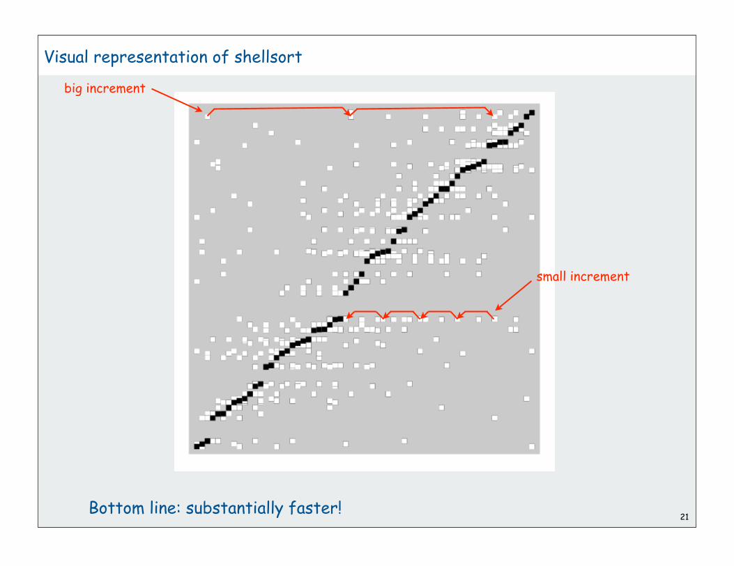
Visual representation of shellsort
Bottom line: substantially faster!21
big increment
small increment

22
Analysis of shellsort
Model has not yet been discovered (!)
102240,000
46720,000
20910,000
935,000
comparisonsN
226680,000
1059855
495349
230143
10658
2.5 N lg NN1.289
22572089
measured in thousands

Why are we interested in shellsort?
Example of simple idea leading to substantial performance gains
Useful in practice
• fast unless file size is huge
• tiny, fixed footprint for code (used in embedded systems)
• hardware sort prototype
Simple algorithm, nontrivial performance, interesting questions
• asymptotic growth rate?
• best sequence of increments?
• average case performance?
Your first open problem in algorithmics (see Section 6.8):
Find a better increment sequence
mail [email protected]
Lesson: some good algorithms are still waiting discovery23

24
rules of the gameshellsortmergesortquicksortanimations

25
Mergesort (von Neumann, 1945(!))
Basic plan:
• Divide array into two halves.
• Recursively sort each half.
• Merge two halves.
trace a[i]
lo hi 0 1 2 3 4 5 6 7 8 9 10 11 12 13 14 15
M E R G E S O R T E X A M P L E
0 1 E M R G E S O R T E X A M P L E
2 3 E M G R E S O R T E X A M P L E
0 3 E G M R E S O R T E X A M P L E
4 5 E G M R E S O R T E X A M P L E
6 7 E G M R E S O R T E X A M P L E
4 7 E G M R E O R S T E X A M P L E
0 7 E E G M O R R S T E X A M P L E
8 9 E E G M O R R S E T X A M P L E
10 11 E E G M O R R S E T A X M P L E
8 11 E E G M O R R S A E T X M P L E
12 13 E E G M O R R S A E T X M P L E
14 15 E E G M O R R S A E T X M P E L
12 15 E E G M O R R S A E T X E L M P
8 15 E E G M O R R S A E E L M P T X
0 15 A E E E E G L M M O P R R S T X
M E R G E S O R T E X A M P L E
E E G M O R R S T E X A M P L E
E E G M O R R S A E E L M P T X
A E E E E G L M M O P R R S T X
plan

Merging. Combine two pre-sorted lists into a sorted whole.
How to merge efficiently? Use an auxiliary array.
26
Merging
A G L O R H I M S T
A G H I L M
i j
k
l rm
aux[]
a[]
private static void merge(Comparable[] a, Comparable[] aux, int l, int m, int r){ for (int k = l; k < r; k++) aux[k] = a[k]; int i = l, j = m; for (int k = l; k < r; k++) if (i >= m) a[k] = aux[j++]; else if (j >= r) a[k] = aux[i++]; else if (less(aux[j], aux[i])) a[k] = aux[j++]; else a[k] = aux[i++]; }
merge
copy
see book for a trickto eliminate these

27
Mergesort: Java implementation of recursive sort
lo m hi
10 11 12 13 14 15 16 17 18 19
public class Merge{ private static void sort(Comparable[] a, Comparable[] aux, int lo, int hi) { if (hi <= lo + 1) return; int m = lo + (hi - lo) / 2; sort(a, aux, lo, m); sort(a, aux, m, hi); merge(a, aux, lo, m, hi); }
public static void sort(Comparable[] a) { Comparable[] aux = new Comparable[a.length]; sort(a, aux, 0, a.length); }}
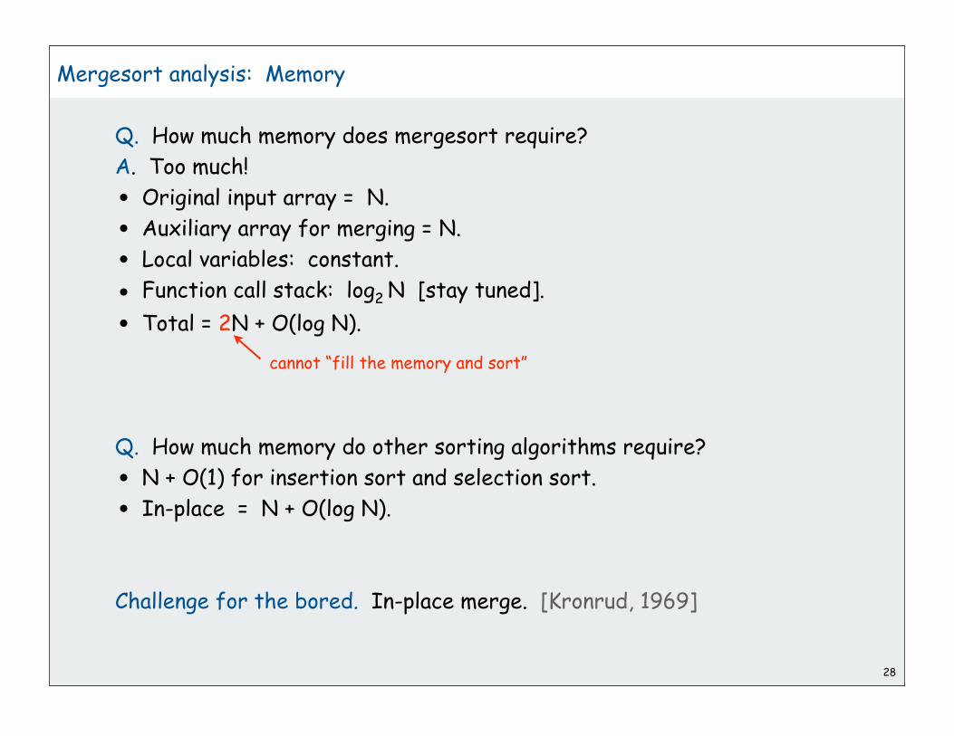
28
Mergesort analysis: Memory
Q. How much memory does mergesort require?
A. Too much!
• Original input array = N.
• Auxiliary array for merging = N.
• Local variables: constant.
• Function call stack: log2 N [stay tuned].
• Total = 2N + O(log N).
Q. How much memory do other sorting algorithms require?
• N + O(1) for insertion sort and selection sort.
• In-place = N + O(log N).
Challenge for the bored. In-place merge. [Kronrud, 1969]
cannot “fill the memory and sort”

29
Mergesort analysis
Def. T(N) number of array stores to mergesort an input of size N
= T(N/2) + T(N/2) + N
Mergesort recurrence
• not quite right for odd N
• same recurrence holds for many algorithms
• same for any input of size N
• comparison count slightly smaller because of array ends
Solution of Mergesort recurrence
• true for all N
• easy to prove when N is a power of 2
T(N) = 2 T(N/2) + N for N > 1, with T(1) = 0
lg N log2 N
T(N) ~ N lg N
left half right half merge

30
Mergesort recurrence: Proof 1 (by recursion tree)
T(N)
T(N/2)T(N/2)
T(N/4)T(N/4)T(N/4) T(N/4)
T(2) T(2) T(2) T(2) T(2) T(2) T(2) T(2)
N
T(N / 2k)
2(N/2)
2k(N/2k)
N/2 (2)
...
lg N
N lg N
T(N) = 2 T(N/2) + N for N > 1, with T(1) = 0
= N
= N
= N
= N
+
...
T(N) = N lg N
(assume that N is a power of 2)

31
Mergesort recurrence: Proof 2 (by telescoping)
Pf.
T(N) = 2 T(N/2) + N for N > 1, with T(1) = 0
T(N) = 2 T(N/2) + N
T(N)/N = 2 T(N/2)/N + 1
= T(N/2)/(N/2) + 1
= T(N/4)/(N/4) + 1 + 1
= T(N/8)/(N/8) + 1 + 1 + 1
. . .
= T(N/N)/(N/N) + 1 + 1 +. . .+ 1
= lg N
T(N) = N lg N
(assume that N is a power of 2)
given
divide both sides by N
algebra
telescope (apply to first term)
telescope again
stop telescoping, T(1) = 0

Claim. If T(N) satisfies this recurrence, then T(N) = N lg N.
Pf. [by induction on N]
• Base case: N = 1.
• Inductive hypothesis: T(N) = N lg N
• Goal: show that T(2N) + 2N lg (2N).
Ex. (for COS 340). Extend to show that T(N) ~ N lg N for general N
32
Mergesort recurrence: Proof 3 (by induction)
T(2N) = 2 T(N) + 2N given
= 2 N lg N + 2 N inductive hypothesis
= 2 N (lg (2N) - 1) + 2N algebra
= 2 N lg (2N) QED
T(N) = 2 T(N/2) + N for N > 1, with T(1) = 0
(assume that N is a power of 2)

Basic plan:
• Pass through file, merging to double size of sorted subarrays.
• Do so for subarray sizes 1, 2, 4, 8, . . . , N/2, N.
33
Bottom-up mergesort
proof 4 that mergesortuses N lgN compares
No recursion needed!
a[i]
lo hi 0 1 2 3 4 5 6 7 8 9 10 11 12 13 14 15
M E R G E S O R T E X A M P L E
0 1 E M R G E S O R T E X A M P L E
2 3 E M G R E S O R T E X A M P L E
4 5 E M G R E S O R T E X A M P L E
6 7 E M G R E S O R T E X A M P L E
8 9 E M G R E S O R E T X A M P L E
10 11 E M G R E S O R E T A X M P L E
12 13 E M G R E S O R E T A X M P L E
14 15 E M G R E S O R E T A X M P E L
0 3 E G M R E S O R E T A X M P E L
4 7 E G M R E O R S E T A X M P E L
8 11 E E G M O R R S A E T X M P E L
12 15 E E G M O R R S A E T X E L M P
0 7 E E G M O R R S A E T X E L M P
8 15 E E G M O R R S A E E L M P T X
0 15 A E E E E G L M M O P R R S T X

34
Bottom-up Mergesort: Java implementation
public class Merge{ private static void merge(Comparable[] a, Comparable[] aux, int l, int m, int r) { for (int i = l; i < m; i++) aux[i] = a[i]; for (int j = m; j < r; j++) aux[j] = a[m + r - j - 1]; int i = l, j = r - 1; for (int k = l; k < r; k++) if (less(aux[j], aux[i])) a[k] = aux[j--]; else a[k] = aux[i++];
}
public static void sort(Comparable[] a) { int N = a.length; Comparable[] aux = new Comparable[N]; for (int m = 1; m < N; m = m+m) for (int i = 0; i < N-m; i += m+m) merge(a, aux, i, i+m, Math.min(i+m+m, N)); }}
tricky mergethat uses sentinel (see Program 8.2)
Concise industrial-strength code if you have the space

35
Mergesort: Practical Improvements
Use sentinel.
• Two statements in inner loop are array-bounds checking.
• Reverse one subarray so that largest element is sentinel (Program 8.2)
Use insertion sort on small subarrays.
• Mergesort has too much overhead for tiny subarrays.
• Cutoff to insertion sort for 7 elements.
Stop if already sorted.
• Is biggest element in first half smallest element in second half?
• Helps for nearly ordered lists.
Eliminate the copy to the auxiliary array. Save time (but not space) by
switching the role of the input and auxiliary array in each recursive call.
See Program 8.4 (or Java system sort)

36
Sorting Analysis Summary
Running time estimates:
• Home pc executes 108 comparisons/second.
• Supercomputer executes 1012 comparisons/second.
Lesson. Good algorithms are better than supercomputers.
Good enough?
computer
home
super
thousand
instant
instant
million
2.8 hours
1 second
billion
317 years
1.6 weeks
Insertion Sort (N2)
thousand
instant
instant
million
1 sec
instant
billion
18 min
instant
Mergesort (N log N)
18 minutes might be too long for some applications

37
rules of the gameshellsortmergesortquicksortanimations

38
Quicksort (Hoare, 1959)
Basic plan.
• Shuffle the array.
• Partition so that, for some i
element a[i] is in place
no larger element to the left of i
no smaller element to the right of i
• Sort each piece recursively.
Q U I C K S O R T E X A M P L E
E R A T E S L P U I M Q C X O K
E C A I E K L P U T M Q R X O S
A C E E I K L P U T M Q R X O S
A C E E I K L M O P Q R S T U X
A C E E I K L M O P Q R S T U X
Sir Charles Antony Richard Hoare1980 Turing Award
randomize
partition
sort left part
sort right part
input
result

39
Quicksort: Java code for recursive sort
public class Quick
{
public static void sort(Comparable[] a)
{
StdRandom.shuffle(a);
sort(a, 0, a.length - 1);
}
private static void sort(Comparable[] a, int l, int r)
{
if (r <= l) return;
int m = partition(a, l, r);
sort(a, l, m-1);
sort(a, m+1, r);
}
}

Quicksort trace
40
a[i]
l r i 0 1 2 3 4 5 6 7 8 9 10 11 12 13 14 15
Q U I C K S O R T E X A M P L E
E R A T E S L P U I M Q C X O K
0 15 5 E C A I E K L P U T M Q R X O S
0 4 2 A C E I E K L P U T M Q R X O S
0 1 1 A C E I E K L P U T M Q R X O S
0 0 A C E I E K L P U T M Q R X O S
3 4 3 A C E E I K L P U T M Q R X O S
4 4 A C E E I K L P U T M Q R X O S
6 15 12 A C E E I K L P O R M Q S X U T
6 11 10 A C E E I K L P O M Q R S X U T
6 9 7 A C E E I K L M O P Q R S X U T
6 6 A C E E I K L M O P Q R S X U T
8 9 9 A C E E I K L M O P Q R S X U T
8 8 A C E E I K L M O P Q R S X U T
11 11 A C E E I K L M O P Q R S X U T
13 15 13 A C E E I K L M O P Q R S T U X
14 15 15 A C E E I K L M O P Q R S T U X
14 14 A C E E I K L M O P Q R S T U X
A C E E I K L M O P Q R S T U X
array contents after each recursive sort
randomizepartition
input
no partition forsubfiles of size 1

Quicksort partitioning
Basic plan:
• scan from left for an item that belongs on the right
• scan from right for item item that belongs on the left
• exchange
• continue until pointers cross
41
array contents before and after each exchange
a[i]
i j r 0 1 2 3 4 5 6 7 8 9 10 11 12 13 14 15
-1 15 15 E R A T E S L P U I M Q C X O K
1 12 15 E R A T E S L P U I M Q C X O K
1 12 15 E C A T E S L P U I M Q R X O K
3 9 15 E C A T E S L P U I M Q R X O K
3 9 15 E C A I E S L P U T M Q R X O K
5 5 15 E C A I E S L P U T M Q R X O K
5 5 15 E C A I E K L P U T M Q R X O S
E C A I E K L P U T M Q R X O S
scans
exchange

private static int partition(Comparable[] a, int l, int r){ int i = l - 1; int j = r; while(true) {
while (less(a[++i], a[r])) if (i == r) break;
while (less(a[r], a[--j])) if (j == l) break;
if (i >= j) break; exch(a, i, j); }
exch(a, i, r); return i;}
42
Quicksort: Java code for partitioning
swap with partitioning item
check if pointers cross
find item on right to swap
find item on left to swap
swap
return index of item now known to be in place
i j
i j
<= v >= v
v
i
<= v >= v
v
v

43
Quicksort Implementation details
Partitioning in-place. Using a spare array makes partitioning easier,
but is not worth the cost.
Terminating the loop. Testing whether the pointers cross is a bit
trickier than it might seem.
Staying in bounds. The (i == r) test is redundant, but the (j == l)
test is not.
Preserving randomness. Shuffling is key for performance guarantee.
Equal keys. When duplicates are present, it is (counter-intuitively)
best to stop on elements equal to partitioning element.

Theorem. The average number of comparisons CN to quicksort a
random file of N elements is about 2N ln N.
• The precise recurrence satisfies C0 = C1 = 0 and for N 2:
• Multiply both sides by N
• Subtract the same formula for N-1:
• Simplify:
44
Quicksort: Average-case analysis
CN = N + 1 + ((C0 + CN-1) + . . . + (Ck-1 + CN-k) + . . . + (CN-1 + C1)) / N
= N + 1 + 2 (C0 . . . + Ck-1 + . . . + CN-1) / N
NCN = N(N + 1) + 2 (C0 . . . + Ck-1 + . . . + CN-1)
NCN - (N - 1)CN-1 = N(N + 1) - (N - 1)N + 2 CN-1
NCN = (N + 1)CN-1 + 2N
partition right partitioningprobability
left

• Divide both sides by N(N+1) to get a telescoping sum:
• Approximate the exact answer by an integral:
• Finally, the desired result:
45
Quicksort: Average Case
NCN = (N + 1)CN-1 + 2N
CN / (N + 1) = CN-1 / N + 2 / (N + 1)
= CN-2 / (N - 1) + 2/N + 2/(N + 1)
= CN-3 / (N - 2) + 2/(N - 1) + 2/N + 2/(N + 1)
= 2 ( 1 + 1/2 + 1/3 + . . . + 1/N + 1/(N + 1) )
CN 2(N + 1)( 1 + 1/2 + 1/3 + . . . + 1/N )
= 2(N + 1) HN 2(N + 1) dx/x
CN 2(N + 1) ln N 1.39 N lg N
1
N

46
Quicksort: Summary of performance characteristics
Worst case. Number of comparisons is quadratic.
• N + (N-1) + (N-2) + … + 1 N2 / 2.
• More likely that your computer is struck by lightning.
Average case. Number of comparisons is ~ 1.39 N lg N.
• 39% more comparisons than mergesort.
• but faster than mergesort in practice because of lower cost of
other high-frequency operations.
Random shuffle
• probabilistic guarantee against worst case
• basis for math model that can be validated with experiments
Caveat emptor. Many textbook implementations go quadratic if input:
• Is sorted.
• Is reverse sorted.
• Has many duplicates (even if randomized)! [stay tuned]
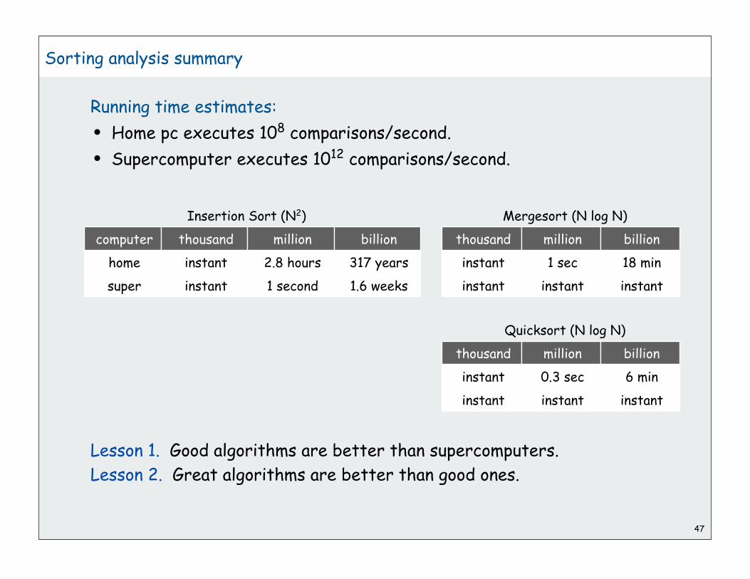
47
Sorting analysis summary
Running time estimates:
• Home pc executes 108 comparisons/second.
• Supercomputer executes 1012 comparisons/second.
Lesson 1. Good algorithms are better than supercomputers.
Lesson 2. Great algorithms are better than good ones.
computer
home
super
thousand
instant
instant
million
2.8 hours
1 second
billion
317 years
1.6 weeks
Insertion Sort (N2)
thousand
instant
instant
million
1 sec
instant
billion
18 min
instant
Mergesort (N log N)
thousand
instant
instant
million
0.3 sec
instant
billion
6 min
instant
Quicksort (N log N)

48
Quicksort: Practical improvements
Median of sample.
• Best choice of pivot element = median.
• But how to compute the median?
• Estimate true median by taking median of sample.
Insertion sort small files.
• Even quicksort has too much overhead for tiny files.
• Can delay insertion sort until end.
Optimize parameters.
• Median-of-3 random elements.
• Cutoff to insertion sort for 10 elements.
Non-recursive version.
• Use explicit stack.
• Always sort smaller half first.
All validated with refined math models and experiments
guarantees O(log N) stack size
12/7 N log N comparisons

49
rules of the gameshellsortmergesortquicksortanimations

Mergesort animation
50
done
merge in progressinput
merge in progressoutput
auxiliary array
untouched

Bottom-up mergesort animation
51
merge in progressinput
merge in progressoutput
this pass
auxiliary array
last pass

Quicksort animation
52
j
i
v
done
first partition
second partition

1
Advanced Topics in Sorting
complexitysystem sortsduplicate keyscomparators

2
complexitysystem sortsduplicate keyscomparators

3
Complexity of sorting
Computational complexity. Framework to study efficiency of
algorithms for solving a particular problem X.
Machine model. Focus on fundamental operations.
Upper bound. Cost guarantee provided by some algorithm for X.
Lower bound. Proven limit on cost guarantee of any algorithm for X.
Optimal algorithm. Algorithm with best cost guarantee for X.
Example: sorting.
• Machine model = # comparisons
• Upper bound = N lg N from mergesort.
• Lower bound ?
lower bound ~ upper bound
access information only through compares

4
Decision Tree
a b c
b < c
yes no
b < c
yes no
a < c
yes no
a < c
yes no
a c b c a b
b a c
b c a c b a
a < b
yes no
code between comparisons(e.g., sequence of exchanges)

5
Comparison-based lower bound for sorting
Theorem. Any comparison based sorting algorithm must use more than
N lg N - 1.44 N comparisons in the worst-case.
Pf.
• Assume input consists of N distinct values a1 through aN.
• Worst case dictated by tree height h.
• N ! different orderings.
• (At least) one leaf corresponds to each ordering.
• Binary tree with N ! leaves cannot have height less than lg (N!)
Stirling's formula
h lg N!
lg (N / e) N
= N lg N - N lg e
N lg N - 1.44 N

6
Complexity of sorting
Upper bound. Cost guarantee provided by some algorithm for X.
Lower bound. Proven limit on cost guarantee of any algorithm for X.
Optimal algorithm. Algorithm with best cost guarantee for X.
Example: sorting.
• Machine model = # comparisons
• Upper bound = N lg N (mergesort)
• Lower bound = N lg N - 1.44 N
Mergesort is optimal (to within a small additive factor)
First goal of algorithm design: optimal algorithms
lower bound upper bound

7
Complexity results in context
Mergesort is optimal (to within a small additive factor)
Other operations?
• statement is only about number of compares
• quicksort is faster than mergesort (lower use of other operations)
Space?
• mergesort is not optimal with respect to space usage
• insertion sort, selection sort, shellsort, quicksort are space-optimal
• is there an algorithm that is both time- and space-optimal?
Nonoptimal algorithms may be better in practice
• statement is only about guaranteed worst-case performance
• quicksort’s probabilistic guarantee is just as good in practice
Lessons
• use theory as a guide
• know your algorithms
don’t try to design an algorithm that uses half as many compares as mergesort
stay tuned for heapsort
use quicksort when time and space are critical

8
Example: Selection
Find the kth largest element.
• Min: k = 1.
• Max: k = N.
• Median: k = N/2.
Applications.
• Order statistics.
• Find the “top k”
Use theory as a guide
• easy O(N log N) upper bound: sort, return a[k]
• easy O(N) upper bound for some k: min, max
• easy (N) lower bound: must examine every element
Which is true?
• (N log N) lower bound? [is selection as hard as sorting?]
• O(N) upper bound? [linear algorithm for all k]

9
Complexity results in context (continued)
Lower bound may not hold if the algorithm has information about
• the key values
• their initial arrangement
Partially ordered arrays. Depending on the initial order of the input,
we may not need N lg N compares.
Duplicate keys. Depending on the input distribution of duplicates, we
may not need N lg N compares.
Digital properties of keys. We can use digit/character comparisons
instead of key comparisons for numbers and strings.
insertion sort requires O(N) compares onan already sorted array
stay tuned for 3-way quicksort
stay tuned for radix sorts

Partition array so that:
• element a[m] is in place
• no larger element to the left of m
• no smaller element to the right of m
Repeat in one subarray, depending on m.
Finished when m = k
10
Selection: quick-select algorithm
public static void select(Comparable[] a, int k){ StdRandom.shuffle(a); int l = 0; int r = a.length - 1; while (r > l) { int i = partition(a, l, r); if (m > k) r = m - 1; else if (m < k) l = m + 1; else return; }}
l m r
if k is hereset r to m-1
if k is hereset l to m+1
a[k] is in place, no larger element to the left, no smaller element to the right

11
Quick-select analysis
Theorem. Quick-select takes linear time on average.
Pf.
• Intuitively, each partitioning step roughly splits array in half.
• N + N/2 + N/4 + … + 1 2N comparisons.
• Formal analysis similar to quicksort analysis:
Note. Might use ~N2/2 comparisons, but as with quicksort, the random shuffle provides a probabilistic guarantee.
Theorem. [Blum, Floyd, Pratt, Rivest, Tarjan, 1973] There exists a
selection algorithm that take linear time in the worst case.Note. Algorithm is far too complicated to be useful in practice.
Use theory as a guide
• still worthwhile to seek practical linear-time (worst-case) algorithm
• until one is discovered, use quick-select if you don’t need a full sort
Ex: (2 + 2 ln 2) N comparisons to find the median
CN = 2 N + k ln ( N / k) + (N - k) ln (N / (N - k))
12
complexitysystem sortsduplicate keyscomparators

13
Sorting Challenge 1
Problem: sort a file of huge records with tiny keys.
Ex: reorganizing your MP3 files.
Which sorting method to use?
1. mergesort
2. insertion sort
3. selection sort

14
Sorting Challenge 1
Problem: sort a file of huge records with tiny keys.
Ex: reorganizing your MP3 files.
Which sorting method to use?
1. mergesort probably no, selection sort simpler and faster
2. insertion sort no, too many exchanges
3. selection sort YES, linear time under reasonable assumptions
Ex: 5,000 records, each 2 million bytes with 100-byte keys.
Cost of comparisons: 100 50002 / 2 = 1.25 billion
Cost of exchanges: 2,000,000 5,000 = 10 trillion
Mergesort might be a factor of log (5000) slower.

15
Sorting Challenge 2
Problem: sort a huge randomly-ordered file of small records.
Ex: process transaction records for a phone company.
Which sorting method to use?
1. quicksort
2. insertion sort
3. selection sort

16
Sorting Challenge 2
Problem: sort a huge randomly-ordered file of small records.
Ex: process transaction records for a phone company.
Which sorting method to use?
1. quicksort YES, it's designed for this problem
2. insertion sort no, quadratic time for randomly-ordered files
3. selection sort no, always takes quadratic time

17
Sorting Challenge 3
Problem: sort a huge number of tiny files (each file is independent)
Ex: daily customer transaction records.
Which sorting method to use?
1. quicksort
2. insertion sort
3. selection sort

18
Sorting Challenge 3
Problem: sort a huge number of tiny files (each file is independent)
Ex: daily customer transaction records.
Which sorting method to use?
1. quicksort no, too much overhead
2. insertion sort YES, much less overhead than system sort
3. selection sort YES, much less overhead than system sort
Ex: 4 record file.
4 N log N + 35 = 70
2N2 = 32

19
Sorting Challenge 4
Problem: sort a huge file that is already almost in order.
Ex: re-sort a huge database after a few changes.
Which sorting method to use?
1. quicksort
2. insertion sort
3. selection sort

20
Sorting Challenge 4
Problem: sort a huge file that is already almost in order.
Ex: re-sort a huge database after a few changes.
Which sorting method to use?
1. quicksort probably no, insertion simpler and faster
2. insertion sort YES, linear time for most definitions of "in order"
3. selection sort no, always takes quadratic time
Ex: A B C D E F H I J G P K L M N O Q R S T U V W X Y Z
Z A B C D E F G H I J K L M N O P Q R S T U V W X Y

21
obvious applications
problems become easy once items are in sorted order
non-obvious applications
Sorting Applications
Sorting algorithms are essential in a broad variety of applications
• Sort a list of names.
• Organize an MP3 library.
• Display Google PageRank results.
• List RSS news items in reverse chronological order.
• Find the median.
• Find the closest pair.
• Binary search in a database.
• Identify statistical outliers.
• Find duplicates in a mailing list.
• Data compression.
• Computer graphics.
• Computational biology.
• Supply chain management.
• Load balancing on a parallel computer.
. . .
Every system needs (and has) a system sort!

22
System sort: Which algorithm to use?
Many sorting algorithms to choose from
internal sorts.
• Insertion sort, selection sort, bubblesort, shaker sort.
• Quicksort, mergesort, heapsort, samplesort, shellsort.
• Solitaire sort, red-black sort, splaysort, Dobosiewicz sort, psort, ...
external sorts. Poly-phase mergesort, cascade-merge, oscillating sort.
radix sorts.
• Distribution, MSD, LSD.
• 3-way radix quicksort.
parallel sorts.
• Bitonic sort, Batcher even-odd sort.
• Smooth sort, cube sort, column sort.
• GPUsort.

23
System sort: Which algorithm to use?
Applications have diverse attributes
• Stable?
• Multiple keys?
• Deterministic?
• Keys all distinct?
• Multiple key types?
• Linked list or arrays?
• Large or small records?
• Is your file randomly ordered?
• Need guaranteed performance?
Elementary sort may be method of choice for some combination.
Cannot cover all combinations of attributes.
Q. Is the system sort good enough?
A. Maybe (no matter which algorithm it uses).
many more combinations ofattributes than algorithms

24
complexitysystem sortsduplicate keyscomparators

25
Duplicate keys
Often, purpose of sort is to bring records with duplicate keys together.
• Sort population by age.
• Finding collinear points.
• Remove duplicates from mailing list.
• Sort job applicants by college attended.
Typical characteristics of such applications.
• Huge file.
• Small number of key values.
Mergesort with duplicate keys: always ~ N lg N compares
Quicksort with duplicate keys
• algorithm goes quadratic unless partitioning stops on equal keys!
• [many textbook and system implementations have this problem]
• 1990s Unix user found this problem in qsort()

Duplicate keys: the problem
Assume all keys are equal.
Recursive code guarantees that case will predominate!
Mistake: Put all keys equal to the partitioning element on one side
• easy to code
• guarantees N2 running time when all keys equal
Recommended: Stop scans on keys equal to the partitioning element
• easy to code
• guarantees N lg N compares when all keys equal
Desirable: Put all keys equal to the partitioning element in place
Common wisdom to 1990s: not worth adding code to inner loop
26
B A A B A B C C B C B A A A A A A A A A A A
B A A B A B C C B C B A A A A A A A A A A A
A A A B B B B B C C C A A A A A A A A A A A

27
3-way partitioning. Partition elements into 3 parts:
• Elements between i and j equal to partition element v.
• No larger elements to left of i.
• No smaller elements to right of j.
Dutch national flag problem.
• not done in practical sorts before mid-1990s.
• new approach discovered when fixing mistake in Unix qsort()
• now incorporated into Java system sort
3-Way Partitioning

28
Solution to Dutch national flag problem.
3-way partitioning (Bentley-McIlroy).
• Partition elements into 4 parts:
no larger elements to left of i
no smaller elements to right of j
equal elements to left of p
equal elements to right of q
• Afterwards, swap equal keys into center.
All the right properties.
• in-place.
• not much code.
• linear if keys are all equal.
• small overhead if no equal keys.
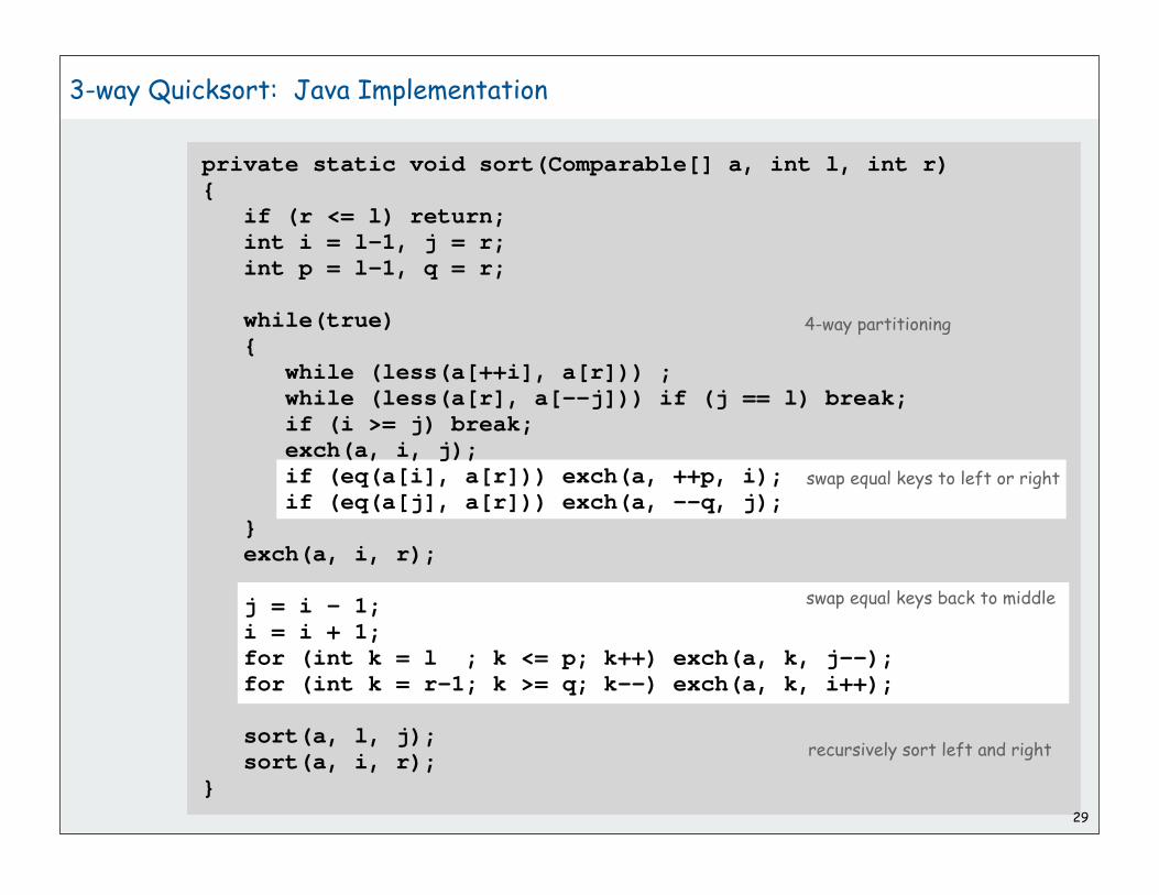
private static void sort(Comparable[] a, int l, int r){ if (r <= l) return; int i = l-1, j = r; int p = l-1, q = r;
while(true) { while (less(a[++i], a[r])) ; while (less(a[r], a[--j])) if (j == l) break; if (i >= j) break; exch(a, i, j); if (eq(a[i], a[r])) exch(a, ++p, i); if (eq(a[j], a[r])) exch(a, --q, j); } exch(a, i, r);
j = i - 1; i = i + 1; for (int k = l ; k <= p; k++) exch(a, k, j--); for (int k = r-1; k >= q; k--) exch(a, k, i++);
sort(a, l, j); sort(a, i, r); }
29
3-way Quicksort: Java Implementation
swap equal keys to left or right
swap equal keys back to middle
recursively sort left and right
4-way partitioning

30
Duplicate keys: lower bound
Theorem. [Sedgewick-Bentley] Quicksort with 3-way partitioning is
optimal for random keys with duplicates.
Proof (beyond scope of 226).
• generalize decision tree
• tie cost to entropy
• note: cost is linear when number of key values is O(1)
Bottom line: Randomized Quicksort with 3-way partitioning reduces
cost from linearithmic to linear (!) in broad class of applications

3-way partitioning animation
31
j q
p i

32
complexitysystem sortsduplicate keyscomparators

33
Generalized compare
Comparable interface: sort uses type’s compareTo() function:
public class Date implements Comparable<Date>{ private int month, day, year;
public Date(int m, int d, int y) { month = m; day = d; year = y; }
public int compareTo(Date b) { Date a = this; if (a.year < b.year ) return -1; if (a.year > b.year ) return +1; if (a.month < b.month) return -1; if (a.month > b.month) return +1; if (a.day < b.day ) return -1; if (a.day > b.day ) return +1; return 0; }}

34
Generalized compare
Comparable interface: sort uses type’s compareTo() function:
Problem 1: Not type-safe
Problem 2: May want to use a different order.
Problem 3: Some types may have no “natural” order.
Ex. Sort strings by:
• Natural order. Now is the time
• Case insensitive. is Now the time
• French. real réal rico
• Spanish. café cuidado champiñón dulce
String[] a;...Arrays.sort(a);Arrays.sort(a, String.CASE_INSENSITIVE_ORDER);Arrays.sort(a, Collator.getInstance(Locale.FRENCH));Arrays.sort(a, Collator.getInstance(Locale.SPANISH));
ch and rr are single letters
import java.text.Collator;

Generalized compare
Comparable interface: sort uses type’s compareTo() function:
Problem 1: Not type-safe
Problem 2: May want to use a different order.
Problem 3: Some types may have no “natural” order.
A bad client public class BadClient
{
public static void main(String[] args)
{
int N = Integer.parseInt(args[0]);
Comparable[] a = new Comparable[N];
...
a[i] = 1;
...
a[j] = 2.0;
...
Insertion.sort(a);
}
}
autoboxed to Integer
autoboxed to Double
Exception ... java.lang.ClassCastException: java.lang.Double
at java.lang.Integer.compareTo(Integer.java:35)

Generalized compare
Comparable interface: sort uses type’s compareTo() function:
Problem 1: Not type-safe
Problem 2: May want to use a different order.
Problem 3: Some types may have no “natural” order.
Fix: generics
Client can sort array of any Comparable type: Double[], File[], Date[], ...
public class Insertion{ public static <Key extends Comparable<Key>> void sort(Key[] a) { int N = a.length; for (int i = 0; i < N; i++) for (int j = i; j > 0; j--) if (less(a[j], a[j-1])) exch(a, j, j-1); else break; }}
Necessary in system library code; not in this course (for brevity)

37
Generalized compare
Comparable interface: sort uses type’s compareTo() function:
Problem 1: Not type-safe
Problem 2: May want to use a different order.
Problem 3: Some types may have no “natural” order.
Solution: Use Comparator interface
Comparator interface. Require a method compare() so that
compare(v, w) is a total order that behaves like compareTo().
Advantage. Separates the definition of the data type from
definition of what it means to compare two objects of that type.
• add any number of new orders to a data type.
• add an order to a library data type with no natural order.

38
Generalized compare
Comparable interface: sort uses type’s compareTo() function:
Problem 2: May want to use a different order.
Problem 3: Some types may have no “natural” order.
Solution: Use Comparator interface
Example:
public class ReverseOrder implements Comparator<String>{
public int compare(String a, String b)
{ return - a.compareTo(b); }
}
... Arrays.sort(a, new ReverseOrder()); ...
reverse sense of comparison

39
Generalized compare
Easy modification to support comparators in our sort implementations
• pass comparator to sort(), less()
• use it in less()
Example: (insertion sort)
public static void sort(Object[] a, Comparator comparator){ int N = a.length; for (int i = 0; i < N; i++) for (int j = i; j > 0; j--) if (less(comparator, a[j], a[j-1])) exch(a, j, j-1); else break;}
private static boolean less(Comparator c, Object v, Object w){ return c.compare(v, w) < 0; }
private static void exch(Object[] a, int i, int j){ Object t = a[i]; a[i] = a[j]; a[j] = t; }

40
Generalized compare
Comparators enable multiple sorts of single file (different keys)
Example. Enable sorting students by name or by section.
Arrays.sort(students, Student.BY_NAME);Arrays.sort(students, Student.BY_SECT);
Andrews
Battle
Chen
Fox
Furia
Gazsi
Kanaga
Rohde
3
4
2
1
3
4
3
3
A
C
A
A
A
B
B
A
664-480-0023
874-088-1212
991-878-4944
884-232-5341
766-093-9873
665-303-0266
898-122-9643
232-343-5555
097 Little
121 Whitman
308 Blair
11 Dickinson
101 Brown
22 Brown
22 Brown
343 Forbes
Andrews
Battle
Chen
Fox
Furia
Gazsi
Kanaga
Rohde
3
4
2
1
3
4
3
3
A
C
A
A
A
B
B
A
664-480-0023
874-088-1212
991-878-4944
884-232-5341
766-093-9873
665-303-0266
898-122-9643
232-343-5555
097 Little
121 Whitman
308 Blair
11 Dickinson
101 Brown
22 Brown
22 Brown
343 Forbes
sort by name then sort by section

Comparators enable multiple sorts of single file (different keys)
Example. Enable sorting students by name or by section.
41
Generalized compare
public class Student
{ public static final Comparator<Student> BY_NAME = new ByName();
public static final Comparator<Student> BY_SECT = new BySect();
private String name;
private int section;
...
private static class ByName implements Comparator<Student>
{
public int compare(Student a, Student b)
{ return a.name.compareTo(b.name); }
}
private static class BySect implements Comparator<Student>
{
public int compare(Student a, Student b)
{ return a.section - b.section; }
}
}only use this trick if no danger of overflow

42
Generalized compare problem
A typical application
• first, sort by name
• then, sort by section
@#%&@!! Students in section 3 no longer in order by name.
A stable sort preserves the relative order of records with equal keys.
Is the system sort stable?
Andrews
Battle
Chen
Fox
Furia
Gazsi
Kanaga
Rohde
3
4
2
1
3
4
3
3
A
C
A
A
A
B
B
A
664-480-0023
874-088-1212
991-878-4944
884-232-5341
766-093-9873
665-303-0266
898-122-9643
232-343-5555
097 Little
121 Whitman
308 Blair
11 Dickinson
101 Brown
22 Brown
22 Brown
343 Forbes
Andrews
Battle
Chen
Fox
Furia
Gazsi
Kanaga
Rohde
3
4
2
1
3
4
3
3
A
C
A
A
A
B
B
A
664-480-0023
874-088-1212
991-878-4944
884-232-5341
766-093-9873
665-303-0266
898-122-9643
232-343-5555
097 Little
121 Whitman
308 Blair
11 Dickinson
101 Brown
22 Brown
22 Brown
343 Forbes
Arrays.sort(students, Student.BY_NAME); Arrays.sort(students, Student.BY_SECT);

43
Stability
Q. Which sorts are stable?
• Selection sort?
• Insertion sort?
• Shellsort?
• Quicksort?
• Mergesort?
A. Careful look at code required.
Annoying fact. Many useful sorting algorithms are unstable.
Easy solutions.
• add an integer rank to the key
• careful implementation of mergesort
Open: Stable, inplace, optimal, practical sort??

44
Java system sorts
Use theory as a guide: Java uses both mergesort and quicksort.
• Can sort array of type Comparable or any primitive type.
• Uses quicksort for primitive types.
• Uses mergesort for objects.
Q. Why use two different sorts?
A. Use of primitive types indicates time and space are critical
A. Use of objects indicates time and space not so critical
import java.util.Arrays;public class IntegerSort{ public static void main(String[] args) { int N = Integer.parseInt(args[0]); int[] a = new int[N]; for (int i = 0; i < N; i++) a[i] = StdIn.readInt(); Arrays.sort(a); for (int i = 0; i < N; i++) System.out.println(a[i]); }}

45
Arrays.sort() for primitive types
Bentley-McIlroy. [Engineeering a Sort Function]
• Original motivation: improve qsort() function in C.
• Basic algorithm = 3-way quicksort with cutoff to insertion sort.
• Partition on Tukey's ninther: median-of-3 elements, each of which is
a median-of-3 elements.
Why use ninther?
• better partitioning than sampling
• quick and easy to implement with macros
• less costly than random
R A M G X JK B E
A MR X KG J EB
K EM
K ninther
medians
groups of 3
nine evenly spaced elementsapproximate median-of-9
Good idea? Stay tuned.

46
Achilles heel in Bentley-McIlroy implementation (Java system sort)
Based on all this research, Java’s system sort is solid, right?
McIlroy's devious idea. [A Killer Adversary for Quicksort]
• Construct malicious input while running system quicksort,
in response to elements compared.
• If p is pivot, commit to (x < p) and (y < p), but don't commit to
(x < y) or (x > y) until x and y are compared.
Consequences.
• Confirms theoretical possibility.
• Algorithmic complexity attack: you enter linear amount of data;
server performs quadratic amount of work.

47
Achilles heel in Bentley-McIlroy implementation (Java system sort)
A killer input:
• blows function call stack in Java and crashes program
• would take quadratic time if it didn’t crash first
Attack is not effective if file is randomly ordered before sort
Java's sorting library crashes, even ifyou give it as much stack space as Windows allows.
250,000 integers between0 and 250,000
more disastrous possibilities in C
% java IntegerSort < 250000.txtException in thread "main" java.lang.StackOverflowError at java.util.Arrays.sort1(Arrays.java:562) at java.util.Arrays.sort1(Arrays.java:606) at java.util.Arrays.sort1(Arrays.java:608) at java.util.Arrays.sort1(Arrays.java:608) at java.util.Arrays.sort1(Arrays.java:608) . . .
% more 250000.txt02187502226621116667224707083339156253...

48
System sort: Which algorithm to use?
Applications have diverse attributes
• Stable?
• Multiple keys?
• Deterministic?
• Keys all distinct?
• Multiple key types?
• Linked list or arrays?
• Large or small records?
• Is your file randomly ordered?
• Need guaranteed performance?
Elementary sort may be method of choice for some combination.
Cannot cover all combinations of attributes.
Q. Is the system sort good enough?
A. Maybe (no matter which algorithm it uses).
many more combinations ofattributes than algorithms
1
Priority Queues
APIelementary implementationsbinary heapsheapsortevent-driven simulation
References:
Algorithms in Java, Chapter 9 http://www.cs.princeton.edu/introalgsds/34pq

2
APIelementary implementationsbinary heapsheapsortevent-driven simulation

3
Priority Queues
Data. Items that can be compared.
Basic operations.
• Insert.
• Remove largest.
• Copy.
• Create.
• Destroy.
• Test if empty.
defining ops
generic ops

4
Priority Queue Applications
• Event-driven simulation. [customers in a line, colliding particles]
• Numerical computation. [reducing roundoff error]
• Data compression. [Huffman codes]
• Graph searching. [Dijkstra's algorithm, Prim's algorithm]
• Computational number theory. [sum of powers]
• Artificial intelligence. [A* search]
• Statistics. [maintain largest M values in a sequence]
• Operating systems. [load balancing, interrupt handling]
• Discrete optimization. [bin packing, scheduling]
• Spam filtering. [Bayesian spam filter]
Generalizes: stack, queue, randomized queue.

5
Priority queue client example
Problem: Find the largest M of a stream of N elements.
• Fraud detection: isolate $$ transactions.
• File maintenance: find biggest files or directories.
Constraint. Not enough memory to store N elements.
Solution. Use a priority queue.
sort
Operation
elementary PQ
binary heap
best in theory
N
space
M
M
M
N lg N
time
M N
N lg M
N
MinPQ<Transaction> pq = new MinPQ<Transaction>();
while(!StdIn.isEmpty()){ String s = StdIn.readLine(); t = new Transaction(s); pq.insert(t); if (pq.size() > M) pq.delMin();}
while (!pq.isEmpty()) System.out.println(pq.delMin());

6
APIelementary implementationsbinary heapsheapsortevent-driven simulation

public class UnorderedPQ<Item extends Comparable>{ private Item[] pq; // pq[i] = ith element on PQ private int N; // number of elements on PQ
public UnorderedPQ(int maxN) { pq = (Item[]) new Comparable[maxN]; }
public boolean isEmpty() { return N == 0; }
public void insert(Item x) { pq[N++] = x; }
public Item delMax() { int max = 0; for (int i = 1; i < N; i++) if (less(max, i)) max = i; exch(max, N-1); return pq[--N]; }}
7
Priority queue: unordered array implementation
no generic array creation

8
Priority queue elementary implementations
Challenge. Implement both operations efficiently.
unordered array
Implementation
ordered array
N
Del Max
1
1
Insert
N
worst-case asymptotic costs for PQ with N items

9
APIelementary implementationsbinary heapsheapsortevent-driven simulation

10
Binary Heap
Heap: Array representation of a heap-ordered complete binary tree.
Binary tree.
• Empty or
• Node with links to left and
right trees.

11
Binary Heap
Heap: Array representation of a heap-ordered complete binary tree.
Binary tree.
• Empty or
• Node with links to left and
right trees.
Heap-ordered binary tree.
• Keys in nodes.
• No smaller than children’s keys.

12
Binary Heap
Heap: Array representation of a heap-ordered complete binary tree.
Binary tree.
• Empty or
• Node with links to left and
right trees.
Heap-ordered binary tree.
• Keys in nodes.
• No smaller than children’s keys.
Array representation.
• Take nodes in level order.
• No explicit links needed since
tree is complete.

13
Binary Heap Properties
Property A. Largest key is at root.

14
Binary Heap Properties
Property A. Largest key is at root.
Property B. Can use array indices to move through tree.
• Note: indices start at 1.
• Parent of node at k is at k/2.
• Children of node at k are at 2k and 2k+1.

15
Binary Heap Properties
Property A. Largest key is at root.
Property B. Can use array indices to move through tree.
• Note: indices start at 1.
• Parent of node at k is at k/2.
• Children of node at k are at 2k and 2k+1.
Property C. Height of N node heap is 1 + lg N .
N = 16height = 5
height increases only whenN is a power of 2
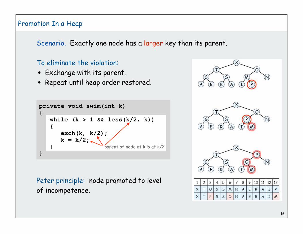
16
Promotion In a Heap
Scenario. Exactly one node has a larger key than its parent.
To eliminate the violation:
• Exchange with its parent.
• Repeat until heap order restored.
Peter principle: node promoted to level
of incompetence.
private void swim(int k){ while (k > 1 && less(k/2, k)) { exch(k, k/2); k = k/2; }}
parent of node at k is at k/2

17
Insert
Insert. Add node at end, then promote.
public void insert(Item x){ pq[++N] = x; swim(N);}

18
Demotion In a Heap
Scenario. Exactly one node has a smaller key than does a child.
To eliminate the violation:
• Exchange with larger child.
• Repeat until heap order restored.
Power struggle: better subordinate promoted.
children of nodeat k are 2k and 2k+1
private void sink(int k){ while (2*k <= N) { int j = 2*k; if (j < N && less(j, j+1)) j++; if (!less(k, j)) break; exch(k, j); k = j; }}
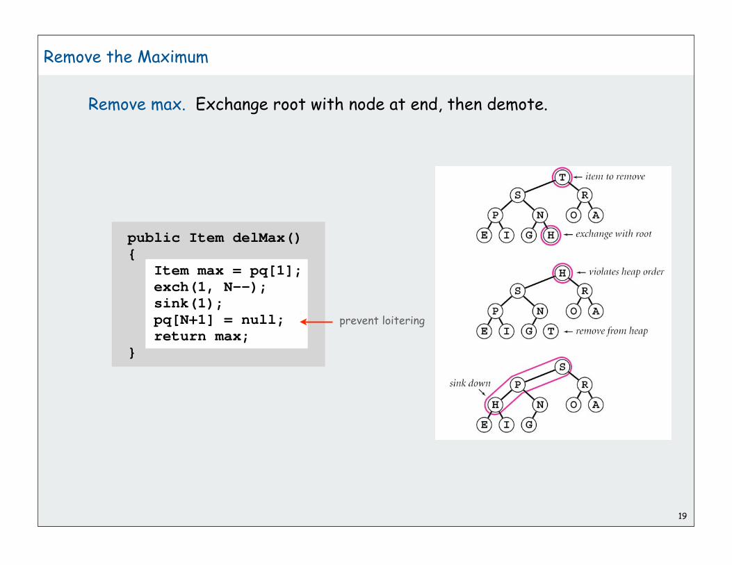
public Item delMax(){ Item max = pq[1]; exch(1, N--); sink(1); pq[N+1] = null; return max;}
19
Remove the Maximum
Remove max. Exchange root with node at end, then demote.
prevent loitering

array helper functions
heap helper functions
PQ ops
20
Binary heap implementation summary
public class MaxPQ<Item extends Comparable>
{
private Item[] pq;
private int N;
public MaxPQ(int maxN)
{ . . . }
public boolean isEmpty()
{ . . . }
public void insert(Item x)
{ . . . }
public Item delMax()
{ . . . }
private void swim(int k)
{ . . . }
private void sink(int k)
{ . . . }
private boolean less(int i, int j)
{ . . . }
private void exch(int i, int j)
{ . . . }
}
same as array-based PQ,but allocate one extra element

21
Binary heap considerations
Minimum oriented priority queue
• replace less() with greater()
• implement greater().
Array resizing
• add no-arg constructor
• apply repeated doubling.
Immutability of keys.
• assumption: client does not change keys while they're on the PQ
• best practice: use immutable keys
Other operations.
• remove an arbitrary item.
• change the priority of an item.
leads to O(log N) amortized time per op
easy to implement with sink() and swim() [stay tuned]

22
Priority Queues Implementation Cost Summary
Hopeless challenge. Make all ops O(1).
Why hopeless?
ordered array
Operation
ordered list
unordered array
unordered list
binary heap
1
Remove Max
1
N
N
lg N
1
Find Max
1
N
N
1
N
Insert
N
1
1
lg N
worst-case asymptotic costs for PQ with N items

23
APIelementary implementationsbinary heapsheapsortevent-driven simulation

24
Digression: Heapsort
First pass: build heap.
• Insert items into heap, one at at time.
• Or can use faster bottom-up method; see book.
Second pass: sort.
• Remove maximum items, one at a time.
• Leave in array, instead of nulling out.
Property D. At most 2 N lg N comparisons.
for (int k = N/2; k >= 1; k--) sink(a, k, N);
while (N > 1{ exch(a, 1, N--); sink(a, 1, N);}

Q. Sort in O(N log N) worst-case without using extra memory?
A. Yes. Heapsort.
Not mergesort? Linear extra space.
Not quicksort? Quadratic time in worst case.
Heapsort is optimal for both time and space, but:
• inner loop longer than quicksort’s.
• makes poor use of cache memory.
25
Significance of Heapsort
in-place merge possible, not practical
O(N log N) worst-case quicksort possible, not practical.

26
Sorting algorithms: summary
# key comparisons to sort N distinct randomly-ordered keys
inplace stable worst average best remarks
selection
insertion
shell
quick
merge
heap
x N2 / 2 N2 / 2 N2 / 2 N exchanges
x x N2 / 2 N2 / 4 N use for small N or partly ordered
x N tight code
x N2 / 2 2N ln N N lg NN log N probabilistic guarantee
fastest in practice
x N lg N N lg N N lg N N log N guarantee, stable
x 2N lg N 2N lg N N lg N N log N guarantee, in-place

27
APIelementary implementationsbinary heapsheapsortevent-driven simulation

Bouncing balls (COS 126)
Review
28
public class BouncingBalls
{
public static void main(String[] args)
{
int N = Integer.parseInt(args[0]);
Ball balls[] = new Ball[N];
for (int i = 0; i < N; i++)
balls[i] = new Ball();
while(true)
{
StdDraw.clear();
for (int i = 0; i < N; i++)
{
balls[i].move();
balls[i].draw();
}
StdDraw.show(50);
}
}
}

Bouncing balls (COS 126)
Missing: check for balls colliding with each other
• physics problems: when? what effect?
• CS problems: what object does the checks? too many checks?
Review
29
public class Ball
{
private double rx, ry; // position
private double vx, vy; // velocity
private double radius; // radius
public Ball()
{ ... initialize position and velocity ... }
public void move()
{
if ((rx + vx < radius) || (rx + vx > 1.0 - radius)) { vx = -vx; }
if ((ry + vy < radius) || (ry + vy > 1.0 - radius)) { vy = -vy; }
rx = rx + vx;
ry = ry + vy;
}
public void draw()
{ StdDraw.filledCircle(rx, ry, radius); }
}
checks for colliding with
walls

30
Molecular dynamics simulation of hard spheres
Goal. Simulate the motion of N moving particles that behave
according to the laws of elastic collision.
Hard sphere model.
• Moving particles interact via elastic collisions with each other,
and with fixed walls.
• Each particle is a sphere with known position, velocity, mass, and radius.
• No other forces are exerted.
Significance. Relates macroscopic observables to microscopic dynamics.
• Maxwell and Boltzmann: derive distribution of speeds of interacting
molecules as a function of temperature.
• Einstein: explain Brownian motion of pollen grains.
motion of individualatoms and molecules
temperature, pressure,diffusion constant

31
Time-driven simulation
Time-driven simulation.
• Discretize time in quanta of size dt.
• Update the position of each particle after every dt units of time, and
check for overlaps.
• If overlap, roll back the clock to the time of the collision, update the
velocities of the colliding particles, and continue the simulation.
t t + dt t + 2 dt(collision detected)
t + t(roll back clock)
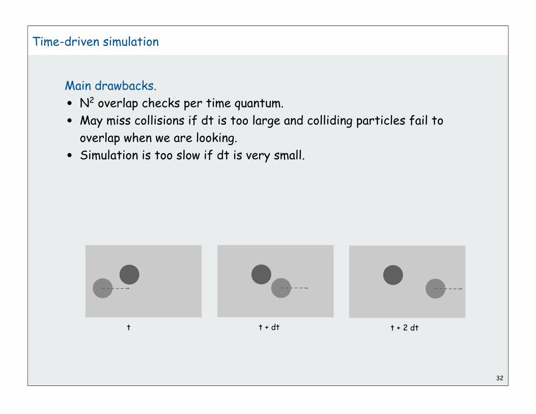
32
Time-driven simulation
Main drawbacks.
• N2 overlap checks per time quantum.
• May miss collisions if dt is too large and colliding particles fail to
overlap when we are looking.
• Simulation is too slow if dt is very small.
t t + dt t + 2 dt

33
Event-driven simulation
Change state only when something happens.
• Between collisions, particles move in straight-line trajectories.
• Focus only on times when collisions occur.
• Maintain priority queue of collision events, prioritized by time.
• Remove the minimum = get next collision.
Collision prediction. Given position, velocity, and radius of a particle,
when will it collide next with a wall or another particle?
Collision resolution. If collision occurs, update colliding particle(s)
according to laws of elastic collisions.
Note: Same approach works for a broad variety of systems

34
Particle-wall collision
Collision prediction.
• Particle of radius at position (rx, ry).
• Particle moving in unit box with velocity (vx, vy).
• Will it collide with a horizontal wall? If so, when?
Collision resolution. (vx', vy') = (vx, -vy).
t =
if vy = 0
( ry)/vy if vy < 0
(1 ry)/vy if vy > 0
(rx, ry)
time = t
(vx, vy) (vx, -vy)
(rx', ry')
time = t + t

35
Particle-particle collision prediction
Collision prediction.
• Particle i: radius i, position (rxi, ryi), velocity (vxi, vyi).
• Particle j: radius j, position (rxj, ryj), velocity (vxj, vyj).
• Will particles i and j collide? If so, when?
j
i
(rxi , ryi)
time = t
(vxi , vyi )
m i
i
j
(rxi', ryi')
time = t + t
(vxj', vyj')
(vxi', vyi')
(vxj , vyj)

36
Particle-particle collision prediction
Collision prediction.
• Particle i: radius i, position (rxi, ryi), velocity (vxi, vyi).
• Particle j: radius j, position (rxj, ryj), velocity (vxj, vyj).
• Will particles i and j collide? If so, when?
t =
if v r 0
if d < 0
- v r + d
v v otherwise
d = ( v r)2 ( v v) ( r r 2 ) = i + j
v = ( vx, vy) = (vxi vx j , vyi vyj )r = ( rx, ry) = (rxi rx j , ryi ryj )
v v = ( vx)2+ ( vy)2
r r = ( rx)2+ ( ry)2
v r = ( vx)( rx)+ ( vy)( ry)

public double dt(Particle b)
{
Particle a = this;
if (a == b) return INFINITY;
double dx = b.rx - a.rx;
double dy = b.ry - a.ry;
double dvx = b.vx - a.vx;
double dvy = b.vy - a.vy;
double dvdr = dx*dvx + dy*dvy;
if(dvdr > 0) return INFINITY;
double dvdv = dvx*dvx + dvy*dvy;
double drdr = dx*dx + dy*dy;
double sigma = a.radius + b.radius;
double d = (dvdr*dvdr) - dvdv * (drdr - sigma*sigma);
if (d < 0) return INFINITY;
return -(dvdr + Math.sqrt(d)) / dvdv;
}
Particle-particle collision prediction implementation
37
Particle has method to predict collision with another particle
and methods dtX() and dtY() to predict collisions with walls

Particle-particle collision prediction implementation
38
private void predict(Particle a, double limit)
{
if (a == null) return;
for(int i = 0; i < N; i++)
{
double dt = a.dt(particles[i]);
if(t + dt <= limit)
pq.insert(new Event(t + dt, a, particles[i]));
}
double dtX = a.dtX();
double dtY = a.dtY();
if (t + dtX <= limit)
pq.insert(new Event(t + dtX, a, null));
if (t + dtY <= limit)
pq.insert(new Event(t + dtY, null, a));
}
CollisionSystem has method to predict all collisions
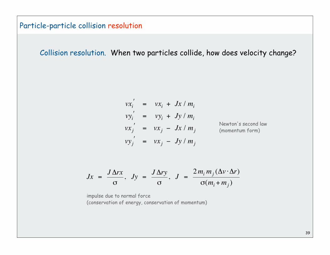
39
Particle-particle collision resolution
Collision resolution. When two particles collide, how does velocity change?
vxi = vxi + Jx / mi
vyi = vyi + Jy / mi
vx j = vx j Jx / mj
vyj = vx j Jy / mj
Jx = J rx
, Jy = J ry
, J = 2mi mj ( v r)
(mi +mj )
impulse due to normal force(conservation of energy, conservation of momentum)
Newton's second law(momentum form)

public void bounce(Particle b)
{
Particle a = this;
double dx = b.rx - a.rx;
double dy = b.ry - a.ry;
double dvx = b.vx - a.vx;
double dvy = b.vy - a.vy;
double dvdr = dx*dvx + dy*dvy;
double dist = a.radius + b.radius;
double J = 2 * a.mass * b.mass * dvdr / ((a.mass + b.mass) * dist);
double Jx = J * dx / dist;
double Jy = J * dy / dist;
a.vx += Jx / a.mass;
a.vy += Jy / a.mass;
b.vx -= Jx / b.mass;
b.vy -= Jy / b.mass;
a.count++;
b.count++;
}
Particle-particle collision resolution implementation
40
Particle has method to resolve collision with another particle
and methods bounceX() and bounceY() to resolve collisions with walls

41
Collision system: event-driven simulation main loop
Initialization.
• Fill PQ with all potential particle-wall collisions
• Fill PQ with all potential particle-particle collisions.
Main loop.
• Delete the impending event from PQ (min priority = t).
• If the event in no longer valid, ignore it.
• Advance all particles to time t, on a straight-line trajectory.
• Update the velocities of the colliding particle(s).
• Predict future particle-wall and particle-particle collisions involving
the colliding particle(s) and insert events onto PQ.
“potential” since collision may not happen ifsome other collision intervenes

public void simulate(double limit)
{
pq = new MinPQ<Event>();
for(int i = 0; i < N; i++)
predict(particles[i], limit);
pq.insert(new Event(0, null, null));
while(!pq.isEmpty())
{
Event e = pq.delMin();
if(!e.isValid()) continue;
Particle a = e.a();
Particle b = e.b();
for(int i = 0; i < N; i++)
particles[i].move(e.time() - t);
t = e.time();
if (a != null && b != null) a.bounce(b);
else if (a != null && b == null) a.bounceX()
else if (a == null && b != null) b.bounceY();
else if (a == null && b == null)
{
StdDraw.clear(StdDraw.WHITE);
for(int i = 0; i < N; i++) particles[i].draw();
StdDraw.show(20);
if (t < limit)
pq.insert(new Event(t + 1.0 / Hz, null, null));
}
predict(a, limit);
predict(b, limit);
}
}
Collision system: main event-driven simulation loop implementation
42
initialize PQ with collision events and redraw event
main event-driven simulation loop
update positions and time
process event
predict new events based on changes
java CollisionSystem 200
43

java CollisionSystem < billiards5.txt
44
java CollisionSystem < squeeze2.txt

java CollisionSystem < brownianmotion.txt
45

java CollisionSystem < diffusion.txt
46

1
Symbol Tables
APIbasic implementationsiteratorsComparable keyschallenges
References:
Algorithms in Java, Chapter 12
Intro to Programming, Section 4.4 http://www.cs.princeton.edu/introalgsds/41st
2
API basic implementationsiteratorsComparable keyschallenges

3
Symbol Tables
Key-value pair abstraction.
• Insert a value with specified key.
• Given a key, search for the corresponding value.
Example: DNS lookup.
• Insert URL with specified IP address.
• Given URL, find corresponding IP address
Can interchange roles: given IP address find corresponding URL
key value
www.cs.princeton.edu
URL IP address
128.112.136.11
www.princeton.edu 128.112.128.15
www.yale.edu 130.132.143.21
www.harvard.edu 128.103.060.55
www.simpsons.com 209.052.165.60

4
Symbol Table Applications
Application Purpose Key Value
Phone book Look up phone number Name Phone number
Bank Process transaction Account number Transaction details
File share Find song to download Name of song Computer ID
Dictionary Look up word Word Definition
Web search Find relevant documents Keyword List of documents
Genomics Find markers DNA string Known positions
DNS Find IP address given URL URL IP address
Reverse DNS Find URL given IP address IP address URL
Book index Find relevant pages Keyword List of pages
Web cache Download Filename File contents
Compiler Find properties of variable Variable name Value and type
File system Find file on disk Filename Location on disk
Routing table Route Internet packets Destination Best route

5
Symbol Table API
Associative array abstraction: Unique value associated with each key.
Our conventions:
1. Values are not null.
2. Method get() returns null if key not present
3. Method put() overwrites old value with new value.
a[key] = val;
public boolean contains(Key key)
{ return get(key) != null; }
Some languages (not Java) allow this notation
enables this code in all implementations:
public class *ST<Key extends Comparable<Key>, Value>
*ST() create a symbol table
void put(Key key, Value val) put key-value pair into the table
Value get(Key key)return value paired with key(null if key not in table)
boolean contains(Key key) is there a value paired with key?
void remove(Key key) remove key-value pair from table
Iterator<Key> iterator() iterator through keys in table
insert
search
stay tuned

ST client: make a dictionary and process lookup requests
Command line arguments
• a comma-separated value (CSV) file
• key field
• value field
Example 1: DNS lookup
6
% more ip.csvwww.princeton.edu,128.112.128.15www.cs.princeton.edu,128.112.136.35www.math.princeton.edu,128.112.18.11www.cs.harvard.edu,140.247.50.127www.harvard.edu,128.103.60.24www.yale.edu,130.132.51.8www.econ.yale.edu,128.36.236.74www.cs.yale.edu,128.36.229.30espn.com,199.181.135.201yahoo.com,66.94.234.13msn.com,207.68.172.246google.com,64.233.167.99baidu.com,202.108.22.33yahoo.co.jp,202.93.91.141sina.com.cn,202.108.33.32ebay.com,66.135.192.87adobe.com,192.150.18.60163.com,220.181.29.154passport.net,65.54.179.226tom.com,61.135.158.237nate.com,203.226.253.11cnn.com,64.236.16.20daum.net,211.115.77.211blogger.com,66.102.15.100fastclick.com,205.180.86.4wikipedia.org,66.230.200.100rakuten.co.jp,202.72.51.22...
% java Lookup ip.csv 0 1adobe.com192.150.18.60www.princeton.edu128.112.128.15ebay.eduNot found
% java Lookup ip.csv 1 0128.112.128.15www.princeton.edu999.999.999.99Not found
URL is key IP is value
IP is key URL is value

7
ST client: make a dictionary and process lookup requests
public class Lookup
{
public static void main(String[] args)
{
In in = new In(args[0]);
int keyField = Integer.parseInt(args[1]);
int valField = Integer.parseInt(args[2]);
String[] database = in.readAll().split("\\n");
ST<String, String> st = new ST<String, String>();
for (int i = 0; i < database.length; i++)
{
String[] tokens = database[i].split(",");
String key = tokens[keyField];
String val = tokens[valField];
st.put(key, val);
}
while (!StdIn.isEmpty())
{
String s = StdIn.readString();
if (!st.contains(s)) StdOut.println("Not found");
else StdOut.println(st.get(s));
}
}
}
process input file
build symbol table
process lookupswith standard I/O

ST client: make a dictionary and process lookup requests
Command line arguments
• a comma-separated value (CSV) file
• key field
• value field
Example 2: Amino acids
8
% more amino.csvTTT,Phe,F,PhenylalanineTTC,Phe,F,PhenylalanineTTA,Leu,L,LeucineTTG,Leu,L,LeucineTCT,Ser,S,SerineTCC,Ser,S,SerineTCA,Ser,S,SerineTCG,Ser,S,SerineTAT,Tyr,Y,TyrosineTAC,Tyr,Y,TyrosineTAA,Stop,Stop,StopTAG,Stop,Stop,StopTGT,Cys,C,CysteineTGC,Cys,C,CysteineTGA,Stop,Stop,StopTGG,Trp,W,TryptophanCTT,Leu,L,LeucineCTC,Leu,L,LeucineCTA,Leu,L,LeucineCTG,Leu,L,LeucineCCT,Pro,P,ProlineCCC,Pro,P,ProlineCCA,Pro,P,ProlineCCG,Pro,P,ProlineCAT,His,H,HistidineCAC,His,H,HistidineCAA,Gln,Q,GlutamineCAG,Gln,Q,GlutamineCGT,Arg,R,ArginineCGC,Arg,R,ArginineCGA,Arg,R,ArginineCGG,Arg,R,ArginineATT,Ile,I,IsoleucineATC,Ile,I,IsoleucineATA,Ile,I,IsoleucineATG,Met,M,Methionine...
% % java Lookup amino.csv 0 3ACTThreonineTAGStopCATHistidine
codon is key name is value

ST client: make a dictionary and process lookup requests
Command line arguments
• a comma-separated value (CSV) file
• key field
• value field
Example 3: Class lists
9
% more classlist.csv10,Bo Ling,P03,bling10,Steven A Ross,P01,saross10,Thomas Oliver Horton Conway,P03,oconway08,Michael R. Corces Zimmerman,P01A,mcorces09,Bruce David Halperin,P02,bhalperi09,Glenn Charles Snyders Jr.,P03,gsnyders09,Siyu Yang,P01A,siyuyang08,Taofik O. Kolade,P01,tkolade09,Katharine Paris Klosterman,P01A,kklosterSP,Daniel Gopstein,P01,dgtwo10,Sauhard Sahi,P01,ssahi10,Eric Daniel Cohen,P01A,edcohen09,Brian Anthony Geistwhite,P02,bgeistwh09,Boris Pivtorak,P01A,pivtorak09,Jonathan Patrick Zebrowski,P01A,jzebrows09,Dexter James Doyle,P01A,ddoyle09,Michael Weiyang Ye,P03,ye08,Delwin Uy Olivan,P02,dolivan08,Edward George Conbeer,P01A,econbeer09,Mark Daniel Stefanski,P01,mstefans09,Carter Adams Cleveland,P03,cclevela10,Jacob Stephen Lewellen,P02,jlewelle10,Ilya Trubov,P02,itrubov09,Kenton William Murray,P03,kwmurray07,Daniel Steven Marks,P02,dmarks09,Vittal Kadapakkam,P01,vkadapak10,Eric Ruben Domb,P01A,edomb07,Jie Wu,P03,jiewu08,Pritha Ghosh,P02,prithag10,Minh Quang Anh Do,P01,mqdo...
% java Lookup classlist.csv 3 1jshJeffrey Scott HarrisdgtwoDaniel GopsteinyeMichael Weiyang Ye
% java Lookup classlist.csv 3 2jshP01AdgtwoP01
login is key name is value
login is key precept is value

10
Keys and Values
Associative array abstraction.
• Unique value associated with each key
• If client presents duplicate key, overwrite to change value.
Key type: several possibilities
1. Assume keys are any generic type, use equals() to test equality.
2. Assume keys are Comparable, use compareTo().
3. Use equals() to test equality and hashCode() to scramble key.
Value type. Any generic type.
Best practices. Use immutable types for symbol table keys.
• Immutable in Java: String, Integer, BigInteger.
• Mutable in Java: Date, GregorianCalendar, StringBuilder.
a[key] = val;

Elementary ST implementations
Unordered array
Ordered array
Unordered linked list
Ordered linked list
Why study elementary implementations?
• API details need to be worked out
• performance benchmarks
• method of choice can be one of these in many situations
• basis for advanced implementations
Always good practice to study elementary implementations
11

12
API basic implementationsiteratorsComparable keyschallenges

13
Unordered array ST implementation
Maintain parallel arrays of keys and values.
Instance variables
• array keys[] holds the keys.
• array vals[] holds the values.
• integer N holds the number of entries.
Need to use standard array-doubling technique
Alternative: define inner type for entries
• space overhead for entry objects
• more complicated code
0 1 2 3 4 5
keys[]
vals[]
it was the best of times
2 2 1 1 1 1
N = 6
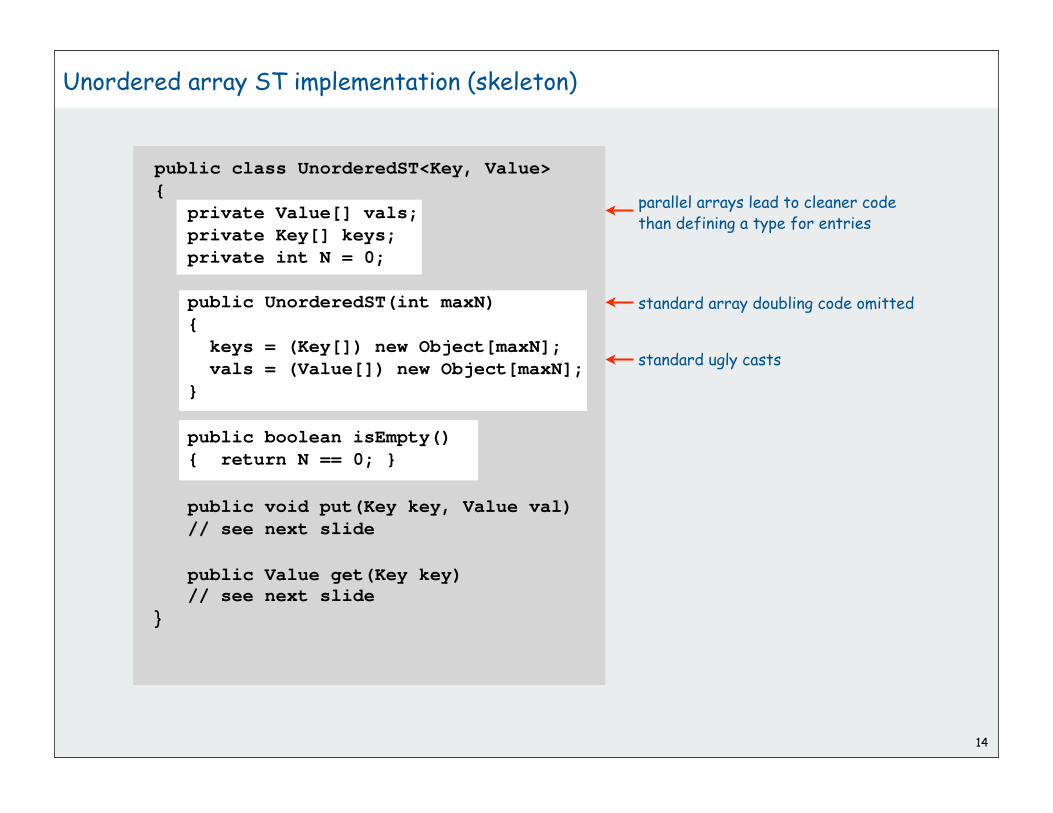
public class UnorderedST<Key, Value>
{
private Value[] vals;
private Key[] keys;
private int N = 0;
public UnorderedST(int maxN)
{
keys = (Key[]) new Object[maxN];
vals = (Value[]) new Object[maxN];
}
public boolean isEmpty()
{ return N == 0; }
public void put(Key key, Value val)
// see next slide
public Value get(Key key) // see next slide
}
14
Unordered array ST implementation (skeleton)
standard ugly casts
standard array doubling code omitted
parallel arrays lead to cleaner codethan defining a type for entries

Key, Value are generic and can be any type
15
Unordered array ST implementation (search)
public Value get(Key key)
{ for (int i = 0; i < N; i++) if (keys[i].equals(key)) return vals[i]; return null;}
0 1 2 3 4 5
keys[]
vals[]
it was the best of times
2 2 1 1 1 1
0 1 2 3 4 5
keys[]
vals[]
it was the best of times
2 2 1 1 1 1
get(“worst”)returns null
Java convention: all objects implement equals()
get(“the”)returns 1

Associative array abstraction
• must search for key and overwrite with new value if it is there
• otherwise, add new key, value at the end (as in stack)16
Unordered array ST implementation (insert)
public void put(Key key, Value val)
{
int i;
for (i = 0; i < N; i++)
if (key.equals(keys[i]))
break;
vals[i] = val;
keys[i] = key;
if (i == N) N++;
}
0 1 2 3 4 5
keys[]
vals[]
it was the best of times
2 2 1 1 1 1
0 1 2 3 4 5
keys[]
vals[]
it was the best of times
2 2 2 1 1 1
put(“the”, 2)overwrites the 1
0 1 2 3 4 5 6
keys[]
vals[]
it was the best of times worst
2 2 2 1 1 1 1
put(“worst”, 1)adds a new entry

17
Java conventions for equals()
All objects implement equals() but default implementation is (x == y)
Customized implementations.
String, URL, Integer.
User-defined implementations.
Some care needed (example: type of argument must be Object)
Equivalence relation. For any references x, y and z:
• Reflexive: x.equals(x) is true.
• Symmetric: x.equals(y) iff y.equals(x).
• Transitive: If x.equals(y) and y.equals(z), then x.equals(z).
• Non-null: x.equals(null) is false.
• Consistency: Multiple calls to x.equals(y) return same value.
is the object referred to by xthe same object that is referred to by y?

Implementing equals()
Seems easy
18
public class PhoneNumber{ private int area, exch, ext;
...
public boolean equals(PhoneNumber y) {
PhoneNumber a = this; PhoneNumber b = (PhoneNumber) y; return (a.area == b.area) && (a.exch == b.exch) && (a.ext == b.ext); }}

Implementing equals()
Seems easy, but requires some care
19
public final class PhoneNumber{ private final int area, exch, ext;
...
public boolean equals( Object y) { if (y == this) return true;
if (y == null) return false;
if (y.getClass() != this.getClass()) return false;
PhoneNumber a = this; PhoneNumber b = (PhoneNumber) y; return (a.area == b.area) && (a.exch == b.exch) && (a.ext == b.ext); }}
If I’m executing this code,I’m not null.
Optimize for true object equality
no safe way to use with inheritance
Must be Object.Why? Experts still debate.
Objects must be in the same class.

Maintain a linked list with keys and values.
inner Node class
• instance variable key holds the key
• instance variable val holds the value
instance variable
• Node first refers to the first node in the list
20
Linked list ST implementation
it
2
was
2
the
1
best
1
of
1
times
1
first

public class LinkedListST<Key, Value>
{
private Node first;
private class Node
{
Key key;
Value val;
Node next;
Node(Key key, Value val, Node next)
{
this.key = key;
this.val = val;
this.next = next;
}
}
public void put(Key key, Value val)
// see next slides
public Val get(Key key) // see next slides
}
21
Linked list ST implementation (skeleton)
instance variable
inner class

Key, Value are generic and can be any type
22
Linked list ST implementation (search)
Java convention: all objects implement equals()
public Value get(Key key)
{ for (Node x = first; x != null; x = x.next)) if (key.equals(x.key)) return vals[i]; return null;}
get(“the”)returns 1
get(“worst”)returns null
it
2
was
2
the
1
best
1
of
1
times
1
first
it
2
was
2
the
1
best
1
of
1
times
1
first

23
Linked list ST implementation (insert)
public void put(Key key, Value val)
{
for (Node x = first; x != null; x = x.next)
if (key.equals(x.key))
{ x.value = value; return; }
first = new Node(key, value, first);
}
put(“the”, 2)overwrites the 1
put(“worst”, 1)adds a new entry
after searching
the entire list
it
2
was
2
the
1
best
1
of
1
times
1
first
Associative array abstractionmust search for key and, if it is there, overwrite with new valueotherwise, add new key, value at the beginning (as in stack)
was
2
the
2
best
1
of
1
times
1
worst
1
first
it
2

24
API basic implementationsiteratorsComparable keyschallenges

Iterators
Symbol tables should be Iterable
Q. What is Iterable?
A. Implements iterator()
Q. What is an Iterator?
A. Implements hasNext() and next().
Q. Why should symbol tables be iterable?
A. Java language supports elegant client code for iterators
25
Iterator<String> i = st.iterator(); while (i.hasNext()){ String s = i.next(); StdOut.println(st.get(s));}
public interface Iterator<Item>
{
boolean hasNext();
Item next();
void remove();
}
for (String s: st) StdOut.println(st.get(s));
optional in Javause at your own risk
“foreach” statement equivalent code
public interface Iterable<Item>
{
Iterator<Item> iterator();
}
java.util.Iterator

Iterable ST client: count frequencies of occurrence of input strings
Standard input: A file (of strings)
Standard output: All the distinct strings in the file with frequency
26
% more tiny.txtit was the best of timesit was the worst of timesit was the age of wisdomit was the age of foolishness
% java FrequencyCount < tiny.txt2 age1 best1 foolishness4 it4 of4 the2 times4 was1 wisdom1 worst
% more tale.txtit was the best of timesit was the worst of timesit was the age of wisdomit was the age of foolishnessit was the epoch of beliefit was the epoch of incredulityit was the season of lightit was the season of darknessit was the spring of hopeit was the winter of despairwe had everything before uswe had nothing before us...% java FrequencyCount < tale.txt2941 a1 aback1 abandon10 abandoned1 abandoning1 abandonment1 abashed1 abate1 abated5 abbaye2 abed1 abhorrence1 abided1 abiding1 abilities2 ability1 abject1 ablaze17 able1 abnegating
tiny example24 words
10 distinct
real example137177 words9888 distinct

27
Iterable ST client: count frequencies of occurrence of input strings
public class FrequencyCount{ public static void main(String[] args) { ST<String, Integer> st; st = new ST<String, Integer>();
while (!StdIn.isEmpty()) { String key = StdIn.readString();
if (!st.contains(key)) st.put(key, 1); else st.put(key, st.get(key) + 1);
}
for (String s: st) StdOut.println(st.get(s) + " " + s);
}}
read a string
insert
print all strings
increment
Note: Only slightly more work required to build an index
of all of the places where each key occurs in the text.

Iterators for array, linked list ST implementations
28
import java.util.Iterator;public class LinkedListST<Key, Value> implements Iterable<Key>
{ ...
public Iterator<Key> iterator() { return new ListIterator(); }
private class ListIterator implements Iterator<Key> { private Node current = first;
public boolean hasNext() { return current != null; }
public void remove() { } public Key next() { Key key = current.key; current = current.next; return key; } }}
import java.util.Iterator;public class UnorderedST<Key, Value> implements Iterable<Key>
{ ...
public Iterator<Key> iterator() { return new ArrayIterator(); }
private class ArrayIterator implements Iterator<Key> { private int i = 0;
public boolean hasNext() { return i < N; }
public void remove() { }
public Key next() { return keys[i++]; } }}

Iterable ST client: A problem?
Clients who use Comparable keys might expect ordered iteration
• not a requirement for some clients
• not a problem if postprocessing, e.g. with sort or grep
• not in API 29
% more tiny.txtit was the best of timesit was the worst of timesit was the age of wisdomit was the age of foolishness
% java FrequencyCount < tiny.txt4 it4 was4 the1 best4 of2 times1 worst2 age1 wisdom1 foolishness
Use UnorderedST in FrequencyCount
% more tiny.txtit was the best of timesit was the worst of timesit was the age of wisdomit was the age of foolishness
% java FrequencyCount < tiny.txt1 foolishness1 wisdom2 age1 worst2 times4 of1 best4 the4 was4 it
Use LinkedListST in FrequencyCount

30
API basic implementationsiteratorsComparable keyschallenges

31
Ordered array ST implementation
Assume that keys are Comparable
Maintain parallel arrays with keys and values that are sorted by key.
Instance variables
• keys[i] holds the ith smallest key
• vals[i] holds the value associated with the ith smallest key
• integer N holds the number of entries.
Note: no duplicate keys
Need to use standard array-doubling technique
Two reasons to consider using ordered arrays
• provides ordered iteration (for free)
• can use binary search to significantly speed up search
0 1 2 3 4 5
keys[]
vals[]
best it of the times was
1 2 1 1 1 2
N = 6

public class OrderedST
<Key extends Comparable<Key>, Value>
implements Iterable<Key>
{
private Value[] vals;
private Key[] keys;
private int N = 0;
public OrderedST(int maxN)
{
keys = (Key[]) new Object[maxN];
vals = (Value[]) new Object[maxN];
}
public boolean isEmpty()
{ return N == 0; }
public void put(Key key, Value val)
// see next slides
public Val get(Key key) // see next slides
}
32
Ordered array ST implementation (skeleton)
standard array doubling code omitted
standard array iterator code omitted

3of3
Keeping array in order enables binary search algorithm
33
Ordered array ST implementation (search)
0 4 8age best it of the times was wisdom worst2 1 4 3 4 2 4 1 1
get(“of”)returns 3
public Value get(Key key) { int i = bsearch(key); if (i == -1) return null; return vals[i]; }
private int bsearch(Key key) { int lo = 0, hi = N-1; while (lo <= hi) { int m = lo + (hi - lo) / 2; int cmp = key.compareTo(keys[m]); if (cmp < 0) hi = m - 1; else if (cmp > 0) lo = m + 1; else return m; } return -1; }
0 1 3age best it of2 1 4 3
2 3it of4 3
lo him

34
Binary search analysis: Comparison count
Def. T(N) number of comparisons to binary search in an ST of size N
= T(N/2) + 1
Binary search recurrence
• not quite right for odd N
• same recurrence holds for many algorithms
• same number of comparisons for any input of size N.
Solution of binary search recurrence
• true for all N
• easy to prove when N is a power of 2.
T(N) = T(N/2) + 1 for N > 1, with T(1) = 0
T(N) ~ lg N
left or right half
can then use induction for general N(see COS 340)
middle

Pf.
35
Binary search recurrence: Proof by telescoping
T(N) = T(N/2) + 1 for N > 1, with T(1) = 0
T(N) = T(N/2) + 1
= T(N/4) + 1 + 1
= T(N/8) + 1 + 1 + 1
. . .
= T(N/N) + 1 + 1 +. . .+ 1
= lg N
T(N) = lg N
(assume that N is a power of 2)
given
telescope (apply to first term)
telescope again
stop telescoping, T(1) = 0

Binary search is little help for put(): still need to move larger keys
36
Ordered array ST implementation (insert)
age best it of the times was wisdom worst2 1 4 4 4 2 4 1 1
public Val put(Key key, Value val) { int i = bsearch(key); if (i != -1) { vals[i] = val; return; }
for ( i = N; i > 0; i-- ) { if key.compareTo(keys[i-1] < 0) break; keys[i] = keys[i-1]; vals[i] = vals[i-1]; } vals[i] = val; keys[i] = key; N++;
}
age best foolish it of the times was wisdom worst2 1 1 4 4 4 2 4 1 1
overwrite with new valueif key in table
put(“foolish”)
move larger keys to make roomif key not in table

Ordered array ST implementation: an important special case
Test whether key is equal to or greater than largest key
If either test succeeds, constant-time insert!
Method of choice for some clients:
• sort database by key
• insert N key-value pairs in order by key
• support searches that never use more than lg N compares
• support occasional (expensive) inserts
37
public Val put(Key key, Value val){ if (key.compareTo(keys[N-1]) == 0) { vals[N-1] = val; return; }
if (key.compareTo(keys[N-1] > 0) { vals[N] = val; keys[N] = key; N++; return; }}

Ordered linked-list ST implementation
Binary search depends on array indexing for efficiency.
Jump to the middle of a linked list?
Advantages of keeping linked list in order for Comparable keys:
• support ordered iterator (for free)
• cuts search/insert time in half (on average) for random search/insert
[ code omitted ]
38
was
2
times
1
the
1
of
1
it
2
best
1
first

39
API basic implementationsiteratorsComparable keyschallenges

Searching challenge 1A:
Problem: maintain symbol table of song names for an iPod
Assumption A: hundreds of songs
Which searching method to use?
1) unordered array
2) ordered linked list
3) ordered array with binary search
4) need better method, all too slow
5) doesn’t matter much, all fast enough
40

Searching challenge 1B:
Problem: maintain symbol table of song names for an iPod
Assumption B: thousands of songs
Which searching method to use?
1) unordered array
2) ordered linked list
3) ordered array with binary search
4) need better method, all too slow
5) doesn’t matter much, all fast enough
41

Searching challenge 2A:
Problem: IP lookups in a web monitoring device
Assumption A: billions of lookups, millions of distinct addresses
Which searching method to use?
1) unordered array
2) ordered linked list
3) ordered array with binary search
4) need better method, all too slow
5) doesn’t matter much, all fast enough
42

Searching challenge 2B:
Problem: IP lookups in a web monitoring device
Assumption B: billions of lookups, thousands of distinct addresses
Which searching method to use?
1) unordered array
2) ordered linked list
3) ordered array with binary search
4) need better method, all too slow
5) doesn’t matter much, all fast enough
43

Searching challenge 3:
Problem: Frequency counts in “Tale of Two Cities”
Assumptions: book has 135,000+ words
about 10,000 distinct words
Which searching method to use?
1) unordered array
2) ordered linked list
3) ordered array with binary search
4) need better method, all too slow
5) doesn’t matter much, all fast enough
44

Searching challenge 4:
Problem: Spell checking for a book
Assumptions: dictionary has 25,000 words
book has 100,000+ words
Which searching method to use?
1) unordered array
2) ordered linked list
3) ordered array with binary search
4) need better method, all too slow
5) doesn’t matter much, all fast enough
45

Searching challenge 5:
Problem: Sparse matrix-vector multiplication
Assumptions: matrix dimension is billions by billions
average number of nonzero entries/row is ~10
Which searching method to use?
1) unordered array
2) ordered linked list
3) ordered array with binary search
4) need better method, all too slow
5) doesn’t matter much, all fast enough
46
A * x = b

Summary and roadmap
• basic algorithmics
• no generics
• more code
• more analysis
• equal keys in ST (not associative arrays)
• iterators
• ST as associative array (all keys distinct)
• BST implementations
• applications
• distinguish algs by operations on keys
• ST as associative array (all keys distinct)
• important special case for binary search
• challenges
47

48
Elementary implementations: summary
Next challenge.
Efficient implementations of search and insert and ordered iteration
for arbitrary sequences of operations.
implementationworst case average case ordered
iteration?operations
on keyssearch insert search insert
unordered array N N N/2 N/2 no equals()
ordered array lg N N lg N N/2 yes compareTo()
unordered list N N N/2 N no equals()
ordered list N N N/2 N/2 yes compareTo()
studying STsfor the midterm?
Start here.
(ordered array meets challenge if keys arrive approximately in order)

1
Binary Search Trees
basic implementationsrandomized BSTsdeletion in BSTs
References:
Algorithms in Java, Chapter 12
Intro to Programming, Section 4.4 http://www.cs.princeton.edu/introalgsds/43bst

2
Elementary implementations: summary
Challenge:
Efficient implementations of get() and put() and ordered iteration.
implementationworst case average case ordered
iteration?operations
on keyssearch insert search insert
unordered array N N N/2 N/2 no equals()
ordered array lg N N lg N N/2 yes compareTo()
unordered list N N N/2 N no equals()
ordered list N N N/2 N/2 yes compareTo()

3
basic implementationsrandomized BSTsdeletion in BSTs

4
Binary Search Trees (BSTs)
Def. A BINARY SEARCH TREE is a binary tree in symmetric order.
A binary tree is either:
• empty
• a key-value pair and two binary trees
[neither of which contain that key]
Symmetric order means that:
• every node has a key
• every node’s key is
larger than all keys in its left subtree
smaller than all keys in its right subtree
smaller larger
x
node
subtrees
the
was
it
of times
best
equal keys ruled out to facilitateassociative array implementations
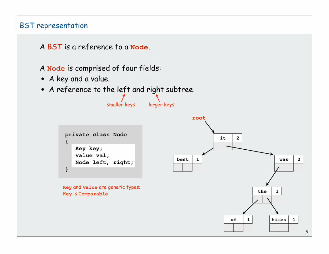
5
BST representation
A BST is a reference to a Node.
A Node is comprised of four fields:
• A key and a value.
• A reference to the left and right subtree.
Key and Value are generic types;Key is Comparable
root
it 2
was 2
the 1
best 1
of 1 times 1
private class Node
{
Key key;
Value val;
Node left, right;
}
smaller keys larger keys

public class BST<Key extends Comparable<Key>, Value>
implements Iterable<Key>
{
private Node root;
private class Node
{
Key key;
Value val;
Node left, right;
Node(Key key, Value val)
{
this.key = key;
this.val = val;
}
}
public void put(Key key, Value val)
// see next slides
public Val get(Key key) // see next slides
}
6
BST implementation (skeleton)
instance variable
inner class

7
BST implementation (search)
public Value get(Key key)
{ Node x = root;
while (x != null) { int cmp = key.compareTo(x.key);
if (cmp == 0) return x.val; else if (cmp < 0) x = x.left;
else if (cmp > 0) x = x.right; } return null;
}
get(“the”)returns 1
get(“worst”)returns null
root
it 2
was 2
the 1
best 1
of 1 times 1

8
BST implementation (insert)
public void put(Key key, Value val)
{ root = put(root, key, val); }
root
it 2
was 2
the 1
best 1
of 1 times 1
put(“the”, 2)overwrites the 1
put(“worst”, 1)adds a new entry
worst 1
private Node put(Node x, Key key, Value val)
{
if (x == null) return new Node(key, val);
int cmp = key.compareTo(x.key);
if (cmp == 0) x.val = val;
else if (cmp < 0) x.left = put(x.left, key, val);
else if (cmp > 0) x.right = put(x.right, key, val);
return x;
}
Caution: tricky recursive code.Read carefully!

9
BST: Construction
Insert the following keys into BST. A S E R C H I N G X M P L

Tree shape.
• Many BSTs correspond to same input data.
• Cost of search/insert is proportional to depth of node.
Tree shape depends on order of insertion
10
Tree Shape
E
S
A
C
H
H
A E I S
C R
R
I
H
A
E
I
S
C
R
typical best
worst

BST implementation: iterator?
11
public Iterator<Key> iterator() { return new BSTIterator(); }
private class BSTIterator implements Iterator<Key>
{
BSTIterator() { }
public boolean hasNext() { }
public Key next() { }
}
E
SA
C
H R
I
N

BST implementation: iterator?
12
public void visit(Node x)
{ if (x == null) return;
visit(x.left) StdOut.println(x.key); visit(x.right);
}
E
SA
C
H R
I
N
Approach: mimic recursive inorder traversal
visit(E) visit(A) print A visit(C) print C print E visit(S) visit(I) visit(H) print H print I visit(R) visit(N) print N print R print S
A
C E
H
I
N R S
EA EEC EE
SI SH I SI SSR SN R SR SS
Stack contents
To process a node
• follow left links until empty
(pushing onto stack)
• pop and process
• process node at right link

13
BST implementation: iterator
public Iterator<Key> iterator() { return new BSTIterator(); }
private class BSTIterator implements Iterator<Key>
{ private Stack<Node>
stack = new Stack<Node>(); private void pushLeft(Node x)
{ while (x != null)
{ stack.push(x); x = x.left; } }
BSTIterator() { pushLeft(root); }
public boolean hasNext() { return !stack.isEmpty(); }
public Key next()
{ Node x = stack.pop(); pushLeft(x.right);
return x.key; }
}
E
SA
C
H R
I
A E
A C E
C E
E H I S
H I S
I N R S
N R S
R S
S
N

1-1 correspondence between BSTs and Quicksort partitioning
14
A
C
E
I
K
L
M
O
P
Q
R
S
T
U
XE
no equal keys

15
BSTs: analysis
Theorem. If keys are inserted in random order, the expected number
of comparisons for a search/insert is about 2 ln N.
Proof: 1-1 correspondence with quicksort partitioning
Theorem. If keys are inserted in random order, height of tree
is proportional to lg N, except with exponentially small probability.
But… Worst-case for search/insert/height is N.
e.g., keys inserted in ascending order
mean 6.22 lg N, variance = O(1)
1.38 lg N, variance = O(1)
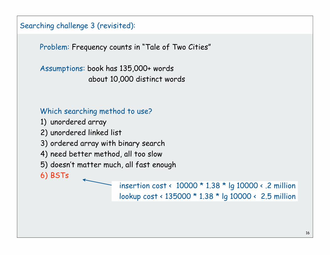
Searching challenge 3 (revisited):
Problem: Frequency counts in “Tale of Two Cities”
Assumptions: book has 135,000+ words
about 10,000 distinct words
Which searching method to use?
1) unordered array
2) unordered linked list
3) ordered array with binary search
4) need better method, all too slow
5) doesn’t matter much, all fast enough
6) BSTs
16
insertion cost < 10000 * 1.38 * lg 10000 < .2 million
lookup cost < 135000 * 1.38 * lg 10000 < 2.5 million

17
Elementary implementations: summary
Next challenge:
Guaranteed efficiency for get() and put() and ordered iteration.
implementationguarantee average case ordered
iteration?operations
on keyssearch insert search insert
unordered array N N N/2 N/2 no equals()
ordered array lg N N lg N N/2 yes compareTo()
unordered list N N N/2 N no equals()
ordered list N N N/2 N/2 yes compareTo()
BST N N 1.38 lg N 1.38 lg N yes compareTo()

18
basic implementationsrandomized BSTsdeletion in BSTs

Two fundamental operations to rearrange nodes in a tree.
• maintain symmetric order.
• local transformations (change just 3 pointers).
• basis for advanced BST algorithms
Strategy: use rotations on insert to adjust tree shape to be more balanced
Key point: no change in search code (!)
19
Rotation in BSTs
h = rotL(u)
h = rotR(v)
A B
C
CB
A
uh
h
vu
v

20
Rotation
Fundamental operation to rearrange nodes in a tree.
• easier done than said
• raise some nodes, lowers some others
private Node rotL(Node h)
{
Node v = h.r;
h.r = v.l;
v.l = h;
return v;
}
private Node rotR(Node h)
{
Node u = h.l;
h.l = u.r;
u.r = h;
return u;
}
root = rotL(A) A.left = rotR(S)

21
Recursive BST Root Insertion
Root insertion: insert a node and make it the new root.
• Insert as in standard BST.
• Rotate inserted node to the root.
• Easy recursive implementation
insert G
private Node putRoot(Node x, Key key, Val val)
{
if (x == null) return new Node(key, val);
int cmp = key.compareTo(x.key);
if (cmp == 0) x.val = val;
else if (cmp < 0)
{ x.left = putRoot(x.left, key, val); x = rotR(x); }
else if (cmp > 0)
{ x.right = putRoot(x.right, key, val); x = rotL(x); }
return x;
}
Caution: very tricky recursive code.
Read very carefully!

22
Constructing a BST with root insertion
Ex. A S E R C H I N G X M P L
Why bother?
• Recently inserted keys are near the top (better for some clients).
• Basis for advanced algorithms.

Randomized BSTs (Roura, 1996)
Intuition. If tree is random, height is logarithmic.
Fact. Each node in a random tree is equally likely to be the root.
Idea. Since new node should be the root with probability 1/(N+1),
make it the root (via root insertion) with probability 1/(N+1).
23
private Node put(Node x, Key key, Value val)
{
if (x == null) return new Node(key, val);
int cmp = key.compareTo(x.key);
if (cmp == 0) { x.val = val; return x; }
if (StdRandom.bernoulli(1.0 / (x.N + 1.0))
return putRoot(h, key, val);
if (cmp < 0) x.left = put(x.left, key, val);
else if (cmp > 0) x.right = put(x.right, key, val);
x.N++;
return x;
}
need to maintain count of nodes in tree rooted at x
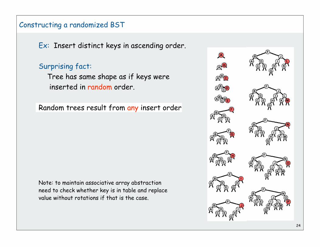
24
Constructing a randomized BST
Ex: Insert distinct keys in ascending order.
Surprising fact:
Tree has same shape as if keys were
inserted in random order.
Random trees result from any insert order
Note: to maintain associative array abstractionneed to check whether key is in table and replacevalue without rotations if that is the case.

25
Randomized BST
Property. Randomized BSTs have the same distribution as BSTs under
random insertion order, no matter in what order keys are inserted.
• Expected height is ~6.22 lg N
• Average search cost is ~1.38 lg N.
• Exponentially small chance of bad balance.
Implementation cost. Need to maintain subtree size in each node.

Summary of symbol-table implementations
Randomized BSTs provide the desired guarantee
Bonus (next): Randomized BSTs also support delete (!)26
implementationguarantee average case ordered
iteration?operations
on keyssearch insert search insert
unordered array N N N/2 N/2 no equals()
ordered array lg N N lg N N/2 yes compareTo()
unordered list N N N/2 N no equals()
ordered list N N N/2 N/2 yes compareTo()
BST N N 1.38 lg N 1.38 lg N yes compareTo()
randomized BST 7 lg N 7 lg N 1.38 lg N 1.38 lg N yes compareTo()
probabilistic, withexponentially small
chance of quadratic time

27
basic implementationsrandomized BSTsdeletion in BSTs

28
BST delete: lazy approach
To remove a node with a given key
• set its value to null
• leave key in tree to guide searches
[but do not consider it equal to any search key]
Cost. O(log N') per insert, search, and delete, where N' is the number
of elements ever inserted in the BST.
Unsatisfactory solution: Can get overloaded with tombstones.
E
SA
C
H R
I
N
E
SA
C
H R
I
N
remove I a “tombstone”

29
BST delete: first approach
To remove a node from a BST. [Hibbard, 1960s]
• Zero children: just remove it.
• One child: pass the child up.
• Two children: find the next largest node using right-left*
swap with next largest
remove as above.
Unsatisfactory solution. Not symmetric, code is clumsy.
Surprising consequence. Trees not random (!) sqrt(N) per op.
Longstanding open problem: simple and efficient delete for BSTs
zero children one child two children

Deletion in randomized BSTs
To delete a node containing a given key
• remove the node
• join the two remaining subtrees to make a tree
Ex. Delete S in
30
E
SA
C
H R
I
N
X

Deletion in randomized BSTs
To delete a node containing a given key
• remove the node
• join its two subtrees
Ex. Delete S in
31
E
A
C
H R
I
N
X
join thesetwo subtrees
private Node remove(Node x, Key key)
{
if (x == null)
return new Node(key, val);
int cmp = key.compareTo(x.key);
if (cmp == 0)
return join(x.left, x.right);
else if (cmp < 0)
x.left = remove(x.left, key);
else if (cmp > 0)
x.right = remove(x.right, key);
return x;
}

Join in randomized BSTs
To join two subtrees with all keys in one less than all keys in the other
• maintain counts of nodes in subtrees (L and R)
• with probability L/(L+R)
make the root of the left the root
make its left subtree the left subtree of the root
join its right subtree to R to make the right subtree of the root
• with probability L/(L+R) do the symmetric moves on the right
32
H R
I
N
X
to join thesetwo subtrees
H
R
N
X
make I the rootwith probability 4/5
I need to join thesetwo subtrees

Join in randomized BSTs
To join two subtrees with all keys in one less than all keys in the other
• maintain counts of nodes in subtrees (L and R)
• with probability L/(L+R)
make the root of the left the root
make its left subtree the left subtree of the root
join its right subtree to R to make the right subtree of the root
• with probability L/(L+R) do the symmetric moves on the right
33X
to join thesetwo subtrees
R
N
X
make R the rootwith probability 2/3
R
N
private Node join(Node a, Node b)
{
if (a == null) return a;
if (b == null) return b;
int cmp = key.compareTo(x.key);
if (StdRandom.bernoulli((double)*a.N / (a.N + b.N))
{ a.right = join(a.right, b); return a; }
else
{ b.left = join(a, b.left ); return b; }
}

Deletion in randomized BSTs
To delete a node containing a given key
• remove the node
• join its two subtrees
Ex. Delete S in
Theorem. Tree still random after delete (!)
Bottom line. Logarithmic guarantee for search/insert/delete34
E
SA
C
H R
I
N
X
E
X
A
C H R
I
N

Summary of symbol-table implementations
Randomized BSTs provide the desired guarantees
Next lecture: Can we do better?35
implementationguarantee average case ordered
iteration?search insert delete search insert delete
unordered array N N N N/2 N/2 N/2 no
ordered array lg N N N lg N N/2 N/2 yes
unordered list N N N N/2 N N/2 no
ordered list N N N N/2 N/2 N/2 yes
BST N N N 1.38 lg N 1.38 lg N ? yes
randomized BST 7 lg N 7 lg N 7 lg N 1.38 lg N 1.38 lg N 1.38 lg N yes
probabilistic, withexponentially small
chance of error

1
Balanced Trees
2-3-4 treesred-black treesB-trees
References:
Algorithms in Java, Chapter 13 http://www.cs.princeton.edu/introalgsds/44balanced
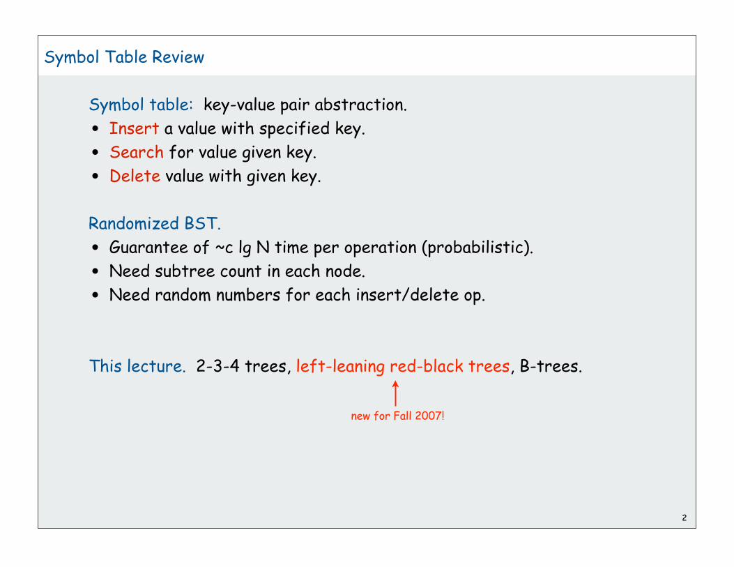
2
Symbol Table Review
Symbol table: key-value pair abstraction.
• Insert a value with specified key.
• Search for value given key.
• Delete value with given key.
Randomized BST.
• Guarantee of ~c lg N time per operation (probabilistic).
• Need subtree count in each node.
• Need random numbers for each insert/delete op.
This lecture. 2-3-4 trees, left-leaning red-black trees, B-trees.
new for Fall 2007!

Summary of symbol-table implementations
Randomized BSTs provide the desired guarantees
This lecture: Can we do better?3
implementationguarantee average case ordered
iteration?search insert delete search insert delete
unordered array N N N N/2 N/2 N/2 no
ordered array lg N N N lg N N/2 N/2 yes
unordered list N N N N/2 N N/2 no
ordered list N N N N/2 N/2 N/2 yes
BST N N N 1.39 lg N 1.39 lg N ? yes
randomized BST 7 lg N 7 lg N 7 lg N 1.39 lg N 1.39 lg N 1.39 lg N yes
probabilistic, withexponentially small
chance of quadratic time

Typical random BSTs
4
N = 250 lg N 81.39 lg N 11
average node depth

5
2-3-4 treesred-black treesB-trees

6
2-3-4 Tree
2-3-4 tree. Generalize node to allow multiple keys; keep tree balanced.
Perfect balance. Every path from root to leaf has same length.
Allow 1, 2, or 3 keys per node.
• 2-node: one key, two children.
• 3-node: two keys, three children.
• 4-node: three keys, four children.
S VF G J
K R
C E M O W
A D L N Q Y Z
smaller than K larger than R
betweenK and R

Search.
• Compare search key against keys in node.
• Find interval containing search key.
• Follow associated link (recursively).
Ex. Search for L
7
Searching in a 2-3-4 Tree
S VF G J
K R
C E M O W
A D L N Q Y Z
found L
smaller than M
betweenK and R

8
Insertion in a 2-3-4 Tree
Insert.
• Search to bottom for key.
Ex. Insert B
S VF G J
K R
C E M O W
A D L N Q Y Z
smaller than K
B not found
smaller than C

9
Insertion in a 2-3-4 Tree
Insert.
• Search to bottom for key.
• 2-node at bottom: convert to 3-node.
Ex. Insert B
S VF G J
K R
C E M O W
D L N Q Y Z
smaller than K
B fits here
smaller than C
A B

Insert.
• Search to bottom for key.
Ex. Insert X
10
Insertion in a 2-3-4 Tree
S VF G J
K R
C E M O W
A D L N Q Y Z
X not found
larger than R
larger than W
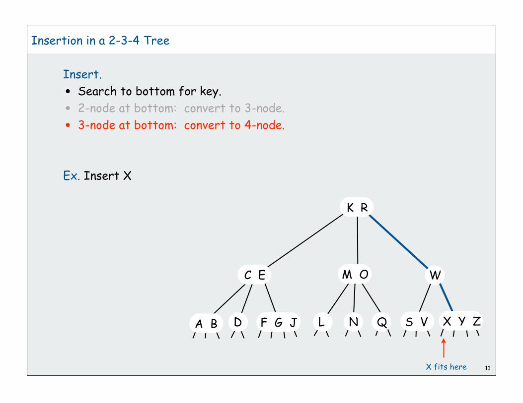
11
Insertion in a 2-3-4 Tree
Insert.
• Search to bottom for key.
• 2-node at bottom: convert to 3-node.
• 3-node at bottom: convert to 4-node.
Ex. Insert X
S VF G J
K R
C E M O W
D L N Q
X fits here
A B X Y Z

Insert.
• Search to bottom for key.
Ex. Insert H
12
Insertion in a 2-3-4 Tree
S VF G J
K R
C E M O W
A D L N Q Y Z
smaller than K
larger than E
H not found

13
Insertion in a 2-3-4 Tree
Insert.
• Search to bottom for key.
• 2-node at bottom: convert to 3-node.
• 3-node at bottom: convert to 4-node.
• 4-node at bottom: ??
Ex. Insert H
S VF G J
K R
C E M O W
D L N Q
H does not fit here!
A B X Y Z

Idea: split the 4-node to make room
Problem: Doesn’t work if parent is a 4-node
Solution 1: Split the parent (and continue splitting up while necessary).
Solution 2: Split 4-nodes on the way down.14
Splitting a 4-node in a 2-3-4 tree
F G J
C E
D
H does not fit here
A BD
H does fit here!
A B
C E G
F J
DA B
C E G
F H J
move middlekey to parent
split remainderinto two 2-nodes

15
Splitting 4-nodes in a 2-3-4 tree
Idea: split 4-nodes on the way down the tree.
• Ensures that most recently seen node is not a 4-node.
• Transformations to split 4-nodes:
Invariant. Current node is not a 4-node.
Consequences
• 4-node below a 4-node case never happens
• insertion at bottom node is easy since it's not a 4-node.
local transformationsthat work anywhere
in the tree

16
Splitting a 4-node below a 2-node in a 2-3-4 tree
A local transformation that works anywhere in the tree
A-C
E-J L-P R-V X-Z
A-C
E-J L-P R-V X-Z
K Q W
D QD
K W
could be huge unchanged
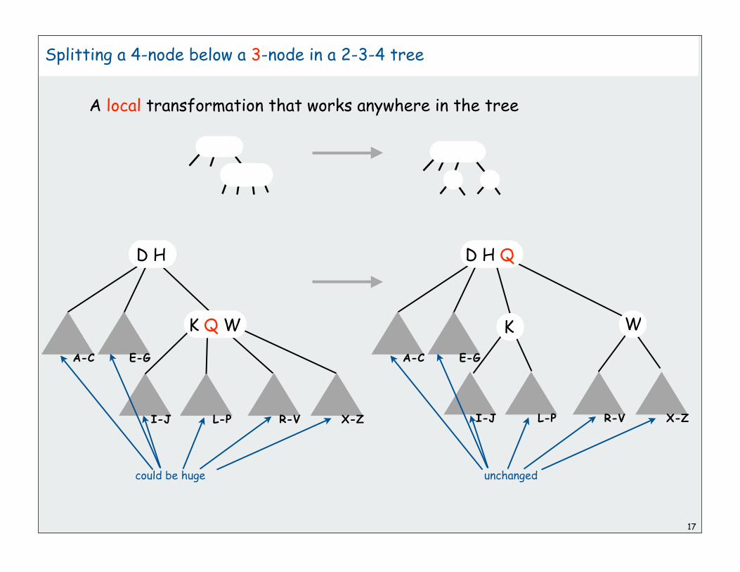
17
A-C
I-J L-P R-V X-Z I-J L-P R-V X-Z
K Q W K W
could be huge unchanged
E-G
D H
A-C E-G
D H Q
Splitting a 4-node below a 3-node in a 2-3-4 tree
A local transformation that works anywhere in the tree
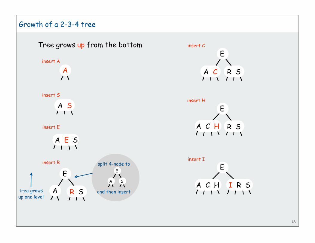
Growth of a 2-3-4 tree
Tree grows up from the bottom
18
A E S
A
A S
insert A
insert S
insert E
insert R
E
A R S
E
A S
split 4-node to
and then insert
insert C
E
R SA C
insert H
E
R S
tree growsup one level
A C H
insert I
E
A C H I R S

Growth of a 2-3-4 tree (continued)
Tree grows up from the bottom
19
split 4-node to
and then insert
tree growsup one level
E
A C H I R S
A C H
E R
I S
SI N
E R
split 4-node to
and then insert
SI N
split 4-node to
and then insert
E C R
A H
E C R
A G H
C
E R
I NA G H
C
E R
S X

20
Balance in 2-3-4 trees
Key property: All paths from root to leaf have same length.
Tree height.
• Worst case: lg N [all 2-nodes]
• Best case: log4 N = 1/2 lg N [all 4-nodes]
• Between 10 and 20 for a million nodes.
• Between 15 and 30 for a billion nodes.

21
2-3-4 Tree: Implementation?
Direct implementation is complicated, because:
• Maintaining multiple node types is cumbersome.
• Implementation of getChild() involves multiple compares.
• Large number of cases for split(), make3Node(), and make4Node().
Bottom line: could do it, but stay tuned for an easier way.
fantasy code
private void insert(Key key, Val val){ Node x = root; while (x.getChild(key) != null) { x = x.getChild(key); if (x.is4Node()) x.split(); } if (x.is2Node()) x.make3Node(key, val); else if (x.is3Node()) x.make4Node(key, val);}

Summary of symbol-table implementations
22
implementationguarantee average case ordered
iteration?search insert delete search insert delete
unordered array N N N N/2 N/2 N/2 no
ordered array lg N N N lg N N/2 N/2 yes
unordered list N N N N/2 N N/2 no
ordered list N N N N/2 N/2 N/2 yes
BST N N N 1.38 lg N 1.38 lg N ? yes
randomized BST 7 lg N 7 lg N 7 lg N 1.38 lg N 1.38 lg N 1.38 lg N yes
2-3-4 tree c lg N c lg N c lg N c lg N yes
constants depend uponimplementation

23
2-3-4 treesred-black treesB-trees
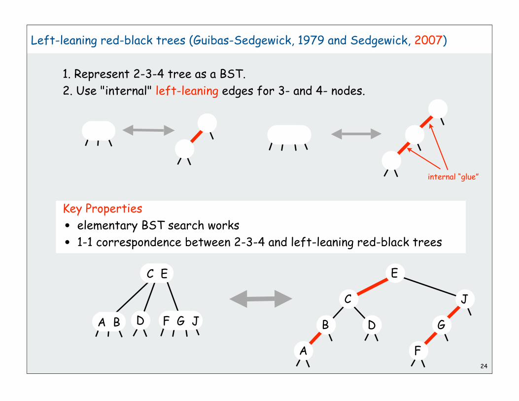
24
Left-leaning red-black trees (Guibas-Sedgewick, 1979 and Sedgewick, 2007)
1. Represent 2-3-4 tree as a BST.
2. Use "internal" left-leaning edges for 3- and 4- nodes.
Key Properties
• elementary BST search works
• 1-1 correspondence between 2-3-4 and left-leaning red-black trees
F G J
C E
D
internal “glue”
A B
A
B
C
D
E
F
G
J

25
Left-leaning red-black trees
1. Represent 2-3-4 tree as a BST.
2. Use "internal" left-leaning edges for 3- and 4- nodes.
Disallowed:
• right-leaning red edges
• three red edges in a row
standard red-black treesallow these two

Search implementation for red-black trees
Search code is the same as elementary BST (ignores the color)
[runs faster because of better balance in tree]
Note: iterator code is also the same.
26
public Val get(Key key)
{ Node x = root;
while (x != null) { int cmp = key.compareTo(x.key);
if (cmp == 0) return x.val; else if (cmp < 0) x = x.left;
else if (cmp > 0) x = x.right; } return null;
}
A
B
C
D
E
F
G
J

Insert implementation for red-black trees (skeleton)
27
public class BST<Key extends Comparable<Key>, Value>
implements Iterable<Key>
{
private static final boolean RED = true;
private static final boolean BLACK = false;
private Node root;
private class Node
{
Key key;
Value val;
Node left, right;
boolean color;
Node(Key key, Value val, boolean color)
{
this.key = key;
this.val = val;
this.color = color;
}
}
public void put(Key key, Value val)
{
root = put(root, key, val);
root.color = BLACK;
}
}
color of incoming link
private boolean isRed(Node x)
{
if (x == null) return false;
return (x.color == RED);
}
helper method to test node color

Basic idea: maintain 1-1 correspondence with 2-3-4 trees
1. If key found on recursive search reset value, as usual
2. If key not found insert a new red node at the bottom
3. Split 4-nodes on the way DOWN the tree.
Insert implementation for left-leaning red-black trees (strategy)
28
[stay tuned]
[stay tuned]
[stay tuned]
[stay tuned]

Inserting a new node at the bottom in a LLRB tree
Maintain 1-1 correspondence with 2-3-4 trees
1. Add new node as usual, with red link to glue it to node above
2. Rotate left if necessary to make link lean left
29
or
or or
OK
rotateleft
rotateleft
rotateleft
OK

30
Splitting a 4-node below a 2-node in a left-leaning red-black tree
Maintain correspondence with 2-3-4 trees
A-C
E-J L-P R-V X-Z
A-C
E-J L-P R-V X-Z
D
K
W
could be huge unchanged
K
Q
W D
Q
left rotate(if necessary)
to make red linklean left
also makethis black
right rotate andswitch colors to
attach middle nodeto node above
b
c
d
b
c
d eb
d
ce

a
31
Splitting a 4-node below a 3-node in a left-leaning red-black tree
A-C
I-J L-P R-V X-Z I-J L-P R-V X-Z
K W
could be huge unchanged
E-G A-C E-G
Maintain correspondence with 2-3-4 trees
also makethis black
b
c
d
eb
c
deb
d
ce
a
a
left rotate(if necessary)
to make red linklean left
right rotate andswitch colors to
attach middle nodeto node above
K
Q
WD
H
HQ
D

a
32
Splitting 4-nodes a left-leaning red-black tree
The two transformations are the same
leftrotate
(if necessary)
also makethis black
rightrotate
b
c
d
eb
c
deb
d
ce
a
leftrotate
(if necessary)right
rotate
b
c
d
e b
c
d eb
d
ce
a
also makethis black

Insert implementation for left-leaning red-black trees (strategy revisited)
Basic idea: maintain 1-1 correspondence with 2-3-4 trees
Search as usual
• if key found reset value, as usual
• if key not found insert a new red node at the bottom
[might be right-leaning red link]
Split 4-nodes on the way DOWN the tree.
• right-rotate and flip color
• might leave right-leaning link higher up in the tree
NEW TRICK: enforce left-leaning condition on the way UP the tree.
• left-rotate any right-leaning link on search path
• trivial with recursion (do it after recursive calls)
• no other right-leaning links elsewhere
Note: nonrecursive top-down implementation possible, but requireskeeping track of great-grandparent on search path (!) and lots of cases.
33
or

Insert implementation for left-leaning red-black trees (basic operations)
Insert a new node at bottom
Split a 4-node
Enforce left-leaning condition
34
rightrotate
fixcolor
or
leftrotate
Key point: may leaveright-leaning linkto be fixed later

Insert implementation for left-leaning red-black trees (code for basic operations)
Insert a new node at bottom
Split a 4-node
Enforce left-leaning condition
35
right
rotate
fix color of
left node
or
left
rotate
private Node splitFourNode(Node h)
{
x = rotR(h);
x.left.color = BLACK;
return x;
}
private Node leanLeft(Node h)
{
x = rotL(h);
x.color = x.left.color;
x.left.color = RED;
return x;
}
if (h == null)
return new Node(key, value, RED);
could be
red or black
h x
hx
could be
left or right
middle node
is red

Insert implementation for left-leaning red-black trees (code)
36
private Node insert(Node h, Key key, Value val) { if (h == null) return new Node(key, val, RED);
if (isRed(h.left)) if (isRed(h.left.left)) h = splitFourNode(h);
int cmp = key.compareTo(h.key); if (cmp == 0) h.val = val; else if (cmp < 0) h.left = insert(h.left, key, val); else h.right = insert(h.right, key, val);
if (isRed(h.right)) h = leanLeft(h);
return h; }
insert new node at bottom
split 4-nodes on the way down
search
enforce left-leaning conditionon the way back up

37
Balance in left-leaning red-black trees
Proposition A. Every path from root to leaf has same number of black links.
Proposition B. Never three red links in-a-row.
Proposition C. Height of tree is less than 3 lg N + 2 in the worst case.
Property D. Height of tree is ~lg N in typical applications.
Property E. Nearly all 4-nodes are on the bottom in the typical applications.

Why left-leaning trees?
38
private Node insert(Node x, Key key, Value val, boolean sw){ if (x == null) return new Node(key, value, RED); int cmp = key.compareTo(x.key);
if (isRed(x.left) && isRed(x.right)) { x.color = RED; x.left.color = BLACK; x.right.color = BLACK; } if (cmp == 0) x.val = val; else if (cmp < 0)) { x.left = insert(x.left, key, val, false); if (isRed(x) && isRed(x.left) && sw) x = rotR(x); if (isRed(x.left) && isRed(x.left.left)) { x = rotR(x); x.color = BLACK; x.right.color = RED; } } else // if (cmp > 0) { x.right = insert(x.right, key, val, true); if (isRed(h) && isRed(x.right) && !sw) x = rotL(x); if (isRed(h.right) && isRed(h.right.right)) { x = rotL(x); x.color = BLACK; x.left.color = RED; } } return x;}
private Node insert(Node h, Key key, Value val){ int cmp = key.compareTo(h.key); if (h == null) return new Node(key, val, RED); if (isRed(h.left)) if (isRed(h.left.left)) { h = rotR(h); h.left.color = BLACK; } if (cmp == 0) x.val = val; else if (cmp < 0) h.left = insert(h.left, key, val); else h.right = insert(h.right, key, val); if (isRed(h.right)) { h = rotL(h); h.color = h.left.color; h.left.color = RED; } return h;}
old code (that students had to learn in the past) new code (that you have to learn)
extremely tricky
straightforward (if you’ve paid attention)
Take your pick:

Why left-leaning trees?
39
Simplified code
• left-leaning restriction reduces number of cases
• recursion gives two (easy) chances to fix each node
• short inner loop
Same ideas simplify implementation of other operations
• delete min
• delete max
• delete
Built on the shoulders of many, many old balanced tree algorithms
• AVL trees
• 2-3 trees
• 2-3-4 trees
• skip lists
Bottom line: Left-leaning red-black trees are the simplest to implement
and at least as efficient
old
new

Summary of symbol-table implementations
40
implementationguarantee average case ordered
iteration?search insert delete search insert delete
unordered array N N N N/2 N/2 N/2 no
ordered array lg N N N lg N N/2 N/2 yes
unordered list N N N N/2 N N/2 no
ordered list N N N N/2 N/2 N/2 yes
BST N N N 1.38 lg N 1.38 lg N ? yes
randomized BST 7 lg N 7 lg N 7 lg N 1.38 lg N 1.38 lg N 1.38 lg N yes
2-3-4 tree c lg N c lg N c lg N c lg N yes
red-black tree 3 lg N 3 lg N 3 lg N lg N lg N lg N yes
exact value of coefficient unknownbut extremely close to 1

Typical random left-leaning red-black trees
41
N = 500
lg N 9
average node depth

42
2-3-4 treesred-black treesB-trees

43
B-trees (Bayer-McCreight, 1972)
B-Tree. Generalizes 2-3-4 trees by allowing up to M links per node.
Main application: file systems.
• Reading a page into memory from disk is expensive.
• Accessing info on a page in memory is free.
• Goal: minimize # page accesses.
• Node size M = page size.
Space-time tradeoff.
• M large only a few levels in tree.
• M small less wasted space.
• Typical M = 1000, N < 1 trillion.
Bottom line. Number of page accesses is logMN per op.
in practice: 3 or 4 (!)

44
B-Tree Example
M = 5
no roomfor 275
no roomfor 737

45
B-Tree Example (cont)
no roomfor 526

Summary of symbol-table implementations
46
implementationguarantee average case ordered
iteration?search insert delete search insert delete
unordered array N N N N/2 N/2 N/2 no
ordered array lg N N N lg N N/2 N/2 yes
unordered list N N N N/2 N N/2 no
ordered list N N N N/2 N/2 N/2 yes
BST N N N 1.44 lg N 1.44 lg N ? yes
randomized BST 7 lg N 7 lg N 7 lg N 1.44 lg N 1.44 lg N 1.44 lg N yes
2-3-4 tree c lg N c lg N c lg N c lg N yes
red-black tree 2 lg N 2 lg N 2 lg N lg N lg N lg N yes
B-tree 1 1 1 1 1 1 yes
B-Tree. Number of page accesses is logMN per op.

47
Balanced trees in the wild
Red-black trees: widely used as system symbol tables
• Java: java.util.TreeMap, java.util.TreeSet.
• C++ STL: map, multimap, multiset.
• Linux kernel: linux/rbtree.h.
B-Trees: widely used for file systems and databases
• Windows: HPFS.
• Mac: HFS, HFS+.
• Linux: ReiserFS, XFS, Ext3FS, JFS.
• Databases: ORACLE, DB2, INGRES, SQL, PostgreSQL
Bottom line: ST implementation with lg N guarantee for all ops.
• Algorithms are variations on a theme: rotations when inserting.
• Easiest to implement, optimal, fastest in practice: LLRB trees
• Abstraction extends to give search algorithms for huge files: B-trees
After the break: Can we do better??
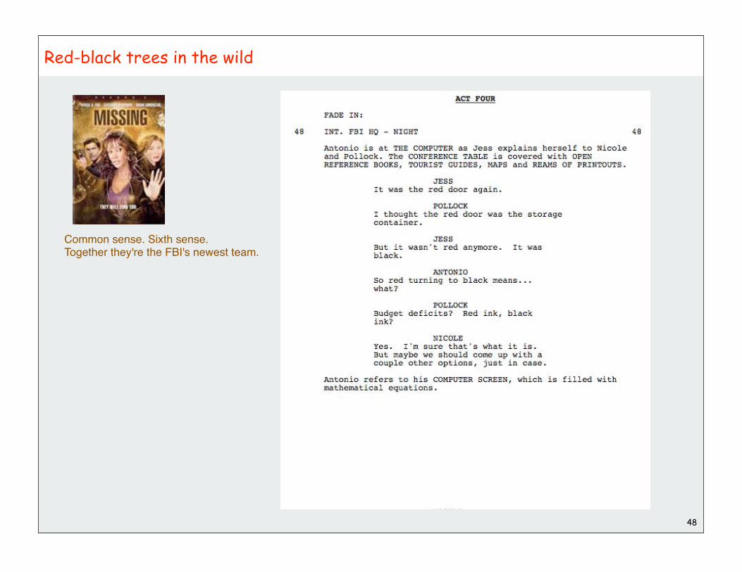
Red-black trees in the wild
48
Common sense. Sixth sense.Together they're the FBI's newest team.

Red-black trees in the wild
49
!!
Common sense. Sixth sense.Together they're the FBI's newest team.
red-black tree

Red-black trees in the wild
50
!!
Common sense. Sixth sense.Together they're the FBI's newest team.
red-black tree

1
Hashing
hash functionscollision resolutionapplications
References:
Algorithms in Java, Chapter 14 http://www.cs.princeton.edu/introalgsds/42hash

Summary of symbol-table implementations
Can we do better?2
implementationguarantee average case ordered
iteration?search insert delete search insert delete
unordered array N N N N/2 N/2 N/2 no
ordered array lg N N N lg N N/2 N/2 yes
unordered list N N N N/2 N N/2 no
ordered list N N N N/2 N/2 N/2 yes
BST N N N 1.39 lg N 1.39 lg N ? yes
randomized BST 7 lg N 7 lg N 7 lg N 1.39 lg N 1.39 lg N 1.39 lg N yes
red-black tree 3 lg N 3 lg N 3 lg N lg N lg N lg N yes

3
Optimize Judiciously
Reference: Effective Java by Joshua Bloch.
More computing sins are committed in the name of efficiency
(without necessarily achieving it) than for any other single reason -
including blind stupidity. - William A. Wulf
We should forget about small efficiencies, say about 97% of the time:
premature optimization is the root of all evil. - Donald E. Knuth
We follow two rules in the matter of optimization:
Rule 1: Don't do it.
Rule 2 (for experts only). Don't do it yet - that is, not until
you have a perfectly clear and unoptimized solution.
- M. A. Jackson
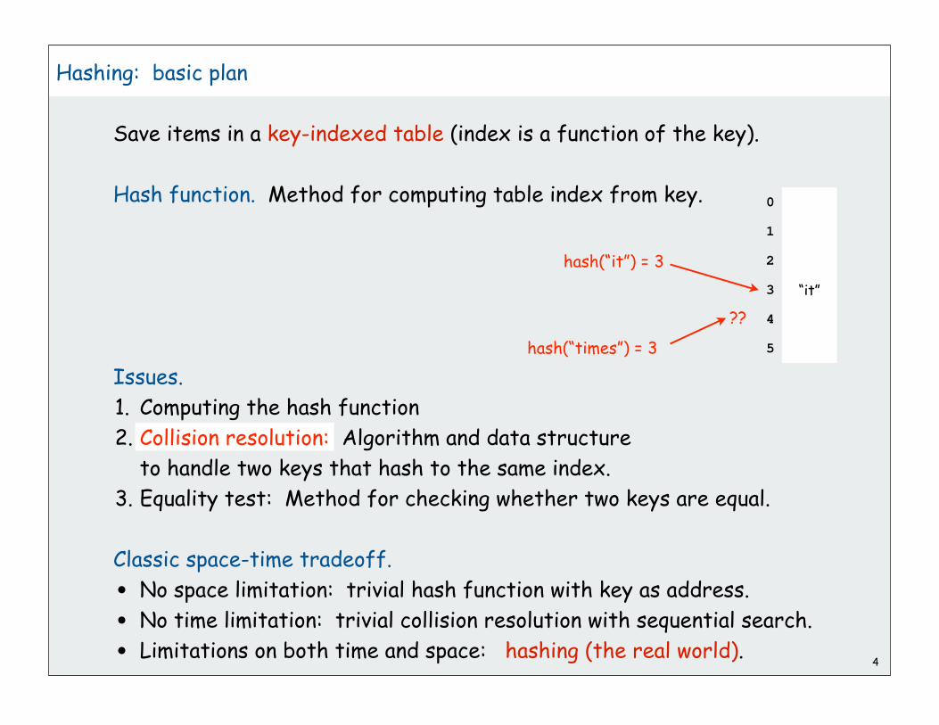
4
Hashing: basic plan
Save items in a key-indexed table (index is a function of the key).
Hash function. Method for computing table index from key.
Issues.
1. Computing the hash function
2. Collision resolution: Algorithm and data structure
to handle two keys that hash to the same index.
3. Equality test: Method for checking whether two keys are equal.
Classic space-time tradeoff.
• No space limitation: trivial hash function with key as address.
• No time limitation: trivial collision resolution with sequential search.
• Limitations on both time and space: hashing (the real world).
0
1
2
3 “it”
4
5
hash(“it”) = 3
hash(“times”) = 3
??

5
hash functionscollision resolutionapplications

6
Computing the hash function
Idealistic goal: scramble the keys uniformly.
• Efficiently computable.
• Each table position equally likely for each key.
Practical challenge: need different approach for each type of key
Ex: Social Security numbers.
• Bad: first three digits.
• Better: last three digits.
Ex: date of birth.
• Bad: birth year.
• Better: birthday.
Ex: phone numbers.
• Bad: first three digits.
• Better: last three digits.
573 = California, 574 = Alaska
assigned in chronological order within a given geographic region
thoroughly researched problem,still problematic in practical applications

7
Hash Codes and Hash Functions
Java convention: all classes implement hashCode()
hashcode() returns a 32-bit int (between -2147483648 and 2147483647)
Hash function. An int between 0 and M-1 (for use as an array index)
First try:
Bug. Don't use (code % M) as array index
1-in-a billion bug. Don't use (Math.abs(code) % M) as array index.
OK. Safe to use ((code & 0x7fffffff) % M) as array index.
String s = "call";int code = s.hashCode();int hash = code % M;
7121 8191
hex literal 31-bit mask
3045982

8
Java’s hashCode() convention
Theoretical advantages
• Ensures hashing can be used for every type of object
• Allows expert implementations suited to each type
Requirements:
• If x.equals(y) then x and y must have the same hash code.
• Repeated calls to x.hashCode() must return the same value.
Practical realities
• True randomness is hard to achieve
• Cost is an important consideration
Available implementations
• default (inherited from Object): Memory address of x ( ! ! ! )
• customized Java implementations: String, URL, Integer, Date.
• User-defined types: users are on their own
x.hashCode()
x
y.hashCode()
y
that’s you!

9
A typical type
Assumption when using hashing in Java:
Key type has reasonable implementation of hashCode() and equals()
Ex. Phone numbers: (609) 867-5309.
Fundamental problem:
Need a theorem for each data type to ensure reliability.
sufficiently random?
exchange extension
public final class PhoneNumber{ private final int area, exch, ext; public PhoneNumber(int area, int exch, int ext) { this.area = area; this.exch = exch; this.ext = ext; } public boolean equals(Object y) { // as before } public int hashCode() { return 10007 * (area + 1009 * exch) + ext; }}

10
A decent hash code design
Java 1.5 string library [see also Program 14.2 in Algs in Java].
• Equivalent to h = 31L-1 s0 + … + 312 sL-3 + 31 sL-2 + sL-1.
• Horner's method to hash string of length L: L multiplies/adds
Ex.
Provably random? Well, no.
String s = "call";int code = s.hashCode();
3045982 = 99 313 + 97 312 + 108 311 + 108 310
= 108 + 31 (108 + 31 (99 + 31 (97)))
ith character of s
Unicodechar
… …
'a' 97
'b' 98
'c' 99
… …
public int hashCode(){ int hash = 0; for (int i = 0; i < length(); i++) hash = s[i] + (31 * hash); return hash;}

11
A poor hash code design
Java 1.1 string library.
• For long strings: only examines 8-9 evenly spaced characters.
• Saves time in performing arithmetic…
but great potential for bad collision patterns.
Basic rule: need to use the whole key.
http://www.cs.princeton.edu/introcs/13loop/Hello.java
http://www.cs.princeton.edu/introcs/13loop/Hello.class
http://www.cs.princeton.edu/introcs/13loop/Hello.html
http://www.cs.princeton.edu/introcs/13loop/index.html
http://www.cs.princeton.edu/introcs/12type/index.html
public int hashCode(){ int hash = 0; int skip = Math.max(1, length() / 8); for (int i = 0; i < length(); i += skip) hash = (37 * hash) + s[i]; return hash;}

Digression: using a hash function for data mining
Use content to characterize documents.
Applications
• Search documents on the web for documents similar to a given one.
• Determine whether a new document belongs in one set or another
Approach
• Fix order k and dimension d
• Compute hashCode() % d for all
k-grams in the document
• Result: d-dimensional vector
profile of each document
• To compare documents:
Consider angle θ separating vectors
cos θ close to 0: not similar
cos θ close to 1: similar
12
cos θ = a b /
|a||b|
ab
θ

Digression: using a hash function for data mining
13
tale.txt genome.txt
i10-grams with
hashcode() ifreq
10-grams with
hashcode() ifreq
0 0 0
1 0 0
2 0 0
435best of ti
foolishnes2
TTTCGGTTTG
TGTCTGCTGC2
8999 it was the 8 0
...
12122 0 CTTTCGGTTT 3
...
34543 t was the b 5 ATGCGGTCGA 4
...
65535
65536
% more tale.txt
it was the best of times
it was the worst of times
it was the age of wisdom
it was the age of
foolishness
...
% more genome.txt
CTTTCGGTTTGGAACC
GAAGCCGCGCGTCT
TGTCTGCTGCAGC
ATCGTTC
...
k = 10d = 65536
cos θ small: not similar
profiles
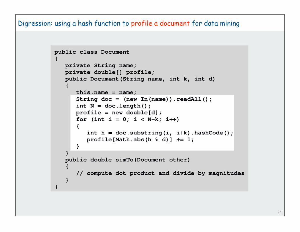
Digression: using a hash function to profile a document for data mining
14
public class Document{ private String name; private double[] profile; public Document(String name, int k, int d) { this.name = name; String doc = (new In(name)).readAll(); int N = doc.length(); profile = new double[d]; for (int i = 0; i < N-k; i++) { int h = doc.substring(i, i+k).hashCode(); profile[Math.abs(h % d)] += 1; } } public double simTo(Document other) { // compute dot product and divide by magnitudes }}

Digression: using a hash function to compare documents
15
public class CompareAll{ public static void main(String args[]) { int k = Integer.parseInt(args[0]); int d = Integer.parseInt(args[1]); int N = StdIn.readInt(); Document[] a = new Document[N]; for (int i = 0; i < N; i++) a[i] = new Document(StdIn.readString(), k, d); System.out.print(" "); for (int j = 0; j < N; j++) System.out.printf(" %.4s", a[j].name()); System.out.println(); for (int i = 0; i < N; i++) { System.out.printf("%.4s ", a[i].name()); for (int j = 0; j < N; j++) System.out.printf("%8.2f", a[i].simTo(a[j])); System.out.println(); } } }

Digression: using a hash function to compare documents
16
% java CompareAll 5 1000 < docs.txt Cons TomS Huck Prej Pict DJIA Amaz ACTGCons 1.00 0.89 0.87 0.88 0.35 0.70 0.63 0.58TomS 0.89 1.00 0.98 0.96 0.34 0.75 0.66 0.62Huck 0.87 0.98 1.00 0.94 0.32 0.74 0.65 0.61Prej 0.88 0.96 0.94 1.00 0.34 0.76 0.67 0.63Pict 0.35 0.34 0.32 0.34 1.00 0.29 0.48 0.24DJIA 0.70 0.75 0.74 0.76 0.29 1.00 0.62 0.58Amaz 0.63 0.66 0.65 0.67 0.48 0.62 1.00 0.45ACTG 0.58 0.62 0.61 0.63 0.24 0.58 0.45 1.00
Cons US Constitution
TomS “Tom Sawyer”
Huck “Huckleberry Finn”
Prej “Pride and Prejudice”
Pict a photograph
DJIA financial data
Amaz Amazon.com website .html source
ACTG genome

17
hash functionscollision resolutionapplications

18
Helpful results from probability theory
Bins and balls. Throw balls uniformly at random into M bins.
Birthday problem.
Expect two balls in the same bin after M / 2 tosses.
Coupon collector.
Expect every bin has 1 ball after (M ln M) tosses.
Load balancing.
After M tosses, expect most loaded bin has (log M / log log M) balls.
0 1 2 3 4 5 6 7 8 9 10 11 12 13 14 15

19
Collisions
Collision. Two distinct keys hashing to same index.
Conclusion. Birthday problem can't avoid collisions unless you have
a ridiculous amount of memory.
Challenge. Deal with collisions efficiently.
Approach 1:
accept multiple collisions
Approach 2:
minimize collisions

20
Collision resolution: two approaches
1. Separate chaining. [H. P. Luhn, IBM 1953]
Put keys that collide in a list associated with index.
2. Open addressing. [Amdahl-Boehme-Rocherster-Samuel, IBM 1953]
When a new key collides, find next empty slot, and put it there.
st[0]
st[1]
st[2]
st[8190]
untravelledst[3] considerating
null
separate chaining (M = 8191, N = 15000)
easy extension of linked list ST implementation
null
null
linear probing (M = 30001, N = 15000)
easy extension of array ST implementation
seriouslyjocularly
listen
suburban
browsing
jocularly
listen
suburban
browsing
st[0]
st[1]
st[2]
st[30001]
st[3]

21
Collision resolution approach 1: separate chaining
Use an array of M < N linked lists.
• Hash: map key to integer i between 0 and M-1.
• Insert: put at front of ith chain (if not already there).
• Search: only need to search ith chain.
3untravelled
3suburban
5017ishmael
0seriously
.. . .
3480
7121
hash
me
call
key
good choice: M N/10
st[0]
st[1]
st[2]
st[8190]
untravelledst[3] considerating
null
seriouslyjocularly
listen
suburban
browsing

Separate chaining ST implementation (skeleton)
22
public class ListHashST<Key, Value>
{
private int M = 8191;
private Node[] st = new Node[M];
private class Node
{
Object key;
Object val;
Node next;
Node(Key key, Value val, Node next)
{
this.key = key;
this.val = val;
this.next = next;
}
}
private int hash(Key key)
{ return (key.hashcode() & 0x7ffffffff) % M; }
public void put(Key key, Value val)
// see next slide
public Val get(Key key) // see next slide}
compare withlinked lists
no generics inarrays in Java
could usedoubling
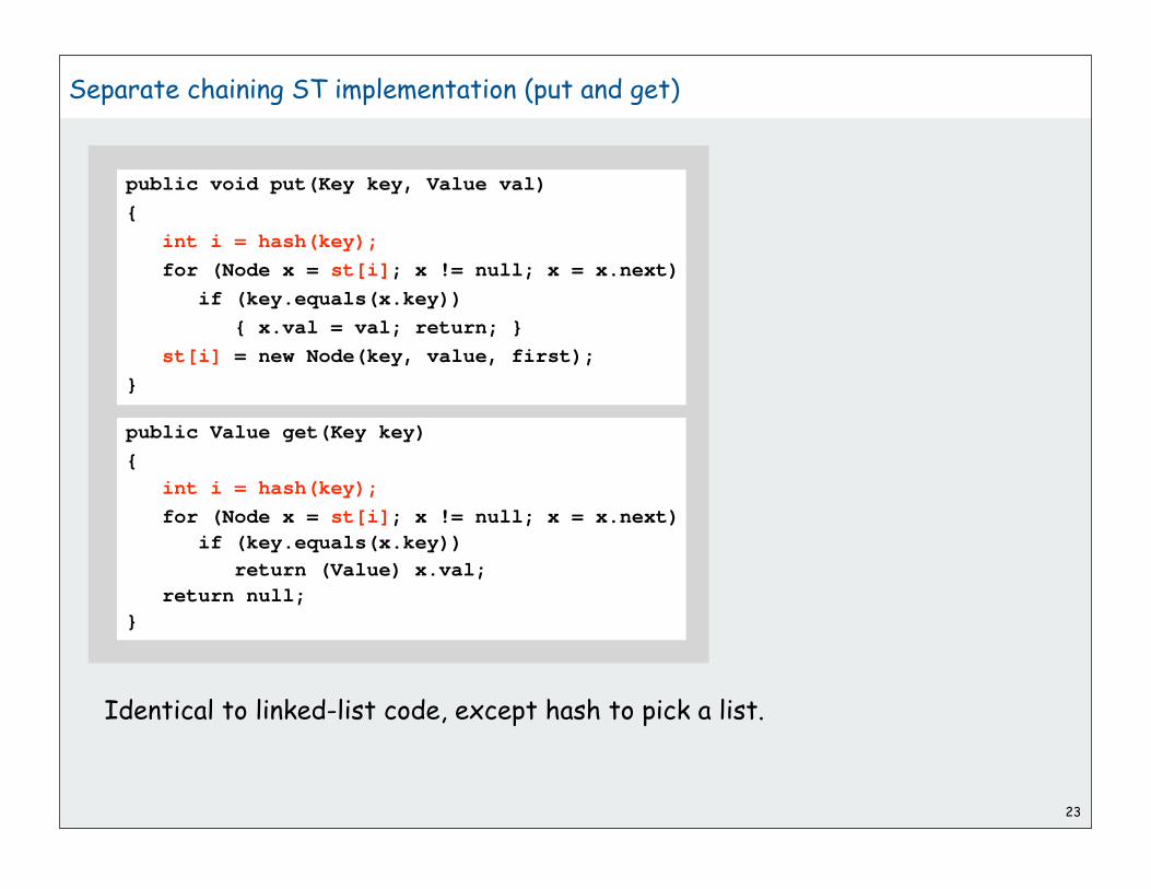
Separate chaining ST implementation (put and get)
23
public void put(Key key, Value val)
{
int i = hash(key);
for (Node x = st[i]; x != null; x = x.next)
if (key.equals(x.key))
{ x.val = val; return; }
st[i] = new Node(key, value, first);
}
public Value get(Key key)
{
int i = hash(key);
for (Node x = st[i]; x != null; x = x.next)
if (key.equals(x.key))
return (Value) x.val;
return null;
}
Identical to linked-list code, except hash to pick a list.

24
Analysis of separate chaining
Separate chaining performance.
• Cost is proportional to length of list.
• Average length = N / M.
• Worst case: all keys hash to same list.
Theorem. Let = N / M > 1 be average length of list. For any t > 1,
probability that list length > t is exponentially small in t.
Parameters.
• M too large too many empty chains.
• M too small chains too long.
• Typical choice: = N / M 10 constant-time ops.
depends on hash map being random map

25
Collision resolution approach 2: open addressing
Use an array of size M >> N.
• Hash: map key to integer i between 0 and M-1.
Linear probing:
• Insert: put in slot i if free; if not try i+1, i+2, etc.
• Search: search slot i; if occupied but no match, try i+1, i+2, etc.
good choice: M 2N
-
0
-
1
-
2
S
3
H
4
-
5
-
6
A
7
C
8
E
9
R
10
-
11
N
12
insert I
hash(I) = 11-
0
-
1
-
2
S
3
H
4
-
5
-
6
A
7
C
8
E
9
R
10
I
11
-
12
insert N
hash(N) = 8-
0
-
1
-
2
S
3
H
4
-
5
-
6
A
7
C
8
E
9
R
10
I
11
N
12

Linear probing ST implementation
26
public class ArrayHashST<Key, Value>
{
private int M = 30001;
private Value[] vals = (Value[]) new Object[maxN];
private Key[] keys = (Key[]) new Object[maxN];
privat int hash(Key key) // as before
public void put(Key key, Value val)
{
int i;
for (i = hash(key); keys[i] != null; i = (i+1) % M)
if (key.equals(keys[i]))
break;
vals[i] = val;
keys[i] = key;
}
public Value get(Key key) {
for (int i = hash(key); keys[i] != null; i = (i+1) % M)
if (key.equals(keys[i]))
return vals]i];
return null;
}
}
standard ugly casts
standardarray doublingcode omitted(double when
half full)
compare withelementary
unordered arrayimplementation

27
Clustering
Cluster. A contiguous block of items.
Observation. New keys likely to hash into middle of big clusters.
Knuth's parking problem. Cars arrive at one-way street with M parking
spaces. Each desires a random space i: if space i is taken, try i+1, i+2, …
What is mean displacement of a car?
Empty. With M/2 cars, mean displacement is about 3/2.
Full. Mean displacement for the last car is about M / 2
- - - S H A C E - - - X M I - - - P - - R L - -
cluster

( )
28
Analysis of linear probing
Linear probing performance.
• Insert and search cost depend on length of cluster.
• Average length of cluster = = N / M.
• Worst case: all keys hash to same cluster.
Theorem. [Knuth 1962] Let = N / M < 1 be the load factor.
Parameters.
• Load factor too small too many empty array entries.
• Load factor too large clusters coalesce.
• Typical choice: M 2N constant-time ops.
but keys more likely tohash to big clusters
1
( 1 α )2
1—2 1 + = ( 1 + α + 2α2 + 3α3 + 4α4 + . . . ) /
2
( ) 1
( 1 α )
1—2
1 + = 1 + ( α + α2 + α3 + α4 + . . . ) /2
Average probes for insert/search miss
Average probes for search hit

Hashing: variations on the theme
Many improved versions have been studied:
Ex: Two-probe hashing
• hash to two positions, put key in shorter of the two lists
• reduces average length of the longest list to log log N
Ex: Double hashing
• use linear probing, but skip a variable amount, not just 1 each time
• effectively eliminates clustering
• can allow table to become nearly full
29

30
Double hashing
Idea Avoid clustering by using second hash to compute skip for search.
Hash. Map key to integer i between 0 and M-1.
Second hash. Map key to nonzero skip value k.
Ex: k = 1 + (v mod 97).
Effect. Skip values give different search paths for keys that collide.
Best practices. Make k and M relatively prime.
hashCode()

31
Theorem. [Guibas-Szemerédi] Let = N / M < 1 be average length of list.
Parameters. Typical choice: α 1.2 constant-time ops.
Disadvantage. Delete cumbersome to implement.
Double Hashing Performance
1
( 1 α )
1—α ln = 1 + α/2 + α2 /3 + α3 /4 + α4 /5
+ . . .
Average probes for insert/search miss
Average probes for search hit
1
( 1 α )= 1 + α + α2 + α3 + α4 + . . .

32
Hashing Tradeoffs
Separate chaining vs. linear probing/double hashing.
• Space for links vs. empty table slots.
• Small table + linked allocation vs. big coherent array.
Linear probing vs. double hashing.
load factor
50% 66% 75% 90%
linear probing
get 1.5 2.0 3.0 5.5
put 2.5 5.0 8.5 55.5
doublehashing
get 1.4 1.6 1.8 2.6
put 1.5 2.0 3.0 5.5
number of probes

Summary of symbol-table implementations
33
implementationguarantee average case ordered
iteration?operations
on keyssearch insert delete search insert delete
unordered array N N N N/2 N/2 N/2 no equals()
ordered array lg N N N lg N N/2 N/2 yes compareTo()
unordered list N N N N/2 N N/2 no equals()
ordered list N N N N/2 N/2 N/2 yes compareTo()
BST N N N 1.38 lg N 1.38 lg N ? yes compareTo()
randomized BST 7 lg N 7 lg N 7 lg N 1.38 lg N 1.38 lg N 1.38 lg N yes compareTo()
red-black tree 2 lg N 2 lg N 2 lg N lg N lg N lg N yes compareTo()
hashing 1* 1* 1* 1* 1* 1* noequals()hashCode()
* assumes random hash code

Hashing versus balanced trees
Hashing
• simpler to code
• no effective alternative for unordered keys
• faster for simple keys (a few arithmetic ops versus lg N compares)
• (Java) better system support for strings [cached hashcode]
• does your hash function produce random values for your key type??
Balanced trees
• stronger performance guarantee
• can support many more operations for ordered keys
• easier to implement compareTo() correctly than equals() and hashCode()
Java system includes both
• red-black trees: java.util.TreeMap, java.util.TreeSet
• hashing: java.util.HashMap, java.util.IdentityHashMap
34

Typical “full” ST API
Hashing is not suitable for implementing such an API (no order)
BSTs are easy to extend to support such an API (basic tree ops)
Ex: Can use LLRB trees implement priority queues for distinct keys35
public class *ST<Key extends Comparable<Key>, Value>
*ST() create a symbol table
void put(Key key, Value val) put key-value pair into the table
Value get(Key key)return value paired with key(null if key is not in table)
boolean contains(Key key) is there a value paired with key?
Key min() smallest key
Key max() largest key
Key next(Key key) next largest key (null if key is max)
Key prev(Key key) next smallest key (null if key is min)
void remove(Key key) remove key-value pair from table
Iterator<Key> iterator() iterator through keys in table

36
hash functionscollision resolutionapplications

37
Set ADT
Set. Collection of distinct keys.
Normal mathematical assumption: collection is unordered
Typical (eventual) client expectation: ordered iteration
Q. How to implement?
A0. Hashing (our ST code [value removed] or java.util.HashSet)
A1. Red-black BST (our ST code [value removed] or java.util.TreeSet)
public class *SET<Key extends Comparable<Key>, Value>
SET() create a set
void add(Key key) put key into the set
boolean contains(Key key) is there a value paired with key?
void remove(Key key) remove key from the set
Iterator<Key> iterator() iterator through all keys in the set
unordered iteratorO(1) search
ordered iteratorO(log N) search

38
SET client example 1: dedup filter
Remove duplicates from strings in standard input
• Read a key.
• If key is not in set, insert and print it.
Simplified version of FrequencyCount (no iterator needed)
public class DeDup{ public static void main(String[] args) { SET<String> set = new SET<String>(); while (!StdIn.isEmpty()) { String key = StdIn.readString(); if (!set.contains(key)) { set.add(key); StdOut.println(key); } } }}
% more tale.txt
it was the best of times
it was the worst of times
it was the age of wisdom
it was the age of
foolishness
...
% java Dedup < tale.txt
it
was
the
best
of
times
worst
age
wisdom
foolishness
...
No iterator needed.Output is in same order
as input withdups removed.

Print words from standard input that are found in a list
• Read in a list of words from one file.
• Print out all words from standard input that are in the list.
39
SET client example 2A: lookup filter
public class LookupFilter{ public static void main(String[] args) { SET<String> set = new SET<String>();
In in = new In(args[0]); while (!in.isEmpty()) set.add(in.readString());
while (!StdIn.isEmpty()) { String word = StdIn.readString(); if (set.contains(word)) StdOut.println(word); } }}
process list
create SET
print words thatare not in list

Print words from standard input that are not found in a list
• Read in a list of words from one file.
• Print out all words from standard input that are not in the list.
40
SET client example 2B: exception filter
public class LookupFilter{ public static void main(String[] args) { SET<String> set = new SET<String>();
In in = new In(args[0]); while (!in.isEmpty()) set.add(in.readString());
while (!StdIn.isEmpty()) { String word = StdIn.readString(); if (!set.contains(word)) StdOut.println(word); } }}
process list
create SET
print words thatare not in list

41
SET filter applications
application purpose key type in list not in list
dedup eliminate duplicates dedup duplicates unique keys
spell checker find misspelled words word exception dictionary misspelled words
browser mark visited pages URL lookup visited pages
chess detect draw board lookup positions
spam filter eliminate spam IP addr exception spam good mail
trusty filter allow trusted mail URL lookup good mail
credit cards check for stolen cards number exception stolen cards good cards

Searching challenge:
Problem: Index for a PC or the web
Assumptions: 1 billion++ words to index
Which searching method to use?
1) hashing implementation of SET
2) hashing implementation of ST
3) red-black-tree implementation of ST
4) red-black-tree implementation of SET
5) doesn’t matter much
42

Index for search in a PC
43
ST<String, SET<File>> st = new ST<String, SET<File>>();for (File f: filesystem){ In in = new In(f); String[] words = in.readAll().split("\\s+"); for (int i = 0; i < words.length; i++) { String s = words[i]; if (!st.contains(s)) st.put(s, new SET<File>()); SET<File> files = st.get(s); files.add(f); }}
SET<File> files = st.get(s);for (File f: files) ...
build index
process lookup
request

Searching challenge:
Problem: Index for a book
Assumptions: book has 100,000+ words
Which searching method to use?
1) hashing implementation of SET
2) hashing implementation of ST
3) red-black-tree implementation of ST
4) red-black-tree implementation of SET
5) doesn’t matter much
44

Index for a book
45
public class Index{ public static void main(String[] args) { String[] words = StdIn.readAll().split("\\s+"); ST<String, SET<Integer>> st; st = new ST<String, SET<Integer>>();
for (int i = 0; i < words.length; i++) { String s = words[i]; if (!st.contains(s)) st.put(s, new SET<Integer>()); SET<Integer> pages = st.get(s); pages.add(page(i)); }
for (String s : st) StdOut.println(s + ": " + st.get(s)); }}
process all words
read book andcreate ST
print index!
Requires ordered iterators (not hashing)

46
Hashing in the wild: Java implementations
Java has built-in libraries for hash tables.
• java.util.HashMap = separate chaining implementation.
• java.util.IdentityHashMap = linear probing implementation.
Null value policy.
• Java HashMap allows null values.
• Our implementation forbids null values.
import java.util.HashMap;public class HashMapDemo{ public static void main(String[] args) { HashMap<String, String> st = new HashMap <String, String>(); st.put("www.cs.princeton.edu", "128.112.136.11"); st.put("www.princeton.edu", "128.112.128.15"); StdOut.println(st.get("www.cs.princeton.edu")); }}

47
Using HashMap
Implementation of our API with java.util.HashMap.
import java.util.HashMap;import java.util.Iterator;
public class ST<Key, Value> implements Iterable<Key>{ private HashMap<Key, Value> st = new HashMap<Key, Value>(); public void put(Key key, Value val) { if (val == null) st.remove(key); else st.put(key, val); } public Value get(Key key) { return st.get(key); } public Value remove(Key key) { return st.remove(key); } public boolean contains(Key key) { return st.contains(key); } public int size() contains(Key key) { return st.size(); } public Iterator<Key> iterator() { return st.keySet().iterator(); }}

48
Hashing in the wild: algorithmic complexity attacks
Is the random hash map assumption important in practice?
• Obvious situations: aircraft control, nuclear reactor, pacemaker.
• Surprising situations: denial-of-service attacks.
Real-world exploits. [Crosby-Wallach 2003]
• Bro server: send carefully chosen packets to DOS the server,
using less bandwidth than a dial-up modem
• Perl 5.8.0: insert carefully chosen strings into associative array.
• Linux 2.4.20 kernel: save files with carefully chosen names.
Reference: http://www.cs.rice.edu/~scrosby/hash
malicious adversary learns your ad hoc hash function
(e.g., by reading Java API) and causes a big pile-up in
single address that grinds performance to a halt

Goal. Find strings with the same hash code.
Solution. The base-31 hash code is part of Java's string API.
49
Algorithmic complexity attack on the Java Library
2N strings of length 2Nthat hash to same value!
Key hashCode()
AaAaAaAa -540425984
AaAaAaBB -540425984
AaAaBBAa -540425984
AaAaBBBB -540425984
AaBBAaAa -540425984
AaBBAaBB -540425984
AaBBBBAa -540425984
AaBBBBBB -540425984
-540425984
-540425984
-540425984
-540425984
-540425984
-540425984
-540425984
-540425984
BBAaAaAa
BBAaAaBB
BBAaBBAa
BBAaBBBB
BBBBAaAa
BBBBAaBB
BBBBBBAa
BBBBBBBB
Key hashCode()
Aa 2112
BB 2112
Does your hash function
produce random values
for your key type??

50
One-Way Hash Functions
One-way hash function. Hard to find a key that will hash to a desired
value, or to find two keys that hash to same value.
Ex. MD4, MD5, SHA-0, SHA-1, SHA-2, WHIRLPOOL, RIPEMD-160.
Applications. Digital fingerprint, message digest, storing passwords.
Too expensive for use in ST implementations (use balanced trees)
insecure
String password = args[0]; MessageDigest sha1 = MessageDigest.getInstance("SHA1");byte[] bytes = sha1.digest(password);
// prints bytes as hex string

1
Undirected Graphs
Graph APImaze explorationdepth-first searchbreadth-first searchconnected componentschallenges
References:
Algorithms in Java, Chapters 17 and 18
Intro to Programming in Java, Section 4.5 http://www.cs.princeton.edu/introalgsds/51undirected

2
Undirected graphs
Graph. Set of vertices connected pairwise by edges.
Why study graph algorithms?
• Interesting and broadly useful abstraction.
• Challenging branch of computer science and discrete math.
• Hundreds of graph algorithms known.
• Thousands of practical applications.

3
Graph applications
communication
graph
telephones, computers
vertices edges
fiber optic cables
circuits gates, registers, processors wires
mechanical joints rods, beams, springs
hydraulic reservoirs, pumping stations pipelines
financial stocks, currency transactions
transportation street intersections, airports highways, airway routes
scheduling tasks precedence constraints
software systems functions function calls
internet web pages hyperlinks
games board positions legal moves
social relationship people, actors friendships, movie casts
neural networks neurons synapses
protein networks proteins protein-protein interactions
chemical compounds molecules bonds

4
Social networks
Reference: Bearman, Moody and Stovel, 2004
image by Mark Newman
high school dating
Reference: Adamic and Adar, 2004
corporate e-mail

5
Power transmission grid of Western US
Reference: Duncan Watts

6
Protein interaction network
Reference: Jeong et al, Nature Review | Genetics

7
The Internet
The Internet as mapped by The Opte Project
http://www.opte.org

8
Graph terminology

9
Some graph-processing problems
Path. Is there a path between s to t?
Shortest path. What is the shortest path between s and t?
Longest path. What is the longest simple path between s and t?
Cycle. Is there a cycle in the graph?
Euler tour. Is there a cycle that uses each edge exactly once?
Hamilton tour. Is there a cycle that uses each vertex exactly once?
Connectivity. Is there a way to connect all of the vertices?
MST. What is the best way to connect all of the vertices?
Biconnectivity. Is there a vertex whose removal disconnects the graph?
Planarity. Can you draw the graph in the plane with no crossing edges?
First challenge: Which of these problems is easy? difficult? intractable?

10
Graph APImaze explorationdepth-first searchbreadth-first searchconnected componentschallenges

G
E
CB
F
D
A
Vertex representation.
• This lecture: use integers between 0 and V-1.
• Real world: convert between names and integers with symbol table.
Other issues. Parallel edges, self-loops.
11
Graph representation
symbol table
6
4
21
5
3
0

12
Graph API
Graph G = new Graph(V, E);StdOut.println(G);for (int v = 0; v < G.V(); v++) for (int w : G.adj(v)) // process edge v-w
Client that iterates through all edges
create an empty graph with V verticesGraph(int V)
public class Graph (graph data type)
create a random graph with V vertices, E edgesGraph(int V, int E)
add an edge v-waddEdge(int v, int w)void
return an iterator over the neighbors of vadj(int v)Iterable<Integer>
return number of verticesV()int
return a string representationtoString()String
processes BOTH v-w and w-v

Store a list of the edges (linked list or array)
13
0-10-60-211-129-129-119-104-35-37-85-40-56-4
Set of edges representation
6
4
21
5
3
0
87
109
1211

Maintain a two-dimensional V V boolean array.
For each edge v-w in graph: adj[v][w] = adj[w][v] = true.
14
Adjacency matrix representation
0 0 1 1 0 0 1 1 0 0 0 0 0 0 1 1 0 0 0 0 0 0 0 0 0 0 0 0 2 1 0 0 0 0 0 0 0 0 0 0 0 0 3 0 0 0 0 1 1 0 0 0 0 0 0 0 4 0 0 0 1 0 1 1 0 0 0 0 0 0 5 1 0 0 1 1 0 0 0 0 0 0 0 0 6 1 0 0 0 1 0 0 0 0 0 0 0 0 7 0 0 0 0 0 0 0 0 1 0 0 0 0 8 0 0 0 0 0 0 0 1 0 0 0 0 0 9 0 0 0 0 0 0 0 0 0 0 1 1 110 0 0 0 0 0 0 0 0 0 1 0 0 011 0 0 0 0 0 0 0 0 0 1 0 0 112 0 0 0 0 0 0 0 0 0 1 0 1 0
0 1 2 3 4 5 6 7 8 9 10 11 12
6
4
21
5
3
0
87
109
1211
two entriesfor each
edge
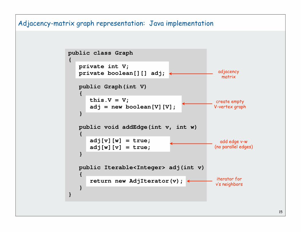
adjacency matrix
create emptyV-vertex graph
add edge v-w(no parallel edges)
15
Adjacency-matrix graph representation: Java implementation
public class Graph{ private int V; private boolean[][] adj;
public Graph(int V) { this.V = V; adj = new boolean[V][V]; }
public void addEdge(int v, int w) { adj[v][w] = true; adj[w][v] = true; }
public Iterable<Integer> adj(int v) { return new AdjIterator(v); }}
iterator forv’s neighbors
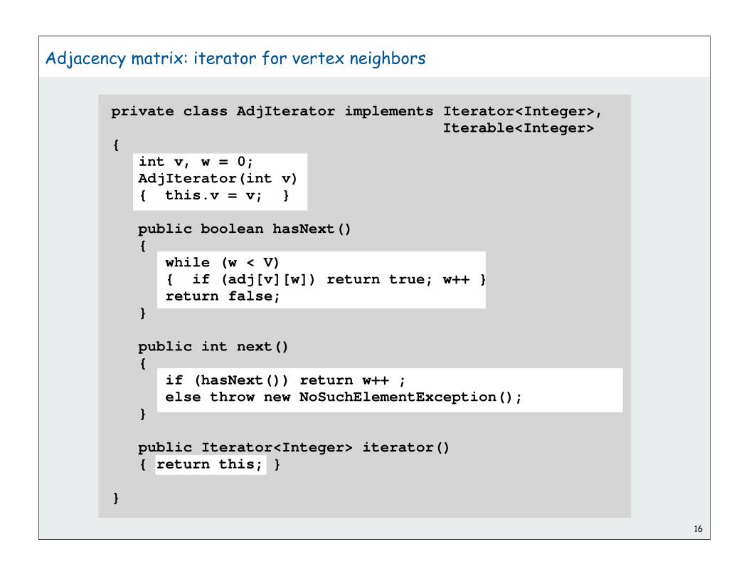
16
Adjacency matrix: iterator for vertex neighbors
private class AdjIterator implements Iterator<Integer>, Iterable<Integer>{ int v, w = 0; AdjIterator(int v) { this.v = v; }
public boolean hasNext() { while (w < V) { if (adj[v][w]) return true; w++ } return false; }
public int next() { if (hasNext()) return w++ ; else throw new NoSuchElementException(); }
public Iterator<Integer> iterator() { return this; }
}

17
Adjacency-list graph representation
Maintain vertex-indexed array of lists (implementation omitted)
0: 5 2 1 6
1: 0
2: 0
3: 5 4
4: 6 5 3
5: 0 4 3
6: 4 0
7: 8
8: 7
9: 10 11 12
10: 9
11: 9 12
12: 9 11
6
4
21
5
3
0
87
109
1211
two entriesfor each
edge

18
Adjacency-SET graph representation
Maintain vertex-indexed array of SETs
(take advantage of balanced-tree or hashing implementations)
0: { 1 2 5 6 }
1:
2:
3:
4:
5:
6:
7:
8:
9:
10:
11:
12:
6
4
21
5
3
0
87
109
1211
{ 0 }
{ 0 }
{ 4 5 }
{ 3 5 6 }
{ 0 3 4 }
{ 0 4 }
{ 8 }
{ 7 }
{ 10 11 12 }
{ 9 }
{ 9 12 }
{ 9 1 }
two entriesfor each
edge

adjacency sets
create emptyV-vertex graph
add edge v-w(no parallel edges)
iterable SET forv’s neighbors
19
Adjacency-SET graph representation: Java implementation
public class Graph{ private int V; private SET<Integer>[] adj;
public Graph(int V) { this.V = V; adj = (SET<Integer>[]) new SET[V]; for (int v = 0; v < V; v++) adj[v] = new SET<Integer>(); }
public void addEdge(int v, int w) { adj[v].add(w); adj[w].add(v); }
public Iterable<Integer> adj(int v) { return adj[v]; }}

Graphs are abstract mathematical objects, BUT
• ADT implementation requires specific representation.
• Efficiency depends on matching algorithms to representations.
In practice: Use adjacency SET representation
• Take advantage of proven technology
• Real-world graphs tend to be “sparse”
[ huge number of vertices, small average vertex degree]
• Algs all based on iterating over edges incident to v.
20
Graph representations
representation spaceedge between
v and w?iterate over edges
incident to v?
list of edges E E E
adjacency matrix V2 1 V
adjacency list E + V degree(v) degree(v)
adjacency SET E + V log (degree(v)) degree(v)*
* easy to also support ordered iteration and randomized iteration

21
Graph APImaze explorationdepth-first searchbreadth-first searchconnected componentschallenges

22
Maze exploration
Maze graphs.
• Vertex = intersections.
• Edge = passage.
Goal. Explore every passage in the maze.

23
Trémaux Maze Exploration
Trémaux maze exploration.
• Unroll a ball of string behind you.
• Mark each visited intersection by turning on a light.
• Mark each visited passage by opening a door.
First use? Theseus entered labyrinth to kill the monstrous Minotaur;
Ariadne held ball of string.
Claude Shannon (with Theseus mouse)

24

25
Maze Exploration

26
Graph APImaze explorationdepth-first searchbreadth-first searchconnected componentschallenges

Flood fill
Photoshop “magic wand”
27
Graph-processing challenge 1:
Problem: Flood fill
Assumptions: picture has millions to billions of pixels
How difficult?
1) any COS126 student could do it
2) need to be a typical diligent COS226 student
3) hire an expert
4) intractable
5) no one knows
28

Goal. Systematically search through a graph.
Idea. Mimic maze exploration.
Typical applications.
• find all vertices connected to a given s
• find a path from s to t
Running time.
• O(E) since each edge examined at most twice
• usually less than V to find paths in real graphs
Depth-first search
Mark s as visited.
Visit all unmarked vertices v adjacent to s.
DFS (to visit a vertex s)
recursive

30
Typical client program.
• Create a Graph.
• Pass the Graph to a graph-processing routine, e.g., DFSearcher.
• Query the graph-processing routine for information.
Decouple graph from graph processing.
Design pattern for graph processing
public static void main(String[] args){ In in = new In(args[0]); Graph G = new Graph(in); int s = 0; DFSearcher dfs = new DFSearcher(G, s); for (int v = 0; v < G.V(); v++) if (dfs.isConnected(v)) System.out.println(v);}
Client that prints all vertices connected to (reachable from) s

true if connected to s
constructor marks verticesconnected to s
recursive DFSdoes the work
client can ask whether any vertex is
connected to s
31
Depth-first search (connectivity)
public class DFSearcher{ private boolean[] marked;
public DFSearcher(Graph G, int s) { marked = new boolean[G.V()]; dfs(G, s); }
private void dfs(Graph G, int v) { marked[v] = true; for (int w : G.adj(v)) if (!marked[w]) dfs(G, w); }
public boolean isReachable(int v) { return marked[v]; }}

32
Connectivity application: Flood fill
Change color of entire blob of neighboring red pixels to blue.
Build a grid graph
• vertex: pixel.
• edge: between two adjacent lime pixels.
• blob: all pixels connected to given pixel.
recolor red blob to blue

33
Connectivity Application: Flood Fill
Change color of entire blob of neighboring red pixels to blue.
Build a grid graph
• vertex: pixel.
• edge: between two adjacent red pixels.
• blob: all pixels connected to given pixel.
recolor red blob to blue

Graph-processing challenge 2:
Problem: Is there a path from s to t ?
How difficult?
1) any CS126 student could do it
2) need to be a typical diligent CS226 student
3) hire an expert
4) intractable
5) no one knows
34
0-10-60-24-35-35-4
6
4
21
3
0
5

Problem: Find a path from s to t.
Assumptions: any path will do
How difficult?
1) any CS126 student could do it
2) need to be a typical diligent CS226 student
3) hire an expert
4) intractable
5) no one knows
Graph-processing challenge 3:
35
0-10-60-24-35-35-40-5
6
4
21
3
0
5

36
Paths in graphs
Is there a path from s to t? If so, find one.

37
Paths in graphs
Is there a path from s to t?
If so, find one.
• Union-Find: no help (use DFS on connected subgraph)
• DFS: easy (stay tuned)
UF advantage. Can intermix queries and edge insertions.
DFS advantage. Can recover path itself in time proportional to its length.
method preprocess time
Union Find V + E log* V
DFS E + V
query time
log* V †
1
space
V
E + V
† amortized

38
Keeping track of paths with DFS
DFS tree. Upon visiting a vertex v for the first time, remember that
you came from pred[v] (parent-link representation).
Retrace path. To find path between s and v, follow pred back from v.

add instance variable for parent-link representation
of DFS tree
initialize it in the constructor
set parent link
add method for client to iterate through path
39
Depth-first-search (pathfinding)
public class DFSearcher{ ... private int[] pred; public DFSearcher(Graph G, int s) { ... pred = new int[G.V()]; for (int v = 0; v < G.V(); v++) pred[v] = -1; ... } private void dfs(Graph G, int v) { marked[v] = true; for (int w : G.adj(v)) if (!marked[w]) { pred[w] = v; dfs(G, w); } }
public Iterable<Integer> path(int v) { // next slide }}

40
Depth-first-search (pathfinding iterator)
public Iterable<Integer> path(int v) { Stack<Integer> path = new Stack<Integer>(); while (v != -1 && marked[v]) { list.push(v); v = pred[v]; } return path; }}

41
DFS summary
Enables direct solution of simple graph problems.
• Find path from s to t.
• Connected components (stay tuned).
• Euler tour (see book).
• Cycle detection (simple exercise).
• Bipartiteness checking (see book).
Basis for solving more difficult graph problems.
• Biconnected components (see book).
• Planarity testing (beyond scope).

42
Graph APImaze explorationdepth-first searchbreadth-first searchconnected componentschallenges

43
Breadth First Search
Depth-first search. Put unvisited vertices on a stack.
Breadth-first search. Put unvisited vertices on a queue.
Shortest path. Find path from s to t that uses fewest number of edges.
Property. BFS examines vertices in increasing distance from s.
Put s onto a FIFO queue.
Repeat until the queue is empty:
remove the least recently added vertex v
add each of v's unvisited neighbors to the queue,
and mark them as visited.
BFS (from source vertex s)

distances from s
initialize distances
44
Breadth-first search scaffolding
public class BFSearcher{ private int[] dist;
public BFSearcher(Graph G, int s) { dist = new int[G.V()]; for (int v = 0; v < G.V(); v++) dist[v] = G.V() + 1; dist[s] = 0; bfs(G, s); }
public int distance(int v) { return dist[v]; }
private void bfs(Graph G, int s) { // See next slide. }
}
answer client query
compute distances

45
Breadth-first search (compute shortest-path distances)
private void bfs(Graph G, int s){ Queue<Integer> q = new Queue<Integer>(); q.enqueue(s); while (!q.isEmpty()) { int v = q.dequeue(); for (int w : G.adj(v)) { if (dist[w] > G.V()) { q.enqueue(w); dist[w] = dist[v] + 1; } } }}

46
BFS Application
• Kevin Bacon numbers.
• Facebook.
• Fewest number of hops in a communication network.
ARPANET

47
Graph APImaze explorationdepth-first searchbreadth-first searchconnected componentschallenges

Def. Vertices v and w are connected if there is a path between them.
Def. A connected component is a maximal set of connected vertices.
Goal. Preprocess graph to answer queries: is v connected to w?
in constant time
Union-Find? not quite
48
Connectivity Queries
H
A
K
EL
F
D
G
M
CJ
B
I
Vertex Component
A 0
B 1
C 1
D 0
E 0
F 0
G 2
H 0
I 2
J 1
K 0
L 0
M 1

49
Goal. Partition vertices into connected components.
Connected Components
Initialize all vertices v as unmarked.
For each unmarked vertex v, run DFS and identify all vertices
discovered as part of the same connected component.
Connected components
preprocess Time
E + V
query Time
1
extra Space
V

component labels
DFS for each component
standard DFS
constant-timeconnectivity query
50
Depth-first search for connected components
public class CCFinder
{
private final static int UNMARKED = -1;
private int components;
private int[] cc;
public CCFinder(Graph G)
{
cc = new int[G.V()];
for (int v = 0; v < G.V(); v++)
cc[v] = UNMARKED;
for (int v = 0; v < G.V(); v++)
if (cc[v] == UNMARKED)
{ dfs(G, v); components++; }
}
private void dfs(Graph G, int v)
{
cc[v] = components;
for (int w : G.adj(v))
if (cc[w] == UNMARKED) dfs(G, w);
}
public int connected(int v, int w)
{ return cc[v] == cc[w]; }
}

51
Connected Components
63 components

52
Connected components application: Image processing
Goal. Read in a 2D color image and find regions of connected pixels
that have the same color.
Input: scanned image
Output: number of red and blue states

53
Connected components application: Image Processing
Goal. Read in a 2D color image and find regions of connected pixels
that have the same color.
Efficient algorithm.
• Connect each pixel to neighboring pixel if same color.
• Find connected components in resulting graph.
0 1 1 1 1 1 6 6
0 0 0 1 6 6 6 8
3 0 0 1 6 6 4 8
3 0 0 1 1 6 2 11
10 10 10 10 1 1 2 11
7 7 2 2 2 2 2 11
7 7 5 5 5 2 2 11
8 9 9 11
8 11 9 11
11 11 11 11
11 11 11 11
11 11 11 11
11 11 11 11
11 11 11 11

54
Connected components application: Particle detection
Particle detection. Given grayscale image of particles, identify "blobs."
• Vertex: pixel.
• Edge: between two adjacent pixels with grayscale value 70.
• Blob: connected component of 20-30 pixels.
Particle tracking. Track moving particles over time.
black = 0white = 255

55
Graph APImaze explorationdepth-first searchbreadth-first searchconnected componentschallenges

Graph-processing challenge 4:
Problem: Find a path from s to t
Assumptions: any path will do
Which is faster, DFS or BFS?
1) DFS
2) BFS
3) about the same
4) depends on the graph
5) depends on the graph representation
56
0-10-60-24-35-35-40-56-41-25-0
6
4
21
3
0
5

Graph-processing challenge 5:
Problem: Find a path from s to t
Assumptions: any path will do
randomized iterators
Which is faster, DFS or BFS?
1) DFS
2) BFS
3) about the same
4) depends on the graph
5) depends on the graph representation
57
0-10-60-24-35-35-40-56-41-25-0
6
4
21
3
0
5

Graph-processing challenge 6:
Problem: Find a path from s to t that uses every edge
Assumptions: need to use each edge exactly once
How difficult?
1) any CS126 student could do it
2) need to be a typical diligent CS226 student
3) hire an expert
4) intractable
5) no one knows
58
0-10-60-24-35-35-40-56-41-25-0
6
4
21
3
0
5

59
The Seven Bridges of Königsberg. [Leonhard Euler 1736]
Euler tour. Is there a cyclic path that uses each edge exactly once?
Answer. Yes iff connected and all vertices have even degree.
Tricky DFS-based algorithm to find path (see Algs in Java).
"… in Königsberg in Prussia, there is an island A, called the Kneiphof;
the river which surrounds it is divided into two branches ... and these
branches are crossed by seven bridges. Concerning these bridges, it
was asked whether anyone could arrange a route in such a way that he
could cross each bridge once and only once…"
Bridges of Königsberg earliest application ofgraph theory or topology

Graph-processing challenge 7:
Problem: Find a path from s to t that visits every vertex
Assumptions: need to visit each vertex exactly once
How difficult?
1) any CS126 student could do it
2) need to be a typical diligent CS226 student
3) hire an expert
4) intractable
5) no one knows
60
0-10-60-24-35-35-40-56-41-22-6
6
4
21
3
0
5

Graph-processing challenge 8:
Problem: Are two graphs identical except for vertex names?
How difficult?
1) any CS126 student could do it
2) need to be a typical diligent CS226 student
3) hire an expert
4) intractable
5) no one knows
61
0-10-60-24-35-35-40-56-4
6
4
21
5
3
0
2-12-42-06-55-33-62-36-4
4
6
0
2
3
5
1

Graph-processing challenge 9:
Problem: Can you lay out a graph in the plane without crossing edges?
How difficult?
1) any CS126 student could do it
2) need to be a typical diligent CS226 student
3) hire an expert
4) intractable
5) no one knows
62
2-12-42-06-55-33-62-36-4
4
6
0
2
3
5
1

1
Directed Graphs
digraph searchtransitive closuretopological sortstrong components
References:
Algorithms in Java, Chapter 19 http://www.cs.princeton.edu/introalgsds/52directed

2
Directed graphs (digraphs)
Set of objects with oriented pairwise connections.
Page ranks with histogram for a larger example
18
31
6
42 13
28
32
49
22
45
1 14
40
48
7
44
10
4129
0
39
11
9
12
3026
21
46
5
24
37
43
35
47
38
23
16
36
4
3 17
27
20
34
15
2
19 33
25
8
0
1
2
3
4
5
6
7
8
9
10
11
12
13
14
15
16
17
18
19
20
21
22
23
24
25
26
27
28
29
30
31
32
33
34
35
36
37
38
39
40
41
42
43
44
45
46
47
48
49
6 22
one-way streets in a map
hyperlinks connecting web pages
dependencies in software modules prey-predator relationships

3
Digraph applications
digraph vertex edge
financial stock, currency transaction
transportation street intersection, airport highway, airway route
scheduling task precedence constraint
WordNet synset hypernym
Web web page hyperlink
game board position legal move
telephone person placed call
food web species predator-prey relation
infectious disease person infection
citation journal article citation
object graph object pointer
inheritance hierarchy class inherits from
control flow code block jump

4
Some digraph problems
Transitive closure.
Is there a directed path from v to w?
Strong connectivity.
Are all vertices mutually reachable?
Topological sort.
Can you draw the digraph so that all edges point
from left to right?
PERT/CPM.
Given a set of tasks with precedence constraints,
how we can we best complete them all?
Shortest path. Find best route from s to t
in a weighted digraph
PageRank. What is the importance of a web page?

5
Digraph representations
Vertices
• this lecture: use integers between 0 and V-1.
• real world: convert between names and integers with symbol table.
Edges: four easy options
• list of vertex pairs
• vertex-indexed adjacency arrays (adjacency matrix)
• vertex-indexed adjacency lists
• vertex-indexed adjacency SETs
Same as undirected graph
BUT
orientation of edges is significant.
0
6
4
21
5
3
7
12
109
11
8

6
Adjacency matrix digraph representation
Maintain a two-dimensional V V boolean array.
For each edge v w in graph: adj[v][w] = true.
0 0 1 1 0 0 1 1 0 0 0 0 0 0 1 0 0 0 0 0 0 0 0 0 0 0 0 0 2 0 0 0 0 0 0 0 0 0 0 0 0 0 3 0 0 0 0 0 0 0 0 0 0 0 0 0 4 0 0 0 1 0 0 0 0 0 0 0 0 0 5 0 0 0 1 1 0 0 0 0 0 0 0 0 6 0 0 0 0 1 0 0 0 0 0 0 0 0 7 0 0 0 0 0 0 0 0 1 0 0 0 0 8 0 0 0 0 0 0 0 0 0 0 0 0 0 9 0 0 0 0 0 0 0 0 0 0 1 1 110 0 0 0 0 0 0 0 0 0 0 0 0 011 0 0 0 0 0 0 0 0 0 0 0 0 112 0 0 0 0 0 0 0 0 0 0 0 0 0
0 1 2 3 4 5 6 7 8 9 10 11 12
from
to
0
6
4
21
5
3
7 12
109
118
one entryfor each
edge

7
Adjacency-list digraph representation
Maintain vertex-indexed array of lists.
0: 5 2 1 6
1:
2:
3:
4: 3
5: 4 3
6: 4
7: 8
8:
9: 10 11 12
10:
11: 12
12:
0
6
4
21
5
3
7 12
109
118
one entryfor each
edge

8
Adjacency-SET digraph representation
Maintain vertex-indexed array of SETs.
0:
1:
2:
3:
4:
5:
6:
7:
8:
9:
10:
11:
12:
0
6
4
21
5
3
7 12
109
118
{ 1 2 5 6 }
{ }
{ }
{ }
{ 3 }
{ 3 4 }
{ 4 }
{ 8 }
{ }
{ 10 11 12 }
{ }
{ 12 }
{ }
one entryfor each
edge

adjacency SETs
create emptyV-vertex graph
add edge from v to w(Graph also has adj[w].add[v])
iterable SET forv’s neighbors
9
Adjacency-SET digraph representation: Java implementation
Same as Graph, but only insert one copy of each edge.
public class Digraph{ private int V; private SET<Integer>[] adj;
public Digraph(int V) { this.V = V; adj = (SET<Integer>[]) new SET[V]; for (int v = 0; v < V; v++) adj[v] = new SET<Integer>(); }
public void addEdge(int v, int w) { adj[v].add(w); }
public Iterable<Integer> adj(int v) { return adj[v]; }}

Digraphs are abstract mathematical objects, BUT
• ADT implementation requires specific representation.
• Efficiency depends on matching algorithms to representations.
In practice: Use adjacency SET representation
• Take advantage of proven technology
• Real-world digraphs tend to be “sparse”
[ huge number of vertices, small average vertex degree]
• Algs all based on iterating over edges incident to v.
10
Digraph representations
representation spaceedge between
v and w?iterate over edges
incident to v?
list of edges E E E
adjacency matrix V2 1 V
adjacency list E + V degree(v) degree(v)
adjacency SET E + V log (degree(v)) degree(v)

11
Typical digraph application: Google's PageRank algorithm
Goal. Determine which web pages on Internet are important.
Solution. Ignore keywords and content, focus on hyperlink structure.
Random surfer model.
• Start at random page.
• With probability 0.85, randomly select a hyperlink to visit next;
with probability 0.15, randomly select any page.
• PageRank = proportion of time random surfer spends on each page.
Solution 1: Simulate random surfer for a long time.
Solution 2: Compute ranks directly until they converge
Solution 3: Compute eigenvalues of adjacency matrix!
None feasible without sparse digraph representation
Every square matrix is a weighted digraph
18
31
6
42 13
28
32
49
22
45
1 14
40
48
7
44
10
4129
0
39
11
9
12
3026
21
46
5
24
37
43
35
47
38
23
16
36
4
3 17
27
20
34
15
2
19 33
25
8

12
digraph searchtransitive closuretopological sortstrong components

13
Digraph application: program control-flow analysis
Every program is a digraph (instructions connected to possible successors)
Dead code elimination.
Find (and remove) unreachable code
Infinite loop detection.
Determine whether exit is unreachable
can arise from compiler optimization (or bad code)
can’t detect all possible infinite loops (halting problem)

14
Digraph application: mark-sweep garbage collector
Every data structure is a digraph (objects connected by references)
Roots. Objects known to be directly
accessible by program (e.g., stack).
Reachable objects.
Objects indirectly accessible by
program (starting at a root and
following a chain of pointers).
Mark-sweep algorithm. [McCarthy, 1960]
• Mark: mark all reachable objects.
• Sweep: if object is unmarked, it is garbage, so add to free list.
Memory cost: Uses 1 extra mark bit per object, plus DFS stack.
easy to identify pointers in type-safe language

15
Reachability
Goal. Find all vertices reachable from s along a directed path.
s

16
Reachability
Goal. Find all vertices reachable from s along a directed path.
s

Digraph-processing challenge 1:
Problem: Mark all vertices reachable from a given vertex.
How difficult?
1) any COS126 student could do it
2) need to be a typical diligent COS226 student
3) hire an expert
4) intractable
5) no one knows
17
0-10-60-23-43-25-45-03-52-16-43-1
6
4
21
3
0
5

18
Depth-first search in digraphs
Same method as for undirected graphs
Every undirected graph is a digraph
• happens to have edges in both directions
• DFS is a digraph algorithm
Mark v as visited.
Visit all unmarked vertices w adjacent to v.
DFS (to visit a vertex v)
recursive

19
Depth-first search (single-source reachability)
Identical to undirected version (substitute Digraph for Graph).
true if connected to s
constructor marks verticesconnected to s
recursive DFSdoes the work
client can ask whether any vertex is
connected to s
public class DFSearcher{ private boolean[] marked;
public DFSearcher(Digraph G, int s) { marked = new boolean[G.V()]; dfs(G, s); }
private void dfs(Digraph G, int v) { marked[v] = true; for (int w : G.adj(v)) if (!marked[w]) dfs(G, w); }
public boolean isReachable(int v) { return marked[v]; }}

DFS enables direct solution of simple digraph problems.
• Reachability.
• Cycle detection
• Topological sort
• Transitive closure.
• Is there a path from s to t ?
Basis for solving difficult digraph problems.
• Directed Euler path.
• Strong connected components.
20
Depth-first search (DFS)
stay tuned

21
Breadth-first search in digraphs
Same method as for undirected graphs
Every undirected graph is a digraph
• happens to have edges in both directions
• BFS is a digraph algorithm
Visits vertices in increasing distance from s
Put s onto a FIFO queue.
Repeat until the queue is empty:
remove the least recently added vertex v
add each of v's unvisited neighbors to the
queue and mark them as visited.
BFS (from source vertex s)
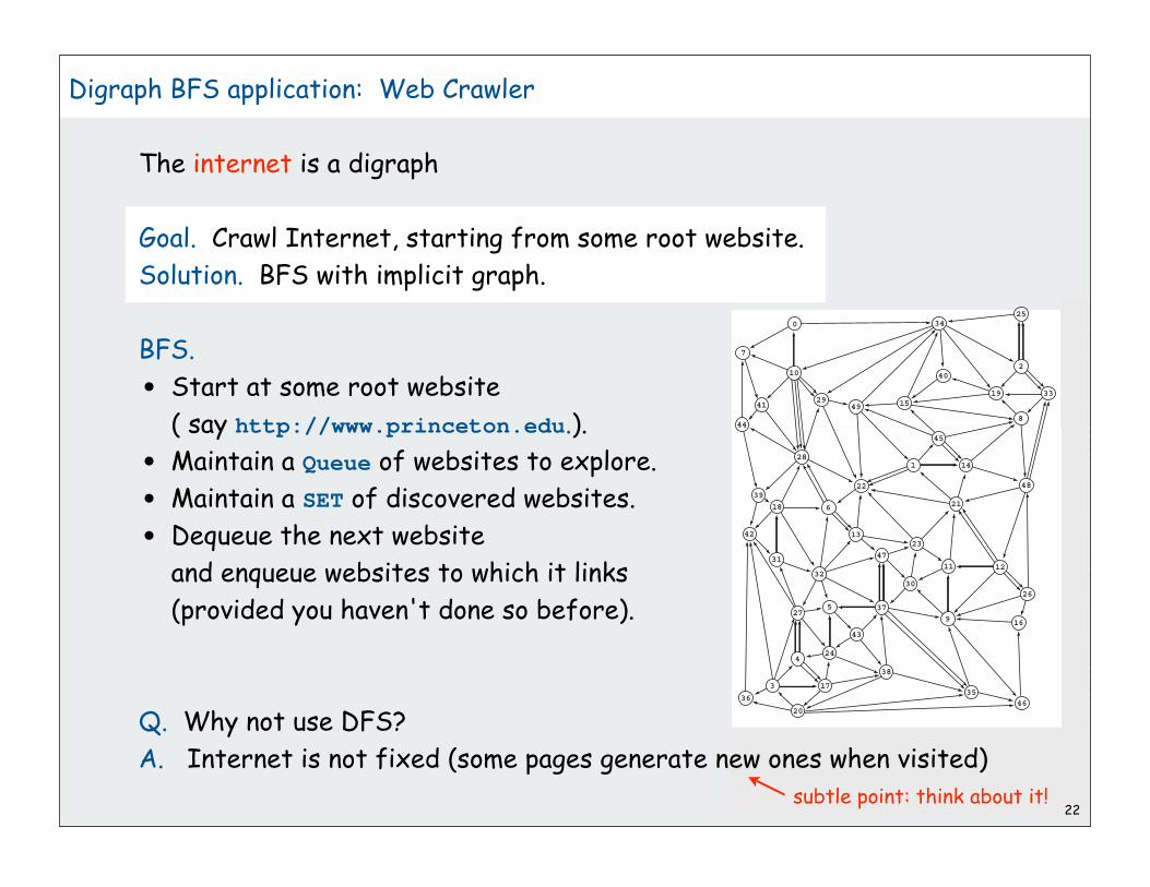
Page ranks with histogram for a larger example
18
31
6
42 13
28
32
49
22
45
1 14
40
48
7
44
10
4129
0
39
11
9
12
3026
21
46
5
24
37
43
35
47
38
23
16
36
4
3 17
27
20
34
15
2
19 33
25
8
0 .0
1 .0
2 .0
3 .0
4 .0
5 .0
6 .0
7 .0
8 .0
9 .0
10 .0
11 .0
12 .0
13 .0
14 .0
15 .0
16 .0
17 .0
18 .0
19 .0
20 .0
21 .0
22 .0
23 .0
24 .0
25 .0
26 .0
27 .0
28 .0
29 .0
30 .0
31 .0
32 .0
33 .0
34 .0
35 .0
36 .0
37 .0
38 .0
39 .0
40 .0
41 .0
42 .0
43 .0
44 .0
45 .0
46 .0
47 .0
48 .0
49 .0
6 22
22
Digraph BFS application: Web Crawler
The internet is a digraph
Goal. Crawl Internet, starting from some root website.
Solution. BFS with implicit graph.
BFS.
• Start at some root website
( say http://www.princeton.edu.).
• Maintain a Queue of websites to explore.
• Maintain a SET of discovered websites.
• Dequeue the next website
and enqueue websites to which it links
(provided you haven't done so before).
Q. Why not use DFS?
A. Internet is not fixed (some pages generate new ones when visited)
subtle point: think about it!

Queue<String> q = new Queue<String>();
SET<String> visited = new SET<String>();
String s = "http://www.princeton.edu";
q.enqueue(s);
visited.add(s);
while (!q.isEmpty())
{
String v = q.dequeue();
System.out.println(v);
In in = new In(v);
String input = in.readAll();
String regexp = "http://(\\w+\\.)*(\\w+)";
Pattern pattern = Pattern.compile(regexp);
Matcher matcher = pattern.matcher(input);
while (matcher.find())
{
String w = matcher.group();
if (!visited.contains(w))
{
visited.add(w);
q.enqueue(w);
}
}
}23
Web crawler: BFS-based Java implementation
read in raw html for next site in queue
use regular expressionto find all URLs in site
if unvisited, mark as visitedand put on queue
http://xxx.yyy.zzz
start crawling from s
queue of sites to crawl
set of visited sites

24
digraph searchtransitive closuretopological sortstrong components

Graph-processing challenge (revisited)
Problem: Is there a path from s to t ?
Goals: linear ~(V + E) preprocessing time
constant query time
How difficult?
1) any COS126 student could do it
2) need to be a typical diligent COS226 student
3) hire an expert
4) intractable
5) no one knows
6) impossible
25
0-10-60-24-35-35-4
6
4
21
3
0
5

Digraph-processing challenge 2
Problem: Is there a directed path from s to t ?
Goals: linear ~(V + E) preprocessing time
constant query time
How difficult?
1) any COS126 student could do it
2) need to be a typical diligent COS226 student
3) hire an expert
4) intractable
5) no one knows
6) impossible
26
0-10-60-23-43-25-45-03-52-16-41-3
6
4
21
3
0
5

27
The transitive closure of G has an directed edge from v to w
if there is a directed path from v to w in G
Transitive Closure
G
Transitive closureof G
TC is usually denseso adjacency matrixrepresentation is OK
graph is usually sparse

Digraph-processing challenge 2 (revised)
Problem: Is there a directed path from s to t ?
Goals: ~V2 preprocessing time
constant query time
How difficult?
1) any COS126 student could do it
2) need to be a typical diligent COS226 student
3) hire an expert
4) intractable
5) no one knows
6) impossible
28
0-10-60-23-43-25-45-03-52-16-41-3
6
4
21
3
0
5

Digraph-processing challenge 2 (revised again)
Problem: Is there a directed path from s to t ?
Goals: ~VE preprocessing time (~V3 for dense digraphs)
~V2 space
constant query time
How difficult?
1) any COS126 student could do it
2) need to be a typical diligent COS226 student
3) hire an expert
4) intractable
5) no one knows
6) impossible
29
0-10-60-23-43-25-45-03-52-16-41-3
6
4
21
3
0
5

30
Transitive closure: Java implementation
public class TransitiveClosure{ private DFSearcher[] tc;
public TransitiveClosure(Digraph G) { tc = new DFSearcher[G.V()]; for (int v = 0; v < G.V(); v++) tc[v] = new DFSearcher(G, v); }
public boolean reachable(int v, int w) { return tc[v].isReachable(w); }}
is there a directed path from v to w ?
Use an array of DFSearcher objects,
one for each row of transitive closurepublic class DFSearcher{ private boolean[] marked; public DFSearcher(Digraph G, int s) { marked = new boolean[G.V()]; dfs(G, s); } private void dfs(Digraph G, int v) { marked[v] = true; for (int w : G.adj(v)) if (!marked[w]) dfs(G, w); } public boolean isReachable(int v) { return marked[v]; }}

31
digraph searchtransitive closuretopological sortstrong components

32
Digraph application: Scheduling
Scheduling. Given a set of tasks to be completed with precedence
constraints, in what order should we schedule the tasks?
Graph model.
• Create a vertex v for each task.
• Create an edge v w if task v must precede task w.
• Schedule tasks in topological order.
0. read programming assignment1. download files2. write code3. attend precept…12. sleep
tasks
precedenceconstraints
feasibleschedule

33
Topological Sort
DAG. Directed acyclic graph.
Topological sort. Redraw DAG so all edges point left to right.
Observation. Not possible if graph has a directed cycle.
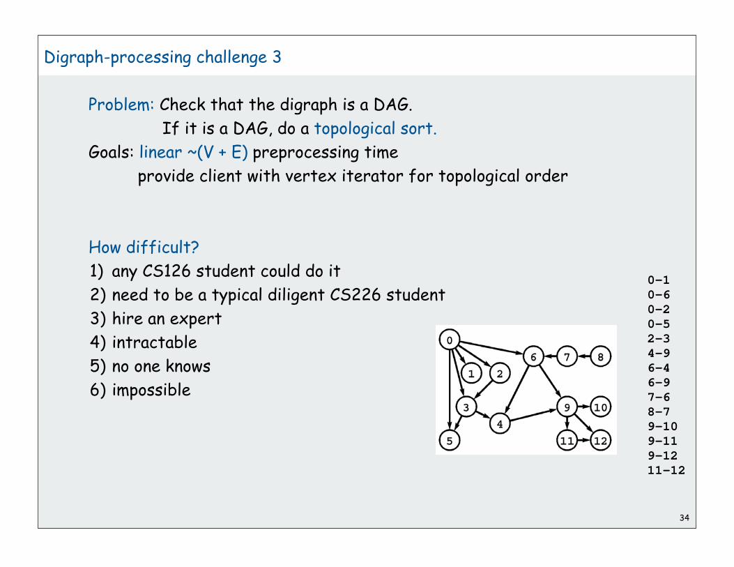
Digraph-processing challenge 3
Problem: Check that the digraph is a DAG.
If it is a DAG, do a topological sort.
Goals: linear ~(V + E) preprocessing time
provide client with vertex iterator for topological order
How difficult?
1) any CS126 student could do it
2) need to be a typical diligent CS226 student
3) hire an expert
4) intractable
5) no one knows
6) impossible
34
0-10-60-20-52-34-96-46-97-68-79-109-119-1211-12

35
Topological sort in a DAG: Java implementation
public class TopologicalSorter{ private int count; private boolean[] marked; private int[] ts;
public TopologicalSorter(Digraph G) { marked = new boolean[G.V()]; ts = new int[G.V()]; count = G.V(); for (int v = 0; v < G.V(); v++) if (!marked[v]) tsort(G, v); }
private void tsort(Digraph G, int v) { marked[v] = true; for (int w : G.adj(v)) if (!marked[w]) tsort(G, w); ts[--count] = v; } }
standard DFSwith 5
extra lines of code
add iterator that returns ts[0], ts[1], ts[2]...
Seems easy? Missed by experts for a few decades

36
Topological sort of a dag: trace
1
4
52
3
0
6
0: 1 2 51: 42:3: 2 4 5 64: 5: 26: 0 4
visit 0: 1 0 0 0 0 0 0 0 0 0 0 0 0 0
visit 1: 1 1 0 0 0 0 0 0 0 0 0 0 0 0
visit 4: 1 1 0 0 1 0 0 0 0 0 0 0 0 0
leave 4: 1 1 0 0 1 0 0 0 0 0 0 0 0 4
leave 1: 1 1 0 0 1 0 0 0 0 0 0 0 1 4
visit 2: 1 1 1 0 1 0 0 0 0 0 0 0 1 4
leave 2: 1 1 1 0 1 0 0 0 0 0 0 2 1 4
visit 5: 1 1 1 0 1 1 0 0 0 0 0 2 1 4
check 2: 1 1 1 0 1 1 0 0 0 0 0 2 1 4
leave 5: 1 1 1 0 1 1 0 0 0 0 5 2 1 4
leave 0: 1 1 1 0 1 1 0 0 0 0 5 2 1 4
check 1: 1 1 1 0 1 1 0 0 0 0 5 2 1 4
check 2: 1 1 1 0 1 1 0 0 0 0 5 2 1 4
visit 3: 1 1 1 1 1 1 0 0 0 0 5 2 1 4
check 2: 1 1 1 1 1 1 0 0 0 0 5 2 1 4
check 4: 1 1 1 1 1 1 0 0 0 0 5 2 1 4
check 5: 1 1 1 1 1 1 0 0 0 0 5 2 1 4
visit 6: 1 1 1 1 1 1 1 0 0 0 5 2 1 4
leave 6: 1 1 1 1 1 1 1 0 6 0 5 2 1 4
leave 3: 1 1 1 1 1 1 1 3 6 0 5 2 1 4
check 4: 1 1 1 1 1 1 0 3 6 0 5 2 1 4
check 5: 1 1 1 1 1 1 0 3 6 0 5 2 1 4
check 6: 1 1 1 1 1 1 0 3 6 0 5 2 1 4
marked[] ts[]
“visit” means “call tsort()” and “leave” means “return from tsort()
adj SETs
3 6 0 5 2 1 4
0
1 2 5
4
3
6

37
Topological sort in a DAG: correctness proof
Invariant:
tsort(G, v) visits all vertices
reachable from v with a directed path
Proof by induction:
• w marked: vertices reachable from w
are already visited
• w not marked: call tsort(G, w) to
visit the vertices reachable from w
Therefore, algorithm is correct
in placing v before all vertices visited
during call to tsort(G, v) just before returning.
Q. How to tell whether the digraph has a cycle (is not a DAG)?
A. Use TopologicalSorter (exercise)
public class TopologicalSorter{ private int count; private boolean[] marked; private int[] ts;
public TopologicalSorter(Digraph G) { marked = new boolean[G.V()]; ts = new int[G.V()]; count = G.V(); for (int v = 0; v < G.V(); v++) if (!marked[v]) tsort(G, v); }
private void tsort(Digraph G, int v) { marked[v] = true; for (int w : G.adj(v)) if (!marked[w]) tsort(G, w); ts[--count] = v; } }

38
Topological sort applications.
• Causalities.
• Compilation units.
• Class inheritance.
• Course prerequisites.
• Deadlocking detection.
• Temporal dependencies.
• Pipeline of computing jobs.
• Check for symbolic link loop.
• Evaluate formula in spreadsheet.
• Program Evaluation and Review Technique / Critical Path Method

39
Topological sort application (weighted DAG)
Precedence scheduling
• Task v takes time[v] units of time.
• Can work on jobs in parallel.
• Precedence constraints:
• must finish task v before beginning task w.
• Goal: finish each task as soon as possible
Example:
index time prereq
A 0 -
task
begin
B 4 Aframing
C 2 Broofing
D 6 Bsiding
E 5 Dwindows
F 3 Dplumbing
G 4 C, Eelectricity
H 6 C, Epaint
I 0 F, Hfinish
4
6
2
5
3
4 60 0
IHG
C
B
E
D
A
F
vertices labelledA-I in topological order

Program Evaluation and Review Technique / Critical Path Method
40
4
6
2
5
3
4 60 0
IHG
C
B
E
D
A
F
PERT/CPM algorithm.
• compute topological order of vertices.
• initialize fin[v] = 0 for all vertices v.
• consider vertices v in topologically sorted order.
for each edge v w, set fin[w]= max(fin[w], fin[v] + time[w])
Critical path
• remember vertex that set value.
• work backwards from sink
4
10
6
19 25
15
13
13
criticalpath
25

41
digraph searchtransitive closuretopological sortstrong components

Strong connectivity in digraphs
Analog to connectivity in undirected graphs
42
06
4
21
5
3
7
12
109
11
8
0 1 2 3 4 5 6 7 8 9 10 11 12
cc 0 0 0 0 0 0 0 1 1 2 2 2 2
public int connected(int v, int w)
{ return cc[v] == cc[w]; }
06
4
21
5
3
7
12
109
11
8
In a Graph, u and v are connectedwhen there is a path from u to v
In a Digraph, u and v are strongly connectedwhen there is a directed path from u to v and a directed path from v to u
0 1 2 3 4 5 6 7 8 9 10 11 12
sc 2 1 2 2 2 2 2 3 3 0 0 0 0
public int connected(int v, int w)
{ return cc[v] == cc[w]; }
constant-time client connectivity query constant-time client strong connectivity query
3 connected components(sets of mutually connected vertices)
4 strongly connected components(sets of mutually strongly connected vertices)
Connectivity table (easy to compute with DFS) Strong connectivity table (how to compute?)

Digraph-processing challenge 4
Problem: Is there a directed cycle containing s and t ?
Equivalent: Are there directed paths from s to t and from t to s?
Equivalent: Are s and t strongly connected?
Goals: linear (V + E) preprocessing time (like for undirected graphs)
constant query time
How difficult?
1) any COS126 student could do it
2) need to be a typical diligent COS226 student
3) hire an expert
4) intractable
5) no one knows
6) impossible
43

44
Typical strong components applications
Strong component: subset with common energy flow
• source in kernel DAG: needs outside energy?
• sink in kernel DAG: heading for growth?
Ecological food web Software module dependency digraphs
Strong component: subset of mutually interacting modules
• approach 1: package strong components together
• approach 2: use to improve design!
Internet explorer
Firefox

Strong components algorithms: brief history
1960s: Core OR problem
• widely studied
• some practical algorithms
• complexity not understood
1972: Linear-time DFS algorithm (Tarjan)
• classic algorithm
• level of difficulty: CS226++
• demonstrated broad applicability and importance of DFS
1980s: Easy two-pass linear-time algorithm (Kosaraju)
• forgot notes for teaching algorithms class
• developed algorithm in order to teach it!
• later found in Russian scientific literature (1972)
1990s: More easy linear-time algorithms (Gabow, Mehlhorn)
• Gabow: fixed old OR algorithm
• Mehlhorn: needed one-pass algorithm for LEDA45

46
Simple (but mysterious) algorithm for computing strong components
• Run DFS on GR and compute postorder.
• Run DFS on G, considering vertices in reverse postorder
• [has to be seen to be believed: follow example in book]
Theorem. Trees in second DFS are strong components. (!)
Proof. [stay tuned in COS 423]
Kosaraju's algorithm
G
GR
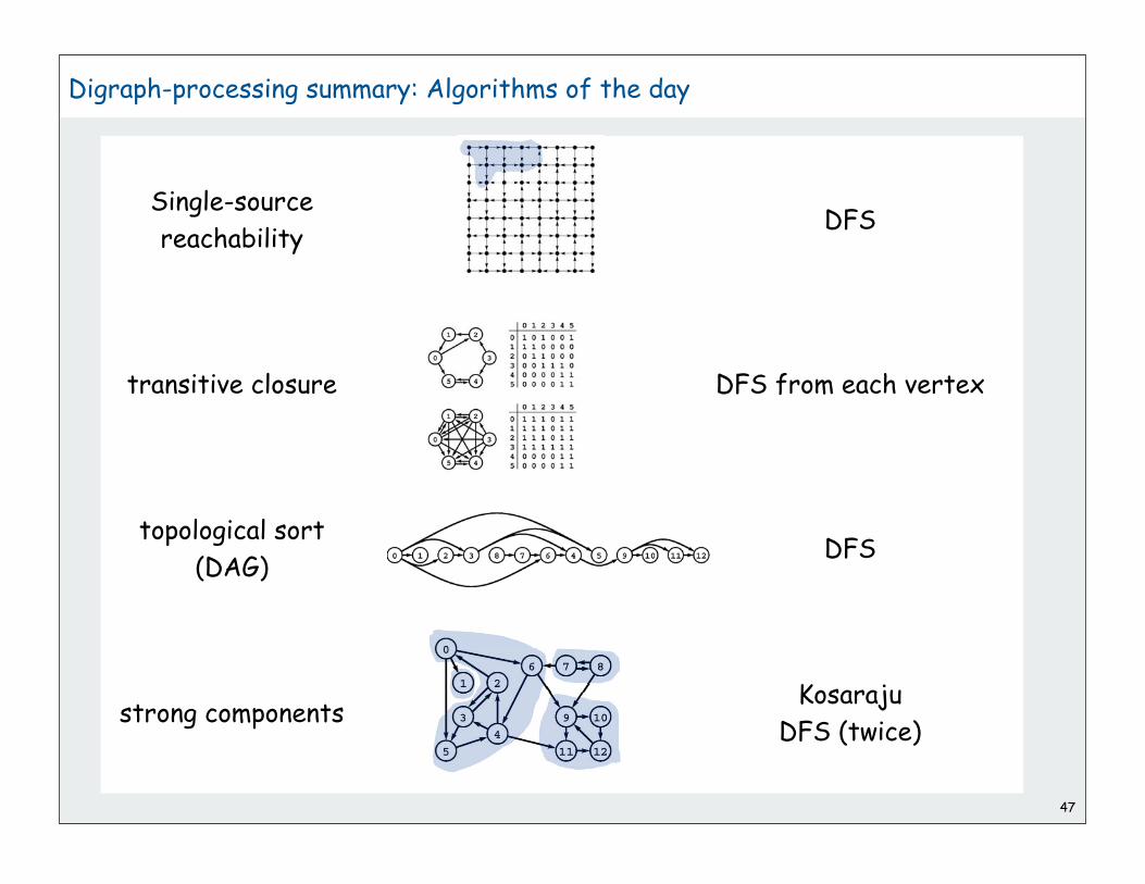
Digraph-processing summary: Algorithms of the day
47
Single-source
reachabilityDFS
transitive closure DFS from each vertex
topological sort
(DAG)DFS
strong componentsKosaraju
DFS (twice)

1
Minimum Spanning Trees
weighted graph APIcycles and cutsKruskal’s algorithmPrim’s algorithmadvanced topics
References:
Algorithms in Java, Chapter 20 http://www.cs.princeton.edu/introalgsds/54mst

2
Minimum Spanning Tree
23
10
21
14
24
16
4
18
9
7
11
8
G
5
6
Given. Undirected graph G with positive edge weights (connected).
Goal. Find a min weight set of edges that connects all of the vertices.

3
Minimum Spanning Tree
Given. Undirected graph G with positive edge weights (connected).
Goal. Find a min weight set of edges that connects all of the vertices.
23
10
21
14
24
16
4
18
9
7
11
8
weight(T) = 50 = 4 + 6 + 8 + 5 + 11 + 9 + 7
5
6
Brute force: Try all possible spanning trees
• problem 1: not so easy to implement
• problem 2: far too many of them Ex: [Cayley, 1889]: VV-2 spanning treeson the complete graph on V vertices.

4
MST Origin
Otakar Boruvka (1926).
• Electrical Power Company of Western Moravia in Brno.
• Most economical construction of electrical power network.
• Concrete engineering problem is now a cornerstone
problem-solving model in combinatorial optimization.
Otakar Boruvka

5
Applications
MST is fundamental problem with diverse applications.
• Network design.
telephone, electrical, hydraulic, TV cable, computer, road
• Approximation algorithms for NP-hard problems.
traveling salesperson problem, Steiner tree
• Indirect applications.
max bottleneck paths
LDPC codes for error correction
image registration with Renyi entropy
learning salient features for real-time face verification
reducing data storage in sequencing amino acids in a protein
model locality of particle interactions in turbulent fluid flows
autoconfig protocol for Ethernet bridging to avoid cycles in a network
• Cluster analysis.

6
Medical Image Processing
MST describes arrangement of nuclei in the epithelium for cancer research
http://www.bccrc.ca/ci/ta01_archlevel.html

7http://ginger.indstate.edu/ge/gfx

8
Two Greedy Algorithms
Kruskal's algorithm. Consider edges in ascending order of cost.
Add the next edge to T unless doing so would create a cycle.
Prim's algorithm. Start with any vertex s and greedily grow a tree T
from s. At each step, add the cheapest edge to T that has exactly
one endpoint in T.
Proposition. Both greedy algorithms compute an MST.
Greed is good. Greed is right. Greed works. Greed
clarifies, cuts through, and captures the essence of the
evolutionary spirit." - Gordon Gecko

9
weighted graph APIcycles and cutsKruskal’s algorithmPrim’s algorithmadvanced topics
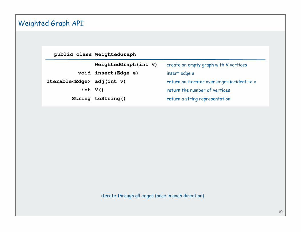
10
Weighted Graph API
iterate through all edges (once in each direction)
create an empty graph with V verticesWeightedGraph(int V)
public class WeightedGraph
insert edge einsert(Edge e)void
return an iterator over edges incident to vadj(int v)Iterable<Edge>
return the number of verticesV()int
return a string representationtoString()String

Identical to Graph.java but use Edge adjacency sets instead of int.
11
public class WeightedGraph{ private int V; private SET<Edge>[] adj;
public Graph(int V) { this.V = V; adj = (SET<Edge>[]) new SET[V]; for (int v = 0; v < V; v++) adj[v] = new SET<Edge>(); }
public void addEdge(Edge e) { int v = e.v, w = e.w; adj[v].add(e); adj[w].add(e); }
public Iterable<Edge> adj(int v) { return adj[v]; }
}
Weighted graph data type

12
Weighted edge data type
public class Edge implements Comparable<Edge>
{
private final int v, int w;
private final double weight;
public Edge(int v, int w, double weight)
{
this.v = v;
this.w = w;
this.weight = weight;
}
public int either()
{ return v; }
public int other(int vertex)
{
if (vertex == v) return w;
else return v;
}
public int weight()
{ return weight; }
// See next slide for edge compare methods.
}
Edge abstractionneeded for weights
slightly tricky accessor methods(enables client code like this)
for (int v = 0; v < G.V(); v++){ for (Edge e : G.adj(v)) { int w = e.other(v);
// edge v-w }}

13
Weighted edge data type: compare methods
public final static Comparator<Edge> BY_WEIGHT = new ByWeightComparator();
private static class ByWeightComparator implements Comparator<Edge>
{
public int compare(Edge e, Edge f)
{
if (e.weight < f.weight) return -1;
if (e.weight > f.weight) return +1;
return 0;
}
}
public int compareTo(Edge that)
{
if (this.weight < that.weight) return -1;
else if (this.weight > that.weight) return +1;
else if (this.weight > that.weight) return 0;
}
}
Two different compare methods for edges
• compareTo() so that edges are Comparable (for use in SET)
• compare() so that clients can compare edges by weight.

14
weighted graph APIcycles and cutsKruskal’s algorithmPrim’s algorithmadvanced topics

15
Spanning Tree
MST. Given connected graph G with positive edge weights,
find a min weight set of edges that connects all of the vertices.
Def. A spanning tree of a graph G is a subgraph T that is
connected and acyclic.
Property. MST of G is always a spanning tree.

16
Greedy Algorithms
Simplifying assumption. All edge weights we are distinct.
Cycle property. Let C be any cycle, and let f be the max cost edge
belonging to C. Then the MST does not contain f.
Cut property. Let S be any subset of vertices, and let e be the min
cost edge with exactly one endpoint in S. Then the MST contains e.
f C
S
e is in the MST
e
f is not in the MST

17
Cycle Property
Simplifying assumption. All edge weights we are distinct.
Cycle property. Let C be any cycle, and let f be the max cost edge
belonging to C. Then the MST T* does not contain f.
Pf. [by contradiction]
• Suppose f belongs to T*. Let's see what happens.
• Deleting f from T* disconnects T*. Let S be one side of the cut.
• Some other edge in C, say e, has exactly one endpoint in S.
• T = T* { e } { f } is also a spanning tree.
• Since ce < cf, cost(T) < cost(T*).
• Contradicts minimality of T*.
f
T*
e
S
C

18
Cut Property
Simplifying assumption. All edge costs ce are distinct.
Cut property. Let S be any subset of vertices, and let e be the min cost
edge with exactly one endpoint in S. Then the MST T* contains e.
Pf. [by contradiction]
• Suppose e does not belong to T*. Let's see what happens.
• Adding e to T* creates a (unique) cycle C in T*.
• Some other edge in C, say f, has exactly one endpoint in S.
• T = T* { e } { f } is also a spanning tree.
• Since ce < cf, cost(T) < cost(T*).
• Contradicts minimality of T*.
f
MST T*
e
S
cycle C

19
weighted graph APIcycles and cutsKruskal’s algorithmPrim’s algorithmadvanced algorithmsclustering

20
Kruskal's algorithm. [Kruskal, 1956] Consider edges in ascending order
of cost. Add the next edge to T unless doing so would create a cycle.
Kruskal's Algorithm: Example
3-5 1-7 6-7
0-2 0-7 0-1 3-4 4-5 4-7
3-5 0.18
1-7 0.21
6-7 0.25
0-2 0.29
0-7 0.31
0-1 0.32
3-4 0.34
4-5 0.40
4-7 0.46
0-6 0.51
4-6 0.51
0-5 0.60

21
Kruskal's algorithm example
25%
50%
75%
100%

22
w
v
C
e
Kruskal's algorithm correctness proof
Proposition. Kruskal's algorithm computes the MST.
Pf. [case 1] Suppose that adding e to T creates a cycle C
• e is the max weight edge in C (weights come in increasing order)
• e is not in the MST (cycle property)

23
w
v
eS
Kruskal's algorithm correctness proof
Proposition. Kruskal's algorithm computes the MST.
Pf. [case 2] Suppose that adding e = (v, w) to T does not create a cycle
• let S be the vertices in v’s connected component
• w is not in S
• e is the min weight edge with exactly one endpoint in S
• e is in the MST (cut property) ■

24
Kruskal's algorithm implementation
Q. How to check if adding an edge to T would create a cycle?
A1. Naïve solution: use DFS.
• O(V) time per cycle check.
• O(E V) time overall.

25
Kruskal's algorithm implementation
Q. How to check if adding an edge to T would create a cycle?
A2. Use the union-find data structure from lecture 1 (!).
• Maintain a set for each connected component.
• If v and w are in same component, then adding v-w creates a cycle.
• To add v-w to T, merge sets containing v and w.
Case 2: add v-w to T and merge sets
v w
Case 1: adding v-w creates a cycle
v
w

Easy speedup: Stop as soon as there are V-1 edges in MST.
sort edges by weight
greedily add edges to MST
return to client iterable sequence of edges
26
public class Kruskal{ private SET<Edge> mst = new SET<Edge>();
public Kruskal(WeightedGraph G) { Edge[] edges = G.edges(); Arrays.sort(edges, Edge.BY_WEIGHT); UnionFind uf = new UnionFind(G.V()); for (Edge e: edges) if (!uf.find(e.either(), e.other())) { uf.unite(e.either(), e.other()); mst.add(edge); } }
public Iterable<Edge> mst() { return mst; } }
Kruskal's algorithm: Java implementation

27
Kruskal's algorithm running time
Kruskal running time: Dominated by the cost of the sort.
Remark 1. If edges are already sorted, time is proportional to E log* V
Remark 2. Linear in practice with PQ or quicksort partitioning
(see book: don’t need full sort)
Operation
sort
union
find
Time per op
E log E
log* V †
log* V †
Frequency
1
V
E
† amortized bound using weighted quick union with path compression
recall: log* V 5 in this universe

28
weighted graph APIcycles and cutsKruskal’s algorithmPrim’s algorithmadvanced topics

29
Prim's algorithm example
Prim's algorithm. [Jarník 1930, Dijkstra 1957, Prim 1959]
Start with vertex 0 and greedily grow tree T. At each step,
add cheapest edge that has exactly one endpoint in T.
0-1 0.32
0-2 0.29
0-5 0.60
0-6 0.51
0-7 0.31
1-7 0.21
3-4 0.34
3-5 0.18
4-5 0.40
4-6 0.51
4-7 0.46
6-7 0.25

30
Prim's Algorithm example
25%
50%
75%
100%

31
Prim's algorithm correctness proof
Proposition. Prim's algorithm computes the MST.
Pf.
• Let S be the subset of vertices in current tree T.
• Prim adds the cheapest edge e with exactly one endpoint in S.
• e is in the MST (cut property) ■
S e

32
Prim's algorithm implementation
Q. How to find cheapest edge with exactly one endpoint in S?
A1. Brute force: try all edges.
• O(E) time per spanning tree edge.
• O(E V) time overall.

33
Prim's algorithm implementation
Q. How to find cheapest edge with exactly one endpoint in S?
A2. Maintain a priority queue of vertices connected by an edge to S
• Delete min to determine next vertex v to add to S.
• Disregard v if already in S.
• Add to PQ any vertex brought closer to S by v.
Running time.
• log V steps per edge (using a binary heap).
• E log V steps overall.
Note: This is a lazy version of implementation in Algs in Java
lazy: put all adjacent vertices (that are not already in MST) on PQ
eager: first check whether vertex is already on PQ and decrease its key

34
Key-value priority queue
Associate a value with each key in a priority queue.
API:
Implementation:
• start with same code as standard heap-based priority queue
• use a parallel array vals[] (value associated with keys[i] is vals[i])
• modify exch() to maintain parallel arrays (do exch in vals[])
• modify delMin() to return Value
• add min() (just returns keys[1])
public class MinPQplus<Key extends Comparable<Key>, Value>
MinPQplus() create a key-value priority queue
void put(Key key, Value val) put key-value pair into the priority queue
Value delMin() return value paired with minimal key
Key min() return minimal key

add to PQ any verticesbrought closer to S by v
35
Lazy implementation of Prim's algorithm
marks vertices in MST
public class LazyPrim{ Edge[] pred = new Edge[G.V()]; public LazyPrim(WeightedGraph G) { boolean[] marked = new boolean[G.V()]; double[] dist = new double[G.V()]; MinPQplus<Double, Integer> pq; pq = new MinPQplus<Double, Integer>(); dist[s] = 0.0; marked[s] = true; pq.put(dist[s], s); while (!pq.isEmpty()) { int v = pq.delMin(); if (marked[v]) continue; marked(v) = true; for (Edge e : G.adj(v)) { int w = e.other(v); if (!done[w] && (dist[w] > e.weight())) { dist[w] = e.weight(); pred[w] = e; pq.insert(dist[w], w); } } } }}
get next vertex
pred[v] is edge attaching v to MST
distance to MST
ignore if already in MST
key-value PQ

36
Prim's algorithm (lazy) example
Priority queue key is distance (edge weight); value is vertex
Lazy version leaves obsolete entries in the PQ
therefore may have multiple entries with same value
0-1 0.32
0-2 0.29
0-5 0.60
0-6 0.51
0-7 0.31
1-7 0.21
3-4 0.34
3-5 0.18
4-5 0.40
4-6 0.51
4-7 0.46
6-7 0.25
0-2 0-7 0-1 0-6 0-5 0-7 0-1 0-6 0-5 7-1 7-6 0-1 7-4 0-6 0-5 7-6 0-1 7-4 0-6 0-5
0-1 7-4 0-6 0-5 4-3 4-5 0-6 0-5 3-5 4-5 0-6 0-5
red: pq value (vertex)
blue: obsolete value

Eager implementation of Prim’s algorithm
Use indexed priority queue that supports
• contains: is there a key associated with value v in the priority queue?
• decrease key: decrease the key associated with value v
[more complicated data structure, see text]
Putative “benefit”: reduces PQ size guarantee from E to V
• not important for the huge sparse graphs found in practice
• PQ size is far smaller in practice
• widely used, but practical utility is debatable
37

38
Removing the distinct edge costs assumption
Simplifying assumption. All edge weights we are distinct.
Fact. Prim and Kruskal don't actually rely on the assumption
(our proof of correctness does)
Suffices to introduce tie-breaking rule for compare().
Approach 1:
Approach 2: add tiny random perturbation.
public int compare(Edge e, Edge f){ if (e.weight < f.weight) return -1; if (e.weight > f.weight) return +1; if (e.v < f.v) return -1; if (e.v > f.v) return +1; if (e.w < f.w) return -1; if (e.w > f.w) return +1; return 0;}

39
weighted graph APIcycles and cutsKruskal’s algorithmPrim’s algorithmadvanced topics

40
Advanced MST theorems: does an algorithm with a linear-time guarantee exist?
Worst Case
E log log V
E log log V
E log* V, E + V log V
E log (log* V)
E (V) log (V)
Discovered By
Yao
Cheriton-Tarjan
Fredman-Tarjan
Gabow-Galil-Spencer-Tarjan
Chazelle
E (V)
optimal
Chazelle
Pettie-Ramachandran
Year
1975
1976
1984
1986
1997
2000
2002
deterministic comparison based MST algorithms
related problems
Problem
Planar MST
MST Verification
Discovered By
Cheriton-Tarjan
Dixon-Rauch-Tarjan
Year
1976
1992
Time
E
E
Randomized MST Karger-Klein-Tarjan1995 E
E ???20xx

41
Euclidean MST
Euclidean MST. Given N points in the plane, find MST connecting them.
• Distances between point pairs are Euclidean distances.
Brute force. Compute N2 / 2 distances and run Prim's algorithm.
Ingenuity. Exploit geometry and do it in O(N log N)
[stay tuned for geometric algorithms]

42
Scientific application: clustering
k-clustering. Divide a set of objects classify into k coherent groups.
distance function. numeric value specifying "closeness" of two objects.
Fundamental problem.
Divide into clusters so that points in different clusters are far apart.
Applications.
• Routing in mobile ad hoc networks.
• Identify patterns in gene expression.
• Document categorization for web search.
• Similarity searching in medical image databases
• Skycat: cluster 109 sky objects into stars, quasars, galaxies.
Outbreak of cholera deaths in London in 1850s.Reference: Nina Mishra, HP Labs

43
k-clustering of maximum spacing
k-clustering. Divide a set of objects classify into k coherent groups.
distance function. Numeric value specifying "closeness" of two objects.
Spacing. Min distance between any pair of points in different clusters.
k-clustering of maximum spacing.
Given an integer k, find a k-clustering such that spacing is maximized.
spacing
k = 4

44
Single-link clustering algorithm
“Well-known” algorithm for single-link clustering:
• Form V clusters of one object each.
• Find the closest pair of objects such that each object is in a
different cluster, and add an edge between them.
• Repeat until there are exactly k clusters.
Observation. This procedure is precisely Kruskal's algorithm
(stop when there are k connected components).
Property. Kruskal’s algorithm finds a k-clustering of maximum spacing.

45
Clustering application: dendrograms
Dendrogram.
Scientific visualization of hypothetical sequence of evolutionary events.
• Leaves = genes.
• Internal nodes = hypothetical ancestors.
Reference: http://www.biostat.wisc.edu/bmi576/fall-2003/lecture13.pdf

46
Dendrogram of cancers in human
Tumors in similar tissues cluster together.
Reference: Botstein & Brown group
Gene 1
Gene n
gene expressed
gene not expressed

1
Shortest Paths
Dijkstra’s algorithmimplementationnegative weights
References:
Algorithms in Java, Chapter 21 http://www.cs.princeton.edu/introalgsds/55dijkstra

2
Edsger W. Dijkstra: a few select quotes
The question of whether computers can think is like
the question of whether submarines can swim.
Do only what only you can do.
In their capacity as a tool, computers will be but a
ripple on the surface of our culture. In their
capacity as intellectual challenge, they are without
precedent in the cultural history of mankind.
The use of COBOL cripples the mind; its teaching
should, therefore, be regarded as a criminal offence.
APL is a mistake, carried through to perfection. It is
the language of the future for the programming
techniques of the past: it creates a new generation
of coding bums.
Edger DijkstraTuring award 1972
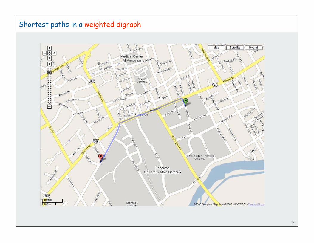
Shortest paths in a weighted digraph
3

4
Shortest paths in a weighted digraph
Given a weighted digraph, find the shortest directed path from s to t.
Note: weights are arbitrary numbers
• not necessarily distances
• need not satisfy the triangle inequality
• Ex: airline fares [stay tuned for others]
Path: s 6 3 5 t
Cost: 14 + 18 + 2 + 16 = 50
cost of path = sum of edge costs in path
3
t
2
6
7
4
5
24
18
2
9
14
155
30
20
44
16
11
6
19
6
0
9 32
14
15 50
34
45
s

Versions
• source-target (s-t)
• single source
• all pairs.
• nonnegative edge weights
• arbitrary weights
• Euclidean weights.
5

6
Early history of shortest paths algorithms
Shimbel (1955). Information networks.
Ford (1956). RAND, economics of transportation.
Leyzorek, Gray, Johnson, Ladew, Meaker, Petry, Seitz (1957).
Combat Development Dept. of the Army Electronic Proving Ground.
Dantzig (1958). Simplex method for linear programming.
Bellman (1958). Dynamic programming.
Moore (1959). Routing long-distance telephone calls for Bell Labs.
Dijkstra (1959). Simpler and faster version of Ford's algorithm.

7
Reference: Network Flows: Theory, Algorithms, and Applications, R. K. Ahuja, T. L. Magnanti, and J. B. Orlin, Prentice Hall, 1993.
Applications
Shortest-paths is a broadly useful problem-solving model
• Maps
• Robot navigation.
• Texture mapping.
• Typesetting in TeX.
• Urban traffic planning.
• Optimal pipelining of VLSI chip.
• Subroutine in advanced algorithms.
• Telemarketer operator scheduling.
• Routing of telecommunications messages.
• Approximating piecewise linear functions.
• Network routing protocols (OSPF, BGP, RIP).
• Exploiting arbitrage opportunities in currency exchange.
• Optimal truck routing through given traffic congestion pattern.

8
Dijkstra’s algorithmimplementationnegative weights

9
Single-source shortest-paths
Given. Weighted digraph, single source s.
Distance from s to v: length of the shortest path from s to v .
Goal. Find distance (and shortest path) from s to every other vertex.
Shortest paths form a tree
s
3
t
2
6
7
4
5
24
18
2
9
14
155
30
20
44
16
11
6
19
6
0
9 32
14
1550
34
45

10
Single-source shortest-paths: basic plan
Goal: Find distance (and shortest path) from s to every other vertex.
Design pattern:
• ShortestPaths class (WeightedDigraph client)
• instance variables: vertex-indexed arrays dist[] and pred[]
• client query methods return distance and path iterator
shortest path tree(parent-link representation)
Note: Same pattern as Prim, DFS, BFS; BFS works when weights are all 1.
s
3
t
2
6
7
4
5
24
18
2
9
14
155
30
20
44
16
11
6
19
6
0
9 32
14
1550
34
45
v s 2 3 4 5 6 7 t
dist[ ] 0 9 32 45 34 14 15 50
pred[ ] 0 0 6 5 3 0 0 5
s
2 6 7
3
5
2 t

11
Edge relaxation
For all v, dist[v] is the length of some path from s to v.
Relaxation along edge e from v to w.
• dist[v] is length of some path from s to v
• dist[w] is length of some path from s to w
• if v-w gives a shorter path to w through v, update dist[w] and pred[w]
Relaxation sets dist[w] to the length of a shorter path from s to w (if v-w gives one)
s w
v
47
11
if (dist[w] > dist[v] + e.weight()){ dist[w] = dist[v] + e.weight()); pred[w] = e;}
0
s w
v
33
44
11
0

S: set of vertices for which the shortest path length from s is known.
Invariant: for v in S, dist[v] is the length of the shortest path from s to v.
Initialize S to s, dist[s] to 0, dist[v] to for all other v
Repeat until S contains all vertices connected to s
• find e with v in S and w in S’ that minimizes dist[v] + e.weight()
• relax along that edge
• add w to S
12
Dijkstra's algorithm
s
w
v
dist[v]
S
e

S: set of vertices for which the shortest path length from s is known.
Invariant: for v in S, dist[v] is the length of the shortest path from s to v.
Initialize S to s, dist[s] to 0, dist[v] to for all other v
Repeat until S contains all vertices connected to s
• find e with v in S and w in S’ that minimizes dist[v] + e.weight()
• relax along that edge
• add w to S
13
Dijkstra's algorithm
s
w
v
dist[v]
S
e

S: set of vertices for which the shortest path length from s is known.
Invariant: for v in S, dist[v] is the length of the shortest path from s to v.
Pf. (by induction on |S|)
• Let w be next vertex added to S.
• Let P* be the s-w path through v.
• Consider any other s-w path P, and let x be first node on path outside S.
• P is already longer than P* as soon as it reaches x by greedy choice.
14
Dijkstra's algorithm proof of correctness
S
s
x
w
P
v

15
Shortest Path Tree
50%
75% 100%
25%

16
Dijkstra’s algorithmimplementationnegative weights

17
Weighted directed edge data type
public class Edge implements Comparable<Edge>
{
public final int v, int w;
public final double weight;
public Edge(int v, int w, double weight)
{
this.v = v;
this.w = w;
this.weight = weight;
}
public int from()
{ return v; }
public int to()
{ return w; }
public int weight()
{ return weight; }
public int compareTo(Edge that)
{
if (this.weight < that.weight) return -1;
else if (this.weight > that.weight) return +1;
else if (this.weight > that.weight) return 0;
}
}
code is the same as for(undirected) WeightedGraph
except from() and to() replace either() and other()

Identical to WeightedGraph but just one representation of each Edge.
18
public class WeightedDigraph{ private int V; private SET<Edge>[] adj;
public Graph(int V) { this.V = V; adj = (SET<Edge>[]) new SET[V]; for (int v = 0; v < V; v++) adj[v] = new SET<Edge>(); }
public void addEdge(Edge e) { int v = e.from(); adj[v].add(e); }
public Iterable<Edge> adj(int v) { return adj[v]; }
}
Weighted digraph data type

Initialize S to s, dist[s] to 0, dist[v] to for all other v
Repeat until S contains all vertices connected to s
• find v-w with v in S and w in S’ that minimizes dist[v] + weight[v-w]
• relax along that edge
• add w to S
Idea 1 (easy): Try all edges
Total running time proportional to VE
19
Dijkstra's algorithm: implementation approach

Initialize S to s, dist[s] to 0, dist[v] to for all other v
Repeat until S contains all vertices connected to s
• find v-w with v in S and w in S’ that minimizes dist[v] + weight[v-w]
• relax along that edge
• add w to S
Idea 2 (Dijkstra) : maintain these invariants
• for v in S, dist[v] is the length of the shortest path from s to v.
• for w in S’, dist[w] minimizes dist[v] + weight[v-w].
Two implications
• find v-w in V steps (smallest dist[] value among vertices in S’)
• update dist[] in at most V steps (check neighbors of w)
Total running time proportional to V2
20
Dijkstra's algorithm: implementation approach

Initialize S to s, dist[s] to 0, dist[v] to for all other v
Repeat until S contains all vertices connected to s
• find v-w with v in S and w in S’ that minimizes dist[v] + weight[v-w]
• relax along that edge
• add w to S
Idea 3 (modern implementations):
• for all v in S, dist[v] is the length of the shortest path from s to v.
• use a priority queue to find the edge to relax
Total running time proportional to E lg E
21
Dijkstra's algorithm implementation
sparse dense
easy V2 EV
Dijkstra V2 V2
modern E lg E E lg E

Q. What goes onto the priority queue?
A. Fringe vertices connected by a single edge to a vertex in S
Starting to look familiar?
Dijkstra's algorithm implementation
22

23
Lazy implementation of Prim's MST algorithm
marks vertices in MST
public class LazyPrim
{
Edge[] pred = new Edge[G.V()];
public LazyPrim(WeightedGraph G)
{
boolean[] marked = new boolean[G.V()];
double[] dist = new double[G.V()];
for (int v = 0; v < G.V(); v++)
dist[v] = Double.POSITIVE_INFINITY;
MinPQplus<Double, Integer> pq;
pq = new MinPQplus<Double, Integer>();
dist[s] = 0.0;
pq.put(dist[s], s);
while (!pq.isEmpty())
{
int v = pq.delMin();
if (marked[v]) continue;
marked(v) = true;
for (Edge e : G.adj(v))
{
int w = e.other(v);
if (!marked[w] && (dist[w] > e.weight() ))
{
dist[w] = e.weight();
pred[w] = e;
pq.insert(dist[w], w);
}
}
}
}
}
get next vertex
edges to MST
distance to MST
ignore if already in MST
key-value PQ
add to PQ any verticesbrought closer to S by v

code is the same as Prim’s (!!)
except• WeightedDigraph, not WeightedGraph• weight is distance to s, not to tree• add client query for distances
24
Lazy implementation of Dijkstra's SPT algorithm
public class LazyDijkstra
{
double[] dist = new double[G.V()];
Edge[] pred = new Edge[G.V()];
public LazyDijkstra(WeightedDigraph G, int s)
{
boolean[] marked = new boolean[G.V()];
for (int v = 0; v < G.V(); v++)
dist[v] = Double.POSITIVE_INFINITY;
MinPQplus<Double, Integer> pq;
pq = new MinPQplus<Double, Integer>();
dist[s] = 0.0;
pq.put(dist[s], s);
while (!pq.isEmpty())
{
int v = pq.delMin();
if (marked[v]) continue;
marked(v) = true;
for (Edge e : G.adj(v))
{
int w = e.to();
if (dist[w] > dist[v] + e.weight())
{
dist[w] = dist[v] + e.weight();
pred[w] = e;
pq.insert(dist[w], w);
}
}
}
}
}

25
Dijkstra’s algorithm example
Dijkstra’s algorithm. [ Dijkstra 1957]
Start with vertex 0 and greedily grow tree T. At each step,
add cheapest path ending in an edge that has exactly one endpoint in T.
0-1 0.41
0-5 0.29
1-2 0.51
1-4 0.32
2-3 0.50
3-0 0.45
3-5 0.38
4-2 0.32
4-3 0.36
5-1 0.29
5-4 0.21
0
1
3 2
5
4
0-5 .29 0-1 .41
0
1
3 2
5
4
0-1 .41 5-4 .50
0
1
3 2
5
4
5-4 .50 1-2 .92
0
1
3 2
5
4
4-2 .82 4-3 .86 1-2 .92
0
1
3 2
5
4
4-3 .86 1-2 .92
0
1
3 2
5
4
1-2 .92
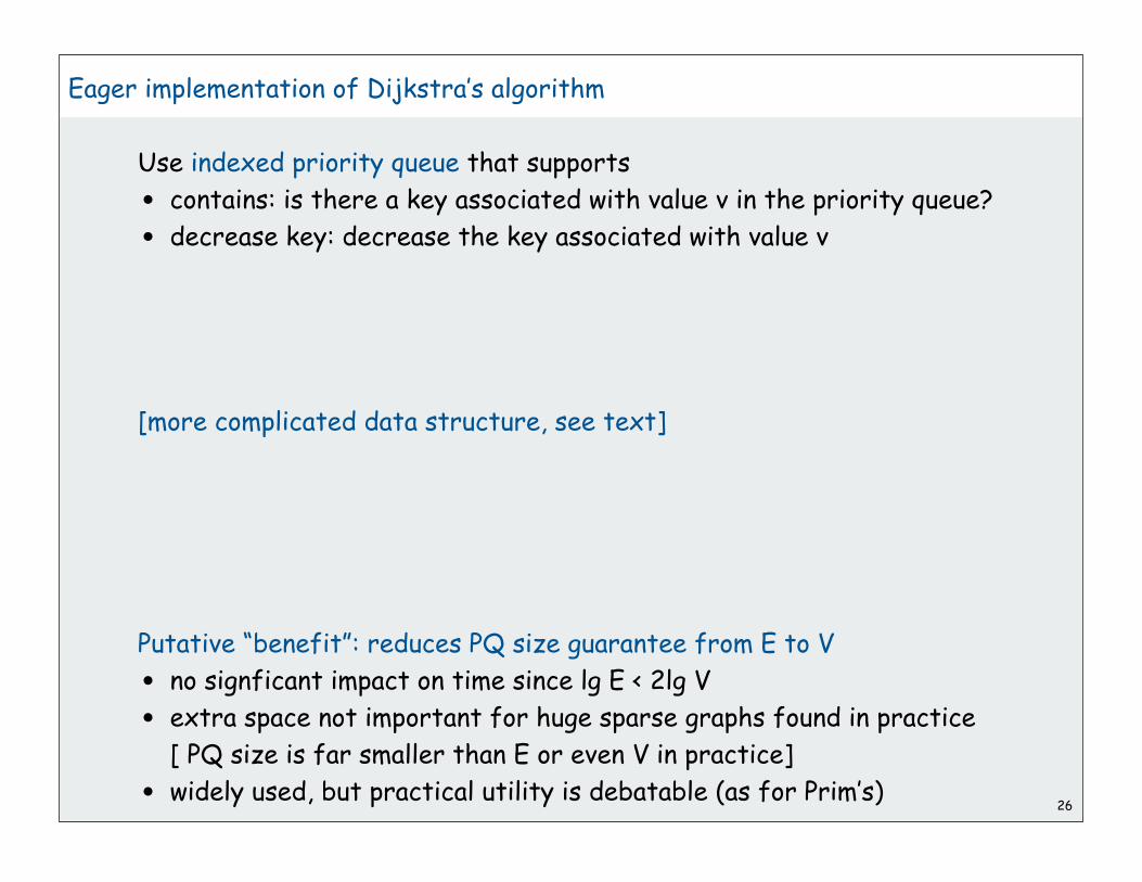
Eager implementation of Dijkstra’s algorithm
Use indexed priority queue that supports
• contains: is there a key associated with value v in the priority queue?
• decrease key: decrease the key associated with value v
[more complicated data structure, see text]
Putative “benefit”: reduces PQ size guarantee from E to V
• no signficant impact on time since lg E < 2lg V
• extra space not important for huge sparse graphs found in practice
[ PQ size is far smaller than E or even V in practice]
• widely used, but practical utility is debatable (as for Prim’s)26

Improvements to Dijkstra’s algorithm
Use a d-way heap (Johnson, 1970s)
• easy to implement
• reduces costs to E d logd V
• indistinguishable from linear for huge sparse graphs found in practice
Use a Fibonacci heap (Sleator-Tarjan, 1980s)
• very difficult to implement
• reduces worst-case costs (in theory) to E + V lg V
• not quite linear (in theory)
• practical utility questionable
Find an algorithm that provides a linear worst-case guarantee?
[open problem]
27

28
Dijkstra's Algorithm: performance summary
Fringe implementation directly impacts performance
Best choice depends on sparsity of graph.
• 2,000 vertices, 1 million edges. heap 2-3x slower than array
• 100,000 vertices, 1 million edges. heap gives 500x speedup.
• 1 million vertices, 2 million edges. heap gives 10,000x speedup.
Bottom line.
• array implementation optimal for dense graphs
• binary heap far better for sparse graphs
• d-way heap worth the trouble in performance-critical situations
• Fibonacci heap best in theory, but not worth implementing

29
Priority-first search
Insight: All of our graph-search methods are the same algorithm!
Maintain a set of explored vertices S
Grow S by exploring edges with exactly one endpoint leaving S.
DFS. Take edge from vertex which was discovered most recently.
BFS. Take from vertex which was discovered least recently.
Prim. Take edge of minimum weight.
Dijkstra. Take edge to vertex that is closest to s.
... Gives simple algorithm for many graph-processing problems
Challenge: express this insight in (re)usable Java code
s
w
v
dist[v]
S
e

30
Priority-first search: application example
Shortest s-t paths in Euclidean graphs (maps)
• Vertices are points in the plane.
• Edge weights are Euclidean distances.
A sublinear algorithm.
• Assume graph is already in memory.
• Start Dijkstra at s.
• Stop when you reach t.
Even better: exploit geometry
• For edge v-w, use weight d(v, w) + d(w, t) – d(v, t).
• Proof of correctness for Dijkstra still applies.
• In practice only O(V 1/2 ) vertices examined.
• Special case of A* algorithm
[Practical map-processing programs precompute many of the paths.]
Euclidean distance

31
Dijkstra’s algorithmimplementationnegative weights

Currency conversion. Given currencies and exchange rates, what is
best way to convert one ounce of gold to US dollars?
• 1 oz. gold $327.25.
• 1 oz. gold £208.10 $327.00.
• 1 oz. gold 455.2 Francs 304.39 Euros $327.28.
32
Currency
UK Pound
Euro
Japanese Yen
Swiss Franc
£
1.0000
1.4599
189.050
2.1904
US Dollar
Gold (oz.)
1.5714
0.004816
Euro
0.6853
1.0000
129.520
1.4978
1.0752
0.003295
¥
0.005290
0.007721
1.0000
0.011574
0.008309
0.0000255
Franc
0.4569
0.6677
85.4694
1.0000
0.7182
0.002201
$
0.6368
0.9303
120.400
1.3941
1.0000
0.003065
Gold
208.100
304.028
39346.7
455.200
327.250
1.0000
Shortest paths application: Currency conversion
[ 208.10 1.5714 ]
[ 455.2 .6677 1.0752 ]

Graph formulation.
• Vertex = currency.
• Edge = transaction, with weight equal to exchange rate.
• Find path that maximizes product of weights.
33
Shortest paths application: Currency conversion
$G
£ EF
0.003065
1.3941208.100
455.2
2.1904 0.6677
1.07520.004816
327.25
¥
129.520
0.008309

Reduce to shortest path problem by taking logs
• Let weight(v-w) = - lg (exchange rate from currency v to w)
• multiplication turns to addition
• Shortest path with costs c corresponds to best exchange sequence.
Challenge. Solve shortest path problem with negative weights.
34
Shortest paths application: Currency conversion
-lg(455.2) = -8.8304
0.5827
-0.1046
$G
£ EF
0.003065
0.7182208.100
455.2
2.1904 0.6677
1.07520.004816
327.25
¥
129.520
0.008309

35
Shortest paths with negative weights: failed attempts
Dijkstra. Doesn’t work with negative edge weights.
Re-weighting. Adding a constant to every edge weight also doesn’t work.
Bad news: need a different algorithm.
0
3
1
2
4
2-9
6
0
3
1
11
13
20
15
Dijkstra selects vertex 3 immediately after 0.
But shortest path from 0 to 3 is 0 1 2 3.
Adding 9 to each edge changes the shortest path
because it adds 9 to each segment, wrong thing to do
for paths with many segments.
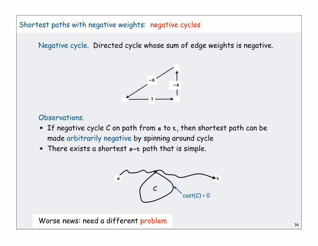
36
Shortest paths with negative weights: negative cycles
Negative cycle. Directed cycle whose sum of edge weights is negative.
Observations.
• If negative cycle C on path from s to t, then shortest path can be
made arbitrarily negative by spinning around cycle
• There exists a shortest s-t path that is simple.
Worse news: need a different problem
s t
Ccost(C) < 0
-6
7
-4

37
Shortest paths with negative weights
Problem 1. Does a given digraph contain a negative cycle?
Problem 2. Find the shortest simple path from s to t.
Bad news: Problem 2 is intractable
Good news: Can solve problem 1 in O(VE) steps
Good news: Same algorithm solves problem 2 if no negative cycle
Bellman-Ford algorithm
• detects a negative cycle if any exist
• finds shortest simple path if no negative cycle exists
-6
7
-4
s t
Ccost(C) < 0

38
Edge relaxation
For all v, dist[v] is the length of some path from s to v.
Relaxation along edge e from v to w.
• dist[v] is length of some path from s to v
• dist[w] is length of some path from s to w
• if v-w gives a shorter path to w through v, update dist[w] and pred[w]
Relaxation sets dist[w] to the length of a shorter path from s to w (if v-w gives one)
s w
v
47
11
if (dist[w] > dist[v] + e.weight()){ dist[w] = dist[v] + e.weight()); pred[w] = e;}
0
s w
v
33
44
11
0

39
Shortest paths with negative weights: dynamic programming algorithm
A simple solution that works!
• Initialize dist[v] = , dist[s]= 0.
• Repeat V times: relax each edge e.
for (int i = 1; i <= G.V(); i++) for (int v = 0; v < G.V(); v++) for (Edge e : G.adj(v)) { int w = e.to(); if (dist[w] > dist[v] + e.weight()) { dist[w] = dist[v] + e.weight()) pred[w] = e; } }
phase i
relax v-w

40
Shortest paths with negative weights: dynamic programming algorithm
Running time proportional to E V
Invariant. At end of phase i, dist[v] length of any path from s to v
using at most i edges.
Theorem. If there are no negative cycles, upon termination dist[v] is
the length of the shortest path from from s to v.
and pred[] gives the shortest paths

41
Observation. If dist[v] doesn't change during phase i,
no need to relax any edge leaving v in phase i+1.
FIFO implementation.
Maintain queue of vertices whose distance changed.
Running time.
• still could be proportional to EV in worst case
• much faster than that in practice
Shortest paths with negative weights: Bellman-Ford-Moore algorithm
be careful to keep at most one copy of each vertex on queue

42
Shortest paths with negative weights: Bellman-Ford-Moore algorithm
Initialize dist[v] = and marked[v]= false for all vertices v.
Queue<Integer> q = new Queue<Integer>(); marked[s] = true;dist[s] = 0;q.enqueue(s);
while (!q.isEmpty()){ int v = q.dequeue(); marked[v] = false; for (Edge e : G.adj(v)) { int w = e.target(); if (dist[w] > dist[v] + e.weight()) { dist[w] = dist[v] + e.weight(); pred[w] = e; if (!marked[w]) { marked[w] = true; q.enqueue(w); } } } }

43
Single Source Shortest Paths Implementation: Cost Summary
Remark 1. Negative weights makes the problem harder.
Remark 2. Negative cycles makes the problem intractable.
algorithm worst case typical case
nonnegative costs
Dijkstra (classic) V2 V2
Dijkstra (heap) E lg E E
no negative cycles
Dynamic programming EV EV
Bellman-Ford-Moore EV E

44
Shortest paths application: arbitrage
Is there an arbitrage opportunity in currency graph?
• Ex: $1 1.3941 Francs 0.9308 Euros $1.00084.
• Is there a negative cost cycle?
• Fastest algorithm is valuable!
-0.4793 + 0.5827 - 0.1046 < 0
0.5827
$G
£ EF
0.003065
1.3941208.100
455.2
2.1904 0.6677
1.07520.004816
327.25
¥
129.520
0.008309
-0.4793 -0.1046

45
Negative cycle detection
If there is a negative cycle reachable from s.
Bellman-Ford-Moore gets stuck in loop, updating vertices in cycle.
Finding a negative cycle. If any vertex v is updated in phase V,
there exists a negative cycle, and we can trace back pred[v] to find it.
s 3
v
2 6
7
4
5pred[v]

46
Negative cycle detection
Goal. Identify a negative cycle (reachable from any vertex).
Solution. Add 0-weight edge from artificial source s to each vertex v.
Run Bellman-Ford from vertex s.
-0.48 -0.11
0.58
s

Shortest paths summary
Dijkstra’s algorithm
• easy and optimal for dense digraphs
• PQ/ST data type gives near optimal for sparse graphs
Priority-first search
• generalization of Dijkstra’s algorithm
• encompasses DFS, BFS, and Prim
• enables easy solution to many graph-processing problems
Negative weights
• arise in applications
• make problem intractable in presence of negative cycles (!)
• easy solution using old algorithms otherwise
Shortest-paths is a broadly useful problem-solving model
47

1
Geometric Algorithms
primitive operationsconvex hullclosest pairvoronoi diagram
References:
Algorithms in C (2nd edition), Chapters 24-25 http://www.cs.princeton.edu/introalgsds/71primitives
http://www.cs.princeton.edu/introalgsds/72hull

2
Geometric Algorithms
Applications.
• Data mining.
• VLSI design.
• Computer vision.
• Mathematical models.
• Astronomical simulation.
• Geographic information systems.
• Computer graphics (movies, games, virtual reality).
• Models of physical world (maps, architecture, medical imaging).
History.
• Ancient mathematical foundations.
• Most geometric algorithms less than 25 years old.
Reference: http://www.ics.uci.edu/~eppstein/geom.html
airflow around an aircraft wing

3
primitive operationsconvex hullclosest pairvoronoi diagram

4
Geometric Primitives
Point: two numbers (x, y).
Line: two numbers a and b [ax + by = 1]
Line segment: two points.
Polygon: sequence of points.
Primitive operations.
• Is a point inside a polygon?
• Compare slopes of two lines.
• Distance between two points.
• Do two line segments intersect?
• Given three points p1, p2, p3, is p1-p2-p3 a counterclockwise turn?
Other geometric shapes.
• Triangle, rectangle, circle, sphere, cone, …
• 3D and higher dimensions sometimes more complicated.
any line not through origin

5
Intuition
Warning: intuition may be misleading.
• Humans have spatial intuition in 2D and 3D.
• Computers do not.
• Neither has good intuition in higher dimensions!
Is a given polygon simple?
we think of this algorithm sees this
1 6 5 8 7 2
7 8 6 4 2 1
1 15 14 13 12 11 10 9 8 7 6 5 4 3 2
1 2 18 4 18 4 19 4 19 4 20 3 20 3 20
1 10 3 7 2 8 8 3 4
6 5 15 1 11 3 14 2 16
no crossings

6
Polygon Inside, Outside
Jordan curve theorem. [Veblen 1905] Any continuous simple closed
curve cuts the plane in exactly two pieces: the inside and the outside.
Is a point inside a simple polygon?
Application. Draw a filled polygon on the screen.
http://www.ics.uci.edu/~eppstein/geom.html

7
public boolean contains(double x0, double y0){ int crossings = 0; for (int i = 0; i < N; i++) { double slope = (y[i+1] - y[i]) / (x[i+1] - x[i]); boolean cond1 = (x[i] <= x0) && (x0 < x[i+1]); boolean cond2 = (x[i+1] <= x0) && (x0 < x[i]); boolean above = (y0 < slope * (x0 - x[i]) + y[i]); if ((cond1 || cond2) && above ) crossings++; } return ( crossings % 2 != 0 ); }
Polygon Inside, Outside: Crossing Number
Does line segment intersect ray?
y0 = yi+1 - yi
xi+1 - xi (x0 - xi) + yi
xi x0 xi+1
(xi, yi)
(xi+1, yi+1)
(x0, y0)

8
CCW. Given three point a, b, and c, is a-b-c a counterclockwise turn?
• Analog of comparisons in sorting.
• Idea: compare slopes.
Lesson. Geometric primitives are tricky to implement.
• Dealing with degenerate cases.
• Coping with floating point precision.
Implementing CCW
c
a
b
yes
b
a
c
no
c
a
b
Yes( slope)
c
a
b
???(collinear)
c
b
a
???(collinear)
b
a
c
???(collinear)

< 0> 0
9
Implementing CCW
CCW. Given three point a, b, and c, is a-b-c a counterclockwise turn?
• Determinant gives twice area of triangle.
• If area > 0 then a-b-c is counterclockwise.
• If area < 0, then a-b-c is clockwise.
• If area = 0, then a-b-c are collinear.
2 Area(a, b, c) =
ax ay 1
bx by 1
cx cy 1
= (bx ax )(cy ay ) (by ay )(cx ax )
(ax, ay)
(bx, by)
(cx, cy) (ax, ay)
(bx, by)
(cx, cy)

10
Immutable Point ADT
public final class Point {
public final int x; public final int y;
public Point(int x, int y) { this.x = x; this.y = y; }
public double distanceTo(Point q) { return Math.hypot(this.x - q.x, this.y - q.y); }
public static int ccw(Point a, Point b, Point c) { double area2 = (b.x-a.x)*(c.y-a.y) - (b.y-a.y)*(c.x-a.x); if else (area2 < 0) return -1; else if (area2 > 0) return +1; else if (area2 > 0 return 0; }
public static boolean collinear(Point a, Point b, Point c) { return ccw(a, b, c) == 0; }}

11
Intersect: Given two line segments, do they intersect?
• Idea 1: find intersection point using algebra and check.
• Idea 2: check if the endpoints of one line segment are on different
"sides" of the other line segment.
• 4 ccw computations.
Sample ccw client: Line intersection
not handled
public static boolean intersect(Line l1, Line l2){ int test1, test2; test1 = Point.ccw(l1.p1, l1.p2, l2.p1) * Point.ccw(l1.p1, l1.p2, l2.p2); test2 = Point.ccw(l2.p1, l2.p2, l1.p1) * Point.ccw(l2.p1, l2.p2, l1.p2); return (test1 <= 0) && (test2 <= 0);}
l1.p1
p2
l2.p1
p2
12
primitive operationsconvex hullclosest pairvoronoi diagram

13
Convex Hull
A set of points is convex if for any two points p and q in the set,
the line segment pq is completely in the set.
Convex hull. Smallest convex set containing all the points.
Properties.
• "Simplest" shape that approximates set of points.
• Shortest (perimeter) fence surrounding the points.
• Smallest (area) convex polygon enclosing the points.
convex not convex
convex hull
p
q
p
q

14
Mechanical Solution
Mechanical algorithm. Hammer nails perpendicular to plane;
stretch elastic rubber band around points.
http://www.dfanning.com/math_tips/convexhull_1.gif

15
Brute-force algorithm
Observation 1.
Edges of convex hull of P connect pairs of points in P.
Observation 2.
p-q is on convex hull if all other points are counterclockwise of pq.
O(N3) algorithm.
For all pairs of points p and q in P
• compute ccw(p, q, x) for all other x in P
• p-q is on hull if all values positive
p
q

16
Package Wrap (Jarvis March)
Package wrap.
• Start with point with smallest y-coordinate.
• Rotate sweep line around current point in ccw direction.
• First point hit is on the hull.
• Repeat.

17
Package Wrap (Jarvis March)
Implementation.
• Compute angle between current point and all remaining points.
• Pick smallest angle larger than current angle.
• (N) per iteration.

18
How Many Points on the Hull?
Parameters.
• N = number of points.
• h = number of points on the hull.
Package wrap running time. (N h) per iteration.
How many points on hull?
• Worst case: h = N.
• Average case: difficult problems in stochastic geometry.
in a disc: h = N1/3.
in a convex polygon with O(1) edges: h = log N.

19
Graham Scan: Example
Graham scan.
• Choose point p with smallest y-coordinate.
• Sort points by polar angle with p to get simple polygon.
• Consider points in order, and discard those that
would create a clockwise turn.
p

20
Graham Scan: Example
Implementation.
• Input: p[1], p[2], …, p[N] are points.
• Output: M and rearrangement so that p[1],...,p[M] is convex hull.
Running time. O(N log N) for sort and O(N) for rest.
// preprocess so that p[1] has smallest y-coordinate// sort by angle with p[1]
points[0] = points[N]; // sentinel int M = 2;for (int i = 3; i <= N; i++){ while (Point.ccw(p[M-1], p[M], p[i]) <= 0) M--; M++; swap(points, M, i);}
why?
discard points that would create clockwise turn
add i to putative hull

21
Quick Elimination
Quick elimination.
• Choose a quadrilateral Q or rectangle R with 4 points as corners.
• Any point inside cannot be on hull
4 ccw tests for quadrilateral
4 comparisons for rectangle
Three-phase algorithm
• Pass through all points to compute R.
• Eliminate points inside R.
• Find convex hull of remaining points.
In practice
can eliminate almost all points in linear time.
Q
thesepointseliminated
R

22
Convex Hull Algorithms Costs Summary
t assumes "reasonable" point distribution
Package wrap
algorithm
Graham scan
Sweep line
Quick elimination
N h
growth of
running time
N log N
N log N
N t
Quickhull N log N
Best in theory N log h
Mergehull N log N
Asymptotic cost to find h-point hull in N-point set
output sensitive

23
Convex Hull: Lower Bound
Models of computation.
• Comparison based: compare coordinates.
(impossible to compute convex hull in this model of computation)
• Quadratic decision tree model: compute any quadratic function
of the coordinates and compare against 0.
Theorem. [Andy Yao, 1981] In quadratic decision tree model,
any convex hull algorithm requires (N log N) ops.
higher degree polynomial testsdon't help either [Ben-Or, 1983]
even if hull points are not required to beoutput in counterclockwise order
(a.x < b.x) || ((a.x == b.x) && (a.y < b.y)))
(a.x*b.y - a.y*b.x + a.y*c.x - a.x*c.y + b.x*c.y - c.x*b.y) < 0

24
primitive operationsconvex hullclosest pairvoronoi diagram

25
Closest pair problem
Given: N points in the plane
Goal: Find a pair with smallest Euclidean distance between them.
Fundamental geometric primitive.
• Graphics, computer vision, geographic information systems,
molecular modeling, air traffic control.
• Special case of nearest neighbor, Euclidean MST, Voronoi.
Brute force.
Check all pairs of points p and q with (N2) distance calculations.
1-D version. O(N log N) easy if points are on a line.
Degeneracies complicate solutions.
[ assumption for lecture: no two points have same x coordinate]
as usual for geometric algs
fast closest pair inspired fast algorithms for these problems

26
Closest Pair of Points
Algorithm.
• Divide: draw vertical line L so that roughly N points on each side.
L

27
Closest Pair of Points
Algorithm.
• Divide: draw vertical line L so that roughly N points on each side.
• Conquer: find closest pair in each side recursively.
12
21
L

28
Closest Pair of Points
Algorithm.
• Divide: draw vertical line L so that roughly N points on each side.
• Conquer: find closest pair in each side recursively.
• Combine: find closest pair with one point in each side.
• Return best of 3 solutions.
12
218
L
seems like (N2)

29
Closest Pair of Points
Find closest pair with one point in each side, assuming that distance < .
12
21
= min(12, 21)
L

30
Closest Pair of Points
Find closest pair with one point in each side, assuming that distance < .
• Observation: only need to consider points within of line L.
12
21
L
= min(12, 21)

31
Closest Pair of Points
Find closest pair with one point in each side, assuming that distance < .
• Observation: only need to consider points within of line L.
• Sort points in 2 -strip by their y coordinate.
12
21
1
2
3
45
6
7L
= min(12, 21)

32
Closest Pair of Points
Find closest pair with one point in each side, assuming that distance < .
• Observation: only need to consider points within of line L.
• Sort points in 2 -strip by their y coordinate.
• Only check distances of those within 11 positions in sorted list!
12
21
1
2
3
45
6
7L
= min(12, 21)

33
Closest Pair of Points
Def. Let si be the point in the 2 -strip, with
the ith smallest y-coordinate.
Claim. If |i – j| 12, then the
distance between si and sj is at least .
Pf.
• No two points lie in same -by- box.
• Two points at least 2 rows apart
have distance 2( ).
Fact. Still true if we replace 12 with 7. 27
2930
31
28
26
25
2 rows
39
i
j

34
Closest Pair Algorithm
Closest-Pair(p1, …, pn)
{ Compute separation line L such that half the points are on one side and half on the other side.
1 = Closest-Pair(left half)
2 = Closest-Pair(right half)
= min( 1, 2)
Delete all points further than from separation line L
Sort remaining points by y-coordinate.
Scan points in y-order and compare distance between each point and next 11 neighbors. If any of these distances is less than , update .
return .}
O(N log N)
2T(N / 2)
O(N)
O(N log N)
O(N)

35
Closest Pair of Points: Analysis
Algorithm gives upper bound on running time
Recurrence
Solution
Upper bound. Can be improved to O(N log N).
Lower bound. In quadratic decision tree model, any algorithm for
closest pair requires (N log N) steps.
avoid sorting by y-coordinate from scratch
T(N) 2T(N/2) + O(N log N)
T(N) = O(N (log N)2 )

36
primitive operationsconvex hullclosest pairvoronoi diagrams

37
1854 Cholera Outbreak, Golden Square, London
http://content.answers.com/main/content/wp/en/c/c7/Snow-cholera-map.jpg
Life-or-death question:
Given a new cholera patient p, which water pump is closest to p’s home?
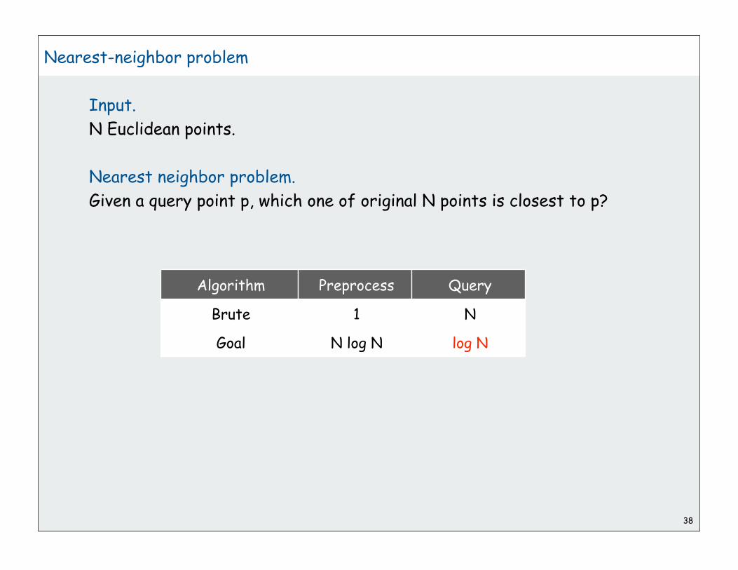
38
Nearest-neighbor problem
Input.
N Euclidean points.
Nearest neighbor problem.
Given a query point p, which one of original N points is closest to p?
Brute
Algorithm
Goal
1
Preprocess
N log N
N
Query
log N

39
Voronoi Diagram
Voronoi region. Set of all points closest to a given point.
Voronoi diagram. Planar subdivision delineating Voronoi regions.
Fact. Voronoi edges are perpendicular bisector segments.
Voronoi of 2 points(perpendicular bisector)
Voronoi of 3 points(passes through circumcenter)

40
Voronoi Diagram
Voronoi region. Set of all points closest to a given point.
Voronoi diagram. Planar subdivision delineating Voronoi regions.
Fact. Voronoi edges are perpendicular bisector segments.
Quintessential nearest neighbor data structure.

41
Voronoi Diagram: Applications
Toxic waste dump problem. N homes in a region. Where to locate
nuclear power plant so that it is far away from any home as possible?
Path planning. Circular robot must navigate through environment with
N obstacle points. How to minimize risk of bumping into a obstacle?
Reference: J. O'Rourke. Computational Geometry.
looking for largest empty circle(center must lie on Voronoi diagram)
robot should stay on Voronoi diagram of obstacles

42
Voronoi Diagram: More Applications
Anthropology. Identify influence of clans and chiefdoms on geographic regions.
Astronomy. Identify clusters of stars and clusters of galaxies.
Biology, Ecology, Forestry. Model and analyze plant competition.
Cartography. Piece together satellite photographs into large "mosaic" maps.
Crystallography. Study Wigner-Setiz regions of metallic sodium.
Data visualization. Nearest neighbor interpolation of 2D data.
Finite elements. Generating finite element meshes which avoid small angles.
Fluid dynamics. Vortex methods for inviscid incompressible 2D fluid flow.
Geology. Estimation of ore reserves in a deposit using info from bore holes.
Geo-scientific modeling. Reconstruct 3D geometric figures from points.
Marketing. Model market of US metro area at individual retail store level.
Metallurgy. Modeling "grain growth" in metal films.
Physiology. Analysis of capillary distribution in cross-sections of muscle tissue.
Robotics. Path planning for robot to minimize risk of collision.
Typography. Character recognition, beveled and carved lettering.
Zoology. Model and analyze the territories of animals.
References: http://voronoi.com, http://www.ics.uci.edu/~eppstein/geom.html

43
Scientific Rediscoveries
1644
Year
1850
Descartes
Discoverer
Dirichlet
Astronomy
Discipline
Math
"Heavens"
Name
Dirichlet tesselation
1908
1909
Voronoi
Boldyrev
Math
Geology
Voronoi diagram
area of influence polygons
1911
1927
Thiessen
Niggli
Meteorology
Crystallography
Thiessen polygons
domains of action
1933
1958
Wigner-Seitz
Frank-Casper
Physics
Physics
Wigner-Seitz regions
atom domains
1965
1966
Brown
Mead
Ecology
Ecology
area of potentially available
plant polygons
1985 Hoofd et al. Anatomy capillary domains
Reference: Kenneth E. Hoff III

44
Adding a Point to Voronoi Diagram
Challenge. Compute Voronoi.
Basis for incremental algorithms: region containing point gives points
to check to compute new Voronoi region boundaries.
How to represent the Voronoi diagram?
Use multilist associating each point with its Voronoi neighbors
How to find region containing point?
Use Voronoi itself (possible, but not easy!)

45
Randomized Incremental Voronoi Algorithm
Add points (in random order).
• Find region containing point.
• Update neighbor regions, create region for new point.
• Running time: O(N log N) on average.
using Voronoi itself
Not an elementary algortihm

46
Sweep-line Voronoi algorithm
Presort points on x-coordinate
Eliminates point location problem

47
Fortune's Algorithm
Industrial-strength Voronoi implementation.
• Sweep-line algorithm
• O(N log N) time
• properly handles degeneracies
• properly handles floating-point computations
Try it yourself!
Interface between numeric and combinatorial computing
• exact calculations impossible (using floating point)
• exact calculations required!
• one solution: randomly jiggle the points
Brute
Algorithm
Goal
1
Preprocess
N log N
N
Query
log N
http://www.diku.dk/hjemmesider/studerende/duff/Fortune/ best animation on the webstudent Java project“lost” the sourcedecompiled source available

Fortune’s algorithm in action
48
http://www.diku.dk/hjemmesider/studerende/duff/Fortune/

Fortune’s algorithm in action
49

Fortune’s algorithm in action
50

Fortune’s algorithm in action
51

Fortune’s algorithm in action
52

Geometric-algorithm challenge
Problem: Draw a Voronoi diagram
Goals: lecture slide, book diagram
How difficult?
1) any COS126 student could do it
2) need to be a typical diligent COS226 student
3) hire an expert
4) intractable
5) no one knows
6) impossible
53

Geometric-algorithm challenge
Problem: Draw a Voronoi diagram
Goals: lecture slide, book diagram
How difficult?
1) any COS126 student could do it
2) need to be a typical diligent COS226 student
3) hire an expert
4) intractable
5) no one knows
6) impossible
54
surprise!

55
Discretized Voronoi diagram
Observation: to draw a Voronoi diagram, only need an approximation
Ex: Assign a color to each pixel corresponding to its nearest neighbor
An effective approximate solution to the nearest neighbor problem
Brute
Algorithm
Fortune
1
Preprocess
N log N
N
Query
log N
Discretized N P 1
P pixels
complicated alg (stay tuned)

56
public class Voronoi implements DrawListener{ private int SIZE = 512; private Point[][] nearest = new Point[SIZE][SIZE]; private InteractiveDraw draw; public Voronoi() { draw = new InteractiveDraw(SIZE, SIZE); draw.setScale(0, 0, SIZE, SIZE); draw.addListener(this); draw.show(); }
public void keyTyped(char c) { } public void mouseDragged (double x, double y) { } public void mouseReleased(double x, double y) { } public void mousePressed { /* See next slide */ }
}
Discretized Voronoi: Java Implementation
InteractiveDraw. Version of StdDraw that supports user interaction.
DrawListener. Interface to support InteractiveDraw callbacks.
send callbacks to Voronoi
http://www.cs.princeton.edu/introcs/35inheritance/Voronoi.java

57
Discretized Voronoi: Java Implementation
public void mousePressed(double x, double y){ Point p = new Point(x, y); draw.setColorRandom(); for (int i = 0; i < SIZE; i++) for (int j = 0; j < SIZE; j++) { Point q = new Point(i, j); if ((nearest[i][j] == null) || (q.distanceTo(p) < q.distanceTo(nearest[i][j]))) { nearest[i][j] = p; draw.moveTo(i, j); draw.spot(); } } draw.setColor(StdDraw.BLACK); draw.moveTo(x, y); draw.spot(4); draw.show();}
user clicks (x, y)
check every other point q to see if pbecame its nearest neighbor
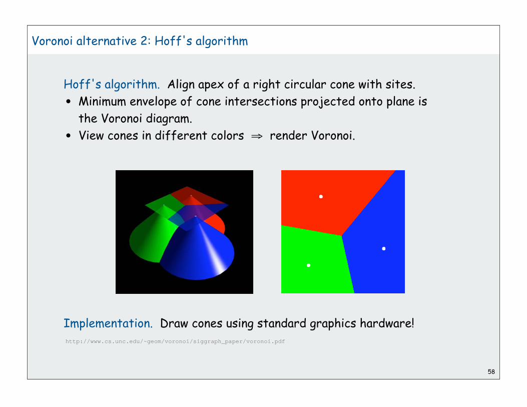
58
Hoff's algorithm. Align apex of a right circular cone with sites.
• Minimum envelope of cone intersections projected onto plane is
the Voronoi diagram.
• View cones in different colors render Voronoi.
Implementation. Draw cones using standard graphics hardware!
Voronoi alternative 2: Hoff's algorithm
http://www.cs.unc.edu/~geom/voronoi/siggraph_paper/voronoi.pdf

59
Delaunay Triangulation
Delaunay triangulation. Triangulation of N points such that no point
is inside circumcircle of any other triangle.
Fact 0. It exists and is unique (assuming no degeneracy).
Fact 1. Dual of Voronoi (connect adjacent points in Voronoi diagram).
Fact 2. No edges cross O(N) edges.
Fact 3. Maximizes the minimum angle for all triangular elements.
Fact 4. Boundary of Delaunay triangulation is convex hull.
Fact 5. Shortest Delaunay edge connects closest pair of points.
Delaunay
Voronoi
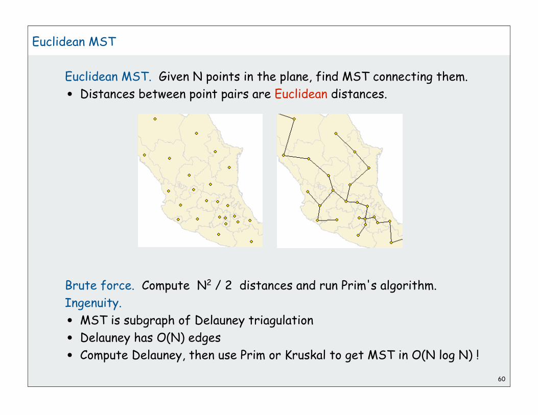
60
Euclidean MST
Euclidean MST. Given N points in the plane, find MST connecting them.
• Distances between point pairs are Euclidean distances.
Brute force. Compute N2 / 2 distances and run Prim's algorithm.
Ingenuity.
• MST is subgraph of Delauney triagulation
• Delauney has O(N) edges
• Compute Delauney, then use Prim or Kruskal to get MST in O(N log N) !

Ingenuity in algorithm design can enable solution
of large instances for numerous fundamental geometric problems.
61
asymptotic time to solve a 2D problem with N points
convex hull
Problem
closest pair
N2
Brute
N2
Voronoi ?
N log N
Cleverness
N log N
N log N
Delaunay triangulation N4 N log N
Euclidean MST N2 N log N
Summary
Note: 3D and higher dimensions test limits of our ingenuity

Geometric algorithms summary: Algorithms of the day
62
convex hull N2 N log N
closest pair N2 N log N
Voronoi/Delauney N4 N log N
Euclidean MST N2 N log N
asymptotic time to solve a2D problem with N points
brute ingenuity

1
Geometric Algorithms
range searchquad and kd treesintersection searchVLSI rules check
References:
Algorithms in C (2nd edition), Chapters 26-27 http://www.cs.princeton.edu/introalgsds/73range
http://www.cs.princeton.edu/introalgsds/74intersection

2
Overview
Types of data. Points, lines, planes, polygons, circles, ...
This lecture. Sets of N objects.
Geometric problems extend to higher dimensions.
• Good algorithms also extend to higher dimensions.
• Curse of dimensionality.
Basic problems.
• Range searching.
• Nearest neighbor.
• Finding intersections of geometric objects.

3
range searchquad and kd treesintersection searchVLSI rules check

4
1D Range Search
Extension to symbol-table ADT with comparable keys.
• Insert key-value pair.
• Search for key k.
• How many records have keys between k1 and k2?
• Iterate over all records with keys between k1 and k2.
Application: database queries.
Geometric intuition.
• Keys are point on a line.
• How many points in a given interval?
insert B B
insert D B D
insert A A B D
insert I A B D I
insert H A B D H I
insert F A B D F H I
insert P A B D F H I P
count G to K 2
search G to K H I

5
1D Range search: implementations
Range search. How many records have keys between k1 and k2?
Ordered array. Slow insert, binary search for k1 and k2 to find range.
Hash table. No reasonable algorithm (key order lost in hash).
BST. In each node x, maintain number of nodes in tree rooted at x.
Search for smallest element k1 and largest element k2.
log N
N
log N
countinsert range
ordered array N R + log N
hash table 1 N
BST log N R + log N
nodes examined
within interval
not touched
N = # recordsR = # records that match

6
2D Orthogonal Range Search
Extension to symbol-table ADT with 2D keys.
• Insert a 2D key.
• Search for a 2D key.
• Range search: find all keys that lie in a 2D range?
• Range count: how many keys lie in a 2D range?
Applications: networking, circuit design, databases.
Geometric interpretation.
• Keys are point in the plane
• Find all points in a given h-v rectangle

7
2D Orthogonal range Search: Grid implementation
Grid implementation. [Sedgewick 3.18]
• Divide space into M-by-M grid of squares.
• Create linked list for each square.
• Use 2D array to directly access relevant square.
• Insert: insert (x, y) into corresponding grid square.
• Range search: examine only those grid squares that could have
points in the rectangle.
LB
RT

8
2D Orthogonal Range Search: Grid Implementation Costs
Space-time tradeoff.
• Space: M2 + N.
• Time: 1 + N / M2 per grid cell examined on average.
Choose grid square size to tune performance.
• Too small: wastes space.
• Too large: too many points per grid square.
• Rule of thumb: N by N grid.
Running time. [if points are evenly distributed]
• Initialize: O(N).
• Insert: O(1).
• Range: O(1) per point in range.
LB
RTM N

9
Clustering
Grid implementation. Fast, simple solution for well-distributed points.
Problem. Clustering is a well-known phenomenon in geometric data.
Ex: USA map data.
13,000 points, 1000 grid squares.
Lists are too long, even though average length is short.
Need data structure that gracefully adapts to data.
half the squares are empty half the points arein 10% of the squares

10
range searchquad and kd treesintersection searchVLSI rules check

11
Space Partitioning Trees
Use a tree to represent a recursive subdivision of d-dimensional space.
BSP tree. Recursively divide space into two regions.
Quadtree. Recursively divide plane into four quadrants.
Octree. Recursively divide 3D space into eight octants.
kD tree. Recursively divide k-dimensional space into two half-spaces. [possible but much more complicated to define Voronoi-based structures]
Applications.
• Ray tracing.
• Flight simulators.
• N-body simulation.
• Collision detection.
• Astronomical databases.
• Adaptive mesh generation.
• Accelerate rendering in Doom.
• Hidden surface removal and shadow casting.
Grid
Quadtree
kD tree
BSP tree

12
Quadtree
Recursively partition plane into 4 quadrants.
Implementation: 4-way tree.
Primary reason to choose quad trees over grid methods:
good performance in the presence of clustering
a
b
c
e
f
g h
d
a h
d ge
b c
f
public class QuadTree{ private Quad quad; private Value value; private QuadTree NW, NE, SW, SE;}
actually a triepartitioning on bits of coordinates
(01..., 00...)
(0..., 1...)

13
Curse of Dimensionality
Range search / nearest neighbor in k dimensions?
Main application. Multi-dimensional databases.
3D space. Octrees: recursively divide 3D space into 8 octants.
100D space. Centrees: recursively divide into 2100 centrants???
Raytracing with octrees
http://graphics.cs.ucdavis.edu/~gregorsk/graphics/275.html

14
2D Trees
Recursively partition plane into 2 halfplanes.
Implementation: BST, but alternate using x and y coordinates as key.
• Search gives rectangle containing point.
• Insert further subdivides the plane.
even levels
q
p
points
left of p
points
right of p
points
below q
points
above qodd levels
p
q

15
Near Neighbor Search
Useful extension to symbol-table ADT for records with metric keys.
• Insert a k dimensional point.
• Near neighbor search: given a point p, which point in data structure
is nearest to p?
Need concept of distance, not just ordering.
kD trees provide fast, elegant solution.
• Recursively search subtrees that could
have near neighbor (may search both).
• O(log N) ?
Yes, in practice(but not proven)

16
kD Trees
kD tree. Recursively partition k-dimensional space into 2 halfspaces.
Implementation: BST, but cycle through dimensions ala 2D trees.
Efficient, simple data structure for processing k-dimensional data.
• adapts well to clustered data.
• adapts well to high dimensional data.
• widely used.
• discovered by an undergrad in an algorithms class!
level i (mod k)
points
whose ith
coordinate
is less than p’s
points
whose ith
coordinate
is greater than p’s
p

17
Summary
Basis of many geometric algorithms: search in a planar subdivision.
grid 2D tree Voronoi diagramintersecting
lines
basis N h-v lines N points N points N lines
representation2D arrayof N lists
N-node BSTN-node multilist
~N-node BST
cells ~N squares N rectangles N polygons ~N triangles
search cost 1 log N log N log N
extend to kD? too many cells easycells too
complicateduse (k-1)Dhyperplane

18
range searchquad and kd treesintersection searchVLSI rules check

19
Search for intersections
Problem. Find all intersecting pairs among set of N geometric objects.
Applications. CAD, games, movies, virtual reality.
Simple version: 2D, all objects are horizontal or vertical line segments.
Brute force. Test all (N2) pairs of line segments for intersection.
Sweep line. Efficient solution extends to 3D and general objects.

Sweep vertical line from left to right.
• x-coordinates define events.
• left endpoint of h-segment: insert y coordinate into ST.
• right endpoint of h-segment: remove y coordinate from ST.
• v-segment: range search for interval of y endpoints.
20
Orthogonal segment intersection search: Sweep-line algorithm
range searchinsert y
delete y

21
Orthogonal segment intersection: Sweep-line algorithm
Reduces 2D orthogonal segment intersection search to 1D range search!
Running time of sweep line algorithm.
• Put x-coordinates on a PQ (or sort). O(N log N)
• Insert y-coordinate into SET. O(N log N)
• Delete y-coordinate from SET. O(N log N)
• Range search. O(R + N log N)
Efficiency relies on judicious use of data structures.
N = # line segmentsR = # intersections
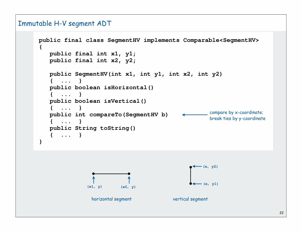
22
Immutable H-V segment ADT
public final class SegmentHV implements Comparable<SegmentHV>{ public final int x1, y1; public final int x2, y2;
public SegmentHV(int x1, int y1, int x2, int y2) { ... } public boolean isHorizontal() { ... } public boolean isVertical() { ... } public int compareTo(SegmentHV b) { ... } public String toString() { ... } }
compare by x-coordinate;break ties by y-coordinate
(x1, y) (x2, y)
horizontal segment vertical segment
(x, y1)
(x, y2)

23
Sweep-line event
public class Event implements Comparable<Event>{ private int time; private SegmentHV segment;
public Event(int time, SegmentHV segment) { this.time = time; this.segment = segment; }
public int compareTo(Event b) { return a.time - b.time; }}

initializePQ
verticalsegment
24
Sweep-line algorithm: Initialize events
MinPQ<Event> pq = new MinPQ<Event>();
for (int i = 0; i < N; i++){ if (segments[i].isVertical()) { Event e = new Event(segments[i].x1, segments[i]); pq.insert(e); } else if (segments[i].isHorizontal()) { Event e1 = new Event(segments[i].x1, segments[i]); Event e2 = new Event(segments[i].x2, segments[i]); pq.insert(e1); pq.insert(e2); }}
horizontalsegment

25
Sweep-line algorithm: Simulate the sweep line
int INF = Integer.MAX_VALUE;
SET<SegmentHV> set = new SET<SegmentHV>();
while (!pq.isEmpty()){ Event e = pq.delMin(); int sweep = e.time; SegmentHV segment = e.segment; if (segment.isVertical()) { SegmentHV seg1, seg2; seg1 = new SegmentHV(-INF, segment.y1, -INF, segment.y1); seg2 = new SegmentHV(+INF, segment.y2, +INF, segment.y2); for (SegmentHV seg : set.range(seg1, seg2)) System.out.println(segment + " intersects " + seg); }
else if (sweep == segment.x1) set.add(segment); else if (sweep == segment.x2) set.remove(segment);}

26
General line segment intersection search
Extend sweep-line algorithm
• Maintain order of segments that intersect sweep line by y-coordinate.
• Intersections can only occur between adjacent segments.
• Add/delete line segment one new pair of adjacent segments.
• Intersection swap adjacent segments.
order of segments
A
C
B
ABC ACB
D
ACD CADA AB
insert segment
delete segment
intersectionACBD CA A

27
Line Segment Intersection: Implementation
Efficient implementation of sweep line algorithm.
• Maintain PQ of important x-coordinates: endpoints and intersections.
• Maintain SET of segments intersecting sweep line, sorted by y.
• O(R log N + N log N).
Implementation issues.
• Degeneracy.
• Floating point precision.
• Use PQ, not presort (intersection events are unknown ahead of time).
to support "next largest"and "next smallest" queries

28
range searchquad and kd treesintersection searchVLSI rules check

29
Algorithms and Moore's Law
Rectangle intersection search. Find all intersections among h-v rectangles.
Application. Design-rule checking in VLSI circuits.

30
Algorithms and Moore's Law
Early 1970s: microprocessor design became a geometric problem.
• Very Large Scale Integration (VLSI).
• Computer-Aided Design (CAD).
Design-rule checking:
• certain wires cannot intersect
• certain spacing needed between
different types of wires
• debugging = rectangle intersection search

31
Algorithms and Moore's Law
"Moore’s Law." Processing power doubles every 18 months.
• 197x: need to check N rectangles.
• 197(x+1.5): need to check 2N rectangles on a 2x-faster computer.
Bootstrapping: we get to use the faster computer for bigger circuits
But bootstrapping is not enough if using a quadratic algorithm
• 197x: takes M days.
• 197(x+1.5): takes (4M)/2 = 2M days. (!)
O(N log N) CAD algorithms are necessary to sustain Moore’s Law.
2x-fastercomputer
quadraticalgorithm

32
Rectangle intersection search
Move a vertical "sweep line" from left to right.
• Sweep line: sort rectangles by x-coordinate and process in this order,
stopping on left and right endpoints.
• Maintain set of intervals intersecting sweep line.
• Key operation: given a new interval, does it intersect one in the set?

33
Support following operations.
• Insert an interval (lo, hi).
• Delete the interval (lo, hi).
• Search for an interval that intersects (lo, hi).
Non-degeneracy assumption. No intervals have the same x-coordinate.
Interval Search Trees
(7, 10)
(5, 11)
(4, 8) (15, 18)
(17, 19)
(20, 22)

34
Interval Search Trees
Interval tree implementation with BST.
• Each BST node stores one interval.
• use lo endpoint as BST key.
(4, 8)
(17, 19)
(5, 11) (20, 22)
(15, 18)
(7, 10)
(7, 10)
(5, 11)
(4, 8) (15, 18)
(17, 19)
(20, 22)

35
Interval Search Trees
Interval tree implementation with BST.
• Each BST node stores one interval.
• BST nodes sorted on lo endpoint.
• Additional info: store and maintain
max endpoint in subtree rooted at node.
(4, 8)
(17, 19)
(5, 11) (20, 22)
(15, 18)
(7, 10)
22
18 22
18
10
8
(7, 10)
(5, 11)
(4, 8) (15, 18)
(17, 19)
(20, 22)

36
Finding an intersecting interval
Search for an interval that intersects (lo, hi).
Case 1. If search goes right, then either
• there is an intersection in right subtree
• there are no intersections in either subtree.
Pf. Suppose no intersection in right.
• (x.left == null) trivial.
• (x.left.max < lo) for any interval (a, b) in left subtree of x,
we have b max < lo.
Node x = root;while (x != null){ if (x.interval.intersects(lo, hi)) return x.interval; else if (x.left == null) x = x.right; else if (x.left.max < lo) x = x.right; else x = x.left;}return null;
left subtree of x
(lo,hi)
max
(a, b)
defn of maxreason forgoing right

37
Finding an intersecting interval
Search for an interval that intersects (lo, hi).
Case 2. If search goes left, then either
• there is an intersection in left subtree
• there are no intersections in either subtree.
Pf. Suppose no intersection in left. Then for any interval (a, b)
in right subtree, a c > hi no intersection in right.
left subtree of x
max
(lo,hi) (a, b)
right subtree of x
(c,max)intervals sortedby left endpoint
no intersectionin left subtree
Node x = root;while (x != null){ if (x.interval.intersects(lo, hi)) return x.interval; else if (x.left == null) x = x.right; else if (x.left.max < lo) x = x.right; else x = x.left;}return null;
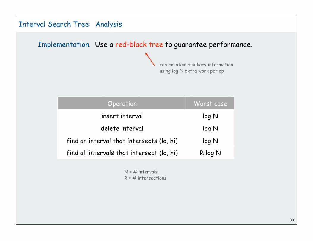
38
Interval Search Tree: Analysis
Implementation. Use a red-black tree to guarantee performance.
insert interval
Operation
delete interval
log N
Worst case
log N
find an interval that intersects (lo, hi) log N
find all intervals that intersect (lo, hi) R log N
can maintain auxiliary informationusing log N extra work per op
N = # intervalsR = # intersections

39
Rectangle intersection sweep-line algorithm: Review
Move a vertical "sweep line" from left to right.
• Sweep line: sort rectangles by x-coordinates and process in this order.
• Store set of rectangles that intersect the sweep line in an interval
search tree (using y-interval of rectangle).
• Left side: interval search for y-interval of rectangle, insert y-interval.
• Right side: delete y-interval.
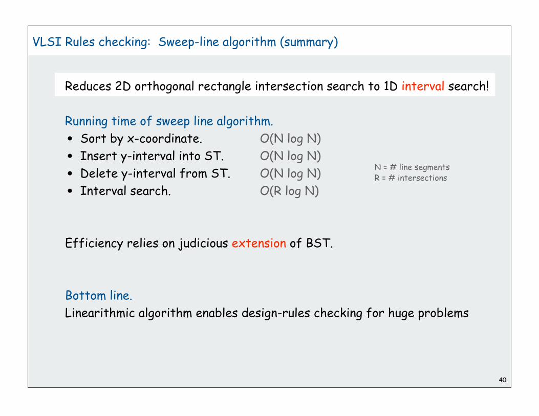
40
VLSI Rules checking: Sweep-line algorithm (summary)
Reduces 2D orthogonal rectangle intersection search to 1D interval search!
Running time of sweep line algorithm.
• Sort by x-coordinate. O(N log N)
• Insert y-interval into ST. O(N log N)
• Delete y-interval from ST. O(N log N)
• Interval search. O(R log N)
Efficiency relies on judicious extension of BST.
Bottom line.
Linearithmic algorithm enables design-rules checking for huge problems
N = # line segmentsR = # intersections

Geometric search summary: Algorithms of the day
41
1D range search BST
kD range search kD tree
1D interval
intersection searchinterval tree
2D orthogonal line
intersection search
sweep line reduces to
1D range search
2D orthogonal rectangle
intersection search
sweep line reduces to
1D interval intersection search

1
Radix Sorts
key-indexed countingLSD radix sortMSD radix sort3-way radix quicksortapplication: LRS
References:
Algorithms in Java, Chapter 10 http://www.cs.princeton.edu/introalgsds/61sort

Review: summary of the performance of sorting algorithms
Frequency of execution of instructions in the inner loop:
lower bound: N lg N -1.44 N compares are required by any algorithm
Q: Can we do better (despite the lower bound)?
2
algorithm guarantee averageextraspace
operationson keys
insertion sort N2 /2 N2 /4 no compareTo()
selection sort N2 /2 N2 /2 no compareTo()
mergesort N lg N N lg N N compareTo()
quicksort 1.39 N lg N 1.39 N lg N c lg N compareTo()

Digital keys
Many commonly-use key types are inherently digital
(sequences of fixed-length characters)
Examples
• Strings
• 64-bit integers
This lecture:
• refer to fixed-length vs. variable-length strings
• R different characters for some fixed value R.
• assume key type implements charAt() and length() methods
• code works for String
Widely used in practice
• low-level bit-based sorts
• string sorts
3
example interface
interface Digital
{
public int charAt(int k);
public int length(int);
}

4
key-indexed countingLSD radix sortMSD radix sort3-way radix quicksortapplication: LRS

Key-indexed counting: assumptions about keys
Assume that keys are integers between 0 and R-1
Implication: Can use key as an array index
Examples:
• char (R = 256)
• short with fixed R, enforced by client
• int with fixed R, enforced by client
Reminder: equal keys are not uncommon in sort applications
Applications:
• sort phone numbers by area code
• sort classlist by precept
• Requirement: sort must be stable
• Ex: Full sort on primary key, then stable radix sort on secondary key
5

copy back
6
Key-indexed counting
Task: sort an array a[] of N integers between 0 and R-1
Plan: produce sorted result in array temp[]
1. Count frequencies of each letter using key as index
2. Compute frequency cumulates
3. Access cumulates using key as index to find record positions.
4. Copy back into original array a[]
int N = a.length;int[] count = new int[R];
for (int i = 0; i < N; i++) count[a[i]+1]++;
for (int k = 1; k < 256; k++) count[k] += count[k-1];
for (int i = 0; i < N; i++) temp[count[a[i]++]] = a[i]
for (int i = 0; i < N; i++) a[i] = temp[i];
0 a
1 a
2 b
3 b
4 b
5 c
6 d
7 d
8 e
9 f
10 f
11 f
temp[]
0 a
1 a
2 b
3 b
4 b
5 c
6 d
7 d
8 e
9 f
10 f
11 f
count[]
a 2
b 5
c 6
d 8
e 9
f 12
countfrequencies
computecumulates
move records

Review: summary of the performance of sorting algorithms
Frequency of execution of instructions in the inner loop:
Q: Can we do better (despite the lower bound)?
A: Yes, if we do not depend on comparisons7
algorithm guarantee averageextraspace
operationson keys
insertion sort N2 /2 N2 /4 no compareTo()
selection sort N2 /2 N2 /2 no compareTo()
mergesort N lg N N lg N N compareTo()
quicksort 1.39 N lg N 1.39 N lg N c lg N compareTo()
key-indexed counting N + R N + R N + Ruse as
array index
inplace version is possible and practical

8
key-indexed countingLSD radix sortMSD radix sort3-way radix quicksortapplication: LRS

Least-significant-digit-first radix sort
LSD radix sort.
• Consider characters d from right to left
• Stably sort using dth character as the key via key-indexed counting.
9
0 d a b
1 a d d
2 c a b
3 f a d
4 f e e
5 b a d
6 d a d
7 b e e
8 f e d
9 b e d
10 e b b
11 a c e
0 d a b
1 c a b
2 e b b
3 a d d
4 f a d
5 b a d
6 d a d
7 f e d
8 b e d
9 f e e
10 b e e
11 a c e
sort must be stablearrows do not cross
sort key
0 d a b
1 c a b
2 f a d
3 b a d
4 d a d
5 e b b
6 a c e
7 a d d
8 f e d
9 b e d
10 f e e
11 b e e
0 a c e
1 a d d
2 b a d
3 b e d
4 b e e
5 c a b
6 d a b
7 d a d
8 e b b
9 f a d
10 f e d
11 f e e
sort key sort key

10
LSD radix sort: Why does it work?
Pf 1. [thinking about the past]
• If two strings differ on first character,
key-indexed sort puts them in proper relative order.
• If two strings agree on first character,
stability keeps them in proper relative order.
Pf 2. [thinking about the future]
• If the characters not yet examined differ,
it doesn't matter what we do now.
• If the characters not yet examined agree,
stability ensures later pass won't affect order.
0 d a b
1 c a b
2 f a d
3 b a d
4 d a d
5 e b b
6 a c e
7 a d d
8 f e d
9 b e d
10 f e e
11 b e e
0 a c e
1 a d d
2 b a d
3 b e d
4 b e e
5 c a b
6 d a b
7 d a d
8 e b b
9 f a d
10 f e d
11 f e e
sort key
in orderby previous
passes

11Assumes fixed-length keys (length = W)
LSD radix sort implementation
public static void lsd(String[] a)
{
int N = a.length;
int W = a[0].length;
for (int d = W-1; d >= 0; d--)
{
int[] count = new int[R];
for (int i = 0; i < N; i++)
count[a[i].charAt(d) + 1]++;
for (int k = 1; k < 256; k++)
count[k] += count[k-1];
for (int i = 0; i < N; i++)
temp[count[a[i].charAt(d)]++] = a[i];
for (int i = 0; i < N; i++)
a[i] = temp[i];
}
}
key-indexedcounting
copy back
countfrequencies
computecumulates
move records
Use k-indexed counting on characters, moving right to left

Review: summary of the performance of sorting algorithms
Frequency of execution of instructions in the inner loop:
12
algorithm guarantee averageextraspace
assumptionson keys
insertion sort N2 /2 N2 /4 no Comparable
selection sort N2 /2 N2 /2 no Comparable
mergesort N lg N N lg N N Comparable
quicksort 1.39 N lg N 1.39 N lg N c lg N Comparable
LSD radix sort WN WN N + R digital

13
Sorting Challenge
Problem: sort a huge commercial database on a fixed-length key field
Ex: account number, date, SS number
Which sorting method to use?
1. insertion sort
2. mergesort
3. quicksort
4. LSD radix sort
B14-99-8765
756-12-AD46
CX6-92-0112
332-WX-9877
375-99-QWAX
CV2-59-0221
387-SS-0321
KJ-00-12388
715-YT-013C
MJ0-PP-983F
908-KK-33TY
BBN-63-23RE
48G-BM-912D
982-ER-9P1B
WBL-37-PB81
810-F4-J87Q
LE9-N8-XX76
908-KK-33TY
B14-99-8765
CX6-92-0112
CV2-59-0221
332-WX-23SQ
332-6A-9877

14
Sorting Challenge
Problem: sort huge files of random 128-bit numbers
Ex: supercomputer sort, internet router
Which sorting method to use?
1. insertion sort
2. mergesort
3. quicksort
4. LSD radix sort

LSD radix sort: a moment in history (1960s)
Lysergic Acid Diethylamide
15
“Lucy in the Sky with Diamonds”
LSD radix sort actually predates computers
card punch punched cards card reader mainframe line printer
card sorter
To sort a card deck1. start on right column2. put cards into hopper3. machine distributes into bins4. pick up cards (stable)5. move left one column6. continue until sorted
LSD not related to sorting

16
key-indexed countingLSD radix sortMSD radix sort3-way radix quicksortapplication: LRS

17
Most-significant-digit-first radix sort.
• Partition file into R pieces according to first character
(use key-indexed counting)
• Recursively sort all strings that start with each character
(key-indexed counts delineate files to sort)
MSD Radix Sort
0 d a b
1 a d d
2 c a b
3 f a d
4 f e e
5 b a d
6 d a d
7 b e e
8 f e d
9 b e d
10 e b b
11 a c e
0 a d d
1 a c e
2 b a d
3 b e e
4 b e d
5 c a b
6 d a b
7 d a d
8 e b b
9 f a d
10 f e e
11 f e d
0 a d d
1 a c e
2 b a d
3 b e e
4 b e d
5 c a b
6 d a b
7 d a d
8 e b b
9 f a d
10 f e e
11 f e d
sort theseindependently
(recursive)
sort key
count[]
a 0
b 2
c 5
d 6
e 8
f 9

18
MSD radix sort implementation
public static void msd(String[] a)
{ msd(a, 0, a.length, 0); }
private static void msd(String[] a, int lo, int hi, int d)
{
if (hi <= lo + 1) return;
int[] count = new int[256+1];
for (int i = 0; i < N; i++)
count[a[i].charAt(d) + 1]++;
for (int k = 1; k < 256; k++)
count[k] += count[k-1];
for (int i = 0; i < N; i++)
temp[count[a[i].charAt(d)]++] = a[i];
for (int i = 0; i < N; i++)
a[i] = temp[i];
for (int i = 0; i < 255; i++)
msd(a, l + count[i], l + count[i+1], d+1);
}
key-indexedcounting
copy back
countfrequencies
computecumulates
move records
Use key-indexed counting on first character, recursively sort subfiles

19
MSD radix sort: potential for disastrous performance
Observation 1: Much too slow for small files
• all counts must be initialized to zero
• ASCII (256 counts): 100x slower than copy pass for N = 2.
• Unicode (65536 counts): 30,000x slower for N = 2
Observation 2: Huge number of small files because of recursion.
• keys all different: up to N/2 files of size 2
• ASCII: 100x slower than copy pass for all N.
• Unicode: 30,000x slower for all N
Solution. Switch to insertion sort for small N.
a[]
0 b
1 a
count[]
temp[]
0 a
1 b
switch to Unicode might be a big surprise!

MSD radix sort bonuses
Bonus 1: May not have to examine all of the keys.
Bonus 2: Works for variable-length keys (String values)
Implication: sublinear sorts (!)20
0 a c e
1 a d d
2 b a d
3 b e d
4 b e e
5 c a b
6 d a b
7 d a d
0 a c e t o n e \0
1 a d d i t i o n \0
2 b a d g e \0
3 b e d a z z l e d \0
4 b e e h i v e \0
5 c a b i n e t r y \0
6 d a b b l e \0
7 d a d \0
19/24 80% of the characters examined
19/64 30% of the characters examined

21
MSD string sort implementation
public static void msd(String[] a)
{ msd(a. 0. a.length, 0);
private static void msd(String[] a, int l, int r, int d)
{
if (r <= l + 1) return;
int[] count = new int[256];
for (int i = 0; i < N; i++)
count[a[i].charAt(d) + 1]++;
for (int k = 1; k < 256; k++)
count[k] += count[k-1];
for (int i = 0; i < N; i++)
temp[count[a[i].charAt(d)]++] = a[i];
for (int i = 0; i < N; i++)
a[i] = temp[i];
for (int i = 1; i < 255; i++)
msd(a, l + count[i], l + count[i+1], d+1);
}
Use key-indexed counting on first character, recursively sort subfiles
don’t sort strings that start with ‘\0’ (end of string char)
key-indexedcounting

22
Sorting Challenge (revisited)
Problem: sort huge files of random 128-bit numbers
Ex: supercomputer sort, internet router
Which sorting method to use?
1. insertion sort
2. mergesort
3. quicksort
4. LSD radix sort on MSDs
216 = 65536 counters
divide each word into 16-bit “chars”
sort on leading 32 bits in 2 passes
finish with insertion sort
examines only ~25% of the data

23
MSD radix sort versus quicksort for strings
Disadvantages of MSD radix sort.
• Accesses memory "randomly" (cache inefficient)
• Inner loop has a lot of instructions.
• Extra space for counters.
• Extra space for temp (or complicated inplace key-indexed counting).
Disadvantage of quicksort.
• N lg N, not linear.
• Has to rescan long keys for compares
• [but stay tuned]

24
key-indexed countingLSD radix sortMSD radix sort3-way radix quicksortapplication: LRS

25
partition 0thchar on b
3-Way radix quicksort (Bentley and Sedgewick, 1997)
Idea. Do 3-way partitioning on the dth character.
• cheaper than R-way partitioning of MSD radix sort
• need not examine again chars equal to the partitioning char
0 d a b
1 a d d
2 c a b
3 f a d
4 f e e
5 b a d
6 d a d
7 b e e
8 f e d
9 a c e
10 e b b
11 b e d
0 b e e
1 b a d
2 a c e
3 a d d
4 f e e
5 f a d
6 d a d
7 c a b
8 f e d
9 d a b
10 e b b
11 b e d
0 a d d
1 a c e
2 b a d
3 b e e
4 b e d
5 f a d
6 d a d
7 c a b
8 f e d
9 d a b
10 e b b
11 f e e
0 a d d
1 a c e
2 b a d
3 b e e
4 b e d
5 f a d
6 d a d
7 c a b
8 f e d
9 d a b
10 e b b
11 f e e
swap b‘s to ends asin 3-way quicksort
3-way partition on b
qsortX(0, 12, 0)qsortX(0, 2, 0)
qsortX(2, 5, 1)
qsortX(5, 12, 0)

26
Recursive structure: MSD radix sort vs. 3-Way radix quicksort
3-way radix quicksort collapses empty links in MSD recursion tree.
MSD radix sort recursion tree(1035 null links, not shown)
3-way radix quicksort recursion tree(155 null links)
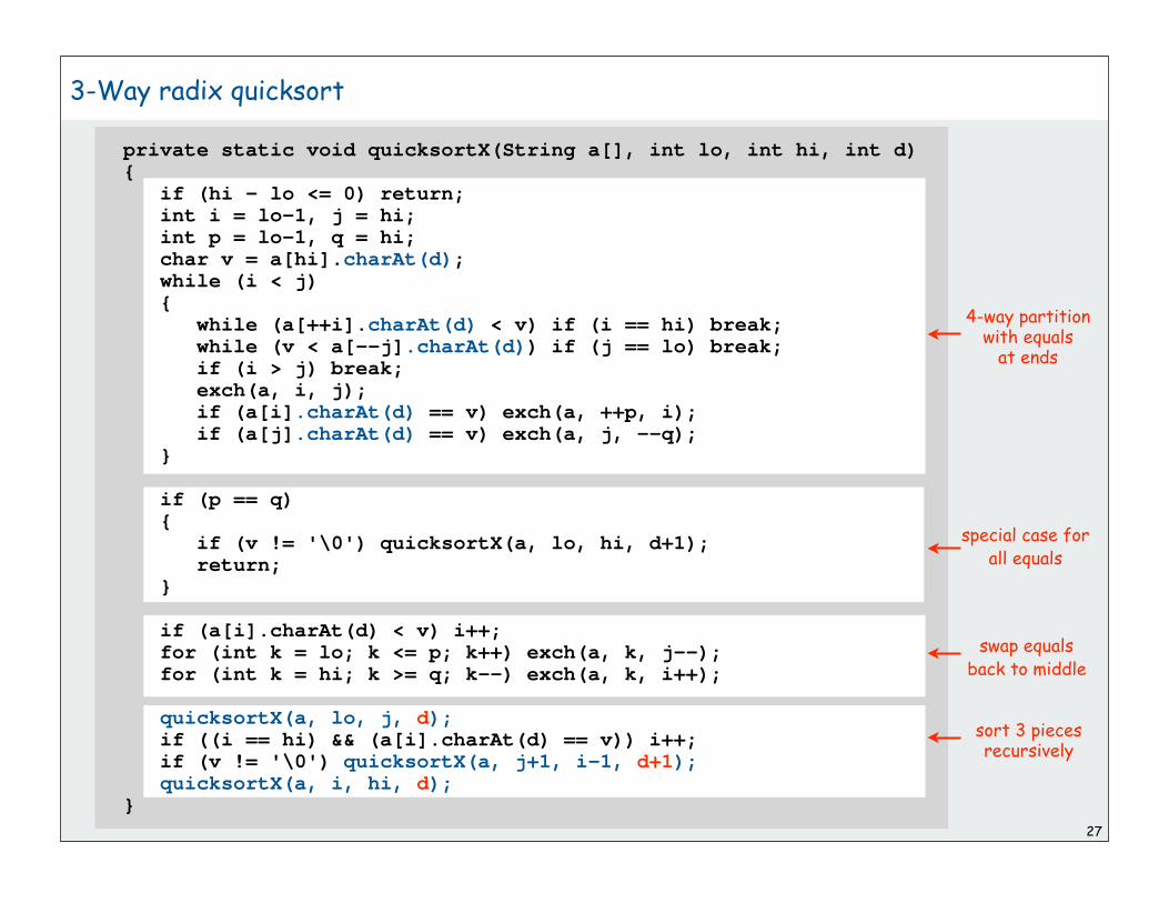
27
private static void quicksortX(String a[], int lo, int hi, int d){ if (hi - lo <= 0) return; int i = lo-1, j = hi; int p = lo-1, q = hi; char v = a[hi].charAt(d); while (i < j) { while (a[++i].charAt(d) < v) if (i == hi) break; while (v < a[--j].charAt(d)) if (j == lo) break; if (i > j) break; exch(a, i, j); if (a[i].charAt(d) == v) exch(a, ++p, i); if (a[j].charAt(d) == v) exch(a, j, --q); }
if (p == q) { if (v != '\0') quicksortX(a, lo, hi, d+1); return; }
if (a[i].charAt(d) < v) i++; for (int k = lo; k <= p; k++) exch(a, k, j--); for (int k = hi; k >= q; k--) exch(a, k, i++);
quicksortX(a, lo, j, d); if ((i == hi) && (a[i].charAt(d) == v)) i++; if (v != '\0') quicksortX(a, j+1, i-1, d+1); quicksortX(a, i, hi, d);}
swap equalsback to middle
3-Way radix quicksort
sort 3 piecesrecursively
special case forall equals
4-way partitionwith equals
at ends

28
3-Way Radix quicksort vs. standard quicksort
standard quicksort.
• uses 2N ln N string comparisons on average.
• uses costly compares for long keys that differ only at the end,
and this is a common case!
3-way radix quicksort.
• avoids re-comparing initial parts of the string.
• adapts to data: uses just "enough" characters to resolve order.
• uses 2 N ln N character comparisons on average for random strings.
• is sub-linear when strings are long
Theorem. Quicksort with 3-way partitioning is OPTIMAL.
No sorting algorithm can examine fewer chars on any input
Pf. Ties cost to entropy. Beyond scope of 226.asymptotically
to within aconstant factor
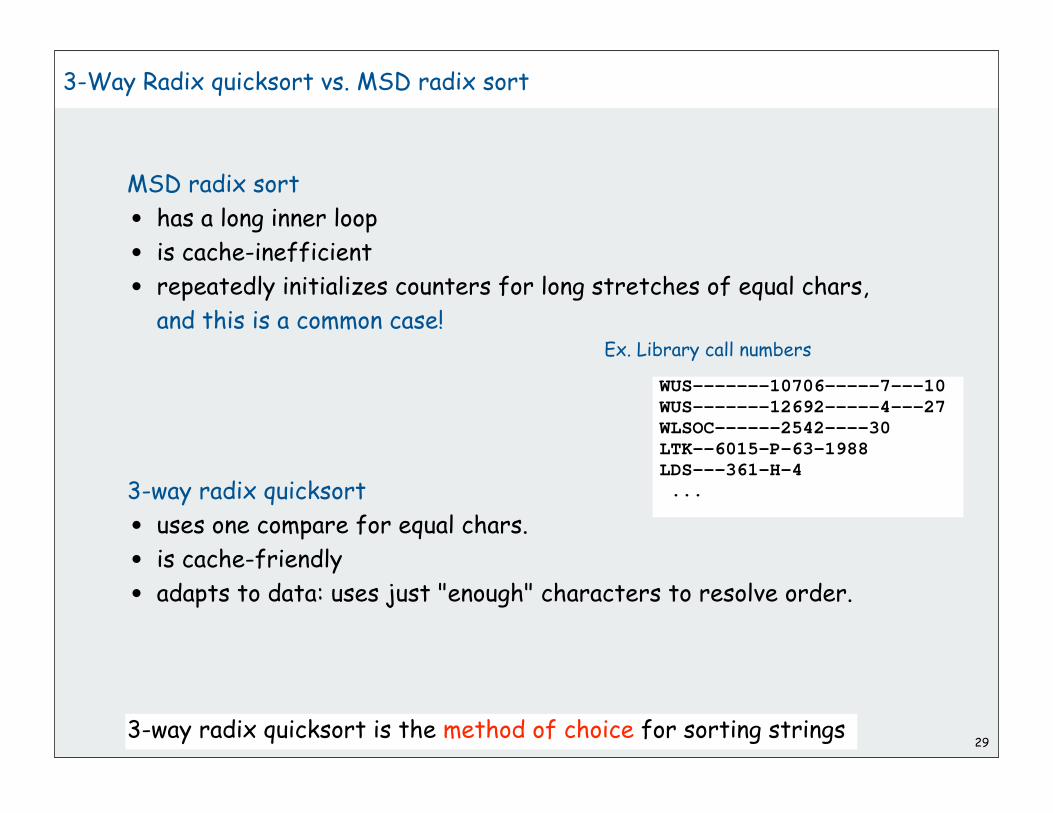
29
3-Way Radix quicksort vs. MSD radix sort
MSD radix sort
• has a long inner loop
• is cache-inefficient
• repeatedly initializes counters for long stretches of equal chars,
and this is a common case!
3-way radix quicksort
• uses one compare for equal chars.
• is cache-friendly
• adapts to data: uses just "enough" characters to resolve order.
3-way radix quicksort is the method of choice for sorting strings
Ex. Library call numbers
WUS-------10706-----7---10WUS-------12692-----4---27WLSOC------2542----30LTK--6015-P-63-1988LDS---361-H-4 ...

30
key-indexed countingLSD radix sortMSD radix sort3-way radix quicksortapplication: LRS

31
Longest repeated substring
Given a string of N characters, find the longest repeated substring.
Ex:
a a c a a g t t t a c a a g c a t g a t g c t g t a c t a
g g a g a g t t a t a c t g g t c g t c a a a c c t g a a
c c t a a t c c t t g t g t g t a c a c a c a c t a c t a
c t g t c g t c g t c a t a t a t c g a g a t c a t c g a
a c c g g a a g g c c g g a c a a g g c g g g g g g t a t
a g a t a g a t a g a c c c c t a g a t a c a c a t a c a
t a g a t c t a g c t a g c t a g c t c a t c g a t a c a
c a c t c t c a c a c t c a a g a g t t a t a c t g g t c
a a c a c a c t a c t a c g a c a g a c g a c c a a c c a
g a c a g a a a a a a a a c t c t a t a t c t a t a a a a

32
Longest repeated substring
Given a string of N characters, find the longest repeated substring.
Ex:
a a c a a g t t t a c a a g c a t g a t g c t g t a c t a
g g a g a g t t a t a c t g g t c g t c a a a c c t g a a
c c t a a t c c t t g t g t g t a c a c a c a c t a c t a
c t g t c g t c g t c a t a t a t c g a g a t c a t c g a
a c c g g a a g g c c g g a c a a g g c g g g g g g t a t
a g a t a g a t a g a c c c c t a g a t a c a c a t a c a
t a g a t c t a g c t a g c t a g c t c a t c g a t a c a
c a c t c t c a c a c t c a a g a g t t a t a c t g g t c
a a c a c a c t a c t a c g a c a g a c g a c c a a c c a
g a c a g a a a a a a a a c t c t a t a t c t a t a a a a

33
String processing
String. Sequence of characters.
Important fundamental abstraction
Natural languages, Java programs, genomic sequences, …
The digital information that underlies biochemistry, cell
biology, and development can be represented by a simple
string of G's, A's, T's and C's. This string is the root
data structure of an organism's biology. -M. V. Olson

34
Using Strings in Java
String concatenation: append one string to end of another string.
Substring: extract a contiguous list of characters from a string.
s t r i n g s
0 1 2 3 4 5 6
String s = "strings"; // s = "strings"char c = s.charAt(2); // c = 'r'String t = s.substring(2, 6); // t = "ring"String u = s + t; // u = "stringsring"

35
Implementing Strings In Java
Memory. 40 + 2N bytes for a virgin string!
could use byte array instead of String to save space
java.lang.String
public final class String implements Comparable<String>
{
private char[] value; // characters
private int offset; // index of first char into array
private int count; // length of string
private int hash; // cache of hashCode()
private String(int offset, int count, char[] value)
{
this.offset = offset;
this.count = count;
this.value = value;
}
public String substring(int from, int to)
{
return new String(offset + from, to - from, value); }
…
}

36
String vs. StringBuilder
String. [immutable] Fast substring, slow concatenation.
StringBuilder. [mutable] Slow substring, fast (amortized) append.
Ex. Reverse a string
quadratic time
linear time
public static String reverse(String s)
{
String rev = "";
for (int i = s.length() - 1; i >= 0; i--)
rev += s.charAt(i);
return rev;
}
public static String reverse(String s)
{
StringBuilder rev = new StringBuilder();
for (int i = s.length() - 1; i >= 0; i--)
rev.append(s.charAt(i));
return rev.toString();
}

Given two strings, find the longest substring that is a prefix of both
Would be quadratic with StringBuilder
Lesson: cost depends on implementation
This lecture: need constant-time substring(), use String37
Warmup: longest common prefix
p r e f i x
0 1 2 3 4 5 6
p r e f e t c
7
h
public static String lcp(String s, String t){ int n = Math.min(s.length(), t.length()); for (int i = 0; i < n; i++) { if (s.charAt(i) != t.charAt(i)) return s.substring(0, i); } return s.substring(0, n);}
linear time

38
Longest repeated substring
Given a string of N characters, find the longest repeated substring.
Classic string-processing problem.
Ex: a a c a a g t t t a c a a g c
Applications
• bioinformatics.
• cryptanalysis.
Brute force.
• Try all indices i and j for start of possible match, and check.
• Time proportional to M N2 , where M is length of longest match.
a a c a a g t t t a c a a g c
j
k k
i
91

39
Longest repeated substring
a a c a a g t t t a c a a g c
a c a a g t t t a c a a g c
c a a g t t t a c a a g c
a a g t t t a c a a g c
a g t t t a c a a g c
g t t t a c a a g c
t t t a c a a g c
t t a c a a g c
t a c a a g c
a c a a g c
c a a g c
a a g c
a g c
g c
c
a a c a a g t t t a c a a g c
a c a a g t t t a c a a g c
c a a g t t t a c a a g c
a a g t t t a c a a g c
a g t t t a c a a g c
g t t t a c a a g c
t t t a c a a g c
t t a c a a g c
t a c a a g c
a c a a g c
c a a g c
a a g c
a g c
g c
c
suffixes sorted suffixes
0
1
2
3
4
5
6
7
8
9
10
11
12
13
14
0
11
3
9
1
12
4
14
10
2
13
5
8
7
6
Suffix sort solution.
form N suffixes of original string.
sort to bring longest repeated substrings together.
check LCP of adjacent substrings to find longest match

40
Suffix Sorting: Java Implementation
% java LRS < mobydick.txt
,- Such a funny, sporty, gamy, jesty, joky, hoky-poky lad, is the Ocean, oh! Th
read input
create suffixes(linear time)
sort suffixes
find LCP
public class LRS {
public static void main(String[] args) {
String s = StdIn.readAll();
int N = s.length();
String[] suffixes = new String[N];
for (int i = 0; i < N; i++)
suffixes[i] = s.substring(i, N);
Arrays.sort(suffixes);
String lrs = "";
for (int i = 0; i < N - 1; i++) {
String x = lcp(suffixes[i], suffixes[i+1]);
if (x.length() > lrs.length()) lrs = x;
}
System.out.println(lrs);
}
}

41
Sorting Challenge
Problem: suffix sort a long string
Ex. Moby Dick ~1.2 million chars
Which sorting method to use?
1. insertion sort
2. mergesort
3. quicksort
4. LSD radix sort
5. MSD radix sort
6. 3-way radix quicksort
only if LRS is not long (!)

42
Suffix sort experimental results
algorithmtime to suffix-sort Moby Dick
(seconds)
brute-force 36.000 (est.)
quicksort 9.5
LSD not fixed-length
MSD 395
MSD with cutoff 6.8
3-way radix quicksort 2.8

Longest match not long:
• hard to beat 3-way radix quicksort.
Longest match very long:
• radix sorts are quadratic
in the length of the longest match
• Ex: two copies of Moby Dick.
Can we do better? linearithmic? linear?
Observation. Must find longest repeated
substring while suffix sorting to beat N2.
43
Suffix Sorting: Worst-case input
Input: "abcdeghiabcdefghi"
abcdefghi abcdefghiabcdefghi bcdefghi bcdefghiabcdefghi cdefghi cdefghiabcdefgh defghi efghiabcdefghi efghi fghiabcdefghi fghi ghiabcdefghi fhi hiabcdefghi hi iabcdefghi i

44
Fast suffix sorting
Manber's MSD algorithm
• phase 0: sort on first character using key-indexed sort.
• phase i: given list of suffixes sorted on first 2i-1 characters,
create list of suffixes sorted on first 2i characters
Running time
• finishes after lg N phases
• obvious upper bound on growth of total time: O( N (lg N)2 )
• actual growth of total time (proof omitted): ~N lg N.
Best algorithm in theory is linear (but more complicated to implement).
not many subfiles if not much repetition
3-way quicksort handles equal keys if repetition

45
Linearithmic suffix sort example: phase 0
0 babaaaabcbabaaaaa0
1 abaaaabcbabaaaaa0
2 baaaabcbabaaaaa0
3 aaaabcbabaaaaa0
4 aaabcbabaaaaa0
5 aabcbabaaaaa0
6 abcbabaaaaa0
7 bcbabaaaaa0
8 cbabaaaaa0
9 babaaaaa0
10 abaaaaa0
11 baaaaa0
12 aaaaa0
13 aaaa0
14 aaa0
15 aa0
16 a0
17 0
17 0
1 abaaaabcbabaaaaa0
16 a0
3 aaaabcbabaaaaa0
4 aaabcbabaaaaa0
5 aabcbabaaaaa0
6 abcbabaaaaa0
15 aa0
14 aaa0
13 aaaa0
12 aaaaa0
10 abaaaaa0
0 babaaaabcbabaaaaa0
9 babaaaaa0
11 baaaaa0
7 bcbabaaaaa0
2 baaaabcbabaaaaa0
8 cbabaaaaa0
sorted
0 12
1 1
2 16
3 3
4 4
5 5
6 6
7 15
8 17
9 13
10 11
11 14
12 10
13 9
14 8
15 7
16 2
17 0
inverseindexsort

46
Linearithmic suffix sort example: phase 1
0 babaaaabcbabaaaaa0
1 abaaaabcbabaaaaa0
2 baaaabcbabaaaaa0
3 aaaabcbabaaaaa0
4 aaabcbabaaaaa0
5 aabcbabaaaaa0
6 abcbabaaaaa0
7 bcbabaaaaa0
8 cbabaaaaa0
9 babaaaaa0
10 abaaaaa0
11 baaaaa0
12 aaaaa0
13 aaaa0
14 aaa0
15 aa0
16 a0
17 0
17 0
16 a0
12 aaaaa0
3 aaaabcbabaaaaa0
4 aaabcbabaaaaa0
5 aabcbabaaaaa0
13 aaaa0
15 aa0
14 aaa0
6 abcbabaaaaa0
1 abaaaabcbabaaaaa0
10 abaaaaa0
0 babaaaabcbabaaaaa0
9 babaaaaa0
11 baaaaa0
2 baaaabcbabaaaaa0
7 bcbabaaaaa0
8 cbabaaaaa0
sorted
0 12
1 10
2 15
3 3
4 4
5 5
6 9
7 16
8 17
9 13
10 11
11 14
12 2
13 6
14 8
15 7
16 1
17 0
inverseindexsort

47
Linearithmic suffix sort example: phase 2
0 babaaaabcbabaaaaa0
1 abaaaabcbabaaaaa0
2 baaaabcbabaaaaa0
3 aaaabcbabaaaaa0
4 aaabcbabaaaaa0
5 aabcbabaaaaa0
6 abcbabaaaaa0
7 bcbabaaaaa0
8 cbabaaaaa0
9 babaaaaa0
10 abaaaaa0
11 baaaaa0
12 aaaaa0
13 aaaa0
14 aaa0
15 aa0
16 a0
17 0
sorted
0 14
1 9
2 12
3 4
4 7
5 8
6 11
7 16
8 17
9 15
10 10
11 13
12 5
13 6
14 3
15 2
16 1
17 0
inverseindexsort
17 0
16 a0
15 aa0
14 aaa0
3 aaaabcbabaaaaa0
12 aaaaa0
13 aaaa0
4 aaabcbabaaaaa0
5 aabcbabaaaaa0
1 abaaaabcbabaaaaa0
10 abaaaaa0
6 abcbabaaaaa0
2 baaaabcbabaaaaa0
11 baaaaa0
0 babaaaabcbabaaaaa0
9 babaaaaa0
7 bcbabaaaaa0
8 cbabaaaaa0

48
Linearithmic suffix sort example: phase 3
0 babaaaabcbabaaaaa0
1 abaaaabcbabaaaaa0
2 baaaabcbabaaaaa0
3 aaaabcbabaaaaa0
4 aaabcbabaaaaa0
5 aabcbabaaaaa0
6 abcbabaaaaa0
7 bcbabaaaaa0
8 cbabaaaaa0
9 babaaaaa0
10 abaaaaa0
11 baaaaa0
12 aaaaa0
13 aaaa0
14 aaa0
15 aa0
16 a0
17 0
17 0
16 a0
15 aa0
14 aaa0
3 aaaabcbabaaaaa0
13 aaaa0
12 aaaaa0
4 aaabcbabaaaaa0
5 aabcbabaaaaa0
10 abaaaaa0
1 abaaaabcbabaaaaa0
6 abcbabaaaaa0
11 baaaaa0
2 baaaabcbabaaaaa0
9 babaaaaa0
0 babaaaabcbabaaaaa0
7 bcbabaaaaa0
8 cbabaaaaa0
sorted
0 15
1 10
2 13
3 4
4 7
5 8
6 11
7 16
8 17
9 14
10 9
11 12
12 6
13 5
14 3
15 2
16 1
17 0
FINISHED! (no equal keys)
inverseindexsort
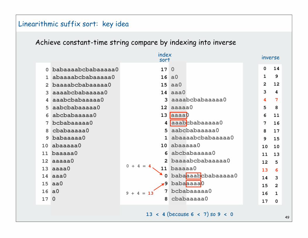
49
Linearithmic suffix sort: key idea
0 + 4 = 4
9 + 4 = 13
0 14
1 9
2 12
3 4
4 7
5 8
6 11
7 16
8 17
9 15
10 10
11 13
12 5
13 6
14 3
15 2
16 1
17 0
Achieve constant-time string compare by indexing into inverse
inverseindexsort
0 babaaaabcbabaaaaa0
1 abaaaabcbabaaaaa0
2 baaaabcbabaaaaa0
3 aaaabcbabaaaaa0
4 aaabcbabaaaaa0
5 aabcbabaaaaa0
6 abcbabaaaaa0
7 bcbabaaaaa0
8 cbabaaaaa0
9 babaaaaa0
10 abaaaaa0
11 baaaaa0
12 aaaaa0
13 aaaa0
14 aaa0
15 aa0
16 a0
17 0
17 0
16 a0
15 aa0
14 aaa0
3 aaaabcbabaaaaa0
12 aaaaa0
13 aaaa0
4 aaabcbabaaaaa0
5 aabcbabaaaaa0
1 abaaaabcbabaaaaa0
10 abaaaaa0
6 abcbabaaaaa0
2 baaaabcbabaaaaa0
11 baaaaa0
0 babaaaabcbabaaaaa0
9 babaaaaa0
7 bcbabaaaaa0
8 cbabaaaaa0
13 < 4 (because 6 < 7) so 9 < 0
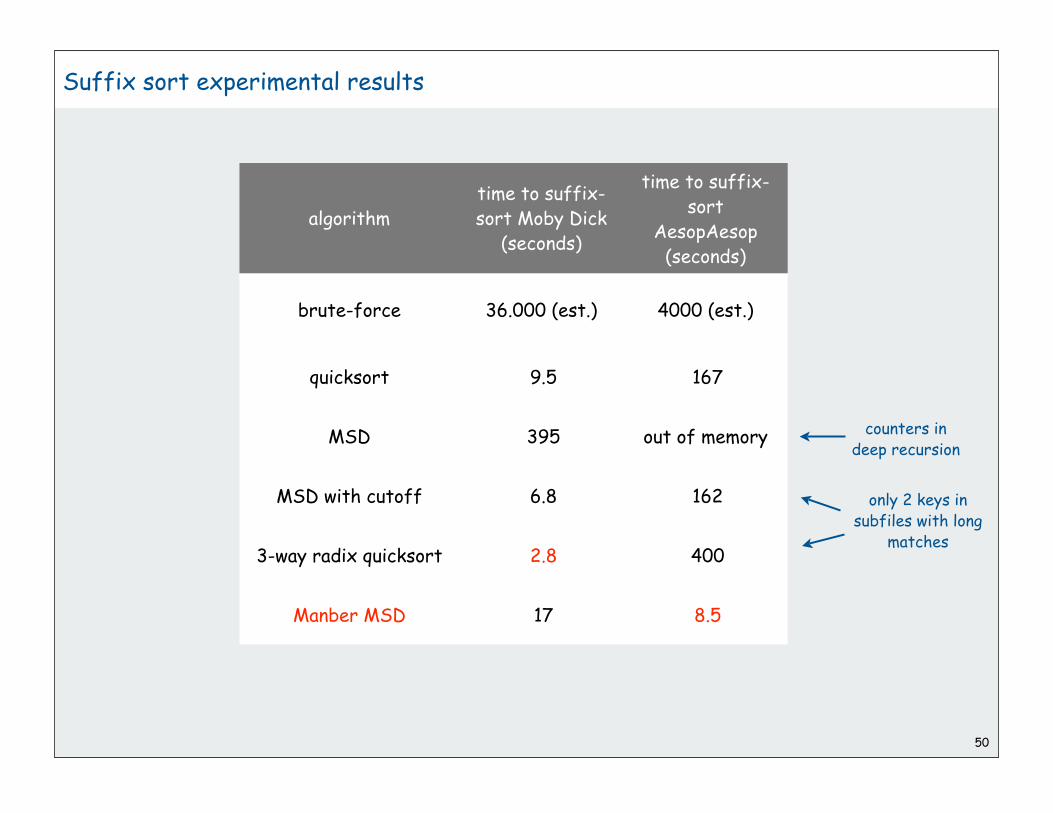
50
Suffix sort experimental results
algorithmtime to suffix-sort Moby Dick
(seconds)
time to suffix-sort
AesopAesop(seconds)
brute-force 36.000 (est.) 4000 (est.)
quicksort 9.5 167
MSD 395 out of memory
MSD with cutoff 6.8 162
3-way radix quicksort 2.8 400
Manber MSD 17 8.5
counters indeep recursion
only 2 keys insubfiles with long
matches

Radix sort summary
We can develop linear-time sorts.
• comparisons not necessary for some types of keys
• use keys to index an array
We can develop sub-linear-time sorts.
• should measure amount of data in keys, not number of keys
• not all of the data has to be examined
No algorithm can examine fewer bits than 3-way radix quicksort
• 1.39 N lg N bits for random data
Long strings are rarely random in practice.
• goal is often to learn the structure!
• may need specialized algorithms
51
lecture acronym cheatsheet
LSD least significant digit
MSD most significant digit
LCP longest common prefix
LRS longest repeated substring

1
Tries
reviewtriesTSTsapplications
References:
Algorithms in Java, Chapter 15 http://www.cs.princeton.edu/introalgsds/62search

2
rules of the gametriesTSTsapplications

Review: summary of the performance of searching (symbol-table) algorithms
Frequency of execution of instructions in the inner loop:
Q: Can we do better?
3
implementationguarantee average case ordered
iteration?operations
on keyssearch insert delete search insert delete
BST N N N 1.38 lg N 1.38 lg N ? yes compareTo()
randomized BST 7 lg N 7 lg N 7 lg N 1.38 lg N 1.38 lg N 1.38 lg N yes compareTo()
red-black tree 2 lg N 2 lg N 2 lg N lg N lg N lg N yes compareTo()
hashing 1* 1* 1* 1* 1* 1* noequals()hashcode()
* assumes random hash code

4
Review
Symbol tables.
• Associate a value with a key.
• Search for value given key.
Balanced trees
• use between lg N and 2 lg N key comparisons
• support ordered iteration and other operations
Hash tables
• typically use 1-2 probes
• require good hash function for each key type
Radix sorting
• some keys are inherently digital
• digital keys give linear and sublinear sorts
This lecture. Symbol tables for digital keys.

Digital keys (review)
Many commonly-use key types are inherently digital
(sequences of fixed-length characters)
Examples
• Strings
• 64-bit integers
This lecture:
• refer to fixed-length vs. variable-length strings
• R different characters for some fixed value R.
• key type implements charAt() and length() methods
• code works for String and for key types that implement Digital.
Widely used in practice
• low-level bit-based keys
• string keys
5
interface
interface Digital
{
public int charAt(int k);
public int length(int);
}

6
Digital keys in applications
Key = sequence of "digits."
• DNA: sequence of a, c, g, t.
• IPv6 address: sequence of 128 bits.
• English words: sequence of lowercase letters.
• Protein: sequence of amino acids A, C, ..., Y.
• Credit card number: sequence of 16 decimal digits.
• International words: sequence of Unicode characters.
• Library call numbers: sequence of letters, numbers, periods.
This lecture. Key = string over ASCII alphabet.

String set. Unordered collection of distinct strings.
Typical client: Dedup (remove duplicate strings from input)
This lecture: focus on StringSET implementation
Same ideas improve STs with wider API7
String Set API
StringSET set = new StringSET();
while (!StdIn.isEmpty())
{
String key = StdIn.readString();
if (!set.contains(key))
{
set.add(key);
System.out.println(key);
}
}
public class StringSET
StringSET() create a set of strings
void add(String key) add string to set
boolean contains(String key) is key in the set?

8
StringSET implementation cost summary
Challenge. Efficient performance for long keys (large L).
N = number of strings
L = length of string
C = number of characters in input
R = radix
red-black
implementation
hashing
L + log N
Search hit
L
log N
Insert
L
typical case
C
Space
C
1.40
moby
0.76
97.4
actors
40.6
dedup
input * L L L 0.26 15.1
* only reads in data
file megabytes words distinct
moby 1.2 210 K 32 K
actors 82 11.4 M 900 K

9
rules of the gametriesTSTsapplications

10
Tries. [from retrieval, but pronounced "try"]
Store characters in internal nodes, not keys.
Store records in external nodes.
Use the characters of the key to guide the search.
Ex. sells sea shells by the sea
Tries
by
sea
sells
shells
the

11
Tries. [from retrieval, but pronounced "try"]
Store characters in internal nodes, not keys.
Store records in external nodes.
Use the characters of the key to guide the search.
Ex. sells sea shells by the sea shore
Tries
by
sea
sells
shells
the
shore

12
Q. How to handle case when one key is a prefix of another?
A1. Append sentinel character '\0' to every key so it never happens.
A2. Store extra bit to denote which nodes correspond to keys.
Ex. she sells sea shells by the sea shore
Tries
by
sea
sells
shells
the
shore
she

13
Branching in tries
Q. How to branch to next level?
A. One link for each possible character
Ex. sells sea shells by the sea shore R-way trie
R empty links on leaves

14
R-Way Trie: Java implementation
R-way existence trie: a node.
Node: references to R nodes.
root
8-way trie that represents {a, f, h}
dcba hgfe
private class Node{ Node[] next = new Node[R]; boolean end;}
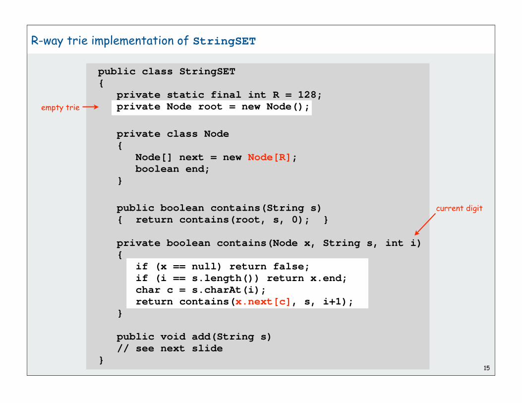
15
R-way trie implementation of StringSET
ASCII
current digit
empty trie
public class StringSET{ private static final int R = 128; private Node root = new Node();
private class Node { Node[] next = new Node[R]; boolean end; }
public boolean contains(String s) { return contains(root, s, 0); }
private boolean contains(Node x, String s, int i) { if (x == null) return false; if (i == s.length()) return x.end; char c = s.charAt(i); return contains(x.next[c], s, i+1); }
public void add(String s) // see next slide}

16
R-way trie implementation of StringSET (continued)
public void add(String s) { root = add(root, s, 0); }
private Node add(Node x, String s, int i) { if (x == null) x = new Node(); if (i == s.length()) x.end = true; else { char c = s.charAt(i); x.next[c] = add(x.next[c], s, i+1); } return x; }

R-way trie performance characteristics
Time
• examine one character to move down one level in the trie
• trie has ~logR N levels (not many!)
• need to check whole string for search hit (equality)
• search miss only involves examining a few characters
Space
• R empty links at each leaf
• 65536-way branching for Unicode impractical
Bottom line.
• method of choice for small R
• you use tries every day
• stay tuned for ways to address space waste
17

Sublinear search with tries
Tries enable user to present string keys one char at a time
Search hit
• can present possible matches after a few digits
• need to examine all L digits for equality
Search miss
• could have mismatch on first character
• typical case: mismatch on first few characters
Bottom line: sublinear search cost (only a few characters)
Further help for Java String keys
• object equality test
• cached hash values
18

19
StringSET implementation cost summary
R-way trie
• faster than hashing for small R
• too much memory if R not small
65536-way trie for Unicode??
Challenge. Use less memory!
N = number of strings
L = size of string
C = number of characters in input
R = radix
red-black
implementation
hashing
L + log N
Search hit
L
log N
Insert
L
typical case
C
Space
C
1.40
moby
0.76
97.4
actors
40.6
dedup
input * L L L 0.26 15.1
R-way trie L << L RN + C 1.12 out of memory
file megabytes words distinct
moby 1.2 210 K 32 K
actors 82 11.4 M 900 K

20
Digression: Out of memory?
"640 K ought to be enough for anybody."
- attributed to Bill Gates, 1981
(commenting on the amount of RAM in personal computers)
"64 MB of RAM may limit performance of some Windows XP
features; therefore, 128 MB or higher is recommended for
best performance." - Windows XP manual, 2002
"64 bit is coming to desktops, there is no doubt about that. But apart from
Photoshop, I can't think of desktop applications where you would need more
than 4GB of physical memory, which is what you have to have in order to
benefit from this technology. Right now, it is costly." - Bill Gates, 2003
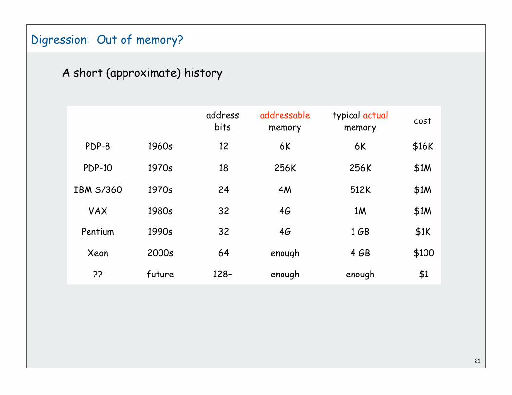
Digression: Out of memory?
A short (approximate) history
21
addressbits
addressablememory
typical actual memory
cost
PDP-8 1960s 12 6K 6K $16K
PDP-10 1970s 18 256K 256K $1M
IBM S/360 1970s 24 4M 512K $1M
VAX 1980s 32 4G 1M $1M
Pentium 1990s 32 4G 1 GB $1K
Xeon 2000s 64 enough 4 GB $100
?? future 128+ enough enough $1

A modest proposal
Number of atoms in the universe: < 2266 (estimated)
Age of universe (estimated): 20 billion years ~ 250 secs < 280 nanoseconds
How many bits address every atom that ever existed ?
A modest proposal: use a unique 512-bit address for every object
512 bits is enough:
current plan:
Use trie to map to current location. 64 8-bit chars
• wastes 255/256 actual memory
• need better use of memory
22
place time cushion for whatever266 bits 80 bits 174 bits
place (ipv6)128 bits 64 bits
place (machine)
maybe OK for Bill Gatesor if memory is tiny

23
rules of the gametriesTSTsapplications

24
Ternary Search Tries (TSTs)
Ternary search tries. [Bentley-Sedgewick, 1997]
• Store characters in internal nodes, records in external nodes.
• Use the characters of the key to guide the search
• Each node has three children
• Left (smaller), middle (equal), right (larger).

25
Ternary Search Tries (TSTs)
Ternary search tries. [Bentley-Sedgewick, 1997]
• Store characters in internal nodes, records in external nodes.
• Use the characters of the key to guide the search
• Each node has three children:
left (smaller), middle (equal), right (larger).
Ex. sells sea shells by the sea shore
Observation. Only three null links in leaves!
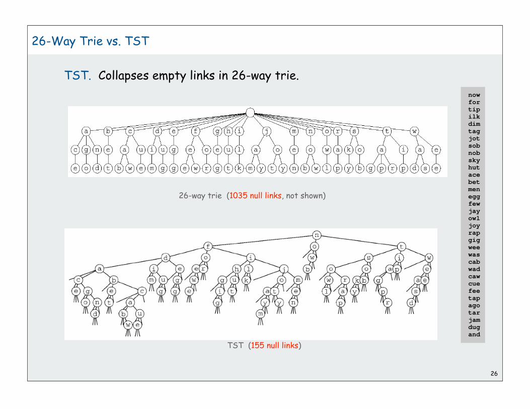
26
26-Way Trie vs. TST
TST. Collapses empty links in 26-way trie.
26-way trie (1035 null links, not shown)
TST (155 null links)
nowfortipilkdimtagjotsobnobskyhutacebetmeneggfewjayowljoyrapgigweewascabwadcawcuefeetapagotarjamdugand

A TST string set is a TST node.
A TST node is five fields:
• a character c.
• a reference to a left TST. [smaller]
• a reference to a middle TST. [equal]
• a reference to a right TST. [larger]
• a bit to indicate whether this
node is the last character in some key.
27
TST representation
root
h
ia
sd
had is
i
p
hip
private class Node{ char c; Node l, m, r; boolean end;}
c
k
hack
hi

Recursive code practically writes itself!
28
TST implementation of contains() for StringSET
public boolean contains(String s){ if (s.length() == 0) return false; return contains(root, s, 0);}
private boolean contains(Node x, String s, int i){ if (x == null) return false; char c = s.charAt(i); if (c < x.c) return contains(x.l, s, i); else if (c > x.c) return contains(x.r, s, i); else if (i < s.length()-1) return contains(x.m, s, i+1); else return x.end;}

29
TST implementation of add() for StringSET
public void add(String s){ root = add(root, s, 0); }
private Node add(Node x, String s, int i){ char c = s.charAt(i); if (x == null) x = new Node(c); if (c < x.c) x.l = add(x.l, s, i); else if (c > x.c) x.r = add(x.r, s, i); else if (i < s.length()-1) x.m = add(x.m, s, i+1); else x.end = true; return x;}
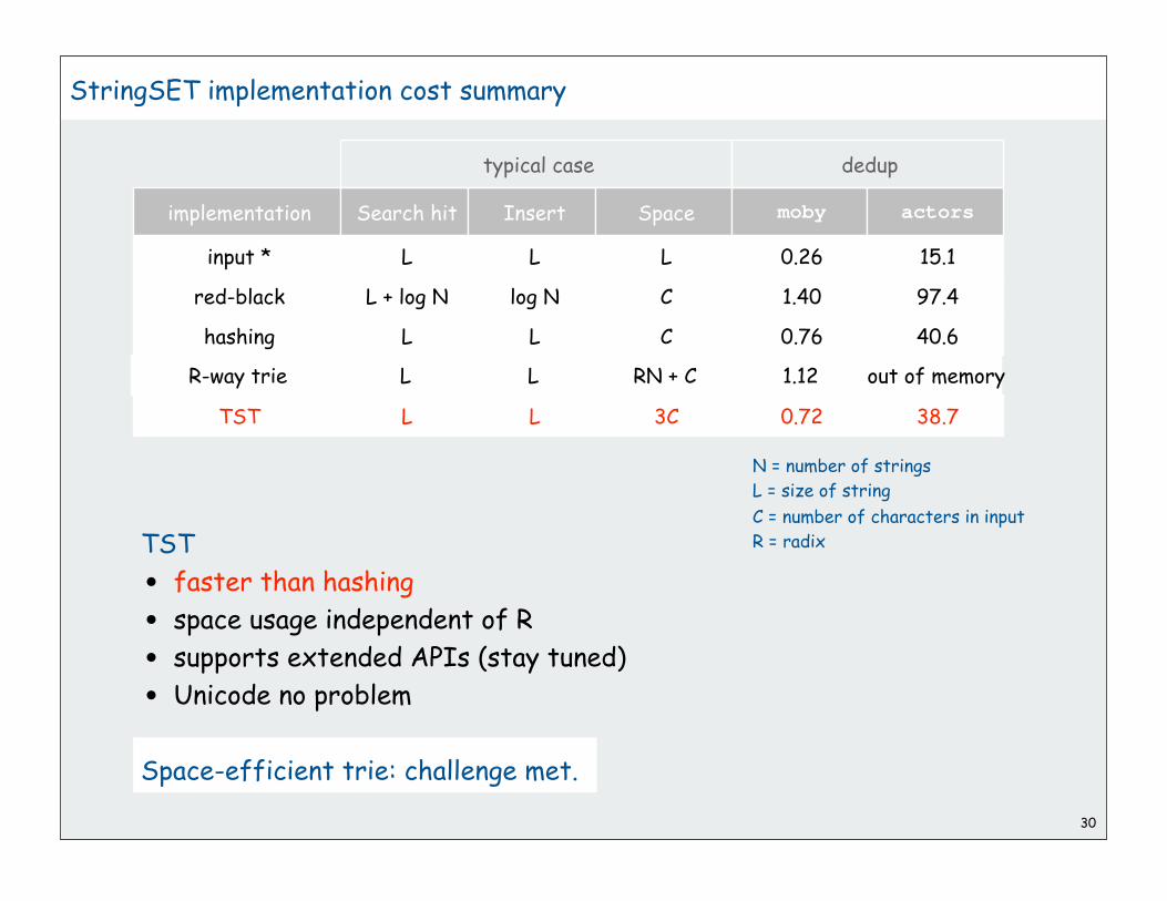
30
StringSET implementation cost summary
TST
• faster than hashing
• space usage independent of R
• supports extended APIs (stay tuned)
• Unicode no problem
Space-efficient trie: challenge met.
N = number of strings
L = size of string
C = number of characters in input
R = radix
red-black
implementation
hashing
L + log N
Search hit
L
log N
Insert
L
typical case
C
Space
C
1.40
moby
0.76
97.4
actors
40.6
dedup
input * L L L 0.26 15.1
R-way trie L L RN + C 1.12 out of memory
TST L L 3C 0.72 38.7

31
TST With R2 Branching At Root
Hybrid of R-way and TST.
• Do R-way or R2-way branching at root.
• Each of R2 root nodes points to a TST.
Note. Need special test for one-letter words.
TST
aa
TST
ab
TST
ac
TST
zz
TST
zy
array of R2 roots
…

32
StringSET implementation cost summary
TST performance even better with nonuniform keys
red-black
implementation
hashing
L + log N
Search hit
L
log N
Insert
L
typical case
C
Space
C
1.40
moby
0.76
97.4
actors
40.6
dedup
input * L L L 0.26 15.1
R-way trie L L RN + C 1.12 out of memory
TST L L 3C .72 38.7
TST with R2 L L 3C + R2 .51 32.7
Ex. Library call numbers
WUS-------10706-----7---10WUS-------12692-----4---27WLSOC------2542----30LTK--6015-P-63-1988LDS---361-H-4 ...
TSTs 5 times faster than hashing

33
TST summary
Hashing.
• need to examine entire key
• hits and misses cost about the same.
• need good hash function for every key type
• no help for ordered-key APIs
TSTs.
• need to examine just enough key characters
• search miss may only involve a few characters
• works only for keys types that implement charAt()
• can handle ordered-key APIs
Bottom line:
TSTs are faster than hashing and more flexible than LL RB trees

34
rules of the gametriesTSTsapplications

35
Extending the StringSET API
Add. Insert a key.
Contains. Check if given key in the set.
Delete. Delete key from the set.
Sort. Iterate over keys in ascending order.
Select. Find the kth largest key.
Range search. Find all elements between k1 and k2.
Longest prefix match. Find longest prefix match.
Wildcard match. Allow wildcard characters.
Near neighbor search. Find strings that differ in P chars.
compareTo()
charAt()
equals()

36
Longest Prefix Match
Find string in set with longest prefix matching given key.
Ex. Search IP database for longest prefix matching destination IP,
and route packets accordingly.
"128"
"128.112"
"128.112.136"
"128.112.055"
"128.112.055.15"
"128.112.155.11"
"128.112.155.13"
"128.222"
"128.222.136"
prefix("128.112.136.11") = "128.112.136"
prefix("128.166.123.45") = "128"

37
R-way trie implementation of longest prefix match operation
Find string in set with longest prefix matching a given key.
public String prefix(String s){ int length = prefix(root, s, 0); return s.substring(0, length);}
private int prefix(Node x, String s, int i){ if (x == null) return 0; int length = 0; if (x.end) length = i; if (i == s.length()) return length; char c = s.charAt(i); return Math.max(length, prefix(x.next[c], s, i+1));}

38
Wildcard Match
Wildcard match. Use wildcard . to match any character.
coalizer
coberger
codifier
cofaster
cofather
cognizer
cohelper
colander
coleader
...
compiler
...
composer
computer
cowkeper
acresceacroachacuracyoctarchsciencescranchscratchscrauchscreichscrinchscritchscrunchscudickscutock
co....er
.c...c.
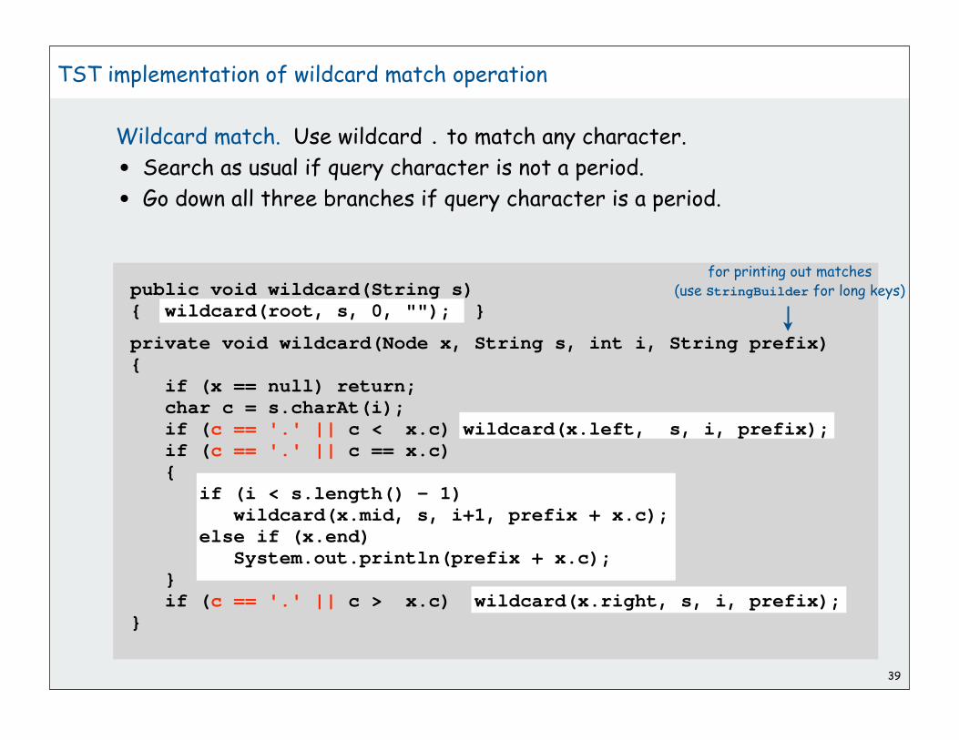
39
TST implementation of wildcard match operation
Wildcard match. Use wildcard . to match any character.
• Search as usual if query character is not a period.
• Go down all three branches if query character is a period.
public void wildcard(String s){ wildcard(root, s, 0, ""); }
private void wildcard(Node x, String s, int i, String prefix){ if (x == null) return; char c = s.charAt(i); if (c == '.' || c < x.c) wildcard(x.left, s, i, prefix); if (c == '.' || c == x.c) { if (i < s.length() - 1) wildcard(x.mid, s, i+1, prefix + x.c); else if (x.end) System.out.println(prefix + x.c); } if (c == '.' || c > x.c) wildcard(x.right, s, i, prefix); }
for printing out matches(use StringBuilder for long keys)

40
T9 Texting
Goal. Type text messages on a phone keypad.
Multi-tap input. Enter a letter by repeatedly pressing a key until the
desired letter appears.
T9 text input. ["A much faster and more fun way to enter text."]
• Find all words that correspond to given sequence of numbers.
• Press 0 to see all completion options.
Ex: hello
• Multi-tap: 4 4 3 3 5 5 5 5 5 5 6 6 6
• T9: 4 3 5 5 6
www.t9.com

41
A Letter to t9.com
To: [email protected]: Tue, 25 Oct 2005 14:27:21 -0400 (EDT)
Dear T9 texting folks,
I enjoyed learning about the T9 text systemfrom your webpage, and used it as an examplein my data structures and algorithms class.However, one of my students noticed a bugin your phone keypad
http://www.t9.com/images/how.gif
Somehow, it is missing the letter s. (!)
Just wanted to bring this information toyour attention and thank you for your website.
Regards,
Kevin
where’s the “s” ??

42
A world without “s” ??
To: "'Kevin Wayne'" <[email protected]>Date: Tue, 25 Oct 2005 12:44:42 -0700
Thank you Kevin.
I am glad that you find T9 o valuable for yourcla. I had not noticed thi before. Thank forwriting in and letting u know.
Take care,
Brooke nyder OEM Dev upport AOL/Tegic Communication 1000 Dexter Ave N. uite 300 eattle, WA 98109
ALL INFORMATION CONTAINED IN THIS EMAIL IS CONIDEREDCONFIDENTIAL AND PROPERTY OF AOL/TEGIC COMMUNICATION

43
TST: Collapsing 1-Way Branches
Collapsing 1-way branches at bottom.
• internal node stores char; external node stores full key.
• append sentinel character '\0' to every key
• search hit ends at leaf with given key.
• search miss ends at null link or leaf with different key.
Collapsing interior 1-way branches
• keep char position in nodes
• need full compare at leaf s
hby the
e shells
l
sea sells

44
TST: Collapsing 1-Way Branches
Collapsing 1-way branches at bottom.
• internal node stores char; external node stores full key.
• append sentinel character '\0' to every key
• search hit ends at leaf with given key.
• search miss ends at null link or leaf with different key.
Collapsing interior 1-way branches
• keep char position in nodes
• need full compare at leaf s
hby the
e
shells
e
shorel
sea sells

45
StringSET implementation cost summary
Challenge met.
• Efficient performance for arbitrarily long keys.
• Search time is independent of key length!
red-black
implementation
hashing
L + log N
Search hit
L
log N
Insert
L
C
Space
C
input * L L L
R-way trie L L RN + C
TST L L 3C
TST with R2 L L 3C + R2
R-way with no 1-way logR N logR N RN + C
TST with no 1-way log N log N C

46
A classic algorithm
Patricia tries. [Practical Algorithm to Retrieve Information Coded in Alphanumeric]
• Collapse one-way branches in binary trie.
• Thread trie to eliminate multiple node types.
Applications.
• Database search.
• P2P network search.
• IP routing tables: find longest prefix match.
• Compressed quad-tree for N-body simulation.
• Efficiently storing and querying XML documents.
(Just slightly) beyond the scope of COS 226 (see Program 15.7)

47
Suffix Tree
Suffix tree.
Threaded trie with collapsed 1-way branching for string suffixes.
Applications.
• Longest common substring, longest repeated substring.
• Computational biology databases (BLAST, FASTA).
• Search for music by melody.
• ...
(Just slightly) beyond the scope of COS 226.

48
Symbol tables summary
A success story in algorithm design and analysis.
Implementations are a critical part of our computational infrastructure.
Binary search trees. Randomized, red-black.
• performance guarantee: log N compares
• supports extensions to API based on key order
Hash tables. Separate chaining, linear probing.
• performance guarantee: N/M probes
• requires good hash function for key type
• no support for API extensions
• enjoys systems support (ex: cached value for String)
Tries. R-way, TST.
• performance guarantee: log N characters accessed
• supports extensions to API based on partial keys
Bottom line: you can get at anything by examining 50-100 bits (!!!)

1
Data Compression
introductionbasic coding schemesan applicationentropyLZW codes
References:
Algorithms 2nd edition, Chapter 22 http://www.cs.princeton.edu/introalgsds/65compression

2
introductionbasic coding schemesan applicationentropyLZW codes

3
Data Compression
Compression reduces the size of a file:
• To save space when storing it.
• To save time when transmitting it.
• Most files have lots of redundancy.
Who needs compression?
• Moore's law: # transistors on a chip doubles every 18-24 months.
• Parkinson's law: data expands to fill space available.
• Text, images, sound, video, …
Basic concepts ancient (1950s), best technology recently developed.
All of the books in the world contain no more information than is
broadcast as video in a single large American city in a single year.
Not all bits have equal value. -Carl Sagan

4
Applications
Generic file compression.
• Files: GZIP, BZIP, BOA.
• Archivers: PKZIP.
• File systems: NTFS.
Multimedia.
• Images: GIF, JPEG.
• Sound: MP3.
• Video: MPEG, DivX™, HDTV.
Communication.
• ITU-T T4 Group 3 Fax.
• V.42bis modem.
Databases. Google.

5
Encoding and decoding
Message. Binary data M we want to compress.
Encode. Generate a "compressed" representation C(M).
Decode. Reconstruct original message or some approximation M'.
Compression ratio. Bits in C(M) / bits in M.
Lossless. M = M', 50-75% or lower.
Ex. Natural language, source code, executables.
Lossy. M M', 10% or lower.
Ex. Images, sound, video.
EncoderM DecoderC(M) M'
uses fewer bits (you hope)
this lecture
"Poetry is the art of lossy data compression."

6
Food for thought
Data compression has been omnipresent since antiquity,
• Number systems.
• Natural languages.
• Mathematical notation.
has played a central role in communications technology,
• Braille.
• Morse code.
• Telephone system.
and is part of modern life.
• zip.
• MP3.
• MPEG.
What role will it play in the future?
Ex: If memory is to be cheap and ubiquitous, why are we doing lossy compression for music and movies??

7
introductionbasic coding schemesan applicationentropyLZW codes
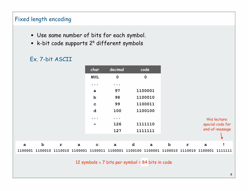
8
Fixed length encoding
• Use same number of bits for each symbol.
• k-bit code supports 2k different symbols
Ex. 7-bit ASCII
char decimal code
NUL 0 0
... ...
a 97 1100001
b 98 1100010
c 99 1100011
d 100 1100100
... ...
~ 126 1111110
127 1111111
a b r a c a d a b r a !
1100001 1100010 1110010 1100001 1100011 1100001 1100100 1100001 1100010 1110010 1100001 1111111
12 symbols 7 bits per symbol = 84 bits in code
this lecture:special code forend-of-message

9
Fixed length encoding
• Use same number of bits for each symbol.
• k-bit code supports 2k different symbols
Ex. 3-bit custom code
Important detail: decoder needs to know the code!
char code
a X000
b X001
c X010
d X011
r X100
! X111
a b r a c a d a b r a !
X000 X001 X100 X000 X010 X000 X011 X000 X001 X100 X000 X111
12 symbols 3 bits 36 bits in code

10
Fixed length encoding: general scheme
• count number of different symbols.
• lg M bits suffice to support M different symbols
Ex. genomic sequences
• 4 different codons
• 2 bits suffice
• Amazing but true: initial databases in 1990s did not use such a code!
Decoder needs to know the code
• can amortize over large number of files with the same code
• in general, can encode an N-char file with N lg M + 16 lg M bits
char code
a X00
c X01
t X10
g X11
a c t a c a g a t g a
X00X X01X 10 X00X X01X X00X 11 X00X 10 11 X00X
2N bits to encodegenome with N codons

11
Variable-length encoding
Use different number of bits to encode different characters.
Ex. Morse code.
Issue: ambiguity.
• • • • • •
SOS ?
IAMIE ?
EEWNI ?
V7O ?

12
Variable-length encoding
Use different number of bits to encode different characters.
Q. How do we avoid ambiguity?
A1. Append special stop symbol to each codeword.
A2. Ensure that no encoding is a prefix of another.
Ex. custom prefix-free code
Note 1: fixed-length codes are prefix-free
Note 2: can amortize cost of including the code over similar messages
char code
a 0
b 111
c 1010
d 100
r 110
! 1011
S • • •
E •
I ••
V •••-
prefix of V
prefix of I, S
prefix of S
a b r a c a d a b r a !
0 1 1 1 1 1 0 0 1 0 1 0 0 1 0 0 0 1 1 1 1 1 0 0 1 0 1 1
28 bits in code

13
How to represent? Use a binary trie.
• Symbols are stored in leaves.
• Encoding is path to leaf.
Encoding.
• Method 1: start at leaf; follow path up
to the root, and print bits in reverse order.
• Method 2: create ST of symbol-encoding pairs.
Decoding.
• Start at root of tree.
• Go left if bit is 0; go right if 1.
• If leaf node, print symbol and return to root.
Prefix-free code: Encoding and Decoding
char encoding
a 0
b 111
c 1010
d 100
r 110
! 1011
a
d
0
c !
r b
1
0 1
0 1 0 1
0 1

14
Providing the code
How to transmit the trie?
• send preorder traversal of trie.
we use * as sentinel for internal nodes
[ what if no sentinel is available? ]
• send number of characters to decode.
• send bits (packed 8 to the byte).
If message is long, overhead of transmitting trie is small.
*a**d*c!*rb120111110010100100011111001011
preorder traversal
# chars to decode
the message bits
char encoding
a 0
b 111
c 1010
d 100
r 110
! 1011
a
d
0
c !
r b
1
0 1
0 1 0 1
0 1
a b r a c a d a b r a !
0 1 1 1 1 1 0 0 1 0 1 0 0 1 0 0 0 1 1 1 1 1 0 0 1 0 1 1

15
Prefix-free decoding implementation
public class PrefixFreeDecoder{ private Node root = new Node(); private class Node { char ch; Node left, right; Node() { ch = StdIn.readChar(); if (ch == '*') { left = new Node(); right = new Node(); } } boolean isInternal() { }
} public void decode() { /* See next slide. */ } }
*a**d*c!*rb
build tree from preorder traversal
a
d
0
c !
r b
1
0 1
0 1 0 1
0 1
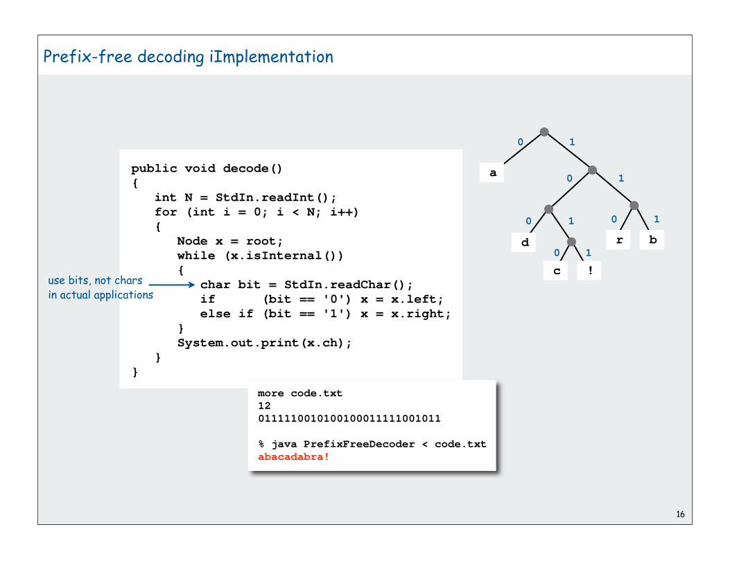
16
Prefix-free decoding iImplementation
public void decode(){ int N = StdIn.readInt(); for (int i = 0; i < N; i++) { Node x = root; while (x.isInternal()) { char bit = StdIn.readChar(); if (bit == '0') x = x.left; else if (bit == '1') x = x.right; } System.out.print(x.ch); }}
use bits, not charsin actual applications
a
d
0
c !
r b
1
0 1
0 1 0 1
0 1
more code.txt
12
0111110010100100011111001011
% java PrefixFreeDecoder < code.txt
abacadabra!

Introduction to compression: summary
Variable-length codes can provide better compression than fixed-length
Every trie defines a variable-length code
Q. What is the best variable length code for a given message?
17
a b r a c a d a b r a !
1100001 1100010 1110010 1100001 1100011 1100001 1100100 1100001 1100010 1110010 1100001 1111111
a b r a c a d a b r a !
X000 X001 X100 X000 X010 X000 X011 X000 X001 X100 X000 X111
a b r a c a d a b r a !
0 1 1 1 1 1 0 0 1 0 1 0 0 1 0 0 0 1 1 1 1 1 0 0 1 0 1 1
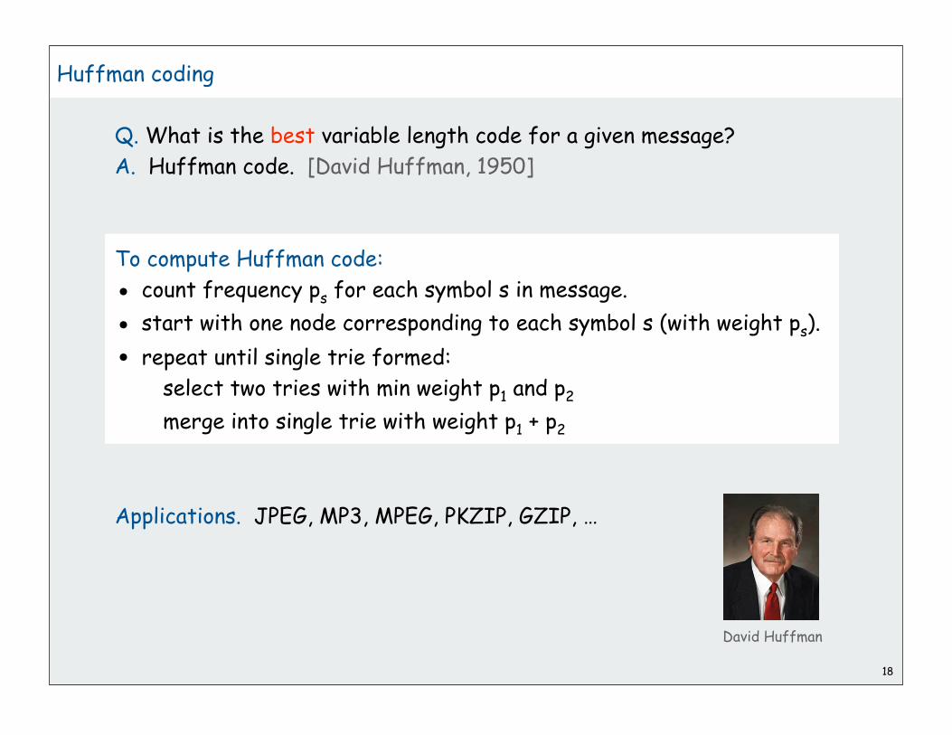
18
Huffman coding
Q. What is the best variable length code for a given message?
A. Huffman code. [David Huffman, 1950]
To compute Huffman code:
• count frequency ps for each symbol s in message.
• start with one node corresponding to each symbol s (with weight ps).
• repeat until single trie formed:
select two tries with min weight p1 and p2
merge into single trie with weight p1 + p2
Applications. JPEG, MP3, MPEG, PKZIP, GZIP, …
David Huffman

Huffman coding example
19
ac d r!
2 51 11
b
2
ad r
2 51
b
2
c !
1 1
2
a
d
r
2 5
1
b
2
c !
1 1
2
3
a
d
5
1
c !
1 1
2
3
r b
2 2
4
a
d
5
1
c !
1 1
2
3
r b
2 2
4
7
a
d
5
1
c !
1 1
2
3
r b
2 2
4
7
12
a b r a c a d a b r a !

20
Huffman trie construction code
int[] freq = new int[128];
for (int i = 0; i < input.length(); i++)
{ freq[input.charAt(i)]++; }
MinPQ<Node> pq = new MinPQ<Node>();
for (int i = 0; i < 128; i++)
if (freq[i] > 0)
pq.insert(new Node((char) i, freq[i], null, null));
while (pq.size() > 1){
Node x = pq.delMin();
Node y = pq.delMin();
Node parent = new Node('*', x.freq + y.freq, x, y);
pq.insert(parent);
}
root = pq.delMin();
internal node marker
total frequency
two subtrees
tabulate frequencies
initialize PQ
merge trees

Theorem. Huffman coding is an optimal prefix-free code.
Implementation.
• pass 1: tabulate symbol frequencies and build trie
• pass 2: encode file by traversing trie or lookup table.
Running time. Use binary heap O(M + N log N).
Can we do better? [stay tuned]
21
Huffman encoding summary
no prefix-free code uses fewer bits
outputbits
distinctsymbols

22
introductionbasic coding schemesan applicationentropyLZW codes

An application: compress a bitmap
Typical black-and-white-scanned image
300 pixels/inch
8.5 by 11 inches
300*8.5*300*11 = 8.415 million bits
Bits are mostly white
Typical amount of text on a page:
40 lines * 75 chars per line = 3000 chars
23

24
Natural encoding of a bitmap
one bit per pixel
000000000000000000000000000011111111111111000000000 000000000000000000000000001111111111111111110000000
000000000000000000000001111111111111111111111110000
000000000000000000000011111111111111111111111111000
000000000000000000001111111111111111111111111111110
000000000000000000011111110000000000000000001111111
000000000000000000011111000000000000000000000011111
000000000000000000011100000000000000000000000000111
000000000000000000011100000000000000000000000000111
000000000000000000011100000000000000000000000000111
000000000000000000011100000000000000000000000000111
000000000000000000001111000000000000000000000001110
000000000000000000000011100000000000000000000111000
011111111111111111111111111111111111111111111111111
011111111111111111111111111111111111111111111111111
011111111111111111111111111111111111111111111111111
011111111111111111111111111111111111111111111111111
011111111111111111111111111111111111111111111111111
011000000000000000000000000000000000000000000000011
19-by-51 raster of letter 'q' lying on its side

25
Run-length encoding of a bitmap
natural encoding. (19 51) + 6 = 975 bits.
run-length encoding. (63 6) + 6 = 384 bits.
5128 14 926 18 7
23 24 4
22 26 3
20 30 1
19 7 18 7
19 5 22 5
19 3 26 3
19 3 26 3
19 3 26 3
19 3 26 3
20 4 23 3 1
22 3 20 3 3
1 50
1 50
1 50
1 50
1 50
1 2 46 2
000000000000000000000000000011111111111111000000000 000000000000000000000000001111111111111111110000000
000000000000000000000001111111111111111111111110000
000000000000000000000011111111111111111111111111000
000000000000000000001111111111111111111111111111110
000000000000000000011111110000000000000000001111111
000000000000000000011111000000000000000000000011111
000000000000000000011100000000000000000000000000111
000000000000000000011100000000000000000000000000111
000000000000000000011100000000000000000000000000111
000000000000000000011100000000000000000000000000111
000000000000000000001111000000000000000000000001110
000000000000000000000011100000000000000000000111000
011111111111111111111111111111111111111111111111111
011111111111111111111111111111111111111111111111111
011111111111111111111111111111111111111111111111111
011111111111111111111111111111111111111111111111111
011111111111111111111111111111111111111111111111111
011000000000000000000000000000000000000000000000011
RLE19-by-51 raster of letter 'q' lying on its side
63 6-bit run lengths
to encode number of bits per line

26
Run-length encoding
• Exploit long runs of repeated characters.
• Bitmaps: runs alternate between 0 and 1; just output run lengths.
• Issue: how to encode run lengths (!)
• Does not compress when runs are short.
Runs are long in typical applications (such as black-and-white bitmaps).
001001001001001 2121212121 10011001100110011001
15 bits 20 bits
10: 201: 1

27
Run-length encoding and Huffman codes in the wild
ITU-T T4 Group 3 Fax for black-and-white bitmap images (~1980)
• up to 1728 pixels per line
• typically mostly white.
Step 1. Use run-length encoding.
Step 2. Encode run lengths using two Huffman codes.
194
3W 1B 2W 2B 194W
1000 010 0111 11 010111 0111
192 + 2
…
…
…
one for white and one for black
00110101 0000110111
white black
0
run
000111 0101
0111 112
1000 103
… ……
00110100 00000110011163
11011 0000001111 64+
10010 000011001000 128+
… ……
010011011 0000001100101 1728+Huffman codes built fromfrequencies in huge sample
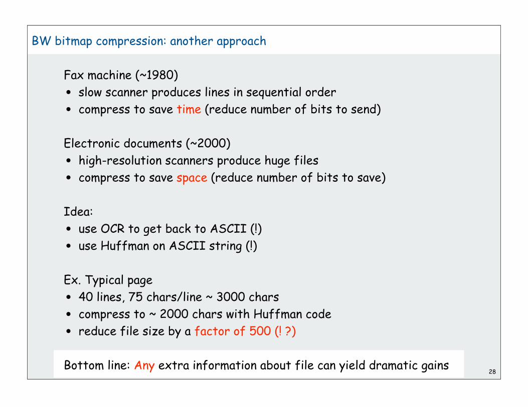
BW bitmap compression: another approach
Fax machine (~1980)
• slow scanner produces lines in sequential order
• compress to save time (reduce number of bits to send)
Electronic documents (~2000)
• high-resolution scanners produce huge files
• compress to save space (reduce number of bits to save)
Idea:
• use OCR to get back to ASCII (!)
• use Huffman on ASCII string (!)
Ex. Typical page
• 40 lines, 75 chars/line ~ 3000 chars
• compress to ~ 2000 chars with Huffman code
• reduce file size by a factor of 500 (! ?)
Bottom line: Any extra information about file can yield dramatic gains28

29
introductionbasic coding schemesan applicationentropyLZW codes

30
What data can be compressed?
US Patent 5,533,051 on "Methods for Data Compression", which is
capable of compression all files.
Slashdot reports of the Zero Space Tuner™ and BinaryAccelerator™.
"ZeoSync has announced a breakthrough in data compression that
allows for 100:1 lossless compression of random data. If this is true,
our bandwidth problems just got a lot smaller.…"

31
Perpetual Motion Machines
Universal data compression algorithms are the analog of perpetual
motion machines.
Closed-cycle mill by Robert Fludd, 1618 Gravity engine by Bob Schadewald
Reference: Museum of Unworkable Devices by Donald E. Simanekhttp://www.lhup.edu/~dsimanek/museum/unwork.htm

32
What data can be compressed?
Theorem. Impossible to losslessly compress all files.
Pf 1.
• consider all 1,000 bit messages.
• 21000 possible messages.
• only 2999 + 2998 + … + 1 can be encoded with 999 bits.
• only 1 in 2499 can be encoded with 500 bits!
Pf 2 (by contradiction).
• given a file M, compress it to get a smaller file M1.
• compress that file to get a still smaller file M2.
• continue until reaching file size 0.
• implication: all files can be compressed with 0 bits!
Practical test for any compression algorithm:
• given a file M, compress it to get a (smaller, you hope) file M1
• compress that file to get a still smaller file M2.
• continue until file size does not decrease

33
A difficult file to compress
fclkkacifobjofmkgdcoiicnfmcpcjfccabckjamolnihkbgobcjbngjiceeelpfgcjiihppenefllhglfemdemgahlbpiggmllmnefnhjelmgjncjcidlhkglhceninidmmgnobkeglpnadanfbecoonbiehglmpnhkkamdffpacjmgojmcaabpcjcecplfbgamlidceklhfkkmioljdnoaagiheiapaimlcnlljniggpeanbmojgkccogpmkmoifioeikefjidbadgdcepnhdpfjaeeapdjeofklpdeghidbgcaiemajllhnndigeihbebifemacfadnknhlbgincpmimdogimgeeomgeljfjgklkdgnhafohonpjbmlkapddhmepdnckeajebmeknmeejnmenbmnnfefdbhpmigbbjknjmobimamjjaaaffhlhiggaljbaijnebidpaeigdgoghcihodnlhahllhhoojdfacnhadhgkfahmeaebccacgeojgikcoapknlomfignanedmajinlompjoaifiaejbcjcdibpkofcbmjiobbpdhfilfajkhfmppcngdneeinpnfafaeladbhhifechinknpdnplamackphekokigpddmmjnbngklhibohdfeaggmclllmdhafkldmimdbplggbbejkcmhlkjocjjlcngckfpfakmnpiaanffdjdlleiniilaenbnikgfnjfcophbgkhdgmfpoehfmkbpiaignphogbkelphobonmfghpdgmkfedkfkchceeldkcofaldinljjcgafimaanelmfkokcjekefkbmegcgjifjcpjppnabldjoaafpbdafifgcoibbcmoffbbgigmngefpkmbhbghlbdjngenldhgnfbdlcmjdmoflhcogfjoldfjpaokepndejmnbiealkaofifekdjkgedgdlgbioacflfjlafbcaemgpjlagbdgilhcfdcamhfmppfgohjphlmhegjechgdpkkljpndphfcnnganmbmnggpphnckbieknjhilafkegboilajdppcodpeoddldjfcpialoalfeomjbphkmhnpdmcpgkgeaohfdmcnegmibjkajcdcpjcpgjminhhakihfgiiachfepffnilcooiciepoapmdjniimfbolchkibkbmhbkgconimkdchahcnhapfdkiapikencegcjapkjkfljgdlmgncpbakhjidapbldcgeekkjaoihbnbigmhboengpmedliofgioofdcphelapijcegejgcldcfodikalehbccpbbcfakkblmoobdmdgdkafbbkjnidoikfakjclbchambcpaepfeinmenmpoodadoecbgbmfkkeabilaoeoggghoekamaibhjibefmoppbhfbhffapjnodlofeihmjahmeipejlfhloefgmjhjnlomapjakhhjpncomippeanbikkhekpcfgbgkmklipfbiikdkdcbolofhelipbkbjmjfoempccneaebklibmcaddlmjdcajpmhhaeedbbfpjafcndianlfcjmmbfncpdcccodeldhmnbdjmeajmboclkggojghlohlbhgjkhkmclohkgjamfmcchkchmiadjgjhjehflcbklfifackbecgjoggpbkhlcmfhipflhmnmifpjmcoldbeghpcekhgmnahijpabnomnokldjcpppbcpgcjofngmbdcpeeeiiiclmbbmfjkhlanckidhmbeanmlabncnccpbhoafajjicnfeenppoekmlddholnbdjapbfcajblbooiaepfmmeoafedflmdcbaodgeahimcgpcammjljoebpfmghogfckgmomecdipmodbcempidfnlcggpgbffoncajpncomalgoiikeolmigliikjkolgolfkdgiijjiooiokdihjbbofiooibakadjnedlodeeiijkliicnioimablfdpjiafcfineecbafaamheiipegegibioocmlmhjekfikfeffmddhoakllnifdhckmbonbchfhhclecjamjildonjjdpifngbojianpljahpkindkdoanlldcbmlmhjfomifhmncikoljjhebidjdphpdepibfgdonjljfgifimniipogockpidamnkcpipglafmlmoacjibognbplejnikdoefccdpfkomkimffgjgielocdemnblimfmbkfbhkelkpfoheokfofochbmifleecbglmnfbnfncjmefnihdcoeiefllemnohlfdcmbdfebdmbeebbalggfbajdamplphdgiimehglpikbipnkkecekhilchhhfaeafbbfdmcjojfhpponglkfdmhjpcieofcnjgkpibcbiblfpnjlejkcppbhopohdghljlcokhdoahfmlglbdkliajbmnkkfcoklhlelhjhoiginaimgcabcfebmjdnbfhohkjphnklcbhcjpgbadakoecbkjcaebbanhnfhpnfkfbfpohmnkligpgfkjadomdjjnhlnfailfpcmnololdjekeolhdkebiffebajjpclghllmemegncknmkkeoogilijmmkomllbkkabelmodcohdhppdakbelmlejdnmbfmcjdebefnjihnejmnogeeafldabjcgfoaehldcmkbnbafpciefhlopicifadbppgmfngecjhefnkbjmliodhelhicnfoongngemddepchkokdjafegnpgledakmbcpcmkckhbffeihpkajginfhdolfnlgnadefamlfocdibhfkiaofeegppcjilndepleihkpkkgkphbnkggjiaolnolbjpobjdcehglelckbhjilafccfipgebpc....
One million pseudo-random characters (a – p)

34
A difficult file to compress
% javac Rand.java
% java Rand > temp.txt
% compress –c temp.txt > temp.Z
% gzip –c temp.txt > temp.gz
% bzip2 –c temp.txt > temp.bz2
% ls –l
231 Rand.java
1000000 temp.txt
576861 temp.Z
570872 temp.gz
499329 temp.bz2
resulting file sizes (bytes)
public class Rand{ public static void main(String[] args) { for (int i = 0; i < 1000000; i++) { char c = 'a'; c += (char) (Math.random() * 16); System.out.print(c); } }}
231 bytes, but output is hard to compress(assume random seed is fixed)

35
Information theory
Intrinsic difficulty of compression.
• Short program generates large data file.
• Optimal compression algorithm has to discover program!
• Undecidable problem.
Q. How do we know if our algorithm is doing well?
A. Want lower bound on # bits required by any compression scheme.

36
Language model
Q. How do compression algorithms work?
A. They exploit statistical biases of input messages.
• ex: white patches occur in typical images.
• ex: ord Princeton occurs more frequently than Yale.
Basis of compression: probability.
• Formulate probabilistic model to predict symbols.
simple: character counts, repeated strings
complex: models of a human face
• Use model to encode message.
• Use same model to decode message.
Ex. Order 0 Markov model
• R symbols generated independently at random
• probability of occurrence of i th symbol: pi (fixed).

A measure of information. [Shannon, 1948]
• information content of symbol s is proportional to 1/lg2 p(s).
• weighted average of information content over all symbols.
• interface between coding and model.
37
Entropy
p0
1/2
p1
1/2
H(M)
1
0.900 0.100 0.469
0.990 0.010 0.0808
1
1
2
3
4 0 0
p(1)
1/6
p(2)
1/6
p(3)
1/6
p(4)
1/6
p(5)
1/6
p(6) H(M)
2.585
Claude Shannon
Ex. 4 binary models (R = 2)
Ex. fair die (R = 6)
1/6
H(M) = p0/lg p0 + p1/lg p1 + p2/lg p2 + ... + pR-1/lg pR-1

38
Entropy and compression
Theorem. [Shannon, 1948] If data source is an order 0 Markov model,
any compression scheme must use H(M) bits per symbol on average.
• Cornerstone result of information theory.
• Ex: to transmit results of fair die, need 2.58 bits per roll.
Theorem. [Huffman, 1952] If data source is an order 0 Markov model,
Huffman code uses H(M) + 1 bits per symbol on average.
Q. Is there any hope of doing better than Huffman coding?
A1. Yes. Huffman wastes up to 1 bit per symbol.
if H(M) is close to 0, this difference matters
can do better with "arithmetic coding"
A2. Yes. Source may not be order 0 Markov model.

39
Entropy of the English Language
Q. How much redundancy is in the English language?
A. Quite a bit.
"... randomising letters in the middle of words [has] little or no effect on the
ability of skilled readers to understand the text. This is easy to
denmtrasote. In a pubiltacion of New Scnieitst you could ramdinose all the
letetrs, keipeng the first two and last two the same, and reibadailty would
hadrly be aftcfeed. My ansaylis did not come to much beucase the thoery at
the time was for shape and senqeuce retigcionon. Saberi's work sugsegts we
may have some pofrweul palrlael prsooscers at work. The resaon for this is
suerly that idnetiyfing coentnt by paarllel prseocsing speeds up regnicoiton.
We only need the first and last two letetrs to spot chganes in meniang."
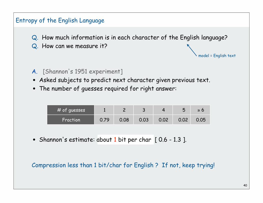
40
Entropy of the English Language
Q. How much information is in each character of the English language?
Q. How can we measure it?
A. [Shannon's 1951 experiment]
• Asked subjects to predict next character given previous text.
• The number of guesses required for right answer:
• Shannon's estimate: about 1 bit per char [ 0.6 - 1.3 ].
Compression less than 1 bit/char for English ? If not, keep trying!
1
0.79Fraction
# of guesses 2
0.08
3
0.03
4
0.02
5
0.02
6
0.05
model = English text

41
introductionbasic coding schemesan applicationentropyLZW codes

42
Statistical Methods
Static model. Same model for all texts.
• Fast.
• Not optimal: different texts have different statistical properties.
• Ex: ASCII, Morse code.
Dynamic model. Generate model based on text.
• Preliminary pass needed to generate model.
• Must transmit the model.
• Ex: Huffman code.
Adaptive model. Progressively learn and update model as you read text.
• More accurate modeling produces better compression.
• Decoding must start from beginning.
• Ex: LZW.

43
LZW Algorithm
Lempel-Ziv-Welch. [variant of LZ78]
• Create ST associating a fixed-length codeword with some
previous substring.
• When input matches string in ST, output associated codeword.
• length of strings in ST grows, hence compression.
To send (encode) M.
• Find longest string s in ST that is a prefix of unsent part of M
• Send codeword associated with s.
• Add s x to ST, where x is next char in M.
Ex. ST: a, aa, ab, aba, abb, abaa, abaab, abaaa,
• unsent part of M: abaababbb…
• s = abaab, x = a.
• Output integer associated with s; insert abaaba into ST.

LZW encoding example
44
input code add to ST
a 97 ab
b 98 br
r 114 ra
a 97 ac
c 99 ca
a 97 ad
d 100 da
a
b 128 abr
r
a 130 rac
c
a 132 cad
d it_
a 134 dab
b
r 129 bra
a 97
STOP 255
key value
0
...
a 97
b 98
c 99
d 100
...
r 114
...
127
key value
ab 128
br 129
ra 130
ac 131
ca 132
ad 133
da 134
abr 135
rac 136
cad 137
dab 138
bra 139
...
STOP 255
To send (encode) M.Find longest string s in ST that is a prefix of unsent part of MSend integer associated with s.Add s x to ST, where x is next char in M.
input: 7-bit ASCIIoutput: 8-bit codewords
ASCII ST

LZW encoding example
45
input code
a 97
b 98
r 114
a 97
c 99
a 97
d 100
a
b 128
r
a 130
c
a 132
d
a 134
b
r 129
a 97
STOP 255
input: 7-bit ASCII 19 chars 133 bits
output: 8-bit codewords 14 chars 112 bits
Key point: no need to send ST (!)

46
LZW encode ST implementation
Q. How to do longest prefix match?
A. Use a trie for the ST
Encode.
• lookup string suffix in trie.
• output ST index at bottom.
• add new node to bottom of trie.
Note that all substrings are in ST
a d
139
c rb
b r ac ad a
r cd ba
137 138 136135
131 133128 129 132 134 130
98 99 100 11497
key value
0
...
a 97
b 98
c 99
d 100
...
r 114
...
127
key value
ab 128
br 129
ra 130
ac 131
ca 132
ad 133
da 134
abr 135
rac 136
cad 137
dab 138
bra 139
...
STOP 255
ASCII ST

Use specialized TST
• initialized with ASCII chars and codes
• getput() method returns code of longest prefix s
and adds s + next char to symbol table
Need input stream with backup [stay tuned]
input stream with lookahead
specialized TST
47
LZW encoder: Java implementation
postprocess to encode in
binary
encode text and build
TST
public class LZWEncoder
{
public static void main(String[] args)
{
LookAheadIn in = new LookAheadIn();
LZWst st = new LZWst();
while (!in.isEmpty())
{
int codeword = st.getput(in);
StdOut.println(codeword);
}
}
}
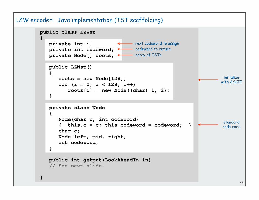
initialize with ASCII
48
LZW encoder: Java implementation (TST scaffolding)
public class LZWst{ private int i; private int codeword; private Node[] roots;
public LZWst() { roots = new Node[128]; for (i = 0; i < 128; i++) roots[i] = new Node((char) i, i); }
private class Node { Node(char c, int codeword) { this.c = c; this.codeword = codeword; } char c; Node left, mid, right; int codeword; }
public int getput(LookAheadIn in) // See next slide.
}
next codeword to assign
codeword to return
array of TSTs
standard node code
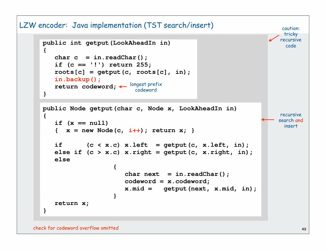
49
LZW encoder: Java implementation (TST search/insert)
public int getput(LookAheadIn in) { char c = in.readChar(); if (c == '!') return 255; roots[c] = getput(c, roots[c], in); in.backup(); return codeword; }
public Node getput(char c, Node x, LookAheadIn in) { if (x == null) { x = new Node(c, i++); return x; }
if (c < x.c) x.left = getput(c, x.left, in); else if (c > x.c) x.right = getput(c, x.right, in); else { char next = in.readChar(); codeword = x.codeword; x.mid = getput(next, x.mid, in); } return x; }
longest prefix codeword
recursive search and
insert
caution: tricky
recursive code
check for codeword overflow omitted

50
LZW encoder: Java implementation (input stream with lookahead)
public class LookAheadIn{ In in = new In(); char last; boolean backup = false; public void backup() { backup = true; } public char readChar() { if (!backup) { last = in.readChar(); } backup = false; return last; } public boolean isEmpty() { return !backup && in.isEmpty(); }}
Provides input stream with one-character lookahead.
backup() call means that last readChar() call was lookahead.

51
LZW Algorithm
Lempel-Ziv-Welch. [variant of LZ78]
• Create ST and associate an integer with each useful string.
• When input matches string in ST, output associated integer.
• length of strings in ST grows, hence compression.
• decode by rebuilding ST from code
To send (encode) M.
• Find longest string s in ST that is a prefix of unsent part of M
• Send integer associated with s.
• Add s x to ST, where x is next char in M.
To decode received message to M.
• Let s be ST entry associated with received integer
• Add s to M.
• Add p x to ST, where x is first char in s, p is previous value of s.

LZW decoding example
52
codeword output add to ST
97 a
98 b ab
114 r br
97 a ra
99 c ac
97 a ca
100 d ad
128 a
b da
130 r
a abr
132 c
a rac
134 d it_
a cad
129 b
r dab
97 a bra
255 STOP
To decode received message to M.
Let s be ST entry associated with received integer
Add s to M.
Add p x to ST, where x is first char in s, p is previous value of s.
key value
0
...
97 a
98 b
99 c
100 d
...
114 r
...
127
key value
128 ab
129 br
130 ra
131 ac
132 ca
133 ad
134 da
135 abr
136 rac
137 cad
138 dab
139 bra
...
255
role of keys and values switched
Use an arrayto implement ST
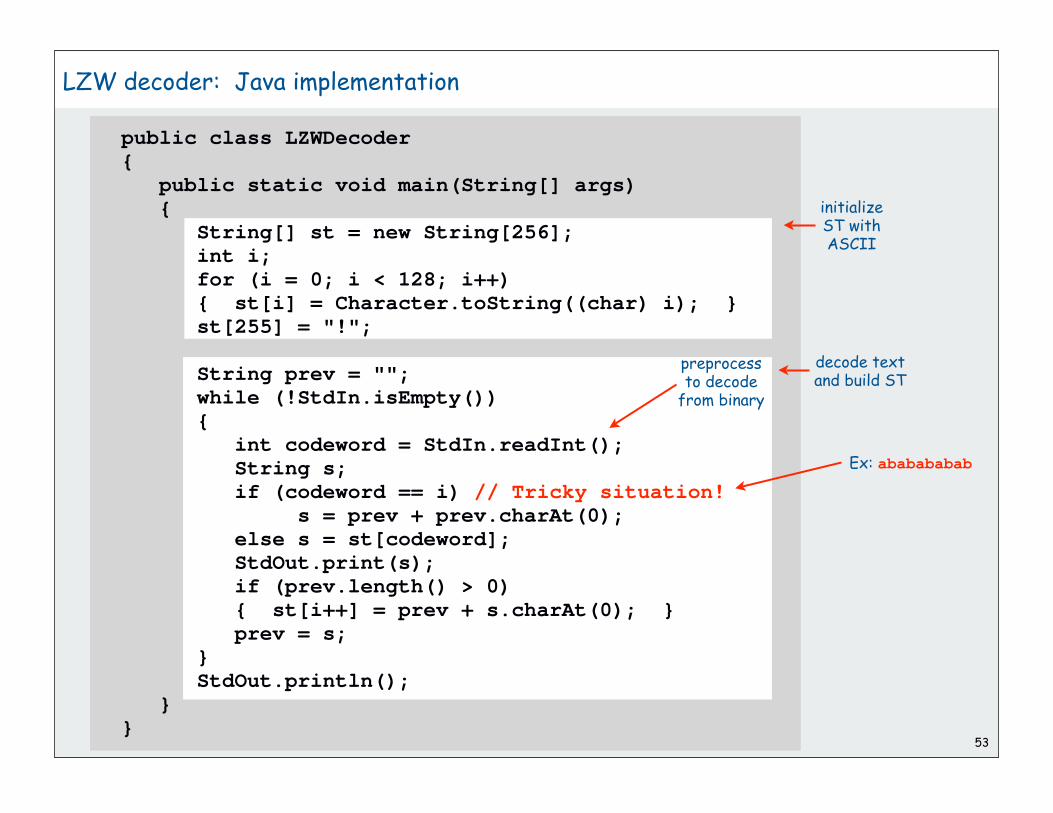
initialize ST with ASCII
decode text and build ST
53
LZW decoder: Java implementation
public class LZWDecoder{ public static void main(String[] args) { String[] st = new String[256]; int i; for (i = 0; i < 128; i++) { st[i] = Character.toString((char) i); } st[255] = "!";
String prev = ""; while (!StdIn.isEmpty()) { int codeword = StdIn.readInt(); String s; if (codeword == i) // Tricky situation! s = prev + prev.charAt(0); else s = st[codeword]; StdOut.print(s); if (prev.length() > 0) { st[i++] = prev + s.charAt(0); } prev = s; } StdOut.println(); }}
preprocess to decode
from binary
Ex: ababababab
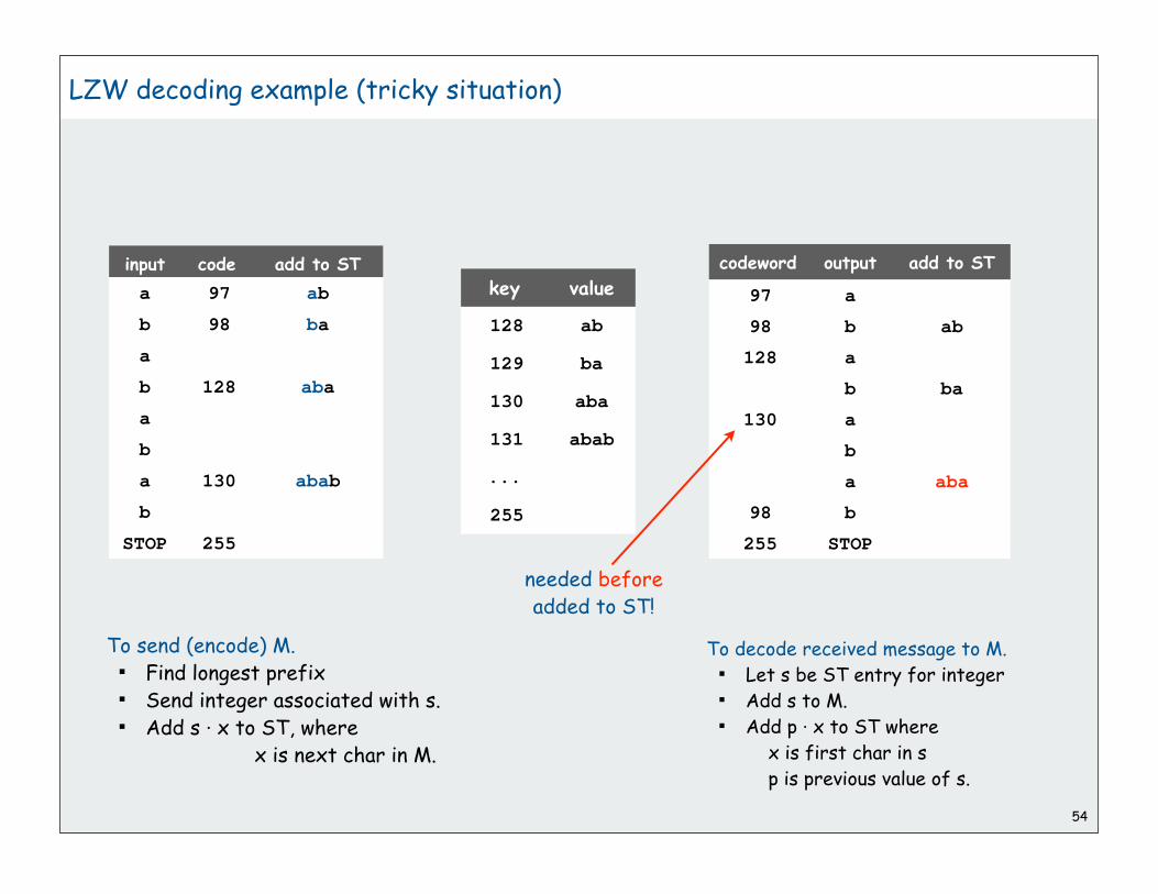
LZW decoding example (tricky situation)
54
codeword output add to ST
97 a
98 b ab
128 a
b ba
130 a
b
a aba
98 b
255 STOP
key value
128 ab
129 ba
130 aba
131 abab
...
255
input code add to ST
a 97 ab
b 98 ba
a
b 128 aba
a
b
a 130 abab
b
STOP 255
To send (encode) M.Find longest prefix Send integer associated with s.Add s x to ST, where x is next char in M.
To decode received message to M.
Let s be ST entry for integer
Add s to M.
Add p x to ST where
x is first char in s
p is previous value of s.
needed beforeadded to ST!

55
LZW implementation details
How big to make ST?
• how long is message?
• whole message similar model?
• ...
• [many variations have been developed]
What to do when ST fills up?
• throw away and start over. GIF
• throw away when not effective. Unix compress
• ...
• [many other variations]
Why not put longer substrings in ST?
• ...
• [many variations have been developed]

56
LZW in the real world
Lempel-Ziv and friends.
• LZ77.
• LZ78.
• LZW.
• Deflate = LZ77 variant + Huffman.
PNG: LZ77.
Winzip, gzip, jar: deflate.
Unix compress: LZW.
Pkzip: LZW + Shannon-Fano.
GIF, TIFF, V.42bis modem: LZW.
Google: zlib which is based on deflate.
never expands a file
LZ77 not patented widely used in open source
LZW patent #4,558,302 expired in US on June 20, 2003
some versions copyrighted

57
Lossless compression ratio benchmarks
ASCII
Scheme
Huffman
LZ77
LZMW
LZH
7.00
Bits / char
4.70
3.94
3.32
3.30
Char by char
Entropy
8 chars at a time
Asymptotic
4.5
Bits/char
2.4
1.3
Move-to-front
Gzip
PPMC
SAKDC
PPM
3.24
2.71
2.48
2.47
2.34
1967
Year
1950
1977
1984
1987
1987
1987
1988
1988
1994
Burrows-Wheeler
BOA
2.29
1.99
1995
1997
RK 1.891999
LZB 3.181987
next assignment
Calgary corpus: standard data compression benchmark

58
Data compression summary
Lossless compression.
• Represent fixed length symbols with variable length codes. [Huffman]
• Represent variable length symbols with fixed length codes. [LZW]
Lossy compression. [not covered in this course]
• JPEG, MPEG, MP3.
• FFT, wavelets, fractals, SVD, …
Limits on compression. Shannon entropy.
Theoretical limits closely match what we can achieve in practice.
Practical compression: Use extra knowledge whenever possible.
Butch: I don’t mean to be a sore loser, but when it’s done, if I’m dead, kill him.
Sundance: Love to.
Butch: No, no, not yet. Not until me and Harvey get the rules straightened out.
Harvey: Rules? In a knife fight? No rules.
Butch: Well, if there ain’t going to be any rules, let’s get the fight started...

1
Pattern Matching
exact pattern matchingKnuth-Morris-PrattRE pattern matchinggrep
References:
Algorithms in C (2nd edition), Chapter 19 http://www.cs.princeton.edu/introalgsds/63long http://www.cs.princeton.edu/introalgsds/72regular

2
exact pattern matchingKnuth-Morris-PrattRE pattern matchinggrep

3
Exact pattern matching
Problem:
Find first match of a pattern of length M in a text stream of length N.
Applications.
• parsers.
• spam filters.
• digital libraries.
• screen scrapers.
• word processors.
• web search engines.
• natural language processing.
• computational molecular biology.
• feature detection in digitized images.
. . .
N = 21
typically N >> M
M = 6n e e d l e
i n a h a y s t a c k a n e e d l e i n a
pattern
text

4
Brute-force exact pattern match
h a y n e e d s a n n e e d l e x
n e e d l e
n e e d l e
n e e d l e
n e e d l e
n e e d l e
n e e d l e
n e e d l e
n e e d l e
n e e d l e
n e e d l e
n e e d l e
Check for pattern starting at each text position.
public static int search(String pattern, String text){ int M = pattern.length(); int N = text.length();
for (int i = 0; i < N - M; i++) { int j; for (j = 0; j < M; j++) if (text.charAt(i+j) != pattern.charAt(j)) break; if (j == M) return i; } return -1; }
pattern start index in text
not found

5
Brute-force exact pattern match: worst case
a a a a a a a a a a a a a a a a b
a a a a a b
a a a a a b
a a a a a b
a a a a a b
a a a a a b
a a a a a b
a a a a a b
a a a a a b
a a a a a b
a a a a a b
a a a a a b
a a a a a b
Brute-force algorithm can be slow if text and pattern are repetitive
but this situation is rare in typical applications
Hence, the indexOf() method in Java’s String class uses brute-force
MN char compares
text length N
pattern length M

6
Exact pattern matching in Java
Exact pattern matching is implemented in Java’s String class
s.indexOf(t, i): index of first occurrence of pattern t
in string s, starting at offset i.
Ex: Screen scraping. Exact match to extract info from website
public class StockQuote
{
public static void main(String[] args)
{
String name = "http://finance.yahoo.com/q?s=";
In in = new In(name + args[0]);
String input = in.readAll();
int start = input.indexOf("Last Trade:", 0);
int from = input.indexOf("<b>", start);
int to = input.indexOf("</b>", from);
String price = input.substring(from + 3, to);
System.out.println(price);
}
}
...
<tr>
<td class= "yfnc_tablehead1"
width= "48%">
Last Trade:
</td>
<td class= "yfnc_tabledata1">
<big><b>688.04</b></big>
</td></tr>
<td class= "yfnc_tablehead1"
width= "48%">
Trade Time:
</td>
<td class= "yfnc_tabledata1">
http://finance.yahoo.com/q?s=goog

7
Algorithmic challenges in pattern matching
Brute-force is not good enough for all applications
Theoretical challenge: Linear-time guarantee.
Practical challenge: Avoid backup in text stream.
Now is the time for all people to come to the aid of their party. Now is the time for all good people to come to the aid of their party. Now is the time for many good people to come to the aid of their party. Now is the time for all good people to come to the aid of their party. Now is the time for a lot of good people to come to the aid of their party. Now is the time for all of the good people to come to the aid of their party. Now is the time for all good people to come to the aid of their party. Now is the time for each good person to come to the aid of their party. Now is the time for all good people to come to the aid of their party. Now is the time for all good Republicans to come to the aid of their party. Now is the time for all good people to come to the aid of their party. Now is the time for many or all good people to come to the aid of their party. Now is the time for all good people to come to the aid of their party. Now is the time for all good Democrats to come to the aid of their party. Now is the time for all people to come to the aid of their party. Now is the time for all good people to come to the aid of their party. Now is the time for many good people to come to the aid of their party. Now is the time for all good people to come to the aid of their party. Now is the time for a lot of good people to come to the aid of their party. Now is the time for all of the good people to come to the aid of their party. Now is the time for all good people to come to the aid of their attack at dawn party. Now is the time for each person to come to the aid of their party. Now is the time for all good people to come to the aid of their party. Now is the time for all good Republicans to come to the aid of their party. Now is the time for all good people to come to the aid of their party. Now is the time for many or all good people to come to the aid of their party. Now is the time for all good people to come to the aid of their party. Now is the time for all good Democrats to come to the aid of their party.
often no room or time to save text
fundamental algorithmic problem

8
exact pattern matchingKnuth-Morris-PrattRE pattern matchinggrep

Knuth-Morris-Pratt (KMP) exact pattern-matching algorithm
Classic algorithm that meets both challenges
• linear-time guarantee
• no backup in text stream
Basic plan (for binary alphabet)
• build DFA from pattern
• simulate DFA with text as input
No backup in a DFA
Linear-time because each step is just a state change
9
Don Knuth Vaughan PrattJim Morris
a a a b a a b a a a b
accept pattern in text
rejectpattern NOT
in text
DFA
for
pattern
a a b a a a
text

Knuth-Morris-Pratt DFA example
10
0b
a
b
a2
a
bb
ab
a
b
a1 3 4 5
DFA
for
pattern
a a b a a a
How to construct? Stay tuned
One state for each pattern character
• Match input character: move from i to i+1
• Mismatch: move to previous state

Knuth-Morris-Pratt DFA simulation
11
0b
ab
a2
a
bb
ab
a
b
a1 3 4 5
a a a b a a b a a a b
0b
ab
a2
a
bb
ab
a
b
a1 3 4 5
a a a b a a b a a a b
0b
ab
a2
a
bb
ab
a
b
a1 3 4 5
a a a b a a b a a a b
0b
ab
a2
a
bb
ab
a
b
a1 3 4 5
a a a b a a b a a a b
0b
ab
a2
a
bb
ab
a
b
a1 3 4 5
a a a b a a b a a a b
0b
ab
a2
a
bb
ab
a
b
a1 3 4 5
0
1
2
2
3

Knuth-Morris-Pratt DFA simulation
12
0b
ab
a2
a
bb
ab
a
b
a1 3 4 5
a a a b a a b a a a b
0b
ab
a2
a
bb
ab
a
b
a1 3 4 5
a a a b a a b a a a b
0b
ab
a2
a
bb
ab
a
b
a1 3 4 5
a a a b a a b a a a b
0b
ab
a2
a
bb
ab
a
b
a1 3 4 5
a a a b a a b a a a b
0b
ab
a2
a
bb
ab
a
b
a1 3 4 5
a a a b a a b a a a b
0b
ab
a2
a
bb
ab
a
b
a1 3 4 5
4
5
3
4
5
accept!

13
Knuth-Morris-Pratt DFA simulation
When in state i:
• have found match in i previous input chars
• that is the longest such match
Ex. End in state 4 iff text ends in aaba.
Ex. End in state 2 iff text ends in aa (but not aabaa or aabaaa).
0 a a a b a a b a a a b1 a a a b a a b a a a b2 a a a b a a b a a a b2 a a a b a a b a a a b3 a a a b a a b a a a b4 a a a b a a b a a a b5 a a a b a a b a a a b3 a a a b a a b a a a b4 a a a b a a b a a a b5 a a a b a a b a a a b a a a b a a b a a a b
0b
a
b
a2
a
bb
ab
a
b
a1 3 4 5

14
KMP implementation
DFA representation: a single state-indexed array next[]
• Upon character match in state j, go forward to state j+1.
• Upon character mismatch in state j, go back to state next[j].
b 0
a 1
0 1 2 3 4 5
0
2
3
2
0
4
0
5
3
6
next 0 0 2 0 0 3only need to
store mismatches
0b
a
b
a2
a
bb
ab
a
b
a1 3 4 5
DFA
for
pattern
a a b a a a

15
KMP implementation
Two key differences from brute-force implementation:
• Text pointer i never decrements
• Need to precompute next[] table (DFA) from pattern.
int j = 0;for (int i = 0; i < N; i++){ if (t.charAt(i) == p.charAt(j)) j++; // match else j = next[j]; // mismatch if (j == M) return i - M + 1; // found}return -1; // not found
Simulation of KMP DFA

16
Knuth-Morris-Pratt: Iterative DFA construction
DFA for first i states contains the information needed to build state i+1
Ex: given DFA for pattern aabaaa.
how to compute DFA for pattern aabaaab ?
Key idea
• on mismatch at 7th char, need to simulate 6-char backup
• previous 6 chars are known (abaaaa in example)
• 6-state DFA (known) determines next state!
Keep track of DFA state for start at 2nd char of pattern
• compare char at that position with next pattern char
• match/mismatch provides all needed info
0 a b a a a a1 a b a a a a0 a b a a a a1 a b a a a a2 a b a a a a2 a b a a a a2 a b a a a a
0b
a
b
a2
a
bb
ab
a
b
a1 3 4 5

KMP iterative DFA construction: two cases
Let X be the next state in the simulation and j the next state to build.
If p[X] and p[j] match, copy and increment
next[j] = next[X]; X = X+1
If p[X] and p[j] mismatch, do the opposite
next[j] = X+1; X = next[X];
17
0 1 2 3 4 5 6 p[] a a b a a a bnext[] 0 0 2 0 0 3 2
0b
a
b
a2
a
bb
ab
a
b
a1 3 4 5
a
b6
DFA fora a b a a a b
0b
a
b
a2
a
bb
ab
a
b
a1 3 4 5
b
a6
j
DFA fora a b a a a a
0 1 2 3 4 5 6 p[] a a b a a a anext[] 0 0 2 0 0 3 3
X j
X
state for a b a a a b
state for a b a a a a

Knuth-Morris-Pratt DFA construction
18
0b
ab
a2
a
bb
ab
a
b
a1 3 4 5
0b
ab
a2
a
bb
ab
a1 3 4 5
0b
ab
a2
a
bb
a1 3 4
0b
ab
a2
a
b1 3
0b
ab
a21
0b
a1
0
0a 0
0 1a a 0 0
0 1 2a a b 0 0 2
0 1 2 3a a b a 0 0 2 0
0 1 2 3 4a a b a a 0 0 2 0 0
0 1 2 3 4 5a a b a a a 0 0 2 0 0 3
DFA X: current state in simulationcompare p[j] with p[X]
match: copy and increment next[j] = next[X];
X = X + 1;
mismatch: do the opposite next[j] = X + 1; X = next[X]; 0
a 1
a b 0
a b a 1
a b a a 2
p[1..j-1] Xmatch
match
match
mismatch
mismatch
X j

Knuth-Morris-Pratt DFA construction examples
19
0a 0
0 1a a 0 0
0 1 2a a b 0 0 2
0 1 2 3a a b a 0 0 2 0
0 1 2 3 4a a b a a 0 0 2 0 0
0 1 2 3 4 5a a b a a a 0 0 2 0 0 3
0 1 2 3 4 5 6a a b a a a b 0 0 2 0 0 3 2
X: current state in simulationcompare p[j] with p[X]
match: copy and increment next[j] = next[X];
X = X + 1;
mismatch: do the opposite next[j] = X + 1; X = next[X];
match
match
match
mismatch
mismatch
X j
match
ex: a a b a a a b
0a 0
0 1a b 0 1
0 1 2a b b 0 1 1
0 1 2 3a b b a 0 1 1 0
0 1 2 3 4a b b a b 0 1 1 0 1
0 1 2 3 4 5a b b a b b 0 1 1 0 1 1
0 1 2 3 4 5 6a b b a b b b 0 1 1 0 1 1 4
match
match
mismatch
X j
ex: a b b a b b b
mismatch
match
mismatch
next[]

20
DFA construction for KMP: Java implementation
Takes time and space proportional to pattern length.
int X = 0;int[] next = new int[M];for (int j = 1; j < M; j++){ if (p.charAt(X) == p.charAt(j)) { // match next[j] = next[X]; X = X + 1; } else { // mismatch next[j] = X + 1; X = next[X]; }}
DFA Construction for KMP (assumes binary alphabet)

21
Optimized KMP implementation
Ultimate search program for any given pattern:
• one statement comparing each pattern character to next
• match: proceed to next statement
• mismatch: go back as dictated by DFA
• translates to machine language (three instructions per pattern char)
Lesson: Your computer is a DFA!
int kmpsearch(char t[]){ int i = 0; s0: if (t[i++] != 'a') goto s0; s1: if (t[i++] != 'a') goto s0; s2: if (t[i++] != 'b') goto s2; s3: if (t[i++] != 'a') goto s0; s4: if (t[i++] != 'a') goto s0; s5: if (t[i++] != 'a') goto s3; s6: if (t[i++] != 'b') goto s2; s7: if (t[i++] != 'b') goto s4; return i - 8;} next[]
assumes pattern is in text(o/w use sentinel)
pattern[]

22
KMP summary
General alphabet
• more difficult
• easy with next[][] indexed by mismatch position, character
• KMP paper has ingenious solution that is not difficult to implement
[ build NFA, then prove that it finishes in 2N steps ]
Bottom line: linear-time pattern matching is possible (and practical)
Short history:
• inspired by esoteric theorem of Cook
[ linear time 2-way pushdown automata simulation is possible ]
• discovered in 1976 independently by two theoreticians and a hacker
Knuth: discovered linear time algorithm
Pratt: made running time independent of alphabet
Morris: trying to build a text editor.
• theory meets practice

Exact pattern matching: other approaches
Rabin-Karp: make a digital signature of the pattern
• hashing without the table
• linear-time probabilistic guarantee
• plus: extends to 2D patterns
• minus: arithmetic ops much slower than char comparisons
Boyer-Moore: scan from right to left in pattern
• main idea: can skip M text chars when finding one not in the pattern
• needs additional KMP-like heuristic
• plus: possibility of sublinear-time performance (~ N/M )
• used in Unix, emacs
23
s y z y g y
a a a b b a a b a b a a a b b a a a b a a
pattern
text
s y z y g yy
s y z y g yy
s y z y g yy

24
Exact pattern match cost summary
† assumes appropriate model
‡ randomized
Cost of searching for M-character pattern in N-character text
algorithm typical worst-case
brute-force
Karp-Rabin
KMP
Boyer-Moore
1.1 N char compares † M N char compares
3N arithmetic ops 3N arithmetic ops ‡
1.1 N char compares † 2N char compares
~ N/M char compares † 3N char compares

25
exact pattern matchingKnuth-Morris-PrattRE pattern matchinggrep

26
Regular-expression pattern matching
Exact pattern matching:
Search for occurrences of a single pattern in a text file.
Regular expression (RE) pattern matching:
Search for occurrences of one of multiple patterns in a text file.
Ex. (genomics)
• Fragile X syndrome is a common cause of mental retardation.
• human genome contains triplet repeats of cgg or agg
bracketed by gcg at the beginning and ctg at the end
• number of repeats is variable, and correlated with syndrome
• use regular expression to specify pattern: gcg(cgg|agg)*ctg
• do RE pattern match on person’s genome to detect Fragile X
gcg(cgg|agg)*ctg
gcggcgtgtgtgcgagagagtgggtttaaagctggcgcggaggcggctggcgcggaggctg
pattern (RE)
text

27
RE pattern matching: applications
Test if a string matches some pattern.
• Process natural language.
• Scan for virus signatures.
• Search for information using Google.
• Access information in digital libraries.
• Retrieve information from Lexis/Nexis.
• Search-and-replace in a word processors.
• Filter text (spam, NetNanny, Carnivore, malware).
• Validate data-entry fields (dates, email, URL, credit card).
• Search for markers in human genome using PROSITE patterns.
Parse text files.
• Compile a Java program.
• Crawl and index the Web.
• Read in data stored in ad hoc input file format.
• Automatically create Java documentation from Javadoc comments.

28
Regular expression examples
A regular expression is a notation to specify a set of strings.
every other stringaabaabaabaabconcatenation
every other stringaaaababaab
a(a|b)aab
parentheses
(ab)*a
ab*a
aa | baab
.u.u.u.
example RE
aaabbba
aababababa
abababa
aaabbba
closure
union
wildcard
operation
every other stringaabaab
succubustumultuous
cumulusjugulum
not in setin set

29
Regular expression examples (continued)
Notation is surprisingly expressive
and plays a well-understood role in the theory of computation
bbbbaabbbaa
bbbaaabbbaababbaa
a* | (a*ba*ba*ba*)*
number of b’s is a multiple of 3
111111111403982772
100023498701234
.*0....
fifth to last digit is 0
subspacesubspecies
raspberrycrispbread
.*spb.*
contains the trigraph spb
gcgcggcggcggcggctggcgcaggctg
gcgctggcgcggctggcgcggaggctg
gcg(cgg|agg)*ctg
fragile X syndrome indicator
regular expression not in setin set

30
Generalized regular expressions
Additional operations are often added
• Ex: [a-e]+ is shorthand for (a|b|c|d|e)(a|b|c|d|e)*
• for convenience only
• need to be alert for non-regular additions (Ex: Java /)
111111111166-54-111
08540-132119072-5541
[0-9]{5}-[0-9]{4}exactly k
decaderhythm[^aeiou]{6}negations
camelCase4illegal
wordCapitalized
[A-Za-z][a-z]*character classes
adebcde
abcdeabcbcde
a(bc)+deone or more
exampleoperation not in setin set

31
Regular expressions in Java
RE pattern matching is implemented in Java’s String class
• basic: match() method
• various other methods also available (stay tuned)
Ex: Validity checking. Is input in the set described by the re?
public class Validate
{
public static void main(String[] args)
{
String re = args[0];
String input = args[1];
System.out.println(input.matches(re));
}}
% java Validate "..oo..oo." bloodroottrue
% java Validate "[$_A-Za-z][$_A-Za-z0-9]*" ident123true
% java Validate "[a-z]+@([a-z]+\.)+(edu|com)" [email protected]
% java Validate "[0-9]{3}-[0-9]{2}-[0-9]{4}" 166-11-4433true
legal Java identifier
valid email address(simplified)
Social Security number
need help solvingcrosswords?

32
Regular expressions in other languages
Broadly applicable programmer's tool.
• originated in UNIX in the 1970s
• many languages support extended regular expressions
• built into grep, awk, emacs, Perl, PHP, Python, JavaScript
PERL. Practical Extraction and Report Language.
print all lines containing NEWLINE which occurs in any file with a .java extension
grep NEWLINE */*.java
egrep '^[qwertyuiop]*[zxcvbnm]*$' dict.txt | egrep '...........'
replace all occurrences of fromwith to in the file input.txt
perl -p -i -e 's|from|to|g' input.txt
perl -n -e 'print if /^[A-Za-z][a-z]*$/' dict.txt
do for each line

33
Regular expression caveat
Writing a RE is like writing a program.
• need to understand programming model
• can be easier to write than read
• can be difficult to debug
"Sometimes you have a programming problem
and it seems like the best solution is to use
regular expressions; now you have two problems."

34
Can the average web surfer learn to use REs?
Google. Supports * for full word wildcard and | for union.

35
Can the average TV viewer learn to use REs?
TiVo. WishList has very limited pattern matching.
Reference: page 76, Hughes DirectTV TiVo manual

36
Can the average programmer learn to use REs?
Reference: http://www.ex-parrot.com/~pdw/Mail-RFC822-Address.htmlPerl RE for Valid RFC822 Email Addresses
(?:(?:\r\n)?[ \t])*(?:(?:(?:[^()<>@,;:\\".\[\] \000-\031]+(?:(?:(?:\r\n)?[ \t])+|\Z|(?=[\["()<>@,;:\\".\[\]]))|"(?:[^\"\r\\]|\\.|(?:(?:\r\n)?[ \t]))*"(?:(?:\r\n)?[ \t])*)(?:\.(?:(?:\r\n)?[ \t])*(?:[^()<>@,;:\\".\[\] \000-\031]+(?:(?:(?:\r\n)?[ \t])+|\Z|(?=[\["()<>@,;:\\".\[\]]))|"(?:[^\"\r\\]|\\.|(?:(?:\r\n)?[ \t]))*"(?:(?:\r\n)?[ \t])*))*@(?:(?:\r\n)?[ \t])*(?:[^()<>@,;:\\".\[\] \000-\031]+(?:(?:(?:\r\n)?[ \t])+|\Z|(?=[\["()<>@,;:\\".\[\]]))|\[([^\[\]\r\\]|\\.)*\](?:(?:\r\n)?[ \t])*)(?:\.(?:(?:\r\n)?[ \t])*(?:[^()<>@,;:\\".\[\] \000-\031]+(?:(?:(?:\r\n)?[ \t])+|\Z|(?=[\["()<>@,;:\\".\[\]]))|\[([^\[\]\r\\]|\\.)*\](?:(?:\r\n)?[ \t])*))*|(?:[^()<>@,;:\\".\[\] \000-\031]+(?:(?:(?:\r\n)?[ \t])+|\Z|(?=[\["()<>@,;:\\".\[\]]))|"(?:[^\"\r\\]|\\.|(?:(?:\r\n)?[ \t]))*"(?:(?:\r\n)?[ \t])*)*\<(?:(?:\r\n)?[ \t])*(?:@(?:[^()<>@,;:\\".\[\] \000-\031]+(?:(?:(?:\r\n)?[ \t])+|\Z|(?=[\["()<>@,;:\\".\[\]]))|\[([^\[\]\r\\]|\\.)*\](?:(?:\r\n)?[ \t])*)(?:\.(?:(?:\r\n)?[ \t])*(?:[^()<>@,;:\\".\[\] \000-\031]+(?:(?:(?:\r\n)?[ \t])+|\Z|(?=[\["()<>@,;:\\".\[\]]))|\[([^\[\]\r\\]|\\.)*\](?:(?:\r\n)?[ \t])*))*(?:,@(?:(?:\r\n)?[ \t])*(?:[^()<>@,;:\\".\[\] \000-\031]+(?:(?:(?:\r\n)?[ \t])+|\Z|(?=[\["()<>@,;:\\".\[\]]))|\[([^\[\]\r\\]|\\.)*\](?:(?:\r\n)?[ \t])*)(?:\.(?:(?:\r\n)?[ \t])*(?:[^()<>@,;:\\".\[\] \000-\031]+(?:(?:(?:\r\n)?[ \t])+|\Z|(?=[\["()<>@,;:\\".\[\]]))|\[([^\[\]\r\\]|\\.)*\](?:(?:\r\n)?[ \t])*))*)*:(?:(?:\r\n)?[ \t])*)?(?:[^()<>@,;:\\".\[\] \000-\031]+(?:(?:(?:\r\n)?[ \t])+|\Z|(?=[\["()<>@,;:\\".\[\]]))|"(?:[^\"\r\\]|\\.|(?:(?:\r\n)?[ \t]))*"(?:(?:\r\n)?[ \t])*)(?:\.(?:(?:\r\n)?[ \t])*(?:[^()<>@,;:\\".\[\] \000-\031]+(?:(?:(?:\r\n)?[ \t])+|\Z|(?=[\["()<>@,;:\\".\[\]]))|"(?:[^\"\r\\]|\\.|(?:(?:\r\n)?[ \t]))*"(?:(?:\r\n)?[ \t])*))*@(?:(?:\r\n)?[ \t])*(?:[^()<>@,;:\\".\[\] \000-\031]+(?:(?:(?:\r\n)?[ \t])+|\Z|(?=[\["()<>@,;:\\".\[\]]))|\[([^\[\]\r\\]|\\.)*\](?:(?:\r\n)?[ \t])*)(?:\.(?:(?:\r\n)?[ \t])*(?:[^()<>@,;:\\".\[\] \000-\031]+(?:(?:(?:\r\n)?[ \t])+|\Z|(?=[\["()<>@,;:\\".\[\]]))|\[([^\[\]\r\\]|\\.)*\](?:(?:\r\n)?[ \t])*))*\>(?:(?:\r\n)?[ \t])*)|(?:[^()<>@,;:\\".\[\] \000-\031]+(?:(?:(?:\r\n)?[ \t])+|\Z|(?=[\["()<>@,;:\\".\[\]]))|"(?:[^\"\r\\]|\\.|(?:(?:\r\n)?[ \t]))*"(?:(?:\r\n)?[ \t])*)*:(?:(?:\r\n)?[ \t])*(?:(?:(?:[^()<>@,;:\\".\[\] \000-\031]+(?:(?:(?:\r\n)?[ \t])+|\Z|(?=[\["()<>@,;:\\".\[\]]))|"(?:[^\"\r\\]|\\.|(?:(?:\r\n)?[ \t]))*"(?:(?:\r\n)?[ \t])*)(?:\.(?:(?:\r\n)?[ \t])*(?:[^()<>@,;:\\".\[\] \000-\031]+(?:(?:(?:\r\n)?[ \t])+|\Z|(?=[\["()<>@,;:\\".\[\]]))|"(?:[^\"\r\\]|\\.|(?:(?:\r\n)?[ \t]))*"(?:(?:\r\n)?[ \t])*))*@(?:(?:\r\n)?[ \t])*(?:[^()<>@,;:\\".\[\] \000-\031]+(?:(?:(?:\r\n)?[ \t])+|\Z|(?=[\["()<>@,;:\\".\[\]]))|\[([^\[\]\r\\]|\\.)*\](?:(?:\r\n)?[ \t])*)(?:\.(?:(?:\r\n)?[ \t])*(?:[^()<>@,;:\\".\[\] \000-\031]+(?:(?:(?:\r\n)?[ \t])+|\Z|(?=[\["()<>@,;:\\".\[\]]))|\[([^\[\]\r\\]|\\.)*\](?:(?:\r\n)?[ \t])*))*|(?:[^()<>@,;:\\".\[\] \000-\031]+(?:(?:(?:\r\n)?[ \t])+|\Z|(?=[\["()<>@,;:\\".\[\]]))|"(?:[^\"\r\\]|\\.|(?:(?:\r\n)?[ \t]))*"(?:(?:\r\n)?[ \t])*)*\<(?:(?:\r\n)?[ \t])*(?:@(?:[^()<>@,;:\\".\[\] \000-\031]+(?:(?:(?:\r\n)?[ \t])+|\Z|(?=[\["()<>@,;:\\".\[\]]))|\[([^\[\]\r\\]|\\.)*\](?:(?:\r\n)?[ \t])*)(?:\.(?:(?:\r\n)?[ \t])*(?:[^()<>@,;:\\".\[\] \000-\031]+(?:(?:(?:\r\n)?[ \t])+|\Z|(?=[\["()<>@,;:\\".\[\]]))|\[([^\[\]\r\\]|\\.)*\](?:(?:\r\n)?[ \t])*))*(?:,@(?:(?:\r\n)?[ \t])*(?:[^()<>@,;:\\".\[\] \000-\031]+(?:(?:(?:\r\n)?[ \t])+|\Z|(?=[\["()<>@,;:\\".\[\]]))|\[([^\[\]\r\\]|\\.)*\](?:(?:\r\n)?[ \t])*)(?:\.(?:(?:\r\n)?[ \t])*(?:[^()<>@,;:\\".\[\]
37 more lines
“Implementing validation with regular expressions somewhat pushes the limits of what it is sensible to do with regular expressions, although Perl copes well.”

37
exact pattern matchingKnuth-Morris-PrattRE pattern matchinggrep

GREP implementation: basic plan
Overview is the same as for KMP !
• linear-time guarantee
• no backup in text stream
Basic plan for GREP
• build DFA from RE
• simulate DFA with text as input
No backup in a DFA
Linear-time because each step is just a state change
38
accept pattern in text
rejectpattern NOT
in text
DFA
for
pattern
gcg(cgg|agg)*ctg
text
actgtgcaggaggcggcgcggcggaggaggctggcga
Ken Thompson

39
Deterministic finite-state automata
DFA review.
int pc = 0;while (!tape.isEmpty()){ boolean bit = tape.read(); if (pc == 0) { if (!bit) pc = 0; else pc = 1; } else if (pc == 1) { if (!bit) pc = 1; else pc = 2; } else if (pc == 2) { if (!bit) pc = 2; else pc = 0; }}if (pc == 0) System.out.println("accepted");else System.out.println("rejected");

40
RE. Concise way to describe a set of strings.
DFA. Machine to recognize whether a given string is in a given set.
Kleene's theorem.
• for any DFA, there exists a RE that describes the same set of strings
• for any RE, there exists a DFA that recognizes the same set of strings
Good news: The basic plan works
(build DFA from RE and run with text as input)
Bad news : The DFA can be exponentially large (can’t afford to build it).
Consequence: We need a smaller abstract machine.
Duality
0* | (0*10*10*10*)*
Ex: set of strings whose number of 1's is a multiple of 3
RE
DFA

41
Nondeterministic finite-state automata
NFA.
• may have 0, 1, or more transitions for each input symbol
• may have -transitions (move to another state without reading input)
• accept if any sequence of transitions leads to accept state
Implication of proof of Kleene’s theorem: RE -> NFA -> DFA
Basic plan for GREP (revised)
• build NFA from RE
• simulate NFA with text as input
• give up on linear-time guarantee
in set: 111, 00011, 101001011
not in set: 110, 00011011, 00110
convention: unlabelled arrowsareε- transitions
Ex: set of strings that do not contain 110

42
Simulating an NFA
How to simulate an NFA? Maintain set of all possible states that NFA
could be in after reading in the first i symbols.

43
NFA Simulation

44
NFA Representation
NFA representation. Maintain several digraphs, one for each symbol in
the alphabet, plus one for .
-graph 0-graph 1-graph

45
NFA: Java Implementation
public class NFA{ private int START = 0; // start state private int ACCEPT = 1; // accept state private int N = 2; // number of states private String ALPHABET = "01"; // RE alphabet private int EPS = ALPHABET.length(); // symbols in alphabet private Digraph[] G;
public NFA(String re) { G = new Digraph[EPS + 1]; for (int i = 0; i <= EPS; i++) G[i] = new Digraph(); build(0, 1, re); }
private void build(int from, int to, String re) { } public boolean simulate(Tape tape) { }}

46
NFA Simulation
How to simulate an NFA?
• Maintain a SET of all possible states that NFA could be in after
reading in the first i symbols.
• Use Digraph adjacency and reachability ops to update.
states reachablefrom next in G[ ]
next = neighborsof pc in G[c]
pc updated pc

47
NFA Simulation: Java Implementation
states reachable fromstart by -transitions
all possible states afterreading character c from tape
follow -transitions
check whetherin accept state at end
public boolean simulate(Tape tape){
SET<Integer> pc = G[EPS].reachable(START);
while (!tape.isEmpty()) { // Simulate NFA taking input from tape.
char c = tape.read(); int i = ALPHABET.indexOf(c); SET<Integer> next = G[i].neighbors(pc);
pc = G[EPS].reachable(next); }
for (int state : pc) if (state == ACCEPT) return true; return false;
}

48
Converting from an RE to an NFA: basic transformations
from toR
start
from
to
c R
from
to
R
c
from
to
R | S
from
to
R S
from
to
c* S
to
S
from
c
Use generalized NFA with full RE on trasitions arrows
• start with one transition having given RE
• remove operators with transformations given below
• goal: standard NFA (all single-character or epsilon-transitions)
union
concatenation closure

49
Converting from an RE to an NFA example: ab* | ab*
0
1
ab* | a*b
0
1
ab*
0
1
a*b2
b*
a
a*b
0
1
a*b
2
3
a
0
1
2
3
a
b b
0
1
2
3
a
b
4
a*
5
4
a
b

private void build(int from, int to, String re)
{ int or = re.indexOf('|');
if (re.length() == 0) G[EPSILON].addEdge(from, to);
else if (re.length() == 1)
{ char c = re.charAt(0);
for (int i = 0; i < EPSILON; i++) if (c == ALPHABET.charAt(i) || c == '.')
G[i].addEdge(from, to); }
else if (or != -1)
{ build(from, to, re.substring(0, or));
build(from, to, re.substring(or + 1)); }
else if (re.charAt(1) == '*')
{ G[EPSILON].addEdge(from, N);
build(N, N, re.substring(0, 1)); build(N++, to, re.substring(2));
}
else {
build(from, N, re.substring(0, 1)); build(N++, to, re.substring(1));
}}
50
NFA Construction: Java Implementation
single char
union
closure
concatenation
from
R | S R S
from
to to
union
R | S
re.charAt(or)
c* S
re.charAt(1)

51
Grep running time
Input. Text with N characters, RE with M characters.
Claim. The number of edges in the NFA is at most 2M.
• Single character: consumes 1 symbol, creates 1 edge.
• Wildcard character: consumes 1 symbol, creates 2 edges.
• Concatenation: consumes 1 symbols, creates 0 edges.
• Union: consumes 1 symbol, creates 1 edges.
• Closure: consumes one symbol, creates 2 edges.
NFA simulation. O(MN) since NFA has 2M transitions
• bottleneck: 1 graph reachability per input character
• can be substantially faster in practice if few -transitions
NFA construction. Ours is O(M2) but not hard to make O(M).
Surprising bottom line:
Worst-case cost for grep is the same as for elementary exact match!

52
Industrial-strength grep implementation
To complete the implementation,
• Deal with parentheses.
• Extend the alphabet.
• Add character classes.
• Add capturing capabilities.
• Deal with meta characters.
• Extend the closure operator.
• Error checking and recovery.
• Greedy vs. reluctant matching.

53
Regular expressions in Java (revisited)
RE pattern matching is implemented in Java’s Pattern and Matcher classes
harvest linksfrom website
harvest patternsfrom DNA
import java.util.regex.Pattern;
import java.util.regex.Matcher;
public class Harvester{
public static void main(String[] args) {
String re = args[0]; In in = new In(args[1]);
String input = in.readAll(); Pattern pattern = Pattern.compile(re);
Matcher matcher = pattern.matcher(input); while (matcher.find())
System.out.println(matcher.group()); }
}
% java Harvester "gcg(cgg|agg)*ctg" chromosomeX.txtgcgcggcggcggcggcggctggcgctggcgctggcgcggcggcggaggcggaggcggctg
% java Harvester "http://(\\w+\\.)*(\\w+)" http://www.cs.princeton.eduhttp://www.princeton.eduhttp://www.google.com
Ex: Harvesting. Print substrings of input that match re
compile() creates aPattern (NFA) from RE
matcher() creates aMatcher (NFA simulator)
from NFA and text
find() looks forthe next match
group() returnsthe substring most
recently found by find()

54
Typical application: Parsing a data file
Example. NCBI genome file, …
String regexp = "[ ]*[0-9]+([actg ]*).*";
Pattern pattern = Pattern.compile(regexp);
In in = new In(filename);
while (!in.isEmpty())
{
String line = in.readLine();
Matcher matcher = pattern.matcher(line);
if (matcher.find())
{
String s = matcher.group(1).replaceAll(" ", "");
// Do something with s.
}
}
LOCUS AC146846 128142 bp DNA linear HTG 13-NOV-2003DEFINITION Ornithorhynchus anatinus clone CLM1-393H9,ACCESSION AC146846KEYWORDS HTG; HTGS_PHASE2; HTGS_DRAFT.SOURCE Ornithorhynchus anatinus (platypus) ORIGIN 1 tgtatttcat ttgaccgtgc tgttttttcc cggtttttca gtacggtgtt agggagccac 61 gtgattctgt ttgttttatg ctgccgaata gctgctcgat gaatctctgc atagacagct // a comment 121 gccgcaggga gaaatgacca gtttgtgatg acaaaatgta ggaaagctgt ttcttcataa ...128101 ggaaatgcga cccccacgct aatgtacagc ttctttagat tg
replace this RE with this string
the part of the match delimitedby the first group of parentheses

55
Algorithmic complexity attacks
Warning. Typical implementations do not guarantee performance!
SpamAssassin regular expression.
• Takes exponential time.
• Spammer can use a pathological email address to DOS a mail server.
java Validate "(a|aa)*b" aaaaaaaaaaaaaaaaaaaaaaaaaaaaaac 1.6 seconds
java Validate "(a|aa)*b" aaaaaaaaaaaaaaaaaaaaaaaaaaaaaaaac 3.7 seconds
java Validate "(a|aa)*b" aaaaaaaaaaaaaaaaaaaaaaaaaaaaaaaaaac 9.7 seconds
java Validate "(a|aa)*b" aaaaaaaaaaaaaaaaaaaaaaaaaaaaaaaaaaaac 23.2 seconds
java Validate "(a|aa)*b" aaaaaaaaaaaaaaaaaaaaaaaaaaaaaaaaaaaaaac 62.2 seconds
java Validate "(a|aa)*b" aaaaaaaaaaaaaaaaaaaaaaaaaaaaaaaaaaaaaaaac 161.6 seconds
java RE "[a-z]+@[a-z]+([a-z\.]+\.)+[a-z]+" spammer@x......................
grep, Java, Perl

56
Not-so-regular expressions
Back-references.
• \1 notation matches sub-expression that was matched earlier.
• Supported by typical RE implementations.
Some non-regular languages.
• set of strings of the form ww for some string w: beriberi.
• set of bitstrings with an equal number of 0s and 1s: 01110100.
• set of Watson-Crick complemented palindromes: atttcggaaat.
Remark. Pattern matching with back-references is intractable.
java Harvester "\b(.+)\1\b" dictionary.txtberibericouscous word boundary

57
Context
Abstract machines, languages, and nondeterminism.
• basis of the theory of computation
• intensively studied since the 1930s
• basis of programming languages
Compiler. A program that translates a program to machine code.
• KMP string DFA.
• grep RE NFA.
• javac Java language Java byte code.
KMP grep Java
pattern
parser
compiler output
simulator
string RE program
unnecessary check if legal check if legal
DFA NFA byte code
DFA simulator NFA simulator JVM

58
Summary of pattern-matching algorithms
Programmer:
• Implement exact pattern matching by DFA simulation (KMP).
• REs are a powerful pattern matching tool.
• Implement RE pattern matching by NFA simulation (grep).
Theoretician:
• RE is a compact description of a set of strings.
• NFA is an abstract machine equivalent in power to RE.
• DFAs and REs have limitations.
You: Practical application of core CS principles.
Example of essential paradigm in computer science.
• Build intermediate abstractions.
• Pick the right ones!
• Solve important practical problems.
1
Linear Programming
brewer’s problemsimplex algorithmimplementationlinear programming
References:
The Allocation of Resources by Linear Programming,
Scientific American, by Bob Bland
Algs in Java, Part 5

Overview: introduction to advanced topics
Main topics
• linear programming: the ultimate practical problem-solving model
• reduction: design algorithms, prove limits, classify problems
• NP: the ultimate theoretical problem-solving model
• combinatorial search: coping with intractability
Shifting gears
• from linear/quadratic to polynomial/exponential scale
• from individual problems to problem-solving models
• from details of implementation to conceptual framework
Goals
• place algorithms we’ve studied in a larger context
• introduce you to important and essential ideas
• inspire you to learn more about algorithms!
2

3
Linear Programming
What is it?
• Quintessential tool for optimal allocation of scarce resources, among
a number of competing activities.
• Powerful and general problem-solving method that encompasses:
shortest path, network flow, MST, matching, assignment...
Ax = b, 2-person zero sum games
Why significant?
• Widely applicable problem-solving model
• Dominates world of industry.
• Fast commercial solvers available: CPLEX, OSL.
• Powerful modeling languages available: AMPL, GAMS.
• Ranked among most important scientific advances of 20th century.
see ORF 307
Ex: Delta claims that LPsaves $100 million per year.

4
Applications
Agriculture. Diet problem.
Computer science. Compiler register allocation, data mining.
Electrical engineering. VLSI design, optimal clocking.
Energy. Blending petroleum products.
Economics. Equilibrium theory, two-person zero-sum games.
Environment. Water quality management.
Finance. Portfolio optimization.
Logistics. Supply-chain management.
Management. Hotel yield management.
Marketing. Direct mail advertising.
Manufacturing. Production line balancing, cutting stock.
Medicine. Radioactive seed placement in cancer treatment.
Operations research. Airline crew assignment, vehicle routing.
Physics. Ground states of 3-D Ising spin glasses.
Plasma physics. Optimal stellarator design.
Telecommunication. Network design, Internet routing.
Sports. Scheduling ACC basketball, handicapping horse races.

5
brewer’s problemsimplex algorithmimplementationlinear programming

6
Toy LP example: Brewer’s problem
Small brewery produces ale and beer.
• Production limited by scarce resources: corn, hops, barley malt.
• Recipes for ale and beer require different proportions of resources.
Brewer’s problem: choose product mix to maximize profits.
corn (lbs) hops (oz) malt (lbs) profit ($)
available 480 160 1190
ale (1 barrel) 5 4 35 13
beer (1 barrel) 15 4 20 23
all ale (34 barrels)
179 136 1190 442
all beer(32 barrels)
480 128 640 736
20 barrels ale20 barrels beer
400 160 1100 720
12 barrels ale28 barrels beer
480 160 980 800
more profitableproduct mix?
? ? ? >800 ?
34 barrels times 35 lbs maltper barrel is 1190 lbs
[ amount of available malt ]

7
Brewer’s problem: mathematical formulation
ale beer
maximize 13A + 23B profit
subjectto the
constraints
5A + 15B 480 corn
4A + 4B 160 hops
35A + 20B 1190 malt
A 0
B 0
Small brewery produces ale and beer.
• Production limited by scarce resources:
corn, hops, barley malt.
• Recipes for ale and beer require
different proportions of resources.
Mathematical formulation
• let A be the number of barrels of beer
• and B be the number of barrels of ale

8
Brewer’s problem: Feasible region
Ale
Beer
(34, 0)
(0, 32)
Corn5A + 15B 480
Hops4A + 4B 160
Malt35A + 20B 1190
(12, 28)
(26, 14)
(0, 0)

9
Brewer’s problem: Objective function
13A + 23B = $800
13A + 23B = $1600
13A + 23B = $442
Profit
Ale
Beer
7
(34, 0)
(0, 32)
(12, 28)
(26, 14)
(0, 0)

10
Brewer’s problem: Geometry
Brewer’s problem observation. Regardless of objective function
coefficients, an optimal solution occurs at an extreme point.
extreme point
Ale
Beer
7
(34, 0)
(0, 32)
(12, 28)
(26, 14)
(0, 0)

11
Standard form linear program
Input: real numbers aij, cj, bi.
Output: real numbers xj.
n = # nonnegative variables, m = # constraints.
Maximize linear objective function subject to linear equations.
“Linear” No x2, xy, arccos(x), etc.
“Programming” “ Planning” (term predates computer programming).
maximize c1 x1 + c2 x2 + . . . + cn xn
subject to the constraints
a11 x1 + a12 x2 + . . . + a1n xn = b1
a21 x1 + a22 x2 + . . . + a2n xn = b2
...
am1 x1 + am2 x2 + . . . + amn xn = bm
x1 , x2 ,... , xn 0
n variables
m e
quat
ions
maximize cT x
subject to the constraints
A x = b
x 0
matrix version

12
Converting the brewer’s problem to the standard form
Original formulation
Standard form
• add variable Z and equation corresponding to objective function
• add slack variable to convert each inequality to an equality.
• now a 5-dimensional problem.
maximize 13A + 23B
subjectto the
constraints
5A + 15B 480
4A + 4B 160
35A + 20B 1190
A, B 0
maximize Z
subjectto the
constraints
13A + 23B Z = 0
5A + 15B + SC = 480
4A + 4B + SH = 160
35A + 20B + SM = 1190
A, B, SC, SH, SM 0

13
A few principles from geometry:
• inequality: halfplane (2D), hyperplane (kD).
• bounded feasible region: convex polygon (2D), convex polytope (kD).
Convex set. If two points a and b are in the set, then so is (a + b).
Extreme point. A point in the set that can't be written as (a + b),
where a and b are two distinct points in the set.
Geometry
convex not convex
extremepoint

14
Geometry (continued)
Extreme point property. If there exists an optimal solution to (P),
then there exists one that is an extreme point.
Good news. Only need to consider finitely many possible solutions.
Bad news. Number of extreme points can be exponential !
Greedy property. Extreme point is optimal
iff no neighboring extreme point is better.
local optima are global optima
Ex: n-dimensional hypercube

15
brewer’s problemsimplex algorithmimplementationlinear programming

16
Simplex Algorithm
Simplex algorithm. [George Dantzig, 1947]
• Developed shortly after WWII in response to logistical problems,
including Berlin airlift.
• One of greatest and most successful algorithms of all time.
Generic algorithm.
• Start at some extreme point.
• Pivot from one extreme point to a neighboring one.
• Repeat until optimal.
How to implement? Linear algebra.
never decreasing objective function

17
Simplex Algorithm: Basis
Basis. Subset of m of the n variables.
Basic feasible solution (BFS).
• Set n - m nonbasic variables to 0, solve for remaining m variables.
• Solve m equations in m unknowns.
• If unique and feasible solution BFS.
• BFS extreme point.
Ale
Beer
Basis{A, B, SM }
(12, 28)
{A, B, SC }
(26, 14)
{B, SH, SM }
(0, 32)
{SH, SM, SC }
(0, 0)
{A, SH, SC }
(34, 0)
Infeasible{A, B, SH }
(19.41, 25.53)
maximize Z
subjectto the
constraints
13A + 23B Z = 0
5A + 15B + SC = 480
4A + 4B + SH = 160
35A + 20B + SM = 1190
A, B, SC, SH, SM 0

18
Simplex Algorithm: Initialization
basis = {SC, SH, SM}
A = B = 0Z = 0
SC = 480
SH = 160
SM = 1190
maximize Z
subjectto the
constraints
13A + 23B Z = 0
5A + 15B + SC = 480
4A + 4B + SH = 160
35A + 20B + SM = 1190
A, B, SC, SH, SM 0
Start with slack variables as the basis.
Initial basic feasible solution (BFS).
• set non-basis variables A = 0, B = 0 (and Z = 0).
• 3 equations in 3 unknowns give SC = 480, SC = 160, SC = 1190 (immediate).
• extreme point on simplex: origin

basis = {SC, SH, SM}
A = B = 0Z = 0
SC = 480
SH = 160
SM = 1190
maximize Z
subjectto the
constraints
13A + 23B Z = 0
5A + 15B + SC = 480
4A + 4B + SH = 160
35A + 20B + SM = 1190
A, B, SC, SH, SM 0
19
Simplex Algorithm: Pivot 1
Substitution B = (1/15)(480 – 5A – SC ) puts B into the basis
( rewrite 2nd equation, eliminate B in 1st, 3rd, and 4th equations)
basis = {B, SH, SM}
A = SC = 0
Z = 736B = 32 SH = 32
SM = 550
maximize Z
subjectto the
constraints
(16/3)A - (23/15) SC Z = -736
(1/3) A + B + (1/15) SC = 32
(8/3) A - (4/15) SC + SH = 32
(85/3) A - (4/3) SC+ SM = 550
A, B, SC, SH, SM 0
which variable does it replace?

20
Simplex Algorithm: Pivot 1
Why pivot on B?
• Its objective function coefficient is positive
(each unit increase in B from 0 increases objective value by $23)
• Pivoting on column 1 also OK.
Why pivot on row 2?
• Preserves feasibility by ensuring RHS 0.
• Minimum ratio rule: min { 480/15, 160/4, 1190/20 }.
basis = {SC, SH, SM}
A = B = 0Z = 0
SC = 480
SH = 160
SM = 1190
maximize Z
subjectto the
constraints
13A + 23B Z = 0
5A + 15B + SC = 480
4A + 4B + SH = 160
35A + 20B + SM = 1190
A, B, SC, SH, SM 0
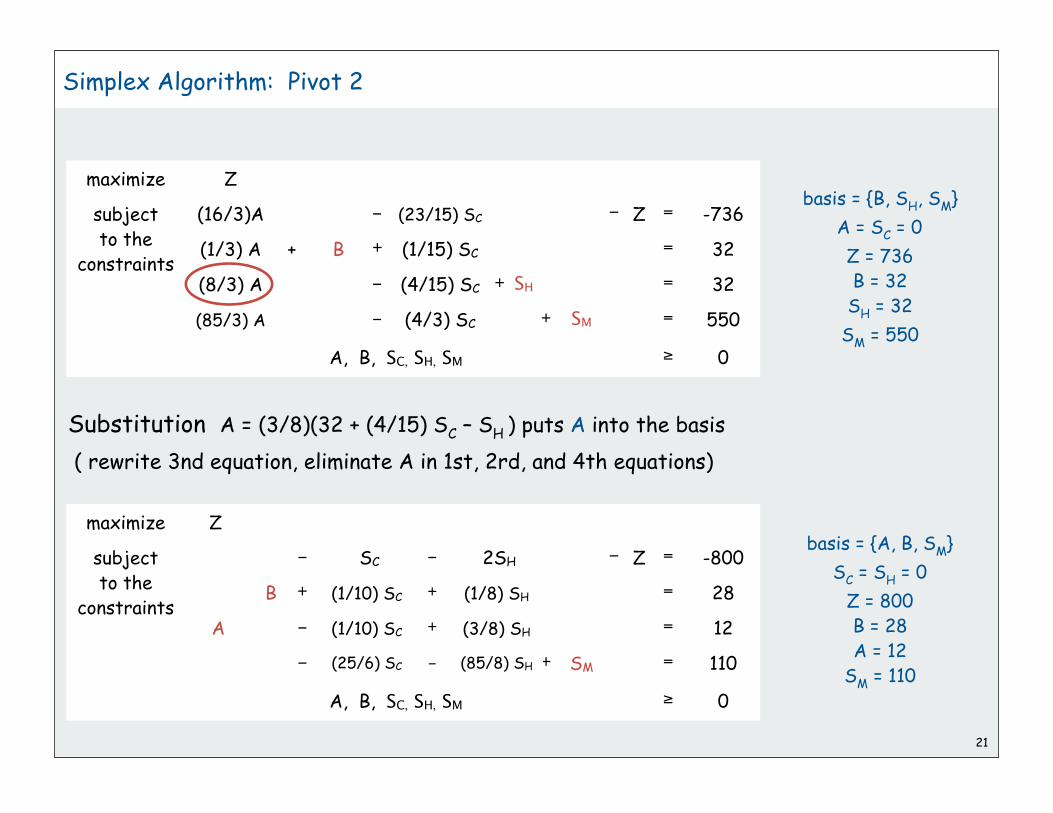
basis = {B, SH, SM}
A = SC = 0
Z = 736B = 32 SH = 32
SM = 550
maximize Z
subjectto the
constraints
(16/3)A - (23/15) SC Z = -736
(1/3) A + B + (1/15) SC = 32
(8/3) A - (4/15) SC + SH = 32
(85/3) A - (4/3) SC + SM = 550
A, B, SC, SH, SM 0
21
Simplex Algorithm: Pivot 2
basis = {A, B, SM}
SC = SH = 0
Z = 800B = 28 A = 12
SM = 110
maximize Z
subjectto the
constraints
- SC - 2SH Z = -800
B + (1/10) SC + (1/8) SH = 28
A - (1/10) SC + (3/8) SH = 12
- (25/6) SC - (85/8) SH + SM = 110
A, B, SC, SH, SM 0
Substitution A = (3/8)(32 + (4/15) SC – SH ) puts A into the basis
( rewrite 3nd equation, eliminate A in 1st, 2rd, and 4th equations)

22
Simplex algorithm: Optimality
Q. When to stop pivoting?
A. When all coefficients in top row are non-positive.
Q. Why is resulting solution optimal?
A. Any feasible solution satisfies system of equations in tableaux.
• In particular: Z = 800 – SC – 2 SH
• Thus, optimal objective value Z* 800 since SC, SH 0.
• Current BFS has value 800 optimal.
basis = {A, B, SM}
SC = SH = 0
Z = 800B = 28 A = 12
SM = 110
maximize Z
subjectto the
constraints
- SC - 2SH Z = -800
B + (1/10) SC + (1/8) SH = 28
A - (1/10) SC + (3/8) SH = 12
- (25/6) SC - (85/8) SH + SM = 110
A, B, SC, SH, SM 0

23
brewer’s problemsimplex algorithmimplementationlinear programming

Encode standard form LP in a single Java 2D array
Simplex tableau
24
A
c
bI
0 0
m
1
n m 1
maximize Z
subjectto the
constraints
13A + 23B Z = 0
5A + 15B + SC = 480
4A + 4B + SH = 160
35A + 20B + SM = 1190
A, B, SC, SH, SM 0
5 15 1 0 0 480
4 4 0 1 0 160
35 20 0 0 1 1190
13 23 0 0 0 0

Encode standard form LP in a single Java 2D array (solution)
Simplex algorithm transforms initial array into solution
Simplex tableau
25
A
c
bI
0 0
m
1
n m 1
0 1 1/10 1/8 0 28
1 0 1/10 3/8 0 12
0 0 25/6 85/8 1 110
0 0 -1 -2 0 -800
maximize Z
subjectto the
constraints
- SC - 2SH Z = -800
B + (1/10) SC + (1/8) SH = 28
A - (1/10) SC + (3/8) SH = 12
- (25/6) SC - (85/8) SH + SM = 110
A, B, SC, SH, SM 0

26
Simplex algorithm: Bare-bones implementation
Construct the simplex tableau.
A
c
bI
0 0
public class Simplex{ private double[][] a; // simplex tableaux private int M, N;
public Simplex(double[][] A, double[] b, double[] c) { M = b.length; N = c.length; a = new double[M+1][M+N+1]; for (int i = 0; i < M; i++) for (int j = 0; j < N; j++) a[i][j] = A[i][j]; for (int j = N; j < M + N; j++) a[j-N][j] = 1.0; for (int j = 0; j < N; j++) a[M][j] = c[j]; for (int i = 0; i < M; i++) a[i][M+N] = b[i]; }
m
1
n m 1
put A[][] into tableau
put I[] into tableauput c[] into tableauput b[] into tableau
constructor

27
Simplex algorithm: Bare-bones Implementation
Pivot on element (p, q).
public void pivot(int p, int q){ for (int i = 0; i <= M; i++) for (int j = 0; j <= M + N; j++) if (i != p && j != q) a[i][j] -= a[p][j] * a[i][q] / a[p][q]; for (int i = 0; i <= M; i++) if (i != p) a[i][q] = 0.0;
for (int j = 0; j <= M + N; j++) if (j != q) a[p][j] /= a[p][q]; a[p][q] = 1.0;}
p
q
scale all elements butrow p and column q
zero out column q
scale row p

28
Simplex Algorithm: Bare Bones Implementation
Simplex algorithm.
find entering variable q(positive objective function coefficient)
find row p accordingto min ratio rule
+p
q
+
+
public void solve(){ while (true) { int p, q; for (q = 0; q < M + N; q++) if (a[M][q] > 0) break; if (q >= M + N) break;
for (p = 0; p < M; p++) if (a[p][q] > 0) break; for (int i = p+1; i < M; i++) if (a[i][q] > 0) if (a[i][M+N] / a[i][q] < a[p][M+N] / a[p][q]) p = i; pivot(p, q); }}
min ratio test

29
Simplex Algorithm: Running Time
Remarkable property. In practice, simplex algorithm typically
terminates after at most 2(m+n) pivots.
• No pivot rule that is guaranteed to be polynomial is known.
• Most pivot rules known to be exponential (or worse) in worst-case.
Pivoting rules. Carefully balance the cost of finding an entering
variable with the number of pivots needed.

30
Simplex algorithm: Degeneracy
Degeneracy. New basis, same extreme point.
Cycling. Get stuck by cycling through different bases that all
correspond to same extreme point.
• Doesn't occur in the wild.
• Bland's least index rule guarantees finite # of pivots.
"stalling" is common in practice

To improve the bare-bones implementation
• Avoid stalling.
• Choose the pivot wisely.
• Watch for numerical stability.
• Maintain sparsity.
• Detect infeasiblity
• Detect unboundedness.
• Preprocess to reduce problem size.
Basic implementations available in many programming environments.
Commercial solvers routinely solve LPs with millions of variables.
requires fancy data structures
31
Simplex Algorithm: Implementation Issues

Ex. 1: OR-Objects Java library
Ex. 2: MS Excel (!)32
import drasys.or.mp.*;
import drasys.or.mp.lp.*;
public class LPDemo
{
public static void main(String[] args) throws Exception
{
Problem prob = new Problem(3, 2);
prob.getMetadata().put("lp.isMaximize", "true");
prob.newVariable("x1").setObjectiveCoefficient(13.0);
prob.newVariable("x2").setObjectiveCoefficient(23.0);
prob.newConstraint("corn").setRightHandSide( 480.0);
prob.newConstraint("hops").setRightHandSide( 160.0);
prob.newConstraint("malt").setRightHandSide(1190.0);
prob.setCoefficientAt("corn", "x1", 5.0);
prob.setCoefficientAt("corn", "x2", 15.0);
prob.setCoefficientAt("hops", "x1", 4.0);
prob.setCoefficientAt("hops", "x2", 4.0);
prob.setCoefficientAt("malt", "x1", 35.0);
prob.setCoefficientAt("malt", "x2", 20.0);
DenseSimplex lp = new DenseSimplex(prob);
System.out.println(lp.solve());
System.out.println(lp.getSolution());
}
}
LP solvers: basic implementations

33
set PROD := beer ale;set INGR := corn hops malt;
param: profit :=ale 13beer 23;
param: supply :=corn 480hops 160malt 1190;
param amt: ale beer :=corn 5 15hops 4 4malt 35 20;
LP solvers: commercial strength
AMPL. [Fourer, Gay, Kernighan] An algebraic modeling language.
CPLEX solver. Industrial strength solver.
set INGR;set PROD;param profit {PROD};param supply {INGR};param amt {INGR, PROD};var x {PROD} >= 0;
maximize total_profit: sum {j in PROD} x[j] * profit[j];
subject to constraints {i in INGR}: sum {j in PROD} amt[i,j] * x[j] <= supply[i];
beer.dat
beer.mod
separate data from model
ale beer
maximize 13A + 23B profit
subjectto the
constraints
5A + 15B 480 corn
4A + 4B 160 hops
35A + 20B 1190 malt
A 0
B 0

34
History
1939. Production, planning. [Kantorovich]
1947. Simplex algorithm. [Dantzig]
1950. Applications in many fields.
1979. Ellipsoid algorithm. [Khachian]
1984. Projective scaling algorithm. [Karmarkar]
1990. Interior point methods.
• Interior point faster when polyhedron smooth like disco ball.
• Simplex faster when polyhedron spiky like quartz crystal.
200x. Approximation algorithms, large scale optimization.

35
brewer’s problemsimplex algorithmimplementationlinear programming

Linear programming
Linear “programming”
• process of formulating an LP model for a problem
• solution to LP for a specific problem gives solution to the problem
1. Identify variables
2. Define constraints (inequalities and equations)
3. Define objective function
Examples:
• shortest paths
• maxflow
• bipartite matching
• .
• .
• .
• [ a very long list ]
36
easy part [omitted]:convert to standard form
stay tuned [this lecture]

37
Single-source shortest-paths problem (revisited)
Given. Weighted digraph, single source s.
Distance from s to v: length of the shortest path from s to v .
Goal. Find distance (and shortest path) from s to every other vertex.
s
3
t
2
6
7
4
5
24
18
2
9
14
155
30
20
44
16
11
6
19
6

LP formulation of single-source shortest-paths problem
38
s
3
t
2
6
7
4
5
24
18
2
9
14
155
30
20
44
16
11
6
19
6
minimize xt
subjectto the
constraints
xs + 9 x2
xs + 14 x6
xs + 15 x7
x2 + 24 x3
x3 + 2 x5
x3 + 19 xt
x4 + 6 x3
x4 + 6 xt
x5 + 11 x4
x5 + 16 xt
x6 + 18 x3
x6 + 30 x5
x6 + 5 x7
x7 + 20 x5
x7 + 44 xt
xs = 0
x2 , ... , xt 0
One variable per vertex, one inequality per edge.

LP formulation of single-source shortest-paths problem
39
s
3
t
2
6
7
4
5
24
18
2
9
14
155
30
20
44
16
11
6
19
6
0
9 32
14
15 50
34
45
minimize xt
subjectto the
constraints
xs + 9 x2
xs + 14 x6
xs + 15 x7
x2 + 24 x3
x3 + 2 x5
x3 + 19 xt
x4 + 6 x3
x4 + 6 xt
x5 + 11 x4
x5 + 16 xt
x6 + 18 x3
x6 + 30 x5
x6 + 5 x7
x7 + 20 x5
x7 + 44 xt
xs = 0
x2 , ... , xt 0
xs = 0
x2 = 9
x3 = 32
x4 = 45
x5 = 34
x6 = 14
x7 = 15
xt = 50
solution
One variable per vertex, one inequality per edge.

3
3
40
Maxflow problem
Given: Weighted digraph, source s, destination t.
Interpret edge weights as capacities
• Models material flowing through network
• Ex: oil flowing through pipes
• Ex: goods in trucks on roads
• [many other examples]
Flow: A different set of edge weights
• flow does not exceed capacity in any edge
• flow at every vertex satisfies equilibrium
[ flow in equals flow out ]
Goal: Find maximum flow from s to t
2 3
1
2
s
1
3 4
2
t
1 1
s
1
3 4
2
t
flow out of s is 3
flow in to t is 3
1 2
10
1 1
2 1
flow capacityin every edge
flow inequals
flow outat each vertex

LP formulation of maxflow problem
41
maximize xts
subjectto the
constraints
xs1 2
xs2 3
x13 3
x14 1
x23 1
x24 1
x3t 2
x4t 3
xts = xs1 + xs2
xs1 = x13 + x14
xs2 = x23 + x24
x13 + x23 = x3t
x14 + x24 = x4t
x3t + x4t = xts
all xij 0
One variable per edge.
One inequality per edge, one equality per vertex.
3
3
2 3
1
2
s
1
3 4
2
t
1 1
s
1
3 4
2
t
add dummyedge from
t to s
equilibriumconstraints
capacityconstraints

1
2 2
11
1
2 2
LP formulation of maxflow problem
42
maximize xts
subjectto the
constraints
xs1 2
xs2 3
x13 3
x14 1
x23 1
x24 1
x3t 2
x4t 3
xts = xs1 + xs2
xs1 = x13 + x14
xs2 = x23 + x24
x13 + x23 = x3t
x14 + x24 = x4t
x3t + x4t = xts
all xij 0
xs1 = 2
xs2 = 2
x13 = 1
x14 = 1
x23 = 1
x24 = 1
x3t = 2
x4t = 2
xts = 4
solution
One variable per edge.
One inequality per edge, one equality per vertex.
3
3
2 3
1
2
s
1
3 4
2
t
1 1
s
1
3 4
2
t
add dummyedge from
t to s
maxflow value
equilibriumconstraints
capacityconstraints

Maximum cardinality bipartite matching problem
Given: Two sets of vertices, set of edges
(each connecting one vertex in each set)
Matching: set of edges
with no vertex appearing twice
Interpretation: mutual preference constraints
• Ex: people to jobs
• Ex: medical students to residence positions
• Ex: students to writing seminars
• [many other examples]
Goal: find a maximum cardinality matching
43
A B C D E F
0 1 2 3 4 5
Alice
Adobe, Apple, Google
Bob
Adobe, Apple, Yahoo
Carol
Google, IBM, Sun
Dave
Adobe, Apple
Eliza
IBM, Sun, Yahoo
Frank
Google, Sun, Yahoo
Example: Job offers
Adobe
Alice, Bob, Dave
Apple
Alice, Bob, Dave
Alice, Carol, Frank
IBM
Carol, Eliza
Sun
Carol, Eliza, Frank
Yahoo
Bob, Eliza, Frank
A B C D E F
0 1 2 3 4 5

LP formulation of maximum cardinality bipartite matching problem
44
maximizexA0 + xA1 + xA2 + xB0 + xB1 + xB5
+ xC2 + xC3 + xC4 + xD0 + xD1
+ xE3 + xE4 + xE5 + xF2 + xF4 + xF5
subjectto the
constraints
xA0 + xA1 + xA2 = 1
xB0 + xB1 + xB5 = 1
xC2 + xC3 + xC4 = 1
xD0 + xD1 = 1
xE3 + xE4 + xE5 = 1
xF2 + xF4 + xF5 = 1
xA0 + xB0 + xD0 = 1
xA1 + xB1 + xD1 = 1
xA2 + xC2 + xF2 = 1
xC3 + xE3 = 1
xC4 + xE4 + xF4 = 1
xB5 + xE5 + xF5 = 1
all xij 0
One variable per edge, one equality per vertex.
constraints on top vertices
A B C D E F
0 1 2 3 4 5
Theorem. [Birkhoff 1946, von Neumann 1953]
All extreme points of the above polyhedron have integer (0 or 1) coordinates
Corollary. Can solve bipartite matching problem by solving LP
constraints on bottom vertices
Crucial point: not always so lucky!

LP formulation of maximum cardinality bipartite matching problem
45
maximizexA0 + xA1 + xA2 + xB0 + xB1 + xB5
+ xC2 + xC3 + xC4 + xD0 + xD1
+ xE3 + xE4 + xE5 + xF2 + xF4 + xF5
subjectto the
constraints
xA0 + xA1 + xA2 = 1
xB0 + xB1 + xB5 = 1
xC2 + xC3 + xC4 = 1
xD0 + xD1 = 1
xE3 + xE4 + xE5 = 1
xF2 + xF4 + xF5 = 1
xA0 + xB0 + xD0 = 1
xA1 + xB1 + xD1 = 1
xA2 + xC2 + xF2 = 1
xC3 + xE3 = 1
xC4 + xE4 + xF4 = 1
xB5 + xE5 + xF5 = 1
all xij 0
One variable per edge, one equality per vertex. A B C D E F
0 1 2 3 4 5
A B C D E F
0 1 2 3 4 5
xA1 = 1
xB5 = 1
xC2 = 1
xD0 = 1
xE3 = 1
xF4 = 1
all other xij = 0
solution

Linear programming perspective
Got an optimization problem?
ex: shortest paths, maxflow, matching, . . . [many, many, more]
Approach 1: Use a specialized algorithm to solve it
• Algs in Java
• vast literature on complexity
• performance on real problems not always well-understood
Approach 2: Use linear programming
• a direct mathematical representation of the problem often works
• immediate solution to the problem at hand is often available
• might miss specialized solution, but might not care
Got an LP solver? Learn to use it!
46

LP: the ultimate problem-solving model (in practice)
Fact 1: Many practical problems are easily formulated as LPs
Fact 2: Commercial solvers can solve those LPs quickly
More constraints on the problem?
• specialized algorithm may be hard to fix
• can just add more inequalities to LP
New problem?
• may not be difficult to formulate LP
• may be very difficult to develop specialized algorithm
Today’s problem?
• similar to yesterday’s
• edit tableau, run solver
Too slow?
• could happen
• doesn’t happen47
Ex. Airline scheduling[ similar to vast number of other business processes ]
Ex. Mincost maxflow and other generalized versions
Want to learn more? ORFE 307

48
Is there an ultimate problem-solving model?
• Shortest paths
• Maximum flow
• Bipartite matching
• . . .
• Linear programming
• .
• .
• .
• NP-complete problems
• .
• .
• .
Does P = NP? No universal problem-solving model exists unless P = NP.
tractable
Ultimate problem-solving model (in theory)
[see next lecture]
intractable ?
Want to learn more? COS 423

49
LP perspective
LP is near the deep waters of intractability.
Good news:
• LP has been widely used for large practical problems for 50+ years
• Existence of guaranteed poly-time algorithm known for 25+ years.
Bad news:
• Integer linear programming is NP-complete
• (existence of guaranteed poly-time algorithm is highly unlikely).
• [stay tuned]
An unsuspecting MBA student transitions to the world of intractability with a single mouse click.
constrain variables to have integer values

1
Reductions
designing algorithmsproving limitsclassifying problemsNP-completeness

2
Bird’s-eye view
Desiderata.
Classify problems according to their computational requirements.
Frustrating news.
Huge number of fundamental problems have defied classification
Desiderata'.
Suppose we could (couldn't) solve problem X efficiently.
What else could (couldn't) we solve efficiently?
Give me a lever long enough and a fulcrum on which to
place it, and I shall move the world. -Archimedes

3
Reduction
Def. Problem X reduces to problem Y
if you can use an algorithm that solves Y to help solve X
Ex. Euclidean MST reduces to Voronoi.
To solve Euclidean MST on N points
• solve Voronoi for those points
• construct graph with linear number of edges
• use Prim/Kruskal to find MST in time proportional to N log N
instance I(of X)
Algorithm for X
solution to IAlgorithm
for Y

4
Reduction
Def. Problem X reduces to problem Y
if you can use an algorithm that solves Y to help solve X
Cost of solving X = M*(cost of solving Y) + cost of reduction.
Applications
• designing algorithms: given algorithm for Y, can also solve X.
• proving limits: if X is hard, then so is Y.
• classifying problems: establish relative difficulty of problems.
number of times Y is used

5
designing algorithmsproving limitsclassifying problemsNP-completeness

number of times Y is used
6
Reductions for algorithm design
Def. Problem X reduces to problem Y
if you can use an algorithm that solves Y to help solve X
Cost of solving X = M*(cost of solving Y) + cost of reduction.
Applications.
• designing algorithms: given algorithm for Y, can also solve X.
• proving limits: if X is hard, then so is Y.
• classifying problems: establish relative difficulty of problems.
Mentality: Since I know how to solve Y, can I use that algorithm to solve X?
Programmer’s version: I have code for Y. Can I use it for X?

7
Reductions for algorithm design: convex hull
Sorting. Given N distinct integers, rearrange them in ascending order.
Convex hull. Given N points in the plane, identify the extreme points
of the convex hull (in counter-clockwise order).
Claim. Convex hull reduces to sorting.
Pf. Graham scan algorithm.
convex hull
1251432
2861534
3988818
4190745
13546464
89885444
sorting
linearithmic linear
Cost of convex hull = cost of sort + cost of reduction

Reductions for algorithm design: shortest paths
Claim. Shortest paths reduces to path search in graphs (PFS)
Pf. Dijkstra’s algorithm
8
linear length of path
Cost of shortest paths = cost of search + cost of reduction
s
w
vS
s
3
t
2
6
7
4
5
24
18
2
9
14
155
30
20
44
16
11
6
19
6
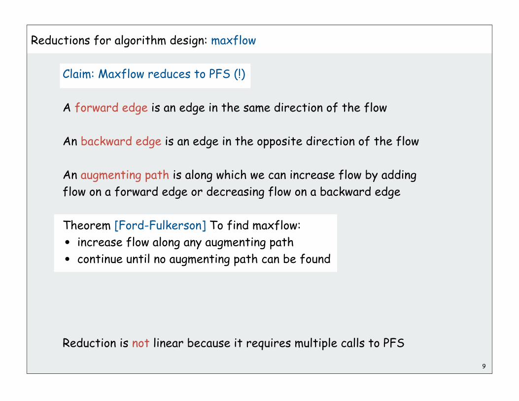
Reductions for algorithm design: maxflow
Claim: Maxflow reduces to PFS (!)
A forward edge is an edge in the same direction of the flow
An backward edge is an edge in the opposite direction of the flow
An augmenting path is along which we can increase flow by adding
flow on a forward edge or decreasing flow on a backward edge
Theorem [Ford-Fulkerson] To find maxflow:
• increase flow along any augmenting path
• continue until no augmenting path can be found
Reduction is not linear because it requires multiple calls to PFS
9

Reductions for algorithm design: maxflow (continued)
Two augmenting-path sequences
10
s
1
3 4
2
t
2
s
4
2
linear linear
Cost of maxflow = M*(cost of PFS) + cost of reduction
3
s
1
4
2
s
1
3 4
2
t
s
2
t
3
t
depends on path choice!
t
s
1
4
t
s
1 2
3
t
4
1
3 4
back edge(remove flow)
1
3

Reductions for algorithm design: bipartite matching
Bipartite matching reduces to maxflow
Proof:
• construct new vertices s and t
• add edges from s to each vertex in one set
• add edges from each vertex in other set to t
• set all edge weights to 1
• find maxflow in resulting network
• matching is edges between two sets
Note: Need to establish that maxflow solution
has all integer (0-1) values.
11
A B C D E F
0 1 2 3 4 5
A B C D E F
0 1 2 3 4 5
s
t

Bipartite matching reduces to maxflow
Proof:
• construct new vertices s and t
• add edges from s to each vertex in one set
• add edges from each vertex in other set to t
• set all edge weights to 1
• find maxflow in resulting network
• matching is edges between two sets
Note: Need to establish that maxflow solution
has all integer (0-1) values.
Reductions for algorithm design: bipartite matching
12
A B C D E F
0 1 2 3 4 5
A B C D E F
0 1 2 3 4 5
A B C D E F
0 1 2 3 4 5
s
t
linear
Cost of matching = cost of maxflow + cost of reduction

Reductions for algorithm design: summary
13
LP
element
distinctnesssorting
shortest
paths
bipartite
matching
maxflow
PFS
Some reductions we have seen so far:
LP (standard form)
convex hullmedian
finding
arbitrage
shortest paths
(neg weights)
Voronoi
closest
pair
Euclidean
MST

Reductions for algorithm design: a caveat
PRIME. Given an integer x (represented in binary), is x prime?
COMPOSITE. Given an integer x, does x have a nontrivial factor?
A possible real-world scenario:
• System designer specs the interfaces for project.
• Programmer A implements isComposite() using isPrime().
• Programmer B implements isPrime() using isComposite().
• Infinite reduction loop!14
public static boolean isComposite(BigInteger x){ if (isPrime(x)) return false; else return true;}
public static boolean isPrime(BigInteger x){ if (isComposite(x)) return false; else return true;}
PRIME reduces to COMPOSITE
COMPOSITE reduces to PRIME
COMPOSITE
PRIME
whose fault?

15
designing algorithmsproving limitsclassifying problemspolynomial-time reductionsNP-completeness

16
Linear-time reductions to prove limits
Def. Problem X linear reduces to problem Y if X can be solved with:
• linear number of standard computational steps for reduction
• one call to subroutine for Y.
Applications.
• designing algorithms: given algorithm for Y, can also solve X.
• proving limits: if X is hard, then so is Y.
• classifying problems: establish relative difficulty of problems.
Mentality:
If I could easily solve Y, then I could easily solve X
I can’t easily solve X.
Therefore, I can’t easily solve Y
Purpose of reduction is to establish that Y is hard
NOT intended for useas an algorithm

17
Proving limits on convex-hull algorithms
Lower bound on sorting: Sorting N integers requires (N log N) steps.
Claim. SORTING reduces to CONVEX HULL [see next slide].
Consequence.
Any ccw-based convex hull algorithm requires (N log N) steps.
need “quadratic decision tree” model of computation that allows tests of the form xi < xj or (xj - xi) (yk - yi) - (yj - yi) (xk - xi) < 0
convex hull
1251432
2861534
3988818
4190745
13546464
89885444
sorting

Sorting instance.
Convex hull instance.
Observation. Region {x : x2 x} is convex all points are on hull.
Consequence. Starting at point with most negative x,
counter-clockwise order of hull points yields items in ascending order.
To sort X, find the convex hull of P.
18
Sorting linear-reduces to convex hull
X = { x1, x2, ... , xN }
P = { (x1 , x12 ), (x2, x2
2 ), ... , (xN , xN2 ) }
f(x) = x2
(x1 , x12 )
(x2 , x22 )

19
3-SUM reduces to 3-COLLINEAR
3-SUM. Given N distinct integers, are there three that sum to 0?
3-COLLINEAR. Given N distinct points in the plane,
are there 3 that all lie on the same line?
Claim. 3-SUM reduces to 3-COLLINEAR.
Conjecture. Any algorithm for 3-SUM requires (N2) time.
Consequence. Sub-quadratic algorithm for 3-COLLINEAR unlikely.
recall Assignment 2
your N2 log N algorithm from Assignment 2 was pretty good
see next two slides

20
3-SUM reduces to 3-COLLINEAR (continued)
Claim. 3-SUM L 3-COLLINEAR.
• 3-SUM instance:
• 3-COLLINEAR instance:
(1, 1)
(2, 8)
(-3, -27)
-3 + 2 + 1 = 0
x1, x2, ... , xN
(x1 , x13 ), (x2, x2
3 ), ... , (xN , xN3 )
f(x) = x3
Lemma. If a, b, and c are distinct, then a + b + c = 0
if and only if (a, a3), (b, b3), (c, c3) are collinear.
Pf. [see next slide]
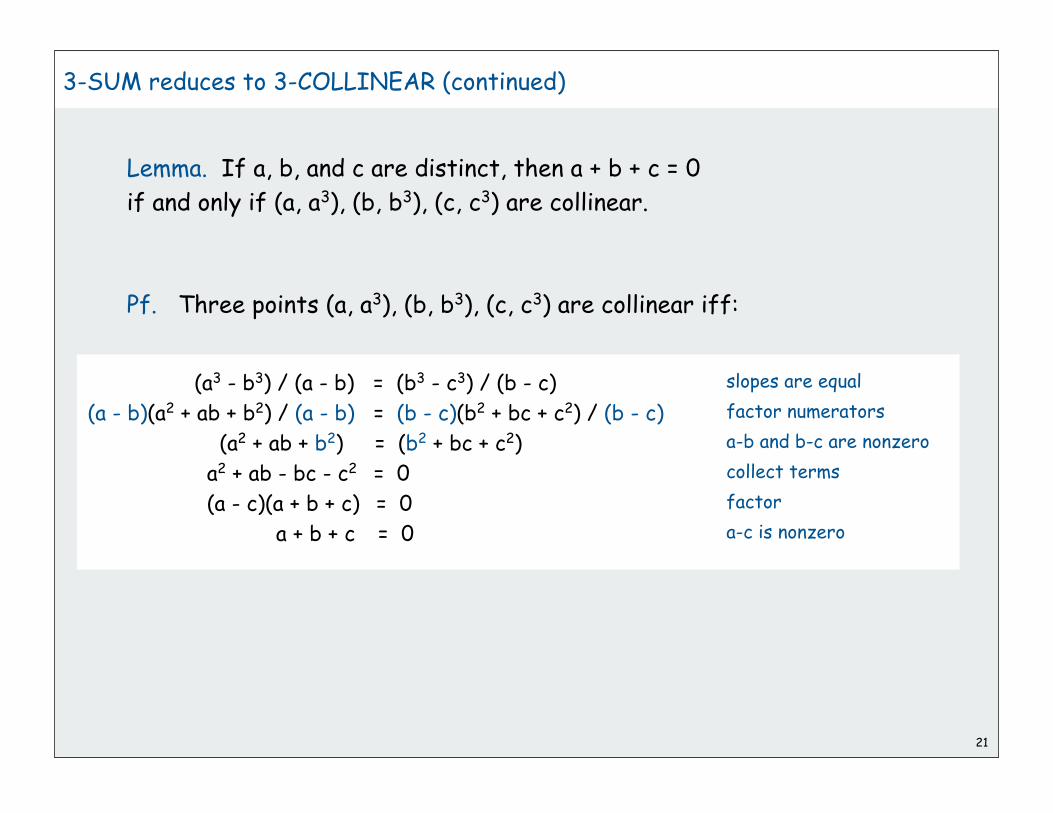
21
3-SUM reduces to 3-COLLINEAR (continued)
Lemma. If a, b, and c are distinct, then a + b + c = 0
if and only if (a, a3), (b, b3), (c, c3) are collinear.
Pf. Three points (a, a3), (b, b3), (c, c3) are collinear iff:
(a3 - b3) / (a - b) = (b3 - c3) / (b - c)
(a - b)(a2 + ab + b2) / (a - b) = (b - c)(b2 + bc + c2) / (b - c)
(a2 + ab + b2) = (b2 + bc + c2)
a2 + ab - bc - c2 = 0
(a - c)(a + b + c) = 0
a + b + c = 0
slopes are equal
factor numerators
a-b and b-c are nonzero
collect terms
factor
a-c is nonzero

Reductions for proving limits: summary
22
Want to be convinced that no linear-time convex hull alg exists?Hard way: long futile search for a linear-time algorithm Easy way: reduction from sorting
Want to be convinced that no subquadratic 3-COLLINEAR alg exists?Hard way: long futile search for a subquadratic algorithm Easy way: reduction from 3-SUM
sorting
convex hull
3-SUM
3-COLLINEAR
Establishing limits through reduction is an important tool
in guiding algorithm design efforts

23
designing algorithmsproving limitsclassifying problemsNP-completeness
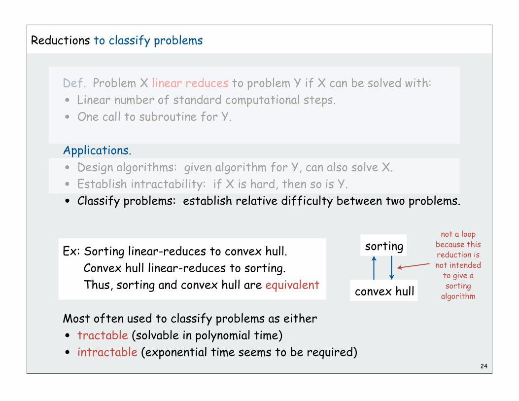
24
Reductions to classify problems
Def. Problem X linear reduces to problem Y if X can be solved with:
• Linear number of standard computational steps.
• One call to subroutine for Y.
Applications.
• Design algorithms: given algorithm for Y, can also solve X.
• Establish intractability: if X is hard, then so is Y.
• Classify problems: establish relative difficulty between two problems.
Ex: Sorting linear-reduces to convex hull.
Convex hull linear-reduces to sorting.
Thus, sorting and convex hull are equivalent
Most often used to classify problems as either
• tractable (solvable in polynomial time)
• intractable (exponential time seems to be required)
convex hull
sortingnot a loop
because this reduction is not intended
to give a sorting
algorithm

25
Polynomial-time reductions
Def. Problem X polynomial reduces to problem Y if arbitrary instances
of problem X can be solved using:
• Polynomial number of standard computational steps for reduction
• One call to subroutine for Y.
Notation. X P Y.
Ex. Any linear reduction is a polynomial reduction.
Ex. All algorithms for which we know poly-time algorithms
poly-time reduce to one another.
Poly-time reduction of X to Y makes sense
only when X or Y is not known to have a poly-time algorithm
critical detail (not obvious why)

26
Polynomial-time reductions for classifying problems
Goal. Classify and separate problems according to relative difficulty.
• tractable problems: can be solved in polynomial time.
• intractable problems: seem to require exponential time.
Establish tractability. If X P Y and Y is tractable then so is X.
• Solve Y in polynomial time.
• Use reduction to solve X.
Establish intractability. If Y P X and Y is intractable, then so is X.
• Suppose X can be solved in polynomial time.
• Then so could Y (through reduction).
• Contradiction. Therefore X is intractable.
Transitivity. If X P Y and Y P Z then X P Z.
Ex: all problems that reduce to LP are tractable

27
Literal: A Boolean variable or its negation.
Clause. A disjunction of 3 distinct literals.
Conjunctive normal form. A propositional
formula that is the conjunction of clauses.
3-SAT. Given a CNF formula consisting of k clauses over n literals,
does it have a satisfying truth assignment?
Applications: Circuit design, program correctness, [many others]
3-satisfiability
(¬x1 x2 x3) (x1 ¬x2 x3) (¬x1 ¬x2 ¬x3) (¬x1 ¬ x2 x4) (¬x2 x3 x4)
(¬T T F ) (T ¬T F ) (¬T ¬T ¬F ) (¬T ¬T T) ( ¬T F T)x1 x2 x3 x4
T T F T
xi or ¬xi
Cj = (x1 ¬x2 x3)
CNF = (C1 C2 C3 C4)
yes instance
(¬x1 x2 x3) (x1 ¬x2 x3) (¬x1 ¬x2 ¬x3) (¬x1 ¬ x2 ¬ x4) (¬x2 x3 x4)
no instance

3-satisfiability is intractable
Good news: easy algorithm to solve 3-SAT
[ check all possible solutions ]
Bad news: running time is exponential in input size.
[ there are 2n possible solutions ]
Worse news:
no algorithm that guarantees subexponential running time is known
Implication:
• suppose 3-SAT poly-reduces to a problem A
• poly-time algorithm for A would imply poly-time 3-SAT algorithm
• we suspect that no poly-time algorithm exists for A!
Want to be convinced that a new problem is intractable?
Hard way: long futile search for an efficient algorithm (as for 3-SAT)
Easy way: reduction from a known intractable problem (such as 3-SAT)
28
hence, intricate reductions are common

29
Graph 3-colorability
3-COLOR. Given a graph, is there a way to color the vertices
red, green, and blue so that no adjacent vertices have the same color?
yes instance

30
Graph 3-colorability
3-COLOR. Given a graph, is there a way to color the vertices
red, green, and blue so that no adjacent vertices have the same color?
yes instance

3-COLOR. Given a graph, is there a way to color the vertices
red, green, and blue so that no adjacent vertices have the same color?
31
Graph 3-colorability
no instance

32
3-satisfiability reduces to graph 3-colorability
Claim. 3-SAT P 3-COLOR.
Pf. Given 3-SAT instance , we construct an instance of 3-COLOR
that is 3-colorable if and only if is satisfiable.
Construction.
(i) Create one vertex for each literal and 3 vertices
(ii) Connect in a triangle and connect each literal to B.
(iii) Connect each literal to its negation.
(iv) For each clause, attach a 6-vertex gadget [details to follow].
F T B
F T B
B
x1 ¬x1 x2 ¬x2 x3 ¬x3 xn ¬xn. . .
F
B
truefalse
base
T

33
3-satisfiability reduces to graph 3-colorability
Claim. If graph is 3-colorable then is satisfiable..
Pf.
• Consider assignment where corresponds to false and to true .
• (ii) [triangle] ensures each literal is true or false.
F
B
truefalse
base
x1 ¬x1 x2 ¬x2 x3 ¬x3 xn ¬xn. . .
T
F T

34
3-satisfiability reduces to graph 3-colorability
Claim. If graph is 3-colorable then is satisfiable..
Pf. Suppose graph is 3-colorable.
• Consider assignment where corresponds to false and to true .
• (ii) [triangle] ensures each literal is true or false.
• (iii) ensures a literal and its negation are opposites.
x1 ¬x1 x2 ¬x2 x3 ¬x3 xn ¬xn. . .
F
B
truefalse
base
T
F T

35
3-satisfiability reduces to graph 3-colorability
Claim. If graph is 3-colorable then is satisfiable.
Pf.
• Consider assignment where corresponds to false and to true .
• (ii) [triangle] ensures each literal is true or false.
• (iii) ensures a literal and its negation are opposites.
• (iv) [gadget] ensures at least one literal in each clause is true.
T F
B
6-node gadget
true false
(x1 ¬x2 x3)
x1 ¬x2 x3
F T
stay tuned

36
3-satisfiability reduces to graph 3-colorability
Claim. If graph is 3-colorable then is satisfiable.
Pf.
• Consider assignment where corresponds to false and to true .
• (ii) [triangle] ensures each literal is true or false.
• (iii) ensures a literal and its negation are opposites.
• (iv) [gadget] ensures at least one literal in each clause is true.
Therefore, is satisfiable.
T F
B
6-node gadget
true false
x1 ¬x2 x3
??
F F
(x1 ¬x2 x3)

37
3-satisfiability reduces to graph 3-colorability
Claim. If is satisfiable then graph is 3-colorable.
Pf.
• Color nodes corresponding to false literals T and to true literals F .
x1 ¬x2 x3
(x1 ¬x2 x3)
at least onein each clause

38
3-satisfiability reduces to graph 3-colorability
Claim. If is satisfiable then graph is 3-colorable.
Pf.
• Color nodes corresponding to false literals T and to true literals F .
• Color vertex below one T vertex F , and vertex below that B .
T
x1 ¬x2 x3

39
3-satisfiability reduces to graph 3-colorability
Claim. If is satisfiable then graph is 3-colorable.
Pf.
• Color nodes corresponding to false literals T and to true literals F .
• Color vertex below one T vertex F , and vertex below that B .
• Color remaining middle row vertices B .
T
x1 ¬x2 x3
(x1 ¬x2 x3)
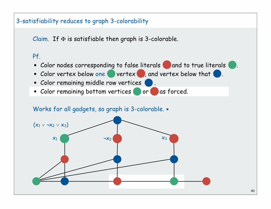
40
3-satisfiability reduces to graph 3-colorability
Claim. If is satisfiable then graph is 3-colorable.
Pf.
• Color nodes corresponding to false literals T and to true literals F .
• Color vertex below one T vertex F , and vertex below that B .
• Color remaining middle row vertices B .
• Color remaining bottom vertices T or F as forced.
Works for all gadgets, so graph is 3-colorable.
x1 ¬x2 x3
(x1 ¬x2 x3)
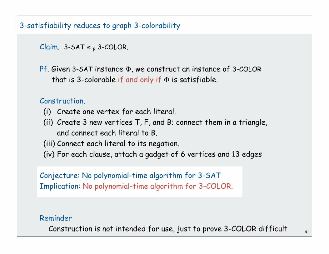
41
3-satisfiability reduces to graph 3-colorability
Claim. 3-SAT P 3-COLOR.
Pf. Given 3-SAT instance , we construct an instance of 3-COLOR
that is 3-colorable if and only if is satisfiable.
Construction.
(i) Create one vertex for each literal.
(ii) Create 3 new vertices T, F, and B; connect them in a triangle,
and connect each literal to B.
(iii) Connect each literal to its negation.
(iv) For each clause, attach a gadget of 6 vertices and 13 edges
Conjecture: No polynomial-time algorithm for 3-SAT
Implication: No polynomial-time algorithm for 3-COLOR.
Reminder
Construction is not intended for use, just to prove 3-COLOR difficult

42
designing algorithmsproving limitsclassifying problemspolynomial-time reductionsNP-completeness

43
More Poly-Time Reductions
3-SAT
3DM VERTEX COVER
HAM-CYCLECLIQUE
INDEPENDENT SET
3-COLOR
PLANAR-3-COLOREXACT COVER
HAM-PATHSUBSET-SUM
PARTITION INTEGER PROGRAMMING
KNAPSACK
Dick Karp'85 Turing award
3-SAT
reduces to 3-COLOR
TSP
BIN-PACKINGConjecture: no poly-time algorithm for 3-SAT.
(and hence none of these problems)

44
Cook’s Theorem
NP: set of problems solvable in polynomial time
by a nondeterministic Turing machine
THM. Any problem in NP P 3-SAT.
Pf sketch.
Each problem P in NP corresponds to a TM M that accepts or rejects
any input in time polynomial in its size
Given M and a problem instance I, construct an instance of 3-SAT
that is satisfiable iff the machine accepts I.
Construction.
• Variables for every tape cell, head position, and state at every step.
• Clauses corresponding to each transition.
• [many details omitted]

45
Implications of Cook’s theorem
3-SAT
3DM VERTEX COVER
HAM-CYCLECLIQUE
INDEPENDENT SET
3-COLOR
PLANAR-3-COLOREXACT COVER
HAM-PATHSUBSET-SUM
PARTITION INTEGER PROGRAMMING
KNAPSACK
TSP
BIN-PACKING
3-COLOR
reduces to 3-SAT
All of these problems (any many more)polynomial reduce to 3-SAT.
Stephen Cook'82 Turing award

46
Implications of Karp + Cook
3-SAT
3DM VERTEX COVER
HAM-CYCLECLIQUE
INDEPENDENT SET
3-COLOR
PLANAR-3-COLOREXACT COVER
HAM-PATHSUBSET-SUM
PARTITION INTEGER PROGRAMMING
KNAPSACK
3-SAT
reduces to 3-COLOR
TSP
BIN-PACKINGConjecture: no poly-time algorithm for 3-SAT.
(and hence none of these problems)
3-COLOR
reduces to 3-SAT
All of these problems poly-reduce to one another!

47
Poly-Time Reductions: Implications

48
Poly-Time Reductions: Implications

49
Poly-Time Reductions: Implications

50
Summary
Reductions are important in theory to:
• Establish tractability.
• Establish intractability.
• Classify problems according to their computational requirements.
Reductions are important in practice to:
• Design algorithms.
• Design reusable software modules.
stack, queue, sorting, priority queue, symbol table, set, graph
shortest path, regular expressions, linear programming
• Determine difficulty of your problem and choose the right tool.
use exact algorithm for tractable problems
use heuristics for intractable problems

1
Combinatorial Search
permutationsbacktrackingcountingsubsetspaths in a graph

2
Overview
Exhaustive search. Iterate through all elements of a search space.
Backtracking. Systematic method for examining feasible solutions
to a problem, by systematically eliminating infeasible solutions.
Applicability. Huge range of problems (include NP-hard ones).
Caveat. Search space is typically exponential in size
effectiveness may be limited to relatively small instances.
Caveat to the caveat. Backtracking may prune search space to
reasonable size, even for relatively large instances

1 1 1 0
1 1 0 0
1 0 0 0
0 0 0 0
3
Warmup: enumerate N-bit strings
Problem: process all 2N N-bit strings (stay tuned for applications).
Equivalent to counting in binary from 0 to 2N - 1.
• maintain a[i] where a[i] represents bit i
• initialize all bits to 0
• simple recursive method does the job
(call enumerate(0))
Invariant (prove by induction);
Enumerates all (N-k)-bit strings and cleans up after itself.
private void enumerate(int k){ if (k == N) { process(); return; } enumerate(k+1); a[k] = 1; enumerate(k+1); a[k] = 0;} clean up
starts with all 0s
0 0 0 0
0 0 0 1
0 0 1 0
0 0 1 1
0 1 0 0
0 1 0 1
0 1 1 0
0 1 1 1
1 0 0 0
1 0 0 1
1 0 1 0
1 0 1 1
1 1 0 0
1 1 0 1
1 1 1 0
1 1 1 1
example showingcleanups that
zero out digits
ends with all 0s

4
Warmup: enumerate N-bit strings (full implementation)
Equivalent to counting in binary from 0 to 2N - 1.
public class Counter{ private int N; // number of bits private int[] a; // bits (0 or 1)
public Counter(int N) { this.N = N; a = new int[N]; for (int i = 0; i < N; i++) a[i] = 0; enumerate(0); }
private void enumerate(int k) { if (k == N) { process(); return; } enumerate(k+1); a[k] = 1; enumerate(k+1); a[k] = 0; }
public static void main(String[] args) { int N = Integer.parseInt(args[0]); Counter c = new Counter(N); }}
all the programsin this lectureare variationson this theme
private void process()
{
for (int i = 0; i < N; i++)
StdOut.print(a[i]);
StdOut.println();
}
optional (in this case)

5
permutationsbacktrackingcountingsubsetspaths in a graph

6
N-rooks Problem
How many ways are there to place
N rooks on an N-by-N board so that no rook can attack any other?
No two in the same row, so represent solution with an array
a[i] = column of rook in row i.
No two in the same column, so array entries are all different
a[] is a permutation (rearrangement of 0, 1, ... N-1)
Answer: There are N! non mutually-attacking placements.
Challenge: Enumerate them all.
int[] a = { 1, 2, 0, 3, 6, 7, 4, 5 };
0 1 2 3 4 5 6 7
0
1
2
3
4
5
6
7
original problem: N = 8

7
Enumerating permutations
Recursive algorithm to enumerate all N! permutations of size N:
• Start with 0 1 2 ... N-1.
• For each value of i- swap i into position 0
- enumerate all (N-1)! arrangements of a[1..N-1]- clean up (swap i and 0 back into position)
3 1 2 03 1 0 23 2 1 03 2 0 13 0 2 13 0 1 2
1 0 2 31 0 3 21 2 0 31 2 3 01 3 2 01 3 0 21 3 2 01 0 2 30 1 2 3
2 1 0 32 1 3 02 0 1 32 0 3 12 3 0 12 3 1 0
3 followed by
perms of 1 2 0
0 followed by
perms of 1 2 3
1 followed by
perms of 0 2 3
2 followed by
perms of 1 0 3
0 1 20 2 11 0 21 2 02 1 02 0 1
0 11 0
0 1 2 30 1 3 20 2 1 30 2 3 10 3 2 10 3 1 2
example showing cleanup swaps that bring perm back to original

public class Rooks{ private int N; private int[] a;
public Rooks(int N) { this.N = N; a = new int[N]; for (int i = 0; i < N; i++) a[i] = i; enumerate(0); }
private void enumerate(int k) { /* See next slide. */ }
private void exch(int i, int j) { int t = a[i]; a[i] = a[j]; a[j] = t; }
private void process() { for (int i = 0; i < N; i++) StdOut.print(a[i] + " "); StdOut.println(); }
public static void main(String[] args) { int N = Integer.parseInt(args[0]); Rooks t = new Rooks(N); t.enumerate(0); }} 8
N-rooks problem (enumerating all permutations): scaffolding
initialize a[0..N-1] to 0..N-1

private void enumerate(int k)
{
if (k == N)
{
process();
return;
}
for (int i = k; i < N; i++)
{
exch(a, k, i);
enumerate(k+1);
exch(a, k, i);
}
}
N-rooks problem (enumerating all permutations): recursive enumeration
9
clean up
Recursive algorithm to enumerate all N! permutations of size N:
• Start with 0 1 2 ... N-1.
• For each value of i- swap i into position 0
- enumerate all (N-1)! arrangements of a[1..N-1]- clean up (swap i and 0 back into position)

10
4-Rooks search tree
solutions
. . .

N-rooks problem: back-of-envelope running time estimate
[ Studying slow way to compute N! but good warmup for calculations.]
11
% java Rooks 10
3628800 solutions
% java Rooks 11
39916800 solutions
% java Rooks 12
479001600 solutions
instant
about 2 seconds
about 24 seconds (checks with N! hypothesis)
Hypothesis: Running time is about 2(N! / 11!) seconds.
% java Rooks 25millions of centuries

12
permutationsbacktrackingcountingsubsetspaths in a graph

How many ways are there to place
N queens on an N-by-N board so that no queen can attack any other?
Representation. Same as for rooks:
represent solution as a permutation: a[i] = column of queen in row i.
Additional constraint: no diagonal attack is possible
Challenge: Enumerate (or even count) the solutions13
N-Queens problem
0 1 2 3 4 5 6 7
0
1
2
3
4
5
6
7
original problem: N = 8
int[] a = { 4, 6, 0, 2, 7, 5, 3, 1 };

14
4-Queens search tree
solutions

15
Iterate through elements of search space.
• when there are N possible choices, make one choice and recur.
• if the choice is a dead end, backtrack to previous choice,
and make next available choice.
Identifying dead ends allows us to prune the search tree
For N queens:
• dead end: a diagonal conflict
• pruning: backtrack and try next row when diagonal conflict found
In general, improvements are possible:
• try to make an “intelligent” choice
• try to reduce cost of choosing/backtracking
N Queens: Backtracking solution

16
4-Queens Search Tree (pruned)
Backtrack on diagonal conflicts
solutions

17
N-Queens: Backtracking solution
private boolean backtrack(int k)
{
for (int i = 0; i < k; i++)
{
if ((a[i] - a[k]) == (k - i)) return true;
if ((a[k] - a[i]) == (k - i)) return true;
}
return false;
}
private void enumerate(int k)
{
if (k == N)
{
process();
return;
}
for (int i = k; i < N; i++)
{
exch(a, k, i);
if (! backtrack(k)) enumerate(k+1);
exch(a, k, i);
}
}
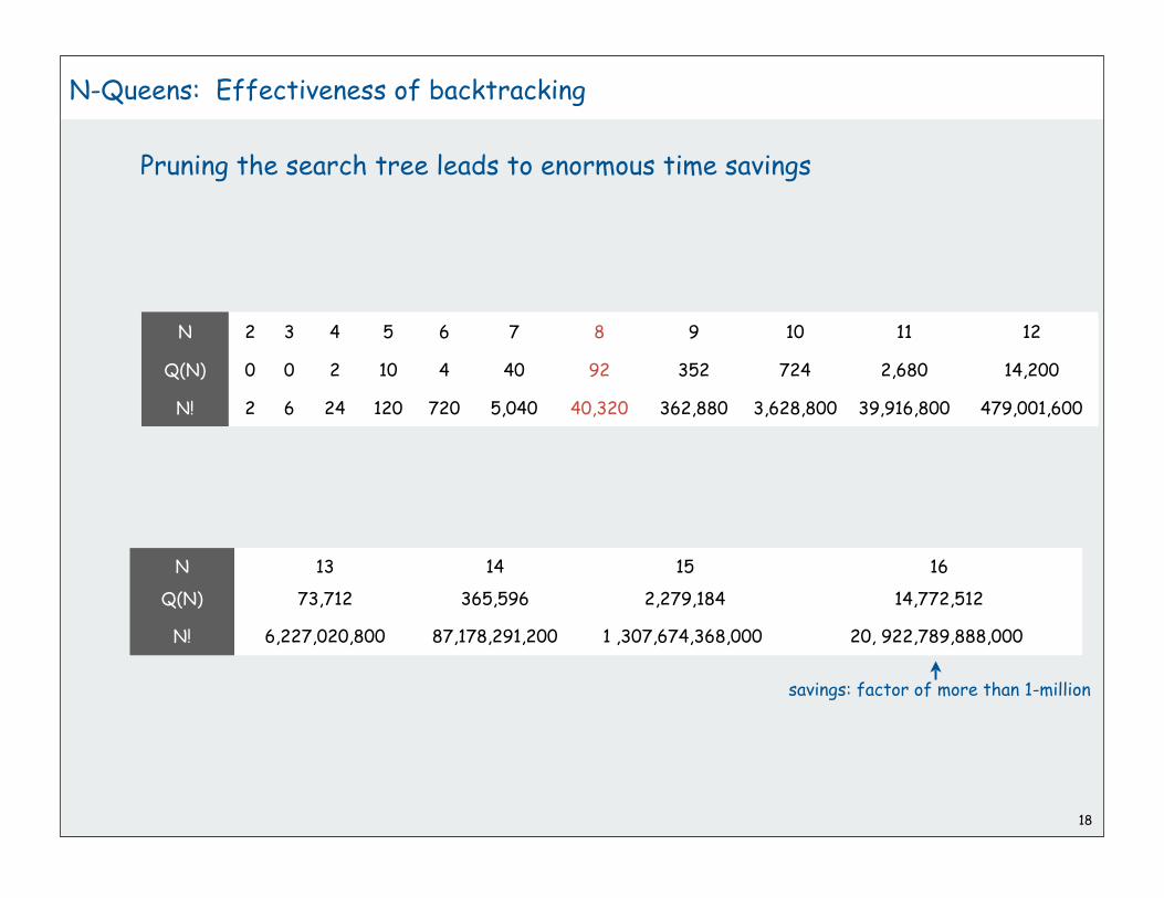
N-Queens: Effectiveness of backtracking
Pruning the search tree leads to enormous time savings
18
N
Q(N)
N!
2 3 4 5 6 7 8 9 10 11 12
0 0 2 10 4 40 92 352 724 2,680 14,200
2 6 24 120 720 5,040 40,320 362,880 3,628,800 39,916,800 479,001,600
N
Q(N)
N!
13 14 15 16
73,712 365,596 2,279,184 14,772,512
6,227,020,800 87,178,291,200 1 ,307,674,368,000 20, 922,789,888,000
savings: factor of more than 1-million

N-Queens: How many solutions?
Answer to original question easy to obtain:
• add an instance variable to count solutions (initialized to 0)
• change process() to increment the counter
• add a method to return its value
19
N
Q(N)
2 3 4 5 6 7 8 9 10 11 12 13 14 15
0 0 2 10 4 40 92 352 724 2,680 14,200 73,712 365,596 2,279,184
N
Q(N)
16 17 18 19 25
14,772,512 95,815,104 666,090,624 4,968,057,848 . . . 2, 207,893,435,808,350
took 53 years of CPU time (2005)
Source: On-line encyclopedia of integer sequences, N. J. Sloane [ sequence A000170 ]

N-queens problem: back-of-envelope running time estimate
Hypothesis ??
20
% java Queens 13
73712 solutions
% java Queens 14
365596 solutions
% java Queens 15
2279184 solutions
% java Queens 16
14772512 solutions
about a second
about 7 seconds
about 49 seconds
Hypothesis: Running time is about (N/2) ! seconds.
% java Queens 25about 54 years
about 360 seconds
ratio
6.32
6.73
7.38

21
permutationsbacktrackingcountingsubsetspaths in a graph

22
Counting: Java Implementation
private static void enumerate(int k){ if (k == N) { process(); return; }
for (int n = 0; n < R; n++) { a[k] = n; enumerate(k + 1); } a[k] = 0;}
Problem: enumerate all N-digit base-R numbers
Solution: generalize binary counter in lecture warmup
0 0 00 0 10 0 20 1 00 1 10 1 20 2 00 2 10 2 2
1 0 01 0 11 0 21 1 01 1 11 1 21 2 01 2 11 2 2
2 0 02 0 12 0 22 1 02 1 12 1 22 2 02 2 12 2 2
private void enumerate(int k)
{
if (k == N)
{ process(); return; }
enumerate(k+1);
a[k] = 1;
enumerate(k+1);
a[k] = 0;
} clean up
0 2 00 0 0
example showingcleanups that
zero out digits
enumerate binary numbers (from warmup)enumerate N-digit base-R numbers
clean up not needed: Why?

23
8
5
2 1
3
4
3 8
1
2 6
9
9 6
7
4
5
7
Problem:
Fill 9-by-9 grid so that every row, column, and box
contains each of the digits 1 through 9.
Remark: Natural generalization is NP-hard.
Counting application: Sudoku
2
9 3 4
1 6
9 4 6
5
7 3 8
1 5
6 7 8
2 4 9
1 7
6 9
8 5 2
5 9 3
4 2
6 7
8
1 5 7
4 3
2 3
4 8 1
6 7 5
1 5
3 9
8 2 4
7 8
6 2
9 3 1

24
Problem:
Fill 9-by-9 grid so that every row, column, and box
contains each of the digits 1 through 9.
Solution: Enumerate all 81-digit base-9 numbers (with backtracking).
Counting application: Sudoku
2 1
7 8
5
3
4
3 8
1
2 6
9
9 6
7
4
5
2
9 3 4
1 6
9 4 6
5
7 3 8
1 5
6 7 8
2 4 9
1 7
6 9
8 5 2
5 9 3
4 2
6 7
8
1 5 7
4 3
2 3
4 8 1
6 7 5
1 5
3 9
8 2 4
7 8
6 2
9 3 1
using digits 1 to 9 8 67 1 3 4 5 3 8 … 80
2 60 1 3 4 5 7 8 80

25
Iterate through elements of search space.
• For each empty cell, there are 9 possible choices.
• Make one choice and recur.
• If you find a conflict in row, column, or box, then backtrack.
Improvements are possible.
• try to make an “intelligent” choice
• try to reduce cost of choosing/backtracking
Sudoku: Backtracking solution
5
2 1
3 8
1
2 6
9
6
7
4
5
2
9 3 4
1 6
9 4 6
5
7 3 8
1 5
6 7 8
2 4 9
1 7
6 9
8 5 2
5 9 3
4 2
6 7
8
1 5 7
4 3
2 3
4 8 1
6 7 5
1 5
3 9
8 2 4
7 8
6 2
9 3 1
4
9
7 8 3

26
Sudoku: Java implementation
private static void solve(int cell){
if (cell == 81) { show(board); return; }
if (board[cell] != 0) { solve(cell + 1); return; }
for (int n = 1; n <= 9; n++) { if (! backtrack(cell, n)) { board[cell] = n; solve(cell + 1); } }
board[cell] = 0;}
clean up
try all 9 possibilities
unless a Sudokuconstraint is violated
(see booksite for code)
Works remarkably well (plenty of constraints). Try it!
already filled in

27
permutationsbacktrackingcountingsubsetspaths in a graph

28
Enumerating subsets: natural binary encoding
Given n items, enumerate all 2n subsets.
• count in binary from 0 to 2n - 1.
• bit i represents item i
• if 0, in subset; if 1, not in subset
0 0 0 00 0 0 10 0 1 00 0 1 10 1 0 00 1 0 10 1 1 00 1 1 11 0 0 01 0 0 11 0 1 01 0 1 11 1 0 01 1 0 11 1 1 01 1 1 1
0123456789101112131415
empty122 133 13 23 2 144 14 24 2 14 34 3 14 3 2
4 3 2 1
4 3 2 14 3 24 3 14 34 2 14 24 14
3 2 13 23 132 121
empty
i binary subset complement

29
Enumerating subsets: natural binary encoding
Given N items, enumerate all 2N subsets.
• count in binary from 0 to 2N - 1.
• maintain a[i] where a[i] represents item i
• if 0, a[i] in subset; if 1, a[i] not in subset
Binary counter from warmup does the job
private void enumerate(int k){ if (k == N) { process(); return; } enumerate(k+1); a[k] = 1; enumerate(k+1); a[k] = 0;}

30
Digression: Samuel Beckett play
Quad. Starting with empty stage, 4 characters enter and exit
one at a time, such that each subset of actors appears exactly once.
ruler function

31
Binary reflected gray code
The n-bit binary reflected Gray code is:
• the (n-1) bit code with a 0 prepended to each word, followed by
• the (n-1) bit code in reverse order, with a 1 prepended to each word.

32
Beckett: Java implementation
public static void moves(int n, boolean enter){ if (n == 0) return; moves(n-1, true); if (enter) System.out.println("enter " + n); else System.out.println("exit " + n); moves(n-1, false);}
% java Beckett 4
enter 1
enter 2
exit 1
enter 3
enter 1
exit 2
exit 1
enter 4
enter 1
enter 2
exit 1
exit 3
enter 1
exit 2
exit 1
stage directionsfor 3-actor playmoves(3, true)
reverse stage directionsfor 3-actor playmoves(3, false)

33
More Applications of Gray Codes
3-bit rotary encoder
Chinese ring puzzle
8-bit rotary encoder
Towers of Hanoi

34
Enumerating subsets using Gray code
Two simple changes to binary counter from warmup:
• flip a[k] instead of setting it to 1
• eliminate cleanup
Advantage (same as Beckett): only one item changes subsets
private void enumerate(int k){ if (k == N) { process(); return; } enumerate(k+1); a[k] = 1 - a[k]; enumerate(k+1);}
private void enumerate(int k)
{
if (k == N)
{ process(); return; }
enumerate(k+1);
a[k] = 1;
enumerate(k+1);
a[k] = 0;
} clean up
standard binary (from warmup)Gray code enumeration

35
Scheduling
Scheduling (set partitioning). Given n jobs of varying length, divide
among two machines to minimize the time the last job finishes.
Remark: NP-hard.
1.41
1.73
2.00
2.23
0
0
2
3
lengthjobor, equivalently, difference
between finish times
public double[] finish(int[] a) { double[] time = new double[2]; time[0] = 0.0; time[1] = 0.0; for (int i = 0; i < N; i++) time[a[i]] += jobs[i]; return time; }
private double cost(int[] a) { double[] time = finish(a); return Math.abs(time[0] - time[1]); }
2
1
3
0
3
1 2
machine 0
machine 1
machine 0
machine 1
cost
1
i a[] time[0] time[1]
0 1 1 0 1.41 00 0 1 1 0 1.41 01 0 1 1 0 1.41 1.732 0 1 1 0 1.41 3.733 0 1 1 0 3.64 3.73 3.64 3.73
cost: .09

36
Scheduling (full implementation)
public class Scheduler{ int N; // Number of jobs. int[] a; // Subset assignments. int[] b; // Best assignment. double[] jobs; // Job lengths.
public Scheduler(double[] jobs) { this.N = jobs.length;; this.jobs = jobs; a = new int[N]; b = new int[N]; for (int i = 0; i < N; i++) a[i] = 0; for (int i = 0; i < N; i++) b[i] = a[i]; enumerate(0); }
public int[] best() { return b; }
private void enumerate(int k) { /* Gray code enumeration. */ }
private void process() { if (cost(a) < cost(b)) for (int i = 0; i < N; i++) b[i] = a[i]; }
public static void main(String[] args) { /* Create Scheduler, print result. */ }}
% java Scheduler 4 < jobs.txt
a[] finish times cost
trace of

Large number of subsets leads to remarkably low cost
Scheduling (larger example)
37
java SchedulerEZ 24 < jobs.txt
MACHINE 0 MACHINE 1
1.4142135624
1.7320508076
2.0000000000
2.2360679775
2.4494897428
2.6457513111
2.8284271247
3.0000000000
3.1622776602
3.3166247904
3.4641016151
3.6055512755
3.7416573868
3.8729833462
4.0000000000
4.1231056256
4.2426406871
4.3588989435
4.4721359550
4.5825756950
4.6904157598
4.7958315233
4.8989794856
5.0000000000
------------------------------
42.3168901295 42.3168901457

Scheduling: improvements
Many opportunities (details omitted)
• fix last job on machine 0 (quick factor-of-two improvement)
• backtrack when partial schedule cannot beat best known
(check total against goal: half of total job times)
• process all 2k subsets of last k jobs, keep results in memory,
(reduces time to 2N-k when 2k memory available).
38
private void enumerate(int k){ if (k == N-1) { process(); return; } if (backtrack(k)) return; enumerate(k+1); a[k] = 1 - a[k]; enumerate(k+1);}

Backtracking summary
N-Queens : permutations with backtracking
Soduko : counting with backtracking
Scheduling: subsets with backtracking
39

40
permutationsbacktrackingcountingsubsetspaths in a graph

41
Hamilton Path
Hamilton path. Find a simple path that visits every vertex exactly once.
Remark. Euler path easy, but Hamilton path is NP-complete.
visit every edgeexactly once

42
Knight's Tour
Knight's tour. Find a sequence of moves for a knight so that, starting
from any square, it visits every square on a chessboard exactly once.
Solution. Find a Hamilton path in knight's graph.
legal knight moves a knight's tour
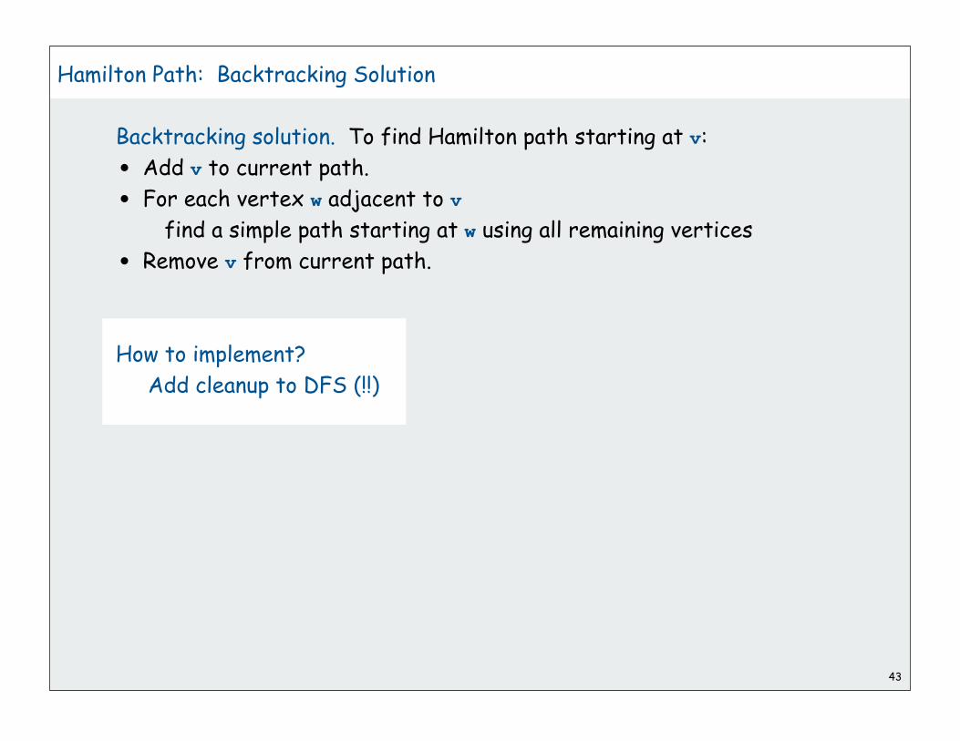
43
Hamilton Path: Backtracking Solution
Backtracking solution. To find Hamilton path starting at v:
• Add v to current path.
• For each vertex w adjacent to v
find a simple path starting at w using all remaining vertices
• Remove v from current path.
How to implement?
Add cleanup to DFS (!!)
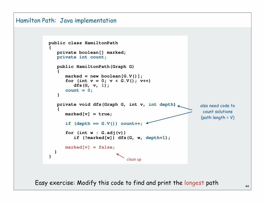
44
Hamilton Path: Java implementation
public class HamiltonPath{ private boolean[] marked; private int count;
public HamiltonPath(Graph G) { marked = new boolean[G.V()]; for (int v = 0; v < G.V(); v++) dfs(G, v, 1); count = 0; }
private void dfs(Graph G, int v, int depth) { marked[v] = true;
if (depth == G.V()) count++;
for (int w : G.adj(v)) if (!marked[w]) dfs(G, w, depth+1);
marked[v] = false; }}
also need code to
count solutions
(path length = V)
clean up
Easy exercise: Modify this code to find and print the longest path

45
The Longest Path
Woh-oh-oh-oh, find the longest path!Woh-oh-oh-oh, find the longest path!
If you said P is NP tonight,There would still be papers left to write,I have a weakness,I'm addicted to completeness,And I keep searching for the longest path.
The algorithm I would like to seeIs of polynomial degree,But it's elusive:Nobody has found conclusiveEvidence that we can find a longest path.
I have been hard working for so long.I swear it's right, and he marks it wrong.Some how I'll feel sorry when it's done: GPA 2.1Is more than I hope for.
Garey, Johnson, Karp and other men (and women)Tried to make it order N log N.Am I a mad foolIf I spend my life in grad school,Forever following the longest path?
Woh-oh-oh-oh, find the longest path!Woh-oh-oh-oh, find the longest path!Woh-oh-oh-oh, find the longest path.
Recorded by Dan Barrett in 1988 while a student at Johns Hopkins during a difficult algorithms final.