SPACECRAFT DYNAMICS
454
SPACECRAFT DYNAMICS Thomas R.Kane, Peter W Likins,. and David A. Levinson
-
Upload
independent -
Category
Documents
-
view
0 -
download
0
Transcript of SPACECRAFT DYNAMICS

SPACECRAFTDYNAMICS
Thomas R. Kane, Peter W Likins,.and David A. Levinson

Spacecraft DynamicsThomas R. Kane, Stanford University
Peter W. Likins, Lehigh UniversityDavid A. Levinson, Lockheed Palo Alto Research Laboratory
Copyright 2005 by the authors
Previously published byMcGraw-Hill Book Company, 1993
Now published byThe Internet-First University Press
This manuscript is among the initial offerings beingpublished as part of a new approach to scholarlypublishing. The manuscript is freely available from theInternet-First University Press repository within DSpaceat Cornell University at:
http://dspace.library.cornell.edu/handle/1813/62
The online version of this work is available on an openaccess basis, without fees or restrictions on personal use.A professionally printed and bound version may bepurchased through Cornell Business Services bycontacting:
All mass reproduction, even for educational or not-for-profit use, requires permission and license. For moreinformation, please contact
[email protected], N.Y.January 2005

£NGJN. MOV 1 1982
CORNELL UNIVERSITYLIBRARIES
ITHACA, N. Y. 14853
Engineering LibraryCarpenter Hall


SPACECRAFTDYNAMICS
Thomas R. KaneStanford University
Peter W. LikinsLehigh University
David A. LevinsonLockheed Palo Alto Research Laboratory
McGraw-Hill Book Company
New York St. Louis San Francisco Auckland Bogota HamburgJohannesburg London Madrid Mexico Montreal New Delhi
Panama Paris Sao Paulo Singapore Sydney Tokyo Toronto

This book was set in Times Roman by Andover Graphics.The editors were Diane D. Heiberg and Madelaine Eichberg;the production supervisor was Leroy A. Young.New drawings were done by Danmark & Michaels, Inc.The cover was designed by Mark Wieboldt.Halliday Lithograph Corporation was printer and binder.
SPACECRAFT DYNAMICS
Copyright © 1983 by McGraw-Hill, Inc. All rights reserved.Printed in the United States of America. Except as permitted underthe United States Copyright Act of 1976, no part of this publication maybe reproduced or distributed in any form or by any means, or storedin a data base or retrieval system, without the prior written permissionof the publisher.
1 2 3 4 5 6 7 8 9 0 H D H D 8 9 8 7 6 5 4 3 2
ISBN 0-Q7-Q37flM3-b
Library of Congress Cataloging in Publication Data
Kane, Thomas R.Spacecraft dynamics.
Includes index.1. Space vehicles—Dynamics. I. Likins, Peter W.
II. Levinson, David A. III. Title.TL1050.K36 629.47'0r53111 81-8431ISBN 0-07-037843-6 AACR2
j >

CONTENTS
Chapter 1
l
1.11.21.31.41.51.61.71.81.9.10.11.12.13.14.15.16.17.18.19.20.21
PrefaceTo the Reader
KinematicsSimple RotationDirection CosinesEuler ParametersRodrigues ParametersIndirect Determination of OrientationSuccessive RotationsOrientation AnglesSmall RotationsScrew MotionAngular Velocity MatrixAngular Velocity VectorAngular Velocity ComponentsAngular Velocity and Euler ParametersAngular Velocity and Rodrigues ParametersIndirect Determination of Angular VelocityAuxiliary Reference FramesAngular Velocity and Orientation AnglesSlow, Small Rotational MotionsInstantaneous AxisAngular AccelerationPartial Angular Velocities and Partial Velocities
viixi
114
12162023303842474953586268717378818487
iii

iv CONTENTS
Chapter 2 Gravitational Forces2.1 Gravitational Interaction of Two Particles2.2 Force Exerted on a Body by a Particle2.3 Force Exerted on a Small Body by a Particle2.4 Force Exerted on a Small Body by a Small Body2.5 Centrobaric Bodies2.6 Moment Exerted on a Body by a Particle2.7 Moment Exerted on a Small Body by a Small Body2.8 Proximate Bodies2.9 Differentiation with Respect to a Vector
2.10 Force Function for Two Particles2.11 Force Function for a Body and a Particle2.12 Force Function for a Small Body and a Particle2.13 Force Function in Terms of Legendre Polynomials2.14 Force Function for Two Small Bodies2.15 Force Function for a Centrobaric Body2.16 Force Function for a Body and a Small Body2.17 Force Function Expressions for the Moment Exerted
on a Body by a Particle2.18 Force Function Expression for the Moment Exerted
on a Small Body by a Body
Chapter 3 Simple Spacecraft3.1 Rotational Motion of a Torque-Free, Axisymmetric
Rigid Body3.2 Effect of a Gravitational Moment on an Axisymmetric
Rigid Body in a Circular Orbit3.3 Influence of Orbit Eccentricity on the Rotational Motion of
an Axisymmetric Rigid Body3.4 Torque-Free Motion of an Unsymmetric Rigid Body3.5 Effect of a Gravitational Moment on an Unsymmetric Rigid
Body in a Circular Orbit3.6 Angular Momentum, Inertia Torque, and Kinetic Energy of
a Gyrostat3.7 Dynamical Equations for a Simple Gyrostat3.8 Rotational Motion of a Torque-Free, Axisymmetric Gyrostat3.9 Reorientation of a Torque-Free Gyrostat Initially at Rest
3.10 Effect of a Gravitational Moment on an AxisymmetricGyrostat in a Circular Orbit
3.11 Effect of a Gravitational Moment on an UnsymmetricGyrostat in a Circular Orbit
Chapter 4 Complex Spacecraft4.1 Generalized Active Forces4.2 Potential Energy4.3 Generalized Inertia Forces4.4 Kinetic Energy

CONTENTS V
4.5 Dynamical Equations 2754.6 Linearized Dynamical Equations 2774.7 Computerization of Symbol Manipulation 2794.8 Discrete Multi-Degree-of-Freedom Systems 2844.9 Lumped Mass Models of Spacecraft 296
4.10 Spacecraft with Continuous Elastic Components 3184.11 Use of the Finite Element Method for the Construction of
Modal Functions 332
Problem Sets 344Problem Set 1 344Problem Set 2 358Problem Set 3 378Problem Set 4 395
Appendixes 422I Direction Cosines as Functions of Orientation Angles 422
II Kinematical Differential Equations in TermsOrientation Angles 427
Index 433


PREFACE
This book is the outgrowth of courses taught at Stanford University and atthe University of California, Los Angeles, and of the authors' professionalactivities in the field of spacecraft dynamics. It is intended both for use asa textbook in courses of instruction at the graduate level and as a referencework for engineers engaged in research, design, and development in this field.
The choice and arrangement of topics was dictated by the following con-siderations.
The process of solving a spacecraft dynamics problem generally neces-sitates the construction of a mathematical model, the use of principles ofmechanics to formulate equations governing the quantities appearing in themathematical model, and the extraction of useful information from the equa-tions. Skill in constructing mathematical models of spacecraft is acquiredbest through experience and cannot be transmitted easily from one individ-ual to another, particularly by means of the printed word. Hence, this sub-ject is not treated formally in the book. However, through examples, thereader is brought into contact with a considerable number of mathematicalmodels of spacecraft and, by working with the book, he can gain much ex-perience of the kind required. By way of contrast, the formulation of equationsof motion is a subject that can be presented formally, and it is essential thatthis topic be treated effectively, for there is no point in attempting to extractinformation from incorrect equations of motion. Now, every spacecraft dy-namics analysis necessitates use of various kinematical relationships, some ofwhich have played such a small role in the development of technology priorto the space age that they have been treated only cursorily, if at all, in thegeneral mechanics literature. Accordingly, the book begins with what is meant
vii

Vill PREFACE
to be a unified, modern treatment of the kinematical ideas that are most usefulin dealing with spacecraft dynamics problems.
To place the topics to be treated in the book into perspective, we turnto the familiar relationship F=ma, here regarding it as a conceptual guidelinerather than as the statement of a law of physics. Seen in this light, the arepresents all kinematical quantities, the F all forces that come into play, them all inertia properties, and the sign of equality the assertion that kinematicalquantities, forces, and inertia properties are related to each other. It is thenclear that one should deal with the topics of kinematics, forces, and inertiaproperties before taking up the study of a technique for formulating equationsof motion.
The subject of inertia properties, that is, the finding of mass centers,moments and products of inertia, principal axes of inertia, and so on, is treatedextensively in available textbooks and acquires no new facets in connectionwith spacecraft. Hence, we presume that the reader knows this material.Detailed information regarding forces that affect the behavior of spacecraft isnot so readily accessible. Therefore, we address this topic in Chapter 2,confining attention to gravitational forces, which play a preeminent role inspacecraft dynamics. This brings us into position to attack specific problemsin Chapters 3 and 4, these chapters differing from each other in one importantrespect: throughout Chapter 3, which deals with relatively simple spacecraft,we rely solely upon the angular momentum principle for the formulation ofdynamical equations of motion, whereas in Chapter 4, where we are con-cerned with complex spacecraft, we first develop and then use a more pow-erful method for formulating equations of motion, one that is particularly wellsuited for problems involving multi-degrees-of-freedom spacecraft.
Most sections of the book are arranged as follows. They begin with thepresentation of theoretical material in the form of categorical statements thateither constitute definitions or that can be shown to be valid by means ofdeductive arguments. In the latter case, the arguments are presented underthe heading "Derivations"; each section contains, in addition, an example inthe application of the theory set forth in the section. In the classroom, aninstructor can, therefore, focus attention wherever he pleases, that is, on thepresentation of theory, on formal proofs, or on examples, leaving it to hisstudents to devote time outside of the classroom to the matters not pursuedin depth in class.
In addition to the examples appearing in the text, the book contains foursets of problems, each set associated intimately with one of the four chapters.To acquire mastery of the material in the book, a student should solve everyone of these problems, for each covers material not covered by any other.Results are given wherever possible, so that one always can determine wheth-er or not one has solved a problem correctly.
To cover all of the material in the book is rather difficult in the timegenerally available in a graduate curriculum. However, the material lends itselfwell to presentation in two courses dealing, respectively, with Sections

PREFACE ix
1.1-1.20, 2.1-2.8, 3.1-3.11, and Sections 1.21, 2.9 -2.18, and 4.1-4.11. Thefirst course, covering kinematical fundamentals, the vectorial treatment ofgravitational forces and moments, and simple spacecraft, can prepare a stu-dent to work effectively on spacecraft dynamics problems and to pursue fur-ther studies in this field; successful completion of the second course, whichconcentrates upon new kinematical ideas, gravitational potential theory, anew approach to the formulation of equations of motion, and complex space-craft problems, enables one to undertake work at the forefront of spacecraftdynamics.
The use of computers in the solution of spacecraft dynamics problemsis so pervasive that familiarity of a worker in this field with programmingconcepts must be presumed. The writing and running of computer programsare meant to take place in connection with courses based on this book, butare not absolutely essential; that is, most problems are set up in such a waythat considerable benefit can be obtained by studying them even without theaid of a computer.
Since it was our intention to produce a self-contained book, we haveomitted all references to the extensive literature on spacecraft dynamics.However, we gratefully acknowledge our debt to the many authors whosework has influenced our thinking, and we wish to express our thanks tostudents who, with comments and suggestions, have aided us in writing thisbook, as well as to Stanford University and the University of California atLos Angeles, which supported this undertaking by generously making timeand computational resources available to us.
Thomas R. KanePeter W. Likins
David A. Levinson


TO THE READER
Each of the four chapters of this book is divided into sections. A section isidentified by two numbers separated by a decimal point, the first numberreferring to the chapter in which the section appears, and the second identi-fying the section within the chapter. Thus, the identifier 2.13 refers to thethirteenth section of the second chapter. A section identifier appears at thetop of each page.
Equations are numbered serially within sections. For example, the equa-tions in Sees. 2.12 and 2.13 are numbered (1M46) and (1H31), respectively.References to an equation may be made both within the section in which theequation appears and in other sections. In the first case, the equation numberis cited as a single number, whereas, in the second case, the section numberis included as part of a three-number designation. Thus, within Sec. 2.12, Eq.(1) of Sec. 2.12 is referred to as Eq. (1), whereas, in Sec. 2.13, the sameequation is referred to as Eq. (2.12.1). To locate an equation cited in thismanner, one may make use of the section identifiers appearing at the tops ofthe pages.
Figures appearing in the chapters are numbered so as to identify thesections in which the figures appear. For example, the two figures in Sec. 3.9are designated Fig. 3.9.1 and Fig. 3.9.2. To avoid confusion of these figureswith those in problem sets, the figure number is preceded by the letter P inthe case of the latter; the double number that follows this letter refers to theproblem statement in which the figure is introduced. For example, Fig. P3.8is introduced in Prob. 3.8. Similarly, Table 1.15.2 is the designation for a tablein Sec. 1.15, whereas Table PI.21 is associated with Prob. 1.21.
Thomas R. KanePeter W. Likins
David A. Levinson
xi


CHAPTER
ONEKINEMATICS
Every spacecraft dynamics problem involves considerations of kinematics.Indeed, the solution of most such problems begins with the formulation ofkinematical relationships. Hence, this topic requires detailed attention.
The first nine sections of this chapter deal with changes in the orientationof a rigid body in a reference frame, without regard to the time that necessarilyelapses when a real body experiences a change in orientation. Time entersthe discussion in the remaining sections, in all of which the concept of angularvelocity plays a central role. The concluding section contains the definitionsof quantities employed to great advantage, in Chap. 4, in connection with theformulation of dynamical equations of motion of complex spacecraft. Thissection (and Probs. 1.27-1.31) may be omitted by readers concerned primarilywith simple spacecraft, such as those treated in Chap. 3.
1.1 SIMPLE ROTATION
A motion of a rigid body or reference frame B relative to a rigid body orreference frame A is called a simple rotation of B in A if there exists a lineL, called an axis of rotation, whose orientation relative to both A and Bremains unaltered throughout the motion. This sort of motion is importantbecause, as will be shown in Sec. 1.3, every change in the relative orientationof A and B can be produced by means of a simple rotation of B in A.
If a is any vector fixed in A (see Fig. 1.1.1), and b is a vector fixed inB and equal to a prior to the motion of B in A, then, when B has performeda simple rotation in A, b can be expressed in terms of the vector a, a unitvector k parallel to L, and the radian measure 6 of the angle between twolines, LA and LB, which are fixed in A and B, respectively, are perpendicularto L, and are parallel to each other initially. Specifically, if 6 is regarded as

2 KINEMATICS 1.1
Figure 1.1.1
positive when the angle between LA and LB is generated by a X-rotation ofLB relative to LA, that is, by a rotation during which a right-handed screwfixed in B with its axis parallel to X advances in the direction of X when Brotates relative to A, then
b = a cos0 - a x X sin0 + a • XX(l - cos0)
Equivalently, if a dyadic C is defined as
C = U cos0 - U x X sin0 + XX(l - cos0)
where U is the unit (or identity) dyadic, then
b = a • C
(1)
(2)
(3)
Derivations Let ax and a2 be unit vectors fixed in A, with ax parallel to LA
and a2 = A. x a,; and let 0, and fi2 be unit vectors fixed in B, with 0, parallelto LB and /32 = X x fix, as shown in Fig. 1.1.1. Then, if a and b are resolvedinto components parallel to a!, a2, X and p{, #>, K respectively, correspond-ing coefficients are equal to each other because ax = 0, , a2 = fa, and a = bwhen 0 = 0. In other words, a and b can be expressed as
anda = pa.\ + qa2 + rX
b = pfi, + 4/32 + rX
(4)
(5)
where /?, q, and r are constants.Expressed in terms of a, and a2, the unit vectors 0, and /32 are given by
= cos0 sin0 OL2 (6)

1.1 SIMPLE ROTATION 3
Figure 1.1.2
and p2 = - sin0 a! + cos0 a2 O)
so that, substituting into Eq. (5), one finds that
b = (p cos0 - q sin0)at + (p sin0 + q cos0)«2 + rk (8)
The right-hand member of Eq. (8) is precisely what one obtains by carryingout the operations indicated in the right-hand member of Eq. (1), using Eq.(4), and making use of the relationships k x a{ = a2 and X x a2 = —ax. Thusthe validity of Eq. (1) is established, and Eq. (3) follows directly from Eqs.(1) and (2).
Example A rectangular block B having the dimensions shown in Fig. 1.1.2forms a portion of an antenna structure mounted in a spacecraft A. Thisblock is subjected to a simple rotation in A about a diagonal of one faceof B, the sense and amount of the rotation being those indicated in thesketch. The angle </> between the line OP in its initial and final positionsis to be determined.
If a,, a2, and a3 are unit vectors fixed in A and parallel to the edgesof B prior to ZTs rotation, then a unit vector k directed as shown in thesketch can be expressed as
3a2 + 4a3k = (9)

4 KINEMATICS 1.2
And if a denotes the position vector of P relative to O prior to 5 ' s ro-tation, then
a = - 2a! + 4a3 (10)
- 12a! + 8a2 - 6a3a x X = (11)
and48a2 + 64a3a A X = (12)
Consequently, if b is the position vector of P relative to O subsequentto fTs rotation,t
, * A . ft 12ai — 8a2 + 6a3 . TTb = ( - 2at + 4a3) cos — + sin —
(i) 6 5 6
48a2 + 64a:+ 25
+ 64a3 / IT
25 { l - C O S 6= - 0.532a, - 0.543a2 + 4.407a3 (13)
Since <f> is the angle between a and b,
c o s * =
where la I and Ibl denote the (equal) magnitudes of a and b. Hence
(-2K-0.532) + 4(4.407) = 0 _ 9 3 5
(4 + 16)1/2 (4 + 16)1
and <f> = 20.77°.
1.2 DIRECTION COSINES
If a,, a2, a3 and bi , l>2, b3 are two dextral sets of orthogonal unit vectors, andnine quantities Q (i,j = 1, 2, 3), called direction cosines, are defined as
Q A a . , b , ( / ^ . = l f 2 , 3) (1)
then the two row matrices [ai a2 a3] and [bj b2 b3J are related to eachother as follows:
[bi b2 b3] = [a! a2 a3] C (2)
t Numbers beneath signs of equality are intended to direct attention to equations numberedcorrespondingly.

1.2 DIRECTION COSINES 5
where C is a square matrix defined as
Cn C\2 C13
C21 C22 C23
C31 C32 C33
(3)
If a superscript T is used to denote transposition, that is, if CT is defined as
-11 C21 C31
C13 C23 C*33_
then Eq. (2) can be replaced with the equivalent relationship
[ai a2 a3] = [bj b2 b3] CT
(4)
(5)
The matrix C, called a direction cosine matrix, can be employed to de-scribe the relative orientation of two reference frames or rigid bodies A andB. In that context, it can be advantageous to replace the symbol C with themore elaborate symbol ACB. In view of Eqs. (2) and (5), one must then regardthe interchanging of superscripts as signifying transposition; that is,
BCA = (ACBf (6)
The direction cosine matrix C plays a role in a number of useful relation-ships. For example, if v is any vector and Av, and *v, (/ = 1, 2, 3) are defined as
andV - v a , . (i = l ,2 ,3)
, = v b , 0 = 1,2,3)
(7)
(8)
while Av and Bv denote the row matrices having the elements Avl9 Av2,
Av3
and Bvl9 Bv2, *v3, respectively, then
By = AVC (9)
Similarly, if D is any dyadic, and AA, and BDU (i9j = 1, 2, 3) are defined as
(10)and
BDij = b, • D • b, (1, j = 1, 2, 3) (11)
while AD and BD denote square matrices having ADtj and BDijy respectively,as the elements in the ith rows and yth columns, then
BD = CTADC (12)
Use of the summation convention for repeated subscripts frequentlymakes it possible to formulate important relationships rather concisely. Forexample, if 80- is defined as

100
010
001
6 KINEMATICS 1.2
«</ = 1 - i (/ "7)2[5 - (i -j)2] (i, j = 1, 2, 3)
so that 8jj is equal to unity when the subscripts have the same value, and equalto zero when the subscripts have different values, then use of the summationconvention permits one to express a set of six relationships governing direc-tion cosines as
Cik C-k — 8i (/, j = 1, 2, 3) (14)
or an equivalent set as
Cv CV = 8 (i i ' = 1 2 3 ) (15)
Alternatively, these relationships can be stated in matrix form as
C CT = U (16)and
CTC = U (17)
where U denotes the unit (or identity) matrix, defined as
U= 0 1 0 (18)
Each element of the matrix C is equal to its cofactor in the determinantof C; and, if \C\ denotes this determinant, then
\C\ = 1 (19)
Consequently, C is an orthogonal matrix, that is, a matrix whose inverse andwhose transpose are equal to each other. Moreover,
\C - U\ = 0 (20)
Hence, unity is an eigenvalue of every direction cosine matrix. In other words,for every direction cosine matrix C there exist row matrices [KX K2 K3],called eigenvectors, which satisfy the equation
[*1 K2 K3] C = [*i K2 K3] (21)
Suppose now that a, and b, (i = 1, 2, 3) are fixed in reference frames orrigid bodies A and /?, respectively, and that B is subjected to a simple rotationin A (see Sec. 1.1); further, that a, = b, (i = 1, 2, 3) prior to the rotation, thatX and 6 are defined as in Sec. 1.1, and that A, is defined as
K•, = k a, = X • b, (/ = 1,2,3) (22)
Then the elements of C are given by
C , = cos(9 4- \,2(1 - cos6) (23)
C12 = - A3 sin0 + A1A2O - cos0) (24)

1.2 DIRECTION COSINES 7
Cn = X2 sin0 + X3Xi(l - cos0)
C2\ = X3 sin0 + XiX2(l - cos0)
Cn = cos0 + \22(l ~ cos0)
C23 = - X, sin0 + X2X3(l - cos0)
C3i = - X2 sin0 + X3X,(l - cos0)
C32 = X! sin0 + X2X3(l - cos0)
C33 = cos0 + X32(1 - cos0)
(25)
(26)
(27)
(28)
(29)
(30)
(31)
Equations (23)—(31) can be expressed more concisely after defining eijk as
eijk = \ (/ -j)(j - k)(k - i) ( i , j , k = 1, 2, 3) (32)
(The quantity eijk vanishes when two or three subscripts have the same value;it is equal to unity when the subscripts appear in cyclic order, that is, in theorder 1, 2, 3, the order 2, 3, 1, or the order 3, 1,2; and it is equal to negativeunity in all other cases.) Using the summation convention, one can thenreplace Eqs. (23)—(31) with
Cij = 8ij cos0 - eukkk sin0 + X,Xy(l - cos0) (/, j = 1, 2, 3) (33)
Alternatively, Cy can be expressed in terms of the dyadic C defined in Eq.(1.1.2):
Q = a, - ( a - C ) ( i , . / = 1 , 2 , 3) (34)
All of these results simplify substantially when A. is parallel to a,, andhence to b, (i = 1, 2, 3). If C,(0) denotes C for X = a, = b,, then
C,(0) =
C2(0) =
C3(0) =
1 0 00 cos 0 —sin 00 sin 0 cos 0
cos 0 00 1
-s in 0 0
sin 00
cos 0
COS 0
sin 00
-s in 0 0cos 0 00 1
(35)
(36)
(37)
It was mentioned previously that unity is an eigenvalue of every directioncosine matrix. If the elements of a direction cosine matrix C are given by Eqs.(23)—(31), then the row matrix [K{ X2 X3] is one of the eigenvectors corre-sponding to the eigenvalue unity of C; that is,
[X, X2 X3] C = [X, X2 X3] (38)

8 KINEMATICS 1.2
Equivalently, when C is the dyadic defined in Eq. (1.1.2), then
k • C = k (39)
Derivations For any vector v, the following is an identity:
v = (a! • v)ai + (a2 • v)a2 + (a3 • v)a3 (40)
Hence, letting bi play the role of v, one can express bi as
b, = (a, • b,)a, + (a2 • b,)a2 + (a3 • b,)a3 (41)
or, by using Eq. (1), as
bi = C\\ 2i\ 4- Cu a2 H- C3i a3 (42)
Similarly,b2 = Cn a, + C22 a2 + C32 a3 (43)
andb3 = Cn a, + C23 a2 + C33 a3 (44)
These three equations are precisely what one obtains when forming expres-sions for bi, b2, b3 in accordance with Eq. (2) and with the rules for matrixmultiplication; and a similar line of reasoning leads to Eq. (5).
To see that Eq. (9) is valid one needs only to observe that
Bv, = v • (a, Cu + a2 C2i + a3 C3/)(8.2)
= v • ai Cu + v • a2 C2i + v • a3 C3/
= Av, Cu + Av2 C2i + Av3 C3/ (45)
and to recall the definitions of Av and Bv. Similarly, Eq. (12) follows from
BDij j=2(ai Cu + a2 C2i + a3 C3/) • D • (ai CXj 4- a2 C2j 4- a3 Cy)
(= C u (ADn CXj +
ADl2 C2j + ADl3 C3j)
+ C2i ( D2\ C\j + D22 C2j 4- £>23 Cy)
+ C3/ (AD3l CXj +
AD32 C2j + AD33 Cy) (46)
and from the definitions of AD and BD.As for Eqs. (14) and (15), these are consequences of (using the summation
convention)
a, • a,- = Cik Cjk (i, j = 1, 2, 3) (47)and (It
bibj = C , Q (/,y = l ,2 ,3) (48)
respectively, because a, • a7 is equal to unity when i =j9 and equal to zerowhen / 7^7, and similarly for b, • b7; and Eqs. (16) and (17) can be seen to

1.2 DIRECTION COSINES 9
be equivalent to Eqs. (14) and (15), respectively, by referring to Eqs. (3), (4),and (18) when carrying out the indicated multiplications.
To verify that each element of C is equal to its cofactor in the determinantof C, note that
b, = Cn a, + C21 a2 + C31 a3 (49)and (2)
b2 x b3 = (C22 C33 - C32 C23)a! + (C32 C13 - Cl2 C33)a2
+ (C 1 2C 2 3-C 2 2C 1 3)a 3 (50)
so that, since b{ = b2 x b3 because bi, b2, b3 form a dextral set of orthogonalunit vectors,
Cn = C22 C33 — C32 C23 (51)
C2i = C32 Cn — Cn C33 (52)and
C3J = Cn C23 — C22 Cn (53)
Thus each element in the first column of C [see Eq. (3)] is seen to be equalto its cofactor in C; and, using the relationships b2 = b3 x bi and b3 = bi x b2,one obtains corresponding results for the elements in the second and thirdcolumns of C. Furthermore, expanding C by cofactors of elements of the firstrow, and using Eq. (14) with i =j= 1, one arrives at Eq. (19).
The determinant of C — U can be expressed as
\C - U\ = \C\ + Cn + C22 + C33 4- Cl2 C21 + C23 C32 + C31 C13
- (Cn C22 + C22 C33 + C33 C,,) - 1 (54)
Hence, replacing C n , C22, and C33 with their respective cofactors in |C|, onefinds that
| C - C / | = | C | - l ( = 0 (55)
in agreement with Eq. (20); and the existence of row matrices [K, K2 K3]satisfying Eq. (21) is thus guaranteed.
The equality of X • a, and X • b, in Eq. (22) is a consequence of the factthat these two quantities are equal to each other prior to the rotation of Brelative to A, that is, when a, = b,, and that neither X • a, nor X • b, changesduring the rotation, since, by construction, X is parallel to a line whose ori-entation in both A and B remains unaltered during the rotation.
With a and b replaced by a, and by, respectively, Eq. (1.1.3) becomes
by = ay • C (56)
Hence
Q = a, • by = a,- • (ay • C) (1, j = 1, 2, 3) (57)(1) (56)

10 KINEMATICS 1.2
Figure 1.2.1
which is Eq. (34). Moreover, substituting for C the expression given in Eq.(1.1.2), one finds that
Cij = a, • 2Lj cos0 - a, • a, x X sin0 + a, • XX • a,(l - cosO)
( i , y = l , 2 , 3) (58)
and this, together with Eq. (22) leads directly to Eqs. (23)—(31), or, in viewof Eq. (32), to Eq. (33).
Equation (35) is obtained by setting k{ = 1 and X2 = A3 = 0 in Eqs.(23)—(31) and then using Eq. (3). Similarly, X, = 0, \2 = 1, and X3 = 0 lead toEq. (36), and X, = A2 = 0, X3 = 1 yield Eq. (37).
Finally, Eq. (39) is derived from the observation thatt
X • C = X • U cos0 - X x X sin0 + X2X(1 - cos0)(1.1.2)
= X cos0 + 0 + X(l - cos0) = X (59)
since X is a unit vector, so that X2 = X • X = 1; and the equivalence of Eqs.(38) and (39) follows from Eqs. (22) and (34).
Example In Fig. 1.2.1, B designates a uniform rectangular block whichis part of a scanning platform mounted in a spacecraft A. Initially, theedges of B are parallel to unit vectors a,, a2 and a3 which are fixed in A,and the platform is then subjected to a simple 90° rotation about a diagonalof B, as indicated in the sketch. If I is the inertia dyadic of B for the masscenter B* of B, and AIU is defined as
t When it is necessary to refer to an equation from an earlier section, the section numberis cited together with the equation number. For example, (1.1.2) refers to Eq. (2) in Sec. 1.1.

1.2 DIRECTION COSINES 11
% = a, - I - a y (1,7 = 1 ,2 ,3) (60)
what is the value of AItj (i,j = 1, 2, 3) subsequent to the rotation?Let b, (i = l, 2, 3) be a unit vector fixed in B and equal to a, (i = l, 2, 3)
prior to the rotation; and define BIij as
i , J = 1 , 2 , 3 ) (61)
Then bi, b2, and b3 are parallel to principal axes of inertia of B for B*,so that
Bj _ Br — Br — BT — BJ _ Br __ f\'12 — '21 — '23 — '32 — '31 ~ ' 13 ~ v
and, if m is the mass of B,
(62)
(63)
= ^ (32 + 42)L2 = ^and
(64)
(65)
Hence, if */ denotes the square matrix having % as the element in the/th row and jth column, then
mL 153 0 00 25 00 0 160
The unit vector A shown in Fig. 1.2.1 can be expressed as
_ 4 a l + 12a2 + 3a3 = ± a + .12 ? ^J_a
(66)
(67)(42 + 122 + 32)"2 13 ' ' 13 - ' ' 13
Consequently, Xt, X2, and X3, if defined as in Eq. (22), are given by
A , = £ X2 = ^ X3 = ^ (68)
and, with 6 = TT/2 rad, Eqs. (23)—(31) lead to the following expression forthe direction cosine matrix C:
1
169
1687
-144
914488
168-16
9(69)
If Al is now defined as the square matrix having % as the elementin the /th row and Jth column, then
BI = CTAIC(12)
(70)

12 KINEMATICS 1.3
and simultaneous premultiplication with C and postmultiplication with CT
gives
(70) (16)(71)
Consequently,
AI =mL2
(66,69,71) 12 X 169 X 169
mL2
16 9 168
87 144 -16-144 88 9
153 0 0
0 25 0
0 0 160
16 87 -144
9 144 88168 -16 9
12 X 169 X 169
4,557,033 -184,704 -90,792-184,704 1,717,417 -1,623,024-90,792 -1,623,034 3,379,168
and
= 4,557,033 mL2
11 ~ 12 x 169 x 169AT — — 184,704 mL2
12 x 169 x 169
and so forth.
1.3 EULER PARAMETERS
(72)
(73)
The unit vector k and the angle 0 introduced in Sec. 1.1 can be used to asso-ciate a vector €, called the Euler vector, and four scalar quantities, €1, . . . , €4,called Euler parameters, with a simple rotation of a rigid body B in a referenceframe A by letting
€ = X sin -
€, = € • a, = € • b, (1 = 1, 2, 3)
andA 6
€4 = COS -
(1)
(2)
(3)
where ai, a2, a3 and bi, b2, b3 are dextral sets of orthogonal unit vectors fixedin A and B respectively, with a, = b, (1 = 1, 2, 3) prior to the rotation. (Wherea discussion involves more than two bodies or reference frames, notationssuch as AeB and Ae* will be used.)
The Euler parameters are not independent of each other, for the sum oftheir squares is necessarily equal to unity:
€,2 + €22 + €3
2 + €42 = C2 + €4
2 = 1 (4)
An indication of the utility of the Euler parameters may be gleaned from

1.3 EULER PARAMETERS 13
the fact that the elements of the direction cosine matrix C introduced in Sec.1.2 assume a particularly simple and orderly form when expressed in termsof €,, . . . , e4 : If Cij is defined as
thenQ = a,- •
C n — €1 — €2
C12 = 2(e, e2 -
C,3 = 2(e3 «i +
C2, = 2(e, e2 +
C2 2 = e22 - e3
2
C2 3 = 2(e2 e3 -
C 3 ) = 2(e3 €| -
C3 2 = 2(e2 e3 +
C3 3 = e32 - e,2
b, (i,j =
- €32 + €4
2 = ]
e3€4)
e2 e4)
e3 e4)
- €,2 + e42 = :
Ci €4)
€2€4 )
€1 e4)
- e22 + €4
2 = :
1, 2, 3)
I - 2C22 -
1 - 2€32 -
1 - 2c,2 -
2e32
2c,2
2c22
(5)
(6)
(7)
(8)
(9)
(10)
(11)
(12)
(13)
(14)
The Euler parameters can be expressed in terms of direction cosines insuch a way that Eqs. (6)-(14) are satisfied identically. This is accomplishedby taking
C 3 2 — C 2 3
C13 — C3162 = —4^-
^ — (17)
and
C22 + C33)1/2 (18)
Since Eqs. (1) and (3) are satisfied if
€, at + €2 a2 + €3 a3
(€,2 + €22 + €3
2)1/2
and6 = 2 cos"1 e4 0 < 0 < 7T (20)
one can thus find a simple rotation such that the direction cosines associatedwith this rotation as in Eqs. (1.2.23)—(1.2.31) are equal to corresponding ele-

14 KINEMATICS 1.3
ments of any direction cosine matrix C that satisfies Eq. (1.2.2). In otherwords, every change in the relative orientation of two rigid bodies or referenceframes A and B can be produced by means of a simple rotation of B in A.This proposition is known as Eulefs theorem on rotation.
As an alternative to Eqs. (1.1.1) and (1.1.3), the relationship between avector a fixed in a reference frame A and a vector b fixed in a rigid bodyB and equal to a prior to a simple rotation of B in A can be expressed interms of € and €4 as
b = a + 2[e4 c x a + € x (c x a)] (21)
Derivations The equality of € • a, and € • b, [see Eq. (2)] follows from Eqs.(1) and (1.2.22); Eqs. (4) are consequences of Eqs. (l)-(3) and of the fact thatX is a unit vector; and Eqs. (6)-(14) can be obtained from Eqs. (1.2.23)-(1.2.31) by replacing functions of 6 with functions of 0/2 and using Eq. (1.2.22)together with Eqs. (l)-(4). For example,
and
C n = 2 cos2 ? - 1 + 2X,2 sin2 % (22)(1.2.23) 2 2
j sin x = X • ai sin x = € • a, = €i (23)2 (1.2.22) 2 (1) (2)
while
(24)I (3)
Hence,Cn = 2e4
2 - 1 + 26,2 = € l2 - €2
2 - €32 + e4
2 (25)
in agreement with Eq. (6).The validity of Eqs. (15)—(18) can be established by showing that the
left-hand members of Eqs. (6)-(14) may be obtained by substituting from Eqs.(15)-(18) into the right-hand members. For example,
1 - 2€22 " 2€3
2
2(1 + Cn + C22 + C33) — Cn + 2Cn C31 — C31 — C21 + 2Cn C21 — C12
(16-18) 2(1 + Cn + C22 + C33)
12 C21C\\ + C22 + C33 + C13 C31 4- C12 C21 + Cn(26)
(1.2.14) 1 + C\\ + C22 + C33
But, since each element of C is equal to its cofactor in |C|,
C13 C31 = C n C33 — C22 (27)
and
C12 C21 = C n C22 - C33 (28)

1.3 EULER PARAMETERS 15
Consequently,
1 2 e 2 2C3 " cu + c22
as required by Eq. (6).To see that Eqs. (1) and (3) are satisfied if X and 0 are given by Eqs.
(19) and (20), note that
cos ^ = €4 (30)2 (20) V
which is Eq. (3), and that
so that
sin § ( = ( 1 - €42)1/2 = (e,2 + e2
2 + e32)1/2 (31)
X sin ~ = €1 a! + c2 a2 + e3 a3 = € (32)2 (19) (2)
as required by Eq. (1). Finally, Eq. (1.1.1) is equivalent to
b = a + X x a s i n 0 + X x ( X x a)(l - cos 0)
= a + 2c x a cos | + 2c x (c x a) = a + 2 [€4 € x a + € x (€ x a)] (33)
in agreement with Eq. (21).
Example Triangle ABC in Fig. 1.3.1 can be brought into the positionA'B'C by moving point A to A', without changing the orientation of thetriangle, and then performing a simple rotation of the triangle while keep-ing A fixed at A'. To find X, a unit vector parallel to the axis of rotation,and to determine 0, the associated angle of rotation, let the unit vectorsa, and b, (/ = 1, 2, 3) be directed as shown in Fig. 1.3.1, thus insuring thata, = b, (i = 1, 2, 3) prior to the rotation; determine Q by evaluatinga, • b,; and use Eqs. (15)-(18) to form e, (/ = 1, . . . , 4):
e4 = - (1 + ai • bi + a2 • b2 + a3 • b3)1/2
(18)2
= ± ( 1 + 0 + 0 + 0)1/2 = X- (34)
» • » • - » • > , . l ^ . . . (35)a3 • b 2 "~ a2 *
4(0a, • b3 — a3
b3
b,
1 - 0
2
- 1 -2
0
12
12 (36)
(16)

Figure 1.3.1
= a2 • bi - ai • tfc = - 1 - 0 = __1(17)
(37)
Then
and
x =(19)
\ ai - \ a2 - \ as _ at - a2 - a3X1/2
. ! 2TT ,0 = 2 cos - = — rad(20) 2 3
(38)
(39)
1.4 RODRIGUES PARAMETERS
A vector p , called the Rodrigues vector, and three scalar quantities, p\, p 2 ,p 3 , called Rodrigues parameters, can be associated with a simple rotation ofa rigid body B in a reference frame A (see Sec. 1.1) by letting
and
A w 6p = X tan ~
p, = p • a, = p • b, (i = 1, 2, 3)
(1)
(2)
where X and 6 have the same meaning as in Sec. 1.1, and a,, a:, a3 and bi,b2, b3 are dextral sets of orthogonal unit vectors fixed in A and By respec-

1.4 RODRIGUES PARAMETERS 17
tively, with a, = b, (i = 1, 2, 3) prior to the rotation. (When a discussioninvolves more than two bodies or reference frames, notations such as ApB andAPtB will be used.)
The Rodrigues parameters are intimately related to the Euler parameters(see Sec. 1.3):
p. = J (/ = 1,2,3) (3)
An advantage of the Rodrigues parameters over the Euler parameters is thatthey are fewer in number; but this advantage is at times offset by the factthat the Rodrigues parameters can become infinite, whereas the absolute valueof any Euler parameter cannot exceed unity.
Expressed in terms of Rodrigues parameters, the direction cosine matrixC (see Sec. 1.2) assumes the form
1
>-
+ p.2
2(p,
2(p3
—
Pi
Pi
pi+- PI)
P32 2(pi
1 +P12
2(P2
Pi
-
Pi
—
P32
+
Pi)
-
Pd
P.22(P3
2(P2
1 + P 3 2
Pi
P3
-
+ Pi)
"Pi)
P 2 2 .
C = (4)1 + Pi' + P22 + P32
The Rodrigues vector can be used to establish a simple relationship be-tween the difference and the sum of the vectors a and b defined in Sec. 1.1:
a - b = (a + b) x p (5)
This relationship will be found useful in connection with a number of deriva-tions, such as the one showing that the following is an expression for aRodrigues vector that characterizes a simple rotation by means of which aspecified change in the relative orientation of A and B can be produced:
= (<*1 - ft) >< («2 ~ ft)9 (a, + ft) • (a2 - ft) U
where a, and ft (/ = 1, 2) are vectors fixed in A and B, respectively, and«/ = ft (i = 1, 2) prior to the change in relative orientation. Rodrigues param-eters for such a rotation can be expressed as
1 + d i + C22 + C33
= C13 ~ C3191 1 + C,i + C22 + C33
y )
- C21 ~ C12P 3 1 + Cn + C22 + C33
l ;
Derivations The equality of p • a, and p • b, [see Eq. (2)] follows from Eqs.(1) and (1.2.22); and Eqs. (3) are obtained by noting that

18 KINEMATICS 1.4
- = X tan - = p (10)€ 4 (1.3.1, 2 (1)
1.3.3)
so that
Pi==±U±=ti ( f - , , 2 , 3 ) (11)(2) e 4 (1.3.2) € 4
From Eq. (1.3.4),
1 = €,2 + €22 + €3
2 + e42 = (Pi2 + p2
2 + P32 + 1)€42 (12)
(3)
1 — *r 2 — - c 2 - - c 2 4 - ^ 2 — r> 2 ^ 2 — ^ 2 - r 2 ^ 2 - r 2 - U ^ 2
n — €1 — €2 — €3 + e 4 — p i € 4 — P2 e 4 — P3 € 4 -1- € 4
(1.3.6) (3)
= (P2 *' ~ ?' ~ + '
Hence,
and
= (P. 2 " P,2 " P32 + DC 2 = * ? ^ ++ '2 (14)
1 + P,2 + P22 + P3
2
in agreement with Eq . (4), and the remaining e lements of C are found sim-ilarly.
As for Eq . (5), note that cross-multiplication of Eq . (1.3.21) with e yields
€ X b = € X a + 2 { € 4 e x ( € X a ) + € X [ € X ( € X a ) ] } ( 1 5 )
Hence,
= 2{c x a + e4 € x (c x a) + € x [c x (c x a)]} (16)
Now
€ X [€ X (€ X a)] = ~€ 2 € X a = ~(€i2 + €22 + €3
2)e X a
^ - I X x ' a (17)
Consequently,e x (a + b) = 2€4[e4 € x a + e x (€ x a)] = €4(b - a) (18)
(16,17) (1.3.21)
and
a - b = (a + b) x - = (a + b) x k tan = (a + b) x p (19)(18) € 4 (1.3.1, 2 (1) r V
1.3.2)
which is Eq . (5).Equat ion (6) can now be obtained by observing that
a , - 0 , = (a , +Pi)xp (20)and
<*2 - Pi = (a2 + p2) x p (21)

1.4 RODRIGUES PARAMETERS 19
so that
X («2 " Pi) (=[(«i +
(21)
) x p] x (tt2 - 02)
* («2 - /*2)p ~ («i +
' («2 - /32)p - 0
(a2 - Pi)
(22)
from which Eq. (6) follows immediately.Finally, to establish the validity of Eqs. (7)-(9), note that
Pi = —(3) € 4 (1.3.15)
C 3 2 - C 2
4e42 Cn + C2
(23)
in agreement with Eq. (7); and Eqs. (8) and (9) can be obtained by cyclicpermutation of the subscripts in Eq. (7).
Example Referring to Fig. 1.4.1, which depicts the rigid body B previ-ously considered in the example in Sec. 1.1, suppose that B is subjectedto a 180° rotation relative to A about an axis parallel to the unit vectorX; and let b, be a unit vector fixed in B and equal to a, (1 = 1, 2, 3) priorto the rotation. The direction cosine matrix C satisfying Eq. (1.2.2) sub-sequent to the rotation is to be determined.
For 6 = 7T rad, Eq. (1) yields a Rodrigues vector of infinite magnitude,and Eqs. (2) and (4) lead to an indeterminate form of C. To evaluate this
Figure 1.4.1

20 KINEMATICS 1.5
indeterminate form, one may express each element of C in terms of 0 andk • a, (i = l, 2, 3) by reference to Eqs. (1) and (2), and then determinethe limit approached by the resulting expression as 6 approaches TT rad.Alternatively, one can use either Eqs. (1.2.23)—(1.2.31) or Eqs. (1.3.6)—(1.3.14) to find the elements of C. The latter equations are particularlyconvenient, because, for 6 = TT,
€ o lo X ( 2 4 )
so that€ , - ( = 2 ) A- a / (i = 1, 2, 3) (25)
and€4 = 0 (26)
(1 .3 .3)
Hence, with
k = ^a2 + ^a3 (27)
one finds immediately that
€ , = 0 € 2 = ; €3= 4? (28)
and substitution into Eqs. (1.3.6)—(1.3.14) then gives
-25 0 00 - 7 24 (29)0 24 7
1.5 INDIRECT DETERMINATION OF ORIENTATION
If ai, a2, a3, and b,, l>2, l>3 are dextral sets of orthogonal unit vectors fixedin reference frames A and B respectively, and the orientation of each unitvector in both reference frames is known, then a description of the relativeorientation of the two reference frames can be given in terms of directioncosines C,y (i,j = 1,2, 3), for, in accordance with Eq. (1.2.1), these can befound by simply evaluating a, • by (i,j = 1,2, 3). But, even when these dotproducts cannot be evaluated so directly, it may be possible to find Q(ij = 1, 2, 3). This is the case, for example, when each of two nonparallelvectors, say p and q, has a known orientation in both A and B, so that thedot products a, • p, a, • q, b, • p, and b, • q (i = 1, 2, 3) can be evaluateddirectly. In that event, one can find Cy as follows: Form a vector r and adyadic cr by letting
r = p x q (1)and
A p x q r + q x r p + r x pqa = ? (2)

1.5 INDIRECT DETERMINATION OF ORIENTATION 2 1
Next, express the first member of each dyad in Eq. (2) in terms of a,, andthe second member in terms of b, (i = 1, 2, 3). Finally, carry out the multi-plications indicated in the relationship
Q = a, c r b , ( i j = l , 2 , 3 ) (3)
Derivation It will be shown that the dyadic a defined in Eq. (2) is a unitdyadic, that is, that for every vector v,
V = V • €T (4)
The validity of Eq. (3) can then be seen to be an immediate consequence ofthe definition of Q , given in Eq. (1.2.1).
If p and q are nonparallel, and r is defined as in Eq. (1), then every vectorv can be expressed as
v = ap + /3q + yr (5)
where a, /3, and y are certain scalars. From Eq. (5),
v • (q x r) = ap • (q x r) + 0q • (q x r) + yr • (q x r)
= a(p x q) • r + 0 + 0 = ar2 (6)(i)
so that
q x ra = v • ^-j- (7)
(6) r
S i m i l a r l y , s c a l a r m u l t i p l i c a t i o n o f E q . (5) w i t h r x p a n d p x q l e a d s t o t h ec o n c l u s i o n t h a t
/3 = v ^ (8)
a n d
y = v • L
Substituting from Eqs. (7)-(9) into Eq. (5), one thus finds that
v • (q x r)p + v • (r X p)q + v • (p x q)rV ~ r2
(2)

22 KINEMATICS 1.5
Figure 1.5.1
Example Observations of two stars, P and Q, are made simultaneouslyfrom two space vehicles, A and B, in order to generate data to be usedin the determination of the relative orientation of A and B. The observa-tions consist of measuring the angles cf> and iff shown in Fig. 1.5.1, whereO represents either a point fixed in A or a point fixed in B, R is eitherP or Q, and Ci, c2, c3 are orthogonal unit vectors forming a dextral setfixed either in A or B. For the numerical values of these angles given inTable 1.5.1, the direction cosine matrix C is to be determined.
If R is defined as a unit vector directed from O toward R (see Fig.1.5.1), then
R = cos i/> cos 0 Ci + cos \\f sin $ c2 + sin \fj c3 (11)
Hence, letting p and q be unit vectors directed from O toward P andtoward Q, respectively, and referring to Table 1.5.1, one can express eachof these unit vectors both in terms of aj, a2, a3 and in terms of bi, b2,b3, as indicated in lines 1 and 2 of Table 1.5.2; and these results can thenbe used to evaluate r [see Eq. (1)], q x r, and r x p. Noting that (seeline 3 of Table 1.5.2)
2 = A-F " 16
Table 1.5.1 Angles </> and i|/ indegrees
16 16Z8
(12)
ci= bi
p
0
90
135
*
45
0
0
30
90
Q
*
0
60

1.6 SUCCESSIVE ROTATIONS 23
Table 1.5.2 Vectors appearing in cr
Line
1
2
3
4
5
one thus
Vector
P
q
r p x q
q x r
r x p
obtains
0
VT2
-V24
-V68
VJ2
V22
2
V64
3V28
14
«3
V22
0
-V64
V22
14
bi
-V22
0
V64
b2
V22
12
V64
b3
0
V32
-V24
_ ' 2 v 6 v 6 \ /v 6 v 6 v 2W — I I 7-8) H ^ 8 2 7-83 I I ——Di H 7~b2 ~I
( 2 ) L \ 4 4 4 / \ 4 4 43V2" v/2"
+ l% + -«3J (^ -yb, + -ylh + Objj
and
,2 I
Cl3 = a, •o - -<3)
and so forth; that is,
8 2
8 1 - 0(42 4l- r - - r - +
\ 4 4
C =0 0 10 1 0
- 1 0 0
(13)
(14)
(15)
(16)
(17)
1.6 SUCCESSIVE ROTATIONS
When a rigid body B is subjected to two successive simple rotations (see Sec.1.1) in a reference frame A, each of these rotations, as well as a singleequivalent rotation (see Sec. 1.3), can be described in terms of direction

24 KINEMATICS 1.6
cosines (see Sec. 1.2), Euler parameters (see Sec. 1.3), and Rodrigues param-eters (see Sec. 1.4); and, no matter which method of description is employed,quantities associated with the individual rotations can be related to thosecharacterizing the single equivalent rotation. In discussing such relationships,it is helpful to introduce a fictitious rigid body B which moves exactly likeB during the first rotation, but remains fixed in A while B performs the secondrotation. For analytical purposes, the first rotation can then be regarded asa rotation of B relative to A, and the second rotation as one of B relativeto B.
If a, (/ = 1, 2, 3), b,- (i = 1, 2, 3), and b, (/ = 1,_2, 3) are three dextral setsof orthogonal unit vectors fixed in A, B, and B, respectively, such thata, = b, = b/ (i = l, 2, 3) prior to the first rotation of B in A, and if ACB, BCB,and ACB are the direction cosine matrices characterizing, respectively, thefirst, the second, and the single equivalent rotation, so that
* (1)
(2)
(3)
by
(4)
(5)
To state the analogous relationship in terms of Euler^ parameters, we firstdefine three sets of such parameters as follows: With b, and b, (/ = 1, 2, 3)directed as after the second rotation, and with 0x, 02, and 6 denoting respec-tively the radian measures of the first, the second, and the equivalent rotation,
and
then ACB,
Similarly,
[b, b2
[b, b2
[b, b2
expressed in terms
b;
b3
b:
of
AC
for Rodrigues vectors,
AA B
P
1PS
i] = [a, a2 a 3 ] A
lj — [Di D2 D3J
j] = [a, a2 a 3 ] A
AC* and BCB, is
B A/^B B/^B
+ V + V xA
1 - V • BPB
cB
<cB
c»
gi
ACB ±A
B,B ± B€,- - 1
*€? = A
€B • a,
eB • b ,
e" ' a,
=v=v
B B A
AuB =
b,
b,
b,
cos
COS
COS
0i2
02
2
02
(1 =
(« =
(« =
1,
1,
1,
2,
2,
2,
3)
3)
3)
(6)
(7)
(8)
(9)
(10)
(ID

1.6 SUCCESSIVE ROTATIONS 25
It then follows that
Furthermore,
and
V
=
V
—A€ B
A
V-V
A e 2f f
Ae?-Aef
-V
V
V x
•V
\B
VV
(12)
(13)
(14)
Equations (4), (5), (12), and (13) all reflect the fact that the final orientationof B in A depends upon the order in which the successive rotations areperformed. For example, in Eq. (4), ACB and BCB cannot be interchangedwithout altering the result, and in Eq. (13) the presence of a cross productshows that order cannot be left out of account.
Repeated use of Eqs. (4)-(14) permits one to construct formulas for quan-tities characterizing a single rotation that is equivalent to any number ofsuccessive rotations. For example, for three successive rotations,
ACB = ACBBCBBC (15)
where AC*, F C f , and ^CB are direction cosine matrices associated with thefirst, the second, and the third rotation, respectively.
Derivations Substitution from Eq. (1) into Eq. (2) gives
[b, b2 b3] = [ai a2 a3]AC"c* (16)
and comparison of this equation with Eq. (3) shows that Eq. (4) is valid.To obtain Eq. (5), let a, b, and b be vectors fixed in A, By and B,
respectively, and choose these in such a way that a = b = b prior to the firstrotation of B in A. Then, in accordance with Eq. (1.4.5), there exist Rodriguesvectors ApB, BpB
and
and ApB satisfying the equations
a - b = (a + b) x ApB
b - b = (b + b) x V
a - b = (a + b) x ApB
(17)
(18)
(19)
Cross-multiply Eqs. (17) and (18) with BpB and ApB, respectively; subtract theresulting equations; and use the fact that
= V • b (20)
= V - b (21)and
v

2 6 KINEMATICS 1.6
to eliminate b wherever it appears as a member of a scalar product. Thisleads to
b x ( V + V ) = a x V + b x V + (a - b )V • V+ (a + b) x ( V x V ) (22)
Next, add Eqs. (17) and (18), eliminate b by using Eq. (22), and solve fora — b, thus obtaining
(23)
Together, Eqs. (23) and (19) imply the validity of Eq. (5), for Eqs. (23) and(19) can be satisfied for all choices of the vector a only if Eq. (5) is satisfied.
As for Eqs. (13) and (14), note that it follows from Eqs. (1.3.1), (1.3.3),and (1.4.1) that
V = T (24)
V = r (25)
and
V = 4 (26)€4
Consequently,
A-B - Ar B A* A B V + V + V1-VV
V A64g + V X A
=(24,25) C4 "€4S V " V • V
( '
and, dot-multiplying each side of this equation with itself and using Eq. (1.3.4),one finds that
1 ~ iA€? *€AB - A€* • *€B)2
y € ) — ( €4 ; /A BB B A~^B B B\2 ^ '
\ €4 €4 — € • € ;
But,( V ) * = 1 ~ (A€4*)2 (29)
(1.3.4)
Hence,(^€/)2 = (A€4**€4
B ~ AJ ' V ) 2 (30)(28,29)
and\ B = ± (A€ / B€B _ A€B . BeB) ( 3 1 )
(30)

1.6 SUCCESSIVE ROTATIONS 27
so that, using the upper sign, one obtains Eq. (14). Furthermore, substitutioninto Eq. (27) then yields Eq. (13).
Finally, to establish the validity of Eq. (12), it suffices to show that thefour scalar equations implied by this matrix equation can be derived from Eqs.(13) and (14). To this end, one may employ Eqs. (6) and (J) to resolve theright-hand member of Eq. (13) into components parallel to b l 9 b2 , and b3 andthen dot-multiply both sides of the resulting equation successively with b , ,b2 , and b3 , using Eq. (8) to evaluate A<? • b, and Eqs. (1.3.6H1.3.14) to formb, • b7 , which gives, for example,
K — If8* BD3 — Z\ €2(1.3.11)
B. B€4 (32)
In this way one is led to the first three scalar equations corresponding to Eq.(12), and the fourth is obtained from Eq. (14) by making the substitution
BJB _ Afc —
(6,7)
B B _ B€ + V
B.B (33)
Example In Fig. 1.6.1, ai, a2, and a3 are mutually perpendicular unitvectors; X and Y are lines perpendicular to a, and making fixed angleswith a2 and a3; and B designates a body that is to be subjected to a 90°rotation about line X and a 180° rotation about line Y, the sense of eachof these rotations being that indicated in the sketch.
Suppose that the rotation about X is performed first. Then, if b t , b2 ,and b3 are unit vectors fixed in B and respectively equal to a,, a2, anda3 prior to the first rotation, there exists a matrix Cx such that, subsequentto the second rotation of B,
[b, b, b3] = [a, a2 a3] Cx (34)
30 Y
Figure 1.6.1

28 KINEMATICS 1.6
Similarly, if the rotation about Y is performed first, there exists a matrixCy such that, subsequent to the second rotation of B,
[bi b2 b3] = [ai a2 a3]Cy (35)
Cx and Cy are to be determined.In order to find Cx by using Eq. (4), one may first form ACB by
reference to Eqs. (1.2.23)-(1.2.31) with 0 = TT/2 and
= 0 X2 = ^ (36)
which gives
0
12
- V I2
1234
>/T4
VI2
VI414
(37)
Next, to construct the matrix BCB, one must express^ unit vector A, whichis parallel to Y in terms of suitable unit vectors bj, b2 and b3. This isaccomplished by noting that X, resolved into components parallel to a,,a2, and a3, is given by
(38)X = i a2 + - r - a3
so that, using Eq. (1.2.9) and ACB, one obtains
= - - b, + - b2 + — b3
2 4 4
With d = 77, Eqs. (1.2.23)-(1.2.31) then provide
BCB =
(39)
12
34
- N / I
34
18
3VT
-V34
3VT8
5
(40)

1.6 SUCCESSIVE ROTATIONS 29
Consequently,
c, =(4)
s c B =
0
- 1
0
1
20
2
-VI2
0]_
2
(41)
Cy can be found similarly. Alternatively, one may use Euler param-eters, proceeding as follows:
With X expressed in terms of aj, a2, anda3, and with 6 = TT, Eq. (1.3.1)gives
and, from Eq. (1.3.3),
V = 0Similarly, for the second rotation
V = ( f a2 + ia3)f(1.3.1) \ 2 2 7 2
and
Hence,
= >H(1.3.3) 2
so that, in accordance with Eq. (8),
^24
while
^24
V6
V64
(M)
(42)
(43)
(44)
(45)
(46)
(47)
(48)
The elements of Cy can now be obtained by using Eqs.(1.3.6H1-3.14), which gives
0 1 0
-I o ^2 U 2
(49)

30 KINEMATICS 1.7
1.7 ORIENTATION ANGLES
Both for physical and for analytical reasons it is sometimes desirable to de-scribe the orientation of a rigid body B in a reference frame A in terms ofthree angles. For example, if B is the rotor of a gyroscope whose outer gimbalaxis is fixed in a reference frame A, then the angles </>, 0, and \jj shown inFig. 1.7.1 furnish a means for describing the orientation of B in A in a waythat is particularly meaningful from a physical point of view.
One scheme for bringing a rigid body B into a desired orientation in areference frame A is to introduce a!, a2, a3 and bi, ^ , b* as dextral sets oforthogonal unit vectors fixed in A and B, respectively; align b, with a,(i = 1, 2, 3); and subject B successively to an a, rotation of amount 8X, ana2 rotation of amount 02, and an a3 rotation of amount 03. (Recall that, forany unit vector A, the phrase "A rotation" means a rotation of B relative toA during which a right-handed screw fixed in B with its axis parallel to Xadvances in the direction of X.) Suitable values of 6\, 62, and 03 can be foundin terms of elements of the direction cosine matrix C (see Sec. 1.2), which,
Line fixed in A
Inner gimbal axis
Line fixed in B,perpendicularto rotor axis
Outer gimbalaxis
Figure 1.7.1

1.7 ORIENTATION ANGLES 31
if s, and c, (i = 1, 2, 3) denote sin 0, and cos 0, (i = 1, 2, 3) respectively, isgiven by
*~i
C2C3 S,S2C3 - S3C1 C1S2C3 "I" S3S,
C2S3 S1S2S3 + C3C1 C!S2S3 - C3S,
- S 2
Specifically, if |C3i| 1, take
02 = sin"1 (-C31)
Next, after evaluating c2, define a as
CiC2
-!<*<!
A . _ , C32 IT TT
a = sin — — < a ^ -rc2 2 2
and let
if C33 2= 0- a if C33 < 0
Similarly, define /3 as
and take
If |C3i| = 1, take
7T 7T
c2
03 =if C11 0if C11 < 0
and, after defining a as
7T-
let
and
a = sin ' (-C23)
f a if C22 >1 1 v - a if C22 <
77
(1)
(2)
(3)
(4)
(5)
(6)
(7)
(8)
(9)
(10)
In other words, two rotations suffice in this case.A second method for accomplishing the same objective is to subject B
successively to a b t rotation of amount 0\, a b2 rotation of amount 02, and

32 KINEMATICS 1.7
a b3 rotation of amount #3. The matrix C relating aj, a2, a3 to bi, b2, b3 asin Eq. (1.2.2) subsequent to the last rotation is then given by
C =c 2 c 3 -C2S3 s 2
S1S2C3 + S3C1 -S1S2S3 + C3C1 -S1C2
+ S3S! dS 2 S 3 + C3S! CiC2
(11)
and, if |C131 ¥^ 1, suitable values of 0l9 02, and 03 are obtained by taking
! !02 = sin"1 C , -~<62<-
A . _i —C23a = sin
c2
7T
2
ifC33^O- a if C33 < 0
A . _! ""^12
= smc2
2
if C,, >0ifd, <0
(12)
(13)
(14)
(15)
(16)
whereas, if |C7I31 = 1, one may let
77
^2 =
2 i f C l 3 = 1
77- - ifC13 = -1
a = sin ' C77" 77
32
f a ifC22aO1 l 7 r - a ifC2 2<0
(17)
(18)
(19)
(20)
so that, once again, only two rotations are required.The difference between these two procedures for bringing B into a desired
orientation in A is that the first involves unit vectors fixed in the referenceframe, whereas the second involves unit vectors fixed in the body. What thetwo methods have in common is that three distinct unit vectors are employedin both cases.
It is also possible to bring B into an arbitrary orientation relative to Aby performing three successive rotations which involve only two distinct unitvectors, and these vectors may be fixed either in the reference frame or in

1.7 ORIENTATION ANGLES 3 3
the body. Specifically, if B is subjected successively to an ai rotation ofamount 0i, an a2 rotation of amount 02, and again an a, rotation, but this timeof amount 03, then
c =C2 SiS2 C1S2
S2S3 -S1C2S3 + C3C1 -C1C2S3 - C3S1
-S2C3 S1C2C3 + S3C1 C1C2C3 - S3S1
and, if \Cn\ ^ 1, one can take
02 = cos"1 Cn 0 < 02 < 77
77 _ _ 77A . _i Cna = sin l ~JL
s2
- a
A . _i C21= sin ' —**
s2
if Ca ^ 0if Cu < 0
if C31 < 0if C31 ^ 0
while, if | C n | = 1, one may let
:
if C n = 1if C n = -
77a = sin"1 (-C23)
fa if C22 a 01 1 77 - a if C22 < 0
03=0
77
(21)
(22)
(23)
(24)
(25)
(26)
(27)
(28)
(29)
(30)
Finally, if the successive rotations are a b! rotation of amount 0i, a b2
rotation of amount 02, and again a bj rotation, but this time of amount 03,then
C =C2 S2S3 S2C3
S,S2 - S ! C 2 S 3 + C3C1 - S , C 2 C 3 - S3C,
- C 1 S 2 C1C2S3 + C3S, C1C2C3 - S3S!
and, if \Cn\ ¥* 1, $i9 02, and 03 may be found by taking
02 = cos"1 Cn 0 < 02 < 77
A . _j C
a = sin ' -^s2
f
(31)
(32)
(33)

34 KINEMATICS 1.7
a if Cn < 0- a if C3I ^ 0
f fi if C,j ^ 0ft~lir-/8 i fC 1 3 <0 ( 3 6 )
while, if |Cn| = 1, one can use
% j o if c = 1
a = sin"1 C32 - | < a < | (38)
if C22 > 0 „r - a i fC 2 2 <0 ( 3 9 )
03 = 0 (40)
The matrices in Eqs. (1) and (11) are intimately related to each other:either one may be obtained from the other by replacing 0, with -0 ,(i = 1, 2, 3) and transposing. The matrices in Eqs. (21) and (31) are relatedsimilarly. These facts have the following physical significance, as may beverified by using Eq. (1.6.4): If B is subjected successively to an ai, an a2,and an a3 rotation of amount 0i, 02, and 03, respectively, then one can bringB back into its original orientation in A by next subjecting B to successive—bi, —b2, and —b3 rotations of amounts 8\, 02, and 03, respectively. Similarly,employing only four unit vectors, one can subject B to successive rotationscharacterized by 0^1, 02a2, 03ai, -0ibi, -ft lh, and -03bi without producingany ultimate change in the orientation of B in A. Furthermore, it does notmatter whether the rotations involving unit vectors fixed in A are precededor followed by those involving unit vectors fixed in B; that is, the sequencesof successive rotations represented by 0ibi, 02b2, 03b3,-0,ai, -02a2, -03a3
and by 0ibi, 02b2, 03bi, -ftai, -02a2, -03^ also have no net effect on theorientation of B in A.
To indicate which set of three angles one is using, one can speak ofspace-three angles in connection with Eqs. (1)—(10), body-three angles forEqs. (11)—(20), space-two angles for Eqs. (21)-(30), and body-two angles forEqs. (31)-(40); and this terminology remains meaningful even when the anglesand unit vectors employed are denoted by symbols other than those used inEqs. (l)-(40). Moreover, once one has identified three angles in this way, onecan always find appropriate replacements for Eqs. (1), (11), (21), or (31) bydirect use of these equations. Suppose, for example, that x, y, z and £, ij,£ are dextral sets of orthogonal unit vectors fixed in a reference frame A and

1.7 ORIENTATION ANGLES 35
in a rigid body B, respectively; that x = £, y = TJ, and z = £ initially; that £is subjected, successively, to a z rotation of amount y, ay rotation of amount/3, and an x rotation of amount a; and that it is required to find the elementsLij (/, j = 1, 2, 3) of the matrix L such that, subsequent to the last rotation,
B ii {] = [i y *]L (41)
Then, recognizing a, /3, and y as space-three angles, one can introduce a,,b,-, and 0, (i = 1, 2, 3) as
A
a, = zA
a2 = yb2 = r)
A
a3 = - x
and
(42)
(43)
(44)
in which case the given sequence of rotations is represented by 0iat, 02a2,and 03 a3; and Lu can then be found by referring to Eq. (1) to express the scalarproducts associated with Ly in terms of a, /3, and y. For instance,
= y ' £ = a2 • (~b3)
dl,) " C23 (7) "ClS2S3 + C3Sl
= cos y sin /3 sin a 4- cos a sin y (45)
In the spacecraft dynamics literature one encounters a wide variety ofdirection cosine matrices. Twenty-four such matrices are tabulated in Appen-dix I.
Derivations _To_ e§tablish=the validity of Eq. (1), one may use Eq. (1.6.15),forming ACB, BCB, and BCB with the aid of Eq. (1.2.35) and Eqs. (1.2.23)-(1.2.31). Specifically, to deal with the a, rotation, let
(46)
Next, to construct a matrix BCB that characterizes the a2 rotation, let Ak andBk denote row matrices whose elements are a2 • a, (/ = 1, 2, 3) and a2 • b,(i = 1, 2, 3), respectively. Then
AcB =(12.35)
10
0
0Ci
Si
0- S i
Ci
= [ 0 1 0 ]
Bk = AkACB = [0 c, - s , ](1.2.9) (46,47)
(47)
(48)
and, from Eqs. (1.2.23)-(1.2.31), with X, = 0, k2 = c,, X3 = ~ s , , and 9 = 02,

36 KINEMATICS 1.7
BQB =
C2 S iS 2 C1S2
-S1S2 1 + Si2(C2 ~ 1) S!Ci(C2 - 1)
-C1S2 S!Ci(C2 - 1) 1 + C,2(C2 - 1)
(49)
A matrix AC* associated with a simple rotation that is equivalent to thefirst two rotations is now given by
(1.6.4) (46,49)
C2 SiS2 CiS2
0 c, -si
- S 2 SiC2 CiC2
(50)
and, to resolve a3 into components required for the construction of a matrixBCB, one may use Eq. (1.2.9) to obtain
= [-s2 slC2 Clc2](50)
[0 0
after which Eqs. (1.2.23)-(1.2.31) yield
S22 + C22C3 -C2[C,S3 + S , S 2 ( 1 - C 3 ) ] C 2 [ s ,S3-C,S 2 ( l ~ C 3 ) ]
BCB =
(51)
_-C 2 [S 1S 3+C 1S 2 (1-C 3 ) ] -s2s3+s1c,c22(l-c3) 1 - (S 2
2 +S 12 C 2
2 ) (1-C 3 )
(52)
and substitution from Eqs. (46), (49), and (52) into Eq. (1.6.15) leads directlyto Eq. (1).
Equation (11) may be derived by using Eq. (1.6.15) with
(53)AcB =(1.2.35)
BCB =
(1.2.36)
10
0
1 -
0Ci
Si
c2
0
- s 2
01
0
0- S i
Ci
s2
0
c2and
(1.2.37)
" c 3 - s 3 0 1s3 c3 00 0 l j
(54)
(55)
Equations (2)-(10) and (12)-(20) are immediate consequences of Eq. (1) andEq. (11), respectively; and Eqs. (21)-(40) can be generated by proceduressimilar to those employed in the derivation of Eqs. (l)-(20).

1.7 ORIENTATION ANGLES 37
Example If unit vectors ax, a2, a3 and bi, b2, b3 are introduced as shownin Fig. 1.7.2, and the angles </>, 0, and i// shown in Fig. 1.7.1 are renamed#!, 02, and 03, respectively, then 6{, 02, and 03 are body-two angles suchthat Eqs (31)-(40) can be used to discuss motions of B in A. However,as will be seen later, it is undesirable to use these angles when dealingwith motions during which the rotor axis becomes coincident, or evennearly coincident, with the outer gimbal axis. (Coincidence of these twoaxes is referred to as gimbal lock.) Therefore, it may be convenient toemploy in the course of one analysis two modes of description of theorientation of B in A, switching from one to the other whenever 02
acquires a value lying in a previously designated range. The following sortof question can then arise: If (f>{, <fe, and <fh, are the space-three anglesassociated with aj, a2, a3 and b,, \h, ^ , what are the values of these anglescorresponding to (9, = 30°, 02 = 45°, 03 = 60°?
Inner gimbal axis
Outer gimbal axis
Figure 1.7.2

38 KINEMATICS 1.8
Inspection of Eqs. (2)-{6) shows that the elements of C required forthe evaluation of fa, fa, and fa are C3!, C32, C33, C2\, and Cn. FromEq. (31),
C3, = - ^ - - y = -0.612 (56)
i i = ».78O ,57,
i.-O.^ (58,
l>/2C2I = - — = 0.354 (59)
CM = — = 0.707 (60)
Hence,<fc = sin"' 0.612 = 37.7° (61)
(2)
0, = 99.6° p = 26.6° fa = 26.6° (63)(4) (5) (6)
1.8 SMALL ROTATIONS
When a simple rotation (see Sec. 1.1) is small in the sense that second andhigher powers of 8 play a negligible role in an analysis involving the rotation,a number of the relationships discussed heretofore can be replaced with sim-pler ones. For example, Eqs. (1.1.1) and (1.1.2) yield, respectively,
b = a - a x k8 (1)and
C = U - U x k8 (2)
while Eqs. (1.3.1), (1.3.3), and (1.4.1) give way to
e = 5 A0 (3)
€4 = 1 (4)
andP = i Afl (5)
which shows that, to the order of approximation under consideration, theRodrigues vector is indistinguishable from the Euler vector.

1.8 SMALL ROTATIONS 39
As will be seen presently, analytical descriptions of small rotations fre-quently involve skew-symmetric matrices. In dealing with these, it is conven-ient to establish the notational convention that the symbol obtained byplacing a tilde over a letter, say q, denotes a skew-symmetric matrix whoseoff-diagonal elements have values denoted by ±qx (/ = 1, 2, 3), these elementsbeing arranged as follows:
0 -<?3 q
q = 0 -qx
q\ 0(6)
Using this convention, one can express the results obtained by neglectingsecond and higher powers of 0 in Eqs. (1.2.23)—(1.2.31) as
kO (7)C = [/
Similarly, Eqs. (1.3.6)-(1.3.14) yield
C = U + 21 (8)
Considering two successive small rotations, suppose that AC* and BCB aredirection cosine matrices characterizing the first and second such rotation asin Sec. 1.6. Then, instead of using Eq. (1.6.4), one can express the directioncosine matrix ACB associated with a single equivalent small rotation as
*CB = U + (ACB + BCB - 2U) (9)
Similarly, for three small rotations, Eq. (1.6.15) leads toACB = U + (ACB + BCB + BCB - 3U) (10)
Rodrigues vectors A / / , BfP> and AfP associated, respectively, with a first,a second, and an equivalent single small rotation satisfy the equation
V = V + V (11)Both this relationship and Eq. (9) show that the final orientation of B in Ais independent of the order in which two successive small rotations are per-formed.
Finally when 0l9 02, and 03 in Eqs. (1.7.1)—(1-7.40) are small in the sensethat terms of second or higher degree in these quantities are negligible, thenEqs. (1.7.1) and (1.7.11) each yield [see Eq. (6) for the meaning of 0]
C = 0 (12)
showing that it is immaterial whether one uses space-three angles or body-three angles under these circumstances. The relationship corresponding to Eq.(12) for either space-two or body-two angles, namely
C =(1.7.21)
00
- 0 2
00
03+01
02
(13)

40 KINEMATICS 1.8
is less useful because this equation cannot be solved uniquely for 6X and 03
as functions of Cy (i,j = 1,2, 3).
Derivations Equation (1) follows from Eq. (1.1.1) when sin 6 is replaced with6 and cos 6 with unity. The same substitution in Eq. (1.1.2) leads to Eq. (2).Equations (3) and (4) are obtained by replacing sin (6/2) with 6/2 and cos (6/2)with unity in Eqs. (1.3.1) and (1.3.3), and Eq. (5) follows from Eq. (1.4.1) whentan (6/2) is replaced with 6/2.
Equation (7) follows directly from Eqs. (1.2.23)-(1.2.31), and Eq. (8)results from dropping terms of second degree in d , e2, and/or e3 when formingCu in accordance with Eq. (1.3.6) — (1.3.14), which is justified in view of Eqs.(3) and (1.3.2).
To establish the validity of Eq. (9) one may proceed as follows: UsingEq. (7), one can express the matrices ACB and BCB introduced in Sec. 1.6 as
and
ACB = C/
BCB = U
k6 (14)
(15)
where 6 and </> are, respectively, the radian measures of the first and of thesecond small rotation, and k and /I characterize the associated axes of ro-tation. Substituting into Eq. (1.6.4), and dropping the product k Ji6<f), one thenobtains
AcB = u + xo + ji<t>= U + (U + X0 U + £- U + (ACB + BCB - 2U)
A similar procedure leads to Eq. (10).
- 21/)
(16)
Figure 1.8.1

1.8 SMALL ROTATIONS 41
Finally, Eq. (11) may be obtained by using Eq. (5) in conjunction withEq. (1.6.5), and Eqs. (12) and (13) result from linearizing in 0, (i = 1, 2, 3) inEqs. (1.7.11) and (1.7.21), respectively, and using the convention establishedin Eq. (6).
Example In Fig. 1.8.1, ai, a2, and a3 form a dextral set of orthogonal unitvectors, with a, and a2 parallel to edges of a rectangular plate B\ and Xand Y designate lines perpendicular to ai and a2, respectively. When Bis subjected, successively, to a rotation of amount 0.01 rad about X anda rotation of amount 0.02 rad about Y, the sense of each rotation beingthat indicated in the sketch, point P traverses a distance d. This distanceis to be determined on the assumption that the two rotations can beregarded as small.
If a designates the position vector of point P relative to point O beforethe rotations are performed, and b the position vector of P relative to Osubsequent to the second rotation, then
d = |b - a| (17)with
a = L(3a, + 4a2) (18)and
b = a - a x k$ (19)(i)
where X and 6 are, respectively, a unit vector and the radian measure ofan angle associated with a single rotation that is equivalent to the twogiven rotations. To determine the product kd, let p be the Rodriguesvector for this equivalent rotation, in which case
kd = 2p (20)
and refer to Eq. (11) to express p as
P — px "r p y — - Ajf T ^ A.y V^l/(5) I I
where kx and ky are unit vectors directed as shown in Fig. 1.8.1; that is,
K = 7 2 ( a 2 + a3) (22)
and
ky = \ (>/3 a, + a3) (23)
thenk0 = 0.01V, + 0.02X,
(20,21)
0 01= -7=- [>/6ai + a2 4- (1 + v2)a3] (24)
(22,23) J ?

42 KINEMATICS 1.9
b - a = - a x (kd)(19)
= -^=-[-4(1 + ^2)a, +3(1 + >/2)a2 + (4>/6 - 3)a3]L (25)(18,24) y/2
and[" 16(1 + >/2)2 + 9(1 + V2)2 + (4V6 -
(17,25) L 2 0 , 0 0 0
1.9 SCREW MOTION
M"» = QmL
J v '
If P, and P2 are points fixed in a reference frame A, and a point P is movedfrom Pi to P2, then P is said to experience a displacement in A, and the po-sition vector of P2 relative to Pi is called a displacement vector of P in A.
When points of a rigid body B experience displacements in a referenceframe A, one speaks of a displacement of B in A; and a displacement of Bin A is called a translation of 5 in A if the displacement vectors of all pointsof B in A are equal to each other.
Every displacement of a rigid body B in a reference frame A can be pro-duced by subjecting B successively to a translation in which a basepoint Pof B, chosen arbitrarily, is brought from its original to its terminal position,and a simple rotation (see Sec. 1.1) during which P remains fixed in A. TheRodrigues vector (see Sec. 1.4) for the simple rotation is independent of thechoice of basepoint, whereas the displacement vector of the basepoint de-pends on this choice. When the displacement vector of the basepoint is parallelto the Rodrigues vector for the rotation, the displacement under considerationis said to be producible by means of a screw motion.
Every displacement of a rigid body B in a reference frame A can be pro-duced by means of a screw motion. In other words, one can always find abasepoint whose displacement vector is parallel to the Rodrigues vector forthe simple rotation associated with a displacement of B in A. In fact, thereexist infinitely many such basepoints, all lying on a straight line that is parallelto the Rodigues vector and bears the name screw axis; and the displacementvectors of all points of B lying on the screw axis are equal to each other andcan, therefore, be characterized by a single vector, called the screw transla-tion vector. Moreover, the magnitude of the screw translation vector is eithersmaller than or equal to the magnitude of the displacement vector of anybasepoint not lying on the screw axis.
If 8 is the displacement vector of an arbitrary basepoint P, 8 is the Rod-rigues vector for the rotation associated with a displacement of B in A, andP* is a point of B lying on the screw axis (see Fig. 1.9.1), then the positionvector a* of P* relative to P prior to the displacement of B in A satisfiesthe equation
a» = p x 8 + ( p 2 x 6 ) x p + w > ( 1 )

B prior todisplacement
Figure 1.9.1
1.9 SCREW MOTION 43
Screw axis
B subsequent todisplacement
where ^ depends on the choice of P*; and the screw translation vector 8*is given by
8* = —y-p (2)
Derivation If both P* and P are points of B selected arbitrarily, and a* is theposition vector of P* relative to P prior to the displacement of B in A, whileb* is the position vector of P* relative to P subsequent to this displacement,then the displacement vector S* of P* can be expressed as (see Fig. 1.9.1)
5* = 8 + b* - a*
where 8 is the displacement vector of P; and
so that
b* - a* = p x (a* + b*)(1.4.5) r
8* = 8 + p x (a* + b*)(3,4)
(3)
(4)
(5)
Hence, if P* is to be chosen such that 8* is parallel to p, in which case p x 8*is equal to zero, then a* must satisfy the equation
p x 8 + p x [p x (a* + b*)] = 0(5)
or, equivalently,
p x 8 + p • (a* + b*)p - p2(a* + b*) = 0
so that
(7)
(6)
(7)
(8)

44 KINEMATICS 1.9
and8
(9)
(10)
in agreement with Eq. (2). As for Eq. (1), one may solve the equation
p x 8b* - a* = p x r
(4,8) p
for b*, substitute the result into Eq. (8), obtaining
a* = P * 6 + ( p * 6 ) x p + Plfp (11)2p2 p2
and then simply define (JL as p • a*/p2. Moreover, this equation shows thatthe locus of basepoints whose displacement vectors are parallel to p is astraight line parallel to p.
The contention that the magnitude of the screw translation vector is eithersmaller than or equal to the magnitude of the displacement vector of any pointnot lying on the screw axis is based on the observation that
(2) V' I P - S |" IPI
or equivalently,
8
(12)
(13)
Example The example in Sec. 1.3 dealt with a displacement of the triangleABC shown in Fig. 1.9.2. The displacement in question was one that could
Figure 1.9.2

1.9 SCREW MOTION 45
be produced by performing a translation of the triangle during which pointA is brought to A', and following this with a rotation during which pointA remains fixed at A'; and the Euler vector e and Euler parameter c4 forthe rotation were found to be
€ = -(a, - a2 - a3) (14)
and
«4 = \ (15)
where a,, a2, and a3 are unit vectors directed as shown in Fig. 1.9.2. Todetermine how the triangle can be brought into the same ultimate positionby means of a screw motion, form p by reference to Eqs. (1.4.2) and(1.4.3), obtaining
p = a, - a2 - a3 (16)
Next, let 8 denote the displacement vector of point A (see Fig. 1.9.2);that is, let
8 = L ( a , + a 2 - a 3 ) (17)Then
p x 8 = 2L(a, +a3) (18)
(pxS)x p = 2L(a, + 2a2 - a3) (19)
and the position vector a* of any point P* on the screw axis relative topoint A prior to the displacement of the triangle is given by
* 2L(at + a3) + 2L(ax + 2a2 - a3) ,* c" + flP
= ^ (a, + a2) + fip (20)
Hence, if fi is arbitrarily taken equal to zero, then P* is situated as shownin Fig. 1.9.3 when the triangle is in its original position, and the screwaxis, being parallel to p, appears as indicated. Furthermore, the screwtranslation vector 8* is given by
** t - a2 - a3) - (at + a2 - a3)8* = r (aj - a2 - a3)(2) 3
= f (a, - a 2 -a 3 ) (21)so that
I8*l = = (22)
while the amount 0 of the rotation associated with the displacement ofthe triangle, found in the example in Sec. 1.3, is given by

46 KINEMATICS 1.9
Screw axis
Figure 1.9.3
Screw axis
Figure 1.9.4

1.10 ANGULAR VELOCITY MATRIX 4 7
. 27T J
0 = — rad (23)
Hence, to bring the triangle into the desired position, one may proceedas follows: Perform a translation through a distance L/VT, as indicatedin Fig. 1.9.4, and follow this with a rotation of amount 2TT/3 rad aboutthe screw axis, choosing the sense of the rotation as shown in Fig. 1.9.4.
1.10 ANGULAR VELOCITY MATRIX
If ai, a2, a3, and bi, b2, bs are two dextral sets of orthogonal unit vectorsfixed, respectively, in two reference frames or rigid bodies A and B whichare moving relative to each other, then the direction cosine matrix C and itselements Q, (i,j = 1, 2, 3), defined in Sec. 1.2, are functions of time t. Thetime derivative of C, denoted by C and defined in terms of the time derivativesCtj of Cu (i,j= 1 ,2 ,3) as
"~r r rt-'ll ^12 <-13
C21 C22 C23 (1)
_C3i C32 C33
can be expressed as the product of C and a skew-symmetric matrix 5 calledan angular velocity matrix for B in A and defined as
In other words, with £> defined as in Eq. (2),
C =CS
(2)
(3)
If functions (Oi(t), o)2(t), and <o3(t) are introduced in accordance with thenotational convention established in Eq. (1.8.6), that is, by expressing 5> as
0) = (4)
0 —O>3 (W2
O)3 0 —O)i
— O)2 (O\ 0 —
then 0)1, o)2, and 0)3 are given by
0)1 = C o C12 + C23 C22 + C33 C32 (5)
0)2 = C21 C23 + C31 C33 + Cn C13 (6)
0)3 = C32 C31 + C12 Cn + C22 C21 (7)
These equations can be expressed more concisely after defining TJI7* as
j)Uk = j eijk{eijk + 1) (ij, k = 1, 2, 3) (8)
where €/,* is given by Eq. (1.2.32). (The quantity r)ijk is equal to unity when

48 KINEMATICS 1.10
the subscripts appear in cyclic order; otherwise it is equal to zero.) Using thesummation convention for repeated subscripts, one can then replace Eqs. (5)-(7) with
M = n • t C C u (i = 1 2 ^ (9}«*i 'ligh ^jg ^jh \ l *> **» -V V-7/
Similarly, Eqs. (3) can be expressed as
Cij = Cig <oh €ghj ( i , y = l , 2 , 3 ) (10)
or, explicitly, as11 — ^12 CO3 — C 13 0)2 VA 1 /
C12 = C13 O)i — C11 0)3 (12)
C13 = C n 0)2 ~ C12 O), (13)
C2i = C 2 2 co3 - C 2 3 co2 (14)
C2 2 = C 2 3 co, - C2i 0)3 (15)
C23 = C2i o)2 — C22 coi (16)
C31 = C32 CO3 — C33 0)2 (17)
C32 = C33 0)1 — C31 0)3 (18)
C33 = Cn o)2 - C32 co, (19)
Equations (10) are known as Poisson's kinematical equations.
Derivations Premultiplication of S with C gives
C w =CCTC = C (20)(2) (1.2.16)
in agreement with Eq. (3).To see that co as defined in Eq. (2) is skew-symmetric, note that
=(CTC)T
(2)C = CTC
dt
Hence,o ) r = —
Equations (5)-(7) follow from Eqs. (2) and (4), that is, from
00)3
- 0 ) 2
- 0 ) 3
0CO,
O)2
- 0 ) i
0_
=C n C21 C31
C12 C22 C32
Ci3 C23 ^33
C21 C22 C23
Cu Cy> C33
(21)
(22)
(23)

1.11 ANGULAR VELOCITY VECTOR 49
Example The quantities o>,, o>2, and co3 can be expressed in a simple andrevealing form when a body B performs a motion of simple rotation (seeSec. 1.1) in a reference frame A. For, letting 0 and A, (i = 1, 2, 3) havethe same meanings as in Sees. 1.1 and 1.2, and substituting from Eqs.(1.2.23)-(1.2.31) into Eq. (5), one obtains
co, = [A2 sin 0 + A3A,(1 - cos 0)](-A3 cos 0 + A^2 sin 0)0
- [ - Ai sin 0 + A2A3(1 - cos 0)](A32 + A!2) sin 6 0
+ [1 - (A!2 + A22)(l - cos 0)](A! cos 0 + A2A3 sin 0) 0
= [A^A,2 + A22 + A3
2)
+ (1 - A,2 - A22 - A3
2)(Ai cos 0 + A2A3 sin 0 - A2A3 sin 0 cos 0)]0(24)
which, sinceA,2 + A2
2 + A32 = 1 (25)
reduces too>, = A, 0 (26)
Similarly,o>2 = A2 0 (27)
ando>3 = A3 0 (28)
1.11 ANGULAR VELOCITY VECTOR
The vector co defined as
CO = Q)\ bi + 0)2 lh + <*h, b3 (1)
where co, and b, (i = 1, 2, 3) have the same meaning as in Sec. 1.10, is calledthe angular velocity of B in (or relative to) A. At times it is convenient touse the more elaborate symbol Acofl in place of co. The symbol BtoA thendenotes the angular velocity of A in B, and
A<oB= -Bc*A (2)
If the first time-derivative of b, in reference frame A is denoted by b,, thatis, if b,, is defined as
M a ^ a y - b , ) (/ = 1,2,3) (3)
where the summation convention for repeated subscripts is used and at, a2,a3 form a dextral set of orthogonal unit vectors fixed in A, then co can beexpressed as
co = b! b2 • b3 + b2b3 • b! + b3b, • b2 (4)

5 0 K I N E M A T I C S 1.11
When the motion of B in A is one of simple rotation (see Sec. 1.1), theangular velocity of B in A becomes
o>= Ok (5)where 0 and k have the same meaning as in Sec. 1.1.
One of the most useful relationships involving angular velocity is thatbetween the first time-derivatives of a vector v in two reference frames A andB. If these derivatives are denoted by Ad\ldt and Bd\/dt, that is, if
— 4 a . — (v • a,) (6)
and
—f = b, — (v • b,) (7)
then this relationship assumes the formAJL =
Bf+A{asXV (8)
Applied to a vector /3 fixed in B, Eq. (8) gives
^ = A<oB x p (9)at
In view of this result one may regard the angular velocity of B in A as an"operator" which, when operating on any vector fixed in B, produces thetime-derivative of that vector in A.
Derivations For / = 2, the scalar product appearing in Eq. (3) can be ex-pressed as
a, • b2 = CJ2 (10)
(11)
(12)
(13)
(14)
b! • b2 = to3 (15)
Substituting into Eq. (1), one thus arrives at Eq. (4).When the motion of B in A is one of simple rotation, Eqs. (1.10.26)-
(1.10.28) may be used to express the angular velocity of B in A as
Consequently,
and, expressing
one finds that
Similarly,
and
b3
b2
as
b3
b2 = a(3)
b 3 = <<(1.2.1)
1 C\2
ii C
•12 +
b3
+ a2 C22 -
3 + a2 C23
C23 Cn "1"
• b i = ot>2
+- a3 C 3 2
+ a3 C 3 3
C 3 3 C 3 2 =(1.10

1.11 ANGULAR VELOCITY VECTOR 5 1
o> = (A, b! + k2 b2 + X3 b3)0 } = (X • b, b! + X • b2 b2 + X • b3 b3)0
= X0 (16)
in agreement with Eq. (5).To establish the validity of Eq. (8), let Av,, Bvi9
Av, and Bv have the samemeanings as in Sec. 1.2. Then, from Eqs. (6) and (1.2.7),
Ad\— = Av, a, + Av2 a2 +
Av3 a3 = Av[a, a2 a3]7 (17)
Now,d
and
Hence,
(1.2.17,1.10.2)
Av = T(BvCT)=BvCT + BvCT (18)(i.2.9) at
[a, a2 a3]7 = C [b, b2 b3]7 (19)(1.2.2)
[b, b2 b j r + ^ v ^ C C b , b2 b3f
b2 b 3 f+ f i vS 7 [b , b2 b3f (20)
Furthermore, from Eqs. (7) and (1.2.8)
M b , b2 b3f = ^ (21)
while it follows from Eqs. (1) and (1.10.4) thatBv S r[b, b2 b3]
T = Ab>" x v (22)
Consequently,Ad\ Bd\ . .
— = — + ^ - X T (23)
Finally, Eq. (2) follows from the fact that, interchanging A and B in Eq.
(8), one obtains
and, adding corresponding members of this equation and of Eq. (8), onearrives at
Ad\ Bd\ Bd\ Ad\ A B B A,— + — = — + - T - + (AcoB + Ba>A) X v (25)dt dt dt dt v '
or(A<oB + flcoA) x v = 0 (26)

5 2 KINEMATICS 1.11
This equation can be satisfied for all v only ifA<oB = - B < o A (27)
Example When a point P moves on a space curve C fixed in a referenceframe A (see Fig. 1.11.1), a dextral set of orthogonal unit vectors bi, b2,b3 can be generated by letting p be the position vector of P relative toa point Po fixed on C and defining bi, b2, and b3 as
= p
**£(28)
(29)
* ? • (30)
where primes denote differentiation in A with respect to the arc lengthdisplacement s of P relative to Po. The vector bj is called a vector tan-gent, b2 the vector principal normal, and b3 a vector binormal of C atP; and the derivatives of bi, b2, and b3 with respect to s are given bythe Serret-Frenet formulas
Xb3
(31)
(32)
Figure 1.11.1

1.12 ANGULAR VELOCITY COMPONENTS 53
j = - X b 2 (33)
where p and A., defined as
and
X = p2p' • p" x p " (35)
are called the principal radius of curvature of C at P and the torsion ofC at P.
If B designates a reference frame in which bi, b2, and b3 are fixed,the angular velocity <o of B in A can be expressed in terms of bi, b2, b3,p, X, and s by using Eq. (4) together with
b, = b(i = ^ (36)
b3 = - Xlh s (38)
b, • b2 = - b2 • b3 = ks b3 • b, = 0 (39)(36) p (37) (38)
to obtain
<o = ( A b 1 + ^ ) i (40)
The term torsion as applied to X is seen to be particularly appropriate inthis context.
1.12 ANGULAR VELOCITY COMPONENTS
The expression for o> given in Eq. (1.11.1) involves three components, eachof which is parallel to a unit vector fixed in B. At times it is necessary toexpress co in other ways, for example, to resolve it into components parallelto unit vectors fixed in A. Whichever resolution is employed, one may wishto know what the physical significance of any one component of co is.
In certain situations physical significance can be attributed to angularvelocity components by identifying for each component two reference framessuch that the angular velocity of one of these relative to the other is equalto the component in question. As will be seen later, this is the case, forexample, when the angular velocity of B in A is expressed as in Eq. (1.16.1).In general, however, it is not a simple matter to discover the necessary ref-erence frames. For instance, such reference frames are not readily identifiablefor the components Xibi and (s7p)l>3 of the angular velocity found in theexample in Sec. 1.11.

5 4 KINEMATICS 1.12
Figure 1.12.1
An essentially geometric interpretation can be given to the quantities coi,o>2> and ft>3 appearing in Eq. (1.11.1), and thus to the components a>/b/(/ = 1, 2, 3) of co, by introducing a certain space-average value of the firsttime-derivative of each of three angles.t Specifically, let a be a generic unitvector fixed in reference frame A, ft, the orthogonal projection of a on a planenormal to b, (i = 1, 2, 3), 0, the angle between fix and b3, 02 the angle betweenfi2 and bi, and 03 the angle between ft3 and b>2, as shown in Fig. 1.12.1. Next,letting 5 be a unit sphere centered at a point O, and designating as P thepoint of 5 whose position vector relative to 0 is parallel to a (see Fig. 1.12.2),associate with P the value of 0, and define #, as
(1)
(2)
(3)
da ( / = 1, 2, 3)
where da is the area of a differential element of 5 at P. Then
o > , = ^ ( / = 1 ,2 ,3)
Derivation Defining a, as
a, = a • b, (i = 1, 2, 3)
tThe authors are indebted to Professor R. Skalak of Columbia University for this idea.

1.12 ANGULAR VELOCITY COMPONENTS 55
one can express 0\ (see Fig. 1.12.1) as
$i = tan"1 —
from which it follows that
d 2 «3 — 0:3 c0. =
BdaNow, —7— is given both by
and by
—— = B€oA x a = -a/ (i.n.9) (i.u.2)
= ( a 2 a>3 -(l.n.i)
Figure 1.12.2
X a
( a 3 a>i —
-I-
Consequently,
anda Tot) ViJk
• =(5)
(4)
(5)
(6)
(7)
(8)
_ (9)

56 KINEMATICS 1.12
To perform the integration indicated in Eq. (1), introduce the angles <t> andiff shown Fig. 1.12.2, noting that a then can be expressed as
a = cos 0 b{ + sin $ cos i// b2 + sin <\> sin i// b3 (10)so that
ot\ = cos </> a2 = sin 0 cos iff a3 = sin 0 sin i// (11)while
Jo- = sin cf> d(j)d\lf (12)Consequently,
4TT6I = coij I sin 0 difj \d<j) - co21 I cos </> cos i// d\f/ \d<t>
— a>31 I cos </> sin i// </i// L/</> (13)
The first double integral has the value 4TT, and the remaining two doubleintegrals are equal to zero. Hence,
01 = co, (14)Similarly,
0 2 = CO2 (15)
and _03 = o>3 (16)
Example In Fig. 1.12.3, B designates a cylindrical spacecraft whose atti-tude motion in a reference frame A can be described as a combinationof coning and spinning, the former being characterized by the angle <f>and involving the motion of the symmetry axis of B on the surface of acone that is fixed in A and has a constant semivertex angle 0, while thelatter is associated with changes in the angle ijj between two lines whichintersect on, and are perpendicular to, the symmetry axis of B, one linebeing fixed in B and the other one intersecting the axis of the cone. Underthese circumstances, the direction cosine matrix C such that
[bi b2 b,] = [a, a2 a3] C (17)
where a, and b, (/ = 1, 2, 3) are unit vectors directed as shown in Fig.1.12.3, can be expressed as
C = CI((/>)C3(0)C1(i/;) (18)(1.6.15)
or, after using Eqs. (1.2.35) and (1.2.37), as
C0 -S0C</f S0SI/I
C = s0 C(/> c0 cc/> ci// - s</> si// - c 0 c</> si// - s</> ci// I (19)
S 0 S</> C 0 S</) Cl// + C</> Si// —C0 S</> Si// + C<J1

1.12 ANGULAR VELOCITY COMPONENTS 57
Figure 1.12.3
where s0 and c0 denote sin 6 and cos 0, respectively, and similarly for<f> and \p. Forming cou o>2, and o>3 in accordance with Eqs. (1.10.5)—(1.10.7),one then obtains the following expression for the angular velocity o> ofB in A:
o> = c0) b , - (/> s0 b2 sO si// b3 (20)
A more efficient method for obtaining this result is described in Sec. 1.16.For present purposes, what is of interest is the fact that the b, component(/ = 1, 2, 3) of o> does not have a readily apparent physical significance,but that, when co is rewritten as
- s0 ci// b2 b3)
(18,19)-f (21)
then each component has the same form as the right-hand member of Eq.(1.11.5) and can, therefore, be regarded as the angular velocity of a body

5 8 KINEMATICS 1.13
performing a motion of simple rotation. Specifically, designating as Ax areference frame in which the axis of the cone and the symmetry axis ofB are fixed, one can observe that Ax performs a motion of simple rotationin A; moreover, that B performs such a motion in A{\ and, finally, thatthe associated angular velocities are
W * = * a, (22)
Al€oB = i// b, (23)and
Thus, it appears that(24)
1.13 ANGULAR VELOCITY AND EULER PARAMETERS
If ai, a2, a3, and bi, b2, b3 are two dextral sets of orthogonal unit vectors fixedrespectively in reference frames or rigid bodies A and B which are movingrelative to each other, one can use Eqs. (1.3.15)—(1.3.18) to associate with eachinstant of time Euler parameters €i, ..., €4; and an Euler vector e can then beformed by reference to Eq. (1.3.2). In terms of e and €4, the angular velocityof B in A (see Sec. 1.11) can be expressed as
de- • x
Conversely, if co is known as a function of time, the Euler parameters canbe found by solving the differential equations
€ = ;(€4 CO + € X O>) (2)dt
ande 4 = - -<*> * € (3)
Equations equivalent to Eqs. (l)-(3) can be formulated in terms of ma-trices a), €, and E defined as
and
ft) = [ft>i ft>2 ft>3 0 ]
€2 e3 e4]e =
E =
These equations are
€4 ~ € 3 €2 €i
€3 €4 ~€i €2
"€2 €i €4 €3
~€i ~€2 ~e3 € 4
ft> = 2eE
(4)
(5)
(6)
(7)

1.13 ANGULAR VELOCITY AND EULER PARAMETERS 59
and e=-2a>ET (8)
Derivations Substitution from Eqs. (1.3.6)—(1.3.14) into Eqs. (1.10.5H110.7)gives
0>i = 4(€3 €1 + €2 €4)( €1 €2 + €1 €2 - €3 €4 - €3 €4)
+ 4(e2 €3 - €1 €4)(c2 €2 - €3 €3 - €1 €1 + €4 e4)
+ 2(1 - 2 € l2 - 2€2
2)( €2 €3 + €2 €3 + C, €4 + €, €4)
= 2( €1 €4 + €2 €3 ~~ €3 €2 ~ 64 €1) (9)
(o2 = 2( €2 €4 + €3 €1 - 61 €3 - u e2) (10)
O)3 = 2( €3 €4 + €1 €2 ~ €2 €1 - €4 €3) (11)
and these are three of the four scalar equations corresponding to Eq. (7). Thefourth is
0 - * « , « , e3 e3 + €4 €4)
and this equation is satisfied because
€1 €1 + €2 e e 3 e 3 + €4 €4 = ~ —I at
(12)
e42) = 0 (13)
(1.3.4)
Thus the validity of Eq. (7) is established; and Eq. (1) can be obtained bynoting that
CO = 0>i b i + O>2 l>2 + CO3 b 3
(1.11.1)
= 2[( €1 e4 " €4 €,) b ,
+ ( e 2 €4 + €3 €1 - €1 €3 - €4 €2) b 2
4- (€3 €4 + €1 €2 ~~ €2 €1 ~ €4 63) b3j
= 2[€4( €1 b, + €2 b2 + €3 b3) - €4(€, b, + i
+ (€2 €3 — €3 €2) bj H- (€3 €1 — €i €3) b2
Bd€\
b2 + €3 b3)
( € , €2 - € 2 €1) b3]
= 2(e4 —£- - €4 e - €1.3.2) \ at
\l
(1.3.2) \ at dt 1
Postmultiplication of both sides of Eq. (7) with ET gives
(14)
(15)
Now, using Eq. (1.3.4) and referring to Eq. (6), one finds that
"l 0 0 0"
7T_ o i o o0 0 1 00 0 0 1
(16)

6 0 KINEMATICS 1.13
Consequently,
in agreementFinally,
as in Eq. (3);Bdedt (i
with
c-4
and
.3.2)
(8)
Eq.
(8)
€1 bj
(8).
j(^l
+ €2
€4 -
€1
b2
O>2
+
+
€3
OJET
<*>2
€3
+
€2
b3
0*
= 2e
+ O>3
€ 2 ) b
_
€3)
1 +
(0>i
= — r co • €(1.11.1, 2
1.3.2)
(o>l 63 + OJ2 €4 "~ CO3 €1)
1 ^2 — ^ 2 ^1 — ^ 3 €4 ) b3
(17)
(18)
The right-hand member of this equation is equal to that of Eq. (2).
Example Suppose that the inertia ellipsoid of B for the mass center B*of B is an ellipsoid of revolution whose axis of revolution is parallel tob3. Then, if I denotes the inertia dyadic of B for B*, and if / and J aredefined as
/ = b, • I • b, = b2 • I • b2 (20)and A
J = b3 • I • b3 (21)
the angular momentum H of B in A with respect to B* is given by
H = /o>, b! + I0J2 b2 + J(O3 b3 (22)
and the first time-derivative of H in A can be expressed asAdU BdH
dt (1.11.8) dt+ o> x H
= [Id>i + ( / — 7)o>2 o)3]bi + [16)2 — (J — /)o>3 G>i]b2 4- Jd>3 b3 (23)(22)
Hence, if B moves under the action offerees the sum of whose momentsabout B* is equal to zero, and if A is an inertial reference frame, so that,in accordance with the angular momentum principle, AdH/dt is equal tozero, then cut, o>2, and o>3 are governed by the differential equations
d>i — a>2 a>3 = 0 (24)
6)2 H — a>3 a)\ = 0 ( 2 5 )
d>3 = 0 (26)
Letting w, denote the value of co, (/ = 1, 2, 3) at / = 0, and defininga constant s as

1.13 ANGULAR VELOCITY AND EULER PARAMETERS 6 1
(27)
one can express the general solution of Eqs. (24)-(26) as
o)i = aii cos st 4- o72 sin st (28)
0)2 = —o)j sin st + o)2 cos sf (29)
0)3 = 0)3 (30)
and, to determine the orientation of B in A, one then can seek the solutionof the differential equations
i€i = I (0)j €4 — 0)2 €3 + 0)3 €2)
(8) 2
= r [(o)! cos st + o)2 sin st)e* 4- (o7i sin sf — o72 cos sf)€3 4- o73 e2] (31)(28-30) Z
€2 = r (0)1 €3 4- 0)2 €4 ~~ 0)3 €1)(8) 2
1 . .= ; [ ( ^ I cos st 4- o)2 sin s/)€3 — (0)1 sin 5/ — co2 cos s f ta — co3 en (32)
(28-30) 2
€3 = " (~0) i €2 "+" 0)2 €1 + 0)3 €4)(8) 2
= - [—(0)1 cos 5 H- o)2 sin st)e2 + (—o7i sin sf -I- w2 cos st)e{ + 0)3 €4](28-30) ( 3 3 )
€4 = — " (0)i €1 + 0)2 €2 + 0)3 €3)(8) 2
= — - [(aii cos sf 4- o)2 sin ^O i 4- (-0)1 sin st 4- co2 cos s/)€2 + o73 €3]
(34)
using as initial conditions
€1 = €2 = €3 = 0 € 4 = 1 at t = 0 (35)
which means that the unit vectors ai, a2, and a3 have been chosen suchthat a, = b, (1 = 1, 2, 3) at / = 0.
Since Eqs. (31)—(34) have time-dependent coefficients, they cannot besolved for €1, ..., €4 by simple analytical procedures. However, attackingthe physical problem at hand by a different method (see Sec. 3.1), anddefining a quantity p as
[ / 7\2"|1/2
O ) i ~ H o ) 2 4 - ( o ) 3 ~ r ) (36)
one can show that eu e2, €3, and e4 are given by
_ _ sin (pt/2) / _ _ st k ^ .o)! cos — + o)2 sin — j (37)

62 KINEMATICS 1.14
sin (pt/2) I _ s£ _2 f)
_ J . pt st pt . ste3 = a)3 — sin — cos — + cos — sin —
Ip 2 2 2 2
^ J . pt . st pt st€4 = -<«3 — sin —- sin — -f cos — cos —
Ip 2 2 2 2
(38)
(39)
(40)
and it may be verified that these expressions do, indeed, satisfy Eqs.
1.14 ANGULAR VELOCITY AND RODRIGUES PARAMETERS
If ai, a2, a3 and bi, b2, b3 are two dextral sets of orthogonal unit vectors fixedrespectively in reference frames or rigid bodies A and B which are movingrelative to each other, one can use Eqs. (1.4.7)-( 1.4.9) to associate with eachinstant of time Rodrigues parameters px, p2, and p3; and a Rodrigues vectorp can then be formed by reference to Eq. (1.4.2). The angular velocity of Bin A (see Sec. 1.11), expressed in terms of p, is given by
CO ='dp
Conversely, if o> is known as a function of time, the Rodrigues vector canbe found by solving the differential equation
— / _1_ \ / _1_ ^ f}\
dt 2
Equations equivalent to Eqs. (1) and (2) can be formulated in terms ofmatrices o>, p, and p defined as
and
These equations are
and
A(O = O>2 ^ 3 ]
P = [Pl Pl P3]
^ - A
p =
0 -Pi PI
P3 0 - p ,-P2 P> 0
2p(U + p)W l + P P r
1P = T C - p + p p)
(3)
(4)
(5)
(6)
(7)

1.14 ANGULAR VELOCITY AND RODRIGUES PARAMETERS 63
Like its counterparts for the direction cosine matrix and for Euler parameters[see Eqs. (1.10.3) and (1.13.8)], Eq. (7) is, in general, an equation with variablecoefficients. Since it is, moreover, nonlinear, one must usually resort to nu-merical methods to obtain solutions.
Derivations Using Eqs. (1.3.1), (1.3.3), and (1.4.1), one can express € and€4 as
€ = p(l + p2ym (8)and
e4 = (1 + p2)-"2 (9)
respectively. Consequently,
"3T = "3T 0 + P2)""2 - P<* + P2)"3'2 P • - 3T ( 1 0 )
at at at
e4 = - (1 + p2)~3/2 p * —— (11)
and
» - A'"/= 2r^p-(i+p2)--p(i+p2r2p-^p-.13.0 L at dt
which is equivalent to Eq. (1).Cross-multiplication of Eq. (1) with p yields
2 lBdp 2Bdp "dp \
'dp , 2 "dpdt
while dot-multiplication produces
<=<*-2^f + 7 T 7 * pp (13)
2 "dp" • ' = 7T7-/"P (14)
Consequently,Bdp
co x p = co - 2 —— + co • pp (15)at
in agreement with Eq. (2).The validity of Eqs. (6) and (7) may be verified by carrying out the indi-
cated matrix multiplications and then comparing the associated scalar equa-tions with the scalar equations corresponding to Eqs. (1) and (2).

64 KINEMATICS 1.14
Example The "spin-up" problem for an axially symmetric spacecraft Bcan be formulated most simply as follows: taking the axis of revolutionof the inertia ellipsoid of B for the mass center B* of B to be parallelto b3, assuming that B is subjected to the action of a system of forceswhose resultant moment about B* is equal to Mb3 , where M i s a con-stant, and letting cou eo2, and co3 have the values
(x)\ = 0)\ 0>2 = C03 = 0 (16)
at time t = 0, determine the orientation of B in an inertial reference frameA for t > 0. (The reason for taking co2 equal to zero at t = 0 is that theunit vectors b{ and b2 can always be chosen such that b2 is perpendicularto o> at / = 0, in which case co2 = co • b2 = 0. As for o>3, this is taken equalto zero at / = 0 because the satellite is presumed to have either no rota-tional motion or to be tumbling initially, tumbling here referring to amotion such that the angular velocity is perpendicular to the symmetryaxis.)
Letting I denote the inertia dyadic of B for B*9 and defining / and/ as
/ = b, • I • b, = b2 • I • b2 (17)and
J = b3 • I • b3 (18)
one can use the angular momentum principle to obtain the following dif-ferential equations governing <ou co2, and o>3:
/ -J6*1 = — CO2CO3 (19)
0)2 = 0)3 0)! (20)
<*=y (21)
Since M and / are constants,
(21,16) J
and1 ~ J M
co, = — -t o>2 (23)(19,22) / J
I - J M(x)2 = - f o)x (24)
(20,22) / J
The solution of these equations is facilitated by introducing a function<f> a s

1.14 ANGULAR VELOCITY AND RODRIGUES PARAMETERS 65
Then(26)i
(23,25)
d)2 ( 2=5 )-^a,, (27)
d<f) (26)
d(o2 _
d(f) (27)so that
(28)
(29)
= 0 (30)(28,29)
+ C2cos0 (31)and
&)2 = C\ cos<t> — C2 sin</> (32)(28,31)
where C\ and C2 are constants which can be evaluated by noting that <f>[see Eq. (25)] vanishes at / = 0. That is,
w, = C2 (33), (16,31)
and0 = C, (34)
(16,32)
Consequently,o)\ — (O\ cosd) (35)
- (3D
and(o2 = — o>i sin<f> (36)
(32)
Equations governing the Rodrigues parameters pu p2, and p3 can nowbe formulated by referring to Eqs. (3), (4), (5), and (7) to obtain
l - p3) + O>3(p3Pl + P2)
- <o{ sin<f>(pip2 - p3) + ~jt (p3pi + p2) (37)
(38)
(39)
2p2
2p3
— fc>l (pi p 2 + p3)
= ^cos<t>(piP2
= 0)l(p3pl - P2)
= 0>i COS</>(p3pi
+ 0^(1 + p2 )
4- p3) — o)\ sin
+ (O2(p2p3 + pi
— p 2 ) — coi sin
+• (DiijhP
0(1 +p2
i) + M l
3 ~ Pi)
2) + Jt (P2P3
+ P32)
- Pi) + -yt (1 "
- P i )
^P32)

66 KINEMATICS 1.14
and, if at, a2, and a3 are chosen such that a, = b, (i = 1, 2, 3) at t = 0,then pi, p2, and p3 must satisfy the initial conditions
p,(0) = 0 ( / = 1 , 2 , 3 ) (40)
Suppose now that one wished to study the behavior of the symmetryaxis of B, say for 0 < airf < 10.0, by plotting the angle 6 between this axisand the line fixed in A with which the symmetry axis coincides initially.Once the dimensionless parameters / / / and MI(JZ>X
2) have been spec-ified, pi, p2, and p3 can be evaluated by integrating Eqs. (37)-(39) numer-ically, and 0 is then given by
u = cos (83 • D3) = cos C33 = cos 2 2 2 \**)(1.2.2, (1.4.4) 1 4" px 4" p 2 + P31.2.3)
Table 1.14.1 shows values of pi, p2, P3, and 6 obtained in this wayfor JII = 0.5 and MI(JW) = 0.1. The largest value of (Hit appearing inthe table is 3.0, rather than 10.0, because during integration from 3.0 to3.5 the values of px, p2, and p3 became so large that the integration couldnot be continued. To overcome this obstacle, Eqs. (37)—(41) were replacedwith [see Eq. (1.13.8)]
__ _ M2k\ = o>i cos</> €4 4- o>! sin<£ €3 4- — t e2 (42)
- _ . M2c2 = ct>i cos<6 €3 — o>i sin<f> €4 — ~ / €1 (43)
J
__ _ M2k-\ = — o)i cosd) €2 ~ <o\ sind) €1 4- —/ €4 (44)
J
Table
oil/
0.0
0.5
1.0
1.5
2.0
2.5
3.0
1.14.1
p i
0.00
0.26
0.55
0.93
1.56
3.06
16.94
P2
0.00
-0.00
-0.01
-0.04
-0.11
-0.33
-2.69
P3
0.00
0.00
0.03
0.06
0.13
0.27
1.41
0 (deg)
0
29
51
86
115
143
169

1.14 ANGULAR VELOCITY AND RODRIGUES PARAMETERS 67
(deg)
Figure 1.14.1
2e4 = —oM
€2 — j t e3J
€ 4 ( 0 ) =
and
6 = cos(1.3.14)
"1(l-2€12-2€2
2)
(45)
(46)
(47)
respectively, and a numerical integration of these equations, performedwithout difficulty because - 1 < €, < 1 (/ = 1, . . . , 4), produced the valueslisted in Table 1.14.2. These results not only permit one to plot 0 versuso>ir, as has been done in Fig. 1.14.1, but they indicate quite clearly whythe numerical solution of Eqs. (37)-(39) could not proceed smoothly: €4changes sign between aiit = 3.0 and a)\t = 3.5, and again betweenZiyi = 8.5 and a7,f = 9.0, whereas €, (1 = 1, 2, 3) do not change sign inthese intervals. Hence €4 vanishes at two points at which €, (1 = 1, 2, 3)do not vanish, and since
1 (i = l , 2 , 3 ) (48)
the Rodrigues parameters become infinite at these two points.

6 8 KINEMATICS 1.15
Table 1
0.0
0.5
1.0
1.5
2.0
2.5
3.0
3.5
4.0
4.5
5.0
5.5
6.0
6.5
7.0
7.5
8.0
8.5
9.0
9.5
10.0
.14.2
0.00
0.25
0.48
0.68
0.84
0.94
0.98
0.%
0.86
0.71
0.50
0.26
0.02
-0.22
-0.42
-0.55
-0.61
-0.59
-0.49
-0.33
-0.13
€2
0.00
0.00
-0.01
-0.03
-0.06
-0.10
-0.16
-0.21
-0.26
-0.30
-0.30
-0.26
-0.17
-0.04
0.13
0.33
0.53
0.71
0.84
0.90
0.86
€3
0.00
0.01
0.02
0.05
0.07
0.08
0.08
0.06
0.00
-0.01
-0.18
-0.30
-0.41
-0.51
-0.57
-0.58
-0.51
-0.37
-0.17
0.09
0.36
€4
1.00
0.97
0.88
0.73
0.54
0.31
0.06
-0.20
-0.43
-0.64
-0.79
-0.88
-0.89
-0.83
-0.70
-0.50
-0.28
-0.06
0.14
0.28
0.34
0 (deg)
0
29
57
86
115
143
169
157
129
100
71
44
20
26
52
80
108
136
155
146
120
1.15 INDIRECT DETERMINATION OF ANGULAR VELOCITY
When a rigid body B can be observed from a vantage point fixed in a referenceframe A, the angular velocity co of B in A can be determined by using Eq.(1.11.4). If observations permitting such a direct evaluation of o> cannot bemade, it may, nevertheless, be possible to find o>. This is the case, for exam-ple, when two vectors, say p and q, can each be observed from a vantagepoint fixed in A as well as from one fixed in B, for o> can then be found byusing the relationship
= (Adp/dt - Bdp/dt) x (Adq/dt - Bdq/dt)^ (Adp/dt - Bdpldt) • q ( }
To carry out the algebraic operations indicated in this equation, one must beable to express all vectors in a common basis. This can be accomplished byusing Eq. (1.2.9) after forming a direction cosine matrix by reference to Eq.(1.5.3).

1.15 INDIRECT DETERMINATION OF ANGULAR VELOCITY 69
Derivation From Eq. (1.11.8),
i - i = w x p (2)
and
HenceAdp dp\ w (Ad
1 x 1 q dq\t dt)
(Adp
Adp
ft*
/Vp
dp
Bdp
Bdp
"dp\ dt dt
and, solving for co, one arrives at Eq. (1).
(4)
Example Observations of two stars, P and Q, are made simultaneouslyfrom two space vehicles, A and B, these observations consisting of meas-
Figure 1.15.1

7 0 KINEMATICS 1.15
Table 1
c/ = a,
c,- = b,
.15.1p
(deg)
90
135
(deg)
45
0
(rad/sec)
- 2
0
*(rad/sec)
1
(deg)
30
90
*(deg)
0
60
i(rad/sec)
0
3vT
*(rad/sec)
i-vr0
uring the angles <f> and \jj shown in Fig. 1.15.1, where O represents eithera point fixed in A or a point fixed in B, R is either P or Q, and Ci, c2,c3 are orthogonal unit vectors forming a dextral set fixed either in A orin B.
For a certain instant, the angles and their first time-derivatives arefound to have the values shown in Table 1.15.1. The angular velocity o>of B in A at that instant is to be determined.
The situation under consideration is the same as that discussed in theExample in Sec. 1.5. Hence, if v is any vector and Av and Bv are rowmatrices having v • a, and v • b, (/ = 1, 2, 3) as elements, then
Bv = Av(1.2.9)
0 0 10 1 0
- 1 0 0(5)
Furthermore, if R is again defined as a unit vector directed from O towardR (see Fig. 1.15.1), then
R = cos \fj cos 0 Cj + cos \ff sin </> c2 + sin i/> c3 (6)
and the first time-derivative of R in a reference frame C in which Ci, c2,and c3 are fixed is given by
cdR. = — ( s i n i/i c o s <f> I/J + c o s I/J s i n <f> </>)ci
dt (6)
- (sin t// sin 0 i// - cos i/i cos $
+ COS l|f l|f C3 (7)
Consequently, letting p and q be unit vectors directed from O toward Pand Q respectively, and referring to Table 1.15.1, one can express thetime-derivatives of p and q in A as
— = V2 a, - — a2 + — a3a/ (7) 2 2
(8)

1.16 AUXILIARY REFERENCE FRAMES 71
Table 1.15.2 Vectors appearing in Eq. (1)
Line Vector bi b2 b3
^dp_B_dp _ V ? _V2 5V2dt dt 2 2 2
6 ^ M _ _ ^ H :L^r--^ 0 0dt dt 2 2
_ /AJp fli/p\ /AJq % \ n 5V2/5VI 1\ V2 /5VI _ r7 l"5T""5Tj X l"5T~"5Tj ° ^ ~ \ ^ ~ 2; T \ T " 2,
and -7 i=
A (7)
Next, one can express these derivatives in terms of bi, b2, and b3, asindicated in lines 1 and 2 of Table 1.15.2, and lines 3 and 4 can beconstructed similarly. Lines 5, 6, and 7 then can be formed by purelyalgebraic operations, and the scalar product appearing in the denominatorof the right-hand member of Eq. (1) is given by (see line 2 of Table 1.5.2)
Consequently,
(i) / 5 V 3 _ _ 1 \ V 2
U 2J 2= 5b2 + b3 rad/sec (11)
1.16 AUXILIARY REFERENCE FRAMES
The angular velocity of a rigid body B in a reference frame A (see Sec. 1.11)can be expressed in the following form involving n auxiliary reference framesA\, . . . , An:

72 KINEMATICS 1.16
CO ^~ CO ~T~ CO "i * i " ~ CO " i~ "CO i l l
This relationship, the addition theorem for angular velocities, is particularlyuseful when each term in the right-hand member represents the angular ve-locity of a body performing a motion of simple rotation (see Sec. 1.1) and can,therefore, be expressed as in Eq. (1.11.5).
Derivation For any vector c fixed in B,
-^ = A<»B x c (2)at (i.n.9)
Axdc- P = Ai<oB x c (3)dt (i.n.9)
andAdc Aldcdt (i.n.8) dt
so that
+ AcoAl x c (4)
A€OB x c = AcoAl x c + M<oB x c (5)
(2-4)
or, since this equation is satisfied for every c fixed in B,Aa>B =Ac*Al +AlaB (6)
which shows that Eq. (1) is valid for n = 1. Proceeding similarly, one canverify that
Al€OB = A lft/2 + A W (7)
and substitution into Eq. (6) then yieldsA<oB = Ao>Al + AloiA2 + A W (8)
which is Eq. (1) for n = 2. The validity of Eq. (1) for any value of n can thusbe established by applying this procedure a sufficient number of times.
Example In Fig. 1.16.1, 0, </>, and i// designate angles used to describe theorientation of a rigid cone B in a reference frame A. These angles areformed by lines described as follows: Lx and L2 are perpendicular to eachother and fixed in A; L3 is the axis of symmetry of B\ L4 is perpendicularto L2 and intersects L2 and L3; L5 is perpendicular to L3 and intersectsL2 and L3; L6 is perpendicular to L3 and is fixed in B; and L7 is perpen-dicular to L2 and L4. To find the angular velocity of B in A, one candesignate as At a reference frame in which L2, L4, and L7 are fixed, andas A2 a reference frame in which L3, L5, and L7 are fixed, observing thatL2 is then fixed both in A and Aj, L7 is fixed both in Ax and A2, andL3 is fixed both in A2 and B, so that, in accordance with Eq. (1.11.5),
Alo>A2 = 0X7 A V = i/>X3 (9)

1.17 ANGULAR VELOCITY AND ORIENTATION ANGLES 73
Figure 1.16.1
where k2, ^3, and k7 are unit vectors directed as shown in Fig. 1.16.1.It then follows immediately that
*,.*B _ (10)
1.17 ANGULAR VELOCITY AND ORIENTATION ANGLES
When the orientation of a rigid body B in a reference frame A is describedby specifying the time dependence of orientation angles 0u 02, and 03 (seeSec. 1.7), the angular velocity of B in A (see Sec. 1.11) can be found by usingthe relationship
where M is a 3 x 3 matrix whose elements are functions of 0i, 02, and 03.Conversely, if a>i, o>2, and a>3 are known as functions of time, then 0x, 02, and03 can be evaluated by solving the differential equations
[ 0 1 02 0 3 ] = [O>, Ce>2 O)3]M~]
For space-three angles, the matrices M and M~l are
(2)

7 4 KINEMATICS 1.17
M =1 0 00 ci -Si
- s 2 s,c2
and
c2 0 0SiS2 CiC2 Si
C1S2 — S1C2 Ci
For body-three angles,
and
M =
c2
c2c3 - c 2 s 3
S3 C3
0 0
c3 c2s3-S3 C2C3
0 0
s201
-S2C3
S2S3
c2
(3)
(4)
(5)
(6)
For space-two angles,
and
M =1 0 00 ci -Si
_C2 S1S2 C1S2
s2 0 0- S 1 C 2 C1S2 Si
- C 1 C 2 - S 1 S 2 C!
(7)
(8)
Finally, for body-two angles,
M =
and
c201
r- 0S3
c3
s2s.c3
0
1 S2C3
~s3
0
0S2C3
- S 2 S 3
-
s2
- C 2 S 3
- C 2 C 3 _
(9)
(10)
When c2 vanishes, M as given by Eq. (3) or by Eq. (5) is a singular matrix,and M"1 is thus undefined. Hence, given <ou o>2, and o>3 one cannot use Eq.(2) to determine 0u ^2, and 63 if 0\> $i, and d3 are space-three or body-three

1.17 ANGULAR VELOCITY AND ORIENTATION ANGLES 75
Figure 1.17.1
angles and c2 = 0. Similarly, if 0u 02, and 03 are space-two or body-two angles,Eq. (2) involves an undefined matrix when s2 is equal to zero.
When the angles and unit vectors employed in an analysis are denotedby symbols other than those used in connection with Eqs. (l)-(10), appropri-ate replacements for these equations can be obtained directly from Eqs.(l)-(10) whenever the angles have been identified as regards type, that is, asbeing space-three angles, body-three angles, etc. Suppose, for example, thatin the course of an analysis involving the cone shown in Fig. 1.16.1, andpreviously considered in the example in Sec. 1.16, unit vectors b r , bv, andbz, fixed in B as shown in Fig. 1.17.1, have been introduced, and it is nowdesired to find CJX, COV, and o>,, defined as
= co • bv ft)v = CO ' D V CO- = O> b- (11)
where co denotes the angular velocity of B in A. This can be done easily byregarding </>, 0, and i// as body-two angles, that is, by introducing unit vectorsa,, a2, a3 as shown in Fig. 1.17.1, defining bu b2, and b3 as
and taking
= -0 03= ~4
(12)
(13)

76 KINEMATICS 1.17
For it then follows immediately from Eqs. (1) and (9) that
[toy <oz (ox] =
so that
<*>x
(Oy
- b
= —
= </>
COS0
01
0 sin0 cosi// —
COS0 — \jj
sin0 sint// — 0
sin0 sinipCOSl/f
0
0 sini/;
cosi//
- s in0 cosi//sini//
0
(14)
(15)
(16)
(17)
In the spacecraft dynamics literature one encounters a wide variety of dif-ferential equations relating angular velocity measure numbers to orientationangles and their time-derivatives. Twenty-four such sets of kinematical differ-ential equations are tabulated in Appendix II.
Derivations From Eqs. (1.10.5) and (1.7.1),
COi = (C1S2C3 + S3S,) -Jt (S1S2C3 - S3C1)
+ (C1S2S3 - C3S1) -Jt (S!S2S3 + C3C1) + C1C2 -Jt (S1C2)
(18)
Similarly, from Eqs. (1.10.6) and (1.7.1),
<o2 = 02 c, + 03SiC2 (19)
and from Eqs. (1.10.7) and (1.7.1)
O>3 = - 0 2 Sj + 03CiC2 (20)
These three equations are the three scalar equations corresponding to Eq. (1)when M is given by Eq. (3).
Equation (2) follows from Eq. (1) and from the definition of the inverseof a matrix; and the validity of Eq. (4) may be established by noting that theproduct of the right-hand members of Eqs. (3) and (4) is equal to U, the unitmatrix. Proceeding similarly, but using Eq. (1.7.11), (1.7.21), or (1.7.31) inplace of Eq. (1.7.1), and Eqs. (5) and (6), Eqs. (7) and (8), or Eqs. (9) and(10) in place of Eqs. (3) and (4), one can demonstrate the validity of Eqs.
Example Figure 1.17.2 shows the gyroscopic system previously discussedin Sec. 1.7, where it was mentioned that one may wish to employ space-three angles </>i, <f>2, and $3, as well as the body-two angles 6U 02, and 03shown in Fig. 1.17.2, when analyzing motions during which 02 becomes

1.17 ANGULAR VELOCITY AND ORIENTATION ANGLES 7 7
Figure 1.17.2
small or equal to zero. Given 0, and 0, (i = 1, 2, 3), one must then beable to evaluate 0, and 0, (/ = 1, 2, 3).
Suppose that, as in the example in Sec. 1.7, 8{ = 30°, 02 = 45°, and03 = 60° at a certain instant and that, furthermore, 0, = 1.00, 02 = 2.00,03 = 3.00 rad/sec. What are the values of 0 i , 02 , and 03 at this instant?
From Eqs. (2) and (4),
192 COS 02
COS 02 0
sin02 cos0, cos 02sin02 -sin0i cos02
(21)
or, using the values of <f>\ a n ^ 0: found previously,

7 8 KINEMATICS 1.18
[01 02 03] —(02
0.791
0.791 0 00.603 -0.138 0.985
-0.107 -0.780 -0.174(22)
Now, from Eqs. (1) and (9),
[to, 03]cos $2 sin 02 sin 03
01
cos 020
sin d2 cos 63
—sin 03
0
= [1.00 2.00 3.00]0.70701
= [3.707 1.612 -1.378]
Hence
0.6120.5000
0.354-0.866
0
(23)
and
[3
= [5
= 5.
.707
.12
12
1.0
1.08
fa
612 - 1.791
2.31]
= 1.08
.378]
03 =
0.791
\J.O\Jj
_-0.107
00 118U. I J O
-0.780
2.31 rad/sec
0
u.- 0 . 174 _
(24)
(25)
1.18 SLOW, SMALL ROTATIONAL MOTIONS
If at, a2, a3, and b,, b2, b3 are two dextral sets of orthogonal unit vectors fixedrespectively in reference frames or rigid bodies A and B which are movingrelative to each other, one can use Eqs. (1.3.18) and (1.3.20) to associate witheach instant of time an angle 0, and the motion is called a slow, small rota-tional motion when all terms of second or higher degree in 0 and 0 play anegligible role in an analysis of the motion. Under these circumstances, anumber of the relationships discussed previously can be replaced with simplerones. Specifically, in place of Eqs. (1.13.1) and (1.13.3) one may then use
and
€0 = 2
€4 = 1
»d€_
dt(1)
(2)

1.18 SLOW, SMALL ROTATIONAL MOTIONS 7 9
Equations (1.14.1) and (1.14.2) can be replaced with
and, if Bu 02, and 0j are chosen such that terms of second or higher degreein 0, and/or 0, (i,j = 1, 2, 3) are negligible, then Eq. (1.17.1) together withEq. (1.17.3) or Eq. (1.17.5) leads to
[o>i o>2 o)3] = [ 0 , 02 03] (4)
which shows that it does not matter whether one uses space-three angles orbody-three angles when dealing with slow, small rotational motions.
Derivations From Eqs. (1.8.3) and (1.8.4),
€ = l-\6 (5)and
€4 = 1 (6)
Hence,Bde B
and, substituting into Eq. (1.13.1) and retaining only terms of first degree in0 and 0 , one obtains
in agreement with Eq. (1). Equation (2) is the same as Eq. (1.8.4).Equation (3) follows immediately from Eq. (1), since p and e are equal to
each other to the order of approximation under consideration, as is apparentfrom Eqs. (1.8.3) and (1.8.5). Finally, Eq. (4) results from substituting M asgiven in Eq. (1.17.3) or (1.17.5) into Eq. (1.17.1) and then dropping all non-linear terms.
Example In Fig. 1.18.1, B designates a rigid body that is attached bymeans of elastic supports to a space vehicle A which is moving in sucha way that the angular velocity NcoA of A in a Newtonian reference frameN is given by
a>2a2 + o>3a3 (9)
where o>i, o>2, o>3 are constants and a,, az, a3 form a dextral set of orthog-onal unit vectors fixed in A. Point B* is the mass center of B, and bi ,b2, l^ are unit vectors parallel to principal axes of inertia of B for B*,the associated moments of inertia having the values Iu h, and / 3 .
In preparation for the formulation of equations of motion of B, the

8 0 KINEMATICS 1.18
s' al
Figure 1.18.1
first time-derivative, in N, of the angular momentum H of B relative to£* in N is to be determined, assuming that all rotational motions of Bin A are slow, small motions. The orientation of B in A is to be describedin terms of body-three angles ft, ft, and ft, all of which vanish whena, = b, (i = 1,2,3).
The angular velocity Na>B of B in N can be expressed as
uB (10)NioB = No>A
(1 .16.1)
Referring to Eqs. (1.2.5) and (1.8.12), one can writeNa>A = (o>, + w2ft - w3ft)b!
- w,ft)b2
- co2ft)b3and, from Eq. (4),
Hence,
and
= ftb, + ftb2 + ftb3
( « 0 , 2 )
(11)
(12)
(13)
(14)*1 1\(CO\ ~r COyt/x CO T. u-y ~\~ d\)\}\ ~\~ ' ' '(13) z u
To evaluate the first time-derivative of H in N, it is convenient to use therelationship
Nd¥L BdH v Rv«>* x H (15)
withVH
dt ( i n s ) dt
= i i(Ct)2 6J3 — CO3 0 2 (16)

1.19 INSTANTANEOUS AXIS 81
and
VxH =(13,14)
(73 - / 2 ) (a> 2 + a>3 0! - cMs + 02)(OJ3 + Qjl02-QJ2el + 03)bi + * ' ' (17)
where, however, all nonlinear terms are to be dropped. Thus, one findsthatNdH f ..- ^ - = U l »1 + ( - / l " /2 + /3)O>3 «2 " ( - / l + /2 - /3)O>2 03
+ (73 - /2)[ft)2ft)3 - (C>22 ~ W32)0i + (0x0)202 ~ OJi<O303]\bl + ' ' ' (18)
1.19 INSTANTANEOUS AXIS
At an instant at which the angular velocity co of a rigid body B in a referenceframe A is equal to zero, the velocities of all points of B in A are equal to eachother. Whenever co is not equal to zero, there exist infinitely many points of Bwhose velocities in A are parallel to co or equal to zero. These points all havethe same velocity v* in A and they form a straight line parallel to <o and calledthe instantaneous axis of B in A. The magnitude of v* is smaller than themagnitude of the velocity in A of any point of B not lying on the instantaneousaxis.
If yQ is the velocity in A of an arbitrarily selected basepoint Q of B, andP* is a point of the instantaneous axis, then the position vector r* of P* relativeto Q can be expressed as
€o x \Q
r* = -2— + M*G> (1)o>
where /x* depends on the choice of P*; and v* is given byCO - Y Q
Derivation In Fig. 1.19.1 both P and Q are arbitrarily selected points of B, pand q are their respective position vectors relative to a point O that is fixed inA, and r is the position vector of P relative to Q. Hence,
P = q + r (3)
andAdp Adq Adv Adq
dt o) dt dt (1.11.9) dt
or, since the velocities v^ and \Q of P and Q in A are equal to Adp/dt andAdq/dt, respectively,

8 2 KINEMATICS 1.19
Figure 1.19.1
v* = yQ + co x r (4)
If co 9^ 0, the vector r can always be expressed as the sum of a vector, says, that is perpendicular to co, and the vector /xco, where /JL is a certain scalar;that is,
withr = s 4-
co • s = 0
Consequently, \p can be expressed as
and
\p = \Q + co x s(4,5)
CO X V7* = CO X \ Q + CO • SCO - CO2S(7)
= co X yQ - co2s(6)
(5)
(6)
(7)
(8)If P is now taken to be a point P* whose velocity v* in A is parallel to co, andthe associated values of r, s, and JJL are called r*, s*, and //,*, then
0 = co x \Q - co2s*(8)
<OX\Q
r* = s* + /x*co =(5) (9) CO
(9)
(10)
in agreement with Eq. (1), and
v* = \Q + co x s* = \Q +(7) (9)
CO YQ<0 -
co X (co X \Q)
COCO co2 (11)
in agreement with Eq. (2).

1.19 INSTANTANEOUS AXIS 83
Example In Fig. 1.19.2, B represents a slowly spinning cylindrical satellitewhose mass center B* moves on a circular orbit of radius R fixed in areference frame A. Throughout this motion the symmetry axis of B isconstrained to remain tangent to the circle while B rotates about this axisat a constant rate such that a plane fixed in B and passing through theaxis becomes parallel to the orbit plane twice during each orbital revolu-tion of B*. The instantaneous axis of B in A is to be located for a typicalinstant during the motion.
Letting A* be the center of the circle on which B* moves, and des-ignating as C a reference frame in which the normal to the circle at A*and the line joining A* to 5* are both fixed, one can express the angularvelocity of B in A as
CO =(1.16.1)
(12)
Furthermore, if ft denotes the rate at which the line joining A* to B*rotates in A, then
and
Acoc =(1.11.5)
c<oB = He,(1.11.5)
(13)
(14)ctoB =(1.11.
where d and c2 are unit vectors directed as in Fig. 1.19.2. Hence
to = fl(Cl + c2) (15)
The velocity \B* of B* in A is given by
(16)
Figure 1.19.2

84 KINEMATICS 1.20
Consequently, if P* is a point on the instantaneous axis of B in A, thenthe position vector r* of P* relative to 2?* is given by
(17)
Hence, the instantaneous axis of B in A passes through the midpoint ofthe line joining A* to B*, is perpendicular to c3, and makes a 45° anglewith each of Ci and c2, as indicated in Fig. 1.19.2.
1.20 ANGULAR ACCELERATION
The angular acceleration a of a rigid body B in a reference frame A is definedas the first time-derivative in A of the angular velocity o> of B in A (see Sec.1.11):
A Ada> ...( 1 )
Frequently, it is convenient to resolve both co and a into componentsparallel to unit vectors fixed in a reference frame C, that is, to express co anda as
co = co>iCi + cct)2c2 + ceo3c3 (2)and
a = caiCi + ca2c2 + ca3c3 (3)
where Ci, c2, c3 form a dextral set of orthogonal unit vectors. When this isdone,
ca( = c<o, + ft x co • c, (i = 1, 2, 3) (4)
where ft is the angular velocity of C in A. In other words, depending on themotion of C in A, ca, may, or may not, be equal to co>/.
Derivations Using Eq. (1.11.8), one can express a as
(i) at
= c<b,c, + cw2c2 + cd>3c3 + ft X €o (5)
(2)
Consequently, when a is expressed as in Eq. (3), thencaiCi + ca2c2 + ca3c3 = ccb,Ci + co>2c2 +
ccb3c3 + ft X co (6)
and dot-multiplication with c, (i = 1, 2, 3) gives

1.20 ANGULAR ACCELERATION 85
ca, = cd)i + ft X ( ' - (7)
Example Figure 1.20.1 depicts the system previously considered in theexample in Sec. 1.12. In addition to the unit vectors used previously,orthogonal unit vectors c,, c2, and c3 are shown, and a reference frameC, in which these are fixed, is indicated. Considering only motions suchthat 4> and ij/, as well as 0, remain constant, the quantities Aah *«,-, andca, (i = l, 2, 3) are to be determined, these being defined as
A A
at = a ' a, V, ^ a • b, = a • c, (' = 1,2,3)
where a is the angular acceleration of B in A.The angular velocity w of 5 in A can be expressed as
co = s0 s0 s<£ a3
or as
or as
co = (i/i + </> c0)b, - </> s0 ci/i b2 + 0 S0 si// b3
(8)
(9)
(10)
Figure 1.20.1

86 KINEMATICS 1.20
CO = (l// + <j> C0)C, - <f> S0 C2 ( 1 1 )
Using Eq. (4), with C replaced by A, and hence ft = 0, one obtains byreference to Eq. (9)
Aax = - j - tyr C0 + 0) = 0 (12)
Aa2 = - j - (* s» c0) = -Ws6s<f> (13)a/
Similarly, with C replaced by B in Eq. (4), so that ft = o>, Eq. (10) permitsone to write
% = ^ r ( ^ + 0c0) = O (15)
Ba2 = — ( - 0 s0 ci//) = </«// s8 si// (16)a/
% = — (j>sO si//) = ^ s^ a// (17)
a/
Finally, with
ft = Aa>c = fad C, ~S(9C2) (18)so that
ft x a> = # sd c3 (19)(11,18)
it follows from Eq. (4) together with Eqs. (11) and (19) that
cax = — (i// + <j> c0) + < )i// S0 c3 • Ci = 0 (20)at
ca2 = — ( - 0 sfl) + (#>i// S0 c3 • c2 = 0 (21)at
andca3 = ^ sfl (22)
Thus, with the exception of ca3 , every one of the quantities defined inEqs. (8) is equal to the time-derivative of the corresponding angularvelocity measure number.

1.21 PARTIAL ANGULAR VELOCITIES AND PARTIAL VELOCITIES 8 7
1.21 PARTIAL ANGULAR VELOCITIESAND PARTIAL VELOCITIES
For reasons that will become apparent later, it is often convenient, whendealing with a system S whose configuration in a reference frame A is char-acterized by n generalized coordinates ql9 . . . , qn, to introduce n quantitiesiii, . . . , « „ , called generalized speeds for 5 in A, as linear combinations ofqx, . . . , qn by means of equations of the form
ur = ^Yrsqs+Zr (r = 1, . . . , * ) (1)s = l
where Yrs and Zr are functions of q\, . . . , qn, and f, and Fr5 (r, ^ = 1, . . . , ri)are chosen such that Eq. (1) can be solved uniquely for qx, . . . , qn. When thisis done, o>, the angular velocity in A of a rigid body B belonging to 5, andv, the velocity in A of a particle P belonging to S, can be expressed uniquelyas
n
o> = ]To>r ur + co, (2)r = l
and
v = ]Tvr ur + v, (3)r = l
where <or, vr (r = 1, . . . ,«) , cof, and v, are functions of <gri, . . . , qn, and r. Thevector cur, called the rth partial angular velocity of B in A, and the vectorvr, called the rth partial velocity of P in A, are formed by inspection ofexpressions having the forms of the right-hand members of Eqs. (2) and (3),respectively; ux, . . . , un need not be introduced in the formal manner indicatedin Eq. (1). When dealing with a specific problem, one selects the generalizedspeeds so as to arrive at especially simple expressions for angular velocitiesof rigid bodies and velocities of points of the system under consideration,frequently doing this without first explicitly designating generalized coordi-nates. At times it is convenient to take ur = qr for some or all values of r.
As will become apparent in Chap. 4, the use of generalized speeds, partialangular velocities, and partial velocities permits one to formulate expressionsfor generalized forces in a particularly effective way and enables one to con-struct, with a minimum amount of labor, equations of motion having thesimplest form possible.
Derivations Solution of Eq. (1) for qx, ...,qn leads to
qs = %Wsrur+Xs (j = l, . . . , / !) (4)
where Wsr and Xs are certain functions of qx, ...,qn, and t. Now, if bi, th,b3 form a dextral set of mutually perpendicular unit vectors fixed in J3, and

88 KINEMATICS 1.21
if b, denotes the first time-derivative of b, in A, then
' ~ ^i dqs q* dt
* * ^ ( '" ' .2 .3)
where all partial differentiations of b, are performed in A. Consequently,
? y —L * b2 W5r ur + V — i • b2Z5 + —L • b2) (6)* f?\ d(is fr{ oqs dt /
and, if cor and <at are defined as
A ^^ / db2 5b3 5bj \and a*/ = 2 I bj — • b3 + b2 — • bi + b3 — • b21 Xs
+ b, —- • b3 + b2 —- • bi + b3 —- * b2 (8)
respectively, then substitution from Eqs. (7) and (8) into Eq. (6) leads directlyto Eq. (2).
If p is the position vector from a point O fixed in A to a generic particleP of 5, and if p denotes the first time-derivative of p in A, then, by definition,
at

1.21 PARTIAL ANGULAR VELOCITIES AND PARTIAL VELOCITIES 89
Hence, after defining \r and v, as
and nA X
one arrives at Eq. (3).
3t
(10)
(11)
Example In Fig. 1.21.1, B represents a rigid body whose mass center, 2?*,is made to move with a constant speed V on a circular orbit C that isfixed in a reference frame A and has a radius /?. ft], a2, a3 and bi, b2,b3 form dextral sets of mutually perpendicular unit vectors fixed in A andB, respectively, and r is a unit vector tangent to C at 5*.
Because the motion of B* in A is prescribed, three generalized coor-dinates suffice to characterize the configuration of B in A. Without intro-ducing coordinates explicitly, one can define generalized speeds in termsof br and the angular velocity co of B in A as
AUr = CO br (r= 1,2,3) (12)
from which it follows immediately that
Figure 1.21.1

90 KINEMATICS 1.21
CO = Wjbi + M2b2 + W3b3 (13)
Comparing Eqs. (2) and (13), one thus finds that the partial angular ve-locities of B in A are given by
cor = br ( r = l , 2 , 3) (14)
If P is a point of B whose position vector relative to B* is the vectorrbi, then the velocity v of P in A can be expressed as
v = VT + co x ( )
(15)
The partial velocities of P in A are thus [compare Eqs. (3) and (15)]
•i = 0 v2 = ~rb3 v3 = rlh (16)
Suppose one decided to use for generalized coordinates space-threeangles qx, q2, <?3 relating the unit vectors at, a2, a3 to unit vectors hx,\h,b3 as in Sec. 1.7. Then co would be given by [see Eqs. (1.17.1) and (1.17.3)]
<*> = (qx- s2 <?3)bi + (c, q2 + S!C2 q*)\h + ( - s, q2 + CiC2 <?3)b3 (17)
and Wj, « 2 , w3 would be related to q{, q2, q3 as fo l lows [see Eqs . (13)and (17)]:
Ui=q{- s2q3 (18)
u2 = c, q2 + SiC2^3 (19)
H3 = - S! q2 + c,c2 ^3 (20)
These equations have the form of Eq. (1). Note that it was not necessaryto use them in order to formulate expressions for the partial angularvelocities cor and partial velocities vr (r = 1, 2, 3).
As an alternative to Eq. (12), one could define ur as
ur = qr ( r = l , 2 , 3) (21)
Clearly, these equations are simpler than Eqs. (18)-(20); but expressionsfor €o, cor, v, and vr (r = 1, 2, 3) tend to be more complicated when ur
is defined in this way than when Eqs. (12) are employed. Specifically, therelationships
co = (wi - s2 w3)bi + (Ci u2 + SiC2 w3)b2 + ( - Si u2 + CiC2 w3)b3 (22)
co, = bi co2 = Cib2 - Sib3 co3 = - s2b, + SiC2b2 + c,c2b3 (23)
v = VT + r[( - s, u2 + c,c2 w3)b2 - (Ci u2 + SiC2 w3)b3] (24)
Vi = 0 v2 = r( - Sjb2 - d b 3 ) v3 = r(ciC2b2 - s,c2b3) (25)
take the place of Eqs . (13)—(16).

CHAPTER
TWOGRAVITATIONAL FORCES
The solution of most spacecraft dynamics problems requires consideration ofgravitational forces and moments. In this chapter, Newton's law of gravitationis used as the point of departure for the development of force and momentexpressions of particular interest in this context.
In the first eight sections of the chapter, only vector-algebraic methodsare employed; that is, no use is made of partial differential calculus. Onesection is then devoted to the development of partial differentiation techniquesthat come into play in the remaining sections, which deal with force functions.Since in Chaps. 3 and 4 only sparing use is made of material from Sees.2.9-2.18, these sections (and Probs. 2.18-2.38) may be omitted by readerswishing to move on to Chaps. 3 and 4 as rapidly as possible.
2.1 GRAVITATIONAL INTERACTION OF TWO PARTICLES
A particle P of mass m experiences in the presence of a particle P of massm a force F acting along the line joining P to P, directed from P toward P,and having a magnitude proportional to the product of m and_m and inverselyproportional to the square of the distance between P and P. Hence, if p isthe position vector from P to P (see Fig. 2.1.1), the force F can be expressedast
tThe superscript 2 on a vector indicates scalar multiplication of the vector with itself, i.e.,squaring the magnitude of the vector.
91

92 GRAVITATIONAL FORCES 2.2
Pirn)
Figure 2.1.1
F = -Gmmp(p 2 r 3 / 2 (1)
where G is the universal gravitational constant, given numerically bytG ~ 6.6732 x 10"11 N • m2 kg"2.
The force F experienced by P in the presence of P is
F = - F (2)
in conformity with Newton's third law.
Example If m is the mass of the Earth, m the mass of the Moon, and pthe vector from the mass center of the Earth to the mass center of theMoon, and if the numerical values of m, m and |p | are given approximate-ly by m « 5.97 x 1024 kg, m ~ 7.34 x 10²² kg, and |p | * 3.844 x 10⁸ m,what is the magnitude of the force F exerted on the Moon by the Earth?
As Eq. (1) applies solely to particles, it can be used for the purposeat hand only with the supposition that the Earth and Moon can be replacedwith particles situated at their mass centers and having masses wf and m,respectively. In that case,
|F| = Gmm |p|(p2) "3/2 « 1.98 x 10²⁰ N (3)
2.2 FORCE EXERTED ON A BODY BY A PARTICLE
The system of gravitational forces exerted by a particle P of mass m on th<eparticles of a (not necessarily rigid) body B is equivalent to a single force F
*f"E. A. Mechtly, "The International System of Units: Physical Constants and ConversionFactors," NASA SP-7012, revised, 1969.

2.2 FORCE EXERTED ON A BODY BY A PARTICLE 93
whose line of action passes through P, but not necessarily through the masscenter B* of B. If B consists of particles Px, . . . , PN of masses m^ . . . , mN
and if Pi, . . . , PAT are the position vectors of Px, . . . ,/V relative to P (see Fig.2.2.1), then F is given by
F= -Gm5>,p,(p,2)-3'2 (1)1=1
whereas, if B is a continuous distribution of matter, p is the mass densi-ty of B at a generic point P of B, p is the position vector of P relative toP (see Fig. 2.2.2), and dr is the length, area, or volume of a differentialelement of the figure (curve, surface, or solid) occupied by B, then F can beexpressed as
F = -GmJp(p2)-3/2pJr (2)
Once the line of action of the force F in Eq. (1) or Eq. (2) has beenestablished, it is always possible to locate a point B' on this line such thatthe force exerted by P on a particle placed at B' and having a mass equalto that of B is equal to the force F exerted by P onB. The point B\ calledthe center of gravity of B for the attracting particle P, does not, in general,coincide with the mass center of B. If R' is the distance from P to the centerof gravity B', then _
where F is obtained from Eq. (1) or Eq. (2), and m is the mass of B.

94 GRAVITATIONAL FORCES 2.2
Pifn)
Figure 2.2.2
Derivations The force d¥ exerted byJP on a differential element of B at pointP acts along the line joining P to P and is given by
d¥ = - Gmp(p2)"3
(2.1.1)p dr (4)
By definition, two systems of forces are equivalent if they have equalresultants and equal moments about one point. Now, on the one hand, theresultant of the system of forces exerted by P on all differential elements ofB is given by
jd¥ = -Gmjp(p2)-3/2pdr (5)
and the moment of the system of forces about point P is equal to zero, becaused¥, acting along the line joining P to P, has zero moment about P. On theother hand, the resultant of a system of forces containing but one force F isF itself, and the moment ofjhis system about point P is zero if the line ofaction of F passes through P. Hence, if F is given by Eq. (2) and acts alonga line passing through P, then F is equivalent to the system offerees exertedby P on all differential elements of B.
A parallel proof may be constructed for Eq. (1), which replaces Eq. (2)when B consists of a finite number of particles.
The truth of the assertion that the line of action of the force F does notnecessarily pass through B* is most easily demonstrated by an example.Finally, Eq. (3) follows directly from Eq. (2.1.1) and the definition of /?'.
Example A uniform thin rod B of lengthL and mass m is subjected tothe gravitational attraction of a particle P of mass ra, as shown in Fig.

2.2 FORCE EXERTED ON A BODY BY A PARTICLE 9 5
Pirn)
Figure 2.2.3
2.2.3. The system of forces exerted by P on the particles comprising J?is to be replaced with a force F whose line of action passes through P,and an expression is to be found for the distance Rr between P and thecenter of gravity B' of B for P.
If the rod is regarded as matter distributed along a straight line seg-ment, then the position vector p of a generic point P of the rod relativeto P can be expressed as
p = ybx - ab2 (6)
where bi and l>2 are unit vectors directed as shown in Fig. 2.2.3 and wherey varies from 0 to L. The mass density p of B at P is then equal tom/L,and a differential element of B has a length dy. Hence, the force F,resolved into components parallel to bi and b2, can be written
F =F,b, +F2b2 = - Gm f (yb, - ab2)(a2 + y2)"3'2 ^ dy
(2) J o L
and integration yields
(7)
F , = -Gmm[(l +a2/L2)m -a/L]
a(a2 + L1)2\l/2 (8)

96 GRAVITATIONAL FORCES 2.2
_ Gmm
* a(a2+L2)112
From Fig. 2.2.3 it can be seen that the distance e between the masscenter B* of B and the intersection of B with the line of action of F isrelated to Fx and F2 by
so that
1-1 EH - I £LfY £L\ ±\L w 2 + L F 2 (879) 2 L | A 1 + L 2 J Lj ( U )
The ratio elL from Eq. (11) is plotted versus alL in Fig. 2.2.4. Sincetwo bodies cannot occupy the same point in space, the limiting casealL = 0 must be excluded from consideration. However, as this limit isapproached, the ratio e/L approaches the value 1/2 and the line of actionof F approaches coincidence with 2?. For any finite value of a/L, Fig. 2.2.4indicates that the line of action of F cannot pass through both ^ a n d B*.
The distance R' from P to the center of gravity B' of B for P is givenby
= f Gmm f2 =
0) UF,2 +F22)1 / 2J (8,9) y ] }
It is clear from this example that the location of the center of gravity B1
is not, in general, a property of body B alone, but depends on the positionof the attracting particle P.
l.Or
e/L 0.5
0.0 0.5 1.0 1.5 2.0a/L
Figure 2.2.4

2.3 FORCE EXERTED ON A SMALL BODY BY A PARTICLE 97
2.3 FORCE EXERTED ON A SMALL BODY BY A PARTICLE
When a body B is subjected to the gravitational attraction of a particle Premoved so far from the mass center B* of B that the largest distance fromB* to any point P of B is smaller than the distance R between P and 5*, auseful form of the expression for the force F given in Eq. (2.2.2) can be foundas follows: replace p with the sum of R, the position vector of B* relativeto P, and r, the position vector of P relative to B* (see Fig. 2.3.1), and thenexpand the integrand in ascending powers of \r\/R to obtain
(1)
where f(0 is a collection of terms of/th degree in \r\/R, m and m are the massesof B and P, Gjs the universal gravitational constant, and a, is a unit vectordirected from P toward B*, so that
(2)
(3)
where I is the central inertia dyadic of B, and tr(I) denotes a scalar invariantof I, called the trace of I and defined in terms of any mutually orthogonalunit vectors ni, n2, and n3 as
R = fla,
In particular, f(2) is given by
f(2) - ^ p f f [tr(D - 5ai • I • aja, + 31 • a,}
tr(I) = n, • I ni + n2 I n2 + n3 I n3 (4)
Pirn)
Figure 2.3.1

98 GRAVITATIONAL FORCES 2.3
Equation (1) suggests two useful approximations, namely,
and __
Two expressions for f® which sometimes furnish convenient alternativesto the one given in Eq. (3) are obtained as follows: introduce unit vectors a2
and a3 such that a,, a2, and a3 form a dextral, orthogonal set, and let bi, b2,and b3 be unit vectors respectively parallel to principal axes of inertia of Bfor B* and also forming a dextral orthogonal set. Next, define Ijk and /, as
/y* = « r l ' « * U, k = 1 , 2 , 3) (7)and
/, = b , I b , ( ; = 1,2, 3) (8)Finally, let
Q = a, -b , ( / , / = 1,2,3) (9)
Then f® may be written either as
or as
f(2) = - ^ 5 {\ frd ~ 3Cn2> + ^ O "" 3ci22) + ^(1 - 3C,32)]a,
+ (IiCnCn +/2C22C12 +/3C23C13)a2
+ (/iC3IC,, + hCnCn + /3C33C13)a3} (11)
The relative simplicity of Eq. (10) is a result of the use of variable momentsand products of inertia [see Eq. (7)]. By way of contrast, the principal mo-ments of inertia appearing in Eq. (11) are constants, and the orientation ofB relative to a t, a2, and a3 now comes into evidence through the directioncosines relating the two sets of unit vectors at, a2, a3 and bx, ^ , b^.
Derivations Replacing p in Eq. (2.2.2) by R + r (see Fig. 2.3.1) provides
F = - Gm f(R + r)(R2 + 2R • r + i-2)'3'2 p dr (12)
In terms of tbe vector q defined as
_ A r
and the unit vector a, satisfying
•i = „(2) R

2.3 FORCE EXERTED ON A SMALL BODY BY A PARTICLE 99
the force becomes
^ / i + q ) 0 + 2 a i ' q + q2)"3/2 p rfT
and application of the binomial series expansion
(1 + *)" = 1 +A2Jt+-^rt(AZ - l)jt2+yj-Al(rt - 1)(>1 - 2)jC3 + * ' ' (16)
(valid for x < 1) to the exponentiated quantity then yields, for 2ai • q + q2 < 1,
+ q(l - 3a, • q + -)}p dr (17)
where three dots represent terms of degree three and higher in |q|. Thisexpression can be simplified by taking advantage of the fact that B* is the^mass center of B, for this means that
j (18)so that
\ [ 2 +F(17=18) ~~ W \ [El I a ' q + T
Furthermore, replacing q with TIR and observing that
(pdT = m (20)
one arrives atGmm 3Gm ( f 7 , f
F(13,=,20) " "I?- 8l + 2J?" I"1 J r P " 5aiai ' J
+ 2 frrpt/r • a , W ••• (21)
One can relate the integrals appearing in Eq. (21) to inertia properties ofB by introducing two quantities, namely, the central inertia dyadic I of B,defined as
1 = /"(UH-nflpdr (22)
where U denotes the unit dyadic, and the trace of I, defined in Eq. (4); forit follows from Eqs. (22) and (4) that
tr(I) = I [Ir2 - (n, • rr • ni + n2 • rr • n2 + n3 • rr • n3)]p dr
= [ (31-2 - r^p dr = 2 f r p dr (23)

100 GRAVITATIONAL FORCES 2.3
so that l^pdr = \ tr(I) (24)
and
f rrp dr = U f r*p dr - I = U ^ - - I (25)J (22) J (24) 2
Consequently,
Gmm 3Gm r ,_. _ ¥ 1 3GmF = - - — 2 - a, - — - r [tr(I) - 5a, • I • a,]a, - - r j r I * *i + "' * (26)
(21,24,25) R 2R R
and the equivalence of Eqs. (1) and (26) becomes apparent if one uses Eq.(3) and recognizes that the three dots in Eq. (26) stand for terms of degreethree and higher in \r\/R, these terms being represented in Eq. (1) by f(0 for/ > 3 .
Referring to Eq. (7), one can express I as
I = Iua\a\ + /i2aia2 + /138183
+ /3ia3a, + /32a3a2 + /33a3a3 (27)
from which it follows that
I • = /,,ai + /2ia2 + /3ia3 (28)
Substituting from this equation into Eq. (3) and noting that
tr(I) = / „ + /22 + /33 (29)while (4'7)
a, • I • a, = / „ (30)one arrives at Eq. (10).
Finally, one can obtain Eq. (11) from Eq. (10) after observing that, in viewof Eq. (8) and of the assumption that b t , b2, and b3 are parallel to principalaxes of inertia of B for B*, I can be expressed as
I = bibi + /2b2b2 + /3b3b3 (31)so that
In = I\*\ * b,bi • a, 4- /2aj • b2b2 • a, + /3a, • b3b3 • a,(7)
= /1C1 12+/2C1 2
2+/3C1 32 (32)
(9)
and, similarly,hi = IxCixCn + hC21Cn + hC23Cl3 (33)
and so forth. Substitution into Eq. (10) then yields Eq. (11) if one makes useof the fact that d 2 + Cl2
2 + Cl32 = 1 for i = 1, 2, 3.
Example An approximate expression is required for the force ¥ exertedon a uniform thin rod B of mass m and length L by a particle P of mass

2.3 FORCE EXERTED ON A SMALL BODY BY A PARTICLE 101
m located relative to B as shown in Fig. 2.3.2, with R » L. Body Bis to be idealized as matter distributed uniformly along a straight linesegment.
When f(3), f(4), etc., are omitted, Eq. (6) provides the required approx-imate force expression. If bj, b2 , and b3 are introduced as a set of dextral,orthogonal unit vectors, with bi parallel to the rod axis, then the inertiadyadic I of B for B* is given by
(34)
which, when substituted into Eq. (3), introduces into the force expressionthe dot products b2 • a! and b3 • a,. To evaluate these, let \jj be the anglebetween bi and ai, and note that
b2 • a! = - sini/> b3 • a! = 0so that
3 (ml? 5mL2
2s m
3mL2
(6) (6,36,37)36,37) R I L OR
(35)
(36)
(37)
a) mR2 \_2\ 6
Hence, after using
b2 = a2 cos t/» — a, sin >/»
and omitting f<3), f(4), etc., one arrives at
3sin2^)|-a2^sin2^[ (38)
B{m)

102 GRAVITATIONAL FORCES 2.3
This result could have been obtained as easily from Eqs. (1), (6), and (11),with the substitution of direction cosines available from Fig. 2.3.2 as
c,,c2,c3,
Cn
C22
C32
co~C23
C33
=
cosi// —sini// 0sinijj cosi// 00 0 1
(39)
and with Ix = 0, I2 = h = ml2111._ When the rod is aligned with the line joining its mass center B* toP, so that i// = 0, the force becomes
F = - ^ ( l + ^ V ) a , (40)(38) /? V 4R ]
and when the rod is perpendicular to this line, so that i|> = TT/2 rad,
Gmm/. L2
F = -(38) R2 (41)
Since in these special cases lines passing through B* and parallel to a!,a2, and a3, are central principal axes of inertia of B, Eqs. (40) and41) could have been obtained most directly by using Eq. (10), withh\ = /31 = 0 and, for \fj = 0,
/ n - 0
whereas, for 1// = TT/2,
7 I , =mL2
12
12
hi = 0 733 =12
(42)
(43)
Note that the term (GmmL2/8/?4) sin2t/> a2 in Eq. (38) represents aforce directed normal to the line joining P to B*. Such force componentscause bodies to move in orbits differing from the Keplerian orbits asso-ciated with particles, but this effect is so small that it can generally beignored, even in high-precision orbital calculations.
Certain differences between the example in Sec. 2.2 and the presentexample should be noted carefully. For instance, Eq. (38) is valid onlywhen (L/R) a, • b! + L2/4R3 < 1, as required for the underlying seriesexpansion in Eq. (17), whereas Eqs. (2.2.7)-(2.2.9) in the example iri^Sec.2.2 are not subject to any such restriction; and the line through P andnormal to B passes through the end of B in Fig. 2.2.3, but need not doso in Fig. 2.3.2. For the special case in which P in Fig. 2.3.2 lies on thenormal to B passing through the end of B, as in Fig. 2.2.3, cos ifj and sin ifjare given by
andr / L \ 2 i i / 2
sm^= 1 - h^j)
(44)
(45)

2.4 FORCE EXERTED ON A SMALL BODY BY A SMALL BODY 1 0 3
but the form of Eq. (38) applicable to this case would not be obtainedsimply by substituting these expressions into Eq. (38); rather, it is neces-sary to expand sin iff in ascending powers of L IR and then to drop termsof degree three or higher after substituting into Eq. (38), which gives
2.4 FORCE EXERTED ON A SMALL BODY BY A SMALL BODY
When the distance R between the mass centers B* and #* of two (not neces-sarily rigid) bodies B and B exceeds in the case of each body the greatestdistance from the mass center to_any point of the body, the system of grav-itational forces exerted on B by B has a resultant F which can be expressedas
F = - n | r [a, + 2 f(/> + 2 f<0 + 2 2K L /=2 /=2 i=2 j=2
where ai is a unit vector directed from B* toward 5* , G is the universalgravitational constant, and m and m are the masses of B and\ B, respectively,and where f ° is a collection of terms of ith degree in \r\/R, f(0 is a collectionof terms of ith degree in \r\/R, and f{iJ) is a collection of terms in the product(\r\/RY(\f\/R)J, with r and r position vectors of generic points of B and Brelative to B* and B*, respectively. In particular,
f(2) = ^ { } [tr(I) - 5a, • I • a,]a, + 31 • a,} (2)
f(2) = =j£ { | [tr(I) - 5a, • I • a,]a, + 31 • a,} (3)
and
where I and I are the inertia dyadics of B for B* and of B for B*, respectively.If a2 and a3 are defined so as to establish a dextral, orthogonal set of unit
vectors ai, a2, a3, then f(2) and f(2) can be expressed in terms of these unitvectors and the moments and products of inertia of B and B for axes parallelto a,, a2, and a3 and passing through the mass centers of the individual bodies.To this end, Ijk and Ijk are defined as
Ijk = a y I - a , (j,k= 1,2,3) (4)and
after which f(2) and f(2) may be written
f(2) = —2[~ (In + /33 - 2/n)a, + /21a2 + /31a3] (6)

104 GRAVITATIONAL FORCES 2.4
3 n - - - - - 1and f2) = — - (722 4 733 - 27,0 ai 4- 721 a2 + 731 a31 (7)
Alternatively, f(2) and f(2) can be expressed in terms of principal moments ofinertia of B for B* and of B for B*. To accomplish this, two sets of dextral,orthogonal unit vectors, bi, b^, b3, _and bi, b2, b3, parallel to principal axesof inertia of BJor B* and of B for B*, respectively, are introduced, and 7,,Ij, Cij, and Cij are defined as
7, = b , - I - b , 0 = 1 , 2 , 3 ) (8)
7, = b , - i - b , 0 = 1 , 2 , 3 ) (9)and
C ^ a / ' b , (/,./ = 1,2,3) (10)
C ^ a r b , (/,./= 1,2,3) (11)
Thus one obtains
f® = - ^ 2 f \ [7,(1 - 3C,,2) + 72(1 - 3C,22) + 73(1 - 3C,3
2)]a,
+ (7i C2, C,i 4- 72 C22 C,2 4- 73 C23 C13)a2
+ (7, C31 Cu +12 Cn C12 + 73 C33 C,3)a3} (12)
and
¥2) = z^-r f \ [7,(1 - 3C,,2) + 72(1 - 3C,22) + 73(1 - 3C,3
2)]a,mR2 12
•I" (7i C2 , C,, 4- li C22 C,2 4 73 C23 C,3)a2
+ (7i C3, Cn 4- 72 C32 C,2 + 73 C33 C,3)a3J (13)
A useful approximation to F in Eq. (1) may be obtained by defining Fsuch that
F « p = . 9IHL [ a i + f(2) + f(2)"| ( 1 4 )
with f(2) and f(2) given by either Eqs. (2) and (3), or Eqs. (6) and (7), or Eqs.(12) and (13).
Derivations To establish the validity of Eqs. (1), (2), (3), (6), (7), (12), and (13),expressions given in Sec. 2.3 may be used to represent the force ^xerted onB by a differential element of B located at a generic point P of B (see Fig.2.4.1), and the total force F jipplied to B by fi then can be obtained b ^integrating over the figure of B. Specifically, if R is the distance between P

2.4 FORCE EXERTED ON A SMALL BODY BY A SMALL BODY 105
Figure 2.4.1
djB*, aj is a unit vector directed from P toward /?*, p is thejnass_densityof B at P, and dr is the volume of a differential element of B at P, then,from Eqs. (2.3.1)—(2.3.3) with R, au and m replaced by R, at, and pt/r,respectively,
F = " /~W (5 3 I
(15)where the three dots represent terms of third or higher degree in \r\IR. Now,if R denotes the position vector of B* relative to P, and R the position vectorfrom 5* to B*, then (see Fig. 2.4.1)
^ = R(R2)-3/2 = - (R + F)(R2 + 2R • ? + ?2)~3/2
R(16)
Hence,
¥ = Gm f(R + r)(R2 + 2R • r + r2)~3/2p dr(15.16) J
31 • I,} (17)
The first integral in this equation has precisely the same form as the integralin Eq. (2.3.12). Consequently, proceeding as before, one obtains results anal-ogous to Eqs. (2.3.26), namely,
Gm f (R + r)(R2 + 2R • F + ?2)"3 / 2p dr
= - ^ " ( a , + ^ i { | [tr(i) - 5a, • I • a,]a, + 31 • a, + • • • } ) (18)

106 GRAVITATIONAL FORCES 2.4
where the three dots represent terms of third or higher degree in \r\/R. Inthe second integral in Eq. (17), R and ai may be replaced with R and ai,respectively, because every term in the integrand involves quantities of secondor higher degree in |r|, so that no terms of interest for the purposes at handare lost through this replacement; and, once the replacement has been made,the portion of the integral displayed explicitly in Eq. (17) can be evaluatedreadily. Thus, one obtains
Gmm I 1 (3 r - - , - 1F = -T— a, 4- =-=• \ - [tr(I) - 5ai • I • a,]a! + 31 • a, + • • • \
(17,18) Rz \ mR2 [2 J
~ 5 a i " l ' a i ] a i + 3 I • a i + " '
where the three dots now represent terms of third or higher degree either in\r\/R or in \f\/R or terms involving the product (|r|/JR)'(|r|//i>/, with neither1 nor j_equal to unity, because r and r are drawn from the mass centers ofB and B, respectively. Equation (1) now follows directly from Eq. (19) togeth-er with the definitions in Eqs. (2) and (3).
The relationship between Eqs. (2), (6), and (12) is completely analogous tothat between Eqs. (2.3.3), (2.3.10), and (2.3.11); similarly, for Eqs. (3), (7), and(13). Hence, to establish the validity of Eqs. (6), (7), and (13), one can proceedexactly as in the corresponding derivations in Sec. 2.3.
Example An approximate expression is required for the force exerted bya homogeneous, oblate spheroid 5 o n a homogeneous rectangular paral-lelepiped B having the dimensions shown in Fig. 2.4.2. The approximationto F denoted by F in Eq. (14) is to be employed, and the three additiveterms in this expression are to be compared with each other. For purposesof numerical comparison, the values a = 6.38 x 10⁶ m, /3 = 6.36 x 10⁶ m,a = 16 m, p < a, and R = 6.6a = 4.2108 x 10⁷ m are to be used. Thesystem then roughly approximates that of the Earth (B) and a large,synchronous-altitudet artificial satellite (B).
Equations (12) and (13) provide a convenient point of departure forthe required comparisons. The principal moments of inertia appearing inthese equations are given by
/ , = ^ (a2 + a2) (20)
/ 2 = / 3 = -^"(a2 + /82) (21)
t A satellite in a circular, equatorial orbit at synchronous altitude remains above a point fixedon the Earth.

2.4 FORCE EXERTED ON A SMALL BODY BY A SMALL BODY 107
a /
Figure 2.4.2
for the rectangular parallelepiped B, and by
I = y (a2 + a2) (22)
(23)
for the spheroid B. Later work is facilitated by eliminating_^8 and (3through the introduction of the eccentricity e of the spheroid B with thesubstitution _
and a similar quantity e for body B with the substitution
/32 = a\\ - e)
The vector f(2) then becomes
f(2) (= ^ 7 { [3 " 3 ( C " 2 + C>22 + C13
2) - y (2 - 3C122 - 3C1 3
2)]
(25)
+ 2[CMCH
C22Cn + CnCu - y (C22Ci2 + C23C,.,)
(continued on next page)

108 GRAVITATIONAL FORCES 2.4
3 ^ , , + C32Cn + C J J C J - y (C 3 2 C l 2 + Cj jC^
or, after simplification by reference to Eq. (1.2.14),
(26)
f(2) = C21Cna2 + C j , C , a3l (27)J
4£ l i C1 3C,,)(26) 4/C L2
By using Eq. (1.2.15), one can now express the magnitude |f<2>| of f(2) as
a2e2
1 <27>(1 - 2C,,2 + 5C,,4)1
Similarly,
f(2) = ^ ^ \ \ (1 - 3Cn2)a, + C21Cna2 + C3 iCna3 l
and,
|f(2>| = *" V
(28)
(29)
(30)
Figure 2.4.3, showing a plot of the function (1 - 2x2 + 5x4)112 versusx in the range - 1 x =s_l, can be used to find extremals of |f<2>| and |f(2)|by substituting CM and Cu for x. By reference to Eqs. (28) and (30) itcan thus be concluded that
and3a2e2
aV
3a 2 i 2
57?2
(31)
(32)
5x4)1 / 2

2.5 CENTROBARIC BODIES 109
and substitution of the given numerical values then yields
|f(2)
^ < 1012 52 i2 ~ 12(6.38)2 x 10¹²(0.006)
and
( 3 3 )
Equation (34) shows that, for a large, synchronous-altitude satelliteof the Earth, the leading term in the series for F in Eq. (1) has a magnitudefar exceeding that of f(2), a vector which reflects the oblateness of theEarth through the presence of € in Eq. (30); and [see Eq. (33)] |f(2)| is muchsmaller than even |f(2)|.
It is noteworthy that f(2) [see Eq. (27)] depends on Cn, Clx, and C3i,and hence on the orientation of the satellite relativejo aj, a2, and a3,whereas f(2) [see Eq. (29)] involving C n , C2i, and C3, depends on theorientation of the satellite's orbital plane relative to the spheroid. For anequatorial orbit, f(2) reduces to
j(2) = _ ! f*V a i ( 3 5 )
(29) 5R
and the addition of this vector to the term a, in Eq. (14) is of littleconsequence [see Eq. (34)]. By way of contrast, if B* moves in a non-equatorial orbit, oblateness effects may be significant despite the fact thatf(2) is small in comparison with a!, because f(2) then has components per-pendicular to at.
2.5 CENTROBARIC BODIES
As notedjn Sec. 2.2, the center of gravity B' of a body B for an attractingparticle P does not in general coincide with the mass center B* of B, How-ever, there exist bodies for which the center of gravity and center of massnecessarily coincide. Such bodies are called centrobaric A Thus, a body B ofmass m is centrobaric if the force F exerted on B by every particle P of massm is given by
F= -<§*-., (1)
where G is the universal gravitational constant, R is the distance between Pand 2?*, and at is a unit vector directed from P toward B*.
t In the classical literature, the term center of gravity is sometimes so defined that onlya centrobaric body has a center of gravity; then the center of mass coincides with the centerof gravity whenever the latter exists.

1 1 0 GRAVITATIONAL FORCES 2.5
Centrobaric bodies, which possess a variety of shapes and mass distribu-tions, have the following property: a centrobaric body has the same momentof inertia about every line passing through its mass center. In other words,the central inertia ellipsoid of a centrobaric body is a sphere. However, notevery body possessing this property is centrobaric.
Derivations The existence of centrobaric bodies is most easily established byciting a specific case (see the example, in which a solid sphere is shown tobe centrobaric if its mass density at any point is a function only of the distancefrom the point to the center of the sphere).
To prove that a centrobaric body B has the same moment of inertia aboutevery line passing through its mass center 2?*, it is sufficient to show that thequantity a! • I • a, has a value independent of ai, where I is the inertia dyadicof B for B*. Now, taken in conjunction, Eq. (1) and the series expansion forF given in Eq. (2.3.1) imply
00
I f" = 0 (2)
The terms in this summation are independent of each other in the sense thatf(2) is proportional to R~2, f(3) is proportional to R~\ and so forth. It followsthat they must vanish separately, that is, that
f(0 = 0 ( i = 2 , ...,») (3)Hence,
a, • f(2) = 0 (4)
and, using the expression for f(2) given in Eq. (2.3.3), one finds that
at - I - a i = h r ( I ) (5)
Since tr(I) is an invariant, it follows that the moment of inertia of B aboutthe line that passes through B* and is parallel to a, has the same value forall orientations of a, relative to B.
Example To show that a solid sphere S of mass m is centrobaric if themass density p at a point P depends only on the distance r between Pand the center S* of 5, the force F exerted on 5 by a particle P of massm will be calculated. _
The position vector p of P relative to P, expressed injterms of thespherical polar coordinates r, 0, i//, the distance R between P and S*, andthe unit vectors ai, a2, a3 shown in Fig. 2.5.1, is given by
p = (R + r cos t/j)ai + r sin t/> sin 6 a2 + r sini/i cos 0 a3 (6)
The volume dr of a differential element of 5 is
dr = r1 sin ij; dr dd dty (7)
and, with p = p(r), the mass m of S can be expressed as

2.5 CENTROBARIC BODIES 111
m
or
= \ pdr = I r2p J sin \fj f dO dijj drJ Jo J o Jo
ffl
Jo
where a is the radius of 5. _The force F exerted by P on 5 is given by
¥ = -Gm(2.2.2)
or, in somewhat more explicit terms, by
F = -Gm(10,6,7)
f r 2P f sin </»(/?2 + 2Rr cos«/» + r2)"3'2 f p
(8)
(9)
(10)
<dr (11)
Pirn)
Figure 2.5.1

1 1 2 GRAVITATIONAL FORCES 2.6
Using Eq. (6), one obtains the innermost integral in Eq. (11),
+ r cos i/>)ai + r sin iff sin 6 a2 + r sin i// cos 0 a3] </0r2"
Jo(12)
so thatr2o sin\b(R2 + 2Rr cos i// + r2)~3/2 (R
Jo+ r cos iff) diff dr a, (13)
Integration is now facilitated by the introduction of a new variable v definedsuch that
v2 = R2 + 2/?r cos ^ + r2 (14)which implies
v dv
andv2 4- /? 2 — r2
R+ + ~2R
so that substitution into Eq. (13) leads to
[R~r v2 + R2 - r2TrGm (a [R~r
= —— rpK JO JR+r
2.6 MOMENT EXERTED ON A BODY BY A PARTICLE
The system of gravitational forces exerted on a (not necessarily rigid) bodyB of mass m by a particle /* of mass m produces a moment M about themass center 5* of B. M is given by
M = - R x F (1)
where F is the resultant of the system of forces [see Eqs. (2.2.1), (2.2.2), and(2.3.1)] and R is the position vector from P to B*. If the distance R betweenP and B* exceeds the greatest distance from B* to any point P of B, thismoment can be expressed as
3Gm w Gmm ^ ,.*M = — 3 - a, x I • a, + — — 2 mw (2)
where ai is a unit vector directed from P toward B*, G is the universal

2.6 MOMENT EXERTED ON A BODY BY A PARTICLE 113
gravitational constant, I is the inertia dyadic of B for B*, and the dimen-sionless vector m(0 is a collection of terms of ith degree in \r\/R, with r theposition vector of a typical point P of B relative to B*.
Equation (2) suggests the approximation
~ A 3GmM —5~ A 3Gm
M « M = — 5 - a, x I • a, (3)
Expressed in terms of scalars Ijk(j\ k = 1, 2, 3) defined as
IJk = *j - I - a , (j,k = 1,2,3) (4)
the vector M is given by
M — 3 (I2X a3 — /3i a2) (5)R
Alternatively, one can introduce a dextral set of orthogonal unit vectors bi,b2, b3 parallel to the principal axes of inertia of B for B*, and express M interms of the principal moments of inertia Ix, I2, /3 of B for B* and the directioncosines C/y (/,j = 1, 2, 3) defined, respectively, as
I j ^ b j l b j ( 7 = 1 , 2 , 3 ) ( 6 )
a n d
C<, = a , b y (i,j = 1 , 2 , 3 ) ( 7 )
thus obtaining
M = ^ p 5 - [-bi(/3 _ /2)C12C13 + b2(/, - /3)C13C,, + b3(/2 - /,)CnC12] (8)
Equation (5), despite its apparent simplicity, is less useful than Eq. (8),both because the products of inertia I2X and /3i vary with the orientation ofa, relative to B and because the rotational equations of dynamics are generallymost easily formulated in terms of the vector basis bi, b2, \h,.
It should be noted that M, which by Eq. (3) is the firs^term in Eq. (2),can vanish when M does not vanish. Hence, when using M as an approxi-mation to M one is not necessarily retaining the largest term in the seriesexpansion for M. Specifically, M vanishes whenever a, is parallel to a centralprincipal axis of inertia of B, but this state^)f affairs need not produce a zerovalue for M (see Prob. 2.14). Moreover, M is identically zero for any bodywith a spherical central inertia ellipsoid, whereas M is identically zero onlyif the body is also centrobaric (see Sec. 2.5 and Prob. 2.13).
Derivations If B is a continuous distribution j)f matter, then the resultant Fof the gravitational forces_exerted on B by P can be expressed in terms ofthe force dF exerted by P on a differential element of B at a generic pointP of B as
F = J dF (9)

114 GRAVITATIONAL FORCES 2.6
Pirn)
Figure 2.6.1
and, if r is the position vector of P relative to the mass center 2?* of B, thenthe moment M of the system of gravitational forces about B* is
M= rxrfFSubstituting
r = - R + p
(10)
(11)
where R is the position vector of 5* relative to P and p is the position vectorof P relative to P (see Fig. 2.6.1), yields
M = [ ( - R + p) x rfF = - R x F + fp xdFJ (9) J
But d¥ is parallel to p, so that p x d¥ = 0 and
M = - R x F(12)
(12)
(13)
in agreement with Eq. (1). Alternatively, this result can be inferred from Sec.2.2 and from the fact that two equivalent systems of forces have equalmoments about every point. Hence it applies also when B consists of a finitenumber of particles, Px, . . . , PN.
The validity of Eq. (2) is to be established subject to the same restrictionson R and on the dimensions of B as apply to the expression for F in Eq.(2.3.1). Under these circumstances, substitution from Eqs. (2.3.1) and (2.3.2)into Eq. (13) yields
Gmm < „,., GmmM = —-— a, x 2 f() = — —
K 1.2 /<2 a, x f"»l/=3 J
(14)

2.6 MOMENT EXERTED ON A BODY BY A PARTICLE 115
and use of Eqs. (2.3.3) and (2.3.4) gives
3Gtn Gmm ^ (FiM = — j - at x I • a, + — — 2 a, x f<«> (15)K K l=3
which is equivalent to Eq. (2) if m(0 is defined as
m(0 = a, x f ° ( i = 3 , . . . ,00) (16)
Substitution into Eq. (3) ofbi + C, 2 b 2 +C 1 3 b 3 (17)
and " (122)
1 = 2 S //**>»* (is)
leads to Eq. (5), and use of
1=7,5,5, +/2b2b2 +/3b3b3 (19)(6)
in place of Eq. (18) produces Eq. (8).
Example The vector M defined in Ec^ (3) is to be used to approximatethe moment M exerted by a particle P of mass m about the mass centerB* of a homogeneous, right circular cylinder B having moments of inertiaJ and / , respectively, about the symmetry axis and about any line throughB* and normal to the symmetry axis. The result is to be expressed in termsof two angles, <f> and 0, used to specify the orientation of the symmetryaxis of B relative to a dextral, orthogonal set of unit vectors a,, a2, a3.Specifically, as shown in Fig. 2.6.2, 0 is the angle between a3 and thesymmetry axis of B, and </> is the angle between a2 and the intersectionof the plane P passing through 5* and normal to a3 with the plane Qdetermined by the symmetry axis of B and a line passing through B* andparallel to a3. ^
Of the alternative expressions for M given in Eqs. (3), (5) and (8), thelast is the most convenient, since suitable unit vectors b,, b2, and b3 canbe introduced readily, for example, as shown in Fig. 2.6.2, where b, isnormal to plane Q. Using Eq. (7), one thus finds
C,, = cos0 C,2 = — cos 0 sin $ C,3 = sin 0 sin $ (20)
and, in accordance with Eq. (6), /, = / 2 = / , /3 = / . Hence,
M = —™ (/ - / ) sin 0 sin <£(b, cos 6 sin </> + b2 cos <f>) (21)(8) R
If / 7* 7, M vanishes only when at least one of the following conditionsis fulfilled: sin </> = 0, sin $ = 0, or cos 6 = cos <f> = 0. In all of these c a s e ^the symmetry axis of B is either normal or parallel to the line joining P

116 GRAVITATIONAL FORCES 2.7
Figure 2.6.2
and #*, and considerations of symmetry indicate that M also vanishesunder these circumstances. Thus it appears that M = 0 can imply M = 0for a particular body, although this implication is not valid in general.
2.7 MOMENT EXERTED ON A SMALL BODY BY A SMALL BODY
When the distance R between_the mass centers £* and 5* of two (not nec-essarily rigid) bodies B and B exceeds the greatest distance from the masscenter of either body to any point of that body, the system of gravitationalforces exerted on B by B produces a moment M about #* which can beexpressed as
3Gm Gmm <A ,n GmmM = — j - a, x I • a, 4- — — 2J m(<) + p
/v I\ ,=3 /vi-2 7=2
r,C7) (1)
where ai is a unit vector directed from B* toward 5*, I is the cejitral inertiadyadic of B, m and m are, respectively, the masses of B and B, G is theuniversal gravitational constant, and the dimensionless vector m(0 is a collec-

2.7 MOMENT EXERTED ON A SMALL BODY BY A SMALL BODY 117
tion of terms of /th degree in \r\/R while the dimensionless vector m('y) is acollection of terms in the product (|rj//?)'(|r|//?y, with r and r the positionvectors of generic points of B and B relative to B* and /?*, respectively.
The similarity of Eqs. (1) and (2.6.2) suggests that an approximate rela-tionship similar to Eq. (2.6.3), namely,
w ~ A 3GmM « M = —-j- a, x I • a, (2)
may prove useful. The vector M thus defined can be expressed as
3GmM =
R3 - /3) a2)
or as
M =3GmR3 b2(7, -
(3)
(4)
where a,, b,, / , , /#, and Co have the same meaning as in Sec. 2.6, and M,that is, the first term in Eq. (1), can be dominated by other terms in the series.A significant difference between Eq. (2.6.2) and Eq. (1) is that the former canbe replaced with Eq. (2.6.1), whereas the latter cannot be so replaced, evenif R_and F are redefined, respectively, as the position vector of B* relativeto B* and as the resultant force exerted on B by B.
Derivations The validity of Eq. (1) can be established by using Eq. (2.6.2) torepresent the moment exerted on_Z? about B* by a differential element of Blocated at a generic point P of B (see Fig. 2.7.1) and then integrating over
Figure 2.7.1

1 1 8 GRAVITATIONAL FORCES 2.7
the figure of B. Specifically, if R is the distance between P and_#*, 5, is aunit vector directed from P toward B*, p is the mass density of B at P, anddr is the volume _of a differential_element of_£ at P, then, from Eq. (2.6.2),with R, ai, and m replaced by R, a t, and prfr, respectively,
M = 1 ( ^ - 1 , x l i 1 + • -)p«/? (5)
where the three dots represent terms of third or higher degree in \r\/R. Be-cause I consists of terms of second degree in \r\/R, the integration in Eq. (5)can produce only terms of second and higher degree in |r|AR, and the sub-stitution of ai for Ii and R for R cannot result in the loss of any terms ofinterest. These substitutions permit the first term in parentheses to be removedfrom the integrand, leaving as a factor an integral equal to the mass m of B,in agreement with the first term in Eq. (1); and they yield the first series inEq. (1). The second series in Eq. (1) reflects the deviations of a{ from ai andR from R. Every term in this series involves \r\/R, and the series does notcontain terms linear in \r\/R because r is drawn from the mass center of B.
Equations (3) and (4) can be obtained from Eq. (2) by a procedure anal-ogous to that used to derive Eqs. (2.6.5) and (2.6.8) from Eq. (2.6.3).
Example In the example of Sec. 2.4 (see Fig. 2.4.2) an approximate ex-pression was developed for the force exerted by a homogeneous oblatespheroid B on a homogeneous rectangular parallelepiped B. Now an a ^proximate expression is to be obtained for M, the moment exerted by Bon B about the mass center 2?* of B. To this end, M as given by Eq.(4) is to be formed, and the magnitude of M is to be determined form = 6 x 1024 kg, m = 160 kg, a = 16 m, £ = 4 m, R = 4.2108 x 10⁷ m,and G = 6.6732 x 10"11 N • m2 kg"2.
As in the example of Sec. 2.4, the system roughly approximates theEarth (B) and a large, synchronous-altitude artificial satellite (B).
The symmetry of B permits the substitution of h for 73 in Eq. (4),furnishing
^ T Vi ~ h)Cn(Cnb2 - C12b3) (6)
from which
(1.2.14) R
Variations in the magnitude of M resulting from changes in the relativeorientation of B and B thus depend only on changes in the angle betweena, and bi, and |M| attains its maximum value when this angle is equalto TT/4 rad, since the derivative of |M| with respect to d vanishes whenCw is 1/VT. Thus, for any body B with h=I2,

2.8 PROXIMATE BODIES 119
and for the given rectangular parallelepiped, for which
/ , = ma
and
| M | m a x becomes
m
| M | m a x =Gmmja2 - /32)
SR3
or, when the given numerical values are used,
|M|«2 .6 x 1(T5N • m
(8)
(9)
(10)
(11)
(12)
2.8 PROXIMATE BODIES
When dealing with the gravitational interaction of two bodies in close prox-imity, one can at times make effective use of results which, at first glance,may appear to be inapplicable because they were encountered initially inconnection with the analysis of the gravitational interaction of two widelyseparated bodies. For instance, consider Eq. (2.7.2), which furnishes an ap-proximation that becomes ever better as the distance R between B* and B*(see Fig. 2.8.1) grows in comparison with the largest, dimension of either body.Equation (2.7.2) can be useful also when B and B are near each other (seeFig. 2.8.2), provided B does not differ too much from a centrobaric body (seeSec. 2.5) ajid R is sufficiently large in comparison with the largest dimensionof /?, for B then acts nearly like a particle of mass m situated at the masscenter £* of B\ the resultant moment about 5* of the forces exerted on B
Figure 2.8.1

120 GRAVITATIONAL FORCES 2.8
R
P(m)
B{m)
.a2
Figure 2.8.2 Figure 2.8.3
by such a particle is given to a good approximation by Eq. (2.6.3); and thisequation is identical with Eq. (2.7.2).
Example Figure 2.8.3 shows a particle P of mass m situated on the axisof revolution of a uniform oblate spheroid B of mass ra, at a distance Rfrom the mass center B* of B. To explore the utility of Eq. (2.3L6) insituations involving proximity of a particle and a bodys the ratio F/F isto b£ plotted versus /3 for various values of e, where F is the magnitudeof F as given in Eq. (2.3.6), F is the magnitude of F as given in Eq.(2.2.2), and /3 and € are defined as (see Fig. 2.8.3 for a and b)
Rand
• [• - o r
(l)
(2)
If a! and a2 are unit vectors as shown in Fig. 2.8.3, and a3 = a, x a2,then the associated moments and products of inertia of B for Z?* aregiven by
/„ =2ma2
m
Hence,
hi = hi = j (a2 + b2) In = 723 = /3, - 0
f(2)
(2.3.10) 5R
Gmm f
- - S T I1-
(3)
(4)
3 /3V_ Gmm / _ 3 /3V \
M " R2 V 5 1-«Va ' (5)

2.8 PROXIMATE BODIES 121
and GmmR2
3 ffV5 1 - e 2 (6)
For the evaluation of the integral in Eq. (2.2.2), it is convenient tointroduce the coordinates r, 0± and z shown in Fig. 2.8.4 and to note thatp, the position vector from P to P, then can be expressed as
p = (R - z)a! + r sin0 a2 + r cos0 a3 (7)
dr = r dO dr dz (8)
As for p, the mass density of B, this is given by p = 3m/(4Trba2). Hence,
_ 3Gmm C92 CZ2 Cn(R — z)&\ + r sin0 a2 + r cos0 a3
(2.2.2) 4TT^2 J J J [(R - z)2 + r2]3/2
(y)
where
while
= 0 = 2TT r, =
(10)
and, after carrying out the indicated integrations and using Eqs. (1) and(2) to eliminate bIR and alb, one arrives at
,7, (11)

122 GRAVITATIONAL FORCES 2.8
6 = 01.00000
0.99999
0.2 0.4 0.6 0.8 1.0
Figure 2.8.5
where H is defined as
nA . _, 1 - 62(1- /82)]"2
A . _, 1 € (1 ' ,= sin lT- T7, ^TT?7i ( 1 2 )
Consequently,
| l - f [ £ 2 € 2 / ( l -F (6,ii) 3(1 - e 2 ) |1 - [(1 - e2)1
In Fig. 2.8.5, FIF as given by Eq. (13) is plotted versusjS for fourvalues of €. Note that small values of (3 correspond to placing P at a greatdistance from B* [see Eq. (1)]. Hence it is not surprising that, regardlessof the values of e, FIF approaches unity as /3 approaches zero. Converse-ly, values of fi near unity represent situations in which the particle comesrelatively close to the spheroid, and the error one then makes when usingF in place of F can be seen to depend on e, larger departures of F IFfrom unity being associated with larger values of e, that is, with a morepronounced flattening of the ellipsoid [see Eq. (2)]. However, it appearsthat even for /3^~ 1.0, that is, for a particle that is nearly in contact withthe spheroid, FIF departs only very slightly from unity so long as€ < 0.10, which is the case, for example, when € = €*, where €* is theeccentricity of a spheroid whose major semidiameters are equal to the

2.9 DIFFERENTIATION WITH RESPECT TO A VECTOR 1 2 3
Earth's polar and equatorial radii. Consequently, Eq. (2.3.6) may be ex-pected to yield highly accurate results when used in an analysis concernedwith a near-Earth satellite idealized as a particle.
2.9 DIFFERENTIATION WITH RESPECT TO A VECTOR
It is sometimes convenient to employ vector operations on scalar functionsin order to express gravitational forces and moments. These operations maybe interpreted as ordinary and/or partial differentiations of scalar functionswith respect to vector variables. In some cases the vector in question is aposition vector, and the ordinary derivative is then a spatial gradient. Whenthe differentiation of a scalar function produces a force, the scalar functionis called a force function. In other cases, differentiations with respect to othervectors are employed, as in the representation of gravitational moments interms of derivatives with respect to unit vectors. To unify the presentationof this subject in Sees. 2.10-2.18, the mathematical tools there employed arefirst discussed briefly in the present section.
If a scalar quantity F depends on a vector v, then it is useful to definea vector denoted by VVF as follows: introduce an arbitrary set of mutuallyperpendicular unit vectors a u a2, and a3; let v, = v • a, (i = 1, 2, 3); regardF as a function of Vi, v2, and v3; and let
„ A aF dF dFVVF = — a, + — a2 + —- a3 (1)
dVi dv2 dv3
The vector VVF constructed according to Eq. (1) is invariant with respectto the choice of vector basis SL{ , a2, a3. The operation denoted by Vv may betermed differentiation with respect to v.
Similarly, if a vector quantity F depends on a vector v, and for somearbitrary orthogonal vector basis ai, a2, a3 one lets F,• = F • a, and v, = v • a,(/ = 1, 2, 3), then a scalar and a dyadic may be defined as
andVVF = (VvF0a, + (VvF2)a2 + (VvF3)a3 (3)
The quantities defined by Eqs. (2) and (3) do not depend upon the choice ofvector basis a], a2, a3.
Further useful quantities are at times obtained by cascading some of thesedefinitions. For example, when the operation defined in Eq. (2) is performedon the vector defined in Eq. (1), the result is a scalar denoted by VV
2F:
VV2F = Vv • (VVF) (4)
When v is a position vector p, and when p can be inferred from thecontext, the subscript v = p is often omitted; the quantities VF, V • F, VF,

124 GRAVITATIONAL FORCES 2.9
and V*F are then called the spatial gradient of F, the spatial divergence ofF, the spatial gradient of F, and the spatial Laplacian of F, respectively.
As a consequence of the definitions given in Eqs. (l)-(4) and of varioustheorems of the differential calculus of functions of one or more scalar vari-ables, the quantities VVF, Vv • F, and VV
2F satisfy many relationships havingcounterparts in this calculus. For example, if v = w + c, where c is indepen-dent of v, and iff F(v) and G(w) are functions such that G(w) = F(w + c), then
VVF = VWG (5)
Or, suppose that \(gi, . . . , gn) denotes a vector function in a reference frameA of the scalar independent variables gx, . . . , gn. Suppose further, that F(v)and G(gx, . . . , gn) are functions such that G(gl, . . . , gn) = F[v(g, , . . . , gn)].Finally, let ai, a2, a3 be mutually perpendicular unit vectors fixed in A, expressVVF as in Eq. (1), and denote the partial derivative of v with respect to gr
in A by d\/dgr. Then
£ ^ = V , F . | L (,• = ! , . . . , „ ) (6)
Three differentiation formulas involving a unit dyadic U and a unit vectoru having the same direction as a vector v will prove useful in the sequel. Theseare
Vyv = U (7)
Vvv = u (8)and
Vvii = v ' ( U - u u ) (9)
where v = v • u, so that v = vu.In dealing with gravitational moments, it is at times convenient to invoke
the idea of partial differentiation with respect to a vector in a referenceframe, in the following sense: suppose that a t , a2, a3, v, v, u, and F havethe same meanings as heretofore; let «,• = u • a, (/ = 1, 2, 3); and let v(u, v)and G(u, v) denote, respectively, a vector function and a scalar function ofiti, u2, u3, and v, choosing G(u, v) such that G(u, v) = F[v(u, v)]. Then,defining dG/du as
dG A dG dG dG— = — a, + — a2 + — a3 (10)dll dux du2 du3
one can write^ . V v u + ^ u (11)du dv
t As a notational convenience, a scalar quantity such as F which depends upon the vector vis designated F(v); the functional representation of this quantity [as required by Eqs. (l)-(4)] iswritten F(vi, V2, vi) or F(vJ, v^, v^), where v, ^ v • a/ and v/ k v • a- (/ = 1, 2, 3) for arbitraryvector bases a j , a2 , a3 and aj , a2, a3.

2.9 DIFFERENTIATION WITH RESPECT TO A VECTOR 1 2 5
or, in view of Eq. (9),l dG (dG l dG \= - — + u uv du \dv v du J
(12)
It follows from this equation and from v = vu that
v x VVF = u x (13)dll
Derivations In characterizing a quantity as a function of a vector, one impliesthat the quantity is represented in terms of the scalar components of the vectorby a functional relationship that is independent of the vector basis employed.Thus, for example, if the scalar quantity F is a function of the vector v, andv, = v • a, and v\ = v • a,f (/ = 1, 2, 3) for arbitrary orthogonal vector basesai9 a2, a3 and af, a2, a3', then, in functional notation,
v ^ v 9 (14)
Using this relationship, one can prove the in variance of VVF, Vv • F, VVF,and VV
2F with respect to the choice of vector basis by establishing the equalityof alternative representations of each of these quantities in terms of the arbi-trary orthogonal vector bases ai, a2, a3 and a(, a2, a3. This objective can beaccomplished as follows:
Letting Cu = a, • aj (ij = 1 , 2 , 3), one can write (using the summationconvention)
a, = a; Q (15)
F,=FjCu (16)and
v!=vjCji (17)
from the last of which it follows that
7 * = Cj, (18)
dVj
Consequently, using familiar differentiation theorems, one can write
dF = dF_ dv[ = d^cdV{ (14) dVj dVi (18) dVj U
and
^ a , = ^ Q a l C , (20)dVi (19,15) dVj
But,CijCik = 8jk (21)
(1.2.15)
Hence,dF dF , . dF ,— *i = —, a* &jk = —, a,' (22)dV{ (2o,2i) dVj dVi

126 GRAVITATIONAL FORCES 2.9
which establishes the invariance of V,F. For V, • F, one has [see Eq. (2)]
EL = ELC.. = EI^JLC..dVi (16) d v , " dv'k dv, "
_ dF[ dF[
o*> dvl Cik CiJ , ,1 ,5, dv! ( 2 3 )
and the proofs for VVF and Vv • VVF proceed similarly.When F in Eq. (3) is replaced with v, one has
Vvv = (Vvv,M- (24)Now,
dVjVvv/ = —- ay = 8ij 2Lj = a,- (25)
(i) dVj
Hence,Vvv = a/a,- = U (26)
in agreement with Eq. (7).If v = vu, so that u has the same direction as v, then
v = (V • v)1/2 (27)
and
Vvv = Vv(v • v)1/2 = l2(\ • v)"1/2 [(Vvv) • v + v • (Vvv)]
= ^v~1(v + v ) =v"1v = u (28)(26,27)
which proves the validity of Eq. (8).As for Eq. (9),
Vvu = Vy(v'1 v) = (VvV'V + v'1 Vvv
= ( - v"2 Vvv)v 4- v"1 Vvv
= ( - v~2 u)vu + v"1 U(7,8)
= v - ' ( U - u u ) (29)
Finally, in connection with Eq. (11), note that both ut and v can beexpressed as functions of vI? v2 , v3 (where v, = v • a,); that is,
*i = viivi2 + v22 + v3
2)-1 /2 v = (v,2 + v22 + v3
2)1/2 (30)
It follows thatdF^_dG_dUj_ dG_dv_dVi dUj dVi dv dVi
so thatdF dG did, dG dv
= —af- = — T^ a, + —- — a,-(i) dVi (3i) dUj dVj dv dVi
(continued on next page)

2.9 DIFFERENTIATION WITH RESPECT TO A VECTOR 127
dG „ dG= — Vvuj + — Vvv(i) dUj dv
(10,8)
dG dG— + —- udu dv
,_ . dG ^ dG= (Vvu) • — + — u(3) dU dV
(32)
and this is equivalent to Eq. (11) since Vvu is a symmetric dyadic, as isapparent from Eq. (9).
Example In Fig. 2.9.1, r, X, (3 are spherical coordinates of a point P, andbi, b2, b3 are unit vectors pointing, respectively, in the directions in whichP moves when r, X, f3 are made to vary, one at a time. The position vectorp of P relative to O may be expressed as
p(r, X, j8) = r(cX c/3 ai + sX c/3 a2 + s/3 a3) (33)
where ai, a2, a3, are mutually perpendicular unit vectors fixed in a ref-erence frame A. If F(p) denotes a function of p, and if G(r, X, f3) isdefined as
G(r, X, j8)=F[p(r , X, (34)
then Eq. (6) can be used to express the spatial gradient of F in thefollowing frequently convenient form:
VF-f b1dr
b2 + b3r c/3 dX r dp
(35)
Figure 2.9.1

128 GRAVITATIONAL FORCES 2.9
To show this, one may begin by evaluating the partial derivatives of pwith respect to r, X, and /3 in A:
— = cX Cj8 a! + sX c/3 a2 + s/3 a3 = b, (36)dr (33)
- ^ = r( - sX c/3 a, + cX c/3 a2) = r c/3 b2 (37)dX (33)
- ^ = r( - cX s]8 a, + sX s/3 a2 + c/3 a3) = rb3 (38)d/3 (33)
Next, from Eq. (6), and with V written in place of Vp,
— = VF • — = VF • b, (39)dr dr (36)
4r r ^5X dX (37)
4 ^ = VF # 5" = ^ VF • b3 (41)d/3 5j8 (38)
Now, since b i ^ + ^ ^ + b3b3 is a unit dyadic, one may write
VF = VF • (b!b, + b2b2 + k k )= VF • b,b, + VF • b2b2 + VF • b3b3 (42)
Solving Eqs. (39)-(41) for VF • bi, VF • ^ , and VF • bs, and substitutinginto Eq. (42), one arrives at Eq. (35).
The spatial Laplacian of F may be expressed as
w 2 r l[d/2dG\ 2 d2G d( dG\lVF=7[»r I T ) + s e c ^ +sec ^ ( c ^ ) J (43)
by using Eq. (4) in conjunction with Eq. (35), as follows.
V^F = V • VF = (-£- b, + —-(4) (35) \dr r cp= V • VF = (-£- b, + — - -%r b2 + - ^ r b3) • VF
35) \dr r cp d\ r dp /
= b, • j - (VF) + -^— b2 • ^r (VF) + - b3 ~ (VF) (44)dr r c/3 aX r 5/3
The partial differentiations indicated in this equation must be performedin reference frame A. Displaying only terms that will not be eliminatedby subsequent dot-multiplication, one has
5 ? , + --- (45)(35) dr
dX (35) dr dX r c/3 dX2 r dp dX
(continued on next page)

2.10 FORCE FUNCTION FOR TWO PARTICLES 129
(46)- R h 4-dr ^H " 2 ^ r
d dG dh\ 1 i
dp (35) dr dp r
dG 1 o (
and substitution into Eq. (44) then
V2F d2G 2 dG 1v r — -> • ' •> -dr r dr r c'
which is equivalent to Eq. (43).
1 d G
c/3 d\2
8ft b3 '
i
yields
1P dk2
12
r
r2cj8
dp S/
1 d Cjr
' r 2 a^S2
<47>
( 4 8 )
2.10 FORCE FUNCTION FOR TWO PARTICLES
The gravitational force F exerted on a particle P of mass m by a particle Pof mass m (see Sec. 2.1) can be expressed as
F = VPV = VV (1)
where p is the position vector of P relative to P and V is given by
V = Gmmp-1 + C (2)
with p defined asA , 2x1/2 .-j^
P = (P ) (3)and C an arbitrary constant, while G is the universal gravitational constant.
A scalar function of a vector variable is called a force function if thederivative of the function with respect to the variable is equal to a force. ThusV is a force function associated with the gravitational interaction of twoparticles.
The spatial Laplacian of V (see Sec. 2.9) is zero:
V2V = 0 (4)
Equation (4) is known as Laplace's equation. Any solution of this equationis called a spherical harmonic; in the context of gravitational problems it iscalled a gravitational potential. For the purpose of characterizing the inter-action force F between two particles, however, only that special sphericalharmonic given by Eq. (2) provides the force function appropriate for substi-tution into Eq. (1).
Derivations Differentiation of V with respect to p gives
= GmmVp-1 = -Gmmp-2u (5)(2) (2.9.8)

1 3 0 GRAVITATIONAL FORCES 2.10
where u is the unit vector in the direction of p, that is,
u=plpConsequently,
The Laplacian of V is
W = -Gmmp-3p = F(2.1.1)
(6)
(7)
V2V = V(2.9.4)
= - GrnmV • (/?"3p)(7) ^ r /
= - G7nm(3p~4u • p - 3/T3) = 0(2.9.8, r
2.9.2)
(8)
Example A particle P of mass m and two particles P\ and P2, each ofmass m, are situated as shown in Fig. 2.10.1, where r, X, /3 are sphericalcoordinates of P, and bi, b2, l>3 are unit vectors pointing in the directionsin which P moves when r, X, /3 are made to increase, one at a time. Aforce function V for the resultant gravitational force F acting on P is tobe constructed, and this function is to be used to express F in terms ofcomponents parallel to bi, lh, b3.
The forces Fi and F2 exerted on P by Pi and P2, respectively, canbe expressed as
F,= VKV, (1 = 1,2) (9)
where p, is the position vector of P relative to Pt and where V,(p,) andV2(p2) are given by
Vt = GmmpT1 4- Q (i = 1, 2)
with pi equal to the magnitude of p,. Hence
(10)
a3
a 2
Figure 2.10.1

2.10 FORCE FUNCTION FOR TWO PARTICLES 131
F = F , + F 2 = VP1V,+ VP2V2 (11)
If p is now introduced as the position vector of P relative to 0 , thenp, = p + c, (/ = 1, 2), where c, is independent of p, (see Fig. 2.10.1); and,if W(p) is defined as
Wi(p) = Vi(p + cd (i = l , 2 ) (12)then
Hence,F j=| VpW, + VPW2 = VP(IV, + W2) = VPV (14)
if V is defined as
V A wx + W2 = V, + V2(= GST/nOT1 +P2"1) + C (15)
V is the desired force function.To express F in terms of components parallel to bi, b2 , b3 , note that
px = (r2 +L1 - 2rL sin f3)m (16)and
p2 = (r2 + L2 4- 2rL sin j8)1/2 (17)
and define a function W of r, X, )8 as
W = Gmm[(r2 + L2 - 2rL sin P)~m + (r2 + L2 + 2rL sin /3)"1/2] + C(18)
ThenV = W (19)
(15-18) V 7
and, in accordance with Eq. (2.9.35),
„„ d\v ^ l
= - Gmm{[(r2 + L2 - 2rL sin )8)"3/2(r - L sin 0)
°8) + (r2 + L2 4- 2rL sin /S)"3/2(r + L sin j8)]b,
- [(r2 + L2 - 2rL sin ^)"3 /2 L cos )3
- (r2 + L2 + 2rL sin j8)"3/2 L cos /3]b3} (20)
Substituting from Eq. (20) into Eq. (14), one arrives at the desired expres-sion for F.

1 3 2 GRAVITATIONAL FORCES 2.11
2.11 FORCE FUNCTION FOR A BODY AND A PARTICLE
The resultant gravitational force F exerted by a particle P of mass m onthe particles of a (not necessarily rigid) body B (see Sec. 2.2) can be ex-pressed as
F = VRV (1)
where R is the position vector of the mass center B* of B relative to P andV is a force function given by
N
V = Gm 2 m,pTl + C (2)
withPi = (Pi2y12 (1 = 1, . . . , A O (3)
andp, = R + r, (i = l, . . . ,A0 (4)
Here B is presumed to consist of particles Pi, . . . , PN of masses mx, . . . , mN,p, is the position vector of Pi relative to P, assumed nonzero, r, is the positionvector of P, relative to B*9 C is an arbitrary constant, and G is the universalgravitational constant. If_Z? is a continuous distribution of matter not includingthe point occupied by P, then V is given by
V = Gm I p~xpdr + C (5)
withP = (P2)I/2 (6)
and p = R + r, where p is the mass density of B at a generic point P of B,p is the position vector of P relative to P, r is the position vector of P relativeto B*9 and dr is the length, area, or volume of a differential element of thefigure (curve, surface, or solid) occupied by B.
The force functions in Eqs. (2) and (5) both satisfy Laplace's equation:
V2V = 0 (7)
Derivations Differentiation of V with respect to R givesN
VRV = -GmJ, miP72 VRp, (8)(2) , = 1
Now,
VEp, (3=4) VR[(R + r,-)2]1/2 = [(R + r,.)2]-1/2 (R + r,) • VR(R + r,-)
=4) PTl Pi ' VR (R + r,) (2=7) p7l Pi • (U + 0) = pi1 p, (9)
Hence,N
V V iS^^F (10)

2.11 FORCE FUNCTION FOR A SMALL BODY AND A PARTICLE 133
£*<>
Pirn)
B(m)
Figure 2.11.1
A parallel derivation shows that Eq. (1) remains valid when Eq. (2) isreplaced by Eq. (5).
Equation (7) follows directly from Eq. (2.10.8), since the order of theoperations of evaluating the gradient and integrating over B is immaterial.
Example A uniform thin rod B of length L and mass m is subjected tothe gravitational attraction of a particle P of mass m. The value of a forcefunction V associated with the resultant gravitational force exerted by Pon B is to be determined in terms of the Cartesian coordinates x, y ofP for a coordinate system with origin at the mass center B* of B, as shownin Fig. 2.11.1. The constant C in Eq. (3) is to be chosen such that Vapproaches zero when y = L/2 and Llx approaches zero.
If the rod is regarded as matter distributed along a straight line seg-ment, then the distance p from P to a generic point P of the rod can beexpressed as p = (x2 + i?2)1/2, where TJ varies from y - L/2 to y + L/2.The mass density p of B at P is equal to m/L, and a differential elementof B has a length di). Hence,
(3) Lv / 2
y_LI2
In-LI2 + y/x2 + (y -L/2)2 J
+ C (ll)
and, when y = L/2, the limit approached by V as Llx approaches zerois C. Hence C = 0.
2.12 FORCE FUNCTION FOR A SMALL BODY AND A PARTICLE
When a body B is subjected to the gravitational attraction of a particle Premoved so far from the mass center B* of B that the largest distance fromB* to any point P of B is smaller than the distance R between P and B*,
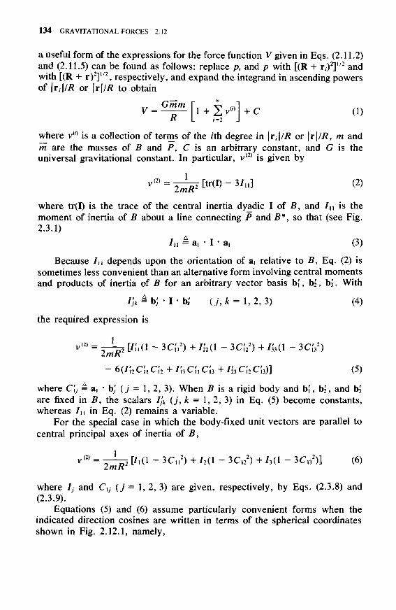
1 3 4 GRAVITATIONAL FORCES 2.12
a useful form of the expressions for the force function V given in Eqs. (2.11.2)and (2.11.5) can be found as follows: replace p{ and p with [(R 4- r,)2]1/2 andwith [(R + r)2]1/2, respectively, and expand the integrand in ascending powersof \Ti\/R or \r\/R to obtain
l (1)1=2 J
where v(0 is a collection of terms of the ith degree in |r,|//? or \r\/R, m andm are the masses of B and P, C is an arbitrary constant, and G is theuniversal gravitational constant. In particular, v(2) is given by
where tr(I) is the trace of the central inertia dyadic I of B, and In is themoment of inertia of B about a line connecting P and 5*, so that (see Fig.2.3.1)
7,i = a, • I • a, (3)
Because Iu depends upon the orientation of aj relative to B, Eq. (2) issometimes less convenient than an alternative form involving central momentsand products of inertia of B for an arbitrary vector basis b[, b^, b3. With
Fjk = bj I • bl (j,k= 1,2,3) (4)
the required expression is
v(2) = ~ 2 [/;,(i - 3d,2) + / M I - 3c;22) + /Mi - 3c;3
2)
- 6(/;2 c[, c;2 + /[3 Cn c;3 + /;3 c;2 c y ] (5)
where C\j - a, • bj (j = 1, 2, 3). When £ is a rigid body and b[, b2, and b3
are fixed in B, the scalars Ijk (j9 k = 1, 2, 3) in Eq. (5) become constants,whereas 7n in Eq. (2) remains a variable.
For the special case in which the body-fixed unit vectors are parallel tocentral principal axes of inertia of B,
v(2) = T - J - 5 [7.(1 - 3Cn2) + 72(1 - 3C12
2) + 73(1 - 3C132)] (6)
LYYlK
where Ij and CXj (j = 1, 2, 3) are given, respectively, by Eqs. (2.3.8) and(2.3.9).
Equations (5) and (6) assume particularly convenient forms when theindicated direction cosines are written in terms of the spherical coordinatesshown in Fig. 2.12.1, namely,

2.12 FORCE FUNCTION FOR A SMALL BODY AND A PARTICLE 1 3 5
V ( 2 ) =
4mR: [{Hi +122 ~ 2 / y (3 sin2/3 - 1) - 3(71, -1'12) cos2j3 cos 2X
- 6(/;2 cos2/3 sin 2A + 7[3 sin 2/3 cos A + 7^ sin 2/8 sin A)] (7)and
72 - 2/3) (3 sin2/? — 1) — 3(Z, — 72) cos20 cos2X] (8)
Often it is desirable to introduce some measure of the dimensions of Binto v(2) in order to obtain an expression involving dimensionless constantsand dimensionless variables. If the symbol RB is assigned to the selectednormalizing dimension, and the symbols
1
2mRB
(7, + 72 - 273)
and
A€ = ~
2mRB(11 - h)
(9)
(10)
are introduced, then Eq. (8) may be rewritten
j
v« = - -
If F is the approximation to F defined in Eq. (2.3.6), then F can beexpressed as

136 GRAVITATIONAL FORCES 2.12
F = VR V (12)where V is given by
V [ 1 v ] + c
Rand R is the position vector of B* relative to P. In other words, V is a forcefunction suitable for dealing with the gravitational interaction of a body anda remote particle when F is used to approximate F.
Derivations Replacing p in Eq. (2.11.5) with [(R + r)2]1/2 gives
R2 + 2 R T + r2)'172 p dr + C (14)
Introducing q as q = r/R, noting that R/R = a,, and applying the binomialseries, convergent for |2R • r + r2! < 1, leads to
V = ^L f ( 1 + 2 a i • q + q V / 2 p dr + C
= -^-J [l " a, • q - - q2 + - (a, • q)2 + • • • jp </T + C
G7n f f a, f
l J p / - J r p < / T
} C (15)
Now,
j pdr = m (16)
f rp rfr = 0 (17)
and
| [r2 - 3(a, • r)2]p dr = 3 | [r2 - (a, • r)2]p dr - 2J r2p dr (18)
Furthermore,
J r ? - ( a , T ) 2 ] p d T = /I, (19)
and
2 [ i p rfr = tr(I) (20)
Hence,

2.12 FORCE FUNCTION FOR A SMALL BODY AND A PARTICLE 137
[r2 - 3(a, • r)2]p dr = 3/,, - tr(I) (21)(18-20)
(15-17,21) R ' ^ « - » z J I v '
and
in agreement with Eqs. (1) and (2).Equation (5) follows directly from Eq. (2) when / u is formed in accordance
with Eq. (3) and I is expressed as
(23)
With the aid of these relationships, one finds that3 3 3
V( 2 ) =
,',(! - 3C,',2) + / i ( l - 3C,'22) + /(,(! - 3C,'3
2)2mR2
— 3 (7[2 C(i C[i + 7|3 C(i C13 + /21 C12 C{i + I23 C\2 C\3
+ I' C C + / ' C" C )1 (24)
which, since /^ = / ^ , reduces to Eq. (5). Equation (6) is merely the specialcase of Eq. (5) with vanishing products of inertia and new notation, and Eqs.(7) and (8) are the special cases of Eqs. (5) and (6) in which the relationship
aj = - cos/3 cosX b; - cos/3 sinX b2 - sin/3 b3 (25)
(see Fig. 2.12.1) has been used to obtain for the required direction cosinesthe expressions
C(, = -cos/3cosX C{2= -cos/3sinX C,'3 = - sin/3 (26)
Substitution from Eqs. (26) into Eq. (5) produces
v(2) = —l—j\I[\(\ ~ 3 cos2/3 cos2X) + /22(1 - 3 cos2/3 sin2X)2mR
+ 7^3(1 - 3 sin2/3) - 6(7J2 cos2j8 cosX sinX
4- 7(3 cos/3 cosX sin/3 + 7^ sin/3 cosjS sinX)]
(continued on next page)

138 GRAVITATIONAL FORCES 2.12
- /^(3 sin2/? - 1) - 6\l[2 c o s 2 / ? ^ sin2x)
+ In cos X (- sin 2#) + I-a sin X (- sin 2/3) 11
^ W I P " 3(1 - sin2/?)] + 722[2 - 3(1 - sin2/3)]
- 2/fc(3 sin2/3 - 1) - 3(/[, - 722) cos2/3 cos2X
- 6(/,'2 cos2/3 sin2X + 7|3 cosX sin 2/8 + 723 sinX sin
n + ^ - 2 /^ (3 sin2/8 -
- 3(/{, - I'-a) cos2j3 cos2X - 6(/,'2 cos2/3 sin2X
+ /J3 sin 2/3 cos X + I'n sin 2/3 sin X)] (27)
in agreement with Eq. (7). Equation (8) is the special case of Eq. (7) involvingprincipal moments of inertia, and Eq. (11) is a restatement of Eq. (8) in termsof the symbols defined in Eqs. (9) and (10).
Differentiation of Eq. (13) gives
i- vo>] + ^innL vRv(2) (28)
From Eqs. (2.9.8) and (2.9.9),
and from Eq. (2), with 7n replaced by a, • I • ai,
VRv(2) = l—3 VR/?[tr(I) - 3a, • I • a,] - - ^ VRa, • I • a,
= - - W ["itrO " 6 a ' a ' • I ' a, + 31 • a,] (30)(29) mR
Substituting from Eqs. (29) and (30) into Eq. (28) and using Eq. (2), one canthus write
VRV = - ^ {a, + ^ 5 [«ttr(D - 3a,a, • I • a,]
(continued on next page)

2.12 FORCE FUNCTION FOR A SMALL BODY AND A PARTICLE 139
—jg [aitr(I) - 6a, a, • I • a, + 31 • a,]}
(2.3.3) R (2.3.6)
which establishes the validity of Eq. (12).
(31)
Example Figure. 2.12.2 shows a thin ro<^2? of mass m and a particle Pof mass m. If the distance R between P and the mass center B* of Bis larger than the length L of B, and if B is idealized as matter distributedalong a straight line segment, then, in accordance with the resulte of theexample in Sec. 2.3, the gravitational force F exerted on B by P is ap-proximately equal to a force F given by (see Fig. 2.12.2 for \jj and aO
F = -Gmm [ L2 L2 1
a, + g^5 (2 - 3 sin21/0 a, - ^ sin 2^ a2j
(32)
A force function V such that Eq. (12) is satisfied can be found by using
mL2
1 = 12(33)
Pirn)Figure 2.12.2

140 GRAVITATIONAL FORCES 2.12
to evaluate tr(I) and In as
tr(I) = f /n = a, • I • a, = f sin2 * (34)
after which substitution into Eqs. (2) and (13) gives
+ C ( 3 5 )
In order to obtain this result by means of Eq. (11) rather than Eq.(2), one must recognize by comparing Figs. 2.12.1 and 2.12.2 that now/3 = 0 and A = - * . With
mL2
7 , = 0 7 2 =/ 3 = — (36)
Eq. (11) thus provides
v(2) = ~ r ( - ^ ) (~1) + 9(~I7") (I)cos2* (37)
where _ . 2
24/?and
/ = 1 / mL2 2mL\ L<9) 2mRB
2\ 12 12 / 24/
£2€ w " 2mRB
2 V " " I T J = 8#7 (39)
Although it is customary to make a specific choice for RB (such asRB = L12) in order to obtain numerical values for J and €, it is apparentthat in combining Eqs. (37)-(39) one can cancel RB from v(2), so that thechoice of RB does not affect v(2); that is,
(2) = *L(L . ±
+ 3(1 - 2 sin2^)] = ^ 5 (2 - 3 sin2*) (40)
and substitution from Eq. (40) into Eq. (13) leads to Eq. (35).To verify that Eq. (12) is indeed satisfied, one may proceed as follows:
(35)
CJnm L2 L2
[ 7 (2 - 3 sin2 *)VRR - —2 sin2* V,*] (41)
Now,R = R (cos * b, - sin i// b2) (42)
Hence,

2.13 FORCE FUNCTION IN TERMS OF LEGENDRE POLYNOMIALS 141
VRR = VR /?(cos if* bi - sini// b2)
+ /?(•"• sini//VRi/j bi — cost// VRi// b2) (43)
or, in view of Eqs. (2.9.7) and (2.9.8),
U = ai(cosi/> b! — sini/i b2) - R VRi/i(sini/j bi + cost/i b2)
= a, a, - RVR\lf a2 (44)
Dot-multiplication with a2 thus gives
a 2 = -RVR$ (45)
and using VRR = a, and VRi// = — a2//?, one obtains
VRV(41)
2.13 FORCE FUNCTION IN TERMS OFLEGENDRE POLYNOMIALS
The quantities v(0 (i = 2, . . . , oo) appearing in Eq. (2.12.1) can be expressed as
vW = 3 f (TTY ^/(cosa)p rfr (i = 2, ..., oo) (1)
= " ^T1 [ai + 5^2 (2 " 3 sin2i/0a! - ^ r sin2i//a2l = F (46)41) K I OK OK J (32)
where r is the distance from B* to a generic point P of B (r must be smallerthan R for all points of B), p is the mass ^tensity of B at P, a is the anglebetween the lines joining B* to P and to P (see Fig. 2.13.1), P,(cosa) is aLegendre polynomial, to be defined presently, and dr is the volume of adifferential element of the figure occupied by B.
By definition, the Legendre polynomials Po(y), Pi(y), . . . are given by
Po(y) = 1 (2)
1-3 ( " - U f ' W - Q -2
/ ( / - 1 K / - 2 X / - 3 ) ,-4 + . . . 1 / = ! , ( 3 )
(2/ - l)(2i - 3) • 2 • 4 ^ J V ' ' ' W
where the last term in the bracketed series involves y° if i is even and y1 if/ is odd. For example,
3v2 - 1 5v3 - 3yPi(y) = y ft(y) = ^j— ft(y) = 2 (4)
The integrand in Eq. (1) depends on the position of P relative to B becauseit involves the angle a._To express v(0 in terms of integrals that are indepen-dent of the position of P and, therefore, can be evaluated as soon as the mass

142 GRAVITATIONAL FORCES 2.13
Figure 2.13.1
distribution of B has been specified, one works with associated Legendrefunctions, defined as
Pj(y) * (2Q!(i-yV/2 r _, _ (i-na-j-i) , ,_2
27!(/ -j)\ L (2/ - 1) • 2 y
0-7)(/-7-l)0'-y-2)(/-^3) 1(2/ - l)(2i - 3) • 2 • 4 J J
(/,y = 0, 1, ...,oo) (5)
where the last term in the bracketed series involves y° if i -j is even andyl if i -j is odd. For example,
/VOO = (1 - y2)1'2 P2l(y) = 3y(l - y2)m P2
2(y) = 3(1 - y2) (6)
and, as can be seen by reference to Eq. (3),
The mass distribution of B is taken into consideration via constants Q andSij defined as
Co = j(j^j pi (sinr)p dr (8)
i = 2 , . . . , o o ; < / = i , . . . , o o ) ( 9 )

2.13 FORCE FUNCTION IN TERMS OF LEGENDRE POLYNOMIALS 143
( 1 = 2 , . . . , o o ; J = 1 , . . . , o o ) ( 1 0 )
where /A, y, and r are the spherical coordinates of P shown in Fig. 2.13.1,and RB, an arbitrary quantity having the dimensions of length, is introducedto render Q and Sy dimensionless. Expressed in terms of the quantities justdefined, v(0 is given by
cosjX + Su sin/A) (i = 2, . . . , oo) (11)
where A, /3, and R are the spherical coordinates of P shown in Fig. 2.13.1.Substitution from Eq. (11) into Eq. (2.12.1) leads directly to
V = P{ 2[(^) cosyx + Stj sin/xl j + C (12)
Here V is written in the form adopted as a standard representation by theInternational Astronomical Union for the case when B is the Earth, in whichcontext RB is taken to be the Earth's mean equatorial radius. Since the seriesconverges only for R >RB, it fails to converge for points in a certain regionof space above the surface of the Earth, this region varying in thickness fromzero at the equator to approximately 20 km at the poles.
If B is axisymmetric and the symmetry axis of B is the line y = TT/2 inFig. 2.13.1, then Su = 0 (ij = 0, . . . , oo), Q = 0 (ij = 2, . . . , oo), and thesymbol / , is traditionally introduced as
// = -C,0 ( i = 2 , . . . , « ) (13)Only the j = 0 term in Eq. (12) survives under these circumstances, so that,referring to Eq. (7), one can write
V = £|2L[i - | ( ^ ) Wsinf l ] + C (14)
Derivations If p is the distance between P and P in Fig. 2.13.1, thenp2 =R2 - 2rR cos a + r2 and
V = ^ f [ l - 2£cos« + (£)TprfT + C (15)(2.H.5) R J L R \K / J
Use of the identity!00
(1 - 2 y J t + y 2 ) - | / 2 = 2 / ^ ( * ) (16)o
which applies if \y\ < 1, permits the replacement of Eq. (15) with
tO. D. Kellogg, Foundations of Potential Theory, Ungar Publishing Company, New York,1929, p. 128.

144 GRAVITATIONAL FORCES 2.13
V = - 2 f (£ ) ' P,(cos a)pdr + C (17)R i=Q J \K I
if rlR < 1 for all points of B. The first two terms of Eq. (17) simplify since[see Eqs. (2) and (4)] P0(cosa:) = 1 and Pi (cos a) = cos a, so that
)ll) P o ( C ° S a)f>dr =
andr / r \ 1 \ C
<dT
The last integral vanishes by virtue of the definition of B* as the mass centerof B. Consequently,
v = ^HL\l+±±l(L.]pi{cosa)pdT\+c (20)d7-i9) R L i=im J \RJ J
Equation (1) follows directly from this relationship and Eq. (2.12.1).To establish the validity of Eq. (11), we first form cos a by dot-multiplying
a_unit vector directed from B* to P with a unit vector directed from B* toP, which gives
cosa = sin/3 siny + cos/3 cosy cos(X - /JL) (21)
and then take advantage of the fact that, with the aid of Eq. (21), one maywritet
P,(cosa) =P,(sin/3)/>,(siny) + 2 ^ li-Z^jp/fsinjS) P/fsiny) cos[j(\ - /*)]
( i = 2 , . . . , » ) (22)so that substitution into Eq. (1) yields
(i) Pt(sinp) f ( r \= m j ^
+ — ?+ sin/Xj ^ j P/fsiny) sin/>
(8-10) \ R
) ' 5 > Q cosj'A + 5V sin/A) (/ = 2, . . . , » ) (23)
which, in view of Eq. (7), is seen to be equivalent to Eq. (11).
tW.E. Byerly, An Elementary Treatise on Fourier Series and Spherical, Cylindrical, andEllipsoidal Harmonics, Ginn and Company, Boston , 1893, p. 211.

2.13 FORCE FUNCTION IN TERMS OF LEGENDRE POLYNOMIALS 145
Example An approximate force function V is to be constructed for thegravitational interaction of a uniform circular ring B of radius r and massm and a particle P of mass m, the particle being situated as shown inFig. 2.13.2, where Xx, X2, X3 are mutually perpendicular lines.
Since the ring is axisymmetric, Eq. (14) may be used. This requiresevaluation of 7, and P,(sin/3) for i = 2, 3, . . . , » . We shall consider only/ = 2 ,3 ,4 .
From Eq. (13),
£ / ( £ ) T (24)
(25)
(26)
(27)
Setting y = 0 (see Figs. 2.13.1 and 2.13.2), we have
P2(siny)=P2(0) = - \(4) 2
so that
while
P2(sin/8) = - ( 3 s i n 2 / 3 -(4) 2
Proceeding similarly, one finds that J} = 0 and that
B(m)
Piffi)
Figure 2.13.2

146 GRAVITATIONAL FORCES 2.14
/4 = ~ i G r ) (28)
whileP4(sin0) = I (35 sin4 0 - 3 0 sin2 0 + 3) (29)
(3) ©
Hence,
(30)(j) (35 sin40 - 30 sin20 + 3)] + C
2.14 FORCE FUNCTION FOR TWO SMALL BODIES
When the distance R between the mass centers B* and 5* of two (not nec-essarily rigid) bodies B and B exceeds in the case of each body the greatestdistance from the mass center to any point of the body, so that the resultantof the system of gravitational forces exerted on B by B can be approximatedby a force F defined as [see Eq. (2.4.14)]
F ^ - ^ » [ . I + f« + f«] (1)
where G is the universal gravitational constant, m and m are the masses ofB and B, a{ is a unit vector directed from B* to B* , and f(2) and f(2) are givenby Eqs. (2.4.2) and (2.4.3), then a force function V such that
F =VRV (2)where R = R^, is given by
V = < ^ [ l + V ( 2 ) + v ( 2 ) ] + C (3)R
withv<2) = ^ [ t r ( D - 3 / u ] (4)
and
where tr(I) and tr(f) are the_traces of the central inertia dyadics of B and B,respectively, while In and In are, respectively, the moments of inertia of Band B about the line connecting B* and B*.
Derivation Differentiating Eq. (3) with respect to R and then proceeding asin the derivation of Eq. (2.12.13), one arrives at

2.15 FORCE FUNCTIONS FOR A CENTROBARIC BODY 147
Gmm I 1( + - 5a,
131 • a,]
— [tr(I) - 5ai • I - a 1 ] a 1 + 3 I - a I } ) (6)
and use of Eqs. (2.4.2) and (2.4.3) then gives
VR V = - ^ - ^ [ a , + f(2) + f(2)] = F (7)
Example The example in Sec. 2.4 deals with an approximation F to thegravitational force exerted on a rectangular parallelepiped by an oblatespheroid. To construct a force function V that satisfies Eq. (2), note thatthe moments of inertia Iu and In can be expressed as
> - e 2 + (a, -bOV] (8)
2 - i 2 + (a, -b0 2 i 2 ] (9)
while 2
tr(I) = ^ - (3 - e2) (10)o
and^ 3 - i 2 ) (11)
V, formed by substituting into Eqs. (3)-(5), is given by
^ 2 } (12)and it may be verified that differentiation of V with respect to R [usingEqs. (2.9.8) and (2.9.9)] leads to F as given by Eqs. (2.4.14) together withEqs. (2.4.26) and (2.4.29).
2.15 FORCE FUNCTIONS FOR A CENTROBARIC BODY
Since for purposes of dealing with gravitational effects a centrobaric body (seeSec. 2.5) may be replaced with a particle situated at the mass center of thebody, force functions suitable for dealing with the gravitational interaction ofa centrobaric body and a particle, a centrobaric body and any body whatso-ever, or a centrobaric body and a remote body can be obtained directly fromEqs. (2.10.2), (2.11.2), (2.11.5), (2.12.1), (2.13.12), or (2.13.14).

148 GRAVITATIONAL FORCES 2.16
Figure 2.15.1
Example The gravitational force F exerted by a uniform sphere S of massM on a dumbbell of mass 2m (see Fig. 2.15.1) can be expressed as
F = VRV (1)with
V 2 = 2 GMm{[(R + Ln)2]-1/2 + [(R - Ln)2]"1/2} + C (2)
where n is a unit vector directed as shown in Fig. 2.15.1.
2.16 FORCE FUNCTION FOR A BODY AND A SMALL BODY
When the distance between the mass centers B* and B* of two bodies B andB exceeds the greatest distance from_#* to any point of B, and a forcefunction V(p) for the force exerted by B on a particle of unit mass at a point/^situated as shown in Fig. 2.16.1 is available, then thereexists a functionV(R), where R is the position vector of B* relative to B*, such that the
resultant of jill gravitational forces exerted by B on B can be approximatedby a force F expressed as
F = V V(R) (1)
where the symbol V denotes differentiation with respect to R. The functionV(R) is given byt
V(R) = mV(R) - ^ I : VW(R) + C (2)
where m is the mass of B, I is the central inertia dyadic of B, and C is anarbitrary constant.
tThe double dot product in Eq. (2) is defined such that, for two dyads U1U2 and V1T2,(U1U2) : (V1V2) = (ui • vi)(ii2 * V2); and it obeys the distributive law when applied to dyadics:
(aja2 + bib2 + * ' *) : (Ai A2 + B1B2 + • • ) = aia2 : Ai A2 + aia2 : B1B2 -I- * ' "
+ bib2 : A1A2 + bjb2 : B1B2 + • • *

2.16 FORCE FUNCTION FOR A BODY AND A SMALL BODY 149
Figure 2.16.1
Derivations The gravitational force d¥ exerted by B on a differential elementof B at P can be expressed as ,
d¥ = \Vpdr(2 .11.1)
(3)
where p is the mass density of B at P while dr is the volume of the element.Consequently, the resultant F of all gravitational forces exerted by B on Bis given by
F = dr (4)
To obtain the desired approximation F to F, one can expand V(p) in aTaylor series about p = R, retaining only terms up to and including those ofdegree 3 in |r|, where r = p - R (see Fig. 2.16.1); differentiate with respectto p; and then carry out the integration indicated in Eq. (4). These tasks arefacilitated by introducing a function W(r) = V(r + R), which permits one towrite
and= VrW
(2.9.5)
(4.5) J
(5)
(6)
If n,, n2, n3 are any mutually perpendicular unit vectors and r,• = r • n,(i - 1, 2, 3), the Taylor series expansion of W about r = 0 can be written(using the summation convention)
W = W(0) + r,W,, + ^ r,rj — W,ijk (7)
where

150 GRAVITATIONAL FORCES 2.16
A(1 = 1,2,3) W,tj =
r=0 r( dr,(/,./ = 1,2, 3) (8)
r=0
and so forth. Differentiating E q . (7) with respec t to r / 5 one obta ins
^- = o + 8aW9i + ;Jr(8,/#v + r,OA*/ (7,8) 2!
+
^ ,,7/ + • • • (9)
Hence,
2=^ (Vr W)r=0 + r • (VrVrW)r=0 + \ rr : (VrVrVrW)r=0 + ' ' ' (10)
Substituting into Eq. (6) only the terms here displayed explicitly and notingthatB
jpdr = m jrpdT = 0 [IT p dr = tr(I)U - I (11)
where U is the unit dyadic, one can now write
F = m(VrW)r=0 + ^ tr(I)U - i ] : (VrVrVrW)r=0 (12)
or, after using Eq. (5),
F = (vp{mV + i [ i tr(I)U - i ] : VpVpv} + c ) (13)
where C is an arbitrary constant. Now, differentiating V(p) with respect top and then setting p equal to R is precisely the same as differentiating V(R)with respect to R. Hence, if V denotes differentiation with respect to R, then
F = vjmV(R) + i | ^ tr(I)U - i l : VVV(R) + c\ (14)
and, since
U : VVV(R) =,V • VV(R) = V2V(R) 2 = ? 0 (15)
Eq. (1) follows immediately if Eq. (2) is used to form V(R).
Example When V(R) is available in the form of an explicit functionV*(R, X, /3) of the spherical coordinates R, k, /3 shown in Fig. 2.16.2,where ni, n2, n3 are any mutually perpendicular unit vectors fixed in a

2.16 FORCE FUNCTION FOR A BODY AND A SMALL BODY 151
Figure 2.16.2
reference frame N, one can formulate F as follows: let ai, a2, a3 be mutuallyperpendicular unit vectors pointing, respectively, in the directions inwhich B* moves when R, A, @ increase one at a time. Define Ijk as
/ ^ a y - I - a * U,k = 1,2, 3)
and Qij (ij = 1, 2, 3) and V*(R, X, p) as
Q22 = -^3V* sec2/3 d2V* tan p dV*
+R dR R2 dk2
1 d2V*
R2
R dR R2 dp2
d2V*
andV*(i?, X, /3) = mV* - I (/,,(?„ + Z22&2 + /33G33)
(16)
(17)
(18)
(19)
(20)
(21)
(22)
(23)

152 GRAVITATIONAL FORCES 2.16
Then
= a i a2
sec i3 1 aV*(24)
dR ^ R dk R dpTo establish the validity of Eq. (24), it is helpful to note that the partial
derivatives of a t, a2, a3 with respect to R, X, p in N are given by
dR
da2
dR
da3
^R
dk
da2
dk
da3
~dk
dpaa2
a/3da3
Jp
0 c/8 a2 a3
0 -c/3 ai + s/3 a3 0
0 -sp a2 -a i
(25)
Also, proceeding as in the example in Sec. 2.9, one can verify that, if= V*(R,X,j8), then
dV* l av* l av*W ( R ) = a, - ^ - + a2 -^-777 ^ ^ + a3 - •ax dp
(26)
Differentiating once more with respect to R and using Eq. (25), one thenfinds that
ii (27)
(28)
(29)
Similarly, the inertia dyadic I can be expressed as3 3
I =
Hence,(16) j = l k=l
I : VW(R) = InQn + I22Q22 + I33Q33(27,28)
With V* in place of V(R), one thus obtains from Eq. (2),
V(R) = mV* -\{IuQu+ hlQzt + /33 033)
- (I12Q12 + hiQ2j + InQn) + C (30)
Moreover, defining V*(R, X, P) as the right-hand member of this equa-tion, which yields Eq. (23), one can write [compare with Eq. (26)]
VV(R) = aidV
dR L R dk
Substitution into Eq. (1) then produces Eq. (24).
dV* av*(31)

2.17 EXPRESSIONS FOR THE MOMENT EXERTED ON A BODY BY A PARTICLE 1 5 3
2.17 FORCE FUNCTION EXPRESSIONS FOR THE MOMENTEXERTED ON A BODY BY A PARTICLE
Force functions (see Sees. 2.10-2.16) can be used in connection with gravita-tional moments. For the interaction of a particle and a (not necessarily rigid)body, the moment M given by Eq. (2.6.1) can be expressed as
M = - R x VV (1)
where V(R) is given by Eq. (2.11.2) or by Eq. (2.11.5) and W = VRV; or,if W is defined as W(al9R) = V[R(a,,/?)], M is given also by
dWM = - a, x — (2)
Similarly, for M as defined in Eq. (2.6.3), one can write
M = - R x VV (3)
where V is given by Eq. (2.12.13); or M can be expressed as
~ dWM = - a i x — ( 4 )
where W is a function of ai and R, defined in terms of the moment of inertia / n
of B about the line connecting P and B* as
^ c
Derivations Equation (1) is obtained by substituting from Eq. (2.11.1) into Eq.(2.6.1); and Eq. (2) then follows if one uses Eq. (2.9.13).
Referring to Eqs. (2.3.6) and (2.3.3), one can write
- Ra{ x F = —rai x I • a, = M (6)R (2.6.3)
and, replacing /?a, with R, one then arrives at Eq. (3) after using Eq. (2.12.12)to eliminate F.
If W is defined as
?) (7)
then __
and

1 5 4 GRAVITATIONAL FORCES 2.17
or, since tr(I) is independent of ai,
Consequently,
in agreement with Eq. (4).
M = - a , x f0) da.
(10)
(11)
Example In Fig. 2.17.1^ a,, a2, a3 and b,, b2, b3 are dextral sets of or-thogonal unit vectors, P is a particle of mass m, and B is a rigid body ofmass m. The unit vector a, is chosen such that the position vector R of themass center B* of B relative to P is given by R = Ra{; and bi, b2 , b3 arefixed in B.
If 0,, 02, 03 are body-two orientation angles (see Sec. 1.7) for B in areference frame in which aj, a2, a3 are fixed, one can express R as
, 0,, 02, 03) = /? (c2 b, + s2s3 b2 + s2c3 b3)(1 .7 .31)
(12)
Given a force function V(R) for the gravitational force exerted on B by P,one can, therefore, define a function W(R,6X ,02,03) as
W(R,0l90290>)±V\R(R902,e>)] (13)
The moment M exerted by P on B about £* then can be expressed interms of partial derivatives of W with respect to 02 and 03 by proceedingas follows.

2.17 EXPRESSIONS FOR THE MOMENT EXERTED ON A BODY BY A PARTICLE 155
Partial differentiation of R with respect to R, 02, and 03 in B yields
dR— = c2bi + s2s3b2 + s2c3b3 (14)dR (12)
r)R— = / ? ( - s.b, + c2s3b2 + c2c3b3) (15)dO2 (12)
— = R(s2c3 b, - s2s3 b3) (16)OU3 (12)
From Eq. (2.9.6),
I ? = W • | § = c2W • b, + s2s3W • b2 + s2c3W • b3 (17)dR dR (14)
^ = VV • — = / ? ( - s 2 W • b! + c 2 s 3 W • b2 + c 2 c 3 W • b3) (18)302 dd2 (15)
S " = W ~ = /?(s2c3W • b2 - s2s3W • b3) (19)80} d03 (16)
Equations (17)—(19) may be solved for the dot products W • b,,W • b2, W • b3; and W then can be expressed as
W = W • b,b, + W • b2b2 + W • b3b3
/dW 1 dW \. (BW 1 dW idW
aws3\) b (20)
Consequently,
dW (dW a ^
(1) (12,20) ^ ^ 3 \ d # 2 O^3 S2
This equation does not involve 9\ explicitly; but, referred to a,, a2, a3,rather than to b,, b2, b3, M is given by [use Eq. (1.7.31)]
( 2 2 )
which brings the dependence of M on dx into evidence.

156 GRAVITATIONAL FORCES 2.18
2.18 FORCE FUNCTION EXPRESSION FOR THE MOMENTEXERTED ON A SMALL BODY BY A BODY
When the distance between the mass centers B* and B* of two bodies B andB exceeds the greatest distance from B* to any point of B, and a forcefunction V(p) for the forces exerted by B on a particle of unit mass at a pointP situated as shown in Fig. 2.16.1 is available, then the system of gravitationalforces exerted by B on B produces a moment about B* that is given approx-imately by
M = - I x VW(R) (1)
where I is the central inertia dyadic of B, R is the position vector of B* relativeto B*9 and V denotes differentiation with respect to R.t
Derivation The system of gravitational forces exerted by B on B produces amoment M about B* such that
M = [r x Vp V p dr (2)
Expanding VPV in a Taylor series by proceeding as in the derivation of Eq.(2.16.10), one obtains
VPV = W(R) + r • VVV(R) + • • • (3)
so that, retaining only terms displayed explicitly, one arrives at
M = fr x VV(R)p dr + [r x [r • VW(R)]p dr (4)(2) J J
The first integral vanishes because r originates at the mass center of B*, and
r x [r • VW(R)] = rr x VVV(R) (5)Hence,
M = ( (rrp dr) x VW(R) = |"y tr(I)U - i l x VW(R) (6)
But VW(R) is a symmetric dyadic, and the cross-dot product of U and anysymmetric dyadic is equal to zero. Hence Eq. (6) reduces to Eq. (1).
Example: When V(R) is available in the form of an explicit functionV*(R, X, J3) of the spherical coordinates R, X, )8 shown in Fig. 2.16.2, onecan find M as follows.tThe cross-dot product in Eq. (1) is defined such that, for two dyads U1112 and V1V2,
(U1U2) ?(viV2) = (m x vi)(u2 • V2); it obeys the distributive law when applied to dyadics:( y• • •) x (A1A2 + B1B2 + • • • ) = aia2 x Ai A2 -I- aja2 x B1B2
+ b i b 2 x A1A2 + b 2 b 2
x B1B2 +

2.18 EXPRESSION FOR THE MOMENT EXERTED ON A SMALL BODY BY A BODY 157
Differentiate Eq. (2.16.2) to verify that
VW(R) = t 2 Q.apj (7)
where Qu (i,j = 1, 2, 3) are given in Eqs. (2.16.17)-(2.16.22). Next, let
Ijk = ay • I • a* 0", * = 1, 2, 3) (8)Then
(i)
+ VnQn ~ Qi^In + (7j3 - Iu)Qn - (Qn - fiiO/si]*
+ [/3lG23 " S3./23 + (/„ " /22)e.2 " (Qu ~ e22)/,2]a3 (9)


CHAPTER
THREE
SIMPLE SPACECRAFT
This chapter deals with two kinds of spacecraft, namely, those that can be modeledas single rigid bodies and those forming simple gyrostats. Such spacecraft haveplayed an important role in the exploration of space and, by studying their behavior,one can learn a great deal that is of interest also in connection with more complexspacecraft.
Throughout this chapter, the formulation of dynamical equations of motion isbased on the angular momentum principle. Hence, knowledge of Lagrange's equa-tions or other methods of analytical mechanics is not needed. In the first five sec-tions, spacecraft consisting of a single rigid body are studied, primarily with a viewto determining the effects of gravity and orbit eccentricity on the attitude motionsof such vehicles. The remaining sections, devoted to gyrostats, contain materialthat is central in connection with dual-spin spacecraft.
3.1 ROTATIONAL MOTION OF A TORQUE-FREE,AXISYMMETRIC RIGID BODY
When an axisymmetric rigid body B (see Fig. 3.1.1) is subjected to the action offorces whose resultant moment about the mass center B* ofB is equal to zero, therotational motion of B in a Newtonian reference frame AT can be described in termsof two motions of simple rotation (see Sec. 1.1), each performed with an angularvelocity of constant magnitude. One of these is the motion of B in a reference frameC in which the angular momentum H of B relative to S* in AT (a vector fixed in N)and the symmetry axis of B are fixed; the other is the motion of C in N. Theassociated angular velocities are called the angular velocity of spin and the angular
159

1 6 0 SIMPLE SPACECRAFT 3.1
Figure 3.1.1
velocity of precession, respectively, and can be expressed as
and
ccoB = sc3
N<oc =ph
(1)
(2)
where h is a unit vector having the same direction as H (see Fig. 3.1.1); C3 is a unitvector parallel to the symmetry axis of B\ s and/?, called, respectively, the spinspeed and the precession speed, are defined as
k
and
A H
(3)
(4)
where H is the (constant) magnitude of H; / and J are the moments of inertia of Babout lines passing through B* and respectively perpendicular and parallel to c3; and0)3 is the value of NCJB • c3 at time t = 0.
To describe the orientation of B in TV for t > 0, one can let ni, n2, n3 be a dex-tral set of orthogonal unit vectors fixed in N, choosing these such that n3 = c3 at

3.1 ROTATIONAL MOTION OF A TORQUE-FREE, AXISYMMETRIC RIGID BODY 1 6 1
t - 0 and n2 has the same direction as H X n3; and introduce bi, b2, b3 as a setof unit vectors fixed in B, with b, = n, (/ = 1, 2, 3) at t = 0 (see Fig. 3.1.1). TheEuler parameters eu . . . , e4 (see Sec. 1.3) relating n,, n2, n3 to bu b2, b3 thencan be expressed as
, pt st€\ = —sin <p sin — cos —
i Pt . ste2 = sm cp sin — sin —
pt st pt . st£ sine3 = cos (f) sin — cos — 4- cos — sin —
, pt . st pt ste4 = —cos q> sin — sin — 4- cos — cos —
where </>, the angle between h and c3 (see Fig. 3.1.1), is given by
Js(f> = cos
H = cos- 1
(/ ~ J)p0 < (j> < 77
(5)
(6)
(7)
(8)
(9)
The rotational motion of B can be described also by reference to the rolling mo-tion of a spheroid cron a plane TT, the so-called Poinsot construction. Specifically,let a be a spheroid whose center O is fixed in N, whose principal semidiameters are
Figure 3.1.2

1 6 2 SIMPLE SPACECRAFT 3.1
equal to kl~l/2 and fc/~1/2, where k is any constant, and whose symmetry axis (axisof revolution) is at all times parallel to c3 (see Fig. 3.1.2); and let TT be the tangentplane to a at Q, the point of intersection of the surface of a with the ray that passesthrough O and has the same direction as N<oB at some instant f *. Then TT is a uniqueplane, fixed in TV at a distance d = k(N(oB • H)l/2/H from O and perpendicular toH; and the rotational motion of B in N can be duplicated by a rolling motion of aon TT. The loci traced out by Q on a and on TT during such rolling are called, respec-tively, the polhode and the herpolhode.
Finally, one can also establish a correspondence between the rotational motionofBinN and a rolling motion of one cone upon another. To this end, let a be aright-circular cone whose vertex O is fixed in N, whose semivertex angle a* isequal to the angle between NioB and H, and whose axis is parallel to H, as shownin Fig. 3.1.3; and let /3 be a right-circular conical surface whose vertex coincideswith O, whose semivertex angle /3* is equal to the angle between Na>B and c3, andwhose axis is at all times parallel to c3, as shown in Fig. 3.1.3, which applies ifa is a prolate spheroid. When a is oblate, refer to Fig. 3.1.4. The cones a and /3are called respectively the space cone and the body cone, and the rotational motionofBinN can be duplicated by a rolling motion of the body cone on the space cone.
Derivations In Fig. 3.1.5, bi, b2, b3 form a dextral set of orthogonal unit vectorsfixed in B, with b3 parallel to the symmetry axis of B\ and Ci, c2, c3 form a similar
Figure 3.1.3

3.1 ROTATIONAL MOTION OF A TORQUE-FREE, AXISYMMETRIC RIGID BODY 1 6 3
Figure 3.1.4
Figure 3.1.5

1 6 4 SIMPLE SPACECRAFT 3.1
set fixed in a reference frame C, with c3 = b3 for all values of the time t and c, = b,(i = 1, 2) at t = 0. The motion of B in C is thus necessarily a motion of simplerotation (see Sec. 1.1), and the angular velocity of B in C can be expressed as
c<oB = 0 c 3 (10)(1.11.5)
where 0 is the angle between bi and Ci, as shown in Fig. 3 .1 .5 .If a)i is defined as
c o i = N € o B - c i (i = l , 2 , 3 ) (11)
then the angular velocity of C in N and the angular momentum of B relative to B*in N can be expressed as
N€OC = N<0B + BiOC = N<OB ~ C*>B = 0>,C, + CU2C2 + (CU3 - 0 ) C 3 ( 1 2 )
(1.16.1) (1.11.2) (10,11)
and
H = Hh = 7o>iCi + /a>2c2 4- /a>3c3 (13)
Differentiating H with respect to t in N, one obtains
hN<oc XHdt ( i n s ) dt
(12,13) !
and, in accordance with the angular momentum principle, the coefficients of Ci, c2,and c3 in this equation must vanish. Moreover, 0may be chosen at will. If one takes
0 =
in order to simplify the coefficients of Ci and c2, one obtains from Eq. (14),
ai,. = 0 (i = l , 2 , 3 ) (16)
and, after defining cS, as
d>t = (Na>B • cf)r=o (/ = 1 , 2 , 3 ) (17)
one can write
w . = <fl. (/ = 1, 2, 3) (18)
and
7 A / /h
which is Eq. (2). Furthermore,

3.1 ROTATIONAL MOTION OF A TORQUE-FREE, AXISYMMETRIC RIGID BODY 1 6 5
A.(20)
in agreement with Eq. (1).Since H can be expressed as
H = l(hxcx + /a>2c2 + Ja>3c3 (21)
this vector has a fixed orientation in C; and the angle <f> between H and c3 is givenby
* " C O S"' ( h ' C3),li»COS"1 ^(3=4)C O S"' 7 ^ ( 2 2 )
which is Eq. (9).The unit vectors Ci and c2 always can be chosen such that Ci = iij and c2 = n2
at t = 0. As the motion of C in N is a motion of simple rotation, a matrix L suchthat at time t
[ci c2 c3] = [ni n2 n3] L (23)
therefore can be formed by using Eqs. (1.2.23)—(1.2.31) with
8 = pt \{ = -s in <f> A2 = 0 A3 = cos <f> (24)
Similarly, the motion of B in C is such that one can write
[bi b2 b3] = [ci c2 c3] M (25)
with M =(1.2.37)
cos st —sin st 0sin st cos st 0 I (26)
0 0 1
From Eqs. (23) and (25) it then follows that
[b, b2 b3] = [n, n2 n3] W (27)
where W = LM\ and, once the elements Wtj (/, j = 1, 2, 3) of W have been found,€i, . . . , e4 can be formed by letting Wy play the part of Co in Eqs. (1.3.15)-(1.3.18), which leads to Eqs. (5)-(8).
In connection with the Poinsot construction, two observations regarding thespheroid cr are in order. First, if r is the position vector from point O (see Fig.3.1.2) to a point R on the surface of cr, then the equation of this surface can be ex-pressed as
/ (r) = r - K - r - f c 2 = 0 (28)
where K is the inertia dyadic of B for B*. One way to see this is to express r andKas
r = *! Ci + *2c2 + x3c3 (29)
and K = 7c,Ci + /c2c2 + 7c3c3 (30)

1 6 6 SIMPLE SPACECRAFT 3.1
and then to carry out the dot-multiplications indicated in Eq. (28), thus obtaining
Ixx2 + Ix2
2 + /x32 = k2 (31)
which is the Cartesian form of the equation of a spheroidal surface whose axis ofsymmetry is parallel to c3 and whose principal semidiameters are equal to kl~{/2
and &/~1/2. Second, the plane that is tangent to a at R is normal to the vector V r / ;and, if U is a unit dyadic,
V r / = U K r + r K U = 2 K r (32)(28)
Now let q be the position vector of Q (see Fig. 3.1.2) relative to O, so that qcan be expressed as
q = A N<oB (33)
where A is a positive scalar. Then the plane that is tangent to a at Q is normal tothe vector v given by
v = 2K • q = 2AK • N<aB (34)(32) ^ (33)
But K • N€oB = H, and H has a fixed orientation in N. Thus, the plane that is tan-gent to a at Q is seen to have the same orientation in N regardless of the choice off*. Furthermore, since Q is a point of the surface of a,
q-K-q-^O ( 3 5 )
A2 NtoB • K • NtoB = k2 (36)(33,35)
and A = * ( W • K • W ) - " 2 = lc(NtoB • H)"1/2 (37)(36)
The distance d from O to IT (see Fig. 3.1.2) thus can be expressed as
| q - H | = A | W - H[ = * ( W • H)1/2
H (33) H (37) H ^ }
which shows that this distance is independent of the choice of f *, for Nc*B - H andH are constants [see Eqs. (11), (16), and (21)]. One must conclude, therefore, that77 is a unique plane fixed in N. Moreover, if a is made to move in such a way thatN(oa = Na)B, then a duplicates the rotational motion of B in N; and a is seen tobe rolling on IT because the velocity of the point of a that is in contact with TT isgiven by
"to" X q = A Nc*B x NCJB = 0 (39)(33)
Finally, to prove that the rotational motion of B in Af can be duplicated by arolling motion of the body cone /3 on the space cone a, it will be shown that j8 rollson a if j8 moves in such a way that N<o& = N<oB.

3.1 ROTATIONAL MOTION OF A TORQUE-FREE, AXISYMMETRIC RIGID BODY 1 6 7
Three vectors play important parts in connection with a and /3, namely, h, c3,and N€oB. These are related to each other because
Na>B = N€oc + ctoB = ph + I 1 - 7 )o>3c3(1.16.1) (1 -3 )^ \ If
(40)
Now, p is intrinsically positive [see Eq. (4)], and c3 always can be chosen such thatd>3 is positive. When this is done, the angle between h and c3 cannot exceed 90°;and, if a is a prolate spheroid, that is, if J < /, then h, c3, and Na>B are orientedrelative to each other as shown in Fig. 3.1.6, whereas, if a is an oblate spheroid,that is, if J > /, then Fig. 3.1.7 applies. By construction, the cones a and j8 thushave a contact line parallel to NcoB, as shown in Figs. 3.1.3 and 3.1.4. ifR is a pointof j8 lying on this line, and if r is the position vector of R relative to 0, then
r = ixN<oB(41)
where p is some scalar; and, when /? moves in such a way that Ntofi = N<oB, thenthe velocity of R in Af is given by
= nNa>B x N(oB =r x = nNa>B x N(oB = 0(41) ^
(42)
which means that /3 is rolling on a.
Figure 3.1.6 Figure 3.1.7

1 6 8 SIMPLE SPACECRAFT 3.1
(j)
Figure 3.1.8
Example A solid right-circular cylinder B is to be set into motion in such away that d>, the initial angular velocity of B, is parallel to the cylinder's sym-metry axis. However, an "injection" error of as much as 1° (see Fig. 3.1.8) isanticipated, and the angle between the symmetry axis at time t and the (fixed)line with which the symmetry axis coincides at t = 0 may, therefore, differfrom zero, acquiring a maximum value S that depends on the "shape factor"hlr. To study this dependence, 5 is to be plotted versus hlr for 0 ^ hlr < 2.
The symmetry axis of B has at each instant the same orientation as thesymmetry axis of the body cone (3 (see Figs. 3.1.3 and 3.1.4). Hence,
8 = 2<f> = 2(9) H
where H can be expressed as
H - l(Iu>2)2
(43)
(44)
since the unit vectors b, and b2, and thus also C| and c2, can be introduced insuch a way that a>i = 0. Consequently,
S = 2 cos(43,44) -HOW a n - ' l j ^ ) (45)
Furthermore,
^ = tan 1° = 0.017455 (46)
and, if M is the mass of B, then
MI = — (3r2 + 4h2) (47)

3.2 GRAVITATIONAL MOMENT ON AXISYMMETRIC RIGID BODY IN CIRCULAR ORBIT 1 6 9
(deg)
- —
/
V
while
Thus,
0.5 1.0 1.5 2.0h/r Figure 3.1.9
J =Mr2
[ H (*)']}Figure 3.1.9 shows the desired plot of this relationship.
8 = 2 tan"' {0.017455(45)
(48)
(49)
3.2 EFFECT OF A GRAVITATIONAL MOMENT ON ANAXISYMMETRIC RIGID BODY IN A CIRCULAR ORBIT
In Fig. 3.2.1, O designates a point fixed in a Newtonian reference frame N, B* isthe mass center of an axisymmetric rigid body B, R is the distance between O andB*, and a, is a unit vector. B is presumed to be subjected to the action of a forcesystem S such that F, the resultant of 5, and M, the total moment of 5 about B*,are given by
F = -fj.mR~2ai (1)and
M = -p a, x I • a, (2)
where fx is a constant, m is the mass of B, and I is the central inertia dyadic of B.

1 7 0 SIMPLE SPACECRAFT 3.2
Figure 3.2.1
[If \x is set equal to^Gm, F becomes equal to F as defined in Eq. (2.3.5), while Mbecomes equal to M as defined in Eq. (2.6.3). The force system 5 is then approxi-mately equivalent to the system of gravitational forces exerted on B by a particleof mass Jn at point O. ]
Due to the action of 5, the rotational motion of B in N depends on the trans-lational motion of B* in N, but not vice versa, because R appears in Eq. (2), butno variable involving the orientation of B in N appears in Eq. (1); and one possiblemotion of £* is motion in a circular orbit that is fixed in N, has a radius R, and isdescribed with an angular speed ft given by
ft = (/xR ) ' (3)
When £* moves in this fashion, the rotational motion of B in N proceeds in sucha way that
2ei = 62(o)3 - 5 + ft) — 63O>2 + €4COi
2e2 = €3(Ol + €4(O2 - €i(<&3 - 5 + ft)
2e3 = 64(0)3 - s - ft) + 6)0)2 ~ €2(JO{
2e4 = -excox - e2o>2 - e3(a)3 - s - ft)
- 6364X636!
~ 6ft2(636, + 6264)(1 - 2622 " 263
2)]
a>3 = a>3, a constant
(4)
(5)
(6)
(7)
(8)
(9)
(10)
where 6, (i = 1, . . . , 4), ajj (j = 1, 2, 3), 5, /, and 7 are defined as follows: LetCj, c2, c3 be a dextral set of orthogonal unit vectors such that c3 is parallel to the

3.2 GRAVITATIONAL MOMENT ON AXISYMMETRIC RIGID BODY IN CIRCULAR ORBIT 1 7 1
Figure 3.2.2
symmetry axis of B (c3 is thus fixed in B, but Cj and c2 need not be fixed in B), andintroduce unit vectors a2 and a3 (see Fig. 3.2.2) such that a t, a2, a3 form a dextral,orthogonal set with a2 = (Nda\/dt)il~\ so that a3 is normal to the orbit plane; letC(j — a, • Cj (i, j = 1,2,3), and form e, (i = 1, . . . , 4) in accordance with Eqs.(1.3.15)—(1.3.18), thus making e, (i = 1, . . . , 4) Euler parameters which deter-mine the orientation of a reference frame C, in which Ci, c2, c3 are fixed, relativeto a reference frame A in which ai, a2, a3 are fixed. Next, denoting the angular ve-locities of B in N and in C by N€OB and c<oB, respectively, let
A(Of = U = (11)
and
s = c<oB - c 3 (12)
which means that | | is equal to the magnitude of c(oB, since CCJB is necessarilyparallel to c3. Finally, let
and
/ = c, I • c, = c2 I c2
J = c3 • I • c3
(13)
(14)
In Eqs. (4)-(9), s and d)3 are ktfree" quantities; that is, s can be taken to be anydesired function of time and cO3 can have any constant value. As for e,, . . . , e4,

1 7 2 SIMPLE SPACECRAFT 3.2
(ou and (o2, the nonlinearity and strong coupling of the equations prevent one fromfinding general expressions for these in terms of finite numbers of elementary func-tions. However, the equations are written in a form that is convenient for purposesof numerical integration, and they possess particular solutions of practical interest.Hence, they can furnish useful information about effects of M on the rotational mo-tion of B in N. Suppose, for example, that N<oB is parallel to c3 at t = 0. Then, ifB were torque-free, c3 would remain fixed in TV for t > 0 (see Sec. 3.1), and theangle t/f between c3 and a3 (see Fig. 3.2.2) would thus remain equal to its initialvalue, say i/i. The behavior of ijj in the presence of M can be studied by means ofnumerical solutions of Eqs. (4)-(9), since
if/ = cos l (a3 c3) = cos(1.3.14)
- 2e22) (15)
However, to carry out such a solution, one must first (in addition to specifying sand a>3) choose an initial orientation of Ci, c2, c3 relative to aj9 a2, a3 in order tobe able to give meaningful initial values to e{ (i = 1, . . . , 4). ((ox and a)2 are ini-tially equal to zero, by hypothesis.) For instance, if at r = 0 these two sets of unitvectors are oriented relative to each other as shown in Fig. 3.2.3, then the initialvalues of el (i = 1, . . . , 4) are, respectively [see Eqs. (1.3.1)—(1.3.3)], 0,sin(i£/2), 0, and cos(<£/2).
Figure 3.2.4, obtained by using these initial conditions with \jt = 0.1 rad,shows plots of \\t versus the number of orbits traversed by fl*, for various valuesof the dimensionless parameters x and y defined as
1 = d> (16)
The fact that in some of these plots ijj departs markedly from ip means that M canhave a profound effect on the rotational motion of B under certain circumstances.This conclusion is supported by the following considerations: B can move in sucha way that c3 = a3 for all t and NtoB = c53 a3, a motion that corresponds to
Figure 3.2.3

3.2 GRAVITATIONAL MOMENT ON AXISYMMETRIC RIGID BODY IN CIRCULAR ORBIT 1 7 3
(deg) (deg)
0 1 2 3 4Number of orbits
(deg)
0 1 2 3 4Number of orbits
0 1 2 3 4Number of orbits
* = 1 ( d e g ) 9 0
0 1 2 3 4Number of orbits
x = - 0.4
0 1 2 3 4
Number of orbits
0 1 2 3 4Number of orbits
Figure 3.2.4
s = a>3 —
and
€\ = €2 ~ €3 = O)\ = (O2 = 0 €4 — 1
(17)
(18)
which is a particular solution of Eqs. (4)-(9); and this solution is unstable wheneverJII and <S3/ft have values such that the point with coordinates x and y as definedin Eqs. (16) lies in a shaded region of Fig. 3.2.5, that is, in a region such that atleast one of the following inequalities is satisfied:
Mx, y) = 1 + 3x + [x + y(l + x)]2 < 0
fi(x, y) = [x + y(l + x)][4x + ?(1 + x)] < 0
M ) / 2 4 / < 0
(19)
(20)
(21)
The points in Fig. 3.2.5 corresponding to the plots in Fig. 3.2.4 are circled, andit can be seen that large values of ty are encountered precisely when x and y havevalues such that the motion under consideration is unstable.
Figures 3.2.4 and 3.2.5 both suggest that the effect of M on the motion of Bcan be reduced by increasing |a>3/ft|. This is the idea underlying spin stabilizationof satellites. More specifically, if in addition to |<S3 A*l the initial values of |a)^/^ \and |a>3/cu2| are sufficiently large, and if the symmetry axis of B is not initially

1 7 4 SIMPLE SPACECRAFT 3.2
4
3
2
/2=01 o / 2 o
0.2/0.4 0.6 0.8
Figure 3.2.5
normal to the orbital plane, then the orientation of the symmetry axis in N changesslowly, in the following way: The plane determined by the orbit normal and thesymmetry axis rotates nearly uniformly about the orbit normal, turning in N throughan angle A a given by
ACT « 3 T T — (IJ~l - 1) cos \p0)3
rad (22)
during each orbital revolution of B* in N; and the angle between the orbit normaland the symmetry axis remains nearly constant.
Derivations The kinematical Eqs. (4)-(7) will be obtained by using Eq. (1.13.8)with
(O = [A(OC • Cj ^Ol*7 • C2 ACOC • C3]
and A<oc • c, (i = 1, 2, 3) expressed in terms of e* (k = 1,2, 3) as defined in Eq. (11), and s as defined in Eq. (12).
Note, first, that
(23)
• , 4 ) , cojij = 1,
A<OC = A€ON
( 1 . 1 6 . 1 )BO)C = - N€OA
( 1 . 1 1 . 2 )- C<OB (24)
Next, resolve NcoA, NCJB, and co}B into components parallel to c, (/ = 1, 2, 3) bytaking advantage of the following facts: The motion of A in N is one of simplerotation such that

3.2 GRAVITATIONAL MOMENT ON AXISYMMETRIC RIGID BODY IN CIRCULAR ORBIT 1 7 5
- e2e4)Ci + 2(e2e3 + e164)c2(1.11.5) (1.3.12-
1.3.14)
+ (1 - 2€,2 - 2£22)c3] (25)
In accordance with Eq. (11),NCJB — (O\C\ + o)2c2 + (O3C3 (26)
and, since CCJB is necessarily parallel to c3,C€OB = 5C3 (27)
(12) V ;
Substitution from Eqs. (25)-(27) into Eq. (24) and subsequent dot-multiplicationswith c, (i = 1, 2, 3) thus yield
A(oc • c, = -2ft(e3€i - €2€4) + (o{ (28)
\ » c • c2 = -2 f t ( e 2 e 3 + €i€4) + 02 (29)
W • c3 = -12(1 - 2e,2 - 2e22) + a>3 - s (30)
Using Eq. (1.13.8) together with Eq. (23), one can, therefore, write, for example,
€X = - (Aa>c - c,e4 - Ao)c - c2e3 + Aa>c • c362 j
= i f € 2 [ - n ( l " 2e,2 " 2622) + (O3 - S] + 63[2fl(6263 + €,€4) - 6>2]
(28-30) 2 [
- e2€4) + <D{] \
2623 + 262€3
2 + 2€2642)
= Z € 2 ^ 3 ~ 5) ""
+ n(-€2 + 2€2€
= X € 2 ^ 3 " 5 ^ "
)
= x €2((o3 - s + ft) - e3a>2 + €4a>i
(1.3.4) 2 [ J
2e22 + 2€3
2 + 2e42)
(31)
This equation differs from Eq. (4) only because it contains o>3 rather than a>3. Equa-tions differing from Eqs. (5)-(7) in the same way are obtained similarly. Hence,the derivation of Eqs. (4)-(7) will be complete once it has been established that o>3
must remain constant. This, as will now be shown, can be done by using the angularmomentum principle.
The angular momentum H of B relative to £* in N can be expressed as
H = 7o>iCi + /o>2c2 + Jo)3c3 (32)
and, differentiating H with respect to t in N, one obtains

1 7 6 SIMPLE SPACECRAFT 3.2
- (J - I)(o3a)i]c2 + J(o3c3 (33)
dt (i.n.8)
=(32,26,27)
To resolve M [see Eq. (2)] into components parallel to c, (/ = 1, 2, 3), notethat, from Eqs. (1.3.6)-(1.3.8),
a, = (1 - 2e22 - 2e3
2)c, + 2(6,e2 - 6364)c2 + 2(e3e, + £264)c3 (34)
so that
Hi X I • 8i = [4(6^2 - €364X636! + €264)(J ~ /)]Ci
+ [2(636, + 6264)(1 ~ 2622 - 263
2)(/ " J)]C2 (35)
M can then be formed by substituting from this equation into Eq. (2); and, afterusing Eq. (3) to eliminate /LA, one obtains the following equations by substitutingfrom Eq. (33) into NdH/dt = M:
/(o>, + so)2) + (J - I)(o2a)3 = 12a2(6,62 - 6364X636, + €2e4)(J - I) (36)
I((b2 ~ sa>x) - (J - /)a>3a>, = 6fl2(636, + 6264)(1 - 2622 - 263
2)(/ - J) (37)
cb3 = 0 (38)
The last of these requires that a)3 be a constant, say oi3, and the first two are thusequivalent to Eqs. (8) and (9).
To show that Eqs. (18) comprise an unstable solution of Eqs. (4)-(9) under cer-tain conditions, we introduce functions %(i) (1 = 1, . . . , 4) and 5,(0 (j = 1, 2)by expressing e, (i = 1, . . . , 4) and o>; 0 = 1, 2) as
€/ = cj (1 = 1, 2, 3) (39)
64 = 1 + 64 (40)
cojs = 75j 0 = 1 ,2 ,3) (41)
and then substitute into Eqs. (4)-(9), dropping all terms which are nonlinear inthese functions. With x and y as in Eqs. (16), and, with s as in Eq. (17), this leadsto the linearized variational system
6, = il T2 + j w , (42)
62 = 5 5 2 " ft?i (43)
% = % = 0 (44)
o>i = " [y + *(1 + J ) ]H5 2 (45)
o)2 = [y + x(l H- j ) ] H 5 , - 6xfl2?i (46)
or, in matrix form,
z = zA (47)

3.2 GRAVITATIONAL MOMENT ON AXISYMMETRIC RIGID BODY IN CIRCULAR ORBIT 1 7 7
where
andz = (O2] (48)
A =
with
0
n00
1/20
-a0000
1/2
e^
000000
+
000000
yO
00000
-QSl
• +x)
0
00
Ql0
(49)
(50)
The eigenvalues of A are the values of A satisfying the characteristic equation
\A - kU\ = 0 (51)
where U is the 6 x 6 unit matrix. In detail, this equation is
A2(A4 + 2b\2 + c) = 0 (52)
with
= I n + + (53)
Consequently, the six eigenvalues of A are
0, 0, ± [-b ± (b2 - c)1 /2]1 /2 (54)
Now, Eqs. (18) comprise an unstable solution of Eqs. (4)-(9) whenever anyeigenvalue of A has a positive real part; and this occurs whenever any one of thefollowing conditions is satisfied:
b < 0 c < 0 b2 - c < 0 (55)
Expressing these inequalities in terms of JC and y by reference to Eqs. (50) and (53),one arrives at the inequalities (19)—(21).
To obtain an approximate description of the motion of the symmetry axis of Bin Af that is valid when |cu3| is large in comparison with fl and with the initial valuesof 1^1 and |G>2|, we take advantage of the fact that s [see Eq. (12)] can be chosenfreely. That is, we require that Ci remain normal to a3, and hence in the ai-a2 plane,as indicated in Fig. 3.2.6. The orientation of the symmetry axis of B in A then canbe discussed in terms of the angle <f> between a, and Ci and the angle i// between a3
and c3; and the motion in AT of the plane determined by a3 and c3 depends only onthe angle a between Ci and a line L fixed in the orbit plane, as shown in Fig. 3.2.6.
When the ft-dependent terms in Eqs. (8) and (9) are omitted (on the groundsthat O < < |ctf3|), these two equations possess the integral
(56)OJi2 — O>2
2

1 7 8 SIMPLE SPACECRAFT 3.2
O Figure 3.2.6
where <b\ and a>2 are the initial values of <*)\ and a)2. This shows that \co\\ and |o>2|remain small in comparison with |a>3| if |cfli| and |<o2| meet this requirement. Ac-cordingly, the angular momentum can be written, approximately, as
so that
or
NdH
dt dt
Nd¥L
dt
H ~ JW3C3(32) 3 3
X c3 =
'• Ja>-j(& s in (ft C\ — i/'C2)
X c3
For the unit vector ai one can write
a, = cos <f> Ci - sin (f> (cos ip c2 - sin ^ c3)
(57)
(58)
(59)
(60)
and this, together with Eqs. (3), (13), and (14), permits one to express M as
M = 3fl2(/ — J) sin if/ sin <f> (sin <f> cos ip d + cos $ c2) (61)
Substitution into NdH/dt = M thus leads to
w3J& « - fl2(/ - 7) cos ~ cos [2(<7 -
and
- H2(7 - 7) sin i/f sin [2(cr -
(62)
(63)
where 0 is the angle between line L and line OB* (Fig. 3.2.6), so that 0 = ft and& and (/f can be expressed as

3.2 GRAVITATIONAL MOMENT ON AXISYMMETRIC RIGID BODY IN CIRCULAR ORBIT 1 7 9
c ,Consequently,
and
in if/ sin [2(a — 6)] (66)
These equations show that a and if/ remain nearly constant when ft/a>3 is suffi-ciently small. Hence one may expect to obtain meaningful results by "averaging"over one orbital revolution of fi* in N, that is, by integrating both sides of eachequation with respect to 6, from 0 to 2TT, keeping everything but 6 constant. Thisleads to
S ( « ) i S v " V 0 0 8^ (67)
and
(68)
(69)
(70)
from which it
and that
This, in turn,
follows that
dad6
means that
(68)
3(67,69) 2
— T
7d
A,
< A ,
= 0(66)
a constant
// _ AV /
2 (O3\
which shows that cr changes by an amount ACT given by Eq. (22) when 6 increasesby 2TT rad.
Example B can move in such a way that c3 remains perpendicular to a!? theangle if/ between c3 and a3 (see Fig. 3.2.2) has a constant value, say if/, and theangular velocity of B in A is given by
Aa>B = Z O c 3 (72)
where Z is a constant. However, this motion is possible only if if/ and Z are re-lated properly to / and J. To verify this claim, and to discover the relationshipbetween <£, Z, /, and J that must be satisfied, orient Ci and c2 as shown in Fig.3.2.3, form C,7 = a, c,(/, ; = 1, 2, 3), and use Eqs. (1.3.15)-(1.3.18) todetermine e, (/ = 1, . . . , 4):

1 8 0 SIMPLE SPACECRAFT 3.3
€\ = sin — e2 = 63 = 0 e4 = cos — (73)
Next, find o)j (j = 1, 2, 3) for the given motion by writingN€oB = N€oA + A<oB = f la 3 + z n c 3 (74)
(72)
and, from Eq. (11),
a>j = (fla3 + Z(lc3) • c, (; = 1, 2, 3) (75)
ora>i = 0 cu2 = fi sin i r co3 = ft cos ( 4- Zfl (76)
Now substitute from Eqs. (73) and (76) into Eqs. (4)-(10); Eqs. (4), (7), and(9) are satisfied identically; Eqs. (5) and (6) each require
£1 cos i/> - o>3 + s = 0 (77)
and, from Eqs. (8) and (10),
s = (1 - Jrx)w3 (78)
Finally, eliminate o>3 and s from the first of these equations^ by using theremaining two, which gives the desired relationship between $, Z, I, and 7,namely,
Z = (JIX - 1) cos t/f (79)
3.3 INFLUENCE OF ORBIT ECCENTRICITY ON THEROTATIONAL MOTION OF AN AXISYMMETRIC RIGID BODY
Under the circumstances described at the beginning of Sec. 3 .2 ,5* can move alsoin an elliptic orbit that is fixed in N, has an eccentricity e and major semidiametera, and is traversed in a time T related to f± and a by
n k 2TTT~X = 0LUT 3 ) 1 / 2 (1)
The polar coordinates, R and 6, of 5* (see Fig. 3.3.1) satisfy the equation
R = a(\ - e2)(l + ecos d)~l (2)
and 6 is governed by the differential equation
ft = 0 = na2(\ - e2)l/2R~2 (3)
while the rotational motion of B in N proceeds in such a way that
2ei = e2(o>3 — 51 + O) — e3ci>2 + e4o>i (4)
2e2 = e3a>i + e4co2 — €i(a>3 — 5 + 1 1 ) (5)

3.3 INFLUENCE OF ORBIT ECCENTRICITY 181
a(l-e2)1'2
aO-e2)1'2
f °'Vi
(1 -e)a
~»~
ea
a
(
ea
a2
\ ^ai
P(1 -e)a
4 a
P
Figure 3.3.1
2 e 3 = 64(0)3 — s — ft)
2 e 4 = ~€ifi>i ~ 62co2 ~ 63(0)3 - s - ft)
<&3 ~ l2n2a3R~3(€i€2 - €364X636!
- 6n2a3R-3(e3el + 6264)(1 - 2e2
(6)
(7)
(8)
(o2 = s<x)X - (1 - y/-')[^ia)3 ~ 6nza'R-'(€3el + 6264)(1 - 2e2z - 2e3
2)] (9)
o>3 = a>3, a constant (10)
where 6,(i = 1, . . . , 4), COJ (j = 1, 2, 3), 5, /, and 7 are defined as in Sec. 3.2,with ft given by Eq. (3) rather than by Eq. (3.2.3). Thus, Eqs. (3.2.11)-(3.2.14)apply, s may be any desired function of time, and a>3 can have any constant value.
One way to study the effect of e on the rotational motion of B is to comparethe results of numerical solutions of Eqs. (2)-(9) corresponding to various valuesof ey but satisfying identical initial conditions. Suppose, for example, that, att = 0, B* is at the periapsis P (see Fig. 3.3.1), N€oB is parallel to c3, and d , c2, c3
are oriented relative to ai, a2, a3 as shown in Fig. 3.2.3, so that the initial valuesof 0, €, (i = 1, . . . , 4) and <oj (7 = 1, 2) are, respectively, 0, 0, sin (<A/2), 0,cos (<£/2), 0, 0, the last six of which are the same as those used in connection withFig. 3.2.4. Then, with J/I = 1.2, d>3/n = 2, and <A = 0.1 rad, one obtains fore = 0, 0.1, and 0.5 the plots shown in Fig. 3.3.2, where, as in Sec. 3.2, </fis theangle between a3 and c3. [The plot for e = 0 is simply a magnified version of theplot corresponding to x = 0.2 and y = 1 in Fig. 3.2.4, since the present problembecomes the earlier one when e = 0 and R = a, in which case, from Eq. (3),ft = n, so that a>3/n = a)3/ft, and, in accordance with Eqs. (3.2.16), x = 1.2 -1.0 = 0.2 and y = 2 - 1 = 1.] Evidently, the behavior of \fj depends intimatelyon the value of e, A stability analysis analogous to the one performed in connectionwith Eqs. (3.2.18) sheds further light on this dependence. Specifically, B can onceagain move in such a way that c3 remains parallel to a3 and Nc*B = <o3a3, for thismotion corresponds to Eqs. (3.2.17) and (3.2.18), which comprise a particular so-

1 8 2 SIMPLE SPACECRAFT 3.3
(deg)
10r
(deg)
00
10r-
(deg)
15 -
10 -
Figure 3.3.2
= 0.0I I
10
= OAI
4 6
Number of orbits
lution of Eqs. (4)-(9), regardless of the value of e. But the stability of this motiondoes depend on e, as well as on x and y, defined by analogy to Eqs. (3.2.16) as
- 1 y = - 1 (11)
This dependence is illustrated in Fig. 3.3.3, where a cross means that Eqs. (3.2.17)and (3.2.18) constitute an unstable solution of Eqs. (4)-(9) for the correspondingvalues of JC, y, and e. The chart for e = 0 deals with precisely the same situationas does Fig. 3.2.5 and thus serves as a check on the procedure used to obtain the

3.3 INFLUENCE OF ORBIT ECCENTRICITY 1 8 3
2.0)
1 Ox
i—
*-*
-1.0)
-2.0)
-3.0): i
^
i
MuIr ^ (
2.0)
1.0)
-1.0)
2.0)
-3.0* ^ >
V
2.0)
1.0)
( -1.0:
' - 2 . 0 3
3 . 0 ) "-) —*
1 J
M- 1 . 0 - . 6 - . 2 .2 .6 1.0 - 1 . 0 - . 6 - . 2 .2 .6 1.0 - 1 . 0 - . 6 - . 2 .2 .6 1.0
e = 0 e = 0A e = 0.5
Figure 3.3.3
present results. The point of each chart corresponding to a plot in Fig. 3.3.2 is cir-cled, and it appears once again that large values of i// are associated with instabilityof the motion under consideration. Finally, the fact that successive charts containprogressively more crosses means that regions of instability in the x-y plane growwith increasing e. Moreover, when e ¥= 0, instability can be associated with pointsin the first quadrant of the x-y plane, which is not the case when e = 0.
The eccentricity also makes itself felt during motions of the kind considered atthe end of Sec. 3.2, that is, motions such that \a>3/n\ and the initial values of |a>3/a>i|and |(63/0)21 are large. If the symmetry axis of B is not initially normal to the orbitalplane, then the plane determined by the orbit normal and the symmetry axis againrotates nearly uniformly about the orbit normal, but it now turns in N during eachorbital revolution of /?* through an angle ACT given by
A o- * 3 7 T - ^ -<o3
cos rad (12)
The angle \p between the orbit normal and the symmetry axis remains nearly con-stant, as before.
Derivations Equation (2) is the equation of an ellipse such that the sum of the dis-tances from B* to O and to O' is equal to 2a. The area A enclosed by the ellipseand the radius of curvature p at point P are given by
A = iraW - e2)l/2 (13)
and
p = - e2) (14)
respectively.The a2 component of the acceleration of 5* in JV is equal to zero if the resultant
of the forces acting on B is given by Eq. (3.2.1). Thus,

1 8 4 SIMPLE SPACECRAFT 3.3
j-t(R2d) = O (15)
and
R26 = C, a constant (16)
Now, if a is the area of the surface bounded by OP, OB*, and by the portion ofthe ellipse connecting P to B*, then
§-!„.«Hence,
dt (16,17) 2
and the area A swept out by OB* during the time T required for one orbital revo-lution of B* is given by
CT
A = f (19)(18) 2
Thus,
and
C = 2irT~xa2(\ - e2)l/2 (20)(19,13)
0 = 27rr-V(l - e2)l/2R'2 (21)(16,20)
or0 = m*2(l - e 2) 1 / 2 / r 2 (22)
( i)
in agreement with Eq. (3).When B* is at P, the aj component of the acceleration of B* in N is equal to
-/?202p"1a1, so that
-mR262p-{ = -ixmR-2 (23)(3.2.1)
or
But, when B* is at P,
<92 = Aipfl-4 = fjia(\ - e2)R~4 (24)(14)
R = fl(l - e) (25)
and
- e)'2 (26)

3.3 INFLUENCE OF ORBIT ECCENTRICITY 1 8 5
Consequently,
n2 =(24-26)
ixa3 (27)
from which Eq. (1) follows immediately.Equations (4)-(10) may be obtained in precisely the same way as Eqs. (3.2.4)-
(3.2.10). To show that Eqs. (3.2.18) comprise an unstable solution of Eqs. (4)-(9)under certain conditions, we again introduce functions %{i) (i = 1, . . . , 4) and2>,(0 (7 = 1, 2) by expressing €, (/ = 1, . . . , 4) and o>, (j = 1, 2) as
€i =
64= 1 +
= ft),
(i = 1, 2, 3)
0" = 1, 2)
(28)
(29)
(30)
and take
s = . - n (3i)
Substitution into Eqs. (4)-(9) then leads to the linearized variational system
t{ = fl?2 + 2"1o>1 (32)
62 = 2-1o72 ~ ft?i (33)
% = % = 0 (34)
£, = [ft - (1 +3c)(l + y)n]w2 (35)
o>2 = — [ft — (1 + x)(l + j/)n]Si — 6xn2a3 R~3 ~€2 (36)
where 3c and y are given by Eqs. (11). This system of equations differs from itscounterpart in Sec. 3.2 in one important respect: it is a system with time-dependent,rather than constant, coefficients, since ft is a function of R [see Eq. (3)] and R istime-dependent. In fact, the coefficients arc periodic functions off, of period T [seeEq. (1)].
The linearized variational system can be expressed in matrix form as
(37)£ = zA
where
and
z = I <
- A') =
0ft0
02"1
0
-ft00
00
2"'
000000
4
000000
».
000
00
V
<x>2]
0
w0
0-V
0
(38)
(39)

1 8 6 SIMPLE SPACECRAFT 3.3
with
V = fi - (1 + JC)(1 + y)n W = -6xn2a3R~3 (40)
And, if H(t) is now defined as the 6 x 6 matrix which satisfies the differentialequation
H =HA (41)
and the initial condition
H(0) = U (42)
where U is the 6 x 6 unit matrix, then Eqs. (3.2.18) comprise an unstable solutionof Eqs. (4)-(9) whenever the modulus of any eigenvalue of H{T) exceeds unity.The plots in Fig. 3.3.3 can thus be constructed by performing simultaneous numer-ical integrations of Eqs. (3) and (41), using as initial conditions 0(0) = 0 and Eq.(42), and terminating the integrations at t = T, with T given by Eq. (1); finding thesix eigenvalues of H{T)\ and examining the modulus of each eigenvalue.
Equation (12) can be obtained by proceeding as in the derivation of Eq.(3.2.22) up to Eq. (3.2.61), which must be replaced with
M = 3n2a3R~3(I — J) sin t/f sin 4> (si*1 $ c o s *A ci + c o s $ C2) (43)
because Eq. (1), rather than Eq. (3.2.3), must now be used to eliminate /JL. Apply-ing the angular momentum principle, one then obtains
d)3Ja « | n2a3R~3(I - J) cos t//{I - cos[2(cr - 0)]} (44)
and
-d)3Jijj « - n2a3R~3(I - J) sin if/ s'm[2(a - 0)] (45)
Moreover,
da • da -» -,,/-, -,a = — 0 = — na2(\ - e2)l/2R~2 (46)
and
<A = ^ ^ 2 ( 1 - e2y/2R~2 (47)ctu
Consequently,
da 3naR'dO (44,46) 2d>3 \J
and
I _ } , _
da (45,46) 2a>3sin i/j sin[2(o- - 0)] (49)

3.4 TORQUE-FREE MOTION OF AN UNSYMMETRIC RIGID BODY 1 8 7
or, after elimination ofR by reference to Eq. (2),
. I W w , cos ^(1 + e cos 0)|1 - cosdV 2 o) '
and
sin </>(! H- e cos 0) sin[2(cr -dd 2 d)3 \J
"Averaging" by integrating with respect to 6, from 0 to 2TT, now yields
^ - — ( 7 - l ) d - I2)""2 cos ^ (52)rf^ (50) 2 (t)3 \J /
and
t/0 (51)
so that
\\f ~ ^, a constant (54)
and
^ « £ JL I - 1 (i - ^}-3/2 ( cos ^ ) e ( 5 5 )
(52) 2O)3 V /
It follows that o-changes by an amount A a given by Eq. (12) when 0 increases by
2TT rad.
Example Applying Eq. (12) to the motion of the Earth by taking
JL^-L jj-i^^l * « 0.017 <A^23.5° (56)<&3 365 304
one obtains
AO--2.57T x 10"5rad (57)
Correspondingly, the time required for the line of intersection of the Earth'sequatorial plane with the ecliptic plane to turn through 2TT rad in AT is approx-imately 80,000 years. Astronomical observations indicate that 26,000 years isa more nearly correct value. This discrepancy is attributable to leaving the ef-fect of the Moon on the Earth's rotation out of account.
3.4 TORQUE-FREE MOTION OF AN UNSYMMETRICRIGID BODY
When an unsymmetric rigid body B is subjected to the action of forces whose re-sultant moment about the mass center 5* of B is equal to zero, the angular velocity
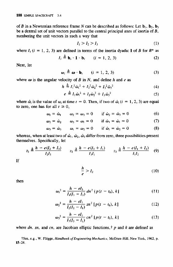
1 8 8 SIMPLE SPACECRAFT 3.4
of B in a Newtonian reference frame N can be described as follows: Let bj, b2, b3
be a dextral set of unit vectors parallel to the central principal axes of inertia of B,numbering the unit vectors in such a way that
h>h>h (0where / , (i = 1, 2, 3) are defined in terms of the inertia dyadic I of B for B* as
Next, let
/, = b , I b , (i = 1 , 2 , 3 ) (2)
«i = « ' b , - (/ = 1 , 2 , 3 ) (3)
where co is the angular velocity of B in N, and define h and e as
h = IX2G>X
2 + 722o>2
2 + /32o>3
2 (4)
e = / io>, 2 + /2a)22 + /3o>3
2 (5)
where co, is the value of w, at time t = 0. Then, if two of a>, (i = 1 , 2 , 3 ) are equalto zero, one has for all / > 0,
cj\ = 6)\ o)2 — o>3 = 0 if o>2 = o>3 = 0 (6)
o>2 = o>2 o>3 = o)\ = 0 if o>3 = a)\ = 0 (7)
o>3 = o>3 a>i = o>2 = 0 if (b\ = o>2 = 0 (8)
whereas, when at least two of d>i, G)2, CO3 differ from zero, three possibilities presentthemselves. Specifically, let
/ . ( / •
^ -
h -
-h)eh
- / . )eh
& h - e(I2 + h) A h - e(h + h) A h -Zl = 71 Zl = 71 Z3 = 71 yy)
hh hh hhIf
-e>h (io)
then
-to), k] (11)
2 » w 22 - SHl
en2 [p(t - to), k] (13)
where dn, sn, and en, are Jacobian elliptic functions,t p and k are defined as
tSee, e.g., W. Fliigge, Handbook of Engineering Mechanics, McGraw-Hill, New York, 1962, p.15-24.

3.4 TORQUE-FREE MOTION OF AN UNSYMMETRIC RIGID BODY 1 8 9
and t0 is a constant that can be expressed in terms of cO, and /, (i = 1, 2, 3) by settingt equal to zero in any one of Eqs. (11)—(13). For example, from Eq. (12),
d)22 = _*I sn2(-pt0, k) (15)
If [by contrast with (10)]
*<6 06)
then Eqs. (11)—(13) give way to
- t0), k] (17)
hhil
h
\ ~ h)
-eh'2 - h)
-eh
withp A ( z 3_Z 2 ) i /
and Eq. (15) may be replaced with
" d] sn\-
Finally, if
- fo). *] (19)
sn\-pto, k) (21)
- = h (22)e
then
-t0)] (23)
< 2 4 )
< 2 5 )
where
P = ( z , - z2)1/2 (26)
and to may be found from

1 9 0 SIMPLE SPACECRAFT 3.4
= [777—TTL / 3 ( / 3 — / i j
< 2 7 )
To choose appropriate signs for a>, (/ = 1,2,3), one can use knowledge of thesigns of any two of a), (/ = 1, 2, 3) that differ from zero, in conjunction with Ta-ble 3.4.1, which shows all permissible combinations of signs of (nonvanishing) CD,(/ = 1, 2, 3). For example, suppose h/e > I2, (*)i > 0, d)2 < 0, and a>3 = 0.Then, from Eqs. (11)—(13) and the first row of Table 3.4.1,
f h - eh 11 / 2
** = 777 f\ dn [P« ~ 'o)' k] (28)
y\(i\ — 13)\f h - eh 11 / 2
0)2 = " 777 h sn [P(t ~ ro)' k] (29)
L/2U2 ~ ' i / Jen [p{t - to), k] (30)
At times, it may be necessary to reorient b, (1 = 1, 2, 3) before one can find suit-able entries in Table 3.4.1. For instance, if a)U cS2, <S3 all are positive for a givenchoice of b, (/ = 1, 2, 3), then Table 3.4.1 contains no corresponding row; but b,can be replaced with —b, (/ = 1, 2, 3), in which case co, is replaced with —a),(i = l, 2, 3), and the last row of Table 3.4.1 accommodates this possibility.
Once a)i (i = 1, 2, 3) are known as functions of f, space-three angles 0, (/ =1, 2, 3) (see Sec. 1.7) relating b, (/ = 1, 2, 3) to a dextral set of orthogonal unitvectors n, (1 = 1, 2, 3) fixed in Af can be found as follows: When two of wu a>2,a>3 are equal to zero, choose n, such that n, = b, (1 = 1, 2, 3) at t = 0. Then
0! = (bit 02 = 03 = 0 if O>2 = O>3 = 0 (31)
02 = a)2t 03 = 0i = 0 if cb3 = o>, = 0 (32)
03 = o)3r 0i = 02 = 0 if o>, = o>2 = 0 (33)
When at least two of (bu a>2, a>3 differ from zero, choose n3 such that
n3 = H / T 1 / 2 (34)
where H is the angular momentum of B with respect to B* in N. Then take
02 = sin-^-lKOth-1'2) - I < 02 < ^ (35)
Table 3.4.1
(O\ (O2 Cl>3

3.4 TORQUE-FREE MOTION OF AN UNSYMMETRIC RIGID BODY 1 9 1
Next, let
and take
a =sin l — - - < a < - (36)cos 02 2 2
01 ~ [IT-a ifo,3<0 ( 3 7 )
Finally, determine 03 by solving the differential equation
The rotational motion of B can be described also by reference to the rollingmotion of an ellipsoid cron a plane TT, the so-called "Poinsot construction." Let abe an ellipsoid whose center O is fixed in N, whose principal semidiameters areequal to kl~X11 (j = 1, 2, 3), where k is a constant, and whose principal axes areat all times parallel to the principal axes of inertia of B forfi*; and let Trbe the planethat is tangent to a at Q, the point of intersection of the surface of cr with the raythat passes through O and has the same direction as w at some instant t*. Then TTis a unique plane, fixed in N at a distance d = k((o • H)l/2/h2 from O and perpen-dicular to H; and the rotational motion of B in N can be duplicated by a rollingmotion of a on TT. The loci traced out by Q on a and on TT during such rolling arecalled, respectively, the polhode and the herpolhode.
Equations (31)—(33) describe motions during which a principal axis of inertiaof B for B* plays the part of an axis of rotation (see Sec. 1.1). Such a motion isstable if and only if the axis of rotation is the axis of maximum or minimum momentof inertia of B for £*. That is, if b, = n, (i = 1, 2, 3) at t = 0, where n, ( 7 = 1 , 2, 3)are fixed in N, then the angle between bi and nx can be kept arbitrarily small fort > 0 by making d>2/(Oi and a>3/o>i sufficiently small; the angle between b3 and n3
can be kept arbitrarily small for t > 0 by making d>i/a>3 and co2/^3 sufficientlysmall; but the angle between b2 and n2 cannot be kept arbitrarily small for t > 0by making (o3/d>2 and 0)1/0)2 sufficiently small.
Derivations. In accordance with the angular momentum principle, co, (/ = 1,2, 3) are governed by
I{(bx - (I2 - h)(o2a)3 = 0 (39)
I2(o2 - (h - /i)«3«i = 0 (40)
/3a>3 - (/1 - I2)o>\o>2 = 0 (41)
It can be verified by inspection that Eqs. (6)-(8) furnish solutions of Eqs. (39)-(41).
Multiplication of Eqs. (39), (40), and (41) by Ixcou I2a)2, and /3a>3, respec-tively, and subsequent addition yield the angular momentum integral, that is, theequation

1 9 2 SIMPLE SPACECRAFT 3.4
/ , W + I22(O2
2 + / 3 W = h (42)
where h is the constant defined in Eq. (4). Similarly, multiplication of Eqs. (39),(40), and (41) with a)\, co2, and a>3, respectively, and subsequent addition lead tothe kinetic energy integral,
+ I2(o22 + ho)3
2 = e (43)
where e is the constant defined in Eq. (5).We now define z as
z = -(a>{2 + o)2
2 + co,2) (44)
and note that
Z = —2((O\(bi + Q)2(b2 + C03O)3) (45)
or, after using Eqs. (39), (40), and (41) to eliminate o>i, o>2, <i>3,
z = 2A z J (46)
where A is defined as
A ^
1 1 1
/ 2 / 2 / 2= (/i - /2X/2 - /3X/3 - /.) (47)
1" 12' 'i'
Moreover, solving Eqs. (42), (43), and (44) for a)2, co22, and o>3
2, we have
M " - ^ ' (49)
w.)1'-'11 <50)
where z, (/ = 1, 2, 3) are given by Eqs. (9). Substituting from Eqs. (48)-(50) intoEq. (46), we thus arrive at
z = 2[(z - zx)(z - z2)(z - z3)]1/2 (51)
The nature of the solution of Eq. (51) depends on the relative magnitudes ofZj, z2, z3. These, as will now be shown, depend, in turn, on the relative magnitudesof h/e and I2.
Eliminating a>i2 from Eqs. (42) and (43), one can write
/2(/i " hW + /3(/, - /3)o>32 = * / , - * (52)
which shows, in view of (1), that
eh-h>0 (53)

3.4 TORQUE-FREE MOTION OF AN UNSYMMETRIC RIGID BODY 1 9 3
Similarly, eliminating a>32, one finds
Now, from Eqs. (9),
Zl - Z2 =
z3 - zi =
eh ~ h < 0
(h ~ h)(h ~ eh)hhh
(h ~ h)(h ~ eh)hhh
(h ~ h)(h ~ eh)hhh
Hence,
and
zx - z2 > 0 z2 - z3 < 0
< 0 if - > he
(54)
(55)
(56)
(57)
(58)
z3 - > 0 if - < h
= 0 if - = he
(59)
Table 3.4.2 shows zu z2, and z3 ordered in accordance with (58) and (59) in relationto h/e.
Returning to Eq. (51), we note that the general solution of the equation
i = 2[(z - yx)(z - y2)(z - ys)V/2 (60)
can be expressed as
z = yi + (y2 - yi) sn2[p(t - t0), k] (61)
provided j , (i = 1, 2, 3) be constants such that
yx<y2< J3 (62)
and p and k be defined as
Table 3.4.2
Z\ > Z3 > Z2
Z3> Zi > Z2
z 3 = z ] > z2

1 9 4 SIMPLE SPACECRAFT 3.4
P k (y3 ~ yJ'2 k^{y2-y^'2p-' (63)
Hence, if h/e > I2, we take
y \ = Z2 yi = Z3 )>3 = Z\ (64)
to bring the first row of Table 3.4.2 into accord with (62). From Eqs. (61) and (64)we then have
z = z2 + (z3- z2) sn2[p(t - t0), k] (65)
with
in agreement with Eqs. (14). Furthermore,
- « - * » <67)
<69)
Eliminating z, (/ = 1, 2, 3) by using Eqs. (9), and noting that
1 - k2sn2[p(t - t0), k] = dn2[p(t - r0), *] (70)
while
1 - sn2[p(t - t0), k] = cn2[p(t - t0), k] (71)
we thus arrive at Eqs. (11)—(13).For h/e < I2, one obtains Eqs. (17)-(20) by proceeding similarly after replac-
ing Eqs. (64) with
y\ = ?2 yi = z\ 3 = zi (72)
in order to bring the second row of Table 3.4.2 into accord with (62).Finally, if h/e = I2, Eq. (51) becomes (see Table 3.4.2)
z = 2(z - z,)(z - z2)1/2 (73)
which possesses the integral
where p is given by Eq. (26). It follows that
_ r i + e , p [ 2 , ( | A , ) ] | = 2 c m h 2 [ ( , _[ 1 - e x p [2p(t - t ) ] j

3.4 TORQUE-FREE MOTION OF AN UNSYMMETRIC RIGID BODY 1 9 5
and from this that
z - Zl=z - z3= p2{ctnh2[p(t - t0) - 1]} = p2csch2[p(t - t0)] (76)
Equations (23)-(25) can now be obtained by substituting into Eqs. (48)-(50).To deal with the question of appropriate signs for a>, (j = 1, 2, 3), consider
first Eqs. (11)—(13). Taking square roots of both sides of each of these, one canwrite
dn[p(t - t0), k] (77)
h-elx |1/2
~ L73(/3 - /l)J
1/2cn[/>(/ - r0), *] (79)
and, differentiating with respect to t,
^ = + p k 2 \ rh ~ e[3 J'2 s n W " ro)' *] cn[p(t " ro)' ] (80)
L/i(/i - h)\
"2 = ± P \rh~eI,\]1'2 cn[P(t " ro)' ^] rf/l[p(r ~ ro)' k] ( 8 1 )
[ * "g/' T / 2 fc), *] (82)[L/3U3 ""
If one now substitutes into Eqs. (39)-(41), using, for example, the upper signs forco, and cu, (1 = 1, 2, 3), and eliminating/? and k by reference to Eqs. (9) and (14),one finds that Eq. (40) is satisfied identically while Eqs. (39) and (41) require that
( -1 - 1) sn[p(t - t0), k] cn[p(t - t0), k] = 0 (83)
which cannot be satisfied for all t. Hence, one is dealing with an inadmissible com-bination of signs. If, however, one uses any of the combinations of signs shown inTable 3.4.1, each of Eqs. (39)-(41) is satisfied identically. Moreover, the sameconclusion emerges when one works with Eqs. (17)—(19) or (23)-(25) in place ofEqs. (11)-(13).
Turning to the determination of the space-three orientation angles ft- (1 = 1,2, 3) (see Sec. 1.7) relating b, (/ = 1, 2, 3) to a dextral set of orthogonal unit vec-tors n7 (i = l, 2, 3) fixed in N, we refer to Eqs. (1.17.2) and (1.17.4) to write thefollowing differential equations governing 0, (1 = 1, 2, 3):
. , CU2S1S2 + CO3C1S20, = + )
02 = ^2^1 ~ <t>3Sl (85)
=c2

1 9 6 SIMPLE SPACECRAFT 3.4
If n, = b, (/ = 1, 2, 3) at t = 0, then 0,(f) (/ = 1, 2, 3) must satisfy, in additionto Eqs. (84)-(86), the initial conditions
0.(0) = 0 (i = l , 2 , 3 ) (87)
Suppose now that two of a>, (i = 1, 2, 3) are equal to zero, so that Eqs. (6)-(8)describe o>, (i = 1, 2, 3). Then it can be verified by inspection that Eqs. (31)—(33)furnish corresponding expressions for 0, (i = 1, 2, 3) that satisfy Eqs. (84)-(87).
When at least two of d>\, a>2, o)3 differ from zero, then H, the angular momen-tum of B with respect to /?*, can be expressed as
H = Ix<oxhx + I2<o2h2 + h(o3h3 (88)
which shows that h as defined in Eq. (4) is equal to H2. Since during torque-freemotion H has a fixed orientation in N, one can, therefore, fix a unit vector n3 in Nby making
n3 = H/T1 / 2 = (Aco,!)! + I2(o2b2 + /3co3b3)/r1/2 (89)(88)
If Cij is now defined as
one has
C(j = n t bj ( i j = 1 , 2 , 3 ) (90)
Cv =Ija>jh-1'2 0 = 1 , 2 , 3 ) (91)
and since |C3J| =£ 1 [see Eqs. (11), (17), and (23)], one can find d\ and 02 by usingEqs. (1.7.2)-(1.7.4), thus arriving at Eqs. (35)-(37). As for 03, note that
o\L2 — ^32 — i2(o*>n \y^)(1.7.1) (91)
whileCiC2 — C 3 3 — 13(0311 \s3)
Hence,
and
• _I2co22
I2a>2 hoij
' (92,C2 / I1 / 2 1<43)C2/lt /2 ^ '
=C2
2/l1/2 05.(1 -
_ , i / 2 e / | faj ,
(43, h h W { '
in agreement with Eq. (38).The validity of the Poinsot construction may be established by proceeding as
in Sec. 3.1, with the exception that Eqs. (3.1.29)—(3.1.31) must be replaced with
r = x,b, + x2b2 + x3bi (96)
K = / ,b,b, + /2b2b2 + /3b3b3 (97)

3.4 TORQUE-FREE MOTION OF AN UNSYMMETRIC RIGID BODY 1 9 7
and W + W + 73Jc32 = k2 (98)
respectively.In preparation for proving that the motions described by Eqs. (31) and (33) are
stable, whereas those corresponding to Eqs. (32) are unstable, we refer to Eq. (88)to note that the angle between H and bj can be expressed as
and if bi = ni at t = 0, then the angle between H and ni is given by
Now, in order for the angle between bj and ni to be small, it is necessary and suffi-cient that 4.(H, bj) and 4_(H, ni) each be small. Hence the stability of the motiondescribed by Eqs. (31) hinges upon the relationship between the magnitudes ofCD2/G>I and a>3/a>i, on the one hand, and the magnitudes of 4 (H , b{) and 4_(H, nx),on the other hand.
As regards 4_(H, nO, it follows immediately from Eq. (100) that this angle be-comes small when ct>2/c0i and a>3/<&i become small. To prove that this is the casealso for 4_(H, bj), we introduce 6, (i = 1, 2) as
e , 4 i ? i (/ = 2 ,3) (101)
and use Eqs. (4) and (5) to write
h __ I? + hW + /32e32
which shows that h/e becomes nearly equal to Ix when e2 and e3 become small.Since /, > 72 by (1), this means that h/e > h for small e2 and e3, and we may thususe Eqs. (11)—(13) to study a>, 0 = 1, 2, 3). Now, using Eqs. (4), (5), and (101),we find that
h - eh
From Eqs. (11)-(13) it can thus be seen that o)X2 does not become small, but (o2
2
and <o32 do, when e2 and e3 become small; and Eq. (99) therefore implies that
4 (H, b,) , like 4-(H, nO, becomes small when c&2/<S, and co3/co, become small.Consequently, Eqs. (31) describe a stable motion.

1 9 8 SIMPLE SPACECRAFT 3.4
The stability of the motion corresponding to Eqs. (33) can be established byproceeding similarly. To deal with Eqs. (32), we introduce rjt as
Vi k^L (i = l, 3) (106)
and use Eqs. (4) and (5) to show that h/e becomes nearly equal to I2 when j]x and773 become small, so that one cannot tell at a glance whether Eqs. (11)—(13) or Eqs.(17)—(19) should be used to determine the character of cot (/ = 1, 2, 3). However,the coefficients of the elliptic functions in the expressions for a)\2 in Eqs. (11) and(17) are the same, as are those in the expressions for co3
2 in Eqs. (13) and (19).Hence, it is unnecessary to make a choice, and we note that OJ2 and o>3
2 depend on
h - eh— h) (4,5)
h(h - o>22
and on
h — el i [hi?!777 — = 777*3\*3 — *\) (4.5) |_i3v'3
(107)
(108)
respectively. Clearly, these quantities cannot be made small by making 171 and 173small. Consequently, the angle between H and b2 cannot be kept arbitrarily smallfor t > 0 by making a>3/c02 and d)i/d>2 sufficiently small, and it follows that themotion described by Eqs. (32) is unstable.
Example As an alternative to the procedure just employed to establish the in-stability of "rotation about the intermediate axis," as the motion described byEqs. (32) is sometimes called, one can proceed directly from the differentialequations (39)-(41) to the linearized variational system associated with Eqs.(32) by introducing 5T, (1 = 1, 2, 3) such that
(O\ = (O\ co2 — d)2 + co2 CO3 = S 3 (109)
and linearizing in £>, (/ = 1, 2, 3), which gives
U>\
- h)
0
0
0
0
0
(110)
The characteristic equation for this system is
2 (/l " /2)(/2 " h) ,(111)
and it follows from (1) that this equation possesses one positive root.The stability of rotations about the axes of maximum and minimum mo-

3.5 GRAVITATIONAL MOMENT ON UNSYMMETRIC BODY IN CIRCULAR ORBIT 1 9 9
ment of inertia of B for B* can also be established without reference to explicitexpressions for a>,(f) (i = 1, 2, 3). For example, when attempting to prove thatEqs. (31) describe a stable motion, one can introduce Z as
Z = elx-h = I2(IX - hW + h(h - hW (112)(42,43)
and note that Z is a constant (since e, lx, and h are constants), so that throughoutany motion,
73( / , - /3)o>32 = hih ~ /3)o>3
2 (113)
The right-hand member of this equation can be made arbitrarily small by mak-ing a>2 and d)3 sufficiently small. The left-hand member vanishes only when a>2
and o>3 each vanish, since Ix - I2 and Ix - h are positive by (1). Hence a)2 andw3 can be kept arbitrarily small by making d)2 and co3 sufficiently small, a factpreviously established by using Eqs. (11)—(13).
3.5 EFFECT OF A GRAVITATIONAL MOMENT ON ANUNSYMMETRIC RIGID BODY IN A CIRCULAR ORBIT
In Fig. 3.5.1, O designates a point fixed in a Newtonian reference frame N, B* isthe mass center of an unsymmetric rigid body B, R is the distance between O and#*, and a, is a unit vector. B is presumed to be subjected to the action of a forcesystem 5 such that F, the resultant of S, and M, the total moment of S about £*,are given by
F = - a, (1)
and
= ^ a, x I (2)
Figure 3.5.1

2 0 0 SIMPLE SPACECRAFT 3.5
where /JL is a constant, m is the mass of B, andl is the central inertia dyadic of B.[If fi is set equal to GTn, F becomes equal to F as defined in Eq. (2.3.5) while M
becomes equal to M as defined in Eq. (2.6.3). The force system S is thus seen tobe approximately equivalent to the system of gravitational forces exerted on B bya particle of mass m at point O.]
Due to the action of 5, the rotational motion of B in TV depends on the transla-tional motion of B* in N, but not vice versa, because R appears in Eq. (2), but novariable involving the orientation ofBinNappears in Eq. (1). One possible motionfor B* is motion in a circular orbit that is fixed in N, has a radius R, and is describedwith an angular speed ft given by
ft = (fiR-3)l/2 (3)
When fi* moves in this fashion, the rotational motion of B in N proceeds in sucha way that
C31 = C32o>3 ~ C33o)2 (4)
C32 = C 3 3 ^ l - C31CO3 (5)
C33 = C3X<o2 - C32(ox (6)
C11 = Cl2co3 - Cuo2 + ft(C,3C32 - Cl2C33) (7)
C12 = C13CO1 - Cnco3 + ft(CnC33 - C13C31) (8)
C13 = CU(O2 - C\2u)\ + ft(Ci2C3i - C11C32) (9)
- 3ft2C12C13) (10)
- 3 f t 2 C 1 3 C n ) (11)
-3n2CuCl2) (12)
where Cij9 (ot, and Kt (/, j = 1, 2, 3) are defined as follows: Let b, (/ = 1, 2, 3)be a dextral set of unit vectors parallel to the central principal axes of inertia ofB, and introduce unit vectors a2 and a3 (see Fig. 3.5.2) such that ai, a2, a3 form adextral, orthogonal set with a2 = (Ndski/dt)il~\ so that a3 is normal to the orbitplane; let
dj = a, b, (ij = 1 ,2 ,3 ) (13)
and take
tot = NtoB • b, (i = l, 2, 3) (14)
where Nct>B denotes the angular velocity of B in N. Finally, with
/, = b , - I - b , (j = 1 , 2 , 3 ) (15)
let
A h - h „ A h - U „ A U - h n , .= — - — K 2 = — - — A3 = — - — (16)
1] h h

3.5 GRAVITATIONAL MOMENT ON UNSYMMETRIC BODY IN CIRCULAR ORBIT 2 0 1
Figure 3.5.2
noting that Kt (i = 1, 2, 3) are not independent of each other, any one of the threebeing expressible in terms of the remaining two. For example,
Kx + K2
KXK2(17)
Moreover,
- 1 < A T , < 1 (i = l , 2 , 3 ) (18)
The nonlinearity and strong coupling of Eqs. (4)-(12) prevent one from obtain-ing the general solution of these equations in closed form. However, the equationsare written in a form that is convenient for purposes of numerical integration, andthere exist four integrals of the equations, namely,
' I2C12 + C13C33 = 0 (19)C,,C3i
Cn2 + Ca2 + = 1 a = i , 3 ) (20)
and
z = i - ac3,)2/, - ac32)2/2
+ ®L {-Kxh c322 + £2/2(C312 + 3C13
2) - 3K3I3Cl22] = constant (21)
which can be used to check on the accuracy of such integrations. Furthermore, Eqs.(4)-(12) possess particular solutions of practical interest. Hence, they can fur-nish useful information about effects of M on the rotational motion of B in N. Con-sider, for example, motions during which B remains at rest in a reference frame A

2 0 2 SIMPLE SPACECRAFT 3.5
in which£* and a, (/ = 1,2, 3) are fixed (see Fig. 3.5.2). Such a motion is possibleif and only if each principal axis of inertia of B for 7?* is parallel to one of a, (/ =1, 2, 3), and Eqs. (4)—(12) can be used to prove that it is a stable motion when Kx
and K2 have values corresponding to the unshaded region of the stability chartshown in Fig. 3.5.3, whereas it is an unstable motion when K\ and K2 have valuescorresponding to the cross-hatched portions of this diagram. As used here, the termstable means that Cu — 1, Cx2, Ci3, C3i, C32, and C33 — 1 can be kept arbitrarilysmall for t > 0 by making these quantities, as well as to\, co2, and o>3 — fl, suffi-ciently small at t = 0. Now, when stability is defined in this way, the rotational mo-tion under consideration is unstable for all Kx and K2 in the absence of M. Hence,one may say that M can have a stabilizing effect. Suppose, however, that one callsthe motion stable when the angle between a3 and b3 can be kept arbitrarily smallfor t > 0 by making this angle, as well as <ox and co2, sufficiently small at t = 0,this being the definition of stability that corresponds to the one used in connectionwith torque-free motion in Sec. 3.4. Then, if 73 > Ix and 73 > I2 or if/3 < I\ and73 < 72, the motion is stable when M = 0, but it can be unstable when M ^ 0. Inthis sense, M can have a destabilizing effect. No matter which of these two defini-tions of stability is used, the stability of the motion in question can be rather tenu-ous. That is, even if all stability requirements are met, if the principal axes of inertiaof B for 5* are nearly parallel to a, (1 = 1, 2, 3) at t = 0, and if |Aco*| is small att = 0, it may occur that the principal axes become markedly misaligned from a,0 = 1, 2, 3) at some time subsequent to t — 0. This is illustrated in Fig. 3.5.4,
Figure 3.5.3

3.5 GRAVITATIONAL MOMENT ON UNSYMMETRIC BODY IN CIRCULAR ORBIT 2 0 3
(deg)
Figure 3.5.4
4 6
Number of orbits
10
which shows a plot of the angle </> between a3 and b3 as a function of the numberof orbits traversed by 5* subsequent to t = 0. This plot was obtained by integrat-ing Eqs. (4)-(12) numerically with Kx = - 0 . 5 , K2 = 0.9 (and, hence, /3 > Iu
h > / 2 ) , and
Cn(0) = 0.9924 C12(0) = -0.0868 C13(0) = 0.0872 (22)
C31(0) = -0.0789 C32(0) = 0.0944 C33(O) = 0.9924 (23)
Wl(0) = o,2(0) = 0.1ft (O3(0) = 1.1ft (24)
so that the initial values of C(j (i = 1, 3\j = 1, 2, 3) and co( (i = 1, 2, 3) differrelatively little from the values of the corresponding quantities during a motion thatis stable by either definition of stability, namely,
C,, = 1.000 C12 = 0 C13 = 0 (25)
C31 = 0 C32 = O C 3 3 = 1.000 (26)
a>, = o>2 = 0 (o3 = ft (27)
Nevertheless, 0 is seen to acquire values larger than five times its initial value,which shows that a relatively small disturbance can have a quite pronounced effecton a so-called stable motion.
Derivations The angular velocity of B in A can be expressed as
Aa>B = A<oN
(1.16.1)
NioB = -*(1.11.2) ( 1 . 1 1 . 5 )
(28)
Consequently,

2 0 4 SIMPLE SPACECRAFT 3.5
A€oB • b, = - a c 3 i + <ox (29)
(13,14)
A(oB • b2 = - O C 3 2 + <o2 (30)A€oB • b3 = - n c 3 3 + o>3 (31)
With i = 3 andy = 1, Eq. (1.10.1) now gives
C31 = C32 W • b3 - C33 W • b2 (3=3i) C3 2(-flC3 3 + o>3) - C 3 3 ( - aC 3 2 + o>2)(32)
which is Eq. (4), while for / = 1 andy = 3 one has
= c n ( - n c 3 2 + co2) - c1 2(-nc3 , + Wl)(29,30)
= C,,<»2 - C12w, + il(Cl2C3l - CUC32) (33)
in agreement with Eq. (9). Equations (5)-(8) are obtained similarly.The angular momentum H of B relative to B* in N can be expressed as
H = I\O)\b\ + I2co2b2 + /3w3b3 (34)and differentiation with respect to t in TV gives
Nd¥L BdH N B „—— = —- + N<oB x H
dt d.11.8) dt
= I\(d)x - K\U)2<jj3)b\ 4- / 2 ( o ) 2 - K2<A)3(x)\)b2 + 73(o>3 - Ar3a>,CL>2)b3 (35)(16)
while M, resolved into components parallel to b, (/ = 1, 2, 3) by reference to Eqs.(2), (3), (16), and (2.6.8), is given by
M = -m2{IxKxCnCnbx + I2K2Cl3Cnb2 + / 3 # 3 C, , C12b3) (36)
Substitution from Eqs. (35) and (36) into Nd¥L/dt = M then yields Eqs. (10)—(12).Equations (16) can be written
K ( 3 7 )
h h
Solution of Eqs. (37) for I\/I3 and 72//3 gives
h = _LzIi_ h = 1 +Kx/ \ A- V V 1 1 _L V V \~* * t
3 1 ' ^\^2 *3 A ' ^ 1 ^ 2
and substitution from Eqs. (39) into Eq. (38) yields Eq. (17).The inequalities (18) follow from the fact that the sum of two principal mo-

3.5 GRAVITATIONAL MOMENT ON UNSYMMETRIC BODY IN CIRCULAR ORBIT 2 0 5
ments of inertia must exceed the third, while the difference between them must besmaller than the third principal moment of inertia. Thus, for example,
/i + h > h (40)
and
h~h<I\ (41)
so that
£-f£>-l (42)IX (40)
and
I-^rL < i (43)IX (41)
in agreement with (18) for / = 1.Equation (19) is obtained by setting i = 1 and j = 3 in Eq. (1.2.14); and
taking i = j = 1 and i = j = 3 in Eq. (1.2.14) leads to Eqs. (20). The validity ofEq. (21) may be verified by differentiating the left-hand member with respect tot, eliminating Q and <bj (i = 1, 3;j = 1, 2, 3) by using Eqs. (4)-(12), and ob-serving that the result vanishes identically. However, this does not reveal the originof the equation, which will now be discussed.
When B remains at rest in A, the acceleration a of a generic particle P of B inN is given by
a = a2a3 x [a3 * (*a, + r)] (44)
where r is the position vector of P relative to 5* (see Fig. 3.5.5). This accelerationis "centripetal" in the sense that it has the same direction as the vector PQ, whereQ is the foot of the perpendicular dropped from P onto the line that passes throughO and is parallel to a3. A "centrifugal" force d¥ can be associated with P by letting
d¥ = - ap dr (45)
where p is the mass density of B at P and dr is the volume of a differential element
d¥ = - padr

2 0 6 SIMPLE SPACECRAFT 3.5
of B, and requiring that this force be applied at P (see Fig. 3.5.5). The sum of themoments about B* of all such forces is then called the centnfugal moment and isgiven by
M * = f r X d¥ = - f r X a p drJ (45) J
= - a 2 I r X {a3 X [a3 X (Rax + r)]}p dr(44) J
= -/?a2( [ rpdr] x [a3 x (a3 x a,)]
-il2 f r x [a3 x (a3 x r)]p dr (46)
The first of the last two integrals is equal to zero because r originates at the masscenter fi* of B. As for the last integral,
fr x [a3 x (a3 X r)]p dr = fa3 x r r • a3p dr = a3 X I • a3 (47)
where, as before, I is the central inertia dyadic of B. Hence,
M* = - f l 2 a 3 x I a3 (48)
and it may be noted that the centrifugal moment bears a striking resemblance tothe gravitational moment M as given in Eq. (2.6.3). This resemblance suggests thepossibility of expressing M* in a form analogous to that employed in connectionwith M in Eq. (2.17.4). That is, one is motivated to seek a function W* of a3 suchthat
dW*M* = - a 3 x — - (49)
da3
Not surprisingly, this function exists and can be expressed as
W* = ^ a3 • I • a3 = ^ (/,C312 + /2C32
2 + /3C332)
( = y [(/i - /3)C312 + (72 - /3)C32
2 + 13]
(= - y (K212 C3I2 - AT, 7, C32
2 - 73) (50)
Similarly, for M expressed as
M = 3ft2a, x I • a, (51)
one can introduce a function W of a] such that
M = a, x ^ (52)da

3.5 GRAVITATIONAL MOMENT ON UNSYMMETRIC BODY IN CIRCULAR ORBIT 2 0 7
by letting
(20)
(16)
Finally, consider
— a l a
— [/. + (/2
— (/ -K
the rotational
W I W[(a), - nc3i)
3ft2 2 2
/ 3 C 1 22 + /^2/2C13
2)
kinetic energy of £ in A, that
2I\ + (o>2 — flC3 2)2 /2 H- (a>3 —
+ / 3 C 1 32 )
is, AT defined
ftC33)2/3]
(53)
as
(54)
The quantity Z defined in Eq. (21) now can be seen to be given by
Z = K - W - W* + y (/3 - 3/0 (55)
The motivation for subtracting W and W* from A' is that energies are generally thenegatives of force functions [see, for example, Eqs. (2.17.3) and (2.17.7)]. As forthe last term in Eq. (55), this is the sum of the time-independent terms in the ex-pressions for W and W*, and it is included in Z in order that Z vanish whenever Bremains at rest in A with each central principal axis of inertia of B parallel to oneof a, (i = 1, 2, 3). In conclusion, then, Z is simply a sum of three energies asso-ciated, respectively, with the motion of B in A, with the gravitational moment M,and with the centrifugal moment M*. (Z can also be regarded as the "rotational"Hamiltonian for B in N.)
The centrifugal moment M* is of interest also in connection with the questionof the possibility of motions during which B remains at rest in A, for such a motionis possible if and only if
M + M* = 0 (56)
or, in view of Eqs. (48) and (51),
3a, x I • a! - a3 x I • a3 = 0 (57)
If Jkl (k, I = 1, 2, 3) now are defined as
Jkl = a , I a/ (*, / = 1, 2, 3) (58)
then
I • a, = 7uai + y2!a2 + 731a3 (59)
and
a, x I • a, = - J3ia2 + J2,a3 (60)

2 0 8 SIMPLE SPACECRAFT 3.5
Similarly,
a3 x I • a3 = - J2i*i + J\&2 (61)
and the three scalar equations corresponding to Eq. (57) are satisfied if and only if
Jn = J23 = J3i=0 (62)
which is the case if and only if each of a, (/ = 1, 2, 3) is parallel to a principal axisof inertia of B for B*.
To show that a motion of the kind just considered is stable when Kx and K2 havevalues corresponding to the unshaded region of Fig. 3.5.3, we note that such amotion can be defined with precision by requiring that
b , = a , (i = l , 2 , 3 ) (63)
for all t. Throughout the motion, one then has
Ci, - 1 = Cn = C13 = C3, = C32 = C33 ~ 1 = 0 (64)
o)\ = (o2 = co3 — Cl — 0 (65)
Now consider the most general motion, that is, the motion that ensues if, at t = 0,
Cij=Cij coi = cbi ( 1 , 7 = 1 , 2 , 3 ) (66)
Throughout this motion,
- ac 3 2 ) 2 / 2 + (co3 - nc 3 3 ) 2 / 3
- * i / i C 3 22 + K2I2(C31
2 + 3C132) - 3#3 /3c1 2
2]
= (&i - ftc3i)2/, + (w2 - nc 3 2 ) 2 / 2 + (d>3 - nc 3 3 ) 2 / 3
+ n 2 [ - ^ , / 1 C 3 22 + K2I2(C3l
2 + 3C132) - 3K3I3Cl2
2] (67)
The right-hand member of this equation vanishes if
Cl2 = C13 = C31 = C32 = C33 - 1 = 0 (68)
and
a>i = d)2 = d)3 - fl = 0 (69)
Hence, the left-hand member can be kept arbitrarily small by making C12, C\3, C3i,C32, C33 — 1, c&i, o>2> and <*>3 — H sufficiently small. Now, if
tf, < 0 K2 > 0 /^3 < 0 (70)
then the left-hand member is either positive or equal to zero. Hence, under thesecircumstances, Cj2, C\3, C3i, and C32 can be kept arbitrarily small by the samemeans which keep the left-hand member small. As for Cu — 1 and C33 — 1, itfollows from what has just been established and from Eq. (20) that these quantitiescan be kept arbitrarily small by making Cu — 1, as well as C12, C13, C3i, C32, andC33 — 1, sufficiently small. What remains to be verified is that the inequalities (70)are satisfied in the unshaded portion of Fig. 3.5.3. For the first two of these, this

3.5 GRAVITATIONAL MOMENT ON UNSYMMETRIC BODY IN CIRCULAR ORBIT 2 0 9
is self-evident, and to see that the third is satisfied, one needs only to refer to Eq.(17) after noting that Kx + K2 > 0 and 1 + Kx K2 > 0 in the region of interest.
For values of K\ and K2 belonging to the cross-hatched portion of Fig. 3.5.3,the instability of the motion described by Eqs. (64) may be established by workingwith linearized forms of Eqs. (4)-(12) and (19). That is, Cu and 04 (/ = 1, 3;j = 1, 2, 3) are expressed as
Cii = 1 + Cn C33 = 1 + C33 (71)
C\2 ~ C\2 C13 = C13 C31 = C31 C32 = C32 (72)
0 )1=07! o)2 = o)2 0)3 = f l + £)3 (73)
and the equations obtained by substituting these expressions into Eqs. (4)-(12) and(19) are linearized, which gives
c3, = c 3 2 n - o)2 c32 = Si - c31 a c33 = oCn = 0 Cn = - S>3 + ftC33 C13 = S)2 - a c 3 2
(74)
(75)
(76)and
C13(=O (77)
Solving the second of Eqs. (75) for aT3, substituting into the third of Eqs. (76), andusing the third of Eqs. (74), one now has
tn - 3£l2K3Cl2 = 0 (78)
while the first two of Eqs. (74) and (76), together with Eq. (77), permit one to write
c31
% • .
0- f t
0
ft0
0
0
01
0
- 1
0
ft A:.
o _
c 3 ;c32 (79)
The characteristic equations associated with Eqs. (78) and (79) are, respectively,
A2 - 3/t:3ft2 = 0 (80)
and
- ^ ft 0 - 1- f t - ^ 1 00 0 -fx
3il2K2 0 ftAT2
and these have roots with positive real parts if
= ix4 + (1 - KXK2 + 3/sT2)ft2M:2 . . 2
= 0 (81)
(82)
or if any one of the following is satisfied:

2 1 0 SIMPLE SPACECRAFT 3.5
KxK2>0
1 - Kx K2 + 3K2
KXK2 + 3K2)2 0
(83)
(84)
(85)
As may be seen by reference to Fig. 3.5.3, at least one of these conditions is satis-fied at every point of the cross-hatched portions of this diagram. Consequently,Eqs. (64) describe an unstable motion whenever Kx and K2 have values belongingto such a region. The solid black region in Fig. 3.5.3 represents values of K\ andK2 for which we have not established either the stability or the instability of the mo-tion under consideration.
Example B can move in such a way that b3 remains equal to a3 at all timeswhile the angle 0 between a] and bi (see Fig. 3.5.6) varies with time. It is tobe shown that 0 is either a periodic or a monotonic function of t.
During the motion in question,
(86)c,,c21c,,
CnC22
C32
CnC23
C33( 1 . Z . J 1)
cossin
0
ee
- s incos
0
ee
001
and
(O\ = (o2 = 0 co3 = ft + 0
Equations (4)—(11) are satisfied identically, but Eq. (12) requires that
0 + p 2 sin 0cos 0 = 0 (87)
where /?2, defined as
\l6)(88)
a3 ,b3
Figure 3.5.6

3.6 ANGULAR MOMENTUM, INERTIA TORQUE, AND KINETIC ENERGY OF A GYROSTAT 2 1 1
may be regarded as intrinsically nonnegative since the unit vectors bj and b2
can always be chosen such that I2 ^ I\. Introducing a as
a ±26one can replace Eq. (87) with
a + p2 sin a = 0
(89)
(90)
which is recognizable as the equation of motion of a simple pendulum in a uni-form gravitational field (see Fig. 3.5.6). Consequently, a is either a periodicor a monotonic function of t\ and, since 0 = a / 2 , the same is true for 6.
3.6 ANGULAR MOMENTUM, INERTIA TORQUE, ANDKINETIC ENERGY OF A GYROSTAT
Figure 3.6.1 represents a simple gyrostat G formed by a rigid body A that carriesan axisymmetric rotor B whose axis and mass center /?* are fixed in A. F designatesan arbitrary frame of reference.
The angular momentum HG of G in F relative to the mass center G* of G, theinertia torque TG of G in F, and the kinetic energy KG of G in F each can be ex-pressed as the sum of two quantities, one associated with a (fictitious) rigid bodyR that has the same mass distribution as G, but moves like A, and the other ac-counting for "internal" motions, that is, rotation of B relative to A. In other words,one can write
Figure 3.6.1

2 1 2 SIMPLE SPACECRAFT 3.6
HG = H* + H, (1)
TG = T* + T7 (2)
and
KG=KR + Kf (3)
where HR is the angular momentum of R in F relative to G*, TR is the inertia torque
of R in F, KR is the kinetic energy of R in F, and Hy, T7, and K{ are given by
H,=;Vj8 (4)
T ; = -J(A<bB(i + A<oBF<oA X 0 ) (5)
and
with fi, A(oB, Fa>A, and J defined as follows: /J is a unit vector parallel to the axisof symmetry of B (see Fig. 3.6.1); AcoB = A€oB • 0 , where ^co* is the angular ve-locity of B in A (see Sec. 1.11); FoiA is the angular velocity of A in F; and 7 is themoment of inertia of B about the axis of symmetry of B.
K, the rotational kinetic energy of G in F, can be expressed as
K = | (HG • IcT1 • HG + J - ' H , 2 - H7 • I ^ 1 • H7) (7)
where IG is the central inertia dyadic of G; and this result can be used to show thatK must lie between two values that depend on the magnitudes of HG and H7, as wellas on 7, /min and /max, the latter two being the minimum moment of inertia of G andthe largest central moment of inertia of G, respectively. Specifically,
^min — K ^ Amax (8)
where
i (^ + ^ - H, • Ic"' • H,) (9)2 \ /
and
- f - H7 IG-' • H71 (10)
Whenever B is at rest in A, G is said to be moving quasi-rigidly in F. Underthese circumstances, K = Kmin if and only if FtoA is parallel to the axis of maximumcentral moment of inertia of G, and K = ^max if and only if FioA is parallel to theaxis of minimum moment of inertia of G.
Derivations Let mA and mB be the masses of A and B, respectively, and let a andb be the position vectors (see Fig. 3.6.1) from G*, the mass center of G, to A* and

3.6 ANGULAR MOMENTUM, INERTIA TORQUE, AND KINETIC ENERGY OF A GYROSTAT 2 1 3
/?*, the mass centers of A and B, respectively. Then
mAa + mBb = 0 (11)
and HA, the angular momentum of A in F relative to G*, is given by
HA = lA Fa>A + mAa x V * (12)
where 1 is the central inertia dyadic of A and F\A* is the velocity of A* in F. Sim-ilarly,
HB = lB Fc*B + mBb x V (13)
so that HG , which is the sum of H^ and HB, can be expressed as
H G = IA F€oA + 1B • F<oB + mA2L x V * + mBb X Fv** (14)
Now,FCOfl = F€OA + Aft>fl ( 15 )
(1.16.1) v 7
Consequently,
H c = IA FwA + lB - Fa>A + lB • W + ^ a x Fvc*
(14) (15) n (16)
+ mAa x (F€oA x a) + mfl b x F\G* + Wflb x (FioA x b)
= [lA + mA(a • aU - a a ) + Ifl 4- mB(b • bU - bb)] • F a /
mBb) • FvG* + Ifl • W (18)
The quantity within the square brackets is the central inertia dyadic of R. Hence,the first line of the right-hand member of Eq. (18) is HR, the angular momentumof R in F relative to G *; the first term in the second line vanishes in accordance withEq. (11), and, since B is axisymmetric and A<oB = A<oB /?, the last term is equal toJ AcoB /?. Substitution from Eq. (18) into Eq. (1) thus leads immediately to Eq. (4).
The inertia torques TG and TR can be expressed as
Differentiation of Eq. (1) with respect to t therefore produces
= TR - J(Ad)Bp + AwB F€OA X f}) (20)
and substitution into Eq. (2) establishes the validity of Eq. (5).Forming 2KG as the sum of contributions from A and B, one has

2 1 4 SIMPLE SPACECRAFT 3.6
2KG = mA(F\Ay + Fa>A • lA • F€OA + mB(Fy")2 + W • I* • Fo>* (21)
or, after using Eqs. (15)—(17) to eliminate W , FvA \ and Fv**,
2*TC = mA(FvG*)2 + mA(F*)A x a)2 + 2m/vG* • V x a
+ mfl(FvG*)2 + mB{F<oA X b)2 + 2m/vG* FioA x b
+ F<oA • IA • F o / + F€oA • lB • V + Ao>* • IB • Aa>B
+ 2FcoA • I* • W (22)
Now,
(FioA x a)2 = (FcoA x a) • Fa>A x a = (FwA x a) x Fa>A • a
= CW4)2 a • a - FioA • a a • FcoA
= F « / (a a U - a a ) • F<oA (23)
and, similarly,
(F<oA X b)2 = FwA (b b U - b b ) F<oA (24)
Hence,
2KG =2)(mA +mB)(FyG*)2
+ FcoA • [lA + mi4(a • a U — a a) + lB + mB(b • b U — bb) ] • FioA
+ 2FvG* • (mAa + mBb) • FwA + 2FwA • Ifl • Awfl + A*>B • Ifl • W (25)
The first two lines of the right-hand member of this equation form 2KR; the firstterm in the third line vanishes in accordance with Eq. (11), while the second termis equal to 2JACJB • /3; and the last term in the equation is equal to J(ACJB)2. Equa-tion (6) thus follows from Eqs. (3) and Eq. (25). To establish the validity of Eq.(7), we begin by writing
2K = 2KG - (mA + m*)(FvG*)2 = 2KR + 2K, - (mA + m*)(FvG*)2
= F€OA • I G • F€OA + J(AO)B)2 + 2F€OA ' (J A(x)B P) (26)
(6)
Next, to eliminate angular velocities, we note that
H* = F<oA • IG (27)
so that
H G = F<oA ^ lG + H 7 (28)
orFoiA = (HG - H7) • l a" 1 (29)
(28)
Also,J(AcoB)2 = ^f- JAwBp = H, (30)
(4) J (4)

3.6 ANGULAR MOMENTUM, INERTIA TORQUE, AND KINETIC ENERGY OF A GYROSTAT 2 1 5
Consequently,
1K = ( H c - H7) - lG~l - IG • (HG - H7) • IcT1 + ^(26) ( 2 9 ) J
(30)
+ 2 ( H G - H / J - I c " 1 H 7(29) (30)
= (H c - H7) • (HG • I G - ' - H7 • lG~') + ^
+ 2HC-IC"1 H7 - 2 H . - I G - 1 H7 (31)
and this reduces to Eq. (7) when one takes advantage of the fact that I G- 1 is a
symmetric dyadic.To establish the validity of (8), it suffices to show that
*min( 3 2 )
To this end, mutually perpendicular unit vectors at, a2, a3 are introduced, with a,and a3 parallel, respectively, to the axis of maximum and minimum central momentof inertia of G; and a unit vector a is defined as
a = HGIHGI" 1 (33)
where |HG| denotes the magnitude of HG. If, in addition, a; and /, are defined as
<x}( = a • a; /, = a, • IG • a; (7 = 1, 2, 3) (34)
one then has
a,2 + a22 + a3
2 = 1 (35)
and
/max = I\> h> h — I mm (36)
Moreover, it follows from Eqs. (33) and (34) that
HG = |HG|(aia, + a2a2 + a3a3) (37)
and that
lG~l = a , a , / f * + a2a2/2"1 + a ^ / r 1 (38)
Hence,
HG lG l HG = H G
2 (a , 2 /r 1 + a22l2-
1 + a3%~1) (39)(37,38)
or, after elimination of ax by reference to Eq. (35),
In view of (36), Eq. (40) shows that HG • IG ' • HG > He2/,"1, which is equiv-

2 1 6 SIMPLE SPACECRAFT 3.6
alent to the left-hand portion of (32). Similarly, elimination of a3 from Eq. (39)establishes the validity of the right-hand portion of (32).
When G is moving quasi-rigidly in F, that is, when B is at rest in A (so thatH; = 0 ) , then
H C ( = ^ - I C (41)
2K = H c • Ic"1 • H c = FtaA • IG • W (42)
and, if w, is defined as
one can write
<oi=ai-F(aA 0 = 1 , 2 , 3) (43)
Hc2 = / . W + / 2 W + / 3 W (44)
(43)
and
2K = Ixcox2 + I2(o2
2 + I3w32 (45)
It follows that
2 H G2 - I2
2<o22 - /3
2a>32
^ 2 s
2 t±G I\ GJl 12 W2
and
H^2 - /,2™,2 - A2™.2
(47)(44) If
so that, if o>, is eliminated from Eq. (45) with the aid of Eq. (46), one has
whereas elimination of co3 by reference to Eq. (47) gives
(48)
+ /,(/, / , ) ^ + / 2 ( r 2 / , W | (49)H J
Moreover, when H7 = 0, then
H 2 H 2
2Kmin = - 5 - = - 2 - (50)(9) / m a x (36) / 1
and
U 2 U 2
(51)CO) / m i n (36) / 3
Suppose now that K = ^rmjn. Then, from Eqs. (48) and (50),
/2(/i " hW + hd\ ~ hW = 0 (52)

3.6 ANGULAR MOMENTUM, INERTIA TORQUE, AND KINETIC ENERGY OF A GYROSTAT 2 1 7
and, since the coefficients of o>22 and o>3
2 are intrinsically positive by (36), <o2 ando)3 must be equal to zero, which means that FcoA is parallel to a,, that is, to the axisof maximum central moment of inertia of G; and conversely, if Fa>A is parallel toal9 then <o2 = co3 = 0 and, from Eqs. (48) and (50), K = Kmin. Similarly, if K =#max, it follows from Eqs. (49) and (51) that F<oA is parallel to a3, and hence to theaxis of minimum moment of inertia of G; and conversely, if FcoA is parallel to a3,then coi = o)2 = 0 and, from Eqs. (49) and (51), K = Kmax.
Example A simple gyrostat G, formed by a rigid body A that carries an axi-symmetric rotor B whose axis and mass center are fixed in A, is at rest in aNewtonian reference frame N, and no forces act on A or B except those exertedby A on B and vice versa. It is to be shown that any rotation of B relative toA, brought about, say, by means of a motor each of whose parts belongs eitherto A or B, is accompanied by a rotation of A in N about an axis that is fixedboth in A and N, passes through the mass center G* of G, and is parallel to theunit vector n given by
where IG is the central inertia dyadic of G and /J is a unit vector parallel to theaxis of B.
So long as no external forces act on G, G* remains at rest in TV; and HG ,the angular momentum of G in N relative to G*, remains equal to zero. Con-sequently,
H* + H, = 0 (54)
Now,
H* = N<oA • IG (55)
and
H 7 = 7 A(oBfJ (56)
Hence,NCJA • IG +JA<DBP = 0 (57)
from which it follows thatN<oA = -JAa)BP'lG-{ (58)
Let n be the unit vector defined as
(The sign ambiguity arises from the fact that AwB can be positive or negative.)Since fi and IG are independent of time tin A, the derivative of n with respect

2 1 8 SIMPLE SPACECRAFT 3.7
to t in A vanishes. It follows that the derivative of n with respect to t in N alsovanishes, for
^ n Adndt (i.n.8) dt
N<oA x n = 0 4- NaN<oA
\N<oA = 0 (60)
In other words, n is fixed both in A and in TV; and, since NioA is parallel to n,NioA has a fixed orientation in both A and N. The only motions for which thisis true and G* remains fixed in N are rotations of A in N about an axis thatpasses through G* and is parallel to n.
3.7 DYNAMICAL EQUATIONS FOR A SIMPLE GYROSTAT
In Fig. 3.7.1, G designates a simple gyrostat consisting of a rigid body A and anaxisymmetric rotor B whose axis and mass center, fl*, are fixed in A; 2LX , a2, a3 forma dextral set of mutually perpendicular unit vectors fixed in A, each parallel to acentral principal axis of inertia of G. The axis of B is parallel to a unit vector ft,and G has central principal moments of inertia I\, I2, h, while B has an axial mo-ment of inertia J.
After defining AcuB, oi,3 A
A
A
, and
w-NtoA •
0 a
Mi as
03/ a =
(i =
1,
1,
2,
2,
3)
3)
(1)
(2)
(3)
Figure 3.7.1

3.7 DYNAMICAL EQUATIONS FOR A SIMPLE GYROSTAT 2 1 9
and
Mi = M a, (i = l , 2 , 3 ) (4)
where Aa>B is the angular velocity of B in A, N<oA is the angular velocity of A in aNewtonian reference frame N, and M is the moment about the mass center G* ofG of all forces acting on G, one can write the following set of coupled differentialequations governing Ao)B and to, (i = 1, 2, 3):
- (33<o2) -
- M2]
- M3] (5)
where MA/B is the moment about B* of all forces exerted by A on B; and
7,a)! = (72 - I3)o)2(o3 - J[A(bB px - AooB(p2a)3 - p3(o2)] + Af, (6)
I2(b2 = (73 — 7i)o)3O)i — J[A(bB P2 — A0)B(P3(Oi — P\(x)3)] + M2 (7)
73o>3 = (7j - 72)a)ia>2 - J[AcbBp3 - AcoB(pxco2 - p2(ox)] + M3 (8)
If the axis of B is parallel to a central principal axis of inertia of G, the com-plexity of these equations is reduced considerably; and further simplifications canbe made if B is completely free to rotate relative to A or if B is made to rotate rela-tive to A with a constant angular speed, say by means of a motor each part of whichbelongs either to A or to B. Under these circumstances, and with /? = a3, the dif-ferential equations governing coXy o>2, a)3 can be written
Ixd)x = (72 - I3)(o2(o3 - Jao)2 + Mx (9)
I2(b2 = (7 3 — Ix)(o3(ox + Jcr<A)x + M2 (10)
73ci>3 = (7i — I2)o)x(o2 + M3 (11)
where 73 and a are given in Table 3 .7 .1 , with Aa>B and c53 denoting the initial valuesof A(oB and o>3, respectively.
Table 3.7.1
Rotor motion
Free
73
h-J
h
cr

2 2 0 SIMPLE SPACECRAFT 3.7
Derivations The inertia torque TB of B in N is given by
TB = - NaB • IB - N€oB x 1B • V (12)
where *afi and Na>B are, respectively, the angular acceleration and the angular ve-locity of B in N, and lB, the central inertia dyadic of B, can be expressed as
h = K(yy + 55) + Jfifi
= KV + (J - K)Pfi (13)
Here K is the transverse central moment of inertia of B, y and 5 are unit vectorssuch that fi, y, and 5 are mutually perpendicular, and U is the unit dyadic. Hence,
and
NaB • IB = KNaB + (J - K)NaB • pp (14)(13)
N(oB x lB - W = (7 - / O V x 0/3 • NioB (15)
from which it follows that
TB P = -JNaB p (16)
Since, by D'Alembert's principle,
TB P + MA/fl • 0 = 0 (17)
one thus has
JNaB • P = MA/* • 0 (18)(16,17) ^
Now,
(1.20.1) rff (1.16.1)
Consequently,
and, since
= NaA +A<bBp +A<oBN<oA x p (19)(1.20.1) O-H.9) ^
+ \ i*) = /» • MAIB (20)19) (18) ^
NaA • P = o>!j8i + a>2j32 + 6i3j83 (21)
one can write
J(<*)\fi\ + fc>2j32 + CO3 83 H- OJ*) = B • MA/fl (22)(20)
TR, the inertia torque of a rigid body R that has the same mass distribution asG but moves like A, is given by

3.7 DYNAMICAL EQUATIONS FOR A SIMPLE GYROSTAT 2 2 1
TR = - NaA • IG - Na>A x IG • W (23)
Hence, TG, the inertia torque of G in N, can be expressed with the aid of Eqs.(3.6.2) and (3.6.5) as
T G = - NaA • I G - N<oA X I G • Na>A - J(Ad>B fi + Aa>BN<oA X fi) (24)
Carrying out the operations indicated in Eq. (24) after noting that
IG = /taiai + /2a2a2 + /3a3a3 (25)
and then appealing to D'Alembert's principle to write
TG + M = 0 (26)
one arrives at Eqs. (6)-(8); and solution of these equations for (bu o>2, o>3, followedby substitution into Eq. (22), produces Eq. (5).
Suppose now that fi = a3, so that [see Eq. (3)]
ft = ft = 0 ft = 1 (27)Then
h) (5)
and
1 l (6)
/2o>2 = (h — /I)G>3<WI + JA(*>B (O\ + M 2 (30)(7)
/3a>3 = (/i - /2)o>io>2 - yAo>fl + M3 (31)(8)
If fi is completely free to rotate relative to A, that is, if fi • MAIB = 0, then [see Eqs.(22) and (27)]
o»3 + V = 0 (32)
which implies that
<u3 + V = o>3 + Ao>B (33)
where w3 and A<SB are the initial values of o>3 and Ac*B, respectively. Hence,
(2
- 7(a>3 + AAB) + Mx (34)
Similarly, from Eqs. (30) and (33),
h<o2 = (h~J- Ix)(o3(Oi + i(o>3 + A w B ) + M2 (35)
Furthermore,

2 2 2 SIMPLE SPACECRAFT 3.7
A(bB =At.
(28) 73 - J
and substitution into Eq. (31) yields
( / 3 -
h ~ J(36)
- M3 (37)
Replacing 73 - J with 73 and a>3 + AwB with a in Eqs. (34), (35), and (37), one
arrives at Eqs. (9), (10), and (11), respectively. On the other hand, if B is madeto rotate relative to A with the constant angular speed Ad)B, then Eqs. (29)—(31)become Eqs. (9)-(l 1) when 73 is replaced with h,Aa)B is replaced with cr, and A<oB
is set equal to zero. Thus Eqs. (9)-(l 1) apply in both cases, provided 73 and a beinterpreted in accordance with Table 3.7.1.
Example In Fig. 3.7.2, O designates a point fixed in N, R is the distance be-tween O and G*, and d is a unit vector. G is presumed to be subjected to theaction of a force system S such that F, the resultant of S, and M, the total mo-ment of S about G*, are given by
and
F = -/jmR~2ei
= -£ c x la • e,
(38)
(39)
Figure 3.7.2

3.7 DYNAMICAL EQUATIONS FOR A SIMPLE GYROSTAT 2 2 3
where /JL is a constant, m is the mass of G, and IG is the central inertia dyadicof G. [If /ut is set equal to Gm, where G is the universal gravitational constant,then F becomes equal to F as defined in Eq. (2.3.5) while M becomes equalto M as defined in Eq. (2.6.3). The force system S is thus approximately equiv-alent to the system of gravitational forces exerted on G by a particle of massm at point O.]
Due to the action of 5, the rotational motion of A in N depends on the trans-lational motion of G* in N, but not vice versa, because R appears in Eq. (39),but no variable involving the orientation of A in N appears in Eq. (38); and onepossible motion of G* is motion in a circular orbit that is fixed in N, has a radiusR, and is described with an angular speed H given by
n = (fjiR-3y/2 (40)
If G* moves in this fashion, and if G is an axisymmetric gyrostat whose axisof symmetry is parallel to that of B, that is, if
/i = h (41)
then dynamical equations governing the rotational motion of A in TV can be ex-pressed in the form
a), = / i (0 i , 02, 03, <o2) (42)
o>2=/2(0i, 02, 03, (oi) (43)
O)3 = O>3 ( 4 4 )
where oi3 is the permanent value of o>3, and 0i, 02, 03 are body-three orientationangles (see Sec. 1.7) relating a, to e, (i = 1, 2, 3), with e2 = (Ndex/dt)Q,~l ande3 = Cl x e2, so that e3 is normal to the orbit plane (see Fig. 3.7.2). The func-tions /i and/2 are to be determined.
To express M [see Eq. (39)] in terms of al9 a2, a3, note that
- c2s3a2 + s2a3 (45)(1.7.11)
Next, with
IG = 7i(aiai 4- a2a2) + 73a3a3 (46)
carry out the multiplication indicated in Eq. (39) to obtain, with the aid of Eq.(40),
M = 3ft2(7, - 73)s2c2(s3a, + c3a2) (47)
Next, use Eqs. (11) and (41) to verify Eq. (44). Finally, write
I\d)\ — (72 — 73)o)2o)3 + y3cro)2 = 3fl (7, — 73)s2c2s3 (48)(9)
and
72o)2 "" (73 ~ 7i)o>3o)i "~ 73cro)i = 311 (I\ — 73)s2c2c3 (49)

2 2 4 SIMPLE SPACECRAFT 3.8
and compare these equations with Eqs. (42) and (43) to conclude that
and
h = "
1 - f )S2C2S3 (50)
(51)
3.8 ROTATIONAL MOTION OF A TORQUE-FREE,AXISYMMETRIC GYROSTAT
In Fig. 3.8.1, A designates a rigid body whose central inertia ellipsoid EA (notshown) may have three unequal principal diameters, whereas B is a rigid bodywhose central inertia ellipsoid EB is an ellipsoid of revolution. B is connected to Ain such a way that both the mass center £* of B and the axis of revolution of EB
are fixed in A, but B can rotate relative to A about this axis. The body G formedby A and B is thus a simple gyrostat; and, if the inertia ellipsoid EG of G for themass center G* of G is an ellipsoid of revolution, G is called a simple axisymmetricgyrostat.
Figure 3.8.1

3.8 ROTATIONAL MOTION OF A TORQUE-FREE, AXISYMMETRIC GYROSTAT 2 2 5
If the axes of revolution of EB and EG are parallel to each other and G is sub-jected to the action of forces whose resultant moment about G* is equal to zero, therotational motion of G in a Newtonian reference frame N proceeds much like thatof a single, axisymmetric rigid body (see Sec. 3.1); that is, while B rotates relativeto A with, in general, variable angular speed, the rotational motion of A in N canbe described in terms of two motions of simple rotation (see Sec. 1.1). One of theseis the motion of A in a reference frame C in which the angular momentum HG ofG relative to G* in N (a vector fixed in N) and the symmetry axis of EG are fixed;the other is the motion of C in N. The associated angular velocities are called, re-spectively, the angular velocity of spin and the angular velocity of precession, andthey can be expressed as
c<oA = sc3 (1)
andNc*c=ph (2)
Here h is a unit vector having the same direction as HG (see Fig. 3.8.1); c3 is a unitvector parallel to the symmetry axis of EG; s and p, called the spin speed and theprecession speed, respectively, are given by
/ - J Jd)3 + Kf Ks=— - jr (3)
and
P=J (4)
where H is the (constant) magnitude of H c ; / and J are the moments of inertia ofG about lines passing through G* and, respectively, perpendicular and parallel toc3; K is the moment of inertia of B about the symmetry axis of B; r = A€oB • c3; ris the value of r at t = 0; and <S3 is the value of Na>A • c3 at t = 0. The quantity rsatisfies the differential equation
' M " (5>
where MA/fl is the moment about 5* of all forces exerted by A on B.Throughout the motion of G, the angle <f> between c3 and HG remains constant
and is given by
* * (6)
Derivations In Fig. 3.8.1, Ci and c2 are unit vectors not fixed either in A or in B,but such that Ci x c2 = c3. If C is a reference frame in which Ci, c2, and c3 are fixed,then, since c3 is permanently parallel to the axis of revolution of EB, and since thisaxis is fixed in A, the angular velocity of A in C is necessarily parallel to c3 and,therefore, can be expressed as

2 2 6 SIMPLE SPACECRAFT 3.8
c(oA = sc3 (7)
Similarly, as B is constrained to rotate relative to A about a line parallel to c3, theangular velocity of B in A can be written
AioB = rc3 (8)
Finally, the angular velocity of C in N always can be expressed in terms of functionsPu P2, and/73 of / as
Ntoc = pxcx + p2c2 + p3c3 (9)
Consequently,N€OA = N(OC + C{0A = pxCx + p2C2 + (p3 + S)C3 (10)
(1.16.1) (7,9) r r r
and
\I A *^ M A y • -v • • •
TR, the inertia torque ofR in N, where /? is a rigid body having the same mass dis-tribution as G but moving like A, is thus given by
T* = - NaA • IG - Na>A X IG • N<oA
= - {Ipx + [(J -I)p, + Js]P2}cx
~ {Ipi ~ l(J ~ Dpi + Js]pi}c2 - J(P3 + i)c3 (12)
while T7, the internal inertia torque of G, can be written
T7 = - K(rc3 + r V 4 X c3)(3.6.5)
= - t f [ r c 3 + r(/72c, - p , c 2 ) ] (13)
If G is subjected to the action of forces whose resultant moment about G* isequal to zero, the inertia torque of G in N, that is, the sum of TR and T7 [see Eq.(3.6.2)], vanishes identically. Hence, Eqs. (12) and (13) lead directly to
Ipx + [(J - Dpi + J S + Kr]p2 = 0 (14)
Ipi ~ [U ~ Dpi + Js+ Kr]px = 0 (15)
J(p3 + s) + Kr = 0 (16)
The quantity s, introduced in Eq. (7), may be chosen at will. A choice thatsimplifies subsequent analysis is
s = ( / 7 ) f * r (17)
because this permits one to replace Eqs. (14)—(16) with

3.8 ROTATIONAL MOTION OF A TORQUE-FREE, AXISYMMETRIC GYROSTAT 2 2 7
Pi = Pi = h = 0 (18)
from which it follows that
P\=Px Pi=Pi Pi=Pi (19)
where p, denotes the initial value of p( (/ = 1, 2, 3).HR, the angular momentum of R in N relative to G*, is given by
p2c2)
x + p2c2) + (Ip3 - Kr)c3 (20)
while H7, the internal angular momentum of G, can be expressed as
Hence,
H7 = Krc3 (21)(3-6.4) ( 8 )
(3, r2o.21, (22)
Also,
. . . « ' - — ( 2 3 )
Thus, N(oc is seen to be parallel to HG ; and, if h is a unit vector having the samedirection as H G , and H denotes the magnitude of H G , then
Ntoc = j h (24)
which establishes the validity of Eqs. (2) and (4).a>3, the value of N<oA • c3 at t = 0, is given by
, . « ^ » . ( 2 5 )(17) J
Also,
(I - J)p3 - Krs = ; (26)
(17) J V '(19)
Solving Eq. (25) forp3 and substituting into Eq. (26) produces Eq. (3).Let TB denote the inertia torque of B in N. Then, since EB is an ellipsoid of
revolution whose axis is parallel to C3,
c3 • TB = - c 3 • Na"K (27)
Moreover,

2 2 8 SIMPLE SPACECRAFT 3.8
c . NaB _ c . — — = p + j + r = r — - — (28)
(1.20.1) dt (17,18) 7
Hence, if MAIB is the moment about J5* of all forces exerted by A on B, so that
c3 • (MA/B + TB) = 0 (29)
then
„ . M- - iH^-0 (30,(27,28)
which is equivalent to Eq. (5).By definition,
<f> = c o s ' ^ h • c3) (31)
where
h = if &) h(/3iCi + p2Ci + hCi) (32)
Hence,
os"1 (^ = c s"1 (Mi + Kf
in agreement with Eq. (6).
Example Figure 3.8.2 represents an axisymmetric gyrostat G consisting oftwo rigid bodies A and B. A is formed by removing from a rigid, uniformright-circular cylinder of radius R and height 3R the material within a right-circular cylinder of radius R/4 and height R; and B is a rigid, uniform, right-circular cylinder, made of the same material as A and completely filling thecavity in A.
At a certain instant, say t = 0, the angular velocity of A in a Newtonianreference frame N has components of magnitude 3(1 and 8(1, directed as shownin Fig. 3.8.2, and B is at rest in A. If B is now made to rotate relative to A ina suitable manner for 0 ^ t < T, then the motion of A in N for t > T is a mo-tion of simple rotation (see Sec. 1.1), performed with a constant angular speedn(l . The number n and the way in which B must move relative to A are to bedetermined.
The moments of inertia /, 7, and K are
(34)
where m is the mass of G. The central angular momentum of G thus has themagnitude

3.8 ROTATIONAL MOTION OF A TORQUE-FREE, AXISYMMETRIC GYROSTAT 2 2 9
Figure 3.8.2
so that
and
H = [(3H/)2 + (8H7)2]1/2 = 5mR2n
p = 5CL(4)
(35)
(36)
(37)
The motion of A in N is a simple rotational motion for / > T if s = 0 fort > T; and the associated angular speed is then equal to p. Hence, n = 5 and,for t > T, B must move relative to A in such a way that
r = 4(768)11 = 307211(37)
(38)
In other words, for t > T, the angular velocity of B in A must satisfy the equa-tion
A(oB • c3 = 307211(8)
(39)

2 3 0 SIMPLE SPACECRAFT 3.9
3072ft
Figure 3.8.3
where c3 is a unit vector directed as shown in Fig. 3.8.2. The time history ofr depicted in Fig. 3.8.3 thus serves to accomplish the desired objective.
3.9 REORIENTATION OF A TORQUE-FREE GYROSTATINITIALLY AT REST
Figure 3.9.1 represents a simple gyrostat G formed by a rigid body A that carriesan axisymmetric rotor B whose axis and mass center 5* are fixed in A. No forcesact on A or B except those exerted by A on B and vice versa, and G has the followinginertia properties: A and B have masses mA and mB, respectively. A has a centralinertia dyadic lA, and B has an axial moment of inertia J and a central transversemoment of inertia K.
Subsequent to any instant at which A and B are at rest in a Newtonian referenceframe N, A can be made to perform a simple rotational motion (see Sec. 1.1) in N.This is accomplished by making B rotate relative to A, say by means of a motor eachpart of which belongs either to A or B; and, by orienting the axis of B suitably inA, one can make the axis of rotation of A in N parallel to any desired unit vectorv. To this end, designate as ft a unit vector parallel to the axis of B; let c be theposition vector of B* relative to A*; and introduce L, j5, and M as
L 4 iA +mA + mB
(c2U - cc) (1)
and
Then take
M = L + (J -
p = -
(3)
(4)
By choosing a suitable value for A0B, the angle of rotation of B in A, one can causeN6A, the angle of rotation of A in N, to have any desired value. Specifically, if A0B

3.9 REORIENTATION OF A TORQUE-FREE GYROSTAT INITIALLY AT REST 2 3 1
® X
p— — •
7V-
fA*
J
\Figure 3.9.1
and N6A are regarded as positive for rotations that are right-handed with respect toP and v, respectively, and if both angles are taken equal to zero at an instant atwhich A and B are at rest in N, then
NQAQA(5)
M - I I
Derivations As was shown in the example in Sec. 3.6, every rotation of B relativeto A is accompanied by a simple rotation of A in N such that the associated axis ofrotation is parallel to a unit vector v that satisfies the equation
j3 IGv + fi'lG~X = 0
(3.6.53)
(6)
where IG is the central inertia dyadic of G. Scalar multiplication of this equationwith lG produces
P
Now, IG can be expressed as
lr=lA+KUmAmB
1A + mB
= 0
(c2U - cc) -K)pfi
so that
Hence,
I G = L
(7)
(8)
(9)

2 3 2 SIMPLE SPACECRAFT 3.9
or, equivalently,
which shows that fi is parallel to v • L. Consequently, if a unit vector ]$ is definedas in Eq. (2), then fi is equal either to /J or to -]2. To determine which sign isappropriate, define M as in Eq. (3) and note that, both with fi = jJ and with0 = - # , it follows from Eqs. (3) and (9) that IG = M. Next, multiply Eq. (6)scalarly with i>, obtaining
(12)
which shows that p • lG x • v is necessarily negative. Consequently, if Jl •
lG~l ' v is negative, then /3 = /J, whereas, if p • IG~l • f is positive, then/3 = — j j . This is precisely what Eq. (4) asserts. In the example in Sec. 3.6, it wasshown also that
(3.6.58) P G
where A<oB = A(oB - p. Hence, if NOJA is defined as "a / = N<oA • i/, then scalarmultiplication of Eq. (13) with v yields
%*/ = —JA(oB P - IG~l • v
^"'w^'J'"'^-1^ (14)
NCDA
A<oB = (15)
so that (recall that M = IG)
Equation (5) follows directly from this relationship and from the definitions of A8B
and N0A.
Example Figure 3.9.2 shows a simple gyrostat G formed by a uniform rectan-gular block A of mass 1200 kg and a thin circular disk B of mass 20 kg. A hassides of length 3 m, 4 m, 7 m, and B has a radius of 1 m. The center of B issituated at a corner of A.
A unit vector p parallel to the axis of B and an angle A0B are to be foundsuch that a rotation of B in A characterized by the vector A6B P will cause Ato acquire the same change in orientation in a Newtonian reference frame TV thatresults from subjecting A successively to the two rotations characterized by thevectors (77/2)11! rad and (7r/2)n3 rad, where ni and n3 are unit vectors fixedin Af and directed as shown in Fig. 3.9.2.

3.9 REORIENTATION OF A TORQUE-FREE GYROSTAT INITIALLY AT REST 2 3 3
Figure 3.9.2
To determine a single rotation that is equivalent to the two successive rota-tions, introduce the Rodrigues vectors (see Sec. 1.4) associated with the tworotations, expressing these as (see Sec. 1.6)
V = V = n3 (16)
where A is a fictitious body which moves like A during the first rotation, butremains fixed in N while A performs the second rotation. Then V ' t h e R o d "rigues vector for a single rotation of A in N that produces the same orientationchange resulting from the two successive rotations, is given by
NQA _H (1.6.5)
= m + n2 + n3 (17)
Hence, if Vis a unit vector and N6A is an angle such that the vector N0A v char-acterizes the single rotation, then
= i>tan("072)
and this equation is satisfied if
= *1 rad v —n2 + n3
V3(19)
2 3 4 SIMPLE SPACECRAFT 3.10
The central inertia dyadic of A can be written
IA = 2500 n ^ ! + 6500 n2n2 + 5800 n3n3 (20)
and the position vector c from the mass center of A to that of B is
c = 3 . 5 ^ + 1.5n2 + 2.0n3 (21)
while the axial and central transverse moments of inertia of B are
J = 10 kg • m2 K = 5 kg • m2 (22)
Hence,
L = 2628n^! - 103.311^2 - 137.7n,n3
- 103.3n2n! + 6825n2n2 - 59.02n2n3
- 137.711311! - 59.02n3n2 + 6090n3n3 (23)
and
so that
and
v • L = 1378 ni + 3847 n2 + 3402 n3 (24)
p = 0.2592 n, + 0.7235 n2 + 0.6398 n3 (25)
M = 262811,11! - 102.4nin2 - 136.9nin3
- 102.4n2n! + 6828n2n2 - 56.71 n2n3
- 136.9n3n! - 56.71 n3n2 + 6092n3n3 (26)
from which it follows that
p M * = 1.085 x 10⁻⁴(n, + n2 + n3) (27)
Consequently, /£ • M"1 • vis positive, and the desired unit vector is given by
p = -(0.2592 ni + 0.7235 n2 + 0.6398 n3) (28)(4)
while
A0B = — = 1 1 1 4 rad (29)<5> 3 x 10 x 1.085 x 10"4 x V3
3.10 EFFECT OF A GRAVITATIONAL MOMENT ON ANAXISYMMETRIC GYROSTAT IN A CIRCULAR ORBIT
In Fig. 3.10.1, O designates a point fixed in a Newtonian reference frame N, G*is the mass center of a gyrostat G formed by a rigid body A and an axisymmetricrotor B whose axis and mass center B* are fixed in A, R is the distance between O

3.10 GRAVITATIONAL MOMENT ON AN AXISYMMETRIC GYROSTAT 2 3 5
Figure 3.10.1
and G*, and ex is a unit vector. G is a simple axisymmetric gyrostat; that is, the cen-tral inertia ellipsoid of G is an ellipsoid of revolution; and the symmetry axis of Gis parallel to the rotor axis. G is presumed to be subjected to the action of a forcesystem S such that F, the resultant of 5, and M, the total moment of S about G*,are given by
F = — 2 e i
and
(1)
~ „ ! Cl X \f (2)
where fx is a constant, m is the mass of G, and IG is the central inertia dyadic ofG. [If/u is set equal to Gm, F becomes equal to F as defined in Eq. (2.3.5) while Mbecomes equal to M as defined in Eq. (2.6.3). The force system S is thus ap-proximately equivalent to the system of gravitational forces exerted on G by aparticle of mass In at O.]
Due to the action of 5, the rotational motion of A in N depends on the transla-tional motion of G* in N, but not vice versa, because R appears in Eq. (2), but novariable involving the orientation of A in N appears in Eq. (1). One possible motionof G* is motion in a circular orbit that is fixed in N, has a radius /?, and is describedwith an angular speed fl given by
n = (tiR~')l/2 (3)
When G* moves in this fashion and B either is completely free to rotate relative to

2 3 6 SIMPLE SPACECRAFT 3.10
A or is made to rotate relative to A with a constant angular speed, then the rotationalmotion of A in N proceeds in such a way that
(4)
a>2c3 — ftsi (5)
(6)
j8ft2s2c2s3 (7)
6)2 — — afta>i + j3fl2s2c2c3 (8)
a>3 = a>3, a constant (9)
where a , j8, ft, a>i9 s,, c,- (/ = 1, 2, 3) are defined as follows: Let a t , a2, a3 be adextral set of orthogonal unit vectors fixed in A such that a3 is parallel to the sym-metry axes of G and B (ai, a2, a3 are thus parallel to central principal axes of inertiaof G); and introduce unit vectors e2 and e3 (see Fig. 3.10.1) such that e t , e2, e3 forma dextral, orthogonal set with e2 = (Ndei/df)Cl~l, so that e3 is normal to the orbitplane. Next, let 0u #2, fy be body-three orientation angles (see Sec. 1.7) relatinga, to c,- (i = 1, 2, 3); define s, and c, as s,- = sin ft, c, = cos ft (i = 1, 2, 3); andtake
c o , = W . a , (1 = 1 ,2 ,3) (10)
Finally, let
and
where / i , 73, 73, 7, and o- have the same meaning as in Sec. 3.7.G can move in such a way that the symmetry axis of G remains normal to the
orbit plane while A rotates with a constant angular speed d>3 in Af and B rotatesrelative to A with a constant angular speed Aa>B. This motion is unstable if x and y,given by
h t (o>3 - n ) / 3 + A6)BJ
have values such that the point with coordinates x and y lies in one of the shadedregions of Fig. 3.2.5, these being regions in which at least one of the inequalities(3.2.19)-(3.2.21) is satisfied.

3.10 GRAVITATIONAL MOMENT ON AN AXISYMMETRIC GYROSTAT 2 3 7
Derivations If E is a reference frame in which ei, e2, e3 are fixed, thenN(OA = N€OE + E€OA (14)
(1.16.1)
with
and
Na>E =
^ [ ( i 2 3 3 ! ) i (cis2s3 + c3s,)a2 + c,c2a3] (15)
l = l) (0iC2c3 + 02s3)a! - (0,c2s3 - 02c3)a2 + (0,s2 + 03)a3 (16)
so that, from Eq. (10),
^i = (0ic2 - ftc!S2)c3 + (02 + as!)s3 (17)
- nc,s2)s3 + (62 + ns,)c3 (18)
(93 + ftC!C2 (19)
Solution of these equations for 0,, 02, 03 produces Eqs. (4)-(6); and Eqs. (7)-(9)follow directly from Eqs. (3.7.42)-(3.7.44) together with Eqs. (3.7.50), (3.7.51),(11), and (12).
To deal with the stability of motions such that the symmetry axis of G remainsnormal to the orbit plane and A rotates with a constant angular speed a>3 in N, beginby observing that Eqs. (4)-(9) are satisfied if
0! = 02 = o>! = OJ2 = 0 (20)while
03 = rt w3 = o>3 (21)
with
r = 6J3 - ft (22)
Next, introduce perturbations 0i, 02, and 03 by letting
0i = 0i 02 = 02 03 = rt + 03 (23)
and substitute into Eqs. (17) and (18), dropping all terms that are nonlinear in theperturbations, which gives
o)x = (?, - (Y02)cos rt + (02 + fl0,)sin rt (24)
<*>i = -(Ox - ft02)sin rt + (02 + ft3i)cos rr (25)(18)
Now use these equations to eliminate o)x and o)2 from Eqs. (7) and (8), obtaining
(Sx + [r - (1 + a)ft]^2 " (r - aft)n0,}cos rr
+ { 2 " [r ~ (1 + a)n]^i + [r - (a + j8)n]O?2}sin rr = 0 (26)

2 3 8 SIMPLE SPACECRAFT 3.10
and
{?i + [r - (1 + a)(l]S2 ~ (r - atytie^sin rt
+ {% ~ [r ~ (1 + a)n]6f, + [r - (a + j3)n]nft}cos rf = 0 (27)(8)
The coefficients of sin rt and cos r/ in these equations must vanish separately.Hence, one may write the matrix differential equation
Av + Bv + Cv = 0 (28)
where A is the 2 x 2 unit matrix, while
A T 0 r - (1 + a)O]\_-r - (1 + a)ft 0 J
1)ft]aj
Vr m n - - ( 2 9 )
C ' ^ r - ( a
and(30)
The characteristic equation associated with Eq. (28) may be written by setting thedeterminant of the matrix A\2 + BX + C equal to zero:
Now introduce Q and x as
O = — - = - - (32)
Then
A4 + (1 + Q2 + 3x)ft2A2 + G(G + 3x)fi4 = 0 (33)
or
A4 + 26A2 + c = 0 (34)
whereA ^ A
c k Q(Q + 3A:)fl4 (35)
Moreover, if y is defined as
y = j (36)
then
Q = x + y(l + x) (37)

3.10 GRAVITATIONAL MOMENT ON AN AXISYMMETRIC GYROSTAT 2 3 9
Equations (35) and (37) are identical with Eqs. (3.2.53) and (3.2.50), respectively,a fact that will prove useful presently.
Equations (20) and (21) comprise an unstable solution of Eqs. (4)-(9) when-ever any root of Eq. (34) has a positive real part, that is, whenever any one of theinequalities (3.2.55) is satisfied; and, as in Sec. 3.2, these inequalities imply theinequalities (3.2.19)-(3.2.21).
It remains to verify Eqs. (13). The first of these is an immediate consequenceof the definitions of /? and x, given in Eqs. (12) and (32), respectively. As for thesecond, note that
= r/n-a+ p/3 = Vih + L^-x (my V '+y (36,32) 1 - 0/3 (11,12,22) fl / 3 / 3 fi
Now suppose that B is completely free to rotate relative to A. Then, in accordancewith Table 3.7.1, p. 219,
HHdf)'in agreement with the second of Eqs. (13). Similarly, if B is made to rotate relativeto A with a constant angular speed, then Eq. (38) together with values for 73 anda taken from Table 3.7.1 leads to the second of Eqs. (13).
Example The gyrostat G considered in the example in Sec. 3.8 and shown inFig. 3.8.2 is to be placed in a circular orbit about the Earth in such a way thatthe inertial orientation of A remains fixed, c3 is normal to the orbit plane, andB rotates relative to A with a constant angular speed Aa>B. Values of Ad>B forwhich such motions are unstable are to be determined.
The system of gravitational forces exerted on G by the Earth can be ap-proximated with 5; and, if all other forces, such as those arising from solar ra-diation, the Earth's magnetic field, etc., are regarded as negligible, the instabil-ity conditions (3.2.19)—(3.2.21) apply with JC and y given by Eqs. (13), where
and cS3 = 0 [see Eqs. (9) and (10)]. Thus
x = -0 .5 y = -768 ft
The points of the line x = —0.5 that lie in a shaded portion of Fig. 3.2.5have coordinates such that
-4.367 < y < 4.000 (42)
Hence the motion under consideration is unstable if
-2819ft < Ad)B < 3840H (43)

2 4 0 SIMPLE SPACECRAFT 3 .11
3.11 EFFECT OF A GRAVITATIONAL MOMENT ON ANUNSYMMETRIC GYROSTAT IN A CIRCULAR ORBIT
In Fig. 3.11.1, O designates a point fixed in a Newtonian reference frame N, G*is the mass center of a gyrostat G formed by a rigid body A and an axisymmetricrotor B whose axis and mass center £* are fixed in A, R is the distance between Oand G*, and d is a unit vector. The axis of B is parallel to a central principal axisof inertia of G, and G is presumed to be subjected to the action of a force systemS such that F, the resultant of S, and M, the total moment of S about G*, are givenby
and
F = — jxmR 2ei
= - ^ e , x I c . e ,
(1)
(2)
where [x is a constant, m is the mass of G, and I c is the central inertia dyadic ofG. [If fji is set equal to Gm, F becomes equal to F as defined in Eq. (2.3.5) whileM becomes equal to M as defined in Eq. (2.6.3). The force system 5 is thus ap-proximately equivalent to the system of gravitational forces exerted on G by a par-ticle of mass m a t O . ]
Due to the action of 5, the rotational motion of A in N depends on the transla-tional motion of G* in TV but not vice versa, because R appears in Eq. (2), but novariable involving the orientation of A in N appears in Eq. (1). One possible motion
Figure 3.11.1

3.11 GRAVITATIONAL MOMENT ON AN UNSYMMETRIC GYROSTAT 2 4 1
of G* is motion in a circular orbit that is fixed in N, has a radius R, and is describedwith an angular speed O given by
fi = (,ji/r3)1/2 (3)
When G* moves in this fashion and B either is completely free to rotate relative toA or is made to rotate relative to A with a constant angular speed, then the rotationalmotion of A in N proceeds in such a way that
C3X = C32<o3 - C33co2 (4)
C32 = C33coi - C3l(o3 (5)
C33 = C3l(o2 - C32<0\ (6)
Cn = Cl2co3 - CX3(o2 + il(Cx3C32 - C1 2C3 3) (7)
C12 = Cx3cox - Cna)3 + £l(CxxC33 - C13C31) (8)
C13 = Cno>2 - C12ct>i + fl(Ci2C3 i - C11C32) (9)
Co, = Kx(o2a>3 - 3a2KlCl2Cl3 -
6)2 = K2(x)3(ox — 3ft2A r2Ci3Cii -f cro>i( — I (11)
V2/
6)3 = K3(O\(o2 — 3£l2K3CuC\2 (12)
where Cij9 coi9 lh Kiy K{ (/, y = 1,2, 3), 73, 7, and o- are defined as follows: Leta, (/ = 1, 2, 3) be a dextral set of unit vectors parallel to the central principalaxes of inertia of G, with a3 parallel to the axis of B {&x, a2, a3 are thus fixed in A);and introduce unit vectors e2 and e3 (see Fig. 3.11.1) such that ex, e2, e3 form adextral, orthogonal set with e2 = (Ndex/dt)£l~l, so that e3 is normal to the orbitplane; let
dj = e , - a ; ( / , ; = 1 ,2 ,3) (13)
and take
at =»«>*•*, 0 = 1 , 2 , 3 ) (14)
Next, with
/, = a r I G - a ; (j = 1,2,3) (15)
let
A h - h A h - h „ ±I\-~h ,1AvKx - —-— K2 - —-— A3 - —- (lo)
l\ h hand
p A 2 ~" h ~p A 3 ~ I\ 7p A 1 ~ *2 / 1 7 \K{ -—-— K2- - /C3 - - (if)
h h l3

2 4 2 SIMPLE SPACECRAFT 3 .11
Finally, let /3, 7, and o-have the same meaning as in Sec. 3.7.G can move in such a way that a, = e, (/ = 1, 2, 3) while ACJB • a3 has the
constant value A(bB. This motion is unstable if
K3 > 0 (18)
or if any one of the following is satisfied:
b <0 c < 0 b2 - c < 0 (19)
where b and c are given by
b-i[ KxKl 3K2 + l i r j — u — [IT) TJA (20)
and
Derivations Equations (4)-(9) are identical with Eqs. (3.5.4)-(3.5.9) respec-tively. For the derivation of the latter, see Eqs. (3.5.28)-(3.5.33).
If M, = M • a,- (/ = 1, 2, 3), where M is given by Eq. (2), then, making useof Eqs. (3), (16), and (2.6.8), one can write
M, = -3n 2 / , J r , C12CI3 (22)
M2= -3n2I2K2Cl3Cu (23)
M 3 = -3a2I3K3CnCl2 (24)
and substitution into Eqs. (3.7.9)-(3.7.11) leads directly to equations that can beseen to be equivalent to Eqs. (10)—(12), once Eqs. (17) have been brought intoplay.
When G moves in such a way that a, = e, (/ = 1, 2, 3), then
C n - 1 = C12 = C13 = C31 = C32 = C33 - 1 = 0 (25)
and
a)\ = a)2 = co3 — f l = 0 (26)
To verify that this is a possible motion, note that Eqs. (4)—(12) are satisfied whenCtj and ojj (i = 1,3; j = 1,2, 3) have values compatible with Eqs. (25) and (26);and, to establish conditions under which the motion is unstable, introduce perturba-tions C,y and S, (/ = 1,3;./' = 1,2, 3) as in Eqs. (3.5.71 )-(3.5.73), substitute intoEqs. (4)—(12), and linearize the resulting equations, which produces
. C31 = C 3 3 a - S 2 C32 = S, - C31H C33 = 0 (27)
C\\ = 0 Cn = - S 3 + ftC33 C\3 = a>2 - HC32 (28)

3.11 GRAVITATIONAL MOMENT ON AN UNSYMMETRIC GYROSTAT 2 4 3
(29)~ <TCO2 —
h(30)
(31)
0)2 = K2£l(x)\ — 3 (1 ^2^13
ct>3 = 3 1 1 K^C\2
Also, note that [see Eqs. (1.2.14) with / = \J = 3]
11C31 -r C12C32 T- C13C33 — U ysL)
so that, in view of Eqs. (3.5.71) and (3.5.72), one has after linearization,
C31 + C13 = 0 (33)
Now solve the second of Eqs. (28) for c?3, substitute into Eq. (31), and use the thirdof Eqs. (27) to obtain
t n ~ 3fi2^3C12 = 0 (34)
and refer to the first two of Eqs. (27) and (28) together with Eq, (33) to write
C31"
a>2
where K\* and AT2* are defined as
0 a 0- a 0 10 0 0
d 0
- 10
0
(35)
* A £ A 77 (36)
The characteristic equations associated with Eqs. (34) and (35) are, respectively,
A2 - 3(12K3 = 0 (37)
and
-\x ft 0 - 1—.. 1 n
3AT2)ftV- f t - /A 10 0 -i
0
HK{0 ft tf2
- KX*{K2* + 3AT2)ft4 = 0 (38)
or/tt4 + 2bix2 + c = 0
where b and c are defined as
A *b--{\- K,*K2* 3/sT2)ft2 c = -
(39)
(40)
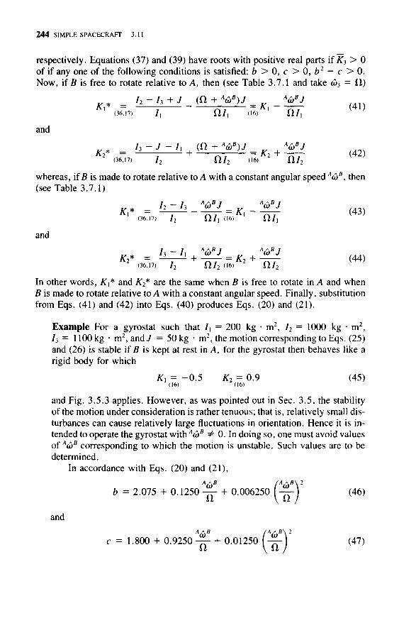
2 4 4 SIMPLE SPACECRAFT 3.11
respectively. Equations (37) and (39) have roots with positive real parts if K3 > 0of if any one of the following conditions is satisfied: b > 0, c > 0, b2 - c > 0.Now, if B is free to rotate relative to A, then (see Table 3.7.1 and take co3 = ft)
* - K
aT; (» ' a/,and
(36,17) /2 ft/2 (16), Kl + ^ ( 4 2 )16) fl/
whereas, if B is made to rotate relative to A with a constant angular speed AtbB, then(see Table 3.7.1)
h-h
and
»,. . h^Jl + %1 . Kl + ^ ,44,(36,17) /2 ft/2 (16) ft/2
In other words, K\* and AT2* are the same when B is free to rotate in A and whenB is made to rotate relative to A with a constant angular speed. Finally, substitutionfrom Eqs. (41) and (42) into Eqs. (40) produces Eqs. (20) and (21).
Example For a gyrostat such that /, = 200 kg • m2, I2 = 1000 kg • m2,h = 1100 kg • m2 ,and7 = 50 kg • m2, the motion corresponding to Eqs. (25)and (26) is stable if B is kept at rest in A, for the gyrostat then behaves like arigid body for which
Kx = - 0 . 5 K2 = 0.9 (45)(16) (16)
and Fig. 3.5.3 applies. However, as was pointed out in Sec. 3.5, the stabilityof the motion under consideration is rather tenuous; that is, relatively small dis-turbances can cause relatively large fluctuations in orientation. Hence it is in-tended to operate the gyrostat with Aa>B =£ 0. In doing so, one must avoid valuesof AwB corresponding to which the motion is unstable. Such values are to bedetermined.
In accordance with Eqs. (20) and (21),
and
b = 2.075 4-0.1250—4- 0.006250 I — ) (46)
Ad)B
c = 1.800 + 0.9250 — + 0.01250 I — ) (47)

3.11 GRAVITATIONAL MOMENT ON AN UNSYMMETRIC GYROSTAT 2 4 5
so that
b2 - c = 2.506 - 0.4063 -j- + 0.02906 (-j-\
+ 1.5625 x 10"3 f-^-J + 3.9063 X 10'5 f-^-j (48)
Now,
(0.1250)2 - 4(2.075)(0.006250) < 0
Hence, b cannot vanish; and, since b is positive for A<hB/£l = 0, it is positivefor all Aa>B/il. The first of conditions (19) thus imposes no restrictions onAo)B/(l. On the other hand, c is negative for - 7 2 < A<bB/£l < - 2 . Therefore,this range of values must be avoided. Finally, b2 — c is intrinsically positiveso that the third of conditions (19) imposes no restrictions on Aa)B/Cl.
The instability associated with — 72 < Aa>B/il < — 2 comes to light clearlywhen one plots the angle </> between e3 and a3 as a function of the number oforbits traversed by G* subsequent to t = 0, doing so for various values ofAo)B/il. Figure 3.11.2 shows such plots for a gyrostat whose rotor is made to
(deg) 90
0.2 0.4 0.6Number of orbits
0.8 1.0
Figure 3.11.2

2 4 6 SIMPLE SPACECRAFT 3.11
rotate relative to the carrier with a constant angular speed and which has inertiaproperties such that A = 200 kg • m2, 72 = 1000 kg • m2, /3 = 1100 kg • m2,and/ = 50 kg • m2, so that [see Eqs. (16)] Kx = -0.5 and K2 = 0.9. The ini-tial conditions used to generate the plots in Fig. 3.11.2, given in Eqs. (3.5.22)-(3.5.24), represent a disturbance, at t = 0, of the motion corresponding to Eqs.(25) and (26); and the plots show that the disturbance has a far greater effecton <f> when Aa>B/tl = -10 than when Aa>7n = -100.

CHAPTER
FOURCOMPLEX SPACECRAFT
Whereas the formulation of dynamical equations of motion for simple spacecraftcan be accomplished with essentially equal ease by means of any one of a numberof methods, the task of formulating such equations for complex spacecraft can be-come prohibitively laborious unless a particularly efficacious method is employed.The first seven sections of this chapter address this important matter, and the meth-odology there set forth is then employed in the remaining four sections to show howto deal with spacecraft consisting either entirely or in part of elastic components.The last section, which contains an introduction to finite element analysis, indicateshow this discipline can be brought to bear on problems involving large motions ofdeformable spacecraft.
4.1 GENERALIZED ACTIVE FORCES
Given a system 5 consisting of N particles P\9 . . . , PN, suppose that n general-ized speeds are defined as in Eq. (1.21.1). Let v / ' denote the rth partial velocityof Pi in A (see Sec. 1.21), and let R, be the resultant of all contact and body forcesacting on Pt. Then Fx, . . . , Fn, called generalized active forces for S in A, are de-fined as
N
Fr = Ev/ ' -R, (r = l, «) (1)1=1
Some forces that contribute to R,(i = 1, . . . , N) make no contributions toFr(r = 1, . . . , n). (Indeed, this is the principal motivation for introducing gener-alized forces.) For example, the total contribution to Fr of all contact forces exerted
247

2 4 8 COMPLEX SPACECRAFT 4.1
on particles of S across smooth surfaces of rigid bodies vanishes; and, if B is a rigidbody belonging to 5, the total contribution to Fr of all contact and gravitationalforces exerted by all particles of B on each other is equal to zero.
If a set of contact and/or body forces acting on a rigid body B belonging to 5is equivalent to a couple of torque T together with a force R applied at a point Qof B, then {Fr)B, the contribution of this set of forces to Fr, is given by
(Fr)B =€Or T + v r R (r = 1, . . . , * ) (2)
where cor and vr are, respectively, the rth partial angular velocity of B in A and therth partial velocity of Q in A.
Derivations Let C be a contact force exerted on a particle P of S by a smooth rigidbody B. Then, if n is a unit vector normal to the surface of B at P,
C = Cn (3)
where C is some scalar. Next, consider A\p, the velocity of P in A. This can be ex-pressed as
*yP = V + B\P (4)
where A\B is the velocity in A of that point B of B that is in contact with P, B\p isthe velocity of P in B, and Byp must be perpendicular to n if P is neither to lose con-tact with, nor to penetrate, B. Moreover,
Bvrp • n = 0 (5)
because otherwise there can exist values of uu . . . , un such that B\p is notperpendicular to n. Now suppose that B is a part of 5. Then
= AyB(4)
Consequently,
(A\rp - A\B) • n = B\r
p - n = 0 (7)(6) (5)
and the contribution to Fr of the forces exerted on each other by P and B is [seeEq. (1)]
A\rp • (Cn) + A\B • ( - C n ) = C(A\r
p - A\B) • n = 0 (8)
Alternatively, suppose that Bis not a part of 5 . Then u\, . . . , un always can bechosen in such a way that ^v* is independent of u\, . . . , « „ , which means that
V = V (r = 1, . . . ,n) (9)(4)
and that the contribution to Fr of the contact force exerted by B on P is [see Eq. (1)]
A\rp • (Cn) = CB\r
p • n = 0 (10)(9) (7)

4.1 GENERALIZED ACTIVE FORCES 2 4 9
In both cases, therefore, the contact forces exerted across a smooth surface of arigid body contribute nothing to Fr (r = 1, . . . , n).
In Fig. 4.1.1, Pt and Pj designate particles of a rigid body B belonging to 5,Ry is the resultant of all contact and gravitational forces exerted on P, by Pj, andRji is the resultant of all contact and gravitational forces exerted on Pj by Ph Toshow that the total contribution of Ry and R;/ to Fr (r = 1, . . . , n) is equal to zero,it is helpful to note (see Prob. 1.31) that the partial velocities v / ( and \r
pj of P, andPj in A are related to the partial angular velocity <or of B in A by
\/j = V/< + O)r X P y (a)
where Py is the position vector from P, to Pj.The Law of Action and Reaction asserts that Ry and R;/ have equal magnitudes
and opposite directions, and that the lines of action of Ry and R;/ coincide. Further-more, the line of action of Ry must pass through P{, and that of R;, through Pj. Con-sequently,
Rp = Rj (12)
and R/; is parallel to p / ; , so that
Pu x Ry = 0 (13)
The total contribution of R/; and R;/ to Fr (r = 1, . . . , n) is thus [see Eq. (1)]
^ - ^ . p y X R y . ^ 0 (14)
To establish the validity of Eq. (2), we introduce forces Ki, . . . , KN> actingon particles P\, . . . , PN of a rigid body B (see Fig. 4.1.2), and let p1? . . . , pN
be the position vectors from a point Q fixed in B to Pi, . . . , PN , respectively.
Figure 4.1.1 Figure 4.1.2

2 5 0 COMPLEX SPACECRAFT 4.1
Then, by definition of equivalence, the set of forces Kx, . . . , KN> is equivalent toa couple of torque T and a force R applied at Q if and only if
T = S p, x K, (15)
andN'
R = 2 K, (16)
where p, is the position vector from Q to P,. Also by definition, the contributionof Ki, . . . , Kjy to the generalized active force Fr is
N'
(Fr)B = K, (r = 1, n) (17)
Now, referring once again to Prob. 1.31, one can write
v / ' = v re + « r x p, (18)
Hence,N' N' N'
(Frh = X (vr° + Or x p,) • K, = ft>r • 2 P, x K, + yrQ • 2 K, (19)
and, using Eqs. (15) and (16), one arrives at Eq. (2).Example Figure 4.1.3 shows a uniform rod B of mass m and length L. B isfree to move in a plane fixed in a reference frame N. P is a particle of mass m,fixed in N, and #,, <?2, and q3 are generalized coordinates characterizing theconfiguration of B in N. _ ^
Suppose that the resultant force exerted by P on B is approximated with Fas defined in Eq. (2.3.6) and that the moment about B* of all forces exerted
Figure 4.1.3

4.1 GENERALIZED ACTIVE FORCES 2 5 1
by P on B is approximated with M as defined in Eq. (2.6.3). Then the set offorces exerted on B by P is equivalent to a couple of torque T together with aforce R applied at £*, with
ai 1 + YJ (2 - 3 sin2 2^)1 - a2 j ^ sin 2q3\^ , = 2 ) - ^ ^ l 1 + ^ ( 2 - 3 s i n 2 2 ^ l - a ^ s i n 2 ^ (20)
and
T = ^ a , x l ' a , (21)(2.6.3) q2
5
where a} and a2 are unit vectors directed as shown in Fig. 4.1.3, and I is thecentral inertia dyadic of B. Hence, T can be expressed also as
^ GmmL2 . „T = — y - sin 2<?3ai x a2 (22)
If Mi, M2, M3 are defined as
ur=qr (r = l, 2, 3) (23)
then co, the angular velocity of B in N, and v, the velocity of B* in N, are givenby
+ M3)a! x a2 v = M2a! + M, 2a2 (24)
so that the partial angular velocities of B in Af and the partial velocities of B*in N (see Sec. 1.21) are
Wi = ai x a2 <o2 = 0 co3 = a, x a2 (25)
and
v, = ?2a2 v2 = a! v3 = 0 (26)
The contributions of forces exerted by P on B to the generalized active forcescorresponding to uu w2, M3 are thus, respectively,
/ GmmL1 . „(F\)B = ai x a2 • —3— sin 2^3ai x a2
(2) (25) \ ^2(22)
(26) \ Hi I I QCil (20)
Sq
Gmm
- a2 —2 sin 293 M = 0 (27)
( 2 8 )

2 5 2 COMPLEX SPACECRAFT 4.2
GmmL2 .s i n 2 * ( 2 9 )
(22,25)
4,2 POTENTIAL ENERGY
If the configuration of a system 5 in a reference frame A is characterized by n gen-eralized coordinates qx, . . . , qn, there may exist a function W of qx, . . . , qn,and r such that all n generalized active forces Fu . . . , Fn for 5 in A (see Sec. 4.1)can be expressed as
F r = - ^ (r = l , . . . , n ) (1)dqr
In that event, W is called a potential energy of 5 in A. [One speaks of "a" ratherthan "the" potential energy of 5 in A because, if W satisfies Eq. (1), then so doesW + /, where / is any function of t. ]
In some situations, force functions discussed in Sees. 2.10-2.19 furnish poten-tial energies. For example, when S consists of a single particle P of mass m movingin A under the action of the gravitational force exerted on P by a particle P of massm fixed in A, then V as given in Eq. (2.10.2) can be regarded as the negative of apotential energy of P in A; and V also provides the negative of a potential energyif 5 consists of two particles moving in A under the action of their mutual gravita-tional attraction. In other situations, potential energies cannot be found so easily,but some of the force functions of Sees. 2.10-2.14 are, nevertheless, useful, forthey produce contributions to potential energies. For example, if 5 consists of arigid body B of mass m and two particles Px and P2 of masses mx and m2, respec-tively, and if these objects move in a reference frame A under the action of mutualgravitational attractions, then Eqs. (2.10.2) and (2.11.5) lead to a potential energyof 5 in the form
W = -G\mxm2p0-1 + mx ( px~
l pdr + m2 j p2'1 pdr) (2)
where p0 is the distance between Px and P2, Pi is the distance from P, (/ = 1, 2) toa generic point P of B, and p is the mass density of B at P.
Although force functions associated with approximations to gravitational forcesand moments can at times be used in the formulation of a potential energy, it canoccur that apparently relevant force functions exist when potential energies do notexist. For example, let S consist of a rigid body B of mass m moving under theaction of gravitational forces exerted by a particle P of mass m fixed in a referenceframe A, and suppose that the resultant gravitational force exerted on B by P isapproximated with F as defined in Eq. (2.3.6), while the moment about the masscenter B* of B of all forces exerted on B by P is approximated with M as definedin Eq. (2.6.3). Then a potential energy of B in A can be expressed as
W = - V (3)

4.2 POTENTIAL ENERGY 2 5 3
with V given by Eq. (2.12.13); but, if FJs approximated with F as defined in Eq.(2.3.5), while M is approximated with M, then there exists no potential energy,despite the fact that force functions for F and M do exist in the sense that F andM can be expressed as F_j= VRVi and M = - R x VRV2, where R is the positionvector of B* relative to P while Vx = GrhmR~x and V2 = GmmR~xv{2) with v(2)
given in Eq. (2.12.2). The nonexistence of a potential energy under these circum-stances may be inconvenient, but it does not invalidate approximating F with F andM with M. On the contrary, precisely these approximations are particularly usefuland are employed extensively in the analysis of motions of spacecraft.
When an expression for a potential energy W of 5 in A is readily available, gen-eralized active forces for 5 in A usually can be found more expediently by differen-tiating W [see Eq. (1)] than by any other means. By the same token, when knowl-edge of generalized active forces is required for the formulation of W, the use ofW cannot facilitate the determination of generalized active forces. However, evenunder these circumstances, a potential energy may be of interest, for instance, inconnection with the construction of integrals of equations of motion. Finally, in theevent that there exists no potential energy function, generalized active forces al-ways can be evaluated by means of Eqs. (4.1.1) and (4.1.2).
Derivations The resultant of all contact and body forces acting on a single particleP_ of mass m moving under the action of the gravitational force exerted by a particleP of mass m is given by
F = - Gmmp(p2r3/2 (4)(2.1.1) r V K V ;
From Prob. 1.29, the rth partial velocity of P in A can be expressed as
Consequently,
v r = - ^ - (r = l , 2 , 3) (5)dqr
Fr = Vr • F = - Gmm — • p(p2) 3/2
(4.i.i) (4,5) dqr
dqr I " J dqr
= | ^ (r = 1,2, 3) (6)(2.10.2) d# r
Hence, if W is defined as
W = -V (7)
then
F . r , - ^ (r = l , 2 , 3 ) (8)

2 5 4 COMPLEX SPACECRAFT 4.2
and W is a potential energy of P in A. Similarly, if 5 consists of both P and P, theresultants F and F of the forces acting on P and on P are given by
F (2=i} - Gmm(Pl - p2)[(Pl - p2)2]"3/2 (9)
and by
F = - F (10)(2.1.2)
respectively, where pi and p2 are, respectively, the position vectors of P and Prelative to a point fixed in A; and
Fr = v / , . F + v /2 . p = / > ! _ $pA . F(4.1.D (io) \dqr dqr/
= - Gmm — (Pi - P2) ' (Pi ~ P2) (Pi ~ P2)2
(9) ldqr J [ J
= - Gmm -B- • p(p2)"3/2 = — (Gmmp-1)dqr dqr
= 4 ^ (r = 1, . . . , 6 ) (11)(2.io.2) dqr
so that W as given in Eq. (7) is once again a potential energy of S in A.When 5 consists of a rigid body of mass m and two particles, Px and P2, of
masses mx and m2, the resultants Fj and F2 of all contact and body forces acting onPx and P2, respectively, are [see Eqs. (2.1.1), (2.1.2), and (2.2.2)]
F! = - Gm1m2Po(Po2)-3/2 + Gm, J P l ( P l2 ) - 3 / 2 prfr (12)
and
F2 = Gm1m2po(po2)"3/2 + Gm2 f p2(P22)~3/2p^T (13)
where p0, Pi, and p2 are position vectors directed as shown in Fig. 4.2.1. The con-tribution to Fr of forces acting on Px and P2 is thus [refer to Eq. (4.1.1), see Fig.4.2.1 for the position vectors Rj and R2, and note that v/1 = dRx/dqr, \/2 =
0r, and!*! - R2 = p0]
+ v/2 . F2 (i = 3) - Gmxm2 ^ • po(po2)-3/2
^ P l ( P i ) p r f r +Gm2{^- p2(p22)"3/2pdr
dqr J dqr
(r = 1, . . . , 12) (14)

4.2 POTENTIAL ENERGY 2 5 5
Figure 4.2.1
As for forces acting on the particles of B, these either are forces exerted by P\ andP2, or they are forces exerted by particles of B on each other. Since B is a rigid body,the latter forces make no contribution to Fr (see Sec. 4.1); and a typical force ofthe former kind can be expressed as
dF (2=j} - G[m lP l(Pl2)-3 /2 + m2p2(p2
2r3/2]p dr (15)
The contribution from this force to Fr is thus given by (see Figure 4.2.1 for p)
yrp - dF = - G m, -fr ' Pi(Pi2)"3/2 + m2 • p2(p2
2)"3/2 pdr
^ - p,(p,2)-3/2 + mx ^ • P l(p,2)-3 / 2 l pdr
\pdr
1, . . . , 12) (16)
and Fr can now be formulated as
Fr = v /» • F, + v/2 . F2 4- {v/ • rfF(4.1.1) J
= - Gm!m2 - ^ • Po(Po2)~3/2 ~ Gmx [ -^ • Pi(Pi2)"3/2p^T(14,16) (jqr J OQr
(continued on next page)
2 5 6 COMPLEX SPACECRAFT 4.2
Gm,|(p,2)-I/2pdT + Gm2j(p22)-^pdr\
(r = 1, . . . , 12) (17)
Pi = (P/)1 /2 U = 0. 1, 2) (18)
or, with
as
r _ d / -i ^ r -i , ^ ^ r -i ^Fr — — I Gfti\Wi2Po • Gtti\ I p\ paT ~r Cjtfi2\ Pi pdi
(n,i8) dqr \ J J
= _ £ ^ (r = 1, . . . , 12) (19)(2) dqr
In accordance with Eq. (1), W as given by Eq. (2) is thus a potential energy of 5.Now consider a rigid body B of mass m moving under the action of gravita-
tional forces exerted by a particle P of mass m fixecHn a reference frame A, andlet the resultant gravitational force exerted on B by P be approximated with F asdefined in Eq. (23.6) while the moment about the mass center £* of B of all forcesexerted on B by P is approximated with M as defined in Eq. (2.6.3). Then
Fr = €Or • M + vr • F (r = 1, 2, 3) (20)
(4.1.2)
where vr, the rth partial velocity of £* in A, can be expressed as (see Prob. 1.29)
d (*a!) (r = l , 2 , 3) (21)dqr
with R and a, as defined in Sec. 2.13. Using Eqs. (2.3.6) and (2.6.13), one thusobtains
^ 3Gm ,F ( x ! )
[a, + f(2)] • (i?a.) (r = 1, 2, 3) (22)R2
or, equivalently,
^ 3Gm , x /T
Fr = -zr (<or x ai) • (I • a,)A
Gmm
Now,
L • j - (Rax) + f(2) • / - (tfaol (r = 1, 2, 3) (23)L ^ r dqr J
f (*.,) = f - a, + R ( r - 1 . 2 , 3 ) (24)a^ d# a^

4.2 POTENTIAL ENERGY 2 5 7
and, using a superscript B to denote differentiation in B, one can write (see Prob.1.29)
? ^ ) r x a i (r = l , 2 , 3) (25)dqr dqr
so that
(«- x a_) • (I • a.) = ^ • I • a. - ^ • I • a, (r = 1, 2, 3) (26)(25) dqr dqr
or, since I is independent of qx, q2, q3 in B,
(i0r x aO • (I • aO = - ^ • I • ^ - - — to • I • a,)dqr 2 dqr
= — • I • a! - \ — (r = 1, 2, 3) (27)dqr 2 d#r
where / n is the moment of inertia of B about a line passing through B* and parallelto ai. Substituting from Eqs. (24) and (27) into Eq. (23), one thus arrives at
F = 3 _ _ 5 / _ _ _ . . __.___,"
( r = l , 2 , 3) (28)
Since d&i/dqr is necessarily perpendicular to a1; the dot-product of da\/dqr with a,is equal to zero. Expressing f(2) as in Eq. (2.3.3), one can, therefore, rewrite Eq.(28) as
_ _ Grnm dR 3Gmi? [ t r ( I )" 3 / i i ] + ir)R dqr dqr)
R2 dqr 2/
Differentiation of V as given in Eq. (2.12.13) gives
_ / _ _ Gmm dR_ _Gm,dR^ (2) Gmm av(2)
d r "" /?2 dtfr R2 dq/ R dqr
Gmm dR Gm dR
Gmm f 1/? m/?
= Fr (r = l , 2 , 3) (30)

2 5 8 COMPLEX SPACECRAFT 4.2
In accordance with Eq. (1), W as given in Eq. (3) is thus a potential energy of Bin A.
Example Figure 4.2.2 shows a uniform rod B of mass m and length L movingin a plane fixed in a reference frame N under the action of gravitational forcesexerted by P, a particle of mass m, fixed in N; qu q2, and q3 are generalizedcoordinates characterizing the configuration of B in N.
If the resultant force exerted by P on B is approximated with F as_de-fined in Eq. (2.3.6) while^the moment about £* of all forces exerted by P onB is approximated with M as defined in Eq. (2.6.3), then W, a potential en-ergy of B in N, constructed by referring to Eqs. (3) and (2.12.13), can be ex-pressed as
W = -Gmm
1 + ( 2 - 3 sin2^) (31)
With the aid of this function and Eq. (1), one can formulate the generalizedactive forces corresponding to ur = qr (r = 1, 2, 3) as
F2 = ~ — = -Gmm
dq2 (3D q22
£21 + -—j ( 2 - 3 sin2
F = -^L= -<i) dq3 (3D 8<?2
3 sin
(32)
(33)
(34)
in agreement with Eqs. (4.1.27)-(4.1.29). _Suppose that the resultant force exerted by P on B is approximated with F
as given in Eq. (2.3.5), rather than with F, but that the moment about £* ofall forces exerted by P on B is approximated as before. Then the generalizedactive forces become [use Eq. (4.1.2)]
Figure 4.2.2

4.3 GENERALIZED INERTIA FORCES 2 5 9
GfnmL2 . Gmm GfnmL2 .F\ = 5—3— sm 2q3, F2 = — ' F3 = 5—3— s m 243 (35)
Now, if there exists a function W that satisfies Eq. (1), then dFl/dq3 = dF3/dqx.Since here these derivatives are given by
dFx GfnmL2 „ dF3 ^—- = —^— cos 2q3 —^ = 0 (36)d<?3(35) 4^2 ^ a^j 05)
one is forced to conclude that a potential energy of B in N does not exist.
4.3 GENERALIZED INERTIA FORCES
Given a system 5 consisting oiN particles Px, . . . , PN, suppose that n generalizedspeeds are defined as in Eq. (1.21.1). Let v/« denote the rth partial velocity of Pt
in reference frame A (see Sec. 1.21), and let R,* be the inertia force for P, in A;that is, let
R,* = - m , a , (1 = 1, . . . ,A0 (1)
where m( is the mass of P( and a, is the acceleration of P{ in A. Then Fi*, . . . , Fn *called generalized inertia forces for 5 in A, are defined as
N
Fr* = 2 v/<'• R,* (1 = 1, . . . , n ) (2)
(Fr*)B, the contribution to F r * of all inertia forces for the particles of a rigidbody B belonging to S, can be expressed in terms of R* and T*, defined as
R* = - Ma* (3)
andN
T* = - 2 mtVi x a, (4)
where M is the mass of B, a* is the acceleration of the mass center B* of B in A,nti is the mass of a generic particle Pi of B, N is the number of particles comprisingBy r, is the position vector from B* to P{, and a, is the acceleration of Pj in A. T*is called the inertia torque for fi in A, and (Fr*)B can be written
(Fr*)B = <or T* + vr R* (r = 1, . . . , n) (5)
where vr is the rth partial velocity of fi* in A, and c*r is the rth partial angular ve-locity of B in A (see Sec. 1.21). The utility of Eq. (5) derives from the fact that T*can be expressed in a number of forms making it unnecessary to perform explicitlythe summation indicated in Eq. (4). For example,
T* = - a I - co x I €0 (6)

2 6 0 COMPLEX SPACECRAFT 4.3
where a and to are, respectively, the angular acceleration of B in A and the angularvelocity of B in A, and I is the central inertia dyadic of B; and, if Ci, c2, c3 forma dextral set of mutually perpendicular unit vectors, each parallel to a central prin-cipal axis of inertia of B, but not necessarily fixed in B, and a ; , cu,, and /, are de-fined as
AA= a
A= (O / , = c , - I - c , 0 = 1,
then Eq. (6) can be re-expressed as
T* = - [axh ~ o2w3(I2 - / 3 ) ] c ,
- [a2h ~
- [a3l3 -
2,3) (7)
(8)
When a subset of the particles of 5 forms a gyrostat G (see Fig. 4.3.1) con-sisting of a rigid body C that carries an axisymmetric rotor D whose mass centerD* and axis are fixed in C, then (F r*)G, the contribution to F r* of all inertia forcesfor the particles of G, can be expressed as the sum of two quantities, one associatedwith a (fictitious) rigid body R that has the same mass distribution as G, but moveslike C, and the other accounting for rotation of D relative to C; that is, one can write
(Fr*)G = (Fr*h + (/v*)/ (r - 1, . . . . n) (9)
where (/v*)* is the rth generalized inertia force associated with the motion of R inA, a quantity one can form most conveniently by using Eq. (5), and (Fr *)/ takes oneof two forms, depending on whether the motion of D in C is prescribed as a functionof time, in which event none of the generalized coordinates characterizing themotion of S in A is associated with rotation of D relative to C, or D is completelyfree to rotate relative to C. When the motion of D in C is prescribed (which impliesthat C exerts on D such forces as are required to produce the prescribed motion),then
Figure 4.3.1

4.3 GENERALIZED INERTIA FORCES 2 6 1
(Fr*)7 = 7 [ f t ( - o>2Ci + W!C2) - fic3] • (or (r = 1, . . . , n) (10)
where Ci, c2, c3 form a dextral set of mutually perpendicular unit vectors fixed inC, with c3 parallel to the axis of D (see Fig. 4.3.1); J is the moment of inertia ofD about the axis of symmetry of D; fl = c(oD • c3; o>, = A(oc • c, (i = 1, 2, 3); and(or is the rth partial angular velocity of C in A (see Sec. 1.21). Alternatively, whenD is completely free to rotate relative to C, one can always define un, the nth gen-eralized speed for 5 in A (see Sec. 1.21), as un = c(oD • c3, and Eq. (10) then givesway to
(/V*)/ = J[un{- o>2Ci + a>!C2) - wnc3] • (or (r = 1, . . . , n - 1) (11)
together with
(Fn*)i = -J(<i>3 + " J (12)
Moreover, (Fn*)R vanishes under these circumstances.
Derivations With mi9 r,, and a, as defined,
N
2 m,r,. = 0 (13)i = 1
and a, can be expressed in terms of the acceleration a* of the mass center of B inA, the angular acceleration a of B in A, and the angular velocity (o of B in A as
a . = a* + a X Ti> + (o X ((o x r,) (i = 1, . . . , N) (14)
Consequently,
N N N i N v
/, m,a, = ^ ntiSr -r & x £, W,T, + w x w x ^ W/f, I — Msr = — K*
(15)
Now, (Fr*)fl = - S ^ / v / ' - a , (r = 1, . . . , n) (16)
and (see Prob. 1.31)
v / ' = vr + (or x r, (r = 1, . . . , n\ i = 1, . . . , N) (17)
Hence,
JLm,(vr + (or x r,) • a,
= - vr • 2 "1/*; ~ wr ' 2 m«r/ x a,1=1 1=1
= v r R * + (or T * ( r = 1 , . . . , « ) ( 1 8 )(15,4)
which establishes the validity of Eq. (5).

2 6 2 COMPLEX SPACECRAFT 4.3
With the aid of Eq. (14), one can express T* as
N
T* = - X mPt X [a* + a X r,- + w x (w x r,)]
Now,
N N
X rritTi X (a x r,) - 2 ™?i x [co x (co x r,)] (19)
N N
S niiVi X (a X T() = 2 wi/(r/2a - a • r,-!-,)
= a • X MiiffV - ri*i)
= a I (20)
and
2 w/rf- x [w x (w x rf)] = - 2
= - CD X
[|-*--H= - co X | Z m/fr/r/ - r>U) 1 • co
= w x l w (21)
Substitution from Eqs. (20) and (21) into Eq. (19) produces Eq. (6).With oij, a)j, and /, as defined,
I = /iCiCi + / 2 c 2 c 2 H- /3C3C3 (22)
so that
a • I = ct\I\C\ + a2/2c2 4- CK3/3C3 (23)
and
co X (I • co) = — a>2a>3(/2 — /3)Ci — co3O>i(/3 — / i ) c 2 — a>io>2(/i — /2)C3 (24)
Equation (8) thus follows directly from Eqs. (6), (23), and (24).Turning to the derivation of Eqs. (9)—(12), we let P and Q be generic points
of C and D, respectively, and note that there corresponds to Q a certain point of/?, the rigid body_having the same mass distribution as G, but moving like C.Calling this point Q, we now make a number of purely kinematical observations,

4.3 GENERALIZED INERTIA FORCES 2 6 3
regarding D as completely free to rotate relative to C for the time being and takingun 4 w . C3
The partial velocities of Q and D* in A are related to the partial angularvelocities of C in A by (see Prob. 1.31)
vr^ = vrD* + €orXrQ ( r = 1, . . . , n) (25)
where rG is the position vector from D* to (?; and vn^ = 0, because \nD* = con = 0
since the velocity of D* in A and the angular velocity of C in A are independent ofun. To discover the relationship between the partial velocities of Q and D* in A,we note first that the velocities of Q and D* in A are related by
VG = y°* + (Awc + M ^ 3 ) x r e ( 26)
from which it follows that
yrQ = vr
D* + ft)rxrc (r = 1, . . . , n - 1) (27)
while
v,* = c3 x r^ (28)
The angular acceleration of D in A can be formulated asAd
OLD = - (A<oc + w,c3) = a c + w cs + unA€oc X c3 (29)
( L 2 0 1 ) d t (1.16.1) (1.11.9)
and this result may be used to express the acceleration of Q in A as
aG = aD* + a D x rQ + (Aaic + Mnc3) x [(A<oc + M/lc3) x rQ]
= aD* + a c x rQ + Acoc x (Aioc x rG) + ^ c , x rQ
(29)
+ 2 M / W C x (c3 x rQ) 4- «n2c3 x (c3 x r e ) (30)
Similarly, the acceleration of Q in A is given by
a^ = aD* + ac x r e + Aoic x (Awc x rG) (31)and, using Eqs. (25), (31), (27) and (30), one can write (after considerable rear-ranging)
\? • 2fi - \rQ • aG = - eor • [wnr
G x (c3 x rQ) + 2unA<oc • r^r^ x c3
- un2c3 • r G r2 x c3] - vr
D* • [iinc3 x r^
+ 2unAcjc x (c3 x r e ) + un
2c3 x (c3 x rQ)]
( r = 1, . . . , / i - 1) (32)
To construct generalized inertia forces for G, we now let m p and mQ denote themasses of P and Q, respectively, and use the symbols 2 C and 2 D to denote summa-tions extended over the particles of C and D, respectively. Referring to Eqs. (1) and(2), we can thus write for G

2 6 4 COMPLEX SPACECRAFT 4.3
(Fr*)G = - £ C mpyf • ap - 2 ° mcv rc • a* (r = 1, . . . , n) (33)
and for/?, the rigid body that has the same mass distribution as G but moves like C,
(Fr*)R = - S C m ' v / • ap - S ° mev re • afi (r = 1, . . . , n) (34)
Consequently,
(Fr*)c = (Fr*)R + E ° m2(vre • 8 e - vre • a^) (r = 1, . . . , n) (35)(33,34)
from which Eq. (9) follows immediately if (Fr*)7 is defined as
(Fr*)i = E D /nG(vr^ - vfi - y° • aG) (r = 1 /i) (36)
We shall presently substitute from Eq. (32) into Eq. (36). Before doing so, it isworth noting that each member of the second bracketed term of Eq. (32) involvesr c , so that each such term will give rise to the sum 2D mQrQ, which is equal to zerobecause rQ is the position vector from the mass center of D to a generic particle ofD. By way of contrast, the first bracketed term of Eq. (32) leads to sums of theforms ^DmQrQ X (c3 x rQ) and 2D mQrQrQ x c3, and these can be expressed asfollows:
E D mQr<2 x (c3 x rQ) = c3 • 2 * mc[(rG)2U - r^rQ]
= c3 J (37)
where J is the central inertia dyadic of D. Since c3 is parallel to a central principalaxis of inertia of D, c3 • J is parallel to c3, and
c3 J = 7c3 (38)
where J is the moment of inertia of D about its axis of symmetry. As for the secondsum, one can write
x c3 = Vz° mQ^fV - j j x c3
(39)
Substitution from Eq. (32) into Eq. (36) thus produces
(Fr*)7 = - (or [iinJc3 + unJ(- eo,c2 + o)2c,)] (r = 1, . . . , n - 1) (40)(37,38)
in agreement with Eq. (11). As for Eq. (12), this can be obtained by proceedingsimilarly, but using Eq. (28) in place of Eq. (27). Finally, if the motion of D in Cis prescribed, the validity of Eq. (10) can be established by proceeding as in the der-ivation of Eq. (11), but replacing un with ft.

4.3 GENERALIZED INERTIA FORCES 2 6 5
Figure 4.3.2
Example Figure 4.3.2 shows a system 5 composed of a particle P of mass mand a uniform rectangular block B that has a mass M and sides of lengths Lu
L2, L3. P is constrained to remain on a line L fixed in B and is attached to Bby means of a spring and a damper. Yu Y2, F3 are lines passing through /?*,the mass center of B, and parallel to the edges of B; L is parallel to Ki at a dis-tance b from Fi; and the spring is presumed to be undeformed when P lies onY2. Thus q, the distance from P to K2, measures the deformation of the spring.
Generalized speeds Mi, . . . , w7 for S in a reference frame A can be definedin terms of co, the angular velocity of B in A, and v*, the velocity of 5*, themass center of 5, in A:
AM, =
to • b,
b,_4
(i = 1,2,3)(i = 4)(» = 5, 6, 7)
(41)
where bi, b2 , b3 are unit vectors respectively parallel to YUY2,Y3. The angularvelocity and angular acceleration of B in A then can be expressed as
co = + w2b2 + M3b3 (42)
and
a = w2b2 + M3b3 (43)

2 6 6 COMPLEX SPACECRAFT 4.3
while the velocities of B* and P in A are given by
vB* = v,**b, + v2B*b2 + v3
B*b3 (44)
and
vp = vi'b, + v / b 2 + v / b 3 (45)
where
A m „ ,Ar.
= «5 H ;—^ (OM3 — M4) (46)
qu} (47)
(qu2 - fc«,) (48)
- «4) (49)
(50)
A Mv / = M7 —-r. (qu2 - bux) (51)
m + MThe accelerations of 5* and P in A, found by differentiating Eqs. (44) and (45)with respect to fin A, are
m
m
m
m
m
m
m+
M
M
M
M
M
M
M
"6 TTTA (M4W3 + ^ M 3 ) 4- u3vxB* - u{v3
B* b 2
B ' -« 2v, f l- b3 (52)
andJ
["5 m + M "3 "4 + "2V3 "3V>2 J
4- I w6 H — («4«3 4- ^M3) 4- M3Vi ~ U\V{ D2
L m 4- M J
+ M*7 7~M (U4U2 4- W 2 — foil) 4- M i v / — M2Vi/> b 3 (53 )
L m + M JThe partial angular velocities of B in A and the partial velocities of B* and
P in A, formed by reference to Eqs. (42) and (44)-(51), are recorded in Table

4.3 GENERALIZED INERTIA FORCES 2 6 7
Table 4.3.1
€Or
b,
b2
b3
m
mm +
mm + Af '
+ M
m
bb3
- qb2)
m + M
b,
b2
b3
Mm -
m
Mm +
m
M+ M
M+ M
b,
b2
b3
7 U 3
<?b3
b, - ^ b 2 )
b,
4.3.1, and these are used to construct (Fr*)B and (Fr*)P, the contributions ofB and of P to the generalized inertia force Fr* for S in A. To this end, the inertiatorque T* for B in A is expressed as [see Eqs. (42) and (43)]
T* = - [uxBx - u2u3(B2 - £ 3(8)
- [u2B2 - w3«i(£3 - B i ) ] b 2
- [ii3B3 - uxu2{Bx - B2)]b3 (54)
where
M A MBx \2 {Ll + U } S2 n (L3 + Ll } *
and Eq. (5) then yields [see also Eqs. (3) and (52)]
(F\*)B ~ ~~ uxBx — u2u3(B2 — B3)
mM
= ^ ( ^ 2 + ^ 2 ) (55)
[. mm + M"\"' m + M
= — U2B2 — M3Mi(fi3 — B\)
mM
(u4u2 + qu2 — biix) •+• uxv2B* — u2vx
B* (56)
m m + M(M4M2 -u2vr\ (57)
and so forth, while Eqs. (1), (2) and (53) lead to

2 6 8 COMPLEX SPACECRAFT 4.3
b\u7-M
m + M— bu\)
(58)
and so forth. The generalized inertia forces for 5 in A now can be written bysimply adding the contributions of B and P. Thus, for example,
mM
m Mb(2u2u4 + qu2 — (59)
Now consider the system 5 obtained by modifying 5 as follows: let D be a uni-form axisymmetric rotor made of the same material as B; remove from B acylindrical portion just big enough to accommodate D, letting the axis of thecylindrical cavity thus created be parallel to Y3 and calling C what now remainsof B; and place D into the cavity. Then C and D form a gyrostat G (see Fig.4.3.3) with a mass distribution identical to that of B, and the generalized inertiaforces, ? ! * , . . . , F7*, for 5 in A can be obtained simply by adding to thosefor 5 in A terms generated with the aid of Eq. (10) or Eqs. (11) and (12). Sup-pose, for example, that D is presumed to be driven relative to C, say by meansof a torque motor, in such a way that ft, defined as ft = CCJD • b3, remainsconstant. Then, if J is the moment of inertia of D about its axis,
F,* = F,* - 7ftw2 (60)
Figure 4.3.3

4.4 KINETIC ENERGY 2 6 9
and so forth. If D is completely free to rotate relative to C, then a generalizedspeed M8, defined as «8 = c€oD • b3 , must be added to those introduced inEq. (41); Eq. (60) is replaced with [see Eq. (11)]
Fx* = F,* - Jusu2 (61)
and Eqs. (9) and (12) furnish one relationship in addition to those available be-fore, namely,
F8* = - J(ii3 + us) (62)
4.4 KINETIC ENERGY
If the configuration of a system S in a reference frame A is characterized by n gen-eralized coordinates qx, . . . , qn, and if n generalized speeds uu . . . , un are de-fined as in Eq. (1.21.1), then the kinetic energy AT of 5 in A can be expressed as
K = AT0 + # , + K2 (1)
where Kj is homogeneous and of degree j in the variables u\9 . . . , un.ln particu-lar, K2 is given by
•, n n
K2 = - 2 2 Mrsurus (2)
where Mr5, called an inertia coefficient for 5 in A, is a function of qx, . . . , #„, andt that is defined in terms of the masses and partial velocities of the particles of Sin A (see Sec. 1.21) as
N
Mrs = X /n,v/' • v/' (r, s = 1, . . . , n) (3)1 = 1
where N is the number of particles of S.The inertia coefficients furnish a measure of dynamic coupling: the generalized
speeds ur and M are said to be coupled dynamically if Mrs ^ 0, and uncoupled ifMrs = 0.
If B is a rigid body belonging to 5, then (Mrs)B, the contribution of B to Mrs,is given by
(Mrs)B = m\r - \s + <or - 1 - o)s (r, 5 = 1, . . . , n) (4)
where m is the mass of B, \r and v, are, respectively, the rth and the 5th partial ve-locity of the mass center of B in A, <or and <os are, respectively, the rth and the sthpartial angular velocity of B in A, and I is the central inertia dyadic of B.
If the generalized speeds are chosen as
wr = qr (r = 1, . . . , n) (5)
and the kinetic energy of 5 in A is regarded as a function of the In + 1 independent

2 7 0 COMPLEX SPACECRAFT 4.4
variables qu . . . , qn9 qx, . . . , qn9 and t, then the generalized inertia forces for5 in A (see Sec. 4.4) can be expressed as
dqr dt dqr
Derivations Regard 5 as composed of N particles Pu . . . , PN, and let \p>and v / 'denote the velocity of P, in A and the rth partial velocity of P, in A, respectively.Then
n
\"< = 2 v/'«r + v,'"' (i = 1 , V) (7)( 1 . 2 1 . 3 ) ^ _ j
where v / ' is a function of q{, . . . , qn, and t; and
(v'O2 = S S v / ' • v/'uru, + 2 ^ v / ' • v / '« r + (v /0 2
( 7 ) r=l F l r=l
(i = 1, AT) (8)
By definition,
K = \ E mKv''')2 (9)
where m, is the mass of P,. Hence,, yV n n N n + N
K = O 2 X S ^/V/' • v/'WrM, + 2 2) W/V/' • v/'Mr + " 2 W/(V/')2
(8-9) Z / = 1 r = 1 J = , / = 1 r = , I / = ,
(10)
and, if Ko, K\, and ^ 2 are defined as
Ko = \ £ m,-(v/')2 (ID
^i = E 2 «,-v/' • v/'«r (12)1=1 r = l
and K2 ± i S £ £ m,v/< • v/ ' Mr«s (13)^ ;=1 r=\ 5=1
then Eq. (1) follows immediately. Moreover, since the order in which the summa-tions in Eq. (13) are performed is immaterial, K2 can be expressed as
1 n n N
Ki = - 2 2 2 w.-v/' • v/'«r«,^ r = l 5 = 1 i = l
which, together with Eq. (3), leads directly to Eq. (2).
(14)

4.4 KINETIC ENERGY 2 7 1
To establish the validity of Eq. (4), let the rigid body B consist of the first Nparticles of 5, let r, be the position vector from the mass center £* of B to Ph andnote that (see Prob. 1.31)
v / i = Vr + €orx r, (i = l, . . . 9N) (15)
where vr is the rth partial velocity of B* in A. Hence,
N
(Mrs)B = 2 Wi[vr • v, + vr • €os x r, + o>r x r, • \s(3) , = 1
+ {(or X r,) • (a>s X r,)] (r, s = 1, . . . , n)
N
Vr • (Os X/=l /
/ ]v \ r 5v -i
I 2 rnji) ' v5 + wr • 2 /H,-(r/2U - r,r,)
But,
r X )
( r , 5 = 1 , . . . , « ) ( 1 6 )
Z w,-r, = 0 2J w,(r,2U - r,r,) = I (17)/= i /= i
Hence, Eq. (4) is equivalent to Eq. (16).Finally, let a, be the acceleration of P, in A; write (see Prob. 1.30)
2
and, recalling that [see Eqs. (4.3.1) and (4.3.2)]
N
2 "*/v/< - a , (r = 1 w) (19)
proceed to
F* = ir 0819) 208.19) 2 ^ m ' [ ^ r rfr dqr
^ r L 2 '=1 J dtd<lr[2i=x J
dK d dK
in agreement with Eq. (6).

2 7 2 COMPLEX SPACECRAFT 4.4
Example Figure 4.4.1 shows a system S consisting of a thin rod B of length2L and mass m and a particle P, also of mass m. P can slide on B, but is at-tached to one end of B by means of a spring. Xi and X2 are Cartesian coordinateaxes fixed in a reference frame A, and qu • . • , q* are generalized coordinatesfor 5 in A, 5 being constrained to move in the Xx-X2 plane.
The velocities of the mass center £* of B and of the particle P in A aregiven, respectively, by
v * * = q2a2
and
vp = q22i2
(21)
(22)
where at, a2, bi, and b2 are unit vectors directed as shown in Fig. 4.4.1, andthe angular velocity of B is
(o = q3b\ X b2
Hence, the kinetic energy of S in A is
K = \m{y»y + X-^y co2 + \ m(yp
(23)
pf
(2U2)
COS q3
sin ^3} (24)
Figure 4.4.1

4.4 KINETIC ENERGY 2 7 3
and, if qu . . . , q4 are chosen as generalized speeds, then the associated gen-eralized inertia forces, found by using Eq. (6) together with
— = 0 — = m[2qx + q4 cosq3 - q3(L + q4) smq3] (25)dqx dqx
— = 0 — = m[2q2 + q3(L + q4) cosq3 + q4 sinq3] (26)dq2 dq2
— = m{[qxq4 - q2q3{\ + q4)] sinq3dq3
(27)
q42)q3 + q2(L + #4) cos^3 - ^!(L + q4) sinq3] (28)
— = m(q4q32 + ^2^3 cos#3 - ^,^3 sin^3) (29)
dq4
—- = m(q4 + 4! cos^3 + #> sin ^3) (30)
d^4
are
Fi* = - m[2q{ H- 4f4 cos^3 - 2<?4^3 sin<73 - (L + q*)(q3 sinq3
+ ^32cos^3)] (31)
F2* = - m[2q2 + ^4 sin#3 + 2^4^3 cos^3 + (L + ^4)(4f3 cos^3
- 432sin<?3)] (32)
F3* = - m[(L + ^4)(^2 - 4f, sin^3) + ( | L 2 + «42)4f3 + 2^4<?4] (33)
F4* = - m(q4 + qi cosq3 + f2 sin^3 - <?4#j2) (34)
It is worth noting that these results can be obtained with less effort as follows.The accelerations of B* and of P in A, found by differentiating \B* and \p,
are
9 i i ^ 2 <?32£b, + #>£b2 (35)
ap = <?ia, + #>a2 + (q4 - ^ 32^)bi + ( 3<74 + 2^3^4)b2 (36)
and the angular acceleration of B in A is
a = <?3b, x b2 (37)
so that the inertia torque for fi in A can be expressed as
T*«i6)-'f^xb> (38)

2 7 4 COMPLEX SPACECRAFT 4.4
Hence [see Eqs. (4.3.2), (4.3.3), and (4.3.5)],
Fr* = _ my/ a>> + Mr T* - mvrfl* • a** (r = 1, . . . , 4) (39)
where the partial velocities v / and \rB* (r = 1, . . . , 4) can be written by in-
spection of Eqs. (21) and (22), and the partial angular velocities a>x, . . . , <o4
all are equal to zero, except for o>3, which is equal to bi X b2 [see Eq. (23)].Substitution from Eqs. (35)-(38) into Eq. (39) leads directly to Eqs. (32)-(34). For example,
F4* = - mb, • ap 4- 0 • T* - 0 • a**(39)
= - m(qx cosq3 4- q2 sinq3 + q4 - q32qA) (40)
(36)
in agreement with Eq. (34).If, instead of using qu . . . , q4 as generalized speeds, one defines
Mi, . . . , M 4 a s
Mi = qx cos #3 + q2 sin q3 (41)
u2— — q\ sin 3 4- q2 cosq3 4- q3L (42)
\B*
yp
AM4 = i
= «,b,
= (Ml H
= M 3 b,
+ w2b2
- «4)b, H-
x b2
- [u2-\I" (94 - L ) « 3 ] b 2
(43)
? (44)
thenB* (45)
(46)
(47)
afl* = (M, - M2M3)b, + (M2 4- M3M,)b2 (48)(45)
ap = {«, -h M4 - u3[u2 4 (<74 - L)M3]}b!(46)
+ [M2 4- 2M4M3 4- (qA - L ) I I 3 4- M3Mi]b2 (49)
a = M3bi x b 2 (50)(47)
and the generalized inertia forces F i* , . . . , F 4 * associated with u\, . . . , M4
are [see Eq. (39)]
F , * = - m{2M, 4- M4 - M3[2M2 4- (qA - L)u3]}
F 2 * = - m[2M2 4- 2M4M3 + (q4 - L ) M 3 - 2M3M,]
3
(51)
(52)
(53)F 3 * = - m(qA- L)[u2 + 2M4M3 -h (^4 - L )M 3 4-
F 4 * = - m{ux 4- M4 - M3[M2 4- (<?4 - L ) M 3 ] } (54)

4.5 DYNAMICAL EQUATIONS 2 7 5
These expressions have a number of advantages over their counterparts, Eqs.(31)—(34). Not only are Eqs. (51)-(54) free of trigonometric functions andshorter than Eqs. (31)—(34), but each contains only two of uu . . . , w4,whereas each of Eqs. (31 )-(34) involves three of q{, . . . , q4. The underlyingreason for this is that uu . . . , u4 are less strongly coupled dynamically thanare qu . . . , q4, a fact that can be ascertained by forming inertia coefficients[see Eqs. (3) and (4)] for both choices of generalized speeds. In the first case,
M12 = 0 M B = - m(q4 + L) sin<?3 MX4 = m cosq3 (55)
M23 = m(q4 + L) cosq3 M24 = m sin<?3 Af34 = 0 (56)
while in the second case,
M12 = 0 M13 = 0 Af M = m (57)
M23 = m(q4 - L) M24 = 0 M34 = 0 (58)
Thus, only two uncouplings occur when qx, . . . , <?4 are used as generalizedspeeds, whereas four take place when generalized speeds are defined in accord-ance with Eqs. (41)-(44).
4.5 DYNAMICAL EQUATIONS
Given a system 5 possessing n degrees of freedom in a Newtonian reference frameN, let uu . . . , un be generalized speeds for S in N (see Sec. 1.21), and formFu . . . , Fn, the associated generalized active forces for SinN (see Sec. 4.1), andFi*, . . . , Fn*, the associated generalized inertia forces for S inN (see Sec. 4.3).Then all motions of 5 are governed by the equations
Fr + / v * = 0 (r = 1 /i) (1)
These equations are called Kane's dynamical equations.
Derivation Regard 5 as composed of v particles Pu . . . , Pv having massesmi, . . . , /?!„, respectively, and let R, be the resultant of all contact and bodyforces acting on Pt. Then, in accordance with Newton's second law,
R, = m,*,- (i = 1, • • . , v) (2)
where a, is the acceleration of Pt in N. Equivalently, if the inertia force R, * for Pt
in N is defined as
R,* = - m,a, (I = 1 , . . . , I / ) (3)
then
R, + R,* =2) 0 (/ = ! , . . . , ! / ) (4)

2 7 6 COMPLEX SPACECRAFT 4.5
and dot-multiplication with v / ' , the rth partial velocity of P, in N (see Sec. 1.21),gives
v / ' • R, + v / ' • R,* = 0 (r = 1, . . . , w; i = 1, . . . , v) (5)
Summing over all particles of 5, one can thus write
V V
2 v/' • R/ + 2 v/< • R,-* = 0 (r = 1, . . . , n) (6)
and, using Eqs. (4.1.1) and (4.3.2), one arrives at Eq. (1).
Example Suppose that the system 5 described in the example in Sec. 4.3moves in N in the absence of external forces, and let a be a function of q andM4 such that the force R exerted on P by the spring and damper is given by
R = - C7b! (7)
Then the force exerted on B by the spring and damper is equal to — R. Thevelocity in N of the point Q (see Fig. 4.3.2) at which the latter force is ap-plied is
\Q = \B* + <o x ( - hbx + bb2) (8)
or, in view of Eq. (4.3.42),
\Q = \B* - few3bi - hu3b2 + (&K, + hu2)b3 (9)
Hence, the partial velocities of Q are
vi e = \iB* + bb3 \2Q = v/* + hb3 \3
Q = \3B* - bbx (10)
vrQ = yr
B* (r = 4, . . . , 7 ) (11)
and the generalized active forces for 5 in TV, found by substituting into
Fr = v / R + yrQ • ( - R ) = ( v / - yr
Q) R (r = 1, . . . , 7) (12)(4.1.1)
are [see Table 4.3.1 for v / and \rB* (r = 1, . . . , 7)]
( 0 (r = 1,2, 3 , 5 , 6 , 7 )' r l - o - (r = 4 )
With r = 1, one thus obtains the dynamical equation [see Eq. (4.3.59) for F\*]
- uxBx + (£ 3 ~ B2)u2u3
+ b ( 2 u 2 u 4 + <7M2 - foiii - gwiw3 - foM2M3) = 0 (14)( 1 1 3 )m ~r M (1,13)
and similarly for r = 2, . . . , 7. For instance, the dynamical equation corre-sponding to r = 4 is

4.6 LINEARIZED DYNAMICAL EQUATIONS 2 7 7
~ a + m"TM [Z?("3 " UxUl) " "4 + ' ^ + WB2)1 = ° (15)
4.6 LINEARIZED DYNAMICAL EQUATIONS
When the formulation of dynamical equations (see Sec. 4.5) for a system 5 is un-dertaken for the purpose of analyzing the stability of a particular motion of S or inconnection with, say, designing a control system, it may occur that one is interestedsolely in linearized dynamical equations, that is, equations obtained from dynami-cal equations by dropping all terms of second or higher degree in some (or all) ofqu . . . , qn, u\, . . . , un. Such equations can be formulated, without first writingexact dynamical equations, by proceeding as follows: Develop fully nonlinear ex-pressions for angular velocities of rigid bodies belonging to 5, for velocities of masscenters of such bodies, and for velocities of particles belonging to 5, and use theseto determine partial angular velocities and partial velocities (see Sec. 1.28) by in-spection. Next, linearize all angular velocities, velocities, partial angular veloci-ties, and partial velocities, and use the linear forms to construct generalized activeforces (see Sec. 4.1) and generalized inertia forces (see Sec. 4.3), discarding allterms of second or higher degree. Finally, substitute into Eq. (4.5.1) to obtain thedesired equations.
Example In the absence of external forces, the system S considered in the ex-ample in Sec. 4.3 can move in a Newtonian reference frame in such a way thatq = u2 = • • • = u-j = 0 (but Mi =£ 0), provided the spring is unstretched whenq = 0 and the damper exerts no force when u4 = 0. To study the stability ofsuch a motion, one may wish to construct dynamical equations linearized in q,w2, . . . , w7. To obtain these, begin by expressing (o, \B\ and \p as in Eqs.(4.3.42)-(4.3.51), and record partial angular velocities and partial velocitiesas in Table 4.3.1. Next, linearize, obtaining for to, vfi* and vp,
to = U\b\ + w2b2 + M3b3 (1)
m
m + M J \ m + M
m ~ W4)lbl
JNote that Table 4.3.1 need not be altered since it is free of nonlinearities.Now differentiate Eqs. (1), (2), and (3) with respect to time in N to find
a = i<i bi + w2b2 + W3b3 (4)
f • m . x mbuxu2\= U s + TTT (foM3 ~ "4) —-T/i b l
L m + M m + M J
2 7 8 COMPLEX SPACECRAFT 4.6
Mpa =
M / \ m + M
Representing the action of the spring and damper as in the example in Sec.4.5, and assuming that a vanishes when q = u4 = 0, one can expand a in aTaylor series in q and w4, retaining only terms linear in these variables, whichgives
da daa = — q + u4 (7)
dq du4
where the partial derivatives are evaluated at q = u4 = 0. Proceeding as in thederivation of Eq. (4.5.13), one then obtains
0 (r = 1, 2, 3, 5, 6, 7)F'-<-(^+4%.) (-4) ( 8>
The linearized form of the inertia torque T* for B in N is [see Eqs. (1)and (4)]
1 == UXiJXUX [ 2^*2 ' \BX 3-x)ll3llX\\32(4.3.8)
- [ii3B3 + (fi2 - Bx)uxu2]b3 (9)
where 2?i, B2, B3 are given in Eqs. (4.3.55), and generalized inertia forces nowcan be formed as
Fr* = (or T* + \rB* • (-Ma**) + v / • (-map) (r = 1, . . . , 7) (10)
so that, for r = 1 [see Table 4.3.1 and Eqs. (5) and (6)],
Fl* = _ Ux i mMb2\x (11)V l m + M / M l
and similarly for r = 2, . . . , 7. Finally, substitution into Eq. (4.5.1) yields
ux = 0 (12)(8,11)
and so forth. For instance, the linearized equation corresponding to r - 4 is{da ^da_ \ _
I du4 ) m
Equations (12) and (13) can be generated, alternatively, by linearizingEqs. (4.5.14) and (4.5.15).

4.7 COMPUTERIZATION OF SYMBOL MANIPULATION 2 7 9
4.7 COMPUTERIZATION OF SYMBOL MANIPULATION
The labor required to formulate dynamical equations (see Sec. 4.5) can becomevery burdensome when a system consists of more than a few rigid bodies and/orparticles. In that event, it is advantageous to resort to the use of a computer to per-form such tasks as differentiations, multiplications, substitutions, and so forth, inliteral form. Indeed, when one's ultimate goal is the numerical solution of differen-tial equations of motion, one may be able to employ computerized symbol manip-ulation to bypass the explicit writing of equations of motion, that is, to proceed di-rectly from a few handwritten equations to the creation of a computer program thatyields simulation results. An additional advantage of this procedure over that offormulating explicit equations of motion by hand and then writing a program tosolve them is that it offers one fewer opportunities to make mistakes.
Example Figure 4.7.1 is a schematic representation of a space shuttle Aequipped with a manipulator arm consisting of n pin-connected bars Bx, . . . ,Bn. Simulations of motions of this system are to be performed in order to ex-plore effects of arm movements on the motion of body A. Specifically, the an-gles qu . . . , qn indicated in Fig. 4.7.1 will be specified as functions of time;control forces acting on A will be presumed to be equivalent to a couple oftorque T together with a force S applied at the mass center A* of A, where Tand S are prescribed functions of generalized speeds characterizing the motionof A in a Newtonian reference frame TV; and the time-history of toA, the angularvelocity of A in N, and \A\ the velocity of A* in N, will then be found by
Figure 4.7.1

2 8 0 COMPLEX SPACECRAFT 4.7
integrating numerically the differential equations governing the generalizedspeeds defined as
A f a / - a , (y = 1,2, 3)Uj ^ - a , - , 0 = 4 , 5 , 6 )
where ai, a2, a3 form a dextral set of mutually perpendicular unit vectors fixedin A, each parallel to a central principal axis of inertia of A.
To locate the mass center Bt* of B{ relative to A*, we introduce p, as
Pi = \d\ + 2 £, cos ( 2 ft I - " cos ( 2 4*) a!L ;=l \*=l / z \*=l /J
2 + 2 ^; sin ( 2 qk I ~ ^r sin ( 2 ft I a2
(i = 1, • • • , " ) (2)
where dx and d2 are distances used to select the point at which Bx is attachedto A, as shown in Fig. 4.7.1, and Lj is the length of Bj. Next, we express theangular velocities of A and Bu . . . , Bn in Af as
i i 4- w2a2 + w3a3 (3)
w2a2 + (M3 + 2 <?;)a3 (r = 1, . . . , ri) (4)
and write the velocities of A* and 5 , * in iV as
\A* = «4ai + M5a2 + w6a3 (5)
y ^ + + W x p ( 6 )
at
Furthermore, we note that the angular accelerations of A and Bu . . . , Bn inN are given by
Aa = IT
A J B •
aB> = _ £ ^ L ! + ^ x t o 8 ' ( i = 1 , . . . . n ) ( 8 )at
while the accelerations of A* and B)*, . . . , Bn* in N axe
dt
Ad\A*aA* = - ^ r - + ft»A x v A ' (9)

4.7 COMPUTERIZATION OF SYMBOL MANIPULATION 2 8 1
Ad\Bi*a*'* = -=j- + €oA x vfl'* (10)
If Au A2, A3 denote the central principal moments of inertia of A, and /,is the central transverse moment of inertia of B(, then the central inertia dyadicsof A and Bt are
lA = A\a{ai + A2a2a2 + A3a3a3 (11)
and
sin2! X qj)*\&\ - sin 2 qA cos 2 «/)(aia2 + a2a,)
4- cos2 2 «/)a2a2 + a3a3 (i = 1, . . . , w) (12)\;=i / J
and the inertia torques for A and Bt in TV are given by
T A * = - aA lA - <oA X I A <oA (13)
T,* = - aBi • I, - <oB X I, • wfl' (14)
The generalized inertia forces (see Sec. 4.3) associated with uu . . . , u6 canbe written
n
F* = torA • TA* - mA\A' • aA* + S («r
B' • X* - m(vr*'' • a8'*)1=1
(r = 1, . . . ,6 ) (15)
where wA is the mass of A, m( is the mass of Bi9 and o>/, v/*, iorB ', v/1* are,
respectively, the rth partial angular velocity of A in N, the rth partial velocityof A* in N9 and so forth; and, after expressing the aforementioned controltorque T and control force S as
T = Tx*x + T2a2 + T3a3 (16)
S = 5,a, + 52a2 + 53a3 (17)
one can formulate the generalized active forces (see Sec. 4.1) associated withHi, . . . , « 6 as
Fr = o i rA - T + v / * - S (r = 1, . . . ,6 ) (18)
To generate the differential equations governing uu - • • , w6, what re-mains to be done is to perform the differentiations, dot multiplications, and soforth, indicated in Eqs. (6)—(18) and then to substitute the resulting expressionsfor Fr* and Fr (r = 1, . . . , 6) into Eq. (4.5.1). These are the tasks that can

2 8 2 COMPLEX SPACECRAFT 4.7
be relegated to a computer. For example, a FORMACt program created forthis purpose yields, for r — 1 and n = 2, the equations shown in Fig. 4.7.2,which, written in terms of symbols employed so far, are the equations
Fi* = - mx(d2 + \L\
+ \L\U\ sin^i +
+ dxuxu3 — dxu2
- m2[d2 + \L2 sinO?! + q2) + Li sinqx][ii6 + H2W1W3 c o s ^ + q2)
•f L2Wi^i cos(^, + #2) + £ 2 ^ 2 cos(^i + q2) 4- ^L2Mj sin(^! + q2)
Lxu2u3 sinqx
cosqx + Lxuxqx cos qx
sinqx + Lxu2qx singi — \Lxu2
d2ux + d2u2u3 + u5ux — u2u4]
O?! + q2) + Li sinqx][ii6 + H2W1W3 c o s ^ +
#2) + £ 2 ^ 2 cos(^i + q2) 4- ^L2Mj sin(^! +
+ q2) + L2u2qx sm(qx + q2) + L2w2^2 s i n ^ !
q2) H- Lxuxui cos^i + 2Lxuxqx cosqx -f Li«i
2Lxu2qx sinqx — Lxu2 cos^i H- dxuxu3 — dxu2
— M2M4] —
sin
- uxqx) sinqx cosqx - Axux + w2w3(A2 - A3)
Jxu2 cos2qx + (w3 4- qx
4- q2) 4- 72M2 COS2(^! 4- ^ ) ] (19)
^ (20)
The generalized inertia forces and generalized active forces corresponding tor = 2, . . . , 6 are obtained similarly. Now, since our goal is the numericalintegration of the equations of motion, it is desirable to express the system ofsuch equations in the form
Xu = Y (21)
where u is the 6 x 1 matrix having ux, . . . , ii6 as elements, X is a 6 x 6 ma-trix whose elements are functions of qx and q2, and K is a 6 X 1 matrix havingas elements functions of qu q2, qx, q2, qx, ij2, ux, . . . , u6. The matrices X and
tFORMAC is one of several symbol manipulation languages available at present (K. Bahr,"SHARE FORMAC/FORMAC73," SHARE Program Library Agency, Triangle Universities Compu-tation Center, Research Triangle Park, N.C., Program 360D-03.3.013, July 1975). Some others areSYMBAL (M. E. Engeli, "User's Manual for the Formula Manipulation Language SYMBAL," Uni-versity of Texas at Austin Computation Center, July 1969), MACSYMA ("MACSYMA ReferenceManual," The Mathlab Laboratory for Computer Science, Version 9, M.I.T., 1977), REDUCE 2(A. C. Hearn, "REDUCE 2 User's Manual," 2d ed., University of Utah Computational Physics GroupReport No. UCP-19, 1973).

4.7 COMPUTERIZATION OF SYMBOL MANIPULATION 2 8 3
FSTAR(I) = - M(1) ( D2 • 1/2 L(1) SIN ( Q(1) ) ) ( UD(6) • 1/2 L M ) U(1
) U(3) COS ( Q(1) ) • L M ) U(1 ) QD(1) COS ( Q M ) ) + 1/2 L M ) U D M > SIN
( Q( 1 ) ) • 1/2 L( 1 ) U(2) U(3) SIN ( Q( 1 ) ) • L( 1 ) U( 2 ) QD( 1 ) SIN ( Q( 1 )
) - 1/2 L M ) UD(2) COS ( Q(1) ) + 0 1 U( 1 ) U(3) - D1 UD(2) • D2 UD( 1 ) •
D2 U(2) U(3) • U(5) U( 1 ) - U( 2) U(4) ) - M( 2) ( D2 • 1/2 L< 2 ) SIN ( Q( 1 )
• Q(2) ) • L( 1 ) SIN ( Q( 1 ) ) ) ( UD(6) • 1/2 L( 2 ) U( 1 ) U(3) COS ( Q( 1 )
• Q(2) ) • L(2) U( 1 ) QD(1) COS ( Q( 1 ) • Q( 2) ) • L( 2 ) U( 1 ) QD(2) COS (
Q( 1 ) • Q(2) ) • 1/2 L(2) UD(1) SIN ( Q M ) • Q( 2) ) • 1/2 L( 2) U( 2) U(3)
SIN ( Q( 1 ) + Q(2) ) • L(2) U(2) QD( 1 ) SIN ( Q M ) + Q( 2 ) ) • L( 2 ) U( 2 ) QD
(2) SIN ( Q(1) • Q(2) ) - 1/2 L(2) UD<2) COS < Q( 1 ) • Q( 2) ) • L( 1 ) U( 1 )
U(3) COS ( Q( 1 ) ) • 2 L( 1 ) U( 1 ) Q D M ) COS ( Q( 1 ) ) • L( 1) UD( 1 ) SIN ( Q
( U ) • 1.(1) U(2) U(3) SIN ( Q( 1) ) • 2 L( 1 ) U( 2) QD( 1 ) SIN ( Q( 1 ) ) - L
(1) UD(2) COS ( Q M ) ) • D1 U(1 ) U(3) - D1 UD(2) • D2 UD(1 ) + 02 U(2 ) U(
3) • U(5) U(1) - U(2) U(4) ) - J(2) U(2) ( U(3) • QD(1) • QD(2) ) - J(2)
2( UD(1) • U(2) Q D M ) • U(2) QD(2) ) SIN ( Q( 1 ) • Q( 2 ) ) • J(2) ( UD(2)
- U( 1 ) Q D M ) - U( 1 ) QD(2) ) SIN ( Q( 1 ) + Q( 2 ) ) COS ( Q( 1 ) + Q( 2 ) ) - J
2(1) U(2) ( U(3) • QD(1) ) - J(1) ( U D M ) • U( 2 ) QD( 1 ) ) SIN ( Q( 1 ) ) •
J ( 1 ) ( U D ( 2 ) ~ U ( 1 ) Q D ( 1 ) ) S I N ( Q ( 1 ) ) COS ( Q ( 1 ) ) - A1 U D ( 1 ) • U ( 2 )
U ( 3 ) ( A2 - A 3 ) • ( U ( 3 ) + Q D M ) ) ( - J M ) U M ) S I N ( Q M ) ) COS ( Q(
21 ) ) • J M ) U ( 2 ) COS ( Q M ) ) ) • ( U ( 3 ) • Q D M ) • Q D ( 2 ) ) ( - J ( 2 ) U<
1 ) S I N ( Q M ) • Q ( 2 ) ) COS ( Q( 1 ) • Q( 2 ) ) • J ( 2 ) U( 2 ) COS ( Q M ) + Q( 2
F M ) = T M )
Figure 4.7.2
Y can be formed readily with the aid of the computer. For example, the matrixelements X2X and Y5 are displayed in Fig. 4.7.3. Here SQ(1) = SIN (Q(l)),CQ(1) = COS (Q(l)), SQ(2) = SIN (Q(l) + Q(2)), CQ(2) = COS (Q(l) +Q(2)); and QDD(l) and QDD(2) stand, respectively, for qx and q2. Moreover,to produce a computer program for the numerical solution of Eq. (21), one doesnot need to write out and then code the elements of X and Y. Instead, one canproceed directly from the symbol manipulation program that produces the ele-ments of X and Y in literal form to a punched deck of cards, a disk file, or amagnetic tape to be incorporated in a numerical integration program.
The use of a computer to formulate literal equations of motion is particu-larly advantageous when one must deal with several configurations of a systemunder consideration. For instance, to obtain equations of motion for the system

284 COMPLEX SPACECRAFT 4.8
2
X ( 2 , 1 ) = 1 / 2 C q ( 2 ) SQ( 1 ) M ( 2 ) L ( 2 ) L ( 1 ) • 1 / 4 C q ( 2 ) S q ( 2 ) M( 2 ) L ( 2 )
cq(2) sq(2) J(2)
• sq( 1 )
+ sq(1 )
L( 1 ) D2
• 1/2 Cq(2)
2cq( 1) M(2) L( 1 ) +
M(2) L( 1I ) 01 • 1/2
• Cq( 1 ) M(2) L( 1 ) 02
M(2)
sqd )
cq(1 )
• 1/2
L(2) D2 • 1
CQM ) J(1 )
Sq(2) M(2)
sq(2) M(2)
/4 Sq(1 ) cqd ) MM
• 1/2 Sq(1 ) M(1 )
1(2) L( 1
L(2) 01
) • 1/2
• M( 1 )
2
) 1(1 )
L( 1 )
cq( 1 )
01 02
01
M( 1 )
• M(2
Y(5) = - S(2) • MA ( - U(6) U( 1 ) + U(3) U( 4) ) • M( 1 ) ( - SQ( 1 ) L( 1 )
2 2U(3) QD(1) - 1/2 SQ(I) L(1)U(I) - 1/2 SQ( 1 ) L( 1 ) U(3) - 1/2 SQ( 1 ) L
2(1) QD(1) • 1/2 CQ(1) 1(1) U(1 ) U(2) • 1/2 CQ(1) L(1) QDD(I) • D1 U( 1)
2 2
U(2) - 02 U(1) - D2 U(3) - U(6) U( 1 ) • U(3) U(4) ) • M( 2 ) ( 1/2 Cq(
2) L(2) U( 1 ) U(2) • 1/2 CQ(2) L( 2) QDD( 1 ) • 1/2 CQ( 2) L( 2) QDD(2) - 2 SQ
2 2(1 ) L( 1 ) U(3) QD(1) - SQ(1) L(1) U(1 ) - SQ(1 ) L(1) U(3) - SQ(1 ) L(1 )
2
qo(i) • CQ(i) L(i) U d ) U(2) • cqn ) L d ) qDDd) - sq(2) L(2) U(3) QD
(1) - Sq(2) L(2) U(3) qD(2) - Sq( 2) L(2) qO( 1 ) qD(2) - 1/2 Sq(2) L(2) U(
2 2 21) - 1/2 Sq(2) L(2) U(3) - 1/2 Sq( 2 ) L( 2 ) qD( 1 ) - 1/2 Sq( 2 ) L(2)
2 2 2qO(2) • 01 U( 1 ) U(2) - 02 U(1) - D2 U(3) - U(6) U( 1 ) • U(3) U(4) )
Figure 4.7.3
in Fig. 4.7.1 when the arm consists of three bars, rather than two, one simplyreruns the symbol manipulation program with n = 3 in place of n = 2, obtain-ing, for example, the expression for F\* shown in Fig. 4.7.4, where L(3),M(3), J(3), Q(3), QD(3) respectively denote L3, m3, 73, q3, q3. A comparisonof Figs. 4.7.2 and 4.7.4 reveals that the addition of B3 to the system is accom-panied by a substantial increase in the number of terms in the equations of mo-tion, the derivation of which by hand is a burdensome chore. Moreover, by us-ing the computer to produce the augmented versions of the matrices X and Yin Eq. (21), one is freed from the task of extracting 42 matrix elements fromthe expressions for Ff, . . . , F6*, Fu . . . , F6.
4.8 DISCRETE MULTI-DEGREE-OF-FREEDOM SYSTEMS
When the number of degrees of freedom of a system is sufficiently large, the pro-cess of solving numerically the differential equations governing the motion of the

F S T A R ( I ) = - M M ) ( 0 2 • 1 / 2 1 ( 1 ) S I N ( Q M ) ) ) ( U 0 ( 6 ) • 1 / 2 L( 1 ) U M
) U ( 3 ) COS ( Q ( 1 ) ) + L M ) U( 1 ) Q D M ) COS ( Q ( U ) • 1 / 2 L ( 1 ) U 0 ( 1 ) S I N
( Q( 1 ) ) • 1 / 2 L ( 1 ) U ( 2 ) U ( 3 ) S I N ( Q( 1 ) ) + L( 1 ) U( 2 ) QD( 1 ) S I N ( Q( 1 )
) - 1 / 2 L ( 1 ) U D ( 2 ) COS ( Q ( 1 ) ) + 0 1 U ( 1 ) U ( 3 ) - D1 U D ( 2 ) • D2 U D ( 1 ) •
D2 U ( 2 ) U ( 3 ) - U ( 4 ) U ( 2 ) • U ( 5 ) U( 1 ) ) - M( 2 ) ( D2 • 1 / 2 1 ( 2 ) S I N ( Q( 1 )
• Q ( 2 ) ) • L ( 1 ) S I N ( Q M ) ) ) ( U D ( 6 ) • 1 / 2 L( 2 ) U( 1 ) U( 3 ) COS ( Q( 1 )
• Q ( 2 ) ) • L ( 2 ) U ( 1 ) Q D M ) COS ( Q( 1 ) • Q( 2 ) ) • L( 2 ) U( 1 ) QD( 2 ) COS (
Q ( 1 ) • Q ( 2 ) ) • 1 / 2 L ( 2 ) U 0 C 1 ) S I N ( Q( 1 ) • Q ( 2 ) ) • 1 / 2 L< 2 ) U( 2 ) U( 3 )
S I N ( Q( 1 ) • Q ( 2 ) ) • L ( 2 ) U ( 2 ) QD( 1 ) S I N ( Q( 1 ) • Q( 2 ) ) • L( 2 ) U( 2 ) QD
( 2 ) S I N ( Q( 1 ) • Q ( 2 ) ) - 1 / 2 L ( 2 ) U D ( 2 ) COS ( Q( 1 ) • Q( 2 ) ) • L( 1 ) U( 1 )
U ( 3 ) COS ( Q( 1 ) ) • 2 L ( 1 ) U( 1 ) Q D M ) COS ( Q( 1 ) ) + L M ) U D M ) S I N ( Q
( 1 ) ) • L M ) U ( 2 ) U ( 3 ) S I N ( Q M ) ) • 2 L M ) U( 2 ) Q D M ) S I N ( Q( 1 ) ) - L
( 1 ) U D ( 2 ) COS ( Q M ) ) • D1 U( 1 ) U( 3 ) - D1 U D ( 2 ) • 0 2 U D M ) • D2 U( 2 ) U(
3 ) - U ( 4 ) U ( 2 ) • U ( 5 ) U M ) ) - M ( 3 ) ( D2 • L( 2 ) S I N ( Q M ) + Q ( 2 ) ) • 1 /
2 L ( 3 ) S I N ( Q ( 3 ) • Q M ) • Q( 2 ) ) • L M ) S I N ( Q M ) ) ) ( U D ( 6 ) • L( 2 ) U
( 1 ) U ( 3 ) COS ( Q M ) • Q ( 2 ) ) • 2 L( 2 ) U M ) Q D M ) COS ( Q M > • Q( 2 ) ) • 2
L ( 2 ) U M ) Q D ( 2 ) COS ( Q M ) • Q( 2 ) ) • L ( C ) U D M ) S I N ( Q M ) • Q( 2 ) ) •
L ( 2 ) U ( 2 ) U ( 3 ) S I N ( Q M ) • Q( 2 ) ) • 2 L ( 2 ) U( 2 ) Q D M ) S I N ( Q M ) • Q( 2 )
) + 2 L ( 2 ) U ( 2 ) Q D ( 2 ) S I N ( Q M ) • Q( 2 ) ) - L( 2 ) U D ( 2 ) COS ( Q M ) • Q( 2
) ) • L ( 3 ) Q D ( 3 ) U M ) COS ( Q ( 3 ) • Q M ) • Q( 2 ) ) • L ( 3 ) Q D ( 3 ) U( 2 ) S I N
( Q ( 3 ) • Q M ) • Q ( 2 ) ) • 1 / 2 L ( 3 ) U M ) U ( 3 ) COS ( Q ( 3 ) • Q M ) • Q( 2 ) )
• L ( 3 ) U M ) Q D M ) COS ( Q ( 3 ) • Q M ) • Q( 2 ) ) • L( 3 ) U M ) Q D ( 2 ) COS ( Q(
3 ) • Q M ) • Q ( 2 ) ) • 1 / 2 L ( 3 ) U D M ) S I N ( Q ( 3 ) • Q M ) • Q( 2 ) ) • 1 / 2 L( 3
) U ( 2 ) U ( 3 ) S I N ( Q ( 3 ) • Q M ) • Q( 2 ) ) • L( 3 ) U( 2 ) Q D M ) S I N ( Q ( 3 ) • Q(•,
1 ) • Q ( 2 ) ) • L ( 3 ) U ( 2 ) Q D ( 2 ) S I N ( Q ( 3 ) • Q M ) • Q ( 2 ) ) - 1 / 2 L ( 3 ) U D ( 2
) COS ( Q ( 3 ) • Q M ) • Q ( 2 ) ) • L M ) U M ) U( 3 ) COS ( Q M ) ) • 2 L M ) U M )
Q D M ) COS ( Q M ) ) • L M ) U D M ) S I N ( Q M ) ) • L M ) U( 2 ) U( 3 ) S I N ( Q M
) ) • 2 L M ) U ( 2 ) Q D M ) S I N ( Q M ) ) - L M ) U D ( 2 ) COS ( Q M ) ) • 0 1 U M )
U ( 3 ) - 0 1 U D ( 2 ) • D2 U D M ) • D2 U( 2 ) U( 3 ) - U ( 4 ) U( 2 ) • U( 5 ) U M ) ) - J
( 2 ) U ( 2 ) ( U ( 3 ) • Q D M ) • Q D ( 2 ) ) - J ( 2 ) ( U D M ) • U( 2 ) Q D M ) • U( 2 ) QD(
2
2 ) ) S I N ( Q M ) • Q ( 2 ) ) • J ( 2 ) ( UD( 2 ) - U M ) Q D M ) - U M ) QD( 2 ) ) S I N
( Q M ) • Q ( 2 ) ) COS ( Q M ) • Q( 2 ) ) - J ( 3 ) U( 2 ) ( Q D ( 3 ) • U ( 3 ) • Q D M )
2
• Q D ( 2 ) ) - J ( 3 ) ( U D M ) • Q D ( 3 ) U( 2 ) • U( 2 ) Q D M ) • U( 2 ) Q D ( 2 ) ) S I N
( Q ( 3 ) • Q M ) • Q ( 2 ) ) • J ( 3 ) ( U D ( 2 ) - Q D ( 3 ) U M ) - U M ) Q D M ) - U M )
Q D ( 2 ) ) S I N ( q ( 3 ) • Q M ) • Q( 2 ) ) COS ( Q( 3 ) • Q M ) • Q( 2 ) ) - J M ) U( 2
2) ( U ( 3 ) • Q D M ) ) - J M ) ( U D M ) • U( 2 ) Q D M ) ) S I N ( Q M ) ) • J M ) (
U D ( 2 ) - U M ) Q D M ) ) S I N ( Q M ) ) COS ( Q M ) ) - A1 U D M ) • U( 2 ) U( 3 ) (
A2 - A3 ) • ( Q D ( 3 ) • U ( 3 ) • Q D M ) • Q D ( 2 ) ) ( - J ( 3 ) U M ) S I N ( Q ( 3 )
2
• Q( 1 ) • Q ( 2 ) ) COS ( Q ( 3 ) • Q M ) • Q( 2 ) ) • J ( 3 ) U( 2 ) COS ( Q ( 3 ) • Q(
U • Q ( 2 ) ) ) • ( U ( 3 ) • Q D M ) ) ( - J M ) U M ) S I N ( Q M ) ) COS ( Q M )
2) • J M ) U ( 2 ) COS ( Q M ) ) ) • ( U ( 3 ) • Q O M ) • Q D ( 2 ) ) ( - J ( 2 ) U M )
2S I N ( Q M ) • q ( 2 ) ) COS ( Q M ) • Q( 2 ) ) • J ( 2 ) U( 2 ) COS ( Q M ) • Q( 2 )
Figure 4.7.4
285

2 8 6 COMPLEX SPACECRAFT 4.8
system can become prohibitively time-consuming. In some situations this difficultycan be surmounted by transforming from certain coordinates associated with vibra-tory motions of the system under consideration to normal coordinates arising inconnection with a related classical vibrations problem, introducing correspondinggeneralized speeds, formulating equations of motion in terms of these, and thenexcluding all but a few of the equations when performing numerical integrations.This method rests upon certain results of classical vibrations theory,t which wereview before proceeding to an illustrative example.
If M and 5 are constant n X n matrices such that the matrix M~XS possessesdistinct, nonvanishing eigenvalues, and if JC(0 is an n x 1 matrix that satisfies thedifferential equation
Mx + Sx = 0 (1)
then an approximation to x can be obtained by forming the product of an n x v(v < n) constant matrix A and a i ^ x l time-dependent matrix q(t), that is, bytaking
x = Aq (2)
For v = n, Eq. (2) furnishes directly the exact, general solution of Eq. (1) whenA and q are constructed as follows.
Let Ai, . . . , A, be the first v eigenvalues of M~XS, and introduce the n x 1matrix Bt as an eigenvector of M'lS corresponding to A, (/ = 1, . . . , v). [WhenM~lS is unsymmetric, but M is symmetric, one can, nevertheless, work with asymmetric matrix by taking advantage of the facts that the eigenvalues of M~XS arethe same as those of the symmetric n x n matrix W = (V~l)TSV~\ where V is anupper-triangular n x n matrix such that M = VTV and that, if C, is an eigenvectorof W corresponding to A,, then V~lCt is an eigenvector of M~lS corresponding toA,. When M is diagonal, then V = M1/2.] Form normalization constants
'2 ( / = 1, . . . , v) (3)
and normalized n x 1 eigenvectors Au • • • , Av as
A , = ^ ( i = l , . . . , i > ) ( 4 )
Now construct the n x v modal matrix A in accordance with
A = [A, A2 . . . Av] (5)
Next, denoting the initial values of x and x by *(0) and i (0) , respectively, expressthe initial values of q and q as
q(0) = ATMx(0) q(0) = AT Mx(0) (6)
tSee S. Timoshenko, D. H. Young, and W. Weaver Jr., Vibration Problems in Engineering,chap. 4, 4th ed., John Wiley & Sons, New York, 1974.

4.8 DISCRETE MULTI-DEGREE-OF-FREEDOM SYSTEMS 2 8 7
Also, introduce circular frequencies pu . . . ,pv as
and define diagonal v x v matrices / and g as
c o s p \ t 0 . . . 0
A 0 c o s p 2 t . . . 0
0 0 . . . cospj
(7)
(8)
A
8 =
P\ 0p2~
l sinp2t00
Finally, takeA gq{0)
(9)
(10)
(The elements of q are called normal coordinates.)The matrix A defined in Eq. (5) satisfies two equations that will be of interest
to us shortly. If U is the v x v unit matrix and A is the v x v diagonal matrix havingA, as the element in the rth row (and ith column), then, if M and 5 are symmetric,
ATMA = U ATSA = A (11)
Example Figure 4.8.1 shows n spring-connected particles Pu . . . ,Pn(n>2)and a cylindrical body C. The particles are constrained to move on a line D thatis fixed in C, and only motions during which D remains in a plane that is fixedin a Newtonian reference frame TV are to be considered. The system formed by
Figure 4.8.1

2 8 8 COMPLEX SPACECRAFT 4.8
Pi, . . . , Pn and C is free of external forces. Its motion, presumed known fort = 0, is to be determined for t > 0.
To characterize the motion of C in N, introduce a dextral set of mutuallyperpendicular unit vectors Ci, c2, c3 fixed in C as shown in Fig. 4.8.1 and definegeneralized speeds u\, u2, M3 as
Ui = V ^ - c , (/ = i , 2 ) ii3 = %o c - c 3 (12)
where N\c* is the velocity in N of the mass center C* of C and Aiwc is the angularvelocity of C in N. Then it follows immediately that
N\c* = K,C, + u2c2 "<oc = W3C3 (13)
Next, after designating as L the common, natural length of all springs, let xt
be the distance from the point on D that P( occupies when all springs are un-stretched to the point on D with which P{ coincides at time f, regarding xt aspositive when the distance from point Q (Fig. 4.8.1) to / exceeds iL. Takingv < n, express JC, as
V
xi = J , A i j q j ( i = \ , . . . , n ) (14)7=1
where Atj is an, as yet, totally unrestricted constant and q^ is an equally un-restricted function of t. Then the velocity of Pt in C is given by
V
C P • V A ' / ' I \ /1C\
v * = jt/Ci = ZJ AtfjCi (i = 1, . . . , n) (15)7 = 1
which, if v generalized speeds are defined [in addition to those introduced inEqs. (12)] as
u?>+k = qk \k = 1> • • • 9 v) (Ao)
can be writtenV
c\Pi = z \ AtjUi+jCi (i = 1, . . . , n) (17)(15,16) j = l
J J
The velocity of Pi in N can thus be expressed as
3 17) ( I + 2 ^113+Jc, + 112 + «3f^ + «X + 2 A ^ j c2
(1 = 1, . . . , f i ) (18 )
where R is the radius of C, and partial angular velocities and partial velocities(see Sec. 1.2.1) of interest, formed by inspection of Eqs. (13) and (18), nowcan be recorded as in Table 4.8.1.
The angular acceleration of C in N isNac = M3C3 (19)
(13)

4.8 DISCRETE MULTI-DEGREE-OF-FREEDOM SYSTEMS 2 8 9
Table 4.8.1r
12
3
3 + k (k= 1, . . . , v)
<orc
00
c3
0
Ci
c2
0
0
v / < ( i = l , . . . , * )
Ci
c2
[R + iL + 2 A/,<7,)c2V 7=1 /
while the accelerations of C* and Pi in Af are
- ( « 2 (20)
and
iLN P r • v . • r ^a ' = S Mi + Z^ A/M3+; ~ W3 M2 4- M3(18) I _, I
^ J-* L
4. [ • + • (* + V 4. ^H- M2 H- M31 A -+• iL + 2.
I \ %+ uJui + 2 AijU3+j\ c2 (/ = 1, . . . , « ) (21)
To express this in a more convenient form, one can introduce a ; , )3,, and y, as
iL + E U (i = 1, . . . , n) (22)
j=\
a, =
which permits one to write
( / = 1, . . . , * ) (24)
The contribution of C to the generalized inertia force F r* (see Sec. 4.3) is
(Fr*)c (4=5) w rc • T* + vr
c* R* (r = 1, . . . , 3 + v) (25)
where the inertia torque T* and inertia force R*, expressed in terms of J, theaxial moment of inertia of C, and /i, the mass of C, are given by
/ = 1, • . . , n) (23)
(M2 + w3«/ + y,-)c2
T* 4= - 7M R* = 3 ) - ii2 + w3wi)c2] (26)
Referring to Table 4.8.1, one thus finds

2 9 0 COMPLEX SPACECRAFT 4.8
(Fi*)c = ~~ /^(wi — U3U2), (F2*)c = ~~ fliui + W3M1), ( F 3 * ) c = — JU3 (27 )
(F3+ ,*)c = 0 (* = 1, . . . , v) (28)
Similarly, the contribution of P( to Fr* is
(Fr*)P, (4=2) v / ' R * = - mv/ ' • V
( r = 1 3 + ir, 1 = 1 n) (29)
where An is the mass of each of Pi, . . . , Pn. With the help of Table 4.8.1, onethus finds that
(Fx*)Pi = - ml ux + X AijU3+j + PA ( i = l , . . . , n ) (30)7=1 /
(/r2*)/>, = - m(ii2 + u3ai + y,) ( I = 1 , . . . , / I ) (31)
(/r3*)/>/ = ~ mctifa + w3at + r , ) (i = 1, . . . , H) (32)
(F3+k*)P = ~ mAik[ U\ + 2J AtjU3+j + Pi) (k = 1, . . . , v\\ 7=1 /
1 = 1, . . . , n ) (33)
The complete generalized inertia forces, given byn
Fr* = (Fr*)c + 2 (/?•),, (r = 1, . . . , 3 + v) (34)1=1
are thus
FX* = ~ (fl + AlAn)M! + /XM3M2 ~ An 2^ Z 4 ; "3+; + Z Pi) (35)\/=l y=l i=l /
( n n \
"3 2) «/ •+• 2 T/j (36)
J + m 2J oti )U3 — m 2J otiU2 — m 2J 7I (37)
rt « v n
F3+k* — ~ An 2ii AikU\ — Tti 2*i 2*i AijAjkUi+j — m 2^ A,jtj8,
(k=l, . . . ,v) (38)
If all of the springs are linear and have a common spring constant a, theresultants of all contact forces acting on C and Pt are, respectively,
F c = O-JC, c, (39)
and
(i = 1)
</ = 2 # i — l ) (40)
(i = n)

4.8 DISCRETE MULTI-DEGREE-OF-FREEDOM SYSTEMS 2 9 1
The velocity of point Q, the point of application of F c , is
NyQ = NyC* + NWC
so that the partial velocities of this point arec G G e = 0 (Jfc=l , . . . , ! / ) (42)
Consequently, the contributions of C to the generalized active force Fr (see Sec.4.1), which is given by,
(Fr)c = vrQ 'Fc ( r = 1, . . . , 3 + i/) (43)
are
(FOc = <™, (F2)c = (F3)c = (F3+*)c = 0 (* = 1, . . . , v) (44)
while the contribution of P( to Fr is
(Fr)P, = v / ' • Fp' (r = 1, . . . , 3 + v9 i = 1, . . . , n) (45)
or, in view of Table 4.8.1 and Eq. (40),
{ (r(x2 - 2JC,) (I = 1)
aiXi-r - 2Xi + JC /+1) (i = 2 , . . . , n - 1) (46)
o-Un-i - xn) (i = n)
0 (i = l , . . . , n ) (47)
0 (i = l , . . . , n ) (48)
(<rAlk(x2 - 2xx) (i = 1)] A^Xi-x ~ 2x{ + jcf>1) (i = 2, . . . , n - 1) (49)
(/: = 1, . . . , v) [aAnkiXn-i - xn) (i = ri)
The complete generalized active forces, given byn
Fr = (Fr)c + 2 (Fr)p, (r = 1, . . . , 3 + v) (50)
are thus
r "-1 ~\" (51)
F2 = F3 = 0 (52)
= o-L + ^ - 2JC, + 2 U- i - 2x, + xi+l) + xn-x - xn = 0
= F3 = 0
= o- A,t(jr2 - 2xi) + 2 ,*(-«i-i ~ 2xt + xi+i) + A^Xn-i - xn)\
(k=l,...,v) (53)
and the following dynamical equations now can be written in accordance withEqs. (4.5.1):

2 9 2 COMPLEX SPACECRAFT 4.8
n v n
(IJL + nm)u\ + m 2 2 AyUs+j = Atw3w2 " ^ Z A (54)
« n
(/x, + nm)u2 + 2 «/M3 = - ^ 3 ^ 1 " ^ E 7/ (55)/=i i=i
2 «/«2 + \J + "I 2 a<2)«3 = - m E % (56)i=l \ i=l / i = l
n n p n r
m 2 A,-* iii + m E E AijAiku3+j = - m E A * j3,- + o* A u ( x 2 - 2xx)i=\ / = 1 ; = 1 J = 1 L
n-\ |
= 1, . . . , v) (57)n-\ -|
2 A^U-, - 2jd + JC,+ I) + A^U,-! - JCB)i=2 J
where JCI, . . . , xn are given by Eqs. (14).Equations (16) and (54)-(57) form a set of 3 + 2 v equations that suffice
[with the aid of Eqs. (14), (22), and (23)] for the determination, by numericalintegration, of the 3 + 2 v quantities ^ , . . . , qv, uu . . . , u3+p whenever theinitial values of these variables are known. Now, the initial values of uu u2,u3 [see Eqs. (12)] may be presumed to be given; but those of qk and w3+*(it = 1, . . . , v), introduced in Eqs. (14) and (16), are not so readily avail-able, for it is not realistic to regard these as given. Rather, one must supposethat JC,(O) and JC,-(O), the initial values of xt and xt (i = 1, . . . , n)9 respec-tively, are specified. Consequently, <7i(0), . . . , qv{G) must be found by solv-ing the equations
V
J = l
and, similarly, w3+7(O) (j = 1, . . . , v) must satisfy the equationsV
MO) = 2 Atf«3+/0) (/ = 1, . . . , n) (59)(14,15) j = l
It is a straightforward matter to solve these two sets of linear equations ifv = n. When v < n, so that each set of equations contains fewer unknownsthan equations, one can determine #*(0) and M3+*(0) (it = 1, . . . , v) uniquelyso as to satisfy all equations, provided one chooses Au (i =• 1, . . . , « ; j =1, . . . , v) properly. We shall pursue this matter presently. First, however, itis important to note that, if v = n, the simultaneous solution of Eqs. (16) andEqs. (54)-(57) furnishes an exact description of the motion in question for anychoice of Atj (i, j = 1 , . . . , « ) such that the determinant having Atj as theelement in the ith row and7th column does not vanish, for Eqs. (14) then simplyamount to a linear transformation from the dependent variables x{, . . . , xn tothe new dependent variables qu . . . , qn- When v < n, on the other hand, so-lution of Eqs. (16) and (54)-(57) necessarily leads to an approximate descrip-tion of the motion under consideration, no matter how Atj (i = 1, . . . , n\j = 1, . . . , v) are chosen.

4.8 DISCRETE MULTI-DEGREE-OF-FREEDOM SYSTEMS 2 9 3
Returning to the matter of determining ^ ( 0 ) and w3+*(0) (k = 1, . . . , v)so as to satisfy Eqs. (58) and (59) when v < n, we now focus attention on aclassical vibrations problem intimately related to the problem at hand, namely,the free vibrations of the set of particles Pi, . . . , Pn when body C is held fixedin N. In that event, one can introduce generalized speeds ~uu . . . 9un as
ur =xr (r = 1, . . . , n ) (60)
so that the velocity of P, in N is w,Ci and the partial velocities of Pt, denotedby ViP|", . . . , \n
Pi, are given by
v / ' = S,rc, (r, i = 1, . . . , n) (61)
where 8ir is the Kronecker delta, while the acceleration of P, in TV is
a ' — UjC\ {i — 1, . . . , n) \v£)
The generalized inertia forces thus can be writtenn n
— ^ * p p ST* o — —
• i (61,62) • | (60)
(r = 1, . . . , * ) (63)
and the generalized active forces aren n-\
i= l i=2
\ y - - 1(61,40) ° [ _ lr Xl XX
/=2 ir Xl~X X' X'+l ^ Xn~l Xn J
[ / » c i c \ i ' V /ff off i f f \
(— Zd\r T Oir)X\ ~T / . \Oi-\ r — LOir "T O{+\ r)Xji-2
+ (8n-Ur ~ 8nr)xn\ (r = l, . . . , n ) (64)
Consequently, the dynamical equations are nowmxr + a\ (28)r — b2r)%\ + 2^ (28,r — 5,_i r — 5,+i r)jc, + (Snr — 8n~\ r)xn
L i-2 ' ' J= 0 (r = 1 w) (65)
and these can be cast into the form of Eq. (1) if one defines x as the n x 1matrix having xr as the element in the rth row, M as the n x n matrix
M = mU (66)
where {/ is the n x n unit matrix, and 5 as the n x n matrix whose nonzeroelements are
Sw = 2cr 0" = 1 #i — l) (67)

2 9 4 COMPLEX SPACECRAFT 4.8
S/,,+i = S , + u = -<r (i = 1, . . . ,n - 1) (68)
Snn = <r (69)
Now let Atj in Eqs. (14) be the element in the /th row and 7th column of thematrix A introduced in Eq. (5), and let qj in Eqs. (14) be theyth element of thematrix q of Eq. (10). In other words, use Eqs. (14) to make a very special trans-formation from JCI, . . . , xn to new variables, namely, a transformation involv-ing the modal matrix A and the normal coordinates qx, . . . , qv associated withthe vibration problem involving M and S as defined in Eqs. (66) and (67)-(69).Then Eqs. (2) and (14) are one and the same, and Eqs. (6) therefore furnish thesolution of Eqs. (58) and (59) for qk(0) and w3+*(0); that is,
n n
<7*(0) = 2 X AjkMjixM (k = 1, . . . , v) (70)
n n
w3+*(0) = 2 2 A,*My,i,(0) (* = 1, . . . , v) (71)i = l ; = 1
Moreover, if Ay is chosen as just described, Eq. (57) can be replaced with asimpler relationship. To this end, use Eqs. (14) to eliminate xu • • • , xn fromEq. (53), and verify with the aid of Eqs. (67)-(69) that the resulting equationcan be written
= - ATSAq = - \q (72)
Consequently,
and Eqs. (57) cann
i=\
Fl + k ~ h-kQk
be replaced withn v
ikux + m 2J 2 AijAui = l ; = 1
(k
ku3+j =
= 1,
— mn
2'i = i
, )
(* =
- A* (?*
1, . . . ,
(73)
(74)
The appearance of A* in this equation imposes no burden since A* must befound, in any event, before A can be constructed.
To illustrate the use of the method under consideration, we turn to a specificcase, taking n — 10, /JL — 10 kg, 7 = 5 kg • m2, R = 1 m, L = 1 m, a =1000 N/m, m = 10kg, w,(0) = w2(0) = JC^O) = JC,(O) = 0(i = 1, . . . , 10), and
M3(0) = 2 rad/sec. In other words, we consider a motion that begins with C* at restin N, with Pu . . . , P10 at rest in C, with all springs undeformed, and with Crotating at a rate of 2 rad/sec.
In preparation for a numerical integration of the equations of motion, M and5 are formed in accordance with Eqs. (66) and Eqs. (67)-(69), respectively; thefirst ^eigenvalues and eigenvectors of M~lS are found; Eqs. (3)-(5) are used to

4.8 DISCRETE MULTI-DEGREE-OF-FREEDOM SYSTEMS 2 9 5
construct A; and ^(0) and u3+k(0) (k = 1, . . . , v) are set equal to zero in viewof Eqs. (70) and (71) and the given initial values of JC, and i,(/ = 1, . . . , n). Withv - 1 and v = 10, numerical integration of the equations of motion then leads tothe M3 versus t plots shown in Fig. 4.8.2, where the solid curve represents v — 10,i.e., the exact solution of the equations of motion, and the dashed curve corre-sponds to v — 1, that is, to the exclusion of nine modes. Clearly, the one-modeapproximation leaves something to be desired. The effect of taking one additionalmode into account becomes apparent in Fig. 4.8.3.
2.4 r
2.0 -
(rad/sec)1.6 -
1.2 -
0.8
- -
\ 1 A\\ 1 \\A // A\ // A\ .7 A- \ // A
= l
/
/ // /
/ /
/ /
/ /
v -
JA\ \\ \\ \\ )\\
10
J
1v
/ \/ *//
Figure 4.8.2
2.4 r
2.0
(rad/sec)
1.2
0.8
1 2 3r(sec)
v= 2 = 10
/ (sec)
Figure 4.8.3

2 9 6 COMPLEX SPACECRAFT 4.9
The value of v that must be used to obtain satisfactory results depends on initialconditions and is not always so small as in the present example. Moreover, in theabsence of the exact solution of a problem, one can never be completely certain thatthe omission of some modes will not lead to incorrect results.
4.9 LUMPED MASS MODELS OF SPACECRAFT
Certain spacecraft can be modeled as sets of elastically connected particles. Forexample, when a spacecraft is an unrestrained truss formed by a relatively largenumber of prismatic members, its motions may be analyzed by considering a setof particles placed at the joints of the structure, each particle having a mass equalto one-half the sum of the masses of all truss members meeting at the joint and theparticles being connected to each other with massless springs whose stiffnessesreflect the elastic properties of the truss members. The differential equations gov-erning the motions of such a set of particles can be formulated straightforwardly,and, in principle, can be integrated numerically to obtain descriptions of joint mo-tions. However, when the number of structural elements is sufficiently large, theintegration process can become prohibitively time-consuming. In this event, onecan resort to the technique discussed in Sec. 4.8, which becomes particularly effec-tive when one has access to a computer program capable of furnishing the elementsof a structural stiffness matrix of the truss. (For a detailed discussion of this topic,see W. Weaver, Jr., and J. Gere, Matrix Analysis of Framed Structures, 2d ed.,D. Van Nostrand Co., New York, 1980, pp. 254-263.) What follows is an initial-value problem solution algorithm that involves exclusion of modes.
Given a truss whose motion is to be simulated, number the members from 1to m and the joints from 1 to n, and specify Young's modulus Ek, the cross-sectionarea Ak, and the mass per unit of volume pk of member k (k = 1, . . . , m). In-troduce a Newtonian reference frame N, a point N* fixed in N, and a dextral set oforthogonal unit vectors ni, n2, n3 fixed in N. Regarding the ith joint as a point P,,and letting p, be the position vector from TV* to Pt, specify the position of Pi in Nfor time t = 0 by assigning values to jt3/_3+;(O), defined as the value of jc3,_3+y att = 0 (i = 1, . . . , n;j = 1, 2, 3), where JC3,_3+; is, in turn, defined as JC3,_3+; =Pif • n,(i = 1, . . . , n\j = 1, 2, 3). Similarly, to characterize the motion of thetruss at t = 0, assign values to jt3/_3+;(O), defined as the value of JC3/-3+ ; at t = 0(/ = 1 , . . . , n\j = 1, 2, 3), where i 3 / - 3 + ; = V ' • n, (i = 1, . . . , n\ j = 1,2, 3) and ^v^' denotes the velocity of P, in N.
In preparation for performing a modal analysis of the truss, position the trussin its undeformed state in N in such a way that Pi occupies nearly or exactly the sameposition as it does at t = 0; and evaluate x3i-3+j, defined as JC3/-3+, = p, • n,(/ = 1, . . . , n\ j = 1, 2, 3), where p, is the position vector from N* to P,(i = 1, . . . , « ) when the truss is positioned in N as just specified.
To account for external loads acting on the truss (e.g., control forces, gravita-tional forces, solar radiation pressure), let QP|i be the resultant of all external forcesapplied at Pt (i = 1, . . . , ri). Form (?3/-3+; as

4.9 LUMPED MASS MODELS OF SPACECRAFT 2 9 7
Qu-3+j = QP ' (C,,n, + C2,n2 + C3,n3) (i = 1, . . . , w; j = 1, 2, 3) (1)
and then, wherever Jt3,_3+7- or jc3l_3+y appear, replace them in accordance with3
*3i-3+/ = Zj + 2 )>3,--3+*C/* (i = 1, . . . , n; j = 1, 2, 3) (2)
3
*3i-3+j = i; + X (y3i-3 + *Q* + >3,"-3+ * Q*) (l = 1, . . . , H\ j = 1, 2, 3) (3)
The stage is now set for the determination of xu • • • , x3n for t > 0, a processthat begins with the formation of a 3n x 3n structural stiffness matrix S. Next, letm, be half the total mass of all truss members meeting at Pt, and form the elementsMrs (r, 5 = 1, . . . , 3ri) of a 3n x 3n diagonal mass matrix M by setting
Af3l--3+rf3/_3+r = /H/5// (i, / = 1, . . . , n\ r = 1, 2, 3) (4)
Now introduce a 3 AT X 3n symmetric matrix W as
W = M~l/2SM-l/2 (5)
and, after assigning a value to v (1 < i/ < 3n — 6), discard the first six eigenvaluesof W; arrange any v of the rest in ascending order, calling these v eigenvaluesAj, . . . , A,,, and let BXr, . . . , B3nr be the elements of the eigenvector of M~lScorresponding to Ar, this eigenvector being obtained by premultiplying with M~1/2
the eigenvector of W corresponding to Ar (r = 1, . . . , v). Finally, form the ele-ments Atj of the modal matrix normalized with respect to the mass matrix as
» ,Yl/2
, MkkBkj2 Bij (i = 1, . . . , 3n;j = 1, . . . , v) (6)
i /
This completes the aforementioned modal analysis. The next task is that of formu-lating and integrating the differential equations that govern the motion of the trussinN.
The initial values of JCI, . . . , jc3nand;ci, . . . , x3n that is, JCI(O), . . . , x3n(0)and JCI(O), . . . , x3n(O)9 have been assigned already. To determine associatedinitial values of Cjk, Zj {j, k = 1, 2, 3), qr (r = 1, . . . , v), and us (s =1, . . . , 6 4- v) (these are the dependent variables in the differential equations tobe solved), form Krs (r = 1, . . . , 3n\ s = 1, . . . , 6 + v) as
i 3
ff3/-3+M = - o 2 U - *X* - Od - ./>3/-3 + ,(O)
( i = l , . . . ,n;j,k= 1, 2, 3) (7)
*3i-3+;.3+* = 8jk (i = 1, . . . , w;y, k = 1, 2, 3) (8)
Kit6+j = Au ( i = l , . . . , 3 n ; y = 1, . . . , v) (9)
where So is the Kronecker delta; and let b be the 3n x 1 matrix whose elements
are
6. = x , ( 0 ) - i / (i = l , . . . , 3n) (10)

2 9 8 COMPLEX SPACECRAFT 4.9
Next, letting K be the matrix having Krs as the element in the rth row and 5thcolumn, form a (6 + v) x 1 matrix c as
c = (KTK)~lKTb (11)
where KT is the transpose of K. Now, letting cr be the element in the rth row ofc, find z,-(0), the initial value of z,, from
Z|-(0) = c3+l- (i = 1 ,2 ,3) (12)
and, after introducing e^ (/, j = 1, 2, 3) asi 3
e ^ = - E (i ~ j)U - k)(k ~ i)ck ( i ,7 = l, 2, 3) (13)
find Cy-(O), the initial value of Cij9 from
C..(0) = 8ij + €y ( i ,7 = 1 ,2 ,3) (14)
Furthermore, find g*(0) and y3/-3+/(O) from
qk(0) = c6+k (* = 1, . . . , v) (15)
andV
y3l--3+/(O) = JC3.--3+/ + 2 A3/-3+/,*?*(O) (i = 1, . . . , n; / = 1, 2, 3) (16)
Finally, formLr5(r = 1, . . . , 3AZ;^= 1, . . . , 6 + v) and dr(r = 1, . . . , 3«)as
1 3
L3,--3+M = T 2 0' - *)(* - /)(/ -7)y3,--3+/(O)
(i = l , . . . ,n;j,k = 1 ,2 ,3) (17)
L3i-3+/,3+* = 8^ (i = 1, . . . , n;j9 k = 1, 2, 3) (18)
£«.6+; = Aij ( i = l , . . . , 3n;7 = 1, . . . , v) (19)
and as
*/-2 = x3i-2{0) - i3i-i(O)€12 + i3/(O)e31 (i = 1, . . . , n) (20)
* / - ! = *3,-l(0) - JC3l-(O)€23 + JE3,--2(O)€12 (l = 1 , . . . , * ) (21)
*.• = JC3,'(0) - JC3/-2(0)€3, + JC3/-1 (0)623 (/ = 1, . . . , «) (22)respectively; let rf be the 3n x 1 matrix whose elements are <ij, . . . , d3/I; let er bethe element in the rth row of the (6 + v) x 1 matrix e given by
e = (LTLYxLTd (23)
and find wr(0), the initial value of Mr, from
«r(0) = er ( r = 1, . . . , 6 + i/) (24)
The formulation of the differential equations to be solved is facilitated by firstforming y3l--3+;, J3/-3+;, v0, au, Ijk, Wj (i = 1, . . . , n\ 7, t = 1, 2, 3), G/(/ = 1, . . . , v), and m as

y3i-3+j
4.9 LUMPED MASS MODELS OF SPACECRAFT 2 9 9
v
= *3/-3+, + 2 A3i-3+lkqk (i = 1, . . . , n\ j = 1, 2, 3) (25)
J3/-3+; = 2 ^3/-3+/,*M6+* (/ = 1, . . . , H\ j = 1, 2, 3) (26)k=\
vM = M4 + W2J3/ ~ u3y3i-\ + J3/-2
V/2 = "5 + W3J3/-2 - «1 3i + J3/-1
v,-3 = "6 + W1J3/-1 - W2J3/-2 + J3/
Oil = "2(j3/ + V,3) - M3(y3i-1 + V,2)
fl/2 = M3(y3i-2 + v n ) - Wi(j3/ + v,3)
an = ux(y3i-x + vi2) - u2{y3i-2 + vn) (i = 1n r / 3 \ 1
Ijk = 2 ^/ 5;it I 2 J3/-3 + /2 I - y3i-3+jy3i-3+* ( . / ,* = 1, 2, 3) (33)i=l L \/=l / J
w, = 2 miy*i-*+j 0' = U 2» 3) (34)1=1
n 3
SE 3/-3+; (/ = 1, . • • , v) (35)
0= l, • •(«• = 1 , • •
( i= 1, • •
(i= 1, • •
( i= 1, • •
( i = 1 , • •
• , « )
• ,n)
• , n )
• , « )
• , « )
. . n)
(27)
(28)
(29)
(30)
(31)
(32)
m =ZJmi (36)
Having formed these quantities, solve simultaneously the differential equations
1 3 3
Cjk = 2 ? ? CjgUh(8 ~ h)(h ~ k)(k ~8) U , k = 1 , 2 , 3 ) ( 3 7 )
3
ij = 2 u3+jCJk 0 = 1, 2, 3) (38)
4k = ue+k (k = 1, . . . , v) (39)
- VV2M6
7=1 i = l
= i ^3,-1 3, m,a,3 y3l 3,-1 m,a,2 j
/21M1 + /22M2 + ^23^3 — Wi«6 + VV3M4
(41)= 2 j3/(G3i-2 ~ Wlf il) ~ j3i-2G3i - W/tf/3)

3 0 0 COMPLEX SPACECRAFT 4.9
/32M2 + /33W3 ~ H>2W4 + W1M5
= 2 y3i-2(G3i-i - nuan) - yn-iiQu-i ~ m^n) (42)
w3M2 " w2w3 + mii4 = 2 (G3/-2 ~ mi an) (43)1=1
W1M3 - w3M! + /n«5 = 2 (G3/-1 - "W2) (44)
n
w{u2 + m«6 = 2 (Gs/ - 01,0,3) (45)
1=1
= - Gk
(k=l,...,v) (46)
Finally, form yu . . . , y3n with the aid of Eq. (25), and find xu . . . , x3n bysubstituting into Eq. (2). (The foregoing algorithm involves a number of proceduresthat can be replaced with other, computationally more efficient ones. In arriving atour choice of these, we have assigned a higher priority to clarity of presentationthan to computational efficiency.)
Derivations Considering a truss having n joints and m members, let Af* be a pointfixed in a Newtonian reference frame N; designate as Pt a typical joint of the truss;let p, and p, be the position vectors from N* to Pf at an instant at which the trussis undeformed and at a general time r, respectively, noting that Pi, . . . , pn can bechosen in infinitely many ways, because the truss is unrestrained; and let N\Pi be thevelocity of Pt in Af at time t. Then, if Ek, Ak, and pk denote Young's modulus, thecross-section area, and the mass per unit of volume of the fcth member of the truss,the problem to be solved is this: given p, and for f = 0, p, (1 = 1, . . . , n),and Ek, Aky pk (k = 1, . . . , m), find p, for t > 0 (1 = 1, . . . , n).
The first step in the solution is that of "discretizing" the truss by placing at jointPi a particle of mass m( equal to half the total mass of all truss members meetingat Px (i = 1, . . . , n). (The mass of member k is pkAkLk, where Lk is the lengthof member k.) Once this step has been taken, one can proceed to the formulationof differential equations of motion of a set of particles situated at P\, . . . , Pn,

4.9 LUMPED MASS MODELS OF SPACECRAFT 3 0 1
having masses mu . . . , mn, respectively, and connected to each other by mass-less, linear springs, each such spring representing a truss member, and the kthmember having a spring constant equal to AkEk/Lk.
For the formulation of differential equations of motion, it is helpful to introducean auxiliary reference frame R and two dextral sets of orthogonal unit vectors,namely nu n2, n3, fixed in N, and ri, r2, r3, fixed in R. Furthermore, one may letR* be a point fixed in R, denote the position vector of/?* relative to N* by p*, anddefine x3i-3+j, x3i-3+j, y3i-3+j, zh and Cjk (i = 1, . . . , n;j, k = 1, 2, 3) as
*3,-3+, - P, • n, 0 = 1 , . . . , n\j = 1, 2, 3) (47)
*3i-3+/ = P/ • n, (i = 1, . . . , n\j = 1, 2, 3) (48)
>>3/-3+, = (p,- - P*) • r, (i = l , . . . , n;j = 1, 2, 3) (49)
z , = p * - n , 0 = 1 , 2 , 3 ) (50)
and
Cjk = n, rk (j,k = 1 , 2 , 3 ) (51)
(Note that xi9 being defined in terms of p , , is not unique.)Six kinematical differential equations governing the motion of R in N may be
generated as follows. In view of Eqs. (48)- (50) , one can write
y3i-2^\ ~^~ j3 / - l r 2 + j3 / r 3 ~~ (x3i-2 z l ) n l + C*3i-1 ~~ Z2)n2 + (*3i ~" Z3)n3
(i = 1, . . . , n) (52)
which, upon successive scalar multiplication with ru r2, r3 and subsequent use ofEq. (51), yields
3
>3/-3+; = 2 (*3;-3+* ~ zk)Ckj (i = 1, . . . , /i;./ = 1, 2, 3) (53)
Next, generalized speeds ui, . . . , K6 are defined in terms of the angular velocityof R in N, denoted by N<aR, and the velocity of R* in A , written v *:
° = 1 '2 '3 ) (54)vRm • r,-3 (i = 4, 5, 6) K }
Poisson's kinematical equations [see Eq. (1.10.10)1 then can be stated as
. 3 3
Cjk = 2 ? ? CJguh(g - h)(h - k)(k - g) O\ k = 1, 2, 3) (55)
and three additional kinematical differential equations result from the differentia-tion of Eq. (50) with respect to time, which yields
AJX 5 j 2 u 6 C j 3 0"=l , 2, 3) (56)

3 0 2 COMPLEX SPACECRAFT 4.9
or equivalently,3
ij< = S u3+kCjk (7 = 1 , 2 , 3 ) (57)k=\
In preparation for the formation of partial velocities of Pi, one can expressV< as
NyPi = RyPt + V ' (/ = 1 /i) (58)
where ^v^ is the velocity of P( in R and ^v*' is the velocity in N of the point /?, ofR that coincides with P{. From Eq. (49),
*vP' = y3i-2ri + 3?3,--ir2 + j 3 l r 3 (/ = 1, . . . , n) (59)
As for ^v*', this is given by
V ' = NVR* + W X (P/ - P*) (5 = 9)
(/ = 1, . . . , n) (60)
Substituting from Eqs. (59) and (60) into Eq. (58), one thus finds
NyPi = (hi-i + «4 + W2J3/ - w3y3/-i)ri
+ (J3/-1 + M5 + W3J3/-2 - uxy3i)v2
+ (J3, + "6 + wi^3i-i - w2j3,-2)r3 (/ = 1, . . . , n) (61)
We shall return to this equation presently. First, however, we fix in R an "image"of the undeformed structure byjetting Pt be a point fixed in R in such a way thatthe position vector from /?* to Pt is given by [see Eq. (47) for the definition of i , ]
P/ = i3/-2i*i + x3i-xY2 + i 3 / r 3 (1 = 1, . . . , n) (62)
and we use the position vector from P, to P(, that is, p, — p* — "p,, to define "dis-placements" A j , . . . , A3n as
A3/_3+; = (P / - p* - p,) • r ; (i = l , . . . , n\j = 1, 2, 3) (63)
It then follows directly from Eqs. (49) and (62) that
A, =y( - xi (/ = 1 , . . . , 3n) (64)
and, that A,, like i , , is not unique. Next, we express the displacements in terms"generalized coordinates" qu . . . , qv (1 ^ v < 3n - 6) by setting
V
A,- = ^Aijqj ( i = l , . . . , 3 M ) ( 6 5 )
where Ay (/ = 1, . . . , 3n;j = 1, . . . , v) are, as yet, any constants, whatsoever.Furthermore, we define generalized speeds w7, . . . , u6+p as
K = 9* ( * = 1 , . . . , * ) (66)

4.9 LUMPED MASS MODELS OF SPACECRAFT 3 0 3
From these definitions it follows thatV V
and thus that
(61)
(u5 + M3J3/-2 - uiy3i + 2 A3/-1JM6-Hy )r2
/(6 x y 3 i x 2 y 3 i i 2 3 U « 6 + < / ) r 3
; = i /
(I = 1 , . . . , / I ) (68)
Now, referring to Eqs. (48) and (51), one can express N\Pi also as3 3
" v p ' = 2 2 * 3 / - 3 + , C , * r * (i = 1, . . . . « ) ( 6 9 )7=1 *=1
Hence, equating the right-hand members of Eqs. (68) and (69), one arrives at thefollowing equations, which will prove useful in the determination of initial valuesof iii, . . . , M 6 + P :
w4 + u2y3i -
( I = 1 , . . . , / I ) (70)
(i = 1, . . . , n ) (71)V
#6 ~r U\y-$j—\ W2y3j—2 ' / J AsijUft+j = X$i—2 013 ~r ^3 j - iC23 ' -^3/^33
(1 = 1 ,«) (72)
Partial velocities of Ph denoted by v / ' (j = 1, . . . , 6 + v), can be writtendown by inspection of Eq. (68):
v,p' = ->3,r2 + y3 l- . r3 (i = 1, . . . , « ) (73)
V2Pl = y u * - y 3 , - 2 T 3 ( i = 1 , . . . , « ) (74)
v3/>1 = -y 3 i - i r , + y3,-2r2 (i = 1, . . . , n) (75)
v/'=r, 0 = 1 «) (76)
v5^=r2 (/ = 1, n) (77)

3 0 4 COMPLEX SPACECRAFT 4.9
v 6p ' = r 3 (i = l, . . . , / ! ) (78)
\6+kPi = A3l-_2,*ri + A 3 ,_ u r 2 + A 3 a r 3 (i = 1, . . . , n; * = 1, . . . , i>) (79)
Equation (68) serves, in addition, as the point of departure for the determination ofaP/, the acceleration of Pt in N, which is found by differentiating Eq. (68) withrespect to t in N. Before doing so, however, we define vtj and atj (i = 1, . . . , n;j = 1, 2, 3) as
vn = w4 + u2y3i
uxy3i
= u6 -f
and
fl/i = "2(y3i + v/3) - «3(y3l--i + vi2)
tf/2 - «3(y3/-2 + vn) ~ «i(y3i + v/3)
ai3 = Mi(y3i-i + v/2) - u2(y3i-2 + vn)
which makes it possible to express aP| as
( v
w4 X
= 1, . . .
= 1, . . .
= 1 , . . .
(i = 1, • .
(i = 1, • •
0 = 1 , . .
, ri)
,«), n)
• , n )
• , n )
• , « )
(80)
(81)
(82)
(83)
(84)
(85)
(i = 1, . . . , n) (86)
The generalized inertia force Fr* associated with ur, defined asn
Fr* = - E w,v/' -a'' (r = 1, . . . , 6 + v) (87)1 = 1
now can be found by substitution from Eqs. (73)-(79) and (86) into Eq. (87), whichleads to n r / v
\* = - 2 ^« - J3,( W5 + W3J3/-2 - «l}>3; + E A3/-l,;W6+; + <*/=i L \ ;=i
«6 + UXy3i-X - li2y3i~2 •+• 2 A3/,y«6+y + fl/3)7=1 /J
" r / v \2* = - 2 rn\ yJ ii4 + w2J3J ~ w3y3,--i + 2 A3/-2,; w6+; + an )
i=l L V 7-1 /
a / 3 )
/J3>3/-2( W6 + Uiy3i-X ~ U2y3i-2 + 2 , A3/.y«6+y + «i3 ) | (89)

4.9 LUMPED MASS MODELS OF SPACECRAFT 3 0 5
an
n r / v
Fj* = - J ) m \ - yy , ( M4 + M2V3 - H3V3 , + 2 ) Aj- 2 M6
<-i L \ * 2 3 ' 3 3 ' " ' j-i 3 '"2 '7 6
+ yji-ilus + u3y3i-2 ~ uiy3, + 2 A3l-_, ;M6+, + a,:) (90)
F4* = - 2) w, «4 + M2J3, - "3^3,-1 + E A3i-2,j,"6+J/ + a,, (91)
F5* = - 2 , «/( «s + M3y3*-2 - «iy3* + Z. Au-ijue+j + an) (92)
F6* = - Z, m,[ ii6 + uiy3,-i ~ u2ya-2 + L A3, ,M6+, + ai3 (93).=1 V j-i )
F6+k* = - E mLv 2k(u4 + u2y3i - «3y,, , + 2 A3I 2 «6+ + «„)-=i L 3 ' 2' \ ' ' ' 7=1 3 ' 2'jU6+J a ' /
4 - 4 Z' - 4 . • • 4 - V 4 - 4 . ^t" /i3i-i,fcl W5 "T M3J31-2 — ^1^3,- "r £j ^ 3 i - l , j M6+J- ~r CZ,2 I
( v \ "I
"6 + Ml?3i -1 - M2J3/-2 + 2 A3iJU6+j + ai3)
(k= 1, . . . , v) (94)
The next task is that of formulating expressions for the generalized activeforces associated with u\, . . . , u6+v. Here, two kinds of forces acting on P( mustbe taken into account, namely, SPi, the resultant of all forces exerted on Pt by trussmembers, and QPi
y the resultant of all external forces acting on P, (that is, contactand body forces exerted on Pt by agencies other than truss members). Q^1 must bespecified by the analyst as a function of, in general, xu • • • , x3n9 xu . . . , jc3n,and t, but can always be written
QP' = Q3/-2I-! + G3 ,- ,r2 + e 3 , r 3 (i = 1, . . . , n) (95)
As for S^1, this can be expressed in terms of the elements of a 3n x 3n structuralstiffness matrix 5 and the displacements Aj, . . . , A3n introduced in Eq. (63), pro-vided that the following requirements be met when 5 is formed: the joints are num-bered as heretofore; nu n2, n3 are oriented in TV as heretofore, and, for the perform-ance of the structural analysis leading to 5, the truss is placed in Af in such a waythat the position vector of P( relative to N* is the vector p, (i = 1, . . . , n) usedheretofore. Under these circumstances,
3n
SPi = - 2 (S3/-2,,r, + S 3 / - U r 2 + S3 / Jr3)A; (i = 1, . . . , ri) (96)
where Sjk is the element in the jth row and kth column of S.Fr, the generalized active force associated with ur, is given by

3 0 6 COMPLEX SPACECRAFT 4.9
( r = l ,6+v) (97)
Referring to Eqs. (73)-(79) for v /s . . . , ¥„+/', and to Eqs. (95) and (96) for Q 'and SPi, one thus finds that
n r 3" / \ iFi = 2s\- yvQii-i + J3/-1G3/ + Z [ysiSsi-u - j 3 , - ,5 3 / J A ; (98)
. • -1L 7=1 V / Jn r " / \ ~~\
,-! L^ ' 3'"2 }'3'"2 3' ;=l V >'3' 3'"2'; ^'^ 3 l 7 J
v r v / \ 1(-1 L ;=i V / J
(100)
(101)
) (102)
( ^ 7 ) (103)»'=1 V 7 = 1
« r6+it = 2 A3I-2 ,*G3I-2 + A3l-_i,ikG3i-l + A3/f*G3i
i=\ L3 v -1
i-2,*53/-2,y + ^3i-l,*S3/-i,y- + An^Siij I Ay
/ J( * = 1, . . . , 1/) (104)
Now, as an immediate consequence of the definition of Sy,
2 (J3/S3,-,,, - y3i-iS3ij) = 0 (> = 1, . . . , 3n) (105)1=1
n
S (^3,-253,,; - ^3,53,-2,^ = 0 (y = 1, . . . , 3ll) (106)7 = 1
n
S (y3i-iS3,-2J - y3,-253,-M) = 0 (; = 1, . . . , 3n) (107)
S^3,--2.>=0 0 = 1 , 3«) (108)
/ = 1
n
E S 3 H J = 0 0" = 1, . . . , 3n) (109)

4.9 LUMPED MASS MODELS OF SPACECRAFT 3 0 7
n
S 53lJ- = 0 (j = 1, . . . ,3n) (110)1=1
Hence, Eqs. (98)-(103) reduce to
n
n
Fi = E ( - yu-iQu + J3/G3/-2) (112)
*» = 2 ( - y3,--iG3/-2 + y3.--2G3.--1) (113)1=1
n
F4 = E e5,-2 (H4)
F5 = E 23/-i (115)1=1
n
^6=2(23/ (116)
To accomplish a corresponding simplification of Eq. (104), we define G/ asn 3
G / = ^ S A3l-_3+/i/g3i-3+/ (/ = 1, . . . , V) (117)
and eliminate Ay by reference to Eq. (65), obtainingv r n 2>n
in +v r n 2>n
6+k = Gk — 2J ^ 2J (A3i-2,kS3j-2j/ = i L *=i ; = i
(it = 1, . . . , v) (118)J
or, equivalently,
^6+* = Gk - 2 2 2 AjkSijAjiqt (A: = 1, . . . , i>) (119)
The dynamical differential equations governing all motions of the truss nowcan be formulated by substituting from Eqs. (88)-(94), (111)-(116), and (119) into
Fr + F r* = 0 (r = 1, . . . , 6 + v) (120)
which for r = 1, . . . , 6, leads to Eqs. (40)-(45) when Ijk, w;, and m are intro-duced as per Eqs. (33), (34), and (36), respectively. Before writing the equationscorresponding to r = 6 + k (k = 1, . . . , v), we note that, if v = 3n — 6, thenthe number of differential equations furnished by Eq. (120) is 3n, which is preciselythe number of degrees of freedom of the set of n particles under consideration.

3 0 8 COMPLEX SPACECRAFT 4.9
Hence, if v — 3n — 6 and the constants Ay- (i = 1, . . . , 3n\ j = 1, . . . , v) inEqs. (65) are such that these equations can be solved uniquely for qu . . . , q^s,then the solution of the dynamical equations leads to an exact description of the mo-tion under consideration. But what if one takes v < 3n — 6, which one is well mo-tivated to do in order to reduce the number of differential equations one must solvesimultaneously? In that event, the solution of the dynamical equations leads to anapproximate solution; and, if the constants Ay- (/ = 1, . . . , 3n; j = 1, . . . , v)are chosen "properly," one may obtain very good approximations to the exact solu-tion, even with ^rnuch smaller than 3n — 6. How, then, can one assign "suitable"values to these constants? One way, it turns out, is to make use of the eigenvectorsarising in connection with free vibrations of the unrestrained structure, which maybe found as follows.
Construct a 3n x 3n diagonal mass matrix M by taking
Af3i-3+r,3/-3 + r = "*/ 8// (l , / = 1, . . . , /!; T = 1, 2, 3) (121)
Next, consider the eigenvalues of the matrix M~1/2SM~l/2, where S is the stiffnessmatrix used previously. (The eigenvalues of M~1/2 SM~l/2 are the same as those ofM~XS, but they can be found more easily because M~1/2 S~1/2 is a symmetric ma-trix, whereas M~lS, in general, is not symmetric.) If the eigenvalues are arrangedin ascending order, the first six (corresponding to "rigid-body" modes) will neces-sarily be equal to zero (or they will differ very slightly from zero, due to truncationerrors, but they will be noticeably smaller than all remaining eigenvalues). Desig-nate as Ai, . . . , \v anyt ^nonzero eigenvalues arranged in ascending order; formthe corresponding eigenvectors; and premultiply each such eigenvector with M"1/2,thus obtaining associated eigenvectors BiU . . . , Biv (i = 1, . . . , 3ri) of M~lS.Now introduce normalization constants
3« \ - i / 2
2 MkkBkj2J (j = 1, . . . , v) (122)
and use these to express Ay as
Au = ftBij (/ = 1, . . . , 3n;j = 1, . . . , v) (123)
When Aij is defined in this way, it can be shown thatt
X S AaSyAj, = \,Slk (k,l=l,...,v) (124)7 = 1 >=1
Consequently, Eq. (119) then can be replaced with
(k=\ ,v) (125)
t The most common practice is to use the first v nonzero eigenvalues. The selection of eigenvaluesother than these should be considered when there is reason to believe that particular vibration modesmay become excited, say, due to the action of certain control forces.
tS . Timoshenko, D. H. Young, and W. Weaver, Jr., Vibration Problems in Engineering, 4th ed.,John Wiley & Sons, New York, 1974, pp. 298-300.

4.9 LUMPED MASS MODELS OF SPACECRAFT 3 0 9
The definition of Atj as per Eq. (123) also leads to a simplification of Eqs.(91)-(94). Specifically, as will be shown presently,
n
2 m,Aj,-3+],.t = 0 (J = 1, 2, 3; * = 1, . . . , v) (126)1=1
andn 3
2 2 5;* (j, k = 1, . . . , I/) (127)
so that in Eqs. (91)-(93) the terms involving M6+7 (j = 1, . . . , v) vanish whileEq. (94) can be replaced with
n
2 i + an)
(fc= 1, . . . , v) (128)
To establish the validity of Eq. (126), we begin by noting that since m, and Ay-are, respectively, a generic mass and a generic element of an eigenvector associatedwith an unrestrained structure, we can discover certain facts regarding these quanti-ties by considering any particular motion that the unrestrained structure can per-form. For instance, an unrestrained structure is capable of moving in such a waythat its inertial linear momentum is initially equal to zero, in which event
n 3
E 2 "t, J3,-3+,(0)n, = 0 (129)i = l ; = 1
so that, whenx3 /-3+; is expressed in terms of A3/_3+;Jt ( / := 1, . . . , v) and ^func-tions of time, say qu . . . , qv, as
V
X3i-3+j = E A 3 , - 3 + M ? * ( i = 1, . . . , « ; ; = 1 , 2 , 3 ) ( 1 3 0 )*=1
one hasn 3 v
E S S m,A3,-3+M^(O)n, = 0 (131)/=1 j=\ k=l
which implies thatv n
X 2 m,A3l-3+J.rfk(0) = 0 0 = 1, 2, 3) (132)*=1 1=1
Moreover, since one always can choose jcf-(0) (/ = 1, . . . , 3n) such that a partic-ular one of <?i(0), . . . , <?*,(()) differs from zero while all the rest vanish, the coef-ficient of jt(O) in Eq. (132) must vanish; that is, Eq. (126) must be satisfied.
As for Eq. (127), this is simply an alternative way of expressing the orthogo-

3 1 0 COMPLEX SPACECRAFT 4.9
nality relationship!3« 3/i
2 2 AijMuA* = 8jk ( y , * = = 1 , . . . , * > ) ( 1 3 3 )i=i /=i
since this equation can be rewritten asn n 3
S E X A3,--3+rf;-A#3I-_3+r,3/-3+rA3/-3+r,* = 5/* 0', fc = 1, . . . , v) (134)i = l /=1 r = l
which reduces to Eq. (127) when Eq. (121) is taken into account.The equation to which Eq. (120) leads for r = 6 + i f c ( & = l , . . . , v) now can
be written by making use of Eqs. (125) and (128), which brings one directly to Eq.(46). Thus, all of the differential equations required for the solution of the probleminitially posed are in hand. They are Eqs. (55), (57), (66) and the differentialequations corresponding to Eq. (120), that is, Eqs. (40)-(46); and this set offirst-order differential equations governs the unknowns Cjk (j, k = 1 ,2 ,3) , Zj (j =1, 2, 3), qj (j = 1, . . . , i>), and ur (r = 1, . . . , 6 + v), all of whose initial val-ues must be known before a solution of the equations can be undertaken. Now,since p, at t = 0 and v ' at t — 0 are regarded as given, the only scalar variableswhose initial values can be presumed to be readily available are [see Eq. (48)] the6n quantities xx (i = 1, . . . , 3n) and xt (i = 1, . . . , 3n). Hence, one must ex-press the 9 + 3 + J > + 6 + v= 18 + 2v needed quantities in terms of the 6n avail-able ones before one can hope to solve a realistically posed initial-value problem.We shall now show how to do this.
Throughout the sequel, the value of a function/of t at t = 0 is denoted by/(O).Thus, referring to Eq. (53), one may write,
3
J3,_3+;(0) = E [jC3/-3+t(O) - Z*(0)]Cy(0)k=\
(/ = 1 , . . . ,n;j = 1, 2, 3) (135)
Similarly, after eliminating A, from Eqs. (64) and (65), one hasV
y3i-3+y = -*3i-3+y + 2 A 3 l - - 3 + M0* (l = 1 , . . . , H'9 j = 1, 2, 3) (136)*=1
and, upon setting t = 0,V
y3,-3+,(O) = je3/-3+, + 2 A 3 , - 3 + M 9 * ( 0 ) (/ = I /»;y = i, 2, 3) (137)k=\
Hence, one can equate the right-hand members of Eqs. (135) and (137), obtaining3 v
2 [*3i-3+*(O) - Zk(0)]Ckj(0) = X3i-3+j + 2 A3
(i = 1, . . . ,n;j = 1 , 2 , 3) ( 1 3 8 )
t S. Timoshenko, D. H. Young, and W. Weaver, Jr., Vibration Problems in Engineering, 4th ed.,John Wiley & Sons, New York, 1974, p. 229.
4.9 LUMPED MASS MODELS OF SPACECRAFT 3 1 1
To this set of 3n equations in the 12+ v unknowns z,(0), Q(0 ) , qk(0) (i, y = l ,2, 3; t = l , . . . , v one must add six independent equations expressing the factthat ri, r2, r3 are mutually perpendicular unit vectors, namely, any six of the nineequations
3
2 Cki(0)Ckj(0) = 8ij (/, j = 1, 2, 3) (139)
Thus, we have here 3n + 6 independent equations governing 12 + v unknowns.Now, 3n + 6 exceeds 12 + y, except when ^ = 3n — 6. Hence, precisely in thesituations of greatest interest to us, that is, when v < 3n — 6, we have more equa-tions than unknowns, which means, in general, that there exists no set of values ofthe unknowns that satisfies all of the equations. Moreover, the equations are non-linear, so that solving them is not a simple matter, in any event. However, thesedifficulties can be surmounted by taking advantage of the fact that xx, . . . , x3n arenot unique, which permits one to reason as follows.
If the truss were undeformed at t = 0, then xu . . . , x3n could be assignedvalues such that
*. =JC.(O) (« = 1 3«) (140)
and Eqs. (138) and (139) then would be satisfied identically by
2,(0) = 0 Q ( 0 ) = S,7 *t(0) = 0 (ij = 1 ,2 , 3 ; * = 1, . . . , v) (141)
Now, in actuality, the truss is deformed only slightly, at most, at t = 0, for we areconcerned solely with motions satisfying the requirements of linear structural the-ory. Hence, it is always possible to position the truss in N in its undeformed statein such a way that i , differs only slightly from Jt,(O) (/ = 1, . . . , 3n) and that,consequently, z,(0), C0(0), and ( 0 ) differ only slightly from 0, 50 , and 0, re-spectively; and, after introducing €y by writing
C / .(0) = Sy + €0. (ij = 1 , 2 , 3 ) (142)
one then may linearize Eqs. (138) and (139) in z,(0), €ij9 and #*(()) (i,j= 1, 2, 3;k = 1, . . . , v), obtaining from Eq. (138),
3+*(O) - zk(0)]Skj + *3 /-3
(i = l , . . . 9n;j = 1 , 2 , 3 ) (143)
and, from Eq. (139),3
2 (SktSkj + eki8kj + Skiekj) = Sij ( i j = 1 , 2 , 3 ) (144)
which gives rise to the six independent equations
€\\ = €22 = €33 = 612 + €21 = €23 + 632 = €31 + €13 = 0 (145)
with the aid of which Eqs. (143) can be replaced with

3 1 2 COMPLEX SPACECRAFT 4.9
v
*3/-2(O) - zi(O) - JC3,-,(O)€12 + *3,(O)e31 = Jcn-2 + 2 A3i-2,kqk(O)
0 = 1 , n) (146)
x3/-i(0) - z2(0) - *3/(0)e23 + ^3/-2(0)e12 = i3 ,-i + X A ^ - u ^ O )
( / = 1, . . . ,n) (147)
*3l(0) - z3(0) - -X3,-2(O)e3, + x3/_i(0)623 = i3l- + 2) ^3/,*9*(0)
( / = 1, . . . , n ) (148)
Now we are dealing with a set of linear equations, but we must still come to gripswith the fact that the number of these equations, that is, 3n, exceeds the numberof unknowns, which is 6 + v, the unknowns being z^O), z2(0), z3(0), en, *23, €31,and <?i(0), . . . , qP(0). The resolution of this dilemma is to seek a "best approxi-mate solution" by proceeding as follows.t Let b, c, and K be, respectively, the3 n x l , ( 6 + i / ) x l , and 3n x (6 + v) matrices whose elements are defined as
b, = *,<0) -A
Ci = € 2 3
C4 = Z,(0)
c6+k = <7*(0
Xi
c2
')
a = 1,.A.
= z2(0) -
( * = 1, .
. . , 3n)A
3 = €12
C6 = Z3(0)
. . , V)
(149)
(150)
(151)
(152)
1= " X 2 (7 "
( i = l , . . . , n j , k = 1 , 2 , 3 ) ( 1 5 3 )
# 3 , - 3 + , , 3 + * = S,* ( / = 1 , . . . , / i ; y , t = 1 , 2 , 3 ) ( 1 5 4 )
* / . 6 + y = Aij ( i = l , . . . , 3 n ; ; = 1 , . . . , v) ( 1 5 5 )
Then Eqs. (146)-(148) are equivalent to the matrix equation
Kc = b (156)
Since K is not a square matrix, and hence cannot be inverted, this equation cannotbe solved for c. But KTK, where KT denotes the transpose of AT, is a square matrix(nonsingular, in general). Hence, premultiply Eq. (156) with KT and then solve forc, obtaining
c = (KTKylKTb (157)
(This "pseudo-inversion" of K can be performed even if KTK is singular.)
tR. Penrose, "On Best Approximate Solutions of Linear Matrix Equations," Proc. CambridgePhil. Soc, vol. 52, part 1, 1956, pp. 17-19; E. H. Moore, "General Analysis, part 1," Mem. Amer.Phil. Soc., vol. 1, 1935, pp. 197-209; R. Penrose, "A General Inverse for Matrices," Proc. CambridgePhil. Soc, vol. 51, part 1, 1955, pp. 406-413.

4.9 LUMPED MASS MODELS OF SPACECRAFT 3 1 3
Equation (157) furnishes the desired "best approximate solution" of Eqs.(146)—(148) and, hence, a satisfactory solution of Eqs. (138) and (139). That is,once c has been determined, one can form z,(0) (/ = 1, 2, 3) by using Eqs. (151),Cij(0) (i, j = 1, 2, 3) by reference to Eqs. (142), (145) and (150), and qk(0)(k = 1, . . . , v) with the aid of Eq. (152); and j ,(0) (i = 1, . . . , 3n) then canbe found by substitution of the now known values of qk(0) (k = I, . . . , v) intoEq. (137). What remains to be done is to determine the initial values of ur (r =1, . . . , 6 + v), which can be accomplished by using a pseudo-inverse once more,this time in conjunction with Eqs. (70)-(72). That is, after introducing d, e, andL as 3n x 1, (6 + v) x 1, and 3n x (6 + v) matrices, respectively, defining theirelements as
d3i-2 = JC3,-2(O) - JC3,--l(0)€i2 + -*3, (0)€3i (l = 1, . . . , rt) (158)
*,•-! = *3,-l(0) - JC3|-(O)€23 + *3,-2(O)e12 (l = 1 , . . . , * ) (159)
du = JC3*(O) - *3,-2(O)e3i + i3/-i(0)623 (i = 1, . . . , ri) (160)
er = wr(0) (r = 1, . . . , 6 + v) (161)i 3
A 1 ^^£ . = _ y (j k)(k / ) ( / / ) v (0)
(i = l , . . . , n;j9 k = 1, 2, 3) (162)
L3i-3+j,3+k = 8jk ( i = l , . . . , n - J , * = 1, 2, 3) (163)
LiMj = Au (i = 1, . . . , 3n;j = 1, . . . , v) (164)
one can write Eqs. (70)-(72) for t = 0 as
Le = d (165)
and then "solve" for e as
e = (LTL)~lLTd (166)
whereupon Eq. (161) furnishes wr(0) (r = 1, . . . , 6 + *>).Once the differential equations of motion have been solved, that is, once Cjk
(;, k = 1, 2, 3), z, 0* = 1, 2, 3), q} (j = 1, . . . , i/), and ur (r = 1, . . . , 6 + v)have been determined for t > 0, one final, important task remains, namely, that ofevaluating JCI, . . . , x3n, these being the quantities one needs to form p, in accor-dance with
3
p, = X x3i-3+jnj (i = 1, . . . , n) (167)i— 1
To find jti, . . . , JC3n, one needs only to perform successive scalar multiplicationsof Eq. (52) with n l9 n2, n3, which yields, with the aid of Eq. (51),
3
J C 3 , _ 3 + , = zj + X 3 > 3 i - 3 + * Q * ( i = l , . . . , n \ j = 1 , 2 , 3 ) ( 1 6 8 )

3 1 4 COMPLEX SPACECRAFT 4.9
Example Figure 4.9.1 shows a truss consisting of members numbered from 1to 57, these members meeting variously at joints numbered from 1 to 21. Mem-bers 1, 2, and 3 form a right-isosceles triangle, the right angle being at joint1; and members 1 and 3 each have a length of 2 m. Members 4, 5 and 6 forma triangle congruent to that formed by members 1,2, and 3, and similarly for
Figure 4.9.1

4.9 LUMPED MASS MODELS OF SPACECRAFT 3 1 5
7, 8, and 9, . . . , 19, 20 and 21. Members 22, . . . , 39 all are 2 m long.Young's modulus for all members has the value 109 N/m2; the cross-sectionarea of each member is equal to 10~4 m2; and each member has a mass densityof 104 kg/m3.
Also shown in Fig. 4.9.1 is a dextral set of mutually perpendicular unitvectors Hi, n2, n3, presumed fixed in a Newtonian reference frame N. The mo-tion of the truss in TV is to be simulated for time t > 0, assuming that at t = 0the truss is oriented relative to n1? n2, n3 as shown, that joint 19 coincides att = 0 with a point N* fixed in N, that the truss is undeformed at t = 0 , thatthe truss is moving at t = 0 as if it were a rigid body rotating with an angularspeed of 0.1 rev/sec about a line that passes through joint 10 and bisects theangle between members 10 and 12, the associated angular velocity vector beingdirected as shown in Fig. 4.9.1, and that two external forces, each of magni-tude F, act on the truss, one applied at joint 3 and directed toward joint 6, theother applied at joint 20 and directed toward joint 17.
The quantities jt,(O) (i = 1, . . . , 63) are found by reference to Fig.4.9.1. For example, since
p5 = 10ni + 2n2 (169)
it follows that
*i3(0) = JCi5-3+i(O) = p5 • n, = 10 m (170)
*i4(0) = *i5-3+2(O) = p5 n2 = 2 m (171)
*i5(0) = *15-3+3(O) = p5 ' n3 = 0 (172)
To determine i,(0) (i = 1, . . . , 63), note that, for t = 0,
Ny* = 0.27T112 V 1 3 x (p, - p10) (i = 1, . . . , 21) (173)V 2
and that
Pi - Pio = (*3/-2 ~ *28)ni + (*3/-i - *2 9)n2 + (*3l- - *3O)n3
(/ = 1 , . . . , 2 1 ) (174)
so that
' V ' = ^—=r [(x3i - x30 - x3i-} + x29)nl + (x3i-2 - ^ s ) n 2V 2
+ U28 - JC3/-2)n3] (i = 1, . . . , 2 1 ) (175)
Consequently, for example,
• n2 = —^ [xn(0) - *28(O)]
(176)^ ( 1 0 6 ) ^V2 V2

3 1 6 COMPLEX SPACECRAFT 4.9
Since the truss is undeformed at t = 0, we take
Xi =Jt , (O) (i = l 63) (177)
in order to satisfy the requirement that, for the purpose of performing a modalanalysis, the undeformed truss be positioned in N in such a way that Pu . . . ,P2i occupy nearly or exactly the same positions as they do at t = 0. [If theinitial conditions were altered slightly, by requiring, say, that at t = 0 joint 5be displaced 0.01 m in the direction of n3, then Eq. (172) would be replacedwith xl5(0) = 0.01 m; Eq. (177) would apply for all values of 1 except 15; and,for 1 = 15, we would have i1 5 = 0.00 m.]
The forces of magnitude F applied to joints 3 and 20 give rise to six non-zero quantities of the kind previously designated Qx (i = 1, . . . , 63). Con-sider, for example, the force applied at joint 3. This can be expressed as
(178)
079)
= Fn
where n is a unit vector directed from joint 3 toward joint 6, that is,
Now,
p6 = *16ni 4- xxln2
Hence,
| P 6 - Ps|
p3 = JC7II1 + xsn2 + x9n3 (180)
(181)
n _
[(•*16 "
\ with Eq
[0*16
l(-*16
x7)n{ 4
. (1),
^7)C,, -
- x7)2 4
" \X\7
\X\7
+ (JC17
- ^8)n2 + u , 8 -- xs)
2 + (*i8 - x
~ X$)C2\ •+• (JC18
"" -*8)C22 + (*18
— JC8) H" (JCJ8 — J
— ^ 8 ) C 2 3 •+• (^18
x9)n3
JC9) 031 JP \2i1/2
- X 9 ) C 3 2 ]
— ^ 9 - 3 + 3 —
Finally, JC7, . . . , JCI8 must be expressed in terms of yt, zj9 Cjk(i = 1,j , k = 1, 2, 3) in accordance with Eq. (2). For example,
= *i8-3+i = +
. . ,63;
(185)
Using the numbering of members and joints indicated in Fig. 4.9.1, oneobtains the following as representative elements of the structural stiffness ma-trix of the truss: S4,6 = S6A = - 9 . 6 2 x 10³, S7,n = Si 1,7 = 0, S37,5o = S5O,37
=
1.77 x 10⁴. As for the mass matrix M, consider, for example, joint 7. Themembers that meet there are 7, 9, 23, 24, 42, and 53. The first four each have

4.9 LUMPED MASS MODELS OF SPACECRAFT 317
a length of 2 m, whereas each of the last two is iVl m long. The total massof the members meeting at the joint is thus [(4)(2) + (2)(2V2)](10~4)(104) kg,so that m7 = 6.83 kg. Consequently, the elements M19,i9, M2O,2o, and Af 21,21each have the value 6.83.
Suppose that v is assigned the value 3 and that all but the first three "elas-tic" modes are to be excluded from the simulation to be performed. Then thefirst nine eigenvalues of the matrix W defined in Eq. (5) are found to have thevalues - 1 . 0 6 x 10"15, - 3 . 0 4 x 10"15, - 5 . 6 9 x 10"15, - 7 .28 x 10~15,- 1 .45 x 10"14, - 1 . 5 0 x 10"14, 65.3, 145.2, 232.7. Hence, A, = 65.3, A2 =145.2, A3 = 232.7; and Eq. (6) yields, for example, A4 2 = - 1 . 3 8 x 10"2andA42,i = 6.17 x 10"2.
The initial values of Cjk, zj (j, k= 1, 2, 3), qr (r = 1,2, 3), and us (s =1, . . . , 9), determined by means of Eqs. (7)-(24), are C0(0) = S(j (i, j = 1,2, 3), z,(0) = 0 0 = 1, 2, 3), qr(0) = 0 (r = 1, 2, 3), M,(0) = 0 (1 = 1, 4,7, 8, 9), M2(0) = M3(0) = 4.44 x 10"1 rad/sec, u5(0) = -u6(0) = - 2 . 6 7 m/sec;and the simultaneous solution of Eqs. (37)-(46), carried out by using a com-puter program that incorporates Eqs. (25)-(36), can be performed once F, themagnitude of the forces applied at joints 3 and 20, has been specified. SettingF = 300 N for the first 2 sec of the motion, and equal to zero thereafter, wethus find with the aid of Eq. (2) that, during the first 4 sec of the motion, V2x29
and V2.X30 each have the values plotted as "Displacement of P " in Fig. 4.9.2,while x28 is equal to 6 m. In other words, joint 10 (that is, point P of Fig. 4.9.1)
Displacementof/> -0.1(m)
-0.2
Figure 4.9.2

3 1 8 COMPLEX SPACECRAFT 4.10
moves in a straight line, in the direction of the vector — (n2 + n3).Our reason for reporting results corresponding to v = 3 is that these results
agree to five significant figures with those corresponding to v = 2. In otherwords, "convergence" seems to have occurred. Of course, this does not guar-antee that modes higher than the third would not contribute significantly if theywere taken into account.
4.10 SPACECRAFT WITH CONTINUOUS ELASTICCOMPONENTS
When a spacecraft consists in part of continuous elastic components supported byrigid bodies, small motions of the components relative to the rigid bodies generallyare governed by partial differential equations that cannot be solved by the methodof separation of variables. But it can occur that the partial differential equations gov-erning certain motions of the components can be solved by this method, as is thecase, for example, when a component is a uniform cantilever beam and one consid-ers motions during which the supporting rigid body is fixed in a Newtonian refer-ence frame. Under these circumstances, one can formulate equations governing mo-tions of the spacecraft approximately by employing generalized speeds intimatelyrelated to vibration modes associated with the behavior governed by the separableequations. We shall illustrate this with an example after reviewing those portionsof beam vibrations theory needed in the sequel.
Figure 4.10.1 shows a cantilever beam B of length L, constant flexural rigidityEl and constant mass per unit of length p. When B is supported by a rigid body fixedin a Newtonian reference frame, small flexural vibrations of B are governed by theequationt
t W. Flugge, Handbook of Engineering Mechanics, McGraw-Hill, New York, 1962, pp. 61-6-61-11.
Figure 4.10.1

4.10 SPACECRAFT WITH CONTINUOUS ELASTIC COMPONENTS 3 1 9
and by the boundary conditions
y(0, t) = / ( 0 , i) = y"(L, 0 = ym(L, 0 = 0 (2)
The general solution of Eq. (1) satisfying Eqs. (2) can be expressed as
y = i faqt (3)1=1
where </>, and ~qt are functions of x and ty respectively, defined as-r A , A/jc \jX cosh A, + cos A, / . , A,JC . A,;c\fa = cosh — cos — . . sinh — sin —- (4)
L L sinh A; -I- sin A, \ L L J
~qx = a, cospit + j8, sinp/f (5)
and A, (i = 1, . . . , oo) are the consecutive roots of the transcendental equation
cos A cosh A + 1 = 0 (6)
while
and a, and j8, are constants that depend upon initial conditions. The first 30 posi-tive roots of Eq. (6) are listed in Table 4.10.1, as are those of the equationcos A cosh A — 1 = 0 , which replaces Eq. (6) when B is an unrestrained beam.
The functions 0, satisfy the orthogonality relations
i *>j pdx = mB Sij (i, j = 1, . . . , oo) (g)'o
and
El \L fa" fa" dx = pfmadij (ij = 1, . . . , oo) (9 )Jo
where mB is the mass of the beam and 5y is the Kronecker delta.
Example In Fig. 4.10.2, a schematic representation of a spacecraft 5 formedby a rigid body A that supports a uniform cantilever beam B of length L,flexural rigidity El, and mass per unit of length p , O designates a particle ofmass m0 that is fixed in a Newtonian reference frame N. In addition to gravi-tational forces exerted on S by O, certain control forces, to be described in moredetail later, act on 5. Only planar motions of S are to be considered.
Generalized speeds uu u2, and w3, used to characterize the motion of A inN, are defined as
Ui = N\A* • a, (i = l, 2) M3 = N<oA - a3 (10)
where ^v^* is the velocity in N of the mass center A* of A, N€OA is the angularvelocity of A in N, and al9 a2, a3 form a dextral set of mutually perpendicular

3 2 0 COMPLEX SPACECRAFT 4.10
Table 4.10.1 Roots of characteristicequations for continuous beams
Root
123456789101112131415161718192021222324252627282930
cos A cosh A + 1 = 0(cantilever beam)
1.87510406871204.69409113297427.854757438237610.99554073487514.13716839104617.27875953208820.42035225104123.56194490180626.70353755551829.84513020910332.98672286269336.12831551628339.26990816987242.41150082346245.55309347705248.69468613064251.83627878423254.97787143782158.11946409141161.26105674500164.40264939859167.54424205218170.68583470577073.82742735936076.96902001295080.11061266654083.25220532013086.39379797371989.53539062730992.676983280899
cos A cosh A — 1 = 0(free-free beam)
4.73004074486277.853204624095810.99560783800214.13716549125717.27875965739920.42035224562623.56194490204026.70353755550829.84513020910332.98672286269336.12831551628339.26990816987242.41150082346245.55309347705248.69468613064251.83627878423254.97787143782158.11946409141161.26105674500164.40264939859167.54424205218170.68583470577073.82742735936076.96902001295080.11061266654083.25220532013086.39379797371989.53539062730992.67698328089995.818575934489
unit vectors fixed in A and directed as shown in Fig. 4.10.2. It follows imme-diately that
N\A* = U2B2NCJA = w3a3 (11)
Deformations of B can be discussed in terms of the displacement y of ageneric point P of B situated at a distance x from point Q, the point at whichB is attached to A, and y is expressed as
y = (12)
where <£, is an, as yet, totally unrestricted function of x, qt is an equally unre-stricted function of f, and v is any positive integer. Generalized speeds w3+,(i = 1, . . . , v) are introduced as

4.10 SPACECRAFT WITH CONTINUOUS ELASTIC COMPONENTS 3 2 1
Figure 4.10.2
"3 + / = 4i (l = 1, . . . , I>)
which makes it possible to write the velocities of P in Q in N as
u2 + (b
(13)
N\p = - u3 2 faqj a, + \ f.«3+I. a 2 (14)
(15)
where b is the distance from A* to (?. Partial velocities and partial angularvelocities of interest, formed by inspection of Eqs. (11), (14), and (15), thenmay be recorded as in Table 4.10.2.
The angular acceleration of A and the accelerations of A* and P in N,needed for the formation of generalized inertia forces, are
(16)NaA = w3a3
do
'V = «i -< 1 4 > | _
+ W2
(17)
~ (b 2W3K3 +/) aj
J
i) »2 (18)
and, if mA and 73 are the mass of A and the moment of inertia of A about a linepassing through A* and parallel to a3, then the generalized inertia force Fr*,formed in accordance with Eqs. (4.3.1)-(4.3.8), is given by
Jo( r = 1, . . . , 3 + v) (19)

3 2 2 COMPLEX SPACECRAFT 4.10
Table 4.10.2
r
1
2
3
3 + ; O ' = l v)
v / '
aia2
0
0
0
0
a3
0
v /
a,
a2
qt*x + (/? + X)2L2
a,
a2
ba2
0
Before substituting into this equation from Table 4.10.2 and Eqs. (16)—(18),we define constants mB, eB, IB, Ei9 Ft, and G/; as
mB = p dx eB = I xp dx IB = x2 p dx (20)Jo Jo Jo
A fL A fL A fL
Et = I fa p dx Ft = I x & p dx Gij = <£,(/>, p dxJo Jo Jo
(ij= 1, . . . , i/) (21)
Equation (19) then leads to
i - M2W3)1=1 1=1
u32(bmB
F2* = -
W32
1=1
F3* = (iii - u2u3) 2 F/9/ - («2 + u2ux)(bmB1=1
- ii3(b2mB -h
1=1
( y = 1, . . . , 1/)
(22)
(23)
(24)
(25)
As for generalized active forces, contributions to these are made by inter-nal forces, by gravitational forces exerted on 5 by the particle at point O, andby control forces. Considering the internal forces first, we begin by noting thatd¥, the net force exerted on a generic differential element of B by contiguouselements, is given by
d¥ = - —- dx a2
dx(26)

4.10 SPACECRAFT WITH CONTINUOUS ELASTIC COMPONENTS 3 2 3
where V(x, t) is the shear at point P. Moreover, if rotatory inertia is left out ofaccount, then V may be expressed in terms of the bending moment M(x, t) as
v = Tx (27)
Since
M=EI^2 (28)
Eqs. (26)-(28) thus yield
d¥ = -^-2 (EI ^-2) dx a2 (29)
The system of forces exerted on A by B is equivalent to a couple of torqueA/(0, r)a3 together with a force — V(0, t)a2 applied at point Q. Hence, (Fr)/,the contribution of internal forces to the generalized active force Fr, is givenby
be 0 = 1, . . . , 3 + v) (30)
which, with the aid of Table 4.10.2 and Eq. (12), leads to
(F,), = 0 (F2), = - 2) q> K W ' ) , = o + \L {EI<t>!')" dx] (31)
^ f rL , 1(^3)/ = b{Fi)i + 2J <Ii\ \EI<Pi ) =o ~ x(EI<pi ) ax (32)
1=1 L J° J
(F$+j)i — — ZJ QI \ fyiEIfa")" dx (j = 1, . . . , v) (33);=i Jo
We now impose restrictions on </>, so as to ensure that y and y' vanish atx = 0 while M and V vanish at x = L\ that is, we require [see Eq. (12) and Eqs.(27) and (28)]
</>,(0) = <f>i'(0) = </>,"(L) = <f>i'"{L) = 0 ( i = l , . . . , i / ) (34)
When the integrations indicated in Eqs. (31)—(33) are carried out [integra-tion by parts, in the case of Eqs. (32) and (33)] and Eqs. (34) are taken intoaccount, the following expressions result for the contribution of internal forcesto generalized active forces:
(Fx), = (F2)I = (F3)7 = 0 (35)
(F3+J), = -^Hijqi (j = 1, v) (36)

3 2 4 COMPLEX SPACECRAFT 4.10
where Htj is defined as
Htj = [L Elfr'fy' dx (ij = 1, . . . , v) (37)Jo
To determine (Fr)G, the contribution to Fr of gravitational forces exertedon 5 by the particle O, we assume that the maximum dimension of A is so smallin comparison with the distance R between O and A* that the system of forcesexerted by O on A may be replaced with a couple of torque X* given by
x lA • g (38)
together with a force F applied at A* and expressed as
where G is the universal gravitational constant, g is a unit vector directed fromA* toward 0, and lA is the central inertia dyadic of A. Letting 6 denote the anglebetween the line joining O to A* and the neutral axis of the undeformed beam,as shown in Fig. 4.10.2, defining y as
y = Gm0 (40)
and introducing Jx and J2 as
Jt = a, lA a, (i = 1,2) (41)
one can replace Eqs. (38) and (39) with
T* = ~ S (J2 ~ Ji) sin 6 cos 0 a3 (42)A
(cos 0 ai - sin 6 a2) (43)A"
The particle O exerts gravitational forces also on B} the force acting on adifferential element of B being
d¥B = yp(p2y3/2pdx (44)
where p, the position vector from P to O} is given by
p = Rg - (b + jc)a, - ya2 (45)
Substituting from Eq. (45) into Eq. (44), and dropping all terms of second orhigher degree in \(b 4- x)/R\ and \y/R\, one arrives at
+ JC)(3 cos2 8 — 1) — 3v sin 6 cos 0l
—rc (46)

4.10 SPACECRAFT WITH CONTINUOUS ELASTIC COMPONENTS 3 2 5
and (Fr)G can now be formed by substituting from Eqs. (42), (43), and (46) into
(Fr)G = <orA • TA + v/* • FA + \L v / • d¥B (r = 1, . . . , 3 + v) (47)
Joand using Table 4.10.2, which gives
( 3 c o s 2 0 - \)(bmB + eB)RmB) cos 6
y [. . 3 sin 0 cos 0 (fcmB + eB)(FI)G = ^2 (WA + "**) sin 0= ^ 2 (
3 s in 20- 1 v+ ! 5
1 ,,™
= •=! \ (bmB + eB) sin 0
3(JX - J2 ~ b2mB - 2beB - IB) sin 0 cos 0
-L V \i7 /» • 3(fc£f--h f j ) ( l - 2 cos2 0)1 1+ 2^ ^i cos 0 H q( > (50)
i=\ L ^ J Jy I" . ^ 3(Ws, + F) sin 0 cos 0
= —2 £ ; sin 0 =* —R I R
Finally, we must deal with (/v)o the contribution to Fr of control forcesacting on 5. Supposing that the system of all such forces is equivalent to_acouple of torque Tc applied to body A together with a force F c applied at P,the free end of B (see Fig. 4.10.2), and taking
Tc = Ta3 F c = Fa2 (52)
where F and T are unrestricted, we have
(Fr)c = <orA • Tc + v / • F c (r = 1, . . . , 3 + v) (53)
(4.1.2)
or, after using Eqs. (52) and Table 4.10.2,
(F,)c = 0 (F2)c = F (F3)c = (b + L)F+T (54)
(F3+J)c = F<f>j(L) {j = \ , . . . , P) (55)In accordance with Eqs. (4.5.1), dynamical equations now can be written
by substituting from Eqs. (35), (36), (48)-(51), (54), (55), and (22)-(25) into

3 2 6 COMPLEX SPACECRAFT 4.10
(Fr)i + (Fr)G + (Fr)c + /V* = 0 (r = 1, . . . , 3 + v) (56)
which leads to
ux(mA 4- mB) - M3 S £;<?/ ~ («A + mB)u2u3 - 2u3i = 1
- u32(bmB + efi) 4- ^ (mA 4- mfl) cos^ (
in 8 cos 0 j , £ ] = Q(1—3 cos2 d)(bntR + eg) 3 sin o x . . ,_„+ ^ + ^ 2J Etqi | = 0 (57)
V
u2(mA + mB) + u3(bmB 4- eB) + 2 £/W3+, 4- (m^ 4- mB)u3ux
3 si, 7 f sin 0 .,= i *\ i /?
i.^J - F = 0+ Ll±iB*°iEiqi\-F = 0 (58)/v / = 1
tqi - u1{bmB 4- eB) - u3(b2mB + 2beB
: + Fi)u3+i — u2u3 2J Eiqt — u3ux{bmB 4- eB)1 = 1
3(7i — J2 — b2mB — 2beB — IB) sin 6 cos 0e») sin 6 H
/?
?/ cos 0 + 3(bEt 4- /^)(1 — 2 cos2 0)] qt >
4- (Z? 4- L)F + r = 0 (59)
/= ! j=l
i=i R l L
3 sing cos
= 0 ( ; = 1 ) (60)
Before these equations can be employed for a numerical simulation of themotion of 5, a number of additional relationships must be generated. Spe-cifically, since Eqs. (57)-(60) involve the 5 4- 2v dependent variablesHi, . . . , u3+P9 q\, . . . , qp, R, and 6, these 3 4- v equations must be aug-mented by 2 + v kinematical equations; more must be said about the quantities

4.10 SPACECRAFT WITH CONTINUOUS ELASTIC COMPONENTS 3 2 7
mB, eB, h, Eiy Fh Gij9 Hij9 and <£;(L), the last five of which depend on<£i, . . . , <f)v\ and the functional forms of the quantities T and F introduced inEqs. (52) must be specified.
To generate the requisite kinematical equations, we note that Eq. (13) fur-nishes v of these. In addition, we express the velocity of A* as
N\A* = [R cos 0 + R(u3 - 0) sin 0]ai + [R(u3 - 0) cos 0 - R sin 0]a2
(61)
and, after equating the right-hand member of this equation to that of the firstof Eqs. (11), solve the associated two scalar equations for R and 0, obtaining
R = u\ cos 0 - u2 sin 0 (62)
. ux sin 0 + u2 cos 0u — «3 — (63)
The constants mB, eB, and IB, defined in Eqs. (20), can be expressed di-rectly in terms of system parameters because we are dealing with a uniformbeam, so that p is independent of JC, and the indicated integrations yield
As for Ei9 Fi9 Gij9 defined in Eqs. (21), and Hij9 introduced in Eq. (37), thequestion that must be settled first is what to use for <f>x, . . . , <f>V9 which are,up to now, restricted only by Eqs. (34). Now, if the motion of B relative to Ais not affected too profoundly by the motion of A in N, that is, if B moves inA almost as if A were fixed in a Newtonian reference frame, then </>, should notdiffer greatly from $, as given in Eq. (4). Hence, taking </>, = </>, may be phys-ically sound. Moreover, this choice of </>, brings with it the analytical advantageof facilitating the evaluation of G/; and Hu by reference to Eqs. (8) and (9), re-spectively. Accordingly, we take
4>i — <f>i (i — 1 , • • • , v) (65)
which leads to
2mB{\ + e~2X' + 2g-A 'cosAf) ,. tEi = ——; TT —r—:——- (i = 1, . . . , v) (66)(2i,4) A,(l - e~2X' + 2e~ki sin A,)
2mBL1,4) A,
; = mB Sfj Ha = ——T— 8jj (/, j = 1, . . . , v) (68)(21,8) J './ ,- ,-7«-.* r 3 'J J
Fi..= .-TT- a = 1 , . . . , » ' ) ( 6 7 )
I- e ') s i n A^ - c o s Ay (1 - e ')]
(T) 1 - e~2Ki + 2e~Ki sin \j( 7 = 1, . . . . i/) (69)

3 2 8 COMPLEX SPACECRAFT 4.10
[The reason for writing Eqs. (66) and (69) in forms involving solely negativeexponents is that this precludes the appearance of large, computationally incon-venient numbers otherwise associated with the larger ones of Ai, . . . , A,,.]
Finally, to dispose of the matter of specifying the control quantities T andF appearing in Eqs. (52), we note that the choices one makes in this connec-tion depend on the control objective under consideration. For example, supposeone wished to have A* move in a circular orbit centered at O while 0(0 =y(x, 0 = 0 for all t. We shall examine what happens when one chooses T andF in a manner that would help one accomplish this objective if B were a rigidbody rather than an elastic beam. In this way we shall gain some insights intothe effects of flexibility on system behavior.
In Fig. 4.10.3, the system S is shown in a general orientation, but with Bundeformed. S* designates the system mass center, R* is the distance from Oto 5*, and if/ denotes the angle^between lines OS* and A*S*. As before, a forceof magnitude F is applied at P and a couple of torque T acts on A, as indicatedin the sketch. Suppose now that B is a rigid body and that F and T vanish whent/f = 0. Then the system can move in such a way that 5* and A* trace out circlescentered at O while if/ and 0 remain equal to zero, and motions during whichif/ is sufficiently small are governed by (see Sec. 3.5)
where /?, /3, and s, the distance from P to 5*, are given by
(70)
(71)
Figure 4.10.3

4.10 SPACECRAFT WITH CONTINUOUS ELASTIC COMPONENTS 3 2 9
A mAmB{b + HI)1 mBL2
h~h+ mA+mB + 1 T (?2)
s A mA(b +L) + mfiL/2W + m
and ft is the spin rate in N of the line connecting O to 5*. To drive if/ to zerosubsequent to an instant at which a disturbance has caused if/ to depart fromzero, one can make T and F linear functions of the attitude rate a) or the tipspeed v, defined as
co = if/ v = sij/ (74)
That is, one can set
F = - (K^o) + Kvv) T = - (L^co + Lvv) (75)
where Ka, KV,LW, Lv are nonnegative constants, for Eq. (70) then leads to theequation of a damped oscillator, namely,
ip + 2/jLpijj + p2i// = 0 (76)
with /n defined as
A Lw + (Lv + KJs + /fvs2
2/>/
The oscillator is "critically" damped when /JL = 1.Motivated by these considerations, we now investigate the desirability of
employing, for the purpose of controlling S when B is deformable, the controllaw stated in Eqs. (75), but first we redefine o> and v [see Eqs. (74)] so as toexpress attitude rate and tip speed in ways that are appropriate under the newcircumstances; that is, we let C be a reference frame in which A* and line OA*are fixed and replace Eqs. (74) with
a A C(OA . a3 y A cyp . 0 2 ( 7 8 )
so that, expressed in terms of variables appearing in the equations of motion,o) and v become
V
a) = 6 v = (b + L)6 + 2 <t>i(L)u3+i (79)1=1
Moreover, we shall confine attention to cases in which only one of the fourconstants in Eqs. (75) differs from zero. We note that under these circum-stances the critical values of the constants, that is, the values for which \x = 1,are
Lw* = 2/7/3 ffv* = ^ r Lv* = Kw* = ^ (80)
To investigate the effect of beam flexibility on the behavior of 5, we let Abe a solid, rectangular parallelepiped of mass 120 kg and having sides of

3 3 0 COMPLEX SPACECRAFT 4.10
lengths 2 m, 3 m, and 1 m, parallel to a t , a2, a3, respectively, so that [seeEq. (41)] Jx = 100 kg • m2, J2 = 50 kg • m2, J3 = 130 kg • m2; let L =20 m, fc = 1 m, £ / = 5 N • m2, p = 0.2 kg/m, y = 3.9860 X 10¹⁴ m3/sec2
(corresponding to Earth); and set R(0) = 7 x 10⁶ m, R(0) = 0, 0(0) = 45°,0(0) = 0, M3(0) = [y/R\0)]U2 = 1.0780 x 10~3rad/sec, ii,(0) = rt(0)cos 0(0)+ /?(0)[«3(0) - 0(0)] sin 0(0) = 5.3359 x 10³ m/sec, w2(0) = - R(0) sin 0(0)+ R(0)[u3(0) - 0(0)] cos 0(0) = 5.3359 x 10³ m/sec [see Eqs. (11) and (61)].This choice of initial values corresponds to placing A* at a point 7 x 10⁶ mfrom the center of the Earth (or 622 km above the Earth's surface), giving A*an initial velocity in N equal to the velocity of a particle that occupies the sameposition as A* and is moving on a circular orbit, and letting A and C havethe same initial angular velocity in N, so that A is not rotating initially rela-tive to the line joining O to A*. Finally, we take q((0) = w3+/(0) = 0(/ = 1, . . . , i>), thus dealing with a beam that is initially undeformed and atrest in C.
The value of Lw* obtained from Eq. (80), with the aid of Eqs. (71) and (72)is 2.37 N • m • sec. Taking Lw = 1.5 N • m • sec (and Lv = Ku = Kv = 0), sothat we are dealing with what may be expected to be a slightly underdampedsystem, we set v = 3 and perform a numerical integration of the equations ofmotion, Eqs. (57)-(60), (62), and (63), to generate the 0 versus t plot dis-
45
30
(deg)15
-15 I1000 2000
t (sec)
3000 4000
Figure 4.10.4

4.10 SPACECRAFT WITH CONTINUOUS ELASTIC COMPONENTS 3 3 1
played in Fig. 4.10.4, which shows that 0 decreases from its initial value of 45°to a value of less than 1° in 4000 sec (the orbital period is 5829 sec). Through-out this time interval, 5, the deflection of point P, decays and never exceeds0.02 m. Thus the anticipated damping is, in fact, occurring. Next, we repeatthe integration with the same initial conditions but with Lv = 0.07 N • sec (andLa, = Ku = Kv = 0). Since Lv* = 0.115 N • sec, one might once again expect6 to decrease and 5 to decay. Instead, plots of 8 and 5 versus t appear as shownin Figs. 4.10.5 and 4.10.6, respectively, which reveal that the control systemis, in fact, causing divergent behavior. Moreover, the instability here encoun-tered is attributable to the flexibility of the beam, for no such instability ariseswhen the beam is regarded as rigid, that is, when one uses Eq. (70) with F = 0and T = - 0.07 sip.
Responses similar to those just considered manifest themselves when Kv —3.5 x 10~3 N • sec/m and when Kw = 0.07 N • sec (the associated values ofKv* and K^* are 5.57 x 10"3 N • sec/m and 0.115 N • sec, respectively); thatis, damping comes into evidence in the first case, and instability in the second.Again, the instability would be absent if the beam were rigid. These resultscan be summarized as follows. When the sensor and the actuator of the controlsystem are colocated, that is, when the attitude rate of A is sensed and a con-trol torque is applied to A, or when tip speed is sensed and a control force is
(cleg)
-151000 2000 3000 4000
r(sec)
Figure 4.10.5

3 3 2 COMPLEX SPACECRAFT 4.11
7 r
6(m)
0
Figure 4.10.6
1000 2000
t (sec)
3000 4000
applied at P, damping results; conversely, when the sensor and the actuator areseparated, that is, when a control torque is applied to A in response to a tip-speed error signal, or when a control force is applied at P in response to anattitude-rate error signal, instability results.
4.11 USE OF THE FINITE ELEMENT METHOD FOR THECONSTRUCTION OF MODAL FUNCTIONS
In Sec. 4.10, modal functions associated with certain free vibrations of a compo-nent of a spacecraft were used to express displacements of that component occur-ring during actual motions of the entire spacecraft as products of space-dependentand time-dependent functions [see Eqs. (4.10.12), (4.10.65), and (4.10.4)]. Themodal functions <f>u </>2, . . . employed for this purpose were "exact" in the sensethat they were obtained in the course of solving analytically (by the method of sep-aration of variables) the partial differential equations governing certain vibrations

4.11 USE OF FINITE ELEMENT METHOD FOR CONSTRUCTION OF MODAL FUNCTIONS 3 3 3
Figure 4.11.1
of the component under consideration. Alternatively, approximate modal functionscan be constructed by means of a finite element analysis of the free vibrations.Since this technique is viable even when the partial differential equations governingthe vibrations of interest cannot be solved analytically, as is the case, for example,when El and/or p are discontinuous functions of x, one can formulate equations ofmotion of the spacecraft under these circumstances by proceeding as in Sec. 4.9,but use the finite element method to construct a substitute for Eq. (4.10.4). We shallillustrate this with an example after reviewing those portions of finite elementtheoryt needed subsequently.
Figure 4.11.1 depicts a beam regarded as consisting of m prismatic elements,the ith element having a length L,, flexural rigidity (£/) , , and mass per unit oflength Pi. The straight line X is the locus of cross-section centroids or the neutralaxis of all elements when the beam is undeformed. In Fig. 4.11.2, the neutral axisX, of the ith element is shown in a state of displacement relative to X, the latter nowbeing regarded as fixed in a Newtonian reference frame TV; Q{ and Rt designate,respectively, the left end and the right end of X,; z2i-\ and z2i are, respectively, thedisplacement of Qt from X and the angle between X the tangent to X,, at (?,; andsimilarly for z2i+i and z2/>2 at /?,. Finally, P{ is a generic point of X,, and xf and yf
are distances used to locate P,.Two fundamental assumptions are made regarding yj(xit t), namely, that this
function can be expressed both as a linear function of the four time-dependent quan-
tSee J. S. Przemieniecki, Theory of Matrix Structural Analysis, McGraw-Hill, New York, 1968.
Figure 4.11.2

3 3 4 COMPLEX SPACECRAFT 4 .11
tities Z2,--i(0> z2i(t), z2i+\(t), Z2/+2W a n d as a cubic polynomial in xi9 that is, thatthere exist functions i^nU,), • . . , IAMC*,) and functions a,(f), b,(0, c,-(f), rf/(Osuch that
yt = Zli-lfal + *2i0/2 + Z2i+\tl*i3 + ^2i + 20i'4 ( / = 1 , . . . , / « ) ( 1 )
and
j ; = a,- + 6/jc/ + c,-*,-2 + rff-x/3 (/ = 1, . . . , m) (2)
Now, by definition (see Fig. 4.11.2),
z2/-i(0 = y/(0, 0 z2/+1(0 = ^ (L , , /) (/ = 1, . . . , m) (3)
and, if z2l- and z2/+2 are "small," which we presume, one may write (see Fig. 4.11.2)
/ = , , . . . , w )
It follows from these relationships that the "shape functions" if/iU . . . , iftiA aregiven by
*l*u(Xi) = 1 —7~T + ~TT (/ = 1, . . . , m) (5)
ibi2(Xj) = JC, — H — ^ (/ = 1, . . . , m) (6)Lt Li
«M*i) = y r ~ 7~r (/ = l, . . . , m) (7)
x 2 x 3
«AI4UI) = y - + T 4 (/ = 1, . . . , m) (8)
Regarding z'j, . . . , z'2m+2 as generalized speeds and letting z be the(2m + 2) x 1 matrix having zk as the element in the A:th row, one can show byusing Eq. (4.5.1) with n = 2m + 2 that free vibrations of the unrestrained beamare governed by the differential equation
Mz + Sz = 0 (9)
where M and S are (2m + 2) x (2m + 2) matrices, called, respectively, the globalmass matrix and the global stiffness matrix of the unrestrained beam. The elementsof M can be expressed in terms of the elements of 4 x 4 matrices Mu . . . , Mm,called beam-element mass matrices; similarly for S and the 4 X 4 matrices Si,. . . , Sm, called beam-element stiffness matrices. The elements of M, and S/, de-noted by Miab and Siab, respectively, are defined as
Miab = pi tyiatyib dxi (i = 1, . . . , m; a, fe = 1, . . . , 4) (10)Jo
and
)i tyiatyib d*i (/ = 1, . . . , m ; a , fo = 1, . . . , 4) (11)Jo

4.11 USE OF FINITE ELEMENT METHOD FOR CONSTRUCTION OF MODAL FUNCTIONS 3 3 5
Consequently [see Eqs. (5)-(8)],
156 22L, 54
420
-13L,
and
22L, 4L,2 13L, - 3 L , 2
54 13L, 156 -22L,
-13L, - 3 L , 2 -22L, ALt2
6 3L, - 6 3L,3L, 2L,2 - 3 L , L,2
- 6 - 3 L , 6 - 3 L ,
3L, L,2 - 3L , 2L,2
(12)
( i = 1, . . . ,«!) (13)
To express the elements of M in terms of those of A/,, . . . , Mm, and the elementsof 5 in terms of those of Si, . . . , Sm, it is helpful to introduce A,-, Bj, Ch Dj as
A 2j - 3 - ( -" 4
„ A 7 + ( -
j = 3 2 m ; m > (14)
j = Cj - 2 (j = 3, . . . , 2m; m > 1) (15)
Letting Mab and 5ai be the elements in the ath row and bth column of M and 5,respectively, one then has
Wlab
WAc\
Ayq3 + WBjDj\
AjCj4 + ^B.D.2
wBjDi4
(a = 1, 2;/? = 1, 2, 3, 4)
(a =j;b = 2Aj - l;j = 3 , . . . , 2m; m > 1)
{a = j\b = 2Aj\ 7 = 3 , . . . , 2m; m > 1)
(a =j;b = 2Aj + 1;7 = 3, . . . , 2/n; m > 1)
(a =j;b = 2Aj + 2; 7 = 3, . . . , 2m; m > 1)
(a = 7 ; 6 = 2Bj+ \;j = 3, . . . , 2m; m > 1)
(a = j ; b = 2Bj + 2; 7 = 3, . . . , 2/n; w > 1)
(a = 2m + 1; & = 2m - 2 + 7;
/ = 1 , 2 ; 7 = 1 , 2 , 3 , 4 )otherwise
(16)
where the symbol W is to be replaced with M and 5, respectively, when Mab andS^ are being formed. For example,
(17)
and

3 3 6 COMPLEX SPACECRAFT 4 .11
(16) ' ^ ( 1 3 )(18)
When the beam is restrained, that is, when it is attached to a support fixed inN in such a way that r of zu . . . , z2m+2 vanish throughout the motion of the beam,then the remaining elements of z form a (2m + 2 — r) x 1 matrix T governed bythe differential equation
Kit + 5 r = o (19)where M and J , called, respectively, the global mass matrix and the global stiffnessmatrix of the restrained beam, are (2m + 2 — r) x (2m + 2 — r) matrices formedby deleting from M and S the r rows and columns associated with vanishing ele-ments of z. For instance, if m = 2 and the left end of the beam is clamped whilethe right end is simply-supported, so that z{ = z2 = z5 = 0, then the first, second,and fifth rows and columns are deleted from M and S to form M and 5, respectively,and the matrices T, M, and S" are given by
z = M =A/33
A/43
A/63
A/34
A/44
A/64
A/36
A/46
A/66
5 =33
S34 S36
5 C C43 O44 O46
563 ^64 ^66
(20)
Since Eqs. (9) and (19) each have the same form as Eq. (4.8.1), each impliesthe existence of a modal matrix defined as in Eq. (4.8.5). When z2i-\, z2/, z2,+i, z2/+2
in Eq. (1) are replaced with respective elements of theyth column of such a modalmatrix, then the resulting equation characterizes theyth mode of vibration of thebeam and can be used as a substitute for Eq. (4.10.4).
Example We consider the same system analyzed in the example in Sec. 4.10,but suppose that B, rather than being uniform, is a stepped beam consisting ofportions C and D, as shown in Fig. 4.11.3. C has a length Lc, flexural rigidity(EI)c, and mass per unit of length pc, and the corresponding values for D areLD , (EI)D, and p D .
The dynamical equations formulated previously, Eqs. (4.10.57)-(4.10.60), remain in force, but the constants mB, eB, IB, Et, F{, G o , Hx], and
Figure 4.11.3

4.11 USE OF FINITE ELEMENT METHOD FOR CONSTRUCTION OF MODAL FUNCTIONS 3 3 7
A1 2 • • • mc + 1 mc + 2 mc + mD
Figure 4.11.4
4>i(L) (i, j = 1, . . . , v) appearing in these equations must be reevaluatedsince the expressions given for them in Eqs. (4.10.64) and (4.10.66)-(4.10.69) were found by using Eqs. (4.10.20), (4.10.21), (4.10.37), and(4.10.4), all of which involve JC-dependent quantities, such as p, £7, and #,.
As a first step in the evaluation ofmB,eB, . . . , we divideB into elementsin such a way that C contains mc elements, each of length Lclmc, and D con-tains mD elements, each of length LDlmD\ number the elements as shown inFig. 4.11.4; record the lengths, masses per unit of length, and flexural rigiditiesof the elements as in Table 4.11.1; set
IYI — YYIQ "T" WID
and introduce x and sf as shown in Fig. 4.11.5, so that
= 0 Si = (/ = 2, . . . , m)
(21)
(22)
with the aid of which we form mB,eB, and IB in accordance with Eqs. (4.10.20)as
m ,
-11Pi dxt =
m . m
<?B = E f ' (s( + xdpi dXi = 21=1 Jo 1=
m L m F
;=i Jo ;=i [
-^-) P2 /
L,)/ 3~lTJ- P,3 J
(23)
(24)
(25)
Turning to the construction of a substitute for Eq. (4.10.4), we begin bynoting that, since B is clamped at A,
zx = z2 = 0
Next, after introducing Y\, . . . , T2m+2 such that
T/ = z;+2 0' = 1, . . . , 2w)
Table 4.11.1
(26)
(27)
I
1, . . . , mc
mc + 1, . . . , mo
Li
LclmcLojmo
Pi
PcPD
(El),
(EI)c(EI)D

3 3 8 COMPLEX SPACECRAFT 4.11
Figure 4.11.5
and defining M and S as
A f 3 3 . . . A . . . S3,2m +
(28)
where Mu and Sy (i, j = 3, . . . , 2m + 2) are given by Eq. (16), we use theprocedure set forth in Sec. 4.8 to construct the first v (v < 2m) eigenval-ues, Ai ,^ . . , A,,, and the respective eigenvectors, A\, . . . 9AV, of M 1 ? .Letting A(j be the element in the /th row of A,-, we then write by reference toEqs. (1), (26), and (27)
(0 < x < L,)
A2k-2J
0=1 , . . . ,
(sk < x < 5jt+i; £ = 2, . . . , m;
Proceeding as before [see Eq. (4.10.65)], we now set
</>, = <t>i (i — 1, . . . , v)
after which we have from Eq. (4.10.21)
~ Sk)
= L)
(29)
(30)
E ' - \ L
Jo
k=2- sk)
- Sk)
0 = 1, . . . , v) (31)

4.11 USE OF FINITE ELEMENT METHOD FOR CONSTRUCTION OF MODAL FUNCTIONS 3 3 9
or, equivalently,
[Aijfaixi) + A2j^\4(x\)]p\ dxx
0
m
*=2 JOO
kJ^k4(xk)]pk dxk
0 = 1, . . . , v) (32)
Since t/^(i = 1, . . . , m\ j — 1, . . . , 4) are available in Eqs. (5)-(8), thequadratures indicated in Eq. (32) can be performed explicitly. However, it ismore convenient to note that, from Eqs. (5) and (7),
<fei + <A*3= 1 ( * = 1, • • • ,m) (33)
so that multiplication with \\tka produces
<fca = ^ka^ki + ^ka^k3 (* = 1, . . . , m; a = 1, . . . , 4) (34)
Integrating both sides of this equation from xk = 0 to xk = Lk and multiplyingwith pk, one has
J rLk
tyka dxk = M^x + Mka3 (k = 1, . . . , m\ a = 1, . . . , 4) (35)o (10>
and, upon substituting into Eq. (32),
Ej = AXj(Mm + Mm) + A2j(Mm + M143)
+ 2 [A2t-3,y(MH. + MH3) + A2k-2J(Mk2l Afc
+ Mk33) + A2kJ{Mk4l + Mk43)]
0 = 1 ,v) (36)
or, after using Eq. (12),
J 6
+ 2J ~^r A2k-3j + A2k-\j +
0 = 1, . . . , v) (37)
Similarly, substitution from Eq. (29) into the second of Eqs. (4.10.21) leadsto

3 4 0 COMPLEX SPACECRAFT 4 .11
J rLi ^ _
xdAxjfaixx) + A2J^H(X\)]PI dxx
\
J rLi ^
0
*=2 JO=2
+ 4 - i , i ^ 3 W + A2kJil/kdXk)]Pk dxk (y = 1, . . . , i/) (38)
and now one can make use of the fact that
xk = <A*2 + £*<A*3 + ^*4 (fc = 1, . . . , m) (39)(6-8)
so that
( * = 1, . . . , /w ; f l= 1, . . . , 4 ) (40)
Integrating both sides of this equation from xk = 0 to xk = Lk, and using Eq.(10), one thus finds that
J rLk *
*k tyka Pk dxk = Mka2 + LkMka30 ( / := 1, . . . ,m\a = 1, . . . , 4 ) (41)
and use of this result together with Eqs. (35) and (12) then yields
k=2J
(j= U . . . ,v) ( 42 )
As for Gij9 substitution from Eq. (29) into the third of Eqs. (4.10.21) and sub-sequent use of Eq. (10) leads to
- M2n) + AUA
+ Ai/A3y M213 + ^1/^4; A/214 + A2iAlj(Ml43 + M22l)
+ A2/A2;(A/144 -f M222) + A2jA3j M223 + A2/A4_y A/224
+ • • • + A2mJA2mJ Mm44 (1, 7 = 1, . . . , v) (43)
and comparison of this equation with Eq. (16) enables one to write1m 1m
Gu = S X AriAir,A^, (i,j = \, . . . , u) (44)r=l j=l

4.11 USE OF FINITE ELEMENT METHOD FOR CONSTRUCTION OF MODAL FUNCTIONS 3 4 1
where Mrs is the element in the rth row and 5th column of M as given in Eq.(28). Moreover, the first of Eqs. (4.8.11) permits one to conclude that
(i, j = 1, . . . , v) (45)
where 5y is the Kronecker delta.The evaluation of H^ in accordance with Eq. (4.10.37) and Eq. (29) be-
comes a simple matter when Eq. (11) is taken into account, for this shows that2m 2m
Hv = X E AriJrsAsj (i, j = 1, . . . , v) (46)r=l s=l
so that, with the aid of the second of Eqs. (4.8.11), one has
Hij= 8uXj (i,j= 1 , . . . , v) (47)
Finally, <f>j(L), needed for substitution into the last term of Eq. (4.10.60),is formed by using Eq. (29) with k = m, x = L, andL - sm = Lm, which gives
(48)
45
30
(deg) 15
-151000 2000
t (sec)
3000 4000
Figure 4.11.6

3 4 2 COMPLEX SPACECRAFT 4 .11
or, in view of Eqs. (5)-(8),
ct>j(L) = A 2 m - h j ( j = 1 , . . . , v) (49)
In summary, Eqs. (23)-(25), (37), (42), (44), (47), (49) replace Eqs. (4.10.64)and Eqs. (4.10.66)-(4.10.69).
To illustrate the use of these results, we turn to the following question con-cerning the system considered in the example in Sec. 4.10 (see Fig. 4.10.2):By stiffening a portion of B near the clamped end of B, to what extent can onebring about an attenuation of the effects of the instability manifested in Figs.4.10.5 and 4.10.6? In what follows, it is shown how one can deal with suchquestions.
Let D (see Fig. 4.11.3) have the same mass per unit of length and flexuralrigidity as the beam in the example in Sec. 4.10, that is, take (see Table 4.11.1)pD = 0.2 kg/m and (EI)D = 5 N • m2, and set pc = 4pD = 0.8 kg/m and(EI)C = 16 (El)D = 80 N • m2, which corresponds to regarding C and D ashaving circular cross sections such that C has twice the radius of D. TakingLc = LD = 10 m, divide C and D each into five elements of equal length, that
8(m)
-1
-3
-5
-71000 2000 3000 4000
/(sec)
Figure 4.11.7

4.11 USE OF FINITE ELEMENT METHOD FOR CONSTRUCTION OF MODAL FUNCTIONS 3 4 3
is, let (see Table 4.11.1) mc = mD = 5, and, after forming M and ? inaccordance with Eq. (28), determine X, and A^ (i = 1, 2, 3), the first threeeigenvalues and eigenvectors, respectively, of M~x S. (The reason for workingwith three modes is that Figs. 4.10.5 and 4.10.6 were generated with v = 3.)Evaluate mB, eB, IB by reference to Eqs. (23)-(25), and form Eh Fi9 Gtj, Hij9
<f>i(L) (i, j = 1, 2, 3) in accordance with Eqs. (32), (42), (45), (47), (49),respectively. Finally, perform a numerical integration of Eqs. (4.10.57)-(4.10.60), using the same initial conditions and feedback gains previouslyemployed in connection with Figs. 4.10.5 and 4.10.6. This leads to the plotsshown in Figs. 4.11.6 and 4.11.7.
Comparison of Figs. 4.11.6 and 4.10.5 reveals that, so far as 6 is con-cerned, the stiffening brought about by making (EI)C > (EI)D is, indeed,effective, at least throughout the first 4000 seconds of the motion. Similarly,after comparing Fig. 4.11.7 with Fig. 4.10.6, it becomes clear that, althoughthe tip of B performs an unstable motion in any event, one can reduce theassociated amplitudes considerably by stiffening the beam.

PROBLEM SETS
PROBLEM SET 1
1.1 A dextral set of orthogonal unit vectors at, a2, a3 is fixed in a reference frameA, and a similar set of unit vectors bi, b2, b3 is fixed in a rigid body B. Initially theorientation of B in A is such that
[b, b2 b3] = a2 a3]M
where
M =0.9363 -0.2896 0.19870.3130 0.9447 -0.0981
-0.1593 0.1540 0.9751
Body B is then subjected to a 30° A-rotation relative to A, where
_ 2ai + 3a2 + 6a3A " 7
Find the matrix N such that, subsequent to the rotation,
[bi b2 b3] = [ai a2
ResultN =
0.6527 -0.6053 0.45560.7103 0.6981 -0.0903
-0.2634 0.3825 0.8856
1.2 By definition, the eigenvalues of a direction cosine matrix C are values of ascalar quantity /JL that satisfy the characteristic equation
344

PROBLEM SET 1 3 4 5
\C - fiU\=O
Show that this equation can be expressed as
(1 - /LI)(1 + ixB + M2) = 0
where
B = \ - (CH + C22 + C33)
1.3 In Fig. PI .3 , ai, a2, a3 andbi, b2, b3 aredextral sets of orthogonal unit vectors,with a, parallel to the line connecting a particle P and the mass center B* of a rigidbody B, and bi, b2, b3 each parallel to a principal_axis of inertia of B for B*.
The system of gravitational forces exerted by P on B produces a moment Mabout B*. If the distance R between P and 2?* exceeds the greatest distance fromB* to any point of B, M can be expressed approximately as (see Sec. 2.6)
M « M = 3Gm/T 3 a, x I • a,
where G is the universal gravitational constant, m is the mass of P, and I is theinertia dyadic of B for /?*. M thus depends on the orientation of ai relative to bi,b2, b3.
Letting eu e2, e3, e4 be Euler parameters characterizing the relative orientationof ai, a2, a3 and bi, b2, b3, express M in terms of these parameters, the unit vectorsbi, b2, b3, and the principal moments of inertia Iu /2, /3 of B for B*.
Result M = 6GmR^[2{exe2 - e3e4)(63ei + 62€4)(/3 - / 2 )b ,
+ (€3€, + €264)(1 " 2e22 - 263
2)(/, - / 3 )b 2
+ (1 - 2e22 - 2e3
2)(e,e2 - e3€4)(I2 - / , )b 3 ]
a2
Figure PI.3

3 4 6 PROBLEM SETS
Figure PI.4
1.4 In Fig. PI .4, L\ is the axis of a cone C of semivertex angle </>; L2 is perpendic-ular to Lx and fixed in C; L3 is the axis of symmetry of a cylindrical body B whichmoves in such a way that L3 always coincides with a generator of C; L4 is perpen-dicular to Lx and lies in the plane determined by Lx and L3; L5 is perpendicular toL3 and lies in the plane determined by Lx and L3; L6 is perpendicular to L3 and fixedin B; L7 is a generator of C that intersects L2; and L8 is perpendicular to L7 and liesin the plane determined by Lx and L7.
Assuming that B moves in such a way that the angle between L2 and L4 isequal to pt while the angle between L5 and L6 is equal to sf, and letting a t , a2, a3
and bi, b2, b3 be dextral sets of orthogonal unit vectors directed as shown, expressthe Euler parameters €u . . . , €4 relating ai9 a2, a3 to bj, b2, b3 as functions of </>,p, 5, and r.
Suggestion'. Introduce a set of unit vectors Cj, c2, c3 as shown, and use Eqs.(1.2.23)—(1.2.31) to generate a direction cosine matrix L such that
[ci c2 c3] = [a, a2 a3]L
Next, use Eq. (1.2.37) to find a matrix M such that
[b, b2 b3] = [c, c2 c3]M

PROBLEM SET 1 3 4 7
Then
[bi b2 b3] = [a! a2
where
N = LM
a n d t h e e l e m e n t s o f N c a n b e u s e d i n E q s . ( 1 . 3 . 1 5 ) — ( 1 . 3 . 1 8 ) t o f ind 6 i , . . . , e 4 .
Result . . . pt st€\ = - sin (f> sin *— cos —
. . . pt . ste2 = sin <p sin — sin —
, . pt st pt . ste3 = cos <p sin — cos —f- cos — sin —
, • Pt . st Pt ste4 = — cos <p sin — sin — + cos — cos —
1.5 Dextral sets of orthogonal unit vectors ai, a2, a3 and bj, b2, b3 are fixed in bod-ies A and B, respectively. At t = 0, a, = b, (/ = 1, 2, 3). B then moves relativeto A in such a way that the first time-derivatives of bi and b2 in A are given by
Adh—
x u Adb2 . u
= - cosptbi - ^ - = sin/?rb3
During this motion, the Euler parameters associated with any relative orientationof a t, a2, a3 and bu b2, b3 must satisfy a set of differential equations that can beexpressed in the form
[* 62 63 6 4 ] = 5 [ / l Si /3 SAW
where / ! , . . . , /4 are functions of /?r and where M is a 4 x 4 matrix whose ele-ments depend solely on ei, . . . , e4.
Find the set of differential equations governing the Euler parameters.Suggestion: Use Eqs. (1.2.2) and (1.2.5) to formulate general expressions for
Adbx/dt and Adb2/dt in terms of bi, b2, b3 and the elements Cu (/, j = 1, 2, 3) ofthe direction cosine matrix relating a^ a2, a3 to bi, b2, b3; and substitute the result-ing expressions into the given equations for Adbx/dt and Adb2/dt. Noting that onlythree of the six scalar equations thus obtained are linearly independent and not sat-isfied identically, use Eqs. (1.3.6)—(1.3.14) to express these three equations, to-gether with the equation
€\€\ + e2e2 + e3e3 + e4e4 = 0
in the form
[61 e2 e3 e4]N = {-[0 0 cospt -sinpt]

3 4 8 PROBLEM SETS
Finally, verify that NNT = £/, and use this fact to find the desired expressions for
€ ! , . . . , €4.
Result 2ei = — 63 cos pt + e4 sin pt
2e2 = 63 sinpt + e4
2e3 = ej cospr - e2 sin/?f
2e4 = — 61 sin/?r — e2 cospf
1.6 Dextral sets of orthogonal unit vectors ai, a2, a3 and bi, b2, b3 are fixed in rigidbodies A and B, respectively, and two vectors, p and q, are observed simultane-ously from A and B in order to determine the twelve quantities a, * p, b,- - p, a, • q,b,- • q (1 = 1, 2, 3). For the values of these quantities recorded in Table PI.6, de-termine C such that Eq. (1.2.2) is satisfied.
Table
i = 1i = 21 = 3
Result
P1.6
a, p
-0.092-0.208-0.974
b, p
0.928-0.349
0.130
a, q
0.554-0.803-0.221
c ="-0.138
0.168-0.976
b
0- 0
0
000
q
004658753
.253
.958
.130
0.957-0.229-0.175
1.7 A rigid body is subjected to successive rotations characterized by Rodriguesvectors pu p2, pi. Show that the Rodrigues vector p characterizing a single equiv-alent rotation can be expressed as
P = (Pi + Pi + P3 - P\ X Pi ~ Pi X P3 + P3 X Pi - Pi ' Plpl
+ P3 ' Plp2 ~ Pi " P2P3)/(1 ~ Pi ' Pi ~ Pi ' P3 ~ P3 ' Pi
+ Pi ' Pi X P3>
1.8 A rigid body B is brought into a desired orientation in a reference frame A bybeing subjected successively to an arrotation of amount 6U an a2-rotation ofamount 02, and an a3-rotation of amount 03, where aJ? a2, a3 form a dextral set oforthogonal unit vectors fixed in A.
Show that the Rodrigues vector p associated with a single rotation by meansof which B can be brought into the same orientation in A is given by
P = |_(t2 (r3 -
where u = tan (ft/2) (/ = 1, 2, 3).

PROBLEM SET 1 3 4 9
1.9 Letting 6{, 02, 03 be a set of body-two angles used to describe the orientationof a rigid body, express the associated Euler parameters in terms of these angles.
Result e] = cos (02/2) sin [(0, + 03)/2]
e2 = sin (02/2) cos [(0, - 03)/2]
e3 = sin (02/2) sin [(0, - 03)/2]
e4 = cos (02/2) cos [(0] + 03)/2]
1.10 A dextral set of orthogonal unit vectors ai, a2, a3 is fixed in a reference frameA; bi, b2, b3 is a similar set fixed in a rigid body B\ and Ct, c2, c3 is a third suchset fixed in a rigid body C. Initially a, = b, = c, (1 = 1, 2, 3), and B is then sub-jected to successive rotations 0^1 , 02a2, 03a3 while C undergoes successive rota-tions 03C3, 02C2, 0iCj.
Show that b, = c, (i = 1, 2, 3) when all rotations have been completed.
1.11 At a certain instant the angles 4>, 0, and \\t shown in Fig. PI. 11 have the
Figure PI. 11

3 5 0 PROBLEM SETS
values (f> = 63.03°, 0 = 20.56°, and if/ = -55.55°. The angles are then changedin such a way that the rotor B experiences a 30° A-rotation relative to the frame A,where
2ai + 3a2 + 6a3A 7
Determine the changes A</>, A0, and A ^ in the angles </>, 0, and (//.Suggestion: Use the results of Prob. 1.1 after verifying that, when </>, 0, and
i/f have the given values,
[bi b2 b3] = [ai a2 a3]M
with M as in Prob. 1.1.
Results Ac}) = 6.62°, A0 = 28.69°, At// = 2.52°
1.12 Dextral sets of orthogonal unit vectors ai, a2, a3 and bi, b2, b3 are fixed ina reference frame A and in a rigid body B, respectively. Initially a, = b, (/ = 1,2, 3), and B is then subjected to successive rotations </>a2, i//a3, and 0a2.
Letting s$ = sin<£, ccf> = c o s $ , etc., determine M such that subsequent tothe last rotation
[b, b2 b3] = [a, a2 a3]M
Result c<f)cil/cd — sdscf) —
—C(f)Cijjsd — c6s<f)
1.13 Two rigid bodies, A and B, are attached to each other at a point P, and dextralsets of orthogonal unit vectors a t, a2, a3 and bi, b2, b3 are fixed in A and B, re-spectively. Initially a, = b, (/ = 1, 2, 3), and B is then subjected to successiverotations 0]bi, 02b2, 03b3.
Letting I denote the inertia dyadic of B for P, and defining Atj and B{j as
Ajj = a, I ay- Bij = bf- • I • b;- (i, j = 1, 2, 3)
express An and A23 in terms of Btj (/, 7 = 1,2, 3), assuming that terms of secondor higher degree in 0u 02, 03 are negligible.
Results An = #n + 2(02£31 -
A23 = B23 + 01 (^22 ~ £33) ~~ 02^12 + 03^31
1.14 In Fig. PI . 14, Xi, X2, X3 are mutually perpendicular lines, and ABCD is asquare plate which is to be brought from the X\-X2 plane into the X1-X3 plane bymeans of a translation followed by a rotation. Determine the minimum magnitudeof the translation.
Result 2V3L

PROBLEM SET 1 3 5 1
B
L
L
L
C
L 2L
A
D
Figure PI. 14
1.15 Referring to Prob. 1.11, and supposing that B moves in such a way that ata certain instant <f) = 6 = \\t = TT/4 rad while the angular velocity co of B in A isgiven by
co = a, + a2 + a3 rad/sec
determine M22 for this instant.
Result M 22 = sec - l
1.16 In Fig. PI. 16, L represents the line of sight from an Earth satellite to a star;B\, B2, B3 are lines fixed in the satellite; and M is the intersection of the planedetermined by Bl and B2 with the plane determined by B3 and L.
hi
Figure PI.16

3 5 2 PROBLEM SETS
Letting <j> and ty be the angles shown, express <j> and ij/ in terms of 0 , if/, andcot (i = 1, 2, 3), where
cot = to • b, (/ = 1, 2, 3)
and w is the angular velocity of the satellite in a reference frame in which L remainsfixed, while b ; is a unit vector parallel to line Bh
Result </> = (o>i COS <j> + co2 sin 0) tan if/ — (o3
(/r = — o)\ sin </> H- (o2 cos </>
1.17 The time-derivatives of a dyadic D in two reference frames A and B are de-fined as
AdD A d , ^
and
? * * . , £ ft,-D-b,)where a, and b, (i = 1, 2, 3) are sets of orthogonal unit vectors fixed, respectively,in A and B, and the summation convention is used for repeated subscripts. Showthat these two derivatives are related to each other and to the angular velocity A<oB
of B in A as follows:
1.18 Solve Prob. 1.5 by using the given expressions for Adbx/dt and Adb2/dt to-gether with Eqs. (1.11.1) and (1.11.4) to find (ou a>2, co3 and then substituting intoEq. (1.13.8).
1.19 Defining cot (/ = 1,2,3) and e as in Sees. 1.10 and 1.13, respectively, showthat Eq. (1.13.8) is equivalent to
e = eilwhere
0 — co3 co2 — aCO3 0 — o)\ — co2
~O)2 O)\ 0 — O>3
CO\ CO2 CO3 0
1.20 The angular velocity co of an axisymmetric rigid body B in an inertial refer-ence frame A, when B is subjected to the action of a body-fixed, transverse torqueof constant magnitude T, can be expressed asf
t Eugene Leimanis, The General Problem of the Motion of Coupled Rigid Bodies About a FixedPoint, Springer-Verlag, New York, 1965, p. 138.

PROBLEM SET 1 353
and -
ol = wl cosrt + (Z2 + p) sinrr
w2 = -p - El sin rt + (G2 + p) cos rt
03 = G3
where bl, b2, b3 are mutually perpendicular unit vectors fixed in B and parallel to central principal axes of inertia of B; b3 is parallel to the symmetry axis of B; bl is parallel to the applied torque; G1, G2, G3 are the initial values of o l , 02 , w3; r and p are defined as
and I and J are, respectively, the transverse and the axial moment of inertia of B. Letting C$ be the angle between the symmetry axis of B and the line fixed in A
with which the symmetry axis coincides initially, determine C$ for t = 1, 2, . . . , 10 sec if i3, = B2 = 1.0 radlsec, 5 3 = 1.5 radlsec, I = 60 kg . m2, J = 40 kg . m2 andT = 1.5 N - m.
Result Table PI. 20
Table P1.20
1.21 Dextral sets of orthogonal unit vectors a l , a2, a3 and b,, b2, b3 are fixed in rigid bodies A and B, respectively, and two vectors, p and q, are observed simulta- neously from A and B in order to determine a i . p, bi . p, a i q , bi . q, as well as (Adpldt) a i , (Bdpldt) . bi , (Adqldt) . a i , (Bdqldt) . bi (i = 1, 2, 3).
Letting o be the angular velocity of B in A, refer to Tables PI. 6 and PI. 2 1 to determine o . a i (i = 1, 2, 3).
Table P1.21
Result -8.808, 3.827, 15.053 radlsec

3 5 4 PROBLEM SETS
Figure PI.22
1.22 The mass center B* of a rigid body B moves in a circular orbit fixed in a ref-erence frame C and centered at a point P, as shown in Fig. PI .22, where a]9 a2, a3
are mutually perpendicular unit vectors, a, being parallel to line P/?*, a2 pointingin the direction of motion of B* in C, and a3 thus being normal to the orbit plane.If 0\, 02, 03 are space-three angles governing the orientation of B in a referenceframe A in which a,, a2, a3 are fixed, the angular velocity of B in C can be expressedas c«> = a>\2i\ + a>2a2 + &>3a3; and 0, (/ = 1, 2, 3) can be expressed as a functionft of 0i, 02, 03, o)\9 (o2, co3, and ft, the angular speed of line PB* in C.
Determine/i,/2,/3, using the abbreviations s, = sin 0,, c, = cos 0, (i = 1, 2, 3).
Result fx = (c3w! + s3w2)/c2
/ 2 = - S 3 O > ! + C3CU2
/ 3 = (c3o>i + s3a>2)(s2/c2) + o>3 - ft
1.23 Derive Eq. (1.17.5) by using Eq. (1.16.1), selecting auxiliary referenceframes such that each term in Eq. (1.16.1) represents the angular velocity of a bodyperforming a motion of simple rotation and can, therefore, be expressed as in Eq.(1.11.5). Noting that a similar derivation can be used to obtain Eq. (1.17.9), com-ment on the feasibility of using this approach to derive Eqs. (1.17.3) and (1.17.7).
1.24 The orientation of a rigid body B in a reference frame A is described in termsof the angles 0 , ijj, 0of Prob. 1.12. Letting a>* = to • b, (i = 1, 2, 3), where co

PROBLEM SET 1 3 5 5
is the angular velocity of B in A, find the matrix L such that
[co\ co2 ^3] = [<f> ty
Result
L =0 1 0
— S0 0 C(f>
1.25 Two rigid bodies, B and C, are connected to each other at one point. At acertain instant the velocity of this point and the angular velocities of the bodies ina reference frame A are given by
v = V(a, + a2)
toB = (laj €oc = fta2
where ai and a2 are unit vectors which are perpendicular to each other. Determinethe distance between the instantaneous axes of B and C in A at this instant.
Result 2V/n
1.26 A rigid body B performs slow, small rotational motions in a reference frameA while carrying a rotor C. The orientation of B in A is specified in terms of body-three or space-three angles ft, ft, ft relating unit vectors a,, a2, a3 fixed in A to unitvectors bi, b2, b3 fixed in B, and the angular velocity of C in B is equal to ftbi,where ft is time-dependent.
The angular acceleration of C in A can be expressed as
a = ax2L\ + a2a2
Determine al9 a2, a3.
+ Oft= ft -
1.27 In Fig. PI .27, A, Z?, and C designate the rotor, the inner gimbal, and the outergimbal of a gyroscopic device carried by a spacecraft D; a, b , and c are unit vectorsrespectively parallel to the rotor axis, the inner gimbal axis, and the outer gimbalaxis, with a perpendicular to b, and b perpendicular to c; and d is a unit vector fixedin D and perpendicular to c. By means of a motor attached to B, A is driven rela-tive to B in such a way that ft, defined as ft = B<oA - a, is a prescribed functionof time t.
Denoting by q\ and q2 the radian measures of the angles between a and c andbetween b and d, respectively, letting qx and q2 serve as generalized coordinatescharacterizing the configuration in D of the system formed by A, B, and C (<?i andq2 are positive for the configuration shown), and defining ur as ur = qr(r = 1,2),determine the partial angular velocities of A, B, and C in D.

3 5 6 PROBLEM SETS
D
Figure PI.27
Result Table PI.27
Table P1.27
r
12
b- c
D<orB
b—c
0- c
1.28 Figure PI .28 is a schematic representation of a spacecraft S modeled as a rigidbody A that carries a planar linkage L\-L2-L3-L4 which, in turn, supports a particleP that can slide on L2-L3; a}, a2, a3 form a dextral set of mutually perpendicularunit vectors fixed in A, and the linkage lies in a plane perpendicular to a3.
With uu . . . , w8 defined as
a,* a,_3
sin 0 — r
(i = 1,(i = 4,
(/ = 7)(i = 8)
2.5,
3)6)
where <o is the angular velocity of A in N, \A* is the velocity of >4* in N, and b, 6,and r are shown in Fig. PI . 28, determine the partial angular velocities of A in N,the partial velocities of A* in TV, and the partial velocities of P in TV.

PROBLEM SET 1 3 5 7
Figure PI.28
Result Table PI.28
Table PI.28
i
12345678
CO,
a.a2a300000
v,A*
000a.a2a300
(c - r - b cos 0)a3—b sin 0 a3
— (c — r — b cos 0)ai + b sin 0 a2
a.a2a3
cos 6 a.a2
1.29 The configuration of a system 5 in a reference frame A is characterized by ngeneralized coordinates qu . . . , qn. Taking ur = qr (r = 1, . . . , n), letting v,be the rth partial velocity of a generic particle P of S, and letting o>r be the rth par-tial angular velocity of a rigid body B belonging to 5, verify that
Ad\r Ad\s— = T— (r, s = 1, . . . , n)
3« ^^
dqr
where p is the position vector of P relative to a point fixed in A; and show that, ifb is a vector fixed in B, the partial derivatives of b with respect to qr in A are givenby
Adb— = (Or Xd7
( r - 1 , . . . , » )

3 5 8 PROBLEM SETS
1.30 Referring to Prob. 1.29, letting v and a denote the velocity of P in A and theacceleration of P in A, respectively, and regarding v as a function of qx, . . . , qn,qu . • • , qn, and t in A, verify that
1 Id d\2 d\2\\r • a = - — —- - —- (r = 1, . . . , n)
2 \dt dqr dqr)
1.31 X and Y are points of a rigid body B moving in a reference frame A, and vrx,
v / , and cor are, respectively, the rth partial velocity of X in A, the rth partial ve-locity of Y in A, and the rth partial angular velocity of B in A. Show that
\rY = \r
x + cor X z (r = 1, . . . , M)
where z is the position vector from X to Y.
PROBLEM SET 2
2.1 Letting P and P be particles of mass m and m, respectively, and assuming thatthe law used in Sec. 2.1 to construct an expression for the force F experiencedby P in the presence of P applies equally well to the force F experienced by P inthe presence of P, show that F is given by Eq. (2.1.2).
2.2 The magnitude of the gravitational force exerted on a particle P of mass m bythe Earth can be expressed as mg. Assuming that, for the purpose of calculating thisforce, the Earth may be replaced with a particle situated at the Earth's mass center,and taking the distance from this point to P to be 6.373 x 10⁶ m, determine g.
Result 9.81 m/sec2
2.3 Particles Pi, P2, and Q of equal mass are placed as shown in Fig. P2.3. Letting
Figure P2.3

PROBLEM SET 2 3 5 9
C be the center of gravity of Pi and P2 for Q, (a) determine the X and Y coordinatesof C for 6 = 45° and a = 0.56, a = 6, a = 26; (6) letting d be the distance be-tween Q and C, and taking 0 = 0, determine d/# when Q is placed so as to maked as small as possible.
Results (a) (0.426, -1.216), (0.346, -0.946), (0.296, -0.616); (6) 33/4
2.4 A particle P of mass m is placed in the gravitational field of an infinitely long,uniform rod R of mass p per unit of length. The distance from P to R is equal tor. Determine the magnitude of the gravitational force exerted by R on P.
Result 2Gpm/r
2.5 In Fig. P2.5, P designates a particle of mass m, B is a uniform, thin rod oflength L and mass m, at and a2 are unit vectors, and R denotes the distance fromP to the midpoint of B. _
(a) Verify that the gravitational force F exerted on B by P can be expressed(exactly) as
F = - ^ ( a 1 + f1 + f2)
where
fl = i " 2 a 2 )
and that, for if/ = TT/4 rad, Eq. (2.3.38) can be written
(6) To acquire a measure of the relative importance of f, and f2, evaluate|f2 • ai/fi • a,| for L/R = 0.1, 1, 3, 5, 10, 100, 1000.
Results (6) 4.066 x 10~3, 4.239 x 10"1, 1.558, 1.377, 1.128, 1.002, 1.000
B{m)
Tijn) Figure P2.5

3 6 0 PROBLEM SETS
P(m)
Figure P2.6(a)
2.6 A solid, uniform right-circular cylinder J? of radius r, height h, and mass mmoves in the gravitational field of a particle P of mass m. At a certain instant, thedistance between P and 5*, the mass center of B, is equal to R, and 5* is moving ona curve C, as indicated in Fig. P2.6(a), which shows also T, the tangent to C at £*,and Cj, c2, c3, a^extral set of mutually perpendicular unit vectors. The plane deter-mined by lines PB* and T is perpendicular to c3, and the orientation of the axis ofB relative to Ci, c2, c3 is shown in Fig. P2.6(b) where line L is perpendicular to c2.
The gravitational force F exerted on B by P can be expressed as
Figure P2.6(b)

PROBLEM SET 2 3 6 1
F = " H2c2 + //3c3)
Taking 0 = 30°, A = 40°, /i = 50°, and rlR = hIR = 0.01, determine Hu H2y
H3 approximately, (a) treating B as a particle and (b) taking into account the factthat B is an extended body.
Results (a) 0.866025, -0.500000, 0
(b) 0.866048, -0.500011, 0.896841 x 10 - 6
2.7 At times it is convenient to evaluate integrals such as the one in Eq. (2.2.2)by means of numerical procedures (for example, Simpson's rule). DetermineF/(GmM), where F is the magnitude of the gravitational force exerted on a particleP of mass m by_a thin, circular ring of mass M, assuming that the ring has a radiusof 1 m and that P is placed at the point (10 m, 10 m, 10 m) in a rectangular Cartesiancoordinate system originating at the center of the ring and having the normal to theplane of the ring as one of the coordinate axes.
Result 3.33332 x 10"3 m"2
2.8 Referring to Prob. 2.7, determine F/(GmM) approximately by using Eqs.(2.3.5) and (2.3.6).
Results 3.33333 x 10~3 m"2, 3.33334 x 10"3 m"2
2.9 A particle P is placed into the gravitational field produced by a particle P anda thin, circular ring R centered at P and having a radius r. Letting P and R havethe same mass, determinejhe distance from P to a point Q such that the total gravi-tational force exerted on P by P and R vanishes when P is placed at Q.
Result 0.83r
2.10 Figure P2.10 shows two identical, uniform, thin, circular disks, D and D,each of mass m and radius r. Letting R be the distance between C and C, the cen-ters of the disks, and dropping terms of degree three or higher in r/R, determine themagnitude of the gravitational force exerted on D by D.
D D
Figure P2.10

3 6 2 PROBLEM SETS
Result ¥H®\2.11 One way to find the gravitational force F exerted on a body B by a particleP is to divide the figure (curve, surface, or solid) occupied by B into n elements,place within each element a particle having the same mass as the element, and cal-culate the gravitational force F' exerted by P on the set of particles thus formed.F' then furnishes an approximation to F, and this approximation improves with in-creasing n. For example, suppose B is a uniform rod of length L and mass m, andP is situated relative to B as shown in Fig. P2.1 l(a). If Ph the ith of n particles,is placed at the midpoint of the ith of n elements, each of length L/n, as indicatedin Fig. P2.1 l(a), and if F and F' are expressed as F = F,b, + F2b2 and F' = Fib, +F2'b2, respectively, then it may be verified with the aid of Eq. (2.2.7) that, for in-stance,
-3/2
so that, for n = 5, 10, 20, F2'IF2 has the values 1.000049, 1.000012, 1.000003,respectively.
Formulate an approximate expression for |F|, the magnitude of the gravita-tional force exerted by one of the two identical, uniform rods depicted in Fig.P2.1 l(b) on the other rod, using (a) the method just described (divide each rod inton elements of equal length), and (b) Eq. (2.4.14). Evaluate the ratio of the resultsof (a) and (b) for n = 5 and n = 10, and use these values to determine whether Eq.(2.4.14) furnishes an upper or a lower bound for F2.
Results 1.00011, 1.00004, lower
B{m)
P(m)
(/ - 0.5)L
Lin
L/n
101
Figure P2.11(a)

PROBLEM SET 2 3 6 3
B(m) B(m)
101
Figure P2.11(b)
2.12 Particles of masses M and NT are placed on the axis of a thin, uniform hem-ispherical shell, as shown in Fig. P2.12. Determine the value of MINT for whichthe gravitational forces exerted on the shell by the particles are equal in magnitude.
Result 0.25
Figure P2.12
2.13 Noting that eight identical particles situated at the corners of a cube form abody that has a spherical central inertia ellipsoid, show that this body is not cen-trobaric.
2.14 Figure P2.14 shows a body B consisting of particles P\, P2, P3 having massesof 2 kg, 1 kg, and 1 kg, respectively. The system of gravitational forces exerted

3 6 4 PROBLEM SETS
lm
lm
lm
90°
lm
90°
10m
Figure P2.14
on B by a particle P that has a mass of 10 kg and is placed as indicated producesa moment about the mass center of B. Determine (a) the magnitude of this moment,and (b) the magnitude of the vector M defined in Eq. (2.6.3).
Results (a) 7.9 x 10"13 N • m; (b) 0
2.15 A uniform, rectangular plate P having the dimensions shown in Fig. P2.15is placed in the gravitational field of two uniform spheres, S\ and 52, of masses3 x 1023 kg and 1024 kg, respectively. Determine the "zero-moment" orientation ofthe plate; that is, find 0 (0 < 0 < 180°) such that the total moment about the masscenter of the plate of all gravitational forces exerted on the plate by S\ and S2 is equalto zero.
Result 20.44°
2.16 In Fig. P2.16, A represents a satellite modeled as a dumbbell consisting oftwo particles connected by a light, rigid rod of length 2a. Bis a damper boom mod-eled similarly and hinged to A at point Of the two particles forming B each havinga mass /3 and being separated by a distance 2b. E designates the Earth, regardedas a homogeneous sphere of mass 6.
To compare the moments about O of the gravitational forces exerted on A byB and by E, let z be the ratio of the magnitudes of these moments and determinethe maximum value of z (by varying 0) for (a) a = 11 m, b = 10 m, and (b) a =

PROBLEM SET 2 3 6 5
3 X 1 0 ' m
Figure P2.15
Figure P2.16

3 6 6 PROBLEM SETS
0.11 m, b = 0.10 m, taking /3 = 10 kg, e = 6 x 1024 kg, and R = 7 x 10⁶ m inboth cases.
Results (a) 13 x 10~6; (b) 13
2.17 A body B is placed in the gravitational field of an infinitely long, uniform rodR of mass p per unit of length. The largest dimension of B is small in comparisonwith the distance s from R to the mass center B* of B.
Letting M be the moment about B* of all gravitational forces exerted on B byR, express M in terms of p , s, nu n2, I, and G, where iij is a unit vector parallelto R, n2 is a unit vector perpendicular to R and parallel to the plane determined byR and B*, I is the central inertia dyadic of B, and G is the universal gravitationalconstant.
Result 2Gp(ni x I • iij + 2n2 x I • n2)/s2
2.18 F and G are, respectively, a scalar function of a vector v and a vector functionof v. Show that
VyFn = nFn~%F
Vv(G2r = 2 H ( G 2 ; T 1 G • VVG
VV(FG) = (VVF)G + FVVG
2.19 In Fig. P2.19, r, 6, and z are cylindrical coordinates of a point P and bj, b2,b3 are unit vectors pointing, respectively, in the directions in which P moves whenr, 0, z are made to vary, one at a time. Letting p(r, 0, z) be the position vector ofP relative to O, F (p ) a function of p, and G(ry 8,z) = F[p(r, 6, z)], express V2Fin terms of partial derivatives of G.
Resultd2G ldr2 r
dG
dr r dd2 i
d2G
dz2
Figure P2.19

PROBLEM SET 2 3 6 7
2.20 If ai, a2, a3 designate orthogonal unit vectors fixed in a reference frame A,O is a point fixed in A, and p is the position vector from O to a point P, then p canbe expressed as p = pxax + p2a2 + /?3a3; and, if pr (r = 1, 2, 3) is regarded as afunction of three scalar quantities sx, 52, 53, then these quantities are called curvilin-ear coordinates of P in A. For example, the quantities r, A, /3 in the example inSec. 2.9 are curvilinear coordinates.
The partial derivatives of p with respect to sr (r = 1, 2, 3) in A always can beexpressed as
| P =hrCr ( r = i ? 2 , 3 )dsr
where /ir is a function of 5i, 52, 53 and c r is a unit vector. If |ci • c2 X c3 | = 1 forall s\, 52, 53, then s\, s2, s3 are called orthogonal curvilinear coordinates.
(a) Letting F denote a function of p, and defining a function G of su s2, s3 asG(5i, 52, 53) = F[p(5i, 52, 53)], show that, if 5i, 52, 53 are orthogonal curvilinearcoordinates, then
V F = - — c + - — + - —p h\ ds\ h2 ds2 h3 ds3
(b) Verify that r, A, j8 are orthogonal curvilinear coordinates and that the asso-ciated expressions for hx, h2, h3 are hx = ± 1 , h2 = ±rcj8, h3 = ±r.
(c) Show that, if 5i, s2, 53 are orthogonal curvilinear coordinates, then
h3 dG
hx dsx) ds2 \ h2 ds2j ds3 \ h3 ds3
Suggestion: Make use of the fact that, for example,
ds\ ds2 ds2
which implies
dhi . , ac, dh2 dc2— Ci + hx —• = — c2 + h2 —-d52 O52 OS\ OS\
from which it follows that
2.21 A particle P of mass m and two particles Px and P2, each of mass m, are situ-ated as shown in Fig. P2.21, where r, 6, z are cylindrical coordinates of P, and Ci,c2, c3 are unit vectors pointing in the directions in which P moves when r, 6, z aremade to increase, one at a time. Use a force function for the gravitational force Fexerted on P by Pi and P2 to express F in terms of components parallel to c,, c2,c3. Compare this method for constructing F with the use of Eq. (2.2.1).

3 6 8 PROBLEM SETS
P2(m)
P{m)
Figure P2.21
Result -Gmm({r[r2 + (z + L)2]~3/2 + r[r2 + (z - L)2r3 /2}d
+ {(z + L)[r2 + (z + L)2]"3/2 + (z - L)[r2 4- (z - L)2]"3/2}c3)
2.22 A particle P of mass m is situated on the axis of a thin circular disk D of radiusr and mass m. Letting R be the distance from the center of D to P, construct a forcefunction for the gravitational force exerted on D by P.
Result 2GmM{[\ + (R/r)2]l/2 - R/r}r~l
2.23 Use the result of Prob. 2.22 to find a force functioji for the gravitational forceexerted on a uniform sphere 5 of mass m by a particle P of mass m, assuming thatP and the center of S are separated by a distance p that exceeds the radius of S.
Result Gmmlp
2.24 Show that any constant is a force function for the force exerted on a uniformspherical shell by a particle situated inside the shell.
2.25 Figure P2.25 shows a rectangular parallelepiped B of mass m and a particleP of mass m located a distance R from the mass center £* of_#. The lines X1? X2,X3 are parallel to central principal axes of inertia of B, and P has coordinates x\,JC2, JC3 with respect to these axes. The sides of B have lengths 2a, 2b, 2c, as shown.
(a) Assuming that/? exceeds (a2 + fc2 + c2)1/2, construct an^approximation Vto a force function for the gravitational force exerted on B by P.
(b) It is known that, so long as P_ lies outside of B, a force function V for thegravitational force exerted on B by P can be expressed exactly ast
V =Gmm
(JC, + a)(x2 + b) In2c
- 2c{continued on next page)
tW. D. Macmillan, 77^ Theory of the Potential, Dover, New York, 1958, pp. 72-79.

PROBLEM SET 2 3 6 9
P(m)
Figure P2.25
a)(x2 - b) in
r2 + r4 — 2b
- a)(x2 + b) Inr5 -t- r 6 —
c) In —
r2 + rA + 2Z?- c) In— — + (*, - a)(x2 - b) In
r + r 2b
- a)(x3 - c) In
- (JC, - fl)(jc3 + c) In r 5 r ? — + (JC2 + 6)(JC3 + c) In+ 7*7 ~~
- c) In r2~(x2-
- (x2 - b)(Xi + c) In
2a
r2 + r6 - 2a
r3 4- r7 4- 2a
7*3 + r7 — 2a
- c) In
r, + r3 -
r7 + r8 +r7 + r8 -
r6 + r8 +r6 ~^~ r% ~
t~\ + T5 ~h
r. + r5 -
4 + Tg +
2c2c
2*2b
2a2a
2ar4 + r8 - 2a
+ \{xx 4 fl)2 tan"1
a)r2- tan
a)rx
. (JC2 ~ fc)(^3 + C) _j U 2 ~4 tan ; ; tan — + a)r4 J
(continued on next page)

3 7 0 PROBLEM SETS
c) , (x2 + ft)(jc3 - c)- tan\ ; tan
(JCI — a)r5 (x\ ~ a)r6
, - , f e - b)(x3 - c) _, (x2 - b)(x3 + c)]tan ' — tan —
(xi - fl)r8 Ui - a)r7 J
L -1 fa ~ fl)(*3 + C)\ tan ! —-———
_L 1/ _L i ^ L -1 fa fl)(*3 + C) «.+ 2U2 •+• by\ tan ! —-——— tan
^><^3 - c)
- b)r3 (x2 ~ b)r7
, _! Ui )(x3 - c) t Ui -f fl)(jc3 - c)]tan —; r^ tan —; ^
(x2 - b)r8 (x2 -+ c)2 tan ! —-——— tantan
H- c)r3 U 3 + c)rx
_x {xx - a)(x2 + fc) _, (JCX - a)(x2 - b)'tan — - — - — tan — - — —
(*3 + c)r5 (x3 + c)r7
- t a n -- c)r4
_, (JCI a)(jc2 - b)+ tan — tantan
(X3 - c)r% (XT, - c)r6
where
r, = [(JC, + a)2 + (x2 + bf + (Xi + cfV'2
ri = [(JC, + a)2 + (x2 + b)2 + (JC3 - c)2]1/2
J J
r3 = [(xt + a)2 + (x2 - b)
2 + (x3 + c)2]1/2
r4 = [(JC, + a ) 2 + (x2 - ft)2 + (jc3 - c)2]l/2
r5 = [(xt - a)2 + (JC2 + ft)
2 + (jc3 + c)2]1/2
r6 = [(x, - a ) 2 + (JC2 + b)2 + (jc3 - c)2]1/2
r7 = [(JC! - a ) 2 + (JC2 - b)2 + (JC3 + c)2]l/2
Taking a = 1 m, b = 2 m,^c = 9 m, x, = 1.01 m, x2 = 3.01 m, and JC3 = 1 m,9.01 m, 100 m, determine VIV and commentJpriefly on the results.
(c) For xx = x2 = x3 = 107 m, evaluate V/(Gmm/R) and VI{GmmlR), thencomment briefly on the utility of the "closed form" expression for the Force func-tion.

PROBLEM SET 2 3 7 1
• - *
+ (c2 + a2) 1 - + (fl* + Wi-±§-3*2R2
(b) 0 .43,0 .91, 0.999990
2.26 Figure P2.26 depicts a satellite 5 consisting of an axisymmetric body B ofmass m that carries an axisymmetric rotor B' of mass rri. #* is the common masscenter of B and B'', and Bl9 B2, B3 are mutually perpendicular axes fixed in B. B2
is fixed also in /?', thus serving as the axis of rotation of B' relative to B. The mo-ments of inertia of B and Bf about B h B2, B3 have the values /, /, J and / ' , 7 \ / ' ,respectively.
S moves in the gravitational field of a particle P of mass m, the distance /? be-tween P and 5* being large in comparison with the largest dimension of B. To de-scribe the orientation of Bu B2, B3 relative to mutually perpendicular axes A\,
Figure P2.26

3 7 2 PROBLEM SETS
A2, A3, with A\ the extension of line PB*, body-three orientation angles du 02, 63(see Sec. 1.7) are employed. _
Verify that a force function V for the gravitational force exerted on S by P canbe expressed approximately as
Gm\ ^ .1 m + m +R 2R2 *]
where a and (3 are functions of 61,62,63. Evaluate a and (3 for 6X = 10°, 62 = 30°,03 = 60°.
Result a = \ , )8 = - ^
2.27 A circular ring of radius r is centered at the origin of a set of rectangulai^Car-tesian coordinate axes Xu X2, X3 and lies in the X]-X2 plane. A particle P hascoordinates X\,x2, Jt3 relative to these axes. Compute the quantity v(2) by using (a)Eq. (2.13.1) and (b) Eq. (2.12.2).
r20c,2 + x22 - 2x3
2)Result x2
2 -f J32)2
2.28 For/ = 2, the quantities defined in Eqs. (2.13.8)-(2.13.10) can be expressedin terms of I/k defined as I/k = bj • I • b^ (j, k = 1, 2, 3), where I is the centralinertia dyadic of B and b{, h2, b3 are mutually perpendicular unit vectors directedas shown in Fig. 2.12.1.
(a) Refer to Eqs. (2.12.7) and (2.13.11) to verify that
r _ In + In ~ 2/33Cl° " 2mRB
2
J ' T ' T r
r> — ~ n n — n ~ 22
4mRB
^21 ~ m^B2 i22 " 2mRB
2
(b) Measurements of gravitational forces exerted on objects at the Earth's sur-face and on artificial satellites show that, if RB is taken to be the Earth's mean equa-torial radius, then C20 « -1.0827 x 10"3, C2j « 0, 52; « 0 (j = 1, 2). Assum-ing that the Earth is a homogeneous spheroid having a polar radius Rc, show thatRC/RB ~ 0.9973.
2.29 Referring to Prob. 2.27, determine v(2) by using Eq. (2.13.11).
r\xx2 4- J2
2 - 23c32)
Result4(J,2 4- J2
2 + J32)2
2.30 Figure P2.30 shows a particle P and a rigid body B of mass density p. Mu-tually perpendicular axes Bu B2, B3 are fixed in B and originate at the mass cen-ter B* of B; P has coordinates JCI, 3c2,3c3 relative to i5i, B2, 53; and a point P of Bhas coordinates JCI, JC2, JC3.

PROBLEM SET 2 3 7 3
Figure P2.30
(a) If R = (*!2 + *22 + * 3
2 ) 1 / 2 , m is the mass of B, and dr is the volume of adifferential element of S, verify with the aid of Eqs. (2.13.1) and (2.13.3) that v(4)
of Eq. (2.12.1) can be expressed as
vv ' = 8m/?4 4*i3*3/3Oi
4*23*3/O31 + 4*3
3*1/K)3 + 4* 33 * 2 /O i 3
x3Xi^2 772K * ^ 2 ^040 -^3 ^004 * 1 ^220 - 1 202
Xl hl2 + *2 220 + - 3 202 "+" - 3 022 "+" 2^1^2/310 + 2*1X2/130
2*2*3/031 + 2*2*3/013
2*2*3/211 + 2*3*1/121)
3*i/3O i + 2*1*2/112
/oo4 + 2/22O + 2/022 + 2/202)
where
/111 = P f Xiixjx3k dr (i , j 9 k * 0, 1, 2, 3,4)
(b) Letting B be a rectangular parallelepiped having sides of lengths 2a, 2by 2cparallel to Si, S2, S3, respectively, verify that
=ijk ~ 1)0*
(ij, k =0, 1, 2, 3, 4)
2.31 A particle P of mass m is situated at the point *i, *2, *3 of a rectangular Car-tesian coordinate system whose axes XUX2, ^3 originate at the center of a circularring of radius r and mass m. Assuming that the ring lies in the Xx-X2 plane and that

3 7 4 PROBLEM SETS
X\2 + JC22 + JC3
2 < r2, construct a force function for the gravitational force exertedon P by the ring. Express the result in terms of ascending powers of x-Jr (i = 1,2, 3), displaying only terms of degree less than four in these quantities.
_ « GYYIYYIResult ——
Ar
2.32 In Fig. P2.32, 5 and 5 designate a set ofn particles Pu . . . , Pn of massesmu . . . , mn and a set of n particles Pu ._. . , Pw of masses rhx, . . . ,/w^ Respec-tively; pij denotes the distance from P( to Py R is the position vector from Q to Q,these being two arbitrary points; and r, and r ; are the position vectors from Q toPt and from Q to Ph respectively.
Letting
V G £ £/=1 ;=1 Pi)
and considering changes in the positions of Pi, . . . , Pn, Pu . . . , Pn, Q, and Qsuch that ri, . . . , rn and_Fi, . . . , r^ remain unaltered, show that the gravita-tional force F exerted by 5 on 5 is given by
F = VRV
Figure P2.32
2.33 The distance between the mass centers £* and B* (see Fig. P2.33) of twobodies B and B exceeds the greatest distance from B* to any point of B, and a forcefunction V(p) for the force exerted by B on a particle of unit mass at a point P ofB is known in all detail. Moreover, V(R) is available in the form of an explicit func-tion V* of the cylindrical coordinates r, 6, z shown in Fig. P2.33. Under these cir-cumstances, there exists a function V^R), such that the resultant of all gravitationalforces exerted on B by B can be approximated by F = VR V(R), with V(R) ex-

PROBLEM SET 2 3 7 5
n 3
Figure P2.33
pressed as V(R) = mV* - \{IuQxx + hiQn + /33G33) - (/12G12 + /23G23 +/31Q31), where /# = n, • I • n ; (i, 7 = 1,2, 3), I is the central inertia dyadic of B,and ni, n2, n3 are mutually perpendicular unit vectors (see Fig. P2.33). Determinefill, G22, (?33, Ql2, G23, G31.
Results Qn = d2v* 1dr2 ®22 ~ 72
i av* 1 a2v*
1 dv*r dr dz2
1Q23 — ~
rr dddz (231 =
a2v*drdz
2.34 Using Eq. (2.10.2) to form a force function V for two particles, determineVV V with m = 1 and show that this result, together with Eq. (2.16.2) leads to Eq.(2.12.13) with v(2) given by Eq. (2.12.2).
Result -Gm(p-3U - 3p"5pp)
2.35 Figure P2.35 shows a uniform rod B of mass M and a uniform prolate spher-oid B of mass M.
(a) Restricting attention to situations in which a and b are small in comparisonwith (x2 + JC2
2)1/2, but L is unrestricted, construct a force function for the gravita-tional interaction of B and B.
(b) Referring to Eq. (2.14.3) to construct a force function that applies when a,b, and L all are small in comparison with (xx
2 + * 22 ) 1 / 2 , and setting the arbitrary con-
stant in both this force function and the one found in (a) equal to zero, determinethe ratio of the two functions for L = 10,000 m, a = 20 m, i = 10m, and JCI =x2 = 103 m, 5 x 10³ m, 25 x 103 m.
Results (a)GM r i
l n
A + L - 2xx
B - L - 2JC, »]/2G2) +C

3 7 6 PROBLEM SETS
where
A = [(2JC, - L)2 + 4x22]1/2 £ = [(2*, + L)2 + 4x2
2]1/2
2Mfe2 M(a2 + 62)
/,= — h = 5
Qx = 4 ( A + L - 2xxy2[(2xl - L)AX - 1] + 4(A + L - 2xxy
x[A'x
- (2x] - L)2A~3] - 4(B - L - 2x[y2[(2xl + L)BX - 1]
- 4(B - L - 2xxyx [B'x - (2xx + L)2B'3]
Q2 = 8(A + L - 2xxy2x2A~x + 4(A + L - 2JC0"1 (A^1 - 4x2
2A~3)
- 8(B - L - 2xly2x2B'x - 4{B - L - 2xxy
x{B~x - 4x22B~3)
(b) 0.3, 0.98, 0.99997
2.36 The mass center 5* of a body B of mass m is situated at the point X\*, JC2*,
JC3* of a rectangular Cartesian coordinate system whose axes Xx, X2, X3 originateat the center O of a circular ring of radius r and mass m. Assuming that the ringlies in the X\-X2 plane and that the distance from O to any point of B is smaller thanr, determine (a) the gravitational force exerted on B by the ring and (b) the momentabout B* of the gravitational forces exerted on B by the ring. Express the resultsin terms of unit vectors n h n2, n3 pointing in the directions of the positive X\, X2,X3 axes, respectively, displaying only terms of degree less than three in X\*/r, x2*lr,jc3*/r.
Results (a) (Gmm/2r3)(xl*nl + jc2*n2 - 2x3*n3)
(b) - / 3 1 n 2 )

PROBLEM SET 2 3 7 7
where /23 = n2 • I • n3 and /31 = n3 • I • n1? with I the inertia dyadic of B for B*.
2.37 In Fig. P2.37, B is a rigid body of mass m, P is a particle of mass m, aj, a2,§3 form a dextral set of orthogonal unit vectors such that R, the position vector fromP to £*, can be written R = /?ai, and bi, b2 , b3 form a dextral set of orthogonalunit vectors fixed in B.
If the orientation of B in a reference frame in which aj, a2, a3 are fixed is de-scribed in terms of body-three orientation angles ft, ft, ft, then the_existence ofthe force function V(R) for the gravitational force exerted on B by P implies theexistence of a function W of ft, ft, ft, and R such that the total moment M aboutB* of all gravitational forces exerted on B by P can be expressed as
M =dW dW dW
a3
where C, D, E, F are functions of ft and ft. Determine these functions.
Results Ci, - S j / c 2 , S i , C i / c 2
B(m)
P(m) Figure P2.37
2.38 Referring to Prob. 2.35, and again restricting attention to situations in whicha and b are small in comparison with (x\2 + * 2
2 ) 1 / 2 , but L is unrestricted, constructan approximate expression for the^magnitude of the moment about 5* of the grav-itational forces exerted on B by B.
Result 8 G M 1 — - b2) (A + L - 2xly2x2A-l[(L - 2xx)A~x + 1]
+ (A + L - 2xx)~x(L - 2JC,)JC2A"3 + (B - L - 2x1)"2jc2fi"1 [(L
+ 2xx)Bx - 1] + (B - L - 2 j t 1 r 1 (£ + 2jC!)jc2fi-

3 7 8 PROBLEM SETS
where
A = [(2*, - L)2 + 4JC22]1/2 B = [(2JC, + L)2 + 4x2
2] 1/2
PROBLEM SET 3
3.1 A uniform rectangular block having the dimensions shown in Fig. P3.1 per-forms a torque-free motion. Initially, <o, the angular velocity of the block, has amagnitude of 10 rad/sec and is directed as indicated. Letting L be an inertially fixedline that is parallel to the edge AB initially, determine the angle between L and ABfor t = 1, 5, 10 sec.
Results 75.7°, 84.4°, 58.6°
3.2 Letting K denote the rotational kinetic energy of an axisymmetric rigid body,express K in terms of//, /, 7, and </>, defined as in Sec. 3.1.
l + l i -Result
3.3 An Earth satellite formed by a uniform circular disk D and a uniform rod Rhaving the dimensions shown in Fig. P3.3 is intended to move in a circular orbit
4m
Figure P3.1

PROBLEM SET 3 3 7 9
in such a way that R remains normal to the orbit plane at all times. D and R are madeof the same material, and the satellite is to be spin-stabilized; that is, D is to performa uniform rotational motion, completing Z rotations in a Newtonian reference frameN during each orbital revolution of the center of D. These rotations are to proceedin such a way that NtoD X N\D* points from D* toward the center of the orbit.
(a) For Z = 2, determine the smallest value of L* such that the motion is un-stable i f ! > L * .
(b) For L = 20 m, determine the largest value of Z* such that the motion isunstable if 0 < Z < Z*.
Results (a) L* = 12.2 m; (b) Z* = 12.3
3.4 Referring to Prob. 3.3 and letting I/J be the angle between R and a unit vectork that is normal to the orbit plane, consider motions such that, at t = 0, if/ has avalue i//, R lies in the plane determined by the orbit normal and the line joining theorbit center to D*, the center of D, and the inertial angular velocity of D is parallelto R, as shown in Fig. P3.4(a), where the velocity of D* is presumed to have thesame direction as k X Na)D. Finally, let Z be the ratio of the initial magnitude ofN€OD to the orbital angular speed.
Taking L = 20 m, make two plots of if/ versus the number of orbits traversedby D*, one plot applicable to Z = 11, the other to Z = 14, and each showing twocurves, one corresponding to if/ = 0.1 rad, the other to <// = 0.05 rad. Commentbriefly on the results.
Results Figures P3.4(b), P3.4(c)
Orbit center
D
Figure P3.4(a)

3 8 0 PROBLEM SETS
(deg)
40.0 r
30.0
20.0
10.0
Z= 11
I
2 3
Number of orbits Figure P3.4(b)
(deg)
10.0 r-
7.5
5.0
2.5
Z= 14
1 2
Number of orbits Figure P3.4(c)
3.5 To explore the utility of Eq. (3.2.22), compare the results of using this equa-tion with those of numerical solutions of the equations of motion governing the be-havior of the satellite considered in Prob. 3.3. Take L = 20 m; let <f> be the anglebetween the plane P determined by R and the orbit normal, on the one hand, andthe inertially fixed plane with which P coincides initially, on the other hand; andplot <t> versus the number of orbits traversed by D*, using the same initial conditionsas in Prob. 3.4, with \jj = 30° and Z = 20, 40, 80. Display results for two orbits.

PROBLEM SET 3 381
(deg)
180 r
150
120
90
60
30
Z=20
0.4 0.8 1.2Number of orbits
1.6 2.0
Figure P3.5
Also, determine in each case the maximum value of \ift — \jj\. Comment briefly onthe results.
Results Figure P3.5; 11°, 4°, 2°
3.6 The satellite described in Prob. 3.3 is to be placed into an elliptic orbit havingan eccentricity of 0.5. Once again R is to remain normal to the orbit plane at alltimes, and D is to perform a uniform rotational motion, completing Z rotations inan inertial reference frame during each orbital revolution of D*.
(a) ForZ = 2, determine the smallest value of L* such that the motion is un-stable if L* <L < 8.0 m.
(b) Taking L = 20 m, and considering only motions satisfying the initial condi-tions stated in Prob. 3.4 (with D* at the periapsis at t = 0), determine the smallestpositive integer value of Z* such that, if Z > Z*, then if/ does not exceed 10° duringthe first five orbital revolutions of D*.
Results (a) L* = 6.7 m; (b) Z* = 32

3 8 2 PROBLEM SETS
3.7 For e - 0.3, construct an instability chart such as those in Fig. 3.3.3.
Result Figure P3.7
V
3.0
2.0
1.0
C - 1 . 0
C-2 .0
C-3 .0-1.0 -.6 -.2 .2 .6 1.0 Figure P3.7
3.8 At time t = 0, the inertial angular velocity of a rectangular plate in torque-freemotion has a magnitude Cl and is directed as shown in Fig. P3.8. Determine (a) the
41
3L
B
Figure P3.8

PROBLEM SET 3 3 8 3
maximum magnitude of the angular velocity subsequent to t = 0 and (b) the timeat which the maximum angular velocity is first acquired.
Results (a) 1.049H; (b) 3.3(1- l
3.9 Referring to Prob. 3.8, let n be a unit vector normal to the plate and supposethat at t = 0 the angular velocity a) of the plate has a magnitude ft, is perpendicularto n, and makes a small angle with the side of length 3L. Determine approximatelythe largest value acquired by io • n for t > 0 and relate the result to considerationsof stability of simple rotational motions of the plate.
Result 0.5311
3.10 If /i, 12,13 are the central principal moments of inertia of a rigid body B, andKx and K2 are defined as
K =A h ~ h
K2 =A h -
hthen every real body is represented by a point having coordinates x = K{, y = K2
in a rectangular Cartesian coordinate system; and all such points lie within a squarebounded by the lines x = —l,y= —l,x= l,y = 1. Draw this square and shadethose of its portions corresponding to unstable simple rotational motions if B istorque-free and the inertial angular velocity of B is parallel to the 3-axis.
Result Figure P3.10
( -1 , 1)
( -1,-1
Figure P3.10

3 8 4 PROBLEM SETS
3.11 A uniform rectangular block B has the dimensions shown in Fig. P3.11(a).XUX2, X3 are the central principal axes of inertia of B. In Fig. P3.1 l(b), six regionsof the K\-K2 space of Fig. 3.5.3 are labeled 1, . . . , 6.
Referring to Sec. 3.5, suppose that B remains at rest in A with each of Xx, X2,X3 parallel to one of ai, a2, a3. To each such alignment there corresponds one ofthe numbers in Fig. P3.11(b). For example, the arrangement indicated in Fig.P3.11(c) corresponds to region 6. Draw sketches similar to Fig. P3.11(c) for re-gions 1, . . . , 5.
Results Figure P3.11(d)
10 m
Figure P3.1 l(b) Figure P3.11(c)

PROBLEM SET 3 3 8 5
Figure P3.11(d)
3.12 Referring to Problem 3.11, consider the motions associated with regions 1,2, and 4. Assume that, at t = 0, co3/fl = 1.0, and Xu X2, X3 are suitably alignedwith ai, a2, a3, but, as the result of a disturbance, o>i/fl = a)2/£l = 0.1. Plot theangle (/> between the orbit normal and that one of Xu X2, X3 that is aligned with theorbit normal at t = 0 , displaying results for 10 orbits and showing two curves ineach case, one obtained by ignoring the gravitational moment M, the other resulting
0(deg)
Region 1
4 6Number of orbits
Figure P3.12(a)

3 8 6 PROBLEM SETS
from taking this moment into account. Comment on the relationship between thesecurves, Fig. P3.10, and Fig. 3.5.3.
Results Figures P3.12(a)-P3.12(c)
180 n
(deg)
4 6Number of orbits
10
Figure P3.12(b)
3.13 To form a conjecture regarding the stability of motions associated with theblack region in Fig. 3.5.3, construct a plot containing two curves of the kind shownin Fig. 3.5.4, taking Kx = 0.3 and K2 = —0.1. For both curves, let each centralprincipal axis of inertia of B be initially aligned with one of a!5 a2, a3, but takeo>i(0) = cu2(0) = 0. i n , co3(0) = Cl in the first case, and <ox(0) = <o2(0) = 0.05O,(O3(0) = il in the second case. Display results for ten orbits. Would the conjectureyou form in this way be altered if only two orbits were considered?
Result Figure P3.13
3.14 Referring to Sec. 3.6, and letting c be the position vector from A* to #*,verify that IG can be expressed as

PROBLEM SET 3 3 8 7
180
150
120
0(deg) 90
60
30
Region 4
4 6
Number of orbits
10
Figure P3.12(c)
IG = lBmAmB
mA + mL(Uc2 - cc)
3.15 Figure P3.15 shows a simple gyrostat G formed by a uniform rectangularblock A of mass 1200 kg and a thin circular disk of mass 100 kg. The sides of Ahave lengths 4 m, 6 m, 12 m, and B has a radius of 2 m. The center of B is situatedat a corner of A, and the axis of B is parallel to the unit vector a t.
B is driven relative to A in such a way that the angular velocity of B in A is atall times equal to 500a! rad/sec. At a certain instant, the velocity of the mass centerof A, the angular velocity of A, and the angular acceleration of A are given by 200aim/sec, 20a2 + 10a3 rad/sec, and 30ai rad/sec2, respectively. For this instant, de-termine the central angular momentum of G, the inertia torque of G, and the kineticenergy of G.
Results HG = (1.39a! + 4.40a2 + 1.87a3) x 105 kg • m2/sec
TG = (0.460a, - 1.421a2 4- 2.73a3) x 106 N • m
KG = 5.56 X 10⁷ N • m

388 PROBLEM SETS
180 r
(deg)
= O.O5I2
4 6
Number of orbits
10
Figure P3.13
6 m12m
4 m Figure P3.15

PROBLEM SET 3 3 8 9
3.16 Referring to Prob. 3.15, suppose that A and B are at rest in a Newtonian ref-erence frame N, that no forces act on A or B except those exerted by A on B andvice versa, and that, beginning at some instant, B is made to rotate relative to A bymeans of a motor that connects A to B and has negligible mass. Then A begins torotate in N at this instant about a line L that passes through the mass center of G.Determine the angle between L and SL{ , and find the number of revolutions B mustmake relative to A in order for A to complete one revolution in N.
Results 5.73°, 32 rev
3.17 Assuming that the gyrostat G of Prob. 3.15 is moving in a Newtonian refer-ence frame under the action of forces whose resultant moment about the mass centerof G is equal to zero, determine the smallest and largest values that the rotationalkinetic energy of G can possibly have during the motion under consideration.
Results 2.97 x 10⁷ N • m, 4.38 x 10⁷ N • m
3.18 The rotor B of a simple gyrostat G is driven with a constant angular speed Aa>B
relative to the carrier A, and the system of all forces acting on G has zero momentabout the mass center of G. Under these circumstances, NtoA, the angular velocityof A in a Newtonian reference frame N, can be permanently equal to zero; and, toexplore the stability of this motion, one may construct the set of linearized differen-tial equations governing o>, (i = 1,2,3) defined as co, = N<oA • a,, where a, (i = 1,2, 3) are unit vectors fixed in A, each parallel to a central principal axis of inertiaof G.
Formulate the characteristic equation for the linearized differential equations(that is, let o>, = C{e
k\ where C, and A are constants, and set the determinant ofthe coefficients of d , C2, C3 equal to zero), letting /,, 72, /3 denote the central prin-cipal moments of inertia of G, J the axial moment of inertia of B, and /3, = /J • a,(i = 1, 2, 3), where /} is a unit vector parallel to the axis of B.
Result A3 + A(J^)2 (££ + &- + &) = 0
3.19 Letting a t, a2, a3 be unit vectors parallel to the central principal axes of inertiaof a gyrostat G formed by a rigid body A and a rotor B, suppose that B is completelyfree to rotate relative to A, that the axis of B is parallel to a3, and that the systemof all forces acting on G has zero moment about G*, the mass center of G. Thenone possible motion of G is described as follows: B rotates relative to A with a con-stant angular speed Ad)B, and the angular velocity of A in a Newtonian referenceframe is permanently parallel to a3 and has a constant magnitude a)3.
Taking Ad)B and a>3 positive when ACJB and NioA have the same direction as a3,show that this motion is unstable if
((hi, I \ J O)3

3 9 0 PROBLEM SETS
where /, is the moment of inertia of G about a line passing through G* and parallelto a, (i = 1, 2, 3) and / is the axial moment of inertia of B.
Verify that this result remains unaltered if B is driven relative to A with aconstant angular speed Ad>B.
3.20 Figure P3.20 shows a gyrostat G formed by a uniform, rectangular block Athat contains a cylindrical cavity which is completely filled by a uniform rotor Bmade of the same material as A. The system of all forces acting on G has zero mo-ment about the mass center of G, and the angular velocity of A in a Newtonian ref-erence frame N is parallel to the axis of B (which is parallel to the axis of maximumcentral moment of inertia of G).
As is shown in Sec. 3.4, this motion is stable if B is held fixed in A. To showthat a rotor can have a destabilizing effect, assume that B is rotating relative to Awith an angular velocity having a constant magnitude and directed oppositely to thatof A in N, and verify that the motion of G is unstable if the ratio of the magnitudeof the angular velocity of B in A to the magnitude of the angular velocity of A inAT lies between 9.82 and 49.1.
1 m
0.5 m
2 m Figure P3.20
3.21 The gyrostat G shown in Fig. P3.21 consists of a thick, right-circular, cylin-drical shell A and a uniform right-circular cylinder B whose axis coincides with thatof A. The mass density of B is equal to that of A. G is to be set into motion in sucha way that Nct*A, the initial angular velocity of A in a Newtonian reference frame N,is parallel to the axis of symmetry of G; but an "injection" error of as much as 1°(see Fig. P3.21) is anticipated, and the angle between the symmetry axis at timet and the (fixed) line with which the symmetry axis coincides at t = 0 may, there-fore, differ from zero, acquiring a maximum value S.
Letting f and a> denote the initial values of A<oB • n and NioA • n, respectively,where n is a unit vector parallel to the axis of G, determine r/w for 5 = 0 . 1 ° , 1°,and 10°, and find 8 for rl<b = - 15.9.
Results 357, 21, - 1 2 ; 146°

PROBLEM SET 3 3 9 1
2.0 m
Figure P3.21
3.22 Referring to Prob. 3.15, suppose that A and B are at rest in a Newtonian ref-erence frame N, that no forces act on A or B except those exerted by A on B andvice versa, and that, beginning at some instant, B is made to rotate relative to A bymeans of a motor that connects A to B and that has negligible mass. Then (see Prob.3.16) A begins to rotate in N at this instant about a line that passes through the masscenter of G and that makes an angle of 5.7° with aj. In order to make A rotate, in-stead, about a line parallel to Hi, one can leave the center of B in place, but reorientthe axis of B, making it parallel to a certain unit vector /?.
Determine the angle between /J and ai, and find the number of revolutions Bmust make relative to A in order for A to complete one revolution in N.
Results 17.1°, 34.5 rev
3.23 A torque-free simple gyrostat that is initially at rest is to be reoriented bymeans of a rotation of the rotor relative to the carrier. The associated rotation of thecarrier is to take place about a central principal axis of inertia of the gyrostat. Showthat this is impossible unless the principal axis under consideration is parallel to therotor axis.

3 9 2 PROBLEM SETS
3.24 An Earth satellite formed by a uniform circular disk D and a uniform rod Rhaving the dimensions shown in Fig. P3.24(a) is intended to move in a circular orbitin such a way that R remains normal to the orbit plane at all times while D rotatesuniformly, completing two rotations in a Newtonian reference frame N during eachorbital revolution of the center of D. The rotations are to proceed in such a way thatN(oD X NyD* points from D* toward the center of the orbit. D and R are made ofthe same material.
As was shown in Prob. 3.3, part (b), this motion is unstable. To overcome thisdifficulty, C, a central portion of D, is to be used as a rotor that is driven with aconstant angular speed relative to the remaining peripheral part of D [see Fig.P3.24(b)]. If C has a radius of 0.8 m, what is the range of values of DOJC/CI thatmust be excluded in order to avoid instability?
Result - 23 .9 < Dcoc/Q, < 25.2
10 m
10m
1.00 m
Figure P3.24(a) Figure P3.24(b)
3.25 In Fig. P3.25(a), which shows the satellite considered in Prob. 3.24, d , e2,e3 form a dextral set of mutually perpendicular unit vectors; e3 is normal to the orbitplane; e2 points in the direction of motion of D*.
Suppose that, at t = 0, R is aligned with e3 and the angular velocity of D ina Newtonian reference frame N is given by
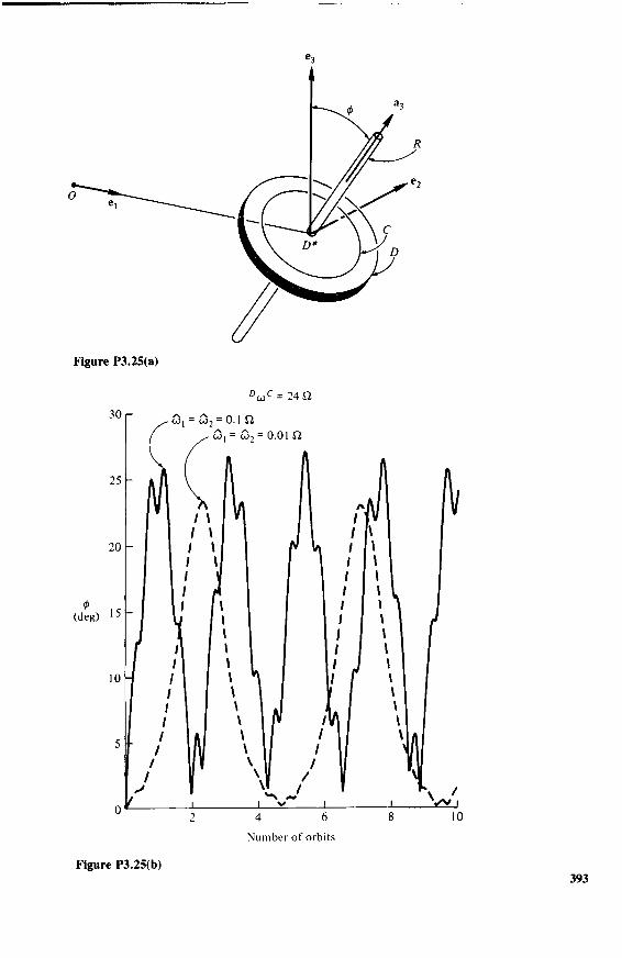
Figure P3.25(a)
Du>c= 24 ft
(deg)
Number of orbits
Figure P3.25(b)393

3 9 4 PROBLEM SETS
Letting D6f = D€ocv o>3e3
a3, where a3 is a unit vector directed as shown, make twoplots of </>, the angle between R and e3, versus the number of orbits traversed byD*, one plot applying to %c = 24ft, the other to %c = - 2 4 f t , and each contain-ing two curves, one corresponding to a>i = d)2 = 0. lf t , w3 = 2ft, the other to d>\ =a>2 = 0.01O, a>3 = 2ft. Discuss the results in relationship to those of Prob. 3.24.
Results Figures P3.25(b) and P3.25(c).
(deg)
= 0.0112
10
Number of orbits
Figure P3.25(c)
3.26 Since neither K3 as definedin Eq. (3.11.16) nor b and c as given by Eqs.(3.11.20) and (3.11.21) involve /3 or <r, the instability conditions (3.11.18) and(3.11.19) apply both when B is completely free to rotate relative to A and when Bis made to rotate relative to A with a constant angular speed. However, the motionof G may proceed quite differently in the two cases. To verify this, plot two curvesof the kind shown in Fig. 3.11.2, one applicable to the free rotor case, the other

PROBLEM SET 4 3 9 5
to the constant angular speed case. Use the same inertia properties as in the examplein Sec. 3.11, and let Q (i = 1,3;./'= 1,2, 3), <of (i = 1, 2, 3), and AcoB have thefollowing initial values: Ctj = 5/; (/ = 1 ,3; . /= 1,2, 3), o>i = o>2 = 0.1O, co3 =fi, Aa>B = — lOfi. Display results for the two orbits. Also, determine the maximumand minimum values of AcoB during the first two orbits.
Results Figure P3.26; (AcoB)max = - 7 . 4 9 0 , ( V ) m i n = - 1 0 . 1 2 0
(deg)
30 -
0.8 1.2
Number of orbits1.6 2.0
Figure P3.26
PROBLEM SET 4
4.1 Figure P4.1 shows a rigid body B carrying two particles, P, and P2, constrainedto move in a smooth tube T that is fixed in B. Pj is connected to £ and to P2 by meansof light linear springs having spring constants kx and k2 and unstretched lengths Lx
and L2. Thus s\ and s2 in Fig. P4.1 measure spring extensions.The system S formed by B, Pu and P2 moves in a reference frame A in the
absence of external forces. Letting

3 9 6 PROBLEM SETS
Figure P4.1
v •
S\
S\
b,b,-3
(i — 1>
a = 4,(«• - 7)
(i - 8)
2,5,
3)6)
where to is the angular velocity of B in A, v is the velocity of B* in A, and bj, b2,b3 are mutually perpendicular unit vectors directed as shown, determine the gener-alized active forces F\% . . . , F8 for S in A.
Results Fx = • • • = F6 = 0, F7 = -k{s{ + k2s2, Fg = -k2s2
4.2 Referring to Prob. 1.28, suppose that equal torsional springs and dampers atpoints Lx and L4 resist rotation of the linkage relative to A and that an extensionalspring and damper connect P to point L2 (dampers are not shown in Fig. PI .28).The resultant force exerted on P by the extensional spring and damper is given bycra2, where a is a function of r and r , and the torque associated with the action ofeach torsional spring and damper on a link is ra3, with r a function of 6 and 0.Assume that the linkage is sufficiently light to be treated as massless, and let theset of all external body and contact forces acting on S be represented by a forcefliaj + R2a2 + /?3a3 applied to P, a force Sx*\ + 52a2 + 53a3 applied to A at A*,and a couple of torque T{a{ + T2a2 + T3a3 applied to A.
With Mi, . . . , w8 defined as in Prob. 1.28, determine the generalized activeforces Fi, . . . , F8.

PROBLEM SET 4 3 9 7
Results Fx = Tx + (c - r - b cos 0)R3
F2 = T2~ bR3 sin 6
F3 = T3 - (c - r - b cos 0)/?! + W?2 sin 0
FA = /?! -f 5!
F5 = fl2 + 52
F6 = R3 + S3
F7 = 2r/b - a sin 0 + /?i cos 0
F8 = O" + # 2
4.3 In general, the set of gravitational forces exerted on the particles Px, . . . , PN
of a system 5 by a body B not belonging to S cannot be represented in a simple way.However, for the purposes of a particular analysis, it may be adequate to assumethat G,-, the gravitational force exerted by B on Pi9 is given by
G, = m / g (i = 1, . . . ,A0
where m, is the mass of Pi and g is a vectorial "constant of proportionality." Showthat under these circumstances (F r)G, the contribution to Fr of the gravitationalforces exerted on S by B, is given by
(Fr)G = mg - \r (r = 1, . . . , n)
where m is the total mass of 5 and vr is the rth partial velocity of the mass centerof 5.
4.4 In Fig. P4.4, A designates a sun gear, B one of four identical planet gears, andC a ring gear. The axes of A and C coincide and are fixed in a reference frame D.A is the point of A that is in contact with B, B is the point of B that is in contactwith A, and C is the point of C that is in contact with B. The radii of A and B area and b, respectively.
So long as B rolls on A and C without slipping, two generalized coordinatescharacterize the configuration in D of the system 5 formed by A, B, and C. DefiningMi and u2 as
Mi = DCJA • n3 M2 = DCJB • n3
and expressing the forces exerted by A on B and by B on C as
FA/B = Pxnx + P2n2 + P3n3 FB/C = Gin , + <22n2 + G3n3
where nu n2, n3 are mutually perpendicular unit vectors directed as shown, deter-mine (a) the contributions of ¥A/B to the generalized active forces F, and F2, (fc) thecontributions of the force exerted by B on A to Fx and F2, (c) the contributions ofFB/C to Fi and F2, and (d) the total contributions to Fx and F2 of all forces exertedon each other by A and B and by B and C.
(a) aP2, 0; (b) -aP2, 0; (c) aQ2, 2bQ2; (d) 0, 0

3 9 8 PROBLEM SETS
Figure P4.4
4.5 A uniform sphere 5 of radius R is placed in a spherical cavity of a rigid bodyB, as indicated in Fig. P4.5. The radius of the cavity is only slightly greater thanthat of 5, and the space between 5 and B is filled with a viscous fluid. The systemformed by 5 and B moves in a reference frame C in the absence of external forces.
Defining uu - . . , w9 in terms of the angular velocities of B and 5 in C and thevelocity of the center 5* of 5 in C as
»* b,
<os b,_3
v5* • hi-*
(i = 1,2,3)
(i = 4, 5, 6)
(i - 7, 8, 9)
where bi, b2, b3 are mutually perpendicular unit vectors fixed in B, and assumingthat the force d¥ exerted on 5 by the fluid across a differential element of 5 can beexpressed as
d¥ = - c V dA
where c is a constant, B\p is the velocity in B of a point P of 5 lying within the ele-ment under consideration, and dA is the area of the element, determine the gener-alized active forces F2 and F4 for the system in C.
Results F2 = f 7TCR\U5 - u2) F4 = f TTCR\UX - u4)

PROBLEM SET 4 3 9 9
Figure P4.5
4.6 Referring to the example in Sec. 4.2, suppose that a contact force is appliedto B at £* in such a way that the motion of B* in N is prescribed as a function oftime, so that the configuration of B in N can be characterized by a single generalizedcoordinate. Show that under these circumstances a potential energy of B in N isgiven by
W = -GmmL
COS 2^3
if the gravitational forces exerted on B by P are replaced with a couple of torqueT and ajorce R applied at £*, with (a) T = M, R = F and (b) T = M, R = F,where M, F, and Fare given in Eqs. (2.6.3), (2.3.6), and (2.3.5), respectively.
4.7 Referring to Prob. 4 .1 , introduce generalized coordinates qu . . . , q% by let-ting ql9 q2, #3 be body-three orientation angles for B in A (see Sec. 1.7), defining<?4, #5, #6 as rectangular Cartesian coordinates of £* in A, and setting q7 = s]9 q$ =s\ + s2. Construct an expression for a potential energy W of 5 in A, both for ur
(r = 1, . . . , 8) as defined in Prob. 4.1 and for ur = qr (r = 1, . . . , 8). Showthat, if a force Fbj is applied to B at £*, with F a constant, then there exists apotential energy of S in A if Mr (r = 1, . . . , 8) are defined as in Prob. 4 .1 , butnot if ur = qr (r = 1, . . . , 8).
Result W = jlkiq-j2 + &2(<78 ~ #?)2]
4.8 One point of a rigid body B is fixed in a reference frame A; and, when space-three orientation angles qx, q2, q3 relating mutually perpendicular unit vectors a},a2, a3 fixed in A to similar unit vectors bi, b2, b3 fixed in B are used as generalizedcoordinates, and generalized speeds are defined as w, = q, (i = 1, 2, 3), then Bpossesses a potential energy W{qx, q2, q3).

4 0 0 PROBLEM SETS
Suppose that generalized speeds are introduced as w, = a> • b, (/ = 1, 2, 3),where to is the angular velocity of B in A. Then the generalized active force Ft as-sociated with Uf can be expressed in terms of qu q2, <?3, dW/dqu dW/dq2j dW/dq3.Letting s,- = sin q, and c, = cos q{ (i = 1, 2, 3), determine Fu F2, F3.
n f dWResults F i =
a^2 — C{C2 h Si I S2
c2 |_ dq2 \ dc
If" / dW dW\ dW~\3 = C, S 2 - — + - — - S , C 2 —
c 2 1 v dci\ dqi/ 5<?2j4.9 Show that T* as defined in Eq. (4.3.4) can be expressed as
T* = - H
where H is the central angular momentum of 5 in A and the dot denotes time-differentiation in A.
4.10 Referring to Prob. 1.28, let P have a mass m, and A a mass M; regard the link-age as massless; assume that the central principal axes of inertia of A are parallelto ai, a2, a3; and let the associated moments of inertia have the values / j , 72, 7v Let-ting q7 = r and q% — 6, determine the generalized inertia forces F{*, F5*, and F8*for 5 in N.
Results F j* = — m(c — q-i — bc%) [ u^ + U\U5 — u2u4
+ (MI + u2u3)(c ~ qi ~ bc8) - (w2 -
+ 2(MJW8 - w2w7c8)] - l\d\ + w2w3(/2 - 73)
F 5 * = — M(ii5 -f W3M4 — U\U(y) — m[ii5 + w
+ (M 3 H- M,M2)fcs8 + 2w3w7c8 - (w32 + W!2)(c - qi - bcs)]
F 8 * = — m[w 5 + W3M4 — WiM6 -f w8 + (w3 -f U\U2)bs$ + 2w3w7c8
- (w32 + w,2)(c - (77 - 6c8)]
4.11 The system considered in Prob. 4.10 is modified by the addition of a particleP of mass m at point L2. Determine the contribution of P to the generalized inertiaforce F7*.
Result — m{c8[w4 + w7c8 — w3(c — bc8) + u2u6 — u^u5 + u\U2(c —
2 2 S8[W5 + W7S8 + W3/?S8 4-
- (M32 + w
4.12 The system considered in Prob. 4.10 is modified as follows: a uniform right-cylindrical rotor B of radius R, made of the same material as A and having a mass

PROBLEM SET 4 4 0 1
M/10, is installed in a cavity in A, the cavity being just big enough to accommodateB. Placing the axis of B parallel to a3, calling C the portion of A that remains, andassuming that B is driven relative to C by means of a torque motor in such a waythat ft, defined as ft = c<oB • a3, is given by ft = 10(1 + 0.1 sin It) rad/sec,determine the generalized inertia forces F3* and F5* for the system formed by B,C, and P.
Results F 3 * = — m{frs8[w5 4- u3uA — U\U^ 4- ii8 4- (w3 -I- U\U2)bs%
+ 2u3u7cs - w,2(c - <?7 - fcc8)] - (c - 07 - bcs)[ii4
w7c8 - (w3 - uxu2)(c ~ qi ~ bc%) - 2u3u%
- u72ss/b - u2
2bss]} - I3ii3 + M,W2(/I ~ /2) - (M/\0)R2 cos 2r
F5* = — M(u$ 4- M3W4 — WiW6) — m[w5 4- w3w4 — uxu6 4- w8
4- (w3 + uxu2)bss 4- 2w3w7c8 - (w32 -f Wi2)(c - q7 - bcs)]
4.13 Referring to Prob. 1.28, let P have a mass m, and A a mass M; regard the link-age as massless; assume that the central principal axes of inertia of A are parallelto Hi, a2, a3; and let the associated moments of inertia have the values Iu /2, /3. In-troduce generalized coordinates qu . . . , q% as follows: let qu q2, q3 be the radianmeasures of body-three orientation angles (see Sec. 1.7) relating a,, a2, a3 to a dex-tral set of mutually perpendicular unit vectors n,, n2, n3 fixed in N\ let q4 = p • ii],q5 = p • n2, q6 = p • n3, where p is the position vector of A* relative to a pointfixed in N; and take q7 = r, qs = 6 (see Fig. PI.28).
After verifying that the kinetic energy of S in TV can be expressed as
K = (M/2)(v,2 + v22 4- v3
2) + (m/2){[v, + bq%c* - co3{c - q7 - foc8)]2
+ (v2 4- ^ 8 s 8 - q7 4- co3bss)2 4- [v3 + CJX(C - q7 - fcc8) - w2bss]
2}
4- (/,o>i2 4- /2a>22 4- /3o>3
2)/2
where a>, = ^ai14 • a, and v, = Nv^* • a, (/ = 1, 2, 3), use Eq. (4.4.6) to form thegeneralized inertia force associated with qu assuming that qu . . . , q% are used asgeneralized speeds. Use the notations s, = sin qh c, = cos qx (i = 1, . . . , 8) toexpress the result, and comment briefly on the amount of labor required to obtainthis result, on the one hand, and Fx* in Prob. 4.10, on the other hand.
Result [06(sis2c3 4 s3c0 - q5(- C!S2c3 4- s3Si)]{Mvx 4- m[vx 4- ^ 8
- w3(c - q7 - bcs)]} + [qe(~ SiS2s3 + c3c,)
4- c3s,)][Mv2 4- m(v2 4- bq%s% - q7 4-
05Ci)c2{Mv3 + m[v3 4- wj(c - q7 - bcs) -
- m{- [vi 4- fc(<?8c8 - 082s8) ~ w3(c - (?7 - ^c8)
- a)3(bq%ss - q7)]s2(c - q7 - bcg) - [vx + bqscs
- a)3{c - qi - bcs)][q2c2(c - q7 - bc%) + s2(fc^8s8 - q7)]
(continued on next page)

4 0 2 PROBLEM SETS
+ [v2 4- b(q
4- (v2 4- bq%<
4- [v3 4- o)!(<
" o)2q,bcs][i
~ co2bs,][-
+ ( " ^2S2S3
- ^ ( ^ 2 s 2 c 3
- /3(a)3s2 +
8s8 + <?82
?8 - qi H
- - 9 7 -
: 2c 3 (c -
(92S2C3 H
+ 93C2C3
+ ?3C2S3
CU3^2C2)
C 8) — ^7 + &»3^S8 + &>3i>^8C8]S2.
- (O)bs%)b(q2C2S% + <?8S2C8)
• Z?C8) + ^ ( f r ^ S s - ?7) - C 2fos
( 7 - Z?C8) 4- C2S3fos8] + [V3 + C
^ ^3C2s3)(c — q7 — bcs) 4- c2c3(
)i>S8 4- C2S3fo^8C8]} — I\[(b\C2C3
)] 4- 72[o>2c2s3 4- co2(- q2s2s3 4-
bs8
8
0\(c - q
bqsss ~
^3C2C3)]
4.14 Referring to Probs. 1.28, 4.2, and 4.10, and assuming that N is a Newtonianreference frame, formulate the dynamical equations associated with uu w5, and M8.
Results T\ + {c — q7 — bcs)R3 — m(c — q7 — c8)[w6 4- U\U5 — u2uA
4- (w, 4- w2w3)(c - q7 - bcs) - (u2 ~ u3ux)bs%
4- 2(MIW8 - M2W7C8)] ~ I\ii\ 4- w2w3(/2 - / 3) = 0
^2 4- S2 — M(ii5 4- w3w4 — WiW6) — m[w5 4- w3w4 — U\U6 + M8
4- (ii3 4- uxu2)b%% 4- 2M3M7C8 - (W32 4- Mj2)(c - qi - &c8)] = 0
cr 4- /?2 — m[w5 4- w3w4 — MjWe + w8 4- (w3 4- w1w2)fes8
4- 2w3w7c8 - (w32 4- Wi2)(c - 97 ~ ftcs)] = 0
4.15 Referring to Probs. 1.28 and 4.2, let P have a mass m, andA a mass M; regardthe linkage as massless; assume that the central principal axes of inertia of A areparallel to a t, a2, a3; let the associated moments of inertia have the values Iu 72, 73;and 'et iVbea Newtonian reference frame. Introduce q7 and q% as
A . A n 77q7 = r - L qs = 6 - — rad
where L is the natural length of the spring that connects P to L2, and assume thatthe torsional springs at Lx and L4 are undeformed when 6 = TT/2 rad. Finally, de-fine Mi, . . . , M8 as
•a , (/ = 1 ,2 ,3)
A I v^1 • a,_3 (1 = 4, 5, 6)Ui = { - (1 = 7)
- 7 (1 = 8)
where co is the angular velocity of A in N, and vA* is the velocity of A* in N.In the absence of external forces, the system can remain at rest in N with ux =
• • • = M8 = q7 = q% = 0. Derive dynamical equations governing "small" depar-

Results
PROBLEM SET 4 4 0 3
tures from this state of rest, that is, equations linearized in u\, . . . , w8, #7, and #8,taking a = ~kxqi and r = -k2qg, where fcj and fc2 are constants.
[I{ + m(c - L)2]ii{ + m(c - L)(w6 - 6w2) = 0
(/2 + mfc2)w2 ~ mb[(c - L)ux + w6] = 0
+ m(c - L)2 4- mZ?2]w3 + m[b(u5 + M8) - (c - L)M 4 ] = 0
(M + m)«4 — m(c — L)M3 = 0
(M + m)w5 + m(ii$ + ftw3) = 0
(M -h m)w6 + m[(c - L)MJ - to2] = 0
- 2k2qs/b = 0
= 0
4.16 Figure P4.16 shows n identical rigid bars Bu . . . , Bn forming an n-tuplependulum attached to a rigid circularly cylindrical body C of radius R. The bars areconnected to each other with pins whose axes all are parallel to the axis of C, andonly motions during which these axes remain perpendicular to a plane that is fixedin a Newtonian reference frame N are considered.
Each bar has a length L and mass m; the mass center 5,* of 5, is at the midpointof Bh and the moment of inertia of B, about a line parallel to the pin axes and pass-ing through £, is / (7 = 1, . . . , n). C has a mass M and an axial moment of inertiaJ. A linear torsional spring of modulus a is located at each joint; when all springsare undeformed, all bars coincide with the line Z passing through the mass centerC* of C and through the point at which B{ is attached to C.
Introduce mutually perpendicular unit vectors Ci, c2, c3 as shown in Fig. P4.16.Define generalized speeds u\, «2, w3 as
Uj = V C - C , 0 = 1, 2) * C3
Figure P4.16

4 0 4 PROBLEM SETS
Let 0, denote the angle between £, and Z, and express 0, asV
ft = 2 Aijqj (i = 1, . . . , n)
where Ai} (i = 1, . . . , n; j = 1, . . . , v) are constants. With w3+; defined as
"3+; = 4j 0' = 1, . . . , I/)
and assuming that qu . . . , qp remain "small," verify that the dynamical equationsgoverning Mi, . . . , w3+l, can be expressed as
n n
(M + nm)wj — m 2 A^3 = Mu2u^ — m 2 7// = i / = I
v n / i A \
(M + nm)w + mX a« + ^ S S S A ^ I "\;=1
(Mu3U\ + m
m 2J (3iU\ — m 2J otjU2 — I w 2^ a,2
i=\
v n V / i A \ ~l
- 2 2 "^«i ( 2 A;* r ) + /Aft*=i 1=1 L \y=i z / J
M 3+*
= m X1=1
V ^ / <=
J 5-^+/AJ«3
;=i z / \ / = i z / J
A,^, + 2 Wi-l.s " A^Kfl,--, - f t ) ( 5 = 1 , . . . , ! / )
where a,, /3,, %•, <5, are given by
£*/ = /? + /L - -

PROBLEM SET 4 4 0 5
(u2
5, =
i - L 2L*=1
4.17 Figure P4.17 shows a planar double pendulum consisting of two identical,uniform, pin-connected rods, each of length L and mass m. Equal linear torsionalsprings of modulus a are attached as indicated and both springs are undeformedwhen the angles qx and q2 are equal to zero.
Considering "small" motions during which the pendulum remains in a horizon-tal plane, (a) show that the equations of motion can be written
Mq + Sq = 0
where
1 c A °" [ 11 2 ~
(b) form the upper triangular matrix V such that M = VTV; (c) letting W =(V ~ l)TSV~\ determine the eigenvalues of W and show that they are equal to thoseof M " 1 5 ; (d) verify that if C, and C2 are eigenvectors of W, then V"1 C, and V"1 C2
are the corresponding eigenvectors of M 1 S.
Results (b) TV8 3/VTl[ 0 V7/V8J
(c) 0.3409a/(mL2), 15.09cj/(mL2)
Figure P4.17
4.18 After showing that there exist no values of xl and x2 such that all five of theequations JCI + 2x2 = 1, 2xx + 3*2 = 2, 3*, + 4*2 = 1, 4*, + 5x2 = 2, and 5*, +6x2 = 1 are satisfied simultaneously, (a) find values *,* and x2* of x, and JC2, re-

4 0 6 PROBLEM SETS
spectively, representing the "best approximate solution" of the equations, using themethod employed to solve Eq. (4.9.156); (b) with S(xu x2) defined as
S{xu x2) = 2x2 - I)2 + (2JCI + 3x2 - 2)2 (5*, + 6x2 - I)- I)2
evaluate S(x\*, x2*) and compare the result with S(xu x2), where xx and x2 are anynumbers whatsoever.
Results (a) -1.4, 1.4(b) l.2,S(xl*,x2*)<S(xux2)
4.19 Figure P4.19 shows a plane truss T that has n joints Px, . . . , Pn, and movesin its own plane, which is fixed in a Newtonian reference frame N. Mutually per-pendicular lines N\ and N2 are fixed in N and intersect at point N*. Lines Rx andR2, intersecting at point /?*, are fixed in an auxiliary reference frame R (not shown)that moves relative to N, this motion being characterized by the distances zx and z2
and the angle 6.Dynamical equations governing the motion of T in N are to be formulated after
T has been discretized as a set of particles placed at Px, . . . , Pn and connected bymassless, linear springs, the particle at Pt having a mass mx equal to half the totalmass of all truss members meeting at Pt. A force Q, is presumed to be applied toTa tP / .
Introduce 3 + v generalized speeds as
Mi = 0 u2 = "v* • i*! u3 = N\R • r2 u3+k = qk (k = I, . . . , v)
where ^v** is the velocity of /?* in N, I < i < w, and ^ is a generalized coordinate
J
X2i
N*
R2 V ^
z\x2i-\
/ \
Figure P4.19

PROBLEM SET 4 4 0 7
brought into the discussion as follows: if x2,-i, *2t a n d J2/-1, yu are the Cartesiancoordinates of Pt relative to Nu N2 and Ru R2, respectively (see Fig. P4.19), andj?i, . . . , x2n are values of JCI, . . . , xln, respectively, such that T is undeformed,let Ajk(j = 1, . . . , 2n\ k = 1, . . . , v) be constants and express >>y- as
V
yj = *j' + 2 Ajkqk (j = 1, . . . , In)
Show that if Ajk (j = 1, . . . , 2«; A: = 1, . . . , ^) are formed like their coun-terparts in Sec. 4.9 [see Eq. (4.9.123)], then the dynamical equations governingM], . . . , w3+i, can be expressed as
lU\ - W2U2
7 = 1 i =
= 2 [(G2/ - rnia[2)y2l-l - (Q2i-\ ~
mu2 = 21=1
1=1
1=1
wheren n
A V ^ T A V ^ 2 "> \
m = 2J mi ' — 2J mi(y2i-\ + JiV)/=! i=l
wj• = 2 m^2.--2+,- U = l , 2 )
A ^ ^ A ^G2/-1 = Q/ * r l G21 = Q/ * r 2 (/ = 1, . . . , Al)
A /o V ^ 4. j_fl/1 — — Wj I Z ^ /*2i i tw l + it "^ W3 ' Wi>'2
A / - V A 4.^ /2 = u l \ ^ 2J A2i-i,kM3 + k "I" W2 — Wi V2/
G* = S (A2.--uG2.--1 + Az.-jtQz,-) (* = 1, • • • , v)» = 1
and where Ai, . . . , A, are any v nonzero eigenvalues of M~]/2 SM~X/1, arrangedin ascending order, 5 and M being, respectively, the stiffness matrix of T and thediagonal mass matrix of T (see Sec. 4.9).

4 0 8 PROBLEM SETS
4.20 A complete description of the motion of truss T of Prob. 4.19 is said to bein hand when x\, . . . , x2n are known as functions of time. To obtain such a de-scription, one can express JCI, . . . , x2n in terms of zx, z2, 0, and qu . . . , qv afterdetermining these quantities by solving simultaneously the differential equations4k — "3+* (k — 1, . . • , v), the 3 + v dynamical equations developed in Prob.4.19, and three additional kinematical differential equations that relate 0, z\, z2 toMl, I l 2 , W3.
(a) Verify that x\, . . . , x2n are related to z\, z2, 0 and qu . . . , qv by theequations
J C 2 / — i = Z \ + J 2 / - 1 c o s 0 — y 2 i s i n ^ ( / = 1 , . . . , « )
JC2/ = z2 + J2/-1 sin 0 + yn c o s ^ ('' ~ U • • • , w)
(fo) Show that the needed kinematical differential equations are
0 = U\ i\ = «2 cos 0 — u3 sin 0 z2 = w2 sin 0 + w3 cos 0
(c) Assuming that the initial values of JC,- and i , , denoted by ,-(0) and ij(0) (/ =1, . . . , 2n), are given and that i , ~ JC,-(O) (/ = 1, . . . , 2n), show that zi(0),^2(0), 0(0), and qk(0) (k = 1, . . . , v) must satisfy the 2n linear equations
V
z,(0) - JC2I-(0) 0(0) + 2 ^- i ,***(0) = JC2f-i(O) - i 2 , - . (i = 1, . . . , n)
z2(0) + JC2I--I(O) 0(0) + 2 A2l-,*ft(0) = JC2/(O) - x2l ( i = l , . . . , /i)
while Wi(0), w2(0), w3(0), and w3+*(0) (k = 1, . . . , ^) are governed by the linearequations
- y2 /(0)«,(0) + «2(0) + X A 2 l - . u « 3 + / l (0 ) = JC2I-_,(O) + JC2,(
0 = 1, • • • , n)V
y2/-i(0)M,(0) + iij(0) + 2) A2a«3+*(O) = - i2l-_,(O)0(O) + x2i(0)
(1= 1, . . . , n )
where j ;(0) is given byv
yj(0) = Xj + 2 Ay*ft(0) (y = 1, . . . , 2/i)
and is, therefore, available as soon as the equations governing z,(0), z2(0), 0(0),and ^ (0 ) (k - 1, . . . , v) have been solved.
4.21 Figure P4.21(a) shows a triangular truss T that moves in its own plane, whichis fixed in a Newtonian reference frame N. Mutually perpendicular lines N{ and A 2
are fixed in Af and intersect at point N*. Lines flj and R2, intersecting at point /?*,are fixed in an auxiliary reference frame R (not shown) that moves relative to ;V,

PROBLEM SET 4 4 0 9
Figure P4.21(a)
this motion being characterized by the distances z\ and z2 and the angle 6. Each trussmember has a Young's modulus of 109 N/m2, a cross-section area of 10~4 m2, andmass per unit of volume of 104 kg/m3; and, when T is undeformed, the membersconnecting points P\ and P2» ^2 and P3, and P3 and P{ have lengths of 4 m, 5 m,and 3 m, respectively. The N\, N2 coordinates of joint Pt are x2i-\, x2i, respectively(1 = 1, 2, 3), and Xj has the value Xj (j = 1, . . . , 6) when T is undeformed.
(a) Referring to Prob. 4.20, and taking i , = 0, x2 = 0, i 3 = 4 m, x4 = 0,i 5 = 0, JC6 = 3 m, verify that the constants Atj (1 = 1, . . . . , 6; 7 = 1, 2, 3) aregiven by
(b) Taking
-0.285761-0.183059-0.0506765
0.2047010.307052
-0.0701124
^(0) = 0.01 m
x2(0) = 0.02 m
JC3(O) = 4.03 m
JC4(0) = -0 .01 m
JC5(O) = -0 .02 m
*6(0) = 3.04 m
-0.3167590.1752460.321784
-0.0565620-0.0848430
-0.0897081
-0.0767620-0.324885
0.135214-0.0566329-0.0849493
0.347987
JC,(O) = 0.01 m/sec
x2(0) = - 0 . 01 m/sec
JC3(O) = 0.02 m/sec
i4(0) = -0 .02 m/sec
JC5(O) = 0.03 m/sec
JC6(0) = - 0 . 0 3 m/sec
determine the quantities Zu , Z30 in Table P4.21.

4 1 0 PROBLEM SETS
Table P4.21
0(0) (deg)
z,(0) (m)
z2(0) (m)
<?,(()) (kg1/2m)
q2(P) (kg1/2m)
q3(0) (kg1/2m)
w,(0) (rad/sec)
w2(0) (m/sec)
w3(0) (m/sec)
w4(0) (kgl/2m/sec)
w5(0) (kg1/2m/sec)
M6(0) (kg1/2m/sec)
z,z2z3z4
z5
z6z7z8
z9
ZI0
ZM
Z,2Z,3
Z,4
ZI5
Z,6Z,7Z,8
z19
Z20
z2,z22z23z24z25
z26z27z28z29Z30
(c) In Sec. 4.9, linear structural theory is used to characterize truss deforma-tions. Investigate the applicability of this theory to motions during which truss de-formations become large, proceeding as follows.
Let forces Q,, Q2 , Q3 be applied, respectively, to joints Px, P2, P3 of 7\ in sucha way that Qx is directed from P\ to P2, Q2 from P2 to P3, and Q3 from P3 to Px.Let the magnitudes of Q, , Q2 , Q 3 be 4000 N, 5000 N, 3000 N, respectively. (Notethat if T were rigid, this system of forces would be a couple.) Referring to Prob.4.19, verify that A! = 5.87615 x 10³ sec"2, A2 = 1.43990 x 10⁴ sec"2, A3 =1.97248 x 10⁴ sec"2; take v = 3, x,(0) = i , ( i = 1, . . . , 6) [see (a) for i , ] ,Xi(0) = 0 (7 = 1, . . . , 6 ) ; and perform a numerical integration of the equationsof motion of T from t = 0 to t = 0 . 6 sec. Use the results of this numerical inte-gration to plot the angle <f> = if/ - 90° versus /, where if/ is the angle shown in Fig.P4.21(a).
(d) Treating T as a system of three particles connected by massless linearsprings, verify that exact differential equations of motion of this set of particles canbe written as
[FL,+
~ xs)
mxv2
[FLX + kx(dx - - x2)
4- L 3 ) te - Xf,)
= 0
. [FL2 + k2(d2 - L2)](x5 - x3) , * , ( 4 ~ ^ i ) U 3 ~ JCi) n
m2v4 -
d2 dx
[FL2 + k2(d2 - L2)](x6 - x4) , kx(dx - Lx)(x4 - x2)
d2-f = 0

PROBLEM SET 4 4 1 1
[FL3 + k3(d3 - L3)](x{ - x5) k2(d2 - L2)(x5 - x3)m3v5 + = 0" 3 " 2
[FL3 + k3(d3 - L3)](x2 - x6) k2(d2 - L2)(x6 - x4)m3v6 + = 0
d3 d2
xt = v, (/ = 1 6)where
A.
A.
K*3 - xxy -- x3)
2 •
- x5y -
f (x4
+ (x6
+ (x2
v- \2il/2
x2) JX2-I \j2
- x6)2]i/2
while F = 1000 N/m, Lx = 4 m, L2 = 5 m, L3 = 3 m, mx = 3.5 kg, m2 = 4.5kg, m3 = 4.0 kg, kx = 2.5 x 10⁴ N/m, it2 = 2.0 x 10⁴ N/m, it3 = 3.33333 x10⁴ N/m.
(e) Take JCKO) = xt [see (a)], v,(0) = 0 (/ = 1, . . . , 6); for 0 < t < 0.6 sec,perform a numerical integration of the equations given in (d); use the results ofthis numerical integration to plot the angle </> = ^ - 90° versus /, where </> is theangle between the line connecting P{ and P2 and the line connecting P{ and P3.Display this plot and the one generated in (c) on the same set of axes.
Results (b) - 1 . 0 6 x 10"1, 4.09 x 10~\ 1.80 x 10"2, - 7 . 0 4 x 10~2,- 1 . 7 0 x 10~3, 1.85 x 10~2, - 1 . 7 4 x 10~2, 1.82 x 10~2,- 9 . 6 9 x 10~2, 5.23 x 10~3, 1.74 x 10~2, - 7 . 1 9 x 10~2,
3.73 x 10~2, - 1 . 6 1 x 10~3, 1.91 x 10~2, - 1 . 7 7 x 10~2,1.75 x 10~2, 1.86 x 10~2, - 1 . 0 5 x 10"1, 5.64 x 10~\1.82 x 10~2, - 7 . 4 7 x 10~2, 3.97 x 10~2, 5.78 x 10~2,
- 1 . 5 5 x 10~3, 1.89 x 10~2, - 1 . 8 1 x 10~2, 1.87 x 10~2,L75 x 10"2, - 2 . 6 0 x 10~2
(c) Figure P4.21(b)
4.22 Transverse vibrations of an unrestrained beam of length L, constant flexuralrigidity El, and constant mass per unit of length p are governed by Eq. (4.10.1) andby the boundary conditions / ( 0 , t) = / ' ( 0 , t) = / ( L , t) = / ' ( L , t) = 0. Showthat the general solution of Eq. (4.10.1) satisfying these boundary conditions canbe expressed as
X
1=1
where
-r A;X \tx cosh A,- — cos A, / . , A,-JC . \tx\<t>i = cosh •——h cos — 7-7— :—— sinh ——h sin -—
L L sinh A,- - sin A, \ L L jq( = a, cosp^ + Pi sin/?,f

4 1 2 PROBLEM SETS
50 r
(deg) 20 -
-10
Figure P4.21(b)
and A, (i = 1, . . . , oo) are the consecutive roots of the transcendental equation!
cos A cosh A — 1 = 0
while
r\ 1/2
and a, and /?, are constants that depend upon initial conditions.
4.23 Figure P4.23 shows an unrestrained, uniform beam B of length L, constantflexural rigidity El, and constant mass per unit of length p. B moves in a Newtonianreference frame N under the action of gravitational forces exerted by a particle Othat has a mass m0 and is fixed in N. Only planar motions of B are to be considered.
Dynamical equations governing the motion of B in N are to be formulated. Tothis end, an auxiliary reference frame R that moves in N is introduced, as aremutually perpendicular lines R{ and R2 fixed in R and intersecting at a point /?*, asshown in Fig. P4.23, where D denotes the distance from O to /?*, 6 is the anglebetween R^ and the line Z determined by O and /?*, and Q is one of the endpointsof B. R2 is required to pass through Q at all times.
tThe first 30 positive roots of this equation are listed in Table 4.10.1.

PROBLEM SET 4 4 1 3
Figure P4.23
Express the distance y from R{ to a generic point P on the neutral axis of B as
y =1 = 1
where <fr, . . . , < £ „ (1 ^ i> ^ °°) are functions of the distance x from P to R2, and<7i, . . . , qv are functions of the time f; let y = Gmo, where G is the universalgravitational constant; introduce 3 + v generalized speeds as
u, = A NVR* .r3
M3 =
( * = 1, . . . , ! > )
where N\R* is the velocity of/?* in N, N(oR is the angular velocity of R in N, rx andr2 are unit vectors directed as shown in Fig. P4.23, and r3 = rx x r2.
Making use of Eqs. (4.10.20), (4.10.21), and (4.10.37), assuming thatD » L, and proceeding as in the derivation of Eqs. (4.10.48)-(4.10.51) to dealwith the gravitational forces exerted on B by O, formulate the dynamical differen-tial equations governing uu . . . , u^v.
Results U\mB - «3 2 1>Ei ~ fnBu2u3 + eBu^ + 2H3 ^ M3+,-£/1=1 f=i
- mB cos 6 - 3 sin 6 cos 6D

4 1 4 PROBLEM SETS
u2mB + ii3eB
y\\ • * 3 ^ sine cos fl 2 ^ £,(7/1D 1 /
m* sin D
( sin ~ } D,
2 M3+,-F/ = eBu3ux + u2u3i=\ i = l
. 3/* sine cos 0 v f n 3F,(1 - 2 cos2 0)1sm 0 - -JJ-g + g [£, cos 0 + - ^ ^ q
1=1 1=1
^ \ r i 7 • /j 3/} sine cos fl^ j ^ ; sine - - i - g + (3 sin2e - 1) g ^ - J
0 = 1 , . . . , ^ )
4.24 Using for <fr in Eqs. (4.10.21) a n d (4.10.37) the function ~4>t of Prob. 4.22,show that Ei = Fl• = 0 (/ = 1, . . . , v) while Gy = mfl S/, and //^ = p/2mB S^ (/,7 = 1 , . . . , ! ^ ) , where/?, is given by Eq. (4.10.7) and 5/; is the Kronecker delta.
4.25 In Prob. 4.23, 3 + ^dynamical differential equations were formulated. Sincethese equations involve the 5 + 2v variables D, e, uu . . . , u3+v, q\9 . . . , qv,they do not suffice for the determination of these variables. Show that the 2 + vrequired additional equations are the kinematical relationships qt = w3+, (/ = 1,. . . , v), D = u\ cos 6 — u2 sin 6, 6 = u3 — {u\ sin 6 + u2 cos d)ID.
4.26 Figure P4.26(a) shows a system consisting of a block A, a uniform beam 5 ,and a light linear spring S. A is constrained to move in a guide G, one end of B isclamped to A, and 5 connects A to a fixed support.
If W(JC, t) denotes the displacement of a point P located a distance x from theclamped end of B (w = 0 when both £ and S are undeformed), £ / is the flexuralrigidity of B, a is the modulus of S, L is the length of B, p is the mass per unit oflength of B, and #*A is the mass of A, then w is governed by the partial differentialequation
together with the (time-dependent) boundary conditions
, t) d2w(L, t) d3w(Ly t)
dx dx1 dx3
d2w{O,t) , rJ3w(0,»)
= 0

PROBLEM SET 4 4 1 5
Figure P4.26(a)
and the initial conditions
, 0) = = kix)
where g(x) and h(x) are specified functions of JC. The solution of the partial differ-ential equation can be expressed as
W(JC, f) = i sin C,- cos co,-
where
- , v A . A ,* \fX . A ,* A , */•(*) = sin ——h a, cos — smh ——h /3, cosh ——
LJ LJ L L
Here A, (i = 1, . . . , °°) are the roots of the equation
A 4 -paL4
mAEl~K + 5 + e~2x) cos A
mA L+ e'2K) sinA + \(l - e'1K) cosA] - .
and the constants ah (ih wh Bh and C, are defined as
en = {e~ki sinA, + £(1 - e~2k>) + pL(l + e"2A0[l
)]~!(wA A,-)"1}^— e"A|' cos A, — | (1 + e"2A/)]
"Hi - po-LViniAEIX;4)]-1 cos A,
- e-A 'sinA, - 3P - ^"2A'M/r- ^~A
!(-
e 2 A 0}/ [ - e~A' cos A, - 1(1 + e'2A

4 1 6 PROBLEM SETS
rL h(x)Mx)dxo
f g(x)Mx)dx + (mA/p)g(0)M0)Jo
fi2{x)dx + (mA/p)/2(0)
An alternative description of w{x, t), obtained as in Sec. 4.10, can be producedas follows: let y denote the deflection of B at P from its undeformed position [Fig.P4.26(a)], and express y as
v
y = 2 ~4>iqti=\
where </>, is given by Eq. (4.10.4), q( is a function of t, and v is a positive integer.Introduce z as z = w — y (z is the "stretch" of S), and, after defining generalizedspeeds u\, . . . , U\+v as U\ = z, U\+j = qt (i = 1, . . . , v), solve the dynamicalequations of motion governing wi, . . . , U\ + l/, together with the kinematical equa-tions z = Mi, g, = Mi+, (/ = 1, . . . , v). Finally, form w as
V
w = z + E ~4>iqi
(a) Formulate the dynamical differential equations governing uu . . . , u\ + v.(b) Taking mA = 10 kg, L = 10 m, p = 1000 kg/m, £7 = 100 N • m2, a =
394.784 N/m (when a has this value, the system formed by A and S alone has anatural vibration period of 1 sec), and, assuming that the system starts from restwith B undeformed and 5 extended by 0.1 m, make time-plots, for 0 < t < 10 sec,of the displacement w(L, t) of the free end of B, using each of the two above-mentioned methods. Make two sets of plots, first using five terms in the exact solu-tion and v = 4, and then using nine terms in the exact solution and v = 8. Commentbriefly on the relative amounts of computational effort required to implement eachof the two methods.
V
Results (a) (mA + pL)u\ + 2 EiU\+i + crz = 01=1
Ejiix + pLiil+J + — ^ = 0 0 = 1 , . . . , * / )
where A1? . . . , A^ appear in the first column of Table 4 . 1 0 . 1 , and £ , , . . . , Ev
are given by Eq. (4.10.66).
(b) Figures P4.26(b) and P4.26(c).

PROBLEM SET 4 4 1 7
(m)
0.15
0.13
0.11
0.09
0.07
5 terms
0
Figure P4.26(b)
0.15 r
0.13
(m) 0.11
0.09
0.07
4 6t (sec)
(sec)
10
10
Figure P4.26(c)
4.27 A cantilever beam has a length of 20 m, a flexural rigidity of 5 N • m2, anda mass per unit length of 0.2 kg/m. Using a single finite element, find the associated

418 PROBLEM SETS
global mass and stiffness matrices M^and S\ the eigenvalues Xj and X2 of M'x J,andjhe corresponding eigenvectors Ax and A2 of M~l ? , normalized with respectto M.
Results M L-4.1
[-1.1
48571 -4 .19048]
19048 15.2381 J
5 x 10~3 - 7 . 5 x 10"5 x 10~2 1.0
Ai = 1.95003 x 10~3
A2 = 0.189300
1.0097695473 x 10~2
1.4072636342 x 10~*
4.28 The circular frequency /?, associated with the ith mode of free vibrations ofa cantilever beam of length L, flexural rigidity El, and mass per unit of length p isgiven by Eq. (4.10.7), which involves quantities A, (/ = 1, . . . , oc), the first twoof which have the values Ai = 1.87510, A2 = 4.69409. Approximations to/?, canbe found by means of the finite-element method. To test the quality of such approx-imations, let/?,, denote the circular frequency associated with the ith mode whenj elements of equal length are employed in the finite-element analysis of the beamconsidered in Prob. 4.27 and evaluate the ratio/?,,//?, for i = 1, 2 andj = 1, 2, 3.
Suggestion: Letting Mj and Sj denote, respectively, the global mass matrix andthe global stiffness matrix of the beam wheny elements are employed, and designat-ing as \ij(i = 1, . . . , 2j) the consecutive eigenvalues of Mfl Sj, verify that pfj =A,//2; note that An and A2i are available in Prob. 4.27; and use the following asvalues for Ay (i = 1, 2\j = 2, 3): A12 = 1.93349 x 10~\ A22 = 7.71553 x 10~2,A13 = 1.93201 x 10~3, A23 = 7.63614 x 10~2.
Results Table P4.28.
Table
P'j
j -
j =
j ~-
IPi
- i
= 2
= 3
P4.28
i = 1
1.005
1.000
1.000
i
1
1
1
= 2
.580
.008
.003
Table P4.29(a)
|$|=z./2(m = 1)Eq. (4.11.29)
|$|,«L/2("I = 10)Eq. (4.11.29)
iw / 2U / 2Eq. (4.10.4)
Mode number /
1
Qi
Q*
2
(25
(26
3
Qi
Q*

PROBLEM SET 4 4 1 9
4.29 In the finite-element analysis of vibrations of a cantilever beam, the functions$ ( / = 1, . . . , v) defined in Eqs. (4.11.29) play a role analogous to that playedby the functions </>,(/= 1 , . . . , °°) defined in Eq. (4.10.4) in connection with the"exact" analysis of such vibrations. To explore the relationship between <£, and <f>i9
begin by using Eq. (4.11.30), the third of Eqs. (4.10.21), and Eq. (4.11.45) toverify that
<£, $ j p d x = 8ij ( 1 , 7 = 1 , . . . , ! / )IJo
Next, show with the aid of Eq. (4.10.8) that if there exists a constant c such that$• = c(f>i (i = 1, . . . , v), then c = mB
l/2. Finally, considering the midpoint ofthe beam of Prob. 4.27, evaluate the quantities Qu • . . , Q% indicated in TableP4.29(a), using A^ (/, j = 1, 2) as found in Prob. 4.27 when dealing with m = 1,and assigning to AtJ (i = 1, . . . , 20; j = 1, 2, 3) for m = 10 the values shownin Table P4.29(fc).
Results 0.33101, 0.33952, 0.33952, 0.63723,0.71371, 0.71367, 0.01971, 0.01969
Table P4.29(fe)
A, i
1
2
3
4
5
6
7
8
9
10
11
12
13
14
15
16
17
18
19
20
j
1
0.0167735
0.0163703
0.0638710
0.0303259
0.136483
0.0418917
0.229885
0.0511296
0.339524
0.0581528
0.461135
0.0631374
0.590877
0.0663307
0.725479
0.0680579
0.862401
0.0687259
1.00000
0.0688254
2
0.0926354
0.0838835
0.301075
0.116210
0.526168
0.101759
0.683515
0.0505744
0.713713
-0.0226585
0.589515
-0.100977
0.317073
-0.168558
-0.0700400
-0.214396
-0.523786
-0.235492
-1.00007
-0.239055
3
-0.228184
-0.188372
-0.604814
-0.155986
-0.756627
0.0177607
-0.526200
0.203096
-0.0197071
0.277741
0.474000
0.189659
0.657761
-0.0178446
0.395084
-0.236888
-0.228612
-0.367110
-1.00050
-0.392637

420 PROBLEM SETS
4.30 Ei as given in Eq. (4.11.37) represents an approximation to Et mB~l/2 with Et
given by Eq. (4.10.66); similarly for Ft as in Eq. (4.11.42) and Ft mB~l/2 with Ft
as in Eq. (4.10.67). To test the quality of these approximations, evaluate thequantities Qu . . . , Qs indicated in Tables P4.30(a) and P4.30(6).
Table
i = 1
i = 2
P4.3I
Eq'
D(a)
(m =(4.11
(2>
(23
= 1)37) Eq.
(m = 10)(4.11.37)
1.56598
0.867871
Eq. (4.10
(24
/2
.66)
Table
i = l
i = 2
P4.3Fi
Eq.(m
(4.1
Qi
)
= l)1.42)
| F , (m = 10)Eq. (4.11.42)
22.7530
3.63067
F,Eq.
mB~^(4.10.67)
(26
Qs
Results 1.55587, 1.56598, 0.761093, 0.867872,22.7095, 22.7530, 3.50408, 3.63067
4.31 Equations (4.10.13), (4.10.57)-(4.10.60), (4.10.62), and (4.10.63) form aset of 5 + 2^equations governing the quantities/?, 6, qx, . . . , qv, and w1? . . . ,M3+„, all of whose initial values must be known before one can undertake a solutionof the equations. As regards R and 0, this poses no problem, for each of these var-iables has a readily apparent physical significance; similarly for uu «2, w3 [see Eqs.(4.10.10)]; but qk(0) and u3+k(0) (k = 1, . . . , v) generally must be found bymaking use of given information regarding the initial deflection and initial motionof B relative to A, that is, y(x, 0) and dy(x, Oydt^
(a) Taking for ^ in Eq. (4.10.12) the function <f>k defined in Eq. (4.10.4), showthat
qk{0)=—\Ly(x,0)<j>kpdx ( * = l ,'Wfl JO
v)
AWfl Jo Cf
(fe) Referring to Sec. 4.11, show that, for the stepped beam there considered,2m 2m
<?*(0) = 2 E AjkMj{zM (k = 1, . . . , v)
2m 2m
«3+*(0) = 2 2 (k = 1, . . . , v)/=! j=\

PROBLEM SET 4 4 2 1
(c) Referring to the Example in Sec. 4.11, suppose that the initial deflection ofB is given by
•0) - ( £and that B is initially at rest relative to A. Making use of Table P4.31, which con-tains results obtained from a structural analysis of B, determine q5(0) and w8(0).
Table P4.31
i
1
2
3
4
5
6
7
8
9
10
20
2A,5M,,7=I
0.224024
0.0382657
0.385068
-0.00239025
0.157218
-0.0542421
-0.272344
-0.0516500
-0.274485
0.0712732
11
12
13
14
15
16
17
18
19
20
20
; = i
0.196386
0.0476021
0.247772
-0.0394262
-0.168500
-0.0496868
-0.159556
0.0557229
0.128851
-0.0299777
Result 0.001818, 0

APPENDIX
I
DIRECTION COSINES AS FUNCTIONS OFORIENTATION ANGLES(see Sec. 1.7)
In this appendix, the direction cosines associated with each of 24 sets of angles de-scribing the orientation of rigid body B in a reference frame A are tabulated. To usethe tables, proceed as follows: let ai, a2, a3 be a dextral set of mutually perpendic-ular unit vectors fixed in the reference frame A, and let bi, b2, b3 be a similar suchset fixed in the body B. Regard b, as initially aligned with a, (/ = 1, 2, 3); selectthe type of rotation sequence of interest (that is, body-three, body-two, space-three,or space-two); letting du 02, 03 denote the amounts of the first, the second, and thethird rotation, respectively, pick the rotation sequence of interest [for example,3-1-2 (corresponding to a d\b3, 02b}, 03b2 body-three sequence or a 0ja3, 02ai, #382space-three sequence)]; finally, locate the table corresponding to the rotation se-quence chosen. The nine entries in the table [with s, and c, standing, respectively,for sin 0, and cos 0, (1 = 1, 2, 3)1 are the elements C,; of the associated directioncosine matrix, which elements are defined as C/7 = a, • b, (/, j = 1,2, 3). More-over, by reading a row or column of the table, one can determine how to expressany of aj, a2, a3 in terms of bu b2, b3, or any of bi, b2, b3 in terms of a t, a2, a3.For example, in the table corresponding to the body-three 3-1-2 sequence, the thirdrow reveals that a3 = - c2s3b, + s2b2 + c2c3b3, while the second column indi-cates that b2 = - Sic2ai + C]C2a2 + s2a3.
422

APPENDIX I 4 2 3
Body-three: 1-2-3
b, b2 b3
B] C2C3 - C 2 S 3 S2
a2 S1S2C3 + S3C1 —S1S2S3 -I- C3C1 — s,c2
a3 -C1S2C3 -I- S3S1 C1S2S3 + C3S1 Cic2
Body-three:
b,
a, cic2
a2 s2
Body-three:
b,
2-3-1
3-1-2
a , —S1S2S3 + C3C1
a 2 C1S2S3 + C3S1
a 3 - C 2 S 3
Body-three:
b,
ai C2C3
a2 CS2C3 +
a3 s,s2c3 -
Body-three:
b,
1-3-2
S3S1
S3C1
2-1-3
b2
-C1S2C3 + S3S1
c2c3
S1S2C3 + S3C,
b2
c,c2
S2
b2
c,c2
SiC2
b2
c,s
- s ,
- C i
C|S;
S,S;
b3
2S3 +
—c2s
S2S3 •+
b,
S2C3 H
C:C,
b,
C2S3
2 S3 —
'.S3 +
b,
C3S1
- c3c,
S3CI
h s3s,
C3SI
C3C1
a, S1S2S3 -+- c3C| S1S2C3 - S3C1 S!C2
a2 C2S3 C2C3 — s2
83 C1S2S3 - C3S1 C1S2C3 -I- S3S1 C|C:
Body-three: 3-2-1
a,a2
3 3
C1C2
sic2
— S2
C1S2S3 —
s,s2s3 +
C2S3
C3S,
C3C1
CS2C3
S1S2C3
c2
•f- S3S,
- S3C1
C3

424 APPENDIX I
Body-two: 1-2-1
b,
a, c2
a2 Sis2
a3 - c , s 2
Body-two: 1-3-1
b,
ai c2
a2 Cis2
a3 s,s2
Body-two: 2-1-2
b,
ai - s , c 2 s 3 + c3c,
a2 s2s3
a3 - c , c 2 s 3 - c3s,
Body-two: 2-3-2
b,
a, c,C2C3 - s3s,
a2 s2c3
a3 —SiC2c3 — s3Ci
Body-two: 3-1-3
b,
ai - s , c 2 s 3 + c3c,
a2 cic2s3 -l- c3si
a3 s2s3
Body-two: 3-2-3
b,
Hi C!C2C3 - S3S1
a2 s,c2c3 -f s3c,
a3 - s 2 c 3
b2
s2s3
- s , c 2 s 3 •+
C,C2S3 +
b2
- C3C1
C3S,
- s 2 c 3
C,C2C3 - S3S1
SiC2C3 + S3C!
b2
c2
c,s2
b2
-CiS;
c2
b2
- S i C 2 C 3 -
CiC2C3 -
s2c3
b2
~CiC2S3 -
- s , c 2 s 3 4
s2s3
2
- s3c,
S3Si
- C3Si
• c 3 c ,
b3
s2c3
- S , C 2 C 3 - S3C1
C1C2C3 - S3S,
b3
s2s3
— CiC2S3 — C3Si
- s , c 2 s 3 + c3ci
b3
s,c2c3 + s3c,
- s 2 c 3
c,c2c3 - s3s,
b3
c,c2s3 + c3s,
s2s3
- S i C 2 S 3 + C3C,
b3
s,s2
-C1S2
c2
b3
CiS2
s,s2
c2

APPENDIX I 4 2 5
Space-three: 1-2-3
b,
ai c2c3
a2 c2s3
a3 - s 2
Space-three: 2-3-1
b,
a 2 C j s 2 c 3 + S3S1
a 3 C1S2S3 — C3S1
Space-three: 3-1-2
b,
a i S iS 2 s 3 + C3C1
a 2 SiC2
a 3 S1S2C3 - S3C1
Space-three: 1-3-2
b,
a, c2c3
a2 s2
a 3 - C 2 S 3
Space-three: 2-1-3
b,
a, - s , s 2 s 3 + C3C1
a2 S1S2C3 + s3ci
a3 - s , c 2
Space-three: 3-2-1
b,
b2
S1S2C3 - S3C1
S1S2S3 + C3C1
s,c2
b2
~s2
C2C3
C2S3
b2
C i c 2
C1S2C3 + s 3 S |
b2
-C1S2C3 + S3S1
c,c2
C1S2S3 + C3S1
b2
- C 2 S 3
C2C3
S2
b2
b3
CiS2C3 + S3S,
C1S2S3 — C3S1
C1C2
b3
sic2
S!S2C3 - S3C1
S,S2S3 + C3C1
b3
C2S3
- s 2
C2C3
b3
S,S2C3 + S3C1
- S 1 C 2
- s , s 2 s 3 + c3c,
b3
C1S2S3 -I- C3S1
-C1S2C3 + S3S1
c,c2
b,
ai c , c 2 -S1C2 s2
a2 C1S2S3 + C3S1 —S1S2S3 + C3C1 — C2S3
a 3 — C | S 2 c 3 + S3S1 S1S2C3 + S3C1 c 2 c 3

4 2 6 APPENDIX I
Space-two: 1-2-1
b, b2
a.a2
a3
c2
s2s3
- S 2 C 3
SiS2
-S1C2S3 +
S1C2C3 +
C3C1
S3C1
C1S2
-C1C2S3 -
CiC2C3 -
- C3S1
S3S1
Space-two: 1-3-1
b3
ai
a2
a3
c2
s2c3
s2s3
- c , s 2
C1C2C3 - S3S,
C1C2S3 + C3S1
S1S2
- s , c 2 c 3 -
- s , c 2 s 3 +
s3c,
c3c,
Space-two: 2-1-2
ai
a2
a3
-S!C2S3 + C3C,
S1S2
- S ! C 2 C 3 - S3C1
S2S3
C2
S2C3
C1C2S3 + C3S,
-c ,s2
CiC2C3 - S3S,
Space-two: 2-3-2
b2 b3
ai
a2
a3
C1C2C3 -
CiS 2
- C i C 2 S 3 -
S3S1
- c3s,
- S 2 C 3
c2
S2S3
S1C2
-s ,c
C3 +
s,s2
•2 S3 +
S3
c
Ci
3C
Space-two: 3-1-3
b3
« 1
a2
a3
- s , c 2 s 3 -t
SiC2C3 +
s,s2
- c3c,
S3C1
-C1C2S3 -
CiC2C3 -
C1S2
• c3si
S3Si
S2S3
- S 2 C 3
c2
Space-two: 3-2-3
b, b3
a i
a2
a3
C1C2C3 - S3S1
C1C2S3 + C3S,
-C1S2
-s ,c 2c 3 -
-S1C2S3 +
s,s2
• S3C1
C3CI
S2C3
S2S3
c2

APPENDIX
II
KINEMATICAL DIFFERENTIAL EQUATIONS INTERMS OF ORIENTATION ANGLES
(see Sec. 1.7)
In this appendix, the kinematical differential equations associated with each oftwenty-four sets of angles describing the orientation of a rigid body B in a referenceframe A are tabulated. To use the tables, proceed as follows: let ai, a2, a3 be a dex-tral set of mutually perpendicular unit vectors fixed in the reference frame A, andlet bi, b2, b3 be a similar such set fixed in the body B. Regard b, as initially alignedwith a, (/ = 1, 2, 3); select the type of rotation sequence of interest (i.e., body-three, body-two, space-three, or space-two); letting 0l5 02, #3 denote the amounts(in radians) of the first, the second, and the third rotation, respectively, pick the ro-tation sequence of interest [for example, 3-1-2 (corresponding to a 0ib3, 02bj, 03b2
body-three sequence or a 0ia3, 02ai, 03a2 space-three sequence)]; finally, locate thetable corresponding to the rotation sequence chosen. The table contains the rela-tionships between 0,, 02, 03 and coj, co2, o>3, where co, = A(oB • b, (i = 1, 2, 3),Aa)B being the angular velocity of B in A.
Body-three: 1-2-3
o>, =
(02 =
(03 =
0ic2c3 +
- 0ic2s3
0,s2 + 03
02S3
+ 02c3
0 , = ( o >
0 2 = Wl
03 = ( "
,c3 - cu2s3)/c2
S3 + OI2C3
o>iC3 + o>2s3)s2/c2 + co3
427

4 2 8 APPENDIX II
Body-three: 2-3-1
Oil =
OI2 =
Ol3 =
01S2 + 03
0,c2c3 +
- 0ic2s3
02s3
+ 02c3
0i =
02 =
03 =
(ai2c3 -
ai2S3 ~H
aii + (-
- ai3s3)/c2
ai3c3
- OI2C3 + Ol3S3)S2/C2
Body-three: 3-1-2
aii =
ai2 =
013 =
- 0ic2s3
0,s2 + 0
0lC2C3 +
+ 02c3
e2s3
«.=02 =
03 =
(— aiiS3 + ai3c3)/C2
aiiC3 + ai3S3
(a,, s3 - a ) 3 c 3 ) s 2 / c 2 + <o2
Body-three: 1-3-2
„, = e lC2c3 - e2s3
ai2 = ~ 0i S2 "i" 03
ai3 = 01C2S3 + 02C3
0i
02
03
= (ai,c3 -\
= " 01, S3
= (aiic3 H
- ai3s3)/c2
+ ai3c3
H ai3s3)s2/c2 + ai2
Body-three: 2-1-3
aii =
ai2 =
ai3 =
0lC2S3 +
0.c2c3 -
- 0is2 +
02C3
02s3
03
0, = (ai,s3 +
02 = ai,c3 -
03 = (aii s3 +
ai2C3)/c2
ai2 s3
ai2C3)s2/c2 + ai3
Body-three: 3-2-1
aii =
ai2 =
ai3 =
- 0is2 +
0lC2S3 +
0,c 2c 3 -
03
0 2c 3
0 2s 3
0i = (ai2s3
02 = ai2c3
03 = aii +
+ ai3C3)/c2
- ai3s3
(ai 2s 3 + ai3C3)s2/c2
Body-two: 1-2-1
U)X =
ai2 =
ai3 =
0.c2 +
0is2s3
0lS2C3
03
+ 02C3
- 0 2 S 3
01 =
02 =
03 =
(OI2S3
ai2c3
aii -
-1- ai3c3)/s2
- ai3s3
(ai2s3 + ai3c3)c2/s2
Body-two: 1-3-1
Oil = 0lC2 + 03
(02= ~ 0iS2C3 + 02S3
OI3 = 0,S2S3 -H 02C3
0i
0 2
03
~ ai2c3 + ai3S3)/s2
-I- a i 3c 3
(ai2c3 - ai3S3)c2/s2

APPENDIX II 4 2 9
Body-two: 2-1-2
0)x =
0)2 =
O)3 =
0,S2S
6xc2
- e
3 "
4
s2
f 62c3
63
C3 4 02S3
6x =
62 =
63 =
(oi,s3
WiC3
( - a
-
4
>lS3
a)3c3)/s2
W3S3
4 a>3c3)c2/s2 4 a>2
Body-two: 2-3-2
c , = e l S 2c3 - e2s3
Ct>2 == 01C2 4 03
" 3 = 0lS2S3 4 02C3
6x =
62 =
63 =
(a>lC3 4
- O)iS3
OJ
4
j 4
3S3 ) /S2
O)3C3
- cu3s3)c2/s2 4 O)2
Body-two: 3-1-3
a>i
a>2
0^3
= ^ lS 2 S 3
= ^lS 2 C 3
= 6xc2 4
4 02c3
0 2s 3
63
6x
62
63
— (a>iS3 4 cu2c3)/s2
= WiC3 — O)2S3
= — (a>iS3 4 a>2C3)c2/s2 4 0)3
Body-two: 3-2-3
a,, = - <j,s2c3 + e2s3
Cl>2 == 0iS2S3 4 02C3
cu3 := 0i C2 4 03
0.
62
63
= a>,s3 -
= (WiC3
c3 4 cu2s3)/s2
f a>2c3
- w 2 s 3 ) c 2 / s 2 4 a>3
Space-three: 1-2-3
0)\
a>2
a>3
= 6x -
= 62cx
= — 02
^3S2
4 03s,c2
s, 4 03cic2
0i =
62 =
63 =
o)x 4 (a
O)2Cl ~
(a>2s, 4
>2Sj 4 W3C1
W3S,
cu3c,)/c2
)s2/c2
Space-three:
0)x = - 02Si 4
o>2 = 0, - 0 3 s 2
CU3 = 02Ci 4 03
2-3-1^3CiC2
s,c2
0,
62
63
= (WlCi
= («lCi
4
Si
4
o>3Si)s2/c2 4 w2
4 Ct)3Ci
O>3S,)/C2
Space-three: 3-1-2
o>, = 02Ci 4 03SjC2
o)2 = — 02s t 4
Oi3 = 6x — 0 3 S2
^3CiC2
^1 =
62 =
63 =
(o>iS! 4
o>,c, -
{o)xsx 4
o*2Ci)s2/c2 4 o>3
O>2Si
a>2c,)/c2

4 3 0 APPENDIX II
Space-three: 1-3-2
(Ox =
(O2 =
0)3 =
01 +
02si
02c,
03s2
+ 03c,c2
- 03s lC2
0i =
02 =
03 =
(Ox +
(O2Sx
((02CX
( - (O2Cx + CO3 S 1)S2 /C2
+ (O3CX
- o>3Si)/c2
Space-three: 2-1-3
« , =
0)2 =
0>3 =
fcc,
0, +
02S,
- e3s,c2
03s2
+ <J3c,c2
0, = (atiS
82 = oi,c,
ft = ( - «
, - «3C,)S2/C2 + «2
+ O)3S|
tf,S, + »3C,)/C2
Space-three: 3-2-1
CU2 =
w 3 =
0 2 S l
02ci
ft +
+ 03CiC2
03SiC2
P3S2
ft = (02 = 6
03 = (
- (OxCx + 0>2S
O1S1 H- cu2Ci
) s 2 / c 2
C2
+• cu3
Space-two: 1-2-1
(Ox =
(O2 =
0)3 =
0i + 0:
02Ci +
- 02S,
c2
03S]S2
+ 03CiS2
01
02
03
— CO3S1
Space-two: 1-3-1
(Ox =
W 2 =
CU3 =
01 +
02s,
02c,
03C2
- 03CiS2
+ 03s,s2
0i =
02 =
03 =
0)x +
(O2Si
(o>2c, -
+ (O3CX
o>3s,)c2/s2
3 S i ) / s 2
Space-two: 2-1-2
(Ox = 02Cj
o>2 = ft +(O3 = 0 2Si
+ 03s,s2
03c2
~ 03CiS2
ft =
02 =
03 =
( -
ftl,C
Ct>lSi + £t>3Ci)C
+ W3Si
1 - cu3c,)/s2
2 / s 2 + 0)2
Space-two: 2-3-2
0), =
C02 =
« , =
tfl +
e2c,
S, + »3C,S2
e3c2
+ e3s,s2
01 =
02 =
03 =
- («,c,
- CU1S1
((t>|C| "I"
+ co3Si)c2/s2 + cu2
+ W3C1
a>3s,)/s2

APPENDIX II 4 3 1
Space-two: 3-1-3
01 ,=
(D2 =
0)3 =
02Cl
0i +
+ 03SiS2
si + 03c lS2
03C2
0, = - (
02 = 0>,C
03 = (O),
<WlSi
, -
-1-
+ C2COC2/S2 + CO3
o>2s,
o>2Ci)/s2
Space-two: 3-2-3
0H =
0>2 =
(O3 =
02s,
02Ci
0. +
- 03CiS2
+ 03SiS2
03c2
BX = ( 0 , , C , - CO2 S 1 )C2 /S2 + CO3
0 2 = = Cc>i S1 ~l~ 6t>2Ci
03 = = ( &>iCi ~r ( t ) 2 Si ) /S 2


INDEX
Acceleration:angular, 84centripetal, 205
Angles:body-three, 34, 74, 79body-two, 34, 74, 76orientation, 30, 73space-three, 34, 73, 76, 79space-two, 34, 74
Angular acceleration, 84Angular momentum integral, 191Angular velocity:
addition theorem, 72components, 53and Euler parameters, 58indirect determination of, 68matrix, 47and orientation angles, 73partial, 87of precession, 159and Rodrigues parameters, 62of spin, 159vector, 49
Antenna, 3Associated Legendre functions,
142Attitude rate, 329Auxiliary reference frames, 71Averaging, 179, 187Axis:
instantaneous, 81, 83of rotation, 1screw, 42
Axisymmetric gyrostat, 224, 228,234
Axisymmetric rigid body, 159in a circular orbit, 169
Basepoint, 42, 81Beam:
element mass matrices, 334element stiffness matrices, 334unrestrained, 411,412(See also Cantilever beam)
Best approximate solution, 312, 406Binomial series, 99Binormal, 52Body cone, 162Body-three angles, 34, 74, 79Body-two angles, 34, 74, 76
Cantilever beam, 318,417-419Center of gravity, 93Central inertia dyadic, 99Centrifugal moment, 206, 207Centripetal acceleration, 205Centrobaric bodies, 109, 110Characteristic equation, 344
roots of, 320Colocated sensor and actuator, 331Coning, 56Continuous elastic components, 318Coupling, dynamic, 269Critical damping, 329

434 INDEX
Cross-dot product, 156Curvature, radius of, 52, 53Curvilinear coordinates, 367
Differentiation with respect to avector, 123
Direction cosine, 4, 23Direction matrix, 5, 11, 13, 17, 19,
47, 63Discrete systems, 284Discretizing, 300Displacement, 42Displacement vector, 42Divergence, 124Double dot product, 148Double pendulum, 405Dumbbell, 364Dynamic coupling, 269Dynamical equations, 275
linearized, 277
Eigenvectors, normalized, 286Elliptic functions, 188Energy potential, 252-259Euler parameters, 12
angular velocity and, 58Euler theorem on rotations, 14Euler vector, 12Exclusion of modes, 295
Finite element method, 332Fluid, viscous, 398Force function, 123, 129, 132, 133,
141, 146-148, 153, 156for a body and a particle, 132for a small body and a particle, 133in terms of Legendre polynomials,
141for two particles, 129
Generalized coordinates, 87, 89, 90Generalized inertia force, 259Generalized speeds, 87Gimbal, 30Gimbal lock, 37Global mass matrix, 334Global stiffness matrix, 334Gradient, 124Gravitation, law of, 91Gravitational constant, 92, 358Gravitational forces, 91Gravitational interaction of two
particles, 91Gravitational moments, 91Gravitational potential, 129Gyroscope, 30Gyrostat, 211, 218, 224, 240, 260
axisymmetric, 224, 228, 234simple, 211, 230
Herpolhode, 162, 191
Indirect determination:of angular velocity, 68of orientation, 20
Inertia:coefficient, 269dyadic, 99ellipsoid, 60force, 259torque, 259
Injection error, 168, 390Instantaneous axis, 81, 83Integration, numerical, 67International Astronomical Union,
143Invariance, 123
Jacobian elliptic functions, 188
Generalized active force, 247 Kane's dynamical equations, 275

INDEX 435
Kinematical equations, 48Poisson's, 48
Kinetic energy, 269integral, 192
Orthogonal curvilinear coordinates,367
Orthogonality, 309
Laplace's equation, 129Laplacian, 124Legendre, 142Legendre associated functions, 142Legendre polynomials, 141Linearized dynamical equations, 277Lumped mass, 296
Manipulator arm, 279Mass:
of the Earth, 92of the Moon, 92
Mass matrix, 297, 334Modal analysis, 296Modal functions, 332Modal matrix, 297, 336Moment:
centrifugal, 206, 207exerted on a body by a particle,
112exerted on a small body by a small
body, 116
A2-tuple pendulum, 403Newton's law of gravitation, 91Normal coordinates, 287Normalization constants, 286Normalized eigenvectors, 286Numerical integration, 67
Oblate spheroid, 106, 118, 120Orbit eccentricity, 180Orientation:
angles, 30, 73indirect determination of, 20zero moment, 364
Partial angular velocity, 87Partial differentiation, 124Partial velocity, 87Pendulum:
double, 405Az-tuple, 403
Penrose, 312Plane truss, 406Planet gear, 397Poinsot construction, 161, 191Poisson's kinematical equations, 48Polhode, 162, 191Potential:
energy, 252-259gravitational, 129
Precession, 159, 160,225Principal normal, 52Principal radius of curvature, 53Prolate spheroid, 375Proximate bodies, 119Pseudo-inversion, 313
Radius of curvature, 52, 53Reference frames, auxiliary, 71Reorientation, 230Rigid-body modes, 308Ring gear, 397Rodrigues parameters, 16, 24, 62, 65,
67Rodrigues vector, 16, 17, 19, 38, 62,
233Rotation:
axis of, 1simple, 1,3,6, 13, 17, 38,42,49,
50small, 38, 39successive, 23, 39
Rotational motions, slow, small, 78

436 INDEX
Scanning platform, 10Screw axis, 42Screw motion, 42Screw translation, 42, 44Separated sensor and actuator, 332Shape factor, 168Shape functions, 334Shuttle, 279Simple gyrostat, 211, 230Simple rotation, 1, 3, 6, 13, 17, 38,
42, 49, 50Simpson's rule, 361Slow, small rotational motions, 78Space cone, 162Space curve, 52Space shuttle, 279Space-three angles, 34, 73, 76, 79Space-two angles, 34, 74Spatial divergence, 124Spatial gradient, 124Spatial Laplacian, 124Speeds, generalized, 87Spherical coordinates, 127Spherical harmonics, 129Spheroid:
oblate, 106, 118, 120prolate, 375
Spin, 159, 225speed, 160, 225stabilization, 173
Spin-up, 64Spinning, 56
cylindrical satellite, 83Stability chart, 202Stiffness matrix, 297, 334Successive rotations, 23, 39Sun gear, 397Symbol manipulation, 279Synchronous altitude, 109
Torque-free axisymmetric rigid body,159
Torque-free gyrostat, 224Torque-free unsymmetric rigid body,
187Torsion, 53Trace, 97Translation, 42Triangular truss, 408Truss, 296
plane, 406triangular, 408
Tumbling, 64
Unit matrix, 6Universal gravitational constant, 92Unrestrained beam, 411,412Unsymmetric gyrostat, 240
Vector:angular velocity, 49binormal, 52differentiation with respect to a,
123displacement, 42Euler, 12principal normal, 52Rodrigues, 16, 17, 19, 38, 62, 233screw translation, 42tangent, 52
Velocity:angular (see Angular velocity)partial, 87
Vibrations theory, 286Viscous fluid, 398
Tip speed, 329 Zero moment orientation, 364