Analysis Methods for Multi-Spacecraft Data

Reprinted fromAnalysis Methods for Multi-Spacecraft DataGotz Paschmann and Patrick W. Daly (Eds.),

ISSI Scientific Report SR-001 (Electronic edition 1.1)c© 1998, 2000 ISSI/ESA

— 14 —

Spatial Interpolation for Four Spacecraft:Theory

GERARD CHANTEUR

CETP-CNRSVelizy, France

14.1 Introduction

Spatial interpolation of data between the spacecraft and estimation of the effects oftetrahedron shape and attitude are key aspects of data analysis from four spacecraft. Thischapter presents the fundamental concepts of barycentric coordinates and demonstratestheir use for interpolating data within a tetrahedron. The reciprocal vectors, defined as thegradients of the barycentric coordinates, play a key role in the determination of gradients,the characterisation of discontinuities and the analysis of errors related to the uncertaintieson the spacecraft positions. The first application of this formalism to a four spacecraftmission was proposed byChanteur and Mottez[1993]. The method as developed hereapplies to only four spacecraft; it could likely be generalised to more than four spacecraft atthe expense of a greater algebraic complexity, but this development has not been pursued.

Barycentric coordinates are well-known tools in applied mathematics but not in spacephysics. This is why a self-contained and detailed presentation is given in Section14.2together with the introduction of the reciprocal vectors and the demonstration of their fun-damental properties. Linear and quadratic interpolation schemes are presented as well asthe related estimators of gradients. The practical determination of the gradient of the mag-netic field by these and others estimators along realistic orbits in a model magnetosphericfield is the object of Chapter15. Section14.3is devoted to the theoretical analysis of phys-ical and geometrical errors. In a first step the expectation values and covariance matrix ofthe reciprocal vectors are explicitly derived from the uncertainties affecting the spacecraftpositions for any configuration of the cluster. Then use is made of this result to predictthe expectation values and covariances of the estimated components of the gradient of avector field and to separate for errors of physical and geometrical origin. Section14.4gives a detailed analysis of the errors related to the truncation inherent to any interpola-tion scheme. To avoid unnecessary mathematical complication the analysis is conductedfor the one-dimensional model of a thick and planar current sheet. Section14.5presentssome other applications of the barycentric formalism, especially the derivation of the spa-tial aliasing condition for plane waves sampled by a tetrahedron and the characterisationof a planar discontinuity crossed by the cluster of spacecraft, i.e., the determination of thenormal components of the velocity and acceleration of the discontinuity in the frame ofthe cluster. The conclusion section emphasises the usefulness of the barycentric formalism

349

350 14. SPATIAL INTERPOLATION: THEORY

and its possible applications to other topics not investigated in this chapter.

14.2 Interpolation within a Tetrahedron and Estimationof Gradients

In this and following sections involving the barycentric coordinates, dyadic notations⇒14.1will be used systematically. A column vector is denoteda, its transposeaT being a linevector. The dyadaT b denotes the scalar product of two real vectorsa andb, usuallywrittena · b, hence:

a · b = aT b = bT a

Meanwhile the dyada bT is a tensor of rank two, the transpose of which isb aT . Thegradient of the scalar fieldu(r) is the vectorG[u] defined by the differential:

du = drT G[u] (14.1)

Similarly the gradient of the vector fieldv(r) is the tensor of rank twoG[v] defined by thedifferential:

dvT = drT G[v] (14.2)

In cartesian coordinates this definition gives the usual definition for componentkl of G[v]:(G[v]

)kl

= ∂kvl , partial derivative of componentvl with respect to coordinatexk.

14.2.1 Linear Interpolation and Related Estimators

Definitions of the Barycentric Coordinates and Reciprocal Vectors

Let Sα (α = 1, 2, 3, 4) be the vertices of an irregular tetrahedron, or cluster, andrα betheir position vectors. A naturally occurring scalar fieldu(r) or a vector fieldv(r) is knownonly by the valuesuα = u(rα) or vα = v(rα) measured at the verticesSα. The linearinterpolation of these values in the vicinity of the cluster requires four basic interpolatingfunctionsµα which are linear scalar functions of the position vectorr, and which satisfythe constraintsµα(rβ) = δαβ (Kronecker symbol). Let the linearly interpolated fields,denoted byL[u] andL[v] be given by the following expressions:

L[u](r) =

4∑α=1

uαµα(r) (14.3)

L[v](r) =

4∑α=1

vαµα(r) (14.4)

The four valuesµα(r), 1 ≤ α ≤ 4 are the barycentric coordinates of the pointr. Theycan be expressedµα(r) = να + kα.r where theνα andkα are respectively scalar andvector constants to be determined. Using the constraintsµα(rβ) = δαβ we deduce that:

µα(r) = 1 + kα.(r − rα) (14.5)

kα.(rβ − rγ ) = δαβ − δαγ (14.6)

14.2. Estimation of Gradients 351

S 3

S 2

S 1

K4

S4

µ4

Figure 14.1: Barycentric vectors and coordinates. The shaded plane, perpendicular to theaxisµα, is an isovalue surface ofµα.

Equation14.6shows thatkα is normal to5α, the face of the tetrahedron opposite toSα.Hence, for example, by making use ofrβγ = rγ − rβ , k4 can be written:

k4 =r12 × r13

r14.(r12 × r13)(14.7)

it appears to be proportional to the area of the face of the tetrahedron opposite to vertexS4 and inversely proportional to the volume of the tetrahedron. Expressions for the otherreciprocal vectors are obtained through cyclic permutations of the indices. We callkα thereciprocal vectors of the tetrahedron. From equation14.5, they satisfy:

kα = G[µα] (14.8)

Properties of the Barycentric Coordinates and Reciprocal Vectors

From a geometrical point of view, the barycentric coordinates have the following prop-erties (see Figure14.1):

1. µα(r) is constant in a plane parallel to5α, the face of the tetrahedron opposite toSα.

2. µα(r) < 0 in the half space, relative to5α, not containingSα.

3. µα(r) = 0 for all points lying in5α.

4. µα(r) > 0 in the half space, relative to5α, containingSα.

5. 0< µα(r) < 1 for all points lying inside the tetrahedron


It is worth mentioning the following properties of the barycentric coordinates and re-ciprocal vectors due to their importance in numerous topics that can be addressed by a fourspacecraft mission. Firstly, from the definitions themselves it is obvious thatµα(r) andkαare independent of the origin of the position vectors. Secondly, the linear interpolation ofa constant scalar field gives straightforwardly:

4∑α=1

µα(r) = 1 (14.9)

Taking the gradient of both sides of equation14.9leads to:

4∑α=1

kα = 0 (14.10)

Thirdly, r itself is a linear field, hence:

r = L[r] =

4∑α=1

rαµα(r)

According to definitions14.2and14.8, taking the gradient of this equation gives:

4∑α=1

kα rTα = I =

4∑α=1

rα kTα (14.11)

whereI is the unit tensor defined byIij = δij . Equation14.11contains the two followingspecial relations:

4∑α=1

kα · rα = 3 and4∑α=1

kα × rα = 0

Another interesting property is obtained by taking the gradient ofrTA, whereA is aconstant vector:

A =

4∑α=1

(rα · A)kα (14.12)

Linear Estimators of Gradients

The gradients of the linearly interpolated fieldsL[u] andL[v] may be used as estima-tors of the gradients of the sampled physical fieldsu andv.

LG[u] = G [L[u]] and LG[v] = G [L[v]] (14.13)

Hence, from the definitions14.3 and 14.4 and making use of equation14.8 the linearbarycentric estimators are:

LG[u] =

4∑α=1

kαuα (14.14)

LG[v] =

4∑α=1

kα vTα (14.15)

14.2. Estimation of Gradients 353

The linear estimators of the divergence and curl of fieldv are thus:

LD[v] =

4∑α=1

kα · vα (14.16)

LC[v] =

4∑α=1

kα × vα (14.17)

These last expressions solve exactly the equations forLD[v] andLC[v] derived byDun-lop et al. [1990] from Ampere’s and Gauss’s integral theorems combined with linear in-terpolation of the fields.

The differencesLG[u] − G[u] or LG[v] − G[v] are respectively, and by definition,the errors of truncation ofLG[u] or LG[v].

14.2.2 Quadratic Interpolation and Related Estimators

Quadratic Interpolation within a Tetrahedron

The information provided by four samples of a physical fieldu or v, measured si-multaneously at the vertices of the tetrahedron, allows linear interpolation of the field inthe vicinity of the cluster, but not higher order interpolation. Quadratic interpolation re-quires six extra independent simultaneous measurements: for example, the valuesuαβ atthe midpointsSαβ of the linesSαSβ .

The quadratic interpolation uses a base of ten quadratic functions, each of them beingequal to unity on only one node, and zero on all other nodes. Becauseµα vanishes on5α,the face of the tetrahedron opposite toSα, i.e. on the three other vertices and on the threemidpoint nodes belonging to5α, it should be a factor of the basis functionqαα related tovertexSα. The second factor is 2µα − 1 becauseµα =

12 on the remaining three midpoint

nodes betweenSα and5α. Henceµα(2µα − 1) is the desired function, being moreoverequal to 1 on vertexSα whereµα = 1. The midpoint nodeSαβ is the only node whichbelongs neither to5α nor to5β , hence the associated basis function is proportional toµαµβ ; a factor 4 is needed to obtain the right weight on nodeSαβ . The basic quadraticinterpolating functions are thus:qαα = µα(2µα − 1) which is equal to 1 at vertexSα and0 at all other nodes, andqαβ = 4µαµβ which is equal to 1 at midpointSαβ and 0 at allother nodes. Relation14.9can be used to demonstrateqαα = µαµα −6′µαµβ where6′

denotes a sum overβ different fromα. Thus quadratic interpolations may be done withhomogeneous functions of theµα ’s:

Q[u](r) =

4∑α=1

uαqαα +

4∑α=1

∑β>α

uαβqαβ (14.18)

Q[v](r) =

4∑α=1

vαqαα +

4∑α=1

∑β>α

vαβqαβ (14.19)

These formulas reduce to the linear interpolation formulas whenuαβ =12(uα + uβ).


Quadratic Estimators of Gradients

From the definitions of theqαβ ’s it follows that:

G[qαα] = (4µα − 1)kα (14.20)

G[qαβ ] = 4(µαkβ + µβkα) (14.21)

These formulas can be used to define quadratic barycentric estimators of differential opera-tors through the application of these differential operators to the quadratically interpolatedphysical fields, spatially sampled by the spacecraft. The gradients of the quadratically in-terpolated fields are linear functions of the position vector, the gradient of the scalar fieldis defined by:

G [Q[u]] =

4∑α=1

(4µα − 1)kαuα + 44∑α=1

∑β>α

(µαkβ + µβkα)uαβ

and the gradient of the vector field is written:

G [Q[v]] =

4∑α=1

(4µα − 1)kα vTα + 44∑α=1

∑β>α

(µαkβ + µβkα)vTαβ

The quadratic barycentric estimators of the gradients are chosen to be equal to the latterexpressions evaluated at the barycentre of the tetrahedron, i.e.:

QG[u] =

4∑α=1

∑β>α

(kα + kβ)uαβ (14.22)

QG[v] =

4∑α=1

∑β>α

(kα + kβ)vTαβ (14.23)

An Approximate Procedure Taking Advantage of the Orbital Motion

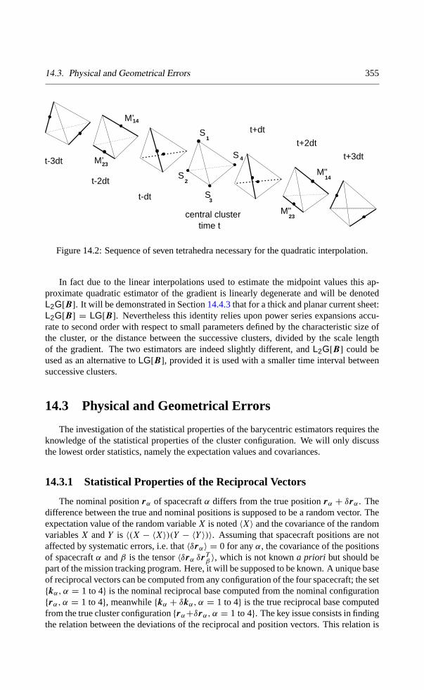
A midpoint sample can only be estimated at the expense of the time resolution bydefining it as the mean value of its nearest vertical neighbours on a supplementary positionof the cluster, but that would lead to midpoint and vertical samples defined at differenttimes. A midpoint sample has to be defined by averaging this mean value on two positionsof the cluster, one retarded and the other advanced with respect to the central position. Oneposition of the cluster giving two independent midpoint samples on opposite edges of thetetrahedron, it appears that only three pairs of retarded/advanced clusters are sufficient toestimate the six midpoint samples. Figure14.2illustrate the following scheme:

u23(t) =1

4(u2(t − 2dt)+ u3(t − 2dt)+ u2(t + 2dt)+ u3(t + 2dt))

u14(t) =1

4(u1(t − 2dt)+ u4(t − 2dt)+ u1(t + 2dt)+ u4(t + 2dt))

The adequate interval of timedt will be specifically determined for each physical field; itshould be small enough to preserve the accuracy of the estimation, but nevertheless largeenough to guarantee the independence of the successive filtered samples of data.

14.3. Physical and Geometrical Errors 355

M’ 14

M’ 23

S1

S2

S3

S 4

M" 23

M" 14

t-3dt

central clustertime t

t-2dt

t-dt

t+3dt

t+2dt

t+dt

Figure 14.2: Sequence of seven tetrahedra necessary for the quadratic interpolation.

In fact due to the linear interpolations used to estimate the midpoint values this ap-proximate quadratic estimator of the gradient is linearly degenerate and will be denotedL2G[B]. It will be demonstrated in Section14.4.3that for a thick and planar current sheet:L2G[B] = LG[B]. Nevertheless this identity relies upon power series expansions accu-rate to second order with respect to small parameters defined by the characteristic size ofthe cluster, or the distance between the successive clusters, divided by the scale lengthof the gradient. The two estimators are indeed slightly different, andL2G[B] could beused as an alternative toLG[B], provided it is used with a smaller time interval betweensuccessive clusters.

14.3 Physical and Geometrical Errors

The investigation of the statistical properties of the barycentric estimators requires theknowledge of the statistical properties of the cluster configuration. We will only discussthe lowest order statistics, namely the expectation values and covariances.

14.3.1 Statistical Properties of the Reciprocal Vectors

The nominal positionrα of spacecraftα differs from the true positionrα + δrα. Thedifference between the true and nominal positions is supposed to be a random vector. Theexpectation value of the random variableX is noted〈X〉 and the covariance of the randomvariablesX andY is 〈(X − 〈X〉)(Y − 〈Y 〉)〉. Assuming that spacecraft positions are notaffected by systematic errors, i.e. that〈δrα〉 = 0 for anyα, the covariance of the positionsof spacecraftα andβ is the tensor〈δrα δrTβ 〉, which is not knowna priori but should bepart of the mission tracking program. Here, it will be supposed to be known. A unique baseof reciprocal vectors can be computed from any configuration of the four spacecraft; the set{kα, α = 1 to 4} is the nominal reciprocal base computed from the nominal configuration{rα, α = 1 to 4}, meanwhile{kα + δkα, α = 1 to 4} is the true reciprocal base computedfrom the true cluster configuration{rα+δrα, α = 1 to 4}. The key issue consists in findingthe relation between the deviations of the reciprocal and position vectors. This relation is


obtained by differentiating equation14.11:

4∑α=1

δkα rTα = −

4∑α=1

kα δrTα

Multiplying right by kβ , then making use of equations14.6 and 14.10 to evaluate theleft-hand side of the above equation, we get:

δkβ = −

4∑α=1

(kTβ δrα

)kα = −

(4∑α=1

kα δrTα

)kβ , for anyβ. (14.24)

The first expression, involving the scalar productskTβ δrα will later appear as the mostuseful. The latter equation14.24ensures that, accordingly to the hypothesis of unbiasedposition measurements, the deviations of the reciprocal vectors have null expectation val-ues:

〈δkα〉 = 0 , for anyα. (14.25)

Equation14.24allows for computing the covariances of the reciprocal vectors alongthe following lines:

δkαi δkβj =

4∑γ=1

4∑ν=1

(kTα δrγ

) (kTβ δrν

)kγ i kνj

ChangingkTβ δrν into the equivalent expressionδrTν kβ , the expectation value of the prod-

uct(kTα δrγ

) (kTβ δrν

)becomeskTα 〈δrγ δr

Tν 〉 kβ , thus revealing the role played by the

covariances of the vector positions of the spacecraft. The general expression for the co-variances of the components of the reciprocal vectors is thus:

〈δkαi δkβj 〉 =

4∑γ=1

4∑ν=1

kTα 〈δrγ δrTν 〉 kβ kγ ikνj (14.26)

The covariance matrices of the spacecraft positions will be determined specifically for agiven mission; they are not knowna priori. Nevertheless, it is very likely that the positionvectors of two spacecraft will be uncorrelated, furthermore it seems reasonable to assumethat the covariance matrix of the position vector will be the same for all spacecraft of thecluster. This means that:

〈δrγ δrTν 〉 = δγ,ν 〈δr δrT 〉 (14.27)

Under these simplifying assumptions the general expression14.26is reduced to:

〈δkαi kβj 〉 = kTα 〈δr δrT 〉 kβ Kij (14.28)

Kij , the last factor, is theij component of the reciprocal tensor defined by:

K =

4∑ν=1

kνkTν (14.29)


14.3.2 Statistical Properties of the Linear EstimatorLG

This section investigates the statistical errors which affect the estimation of the gradientof a vector field sampled by a four spacecraft mission. Two kinds of statistical errors canbe distinguished with regard to their physical or geometric origin. The first type originatesin the measurement of the field itself and involves the results of the error analysis madefor each relevant experiment. Of course, the resulting uncertainties on the gradient dependupon the geometry of the tetrahedron formed by the four spacecraft but only through thenominal configuration. The second type of statistical errors comes from the uncertaintieson the spacecraft positions. Although the present theory is general and valid for any typeof measured field, the discussion of the physical errors usually deserve specific consider-ations depending upon the nature of the measured field. Hence a detailed discussion ofthe accuracy of current determination via magnetic measurements is given in Chapter16and gradients of fields computed from the plasma measurements are discussed in Chap-ter 17. Let us proceed now with the general theory. First we derive expectation valuesand covariances of the components of the linear barycentric estimator of the gradient ofan unspecified vector fieldv, then specific considerations will be made in the case of themagnetic field.

Let vα be any vector field measured by spacecraftα at any given time, meanwhile thetrue field at the same time and location isvα + δvα. It is worth mentioning that shortscale fluctuations should be filtered out from a physical field before trying to estimate itsgradient. Thus the difference between the measured and true vectors is supposed to bea random vector having an expectation value〈δvα〉 that ideally should be equal to zero.Differentiating equation14.15we get the variation of the estimator, the expectation valueof which is1:

〈δLG〉 =

4∑α=1

(kα 〈δvTα 〉 + 〈δkα〉 vTα

)When both the field and the position measurements are not spoiled by systematic errors,i.e. when〈δvα〉 = 0 and〈δkα〉 = 0, the linear barycentric estimator of the gradient of thevector field is not biased, i.e.〈δLG〉 = 0.

The analysis of covariances of the components of〈δLG〉 takes advantage of the statisti-cal independence of the geometrical and physical measurements and of the assumption ofunbiased position measurements to eliminate the covariances of geometrical and physicalvariables:

〈δkαj δvβm〉 = 〈δkαj 〉〈δvβm〉 = 0

Hence the covariance of theij andmn components ofLG can be written:

〈δLGij δLGmn〉 =

4∑α=1

4∑β=1

(〈δvαi δvβm〉 kαjkβn + 〈δkαj δkβn〉 vαivβm

)(14.30)

As far as the magnetic field is concerned the latter expression can be simplified bynoticing that the magnetic measurements on two different spacecraft are statistically inde-pendent, nevertheless each spacecraft will have its own covariance matrix for the magneticmeasurements, this means that:

〈δBαi δBβm〉 = δαβ 〈δB i δBm〉α

1In order to simplify notations, functionalLG[v] is simply writtenLG throughout this section.


Under these simplifying assumptions and those made to get the reduced form (14.28) ofthe covariances of the reciprocal vectors, the following simplified result holds:


4∑α=1

〈δBi δBm〉α kαjkαn +

(4∑α=1

4∑β=1

kTα 〈δr δrT 〉 kβBαiBβm

)Kjn

(14.31)Usually the covariance matrices〈δBi δBm〉α will differ from one spacecraft to the otherand will not be diagonal, consequently further simplifications will be impossible.

Both the general expression14.30and the one specialised to the magnetic field case14.31contain explicitly separated contributions originating in the physical and geometricaluncertainties.

14.3.3 Comparison of the Physical and Geometrical Errors for aRegular Tetrahedron

In order to compare the order of magnitudes of the different contributions to the errorsaffecting the estimation of the gradient of the magnetic field, let us consider the ideal caseof a regular tetrahedron. It is convenient to work in a cartesian frame attached to thetetrahedron such that the four vertices{Sα, α = 1 to 4} have positions:

rT1 = a(−1,−1,−1) , rT2 = a(+1,+1,−1)

rT3 = a(+1,−1,+1) , rT4 = a(−1,+1,+1) (14.32)

The reciprocal vectors are:

kT1 =1

4a(−1,−1,−1) , kT2 =

1

4a(+1,+1,−1)

kT3 =1

4a(+1,−1,+1) , kT4 =

1

4a(−1,+1,+1) (14.33)

It is straightforward to show that the reciprocal tensorK can be written:

K =1

4a2I (14.34)

For the sake of simplicity we make the further but, as already mentioned, unrealistic as-sumptions:

〈δB i δBm〉α = (1B)2 δim and 〈δr δrT 〉 = (1r)2 I

where1B and1r denote respectively the uncertainties on the physical measures and onthe coordinates of the spacecraft:(1B)2 is indeed the variance of the filtered data. It isthen easy to obtain:


(1B

2a

)2

δim δjn +

(1r

2a

)2 δjn

4a2

4∑α=1

4∑β=1

(δαβ −

1

4

)Bαi Bβm


where use has been made of the identitykα · kβ =1

16a2

(4δαβ − 1

). The double sum is of

the order ofB2 and the final result holds for a regular tetrahedron:

physical errors

geometrical errors≈1B

B

2a

1r

In their investigation of errors affecting the estimation of∇ × B Dunlop et al.[1990]evaluate the maximum intrinsic error1B/B to be less or equal to 0.01; this value togetherwith 1r/2a ∼ 0.01, a typical value for the Cluster mission, gives a ratio of errors equalto 1, which means that in most cases the geometrical errors will compare to the physicalones. In case of degraded positional accuracy the geometrical errors will dominate assuggested byDunlop et al.[1990] for the estimation of the current density; this contrastswith the plasma measurements discussed in Chapter17. However the above argumentjust provides orders of magnitude, in practice the errors should be evaluated by formula14.31for the magnetic field, or by the more general formula14.30, possibly combinedwith formula 14.28, for other fields, taking into account the effective covariances of thespacecraft positions and of the measured field components.

14.3.4 Effect of the Orbital Motion on LG

The estimation of the gradient of a physical field will usually require averaging ofthe field samples over some time interval in order to eliminate small scale fluctuations orto implement the approximate quadratic estimator, hence we have to investigate in whichrespect the estimation of the gradient will be affected by the deformation of the tetrahedrondue to slight differences in the orbital motions of the four spacecraft. LetV α be thevelocity of spacecraftα, and1t the finite interval of time required to estimate the gradient;from definition14.15the variation ofLG[B] induced by the orbital motion during1t canbe written:

δLG[B] =

4∑β=1

(δkβB

Tβ + ∆t kβV

TβG[B]

)and the variation of the reciprocal vectorskβ is given by equation14.24which can bewritten:

δkβ = −1t

(4∑α=1

kα V Tα

)kβ

thus leading to:

δLG[B] = ∆t

(4∑α=1

kαVTα

) (G[B] − LG[B]

)The tensor

∑4α=1 kαV

Tα is equal to

∑4α=1 kα (V α−V b)

T , whereV b is the velocity of thebarycentre. The differenceδV α = V α − V b is supposed to be small compared toV b andis computed by using the angular momentumσ α = rα ×mV α and Runge’s vector

Rα = V α × σα −GMm

rαrα

which are approximate invariants of the orbital motion on a time scale1t which is shortcompared to the orbital period. Moreover these invariants should be the same for the four


spacecraft because they have almost the same orbits, thus the velocity of the barycentrecan be written:

V b =σ

σ 2×

(R +

GMm

rbrb

)whereG is the gravitational constant,M the mass of the Earth,m the mass of one space-craft andσ 2

= σ 2x +σ 2

y +σ 2z . Introducingδrα = rα−rb ande = rb/rb, the differentiation

of V b gives:

δV α =GMm

σ 2rbσ(I − e e

T)δrα (14.35)

The cross productσ × a has been replaced byσa, with tensorσ defined by:

σ =

0 −σz σyσz 0 −σx

−σy σx 0

(14.36)

The final result for the variation ofLG[B] is:

δLG[B] = ∆tGMm

σ 2rb

(I − e e

T)σ(LG[B] − G[B]

)(14.37)

For an elliptic orbit

GMm

rb∼ mV 2

b thus, 1tGMm

σrb∼Vb1t

rb

For the Cluster mission,Vb will be of the order of 5 km/s near the perigee (geocentricdistance of 4RE) and of 1 km/s near the perigee at 22RE . A typical1t of 60 s gives:

(apogee) 10−4 <∼ 1t

GMm

σrb

<∼ 10−2 (perigee)

In conclusion the errors induced by the orbital deformation of the cluster onLG[B] aremuch smaller than the differenceLG[B] − G[B], named the truncation error of the linearestimator of the gradient. The next section is devoted to the analysis of this truncationerror.

14.4 Truncation Errors for a One-dimensionalModel: the Thick Plane Current Sheet

Let the magnetic field created by a one-dimensional current sheet be:

B = f (ζ ) u + g(ζ ) v + Bnn

where(u, v, n) is a direct trihedron andζ = Kr · n; K−1 being the thickness of the layer,meanwhile constantBn is the component of the field normal to the sheet. Functionsf andg are such that:

limζ→−∞

B = B1 and limζ→+∞

B = B2

14.4. Truncation Errors for a One-dimensional Model 361

According to definition14.2, the gradient of this field is:

G[B] = Kn

(df

dζu +

dg

dζv

)T(14.38)

The divergence of the field is equal to the trace of this tensor, i.e. zero owing to the or-thogonality of the vectors(u, v, n). The errors of truncation of the linear, quadratic andlinearly degenerate quadratic estimators of the gradient will now be evaluated for this sim-ple model.

14.4.1 Truncation Errors for LG[B]

The position vector of spacecraftα is writtenrα = R(e + εα

)whereRe is the position

vector of the barycentre of the tetrahedron. The corresponding value ofζ is:

ζα = KR e · n +KR εα · n = ζ0 +KR εα

From definition14.15the linear barycentric estimator of the gradient can be written:

LG[B] =

4∑α=1

kα(f (ζα) u + g(ζα) v

)TAssuming that the four small parametersεα have magnitudes comparable toa/R, a beinga length characterising the size of the cluster, the series expansion ofLG[B] accurate tofirst order inKa can be written:

LG[B] =

4∑α=1

kαBT (ζ0)+K

(R

4∑α=1

kα(εα · n)

)(df

dζu +

dg

dζv

)Tζ=ζ0

+KaK(R2

2a

4∑α=1

kαε2α

)(d2f

dζ 2u +

d2g

dζ 2v

)Tζ=ζ0

+ O(K2a2

)the first term is equal to zero due to property14.10and the second factor of the secondterm is equal ton owing to property14.12. Thus the linear estimator of the gradient isequal to:

LG[B] = G0[B] +KaKC1

(d2f

dζ 2u +

d2g

dζ 2v

)T+O

(K2a2

)whereG0[B] is the true gradient of the field at the barycentre of the tetrahedron, i.e.tensor14.38evaluated atζ0, and the second term involvingC1 is the error of truncation.VectorC1 defined by:

C1 =R2

2a

4∑α=1

kα(εα · n)2 (14.39)

depends upon the cluster configuration and the normaln and is generally neither orthog-onal to u nor to v, hence the trace ofLG[B] is generally not equal to zero due to the


errors of truncation, which means that the linear estimation of∇ · B will differ from zero.The tensor of truncation errors being not symmetric will generally affect the estimation ofthe large scale current density. VectorC1 vanishes under exceptional circumstances, forexample whenε2

α is independent ofα.The truncation error can be made more explicit in the ideal case of a regular tetra-

hedron. Considering the frame of reference attached to the tetrahedron, as defined byequations14.32, the normaln to the current sheet has components(nx, ny, nz) and vectorC1 can be written:

C1 = −(nynzx + nznx y + nxny z)

This vector vanishes only when the normaln is parallel to one of the axes of the refer-ence frame, a very unlikely situation. With the latter expression of vectorC1, the linearestimators of the divergence and curl ofB can be written:

LD[B] = −KaK(

d2f

dζ 2(nynzux + nznxuy + nxnyuz)

+d2g

dζ 2(nynzvx + nznxvy + nxnyvz)

)

+O(K2a2

)

(LC[B])z = −KaK(

d2f

dζ 2nz(nyuy − nxux)+

d2g

dζ 2nz(nyvy − nxvx)

)+O

(K2a2

)The other components ofLC[B] are obtained through cyclic permutations of the indicesx, y and z. The divergence ofB being equal to zero, its linear estimation is equal to itstruncation error; this substantiates the intuitive idea of using this estimator to evaluate theerrors of truncations which affect the estimation of the current density. Unfortunately thelatter are not simply related to the former except under special circumstances, for examplewhen the current densityJ has a constant direction (e.g. along vectorv which means thatfunctiong vanishes identically); in this peculiar case the error of truncation affectingJz isproportional to the linear estimation of the divergence:

(LC[B])z

LD[B]=

nz(nyuy − nxux)

nynzux + nznxuy + nxnyuz

This point is further investigated by simulations in Chapter16: the numerical results cor-roborate that generally the linear estimation of∇ · B cannot be used to estimate the errorsof truncation affecting the linear estimation of∇ × B.

14.4.2 Truncation Errors for QG[B]

From definition14.23the quadratic barycentric estimator of the gradient can be writ-ten:

QG[B] =

4∑α=1

∑β>α

(kα + kβ)(f (ζαβ) u + g(ζαβ) v

)T

14.4. Truncation Errors for a One-dimensional Model 363

Making series expansions accurate to second order inKa of f (ζαβ) andg(ζαβ)with ζαβ =

ζ0 +12KR

(εα + εβ

), we get:

QG[B] =

4∑α=1

∑β>α

(kα + kβ)BT (ζ0)

+ K(R

2

4∑α=1

∑β>α

(kα + kβ)(εα + εβ)

)(df

dζu +

dg

dζv

)Tζ=ζ0

+ KaK(R2

8a

4∑α=1

∑β>α

(kα + kβ)(εα + εβ)2

)(d2f

dζ 2u +

d2g

dζ 2v

)Tζ=ζ0

+O(K2a2

)Using properties14.10and14.12once more, it is easily demonstrated that the first andthird terms of the right-hand side are equal to zero meanwhile the second term is equalto the exact gradient at the barycentre of the tetrahedron, thus the quadratic barycentricestimator of the gradient can be written:

QG[B] = G0[B] +O(K2a2

)i.e. the first order errors of truncation vanish exactly whatever is the configuration of thecluster. This expected result demonstrates the improvement achieved by the quadraticinterpolation. Unfortunately we do not have any possibility to measure the midpoint fieldsBαβ and consequently this estimator will not be computable.

14.4.3 Truncation Errors for L2G[B]

We will now demonstrate that the approximate quadratic estimator defined in Sec-tion 14.2.2is indeed linearly degenerate and identical toLG[B] up to the first order inKa.

Let us assume that the six auxiliary clusters we need are deduced from the centralcluster (see Figure14.2) by translations(±qd, for q = 1, 2, 3); this is equivalent to theassumption that the four spacecraft have the same constant velocity. The estimated mid-point fields are defined by:

Bαβ =1

4

(B+α + B−

α + B+

β + B−

β

)which involve functionsf andg evaluated atζ±

α = ζ0 + KR (εα ± qη), where the smallparameterη = R−1d · n is assumed to be of the same order as theεα with q = 1,2,3 for(α, β) = (1, 3) and(2, 4), (2, 3) and(1, 4), and(2, 1) and(3, 4) respectively. The seriesexpansion of14.23computed with the above approximateBαβ , accurate to the first orderin Ka is:

QaG[B] = G0[B]


+KaK(R2

4a

4∑α=1

∑β>α

(kα + kβ)(ε2α + ε2

β)

)(d2f

dζ 2u +

d2g

dζ 2v

)Tζ=ζ0

+O(K2a2

)Terms proportional toη andη2 vanish exactly and the second term is simplified by makinguse of property14.12. It appears that this approximate quadratic estimator is affected bythe same truncation error as the linear estimator, more precisely:

QaG[B] = LG[B] +O(K2a2

)(14.40)

This result means that, for a uniform rectilinear motion of the cluster, the interpolationmade to estimate the midpoint fieldsBαβ causes the degeneracy of the quadratic estimator.This remark justifies the notationL2G[B] adopted forQaG[B].

14.5 Other Applications

14.5.1 Derivation of the Spatial Aliasing Condition

The base of reciprocal vectors allows a simple derivation of the spatial aliasing condi-tion [Neubauer and Glassmeier, 1990]. Let us consider two monochromatic plane wavesdiffering only by their wave vectorsK1 andK2:

B1 = B0 exp i(K1 · r −�t) , and B2 = B0 exp i(K2 · r −�t)

The aliasing problem can be formulated by the question: “What relationship should existbetween wave vectorsK1 andK2 in order to make these two waves undistinguishable bythe cluster?”. In other words the waveformsB(rα, t), α = 1 to 4, recorded by the fourspacecraft should be identical, which means that

(K2 − K1)·rα = 2πnα , for α = 1 to 4, and wherenα are signed integers (14.41)

The solution forK2 − K1 is:

(K2 − K1) = 2π4∑α=1

nαkα (14.42)

wherekα are the reciprocal vectors of the tetrahedron. This is proved at once as follows:any vectorK may be expressed in terms of its componentsκα on the reciprocal base,2 thus

K =

4∑α=1

καkα (14.43)

2It is important to notice that the components of any vector on the four vectors of the reciprocal base aredetermined modulo a real constant due to equation14.10.

14.5. Other Applications 365

hence, equations14.41become

4∑β=1

(κ1,β − κ2,β)kβ · rα = 2πnα , for α = 1 to 4

or, using property14.10to eliminate, for example,k4,

3∑β=1

[(κ1,β − κ1,4)− (κ2,β − κ2,4)

]kβ · rα = 2π(nα − n4) , for α = 1 to 4

then, subtracting the fourth equation from the first three equations

3∑β=1

[(κ1,β − κ1,4)− (κ2,β − κ2,4)

]kβ · (rα − r4) = 2π(nα − n4) , for α = 1 to 3

equation14.6is eventually used to reduce the above set to the following

(κ1,α − κ1,4)− (κ2,α − κ2,4) = 2π(nα − n4) , for α = 1 to 3

which leads to equation14.42. This result is important for wave analyses taking advantageof the four spacecraft, especially fork-filtering technique (see Chapter3).

14.5.2 Characterisation of a Planar Discontinuity

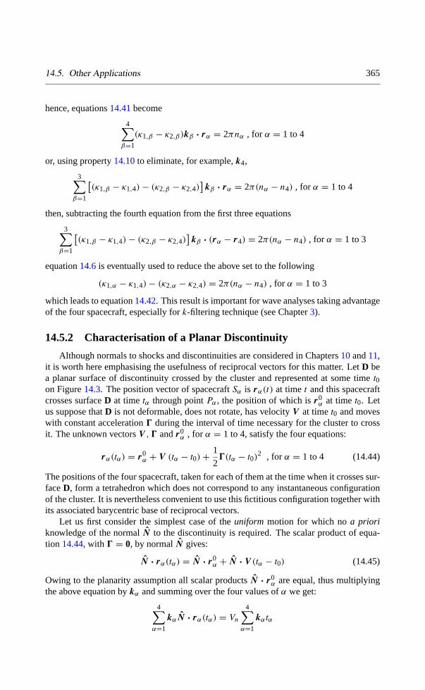
Although normals to shocks and discontinuities are considered in Chapters10and11,it is worth here emphasising the usefulness of reciprocal vectors for this matter. LetD bea planar surface of discontinuity crossed by the cluster and represented at some timet0on Figure14.3. The position vector of spacecraftSα is rα(t) at timet and this spacecraftcrosses surfaceD at timetα through pointPα, the position of which isr0

α at timet0. Letus suppose thatD is not deformable, does not rotate, has velocityV at timet0 and moveswith constant acceleration0 during the interval of time necessary for the cluster to crossit. The unknown vectorsV ,0 andr0

α , for α = 1 to 4, satisfy the four equations:

rα(tα) = r0α + V (tα − t0)+

1

20(tα − t0)

2 , for α = 1 to 4 (14.44)

The positions of the four spacecraft, taken for each of them at the time when it crosses sur-faceD, form a tetrahedron which does not correspond to any instantaneous configurationof the cluster. It is nevertheless convenient to use this fictitious configuration together withits associated barycentric base of reciprocal vectors.

Let us first consider the simplest case of theuniform motion for which noa prioriknowledge of the normalN to the discontinuity is required. The scalar product of equa-tion 14.44, with 0 = 0, by normalN gives:

N · rα(tα) = N · r0α + N · V (tα − t0) (14.45)

Owing to the planarity assumption all scalar productsN · r0α are equal, thus multiplying

the above equation bykα and summing over the four values ofα we get:

4∑α=1

kαN · rα(tα) = Vn

4∑α=1

kαtα


S

α

α

αPn

(D)

Figure 14.3: A surface of discontinuityD that will be crossed by the cluster is representedat some timet0. SpacecraftSα will cross it at timetα through pointPα; and nα is thenormal to the surface determined by spacecraftSα. Each vertex of the tetrahedron islocated at the position of the corresponding spacecraft when it crosses the surface, hencethis tetrahedron does not correspond to any instantaneous configuration of the cluster.

where use has been made of equation14.10. The reciprocal basis presently consideredis the one associated to the fictitious tetrahedron that we have introduced, thus with thehelp of equation14.12the left-hand side of the above equation is just equal toN , which iseventually given by:

N = VnQ1 , where Q1 =

4∑α=1

kαtα (14.46)

The normal component of the relative velocity between the cluster of spacecraft and thediscontinuity is given by the conditionN · N = 1, i.e.:

Vn =(Q1 · Q1

)− 12 (14.47)

This simple result is just the explicit solution of the problem posed byRussell et al.[1983]in their multi-spacecraft study of interplanetary shocks. OnceVn andN have been com-puted with equations14.46and14.47it is necessary to check the consistency of the fourequations14.45 which mean that the four points, forα = 1 to 4, having coordinates(tα, N · rα(tα)

)should be aligned. A dramatic failure of this consistency test would mean

that at least one of our assumptions, the planarity of the discontinuity or the uniformity ofthe motion, is not valid. A rotation or a deformation of the discontinuity, during the timeinterval needed by the cluster to cross it, are quite difficult to discuss.Mottez and Chanteur[1994] proposed a least square method, not related to the barycentric formalism, to deter-mine the relative velocity of a non-planar discontinuity in the rest frame of the cluster,together with estimates of its principal directions and radii of curvature.

Let us now consider the case of the uniformlyacceleratedmotion of a planar discon-tinuity. The normalnα to the surface at the location and time of the crossing by spacecraftSα is determined by measurements made onboardSα only, for example by means of a min-imum variance analysis of the magnetic fluctuations. When the mutual angles made by the

14.5. Other Applications 367

four normals are less than the experimental uncertainties on their directions it is reasonableto assume that the cluster crossed a planar discontinuity and that the relative motion didnot involve a rotation. We will demonstrate at the end of this section that the estimationsof N and0 are invariant in a time translationt −→ t + τ and thatV −→ V − 0τ , as itshould. Thus we chooset0 = 0 for convenience in the following discussion which will befollowed by a short discussion of the uniform motion case.

Derivation of the Estimations

Taking the scalar product of equation14.44with N , for t0 = 0, and using once moreequation14.10, we get the following system of equations:

N · r0α + Vntα +

1

20nt

2α = N · rα(tα) , for α = 1 to 4

whereVn and0n denote respectively the components ofV and0 along the normal. Thefirst terms on the left-hand side of the above equations are equal to zero because of theplanarity assumption, thus multiplying bykα and then summing over the four values ofα

gives, with the help of equation14.12, the normal to the discontinuity in terms of vectorsQ1 andQ2:

N = VnQ1 + 0nQ2 , where Q1 =

4∑α=1

tαkα , and Q2 =1

2

4∑α=1

t2αkα (14.48)

The unknown parametersVn and0n are determined by a constrained least square proce-dure taking into account the fact thatN is a unit vector, i.e. by minimising the expression

ξ =

4∑α=1

(nα − N

)2+ 4(3− 1)

(N

2− 1

)The Lagrange multiplier, written 4(3− 1) for later convenience, is determined by

3 = ±∣∣vQ1 + γQ2

∣∣ (14.49)

where v =Q2

2

(Nmean· Q1

)−(Q1 · Q2

) (Nmean· Q2

)Q2

1Q22 −

(Q1 · Q2

)2 (14.50)

γ =Q2

1

(Nmean· Q2

)−(Q1 · Q2

) (Nmean· Q1

)Q2

1Q22 −

(Q1 · Q2

)2 (14.51)

Nmean =1

4

4∑α=1

nα (14.52)

The normal components of the velocity and the acceleration are

Vn =v

3, and 0n =

γ

3(14.53)


Indeed looking for the extrema ofξ we have found two solutions for3, one of themcorresponds to a minimum ofξ and the other one to a maximum; the right solution isselected by considering that the cosine of the angle between vectorsN andNmeanshouldbe positive, i.e. that

sign(3) = sign[(vQ1 + γQ2

)· Nmean

](14.54)

The Uniform Motion Case

When vectorsQ1 andNmeanare colinear, i.e.Nmean = λQ1, it comes immediatelyfrom equations14.49and following thatγ = 0 andv = λ. In that case

N =Nmean

|Nmean|, and Vn =

1

Q1 · N(14.55)

This result is consistent with our former discussion of the uniform motion case, especiallywith equations14.46and14.47.

Changing the Origin of Time

Equation14.10is used to demonstrate that the time translationt −→ t + τ leavesQ1 invariant and thatQ2 −→ Q2 + τQ1. Using these elementary properties of vectorsQ1 andQ2 it is easily demonstrated that the following expressions are invariant whenchanging the origin of time

Q21Q

22 −

(Q1 · Q2

)2Q2

1

(Nmean· Q2

)−(Q1 · Q2

) (Nmean· Q1

)It follows immediately thatγ is an invariant of the time translation. Then it is readilydemonstrated thatv −→ v− γ τ and that the vectorvQ1 + γQ2 is invariant. Being equalto plus or minus the norm of the latter vector the Lagrange multiplier3 is also invariant.To summarise we have demonstrated the invariance of the estimations ofN and0n givenby equations14.48to 14.54whent −→ t + τ , and thatVn −→ Vn − 0nτ as expected.

14.6 Conclusions

The aim of this chapter was to introduce in a detailed and self-contained way thebarycentric coordinates and the reciprocal vectors of a tetrahedron and to demonstrate thepower of these geometrical concepts to analyse data provided by a four spacecraft mission.All the applications presented in this chapter, the estimation of gradients, the analysis ofdiscontinuities or the spatial aliasing condition, demonstrate that the barycentric formal-ism allows an entirely symmetric handling of the data provided by the four spacecraft,leading to explicit results in which the four spacecraft play identical roles. Moreover thebarycentric formalism allows a complete theoretical analysis of the various kinds of errorsaffecting the estimates of large scale gradients, for any shape of the tetrahedron formed bythe spacecraft. Equation14.31shows that the knowledge of the covariance matrix〈δr δrT 〉

of the uncertainties on the spacecraft positions is mandatory to estimate the geometricalerrors affecting the evaluation of the gradients. The truncation errors of the barycentric

Bibliography 369

estimators of magnetic gradients will generally lead to errors in the estimations of thelarge scale electric currents; this has been demonstrated here for a thick and planar cur-rent sheet and this important point will be again investigated in Chapter15 for a dipolefield. Extensive simulations, making use of the linear barycentric estimators among oth-ers, are discussed in Chapter16 with respect to the accuracy of the current determinationfor simple models of current tubes [see alsoRobert and Roux, 1993]. The analysis of thetruncation errors has emphasised that the linear barycentric estimator of∇ ·B is generallynot equal to zero due to the linear interpolation of the magnetic field, but there is no gen-eral relationship between the truncation errors affecting∇ · B andJ . Although we haveoften focused on magnetic measurements, most of the general results derived here couldbe applied to other fields, for example the plasma velocity moments (see Chapter17).

Bibliography

Chanteur, G. and Mottez, F., Geometrical tools for Cluster data analysis, inProc. Inter-national Conf. “Spatio-Temporal Analysis for Resolving plasma Turbulence (START)”,Aussois, 31 Jan.–5 Feb. 1993, ESA WPP–047, pp. 341–344, European Space Agency,Paris, France, 1993.

Dunlop, M. W., Balogh, A., Southwood, D. J., Elphic, R. C., Glassmeier, K.-H., andNeubauer, F. M., Configurational sensitivity of multipoint magnetic field measurements,in Proceedings of the International Workshop on “Space Plasma Physics Investigationsby Cluster and Regatta”, Graz, Feb. 20–22,1990, ESA SP–306, pp. 23–28, EuropeanSpace Agency, Paris, France, 1990.

Mottez, F. and Chanteur, G., Surface crossing by a group of satellites: a theoretical study,J. Geophys. Res., 99, 13 499–13 507, 1994.

Neubauer, F. M. and Glassmeier, K. H., Use of an array of satellites as a wave telescope,J. Geophys. Res., 95, 19 115–19 122, 1990.

Robert, P. and Roux, A., Influence of the shape of the tetrahedron on the accuracy ofthe estimation of the current density, inProc. International Conf. “Spatio-TemporalAnalysis for Resolving plasma Turbulence (START)”, Aussois, 31 Jan.–5 Feb. 1993,ESA WPP–047, pp. 289–293, European Space Agency, Paris, France, 1993.

Russell, C. T., Mellott, M. M., Smith, E. J., and King, J. H., Multiple spacecraft obser-vations of interplanetary shocks: Four spacecraft determination of shock normals,J.Geophys. Res., 88, 4739–4748, 1983.

Analysis Methods for Multi-Spacecraft Data

Documents

Transcript of Analysis Methods for Multi-Spacecraft Data