JOURHA1 OF COMPUTATIONAL AND AI~HED MATHEMATICS

ELSEVIER Journal of Computational and Applied Mathematics 82 (1997) 105-116

Alternating multi-step quasi-Newton methods for unconstrained optimization

J .A . F o r d a'*, I .A . M o g h r a b i b

a Department of Computer Science, University of Essex, Wivenhoe Park, Colchester, Essex, C04 3SQ, UK b Natural Science Division, Lebanese American University, P.O. Box 13-5053, Beirut, Lebanon

Received 2 September 1996; received in revised form 1 April 1997

Abstract

We consider multi-step quasi-Newton methods for unconstrained optimization. These methods were introduced by the authors (Ford and Moghrabi [5, 6, 8]), who showed how an interpolating curve in the variable-space could be used to derive an appropriate generalization of the Secant Equation normally employed in the construction of quasi-Newton methods. One of the most successful of these multi-step methods employs the current approximation to the Hessian to determine the parametrization of the interpolating curve and, hence, the derivatives which are required in the generalized updating formula. However, certain approximations were found to be necessary in the process, in order to reduce the level of computation required (which must be repeated at each iteration) to acceptable levels. In this paper, we show how a variant of this algorithm, which avoids the need for such approximations, may be obtained. This is accomplished by alternating, on successive iterations, a single-step and a two-step method. The results of a series of experiments, which show that the new algorithm exhibits a clear improvement in numerical performance, are reported.

Keywords." Unconstrained optimization; Quasi-Newton methods; Multi-step methods

AMS classification: 65K10

1. In troduct ion

W e cons ider the uncons t ra ined min imiza t ion o f a funct ion by quas i -Newton techniques. I f we

denote the object ive funct ion by f (where f : R n ---~R) and its gradient and Hess ian b y g and G,

* Corresponding author. E-mail: fordj@essex.ac.uk.

0377-0427/97/$17.00 © 1997 Elsevier Science B.V. All rights reserved PH S 0 3 7 7 - 0 4 2 7 ( 9 7 ) 0 0 0 7 5 - 7

106 J.A. Ford, 1.A. Moghrabi/Journal o f Computational and Applied Mathematics 82 (1997) 105-116

respectively, then such methods proceed iteratively, at each stage determining a new estimate (Xi+l, say) of the desired minimum of f from the current estimate xg. Defining the step-vectors s~ and yi by

def Si ~- Xi+l -- Xi, ( 1 )

def Yi = g(xi+t ) -- g (x i )

= gi+l - gi, say, (2)

then, if Bi denotes the approximation to G at x/, one of the most widely-used quasi-Newton methods for updating Bi is the "Broyden-Fletcher-Goldfarb-Shanno" (BFGS) formula [2, 3, 11, 13], given by

BisisTBi y i y T Bi+l = Bi sTBis------ ~ + s t y ~ . (3)

It is well known that the matrix Bi+I generated by Eq. (3) will satisfy the Secant equation

Bi+lSi = Yi, (4)

which may be regarded as an approximate version of the relation (called the Newton equation by Ford and Saadallah [10]) which is satisfied by the Hessian G(x~+l) itself:

)dx(z*) do(x(r*)) (5) G(Xi+l dr - dr

(In this equation, x(z ) is any differentiable path in ~n passing through the latest iterate X;+l, while r* is the value of • for which x(z*)=x~+l. The relation follows immediately from a straightforward application of the Chain Rule to the vector function g(x(r) ) . ) In fact, the Secant equation (4) may be derived from the Newton equation by taking x(z) to be the straight line passing through x; and x;+l:

x(~) --xi + ~si (6)

and then selecting z* = 1, so that, by virtue of (1), x('c*) =Xi+l. The derivative dg /dz at z = ~* = 1 required for the Newton equation is then approximated (on observing that x(0)= xi) by a backward difference employing the known gradient evaluations:

[g(x(1)) - g(x(O))]/(1 - O)= gi+l - gi

= Yi. (7)

Substitution of the derivative of x(r) and of the derivative approximation y~ in (5) then yields the Secant equation (4), when G(xi+l) is replaced by its approximation B~+l.

In the following sections of this paper, we will describe the development of multi-step quasi- Newton methods. In particular, we will focus attention upon the most successful of a sub-class of multi-step methods introduced in [5] and propose a variant of this method (based on alternating iterations utilizing the chosen multi-step method with "standard" BFGS iterations) which avoids the need for approximations. We will, finally, report and summarize the results of numerical experiments to compare the performance of these two methods with each other and with the standard BFGS algorithm. These experiments provide clear empirical evidence of the superiority of the algorithm proposed here.

J.A. Ford, I.A. MoghrabilJournal of Computational and Applied Mathematics 82 (1997) 105-116 107

2. Multi-step methods

In a series of papers, the authors [5, 6, 8] have developed the concept of multi-step quasi-Newton methods, in which data from several recent steps is employed in the construction of an interpolating path x ( z ) . (We observe, by contrast, that the derivation of the Secant equation described in Section 1 utilizes only data from the most recent step, from xi to xi+l.) The derivative of x('c) and a suitable estimate for dg/d'c are then substituted into Eq. (5) to produce an altemative to the Secant equation:

B i + l r i = W i ( 8 )

(compare Eq. (4)). In (8),

dx(z*) ri -- - - , (9)

d'c

dg(x('c* )) wi ~ d'c (10)

Hessian approximations satisfying the condition (8) may then be obtained, for example, from (3) by substituting the vectors ri and wi for si and Yi, respectively.

One of the approaches introduced by Ford and Moghrabi [5, 6] employs interpolating (vector) polynomials, both to construct the curve x('c) and to produce an approximation (O('c), say) to g(x('c)), from which to estimate the derivative dg/d'c required for the Newton equation. It will be sufficient for our purposes, here, to consider only quadratic interpolations, based on data deriving from the latest three iterates X~-l, xi and xi+ 1 and the associated gradient evaluations. We denote the values of the variable 'c corresponding to these three iterates by "Co, 'cl and 'c2, respectively, so that:

x ( z j ) = X i _ l + j for j = 0, 1,2. (11)

The numerical experiments reported in [5] showed clearly that the performance of algorithms based on such an approach is strongly influenced by the manner in which the defining parameter values {'cj}2:0 are chosen. Of the six multi-step algorithms whose construction is described in [5], the best numerical performance was obtained from the method denoted there by F2, for which the parameters {'cj}j2 0 are derived as follows: we first fix the origin for the variable 'c by specifying that

( 'c*=) 'c2 = 0. (12)

In order to determine the remaining values 'co and "cl, we introduce the following metric, defined o n ~ n :

~bM(z,, z2 ) aef {(z, - z2 )TM(Zl -- z2)} 1/2, ( 13 )

where M is a given n x n symmetric positive-definite matrix. Then the required parameter values 'co and 'el are computed by measuring (with the metric ~bM) the distance of Xs+l from Xs_l and xi, respectively, bearing in mind the relations (11 ):

-- 'Cl = T2 - - 'Cl

= ~ M ( X ( T 2 ) , X ( $ I ) )

= C~M(Xi+1,Xi). (14)

108 J.A. Ford, 1.A. MoghrabilJournal of Computational and Applied Mathematics 82 (1997) 105-116

- - T 0 ~ 2 7 2 - - TO

= q M(X(T2),

= 4 m ( X , + l , X i - 1 ) . (15)

When the values {zj}~= 0 have thus been computed, the form of the interpolating polynomials x ( z ) and O(z) may easily be determined, leading to the vectors ri and wi (Eqs. (9) and (10)) required for the updating of Bi. In fact, it may be shown that, if we define the quantity 6 by the ratio

dej (T 2 __ T1) / ( ,Cl __ ./70), (16)

then (after removal of a common scaling factor) ri and wi are given by the expressions

62 ri = S i 1 + 2 6 si-a' (17)

62 wi = Yi 1 + 26 yi-l" (18)

(Full details may be found in [5].) In the case of the method F2, the matrix M was taken to be B~, the current approximation to the

Hessian. By this means, the measurement of the relevant distances is determined by the properties of the current quadratic approximation (based on Bi) to the objective function. Then we have (using Eqs. (14) and (15))

T 1 = --{sTBisi} I/2, (19)

"~0 ~- --{ (Si "-~ Si-1 )T Bi(si -[- Si-I )}1 /2 . (20)

As these expressions stand, it would probably be considered that they are too expensive to compute at each iteration (because of the matrix-vector products), particularly for higher dimensions. Expressions which are cheaper to evaluate are evidently required. To this end, we observe that, if the new estimate xi+l of the minimum has been obtained by means of a step (determined, for example, by a line-search) along the quasi-Newton search-direction

Pi = -B; - lg i , (21)

then there exists a positive scalar t;, such that

Si = tiPi

and thus,

"~1 = --t i{-- pTi gi } 1/2, ( 2 2 )

It is evident that this expression is considerably less expensive than that given in Eq. (19) to evaluate (indeed, the quantity prg~ may already be available), and that this advantage will grow as the dimension increases.

In order to reduce the cost of computing the corresponding expression for z0 (Eq. (20)), Ford and Moghrabi resorted to an approximation. Although the relevant version of the Secant equation will (in general) not be satisfied by B;, they argued that it was reasonable to assume that such a relation

J.A. Ford, I.A. MoghrabilJournal of Computational and Applied Mathematics 82 (1997) 105-116 109

would hold approximately, given that B; is an approximation to G(x~). Under this assumption, that is, that B~ satisfies

Bisi-1 ~ Yi-1 (23)

and making use of Eq. (21) again, we thus obtain the approximate expression

,Co ~ _{_t2pWg i q_ 2sTyi_a q_ sT_lYi_l } 1/2 (24)

to use for z0. When the algorithm based on these values for {zj}~= 0 (and using the equivalent of the BFGS updating formula) was compared with the standard (single-step) BFGS method, Ford and Moghrabi [5] found that the method F2 showed a substantial improvement, for all but problems of the very lowest dimension. In particular, they observed that computational gains of the order of 20-30% in evaluations, iterations and execution time were obtained for those problems of highest dimension (that is, in the range 46-80) considered in their experiments.

3. An alternating method

Although the assumption made in the previous Section (namely, that B i will approximately satisfy the Secant equation for the step from X;_l to xg) appears to be reasonable and has the virtue of reducing the computational expense involved in determining z0, the argument is evidently open to criticism on the grounds that the degree of approximation may be very poor on some iterations. In certain cases, it may be so poor that the expression within the braces in Eq. (24) turns out to be non-positive, leading to a breakdown in the algorithm as described and necessitating appropriate evasive action in a robust code. To forestall such difficulties, we therefore propose a variant of the F2 algorithm in which the two-step method (as described in Section 2) is alternated with the standard single-step approach on successive iterations. Thus, on every second iteration, when we come to apply the quadratic interpolations required to determine {zj}2=0, 6 and hence ri and w~, the previous iteration (since it executed a "single-step" update, using s~-i and y,-i ) will have produced a Hessian approximation B~ satisfying the Secant equation (23) exactly. It then follows that the expression on the right-hand side of (24) will give the exact value of the parameter "c0 according to the chosen metric. In addition, the expression within the braces is now (barring the effects of rounding error) guaranteed to be positive (as long as xi-1 ~Xi+l).

4. Numerical experiments

The alternating method described in Section 3 (and which we denote by F21) was compared with the standard BFGS method and with the F2 method introduced in [5]. Both the two-step methods F2 and F21 were implemented using the BFGS formula, but with si and yi replaced by ri and wi (in the case of F21, on every other iteration), respectively. (Clearly, multi-step methods may be implemented with any quasi-Newton formula, such as those belonging to the Broyden family ([1, 2]).) The numerical experiments were carried out on a set [6] of 60 test functions (each with four different starting-points), giving a total of 240 test problems with dimensions ranging from 2 to 80. These test functions are taken from standard sets in the literature (such as that of Mor6 et al.

110 J.A. Ford, I.A. MoghrabilJournal of Computational and Applied Mathematics 82 (1997) 105-116

[12], for example) and they are described in detail (with some modifications to starting-points and convergence criteria) in [6]. As in that paper, the sixty test functions were (for convenience) classified into subsets of "low" (2~<n~< 15), "medium" (16~<n~<45) and "high" (46~<n~<80) dimension. In the actual implementation of the methods, we have employed estimates {/-/,-} of the inverse Hessian and the line-searches utilized were required to produce a point xi+l (say) satisfying the following standard stability conditions (see, for example, [4]):

f(Xi+l ) ~ f ( x i ) + 10--4sTg(xi), (25)

sT o(xi+l ) >1 0.9sXi g(xi ). (26)

Furthermore, for problems of dimension ten or higher, the initial approximation to the inverse Hessian was scaled (before the first updating) by the method of Shanno and Phua [14]. For the multi- step methods, the safeguarding parameter 6max [7] was set to the values 4.0 (for F2) and 22.0 (for F21), respectively. These values were determined, for each algorithm, by extensive numerical experimentation, but we stress that the performance of the two methods has not been observed, in either case, to be unduly sensitive to the precise value employed. Hereditary positive-definiteness in the sequence {//,-} is ensured by requiring, on any "multi-step" iteration, that the inequality

rTw i > lO-4[[ri]]2[[wi]]2 (27)

is satisfied (see the outline algorithm below; a fuller discussion of this point may be found in [6]). Such a condition also ensures that we avoid a potential source of numerical instability (namely, a "small" value of rriwi) when computing H,-+I.

In outline, the basic structure of the algorithms we have used in these tests is as follows:-

Step 1: Repeat

Step 2:

Step 3:

Step 4:

Step 5:

Step 6:

Set H0 = I and i = 0; evaluate f (xo) and g(Xo).

p i = - H i g ( x i ) .

If i < n and IIpill2>l, then P i : = Pi/llPill2. Compute x~+~ which satisfies conditions (25) and (26), by means of a line-search from xi along Pi, using safeguarded cubic interpolation. I f a single-step iteration is being executed, then set r~- = si and wi = y~; else compute {z;}f=0 and 6, from Eqs. (22), (24) and (16);

compute ri and wi from Eqs. (17) and (18); I f r~iw,~lO-411r, ll21lw~l[2 or lr]>rmax, then re-compute ri and wi using unit-spacing ([7])

(that is, (17) and (18) with ~ : 1). I f rTw ~ <. 10-4[Ir;ll~[[w, ll~ again, then set r; = si and w; = y;.

I f i = 0 a n d n ~ > 1 0 , then scale H0 by the method of Shanno and Phua [14]. Update/-/,- (by use of a BFGS-type formula) to produce H,-+I satisfying Hi+lwi = ri. Increment i;

Unti l Hg(xi)ll~ <e (where e is a problem-dependent tolerance).

J.A. Ford, I.A. Moghrabil Journal of Computational and Applied Mathematics 82 (1997) 105-116

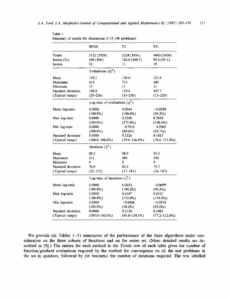
Table 1 Summary of results for dimensions 2-15 (40 problems)

BFGS F2 F21

Totals 5122 (3928) 5224 (3954) 4840 (3658) Ratios (%) 100 (100) 102.0 (100.7) 94.5 (93.1) Scores 12 11 19

Evaluations (El)

Mean 128.1 130.6 121.0 Maximum 614 714 643 Minimum 11 11 11 Standard deviation 108.0 119.4 107.7 ( Typical range) (20-236) (11-250) (13-229)

Log-ratio of evaluations (pf)

Mean log-ratio 0.0000 0.0044 -0.0594 (100.0%) (100.4%) (94.2%)

Max log-ratio 0.0000 0.5390 0.3959 (100.0%) (171.4%) (148.6%)

Min log-ratio 0.0000 -0.7016 -0.5965 (100.0%) (49.6%) (55.1%)

Standard deviation 0.0000 0.2326 0.1817 (Typical range) (100.0-100.0%) (79.6-126.8%) (78.6-113.0%)

Iterations (rx)

Mean 98.2 98.9 91.5 Maximum 411 483 450 Minimum 9 9 9 Standard deviation 76.6 82.3 75.7 (Typical range) (22-175) (17-181) (16-167)

Log-ratio of iterations (2 x)

Mean log-ratio 0.0000 0.0023 -0.0699 (100.0%) (100.2%) (93.3%)

Max log-ratio 0.0000 0.4187 0.2151 (100.0%) (152.0%) (124.0%)

Min log-ratio 0.0000 -0.6886 -0.5878 (100.0%) (50.2%) (55.6%)

Standard deviation 0.0000 0.2136 0.1885 (Typical range) (100.0-100.0%) (81.0-124.1%) (77.2-112.6%)

111

We provide (in Tables 1 -4 ) summaries o f the performance o f the three algorithms under con- sideration on the three subsets o f functions and on the entire set. (More detailed results are de- scribed in [9].) The entries for each method in the Totals row of each table gives the number o f function/gradient evaluations required by the method for convergence on all the test problems in the set in question, fol lowed by (in brackets) the number o f iterations required. The row labelled

112 J.A. Ford, L A. Moghrabi l Journal of Computational and Applied Mathematics 82 (1997) 105-116

Table 2 Summary of results for dimensions 16-45 (100 problems)

BFGS F2 F21

Totals 20871 (18910) 17203 (14760) 15777 (13333) Ratios (%) 100 (100) 82.4 (78.1) 75.6 (70.5) Scores 15 16 76

Evaluations (Ej x)

Mean 208.7 172.0 157.8 Maximum 1059 1272 1074 Minimum 2 2 2 Standard deviation 200.2 190.1 169.8 (Typical range) (9-409) (0-362) (0-328)

Log-ratio of evaluations (pX)

Mean log-ratio 0.0000 -0.1891 -0.2763 (100.0%) (82.8%) (75.9%)

Max log-ratio 0.0000 0.5670 0.3212 (100.0%) (176.3%) (137.9%)

Min log-ratio 0.0000 -2.2138 -2.1117 (I00.0%) (10.9%) (12.1%)

Standard deviation 0.0000 0.2977 0.2898 (Typical range) (100.0-100.0%) (61.5-111.5%) (56.8-101.4%)

Iterations ( / f )

Mean 189.1 147.6 133.3 Maximum 894 1014 902 Minimum 1 1 1 Standard deviation 180.7 157.8 144.8 (Typical range) (8-370) (0-305) (0-278)

Log-ratio of iterations (2 x)

Mean log-ratio 0.0000 -0.2234 -0.3341 (100.0%) ( 80.0%) (71.6%)

Max log-ratio 0.0000 0.3514 0.3137 (100.0%) (142.1%) (136.8%)

Min log-ratio 0.0000 -2.1467 -2.2546 (100.0%) (I 1.7%) (10.5%)

Standard deviation 0.0000 0.2935 0.3135 (Typical range) (100.0-100.0%) (59.6-107.3%) (52.3-98.0%)

Ratios gives the proportion o f evaluations/iterations, expressed as a percentage o f the corresponding figures for the BFGS method. These ratios may thus be regarded as simple estimates o f the relative efficiencies o f each of the multi-step methods, by comparison with the standard BFGS algorithm. In addition, the method yielding the best performance ( judged by the number o f function/gradient evaluations required, with ties being resolved by the number o f iterations) on each problem is

J.A. Ford, LA. Moghrabil Journal of Computational and Applied Mathematics 82 (1997) 105-116

Table 3 Summary of results for dimensions 46-80 (100 problems)

BFGS F2 F21

Totals 18575 (17694) 13487 (12340) 12365 (10580) Ratios (%) 100 (100) 72.6 (69.7) 66.6 (59.8) Scores 9 19 76

Evaluations (E x )

Mean 185.8 134.9 123.7 Maximum 880 505 487 Minimum 2 2 2 Standard deviation 164.2 100.9 90.4 (Typical range) (22-350) (34-236) (33-214)

Log-ratio of evaluations (pf)

Mean log-ratio 0.0000 -0.2459 -0.3176 (100.0%) (78.2%) (72.8%)

Max log-ratio 0.0000 1.0082 0.9808 ( 1 O0.0%) (274.1% ) (266.7%)

Min log-ratio 0.0000 - 1.2962 - 1.0003 (100.0%) (27.4%) (36.8%)

Standard deviation 0.0000 0.2981 0.2764 (Typical ran9 e) (100.0-100.0%) (58.0-105.4%) (55.2-96.0%)

Iterations (/ix)

Mean 176.9 123.4 105.8 Maximum 872 481 468 Minimum 1 1 1 Standard deviation 164.0 96.5 82.8 (Typical range) (13-341) (27-220) (23-189)

Log-ratio of iterations ( i f )

Mean log-ratio 0.0000 -0.2647 -0.3945 (100.0%) (76.7%) (67.4%)

Max log-ratio 0.0000 1.1632 1.0874 (100.0%) (320.0%) (296.7%)

Min log-ratio 0.0000 -1.2462 -1.3004 (100.0%) (28.8%) (27.2%)

Standard deviation 0.0000 0.3221 0.3236 (Typical range) (100.0-100.0%) (55.6--105.9%) (48.8-93.2%)

113

awarded one point, and the entry for each method in the row labelled Scores gives the total number o f points obtained by that method for the test set under consideration.

Each table also contains more detailed comparisons based on the number o f evaluations and iterations required by each method for each problem. Specifically, i f E f a n d / i x (where X m a y be

114 J.A. Ford, LA. MoghrabilJournal of Computational and Applied Mathematics 82 (1997) 105-116

Table 4 Overall summary (240 problems)

BFGS F2 F21

Totals 44568 (40532) 35914 (31054) 32982 (27571) Ratios (%) 100 (100) 80.6 (76.6) 74.0 (68.0) Scores 36 46 171

Evaluations (E x )

Mean 185.7 149.6 137.4 Maximum 1059 1272 1074 Minimum 2 2 2 Standard deviation 174.5 147.9 132.4 (Typical range) (11-360) (2-298) (5-270)

Log-ratio of evaluations (~x)

Mean log-ratio 0.0000 -0.1805 -0.2574 (100.0%) (83.5%) (77.3%)

Max log-ratio 0.0000 1.0082 0.9808 (100.0%) (274.1%) (266.7%)

Min log-ratio 0.0000 -2.2138 -2.1117 (100.0%) (10.9%) (12.1%)

Standard deviation 0.0000 0.2998 0.2829 (Typical range) (100.0-100.0%) (61.9-112.7%) (58.3-102.6%)

Iterations ( / f )

Mean 168.9 129.4 114.9 Maximum 894 1014 902 Minimum 1 1 1 Standard deviation 163.3 124.9 112.9 (Typical range) (6-332) (5-254) (2-228)

Log-ratio of iterations (2 x)

Mean log-ratio 0.0000 -0.2030 -0.3152 (100.0%) (81.6%) (73.0%)

Max log-ratio 0.0000 1.1632 1.0874 (100.0%) (320.0%) (296.7%)

Min log-ratio 0.0000 -2.1467 -2.2546 (100.0%) (11.7%) (10,5%)

Standard deviation 0.0000 0.3081 0.3205 (Typical range) (100.0-100.0%) (60.0-111.1%) (53.0-100.5%)

either BFGS, F2 or F21 ) denote, respectively, the number o f evaluations and the number o f iterations required by the stated method on problem j , we define (for each method X ) the log-ratios

p7 d0f

X def ,~ : ln( IjX /IfiFGS ).

J.A. Ford, I.A. Moghrabi/Journal of Computational and Applied Mathematics 82 (1997) 105-116 115

Then, for the four sets of data {EjX}, {/2x}, {pf} and {2 x} produced by a given method X on all problems in a specified set, we have computed and displayed in the tables the following statistics: • mean, • maximum, • minimum, • standard deviation. In the case of the log-ratio data, each statistic (except the standard deviation) is followed by the corresponding value of the ratio, expressed as a percentage, in order to make the significance of the statistic clearer. To illustrate the standard deviations for each set of data, we have provided a typical range of data for the given method, by displaying an interval one standard deviation either side of the stated mean.

5. Summary and conclusions

A new technique for implementing the two-step quasi-Newton method F2 introduced in [5] has been described. The technique involves alternating F2 with the standard single-step method on suc- cessive iterations, in order that the parameter values required by F2 may be computed exactly, rather than approximately (as was the case with the original version of F2 described in [5]). The experi- ments reported here show that the new version of the method produces a significant improvement in the numerical performance, over and above that already achieved by F2 in comparison with the standard single-step BFGS algorithm. We note that, unlike F2, the new method does not appear to be worse than BFGS for problems of "low" dimension (Table 1). More importantly, for the higher-dimension problems considered here (Table 3), average gains (relative to the performance of the standard BFGS method) of the order of 27-33% in evaluations and 33-40% in iterations were observed (the corresponding figures for F2 being approximately 22-27% and 23-30%, respectively). (It appears that the slightly lower improvements arising from the log-ratio data may be due to an observable tendency (which, in itself, is encouraging) for higher gains to be achieved on problems which, for BFGS, required a greater number of evaluations and iterations.) Finally, we may note (from Tables 2 and 3) that the new method out-performs both BFGS and F2 in over 70% of all the cases of dimension 16 and above considered in these tests (200 problems in all).

Acknowledgements

The authors wish to thank the referee for his constructive and helpful comments on an earlier version of this paper.

References

[1] C.G. Broyden, Quasi-Newton methods and their application to function minimization, Maths. Comp. 21 (1967) 368-381.

[2] C.G. Broyden, The convergence of a class of double-rank minimization algorithms, Parts I and II, J. Inst. Math. Appl. 6 (1970) 76-90 and 222-231.

116 J.A. Ford, I.A. MoghrabilJournal of Computational and Applied Mathematics 82 (1997) 105-116

[3] R. Fletcher, A new approach to variable metric algorithms, Comput. J. 13 (1970) 317-322. [4] R. Fletcher, Practical Methods of Optimization, 2nd ed., Wiley, New York, 1987. [5] J.A. Ford, I.A. Moghrabi, Alternative parameter choices for multi-step quasi-Newton methods, Optim. Meth. Software

2 (1993) 357-370. [6] J.A. Ford, I.A. Moghrabi, Multi-step quasi-Newton methods for optimization, J. Comput. Appl. Math. 50 (1994)

305-323. [7] J.A. Ford, I.A. Moghrabi, Further investigation of multi-step quasi-Newton methods, Scientia Iranica 1 (1995)

327-334. [8] J.A. Ford, I.A. Moghrabi, Minimum curvature multi-step quasi-Newton methods, Comput. Math. Appl. 31 (1996)

179-186. [9] J.A. Ford, I.A. Moghrabi, An alternating multi-step quasi-Newton method for unconstrained optimization, Technical

Report CSM-270, Depart. Comput. Sci. Univ. Essex, 1996. [I0] J.A. Ford, A.F. Saadallah, A rational function model for unconstrained optimization, in: Colloquia Mathematica

Societatis Janos Bolyai, vol. 50, Numerical Methods, 1986, 539-563. [11] D. Goldfarb, A family of variable metric methods derived by variational means, Math. Comp. 24 (1970) 23-26. [12] J.J. Mor6, B.S. Garbow, K.E. Hillstrom, Testing unconstrained optimization software, ACM Trans. Math. Software

7 (1981) 17--41. [13] D.F. Shanno, Conditioning of quasi-Newton methods for function minimization, Math. Comp. 24 (1970) 647456. [14] D.F. Shanno, K.H. Phua, Matrix conditioning and nonlinear optimization, Math. Programming 14 (1978) 149-160.