a continuous newton-type method for unconstrained ...

A CONTINUOUS NEWTON-TYPE METHOD FORUNCONSTRAINED OPTIMIZATION∗

Lei-Hong Zhang, C.T. Kelley† and Li-Zhi Liao‡

Abstract: In this paper, we propose a continuous Newton-type method in the form of an ordinary differentialequation by combining the negative gradient and the Newton direction. We show that for a general functionf(x), our method converges globally to a connected subset of the stationary points of f(x) under some mildconditions, and converges globally to a single stationary point for a real analytic function. The methodreduces to the exact continuous Newton method if the Hessian matrix of f(x) is uniformly positive definite.We report on convergence of the new method on the set of standard test problems in the literature.

Key words: unconstrained optimization, continuous method, ODE method, global convergence, pseudo-transient continuation

Mathematics Subject Classification: 65K10, 65L05, 90C47

1 Introduction

In this paper we consider the solution schemes for the following unconstrained optimizationproblem

minx∈Rn

f(x), f ∈ C2(Rn), (1.1)

by using the so-called continuous method or Ordinary Differential Equation (ODE) method(see [8, 12, 13, 19, 25, 32, 38] and the references therein). Different from the conventionaloptimization approaches, such method adopts some kind of differential equation with theinitial condition to define the trajectory of variable x in terms of a parameter t. By tracingthis trajectory, the stationary point(s) satisfying∇f(x) = 0, or hopefully, the local minimizerof f(x) can be located. To be more precise, let x(t) for t ∈ T ⊆ R, be the solution of thefollowing initial value problem (IVP):

dx(t)

dt = h(x), t ≥ 0x(0) = x0,

(1.2)

∗This research was supported in part by FRG grants from Hong Kong Baptist University and the ResearchGrant Council of Hong Kong.

†The research of C. T. Kelley was supported by National Science Foundation Grants DMS-0404537 andDMS-0707220, and Army Research Office Grants W911NF-04-1-0276, W911NF-06-1-0096, W911NF-06-1-0412, and W911NF-07-1-0112.

‡Corresponding author.

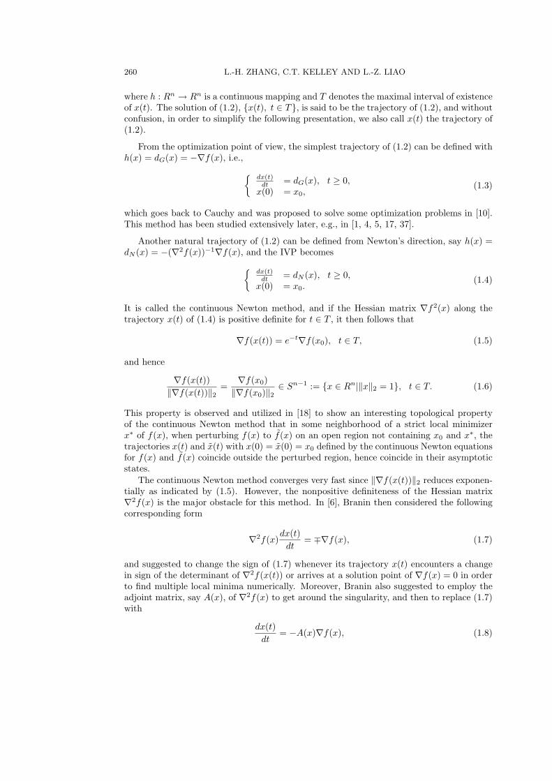
260 L.-H. ZHANG, C.T. KELLEY AND L.-Z. LIAO

where h : Rn → Rn is a continuous mapping and T denotes the maximal interval of existenceof x(t). The solution of (1.2), x(t), t ∈ T, is said to be the trajectory of (1.2), and withoutconfusion, in order to simplify the following presentation, we also call x(t) the trajectory of(1.2).

From the optimization point of view, the simplest trajectory of (1.2) can be defined withh(x) = dG(x) = −∇f(x), i.e.,

dx(t)

dt = dG(x), t ≥ 0,x(0) = x0,

(1.3)

which goes back to Cauchy and was proposed to solve some optimization problems in [10].This method has been studied extensively later, e.g., in [1, 4, 5, 17, 37].

Another natural trajectory of (1.2) can be defined from Newton’s direction, say h(x) =dN (x) = −(∇2f(x))−1∇f(x), and the IVP becomes

dx(t)

dt = dN (x), t ≥ 0,x(0) = x0.

(1.4)

It is called the continuous Newton method, and if the Hessian matrix ∇f2(x) along thetrajectory x(t) of (1.4) is positive definite for t ∈ T , it then follows that

∇f(x(t)) = e−t∇f(x0), t ∈ T, (1.5)

and hence

∇f(x(t))‖∇f(x(t))‖2 =

∇f(x0)‖∇f(x0)‖2 ∈ Sn−1 := x ∈ Rn|‖x‖2 = 1, t ∈ T. (1.6)

This property is observed and utilized in [18] to show an interesting topological propertyof the continuous Newton method that in some neighborhood of a strict local minimizerx∗ of f(x), when perturbing f(x) to f(x) on an open region not containing x0 and x∗, thetrajectories x(t) and x(t) with x(0) = x(0) = x0 defined by the continuous Newton equationsfor f(x) and f(x) coincide outside the perturbed region, hence coincide in their asymptoticstates.

The continuous Newton method converges very fast since ‖∇f(x(t))‖2 reduces exponen-tially as indicated by (1.5). However, the nonpositive definiteness of the Hessian matrix∇2f(x) is the major obstacle for this method. In [6], Branin then considered the followingcorresponding form

∇2f(x)dx(t)

dt= ∓∇f(x), (1.7)

and suggested to change the sign of (1.7) whenever its trajectory x(t) encounters a changein sign of the determinant of ∇2f(x(t)) or arrives at a solution point of ∇f(x) = 0 in orderto find multiple local minima numerically. Moreover, Branin also suggested to employ theadjoint matrix, say A(x), of ∇2f(x) to get around the singularity, and then to replace (1.7)with

dx(t)dt

= −A(x)∇f(x), (1.8)

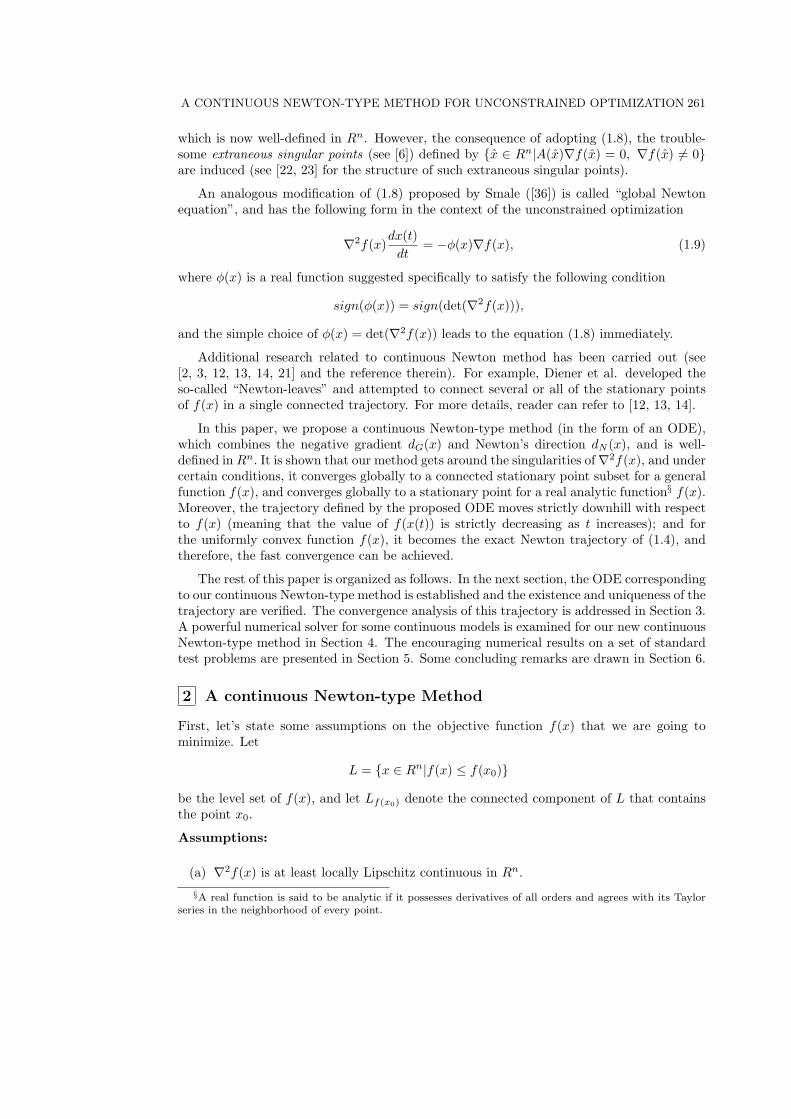
A CONTINUOUS NEWTON-TYPE METHOD FOR UNCONSTRAINED OPTIMIZATION 261

which is now well-defined in Rn. However, the consequence of adopting (1.8), the trouble-some extraneous singular points (see [6]) defined by x ∈ Rn|A(x)∇f(x) = 0, ∇f(x) 6= 0are induced (see [22, 23] for the structure of such extraneous singular points).

An analogous modification of (1.8) proposed by Smale ([36]) is called “global Newtonequation”, and has the following form in the context of the unconstrained optimization

∇2f(x)dx(t)

dt= −φ(x)∇f(x), (1.9)

where φ(x) is a real function suggested specifically to satisfy the following condition

sign(φ(x)) = sign(det(∇2f(x))),

and the simple choice of φ(x) = det(∇2f(x)) leads to the equation (1.8) immediately.

Additional research related to continuous Newton method has been carried out (see[2, 3, 12, 13, 14, 21] and the reference therein). For example, Diener et al. developed theso-called “Newton-leaves” and attempted to connect several or all of the stationary pointsof f(x) in a single connected trajectory. For more details, reader can refer to [12, 13, 14].

In this paper, we propose a continuous Newton-type method (in the form of an ODE),which combines the negative gradient dG(x) and Newton’s direction dN (x), and is well-defined in Rn. It is shown that our method gets around the singularities of∇2f(x), and undercertain conditions, it converges globally to a connected stationary point subset for a generalfunction f(x), and converges globally to a stationary point for a real analytic function§ f(x).Moreover, the trajectory defined by the proposed ODE moves strictly downhill with respectto f(x) (meaning that the value of f(x(t)) is strictly decreasing as t increases); and forthe uniformly convex function f(x), it becomes the exact Newton trajectory of (1.4), andtherefore, the fast convergence can be achieved.

The rest of this paper is organized as follows. In the next section, the ODE correspondingto our continuous Newton-type method is established and the existence and uniqueness of thetrajectory are verified. The convergence analysis of this trajectory is addressed in Section 3.A powerful numerical solver for some continuous models is examined for our new continuousNewton-type method in Section 4. The encouraging numerical results on a set of standardtest problems are presented in Section 5. Some concluding remarks are drawn in Section 6.

2 A continuous Newton-type Method

First, let’s state some assumptions on the objective function f(x) that we are going tominimize. Let

L = x ∈ Rn|f(x) ≤ f(x0)

be the level set of f(x), and let Lf(x0) denote the connected component of L that containsthe point x0.

Assumptions:

(a) ∇2f(x) is at least locally Lipschitz continuous in Rn.

§A real function is said to be analytic if it possesses derivatives of all orders and agrees with its Taylorseries in the neighborhood of every point.


(b) f(x) is bounded from below by f∗ > −∞.

(c) For any x0 ∈ Rn, Lf(x0) is bounded.

It is clear that Assumption (c) is much weaker than the condition that the level setL = x ∈ Rn|f(x) ≤ f(x0) is bounded. For example, if f(x) = sin x, x ∈ R, and for anygiven x0 ∈ R with f(x0) 6= 1, the level set

L =+∞⋃

k=−∞[(2k − 1)π − arcsin f(x0), 2kπ + arcsin f(x0)], k ∈ Z (the integer set),

is unbounded, but

Lf(x0) = [(2k − 1)π − arcsin f(x0), 2kπ + arcsin f(x0)]

for some k ∈ Z with x0 ∈ Lf(x0) is bounded. From Assumption (c), we know also that theset Lf(x0) is compact, and furthermore, for any x0 ∈ Rn, the set Sf(x0) defined by

Sf(x0) := S ∩ Lf(x0), (2.1)

is compact too, where S is the stationary points set of f(x) given by

S := x ∈ Rn|∇f(x) = 0. (2.2)

Consider the following continuous Newton-type differential equation,

dx(t)dt = d(x), t ≥ 0

x(0) = x0,(2.3)

where

d(x) = α(x)dN (x) + β(x)dG(x), (2.4)

with

α(x) =

1, if λmin(x) > δ2,λmin(x)−δ1

δ2−δ1, if δ1 ≤ λmin(x) ≤ δ2,

0, if λmin(x) < δ1;(2.5)

and

β(x) = 1− α(x) =

0, if λmin(x) > δ2,δ2−λmin(x)

δ2−δ1, if δ1 ≤ λmin(x) ≤ δ2,

1, if λmin(x) < δ1.

(2.6)

Here, λmin(x) represents the smallest eigenvalue of ∇2f(x), and δ2 > δ1 > 0 are two prede-fined positive constants. It should be noted that the smallest eigenvalue of ∇2f(x), λmin(x),can be easily estimated from the modified Cholesky factorization in [33] numerically.

A first observation is that for a general function f(x) ∈ C2(Rn), (2.4) is well-definedin Rn; and when ∇2f(x) is uniformly positive definite, i.e., yT∇2f(x)y ≥ δ‖y‖22, for someconstant δ > 0 and ∀y ∈ Rn, the trajectory generated from (2.3) is exactly the continuousNewton trajectory for any 0 < δ1 < δ2 ≤ δ. Since the direction d(x) in (2.4) is continuousin Rn, the Cauchy-Peano existence theorem implies that there is a solution to the IVP(2.3); for the uniqueness of the solution, furthermore, we need to prove d(x) is also locallyLipschitz continuous in Rn. The first result shows that under Assumption (a), λmin(x) islocally Lipschitz continuous in Rn, which is a direct consequence of the following Wielandt-Hoffman lemma.


Lemma 2.1 ([16], p. 396). If A and A + E are n-by-n symmetric matrices, then

|λk(A + E)− λk(A)| ≤ ‖E‖2, k = 1, · · · , n,

where λk(A) designates the kth largest eigenvalue of A.

Since ∇2f(x) is locally Lipschitz continuous by Assumption (a), the previous lemmareveals that for any two points y, z in some neighborhood of any x ∈ Rn,

|λmin(y)− λmin(z)| ≤ ‖∇2f(y)−∇2f(z)‖2 ≤ C1‖y − z‖2, (2.7)

where C1 > 0 is the Lipschitz constant of ∇2f(x), and hence it follows that λmin(x) is locallyLipschitz continuous in Rn. Assumptions (a) also implies that

‖dG(y)− dG(z)‖2 ≤ C2‖y − z‖2, (2.8)

for a constant C2 > 0 and for any two points y, z in some neighborhood of x ∈ Rn.Moreover, from the result in [30] (p.46), we know that for any x ∈ Rn, if λmin(x) > 0,

there exist a γ > 0 and a neighborhood Nτ (x) of x such that ∀y ∈ Nτ (x),∇2f(y) is invertibleand ‖(∇2f(y))−1‖2 ≤ γ. Hence, for any y, z ∈ Nτ (x), it follows

‖(∇2f(y))−1 − (∇2f(z))−1‖2 = ‖(∇2f(y))−1[∇2f(z)−∇2f(y)](∇2f(z))−1‖2≤ γ2 · ‖∇2f(z)−∇2f(y)‖2≤ γ2C1‖z − y‖2, (2.9)

which implies that when λmin(x) > 0, (∇2f(x))−1 is Lipschitz continuous at x too; andadditionally, it is true that

‖dN (y)− dN (z)‖2 ≤ C3‖y − z‖2, ∀y, z ∈ Nτ (x), (2.10)

for some positive constant C3 > 0 and λmin(x) > 0.

Theorem 2.2. Suppose that f(x) satisfies Assumptions (a), (b) and (c), then for anyx(0) = x0 ∈ Rn, there exists a unique solution x(t) to (2.3), and the maximal interval ofexistence of the solution can be extended to [0,+∞).

Proof. See the Appendix.

We next provide a general result which shows that the trajectory x(t) of (2.3) will neverreach the set Sf(x0) at finite time t ≥ 0 provided that∇f(x0) 6= 0. This result is the extensionof Theorem 2(iii) in [26] which obtains the same conclusion for the gradient system (1.3).

Theorem 2.3. Suppose h : Rn → Rn is locally Lipschitz continuous. Then for any x0 =x(0) ∈ Rn with h(x0) 6= 0, the solution to the IVP (1.2), x(t), satisfies h(x(t)) 6= 0 for anyt ∈ T, where T denotes the maximal interval of existence of x(t).

Proof. The proof can be conducted along the same arguments as Theorem 2 (iii) in [26].

Under the Assumptions (a), (b) and (c), (6.1) together with the previous theorem revealsthat f(x(t)) is strictly decreasing along the trajectory as t increases whenever ∇f(x0) 6= 0.This property also guarantees that there is no periodic solution for (2.3).

Theorem 2.4. There is no periodic solution to (2.3) for any x(0) = x0 ∈ Rn with ∇f(x0) 6=0.

Proof. See the Appendix.


3 Convergence Analysis

Since for any x0 ∈ Rn, the solution x(t) of (2.3) is unique and its maximal interval ofexistence can be extended to [0,+∞), we then can apply some results (refer to [31]) of thedynamical system to develop the convergence analysis.

Consider the ODE

dx(t)dt

= h(t). (3.1)

We suppose that for any x0 ∈ Rn, the solution x(t) to (3.1) with x(0) = x0 is unique andits right maximal interval of existence is [0,+∞).

Definition 3.1. A point p ∈ Rn is an ω-limit point of the trajectory x(t) of (3.1) withx(0) = x0 if there is a sequence ti → +∞ (as i → +∞) such that

limi→+∞

x(ti) = p.

The set of all ω-limit points of the trajectory x(t) of (3.1) with x(0) = x0 is called the ω-limitset of x(t) and it is denoted by Ωx0 .

Some properties of the ω-limit set are summarized in the following Lemma 3.2 (see [31],p. 175).

Lemma 3.2. The ω-limit set of a trajectory x(t) of (3.1) with x(0) = x0, Ωx0 , is a closedsubset of Rn and if x(t) is contained in a compact subset of Rn, then Ωx0 is non-empty,connected and compact subset of Rn.

Denote by

dist(x(t),Ωx0) = infx∈Ωx0

‖x(t)− x‖2

the distance of x(t) to the set Ωx0 . If the trajectory x(t) is contained in a compact subsetof Rn, it then is true that

limt→+∞

dist(x(t),Ωx0) = 0,

since otherwise, there exists some ε > 0 and a sequence ti such that ti → +∞ and

dist(x(ti),Ωx0) > ε, i = 1, 2, · · · . (3.2)

The boundedness of x(ti) then implies that there is a convergent subsequence x(t′i) withthe limit point p ∈ Rn. The fact p ∈ Ωx0 then contradicts (3.2).

Applying these results to (2.3), we can analyze the convergence of the trajectory x(t) of(2.3).

Remark 3.3. Let Ωx0 represent the ω-limit set of trajectory x(t) of (2.3) with x(0) = x0 ∈Rn. As indicated by (6.1), Ωx0 ⊆ Lf(x0); and moreover, we can say that the trajectory x(t)converges to the set Ωx0 as t → +∞ in the sense that

limt→+∞

dist(x(t),Ωx0) = 0.


If, in addition, Ωx0 contains only one point p ∈ Rn, it then implies that

limt→+∞

dist(x(t),Ωx0) = limt→+∞

infx∈p

‖x(t)− x‖2 = limt→+∞

‖x(t)− p‖2 = 0,

which equivalently implies that x(t) converges to a single point p ∈ Rn.

The following theorem gives the convergence result for a general function f(x).

Theorem 3.4. Suppose f(x) satisfies Assumptions (a), (b), and (c), and for any x0 ∈ Rn,let x(t) be the trajectory of (2.3) with x(0) = x0 ∈ Rn, and let Ωx0 denote the ω-limit set ofx(t). Then there exists some constant f such that

Ωx0 ⊆ x ∈ Rn|f(x) = f ∩ Sf(x0); (3.3)

and x(t) converges to some connected subset of Sf(x0) as t → +∞, where Sf(x0) is definedby (2.1).

Proof. Since ∇f(x0) = 0 is the trivial case in which the unique trajectory becomes x(t) ≡x0, t ≥ 0 (due to uniqueness), we just consider ∇f(x0) 6= 0.

From (6.1) and Theorem 2.3, it follows that f(x(t)) is strictly decreasing as t increases,but still bounded below by Assumption (b), which consequently implies that there exists aconstant, say f , so that

limt→+∞

f(x(t)) = f .

As a result, for any x ∈ Ωx0 , there exists a sequence ti+∞i=1 such that ti → +∞, x(ti) → xand f(x(ti)) → f(x) = f as i → +∞, which implies Ωx0 ⊆ x ∈ Rn|f(x) = f directly.

Furthermore, the LaSalle invariant set theorem (Theorem 3.4 in [35]) says that for anyx ∈ Ωx0 , we have df(x)

dt = ∇f(x)T d(x) = 0, which is true only when ∇f(x) = 0 by (6.1).Consequently, from Lemma 3.2, Remark 3.3 and x(t) ∈ Lf(x0) for t ≥ 0, we concludeΩx0 ⊆ x ∈ Rn|f(x) = f ∩ Sf(x0), and complete the proof.

Special cases of the set Ωx0 below directly lead to the convergence to a stationary point,and the proof is obvious by Lemma 3.2, Remark 3.3, and Theorem 3.4.

Corollary 3.5. Under the conditions of Theorem 3.4, suppose that x(t) is the trajectory of(2.3) with x(0) = x0 ∈ Rn. If each point in Sf(x0) is isolated from one another, then x(t)converges to a stationary point as t → +∞; and therefore, if there is an x ∈ Ωx0 being astrictly local minimizer of f(x), then x(t) → x as t → +∞.

However, in general, it should be pointed out that converging to a (single) stationarypoint may not be obtained, because it is known that the trajectory of (1.3) will not necessarilyconverge to a single point (see [19], Prop. C.12.1; and see [1] for a counterexample). By onlyendowing f(x) to be real analytic additionally, however, converging to a single stationarypoint is achievable. The proof for this is based on Corollary 3.5 and similar to the proof ofTheorem 2.2 in [1].

Theorem 3.6. Suppose that f(x) is a real analytic function satisfying Assumption (a), (b),and (c). Then for any x0 ∈ Rn, the trajectory x(t) of (2.3) converges to a (single) stationarypoint of f(x) as t → +∞ for any x(0) = x0 ∈ Rn.


Proof. We just need to consider the case ∇f(x0) 6= 0. Let Ωx0 be the ω-limit set of x(t). Ifthere exists an x ∈ Ωx0 such that λmin(x) > 0, then x must be a strictly local minimizer off(x) and Corollary 3.5 completes the proof already; otherwise, ∀x ∈ Ωx0 , λmin(x) ≤ 0. Weprove next that x is the unique point in Ωx0 and therefore limt→+∞ x(t) = x.

Obviously, there exists a neighborhood Nτ1(x) of x such that ∀x ∈ Nτ1(x), λmin(x) < δ1

for the predefined δ1 > 0 in (2.5). Also, since f(x) is real analytic, the following ÃLojasiewiczgradient inequality (see [27]) holds in a neighborhood Nτ2(x) of x,

‖∇f(x)‖2 ≥ c|f(x)− f(x)|σ, ∀x ∈ Nτ2(x),

for some constants c > 0 and σ ∈ [0, 1). We then can assume that for any sufficiently smallε > 0, the ÃLojasiewicz gradient inequality and λmin(x) < δ1 hold in the neighborhood Nε(x).

From Theorem 3.4 and ∇f(x0) 6= 0, it follows that f(x(t)) > f(x) for t ≥ 0. Then forany x(t) ∈ Nε(x), we have

d[f(x(t))− f(x)]dt

= −‖∇f(x(t))‖22 ≤ −c[f(x(t))− f(x)]σ · ‖dx(t)dt

‖2,

or equivalently,

c1d[f(x(t))− f(x)]1−σ

dt≤ −‖dx(t)

dt‖2, (3.4)

where c1 = (c(1− σ))−1 > 0, c > 0 and σ ∈ [0, 1).Note that x is an accumulation point and f(x(t)) → f(x) as t → +∞, there must exist

some t1 ≥ 0 such that the following two inequalities hold simultaneously,

‖x(t1)− x‖2 <ε

2,

c1[f(x(t1))− f(x)]1−σ <ε

2.

Suppose x(t) will leave Nε(x) after t1, and let t2 be the smallest such that ‖x(t2)− x‖2 = ε,then x(t) ∈ Nε(x) for all t ∈ (t1, t2). From (3.4) and the decreasing property of f(x(t)), weget

0 <

∫ t2

t1

‖dx(t)dt

‖2dt ≤ c1[f(x(t1))− f(x)]1−σ − c1[f(x(t2))− f(x)]1−σ

< c1[f(x(t1))− f(x)]1−σ <ε

2.

Therefore,

‖x(t2)− x‖2 ≤ ‖x(t2)− x(t1)‖2 + ‖x(t1)− x‖2≤

∫ t2

t1

(‖dx(t)dt

‖2)dt + ‖x(t1)− x‖2 < ε.

This contradiction implies that ∀ε > 0 arbitrarily small, ∃ a t1 such that ‖x(t) − x‖2 < ε,∀t ≥ t1, this is just the definition of the convergence of x(t) to x as t → +∞.

It should be mentioned that different from Theorem 2.2 in [1], we do not rely on theangle condition

df(x(t))dt

≡ ∇f(x(t))T dx(t)dt

≤ −θ‖∇f(x(t))‖2 · ‖dx(t)dt

‖2, θ > 0, (3.5)


to prove that x(t) converges to a single stationary point. This is due to our special structureof (2.3). Moreover, the converging point of the trajectory x(t) of (2.3) is also a stationarypoint, which is stronger than that of Theorem 2.2 in [1]. In general, Theorem 2.2 of [1] canstill be strengthened to guarantee the convergence to a stationary point of a real analyticfunction f(x), and an analogous version is presented as follows.

Theorem 3.7. Let f(x) be a real analytic function and let x(t) be a C1 curve in Rn withdx(t)

dt = h(x). Assume that there exist a θ > 0 and a real η such that for t > η, x(t) satisfiesthe angle condition (3.5) and

[df(x)

dt= 0] ⇒ [h(x) = 0] ⇒ [∇f(x) = 0]. (3.6)

Then, as t → +∞, either ‖x(t)‖2 →∞ or there exists an x∗ ∈ Rn such that x(t) → x∗ with∇f(x∗) = 0.

Proof. According to Theorem 2.2 in [1], we just need to verify ∇f(x∗) = 0. Lemma 2 in[7] (p. 429) ensures that if there exists an x∗ ∈ Rn such that x(t) → x∗ as t → +∞, thenh(x∗) = 0, and hence by (3.6), it leads to the result.

4 Pseudo-transient Continuation

Pseudo-transient continuation (Ψtc ) is one way to solve (1.2). This Ψtc method was orig-inally designed for finding steady-state solutions to time-dependent differential equationswithout computing a fully time-accurate solution. The approach can also be adapted tooptimization problems. We refer to [24, 9, 15, 20, 11] for the details of the theory andsome applications. In this section we will only summarize the method. We report numericalresults for Ψtc in Section 5.

In the context of optimization, one would integrate (1.2) numerically, managing the“time step”, say ξi, in a way that, while maintaining stability, would increase as rapidly aspossible in order to make the transition to Newton’s method near the solution. One way toimplement this is the iteration

xi+1 = xi − (ξ−1i I + H(xi))−1h(xi), i = 0, 1, · · · , (4.1)

where H(x) is the model Hessian or H(x) = h′(x). A common way to manage the time stepξi is “Switched Evolution Relaxation” (SER) [29]

ξi+1 = ξi‖h(xi)‖/‖h(xi+1)‖, i = 0, 1, · · · . (4.2)

SER is supported by theory, and it is this approach we use in the numerical test in Section5.

One thing we should mention is that for the sequence xi generated from Ψtc , the cor-responding objective function value sequence f(xi) may not be monotonically decreasing.This is different from the continuous method (2.3) where df(x(t))

dt ≤ 0, for t ≥ 0.

5 Computational Experiments

This section deals with the numerical test of our continuous Newton-type method whoseODE is in the form of (2.3) in comparing with the continuous steepest descent method


whose ODE is in the form of (1.3) by using the Matlab ODE solver. In addition, we alsoreport the numerical results of Ψtc in solving the related ODEs. For this purpose, the set ofthe 17 standard test functions (except for the last Chebyquad function) for unconstrainedminimization from [28] is used and tested with their dimensions ranging from 2 to 400.For each test function, the same initial value x0 as in [28] is used. The test problems aresummarized in Table 1.

Table 1. Test ProblemsNo. Function name n mP1 Helical valley function 3 3P2 Biggs EXP6 function 6 m ≥ nP3 Gaussian function 3 15P4 Powell badly scaled function 2 2P5 Box three− dimensional function 3 m ≥ nP6 V ariably dimensioned function n m = n + 2P7 Watson function 2 ≤ n ≤ 31 31P8 Penalty function I n m = n + 1P9 Penalty function II n m = 2nP10 Brown badly scaled function 2 3P11 Brown and Dennis function 4 mP12 Gulf research and development function 3 n ≤ m ≤ 100P13 Trigonometric function n m = nP14 Extended Rosenbrock function n(even) m = nP15 Extended Powell singular function n(multiple of 4) m = nP16 Beale function 2 3P17 Wood function 4 6

5.1 Matlab Platform

All computation in this section is performed on Matlab platform. Before presenting ournumerical results, several points should be clarified. First, the minimum eigenvalue routineused in our tests is directly based on the MATLAB code eig.m, although the attractivemodified Cholesky factorization in [33] can be used for efficiency consideration. Second, foreach test function, the explicit expression of ∇2f(x) is provided. Third, due to the result ofTheorem 3.4, we do not have to require, as Theorem 3.6 states, that the test functions arereal analytic. Finally, we let δ2 = 1000δ1 in (2.5), and fix δ1 to δ(0) = 1e− 9, but if this failsfor some problems, δ1 is set as δ(1) = 1e− 4.

All our tests are performed on a PC with Intel(R) Pentium(R)4 Processor at 3.20GHz.The nonstiff ODE solver ODE113 is used to solve (1.3) and (2.3) with the relative tolerancertol = 1e− 8 and absolute tolerance atol = 1e− 9 to control the accuracy of the integratedtrajectory (see [34] for the details of these options), and ‖ d

dtx(t)‖∞ ≤ 1e− 6 is the stoppingcriterion. The CPU times to obtain the acceptable solutions are summarized in Table 2where ‘∗’ denotes that the algorithm cannot stop within 1000 seconds of the CPU time; andthe CPU times of the continuous steepest descent ODE (1.3) and our continuous Newton-type ODE (2.3) are denoted by CPUG and CPUN , respectively. In addition, we also list thesmallest eigenvalue (labeled as λ∗min) of the Hessian at the computed point x∗ for supportingthe validity of our choices of δ1, δ2 and for detecting whether the computed point is a localminimizer. f∗G and f∗N represent the final computed objective function values from (1.3) and(2.3), respectively.


Table 2. Comparison of (1.3) and (2.3) on ODE113No. n m CPUG(s) CPUN (s) λ∗min f∗G f∗NP1 3 3 2.5781 0.5313 1.4328e− 000 6.4722e− 013 7.9391e− 013P2 6 6 128.9375 165.2656 −4.5330e− 005 3.5509e− 005 3.5509e− 005P3 3 15 0.0938 0.0469 1.3966e− 001 1.1283e− 008 1.1282e− 008P4 2 2 ∗ 604.8594 1.0059e− 006 ∗ 4.1537e− 010

P5 3 10 18.2656 7.3750(δ(1)) 9.1158e− 004 5.6492e− 010 5.6174e− 012

P5 3 20 15.3438 7.2031(δ(1)) 1.6145e− 003 3.1329e− 010 2.8701e− 012P6 5 7 0.1563 0.0625 2.0000e− 000 1.1589e− 015 4.0253e− 011P6 10 12 0.1406 0.0781 2.0000e− 000 1.9155e− 015 5.8237e− 010P6 20 22 0.1719 0.1250 2.0000e− 000 4.6993e− 016 1.9398e− 008P6 30 32 0.1875 0.4375 2.0000e− 000 1.7847e− 016 6.3986e− 008P7 2 31 0.1250 0.0781 2.3977e + 001 5.4661e− 001 5.4661e− 001P7 6 31 ∗ 1.6250 2.8101e− 003 ∗ 2.2877e− 003P7 8 31 ∗ 4.8750 7.5430e− 006 ∗ 1.8162e− 005P8 4 5 20.9688 0.1250 7.9998e− 005 2.2514e− 005 2.2500e− 005P8 10 11 15.0313 0.1719 1.2648e− 004 7.0893e− 005 7.0877e− 005P8 20 21 11.3906 0.1875 1.7887e− 004 1.5780e− 004 1.5778e− 004P8 50 51 9.1563 0.4531 2.8281e− 004 4.3181e− 004 4.3179e− 004P8 100 101 8.7031 1.4531 3.9993e− 004 9.0253e− 004 9.0249e− 004P8 200 201 9.7031 6.5781 5.6554e− 004 1.8611e− 003 1.8611e− 003P9 4 8 0.1719 0.4844 2.9693e− 006 9.4914e− 006 9.3763e− 006P9 10 20 773.6875 0.4531 1.8842e− 005 2.9369e− 004 2.9366e− 004P9 20 40 ∗ 0.3281 1.3795e− 004 ∗ 6.3897e− 003P9 50 100 188.5469 0.5313 1.6645e− 002 4.2961e− 000 4.2961e− 000P9 100 200 2.5000 1.5156 2.2137e− 001 9.7096e + 004 9.7096e + 004P9 200 400 14.3281 5.7188 2.6871e + 002 4.7116e + 013 4.7116e + 013P10 2 3 ∗ 5.2188 2.0000e− 000 ∗ 2.5763e− 015P11 4 10 0.8750 0.3125 4.7720e− 000 1.4432e− 000 1.4432e− 000P11 4 20 4.0625 0.1563 1.5158e + 003 8.5822e + 004 8.5822e + 004P11 4 50 ∗ 0.3594 1.4581e + 009 ∗ 2.6684e + 016P11 4 100 ∗ 0.6406 1.5186e + 018 ∗ 1.5087e + 034P12 3 3 ∗ 0.3438 1.9330e− 006 ∗ 3.2312e− 007P13 5 5 0.4063 0.5156 1.5045e− 001 4.3481e− 011 1.5018e− 011P13 10 10 0.2500 0.6875 9.8024e− 001 2.7951e− 005 2.7951e− 005P14 2 2 10.5625 0.1094 3.9936e− 001 3.9442e− 012 2.9867e− 013P14 10 10 11.2031 0.1250 3.9936e− 001 1.9721e− 011 1.4933e− 012P14 20 20 12.2500 0.2500 3.9936e− 001 3.9442e− 011 2.9867e− 012P14 50 50 15.4063 0.9844 3.9936e− 001 9.8606e− 011 7.4667e− 012P14 100 100 28.2813 4.5938 3.9936e− 001 1.9721e− 010 1.4933e− 011P14 200 200 79.7500 27.0313 3.9936e− 001 3.9442e− 010 2.9867e− 011P14 400 400 340.0625 212.2969 3.9936e− 001 7.8885e− 010 5.9733e− 011P15 4 4 234.0938 3.7656 3.2196e− 008 1.4476e− 009 3.1023e− 015P15 20 20 400.0781 5.3281 3.2596e− 008 7.2380e− 009 1.5628e− 014P15 40 40 606.6875 10.8438 3.2228e− 008 1.4476e− 008 2.4472e− 014P15 100 100 ∗ 46.2813 3.2281e− 008 ∗ 6.3657e− 014P15 200 200 ∗ 198.1563 3.2127e− 008 ∗ 1.1339e− 013P16 2 3 0.6719 0.3281 3.0146e− 001 2.2351e− 012 1.0640e− 013

P17 4 6 23.9219 6.7031(δ(1)) 7.1957e− 001 1.6888e− 012 5.4878e− 013

Except for the second problem P2, where the computed solution x∗ is a saddle point, therest computed points are all local minima. These numerical results clearly demonstrate thatour continuous Newton-type ODE (2.3) is much more efficient and reliable compared withthe steepest descent ODE (1.3), and it converges globally to the regular stationary point(s).

5.2 Ψtc Approach

Though the continuous Newton-type ODE (2.3) can be successively solved by the sophisti-cated ODE solver ODE113, it seems still time-consuming since it is intended to producea high accurate trajectory by cautiously controlling the stepsize. However, for an ODEmodel in optimization, either (1.3) or (2.3), the accuracy of the trajectory is of no essentialconsequence as long as the asymptotical point can be found, and hence the steady-statesolutions of ODE are essential. According to this point, we employ Ψtc which is in the spirit


of efficiently implementing an ODE model in optimization to implement (1.3) and (2.3) for(1.1).

As mentioned in Section 4, Ψtc is a very fast solver for (1.2). Even though the objec-tive function values at the computed points generated by Ψtc would not be monotonicallydecreasing, yet its fast convergence would always provide an attractive and competitive ap-proach for any ODE resulted from the optimization problem. In our Ψtc implementationfor (1.3), we utilize the SER (4.2) strategy to update the time step ξi. Table 3 and Table 4summarize the numerical results with the initial time steps ξ0 = 1e− 1 and ξ0 = 1e− 2 re-spectively, in which Iter represents the number of iterations, f∗ represents the final objectivefunction value, and ξ∗i represents the final value of the time step ξi.

Table 3. Numerical results of Ψtc for (1.3) with ξ0 = 1e− 1No. n m Iter CPU(s) f∗ ξ∗iP1 3 3 41 0.0313 5.8305e− 013 1.9527e + 004P2 6 6 78 0.1719 3.5505e− 005 9.7840e + 006P3 3 15 8 0.0781 1.1279e− 008 1.0285e + 004P4 2 2 42 0.0781 1.3039e− 008 8.5200e + 002P5 3 10 46 0.0313 8.2370e− 019 2.2327e + 007P5 3 20 141 0.0781 3.6143e− 014 1.0918e + 006P6 5 7 11 0.0156 9.8752e− 011 5.1768e + 005P6 10 12 14 0.0313 1.0315e− 009 1.7620e + 006P6 20 22 16 0.0156 1.9000e− 003 4.6426e + 007P6 30 32 17 0.0313 5.5257e− 002 1.3659e + 007P7 2 31 6 0.0155 5.4661e− 001 8.5340e + 006P7 6 31 16 0.1406 2.3000e− 003 1.7110e + 006P7 8 31 18 0.3125 1.8162e− 005 3.0671e + 007P7 9 31 17 0.4063 1.4375e− 006 1.0825e + 007P8 4 5 21 0.0313 2.2501e− 005 2.2898e + 006P8 10 11 13 0.0156 7.4403e− 005 2.3594e + 006P8 20 21 15 0.0313 1.6347e− 004 4.3232e + 007P8 50 51 16 0.0313 1.7000e− 002 3.5908e + 007P8 100 101 17 0.0938 4.5525e− 001 1.1564e + 007P8 200 201 17 0.1563 3.7352e + 001 1.1867e + 007P9 4 8 21 0.0313 9.3763e− 006 6.5247e + 005P9 10 20 32 0.0313 2.9367e− 004 2.1867e + 004P9 20 40 32 0.1250 6.3897e− 003 8.4172e + 005P9 50 100 22 0.0625 4.2961e− 000 2.6271e + 006P9 100 200 19 0.1094 9.7096e + 004 1.8427e + 007P9 200 400 10 0.1406 4.7116e + 013 3.8687e + 005P10 2 3 17 0.0157 1.3580e− 014 1.5268e + 006P11 4 10 85 0.0625 1.4433e− 000 1.0524e + 007P11 4 20 17 0.0313 8.5822e + 004 1.4144e + 007P11 4 50 12 0.0313 2.6684e + 016 1.5367e + 007P11 4 100 12 0.0313 1.5087e + 034 3.3363e + 005P12 3 3 4 0.0313 1.4000e− 003 1.0000e + 005P13 5 5 538 0.2188 4.0773e− 017 2.3249e + 007P13 10 10 664 0.3906 2.7951e− 005 3.2628e + 007P14 2 2 16 0.0155 4.1877e− 015 2.3416e + 004P14 10 10 16 0.0156 2.0939e− 014 2.3416e + 004P14 20 20 16 0.0157 4.1877e− 014 2.3416e + 004P14 50 50 16 0.0313 1.0469e− 013 2.3416e + 004P14 100 100 16 0.0938 2.0939e− 013 2.3416e + 004P14 200 200 16 0.3438 4.1877e− 013 2.3416e + 004P14 400 400 16 1.1719 8.3754e− 013 2.3416e + 004P15 4 4 18 0.0156 2.0684e− 009 1.4122e + 007P15 20 20 18 0.0156 1.0342e− 008 1.4122e + 007P15 40 40 17 0.0313 2.0684e− 008 1.4122e + 007P15 100 100 17 0.0469 5.1711e− 008 1.4122e + 007P15 200 200 17 0.1094 1.0342e− 007 1.4122e + 007P16 2 3 fail fail fail failP17 4 6 61 0.0313 3.5720e− 019 2.0420e + 007


Table 4. Numerical results of Ψtc for (1.3) with ξ0 = 1e− 2No. n m Iter CPU(s) f∗ ξ∗iP1 3 3 76 0.0156 2.4296e− 012 2.0169e + 003P2 6 6 489 0.5938 3.5505e− 005 1.1425e + 005P3 3 15 24 0.0156 1.1279e− 008 5.7233e + 004P4 2 2 37 0.0313 3.3789e− 007 1.8238e + 000P5 3 10 32 0.0155 4.0396e− 013 1.4709e + 005P5 3 20 22 0.0313 1.3365e− 017 1.3774e + 006P6 5 7 11 0.0153 1.1030e− 010 5.2633e + 004P6 10 12 14 0.0156 1.0326e− 009 1.7623e + 005P6 20 22 16 0.0313 1.8704e− 003 4.6426e + 006P6 30 32 17 0.0155 5.5257e− 002 1.3659e + 006P7 2 31 9 0.0153 5.4661e− 001 4.3214e + 005P7 6 31 22 0.1875 2.2877e− 003 3.9246e + 006P7 8 31 25 0.4219 1.8185e− 005 2.8944e + 006P7 9 31 21 0.5000 2.7859e− 006 1.2264e + 006P8 4 5 20 0.0312 2.2501e− 005 1.3018e + 005P8 10 11 13 0.0156 7.4418e− 005 2.9452e + 005P8 20 21 15 0.0313 1.6349e− 004 4.4251e + 006P8 50 51 16 0.0156 1.7070e− 002 3.5939e + 006P8 100 101 17 0.4375 4.5525e− 001 1.1565e + 006P8 200 201 17 0.1250 3.7352e + 001 1.1867e + 006P9 4 8 39 0.0313 9.3763e− 006 3.1829e + 004P9 10 20 34 0.0938 2.9366e− 004 1.3461e + 004P9 20 40 32 0.1250 6.3897e− 003 4.3641e + 004P9 50 100 22 0.0625 4.2961e− 000 2.6661e + 005P9 100 200 19 0.0938 9.7096e + 004 1.8365e + 006P9 200 400 10 0.0938 4.7116e + 013 3.8783e + 004P10 2 3 63 0.0313 4.7304e− 013 1.1728e + 005P11 4 10 85 0.0625 1.4433e− 000 1.0518e + 006P11 4 20 17 0.0156 8.5822e + 004 1.4095e + 006P11 4 50 12 0.0313 2.6684e + 016 1.5367e + 006P11 4 100 12 0.0313 1.5087e + 034 3.3363e + 004P12 3 3 fail fail fail failP13 5 5 792 0.2656 4.1105e− 017 2.3344e + 006P13 10 10 904 0.5938 2.7951e− 005 3.2390e + 006P14 2 2 21 0.0156 9.4629e− 019 1.2025e + 004P14 10 10 21 0.0156 4.7314e− 018 1.2025e + 004P14 20 20 21 0.0153 9.4629e− 018 1.2025e + 004P14 50 50 21 0.0313 2.3657e− 017 1.2025e + 004P14 100 100 21 0.0625 4.7314e− 017 1.2025e + 004P14 200 200 21 0.3125 9.4629e− 017 1.2025e + 004P14 400 400 21 1.2031 1.8937e− 016 1.2025e + 004P15 4 4 18 0.0313 2.1577e− 009 2.0004e + 006P15 20 20 18 0.0154 1.0789e− 008 2.0004e + 006P15 40 40 18 0.0156 2.1577e− 008 2.0004e + 006P15 100 100 18 0.0625 5.3944e− 008 2.0004e + 006P15 200 200 18 0.1406 1.0789e− 007 2.0004e + 006P16 2 3 19 0.0156 7.2047e− 019 2.7779e + 005P17 4 6 48 0.0313 8.2639e− 016 1.6817e + 005

Since the Ψtc method for solving (1.3) already adopts the Hessian of f(x), there is nodirect application of Ψtc to the ODE (2.3). However, we can apply Ψtc partially to solve(2.3). Our test for solving (2.3) is to adopt Newton’s direction if λmin(x) > δ2, otherwisewe adopt the Ψtc direction. The numerical results of this combined method are reported inTable 5 and Table 6, where Iter, f∗, ξ∗i share the same meanings as Table 3 and Table 4;λ∗min denotes the final computed λmin(x). We set δ1 = 1e− 7 and δ2 = 1e− 4 in (2.4).


Table 5. Numerical results of the combined method with ξ0 = 1e− 1No. n m Iter CPU(s) f∗ λ∗min ξ∗iP1 3 3 90 0.0625 1.0225e− 014 1.4328e− 000 1.4013e + 005P2 6 6 78 0.1250 3.5505e− 005 −4.4169e− 005 9.7840e + 006P3 3 15 3 0.0156 1.1279e− 008 1.3966e− 001 2.6052e + 003P4 2 2 36 0.0625 5.0082e− 008 5.7972e− 005 7.3800e + 002P5 3 10 45 0.0313 7.5602e− 002 −5.3429e− 010 6.3309e + 005P5 3 20 fail fail fail fail failP6 5 7 11 0.0156 9.7541e− 011 2.0000e− 000 5.1672e + 005P6 10 12 14 0.0152 1.0314e− 009 2.0000e− 000 1.7620e + 006P6 20 22 16 0.0313 1.9155e− 003 2.0000e− 000 4.6426e + 007P6 30 32 17 0.0156 5.5257e− 002 2.0000e− 000 1.3659e + 007P7 2 31 6 0.0156 5.4661e− 001 2.3977e + 001 1.7146e + 007P7 6 31 13 0.1406 2.2877e− 003 2.8101e− 003 3.3248e + 007P7 8 31 18 0.3281 1.8162e− 005 7.5430e− 006 3.0671e + 007P7 9 31 17 0.4375 1.4375e− 006 3.1599e− 007 1.0825e + 007P8 4 5 17 0.0156 2.2513e− 005 1.0022e− 003 5.1724e + 006P8 10 11 13 0.0156 7.4402e− 005 1.3945e− 002 2.3004e + 006P8 20 21 15 0.0154 1.6347e− 004 5.1832e− 002 4.3120e + 007P8 50 51 16 0.0313 1.7043e− 002 1.5880e− 000 3.5905e + 007P8 100 101 17 0.1250 4.5525e− 001 6.6031e− 000 1.1564e + 007P8 200 201 17 0.2813 3.7352e + 001 5.5580e + 001 1.1867e + 007P9 4 8 28 0.0155 9.3765e− 006 6.2659e− 004 3.9608e + 004P9 10 20 29 0.0313 2.9366e− 004 2.1416e− 003 6.2639e + 005P9 20 40 34 0.0625 6.402e− 003 2.5972e− 004 2.0886e + 006P9 50 100 22 0.0938 4.2961e− 000 1.7843e− 002 2.6228e + 006P9 100 200 19 0.1250 9.7096e + 004 2.2412e− 001 1.8434e + 007P9 200 400 10 0.2188 4.7116e + 013 2.6924e + 002 3.8677e + 005P10 2 3 5 0.0156 9.8341e− 010 2.0000e− 000 5.6000e + 000P11 4 10 85 0.0625 1.4433e− 000 4.7750e− 000 1.0525e + 007P11 4 20 17 0.0155 8.5822e + 004 1.5158e + 003 1.4150e + 007P11 4 50 12 0.0154 2.6684e + 016 1.4581e + 009 1.5367e + 007P11 4 100 12 0.0313 1.5087e + 034 1.5197e + 018 3.3363e + 005P12 3 3 2 0.0153 1.4000e− 003 −9.4304e− 000 1.0000e− 001P13 5 5 653 0.2656 5.0235e− 017 2.3764e− 001 2.2897e + 007P13 10 10 644 0.5000 2.7951e− 005 9.8102e− 001 3.2449e + 007P14 2 2 7 0.0155 6.8653e− 020 3.9944e− 001 3.9929e + 007P14 10 10 7 0.0154 3.4326e− 019 3.9944e− 001 3.9929e + 007P14 20 20 7 0.0156 6.8653e− 019 3.9944e− 001 3.9929e + 007P14 50 50 7 0.0625 1.7163e− 018 3.9944e− 001 3.9929e + 007P14 100 100 7 0.1250 3.4326e− 018 3.9944e− 001 3.9929e + 007P14 200 200 7 0.4219 6.8653e− 018 3.9944e− 001 3.9929e + 007P14 400 400 7 2.7031 1.3731e− 017 3.9944e− 001 3.9929e + 007P15 4 4 17 0.0156 1.7193e− 009 9.0837e− 005 1.2294e + 007P15 20 20 17 0.0313 8.5966e− 009 9.0837e− 005 1.2294e + 007P15 40 40 17 0.0313 1.7193e− 008 9.0837e− 005 1.2294e + 007P15 100 100 17 0.1094 4.2983e− 008 9.0837e− 005 1.2294e + 007P15 200 200 17 0.2813 8.5966e− 008 9.0837e− 005 1.2294e + 007P16 2 3 fail fail fail fail failP17 4 6 14 0.0313 7.8770e− 000 −1.1943e− 001 6.7781e + 007


Table 6. Numerical results of the combined method with ξ0 = 1e− 2No. n m Iter CPU(s) f∗ λ∗min ξ∗iP1 3 3 90 0.0625 1.0225e− 014 1.4328e− 000 1.4013e + 005P2 6 6 78 0.1250 3.5505e− 005 −4.4169e− 005 9.7840e + 006P3 3 15 3 0.0155 1.1279e− 008 1.3966e− 001 2.6052e + 003P4 2 2 36 0.0938 8.6100e− 009 4.9937e− 005 7.6421e + 002P5 3 10 46 0.0313 7.5602e− 002 −8.3937e− 012 2.6963e + 005P5 3 20 145 0.1094 9.5334e− 002 −8.8936e− 008 7.9937e + 006P6 5 7 11 0.0153 9.7541e− 011 2.0000e− 000 5.1672e + 005P6 10 12 14 0.0156 1.0314e− 009 2.0000e− 000 1.7620e + 006P6 20 22 16 0.0313 1.9155e− 003 2.0000e− 000 4.6426e + 007P6 30 32 17 0.0156 5.5257e− 002 2.0000e− 000 1.3659e + 007P7 2 31 6 0.0156 5.4661e− 001 2.3977e + 001 1.7146e + 007P7 6 31 16 0.1406 2.2877e− 003 2.8101e− 003 1.7110e + 006P7 8 31 18 0.3281 1.8162e− 005 7.5430e− 006 3.0671e + 007P7 9 31 17 0.4375 1.4375e− 006 3.1599e− 007 1.0825e + 007P8 4 5 17 0.0156 2.2513e− 005 1.0022e− 003 5.1724e + 006P8 10 11 13 0.0156 7.4402e− 005 1.3945e− 002 2.3004e + 006P8 20 21 15 0.0153 1.6347e− 004 5.1832e− 002 4.3120e + 007P8 50 51 16 0.0313 1.7043e− 002 1.5880e− 000 3.5905e + 007P8 100 101 17 0.1250 4.5525e− 001 6.6031e− 000 1.1564e + 007P8 200 201 17 0.2813 3.7352e + 001 5.5580e + 001 1.1867e + 007P9 4 8 29 0.0156 9.3763e− 006 3.9279e− 005 2.3035e + 005P9 10 20 29 0.0313 2.9366e− 004 2.1416e− 003 6.2639e + 005P9 20 40 34 0.0625 6.4022e− 003 2.0922e− 004 1.2226e + 006P9 50 100 22 0.0938 4.2961e− 000 1.7843e− 002 2.6228e + 006P9 100 200 19 0.1250 9.7096e + 004 2.2412e− 001 1.8434e + 007P9 200 400 10 0.2188 4.7116e + 013 2.6924e + 002 3.8677e + 005P10 2 3 5 0.0150 9.8341e− 010 2.0000e− 000 5.6000e + 000P11 4 10 85 0.0625 1.4433e− 000 4.7750e− 000 1.0525e + 007P11 4 20 17 0.0156 8.5822e + 004 1.5158e + 003 1.4150e + 007P11 4 50 12 0.0156 2.6684e + 016 1.4581e + 009 1.5367e + 007P11 4 100 12 0.0313 1.5087e + 034 1.5197e + 018 3.3363e + 005P12 3 3 2 0.0156 1.4000e− 003 −9.4304e− 000 1.0000e− 001P13 5 5 684 0.2813 5.1161e− 017 2.3764e− 001 2.3107e + 007P13 10 10 644 0.5000 2.7951e− 005 9.8102e− 001 3.2449e + 007P14 2 2 7 0.0156 6.8653e− 020 3.9944e− 001 3.9929e + 007P14 10 10 7 0.0151 3.4326e− 019 3.9944e− 001 3.9929e + 007P14 20 20 7 0.0151 6.8653e− 019 3.9944e− 001 3.9929e + 007P14 50 50 7 0.0625 1.7163e− 018 3.9944e− 001 3.9929e + 007P14 100 100 7 0.1250 3.4326e− 018 3.9944e− 001 3.9929e + 007P14 200 200 7 0.4219 6.8653e− 018 3.9944e− 001 3.9929e + 007P14 400 400 7 2.7031 1.3731e− 017 3.9944e− 001 3.9929e + 007P15 4 4 17 0.0156 1.7231e− 009 9.6064e− 005 1.2314e + 007P15 20 20 17 0.0153 8.6154e− 009 9.6064e− 005 1.2314e + 007P15 40 40 17 0.0313 1.7231e− 008 9.6064e− 005 1.2314e + 007P15 100 100 17 0.1094 4.3077e− 008 9.6064e− 005 1.2314e + 007P15 200 200 17 0.2500 8.6154e− 008 9.6064e− 005 1.2314e + 007P16 2 3 fail fail fail fail failP17 4 6 14 0.0313 7.8770e− 000 −1.1943e− 001 6.7781e + 007

Compared with the results of Table 3 and Table 4, we can see that the combined methodworks well. However a specially designated Ψtc method for (2.3) can be expected to havebetter performance, but this is beyond the scope of this paper.

6 Concluding Remarks

By combining Newton’s direction and the steepest descent direction, a new continuousNewton-type method, whose ODE is given by (2.3), is proposed in this paper. The di-rection

d(x) = α(x)dN (x) + (1− α(x))dG(x)

of the new ODE (2.3) is actually the convex combination of Newton’s direction dN (x) andthe negative gradient direction dG(x). The convergence of this ODE is fully addressed


in Section 3. Our numerical results reported in Section 5 clearly illustrate that our newmethod works well numerically. However, we should point out that the optimal choice ofthe parameters δ1 and δ2 in (2.5) is somehow problem dependent, which can be seen from thenumerical results of problems P5 and P17 in Table 2. Theoretically, (2.3) prefers small δ1

and δ2, and the smaller values of δ1 and δ2 are, the closer trajectory of the proposed methodto the continuous Newton trajectory, and hence the faster convergence. However, if δ1 andδ2 are too small, it could cause numerical difficulties and instability. From our preliminarynumerical results, the values in the examples appear to be proper and they seem to workwell in practice. Even though the Ψtc method cannot be applied directly to solve (2.3), yeta partial implementation of the Ψtc on the new ODE (2.3) also works well as shown in Table5 and Table 6.

References

[1] P.-A. Absil, R. Mahony, B. Andrews, Convergence of the iterates of descent methodsfor analytic cost functions, SIAM J. Optim. 16 (2005) 531–547.

[2] R.G. Airapetyan and A.G. Ramm, Dynamical systems and discrete methods for solvingnonlinear ill-posed problems, Appl. Math. Reviews, 1 (2000), Ed. G. Anastassiou, WorldSci. Publishers, pp. 491–536.

[3] F. Alvarez D and J. M. Perez C, A dynamical system associated with Newton’s methodfor parametric approximations of convex minimization problems, Appl. Math. Optim.38 (1998) 193–217.

[4] N. Andrei, Gradient flow algorithm for unconstrained optimization, ICI Technical Re-port, April, 2004.

[5] C.A. Botsaris, Differential gradient methods, J. Math. Anal. Appl. 63 (1978) 177–198.

[6] F.H. Branin, Jr., A widely convergent method for finding multiple solutions of simul-taneous nonlinear equations, IBM J. Res. Develop. 16 (1972) 504–522.

[7] M. Braun, Differential Equations and their Applications: an Introduction to AppliedMathematics, Springer-Verlag, New York, 1993.

[8] A.A. Brown and M.C. Bartholomew-Biggs, Some effective methods for unconstrainedoptimization based on the solution of systems of ordinary differential equations, J.Optim Theory and Appl. 62 (1988) 211–224.

[9] T. Coffey, C.T. Kelley, and D.E. Keyes, Pseudo-transient continuation and differential-algebraic equations, SIAM J. Sci. Comp. 25 (2003) 553–569.

[10] R. Courant, Variational methods for the solution of problems of equilibrium and vibra-tion, Bull. Amer. Math. Soc. 49 (1943) 1–43.

[11] P. Deuflhard, Adaptive pseudo-transient continuation for nonlinear steady state prob-lems, Tech. Rep. 02-14, Konrad-Zuse-Zentrum fur Informationstechnik, Berlin, March2002.

[12] I. Diener, On the global convergence of path-following methods to determine all solu-tions to a system of nonlinear equations, Math. Program. 39 (1987) 181–188.


[13] I. Diener, Trajectory nets connecting all critical points of a smooth function, Math.Program. 36 (1986) 340–352.

[14] I. Diener and R. Schaback, An extended continuous Newton method, J. Optim. Theoryand Appl. 67 (1990) 57–77.

[15] K.R. Fowler and C.T. Kelley, Pseudo-transient continuation for nonsmooth nonlinearequations, SIAM J. Numer. Anal. 43 (2005) 1385–1406.

[16] G.H. Golub and C.F. Van Loan, Matrix Computations, Johns Hopkins University Press,Baltimore, MD, third edition, 1996.

[17] Q.-M. Han, L.-Z. Liao, H.D. Qi, and L.Q. Qi, Stability analysis of gradient-basedneural networks for optimization problems, J. Global Optim. 19 (2001) 363–381.

[18] R. Hauser and J. Nedic, The continuous Newton-Raphson method can look ahead,SIAM J. Optim. 15 (2005) 915–925.

[19] U. Helmke and J. B. Moore, Optimization and Dynamical Systems, Springer-Verlag,London, UK, 1994.

[20] D.J. Higham, Trust region algorithms and time step selection, SIAM J. Numer. Anal.37 (1999) 194–210.

[21] V. Janovsky and V. Seige, Qualitative analysis of Newton’s flow, SIAM J. Numer. Anal.33 (1996) 2068–2097.

[22] H.TH. Jongen, P. Jonker and F. Twilt, A note on Branin’s method for finding thecritical points of smooth functions, in Parametric Optimization and Related Topics,1987, Int. Conf., Plaue/GDR, 1985, pp. 209–228.

[23] H.TH. Jongen, P. Jonker and F. Twilt, Nonlinear Optimization in Rn, volume II ofMethoden und Verfahren der mathematischen Physik, Bd 32. Peter Lang Verlag, Frank-furt a.M., 1986.

[24] C.T. Kelley and D.E. Keyes, Convergence analysis of pseudo-transient continuation,SIAM J. Numer. Anal. 35 (1998) 508–523.

[25] L.-Z. Liao, H.D. Qi, and L.Q. Qi, Neurodynamical optimization, J. Global Optim. 28(2004) 175–195.

[26] L.-Z. Liao, L.Q. Qi, and H.W. Tam, A gradient-based continuous method for large-scaleoptimization problems, J. Global Optim. 31 (2005) 271–286.

[27] S. ÃLojasiewicz, Ensembles semi-analytiques, Inst. Hautes Etudes Sci., Bures-sur-Yvette,France, 1965.

[28] J.J. More, B.S. Garbow and K.E. Hillstrom, Testing unconstrained optimization soft-ware, ACM Trans. Math. Software 7 (1981) 17–41.

[29] W. Mulder and B.V. Leer, Experiments with implicit upwind methods for the Eulerequations, J. Comp. Phys. 59 (1985), 232–246.

[30] J.M. Ortega and W.C. Rheinboldt, Iterative Solution of Nonlinear Equations in SeveralVariables, Academic Press, New York, 1970.


[31] L. Perko, Differential Equations and Dynamical Systems, Springer-Verlag, New York,1991.

[32] A.G. Ramm, Linear ill-posed problems and dynamical systems, J. Math. Anal. Appl.258 (2001) 448–456.

[33] R.B. Schnabel and E. Eskow, A new modified Cholesky factorization, SIAM J. Sci.Stat. Comput. 11 (1990) 1136–1158.

[34] L.F. Shampine and M.W. Reichelt, The MATLAB ODE Suite, SIAM J. ScientificComput. 18 (1997) 1–22.

[35] J.J.E. Slotine and W. Li, Applied Nonlinear Control, Prentice Hall, New Jersey, 1991.

[36] S. Smale, A convergent process of price adjustment and global Newton methods, J.Math. Economics 3 (1976) 107–120.

[37] J.A. Sturua and S.K. Zavriev, A trajectory algorithm based on the gradient method I.The search on the quasioptimal trajectories, J. Global Optim. 4 (1991) 375–388.

[38] K. Tanabe, Differential geometric methods in nonlinear programming, Brookhaven Lab-oratory, New York, Technical Report 26730-AMD831, Math. Software 10 (1979) 200–316.

Manuscript received 13 July 2007revised 5 September 2007

accepted for publication 28 September 2007

Lei-Hong ZhangDepartment of Mathematics, Hong Kong Baptist UniversityKowloon Tong, Kowloon, Hong Kong, P. R. ChinaE-mail address: [email protected]

C.T. KelleyDepartment of Mathematics, North Carolina State UniversityBox 8205, Raleigh, N. C. 27695-8205, USAE-mail address: Tim [email protected]

Li-Zhi LiaoDepartment of Mathematics, Hong Kong Baptist UniversityKowloon Tong, Kowloon, Hong Kong, P. R. ChinaE-mail address: [email protected]

Appendix:

Proof of Theorem 2.2. We first prove d(x) defined by (2.4) is locally Lipschitz continuousin Rn. For any x ∈ Rn with λmin(x) 6= δ1 and λmin(x) 6= δ2, the local Lipschitz continu-ity of d(x) at x can be immediately obtained from (2.7), (2.8), and (2.10). Suppose nowλmin(x) = δ1. Let ρ > 0 be sufficiently small so that (2.7), (2.8), (2.9), and (2.10) hold in


the neighborhood Nρ(x) of x, and moreover, for any y ∈ Nρ(x), δ2 > λmin(y). Consider anytwo points y, z ∈ Nρ(x), if

(λmin(y)− δ1)(λmin(z)− δ1) ≥ 0,

it then follows‖d(y)− d(z)‖2 ≤ C‖y − z‖2

for some constant C > 0. Otherwise, we assume δ2 > λmin(y) > δ1 > λmin(z), and hence

‖d(y)− d(z)‖2 = ‖α(y)dN (y) + β(y)dG(y)− α(z)dN (z)− β(z)dG(z)‖2≤ |α(y)− α(z)| · ‖dN (y)‖2 + α(z)‖dN (y)− dN (z)‖2+ |β(y)− β(z)| · ‖dG(y)‖2 + β(z)‖dG(y)− dG(z)‖2≤ λmin(y)− λmin(z)

δ2 − δ1· ‖dN (y)‖2 + ‖dN (y)− dN (z)‖2

+λmin(y)− λmin(z)

δ2 − δ1· ‖dG(y)‖2 + ‖dG(y)− dG(z)‖2

≤ (C1‖dN (y)‖2

δ2 − δ1+

C1‖dG(y)‖2δ2 − δ1

+ C2 + C3) · ‖y − z‖2≤ C4‖y − z‖2

for some C4 > 0. This leads to the local Lipschitz condition of d(x) at x.

With the same arguments as the case λmin(x) = δ2, we finally show that d(x) is locallyLipschitz continuous in Rn, from which the existence and uniqueness of the solution of (2.3)are obtained by the Picard-Lindelof theorem.

Furthermore,

df(x(t))dt

= ∇f(x)T d(x)

=

−dN (x)T dG(x), if λmin(x) > δ2,

−λmin(x)−δ1δ2−δ1

dN (x)T dG(x)− δ2−λmin(x)δ2−δ1

‖dG(x)‖22, if δ1 ≤ λmin(x) ≤ δ2,

−‖dG(x)‖22, if λmin(x) < δ1,

(6.1)

which implies that df(x(t))dt ≤ 0 and f(x(t)) is nonincreasing along the trajectory x(t) for

t ≥ 0. Therefore, the solution x(t) will always stay in the compact set Lf(x0), and themaximal interval of existence can be extended to [0,+∞).

Proof of Theorem 2.4. Suppose there is a periodic solution x(t) with its minimal periodT > 0, then f(x(t+ T )) = f(x(t)), for t ≥ 0, which just contradicts the fact that df(x(t))

dt < 0for any t ≥ 0 (by Theorem 2.3). This completes the proof.

a continuous newton-type method for unconstrained ...

Documents

Transcript of a continuous newton-type method for unconstrained ...