www.astesj.com 1099

Load Evaluation with Fast Decoupled-Newton Raphson Algorithms: Evidence from Port Harcourt Electricity

Ogbuefi Uche Chinweoke1,2, Ibeni Christopher*,3

1Department of Electrical Engineering, University of Nigeria, Nsukka, Enugu State, 410001, Nigeria

2Africa Centre of Excellence (ACE-SPED), University of Nigeria, Nsukka, Enugu State, 410001, Nigeria

3Rivers State University, Nkpolu- Oroworukwo, Port Harcourt, Rivers State, 500001, Nigeria

A R T I C L E I N F O A B S T R A C T Article history: Received: 06 June, 2020 Accepted: 11 September, 2020 Online: 20 October, 2020

The undulated power supply has dropped to its worst reliability index in most parts of the city despite the installations of distribution transformers to improve the power. In this work, examination of Port Harcourt Town Zone 4 (Z4), Rivers State power distribution system forcing on its operation, planning for future expansion of the system, and sharing of power between utilities was done. The objective was to unravel the problematic recurrent blackouts as a result high power loss, that is (I2R) in the line; low voltage profile, poor cos∅ at the load end, excessive loading of feeder transformers, and conductors rating inadequacy at the receiving end of the 33KV Distribution part of the substation. A comprehensive study was carried out on the system with the formation of node admittance matrix. Programmable codes were written using MATLAB script to resolve the static power flow equations defined applying Fast decoupled-Newton Raphson calculation procedure centered on the advantages of time and PC memory space (PC-MS). Thus, the node voltage and the other variables like branch flows and phase angles were gotten, and network losses were reduced. However, the results obtained were compared with that gotten from Electrical Transient Analyzer Program (ETAP) application software. It was seen that the two results got were related. The general net power gotten was (129.741 MW, 83.818 MVAr) applying the Fast Decoupled-Newton-Raphson load flow technique in MATLAB programming environment after the addition of receptive power through the means of the capacitor bank to the affected nodes. The total net power that is real and reactive got employing ETAP programming were (125.765 MW, 92.782 MVAr). The overall line losses were enhanced by 0.246 reductions. That is from (4.75MW, 10.05MVAr) to (3.58MW, 7.57MVAr) of the entire real power losses.

Keywords: Load Flow Evaluation Distribution System MATLAB Fast Decoupled Capacitor Bank Injection Substation

1. Introduction

Generally, electrical power is transmitted from the sending end side to the receiving end substations. At the receiving side, the voltage is stepped down to a lesser value of the sending end value, most times accompanied by some technical and economic challenges. As a result of these challenges, electrical energy being the hub of modern technologies as well as the foundation of industrialization, has driven every nation to improve electrical power generation as well as enhancing the power transmission and distribution systems in order to make it efficient and meet-up with

the growing power demand of the respective nations, thus massive upgrading. Despite the perceived upgrade to enhance the power wheeling capacity of the transmission line and its ancillary parts, low voltages are still felt in some areas and this has prompted the installation of distribution generators without adequate arrangement, accordingly causing the over-loading of the different feeders and some other issues. Thus, a few zones are under-used whereas certain transformers are over stacked. In this study, the combined Fast Decoupled - Newton Raphson method was utilized to study the Port Harcourt Zone 4 power network. The Port Harcourt Z4 substation includes 4-distribution transformers using a complete installed capacity/limit of approximately 164.9MVA with nine (9) serving feeders. However, the authority of the substation has attributed blame on poor power situation on

ASTESJ ISSN: 2415-6698

*Corresponding Author *IBENI, Christopher., Rivers State University, Nkpolu- Oroworukwo, Port Harcourt, Rivers State, 500001, Nigeria. cibeni@yahoo.com, uche.ogbuefi@unn.edu.ng,

Advances in Science, Technology and Engineering Systems Journal Vol. 5, No. 5, 1099-1110 (2020)

www.astesj.com

https://dx.doi.org/10.25046/aj0505134

U.C. Ogbuefi & C. Ibeni / Advances in Science, Technology and Engineering Systems Journal Vol. 5, No. 5, 1099-1110 (2020)

www.astesj.com 1100

insufficient megawatts, adding that there had been a reduction in the megawatts allotted to the substation from 693.9MW to between 149.7MW/159.5MW. This shortage of megawatts forced the company to embark on recurrent load shedding to ensure the limited-megawatts available go round consumers. These are the key problems to be looked upon in the distribution network for proper utilization of the available power. Hence, the objective of this paper is to formulate a load flow program based on the combined Fast Decoupled - Newton- Raphson load flow method. Analyze, and take care of the issue of successive blackouts brought about by heavy power (I2R) losses in the line, low voltage experienced, poor cos∅ at the load end, over-loading of feeders, and transformers in the 33kV distribution network.

2. Related Work

Availability of adequate electrical energy supply is an indispensable enabler for the social-economic advance of any nation [1, 2]. Several numeral of resourceful and dependable power flow solution techniques, like, Gauss-Seidel (GS), Newton-Raphson (NR), Fast Decoupled Load Flow (FDLF), and so on were reviewed as in [3, 4]. In an earlier era and now, they were widely and excellently used for network analysis, operation, control, and planning. However, in the investigation of distribution networks with high resistance to reactance proportions (Resistance/Reactance) an exceptional network becomes relevant. Power flow study is an indispensable requirement for power system planning, expansion, and assessment, etc. Many scholars have carried out great research for the improvement of computer programs (CP) to enhance large power system power flow investigation [5, 6]. Though, these comprehensively useful programs may experience convergence complexities with radial distribution networks when many nodes are to be resolved [5-7] and, thus, development of a special program (SP) becomes crucial for distribution study. The result formulation and procedure may be accurate or estimated, with balanced values anticipated for either on-line or detached on line use, and intended to be applied for either single-case several-case assessments [3, 8]. The load flow methodology is a key device in application programming for the network distribution management. These approaches can be classified as node-based or branch-based procedure. The node-based class utilizes node voltages and or currents infusion as state variables to address the load flow issue. Here, the most prominent techniques incorporate system equivalence approach strategy, Z-node approach, Fast Decoupled calculation, and Newton-Raphson's approach. The branch-based procedure uses either branch currents, and or branch flows as main variables for the solution of the load flow issue. Regressive and forward range based procedures, as well as ring impedance calculation algorithms, can be arranged in group ass in [7]. The power losses in electricity are most cases higher at the distribution lines compared to that of the transmission systems. This is usually due to the higher R/X ratio at the distribution lines [2, 6, 9].

2.1. Load Flow Solution methodology for Radial Distribution network

According to [6, 10] power flow procedure is planned for transmission networks rather than distribution systems. Much of the algorithm has been modified in literature. The necessity for dependability, exactness, storage ability, and quick calculation

assumes a significant function in any latest power flow proposed distribution analysis. In this study, it was stated that a new distribution power flow methodology must consider complex network so order that the storing capacity can be reduced to achieve the result fast, and in fewer iteration for both online and offline applications [8, 10].

2.2. The Theory of Diakoptic Built On Fast Decoupled Power Flow Algorithm

The hypothesis is reasonable for dispersed processing of load flow problem. The studies can be performed in a very shorter period if calculations for various subsystems of an incorporated network are done simultaneously utilizing a few workstations. However, when distributed processing preparation is carried out continuously in actual time, information should be gathered from nearby points and only a generally little information base is to be updated locally at normal interims. The Reduction of transmission line information over long significant distances to the central workstation can be achieved [8, 10].

2.3. Load Flow Analysis using ETAP Software Simulation

This product is a computer-based model that simulates a continuous real-time stable state power system process. It facilitates the calculation of system line losses, reactive and real power flow, and node voltage profiles [9-11]. ETAP software is used for designing and coordinating of relays in the distribution network [10, 12]. To carry out a power flow study to analyze the performance of the electrical system during abnormal and normal working conditions, and giving the proof expected to upgrade or optimize circuit uses, create functional voltage profiles; identifies transformer tap settings, minimize MVAr, and MV losses. Besides, to help in developing equipment specification guidelines.

2.4. Analysis of the Load Flow Problem in Power System Planning Studies

According to [7, 11, 13], load flow or power flow is the movement of active and reactive power from generators to different load points of the system. This examination is an exceptionally basic instrument utilized by power system engineers for planning and deciding the steady-state activity of a power network. In [10, 12, 14] power system is presented as an electric circuit that comprises of generators, transformers, circuit breakers, lines, etc. to decide the different hub voltages, phase angles, dynamic and responsive power flows through the system [15]. The analysts or researchers in [14, 16, 17] said that the primary proof acquired from the load/power flow consists of voltage and phase angles at a given node number. The load flow problem equations are nonlinear and this requires an iterative technique to solve it.

2.5. Power Perturbation Technique for Study of Power Network Load Flow

Perturbation technique theory is a new power flow technique which goal is to try to improve the convergence rate by linearizing the load flow equation where more attention is given to the voltage values (V) and the phase angle (δ) in every recalculation step. This

U.C. Ogbuefi & C. Ibeni / Advances in Science, Technology and Engineering Systems Journal Vol. 5, No. 5, 1099-1110 (2020)

www.astesj.com 1101

procedure is quicker, and it gives more precise results than the regular or normal Gauss-Seidal power flow computation method, having been tested on the IEEE 118-node, 30-node, 14-node, and 5-node systems [2, 18, 19]. Reduction of the computational challenges by decreasing the total equations, approximating the Jacobian matrix structure, and other different factors are the opinions of most developed existing algorithms.

3. Methodology of the Research

Among various power flow solution algorithms, power flow models depend more on the Newton-Raphson (NR) based algorithm. Various decoupled polar alternatives of the NR methodology have been tried for minimizing the storage capacity limit and calculation period associated with the load flow remedy. In this study, the tools needed for the study are line parameters, node information, MATLAB applications programming, a PC; MATLAB programming codes utilizing a Fast-decoupled load flow calculations approach. ETAP programming will be additionally utilized for examination, comparism, and result justification. The FDLF technique was utilized for the study being considered. The system was modeled and demonstrated using the Electrical Transient Analyzer Program (ETAP programming) for simulation purposes employing fast decoupled. The universal purpose NR method of power flow studies was used for solving initial values.

3.1. Power Flow Equations

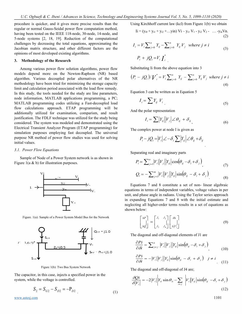
Sample of Node of a Power System network is as shown in Figure 1(a & b) for illustration purposes.

Figure. 1(a): Sample of a Power System Model Bus for the Network

Figure 1(b): Two Bus System Network

The capacitor, in this case, injects a specified power in the system, while the voltage is controlled.

2222 DDG SSS Ρ−=−= . (1)

Using Kirchhoff current law (kcl) from Figure 1(b) we obtain

Ii = (yi0 + yi1 + yi2 +…yin) Vi – yi1 V1 - yi2 V2 - … -yinVn. (2)

∑ ∑= =≠−=

n

j jijn

jijii ijwhereVYYVI0 0 (3)

I iiii VjQP *=+ .

Substituting Ii from the above equation into 3

( ) ∑ ∑= =≠−=−

n

j

n

j jijijiiii ijwhereVYYVjQP V 0 0

*/

(4)

Equation 3 can be written as in Equation 5

∑= iiji VYI. (5)

And the polar representation

ijijjiji VYI δθ +∠= ∑ , (6)

The complex power at node I is given as

∑ +∠−∠=− ijijijiiii YVjQP δθδ

.

Separating real and imaginary parts

( )∑ =+−=

n

j jiijijjii YVVP1

cos δδθ, (7)

( )jiijijm

j jit YVVQ δδθ +−−= ∑ =sin

1 . (8)

Equations 7 and 8 constitute a set of non- linear algebraic equations in terms of independent variables, voltage values in per unit, and phase angle in radians. Using the Taylor series approach in expanding Equations 7 and 8 with the initial estimate and neglecting all higher-order terms results in a set of equations as shown below:

=

∆

∆

∆

∆

δ

V

J

J

J

J

P

Q

2

4

1

3

(9)

The diagonal and off-diagonal elements of J1 are

( )jiijijn

jj ji YVVi

Pi δδθδ

+−=∂∂ ∑ ≠

sin, (10)

( ) ijYVVi

Pijiijijji ≠+−−=

∂∂ δδθδ

sin. (11)

The diagonal and off-diagonal of J4 are;

( )jiijijiji

iiiiii

YVYVVQi δδθθ

δδ

+−−−= ∑≠

sinsin2

(12)

Vi y i1 Vi

V2 Vn

yi2 yin

Yi0

Ii

U.C. Ogbuefi & C. Ibeni / Advances in Science, Technology and Engineering Systems Journal Vol. 5, No. 5, 1099-1110 (2020)

www.astesj.com 1102

( )jiijiiii

YVVQi δδθ +−−=

∂∂ sin

. (13)

Table: 1: 33KV Feeders and Injection Substations at port Harcourt Town Zone 4

Port Harcourt Town 33KV Feeder (Amadi Junction-Nzimiro Road)

33/11KV Injection Substations

Fdr S/N

Feeder Name Installed Transformer Capacity (MVA)

Feeder Name Transformer Installed Capacity (MVA)

1 UST feeder 30 RSUST Agip NAOC

2x15 1x7.5 2x3

2 Secretariat Feeder

45

Secretariat Marine Base Juanuta

2x7.5 2x15 1x2.5

3 Borokiri Feeder

60

Borokiri Eastern Bypass

1x15 1x15

4 Silver Bird Feeder

Silver Bird Kidney Island

1x15 1x1.5

5 UTC Feeder UTC Water Works

1x15 1x15

6 Rumuolumeni Feeder

UOE School of Nursing Naval Base Master Energy

1x7.5 1x15 2x2.5 1x1.5

7

Nzimiro Feeder, etc.

30 Nzimiro-Old Diobu, Owerri Road, etc

3x15

The terms ∆Pi(k) and ∆Qi(k) in Equations 9 are the differences between the computed and scheduled quantities, called power mismatch or residual, expressed as in Equations 14 and 15.

)()()( ki

schi

ki PPP −=∆ (14)

)()()( ki

schi

ki QQQ −=∆ (15)

The new estimates for node voltage are

)()()1( ki

ki

ki P∆−=− δδ . (16)

( ) ( ) ( )kkk ViViVi ∆+=+1

. (17)

3.2. Formulation of Power Flow Equations

A complex unified system with several nodes interconnected through transmission lines can be described as a power system. The load flow issue includes the calculation of voltage values and phase angle at every node, real and reactive power flow in all subsystems in the network under predictable or consistent state condition. Formulation and calculation of node admittance matrix is the starting point in the solution of power flow which is formed from transmission line parameters. In this manner, a contextual analysis is taking from Port Harcourt Town (zone 4) on the 33KV Distribution System of active feeders with 165MVA as a complete installed limit of the Transformers. The breakdown of the distribution transformers added to the incoming substation is as shown in Table 1 while Figure 2 depicts the 33KV Distribution System of the substations used as the case study.

3.3. Line Parameters for Port Harcourt Town, 33KV Distribution Network

Consider the line Parameters of the 33KV Distribution System, the conductors are evenly sorted and are overhead lines. The spacing between FACT as in the case of the Nigerian 33KV distribution system is 88cm. (that is, D = 0.88m) and. Figure 3 is the phi representation of per phase Line.

For the UST Feeder (33KV) on Node 2 at 15.15km to Incoming Substation; with Conductor Cross-Sectional Area, A = 182mm2ACSR/GZ. (Aluminum conductor steel fortified with electrifies).

Radius of conductor, R = �𝐴𝐴𝜋𝜋 m. (18)

R = �182𝑥𝑥10−6

𝜋𝜋= 0.00761 m.

GMD = �𝐷𝐷𝑅𝑅𝑅𝑅 𝑥𝑥 𝐷𝐷𝑅𝑅𝑌𝑌 𝑥𝑥 𝐷𝐷𝑅𝑅𝑌𝑌 = 1.26𝐷𝐷. (19)

DGMD = 1.26D. (20)

U.C. Ogbuefi & C. Ibeni / Advances in Science, Technology and Engineering Systems Journal Vol. 5, No. 5, 1099-1110 (2020)

www.astesj.com 1103

DGMD = 1.26 x 0.88 = 1.1088m or 1.109m.

Resistivity of Aluminum, 𝜌𝜌 = 2.826 𝑥𝑥 10−8Ω.𝑚𝑚 𝑎𝑎𝑎𝑎 200𝐶𝐶

Figure 3: П Representation of a Line (Per Phase)

𝑅𝑅0 = 1000 𝜌𝜌𝐴𝐴(𝑚𝑚2)

Ω𝐾𝐾𝑚𝑚.� (21)

R(UST) = 0.1552Ω 𝑘𝑘𝑚𝑚� x 15.15km = 2.352 Ω.

Per-Kilometer Reactance, (X0)

𝑋𝑋0 = 0.1445 𝑙𝑙𝑙𝑙𝑙𝑙10 �𝐷𝐷𝐷𝐷𝑚𝑚𝐷𝐷𝑅𝑅

� + 0.0157 Ω𝐾𝐾𝑚𝑚� . (22)

X(UST) = 4.970 Ω.

𝑍𝑍(𝑈𝑈𝑈𝑈𝑈𝑈) = 2.352 + 𝑗𝑗4.970 𝛺𝛺.

Per – Kilometer Capacitive Susceptance, (bo),

𝒃𝒃𝒃𝒃 = 𝟕𝟕.𝟓𝟓𝟓𝟓

𝒍𝒍𝒃𝒃𝒍𝒍𝟏𝟏𝟏𝟏�𝑫𝑫𝑫𝑫𝑫𝑫𝑫𝑫𝑹𝑹 �

𝒙𝒙 𝟏𝟏𝟏𝟏−𝟔𝟔 𝟏𝟏 𝜴𝜴.𝒌𝒌𝑫𝑫� . (23)

b(UST) = 3.504 x 10-6 x 15.15km = 53.1 x 10-6 1Ω� or siemens

Shunt admittance (susceptance) value for Node 1-2 for UST Feeder Network.

Given b(UST) = 53.1 x 10-6 1Ω� ,

Qc (UST) = 0.5 x 332 x 53.1 x 10-6 = 0.0289 MVAr.

Per-Unit Values of the Line Parameters for Port Harcourt Town, 33KV Distribution Network

Assume: 100MVA as Base MVA, (S Base)

33KV as Base Voltage

Base impedance, 𝒁𝒁𝒃𝒃 = (𝒌𝒌𝒌𝒌𝒃𝒃𝒃𝒃𝒃𝒃𝒃𝒃𝟐𝟐 )

𝑴𝑴𝒌𝒌𝑴𝑴𝒃𝒃𝒃𝒃𝒃𝒃𝒃𝒃 (24)

Base impedance, 𝑍𝑍𝑏𝑏 = 332

100 = 10.89Ω.

Per Unit impedance of the UST feeder,

𝑍𝑍(𝑈𝑈𝑈𝑈𝑈𝑈)𝑝𝑝𝑝𝑝 = 0.216 + 𝑗𝑗0.456 𝑝𝑝𝑝𝑝.

Per unit capacitive susceptance value for UST feeder, Bpu (UST)

Bpu = (𝑩𝑩𝒃𝒃𝒉𝒉𝒖𝒖𝒖𝒖𝒖𝒖∗𝑴𝑴𝒌𝒌𝑴𝑴𝑴𝑴)𝑺𝑺𝑩𝑩𝒃𝒃𝒃𝒃𝒃𝒃

pu. (25)

Bpu(UST) = (𝑌𝑌𝐵𝐵ℎ𝑝𝑝𝑢𝑢𝑢𝑢𝑢𝑢𝑢𝑢𝐴𝐴𝑢𝑢)𝑈𝑈𝑌𝑌𝑆𝑆𝐵𝐵𝑆𝑆

= 𝑗𝑗0.000289 pu.

We compute the complex power demanded at the load side bearing in mind the percentage loading. Note that, the loading capacity is due to available power

Per Unit Load Parameter at Each Feeder for Port Harcourt Town, 33KV Distribution Network

UST Feeder (Node 1-2) for Port Harcourt Town, 33KV Distribution Network

SD = 30MVA, Percentage loading =60%, Pf= cos𝜑𝜑= 0.8, Rf = sin𝜑𝜑 = 0.6.

SD(1-2) = 30x0.6=18MVA, PD(UST)=18x0.8 =14.4MW, QD(UST)=18x0.6 =10.8MVAr

On 100 MVA base, the per unit values of the complex power demand, we have

𝑃𝑃𝐷𝐷(𝑈𝑈𝑈𝑈𝑈𝑈) = 14.4𝑢𝑢𝑀𝑀100𝑢𝑢𝑢𝑢𝐴𝐴

= 0.144 𝑝𝑝𝑝𝑝 , 𝑄𝑄𝐷𝐷(𝑈𝑈𝑈𝑈𝑈𝑈) = 10.8𝑢𝑢𝑢𝑢𝐴𝐴𝑢𝑢100𝑢𝑢𝑢𝑢𝐴𝐴

=𝑗𝑗0.108 𝑝𝑝𝑝𝑝

𝑆𝑆𝐷𝐷(𝑝𝑝𝑝𝑝) = ( 𝑃𝑃𝐷𝐷(𝑈𝑈𝑈𝑈𝑈𝑈) + 𝑗𝑗𝑄𝑄𝐷𝐷(𝑈𝑈𝑈𝑈𝑈𝑈)) = (𝟏𝟏.𝟏𝟏𝟏𝟏𝟏𝟏 + 𝒋𝒋𝟏𝟏.𝟏𝟏𝟏𝟏𝟓𝟓)𝑝𝑝

Nzimiro-Trans-Amadi Feeder (Node 1-9) for Port Harcourt Town, 33KV Distribution Network

SD = 15MVA, Percentage loading = 80%, Pf = cos𝜑𝜑 = 0.8, Rf = sin𝜑𝜑 = 0.6

SD (1-9) = 15x0.8 = 12MVA, PD (NZ-A.) = 12x0.8 = 9.6MW, QD (NZ-A.) = 12x0.6 = 7.2MVAr

On 100 MVA base, the per unit values of the complex power demand, we have

𝑃𝑃𝐷𝐷(𝑁𝑁𝑁𝑁−𝐴𝐴.) = 9.6𝑢𝑢𝑀𝑀100𝑢𝑢𝑢𝑢𝐴𝐴

= 0.096 𝑝𝑝𝑝𝑝 , 𝑄𝑄𝐷𝐷(𝑁𝑁𝑁𝑁−𝐴𝐴.) = 7.2𝑢𝑢𝑢𝑢𝐴𝐴𝑢𝑢100𝑢𝑢𝑢𝑢𝐴𝐴

=𝑗𝑗0.072 𝑝𝑝𝑝𝑝.

𝑆𝑆𝐷𝐷(𝑝𝑝𝑝𝑝) = ( 𝑃𝑃𝐷𝐷(𝑁𝑁𝑁𝑁−𝐴𝐴) + 𝑗𝑗𝑄𝑄𝐷𝐷(𝑁𝑁𝑁𝑁−𝐴𝐴)) = (𝟏𝟏.𝟏𝟏𝟎𝟎𝟔𝟔 + 𝒋𝒋𝟏𝟏.𝟏𝟏𝟕𝟕𝟐𝟐)𝑝𝑝𝑝𝑝.

Nzimiro-Old-Diobu Feeder (Node 1-10) for Port Harcourt Town, 33KV Distribution Network.

SD = 15MVA, Percentage loading = 80%, Pf = cos𝜑𝜑 = 0.8, Rf = sin𝜑𝜑 = 0.6.

SD (1-10) = 15x0.8 = 12MVA, PD (NZ-OD.) = 12x0.8 = 9.6MW, QD (NZ-OD.) = 12x0.6 = 7.2MVAr

On 100 MVA base, the per unit values of the complex power demand, we have

𝑃𝑃𝐷𝐷(𝑁𝑁𝑁𝑁−𝑂𝑂𝐷𝐷.) = 9.6𝑢𝑢𝑀𝑀100𝑢𝑢𝑢𝑢𝐴𝐴

= 0.096 𝑝𝑝𝑝𝑝 , 𝑄𝑄𝐷𝐷(𝑁𝑁𝑁𝑁−𝑂𝑂𝐷𝐷.) = 7.2𝑢𝑢𝑢𝑢𝑆𝑆𝑢𝑢100𝑢𝑢𝑢𝑢𝐴𝐴

=𝑗𝑗0.072 𝑝𝑝𝑝𝑝.

𝑆𝑆𝐷𝐷(𝑝𝑝𝑝𝑝) = ( 𝑃𝑃𝐷𝐷(𝑁𝑁𝑁𝑁−𝑂𝑂𝐷𝐷) + 𝑗𝑗𝑄𝑄𝐷𝐷(𝑁𝑁𝑁𝑁−𝑂𝑂𝐷𝐷)) = (𝟏𝟏.𝟏𝟏𝟎𝟎𝟔𝟔 + 𝒋𝒋𝟏𝟏.𝟏𝟏𝟕𝟕𝟐𝟐)𝑝𝑝𝑝𝑝.

The complex power received from the grid network to the 33KV node is 165MVA at a power factor of 0.8, we have Srec =

jB/2 jB/2

Z= r +jx

U.C. Ogbuefi & C. Ibeni / Advances in Science, Technology and Engineering Systems Journal Vol. 5, No. 5, 1099-1110 (2020)

www.astesj.com 1104

(130+j100.8) MVA. Where 130MW is the real power and 100.8MVar is the reactive power demanded on the 33kV node.

The summary of the 33kV Distribution node network data under consideration are shown in Tables 2 and 3. It is much better

to compute all other parameters using the per unit values. To realize its real values we multiply the per unit values by the base values assumed at the beginning.

3.4. Mathematical Model of Fast Decoupled Power Flow Method

In a power network, the net infused active and receptive power at an ith node are mathematically represented by:

( )∑=

+=nb

jijijijijjii BGVVP

1sincos|||| θθ

. (26)

( )∑=

−=nb

jijijijijjii BGVVQ

1cossin|||| θθ

. (27)

where Vi and Vj, represent voltage levels at the ith and jth nodes separately; Gij+ jBij is the ijth component of the Y-node; and "n" the entire number of nodes. The linearized power flow Eqns. (26) and (27) are stated or given in reduced forms:

=

∆

∆

∆

∆

θ

V

J

J

J

J

P

Q

2

4

1

3 (28)

We compute the complex power demanded at the load side bearing in mind the percentage loading. Note that, the loading capacity depends on the available power.

Table 2: Line Data for Port Harcourt Town, 33KV Distribution Network

S/No Feeders Impedance code

Impedance, Zseries (pu)

Admittance, Y (pu)

Susceptance B/2 (pu)

1. (Node 1-2) UST

Y1,2 0.2159 + j0.4567 0.8460-j1.7897 j0.0002890

2. (Node 1-3) Secretariat

Y1,3

0.1452 + j0.3072 1.2576-j2.6607 j0.0001940

3. (Node 1-4) Silver bird

Y1,4 0.0436 + j0.0922 4.1916-j8.8638 j0.0000584

4. (Node 1-5) Borokiri

Y1,5 0.1573 + j0.3328 1.1608-j2.4561 j0.0002110

5. (Node 1-6) UTC

Y1,6 0.0427 + j0.0904 4.2719-j9.0441 j0.0000572

6. (Node 1-7) Rumuolemeni

Y1,7 0.2565 + j0.5426 0.7120-j1.5064 j0.0003430

7. (Node 1-8) Owerri Road

Y1,8

0.0003 + j0.0006 666.67-j1333.3 j0.00000038

8. (Node 1-9) Nzimiro Trans- Amadi

Y1,9

0.0003 + j0.0006

666.67-j1333.3

j0.00000038

9. (Node 1-10) Old Diobu

Y1,10 0.0003 + j0.0006 666.67-j1333.3 j0.00000038

Table 3: Node Data for Port Harcourt Town (Zone 4), 33KV Distribution Network (Initials Input)

Node Type Vsp (pu) PD (pu) QD (pu) 1 slack 1.00 0 0 2 PQ 1.00 0.144 0.108 3 PQ 1.00 0.228 0.171 4 PQ 1.00 0.079 0.059 5 PQ 1.00 0.144 0.108 6 PQ 1.00 0.234 0.176 7 PQ 1.00 0.187 0.142 8 PQ 1.00 0.096 0.072 9 PQ 1.00 0.096 0.072 10 PQ 1.00 0.096 0.072

U.C. Ogbuefi & C. Ibeni / Advances in Science, Technology and Engineering Systems Journal Vol. 5, No. 5, 1099-1110 (2020)

www.astesj.com 1105

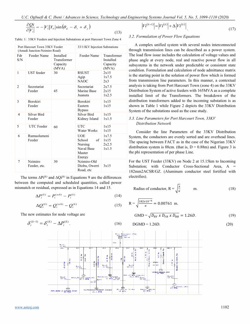
Table 4: Results for the Solutions after Injection of Reactive Power into the Under-Voltage Feeders (ETAP)

Results before Injection of Reactive Power

Results after Injection of Reactive Power

Fe

eder

s

Initial Load (Power) Received

Bus Volts (KV)

% Drop in Volt

Reactive Power Injected

New Bus Volts (KV)

New Net power Received

% Drop in Volt

MW

MVar KV % MVar KV MW

MVar

%

2 12.8 9.6 29.83 9.61 21.7 32.799

13.6 10.2 0.6

3 20.1 15.1 29.37 11.0 33.8 32.333

23.4 17.6 2.0

5 14.4 10.8 30.60 8.3 19.1 32.261

15.5 11.6 2.2

7 13.9 10.4 28.46 13.9 23.9 32.274

16.2 12.2 2.2

The sub-networks J1 and J4 in Eqn. 28, have a similar order because of the absence of the Q-V equations at PV nodes. A few presumptions are made as in previous studies in the formation of the FDPF model from Eqn. (28) the sub-matrices J2 and J3 are disregarded. Subsequent to joining the assumptions, the subsequent FDPF conditions become:

[ ][ ]θ∆=

∆ '' B

VP

. (29)

[ ][ ]VBVQ

∆=

∆ '''

. (30)

where

iShuntstcalculatedfScheduledi

shuntscalculatedtscheduledi

QQQQ

PPPP

,,,

1,1,,

'

'

−−=∆

−−=∆

(31)

The suffix “i” represents the ith node, Q-shunts,i; and P-shunts,i are the reactive and real powers, because of lumped shunts at the ith node. It ought to be noticed that the order for the

Jacobians [ ]'B are (nb-1) by (nb – 1) in Eqns. (29) while that of

[ ]''B in Eqn. (30) is (nb –mb -1) by (nb – mb – 1) where mb is the total number of voltage-controlled nodes. At the point when

both [ ]'B and [ ]''B are of the similar order of (nb -1), the matrices are real, sparse, and just contain system parameters. These matrices are only factorized once, stored, and are held and fixed all through the iteration. The result of Eqns. (29) and (30) are given by Eqn. (32) and (33):

[ ] [ ]

∆=∆ −

VPB '' 1θ

. (32)

[ ] [ ]

∆=∆ −

VQBV '''' 1

. (33)

Thus, by utilizing an abridged fast decoupled load flow technique, the voltage values and change in phase angle can be determined.

3.5. Fast Decoupled Power Flow for Radial Distribution System

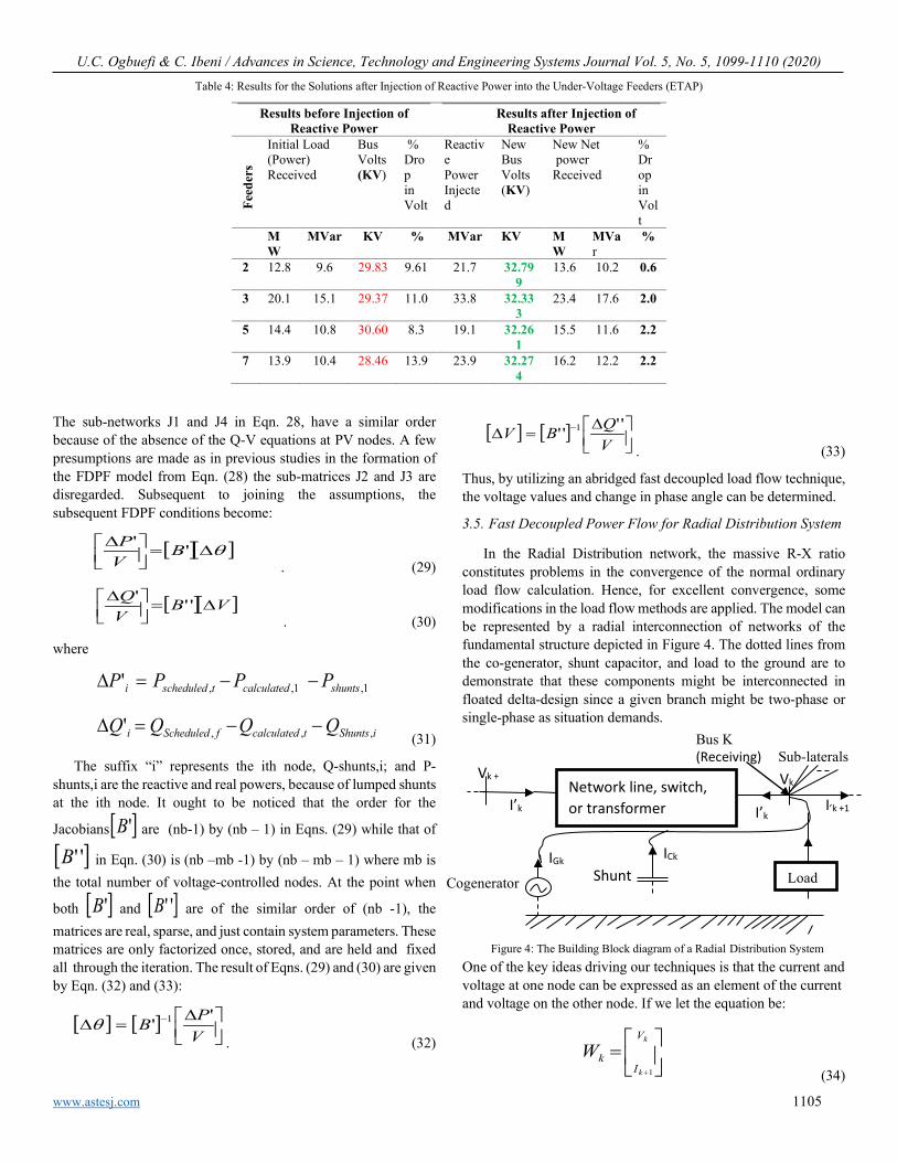
In the Radial Distribution network, the massive R-X ratio constitutes problems in the convergence of the normal ordinary load flow calculation. Hence, for excellent convergence, some modifications in the load flow methods are applied. The model can be represented by a radial interconnection of networks of the fundamental structure depicted in Figure 4. The dotted lines from the co-generator, shunt capacitor, and load to the ground are to demonstrate that these components might be interconnected in floated delta-design since a given branch might be two-phase or single-phase as situation demands.

One of the key ideas driving our techniques is that the current and voltage at one node can be expressed as an element of the current and voltage on the other node. If we let the equation be:

=

+

k

k

V

IkW

1 (34)

Figure 4: The Building Block diagram of a Radial Distribution System

Network line, switch, or transformer

Load

Bus K (Receiving) Sub-laterals

I’k I’k +1

Shunt Cogenerator

IGk ICk

Vk Vk +

I’k

U.C. Ogbuefi & C. Ibeni / Advances in Science, Technology and Engineering Systems Journal Vol. 5, No. 5, 1099-1110 (2020)

www.astesj.com 1106

The branch update function [I] is given beneath as:

)(1 kk WgkW =− (35)

Where Wk is a vector containing the real and imaginary parts of the voltages and current flows at node k. The factor gk is controlled by the sub-laterals joined at node k like as the models for distribution lines, switches, loads, transformers, co-generators, and shunt capacitors. From Vk we can calculate the flows as a result of the loads, co-generators shunt and, capacitors, given Ik + 1 and the currents Ij taken into sub-laterals branching out from node k, applying KCL at node k to the calculate current [I] given by Eq. 36:

∑∈

−++=AKJ

kLKCKGKk IjIIIII 1__' (36)

Where Ak is the set of nodes adjacent to node k on sub-laterals.

From Eqn. (36), we calculate the voltage and current at the main side given the voltage and current at the auxiliary or secondary “I” as in Eq. 37:

=

−1

;'

k

k

ssk

spk

ppk

sp

k

K

K

V

VY

I

I

Y

Y

Y

(37)

Therefore by solving equation (37), we get;

( ) ( )ksskk

spkk VIV YY −=

−

− '

1

1 . (38)

( ) ( )ksskk

ppkk VII YY += −

−

1'

1

. (39)

So that by applying this formulation or definition we get the converged values easily and faster than the other normal techniques.

a. Formulation for Fast Decoupled Power Flow Method

The stepwise calculation procedure to solve the power flow issue by applying the Fast Decoupled Power Flow Method is as given in [3] and as summarized thus: Creation of the node admittance Y as indicated by the lines given by the IEEE standard node test system, identification of all kinds of nodes according to the IEEE standard and setting all node initial value of up.01∠ , Creation of the matrices B1 and B11 Where B1 and B11 are the imaginary part of the node admittance matrix of Ynode, Calculating the value ∆P and ∆Q mismatches, Check the convergence status, Calculation of real and reactive power at every node, and checking if MVAr of generator nodes are within the cutoff points, Update of the voltage magnitude V and the voltage angle δ at every node. The current can then be determined from the calculated Y node using Eqn. (36)

=

−1

'

k

k

psk

ssk

ppk

spk

k

k

V

V

I

I

Y

Y

Y

Y (40)

If convergence is attained Display the load flow result, calculation, and show the line flows, current, and losses.

Percentage Voltage Drop ; %100×−

=S

RSd V

VVV (41)

b. Capacitor Bank

Line compensators are introduced in the network because of line losses and other line limitations to reduce losses. In the system under study, shunt capacitors are applied over an inductive load to give part of the reactive VARs required by the load to keep the voltage within the anticipated range. They can also be applied through capacitive loads and in light load situations to consume some amount of the main (leading) VARs for accomplishing voltage regulation. Capacitors are connected either directly to a node or through the tertiary winding of the primary transformer and are installed along the line as to limit mishaps in form of losses, voltage drop, also improves loading power factor. The shunt capacitor banks introduce reactive power into the system and compensate for line losses. To avoid much harmonic in line FACTS devices suffice.

Implementation of the Fast-Decoupled Load Flow in MATLAB. The program is implemented in the MATLAB programming language and is run in MATLAB Software development environment. The software modules files (M-files) results are as presented in appendices A1 to A3:

3 Results and Analysis

The results obtained are shown in Figs 5, 6, A1 to A3, and Tables 4 to 9 using the Fast decoupled-N-R procedures inserted in ETAP programming. The outcomes of the studied power flow and its parameters determined utilizing MATLAB program are represented in Figs. 5, 6, and Tables 4 and 5. The power flow study of the 33KV Distribution system making use of Port Harcourt Town, Zone 4, are presented in appendix A1 to A3 for different results sections from the utilization of the methods and simulation of the system as follows: Injection of Reactive Power into the Feeder (via Capacitor Bank) using ETAP Feeder 2 (Node 1-2): The initial net load (Power) received was 9.59 MVAr and 12.76 MW with a voltage drop of 0. 961. But after injection of 21.67 MVAr of reactive power through a capacitor bank, (Cap 1- rated 22MVAr), the voltage drop reduces to 0.0059 while the new net load (power) became 10.18 MVAr and 13.57MW, new node voltage becomes 0.994 with an angle of -5.48 degree as in Table 4. Feeder 3 (Node 1-3): The initial net load (Power) received was 15.09 MVAr and 20.14 MW with a voltage drop of 0.11. But, after the injection of 33.79 MVAr of reactive power, - 0.49MW through

U.C. Ogbuefi & C. Ibeni / Advances in Science, Technology and Engineering Systems Journal Vol. 5, No. 5, 1099-1110 (2020)

www.astesj.com 1107

a capacitor bank, (Cap 2- rated 35MVAr), and the voltage drop reduces to 0.02 while the new net load (power) became 17.58 MVAr and 23.46MW. The new node voltage becomes 0.9798 with an angle of -6.08 degree. Table 4 shows the summary of reactive power injected into the feeders to improve the voltage profile and the net power received, using ETAP.

Injection of Reactive Power into the Feeder (via Capacitor Bank) using MATLAB

Figure 5: Feeder Power Losses before Injecting Reactive Power (ETAP)

In the new input node data, we have injected reactive power via the capacitor bank. The results are as in Table 5. The values of the reactive power injected were as follows: Node-2 @ 20 MVar, Node-3 @ 30MVar, Node-5 @ 20MVar and Node-7 @ 22MVar. (Check along QGi)

Table 5: New Input Bus Data Injecting Reactive Power (MATLAB) New Bus Data Input with Capacitor Bank

Bus Type Vsp Theta PGi QGi PLi QLi Qmin Qmax 1 SL 1.00 0.00 0.00 0.00 0.00 0.00 0.00 0.00 2 PQ 1.00 0.00 0.00 20.00 14.40 10.80 -5.00 5.00 3 PQ 1.00 0.00 0.00 30.00 22.80 17.10 -3.00 5.00 4 PQ 1.00 0.00 0.00 0.00 7.90 5.90 0.00 0.00 5 PQ 1.00 0.00 0.00 20.00 14.40 10.80 -5.00 10.00 6 PQ 1.00 0.00 0.00 0.00 23.40 17.60 0.00 0.00 7 PQ 1.00 0.00 0.00 22.00 18.70 14.20 -6.00 15.00 8 PQ 1.00 0.00 0.00 0.00 9.60 7.20 0.00 0.00 9 PQ 1.00 0.00 0.00 0.00 9.60 7.20 0.00 0.00 10 PQ 1.00 0.00 0.00 0.00 9.60 7.20 0.00 0.00

From the voltage profile, the network required more power injection and some tap setting. In Table 7, M means the bus voltage is marginal while C mean critical.

Table 6: Results for 10 Bus/9 Feeder System Load Flow Solutions before Injection of Reactive Power (ETAP)

Bus Type V KV

Angle P. Received PS(rec) QS(rec)

P. Dispatched Pdisp Qdisp MW MVar

Demand -Pnet -Qnet MW MVar

1 slack 33.00 0.0 130.001 100.846 - - - - 2 PQ 29.82 -1.5 0 0 13.905 10.940 12.819 9.614 3 PQ 29.65 -1.5 0 0 21.742 17.203 19.949 14.962 4 PQ 32.64 -0.2 0 0 7.886 5.938 7.818 5.863 5 PQ 30.68 -1.1 0 0 14.026 10.894 13.229 9.922 6 PQ 31.89 -0.5 0 0 24.789 18.928 24.122 18.092 7 PQ 27.81 -2.4 0 0 18.851 15.344 16.415 12.311 8 PQ 32.99 0.0 0 0 9.601 7.200 9.600 7.199 9 PQ 32.99 0.0 0 0 9.601 7.200 9.600 7.199 10 PQ 32.99 0.0 0 0 9.601 7.200 9.600 7.199

Table 7: Line Losses and Voltage Drop before Injection of Reactive Power (using ETAP)

Bus Power Losses PLine QLine (MW) (MVar)

Vd % Drop in Vmag.

conditions Remarks

1-2 1.086 1.325 9.7 9.7% >5% Under Voltage (C ) 1-3 1.791 2.241 11.0 11.0% > 5% Under Voltage (C) 1-4 0.682 0.747 1.08 1.08% < 5% Acceptable 1-5 7.974 9.721 8.3 8.3% > 5% Under Voltage (M) 1-6 6.860 8.485 3.35 3.35% < 5% Acceptable 1-7 2.436 3.034 13.9 13.9% > 5% Under Voltage (C ) 1-8 0.007 0.008 0.01 0.01%<< 5% Acceptable 1-9 0.007 0.008 0.01 0.01% << 5% Acceptable

1-10 0.007 0.008 0.01 0.01% << 5% Acceptable Total 6.8502 8.485

Table 8: Summary of the Bus Voltages before and after Injection of Reactive Power (with MATLAB)

Bus Voltage before Injecting Reactive Power

Bus Voltage after Injecting Reactive Power

B/ No

Bus Volt (KV)

Angle (degree)

% Vd

Bus Volt (KV)

Angle (degree)

% Vd

1 33.000 0.000 0.000 33.000 0.000 0.000 2 30.525 -0.043 7.490 33.244 -0.085 0.740

U.C. Ogbuefi & C. Ibeni / Advances in Science, Technology and Engineering Systems Journal Vol. 5, No. 5, 1099-1110 (2020)

www.astesj.com 1108

3 31.307 -0.045 5.130 33.085 -0.088 0.260 4 32.716 -0.004 0.860 32.703 -0.005 0.910 5 31.574 -0.030 4.320 33.201 -0.062 0.609 6 32.155 -0.012 2.560 32.119 -0.014 2.670 7 29.651 -0.069 10.15 32.567 -0.123 1.310 8 32.997 -0.000 0.000 32.997 -0.000 0.010 9 32.997 -0.000 0.000 32.997 -0.000 0.010 10 32.997 -0.000 0.000 32.997 -0.000 0.010

Figure 6: Bus Voltage before and after Injection of Reactive Power

Table 9: Summary of the Net-load/Power and line Losses before and after Injection of Reactive power into Z4 station

Bus Net Load (Power) Received before Injecting Reactive Power

Bus Net Load (Power) Received after Injecting Reactive Power

B/No PNet (MW)

QNet (MVa)

Line Loss (MW) (MVar)

PNet (MW)

QNet (MVar)

Line Loss (MW) (MVar)

2 14.400 10.774 0.7657 1.6197 14.400 9.229 0.62241 1.31659 3 22.800 17.083 1.3094 2.7704 22.800 12.920 0.99193 2.09863 4 7.900 5.894 0.0398 0.0842 7.900 5.894 0.04313 0.09120 5 14.400 10.780 0.5302 1.1217 14.400 9.221 0.45441 0.96139 6 23.400 17.594 0.3557 0.7530 23.400 17.595 0.38635 0.81795 7 18.700 14.172 1.7492 3.7003 18.700 7.833 1.08263 2.29020 8 9.602 7.201 0.0004 0.0008 9.604 7.196 0.00042 0.00086 9 9.602 7.201 0.0004 0.0008 9.604 7.196 0.00042 0.00086 10 9.602 7.201 0.0004 0.0008 9.604 7.196 0.00042 0.00086 Total 130.406 97.9 4.7512 10.0517 130.412 84.28 3.58212 7.57854

4. Discussion

Power flow is a significant and fundamental device for the study of any power system and also applied in the operation, arranging for future development/upgrade of power systems. It will help in deciding the best mode of operation of the existing networks.

The results of the voltage values in nodes, 2, 3, 5, and 7 were not within the acceptable range because its node voltage was critical while node 6 is marginal and is within the required range. The steady-state MW and MVAr delivered to the slack node is not equal to the sum of the load (Power) demanded at each node. The transmitted/injected power and the power expected/net power at the load point were not equal, due to power losses on each feeder. The total disposable power received was 129.741 MW and 83.818 MVAr with Fast Decoupled Newton-Raphson technique in

MATLAB Environment after incorporation of Capacitor bank to the nodes that were influenced by unsatisfactory voltage drop, while the entire net load got using ETAP programming was 92.782 MVAr and 125.765 MW. The Voltage drop at Node 6, 8, 9, and 10 are within the acceptable range. These nodes Voltage drops are less than or equal to the acceptable 0.05 of the nominal voltage drop. Figure 6 above, shows the Node Voltage profile before and after the injection of Reactive Power. The total power (line) losses on the feeders have been reduced from 10.05MVAr and 4.75MW to 7.57MVAr and 3.58MW. This gives 0.246 reductions of the entire real power loss after the addition of reactive power into the black nodes.

2728293031323334

1 2 3 4 5 6 7 8 9 10

33

30.52531.307

32.716

31.57432.155

29.651

32.997 32.997 32.99733 33.244 33.085 32.703 33.20132.119 32.567

32.99732.997

32.997

Vol

tage

(kV

)

Bus No

Bus Voltage Before and After Injection of Reactive Power

Bus Volt (KV) Bus Volt (KV)

U.C. Ogbuefi & C. Ibeni / Advances in Science, Technology and Engineering Systems Journal Vol. 5, No. 5, 1099-1110 (2020)

www.astesj.com 1109

5. Conclusion

The analysis of this work has revealed the areas of consideration and urgent attention. The use of Fast Decoupled Load Flow study with MATLAB and the use of ETAP programming helps the examination precisely and proactive with less need for memory space. The load dispatched from the grid system to the transmission substation was not satisfactory thus every receiving substation has a fraction of sharing the available power or load. The simulated results show that more power is required from the grid network to the receiving substations through the Port Harcourt Town (Z4) control transmission center. In this way, without a satisfactory power source from the grid system, alternative energy supply or distributed generation suffices or, calls for load shading as the only way out. The entire power losses adding up to 10.05MVAr and 4.75MW on the 33KV distribution system require the update of the system by distributing or adding more load from the grid to these essential distribution centers, or alternative power generation should be sourced to beef up else load shedding becomes the only option. However, the recommendation and installation of the line compensator as “ccapacitor bank” at the affected nodes improved the voltage profile. Giving a 0.246 decrease in real power loss when capacitor banks were introduced on problem nodes for better enhancement.

5.1. Recommendations

1. We recommend that the 33KV distribution system be made more reliable by increasing the number of protective elements, capacitors banks, and transformers as realized from the results obtained. Also, intermittent power flow analysis and maintenance should be carried out.

2. The reactive power required locally at the nodes can be utilized to limit or minimize the losses on the line related with the system.

3. The substations for the network in this study should be made to perform at least 20 to 25 percent below the supply power to the secondary distribution system.

Conflict of Interest

The authors declare no conflict of interest.

Acknowledgment

My warm appreciation & respect to all the staff of the Port Harcourt Electricity Distribution Company of Nigeria (PHEDC), Moscow Road, Port Harcourt; all staff of Transmission Company of Nigeria, Port Harcourt Zone, for making this research work a worthwhile success. My sincere appreciation also goes to all the members of N.S.E and staff of the Rivers State University, Port Harcourt. My inmost sincere thanks to the African Centre of Excellence for Sustainable Power & Energy Development (ACE-SPED) University of Nigeria, Nsukka, Enugu State, Nigeria.

References

[1] I.A. Adejumobi, G. A. Adepoju, and K.A. Hamzat, “ Iterative techniques for load Flow Study: A Comparative Study for Nigeria 330KV Grid System as a Case Study” International Journal of Engineering and Advanced Technology (IJEAT) ISSN: 2249-8958, 3(1), October 2013

[2] C.S Indulkar and K. Ramalingam “Load flow Analysis with voltage-sensitive loads” Joint International Conference on Power System Technology and IEEE Power India Conference 2008. DOI: 10.1109/ICPST.2008.4745151

[3] H. K. Okyere, H. Nouri, H. Maradi and Li Zhenbiao “ Statcom and load tap changing transformer (LTC) in Newton Raphson Power Flow: Bus voltage constraint and losses” 42nd International Universities Power Engineering Conference 2007

[4] M. Sailaja Kumari and M. Sydulu “ A fast and reliable quadratic approach for Q-adjustments in Fast M Applied to power systems, 2006

[5] J. Nanda, V. Bapi Raju, P.R. Bijwe, M. L. Kothari and M. Joma “New findings of convergence properties of fast decoupled load flow algorithms”, IEE Proceedings C- Generation, transmission and Distribution, 1991

[6] T. Ochi, D. Yamashita, K. Koyanagi, & R. Yokoyama, “The Development and Application of Fast Decoupled Load Flow Method for Distribution Systems with High R/X Ratios Lines”, In 2013 IEE PES Innovative Smart Grid Technologies Conference, Washington DC, USA. Retrieved from https://waseda.pure.elsevier.com. 25th, July 2016.

[7] F.S. Abu-Mouti, & M.E. El-Hawary, A New and Fast Power Flow Solution Algorithm for Radial Distribution Feeders including Distributed Generations”, Institute of Electrical & Electronics Engineering Transactions on Power Systems, 2668 – 2672, 2007.

[8] B. Stott and O. Alsace “ Fast Decoupled Loaf Flow” IEEE Transaction on Power Apparatus and Systems, PAS-93, 1974

[9] G. B Jasmon and L.H.C. C Lee, “ Stability of Load flow techniques for distribution system voltage stability analysis”, IEE Proceedings C- generation transmission and Distribution, 138(6), 479-484, Nov 1991

[10] A. Sharma, Deep Kiran and Bijaya K Panigrahi, “ Planning the coordination of overcurrent relays for distribution systems considering network reconfiguration and load restoration”, IET Generation, Transmission and Distribution, 2018

[11] P. S. Bhowmik, S. P. Bose, D. V. Rajan, and S. Deb, “Power flow analysis of power system using power Perturbation method” IEEE Power Engineering and Automation Conference, 2011

[12] H. M. Gibson Sianipar, Giri Angga Setia and M. Fatahillah Santosa, “Implementation of Axis Rotation fast Decoupled Load Flow on distribution systems” 3rd conference on power Engineering and Renewable Energy (ICPERE), 2016

[13] R. Mageshvaran, R.I. Jacob, V. Yuvaraj, P.Rizwankhan, T. Vijayakumar, & V. Sudheera, , “Implementation of Non-Traditional Optimization Techniques (PSO, CPSO, HDE) for the Optimal Load Flow Solution”, TENCON 2008 - 2008 IEEE Region 10 Conference, 19-21.doi:10.1109/tencon.2008.4766839, 2008.

[14] S. Vasanthara, “Electric power systems” Electric renewable Energy Systems, 2016

[15] W. Xi-Fan, Song, Yonghua and Irving Malcolm “Modern Power System Analysis”, (3rd ed.), New York: Mc-Graw-Hill, 2008.

[16] H. A. Raza et al., “Analysis the effect of 500kv High-Voltage Power Transmission Line on the Output Efficiency of Solar-Panels,” in 2019 International Conference on Electrical, Communication, and Computer Engineering, 1–6, 2019. doi: 10.1109/ICECCE47252.2019.8940803

[17] H. D. Chiang, “A decoupled load flow method for distribution power network algorithms analysis and convergence study”, Electric Power Energy System, 3(3), 9-13,1991. https://doi.org/10.1016/0142-0615(91)90001-C

[18] M.S. Srinivas, “Distribution load flows: A Brief Review”, IEEE Power Engineering Society Winter meeting 2000, 2, 942-945,2000

[19] S. M. Lutful Kabir, A Hasib Chowdhury, Mosaddequr Rahman and J. Alam “Inclusion of slack bus in Newton-Raphson load flow study” 8th International Conference on Electrical and Computer Engineering 2014

APPENDIX A: Some Simulated Results

U.C. Ogbuefi & C. Ibeni / Advances in Science, Technology and Engineering Systems Journal Vol. 5, No. 5, 1099-1110 (2020)

www.astesj.com 1110

Figure A1: The Simulated 33KV Distribution Network (with Power Losses indicated) before addition of Capacitors

Bank

Figure A3 4.10: Result of the Simulated 33KV Distribution Network (with % Voltage Drop indicated) after addition of Capacitors Bank

Figure A2: Simulated Result for 33KV Distribution Network (with Power Losses indicated) after the addition of Capacitors Bank