Fuel optimal manoeuvres for multiple spacecraft formation reconfiguration using multi-agent...

INTERNATIONAL JOURNAL OF ROBUST AND NONLINEAR CONTROLInt. J. Robust Nonlinear Control 2002; 12:243–283 (DOI: 10.1002/rnc.684)

Fuel optimal manoeuvres for multiple spacecraft formationreconfiguration using multi-agent optimization

Guang Yang1,y, Qingsong Yang2,z, Vikram Kapila1,*,}, Daniel Palmer3,} andRavi Vaidyanathan4,k

1Department of Mechanical, Aerospace, and Manufacturing Engineering, Polytechnic University,

Brooklyn, NY 11201, U.S.A.2Department of Electrical Engineering and Computer Science, Case Western Reserve University,

Cleveland, OH 44106, U.S.A.3Department of Mathematics and Computer Science, John Carroll University, Cleveland, OH 44118, U.S.A.

4Orbital Research, Inc., 673 G Alpha Drive, Cleveland, OH 44143, U.S.A.

SUMMARY

The Air Force Research Laboratory has identified multiple spacecraft formation flying as an enablingtechnology for several future space missions. A key benefit of formation flying is the ability to reconfigurethe spacecraft formation to achieve different mission objectives. In this paper, generation of fuel optimalmanoeuvres for spacecraft formation reconfiguration is modelled and analysed as a multi-agent optimalcontrol problem. Multi-agent optimal control is quite different from the traditional optimal control forsingle agent. Specifically, in addition to fuel optimization for a single agent, multi-agent optimal controlnecessitates consideration of task assignment among agents for terminal targets in the optimizationprocess. In this paper, we develop an efficient hybrid optimization algorithm to address such a problem.The proposed multi-agent optimal control methodology uses calculus of variation, task assignment, andparameter optimization at different stages of the optimization process. This optimization algorithmemploys a distributed computational architecture. In addition, the task assignment algorithm, whichguarantees the global optimal assignment of agents, is constructed using the celebrated principle ofoptimality from dynamic programming. A communication protocol is developed to facilitate decentralized

Copyright # 2002 John Wiley & Sons, Ltd.

*Correspondence to: Vikram Kapila, Department of Mechanical, Aerospace and Manufacturing Engineering,Polytechnic University, Brooklyn, NY 11201, USA

yE-mail: [email protected]: [email protected]}E-mail: [email protected]}E-mail: [email protected]: [email protected]

Contract/grant sponsor: National Aeronautics and Space Administration Goddard Space Flight Centre; contract/grantnumber: NAG5-11365Contract/grant sponsor: Air Force Research Laboratory VACA, Wright Patterson AFB, OH; contract/grant number.IPA GrantContract/grant sponsor: Air Force Research Laboratory. Kirtland AFB, NM; contract/grant number: STTR GrantF29601-99-C-0172Contract/grant sponsor: The Orbital Research Inc.Contract/grant sponsor: NASA/New York space Grant Consortium; contract/grant number: 39555-6519

decision making among agents. Simulation results are included to illustrate the efficacy of the proposedmulti-agent optimal control algorithm for fuel optimal spacecraft formation reconfiguration. Copyright#2002 John Wiley & Sons, Ltd.

KEY WORDS: spacecraft formation reconfiguration; hybrid optimization; calculus of variation; dynamicprogramming; genetic algorithm

1. INTRODUCTION

Control of multiple, homogeneous/heterogeneous agents is an enabling technology for manymilitary, aerospace, industrial, and commercial applications. For example, concepts ofintelligent vehicle highway system [1] and free-flying aircraft [2, 3] rely on interacting groundand air vehicles, respectively. In addition, the problem of multiple mobile robots performing asingle task jointly is dependent on coordination between the robots [4]. Reconnaissance andother military functions from space, air, ground, and sea may all greatly benefit fromcooperation between spacecraft, aircraft, tanks, carriers, submarines, weapons, etc., [5–8]. Evenas the paradigm of multi-agent missions holds enormous potential, significant issues concerningtheir coordinated control remain unresolved. For example, a number of interesting dynamicsand control-related research problems arise in the control of multiple space vehicles such asmission/path planning, on-board autonomy, orbital-debris avoidance, distributed controlarchitecture, communication and throughput constraints, etc.

A specific multiple aerospace vehicle application, which has recently received significantattention, is distributed spacecraft formation flying (DSFF). DSFF represents the concept ofdistributing the functionality and cost of a large, specialized spacecraft among multiple smaller,less-expensive, cooperative spacecraft. It has been identified as an enabling technology by theAir Force Research Laboratory and NASA for future space missions [9–15]. Specifically, as theAir Force positions itself to become an ‘Air and Space Force’, it is envisaged that the DSFFtechnology will facilitate critical elements of its vision, viz. virtual global awareness and rapidaccess to space [16]. For example, Air Force’s TechSat-21 program [9, 10] relies on successfuldevelopment and deployment of DSFF technologies. Similarly, NASA is seeking rapidadvancements in DSFF technologies to enable the Earth Orbiter-I and the New MillenniumInterferometer programs [6, 11–13], among others. In particular, the DSFF paradigm is beingenvisioned as a versatile, adaptable, and affordable space technology capable of accomplishingdiverse, multiple missions such as synthetic aperture radars, enhanced stellar opticalinterferometers, virtual co-observing, stereo-imaging, correlated real-time sensing, andsimultaneous multipoint probing [14, 17]. The DSFF architecture necessitates interactingspacecraft with system-wide common capabilities (communication, sensing, navigation, control,etc.), operating collectively to accomplish shared mission objectives [9, 10]. The implementationof the DSFF concept requires tight, autonomous, real-time control of the relative distance andattitude between the participating spacecraft.

From a decision theory and control design perspective, the DSFF problem can bedecomposed into two different but closely related phases (i) distributed spacecraft formationkeeping and maintenance (DSFKM) and (ii) distributed spacecraft formation reconfiguration(DSFR). The DSFKM control must be designed to enable the spacecraft to undergo periodicrelative motion such that a relative spatial pattern persists for several orbital periods withminimal propellant expenditure [18]. For DSFKM, linear and nonlinear formation dynamic

G. YANG ET AL.244

Copyright # 2002 John Wiley & Sons, Ltd. Int. J. Robust Nonlinear Control 2002; 12:243–283

models have been developed and a variety of low-level control designs have been proposed toguarantee the desired DSFKM performance [8, 15, 19–27]. Specifically, a linear formationdynamic model known as the Hill’s equations is given in References [19, 20]. Hill’s equationsconstitute the foundation for the application of various linear control techniques to theDSFKM problem [22, 23, 26, 27]. Recently, Sedwick et al. [15] identified the set of feasible initialconditions that annihilate the secular growth in time in the solution of Hill’s equations; thus,yielding periodic relative motion for DSFKM. Based on the work in Reference [15], spatialpatterns for formation design were proposed in Reference [24]. In Reference [8], a class ofcontrol laws was designed based on exact knowledge of the DSFF model that yields localasymptotic position tracking and global exponential attitude tracking. A persistent disturbancewas employed in Reference [8] to account for model imperfection, measurement inaccuracies,etc. In addition, an adaptive position controller was developed in Reference [28] thatcompensates for unknown, constant disturbances while producing globally asymptoticallydecaying position tracking errors. More recently, [21, 29] proposed nonlinear controllers for aleader-follower DSFKM system, which ensure global asymptotic position tracking errors.Furthermore, a formation initialization scheme was developed in Reference [29], which in theideal case yields a no-thrust, periodic relative motion between the leader–follower spacecraftpair, and serves as a desired, relative motion trajectory. Finally, in Reference [25], an analyticalmethod was developed to identify families of formations invariant to the J2 perturbation in thegeopotential, a dominant cause for formation dispersion.

In contrast to the DSFKM problem, the DSFR problem has received scant attention (seeReferences [8, 21, 27, 29, 30–32] for recent exceptions). However, as discussed above, DSFR is anessential component of the DSFF paradigm meriting utmost attention since it enables thespacecraft formation to adaptively assume a desired formation pattern as dictated by missionobjectives. A critical issue in the DSFR problem is to determine fuel optimal manoeuvres whenan initial spacecraft formation is directed to reconfigure to a new formation pattern. In thecurrent literature [8, 21, 27, 29, 30, 32], the DSFR problem is addressed by utilizing low-leveltrajectory tracking controllers, which reconfigure a spacecraft formation by considering theinitial formation to be an initial offset for the new formation pattern. The principal drawback ofthese control designs is their unpredictable and non-optimal fuel expenditure for differentformation reconfiguration processes. In an alternative DSFR approach, fuel optimalmanoeuvres for all the spacecraft can be generated on-board. Subsequently, low-levelcontrollers can be used to track the fuel optimal manoeuvres in order to yield fuel optimalformation reconfiguration. In this framework, the fuel cost for each spacecraft manoeuvre canbe calculated, on-demand, and the total fuel expenditure for formation reconfiguration isminimized. Recall that the linearized relative dynamics of spacecraft, given by Hill’s equations,is known to approximate the dynamic behaviour of spacecraft relative motion fairly well forshort-period manoeuvres and small spatial separation between spacecraft. It is anticipated thatthe typical spacecraft formation reconfiguration manoeuvres will be executed within few orbitalperiods with small spatial separation between spacecraft (few kilometers). Thus, in this paper,we utilize the linearized relative dynamics of spacecraft to construct an optimization algorithmthat generates the fuel optimal formation reconfiguration trajectories with low computationaleffort.

The traditional theory of calculus of variation and optimal control can generate fuel optimaltrajectories for a single spacecraft with various types of boundary conditions. However, for theDSFR problem we face the challenge of generating a set of fuel optimal manoeuvres for

MULTI AGENT OPTIMIZATION 245


multiple spacecraft simultaneously. Specifically, for the DSFR problem we must (i) determinean optimal manoeuvre time interval for each spacecraft to execute its fuel optimal manoeuvreand (ii) solve an assignment problem so that the position arrangement for the spacecraft in thenew formation pattern is optimal. Finally, as shown in Section 2.5 of this paper, frequently, agiven formation pattern may leave certain formation parameters unspecified, which must beselected to ensure fuel optimal spacecraft formation reconfiguration. Thus, the fuel optimalDSFR problem poses a multi-agent optimal control problem necessitating a hybridoptimization involving calculus of variation, task assignment, and parameter optimization. Inthis paper, we develop an optimization algorithm that solves such a problem efficiently. Inaddition, we propose a communication protocol to facilitate a distributed computationalarchitecture for the optimization algorithm.

The contents of this paper are as follows. In Section 2, we present a mathematical model forspacecraft formation reconfiguration. The formation reconfiguration process is analysedqualitatively in Section 3. In Section 4, we develop an optimization algorithm to solve the fueloptimal spacecraft formation reconfiguration problem. Simulation results are included inSection 5 to illustrate the efficacy of the proposed optimization algorithm for spacecraftformation reconfiguration. Finally, concluding remarks are given in Section 6.

2. PROBLEM MODELLING AND ANALYSIS

2.1. Coordinate system description

In the current literature, the DSFF dynamics is typically characterized via a leader-fixed non-inertial coordinate frame [15, 21–24, 26, 27, 29, 31–33]. A schematic drawing of such a coordinateframe is given in Figure 1, where we make the following considerations: (i) an inertial coordinateframe fX ;Y ;Zg is attached to the centre of the Earth; (ii) R‘ðtÞ 2 R3 denotes the position vectorfrom the origin of the inertial coordinate frame to the leader spacecraft; (iii) in the leader-fixednon-inertial coordinate frame fx‘; y‘; z‘g, the y‘-axis points along the direction of the vectorR‘ðtÞ, the z‘-axis points along the direction of the orbital angular momentum of the leaderspacecraft, and the x‘-axis is placed such that fx‘; y‘; z‘g forms a right-handed coordinate frame;and (iv) rðtÞ 2 R3 denotes the position vector from the origin of the coordinate frame fxl ; yl ; zlgto the follower spacecraft.

Unfortunately, in a general problem setting, the leader-fixed non-inertial coordinate framepresents severe constraints. First, any acceleration of the leader spacecraft influences the basicdynamics of the formation significantly. In particular, since the origin of the fx‘; y‘; z‘gcoordinate frame is attached to the leader spacecraft and the fx‘; y‘; z‘g coordinate framerotates with the leader spacecraft’s orbital motion, the follower spacecraft dynamics in such aframe is influenced by some non-inertial forces. If the leader spacecraft is in an exact Keplerian(circular or elliptical) orbital motion, the non-inertial forces entering the follower spacecraftdynamics can be expressed in a relatively simple form [19, 21, 22, 26, 27, 29, 32]. However, whenthe leader spacecraft undergoes a non-Keplerian motion, e.g. during an orbital manoeuvre, thenon-inertial forces in the follower spacecraft dynamics become quite complicated so that onecan hardly predict the follower spacecraft dynamics. Note that, in practice, the leaderspacecraft’s orbit may need to be changed from time to time as dictated by mission

G. YANG ET AL.246


requirements; thus, there is no reason to assume that the leader spacecraft will always be in afixed Keplerian orbit.

Second, in many formation reconfiguration processes, a trivial choice for the leader spacecraftmay not even exist. For example, consider two clusters of spacecraft coasting together in thebeginning, as shown in Figure 2(a). Each cluster of spacecraft is composed of four spacecraftwith one spacecraft located at the geometric centre and the other three spacecraft distributed ona thrust-free periodic relative orbit. The two spacecraft at the two geometric centres are in thesame circular Earth orbit AB and their separation distance is large enough so that the twoclusters do not overlap with one another; yet this distance is quite small compared to the radiusof the orbit AB. Now, let all the spacecraft in the two clusters manoeuvre so that the twoclusters combine into one. In the new formation, all the spacecraft are distributed on twoconcentric thrust-free periodic relative orbits (4 spacecraft on each) and the geometric centre ofthe new formation pattern (not occupied by any spacecraft) moves along the circular Earth orbitAB (as shown in Figure 2(b)). Clearly, in such a formation reconfiguration process there is notrivial choice for a leader spacecraft on which we can attach a non-inertial coordinate framethroughout the process.

Figure 1. Leader-fixed non-inertial coordinate frame in the DSFF system.

Figure 2. (a) Initial two cluster spacecraft formation; (b) reconfigured one cluster spacecraft formation.



In this paper, in order to overcome the aforementioned shortcomings of the leader-fixed non-inertial coordinate frame, we consider a non-inertial coordinate frame fixed on an imaginaryleader spacecraft. Specifically, we attach a non-inertial coordinate frame fxI; yI; zIg to animaginary point, the so called imaginary leader spacecraft, that is orbiting the Earth. LetRIðtÞ 2 R3 denote the position vector of the imaginary leader spacecraft in the Earth-centredinertial coordinate frame and let ’RRIðtÞ 2 R3 be the time derivative of RIðtÞ. Then, we constructthe fxI; yI; zIg coordinate frame such that the yI-axis points along the direction of the vectorRIðtÞ, the zI-axis points along the direction of the vector RIðtÞ � ’RRIðtÞ, and the xI-axis is placedsuch that fxI; yI; zIg forms a right-handed coordinate frame. In this paper, we let RIðtÞ follow anideal Keplerian circular Earth orbit that represents the approximate average motion of thespacecraft formation. In such a coordinate frame, the formation dynamics is characterizedanalogous to the leader-fixed coordinate frame case, where a real leader spacecraft exists in anideal Keplerian orbit. Furthermore, in the proposed fxI; yI; zIg coordinate frame, everyspacecraft in the formation can manoeuvre freely without influencing the basic formationdynamics.

Now in the aforementioned formation reconfiguration example, we can choose an imaginarypoint, which is also in the circular Earth orbit AB and close enough to the initial formation, asan imaginary leader spacecraft. This imaginary leader spacecraft can serve as the origin of thecoordinate frame fxI; yI; zIg throughout the formation reconfiguration process described above.

2.2. Thrust-free periodic trajectory for linearized spacecraft relative motion

In this paper, we limit ourselves to DSFF where an imaginary leader spacecraft can be chosen tofollow an exact circular Earth orbit and all spacecraft in the formation fly along some thrust-freeperiodic trajectories relative to the fxI; yI; zIg coordinate frame. See References[15, 24, 27, 29, 30, 32] for further details on the design of thrust-free periodic formationtrajectories. After the local linearization of the formation dynamics in the fxI; yI; zIg coordinateframe, the thrust-free periodic trajectories for spacecraft in the formation are the periodicsolutions of the homogeneous linear Hill’s equations written in the fxI; yI; zIg coordinate frame[15, 24, 27]. These trajectories form some closed periodic orbits in the fxI; yI; zIg coordinateframe [15, 24, 27]. Generally, in an n spacecraft formation, there are n0 closed periodic orbits,where n04n since more than one spacecraft may be distributed on one closed periodic orbit. Thedistribution of the spacecraft on a particular closed periodic orbit can be specified by the phasedifference of their periodic motion in this closed periodic orbit. This provides us a simple way tostandardize the form of the parametric equations, which are used to describe formation patternsand spacecraft trajectories in the fxI; yI; zIg coordinate frame. Note that for a followerspacecraft the thrust-free periodic solution of the linear Hill’s equation can be expressed as

xðtÞ ¼ �2vy0o

cos ðoðt� t0ÞÞ þ XC

yðtÞ ¼vy0o

sin ðoðt� t0ÞÞ

zðtÞ ¼ z0 cos ðoðt� t0ÞÞ þvz0o

sin ðoðt� t0ÞÞ ð1Þ

where o is the orbital angular velocity of the imaginary leader spacecraft, t0 is the time when thefollower spacecraft passes the xI–zI plane from the yþI side to the y�I side, vy0 and vz0 are the yI

G. YANG ET AL.248


and zI velocity components, respectively, of the follower spacecraft relative to the fxI; yI; zIgcoordinate frame at t0, and z0 is the zI position component of the follower spacecraft relative tothe fxI; yI; zIg coordinate frame at t0. It is not difficult to see that the xI velocity component ofthe follower spacecraft relative to the fxI; yI; zIg coordinate frame is zero at t0. Since the followerspacecraft is passing the xI–zI plane from the yþI side to the y�I side at t0, vy0 is negative. Notethat this trajectory forms a closed elliptical orbit in the fxI; yI; zIg coordinate frame, with thegeometric center located at ðXC; 0; 0Þ [24, 33]. We call such an orbit a primary formation orbit.Let y ¼4 � ot0 be the initial phase angle of the follower spacecraft in such a primary formationorbit, then its trajectory (1) can be expressed as

xðtÞ ¼ �2vy0o

cos ðotþ yÞ þ XC

yðtÞ ¼vy0o

sin ðotþ yÞ

zðtÞ ¼ z0 cos ðotþ yÞ þvz0o

sin ðotþ yÞ ð2Þ

This form of parametric equations will be used as the standard form when we describe thethrust-free periodic spacecraft trajectories in the fxI; yI; zIg coordinate frame and will bementioned as the primary expression in this paper. In the case where the relative motion offollower spacecraft is contained in the xI–zI plane, t0 is arbitrary and vy0 ¼ 0.

Note that if another spacecraft is distributed on the same primary formation orbit, theprimary expression for its thrust-free periodic trajectory will have the same yI and zI relativevelocity components vy0 and vz0 , respectively, and the same zI relative position component z0,when it passes the xI–zI plane from the yþI side to the y�I side. So, a primary formation orbit canbe specified by a set of parameters ðXC; vy0 ; vz0 ; z0Þ, which is called the primary orbital parameterset for the primary formation orbit.

2.3. Formation pattern

In this paper, an n spacecraft periodic spatial formation pattern is modelled as aset of n allowable positions that are distributed on n0 primary formation orbits. Wedescribe this set of allowable positions by primary expressions in the fxI; yI; zIg coordinateframe. Thus, this set of allowable positions represents the locations of the spacecraft in theformation as time-dependent functions. The number of allowable positions in the rth primaryformation orbit, r ¼ 1; . . . ; n0, is denoted as pr, where pr51 and

Pn0

r¼1 pr ¼ n. Furthermore, theallowable positions distributed on the rth primary formation orbit, r ¼ 1; . . . ; n0, are referencedas Pr

i , i ¼ 1; . . . ; pr.Let the primary orbital parameter set for the rth primary formation orbit be

ðXCr; vy0r ; vz0r ; z0r Þ. Then, the primary expression for the allowable position Pr

1 is expressed as

xPr1ðtÞ ¼ �2

vy0ro

cos ðotþ yPr1Þ þ XCr

yPr1ðtÞ ¼

vy0ro

sin ðotþ yPr1Þ

zPr1ðtÞ ¼ z0r cos ðotþ yPr

1Þ þ

vz0ro

sin ðotþ yPr1Þ ð3Þ



In general, for the allowable position Pri , i ¼ 1; . . . ; pr, on the rth primary formation orbit,

r ¼ 1; . . . ; n0, the primary expression is given by

xPriðtÞ ¼ �2

vy0ro

cos ðotþ yPr1þ bi1rÞ þ XCr

yPriðtÞ ¼

vy0ro

sin ðotþ yPr1þ bi1rÞ

zPriðtÞ ¼ z0rcos ðotþ yPr

1þ bi1r Þ þ

vz0ro

sin ðotþ yPr1þ bi1r Þ ð4Þ

where bi1r , i ¼ 1; . . . ; pr, is the phase difference between the periodic motions of the spacecraftlocated at the allowable position Pr

1 and Pri . Note that b11r ¼ 0 is immediate.

To illustrate the above concept, consider a 4 spacecraft, 1 primary orbit formation patternwhose projection on the ground is always a square, with each vertex being the projection of aspacecraft in the formation (see Figure 3). This formation requirement is satisfied by selectingthe primary orbital parameter set for the primary formation orbit as ðXC1

; u; 2u; 0Þ, where u50.Then the formation pattern is a set of allowable positions fXP1

1ðtÞ; . . . ;XP1

4ðtÞg, where

XP1iðtÞ ¼4 ðxP1

iðtÞ; yP1

iðtÞ; zP1

iðtÞÞ, i ¼ 1; . . . ; 4. In addition, xP1

iðtÞ, yP1

iðtÞ, and zP1

iðtÞ satisfy

xP1iðtÞ ¼ �2

u

ocos ðotþ yP1

1þ bi11 Þ þ XC1

yP1iðtÞ ¼

u

osin ðotþ yP1

1þ bi11 Þ

zP1iðtÞ ¼

2u

osin ðotþ yP1

1þ bi11Þ ð5Þ

where i ¼ 1; . . . ; 4, b111 ¼ 0, b211 ¼ p=2, b311 ¼ p, and b411 ¼ 3p=2.For notational convenience, in the balance of this paper, the n allowable positions in

an n spacecraft formation pattern are indexed using only a subscript j, wherej 2 f1; . . . ; p1; p1 þ 1; . . . ; p1 þ p2; . . . ; p1 þ � � � þ pðn0�1Þ þ 1; . . . ; ng. Thus, an allowable positionPri in a subscript-only notation is referenced as Pj, which refers to the jth allowable position in

the formation pattern, where j ¼ p1 þ � � � þ pðr�1Þ þ i.

2.4. Spacecraft permutation in a formation pattern

In many cases, spacecraft locations may be interchangeable among all the allowable positions ina formation pattern. For example, in an n spacecraft formation, the spacecraft can be arrangedonto the n allowable positions in Pn

n ¼ n! many different ways, where P is the permutationoperator defined as Pj

n ¼4 n!=ðn� jÞ! [34] and ‘!’ is the factorial operator [34]. Every sucharrangement is called a spacecraft permutation for the formation pattern. Specifically, we labelthe spacecraft with n consecutive integers from 1 to n and use subscript Si to refer to spacecraft i.Next, we define XSi ðtÞ ¼

4 ðxSi ðtÞ; ySi ðtÞ; zSi ðtÞÞ to denote the thrust-free periodic trajectory forspacecraft i, i ¼ 1; . . . ; n. Then a spacecraft permutation can be given by H ¼ ½h1; . . . ; hn�, wherehi, i ¼ 1; . . . ; n, takes integer values from 1 to n, and hi 6¼ hj for i 6¼ j. Specifically, forpermutationH ¼ ½h1; . . . ; hn�, we have XSh1

¼ XP1; . . . ;XShn

¼ XPn, i.e. spacecraft Sh1 is located at

the 1st allowable position in the formation pattern, etc. For example, if we label the spacecraftwith consecutive integers from 1 to 4 in the 4 spacecraft formation described before, we getXS1 ¼ XP1

, XS2 ¼ XP2, XS3 ¼ XP3

, and XS4 ¼ XP4, which yields a spacecraft permutation

G. YANG ET AL.250


H ¼ ½1; 2; 3; 4�. However, if we let XS4 ¼ XP1, XS2 ¼ XP2

, XS3 ¼ XP3, and XS1 ¼ XP4

, we obtain adifferent spacecraft permutation H ¼ ½4; 2; 3; 1� by interchanging the locations of spacecraft 1and 4 while the formation pattern remains the same.

2.5. Formation reconfiguration

We describe a general formation reconfiguration as follows. Each spacecraft in an n spacecraftformation originally fly along their thrust-free periodic trajectories, which are described by someprimary expressions in fxI; yI; zIg. Such a formation will reconfigure to an m spacecraftformation whose pattern is described by a set of m allowable spacecraft positions, which are alsoexpressed by primary expressions in fxI; yI; zIg. For the new formation, m indicates the numberof spacecraft that are needed to participate in the new formation pattern and it is restricted bym4n.

So far, we have assumed that the new formation pattern is uniquely specified. However, inmany cases, the mission requirements for formation reconfiguration will not provide enoughinformation to uniquely specify the new formation pattern, i.e. in the primary expressions forthe new formation pattern some parameters may be chosen arbitrarily among some allowablevalues permitted by the mission requirements. Thus, there can be a family of new formationpatterns that satisfy the mission requirements. For example, in the 4 spacecraft formation ofFigure 3, if a square projection on the ground with side length 2

ffiffiffi2

pu=o is the only requirement,

then yP11and XC1

can be chosen freely in the primary expressions. In general, we assume that themission requirements leave k independent parameters unspecified in the primary expressions forthe new formation pattern. Let these k independent parameters be denoted by l1; . . . ; lk. In

Figure 3. Spacecraft formation with square projection on the ground.



addition, let L1; . . . ;Lk denote the sets of values for l1; . . . ; lk, respectively, which are permittedby the mission requirements. In this paper, we consider Li, i ¼ 1; . . . ; k, to be bounded sets. Let*ll ¼4 ½l1; . . . ; lk�, where *ll 2 *LL ¼4 L1 � � � � � Lk. Note that, together with the given missionrequirements, *ll 2 *LL uniquely specifies a new formation pattern.

For a spacecraft, a trajectory that smoothly connects the spacecraft’s thrust-free periodictrajectory in the original formation and its thrust-free periodic trajectory in the new formation isreferred to as a spacecraft manoeuvre. Specifically, a manoeuvre for spacecraft i to reach the jthallowable position in the new formation pattern that satisfies the given mission requirementsand is also specified by *ll, starting at the time instant tai and ending at the time instant tbi ,tai5tbi , is defined by

mi; jðt; tai ; tbi ; *llÞ ¼4 ðxmi; j ðt; *llÞ; ymi; j ðt; *llÞ; zmi; j ðt; *llÞÞ; tai4t4tbi ð6Þ

where xmi; j ðt; *llÞ, ymi; j ðt; *llÞ, and zmi; j ðt; *llÞ are the xI; yI, and zI components, respectively, of thespacecraft manoeuvre, and are twice differentiable with respect to t since spacecraft’sacceleration is finite. The statement that the manoeuvre starts at tai and ends at tbi ismathematically interpreted to mean that the spacecraft position and velocity satisfy theboundary conditions

qmi; j ðt; *llÞ��t¼tai

¼ qSiðtÞ

��t¼tai

;d

dtðqmi; j ðt; *llÞÞ

��t¼tai

¼d

dtðq

SiðtÞÞ

��t¼tai

ð7Þ

qmi; j ðt; *llÞ��t¼tbi

¼ qPjðt; *llÞ

��t¼tbi

;d

dtðqmi; j ðt; *llÞÞ

��t¼tbi

¼d

dtðq

Pjðt; *llÞÞ

��t¼tbi

ð8Þ

where q 2 fx; y; zg.We emphasize that ‘starting at tai ’ does not mean that the manoeuvre ðxmi; j ðt; *llÞ; ymi; j ðt; *llÞ,

zmi; j ðt; *llÞÞ is necessarily different from the initial trajectory ðxSi ðtÞ; ySi ðtÞ; zSi ðtÞÞ right after tai .Similarly, ‘ending at tbi ’ does not mean that the manoeuvre ðxmi; j ðt; *llÞ; ymi; j ðt; *llÞ; zmi; j ðt; *llÞÞ cannot match the thrust-free trajectory ðxPj

ðt; *llÞ; yPjðt; *llÞ; zPj

ðt; *llÞÞ in the new formation patternbefore tbi . This enables us to extend the manoeuvre mi; jðt; tai ; tbi ; *llÞ to a manoeuvre that transfersspacecraft i to the jth allowable position in the new formation pattern, starting at t0ai and endingat t0bi , where t0ai4tai5tbi4t0bi . In particular, let

qmei; jðt; *llÞ ¼4

qSiðtÞ t0ai4t4tai

qmi; j ðt; *llÞ tai4t4tbi ; q 2 fx; y; zg

qPjðt; *llÞ tbi4t4t0bi

8>>>><>>>>:

ð9Þ

then we define an extended manoeuvre as

mei; jðt; tai ; tbi ; t

0ai; t0bi ;

*llÞ ¼4 ðxmei; jðt; *llÞ; yme

i; jðt; *llÞ; zme

i; jðt; *llÞÞ; t0ai4t4t0bi ; t

0ai4tai ; tbi4t0bi ð10Þ

which ‘starts at t0ai ’ and ‘ends at t0bi ’. Note that the manoeuvre ‘starts at t0ai ’ and ‘ends at t0bi ’follows from the fact that the boundary conditions (7) and (8) are automatically satisfied at t0aiand t0bi , respectively, by the way we construct ðxme

i; jðt; *llÞ; yme

i; jðt; *llÞ; zme

i; jðt; *llÞÞ in (9). We call

mei; jðt; tai ; tbi ; t

0ai; t0bi ;

*llÞ a primary extension of the manoeuvre mi; jðt; tai ; tbi ; *llÞ from the timeinterval ½tai ; tbi � to the time interval ½t0ai ; t

0bi�. Figure 4 illustrates the notion of extended

manoeuvre.

G. YANG ET AL.252


3. FUEL OPTIMAL SPACECRAFT FORMATION RECONFIGURATION:MATHEMATICAL PRELIMINARIES

In this section, we begin by considering the fuel cost for spacecraft manoeuvres and theirprimary extensions to lay the foundation for developing the fuel optimal formationreconfiguration manoeuvres. First, let the fuel cost for spacecraft i to execute manoeuvremi; jðt; tai ; tbi ; *llÞ be denoted as Iðmi; jðt; tai ; tbi ; *llÞÞ. The specific form of this fuel cost is related tothe formation dynamics model and the spacecraft thrust model as discussed in Section 4.2. Next,note that for the extended manoeuvre ðxme

i; jðt; *llÞ; yme

i; jðt; *llÞ; zme

i; jðt; *llÞÞ in (9), the trajectory

extensions lie on the thrust-free periodic trajectories of spacecraft i in the original formation andin the new formation. Thus, we have the following useful property for the fuel cost of thespacecraft manoeuvre mi; jðt; tai ; tbi ; *llÞ and its primary extension me

i; jðt; tai ; tbi ; t0ai; t0bi ;

*llÞ, evenwithout the explicit knowledge of its specific form,

Iðmei; jðt; tai ; tbi ; t

0ai; t0bi ;

*llÞÞ ¼ Iðmi; jðt; tai ; tbi ; *llÞÞ; t0ai4tai5tbi4t0bi ð11Þ

Next, we assume that each spacecraft in the formation is functionally identical, i.e. everyspacecraft has the capability to perform the same tasks if required. Then, two differentspacecraft permutations for the new formation pattern will not affect the formationperformance. Therefore, in the n to m formation reconfiguration process, a spacecraft startingat its initial thrust-free periodic trajectory can manoeuvre to different allowable positions in thenew formation pattern for different spacecraft permutations.

Before proceeding, for the time interval ½ta; tb�, we define

Tm ¼4 f½tah1 ; tbh1 �; . . . ; ½tahm ; tbhm �g; ta4tahj5tbhj4tb; j ¼ 1; . . . ;m ð12Þ

%TTm ¼4 f½tah1 ; tbh1 �; . . . ; ½tahm ; tbhm �g; tahj ¼ ta; tbhj ¼ tb; j ¼ 1; . . . ;m ð13Þ

Figure 4. (a) Original manoeuvre; (b) extended manoeuvre.



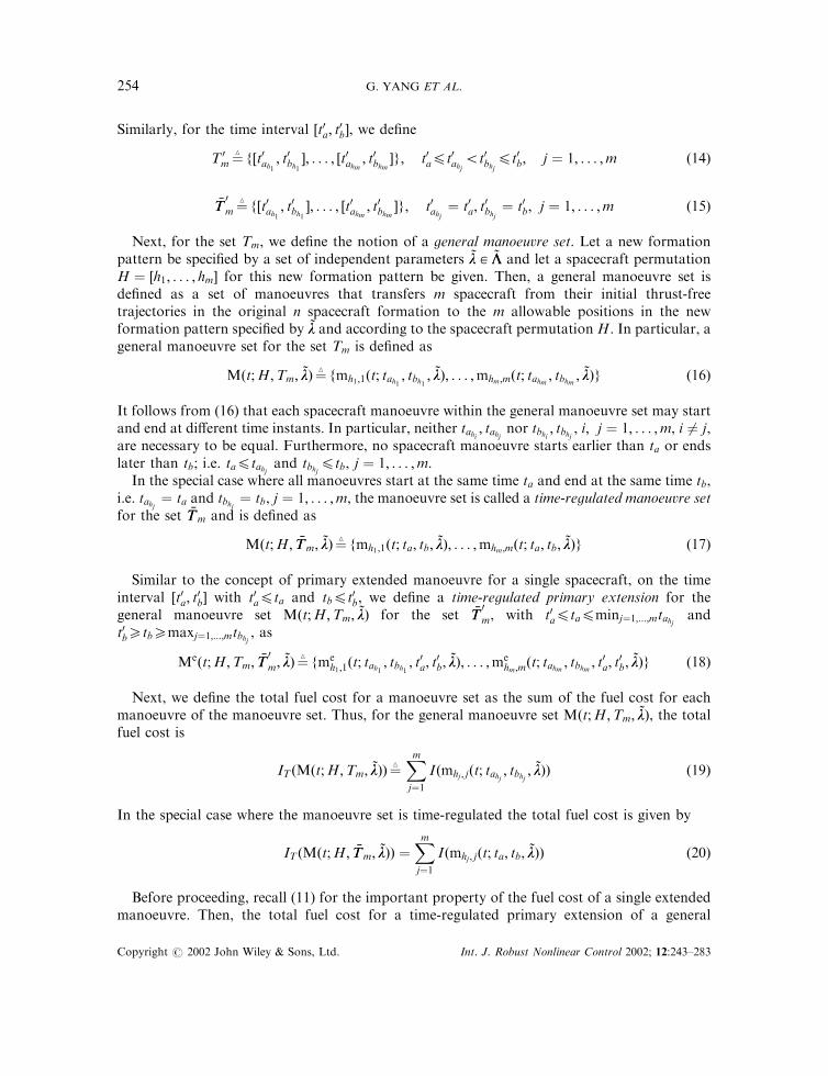
Similarly, for the time interval ½t0a; t0b�, we define

T 0m ¼4 f½t0ah1 ; t

0bh1

�; . . . ; ½t0ahm ; t0bhm

�g; t0a4t0ahj5t0bhj

4t0b; j ¼ 1; . . . ;m ð14Þ

%TT0m ¼4 f½t0ah1 ; t

0bh1

�; . . . ; ½t0ahm ; t0bhm

�g; t0ahj¼ t0a; t

0bhj

¼ t0b; j ¼ 1; . . . ;m ð15Þ

Next, for the set Tm, we define the notion of a general manoeuvre set. Let a new formationpattern be specified by a set of independent parameters *ll 2 *LL and let a spacecraft permutationH ¼ ½h1; . . . ; hm� for this new formation pattern be given. Then, a general manoeuvre set isdefined as a set of manoeuvres that transfers m spacecraft from their initial thrust-freetrajectories in the original n spacecraft formation to the m allowable positions in the newformation pattern specified by *ll and according to the spacecraft permutation H. In particular, ageneral manoeuvre set for the set Tm is defined as

Mðt;H;Tm; *llÞ ¼4 fmh1;1ðt; tah1 ; tbh1 ;

*llÞ; . . . ;mhm ;mðt; tahm ; tbhm ;*llÞg ð16Þ

It follows from (16) that each spacecraft manoeuvre within the general manoeuvre set may startand end at different time instants. In particular, neither tahi ; tahj nor tbhi ; tbhj , i; j ¼ 1; . . . ;m, i 6¼ j,are necessary to be equal. Furthermore, no spacecraft manoeuvre starts earlier than ta or endslater than tb; i.e. ta4tahj and tbhj4tb, j ¼ 1; . . . ;m.

In the special case where all manoeuvres start at the same time ta and end at the same time tb,i.e. tahj ¼ ta and tbhj ¼ tb, j ¼ 1; . . . ;m, the manoeuvre set is called a time-regulated manoeuvre setfor the set %TTm and is defined as

Mðt;H; %TTm; *llÞ ¼4 fmh1;1ðt; ta; tb; *llÞ; . . . ;mhm ;mðt; ta; tb; *llÞg ð17Þ

Similar to the concept of primary extended manoeuvre for a single spacecraft, on the timeinterval ½t0a; t

0b� with t0a4ta and tb4t0b, we define a time-regulated primary extension for the

general manoeuvre set Mðt;H;Tm; *llÞ for the set %TT0m, with t0a4ta4minj¼1;...;mtahj and

t0b5tb5maxj¼1;...;mtbhj , as

Meðt;H;Tm; %TT0m;

*llÞ ¼4 fmeh1;1

ðt; tah1 ; tbh1 ; t0a; t

0b;*llÞ; . . . ;me

hm;mðt; tahm ; tbhm ; t

0a; t

0b;*llÞg ð18Þ

Next, we define the total fuel cost for a manoeuvre set as the sum of the fuel cost for eachmanoeuvre of the manoeuvre set. Thus, for the general manoeuvre set Mðt;H;Tm; *llÞ, the totalfuel cost is

IT ðMðt;H;Tm; *llÞÞ ¼4Xmj¼1

Iðmhj ; jðt; tahj ; tbhj ;*llÞÞ ð19Þ

In the special case where the manoeuvre set is time-regulated the total fuel cost is given by

IT ðMðt;H; %TTm; *llÞÞ ¼Xmj¼1

Iðmhj ; jðt; ta; tb; *llÞÞ ð20Þ

Before proceeding, recall (11) for the important property of the fuel cost of a single extendedmanoeuvre. Then, the total fuel cost for a time-regulated primary extension of a general

G. YANG ET AL.254


manoeuvre set Mðt;H;Tm; *llÞ yields

IT ðMeðt;H;Tm; %TT0m;

*llÞÞ ¼Xmj¼1

Iðmehj ; j

ðt; tahj ; tbhj ; t0a; t

0b;*llÞÞ

¼Xmj¼1

Iðmhj ; jðt; tahj ; tbhj ;*llÞÞ

¼ IT ðMðt;H;Tm; *llÞÞ ð21Þ

i.e. the total fuel cost for a general manoeuvre set Mðt;H;Tm; *llÞ is the same as the total fuel costfor its time-regulated primary extension Meðt;H;Tm; %TT

0m;

*llÞ for any t0a4ta4minj¼1;...;mtahj andt0b5tb5maxj¼1;...;mtbhj .

Among all the manoeuvres mi; jðt; tai ; tbi ; *llÞ that start at tai and end at tbi , tai5tbi , and transferspacecraft i to the jth allowable position in the new formation pattern, which is specified by *ll,we define a fuel optimal manoeuvre m*

i; jðt; tai ; tbi ; *llÞ as a manoeuvre whose fuel cost is smallerthan (or at worst equal to) the fuel cost for any other manoeuvre, i.e.

Iðm*i; jðt; tai ; tbi ; *llÞÞ4Iðmi; jðt; tai ; tbi ; *llÞÞ ð22Þ

for all mi; jðt; tai ; tbi ; *llÞ.Next, for a specified spacecraft permutation H, a set of chosen independent parameters *ll for

the new formation pattern, and a set of manoeuvre time intervals Tm for all spacecraft in ageneral manoeuvre set, we define a fuel optimal manoeuvre set as

M* ðt;H;Tm; *llÞ ¼4 fm*

h1;1ðt; tah1 ; tbh1 ;

*llÞ; . . . ;m*hm ;m

ðt; tahm ; tbhm ;*llÞg ð23Þ

Since the total fuel cost for a manoeuvre set is the sum of the fuel cost for each spacecraftmanoeuvre in that manoeuvre set, using (22), we obtain

IT ðM* ðt;H;Tm; *llÞÞ ¼Xmj¼1

Iðm*hj ; j

ðt; tahj ; tbhj ;*llÞÞ

4Xmj¼1

Iðmhj ; jðt; tahj ; tbhj ;*llÞÞ

¼ IT ðMðt;H;Tm; *llÞÞ ð24Þ

for all Mðt;H;Tm; *llÞ. Thus, it follows from (24) that the total fuel cost for the fuel optimalmanoeuvre set M* ðt;H;Tm; *llÞ is smaller than (or at worst equal to) the total fuel cost for anyother manoeuvre set Mðt;H;Tm; *llÞ, which transfers m spacecraft from their initial thrust-freetrajectories in the original formation to the m allowable positions according to the spacecraftpermutation H in the new formation pattern specified by *ll and whose manoeuvre time intervalsare given by Tm.

Note that the total fuel cost IT ðM* ðt;H;Tm; *llÞÞ is a function of H, Tm, and *ll. Inorder to minimize the total fuel cost for a spacecraft formation reconfiguration process, we mustfind optimal H * ;T *

m ; and *ll* , such that the total fuel cost for M* ðt;H * ;T *m ; *ll* Þ is smaller than

(or at worst equal to) the total fuel cost for M* ðt;H;Tm; *llÞ with any other choice of H, Tm, and*ll; i.e.

IT ðM* ðt;H * ;T *m ; *ll* ÞÞ4IT ðM* ðt;H;Tm; *llÞÞ ð25Þ



Next, for a specified Tm, a choice of H and *ll is called conditionally optimal if the totalfuel cost for M* ðt;H *

Tm;Tm; *ll*

TmÞ is smaller than (or at worst equal to) the total fuel cost for

M* ðt;H;Tm; *llÞ with any other choice of H and *ll, with the specified Tm, i.e.

IT ðM* ðt;H *Tm;Tm; *ll*

TmÞÞ4IT ðM* ðt;H;Tm; *llÞÞ ð26Þ

Now we present the principal result of this section.

Theorem 3.1On the time interval ½ta; tb�, for arbitrary Tm,

IT ðM* ðt;H *%TTm; %TTm; *ll*

%TTmÞÞ4IT ðM* ðt;H *

Tm;Tm; *ll*

TmÞÞ ð27Þ

where Tm and %TTm are given according to (12) and (13), respectively.

ProofFirst, note that H *

%TTmand *ll*

%TTmin (27) represent the conditionally optimal choice of H and *ll for

the specified %TTm. Thus, according to (26), we obtain,


%TTmÞÞ4IT ðM* ðt;H; %TTm; *llÞÞ ð28Þ

for all H and *ll. Next, assume that (27) does not hold for some #TTm, i.e. there exists a#TTm ¼ f½#ttah1 ; #ttbh1 �; . . . ; ½#ttahm ; #ttbhm �g, ta4#ttahj5#ttbhj4tb, j ¼ 1; . . . ;m, such that


%TTmÞÞ > IT ðM* ðt;H *

#TTm; #TTm; *ll*

#TTmÞÞ ð29Þ

Now for the manoeuvre set M* ðt;H *#TTm; #TTm; *ll*

#TTmÞ and its time-regulated primary extension

M*eðt; H *#TTm; #TTm; %TTm; *ll*

#TTmÞ, (21) yields

IT ðM*eðt;H *#TTm; #TTm; %TTm; *ll*

#TTmÞÞ ¼ IT ðM* ðt;H *

#TTm; #TTm; *ll*

#TTmÞÞ ð30Þ

Next, we define a time-regulated manoeuvre set Mðt;H *#TTm; %TTm; *ll*

#TTmÞ ¼4 M*eðt;H *

#TTm; #TTm; %TTm; *ll*

#TTmÞ.

It now follows that

IT ðMðt;H *#TTm; %TTm; *ll*

#TTmÞÞ ¼ IT ðM*eðt;H *

#TTm; #TTm; %TTm; *ll*

#TTmÞÞ ð31Þ

Combining (29)–(31), we obtain


%TTmÞÞ > IT ðMðt;H *

#TTm; %TTm; *ll*

#TTmÞÞ ð32Þ

It follows from (24) that

IT ðMðt;H *#TTm; %TTm; *ll*

#TTmÞÞ5IT ðM* ðt;H *

#TTm; %TTm; *ll*

#TTmÞÞ ð33Þ

Therefore, there exist H *#TTm

and *ll*#TTm

such that


%TTmÞÞ > IT ðM* ðt;H *

#TTm; %TTm; *ll*

#TTmÞÞ ð34Þ

which contradicts (28). Consequently, (27) holds for all Tm. &

According to Theorem 3.1, since (27) holds for arbitrary Tm, it holds for T *m , which is an

optimal choice of Tm. Thus


%TTmÞÞ4IT ðM* ðt;H *

T *m;T *

m ; *ll*T *mÞÞ ð35Þ

G. YANG ET AL.256


Since H *T *m

and *ll*T *m

are conditionally optimal for T *m , which is the optimal choice of Tm, it

follows that

IT ðM* ðt;H *T *m;T *

m ; *ll*T *mÞÞ4 IT ðM* ðt;H *

Tm;Tm; *ll*

TmÞÞ

4 IT ðM* ðt;H;Tm; *llÞÞ ð36Þ

for all H, Tm, and *ll. Combining (35) and (36), we obtain


%TTmÞÞ4IT ðM* ðt;H;Tm; *llÞÞ ð37Þ

for all H, Tm, and *ll.

Corollary 3.1On the time interval ½ta; tb�, H *

%TTm, %TTm, and *ll*

%TTmare optimal in the sense that the total fuel cost for

M* ðt;H *%TTm; %TTm; *ll*

%TTmÞ is smaller than (or at worst equal to) the total fuel cost for M* ðt;H;Tm; *llÞ

with any other choice of H, Tm, and *ll.Now we consider the practical implication of this result to a spacecraft formation

reconfiguration process, where, given by the mission requirement, the earliest allowable startingtime and the latest allowable ending time for spacecraft manoeuvres are ta and tb, respectively.The significance of Corollary 3.1 is that our search space for the optimal choice of H, Tm, and *llcan be reduced to a considerably smaller search space for the conditionally optimal choice of Hand *ll with the specified %TTm when we minimize the total fuel cost IT ðM* ðt;H;Tm; *llÞÞ for aspacecraft formation reconfiguration process. In particular, according to Corollary 3.1, on thetime interval ½ta; tb�, in order to minimize the total fuel cost, we do not have to consider allgeneral manoeuvre sets whose spacecraft manoeuvres may start and end at arbitrary timeinstants between ta and tb. Instead, it suffices to let every spacecraft manoeuvre start at ta andend at tb and obtain the fuel optimal manoeuvre set with the conditionally optimal choice of Hand *ll.

4. FUEL OPTIMAL SPACECRAFT FORMATION RECONFIGURATION:MULTI-AGENT OPTIMIZATION ALGORITHM ARCHITECTURE

In Section 3, we analysed the fuel optimal spacecraft formation reconfiguration problemqualitatively. In this section, we develop an architecture for the optimization algorithm thatgenerates the fuel optimal manoeuvre set for spacecraft formation reconfiguration.

4.1. Multi-agent optimization algorithm architecture overview

Given the set %TTm, to minimize the total fuel cost for formation reconfiguration, our objective isto find a conditionally optimal choice ofH and *ll and the corresponding fuel optimal manoeuvreset. This conditional optimization problem is decomposed into a two step process. In the firststep, for any given choice of *ll 2 *LL, we find a conditionally optimal H *

*llsuch that

IT ðM* ðt;H **ll; %TTm; *llÞÞ4IT ðM* ðt;H; %TTm; *llÞÞ; 8 H ð38Þ

In the second step, we focus on the minimization of the fuel cost by searching for *ll* 2 *LL suchthat

IT ðM* ðt;H **ll *; %TTm; *ll* ÞÞ4IT ðM* ðt;H *

*ll; %TTm; *llÞÞ; 8 *ll 2 *LL ð39Þ



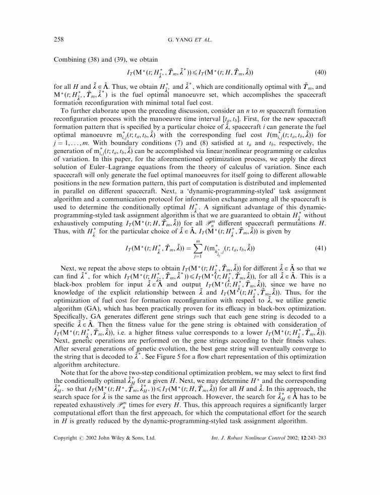
Combining (38) and (39), we obtain

IT ðM* ðt;H **ll *; %TTm; *ll* ÞÞ4IT ðM* ðt;H; %TTm; *llÞÞ ð40Þ

for all H and *ll 2 *LL. Thus, we obtain H **ll *

and *ll* , which are conditionally optimal with %TTm, andM* ðt;H *

*ll *; %TTm; *ll* Þ is the fuel optimal manoeuvre set, which accomplishes the spacecraft

formation reconfiguration with minimal total fuel cost.To further elaborate upon the preceding discussion, consider an n to m spacecraft formation

reconfiguration process with the manoeuvre time interval ½ta; tb�. First, for the new spacecraftformation pattern that is specified by a particular choice of *ll, spacecraft i can generate the fueloptimal manoeuvre m*

i; jðt; ta; tb; *llÞ with the corresponding fuel cost Iðm*i; jðt; ta; tb; *llÞÞ for

j ¼ 1; . . . ;m. With boundary conditions (7) and (8) satisfied at ta and tb, respectively, thegeneration of m*

i; jðt; ta; tb; *llÞ can be accomplished via linear/nonlinear programming or calculusof variation. In this paper, for the aforementioned optimization process, we apply the directsolution of Euler–Lagrange equations from the theory of calculus of variation. Since eachspacecraft will only generate the fuel optimal manoeuvres for itself going to different allowablepositions in the new formation pattern, this part of computation is distributed and implementedin parallel on different spacecraft. Next, a ‘dynamic-programming-styled’ task assignmentalgorithm and a communication protocol for information exchange among all the spacecraft isused to determine the conditionally optimal H *

*ll. A significant advantage of this dynamic-

programming-styled task assignment algorithm is that we are guaranteed to obtain H **llwithout

exhaustively computing IT ðM* ðt;H; %TTm; *llÞÞ for all Pmn different spacecraft permutations H.

Thus, with H **llfor the particular choice of *ll 2 *LL, IT ðM* ðt;H *

*ll; %TTm; *llÞÞ is given by

IT ðM* ðt;H **ll; %TTm; *llÞÞ ¼

Xmj¼1

Iðm*h **llj; jðt; ta; tb; *llÞÞ ð41Þ

Next, we repeat the above steps to obtain IT ðM* ðt;H **ll; %TTm; *llÞÞ for different *ll 2 *LL so that we

can find *ll* , for which IT ðM* ðt;H **ll *; %TTm; *ll* ÞÞ4IT ðM* ðt;H *

*ll; %TTm; *llÞÞ; for all *ll 2 *LL. This is a

black-box problem for input *ll 2 *LL and output IT ðM* ðt;H **ll; %TTm; *llÞÞ, since we have no

knowledge of the explicit relationship between *ll and IT ðM* ðt;H **ll; %TTm; *llÞÞ. Thus, for the

optimization of fuel cost for formation reconfiguration with respect to *ll, we utilize geneticalgorithm (GA), which has been practically proven for its efficacy in black-box optimization.Specifically, GA generates different gene strings such that each gene string is decoded to aspecific *ll 2 *LL. Then the fitness value for the gene string is obtained with consideration ofIT ðM* ðt;H *

*ll; %TTm; *llÞÞ, i.e. a higher fitness value corresponds to a lower IT ðM* ðt;H *

*ll; %TTm; *llÞÞ.

Next, genetic operations are performed on the gene strings according to their fitness values.After several generations of genetic evolution, the best gene string will eventually converge tothe string that is decoded to *ll* . See Figure 5 for a flow chart representation of this optimizationalgorithm architecture.

Note that for the above two-step conditional optimization problem, we may select to first findthe conditionally optimal *ll*

H for a given H. Next, we may determine H * and the corresponding*ll*H * so that IT ðM* ðt;H * ; %TTm; *ll*

H * ÞÞ4IT ðM* ðt;H; %TTm; *llÞÞ for all H and *ll. In this approach, thesearch space for *ll is the same as the first approach. However, the search for *ll*

H 2 *LL has to berepeated exhaustively Pm

n times for every H. Thus, this approach requires a significantly largercomputational effort than the first approach, for which the computational effort for the searchin H is greatly reduced by the dynamic-programming-styled task assignment algorithm.

G. YANG ET AL.258


4.2. Fuel optimal Manoeuvre for a single spacecraft

To generate the fuel optimal manoeuvre for a single spacecraft engaged in formationreconfiguration manoeuvre, we consider the linearized spacecraft relative motion dynamicscharacterized in the fxI; yI; zIg coordinate frame. The linearized spacecraft relative motiondynamics is typically described by the Hill’s equations [19, 20, 22, 23, 26, 27] as below

.xxðtÞ ¼ 2o ’yyðtÞ þ uxðtÞ

.yyðtÞ ¼ �2o ’xxðtÞ þ 3o2yðtÞ þ uyðtÞ

.zzðtÞ ¼ �o2zðtÞ þ uzðtÞ ð42Þ

where ðxðtÞ; yðtÞ; zðtÞÞ is the spacecraft relative motion trajectory expressed in the fxI; yI; zIgcoordinate frame and uxðtÞ, uyðtÞ, and uzðtÞ are the components of the thrust forces per unit massalong the xI, yI, and zI axis, respectively.

Figure 5. Optimization algorithm architecture.



If we prescribe a spacecraft relative motion trajectory ðxðtÞ; yðtÞ; zðtÞÞ in the fxI; yI; zIgcoordinate frame, then the thrust force per unit mass ðuxðtÞ; uyðtÞ; uzðtÞÞ, which enables thespacecraft relative motion ðxðtÞ; yðtÞ; zðtÞÞ, is given by

uxðtÞ ¼ .xxðtÞ � 2o ’yyðtÞ

uyðtÞ ¼ .yyðtÞ þ 2o ’xxðtÞ � 3o2yðtÞ

uzðtÞ ¼ .zzðtÞ þ o2zðtÞ ð43Þ

For notational convenience, in the balance of this subsection, we suppress the explicitdependence of various variables on t.

Let M be the mass of the spacecraft. Restricting consideration to a relatively short period oftime, i.e. several spacecraft orbital periods out of several years long spacecraft life time, itfollows that the mass of the spacecraft during a formation reconfiguration manoeuvre can betaken as a constant. If ðux; uy; uzÞ is the thrust force per unit mass, the total thrust isðM ux;M uy;M uzÞ. The fuel consumption for a spacecraft to apply the thrust ðM ux;M uy;M uzÞis governed by the type of the spacecraft propulsion system on-board. Two common spacecraftpropulsion systems are the constant specific impulse propulsion system and the variable specificimpulse (VSI) propulsion system. Of these, the VSI propulsion system, such as the electricplasma thruster, is particularly relevant to spacecraft orbit control and reconfigurationmanoeuvre. Thus, in this paper, we assume that all spacecraft engaged in formationreconfiguration utilize the VSI propulsion system.

Let ’mm be the fuel mass consumption rate. Then, for a VSI propulsion system, ’mm is given by[35]

’mm ¼M2

2Pðu2x þ u2y þ u2zÞ ð44Þ

where P is the power delivered to the propulsion system. For a time interval ½ta; tb�, the total fuelmass consumption of a spacecraft is

R tb

ta’mm dt. Next, let the fuel cost for spacecraft i to execute a

manoeuvre mi; jðt; ta; tb; *llÞ to relocate to the jth allowable position in the new formation patternthat is specified by *ll be defined as the total fuel mass consumption for this manoeuvre.

Next, we use C to denote the set of all space curves ðx; y; zÞ, where x, y, and z are functionsdefined on ½ta; tb� that have continuous second derivatives on ½ta; tb� and satisfy the boundaryconditions (7) and (8) at t ¼ ta and t ¼ tb, respectively. Thus, every ðx; y; zÞ 2 C is a feasiblespacecraft manoeuvre for spacecraft i to transfer to the jth allowable position in the newformation pattern that is specified by *ll, starting at ta and ending at tb. In particular, x, y, and zrepresent simplified notations for xmi; j ðt; *llÞ, ymi; j ðt; *llÞ, and zmi; j ðt; *llÞ, respectively. Noweliminating ðux; uy; uzÞ in (44) using (43), we obtain the fuel cost for spacecraft i to executemanoeuvre mi; jðt; ta; tb; *llÞ as follows:

Iðmi; jðt; ta; tb; *llÞÞ ¼4

Z tb

ta

’mm dt

¼M2

2P

Z tb

ta

ðð .xx� 2o ’yyÞ2 þ ð .yyþ 2o ’xx� 3o2yÞ2 þ ð .zzþ o2zÞ2Þ dt ð45Þ

G. YANG ET AL.260


For notational convenience, we now define

f ðx; ’xx; .xx; y; ’yy; .yy; z; ’zz; .zzÞ ¼4 ð .xx� 2o ’yyÞ2 þ ð .yyþ 2o ’xx� 3o2yÞ2 þ ð .zzþ o2zÞ2; ðx; y; zÞ 2 C ð46Þ

Jðx; y; zÞ ¼4Z tb

ta

f ðx; ’xx; .xx; y; ’yy; .yy; z; ’zz; .zzÞ dt; ðx; y; zÞ 2 C ð47Þ

Then, using (45)–(47), the fuel cost for spacecraft i to execute manoeuvre mi; jðt; ta; tb; *llÞ isgiven by

Iðmi; jðt; ta; tb; *llÞÞ ¼M2

2PJðx; y; zÞ; ðx; y; zÞ 2 C ð48Þ

To find the optimal manoeuvre m*i; jðt; ta; tb; *llÞ for spacecraft i such that its fuel cost

Iðm*i; jðt; ta; tb; *llÞÞ is minimal, we search for ðx* ; y* ; z* Þ in C such that Jðx* ; y* ; z* Þ is minimal.

This fuel optimization problem is addressed via the theory of calculus of variation. In particular,using the theory of calculus of variation, we can obtain an extremum that satisfies the Euler–Lagrange equations and boundary conditions (7) and (8) at t ¼ ta and t ¼ tb, respectively. Notethat since the set of space curves C defined above is convex, the existence and uniqueness ofminðx;y;zÞ2CJðx; y; zÞ follows from the fact that Jðx; y; zÞ in (47) is a strictly convex functional onC [36]. Thus, it follows that the extremum yields the unique optimal solution ðx* ; y* ; z* Þ forwhich Jðx* ; y* ; z* Þ is minimal.

Next, the Euler–Lagrange equations for the minimization of (47) are given by [37, 38]

@f

@q�

d

dt

@f

@ ’qq

� �þ

d2

dt2@f

@ .qq

� �¼ 0; q 2 fx; y; zg ð49Þ

where, for notational simplicity, we have suppressed the arguments of f (see (46) for details).Now, using (46) in (49), we obtain

d4x

dt4� 4o

d3y

dt3� 4o2 d

2x

dt2þ 6o3dy

dt¼ 0

d4y

dt4þ 4o

d3x

dt3� 10o2 d

2y

dt2� 6o3 dx

dtþ 9o4y ¼ 0

d4z

dt4þ 2o2 d

2z

dt2þ o4z ¼ 0 ð50Þ

The general solution of the set of linear ordinary differential equations (50) is given by

xðtÞ ¼ c1 þ c2tþ c3t2 þ c4t

3 þ c5sin ðotÞ þ c6cos ðotÞ þ c7tcos ðotÞ þ c8tsin ðotÞ

yðtÞ ¼2c2

3oþ

16c4

9o3

� �þ

4c3

3otþ

2c4

ot2 þ

3c7

10oþ

c5

2

� �cos ðotÞ þ

3c8

10o�

c6

2

� �sin ðotÞ

þc8

2tcos ðotÞ �

c7

2tsin ðotÞ

zðtÞ ¼ c9sin ðotÞ þ c10 cos ðotÞ þ c11tcos ðotÞ þ c12tsin ðotÞ ð51Þ

where t 2 ½ta; tb� and ci, i ¼ 1; . . . ; 12, are 12 integration constants, which can be determinedusing the boundary conditions (7) and (8) at t ¼ ta and t ¼ tb, respectively. Since (50) is a



time-invariant linear system, we can shift the time variable from t to t ¼4 t� ta in (51) to obtainan equivalent characterization of the general solution of (50) given by

xðtÞ ¼ c1 þ c2tþ c3t2 þ c4t3 þ c5sin ðotÞ þ c6cos ðotÞ þ c7tcos ðotÞ þ c8tsin ðotÞ

yðtÞ ¼2c2

3oþ

16c4

9o3

� �þ

4c3

3otþ

2c4

ot2 þ

3c7

10oþ

c5

2

� �cos ðotÞ þ

3c8

10o�

c6

2

� �sin ðotÞ

þc8

2tcos ðotÞ �

c7

2tsin ðotÞ

zðtÞ ¼ c9sin ðotÞ þ c10 cos ðotÞ þ c11tcos ðotÞ þ c12tsin ðotÞ ð52Þ

where t 2 ½0;D�, with D ¼4 tb � ta.With the general solution of (50) characterized by (52), an application of the boundary

conditions (7) and (8) at t ¼ ta (equivalently, at t ¼ 0) and t ¼ tb (equivalently, at t ¼ D),respectively, yields a linear system of 12 algebraic equations for ci, i ¼ 1; . . . ; 12. Havingsolved the linear system of 12 algebraic equations for ci, i ¼ 1; . . . ; 12, the 12 integrationconstants are substituted in (52) to produce the extremum that is the unique optimalðx* ; y* ; z* Þ, for all ðx; y; zÞ 2 C. Thus, Jðx* ; y* ; z* Þ is minimal, i.e. Jðx* ; y* ; z* Þ5Jðx; y; zÞfor any other ðx; y; zÞ 2 C. Now the unique fuel optimal manoeuvre m*

i; jðt; ta; tb; *llÞ ¼ðxm*

i; jðt; *llÞ; ym*

i; jðt; *llÞ; zm*

i; jðt; *llÞÞ, ta4t4tb, is obtained from xm*

i; jðt; *llÞ ¼ x* , ym*

i; jðt; *llÞ ¼ y* , and

zm*i; jðt; *llÞ ¼ z* , which guarantees that Iðm*

i; jðt; ta; tb; *llÞÞ5Iðmi; jðt; ta; tb; *llÞÞ for any other

mi; jðt; ta; tb; *llÞ.Finally, with the change of variable t ¼4 t� ta and substitution of (46) and (52), the integral

of (47) yields

Jðx* ; y* ; z* Þ ¼4

9c23 þ

16

9o2c24 þ

o2

10ðc27 þ c28Þ þ 2o2ðc211 þ c212Þ

� �Dþ

4c3c4

3D2 þ

4c243

D3

þ32c7c4

15o�

8c8c3

15

� �sin ðoDÞ �

32c8c4

15oþ

8c7c3

15

� �cos ðoDÞ �

8c8c4

5Dsin ðoDÞ

�8c7c4

5Dcos ðoDÞ þ

3oc7c825

þ 4oc11c12

� �cos2ðoDÞ

þ3o50

ðc28 � c27Þ þ 2oðc212 � c211Þ� �

cos ðoDÞsin ðoDÞ

þ8c7c3

15�

3oc7c825

þ32c8c4

15o� 4oc11c12 ð53Þ

where, as elaborated above, the values of ci, i ¼ 1; . . . ; 12, correspond to the solution of thelinear system of 12 algebraic equations consistent with the boundary conditions (7) and (8) att ¼ ta and t ¼ tb, respectively. Finally, the value of Iðm*

i; jðt; ta; tb; *llÞÞ is given by

Iðm*i; jðt; ta; tb; *llÞÞ ¼

M2

2PJðx* ; y* ; z* Þ ð54Þ

4.3. Dynamic-programming-styled multi-agent task assignment algorithm

4.3.1. Task assignment problemWe begin by considering a general task assignment problem, where m different tasks are to beassigned to n agents, with m4n. Let the minimum cost for agent i to perform task j be denoted

G. YANG ET AL.262


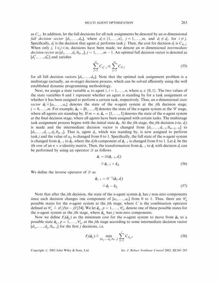
as Ci; j . In addition, let the full decisions for all task assignments be denoted by an m dimensionalfull decision vector ½d1; . . . ; dm�, where dj 2 f1; . . . ; ng, j ¼ 1; . . . ;m, and di 6¼ dj, for i 6¼ j.Specifically, dj is the decision that agent dj performs task j. Then, the cost for decision dj is Cdj ; j.When only j, 14j5m, decisions have been made, we denote an m dimensional intermediatedecision vector as ½d1; . . . ; dj ; 0m�j�, j ¼ 1; . . . ;m� 1. An optimal full decision vector is denoted as½d *

1 ; . . . ; d*m � and satisfies

Xmj¼1

Cd *j ; j4

Xmj¼1

Cdj ; j ð55Þ

for all full decision vectors ½d1; . . . ; dm�. Note that the optimal task assignment problem is amultistage (actually, an m-stage) decision process, which can be solved efficiently using the wellestablished dynamic programming methodology.

Next, we assign a state variable ai to agent i, i ¼ 1; . . . ; n, where ai 2 f0; 1g. The two values ofthe state variables 0 and 1 represent whether an agent is standing by for a task assignment orwhether it has been assigned to perform a certain task, respectively. Thus, an n dimensional statevector *aaj ¼

4 ½a1; . . . ; an� denotes the state of the n-agent system at the jth decision stage,j ¼ 0; . . . ;m. For example, *aa0 ¼ ½0; . . . ; 0� denotes the state of the n-agent system at the ‘0’ stage,where all agents are standing by. If m ¼ n, *aan ¼ ½1; . . . ; 1� denotes the state of the n-agent systemat the final decision stage, where all agents have been assigned with certain tasks. The multistagetask assignment process begins with the initial state *aa0. At the jth stage, the jth decision (viz, dj)is made and the intermediate decision vector is changed from ½d1; . . . ; dj�1; 0m�ðj�1Þ� to½d1; . . . ; dj�1; dj ; 0m�j�. That is, agent dj, which was standing by, is now assigned to performtask j and the value of adj is changed from 0 to 1. Specifically, the full state of the n-agent systemis changed from *aaj�1 to *aaj, where the djth component of *aaj�1 is changed from 0 to 1. Let *eei be theith row of an n� n identity matrix. Then, the transformation from *aaj�1 to *aaj with decision dj canbe performed by using an operator D as follows

*aaj ¼Dð *aaj�1; djÞ

¼4 *aaj�1 þ *eedj ð56Þ

We define the inverse operator of D as

*aaj�1 ¼D�1ð *aaj ; djÞ

¼4 *aaj � *eedj ð57Þ

Note that after the jth decision, the state of the n-agent system *aaj has j non-zero componentssince each decision changes one component of ½a1; . . . ; an� from 0 to 1. Thus, there are Cj

n

possible states for the n-agent system at the jth stage, where C is the combination operatordefined as Cj

n ¼4 n!=j!ðn� jÞ! [34]. We let *aajp , p ¼ 1; . . . ;Cjn, denote one of these possible states for

the n-agent system at the jth stage, where *aajp has j non-zero components.Now we define Fjð *aajp Þ as the minimum cost for the n-agent system to move from *aa0 to a

possible state *aajp , p ¼ 1; . . . ;Cjn, at the jth stage according to some intermediate decision vector

½d1p ; . . . ; djp ; 0m�j� for the first j decisions, i.e.

Fjð *aajpÞ ¼4

min½d1p ;...;djp ;0m�j �

Xj

l¼1

Cdlp ;l ð58Þ



where ½d1p ; . . . ; djp ; 0m�j � is any feasible intermediate decision vector that satisfies

Dð. . .DðDð *aa0; d1p Þ; d2pÞ; . . . ; djp Þ ¼Xj

l¼1

*eedlp

¼ *aajp ð59Þ

Finally, since there are Cmn possible states at the mth decision stage, we have

Xmj¼1

Cd *j; j ¼ min

p¼1;...;Cmn

Fmð *aampÞ ð60Þ

where Fmð *aampÞ denotes the minimum cost for the n-agent system to move from *aa0 to a possible

state *aamp, p ¼ 1; . . . ;Cm

n , at the mth stage according to some full decision vector ½d1p ; . . . ; dmp�.

Note that in the case where m ¼ n, Cmn ¼ Cn

n ¼ 1, i.e., there is only one possible state at the nthdecision stage, which is *aan. Thus, we have,

Xnj¼1

Cd *j; j ¼ Fnð *aanÞ ð61Þ

At the jth decision stage, for a particular *aajp , we assume its j non-zero components arek1p ; . . . ; kjp components. Thus, the set of allowable values for decision djp that brings the state tothis *aajp at the jth stage is Kjp ¼

4 fk1p ; . . . ; kjpg, since k1p ; . . . ; kjp are the only non-zero componentsin the state vector so far. Now, applying the Principle of Optimality [37–39], we obtain thefollowing recurrence relation for Fjð *aajp Þ:

Fjð *aajp Þ ¼ mindjp2Kjp

fCdjp ; j þ Fj�1ðD�1ð *aajp ; djp ÞÞg; p ¼ 1; . . . ;Cjn ð62Þ

Next, we can construct a dynamic-programming-styled task assignment algorithm for allagents since each stage of this algorithm is based on the recurrence relation (62). In order to startthe algorithm, each agent must generate the costs for itself to perform the m different tasks inadvance. For the first stage, F1ð *aa1p Þ ¼ Cp;1, p ¼ 1; . . . ; n, since C1

n ¼ n. At the jth stage, for everypossible state *aajp , agent djp , djp 2 Kjp , needs to take the sum of Cdjp ; j þ Fj�1ðD�1ð *aajp ; djpÞÞ. Notethat Cdjp ; j is the cost of agent djp to perform task j, which is known to agent djp . Furthermore,Fj�1ðD�1ð *aajp ; djp ÞÞ is the result obtained from the last stage for some state D�1ð *aajp ; djp Þ, which hasj � 1 non-zero components and whose djp component is zero. Then the value of Cdjp ; jþFj�1ðD�1ð *aajp ; djp ÞÞ is communicated to the other agents for comparison withCd 0jp ; j

þ Fj�1ðD�1ð *aajp ; d0jpÞÞ, d 0

jp2 Kjp , d 0

jp6¼ djp . In addition, the minimum value of Cdjp ; jþ

Fj�1ðD�1ð *aajp ; djp ÞÞ, djp 2 Kjp , is taken as Fjð *aajp Þ and communicated to all agents for use at thenext stage. After the mth stage, Fmð *aamp

Þ, p ¼ 1; . . . ;Cmn , is known to every agent. Thus, the

agents can easily obtain the value ofPm

j¼1 Cd *j; j and the corresponding optimal full decision

vector ½d *1 ; . . . ; d

*m � by choosing the minimum value of Fmð *aamp

Þ among all *aamp, p ¼ 1; . . . ;Cm

n .In order to show the efficacy of this dynamic-programming-styled task assignment algorithm,

we consider the computational effort for this algorithm. At the jth stage, where 24j4m, apossible state *aajp can be reached by a total of j allowable decision values that belong to the setKjp . Thus, in order to obtain Fjð *aajp Þ for a particular *aajp , the agents need to do j additions toobtain Cdjp ; j þ Fj�1ðD�1ð *aajp ; djpÞÞ for all j allowable values of djp 2 Kjp so that they can comparethese values and find the minimum value of Cdjp ; j þ Fj�1ðD�1ð *aajp ; djp ÞÞ. For all C

jn possible states

at the jth stage, the agents have to do j Cjn additions. Since no calculation is needed for the first

G. YANG ET AL.264


stage, for all m stages, the total effort will bePm

j¼2 j Cjn additions. Note that

Xmj¼2

j Cjn ¼

Xmj¼2

jn!

ðn� jÞ! j!

¼Xmj¼2

ðn� 1Þ! nðn� jÞ! ðj � 1Þ!

¼ nXmj¼2

Cj�1n�1 ð63Þ

For an n-agent-m-task problem, m4n, we denote the total number of additions that are neededfor this algorithm as Eðn;mÞ ¼4 n

Pmj¼2 C

j�1n�1. Specifically, for an n-agent-n-task problem, where

m ¼ n, the total number of additions is

Eðn; nÞ ¼ nXnj¼2

Cj�1n�1

¼ nð2n�1 � 1Þ ð64Þ

In contrast to the above, the exhaustive evaluation ofPm

j¼1 Cdj ; j for all Pmn different agent-

task assignments requires at least #EEðn;mÞ ¼4 Pmn additions, if we assume that for a particular

½d1; . . . ; dm� the evaluation ofPm

j¼1 Cdj ; j requires only one addition. Thus, for a 10-agent-10-taskproblem, Eð10; 10Þ � 5:1� 103 while #EEð10; 10Þ � 3:6� 106, and for a 15-agent-15-taskproblem, Eð15; 15Þ � 2:45� 105 while #EEð15; 15Þ � 1:3� 1012.

Remark 4.1A variety of alternative schemes exists to solve the task assignment problem. For example, linearprogramming (LP) techniques have been adapted to address the task assignment problem.Specifically, the task assignment problem is frequently interpreted and solved as atransportation problem [40, 41]. In addition, the Hungarian method is also used to addressthe task assignment problem [40]. The LP formulations of the task assignment problem can becharacterized as efficient, low computational cost solutions that necessitate an iterative,centralized implementation. In contrast, the proposed dynamic-programming-styled taskassignment algorithm is sequential and decentralized in nature, which requires only m stagesfor an n-agent-m-task problem. Frequently, auction-based algorithms are also used for the taskassignment problem [31]. Unfortunately, task assignment using an auction-based algorithm maynot even yield the optimal solution. In addition, the auction-based algorithms for the taskassignment problem require a central computer processor, which accepts and evaluates bids andassigns tasks [31]. The dynamic-programming-styled task assignment algorithm of this papereliminates the need for a centralized computer since it uses a distributed computationalarchitecture along with a communication protocol (see Section 4.3.2) to generate the optimaltask assignment policy.

Remark 4.2Traditionally, the dynamic-programming-based solution techniques for multistage optimizationproblems have been known to suffer from the curse of dimensionality [39]. Specifically, adynamic programming formulation of any multistage optimization problem involving several



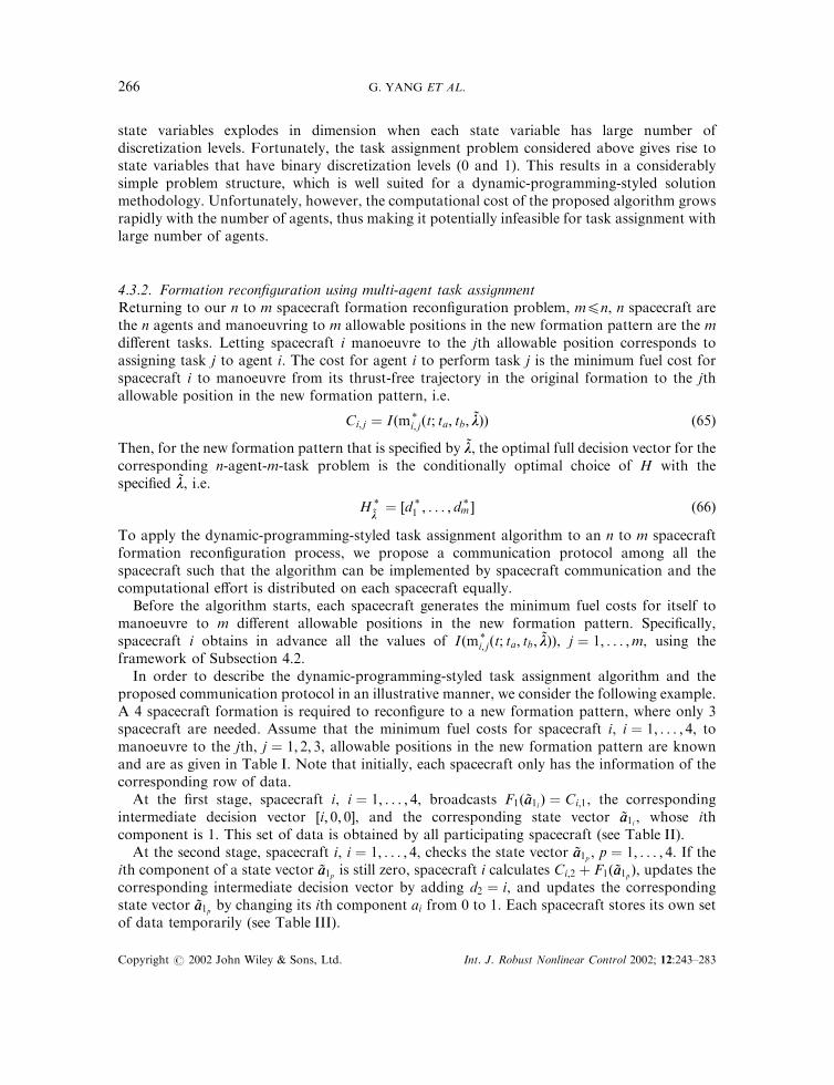
state variables explodes in dimension when each state variable has large number ofdiscretization levels. Fortunately, the task assignment problem considered above gives rise tostate variables that have binary discretization levels (0 and 1). This results in a considerablysimple problem structure, which is well suited for a dynamic-programming-styled solutionmethodology. Unfortunately, however, the computational cost of the proposed algorithm growsrapidly with the number of agents, thus making it potentially infeasible for task assignment withlarge number of agents.

4.3.2. Formation reconfiguration using multi-agent task assignmentReturning to our n to m spacecraft formation reconfiguration problem, m4n, n spacecraft arethe n agents and manoeuvring to m allowable positions in the new formation pattern are the mdifferent tasks. Letting spacecraft i manoeuvre to the jth allowable position corresponds toassigning task j to agent i. The cost for agent i to perform task j is the minimum fuel cost forspacecraft i to manoeuvre from its thrust-free trajectory in the original formation to the jthallowable position in the new formation pattern, i.e.

Ci; j ¼ Iðm*i; jðt; ta; tb; *llÞÞ ð65Þ

Then, for the new formation pattern that is specified by *ll, the optimal full decision vector for thecorresponding n-agent-m-task problem is the conditionally optimal choice of H with thespecified *ll, i.e.

H **ll¼ ½d *

1 ; . . . ; d*m � ð66Þ

To apply the dynamic-programming-styled task assignment algorithm to an n to m spacecraftformation reconfiguration process, we propose a communication protocol among all thespacecraft such that the algorithm can be implemented by spacecraft communication and thecomputational effort is distributed on each spacecraft equally.

Before the algorithm starts, each spacecraft generates the minimum fuel costs for itself tomanoeuvre to m different allowable positions in the new formation pattern. Specifically,spacecraft i obtains in advance all the values of Iðm*

i; jðt; ta; tb; *llÞÞ, j ¼ 1; . . . ;m, using theframework of Subsection 4.2.

In order to describe the dynamic-programming-styled task assignment algorithm and theproposed communication protocol in an illustrative manner, we consider the following example.A 4 spacecraft formation is required to reconfigure to a new formation pattern, where only 3spacecraft are needed. Assume that the minimum fuel costs for spacecraft i, i ¼ 1; . . . ; 4, tomanoeuvre to the jth, j ¼ 1; 2; 3, allowable positions in the new formation pattern are knownand are as given in Table I. Note that initially, each spacecraft only has the information of thecorresponding row of data.

At the first stage, spacecraft i, i ¼ 1; . . . ; 4, broadcasts F1ð *aa1i Þ ¼ Ci;1, the correspondingintermediate decision vector ½i; 0; 0�, and the corresponding state vector *aa1i , whose ithcomponent is 1. This set of data is obtained by all participating spacecraft (see Table II).

At the second stage, spacecraft i, i ¼ 1; . . . ; 4, checks the state vector *aa1p , p ¼ 1; . . . ; 4. If theith component of a state vector *aa1p is still zero, spacecraft i calculates Ci;2 þ F1ð *aa1pÞ, updates thecorresponding intermediate decision vector by adding d2 ¼ i, and updates the correspondingstate vector *aa1p by changing its ith component ai from 0 to 1. Each spacecraft stores its own setof data temporarily (see Table III).

G. YANG ET AL.266


Next, spacecraft 1 broadcasts C1;2 þ F1ð *aa12Þ ¼ 11:3 with the corresponding state vector½1; 1; 0; 0�, C1;2 þ F1ð *aa13 Þ ¼ 9:7 with the corresponding state vector ½1; 0; 1; 0�, and C1;2þF1ð *aa14 Þ ¼ 11:4 with the corresponding state vector ½1; 0; 0; 1�. When the other spacecraft receivethis data, each of them checks whether there is a match for some state vectors with its own set oftemporarily stored data. If there is a match for a particular state vector, a comparison is madebetween the corresponding values of Ci;2 þ F1ð *aa1pÞ, where one of these is from the spacecraft’sown set of temporarily stored data and the other is received from spacecraft 1. If the value fromthe spacecraft’s own set of temporarily stored data is greater than or equal to the value that isreceived from spacecraft 1, the spacecraft deletes the stored value of Ci;2 þ F1ð *aa1p Þ and the

Table I. Formation reconfiguration fuel cost data.

Ci;j ¼ Iðm*i;jðt; ta; tb; *llÞÞ j ¼ 1 j ¼ 2 j ¼ 3

i ¼ 1 6.1 3.2 2.2i ¼ 2 8.1 5.8 3.0i ¼ 3 6.5 7.4 8.1i ¼ 4 8.2 8.9 7.0

Table II. Data broadcast at stage 1.

Broadcast F1ð *aa1p Þ ½d1; 0; 0� *aa1p

Spacecraft 1 F1ð *aa11 Þ ¼ C1;1 ¼ 6:1 [1,0,0] *aa11 ¼ ½1; 0; 0; 0�Spacecraft 2 F1ð *aa12 Þ ¼ C2;1 ¼ 8:1 [2,0,0] *aa12 ¼ ½0; 1; 0; 0�Spacecraft 3 F1ð *aa13 Þ ¼ C3;1 ¼ 6:5 [3,0,0] *aa13 ¼ ½0; 0; 1; 0�Spacecraft 4 F1ð *aa14 Þ ¼ C4;1 ¼ 8:2 [4,0,0] *aa14 ¼ ½0; 0; 0; 1�

Table III. Intermediate data set at stage 2.

Ci;2 þ F1ð *aa1p Þ ½d1; d2; 0� Dð *aa1p ; d2Þ

Spacecraft 1 C1;2 þ F1ð *aa12 Þ ¼ 11:3 [2, 1, 0] [1,1,0,0]C1;2 þ F1ð *aa13 Þ ¼ 9:7 [3, 1, 0] [1,0,1,0]C1;2 þ F1ð *aa14 Þ ¼ 11:4 [4, 1, 0] [1,0,0,1]






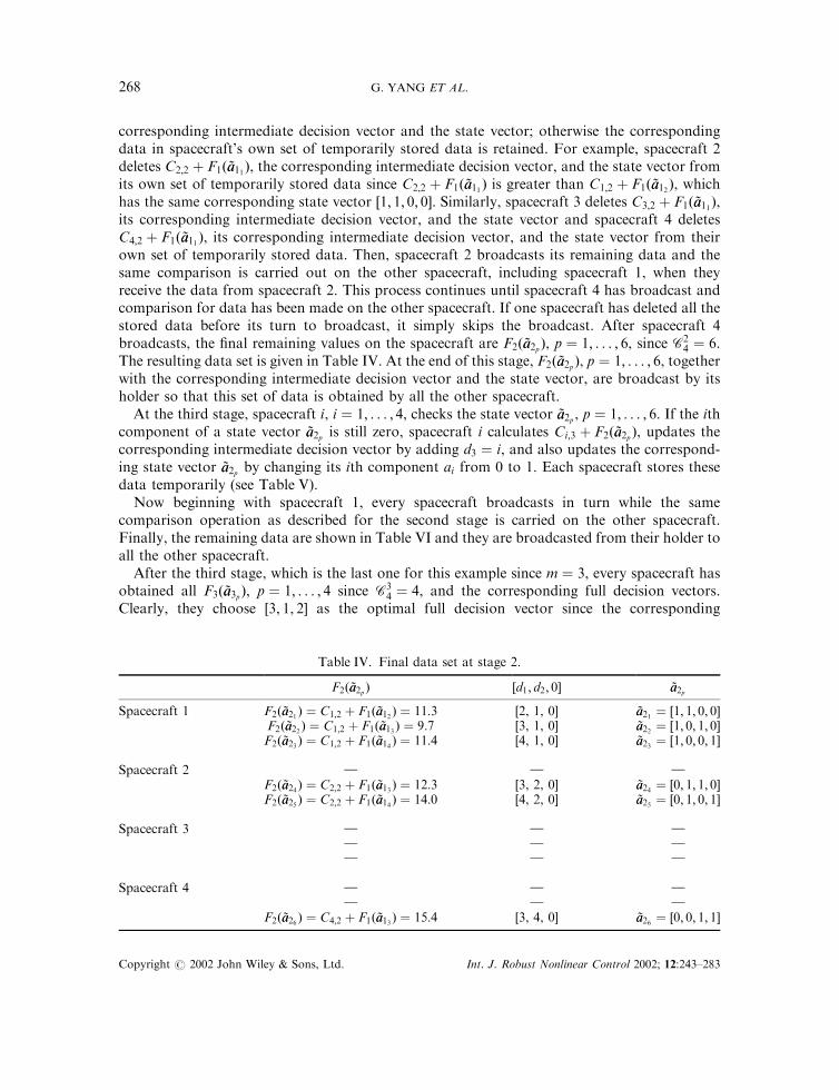
corresponding intermediate decision vector and the state vector; otherwise the correspondingdata in spacecraft’s own set of temporarily stored data is retained. For example, spacecraft 2deletes C2;2 þ F1ð *aa11Þ, the corresponding intermediate decision vector, and the state vector fromits own set of temporarily stored data since C2;2 þ F1ð *aa11 Þ is greater than C1;2 þ F1ð *aa12Þ, whichhas the same corresponding state vector ½1; 1; 0; 0�. Similarly, spacecraft 3 deletes C3;2 þ F1ð *aa11Þ,its corresponding intermediate decision vector, and the state vector and spacecraft 4 deletesC4;2 þ F1ð *aa11 Þ, its corresponding intermediate decision vector, and the state vector from theirown set of temporarily stored data. Then, spacecraft 2 broadcasts its remaining data and thesame comparison is carried out on the other spacecraft, including spacecraft 1, when theyreceive the data from spacecraft 2. This process continues until spacecraft 4 has broadcast andcomparison for data has been made on the other spacecraft. If one spacecraft has deleted all thestored data before its turn to broadcast, it simply skips the broadcast. After spacecraft 4broadcasts, the final remaining values on the spacecraft are F2ð *aa2pÞ, p ¼ 1; . . . ; 6, since C2

4 ¼ 6.The resulting data set is given in Table IV. At the end of this stage, F2ð *aa2p Þ, p ¼ 1; . . . ; 6, togetherwith the corresponding intermediate decision vector and the state vector, are broadcast by itsholder so that this set of data is obtained by all the other spacecraft.

At the third stage, spacecraft i, i ¼ 1; . . . ; 4, checks the state vector *aa2p , p ¼ 1; . . . ; 6. If the ithcomponent of a state vector *aa2p is still zero, spacecraft i calculates Ci;3 þ F2ð *aa2p Þ, updates thecorresponding intermediate decision vector by adding d3 ¼ i, and also updates the correspond-ing state vector *aa2p by changing its ith component ai from 0 to 1. Each spacecraft stores thesedata temporarily (see Table V).

Now beginning with spacecraft 1, every spacecraft broadcasts in turn while the samecomparison operation as described for the second stage is carried on the other spacecraft.Finally, the remaining data are shown in Table VI and they are broadcasted from their holder toall the other spacecraft.

After the third stage, which is the last one for this example since m ¼ 3, every spacecraft hasobtained all F3ð *aa3pÞ, p ¼ 1; . . . ; 4 since C3

4 ¼ 4, and the corresponding full decision vectors.Clearly, they choose [3, 1, 2] as the optimal full decision vector since the corresponding

Table IV. Final data set at stage 2.

F2ð *aa2p Þ ½d1; d2; 0� *aa2p

Spacecraft 1 F2ð *aa21 Þ ¼ C1;2 þ F1ð *aa12 Þ ¼ 11:3 [2, 1, 0] *aa21 ¼ ½1; 1; 0; 0�F2ð *aa22 Þ ¼ C1;2 þ F1ð *aa13 Þ ¼ 9:7 [3, 1, 0] *aa22 ¼ ½1; 0; 1; 0�F2ð *aa23 Þ ¼ C1;2 þ F1ð *aa14 Þ ¼ 11:4 [4, 1, 0] *aa23 ¼ ½1; 0; 0; 1�

Spacecraft 2 } } }F2ð *aa24 Þ ¼ C2;2 þ F1ð *aa13 Þ ¼ 12:3 [3, 2, 0] *aa24 ¼ ½0; 1; 1; 0�F2ð *aa25 Þ ¼ C2;2 þ F1ð *aa14 Þ ¼ 14:0 [4, 2, 0] *aa25 ¼ ½0; 1; 0; 1�

Spacecraft 3 } } }} } }} } }

Spacecraft 4 } } }} } }

F2ð *aa26 Þ ¼ C4;2 þ F1ð *aa13 Þ ¼ 15:4 [3, 4, 0] *aa26 ¼ ½0; 0; 1; 1�

G. YANG ET AL.268


F3ð *aa31 Þ ¼ 12:7 is the minimum total fuel cost. Thus, by communicating with each other, all thespacecraft can reach an agreement for the optimal decision that spacecraft 3 manoeuvres to the1st allowable position, spacecraft 1 manoeuvres to the 2nd allowable position, and spacecraft 2manoeuvres to the 3rd allowable position in the new formation pattern while spacecraft 4remains in its thrust-free trajectory in the original formation. If the new formation pattern isspecified by *ll, then H *

*ll¼ ½3; 1; 2�. Finally, the total fuel cost for IT ðM* ðt;H *

*ll; %TTm; *llÞÞ is

IT ðM* ðt;H **ll; %TTm; *llÞÞ ¼ 12:7.

Table V. Intermediate datat set at stage 3.

Ci;3 þ F2ð *aa2p Þ ½d1; d2; d3� Dð *aa2p ; d3Þ





Table VI. Final data set at stage 3.

F3ð *aa3p Þ ½d1; d2; d3� *aa3p

Spacecraft 1 } } }} } }} } }

Spacecraft 2 F3ð *aa31 Þ ¼ C2;3 þ F2ð *aa22 Þ ¼ 12:7 [3, 1, 2] *aa31 ¼ ½1; 1; 1; 0�F3ð *aa32 Þ ¼ C2;3 þ F2ð *aa23 Þ ¼ 14:4 [4, 1, 2] *aa32 ¼ ½1; 1; 0; 1�F3ð *aa33 Þ ¼ C2;3 þ F2ð *aa26 Þ ¼ 18:4 [3, 4, 2] *aa33 ¼ ½0; 1; 1; 1�

Spacecraft 3 } } }} } }} } }

Spacecraft 4 } } }F3ð *aa34 Þ ¼ C4;3 þ F2ð *aa22 Þ ¼ 16:7 [3, 1, 4] *aa34 ¼ ½1; 0; 1; 1�

} } }



Remark 4.3In the spirit of Morton et al. [31], the minimization of the total fuel cost for formationreconfiguration subject to an equalized fuel use by the spacecraft in formation can beaccomplished by modifying Ci; j , i ¼ 1; . . . ; n and j ¼ 1; . . . ;m, in (65) to include a factor thatweighs the remaining fuel on-board of the spacecraft Si, i ¼ 1; . . . ; n.

Remark 4.4The aforementioned communication protocol is characterized by a distributed implementationof the assignment algorithm and may necessitate a large amount of data communicationthroughout the decision process. Generally, for an n-agent-n-task assignment problem, there areat most (i.e., worst case) ðnþ 2Þ2n�1 floating-point data strings and ðnþ 2Þ2n�1 integer datastrings to be communicated among agents. In an alternative communication strategy, eachagent can broadcast its own initial data set to all the other agents so that all agents obtain thefull set of initial data (i.e. Table I). Next, all agents may execute the assignment algorithm of thissubsection in parallel and independently. At the successful termination of the algorithm, allagents broadcast and cross check their results. The overall computational requirement of thisimplementation is n times larger (thus, potentially, the total computation time may be n timeslonger) than that of the aforementioned distributed implementation. However, this commu-nication strategy significantly reduces the total amount of data communication to about n2 þ nfloating-point data strings and n integer data strings.

4.4. Genetic algorithm

Finally, we address the problem of the search for optimal *ll* 2 *LL such thatIT ðM* ðt;H *

*ll *; %TTm; *ll* ÞÞ is smaller than (or at worst equal to) IT ðM* ðt;H *

*ll; %TTm; *llÞÞ, which results

from any other choice of *ll 2 *LL. Unfortunately, an explicit relationship between the input *ll andthe output IT ðM* ðt;H *

*ll; %TTm; *llÞÞ is unknown for this optimization problem. This eliminates the

possibility of addressing this problem using the calculus-based optimization techniques, whichrely on the existence of the derivative of IT ðM* ðt;H *

*ll; %TTm; *llÞÞ with respect to *ll.

Genetic algorithm (GA) has been widely proven for its efficacy in black-box optimization [42–46]. Thus, in this paper, we adopt GA to search for *ll* . We briefly note that GA is a searchalgorithm that uses random selection as a tool to guide a highly exploitative search through acoding of the parameter space. However, we emphasize that in GA randomized search does notnecessarily imply directionless search. Specifically, GA is directed by the evolutionary rule of thenature in its search for the optimal. In the sequel, we briefly review the basic aspects of GAutilized in this paper, viz. binary coding, Roulette Wheel selection, two-point crossover, jump-creep mutation, elitism, and population re-initialization. See References [42–44] for a detailedexposition of GA.

In this paper, Li, the domain of li, i ¼ 1; . . . ; k, is assumed to be a continuous boundedinterval. We use a 32-bit binary coding to discretize Li to ensure sufficient precision. Thus, agene string of total k� 32-bit length is the unique binary code representation for a particular*ll ¼ ½l1; . . . ; lk� 2 *LL. The k� 32-bit gene string length is also called the parameter length or thechromosome length.

Let N denote the population size, which is the total number of gene strings in one generation.Then, we generate the first generation of N gene strings randomly such that their decoded

G. YANG ET AL.270


representations of *ll are uniformly distributed in *LL. Next, starting from the first generation ofgene strings, GA continues the random selection of gene strings such that the gene strings ofhigher fitness values have a greater probability of selection. The selected gene strings producenew gene strings such that the good genetic information, which is likely to provide higher fitnessvalues, is passed to the next generation whereas the bad genetic information, which causes lowerfitness values, is filtered out after several generations of gene selection. Based on the survival-of-the-fittest mechanism, this evolutionary process drives the whole population to converge to thegene strings of high fitness values.

Specifically, to select good gene strings from a current generation, we define the fitness valuegðxiÞ of a k� 32-bit gene string xi, i ¼ 1; . . . ;N, as

gðxiÞ ¼4 �IT ðM* ðt;H *

*lli; %TTm; *lliÞÞ; i ¼ 1; . . . ;N ð67Þ

where xi is a k� 32-bit coded representation of *lli. This definition ensures that a higher fitnessvalue corresponds to a lower IT ðM* ðt;H *

*ll; %TTm; *ll; ÞÞ.

Next, a Roulette Wheel selection scheme is used for selecting the parent gene strings from acurrent generation of gene strings. In particular, for one generation of gene strings, let gmax andgmin represent the maximum and minimum fitness values, respectively. Next, define

Gi ¼4gðxiÞ � gmin þ 0:01ðgmax � gminÞ ð68Þ

In addition, let R0 ¼4 0 and using (68) define

Ri ¼4Xi

j¼1

Gj ; i ¼ 1; . . . ;N ð69Þ

Note that the length of the interval ½Rði�1Þ;Ri�, i ¼ 1; . . . ;N, is linearly dependent on the fitnessvalue gðxiÞ, i.e. a greater gðxiÞ corresponds to a larger interval ½Rði�1Þ;Ri�. Next, we generate anumber uniformly at random in the range ð0;RNÞ and if it falls into the range ½Rði�1Þ;RiÞ then weselect xi as a parent.

Suppose we have obtained two parent gene strings, then a two-point crossover happens whenp1 > pc, where p1 is a randomly generated number according to uniform distribution on ½0; 1�and pc 2 ½0; 1� is computed adaptively using [47]

pc ¼

gmax � gðx0iÞgmax � %gg

; %gg4gðx0iÞ

1; gðx0iÞ5%gg

8><>: ð70Þ

where gðx0iÞ is the better fitness value from the two parent strings and %gg is the average fitnessvalue for the whole generation. In the crossover operation, two integers l1 and l2, which arecalled crossover positions, are selected uniformly at random from f1; . . . ; k� 32g. The bitsbetween the two selected crossover positions are exchanged between the two parent strings togenerate two new offsprings.

The mutation operation follows crossover if p2 > pm, where p2 is a randomly generatednumber according to uniform distribution on ½0; 1� and pm 2 ½0; 1� is computed



adaptively using [47]

pm ¼

gmax � gðxiÞgmax � %gg

; %gg4gðxiÞ

1; gðxiÞ5%gg

8><>: ð71Þ

where gðxiÞ is the fitness value of gene string xi and %gg is the average fitness value for the wholegeneration. First, in jump mutation a bit is chosen uniformly at random from f1; . . . ; k� 32gand its state is changed from 0 to 1 or vice versa. Next, in creep mutation, we perturb *llcorresponding to a gene string by a small amount d*ll such that ð*llþ d*llÞ 2 *LL, and then codeð*llþ d*llÞ to a new gene string. This bit-wise jump mutation followed by creep mutation hasshowed satisfactory result in our simulation.

In each generation, we leave the gene string having the best fitness value unchanged andpropagate it to the next generation. This operation, which is termed as elitism, guarantees non-decreasing best fitness value in successive generations.

To ensure fast monotone increase of the best fitness value, we use the population re-initialization when the search is considered to be trapped in a local minimum. Specifically, thebest fitness value of each generation is recorded, and the standard deviation (s) of the bestfitness value of the latest s generations, sðsÞ, is used as the criterion for whether or not GAsearch is trapped in a local minimum. We choose two positive integers s1 and s2, s15s2, and asmall positive real number e. If sðs1Þ5e, we reinitialize the population randomly in theneighborhood of the current best individual to accelerate the GA search. If sðs2Þ5e, we considerthe GA search to be trapped in a local minimum and reinitialize the gene strings randomly in thewhole search space *LL while the gene string with the best fitness value is kept. If the populationhas been reinitialized in the whole search space for several times while there is no furtherimprovement in the best fitness value among the population, we consider the highest fitnessvalue has been reached. Then, the decoded value of best gene string, which has the highestfitness value, is considered to be *ll* .

5. ILLUSTRATIVE NUMERICAL EXAMPLES

In this section, we provide two illustrative numerical examples to demonstrate the proposed fueloptimal multiple spacecraft formation reconfiguration framework. The problem data forsimulating the fuel optimal multiple spacecraft formation reconfiguration algorithm is adoptedfrom Reference [9]. Specifically, each spacecraft in the initial formation is assumed to have anequal mass M ¼ 77 kg and a total power input P ¼ 100W for its VSI propulsion system, whichis assumed to have 10 percent efficiency. An imaginary leader spacecraft is assumed to be in aKeplerian circular Earth orbit with radius 7178 km, which corresponds to an orbital periodTI ¼ 1:681 h. For each numerical example, the length of the formation reconfigurationmanoeuvre time interval ½ta; tb� is assumed to be TI, i.e. tb ¼ ta þ TI. Finally, for GA-basedparameter optimization, we used the population size N ¼ 50.

Example 5.1In this example, we assume that initially one spacecraft is coasting near by a cluster of 5spacecraft as shown in Figure 6(a). The initial spacecraft formation pattern consists of threeprimary formation orbits with the initial thrust free periodic trajectories of spacecraft i ¼

G. YANG ET AL.272


1; . . . ; 6 given by

xSi ðtÞ ¼ �2vy0o

cos ðoðt� taÞ þ yþ biÞ þ XC

ySi ðtÞ ¼vy0o

sin ðoðt� taÞ þ yþ biÞ

zSi ðtÞ ¼ z0 cos ðoðt� taÞ þ yþ biÞ þvz0o

sin ðoðt� taÞ þ yþ biÞ ð72Þ

where o ¼ 1:038� 10�3 rad=s is the orbital angular velocity of the imaginary space-craft and y ¼ p=8. In particular, spacecraft 1, 2, and 3 are distributed on the primaryformation orbit specified by (72) with ðXC; vy0 ; vz0 ; z0Þ ¼ ð0;�150om=s;�150om=s; 0Þ.Furthermore, for spacecraft 1, 2, and 3 we are given b1 ¼ 0, b2 ¼ 2p=3, andb3 ¼ 4p=3, respectively. Similarly, spacecraft 4 and 5 are distributed on the primaryformation orbit specified by (72) with ðXC; vy0 ; vz0 ; z0Þ ¼ ð0;�300om=s;�300om=s; 0Þ.Furthermore, for spacecraft 4 and 5 we are given b4 ¼ 0 and b5 ¼ 2p=3, res-pectively. Finally, spacecraft 6, which is coasting near by the cluster of 5 spacecraft,is on the primary formation orbit specified by (72) with ðXC; vy0 ; vz0 ; z0Þ ¼ ð�1000 m; 0; 0; 0Þand b6 ¼ 0, which reduces to a point at ð�1000 m; 0; 0Þ in the fxI; yI; zIg coordinateframe.

Next, the 6 spacecraft are required to combine into one cluster so that a Y-shaped formationpattern can be formed as shown in Figure 6(b), where XC is yet to be determined. Specifically,the allowable positions in the new formation pattern are distributed on two primary formation

Figure 6. (a) Formation pattern at ta; (b) desired formation pattern: Example 1 ($ denotes the imaginaryleader spacecraft).



orbits specified by

xPiðtÞ ¼ � 2

vy0o

cos ðoðt� tbÞ þ yP þ biÞ þ XC

yPiðtÞ ¼

vy0o

sin ðoðt� tbÞ þ yP þ biÞ

zPiðtÞ ¼ z0 cos ðoðt� tbÞ þ yP þ biÞ þ

vz0o

sin ðoðt� tbÞ þ yP þ biÞ ð73Þ

In particular, the allowable positions 1, 2, and 3 in the new formation pattern are dis-tributed on the primary formation orbit specified by (73) with ðXC; vy0 ; vz0 ; z0Þ ¼ðXC;�150om=s;�150om=s; 0Þ. Furthermore, for the allowable positions 1, 2, and 3 in thenew formation pattern b1 ¼ 0, b2 ¼ 2p=3, and b3 ¼ 4p=3, respectively. Similarly, the allowablepositions 4, 5, and 6 in the new formation pattern are distributed on the primary formation orbitspecified by (73) with ðXC; vy0 ; vz0 ; z0Þ ¼ ðXC;�300om=s;�300om=s; 0Þ. Furthermore, for theallowable positions 4, 5, and 6 in the new formation pattern b4 ¼ 0, b5 ¼ 2p=3, and b6 ¼ 4p=3,respectively. Note that in (73) XC and yP are allowed to be selected freely from ½�1000; 1000�mand ½0; 2p=3� rad, respectively.

The optimization algorithm described in Section 4 yields X *C ¼ �182:212 m and y*

P ¼0:423 rad for the new formation pattern. Note that the value of X *

C indicates that the center ofthe initial cluster of 5 spacecraft moves from the origin of the fxI; yI; zIg coordinate frame,which is the location of the imaginary leader spacecraft, closer to the initial location ofspacecraft 6 so as to form the new formation pattern at an intermediate location. Thus, the fuelburden of spacecraft 6 is shared by the other 5 spacecraft even as the total fuel consumption isminimized. The fuel cost for spacecraft Si, i ¼ 1; . . . ; 6, to relocate to the allowable location Pj,j ¼ 1; . . . ; 6, in the new formation pattern specified by X *

C and y*P is given in Table VII. The

dynamic-programming-styled task assignment algorithm yields H * ¼ ½1; 2; 6; 4; 5; 3� to be theoptimal spacecraft permutation in the new formation pattern specified by X *

C and y*P . It is

interesting to observe that the fuel optimal multiple spacecraft formation reconfigurationalgorithm relocates spacecraft 3, which was initially on the inner primary formation orbit, to the6th allowable position in the new formation pattern, which is on the outer primary formationorbit. In addition, spacecraft 6 joins the spacecraft cluster at the 3rd allowable position in thenew formation pattern, which is on the inner primary formation orbit, instead of relocating to avacant position in the initial formation pattern, which was on the outer primary formationorbit. Figure 7 gives the fuel optimal spacecraft formation reconfiguration trajectories for all the6 spacecraft. Furthermore, Figure 8 provides the thrust histories for all the 6 spacecraft. Finally,the total fuel mass consumed by each spacecraft is listed in Table VIII.

Table VII. Formation reconfiguration fuel cost data: Example 1 (unit: 10�3 kg).

Iðm*i; jðt; ta; tb; *ll

* ÞÞ j ¼ 1 j ¼ 2 j ¼ 3 j ¼ 4 j ¼ 5 j ¼ 6

i ¼ 1 0.0896 9.2394 8.4961 3.5600 21.7365 19.7880i ¼ 2 10.1422 0.0875 9.2134 23.1259 2.8933 20.6833i ¼ 3 9.5552 8.4114 0.1051 22.4091 19.9984 2.9238i ¼ 4 2.9218 21.9044 20.3924 0.0933 37.9353 34.4493i ¼ 5 22.8674 3.4408 21.6673 39.0655 0.0892 36.0802i ¼ 6 3.5094 6.2365 4.8546 11.4744 16.8056 13.5798

G. YANG ET AL.274


Figure 7. Relative position. (a) xI, (b) yI, (c) zI: Example 1.



Figure 8. Control input. (a) ux, (b) uy, (c) uz: Example 1.

G. YANG ET AL.276


Example 5.2In this example, we assume that initially 6 spacecraft are distributed on two concentric primaryformation orbits as shown in Figure 9(a). The initial spacecraft formation consists of twoprimary formation orbits with the initial thrust free periodic trajectories of spacecraft Si,i ¼ 1; . . . ; 6, given by (72), with y ¼ p. In particular, spacecraft 1, 2, and 3 are distributed on theprimary formation orbit specified by (72) with ðXC; vy0 ; vz0 ; z0Þ ¼ ð0;�150om=s; 0; 0Þ. Further-more, for spacecraft 1, 2, and 3 we are given b1 ¼ 0, b2 ¼ 2p=3, and b3 ¼ 4p=3, respectively.Similarly, spacecraft 4, 5, and 6 are distributed on the primary formation orbit specified by (72)with ðXC; vy0 ; vz0 ; z0Þ ¼ ð0;�300om=s; 0; 0Þ. Furthermore, for spacecraft 4, 5, and 6 we are givenb4 ¼ 0, b5 ¼ 2p=3, and b6 ¼ 4p=3, respectively.

Table VIII. Spacecraft fuel consumption with optimal permutation: Example 1

Spacecraft i i ¼ 1 i ¼ 2 i ¼ 3 i ¼ 4 i ¼ 5 i ¼ 6 Total

Unit: 10�3 kg 0.0896 0.0875 2.9238 0.0933 0.0892 4.8546 8.1380

Figure 9. (a) Formation pattern at ta; (b) desired formation pattern: Example 2 ($ denotes the imaginaryleader spacecraft).

Table IX. Formation reconfiguration fuel cost data: Example 2 (unit: 10�3 kg).

Iðm*i; jðt; ta; tb; *ll

* ÞÞ j ¼ 1 j ¼ 2 j ¼ 3 j ¼ 4

i ¼ 1 7.1306 8.2036 8.7105 7.1506i ¼ 2 8.2673 14.2557 14.1634 7.6879i ¼ 3 7.0501 12.4297 15.3806 9.5138i ¼ 4 9.0948 7.0934 6.9853 8.4996i ¼ 5 10.8334 18.6632 17.3568 9.0399i ¼ 6 8.3990 15.0112 19.7912 12.6918



Figure 10. Relative position (a) xI, (b) yI, (c) zI: Example 2.

G. YANG ET AL.278


Figure 11. Control input. (a) ux, (b) uy, (c) uz: Example 2.



Next, 4 spacecraft are required to form a new formation pattern that has four allowablepositions distributed on one primary formation orbit (see Figure 9(b)) specified by (73) withðXC; vy0 ; vz0 ; z0Þ ¼ ð1200 m;�200om=s;�200om=s; 0Þ. Furthermore, for the allowable position1, 2, 3, and 4 in the new formation pattern b1 ¼ 0, b2 ¼ p=2, b3 ¼ p, and b4 ¼ 3p=2,respectively. In this example, yP in (73) is allowed to be selected freely from ½0;p=2� rad.

The optimization algorithm described in Section 4 yields y*P ¼ 0:588 rad for the new

formation pattern. The fuel cost for spacecraft Si, i ¼ 1; . . . ; 6, to relocate to the allowablelocation Pj, j ¼ 1; . . . ; 4, in the new formation pattern specified by y*

P is given in Table IX. Thedynamic-programming-styled task assignment algorithm yields H * ¼ ½3; 1; 4; 2� to be theoptimal spacecraft permutation in the new formation pattern specified by y*

P . Note that H *

indicates that spacecraft 1, 2, 3, and 4 participate in the new 4 spacecraft formation whilespacecraft 5 and 6 continue along their initial thrust free periodic trajectories. Figure 10 givesthe fuel optimal spacecraft formation reconfiguration trajectories for spacecraft 1, 2, 3, and 4 aswell as the unaltered thrust free trajectories for spacecraft 5 and 6. Furthermore, Figure 11provides the thrust histories for all the 6 spacecraft. Finally, the total fuel mass consumed byeach spacecraft is given in Table X.

Remark 5.1For the above two examples, utilizing the spherical Earth model leading to nonlinear relativedynamics of spacecraft, we validate our fuel optimal formation reconfiguration algorithm bysimulation. Specifically, we apply the optimal thrust program for spacecraft formation

Table X. Spacecraft fuel consumption with optimal permutation: Example 2.


Unit: 10�3 kg 8.2036 7.6879 7.0501 6.9853 0.0 0.0 29.9269

Figure 12. Target position error under nonlinear simulation: (a) Example 1, (b) Example 2.

G. YANG ET AL.280


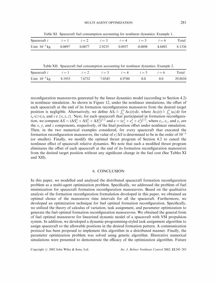
reconfiguration manoeuvres generated by the linear dynamics model (according to Section 4.2)in nonlinear simulation. As shown in Figure 12, under the nonlinear simulations, the offset ofeach spacecraft at the end of its formation reconfiguration manoeuvre from the desired targetposition is negligible. Alternatively, we define DSi ¼

4 R tbtaDviðtÞ dt, where DviðtÞ ¼

4 R t

tajui j dt for

ta4t4tb and i 2 fx; y; zg. Next, for each spacecraft that participated in formation reconfigura-tion, we compute DS ¼ ðDS2

x þ DS2y þ DS2

z Þ1=2 and e ¼ ðe2x þ e2y þ e2zÞ

1=2, where ex, ey, and ez arethe x, y, and z components, respectively, of the final position offset under nonlinear simulation.Then, in the two numerical examples considered, for every spacecraft that executed theformation reconfiguration manoeuvre, the value of e=DS is determined to be in the order of 10�3

(or smaller). Finally, we modify the optimal thrust program of Section 4.2 to cancel thenonlinear effect of spacecraft relative dynamics. We note that such a modified thrust programeliminates the offset of each spacecraft at the end of its formation reconfiguration manoeuvrefrom the desired target position without any significant change in the fuel cost (See Tables XIand XII).

6. CONCLUSION

In this paper, we modelled and analysed the distributed spacecraft formation reconfigurationproblem as a multi-agent optimization problem. Specifically, we addressed the problem of fuelminimization for spacecraft formation reconfiguration manoeuvres. Based on the qualitativeanalysis of the formation reconfiguration formulation developed in this paper, we obtained anoptimal choice of the manoeuvre time intervals for all the spacecraft. Furthermore, wedeveloped an optimization technique for fuel optimal formation reconfiguration. Specifically,we utilized the theory of calculus of variation, task assignment, and parameter optimization togenerate the fuel optimal formation reconfiguration manoeuvres. We obtained the general formof fuel optimal manoeuvre for linearized dynamic model of a spacecraft with VSI propulsionsystem. In addition, we developed a dynamic-programming-styled task assignment algorithm toassign spacecraft to the allowable positions in the desired formation pattern. A communicationprotocol has been proposed to implement this algorithm in a distributed manner. Finally, theparameter optimization problem was solved using genetic algorithm. Illustrative numericalsimulations were presented to demonstrate the efficacy of the optimization algorithm. Future

Table XI. Spacecraft fuel consumption accounting for nonlinear dynamics: Example 1.


Unit: 10�3 kg 0.0897 0.0877 2.9235 0.0937 0.0898 4.8492 8.1336

Table XII. Spacecraft fuel consumption accounting for nonlinear dynamics: Example 2.


Unit: 10�3 kg 8.1953 7.6732 7.0345 6.9780 0.0 0.0 29.8810



work will advance the optimization algorithm to account for perturbation effects, non-circularorbits, and various constraints, e.g. spacecraft permutation constraints, spacecraft distanceconstraint to ensure collision avoidance, thrust magnitude constraint, etc.

ACKNOWLEDGEMENTS

Research supported in part by the National Aeronautics and Space Administration–GoddardSpace Flight Center under Grant NAG5-11365 with Dr. Jesse Leitner as the technical monitor;Air Force Research Laboratory–VACA, Wright Patterson AFB, OH, under an IPA Grant; AirForce Research Laboratory, Kirtland AFB, NM, under an STTR Grant F29601-99-C-0172with Mr. Ross Wainwright as the technical monitor; the Orbital Research Inc.; and the NASA/New York Space Grant Consortium under Grant 39555-6519.

REFERENCES

1. Hedrick JK, Tomizuka M, Varaiya P. Control issues in automated highway systems. IEEE Control SystemsMagazine 1994; 14:21–32.

2. Radio Technical Commission for Aeronautics, Final Report of RTCA Task Force 3: Free Flight Implementation.Tech. Rep. RTCA, Washington, DC, 1995.

3. Pappas G. et al., A next generation architecture for air traffic management systems. Proceedings of the IEEEConference on Decision and Control, San Diego, CA, 1997, 2405–2410.

4. Kang W, Xi N, Fitch O. Mobile robot tracking control in a perceptive frame. Proceedings of the SPIE, Boston, MA,1998.

5. Scientific Advisory Board, UAV technologies and combat operations, Tech. Rep. SAB-TR-96-01, United States AirForce, November 1996.

6. Robertson A, Corazzini T, How JP. Formation sensing and control technologies for a separated spacecraftinterferometer. Proceedings of the American Control Conference, Philadelphia, PA, 1998; 1574–1579.

7. Tomlin C, Pappas GJ, Sastry S. Conflict resolution for air traffic management: a case study in multi-agent hybridsystems. IEEE Transactions on Automatic Control 1998; 43:509–521.

8. Wang, PKC, Hadaegh FY. Coordination and control of multiple microspacecraft moving in formation. Journal ofAstronautical Science 1996; 44(3):315–355.

9. Available on the Web at http://www.vs.afrl.af.mil/factsheets/TechSat21.html and http://www.vs.afrl.af.mil/TechProgs/TechSat21/.

10. Proceedings of the Air Force Research Laboratory } Formation Flying and Micro-Propulsion Workshop, Lancaster,CA, 1998.

11. Bauer F et al. Satellite formation flying using an innovative autonomous control system (AUTOCON) environment.Proceedings of the AIAA Guidance, Navigation, and Control Conference, New Orleans, LA, 1997; 657–666.

12. Guinn JR. Autonomous navigation for the new millennium program earth orbiter 1 Mission. Proceedings of theAIAA Guidance, Navigation, and Control Conference, New Orleans, LA, 1997; 612–617.

13. Lau K et al. The new millennium formation flying optical interferometer. Proceedings of the AIAA Guidance,Navigation, and Control Conference, New Orleans, LA, 1997; 650–656.

14. Leitner J, Beck J, Bell K. Advanced guidance, navigation, and control for remote sensing. 1997, AIAA Paper.15. Sedwick RJ, Kong EMC, Miller DW. Exploiting orbital dynamics and micropropulsion for aperture synthesis using

distributed satellite system: applications to TechSat 21. Defense and Civil Programs Conference, Huntsville, AL,1998, AIAA Paper No. 98–5289.

16. Scientific Advisory Board, New World Vistas Air and Space Power for the 21st Century, 1995, http://ecs.rams.com/afosr/afr/sab/edu/text/any/afrtnwv.htm.

17. Hartman K, Weidow D, Hadaegh F. Management of guidance, navigation, and control technologies for spacecraftformations under the NASA cross-enterprise technology development program (CETDP). Proceedings of the FlightMechanics Symposium, Goddard Space Flight Center, Greenbelt, MD, 1999; 283–294.

18. Chao CC, Pollard JE, Janson SW. Dynamics and control of cluster orbits for distributed space missions. AAS/AIAASpace Flight Mechanics Meeting, 1999, Paper No. AAS99–126.

19. Chobotov VA (ed.) Orbital Mechanics. AIAA: Washington, DC, 1996; 31–33.20. Clohessy WH, Wiltshire RS. Terminal guidance system for satellite rendezvous. Journal of Aerospace Science, 1960;

27(9):653–658.

G. YANG ET AL.282


21. de Queiroz MS, Kapila V, Yan Q. Adaptive nonlinear control of multiple space craft formation flying. Journal ofGuidance, Control, and Dynamics 2000; 23:385–390.

22. Kapila V, Sparks AG, Buffington JM, Yan Q. Spacecraft formation flying:dynamics and control. Journal ofGuidance, Control, and Dynamics 2000; 23:561–564.

23. Redding DC, Adams NJ, Kubiak ET. Linear-quadratic stationkeeping for the STS orbiter. Journal of Guidance,Control, and Dynamics. 1989; 12(2):248–255.

24. Sabol C, Burns R, McLaughlin C. Formation flying design and evolution. Proceedings of the AAS/AIAA SpaceFlight Mechanics Meeting, Paper No. AAS 99–121, 1999.

25. Schaub H, Vadali SR, Junkins JL, Alfriend KT. Spacecraft formation flying control using mean orbit elements.Proceedings of the AAS Guidance and Control Conference, Paper No. 99–310, 1999.

26. Vassar RH, Sherwood RB. Formationkeeping for a pair of satellites in a circular orbit. Journal of Guidance, Control,and Dynamics 1985; 8(2):235–242.

27. Yan Q, Kapila V, Sparks AG. Pulse-based periodic control for spacecraft formulation flying. Proceedings of theAmerican Control Conference, Chicago, IL, June 2000; 374–378.

28. Hadaegh FY, Lu WM, Wang PC. Adaptive control of formation flying spacecraft for interferometry. Proceedings ofthe IFAC Conference on Large Scale Systems, Rio Patras, Greece, 1998; 97–102.

29. Yan Q, Yang G, Kapila V, de Queiroz MS. Nonlinear dynamics, trajectory generation, and adaptive control ofmultiple spacecraft in periodic relative orbits. Proceedings of the AAS Guidance and Control Conference, Paper No.00–013, Breckenridge, CO, 2000.

30. de Queiroz MS, Yan Q, Yang G, Kapila V. Global output feedback tracking control of spacecraft formation flyingwith parametric uncertainty. Proceedings of the IEEE Conference on Decision and Control, Phoenix, AZ, December1999; 584–589.

31. Morton B, Weininger N, Tierno JE. Collective management of satellite clusters. Proceedings of the AIAA Guidance,Navigation, and Control Conference, Portland, OR, August AIAA Paper No. 99–4267, 1999; 1576–1584.

32. Yan Q, Yang G, Kapila V, de Queiroz MS. Nonlinear dynamics and output feedback control of multiple spacecraftin elliptical orbits. Proceedings of the American Control Conference, Chicago, IL, June 2000; 839–843.

33. Yeh H-H, Sparks, AG. Geometry and control of satellite formations. Proceedings of the American ControlConference, Chicago, IL, June 2000; 384–388.

34. Kreyszig EW. Advanced Engineering Mathematics. Wiley: New York, NY, 1998.35. Hill PG, Peterson CR. Mechanics and Thermodynamics of Propulsion. Addison-Wesley: Reading, MA, 1992.36. Luenberger DG. Optimization by Vector Space Methods. Wiley: New York, NY, 1969.37. Kirk DE. Optimal Control Theory. Prentice-Hall: Englewood Cliffs, NJ, 1970.38. Pierre DA. Optimization Theory with Applications. Dover: New York, NY, 1986.39. Bellman R. Dynamic Programming. Princeton University Press: Princeton, NJ, 1957.40. Belegundu AD, Chandrapatla TR. Optimization Concepts and Application in Engineering. Prentice-Hall: Upper

Saddle River, NJ, 1999.41. Hillier FS, Lieberman GJ. Operations Research. Holden-Day Inc.: San Francisco, CA, 1974.42. Davis L. Handbook of Genetic Algorithms. Van Nostrand Reinhold: New York, NY, 1991.43. Goldberg DE. Genetic Algorithms in Search, Optimization, and Machine Learning. Addison-Wesley: New York, NY,

1989.44. Holland JH. Adaptation in Natural and Artificial Systems. University of Michigan Press: Ann Arbor, MI, 1975.45. Krishnakumar K. Micro-genetic algorithms for stationary and non-stationary function optimization. SPIE:

Intelligent Control and Adaptive Systems, Philadelphia, PA, vol. 1196, 1989; 289–296.46. Zalzala AMS, Fleming PJ. Genetic Algorithms in Engineering Systems. IEE Control Engineering Series, Vol. 55,

1997.47. Srinivas M, Patnaik LM. Adaptive probabilities of crossover and mutation in genetic algorithm. IEEE Transactions

on Systems, Man and Cybernetics 1994; 24(4):656–667.



Fuel optimal manoeuvres for multiple spacecraft formation reconfiguration using multi-agent...

Documents

Transcript of Fuel optimal manoeuvres for multiple spacecraft formation reconfiguration using multi-agent...