Chemical Engineering Science 64 (2009) 4040 -- 4050

Contents lists available at ScienceDirect

Chemical Engineering Science

journal homepage: www.e lsev ier .com/ locate /ces

Simulation of dense granular flows: Dynamics ofwall stress in silos

Riccardo Artoni∗, Andrea Santomaso, Paolo CanuDipartimento di Principi e Impianti di Ingegneria Chimica “I. Sorgato”, Università di Padova, Via Marzolo 9, 35100 Padova, Italy

A R T I C L E I N F O A B S T R A C T

Article history:Received 12 January 2009Received in revised form 11 May 2009Accepted 2 June 2009Available online 10 June 2009

Keywords:Dense granular flowsFluctuating energyStress field

A model to simulate the dense flow of granular materials is presented. It is based on continuum, pseudo-fluid approximation. Balance equations and constitutive relations account for fluctuations in the velocityfield, through the `granular temperature' concept. Partial wall slip is also allowed by means of a slip-lengthapproach. The model is applied to an industrial silo geometry, though not limited in its formulation toany geometry or flow configuration. It predicts realistic flow patterns, requiring quantitative validationwith detailed measurements. This work focuses on the prediction of the normal stress at the wall duringdischarge. Profiles closely match available correlations by Jannsen and Walker, including prediction ofpeak pressure where section changes. Connections with literature correlations together with a sensitivityanalysis provide clues to link model parameters to intrinsic material properties.

© 2009 Elsevier Ltd. All rights reserved.

1. Introduction

Dense flow of granular materials is a very common occurrence inseveral industrial chemical and related processes. Applications spanfrom operations expected to be elementary, like transport or dis-charge from storage silos, to more complex ones like moving beds,rotating ovens, mills, granulators, mixers, etc. Difficulties in predict-ing the flow of such material surprisingly persist, despite quite alarge amount of theoretical and semi-empirical studies. In this per-spective, advances in the prediction of stress and flow patterns ofthe material are preliminary to further design goals. Understandingthe stress distribution and the flow behavior of granular materialsin confined geometries has been a research subject for engineers,both from fundamental (Nedderman, 1992; Savage, 1998) and fromtechnological (Bohrnsen et al., 2004; Schulze, 2007) standpoints.

Already in the speculations of Bagnold (1954, 1966) on the flowof particulate materials, three regimes have been identified: (1) thekinetic, collisional regime which has been successfully studied bymeans of corrections of the kinetic theory of gases (Jenkins andSavage, 1983); (2) the quasistatic case, described by plasticity the-ories (Schofield and Wroth, 1968); and (3) the intermediate, denseflowing regime, in which energy is dissipated by inelastic collisionsand interparticle friction (MiDi, 2004).

Among the three regimes, undoubtedly the dense flow is themostpervasive in the process industry. We already contributed with both

∗ Corresponding author.E-mail address: riccardo.artoni@unipd.it (R. Artoni).

0009-2509/$ - see front matter © 2009 Elsevier Ltd. All rights reserved.doi:10.1016/j.ces.2009.06.008

experimental (Santomaso and Canu, 2001; Santomaso et al., 2006)and theoretical (Strumendo and Canu, 2002) studies on the subject.Storage silos and hoppers are considered a reference for this regime,although many different configurations have been studied, as nicelycatalogued in the report of MiDi (2004). Prediction of the flow pat-terns in a silo is required to guarantee an effective use of the silovolume, preventing the formation of stagnant zones of material (dueto core flow and piping regimes) that affect the residence time dis-tribution of the stored material. The issue is relevant when the ma-terial can undergo physical of chemical transformations, changingits nature or applicative properties (Santomaso et al., 2006). In ad-dition, predicting the stress distribution in the flowing material isimportant to prevent (1) arching and flow stoppage, (2) failure ofthe wall structure, and (3) breakage and comminution of particlesdue to stress in the bulk.

At the present, two approaches are used in modeling granularflows: discrete and continuum. The first one, known as DEM (discreteelement method), models the dynamics of the medium at the parti-cle scale, applying force balances on each particle, possibly account-ing for interparticle friction, inelastic collisions, non-spherical andcohesive particles. These attempts date back to the work of Cundalland Strack (1979). Implementations may use different algorithms(Jean, 1999; Van Liedekerke et al., 2006) and computation strategies,and both commercial and open-source simulation softwares are alsoavailable (Renouf et al., 2004). Even if simulation capabilities aregrowing fast, because of both hardware and software evolution, fullsize simulations using real particles (and not virtual, much largerones) are still unachievable. On the other hand, DEM models mayprovide useful and realistic information on the micromechanics ofgranular material at a smaller scale.

R. Artoni et al. / Chemical Engineering Science 64 (2009) 4040 -- 4050 4041

On the larger, industrial scale, continuum models may be an al-ternative; the relation between velocity and stresses, i.e. the consti-tutive relation, has been treated with two approaches, specular in asense. The first is based on elasto-plastic (which describe the stress-rate of strain relationship via a yield surface, a plastic potential anda flow rule) or hypoplastic theories (which specify constitutive re-lations between stress tensor, its Jaumann derivative and the rateof strain, including the effect of void volume and granular skeleton)(Wu et al., 2007; Kolymbas, 2000), which are used to treat the ir-reversible deformation of granular solids. Alternatives are possiblederiving the constitutive relations from analogies with the behaviorof complex fluids, with the hypothesis that the granular material, in-trinsically multiphasic, can be treated as a pseudo-fluid with a suit-able reological behavior. Then, flow and stress distribution might besimulated like other fluids in suitably modified computational fluiddynamics codes, for arbitrary geometries and constitutive models(Artoni et al., 2007). Among the various rheologies proposed, the so-called hydrodynamic models (Savage, 1998; Bocquet et al., 2002),developed from analogies with the kinetic theory of gases, introducea second-order closure, taking into account the fluctuating part ofthe velocity field and its effects on the viscosity. Despite several at-tempts, a fully satisfactory description of granular flows in terms ofa pseudocontinuum is still lacking. Difficulties arise in the originalnature of granular materials, particularly with respect to their meso-scopic and dissipative nature, but also to the loss of continuity ofstress caused by the non-persistence of intergranular contacts.

In this work, we present a phenomenological hydrodynamicmodel, derived from considerations which are peculiar to the dense(and not gas-like) flow of granular materials, first of all the dissipa-tion of mechanical energy due to friction. The model is formulatedfor cohesionless, dry granular materials, very common in manyindustrial scale flows. Fine powders and polymeric materials likelyto accumulate charges and develop significant electrostatics effects,including tribocharging, are beyond the present scope. Because themodel treats the granular material as a pseudo-fluid, it can accountfor mixtures of granules of different nature or size, as long as thephenomenological parameter that describe the materials are deter-mined, the composition and particle size do not vary (in time andspace), additional mechanism not accounted in the model develop-ment becomes relevant (like drag of interstitial fluid or electrostaticinteractions).

The derivations of the equations, together with the constitutivechoices, are illustrated. The application of themodel is here restrictedto a complete silo geometry (bunker plus hopper) with the scope ofillustrating its capabilities in the solution of the stress and the veloc-ity fields. It is shown that the model correctly predicts both stressand velocity fields, a non-trivial task for the continuum approaches(Bohrnsen et al., 2004). The non-obvious issue of wall boundary con-ditions is also addressed and a partial slip model illustrated andapplied.

2. Model outline

Velocity fluctuations are a fundamental concept used in modelsfor the collisional, gas-like regime of granular flows, based on analo-gies with dense gases (Chapman and Cowling, 1991). The notionof granular temperature was introduced to summarize and quantifysuch fluctuations (Jenkins and Savage, 1983), i.e. � = 〈v2〉/3 , wherev is the fluctuating component of the velocity vector. In dense, slowflow of granular materials, even if the mechanisms of dissipation ofenergy are different from the collisional flow, yet velocity fluctua-tions are not negligible. The granular temperature can be assumedas a local measure of the dynamic flowability of the pseudo-fluid, ora local mobility.

Experiments have been done (Natarajan et al., 1995) to measuregranular temperature in vertical chute flows and to include � inmodels of dense granular flow (Savage, 1998; Losert et al., 2000;Bocquet et al., 2002; Strumendo and Canu, 2002). The model pre-sented here is based on conservation laws for the key quantities(mass, momentum and fluctuating energy) and the fundamentalmechanisms are described by constitutive laws relating the un-knowns variables v and �.

2.1. Conservation laws

In order to derive the general balance equations for mass, linearmomentum and translational kinetic energy for granular materials,the macroscopic space-time weighted balance equations have beenwritten as follows:

�t(�) + ∇ · (�v) = 0 (1)

�t(�v) + ∇ · (�vv) = −∇ · T + �g + tF (2)

�t[�(�T + ET )] + ∇ · [�(�T + ET )v]

= −∇ · (T · v + qT ) + �g · v − zT + tF · v + DTF (3)

Equations are based on Babi�c (1997) formulation, but the sign con-vention for the stress tensor and the energy flux has been changed.The meaning of symbols, where not intuitive, is reported in a singlelist at the end.

The balance equation for the angular momentum has been ne-glected, based on the assumption that Cosserat effects are negligiblein the absence of external couples, even if particles are known to rollsomehow at their scale, as demonstrated by Goddard (2008).

Moreover, in most dense, slow flow configurations the momen-tum transport arising from the coupling with the interstitial fluid,i.e. tF and DTF , can be neglected. Taking the product of v with Eq. (1),and considering the tensorial relation:

∇ · (T · v) − v · ∇ · T = T† : ∇v (4)

for the stress tensor T, the following equation can be obtained:

�t(��T ) + ∇ · (��T v) = −T† : ∇v − ∇ · qT − zT (5)

where the twomost significant terms for this study, qT and zT are ev-ident, i.e. the flux of energy and the its dissipation rate, respectively.

By means of the mentioned definition of granular temperature,�, the last equation rearranges to:

32�t(��) + 3

2∇ · (��v) = −T† : ∇v − ∇ · qT − zT (6)

Splitting the stress tensor T into its spherical (pI) and deviatoric (P)part, the linear momentum Eq. (1) simplifies to:

�t(�v) + ∇ · (�vv) = −∇p − ∇ ·P+ �g (7)

Assuming the stress tensor to be symmetric, as a consequence of theabsence of couple stresses and using the splitting of T, Eq. (6) can berewritten as:

32�t(��) + 3

2∇ · (��v) = −p∇ · v −P : ∇v − ∇ · qT − zT (8)

Finally, we assume that the flow is nearly incompressible, i.e.� ≈ const. This is perceived as a crucial issue. As argued by Artoniet al. (2007), allowing for dilatancy effects by assuming a compress-ible pseudo-fluid would be a major advancement both for physicalconsistency of the model and for its practical application. As a mat-ter of fact, in several dense flow configuration the solid fraction �varies more than 10%, like in the discharge region of a silo. The issueis relevant also in those cases where a gas is forced to flow across

4042 R. Artoni et al. / Chemical Engineering Science 64 (2009) 4040 -- 4050

the granular material, to predict preferred paths and residence timedistributions of the gas. So far, whenever � is known to vary lessthan 10%, equations have been derived using the incompressibil-ity assumption. Accordingly, the continuity equation reduces to∇ · v = 0 allowing for simplifications in the linear momentum andenergy balances Eqs. (7) and (8)), leading to their final form usedfor calculations:

32 ��t(�) + 3

2 �v · ∇� = −P : ∇v − ∇ · qT − zT (9)

��t(v) + �v · ∇v = −∇p − ∇ ·P+ �g (10)

On the other hand, when the � variation is significant, the moregeneral Eqs. (7) and (8) should be used, together with some “equationof state”-like relationship to close the system of equations. However,the development of some approximation like Boussinesq's one (i.e.retaining the effect on the density variations only for the body forces)would be helpful to limit mathematical complexity and improvenumerical stability.

2.2. Constitutive relations

The equations listed above are based only on conservational prin-ciples, thus they are always valid under the assumptions made. How-ever, as it is often the case, they do not provide insights into thephysics of the problem, which must be expressed in the form ofconstitutive relations for the unknowns in the system of equations.These unknowns are the stress tensor T, the energy flux vector qT

and the energy dissipation rate zT .In order to solve our system of equations, we need now to express

some constitutive hypothesis for these variables.Energy flux and stress tensor: We assume that fluctuating energy

can propagate by a diffusion-like mechanism, then proportional toits gradient (Savage, 1998),

qT = −K · ∇� (11)

Hereafter we will assume isotropic diffusion, so that the diffusivitytensor K = kI, simplifying to

qT = −k∇� (12)

Regarding the stress tensor, dense granular flows appear to exhibita viscous-like character, whose origin is a matter of debate. Savage(1998) used previous results by Hibler to demonstrate that if aplasticity framework was applied to the instantaneous stress field,with the hypothesis that the fluctuations were Gaussian, the averagestress tensor had a viscous-like dependence on the average strainrate tensor. In this case, we can assume that the deviatoric part ofthe stress tensor can be expressed as

�ij = −�

(�vi�xj

+ �vj�xi

)(13)

meaning that the granular material can be treated as a generalizedNewtonian fluid (Bird et al., 2002). Note that only one viscosity ap-pears due to the usual approximations involving the incompressibil-ity condition, which permit to neglect the bulk viscosity coefficient(Aris, 1962; Bird et al., 2002). The generalized Newtonian fluid isa non-Newtonian fluid whose viscosity can depend on all the vari-ables, particularly on the invariants of the deformation rate tensor.In our case, we aim at highlighting dependencies on the fluctuatingenergy summarized by the granular temperature.

It is worth underlining that this formulation implies that in a ver-tical chute (for example, in the cylindrical section of a silo) the ratioof the stress tensor components Trr and Tzz is 1, because the devi-ator components vanish along those directions. This result was al-ready stated by Savage (1998), and is common to all the generalized

Newtonian models such as Jop et al. (2006)'s one. Such an implica-tion might be questionable; however, there is no clear proof of thecontrary, particularly when dealing with flowing granular materials.This is an often neglected issue which at least needs to be recog-nized, in order to better understand the subtle implications of manymodeling choices.

The next step in the development of constitutive relations is thusthe determination of the constitutive coefficients k and �, whichwill be in general functions of all the dependent and independentvariables and their derivatives. To recover scaling of the flow profileswith particle diameter and bulk density, k and � must depend on �and dp as follows:

k = �d2pk′, � = �d2p�

′ (14)

where primes indicate the functions of the remaining variables. Fork′, we do not follow Savage who suggested k/� ≈ const, extrapolatinga result of Jenkins' kinetic theory, which is not valid in the denseregime under study. So far we consider k′ as a constant.

Granular materials are often considered to belong to the family ofglassy systems (Grebenkov et al., 2008; Tarzia et al., 2004), in whicha transition between flowing and non-flowing behavior is charac-terized by a sharp increase in viscosity, also typical of yield-stressfluids. The liquid-glass transition has been extensively studied, bothexperimentally and theoretically. The empirical equation proposedlong ago by Doolittle (1951) for the fluidity (i.e. the reciprocal ofviscosity, �−1) of a glass is

� = �0 exp

(−

vmvf

)(15)

where vm and vf are the volume of the molecule and the free volume,respectively. This relation has been justified theoretically within afree volume approach (Cohen and Grest, 1979). Analogous expressioncontaining free volumewas derived for the viscosity of simple liquidsby Eyring and coworkers (Glasstone et al., 1941) within the theory ofrate processes, where the deformation of the medium was describedas a thermally activated process in a system characterized by energybarriers imposed by caging effects (considering that in dense mediathe passage of a molecule of fluid from a position to another requiresthat a suitable hole is provided).

We take advantage of these results to formulate a semi-theoretical approximation, considering Doolittle equation to applyto � and identifying an analog of the free volume in the granularmaterial. As a candidate, the simplest choice would be the porositywhich is the quantity with the closest physical meaning. Defined asthe complement of the solid fraction, 1 − �, the porosity measuresthe amount of void volume. However, this analogy does not explainseveral aspects. Porosity is rather a static than a dynamic measureof the free volume. The free volume does not necessarily coincidewith the volume being effectively void, but is rather an expressionof the local `mobility' of the fluid. The role of mobility could bebetter described by the granular temperature, that, being a measureof the amplitude of velocity fluctuations, is indeed related to thelocal ability to move, and thus to the concept of free volume. Alsothe compactivity X introduced by Edwards and Oakeshott (1989) todescribe the packing ability of granular materials through cooper-ative spatial rearrangements (and therefore related to free volumefluctuations) has not been directly correlated with the fluctuationsof velocity.

Intuition suggests that both free volume and velocity fluctuationsare strictly related and play a major role in the dynamics of flowinggranular assemblies. A detailed and reliable microstructural theoryproving the connection between these variables has to be developed.Here the rheological properties of the granular medium have beensemi-theoretically assumed to depend on the velocity fluctuations.

R. Artoni et al. / Chemical Engineering Science 64 (2009) 4040 -- 4050 4043

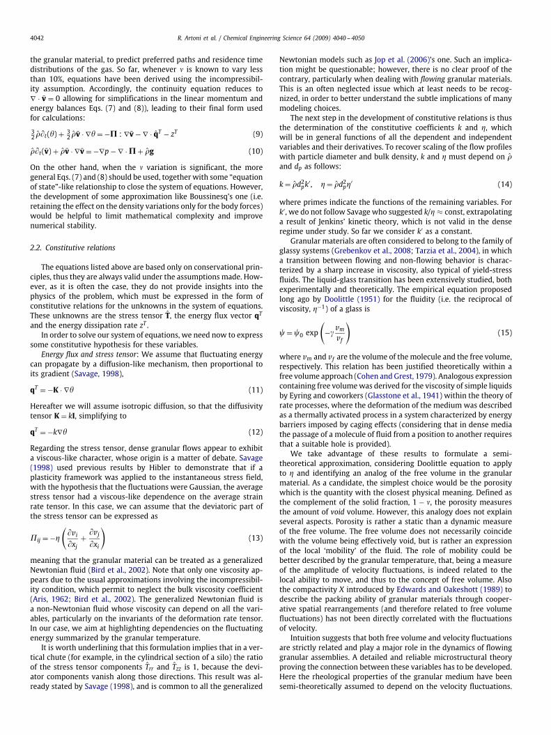
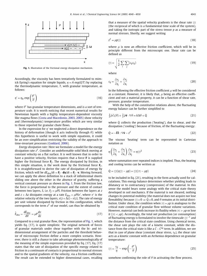
Fig. 1. Illustration of the frictional energy dissipation mechanism.

Accordingly, the viscosity has been tentatively formulated to mim-ick Eyring's equation for simple liquids, � = A exp(E/T) by replacingthe thermodynamic temperature, T, with granular temperature, asfollows:

�′ = �0 exp

(�∗

�

)(16)

where �∗ has granular temperature dimensions, and is a sort of tem-perature scale. It is worth noticing that recent numerical results forNewtonian liquids with a highly temperature-dependent viscositylike magma flows (Costa and Macedonio, 2003, 2005) show velocityand (thermodynamic) temperature profiles which are very similarto those reported for granular chute flows.

In the expression for �′ we neglected a direct dependence on thehistory of deformation (though it acts indirectly through �): whilethis hypothesis is useful to work with simple equations, it couldbe an over-simplification restricting the validity of the approach totime-invariant processes (Goddard, 2006).

Energy dissipation rate: Here we formulate a model for the energydissipation rate zT . Consider an undeformable solid block moving atconstant velocity on a flat surface. It is well known that in order tohave a positive velocity, friction requires that a force F is suppliedhigher the frictional force Ff . The energy dissipated by friction, inthis simple situation, is the work done by the frictional force Ff .It is straightforward to derive the rate of dissipation of energy byfriction, which will be dEdiss/dt = Ff · dx/dt = Ff · v. Moving forward,we can apply the above definition to a stack of infinitesimal sheetssliding one above the other in the absence of gravity, suffering avertical constant pressure as shown in Fig. 1. From the friction law,the force is proportional to the pressure and the extent of contactbetween two layers, S, i.e. Ff = PS. Friction between the layers at zand z + �z dissipates energy at a rate Ediss = PSv′, where v′ is therelative velocity of the two layers, v(z+�z)−v(z). The rate of energyper unit volume dissipated by friction in this configuration, whichcorresponds to the term zT of our model, can thus be obtained by

ˆEdiss = dEdissdV

= Pdvdz

(17)

Compared to a real granular flow, the representation of Fig. 1, whichyields Eq. (17), is quite simplistic. The original network of forcesof granular materials under shear together with the bi- and tri-dimensional arrangement of the particles and the threshold behav-ior of microscopic friction define a more complex scenario. How-ever, there is still a chance to take advantage phenomenologically ofthe meaning of the simple expression provided by Eq. (17). Eq. (17)states that the rate of dissipation of the specific energy related tofriction in a continuum of contacts is proportional to normal stressesand to the spatial gradients of the velocity, via a friction coefficient.The result can be extended to higher dimensional cases, recalling

that a measure of the spatial velocity gradients is the shear rate ||(the reciprocal of which is a fundamental time scale of the system),and taking the isotropic part of the stress tensor p as a measure ofnormal stresses. Shortly, we suggest writing

zT = p|| (18)

where is now an effective friction coefficient, which will be inprinciple different from the microscopic one. Shear rate can bedefined as

|| =√√√√1

2

∑i

∑j

(�ij�ij) (19)

where

�ij =�vi�xj

+ �vj�xi

(20)

In the following the effective friction coefficient will be consideredas a constant. However, it is likely that, being an effective coeffi-cient and not a material property, it can be a function of shear rate,pressure, granular temperature.

With the help of the constitutive relations above, the fluctuatingenergy balance can be further simplified to

32 ��t(�) + 3

2 �v · ∇� = k�� + Q (21)

where Q collects the production (`heating'), due to shear, and thedissipation (`cooling') because of friction, of the fluctuating energy:

Q = −P : ∇v − zT (22)

The viscous `heating' term can be represented in Cartesiannotation as

�

(�vi�xj

+ �vj�xi

)�vi�xj

= �||2 (23)

where summation over repeated indices is implied. Thus, the heatingand cooling terms can be written as

Q = ||(�|| − p) = ||(|�| − p) (24)

to be included in Eq. (21), resulting in the form actually used for cal-culations. This energy balance determines whether yielding leads todilatancy or to contractancy (compression) of the material. In thissense the model bears some analogy with the critical state theorydeveloped in soil mechanics. If the material is not sheared, nothingchanges its potential mobility (the material does not acquire nor loseflowability) because ||=0 ⇒ Q=0, and � remains at its initial distri-bution. Under shear, the condition when |�| =p is analogous to thecritical state condition of granular flow without volume variations.However, material can both increase its fluidity when |�|>p or loseit (|�|<p). Accordingly, the total net production (or consumption)of fluctuating energy is formulated to involve the timescale ||−1 andthe distance from the critical state condition. Using chemical terms,the shear rate plays the role of a kinetic constant, while the dis-tance from the critical state is like a C−Ceq term. In addition, we seethat in case of plane shear (constant shear stress, �0), the shear rateacts as a kinetic constant with an Arrhenius dependence on granulartemperature:

|| = �0�

∼ exp

(−�∗

�

)(25)

somehow confirming the role of � in activating the flow process.

4044 R. Artoni et al. / Chemical Engineering Science 64 (2009) 4040 -- 4050

3. Wall boundary conditions

The issue of boundary conditions is of major importance in densegranular flows. Close to the walls, partial slip, rather than no-slip atall, is the most common behavior.

Traditionally, slip is characterized via a Coulomb yield criterion,relating tangential and normal stresses at the walls through a con-stant friction coefficient. Though appearing a physically sound choiceit has been shown that wall friction coefficient may vary, result-ing in an apparent coefficient, not corresponding to the microscopic,wall–particle friction coefficient. In fact, an investigation of the de-pendence of such effective coefficient on relevant variables is stilllacking and we can speculate that its value will strongly depend onthe flow properties (Artoni et al., 2009), in addition to the local stress.

In this work a different approach based on the so-called Navierslip condition has been used, relating the tangential velocity at theboundary to its gradient in the normal direction through a constantparameter, �, called “slip length”:

ut = �

∣∣∣∣∣�ut�n

∣∣∣∣∣ (26)

This condition allows for a certain amount of slip, which is expressedby means of a simple and measurable quantity. The approach is gen-eral and not restricted to uniformly flat walls; it can be used also forbumpy surfaces which are expected to reduce particle slip, due toa much larger roughness, resulting in a lower coefficient �. Experi-mental and numerical work is needed to calibrate � on material andflow properties, and we are working on it. Nevertheless, the Navierapproach is interesting because (1) it contains both no-slip and per-fect slip situations (in the two limits � → 0 and � → ∞) and (2)because it respects the physics: in the limit of high normal stressno-slip behavior is approached (Artoni et al., 2009). Interestingly, itsimplementation improves convergence with respect to Coulomb'scondition.

In the following the value of the slip length will be quantifiedin terms of particle diameters, provided that dp is the characteris-tic inner length scale of the flowing material. Accordingly, slip willbe characterized by a dimensionless number �/dp. Details about thenon-obvious implementation of conditions given by Eq. (26) are re-ported in the Appendix.

4. Silo with converging hopper

Real scale silos show a complex dynamic behavior (Nielsen, 1998;Schwedes and Feise, 1995). The onset of flow is characterized by apressure wave (see Fig. 2) that changes the stress distribution in theconverging section. The hopper is said to be in an active stress state

Activestressstate

stresspeak Passive

stressstate

stresspeak

Fig. 2. Development of active and passive states in silos. Switch mechanism. Linesrepresent principal stress directions. Modified after Bohrnsen et al. (2004).

(with themajor principal stresses vertically oriented) after filling andin a passive state (with the major principal stresses horizontally ori-ented) when discharging (Nedderman, 1992). The cylindrical part isfrequently assumed to be permanently in an active stress state. Thechange in stress orientation is called the switch. The switch is char-acterized by a marked stress peak at the wall which moves progres-sively from the outlet (at the onset of the flow) up to the transitionbetween the cylindrical and the converging part, where it remains, atsteady state. The steady state stress profile is, however, only an ap-proximation, because the stress field (and the velocity field as well)can be unsteady during discharge, with oscillations and symmetry-breaking effects (Nielsen, 1998; Bohrnsen et al., 2004). Moreover theassessment of the true stress profile is not obvious because exper-imental measurements can be affected by local autoinduced phe-nomena created by load cells. Nevertheless, in axisymmetric silos,where the loss of symmetry is unlikely (Nedderman, 1992), regularflow can be observed and Janssen and Walker solutions can be takenas a reference for wall stress profiles at steady state.

4.1. Numerical calculations

Eqs. (9) and (10) are four PDEs in a 3D geometry. They are coupledbecause granular temperature affects the viscosity in the momen-tum equations, which determine velocities that modify the granulartemperature distribution. Mathematically, Eqs. (9) and (10) are verysimilar to advection and diffusion equations whose solution is imple-mented in many commercial and open source codes, using state-of-the-art numerical methods and graphical pre- and postprocessors toaddress complex geometries. We found more efficient, general andverifiable to implement our model equations in a wide spread FEMcode (COMSOL, 2005). An axisymmetric silo made of a cylindricalsection and a steep hopper were chosen for reference and its dy-namic behavior during discharge up to steady state was simulated.A small hopper angle was chosen to ensure mass flow in the geome-try. This condition was required to compare the numerical solutionswith the analytical models, only available for mass flow regimes. Thegeometry is outlined in Fig. 3.

The model parameters for standard simulation, assumed heuris-tically as typical values for dense flows, are given in Table 1. Asensitivity analysis is presented later, and modified values will bementioned in the text. The momentum balance equations have beenclosed with Navier BCs (Eq. (26)) at the wall, as previously stated, andby a tangential stress free upper boundary. The flowrate was fixed,as common in industrial practice where rotary, screw or belt feed-ers are used and designed to withdraw material at a constant massflow. This simply translates in a constant, plug flow outlet velocityvout . Boundary conditions for the energy equations are “insulation”-type at the walls, constant temperature on the upper, free surfaceset to the average value of the temperature in the cylindrical sectionof the silo.

Calculations assumed that the height of the material in the silowas constant (the no tangential stress upper condition mimicks afree surface) as if the material was constantly replaced; a steadysolution was obtained after all transient effects had finished.

Simulations provide local, instantaneous values of unknown vari-ables (velocity and temperature), together with their fluxes, amongwhich stresses are particularly interesting. Stress distribution underflowing conditions is indeed rarely investigated with hydrodynamicmodels.

4.2. Flow distribution

The model predicts a distribution of velocity in good qualita-tive agreement with available experimental results (e.g. Natarajanet al., 1995). Pointwise, detailed validation requires accurate

R. Artoni et al. / Chemical Engineering Science 64 (2009) 4040 -- 4050 4045

Fig. 3. Geometry of the silo studied in the present work. For better visualization,the coordinates do not scale with each other. Units are expressed in m.

Table 1Basic model parameters.

0.3 –�∗ 10 s2 m−2

�0 1 s−1

k′ 1 s−1

� 1000 kgm−3

dp 3 mm�/dp 1 –vout 5 cm−1 s

measurements, which we were not able to collect in the open lit-erature, notwithstanding the relevance of these data. Within thecontext of an industrial research program, we are currently collect-ing pressure and velocity data, which will be the subject of futurecontributions. Fig. 4 shows that the model correctly predicts thetypical shape of the velocity profile in the cylindrical section, withan inner plug-flow region and a shear band near the wall. Calcu-lation shown in Fig. 4 assumed �/dp = 0.1 to reduce slip and makethe profile structure clearer. The calculated width of the shear bandalways approaches the typical value of 10–15 particle diameters,and is quite independent of the ratio �/dp. The width of the shearbands was observed to depend linearly on the parameter �∗ of themodel, which rules the sensitivity of the apparent viscosity to thelocal granular temperature, according to Eq. (16). It suggests that �∗

might depend on particle diameter since experiments have shownthat the width of shear bands strongly and linearly depends on par-ticle diameter (MiDi, 2004). Again, the issue deserves accurate ex-perimental or DEM data to be thoroughly discussed, while the scopeof this contribution is predictions and analysis of the wall stressdistribution. As a final comment, it is important to highlight that

0 0.1 0.2

1.3

1.4

1.5

1.6

1.7

1.8

r (m)

z (m

)

0 0.1 0.20

0.2

0.4

0.6

0.8

1

r (m)

z (m

)

Fig. 4. Velocity vectors (�/dp = 0.1, other parameters as in Table 1).

the slip-length approach is particularly appropriate and effective topredict the experimentally observed wall slip in granular flows.

An important feature of velocity profiles in dense granular flowsis that shear is typically localized in rather narrow bands: in cylin-drical bins, this structure is best observed far from the orifice, wherethe flow shows a shear zone close to the boundary and a region ofplug flow in the center. In flat-bottomed silos, stagnant zones de-velop in the corners. In the geometry studied here, like many indus-trial applications, stagnant zones are prevented using steep hoppers.The discontinuity in shear is predicted in the cylindrical part, wherethe model describes the formation of shear band. This behavior ispossible in our model because of the balance between generation offluctuating energy due to shear and dissipation due to compression,which defines zones with a different granular temperature, i.e. lo-cal mobility, and thus with a different viscosity (thus difference inshear).

4.3. Stress distribution

Fig. 5 shows the normal stress profile along the walls, obtainedthrough our model with reference parameters of Table 1. We ob-serve that the wall normal stress has the typical features expectedfor a discharging granular material. In the cylindrical upper section,the stress does not increase linearly with the depth (constant ver-tical gradient), like pressure in a fluid, but the increase with depthis smaller and smaller, approaching asymptotically a maximum (theJanssen asymptote). At the transition from the vertical section to thehopper, a local switch stress peak occurs. Below, stress decreases,again asymptotically, toward zero at the hopper's end. This behavioris usually associated to a passive stress state in the convergent hop-per. The consistency of the simulation results both in the upper andin the lower sections of the silo is quite surprising and to authors'knowledge never obtained before by hydrodynamic models simu-lating discharging silos. Although simulations are essentially basedon a model of flow, they also predict the stress distribution with theexpected features. This approach is somehow complementary to theplasticity theories which determine the flow field after complete de-scription of the stress distribution, through a flow rule (Nedderman,1992).

4046 R. Artoni et al. / Chemical Engineering Science 64 (2009) 4040 -- 4050

0 2 4 60

0.5

1

1.5

2

2.5

z (m

)

σ (kPa)

Fig. 5. Wall normal stresses calculated with the parameters of Table 1 (symbols).Line is the best fit approximation with Walker's equations, adjusting w and .

0 2 4 6 80

0.5

1

1.5

2

2.5

z (m

)

σ (kPa)

μ= 0.2μ= 0.4μ= 0.6

Fig. 6. Wall normal stresses varying the parameter , other parameters as in Table 1.

Simulation results can be approximated using the classical modelof Janssen for the upper cylindrical section, and Walker's approachfor the lower, conical one (Nedderman, 1992). The best fit yielded =16.1◦ and w equal to 11.4◦ and 13.3◦ in the upper and lower parts,respectively. In the upper section the stress ratio (Janssen constant)is expected to be K=1 since the model assumes a viscous-like stresstensor with zero normal stress difference. This value was verified inall the numerical simulations.

To better understand the prediction of the model, its capabilityand the influence of its parameters, we carried out a sensitivity anal-ysis on the most critical ones.

Fig. 6 displays the results obtained by varying the parameter ,tuning the ability of the pseudo-fluid to dissipate mechanical energy.This parameter is also expected to be closely related to the internalfriction angle of the material, . Results indicate that decreasing ,wall normal stresses grow in the whole geometry. In the cylindricalsection the saturation value is approached earlier, nicely reproducingthe well-known pressure distribution in a confined bulk of granularmaterial.

0.1 0.2 0.3 0.4 0.5 0.60

20

40

60

μ

φ

φw siloφw hopperφ

0.1 0.2 0.3 0.4 0.5 0.60

0.5

1

μ

tan

(φ)

Fig. 7. Calculated and w vs. coefficient , above. Coefficient of internal friction,tan , (symbols) vs. coefficient , and linear extrapolation of the low-values behavior(line), below.

Experience and static calculations (Nedderman, 1992) report thatthe angle of internal friction affects how rapidly the stress curve sat-urates, but not the saturation value, which depends only on bulk den-sity, bin diameter and wall friction coefficient, w. However, becauseof the slip boundary conditions that we used, the value of the ef-fective wall friction coefficient will depend on the rheological modelassumed for the bulk. This is a consequence of assuming a Navierslip condition at the wall, which is not a model-independent rela-tion, as Coulomb's one; this is indeed due to the fact that Coulomb'slaw directly relates stresses, and so it does not depend on the rhe-ological behavior of the medium, while Navier's condition involvesshear rate, which means that it needs information from stresses andrheology (|| ∼ (�/�)). Therefore the effective friction coefficient atthe wall is expected to be primarily a function w(,�,Vslip, dp), whileother dependencies are minor. The overall effect of bulk on wallstress profiles is therefore a consequence of how it influences theeffective angle of wall friction. Recalling Janssen's equation:

�w = �gD4w

[1 − exp

(−4

wKzD

)](27)

it can be observed that decreasing w has the double effect of in-creasing the stresses in the whole geometry and of slowing downthe approach to the saturation stress: a change in the parameter of our model modifies the wall stress profile in the way representedin Fig. 6, because it indirectly changes the effective wall friction co-efficient w.

The w effect is even clearer when comparing and w valuesthat fit our model results, obtained at different w, Fig. 7. Both in-crease monotonically with ; w in the upper and lower sections ofthe silo does not differ significantly. Remarkably, for low values of , typical of cohesionless particles, correlates to our parameter according to

= tan (28)

implying that the effective coefficient in our model quantitativelyapproaches the coefficient of internal friction, tan . Interestingly,beside providing a physical grounding to the effective parameter by relating it to a characteristic property of the granular material,Eq. (28) allows to estimate the value of to be used in simulatingthe flow of a specific material.

R. Artoni et al. / Chemical Engineering Science 64 (2009) 4040 -- 4050 4047

0 5 10 15 200

0.5

1

1.5

2

2.5

z (m

)

σ (kPa)

λ /dp= 0.1λ /dp= 1.0

λ /dp= 2.0

λ /dp= 5.0

λ /dp= 10.0

Fig. 8. Wall normal stresses varying the parameter �, other parameters as in Table 1.

0 10 20 30 40 500

10

20

30

λ /dp

φ w

φw siloφw hopper

0 10 20 30 40 500.2

0.3

0.4

0.5

λ /dp

tan

(φ)

Fig. 9. Calculated values of w vs. slip length �/dp (above). Coefficient of internalfriction, tan , (symbols) vs. model parameter (dotted line) vs. slip length �/dp

(below).

In Fig. 8 we investigate the effect of varying the slip length to par-ticle diameter ratio �/dp, which determines the amount of slip at thewalls. We expected that a higher slip length corresponds to a lowervalue of the wall friction coefficient, thus higher normal stress at thewall. The results confirm the expectations, both in the upper and inthe lower parts of the silo. A larger slip at the walls determines highwall normal stresses because the wall loses its ability to sustain thematerial. Results are clearer if we determine and compare w foreach value of �/dp, as shown in Fig. 9. We realize that w → 0, mono-tonically when slip length increases. Again, no significant differencebetween the upper and the lower parts of the silo is observed. In ad-dition, in a wide range of �/dp values, the calculated internal frictioncoefficient tan sticks to the value used to obtained the data, andis nearly independent on the slip length. Note that 1<�/dp <30 isquite a broad range, which encompass most practical applications,from extremely rough to perfectly smooth walls. In the no-slip limit,�/dp <1, the calculated values of and w appear to diverge. How-ever, this is likely due to difficulties in the fitting equations that yield

0 1 2 3 4 5 6 70

0.5

1

1.5

2

2.5

z (m

)

σ (kPa)

vout= 1.0 cm/svout= 2.0 cm/svout= 5.0 cm/s

Fig. 10. Wall normal stresses varying the outlet velocity, other parameters as inTable 1.

2 4 6 8 1010

15

20

vout (cm/s)

φ (°

)φw siloφw hopperφ

2 4 6 8 100.26

0.28

0.3

0.32

vout (cm/s)

tan

(φ)

Fig. 11. Calculated and w vs. discharge velocity (above). Coefficient of internalfriction, tan , (symbols) and model parameter (dotted line) as a function ofdischarge velocity (below).

and w values. The no-slip limit requires w– , which causesnumeric instabilities in static calculations that are the basis of thefitting. Moreover, in this limit particles near the wall will likely ap-proach a typical stick-slip behavior, which cannot be captured by theCoulomb slip boundary condition (as assumed in Janssen andWalkerstress analysis), but can be treated within a Navier slip-length ap-proach (Artoni et al., 2009), through a proper average.

Fig. 10 shows the predicted effect on wall normal stresses ofthe discharge velocity. According to our model, the stresses duringdischarge increase with flowrate. Fig. 11 systematically collects theresults, showing that flowrate has amajor effect onwall slip, decreas-ing the corresponding angle of wall friction. In contrast, the outletvelocity (non-material parameter) very weakly affects the calculatedangle of internal friction, further proving that the model parameter can be considered as a material property, which can be estimatedfrom the angle of internal friction by means of Eq. (28), within therange of parameters considered.

4048 R. Artoni et al. / Chemical Engineering Science 64 (2009) 4040 -- 4050

0 0.2 0.4 0.6 0.8 10

0.5

1

1.5

2

2.5

3

3.5x 104

z (m)

σ (P

a)

Time

Fig. 12. Pressure wave in the hopper at the beginning of discharge (times: 10, 20,40, 80, and 400 s).

Fig. 12 illustrates the evolution of wall normal stress distributionat the beginning of the discharge. It has been obtained by gradu-ally increasing the outlet velocity from 0 to 1 cm/s, in a time span of20 s. A traveling wave, with a stress peak moving from the outlet tothe hopper corner can be clearly observed. Such an effect is indeedexpected in real hoppers, reflecting the switch from the active tothe passive stress state (see Fig. 2). Notwithstanding that, the modelpredicts a substantially different mechanism. Instead of a switch be-tween active and passive state, the model describes a transition fromstatic to dynamic conditions, and the switch is between a true hy-drostatic initial solution (at zero velocity), with linearly increasingpressure, to the passive state of discharge. This is a consequence ofconsidering the granular material as a non-Newtonian fluid, withzero shear stress at rest. Future improvement of the model will con-sider allowance for a threshold stress, able to determine the onsetof flow, as in Bingham plastic fluids.

4.4. Experimental determination of model parameters

In the preceding subsection we illustrated the model predictionsof vertical profiles of wall stress, when model parameters are varied.Results follow the expectations, considering the physical meaning ofeach parameter. Here, we briefly discussed the issue of parameterestimation, whereas a detailed illustration of dedicated experimentsfor this scope is the subject of a companion paper. Themodel containsfive parameters, one of which (�) is not a property of the materialitself but of the particle–wall couple. Among these, the temperaturescale, �∗, and the parameters, �0 and k′, mostly affect the velocity andtemperature fields. Their experimental determination is based onmeasurements of velocity profiles in simplified flow arrangements.For the present, it can be assumed that �∗ scales with the particlediameter. The parameter was shown in the preceding section tocorrespond to the internal angle of friction of the material, whichcan be easily measured with shear cells. Parameter � determines theparticle–wall interaction. According to an original approach that wedeveloped, we allow for the possibility of the material to slide onthe wall, to a degree determined by the slip-length coefficient, �.Calibration of � requires dedicated, simple experiments where solidsvelocity profiles close to the boundary are measured, using the sametype of particles and surfaces. Then � can be calculated from itsdefinition, Eq. (26), which implies that � = ut/(|�ut/�n|).

5. Conclusions and perspectives

In this work a novel continuum model to simulate the densegranular flow has been formulated and applied. It is based on con-servation equations for mass, momentum and fluctuating kinetic en-ergy and the rheology is described through a generalized Newtonianmodel whose viscosity depends on granular temperature. The phe-nomenology contained in the fluctuating energy balance implies adynamic interplay between mobility induced by shearing and jam-ming (frictional dissipation) induced by compression.

The model has been applied to a mass flow silo with a converginghopper. This is a reference in the field, but the model is not limitedto any geometry or flow configuration.

The model predicts a distribution of flow in the two silo's sec-tions in agreement with the expected behavior. In this work, wefocused on the stress distribution prediction, which is of great the-oretical and practical interest. The flow model predicts the devel-opment of the typical wall normal stress profiles characterized by apeak at the transition between the cylindrical and the conical sec-tions of the structure. Comparisons were made between the resultsand the static-like solutions of Janssen and Walker, showing a goodagreement and verifying the expected dependence on the amountof slip and flowrate. To the authors' knowledge, it is definitely un-usual for a hydrodynamic continuum model to predict the peculiarstress distribution of granular materials in confined geometries, inaddition to the flow patterns.

An important feature of the model is the allowance of partial wallslip, by means of a Navier slip-length approach, replacing the twounrealistically extreme boundary conditions of no-slip and perfectslip. It is well known that granular material tends to slip, at least par-tially, on surfaces, and a proper quantification is definitely needed;we suggested a viable and promising approach.

The success of the model relies upon the possibility of using it fordesign purposes and this still needs work in order to set the modelon a more quantitative ground. This can be achieved with compari-son with experimental results and discrete element models, in orderto evaluate the parameters of the model and characterize slip. Sofar, a sensitivity analysis gave important information on the corre-lations between model parameters and material properties, such asthe angle of internal friction, limiting the arbitrarity in the model.We believe that we contributed originally to these issues: (1) de-velop a flow model: most of the models of granular flow used indus-trially are actually static. They do not predict flow rates but focuson stresses, assuming the velocity distribution; (2) we introduced asimple, intuitive rheological model based on analogies with liquidsand glasses; (3) we account for particle slip of the walls based ona Navier boundary condition, physically sound; (4) we transferredresults taken from physics literature to the industrial scale (silos);and (5) comparison with well-established correlations. The possibil-ity of our model is huge in principle, not being limited by geome-try of flow arrangements. Results obtained so far are encouraging.However, non-trivial efforts are required to validate and extend it toaccount for more complex effects such as the formation of stagnantzones (i.e. funnel flow). Further developments concern relaxationof the incompressibility hypothesis, by introducing a variable, localdensity and the use of more complex rheologies with yield stressthreshold, and cohesion.

Notation

† transposedp mean particle diameter

DTF source of mechanical energy due to the interstitialfluid

g gravity

R. Artoni et al. / Chemical Engineering Science 64 (2009) 4040 -- 4050 4049

k coefficient of diffusion of fluctuating energyk′ parameter in the diffusion coefficient of fluctuating

energyK fluctuating energy diffusivity tensorp isotropic part of the stress tensor (pressure)qT (diffusive) energy fluxtF drag force exerted by the interstitial fluidT stress tensorv average velocity fieldv fluctuating velocity fieldvout discharge velocityzT dissipation rate of mechanical energy

Greek letters

� non-Newtonian viscosity coefficient�0 parameter in the viscosity coefficient� granular temperature�∗ granular temperature scale in the

viscosity coefficient� slip length effective friction coefficient� solid fractionP deviatoric stress tensor� local density��T =�(v · v)/2 kinetic energy associated with v�ET =�(v · v)/2 kinetic energy associated with v angle of internal friction w wall friction angle

Appendix A. 3D Navier slip boundary condition

It can be useful to represent the generic 3-D formulation of thiscondition, which is often used in microfluidic problems; at first, thecondition asks that the normal velocity vanishes at the boundary:

v · n = 0 (29)

which, together with Eq. (26), which we can rewrite as

u1 = ��′1�

u2 = ��′2�

(30)

where the �′i are the deviatoric components of the stress tensor, from

an appropriate set of boundary condition for the 3-D case. After hav-ing defined an orthonormal basis [n �1 �2] where the first compo-nent is the normal to the surface, while the other two componentsrepresent two tangents identifying the surface. The normal stress isgiven by

� = txnx + tyny + tznz (31)

and the tangential stress is identified by two vectors:

�1 = t · �1

�2 = t · �2 (32)

The deviatoric components of the stress tensor with respect to thesurface are calculated in analogous way, taking into account the fact

that in the present model the deviatoric components of the force perunit area at the boundary are given by

t′i =∑j

nj�

(�ui�xj

+ �uj�xi

)(33)

From this we can derive, for the i-th component of the projectionof u on k (k = 1, 2), i.e. the i-th component of u1 or u2, the relation(where summation over j is implicit, Einzel et al., 1990):

uki = u�ki = �nj

(�ui�xj

+ �uj�xi

)�ki = �nj�ij�ki (34)

We will define two BCs, formally given by (fki is the right memberof Eq. (34), and k = 1, 2)

uk −∑i

fki = 0 (35)

that becomes with implicit summation over i and j

uk − �nj�ij�ki = 0 (36)

or, in a more plain form

uk −∑i

⎧⎨⎩�

∑j

[nj

(�ui�xj

+ �uj�xi

)]�ki

⎫⎬⎭= 0 (37)

References

Aris, R., 1962. Vectors, Tensors, and the Basic Equations of Fluid Mechanics. Prentice-Hall, New York.

Artoni, R., Santomaso, A., Canu, P., 2007. Europhys. Lett. 80 (3), 31304.Artoni, R., Santomaso, A., Canu, P., 2007. Proceedings of Traffic and Granular Flow

'07. Springer, Berlin.Artoni, R., Santomaso, A., Canu, P., 2009. Phys. Rev. E 79, 031304.Babi �c, M., 1997. Int. J. Engng. Sci. 35, 5523–5548.Bagnold, R.A., 1954. Proc. R. Soc. London Ser. A 225, 49.Bagnold, R.A., 1966. Proc. R. Soc. London Ser. A 295, 219.Bird, R.B., Stewart, W.E., Lightfoot, E.N., 2002. Transport Phenomena. second ed.

Wiley, New York.Bocquet, L., Losert, W., Schalk, D., Lubensky, T.C., Gollub, J.P., 2002. Phys. Rev. E 65,

011307.Bohrnsen, J.U., Antes, H., Ostendorf, M., Schwedes, J., 2004. Chem. Eng. Technol. 27

(1), 71–76.Chapman, S., Cowling, T.G., 1991. The Mathematical Theory of Non-Uniform Gases.

Cambridge University Press, Cambridge.Cohen, M.H., Grest, G.S., 1979. Phys. Rev. B 20, 1077.COMSOL, 2005. COMSOL Multiphysics User's Guide. Stockholm: COMSOL AB.Costa, A., Macedonio, G., 2003. Nonlinear Proc. Geophys. 10, 545–555.Costa, A., Macedonio, G., 2005. J. Fluid Mech. 540, 21–38.Cundall, P.A., Strack, O.D.L., 1979. Geotechnique 29, 47–65.Doolittle, A.K., 1951. J. Appl. Phys. 22, 1031–1035.Edwards, S.F., Oakeshott, R.B.S., 1989. Physica A 157, 1080–1090.Einzel, D., Panzer, P., Liu, M., 1990. Phys. Rev. Lett. 64 (19), 2269–2272.Glasstone, S., Laidler, K., Eyring, H., 1941. The Theory of Rate Processes. McGraw-Hill,

New York.Goddard, J.D., 2006. J. Fluid Mech. 568, 1–17.Goddard, J.D., 2008. In Capriz, G., Giovine, P. and Mariano, P.M. (Eds), Mathematical

Models of Granular Matter, Lecture Notes in Applied Mathematics, Vol. 1937,Chapt. 1, pp. 1-20, Springer-Verlag, Berlin, 2008.

Grebenkov, D.S., Pica Ciamarra, M., Nicodemi, M., Coniglio, A., 2008. Phys. Rev. Lett.100, 07801.

Jean, M., 1999. Comput. Meth. Appl. Mech. Engrg. 177, 235–257.Jenkins, J.T., Savage, S.B., 1983. J. Fluid Mech. 130, 187–202.Jop, P., Forterre, Y., Pouliquen, O., 2006. Nature 441, 727–730.Kolymbas, D., 2000 (Ed). Constitutive Modelling of Granular Materials. Springer,

Horton.Losert, W., Bocquet, L., Schalk, D., Lubensky, T.C., Gollub, J.P., 2000. Phys. Rev. Lett.

85, 1428–1432.MiDi, G.D.R., 2004. Eur. Phys. J. E 14, 341–365.Natarajan, V.V.R., Hunt, M.L., Taylor, E.D., 1995. J. Fluid Mech. 304, 1–25.Nedderman, R.M., 1992. Statics and Kinematics of Granular Materials. Cambridge

University Press, Cambridge.

4050 R. Artoni et al. / Chemical Engineering Science 64 (2009) 4040 -- 4050

Nielsen, J., 1998. Phil. Trans. Ser. A 356, 2667–2684.Renouf, M., Dubois, F., Alart, P., 2004. J. Comput. Appl. Math. 168, 375–382 (As regards

open source software, the main ones are LMGC90 (〈http://www.lmgc.univ-montp2.fr/∼dubois/LMGC90/〉), in the context of contact dynamics, and YADE(〈http://yade.wikia.com/wiki/Yade〉), which uses a molecular dynamics scheme).

Santomaso, A.C., Canu, P., 2001. Chem. Eng. Sci. 56 (11), 3563–3573.Santomaso, A.C., Petenò, L., Canu, P., 2006. Europhys. Lett. 75 (4), 576–582.Savage, S.B., 1998. J. Fluid Mech. 377, 1–26.Schofield, A.N., Wroth, C.P., 1968. Critical State Soil Mechanics. McGraw-Hill, New

York.

Schulze, D., 2007. Powders and Bulk Solids—Behavior, Characterization, Storage andFlow. Springer, Berlin.

Schwedes, J., Feise, H., 1995. Chem. Eng. Technol. 18, 96–109.Strumendo, M., Canu, P., 2002. Phys. Rev. E 66 (4), 041304.Tarzia, M., de Candia, A., Fierro, A., Nicodemi, M., Coniglio, A., 2004. Europhys. Lett.

66, 531.Van Liedekerke, P., Tijskens, E., Dintwa, E., Ramon, H., 2006. Powder Technol. 170,

71–85.Wu, Y.-H., Hill, J.M., Yu, A., 2007. Commun. Nonlinear Sci. Numer. Simul. 12 (4),

486–495.