arX

iv:0

806.

2413

v1 [

cond

-mat

.sof

t] 1

5 Ju

n 20

08

Growing length scale in gravity-driven dense granular flow

Shubha Tewari∗ and Bidita Tithi

Department of Physics, Mount Holyoke College,

50 College Street, South Hadley, MA 01075

Allison Ferguson

Department of Biochemistry, University of Toronto, Toronto, Ontario M5S 1A8

Bulbul Chakraborty†

Martin Fisher School of Physics, Brandeis University,

Mailstop 057, Waltham, MA 02454-9110

(Dated: June 15, 2008)

Abstract

We report simulations of a two-dimensional, dense, bidisperse system of inelastic hard disks

falling down a vertical tube under the influence of gravity. We examine the approach to jamming

as the average flow of particles down the tube is slowed by making the outlet narrower. Defining

coarse-grained velocity and stress fields, we study two-point temporal and spatial correlation func-

tions of these fields in a region of the tube where the time-averaged velocity is spatially uniform.

We find that fluctuations in both velocity and stress become increasingly correlated as the system

approaches jamming. We extract a growing length scale and time scale from these correlations.

PACS numbers: 45.70.-n, 81.05.Rm, 83.10.Pp

∗Electronic address: stewari@mtholyoke.edu†Electronic address: bulbul@brandeis.edu

1

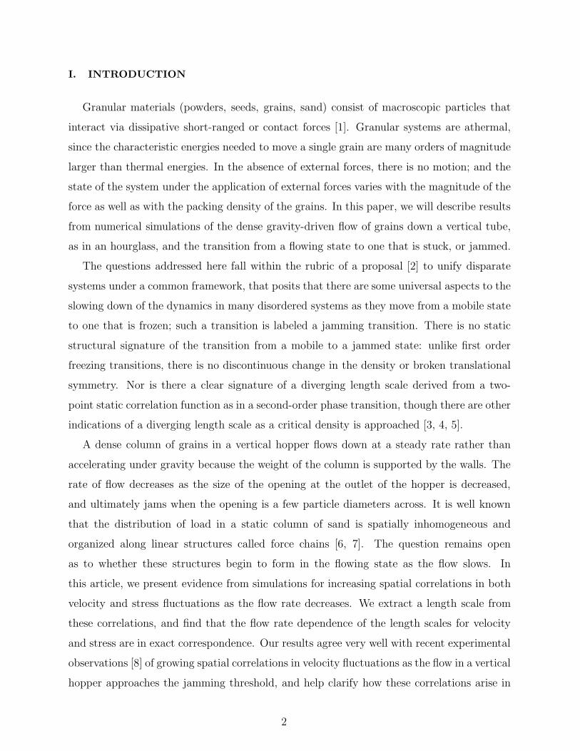
I. INTRODUCTION

Granular materials (powders, seeds, grains, sand) consist of macroscopic particles that

interact via dissipative short-ranged or contact forces [1]. Granular systems are athermal,

since the characteristic energies needed to move a single grain are many orders of magnitude

larger than thermal energies. In the absence of external forces, there is no motion; and the

state of the system under the application of external forces varies with the magnitude of the

force as well as with the packing density of the grains. In this paper, we will describe results

from numerical simulations of the dense gravity-driven flow of grains down a vertical tube,

as in an hourglass, and the transition from a flowing state to one that is stuck, or jammed.

The questions addressed here fall within the rubric of a proposal [2] to unify disparate

systems under a common framework, that posits that there are some universal aspects to the

slowing down of the dynamics in many disordered systems as they move from a mobile state

to one that is frozen; such a transition is labeled a jamming transition. There is no static

structural signature of the transition from a mobile to a jammed state: unlike first order

freezing transitions, there is no discontinuous change in the density or broken translational

symmetry. Nor is there a clear signature of a diverging length scale derived from a two-

point static correlation function as in a second-order phase transition, though there are other

indications of a diverging length scale as a critical density is approached [3, 4, 5].

A dense column of grains in a vertical hopper flows down at a steady rate rather than

accelerating under gravity because the weight of the column is supported by the walls. The

rate of flow decreases as the size of the opening at the outlet of the hopper is decreased,

and ultimately jams when the opening is a few particle diameters across. It is well known

that the distribution of load in a static column of sand is spatially inhomogeneous and

organized along linear structures called force chains [6, 7]. The question remains open

as to whether these structures begin to form in the flowing state as the flow slows. In

this article, we present evidence from simulations for increasing spatial correlations in both

velocity and stress fluctuations as the flow rate decreases. We extract a length scale from

these correlations, and find that the flow rate dependence of the length scales for velocity

and stress are in exact correspondence. Our results agree very well with recent experimental

observations [8] of growing spatial correlations in velocity fluctuations as the flow in a vertical

hopper approaches the jamming threshold, and help clarify how these correlations arise in

2

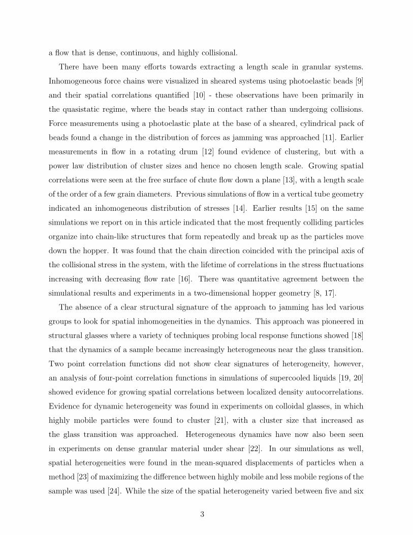
a flow that is dense, continuous, and highly collisional.

There have been many efforts towards extracting a length scale in granular systems.

Inhomogeneous force chains were visualized in sheared systems using photoelastic beads [9]

and their spatial correlations quantified [10] - these observations have been primarily in

the quasistatic regime, where the beads stay in contact rather than undergoing collisions.

Force measurements using a photoelastic plate at the base of a sheared, cylindrical pack of

beads found a change in the distribution of forces as jamming was approached [11]. Earlier

measurements in flow in a rotating drum [12] found evidence of clustering, but with a

power law distribution of cluster sizes and hence no chosen length scale. Growing spatial

correlations were seen at the free surface of chute flow down a plane [13], with a length scale

of the order of a few grain diameters. Previous simulations of flow in a vertical tube geometry

indicated an inhomogeneous distribution of stresses [14]. Earlier results [15] on the same

simulations we report on in this article indicated that the most frequently colliding particles

organize into chain-like structures that form repeatedly and break up as the particles move

down the hopper. It was found that the chain direction coincided with the principal axis of

the collisional stress in the system, with the lifetime of correlations in the stress fluctuations

increasing with decreasing flow rate [16]. There was quantitative agreement between the

simulational results and experiments in a two-dimensional hopper geometry [8, 17].

The absence of a clear structural signature of the approach to jamming has led various

groups to look for spatial inhomogeneities in the dynamics. This approach was pioneered in

structural glasses where a variety of techniques probing local response functions showed [18]

that the dynamics of a sample became increasingly heterogeneous near the glass transition.

Two point correlation functions did not show clear signatures of heterogeneity, however,

an analysis of four-point correlation functions in simulations of supercooled liquids [19, 20]

showed evidence for growing spatial correlations between localized density autocorrelations.

Evidence for dynamic heterogeneity was found in experiments on colloidal glasses, in which

highly mobile particles were found to cluster [21], with a cluster size that increased as

the glass transition was approached. Heterogeneous dynamics have now also been seen

in experiments on dense granular material under shear [22]. In our simulations as well,

spatial heterogeneities were found in the mean-squared displacements of particles when a

method [23] of maximizing the difference between highly mobile and less mobile regions of the

sample was used [24]. While the size of the spatial heterogeneity varied between five and six

3

particle diameters as a function of flow velocity, the ”cage-size” or length scale over which the

heterogeneity was maximized did increase as the flow velocity decreased towards jamming.

However this increase in length scale was typically smaller than a particle diameter, and the

connection with the collisional dynamics and force chains was not clear.

In the current paper, we analyze the development of spatial correlations in both kinetic

and dynamical variables in the flowing state, and show that the extent of these increases as

jamming is approached. We would like to emphasize that the changing length scale is seen

in the two-point correlation functions of the velocity and stress. We also draw qualitative

connections between these correlations and the chains of frequently colliding particles.

In the sections to follow, we first describe the simulation, and our method of defining

coarse-grained velocity and stress fields. We then discuss our results for the time-averaged

fields and the temporal and spatial correlations in both velocity and stress fluctuations, and

conclude with a discussion of our results.

II. DESCRIPTION OF SIMULATION

The results we describe here are obtained from a two-dimensional event-driven simulation

of bidisperse hard disks falling under the influence of gravity in a vertical hopper. We use

the same particle dynamics as Denniston and Li [14], and have described our setup in some

detail in an earlier paper [16]. To summarize: the inter-particle collisions are instantaneous

and inelastic, and there is no friction between the particles. As a result, momentum transfer

between colliding particles always occurs along the vector separating their centers. The

relative velocity between colliding particles i and j is reduced by a coefficient of restitution

µ, defined in the usual way:

(u′j − u

′i).q̂ = −µ(uj − ui).q̂ (1)

where u′j and u

′i are the particle velocities after the collision, and q̂ is a unit vector along

the line separating the centers of the particles. Frictional effects at the wall are simulated by

introducing a coefficient of restitution µwall in the tangential direction: the loss of vertical

momentum at the walls is what allows the flow to reach a steady state. In order to avoid

inelastic collapse, all collisions become elastic when the relative velocity at the collision is

below a certain threshold ucut. A particle exiting the base has a probability p of being

4

reflected, else it exits the system and is re-introduced at the top. The flow rate of particles

in steady state is controlled by the size of the opening at the base. The results described

here are for a simulation of 1000 particles of diameter 1 and 1.2 respectively, where grains

are chosen at random to have one or the other size. The other simulation parameters are

µ = 0.8, µwall = 0.5, p = 0.5 and ucut = 10−3, and the mass of the smaller grains is set

to 1. Lengths are expressed in units of the smaller particle diameter. In these units, the

rectangular region of the hopper has width 20 and height 76.5. The simulation is run for

a total of 1000 simulation time steps, of which the first 500 are discarded. In units of the

simulation time, the average time between collisions for a given particle is on the order of

10−3.

Earlier results reported on these simulations [15, 16] were based on a particle-based

analysis of the system as the size of the opening, or the flow rate, was decreased. Over a

timescale larger than a typical collision time but shorter than the time taken for a particle

to fall through its own diameter, particles with the highest frequency of collisions appear to

repeatedly organize into linear structures that form and break. These structures were shown

to carry much of the collisional stress [16], and their lifetime increased with decreasing flow

rate, but no evidence was found for a growing length scale.

In this paper, we seek to go beyond the particle-level analysis of the system in order to

quantify the correlations signaled by the frequently colliding chains of particles and look for

indications of increasing order in the system as it approaches jamming. Thus in the work

described here, we have constructed coarse-grained variables, looking at the system in terms

of velocity, stress and density fields and the spatial and temporal variations of these fields.

We also view this approach as a useful first step in developing a continuum description of

granular flow.

III. RESULTS

A. Coarse-grained Fields

The system area is divided into square boxes of side equal to two particle diameters. We

define a box velocity

v(r, t) =∑

j

uj(t)/Nj (2)

5

where uj are the velocities of the Nj particles whose centers lie inside a box of center

coordinates r = (x, y) at a given instant t. We do this separately for the vertical (vy, parallel

to flow) and horizontal (vx, perpendicular to the flow direction) velocity components.

Figure (1) shows the time-averaged profile of the velocity components for the slowest flow

rate we report, vflow = 0.60 in units of particle diameters per simulation time. Figure (1a)

shows the vertical velocity component vy over the entire hopper. There is an acceleration

region near the top of the hopper - particles are introduced here, and accelerate under gravity

before they reach an asymptotic density and velocity. For all the analysis described in the

rest of the paper, we will focus on this region of constant velocity, extending from y = 35 to

y = 70. The correlation functions we will present will also exclude the shear layer near the

wall, where the velocity is smaller, but non-zero. Figure (1b) shows the horizontal velocity

component field vx which is structureless in the region of constant vertical velocity. In the

acceleration region, the particles on either side seem to be moving towards the center.

The time-averaged stress fields are calculated by a similar coarse-graining procedure. The

box collisional stress is defined as follows:

σµν(r, t) =1

τA

∑

collisions in τ

Iµrν (3)

where we sum over all collisions in a box occurring within the time interval [t, t + τ ]. I is

the impulse transferred at the moment of collision, r the center to center vector between

colliding particles, and A the box area. Since the particles are hard disks with no inter-

particle friction, all the momentum transfer is in the direction of the vector separating the

centers of the two colliding particles. The above expression then gives us the four stress

components in the lab frame. We pick an averaging time interval τ that is long compared to

the typical collision time but short compared to the time taken for a particle to fall through

its own diameter. These scales are well-separated in a dense flow: both in experiments and

in our simulation a particle undergoes many collisions in the time it takes to fall through

its own diameter. Thus while the velocity profiles indicate that the central region of the

hopper is moving as a plug, the flow is highly collisional and far from static, as found earlier

in experiments [25] and subsequently in simulations [14].

The time-averaged profiles of the stress components are shown in Figure (2). These are

calculated as indicated in the previous paragraph and averaged over the duration of the

entire simulation. Figure (2a) and (2c) show the normal stress components in the x and y

6

x

yv

y

5 10 15

10

20

30

40

50

60

70

0.2

0.4

0.6

0.8

1

1.2

x

vx

5 10 15

10

20

30

40

50

60

70 −0.15

−0.1

−0.05

0

0.05

0.1

FIG. 1: (Color online) Contour plot of the time-averaged spatial profile of the velocity components.

(a) shows the component parallel to the flow, and (b) shows the component of velocity perpendicular

to the flow. We focus on the region where the velocity remains approximately constant.

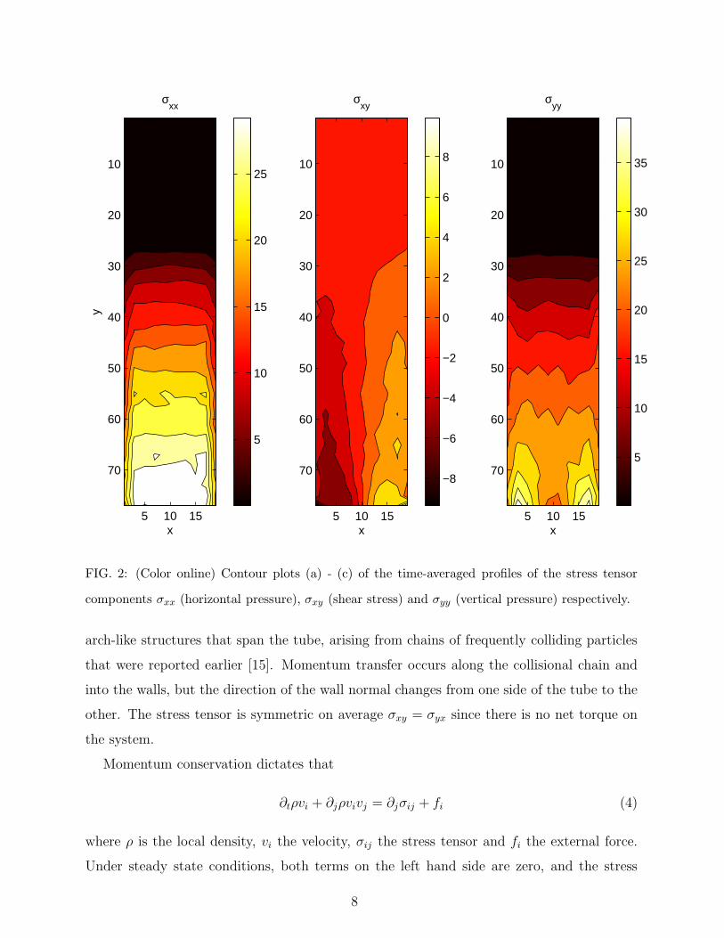
directions respectively. Note the similarity in structure in both, with a positive gradient in

both σxx and σyy in the direction of flow. Thus there is an overall gradient in the pressure in

the region of constant average velocity. Since we only include the collisional contributions to

the stress, there is zero pressure in the acceleration region at the top of the tube since there

are no collisions occurring in this region. Figure (2b) shows the shear stress component.

The shear stress changes sign from the left hand side to the right hand side of the tube, and

has a gradient in the horizontal direction. This appears consistent with the formation of

7

x

yσ

xx

5 10 15

10

20

30

40

50

60

70

5

10

15

20

25

x

σxy

5 10 15

10

20

30

40

50

60

70−8

−6

−4

−2

0

2

4

6

8

x

σyy

5 10 15

10

20

30

40

50

60

705

10

15

20

25

30

35

FIG. 2: (Color online) Contour plots (a) - (c) of the time-averaged profiles of the stress tensor

components σxx (horizontal pressure), σxy (shear stress) and σyy (vertical pressure) respectively.

arch-like structures that span the tube, arising from chains of frequently colliding particles

that were reported earlier [15]. Momentum transfer occurs along the collisional chain and

into the walls, but the direction of the wall normal changes from one side of the tube to the

other. The stress tensor is symmetric on average σxy = σyx since there is no net torque on

the system.

Momentum conservation dictates that

∂tρvi + ∂jρvivj = ∂jσij + fi (4)

where ρ is the local density, vi the velocity, σij the stress tensor and fi the external force.

Under steady state conditions, both terms on the left hand side are zero, and the stress

8

0.9

0.8

0.7

0.6

0.5

0.4

0.3

Stre

ss g

radi

ent

2.01.51.00.5 Vflow

∂xσxy

∂yσyy

Sum

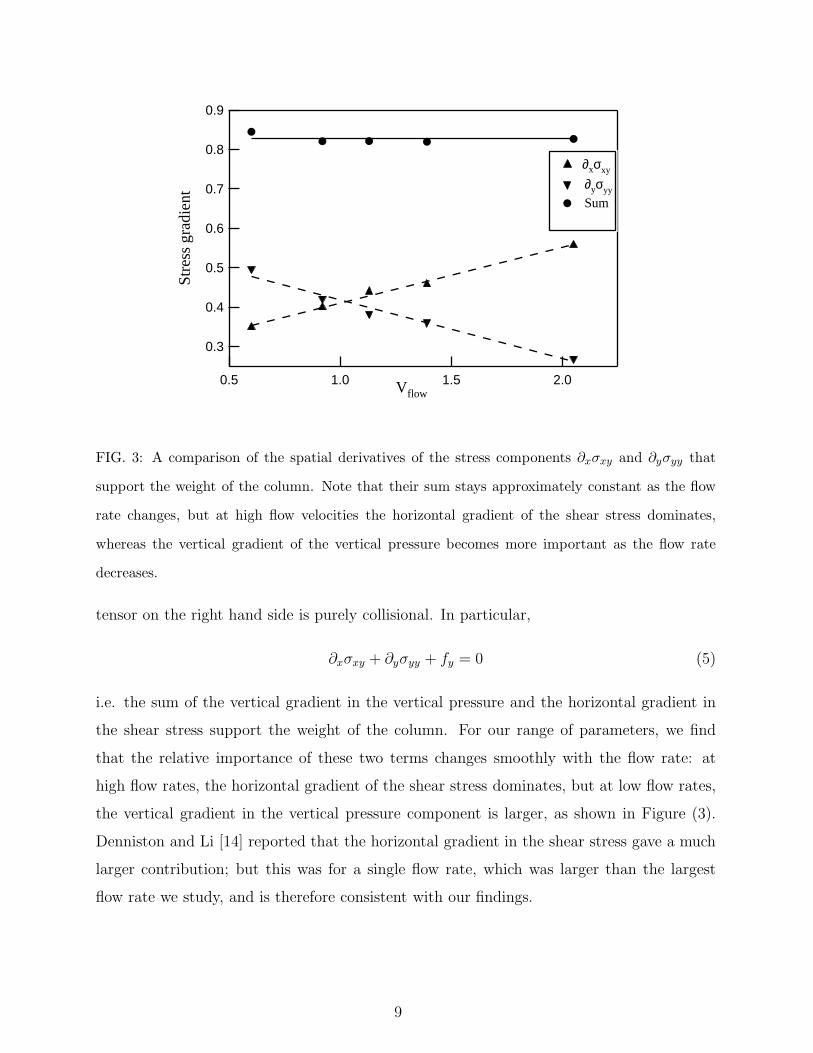
FIG. 3: A comparison of the spatial derivatives of the stress components ∂xσxy and ∂yσyy that

support the weight of the column. Note that their sum stays approximately constant as the flow

rate changes, but at high flow velocities the horizontal gradient of the shear stress dominates,

whereas the vertical gradient of the vertical pressure becomes more important as the flow rate

decreases.

tensor on the right hand side is purely collisional. In particular,

∂xσxy + ∂yσyy + fy = 0 (5)

i.e. the sum of the vertical gradient in the vertical pressure and the horizontal gradient in

the shear stress support the weight of the column. For our range of parameters, we find

that the relative importance of these two terms changes smoothly with the flow rate: at

high flow rates, the horizontal gradient of the shear stress dominates, but at low flow rates,

the vertical gradient in the vertical pressure component is larger, as shown in Figure (3).

Denniston and Li [14] reported that the horizontal gradient in the shear stress gave a much

larger contribution; but this was for a single flow rate, which was larger than the largest

flow rate we study, and is therefore consistent with our findings.

9

B. Relaxation Time: Velocity and Stress Autocorrelations

We first examine fluctuations in the kinematic variables, and how closely fluctuations at

a given spatial point in the flow remain correlated in time. The normalized autocorrelation

Ci(r, t) of the velocity component vi(r, t) at a spatial point r is defined as

Ci(r, t) =〈∆vi(r, t + τ)∆vi(r, t)〉

〈(∆vi(r, t))2〉(6)

where ∆vi(r, t) = vi(r, t) − 〈vi〉 represents the time-dependent fluctuation of the velocity

component, i = x or y, and the averages are over time. This quantity is then spatially

averaged over all the boxes in the region of constant velocity, giving

〈vi(t)vi(0)〉 =1

Ns

∑

r

Ci(r, t) (7)

where Ns is the number of boxes summed over.

The autocorrelations of the fluctuations in both velocity components are shown as a

function of time in Figures (4) and (5) for five different flow velocities. The correlations fall

off fairly rapidly at short times at all flow rates. As one moves from fast to slow flow (from

left to right in the figures), there is a consistent but slow trend towards increasing relaxation

time as the flow rate decreases (note that the x-axis scale has been made logarithmic in the

figure to emphasize this). Thus temporal correlations in the velocity fluctuations do not

provide a strong indication of an impending jam as the flow rate decreases.

Clearer evidence of a growth in the relaxation timescale is seen in the stress. The auto-

correlation of the fluctuations in the stress components 〈σij(t)σij(0)〉 is defined exactly the

same way as for the velocity components, as indicated in Eqs. (6) and (7). These autocor-

relations decay with time with some characteristic timescale; and evidence for an increase

in decay timescale as the flow-rate decreases is seen in all three components. However, the

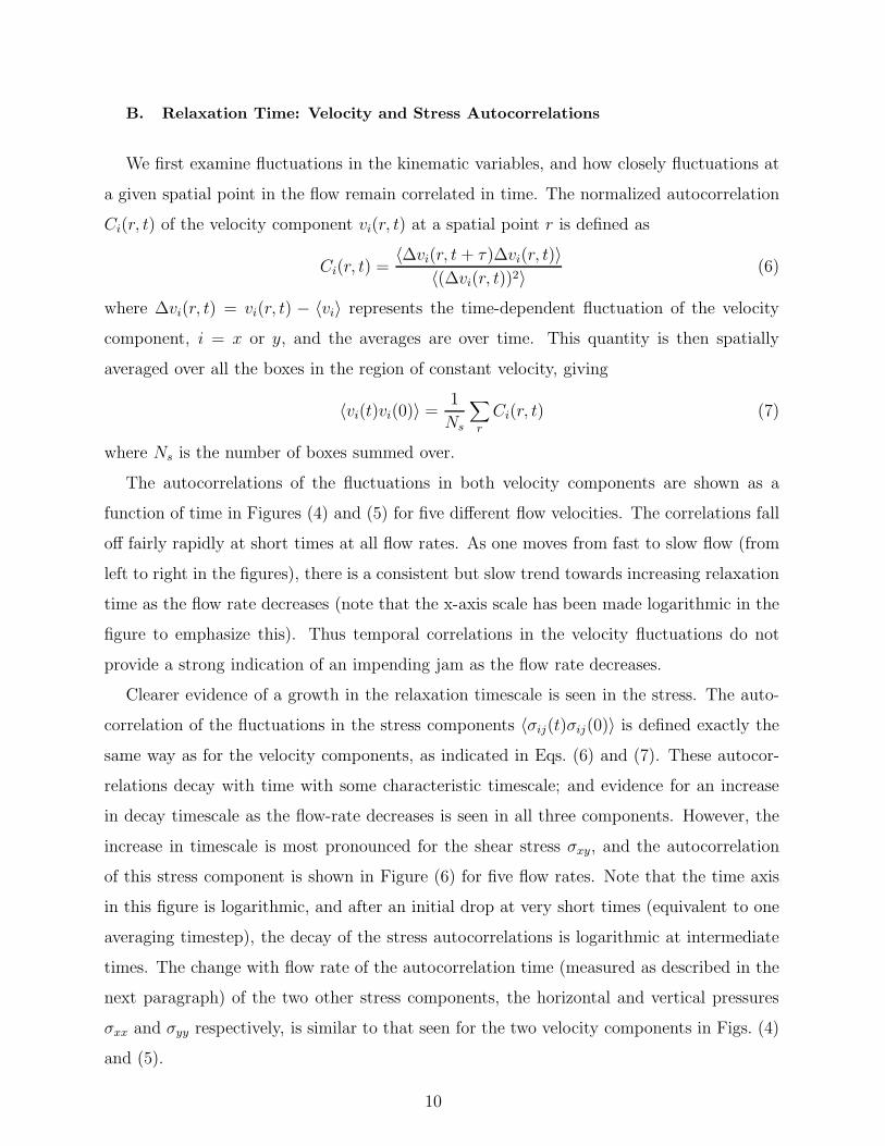
increase in timescale is most pronounced for the shear stress σxy, and the autocorrelation

of this stress component is shown in Figure (6) for five flow rates. Note that the time axis

in this figure is logarithmic, and after an initial drop at very short times (equivalent to one

averaging timestep), the decay of the stress autocorrelations is logarithmic at intermediate

times. The change with flow rate of the autocorrelation time (measured as described in the

next paragraph) of the two other stress components, the horizontal and vertical pressures

σxx and σyy respectively, is similar to that seen for the two velocity components in Figs. (4)

and (5).

10

-0.2

0

0.2

0.4

0.6

0.8

1

0.01 0.1 1 10 100 1000

<v x

(t)v

x(0)

>

Time t

vflow = 2.051.391.130.920.60

FIG. 4: (Color online) Autocorrelation of the velocity component perpendicular to the flow at at

five different flow rates. The flow rates are expressed in units of particle diameters per simulation

time.

-0.2

0

0.2

0.4

0.6

0.8

1

0.01 0.1 1 10 100 1000

<v y

(t)v

y(0)

>

Time t

vflow = 2.051.391.130.920.60

FIG. 5: (Color online) Autocorrelation of the velocity component parallel to the flow at the same

five flow rates.

11

-0.1

0

0.1

0.2

0.3

0.4

0.5

0.6

0.7

0.01 0.1 1 10 100 1000

<σ x

y(t)

σ xy(

0)>

Time t

vflow = 2.05 = 1.39 = 1.13 = 0.92 = 0.60

FIG. 6: (Color online) Autocorrelation of the shear stress at the same five flow rates.

We extract a time scale from these autocorrelation functions by measuring the time at

which the (normalized) autocorrelation function drops to 0.1. This time τ is plotted as a

function of inverse mean flow velocity in Figure (7). Note that while the autocorrelation time

associated with the two velocity components and the two diagonal components of stress all

increase as flow rate decreases, the timescale associated with the shear stress increases more

rapidly than the others as the flow slows. This increase is also more rapid than linear (the

lines in the figure, intended as guides to the eye, are fits to quadratics). As we shall see in the

next section, this increase in autocorrelation time leads to the growth of a region that flows

like a plug, and is consistent with the presence of chains of frequently colliding particles that

begin to span the system at the lower flow rates. Evidence that the dominant contribution

to the principal axis of the collisional stress tensor comes from the most frequently colliding

particles was presented in earlier work [16] on the same simulations. There we found that

the timescale associated with the fluctuations of the principal axis of the stress increased

linearly with inverse flow rate.

12

1.0

0.8

0.6

0.4

0.2

0.0

Cor

rela

tion

time,

τ

1.81.61.41.21.00.80.60.41/vflow

σxy vx

σxx vy

σyy

FIG. 7: (Color online) Time at which the autocorrelations of the different velocity and stress

components drop to 0.1 as a function of the inverse flow velocity. The lines are intended as guides

to the eye and are obtained from quadratic fits to the data. Note the timescale associated with

the shear stress shows a much greater dependence on flow velocity.

C. Length Scales: Spatial correlations in velocity and stress

We next examine the spatial correlations in the fluctuations of both kinematic and dy-

namic variables. We define the normalized equal time spatial correlation function of the

velocity fluctuations as a function of separation as follows:

〈vi(r)vi(0)〉 =

∑ri

∑t ∆vi(ri, t)∆vi((ri + ∆r, t)

Ns

∑t(∆vi(ri, t))2

(8)

where Ns is the number of spatial points (boxes) summed over, and ∆vi(r, t) represents the

velocity fluctuation relative to the long-time average.

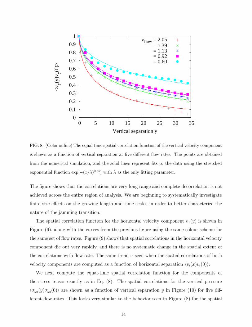
The spatial correlations for the vertical velocity component 〈vy(y)vy(0)〉 are shown as a

function of vertical separation y in Figure (8) for five different flow rates. Note that as the

flow rate decreases, the spatial correlation dies off more slowly, suggestive of an increasing

length scale. Our numerical results are shown by the points in the figure, and the solid lines

are fits to stretched exponential behavior - we shall discuss these fits further in what follows.

13

0

0.1

0.2

0.3

0.4

0.5

0.6

0.7

0.8

0.9

1

0 5 10 15 20 25 30 35

<v y

(y)v

y(0)

>

Vertical separation y

vflow = 2.05 = 1.39 = 1.13 = 0.92 = 0.60

FIG. 8: (Color online) The equal time spatial correlation function of the vertical velocity component

is shown as a function of vertical separation at five different flow rates. The points are obtained

from the numerical simulation, and the solid lines represent fits to the data using the stretched

exponential function exp[−(x/λ)0.55] with λ as the only fitting parameter.

The figure shows that the correlations are very long range and complete decorrelation is not

achieved across the entire region of analysis. We are beginning to systematically investigate

finite size effects on the growing length and time scales in order to better characterize the

nature of the jamming transition.

The spatial correlation function for the horizontal velocity component vx(y) is shown in

Figure (9), along with the curves from the previous figure using the same colour scheme for

the same set of flow rates. Figure (9) shows that spatial correlations in the horizontal velocity

component die out very rapidly, and there is no systematic change in the spatial extent of

the correlations with flow rate. The same trend is seen when the spatial correlations of both

velocity components are computed as a function of horizontal separation 〈vi(x)vi(0)〉.

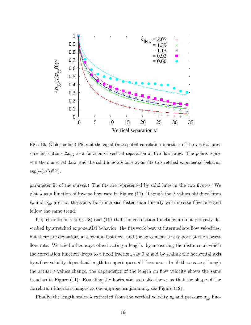
We next compute the equal-time spatial correlation function for the components of

the stress tensor exactly as in Eq. (8). The spatial correlations for the vertical pressure

〈σyy(y)σyy(0)〉 are shown as a function of vertical separation y in Figure (10) for five dif-

ferent flow rates. This looks very similar to the behavior seen in Figure (8) for the spatial

14

-0.2

0

0.2

0.4

0.6

0.8

1

0 5 10 15 20 25 30 35

<v i

(y)v

i(0)>

Vertical separation y

vflow = 2.05 = 1.39 = 1.13 = 0.92 = 0.60

FIG. 9: (Color online) Comparison of the equal time spatial correlation function of the vertical

velocity component from the previous graph (lines and symbols) to the spatial correlations of the

horizontal velocity component (lines) as a function of vertical separation at the same five flow rates.

No fits are shown in this plot, and the lines simply connect the points.

correlations in the vertical velocity. Once again, the points are obtained from the simulations

and the lines represent fits to stretched exponential behavior.

Spatial correlations in the horizontal pressure 〈σxx(x)σxx(0)〉 as a function of horizontal

separation show very similar behavior to that seen in Figure (10), but we have not shown it

because of the limited range available in the x-direction. Equal-time spatial correlations of

the vertical pressure σyy as a function of horizontal separation x and those of the horizontal

pressure σxx as a function of vertical separation y (both not shown) also have the same trend

as a function of flow rate, but show a less pronounced change than the correlations seen in

Figure (10). Interestingly, the shear stress shows no spatial correlations: the equal-time

spatial correlation function in σxy dies very rapidly and shows no change as a function of

flow rate. We will return to this observation in the next section.

We can extract from Figures (8) and (10) a characteristic length scale λ by fitting both

spatial correlation functions to a stretched exponential decay function, exp[−(x/λ)0.55] where

λ is the only fitting parameter. (We estimated the exponent 0.55 by first doing a two-

15

0

0.1

0.2

0.3

0.4

0.5

0.6

0.7

0.8

0.9

1

0 5 10 15 20 25 30 35

<σ y

y(y)

σ yy(

0)>

Vertical separation y

vflow = 2.05 = 1.39 = 1.13 = 0.92 = 0.60

FIG. 10: (Color online) Plots of the equal time spatial correlation functions of the vertical pres-

sure fluctuations ∆σyy as a function of vertical separation at five flow rates. The points repre-

sent the numerical data, and the solid lines are once again fits to stretched exponential behavior

exp[−(x/λ)0.55].

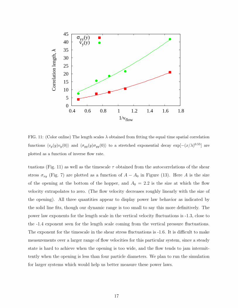
parameter fit of the curves.) The fits are represented by solid lines in the two figures. We

plot λ as a function of inverse flow rate in Figure (11). Though the λ values obtained from

vy and σyy are not the same, both increase faster than linearly with inverse flow rate and

follow the same trend.

It is clear from Figures (8) and (10) that the correlation functions are not perfectly de-

scribed by stretched exponential behavior: the fits work best at intermediate flow velocities,

but there are deviations at slow and fast flow, and the agreement is very poor at the slowest

flow rate. We tried other ways of extracting a length: by measuring the distance at which

the correlation function drops to a fixed fraction, say 0.4; and by scaling the horizontal axis

by a flow-velocity dependent length to superimpose all the curves. In all these cases, though

the actual λ values change, the dependence of the length on flow velocity shows the same

trend as in Figure (11). Rescaling the horizontal axis also shows us that the shape of the

correlation function changes as one approaches jamming, see Figure (12).

Finally, the length scales λ extracted from the vertical velocity vy and pressure σyy fluc-

16

0

5

10

15

20

25

30

35

40

45

0.4 0.6 0.8 1 1.2 1.4 1.6 1.8

Cor

rela

tion

leng

th, λ

1/vflow

σyy(y)vy(y)

FIG. 11: (Color online) The length scales λ obtained from fitting the equal time spatial correlation

functions 〈vy(y)vy(0)〉 and 〈σyy(y)σyy(0)〉 to a stretched exponential decay exp[−(x/λ)0.55] are

plotted as a function of inverse flow rate.

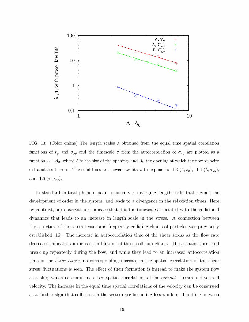
tuations (Fig. 11) as well as the timescale τ obtained from the autocorrelations of the shear

stress σxy (Fig. 7) are plotted as a function of A − A0 in Figure (13). Here A is the size

of the opening at the bottom of the hopper, and A0 = 2.2 is the size at which the flow

velocity extrapolates to zero. (The flow velocity decreases roughly linearly with the size of

the opening). All three quantities appear to display power law behavior as indicated by

the solid line fits, though our dynamic range is too small to say this more definitively. The

power law exponents for the length scale in the vertical velocity fluctuations is -1.3, close to

the -1.4 exponent seen for the length scale coming from the vertical pressure fluctuations.

The exponent for the timescale in the shear stress fluctuations is -1.6. It is difficult to make

measurements over a larger range of flow velocities for this particular system, since a steady

state is hard to achieve when the opening is too wide, and the flow tends to jam intermit-

tently when the opening is less than four particle diameters. We plan to run the simulation

for larger systems which would help us better measure these power laws.

17

0

0.1

0.2

0.3

0.4

0.5

0.6

0.7

0.8

0.9

1

0 2 4 6 8 10 12 14

<v y

(y)v

y(0)

>

y/ys(vflow)

vflow = 2.05 = 1.39 = 1.13 = 0.92 = 0.60

FIG. 12: (Color online) The equal time spatial correlation function of the vertical velocity compo-

nent 〈vy(y)vy(0)〉 is plotted as a function of scaled vertical position y/ys(vflow) where ys(vflow) is a

flow-velocity dependent length. The curves do not superimpose exactly, with a significant change

in shape as the flow approaches jamming.

IV. DISCUSSION

We have observed a growing length scale in dense gravity-driven granular flow as the flow

rate decreases towards jamming. This length scale characterizes the decay of the two-point

spatial correlation functions of the velocity and the normal stress. Correspondingly, there is

a growth in the relaxation time associated with the shear stress. By contrast, the relaxation

times of the velocity fluctuations grow very little, and no accompanying structural changes

in the density are seen. Thus increasing temporal correlations in the shear stress fluctuations

are closely tracked by spatial correlations in the flow velocity and the pressure. Both the

relaxation times and length scales derived from these two-point correlation functions appear

to increase as power laws of the opening size in the dynamic range available to us.

An interesting scenario, that we are in the process of investigating, is whether an increas-

ing length scale in two-point spatial correlation functions of the velocity, as seen here, can

lead to the type of behavior observed in four point density correlation functions [22, 26].

18

0.1

1

10

100

1 10

λ , τ

, with

pow

er la

w f

its

A - A0

λ, vyλ, σyyτ, σxy

FIG. 13: (Color online) The length scales λ obtained from the equal time spatial correlation

functions of vy and σyy and the timescale τ from the autocorrelation of σxy are plotted as a

function A−A0, where A is the size of the opening, and A0 the opening at which the flow velocity

extrapolates to zero. The solid lines are power law fits with exponents -1.3 (λ, vy), -1.4 (λ, σyy),

and -1.6 (τ, σxy).

In standard critical phenomena it is usually a diverging length scale that signals the

development of order in the system, and leads to a divergence in the relaxation times. Here

by contrast, our observations indicate that it is the timescale associated with the collisional

dynamics that leads to an increase in length scale in the stress. A connection between

the structure of the stress tensor and frequently colliding chains of particles was previously

established [16]. The increase in autocorrelation time of the shear stress as the flow rate

decreases indicates an increase in lifetime of these collision chains. These chains form and

break up repeatedly during the flow, and while they lead to an increased autocorrelation

time in the shear stress, no corresponding increase in the spatial correlation of the shear

stress fluctuations is seen. The effect of their formation is instead to make the system flow

as a plug, which is seen in increased spatial correlations of the normal stresses and vertical

velocity. The increase in the equal time spatial correlations of the velocity can be construed

as a further sign that collisions in the system are becoming less random. The time between

19

collisions decreases along with the flow rate, so there are many more collisions in a given

time interval. Thus collisions must occur in a spatially correlated way.

Our results agree well with experiments on gravity-driven hopper flow in two dimensions

[8] in which force-velocity correlations have long-range effects. Our simulations make it clear

that these correlations are also present in the spatial structure of the stress fluctuations. Our

observation that an increasing length is associated with the normal components of the stress

and not in the shear component poses a further puzzle.

Acknowledgments

We wish to acknowledge useful discussions with Narayanan Menon, Nalini Easwar, Giulio

Biroli, Andrea Liu and Douglas Durian. We thank Melanie Finn and Anna-Lisa Baksmaty,

current and former undergraduates at Mount Holyoke College, for their contributions to

this project. ST and BC thank the Aspen Center for Physics for their hospitality. BC

acknowledges the support of nsf-dmr 0549762.

[1] H. M. Jaeger, S. R. Nagel, and R. P. Behringer, Rev. Mod. Phys. 68, 1259 (1996).

[2] A. J. Liu and S. R. Nagel, Nature 396, 21-22 (1998).

[3] L. E. Silbert, A. J. Liu and S. R. Nagel, Phys. Rev. Lett. 95, 098301 (2005).

[4] M. Wyart, S. R. Nagel and T. A. Witten, Europhys. Lett. 72, 486 (2005).

[5] P. Olsson and S. Teitel, Phys. Rev. Lett. 99, 178001 (2007).

[6] P. Dantu, Ann. Pont Chaussees 4, 144 (1967).

[7] C. H. Liu et al., Science 269, 513 (1995).

[8] Emily Gardel, E. Keene, S. Dragulin, N. Easwar and N. Menon, cond-mat/0601022.

[9] D. Howell, R. P. Behringer, C. Veje, Phys. Rev. Lett. 82, 5241 (1999).

[10] T.S. Majmudar and R.S. Behringer, Nature 435, 1079 (2005).

[11] E. I. Corwin, H. M. Jaeger and S.R. Nagel, Nature 435, 1075 (2005).

[12] D. Bonamy, F. Daviaud, L. Laurent, M. Bonetti, and J. P. Bouchaud, Phys. Rev. Lett. 89,

034301 (2002).

[13] O. Pouliquen, Phys. Rev. Lett. 93, 248001 (2004).

20

[14] C. Denniston, and H. Li, Phys. Rev. E 59 3289 (1998).

[15] A. Ferguson, B. Fisher, and B. Chakraborty, Europhys. Lett. 66, 277 (2004).

[16] A. Ferguson and B. Chakraborty, Phys. Rev. E 73, 011303 (2006).

[17] E. Longhi, N. Easwar and N. Menon, Phys. Rev. Lett. 89, 045501 (2002).

[18] M. A. Ediger, Annu. Rev. Phys. Chem. 51, 99 (2000).

[19] C. Dasgupta, A. V. Indrani, S. Ramaswamy and M. K. Phani, Europhys. Lett. 15, 307 (1991).

[20] S. C. Glotzer, V. N. Novikov, and T. B. Schroder, J. Chem. Phys. 112, 509 (2000).

[21] E. R. Weeks, J. C. Crocker, A. C. Levitt, A. Schofield, and D. A. Weitz, Science 287, 627

(2000).

[22] O. Dauchot, G. Marty, and G. Biroli, Phys. Rev. Lett. 95, 265701-1 (2005).

[23] M. M. Hurley and P. Harrowell, Phys. Rev. E 52, 1694 (1995).

[24] A. Ferguson and B. Chakraborty, Europhys. Lett. 78, 28003 (2007).

[25] N. Menon and D. J. Durian, Science 275, 1920 (1997).

[26] A. S. Keys, A. R. Abate, S. C. Glotzer, and D. J. Durian, Nat. Phys. 3, 260 (2007).

21