Particle interactions in a dense monosized granular flow

Physica D 162 (2002) 188–207

Particle interactions in a dense monosized granular flow

Payman Jalalia,∗, William Polashenski Jr.b, Tero Tynjäläc, Piroz Zamankhanca Department of Energy Technology, Lappeenranta University of Technology, Lappeenranta, Finland

b Lomic Inc. State College, Pennsylvania, PA, USAc Laboratory of Fluid Dynamics, Lappeenranta University of Technology, Lappeenranta, Finland

Received 19 October 2000; received in revised form 6 November 2001; accepted 30 November 2001Communicated by R.P. Behringer

Abstract

Simulations of bounded dense sheared granular flows were performed to investigate multi-phase flow phenomena, inparticular the behavior of the ordered phase. In the absence of gravity, collapse of the granular structures was found to occurfor a wide range of shear rate, as evidenced by the disappearance of the signature of the ordered structure in the wall normalstress signal. However, normal stress signals matching those detected in recent experiments were obtained for a system whosedynamics were collision-dominated rather than friction-dominated. Moreover, the system was found to exhibit a similar flowbehavior in the presence of gravity. The stress signals were analyzed using wavelet transforms, which indicated the existenceof stick–slip dynamics, characterized by harmonic frequencies. It is shown that these observations might elucidate the originof stick–slip dynamics in the system, which experienced instability due to gravitational compactification at shear rates belowa certain critical value. © 2002 Elsevier Science B.V. All rights reserved.

Keywords:Particle interactions; Granular flow; Stress signals

1. Introduction

Shear-induced melting is a highly intriguing pheno-menon observed in dense granular systems, as well asother systems such as colloidal suspensions [1], whichare very valuable model systems for investigating theeffect of shear flow on the co-existence of solid andliquid phases. In fact, there are strong analogies bet-ween dense colloidal suspensions, which are systemson a mesoscopic length scale, and macroscopic sys-tems such as granular flows [2], including the observedfeature of solid–liquid phase transformation [3].

Phase transformation in granular systems is stronglydependent on the nature of the interactions between

∗ Corresponding author.E-mail address:[email protected] (P. Jalali).

particles. At high solid fractions, particle interactionscould involve instantaneous inelastic collisions aswell as long lived sliding contacts [4]. Unless the sys-tem is in a state of high agitation, such as may exist inmoderately dense rapid granular flows, its dynamicsis believed to be governed by interparticle friction.However, the physical relevance of the latter effectremains a topic of controversy because of recent ex-perimental evidence [5] that the dynamics of grainsmay be dominated by collisions rather than slidingcontacts even in slow dense flows. This experimentinvolved the measurement of particle displacementsin a dense granular flow in a vertical channel usingdiffusing-wave spectroscopy. The experimental re-sults provide an interesting insight on the dynamicbehavior of particles in dense flows. However, theseresults provide little information about the presence

0167-2789/02/$ – see front matter © 2002 Elsevier Science B.V. All rights reserved.PII: S0167-2789(01)00390-6

P. Jalali et al. / Physica D 162 (2002) 188–207 189

of a strong force network that binds the other grains inplace.

A more comprehensive understanding of the par-ticle interactions in dense flows may be obtained byanalyzing the experimental results of Miller et al. [6]in which the force fluctuations were measured at thewall for a dense granular flow in a Couette geometry.Such information is invaluable in the development ofadvanced theories capable of describing flows at highsolid volume fractions, which are of real significancein facilitating the design of practical granular flowsystems.

In an effort to clarify the issue of how particlesmight interact in dense granular flows, the currentstudy considers the results obtained from computersimulations for several systems in a Couette geometry.The simulations can be divided into two main groups.In one set of simulations the frictional impulsive forcebetween the particles governs the flow dynamics, andin the other group the dynamics of grains is domi-nated by the normal impulsive forces. The objectiveis to study the influence of particle interactions onthe existence of an ordered phase, and to interpretavailable experimental data in light of the simulationresults.

In the simulations, the particles are modeled as hardspheres whose interactions are expressed in terms ofstep potentials, but whose collision events could beinelastic. More details including a geometrical des-cription of the problem have been given previously[7].

The organization of the present paper is as follows.In Section 2, a brief description of the computersimulation method and the physical relevance of thesimulations are given. To focus on the particle inter-actions in the absence of other factors, in Section 3.1conditions were considered in which the effect of thegravity on the particles was neglected. Section 3.2presents the results of the wavelet analysis and inter-prets the findings in light of phenomena observed inphysical systems. Finally, to investigate how the forcedistributions change when the weight of particles aretaken into account, in Section 3.3 the computer simu-lations were modified to include the effects of gravity.Some concluding remarks are given in Section 4.

2. Simple phenomenological model

The experimental evidence [8] has revealed thatzones of stagnation where particles are very nearly incontact much of the time are likely to exist in densegranular flows. Therefore, models such as the distinctelement method (DEM) [9–11] have been proposed inwhich the interparticle contact times are assumed to beof finite duration and as a consequence some particlesmay be in simultaneous contact with several others.In these models particles are assumed to behave asviscoelastic bodies that interpenetrate during a contactwith restoring forces expressed by Young’s moduli,which are typically of the order of 107 kg/m s2. Theshort-range interaction of the particles, therefore, mayresult in a large gradient of the interaction force. Thisimplies that the interaction force between the grainsin contact should be calculated about 1000 times[10,12] during a collision to provide accurate results.In this light, a three-dimensional simulation of a sys-tem such as that in [6] which would require a largenumber of particles does not seem to be feasible usingDEM due to the computational intensity that wouldbe involved. It is worth noting that a previous attempt[13] to simulate the aforementioned system [6] usinga two-dimensional model resulted in a surprisingobservation, namely the apparent inability of DEMto predict the frictional effects. This observation castsdoubt concerning the suitability of two-dimensionalsimulations in obtaining a reasonable picture of thereal systems.

An ultimate aim of the study of granular materialswould be the development of models that could pre-dict the detailed behavior of actual granular systems.However, the investigation of granular materials isstill at the exploratory level, for which simplifiedmodels are required to concentrate upon selected fea-tures of the system. In this context, a simple modelfor systems involving large numbers of grains couldbe useful to illuminate the basic features of the sys-tem. One example of such a simplified model couldbe the modified hard-sphere algorithm [14] whichhas been frequently used [12,15,16]. In this approach,dissipation is introduced through a coefficient of resti-tution, e, and a surface friction coefficient,µ, and

190 P. Jalali et al. / Physica D 162 (2002) 188–207

time advances from one collision to the next, ratherthan with an imposed time step as used in the discreteelement method. Some DEM simulations [17] haverevealed that the contact duration of sand grains couldbe as small as 10−6 s. This finding would seem tosuggest that for simplicity, multiple particle contactscould be resolved as a series of binary collisions.The examples of correlated sequences of binary colli-sions (ring collisions) which resemble three-body andfour-body events are given in Hansen and McDonald[18].

Using this approach, only the pre-collisional andpost-collisional velocities of each pair of collidingparticles are considered without taking into accountthe micromechanics of the collision. Moreover, three-dimensional simulations of a large number of particlescan be conducted in reasonably short run times whichmay justify the use of modified hard sphere model forthe present work.

Following Morgado and Oppenheim [19] andBrilliantov et al. [12], it is assumed that in a granularflow grains interact repulsively through rigid elasticinteractions. The inelasticity of the grains is accountedfor through the normal coefficient of restitution,e,which represents the proportionality relation betweenthe pre- and post-relative velocities of the two pointson the particle surfaces that come together at impact,V imp

ij . That is,

(V ′impij · k)k = −e(V imp

ij · k)k, (1)

wherek is the unit vector directed from the center ofparticlei to that of particlej at the moment of impactand prime indicates the post-collisional value of therelative velocity.

Measurements have shown that the normal restitu-tion coefficient,e, decreases from unity as the normalimpact velocity,Vn = V imp

ij · k, increases from zero[20]. Assuming that the collisions are slow enoughso that no plastic deformation occurs, Schwager andPöschel [21] used a generalization of the Hertz the-ory of elastic impact for the case of viscoelasticcollisions and suggested an approximate functionalform for e(Vn) as 1− e ∼ V

1/5n , which appears to

be in agreement with the experimental data [20].

Following this idea the heuristic functional form forthe coefficient of restitution is assumed to be givenby

e(Vn) = 1 − (1 − e0)

(Vn

V0

)1/5

. (2)

Here e0 and V0 are the adjustable parameters of themodel used to obtain a fit to the data, whereV0 hasthe same dimension asVn.

Considering the particle rotational motion, the rela-tive velocity of the two points on the particle surfacesthat come together at impact,V imp

ij , is given by Allenand Tildesley [22]:

V impij = (Vi − Vj )− 1

2σ k × (ωi + ωj ), (3)

whereσ represents the diameter of particles,Vi , Vj ,ωi , andωj are the translational velocity and the spinvelocity of ith and jth particles, respectively. For thedescription of the tangential forces between grains atthe contact zone, Lun and Savage [23] suggested thatduring a collision the tangential components ofV imp

ijare changed such that

k × (V ′impij × k) = −βk × (V imp

ij × k), (4)

whereβ is the tangential coefficient of restitution.Then the conservation laws yield the following

expression for the impulse:

J = mη1(k · V impij )k +mη2k × (V imp

ij × k), (5)

whereη1 = (1/2)[1 + e(Vn)], η2 = (1/2)(1 + β)K/

(1+K),K = 4I/(mσ 2), andmandI are the mass andthe moment of inertia of the particle, respectively. Thefirst term on the right-hand side of Eq. (5) representsthe normal impulse which is in the direction ofk, andthe second term is the tangential impulse which is inthe direction perpendicular tok. It is worth mentioningthat the kinetic energy of the particles is not conservedin collisions due to the inelasticity and roughness ofthe particles.

It is assumed that Coulomb [24] friction lawdescribes friction between two colliding grains with asurface friction coefficient,µ, when the normal impactvelocity, Vn, is small, namelyη2|k × (Vimp

ij × k)| =µη1|(k·Vimp

ij )k|. Then, an expression for the tangential


coefficient of restitutionβ may be found as

β = −1+µ(1+ e)(

1+ 1

K

) |(k · V impij k)|

|k × (V impij × k)|

. (6)

Note that negative values ofβ in the above expressionindicate a reduction in the component of the post-collisional relative velocity perpendicular tok, withoutany change in its direction [23].

When the normal impact velocity,Vn, is large,namelyη2|k × (Vimp

ij × k)| < µη1|(k · V impij )k|, then

the rolling without slipping at impact may occur withthe parameterβ = 0 [25]. In this case, the averagenormal force results in a large tangential force whichdecelerate the pre-collisional tangential velocity,Vimp

ij × k, without slipping.Having the calculated values for the coefficients of

restitution, the post-collisional velocities and spins canbe determined, which are required in order to createthe particles trajectories using the following equations:

Vi − V′i = V′

j − Vj

= (η1 − η2)(k · Vimpij )k + η2Vimp

ij , (7a)

ω′i − ωi = ω′

j − ωj

= − 2kKσ

× [η2k × (Vimpij × k)]. (7b)

The next necessary step is the calculation of the col-lision times. Following Allen and Tildesley [22], onemay consider a pair of particles at timet located atriand rj having velocitiesvi and vj which experiencethe same acceleration (e.g. gravitational acceleration).If these particles collide at timet + tij thentij may beobtained by finding the smallest real positive root ofthe following quadratic equation [22]:

V 2ij t

2ij + 2bij tij + r2

ij − σ 2 = 0. (8)

Here,Vij = |Vimpij |, and rij = ri − rj represents the

relative position vector of the centers of the collidingparticles. The parameterbij is the projection of relativevelocity vector on the relative position vector, namelybij = Vimp

ij · rij . Note that ifbij > 0, the particles willnever collide.

The calculation of the collision time between twoparticles experiencing different accelerations is more

involved. Consider two spherical particles,i andw,of diameterσ located atri and rw whose velocitiesarevi andvw experiencing different accelerationsaiandaw. If these particles are to collide at timet + tiw,namely|riw+viwtiw+(1/2)aiwt

2iw| = σ , thentiw may

be obtained by finding the smallest real positive rootof the following quartic equation:

14a

2iwt

4iw + ciwt

3iw + (v2

iw + diw)t2iw + 2biwtiw

+ r2iw − σ 2 = 0. (9)

Here,aiw andviw are the values of the relative acce-leration and relative velocity vectors, respectively,between particlesi andw. The parameterciw is the dotproduct of these two vectors, namelyciw = aiw · viw

and the variableriw denotes the distance between thecenters of particles. The parameterdiw = aiw · riw

represents the dot product of relative accelerationand position vectors. The dot product of the relativevelocity and relative position vectors of particlesi, w,is represented bybiw, i.e. biw = riw · viw.

The solutions of Eq. (9) can be explicitly expressedby

tiw =(

− ciw

a2iw

+ 1

2(k4 + k5)

1/2

)

∓ 1

2

(2k4 − k5 + k6(k4 + k5)

−1/2

4

)1/2

, (10a)

tiw =(

− ciw

a2iw

− 1

2(k4 + k5)

1/2

)

∓ 1

2

(2k4 − k5 − k6(k4 + k5)

−1/2

4

)1/2

, (10b)

where the expressions for the variablesk4, k5 andk6

are listed in Table 1.Neither, one, or both pairs of roots may be real. The

smallest positive real root of the quartic equation (9)corresponds to impact. Obviously, the absence of anyreal positive root implies that the pair of particles willnot imminently collide.

In the present approach in which the system evolveson a collision-by-collision basis [22], the collisiondynamics as described in the first part of this section


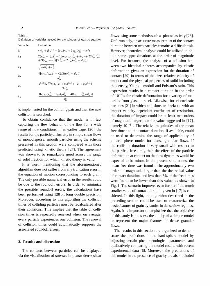
Table 1Definition of variables needed for the solution of quartic equation

Variable Definition

k1 (v2iw + diw)

2 − 6ciwbiw + 3a2iw(r

2iw − σ 2)

k2 2(v2iw + diw)

3 − 18biwciw(v2iw + diw)+ 27a2

iwb2iw

+ 9(r2iw − σ 2)[3c2

iw − 2a2iw(v

2iw + diw)]

k3

√−4k3

1 + k22

k44[(ciw/aiw)

2 − (2/3)(v2iw + diw)]

a2iw

k525/3[(22/3k1)/(k2 + k3)

1/3 + (k2 + k3)1/3]

3a2iw

k616[ciw(v

2iw + diw)/a

2iw − 4(biw + c3

iw/a4iw)]

a2iw

is implemented for the colliding pair and then the nextcollision is searched.

To obtain confidence that the model is in factcapturing the flow behavior of the flow for a widerange of flow conditions, in an earlier paper [26], theresults for the particle diffusivity in simple shear flowsof monodisperse, smooth particles using the schemepresented in this section were compared with thosepredicted using kinetic theory [27]. The agreementwas shown to be remarkably good across the rangeof solid fraction for which kinetic theory is valid.

It is worth mentioning that the aforementionedalgorithm does not suffer from any truncation error inthe equation of motion corresponding to each grain.The only possible numerical error in the results couldbe due to the roundoff errors. In order to minimizethe possible roundoff errors, the calculations havebeen performed using 128 bit long double precision.Moreover, according to this algorithm the collisiontimes of colliding particles must be recalculated aftertheir collisions. This implies that the table of colli-sion times is repeatedly renewed when, on average,every particle experiences one collision. The renewalof collision times could automatically suppress theassociated roundoff errors.

3. Results and discussion

The contacts between particles can be displayedvia the visualization of stresses in planar dense shear

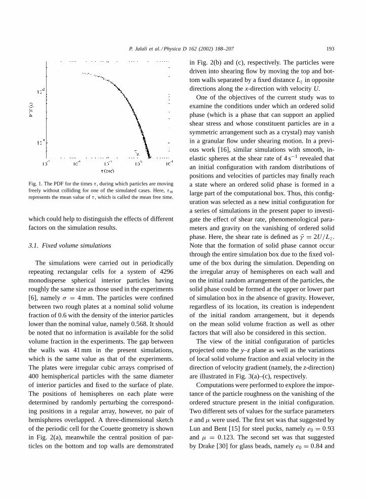
flows using some methods such as photoelasticity [28].Unfortunately, an accurate measurement of the contactduration between two particles remains a difficult task.However, theoretical analysis could be utilized to ob-tain some approximations at the order-of-magnitudelevel. For instance, the analysis of a collision bet-ween two identical spheres accompanied by elasticdeformation gives an expression for the duration ofcontact [29] in terms of the size, relative velocity ofimpact and the physical properties of solid includingthe density, Young’s moduli and Poisson’s ratio. Thisexpression results in a contact duration in the orderof 10−4 s for elastic deformation for a variety of ma-terials from glass to steel. Likewise, for viscoelasticparticles [21] in which collisions are inelastic with animpact velocity-dependent coefficient of restitution,the duration of impact could be at least two ordersof magnitude larger than the value suggested in [17],namely 10−6 s. The relative magnitudes of the meanfree time and the contact duration, if available, couldbe used to determine the range of applicability ofa hard-sphere model for dense granular flows. Ifthe collision duration is very small with respect tothe particle free time, then the effect of the particledeformation at contact on the flow dynamics would beexpected to be minor. In the present simulations, themean free time was found to be approximately twoorders of magnitude larger than the theoretical valueof contact duration, and less than 3% of the free timeswere found to be lower than this value, as shown inFig. 1. The scenario improves even further if the muchsmaller value of contact duration given in [17] is con-sidered. In this light, the algorithm described in thepreceding section could be used to characterize thebasic features of grain dynamics in dense flow regimes.Again, it is important to emphasize that the objectiveof this study is to assess the ability of a simple modelto represent the major features of dense granularflows.

The results in this section are organized to demon-strate the predictions of the hard-sphere model byadjusting certain phenomenological parameters andqualitatively comparing the model results with recentexperimental data [6]. Moreover, the predictions ofthis model in the presence of gravity are also included


Fig. 1. The PDF for the timesτ , during which particles are movingfreely without colliding for one of the simulated cases. Here,τm

represents the mean value ofτ , which is called the mean free time.

which could help to distinguish the effects of differentfactors on the simulation results.

3.1. Fixed volume simulations

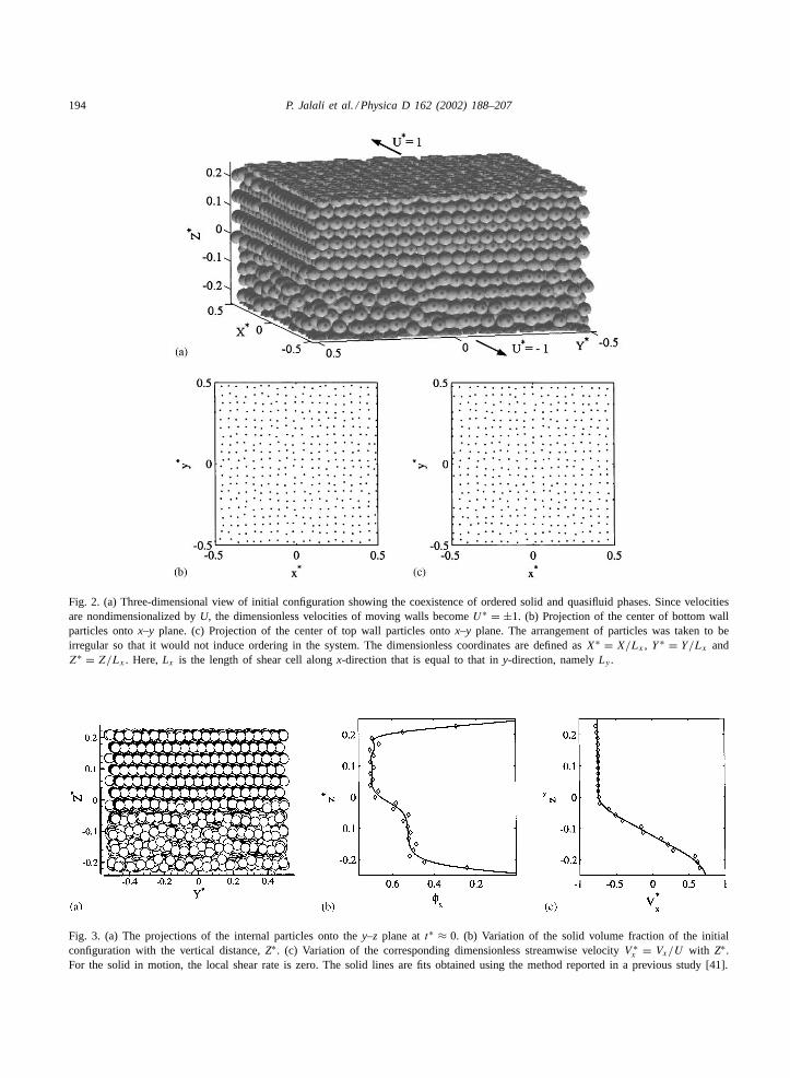
The simulations were carried out in periodicallyrepeating rectangular cells for a system of 4296monodisperse spherical interior particles havingroughly the same size as those used in the experiments[6], namelyσ = 4 mm. The particles were confinedbetween two rough plates at a nominal solid volumefraction of 0.6 with the density of the interior particleslower than the nominal value, namely 0.568. It shouldbe noted that no information is available for the solidvolume fraction in the experiments. The gap betweenthe walls was 41 mm in the present simulations,which is the same value as that of the experiments.The plates were irregular cubic arrays comprised of400 hemispherical particles with the same diameterof interior particles and fixed to the surface of plate.The positions of hemispheres on each plate weredetermined by randomly perturbing the correspond-ing positions in a regular array, however, no pair ofhemispheres overlapped. A three-dimensional sketchof the periodic cell for the Couette geometry is shownin Fig. 2(a), meanwhile the central position of par-ticles on the bottom and top walls are demonstrated

in Fig. 2(b) and (c), respectively. The particles weredriven into shearing flow by moving the top and bot-tom walls separated by a fixed distanceLz in oppositedirections along thex-direction with velocityU.

One of the objectives of the current study was toexamine the conditions under which an ordered solidphase (which is a phase that can support an appliedshear stress and whose constituent particles are in asymmetric arrangement such as a crystal) may vanishin a granular flow under shearing motion. In a previ-ous work [16], similar simulations with smooth, in-elastic spheres at the shear rate of 4 s−1 revealed thatan initial configuration with random distributions ofpositions and velocities of particles may finally reacha state where an ordered solid phase is formed in alarge part of the computational box. Thus, this config-uration was selected as a new initial configuration fora series of simulations in the present paper to investi-gate the effect of shear rate, phenomenological para-meters and gravity on the vanishing of ordered solidphase. Here, the shear rate is defined asγ = 2U/Lz.Note that the formation of solid phase cannot occurthrough the entire simulation box due to the fixed vol-ume of the box during the simulation. Depending onthe irregular array of hemispheres on each wall andon the initial random arrangement of the particles, thesolid phase could be formed at the upper or lower partof simulation box in the absence of gravity. However,regardless of its location, its creation is independentof the initial random arrangement, but it dependson the mean solid volume fraction as well as otherfactors that will also be considered in this section.

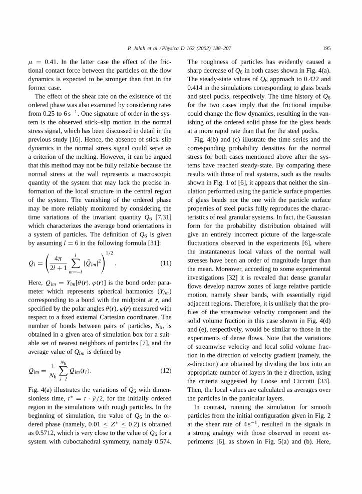
The view of the initial configuration of particlesprojected onto they–z plane as well as the variationsof local solid volume fraction and axial velocity in thedirection of velocity gradient (namely, thez-direction)are illustrated in Fig. 3(a)–(c), respectively.

Computations were performed to explore the impor-tance of the particle roughness on the vanishing of theordered structure present in the initial configuration.Two different sets of values for the surface parameterse andµ were used. The first set was that suggested byLun and Bent [15] for steel pucks, namelye0 = 0.93andµ = 0.123. The second set was that suggestedby Drake [30] for glass beads, namelye0 = 0.84 and


Fig. 2. (a) Three-dimensional view of initial configuration showing the coexistence of ordered solid and quasifluid phases. Since velocitiesare nondimensionalized byU, the dimensionless velocities of moving walls becomeU∗ = ±1. (b) Projection of the center of bottom wallparticles ontox–y plane. (c) Projection of the center of top wall particles ontox–y plane. The arrangement of particles was taken to beirregular so that it would not induce ordering in the system. The dimensionless coordinates are defined asX∗ = X/Lx , Y ∗ = Y/Lx andZ∗ = Z/Lx . Here,Lx is the length of shear cell alongx-direction that is equal to that iny-direction, namelyLy .

Fig. 3. (a) The projections of the internal particles onto they–z plane att∗ ≈ 0. (b) Variation of the solid volume fraction of the initialconfiguration with the vertical distance,Z∗. (c) Variation of the corresponding dimensionless streamwise velocityV ∗

x = Vx/U with Z∗.For the solid in motion, the local shear rate is zero. The solid lines are fits obtained using the method reported in a previous study [41].


µ = 0.41. In the latter case the effect of the fric-tional contact force between the particles on the flowdynamics is expected to be stronger than that in theformer case.

The effect of the shear rate on the existence of theordered phase was also examined by considering ratesfrom 0.25 to 6 s−1. One signature of order in the sys-tem is the observed stick–slip motion in the normalstress signal, which has been discussed in detail in theprevious study [16]. Hence, the absence of stick–slipdynamics in the normal stress signal could serve asa criterion of the melting. However, it can be arguedthat this method may not be fully reliable because thenormal stress at the wall represents a macroscopicquantity of the system that may lack the precise in-formation of the local structure in the central regionof the system. The vanishing of the ordered phasemay be more reliably monitored by considering thetime variations of the invariant quantityQ6 [7,31]which characterizes the average bond orientations ina system of particles. The definition ofQ6 is givenby assumingl = 6 in the following formula [31]:

Ql =(

4π

2l + 1

l∑m=−l

|Qlm|2)1/2

. (11)

Here,Qlm = Ylm[θ(r), ϕ(r)] is the bond order para-meter which represents spherical harmonics (Ylm)corresponding to a bond with the midpoint atr, andspecified by the polar anglesθ (r), ϕ(r) measured withrespect to a fixed external Cartesian coordinates. Thenumber of bonds between pairs of particles,Nb, isobtained in a given area of simulation box for a suit-able set of nearest neighbors of particles [7], and theaverage value ofQlm is defined by

Qlm = 1

Nb

Nb∑i=l

Qlm(ri ). (12)

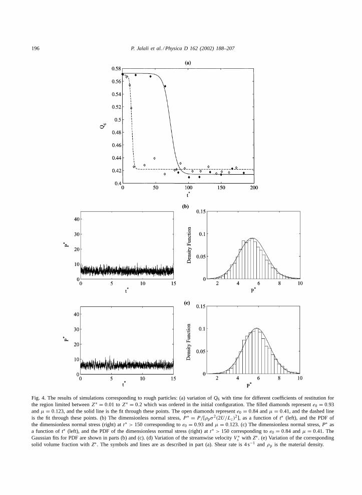
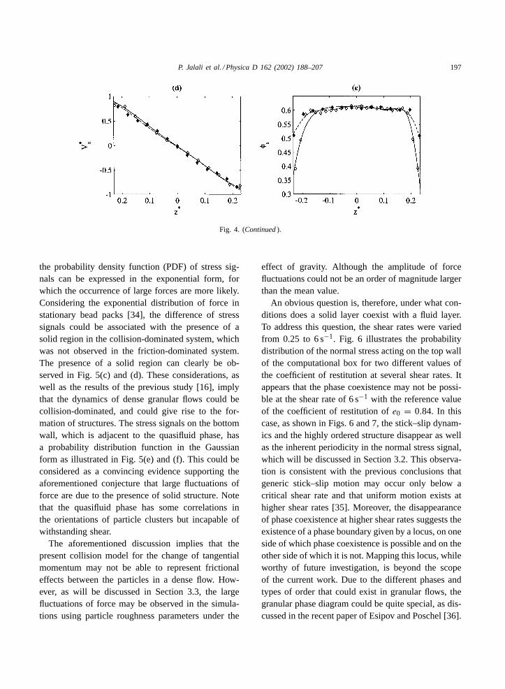
Fig. 4(a) illustrates the variations ofQ6 with dimen-sionless time,t∗ = t · γ /2, for the initially orderedregion in the simulations with rough particles. In thebeginning of simulation, the value ofQ6 in the or-dered phase (namely, 0.01 ≤ Z∗ ≤ 0.2) is obtainedas 0.5712, which is very close to the value ofQ6 for asystem with cuboctahedral symmetry, namely 0.574.

The roughness of particles has evidently caused asharp decrease ofQ6 in both cases shown in Fig. 4(a).The steady-state values ofQ6 approach to 0.422 and0.414 in the simulations corresponding to glass beadsand steel pucks, respectively. The time history ofQ6

for the two cases imply that the frictional impulsecould change the flow dynamics, resulting in the van-ishing of the ordered solid phase for the glass beadsat a more rapid rate than that for the steel pucks.

Fig. 4(b) and (c) illustrate the time series and thecorresponding probability densities for the normalstress for both cases mentioned above after the sys-tems have reached steady-state. By comparing theseresults with those of real systems, such as the resultsshown in Fig. 1 of [6], it appears that neither the sim-ulation performed using the particle surface propertiesof glass beads nor the one with the particle surfaceproperties of steel pucks fully reproduces the charac-teristics of real granular systems. In fact, the Gaussianform for the probability distribution obtained willgive an entirely incorrect picture of the large-scalefluctuations observed in the experiments [6], wherethe instantaneous local values of the normal wallstresses have been an order of magnitude larger thanthe mean. Moreover, according to some experimentalinvestigations [32] it is revealed that dense granularflows develop narrow zones of large relative particlemotion, namely shear bands, with essentially rigidadjacent regions. Therefore, it is unlikely that the pro-files of the streamwise velocity component and thesolid volume fraction in this case shown in Fig. 4(d)and (e), respectively, would be similar to those in theexperiments of dense flows. Note that the variationsof streamwise velocity and local solid volume frac-tion in the direction of velocity gradient (namely, thez-direction) are obtained by dividing the box into anappropriate number of layers in thez-direction, usingthe criteria suggested by Loose and Ciccotti [33].Then, the local values are calculated as averages overthe particles in the particular layers.

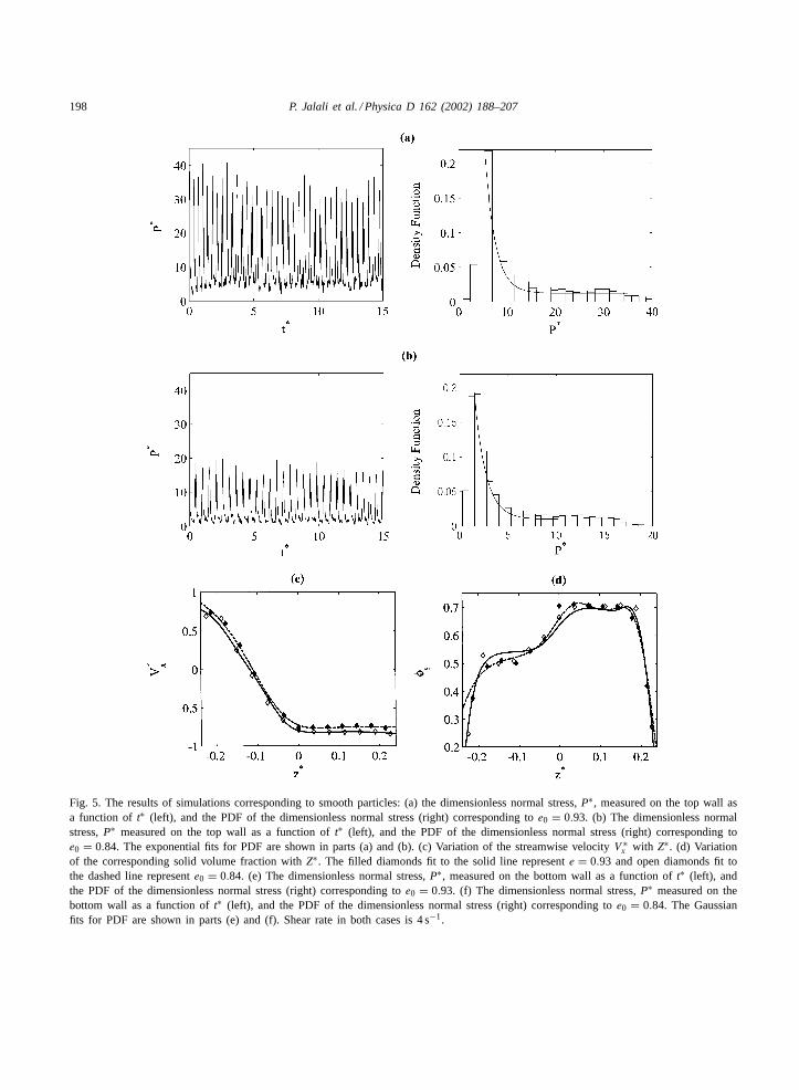
In contrast, running the simulation for smoothparticles from the initial configuration given in Fig. 2at the shear rate of 4 s−1, resulted in the signals ina strong analogy with those observed in recent ex-periments [6], as shown in Fig. 5(a) and (b). Here,


Fig. 4. The results of simulations corresponding to rough particles: (a) variation ofQ6 with time for different coefficients of restitution forthe region limited betweenZ∗ = 0.01 toZ∗ = 0.2 which was ordered in the initial configuration. The filled diamonds represente0 = 0.93andµ = 0.123, and the solid line is the fit through these points. The open diamonds represente0 = 0.84 andµ = 0.41, and the dashed lineis the fit through these points. (b) The dimensionless normal stress,P ∗ = P/[ρpσ

2(2U/Lz)2], as a function oft∗ (left), and the PDF ofthe dimensionless normal stress (right) att∗ > 150 corresponding toe0 = 0.93 andµ = 0.123. (c) The dimensionless normal stress,P∗ asa function oft∗ (left), and the PDF of the dimensionless normal stress (right) att∗ > 150 corresponding toe0 = 0.84 andµ = 0.41. TheGaussian fits for PDF are shown in parts (b) and (c). (d) Variation of the streamwise velocityV ∗

x with Z∗. (e) Variation of the correspondingsolid volume fraction withZ∗. The symbols and lines are as described in part (a). Shear rate is 4 s−1 andρp is the material density.


Fig. 4. (Continued).

the probability density function (PDF) of stress sig-nals can be expressed in the exponential form, forwhich the occurrence of large forces are more likely.Considering the exponential distribution of force instationary bead packs [34], the difference of stresssignals could be associated with the presence of asolid region in the collision-dominated system, whichwas not observed in the friction-dominated system.The presence of a solid region can clearly be ob-served in Fig. 5(c) and (d). These considerations, aswell as the results of the previous study [16], implythat the dynamics of dense granular flows could becollision-dominated, and could give rise to the for-mation of structures. The stress signals on the bottomwall, which is adjacent to the quasifluid phase, hasa probability distribution function in the Gaussianform as illustrated in Fig. 5(e) and (f). This could beconsidered as a convincing evidence supporting theaforementioned conjecture that large fluctuations offorce are due to the presence of solid structure. Notethat the quasifluid phase has some correlations inthe orientations of particle clusters but incapable ofwithstanding shear.

The aforementioned discussion implies that thepresent collision model for the change of tangentialmomentum may not be able to represent frictionaleffects between the particles in a dense flow. How-ever, as will be discussed in Section 3.3, the largefluctuations of force may be observed in the simula-tions using particle roughness parameters under the

effect of gravity. Although the amplitude of forcefluctuations could not be an order of magnitude largerthan the mean value.

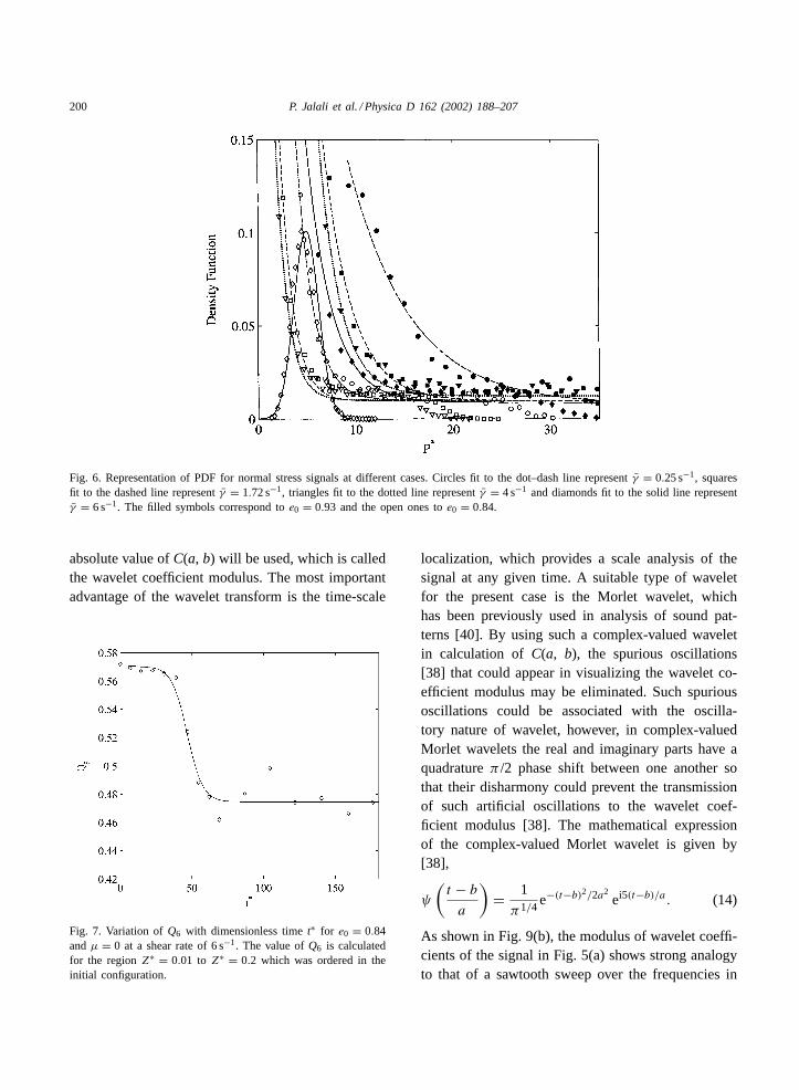
An obvious question is, therefore, under what con-ditions does a solid layer coexist with a fluid layer.To address this question, the shear rates were variedfrom 0.25 to 6 s−1. Fig. 6 illustrates the probabilitydistribution of the normal stress acting on the top wallof the computational box for two different values ofthe coefficient of restitution at several shear rates. Itappears that the phase coexistence may not be possi-ble at the shear rate of 6 s−1 with the reference valueof the coefficient of restitution ofe0 = 0.84. In thiscase, as shown in Figs. 6 and 7, the stick–slip dynam-ics and the highly ordered structure disappear as wellas the inherent periodicity in the normal stress signal,which will be discussed in Section 3.2. This observa-tion is consistent with the previous conclusions thatgeneric stick–slip motion may occur only below acritical shear rate and that uniform motion exists athigher shear rates [35]. Moreover, the disappearanceof phase coexistence at higher shear rates suggests theexistence of a phase boundary given by a locus, on oneside of which phase coexistence is possible and on theother side of which it is not. Mapping this locus, whileworthy of future investigation, is beyond the scopeof the current work. Due to the different phases andtypes of order that could exist in granular flows, thegranular phase diagram could be quite special, as dis-cussed in the recent paper of Esipov and Poschel [36].


Fig. 5. The results of simulations corresponding to smooth particles: (a) the dimensionless normal stress,P∗, measured on the top wall asa function of t∗ (left), and the PDF of the dimensionless normal stress (right) corresponding toe0 = 0.93. (b) The dimensionless normalstress,P∗ measured on the top wall as a function oft∗ (left), and the PDF of the dimensionless normal stress (right) corresponding toe0 = 0.84. The exponential fits for PDF are shown in parts (a) and (b). (c) Variation of the streamwise velocityV ∗

x with Z∗. (d) Variationof the corresponding solid volume fraction withZ∗. The filled diamonds fit to the solid line represente = 0.93 and open diamonds fit tothe dashed line represente0 = 0.84. (e) The dimensionless normal stress,P∗, measured on the bottom wall as a function oft∗ (left), andthe PDF of the dimensionless normal stress (right) corresponding toe0 = 0.93. (f) The dimensionless normal stress,P∗ measured on thebottom wall as a function oft∗ (left), and the PDF of the dimensionless normal stress (right) corresponding toe0 = 0.84. The Gaussianfits for PDF are shown in parts (e) and (f). Shear rate in both cases is 4 s−1.


Fig. 5. (Continued).

3.2. Periodicity and wavelet analysis

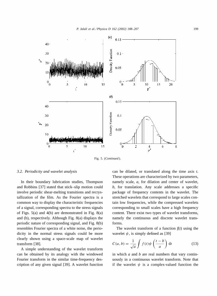
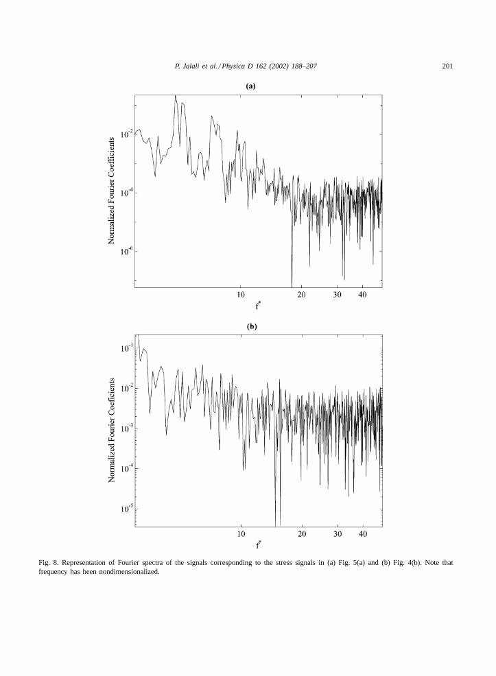
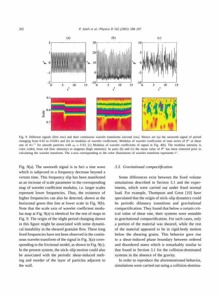
In their boundary lubrication studies, Thompsonand Robbins [37] stated that stick–slip motion couldinvolve periodic shear-melting transitions and recrys-tallization of the film. As the Fourier spectra is acommon way to display the characteristic frequenciesof a signal, corresponding spectra to the stress signalsof Figs. 5(a) and 4(b) are demonstrated in Fig. 8(a)and (b), respectively. Although Fig. 8(a) displays theperiodic nature of corresponding signal, and Fig. 8(b)resembles Fourier spectra of a white noise, the perio-dicity in the normal stress signals could be moreclearly shown using a space-scale map of wavelettransform [38].

A simple understanding of the wavelet transformcan be obtained by its analogy with the windowedFourier transform in the similar time-frequency des-cription of any given signal [39]. A wavelet function

can be dilated, or translated along the time axist.These operations are characterized by two parameters,namely scale,a, for dilation and center of wavelet,b, for translation. Any scale addresses a specificpackage of frequency contents in the wavelet. Thestretched wavelets that correspond to large scales con-tain low frequencies, while the compressed waveletscorresponding to small scales have a high frequencycontent. There exist two types of wavelet transforms,namely the continuous and discrete wavelet trans-forms.

The wavelet transform of a functionf(t) using thewaveletψ , is simply defined as [39]

C(a, b) = 1√a

∫f (t)ψ

(t − b

a

)dt (13)

in which a and b are real numbers that vary contin-uously in a continuous wavelet transform. Note thatif the waveletψ is a complex-valued function the


Fig. 6. Representation of PDF for normal stress signals at different cases. Circles fit to the dot–dash line representγ = 0.25 s−1, squaresfit to the dashed line representγ = 1.72 s−1, triangles fit to the dotted line representγ = 4 s−1 and diamonds fit to the solid line representγ = 6 s−1. The filled symbols correspond toe0 = 0.93 and the open ones toe0 = 0.84.

absolute value ofC(a, b) will be used, which is calledthe wavelet coefficient modulus. The most importantadvantage of the wavelet transform is the time-scale

Fig. 7. Variation ofQ6 with dimensionless timet∗ for e0 = 0.84andµ = 0 at a shear rate of 6 s−1. The value ofQ6 is calculatedfor the regionZ∗ = 0.01 to Z∗ = 0.2 which was ordered in theinitial configuration.

localization, which provides a scale analysis of thesignal at any given time. A suitable type of waveletfor the present case is the Morlet wavelet, whichhas been previously used in analysis of sound pat-terns [40]. By using such a complex-valued waveletin calculation of C(a, b), the spurious oscillations[38] that could appear in visualizing the wavelet co-efficient modulus may be eliminated. Such spuriousoscillations could be associated with the oscilla-tory nature of wavelet, however, in complex-valuedMorlet wavelets the real and imaginary parts have aquadratureπ /2 phase shift between one another sothat their disharmony could prevent the transmissionof such artificial oscillations to the wavelet coef-ficient modulus [38]. The mathematical expressionof the complex-valued Morlet wavelet is given by[38],

ψ

(t − b

a

)= 1

π1/4e−(t−b)2/2a2

ei5(t−b)/a. (14)

As shown in Fig. 9(b), the modulus of wavelet coeffi-cients of the signal in Fig. 5(a) shows strong analogyto that of a sawtooth sweep over the frequencies in


Fig. 8. Representation of Fourier spectra of the signals corresponding to the stress signals in (a) Fig. 5(a) and (b) Fig. 4(b). Note thatfrequency has been nondimensionalized.


Fig. 9. Different signals (first row) and their continuous wavelet transforms (second row). Shown are (a) the sawtooth signal of periodchanging from 0.02 to 0.028 s and (b) its modulus of wavelet coefficients. Modulus of wavelet coefficients of time series ofP∗ at shearrate of 4 s−1 for smooth particles withe0 = 0.93. (c) Modulus of wavelet coefficients of signal in Fig. 4(b). The modulus intensity iscolor coded, from red (low intensity) to magenta (high intensity). In parts (b) and (c) the mean value ofP∗ has been removed prior tocalculating the wavelet transform. Thex-axis corresponding to the color illustrations of wavelet transform representst∗.

Fig. 9(a). The sawtooth signal is in fact a sine wavewhich is subjected to a frequency decrease beyond acertain time. This frequency slip has been manifestedas an increase of scale parameter in the correspondingmap of wavelet coefficient modulus, i.e. larger scalesrepresent lower frequencies. Thus, the existence ofhigher frequencies can also be detected, shown as thehorizontal green thin line at lower scale in Fig. 9(b).Note that the scale axis of wavelet coefficient modu-lus map at Fig. 9(a) is identical for the rest of maps inFig. 9. The origin of the slight period changing shownin this figure might be associated with some dynami-cal instability in the sheared granular flow. These longlived frequencies have not been observed in the contin-uous wavelet transform of the signal in Fig. 3(a) corre-sponding to the frictional model, as shown in Fig. 9(c).In the present system, the stick–slip motion could alsobe associated with the periodic shear-induced melt-ing and reorder of the layer of particles adjacent tothe wall.

3.3. Gravitational compactification

Some differences exist between the fixed volumesimulations described in Section 3.1 and the exper-iments, which were carried out under fixed normalload. For example, Thompson and Grest [10] havespeculated that the origin of stick–slip dynamics couldbe periodic dilatancy transitions and gravitationalcompactification. They found that below a certain crit-ical value of shear rate, their systems were unstableto gravitational compactification. For such cases, onlya portion of the material was sheared, while the restof the material appeared to be in rigid-body motionbelow the shearing grains. This behavior gave riseto a shear-induced phase boundary between orderedand disordered states which is remarkably similar tothat found in Section 3.1 for the collision-dominatedsystems in the absence of the gravity.

In order to reproduce the aforementioned behavior,simulations were carried out using a collision-domina-


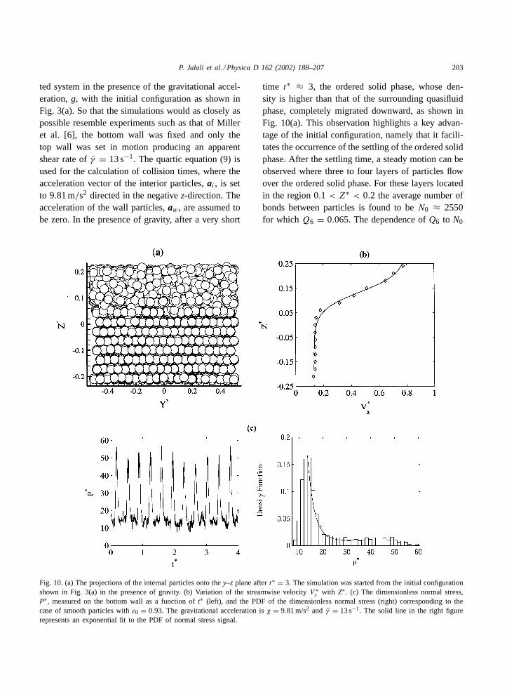
ted system in the presence of the gravitational accel-eration,g, with the initial configuration as shown inFig. 3(a). So that the simulations would as closely aspossible resemble experiments such as that of Milleret al. [6], the bottom wall was fixed and only thetop wall was set in motion producing an apparentshear rate ofγ = 13 s−1. The quartic equation (9) isused for the calculation of collision times, where theacceleration vector of the interior particles,ai , is setto 9.81 m/s2 directed in the negativez-direction. Theacceleration of the wall particles,aw, are assumed tobe zero. In the presence of gravity, after a very short

Fig. 10. (a) The projections of the internal particles onto they–z plane aftert∗ = 3. The simulation was started from the initial configurationshown in Fig. 3(a) in the presence of gravity. (b) Variation of the streamwise velocityV ∗

x with Z∗. (c) The dimensionless normal stress,P∗, measured on the bottom wall as a function oft∗ (left), and the PDF of the dimensionless normal stress (right) corresponding to thecase of smooth particles withe0 = 0.93. The gravitational acceleration isg = 9.81 m/s2 and γ = 13 s−1. The solid line in the right figurerepresents an exponential fit to the PDF of normal stress signal.

time t∗ ≈ 3, the ordered solid phase, whose den-sity is higher than that of the surrounding quasifluidphase, completely migrated downward, as shown inFig. 10(a). This observation highlights a key advan-tage of the initial configuration, namely that it facili-tates the occurrence of the settling of the ordered solidphase. After the settling time, a steady motion can beobserved where three to four layers of particles flowover the ordered solid phase. For these layers locatedin the region 0.1 < Z∗ < 0.2 the average number ofbonds between particles is found to beN0 ≈ 2550for whichQ6 = 0.065. The dependence ofQ6 to N0


for a completely disordered phase in which the bondsare spatially uncorrelated can be obtained [31] as

Q6 = 1√N0

± 1√26N0

. (15)

This equation gives an approximation for the min-imum possible value ofQ6 as (1 ± 0.2)/N1/2

0 =0.020 ± 0.004 with the aforementioned number ofbonds. Therefore, it can be concluded that the phasethat is formed over the ordered solid phase may be

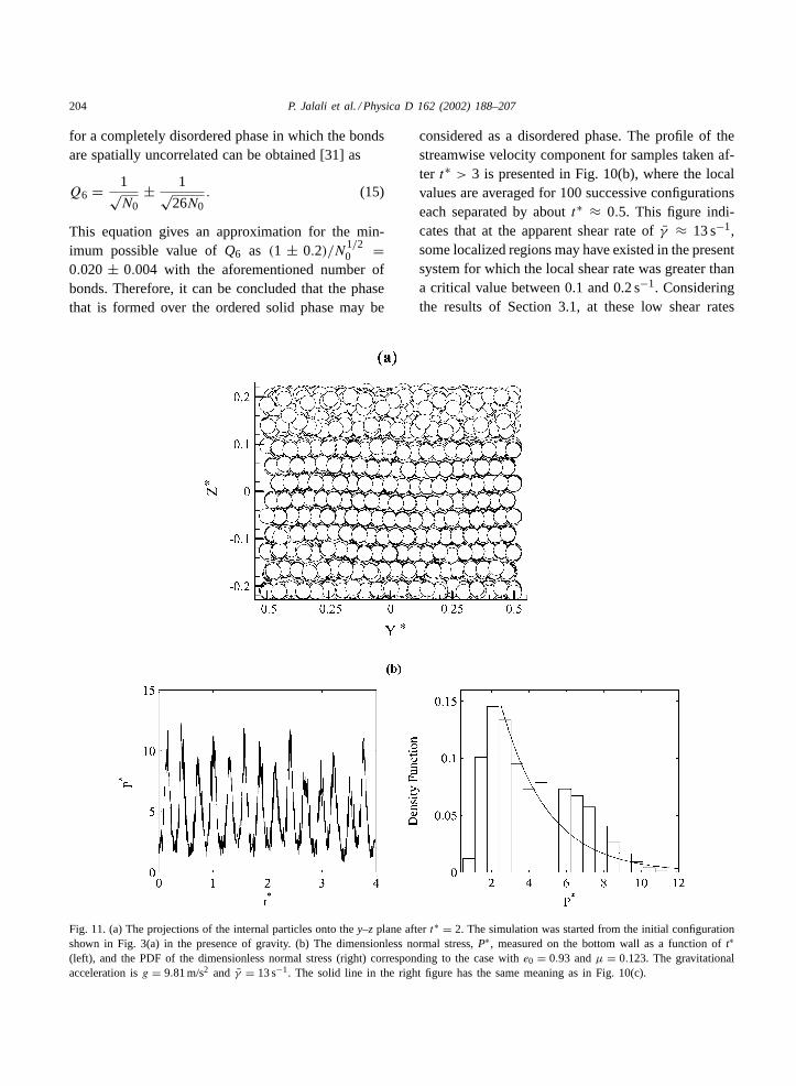
Fig. 11. (a) The projections of the internal particles onto they–z plane aftert∗ = 2. The simulation was started from the initial configurationshown in Fig. 3(a) in the presence of gravity. (b) The dimensionless normal stress,P∗, measured on the bottom wall as a function oft∗(left), and the PDF of the dimensionless normal stress (right) corresponding to the case withe0 = 0.93 andµ = 0.123. The gravitationalacceleration isg = 9.81 m/s2 and γ = 13 s−1. The solid line in the right figure has the same meaning as in Fig. 10(c).

considered as a disordered phase. The profile of thestreamwise velocity component for samples taken af-ter t∗ > 3 is presented in Fig. 10(b), where the localvalues are averaged for 100 successive configurationseach separated by aboutt∗ ≈ 0.5. This figure indi-cates that at the apparent shear rate ofγ ≈ 13 s−1,some localized regions may have existed in the presentsystem for which the local shear rate was greater thana critical value between 0.1 and 0.2 s−1. Consideringthe results of Section 3.1, at these low shear rates


the system is expected to exhibit order without anymelting. Therefore, the stick–slip motion observedin the normal stress signal on the bottom wall, inFig. 10(c), could be the signature of periodic dila-tancy transition due to the shear-induced melting andgravitational compactification at the phase boundarybetween ordered and disordered phases.

The results obtained in Section 3.1 indicate that inthe absence of gravity, melting can occur even at verylow shear rates for a system in which the dynam-ics of the grains is dominated by frictional contact.Therefore, it is interesting to study the behavior ofthe aforementioned system in the presence of gravity.Considering the configuration in Fig. 11(a), which wastaken after the settling process, it may be concludedthat the migration time was too short for melting of thesolid phase to occur. However, after the settling timeof t∗ ≈ 2, the shear-induced melting at low shear ratescan be observed, which was a feature of the results ofSection 3.1. This behavior causes dilatancy transitionscompeting with the instability due to gravitationalcompactification throughout the region−0.2 ≤ Z∗ ≤0.1, which is located below the two to three layers ofthe disordered phase. The signature of this stick–slipdynamics can be observed in the normal stress signalon the bottom wall, as shown in Fig. 11(b). Although

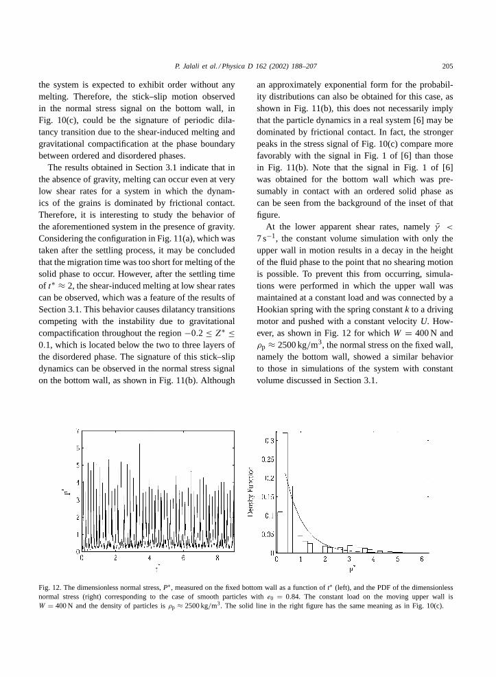
Fig. 12. The dimensionless normal stress,P∗, measured on the fixed bottom wall as a function oft∗ (left), and the PDF of the dimensionlessnormal stress (right) corresponding to the case of smooth particles withe0 = 0.84. The constant load on the moving upper wall isW = 400 N and the density of particles isρp ≈ 2500 kg/m3. The solid line in the right figure has the same meaning as in Fig. 10(c).

an approximately exponential form for the probabil-ity distributions can also be obtained for this case, asshown in Fig. 11(b), this does not necessarily implythat the particle dynamics in a real system [6] may bedominated by frictional contact. In fact, the strongerpeaks in the stress signal of Fig. 10(c) compare morefavorably with the signal in Fig. 1 of [6] than thosein Fig. 11(b). Note that the signal in Fig. 1 of [6]was obtained for the bottom wall which was pre-sumably in contact with an ordered solid phase ascan be seen from the background of the inset of thatfigure.

At the lower apparent shear rates, namelyγ <

7 s−1, the constant volume simulation with only theupper wall in motion results in a decay in the heightof the fluid phase to the point that no shearing motionis possible. To prevent this from occurring, simula-tions were performed in which the upper wall wasmaintained at a constant load and was connected by aHookian spring with the spring constantk to a drivingmotor and pushed with a constant velocityU. How-ever, as shown in Fig. 12 for whichW = 400 N andρp ≈ 2500 kg/m3, the normal stress on the fixed wall,namely the bottom wall, showed a similar behaviorto those in simulations of the system with constantvolume discussed in Section 3.1.


4. Conclusions

Computer simulations were performed for boundeddense shear flows consisting of monosized, sphericalparticles at a solid fraction of 0.568. The particleswere modeled using a modified hard-sphere model,which had been previously shown to replicate theresults predicted by kinetic theory [26] at low andmoderate solid fractions. The goal of the current studywas to investigate whether this model could also pre-dict the observed features of dense sheared granularflows at high solid volume fractions.

In the present study, both collision-dominated(smooth particle) and friction-dominated (rough parti-cle) systems were considered. In an idealized gravity-free system, simulations using the smooth modelrevealed the presence of an exponential behavior ofthe probability distribution function in the normalstress signals exerted on the moving wall for con-ditions similar to those of recent experiments [6].Wavelet transform analysis was used to show theexistence of a characteristic frequency in the normalstress signal, which is an indication of the presenceof stick–slip dynamics. However, at sufficiently highshear rates, the melting of the ordered solid phaseoccurred. For the range of shear rates studied, theresults of the simulations for the rough model didnot show the same stick–slip behavior as a result ofthe vanishing of the ordered solid region due to thepresence of strong frictional interactions.

The impact of the above-mentioned differentbehavior of smooth and rough systems in shearingflows was further investigated in the presence of grav-ity where the systems could be unstable due to gravita-tional compactification. For these cases, the stick–slipdynamics could be observed for both systems on thebottom wall, where the ordered solid phase settles dueto the density difference between the ordered solidand the surrounding fluid. The results of the smoothmodel were found to match the experimental data [6]much more closely than those of the rough model,although the latter model did show a weak stick–slipbehavior due to the competition between the meltingtransitions and gravitational compactification. For theformer model, the normal stress signal revealed the

presence of a strong stick–slip motion, which couldbe a manifestation of the thermodynamic instabilityat the interface due to shear-induced melting andgravitational compactification. The smooth modelpredicted peaks in the normal stress signal whoselargest values are about five times the average value.However, the largest peaks in the experimental resultswere roughly twice as large as those predicted by thesmooth model, and about seven times as large as thosepredicted by the rough model. Therefore, it can beconcluded that both models (i.e. smooth and rough)are capable of describing the qualitative behavior ofthe real system, including the cyclic formation andmelting of ordered phases, with the smooth systemcomparing more favorably with the experiments [6].

Note that in the high-density regions, the collisionsare very frequent, suggesting that if the time-steppingis controlled by a collision list, most of the time theparticles are moving through very small distancesusing very small time steps. In order to mimic thebehavior of stagnated zones, a cut-off frequency maybe introduced. The time-stepping is then controlledby a scan frequency, which is a function of the speedof the fastest particle. Thus, additional study is re-quired on the use of the scan frequency to controlthe time-stepping. This modification may increasethe resolution for stagnated zones; consequently, theobserved features may be predicted quantitatively athigh solid volume fractions.

References

[1] B.J. Ackerson, N.A. Clark, Phys. Rev. Lett. 46 (1981) 123;B.J. Ackerson, N.A. Clark, Phys. Rev. A 30 (1981) 906;B.J. Ackerson, N.A. Clark, Physica (Amsterdam) 118A (1983)221;B.J. Ackerson, P.N. Pusey, Phys. Rev. Lett. 61 (1988) 1033;H. Lowen, Phys. Rep. 237 (1994) 249.

[2] H.M. Jaeger, S.R. Nagel, R.P. Behringer, Phys. Today 49(1996) 32.

[3] P. Pieranski, Am. J. Phys. 52 (1984) 68;J.S. Olafsen, J.S. Urbach, Phys. Rev. Lett. 81 (1998) 4369;P.N. Pusey, W. van Megen, Phys. Rev. Lett. 59 (1987) 2083.

[4] P.C. Johnson, R. Jackson, J. Fluid Mech. 176 (1987) 67.[5] N. Menon, D.J. Durian, Science 275 (1997) 1920.[6] B. Miller, C. O’Hern, R.P. Behringer, Phys. Rev. Lett. 77

(1996) 3110.[7] P. Zamankhan, H. Vahedi Tafreshi, W. Polashenski Jr., P.

Sarkomaa, C.L. Hyndman, J. Chem. Phys. 109 (1998) 4487.


[8] V.V.R. Natarajan, M.L. Hunt, E.D. Taylor, J. Fluid Mech. 304(1995) 1.

[9] P.A. Cundall, O.D.L. Strack, Geotechnique 29 (1979) 47.[10] P.A. Thompson, G.S. Grest, Phys. Rev. Lett. 67 (1991) 1751.[11] K. Yamne, M. Nakagawa, S.A. Altobelli, T. Tanaka, Y. Tsuji,

Phys. Fluids 10 (1998) 1419.[12] N.V. Brilliantov, F. Spahn, J.M. Hertzsch, T. Pöschel, Phys.

Rev. E 53 (1996) 5382.[13] S. Schöllmann, Phys. Rev. E 59 (1999) 889.[14] B.J. Alder, T. Wainwright, J. Chem. Phys. 31 (1959) 459.[15] C.K.K. Lun, A.A. Bent, J. Fluid Mech. 258 (1994) 335.[16] P. Zamankhan, T. Tynjälä, W. Polashenski Jr., P. Zamankhan,

P. Sarkomaa, Phys. Rev. E 60 (1999) 7149.[17] P.K. Haff, in: A. Mehta (Ed.), Granular Matter: An

Interdisciplinary Approach, Springer, New York, 1994(Chapter 5).

[18] J.P. Hansen, I.R. McDonald, Theory of Simple Liquids,Academic Press, London, 1986.

[19] W.A.M. Morgado, I. Oppenheim, Phys. Rev. E 55 (1997)1940.

[20] W. Goldsmith, Impact: The Theory and Physical Behaviourof Colliding Solids, Edward Arnold Ltd., London, 1960.

[21] T. Schwager, T. Pöschel, Phys. Rev. E 57 (1998) 650.[22] M.P. Allen, D.J. Tildesley, Computer Simulation of Liquids,

Clarendon Press, Oxford, 1997.[23] C.K.K. Lun, S.B. Savage, J. Appl. Mech. 54 (1987) 47.[24] C.A. Coulomb, Acad. R. Sci. Membr. Math. Phys. Par Divers

Savants 7 (1773) 343.

[25] J.T. Jenkins, M.W. Richman, Phys. Fluids 28 (1985) 3485.[26] P. Jalali, W. Polashenski, P. Zamankhan, P. Sarkomaa, Physica

A 275 (2000) 347.[27] J.T. Jenkins, M.W. Richman, Arch. Rat. Mech. Anal. 87

(1985) 355.[28] D.W. Howell, R.P. Behringer, C.T. Veje, Fluctuations in

granular media, Chaos 9 (1999) 559.[29] S.P. Timoshenko, J.N. Goodier, Theory of Elasticity, 3rd

Edition, McGraw-Hill, Kogakusha, 1970.[30] T.G. Drake, J. Fluid Mech. 225 (1991) 121.[31] M.D. Rintoul, S. Torquato, J. Chem. Phys. 105 (1996)

9258.[32] D.M. Mueth, G.F. Debregeas, G.S. Karczmar, P.J. Eng, S.R.

Nagel, H.M. Jaeger, Nature 406 (2000) 385.[33] W. Loose, G. Ciccotti, Phys. Rev. A 45 (1992) 3859.[34] C.H. Liu, S.R. Nagel, D.A. Schecter, S.N. Coppersmith, S.

Majumdar, O. Narayan, T.A. Witten, Science 269 (1995)513.

[35] D.M. Hanes, D.L. Inman, J. Fluid Mech. 150 (1985) 357.[36] S.E. Esipov, T. Poschel, J. Stat. Phys. 86 (1997) 1385.[37] P.A. Thompson, M.O. Robbins, Science 250 (1990) 792.[38] M. Farge, Annu. Rev. Fluid Mech. 24 (1992) 395.[39] I. Daubechies, Ten Lectures on Wavelets, SIAM, Montpelier,

VT, 1992.[40] R. Kronald-Martinet, J. Morelet, A. Grossmann, Int. J. Pattern

Recog. Artif. Intell. 1 (1987) 273.[41] P. Zamankhan, P. Malinen, H. Lepomaki, AIChE J. 43 (1997)

1684.

Particle interactions in a dense monosized granular flow

Documents

Transcript of Particle interactions in a dense monosized granular flow