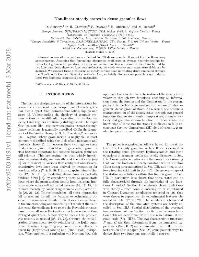
arX

iv:0

803.

0191

v1 [

cond

-mat

.sta

t-m

ech]

3 M

ar 2

008

Non-linear steady states in dense granular flows

D. Bonamy,1 P. H. Chavanis,2 F. Daviaud,3 B. Dubrulle,3 and M. Renouf4

1Groupe fracture, DSM/DRECAM/SPCSI, CEA Saclay, F-91191 Gif sur Yvette - France2Laboratoire de Physique Theorique (UMR 5152),

Universite Paul Sabatier, 118, route de Narbonne 31062 Toulouse, France3Groupe Instabilite & Turbulence, DSM/DRECAM/SPEC, CEA Saclay, F-91191 Gif sur Yvette - France

4Equipe TMI - LaMCoS/INSA Lyon - UMR5259,18-20 rue des sciences, F-69621 Villeurbannes - France

(Dated: March 4, 2008)

General conservation equations are derived for 2D dense granular flows within the Boussinesqapproximation. Assuming that forcing and dissipation equilibrate on average, the relationships be-tween local granular temperature, vorticity and stream function are shown to be characterized bytwo functions. Once these two functions are known, the whole velocity and temperature fields can bededuced. We checked these predictions on steady surface flows in rotating drum simulated throughthe Non-Smooth Contact Dynamics methods. Also, we briefly discuss some possible ways to derivethese two functions using statistical mechanics.

PACS numbers: 45.70.-n, 83.70.Fn, 46.10.+z

I. INTRODUCTION

The intrinsic dissipative nature of the interactions be-tween the constituent macroscopic particles sets gran-ular media apart from conventional solids, liquids andgases [1]. Understanding the rheology of granular sys-tems is thus rather difficult. Depending on the flow ve-locity, three regimes are usually distinguished: The rapid

flow – gaseous-like – regime where grains interact throughbinary collisions, is generally described within the frame-work of the kinetic theory [2, 3, 4]; The slow flow – solid-like – regime, where grain inertia is negligible, is mostcommonly described using the tools of soil mechanics andplasticity theory [5]. In between these two regimes thereexists a dense flow – liquid-like – regime where grain in-ertia becomes important but contacts between grains arestill relevant. This last regime has been widely investi-gated experimentally, numerically and theoretically (see[6] for a review) in various flow configurations. Severalconstitutive laws have been derived by accounting fornon-local effects [7, 8, 9, 10, 11], by adapting kinetic the-ory [12, 13, 14], by modelling dense flows as partiallyfluidized flows [15], by considering them as quasi-staticflows where the mean motion results from transient frac-tures modelled as self activated process [16, 17, 18, 19]or more recently by considering them as visco-plastic flu-ids [20, 21, 22]. To our knowledge, all these approachesfail to account for all the features experimentally ob-served. In some sense, similar difficulties are encounteredin the understanding and modelling of turbulent fluids. Inthat case, the challenge is to relate the Reynolds stresses,based on small scale fluctuations, to large scale or timeaveraged quantities. A new way to tackle this problemwas recently suggested [23, 24, 25], through the consid-eration of non-linear steady solutions of the Euler equa-tions, thereby disregarding any non-universal effects in-duced by (large scale) forcing and (small scale) dissipa-tion. When applied to a turbulent von Karman flow, this

approach leads to the characterization of the steady statevelocities through two functions, encoding all informa-tion about the forcing and the dissipation. In the presentpaper, this method is generalized to the case of inhomo-geneous dense granular flows. As a result, one obtains acharacterization of the steady state through two generalfunctions that relate granular temperature, granular vor-ticity and granular stream function. In other words, theknowledge of these two functions is sufficient to fully re-construct the two-dimensional (2D) field of velocity, gran-ular temperature, and volume fraction.

The paper is organized as follows: In Sec. II, the struc-ture of 2D steady granular surface flows is derived inthe rotating drum geometry. Hydrodynamics and stateequations in granular media are briefly discussed in Sec.IIA. Conservation equations are then rewritten assumingthat volume fraction is nearly constant within the flow(Boussinesq approximation) in Sec. IIB, and then in theforce-free, inviscid limit in Sec. IIC. The general shape ofthe stationary solutions within this limit is given in Sec.IID. In particular, it is shown that these states can befully characterized through the knowledge of two func-tions F and G. Section III confronts these predictionswith steady surface flows in rotating drum as obtainedin Contact Dynamics simulations reported in [26] thatwere shown to reproduce the experimental features ob-served in Refs. [27, 28, 29]. The simulation scheme andthe description of the simulated systems are briefly re-called in Sec. IIIA. Spatial distribution of the averagedtemperature, volume fraction, vorticity and stream func-tion fields are determined within the whole drum, at thegrain scale (Sec. IIIB). The two characteristic functionsF and G are then determined from the numerical ex-periments (Sec. IIIC) and commented (Sec. IIID). In thelast section of this paper (Sec. IV) some possible ways toderive these two functions are briefly discussed.

2

II. THEORETICAL FRAMEWORK:

CONSERVATION EQUATIONS WITHIN THE

BOUSSINESQ APPROXIMATION

A. Granular hydrodynamics

It is commonly assumed that granular media can bedescribed with continuum models. The mass, momentumand energy conservation equations then lead to:

∂tν + ∇ · (νv) = 0,

∂tνv + (v · ∇) νv = −∇P + νg + Fvisc + Fforc,

∂tνT + ∇ · (νTv) = −P∇ · v + Evisc + Eforc. (1)

In these equations, ν(x, z, t) is the field of volume frac-tion, v(x, z, t) the velocity field; g is the gravitationalacceleration; T (x, z, t) is the field of granular tempera-ture defined in term of the RMS part of the velocityfield, T (x, z, t) = 1

2 〈(cb(t)−v(x, z, t))2〉b∈(x,z) where cb(t)refers to the instantaneous velocity of the bead b locatedat time t within the elementary volume located in (x, z);Fforc, Eforc stand for external forcing and Fvisc, Evisc

stand for all dissipative processes. This system has to besupplemented by an equation of state P = g(ν)T andrheology, i.e. some constitutive equations describing thedissipative processes Fvisc, Evisc.

Contrary to classical liquids, the density and temper-ature dependence of transport coefficients play an im-portant role in determining the flow density. For dilutesystems they are usually obtained using kinetic theoryof granular gases [2, 3, 4] within the Enskog approxima-tion. For dense gases, there is no available systematic the-ory allowing their description. They are therefore usuallyprescribed using phenomenological models [13] or fittedusing experimental [21, 22, 30] or numerical [31] data. Inparticular, the equation of state can be written in thehigh-density limit [21, 31]:

P ≃ Kν2∗

ν∗ − νT, (2)

where K is a constant and ν∗ the random closed packedlimit: ν∗ ≃ 0.82 for 2D packing and ν∗ ≃ 0.64 for 3Dpackings. At ν = ν∗ this equation therefore predicts azero granular temperature, consistent with the absenceof motion.

As for the dissipative terms and forcing, their preciseshape shall not be needed in the sequel. This is a distin-guished feature of our approach.

B. The Boussinesq approximation

For simplicity, one focuses on situations where the vol-ume fraction is nearly constant close to the random closedpacked limit ν ≈ ν∗. In the considered system, this ap-proximation is satisfied within 10 percent. Generalization

to non constant volume fraction is possible, but more in-volved. In that limit, the classical Boussinesq approxi-mation is implemented by neglecting the fluctuation ofvolume fraction in the continuity equation so that it be-comes:

∇ · v ≈ 0. (3)

The other conservation equations may then be simplifiedby defining a reference state with v = 0, T = 0, P = P∗,ν = ν∗, so that:

∇P∗ = ν∗g, (4)

i.e. an hydrostatic equilibrium in the vertical direction.Along with non-zero velocity, we introduce temperatureand volume fraction deviations with respect to the refer-ence state, as:

ν = ν∗ − δν; T = δT ; P = P∗ + δP. (5)

The momentum equation can then be written as:

∂tv + (v · ∇)v = −1

ν∇P + g + Fvisc + Fforc,

≈ − 1

ν∗∇δP − δν

ν2∗

∇P∗ + g − 1

ν∗∇P∗

+Fvisc + Fforc,

= − 1

ν∗∇δP − δν

ν∗g + Fvisc + Fforc,(6)

where the hydrostatic equilibrium has been used to sim-plify the last equation. A similar treatment of the tem-perature equation leads to:

∂tδT+(v · ∇) δT = Evisc+Eforc−P∗

ν∗∇·v ≈ Evisc+Eforc.

(7)The system of resulting equations can be further trans-formed so that it involves only temperature fluctuationby using Eq. 2:

δν

ν∗=

(

δT

Tref

)

, (8)

where the reference temperature field Tref(r) is given byTref = P∗/Kν∗, so that g = K∇Tref, and only the firstorder terms in δν/ν∗, δT/Tref and δP/P∗ are kept. Thesystem of equations of the weakly compressible granularmedium then takes the shape:

∇ · v = 0,

∂tv + (v · ∇)v = − 1

ν∗∇ · δP −

(

δT

Tref

)

g + Fvisc + Fforc,

∂tδT + (v · ∇) δT = Evisc + Eforc. (9)

Note that the system can also be formulated in a moreclassical Boussinesq-like equation by introducing the

3

variable θ = δT/Tref and noting that Tref is not a con-stant (it varies along the gravity direction), so that:

∇ · (v) = 0,

∂tv + (v · ∇)v = − 1

ν∗∇ · δP − θg + Fvisc + Fforc,

∂tθ + (v · ∇) θ + (v · ∇) logTref = Evisc + Eforc. (10)

In the sequel, we shall however rather work with the for-mulation (9).

C. 2D case

We now specialize our granular hydrodynamics to thecase of 2D medium, such as flow within a thin rotatingdrum of diameter 2R, rotated along the y axis at a con-stant angular velocity Ω as investigated in Sec. III. If thewidth of the drum in the y direction is thin with respectto the characteristic length scale of (x, z) motions, thevelocity field can be assumed two-dimensional v(x, z, t).In that case, the vorticity is directed along the y axisand the forcing is supplied by the boundary conditions.In that case, one can recast Eq.9 in cartesian coordinates(x, z) as:

∂xvx + ∂zvz = 0 , (11)

∂tvx + vx∂xvx + vz∂zvx = − 1

ν∗∂xδP − gx

(

δT

Tref

)

+F xvisc + F x

forc ,

∂tvz + vx∂xvz + vz∂zvz = − 1

ν∗∂zδP − gz

(

δT

Tref

)

+F zvisc + F z

forc ,

∂tδT + vx∂xδT + vz∂zδT = Evisc + Eforc , (12)

where (vx, vz) (resp. (gx, gz)) denote the components ofthe velocity field (resp. gravity field) in a cartesian ref-erential. Note that the third equation expresses the con-servation of the granular temperature δT . The two otherequations for vx and vz involve a pressure field deter-mined through incompressibility. However, it can be elim-inated by using the stream function ψ defined by:

vx = ∂zψ, and vz = −∂xψ .

The existence of a stream function results from the in-compressibility and the 2D nature of the flow. Calling qthe y-component of the vorticity, one gets:

q = ∂zvx − ∂xvz = ∆ψ. (13)

where ∆ψ = ∂2xψ+∂2

zψ is the Laplacian. Taking the curlof the equation for velocity, the equations (12) can berecast as:

∂tδT + ψ, δT = Evisc + Eforc , (14)

∂tq + ψ, q = KlogTref, δT + ∇× (Fvisc + Fforc)

where ψ, φ = ∂zψ∂xφ − ∂xψ∂zφ is the Jacobian. Therelation between gravity and Tref was also used to sim-plify the buoyancy term. This formulation of the strat-ified Navier-Stokes equation has to be supplemented byappropriate boundary conditions. Notice that only twoscalar fields are sufficient to describe the flows underconsideration: δT , the granular temperature and q, they-component of the vorticity.

D. Steady state solutions

Consider now situations where forcing and dissipationequilibrate on average: Fvisc + Fforc = Evisc + Eforc =0 , so that one gets steady flows. This situation is theone commonly realized in rheometric experiments whenone imposes a given and tuneable forcing Fforc, Eforc toget a measured steady velocity profile v. Variations ofv with respect to forc allows then to find the rheologyof the studied materials, i.e. the relations between thedissipative terms Fvisc, Evisc and the deformation rate.

Here, we focus on the left-hand side of Eqs. 14to see the implications of making Fvisc + Fforc =

Evisc + Eforc = 0 on the form taken by the fields ψ, qand δT . The steady states then obey the averaged equa-tions:

ψ, δT = 0 , (15)

ψ, q = KlogTref, δT.

Neglecting fluctuations ψ, δT ≈ ψ, δT, one gets:

ψ, δT = 0 , (16)

ψ, q = KlogTref, δT ,

where the overlines over q, T and ψ are now omitted forsake of simplicity. The first equation is satisfied if

δT = F (ψ), (17)

where F is an arbitrary function. Using the general iden-tity

f, h(g) = h′(g)f, g = h′(g)f, g, (18)

Where f , g and h are arbitrary functions, the secondequation becomes

ψ, q + F ′(ψ)K logTref = 0. (19)

Therefore, the general stationary solution of Eqs. (14) isof the form

δT = F (ψ) and q +KF ′(ψ) logTref = G(ψ), (20)

Where F and G are arbitrary functions. Recalling theconnection between q and ψ, one can therefore charac-terize the stationary states through the two function Fand G as:

δT = F (ψ),

∆ψ = q = −KF ′(ψ) log Tref +G(ψ). (21)

4

It should be emphasized that the functions F and G de-pend on the forcing and dissipation. Indeed, the com-petition between these two effects are responsible for theselection of the precise shape for F and G. But once thesefunctions are known, one can solve the second equationof (21) to get ψ as a function of x and z, and then derivefrom this expression the temperature and velocity profile.To close the system of conservation equations, it is thensufficient to give the expression for F and G. There areprobably several ways to prescribe these functions. Forexample, one could use a statistical mechanics approachin order to select the “most probable” form of these func-tions depending on microscopic constraints, using meth-ods of information theory (see e.g. refs. [23, 24, 32, 33] forillustrations in turbulence). One could also follow the pro-cedure used in rheology studies, and try to define thesefunctions through “minimal” experimental or numericalmeasurements performed on the considered system.

III. APPLICATION TO SIMULATED STEADY

SURFACE FLOWS

The formalism described in the previous section is nowapplied to the inhomogeneous steady surface flows ob-served in rotating drums.

A. Simulation methodology

The simulations have been performed using Non-Smooth Contact Dynamics approach [34, 35]. The algo-rithms benefit from parallel versions [36, 37] which showtheir efficiency in the simulation of large systems. Thescheme has been described in detail elsewhere [26] andis briefly recalled below: An immobile drum of diameterD0 = 45 cm is half-filled with 7183 rigid disks of densityρ0 = 2.7 g.cm−3 and diameter uniformly distributed be-tween 3 and 3.6 mm. The weak polydispersity introducedin the packing prevents 2D ordering effects. The normalrestitution coefficient between two disks (resp. betweendisks and drum) is set to 0.46 (resp. 0.46) and the frictioncoefficient to 0.4 (resp. 0.95). Once the packing is stabi-lized, a constant rotation speed ranging from 2 to 15 rpmis imposed to the drum. After one round, a steady contin-uous surface flow is reached. One starts then to capture400 snapshots equally distributed over a rotation of thedrum.

For each bead of each of the 400 frames within a givennumerical experiment, one records the position r of itscenter of mass and the “instantaneous” velocity c av-eraged over the time step δt = 6 × 10−3 s of the sim-ulation. The frame ℜ is defined as the frame rotatingwith the drum that coıncides with the reference frameℜ0 = (ex, ez) fixed in the laboratory so that ex (resp. ez)is parallel (resp. perpendicular) to the free surface (Fig.1). The drum is then divided into elementary square cellsΣ(x, z) of size set equal to the mean bead diameter. The

continuum time-averaged field a(x, z) at a position (x, z)is then defined as the average of the corresponding quan-tity defined at the grain scale over all the beads in allthe 400 frames of the sequence whose center of mass iswithin the cell located in (x, z). Figure 1 shows the spatialdistribution of the x-component of the time-averaged ve-locity field v(x, z)as obtained within this procedure. Theflowing layer and the static phase are then defined asthe point where vx is above and below a threshold valuearbitrary chosen to 0.2. Let us note that all the resultspresented below do not depend on this threhold value.The interface between the two phases as defined withinthis procedure is represented as a black line in Fig. 1.

B. Spatial distribution of the relevant continuous

fields within the drum

Let us first determine the granular temperature fieldwithin the drum. Calling ci(t) the instantaneous velocityof a bead i at a given time t, the fluctuating part of thevelocity δci(t) is defined as δci(t) = ci(t)−v(x, z) wherev(x, z) is the mean velocity value on the cell Σ(x, z) thatcontains the bead i. One can then associate a granulartemperature Ti(t) = 1

2δc2i (t) to the considered bead. Fig-

ure 2a shows a typical snapshot of the instantaneous tem-perature distribution within the drum as obtained usingthis procedure. Two phases can be clearly distinguished.Within the static phase, the temperature is very closeto zero. Within the flowing layer, the spatial distributionof instantaneous local temperature shows large fluctua-tions, with hot and cold spots gathered in transient clus-ters of various sizes. This structure of hot/cold aggregatesprobably has its origin in the existence of “jammed” ag-gregates embedded in the flow, as evidenced in rotatingdrum experiments [38]. Since we are primarily interestedin steady averaged fields in relation with the theoreticalframework developed in Sec. II, we focus on the spatialdistribution of the temperature after averaging over the400 snapshots of the sequence. The corresponding time-averaged temperature field is represented in Fig. 2b.

Voronoı tessellation is then used to associate an in-stantaneous elementary volume as defined in ContinuumMechanics to each bead i on each snapshot (see e.g. [26]for related discussion). Calling Ai the area of the Voronoıpolyhedra enclosing the grain i, the instantaneous volumefraction νi is defined as νi = πd2

i /4Ai where di denotesthe diameter of bead i. Typical snapshot of the resultinginstantaneous map of volume fraction is presented in Fig.2c. Apart from a very narrow region – about one beaddiameter wide – at the free surface and along the drumboundary, the volume fraction appears almost constant,around 〈ν〉 ≃ 0.82, with apparent random fluctuationswith standard deviation 〈ν2〉−〈ν〉2 ≃ 0.04. However, thetime-averaged field of volume fraction presented in Fig.2d reveals that ν decreases slightly within the flowinglayer, as expected since dilatancy effects should accom-pany granular deformation [39].

5

To compute the instantaneous vorticity ωi associatedto each bead i of each snapshot at time t, the followingprocedure is adopted: (i) The Voronoı polygon associatedwith the bead i is dilated homothetically by a factor two,so that each edge goes through one of the neighbouringbeads; (ii) the circulation Γi(t) =

∑

j cj(t).sj(t) is calcu-lated around the resulting polygon - each point of a givensegment sj is assumed to have a constant velocity cj(t)equal to the one of the embedded bead; (iii) the instanta-neous vorticity ωi(t) is then defined as qi(t) = Γi(t)/Ai(t)where Ai(t) refers to the area of the initial Voronoı poly-gon.

Typical snapshot of the instantaneous vorticity distri-bution within the drum as obtained using this procedureis presented in Fig. 2e. This distribution is complex. Itexhibits large fluctuations that self-organize into tran-sient network of 1D chains. The characterization of thistransient structure is postponed to future work. Figure2f presents the time averaged vorticity field in the drumfor Ω = 6 rpm.

The last continuous field of interest in relation with thetheoretical framework presented in Sec. II is the streamfunction ψ(x, z). Its value is set to ψ = 0 at the drumboundary. The value ψ(x, z) is then defined as the flowrate going through a line connecting the point M at posi-tion r(x, z) to any point at the drum boundary like e.g.

point M0 at position r0(x,−√

D20/4 − x2):

ψ(x, z) =

∫ z

−

√D2

0/4−x2

ν(x, u)vx(x, u)du (22)

where ν(x, z) and vx(x, z) denote the field of volume frac-tion and x-component of velocity computed before. Theresulting spatial distribution of stream function is shownin Fig. 3.

C. Determination of the two closure functions

within Boussinesq approximation

Let us first determine the value of the parameters Kand ν∗ involved in the equation of state given by Eq.2. This determination requires the pressure field P∗ inthe reference frame, when v = 0. From Eq. 4, one getsP∗(x, z) = −zν∗ cos θ where θ is the slope of the freesurface. Equation 8 can then be rewritten as:

ν(x, z) = ν∗ +Kν∗T (x, z)

z cos θ(23)

The time-averaged local volume fraction ν(x, z) is plot-ted as a function of the ratio T (x, z)/z cos θ in Fig. 4. Thevalues of both ν∗ and K can then be deduced (see Tab I).They are found to be ν∗ ≃ 0.83 and K ≃ 1 respectively,weakly dependent on the rotating speed Ω [40]. The ref-erence temperature field Tref(x, z) = −z cos θ/K is thenknown.

Ω 2 rpm 4 rpm 5 rpm 6 rpm 10 rpm 15 rpmν∗ 0.84 0.86 0.84 0.82 0.83 0.82K 0.4 0.8 1.1 1.1 1 0.8

TABLE I: Variation of the reference volume fraction ν∗ andthe parameter K involved in the state Eq. 2 with respectto the rotating speed Ω of the drum. They are found to beν∗ ≃ 0.83 and K ≃ 1 respectively, weakly dependent on therotating speed Ω [40].

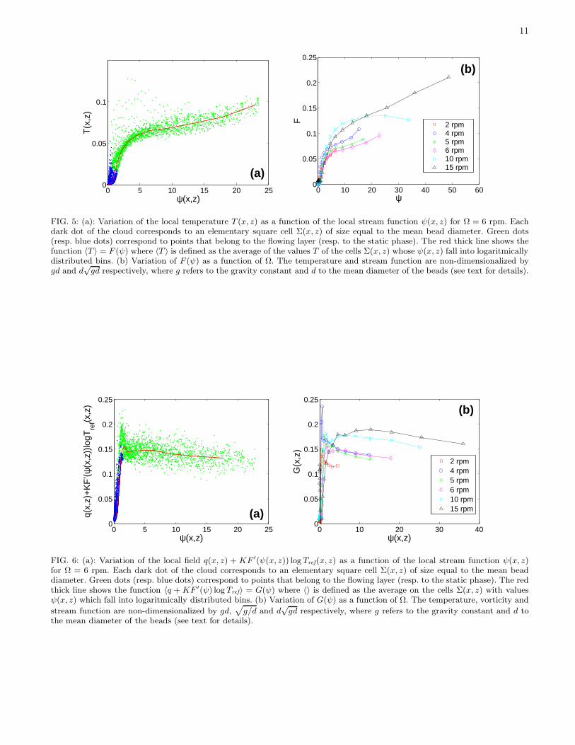
The knowledge of both the field T (x, z) and ψ(x, z) al-lows to check the first prediction (first equation in system21) of the approach derived in Sec. II. Figure 5a showsT (x, z) as a function of ψ(x, z) for Ω = 6 rpm. The pointsclearly gather along a single function. It is worth to em-phasize that such result would have been trivial in homo-geneous flows such as the observed in Couette geometryor inclined plane geometry: in such flows, all the contin-uum quantities depend on a single spatial co-ordinate andare thus naturally related two by two by single functions.On the other hand, the fact that the 2D fields T (x, z)and ψ(x, z) can be related by a single function in theinhomogeneous surface flow considered here, where thecontinuum quantities depend on the both two spatial co-ordinates x and z, is highly non trivial and constitutesthen a rather severe test for the approach derived in Sec.II. The function F (red thick line in Fig. 5a) is thendefined by averaging the values T falling into logarith-mically distributed bins defined along ψ. The functionsF obtained using this procedure for the various rotatingspeeds Ω are represented in Fig. 5b.

One can now determine the second closure relationG(ψ). The function F (ψ) defined in the previous sec-tion (red thick line in Fig. 5a) is first derived numeri-cally. The resulting function is then applied in each point(x, z) to the field ψ(x, z). Since the reference temperatureTref(x, z) = −z cos θ/K and the vorticity field q(x, z) arealso known in each point, one can deduce the value of thefield q(x, z) + KF ′(ψ(x, z)) log Tref(x, z) in each point,and plot it as a function of ψ(x, z) (see Fig. 6a). Thepoints clearly gather along a single function. The func-tion G (red thick line in Fig. 6a) is then defined by aver-aging the values q(x, z)/KF ′(ψ(x, z)) logTref(x, z) fallinginto logarithmically distributed bins defined along ψ. Thefunctions G obtained using this procedure for the variousrotating speeds Ω are represented in Fig. 6b.

D. Discussion of the results

Our determination of the two closure functions callsfor some comments. A first noticeable feature is thatthe closure function extends smoothly, without any no-ticeable transition, from the static to the flowing region.This is quite remarkable, since both phases are character-ized by different dynamical properties, and since our hy-drodynamic description presumably applies best withinthe flowing region. The main difference between the two

6

phases is in the scattering of the data along the fit: It islarger in the flowing region than in the static region. Thismay be traced to correlated fluctuations that have beenneglected in our approach, see after Eq. 15, and that arelarger in the flowing region. It would be interesting tosee if a longer time averaging leads to a reduction of thisscattering.

An interesting comparison can also be made with re-spect to a real fluid system, where a similar approach canbe used and where dissipation is made through ordinaryviscosity. In that case, it has been shown in [25] that thedetermination of the closure function is valid only in thebulk flow region. Outside this region, the data scattersrandomly, without forming any specific shape. A possi-ble explanation was that outside the bulk, i.e. closer tothe boundaries and the flow forcing devices, viscous andforcing processes become important and do not balancelocally on average as assumed here. The reason why itworks so well in the granular case, without any need ofselecting any flow region, may lie in the local characterof the dissipative processes that precludes any long-rangecorrelation between forcing and dissipation.

IV. CONCLUDING DISCUSSION

In this paper, the stationary states of a rotating denseinhomogeneous granular flow have been shown to becharacterized by two functions F and G linking the gran-ular temperature, vorticity and stream functions. Whenvarying the rotation speed of the apparatus, both F andG vary, so that they can be seen as representative of thestate of the system. Conversely, the knowledge of F andG is sufficient to fully reconstruct the 2D fields for tem-perature and velocity. Let us first consider the flowingphase. From Fig. 5 and Fig. 6, one sees that, in thatphase, F is asymptotically linear F ∼ aψ, while G is ap-proximately constant, G ∼ b. Inserting these shapes ineq. (21) leads to:

δT = aψ,

∆ψ = −aK log(−z cos θ/K) + b (24)

Integrating the second equation with respect to z, onefinds:

ψ = (b− aK log(cos θ/K))z2

2+

3

2aKz − aK

2z2 log(−z)

(25)

so that the temperature profile is quadratic, with loga-rithmic correction and the velocity profile is linear, withlogarithmic correction. This is indeed the behaviour ob-served in this type of flow in the flowing phase [6, 11, 26,28].

In the static phase, F appears quadratic in ψ , F ∼ cψ2

and G is linear G ∼ dψ. Therefore, eq. (21) becomes:

δT = cψ2,

∆ψ = (d− 2cK logTref)ψ (26)The solution for ψ is in this case

ψ = ψ0 exp(h(z)),

h′2(z) + h′′(z) = d− 2cK logTref > 0, (27)

so that both the velocity profile and the temperatureprofiles are exponential, with algebraic corrections. Thisis indeed the behaviour observed in the static phase ofthe rotating drum [28, 41, 42].

These simple asymptotics show the importance of un-derstanding the shape of F and G as a function of theforcing and dissipation. From an experimental or numer-ical point of view, one may try and find empirical lawsfrom variation of the control parameters like rotationspeed, size of the beads, friction coefficient, etc. Froma theoretical point of view, one could try to link thesefunctions to the macroscopic flow geometry and the mi-croscopic properties of the flow or rheology through ki-netic equations. In a next paper, we explore an alternatestrategy, based upon the statistical mechanics Jaynes’ in-terpretation in term of information theory. This will leadto Gibbs distributions providing a direct link betweenthe function F and G and the fluctuations of physicalquantities. In this respect, the present approach providesa useful insight for dense granular flow.

Acknowledgments

We gratefully acknowledge O. Dauchot for a crit-ical reading of the manuscript. Simulations are per-formed using LMGC90 software. This work is sup-ported by the CINE (Centre d’Information National

et d’Enseignement) under the project lmc2644. We aregrateful to S. Aumaitre, O. Dauchot, F. Leschenault andR. Monchaux for many enlightening discussions.

[1] H. M. Jaeger, S. R. Nagel, and R. P. Behringer, “Granularsolids, liquids, and gases”, Reviews of Modern Physics68, 1259 (1996).

[2] S. B. Savage and D. J. Jeffrey, “The stress tensor in agranular flow at high shear rates”, J. Fluid Mech. 110,255 (1981).

[3] J. T. Jenkins and S. B. Savage, “A theory for the rapidflow of identical smooth inelastic, spherical particle”, J.Fluid Mech. 130, 187 (1983).

[4] C. K. K. Lun and S. B. Savage, “The effect of an im-pact dependent coefficient of restitution on stresses de-veloped by sheared granular materials”, Acta Mech. 63,

7

15 (1986).[5] R. Nedderman, Statics and Kinematics of Gran-

ular Materials (Cambridge University Press, Cam-bridge,England, 1992).

[6] G.D.R. Midi, “On dense granular flows”, Eur. Phys. J. E14, 341 (2004).

[7] P. Mills, D. Loggia, and M. Texier, “Model for station-nary dense granular flow along an inclined wall”, Euro-phys. Lett. 45, 733 (1999).

[8] B. Andreotti and S. Douady, “Selection of velocity pro-file and flow depth in granular flows”, Phys. Rev. E 63,031305 (2001).

[9] J. T. Jenkins and D. M. Hanes, “Kinetic theory for iden-tical, frictional, nearly elastic spheres”, Phys. Fluids 14,1228 (2002).

[10] D. Bonamy and P. Mills, “Diphasic-non-local model forgranular surface flows”, Europhys. Lett. 63, 42 (2003).

[11] J. Rajchenbach, “Dense rapid flow of inelastic grains un-der gravity”, Phys. Rev. Lett 90, 144302 (2003).

[12] S. B. Savage, “Analysis of slow high concentration flowsof granular materials”, J. Fluid Mech. 377, 1 (1998).

[13] L. Bocquet, W. Losert, D. Schalk, T. Lubensky, andJ. Gollub, “Granular shear flow dynamics and forces: Ex-periment and continuum theory”, Phys. Rev. E 65, 01307(2002).

[14] L. S. Mohan, K. K. Rao, and P. R. Nott, “Frictionalcosserat model for slow shearing of granular materials”,J. Fluid Mech 457, 377 (2002).

[15] I. S. Aranson and L. S. Tsimring, “Continuum theoryof partially fluidized granular flows”, Phys. Rev. E 65,061303 (2002).

[16] O. Pouliquen and R. Gutfraind, “Stress fluctuations andshear zones in quasi-static granular flows”, Phys. Rev. E53, 552 (1996).

[17] G. Debregeas and C. Josserand, “A self-similar model forshear flows in dense granular materials”, Europhys.Lett.52, 137 (2000).

[18] O. Pouliquen, Y. Forterre, and S. L. Dizes, “Slow densegranular flows as a self induced process”, Adv. ComplexSystem 4, 441 (2001).

[19] A. Lemaitre, “The origin of a repose angle: Kinetic rear-rangement for granular materials”, Phys. Rev. Lett. 89,064303 (2002).

[20] I. Iordanoff and M. M. Khonsari, “Granular lubrication:Toward an understanding of the transition between ki-netic and quasi-fluid regime”, ASME J. Tribol. 126, 137(2004).

[21] F. D. Cruz, S. Eman, M. Prochnow, . J.-N. Roux, andF. Chevoir, “Rheophysics of dense granular materials:Discrete simulation of plane shear flows”, Phys. Rev. E72, 021309 (2005).

[22] P. Jop, Y. Forterre, and O. Pouliquen, “A constitutivelaw for dense granular flows”, Nature 441, 727 (2006).

[23] N. Leprovost, B. Dubrulle, and P.-H. Chavanis, “Ther-modynamics of magnetohydrodynamic flows with axialsymmetry”, Phys. Rev. E 71, 036311 (2005).

[24] N. Leprovost, B. Dubrulle, and P.-H. Chavanis, “Dynam-ics and thermodynamics of axisymmetric flows: Theory”,Phys. Rev. E 73, 046308 (2006).

[25] R. Monchaux, F. Ravelet, B. Dubrulle, A. Chiffaudel,and F. Daviaud, “Properties of steady states in turbulentaxisymmetric flows”, Phys. Rev. Lett. 96, 124502 (2006).

[26] M. Renouf, D. Bonamy, F. Dubois, and P. Alart, “Numer-ical simulation of two-dimensional steady granular flows

in rotating drum: On surface flow rheology”, Phys. Fluids17, 103303 (2005).

[27] J. Rajchenbach, “Granular flows”, Adv. Phys. 49, 229(2000).

[28] D. Bonamy, F. Daviaud, and L. Laurent, “Experimen-tal study of granular surface flows via a fast camera: Acontinuous description”, Phys. Fluids 14, 1666 (2002).

[29] D. Bonamy, F. Daviaud, L. Laurent, and P. Mills, “Tex-ture of granular surface flows: experimental investiga-tion and biphasic non-local model”, Gran. Matt. 4, 183(2003).

[30] P. Jop, Y. Forterre, and O. Pouliquen, “Crucial role ofside walls for granular surface flows: Consequences forthe rheology”, J. Fluid Mech. 541, 167 (1990).

[31] R. J. Speedy, “Glass transition in hard disc mixtures”, J.Chem. Phys. 110, 4559 (1999).

[32] P.-H. Chavanis and J. Sommeria, “Thermodynamical ap-proach for small-scale parametrization in 2D turbulence”,Phys Rev. Lett. 78, 3302 (1997).

[33] P.-H. Chavanis and J. Sommeria, “Statistical mechanicsof the shallow water system”, Phys Rev. E 65, 026302(2002).

[34] J.-J. Moreau, in Non Smooth Mechanics and Appli-cations, CISM Courses and Lectures, edited by J.-J.Moreau and e. P.-D. Panagiotopoulos (1988), vol. 302(Springer-Verlag, Wien, New York), pp. 1–82.

[35] M. Jean, “The non-smooth contact dynamics method”,Comp. Meth. Appl. Mech. Engrg 177, 235 (1999).

[36] M. Renouf and P. Alart, “Conjugate gradient type algo-rithms for frictional multicontact problems: Applicationsto granular materials”, Comp. Meth. Appl. Mech. Engrg.194, 2019 (2004).

[37] M. Renouf, F. Dubois, and P. Alart, “A parallel versionof the non smooth contact dynamics algorithm appliedto the simulation of granular media”, J. Comput. Appl.Math. 168, 375 (2004).

[38] D. Bonamy, F. Daviaud, L. Laurent, M. Bonetti, and J.-P. Bouchaud, “Multi-scale clustering in granular surfaceflows”, Phys. Rev. Lett. 89, 034301 (2002).

[39] O. Reynolds, “On the dilantancy of media composed ofrigid particles in contact”, Phyl. Mag. Ser. 5 20, 469(1885).

[40] Strickly speaking, the parameter K is found to be signifi-cantly smaller for Ω = 2 rpm. However, for this particularrotating speed, the flowing layer is very small. As a re-sult, the variation range of both ν(x, z) and T (x, z) arevery small, making the fit with Eq. 23 rather imprecise.

[41] T. S. Komatsu, S. Inagasaki, N. Nakagawa, and S. Na-suno, “Creep motion in a granular pile exhibiting steadysurface flow,”, Phys. Rev. Lett. 86, 1757 (2001).

[42] S. C. du Pont, R. Fisher, P. Gondret, B. Perrin, andM. Rabaud, “Instantaneous velocity profiles during gran-ular avalanches,”, Phys. Rev. Lett. 94, 048003 (2005).

8

0.43 m/s

0 m/s

FIG. 1: Time averaged velocity field in the simulated 2D rotating drum. In this peculiar numerical experiment, the rotationspeed was Ω = 6 rpm. The black line shows the interface between the flowing layer and the “static” packing. Velocities areexpressed in m/s (left-hand colorbar) or non-dimensionalized by

p

(gd) (right-hand colorbar) where g refers to the gravityconstant and d to the mean diameter of the beads (see text for details).

9

(a)

0 m2/s2

0.003 m2/s2

0 m2/s2

0.003 m2/s2

(b)

0(c) 0(d)

(e)26 s−1

−26 s−1

(f)13 s−1

0 s−1

FIG. 2: Spatial dististribution of the various continuous fields measured within the drum. In this peculiar numerical experiment,the rotation speed was Ω = 6 rpm. Left: Typical snapshot of the instantaneous spatial distribution of granular temperature(a), volume fraction (c) and vorticity (e) within the rotating drum. Right: Time averaged field of temperature (b), volumefraction (d) and vorticity (f). The average was taken over the 400 snapshots of the sequence for Ω = 6 rpm. Temperatures areexpressed in m2/s2 (left-hand colorbar) or non-dimensionalized by gd (right-hand colorbar). Vorticities are expressed in s−1

(left-hand colorbar) or non-dimensionalized byp

g/d (right-hand colorbar) where g refers to the gravity constant and d to themean diameter of the beads (see text for details).

10

0 m2/s

0.017 m2/s

FIG. 3: Spatial distribution of the stream function ψ in the drum for Ω = 6 rpm. The stream function is expressed in m2/s

(left-hand colorbar) or non-dimensionalized by dp

(gd) (right-hand colorbar) where g refers to the gravity constant and d tothe mean diameter of the beads (see text for details).

0 0.01 0.02 0.03 0.040.78

0.79

0.8

0.81

0.82

0.83

0.84

−T(x,z)/zcosθ

ν(x,

z)

FIG. 4: Volume fraction ν(x, z) as a function of the ratio T (x, z)/z cos θ for Ω = 6 rpm. For this rotation speed, the mean slopeof the free surface was measured to be θ ≃ 19.7 [26]. The straight line is a fit given by Eq. 23 with K ≃ 1.1 and ν∗ ≃ 0.82.The temperature is non-dimensionalized bygd where g refers to the gravity constant and d to the mean diameter of the beads(see text for details).

11

0 5 10 15 20 250

0.05

0.1

ψ(x,z)

T(x

,z)

(a)0 10 20 30 40 50 60

0

0.05

0.1

0.15

0.2

0.25

ψ

F 2 rpm 4 rpm 5 rpm 6 rpm 10 rpm15 rpm

(b)

FIG. 5: (a): Variation of the local temperature T (x, z) as a function of the local stream function ψ(x, z) for Ω = 6 rpm. Eachdark dot of the cloud corresponds to an elementary square cell Σ(x, z) of size equal to the mean bead diameter. Green dots(resp. blue dots) correspond to points that belong to the flowing layer (resp. to the static phase). The red thick line shows thefunction 〈T 〉 = F (ψ) where 〈T 〉 is defined as the average of the values T of the cells Σ(x, z) whose ψ(x, z) fall into logaritmicallydistributed bins. (b) Variation of F (ψ) as a function of Ω. The temperature and stream function are non-dimensionalized bygd and d

√gd respectively, where g refers to the gravity constant and d to the mean diameter of the beads (see text for details).

0 5 10 15 20 250

0.05

0.1

0.15

0.2

0.25

ψ(x,z)

q(x,

z)+

KF

’(ψ(x

,z))

logT

ref(x

,z)

(a)0 10 20 30 40

0

0.05

0.1

0.15

0.2

0.25

ψ(x,z)

G(x

,z)

2 rpm4 rpm5 rpm6 rpm10 rpm15 rpm

(b)

FIG. 6: (a): Variation of the local field q(x, z) + KF ′(ψ(x, z)) log Tref(x, z) as a function of the local stream function ψ(x, z)for Ω = 6 rpm. Each dark dot of the cloud corresponds to an elementary square cell Σ(x, z) of size equal to the mean beaddiameter. Green dots (resp. blue dots) correspond to points that belong to the flowing layer (resp. to the static phase). The redthick line shows the function 〈q +KF ′(ψ) log Tref〉 = G(ψ) where 〈〉 is defined as the average on the cells Σ(x, z) with valuesψ(x, z) which fall into logaritmically distributed bins. (b) Variation of G(ψ) as a function of Ω. The temperature, vorticity and

stream function are non-dimensionalized by gd,p

g/d and d√gd respectively, where g refers to the gravity constant and d to

the mean diameter of the beads (see text for details).