THE MECHANISM OF SEPARATION

IN DENSE MEDIUM CYCLONES

A Thesis Submitted for the Degree of

Doctor of Philosophy

in The University of London

and the Diploma of Imperial College

by

TIMOTHY JOHN NAPIER-MUNN

Dept, of Mineral Resources EngineeringImperial CollegeLondonDecember, 1980

Mines DivisionDiamond Research LaboratorJohannesburgDecember, 1983

ii

To EJ, BJ, TJ and AJ

f r o m TJ, with love

"To explain all nature is too difficult a task for any one man or even for

any one age. 'Tis much better to do a little with certainty, and leave the

rest for others that come after you, than to explain all things".

- Sir Isaac Newton

"Car moi, je ne crois pas a la mathematique".

- Albert Einstein

i n

ABSTRACT

A review is given of the literature relating to the rheology and

sedimentation of dense suspensions, classifying hydrocyclones, and dense

medium cyclones.

Experiments were carried out with a stable, suspensoid medium in a 30mm

dense medium cyclone. The results confirmed the prediction of simple

theory, that separating density increases with medium viscosity.

Correlations were also obtained for Ep-value, yield of medium to underflow,

and pressure drop, all of which were viscosity-dependent.

A study was made of the sedimentation and rheological properties of

ferrosilicon-water suspensions. The sedimentation rate of these media was

shown to be related to the volume concentration of solids by a modified

Richardson-Zaki equation. A capillary viscometer was assembled for the

rheological measurements, and a data reduction procedure was developed for

obtaining the corrected flow curve. The results showed that these media are

Bingham plastics, with a tendency to dilatancy at higher shear rates.

Apparent viscosity increased with solids concentration, fineness of

particle size and irregularity of particle shape.

Tests were undertaken with ferrosilicon media in a 100mm x 20 ° cyclone. A

mass balance smoothing procedure was developed for the optimisation of the

medium flow and classification data, and specially-manufactured density

tracers were used to determine the intrinsic (low tonnage) Tromp curve for

the density separation. The separating density was found to be a simple

function of the feed and underflow medium densities, and the underflow

density was given by a modification of Hoi 1and-Batt's bulk hydrocyclone

I V

model. This model successfully predicts the onset of density inversion

which was observed in some tests. Inversion was normally accompanied

by unusually-shaped Tromp curves. The separating density decreased

with increasing medium viscosity. The observed density separations

were interpreted in terms of the segregation and classification of the

medium. Correlations were also obtained for the pressure-flowrate

relationship,which was viscosity-dependent at the higher inlet

Reynolds numbers.

V

NOMENCLATURE

A Projected area of particle

Ac Cyclone inner wall area

a Acceleration

C Constant

C Solids concentration by mass

CD Radial drag coefficient

Cv Volume concentration of solids

Dvm Maximum volume concentration of solids

Cy oo Volume concentration of solids for which na + 00

Dc Cyclone diameter

°o Overflow (vortex finder) diameter

Du Underflow (apex) diameter

d Particle diameter (size)

d Geometric mean of particle sizes

dST Equivalent Stokesian mean particle diameter

d50 Separation size

E Quality of separation (6 7 5 -6 5 0 )

Ep Ep-value (eqn. 3.2)

F Centrifugal force vector

fD Fluid drag force on particle

9 Acceleration due to gravity (9.807 ms-2)

9u Proportion of ore to underflow

h Pressure drop expressed as head of medium

K,k1 }k2 etc Constants

k Consistency index

Separation constant

L Pressure loss coefficient or pressure drop factor

(eqn. 3.19)

m Mass of particle

m* Mass of fluid displaced by particle

n Exponent in eqn. 2.1

P Pressure drop

pt Pressure drop, measured at cyclone inlet

Qf Feed flowrate

Qo Overflow flowrate

Qu Underflow flowrate

VI

RmRec

ReiRep

Rf

Rsr

S

S

t

U

u

ur

VaVC

Vc

ViVr

Vt

vsc

vso

VtWW

Yi

Proportion of medium to underflow

Critical Reynolds number for transition to non-laminar

flow.

Cyclone inlet Reynolds number

Particle Reynolds number

Proportional fluid yield to underflow

Proportional solids yield to underflow

Radius

Shear rate

Volume split of pulp to underflow

T ime

Radial flow of water inwards

Ambient particle/f1uid velocity vector

Particle radial velocity

Particle angular (tangential) velocity

Axial velocity of medium/fluid

Tangential velocity of medium/fluid at periphery

Volume of cyclone

Inlet velocity of medium/fluid

Radial velocity of medium/fluid

Tangential velocity of medium/fluid

Ambient particle/fluid velocity

Sedimentation rate

Mean sedimentation rate of medium in cyclone

Sedimentation rate at zero solids concentration

Terminal velocity of particle

Volume of particle

Weight in mass balance optimisation procedure

Density partition number at density, 6

Classification partition number at size, i

Mean sedimentation rate of medium in cyclone

v n

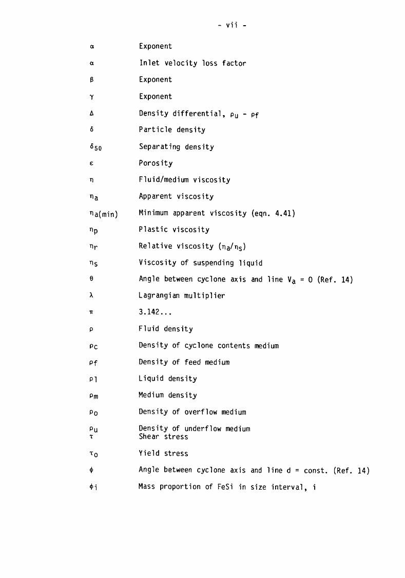
a Exponent

a Inlet velocity loss factor

3 Exponent

y Exponent

A Density differential, pu - pf

6 Particle density

650 Separating density

e Porosity

n Fluid/medium viscosity

na Apparent viscosity

na(min) Minimum apparent viscosity (eqn. 4.41)

nP Plastic viscosity

nr Relative viscosity (na/ns)

ns Viscosity of suspending liquid

e Angle between cyclone axis and line Va = 0 (Ref. 14)

X Lagrangian multiplier

ir 3.142...

P Fluid density

Pc Density of cyclone contents medium

Pf Density of feed medium

PI Liquid density

Pm Medium density

Po Density of overflow medium

Pu Density of underflow mediumT Shear stress

T0 Yield stress

♦ Angle between cyclone axis and line d = const. (Ref. 14)

Mass proportion of FeSi in size interval, i

v m

CONTENTS

Page Number

DEDICATION (ii)

ABSTRACT (iii)

NOMENCLATURE (v)

CONTENTS (viii)

LIST OF TABLES (xii)

LIST OF FIGURES (xiv)

CHAPTER 1 - INTRODUCTION 1

CHAPTER 2 - REVIEW OF PREVIOUS WORK 3

2.1 Classifying Hydrocyclones and theirRelationship to Dense Medium Cyclones 3

2.2 Dense Medium Cyclones 182.3 Properties of Dense Medium Suspensions 49

2.3.1 Introduction 492.3.2 Sedimentation 502.3.3 Rheology 67

CHAPTER 3 - THE INFLUENCE OF MEDIUM VISCOSITYON THE SEPARATION IN A DENSE MEDIUMTTClOnT 94

3.1 Introduction 943.2 Experimental Details 94

3.2.1 The Medium 943.2.2 Test Circuit 963.2.3 Material Treated 983.2.4 Test and Measurement Procedures 993.2.5 Analysis of the Separation -

The Partition Curve 102

3.3 Results 106

3.3.1 Rheology of Medium 1063.3.2 Density Separations and Flow Data 1113.3.3 Summary of Data 111

3.4 Discussion of Results 117

3.4.1 Rheology of the Medium 1173.4.2 The Separating Density, 6 5 0 1183.4.3 Quality of Separation, (6 7 5 - 6 5 0 ) 1283.4.4 Pressure-Flowrate Relationship 1303.4.5 Medium Recovery to Underflow, Rm 133

3.5 Summary and Conclusions 135

IX

CHAPTER 4 - THE SEDIMENTATION AND RHEOLOGY OFFERROSILICON SUSPENSIONS 138

4.1 Introduction 1384.2 Sedimentation of Ferrosilicon Suspensions 139

4.2.1 Introduction and Objectives 1394.2.2 Experimental Details 1414.2.3 Results 1424.2.4 Discussion of Results 1494.2.5 Summary and Conclusions 153

4.3 Rheology of Ferrosilicon Suspensions 154

4.3.1 Introduction and Objectives 1544.3.2 Experimental Details 1564.3.3 Data Reduction and Calibration 1614.3.4 Results 1744.3.5 Discussion of Results 182

4.3.5.1 The Influence of CapillaryDiameter 182

4.3.5.2 The Rheological Nature ofFerrosilicon Suspensions 187

4.3.5.3 The Influence of SolidsConcentration 194

4.3.5.4 The Influence of Particle Size 1994.3.5.5 The Influence of Particle Shape 201

4.3.6 Summary and Conclusions 201

CHAPTER 5 - THE PERFORMANCE OF A 100MM DENSE MEDIUMCYCLONE WITH FERROSILICON MEDIA 204

5.1 Introduction and Objectives 2045.2 Experimental Details 205

5.2.1 Cyclone and Test Circuit 2055.2.2 Experimental Design, and Test Procedure 2115.2.3 The Ferrosilicon 2185.2.4 Particle Size Analysis 2215.2.5 Solids Density Measurement 230

5.3 Data Reduction for Mass Balances 233

5.3.1 Introduction 2335.3.2 Optimisation Procedures 235

5.4 Results 2455.5 Discussion of Results 248

5.5.1 Reproducibility 2485.5.2 The Density of Separation, 6 5 0 2535.5.3 The Underflow Medium Density, pu 2625.5.4 Density Inversion, and the U-Shaped

Tromp Curve 273

5.5.5

x

5.5.5

5.5.65.5.7

5.5.85.5.9

The Influence of Viscosity on the Densityof Separation, 650The Classification of the MediumThe Influence of Apex Diameter on theSeparationThe Quality of Separation Pressure-Flowrate Relationships

283290

296297 300

5.6 Summary and Conclusions 316

CHAPTER 6 - CONCLUSION : THE MECHANISM OF SEPARATIONIN DENSE MEDIUM CYCLONES 323

6.1 Discussion6.2 Conclusions

323333

6.2.1

6.2.26.2.3

Sedimentation and Rheology of Ferrosilicon Suspensions Tests with Stable Media; 30mm x 17° Cyclone Tests with Unstable, Ferrosilicon Media; 100mm x 20 ° Cyclone

334335

336

6.3 Future Work 339

ACKNOWLEDGEMENTS 341

REFERENCES 342

APPENDICES

APPENDIX 1 - Sedimentation Data for Ferrosilicon Suspensions from References 56, 71 and 80 357

APPENDIX 2 - Typical Data Set for Stable Medium Experiments (Chapter 3) 358

APPENDIX 3 - Data from Tests with 30mm Cyclone 359

APPENDIX 4 - Determination of the Particle Reynolds Number, Rep (Section 3.4.2) 363

APPENDIX 5 - Influence of Yield Stress on a Particle Immersed in a Bingham Plastic 366

APPENDIX 6 - Fortran Program for the Processing of Capillary Viscometer Data (Chapter 4) 368

APPENDIX 7 - Typical Output of Capillary Viscometer Computer Program (Chapter 4) 371

APPENDIX 8 - Rheological Data from Capillary Viscometer Measurements, Series R1-R5 (Chapter 4) 372

APPENDIX 9 - Listing of Mass Balance Smoothing Program "0PTIM6" 375

XI

APPENDIX 10 - Measured and Optimised Ferrosilicon Results from lOOmm Cyclone Tests 381

APPENDIX 11 - Tromp Curves from 100mm Cyclone Tests with Ferrosilicon Media 394

APPENDIX 12 - Partition Curves for Classification of Ferrosilicon 400

APPENDIX 13A - Derived Data from Milled Ferrosilicon Cyclone Tests : Series FI, F2, F3 and F6 402

APPENDIX 13B - Derived Data from Atomised Ferrosilicon Cyclone Tests : Series F4 and F5 403

x n

LIST OF TABLES

Page Number

CHAPTER 2

Table 2.1 Correlation of vso - Cv Data for the Sedimentation of Ferrosilicon Suspensions - References 56, 71 and 80 6 6

CHAPTER 3

Table 3.1 Solids Volume Concentration vs. Plastic Viscosity for Quartz/Bromoform Medium 1 1 1

Table 3.2 Summary of Results, Chapter 3 116

Table 3.3 Yp/100 vs Rm for Series B 125

CHAPTER 4

Table 4.1 Details of Media used in Sedimentation Tests 143

Tables 4.2 - 4.4

Summary of Sedimenation Data For Series S1-S3 146

Table 4.5 Estimated Parameters in Equations 2.21 and 2.23 148

Table 4.6 Size Distributions of Ferrosilicon Samples R1-R5 176

Table 4.7 Estimation of Capillary Diameter Correction Factor, 3 184

Table 4.8 Fit of Equation 4.38 to Flow Curve Data of Tests R3/2 and R3/5 190

Table 4.9 Viscosity vs. Solids Concentration for Series R1-R5 196

CHAPTER 5

Table 5.1 Size Distributions Determined by Cyclosizer for Different Sample Sizes 226

Table 5.2 Size Distribution of Milled Ferrosilicon as Determined by Four Analytical Techniques 227

Table 5.3 Size Distribution of Atomised Ferrosilicon as Determined by Four Analytical Techniques 227

Table 5.4 Summary of Cyclone Tests with Milled Ferrosilicon 249

250

251

252

255

261

275

283

289

294

296

301

306

308

x m

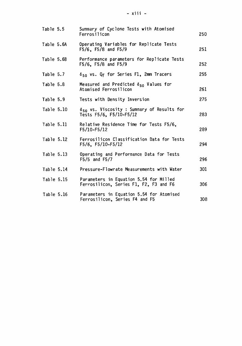
Summary of Cyclone Tests with Atomised Ferrosilicon

Operating Variables for Replicate Tests F5/6, F5/8 and F5/9

Performance parameters for Replicate Tests F5/6, F5/8 and F5/9

6 5 0 vs. Qf for Series FI, 2mm Tracers

Measured and Predicted 6 5 0 Values for Atomised Ferrosilicon

Tests with Density Inversion

6 S 0 vs. Viscosity : Summary of Results for Tests F5/6, F5/10-F5/12

Relative Residence Time for Tests F5/6, F5/10-F5/12

Ferrosilicon Classification Data for Tests F5/6, F5/10-F5/12

Operating and Performance Data for Tests F5/5 and F5/7

Pressure-Flowrate Measurements with Water

Parameters in Equation 5.54 for Milled Ferrosilicon, Series FI, F2, F3 and F6

Parameters in Equation 5.54 for Atomised Ferrosilicon, Series F4 and F5

XIV

LIST OF FIGURES

Page Number

CHAPTER 2

Figure 2.1 Cut-point vs. Underflow Medium Density(Data of Davies et al L48J) 29

Figure 2.2a Classification of Medium in a DM Cyclone(After Tarjan U^J) 3 3

Figure 2.2b Relationship between Locus of Zero Axial Velocity (Va) and Locus of Constant Particle Size (d) (After Tarjan L^J) 33

Figures 2.2 Medium Density Distribution Across the c-f Cyclone Radiusrfor Coarse and Fine Medium

(After Tarjan U^J) 3 4

Figure 2.3a Simple Stability-Measuring Apparatus (AfterGeer et al 1.67J) 5 2

Figure 2.3b Stability Measurement by Pressure Differential (After Nesbitt and Loesch [71]) 52

Figure 2.4 Density Profiles in Settling 50:50 Ferrosilicon/Magnetite Medium (Data from Collins [65]) 5 5

Figure 2.5a Paragenesis Diagram of Sedimentation (AfterFitch 1.74] 9 quoted by Datta [69]) 5 7

Figure 2.5b Sedimentation of Concentrated Suspensions (After Coe and Clevenger [77]s as given by Coulson and Richardson [76]) 5 7

Figure 2.6 Ideal Rheological Types 70

Figure 2.7 General Shape of the Flow Curve forConcentrated Suspensions (from Metzner and Whitlock L9 9J) 70

Figure 2.8 Viscosity-Concentration Relation for Suspension of Non-Interacting Particles (from Chena [107]) 82

Figure 2.9 Dependence of Apparent Viscosity upon Shear Rate for Suspensions of Negligible Inter­particle Attraction (from Cheng [107J)

Figure 2.10 Flow Curves for a Milled Ferrosilicon Suspension at Various Pulp Densities (from Smith [ H 4 J )

82

89

XV

Figure 3.1 30mm Cyclone Test Circuit 97

Figure 3.2 Photograph of Apparatus 97

Figure 3.3 Principal Features of Partition Curve forDensity Separations 104

Figures 3.4A- Flow Curves for Series A-E,M Media 107-1093.4F

Figure 3.5 Plastic Viscosity vs. Solids Concentrationfor Quartz/Bromoform Media 110

Figures 3.6A- Partition Curves for Test Series A-E 113-1153.6E

Figure 3.7 Relative Separating Density vs. InletReynolds Number for Different Particle Sizes 123

Figure 3.8 Proposed Partition Curve for MediumExhibiting a Yield Stress 123

Figure 3.9 Measured vs. Predicted Values of (6 5 0 -p) 127

Figure 3.10 Measured vs. Predicted Values of (6 7 5 -6 5 0 ) 127

Figure 3.11 Measured vs. Predicted Values of InletPressure Drop 132

Figure 3.12 Pressure Loss Coefficient vs. InletReynolds Number 132

Figure 3.13 Measured vs. Predicted values of Rm 132

CHAPTER 4

Figures 4.1 - Ferrosilicon Sedimentation Tests, Series4.3 S1-S3 144-145

Figures 4.4a- Sedimentation Rate vs. Solids Concentration4.4c for Series S1-S3 150

Figure 4.5 Capillary Viscometer 158

Figure 4.6 Check Calibration of Capillary Viscometerwith Aqueous Glycerine Solutions 177

Figures 4.7 - Flow Curves for Series RIA-RIC 177-1784.9

Figure 4.10 Flow Curves from Series RIA, RIB, RIC 179

Figures 4.11- Flow Curves for Series R2-R5 179-1814.14

CHAPTER 3

181

192

192

198

198

207

208

215

223

228

229

257

259

264

274

281

285

285

288

xvi

Size Distributions of Ferrosilicon Samples used in Viscometer Measurements

Apparent (Point) Viscosity vs. Shear Rate for Tests R3/2 and R3/5

Apparent Viscosity vs. Volume Concentration of Solids

Fit of Modified Eiler's Equation (Eqn. 2.33) to Data of Series R4

Size Frequency Distributions of Samples Rl, R2 and R4

Dimensional Drawing of 100mm Cyclone

Flowsheet for lOOnm Cyclone Test Rig

Manual Sampler for Cyclone Medium Products

Sampling Scheme for Comparison of Size Analysis Methods

Size Distribution of Milled Ferrosilicon as Determined by Four Analytical Techniques

Size Distributions of Atomised Ferrosilicon as Determined by Four Analytical Techniques

6 so vs. pu for 2mm Tracers

Measured vs. Predicted 6 5 0 for Milled Ferrosi1 icon

Rm vs. Pu/Pf f°r Milled and Atomised Ferrosi1 icon

Tromp Curves for Tests Fl/1, Fl/2, F6/1 and F6/2

Typical W-Shaped Tromp Curve

Relative Density of Separation vs. Re-j for Tests F5/6, F5/10-F5/12

P c - P f vs. na(min) for Tests F5/6,F5/10-F5/12

Density of Separation vs. Density Difference between Contents and Feed Medium in Tests F5/6, F5/10-F5/12

Figure 5.15 d50 vs. Liquid Viscosity for Tests F5/6, F5/10-F5/12 295

Figure 5.16 Dependence of Ep upon 650 for Milled Ferrosilicon Test, 2mm Tracers 299

Figure 5.17 Pressure vs. Flowrate for Water Tests, 100mm Cyclone 302

Figure 5.18 L vs. Rei for 100mm Cyclone Water Tests 304

Figure 5.19 Qu/Qo vs. Of f°r lOOnim Cyclone Water Tests 304

Figure 5.20 Pressure Loss Coefficient vs. Reynolds Number for Ferrosilicon Tests 310

Figure 5.21 Yield Stress vs. Medium Density for Milled and Atomised Ferrosilicon 312

Figure 5.22 Measured vs. Predicted Values of Inlet Pressure for Series F3 and F6 315

Plate 5.1 100mm Cyclone Test Rig 209

Plate 5.2 Close-up of Cyclone 209

Plate 5.3 Milled Ferrosilicon Particles, -45 +38ym 220

Plate 5.4 Atomised Ferrosilicon Particles, -45 +38ym 220

THE MECHANISM OF SEPARATION IN DENSE MEDIUM CYCLONES

CHAPTER 1

INTRODUCTION

The hydrocyclone is ubiquitous in mineral processing, and in many other

industries. It has also been well researched; Bradley's book [1],

published in 1965, lists over 600 publications on the subject, and the

volume of literature has increased substantially since then. Although many

authors have claimed satisfactory agreement between particular theories and

observations, such theories or models rarely find application beyond the

specific conditions under which they were tested. Even Plitt's semi-

empirical model [2 ], which was specifically designed to achieve general

applicability, has recently been shown to be at variance with data obtained

from operating plants [3], The continued lack of a unified theory of

general validity is due to the complexity of the system and to the large

number of variables involved in defining the system; it is not difficult to

identify at least twelve design and operating variables, which would

require a minimum of 3 1 2 - 1/2 million individual experiments for a

definitive empirical study.

The dense medium cyclone using conventional unstable media, now established

in world-wide use for the concentration of coal, iron ore, tin, fluorspar,

diamonds and many other minerals, exhibits additional analytical

difficulties due to the presence of a third phase (the medium solids). The

process has attracted comparatively little systematic investigation, and

literature on the fundamentals of the dense medium cyclone process is

relatively sparse. As a result, the factors which contribute to

performance are not well understood and design techniques and operating

- 2 -

methods are entirely empirical, even haphazard. Although this has not

obviously detracted from the practical success of the process, the author's

previous research M has suggested that significant advances in design,

operation and control would result from an improved understanding of the

mechanism of separation. In particular, that work demonstrated the

process-determining characteristics of an aspect of operation which had

previously received relatively little attention - the rheological and other

properties of the medium used. It was shown clearly that certain

characteristics of the medium, in particular the size distribution and

particle shape, had a significant influence on the density separation

achieved, greater in many cases than other parameters which have previously

received much attention in the literature and which form the basis of

current operational control, such as the medium density. The purpose of

the present study, therefore, was to carry out experiments which would

elucidate more fully the mechanism of the density separation in dense

medium cyclones, with particular reference to the behaviour of the medium

and the influence of its behaviour on the separation. In the light of this

objective, and in consideration of the anomalies revealed in a detailed

reading of the literature (to be discussed in Chapter 2), the experimental

portion of the present work was undertaken in three parts. These were :

(a) A study of the independent influence of medium viscosity on the

density separation in a 30imi cyclone, using a stable medium of

constant density.

(b) An investigation of the properties of unstable ferrosilicon

suspensions, in terms of rheology (using a capillary viscometer) and

sedimentation characteristics, in an attempt to reconcile the

contradictory views expressed in the literature.

- 3 -

(c) A study of the performance of a 100mm cyclone using a variety of

ferrosilicon media, under various conditions of medium density and

flowrate, in which both the density separation and medium

classification were monitored.

By an integrated interpretation of the results of these separate

approaches, it was hoped both to resolve the anomalies evident in the

literature and to develop a qualitative understanding of the mechanism of

separation in dense medium cyclones.

- 4 -

CHAPTER 2

REVIEW OF PREVIOUS WORK

Much of the previous work on the dense medium cyclone has been interpreted

in the context of the existing understanding of the behaviour of

classifying hydrocyclones. Accordingly any review of the literature should

begin with a summary of the status of hydrocyclone theory. In addition, in

view of the approach which has been taken in the present work, it is

essential also to review the literature on the properties of unstable

suspensions, and in particular dense medium suspensions. The literature

survey is therefore presented in three parts: firstly, work pertaining to

classifying hydrocyclones, secondly, the literature concerning specifically

dense medium cyclones, and thirdly, the work which has been undertaken in

the investigation of the rheological properties of dense medium and other

suspensions.

2.1 Classifying Hydrocyclones and their Relationship

to Dense Medium Cyclones.

The trajectory and destination of a solid particle entering a cyclone

depend upon the forces imposed on the particle by virtue of its

motion, and thus upon the fluid flow patterns. In simple terms, flow

in a hydrocyclone consists predominantly of two vortices rotating in

the same sense, the outer one spiralling down to the apex and the

inner one forming the overflow product, leaving the vessel at the

vortex finder. Simple 2-dimensional vortex flow can be represented

by:

- 5 -

Vt rn = K .... (2.1)

where n = 1 for a free vortex, in which the fluid layers can be

imagined to slide over one another without energy loss due to friction

(angular momentum constant), and n = - 1 for a forced vortex, in which

the fluid rotates as a solid body (angular velocity constant).

Equation 2.1 is hydrodynamically justified only in the limits n = +

1. However it is a useful empirical relationship for vortex flow in

hydrocyclones, and as such has been extensively utilised in defining

tangential velocity profiles in the cyclone [11,12,14].

Measurements using a variety of techniques have suggested values for n

in the range 0.4 < n <0.9, with n = -1 (forced vortex) close to the

air core [l]. Kelsall was the first to provide reliable data

confirming this relationship [7], The evidence of the literature

suggests that n is dependent mainly upon geometrical variables, and

relatively independent of operating variables (such as flowrate), with

the notable exception of viscosity. Bradley states that n decreases

as viscosity increases, leading to a decrease in pressure drop [1 ];

the significance of this in DM cyclone behaviour will become apparent

1 ater.

The tangential flow is only one component of the 3-dimensional flow

which occurs in the cyclone. Any comprehensive analytical description

of the action of the hydrocyclone should incorporate a consideration

of the 3-dimensional dynamics of the fluid flow, in order to define

the tangential, axial and radial components of the velocity vector in

different parts of the cyclone.

- 6 -

The requirement that the momentum of fluid elements be conserved

(which follows from Newton's second law of motion) leads to the

derivation of the well-known Navier-Stokes differential equations of

motion. These equations can sometimes be solved to give the flow

velocity distribution in 3-dimensions, in cases where certain terms

(such as the time-derivative terms in steady state flow) can be

ignored, or other simplifying assumptions introduced. Driessen [5],

for example, treated the flow as a 2 -dimensional (flat), steady,

vortex flow in an incompressible, viscous medium of constant density,

and solved the resulting Navier-Stokes equations to give the

tangential velocity distribution. Bloor and Ingham [6 ] assumed the

flow to be inviscid and axi-symmetric. By incorporating the equation

of continuity into the model (based on the requirement that mass be

conserved) they were able to predict the horizontal and vertical

components of velocity at various levels in the cyclone; the

predictions agreed well with the experimental values determined by

Kelsall [7].

A similar approach was taken by Brayshaw [8], leading to a solution

in which the nature of the vorticity term was used to suggest an

improvement in the geometrical design of the cyclone in order to

obtain a sharper classification. Renner [13] derived a

3-dimensional model of the fluid flow by assuming the usual vortical

motion around the cyclone axis and an inward radial motion, decreasing

proportionally to the radial position (based on Kelsail's measurements

[?]), which also satisfied the continuity equation. He then

incorporated into his analysis a model of creeping (viscous) motion of

a spherical particle in a variable velocity field, developed by other

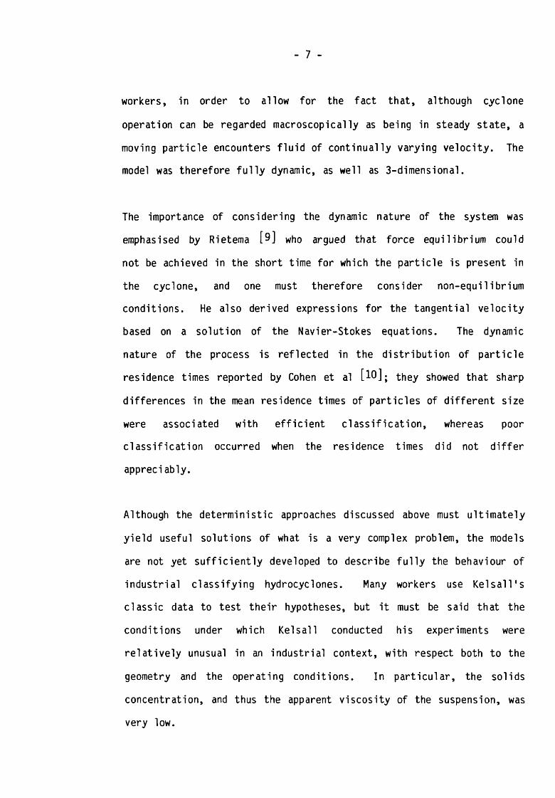
- 7 -

workers, in order to allow for the fact that, although cyclone

operation can be regarded macroscopically as being in steady state, a

moving particle encounters fluid of continually varying velocity. The

model was therefore fully dynamic, as well as 3-dimensional.

The importance of considering the dynamic nature of the system was

emphasised by Rietema [9] who argued that force equilibrium could

not be achieved in the short time for which the particle is present in

the cyclone, and one must therefore consider non-equilibrium

conditions. He also derived expressions for the tangential velocity

based on a solution of the Navier-Stokes equations. The dynamic

nature of the process is reflected in the distribution of particle

residence times reported by Cohen et al [10]; they showed that sharp

differences in the mean residence times of particles of different size

were associated with efficient classification, whereas poor

classification occurred when the residence times did not differ

appreci ably.

Although the deterministic approaches discussed above must ultimately

yield useful solutions of what is a very complex problem, the models

are not yet sufficiently developed to describe fully the behaviour of

industrial classifying hydrocyclones. Many workers use Kelsall's

classic data to test their hypotheses, but it must be said that the

conditions under which Kelsall conducted his experiments were

relatively unusual in an industrial context, with respect both to the

geometry and the operating conditions. In particular, the solids

concentration, and thus the apparent viscosity of the suspension, was

very low.

- 8 -

Departures of analytical theory from observation have been variously

attributed to short-circuit and secondary flows, boundary layer

effects on the cyclone wall, atypical conditions prevailing close to

the air core, and turbulence. Turbulence has been ignored by some

authors [12,13] ancj -js regarded as process-determining by others

[15.16] # As Rietema [17] pointed out, turbulence has two effects

on classification : it reduces the value of n in equation 2 . 1 by

absorbing energy, thus increasing the effective fluid viscosity, which

is reflected in the eddy viscosity terms in the Navier-Stokes

equations, and it causes eddy diffusion of the solid particles

[5.16] . Rietema himself has however explicitly neglected eddy

diffusion in the development of his characteristic cyclone number,

Cy5 0 t®]- Neesse [15] showed that an efficiency (partition) curve

of the type found in practice could be predicted on the basis of the

centrifugal forces acting on the particle, the net force due to

turbulent fluctuations and experimentally-determined velocity

gradients. However Exall [18] has criticised him for neglecting the

effect of the drag on the particle due to the radial velocity of the

fluid. Exall derived a simple model predicting the relative

concentration of particles of given diameter at a given radius, in

terms of the radial and tangential flow velocities and the eddy

diffusivity. Using the model it is possible to draw radial

concentration distribution curves for different particle sizes, and it

might be of interest to compare these with the experimental data of

Renner [13], who obtained samples of solids from within an operating

cyclone using a high-speed sampler.

- 9 -

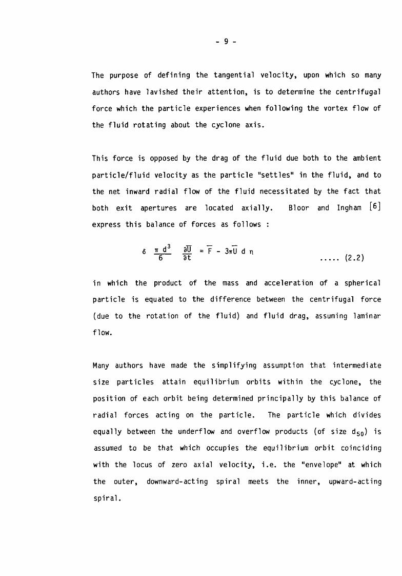
The purpose of defining the tangential velocity, upon which so many

authors have lavished their attention, is to determine the centrifugal

force which the particle experiences when following the vortex flow of

the fluid rotating about the cyclone axis.

This force is opposed by the drag of the fluid due both to the ambient

particle/fluid velocity as the particle "settles" in the fluid, and to

the net inward radial flow of the fluid necessitated by the fact that

both exit apertures are located axially. Bloor and Ingham [6 ]

express this balance of forces as follows :

6 n d3 j)U = ? - 3nU d n6 3t .... (2 .2 )

in which the product of the mass and acceleration of a spherical

particle is equated to the difference between the centrifugal force

(due to the rotation of the fluid) and fluid drag, assuming laminar

flow.

Many authors have made the simplifying assumption that intermediate

size particles attain equilibrium orbits within the cyclone, the

position of each orbit being determined principally by this balance of

radial forces acting on the particle. The particle which divides

equally between the underflow and overflow products (of size d50) is

assumed to be that which occupies the equilibrium orbit coinciding

with the locus of zero axial velocity, i.e. the "envelope" at which

the outer, downward-acting spiral meets the inner, upward-acting

spiral.

- 10 -

This view, first articulated by Kelsall, has come to be known as the

equilibrium orbit hypothesis and has been much utilised to derive

formulae [11*12,14,19,20] expressing the d5 0 (the most significant

performance criterion) in terms of design and operating variables,

which have found considerable application in practice. Bednarski, for

example, writing in 1968, listed 15 such formulae [21], Bradley

[1 ] has pointed out that most of these expressions can be reduced,

for a given cyclone geometry, to the form :

d50

_ 0.5

Q f ( 6 - p )

(2.3)

Tarjan [14] gives an expression of this kind in which the balance of

forces is represented explicitly for a particular radius within the

cyclone, in terms of tangential and radial velocities and the

acceleration due to gravity.

The significance of equation 2.3 to DM cyclone separations is that,

assuming that the concept of a particle dividing equally between

overflow and underflow is deterministic and not probabilistic, and

assuming the validity of the equilibrium orbit hypothesis, it is

possible to derive from this equation an equivalent expression for the

separating density of particles of size, d, by re-arranging equation

2.3 :

- 11 -

650 = P + KDc3 n

Q f d2

(2.4)

The implications of this expression will be developed later in the

thesis.

In the context of DM cyclones, the problem with equation 2.3 is that

it assumes that the particle Reynolds number is small (Rep < 1),

owing to the fine size of particles normally treated in hydrocyclones

(typically less than 300ym), i.e. that Stoke's Law defines the fluid

drag on the particle and thus the terminal ambient particle/fluid

velocity. Bradley U ] has shown that for most practical purposes

this is the case, and most other authors have followed this

assumption. DM cyclones, however, treat particles up to two orders of

magnitude larger than those handled by classifying hydrocyclones, and

although the viscosity of the dense medium is higher than that of

water, it is unlikely that laminar particle flow conditions prevail in

the coarser sizes. Evidence supporting this view will be presented

1 ater.

One of the most important differences between classifying and DM

cyclone operation (apart from the presence of a third phase) is the

relatively high apparent viscosity of the dense medium, which varies

over a wide range, depending as it does upon medium density (i.e.

solids concentration), solids size distribution and shape, and other

factors. The influence of the viscosity terms in hydrocyclone models,

- 12 -

and in particular in equations 2.3 and 2.4, is therefore of particular

interest, and a review of this aspect of the literature is essential.

Fontein et al [22] # Zhevnovatyi [23] and Trinh et al [24] have

all reported a decrease in the recovery of solids to the underflow as

fluid viscosity increased. Agar and Herbst [25] showed, by drawing

partition curves for separations at different viscosities, that this

was due to an increase in the dso, as predicted (qualitatively) by

equation 2.3. Correlation of their data gave d5 0 « nO-58. Agar and

Herbst's data suggested that the efficiency of separation, in terms of

the proportion of solids misplaced to each product, deteriorated as

fluid viscosity increased. Graves [26] also suggested that d5 0

increased with viscosity, but only above a certain value; below this

value the viscosity had no effect, which implies changes in the

particle Reynolds number resulting in the influence of separate

Stokesian and Newtonian flow regimes.

Since the fluid in hydrocyclone operation is almost invariably water,

of relatively constant viscosity, some authors replace the viscosity

term by the solids concentration, reflecting the analagous influence

of slurry viscosity on cyclone performance. Plitt's model for the d5 0

is of this type [2 ], the volume concentration of solids appearing in

exponential form, a consequence of the exponential-type relationship

found between viscosity and the solids concentration of suspensions

(See Section 2.3). The direction of the influence is the same as that

for viscosity indicated in equation 2.3. Marasinghe [27]

investigated specifically the influence of solids concentration on the

performance of a 125mm hydrocyclone. The principal conclusions of

this work were reported recently by Svarovsky and Marasinghe [28].

- 13 -

They are in agreement with earlier workers in respect of the increase

of d50 with viscosity; the data conformed quite well to a correlation

proposed by Svarovsky, in which the volume concentration of solids

again appears in exponential form.

The (6-p)”0*5 buoyancy term in equation 2.3 is also a consequence of

the assumption of laminar (Stokesian) flow conditions mentioned

earlier, and is subject to the same doubts of validity in the case of

large particles in DM cyclones. The term does imply that particles of

different density will separate at different sizes (d50s) in a

hydrocyclone. Although many semi-empirical regression models (such as

those of Plitt [2] and Svarovsky [28]) include the term

arbitrarily, on purely theoretical grounds, there is ample evidence in

the literature that the effect does exist, but there is doubt as to

the correct value of the exponent defining the flow regime. Lynch and

Rao [29] present evidence, based on plant-scale testwork, that the

value is unity, indicating a Newtownian (turbulent) regime, and Barber

et al [30] report additional plant data in terms of Lynch and Rao's

model, supporting this view. Further evidence for the turbulent regime

was obtained for density separations in a heavy liquid by Brien and

Pommier [31], in terms of an exponent for d of unity in a

transformed equation of the kind given above as equation 2.4. However

Bradley [1] maintains, as noted earlier, that most industrial

cyclones operate in the Stokesian regime, except possibly small

cyclones, in which tangential velocities are higher and in which

transitional regime conditions may therefore prevail.

- 14 -

As will be shown in Chapter 3, the question of which regime is

appropriate for a particular separation is very important in the

context of DM cyclone performance. The exponent for the n and (6-p)

terms in equation 2.3, and that for d in equation 2.4, arise in the

evaluation of fluid drag on the particle as it moves radially with a

velocity, v, relative to the fluid. If it is assumed that terminal

velocity is attained in negligible time (as suggested by Bloor and

Ingham [6]) then the resulting force balance is given by :

m ill. dtdv = (m - m*) Vt2 _ fd

r (2.5)

where Fq = CqA 0.5 p vt2 and Jjv = 0dt

For a spherical particle

6 4

and vt = D - d(«-p) Vt2 °‘53 Cg p r ( 2 . 6 )

Tarjan [14], using this approach, equated the terminal velocity of

the particle with the inward radial velocity of the fluid, Vr, and

so derived expressions for the size of particle, d, rotating at an

- 15 -

equilibrium orbit, r. The problem, however, is defining a value for

the radial drag coefficient, Cq , which is a function of the particle

Reynolds number and therefore of the particle velocity, v:

ReD = p v dn .... (2.7)

For a spherical particle, Cq is defined in the limits of laminar and

turbulent flow as follows :

Laminar (Rep < 10"1) Cq = 24/Rep

Turbulent (Rep > 103) Cq = 0.44

In the transitional regime (10 -1 < Rep < 103) the function

Cq = f (Rep) is continuously varying. Tarjan, and many other

workers, cite Allen's law for the transitional regime, but a better

approximation is provided by the recent correlation of Concha and

Almendra [32].

Following Tarjan and generalising we may write, by analogy with

equation 2.3 :

a 3dso = Ki n (<$-p) ......... (2 .8)

where the constant, K*, incorporates all other variables not shown,

and the exponents a and 3 are functions of Rep :

- 16 -

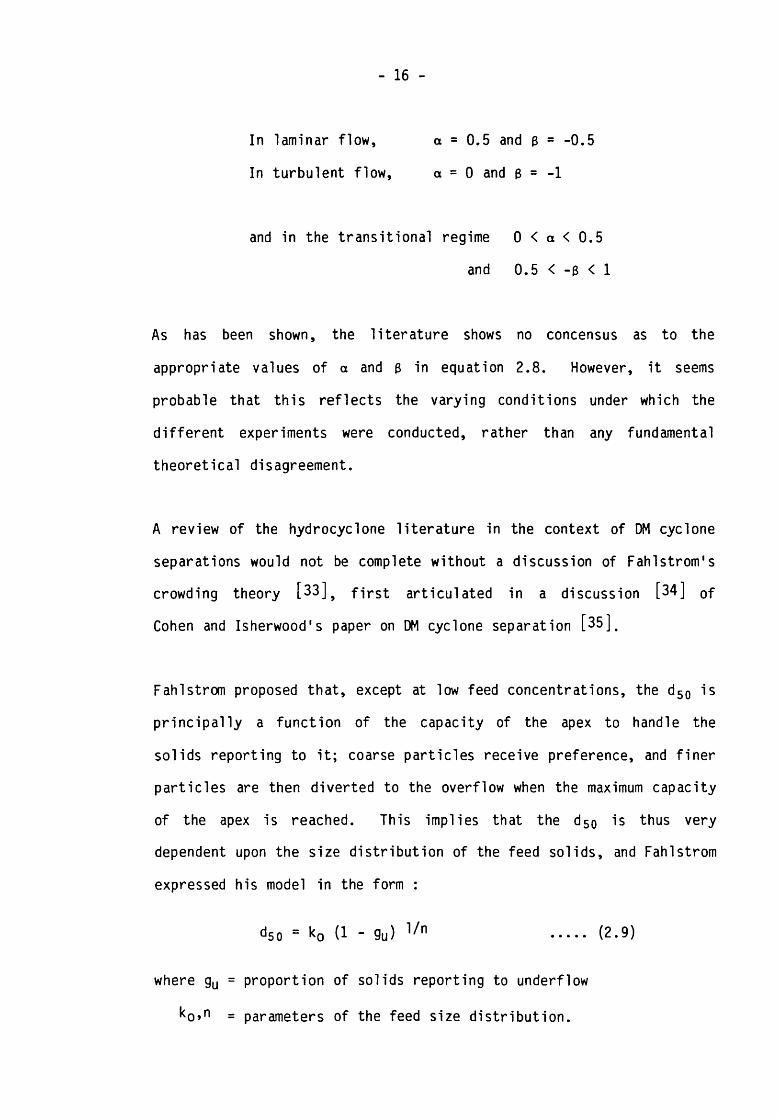
In laminar flow, a = 0.5 and 3 = -0.5

In turbulent flow, a = 0 and 3 = -1

and in the transitional regime 0 < a < 0.5

and 0.5 < - 3 < 1

As has been shown, the literature shows no concensus as to the

appropriate values of a and 3 in equation 2.8. However, it seems

probable that this reflects the varying conditions under which the

different experiments were conducted, rather than any fundamental

theoretical disagreement.

A review of the hydrocyclone literature in the context of DM cyclone

separations would not be complete without a discussion of Fahlstrom's

crowding theory [33]9 first articulated in a discussion [34] of

Cohen and Isherwood's paper on DM cyclone separation [35].

Fahlstrom proposed that, except at low feed concentrations, the d50 is

principally a function of the capacity of the apex to handle the

solids reporting to it; coarse particles receive preference, and finer

particles are then diverted to the overflow when the maximum capacity

of the apex is reached. This implies that the d50 is thus very

dependent upon the size distribution of the feed solids, and Fahlstrom

expressed his model in the form :

<*50 = k0 (1 - 9u) 1/n .... (2.9)

where gu = proportion of solids reporting to underflow

k0,n = parameters of the feed size distribution.

- 17 -

Although this hypothesis is helpful in considering the principles of

hydrocyclone performance, it has not gained wide acceptance, either in

the scientific literature or for design purposes. Nevertheless, it

seems likely that such a model might be particularly appropriate to DM

cyclone operations in which feed solids concentrations of 40% v/v are

not unusual, and in which apex crowding is therefore a probable

phenomenon.

In summarising this brief review of the hydrocyclone literature, one

is forced to the conclusion that the analytical (deterministic)

models, based on solutions to the Navier-Stokes and continuity

equations, are a sterile hunting ground for guides to the mechanism of

separation in DM cyclones, principally because of the complexity of

the 3-phase dense medium system and some of the necessary simplifying

assumptions (e.g. an inviscid fluid). However, a theme common to many

of the theoretical studies is the radial balance of centrifugal and

drag forces which act on the particle. This is the basis of the

equilibrium orbit hypothesis favoured by early workers in the field.

The importance of the prevailing (particle) flow regime in defining

the quantitative influence of the viscosity, n , and the buoyancy

term, (6-p), in this model has been emphasised. The concept will be

developed in the subsequent interpretation of data obtained from

experiments with DM cyclones.

- 18 -

2.2 Dense Medium Cyclones

The literature is well endowed with articles and papers extolling

the virtues of the DM cyclone in an engineering and metallurgical

sense, but sparse in fundamental studies of the mechanism of the

density separation obtained. Much of the early work was conducted

on low-density separations, particularly with magnetite media,

reflecting the initial development of the process by the Dutch

State Mines from about 1939, and its application to coal

preparation. The DSM workers published widely [36,37,38] ancj

many of the significant features of the device were identified in

those early papers, notably its ability to separate ore of a much

finer size than the existing static bath separators (a

consequence of the magnitude of the centrifugal forces involved),

and its ability to operate without difficulty with a medium

exhibiting a yield stress, as a result of the high shearing

forces prevailing in the cyclone. The process was developed

shortly before and after the 2nd World War, following the

fortuitous observation that coal preferentially concentrated in

the overflow product from a cyclone being used to thicken loess

medium for regeneration in a static bath washing plant. The

separation was explained by Krijgsman [37] in terms of a

"barrier" of medium particles which built up in the lower part of

the cyclone. The light coal particles penetrated this barrier by

virtue of the centrifugal force imposed on them by the rotation

of the medium, and then experienced a centripetal force which

moved them to the axis of the cyclone, whence they passed rapidly

to the overflow via the central vortex flow. The importance was

- 19 -

emphasised of utilising medium particles of a size suitable to build

up the barrier, and this led to the preferred use of magnetite as the

medium for coal preparation.

Fontein and Dijksman [38] identified various classes of separation,

depending on whether the medium is stable or unstable, and whether the

separation is made at the density of the medium or at a higher

density. They stated that pure (heavy) liquids or stable media (i.e.

media with particles so fine that no settlement of the particles

occurs relative to the carrier fluid) produce cut-points of density

equal to that of the liquid or medium, a statement which is at

variance with the hydrodynamic model implied in eqn. 2.4. The

performance data given by Fontein and Dijksman to support their view

refer to a sylvite/halite separtion in a medium of fine magnetite and

a saturated solution of NaCl/KCl, but no attempt was made to determine

the actual 6 5 0 for the separation, and it is probable that this was

responsible for a conclusion which has been shown in subsequent

literature, and by the present work, to be erroneous. The authors

also made first mention of what has come to be known as the "water

only cyclone", or "compound water cyclone", in which values of 6 5 0

greater than 1 . 0 are obtained using only water as a medium and a

cyclone of modified geometry (usually incorporating a wide cone

angle). Finally, they discussed at some length the phenomenon of

separating densities higher than those of the unstable medium used (in

a conventional DM cyclone), which is the commonest system currently in

use and the one which has been studied in the present work. Driessen

[36] explained the phenomenon by assuming that the medium particles

have a longer residence time than the carrier liquid, and that the

- 20 -

medium in the cyclone therefore has a density greater than that of the

feed (the data reported in Chapter 5 support this assumption).

However, as Fontein and Dijksman point out, this does not explain why

the light fraction of the ore passes to the overflow in a medium of

lower density. They suggested a dynamic interpretion, in which

particles follow a transverse, "convection" flow in the cyclone; dense

particles are centrifuged rapidly away from the axis, and eventually

report via the cone wall to the apex, but light particles do not

experience sufficient acceleration to be removed in time from the

central, axial flow, and so report to the overflow product.

Driessen [36] and Krijgsman [37] assumed that Allen's Law for the

transitional flow regime describes the terminal velocity of ore

particles settling in a dense medium :

vt = K4g

3 0 p ( n / p ) 0 . 5

2/3. d [«-p]2/3

(2.10)

where K is a shape factor ( = 1 for spheres) and g is replaced by

centrifugal acceleration for cyclones. This expression was used

quantitatively to show that the separating rates in cyclones were very

much faster than those in bath separators.

Krijgsman also included some early data demonstrating the fact that

fine ore separates at higher densities than coarse ore, and that

higher medium viscosities result in additional misplaced material and

thus reduced separating efficiency.

- 21 -

Following the introduction and description of the DM cyclone process

by DSM in the 1940s and early 1950s, a number of other workers carried

out studies of the process, both in low density coal separations and

in high density ore separations, particularly iron ore. Van der Walt,

for example, reported a comprehensive evaluation of the cyclone

washer in a coal preparation application [39], He conducted tests

with a 240mm x 38 ° cyclone, using 99% - 63ym barite (BaSO^) as a

medium. Although the work was specific to a particular coal deposit,

a number of general conclusions were drawn regarding the influence of

certain design and operating variables upon the cyclone operation.

The separating density was found to be approximately constant for ore

above about 2mm in size, but rose rapidly below this size. The

crowding theory of Fahlstrom [33] 9 and the qualitative DM cyclone

model of Cohen and Isherwood [35]# were anticipated in data which

demonstrated the controlling influence of the solids-handling capacity

of the apex. Feed pressure (flowrate) was found to have a variable

influence, with cut-point (and efficiency) increasing up to a critical

value of pressure, and then falling off. The diameter of the feed

pipe was also found to be important, the cut-point for a given

pressure drop increasing with diameter. The author attributed this to

changes in the momentum supplied to the rotating volume of medium in

the cyclone, the larger diameters experiencing less tangential

velocity drop as the medium enters the body of the cyclone (Bradley

[1] also discusses this aspect). The influence of cone angle was

studied using cyclones of 3SP , 259 and 15°, and it was found that the

separating density increased slightly with cone angle, corresponding

to an increased total flow through the cyclone at a given pressure

drop (due to a reduction in the rate of shear of medium, and thus to a

- 22

reduction in friction losses) and an increased proportion of medium

reporting to the overflow. Smaller cone angles were shown to have

larger medium retention times than large angles (notwithstanding the

greater overall flowrates), leading to a greater efficiency of

separation of small particles. Van der Walt pointed out the

importance of selecting a medium of a sufficiently low viscosity, and

showed that rapid increases in viscosity occured above a concentration

of solids of about 30-35% v/v for most media. However no information

was given as to the degree of thickening of the barite medium in the

cyclone.

Belugou and de Chawlowski [40] studied the performance of 150, 350

and 500mm cyclones using barite and shale media in the concentration

of coal. They concluded that under "normal" operating conditions the

only geometrical variables which influenced the separation were the

overflow and underflow orifice diameters; inlet diameter and cone

angle had no effect, except in defining capacity. The separating

density could be increased by increasing the vortex finder diameter or

decreasing the apex diameter. An interesting conclusion was that,

although the separating density was almost invariably greater than the

medium density, the most efficient separation (i.e. lowest Ep-values)

occured when the two densities (almost) coincided. The authors

interpreted this result in terms of a centripetal current existing in

the cyclone when the two exit orifices were significantly different in

size (D0 » Du), a condition necessary to achieve high separating

density. When the separating density approached the medium density,

then the separation was believed to depend on density only (a true

"sink-float" condition) and the proportion of misplaced material was

- 23 -

minimised. The throughput of coal was found not to influence the

quality of separation up to a certain tonnage, beyond which the

separation deteriorated due to increased misplacement of dense

material to the overflow, an effect which one might tentatively

ascribe to spigot crowding (cf. Fahlstrom [33]). As in most other

studies, the separating density and Ep-value* were found to rise below

a certain particle size, though this size was lower for medium of

lower density, implying that the correspondingly lower medium

viscosity allowed efficient separation of finer particles.

Herkenhoff's work, reported in 1953 [41], is significant in two

respects : it was one of the first reported investigations of non-coal

(high density) separations in DM cyclones, and it was also the first

specific study of the influence of medium characteristics on the

separation. Treating -6.35 +0.177nm iron ore in a lOOmn cyclone,

using magnetite and magnetite/FeSi media, Herkenhoff noted that the

medium itself was classified in the cyclone (calculations suggest that

the separating size for a magnetite medium of about 40% v/v was high,

above 150ym), and that the classification effect increased as the feed

density decreased. He also found that the density differential

between the overflow and underflow medium decreased both as back

pressure was applied to the overflow pipe (by throttling) and as the

feed density, and thus viscosity, increased; in this latter case,

underflow density increased rapidly to a constant value and overflow

density increased steadily until the condition pf - pu - Po was

approached. In interpreting the results of the ore separations, the

These, and other performance criteria obtained from the Tromp curve

for the separation, are discussed in Chapter 3.

- 24 -

author unfortunately did not determine the Tromp curve but monitored

instead the Fe assays of feed and products; however some general

conclusions can be drawn about the separating performance. One

interesting observation was that more ore reported to the underflow

when the medium was magnetised. Since it is known that the effect of

magnetisation is to increase viscosity [42], this implies that the

separating density decreased as the viscosity increased. Increasing

the feed density from 2150 to 2350 kg m - 3 produced less Fe recovery

but at a higher grade (due to a corresponding increase in 6 5 0 ), and

also resulted in a small increase in the proportion of medium

reporting to underflow. Tests with three size distributions of

magnetite (85, 69 and 58% -45pm) showed that use of the finer media

resulted in reduced density differentials and reduced recoveries of

medium solids to underflow, which corresponded to increased yields of

ore due to lower 6 5 0 s. Again, finer media have high viscosities

[42]# and Herkenhoff's work seems to imply that higher viscosity

media produce lower ore 6 5 0 s. However, it is not yet clear as to

whether such observations should be interpreted in terms of a

viscosity effect, or in terms of the classification of the medium

which determines the split of medium solids to the two products, and

thus the apex capacity available to handle the ore solids, as

suggested by Cohen and Isherwood [25].

Stas [43] studied the influence of the apex and vortex finder

diameter on the density of (magnetite) medium reporting to underflow

and on the separating density and Ep-value, for coal separations. He

found that below Du/D0 ratios of 1.0, the value of pu increased

rapidly, as did the 6 50. However his data imply that separating

- 25 -

densities <55 0 < pf occurred, even though pu » pf under these

conditions. Both 6 5 0 and Ep increased rapidly as Du/D0 decreased.

The fact that 6 5 0 and Ep were correlated in this way is at variance

with the results of many other early investigations. Tarjan pointed

this out in his discussion of Stas' paper, but, although he offered an

explanation for the generally observed correlation of 55 0 with Du

(in terms of his analysis of separations in DM cyclones [14,44]),

the observed direct variation of 6 5 0 with Ep was not explained; Tarjan

also used Stas' data to deduce a value for n (in eqn. 2.1) of 0.68,

with plain water.

Stas himself, in his reply to the discussion of his paper, suggested

"... the increasing viscosity with the density of separation ..." as

an additional explanation for the anomalous result. This is

interesting in the context of the observations to be presented in

Chapter 3, in which it will be shown that this relationship does hold

for a stable medium for which cyclone performance conforms to a

viscosity model of the general kind suggested in eqn. 2.4. The

present author's earlier work [4] suggested that the exact form of

the 6 5 0 - Ep relationship depended very much upon the particular

combination of prevailing operating conditions, but that, other

factors being equal, high Ep values were obtained when the median

density of the ore coincided with the separating density. It is

perhaps also worth pointing out in this context that Gottfried

predicted the result 6 5 0 * Ep from the mathematical properties of the

generalised partition curves for coal cleaning devices [46], and

quoted operating data to support this view.

- 26 -

Sarkar et al [64], washing coal in a 152mm cyclone with barite

medium, found that increasing amounts of "near gravity" ore (that is,

material of density close to the separating density) resulted in a

deterioration in the quality of separation, i.e. an increase in the

proportion of misplaced material. If one assumes, by analogy with the

work of Cohen et al on hydrocyclones [10], that the residence time

of near gravity material is longer than that of extreme gravity

material, then this observation can be interpreted in terms of an

accumulation of near-gravity material in the cyclone, leading to

misplacement due to obstruction and hindered settling. Previous

unpublished work by the present author [45], in which the residence

times of individual particles of known density were monitored in a

610mm DM cyclone, confirmed the assumption that the longest residence

times were experienced by near-gravity material, and showed that mean

residence time increased with ore feedrate, presumably also due to a

crowding effect.

Sokaski and Geer [47] evaluated the performance of a 254mm x 20P

cyclone in the treatment of a number of coals using magnetite media.

They found that fine media gave sharper separations (less misplaced

material) than coarse media, although cut-points did not vary. They

also noticed with one particular coal, containing a high proportion of

near gravity material, a surging of the underflow product, which they

attributed to cyclic accumulations of dense material near the apex,

leading to intermittent discharges and consequent misplaced light

material in the underflow. The phenomenon disappeared when finer

magnetite was used, and the authors suggested that the problem was

caused by displacement of the finer, dense refuse material by coarse

- 27

magnetite which was present in thickened form close to the apex; the

displaced ore was then caught up in the eddy recycle flows in the

cyclone until sufficient material accumulated to cause discharge.

(Oscillations in the underflow product of a small glass cyclone have

also been observed using high speed photography [63]; the

oscillations appeared when solids, which all reported to the underflow

product, were introduced into the feed).

These observations appear to coincide with the qualitative apex

crowding model of Cohen and Isherwood [35] and are interesting for

the significance which they place on the size distribution of the

medium particles.

Davies et al [48] studied the behaviour of a 150mm x 2(P and 300mm x

2CP cyclone in the treatment of ores other than coal, using both

magnetite and ferrosilicon media. They expressed the stability of the

medium, A, as the feed-underflow density differential,

A = p u - Pf (2.11)

and showed that the quality of separation (expressed as the Ep-value)

deteriorated as A increased, i.e. as the stability decreased. They

noted that the value of A depended upon a number of variables

including the characteristics of the medium (e.g. size distribution,

Pf etc), and stated that although the Ep could be reduced by

reducing A, the separation might improve little or even deteriorate if

this was achieved at the expense of high medium viscosities. This

appears to be the first explicit reference in the literature to the

opposing influence of medium stability and viscosity.

- 28 -

Davies and his co-workers also concluded that, for a given ore, the Ep

increased with 6 5 0 (in agreement with Stas). This relation also held

in respect of ore size. They found that above a certain ore size,

depending on 6 5 0 (the limiting size was 2 mm for one particular set of

conditions), the size had no effect on 6 5 0 , but that below this size

both the 6 5 0 and Ep increased as ore size decreased; a quantitative

relationship was presented expressing the Ep for a given ore size in

terms of the Ep prevailing for lOirm particles. The concept of a

limiting size, above which size has no influence on 6 50, accords with

Van der Walt's observations [39], Davies et al demonstrated that

the medium size distribution, or mean size, could be appropriately

scaled for different diameter cyclones by making use of the relation

that the separating size of the classification is proportional to the

square root of the cyclone diameter, other things being equal, i.e:

By scaling the medium mean size in this way, the value of A, and thus

also the quality of separation, was maintained relatively constant.

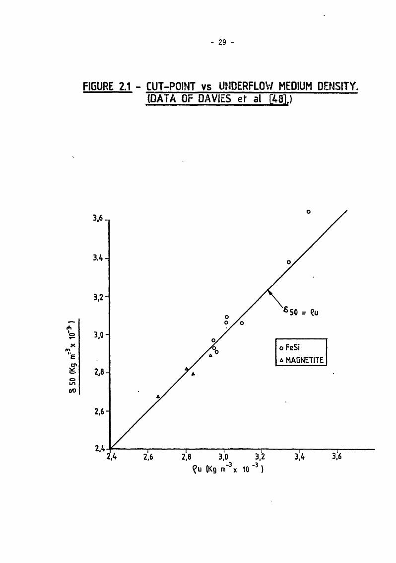
The authors also stated that it was found that an estimate of the

prevailing 6 5 0 acceptable for control purposes could be obtained

directly from the value of pu . Although no direct evidence was

presented, a plot of 6 5 0 vs. pu for the 1 2 suitable results given

in the paper (Figure 2.1) does demonstrate a remarkable

correspondence, for both magnetite and ferrosilicon media. However,

the 97 data points available from the present author's earlier work

[4] suggest that such a relation may only apply under a certain

(fortuitous) combination of operating conditions.

( 2 . 12)

S SO

(Kg

mr3

x 10

'3,)

- 29 -

FIGURE 2.1 - CUT-POINT vs UNDERFLOW MEDIUM DENSITY. (DATA OF DAVIES et al IA81)

- 30 -

Upadrashta and Venkateswarlu [49] obtained arbitrary multiple linear

regression models of the behaviour of a 100mm x 2GP cyclone treating

various ores using an atomised FeSi medium (probably "Cyclone 60"

grade [42]), and used these to relate performance crtieria to

operating variables. They suggested a model for 650 analagous to that

proposed by Fahlstrom [33] for classification (eqn. 2.9):

^50 = ~^i In gu + k2 .... (2.13)

in which gu is the proportion of ore reporting to underflow and k2

is numerically equal to the density of the lowest-density component

in the feed. The model therefore implies that all the feed would

report to the underflow when the separating density equals the lowest

density in the feed (gu = 1, 650 = k2). The authors showed that a

satisfactory fit was obtained to eqn. 2.13 using a combination of

their data and the data of Davies et al [48], comprising seven ores

in all. They proposed that this demonstrated that Fahlstrom's crowding

theory also applies to dense medium separations. The value of

gu itself was found to be a function of the ratio of underflow to

overflow volume flowrates (Qu/Q0 ) - The density of the underflow

medium increased with pf and Pi within certain limits of

Du/D0. The authors found that the Ep varied with ore size, and

correlated their data in a similar way to Davies et al.

The volume split of pulp (S - Qu/Q0 ) was shown to increase with

the volume solids concentration, for a (normal) spray underflow

discharge, as is usual with classifying hydrocyclones [2], Since

the apparent viscosity of the medium increases with solids

- 31

concentration, this may be akin to saying that volume split increases

with viscosity, an effect noted for hydrocyclones operating with true

solutions U]. The pressure drop factor (inlet pressure expressed

as number of inlet velocity heads, P-j/0*5 p V-j2) decreased with

increase in solids concentration, implying that flowrate decreased

with an increase in concentration, at a given inlet pressure. Plitt's

equations [2 ] also reflect such a relationship, although it does not

accord with viscosity effects observed with hydrocyclones [1 ].

However, the situation is complicated by the fact that the two

parameters which are legitimately related hydrodynamically are

pressure drop factor and Reynolds number which between them contain

the variables flowrate, pressure drop and viscosity. The direction of

this relationship itself depends upon the Reynolds number [9], The

effect of suspension viscosity on volume split and pressure drop will

be discussed further in Chapters 3 and 5.

Most of the authors reviewed thus far agree that, under "normal"

operating conditions, a DM cyclone cuts at a density greater than that

of the medium, even for unstable suspensoid media. Such a trend

follows from the model of eqn. 2.4, which, strictly speaking, applies

to true liquids or stable suspensions. Moder and Dahlstrom [50] and

Brien and Pommier [31] have presented data to show that, using true

liquids as media, the cyclone does separate the solids at a density

higher than that of the liquid. Brien and Pommier correlated their

data with a simplified version of eqn. 2.4:

«50 = Pf + J< d ° (2.14)

- 32 -

As already noted, o was found to be unity, indicating a Newtonian

particle flow regime. Viscosity was not considered as a system

vari able.

A number of authors have given attention to the mechanism determining

the separating density for unstable suspensions. The views of

Driessen [36] and Fontein and Dijksman [38] in this respect have

already been discussed. Tarjan [14] was the first to consider in

detail the performance of a DM cyclone in terms of the classification

behaviour of the medium. He defined the density of separation as the

density of the medium prevailing at the locus of zero axial velocity

(the line Va = 0 in Figures 2.2a and 2.2b), and distinguished four

cases. These depended on the relative angles between the axis and the

lines Va = 0 and d = constant (Figures 2.2a and 2.2b, angles 6 and <j>

respectively), and on whether the medium solids were coarse or fine

(Figures 2.2c - 2.2f). For <f> > e (Figures 2.2d and 2.2f), a medium

particle of given size rotating in an equilibrium orbit would always

tend to return to its equilibrium position if displaced, which would

favour the formation of a stable suspension, of density higher than

the feed density, along the line Va = 0; this would result in a

separating density higher than pf. For $ < 6 , a displaced particle

would tend not to find its way back to its equilibrium orbit, which

would prevent the formation of a stable, high density suspension along

the line Va = 0S; this would lead to a separating density close to

Pf. The density of the overflow and underflow medium products, and

the separating density relative to the feed medium density, would

depend upon whether the feed medium was coarse (Figures 2.2c and 2.2d)

- 33 -

FIGURE 2.2a- CLASSIFICATION OF MEDIUM IN A DM CYCLONE (AFTER TA R JA N f14] ).

FIGURE 2.2b- RELATIONSHIP BETWEEN LOCUS OF ZE R O A XIA L VELOCITY (Va) AND LOCUS OF CONSTANT PARTICLE SIZE (d) (AFTER TAR JA N L14] ).

- 34 -

FIGURES 2 .2 c -f MEDIUM DENSITY DISTRIBUTION ACROSS THECYCLONE RADIUS FOR COARSE AND FINE MEDIUM (AFTER TARJAN 1% I )

FIGURE 2.2 c - COARSE MEDIUM$ < ®

FIGURE 2.2d - COARSE MEDIUM<t> > e

FIGURE 2.2e - FINE MEDIUM<J> < ©

FIGURE 2.2 f - FINE MEDIUM<t> > e

NOTE: r MARKS LOCUS OF LINE Va = 0 ( Value of fin at this point definesseparating density i f so)

r= CYCLONE RADIUS

- 35 -

or fine (Figures 2.2e and 2.2f); fine media would tend to produce low

overflow/underflow differentials. The best (sharpest) separations

were assumed by Tarjan to be attained with a fine, stable medium for

which 6 5 0 - pf (i.e. Figure 2.2e), whereas the worst separation

would occur with a fine medium for which 6 5 0 » Pf (i.e. Figure

2.2f). For the condition <f> > 6 , Tarjan predicted density instability

in the high density region (indicated by the dotted lines in Figures

2 .2 d and 2 .2 f) if inadequate coarse particles were available to

maintain the high density which would otherwise develop naturally.

This instability would result in a poorer quality of separation. The

relative values of 6 and <{>, which determine the prevailing mechanism

controlling the 6 50, are defined by the cyclone geometry and the

operating variables such as pressure drop. Tarjan's predictions of the

associated distribution of medium viscosity across the cyclone have

been neglected in this discussion because they rely upon certain

assumptions which, as will be shown later, are in doubt. In

particular, Tarjan assumed that dense medium suspensions are

pseudoplastic in nature, and that the viscosity/density relationship

is described by Einstein's equation for dilute suspensions of spheres.

Gupalo et al [51] proposed that the effective separating density is

given by

650 = Pm — tyvtT .... (2.15)

where Vt here denotes the tangential velocity of an ore particle.

Since ore particles were assumed to "lag behind" the fluid because of

inertial effects, this implies that Vt > vt and thus that 6 5 0 >

Pm-

- 36 -

Data quoted by the authors suggest that V^/v^ = 1.087 for

particles in the size range 50-500ym, and thus that 6 5 0 = 1.18 pm .

This conforms quite well with other data presented in the paper.

Although the authors did not claim their proposal as an exclusive

mechanism in determining 6 5 0 , nevertheless it implies that for fine

particles (Vt - vt), 6 5 0 ♦ Pm» and f°r coarse particles (Vt »

vt). «so » pm . These trends are totally at variance with the

observations of most other workers.

Olfert [52], writing in response to Gupalo et al, claimed that the

difference between the separating density and the medium density is

determined by the separating efficiency (defined by the Ep), and that

this difference increases with increase in medium contamination and

density (pm) and with a decrease in ore size. In an earlier paper

[59], Olfert had shown that the separating density increased and the

efficiency of separation decreased as the proportion of fine coal in

the medium increased (i.e. as the ore-to-medium ratio increased).

Schubert [53] reported data of other workers demonstrating the

classification and consequent thickening of a magnetite medium (of

density 1500 kg nr3, in a 75mm x 2CP cyclone), and cited this as the

reason for the observation that 6 5 0 > pm . Classification of a

magnetite medium was also reported by Khaidakin [54], who observed

that the classification size of the magnetite increased substantially

as the proportion of fine coal added to the medium increased, leading

to reduced segregation of the medium and consequently a change in the

separating density of the coal. He proposed a correlation of the

following form for the 650:

- 37

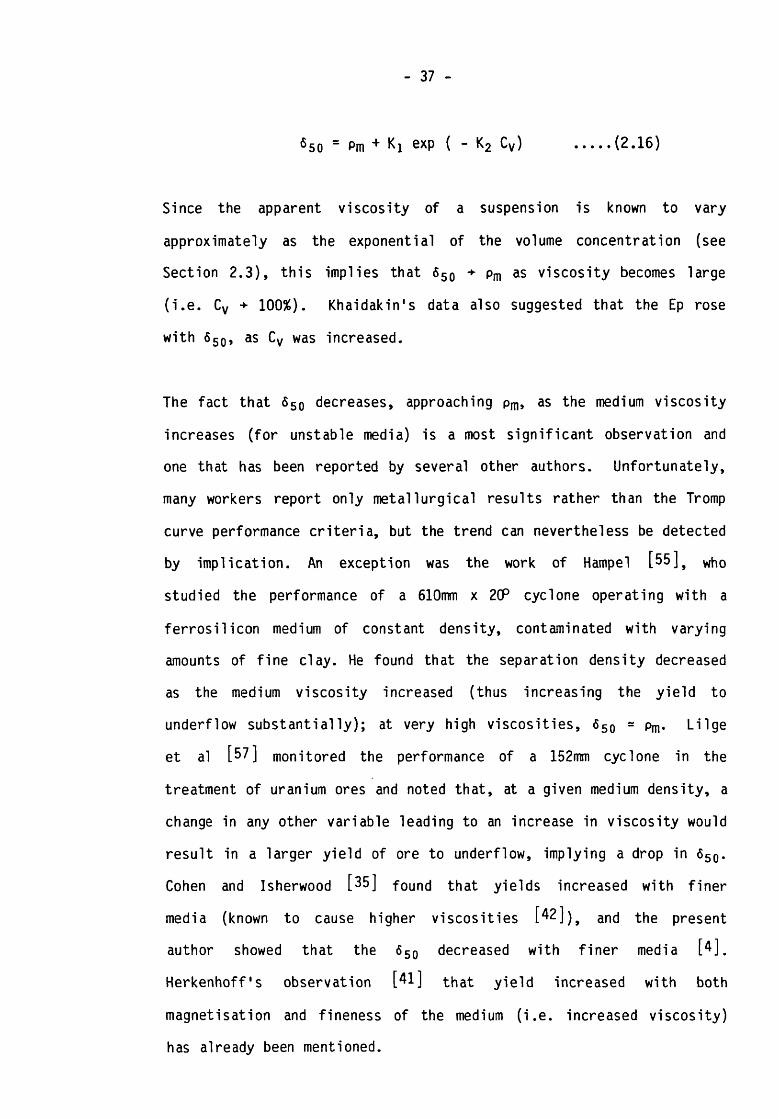
^ 5 0 = Pm + Ki exp ( - K2 Cy) .... (2.16)

Since the apparent viscosity of a suspension is known to vary

approximately as the exponential of the volume concentration (see

Section 2.3), this implies that 650 + Pm as viscosity becomes large

(i.e. Cv 100%). Khaidakin's data also suggested that the Ep rose

with 650, as Cv was increased.

The fact that 650 decreases, approaching pm , as the medium viscosity

increases (for unstable media) is a most significant observation and

one that has been reported by several other authors. Unfortunately,

many workers report only metallurgical results rather than the Tromp

curve performance criteria, but the trend can nevertheless be detected

by implication. An exception was the work of Hampel [55 ]# who

studied the performance of a 610mm x 20P cyclone operating with a

ferrosilicon medium of constant density, contaminated with varying

amounts of fine clay. He found that the separation density decreased

as the medium viscosity increased (thus increasing the yield to

underflow substantially); at very high viscosities, 650 = p ^ Lilge

et al [57] monitored the performance of a 152mm cyclone in the

treatment of uranium ores and noted that, at a given medium density, a

change in any other variable leading to an increase in viscosity would

result in a larger yield of ore to underflow, implying a drop in 650.

Cohen and Isherwood [35] found that yields increased with finer

media (known to cause higher viscosities [42]), and the present

author showed that the 650 decreased with finer media [4],

Herkenhoff's observation [41] that yield increased with both

magnetisation and fineness of the medium (i.e. increased viscosity)

has already been mentioned.

- 38 -

In general, the literature is in agreement that the separating density

(6 5 0 ) decreases as the medium viscosity increases, a trend which is

the exact opposite of that predicted by eqn. 2.4. A discrepancy

therefore exists between theory and observation. Since eqn. 2.4 was

derived from a classification model in which the solid particles are

assumed to move in a true liquid, the discrepancy might be

attributable to the fact that the literature reviewed above refers

to media which consist of unstable suspensions, rather than stable

media or true liquids. In order to investigate this possibility,

experiments were designed to investigate the independent influence of

the viscosity of a stable suspensoid medium upon the density

separation. This work is reported in Chapter 3.

The present author's previous study of the performance of a 610mm DM

cyclone using ferrosilicon media [4] was confined to operating

variables rather than cyclone geometry. It demonstrated that the

separation was controlled principally by the characteristics and

behaviour of the medium, in particular the medium size distribution.

The size distribution was expressed in the form of the Rosin-Rammler

function, and it was found that the gradient of the distribution had a

particularly strong influence on the density separation. Although, as

noted earlier, it was not possible to correlate directly the values of

6 5 0 and pu , both these parameters were strongly influenced by the

gradient of the medium size distribution, suggesting a mechanistic

link between the two. In general, fine media separated at a lower 6 5 0

than coarse media. Although the direct influence of pf was found to

be small (for the 2CP cyclone studied), its relative effect depended

upon the prevailing size distribution of the medium.

- 39 -

It was found that the best separations occurred at a particular value

of 6 50, relative to pf and the median density of the ore. This

finding is analagous to that of Fahlstrom [33] for classifying

hydrocyclones that an optimum d5 0 exists for each cyclone, for which

the quality of separation is maximised.

The work also confirmed that the 6 5 0 varies inversely with ore size.

It showed that the overflow and underflow medium densities are

determined principally by the feed density and by the size

distribution of the medium solids. In the case of pu, the value also

increases slightly with ore feedrate, suggesting again a crowding

mechanism at the apex. Some limited data relating to the

classification of the medium in the cyclone implied that the dso was

an important factor in determining the density differential

(pu - Po)> the differential varying inversely with d50. Plitt's

model [2 ] was shown to provide quite good predictions of the d50,

despite the high solids concentrations prevailing (typically 30% v/v),

and Fahlstrom's crowding theory [33] was also invoked to explain

qualitatively some of the observations. Subsidiary studies of a 200mm

cyclone showed that the d 5 0 was also inversely related to the

differential when density inversion prevailed. Inversion, which is a

condition known to occur in some production operations but which had

never before been explicitly reported in the literature, implies the

reversal of the normal thickening action in the cyclone, such that

Pu < Po» the differential becoming negative; the phenomenon

appeared to have little effect on the density separation. Some of the

authors reviewed above have presented data for which the differential

has approached zero, and Tarjan [14], as noted, has suggested a

- 40 -

mechanism in which this condition might be approached. Lilge [58],

as noted below, reported results from which small negative

differentials could be inferred, but clear examples of a negative

differential had not been specifically reported, possibly because such

observations were attributed to experimental error. The present

author suggested that the phenomenon could arise when a high d5 0

prevails with a fine, viscous medium (i.e. diverting most medium

solids to the overflow) simultaneously with a relatively high

proportion of water reporting to underflow. In view of the probable

importance of the phenomenon in assisting our understanding of the

mechanism of the density separation, experiments were designed to

investigate it further in the present work (see Chapter 5).

Very few authors have attempted either an interpretation of the

density separation mechanism in terms of the properties and behaviour

of the medium, or an examination specifically of the medium

behaviour. In a recent study of the operation of a standard DSM

cyclone, together with other DM vessels, Collins [55] found that the

6 5 0 corresponded to the underflow density, pu, under "normal"

conditions (although some of his data indicated that 6 5 0 > p u under

certain conditions). This conforms to the observations of Davies et

al [48] and Upadrashta et al [49], Both pu and 6 5 0 were found

to vary linearly with the feed density, pf. However, at low values

of pf the cyclone began acting as a classifier of the medium,

resulting in a constant density underflow. Under these conditions the

6 5 0 continued to fall as pf decreased, though at a reduced rate

(i.e. 6 5 0 < pu). Based on observations of the sedimentation of the

various media under gravity, Collins proposed that at normal operating

densities the bulk of the medium in the cyclone was of constant

- 41 -

density, including that portion reporting to underflow, with only a

small zone of low density close to the axis. At some critical value

of pf (2600 kg m~ 3 for a Cyclone 40 ferrosilicon medium, producing a

differential, pu - p0, of 800 kg m-3), the low density zone is

considerably enlarged, due to size segregation, and the density of

this zone then controls the 6 50. Clearly the critical value of pf

will depend upon the properties of the medium and the cyclone geometry

and operating conditions. Collins also reported the usual effect of

6 5 0 increasing as ore particle size decreased; sharpness of separation

(measured by the Ep-value) decreased with decrease in particle size

and increase in differential.

Tarjan [44] used his equilibrium orbit theory and the rheological

data of Govier et al [56] (to be discussed in Section 2.3) to make

theoretical predictions about the velocity gradient and hence the

apparent viscosity at different radii in the cyclone. He also

predicted the equilibrium particle sizes of various media revolving at

different radii, and suggested that those whose equilibrium orbit

coincided with the locus of zero axial velocity made up the "stagnant"

suspension in the central portion of the cyclone; the density of this

suspension defined the density of separation. For high viscosity

suspensions devoid of particles of such sizes the "stagnant"

suspension does not form, and pu « p0. In such cases, 650 = pf.

Apart from emphasising the importance of the medium size distribution,

this argument may also help to explain the experimental observations

reviewed earlier, that 6 5 0 pf as viscosity increases. A

consequence of Tarjan's treatment of the behaviour of the medium is

that, ideally, the medium particles should be of a size close to the

- 42

prevailing d50, so that a greater part of the suspension medium will

take an active part in the production of the "stagnant heavy

suspension". Tarjan's view was that the density of the medium

decreased uniformally from periphery to axis, and that the apparent

viscosity decreased in a similar sense.

The effect of the density change on the viscosity was much larger than

the effect of the increase in shear rate, implied by the decrease in

radius, upon the (apparently) non-Newtonian suspensions involved

(magnetite, galena and ferrosi1 icon). Thus although the viscosity of

the galena and ferrosi1 icon media reached an apparent minimum at a

shear rate of 300 s ~ l [56], corresponding to a radius of 4-5cm, the

viscosity continued to decrease below this radius.

The only reported attempt to measure the density of the medium at

different points in the cyclone was that by Hundertmark [50], who

used a y-radiation attentuation technique to monitor the densities of

ferrosi1 icon media in a 150mm x 3(P cyclone. Some of his results were

perhaps rather surprising, in that they showed a relatively constant

density radially across the cone section, but a sharp minimum (below

that of the feed density) in the central parts of the cylindrical

section, rising rapidly towards the periphery and more slowly towards

the axis. However, other data suggested a gradual increase in density

from axis to periphery.

Receipt of Tarjan's paper by the publishing authority coincided almost

exactly with that of Lilge et al [57], who also utilised the

rheological measurements of Govier et al [56] to interpret the

density separation, but who did this on the basis of shear rate and

- 43 -

metallurgical data obtained from tests with a 152mm x 2CP cyclone

treating uranium ore, using a variety of media. Lilge's paper had

been preceded by one dealing in a general metallurgical sense with the

performance of the same cyclone [58]} in which Lilge had shown that

the size distribution of a magnetite medium significantly influenced

the separation. A coarse medium (84% -75ym) produced an approximately

constant underflow density, regardless of other parameter levels,

resulting in constant metallurgical performance. With a fine medium

(95% -45ym) the feed/overflow differential was essentially zero and

changes in metallurgy could be obtained by changing variables such as

feed density, pressure and "cone ratio" (CR = Du/D0). An increase

in pressure was found to decrease the yield (implying an increase in

650), although with the fine medium little change in differential was

noted. Presumably, therefore, the effect cannot be attributed to

changes in medium behaviour. The results of the pressure testwork are

notable because small negative underflow/overflow density

differentials (up to 400 kg nr3) occurred in seven of the eight tests

(operating at a feed density of about 2500 kg nr3, implying very high

viscosities), although the author did not point this out in the paper.

The 1957/58 paper [57] reported attempts to measure the tangential

velocities at different radii in the cyclone, and hence the velocity

gradients. These were then correlated with the shear rate/shear stress

measurements obtained by Govier et al [56] and reported in detail in

the paper. This allowed the calculation of the apparent viscosity of

a variety of media at different points in the cyclone, and this

information was then used to interpret the results of the

metallurgical testwork. Lilge's work [57,61] -js notable in that it

remains the only recorded attempt to interpret cyclone performance in

- 44 -

terms of measured medium rheology, and is significant in its emphasis

of the importance of medium viscosity. However, the earlier paper

[57] suffers from a number of anomalies and disputed conclusions,

many of which were raised in the published discussion. In particular,

the authors reported a value of 0.268 for n (eqn. 2.1), and found that

the inlet velocity factor a = Vc/V-j had values greater than unity,

based on anemometer measurements of the tangential velocity. Both are

at variance with the results of other workers (who admittedly were not

working with dense medium), and were revised by Lilge in a later

paper, based on pitot-tube measurements [51]. Other doubts were

expressed regarding the effect of solids concentration and size

distribution upon the measurements, and upon the existence or

otherwise of a free (spray) underflow discharge. The assumption of

laminar (streamline) flow, implicit in using concentric-cylinder

viscometer data to predict the viscosities prevailing in the

cyclone, was questioned in the light of the high Reynolds numbers

prevailing in the cyclone. One might also add that the viscosity

experienced by an ore particle moving radially would only be the same

as that determined by the local tangential velocity gradient if the

shearing of the medium (either by the particle during its passage or

by the vortex flow) was isometric. Finally, as will be discussed in

Section 2.3.3 and Chapter 4, the validity of the rheological

measurements themselves must be in some doubt.

Unfortunately, the authors did not determine the Tromp curve for each

separation but only reported metallurgical performance data such as

yield, grade and recovery. However, some interesting results were

obtained. The same value for n was found for both water and a

- 45 -

magnetite medium of density 2400 kg m-3, implying that flow patterns

observed for hydrocyclones operating with water may also apply to DM

cyclones. However, the value for n determined experimentally was

probably incorrect, as different values were quoted in subsequent

papers. The authors' conclusion that any factor which increased

viscosity also increased yield (implying a reduction in 6S0) has

already been mentioned; this effect was particularly noticeable with

media apparently exhibiting dilatant behaviour (galena and

ferrosilicon), and was attributed to the diversion of gangue particles

to underflow by the high viscosity near the axis. A high cone ratio

resulted in higher tangential velocities and thus rates of shear,

producing very high viscosities in the dilatant media. Higher

pressures also resulted in high shear rates, but this was stated to

cause lower viscosities (and thus more efficient separations); this is

presumably true only of the pseudoplastic media, not the dilatant

media.

In his 1962 paper [61], Lilge developed the concept of his "cone

force equation" :

Cn A p Vr2 = 2 (fi - p) W I t lr .... (2.17)

reflecting the balance of radial forces acting on a particle (c.f.

Tarjan [14]). The d50 was then defined as the size of particle

present at the intersection of the envelopes of zero axial velocity

and maximum tangential velocity. For dense media, the viscosity term

- 46 -

(contained in Cg) was determined as before, knowing the shear rate

at this point. The d50 could then be determined for selected particle

densities, and thus the complete density separation predicted. Again,

however, this paper attracted criticism. Implicit in some of the

criticism was that the thickening or classification of the medium

itself had been neglected.

Lilge and Plitt developed the use of the cone force equation in a

subsequent paper [62]# and gave a detailed procedure for its use in

the design of DM cyclones. This included the introduction of a

"separation constant", Ks, defined as

= 50 (5 ■ S50) 0*5 .......(2. 18)

This constant reflected the fact that a spectrum of ore densities was

involved, and the required d50 was therefore not constant. For a

fully-liberated, two component ore system, the cyclone would be

designed to give a finer d50 size for the heavy mineral than the

finest size worth recovering in the underflow. It was also stated

that excessive segregation (thickening) of the medium occurred when

the 90% passing size of the medium solids was half the prevailing d50,

In order to avoid this it was suggested that the dso be set at three

times the 90% passing size.

In the context of the dispute regarding the value of the inlet

velocity factor, a , it is worth noting that Bradley's review [1]

stated that Kelsail's data [?] implied a relationship of the form

- 47

a = K (Re,) 0-14 .... (2.19)

This is turn suggests that a falls as the viscosity rises, which, when

combined with a probable simultaneous decrease in n [l], would

result in significantly decreased centrifugal forces available to

separate particles in the cyclone. The implications of this effect

will be explored later in the thesis.

Cohen and Isherwood [35] described the use of a dense medium as "a

deliberate attempt to interfere with the hydrocyclone's natural

classifying action". They interpreted the mechanism of separation in

terms of the classification of the three solid phases (light ore,

dense ore, and medium), subject to the relative solids handling

capacity of the apex and vortex finder. The size distribution of the

medium was shown to be important in terms of the proportion reporting

to, and therefore required to be handled by, the apex. It was

recommended that the medium solids be fine enough to follow the water

flow (i.e. that the medium be stable), subject to avoiding the

deleterious effect of highly viscous (very fine) media. Their work

might be criticised on the grounds that the medium densities used were

atypically low, and thus the segregation of the medium was more

pronounced than usual. This may account for the authors' observation

that, for the series of tests using "coarse" ferrosi1 icon, the

underflow solids concentration remained constant at 86%, suggesting

that the solids handling capacity of the apex was the controlling

factor under these conditions. The authors anticipated Lilge et al in

suggesting a simple procedure for designing a cyclone for a particular

application, by using an equilibrium-orbit type classification

- 48 -

equation (of Tarjan) to determine the inlet size required to just

recover the dense value at its lowest size. The apex diameter was

approximately determined on the basis of the expected loading in the

underflow.

The DM cyclone literature frequently contains qualitative statements

such as "if variable X is increased, performance parameter Y

decreases", which reflects the difficulty of modelling the process

quantitatively. Some authors have attempted to apply classification

theory to the behaviour of the medium and/or the ore; Tarjan was

perhaps the most persuasive in this respect. Only one group of

workers, Lilge et al, have attempted a general theory and design

procedure for the DM cyclone and, as noted in this review, the attempt

aroused criticism and has not achieved general acceptance. It is

generally agreed that, other things being equal, the 650 is inversely

correlated with ore size, below a certain size. Above this size, the

650 remains relatively constant. Several significant disagreements

exist, notably regarding the relationship between separating density

and efficiency of separation, and the mechanism controlling the

separating density. An important anomaly is the well-established

experimental result that an increase in the viscosity of (unstable)

suspensoid media decreases the separating density, which is at

variance with the equilibrium orbit model of eqn. 2.4. However, one

theme which clearly emerges in much of the literature, whether

explicitly or implicitly, is that the characteristics and behaviour of

the medium are process-determining. This conclusion, coupled with a

general lack of reliable, quantitative data concerning these factors,

resulted in a decision to attack the problem of determining the

mechanism of separation in DM cyclones in the present work from the

point of view of the properties and behaviour of the medium.

- 49 -

2.3 Properties of Dense Medium Suspensions

2.3.1 Introduction

Two properties characterise the suspensions utilised as media in DM

cyclone operations : the sedimentation behaviour, and the rheology,

which reflects behaviour under shear. Although related, both

contribute independently to the performance of a cyclone in

achieving a separation by density. The sedimentation properties,

in particular the settling rate, control the degree to which the

medium segregates in the cyclone, leading to the normally observed

density differential and the effects which this generates;

stability is the inverse of settling rate. The rheology influences

both the flow of the medium in the cyclone and the motion of an ore

particle within the cyclone under the influence of the applied

centrifugal force field. Both the sedimentation and rheological

properties are principally determined by the size distribution and

shape of the medium solids and their volume concentration in the

pulp. Other factors to be considered include the presence of

contaminating fine solids, the degree of magnetisation of the

medium, and the extent of coagulation or flocculation.

The literature on the properties of settling suspensions is

extensive, which is a consequence of the importance of transport

phenomena in many disciplines. The review which follows will

consider separately the literature on sedimentation and rheology.

- 50 -

2.3.2 Sedimentation

Sedimentation under gravity is a process which has been much

studied, mainly in the context of solid-liquid separation

techniques such as thickening. Its importance to dense medium

processes was first established in the development of static bath

devices which require a stable (slow-settling) medium to achieve

effective density separations under gravity. With the advent of

cyclone separators, much more stable media were required to prevent

excessive segregation in the centrifugal force field, which can be

two or three orders of magnitude higher than gravitational force.

Commercial media are generally manufactured in a variety of size

distributions, corresponding to different stabilities for different

applications [42].

Single particles settle at a rate determined by the prevailing flow

regime. In laminar flow the terminal velocity of spheres is

governed by Stokes' law, and in turbulent flow by Newton's law;

various correlations are available for the regime intermediate

between these two. As noted in Section 2.1, Concha and Almendra

have devised a correlation successfully describing all three

regimes [32],

Dilute suspensions behave as single particles, with each particle

size settling at its own terminal velocity. However, as the

suspension becomes more concentrated, hydrodynamic interference and

- 51 -

particle collision dominate, and "hindered settling" prevails.

Under these conditions, the body of solids settles as a continuum,

and all the particles settle at the same rate, a rate which is

slower than those of the individual particles in free settling

conditions. It is this mechanism which operates in the case of

dense media.

A variety of methods has been used to determine the sedimentation

behaviour of dense media; Collins et al [42] have reviewed some

of these. Since dense suspensions settle under hindered settling

conditions, it is often possible to observe a clear mudline, and so

measure the settling rate directly in a simple sedimentation test

using a graduated measuring cylinder; Govier et al [56] 9 De Vaney

and Shelton [56]# Datta [59] and Apian and Spedden [50] all

used this method. Most other workers have used methods of

measuring the change in pulp density with time, at a point in the

settling medium, rather than settling rate directly. The simplest

such technique, reported by Geer et al [57] and Valentyik [58]#

involved the use of the apparatus shown in Figure 2.3(a). The

medium filled the tube, which was shaken vigorously and then

allowed to stand for (say) 60 seconds. The bung was then removed

and the top section of the medium allowed to drain off. By

suitable weighing, it was a simple matter to determine the change

in density in the top section of the tube, relative to the initial

density. Kirchberg [70] ancj Nesbitt and Loesch [71] measured

the change in density with time at a point in the settling

suspension by observing the change in manometric delivery pressure

FIGURE 2.3(a) - SIMPLE STABILITY - MEASURING APPARATUS(AFTER GEER et al R 7 ] . )

FIGURE 2.3(b) - STABILITY MEASUREMENT BY PRESSUREDIFFERENTIAL (AFTER NESBITT & LOESCH [711 )

- 53 -

of a constant flowrate air supply delivered to the suspension; the

apparatus is shown in Figure 2.3 (b). Van der Walt et al [72]

monitored the change in density of magnetite media using a

stationary hydrometer, the upthrust of which was measured by an

electrodynamic balance. The change in density with time was found

to be non-linear, so a semi-logarithmic transformation was used, to

give the following expression for settling rate :

-h d In (p-1) _ivs = -------- — — L cm s 1dt ..... (2.20)

where h = depth of immersion of hydrometer.

Schmeiser [73] USed ^-radiation attentuation to determine the

density of ferrosilicon suspensions in a vessel in which the

suspensions were allowed to settle after mechanical agitation.

The question of whether to use sedimentation rate, or rate of

change in density, to characterise the stability of a dense medium

will depend upon the reason for which the measurement is required.

Sedimentation rate is often easier to determine, and is a useful

comparative measure in the context of the very large academic and

industrial literature on the sedimentation of suspensions. Since

we are concerned with the role of suspensions as media in density

separations, however, the rate of change of density would seem to

be a more relevant parameter. Collins [65] is the only worker to

have measured the sedimentation of ferrosilicon suspensions in

terms of the distribution of density with time at different levels

- 54 -

of the suspension; he then related this information to forced

sedimentation (segregation) in a cyclone. His data are presented

graphically in Figure 2.4. It is of interest that the maximum

density was reached about half way down the column, whereafter it

declined slightly to a value which remained relatively constant

with time. Unfortunately, the duration of the experiment was not

long. However, the author showed that, by assuming a division of

the pulp into an upper zone of 65% and a lower zone of 35%

(simulating a DM cyclone volume split of 35% to underflow) the

differential, pu - p0, increased by 20 kg nr3 with each

doubling of the settling time (15, 30 and 60 seconds). He pointed

out that the observed differential for a cyclone could then be

expressed in terms of equivalent settling time under gravity; in

the case of a Vorsyl separator operating with the appropriate

medium, a differential of 160 kg nr3 was obtained, which equates by

this argument to a settling time of 8 minutes. This simple model

may be useful for comparative purposes, but is probably not capable

of representing the dynamic situation.

All authors agree that the sedimentation rate of any suspension

decreases as solids concentration increases, and this effect seems

likely to play a role in DM cyclone performance. However the exact

form of the correlation will depend upon the prevailing settling

regime. Fitch [74] # quoted by Datta [69] # has presented a

simple representation of the different settling regimes, which is

illustrated in Figure 2.5 (a). Cheng's more recent review [75]

utilises similar concepts. At high dilutions, the clarification

regime prevails. Its main feature is the absence of a clear mudline

MEA

N DE

NSIT

Y (K

g m

3!

FIGURE 2.4 - DENSITY PROFILES IN SETTLING 50:50 FeSi/MAGNETITEMEDIUM. AFTER VARIOUS TIMES (DATA FROM COLLINS 165])

- 56 -

between the settling suspension and the supernatant liquid, due to

a gradation of both particle size and pulp density. As the volume

concentration of the solids increases, they settle as a

consolidated mass with a clearly visible mudline wh i ch F i tch

described as "zone settling". He postulated that at these

concentrations the particles are close enough to cohere as a

plastic structure, into which are locked all particles unable to

exert a stress exceeding the yield stress of the structure.

Particles of all sizes (except the very largest) are therefore

constrained to settle at the same, constant rate. Clearly, as

implied in Figure 2.5 (a), this effect would predominate at higher

dilutions, the higher the tendency for the particles to flocculate

or coagulate naturally due to physico-chemical effects. At very

high solids concentrations, such as are encountered at the base of

gravity thickeners, a compression zone is reached which is

characterised by a reduced settling rate and a channelling of the

liquid upward through the settled pulp.

In the case of dense media, volume concentrations are high

(typically > 2 0 % v/v), zone settling prevails, and unless slimes

are present it is usually possible to observe a mudline settling at

a constant rate (until the compression zone is reached). Data will

be presented in Chapter 4 which conform with this view.

The question of whether the zone of pulp below the clear water

interface is of constant density is a moot one. Coulson and

Richardson in their review of sedimentation [76] # quoting Coe and

Clevenger's classic studies [77], illustrate two settling regimes

- 57

FIGURE 2.5(a) - PARAGENESIS DIAGRAM OF SEDIMENTATION(AFTER FITCH T741. QUOTED BY D A T T a T691)

IN TER -PARTIC LE C O H ESIV EN ESS_ _

FIGURE 2.5(b) - SEDIMENTATION OF CONCENTRATED SUSPENSIONS(AFTER COE + CLEVENGER [7?1 AS GIVEN BY COULSON & RICHARDSON t M )

CLEAR LIQUID— - A

CONSTANTCOMPOSITIONZONE

ZONE OF VARIABLE - COMPOSITIONSEDIMENT -

CLEAR LIQUID--

ZONE OF VARIABLE — COMPOSITION

SEDIMENT

1 - T Y P E 1 S E T T L IN G 2 - T Y P E 2 S E T T L IN G

- 58 -

(see Figure 2.5 (b)). In Type 1, the mudline settles at a constant

rate through a zone in which the concentration is constant and

equal to that of the original dispersed suspension; the settling

rate then declines to zero as the mudline meets first a small zone

of variable composition and then the settled sediment.

Type 2 settling, stated to be less common, occurs when the range of

particle size is very great. In this case, the settling rate

declines progressively because there is no zone of constant

composition. Collins' data [65] quoted earlier (see Figure 2.4)

suggests that there is no zone of constant composition in the case

of DM suspensions. However, the variation in concentration was

small. Both Van der Walt and Fourie [72] and Nesbitt and Loesch

[71] found that the pulp density at a point in the suspension

declined continuously with time, implying that no zone of constant

density existed; indeed, this effect was the basis of their methods

for determining stability. However recent work on the development

of a device to measure the stability of ferrosilicon suspensions

using an inductance coil [79] has suggested that a sharp

interface exists between the settling suspension and the

supernatant, and that very little change in density occurs in the

body of the suspension before the interface passes. Richardson and

Shabi [78] studied the distribution of concentration of fine

polydisperse suspensions, and concluded that for highly

concentrated suspensions the concentration remained constant in the

zone below the mud line.

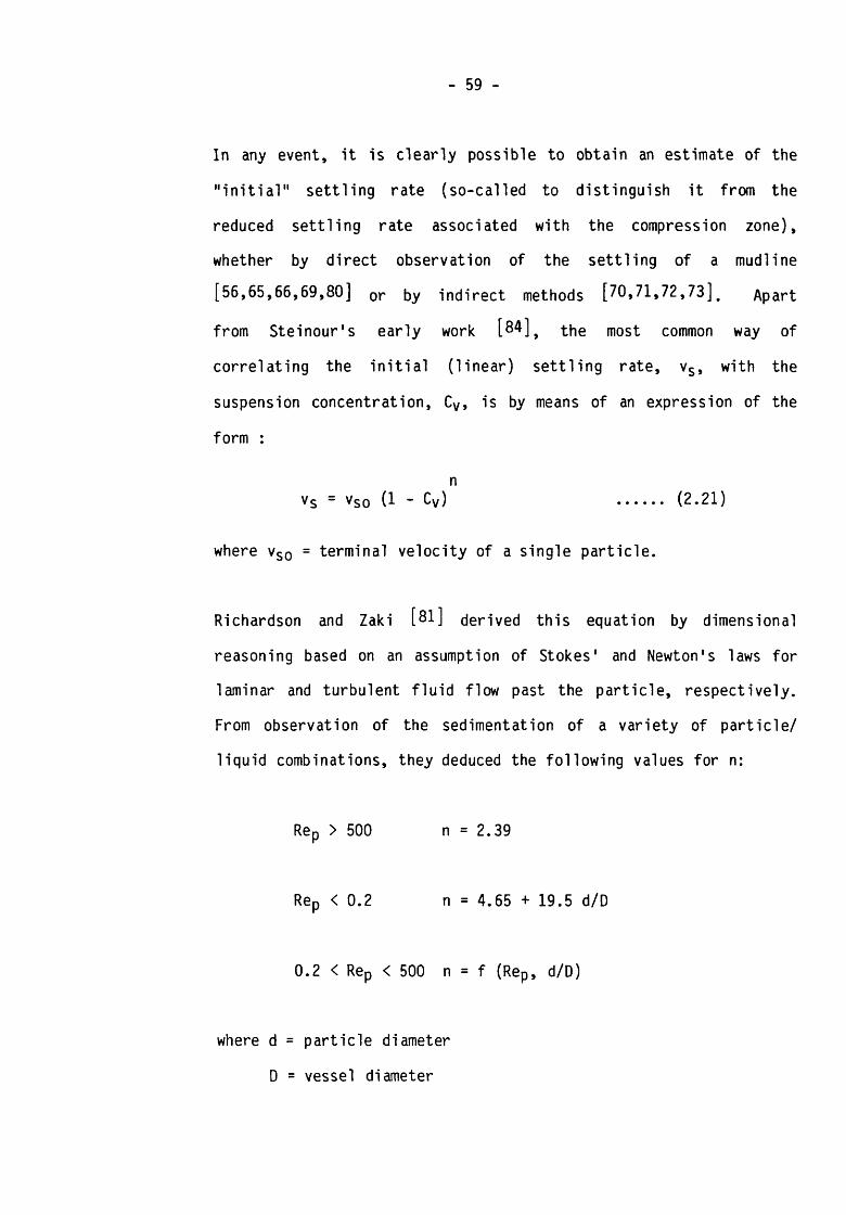
- 59 -

In any event, it is clearly possible to obtain an estimate of the

"initial" settling rate (so-called to distinguish it from the

reduced settling rate associated with the compression zone),

whether by direct observation of the settling of a mudline

[56,65,66,69,80] or by indirect methods [70,71,72,73]. Apart

from Steinour's early work [84] # the most common way of

correlating the initial (linear) settling rate, vs, with the

suspension concentration, Cv, is by means of an expression of the

form :

nvs = vso (1 ” Cv) ..... (2.21)

where vso = terminal velocity of a single particle.

Richardson and Zaki [81] derived this equation by dimensional

reasoning based on an assumption of Stokes' and Newton's laws for

laminar and turbulent fluid flow past the particle, respectively.

From observation of the sedimentation of a variety of particle/

liquid combinations, they deduced the following values for n:

Rep > 500 n = 2.39

Rep <0.2 n = 4.65 + 19.5 d/D

0.2 < Rep <500 n = f (Rep, d/D)

where d = particle diameter

D = vessel diameter

- 60 -

(vso in equation 2.21 is the extrapolated value of vs for Cv

= 0 and represents a common method of determining an "equivalent

Stokes' diameter" for a polydisperse suspension).

Although their work was confined to equi-sized particles in the

range 100-1000 pm, a later paper by Richardson and Meikle [82]

claimed that essentially the same correlations apply to fine,

polydisperse particles; an exception was a value of n = 1 0 . 5

determined for 5-7 pm alumina particles, which was attributed by

the authors to a particle shape effect, possibly associated with

occlusion of liquid by the solids.

An alternative derivation of equation 2.21 has been given by Maude

and Whitmore [8 8 ], They proposed the relation :

a/mvs = vso (1 “ Cv) ..... (2.22)

where m = 1 for Rep < 1

m = 2 for Rep > 1 0 3

For laminar flow (m = 1) and equi-settling spheres, theoretical

considerations lead to limiting values of 1 < a < 8 , although a = 5

in practice (cf. Richardson and Zaki, n = 4.65). Data of other

workers, reviewed by the authors, gave 4.15 < a < 9.35 for a

variety of suspensions. The variation in a, at a given Reynolds

number, was attributed to variations in particle size and shape.

- 61 -

Moreland [85] found that equation 2.21 described the settling of

narrow size fractions of coal, in the range 80-1000 pm, in white

mineral oil, with n = 6.5 - 7.5; the volume concentration was

varied in the range 0-40%. The value of vso was determined

experimentally for individual particles in each size range.

Moreland also claimed that Steinour's data for emery powder [84]

gave n = 6.8 - 7.0, and he suggested that n = 4.65 for spheres but

increases for irregular shapes.

Davies et al [86] postulated that large values of n are

associated with highly hindered systems. Their data on calcium

carbonate settling in various liquids at low concentrations (Cv <

4.28%) gave values in the range 24.4 < n < 74.2. They showed that

n = — where is initial porosity at which solids flux l-£ i

[vs (1 - e) ps] is a maximum; large values of n therefore imply

maximum solids flux at low solids concentration (high e). The

nearer ej is to unity, the more rapid is the decrease of vs with

increase of Cv, implying that the more hindered is the system.

Since the most "hindered" systems are those which show hindrance at

low solids concentrations, hindrance (and thus n) must be a

function of factors in addition to solids concentration. These

include particle-particle interactions between electrical double

layers (particularly for charged particles of high surface area in

polar liquids), and particle-liquid interactions in which liquid is

bound to the solid, thus reducing the effective density of the

solid and/or increasing the effective solids concentration. The

authors presented data of other workers in which high values of n

- 62 -

were associated with systems in which such interactions could be

expected to play an important role. Physico-chemical interactions

of this kind, leading to a modification of sedimentation behaviour,

have also been discussed by Vincent [87] and Sadowski et al

[88].

Scott [89] and Capes [90] (anticipated by Whitmore [150])

have both proposed a modification of equation 2.21, as follows :

vs = vso [1 ” KCV) ..... (2.23)

Scott suggested that n = 4.65 for his calcium carbonate

suspensions, and defined K as the volume of aggregates (floes) per

mass of contained CaC0 3 . KCV thus represents the "effective"

solids concentration and accounts for the effect of liquid

immobilised by the floes. Whitmore termed K the "hydrodynamic

volume factor", and showed that it increased with decreasing

particle size.

Scott [91] has also shown that equation 2.23 fits the

ferrosilicon settling data of Nesbitt [71] (quoted in Ref. 42),

with n = 4.65 and K-values in the range 1.32 - 2.01; the K-values

were higher for the irregular, milled material than for the more

spherical, atomised material (see also Table 2.1 below).

- 63 -

Capes also proposed that K represents the volume of aggregates (fo

fine solids fluidised by a pressurised gas), but that n can vary.

Using data from the literature, and an iterative calculation

procedure, he showed that improved correlations could be obtained

from equation 2.23 over equation 2.21, using K-values in the range

0.951 - 1.695. In so doing, the value of n was reduced from 6.0

(equation 2.21) to 3-3.5 (equation 2.23).

Datta [69] studied the sedimentation of mineral suspensions, and

concluded that the distribution and size moduli ( a and k) of the

Gaudin-Schuhmann function, which described the solids size

distributions, played a part in determining n in equation 2.21. He

found that for a > 1.0 (which is usually the case for ferrosilicon

powders) n had a constant value of 6.5. For a < 1.0, n * 8 . 4 _+ 3

down to sizes of about k = 150 ym, below which n increased

abruptly. However, his data for a > 1.0 do not extend below k = 70

ym, and one of his figures (No. 50) suggests that the increase in n

for a <1.0 may only occur for k < 70 ym. It could therefore be

that a similar trend towards high n-values at finer sizes also

existed for a > 1.0 but was not observed. Certainly, all his work

points to a significant effect of size distribution on

sedimentation. In this context it is interesting to note the

present author's earlier conclusion [4] that the two parameters

of the ferrosilicon size distribution significantly influenced DM

cyclone performance.

Although Collins [65] presented data suggesting that the initial

settling rate at a given volume concentration is not affected by

- 64 -

the type of medium (ferrosilicon or magnetite) or the size

distribution, the general concensus is that the sedimentation of

suspensions is significantly influenced by particle shape and size

distribution, and by physico-chemical particle-particle and

particle-liquid interactions. In the case of dense medium

suspensions, there is clear evidence [42,56,71,80] that settling

rate decreases with fineness and irregularity of particle. The

question of whether the vs - Cv data are best correlated by

equations 2.21 or 2.23 is not clear from the literature. The two

relevant publications of Richardson et al [81,82] argue strongly

in favour of retaining a value n = 4.65 in equation 2.21 for all

suspensions, in cases where Rep < 0.2. However, other data in

the literature require that equation 2.23 be invoked to achieve

this. Certainly, the concept of liquid occlusion by the particles,

resulting in an effective increase in solids concentration, is

intuitively satisfying, and the literature suggests that the high

values of n which have been reported might be attributable to this

effect.

In order to examine the effectiveness of equations 2.21 and 2.23 in

describing the limited volume of sedimentation data which have been

reported for ferrosilicon-water suspensions, the equations were

fitted to appropriate data obtained from references 56, 71 and 80.

The data are given in Appendix 1. In the case of Nesbitt and Loesch

[^1] and Govier et al [56], the data are as reported in their

papers. In the case of Apian and Spedden [80], the data have

been interpolated from graphs given in the paper, and are

accordingly subject to some uncertainty. The equations were fitted

in linear form by least squares regression :

- 65 -

In vs = In vso + n In (1 - Cv) ..... (2.21 a)1/4.65 1/4.65

(vs) = vso (1 ■ KCy) ..... (2.23 a)

The results are summarised in Table 2.1.

Based on the values of r2, and allowing for the fact that the

logarithmic transformation required for equation 2.21a will tend to

inflate r2, the quality of the fits to the two equations are

comparable. The effect of introducing K in equation 2.23 is to

reduce the estimated values of Vso. and the corresponding

calculated values of dST and Rep, to intuitively more

reasonable values, especially in the case of Nesbitt and Loesch's

data [71], However the parameter values determined for their data

must be treated with caution in view of their indirect method of

determining stability.

It is interesting to note that in only one case does equation 2.21

produce a value n < 4.65; all the other values are significantly

greater than 4.65, confirming the findings of other authors working

with a variety of suspensions [69,82,85,86,]. According to Davies

et al [86], this would imply that the systems are highly

hindered.

The values of K estimated in fitting equation 2.23 range from 0.95

(which may be not significantly different to zero) to 2.02. If one

assumes a simple model of a solid sphere immobilising a symmetrical

volume of water around it, so as to effectively increase the

diameter of the sphere by a proportion, p, it is not difficult to

show that :

K = (1 + p)3 (2.24)

TABLE 2.1 - CORRELATION OF vcn - Cu DATA FOR THE SEDIMENTATION OF FERROSILICON SUSPENSIONS - REFS. 56,71 & 80

* Equation 2.21 Equation 2.23Reference No. of

ResultsFerrosillcon

Type-45 urn

(cm” -1)n r2 Rep , Vso-n(cm s A)

K r2 ? S T(p m )

R e p

56(Govier et al) 6 Milled? 75 0.974 10.27 0.951 59 0.57 0.785 1.77 0.938 52 0.41

71(Nesbitt/Loesch) 7 65D Milled 42 14.97 12.71 0.993 393 59 5.11 1.74 0.988 164 8.4

5 100D Milled 55 39.80 17.70 0.987 1177 468 5.60 2.02 0.994 175 9.88 Special Coarse Atomised 27 5.19 8.12 0.997 166 8.6 3.21 1.36 0.998 120 3.99 Cyclone Grade Atomised 71 1.077 9.55 0.998 62 0.67 0.509 1.47 0.995 41 0.21

80t

(Aplan/Spedden) 5 Milled? 60 0.249 4.19 0.987 28 0.07 0.264 0.95 0.992 29 0.079 Atomised 71 0.498 9.17 0.987 41 0.20 0.370 1.55 0.970 35 0.13

Notes; 1. r2 = coefficient of determination for linear regression.

2. d$j = equivalent Stokes diameter; determined from Concha and Almendra's correlation for spheres [32], assuming viscosity of water n * 0.001 Nsm.

3.

4.Rep = Particle Reynolds Number - P_VsoJlST_

n ,Density of solids assumed to be 6800 kg nr .

where p ■ water density n ■ water viscosity

Density of watrer • 1000 kg nr2.

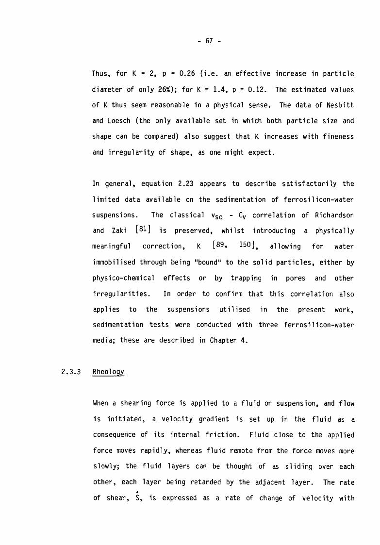
- 67

Thus, for K = 2, p = 0.26 (i.e. an effective increase in particle

diameter of only 26%); for K = 1.4, p = 0.12. The estimated values

of K thus seem reasonable in a physical sense. The data of Nesbitt

and Loesch (the only available set in which both particle size and

shape can be compared) also suggest that K increases with fineness

and irregularity of shape, as one might expect.

In general, equation 2.23 appears to describe satisfactorily the

limited data available on the sedimentation of ferrosilicon-water

suspensions. The classical vso - Cv correlation of Richardson

and Zaki [81] is preserved, whilst introducing a physically

meaningful correction, K [89, 150]# allowing for water

immobilised through being "bound" to the solid particles, either by

physico-chemical effects or by trapping in pores and other

irregularities. In order to confirm that this correlation also

applies to the suspensions utilised in the present work,

sedimentation tests were conducted with three ferrosilicon-water

media; these are described in Chapter 4.

2.3.3 Rheology

When a shearing force is applied to a fluid or suspension, and flow

is initiated, a velocity gradient is set up in the fluid as a

consequence of its internal friction. Fluid close to the applied

force moves rapidly, whereas fluid remote from the force moves more

slowly; the fluid layers can be thought of as sliding over each

other, each layer being retarded by the adjacent layer. The rate

of shear, S, is expressed as a rate of change of velocity with

- 68 -

* dsdistance from the shearing force : S = — 5 where s = velocitydx

and x = distance. The shearing force acts over a given area, and

is therefore expressed as a stress : t = F/A.

In general, the relationship

t = f(S) ..... (2.25)

is characteristic of the fluid or suspension at a fixed temperature

and pressure. The graphical representation of this function, which

can be obtained experimentally, is called the flow curve or

rheogram [69,92,93].

The simplest fluids are those for which the flow curve is a

straight line, passing through the origin :

t = n S ..... (2.26)

The constant of proportionality, n, is called the viscosity, which

can be thought of as the resistance of the fluid to shear. The

dimensions of viscosity can be obtained as follows :

[t ] = [Force/Unit Area] = MLT"2* L~2 = ML-1 T-2

[S] = [Shear Rate] = LT_1«L-1 = T"1

[n] = [t/S] = ML-1 T-2*T = ML"1 T”1

- 69 -

The SI units are [t ] = N m-2

[S] = s-1

[n] = N s nr2 = 10_1 P

Fluids described by equation 2.26 are called Newtonian; their

viscosity is constant over all shear rates, and an infinitesimally

small stress is required to initiate shear. All other types of

fluid are referred to as non-Newtonian. There are many forms of

non-Newtonian behaviour. In the following discussion we

specifically exclude time-dependent fluids (those for which the

nature of equation 2.25 depends upon the shear history) and

visco-elastic fluids (those which exhibit elastic behaviour under

shear). The remainder can be conveniently summarised in terms of

certain ideal rheological types, whose flow curves are illustrated

in Figure 2.6. Curve A represents the simple Newtonian fluid.

Curve B represents a fluid which possesses an internal structure

such that a finite stress (known as the yield stress, t 0 ) is

required to initiate shear; thereafter it behaves as a Newtonian

fluid with a constant plastic viscosity, np. Such fluids are

called Bingham plastics, and their flow equation is :

f = *o + ^p S ..... (2.27)

The plastic viscosity is then given by

(2.28)

- 70 -

FIGURE 2.6 - IDEAL RHEOLOGICAL TYPES.

in inUloc»—i/i

tc.<•uj□Cin

A. NEWTONIAN C. PSEUDOPLASTICB. BINGHAM PLASTIC D. D ILATANT

FIGURE 2.7 - GEN ERAL SHAPE OF THE FLOW CURVE * FOR CONCENTRATED SUSPENSIONS (FROM

M ETZNER & WHITLOCK T99l ).

10° 10*SH EA R R A T E

10*

- 71 -

and thus cannot be determined from a single shear rate/shear stress

measurement; the full flow curve must be determined so that the

intercept, t 0 , can be evaluated.

A pseudoplastic, or shear-thinning, fluid is one for which the

apparent viscosity, na» decreases with increasing shear rate,

i.e. the flow curve is non-linear. It is so-called because

extrapolation from high to low shear rates implies the existence of

a yield stress (the dotted line, curve C, in figure 2.6). The

converse of curve C is curve D, which describes dilatant, or shear

thickening, fluids for which apparent viscosity increases with

increase in shear rate. Real fluids or suspensions rarely exhibit

pure dilatancy or pseudoplasticity over the whole range of shear,

but these models represent useful approximations over shear rate

ranges of practical interest. It should also be noted that fluids

are known which are combinations of these ideal types.

Both pseudoplastic and dilatant fluids can be represented by an

empirical relation known as the "power law" :

• nt = k(S) ..... (2.29)

where k = a consistency index (higher for more viscous fluids)

and n = an exponent, constant over large ranges of shear rate,

and taking the following values :

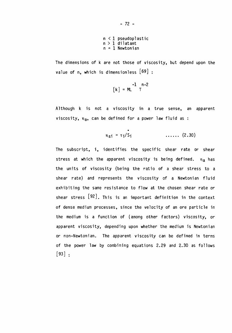
- 72 -

n < 1 pseudoplastic n > 1 dilatant n = 1 Newtonian

The dimensions of k are not those of viscosity, but depend upon the

value of n, which is dimensionless [69] :

-1 n -2[k] = ML T

Although k is not a viscosity in a true sense, an apparent

viscosity, na, can be defined for a power law fluid as :

nai ~ Ti/ i ..... (2.30)

The subscript, i, identifies the specific shear rate or shear

stress at which the apparent viscosity is being defined. na has

the units of viscosity (being the ratio of a shear stress to a

shear rate) and represents the viscosity of a Newtonian fluid

exhibiting the same resistance to flow at the chosen shear rate or

shear stress [92], This is an important definition in the context

of dense medium processes, since the velocity of an ore particle in

the medium is a function of (among other factors) viscosity, or

apparent viscosity, depending upon whether the medium is Newtonian

or non-Newtonian. The apparent viscosity can be defined in terms

of the power law by combining equations 2.29 and 2.30 as follows

[93] :

- 73 -

na = M S ) ..... (2.31)

A wide variety of instruments is available for the determination of

the flow curve of pure liquids. However, practical problems arise in

measurements with settling (unstable) suspensions which are, by

definition, never in equilibrium. If the solids are to be properly

dispersed, some form of agitation is necessary, and this can interfere

with the measurement itself. The problem has been addressed by many

workers, and a variety of solutions has been proposed. One might add

also that a variety of conclusions regarding the rheological

properties of settling suspensions have been reached. This is because

many workers determined only some relative viscosity, in order to

assess its dependence upon factors such as volume concentration,

particle size and shape, and made no attempt to establish the full

flow curve.

A case in point was the work of Purohit and Roy [94,95] who used a

concentric cylinder viscometer in which the suspension was contained

only between the two cylinders, both of which were free to rotate; the

outer cylinder formed the cup, and the inner cylinder, which was

driven, acted as a stirrer. The instrument was calibrated using

glycerol solutions, in terms of a friction factor and Reynolds

number. Working with a variety of slurries in narrow particle size

ranges (10-320ym) at volume concentrations up to 3056 v/v, they

correlated their data by the following expression:

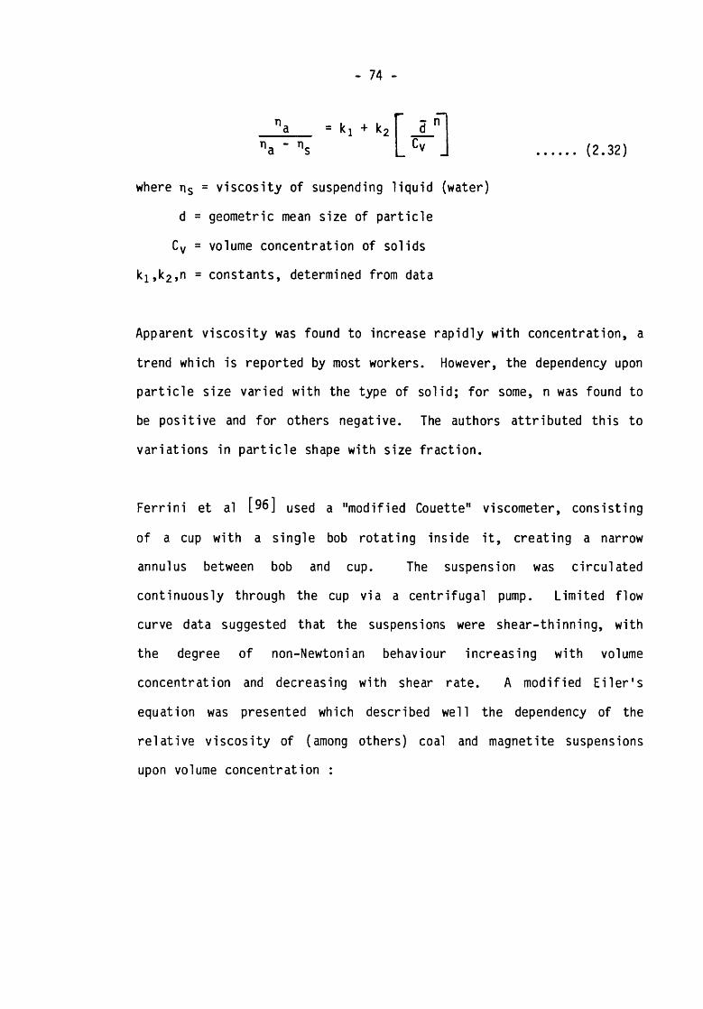
- 74 -

(2.32)

where r\s = viscosity of suspending liquid (water)

d = geometric mean size of particle

Cv = volume concentration of solids

ki,k2 >n = constants, determined from data

Apparent viscosity was found to increase rapidly with concentration, a

trend which is reported by most workers. However, the dependency upon

particle size varied with the type of solid; for some, n was found to

be positive and for others negative. The authors attributed this to

variations in particle shape with size fraction.

Ferrini et al [96] used a "modified Couette" viscometer, consisting

of a cup with a single bob rotating inside it, creating a narrow

annulus between bob and cup. The suspension was circulated

continuously through the cup via a centrifugal pump. Limited flow

curve data suggested that the suspensions were shear-thinning, with

the degree of non-Newtonian behaviour increasing with volume

concentration and decreasing with shear rate. A modified Eiler's

equation was presented which described well the dependency of the

relative viscosity of (among others) coal and magnetite suspensions

upon volume concentration :

= ki + k<- n.

- 75 -

nanr = —

0.5 ni1 + -----------

1 . 1G7 vm

2

(2.33)

where nj = an intrinsic viscosity term

Cvm = maximum possible volume concentration

ni for irregular particles must be determined from the data,

although for spheres m = 2.5, as given by the Einstein equation for

dilute suspensions. Cvm can also be determined from the data,

although the authors point out that the experimentally-measured values

are close to those obtained from the sedimentation procedure suggested

by Robinson [98],

Clarke [97] used a Ferranti Model VL portable concentric cylinder

viscometer inserted in a vessel with an impeller mounted in the base

such that the suspension was constrained to circulate up the sides of

the vessel and down through the cylinder assembly, which was

appropriately modified. The suspensions studied included narrow size

ranges of quartz (44-211pm) in water. In preliminary tests he

reported "anomalous decreases in apparent viscosity" at high shear

rates (> 250s-1), and he attributed this to slip between the coarse

particles and the cylinder walls (rather than to a shear-thinning

effect). To overcome this "slip", grooves were cut into the cylinder

- 76 -

walls, whereupon the anomalous behaviour disappeared. Clarke

concluded that his suspensions were dilatant, the degree of dilatancy

increasing with concentration, size, density and irregularity of

particles. Apparent viscosity increased with concentration, rapidly

so above a critical concentration of about 25% v/v. Viscosity also

increased with particle size, a result which, as Clarke points out,

disagrees with many other workers, although Purohit and Roy (as noted

above) obtained the same trend on some of their suspensions [94,95];

Clarke attributed his result to an inertial effect, which appeared to

be supported by data obtained from particles of varying density.

However, the viscosity of suspensions containing mixtures of size

ranges was lower than those of the individual size ranges. One might

speculate that the results of Clarke, and of Purohit and Roy, should

be considered specific to narrow size ranges (typically /2 sieve

intervals), and may not apply to wider size ranges.

Clarke also found that viscosity increased with irregularity of

particle shape, which he attributed to increased interactions (caused

by particle rotation in a velocity gradient), greater inter-particle

friction, and liquid immobilised by the irregular particles

(cf.Scott's model for sedimentation, equation 2.23).

Dilatancy was also observed by Metzner and Whitlock [99] -jn

suspensions of 0.2 - l.Oym titania in water and sucrose solutions,

using principally a Stormer rotational viscometer; some confirmatory

data were also obtained using a capillary instrument. No dilatancy

was observed in the case of glass beads suspended in sucrose solution;

- 77 -

however the smallest beads used were 18 ym in diameter, and the

authors cite literature which implies that dilatancy might be confined

to very fine particle sizes. For the titania suspensions, dilatancy

occurred only at the higher shear rates and volume concentrations

(above 27% v/v); the shear rate at which the onset of dilatancy was

observed decreased as concentration increased. Below this critical

shear rate, pseudoplasticity occurred. The authors postulated that

concentrated suspensions of this type follow the pattern illustrated

in Figure 2.7. At low shear rates the flow is Newtonian; thereafter

the curve passes through successive pseudoplastic and dilatant

regimes, separated by a point of inflection representing a local

Newtonian regime. They suggested that the pseudoplasticity at

intermediate shearing rates is due to alignment of asymmetric

particles and the break-up of loose agglomerates; as the shearing

forces increase further, momentum transfer occurs between whole layers

of particles, rather than individual particles, thus increasing the

effective mass which has to be moved; the observed onset of

rheological dilatancy follows, but is not coincident with, volumetric

dilation.

Sikdar and Ore studied the rheology of calcium sulphate slurries in

phosphoric acid using a Brookfield rotational viscometer, at volume

concentrations up to 25% [100], They found that the suspensions

were pseudoplastic, the extent of pseudoplasticity (i.e. the departure

from unity of the index, n, in equation 2.29) increasing with volume

concentration and temperature; apparent viscosity (defined by equation

2.31) increased with decreasing particle size. For a given shear

rate, the data were correlated by :

- 78 -

Cv, = Cyco

(2.34)

where Cv» = volume concentration for which the apparent viscosity

tends to infinity.

CVoo may be assumed to be dependent upon suspension characteristics

such as particle size and temperature.

Sarmiento et al used a capillary viscometer and a modified cone-and-

plate viscometer to evaluate the rheology of red mud obtained as waste

from an alumina process [101]. Their data agree with those of

Sikdar and Ore [100], in that the slurry was pseudoplastic at low

shear rates, the extent of pseudoplasticity increasing with solids

concentration (over the range 15-33% v/v). However, at a shear rate

of about 103 s"1, an increase in the value of the power law index

occurred, reducing the extent of pseudoplasticity; in the case of the

lower concentration slurry (15% v/v) the flow became approximately

Newtonian, an effect attributed by the authors to disruption and

dispersion of the floe structure. These observations would seem to

accord quite well with those of Metzner and Whitlock, corresponding to

the central portion of their proposed generalised flow curve (Figure

2.7). However, in their case the transitions occurred at much lower

shear rates.

- 79 -

One of the principal purposes of defining the rheology of liquids and

suspensions is to enable predictions to be made of the behaviour of

particles moving in the liquid or suspension; this is particularly so

with DMS processes. Brien, Pommier and Bhasin studied the terminal

velocities of spheres falling under gravity in non-Newtonian solutions

and suspensions [102-104]# Both the pure solutions and the

suspensions (containing spherical glass beads) were found to be

pseudoplastic, using a Brookfield rotational viscometer, although the

solutions exhibited Newtonian characteristics at low rates of shear.

The suspensions approached Newtonian behaviour as the volume

concentration increased and the particle size decreased. Correlations

were developed for the resistance force and terminal velocity of the

falling spheres for both laminar and turbulent flows, using

dimensional analysis. The power law parameters of the solution/

suspension were included in the correlations. It was found that the

spheres settled more slowly than predicted by assuming Newtonian fluid

behaviour. The power-law parameters estimated from the settling data,

in terms of the new correlations, agreed well with those obtained

directly from viscometry. However, detailed studies of the influence

of suspension particle size were carried out using narrow-sized glass

beads in the range 60-470pm [103,104]# They showed that a critical

size existed at which the suspension was Newtonian. The terminal

velocity of the sphere falling in the turbulent regime could be

predicted from the usual correlations; under the conditions

investigated the critical size was about 90pm. Above the critical

size, sphere velocity decreased with increase in bead size, whereas

below the critical size the sphere velocity increased with increase in

bead size. The drag coefficient was expressed as a function of the

- 80 -

ratio of bead size to critical bead size; resistance force decreased

with concentration for bead sizes above the critical size, and

increased with concentration for bead sizes below the critical size.

The concept of a critical size for suspension particles, defining

different rheological regimes, may account for some of the

disagreement in the literature regarding the influence of particle

size on rheology.

Valentik and Whitmore [105] studied the terminal velocity of spheres

in flocculated china clay suspensions, using apparatus similar to that

of Brien et al [103]# The suspensions were shown by rotational

viscometry to approximate well to Bingham plastics, for which the

yield stress and plastic viscosity increased with solids

concentration. Their results suggested that the terminal velocity

data could be interpreted in terms of spheres settling in a Newtonian

fluid, but carrying with them an envelope of unsheared fluid whose

thickness decreased with velocity.

One of the most important aspects of suspension rheology, from a

practical viewpoint, is the relationship between apparent viscosity

and volume concentration of solids. This has received considerable

attention in the literature. Rutgers reviewed in 1962 about 100

published equations relating viscosity to concentration [106]# and

further equations have been reported since then [107], Nearly all

the equations are expressed in terms of a relative viscosity, nr,

such that :

nr = 2a = f (cv) ns (2.35)

- 81 -

The characteristics of this function for a given system will depend

upon the relative degrees of interparticle attraction (i.e. degree of

flocculation or coagulation, leading to formation of a structure),

particle friction and hydrodynamic interaction. Suspensions will often

undergo changes in rheological character as the rate of shear

increases, and these changes tend to occur at lower shear rates as the

concentration increases. Cheng has produced a useful summary of these

trends [107], reproduced here as Figure 2.9. At low shear rates and

concentrations the behaviour is Newtonian, becoming progressively

pseudoplastic and then dilatant as shear and concentration increase.

At very high concentrations, in which particle friction predominates,

apparently anomalous phenomena are observed which Cheng has termed

"granulo-viscous" behaviour [108]# drawing analogies with the

behaviour of granular materials according to established principles of

soil and powder mechanics.

Cheng's diagram is similar to that given by Vincent for sedimentation

properties [87]. Indeed, the similarity of these two approaches is

a reflection of the strong relationship which exists between

sedimentation and rheological properties; apparent viscosity is

usually directly related to stability.

For suspensions of relevance to DMS, the dependence of apparent or

relative viscosity upon concentration usually follows the general

trend illustrated by Cheng for non-interacting particles, reproduced

here as Figure 2.8. Assuming the suspending liquid is Newtonian, the

suspension at low concentrations remains Newtonian and the viscosity

increases linearly with concentration. At a certain critical

- 82

FIGURE 2.8 - VISCOSITY-CONCENTRATION RELATION FOR SUSPENSION

OF WON-INTERACTING PARTICLES (FROM CHENG [1071)

Viscosity, n

FIGURE 2.9 - DEPENDENCE OF APPARENT VISCOSITY UPON SHEAR RATE FOR

SUSPENSIONS OF NEGLIGIBLE INTERPftRTICLE ATTRACTION (FROM CHENG [1071)

Log (viscosity)

Log (shear rate)

- 83 -

concentration (usually in the range 25-30% v/v) the viscosity begins

to increase rapidly, and approaches infinity at some limiting or

maximum volume fraction, Cvm, which is often assumed to be the

maximum packing density for the particles concerned (e.g. equation

2.33). This behaviour is important in DMS operations because, as has

been noted, the separations are viscosity-dependent. Above the

critical concentration small increases in concentration (or medium

density) result in large increases in viscosity, which can be

deleterious to performance.

Although the literature on the rheology of unstable suspensions is

extensive, that referring specifically to dense medium suspensions is

much less so. One of the first reported investigations was that of

DeVaney and Shelton [66] who used a simple capillary tube apparatus,

the capillary being fitted at its upper end with a reservoir

containing an agitator and baffles. The instrument was calibrated

with Newtonian liquids. No attempt was made to investigate

non-Newtonian behaviour and the apparent viscosities quoted were

relative, being at arbitrary (unknown) shear rates. In studying a

variety of media, including magnetite and ferrosilicon, they found

that the curves of apparent viscosity vs. pulp density were of the

kind shown in Figure 2.8, the critical volume concentration being

about 25-30% v/v in each case. Viscosity at a given pulp density was

found to increase as particle size decreased, and was higher for

irregular than for smooth shapes. Viscosity increased with decrease

in temperature, particularly at the higher concentrations, presumably

reflecting corresponding changes in the viscosity of the carrier

liquid (water). All subsequent investigators have confirmed these

general trends.

- 84 -

Van der Walt and Fourie [109] usecj a modified Stormer rotational

viscometer incorporating an agitation vessel similar to that reported

by Clarke [97], Flow curves for (among others) magnetite suspensions

suggested that they were of the Bingham plastic type. Govier et al

[56] 5 as already noted, investigated the rheology of galena,

magnetite and ferrosilicon media. They used a Fann concentric cylinder

rotational viscometer, but made no attempt to maintain the pulp in

suspension since the cup containing the pulp formed part of the

viscometer itself and therefore agitation could not be used. After

first dispersing the suspension, the torque reading was found to climb

initially to a maximum and then decline. The authors attributed this

to initial delayed equilibration of the liquid level in the testing

annulus, followed by settling of the solids; they took the maximum

reading in each case as the true one. Such a procedure must throw

some doubt on the data since the measurements were not made with a

homogenous, equilibrium suspension. The authors concluded that the

magnetite suspensions were approximately pseudoplastic over the range

of shear rate investigated (5-1000 s”1)* but that the galena and

ferrosilicon suspensions exhibited pseudoplasticity at low shear rates

and dilatancy at high shear rates; the shear rate at which changeover

occurred was about 200 s"1 for the galena media and 300 s_1 for the

ferrosilicon. Although this behaviour might not be unexpected in the

light of the literature reviewed thus far, the data show no evidence

that the critical shear rate reduced at high volume concentrations

(cf. Figure 2.9). Interestingly Govier, in a book published some

years later [93]# utilised some of the data to show that the galena

media followed perfect Bingham plastic behaviour up to 200 s_1. If

this is so then the rheological model for these materials is more

- 85 -

complex than the authors of ref. 56 proposed.

Rheological measurements with viscometers such as that used by Govier

et al are generally based on operating at a known, true shear rate and

determining an apparent viscosity from an expression of the form :

n a = RC

where R = viscometer reading

C = Newtonian calibration factor

If the fluid is Newtonian (i.e. t = naS)

then t = S R C

If however the fluid is a Bingham plastic (i.e. t = t 0 + up S) then

t - t 0 SRC - TgHn = ----------------- = -------------- :------

S S

and Tip = RC - t 0 / S ..... (2.36)

Since the value of x0 cannot be known without plotting the full flow

curve on linear coordinates, there is a tendency to over-estimate the0

value of n by an amount t0/S, which increases at lower shear rates.

This might account for the authors' observation that the ferrosilicon

suspensions were pseudoplastic at low shear rates but dilatant at high

shear rates. It also illustrates the importance of interpreting the

flow curve initially using linear coordinates.

- 86 -

Doubt might therefore be attached to their contention that the

"apparent viscosity" of the galena and ferrosilicon media decreased

with shear rate at low shear rates and then increased at high shear

rates. Certainly, the behaviour of an ore particle moving in a

centrifugal force field through a medium exhibiting Bingham plastic

and dilatant characteristics at different rates of shear cannot be

predicted with any certainty, as was attempted by Tarjan [44] and

Lilge et al [57], using the data of Govier et al [56],

Despite the uncertainties inherent in the work of Govier et al

[56,93]# some confirmatory data have been presented recently by

Collins [55]. He used a Ferranti concentric cylinder viscometer,

with a stirred vessel, to study the rheology of atomised ferrosilicon

and mixtures of ferrosilicon and magnetite. He found that the pure

ferrosilicon showed behaviour similar to the generalised behaviour of

suspensions discussed by Cheng [107] (Figure 2.9). At low

concentrations and low shear rates (< 400 s”1) the suspensions were

Newtonian, becoming dilatant at higher shear rates. At higher

concentrations the suspensions were pseudoplastic at low shear rates

and dilatant at high shear rates, the critical shear rate decreasing

with increased concentration. Mixtures of magnetite and ferrosilicon

were pseudoplastic (1:2 respectively) or Bingham plastics (1:1). The

apparent viscosity, plastic viscosity and yield stress increased with

solids concentration.

Whitmore studied the rheology of a variety of media taken from

operating coal washeries, also using a Ferranti viscometer [HO],

He found that the media were Bingham plastics (up to the maximum

- 87 -

measured shear rate of about 250 s”1)* and that generally media with a

high plastic viscosity tended to have a high yield stress also. He

was able to show that the quality of separation achieved in the

bath-type separators deteriorated with increased plastic viscosity.

Yancey et al used a capillary viscometer in which the applied head was

controlled by air pressure via a pressure diaphragm. The medium was

continually circulated through the instrument using a pump [HI].

Their results with magnetite suspensions, although at much higher

shear rates than those of Whitmore (up to 5000 s-1), also appeared to

show that the media were Bingham plastics. Plastic viscosity and

yield stress both increased with solids concentration and with the

concentration of fine contaminants such as coal and clays. Nesbitt

and Weavind [ H 2 ] s using a modified Stormer viscometer of the type

described by Van der Walt and Fourie [109], also noted an increase

in viscosity with contamination. They showed that viscosity could be

reduced by de-magnetising the ferrosilicon media used. Atomised

(spherical) ferrosilicon produced lower viscosities for a given pulp

density than milled (irregular shaped) ferrosilicon. This result

agrees with the conclusions of other workers, and indeed forms the

basis of the use of atomised ferrosilicon, since much higher densities

can thus be attained before the viscosity becomes excessively high

[42,113], Nesbitt's work [71,112] further confirmed that the

viscosity of both atomised and milled ferrosilicon media, expressed as

a single point determination using the modified Stormer viscometer,

increased with decreasing particle size. This result, though well

established for dense media [42]# appears to conflict with some of

the general literature on suspensions. As noted earlier, this may be

- 88 -

attributable to the different range of particle sizes utilised. Datta

[69]^ for example, has shown that the width of the size distribution

(expressed as the Schuhmann distribution modulus) controls the

concentration at which the rheology of mineral slurries converts from

dilatant to plastic.

Smith [114] carried out measurements on a variety of ferrosilicon

media, using a modified Haake RV3 concentric cylinder viscometer

placed in a stirred vessel similar to that described by Van der Walt

and Fourie [109], in conformity with other workers, he observed that

the apparent viscosity increased with particle fineness, over both

narrow and wide size ranges, and with solids concentration; the

viscosity increased rapidly above a critical concentration, this

concentration being higher for atomised than for milled material.

However, the flow curves indicated a complex rheology, dependent upon

shear rate. Figure 2.10 shows the flow curves for a milled

ferrosilicon over a range of pulp densities from 26% to 42% equivalent

volume concentration. This material exhibits pseudoplastic behaviour

at low shear rates, with some evidence of a yield stress at the higher

concentrations. As the shear rate increases, Newtonian behaviour is

observed, with a tendency to dilatant properties at the high shear

rates; the transition to dilatant behaviour seems to occur at lower

shear rates as the concentration increases. Some of Smith's results

suggest that ferrosilicon suspensions do not depart significantly from

Newtonian behaviour over quite large shear rate ranges, particularly

at the lower concentrations.

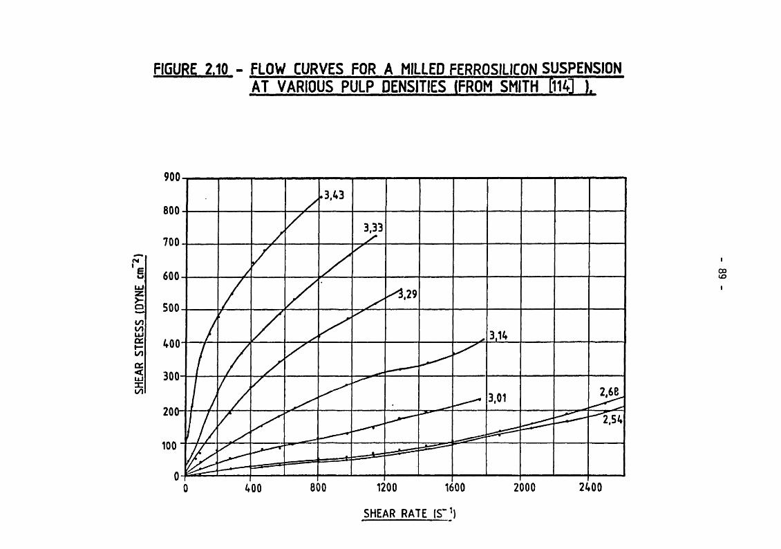
SHEA

R ST

RESS

(DY

NE i

m~2)

FIGURE 2.10 - FLOW CURVES FOR A MILLED FERROSILICON SUSPENSION A T VARIOUS PULP DENSITIES (FROM SMITH fllti ).

SHEAR R A T E ( S '1)

- 90 -

A number of authors have addressed the problem of modifying the

rheological properties of dense media. Valentik and Whitmore [ H 5 ] #

noting that clays are often added to media to achieve stability [66],

deprecated this practice since it leads to an increase in the yield

stress. They advised deflocculating the medium in order to control

yield stress. Geer et al [67] demonstrated that the type of clay

contaminant had a profound influence on the increase in viscosity of

magnetite suspensions. Apian and Spedden [60] reported a study of

the effect of a number of reagents on controlling the viscosity of

dense media. They pointed out that a desirable reduction in viscosity,

achieved by the use of a suitable dispersant, incurred an undesirable

loss of stability. However they showed that an acceptable stability

could be maintained, while reducing viscosity, using carefully

controlled concentrations of the dispersant sodium hexametaphosphate.

They found that the flow curves of uncontaminated, contaminated and

dispersed ferrosilicon suspensions were complex, the rheology varying

with shear rate. They pointed out that in a cyclone, in which the rate

of shear varies in different parts of the vessel, each flow regime

might assume importance at different points.

Klassen et al [H6] showed that both the viscosity and yield stress

of clean (i.e. uncontaminated) ferrosilicon suspensions could be

reduced by the addition of certain peptising agents, including sodium

hexametaphosphate.

The effect was pH-dependent and was more pronounced at higher

concentrations (> 30% v/v). Since no slimes were present, the

mechanism of the effect was not simple dispersion. The authors

- 91 -

proposed that the reagents increased the (negative) electrokinetic

potential, implying an increased hydrated layer on the solid surface,

which has the effect of reducing viscosity and yield stress. They

demonstrated that addition of the reagents improved metallurgical

performance in both static bath separators and cyclones.

Valentyik and Patton [H7] studied the rheology of ferrosilicon and

magnetite media stabilised by polymers and bentonite clays. They found

that the stabilised media behaved as a Bingham plastic, and attributed

the discrepancy between their observations and Apian and Spedden's

identification of dilatant properties [80] to the presence of the

stabilising agent. They regarded the presence of a yield stress as

desirable to achieve stability, together with a low plastic viscosity

in order to achieve efficient separations. Polymer solutions were

preferred to clay slimes in these roles.

Krasnov et al [118] also noted the Bingham plastic behaviour of

media stabilised by clays, and demonstrated the deleterious effect of

a yield stress upon separation efficiency in a static bath separator.

Theoretical and practical studies were made of the behaviour of

particles moving under gravity in such suspensions, and it was shown

that peptising agents (cf Ref. 116) and vibration of the medium,

either separately or together, assisted in weakening the structure of

the medium and so improved the separations.

Collins [85] examined the effect of certain reagents upon the

stability and viscosity of magnetite and ferrosilicon media. The

reagents chosen were those commonly used as dispersants or corrosion

- 92 -

inhibitors. Collins found that most of the reagents reduced viscosity

and/or the yield stress, without modifying the form of the rheology.

Although some concensus exists as to the effects of certain additives,

both natural and manufactured, upon dense medium rheology, there is

comparatively little deliberate use of such additives to control

rheological behaviour in practice. Dispersants are sometimes employed

to avoid excessive viscosity levels in situations in which the medium

tends to be stabilised by clays or other slimes emanating from the ore

being treated. Corrosion inhibitors are also occasionally used,

although their effect upon rheology tends to be fortuitous and

uncontrolled. Otherwise, as noted earlier, rheology is usually

dictated by the shape, size distribution, concentration and other

characteristics of the medium itself.

In considering the literature relating to the rheology of dense medium

suspensions, there is good evidence to support the view that such

suspensions, especially ferrosilicon media, conform quite well to

Cheng's model [10/] (Figure 2.9). Newtonian behaviour is observed at

low concentrations. As the concentration is increased, a structure is

formed which is manifest in the existence of a yield stress.

Pseudoplastic behaviour then appears at low shear rates, the Newtonian

regime being displaced to intermediate shear rates. At higher shear

rates (perhaps > 1 0 0 0 s-1) dilatancy prevails, although the tendency

to dilatancy increases with concentration. The apparent viscosity at a

given rate of shear, as defined by equations 2.28 or 2.39, increases

with solids concentration, fineness of solids, degree of

magnetisation, concentration of stabiliser (e.g. clays) and particle

irregularity.

- 93 -

The rheology of dense medium suspensions is complex, and it is

surprising that some unanimity exists within the literature in view of

the wide range of conditions studied and instruments employed. In the

present work, measurements were carried out with the objective of

characterising the ferrosilicon media utilised in the dense medium

cyclone experiments. It was also hoped to be able to develop a

definitive, quantitative method of obtaining real flow curves using a

simple apparatus.

- 94 -

CHAPTER 3

THE INFLUENCE OF MEDIUM VISCOSITY ON THE SEPARATION IN A

DENSE MEDIUM CYCLONE

3.1 Introduction

In the previous chapter (Section 2.2) it was shown that a significant

anomaly exists in the dependence of separating density, 6 5 0 , upon

medium viscosity, n, as predicted by equation 2.4, and that

experienced in practice using unstable media. Equation 2.4 predicts a

direct dependence of S5 0 upon n, whereas the literature on cyclones

using conventional suspensoid media is unanimous in the view that 6 5 0

decreases as n increases. It was suggested in Section 2.2 that this

discrepancy could be attributed to the unstable characteristics of the

media.

In order to test this hypothesis, experiments were designed to

investigate the independent influence of a stable medium upon the

density separation in a small cyclone.

3.2 Experimental Details

3.2.1 The Medium

It was required that the viscosity of the test medium should

be variable, while maintaining its density constant (so as

to eliminate the separate influence of the density, pm ).

This property is not available from either pure liquids or

- 95 -

conventional suspensoid media, and careful attention was

therefore given to selecting an appropriate medium. After

some preliminary experiments, it was decided to use a

suspension of -38um acid-cleaned quartz in a bromoform/

trichloroethylene mixture of a density equal to that of the

quartz (2,650 kg m"3). This suspension had three important

features :

(i) It was neutrally buoyant, and thus perfectly stable.

No solid-liquid segregation occurred, either when

standing or in the cyclone.

(ii) The apparent viscosity of the suspension could be

increased by addition of quartz without incurring any

corresponding change in medium density.

(iii) It was a two phase (solid/1iquid) system, and in this

respect conformed to conventional, unstable media.

The medium was prepared by first mixing the two liquids in

the correct proportion to achieve a density of 2,650 kg m-3;

the density was checked using a specific gravity bottle, and

adjustments were made by addition of either liquid where

necessary.

The appropriate amount of liquid was then placed in a

2-litre beaker in which was immersed a high-speed stirrer.

The stirrer was switched on, and the desired mass of quartz

- 96 -

powder added slowly. Stirring continued for five minutes

after the quartz had been added, until the mixture was fully

homogeneous. The medium was then ready for use.

The bromoform used was of high purity, with the minimum of

stabiliser, as it was found that the stabiliser caused

frothing in the cyclone circuit. The trichloroethylene was

of commercial grade. The quartz was a pure mineral quartz

screened to pass 38ym and washed 3-4 times with hydrochloric

acid, twice with distilled water, and then dried.

The rheology of the medium is discussed in Section 3.4.1.

3.2.2 Test Circuit

In order to minimise the problems and hazards of handling

heavy liquids, the capacity of the test circuit was

restricted. The cyclone was a glass unit of 30rmi diameter

and 17 ° cone angle. Interchangeable entrance and exit

orifice parts were available, and an appropriate combination

was selected after preliminary tests; the full dimensions

are given in Figure 3.1.

Figure 3.1 also shows the flowsheet of the circuit, and

Figure 3.2 a photograph of the apparatus. A peristaltic pump

was used in order to achieve a reasonable consistency of

flowrate over the wide range of medium viscosities

- 97 -FIGURE 3-1 30mm CYCLONE TEST CIRCUIT

P R E S S U R E

C Y C L O N E D IM E N S IO N S (M M )

C Y C L O N E D IA M E T E R 3 0 ,0 m m

C Y C L O N E L E N G T H 1 U ) ,0 m m

I N L E T D I A M E T E R 6 ,1 m m

W R T E X F IN D E R D IA. 6 , 0 m m

V O R T E X F IN D E R LE N G T H 1 5 , 0 m m

A P E X D I A M E T E R 3 ,0 m m

C O N E A N G L E 1 7 °

T-

1

TO A T M O S P H E R E

A ' Y C L O N E'VERFLOW \THER PIPE

C IR C U L A T IN G M E D IU M S U M P

- PERISTALTIC P U M P( 5 7 S r .p .m .)

B Y - P A S S s y s t e m d r a in )

FIGURE 3 .2 I I I ■

PHOTOGRAPH OF APPARATUS—

- 98 -

investigated. This required the use of two pressure-

equalising cylinders ahead of the cyclone in order to smooth

the flow fluctuations induced by the action of the pump. The

pressure gauge was a mechanical bourdon gauge. About 1 litre

of medium was required to charge the circuit.

3.2.3 Material Treated

Since it was expected that the separating densities

experienced in the work would equal or exceed 2,650 kg nr3,

a test ore was sought with a continuous spectrum of

densities covering this range of interest, so that the

Tromp (partition) curve for each separation could be

accurately determined (see Section 3.2.5). An iron ore with

a small liberation size was selected, to which was added

uncleaned quartz to improve the estimation of the curve at

the medium density. Both the quartz and iron ore were

deslimed by wet screening at 45ym, and then dry screened

into four size ranges for the testwork, as follows :

Series A -105 + 76 ym

Series B -150 +105 ym

Series C -212 +150 ym

Series D -300 +212 ym

A further brief series of tests, Series E, was conducted

with specially manufactured epoxy resin nominally 1mm cubic

tracers, colour-coded in eleven densities over the range

- 99 -

2,500 - 3,500 kg m"3, in increments of 100 kg nr3. The

actual diameter of the tracers was obtained as the mean of

30 individual measurements, using a micrometer screw gauge.

3.2.4 Test and Measurement Procedures

The flow curves for each medium were determined using a

Ferranti VL variable-speed concentric cylinder viscometer.

This instrument enabled five shear rate - shear stress

points to be determined for each sample, and the medium

viscosity was then determined from the flow curve (see

Section 3.4.1).

The viscometer was factory-calibrated, and the apparent

viscosity was determined from the expression (see also

Section 2.3.3):

na = R C

where R = Viscometer reading (on 0-1003S scale).

C = Newtonian calibration factor.

Since for a Newtonian fluid t = na S

then for any fluid t = S R C .... (3.1)

where S (values of which were also provided by the

manufacturers) is defined by the rotational speed and

cylinder geometry [92], The values of C were checked using

- 100 -

aqueous glycerine solutions, and the values of S were

checked by measuring the cylinder diameters and rotational

speeds, and applying the appropriate equations [92], Good

agreement with the manufacturer's data was obtained.

The procedure for each cyclone test was as follows :

The medium was made up to approximately the required

viscosity by addition of weighed amounts of quartz powder

and liquid, and mixed thoroughly for five minutes using a

high-speed stirrer. The density was then checked using a

specific gravity bottle and adjusted where necessary to

2,650 kg nr3 by addition of bromoform or trichlorethylene,

as required. The flow curve of the correct-density medium

was determined using the Ferranti viscometer, and the medium

was then poured into the sump (Figure 3.1). The pump was

started, and the pressure noted. The flowrates of the two

cyclone products were measured by timing and weighing

samples of the flows, once before addition of the feed and

once after; the mean of the two measurements was reported in

each case.

About lOg of feed was added slowly to the circuit, and

allowed to circulate for about one minute after the addition

was complete. The total flows (medium plus feed) from the

cyclone products were then collected in beakers, and the

feed removed from the medium by screening on a vibrating

76pm sieve. The medium was returned for re-use, and (except

- 101 -

for Series E) the separated feed products were washed in

acetone, dried and subjected to heavy liquids analysis. The

density tracers of Series E were handsorted directly

according to the colour coding.

The heavy liquids analysis was carried out by separating

each product into a number of density fractions using

mixtures of methylene iodide and acetone in the density

range 2,300 - 3,300 kg m-3. The actual density of each

liquid was measured accurately using a specific gravity

bottle. The separations were carried out in small separating

funnels fitted with a stop-cock at the lower end. After the

separation, the sink and float fractions were recovered

separately, the liquid drained on a 76ym sieve for re-use,

and the solid fractions washed in acetone, dried and weighed

with a precision of 0,1 mg. The construction of the

partition curve from the heavy liquid analysis data is

described in Section 3.2.5.

The only variables specifically investigated in the testwork

were medium viscosity and feed size range. Each size range

(corresponding to Series A-D) was treated in 4-5 different

medium viscosities, totalling 18 tests. A further two tests

were conducted with the density tracers (Series E).

Ore feedrate was not regarded as a system variable, and in

order to minimise the influence of inter-particle

interference and hindered settling the average medium-to-ore

- 102 -

ratio in circuit was maintained very high, at about 300:1

v/v. It had originally been intended to maintain other

variables, particularly medium flowrate, constant, but it

became apparent during the work that variations in flowrate

were occurring, and that these could be turned to advantage

in the subsequent data analysis. Four further tests were

therefore conducted with medium only (Series M), in order to

provide additional data in this respect. A total of 24 tests

were conducted in all.

All tests were carried out (and the corresponding

rheological measurements made) at ambient temperature (15 °

- 20 °C), and the order of the tests was randomised as far

as possible, commensurate with experimental convenience.

Finally, some measurements were carried out to assess the

dependency of the plastic viscosity of the medium upon the

concentration of quartz powder. Weighed amounts of quartz

and liquid were mixed using a stirrer, and the rheological

measurements were then made with the Ferranti viscometer, at

15 °C ± 2 °C.

3.2.5 Analysis of the Separation - The Partition Curve

All the density separations in this work (and those

described in Chapter 5) were characterised by means of the

partition curve, or Tromp curve [ H 9 ] s for the

- 103 -

separation. The general principles of the computations are

well known, and will not be repeated here. In the present

case, since the total separated feed was subjected to heavy

liquids analysis, each partition number, Yg, could be

calculated directly from the mass of solids fractionated in

the heavy liquids :

Yfi =Mc

Mc + Mt100 %

.... (3.2)

where Mc = Mass of concentrate (underflow) product of

density 6 .

Mt = Mass of tailings (overflow) product of density

6 .

The density, 6 , of each fraction was assumed to be the mean

of the limiting liquid densities. About nine points were

obtained for each curve. A typical set of data, for test B4,

is shown in Appendix 2.

The principal features of a normal partition curve are shown

in Figure 3.3.

The most important performance parameter which can be

obtained from the curve is the separating density, <S50. This

is defined as the density of particles of which 50% report

to the sink product and 50% to the float product. The

quality or efficiency of the separation is judged in terms

of the departure of the curve from the ideal separation,

- 104 -

FIGURE 33 - PRINCIPAL FEATURES OF PARTITION CURVE FOR

DENSITY SEPARATIONS

- 105 -

represented by a vertical line at the 6 50. The error area is

the most comprehensive measure of the difference between the

actual curve and the ideal. However, it is infrequently used

because it requires some computation and because it is

difficult to normalise with respect to density. A more

popular measure is the Ep-value ("Ecart probable moyen"),

defined as :

675 " 625Ep = ---------

2 .... (3.3)

The Ep-value defines the mean "width" of the curve, in

density units, over the central portion. It is easy to

compute, but it averages out any asymmetry of the curve and

omits any information about the upper and lower tails, which

in many applications represent the most significant

performance areas. The proportion of misplaced material

present in each product is also a useful criterion, and can

be calculated directly from the density distribution data.

The main purpose of the present work was to determine the

dependence of the separating density upon medium viscosity.

The <55 0 was thus the principal performance criterion

extracted from the partition curve. However the opportunity

was also taken of assessing the dependence of the quality of

separation upon the operating conditions. In view of the

unusual behaviour of the lower part of the curves

encountered in practice, the resulting strong asymmetry, and

- 106 -

the difficult of establishing the upper and lower end-points

(see Section 3.2.2), a crude measure of efficiency was

defined as

E = ( 6 7 5 - 6 5 0 ) .... (3.4)

with units of density.

3.3 Results

3.3.1 Rheology of Medium

The data obtained from the Ferranti viscometer for each

medium consisted of a series of R-S points, from which t - S

points could be calculated (an example is given in Appendix

2). A plot of t vs. S on linear graph paper represents the

flow curve (Section 2.3.3). Flow curves for the media

utilised in the six test series (A,B,C,D,E and M) are given

in Figures 3.4A - 3.4F respectively. As discussed in Section

3.4.1, the curves are linear, some passing through the

origin and some with a positive intercept, conforming to the

behaviour of a Bingham plastic; the plastic viscosity, np,

and yield stress, t 0 , corresponding to the gradient and

intercept respectively, are therefore given also for each

flow curve.

Plastic viscosities and corresponding solids volume

concentrations for a variety of mixtures (prepared and

measured independently of those utilised in the separation

tests) are given in Table 3.1, and shown graphically in

Figure 3.5.

- 107 -

FIGURE 3.1*A FLOW CURVES FOR SERIES A MEDIA

FIGURE 3*1*B FLOW CURVES FOR SERIES B MEDIA

SHEAR STRESS ( Nm ~2j

12-y

10-

Test (tfm~2) (Nsm^xIO^iB1 0 2.33BP 0 5.11 _B3 2.36 731BL 2.70 9.8BBS 66U 16.13

6-

2 -

2S0— i500

T “7S0 1000

SHEAR RATE (Seer1)

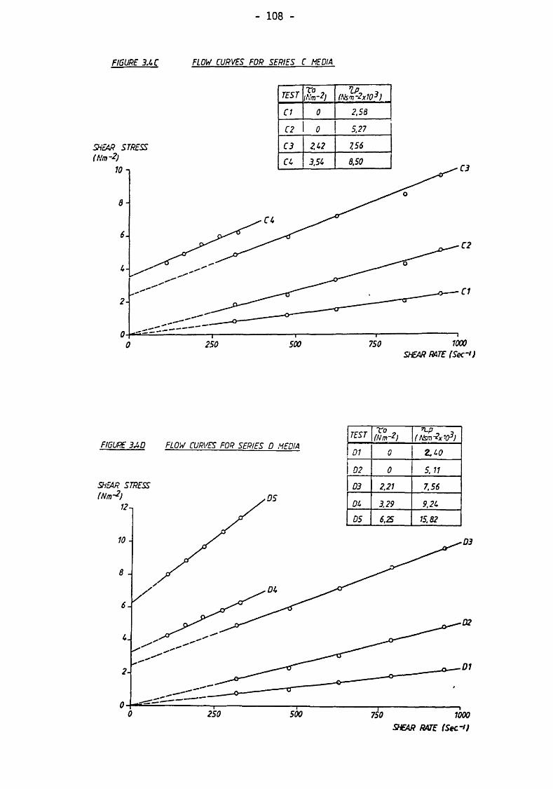
- 108 -

FIGURE 3A C FLOW CURVES FOR SER IES C MEDIA

FIGURE 3AD FLOW CURVES FOR SERIES D MEDIA

SHEAR STRESS (Nm~2)

12

TEST y ° ( Nsm ^Cr)

D1 0 Z.C0

02 0 5. 11

03 2,21 7.56

DC 3,29 9,2U

05 6,25 15,82

SHEAR RATE (Sec~i)

2S0 500 750

- 109 -

FIGURE 3M E FLOW CURVES FOR SERIES E MEDIA

SHEAR STRESS (Nm~2)

V1

8-

6-

U-

SHEAR RATE fSec-l)

FIGURE 3 A F--- FLOW CURVES FOR SERIES M MEDIA

2S0 10000 500 750SHEAR RATE (Secr<)

30

20

10

0

FIGURE 35 PLASTIC VISCOSITY VS SOLIDS CONCENTRATION FOR QUARTZ / BROMOFORM MEDIA

l

O

10

--------------------------- 1-----------------------------------------r20 30

SOLIDS CONCENTRA TION ( VOL.%)

- Ill

TABLE 3.1 - SOLIDS VOLUME CONCENTRATION VS. PLASTIC VISCOSITY,

FOR QUARTZ/BROMOFORM MEDIUM

VolumeConcentration

Cv (v/v)

Plastic Viscosity, nD

(N s m - 2 x 103;

VolumeConcentration

Cv (v/v)

Plastic Viscosity, Tin

(N s nr2 x 103;

0.00 1.93 0.225 6.040.05 2.65 0.25 7.480 . 1 0 3.28 0.275 9.300.125 3.51 0.30 12.380.15 3.90 0.325 16.400.175 4.40 0.34 21.970 . 2 0 4.86 0.353 28.27

3.3.2 Density Separations and Flow Data

The partition and medium flow data for the test series A-E

are given in Appendix 3, and the partition curves are shown

in Figures 3.6A - 3.6E. The flow data for test series M

(medium only) are also given in Appendix 3.

3.3.3 Summary of Data

A summary of the data, including both original measurements

and quantities derived from Figures 3.6A - 3.6E and Appendix

3, is given in Table 3.2.

The values of 6 5 0 and 6 7 5 were determined by interpolation

in Figures 3.6A - 3.6E. The mean particle size, d, was

determined as the geometric mean of the limiting screen

apertures used to prepare the feed material :

- 112

d = / d1 d2 .... (3.5)

This definition was selected in view of the /2 relationship

between adjacent screen sizes in the sieve series used.

The inlet Reynolds number, Re-j, was defined as :

P Vi Di Re i ~ . - —

n p

4 Qfwhere Vn* = -----

« Di2

.... (3.6)

.... (3.7)

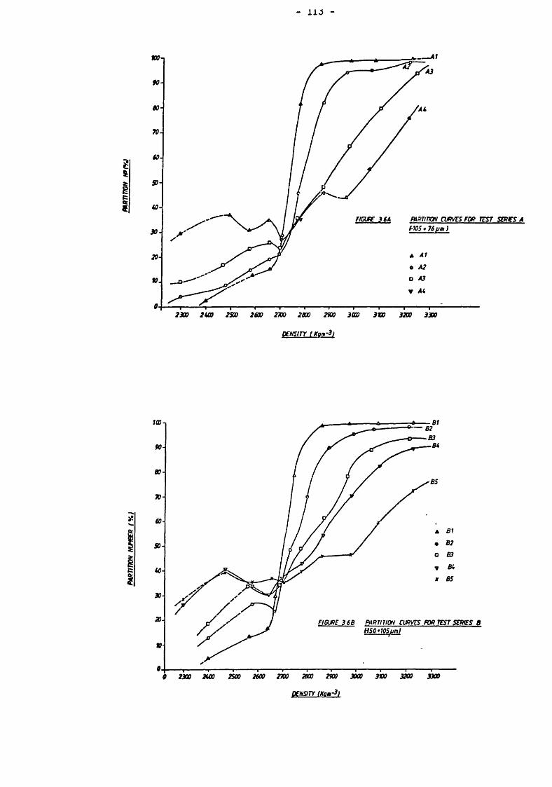
PART

ITION

NUMB

ER (

Y.)

113

DENSITY fKom-3)

DENSITY (Kam-3)

PART

ITION

NUMB

ER (%

)

- 114 -

DENSITY IKotn-3}

115

DENSITY (Kam-3)

TABLE 3.2 - SUMMARY OF RESULTS, CHAPTER 3

ChronologicalOrder

TestNumber

dpm 3^_lm s

(x 1 0 6)

p 2kN w kg m"3

T° 2 N m_z

nP 2 N s nr2(x 1 0 3)

Re-j Qu/Qf = Rtn

650 " p kg m

675 " §50kg nrd

8 A1 89.3 77.3 93 2651 0 . 0 0 2.35 18201 0.186 8 6 3223 A2 89.3 91.1 1 0 0 2648 0.44 4.79 10512 0.190 135 602 0 A3 89.3 79.5 6 6 2652 2.05 7.18 6128 0.252 233 17413 A4 89.3 78.3 62 2650 3.06 8.60 5037 0.314 366 1885 B1 125.5 78.8 93 2650 0 . 0 0 2.38 18314 0.177 54 362 B2 125.5 78.9 72 2650 0 . 0 0 5.11 8540 0.258 8 6 773 B3 125.5 81.8 76 2650 2.36 7.31 6190 0.303 135 166

1 0 B4 125.5 78.6 62 2648 2.70 9.88 4398 0.318 194 18318 B5 125.5 76.7 55 2651 6.64 16.13 2631 0.335 367 2494 Cl 178.3 76.0 93 2650 0 . 0 0 2.58 16294 0.193 64 2 2

1 C2 178.3 82.0 76 2651 0 . 0 0 5.27 8610 0.254 72 552 2 C3 178.3 83.3 74 2652 2.19 7.56 6099 0.253 1 0 2 7516 C4 178.3 80.6 69 2650 3.54 8.50 5245 0.296 116 8719 D1 252.2 72.6 78 2650 0 . 0 0 2.40 16732 0.147 65 36

6 D2 252.2 78.9 72 2650 0 . 0 0 5.11 8541 0.258 55 702 1 D3 252.2 81.5 67 2652 2 . 2 1 7.56 5967 0.250 97 5814 D4 252.2 78.6 62 2650 3.29 9.24 4706 0.310 107 9917 D5 252.2 73.5 50 2650 6.25 15.82 2570 0.379 1 1 0 2151 2 El 1040.0 75.0 90 2650 0 . 0 0 2.36 17578 0.179 7 415 E2 1040.0 82.6 6 6 2648 3.19 8.26 5527 0.293 1 2 26

7 Ml — 76.4 93 2650 0 . 0 0 2.29 18454 0.178 - -

9 M2 - 78.7 6 6 2649 2 . 2 0 7.64 5696 0.298 - -

1 1 M3 - 79.0 6 6 2650 2.91 9.19 4755 0.314 - -

24 M4 - 76.4 57 2648 2.13 7.29 5805 0.264 - -

- 117 -

3.4 Discussion of Results

3.4.1 Rheology of the Medium

Inspection of Figures 3.4A - 3.4F shows clearly that the

medium exhibits Newtonian behaviour at low apparent

viscosities (i.e. low solids concentrations). At higher

apparent viscosities, a yield stress develops which tends to

increase with viscosity; at these higher concentrations, the

medium behaves as a classic Bingham plastic. The rheology of

all the media used in the tests was therefore characterised

by a yield stress, t 0, and a plastic viscosity, np,

determined by fitting a straight line to the flow curve

data, using linear least squares regression.

An interesting and impressive manifestation of the yield

stress was observed during the mixing of the medium prior to

conducting a test in the cyclone. At high solids

concentration, for which the yield stress was large, the

stirrer succeeded in generating a free vortex flow only in

the central portion of the medium present in the beaker. At

a certain critical radius from the central position of the

stirrer, the rate of shear was insufficient to overcome the

internal structure of the medium, and that portion of the

medium from the critical radius to the periphery rotated

slowly as a solid body. When this occurred, precautions had

to be taken to ensure that adequate mixing occurred in all

parts of the medium.

- 118 -

Some subsidiary measurements, given in Table 3.1, were made

to demonstrate the influence of solids concentration upon

viscosity. Figure 3.5 shows the usual relationship, an

approximately linear trend at low concentrations, followed

by a rapid increase in viscosity at higher concentrations.

3.4.2 The Separating Density, 6 ^n

It had originally been intended to investigate only the

effect of viscosity and particle size upon the separating

density. However, as noted earlier, uncontrolled variations

in certain other operating variables prevented a

straightforward analysis. It was therefore decided to

analyse the data by multiple linear least squares regression

analysis [1 2 0 ]# in order to obtain quantitative

expressions for the more important performance criteria. It

was felt that this would achieve two principal objectives :

1. It would allow the effect of np on 6 5 0 to be

assessed independently of the other variables, and so

satisfy the original objective of the work.

2. It would turn to advantage the fortuitous variations

in the other operating variables, and thus allow

other correlations to be examined.

After some preliminary analysis, it was decided to use

dimensional analysis to develop the forms of the models to

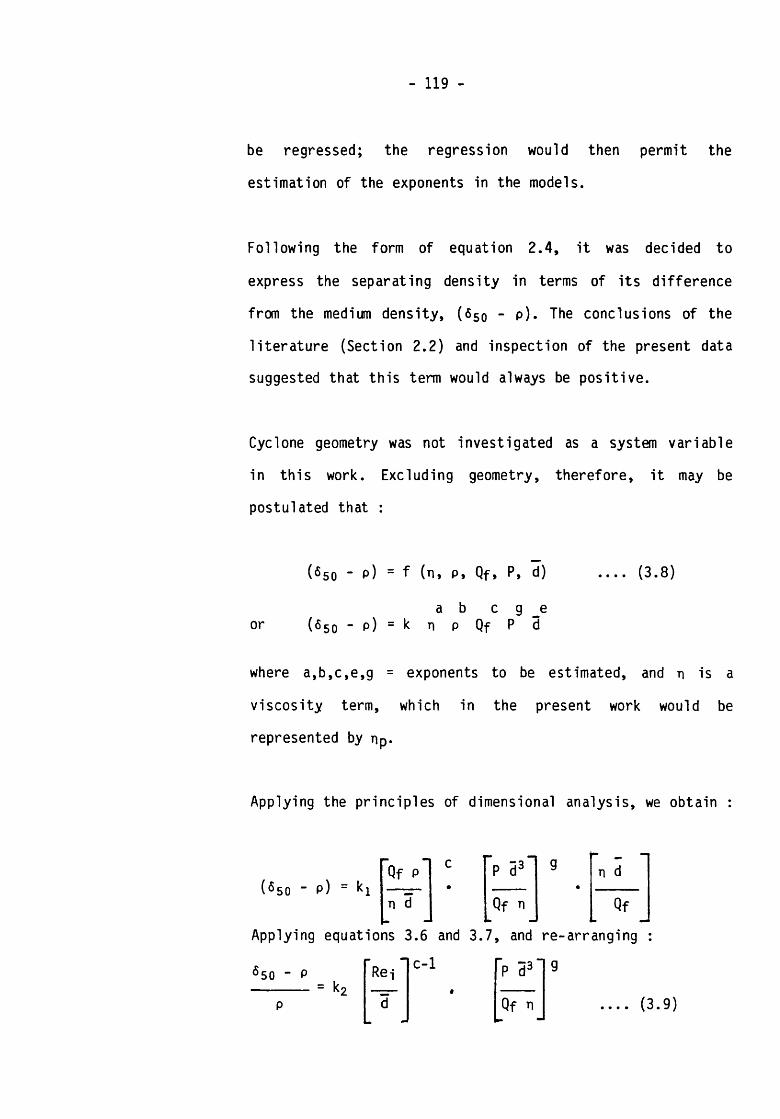
- 119 -

be regressed; the regression would then permit the

estimation of the exponents in the models.

Following the form of equation 2.4, it was decided to

express the separating density in terms of its difference

from the medium density, ($50 " p )- The conclusions of the

literature (Section 2.2) and inspection of the present data

suggested that this term would always be positive.

Cyclone geometry was not investigated as a system variable

in this work. Excluding geometry, therefore, it may be

postulated that :

(6 5 0 - p ) = f (n, p , Qf, P, d) --- (3.8)

a b c g _e or ( 6 5 0 - p ) = k n p Qf P d

where a,b,c,e,g = exponents to be estimated, and n is a

viscosity term, which in the present work would be

represented by np.

Applying the principles of dimensional analysis, we obtain :

( $ 5 0 _ p ) = kiQf p c

•

P d3 g•n d

n d Qf n.

QfApplying equations 3.6 and 3.7, and re-arranging :

9$50 ” P= k? Re-j

c-1 P d3"

P d Qf n .... (3.9)

- 120 -

Given the P - Qf relationship derived in Section 3.4.4

below, equation 3.9 reduces to the simple form (for constant

geometry) :

650 ~ p

P

a= k3 • Re-j *

0d

.... (3.10)

The constant k3 contains a D-j term, rendering equation

3.10 the simplest form of the relation for constant

geometry. Equation 3.10 suggests that, under these

conditions, the relative separating density depends only

upon the inlet Reynolds number and the particle size.

Using data provided by the 20 tests with iron ore, A1-E4

(Table 3.2), the parameters k3, a and 8 were estimated by

multiple linear regression analysis of equation 3.10 in its

linear form :

6 50 " pIn _______ = In k3 + a In Re-j + 8 In d

p

This gave k3 = 1.548 x 10~ 3

a = -0.730 8 = -1.114

(R2 =92.6 %*)

R2 is the coefficient of multiple determination, adjusted for the

degrees of freedom in the regression. It measures how well the

regression equation accounts for the total data variance. R2 = 100%

implies a perfect fit.

- 121

The exponents for Re-j (i.e. for np) and d in equation

(3.10) can be expected to be a function of the prevailing

particle Reynolds number, Rep, as follows [^] :

For laminar flow (Rep < 10"1) a = -1.0, 3 = -2.0

For turbulent flow (Rep > 103) a = 0.0, 3 = -1.0

In the intermediate flow regime (10” 1 < Rep < 103), the

values of a and 3 should lie between the limiting values for

laminar and turbulent flow. On this basis, the values

obtained for the present work imply that the separations

took place predominantly in the intermediate regime, though

the finer particles may have attained laminar flow at the

higher viscosities. A simple calculation (Appendix 4)

provides further evidence of this.

Clearly, the values of a and 3 are interrelated. Since a,

for example, depends upon the prevailing value of Rep#

which in turn is a function of d, we might expect the value

of a to vary with d. By plotting the experimental values of

( 6 5 0 - p ) / p vs. Re -j for the various size fractions

(Figure 3.7), it is possible to see that the absolute value

of the exponent a does indeed decrease steadily as the

particle size (and thus Rep) increases. The values of a in

the equation

( 6 5 0 ■ p) a-------- = K Rei

P .... (3.11)

(given in Figure 3.7) indicate that the Series A and B tests

exhibited predominantly laminar behaviour, whereas Series C

- 122 -

and D departed significantly from laminar conditions (Series

E is not shown because only two tests were conducted). The

value of the viscosity exponent obtained by Agar and Herbst

[25] for classifying hydrocyclones (0.58) is equivalent,

by manipulation of equation 2.3, to a value of 2 x 0.58 =

1.16 for density separations. This compares favourably with

the absolute value of 1.075 obtained for Series A in the

present work.

A problem arises in rigorously invoking the model of

equation 3.10, because of the variable nature of the Rep -

Cp relationship in the intermediate regime [32], This

implies that the exponent a in equations 3.10 and 3.11 is

itself a variable, and one might thus expect a concave

curvature to the plots of Figure 3.7, except in the limiting

cases of a =* 1 (laminar flow) and a = 0 (turbulent flow).

Examination of Figure 3.7 suggests that there is some

evidence for such curvature, although the data are few and

subject to scatter. Accordingly, attempts were made to

include appropriate empirical and semi-empirical terms in

the regression equation for (6 5 0 - p)/p, but no significant

improvement in fit could be obtained over the simple

correlation of equation 3.11.

Although the simple model for density separations in

cyclones, represented theoretically by equation 2.4 and

empirically by equation 3.10, demonstrates why the 6 5 0 is

- 123 -

\ SERIES A : 3= B 9 jum : k - -1 ,075

SERIES C: d= lW / ir n *= -0,520

SERIES B : d= 125,5 um U =-0,99r9

.1 J 1111

SERIES D. c!=252,2pm c< =-0,361

■ »»«««»* ■ t « . j «t«

1O3 7 O '1 103 7 0 4Re,

FIGURE 3.7 RELATIVE SEPARATING DENSITY VS INLET REYNOLDS NUMBER FOR DIFFERENT PARTICLE SIZES (oL = gradient o f line-see eqn. 3.11)

FIGURE 3.8 PROPOSED PARTITION CURVE FOR MEDIUMEXHIBITING A YIELD STRESS

- 124 -

invariably greater than p for such separations, the presence

of a stable medium suggests an additional mechanism. Because

the medium is stable, and thus maintains its density in all

parts of the cyclone, feed of the same density (2,650 kg

m-3) will experience neutral buoyancy and will therefore

divide in the same proportion as the medium, in a manner

analogous to that proposed by Kelsall for fine particles in

classifying hydrocyclones [121], Thus we have the

relation:

YP Qu--- = - = Rm , %100 Qf .... (3.12)

This relation was found generally to hold true in the

present work. Table 3.3, for example, shows the

correspondence between Yp/100 and Rm for test series B,

the partition curves for which are presented in Figure

3.6B. One point on the partition curve is thus defined

independently of the remainder of the curve and any variable

which influences Rm will directly influence the value of

Yp . Assuming the curve retains some semblance of symmetry,

the increase of Yp with viscosity will therefore result in

a simultaneous raising and flattening of the curve, which in

turn implies an increase in the 6 5 0 and in the proportion of

misplaced material. These trends are well illustrated in

Figures 3.6A - 3.6E, and distinguish the DM cyclone from its

cousin, for which Rm is believed not to play a

process-determining role [1»?]. In the limiting case, as

Rm -► 0.5, this argument implies that Y -► 0.5 for all of 6 ,

- 125 -

i.e. that no separation occurs (although this would require

unusual operating conditions, e.g. a combination of high

values of n and Du/D0).

TABLE 3.3 - Yn/100 vs. Rm for Series B

Test Rm

oo

Ql

>-

B1 0.177 0.18B2 0.258 0.25B3 0.303 0.31B4 0.318 0.31B5 0.335 0.36

Consideration of the influence of medium viscosity on the

separation is further complicated when the medium exhibits a

yield stress, as in the present case. The yield stress

defines the shearing stress exerted by an immersed particle

which must be exceeded before the medium will flow and thus

allow the particle to move relative to it. The effect of the

yield stress will therefore be to "lock into" the medium a

larger proportion of the feed particles, for which the

absolute magnitude of d ( 6 - p) is insufficient to exceed

t0. One might expect this to lead to the establishment of

a horizontal plateau region on the partition curve, centred

around 6 = p, as illustrated in Figure 3.8.

Examination of the partition curves of all the tests does

suggest that such a plateau may indeed exist on those curves

for which t 0 > 0 , although in most cases the data in this

area exhibit some scatter. Approximate calculations suggest

that the width of the plateau is of the correct order, as

predicted by theory (Appendix 5). Additional evidence for

- 126 -

the influence of the yield stress emerged from a careful

analysis of the regression which produced the estimates of

the parameters in equation 3.10; this indicated that a small

but significant improvement in the fit could be obtained by

inclusion of a term of the form exp (Kx0/d). The d was

included to reflect the relative influence of particle size

in the yield stress effect, and an exponential form was

chosen to allow for zero values of t 0. This generated the

following correlation :

( 6 5 0 - p ) -0.460 1.030--------- = 2.425 x 10"1** Re-j * d * exp

1.469 x 10-5 t 0

(R2 = 93.956) ___ (3.13)

Analysis of this regression confirmed that t0 has an

influence independent of that of np. Figure 3.9 shows the

measured values of (650 - p) vs. those predicted by equation

3.13; the agreement is satisfactory. The substantial drop in

the absolute value of the exponent for Re-j, as compared

with that determined for equation 3.10, is due to the strong

correlation existing between np and x0 (a correlation

also observed by Whitmore who studied the Bingham plastic

characteristics of aqueous kaolin suspensions [124]).

Whether or not the form of equation 3.13 has relevance to

normal DM cyclone operations will depend partly upon whether

the media used exhibit a yield stress at any point within

the cyclone. The review of Section 2.3 concluded that there

Y U

FIGURE 3.9 MEASURED VS PREDICTED VALUES OF f t fa - t )

MEASURED KS PREDICTED VALUES OF

(§TS~ $So)FIGURE 310

- 128 -

is some disagreement in the literature as to the true

rheological nature of aqueous suspensions of media such as

magnetite and ferrosilicon, although some authors do report

the presence of a yield stress [6 8 , 110, 116], The

additional question of medium classification and segregation

in the cyclone and its effect on the medium rheology, and

thus on the density separation, is crucial [4] and is

discussed in Chapter 5. A mechanism by which this effect may

influence the density separation is proposed briefly in

Section 3.5 below.

3.4.3 Quality of Separation (67S - 6$n)

As noted above, difficulties in characterising the

separations at high and low densities led to the adoption of

(6 7 5 - 6 50) as a crude measure of separation quality. (For a

symmetrical partition curve, this quantity equals the

traditional Ecart Probable, defined by Ep = (6 75 ’ fi25)/2 ).

By dimensional analogy with equation 3.10 we obtain

($75 " ^50) a----------- = K Rei d

p . . . . ( 3 . 1 4 )

for which regression analysis gave K = 1.290, a = -1.214 and

B = -0.802 (R2 = 9 2 . 3 % ) . Inclusion of a yield stress term

produced no significant improvement in the fit, probably

because, as noted earlier, the yield stress would only be

expected to influence Y around 6 = p (i.e. below 650).

Figure 3.10 shows the measured values of (6 7 5 - 6 5 0 ) vs.

- 129 -

those predicted by equation 3.14. The agreement is

satisfactory.

The similarity of the estimated parameters in equations 3.10

and 3.14 demonstrates that the density and quality of

separation are themselves highly negatively correlated,

implying that a large differential between 6 5 0 and p is

associated with a poor quality of separation (i.e. a large

value of 6 7 5 - 6 50). Significantly, Gottfried predicted the

result 6 5 0 « Ep from the mathematical properties of the

generalised partition curve for coal cleaning devices

[46], and indeed one would expect such a trend with stable

media, from the arguments advanced above in Section 3.4.2.

It was found that the (6 7 5 - 6 50) could be represented

directly in terms of (6 S 0 - p) and Rm by the following

regression equation :

(675 - 650) 1 *672 ° * 714----------- = 1.048 x 10” 2 Rm • (650 - p)

P.... (3.15)

(R2 = 91.1%)

In terms of the influence of Rm , equation 3.15 is

analogous to Plitt's regression equation for the

classification efficiency parameter, m, which predicts [2 ]

m « exp (-1.58 Rm). Since a low value of m implies poor

classification, the direction of influence is the same in

each case.

- 130 -

3.4.4 Pressure-Flowrate Relationship

Bradley [1] states that viscosity does not enter into the

correlations for pressure drop in hydrocyclones, although he

does present experimental data which show that pressure drop

decreases as viscosity increases; he attributes the effect

to changes in the exponent n in equation 2 . 1 and the inlet

loss factor. In terms of the factors measured in the present

work :

Pi - f (tip, p, Qf, D-j) .... (3.16)

a b c eor Pi = kx np p Qf Di

Dimensional analysis gives:

Pi = k2

p Qf

rip Di P Di2

Invoking equations 3.6 and 3.7, and re-arranging, gives :

2a UpPi = K Rei • —

.... (3.17)

for which regression analysis using all 24 sets of data gave

K = 6926 and a = 2.30. Equation 3.17 can also be

conveniently expressed in the form

Pi 2.30 _ = 1.53 x 10e Qf • P9 (3.18)

The pressure expressed as head of fluid is thus inversely

related to the kinematic viscosity, a fact not generally

appreciated in the context of DM cyclone operations.

- 131 -

Equation 3.18 implies a drop of almost half in the observed

pressure for a given flowrate over the range of viscosities

encountered in the present testwork, a substantial change.

The exponent for Qf is in good agreement with the

hydrocyclone literature U ] and in exact agreement with

Mitzmager and Mizrahi, who used the dense liquid

tetrabromethane [127], Figure 3.11 shows the measured

values of P vs. those predicted by equation 3.18; the

agreement is satisfactory, particularly since the precision

of the pressure gauge used was no better than ± 5 kNm"2.

Several authors, amongst them Bradley [l] and Mitzmager

and Mizrahi [ 127] have pointed out that the actual P-j -

Qf relationship will depend upon the value of Re-j, since

this will determine the relative contributions of frictional

and centrifugal losses to the overall pressure loss

coefficient, defined as

p iL = ------- (dimensionless)

1/2PV-j2 .... (3.19)

(Here, 1/2 p V-j2 is the inlet velocity head). The relative

influence of these two forms of head loss can be assessed by

plotting L vs. Re-j; a reducing value of L (at low Re-j)

indicates that friction losses predominate, and a rising

value of L (at high Re-j) indicates that centrifugal losses

predominate. Figure 3.12 suggests that the present work

occupied principally the rising part of the curve (as do

most normal cyclone operations), for which equation 3.17

represents an acceptable correlation for the pressure -

flowrate relationship.

FIGURE 3.11 MEASURED US PREDICTED VALUES OF IN IET PRESSU RE DR O P

FIGURE 3.12 PRESSURE LOSS COEFFICIENr VSINUEf REYNOLDS NUMBER

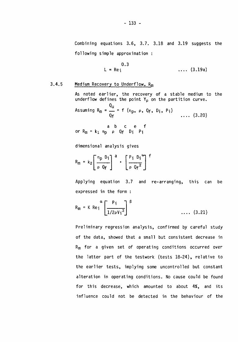
- 133 -

Combining equations 3.6, 3.7. 3.18 and 3.19 suggests the

following simple approximation :

0.3L « Rei .... (3.19a)

3.4.5 Medium Recovery to Underflow, Rm

As noted earlier, the recovery of a stable medium to the underflow defines the point Yp on the partition curve.

QuAssuming Rm = _ = f (np, p , Qf, Di, Pi)

Qf .... (3.20)

a b c e f or Rm = ki np p Qf D-j P-j

dimensional analysis gives

np D-j a•

•Pi Di"-

„ p Qf -P Qf2 .

Applying equation 3.7 and re-arranging, this can be

expressed in the form :

Rm = K Re -jl/2PVi.2 .... (3.21)

Preliminary regression analysis, confirmed by careful study

of the data, showed that a small but consistent decrease in

Rm for a given set of operating conditions occurred over

the latter part of the testwork (tests 18-24), relative to

the earlier tests, implying some uncontrolled but constant

alteration in operating conditions. No cause could be found

for this decrease, which amounted to about 4%, and its

influence could not be detected in the behaviour of the

- 134 -

correlations discussed earlier. However, it did influence

the value of Yp and thus would seem to reflect a real

effect and not an error of measurement. The effect was large

enough to require two separate regression analyses for the

estimation of the constants in equation 3.21. These gave :

Tests 1-17 Tests 18-24

K 7.96 10.59

a -0.336 - 0.285

e -0.205 - 0.669

Figure 3.13 gives the measured values of Rm vs. those

predicted by equation 3.21, for the two sets of data; the

agreement is excellent. By substituting equation 3.17 and

re-arranging, equation 3.21 can be simplified to :

r np^m _ K ---

,pQf

£

where e = 0.4-0.5,.... (3.22)

assuming constant geometry. The proportion of medium

reporting to underflow (and thus by implication the value of

Yp on the partition curve) is therefore substantially

dependent upon the kinematic viscosity. Interestingly, a

similar conclusion is implicit in the data of Agar and

Herbst [25]# though not noted by them. Other workers have

also recorded the increase of Rm with viscosity for

classifying hydrocyclones [l].

- 135 -

3.5 Summary and Conclusions

The principal purpose of this investigation was to determine the

effect of medium viscosity upon the density of separation of mineral

particles in a dense medium cyclone. No specific attempt was made to

study other variables, apart from particle size, and the cyclone

geometry remained constant throughout the testwork. However,

dimensional reasoning coupled with multiple linear regression analysis

has resulted in the development of some useful semi-empirical

correlations for important operating criteria, including the

separating density, the quality of separation, the recovery of medium

to the underflow and the pressure-flowrate relationship. Viscosity was

found to infuence profoundly all these parameters.

The more significant conclusions of the work may be summarised as

follows:

(i) The separating density ( 6 5 0 - p ) increases with viscosity

(expressed in terms of the inlet Reynolds number Re-j) and

decreases with particle size (equation 3.10), as predicted

by simple theory based on the equilibrium orbit hypothesis

(equation 2.4). The absolute value of the exponents in

equation 3.10 depends upon the prevailing particle-fluid

flow regime. Those obtained in the present work suggest that

most of the tests occurred in the intermediate flow regime,

with the finer particles approaching the laminar regime and

thus most susceptible to the direct influence of viscosity.

(ii) The presence of a yield stress in the medium increases the

separating density (equation 3.13) and gives rise to an

- 136 -

approximately horizontal "plateau" on the partition curve

centered around the medium density, p; this effect is

probably attributable to particles with an absolute value of

d(6-p) insufficient to exceed the yield stress. Such

particles would be "locked into" the medium, and thus divide

in the same proportion as the medium.

(iii) The recovery of medium to underflow (Rm ) increases with

viscosity (equation 3.21). For a stable medium, Rm defines

the value of Y on the partition curve corresponding to 6 =

p.

(iv) Increased viscosity induces poorer separation quality

(equation 3.14), which is invariably associated with higher

values of separating density and medium recovery to

underflow (equation 3.15). The form of equation 3.14 implies

that a higher flowrate might compensate for the deleterious

effect of increased viscosity.

(v) The overall effect of viscosity on the partition curve is to

both raise and flatten it, and move it to higher densities,

which (as noted above) is reflected in a simultaneous

increase in separating density and proportion of misplaced

material. The net effect on the separation is thus complex

and will always be difficult to interpret unless the full

partition curve is obtained. This may account for some of

the anomalies in the literature.

- 137 -

(vi) The indicated pressure drop at constant flowrate falls as

viscosity rises (equation 3.18).

(vii) It is suggested that the apparent discrepancy between the

conclusions of the literature and those of the present work

regarding the influence of medium viscosity upon density

separations in cyclones can be attributed largely to the

classification and segregation of the unstable media used in

practice. It is known that the d50 increases with viscosity,

and that the degree of solid-liquid segregation decreases

with increase in viscosity. More medium solids are diverted

to the overflow, thus increasing the density of the overflow

medium at the expense of the underflow medium. This

displaces more (low density) feed solids from overflow to

underflow, due to changes both in the product medium

densities and in the relative crowding effect at each

outlet, thus reducing the separating density. Large feed

particles, which probably move radially in the turbulent

regime (Appendix 4), and upon which changes in viscosity

therefore have little direct effect, are thus significantly

influenced in their behaviour by the indirect effect of

viscosity upon the classification and segregation of the

medium. Small particles are affected both directly and

indirectly.

Further experiments to test this hypothesis are discussed in

Chapter 5.

-138 -

CHAPTER 4

THE SEDIMENTATION AND RHEOLOGY OF FERROSILICON SUSPENSIONS

4.1 Introduction

It is the central thesis of this work that, once the cyclone geometry

has been defined, it is the characteristics and behaviour of the

medium which are process-determining. In the previous chapter, it was

shown that the viscosity of a stable medium profoundly influences

cyclone performance criteria such as the density and quality of

separation, the proportion of medium reporting to underflow, and the

indicated pressure drop. In Chapter 5, cyclone tests will be described

using conventional, unstable ferrosilicon media, in which the

behaviour of the media was monitored. The purpose of the present

chapter is to characterise, in general terms, these ferrosilicon

media.

The two properties characteristic of dense media in the context of DM

cyclone operation are sedimentation behaviour and rheology. The

literature on the sedimentation and rheology of dense suspensions was

reviewed in Section 2.3, and the general rules governing these

properties were established. In this chapter, these rules are applied

to the ferrosilicon suspensions utilised in the experiments described

in Chapter 5, so as to determine the general sedimentation and

rheological nature of these suspensions. Particular attention is given

to examining sedimentation behaviour (under gravity) in the context of

current sedimentation theory, and to establishing the rheological type

- 139 -

of the suspensions. In both cases, the investigation was confined to

the conditions encountered in the subsequent cyclone experiments. No

attempt was made to undertake a quantitative study of the relationship

between sedimentation, rheology and other properties of dense media,

as such investigations have already been reported in the literature.

Sedimentation and rheology are dealt with in Sections 4.2 and 4.3

respectively.

4.2 Sedimentation of Ferrosilicon Suspensions

4.2.1 Introduction and Objectives

The segregation of unstable media in a DM cyclone, which

results in the differential between underflow and overflow

density normally observed, must be to some degree a function

of the sedimentation characteristics of the medium. As noted

in Section 2.3.2, the sedimentation behaviour depends upon

the size distribution, shape and concentration of the solid

particles, among other factors. Commercial ferrosilicon

media are actually classified and sold according to size

distribution and shape, so that the stability, or tendency

to segregate, can be matched to the particular application

[42]. The tendency to segregate is of course more

pronounced in the centrifugal force field experienced in a

cyclone than in gravity-based dense medium separators. In

both cases, however, it is the rate of segregation which

must determine to a large extent the density differential.

- 140 -

Medium is continuously introduced at the feed point, and

removed at the overflow and underflow points. If the rate at

which medium enters and leaves remains constant, then an

equilibria will be set up between the rate of segregation

and the rate of removal of the products. It seems reasonable

to suppose that it is the position of this equilibrium which

defines the value of the differential.

The concensus of the literature reviewed in Section 2.3.2 is

that the sedimentation of dense suspensions occurs by

hindered settling with a clearly defined interface between a

a relatively clear supernatant and the body of the

suspension. Below the interface is a zone of "constant"

density, and below this zone is a compaction zone of

elevated density. Although a few authors have suggested that

there is a density gradient in the zone of "constant"

density, their data demonstrate that the changes in density

are small.

The qualitative effects on sedimentation of properties such

as particle size, shape and concentration are well known for

ferrosilicon suspensions. However their general

sedimentation behaviour, and in particular the applicability

of the laws of sedimentation to the relationship between

sedimentation rate and solids concentration, have not been

established. It is the purpose of this work to explore these

aspects.

- 141

4.2.2 Experimental Details

All the sedimentation tests were carried out in a 1-litre

stoppered glass measuring cylinder, using tap water to make

up the suspensions. Three different ferrosilicon media were

investigated (two milled and one atomised, of varying size

distributions), each at six or seven volume concentrations

over the approximate range 15-35%. The initial pulp density

was determined by weighing the solid and water in the

cylinder, and obtaining the volume directly by reading the

level in the cylinder. Weighing with a precision of O.lg and

estimating the volume with a precision of 1 nut gave a

maximum error in density determination of about 2 kgm~3

(0.002 SG units). The solids volume concentration was

calculated using the measured solids density; the method of

solids density measurement is described in Chapter 5.

Once the pulp density had been determined, the stoppered

cylinder was inverted 20 times in order to mix the

suspension. The cylinder was then allowed to stand, and an

electronic stop-watch started. In each test it was found

that an easily-distinguished interface formed between the

clear supernatant and the settling suspension. The time of

passage of this interface at each 10 m l mark was recorded.

This continued until sedimentation ceased or became very

slow. The data were plotted as volume mark vs. time, and a

straight line fitted to the (initial) linear portion of each

curve using least squares regression :

- 142

v = Sq + a2 t __ (4.1)

where v = volume mark (mi)

t = sedimentation time (s)

a0 = starting point (level of pulp in cylinder - m£)

ax = sedimentation rate (m£ s”1)

ax was converted to a linear sedimentation rate, u, using

the relation :

u = 3.361 x 10"2 ax cm s-1 .... (4.2)

(The mean distance between each 10 m£ mark was 3.361mm).

Successive increasing volume concentrations were obtained by

adding further solids to the pulp in the cylinder, and

re-weighing. All the tests were conducted at ambient

temperature (19-23 °C); the temperature of the supernatant

was recorded after each test.

4.2.3 Results

The three media investigated were labelled SI, S2 and S3.

The size distribution and other details of these media are

given in Table 4.1 :

- 143 -

TABLE 4.1 - DETAILS OF MEDIA USED IN SEDIMENTATION TESTS

Medium

SI SI SI

Type Mi 11ed Milled Atomised

Solids Density (kgm-3) 6897 6897 6947

Size Cum. % Size Cum. % Size Cum. %Size Distribution (ym) Finer (ym) Finer (pm) Finer

67.2 98.8 92.2 100.0 73.7 89.553.4 96.3 73.2 95.8 67.0 84.242.3 89.2 58.1 87.4 58.5 72.638.5 86.5 46.1 75.0 53.2 66.433.6 78.1 36.6 58.3 46.4 62.426.7 63.5 29.0 42.2 36.8 49.421.2 48.4 23.1 33.1 29.3 37.016.8 33.3 18.3 23.4 23.2 29.813.3 20.8 14.5 17.6 18.4 22.310.6 12.6 11.5 13.5 14.6 16.68.4 7.5 9.2 8.5 19.6 10.86.7 2.3 8.3 6.6 9.2 6.55.3 1.3 7.3 3.7

Cyclone tests in Ch. 5in which medium was F6/5 and F6/6 Not Used F4/1

used Directly

The sedimentation measurements are presented in graphical

form in Figures 4.1-4.3. Each measurement point is shown,

together with the straight line fitted to the initial,

linear portion of the sedimentation curve. A summary of the

data, including the initial sedimentation rate determined

from equations 4.1 and 4.2, is presented for series SI, S2

and S3 in Tables 4.2, 4.3 and 4.4 respectively.

VOLUME MAR

K (ml) —

>

- 144 -

FIGURE 4 7 ft?S/ SEDIMENTATION TESTS, SERIES 57

SEDIMENTATION TIME (S)

- 145 -

FIGURE 4 2 FeSi SEDIMENTATION TESTS. SERIES S2

FIGURE U3 FeSi SEDIMENTATION TESTS. SERIES S3

- 146 -

TABLE 4.2 - SUMMARY OF SEDIMENTATION DATA FOR SERIES SI

Test Temperature of Pulp (°C)

Pulp Density (kgnr3)

Vol. Concn. Cy {%)

Sedimentation Rate Vc (cm s"*)

Sl/l 20.0 1890 15.09 5.123 x 10-2Sl/2 20.2 2005 17.04 3.867 x 10-2Sl/3 20.5 2208 20.48 2.364 x 10-2Sl/4 20.9 2415 24.00 1.428 x 10-2Sl/5 21.2 2613 27.35 8.692 x 10-3Sl/6 20.1 2810 30.69 5.569 x 10*3Sl/7 20.5 3050 34.76 3.728 x lO'3

TABLE 4.3 - SUMMARY OF SEDIMENTATION DATA FOR SERIES S2

Test Temperature of Pulp (°C)

Pulp Density(kgm-3 )

Vol. Concn.cv (^)

Sedimentation Rate vs (cm s”1)

S2/1 19.0 1975 16.53 0.1136S2/2 19.0 2185 20.09 6.564 x 10-2S2/3 19.5 2395 23.66 4.384 x 10-2S2/4 20.5 2613 27.35 2.537 x lO*2S2/5 20.8 2804 30.59 1.612 x 10-2S2/6 20.9 2989 33.73 1.181 x 10-2

TABLE 4.4 - SUMMARY OF SEDIMENTATION DATA FOR SERIES S3

Test Temperature of Pulp (°C)

Pulp Density (kgm-3)

Vol. Concn. Cy (%)

Sedimentation Rate Vc (cm s"1)

S3/1 21.2 2028 17.29 0.1150S3/2 21.5 2186 19.94 7.725 x 10-2S3/3 21.8 2413 23.76 4.786 x 10-2S3/4 22.2 2608 27.04 3.316 x 10-2S3/5 22.2 2819 30.59 2.277 x 10-2S3/6 22.8 3047 34.42 1.076 x lO*2

- 147 -

In order to test the efficacy of the models discussed in

Section 2.3.2, equations 2.21 and 2.23 were fitted to the

data given in Tables 4.2 - 4.4, using linear least squares

regression (the linear form of the equations being given as

equations 2.21a and 2.23a). For convenience, the relevant

equations are given again here :

nvs = vso (1 “ Cv) •••• (2*^)

vs = vs0 (1 - KCv)n ; n = 4.65 ___ (2.23)

The estimated parameters for the two equations are given in

Table 4.5, together with estimates of the "equivalent

Stokesian mean diameter" for each ferrosilicon sample,

d$T, and the corresponding particle Reynolds number,

Rep, determined by inserting the value of vso in Concha

and Almendra's correlation for the sedimentation of spheres

[32] (assuming a liquid viscosity of 10“3 Nsm~2).

Also included are the parameters of the Rosin-Rammler

distribution, estimated by linear regression from the size

distribution of each ferrosilicon sample given in Table

4.1. The Rosin-Rammler distribution is given by :

- 148 -

Wr = 100 exp

b

a

where Wr = cumulative weight % retained

d = size (pm)

a,b = parameters

... (4.3)

TABLE 4.5 - ESTIMATED PARAMETERS IN EQUATIONS 2.21 AND 2.23

ParametersTest Series

SI S2 S3

Equation 2.21

vs0 ( cms-1) nR2 *

0.250010.18840.9914

0.63159.88590.9942

0.70429.73190.9928

d$T (pm) Rep

28.10.070

46.00.290

48.60.342

Equation 2.23

vso ( cms-1) KR2 *

0.18251.69550.9856

0.46101.66010.9888

0.49891.62410.9928

d$T (pm) Rep

23.90.044

38.80.179

40.30.201

Rosin-Rammler Size Distribution

(Equation 4.3)

a (pm) bR2*

28.812.2610.974

38.651.7070.997

46.491.6340.991

* R2 = Coefficient of determination for linear regression.

- 149 -

The relationship between sedimentation rate and solids

concentration for the three series of tests is shown

graphically in Figures 4.4A-C, together with the curves

predicted by application of equations 2.21 and 2.23.

4.2.4 Discussion of Results

It is apparent that the relationship between sedimentation

rate and solids volume concentration for all three

ferrosilicon samples is well described by both equation

2.21 and equation 2.23, over the range of concentration

investigated. Examination of Figures 4.4A-C, and reference

to the R2 values in Table 4.5, suggests that equation 2.21

gives marginally better fits than equation 2.23, although

the difference may not be significant.

It is interesting to note that the values of the exponent,

n, determined in the model of equation 2.21 are very similar

for all three samples, even though SI and S2 differed

substantially in size distribution, and S3 differed from the

other two in consisting of particles of rounded, rather than

irregular, shape. The values are higher than the value 4.65

determined by Richardson et al [78,81]# and this would

imply, by the arguments of Davies et al [86] # that the

systems are highly hindered. The mechanism of this high

degree of hindrance can only be surmised. It may be a

consequence of physico-chemical interactions between the

solids and water, in which case one might expect

I3U

VOLUME CONC Cv ( % ) — ^

VOLUME (PNC. Cv(%)___^

VOLUME (PNC. Cv(%) -- }

- 151 -

sedimentation behaviour to be a function of the

characteristics of the aqueous environment. Alternatively,

the effect may be due to trapping and immobilisation of

water by the solids, as described by equation 2.23, the

model of Scott [89] and Capes [90]. This is likely to be

a function of particle size and shape, and may also have a

physico-chemical component. Davies and Dollimore [128]

suggest that hindrance to settling is more likely with

relatively dense solids, as in the present case.

The values of K in equation 2.23 are similar for the three

samples (as one might expect from the similarity in the

values of n in equation 2.21), and are comparable with those

obtained from the literature. There is a small decrease in K

with increasing particle size and with the rounded material,

as found with the literature data reviewed in Section

2.3.2. However, the effective change in the equivalent

spherical diameter of the particles, as determined from

equation 2.24, is only 1% over the three values of K; the

observed differences in K for the three samples are

therefore probably not significant. Considerably more

combinations of particle size and shape would have to be

studied to enable any firm conclusions to be drawn about the

dependence of K upon these factors.

The equivalent Stokesian mean diameters determined as a

function of the characteristic sedimentation rate, vso,

appear intuitively reasonable when compared to the

- 152 -

corresponding size parameter, a, in the Rosin-Rammler

function (Table 4.5). The equivalent particle Reynolds

numbers are all low. Assuming that the flow does not depart

significantly from the laminar regime for Rep < 1.0, all

the tests took place in the laminar regime, justifying the

exponent n = 4.65 for the modified Richardson and Zaki

equation (equation 2.23).

Comparison of the data for series SI and S2 shows that,

other things being equal, the sedimentation rate of the

finer SI material was significantly less than that of the

coarser S2 material.

Finally, it is worth considering these results in the

context of the expected behaviour of ferrosilicon media in a

dense medium cyclone. In the present tests, sedimentation

occurred under gravity. In a cyclone, sedimentation takes

place radially under the influence of a centrifugal

acceleration several times that of gravity. A rough

calculation suggests that a typical centrifugal acceleration

experienced by media in the tests to be described in Chapter

5 would be 25g. Assuming that sedimentation continues to

occur in the laminar regime, then application of Stokes' law

gives :

avsc = vs • - --- (4 -4)

9

where vsc = mean sedimentation velocity in the cyclone.

a = mean centrifugal acceleration in the cyclone.

- 153 -

Applying this relation to the maximum sedimentation rates

encountered in the present work (Tables 4.2 - 4.4), it can

be deduced that the maximum value of Rep likely to be

experienced by media sedimenting in the cyclone is about 3,

and typical values would be less than 1. Under these

conditions, an assumption of laminar conditions would not

incur a serious error, and the use of equation 4.4 is

therefore justified.

4.2.5 Summary and Conclusions

Sedimentation tests with two milled and one atomised

ferrosilicon samples, all particles being less than 100 ym

in size, have shown that the relationship between initial

sedimentation rate and solids volume concentration can be

expressed in the form :

nvs = vso (1 * KCV) .... (2.23)

Here, either K = 1 and n > 4.65 (- 10 in the present work)

or K > 1 and n = 4.65 (K * 1.66 in the present work).

The mean sedimentation rate in a DM cyclone, vsc, assuming

that the sedimentation takes place under laminar conditions,

is then given by :

- 154 -

avsc = vs * — .... (4.4)

9

These relations apply only to the initial (linear) stage of

settling. As a compression zone is reached, the

sedimentation rate will decay rapidly. However, in a cyclone

it is likely that this latter condition will occupy only a

small portion of the flow, since thickened medium is removed

from the cyclone as it is formed, and the mean residence

time of most DM cyclones is only a few seconds. Equations

2.23 and 4.4 are therefore likely to give an adequate

approximation of the sedimentation rates prevailing in the

cyclone, although they ignore the effect of any turbulent

mixing which may occur.

4.3 Rheology of Ferrosilicon Suspensions

4.3.1 Introduction and Objectives

It will be recalled from the discussion in Section 2.3.3

that a surprising conformity exists in the literature as to

the rheological nature of dense suspensions in general, and

of ferrosilicon suspensions in particular. Cheng's model

[1^7] (Figure 2.9) was found to be useful in accounting

for the observed variations in rheology under differing

conditions of solids concentration and rate of shear. It was

concluded that many of those conflicts which did exist in

- 155 -

the literature could be attributed to the complex nature of

dense medium rheology, and its probable true variation with

the conditions under which the observations are made.

For this reason, and in view of the influence of rheology

both on the behaviour of the medium in the cyclone and on

the behaviour of the ore particles being separated, it was

felt to be important to characterise the rheology of the

ferrosilicon media utilised in the cyclone tests to be

described in Chapter 5, under the conditions of particle

size, shape and solids concentration prevailing in the

testwork. As in the case of the sedimentation work, it was

not the purpose of the present investigation to present an

exhaustive, quantitative account of the influence of certain

variables upon rheology, but rather to define in general

terms the rheological type(s) to which the media utilised in

the cyclone testwork conformed.

As a secondary objective, it was hoped to develop a simple

apparatus suitable for the absolute determination of flow

curves for unstable suspensions of this type. In this

respect, cognisance had to be taken of the difficulties of

handling unstable suspensions, and in particular of

maintaining a homogeneous suspension during the measurement.

Finally, it was intended to define specifically an apparent

viscosity for the actual medium used in each cyclone test,

- 156 -

as a prerequisite for assessing the suitability of a

(modified) cyclone model of the type developed in Chapter 3.

4.3.2 Experimental Details

Although it might be supposed that a concentric cylinder

Couette-type viscometer would provide rheological data most

appropriate to the rotational shear which takes place in a

cyclone, a significant problem with this type of instrument

is the maintainance of the solids in homogeneous suspension

while the measurement is made. Various mixing devices have

been described in the literature, but most of these suffer

the disadvantage that the suspension is being sheared

simultaneously both by the viscometer itself and as a

consequence of its own flow. In the case of non-Newtonian

materials, interpretation of the instrument output is

rendered difficult for this reason. Other problems include

slip at the cylinder walls [97] and the migration of

particles in the curvilinear flow field [134],

Accordingly it was decided to adopt a method by which the

flow of the suspension itself was employed to generate the

appropriate data. Capillary viscometers utilise this method,

and have the added benefits of being simple to construct and

of generating the relatively high rates of shear appropriate

to cyclone operation. A capillary viscometer was therefore

designed and constructed, and used to produce all the

rheological data reported herein.

- 157 -

The principle of the device required the medium sample to be

maintained in suspension in a vigorously-agitated reservoir,

which would then gravity-feed the capillary. In this

respect, the instrument is similar to the de Vaney-Shelton

device [66], The flow can be controlled by applying

positive or negative pressure to the lower, closed section

of the apparatus in order to obtain a range of shear rates

with a given capillary.

After some preliminary experiment, the apparatus shown in

Figure 4.5 was evolved. The reservoir is fitted with four

baffles, within which a three-bladed stirrer rotates, driven

by a variable-speed motor. The lower part of the reservoir,

and the point at which the capillary was connected via a

rubber bung, are carefully designed to ensure adequate

mixing and to minimise the hang-up of solids. Flow through

the capillary is initiated by opening a ground glass

(ungreased) tap situated at the base of the reservoir.

The lower vessel, which receives the flow from the

capillary, is inclined slightly to the vertical in order to

allow the capillary discharge to impinge on the vessel wall,

so minimising turbulence and frothing in the vessel which

causes difficulties in reading the level. The lower vessel,

rendered air-tight, is connected via a mercury manometer to

a 5-litre glass conical flask which acts as an air receiver.

158

F IG U R E 4.5 C A P I L L A R Y V ISC O M ETER(NOT TO SCALE )

- 159 -

This receiver is connected to the laboratory vacuum and

compressed air supplies, which provide satisfactory positive

and negative heads (respectively) to add to the static head

of the reservoir and capillary. The additional head is

controlled by means of valves on the incoming supplies and

on the receiver, and is measured in each case using the

manometer.

The following procedure was adopted in making each

measurement. Approximately 200 m£ of the sample to be

measured was prepared and introduced to the upper reservoir

with the stirrer rotating slowly. The stirrer was then set

at the appropriate speed (200-300 rpm, depending on the

suspension density).

The upper tap was then opened and the sample allowed to run

through the capillary with the lower vessel removed. The

first few m i were ignored, since they were generally

over-dense due to unavoidable solids settling adjacent to

the upper tap. Thereafter the suspension was run into a 50

m£ SG bottle in order to obtain an accurate measurement of

the bulk suspension density. (When new conditions were

encountered, e.g. a new grade of medium, several sequential

densities were taken from the capillary flow, in order to

establish the density gradient in the reservoir. If this was

greater than about 30 kg rrr3 over the height of sample in

the reservoir (about 12cm), the stirrer speed was adjusted

to obtain better mixing).

- 160 -

When the suspension density had been established, the sample

was returned to the reservoir, and the lower vessel

attached. The total static head (the vertical distance

between the upper level in the reservoir and the lower end

of the capillary) was measured using a fixed cm rule with a

precision of 1mm.

The additional head was then set to the desired value (± 0.1

cm Hg) by adjusting the appropriate valves. The upper tap

was opened, and the suspension commenced to flow through the

capillary. The time required for the suspension to pass two

marks on the lower vessel (representing a volume of 90.0 ±

0.5 m l ) was determined manually using an electronic

stop-watch, and reported as the efflux time.

The upper tap was then closed and the new (lower) static

head determined. The additional pressure/vacuum was released

by opening the receiver to atmosphere, and the suspension

drained from the lower vessel by opening the lower tap. (The

small amount of solid adhering to the walls of the lower

vessel was allowed to remain, since it made negligible

difference to either the net suspension density or to the

measured volume of the lower vessel. The amount remained

relatively constant from test to test). The suspension was

then returned to the reservoir. If necessary, the density

was re-checked. The test was then repeated at a new

pressure/vacuum setting.

- 161

Normally at least six such measurements would be made for

each sample and each capillary, the apparatus being cleaned

with water and acetone between each test. The static head

reported for each test was the mean of the heads measured

before and after the test. The temperature of the sample in

the reservoir was measured during the first and last test of

the series, and during at least one intermediate test. The

mean of these was reported for the series.

From these data, the flow curve for the particular sample

and capillary could be determined using the data reduction

procedure developed in Section 4.3.3. In some cases, the

same sample was processed through capillaries of different

diameters. The diameter of each capillary was determined by

filling a measured length of the capillary with mercury, and

then weighing the mercury. The diameter, D, was then given

by :

D =

4 m H/2

ir L p .... (4.5)

where m = mass of mercury in length L

p = density of mercury.

4.3.3 Data Reduction and Calibration

The basic data reduction procedure for capillary viscometers

is well known. In the present case, however, particular

attention had to be given to the various corrections to be

applied, the criterion for the transition from laminar to

- 162 -

turbulent flow, and the effect of capillary diameter (this

latter aspect is discussed in Section 4.3.5). A procedure

was developed which allowed the basic measurement data to be

reduced to the flow curve for the particular capillary. The

procedure was embodied in a FORTRAN computer program, which

is listed in Appendix 6. All the rheological data from the

capillary viscometer were processed using this program. A

typical output is shown in Appendix 7. The data reduction

procedure was developed as follows :

The objective was to develop corrected expressions for shear

rate and shear stress in terms of the basic measurements

obtained from the instrument.

Shear Stress is obtained from a force balance. The capillary

wall is taken as a convenient point [92],

AP*R AP»Dtw = ---- = ---- [N nr2] .... (4.6)

2L 4L

Here AP = total head driving the suspension [N m"2]

L = capillary length [m]

D = capillary diameter [m]

Two corrections are required :

i) Due to end effects. These can be reduced or

eliminated by having a long capillary. If a further

correction is required, this can be achieved by

adding a fictitious length to the capillary in the

calculations, based on calibration with a Newtonian

fluid such as aqueous solutions of glycerine; this

was not found to be necessary in the present work.

ii) Due to kinetic energy losses in the effluxing

suspension. This loss is given by [92] :

p Q2

a tt2 R4[N m"2]

where p = suspension density [kg nr3]

Q = mean flowrate [m3 s-1]

= volume/time of efflux

a is a function of the velocity profile, and is thus

dependent upon the non-Newtonian nature of the suspension; a

= 1 for the Newtonian parabolic profile.

The corrected head, APC, is thus given by :

- 164 -

The uncorrected Shear rate at the wall is given by :

dv 4 Q _ 8 Vm

it R3 D .... (4.8)

where Vm = mean velocity of flow [ms-1]

The true shear rate at the wall is obtained using the

Rabinowitsch-Mooney correction, b, which is valid for all

fluids irrespective of type [92] :

3 + b 8 Vm.. • __ __ __ __

4 D

d In (8 Vm/D)where b = --------------

d In (APCR/2L)

dv

dr .... (4.9)

.... (4.10)

b is therefore obtained as the local slope of a log-log plot

of corrected shear stress vs. uncorrected shear rate.

The kinetic energy correction for tw required knowledge of

the rheological nature of the suspension in order to

determine the point value of a. Any fluid can be described

locally (at each x-dv/dr point) by the power law expression

for the flow curve :

T„ = Kdv

dr w .... (4.11)

- 165 -

where n' = local flow behaviour index.

K' = local fluid consistency index.

An estimate of n' can be obtained as the gradient of a

log-log plot of uncorrected shear stress vs. uncorrected

shear rate. It was found that such plots (for a given

capillary) deviated only slightly from a straight line, and

could therefore be well described by an empirical quadratic

function :

The values of the coefficients a0> a: and a2 were

determined in each case by multi-linear least squares

regression. The local value of n' at dv/dr = S is then

obtained by differentiation of equation 4.12 :

2

w

.... (4.12)

n's = aj + 2 a2 (In S) .... (4.13)

The correction factor, a, is given by [92] :

(4 n' + 2) (5 n' +3)a =

3 (3 n' + l)2 .... (4.14)

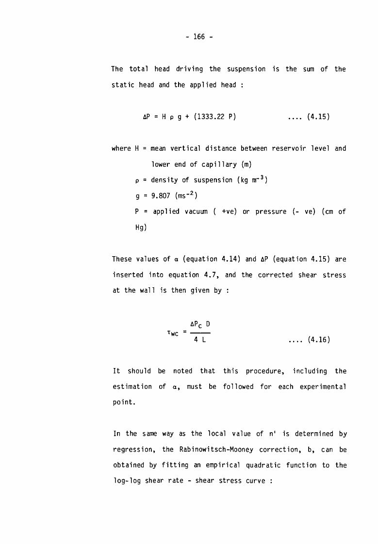
- 166 -

The total head driving the suspension is the sum of the

static head and the applied head :

AP = H p g + (1333.22 P) .... (4.15)

where H = mean vertical distance between reservoir level and

lower end of capillary (m)

p = density of suspension (kg m"3)

g = 9.807 (ms-2)

P = applied vacuum ( +ve) or pressure (- ve) (cm of

Hg)

These values of a (equation 4.14) and AP (equation 4.15) are

inserted into equation 4.7, and the corrected shear stress

at the wall is then given by :

APC DTwc “ -----

4 L

It should be noted that

estimation of a, must be

point.

In the same way as the local value of n' is determined by

regression, the Rabinowitsch-Mooney correction, b, can be

obtained by fitting an empirical quadratic function to the

log-log shear rate - shear stress curve :

.... (4.16)

this procedure, including the

followed for each experimental

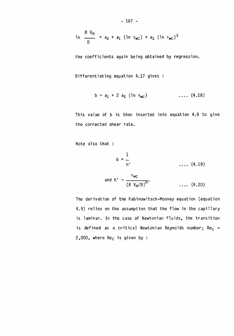
- 167 -

In ---- = a0 + flj (In t w c ) + a£ (In t w c )

D

the coefficients again being obtained by regression.

Differentiating equation 4.17 gives :

b = ax + 2 a£ (In t w c ) ___ (4.18)

This value of b is then inserted into equation 4.9 to give

the corrected shear rate.

Note also that :

1b = —

n ' .... (4.19)

T w r

and K 1 = --------(8 Vm/D)n .... (4.20)

The derivation of the Rabinowitsch-Mooney equation (equation

4.9) relies on the assumption that the flow in the capillary

is laminar. In the case of Newtonian fluids, the transition

is defined as a critical Newtonian Reynolds number; Rec -

2,000, where Rec is given by :

2

- 168 -

P Vm D Rec ~ ------

.... (4.21)

A problem arises in defining Re for non-Newtonian fluids and

suspensions, since by definition n is not constant, but will

vary with Vm . It is possible to determine the transition

by observing the corresponding discontinuity in the x -

dv/dr curve. However, this is tedious since it requires the

plotting of the curve. It is also inefficient since there

will be errors in the calculations resulting from the

departure from laminar flow in the upper part of the curve.

A criterion was therefore sought which would allow those

points obtained under non-laminar conditions to be rapidly

and unambiguously identified.

Metzner and Reed [129] have defined a generalised Reynolds

number based on the laminar friction factor relationship for

Newtonian fluids :

16f = _

Re .... (4.22)

Dn pleading to Re

K' 8 n-1 .... (4.23)

- 169 -

where n = n' for point values, and f is the usual friction

factor. Dodge and Metzner [130] pointed out that the

transition to turbulent flow occurs at increasing values of

Re' for decreasing values of n'. In principle, one could fit

an empirical function

Re'c = f(n)

to the data points given by them. However, only four points

were available, and these gave a misleading linear

relationship. Ryan and Johnson [131] defined a stability

index for which the critical value for turbulence is 808,

and they suggested that the corresponding critical shear

stress at the wall is given by :

Tw critR2 p r2

808* ( n )

__ (4.24)

This is equated to the laminar flow value

3n + 1t w = K

... (4.25)

in order to calculate the maximum flowrate (in terms of r)

at which laminar flow is stable.

Here r is a flow function given by :

r

ttR 3

8 Vr

.... (4.26)4

- 170 -

and $ (n) =.... (4.27)

Equating equations 4.24 and 4.25 gives :

Tw critR2 p r2c

808*(n) = K

3n + 1-i n

.... (4.28)

where rc is given by equation 4.26.

For present purposes it is preferable to define the flow in

terms of a Reynolds number; Metzner and Reed's form,

equation 4.23, is suitable :

P Vm D P Vm DRe'

K S n-1 K re"'1 • 4 n_1.... (4.29)

From equation 4.28 :

2-n rD p rc

4 K

3n + 1 808• _____

*(n) .... (4.30)

Expressing the LHS of equation 4.30 in terms of Re'c

(equation 4.29) :

n2 r 2-n L) p rc= Re c *

4 K 42-n Vm• rc - Re'c •

, 2-n

.... (4.31)

Combining equations 4.30 and 4.31 gives :

3n + 1Re

404 • 4

* (n)

(2-n)

.... (4.32)

- 171

This is the required criterion.

Taking Dodge and Metzner's data [130]# and a single

preliminary result from the present work in which the

transition point was established graphically, this criterion

appears to predict the transition point well :

n Re'c from Experiment Re'c from Equation 4.23

0.4 2800 27200.6 2530 25600.8 2320 23301.0 2100 21001.4 Less than 1840 1710

Equation 4.32 does not appear to hold over all values of n

(= n'), since :

i) It reaches a maximum (~ 2725) at n = 0.37, and starts

to reduce again, and

ii) It approaches Re'c = 0 for n = 0, which does not

conform to Dodge and Metzner's observation [130]

that for n = 0, the f-Re curve is a continuation of

the laminar curve, i.e. turbulent flow is never

reached. However, these facts may be theoretically

reconcilable since for an infinitely pseudoplastic

fluid, viscosities at low shear rates are infinitely

high, and thus Re infinitely low. In any event, the

- 172 -

criterion was satisfactory over the range of

interest, and it was therefore adopted in the present

work.

The calculation of Re'c was incorporated in the computer

program (see Appendix 6). The program was run for each set

of data, and any point for which Re' > Re'c was then

omitted, and the program re-run to give the final flow

curve.

Finally, in discussing the theory of flow in the capillary,

it is worth considering the definition of the local

viscosity at a specific point on the flow curve. The flow

equation for each point is [92,129].

Twc4 n'

3n‘ + 1

n n'

wc (4.33)

Holland [132] gives three versions of the point

viscosity. Perhaps one should select the viscosity which a

particle experiences as it moves relative to the fluid or

suspension. This is :

Twc

8 (dv/dr)wc ....(4.34)

- 173 -

Holland also gives a definition which conforms with the

point value of Re' (equation 4.23) :

n'a = K'

The calculation procedure described above was checked by

preparing flow curves for a number of aqueous' glycerine

solutions using the viscometer. In each case, the density of

the solution was measured using a 50 cm3 specific gravity

bottle, and the temperature of the solution, while in use in

the viscometer, was measured using a thermometer with a

precision of 0.5 °C. The correct Newtonian viscosity for the

solution under these conditions was then determined by

linear interpolation in tables [133] and compared with the

value obtained with the viscometer. The mean discrepancy

between the two was ±536. This was considered satisfactory

since the maximum error in determining the correct viscosity

over the range investigated was estimated at ±4% due to the

cumulative errors in determining density and temperature,

and in interpolation.

The flow curves of four such check calibrations are shown in

Figure 4.6. The points shown are the experimental data, and

the continuous lines represent the true flow curves for the

solutions, assuming the interpolated values of Newtonian

viscosity to be correct. In all cases the agreement is

8 V, -I n -lm

.... (4.35)

- 174 -

sufficient to conclude that the data reduction procedure is

correct (for Newtonian liquids).

4.3.4 Results

Five different media were prepared for measurements with the

capillary viscometer. The media were obtained from the same

feedstock as those utilised in the cyclone experiments

described in Chapter 5, and the sampling procedures used to

prepare sub-samples for analysis are discussed in Chapter 5.

The results of the viscometer measurements are expressed in

terms of the shear rate - shear stress data, obtained from

the data reduction procedure described in Section 4.3.3, and

the corresponding flow curve. The experimental data and

conditions are given in Appendix 8, and the flow curves are

shown in Figures 4.7 - 4.14. The five series of measurements

were as follows :

Series R1 - A milled ferrosilicon sample was obtained from a

commercial "270D" grade [42]# with the +150 ym fraction

removed by dry screening. Measurements were carried out at

three pulp densities, each with three capillary diameters :

2.77; 1.90 and 1.56mm. The principal purpose of these

measurements was to establish the dependency of the observed

flow curve upon capillary diameter, and if possible to

derive a correction for this effect. The results are given

in Appendix 8, and the corresponding flow curves are shown

in Figures 4.7-4.10.

- 175 -

Series R2 - A milled ferrosilicon sample was also obtained

from a commercial 270D grade, but with the +38 ym fraction

removed by screening. Measurements were carried out at a

variety of pulp densities with a single capillary of 1.30mm

diameter. The results are given in Appendix 8, and the

corresponding flow curves are shown in Figure 4.11.

Series R3 - A milled ferrosilicon sample, of nominal size

range -38 +25 ym, was prepared using a Cyclosizer by the

procedure described in Chapter 5. Measurements were carried

out at a variety of pulp densities with a single capillary

of diameter 1.90mm. The results are given in Appendix 8, and

the flow curves in Figure 4.12.

Series R4 - A milled ferrosilicon sample, of nominal size

range -25 +18.6 ym, was prepared using a Cyclosizer.

Measurements were carried out at a variety of pulp densities

with a single capillary of diameter 1.90mm. The results are

given in Appendix 8 and the flow curves in Figure 4.13.

Series R5 - An atomised ferrosilicon sample was obtained

from the commercial "Cyclone 40" grade [42] with the

+150ym fraction removed by dry screening. Measurements were

carried out at two pulp densities with a single capillary of

diameter 1.90mm. The results are shown in Appendix 8 and the

flow curves in Figure 4.14.

- 176 -

In all these cases, the actual size distribution of each

ferrosilicon sample was determined using a Coulter Counter,

according to the procedure described in Chapter 5. The data

are given in Table 4.6, and the distributions are shown

graphically in Figure 4.15. Also included are the

appropriate solid densities, determined by the method

described in Chapter 5.

TABLE 4.6 - SIZE DISTRIBUTIONS OF FERROSILICON SAMPLES R1-R5

Sample

R1 R2 R3 R4 R5

Size Cum. % Size Cum. % Size Cum. % Size Cum. % Size Cum. %

(urn) Finer (ym) Finer (ym) Finer (ym) Finer (ym) Finer

84.7 100.0 60.6 100.0 84.2 100.0 76.4 100.0 105.5 100.067.2 96.2 48.1 100.0 76.5 99.3 60.6 99.4 73.2 95.053.4 91.4 43.7 99.3 66.8 99.1 48.1 99.3 58.1 86.342.4 82.4 38.2 96.2 53.0 98.3 38.2 98.4 46.1 78.438.5 76.3 34.7 91.2 42.1 95.4 30.3 96.3 36.6 66.333.6 70.3 30.3 79.6 38.2 89.0 24.1 79.9 29.0 55.926.7 53.1 24.1 58.2 33.4 70.2 19.1 43.1 23.1 45.021.2 37.7 19.1 39.9 26.5 23.8 15.2 4.6 18.3 34.116.8 25.8 15.2 25.1 21.0 7.1 12.0 4.8 14.5 25.313.3 16.7 12.0 13.0 16.7 5.1 9.6 3.6 11.5 17.810.6 10.3 9.6 3.6 13.3 3.9 7.6 2.7 9.2 11.48.4 5.8 7.6 0.3 10.5 3.0 6.0 1.6 8.3 9.76.7 2.7 8.4 0.9 5.5 1.2 7.3 6.35.3 1.5

Solids Density 6782 kg nr3 Sol ids Density6846 kg m

SHEA

R ST

RESS

(N

m-2

) —>

SHEA

R ST

RESS

(Nm

~2) —

^

- 177 -

SHEAR RATE ( s - 11 — ►

/M7f (s-h

- 1 7 8 -

FIGURE 4 8 FLOW CURVES FOR SERIES RIB. PULP DENSITY m o i 10 kam'3

FIGURE 1.9 FLOW CURVES FOR SERIES RIC PULP DENSITY 2390 t 10 kam'3

SHEAR RATE Is-1) — }

SHEAR STRESS (Nm'2) -

-^

SHEAR STRESS ( Nm~2)

- 179 -

SHEAR RATE (s'1) — ►

SHEAR RATE ( s ' 1) ---^

0 SOOO

SHEAR STRESS t

Nnr2

) —

}

SHEAR STRESS (Nm'2>

180 -

SHEAR RATE (s'1) — ^

SHEAR RATE (s'1)— ►

S H E A R R A T E ( S ' 1 ) — ►

F I G U R E U . 1 S S I Z E D I S T R I B U T I O N S O F F E R R O S / L / C O N S A M P L E S U S E D I N V I S C O M E T E R M E A S U R E M E N T S

tC U M W T % F I N E R

Discussion of Results

4.3.5.1 The Influence of Capillary Diameter

Although the data reduction procedure described in

Section 4.3.3 incorporates the usual shear rate and

shear stress corrections, it does not allow for any

effect due to changes in capillary diameter. It is

clear from Figures 4.7 - 4.9 that identical samples

processed in capillaries of different diameters

produce different flow curves. The apparent

viscosity (defined by equation 4.34) increases with

capillary diameter, to a significant degree. This

effect can be attributed to the migration of

particles in the flowing suspension away from the

capillary walls (where flow is slow) towards the

centre (where flow is rapid). This tends to deplete

the suspension of particles at the wall, the point

at which the flow curve calculations are made, thus

causing the local (measured) viscosity to drop. The

effect is less severe for capillaries of larger

diameter, in which the flow profile across the

diameter is less pronounced. (A similar migration

effect occurs in concentric cylinder viscometers

with suspensions, due to the centrifugal forces

present in curvilinear flow fields [134]).

- 183 -

Whorlow [135] ancj Sarmiento et al [101] have

drawn attention to this problem. Sarmiento et al

developed a correction for the shear rate term to

allow for the resulting dependence of pressure drop

upon capillary diameter. This was :

/8 Vm^ 3

V D J e \ D /„ d (3+1) .... (4.36)

(3 is used here in preference to the symbol, a,

used by the authors).

/8 Vm\ 13 is the gradient of a plot of ( ---- ] vs ---- -\ o j w D(a+1)

where a is chosen to give maximum linearity of the

plot (0.5 < a < 1.0). This correction effectively

gives the flowrate (or mean velocity) in the

absence of a diameter effect, i.e. for an

infinitely wide capillary.

Test series R1 provides data with which this

correction can be tested. Preliminary plotting

suggested that a = 1 (as Ref. 10 proposes). A

smooth curve was then fitted by spline functions to

the (uncorrected)w

vs. (corrected) t w data

from the nine sets of measurements. From these, the

values of/8 Vm \ for certain fixed values of tw

D w

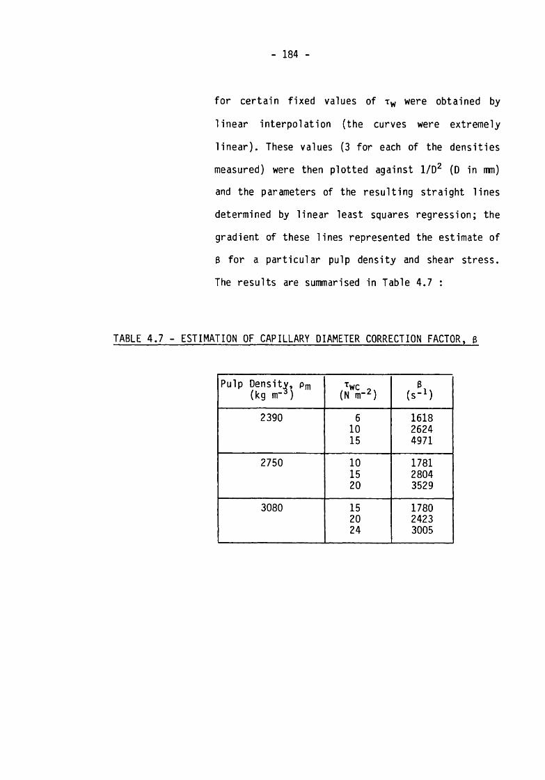
- 184 -

for certain fixed values of t w were obtained by

linear interpolation (the curves were extremely

linear). These values (3 for each of the densities

measured) were then plotted against 1/D2 (D in mm)

and the parameters of the resulting straight lines

determined by linear least squares regression; the

gradient of these lines represented the estimate of

0 for a particular pulp density and shear stress.

The results are summarised in Table 4.7 :

TABLE 4.7 - ESTIMATION OF CAPILLARY DIAMETER CORRECTION FACTOR, 0

Pulp Density, pm (kg nr3 ) /Twc (N m-2)

0(s-1)

2390 6 161810 262415 4971

2750 10 178115 280420 3529

3080 15 178020 242324 3005

- 185

Clearly, 3 depends both upon pulp density and local

shear stress. Normally, a value of 3 would be

calculated separately for every experimental value

of Twc However in the present case it

was decided to attempt to provide a reliable,

empirical relation for 3 in terms of both density

and shear stress. The following expression was

obtained by multiple linear regression :

1.127 -3.6883 = 5340 • T y • Pfp .... (4.37)

Based on 9 points, the coefficient of multiple

determination, R2, was 0.978, which indicates a

good fit. The form of equations 4.36 and 4.37

demonstrates that the magnitude of the correction

for shear rate increases with shear stress (i.e.

with shear rate itself, or flowrate) and decreases

with medium density. Both these trends conform with

the view that the diameter effect is caused by

migration of particles to the centre, since this

effect should, by hydrodynamic reasoning, increase

with flow and decrease with solids concentration.

Using equation 4.37, the correction was calculated

for each experimental point in series R1A, RIB and

R1C (the correction being applied before the

Rabinowitsch-Mooney correction in the computational

sequence), and the resulting corrected flow curve

plotted for each capillary within each density

- 186 -

series. The corrected values of shear rate are

included in Appendix 8, and the corrected curves

are shown in Figures 4.7 - 4.9 for series R1A - R1C

respectively, together with the original

(uncorrected) flow curves for the individual

capillaries. It is clear that application of the

diameter correction has succeeded in reducing the

curves for the individual capillaries to a single

curve, for each medium density. Bearing in mind the

error accumulated in the lengthy procedure by which

equation 4.37 was estimated, there is remarkably

little scatter of points about the corrected

curves. (Interestingly, the scatter increases with

medium density).

The curves show that, if the correction is

neglected, there is a tendency to underestimate the

point viscosity. The magnitude of the correction is

quite large, as can be seen by comparing the

corrected and uncorrected values of shear rate for

series R1A, RIB and R1C in Appendix 8; the

correction to be subtracted from the observed shear

rate can exceed 50% for the smallest capillary.

In view of the time required to perform rheological

measurements in a number of capillaries in order to

estimate the diameter correction, this procedure

was not carried out in the subsequent testwork.

- 187 -

Since the purpose was to observe trends, and draw

qualitative, comparative conclusions, all the

subsequent measurements were made using a single

(1.90mm) capillary. Because the migration effect,

which necessitates the correction, is essentially

hydrodynamic in nature, it is probable that the

magnitude of the correction will alter with both

particle shape and size distribution. Since the

data to be discussed below were obtained with media

which differed in either or both these

characteristics from the sample utilised in Series

Rl, no attempt was made to apply equation 4.37 to

these data. The flow curves presented in Figures

4.10 - 4.14 are therefore uncorrected for the

diameter effect.

4.3.5.2 The Rheological Nature of Ferrosilicon Suspensions

The general rheological behaviour of the

ferrosilicon media studied in this work can be

inferred by inspection of the flow curves (Figures

4.7 - 4.14). Three important properties are

immediately apparent :

i) They are relatively linear over large

portions of the curve; certainly there are

no extreme non-linearities.

- 188 -

ii) There is a slight tendency to dilatancy,

particularly at the higher shear rates.

Figures 4.7 - 4.9 suggest that this tendency

is more apparent when the diameter

correction is applied.

iii) All the media appear to exhibit a yield

stress (indicated by extrapolation of the

flow curve to the shear stress axis - the

dashed lines in Figures 4.10 - 4.14).

Qualitative comparison with the data in the

literature discussed in Section 2.3.3 is difficult

because the media differed in many important

characteristics, such as size distribution and

solids concentration. However the general shape of

the curves is similar to those reported by Smith

[114] (e.g. Figure 2.10) and Collins [65]# and

conforms quite well to the general scheme of Cheng

[107] (e.g. Figure 2.9). The pseudoplasticity

reported by Smith [114] only appeared at high

concentrations, which were not attained in the

present work. As discussed in Section 2.3.3, the

conclusions reached by Lilge et al [56,57] are

almost certainly incorrect because of their failure

to recognise the existence of a yield stress, which

introduced a systematic error into their viscosity

estimates (equation 2.36).

- 189 -

The characteristics of the flow curves suggest a

functional relationship of the form :

t = t 0 + K Sn ___ (4.38)

which is a combination of the Bingham plastic and

power law expressions. K is a "consistency index"

whose units depend upon the value of n; it cannot

therefore be used to define a characteristic

viscosity, as can the plastic viscosity of a pure

Bingham plastic.

The suitability of equation 4.38 in describing the

flow curves obtained in the present work was tested

by fitting it to data from Series R3, specifically

tests R3/2 and R3/5. The equation has to be fitted by

non-linear least squares regression; this was done

using a modified Gauss-Newton algorithm available in

the NAG computer subroutine library [147]. it was

found that the problem had to be scaled carefully in

order to ensure successful convergence of the

estimation routine, and the shear rates were

therefore all divided by 103 before the fitting

procedure. The estimated parameters, and the shear

stresses predicted from the observed shear rates, are

given in Table 4.8 :

- 190 -

TABLE 4.8 - FIT OF EQUATION 4.38 TO FLOW CURVE DATA OF TESTS

R3/2 AND R3/5

R3/2 R3/5

Shear Rate Shear Stress (Nm-2) Shear Rate Shear Stress (Nm“2)(s_1) (s-1)

Observed Predicted Observed Predicted

1016 5.87 5.69 691 9.48 9.912031 9.01 8.94 977 11.83 11.832670 11.40 11.26 1206 14.17 13.623196 13.40 13.30 1571 17.25 16.933781 15.46 15.68 1820 19.45 19.464256 17.51 17.69 2133 22.84 22.954959 20.97 20.78 2488 26.69 27.27

3288 38.63 38.37

To 3.420 Nnr‘i

to 7.284 Nnr'?

K = 3.124 x 10"H K = 8.287 x IQ"5n = 1.284 n 1.585

The agreement between the observed and predicted

shear stresses is excellent, and it is concluded that

equation 4.38 is a satisfactory model for the flow

curves.

As noted in Sections 2.3.3 and 4.3.3, an apparent

point viscosity for a non-Newtonian medium is perhaps

best defined as the ratio of shear stress to shear

rate at a particular shear rate (or stress). This is

probably the local "viscos ity" experienced by a

particle moving relative to the medium as a

consequence of the shear stress imposed by the

particle in its motion :

Ti^ai = —

Si .... (2.30)

- 191

In terms of equation 4.38, nai can be defined as :

T o . n"l nai - ~— + K S-j

Si .... (4.39)

The relationship between apparent (point) viscosity

and shear rate for tests R3/2 and R3/5, obtained from

application of equation 4.39, is shown in Figure

4.16. It is clear that the apparent viscosity at low

shear rates decreases rapidly with increase in shear

rate, to a minimum value, before rising slowly. At

the low shear rates, the value of the apparent

viscosity is dominated by the t q/S-j term, rising

to infinity at zero shear rate. For these dilatant

materials (n > 1), the apparent viscosity reaches a

minimum at a shear rate defined by :

9

S = r t° i 1/n

LK(n-l)_ .... (4.40)

At higher shear rates, the value of apparent

viscosity becomes dominated by the K S-jn“l term.

The value of the minimum viscosity can be deduced

from equations 4.39 and 4.40 as :

n

n-1

(1-1/n) 1/n^a (min) = To • [K(n-1)] *

.... (4.41)

19ZFIGURE 4.76 APPARENT (POINT) VISCOSITY VS SHEAR RATE FOR

TESTS R3/2 AND R3/S( Determ ined from equation 439 J

SHEAR RATE (s-1) —

55

|K-§Ct

o

§I§

FIGURE U 17 APPARENT VISCOSITY VS VOLUME CONCENTRAVON

- 193 -

Figure 4.16, and a similar analysis of the

remainder of the data, demonstrates that this

minimum value increases, and occurs at a

progressively lower shear rate, with increase in

solids concentration. It might be regarded as a

characteristic viscosity of the medium.

The general forms of the curves in Figure 4.16 are

very similar to those presented by Govier et al

[56] and Collins [55] for ferrosilicon

suspensions.

It can be shown from the data reported in Chapter 5

that the shear rates prevailing in the 100mm

cyclone utilised in the experiments were probably

in the approximate range 102 - 103 s_1. Although

few results were available from the capillary

viscometer below a shear rate of about 200 s"1,

inspection of the flow curves suggested that most

of the media investigated did not depart

significantly from the true Bingham plastic

behaviour below a shear rate of 103 s"1. The

dilatant behaviour emerged only at higher shear

rate and high pulp densities (e.g. Figure 4.7).

- 194 -

4.3.5.3 The Influence of Solids Concentration

It is clear from Figures 4.10 - 4.14 that both

point viscosity and yield stress increase with pulp

density (i.e. with solids concentration). In order

to determine the general form of the concentration-

viscosity relationship, point viscosities were

estimated for test series R1-R5 at a shear rate of

103 s"1 by fitting equation 4.38 to each data set,

and substituting S = 103 in equation 4.39.

In comparing point viscosities at various solids

concentrations, a further correction is necessary

in respect of temperature. As noted in Section

2.3.3, nearly all the published correlations are of

the form :

nanr ~ — = f (Cy)

ns .... (2.35)

where ns is the viscosity of the suspending

liquid, in this case water. If the values of na

are determined at different temperatures,

therefore, they can be corrected to a single

temperature using the expression :

- 195 -

1 st'"at = at' • ---

n$t •••• (4.42)

where t = standard temperature.

t'= temperature at which measurement was made.

(see Appendix 8 and Figures 4.10 - 4.14).

In the present work, the results were standardised

to t = 20 °C, and nst' and fist were determined

from published tables [133], The solids volume

concentration corresponding to each measured pulp

density was determined from the formula :

Pm “ PI Cv = -------

PS - PI --- (4.43)

where pm = medium density (kg nr3)

ps = solids density (kg m-3) - see Table 4.6

p-j = liquid density = 1,000 kg nr3

The results are given in Table 4.9 and plotted in

Figure 4.17.

- 196 -

TABLE 4.9 - VISCOSITY VS. SOLIDS CONCENTRATION FOR SERIES R1-R5

TestNumber

Pulp Density (kg nr3 )

Sol idsConcentration

(v/v)

Point Viscosity at 103 s"1 Corrected to 20 °C (Nsitt2 x 103)

R1C/2 2390 0.240 6.0R1B/2 2740 0.301 8.7R1A/2 3080 0.360 14.5

R2/1 1960 0.166 3.3R2/2 2195 0.207 4.2R2/3 2455 0.252 5.4R2/4 2660 0.287 7.1R2/5 2755 0.304 8.0R2/6 2895 0.328 13.3R2/7 3020 0.349 17.1

R3/1 2390 0.240 4.5R3/2 2620 0.280 5.4R3/3 2750 0.303 5.5R3/4 2990 0.344 7.9R3/5 3180 0.377 10.7

R4/1 2150 0.199 3.7R4/2 2770 0.306 9.4R4/3 2990 0.344 14.2R4/4 3120 0.367 18.0

R5/1 2730 0.296 5.1R5/2 3070 0.354 8.2

It is clear from Figure 4.17 that the relationship

conforms to the general trend reported in the

literature - a relatively linear, slow increase in

viscosity at the low concentrations, followed by a

rapid increase above a certain solids

concentration, approximately 20% v/v. As noted in

Chapter 3, Ferrini et al [96] reported that a

modified Eiler's equation (equation 2.33) described

- 197 -

viscosity - concentration data from, among others,

a magnetite suspension. This equation was applied

to all the present data by least squares regression

of equation 2.33 in its linear form :

1 Hi 1

Cy 2('Hy'0*{> - l) Cym .... (4.44)

The best fit was obtained with series R4.

The parameter estimates for this fit were

ni = 1.832

C Yfu = 0.546

with R2 = 0.9998, indicating a very good fit.

The quality of the fit can be further assessed

visually by reference to Figure 4.18, in which the

experimental data are plotted together with the

fitted curve. Again, the fit is seen to be

excellent.

Adequate fits were obtained with the other series,

but it was found that the extreme non-linearity of

the function caused the parameter estimates to be

significantly influenced by single points at the

upper and lower extremes of the curve.

- 198 -

FIGURE 4.18

FIT OF MODIFIED EILER'S EQUATION (eon. 2.33) TO DATA OF SERIES R4

FIGURE t 19 Size FREquenCY DISTRIBUTIONS CF SAMPLES R1.R?ANO Rl

Frequency ( vt.% )

Rorticte size (^pm)

- 199 -

4.3.5.4 The Influence of Particle Size

The viscosity-concentration curves of Figure 4.17

can be used to assess the influence of particle

size on suspension viscosity; the size

distributions of the various media are given in

Table 4.6 and Figure 4.15.

Series R3 and R4 were prepared specifically to

investigate the effect of particle size. They

represent Cyclosizer products with nominal size

ranges -38 +25 m and -25 +18.6 ym respectively.

Figure 4.17 shows that, for a given concentration,

sample R4 has a significantly higher viscosity than

R3. This confirms that viscosity increases with

decreasing particle size, a conclusion which

conforms with the literature's view on dense medium

suspensions [42,66,71,112,114].

A comparison of R1 and R2 is instructive. At the

lower concentration, R1 exhibits higher viscosities

than R2, whereas at the higher concentrations

(above about 31% v/v) the trend is reversed.

Inspection of Figure 4.19, in which the size

distributions of these samples are shown in

frequency form (interpolated from Figure 4.15),

shows that although both distributions peak at

- 2 0 0 -

about the same size, R1 has a wider distribution

than R2, and is thus less rich in the fine sizes

around their common mode. This suggests that the

relative influence of the fines may depend upon

the prevailing solids concentration.

Series R4 exhibits slightly lower viscosities than

either R1 or R2 at the low concentrations, but is

intermediate between the two at the high

concentrations. Figure 4.19 shows that R4 peaks at

about the same size as R1 and R2, but is much

richer in this size, having a very narrow size

distribution. Accordingly, it is depleted in the

ultra-fines (-12ym).

These trends suggest that, although fine media

generally exhibit higher viscosities than coarse

media, the form of the size distribution is

important in defining the viscosity-concentration

relationship. Where the mode or mean size of the

distribution is similar, the viscosity tends to be

determined by the relative frequencies of fines and

ultra-fines. Clarke [97] and Datta [69] have

both suggested that the width of the particle size

distribution influences rheology.

- 201

4.3.5.5 The Influence of Particle Shape

Sample R5 was an atomised ferrosilicon of rounded

shape, whereas samples R1-R4 were of irregular

shape. Photomicrographs of the two basic shapes are

presented in Chapter 5. Figure 4.15 shows that

sample R5 had a similar modal size to samples R1

and R2, but with a rather wider distribution.

Figure 4.17, however, shows that R5 exhibited

significantly lower viscosities than either R1 or

R2; indeed, R5 had the lowest viscosities of any of

the media tested. One may therefore conclude that

media of rounder particle shape exhibit lower

viscosities than those of irregular shape, a

conclusion which conforms with the views of the

literature [42,56,97,112,114]#

4.3.6 Summary and Conclusions

This work has shown that it is possible to obtain meaningful

rheological measurements from unstable ferrosilicon

suspensions, using a simple capillary viscometer. The data

were analysed using a computer program which incorporated

all the usual corrections, together with a new criterion for

the transition from laminar to turbulent flow in the

capillary (equation 4.32). It has been shown that the

correction for capillary diameter proposed by Sarmiento et

al [101] is effective in producing absolute flow curves,

- 202

independent of capillary diameter, for the ferrosilicon

media investigated. The correction is a quantitative

function of shear stress and pulp density (equation 4.37).

The form of this function tends to confirm the view that the

necessity for the correction is attributable to the

migration of particles from the wall to the centre of the

capillary; since this is a hydrodynamic effect, it is

probable that the magnitude of the correction will also be

dependent upon particle size and shape, although this

hypothesis was not tested.

The form of the flow curves obtained indicated that the

media behaved as Bingham plastics at the lower shear rates

(including the range of shear likely to be encountered in a

DM cyclone), tending to dilatancy at higher shear rates.

The entire curve was well described in all cases by a

function which incorporates the features of both Bingham

plastic and power law behaviour :

t = t 0 + K Sn .... (4.38)

The apparent (point) viscosity at a given shear rate can be

defined as :

To . 1-1 nai - — + K Si

Si .... (4.39)

For such dilatant materials (n > 1), the apparent viscosity

is thus high at low shear rates, dropping to a minimum at a

shear rate defined by :

- 203 -

S =To

1/n

K ( n - l ) .... (4.40)

and then increasing slowly with increasing shear rate

(Figure 4.16).

The value of the minimum apparent viscosity can be deduced

from equations 4.39 and 4.40 as :

(1-1/n) 1/n^a (min) = To * [K(n-1)] . n

n-1 -1 .... (4.41)

na (min) might be regarded as a characteristic viscosity

of the medium.

The results showed that both yield stress and point

viscosity increased with solids concentration. A modified

Eiler's equation (equation 2.33) described the

viscosity-concentration relationship satisfactorily.

By inspecting the viscosity-concentration curves for various

media, it was concluded that viscosity increases with

fineness of particle size and with irregularity of particle

shape. The form of the particle size distribution also

influences viscosity.

- 204 -

CHAPTER 5

THE PERFORMANCE OF A 100MM DENSE MEDIUM CYCLONE

WITH FERROSILICON MEDIA

5.1 Introduction and Objectives

The purpose of this, the final experimental phase of the research

programme, was to observe the performance of a real dense medium

cyclone utilising real ferrosilicon media (as characterised in Chapter

4) over a range of operating conditions. By monitoring closely both

the density separation and the corresponding behaviour of the medium

in these experiments, it was hoped to be able to establish the

dependency of one upon the other. By interpreting these experimental

observations in terms of the model developed in Chapter 3 (modified

where appropriate), the performance of dense medium cyclones could

then be described in a concise manner, which would both be useful in a

practical sense and would elucidate the general mechanism by which the

density separation was achieved.

In order to satisfy these objectives, it was necessary to set up an

experimental cyclone circuit in which the cyclone could be operated

with a variety of media, corresponding to different sedimentation and

rheological characteristics, at different flowrates. In each case, the

intrinsic density separation, such as would have prevailed had the

cyclone been treating a real ore (at low tonnage), was monitored using

a novel technique. The cyclone feed and products were sampled and

- 205 -

analysed, and by suitable data reduction the cyclone's performance as

an agent of segregation and classification of the medium was

determined. By relating these two aspects, a general theory of DM

cyclone operation was developed.

This chapter describes the experimental techniques, presents the

results, and discusses them in the context of the general framework

established in Chapters 2, 3 and 4.

5.2 Experimental Details

5.2.1 Cyclone and Test Circuit

In choosing a cyclone for the experimental work, a

compromise was sought between the attainment of results of

practical interest and the constraints involved in

extracting reliable data from an operating plant. The former

favours large, high-throughput units, which generally

utilise relatively coarse media. The latter necessitates

small, low-throughput units which can be easily managed, and

which demand fine media in order to restrict the degree of

medium segregation in the cyclone at the high centrifugal

forces prevailing. In the present work, a cyclone of 100mm

diameter was selected, after preliminary experiments with

several alternatives, and the appropriate circuit was

constructed around it.

- 206 -

A dimensioned section of the cyclone is shown in Figure

5.1. It was constructed of moulded epoxy resin, and had the

facility of a range of interchangeable spigots. However,

since the purpose of the present work was to monitor the

cyclone performance at a fixed geometry, in only one of the

45 experiments was the spigot diameter altered. No changes

were made to the vortex finder. The cyclone had a standard

20 ° included cone angle, with a circular tangentially-

mounted inlet flush with the roof. Preliminary experiments

showed that the selected configuration provided separations

of "normal" characteristics, in respect of overflow-

underflow density differentials and the difference between

650 and pf, when operated under "normal" conditions. In

making this judgement, the author's previously reported

results with a production-scale DM cyclone [4] were taken

as the yardstick.

A flowsheet of the test circuit is shown in Figure 5.2, and

photographs of the apparatus are given in Plates 5.1 and

5.2.

Three measuring instruments were incorporated into the

circuit. The density of the feed medium was measured with a

Kay Ray Model 3600F nucleonic density gauge, using a Ce 137

source of 100 mCi activity. The gauge was mounted on the

25.4mm ID delivery pipe (see Plate 5.1). After repeated

calibrations, it was found that the output of the gauge

tended to drift, and this was attributed by the suppliers to

errors incurred as a result of the low radiation attenuation

obtained with the 25.4mm (1") pipe. The insertion of a

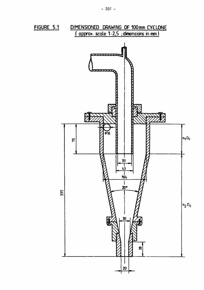
- 207 -

FIGURE J . DIM ENSIONED ORAWINS OF 100mm C YC LO N E ( approx, scale 1 :2,5 ; dimensions in mm)

FIGURE 5.2 FLOWSHEET FOR 100mm CYCLONE TEST RIGTO ATMOSPHERE

K E Y1 100mm x 20° CYCLONE2 M ANUAL SAMPLERS3 SUMP4 1 H VACSEAL CENTRIFUGAL PUMP WTO EXFANDING PULLEY (VARIABLE SPEED)5 NUCLEONIC DENSITY GAUGE6 ULTRASONIC FLOWMETER WITH DIGITAL INDICATOR7 PRESSURE TRANSDUCER

<8> B A LL VALVEX SAUNDERS VALVE

- 209 -

PLATE 5.2 - Close-up of Cyclone. Note (From Left to Right on Cyclone

Feed Pipe) : Flowmeter Transducers, Ball Valves and Pressure Transducer.

Exterior Shape of Cyclone due to Epoxy Resin Casting Requirements.

- 2 1 0 -

'Z'-section in the pipe was recommended, with the gauge then

mounted vertically instead of horizontally so as to increase

the attenuation. However this was not implemented because of

inadequate space and the increased head which would be

imposed on the pump. Accordingly the gauge was used only to

obtain approximate densities (while running the circuit up

to the correct test density), and the test density was

always obtained using a density balance and a sample of the

feed.

The flowrate of medium to the cyclone was measured using a

Clampitron Series 240 ultrasonic flowmeter, with digital

readout. The two transducers of this instrument were

attached via a suitable sonic medium to opposite sides of

the 25.4mm plastic feed pipe (see Plate 5.2). Although

factory-calibrated for water, the instrument had to be

calibrated for the media used in the testwork, and this was

done according to the manufacturers' instructions [136],

The readout was given in Imperial GPM, with a precision of

0.1 GPM (0.45 £/min), less than 1 % of the mean flows

encountered in the testwork.

The inlet pressure to the cyclone, approximating to the

pressure drop across the cyclone, was measured using a Druck

DPI 201 digital pressure indicator with a range of 0-50 PSI

and a precision of 0.1 PSI (less than 1% of the mean

pressure encountered in the testwork). Although factory

calibrated, the transducer was tested before and after the

- 211

testwork using a dead-weight tester, and found to be reading

correctly. The transducer was connected to the cyclone feed

pipe via a brass section inserted into the line about 10cm

upstream of the cyclone inlet. A 5nm screw tapping was

drilled into the brass section, into which was screwed a

brass insert containing a protective steel diaphragm

(contacting the medium), followed by a column of hydraulic

fluid, into which the pressure transducer was fitted. All

connections were fixed securely with the appropriate

fittings to ensure no loss of pressure transmission.

5.2.2 Experimental Design, and Test Procedure

The testwork was originally designed as a two-level

factorial experiment to investigate the influence of three

primary operating variables upon the density separation :

ferrosilicon size distribution, medium density, and

flowrate. Most of the experiments were conducted with milled

(irregular shaped) ferrosilicon, but some later tests were

added to investigate the influence of atomised (spherical

shaped) ferrosilicon, as well as the viscosity of the

carrier medium and the spigot diameter. In the event it was

found to be impossible to control either the ferrosilicon

size distribution or the flowrate range sufficiently

accurately to meet the requirements of a rigorous factorial

analysis, and so the factorial design was utilised only as a

general experimental framework. As in the case of the work

described in Chapter 3, regression analysis was used to

evaluate the results of the experiments.

- 212 -

The general arrangement of the tests was as follows :

Series FI : A factorial design, investigating four levels of

medium density, each at two flowrates, using milled FeSi.

Test F1/6B was added as an attempted replicate of F1/6A, but

the results subsequently showed the FeSi size distribution

to be different.

Series F2 : A factorial design as for Series FI, but with a

slightly coarser milled FeSi. Test F2/2A was an attempted

replicate of F2/2, but the results subsequently showed the

feed densities to have differed.

Series F3 : A sub-set of the basic factorial design, with

much finer FeSi. In the event, only tests F3/3 and F3/7

achieved the necessary fineness.

Series F4 : A sub-set of the basic factorial design using a

coarse, atomised FeSi. Because of the low stability of the

medium, no density separation was achieved.

Series F5 : Tests F5/1 - F5/6 comprised a factorial design

with feed density at three levels and flowrate at two

levels, using a fine atomised FeSi. Test F5/7 was a repeat

of F5/6 but with an enlarged (30mm) spigot. Tests F5/8 and

F5/9 were full replicates of F5/6, and tests F5/10-F5/12

were repeats of F5/6 but with increasing proportions of

glycerine added to the medium.

- 213 -

Series F6 : A study of the behaviour of a very fine milled

FeSi at various feed densities but at a constant flowrate.

Test F6/6 was carried out at a very low feed density to

examine the classification behaviour of the medium, and no

density separation was monitored.

A total of 45 tests was conducted, 28 with milled FeSi and

17 with atomised.

The approximate operating ranges for the testwork were :

flowrate 55-110 1 min-1; feed density 2000-3000 kgm-3. A

spray discharge at the apex was observed for all the tests.

The feed, overflow and underflow medium products were

sampled for both pulp density and ferrosilicon size

distribution. The feed pulp density was measured, while the

circuit was in by-pass mode, by filling a 1-litre measuring

can and weighing this on a spring balance. The balance was

calibrated directly in SG units, and the calibration was

repeatedly checked using water. The feed density was

measured before and after each test, and the mean taken. The

overflow and underflow densities were obtained by running

these products into 2-litre tared measuring cyclinders, and

weighing. The density was then obtained directly as mass

7 volume. These samples were also used to estimate the

volume flowrates of these products, by timing the flow into

the cylinders using an electronic stopwatch. Although the

precision of the stopwatch was 0.01 seconds, the manual

response time was estimated at 0.1 seconds, about 5% of the

- 214 -

typical time periods measured (1.5-3 seconds). The product

flows are thus accurate only to about 5%.

The feed, overflow and underflow media were sampled for

particle size analysis using manual samplers, as sketched in

Figure 5.3. These hand-held samplers were passed repeatedly

across the appropriate stream until approximately 0.2 litres

of medium had been collected. These samples were then sub­

sampled and analysed for size distribution by the methods

described in section 5.2.4.

A similar procedure was used to obtain a sample of the feed

medium for measurement in the capillary viscometer, using

the apparatus and method described in section 4.3.

The instantaneous contents of the cyclone were collected at

the conclusion of each test by rapidly switching the

ball-valves (Figure 5.2) to by-pass the medium, and

simultaneously placing a manual sampler and measuring

cylinder underneath the cyclone to collect the draining

contents. This sample was analysed for pulp density and size

distribution.

The density separation prevailing during each experiment was

determined using density tracers. These consisted of cubic

particles made of cast epoxy resin with suitable fillers

added to elevate the density. A total of eleven densities

was manufactured, in the range 2500-3500 kg nr3 in

- 215 -

4FLOW STREAM

FIGURE 5.3 M ANUAL SAM PLER FOR CYCLONE MEDIUM PRODUCTS

- 216 -

increments of approximately 100 kg m"3, each in two sizes (2

and 4mm). Each density, made to a precision of about 10 kg

m~3, was colour-coded for easy identification. The density

separation was monitored by adding 100 of each size and

density of tracer, collecting the products, and hand-sorting

them by colour (density). It was then a simple matter to

construct the Tromp curves for the separation by computing

directly the proportion of tracers of each density reporting

to the underflow.

This method had three advantages for the task in hand :

1. The results were independent of "ore" feedrate and

density distribution, since the number of "ore"

particles added was very small and therefore not

expected to influence the intrinsic separation.

2. The method was quick, convenient and accurate.

3. The Tromp curves could be plotted at specific, known

densities and not at the mean of density intervals as

is the case for conventional heavy liquids analysis.

The tracers were manufactured commercially to the author's

specifications. The actual densities were checked by the

author using the method described in section 5.2.5.

The procedure followed in each test was as follows :

- 217 -

1. The sump was partly filled with tap water, and the

pump started with the by-pass valve open.

2. The appropriate ferrosilicon was added slowly until

the nucleonic gauge showed the correct density. The

density was then measured accurately using the

balance, and adjusted to the desired value by

addition of water or ferrosilicon as appropriate. Two

samples were taken (one for size analysis and one for

rheological measurement), and the value of density

recorded.

3. The by-pass valve was closed and the medium allowed

to feed the cyclone. The pump speed was then adjusted

until the ultrasonic flowmeter displayed the desired

flowrate. This value was recorded, together with the

indicated pressure.

4. The tracers were then introduced to the sump over a

period of about 30 seconds, and recovered from the

cyclone products via 1mm aperture sieves.

5. The feed density and flowrate were checked, and

adjusted if necessary. The cyclone products were then

sampled for density and particle size distribution,

as described earlier.

- 218 -

6. The cyclone was then switched out by adjusting the

ball valves, and a sample of the cyclone contents was

collected using the manual sampler. A 1mm aperture

sieve was used to remove tracers that had remained in

the cyclone for the 2-3 minutes elapsing between

their introduction and this point in the procedure.

7. A corrosion inhibitor (sodium nitrite) was then added

to the medium, and the drain valve opened to direct

the medium into plastic storage vessels. The

temperature of the medium was noted.

8. The circuit was then thoroughly washed with water,

and all washings collected in the storage vessels.

9. The medium and washings were allowed to stand for

several hours (usually overnight), and then the

supernatant water was decanted by syphoning, so that

the thickened medium could be re-used.

5.2.3 The Ferrosilicon

The commercially available feed stock from which was taken

the ferrosilicon used in these experiments was identical to

that used in the rheological and stability measurements

described in Chapter 4. The milled ferrosilicon was obtained

from Samancor in South Africa, and the atomised ferrosilicon

from Knapsack in West Germany. The specifications of these

materials have been discussed elsewhere [4 2 ].

- 219 -

Photomicrographs of the milled and atomised ferrosi1 icon,

dry-screened to -45 +38 ym, are shown in Plates 5.3 and 5.4

respectively. The difference in particle shape is clearly

apparent.

The material was obtained in a variety of commercial

grades. These grades are defined principally by size

distribution [42]. For the present work, some of the

batches were utilised as received, and others were pre­

classified in the cyclone to provide finer samples for the

experiments. The size distribution of the feed to each test

was measured (as noted above), and these data, smoothed by

the methods described in section 5.3, were therefore used to

characterise each medium, rather than the manufacturers'

size specifications.

The mean surface area of certain ferrosi1 icon samples was

determined using a Monosorb Surface Area Analyser

(Quantachrome Corp., Greenvale, NY). This instrument

utilises the B.E.T. relation, assuming that the intercept of

the plot of l/XmC is zero (where Xm = weight of

adsorbate required for a monolayer, and C is an instrument

constant). Typical values of measured surface area were as

follows :

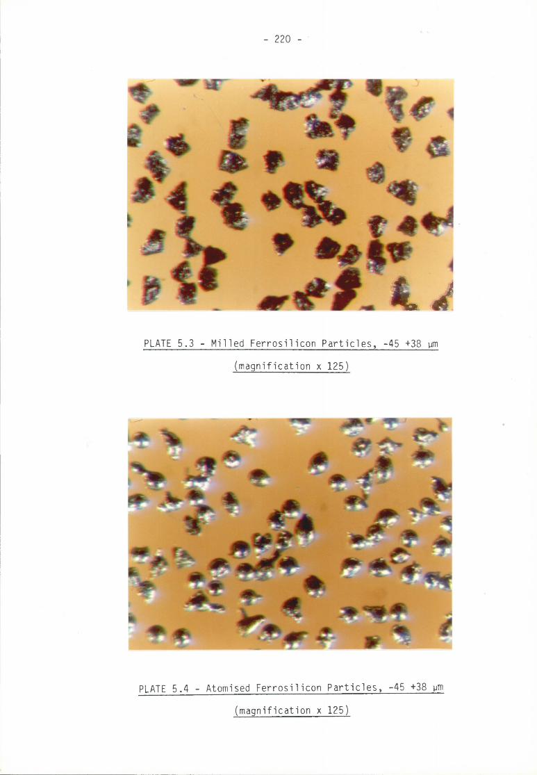
- 220 -

4 JtPLATE 5.3 - Milled Ferrosi1 icon Particles, -45 +38 ym

(magnification x 125)

PLATE 5.4 - Atomised Ferrosi1 icon Particles, -45 +38 ym

(magnification x 125)

- 221

Milled Ferrosilicon

-38 +25 pm 1.41 m 2 g- 1

-25 +18.6 pm 2.07 m 2 g-1

-18.6 +13.6 pm 3.17 m 2 g- 1

-13.6 + 9.6 pm 4.97 m 2 g-1

- 9.6 + 7.9 pm 5.63 m 2 g- 1

Series R1 from viscometry

(see Table 4.6) 4.03 m2 g-1

Series R2 from viscometry

(see Table 4.6) 3.11 m2 g”1

Atomised Ferrosilicon

Sample used for size analysis

comparisons (see Table 5.3) 0.41 m2 g_1

It is clear that the smooth-surfaced atomised material has a

significantly lower surface area than the irregular-surfaced milled

materi al.

5.2.4 Particle Size Analysis

An accurate and reliable technique for analysing the size

distributions of the ferrosilicon samples obtained from the

experiments was essential to the objectives of the test programme.

- 222

Four methods of analysis were considered : square aperture

sieves, round-hole microsieves, the Cyclosizer and the

Coulter Counter. The latter was preferred since it was the

only single technique which covered the full range of

particle sizes expected (nominally 1-100 pm). However, it

was decided to test this method against the others in order

to determine its accuracy, while simultaneously evaluating

the reproducibility of the sub-sampling method used in all

the tests. Accordingly, a sampling scheme was drawn up, as

shown in Figure 5.4; both milled and atomised ferrosilicon

were used.

The techniques of sub-sampling and size analysis were

briefly as follows :

Sub-sampling (wet) : A rotating sampler was used, consisting

of a central sample container rotating at approximately 100

rpm, in which a stirrer was used to maintain the sample in

suspension. A small pipe delivered the sample from the

rotating container to 12 sub-divisions at the periphery of

the sampler. The 12 sub-samples were collected in 50 m l

beakers.

Dry sieving (8" sieves) : Sieving was carried out with a

nest of square aperture sieves on a Pascal 1 sieve shaker

operating for 45 minutes. Approximately 150g of sample was

used.

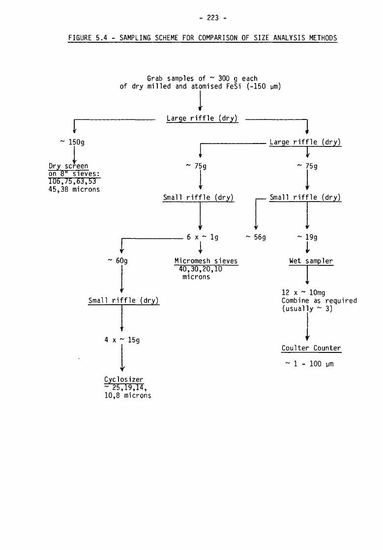
- 223

FIGURE 5.4 - SAMPLING SCHEME FOR COMPARISON OF SIZE ANALYSIS METHODS

r~ 150g

Dry screen on 8" sieves: 106' ,75,33',33' 45,38 microns

Grab samples of ~ 300 g each of dry milled and atomised FeSi (-150 pm)

I

i

Large riffle (dry)

i

jLarge rif1Fie (dry)

■f

Small rif1Fie (dry)

1f6 x ~ lg

i

~ 75 g

YSmall rif1Fie (dry)

1f

56g ~ 19g

l60g Micromesh sieves

40,30,20,10 microns

fSmall ri1rfle (dry)

*

4 x '

r

- 15g

Y

Wet sampler

▼12 x ~ lOmg Combine as required(usual 3)

rCoulter Counter

~ 1 - 100 pm

Cyclosizer ~ 25,19,14, 10,8 microns

- 224 -

Wet sieving (micromesh) : Parallel sub-samples of about lg

were treated on each of the four round-hole micromesh

sieves. The sieving was carried out in an ultrasonic bath

containing water with a drop of wetting agent.

Cyclosizer : The operation and data reduction were carried

out according to the manufacturer's instructions. As noted

below, it was found that the sample size had to be limited

to about 15g.

Coulter Counter : The operation and data reduction were

carried out according to the manufacturer's instructions for

the Model Zg (Industrial) [137], a FORTRAN computer

program was written to carry out the data reduction,

incorporating the Emonet procedure for fine size

extrapolation [137] (i.e. allowing for the proportion of

particles finer than the finest size seen by the

instrument). Either 200 or 280 pm aperture tubes were used,

and particular care was taken not to exceed the 10%

coincidence level as preliminary tests confirmed that this

caused the measured size distribution to appear coarser than

the true distribution, particularly below 10 pm.

A major problem was encountered in trying to maintain the

suspension of dense particles in homogeneous suspension,

which is essential for the proper functioning of the

technique. After considerable preliminary experimentation,

two approaches evolved which together solved the problem :

- 225

1. The use of a round-bottomed sample beaker of about

200 m i capacity.

2. The use of a high viscosity electrolyte, made up as

follows; in a 1-litre measuring cyclinder, add :

lOg NaCl (= 10 g / i )

10 m£ of a 10 g / i solution of Dispex dispersant

(= 100 mg/£)

Fill to 400 m£ with distilled water

Fill to 1000 m£ with glycerol.

After thorough mixing, the electrolyte was filtered once

under vacuum through a Millipore Type HA 0.45 pm filter

immediately before use.

The tendency for the solids to settle was monitored via the

sequence of particle counts made at each particle size. If a

trend was observed with time, the stirrer and/or beaker

position were adjusted until the trend was eliminated.

Table 5.1 gives the size distribution of the ferrosilicon

(sampled as per Figure 5.4), as determined by the Cyclosizer

with three different sample sizes.

- 226 -

TABLE 5.1 - SIZE DISTRIBUTIONS DETERMINED BY CYCLOSIZER

FOR DIFFERENT SAMPLE SIZES

Size(ym)

Sample Wt. 59.Og Sample Wt. 30.Og Sample Wt. 14.6g

Cum. % Finer Cum. % Finer Cum. % Finer

25.1 77.3 62.2 52.918.7 47.3 35.6 36.413.6 19.7 19.0 20.29.6 9.9 9.3 10.57.9 6.5 6.0 7.2

It is clear that the distributions at the two coarsest sizes

become progressively finer as the sample size increases. The

reason for this was observed to be the failure of the first

two cyclones to retain all the accumulated coarse product

because of the high density of the solids and resultant

pulp; portions of the recovered coarse product would

repeatedly slip back into the body of the cyclone, and some

would then be swept to the vortex finder and so be lost to

the next (finer) product. Further experiments demonstrated

that an end-point was reached at about 15g sample size, and

this was therefore taken as the correct mass of sample for

ferrosilicon size analysis using the Cyclosizer.

Tables 5.2 and 5.3 and Figures 5.5 and 5.6 show the size

distributions provided by the four particle size analysis

techniques, as determined in the parallel sampling procedure

shown in Figure 5.4.

- 227 -

TABLE 5.2 - SIZE DISTRIBUTION OF MILLED FERROS1LICON AS DETERMINED

BY FOUR ANALYTICAL TECHNIQUES

Square Aperture Sieves

RoundholeMicrosieves

Cyclosizer Coulter Counter

Size (ym) CPF* Size (ym) CPF* Size (ym) CPF* Size (ym) CPF*

106 99.3 40 69.3 26.0 54.6 73.2 96.175 97.5 30 49.3 19.3 38.1 58.1 93.663 95.5 20 23.9 14.1 20.4 46.1 88.453 91.6 10 4.4 10.0 9.8 36.6 73.445 87.8 8.2 6.1 29.0 59.738 79.4 23.1 45.5

18.3 31.014.5 20.211.5 13.09.2 7.68.3 5.67.3 3.9

* CPF = Cumulative Weight Percent Finer

TABLE 5.3 - SIZE DISTRIBUTION OF ATOMISED FERROSILICON AS DETERMINED

BY FOUR ANALYTICAL TECHNIQUES

Square Aperture Sieves

RoundholeMicrosieves

Cyclosizer Coulter Counter

Size (ym) CPF* Size (ym) CPF* Size (ym) CPF* Size (ym) CPF*

106 97.2 40 65.5 26.0 49.1 73.2 95.075 91.3 30 54.6 19.4 37.7 58.1 86.363 87.3 20 36.3 14.1 23.7 46.1 78.453 81.7 10 12.3 10.1 13.3 36.6 66.345 77.8 8.3 9.4 29.0 55.938 69.9 23.1 45.0

18.3 34.114.5 25.311.5 17.89.2 11.48.3 9.77.3 6.8

CUMU

LATI

VE

% F

INER

-►

un

ct

\-o

oo

vo8

o

o

§

cS

8

80

88

FIG U R E 5 5 S IZE DISTRIBUTIONS OF MILLED FeSi AS DETERMINED BY FOUR ANALYTICAL TECHNIQUES

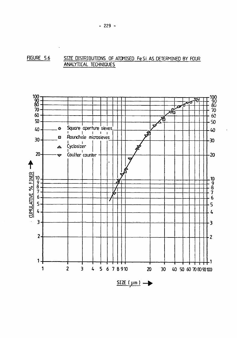
FIGURE 5.6 S IZE DISTRIBUTIONS OF ATOMISED FeSi AS DETERMINED BY FOUR ANALYTICAL TECHNIQUES

S IZ E ( p m )

- 230 -

Figure 5.5 shows that, for the milled, irregularly shaped

material, all the methods agree very closely indeed, with

the exception of the round-hole micromesh sieves which

appear to show a coarser distribution. Reference to Figure

5.5 explains this discrepancy. For the atomised, rounded

material, all four methods agree very closely, including the

round-hole sieves. This is because, for rounded or spherical

material, square and round holes will pass spheres of the

same diameter. However round holes have a smaller projected

area than square apertures, and will therefore pass

proportionately less irregular-shaped material. Compare

Plates 5.3 and 5.4.

Apart from this explicable discrepancy, the four methods

agree remarkably well on both milled and atomised material,

despite the differences in the principles of measurement.

Accordingly, it was concluded that the wet sampler and the

Coulter Counter provided accurate and reproducible size

distributions of ferrosilicon powders, and these techniques

were therefore adopted in the present work.

5.2.5 Solids Density Measurement

In order to determine the mass and volume solids

concentrations corresponding to the various medium densities

encountered in the testwork, it was necessary to establish

the density of the ferrosilicon solids used in each test.

This was done by liquid displacement in a specific gravity

- 231

bottle. Difficulties were encountered, particularly in

ensuring that the fine powder was properly wetted and that

all air was excluded. After lengthy experimentation, the

following procedure was adopted :

1. Select by appropriate sampling procedures (usually

riffling) sufficient solid for at least two

measurements (~ 15g per measurement).

2. Mix with distilled water and place in a vacuum

desiccator for a few minutes. Decant water and

floating solids.

3. Wash with acetone and decant. Wash with

trichloroethylene and decant.

4. Wash with acetone, decant, and dry at low heat.

5. Weigh SG bottle dry_(mass. A).

6. Weigh SG bottle + approx. 15g of sample (mass B).

7. Half-fill bottle with heptane, immersing solids

completely. Place under vacuum for 30 minutes,

turning and tilting the bottle at intervals until no

more air bubbles are observed.

- 232

8. Fill bottle with heptane and stand until temperature

stabilises - test with a thermometer.

9. Top up bottle if necessary. Insert top, dry the

outside of the glassware and weigh after 45 seconds

(mass C).

10. Weigh the bottle filled with distilled water (mass

D) and heptane (mass E).

11. The specific gravity of the solid is then given by :

B - A E-A

E-A + B-C D-A

where (E-A)/(D-A) is the SG of the heptane.

This method was checked using high-density powders of known

density (galena and iron powder) and found to be

satisfactory. Each ferrosilicon sample was measured at least

twice, and a mean density calculated.

The density tracers, being large in size, produced few

problems in their density measurement. A standard SG bottle

procedure was used, and the following precautions were

taken :

- 233 -

1. Distilled water which had been standing for at least

1-2 hours was used. The temperature was recorded and

the appropriate density correction applied.

2. A wetting agent was added to the water to ensure

proper wetting of the tracers. The SG bottle (+

tracers + water) was allowed to stand for about 15

minutes before filling and weighing.

5.3 Data Reduction for Mass Balances

5.3.1 Introduction

As has been stated, the essential mass flow characteristics

(medium flows, densities and particle size distributions)

were measured for all three streams, feed, underflow and

overflow. Accordingly, a high level of data redundancy

prevailed, and a number of different methods of determining

the steady-state materials balance was available. As is so

often the case in such situations, the balances rarely, if

ever, agreed, and the problem became one of choosing an

optimum balance, according to some appropriate criterion.

This type of problem has received considerable attention in

recent years, and the literature on the subject is quite

extensive. Mular [138] and Reid et al [139] have

reviewed the various approaches. In the present work, it was

decided in principle to optimise (or smooth) the measured

- 234

values of medium flows, densities and size distributions

according to the least squares criterion using the method of

Lagrangian multipliers. Cutting [140] has discussed a

general technique of this kind. Initially, the Lagrangian

expression was set up with three mass balance constraints :

1. Pulp flow in = pulp flow out.

2. Solids flow in = solids flow out.

3. Optimised solids yield (determined, for example, from

optimised medium densities by the two-product

formula) = yield determined from raw data by some

other method.

This approach led to the generation of ten non-linear

simultaneous equations, six in the optimal flows and

densities, one in the independent yield estimate and three

in the Lagrangian multipliers. These were solved by the

method of Marquardt using an algorithm available in the NAG

computer subroutine library [141.]. a computer program was

written, incorporating this solution, and the data from all

the tests were processed using this program. However, it

became apparent that the optimal balance was very sensitive

to the relative weights [ 140] allocated to each item of

raw data, in particular the independent estimate of yield.

There are numerous methods of assessing solids yield when a

high level of data redundancy is available, as in the

- 235 -

present case, and many of these alternatives were tried

[142-146], None provided a consistently satisfactory

result, and after many runs of the program it became clear

that any independent estimate of yield in the present work

was subject to large errors, due to the poor ferrosilicon

classification actually achieved in the cyclone. For

example, it can be shown by the theory of the propagation of

error that a yield estimate based on applying the two-

product formula to measured solids concentration could incur

an error in excess of 2 0 %, particularly at the higher feed

densities. In cases where pu = p0, the error tends to

infinity.

It was therefore decided to exclude the solids yields from

the initial optimisation, and to optimise only the medium

flows and densities using the Lagrangian procedure. The

solids yield determined from the optimised balance was then

used to optimise the feed, underflow and overflow

ferrosilicon size distributions, from which the partition

curve for the ferrosilicon classification was then

determined.

5.3.2 Optimisation Procedures

Two steady-state mass balance constraints were invoked in

setting up the Lagrangian expression. These were :

Medium (pulp) volume flow :

Qf = Qu + Qo .... (5.1)

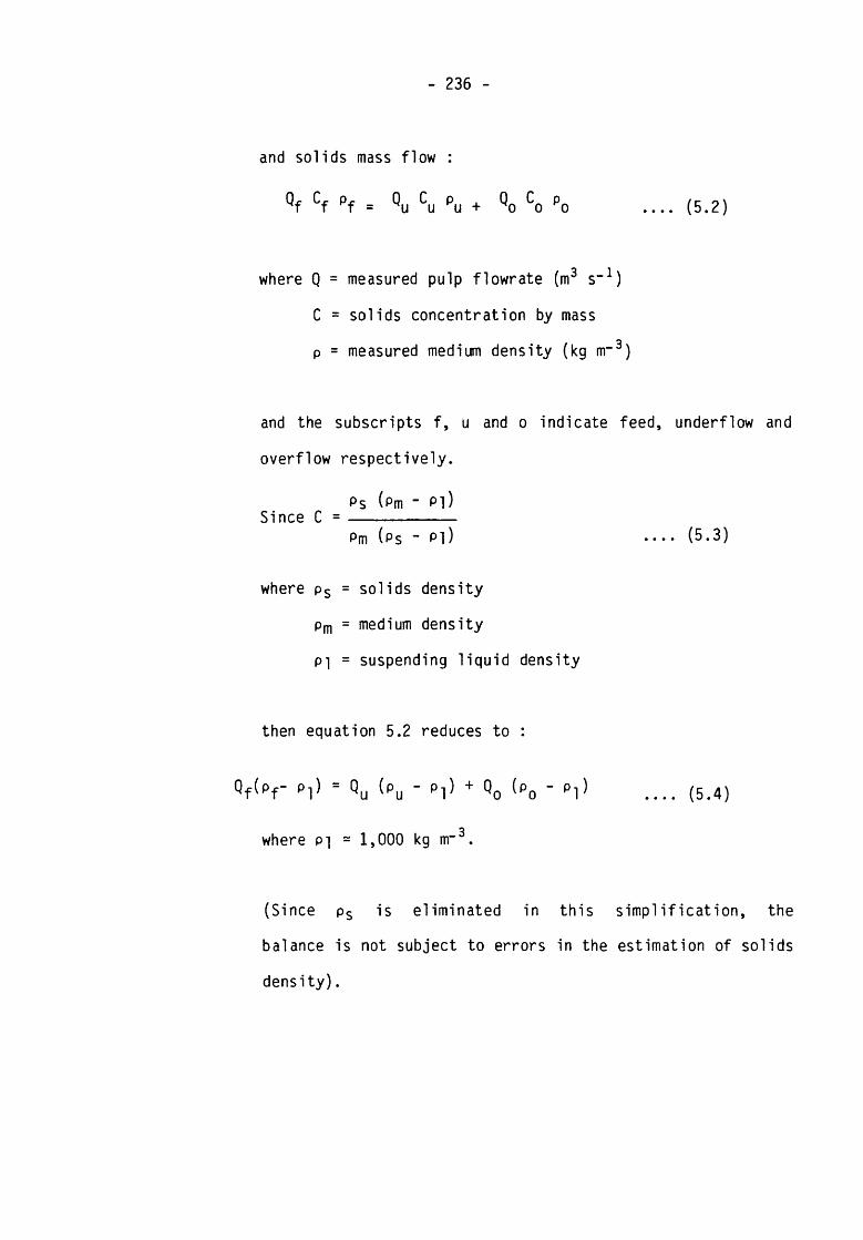
- 236 -

and solids mass flow :

Qr Cr pr Q C P , yf f f = yu U U + Q C p yo o Ko .... (5.2)

where Q = measured pulp flowrate (m3 s_1)

C = solids concentration by mass

p = measured medium density (kg nr3)

and the subscripts f, u and o indicate feed, underflow and

overflow respectively.

Ps (Pm " Pi)Since C = ------------

Pm (ps - Pi) --- (5.3)

where ps = solids density

pm = medium density

PI = suspending liquid density

then equation 5.2 reduces to :

Qf(pf- p ,) ■ Qu (p u - p ,) + Q0 (p 0 - p ,) .... (5 .4)

where pi - 1,000 kg nr3.

(Since ps is eliminated in this simplification, the

balance is not subject to errors in the estimation of solids

density).

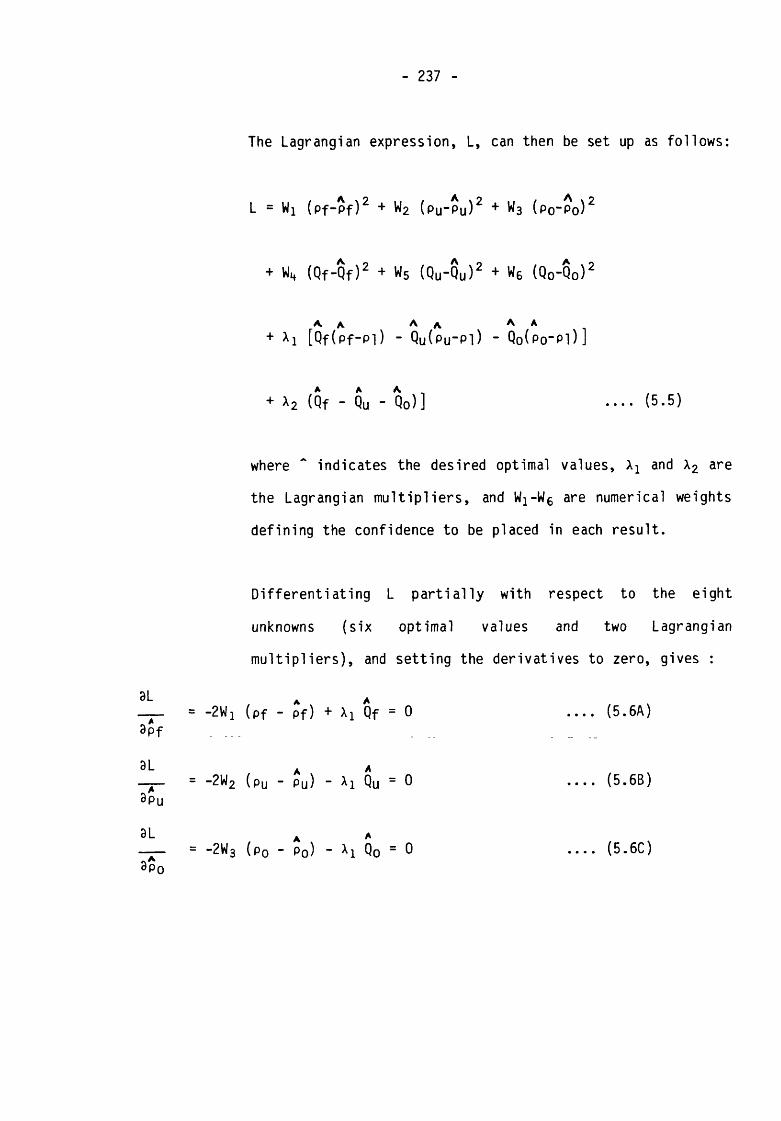
- 237

The Lagrangian expression, L, can then be set up as follows:

L = Wi (pf-pf) 2 + W2 (py-Pu)2 + w3 (po“Po)2

+ W„ (Qf-Qf) 2 + W 5 (Qu-Qu) 2 + W6 (Qo-6 0 ) 2

A A A a A A

+ xi [Qf(pf-Pl) - Qu (p u-p i ) - Qo (po-p i)]

+ ^ 2 (Qf ■ Qu _ Qo)] •••• (5*5)

where ~ indicates the desired optimal values, Aj and X2 are

the Lagrangian multipliers, and Wj-Wg are numerical weights

defining the confidence to be placed in each result.

3L

8 p f

3L

3pU

8 L

3p0

Differentiating L partially with respect to the eight

unknowns (six optimal values and two Lagrangian

multipliers), and setting the derivatives to zero, gives :

= -2W! (pf - pf) + Xi Qf = 0 ---- (5.6A)

= -2W2 (pu - pu) - Xj_ Qu = 0 .... (5.6B)

= -2 W 3 (Pq - Pq ) " ^ 1 Qo = 0 .... (5.6C)

- 238 -

9L A A_ = --2WU (Qf - Qf) + xi (Pf “ Pl) + x2 = 0 .... (5.6D)9Qf

9L A A-j- = .-2WS (Qu - Qu) - (pu - Pl) - x2 = 0 .... (5.6E)3Qu

9L A A= ■-2W6 (Qo ~ Qo) “ (po “ Pl) " x2 = 0 .... (5.6F)

3Qo

9L a * A A A A— i— = Qf(pf-p 1) - Qu (pu-Pl) - Q0(PO“Pl) = 0

.... (5.6G)9XX

9L A A A--- :-- Qf - Qu - Qo = 0 .... (5.6H)9X2

Equations 5.6A-H are non-linear simultaneous equations which

canA

beA

solvedA

for the six optimal valuesAPf,

A APu, Po,

Qf, Qu and Qo, and the two multipliers Xj and x2 (the

values of \ 1 and X2 are of no significance in the subsequent

calculations). This was done using a modified Gauss-Newton

algorithm available in the NAG computer subroutine library

[147],

Using the optimised values of flows and densities, it was

then possible to calculate an optimal solids yield from

either of the two relations :

Rs

A A A(pf - Po) (pu - Pi)

(pu - Po) (pf - Pi) .... (5.7)

- 239 -

(derived from the two-product formula and equation 5.3),

or :

A A

A Qu (pu “ Pi)

f)f (pf - pq) ---- (5.8)

(derived from equation 5.4).

The optimisation procedure constrains the values obtained

from equations 5.7 and 5.8 to be identical.

AUsing the optimal value of solids yield, Rs, it was then

possible to optimise the ferrosilicon size distributions,

also using the method of Lagrangian multipliers with a least

squares criterion.

' Defining <j>ul* and <f>01* as the mass proportion (or

percent) lying in the size interval, i, in the feed,

underflow and overflow ferrosilicon streams respectively,

then for each size interval, i (i = 1 ___ n + 1, where n is

the number of sizes at which the distribution was

determined), the two-product formula gives the following

mass balance constraint :

A Aa 4>fi - <|>oi Rs = _--------

4>ui ~ $oi • • • • (5.9)

The Lagrangian expression is then :

L - W7 ( < f > f ) 2 + Wq U u i “fui)2

+ W9 (<t>oi“^oi)2 + 3ARc -

A A4>f i “4>oiA A<Pui_<t>oi

.... (5.10)

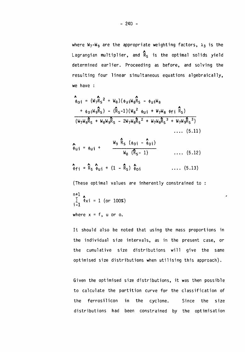
- 240 -

where W7 -W9 are the appropriate weighting factors, A3 is theA

Lagrangian multiplier, and Rs is the optimal solids yield

determined earlier. Proceeding as before, and solving the

resulting four linear simultaneous equations algebraically,

we have :

4*01* = ( 7^s2 + Wq )(^uiWgRs “ <J>uiw8

+ (JjQiWgRs) ■ (Rs“^)(W82 4>ui + ^7^8 ♦fi Rs)

(W7W8fis + W8W9Rs - 2W7W8f)s2 + M e V + u7w9rs3)

A<t>ui = ^ui +

Wg Rs (4*01’ “ <J>Oi)

w8 (%- 1)

.... (5.11)

.... (5.12)

A A A A A<Pfi - Rs ui + U ~ Rs) oi ___ (5.13)

(These optimal values are inherently constrained to :

n+1 AI <f>xi = 1 (or 100%) i-1

where x = f, u or 0 .

It should also be noted that using the mass proportions in

the individual size intervals, as in the present case, or

the cumulative size distributions will give the same

optimised size distributions when utilising this approach).

Given the optimised size distributions, it was then possible

to calculate the partition curve for the classification of

the ferrosilicon in the cyclone. Since the size

distributions had been constrained by the optimisation

- 241

procedure to conform to equation 5.9, any calculation

procedure [142-146] should provide the same partition

numbers. However the graphical method of Svarovsky [ 146]

and Gibson [1^8] was preferred since each partition number

is estimated at an actual particle size, and not over a size

interval; it thus eliminates the problem of defining a

realistic mean size for each interval.

The method involves plotting two cumulative size

distributions against one another on a so-called "square

diagram" with both ordinate and abscissa having the range

0-100%. The partition number corresponding to each size can

then be obtained by appropriate manipulation of the gradient

of the resultant curve at each plotted point. Any two of the

three size distributions can be used. Svarovsky [146]

points out that the underflow and overflow distributions

yield partition numbers with the minimum error. However in

the present case, since the size distributions have been

optimised, any pair will yield the same result. Accordingly

the fee_d_ and underflow, size distributions were selected for

the calculations.

* A

Defining Ff-j and Fuj as the

cumulative percent coarser than

underflow respectively, then :i- A *

YiA

= Rsd Fui

d Pfl.

optimised values of the

size, i, in the feed and

.... (5.14)

where Yi is the required partition number at size i.

- 242 -

Equation 5.14 can be evaluated at each size, i, by fitting a

parabola to each trio of points (i-1 , i and i+1 ) on the

square diagram and differentiating it at point i. The

parabola is given by :

A A A p

Fui = ao + ai Ffi + a2 Ffi • ••• (5.15)

where the coefficients ao, an- and a2 are determined by

multiple linear regression.

Equation 5.15 is then differentiated at size i :

d Fui

d~FfT

Aai + 2 32 Ffi

.... (5.16)

and the partition number determined from equation 5.14. NoteA A A A

that Ff0 = Fu 0 = 0%, and Ff« = Fu«> = 100%; this

enables Y-j to be determined for i = 1 and i = n.

To complete the classification computations, the

classification function of Reid [149] Was fitted to the

corrected partition numbers. The correction is applied to

allow for the bypass flow of fine particles, which are

assumed to divide in the same proportion as the water

[121], The correction is given by :

- 243 -

Yi " RfYci - -------

1 - Rf .... (5.17)

where Rf = proportion of water to underflow.

and Yj & Yc-j are expressed as proportions.

Reid's function is then :m

Yci = 1 - exp [-In 2 (di/d50c) ] .... (5.18)

where d-j = size i

dsoc = corrected separation size

m = Distribution parameter (a high value of m

implies a sharp, efficient classification).

Equation 5.18 was fitted to the corrected partition numbers

by linear regression in its linear form :

In"lnd/l-Yci)

In 2

= m In di - m In d5 Qc.... (5.19)

To check the quality of the fit, predicted values of the

corrected partition numbers, Yc-j, can be determined from

equation 5.18 using the regression estimates of d5 QC and

m.

A FORTRAN computer program, "0PTIM6", was written to carry

out all the calculations described above. A listing of the

program is given in Appendix 9, together with an example of

the input data required.

- 244 -

It incorporated the NAG library routine E04GEF to carry out

the mass balance optimisation procedure. This routine

required the numerical evaluation of the simultaneous

equations 5.6A-H and their first derivatives, which is

effected in subroutine LSFUN2; 30 of the 64 possible first

derivatives are non-zero (see Appendix 9). The computations

require double precision arithmetic.

The selection of weights for the two optimisation procedures

(W1 -W5 for the material balance and W 7 -W9 for the size

distributions) is problematical. An obvious approach is the

use of the reciprocal of the error variance associated with

each measurement [138] However, in the present case no

such estimates were available, and arbitrary weights must

therefore be applied. Since the feed density was estimated

from a sample taken while the cyclone was being by-passed,

and the product densities were obtained by direct weighing

and volume measurement, the following values were selected

for W 1 -W3 :

Wx = 1 W2 = 2 W3 = 2

Similarly, the feed flowrate was determined by a well

calibrated instrument, whereas the product flows were

obtained from short-duration timed samples. Thus :

K = 2 W5 = 1 W6 = 1

- 245

The weights for the size distribution optimisation (which do

not interact with V^-Wg in the computational procedure) were

chosen on the same basis as Wj - W3. Thus :

W 7 = 1 W 8 = 2 W 9 = 2

0PTIM6 also carried out a number of subsidiary calculations

such as the determination of measured and optimised solids

concentrations by mass and volume, and solids, water and

pulp splits. All the material balance and classification

data for the cyclone tests have been reported in the form of

the output from this program.

5.4 Results

The testwork generated a considerable volume of data. The mass balance

data for the medium, including both measured and optimised values of

density, flow, and size distribution, plus the FeSi classification

data, are given for each test in Appendix 10, in the form of the

output of the computer program described in section 5.3.2.

The Tromp curves for the density separation of the tracers are given

in Appendix 11. In all the Series F4 tests, plus tests F5/1, F5/3 and

F5/5, all (or nearly all) of the tracers were recovered to the

overflow (implying a very high separating density). These results are

therefore not included in Appendix 11.

- 246 -

The uncorrected partition curves for the classification of the medium

in each test are given in Appendix 12. On each plot has been drawn a

horizontal line corresponding to the calculated value of water

recovery to the underflow.

Since the form of the flow curve obtained from the feed media was very

similar for each test, and since the curve was in each case well

described by equation 4.38, the flow curves themselves have not been

presented. However the estimated parameters of equation 4.38, plus the

interpolated values of minimum apparent viscosity (equation 4.41),

have been given for each test in the summary tables, Tables 5.4 and

5.5.

A summary of the important data is given in Tables 5.4 and 5.5 for the

milled ferrosilicon (Series FI, F2, F3 and F6) and the atomised

ferrosilicon (Series F4 and F5) respectively. Notes on each item of

data are given by column numbers below :

Cols. 1 & 2 - Rosin-Rammler parameters (eqn. 4.3) for the optimised

FeSi feed size distribution.

Column 3 - Measured pressure drop.

Cols. 4 & 5 - Fitted parameters for equation 4.38.

t o is the yield stress and n is an index of

dilatancy. In cases where n = 1.000, the flow curve was

essentially that of a pure Bingham plastic, and a

straight line was fitted to the data.

- 247

Column 6 - The minimum apparent viscosity, determined by insertion

of the values of x0 and n into equation 4.41,

corrected for temperature using equation 4.39. In cases

where n = 1.000, the value reported is that of the

plastic viscosity.

Cols. 7 - 9 - Optimised medium densities.

Cols. 10-12 - Optimised medium flowrates.

Cols. 13-15 - Optimised values of the proportion of FeSi, water and

medium reporting to underflow.

Column 16 - Gross FeSi classification d50 (i.e. uncorrected for

by-pass), interpolated from the partition curves given

in Appendix 12. Because of the poor quality of

classification, the curves tend to be irregular and the

d50 is correspondingly difficult to estimate.

Uncertainties in estimation are indicated by a question

mark (?). In cases where the curve passes through the

50% level more than once, the highest value of d50 is

reported.

Column 17 - Measured density of cyclone contents.

Cols. 18&19 - Rosin-Rammler parameters of measured size distribution

of cyclone FeSi contents.

- 248 -

Cols. 20-23 - Separating density and Ep-value for 2 and 4mm tracers,

interpolated numerically from the original data (see

curves in Appendix 11) using the smooth curve-fitting

procedure of Akima [154], in some cases, the value of

650 was greater than the highest density tracer used

(3490 kg m-3), and in such cases neither 650 nor Ep

could be determined.

Cols, 24&25 - Error area for the density separations of 2 and 4mm

tracers, determined from the original data by numerical

integration. The same remarks as for Cols. 20-23 apply.

Col. 26 - Temperature of medium after discharge from plant into

storage vessels.

Quantities derived from these basic data are presented in Appendix 13.

5.5 Discussion of Results

5.5.1 Reproducibi1ity

Tests F5/6, F5/8 and F5/9 were included as replicates to

test the consistency of the cyclone performance and the

reproducibility of the experimental and analytical

techniques. A summary of the operating variables for the

three tests is given in Table 5.6A, and a summary of the

performance parameters in Table 5.6B :

T A flLE 5 .4 SUMMARY O F CYC LO NC T E S T S W ITH M IL t .F D F E R R O S I L IC O N

TestNumber

SizeDistribution of Food FeSI

PressureFlow Curve for Feed Medium

Medium Densities (kg m-3)

Medium Flowrates (1 min-')

Proportion Reporting to

Underflow

Classificationof

FeSI

O.

c

intentsof

/c 1 oneDen slty Seperat Ion

Medluii

RRa(K m )

RRb kN/m2(Nm z)

n 7a(ml n) (Ns m-2 x 103>

Feed Underflow Overflow Feed Underflow Overflow Solids(Wt.O

Water(Wt.Jf)

Modlim(Vol.j!)

Gross

d50J|4m)

Density (kg m-3)

FoSt Size Distribution

£ 5 0 <k9 m~3 Fp <9 m Error Area TenperatureCC)

RR0y im )

RRb 2 mm 4mm 2mm 4 mm 2mm 4mm

FI/I 33.3 1 .941 84.8 5.51 1 .370 9.11 3053 2858 3262 78.1 40.4 37.7 46.8 54.4 51.7 54 7 3128 30.5 1.933 U-sh sped T -onp C irves 50

FI/2 33.7 1 .885 44.8 5.84 1.322 9.49 2945 2820 3242 55.5 39.1 16.4 65.9 72.7 70.4 52 7 3037 32.7 2.152 W-sheped Troup Curves 35

FI/3 31.3 2.116 114.5 2.11 1.071 3.92 2687 2993 2524 87.4 30.3 57.0 41.0 32.1 34.7 41 2796 29.8 2.023 3353 3345 0.077 0.035 10.28 5.28 33.8

FI/4 30.9 1.933 51.7 2.15 1.004 2.95 2674 2740 2626 53.4 22.5 30.9 43.8 41.4 42.1 35 2756 32.2 1.654 3224 3221 0.064 0.045 12.36 6.50 41

FI/5 30.7 1.780 116.5 2.08 1.096 2.54 2430 3150 2163 93.4 25.3 68.1 40.7 22.5 27.1 56 2535 28.0 1.709 3365 3335 0.079 0.039 9.59 5.22 36

FI/6A 31.8 1.845 45.2 2.72 1.136 2.17 2417 2782 2172 56.4 22.7 33.8 50.5 36.8 40.2 20 2508 33.2 1.890 3150 3139 0.043 0.043 9.16 6.49 41

F1/6B 36.0 1.765 49.3 3.25 1.114 2.63 2401 2888 2171 57.1 18.3 38.8 43.2 28.4 32.0 52 7 2562 34.1 2.085 3172 3161 0.038 0.027 7.81 4.71 30

FI/7 33.8 1.979 127.2 1.66 1.314 2.06 2052 3369 1634 105.9 25.5 80.4 54.2 17.3 24.1 53 7 2129 35.1 1.852 3327 3257 0.067 0.033 9.11 5.73 37

F1/8 36.8 1.746 56.5 1.66 1.314 2.28 2043 3054 1654 67.2 18.7 48.5 54.8 21.8 27.8 26 2139 32.3 1.766 3117 3139 0.058 0.043 9.20 5.54 32

F2/I 34.2 2.110 87.9 3.96 1.237 5.55 3000 3293 2763 75.2 33.7 41.5 51.4 41.4 44.3 44 7 3142 35.8 2.106 - 3492 - - - - 36F2/2 33.7 2.022 57.2 7.02 2.048 4.11 2969 2883 3282 57.4 45.0 12.4 75.1 80.2 78.5 7 3113 35.7 1.991 3459 - - - - - 37F2/2A 34.4 2.259 67.2 3.03 1 .009 3.43 2912 3233 2646 68.6 31.1 37.6 52.9 41.6 45.3 27 3089 30.7 2.220 «$50 a 3500 kg m“- for and mm 37 |

F2/3 33.4 1 .917 109.6 1.91 1 .000 2.64 2713 3507 2536 91.9 29.6 62.3 47.2 26.1 32.2 7 2745 29.9 1.510 S * 0 > 3500 kg m“3 for 2 end 4mm 3«)F2/4 35.0 2.037 59.0 2.01 1.000 2.82 2661 3115 2325 68.3 29.0 39.3 54.1 37.9 42.5 27 2848 36.2 2.077 3442 3429 - 0.072 - 9.26 34F2/5 36.4 2.136 108.2 0.61 1.008 2.69 2448 3483 2002 105.0 31.6 73.3 51.7 23.1 30.1 7 2421 31.7 2.024 ^50 ► 3500 kg in-- for and 'mm 38F2/6 33.9 2.224 52.4 5.95 2.337 3.06 2396 3084 1958 66.5 25.9 40.6 58.1 33.0 38.9 20 2463 22.9 2.425 3345 3325 0.127 0.057 16.14 8.95 29F2/7 38.0 2.203 103.8 5.98 4.168 1.68 2095 3483 1579 99.2 26.9 72.3 61.5 19.3 27.1 19 2088 33.5 2.123 3443 3385 - 0.060 - 6.64 37F2/8 38.8 2.210 53.1 5.98 4.168 1.94 2046 3135 1490 71.7 24.3 47.4 69.0 26.2 33.8 11 1961 36.7 2.272 3172 3150 0.110 0.054 13.25 7.70 30

F3/I 34.1 2.070 106.9 5.35 1.164 5.94 2928 2974 2914 77.6 18.3 59.3 24.1 23.3 73.6 t74 2949 41.6 1.867 3273 3250 0.090 0.037 13.48 6.80 38F3/3 28.4 2.273 137.2 4.86 1.497 3.96 2672 2752 2630 84.0 29.4 54.6 36.7 34.3 35.0 30 2776 27.8 2.186 3205 3243 0.088 0.030 9.50 5.33 32F3/4 38.6 2.138 70.7 3.59 1.158 3.41 2673 2648 2723 64.7 43.4 21.3 66.1 67.5 67.1 7 2768 43.5 2.225 3215 3215 0.050 0.045 8.86 5.69 39.5F3/7 24.2 1.962 167.2 3.02 1 .369 2.07 2049 2823 1821 101.9 23.2 78.7 39.5 19.1 22.7 29 2206 24.5 1.966 2966 2996 0.028 0.035 9.09 6.56 34

F6/1 28.2 2.358 62.4 4.67 1.153 5.97 2828 2755 2907 62.4 32.5 29.9 50.0 53.0 52.1 23 7 2976 29.3 2.466 W-sheped Troup Curves 30F6/2 27.8 2.205 66.2 9.82 2.844 7.75 2930 2740 3126 64.9 33.0 32.0 45.8 53.2 50.8 8 7 2946 23.8 2.873 W-sheped Troop Curves 30F6/3 27.9 2.361 60.3 2.74 1.088 2.82 2369 2627 2249 62.4 19.8 42.6 37.7 29.9 31.7 41 2458 23.3 2.841 3005 2996 0.045 0.035 10.46 6.36 27F6/4 27.7 2.479 54.1 3.44 1.708 2.31 2079 2716 1802 62.0 18.8 43.2 48.2 26.3 30.3 29 2140 28.0 2.644 2905 2906 0.032 0.038 6.06 5.17 27F6/5 28.0 2.343 62.4 3.77 1.163 3.96 2647 2618 2664 61.9 22.6 39.3 35.9 36.8 36.3 47 2724 29.6 2.385 3117 3117 0.068 0.054 9.87 7.43 30F6/6 29.8 2.327 49.3 * 1343 2655 1100 72.3 11.3 61.0 75.3 11.9 15.6 12 1350 27.3 2.402 No tracei s edck d -

Column 1 2 3 4 5 6 7 8 9 10 11 12 13 14—

15 16 17 18 19j d 21 1

22 23j d

25 26

Note : Minor accumulation of some tracers In cyclone contents occurred In most tests.Significant accumulation occurred as follows :

FIn t 9| of 3?70 kg m-3.F1/8 : 61 of 3090 kg m-3.

________ F3/7 ; 31* of 2900 kg m~3 and 1 IS of 3090 kg m~3.______________________________

TABLE r>.5 - SUMMARY OF CYCLONE TESTS WITH ATOMISED FERROSILICON

TestNumber

SizeDistribution of Feed FeSI

PressureFlow Curve for Feed Median

Modi izn Densities (kg m"3)

Modi an Flowrates (1 min"*)

Proportion Reporting to

Undorflow

Classificationof

FeSI

Contentsof

Cyc1 oneDensity Separation*

MedianTenperature

CC)RR0y»m)

RRb kN/m2 t o(Nm"2>

n *Ia(ml n) (Ns m"2 x 103>

Feed Underflow Overflow Food Underflow Overflow Solids(Wt.t)

Water(Wt.O

Median(Vol.*>

Gross

<*50m)

Density (kg m"3)

FeSI Size 01strlbutlon

$50 (k9 m~* Ep tg m “3) Error Area

RRayim)

RRb 2mm 4mm 2mm 4mm 2mm 4mm

F4/1 49.2 1.694 137.2 4.48 1.244 3.32 3047 3518 2859 85.7 24.5 61.3 35.1 25.1 28.5 73 3244 43.0 1.642

oo

ecovo y of il 1 tr icers o 0/F 35.5F4/2 44.1 1.659 78.6 8.14 2.568 3.66 2986 3345 2836 63.1 10.5 44.6 34.7 26.7 29.3 71 3197 39.8 1.725 100* recovery of all tracers to 0/F 31F4/3 34.0 1 .640 154.4 5.89 2.529 2.77 2805 3778 2466 91.6 23.6 68.0 39.7 19.7 25.0 64 2946 33.7 1.595 100* recovery of all tracers to O/F 34

F4/4 33.5 1 .590 60.0 4.85 1.786 3.13 2717 3356 2434 57.5 17.7 39.8 42.1 26.1 30.7 68 7 2945 34.5 1.736 100* recovery of all tracers to 0/F 27F4/5 40.9 1.587 133.1 3.05 1.090 3.68 3040 3450 2096 85.2 22.0 63.2 31.1 23.1 25.9 60 3203 34.8 1 .690 100* recovery of all tracers to 0/F 33

F5/1 23.8 1.550 152.7 3.13 1.102 3.78 3027 3000 3035 70.7 18.3 60.5 22.9 23.4 23.2 51 3149 26.3 1.555 100* recovery of all tracers to 0/F 33F5/2 25.9 1.770 86.5 3.29 1.091 3.98 2979 2827 3029 58.7 14.5 44.2 22.8 25.7 24.7 57 3031 25.3 1.674 25 3500 kg m‘° for 2 and 4mm 29F5/3 27.3 1.675 160.3 3.58 1.515 3.05 2670 2B89 2615 89.1 18.0 71.2 22.8 19.1 20.2 +68 2864 25.9 1.830 100* recovery of al1 tracers to 0/F 31F5/4 27.0 1.677 69.6 3.19 1.422 3.34 2674 2818 2624 58.6 15.1 43.4 28.0 24.9 25.8 45 2716 30.0 1.690 3365 3375 0.038 0.038 4.97 3.90 26F5/5 25.6 1.568 169.7 3.13 1.609 2.55 2358 2872 2232 93.7 18.5 75.2 27.2 17.5 19.7 37 2504 27.6 1.731 25 >500 kg m0 'or 2mmF5/6 24.8 1.671 67.9 2.51 1.463 2.93 2397 2806 2262 59.9 14.8 45.1 32.0 22.5 24.7 34 2537 25.0 1.794 3224 316) 0.040 0.027 7.82 3.53 24F5/7 24.3 1.717 159.3 1.90 1.228 2.53 2419 3372 1939 93.0 31.2 61.9 56.0 26.3 33.5 15 2400 26.0 1.736 3245 3235 0.026 0.022 9.91 4.18 32F5/8 24.2 1 .751 69.6 2.47 1.409 2.64 2363 2793 2240 62.1 13.8 40.3 29.2 20.1 22.2 39 2406 22.1 2.419 3205 3161 0.040 0.027 5.85 3.82 26 CF5/9 24.7 1 .788 67.6 3.36 1.548 2.88 2377 2783 2241 60.4 15.2 45.2 32.6 22.9 25.2 36 2488 26.8 1.799 3172 3161 0.033 0.022 5.20 3.04 22 C

F5/10 26.7 1.756 61.4 1.87 1.043 4.69 2467 2517 2450 51.5 12.8 38.8 25.7 24.5 24.8 43 2537 27.6 1.041 3015 3053 0.049 0.020 10.19 5.84 28F5/11 25.1 1.842 67.9 1.90 1.000 6.12 2431 2658 2372 59.2 12.3 46.9 24.3 19.7 20.7 44 2493 26.4 1.802 2895 2960 0.034 0.018 6.13 4.63 32F5/12 24.3 1.744 57.9 2.59 1.082 12.42 2451 2552 2415 55.4 14.4 41.0 28.0 25.4 26.0 58 2475 27.6 1.908 2755 2702 0.035 0.027 8.24 5.55 39

Column 1 2 3 4 5 6 7 8 9 10 11 12 13 14 15 16 17 18 19 20 21 22 23 24 25 26

* Note : Minor accumulation of some tracers In cyclone contents occurred In most tests*Significant accumulation occured as follows :

F5/5 : 35* of 3410 kg m"3 and 97* of 3500 kg m"3.F5/6 : 82* of 3210 kg m"3 and 74* of 3270 kg nf3.F5/7 : 0* of 3210 kg m-3 and 22* of 3270 kg m*3.F5/8 : 77* of 3210 kg m-3 and 79* of 3270 kg m“3.F5/9 : 12* of 3090 kg m"3, 54* of 3210 kg m~3 and 55* of 3270 kg m"3.

TABLE 5.6A - OPERATING VARIABLES FOR REPLICATE TESTS

F5/6, F5/8, F5/9 (TAKEN FROM TABLE 5.5)

Test R R a(pm)

RRb(pm)

Pressure(kNm-2)

Flow Curve Feed Density (kg m-3)

Feed Flowrate (A min-1)

,T°(Nnr2)n

(Nsnr2 x 103)

F5/6 24.8 1.671 67.9 2.51 1.463 2.93 2397 59.9F5/8 24.2 1.751 69.6 2.47 1.409 2.64 2363 62.1F5/9 24.7 1.788 67.6 3.36 1.548 2.88 2377 60.4

Mean 24.56 1.737 68.4 2.78 1.473 2.82 2379 60.80

StandardDeviation 0.321 0.060 1.08 0.50 0.070 0.16 17.1 1.15

Coefficient ofVariation (%) 1.3 3.4 1.6 18.1 4.8 5.5 0.7 1.9

TABLE 5.6B - PERFORMANCE PARAMETERS FOR REPLICATE TESTS

F5/6, F5/8, F5/9 (TAKEN FROM TABLE 5.5)

Test

Medium Density (kg m-3)

Medium Flowrates (i min-1)

Proportion Reporting to Underflow

GrossJso(urn)

Contents of Cyclone Density Separation

U/Flow O/Flow U/Flow O/Flow (Wt. X)Sol Ids

(Wt. X) Water

(Vol. X) Medium

Density (kg m-1)

RRa(urn)

RRb «5o (kg nr3) Ep (kg m-3) Error Area

2mm 4mm 2rmi 4mm 2mm 4mm

F5/6 2806 2262 14.8 45.1 32.0 22.5 24.7 34 2537 25.0 1.794 3224 3161 0.040 0.027 7.82 3.53F5/8 2793 2240 13.8 48.3 29.2 20.1 22.2 39 2486 22.1 2.419 3205 3161 0.040 0.027 5.85 3.82F5/9 2783 2241 15.2 45.2 32.6 22.9 25.2 36 2488 26.8 1.799 3172 3161 0.033 0.022 5.20 3.04Mean 2794 2248 14.6 46.2 31.3 21.8 • 24.0 36.3 2504 24.6 2.004 3200 3161 0.038 0.025 6.29 3.46

StandardDeviation 11.5 12.4 0.72 1.82 1.81 1.51 1.61 2.5 28.9 2.4 0.359 26.3 0 0.004 0.003 1.36 0.39

Coefficient ofVariation (X) 0.4 0.6 4.9 3.9 5.8 6.9 6.7 6.9 1.2 9.6 17.9 0.8 0 10.7 11.4 21.7 11.4

- 253 -

Inspection of these results, particularly the means,

standard deviations and coefficients of variation

(mean/standard deviation), shows that both the operating

variables and the corresponding performance parameters are

extremely reproducible. The relatively high standard

deviations for the flow curve parameters (Table 5.5A) can be

attributed to variations in temperature between the tests.

All the density measurements were very repeatable. In the

case of the estimated separating density for the 4mm

tracers, the three values were actually identical. The range

of separating density for the 2mm tracers was 52kg m"3,

which is a useful yardstick for judging the success of the

regression analyses to be discussed later.

In general, the performance of the cyclone was extremely

reproducible, and the data obtained from the testwork can be

regarded as reliable.

5.5.2 The Density of Separation, 6 ^n

The density of separation is the single most important

parameter of any density separation. In the present work, as

noted earlier, the density of separation experienced by

tracers fed to the cyclone at a low rate represents the

intrinsic separation, unaffected by the particle crowding

which prevails when the cyclone treats substantial volumes

of ore.

- 254 -

As a first step in correlating the separation data given in

Tables 5.4 and 5.5, and Appendix 13, the expressions derived

by dimensional analysis in Chapter 3 (e.g. eqn. 3.10) were

fitted to the data. The results were quite unsatisfactory,

although in every test the separating density exceeded the

feed medium density, as predicted. After some further

manipulation it became clear that the correlations which had

proved appropriate for the stable media used in the

experiments described in Chapter 3 were not suitable for

unstable ferrosilicon suspensions. This important finding

confirmed the conclusions implicit in the literature, as

discussed in Chapter 2, viz. that unstable media are subject

to trends which are the reverse of those predicted by simple

theory for stable media and pure liquids.

A good example of this can be obtained by inspection of

Table 5.4, Series FI. The tests Fl/3 : Fl/4, Fl/5 : F1/6A,

and Fl/7 : Fl/ 8 represent pairs for which variables such as

ferrosilicon size distribution and feed medium density were

relatively constant, but within which the feed flowrates

differed. Simple theory (eqn. 2.4) and dimensional analysis

(eqn. 3.10) predict that the separating density will

decrease with increasing flowrate. The present data however

reflect a reversed trend. The data for the 2rmi tracers are

summarised in Table 5.7 :

- 255 -

TABLE 5,7 - 6 So vs Qf FOR SERIES FI, 2mm TRACERS

Test 650 - (kg nr3)

Qf(Jt min-1) (kg nr3)

pu, (kg nr3)

Po, (kg nr3)

Fl/3 3353 87.4 2687 2993 2524Fl/4 3224 53.4 2674 2740 2626

Fl/5 3365 93.4 2430 3150 2163F1/6A 3150 56.4 2417 2782 2172

Fl/7 3327 105.9 2052 3369 1634Fl/ 8 3117 67.2 2043 3054 1654

Thus, although the feed medium densities within each pair of

tests are very similar, the separating density falls

significantly as the flowrate decreases. Table 5.7 also

demonstrates that the underflow medium density, pu,

follows the 6 5 q trend, whereas the overflow density, p0 ,

remains relatively unchanged.

It seems reasonable, therefore, to presume that the

separating density is, at least in part, controlled by the

behaviour of the medium in the cyclone, and specifically by

the prevailing underflow density.

Three groups of workers [48,49,65] have proposed that the

separating density is equal to the underflow density, under

"normal" (non-segregating) conditions [65] ;

650 " Pu .... (5.20)

- 256 -

In the present author's experience, dealing with ores in

which the yield to underflow is usually small, this is

rarely, if ever, the case. For example, in the author's

previous work with a 610nm cyclone using ferrosilicon media

[4], 92 of the 97 tests returned values of 650 which

exceeded pu; two tests conformed approximately to eqn.

5.20, and in three cases 6 5 0 was less than pu . In the

present work, Figure 5.7 demonstrates that only three of the

27 2nm tracer results, in which a value for 650 could be

estimated, fall below the line defining 6 5 0 = p u . The

remaining 24 results lie above this line, most of them

significantly so (cf. Figure 2.1). Further, Figure 5.7 shows

that there is no clear relationship between 6 5 0 and pu,

although the linear correlation coefficient, r, for the data

is 0.648, which is significant at the 99% level of

confidence [151], This implies that one or more additional

variables contribute to defining 6 50.

There is no doubt that the feed medium density, pf, must

exercise some control over the separation. The form of the

correlation for 6 5 0 developed in Chapter 3 utilises the

density difference, (6 5 0 - pf), and inspection of the

present data shows that there are occasions on which 650

follows pf while p u remains relatively constant (e.g.

tests F1/6B : F2/2, and Fl/ 8 : F2/6). Accordingly, a simple

linear relationship between 6 5 0 , Pf and pu was

postulated :

55 0 = a + b pf + c pu .... (5.21)

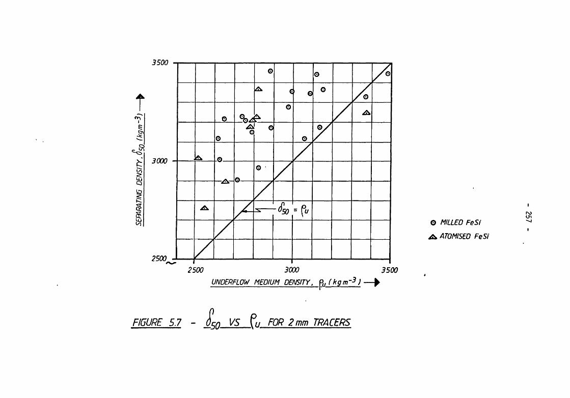
SEPARATING DENSITY,

lkgm-3)--

>

UNDERFLOW MEDIUM DENSITY, p, (kgm~3 ) — ^

O MILLED FeSi ATOMISEO FeSi

FOR 2 mm TRACERSFIGURE 57

- 258 -

where a, b and c are constants for a particular system.

(Assuming "a" has the dimensions of density and b, c are

dimensionless, eqn. 5.21 is dimensionally consistent).

Equation 5.21 was fitted to the 2mm and 4mm tracer data for

the milled ferrosilicon (Table 5.4) using multiple linear

regression. The estimated parameter values were as follows :

2 mm Tracers 4mm Tracers

a = 143 a = 409.5b = 0.473 b = 0.459c = 0.659 c = 0.577R2 = 0.990 R2 = 0.980

The R2 values indicate an exceptionally good fit in both

cases. This is confirmed by Figure 5.8, in which the

observed 6 5 0 values are compared with the values predicted

by eqn. 5.21; the agreement is excellent.

Other indications of the predictive error are as follows :

2mm Tracers 4mm Tracers

Range of Measured 6 5 0 (kg rrr3) 538 523Mean Absolute Error (kg m“3) 13 17Maximum Error (kg nr3) 36 38

This is further evidence of the good fit, since the range of

6 5 0 for the rep!icated 2mm results was 52 kg nr3 (Section

5.5.1).

PRED

ICTED

Sty

f kgm

~3)

- 259 -

MEASURED Sgn(kQm~3)---^

MEASURED VS PREDICTED FOR MILLED FeSiFIGURE 5.8

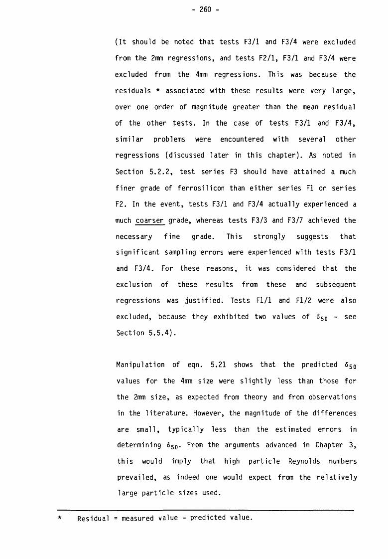
- 260 -

(It should be noted that tests F3/1 and F3/4 were excluded

from the 2mm regressions, and tests F2/1, F3/1 and F3/4 were

excluded from the 4mm regressions. This was because the

residuals * associated with these results were very large,

over one order of magnitude greater than the mean residual

of the other tests. In the case of tests F3/1 and F3/4,

similar problems were encountered with several other

regressions (discussed later in this chapter). As noted in

Section 5.2.2, test series F3 should have attained a much

finer grade of ferrosilicon than either series FI or series

F2. In the event, tests F3/1 and F3/4 actually experienced a

much coarser grade, whereas tests F3/3 and F3/7 achieved the

necessary fine grade. This strongly suggests that

significant sampling errors were experienced with tests F3/1

and F3/4. For these reasons, it was considered that the

exclusion of these results from these and subsequent

regressions was justified. Tests Fl/1 and Fl/2 were also

excluded, because they exhibited two values of 650 - see

Section 5.5.4).

Manipulation of eqn. 5.21 shows that the predicted 650

values for the 4mn size were slightly less than those for

the 2mm size, as expected from theory and from observations

in the literature. However, the magnitude of the differences

are small, typically less than the estimated errors in

determining S50. From the arguments advanced in Chapter 3,

this would imply that high particle Reynolds numbers

prevailed, as indeed one would expect from the relatively

large particle sizes used.

* Residual = measured value - predicted value.

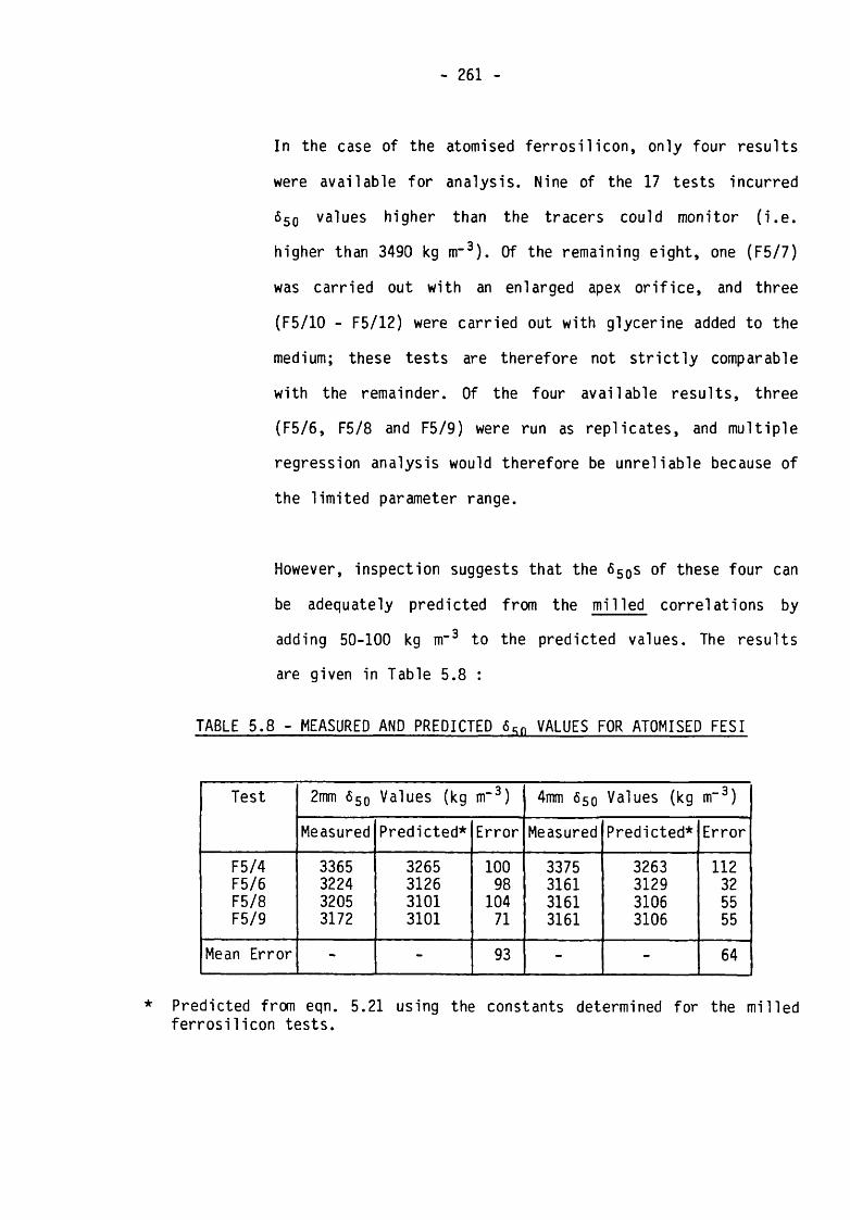
- 261

In the case of the atomised ferrosilicon, only four results

were available for analysis. Nine of the 17 tests incurred

650 values higher than the tracers could monitor (i.e.

higher than 3490 kg m-3). Of the remaining eight, one (F5/7)

was carried out with an enlarged apex orifice, and three

(F5/10 - F5/12) were carried out with glycerine added to the

medium; these tests are therefore not strictly comparable

with the remainder. Of the four available results, three

(F5/6, F5/8 and F5/9) were run as replicates, and multiple

regression analysis would therefore be unreliable because of

the limited parameter range.

However, inspection suggests that the 650s of these four can

be adequately predicted from the milled correlations by

adding 50-100 kg m”3 to the predicted values. The results

are given in Table 5.8 :

TABLE 5.8 - MEASURED AND PREDICTED 6qn VALUES FOR ATOMISED FESI

Test 2mm 650 Values (kg nr3) 4mm 650 Values (kg m“3)

Measured Predicted* Error Measured Predicted* Error

F5/4 3365 3265 100 3375 3263 112F5/6 3224 3126 98 3161 3129 32F5/8 3205 3101 104 3161 3106 55F5/9 3172 3101 71 3161 3106 55

Mean Error - - 93 - - 64

* Predicted from eqn. 5.21 using the constants determined for the milled ferrosilicon tests.

- 262 -

Thus a correlation of the form of eqn. 5.21 appears to

describe the data from both the milled and atomised

ferrosilicon data satisfactorily.

It is worth noting that the addition of a p0 term in eqn.

5.21 achieved no significant improvement in fit, and the

substitution of p0 for pu reduced substantially the

quality of fit. This fact, together with the very high

predictive capability of eqn. 5.21, strongly suggests that

both the feed and underflow medium densities play a

mechanistic role in determining the separating density.

Since the feed medium density is a controllable variable,

which can be defined by the experimenter, it is clearly

desirable to establish some correlation for the resulting

underflow density. A successful prediction of pu should

suggest a mechanism by which 650 is determined.

5.5.3 The Underflow Medium Density, pu

Two mechanisms can be postulated for the thickening of

medium in the cyclone, and thus the determination of the

underflow density :

i) Classification of the medium.

ii) Bulk sedimentation of the medium.

- 263 -

It seems likely that both mechanisms play a role, the

relative value of their contributions depending upon the

prevailing conditions, in particular the solids

concentration in the feed.

A problem arises in defining the degree of thickening. Many

authors have used the density difference between the

underflow medium and the feed or overflow medium (pu -

Pf> or pu - p0). in the present case, a dimensionless

term is to be preferred - pu/pf. The value of this term

is given for each test in Appendix 13.

Inspection of the data suggests that the degree of

thickening is inversely related to the volume recovery of

the medium to the underflow, Rm (Col. 15 in Table 5.4 and

5.5), at least for the milled ferrosilicon (see Figure

5.9). In Chapter 3, it was shown that Rm is determined by

the inlet Reynolds number, Re-j, and the pressure loss

coefficient, L, both dimensionless numbers. Further, it was

shown in Section 4.2 that the sedimentation rate of

ferrosilicon suspensions is a function of the solids

concentration, expressed as (1-CV). One might therefore

postulate the following dimensionless relation :

Pu

Pf

a 3 y = K (1-CV) (Re,) L

___ (5.22)

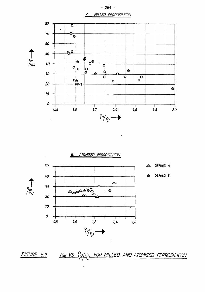
- 264 -A MILLED FERROSILICON

TRm(%)

BO -i

70 -o

_rj—

f>0 -C»

Q\J

50 -

LO - o «L © °HU

30 -C o O

P___<c

3 Sb A o

Of) _ ?0c'

o(> oo

10 -rj/J

oIU

0 -0,8 1,0 1,2 7,4 1,6 1,8 2,0

B. ATOMISED FERROSIUCON

s o “ l

/ n _

^ S E R I E S 4

O S E R I E S SVI/

t * nk

( % )o n —

O o

k-A.O

1 0 —/l/

0 -

0,8 1,0 7/ 7,4 1,6

Rm VS ?ulQf FOR MILLED AND ATOMISED FERROSIUCONFIGURE 5.9

- 265

This expression was fitted, with moderate success, to the 24

available cases of milled FeSi data, excluding again tests

F2/1, F3/1 and F3/4. The estimated parameter values were as

follows :

K = 0.804

a = 1.735

3 = 0.115

T = -0.372

R2 = 0.950

Thus the degree of thickening increases with decrease in

solids concentration and with increase in Reynolds number,

as one might expect.

Although eqn. 5.22 is useful in identifying those variables

which contribute to determining pu, and the direction of

their influence, it does not in itself permit the mechanism

by which pu is controlled to be elucidated. A theoretical

approach to the problem was therefore sought.

An appropriate theoretical framework was identified in the

bulk hydrocyclone model described by Holland-Batt [152],

This model invokes a simplified continuity equation to

relate the volume concentration of solids of a given size

entering the cyclone to the concentration prevailing when

the depleted suspension exits at the overflow. Using time-

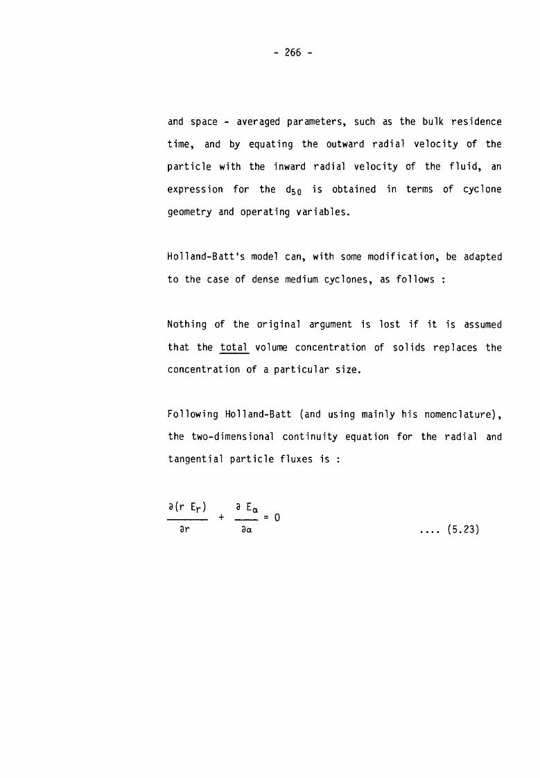
- 2 6 6 -

and space - averaged parameters, such as the bulk residence

time, and by equating the outward radial velocity of the

particle with the inward radial velocity of the fluid, an

expression for the d5 0 is obtained in terms of cyclone

geometry and operating variables.

Holland-Batt's model can, with some modification, be adapted

to the case of dense medium cyclones, as follows :

Nothing of the original argument is lost if it is assumed

that the total volume concentration of solids replaces the

concentration of a particular size.

Following Holland-Batt (and using mainly his nomenclature),

the two-dimensional continuity equation for the radial and

tangential particle fluxes is :

3(r Er )= 0

3r+

3a .... (5.23)

- 267

where Ep = Up Cy

Ea ~ ua Cvur = particle radial velocity

ua = particle angular (tangential) velocity

r = radius

a = extent of angular motion (radian)

Cv = total solids volume concentration

If Up and ua are "average" (constant) values

dCvthen Up Cv + ua --- = 0

da .... (5.24)

Integrating between Cvf and Cvo (the concentration at

the overflow after the suspension has traversed a radians in

the cyclone) gives :

ua / C vf\ur = _ In I _— }=a V v o /

Vc - U.... (5.25)

since ur is a net value relative to the cyclone walls, and

is the resultant of the settling velocity of the particles

(vs) and the radial flow of water inwards (U).

Holland-Batt defines U as :

U = Qf/Ac

and the mean residence time, t, as :

(5.26)

t = Vc/Qf .... (5.27)

- 268 -

where Ac is the cyclone inner wall area, given

approximately by :

rAc = IT Dr2|ni + --

[ 2 J .... (5.28)

and Vc is the cyclone volume, given approximately by :

nx = cyclone height / Dc

x\2 - cone height / Dc

(See also Figure 5.1).

In time, t, the medium will

t. The equivalent angular mot

the radius of motion :

2 utt t a =

Dc

2 ua Vc uaThus a = ------- and — =

Dc Qf «

Combining eqns. 5.25, 5.26 and

But the sedimentation results

nvs = vso “ Cvf)

4.65or VS = VS0 (1 - K Cvf)

___ (5.29)

have travelled a distance ua

on is obtained by dividing by

.... (5.30)

Qf Dc

2 Vc .... (5.31)

5.31 :

___ (5.32)

described in Section 4.2 gave:

.... (2.21)

.... (2.23)

- 269 -

in a gravitational field, or (for example)

ar 4.65Vs = — vso (1 - K Cyf)

g ___ (5.33)

in a centrifugal field, where ar is the acceleration

averaged over the cyclone radius.

Holland-Batt gives :

[r " ---r

4ghand thus ar = .... (5.34)

where Vt = "average" tangential velocity (m s"1)

and h = pressure drop in m of suspension.

4.65Writing z = vso (1 - K Cvf)

and combining eqns. 5.32, 5.33 and 5.34 gives

.... (5.35)

Simplifying and re-arranging :

8 h z Vc 2 Vc.... (5.36)= exp

Qf Dc 2 Ac DcCvf

2 Vc 8 h z Vc

Ac Dc Qf Dc 2

or (pq-p i) = (pf-Pl) exp

- 270 -

where p-j = density of liquid (usually water).

Thus the overflow density can be predicted from the feed

density, the cyclone geometry, the pressure drop, the

flowrate, and the sedimentation behaviour of the medium (z).

In the present work, the following approximate dimensions

applied :

Vc = 1.37 x 10-3 m3

Ac = 6.69 x 10-2 m2

Dc = 104 x 10"3 m

”i = 0.72

n2 = 2.50

Thus the constant geometry term in eqn. 5.37 is :

2 Vc------ = 0.394Ac Dc

Unfortunately, the sedimentation characteristics of the

medium used in each test were not monitored. In any event,

the value of z in eqn. 5.37 is an average value, since the

actual sedimentation rate will vary across the cyclone

radius with local acceleration, local solids concentration

and other factors. It is therefore probably difficult to

measure statically. However, all the other variables in

eqn. 5.37 were measured, and it is therefore possible to

re-arrange the expression so as to calculate a value for z

for each test :

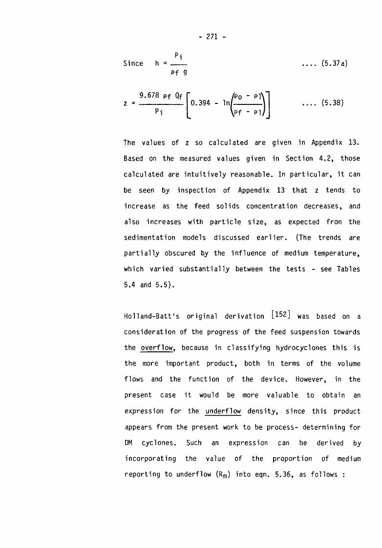
- 271 -

Since h =Pf 9

(5.37a)

z9.678 pf Qf

P i

0.394 - Inj(Po - Pr

\Pf ~ PI(5.38)

The values of z so calculated are given in Appendix 13.

Based on the measured values given in Section 4.2, those

calculated are intuitively reasonable. In particular, it can

be seen by inspection of Appendix 13 that z tends to

increase as the feed solids concentration decreases, and

also increases with particle size, as expected from the

sedimentation models discussed earlier. (The trends are

partially obscured by the influence of medium temperature,

which varied substantially between the tests - see Tables

5.4 and 5.5).

Holland-Batt's original derivation [152] was based on a

consideration of the progress of the feed suspension towards

the overflow, because in classifying hydrocyclones this is

the more important product, both in terms of the volume

flows and the function of the device. However, in the

present case it would be more valuable to obtain an

expression for the underflow density, since this product

appears from the present work to be process- determining for

DM cyclones. Such an expression can be derived by

incorporating the value of the proportion of medium

reporting to underflow (Rm ) into eqn. 5.36, as follows :

- 272

Assuming a steady state mass and volume balance,

Qf = Qu + Qo (flow) --- (5.39a)

Cvf Qf = vu Qu + Dvo Qo (solids) .... (5.39b)

From eqns. 5.39a and 5.39b,

Cvf Qf “ Cvu QuCvo = ______________ ___ (5.39c)

Qo

Substituting this in eqn. 5.36 gives :

Cvf Qf ~ vu Qu

Qo= Cvf exp

“ 2 Vc

L Ac Dc

8 h z Vc'

Qf Dc2 ..... (5.39d)

and Cvu Qu - Cvf Qf " Cvf Qo exP‘ 2 Vc

_ Ac Dc

8 h z Vc

Qf Dc2(5.39e)

Substituting Qo = Qf - Qu (from eqn. 5.39a) and

simplifying gives :

Dvu Qf / Qf\ 2 Vc 8 h z Vc--- = — + 11 - — l* exp ----- ----------Cvf Qu \ Qu/ _ Ac Dc Qf Dc2

(5.39f)

- 273 -

QuSubstituting Rm = — and re-arranging :

Qf

(pu " Pi) = (Pf-Pl) — + ( 1

Rm

2 Vc 8 h z Vc~

Ac Dc Qf Dc2

(5.39g)

This is the required expression for the underflow density.

It cannot of course be used, a priori, to predict pu from

the proposed operating conditions of a test, because it

demands knowledge of the value of Rm , which is itself a

dependent variable. However, given the established

relationships between h, P-j and Q f (see eqn. 5.37a and

section 5.5.9), eqn. 5.39g does predict that pu increases

with flowrate (other factors being equal), a trend which is

observed in practice.

5.5.4 Density Inversion, and the U-Shaped Tromp Curve

In nine tests, density inversion (p0 > pu) occurred. In

four of these tests, Tromp curves of a very unusual shape

were observed, for both the 2mm and 4mm tracers. It must be

emphasised that these curves were real, and fully

reproducible. The tests are listed in Table 5.9, and the

unusual Tromp curves are shown in Figure 5.10.

- 274 -

DENSITY f k a m - 3 ) -------- ^ © 2mm TRACERS

Q 4 mm TRACERS

FIGURE 5.10 TROMP CURVES FOR TESTS F1/1, F1/2, F6/1 AND F6/2

- 275 -

TABLE 5.9 - TESTS WITH DENSITY INVERSION

Test Number pu-Pf (kg nr3) Rm (*) Comments on Tromp Curve

FI/I -195 51.7 U-shaped curveFl/2 -125 70.4 W-shaped curveF2/2 - 86 78.5 No curve visibleF3/4 - 25 67.1 Normal curveF6/1 - 73 52.1 W-shaped curveF6/2 -190 50.8 W-shaped curveF6/5 - 29 36.5 Normal curveF5/1 - 27 23.2 Normal curveF5/2 -152 24.7 No curve visible

The following observations are pertinent :

i) The unusual Tromp curves only occurred when inversion

prevailed.

ii) Apart from two tests in which the density of

separation was too high to be monitored (F2/2 and

F5/2), those tests in which inversion occurred but

the Tromp curve was normal all exhibited low negative

differenti als.

iii) Extreme inversion, and the associated U-shaped

curves, always occurred with fine media at high feed

densities, for which t 0 and na were high.

- 276 -

i v) Little or no classification of the ferrosilicon

occurred (Appendix 12); indeed, the partition curves

for tests Fl/1, Fl/2, F6/1 and F6/2 suggest a degree

of reverse classification. This may imply destruction

of the toroidal sorting zone proposed by Renner

high, being greater than 50% for the milled

ferrosilicon (Figure 5.9).

vi) The centre, or the peak of the centre, of the

W-shaped Tromp curves coincided approximately with

the density of the cyclone contents in each case.

The phenomenon of inversion is entirely predictable using

the modified Holland-Batt model described in the previous

section, and no special assumptions need be invoked.

Inversion occurs when p0 > Pu> or Pf > Pu* The

limiting condition is therefore pf = p0, or, from eqn.

5.37 (for the present cyclone) :

8 h z Vc 2 Vc

v) The proportion of medium reporting to underflow was

= 0.394Qf Dc2 Ac Dc .... (5.40)

Pi zor = 3.815

Pf Qf .... (5.41)

- 277 -

and inversion occurs when

Pi z----- < 3.815Pf Qf

Given the dimensionally-derived Pi/pf/Qf/n relation­

ships (Chapter 3), this implies that inversion depends upon

i) A low flowrate.

ii) A low sedimentation rate (fine particles, high

concentration).

iii) A high kinematic viscosity.

(The last two requirements are fully compatible).

The viscosity enters as a variable via the relationship

between pressure drop and the cyclone velocity constant, n,

which decreases as viscosity increases U L

Eqns. 5.37 and 5.40 also demonstrate that inversion can be

induced if the geometry term, 2VC/ACDC, is maximised.

From eqns. 5.28 and 5.29,

2 Vc

Ac Dc

1

2

+ n2/3

n: + n2 / 2 .... (5.42)

- 278 -

Thus n2 must be minimised, which implies a wide cone angle.

This treatment suggests that the sustaining of inversion

essentially requires a residence time long enough to allow

the slow-settling solids to migrate to the overflow, which

in turn implies a slow rate of revolution, a high inlet

velocity loss factor, and a low cyclone velocity constant,

n, all of which are likely to be associated with a high

viscosity [1], There may therefore be points in the

cyclone in which solid body rotation is approached (n = -1 ),

compounded by the presence of a yield stress which will not

be overcome if the shear rates in the cyclone are low. The

tangential velocity may not therefore vary much across the

radius.

Three species of tracer (or particle) can now be

distinguished, according to density :

i) Low density - Easily centrifuged to the periphery,

where low medium densities prevail, but unable to

penetrate the slowly moving mass of high density

medium in the central section and near the axis.

ii) High density - Also centrifuged to the periphery and

recovered in the underflow product in the usual way.

In fact, the upper part of the curve might be

regarded as the normal Tromp curve.

- 279 -

iii) Intermediate density - Invoking the model of a stable

medium, described in Chapter 3, one might postulate a

range of particle densities, centred on the density

of the contents medium, which are "locked into" the

medium and divide in the same proportion as the

medium.

Inspection of the W-shaped curves of tests Fl/2, F6/1 and

F6/2 shows them to be similar in the central and upper

sections to those described in Chapter 3 (cf. Figure 3.8).

The "hump" in the central part of the curve, is, however,

missing in test Fl/1. Using the arguments advanced in

Chapter 3, the range of critical density (for spheres)

depends upon the yield stress, t 0, and is given by :

3ir T0(« - p )c =

2 d a .... (A5.2)

Vt2and since a = ---

r

then (6 - p)c cc x0/Vi2 .... (5.43)

assuming V-j (the inlet velocity) can be utilised

characteristic tangential velocity. The observed values of

T0/V-j2 are as follows :

Test Tn/Vi2 (kq nr

Fl/l 0 . 2 1 1

Fl/2 0.441F6/1 0.279F6/2 0.543

- 280 -

Significantly, the term for test Fl/1 (in which no "hump"

appeared) is the smallest, suggesting that this term must

exceed a certain minimum value before the effect of yield

stress is detectable.

If (as in Chapter 3) we take Vt = Vi, r = R, and a (the

inlet velocity loss factor) = 0.5, then for test F6/1, and d

= 2 mm :

( 6 - P)c = 137 kg nr3

Since the contents density was 2976 kg nr3, the range of

influence is therefore estimated as 2839 - 3113 kg m“3,

which conforms well to the region occupied by the "hump" in

Figure 5.10, test F6/1.

Such calculations are, at best, only approximate, since :

i) na, and thus t 0 , are certainly underestimated,

possibly by a factor of 2 , due to the capillary

diameter effect (see Section 4.3.5.1).

ii) The extent to which a and n are modified by the high

values of m a and t 0 is not known, and thus a is

not known (although V-j is accurately known).

- 281

However, these arguments do provide an acceptable scenario

for the explanation of the "hump" which is superimposed on

the U-shaped curves of tests Fl/2, F6/1 and F6/2. A typical

such curve is shown in Figure 5.11, divided into key

sections :

FIGURE 5.11 - TYPICAL W-SHAPED TROMP CURVE

% to

Underflow

Density

- 282

Section A - Normal Tromp curve for dense particles.

Section B - Hump caused by near-density particles (of

density close to that of the cyclone contents) locked into

the medium, due to the prevailing yield stress. Since there

is a density differential across the cyclone (even if

negative), the proportion of such particles reporting to the

underflow will not necessarily equal Rm , as was the case

with the stable media of Chapter 3. The proportion will

equal that proportion of the medium of critical density

range which reports to the underflow.

Section C - Continuation of normal curve, displaced by yield

stress effect.

Section D - Reverse curve for light particles, caused by

negative differential.

Thus it can be seen that density inversion, and the

associated U-shaped and W-shaped Tromp curves, are entirely

explicable within the theoretical framework already

established. The phenomenon arises as a consequence of an

(unusual) combination of high medium viscosities, and

associated yield stresses, together with an appropriate

cyclone geometry. It is therefore rarely, if ever,

encountered in practice. Inversion was reported in the

author's previous study [4], but no unusual Tromp curves

were observed. However this was probably due to the curves

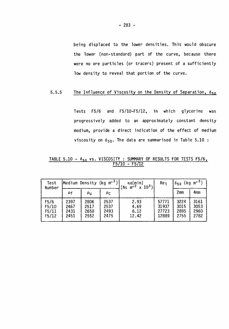
- 283 -

being displaced to the lower densities. This would obscure

the lower (non-standard) part of the curve, because there

were no ore particles (or tracers) present of a sufficiently

low density to reveal that portion of the curve.

5.5.5 The Influence of Viscosity on the Density of Separation, 6 c;n

Tests F5/6 and F5/10-F5/12, in which glycerine was

progressively added to an approximately constant density

medium, provide a direct indication of the effect of medium

viscosity on 6 50. The data are summarised in Table 5.10 :

TABLE 5.10 - 6 sn vs. VISCOSITY : SUMMARY OF RESULTS FOR TESTS F5/6,F5/10 -F5/12

TestNumber

Medium Density (kg m"3) na(min)(Ns m" 2 x 103)

Re 5so (kg nr3)

pf Pu Pc 2 mm 4mm

F5/6 2397 2806 2537 2.93 57771 3224 3161F5/10 2467 2517 2537 4.69 31937 3015 3053F5/11 2431 2658 2493 6 . 1 2 27723 2895 2960F5/12 2451 2552 2475 12.42 12889 2755 2782

- 284 -

(There is evidence from the original data, and subsequent

regressions, that the value of pu in Test F5/10 is in

error).

It is clear that both pu and 6 5 0 fall as the viscosity

increases. The trend for 6 5 0 is therefore in accordance with

the literature, but does not conform to the theory for

stable media successfully applied in Chapter 3. This

confirms the discrepancy between theory and observation for

unstable media identified in Chapter 2, and strongly

suggests that the observed trend is attributable to the

influence of the viscosity of the carrying liquid on the

behaviour of the medium particles.

The 6 5 0 - na trend is illustrated in Figure 5.12, and can

be quantified using the dimensionless relation :

6 50 - Pf a-------- = K Ren-

Pf .... (5.44)

The parameters estimated by linear regression were :

2 mm 4mm

K 1.917 x 10-1* 5.850 x 10“a 0.681 0.577R 2 0.990 0.995

&0-

(V

FIGURE 5.12 RELATIVE DENSITY OF SEPARATION vs Rei FOR TESTS F5/6, FS/10 - FS/12

~ f

f (k

cjm

~3)

FIGURE S.13 v sV„ (min) FOR TESTS FS/6. FS/10 -FS/12

Il \300cni

- 286

The fit is shown by the values of R2 and Figure 5.12 to be

exellent. The exponent, a, is positive in both cases,

instead of negative as found for stable media, confirming

the reverse trend.

One might attribute this trend to the drop in pu arising

from the increase in liquid viscosity which is both observed

in these data and predicted from the modified Holland-Batt

theory (eqns. 5.37 and 5.39g in Section 5.5.3). However, the

correlations for 6 5 0 in terms of pf and pu, developed in

Section 5.5.2 (eqn. 5.21), tend to overestimate 6 5 0 to an

increasing extent as the viscosity rises. This implies that

the viscosity of the carrying liquid has an effect on 6 5 0

additional to the influence which it exerts indirectly

through its effect on p u .

An explanation for these trends can be found by studying the

behaviour of the density of the cyclone contents, pc, and

considering the implications of variations in the relative

residence times of medium solids and liquid. Inspection of

Tables 5.4 and 5.5 shows that the contents density nearly

always exceeds the feed density (in 41 out of 45 cases),

implying that the solids experience a longer bulk residence

time than the liquid. The difference between the contents

and feed densities, pc - Pf, appears to be an inverse

function of the medium viscosity. The data for tests F5/6,

F5/10-F5/12 are shown graphically in Figure 5.13, together

with the predicted relationship obtained by regression :

- 287 -

-1.194(Pc ” Pf) = 492.5 na(min) (R2 = 0*987) .... (5.45)

The density of separation is clearly related directly to

this density difference, as shown in Figure 5.14, 6so

increasing with increasing (pc - pf).

Using simple mass balance concepts, it can be shown that the

residence time of the solids and liquid can be calculated

from the bulk volumetric residence time (Vc/Qf) and the

feed and contents medium densities. The expressions so

derived are as follows :

tc =Vc Pc - PI

usQf ’ Pf - PI ___ (5.46)

*1 =vc PS “ Pc

Qf Ps - Pf ___ (5.47)

*s Pc - PI Ps - Pf___ (5.48)

*1 Pf “ PI Ps" Pc

where PS = solids density

PI = liquid density

ts = residence time of solids

t] = residence time of liquid

- 288

FIGURE 5 % DENSITY OF SEPARATION vs DENSITY DIFFERENCE BETWEEN CONTENTS AND FEED MEDIUM:TESTS F S /6 , F 5 /1 0 -F S /1 2

I Pc- & ) ( k Q m ~ 3) --- ^

- 2 8 9 -

The value of the ratio ts/t] is directly related to the

term (pc - pf) :

TABLE 5.11 - RELATIVE RESIDENCE TIME FOR TESTS F5/6, F5/10-F5/12

TestNumber & ts/t! na(min)

(Nsnr* x 103)

F5/6 140 1.136 2.93F5/10 72 1.065 4.69F5/11 62 1.058 6.12F5/12 24 1.022 12.42

Thus, as the fluid viscosity increases, the proportion of

medium particles dragged with the fluid increases, which

reduces the difference between the solids and liquid

residence times. This must also influence the distribution

of medium density in the cyclone by reducing the segregation

effect and thus increasing the proportion of the cyclone

volume occupied by medium of density approaching that of the

feed, i.e. pc -► pf, and (pc - pf) -► 0. (Although the

increasing liquid viscosity causes an increase in the

classification size, dso, [see Section 5.5.6], this is

compensated for by a decrease in the quality of separation

and thus an increase in the proportion of misplaced sizes;

the proportion of solids reporting to underflow thus falls

only slightly - see Table 5.5). The sorting effect, usually

present as a consequence of the strong density gradients

across the cyclone, is therefore reduced, and more tracers

will penetrate into the underflow product, thus reducinq the

650-

- 290 -

The reduction of 650 with increasing medium viscosity is

thus seen to be a consequence of two factors : the direct

effect of the associated reduction in underflow density, and

the modification of density gradients within the cyclone as

a result of the reduction of the differences between the

residence time of medium solids and liquid.

5.5.6 The Classification of the Medium

It has already been inferred that the density separation is

influenced by both medium segregation and classification.

The modification of Holland-Batt's theory, applied

successfully in Sections 5.5.3 and 5.5.4, contains elements

of both phenomena.

The fact that classification of the medium does occur is

clearly evident from the partition curves shown in Appendix

12. The following observations can be made :

i) Some degree of classification occurs in most of the

tests, except at very high feed densities.

ii) When density inversion occurs, this can be associated

with reverse classification (e.g. F6/1, F6/2).

iii) In general, the lower tails (fine particle recovery)

of the curves do not coincide with the water recovery

(the horizontal lines in Appendix 12). Thus the

- 291

bypass mechanism associated with normal hydrocyclone

classification does not appear to operate in the

dense medium case.

iv) The classifications are generally of poor quality.

The lack of a bypass mechanism is particularly interesting.

There seems to be no consistent trend regarding the position

of the water recovery level relative to the partition curve;

the relationship seems entirely random. Even test F6/6,

which was deliberately conducted at a very low feed solids

concentration (5.8% v/v) in order to establish whether

"conventional" classification occurred, produced a

considerable discrepancy between the water recovery and fine

particle recovery; the underflow density was high, at 2655

kg m"3 (28.2% solids, v/v). Austin and Klimpel [145]

reported a similar phenomenon with a classifying

hydrocyclone, and pointed out that high-density underflow

products could entrain particles of all sizes; there was

therefore no reason why the fine particle recovery should

equal the water recovery under such conditions. Finch

[153] drew attention to the existence of unusually-shaped

lower tails in some classification curves. He modelled such

curves by assuming that the entrainment of particles in the

water was an inverse linear function of particle size, but

also mentioned agglomeration and "dense media" effects as

possible mechanisms.

- 2 9 2 -

Thus it seems that with dense media, for which the underflow

density usually exceeds 25% solids v/v, there is no fixed

relationship between water recovery and fine-size particle

recovery owing to the entrainment of particles of all sizes

in the underflow mediurn (as distinct from the underflow

water). In this context, it is worth recalling the

conclusion of Davies and Dollimore [128] that hindrance to

settling of suspensions is more likely with dense solids. It

may be therefore that the type of classification observed is

peculiar to dense medium separations using very dense solids

(e.g. ferrosilicon). This might also imply that the

proportion of the observed segregation or thickening of the

medium contributed by classification effects (as distinct

from sedimentation) might be less for denser solids. It

might also account partly for the generally poor quality of

classification observed.

Inspection of the data in Tables 5.4 and 5.5 suggests that

the classification size, d50, although difficult to

determine in many cases, increased with flowrate, the exact

opposite of the trend expected from theory (e.g. eqn. 2.3).

This suggests a crowding mechanism at the apex. The

sedimentation of the medium increases with flowrate, which

leads to an increased underflow density. This in turn

selectively excludes finer particles from the underflow

product, thus increasing the d50. The classification of the

medium appears therefore to be controlled by the degree of

medium sedimentation, and the two mechanisms which determine

- 293 -

the underflow density (and hence the 650) are thus

inextricably linked. In view of the probability of crowding

as a process-determining factor, Fahlstrom's equation [33]

was fitted to some of the data, but unsuccessfully.

Inspection of the data in Tables 5.4 and 5.5 suggests that

the d50 increased with feed solids concentration, as

expected from the literature. An expression of the kind

suggested by PIitt [3] and Svarovsky and Marasinghe [28]

was fitted to the six data points of Series F6, for which

the flowrate remained relatively constant. The expression

obtained was :

dso = 8.58 exp (0.0637 Cvf) ___ (5.49)

(R2 = 0.985; Cvf expressed as a percentage).

The coefficient for Cvf was almost exactly the same as

that reported by PIitt (0.063) but about twice that reported

by Svarovsky et al (0.032). It should be noted, however,

that the d50 was uncorrected for bypass, unlike those of

Plitt and Svarovsky et al.

Tests F5/6 and F5/10-F5/12 provide an opportunity to examine

the dependency of (uncorrected) dso on liquid viscosity. The

relevant data are given in Table 5.12 :

- 294 -

TABLE 5.12 - FERROSILICON CLASSIFICATION DATA FOR TESTS F5/6, F5/1Q-F5/12

TestNumber

LiquidSG

Temperature(°C)

Viscosity,* n (Nsm“2 x 103)

d50(urn)

F5/6 1.000 24 0.91 34F5/10 1.065 32 1.58 43F5/11 1.091 39 1.69 44F5/12 1.130 26 5.16 58

(* obtained from Tables [133])

The equation fitted was :

0.296d50 = 36.4 n (R2 = 0.970) .... (5.50)

The data and the fitted line are shown in Figure 5.15.

The exponent for n is about half that reported by Agar and

Herbst [25] and less than the theoretical value of 0.5

(e.g. eqn. 2.3). This is probably due to the contribution of

the high solids content, and consequent hindrance and

crowding effects, to the classification mechanism.

In summary, classification of the medium does occur, except

at very high feed solids concentrations (typically greater

than 30% v/v). The d50 increases both with liquid viscosity

and solids concentration, as expected. However, the

sedimentation of the medium in the cyclone interferes with

the normal classification mechanisms, causing there to be a

lack of correspondence between water recovery and fine-

particle recovery, and inducing a direct relationship

between d50 and flowrate, instead of the inverse trend

expected from theory.

FIGURE 5.75 dgn vs LIQ U ID VISCOSITY FOR TESTS FS/6. F5/1Q-FS/

LIQUID VtSCOSrTY ( Nsnr^x 10*) — ^

- 2 9 6 -

5.5.7 The Influence of Apex Diameter on the Separation

Test F5/7 was carried out with the 20mm spigot insert

removed, leaving an apex orifice of 30mm, 2.25 times larger

in area. In terms of operating conditions, this test

conformed most closely to F5/5, with almost identical

ferrosilicon sizes, flowrates and medium viscosities; the

feed densities differed by only 61 kg m~3. Comparison of

these two tests therefore offers the possibility of

determining the effect of apex diameter on both the density

separation and the ferrosilicon classification. The relevant

data are given in Table 5.13 :

TABLE 5.13 - OPERATING AND PERFORMANCE DATA FOR TESTS F5/5 AND F5/7

V ar i ab 1 e Test F5/5 (20mm Apex)

Test F5/7 (30mm Apex)

pf (kg m-3) 2358 2419pu (kg m',) 2872 3372Po (kg nr-) 2232 1939pc (kg nr*) 2504 2400Rm 19.7 33.5650 (2mm) > 3490 > 324565n (4mm) > 3490 > 3235ts/tw 1.145 0.982dso (pm) 37 15pu/pf , 1.218 1.394z (ms-1 x 10u ) 1.50 2.07

As expected, the 650 and the d50 both fall, and the

proportion of medium reporting to the underflow rises, as

the apex diameter increases. However, the underflow density

increases significantly at the larger apex. This is

- 297 -

reflected also in the larger value of the effective

sedimentation rate, z, calculated from eqn. 5.38. Since the

medium characteristics did not change significantly, this

suggests that the modified Holland-Batt equations (5.37,

5.38 and 5.39g) should incorporate a term allowing for

variations in orifice geometry, possibly a constant

multiplier for z.

The magnitude of the increase in pu, although at least

partly accounted for by the drop in d50, suggests that the

flow pattern in the cyclone changed, causing a higher degree

of segregation to take place in the cone section.

These results confirm that the quantitative correlations for

650 in terms of pf and pu derived earlier (eqn. 5.21)

can only apply within a constant geometry.

5.5.8 The Quality of Separation

The quality of separation is conventionally expressed in

terms of the Ep-value (eqn. 3.3), obtained from the Tromp

curve. A high Ep-value indicates a large proportion of

misplaced material, and thus a poor quality of separation.

It proved impossible to obtain accurate correlations for Ep

in the present work. This was probably due to the relatively

small number of particles (tracers) used to determine each

Tromp curve, and to the lack of factors which might be

- 298 -

expected to exert a strong influence on Ep, in particular a

crowding effect. Nevertheless, two trends are apparent :

i) The Ep for the 4nm tracers was almost always less

than that for the 2mm tracers (20 out of the 24 cases

in which comparisons were possible).

ii) The Ep generally increased with 650; this is clearly

shown in Figure 5.16.

These two trends are compatible, since it has already been

demonstrated (Section 5.5.2) that the 6S0 for the 4mm

tracers was generally less than that of the 2mm tracers.

They also appear to conform with the literature reviewed in

Section 2.2. Stas [43] # Davies et al [48] and Khaidakin

[54] all report a direct relationship between 650 and Ep,

and Tarjan [14] implies it by deducing that the best

separations are achieved as 650 -► pf. As noted earlier, Ep

« d50 is also inherent in Gottfried's mathematical treatment

of the Tromp curve [48]. Davies et al [48] and Collins

et al [55] interpret this trend in terms of the density

differential between underflow and overflow (or feed),

observing that the Ep increases as stability deteriorates.

Such a correlation was not readily apparent in the present

work, possibly for the reasons outlined earlier. However it

is implicit in the correlation for 650 in terms of pf and

pu (eqn. 5.21) if one accepts the observation that Ep

increases with 650 (Figure 5.15).

Ep

-VA

LU

E

299

FIGURE S.16 DEPENDENCE OF Ed UPON Sv) FOR MILLED TEST. 2mm TRACERS

t

SEPARATING DENSITY, S lg f kgm*)

- 300 -

These trends can probably be attributed to the effective

increase in "near-density" material which is a consequence

of large density differentials across the cyclone radius.

Such material is subject to more uncertainty as to its

ultimate destination. This has the effect of flattening the

Tromp curve and thus increasing the Ep.

5.5.9 Pressure-Flowrate Relationships

The relationship between pressure drop (or inlet pressure)

and medium flowrate for dense medium cyclones has received

little attention in the literature. The relationship is

important academically because it defines the flow regime in

which the cyclone operates, and practically because it

determines the pumping requirements and because pressure can

be used as an indicator of flowrate, which is itself an

important process variable.

In order to establish the characteristics of the cyclone

used in the present work, nine tests were first run with

water only, at increasing levels of flowrate. The flowrates,

inlet pressure (P-j) and water temperature were measured.

The feed flowrate (Qf) was measured using the flowmeter,

and the product flowrates were measured using a bucket and

stopwatch. The results were balanced using the methods

described in Section 5.3.

- 301 -

The effective water viscosity (n) at the prevailing

temperature was obtained from tables [133]. The results

are given in Table 5.14 :

TABLE 5.14 - PRESSURE-FLOWRATE MEASUREMENTS WITH WATER

TemperatureP C )

Viscosity, n (Nsnr2 x 103)

Pressure, Pi (kNm'2)

Flowrates (£ min-1) Y 5 f ReynoldsNumber

Rei

PressurLoss

FactorL

FeedQf

U/FQu

0/FQo

20 1.005 40.7 62.3 5.09 57.2 8.90 73,082 4.88920.5 0.993 54.5 71.9 5.46 66.5 8.21 85,362 4.91521.5 0.969 69.0 77.0 5.46 71.5 7.63 93,681 5.42622 0.958 83.4 83.8 5.68 78.1 7.28 103,125 5.53723 0.936 97.9 89.4 5.96 83.4 7.14 112,603 5.711

24.5 0.904 112.4 95.3 6.14 89.1 6.88 124,282 5.77026 0.874 126.2 99.0 6.50 92.5 7.03 133,540 6.00327 0.855 140.0 103.0 6.59 96.4 6.84 142,023 6.15324 0.914 152.4 106.9 7.00 99.9 7.01 137,885 6.218

A log-log plot of pressure vs flowrate is shown in Figure

5.17, together with the line predicted from the equation :

2.48Pi = 1.433 x 10-3 • Qf .... (5.51)

(R2 = 0.9980; Pi in kNrtr2, Qf in i min'1)

The fit is seen to be excellent. However, since the water

viscosity varied by about 15% during the tests, a viscosity

term was added to the expression, with the following result:

2.42 -0.19Pi = 1.801 x 10'3 • Qf • n ___ (5.52)

(R2 = 0.9981; Pi in kNm'2 , Qf in i min'1, n in Nsm'2 xlO3)

- 302 -

FIGURE 5.17 PRESSURE vs FLOWRATE FOR WATER TESTS 100 mm CYCLONE

FLOWRATE, Of l Lmin~1l

- 303 -

The viscosity term is thus a significant addition, and a

comparison of the measured and predicted values of Pi

shows that eqn. 5.52 has a slightly improved predictive

capability over eqn. 5.51. Eqn. 5.52 shows that the

viscosity variation of about 15% experienced during the

measurements equated to an equivalent pressure drop

variation of about 3%. The exponents in eqn. 5.52 should be

compared with those obtained in the experiments with a

stable medium and a 30mm cyclone (Chapter 3, eqn. 3.18) :

Exponent for : Eqn. 3.18 Eqn. 5.52

Qf 2.30 2.42

n -0.30 -0.19

The drop in the absolute value of the viscosity exponent,

and the corresponding increase in the flowrate exponent, is

probably due to the fact that the water tests with the 100mm

cyclone took place in a somewhat different Re-j - L regime

(compare Figure 5.18 with Figure 3.12), in which centrifugal

head loss predominated over friction losses. The exponent

for Qf in eqn. 5.52 is in quite good agreement with

Bradley's figure of 2.35 [1],

The ratio Qu/Q0 is shown plotted against Qf in Figure

5.19. The best-fit equation is :

Qu -0.473_ = 61.1 • QfQ0 (R2 = 0.905) ___ (5.53)

304 -

FIGURE 5.18 L vcs Re; FOR 100 mm CYCLONE WATER TESTS

tg b

I

FIGURE 5.19 °u /Q c vs Of FOR 100mm CYCLONE MTER TESTS

t•9<31 EXPERIMENTAL DATA

FITTED EQU. 15 531

Q t( Lmin~1I

- 305

The exponent for Qf compares favourably with Bradley's

quoted range of -0.75 to -0.44 [1],

The relevant data relating to the tests with ferrosilicon

media are given in Tables 5.4 and 5.5, and Appendix 13. In

Chapter 3 it was shown that the pressure-flowrate

relationship obtained by dimensional analysis was :

a n2P-j = K Rei — ___ (3.17)

P

This can also be conveniently expressed in the form (see

eqn. 3.18) :

Pi a ^a(min)--- = K • Qf • -----1Pf9 Pf

(K, a and 3 signify parameters to be evaluated by

regression).

In these experiments with ferrosilicon, the medium viscosity

is of course defined as na(min)> ln terms of the arguments

expressed in Section 4.3.5.2 (eqn. 4.41), which is not

strictly comparable to the plastic viscosity utilised in

Chapter 3.

3.... (5.54)

- 306 -

Eqn. 5.54 was applied to the milled ferrosilicon data

(Series FI, F2, F3 and F6), the parameters being estimated

by multiple linear regression. The result was

unsatisfactory, the fit being relatively poor (R2 = 0.876

with 27 data points). The equation was then fitted to the

data from the individual test series separately. Much

improved fits resulted. The values of the parameters

estimated are given in Table 5.15 :

TABLE 5.15 - PARAMETERS IN EQUATION 5.54 FOR MILLED FERROSILICON,

SERIES FI, F2, F3 AND F6

Parameter Series FI Series F2 Series F3 Series F6

K 1.578 x 10-3 2.271 x 10-3 1.238 x 10-1* 3.188 x 10-*’a 1.779 1.653 2.409 2.192

-0.213 -0.015 -0.201 -0.267R2 0.989 0.959 0.993 0.991

No. of Data Points 9 9 4 5

UNITS : [Pi] = kNm-:2;[Pf] = kgm~3 ; ;g] = ms-2 ; [Qf ] == Imin"1; [na] = Nsm-2 x 103

It is clear that, although the individual fits are good, the

parameters vary between the test series. In particular, the

absolute value of the exponent, 3, for Series F2 was very

low, suggesting that viscosity played little role in

determining the pressure drop for those particular

experiments. In seeking an explanation for these

observations, it was noticed that Series F2 utilised the

- 307 -

coarsest ferrosilicon particle size, which would be expected

to have the lowest viscosities (other things being equal).

Inspection of Table 5.4 confirmed this. It seemed,

therefore, that the pressure-flowrate-viscosity relationship

was in some way dependent upon the ferrosilicon

characteristics (particularly the size distribution), and

thus presumably upon the behaviour of the medium in the

cyclone. A particle size term, RRa (Table 5.4, Col. 1),

was therefore added to eqn. 5.54 and all 27 data sets were

included in the regression. The fit was improved over that

without the size term (R2 = 0.928), but was still not

altogether satisfactory. It seems that a size term alone is

therefore not sufficient. It would probably be preferable to

obtain an independent estimate of, say, the sedimentation

rate of each medium to incorporate in the relationship,

instead of the value, z, calculated from the data.

Unfortunately, such information was not available in the

present work.

Eqn. 5.54 was also applied to the atomised ferrosilicon data

of Series F4 and F5, with the results shown in Table 5.16 :

- 308 -

TABLE 5.16 - PARAMETERS IN EQN. 5.54 FOR ATOMISED FERROSILICON,

SERIES F4 AND F5

Parameter Series F4 Series F5

K 1.956 x 10- 3 1.270 x 10- 3

a 1.757 1.895-0.405 -0 . 0 1 1

R2 0.997 0.980No. of Data Points 5 1 2

Units as for Table 5.16

Again, one group of tests (Series F4) shows a relatively

strong viscosity dependency, whereas the other (Series F5)

does not. However in this case the viscosity dependency is

exhibited by the ferrosilicon with the coarser size

distribution (Table 5.4), a reverse trend to that shown by

the milled ferrosilicon.

Mitzmager and Mizrahi [127] have pointed out that the

pressure drop head is composed of three main components :

a) Inlet velocity head - the work input necessary to

bring the fluid from rest to the inlet velocity.

b) Centrifugal head - the major resistance to the fluid

flow.

c) Friction loss head - boundary layer resistance and

eddy turbulence.

- 309 -

They emphasised that the inlet flow regime has a significant

effect on the pressure drop relationship, and noted that the

pressure loss factor vs inlet Reynolds number curve can be

used to define the relative influence of the components of

pressure drop : at low Reynolds numbers (or, more

particularly, in the falling section of the curve) friction

loss is the major contributor, whereas at high Reynolds

numbers (the rising section of the curve) centrifugal head

losses predominate. Thus, as noted in Chapter 3, the value

of the exponents in the pressure-flowrate-viscosity

relationship (eqn. 5.54) will depend upon the prevailing

flow regime.

In order to reconcile the apparent anomalies in the

observations described above, the L-Re-j curve was plotted

for each of the test series; the results are shown in Figure

5.20. Although some scatter is evident, the conclusions are

clear : those test series which exhibited a relatively

strong pressure dependency on viscosity (FI, F3, F6 and F4)

lie on a rising curve, whereas those which did not (F2 and

F5) lie on a falling curve.

The absolute position of each curve relative to the others

(in terms of Reynolds number) cannot be firmly identified

since the value of viscosity used was the "minimum apparent

viscosity" defined by eqn. 4.41, which is not necessarily

the "flow viscosity" prevailing in the inlet. Also, this

viscosity was not corrected for the capillary diameter

PRES

SURE

LOS

S CO

EFFIC

IENT.

L

- 310 -

FIGURE 5.20 PRESSURE LOSS COEFFICIENT vs REYNOLDS NUMBER FOR FERROS/UCON TESTS

10& 2x10u 10-

C CtS §■ -ET

3T0

3 1O G - X "

^ d; V

D

3

X

SERIES FI__ SERIES F3 SERIES F6

!

i £>SERIES F2_

•

.____ □o□ * G 1 1* 1

LI l T ID—

&O’

I)

3

S

S

FRIES Fit —

FRIES FS

u3

65

It

3

2

10*> 10s 2x10* 10s

REYNOLDS NUMBER. Re;-- ^

- 311 -

effect (Section 4.3.5.1). The values of Re-j quoted are

therefore not strictly comparable with those reported by

other workers. However, this is not important since the

trends in the relationships are relatively unambiguous.

The fact that significant numbers of tests lay on the lower,

falling part of the curve (i.e. at low values of Re-j),

unlike most hydrocyclone operations which generally lie on

the rising portion, can be attributed to the higher

viscosities prevailing with dense media (up to ten times

that of water).

However, the reason for the different test series lying on

different portions of the curve is not at first clear.

Inspection of Tables 5.4 and 5.5 suggested that the values

of yield stress, relative to the prevailing medium density,

varied substantially between the test series. The results

are plotted for the milled and atomised series in Figure

5.21. (The last 3 tests of Series F2 were excluded because

of anomalously high values of yield stress at the lower

densities). Although the t 0 - pf relationships

themselves exhibit a lot of scatter, the differences between

the test series are relatively clear, particularly for the

atomised tests. Those tests for which a relatively strong

P-j-Tia relation was noted, and which lay on the rising

portion of the L-Rei curve (Series FI, F3, F6 and F4),

exhibited higher yield stresses at a given density than

- 312 -FIGURE 521 YIELD STRESS vs MEDIUM DENSITY FOR MILLED

AND ATOMISED FeSi

I

6

&BoUj

A. MILLED FeSi

Q SERIES F1

X

n SERIES F2 D (EXCLUDING F2/6- A SERIES F3X SERIES F6

F2/B)□

> X

\ H _____ © /

/1

X G \ \ \ \ □ \

_______rj

<D---- ^ □

~ 2000 2500 3000 3300FEED MEDIUM DENSITY. Pf (kqm-3)

i

&

BCjg

a. ATOMISED FeSiG

O SERIES FU ^ SERIES F5

■ O

O O ^

-------r

____

t>

•

~ 2000 2S00 3000 3300

FEED MEDIUM DENSITY, Fftkom'3)

- 313 -

those for which the Pj-r)a relation was weak and which

lay on the falling portion of the L-Re-j curve (Series F2

and F4). The division between the two groups is indicated by

the dashed lines in Figure 5.21.

As noted earlier, the rising (upper) portion of the L-Re-j

curve is associated with a predominance of centrifugal head

loss, since "... the revolving liquid shells are pressing

outwards upon one another" [127]# it was suggested earlier

that, with dense media, shear rates in the cyclone are

relatively low owing to a low value of the cyclone constant,

n, and an increase in the inlet velocity loss factor, a. In

extreme cases in the present work, the presence of a yield

stress was inferred from unusually-shaped Tromp curves

(Section 5.5.4). It seems reasonable to suppose, therefore,

that the existence of a yield stress in the low-shear parts

of the cyclone would absorb a portion of the kinetic energy

of the entering medium, and so contribute to a high

centrifugal head loss. Since yield stress is usually

strongly correlated with apparent viscosity, this would be

reflected in a (relatively) strong pressure drop-viscosity

relationship. Thus we are drawn to the interesting

conclusion that the observed pressure drop across a dense

medium cyclone is a function of the total medium rheology.

The success of eqn. 5.54 in describing data which fall on a

smooth L-Re-j curve can be deduced by examination of the

results of test Series F3 and F6 . Figure 5.20 shows that the

- 314 -

nine data points from these two groups of tests fall on the

same smooth L-Rei curve. Regression of the basic data in

the form of eqn. 5.54 gives :

pi „---- = 1.684 x 10-*Pf 9

afmin)-0.254Pf

2.344

Qf.... (5.55)

(R2 = 0.996; units as given in Table 5.16).

The value of R2 is very high, and the predictive capability

of the correlation can be assessed from Figure 5.22; the

agreement between the predicted and measured values of inlet

pressure is excellent over the whole range.

It can therefore be concluded that a correlation of the form

of eqn. 5.54 (or eqn. 3.18) adequately describes the

pressure-flowrate-viscosity relationship for DM cyclones.

For the higher inlet Reynolds numbers, the exponent, 3 , for

the kinematic viscosity term is invariably negative and

takes the absolute value 0.2 - 0.4; a value of 0.25

represents a useful compromise, which is close to the value

0.30 reported for the stable media experiments in Chapter

3. The actual value depends upon the prevailing L-Rei

relationship which in turn is a function of the medium

rheology. For the lower inlet Reynolds numbers, the exponent

is not significantly different to zero.

PREDICTED INLET PRESSURE (KNm-2)

- 315 -

FIGURE 5.22 MEASURED re PREDICTED VALUES OF INLET PRESSURE FOR SERIES F3 AND F6

t

MEASURED INLET PRESSURE (KNm~2) — ►

- 316 -

The exponent, a, for flowrate is invariably positive, and

ranges from 1.65 for results lying on the lower portion of

the L-Rei curve to 2.41 for results lying on the upper

portion of the curve. It is interesting to note that the

highest value of this exponent (2.41; Series F3) coincided

almost exactly with that obtained with water (2.42; eqn.

5.52); in both cases, the results lay on the upper, strongly

rising and well developed portion of the L-Rei curve (cf

Figures 5.18 and 5.20).

5.6 Summary and Conclusions

The work with the 100mm cyclone and ferrosilicon media has shown that

the correlation for 6 5 0 utilised successfully in Chapter 3 with stable

media cannot be applied directly to unstable media. This is

attributable to the segregation and classification of such media in

the cyclone. In particular, it has been shown that the separating

density, 6 50, is not a simple function only of the Reynolds number and

particle size, and the dependency on flowrate is actually the reverse

of that predicted by theory.

There is substantial evidence in the literature that, in normal ore

separations, the separating density equals the underflow medium

density [48,49,65]. the present work, however, and similarly for

an extended test programme carried out by the author previously on a

610mm cyclone with real ores [4], the 650 almost always exceeded

pu. Inspection of the results suggested that 6 5 0 followed both pf

and pu (but never p0) on different occasions, and so the following

simple model was fitted to the data :

- 317

6 5 0 = 3 + b pf + c Pu .... (5.21)

The fit was found to be excellent, and the predictive capability of

eqn. 5.21 was extremely good. The 6 5 0 for the 4mm tracers was slightly

lower than that for the 2 imi tracers (as expected), and the 6 5 0 for the

atomised ferrosilicon was somewhat higher than that for the milled.

Eqn. 5.21 implies that both the feed density and the mechanism(s)

controlling the underflow density are deterministic influences on

6 5 q . Since pf is a controllable system variable, the factors which

determine the degree of medium thickening in the cyclone, and thus

pu, were considered. Two mechanisms were postulated

classification, and bulk sedimentation. Observation suggested that the

degree of thickening was related to the recovery of medium to the

underflow, Rm , (Figure 5.9) and by analogy with the findings of

Chapter 3, the following expression was tested against the data :

p u a 3 - y_ = K (1 - Cv) • Rei • LPf .... (5.22)

The fit was adequate (but not excellent), and the direction of the

influence of Cv and Re-j was as expected if the value of pu/pf

was being controlled solely by forced sedimentation effects. However,

there was also strong evidence of classification occurring (Appendix

1 2 ), and so a theoretical approach was sought which contained elements

of both segregation and classification. Such a theoretical framework

was found in the bulk hydrocyclone model of Holland-Batt [152] # with

appropriate modification and development, the following expression was

obtained :

- 318 -

Po-Pl f 2 Vc 8 h z Vc----- = exp ------ - --------Pf-Pl _AC Dc Qf Dc 2

.... (5.37)

Here, z is a bulk sedimentation rate, and 2VC/ACDC is a cyclone

geometry term. Although this is a quantitative equation requiring no

constants to be estimated from data, values of z were not available in

the present work. However, values of z calculated by inserting the

values of p0 in eqn. 5.38 were found to be intuitively reasonable,

based on the sedimentation results obtained in Chapter 4. In

particular, z increased with decreasing feed solids concentration.

Although in Chapter 4 it was found that ferrosilicon sedimentation

data required an increase in the effective value of Cv, to allow for

liquid "bound" to the particles and thus effectively removed from the

suspension, it may be that such bound liquid is stripped away in the

centrifugal force field in the cyclone. In such a case one might

expect the Richardson and Zaki equation to apply without modification,

and it might therefore be possible to estimate z from simple

sedimentation tests, and so predict p0 from first principles (eqn.

5.37).

If the pressure drop, expressed as head of medium, is proportional to

Qfm , where m >, 1.6 (Section 5.5.9), then eqns. 5.21, 5.37 and

5.39g demonstrate that pu (and thus 6 5 0 ) increases with feed

density, flowrate and sedimentation rate, assuming constant geometry.

The effective sedimentation rate is thus seen to be a crucial property

of the medium.

- 319 -

Although the modified Holland-Batt theory appears to be successful in

describing the segregation of the medium in a DM cyclone, it is worth

noting some of the assumptions implicit in the derivation :

i) Flow in the third dimension (axial flow) is ignored.

ii) The quantities are all time- and distance-averaged.

iii) The geometry terms ignore the apex and vortex finder

dimensions.

iv) It is implied that the flow of suspension to the overflow

product is process determining.

v) The "mean" tangential velocity is expressed as :

Vt = /2gh" .... (5.34)

This last is perhaps the least defensible simplification, but it may

be justified since the entire derivation rests on the assumption of

bulk and averaged quantities.

One of the successes of the theory is the quantitative prediction of

the phenomenon of density inversion (pu < pf), which was observed

several times in the present work. It demonstrates that inversion is

favoured by low flowrates, a low sedimentation rate and a high

viscosity, the last two of which are fully compatible. It can also be

induced by an appropriate cyclone geometry, in particular a large cone

angle. Inversion is associated with long residence times, and probably

with a high inlet velocity loss factor, a, and a low tangential

velocity exponent, n.

- 320 -

It was found that density inversion of a sufficient magnitude produced

U-shaped or W-shaped Tromp curves, which have never been reported

before (Figure 5.10). The upper part of these curves conform to a

normal Tromp curve, recording the recovery of high density particles

to the underflow. However, there is probably a tendency under such

conditions to solid body rotation in parts of the cyclone, with little

shearing of the medium and little variation in tangential velocity

with radius. Apparent viscosities are high, and low-density particles

cannot penetrate the slow moving, intermediate-density high-viscosity

mass of medium in the central portion of the cyclone, and so report to

the underflow. In some cases, the intrinsic yield stress of the mediumA

(and in particular the characteristic term T0/Vi ) is sufficiently

high to "lock" intermediate-density particles into the medium, such

that they divide in the proportion of the medium. This produces a

"hump" in the U-shaped curve, inducing a W-shape. The phenomenon is

essentially identical to that recorded for a stable medium in Chapter

3.

Because of the unusual combination of circumstances required to induce

inversion, and the corresponding unusual Tromp curves, these phenomena

have not been noted before in the literature. However, they are

entirely reproducible and explicable.

Some experiments with high-viscosity glycerine added to the medium

confirmed that the 6 5 0 fell as viscosity rose, but by more than eqn.

5.21 predicted as a consequence of the corresponding reduction in

p u . It was found that under these conditions the residence time of

the water increased relative to that of the medium solids to a point

- 321

where both phases had a similar residence time, and the density of the

cyclone contents approached that of the feed. The lack of density

gradients in the cyclone, and the resulting reduction in sorting

effects, probably therefore allowed more tracers to report to

underflow, thus reducing the 6 5 9 .

Classification of the ferrosilicon was found to occur in most of the

tests, except those at high density. However the quality of

classification was relatively poor, and no by-pass effect was noted,

as evidenced by the total lack of correspondence between the

recoveries of fine particles and water. This can be attributed to the

entrainment of particles of all sizes in the medium (as distinct from

the water) due to strongly developed hindered settling effects. The

classification size, d50, increased with flowrate, the reverse trend

to that predicted by theory. This was probably due to the increased

segregation, and thus apex crowding, associated with higher flowrates,

as predicted by the modified Holland-Batt theory.

Thus the classification and sedimentation mechanisms are seen to be

strongly connected through interference effects. The ds0 was found to

increase with both solids concentration and liquid viscosity, as

expected.

A single test with an enlarged apex confirmed that both 6 5 0 and d5 0

increased with apex diameter, but pu also increased, possibly due to

changed flow characteristics within the cone of the cyclone. These

observations emphasised that many of the correlations developed during

this work apply only to a fixed geometry, and suggested that the

- 322 -

modified Holland-Batt model (eqns. 5.37 and 5.39g) should incorporate

the apex and vortex finder diameters as variables.

The quality of density separation, expressed as the Ep-value, was

difficult to correlate quantitatively. However the Ep increased with

6 50, and was in general lower for the 4mm tracers than for the 2mm

tracers.

The 100mm cyclone produced a conventional P-j-Qf relationship when

operated with water, but the introduction of a viscosity term (to

allow for changes in water temperature) indicated a significant

viscosity effect.

The dimensionally-derived correlation

Pi--------- = 'K • Qfpf g

-B

^aCmin)

Pf J

.... (5.54)

fitted the data from individual test series very well, but not the

combined data. This was shown to be due to variations in the position

of the various test series on the L-Re-j curve. On the falling part

of the curve (low Ren*) there is little viscosity influence since the

main contributor to pressure drop is friction loss. However, on the

rising part of the curve (high Re-j), the kinematic viscosity term is

significant since centrifugal head losses predominate, and the

flowrate exponent, a, rises to approach that for water (2.42 in the

present work). The data strongly suggest that the position on the

L-Rei curve is at least partly determined by the relative magnitude

of the yield stress, t 0 . A high value of t 0 , relative to the

medium density, produces a strong dependence of pressure drop upon

kinematic viscosity.

- 323

CHAPTER 6

CONCLUSION - THE MECHANISM OF SEPARATION IN DENSE MEDIUM CYCLONES

6.1 Discussion

This work was motivated principally by the identification of a

discrepancy between simple theory and observation. Theory predicts

that the separation density in a DM cyclone, 6 50, should increase with

the apparent viscosity of the medium. However, the evidence of the

experimental literature, both direct and indirect, is unanimous in

expressing the opposite view.

The "theory" utilised initially was a re-arrangement of Bradley's

expression for the classification size, d50, derived by dimensional

analysis and based on the equilibrium orbit hypothesis [1], The

resulting expression was :

$50 = p + K.... (2.4)

Two important assumptions inherent in this derivation are :

D The particle Reynolds numbers are low, laminar flow

prevails, and Stokes' Law therefore defines the terminal

velocity of the (spherical) particles in the centrifugal

force field.

- 324 -

ii) The system is two-phase : solid particles are separated in a

single liquid medium of constant density, p, and constant

viscosity, n.

The discrepancies between this theory and the observations of the

literature were attributed to the fact that these assumptions, in

particular the second, are not fulfilled in the case of DM cyclones

operating with unstable media. In such three-phase systems, the

behaviour of the medium particles in the carrier liquid (usually

water) must be considered separately from that of the ore particles,

which may be up to two orders of magnitude larger in size. It is well

known that the instability of a conventional suspensoid medium

subjected to centrifugal forces in the cyclone results in 3 density

gradient across the cyclone radius, leading to the commonly-observed

thickening effect and density differential between the media reporting

to overflow and underflow. The evidence of the literature, especially

the author's previous study [4], suggested that this behaviour, and

thus the properties of the medium contributing to such behaviour,

might be process-determining in respect of the separation of ore

particles by density.

Operational trends in DM cyclone performance are quite well documented

in the literature, and there is some conformity in the conclusions

reported. However, few authors have sought an understanding of the

basic mechanisms underlying such trends, and in this aspect of the

problem there is some lack of agreement.

- 325 -

The conclusions of the limited number of fundamental investigations

which have been reported can be divided into three principal groups :

i) Those which interpret observed trends in terms of the

rheology and/or sedimentation of the medium; Li 1ge et al

[57], Tarjan [14] and Collins et al [55] are of this

type. Li 1 ge [57] concluded that any variable which

increases apparent viscosity will increase the proportion

of ore reporting to underflow (implying a decrease in 6 5o ) •

For example, for "dilatant" media such as ferrosilicon

[56], an increase in shear rate (e.g. by increasing

flowrate) will increase viscosity and thus increase the

yield. Collins [65] interpreted his data in terms of the

observed cyclone differential, pu-p0, and the

sedimentation and classification behaviour of the medium.

Under stable conditions (a low differential) "the bulk of

the medium ... would be at a relatively constant density, a

zone of low density occurring near the cyclone axis". Little

classification occurs, and since the "normal" yield of

medium to underflow is 35-40%, "the controlling density for

separation should be the cyclone underflow density". This

was evidenced by the observation that 6 5 0 = pu. At a

certain critical differential, however, segregation

(classification) occurred, pu reached a constant value,

and 6 5 0 < pu. Collins postulated that, under segregation

conditions, the zone of low density is considerably enlarged

and the density of this zone then becomes controlling.

Tarjan [14] treated the DM cyclone as a classifier of the

- 326 -

medium particles, and proposed that 650 is defined by the

medium density prevailing at the locus of zero axial

velocity. The rheology and size distribution of the medium,

and the cyclone geometry, then control the density

distribution across the cyclone, and thus the separating

density.

ii) Those which regard crowding at the apex as process­

controlling. Cohen and Isherwood [35] first articulated

this view, and a more recent study by Upadrashta and

Venkateswarlu [49] showed that a form of Fahlstrom's

equation [33] (based on his crowding hypothesis)

correlated theirs and Davies et al's [48] dm cyclone data

well. This approach describes the DM cyclone as a classifier

of all solid particles reporting to it. The coarse and dense

solids then compete for the limited volume available at the

apex, and the finer or less dense particles report by

displacement to the overflow. In this scenario, the medium

particles "constitute a deliberate attempt to interfere with

the hydrocyclone's natural classifying action"[35]# Less

dense (though coarse) ore particles are thus displaced by

the more dense (though fine) medium.

iii) Those which postulate other mechanisms for the density

separation, principally the Russian school of authors.

Gupalo et al [51] and Olfert [52] both dealt with the

reasons for the observation that the separating density

always exceeds the feed density. Gupalo et al attributed

- 327

this to inertial effects which result in the tangential

velocities of the water being higher than those of the

solids. Olfert, however, stated that 6 5 0 is a direct

function of Ep, and Ep depends upon medium yield stress and

ore particle size.

The principal conclusion of the present work is that DM cyclone

operation with stable media or pure liquids follows simple theory

(based on the equilibrium orbit hypothesis), whereas with unstable

media it does not. The former observation is reflected in the

following expression, derived by dimensional analysis, which

successfully correlated the data obtained from a 30nm DM cyclone using

stable media :

650 - P -a------- = K • Rei • d

p .... (3.10)

(The exponents, a and e, arise from consideration of fluid drag on the

particles). 6 5 0 thus increases with increase in viscosity and

decreases with increase in flowrate.

The most significant equation illustrating the latter observation is

the expression which demonstrates that 6 5 0 is a quantitative function

of only the feed and underflow densities :

6 5 0 = a + b pf + c pu .... (5.21)

This expression implies that 6 5 0 is determined by the density

distribution of the medium in the cyclone, since both pf and pu

are present. Only Hundertmark [60] has observed this directly and he

- 328 -

reported a minimum in the central part of the cyclone radius,

increasing steeply to the periphery and slowly to the axis; at a given

radius, the density increased down the vessel (towards the apex).

Tarjan [14] made predictions of the density distribution, based on

classification theory (Figures 2.2a - 2.2f of this thesis). He

presented four scenarios, depending on operating conditions and medium

size distribution. However none of them correspond to Hundertmark's

observations; this may be due to a failure to take sedimentation

effects (as distinct from classification) into account.

There is an important discrepancy between eqn. 5.21 and the

observation of three groups of workers [48,49,65] that

^ 5 0 = Pu •••• (5.20)

which conforms best to Tarjan's scenario, Figure 2.2d.

Of course, eqn. 5.20 is a special case of eqn. 5.21. Substituting

eqn. 5.20 into eqn. 5.21 for the 2mm tracers, milled ferrosilicon,

gives (Section 5.5.2) :

6 5 0 = Pu = 419 + 1.387 pf .... (5.56)

However, inspection of Table 5.4 suggests that this will only hold at

low feed densities, e.g. for pf = 2000 kg m“3, pu = 3193 kg nr3.

This is in contradiction to the conclusion of Collins [65] who

states that eqn. 5.20 applies to conditions in which the differential,

Pu"Po> 1S low and therefore stability is high. At higher

- 329 -

differentials, he states that 650 < pu, which may conform to

Tarjan's scenarios, Figures 2.2c and 2.2e. This again is in

contradiction to the observations of the present work, which appear to

conform best to Tarjan's Figure 2.2f.

In attempting to reconcile these important differences, it is worth

noting that eqn. 5.20 applied only to the total ore tested in each

case [48,49,65]• several of the individual finer size ranges

separated such that 6S0 > pu, and it is difficult therefore to find

a convincing explanation for the apparent coincidence that all the

sizes taken together separated at 650 = pu. However, the most

important difference in operating condition between those three

investigations and the present one was the presence of a significant

tonnage of ore in their work, and the absence of such tonnage in the

present work. Perhaps more important, the three other investigations

all produced significant yields to the underflow, of 30% and above.

This suggests the following explanation.

If one considers the sedimentation of a dense medium as consisting of

water being displaced by medium particles, channelling past the

sedimenting volume, it follows that a very large particle settling in

the sedimenting medium will displace water rather than medium in its

passage. In the cyclone context, this would result in a local increase

of the underflow medium density. However, if the underflow medium

forms a relatively small proportion of the total, this might not

significantly affect 650, particularly since, if there is competition

for volume at the apex, 65q will be determined more by a crowding

mechanism than a strict dependency upon medium densities. Under these

conditions, 650 + pu.

- 330 -

Two forms of confirmation of this hypothesis were obtained by

inspection of some of the results of the author's previous study of a

large cyclone with real ores at high tonnages [4], Firstly, the

correlation for pu obtained from that work was of the form :

Pu = K + 0.675 F kg nr3 .... (5.57)

where K incorporates all other operating variables, and F = ore

feedrate (t/hr).

Thus, an increase in feedrate from zero to 100 t/hr would induce an

increase in pu of about 70 kg m-3.

Secondly, although most of the tests produced very low underflow

yields (typically about 1%), a few produced significant yields

(30-40%). Comparison of groups of tests for which other factors were

equal showed that the underflow densities for the high yield tests

were about 50 kg nr3 higher than those for the low yields, despite the

medium being finer in the former case.

Both these observations indicate that ore tonnage, and particularly

the tonnage reporting to underflow, influence the underflow medium

density, which may account for the discrepancies between eqns. 5.20

and 5.21. One might postulate that a crowding mechanism leads to eqn.

5.20, whereas the intrinsic separation (neglecting the influence of

the ore, and assuming a constant liquid viscosity) is controlled by

eqn . 5.21. Alternatively, one could state that the constants a,b and

c in eqn. 5.21 are themselves functions of tonnage, yield and ore size

and density distribution.

- 331

In the present work, it has been shown that the bulk hydrocyclone

model of Holland-Batt, suitably modified, successfully predicts the

trends in the overflow and underflow densities. This model contains

elements of both classification and sedimentation, and is essentially

a residence time model in the sense that it predicts the overflow and

underflow densities on the basis of the time required for medium

particles to migrate to the periphery, relative to the bulk residence

time. It has been shown that the medium solids generally have a

residence time longer than that of the water, due to inertial and

fluid drag effects. However, as the fluid viscosity increases due to

the addition of glycerine (or, in the practical situation, fine

contaminants), the difference in residence time reduces, in the limit

to zero. This causes the density of the cyclone contents to approach

that of the feed. The 650 then decreases due to the weakening of the

density gradients in the cyclone and the consequent reduction in

sorting effects.

The intrinsic density separation is thus seen to be dependent upon the

behaviour of the medium in the cyclone, which is reflected in its

numerical dependency upon pf and pu (eqn. 5.21). The equations

derived from Hoiland-Batt's theory (eqns. 5.37 and 5.39g) are useful

in assessing the influence of various parameters upon p u , and thus

650. Substituting into eqn. 5.39g the pressure-flowrate relationship

(eqn. 5.54), with values of the flowrate exponent, a = 2, and the

viscosity exponent, 3 = -0.2, gives :

Pu-Pl = (Pf-Pl)Of Pf

0.2--»

afmin)0 . 2

.... (5.58)

where ki and k z are geometry constants.

- 332 -

Since viscosity, na» is directly proportional to an exponential

function of density (see Section 4.3.5.3), and bulk sedimentation

rate, z, is inversely proportional to an exponential function of

density (see Section 5.5.3), the following trends can be predicted :

At low feed density, na is approximately constant but z decreases

rapidly with increase in pf, compensating for the increase in pf.

This accounts for the observation that, below a certain feed density,

the underflow density can remain approximately constant. At high feed

density and low flowrate, z is low but na can be sufficiently high

to render the exponential term in eqn. 5.58 less than unity, inducing

density inversion.

A final point of interest is the clear difference in behaviour of the

milled and atomised ferrosilicon, with respect both to the medium

itself and the resulting density separations. The observed differences

were as follows :

i) The milled ferrosilicon showed a decreasing medium yield to

underflow with increased thickening effect, whereas the

atomised showed no trend (Figure 5.9).

ii) The predicted values of 650 were higher for the atomised

than for the milled ferrosilicon, for the same values of

pf and pu (Table 5.8).

iii) The values of (pc-Pf) were generally higher for the

atomised than for the milled ferrosilicon (Tables 5.4 and

5.5).

- 333 -

iv) There was a greater tendency for tracers of density close to

the separating density to accumulate or "hang up" in the

cyclone in the atomised tests than in the milled tests

(Tables 5.4 and 5.5).

One must therefore postulate that the mechanism of the density

separation differs somewhat for the different ferrosilicon shapes.

Taking the four points together, one could tentatively attribute the

discrepancy to a difference in density gradient and flow pattern

within the cyclone, possibly due to a different rheology and packing

characteristic. Certainly, the apparent viscosities of the atomised

media showed relatively little change with density (Table 5.5),

whereas the apparent viscosity of the milled media increased

significantly with density (Table 5.4). From the arguments advanced

earlier, this would imply differences in the inlet velocity loss

factor and the cyclone tangential velocity constant, n, implying a

change in flow pattern, particularly a more strongly developed

vertical convection flow. This would lead, in the case of the atomised

media, to higher tangential velocities, steeper density gradients, and

a higher underflow density for a given feed density, with a consequent

increase in sorting effects and thus in 650-

6.2 Conclusions

The principal conclusions of this work may be summarised as follows :

- 334 -

6.2.1 Sedimentation and Rheology of Ferrosilicon Suspensions

6.2.1.1 Ferrosilicon/water suspensions sediment under gravity

according to a modified Richardson and Zaki equation :

4.65v«j = v<jq (1 - K Cy) .... (2.23)

where K = 1.7, indicating water bound to the particles,

effectively increasing the solids concentration. The

sedimentation rate decreases as the particle size becomes

finer.

Measurements with a capillary viscometer, using a specially-

developed data reduction procedure, showed that ferrosilicon

media are Bingham plastics with a tendency to dilatancy at

the higher shear rates. The flow curve is well described by

the equation :

,nt = t 0 + K S (n > 1) .... (4.38)

$The apparent viscosity at a shear rate, S-j, can be defined as :

Tinai = 7— ,

S-j ....(2.30)

A minimum apparent viscosity is then then evident, defined

by :

6.2.1.2

(1-1/n) 1/n ( n \^a(min) = To * [K(n-1)] •(---1

\n-1 / .... (4.41)

- 335 -

na(min) increases, and occurs at a lower shear rate, with

increasing solids concentration. Viscosity also increases

with decreasing particle size and with irregularity of

particle shape.

6.2.2 Tests with Stable Media; 30mm x 17 ° Cyclone

6.2.2.1 With a stable, non-segregating medium, the separating

density in a DM cyclone conforms to simple theory based on

the equilibrium orbit hypothesis. The following expression,

derived by dimensional analysis, correlated the data well :

650 - p a 6------- = K • Re-j • d

p .... (3.10)

For laminar flow (Rep < 1) : a = -1.0, 3 = -2.0

For turbulent flow (Rep > 103) : a = 0.0, 3 = -1.0

(The separations actually took place in the laminar and

intermediate regimes).

650 thus increases’ with medium viscosity. The Ep value

increases with 650.

6.2.2.2 The yield stress of the medium also increases the 650, and

induces a horizontal plateau in the lower part of the Tromp

curve. This is due to particles for which the value of

d(6-p) is insufficient to allow them to move relative to the

medium. The central point of the plateau defines a point on

the Tromp curve for which Yp = Rm .

- 336 -

6.2.2.3 The yield of medium to the underflow is a function of the

inlet Reynolds number, Re-j, and pressure loss factor, L.

6 . 2 . 2 . 4 The pressure drop is given by :

-0.30Pi 2.30------- = K • Q f

p g

r vLP (3.18)

The pressure drop, expressed as head of medium, is thus

inversely related to kinematic viscosity.

6.2.3 Tests with Unstable, Ferrosilicon Media; 100mm x 20 °

Cyclone

6.2.3.1 The correlation for 650 appropriate to stable media (eqn.

3.10) does not apply to unstable media.

The correlation for intrinsic (low feedrate) separation in

unstable media, assuming constant geometry, is :

<S50 = a + b pf + c pu .... (5.21)

The 650 is higher for finer particles, the magnitude of the

difference depending on the particle flow regime. In

turbulent flow, there is little difference.

6.2.3.2 The overflow density, p0, is given by a modification of

the Holland-Batt bulk hydrocyclone model :

- 337 -

Po-Pl = (pf-Pl) * exp2 Vc 8 h z Vc

.... (5.37)Ac Dc Qf Dc

and the underflow density is then given by :

Pu"Pl = (Pf-Pl)\ l ( 1 \ ' 2 V c 8 h z— +[1 - — J .exp -

_ R m \ fyn / Ac D c Qf D c 2 _

___(5.39g)

Underflow density (and thus 6S0) increases with increasing

flowrate, feed density and sedimentation rate, and decreases

with increasing apparent viscosity.

6.2.3.3 Under certain conditions, density inversion occurs (pu <

p0, or p0 > pf). Eqn. 5.37 predicts inversion to occur

when :

8 h z Vc 2 Vc--------- < -----Qf Dc2 Ac Dc

Inversion is thus favoured by a low flowrate, a low

sedimentation rate, a high viscosity and a wide cone angle.

6.2.3.4 Inversion is usually associated with U-shaped Tromp curves,

caused by rejection of light particles by the high density

medium close to the axis. If the yield stress, and

particularly the term T0/V-j2, is high, sol id body

rotation may occur in parts of the cyclone. This leads to

capture by the medium of particles of density close to that

of the medium, inducing a W-shape in the Tromp curve.

- 338 -

6.2.3.5 Classification of the ferrosilicon particles occurs in all

but the highest-density conditions, but the quality of

classification is relatively poor. There is no

correspondence between the recovery of fine particles and

water, indicating the lack of a conventional by-pass

mechanism. The (uncorrected) d50 increases with solids

concentration and with liquid viscosity.

6.2.3.6 The 650 falls, and pu increases, with an enlarged spigot,

other conditions remaining constant.

6.2.3.7 The 650 decreases with increase in fluid viscosity, by more

than the amount predicted as a consequence of the

corresponding decrease in pu. This is attributed to a

reduction in density gradient across the cyclone radius,

which is reflected in the observations that the density of

the cyclone contents approaches that of the feed, and the

residence time of the medium particles (normally higher than

that of the liquid) approaches that of the liquid.

6.2.3.8 The pressure drop can be correlated by an expression similar

to that applying to stable media :

Pi---- = K • Qfpf g

^a(min) e

Pf .... (5.54)

The values of the exponents, a and 3, depend upon the

prevailing position on the Re-j-L curve. On the falling

portion of the curve (low Re-j), 3 - 0. On the rising

- 339 -

portion (high Re-j), -3 = 0.2-0.4. The value of a ranges

from 1.65 to 2.41; the value for water is 2.42.

6.2.3.9 The Ep-value increases with 650*

6.2.3.10 Atomised and milled ferrosilicon media differ in respect of

both the medium behaviour and the density separation. This

is attributable to a differing rheology, and its effect upon

the flow patterns in the cyclone.

6.2.3.11 The separation of ore particles by density in a DM cyclone

is governed principally by the behaviour of the medium, and

thus by its sedimentation and rheological properties. The

important cyclone "constants", inlet velocity loss factor,

a, and tangential velocity constant, n, are probably

significantly modified by variations in medium rheology.

This leads to changes in the nature and extent of the

gradient of medium density across the cyclone radius, with

consequent changes in the density sorting effects. The

presence of a significant volume of ore, particularly if a

large yield to underflow prevails, modifies the intrinsic

sorting effect to the extent that an apex crowding mechanism

may then become process-determining.

6.3 Future Work

The following aspects are deemed worthy of further investigation :

- 340 -

6.3.1 The distribution of medium densities within the cyclone

should be established for different operating conditions,

perhaps using the apparatus described by Renner [13], Such

apparatus, appropriately modified, might also be capable of

establishing local flow velocities, and thus assessing the

influence of medium properties upon the inlet velocity loss

factor, a, and tangential velocity constant, n.

6.3.2 Further experiments of the kind described in Chapter 5

should be conducted, in which the gravitational

sedimentation rate of each medium is first measured, to

determine whether the bulk sedimentation term, z, in the

modified Holland-Batt model (eqn. 5.37) can be evaluated

independently. Attention should also be given to

modification of this model to incorporate the vortex finder

and apex diameters as variables, and to the establishment of

scale-up procedures using the model. A refinement of the

model should be sought in order to derive an expression for

p u directly from first principles, possibly taking into

account the different residence times of solid and liquid

and the division of flow between overflow and underflow.

6.3.3 Further research into the properties of ferrosilicon

suspensions should aim at extending the reliable measurement

of flow curves to lower shear rates. A study of the effect

of electrochemical factors on sedimentation and rheology

should be undertaken, and attention should be given to

establishing the sedimentation characteristics of dense

media (including the variation of both density and particle

size distribution with depth) in centrifugal force fields.

- 341 -

ACKNOWLEDGEMENTS

The experimental work described in this thesis was undertaken while I was a lecturer in the Department of Mineral Resources Engineering, Imperial College, London, and the thesis was written while I was an employee of the De Beers Diamond Research Laboratory in Johannesburg. I am grateful to my colleagues in both establishments for their forbearance in tolerating the occasional neglect of my duties which these activities inevitably demanded.

I profited from many useful discussions with my colleagues, and I would like to thank particularly Dr. Rod Gochin, Dr. Peter Ayers and Dr. Uri Andres at Imperial College, and Eddie Hyland, Michael Hunt, Ken Stratford and Tim Reeves at the DRL, for their comments and suggestions. I would also like to acknowledge with gratitude the expert and hard-working assistance which I received throughout the experimental work from the technical and workshop staff of the Department of Mineral Resources Engineering, Imperial College.

I was assisted in certain aspects of the experimental work with the 100mm cyclone by Gaynor Lewis and Greg Warren, to whom I would like to express my thanks.

Mrs. Pam Muller typed the thesis (the second which she has typed for me). Her outstanding abilities as a technical typist permitted me considerable flexibility in organising the writing, and I am very grateful to her for all her hard work.

The research was financially supported by De Beers Industrial Diamond Division (Pty) Ltd. I would like to thank the Company, and in particular the Director of Research and Technical Director, Dr. Corrie Phaal, for the generosity of the arrangement by which they permitted the work to be undertaken.

I would like to express my gratitude to my supervisor, Prof. E. Cohen, who provided valuable advice and encouragement at critical points in the work, and kindly tolerated the inconvenience of reviewing the thesis while we were domiciled in different hemispheres.

Finally, I must thank my wife for her encouragement throughout the enterprise (despite, or perhaps because of, being wedded to a thesis for most of her married life), and my three sons, whose unsolicited contributions added at least a year to the writing but who also provided some essential light relief.

- 342 -

1. Bradley, D.

REFERENCES

"The Hydrocyclone" Pergamon Press (1965).

2. Plitt, L.R. "A Mathematical model of the hydrocyclone Classifier" CIM Bulletin, December, 1976, 114-123.

3. Apling, A.C.Montaldo, D. and Young, P.A.

"Hydrocyclone Models in an Ore-Grinding Context". Int. Conf. on Hydrocyclones, Cambridge, Oct. 1980, Paper 9 (BHRA).

4. Napier-Munn, T.J. "Dense Medium Cyclones in Diamond Recovery". M.Sc. (Eng) thesis, University of the Witwatersrand (July, 1977).

5. Driessen, M.G. "Theory of Flow in a Cyclone". Int. Conf. Coal Preparation, Paris, 1950, 449-461.

6. Bloor, M.I.G. and Ingham, D.B.

"Theoretical Investigation of the Flow in a Conical Hydrocyclone". Trans. Institution Chem. Engrs., 51, 1973, 36-41.

7. Kelsall, D.F. "A Study of the Motion of Solid Particles in a Hydraulic Cyclone". Trans. Institution Chem. Engrs., 30, 1952, 87-108.

8. Brayshaw, M.D. "The Sharpening of the Hydrocyclone Efficiency Curve by Modification of the Flow Field Vorticity Function using a Numerical Model". Ph.D. thesis, University of Natal, June, 1978.

9. Rietema, K. “Performance and Design of Hydrocyclones I-IV". Chem. Eng. Sci., 15, 1961, 298-325.

10. Cohen, E.,Mizrahi, J.,C.H.J., Beaven, and Fern, N.

"The Residence Time of Mineral Particles in in Hydrocyclones" Trans. Inst. Min. Met., 75, 1966, C129-C138. —

11. Bradley, D. "A Theoretical Study of the Hydraulic Cyclone". The Ind. Chem., Sept. 1958, 473-479.

- 343 -

12. Lilge, E.O. "Hydrocyclone Fundamentals". Inst. Min. Met. Bull., March 1962, 185-337.

13. Renner, V.G. "The Action of the Hydrocyclone". PhD Thesis, Imperial College, University of London, April, 1976.

14. Tarjan, G. "Some theoretical questions on Classifying and Separating Hydrocyclones". Acta. Tech. Acad. Sci. Hung., 32, 3/4, 1961, 357-388.

15. Neesse, T.H. "The Hydrocyclone as a Turbulence Classifier". Chemie Tech., 23, 1971, 146-152.

16. Schubert, H. and Neesse, T.H.

"The Role of Turbulence in Wet Classification". Proc. 10th Int. Min. Proc. Cong., London, 1973, 213-239.

17. Rietema, K. "Liquid-Solids Separation in a Cyclone. The Effect of Turbulence on Separation". Symp. on Interaction between fluids and particles, London, 1962, Inst. Chem. Engrs., 275-281.

18. Exall, D.I. "An Analysis of Particle Distribution in a Hydrocyclone". CSIR Report CENG 018, Pretoria, November, 1973.

19. Dahlstrom, D.A. "Cyclone Operating Factors and Capacities on Coal and Refuse Slurries". Min. Trans. AIME, 184, Sept. 1949, 331-344.

20. Yoshioka, N. and Hotta, Y.

"Liquid Cyclone as a Hydraulic Classifier". Chem. Eng., Japan, 1£, 12, 1955, 632.

21. Bednarski, S. "Comparison of Methods for the Calculation of Hydrocyclones". Chem. Tech., 20, 1, Jan. 1968, 12-18. —

22. Fontein, F.J.Van Kooy, J.G. and Leniger, H.A.

"The Influence of some Variables upon Hydrocyclone Performance". Brit. Chem. Eng., 7,6, June 1962, 410-421.

- 344 -

23. Zhevnovatyi, A.N. "The Influence of the Basic Parameters of Hydrocyclone Thickeners on their Operating Efficiency". Int. Chem. Eng., 2, 4, Oct. 1962, 580-584.

24. Trinh, T.,Monge, J.J. and Chrusciel, W.A.

"Efficiency of Particle Removal from Viscous Liquids with a Hydrocyclone". Oak Ridge Natl. Lab. Report, ORNL/MIT-237, October, 1976.

25. Agar, G.E. and Herbst, J.A.

"The Effect of Fluid Viscosity on Cyclone Classification". Trans. Soc. Min. Eng. June 1966, 145-149 (+ correction in Dec. 1966, p.404)

26. Graves, R.A. "The Effect of Viscosity on the Classification Performance of a Hydrocyclone". B.Sc. dissertation, Royal School of Mines, London, June 1962.

27. Marasinghe, B.S. "The Effect of Feed Concentration on the Performance of Hydrocyclones". M. Phil. Thesis, University of Bradford, 1980.

28. Svarovsky, L. and Marasinghe, B.S.

"Performance of Hydrocyclones at High Feed Solids Concentrations" Int. Conf. on Hydroc., Cambridge, Oct. 1980, BHRA, 127-142.

29. Lynch, A.J. and Rao, T.C.

"Modelling and Scale-up of Hydrocyclone Classifiers". Xlth Int. Min. Proc. Cong., Cagliari, 1975 (Paper 9).

30. Barber, S.P.Cutting, G.W. and Orrock, P.J.

"Cyclones as Classifiers in Ore Grinding Circuits "A Case Study". Int. Conf. on Hydroc., Cambridge, Oct. 1980, BHRA, 7-21.

31. Brien, F.B. and Pommier, L.W.

"Results of an Investigation of the Use of Heavy Liquids in a Cyclone for Concentrating Values from Tin Ores". Trans. AIME, Dec. 1964, 335-341.

32. Concha, F. and Almendra, E.R.

"Settling Velocities of Particulate Systems. 1. Settling Velocities of Individual Spherical Particles". Int. J. Min. Proc., 5, 1979, 349-367.

- 345 -

33. Fahlstrom, P.H. "Studies of the Hydrocyclone as a Classifier". Proc. 6th Int. Min. Proc.Cong., Cannes, 1963, 87-108.

34. Fahlstrom, P.H. Discussion of Ref. 35, 632-643.

35. Cohen, E. and Isherwood, R.J.

"Principles of Dense Media Separation in Hydrocyclones" Proc. Int. Min. Proc. Cong., London, 1960, 573-591.

36. Driessen, M.G. "The use of centrifugal force for cleaning fine coal in heavy liquids and suspensions with special reference to the cyclone washer". 0, Inst. Fuel, JJ9, December 1945, 33-47,50.

37. Krijgsman, C. "The Dutch State Mines Cyclone Washer" Symp. Coal Prepn., Leeds, November 1952, 83-112.

38. Fontein F.J. and Dijksman. C.

"The hydrocyclone, its application and its explanation". Symp. on Recent Developments in Mineral Dressing, London, 1953, 229-246.

39. Van der Walt, P.0. "A study of the application of the cyclone washer and its application to Witbank fine coal". J. Chem. Met. Min. Soc. S.A., 51, 2, August, 1950, 19-103.

40. Belugou, P. and de Chawlowski, S.

"Experimental study of the cyclone washer". Proc. Int. Conf. on Coal Prepn., Paris, 1950, 520-531.

41. Herkenhoff, E.C. "Factors affecting ore separations in a 4" DSM cyclone separator". Eng. and Min. J., 154, 8 (88-91) and 9 (95-99,206), August/September, 1953.

42. Collins, B.Napier-Munn, T.O. & Sciarone, M.

"The production, properties and selection of ferrosilicon powders for heavy-medium separation". J.S.A. Inst. Min.Met., 75 , 5, December, 1974, 103-119.

43. Stas, M. "The influence of the orifices on the washing characteristics of the hydrocyclone". Int. Min. Dress. Cong., Stockholm, 1957, 161-192.

- 346 -

44. Tarjan, G. "On the heavy suspension developing in the hydrocyclone". Acta Tech. (Hungary), 21, 1958, 387-399. —

45. Napier-Munn, T.J. "The residence time of mineral particles in aheavy media cyclone". Unpublished Diamond Research Laboratory report, July 1974.

46. Gottfried, B.S. "A generalisation of distribution data for characterising the performance of float-sink coal cleaning devices". Int. J. Min. Proc., 5, 1978, 1-20.

47. Sokaski, M. and Geer, M.R.

"Cleaning unsized fine coal in a dense-medium cyclone pilot plant". USBM RI 6274, 1963.

48. Davies, D.S., “Advances in hydrocyclone heavy media separationDreissen, H.H. and technology for fine ores". Proc. 6th Int. Min.Oliver, R.H. Proc. Cong., Cannes, 1963, 303-321 (pub.

Pergamon, 1965).

49. Upadrashta, K.R. and "Study of hydrocyclone as heavy media separator" Venkateswarlu, D. Proc. Powder Europa, Wiesbaden, January 1980

50. Moder, J.J. and Dahlstrom, D.A.

(Int. Powder Inst., London).Also published in J. Powder and Bulk Solids Tech., 6, 3, 1982, 22-32.

"Fine-size, close-specific-gravity separation with the liquid-solids cyclone". Chem. Eng. Prog., 48, 2, 1952, 75-87.

51. Gupalo, Y.P., Zarubin, L.S.,

"Mechanism of the increase in the density of separation during the cleaning of coals in

Zernitskii, V.G. and hydrocyclones". Coke and Chem. (USSR), 1966,Yurovskii, A.Z. 1,10-11.

52. Olfert, A.I. "Causes of the discrepancy between the actual density of separation and the density of the mineral suspension in coal cleaning". Coke and Chem. (USSR), 1966, 5,14-16.

53. Schubert, H. "Sorting according to density in centrifugal force fields". Bergakademie, Leipzig, 17, 5, 1965, 293-297.

- 347 -

54. Khaidakin, V.I. "Effect of the slurry content of the suspension on coal cleaning conditions in a cascade hydrocyclone". Coke and Chem. (USSR), 1975, 7, 12-13.

55. Hampel, B.W. The influence of clay contamination and medium viscosity on the treatment of CDM ore in a 610mm HM cyclone". Unpublished Diamond Research Laboratory Report, April 1976.

56. Govier, G.W., Shook, C.A. and Lilge, E.O.

"The rheological properties of water suspensions of finely subdivided magnetite, galena and ferrosilicon". Trans. Can. Inst. Min. Met., 60, 1957, 147 - 154.

57. Lilge, E.O.,Fregren, T.E. and Purdy, G.R.

"Apparent viscosities of heavy media and the Driessen Cone". Trans. Inst. Min. Met., 67, 6, 1957-58, 229-249. (Discussion 475-480).

58. Lilge, E.O. "The operating variables of the Driessen Cone Heavy Media Concentrator". Trans. Can. Inst. Min. Met., UX, 1956, 404-409.

59. Olfert, A.I. "Influence of coal slurries on the efficiency of the cleaning of small classes in heavy suspensions". Coke and Chem. (USSR), 8, 1961, 15-18.

60. Hundertmark, A. "Investigation of the solid material distribution in hydrocyclones with the aid of radioactive irradiation". Inst. for Min. Ore Dress., Clausthal, XVIII, 8, 1965, 403-412.

61. Lilge, E.O. "Hydrocyclone fundamentals". Trans. Inst. Min. Met., 71, March, 1962, 285-337 (Discussion 71, June 1963, 523-546).

62. Lilge, E.O. and Plitt, L.R.

"The Cone Force Equation and hydrocyclone design" Proc. Interamerican Conf. on Matls. Tech., May 1968, San Antonio, ASME, 108-118.

63. Cohen, E. Private Communication, 1981.

64. Sarkar, G.G. Mitra, S.K. Chakravarti, A.K. Lahiri, A.

"Effect of near-gravity materials on the performance of dense media coal washing units".

& J. Sci. Industr. Res., 18B, July 1959, 295-302.

- 348 -

*65. Collins, D.N. "Dense Medium Separation in Cyclones". Warren Spring Laboratory Report PR37 (MP), 1982.

66. De Vaney, F.D. and Shelton, S.M.

"Properties of suspension mediums for float-and-sink concentration", U.S. Bureau of Mines, RI 3469/R, May 1940.

67. Geer, M.R. Sokaski, M. West J.M. and Yancey, H.F.

"The role of viscosity in dense-medium coal cleaning". US Bureau of Mines, RI 5354, August, 1957.

68. Valentyik, L. "Rheological properties of heavy media suspensions stabilised by polymers". Trans. AIME, 252, March, 1972, 99-105.

69. Datta, R.S. "Rheology and stability of mineral suspensions". PhD Thesis, Penn. State Univ., 1977.

70. Kirchberg, H.V. "The character of dense medium and the quality of the feed in its influence on the separating sharpness of a heavy medium separator". Bergakademie, Freiburg, No. 5, 1959, 272-279 (in German).

71. Nesbitt, A.C. and Loesch, R.P.

"Heavy medium properties". Unpublished Diamond Research Laboratory Report, May, 1963.

72. Van der Walt, P.O., Fourie, A.M. and Van Doornum, G.A.W.

"A method for determining the settling rate of heavy medium suspensions". Fuel Research Institute, Pretoria, June, 1959.

73. Schmeiser, K. "Stability measurements of ferrosilicon suspensions using radioactive irradiation". Zeitschrift fur Erz. und Metal 1. Wesen, JA_, 5, 1961, 235-237 (in German).

* Also published as: Collins, D.N., Turnbull, T., Wright, R. and Ngan, W.

"Separation efficiency in dense media cyclones". Trans. IMM, 92, March, 1983, C38-C51.

- 349 -74. Fitch, B. "Sedimentation process fundamentals". Trans.

AIME, 233, 1962, 129.

75. Cheng, D.C-H. "Sedimentation of suspensions and storage stability". Chem. and Ind., 17 May 1980, 407-414.

76. Coulson, J.M. and Richardson, J.F.

"Chemical Engineering : Volume 2". Pergamon, 3rd Ed. (1980), Chap. 5.

77. Coe, H.S. and Clevenger, G.H.

"Methods for determining the capacities of slime settling tanks". Trans. AIME, 55, 1916, 356.

78. Richardson, O.F. & Shabi, F.A.

"The determination of concentration distribution in a sedimenting suspension using radioactive solids". Trans. Instn. Chem. Engrs., 38, 1960, 33-42.

79. Roberts, D.E. and Cragg, G.L.

"Development and evaluation of a stability measuring device". Unpublished Diamond Research Laboratory Report, May 1981.

80. Apian, F.F. and Spedden, H.R.

"Viscosity control in Heavy-Media suspensions". Proc. 7th IMPC, New York, 1964 (Gordon and Breach, 1965), 103-114.

81. Richardson, J.F. & Zaki, W.N.

"Sedimentation and Fluidisation : Part 1". Trans. Instn. Chem. Engrs., 32, 1954, 35-53.

82. Richardson, J.F. & Meikle, R.A.

"Sedimentation and Fluidisation : Part III : The sedimentation of uniform fine particles and of two-component mixtures of solids". Trans. Instn. Chem. Engrs., 39, 1961, 348-356.

83. Maude, A.D. and Whitmore, R.L.

"A generalised theory of sedimentation". Brit. 0. Appl. Phys., 9, Dec. 1958, 477-482.

84. Steinour, H.H. "Rate of sedimentation". Ind. Eng. Chem., 36, 1944, 618, 840 and 901.

85. Moreland, C. "Settling velocities of coal particles". Can. J. Chem. Eng., June, 1963, 108-110.

- 350 -

86. Davies, L.Dollimore, D. and Sharp, J.H.

"Sedimentation of suspensions : Implications of theories of hindered settling". Powder Tech., 13, 1976, 123-132.

87. Vincent, B. "The stability of particulate suspensions" Chem. and Ind., 15 March 1980, 218-224.

88. Sadowski, Z., Mager, J. and Laskowski, J.

"Hindered Settling of Coagulating Suspensions". Powder Tech., 21, 1978, 73-79.

89. Scott, K.J. "Thickening of calcium carbonate slurries". I & E.C. Fund., _7, 4, November, 1968, 582-594.

90. Capes, C.E. "Particle Agglomeration and the value of n in the Richardson-Zaki equation". Powder Tech., 10, 1974, 303-306.

91. Scott, K.J. Private communication, December, 1977.

92. Van Wazer, J.R., Lyons, J.W.Kim, K.Y. and Colwell, R.E.

"Viscosity and Flow Measurement" Interscience Publishers, (1963).

93. Govier, G.W. and Aziz, K.

"The Flow of Complex Mixtures in Pipes". Van Nostrand Reinhold Co., (1972), Chs. 1-3.

94. Purohit, N.K. and Roy, A.N.

"Studies on the Rheological Properties of Rapidly Settling Suspensions including Minerals". Proc. 8th Comm. Min. Met. Cong. (Australia and New Zealand), 1965.

95. Purohit, N.K. and Roy, A.N.

"Rheological Properties of Rapidly Settling Suspensions : Part II". Ind. Chem. Eng., April 1968, 60-66.

96. Ferrini, F.Ercolani, D. et al

"Shear viscosity of settling suspensions" Rheol. Acta, 18, 1979, 289-296.

97. Clarke, B. "Rheology of coarse settling suspensions". Trans. Instn. Chem. Engrs., 45, 1967, T251-T256.

- 351 -

98 Robinson, J.V. "The Viscosity of Suspensions of Spheres, III; Sediment Volume as a Determining Parameter". Trans. Soc. Rheol. _1, 15-24, 1957.

99. Metzner, A.B. and Whitlock, M.

"Flow Behaviour of Concentrated (Di1 atant) Suspensions". Trans. Soc. Rheol. 2, 1958, 239-254.

100. Sikdar, S.K. and Ore, F.

"Viscosity measurement of non-Newtonian slurry suspensions using rotating viscometers". Ind. Eng. Chem. Proc. Des. Dev., JL8, 4, 1979, 722-726.

101. Sarmiento, G.Crabbe, P.G. et al

"Measurement of the rheological characteristics of slowly settling flocculated suspensions". Ind. Eng. Chem. Proc. Des. Dev., 18, 4, 1979, 746-751.

102. Brien, F.B. and Pommier, L.W.

"An investigation of the rheological properties of solid-liquid systems". Trans. AIME, March, 1967, 104-112.

103. Brien, F.B.Pommier, L.W. and Bhasin, A.K.

"Rheological properties of solid-liquid suspensions, I : Movement of immersed bodies in the turbulent flow range". Trans. AIME, 244, Dec. 1969, 453-460.

104. Brien, F.B.Pommier, L.W. and Bhasin, A.K.

"Rheological properties of solid-liquid suspensions, II : Proposed velocity and resistance equations for the turbulent flow range". Trans. AIME, 247, March 1970, 32-38.

105. Valentik, L. and Whitmore, R.L.

"The terminal velocity of spheres in Bingham plastics". Brit. J. App. Phys., 16, 1965, 1197-1203. —

106. Rutgers, R. "Relative viscosity and concentration". Rheol. Acta., 2, 4, 1962, 305-348.

107. Cheng, D. C-H. "Viscosity-concentration equations and flow curves for suspensions". Chem. and Ind., 17 May 1980, 403-406.

- 352 -

108. Cheng, D. C-H. and "Some observations on the rheological behaviourRichmond, R.A. of dense suspensions". Rheol. Acta., 17, 1978,

446-453.

109. Van der Walt, P.J. & "Determination of the viscosity of unstableFourie, A.M. industrial suspensions with the aid of a Stormer

Viscosimeter". O.S.A. Inst. Min. Met. July 1957, 709-723.

110. Whitmore, R.L. "Coal Preparation : The Separation efficiency of dense medium baths". J. Inst. Fuel, 31, October, 1958, 422-428.

111. Yancey, H.F., Geer, M.R. and Sokaski, M.

"Viscosity - its measurement and importance in dense-medium cleaning of the fine sizes of coal". Proc. 3rd Int. Coal Prepn. Conf., Liege, 1958, 583-591.

112. Nesbitt, A.C. and Weavind, R.G.

"Study of the efficiency of dense media separators used in diamond dressing". Proc. Int. Min. Proc. Cong. London, 1960; Discussion pp. 628-629.

113. Rodis, F. and Cremer, d.

"Why atomised ferrosilicon proves superior for heavy media plants". World Mining, March, 1960, 32-35.

114. Smith, J.A. "The Rheology of Ferrosilicon Suspensions". Unpublished Diamond Research Laboratory Report, December 1976.

115. Valentik, L. and Whitmore, R.L.

"Controlling the Performance of Dense Medium Baths". Proc. VII Int. Min. Proc. Cong., New York, 1964, 87-94.

116. Klassen, V.I.,Litovko, V.I. and Myasnikov, N.F.

"Improvement of Physical and Mechanical Properties of Ferrosilicon Suspensions with help of Reagents". Proc. VII Int. Min. Proc. Cong., New York, 1964, 95-101.

117. Valentyik, L. and Patton, J.T.

"Rheological Properties of Heavy-Media Suspensions Stabilised by Polymers and Bentonites". Trans. AIME, 260, June 1976, 113-118.

- 353 -

118. Krasnov, G.D.,Fil'Shin, J.I., Badeyev, J.S. and Bogdanovich, A.V.

"New Methods of Increasing the Effectiveness of Mineral Processing in Heavy-Density Media". Proc. XII Int. Min. Proc. Cong., Sao Paulo, 1977.

119. Tromp, K.F. "New Methods of Computing the Washability of Coals". Colliery Guardian, CLIV, 3986, 21st May, 1937.

120. Draper, N.R. and Smith, H.

“Applied Regression Analysis". John Wiley, (1966).

121. Kelsall, D.F. "A Further Study of the Hydraulic Cyclone". Chem. Eng. Sci., 2 , 1953, 349-367.

122. Batchelor, G.K. "An Introduction to Fluid Dynamics". Cambridge University Press, (1967).

123. Craescu, I. and Dumitru, C.

"The Rheological Properties of Suspensions and their Influence on Beneficiation of Heavy Media". Revista Minealor, 20, 1, 1969.

124. Whitmore, R.L. "Drag Forces in Bingham Plastics". Proc. 5th Int. Cong, on Rheology, Ed. S. Onogi, Vol.l.,1968, Univ. of Tokyo Press and Univ. Park Press,1969.

125. Boardman, G. and Whitmore, R.L.

"Yield Stress Exerted on a Body Immersed in a Bingham Fluid". Nature, 187, 4731, 2nd July, 1960, 50-51.

126. Andres, U. Ts. "Equilibrium and Movement of a Sphere in a Visco-Plastic Fluid" DOKL. Akad. Nauk. USSR, 133, 1960, 777-780.

127. Mitzmager, A. and Mizrahi, J.

"Correlation of the Pressure Drop through small Cyclones operating with Dilute Pulps of Various Liquids". Trans. Instn. Chem. Engrs., 42, 1964, T152-T157.

128. Davies, L. and Dollimore, D.

"Sedimentation of Suspensions : The Influence of Solid Density and Suspension Viscosity on Hindrance to Settling". Powder Technology, 16, 1977, 59-61.

- 354 -

129. Metzner, A.B. & Reed, J.C.

"Flow of Non-Newtonian Fluids - Correlation of the Laminar, Transition and Turbulent Flow Regions". A.I.Ch.E.J., 1, 4, December, 1955, 434-440.

130. Dodge, D.W. and Metzner, A.B.

"Turbulent Flow of Non-Newtonian Systems". A.I.Ch.E.J., 5, 2, June, 1959, 189-204.

131. Ryan, N.W. and Johnson, M.M.

"Transition from Laminar to Turbulent Flow in Pipes". A.I.Ch.E.J., 5, 4, December, 1959, 433-435.

132. Holland, F.A. "Fluid Flow for Chemical Engineers". Edward Arnold, (1973).

133. Handbook of Chemistry and Physics, Chem. Rubber Publ. Co., 44th Ed., (1963).

134. Harris, J. "Rheology and Non-Newtonian Flow". Longman, (1977).

135. Whorlow, R.W. "Rheological Techniques". Ellis Horwood, (1980).

136. Installation Manual for Clampitron Series 240 Ultrasonic Flowmeter,Bulletin 240-IM. Controlotron Corp., Hauppauge, NY, USA, 1979.

137. Instruction Manual for the Coulter Counter Model Zg (Industrial). 4th Edn., Feb. 1978, Coulter Electronics Ltd.

138. Mular, A.L. "Data Adjustment Procedures for Mass Balances". Ch. 4 (pp. 843-849) in "Computer Methods for the 80's in the Mineral Industry" AIME, Ed. Weiss (1979).

139. Reid, K.J. Smith, K.A. Voller, V.R. Cross, M.

"A Survey of Material Balance Computer Packages in the Mineral Processing Industry". Ch. 6, 17th APCOM, 41-62.

140. Cutting, G.W. "Estimation of Interlocking Mass-Balances on Complex Mineral Beneficiation Plants". Int. J. Miner. Proc., 3, 1976, 207-218.

- 355 -

141. Numerical Algorithm Group (NAG) Library Routine E04GAF (Introduced Mk.5, December 1975).

142. Luckie, P.T. and Austin, L.G.

"Technique for Derivation of Selectivity Functions from Experimental Data". Proc. 10th Int. Miner. Proc. Cong., London, 1973.

143. Nageswararo, K. "A Study of 120cm Hydrocyclone Classifiers".Julius Krutschnitt Res. Centre, Univ. of Queensland, 1977.

144. K1impel, R. "Estimation of Weight Ratios given ComponentMake-up Analyses of Streams". SME of AIME, New Orleans, February, 1979.

145. Austin, L.G. and Klimpel, R.R.

"An Improved Method for Analysing Classifier Data". Powder Tech., 29, 1981, 277-281.

146. Svarovsky, L. "Efficiency of Separation of Particles fromFluids". Ch. 3 of "Solid-Liquid Separation", Ed. Svarovsky, Butterworths, (1979).

147. Numerical Algorithm Group (NAG) Library Routine E04GEF (Introduced Mk. 9, February, 1982).

148. Gibson, K.R. "Particle Classification Efficiency Calculationsby Geometry". Powder Tech., 18, 1977, 165-170.

149. Reid, K.J. "Derivation of an Equation for Classifier-ReducedPerformance Curves". Can. Metall. Q., 10, 1971, 253-254.

150. Whitmore, R.L. "Relationship of the Viscosity to the SettlingRate of Slurries".J. Inst. Fuel, May 1957, 238-242.

151. Snedecor, G.W. and "Statistical Methods".Cochran, W.G. Iowa State Univ. Press, 6th Ed., (1968).

152. Hoi 1and-Batt, A.B. "A Bulk Model for Separation in Hydrocyclones".Trans. IMM, 91, March, 1982, C21-C25.

- 356 -

153. Finch, J.A. "Modelling a Fish-hook Selectivity Curves".Powder Tech., 36, 1983, 127-129.

in Hydrocyclone

154. Akima, H. "A New Method of Interpolation and Smooth Curve Fitting Based on Local Procedures".J. Assoc. Comp. Machinery, _17> 4, October, 1970, 589-602.

- 357

APPENDIX 1 - SEDIMENTATION DATA FOR FERROSILICON SUSPENSIONS

FROM REFERENCES 56, 71 AND 80

Reference 56 Reference 80(Govier et al) (Apian and Spedden)

Milled Atomised

Cv vs lx Cv vs ,(cm s"1)

Cv vs,(cm s"1)(cm s )

0.138 0.268 0.181 0.105 0.181 0.1130.172 0.135 0.259 0.0300 0.257 0.07670.207 0.0758 0.295 0.0183 0.291 0.06330.241 0.0480 0.326 0.0117 0.347 0.04330.276 0.0321 0.414 0.0050 0.378 0.03500.310 0.0276 0.412 0.0267

0.447 0.01830.481 0.01000.567 0.0083

Reference 71 (Nesbitt and Loesch)

65D Milled 100D Milled Special Coarse Cyclone GradeAtomised Atomised

Cv , vs 1% , vs . vs lx vs i(cm s ) (cm s“A) (cm s ) (cm s"1)

0.276 0.250 0.1250.293 0.200 0.08330.310 0.125 0.0625 0.250 0.03130.328 0.0909 0.0370 0.200 0.02500.345 0.0667 0.0204 0.167 0.01960.362 0.0500 0.143 0.01450.379 0.0370 0.111 0.01080.397 0.0833 0.00830.414 0.0667 0.00650.431 0.0526 0.0039

- 358 -

APPENDIX 2

TYPICAL DATA SET FOR STABLE MEDIUM EXPERIMENTS (Ch.3)

Test B4 : -150 +105pm

Partition Curve Data

Nominal Density Range

(kg itT 3 )

Lower Liquid Density (kg nr3)

Mean Density (kg nr3)

ConcentrateMass

(g)

TailingsMass

(g)

Partiton Number {%)

Yfi

-3300 +3100 3139 3227 0.6061 0.0723 89.34-3100 +3000 3053 3096 0.3847 0.0828 82.29-3000 +2900 2912 2983 0.7143 0.3032 70.20-2900 +2800 2823 2868 0.5449 0.4579 54.34-2800 +2700 2739 2781 0.5154 0.6867 42.87-2700 +2650 2655 2697 0.5308 0.9063 36.94-2650 +2600 2632 2644 0.1808 0.4139 30.41-2600 +2500 2521 2577 0.0460 0.0892 34.02-2500 +2400 2418 2470 0.0056 0.0083 40.29-2400 - -2418 0.0045 0.0126 26.32

Totals - - 3.5332 3.0332 -

Rheological Data

Ferranti VL, Cylinder B

SpeedNo.

Shear Rate S

(s-1)

Reading(0-100)

Equivalent Newtonian

Viscosity, n (N s nr2 x 103)

Shear Stress, x (N m"2)

1 109.6 18.9 34.40 3.772 163.8 21.7 26.26 4.303 216.6 24.5 22.49 4.874 273.6 27.1 19.78 5.415 327.6 29.5 18.05 5.91

Notes 1 2 3 4

Notes : 1. Fixed for speed/cylinder combination; given bymanufacturers, and checked by direct measurement of cylinder geometry and rpm.

2. Read from torque spring dial indicator.

3. Calculated by multiplying reading by manufacturer's calibration factor; this factor checked using aqueous glycerine solutions.

4. Calculated as t = nS (see also discussion Section 2.3.3, equation 2.36).

- 359 -APPENDIX 3

DATA FROM TESTS WITH 30MM CYCLONE

Test A1 Test A2 Test A3

Mean Liquid Partition Mean Liquid Partition Mean Liquid PartitionDensity * (kg nr3)

Number(X)

Density * (kg nr3)

Number(X)

Density * (kg m-3)

Number(X)

3,223 99.7 3,216 98.4 3,244 94.03,079 99.0 3,067 95.1 3,103 80.02,983 98.8 2,969 94.3 2,979 64.82,885 97.4 2,875 82.1 2,874 48.32,778 81.5 2,774 45.7 2,770 35.32,706 28.6 2,699 21.3 2,699 23.72,659 15.0 2,657 19.2 2,658 25.82,590 12.7 2,580 14.7 2,577 23.2-2,547 2.5 2,480 8.6 2,467 16.5

-2,435 4.0 -2,417 9.9

Medium Volume Medium Volume Medium VolumeFlowrates Flowrates Flowrates

(m3 s-1 X 106) (m3 s-1 X 106) (m3 s-1 X 106)Underflow 14.4 Underflow 17.3 Underflow 20.0Overflow 62.9 Overflow 73.8 Overflow 59.5

Test A4 Test B1 Test B2

Mean Liquid Partition Mean Liquid Partition Mean Liquid PartitionDensity * (kg nr3)

Numberw

Density * (kg nr3)

Number(X)

Density * (kg nr3)

Number(X)

3,212 76.1 3,226 99.9 3,210 98.13,061 55.7 3,089 99.7 3,071 97.32,967 44.1 2,974 99.5 2,992 95.42,874 46.0 2,862 98.8 2,894 89.82,776 35.2 2,746 78.4 2,801 69.92,705 26.9 2,671 29.6 2,730 48.52,655 34.8 2,640 16.5 2,665 23.32,578 30.8 2,566 13.1 2,581 26.52,474 37.1 -2,518 4.5 -2,529 12.7-2,420 29.5

Medium Volume Medium Volume Medium VolumeFlowrates Flowrates Flowrates

(m3 s-1 X 106) (m3 s"1 X 106) (m3 s'1 X 106)Underflow 24.6 Underflow 13.9 Underflow 20.4Overflow 53.7 Overflow 64.9 Overflow 58.6

★ Mean of limiting liquid densities in the heavy liquids analysis.

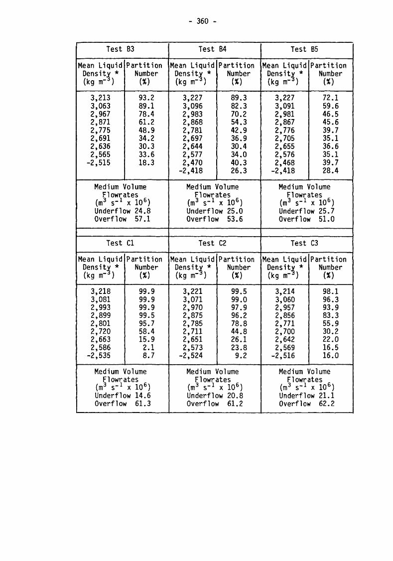
- 360 -

Test B3 Test B4 Test B5

Mean Liquid Partition Mean Liquid Partition Mean Liquid PartitionDensity * Number Density * Number Density * Number(kg nr3) w (kg m-3) w (kg m”3) (*)

3,213 93.2 3,227 89.3 3,227 72.13,063 89.1 3,096 82.3 3,091 59.62,967 78.4 2,983 70.2 2,981 46.52,871 61.2 2,868 54.3 2,867 45.62,775 48.9 2,781 42.9 2,776 39.72,691 34.2 2,697 36.9 2,705 35.12,636 30.3 2,644 30.4 2,655 36.62,565 33.6 2,577 34.0 2,576 35.1

-2,515 18.3 2,470 40.3 2,468 39.7-2,418 26.3 -2,418 28.4

Medium Volume Medium Volume Medium VolumeFlowrates Flowrates Flowrates

(m3 s"1 x 106) (m3 s-1 x 106) (m3 s-1 x 106)Underflow 24.8 Underflow 25.0 Underflow 25.7Overflow 57.1 Overflow 53.6 Overflow 51.0

Test Cl Test C2 Test C3

Mean Liquid Partition Mean Liquid Partition Mean Liquid PartitionDensity * Number Density * Number Density * Number(kg m"3) oo (kg m-3) w (kg m-3) (*)

3,218 99.9 3,221 99.5 3,214 98.13,081 99.9 3,071 99.0 3,060 96.32,993 99.9 2,970 97.9 2,957 93.92,899 99.5 2,875 96.2 2,856 83.32,801 95.7 2,785 78.8 2,771 55.92,720 58.4 2,711 44.8 2,700 30.22,663 15.9 2,651 26.1 2,642 22.02,586 2.1 2,573 23.8 2,569 16.5-2,535 8.7 -2,524 9.2 -2,516 16.0

Medium Volume Medium Volume Medium VolumeFlowrates Flowrates Flowrates

(m3 s-1 x 106) (m3 s"1 x 106) (m3 s"1 x 105)Underflow 14.6 Underflow 20.8 Underflow 21.1Overflow 61.3 Overflow 61.2 Overflow 62.2

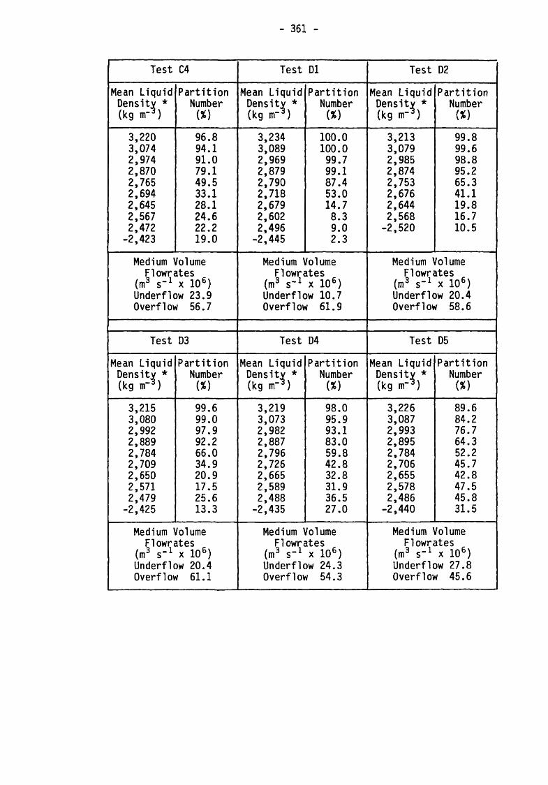
- 361

Test C4 Test D1 Test D2

Mean Liquid Density * (kg nr3)

PartitionNumber(X)

Mean Liquid Density * (kg m"3)

PartitionNumber(X)

Mean Liquid Density * (kg m“3)

PartitionNumber(X)

3,220 96.8 3,234 100.0 3,213 99.83,074 94.1 3,089 100.0 3,079 99.62,974 91.0 2,969 99.7 2,985 98.82,870 79.1 2,879 99.1 2,874 95.22,765 49.5 2,790 87.4 2,753 65.32,694 33.1 2,718 53.0 2,676 41.12,645 28.1 2,679 14.7 2,644 19.82,567 24.6 2,602 8.3 2,568 16.72,472 22.2 2,496 9.0 -2,520 10.5

-2,423 19.0 -2,445 2.3

Medium Volume Medium Volume Medium VolumeFlowrates Flowrates Flowrates

(m3 s-1 x 106) (m3 s"1 x 106) (m3 s'1 x 10b)Underflow 23.9 Underflow 10.7 Underflow 20.4Overflow 56.7 Overflow 61.9 Overflow 58.6

Test D3 Test D4 Test D5

Mean Liquid Partition Mean Liquid Partition Mean Liquid PartitionDensity * Number Density * Number Density * Number(kg m”3) (*) (kg nf3) (X) (kg m“3) (X)

3,215 99.6 3,219 98.0 3,226 89.63,080 99.0 3,073 95.9 3,087 84.22,992 97.9 2,982 93.1 2,993 76.72,889 92.2 2,887 83.0 2,895 64.32,784 66.0 2,796 59.8 2,784 52.22,709 34.9 2,726 42.8 2,706 45.72,650 20.9 2,665 32.8 2,655 42.82,571 17.5 2,589 31.9 2,578 47.52,479 25.6 2,488 36.5 2,486 45.8

-2,425 13.3 -2,435 27.0 -2,440 31.5

Medium Volume Medium Volume Medium VolumeFlowrates Flowrates Flowrates

(m3 s-1 x 106) (m3 s-1 x 10b) (m3 s-1 x 10b)Underflow 20.4 Underflow 24.3 Underflow 27.8Overflow 61.1 Overflow 54.3 Overflow 45.6

- 362

Test El Test E2

Tracer Density Partition Tracer Density Partition(kg m"3) Number (%) (kg m’3 Number (%)

3,300 100.0 3,300 100.03,200 100.0 3,200 100.03,100 100.0 3,100 100.03,000 100.0 3,000 100.02,900 99.0 2,900 100.02,800 100.0 2,800 100.02,700 95.0 2,700 81.02,600 0.0 2,600 3.62,500 1.0 2,500 0.0

Medium Volume Medium VolumeFlowrates Flowrates

(m3 s"1 x 106) (m3 s'1 x 106)Underflow 13.4 Underflow 24.3Overflow 61.5 Overflow 58.4

Test Series M (Medium Only)

Medium Volume Flowrates

(m3 s"1 x 106)

TestMl

TestM2

TestM3

TestM4

Underflow 13.6 23.4 24.8 20.2

Overflow 62.8 55.3 54.2 56.2

- 363 -

APPENDIX 4

DETERMINATION OF THE PARTICLE REYNOLDS NUMBER, Rep (Section 3.4.2)

The particle Reynolds number is given by

p v d Rep ------

n p . . . . ( A 4 . 1 )

Here, v is the ambient velocity of the particle in the fluid. Assume

for simplicity a spherical particle which attains a terminal velocity

v = vt radially, vt can be determined using the expression of

Concha and Almendra [32], replacing g by the radial acceleration of

the particle, a = Vt2/r. Assuming the validity of the semi-empirical

relation U ]

Vt rn = K, 0 < n < 1 ___ (A4.2)

. _(2n+l)we obtain a = K r ___ (A4.3)

Unfortunately, neither K nor n is known (indeed, there is evidence

that n itself varies with viscosity U]), and the selection of an

appropriate value of r is also problematical. Accordingly, in order to

achieve a representative estimate of a, sufficient for the present

purpose, we assume Vt = Vi = 2.70 ms"1, and r = R = 0.015 m,

giving a = 487 m s-2 (- 50 g). Inserting this value into Concha and

Almendra's expression for vt, and assuming (6 - p) = 350 kg m

(i.e. 6 = 3000 kg m“3) it is possible to calculate Rep for various

values of d and np. The resulting family of curves is shown in

Figure A4.1, from which it is apparent that the intermediate flow

regime probably prevailed in most of the tests conducted.

- 364 -

It is interesting to note that similar calculations for a 610mm dense

medium cyclone [4], for which a is about half that for the 30mm

cyclone, suggest that particles below about 7mm also settle in the

intermediate regime, and so will be susceptible to the influence of

medium viscosity.

It is also important to realise that Rep will fall as 6 -► p;

viscosity will therefore tend to have its maximum influence on the

separation of so-called "near gravity" material.

- 365 -

FIGURE A U PARTICLE REYNOLDS N° l# FLUID VISCOSITY CALCULATED FOR CONDITIONS GIVEN IN A PR U

- 366 -

APPENDIX 5

INFLUENCE OF YIELD STRESS ON A PARTICLE IMMERSED IN A BINGHAM PLASTIC

It can be shown [122, 123] that the shear stress imposed on a

Newtonian fluid by a spherical particle immersed in the fluid is

independent of Rep and is given by

d (6 - p) aT = ---------------------------------

6 .... (A5.1)

Unfortunately, the situation is more complicated when the fluid or

suspension is a Bingham plastic [124], Boardman and Whitmore [125]

showed that there is no concensus in the literature as to the value of

t0 prevailing for a particle held in such a suspension, and their

experiments suggested that "... yield stresses obtained from

viscometer measurements may not be of much use in predicting

instability towards bodies immersed in (Bingham plastic

suspensions)". However, in order to obtain some idea of the magnitude

of the effect prevailing in the present work, use has been made of an

expression given by Andres [126] for the limiting size of a sphere

for which t = t 0 . After re-arranging, this gives for the

corresponding limiting density difference

3 ^ x0(6 - p)c = ------

2 d a .... (A5.2)

Considering test series B, and assuming (as in Appendix 4) a

representative value of a = 487 ms-2, we have from equation A5.2 :

- 367 -

Test t0 (6 - p)c N m"z kg m"3

B3B4B5

2.362.706.64

182208512

The width of the "plateau" on the partition curve due to the capture

by the medium of particles for which t 0 > i may be assumed to be

equal to 2(6 - p)c. Allowing for difficulties in defining the

plateau, reference to Figures 3.6A-3.6E suggests that the estimated

values of (6 - p)c are somewhat high, but of the correct order and

within the limits of accuracy attributable to errors in the assumed

value of a, particularly as a is probably underestimated.

OS FO

00010002

0003000400050006000700080009001000110012001300140015001600170018001900200021002200230024

0025002600270023002900300031003200 330034003500360037

00380039

004000410042004300440045004600470048

APPENDIX 6 - FORTRAN PROGRAM FOR THE PROCESSING OF

CAPILLARY VISCOMETER DATA (CHAPTER 4)

- 368 -

IV 360N-FO-479 3-8 HAINPGM DATE 17/05/83 TIME 12.43.22

IMPLICIT REAL*8(A-H»0-2)DIMENSION P 120),T(20),PN(20),TAUl20J,S(20),TAUP(20),SLOPE(20),ALPH

1A(20),PNC(20).STRESS(20),B(20),RATE(20),AVISC(2 0 J,k E (20),Z (20),V IS 2C1 (20) .C0RR120) .RECRITC20) . V ISC2 ( 20) . T1TLEK3)V0L=95.0E-06

5 READ(1,10) NIFIN.EO.O) GO TU 250 R E A C H , 20) TITLE1 READ(1,30) D,CL.HEAD,SG PEADll,40) (P(l)>Ttl)yI-L»N)

10 FORMAT I 12)20 FORMAT(3A8)30 FORMAT(4F10.0)40 FORMAT(OF 10.0)

D=D/1000.0 SG=SG*1000.0 DO 50 1=1,NPN(I)=HEAD*SG*9.807+P(I)*1333.22 TAU(I)=PN(1)*D/(4.0*CL)

50 S(I)=10.1859*V0L/(T(I)*D*D*D)CALL KEGRE(TAU,S,N,80,B1,B2*CD1)DO 60 1=1,NTAOP(I) =BO+Bl*DLOG(SI I) )+B2*(DLQGCS(I)) )**2 TAUP(I)=DEXP(TAOP(I))SLOPE H )=B1+2.0*82*DL0G( S( I) )ALPHAH) = (4.0*SL0PEH)+2.0)*15.0*SL0PEI I)+3.0)/13.0*13.0*SL0PEII)♦

11.0)**2)CORRII)=1.62114*V0L*V0L*SG/((D**4)*T(I)*T(II*ALPHA(I))P N C H ) = PN(I )-CORR(I)

60 STk ESSCI )=PNC(I)*D/(4.0*CL)CALL REGRE(S,STRESS,N,CO,Cl,C2,CD2)K=0DO 70 1=1,NB (I)=C1+2.0*C2*DLOG(STRESS(I))Z(I)=1.0/B(I)AV1SC(I)=STRESS(I)/(S (1)**ZlI)}RATE(I)=(0.75+0.25*0(1))*SII)VI SC 1(11=1000.0*AVISC(1 )*IS(I)**(Z(1)-1.0))VISC2(I)=1000.0*STRESS(I)/KATE(I)PH I = ( (3.0*Z(I) + 1.0)**2)*(1.0/(Z(I )+2.0))**({ZII)+2.0)/(Z (I) + 1.0)I/1Z( 1)RECRITII) = (((3.0*Z(1J + l-Ol/ZCI))**Z(I))*404.0*4.0**12.0-Z(11)/PHI

70 RE(I)=D**Z(I)*(1.2732*V0L/(T(I)*D*D))**(2.0-ZlI))*SG/(AV I S C H )*8.0 1**(Z(I)— 1.0))DO 75 1=1,NIF(REH).GT.RECRITCI)) GO TO 80

75 CONTINUE GO TO 85

80 K= I85 WRITEI3,100)

WRITE(3,110) TITLE1 WRITE(3»120)KRI1E (3,130)WRITE(3,140) (I,STRESS(I),RATE(1),AVI SC(I),Z11),VI SCl(I),VISC2(I),

IRE(1),RECR1T(I),I=1,N)IFU.EQ.O) GO TO 90 WRITEI3,145) K

90 WRITEI3,150)WRITE(3,160) CD1 WRITE(3,170) CD2

DOS FC

005500560057

0058

005900600061006200630064006500660067006800690070.0071

0072

0073

0074007500760077

0078007900800081

APPENDIX 6 - Continued

- 369 -

IV 360N-FU—479 3-8 MAINPGM DATE 17/05/83 TIME 12.43.22

100 FORMAT(1HI»//»24X,'CAPILLARY VISCOMETER RESULTS'I 110 FOr.MAT { / »24X,' T C S T - *f3A8)120 FORMAT!//,IX,'READING SHEAR STRESS SHEAR RATE LOCAL POWER LAW

LAPP.VISC.-MPAS REYNOLDS NJS')130 FORMAT(IX,'NUMBER ', 6X,' N/M2 • ,BX, »SEC-1 • ,6X, • K N',4X,' PO

1WER NEWT. MEAS. CRIT.',/)140 FORMATl3X,12,3X,T10.2,6X,F8.1,2X,E10.4, IX,F6.3,IX,2F7.2,1X.2F7.0)145 FORMAT(/,IX»•WARNING - CRITICAL RE EXCEEDED FROM READING NO. ',12)150 FORMAT!//,17X,'COEFFICIENTS OF DETERMINATION FOR CURVE FITS:')160 FORMAT 1/,20X,'KINETIC ENERGY CORRECTION = ',F8.3,' PCT.')170 FORMAT(21X,'RABINOWITSCH CORRECTION =',F8.3»' PCT.',//)

WRITE(3,180)WRITE(3,190)WRITE13,195)WRITE(3,200) (I,PN(I),CORRlI).SLOPE(I ),ALPHAII),TAUII),S (I),1=1,N) WRITC(3,210)WRITEl3,220)WRITF(3,230 I BO,CO,B1,C1,B2,C2

180 FORMAT(//,IX,'READING / KINCTIC ENERGY CORRECTION FOR NET HEAD AND 1 SHEAR STRESS/ UNCORRECTED') '

190 FORMAT(IX,'NUMBER MEASURED NET CORRECTION KE CORR FACTOR 'UN 1C0KR.SHEAR SHEAR RATE')

195 FORMAT(1IX,'HEAD IN/M2)'»5X,'(N/M2) SLOPE ALPHA STRESSIN/M12) (SEC-1)',/)

200 F0RMAT(3X,I3,3X,F10.1,5X,F8.1,4X,F6.3,4X,F6.3,2X,F7.2,5X,F10.1)210 FORMAT!//,25X,'COEFFICIENTS FOR CURVE FITS')220 FORMAT(/,23X, 'KE CUk RECTION RAB.CORRECT ION')230 FORMAT!18X,'AO',3X,F10.4 ,6X, F10.4,/,18X,'A1•,3X,F10.4,6X,F10.4,/,l

18X,■A2',3X,F10.4,6X,F10.4,//I GO TO 5

250 CONTINUE STOP END

oo

oo

oo

oo

oo

o©

oo

oo

oo

oo

oo

oo

UJO

JO

JUJo

juJ

UJf

uM

ro

/v

rv

j

o o

o

o N> N)

•P* U)

oo

oo

co

oo

oooooooo

Wr

OO

OO

NO

'Ul

o o

o o

o o

o

o o o o o o o

p* ►

- p*

O

Ouj

r\j h

- o

cd

o o o o o © o

o o

o o

o o

o

o o

o o

o o

o

•*4 O'

V)

W l\>

i-

o o 00 ■n o 70

onU1

Ul

Ul

Ul

OJ-p*

u>fNJ

oO'

oo

co

oo

M*H

zm

jnX

-<O

O o

ooo

-<o

-<*»

>>

«p*«

Oas

> 0

0 00

COto

moo

COco

O o

oa

■HX

X-<

o o

—CO

1z

m1—

•**O

Oz

z z

o07

oh-

HM

WII

IIII z

zz

Zz

z22

z o

zo

zfNJ

o—

zc

-no

X0*

II—

>>

IIw

IIII

w^

^

M*

M*

iiM4

Z 13

©c

Cw

on x

M*if

lHU

I30

4*•*

wH

HX

CD

XO

'W

lU

lN

4- U

lU

l T1

•M•M

M*ui

m r

z1

30W

II■P'

o O

W 0*

u>IIoo

oo•>

44z

z z

— —

ww

ww

Ww

Mr*

WIIo

2 «

o*

ZilD

o o

wII —

o00 Z

z-1

144

1444

44 II IIii

iiII

IIII

IIO

IIo

o11

iiO

own

cX

a m

•II

00 —

zz

03 N;C/l 00 oo

00 oo

toO'

Cn00

CO00

o>

Xo

r*-H

Om

X►->

oCO

Z II

H-40*

O'H-

44w

ZZ

z z

zz

Zz

zz

zM

•X

h-i-

oM

C H

H-4X

"CII

44z

~ >

IIO

*■*00

X—*

—•«

^ ^

#-*«■*%

IIo

IIo

oit

Zto

•V»—

CO

■c o

w1

za

N)U

lM

ax

O'U1

OJrv

jh-

2<n

*-4.

M*

Xm

|*<

- _s

—

+*•

X >

m••

z*—

-<•< rr

COX

a■r

>z

H(VJ

X1

11

+

++

++

+z

M*

14X

z—

>M

z o

w—

x Z

Z44

wOO

(/>00 X

X<

XX

XX

Xz

oX

M*

ZN

rm

w+

•< 4

400

1z

zZ

W P

I-*

f\Jro

1—1—

O 4

4o

WX

Z X

z00

M*

W*.

CD

w00

■<■>

xz

»-*

M« M

4W

»-l

N*w

mm

wz

A-1

—U

i«M» W w

ww

x >

HHM »—•

w44

44*

44

44

4444

44M

|

-<•—

M W

1(/>

00 O

o *<

•<

XX

X**■*

X*•

o1

— ♦

>44

Zz

Z —

• —M

isjM

*ro

«•

X-<

1 >

M*OO

M ^

Mo

o**

70cc

*< r

u*

ZM*

UJh— w

wMl

-4“

1<•

m>

a> *

OOM*

w««

Ww

w*•

N»zz

Cl70

> X

zO'

w»w

wX

—z

zw

70 IN

J44

4444

rum

*W 0

*M*

0*

>»•

>*

#

w1

XH

—1

N>o

N>* x

w>

zZ

Zo

«•cu

Xf\J

4444

44w

>-H

*OO

co00

2Z

zZ

OO*• -4 00

T T T

oo 00

oo Z Z Z

(jJ lw

*

*

4400 l/l GO

Z2Z

** WOO'

N o

o ►

3» -a ~o 0

►—< X o> 1 o o 3 c 0) C

L

CO XI o

1 00 2ru .p* •P' 4» -4

APPENDIX 7 - TYPICAL OUTPUT OF CAPILLARY VISCOMETER

COMPUTER PROGRAM (CHAPTER 4)

- 371 -

CAPILLARY VISCOMETER RESULTS

TEST - SERIES R 3 , TEST R3/4

REAOING SHEAR STRESS SHEAR RATE LOCAL POWER LAW APP.VISC .-MPAS REYNOLDS NOSNUMBER N/M2 SEC-1 K N POnER NEWT. MEAS. CRIT.

1 5.85 562.2 0.1686D 00 0.576 12.33 10.41 52. 2590.2 9.32 1242.5 0.8431D-0I 0.678 8.84 7.90 170. 2474.3 11.94 1593.9 0.59640-01 0.727 8.19 7.49 240. 2416.4 15.85 2200.6 0.3I83D-0I 0.813 7.62 7.20 368. 2314.5 18.48 2587.5 0.2084D-01 0.868 7.41 7.14 454. 2250.6 21.22 2986.6 0.1326D-01 0.924 7.25 7.10 545. 2184.7 23.96 3328.3 0.8484D-02 0.980 7.23 7.20 618. 2121.8 28.04 3881.6 0.41940-02 1.064 7.12 7.22 747. 2030.

COEFFICIENTS OF DETERMINATION FOR CURVE FITS:

KINETIC ENERGY CORRECTION = 99.998 PCT.RA8INOWITSCH CORRECTION = 99.982 PCT.

REAOING / KINETIC ENERGY CORRECTION FOR NET HEAD AND SHEAR STRESS/ UNCORRECTEDNUMBER MEASURED NET CORRECTlUN KE CORR FACTOR UNCORR.SHEAR SHEAR RATE

HEAD (N/M2J (N/M2) SLOPE ALPHA STRESSIN/M2) 1 SEC-1J

1 8840.6 32.6 0.516 1.164 5.87 474.72 14973.4 193.5 0.718 1.076 9.95 1110.93 18306.5 339.6 0.782 1.055 12.16 1457.44 24572.6 708.3 0.867 1.031 16.32 2080.85 28838.9 1027.0 0.910 1.020 19.16 2492.66 33371.9 1428.7 0.948 1.0L1 22.17 2926.97 37904.8 1840.8 0.977 1.005 25.18 3311.78 44837.6 2629.2 1.019 0.996 29.79 3940.8

COEFFICIENTS FOR CURVE FITS

KE CORRECTION RAB.CORRECTIONAO 3.0968 2.3048 'A1 -0.9466 2.6366A2 0.1187 -0.2545

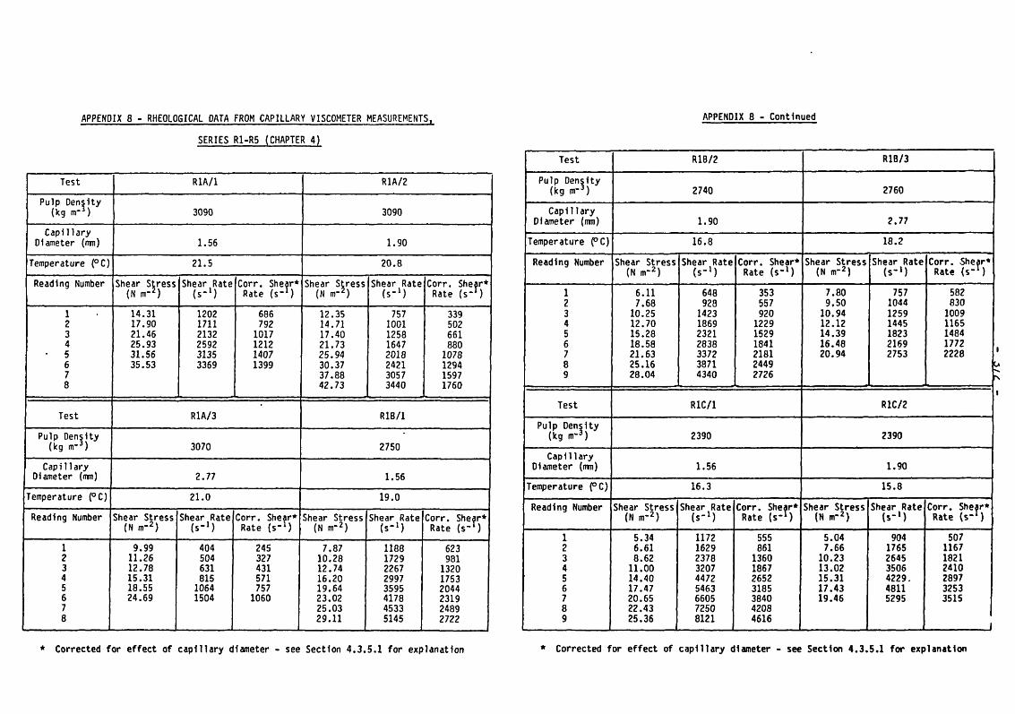
APPENDIX 8 - RHEOLOGICAL DATA FROM CAPILLARY VISCOMETER MEASUREMENTS

SERIES R1-R5 (CHAPTER 4)

Test R1A/1 R1A/2

Pulp Density (kg nr3) 3090 3090

Capi 1lary Diameter (mm) 1.56 1.90

Temperature (°C) 21.5 20.8

Reading Number Shear Stress (N nr2)

Shear Rate (s-1)

Corr. Shear* Rate (s_1)

Shear Stress (N nr2)

Shear Rate (s-1)

Corr. Shear* Rate (s‘*)

1 14.31 1202 686 12.35 757 3392 17.90 1711 792 14.71 1001 5023 21.46 2132 1017 17.40 1258 6614 25.93 2592 1212 21.73 1647 880

• 5 31.56 3135 1407 25.94 2018 10786 35.53 3369 1399 30.37 2421 12947 37.88 3057 15978 42.73 3440 1760

Test R1A/3 R1B/1

Pulp Density (kg m"3) 3070 2750Capi1lary

Diameter (mm) 2.77 1.56

Temperature (°C) 21.0 19.0

Reading Number Shear Stress Shear Rate (s-1)

Corr. Shear* Rate (s_l)

Shear Stress Shear Rate Corr. Shear* Rate (s~1)(N m-2) (N nr2) (s-1)

1 9.99 404 245 7.87 1188 6232 11.26 504 327 10.28 1729 9813 12.78 631 431 12.74 2267 13204 15.31 815 571 16.20 2997 17535 18.55 1064 757 19.64 3595 20446 24.69 1504 1060 23.02 4178 23197 25.03 4533 24896 29.11 5145 2722

* Corrected for effect of capillary diameter - see Section 4.3.5.1 for explanation

APPENDIX 8 - Continued

Test R1B/2 R1B/3

Pulp Density (kg m-3) 2740 2760

Capillary Diameter (nm) 1.90 2.77

Temperature (°C) 16.8 18.2

Reading Number Shear Stress Shear Rate Corr. Shear* Shear Stress Shear Rate Corr. Shear* Rate (s~l)(N m~2) (s-1) Rate (s~l) (N m-2) (s-1)

1 6.11 648 353 7.80 757 5822 7.68 928 557 9.50 1044 8303 10.25 1423 920 10.94 1259 10094 12.70 1869 1229 12.12 1445 11655 15.28 2321 1529 14.39 1823 14846 18.58 2838 1841 16.48 2169 17727 21.63 3372 2181 20.94 2753 22288 25.16 3871 24499 28.04 4340 2726

Test R1C/1 R1C/2

Pulp Density (kg nr3) 2390 2390

Capi1lary Diameter (mm) 1.56 1.90

Temperature (°C) 16.3 15.8

Reading Number Shear Stress (N m“2)

Shear Rate (s-1)

Corr. Shear* Rate (s_1)

Shear Stress (N m-2)

Shear Rate (s-1)

Corr. Shear* Rate (s_1)

1 5.34 1172 555 5.04 904 5072 6.61 1629 861 7.66 1765 11673 8.62 2378 1360 10.23 2645 18214 11.00 3207 1867 13.02 3506 24105 14.40 4472 2652 15.31 4229. 28976 17.47 5463 3185 17.43 4811 32537 20.65 6605 3840 19.46 5295 35158 22.43 7250 42089 25.36 8121 4616

_________

* Corrected for effect of capillary diameter - see Section 4.3.5.1 for explanation

TPT

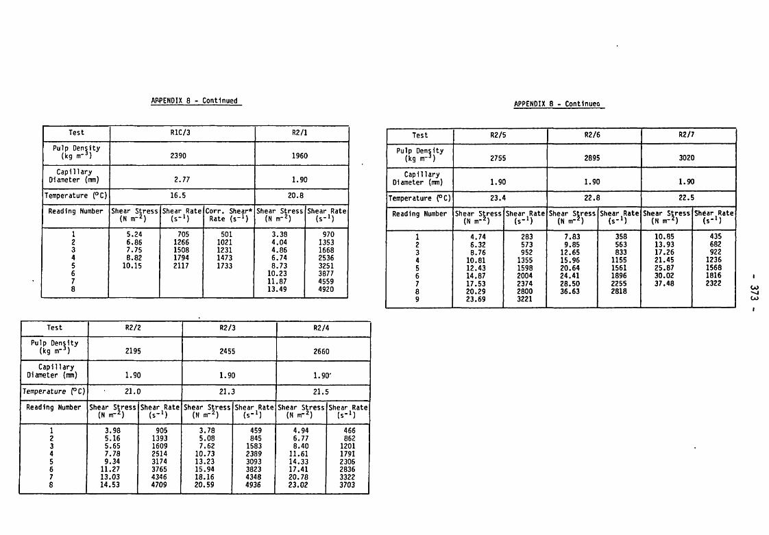
AP-PENPIX 8 - Continued

Test R1C/3 R2/1

Pulp Density (kg nr3) 2390 1960

CapillaryDiameter (mm) 2.77 1.90

Temperature (°C) 16.5 20.8

Reading Number Shear Stress Shear Rate Corr. Shear* Shear Stress Shear Rate(N m~2) (s-1) Rate (s-1) (N nr2) (s-1)

1 5.24 705 501 3.38 9702 6.86 1266 1021 4.04 13533 7.75 1508 1231 4.86 16684 8.82 1794 1473 6.74 25365 10.15 2117 1733 8.73 32516 10.23 38777 11.87 45598 13.49 4920

Test R2/2 R2/3 R2/4Pulp Density(kg m-3) 2195 2455 2660

CapillaryDiameter (mm) 1.90 1.90 1.90'

Temperature (°C) 21.9 21..3 21.5

Reading Number Shear Stress Shear Rate Shear Stress Shear Rate Shear Stress Shear Rate(N m-2) (s-1) (N m-2) (s-1) (N m*2) (s-1)

1 3.98 905 3.78 459 4.94 4662 5.16 1393 5.08 845 6.77 8623 5.65 1609 7.62 1583 8.40 12014 7.78 2514 10.73 2389 11.61 17915 9.34 3174 13.23 3093 14.33 23066 11.27 3765 15.94 3823 17.41 28367 13.03 4346 18.16 4348 20.78 33228 14.53 4709 20.59 4936 23.02 3703

APPENDIX 8 - Continued

Test R2/5 R2/6 R2/7

Pulp Density (kg m~3) 2755 2895 3020

CapillaryDiameter (mm) 1.90 1.90 1.90

Temperature (°C) 23.4 22.8 22.5

Reading Number Shear Stress Shear Rate Shear Stress Shear Rate Shear Stress Shear Rate(N m-2) (s-1) (N nr2) (s-1) (N nr2) (s-1)

1 4.74 283 7.83 358 10.85 4352 6.32 573 9.85 563 13.93 6823 8.76 952 12.65 833 17.26 9224 10.81 1355 15.96 1155 21.45 12365 12.43 1598 20.64 1561 25.87 15686 14.87 2004 24.41 1896 30.02 18167 17.53 2374 28.50 2255 37.48 23228 20.29 2800 36.63 28189 23.69 3221

APPENDIX 8 - Continued

Test R3/1 R3/2 R3/3

Pulp Density(kg m-3) 2390 2620 2750

CapillaryDiameter (mm) 1.90 1.90 1.90

Temperature (°C) 21.3 21.7 21.

Reading Number Shear Stress Shear Rate Shear Stress Shear Rate Shear Stress Shear Rate(N nr2) (s-1) (N nr2) (s-1) (N nr2) (s-1)

1 2.81 523 5.87 1016 4.29 4492 5.56 1203 9.01 2031 6.00 10763 . 8.75 2505 11.40 2670 8.84 • 18424 12.28 4022 13.40 3196 11.90 25175 14.96 5052 15.46 3781 14.10 29536 16.50 5771 17.51 4256 16.25 33417 19.13 6667 20.97 4959 18.97 37658 22.16 4279

Test R3/4 R3/5 R4/1

Pulp Density(kg m-3) 2990 3180 2150

CapillaryDiameter (mm) 1.90 1.90 1.90

Temperature (°C) 23.8 24.1 21.0

Reading Number Shear Stress Shear Rate Shear Stress Shear Rate Shear Stress Shear Rate(N m-2) (s-1) (N m-2) (s-1) (N m-2) (s-1)

1 5.85 532 9.48 691 2.76 6172 9.83 1176 11.83 977 3.45 8113 11.96 1509 14.17 1206 4.96 14084 15.90 2082 17.25 1571 7.05 21995 18.55 2448 19.45 1820 9.12 30056 21.32 2825 22.84 2133 11.28 37317 24.08 3147 26.69 2488 13.52 44408 28.22 3670 38.63 3288 16.22 51819 1 _______1 18.07 5707

APPENDIX 8 - Continued

Test R4/2 R4/3 R4/4

Pulp Density(kg m-3) 2770 2990 3120

CapillaryDiameter (mm) 1.90 1.90 1.90

Temperature (°C) 22.5 23.0 24.0

Reading Number Shear Stress Shear Rate Shear Stress Shear Rate Shear Stress Shear Rate(N nr2) (s-1) (N nr2) (s-1) (N nr2) (s-1)

1 5.02 274 7.51 321 8.25 2842 7.13 574 9.80 501 13.02 5563 8.87 812 12.26 692 17.06 8124 11.13 1116 16.27 1093 21.43 10675 15.07 1627 20.01 1347 25.78 13716 17.45 1899 23.38 1608 30.21 16347 20.99 2282 26.75 1789 37.93 19908 24.94 2606 29.60 1934 43.11 22479 28.29 2976-

Test R5/1 R5/2

Pulp Density(kg nr3) 2730 3070

CapillaryDiameter (mm) 1.90 1.90

Temperature (°C) 20.9 18.8

Reading Number Shear Stress Shear Rate Shear Stress Shear Rate(N nr2) (s-1) (N nr2) (s-1)

1 4.84 894 7.10 8522 5.60 1120 9.40 12913 7.67 1698 12.18 17624 9.90 2388 14.41 21405 11.89 2966 17.12 27096 14.48 3585 19.61 30597 16.77 4233 21.92 33808 18.65 4649 24.28 37109 20.53 5093 26.52 4027

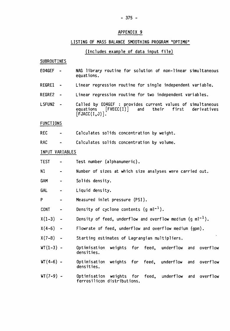
- 375 -

APPENDIX 9

LISTING OF MASS BALANCE SMOOTHING PROGRAM "OPTIMe”

(Includes example of data input file)

SUBROUTINES

E04GEF - NAG library routine for solution of non-linear simultaneous equations.

REGRE1 - Linear regression routine for single independent variable.

REGRE2 - Linear regression routine for two independent variables.

LSFUN2 - Called by E04GEF : provides current values of simultaneous equations [FVECC(I)] and their first derivatives [FJACC(I,J)].

FUNCTIONS

REC

RAC

INPUT VARIABLES

TEST

Nl

GAM

GAL

P

CONT

X(l-3) -

X (4-6) -

X (7—8) -

Calculates solids concentration by weight.

Calculates solids concentration by volume.

Test number (alphanumeric).

Number of sizes at which size analyses were carried out.

Solids density.

Liquid density.

Measured inlet pressure (PSI).

Density of cyclone contents (g ml-1).

Density of feed, underflow and overflow medium (g ml”1).

Flowrate of feed, underflow and overflow medium (gpm).

Starting estimates of Lagrangian multipliers.

WT(1-3) - Optimisationdensities.

weights for feed, underflow and overflow

WT(4-6) - Optimisationdensities.

weights for feed, underflow and overflow

WT(7-9) - Optimisation weights for feed, underflow and overflowferrosilicon distributions.

- 376 -

PF(I)

PU(I)

PO(I)

PC(I)

D(I)

Percent in size intervals for feed ferrosilicon.

Percent in size intervals for underflow ferrosilicon.

Percent in size intervals for overflow ferrosilicon

Percent in size intervals for contents ferrosi1 icon.

Sizes at which size analyses were carried out (pm).

DESCRIPTION

This FORTRAN program smoothes flowrates and pulp densities around a DM

cyclone using the Lagrangian multiplier optimisation procedure. The raw

data (flowrates, densities and size distributions for all three products)

can be weighted according to the estimated reliability of each result. The

resulting eight non-linear simultaneous equations are solved using the NAG

library routine E04GEF, which calls subroutine LSFUN2 to calculate the

current values of the equations and their first partial derivatives.

X(I), I = 1,6, are the optimised values, with starting values provided by

the raw data. X(7) and X(8) are the calculated Lagrangian multipliers,

which are not output.

Smoothed medium size distributions are also produced by Lagrangian

optimisation, using the smoothed value of solids yield, by algebraic

solution of the resulting four linear simultaneous equations. The smoothed

size distributions are used to produce gross and corrected partition

numbers for the medium classification by the graphical (square diagram)

method of Svarovsky.

A number of additional mass balance quantities are generated.

377

«ZoH

-

5^

A

A W

v B

4 a

a o

©

O ©

O«

o

o o

o

a a

< <© o5 5o ©

■ tnpv a a a 3^oijo?

©

» -

»o

= 555J

4 O ©

© v-/

©(A

•

•

•

'’N /*\ <

^ ^

^

N n

W W

|

W V

W

bu 3

wo

U

U

© ©

a. ou © x<—>

M '

4CM

<nw

ww

te«X

zV

)CO

CO\mS

XX

Xo

Hbu

oX

XX

TCO

fluflu

fluu

ou

V)*r\

O1

■1

uo

u•<

<<

oOS

o3to

KOS

o2a

X4

asas

as■

11

■f-*

•a

l>

>>

ato

1-4tea

oV

)to

COCO

COto

soa

teaV

Oo

buo

fluo

buo

0Ufla

Ouo

uu

Uo

ues

>u

u

a x

w w

)_( w;

■— •« u

\/n

O CM

bu- 3

O

O

x

I

CL) x

Or X

■

a

■ ■

■ ■

© © o x 3 u o o o u u u j

j j

&

eu flu 0 Q Q U U U

VW

W

| |

T

gg

g®

°®

-3 a

a O

O O

a a

a o

o o

9 t

t H i—U H

I

ll

a ©

a

MM

MO

|

w w

w

a a

a

© a X 3 U O U

O ©

U O

X

© Ou

&u X

Ou© a © © o ©

a o

© w

0

00x

3© X

X

X

X X

X

o ©

o ou o

, x

<<

<©

©©

wp

> N

X

coo

t ou a

Xa

O

O

X >

^ >

* »

«3

p>n;j

i •O CU (D H

•9

U —

« W

c-> < v

v©

w

- CM

©•x /-»x

x•91 U

U*—N •—

>u -

O w

-«

-s«

ub

Hw

u ©

NU

Z

pi

X fltu CM

X•

b4«

© W

UM

^

+P

U<

CM

•1

*-491

-O

pi

M

Z—

9

- O•

wO

l -CM

Oa

—M

flu

< W

© ©

•>- ©

CM At

o ^

^N

© W

-

• HO

flLu CM U-V

^ -f

CM ©

►< COM

^4

£^

z0

««

3a

wa

. 9i 9

i xo

Ou o

- —• —l 3

u*

Ou/>

N/ N

/ Q/-N

»

0 3

0

-X

MCM

© bu

N/ b4

w CL flu

ao

+

a ©

© w

<flU ^4

x

- - x

u• 2

• /s

/-* w

cs

ai

sji aI

BO

3 -u

-« a

3

- -

•>4

flup

^n

i -— n

/

-U

N-

^

« a

•

X w

X 3

/-s-

1 1

1 H

fiU1

X ©

X ©

-u »-i a

►4

•

• ^4

O X

X X

CM ^

>a

z

- •

•l /-s ^

- .©

UV

J|

<• /

\ u-s

AH

H H

X ^

»

• X -h ©

H a

aH

WW

Z1

91 u-N

^ 3

-

IO v

s/

w t4

tea w

Y*

4 tei W

fig Kw

om

«-a

Mm

>■

K *

*

xs

«

CM <

«

w

*

5a

W mpZ

X "* Mi

Q J

«

a 4

u

Z H

*

«

i/N

nA

w CO

U4M

•M* W

WA

Ho

^ S

2ste* CO «+

W

AM

AflS

N<

CO «

wtea

WA

HH

H

m

zbe w

ZO

f

tet IO

X'"N

tea CO

a>4•n

H4 «

flC1

*44-N

WA

*A

bJf

lfl

IOCO

<tea W

COefl

4ro

1 H

Z

*1

««

Q<*s

CO «

Aw

^4 «Z

ao

COp%

HW

««

N

v

Oa

<X

«A

VU

Ha

Zfl U

}5

bJ<

1-4w

5 «

MX

z-v to

h T

A

a >4

as

A Z

Sy-s

ur>

o«

M

wr+s

tea CO

XH

w M

AW

(U A

Hu

o

aU

X H

H O

)

(Ow

1 H

1 =>

W &a «

to

COO

bJX

Z4-v BQ

o *

o

eso

• oM

CM 1-4

tea • «

tea•-4

COX

HW

tcw

® CM

101

to^

Za

frH1

o<

A A

^ <

A >4

4-n aa

. p>

a. ©

bJ bJ

JMa

a a

-

3

•to

wto

< <

3

x^

£SO

w Q

x a

© u

©

<• 2

O X

*-4

w 1-4

- - ©

53

5

«

© H

~

4W flfl» bJu te.

z z a -4 4 < -a *4

44

HO

JO

H

*yi© u o z - * -2-*o•

• »

0

PuO

wtfl

/^/-N^O-urM-NO*

30— CMP-|>-PwwwwP^b) >/s

WW

H

a

« «-/

X i-l X

-3

©©

CM 1-1

W -

J H

x

a 4

a o

< to

CO H

X a

X

h

X

» ©

ax a

<> h-

© flu

2

-u ox ®a

w x

u. ufl

h m

M • a

“

© a

os -J

H H

SO

<

ws

/U

bu

a u

< N

©

M

I to

pm a

w u

X

X

w {_>

« O

« o

r\ 2

CN to

* V I to Z' H

to oc

apii i»« —30 * ae n © <

>"

v«

tn a

fi»«ecw

CT> •*H

to

X

H

91 (A

Ww-*u-/qf

« «

* H «

<i ^<^3 p CO

O SO «

9*

SO • w

p*n w

nfl —< F- r- H

* I 3 '-'X

'-'tn

+

M —

NMOW3 + Z

>p

ofi S/J

+

a

• h v

^a t/i h

P

J

I «

tO

>-

■ '"N/Nflfl 3

Hvin a«■ in v

to _ —

flfl H tn /- * i*

efl a

'csO « w

o> <—»

tn tr

^ r-

tn 3

luwKIN -

in n

378

O'

-• Nor I- Mor - o

' i-i

O'

n n •< X

N-

-aN

NU

< so -

PM CJ U H H -

w OU aa a

,Cu uCJ -

ao

oo

oo

am

am

oJ

lvO

NC

O^

O^

rfNN

nn

nn

n n

<j <j* <r

aaaaaaaaaaa

HH

HH

HH

HH

HH

H<—i

•—( i—I •—i •—i *—i i—r t—<

>—• ►—<

XXXXXXXXXXXXX XXXXXXXX 22

22222222

UU''''U H

H O

PM H

a a • • Mx x O' O'XH

M U

U H

.>

oOi

Xin

•U

fluCO

o(»«

XX

HH

o»

Zz

MN

XH

Xra u]

ou.

mX

X H

►Mo*

pa>>» z

Ho

COk

(SIo o

<flu

■PS X

uX

fluX

>0o

fluH

Nflu

aa

U-

1z

5CO

ato*

a«X

aa

| t/1 U

,PN O

S’** »a

X1

fa]z

=>to

zM

H1

«M O

^ o

s* X

<a

Hb

- pa

h« u

• mU

Ou«

• MX

N CO

”l CO

o"i -*

xK

Xo

PM tb ZI

aua

1 f-»

opa

« - U

lbi

aua

1 o

XH

H»> -

a ^

• a

o*•

fl*m

COo

<

i a

O

1 - O

XuS

flu-

Bu•

1 X

COX

HN

mQ

W-

O J

P» 1 \0

Xr>

m•

•U

X»

• tb

* * H

-CM 04

ta4#

fluo

a -

aX

X

• ^s• to

fs*z

a

-aoi m

cm Ha

r*>X

(Ua

x a

* * U* O

Hflu X

<nX

H o

'in- ao

o fn cu

zr> e>3

Xo

CO I-I -

a• H

OIa

a -

|s N X

HH

X

<H

- Z

flu flu OI 2Z

m »

cn- M

cn o

• s/

o<

•

os os os2

2 2 OS X fb (b OS 2 2 a a 2

o m

o *n

o\ O o —< a H tS N

N N

o o

o

o

n n

■» ioN N

N N

pm x:

• *

cnto - -

«a

a

•M

as COa

a

< -

ho CO Id a aCO

CO x co O

“-

u -

ou - -

-as »-

-pm

X a, X «x S'S- - -» X -a-^ »x

N\/2

H X H -H X< m < -m c

o

H o

x

o —

ilb O lb - X *O

O

IPI

• 2CO O H<lbUU'i

oo

oo

oo

oo

oa

N^irivONJOWOH

pa ono nn pi ia a a

§£

£

w X

v-'

sH

CM>0 1 *

oCO04a

CMm

MM

S** QuCJ

oa

MP

' za

wH

HUCJ■

1CJ

a>pU

u/hU U/OS

><HU1 HU

oo

az

aOI

a<

a•HU

*CJ CO

> CO04• 04

zOu

Cb<

3flu

&4*CM •

2«X

OHU

I-IaCJ

04Cd*

1 s—*z

aua

HHUW

CJX

S-NM HU U

oigU3

GOca «toXo

F-tCO

COU

s/- z

.JXa

Hi

UJuXX2

u*lft4CO to

aa

OJo

CJo«HCJ

s«sCJ CJ

OSXa

vsa qOIu

Oo

k-4•

*uCM

o cc

oo

oo

au pU

n s-\i«-S

/**ou

oo

UJm wCO

o mo

m a

oO

O ma m

ao m

oo

ma

o o flu o

'J m04a

aa

o*

oso>«H O

o p* H Nr>in msO

0 r-oo00o pU p4"MU4 ru04

fl-a

oo

r-4p-4 s-sO

'O'04

sDo a pm CMCM (M CMCM

CMCM CM CMCMCMcn cn r>cn 04 mCJ COo

om

o« z «M

««z

HpHS*N *

a*O'

O' 2>

O'00

ao

oCOUJ UJa

a a Jdfld

a fld oJoJbdfldUJ UJ

UJ ojUJ• UJpp a

’jd04

•u« M UMOI

««

HH

«H fN1

oM

H HH

H HHh

HH

HH

HH

HHH

HH s-N H

a H

XXH

H ■ /-NW ICJ

O' O' O' > >>z

zO'O'O' to

O' O'o OS< 1PC HUHUHHM

HUHUHUHU

HU HUHU hUHU hUHUU HUW HUcj 03 Xz t-Uh-4

O •“< OI>•

« «totoCOO

o «K•«*

«00 a HU1 a002x a x

DC DScC

DCDCcc

DCDCOS

X X

DC S- XM

XOjJ

oX

>* 1ow to to U.=)

oO CJtoo

' o' w

ao O' o

' or >>>a HUHUH H H

hUHU HUHUHU

HUHUhU hU HU-4CO M => HUa?» u in

X 1 Ka(u

o uuoaato « Ut rXi

o>*

U4O

CJmHUH

s—sO W 04 w

OJzNooH S-N CO y-\Mou

oua12 >

cc to flucd >a tu

o CJCJo« pj CTiMU3UJUJ Ad -Jfld UJUJ UJ Jj -UUJUJUJUJ

j3 afld 0« bd• UJ

•Joo H

M ~uHUo1 aa> >> RH

1to CJuj CJ

a a.<CMCM

OCHHH

H HH FtH HH HH HH HH HH

-H'-'H

oJu5M

OItototo tototo

zzto

ato

Ja 1 >> >Ru

flu042HUHUH M M

HUHUHU

HUHU

HUH-l HU

HUHU

hU HUHU ^ HUHU HU<

mo

o

x oDOOIO aU4

'Z*o (u

oo

o CO to'2 2o

O flua flu

o a.

DOCJCJcd

DCx a atc

DCXfd0

CCX

X X

•-U xX

CJ Q•->

aX

>*><

O' o

oo CJCJ CJCJCJfl£ oC>> CJuu CJU ua

>*X222 2 2222 22 2

JZ22

22

22

^2

O 2

OCJ

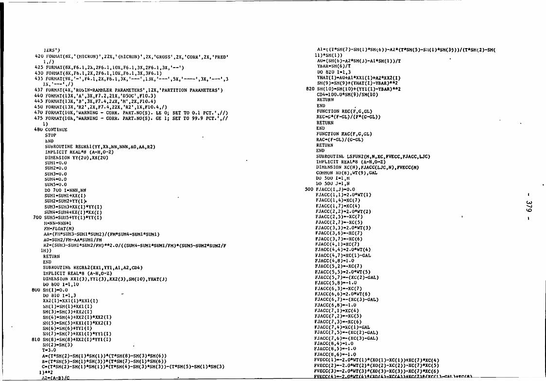
FVECC(5)«-2.0*WT(5)*(XO(5)-XC(5))-XC(7)*(XC(2)-GAL)-XC(8) FVECC(b)— 2.0*WT(6)*(X0(6)-XC(6))-XC(7)*(XC(3)-GAL)-XC(») FVECC(7)-XC(4)*(XC(1)-GAL)-XC(5)*(XC(2)-GAL)-XC(6)*(XC(3)-GAL) FVECC(8)-XC(4)-XC(5)-XC(6)RETURNEND

INPUT DATA FILE FOR TEST Fl/1

FI/l II 6.747 1.0 12.3 3.1280.1 0.1 0.1

3.045 2.860 3.26417.1 9.02 8.44

..0 2.0 2.0 2.0 1.0 1.0 1.0 2.0 2.03.15 3.68 2.37 2.01 75.131.82 2.76 1.48 1.34 59.638.06 6.66 8.59 3.36 47.33

13.33 8.50 11.33 8.97 37.5614.61 15.55 13.10 16.35 29.8218.67 14.88 17.77 19.48 23.6613.67 13.45 16.03 12.41 18.78 1

8.66 12.14 11.09 13.91 14.91 Go7.68 8.05 6.88 8.07 11.83 CO

3.85 4.89 4.68 4.85 9.39 o

2.70 4.02 2.87 3.94 7.45 13.58 5.42 3.82 5.31

- 381 -

APPENDIX 10

MEASURED AND OPTIMISED FERROSILICON RESULTS FROM 100MM CYCLONE TESTS

Given as the output from the program "0PTIM6"

(see Appendix 9)

— ' RESULTS FOR TEST NO. ri/i —

sotl us y , - 6.747 LlOUlb SO • 1.000

FLLF FLOWRATES - L/H1N FULF DENSITIES - EL/M3pled U/F o/r PEED U/F o/r CONTENTS

KtASUKLb 77.74 41.01 3S.37 304). I860. 3264. 3128.OPTIMISED 7e.u7 40.33 37.71 305). 2E3H. 3262. _WEIGHTS 4.0 1.0 1.0 1.0 2.0 2.0 —

SOLlbS CONCENTRATION (WT.FCT) SOLIUS C0NCEKTJUT10N (VOL.FCT)FEED L/F o/r CUNTLNTS peed U/F o/r CONTENTS

HLAS. 76.13 76.33 81*4) 7S.R7 33.38 32.36 39.39 37.03OFT. 74.93 76.32 81.41 35.73 32.33 39.36 —

SOLIDS Sn.IT FCT WATER SFLIT FCT PULP SFLIT FCT FEESSURE

HUS. A*.)0 MIAS. 36.92 HEAS* 31.66 12.3 FSIOFT. 46.77 OPT. 34.42 OPT. 31..69 84.R RN/K2

--- RESULT! rot T U T NO. F1/Z

SOLIDS SC • 6.7A7 Ligoiu SC - 1.000

FULF FLOWRATES - L/MM FULF DENSITIES - KG/M3FEU) U/F o/r PE ID u/ f o/r CONTENTS

MEASURED 36.37 37.37 14.73 3013. 2796. 3232. 3037*optimised 33.32 39. OS 16.4A 2943. 2820. 3242. — •WEIGHTS 2.0 1.0 1.0 1 .0 2.0 2.0 —

SOLIDS COKCINTRATJOM (WT.FCT) SOLIDS CONCENTRATION (VOL.lCT)PUD U/F o/r CONTENTS PEED u/r o/r CONTENTS

KEAS. 78.44 73.41 11.08 78.74 33.06 31.23 38.8A 33.46OPT. 77.34 73.78 61.19 — 33.83 31.48 39.02

ROLIDt RFLIT FCT WATER (FLIT FCT PULP SFL1T FCT PRESSURE

HEAS. AA.3R MIAS. 32.69 HLAS. 71.73 6.3 riiOPT. 43.R7 OPT. 72.70 OPT. 70.39 44.8 KN/H2

SIZE D1STNI1UTIONS SIZE blSTRIRUTlONS

TZLD UNDERFLOW OVERFLOWSIZE NEAS. OPTIMISED HUS.. OPTIMISED HEAS,> OPTIMISED

MICKOfc PCI FCT CPF FCT FCT CFF FCT FCT CFF

73.1 3.1 3.0 97.0 3.7 3.7 96.1 2.A 2.A 97.639.6 t.S 2.0 93.0 2.6 2.7 91.6 1.3 2.7 96.247.3 8.1 7.8 87.2 6.7 6.7 86.8 8.6 6.7 87.337.6 13.3 10.7 76.3 8.3 9.1 77.7 11.1 9.1 71.329.8 14.6 14.3 62.2 13.6 13.* 62.1 13.1 13.6 62.323.7 18.7 16.9 43.3 14.9 13.3 46.8 17.6 13.1 AA.OU . 8 13.7 14.6 30.7 11.4 13.2 13.6 16.0 13.2 28.314.9 8.9 11.0 19.7 12.1 11.6 21.9 11.1 11.6 17.711. S 7.7 7.3 12.2 8.1 8.1 13.8 6.9 8.1 10.89.4 3.9 4.6 7.6 4.9 4.7 9.1 A.7 6.7 6.37.4 2.7 3.3 4.4 4.0 3.9 3.2 2.9 3.9 3.6

- 7.4 3.6 6.6 — 3.4 3.2 — . 3.8 3.6TOTAL 100.0 100.0 — 100.0 loo.o — 100.0 100.0 —WEIGHTS 1.0 2.0 2.0

rtEb UNDERFLOW OVERFLOWSIZE HEAS. OPTIMISED HUS. OPTIMISED HUS. OPTIMISED

H1CA0N FCT FCT CFF FCT FCT err FCT FCT CFF

73.1 2.0 2.9 97.1 2.6 2.2 97.8 4.3 A. 1 93.939.6 3.0 A.6 92.3 6.4 3.8 91.9 2.3 3.8 93.434.2 3.3 2.3 90.0 2.3 2.7 89.2 2.1 2.7 91.447.3 3.1 4.0 86.0 1.9 1.7 87.3 8.3 1.7 83.037.6 6.1 9.8 76.2 14.1 12.9 74.6 4.4 12.9 79.229.8 16.A 14.8 61.4 11.1 11.8 60.8 16.4 13.8 62.623.7 18.8 16.0 43.4 14.2 13.1 43.7 17.2 13.1 44.918.8 13.9 13.3 11.9 11.8 12.6 11.1 14.7 12.6 29.814.9 10.7 10.2 21.7 10.3 10.4 22.6 9.7 10.4 20.011.8 8.6 8.3 11.6 8.0 8.1 14.3 8.4 8.1 11.39.4 7.9 3.9 7.6 3.6 4.3 8.2 6.7 6.3 6.37.A 1.9 3.3 4.3 6.0 3.3 A.7 2.9 3.3 3.4

- 7.4 2.3 4.3 — 3.3 4.7 — 3.9 1.6 —TOTALVE1CHTS

100.0 loo.o1.0

100.0 100.02 .0

100.0 100.02.0

R0S1N-RAMMLER PARAMETERSA JJ 29 32.93 33.36 ROSIN-RAKMUI PARAMETERS• 1.9410 1.8214 2.U642 A 33.67 13.11 14.24S3 0.9889 0.9876 0.9892 B 1.8848 1.8461 1.9766

U 0.9873 0.9894 0.9804

DISTRIBUTION OP CONTENTS CLASSIFICATION DATAS U B DISTRIBUTION OF CONTENT! CLASSIFICATION DATA

si:e FCT CFF SIZE PARTITION NUMBERS(MICRON) (MICRON) CROSS CORR PRED SIZE FCT CFF SIZE PARTITION NUMBERS

7>.l(HICRON) (H1CK0N) CROSS CORN PRED

2.0 98.0 73.1 6U.6 11.359.o 1.3 96.6 39.6 38.0 7.9 0.) 73.1 2.0 98.0 73.1 61.6 0.1 —*;.j J.4 93.3 47.1 40.3 U.l 0.) 39.6 1.0 97.0 39.6 73.0 S.4 O.B37.8 V.0 84.3 17.6 44.7 U.l 0.2 34.2 3.4 93.6 34.2 33.8 0.1 0.729.8 1..4 68.0 29.8 47.1 0.1 0.2 47.1 3.0 90.6 47.3 44.9 0.1 0 .62J.7 l*.3 48.3 ’ 23.7 42.4 U.l 0.2 37.6 11.8 78.8 17.6 76.7 14.6 0.4lb.8 12.4 16.1 18.8 46.3 0.1 0.2 29.8 13.3 63.3 29.8 61.9 0.1 0.)14.9 1 J.9 22.2 14.9 3U.1 0.1 0.2 23.7 13.9 47.4 23.7 62.0 0.1 0.2tl.4 ».l 14.1 11.8 49.0 0.1 0.2 18.8 14.3 32.9 18.8 64.9 U.l 0.29.4 «.9 9.3 9.4 32.3 0.1 0.2 i«.v 13.3 19.6 14.9 63.6 0.1 0.17.4 J.y 3.1 7.4 33.9 i.l 0.2 11.8 8.1 11.3 11.8 68.1 0.1 0.1

- 7.4 3.3 — — ___ 9.4 6.4 3.1 9.4 71.2 0.1 0.17.4 2.2 2.9 7.4 71.3 0.1 0.1

IN-RA ‘OiLKR PARAMETERS PARTITION PARAMETERS - 7.4 2.9 — — — —A »U.5U OSOCR*******4*A t . * m M 0 >zz: b R081N-RAMHUSR PARAMETERS PARTITION PARANLTINSR2 0.9861 RZ 0.0087 A )<!.tb D3UC 1830.793

WARM NO8 2.152) M 1.2959

- OJMR. rART.NO(S). U 0| 8LT TO 0.1 rci. • R2 0.979# K2 0,.2 J O

WArNIBC - U'RR. FART.LOU). LE 0! NLT TO 0.1 FLT,

RESULTS FOR TEST NO. F l/3RESULTS FOR TUT NO. FI/4

I0L1DI SC - 4.747 Liquio SC • I.000SOLIDS SC • 6.7A7 uyuiu sc • l.000

PULP FLOWRATES - L/HIN FULF DENSITIES - RC/N3PULP FLOWRATES - L/HIN PULP DENSITIES - EC/H3 FEED U/F 0/F n to o/F 0/F CONTENTSFEED U/F o / r FEED U/F 0/F CONTENTS

MEASURED 13.64 21.91 30.32 2703. 2736. 2617 nil.HUSURLb 89.36 23.96 32.64 2700. 2991. 2320. 2796. OPTIMISED 33.36 22.4t 30.89 2674. 2740. 2626.OPTIMISED 87.37 3U.34 37.03 2687. 2991. 2326. -- WEIGHTS 2.0 1.0 1.0 1.0 2.0 2.0 ~ T.WE1QITS 2.0 1.0 1.0 1.0 2.0 2.0 ~

SOLIDS CONCENTRATION (WT.FCT) SOLIDS CONCENTRATION (VOL.FCT)S0L108 CONCENTRATION (WT.FCT) 60L10S CONCENTRATION (VOL.FCT) FEED U/F 0/F CONTENTS FEED U/F 0/P CONTENTSFLED U/F 0 I t CONTENTS FELD U/F 1D /r CONTENTS

HUS. 74.00 74.44 71.34 74.10 29.67 30.17 28.14 30.38HLAS. 7)..92 78.13 70.81 75.41 29.38 1A.64 26.41 31.23 OFT. 73.,30 74.36 72.69 _ 29.1) io.:19 28.29 —OPT. 7).,71 78.18 70.89 — 29.36 34.66 26.32 --

SOLIDS SFLIT PCT WATTE SPLIT FCT PULP SPLIT FCT PRUSUR1SOLIDS SPLIT PCT WATER SPLIT PCT PULP (FLIT FCT PRESSURE

NIAS. 74.49 MBAS* 74.87 NEAS. 41.93 7.i r s tHUS. 44.76 KUS. 3S.A7 KEAS. 33.01 18.6 FBI OFT. 41.79 OPT. 41.43 OPT. 42.12 31.7 RM/N2OFT. 41.01 OPT. 32.11 OPT. 16.71 114.3 RM/H2

SIZE DISTRIBUTIONSSIZI DISTRIBUTIONS

RED vtfDtmov o m r t o wFEED UNDERFLOW OVERTLOW SIZE HEAS. OPTIMISED HUS. OPTIMISED WAS. optimised

SIZE HUS. OPTIMISED HUS. OPTIMISED HUS.> OPTIMISED KICKON FCT FCT CFF FCT FCT CFF FCT FCT CFFHICRON FCT FCT CFF FCT FCT CFF FCT FCT CFF

75.1 0.1 1.4 91.6 2.4 2.3 97.F 0.9 0.8 99.239.6 2.1 4.0 96.0 2.1 4.8 93.2 2.4 2.0 98.0 39.4 1.1 1.4 97.0 3.4 7.3 94.3 0.1 3.3 98.934.2 2.3 2.0 94.0 3.3 3.A 89.8 0.9 3.4 96.9 34.2 2.2 1.2 94.t 3.4 3.6 90.9 1.1 3.6 97.847.3 3.9 3.7 9U.2 3.0 3.0 8A.S 2.8 3.0 94.0 47.3 1.7 3.4 91.1 4.8 A.A 86.4 1.6 6.4 94.837.6 4.6 8.3 81.7 11.7 11.0 73.9 7.9 ll.Q 87.2 37.6 9.3 10.0 81.a 14.4 14.3 71.0 6.4 16.3 88.329.8 14.2 13.3 66.2 1A.8 1A.3 39.4 16.6 14.3 71.0 29.8 13.4 14.2 66.9 13.3 13.6 18.A 14.6 11.6 73.623.7 17.8 18.9 47.3 16.3 16.2 43.1 21.0 16.2 30.3 23.7 21.0 11.9 48.0 16.8 17.3 41.1 19.7 17.3 33.318.8 14.9 16.1 31.2 16.9 IA.7 26.4 17.4 14.7 33.2 18.8 16.3 14.4 31.6 13.1 13.1 28.0 11.9 13.1 34.A14.9 14.4 12.4 18.8 10.2 10.6 17.9 11.1 10.6 19.3 14.9 11.9 10.6 21.0 10.2 10.3 17.3 10.1 10.3 23.811.8 8.6 6.6 12.2 6.3 6.7 11.2 6.0 6.7 12.9 11.8 7.9 3.9 13.1 4.4 6.9 10.7 4.6 4.9 18.69.4 6.8 3.1 7.1 4.6 3.0 4.2 4.7 3.0 7.7 9.4 1.3 3.9 9.2 • *•* 4.3 4.4 7.3 4.3 11.47.6 4.1 3.0 4.0 2.4 2.7 1.3 2.9 2.7 4.4 7.4 3.0 3.9 3.3 3.0 2.8 3.7 3.1 2.9 4.4

- 7.4 3.8 A.I — 3.2 3.3 — 3.9 4.4 — - 7.4 3.9 3.3 — 4.0 3.7 — 7.0 8.6 _TOTAL 100.0 100.0 — 1U0.0 100.0 -- 100.0 100.0 — TOTAL 100.0 100.0 — 100.0 100.0 — 100.0 100.0 —•E1CHTS 1.0 2.0 2.0 WEICHTS 1.0 2.0 2.0

SOSIN-NAMMLEI PARAKZTERS ROSINHUUMLER PARA7CTRUA 31.23 33.94 29.13 A 10.92 34.33 27.92B 2.1138 2.0626 2.1886 • 1.9314 2.0232 1.9381R2 0.9929 0.9916 0.9946 U 0.9914 0.9933 0.9910

R I U D1STRIRUTI0N OF CONTENTS . CUSSIFICATION DATA S 1 U DltTRIRUTlOR OF CONTRNTS CLARSIUCATIOM DATA

SIZE FCT CFF SIZE PARTITION NUMBERS SIZI FCT CFF I1ZR PAITITtOV HUMBKRB(HICRON) (HICRON) CROSS CORR FRED (MICRON) (NICRON) CROSS CORR rtto

39.6 4.9 93.1 39.6 69.2 34.7 _ 73.1 3.6 96.4 73.1 71.7 63.434.2 U.7 94.4 34.2 63.9 46.9 24.1 39.6 3.1 90.4 39.6 81.2 47. R 14.647.3 2.3 91.9 47.3 34.2 12.3 24.1 34.2 1.0 19.6 34.2 44.7 39.7 20.137.» 8.2 83.7 37.6 47.7 23.0 19.9 47.3 4.3 (1.1 47.1 14.1 23.0 13.729.8 10.8 72.9 29.8 36.9 7.1 16.4 37.4 1.7 7t.4 37.6 34.4 22.6 4.723.7 20.1 32.8 23.7 36.3 6.4 13.3 29.1 11.7 64.7 29.8 41.0 O.X 3.318.8 16.0 3*.B 16.8 16.1 3.1 11.0 23.7 10.1 34.6 21.7 17.1 0.1 1.614.9 12.6 24.2 14.9 39.2 1U.4 9.0 18.R 17.2 17.4 18.8 60.1 0.1 0.711.4 10.0 14.2 11.8 40.6 12.3 7.3 14.9 10.1 26.6 16.9 48.2 11.3 0.69.4 ».U 8.2 9.4 17.4 7.R 6.0 11.( 9.7 16.9 11.8 41.2 0.1 0.27.4 3.3 4.7 7.4 33.8 3.3 4.8 9.4 3.3 11.6 9.4 31.2 0.1 0.1

- 7.4 4.7 — — -- — - — 7.4 A.t 6.6 7.4 30.6 0.1 0.0' 7.4 6.6

Rk'NlN-RAJOtU.K PARAMETER* PARTITION PARAMETERSA 29.7% U3UC 128.323 tOSIN-RAHNLRl PARAMETER! FA8TITI0N FARAWTtMB 2.U227 H 0.9262 A 32.17 030C 76.613R2 0.9844 R2 U. 3323 1 1.6343 N }..2209

U 0.9R40 R2 0.3623

HARNIK; - CORR. FART.DO(S). U 0| SET TO 0.1 FCT.

RESULTS rot TEST NO. FI/) --- ---RESULTS rut TEST NO. f|/6A

SOLI OS SO • 4.747 LIQUID EC • 1.000 SOLIDS SC • 4.747 LIQUID SC • 1.000

FULF FLOWRATES FELO U/F

• L/M1No/r

FULF DENSITIES - FEED U/F 0/F

EC/M3CONTENTS

FULF FLOWRATES - L/NIN FEED U/F 0/F

fulf DENSITIES - FEED U/F 0/F

RC/H3CONTENTS

UKTlHlSLUWtlCKTI

*4.14*3.402.0

22.*4 23.27 1.0

43.134R.141.0

2420.2430.1.0

3131. 2144. 3130. 2143. 2.0 2.0

2333. HUSU8CDOPTIMISEDVKICHTS

34.E3 34.44 2.0

21.*1 22.48 1.0

33.0033.771.0

2423.2417.1.0

2780. 214*. 27S2. 2172. 2.0 2.0

2 SOS.

SOLIUSr u n

CONCENTRATION (WT.FCT) U/F 0/r CONTENTS

SOLIUS FEED

CONCENTRATION U/F 0/F

(VOL.FCT) CONTENTS

SOLIDSFEED

CONCENTKATXON U/F 0/F

(WT.FCT)CONTENTS

SOLIDSFELD

CONCENTRATIONu/r o/r

(VOL. FCT) CONTENTS

HUS. 68.0* OPT* 69.08

SO.14EO. 13

43.2043.11

71.0* 24.71 24.S7

37.43 20.2* 37.41 20.23

24.71 MEAS. 68.99On. 68.82

73.1773.20

43.2743.34

70.3* 24.SO 24.43

30.97 20.34 31.00 20.38

24.24

SOLIDS SFLIT FCT WATER SPLIT FCT FULF SPLIT FCT PRESSURE SOLIDS SPLIT FCT WATER SFLIT.FCT FULF SFLIT FCT PRESSURE

KZAJ. 39.04 OFT. 40.6S

MU5*on.

21.4322.34

MZAS,OFT.

23.04 It.* FBI 27.03 114.3 EN/M2

NEAR. 32.34 OFT. 30.33

MUS.OFT.

30.4434.7*

MZAJ,OFT.

3*.*0 4.4 H I 40.17 43.2 EN/H2

SIZE D1STSISUT10NS SIZE DtSTSISUTIONS

FEED UNDERFLOW OVERFLOWSIZE KEAS . OPTIMISED KEAS., OPTIMISED HZ AS.. OPTIMISED

MICRON FCT FCT CFF FCT FCT CFF FCT FCT CFF

73.1 l.S 1.7 *8.3 1.3 1.3 98.7 2.0 2.0 98.039.4 1.8 1.7 *4.4 3.4 3.4 *3.1 0.3 3.4 *7.734.2 l.S 2.7 93.9 3.0 2.S *2.3 2.9 2.8 93.147.3 0.7 3.1 *0.8 3.S 3.3 89.0 3.7 3.3 92.137.4 7.2 11.4 7*.3 13.1 14.3 74.7 10.4 14.3 82.72*.8 11.1 12.4 47.1 10.3 10.2 44.3 14.3 10.2 48.823.7 IS.3 19.1 47.9 19.4 1>.3. 43.2 19.3 19.3 4).81S.S 19.2 14.3 31.4 13.9 14.4 30.8 17.1 14.4 31.914.9 11.1 10.3 21.2 9.4 9.S 21.0 10.4 9.8 21.211.8 9.0 S.l 13.1 7.9 t.l 12.9 7.8 t.l 13.27.4 4.3 3.4 9.7 3.2 3.4 9.3 3.1 3.4 9.8

- 7.4 3.S 4.3 — 4.3 4.3 — 4.2 4.3 —TOTAL 100.0 100.0 — 100.0 100.0 — 100.0 100.0 —WE1CHIS 1.0 2.0 • 2.,0

FEED UNDERFLOW OVERFLOWSIZE KEAS. OPTIMISED MEAS.. OPTIMISED MEAS.. OPTIMISED

MICRON FCT FCT CPF PCT FCT err FCT FCT CFF

73.1 2.2 2.0 *8.0 3.8 3.8 *4.2 0.0 0.1 99.939.4 1.4 3.4 94.4 4.7 4.3 89.9 0.9 4.3 99.434.2 4.0 3.2 91.4 4.2 4.4 83.3 1.7 4.4 97.347.3 2.3 4.0 87.3 4.2 3.9 79.4 2.4 3.9 93.337.4 7.3 7.4 80.1 9.0 9.0 70.4 3.7 9.0 89.829.8 13.3 13.f 44.2 18.2 17.4 33.0 14.7 17.4 73.723.7 13.2 14.3 47.9 13.4 13.3 37.7 17.4 13.3 38.4It.8 14.4 9.9 38.0 10.4 11.7 23.9 7.0 11.7 30.314.9 12.1 13.4 24.3 8.4 8.3 17.7 19.1 8.3 31.311.8 10.2 9.4 13.0 4.3 4.7 11.0 12.3 4.7 19.19.4 4.3 4.0 9.0 4.8 4.9 t.l 7.1 4.9 11.97.4 4.4 3.8 3.1 2.3 2.4 l.S 4.9 2.4 4.9

- 7.4 4.0 3.1 — 3.3 3.3 4.4 4.9TOTALWEIGHTS

100.0 100.01.0

100.0 100.02<.0

100.0 100.02..0

ROStN-RJOCUXB PARAMETER!A 30.74 31.72 30.01 ROSIir-RAMKLCR PARAMETERS1 I. .77*7 1.7393 1.8002 A n.?s 37.04 23.6612 c1.9840 0.9*00 0.9813 R 1.844* 1.9329 1.9431

12 0.9873 0.9913 0.9*30

SIZE DISTRIBUTION OF CONTENTS CLASSIFICATION DATA8 I U DISTRIBUTION OF CONTENTS CLASSIFICATION DATA

SIZE FCT CFF SIZE PARTITION NUMIEM(MICRON) (MICRON) CROSS CORE FRED SIZE FCT CFF SIZE PARTITION NUMBERS

(MICRON) (MICRON) CROSS CORA FRED73.1 0.8 99.2 73.1 39.4 47.6 —39.4 2.3 96.9 39.4 70.2 61.3 32.8 73.1 3.3 94.3 73.1 94.4 94.3 _34.2 0.4 94.3 34.2 43.0 26.3 31.9 39.8 3.3 93.0 39.6 81.1 70.1 •3.947.3 3.1 *1.4 47.3 44.9 24.8 30.7 34.2 0.8 92.2 34.2 72.4 36.3 73.837.4 4.4 84.4 37.4 42.7 26.1 28.8 47.3 4.2 18.0 47.3 70.2 32.8 37.829.8 13.0 71.8 29.8 34.3 18.0 24.9 37.6 9.0 79.0 37.4 39.9 36.3 33.323.7 13.2 34.3 . 23.7 38.0 20.0 23.2 29.8 17.3 81.8 29.8 31.8 23.8 17.6U.8 18.7 37.8 18.8 37.3 19.3 23.3 23.7 16.3 43.) 23.7 33.0 28.9 8.714.9 13.3 24.4 14.9 39.9 22.4 21.9 18.8 13.8 31.4 It.8 47.3 16.9 4.211.8 8.3 14.1 11.8 40.7 23.3 20.4 14.9 9.9 21.3 14.9 33.4 0.1 2.07.4 3.8 12.3 7.4 40.3 23.1 17.7 11.8 9.0 12.3 11.8 38.8 3.2 1.0

- 7.* 3.1 — — - ---- — — 9.4 4.3 8.2 9.4 37.2 0.7 0.37.4 3.3 4.7 7.4 34.3 0.1 0.2

ROJ IN-RA.VU.ER FARAMETRU PARTITION PARAMETERS - 7.4 4.7 — - _A :8.U3 D50C 304.^59• I.7U89 M 0.,J4I3 ROSIN-RAMMUR PARAMETERS PARTITION PARAMETERS12 0.9833 82 0..2831 A 33.73 D30C 44.227

• 1.8900 N 3.2411WAHINC - CURB. FART.NO(S). LX 0| RET TO 0.1 FCT. R2 0.9873 *1 0. 7771

WAR*lNO - COSR. FAST.NO(S). U 0| SET TO O.l FCT.

RESULTS FOR TEST NO. Fl/tt

SOLIDS SO • 4.747 LIQUID SO • 1.000

PULP FLOWRATES - L/M1N FULP DENSITIES - EC/M)FRED U/F 0/F PERU u / r o/F CONTENTS

. . . aSUSED 36.13 11.91 39.46 2410. 2866. 2164. 2342.OPTIMISED 37.14 11.2* 36.14 2401. 2SSS. 2171. “WEIGHTS 2.0 1.0 1.0 1 .0 2.0 2.0

SOLIDS CONCENTRATION (WT.FCT) SOLIDS CONCENTRATION (VOL.FCT)FEED U/F 0/F CONTENTS PEED U/F 0/F CONTENTS

KEAS. 6S.49 74.72 63.23 71. SS 26.3) 32.S2 20.32 27.IEOFT. 4S.49 76.74 43.33 — 24.37 32.14 20.31

SOLIDS SPLIT rCT WATER SFLIT PCT PULP SPLIT FCT PRESSURE

MEAS. 43.OS MEAS. 30.01 MEAS 32.40 7.1 PSIOFT. 43.13 OFT. 2S.43 OPT. 32.02 19.3 EN/Nl

--- RESULTS FOE T U T NO. Fl/7

SOLIDS SC • 8.747 Llguio to - 1.000

PULP PLOWRATES • L/NIN PULP DENSITIES - XC/N3rtoi U/F 0/F FEED u / r 0/F CUNTENTI

MEASURED 107.29 22.82 77.74 1990. 3378. 1438. 2129.OPTIMISED 103.94 23.31 80.43 2032. 3349. 1434. —WtlCMTS 2.0 1 .0 1 .0 1 .0 2.0 2.0

~

SOLIDS CONCENTRATION (WT.FCT) SOLIDS CONCENTRATION (VOL. PCT)FEED U/F 0/F CONTENTS F E U U/F 0/F CONTENTS

NEAR. SB.41 El.63 44.39 62.28 17.23 41.34 11.43 19.43OFT. 40.19 92.33 43.37 IE. 31 41.21 11.04 '

SOLIDS SPLIT FCT WATER SPLIT FCT PULP SPLIT FCT PRESSURE

HEAR. 44.38 KEAS. 13.89 KEAS 22.49 18.4 FBIOFT. 34.22 OFT. 17.33 OFT. 24,.00 127.2 IM/HX

SIZE DISTRISUTIONS

FEED UNDERFLOW OVERFLOWSIZE HZAS . OPTIMISED MEAS. OniMISED MEAS. OPTIMISEDMICRON FCT FCT CPF FCT FCT CFF FCT FCT CFF

73.3 3.7 4.4 93.6 9.7 9.) 90.3 0.7 0.3 99.339.0 8.4 6.4 64.8 10.2 10.3 80.0 3.6 10.3 93.333.8 3.4 2.4 86.4 1.8 2.3 77.3 1.3 2.3 93.244.8 3.3 3.9 60.3 7.9 7.9 49.6 4.3 7.9 88.837.2 13.8 13.2 67.) 13.6 13.8 33.9 11.1 13.8 77.)29.3 11.0 14.6 32.7 13.7 12.9 40.9 16.9 12.9 81.823.4 12.6 13.B 34.9 11.2 11.0 29.9 14.2 11.0 43.714.6 11.4 9.7 29.) 8.4 t.t 21.2 9.8 8.8 33.414.6 7.8 9.) 19.9 8.9 8.4 14.4 11.8 8.8 24.011.7 8.3 4.4 13.4 3.1 3.1 9.4 7.3 3.1 16.79.3 3.1 3.1 4.3 3.8 3.8 3.7 6.1 3.8 10.47.4 3.8 3.6 4.9 2.4 2.4 3.2 4.) 2.4 6.1

- 7.4 3.0 4.9 — 3.2 3.2 — 4.1 6.1 —TOTAL 100.0 100.0 — 100.0 100.0 — • 100.0 100.0 —WEIGHTS 1.0 2.0 2.0

ROSIN-RAMI Lift A

PARAMETER!34.04 43.20 30.49

S 1.744) 1.4201 1.8437u 0.9934 0.993) 0.9978

SIZE DISTRIBUTIONS

PIED UNDERFLOW OVERFLOWSIZE KEAS. oriiMtsto ME AS. oniHlSED HEAS. OPTIMISED

MICRON PCI FCT CFF FCT FCT CFF FCT FCT CFF

74.) 3.2 3.3 94.3 3.9 3.8 94.2 0.7 0.7 99.)39.0 2.) 2.3 94.0 3.3 3.3 90.7 1.3 3.3 *7.f33.4 3.0 2.1 91.9 2.2 2.3 01.) 1.3 2.3 *4.244.0 3.9 2.6 89.) 1.) 1.7 84.6 3.) 1.7 *2.637.2 8.0 8.7 80.8 7.1 8.9 79.6 11.0 8.9 81.129.3 13.4 19.2 81.4 28.8 23.8 33.9 12.4 23.8 70.)23.4 13.3 24.6 34.8 40.4 37.4 14.) 16.4 37.4 36.310.6 13.1 9.1 23.7 3.3 4.4 12.1 13.0 4.4 41.814.0 11.4 7.8 17.9 3.4 4.6 7.3 10.1 4.4 30.111.7 8.0 6.0 11.8 1.9 2.4 3.1 9.9 2.4 If.89.) 4.) 4.3 7.), 1.4 1.9 3.2 7.1 1.9 12.)7.4 4.1 3.1 4.2 1.1 1.4 1.8 3.0 1.4 2.1

- 7.4 3.4 4.2 — 1.4 1.8 — 6.8 1.1 —TOTAL 100.0 100.0 — 100.0 100.0 — 100.0 100.0 —WEIGHTS 1.0 2.0 2.0

i h i i h u m i u i n u o u c m iA 3) .78 39,.49 27 .8)S 1.9788 2.41)1 1.907Su 0.987) o . m s 0»f940

SIZE DISTRIBUTION OF CONTENTS CLASSIFICATION DATA SIZE D1ST1IEUT10N OF CONTENTS CLASSIFICATION DATA

ttZE FCT err S U E FART IT ION NUMBERS SIZE FCT e r r SIZE PARTITION NUH9ERS(MICRON) (MICRON) CROSS C O M FEED (MICRON) (N1CR0H) CROSS C O M FRED

73.) 2.4 *7.) 7).3 82.S 73.8 _ 74.) 3.) 9S.7 74.) 11.4 77.6 —39.0 4.) 92.7 39.0 30.3 30.* 40.7 )9.0 4.4 92.3 )9.0 61.) 61.6 34.833.6 0.6 92.1 33.6 48.6 28.2 33.8 33.4 2.9 19.4 33.6 30.6 40.2 30.646.8 3.3 66.S 46.S 33.7 38.1 2».7 46. ■ 1.6 10.9 46.1 37.1 23.9 44.937.2 14.3 72.) 37.2 *3.2 23.3 21.1 37.2 13.9 66.9 37.2 32.4 42.4 34.129.3 13.8 3S.) 29.) 36.2 10.* 14.9 29.3 12.4 34.) 29.3 74.2 4E.7 28.)23.4 12.4 46.0 23.4 37.2 12.) 10.) 23.4 14.S 39.3 23.4 3B.0 26.0 22.118.6 14.6 )i.: 11.6 34.S t.f 7.1 IE.* 10.) 29.2 l«.6 29.2 14.) 17.)14.1 13.4 13.4 14.1 33.0 6.4 4.9 14.1 E.3 20.7 14.1 26.2 10.0 13.)11.7 4.9 10.9 11.7 33.2 4.2 ).) 11.1 7.9 12.0 11.2 22.3 6.) 10.19.) 4.4 6.4 1.) 30.) 2.6 I.I 9.) 3.1 7.7 9.) 23.3 7.4 1.77.4 3.8 2.6 7.4 21.8 0.3 1.) 7.4 3.) 4.4 7.4 23.3 7.4 ).0

- 7.« — — — — — - 7.4 4.4 — — — ~

RU31X-RAMMLER PARAMETERS PARTITION PARAMETER! aOttIMMMILU FAXAPSTEEE PARTITION PARAMETERSA 3a .I0 D30C 69.218 A 33.14 D30C 32.E71| 2.0*3) H 1.6*61 B 1.(322 N 1.2407RZ 0.9*18 82 0.V492 E2 0.9944 U 0 .7*39

WARM NO - CORE. rAET.NOlS). U 0| SET TO 0.1 FCT. . WARNING - CORE. FRET.NO(S). U Ol SET TO 0.1 rcr.

result* pur tzst no. n/t

SOLIDS SC • *.7*7 LIQUID SC • 1.000

I'll* plowratrs - l/hih tulp densities - e o/mjPEED L/P 0 It PEED U/P 0/P CONTENTS

"LASURED *7.21 11.4* 4S.2S 2015. 303S. Itt*. 2139.OPTIMISED *7.17 1«.«7 41.30 20*3. 303*. 1*3*. — -WtlCHTS 2.0 1.0 1.0 1.0 2.0 2.0 —

SOLIDS CONCENTRATION (WT.PCT) SOLIDS CONCENTRATION (VOL.PCT)PLED U/P 0/P CONTENTS PEED U/P 0/P CONTENTS

MEAS. 39.1* 79.01 **.S3 *2.31 17.tt 33.11 11.33 19.82OPT. 39.9* 7*. 9* **.*1 — IS.13 33.7* 11.3S —

SOLIDS SPLIT PCT WATER SPLIT PCT PULP SPLIT PCT PRESSURE

KEAS. 51 .03 KEAS* 19.*3 KEAS. 27..it 8.2 PIIOPT. 3* .73 OPT. 21.13 OPT. 27..SO 3*.3 EN/M2

sekults rot TEST NO. tinSOLIDS SC • *.197 LIQUID SC « 1.000

PULP FLOWRATES - L/MIN PEED D/P 0/P

PULP DENSITIES - PEED U/P 0/P

E0/M3OUNTENTS

MEASURED 73.01 OPTIMISED 73.13 WEICHTS 1.0

33.7333.**2.0

*1.3341.412.0

3023.3000.1.0

3217. 273*. 3293. 2763. 2.0 2.0

3142.

SOLIDS CONCENTRATION PEED U/P 0/P

(WT.PCT)CONTENTS

SOLtUS PEED

CONCENTRATIONU/P 0/P

(VOL.PCT) CONTENTS

KEAS. 71.29 (1.31 OPT. 77.97 *1.4*

74.32 7*.*3

79.73 34.3433.92

3S.7S 29.7* IS.IS 29.S9

3*.32

SOLIDS SPLIT PCT WATER SPLIT PCT PULP SPLIT PCT PRESSURE

MEAS. 37.11 OPT. 31.33

MEAS.OPT.

*7.2341.44

KEAS.OPT.

44.(1 12.S PSI 44.10 17.9 EN/K2

S U E DISTEIKUTIONS S U E DISTSIBUTIONS

PEED UNDERPLOW OVERFLOW PEED UMDEKrt/HlS U E MEAS. OPT Lit SCO KEAS., OPTIMISED KEAS., OPTIMISED SIZE MEAS . OPTIMISED KEAS . OPTIMISM KEAS.

PCTMICRON PCT PCT CPP PCT PCT CPP PCT PCT CPP MICRON PCT PCT CPP PCT PCT CPP

74.3 4.3 *.3 93.5 9.0 6.5 91.3 4.3 4.0 96.0 73.2 7.0 2.4 97.8 0.3 1.7 98.3 2,o39.0 3.9 3.7 17.1 7.9 7.4 14.1 4.1 7.4 92.3 31.1 3.4 2.7 94.9 2.4 3.0 93.3 1.833.* 2.3 4.3 13.3 4.9 4.4 79.7 4.* 4.4 11.1 32.1 4.1 3.7 91.2 3.8 3.9 91,3 3.3*6.1 3.7 3.7 79.1 5.4 3.4 74.3 1.7 3.4 16.4 46.1 7.1 3.1 85.4 8.8 8.9 84.4 4.437.2 9.0 12.3 *7.3 1*.* 15.7 31.7 1.9 13.7 71.2 36.6 13.3 12.4 73.0 8.1 8*3 76.1 16.429.3 14.9 13.2 34.3 14.4 14.8 43.9 10.9 14.1 *7.0 29.0 13.3 17.6 33.3 20.0 19.4 38.7 16.223.4 14.0 12.9 41.3 10.4 11.0 31.9 14.9 11.0 31.9 23.1 14.2 17.0 38.4 17.8 18.8 39.9 17.9IS.* 12.9 12.7 21.7 11.4 11P4 21.3 14.3 11.4 37.3 11.3 10.3 12.3 23.9 13.7 13.1 26.7 12.314.1 10.0 8.3 20.2 i.l *.5 13.0 10.7 t.S 2*.3 14.3 7.9 S.8 17.1 9.8 9.4 17.4 8.311.7 7.7 7.3 13.0 3.3 3.4 9.1 9.4 3.4 17.0 11.3 3.1 3.7 11.3 3.7 3.7 11.6 3.7

8.39.3 *.0 4.9 S.O 3.4 3.7 *.0 *.2 3.7 10.3 9.1 4.1 6.3 3.0 8.9 8.3 3.17.4 4.* 3.4 4.* 2.2 2.4 3.4 4.2 2.6 t.l 7.3 2.1 2.2 2.9 2.2 2.2 i.l 2.1- 7.4TOTALWEIGHTS

».l100.0

4.*100.0

1.0

2.9100.0

3.4100.0

2..0

3.7100.0

*.l100.0

2.0

- 7.3 TOTAL WE1CHTR

2.S 2.9100.0 100.0

1.0

2.9100.0

2.9100.0

2. o1 1j

2.8100.0

RJSIN-RAMMLER PARAMETERS A H.lt■ 1.7*3*12 O .SSS*

* 1.111.8*38o . m t

31.11l.*11«0.380*

B0S2N-RAMMLER PARAMETERS A 3*.17* I.IOSP*2 0.9*97

33. *3 2.11*9 0.919*

3*.71 2. 10*1 0.9*9*

S U E DISTRIBUTION OP CONTENTS CLASSIFICATION DATA

S U E(MICRON)

PCT CPP S U E(MICRON)

PARTITION NUMBERS CROSS C O M PREO

74.3 2.4 97.* 74.1 71.3 *1.1 _39.0 4.2 91.6 39.0 *2.6 31.9 *0.951.k 1.0 90.3 31.6 *S.3 39.7 38.446.8 1.9 S*.k 46.R 77.1 7U.7 54. f37.2 U.6 7..0 17.2 63.8 36.1 49.229.3 12.• *1.2 29.3 36.0 *1.1 41.721.4 14. S 4*.k • 21.4 *7.9 11.3 38.*1S.» 11.7 3«.t IB.* *6.3 29.0 34.014.S 11.1 21.* l*.S *1.0 2*.* 29.711.7 k.S 1».7 11.7 *0.8 24.3 21.99.1 ».l 9.9 9.1 40.9 24.1 22.47.4 6.2 3.7 7.* 40.7 24.1 19.4

- 7.4 3.7 — — — — —

SIZE DISTRIBUTION OP 00NT1NTS CLASSIFICATION DATA

S U 1(MICRON)

PCT CPP SIZE(MICRON)

PARTITION NUMBERS CROSS CORR PRED

73.2 2.0 9S.0 73.2 41.1 7.938.1 1.7 92.1 38.1 36.2 21.1 17.332.S 1.0 89.3 32.S 37.4 27.1 17.34t.l 4.6 84.7 46.1 32.4 11.7 17.t36.6 20.6 *4.1 36.6 43.7 1.9 17.729.0 12.1 11. S 29.0 31.7 20.9 17.123.1 17.1 34.S 21.1 32.3 11.9 17.t18.1 11.1 21.7 18.3 34.2 21.1 17.914.3 7.0 14.» 14.3 32.* 19.1 IS.O11.3 k.S 9.8 11.3 32.1 11.1 IS.l9.1 4.7 3.1 9.1 32.3 11.9 IS.27.1 2.2 2.9 2.3 32.4 11.7 IB.3

* 7.3 2.9 — — . . . . . . .B**S 1 N-RA.'CtLER PARAMETERS

A J2.2*8 1.7*62U 0.9932

PARTITION PARAMETERS D30C 3*.«lkH 0.70*9R2 0.**1U

rosin-rammls* parametusA 13.128 2.10*1R2 0.99*1

PARTITION PARAMETERSDSOC 0.000n -o.o:»iR2 0.0010

- CURB. PART.NO(S). U 0| SET TO 0.1 PCT. UARNINU - CORN. PART.NO(S). LE 0| SET TO 0.1 PCT.WAENINC

--- RESULTS PUR TEST NO. till ---

SOLIDS SC - *.S7* LIQUID SC - 1.000

--- RESULTS POR TEST NO. P2/2A —

SOLIDS SC - S.S79 LIQUID SC • 1.000

PULP PLOWRATES - L/HIN PULP DENSITIES - EC/MIPEED U/P o/r PEED U/P 0/P CONTENTS

MEASURED 58.8) **.19 13.30 1010. 28*7. 1271. 3113.OPTIMISED 57.10 *3.0* 12.3* 29*9. 2SS1. 1282. —WEIGHTS 2.0 1.0 1.0 1.0 2.0 2.0 —

SOLIDS CONCENTRATION (WT.PCT) SOLIDS CONCENTRATION (VOL.PCT)FEED UIt 0/P CONTENTS PEED U/P 0/P CONTENTl

MEAS. 71.1* 7*.20 81.31 79.42 34.19 31.7* 31.73 33.1*OPT. 77.60 7*.*2 81.36 — 33.49 32.03 11.12 —

SOLIDS SPLIT PCT WATER ISPLIT PCT ' ruLP SPLIT PCT russuiz

MIAS. *0.37 MEAS. 67*62 MEAS. 77.1S (.3 PSIOPT. 73.03 OPT. 80.20 OPT. 71.47 37.2 EN/K2

PULP PLOWIATRIi - L/MIN PULP DENSITIES - tC/N)PED U/P 0/P PIED U/P D/P CONTEXTS

MEASURED tl.*3 31.00 37.31 2993. 321*. 2*2). 1009.OPTIMISED »t.*2 31.0* 37.3* 2912. 32)3. 2*4*. — -WE1CMTS 2.0 t.O 1.0 1.0 2.0 2.0 —

SOLIDS CONCENTRATION (WT.PCT) SOLIDS CO NCZ NT RATION (VOL.PCT)PEED UI t o / r CONTENTS PEED U/P 0/P CONTENTS

WAS. 77.94 SO.kO 72.40 79.11 11.93 37.tt 27.(1 33.11OPT. 76.S2 SO.SI 72.79 — 32.31 IT.9* 21.00 —

SOLIDS SPLIT PCT WATER SPLIT PCT PULP SPLIT PCT PRES SUSP

MEAS. *9.13 KEAS. 39.40 NEAR *3.2* f.l PStOPT. 32.R7 OPT. *1.80 OPT. *3.2* 117.2 RM/N2

S U E DISTRIBUTIONS

PIED UNDERPLOW OVERFLOWS U E MEAS . OPTIMISED KEAS OPTIMISED MEAS OPTIMISED

MICRON PCT PCT CPP PCT PCT CPP PCT PCT CPP

71.2 2.3 2.* 97-4 3.0 2.9 97.1 1.3 1.3 IS.l38.1 3.3 3.2 94.2 2.1 3.0 94.1 3.8 3.0 84.432.8 3.* 1.) 90.9 3.0 1.9 90.1 1.2 3.9 92.94**1 4.1 4.* 86.4 4.) 4.1 St.2 *.0 4.1 St.f3*.* 13.3 14.0 72.3 11.S 14.) 71.8 12.9 14.3 73.919.0 16.0 1*.) 54.0 17.4 17.3 36.3 13.2 17.1 *0.723.1 16.3 13.) 40.8 13.1 13.7 38.S 13.7 13.7 *t.a11.3 9.7 12.1 28.7 14.2 11.3 23.3 S.S 11.3 38.314.3 S.S S.7 20.0 t.l f.l U.) 7.4 9.1 30.D11.3 3.2 7.1 12.8 *.3 3.7 10.» 11. t 3.7 19.39.1 3.4 7.1 3.7 3.2 4.3 *.1 13.2 4.3 *.37.) 2.3 2.4 3.2 2.7 2.* 3.3 1.9 2.* 2.3

- 7.3 3.1 3.2 -- 3.3 3.3 — 2.* 2.3 —

TOTALWEICHTS

100.0 100.01 0

100.0 100.02 0

100.0 100.02 0

ROSIN-RAMMUR PARAMETERSA 3).*3 16.41 31.S*• 2.0221 2.03*1 2.037382 0.9872 0.99*1 0.9*13

ft CD

SUE DISTRIBUTIONS

UNDEIPLOW OVERFLOWSUE MEAS. OPTIMISED WAS. OPTIMISED MEAS OPTIMISEDMICRON PCT PCT CPP PCT PCT CPP PCT PCT CPP

71.2 2.2 l.« 91.4 2.3 2.3 97.3 0.* 0.7 99.35S.1 3.1 1.2 93.2 4.S «.a 12.t l.« k.S 97.932.S 1.9 2.* 92.6 4.. *.* SS.3 0.1 *.* 97.3 »**.l 3.1 5.2 87.* 4 .6 t.2 S2.1 6.1 *.2 93.336.* 18.2 It.7 70.7 1S.7 19.1 *1.0 13.» 19.1 79.329.0 17.9 1*.* 36.1 17.0 IT.* *3.* 14.9 17.* *4.1 |23.1 i«.a 17.2 37.1 17.4 1«.S 2S.S 11.2 l».S 4*.4IS.3 1*.* 11.* 23.7 10.3 10.3 IS.2 It.* 10.3 29.1 C O

CO16.3 9.0 ».( 14.S 7.D 7.9 10.4 S.9 7.9 19.•11.3 3.1 3.2 9.7 2.9 3.1 7.3 7.* 3.1 12.39.1 *.9 3.7 4.0 3.3 3.0 2.3 I . l 3.0 3.97.1 1.7 1.7 2.3 , 1.0 1.0 1.3 2.3 1.0 3.4

- 7.3 2.2 2.1 1.3 1.1 — 3.* S.t — 1TOTAL 100.0 100.0 — WIICHTS 1.0

R0S1N-RAMMLRR PARAWTCXS A 34.«)■ 2.238* R2 0.990*

100.0 100.0 — 2.0

37.M 2.*411 0.9S71

100.0 100.0 — 2.0

30.42l.ltll0.9913

DISTRIBUTION OP CONTENT. CLAS8Ir1CAXIOM DATA 8IZ8 DISTRIBUTION OP CUNT ERIE CUSRIPICAT10N DATA

S U E PCT CPP S U B PARTITION NUMBERS m i PCT CPP s i z e PARTITION NUMBERS(MICRON) (MICRON) CROSS CORR FRED (MICRON) (MICRON) CROSS CORR PRED

73.2 3.7 94.) 73.2 77.9 0.1 _ 73.2 0.6 ft.* 73.2 79.9 *3.3 —

3B.1 3.0 91.) 38.1 71.3 0.1 0.1 31.1 2.0 3S.I S4.7 73.7 •2.3i:.« 1.3 87.S 32.S 79.1 0.1 0.1 32.1 l.i 32.S *0.3 **.2 *9.346.1 *.l SI.7 46.1 *9.7 0.1 0.1 «*.l 2.) **.l *2.9 3*.3 49.*36.* 12.2 *9.3 l*.t 7S.2 0.1 0.1 )*.* 11.7 3*.* 3S.3 2S.7 23.129.0 16.0 31.3 29.0 7S.3 U.l 0.1 29.0 17.9 *3.9 29.0 34.0 21.2 10.223.1 13.7 37.1 23.1 SO. 2 0.1 0.1 23.1 1».» *7.3 23.1 43.9 7.4 *.21R.3 13.0 24.7 IS.l SU.2 0.2 0.1 11.3 17.* 29.S 18.3 44.1 3.3 1.714.3 7 .6 17.2 16.3 61.» 0.1 0.2 14.3 12.6 17.4 14.1 37.3 0.1 0.711.3 6.0 11.2 11.3 33.9 0.1 0.2 11.3 t.S ll.S 38. * 0.1 0.39.1 3.3 3.6 9.1 71.9 0.1 0.2 f.l 7.0 3.3 9.1 34.3 0.1 0.17.) : . * 3.2 7.3 •0.) 0.7 0.2 7.) 2.* 7.3 30.2 0.1 0.0

- 7.1 3.2 — — — — — - 7.3 3.1 — — —

N-RAMMLER PARAMETERS PARTITION PARAMETERS ROSIN-RAMHIXR PARAMETERS PARTITION rARAM*TIESA 33.73 DSOC 0.000 A 30.73 DSUC 4*.207R 1.9910 M -0.4*17 • 2.220* N 4.0U7SR2 0.9910 R2 .2*31 R2 0.9900 R2 0.9123

WARRING • CORE. FART.MO(*>. LX 0{ RET TO 0.1 rcr. WARN1M - COER. PART.DO(S). U 0| SET TO 0.1 rcr.

— RESULT! FOR T U T NO. F2/3 —

SOLIDS SC - 6.SIS LiqUID sc - 1.000

PLLP PLOVLATKS: - L/NIN PULP DENSITIES - KC/H3nib L/F 0/F peed U/F 0/F CONTENTS

.LASURED *0.92 31.10 66. IS 2730, 3106. 21)0. 2743.optimism) PI. S7 IS.SI 62.21 2713. 1107. 2)16. —WLlCMTS 2.0 1.0 1.0 1.0 2.0 2.0 —

SOLIDS CONCENTRATION (NT.FCT) SOLIDS CONCENTRATION (VOL.PCT)peed t it 0/F CONTENTS PELD U/F 0/F CONTENTS

KEAS. 74.15 S5.S2 66.7» 76.SB 29.43 62.19 22.62 29.S8OPT. 75.6S 8).44 66.SI — 29.14 62.66 22.72 —

SOLIDS SFLIT FCT WATER SFLIT FCT FULP SFLIT ra PRESSURE

NIAS. 69.32 HEAS. 27.72 ME AS. 32.94 13.9 FBIOFT. 67.17 OPT 26.09 OPT. 32.23 109. 6 EN/M2

SIZE DISTRIBUTIONS

reco UNDER/LOW OVERFLOWSIZE KZAS.. OPTIMISED MIAS.. OPTIMISED ME AS.. OPTIMISED

MICRON p a FCT CFF s a FCT CFF p a FCT CPF

71.2 6.) 2.) 97.7 0.9 1.4 98.4 2.4 1.1 96.9IS.l 3.S 3.6 96.1 4.0 4.0 94.6 1.2 4.0 93.412.S 3.2 2.6 91.3 2.3 2.7 91.9 2.) 2.7 91.266.1 8.7 6.6 66.7 4.6 7.0 84.9 6.0 7.0 84.416.6 16.3 16.3 70.3 16.2 14.2 70.7 14.S 14.2 69.929.0 12.7 11.6 38.6 11.7 11.9 38.7 11.1 11.9 38.321.1 16.7 18.4 60.3 21.6 20.; 3S.0 17.3 20.7 42.211.) 10.6 12.1 28.2 12.4 12.2 23.8 12.3 12.2 30.3.6.) 8.0 9.2 19.0 9.4 9.1 16.7 9.3 9.1 21.111.1 6.6 6.3 12.3 3.4 5.3 11.2 7.3 3.3 13.69.1 1.9 4.9 7.3 4.3 4.3 4.9 3.t 4.3 8.07.) 2.1 2.9 6.7 2.S 2.6 4.3 3.3 2.6 3.0

- 7.3 7.1 4.7 — 3.7 4.) — 4.6 3.0 _TOTAL 100.0 100.0 -- 100.0 100.0 100.0 100.0 —VIICHTS 1..0 2..0 2.0

IOSIN-IUKXLEA PAAAMETUSA 33.*2 33..33 13.26S 1.9170 2.0032 1.8469B2 0.996S 0.9962 0.994S

— USULTI FUN T U T NO. PI/4 —

SOLIDS SC • 4.179 LIQUID SC • 1.000

PULP PLOWRATES - L/NIN PULP OZNSITIES - RU/M)PEED U/F 0/F FEED U/F 0/F CONTENTS

MEASURED 48.19 29.19 19.44 2710. 1103. 2)11. 2I4S.OPTIMISED 48.28 29.00 19.28 2661. 111). 2)23. —WEIGHTS 2.0 1.0 1.0 1.0 2.0 2.0

SOLIDS CONCENTRATION (WT.PCT) EOLtUS CONCENTRATION (VOL.FCT)m u U/F 0/F CONTENTS FEED 0/F 0/F CONTENTS

KEAS. 73.S3 79.33 46.3S 73.92 29.09 33. SI 22.10 11.43OPT. 73.03 79.43 66.69 — 28.23 13.96 22.34 —

SOLIDS SPLIT F a WATRR IPLIT F a PULP SFLIT F a PRESSURE

KEAI. 61.84 MEAJ. 43.69 HEAS. 42 .32 8.6 FSIOFT. 34.10 OPT. 37.90 orr. 42 .46 19.0 KN/N2

SIZE D1STRIIUTI0NS

PEED UNDERFLOW OVERFLOWSIZE HEAR • OPTIMISED MEAS OPTIMISED HEAS. OPTIMISED

MICRON p a p a CPF p a PCT CPF p a p a CFF

73.2 3.0 2.6 97.4 2.7 2.8 97.2 2.2 2.) 97.738.1 3.2 A.6 92.1 6.4 6.6 90.6 2.2 6.6 93.432.1 3.3 3.1 89.7 2.6 2.9 87.7 3.) 2.9 92.146.1 6.0 1.4 84.1 7.0 7.1 SO.3 ).) 7.1 88.716.6 12.7 16.1 68.2 20.1 19.) 61.2 11.2 19.3 76.)29.0 12.3 14.7 13.1 16.) 13.6 43.4 11.8 13.8 63.121.1 17.7 11.6 17.9 11.6 14.2 11.2 16.8 14.2 43.8IS.3 12.1 12.6 21.3 10.2 10.1 21.1 13.6 10.1 30.)14.) 10.4 8.6 16.7 7.1 7.6 11.) 9.4 7.6 20.)11.) 6.) 1.7 11.0 4.) 4.7 S.S 4.8 4.7 13.69.1 4.S 1.1 3.6 4.2 4.1 4.7 6.9 4.1 6.87.3 2.3 2.4 3.2 2.0 2.0 2.6 2.9 2.0 3.9

- 7.3 3.) 1.2 — 2.4 2.6 — S.t 3.9 —TOTAL 100.0 100.0 — 100.0 100.0 — 100.0 100.0 —

WEICHTS 1 0 2 0 2 0

ROSlN-RAKMLEt PARAMETERSA 31.00 37 37 32 101 2.0)61 2.103) 1.988)R2 0.S93S 0.997) 0.9879

SIZE DISTRIBUTION Of CONTENTS CLASSIFICATION DATA SIZE DISTRIBUTION OF CONTENTS CLASSIFICATION DATA

SIZE FCT CFF SIZE PARTITION MUMRER1 SUB r a CFF SIZE PARTITION NUMSERS(MICRON) (MICRON) CROSS CORA FREO (MICRON) (MICRON) CROSS COM FRED

71.2 2.6 97.4 73.2 17.9 U.O 73.2 3.0 93.0 73.2 63.8 44.9 —36.1 6.4 91.0 38.1 30.7 33.3 33.) 38.1 0.9 94.1 38.1 61.4 37.9 41.432.8 2.1 88.9 32.8 49.4 31.4 12.7 32.8 4.) 89.6 32.8 38.4 33.0 38.646.1 3.8 81.2 46.1 48.1 29*8 11.8 46.1 3.1 84.) 46.1 69.7 31.2 34.9)6.6 9.4 71.6 16.6 47.4 28.9 10.) 16.6 16.4 68.2 36.6 61.3 37.9 29.229.0 12.f 60.7 , 29.0 30.2 32.7 28.8 29.0 18.1 30.1 29.0 34.0 23.f 24.321.1 9.2 11.) 21.1 49.9 32.2 27.) 21.1 17.1 33.0 23.1 46.0 13.1 20.116.) 1.6 42.9 18.) 47.) 28.7 26.1 18.) 10.7 22.3 IN.3 46.0 13.1 16.3U.) ».l )».? 14.) 42.) 22.2 24.8 14.) 7.8 14.6 14.3 43.8 12.7 13.311.) «.6 32.1 11.3 40.1 18.9 23.4 11.) 3.1 9.3 11.3 43.1 8.4 11.09.1 11.) 18.6 9.1 42.) 22.2 22.4 9.1 4.) 3.2 9.1 43.8 9.3 9.07.) 11.8 4.8 7.) 41.) 23.8 21.3 7.) 2.) 3.0 7.3 44.7 10.9 7.3

- 7.) «.B — — — — - 7.3 1.0

N-RAXMLER parameters PARTITION PARAMETERS ROSIN-IAKKLER PARAMETERS PARTITION FARANtTEUA :«.«9 D3UC 482.882 A 3..20 D30C 76.699R 1.3097 M 0 2531 • 2.0772 M 0.93918/ 0.92)0 82 0.6)66 R2 0.992) 82 0.8233

WARXINU - CORN . rART.NO(S). LR 0| SET TO 0.1 per. . WARNING - COBS. FAST.80(8). LR 0| 8RT TO 0. pa.

----- RESULTS FUR TEST NO. F 2 /J RESULTS for t u t n o. F2/4

SOLIDS SO • 4.879 LIQUID SC • 1.000 SOLIDS SC • S.S7S LIQUID SC • 1.000

PULP flowrates - L/M1N PULP DENSITIES - EC/H3 PULP FLOWRATES - L/NIN pulp d c m i t i e s - RC/H3SEED U/F 0/F F E U 0/F 0/F CONTENTS F E U U/F 0/F F E U U/F o/r CONTENTS

MEASURED 103.01 31.31 73.24 2403. 3490. 2017. 2421. HEASU8U 44.37 24.00 40.71 2190. 1081. 1980* 3883.OPTIMISED 104.97 31.44 73.33 2448. 3*83. 2002. — - OPTIMISED 66.41 21.14 *0.19 1396. 3084. 1958.WtlOHTS 3.0 1.0 1.0 1.0 2.0 2.0 — WEICHTS 2.0 1.0 1.0 1.0 2.0 3.0 —

SOLIDS CONCENTRATIONp e e d u/r o/r

(WT.PCT)CONTENTS

SOLIDSFEED

CONCENTRATIONU/F 0/F

(VOL.PCT)CONTENTS

SOLIDS CONCENTRATIONF E U U/F 0/F

(WT.FCT)CONTENTS

SOLIDSF E U

CONCENTRATIONU/P o/r

(VOL.PCT)CONTENTS

KEAS.OPT.

48.36 81.48 49.22 81.42

19.0018.16

68.68 23.9024.84

42.31 17.30 42.24 17.04

24.17 NIAS.OPT.

68.03 79.08 68.18 79.07

37.3137.23

*9.30 23.6423.71

31.4F 16.11 33.44 16.30

24.89

SOLIDS SPLIT F a WATER SPLIT F a PULP SFLIT PCT PEESSURE SOLID. SPLIT r a WATER SPLIT PCT FULP SPLIT PCT PRESSURE

KEASOPT.

46.4811.68

KEAS.OPT.

19.9523.10

KEAS<OPT.

30.11 13.7 FBI 30.14 108.2 RN/K2

NBASOPT.

. 17.11 38.08

KEAS.OPT.

12.3012.93

NEAR.OPT.

3S.96 7.6 PEI 3E.92 32.4 EM/H2

S U E DISTRIBUTIONS

F E U UNDERFLOW OVERFLOWSIZE HEAS. OPTIMISED KEAS. OPTIMISED KEAS. orTiMisn

MICUN PCT FCT CFF PCT PCT CFP PCT r a err

71.2 3.2 2.1 97.9 2.2 2.3 97.1 1.4 1.7 98.118.1 4.1 3.7 91.2 4.6 4.7 92.8 4.1 4.7 91.712.8 2.1 3.3 88.9 3.1 2.9 89.9 4.1 2.9 87.944.1 4.1 7.3 81.4 7.2 6.8 83.1 8.7 6.8 79.136.6 13.1 13.6 63.8 17.7 17.6 63.3 13.1 17.6 66.229.0 17.6 17.6 48.2 16.6 16.6 48.8 18.7 16.6 47.121.1 11.3 14.4 13.4 17.1 17.0 31.8 12.2 17.0 31.118.3 11.1 11.1 22.1 11.6 11.6 20.2 10.6 11.6 24.914.3 8.4 8.1 14.2 7.3 7.6 12.6 8.9 7.6 16.011.3 3.9 1.0 9.2 4.4 4.7 7.9 1.2 4.7 10.69.1 1.7 4.4 4.6 3.6 1.9 4.0 1.1 1.9 1.27.1 2.1 2.0 2.6 1.7 1.7 2.1 2.2 1.7 2.9

- 7.1 2.7 2.6 — 2.1 2.1 -- 2.9 2.9 —TOTAL 100.0 100.0 — 100.0 100.0 100.0 100.0 —WEICHTS 1,.0 2,.0 2,.0

80SI6-RAMMLZS PARAWTE88A 36..16 34..70 34..00ft 2.1344 2.2230 2.0114U 0.9960 0.9958 0.9949

SIZE HEARn u

S U B DISTRIBUTIONS

UNDERFLOW OTEA/LOW. OPTIMISED KEAS. OPTIMISED KEAS.. OPTIMISEDMICRON r a PCT err r a r a CPF r a PCT CPF

73.2 2.6 1.2 98.8 t.S 1.8 98.2 0.0 0.3 St.7SS.l 4.1 2.2 93.7 4.0 4.3 93.9 1.3 4.3 SS.l52. • 2.1 3.3 92.2 3.3 3.1 88.8 1.3 S.I tt.s48.1 S.S 4.3 87.9 3.4 3.7 83.1 2.1 3.7 S4.434.8 17.3 14.7 73.2 13.1 13.8 67.3 12.4 13.8 81.3 i29.0 13.9 11.3 34.7 21.1 20.3 47.0 14.4 20.3 S3.A

(a )23.1 17.9 17.1 37.4 16.7 16.9 30.0 17.2 14.9 41.0IS.3 11.7 13.7 23.9 13.8 13.2 16.8 14.8 13.2 33.4 0 014.5 8.4 9.2 14.7 *.8 6.4 10.3 13.0 4.4 70. • C D11.5 4.2 3.8 10.9 2.9 3.1 7.2 4.4 3.1 18.09.1 3.4 4.4 *•» , 4.7 2.3 9.1 4.7 7.1 |7.3 1.9 1.9 2.1 1.1 1.1 1.4 3.1 1.1 4.1- 7.3 2.3 2.3 — 1.4 1.4 _ 4.1 4.1

TOTAL 100.0 100.0 — VIICHTS l.o

808IN-RAMKU1 PARAMETER!* 31.18 ■ 2.2218 RE 0.9924

100.0 100.0 — 2.0

37.191.44030.9914

100.0 100.0 — 2.0

29.201.12420.9931

S I U DISTRIBUTION OF CONTENTS . CLASSIFICATION DATA SIZE DUTRIBUTIOR OF CONTENTS CLASSIFICATION DATA

SIZE(MICRON)

fct CPf B U S(MICRON)

PARTITION NUMBERS CROSS CORA FRED

S U B(MICRON)

PCT CPF 1 U E(MICRON)

PARTITION NUMBERS CUSS C O U FRED

73.2 l.S 98.2 73.2 36.2 43.0 _ 73.2 0.0 100.0 7).2 •7.3 • 1.038.1 2.4 93.9 38.1 44.2 27.4 33.2 38.1 3.4 94.6 38.1 • 1.1 71.S •S.S32.8 2.0 93.9 32.8 41.2 28.8 33.0 32.8 1.0 93.7 32.8 • 1.1 71.8 7S.746.1 3.2 90.7 46.1 10.1 33.6 34.8 44.1 4.0 91.6 66.1 73.6 40.7 At.!J6.4 13.7 76.9 36.6 11.9 40.1 34.4 36.6 3.3 88.1 36.6 83.2 45.1 5I.S29.0 13.6 61.3 29.0 11.2 41.7 33.9 29.0 3.8 82.6 29.0 60.» 41.2 34. t23.1 17.0 46.3 23.1 16.7 43.7 33.3 23.1 13.8 66.7 23.1 36.6 35.3 23.f18.3 13.7 30.1 18.3 10.3 31.4 33.1 18.3 16.1 30.1 18.3 *7.3 21.4 13.414.1 9.9 20.7 14.3 47.9 32.2 32.7 14.3 17.4 32.6 14.3 *3.3 18.7 9.7ll.S 7.4 13.2 11.1 *1.7 29.4 32.) 11.1 9.0 23.) 11.3 43.2 18.3 4.1V.l 4.4 4.8 8.1 41.0 28.4 31.9 9.1 13.3 10.0 9.1 33.4 3.4 3.77.3 2.9 3.9 7.3 41.1 29.1 31.1 7.3 4.3 1.1 7.3 33.1 0.4 1*3- 7.3 3.9 — — — — — - 7.3 3.8 — —

ROSIN-RAMMLLR PARAMETERS PARTITION FARAMHTEU SOSlIMUMHUt FARAWTEU PARTITION PRAAM TEASA 31.49 D30C 83904.798 A 22*9) DSOC 33.471• 2.0234 N 0.0663 • 2.42)0 N 2.1300R2 U.SS04 82 0.0317 *2 0.821) E2 0.8071

WARN INC - COER. FART.NU(S). LR 0 | SET TO 0.1 FCT. UAU IW - ( M l . FART.NO(S). U 0 | SET TO 0 .1 fCT,

USULTE rUK TEST NO. P2/7 results for m i n u. tut

PULP PLOViATES - L/HIN

LIQUID SC - 1.000

PULP DENSITIES - KC/M]

SOLIDS SC - 4.SIS

PULP FLOWRATES - L/NIN

LIQUID SC • 1.000

PULP DENSITIES - RC/NlFEED t/P 0/P PEED U/P 0/P CONTENT! PEED U/P 0/P PEED u /p o/r CONTENTS

MEASURED 101.81 23.39 70.94 2020. 1491. 1404. 2088. MEASURED 72.24 21.U3 44.21 2010. 1141. 1302. 1941.UKTIHISED 99.20 24.91 72.28 2093. 3481. 1379. — OPTIMISED 71.44 24.21 47.4] 2044. 1113. 1490. — -WEZCHTS 1.0 2.0 2.0 1.0 2.0 2.0 WEIGHTS 2.0 1.0 1.0 1.0 2.0 2.0 —

SOLIDS CONCENTRATION (WT.PCT) SOLIDS CONCENTRATION (VOL.PCT) SOLIDS CONCENTRATION (WT.PCT) B0L1DS CONCENTRATION (VOL.PCT)PEED U/P D/P CONTENTS PEED U/P 0/P CONTENTS PEED U/P 0/P CONTENTS PEED U/P 0/P CONTENTS

MEAS. 39.08 81.31 44.13 40.97 17.13 42.41 10.11 18.31 MEAS. 38.80 79.74 19.11 17.14 17.18 14.42 8.34 14.33OPT. 41.14 81.41 42.89 — 18.41 42.21 9.84 — on. 39.83 79.48 18.48 17.80 14.11 4.11

SOLIDS SPLIT PCT WATER SPLIT PCT PULP 8PL1T PCT PRESSURE SOLIDS SPLIT PCT WATCI SPLIT PCT PULP SPLIT PCT PRESSURE

XZAS. 31.42 HZAJ. 13.29 MEAS, 24.11 13.1 PSI KEAS 411.70 MEAS. 21.79 KEAS. 31.27 7.7 PSIDPT. 41.30 orr. 19.24 OPT. 27.11 101.4 KN/H2 on. 49.02 OFT. 24.21 OPT. 11.81 31.1 KN/M2

SIZE DISTEISUTIONS SIZI DISTRIBUTIONS

SIZEMICRON

74.1 39.0 31.4 44. B17.229.321.418.4 14.B 11.79.1 7.4

- 7.4 TJTAL VZIGHTS

PEEDHEAS. OPTIMISED PCT PCT CPP

2 .24.43.92.9 14.217.0 14. B14.1B.44.13.9 1.72.2

2.83.91.84.4 13.8 18.213.212.27.0 4.2 4.71.42.1

UNDERPLOW OVERFLOWMEAS. OPTIMISED MEAS. OPTIMISEDPCT PCT CPP PCT PCT CPP

97.291.287.3 81.143.147.1 11.919.712.7 8.1 1.8 2 .1

1.07.41.39.7 13.7 21.014.311.34.71.21.4 0.9 1.2

2 .87.14.2 8.413.820.4 14.112.43.11.2 4.0 0.9 1 .2

97.290.1 83.977.1 41.4 40.824.314.4 9.24.12.1 1.2

100.0 100.0 — 100.0 100.0 —1.0

L2S1N-RAMMLER PARAMETERS A 18.008 2.Z03482 0.9917

1.04.12.41.413.414.414.4 11.99.93.93.4 2 .8 1.7

100.0

2.97.14.2 8.413.820.414.112.13.11.2 4.0 0.9 1.7

100.0

SIZEMICRON

74.1 39.0 31.444.817.229.321.418.414.8 11.79.1 7.4

- 7.4 TOTAL

PEEDMEAS. OPTIMISED PCT PCT CPP

4.43.94.74.910.918.9 14.4 10.28.7 4.2 1.01.42.1

4.4 4.81.17.4

13.917.313.411.87.14.04.41.1 2.0

93.490.787.479.841.944.4 11.0 19.211.9 7.9 1.1 2.0

UNDERPLOW OVERPLOWMEAS. OPTIMISED MEAS. OPTIMISEDPCT PCT CPP PCT PCT CPP

3.44.12.3

100.0 100.0 —

21.214.813.710.74.81.02.8 1.0 1.0 1.2 1.1

100.0 100.0

3.44.4 2.9 8.119.317.3 14.2 10.13.1

1.0

94.487.884.874.8 37.1 40.021.811.78.43.12.1 1.1

1.8U.41.94.78 .817.8 11.411.911.13.97.3 2.71.4

1 .84.42.98.119.317.114.210.13.3 3.13.01.01.4

98.297.491.184.778.740.844.931.119.811.9 4.1 1.4

— 100.0 100.0 —2.0 ' 2.0 WEIGHTS 1.0

803IN-RAMMLE)I PARAMITERS

2.0 2.0

40.27 14.44 A 1S.S2 41.81 12.202.4404 1.9734 I 2.2099 2.1971 2.04430.9911 0.9912 U 0.9918 0.9910 0.9849

SIZE DISTRIBUTION OF CONTEXT! CLASSIFICATION DATA SIZE DISTRIBUTION OP CONTENTS CLASSIFICATION DATA

SIZE PCT CPP SIZE PARTITION HUHRCRS SUE PCT CPP SIZE PARTITION NUMIERS(MICRON) (MICRON) CROSS CORE FRED (MICRON) (MICRON) CROSS CORA FRED

74.1 2.1 97.8 74.1 43.0 34.7 __ 74.3 1.2 98.8 74.3 91.0 87.8 __

39.0 1.4 94.4 39.0 70.7 43.8 71.8 19.0 7.0 91.8 39.0 73.1 66.1 69.431.4 1.8 »;.» 31.4 71.8 47.5 69.1 11.6 1.1 90.1 31.6 43.0 32.6 67.246.8 1.4 91.0 44.4 74.4 71.0 63.1 46.8 6.1 84.0 46.8 76.8 68.1 63.817.2 11.8 77.2 37.2 43.4 37.1 38.4 37.2 17.4 66.2 17.2 76.7 68.4 38.129.3 11.1 I M 29.3 43.4 54.7 31.9 29.3 19.4 46.9 29.1 70.1 19.8 12.421.4 21.0 19.1 . 23.4 39.S 30.2 43.6 21.4 11.1 11.1 21.4 44. S 32.1 46.918.4 11.2 27.9 IS.4 30.7 14.9 39.8 11.4 12.2 20.9 18.6 31.1 37.4 41.814.4 11.8 W.2 14.1 45.7 12.7 34.3 14.1 7.7 11.1 14.8 12.4 16.0 17.011.7 4.8 11.4 11.7 49.0 36.9 29.7 11.7 4.1 9.0 11.7 10.7 11.2 12.69.1 3.9 3.1 9.1 14.8 24.1 23.4 9.1 3.4 1.6 9.1 41.4 26.0 21.67.4 2.4 l.l 7.4 )4.0 18.2 21.7 7.4 1.3 2.0 7.4 44.1 24.8 21.0

- 7.4 1.1 — ... — — — - 7.4 2.0 * ' .— — — —

1N-RAMMLER PARAMKTUS PARTITION PARAMETERS 10S1N-RAMHLER PARAMRTRRS PARTITION PARAMETERSA ij.:14 U50C 27.372 A 16.74 D30C 26.7088 2,1214 M 0.7914 8 2.2724 H 0.681082 0.9874 K2 0 .8368 82 0.9910 R] 0.8684

WARNING - CURR. PART.KO(S). U 0; SET TO 0.1 PCT. WARNING - CORI. PART.NO(l). LS 0| 8RT TO 0.1 PCT.

RESULTS FOR T U T NO. Pl/1--- RESULTS PUR TEST NO. Pl/1 —

SOLIDS SO • 4.822 LIQUID SC ■ 1.000

PULP PLWRATES - L/HIN PULP DENSITIES - EC/M1PEED U/P 0/P PEED U/P 0/P CONTENTS

MEASURED 77.97 OPTIMISED 77.39 WtlOHTS 2.0

17.3311.291.0

34.1139.101.0

2990.2928.1.0

I96T.2974.2.0

2190.2914.2.0

2949.

SOLIDS CONCENTRATION PEED U/P 0/P

(WT.PCT)CONTENTS

SOLIDSTEED

CONCENTRATIONUIt 0/P

(VOL.PCT)CONTENTS

HEAS. PP.99 77.4E OPT. 77.16 77.78

76.6176.96

77.44 14.1831.12

11.7911.91

12.4432.87

11.48

SOLIDS SPLIT PCT WATER SPLIT PCT PULP SPLIT PCT P U t S U U

MEAS. 128.37 OPT. 24.14

MEAS.on.

110.6323.30

MEAS.OPT.

21.21.

• 04 11.1 FIX 3* 106.9 RN/N2

SOLIDS SC ■ 6.822 LIQUID (C • 1.000

PULP FLOWRATES1 - L/NIN PULP OtNSITIEf - RC/H1PEED u/r 0/P PEED U/P 0/P CONTENTS

NEA8UEED 17.28 21*12 4E.0I 2703. 2746. 1619. 1774.OPTIMISED 81.99 29*40 34.38 1672. 1732. 2610. —WEIGHTS 2.0 1.0 1.0 1.0 2.0 2.0 —

SOLIDS CONCENTRATION (WT.PCT) SOLIDS CONCENTRATION (VOL. PCT)PEED U/P 0/P CONTENTS ms U/P o/r CONTENTS

MAI. 71.14 74.30 72.44 74.97 29.29 21.S9 27.81 10. JOOPT. 71.11 74.39 72.42 — 24.72 10.09 27.99 —

SOLIDS SPLIT PCT WATft SPLIT PCT PULP SPLIT PCT m s s u u

MEAS. 49.14 HEAS. 67.04 HEAS. 12..22 119.9 PllOPT. 14.47 OPT. 14.14 o n . 13..01 117.2 RN/H2

S U E DISTRIBUTIONS SIZE DISTRIBUTIONS

S U E MEASFEED• optimised

UNDERFLOW MEAS. OPTIMISED

OVERFLOW KEAS. OPTIMISED SIZE HEAS

PEED. OPTIMISED

UNDERFLOW MAS. OPTIMISED

OVERFLOW MEAS. OPTIMISED

MICRON PCT PCI CPP PCT PCT CPP PCT PCT CFF M1CI0N PCT PCT CPP PCI PCT CPP PCT PCT CPF

73.7 10.0 1.1 96.7 4.6 3.3 94.3 0.0 2.6 97.4 31.9 1.2 2.7 97.1 4.1 4.2 93.8 1.4 1.8 90.2IS.} 3.1 2.4 94.4 2.1 2.4 92.1 1.9 2.4 93.1 42.8 1.1 8.1 90.3 10.6 10.1 83.4 3.1 10.1 93.511.1 3.1 2.1 91.■ 3.7 4.0 88.1 l.l 4.0 93.0 38.9 3.1 1.1 81.5 4.1 4.3 81.0 3.4 4.3 00.146.4 4.4 1.7 48.2 2.4 2.9 • 3.2 3.6 2.9 •9.1

76.314.0 7.3 8.2 77.1 12.3 12.1 48.8 6.2 12.1 02.1

16.9 11.7 11.1 71.1 20.7 20.7 64.4 10.4 20.7 27.0 17.1 14.7 60.6 17.1 17.2 31.8 14.2 17.2 63.729.3 1S.1 18.4 36.7 11.4 11.6 30.9 19.9 13.6 30.6 21.4 11.1 13.8 44.7 11.0 14.9 16.7 16.4 14.9 49.621.2 11.4 16.4 40.2 14.1 11.9 17.0 IS.7 13.9 41.2 17.0 14.« 11.1 29.4 12.0 11.9 24.8 17.0 11.9 32.314.4 10.0 13.3 26.6 9.1 9.1 27.9 16.3 9.1 26.2 13.1 10.8 10.2 19.4 8.3 8.4 18.2 11.0 8.4 21.314.6 7.9 9.7 14.9 9.1 9.4 18.1 10.4 9.6 16.3 10.7 7.7 7.4 12.0 3.4 3.4 10.3 (.4 3.6 12.011.4 4.7 3.3 11.4 4.1 4.2 12.2 3.6 6.2 11.2 (.1 1.1 4.4 7.6 3.7 1.8 8.7 4.3 1.8 0.19.2 4.4 3.9 1.1 6.4 6.4 3.7 6.4 6*4 3.4 6.7 4.1 4.8 1.0 . 1.8 1.1 3.1 1.8 2.97.1 2.0 2.4 1.1 2.3 2.3 3.1 2.3 2.3 3.1 3.4 1.4 l.l l.P 1.3 1.1 1.7 1.2 1.1 1*7

- 7.1 2.7 1.1 — 1.1 1.1 3.3 3.1 - 1.4 1.9 1.7 — I.T 1.7 — 1.6 1.7 —TOTAL 100.0 100.0 — 100.0 100.0 100.0 100.0 TOTAL 100.0 100.0 — * 100.0 100.0 — 100.0 100.0 —WEIGHTS 1.0 2 0 2 0 WEIGHTS 1.0 2 0 2 0

ROSIN-RAMHLEI PAXAMETZRf A 14.07 18.03 33.44

ROf INHtAMNLZt PAIAMTEM A 28.40 11.00 26.98

0 2.0730 1.1473 2.1100 8 2.2728 2.1920 1.1124U 0.9800 0.9880 0.9001 82 0.9911 0.9991 0.9(16

Ioo0003

I

DISTRIBUTION or 00NTRXT8 CLASSIFICATION DATA

SIZI(MICRON)

PCT CPP S U E PARTITION NUHSEU (MICRON) CROSS CORR FRED

71.7 11.7 84.1 71.7 11.3 10.7 —38.1 1.1 82.7 5S.1 11.2 10.3 1.231.1 2.4 80.0 31.1 30.2 9.0 1.246.4 2.2 77.8 46.4 21.4 0.1 1*216.9 19.1 31.7 16.9 29.8 8.5 1.229.1 14.1 44.8 29.1 19.1 0.1 1.221.2 12.9 11.7 21.2 18.0 0.1 1.211.4 10.1 21.2 18.4 20.7 0.1 1.214.6 7.1 14.1 14.8 21.8 1.4 1.211.* 4.4 8.7 11.6 26.4 4.1 U 19.2 4.4 3.2 8.2 21.4 2.8 1.27.1 Z.l 1.0 7.1 21.1 2.4 1.2- 7.1 1.0 — — —

n-r a k m u rA1R2

FARAMKTBRS41.381.86.80.9834

PARTITION PARAMKTKUD30C 0.000 M *O.OZ96 R2 0.0001

WARM M2 - CORK • FAAT.NO(S). U 0| RET TO 0.1 PCT. •

SIZE DISTRIBUTION OP CONTENTS CLASSIFICATION DATA

S U E PCT err SIZE PARTITION (UMBERS(MICRON) (MICRON) CROSS C O U PIED

11.9 2.1 97.9 11.9 37.1 34.9 _42.8 4.7 91.2 42.8 42.1 12.4 3.718.9 1.9 87.2 18.9 40.7 9.6 1.214.0 8.8 78.3 14.0 44.1 21.9 2.727.0 IS.I 39.P 27.0 16.2 2.8 1.921.4 14.4 43.1 2P.4 11.7 0.1 1.417.0 11.9 11.4 17.0 10.1 0.1 1.011.3 10.1 21.1 11.1 29.1 0.1 0.710.7 8.1 11.0 10.7 10.1 0.1 0.18.1 4.4 8.7 8.3 10.3 0.1 0.46.7 4.8 1.8 6.7 11.6 1.8 0.11.4 1.6 2.2 3.6 17.3 4.8 0.1

- 1.4 2.1 — — — . . . —

N0S1N-RANNUR PARAMTIU PARTITION PARAHRTEMA 27.73 D30C 130.997■ !.!•«) N 1..190082 0.994] 12 0,,1904

w a w i m : - ODER. PAIT.NO(S). LR 0| (IT TO 0.1 PCT.

(EXULTS FUt TEST NO. ri/4 ---

SC - S.S22 LIQUID SC - 1.000

PULP DENSITIES - XC/H)FULF FLUWKATKI - L/MINnot U/F O/F FEED U/F O/F CONTENTS

•'ASUXLD *4.37 66.10 21.96 2693. 2661. 2719. 2768.OPTIMISED *«.7t 63.62 21.2S 2673. 2668. 2723. — -WEILHTS 2.0 1.0 1.0 1.0 2.0 2.0

SOLIDS CONCENT NATION (VT.FCT) SOLIDS CONCENTSATION (VOL.ECT )FEED U IT 0 IT CONTENTS FEED U/F O/F CONTENTS

HZAS. 73.70 72.El 76.08 76.86 29.11 28.19' 29.33 10.17O K . 73.36 72.93 76.16 28.73 28.11 29.39 ~ “

SOUDS SFLIT FCT HATES SFLIT FCT FULF SFLIT FCT FSESSUIE

MEAS. 29.79 KEAS. 31.17 MEAS. 66.76 10.3 FSIO R . 66.11 OPT. 67.30 0 FT. 67.11 70.7 EN/H2

--- SESULTS TUX TEST NO. Fl/7

SOLIDS SC • 6.822 LIQUID SC

EULE F U M RATES - L/MIN EULr DENSITIES - XU/M)FEED U/F O/F FEED U/F 0/E CUWTEffTS

MEASUSEO 101.63 19.6S 73.26 2003. 2828. ISIS. 220*.0ET1HISED 101.90 23.IS 78.71 2069. 2823. 1821. — -WEILHTS 2.0 1.0 1.0 1.0 2.0 2.0 —

SOLIDS CONCENTNATION (WT.FCI) SOLIDS CONCENTSATION (VOL.PCT)FEED U/F O/F CONTENTS FEED U/F O/F CONTENTS

MEAS. 38.71 73.76 33.62 66.06 17.26 11.60 16.19 20.71'OK. 39.99 73.67 32.83 — 18.02 11.31 16.10 _

SOLIDS SFLIT FCT HATES SFLIT FCT FULF SFLIT FCT PRESSURE

MEAS. 30.68 HEAS. 13.99 KEAS, 20.■ 76 26.1 FSIOFT. 19.33 OPT. 19.03 OFT. 22,>76 167.2 EM/Hl

S U E DISTRISUTIONS S U E DISTSISUTIONS

PEED UNDERFLOW OVERFLOW PEED UNDERFLOW 0VES7L0USIZE H U S . OKIMISEO MEAS. OPTIMISED MEAS. OPTIMISED SIZE KEAS. OPTIMISED MEAS. OFTIHISeO KEAS. OPTIMISED

HICRQfc PCT PCT CPP FCT PCT cpt FCT FCT CFF MICRON PCT PCT CFF FCT FCT CFF FCT FCT CFF

73.7 6.1 3.8 96.2 6.1 3.3 94.3 0.0 0.6 99.6 38.3 3.3 1.1 98.9 0.7 1.1 9S.9 0.3 1.1 98.950.5 4.2 4.6 91.6 6.1 3.9 88.3 1.9 3.9 97.7 46.4 2.3 1.6 97.0 3.1 3.2 93.7 0.8 3.2 97.933.1 4.6 3.2 88.4 3.3 3.8 84.8 1.9 3.S 93.6 36.9 9.4 3.1 91.9 9.1 10.6 83.1 0.2 10.6 96.446.4 8.6 9.7 78.7 13.6 13.3 71.3 2.9 13.3 92.9 29.3 11.2 11.6 <0.3 13. S 15.7 69.4 8.9 13.7 (7.336.9 26.2 18.9 39.8 16.8 17.2 34.3 21.0 17.2 70.6 23.2 14.7 16.3 43.9 IS.i 17.S 51.6 14.2 17.8 71.929.3 17.3 16.2 43.7 16.1 14.6 39.8 19.1 16.6 31.3 18.4 13.6 18.7 63.1 13.0 16.4 37.2 22.3 16.4 30.423.2 10.2 13.1 28.6 13.1 13.3 26.3 19.0 13.3 33.1 14.6 12.9 11.6 33.4 11.6 11.8 23.6 11.1 11.1 3S.918.4 9.1 10.1 18.3 9.3 9tl 17.2 12.3 9.1 21.0 11.6 10.9 11.0 22.3 1.2 8.2 17.2 13.0 (.2 24.014.6 4.7 3.9 12.3 3.6 5.0 12.1 7.S 3.0 13.6 9.2 8.7 9.3 13.2 7.4 7.2 10.0 10.8 7.2 13.411.6 2.9 4.1 8.3 6.1 3.7 8.4 6.9 3.7 6.6 7.3 4.7 3.6 7.7 4.4 6.2 3.7 6.7 6.2 9.09.2 2.7 4.2 4.3 6.3 3.8 4.6 3.2 3.9 3.7 - 7.3 6.4 7.7 — 4.0 3.7 — 9.3 1.9 —7.3 1.3 1.9 2.4 2.1 2.0 2.6 1.7 2.0 2.1 TOTAL o o o 100.0 — 100.0 100.0 — 100.0 100.0 —

- 7.3 1.9 2.4 2.8 2.6 2.2 2.1 WEIGHTS 1.,0 2,0 2,,0TOTAL 100.0 100.0 100.0 100.0 100.0 100.0 —

WIICHTS 1,.0 2,.o’ 2,.0 R09IN-RAXMLER PARAMETERSA 24,■ It 27..11 22,.26

SOSIN-SAKMLES FAKAMETESS 8 1.9621 2.0710 1.9323A 38..62 41.,07 33,.61 R2 0.9920 0.99S1 0.98061 2.1373 2.0360 2.4343 0R2 0.9967 0.9976 0.99*1

SIZE DISTRIBUTION OE CONTENTS CLASSIFICATION DATA

DISTS1SLT10M or CONTENTS CLASSIFICATION DATA SUE FCT err S U E PARTITION NUM1ESS(MICRON) (MICRON) CROSS CORN FRED

SIZE FCT CFF SIZE PARTITION NUM8ER8(MICRON) (MICRON) CROSS CO SR PSED 18.1 1.7 98.1 38.1 10.2 IS.) —

46.6 1.9 96.4 66.6 72.0 83.4 39.873.7 3.0 97.0 73.7 91.S 76.6 _ 16.9 1.1 90.9 16.9 71.1 67.0 30.036.3 9.3 87.4 3S.3 SI.2 62.2 6.S 29.1 S.S 82.1 29.1 69.2 17.2 40.931.1 8.7 78.7 33.1 Sl.O 41.6 1.4 21.2 18.6 61.7 23.2 16.9 22.1 33.046.4 8.8 69.9 66.6 80.1 38.7 1.9 18.4 1S.0 47.7 18.4 16.1 21.) 28.)36.9 20.0 69.2 36.9 39.S 0.1 2.2 16.6 11.1 12.1 14.6 16.4 19.2 20.729.3 16.9 32.1 29.3 39.3 0.1 l.l 11.6 9.7 22.f 11.6 10.1 13.6 14.223.2 14.3 17.7 23.2 39.4 0.1 0.7 9.2 10.6 12.2 9.2 10.4 16.1 12.3(0.4 4.4 17.1 18.6 37.3 0.1 0.4 7.1 1.1 7.0 7.1 29.9 13.4 9.714.6 4.3 S.S 14.6 3S.9 0.1 0.2 - 7.1 7.0 _ ---* —11.6 3.6 3.2 11.4 60.) 0.1 0.19.2 1.7 1.3 9.2 67.3 0.0 0.1 SOSIN-RAHMLER PAEANS TEES PARTITION FARAMkTtRS7.3 Ii3 2.0 7.1 70.1 10.1 0.0 A 24.6} D10C 36.867

- 7,) 1.9 _ _ __ S 1.9662 N 1,.1841Si U.9SJS S2 0.S610

1M-RAHMUR FASAWTESS PARTITION PARAMETERSA 43.69 D30C 147.220 HARMING - CONS. FAST.NO(S). U U| SIT TO 0.1 FCT.8 2.2243 M 2.,4719R2 U.9973 82 0.299S

WAXNIK: - CUSS. FAST.NO(S). U 0 | SET TO 0 .1 FCT.

SESULTS rot TEST NO. F6/2RESULTS FUS TEST NO. F4/1

SOLIDS SC - S.94S LIQUID SC • 1.000 SOLID* SC - S.94S LIQUID SC • 1.000

PULP PLOWRATES - L/HIN FULF DENSITIES - EC/Hl PULP PL0W1ATES • L/MlH FULF DENSITIES - SC/NlFEED U/F O/F FEED u/r o/F CONTENTS FRED U/F o/r FSSD U/F U/F CONTENTS

MEASURED ■ 3.47 21.00 81.11 1011. 1121. 2871. 1244. M A I M E D 82.28 20.01 41,10 299). 1)44. 28)1. 1197.OPTIMISED 83.74 24.46 81.28 1067. 1118. 2819. — OPTIMISED 81.01 18.10 44.13 2988. 1)4). ISIS. —WEIGHTS 2.0 1.0 1.0 1.0 2.0 2.0 HE1CHTS 2.0 1.0 i.O 1.0 2.0 2.0 —

SOLIDS CONCENTRATION (WT.PCT) SOLIDS CONCENTSATION (VOL. FCT) SOLIDS CONCENTRATION (VT.FCT) SOLIDS C0NC2NTSATI0N (TOl.FCT)PEED O/F O/F CONTENTS FEED u/r o/r CONTENTS FEED u/r O/F CONTENTS FEED U/F O/F CONTENTS

MEAS* 78*07 83.64 76.11 SO. 80 13.SI 42.42 11.46 17.71 MEAS. 77.Si Sl.SI 71.1* M.I7 11.34 39.41 10.82 16.94OPT. 78*48 63.61 73.96 — 14.42 42.14 11.24 — orr. 77.89 81.89 71.81 3J.3S 19.4] 10.S7

SOLIDS SPLIT FCT HATES SPLIT PCT rULP SPLIT PCT rtESSUSE SOLID* SPLIT FCT HATES SFLIT FCT FULF SPLIT FCT P S U S U U

KEAS. 27.65 HCAS. 19.21 MEAS. 2S.S0 119.9 FSI M A S . 17.21 MEAS. 21.90 MEAS. 10.11 11.4 PSIO K . 13.09 OPT. 23.08 OPT. 2S.11 117.2 EX/M2 OPT. IS.Rt OPT. 28.SS on. 29.14 78.6 EM/H2

S U E DISTSISUT10NS SIZE DISTSISUTIONS

S U E MEASPEED. OPTIMISED

UNDERFLOW MEAS. OPTIMISED

OVERFLOW MEAS. OPTIMISED S U E M A S

PEED• OPTIMISED

UNDERFLOW KEAS. OPTIMISED

OTI(FLOW MAS. OniMISED

MICRON FCT FCT CFF FCT FCT err FCT FCT e r r MICRON fct FCT err FCT fct err FCT FCT e r r

71.7 10.8 11.0 87.0 24.9 24.) 73.3 7.6 S.S 91.2 71.7 13.2 S.7 91.) 12.* 14.0 S4.0 1.1 1.9 94.187.0 1.1 1.7 Bl.l 7.1 7.0 68.) 3.1 7.0 SB.2 SS.3 13.1 14.8 78.7 19.1 19.4 44.7 11.9 19.4 S2.138.3 11.S 11.1 70.2 8.6 S.7 39.8 12.2 8.7 73.S 11.1 3.7 4.) 72.4 2.9 1.2 61.) 4.) 1.2 77.131.1 8.2 4.1 63.7 6.7 7.0 32.9 2.7 7.0 72.8 48.4 8.7 S.l 84.) 7.) 7.) 16.2 8.9 7.) 48.748.4 4.0 7.4 38.2 7.9 7.) 43.8 S.4 7.1 81.1 16.9 to.) 12.8 51.* IS.. IS.4 J7.« 10.) IS. 4 39.216.9 11.0 12.7 43.3 14.0 14.0 11.) 11.9 14.0 11.1 29.1 12.4 10.7 41.0 8.6 4.9 10.9 12.2 4.9 48.429.1 12.4 11.7 33.. 9.7 9.1 21.7 12.) 9.8 40.4 21.2 10.) 10.1 11.0 10.) 10.) 20.6 9.9 10.) 36.)21.2 7.2 7.4 26.4 3.6 3.4 16.4 S.6 3.4 11.9 18.4 1.2 7.8 21.4 6.1 1.6 11.0 9.4 1.4 27.■16.4 7.5 7.2 19.2 3.S 3.9 10.) 7.9 1.9 21.9 14.4 6.4 7.0 18.4 1.9 1.8 11.2 S.S 1.1 19.214.6 1.7 3.1 13.9 1.4 3.4 7.1 4.1 1.4 17.6 11.6 4.1 3.8 10.S 4.4 4.1 7.1 4.9 4.1 12.S11.6 3.1 3.0 8.9 2.4 2.) 4.3 6.1 2.1 11.3 9.2 1.) 3.7 7.1 2.* 2.7 4.4 4.4 2.7 1.69.2 4.1 1.1 3.4 1.9 2.0 2.) 4.0 2.0 7.0 7.1 2.2 1.1 4.1 ' 2.1 1.9 2.3 1.9 1.9 4.97.1 2.S 2.1 1.1 1.0 1.1 1.4 2.9 1.1 4.0 - 7.1 2.9 4.1 —— 1.7 2.) — 1.) 4.9 —

- 7.1 1.7 3.1 — 1.1 1.4 3.8 4.0 — TOTAL 100.0 100.0 — 100.0 100.0 — 100.0 100.0 —TOTALWEICHTS

100.0 100.0l.0

100.0 100.02,.0

100.0 100.02.0

WtlCMTS 1,.0 2 .0 2.0

NOStNHUOfMLEK F ARAM TEASROSIN-RAHMLER PARAMETERS A 44.06 12.19 19.94

A 49.24 40. )■ 41.2) • 1.4)9) 1.7848 1.417)S 11.49)9 1.9182 1.4711 U Q1.9947 0.99)7 0.99)6R2 c1.9942 0.9988 0.992)

■III DISTRIBUTION or CDNitNia CLASSIFICATION DATAS U E DISTRIBUTION OF CONTENT* CLASSIFICATION DATA

8118 ret err S U E PARTITION NUMBERSS U E fct err S U E PARTITION NUMBERS (H1C80N) (MICRON) 1CROSS C O M FRED

(MICRON) (MICRON) CROSS C O M FRED71.7 7.4 92.6 71.7 52.1 M.7 —

71.7 9.) 90.7 71.7 30.3 11.6 — 18.1 9.8 82.8 18.) 10.1 4.7 8.467.0 8.9 Sl.S 87.0 18.0 17.) 12.9 31.1 2.7 su.i 11.1 27.) 1.1 6.938.3 6.9 77.0 38.1 48.1 28.1 22.9 48.4 10.8 69.8 46.4 18.9 14.6 1.031.1 6.) 70.7 31.1 48.4 28.1 17.) 34.9 8.8 81.0 16.9 11.) 11.7 2.84».4 7.6 6).I 46.4 16.0 14.4 11.8 29.) 14.4 48.8 29.) 29.0 1.2 1.6)».9 3.8 17.) 36.9 11.9 11.* 3.8 21.2 9.1 17.1 21.2 29.9 4.4 0.929.) 12.7 44.6 29.) 26.9 2.1 2.8 18.4 11.) 28.0 18.4 22.2 0.1 0.)21.2 11.4 11.2 23.2 27.0 2.) 1.4 14.4 7.4 18.6 14.6 22.8 0.1 0.)18.4 8.9 24.) 14.4 21.2 0.2 0.7 11.6 4.0 12.4 11.6 21.2 0.1 0.214.6 7.4 16.9 14.6 20.2 0.1 0.) 9.2 1.6 7.0 9.1 21.2 0.1 0.111.6 3.4 U.l 11.4 19.4 0.1 0.2 7.) 1.0 4.0 7.) 21.) 0.1 0.19.2 4.) 6.9 9.2 IS.O 0.1 0.1 - 7.) 4.0 •— — —-7.) 1.0 4.0 7.) 14.1 0.1 0.0

- 7.1 3.9 — — -—- — > — IDSlN-tAMMJM PARAMETERS PARTITION FA8AMTEMA 18.78 D10C 1)1.141

80S IN*RANMLER PARAMETERS PARTITION PARAMETERS 8 1.7247 N 2,.47)1A 43.116 D30C 79.687 R2 0.989) R1 0.674*8 1.6417 M 3,■ 171*R2 0.9896 R2 0..8120 . UAINlNtf - CUM. FART.NU(S). U 0| SET TO *.1 PCT.

IGO00

I

WARNINC - cost. rAST.NO(S). U 0| SET TO 0.1 FCT.

--- RESULTS FOR TEST NO. P4/3 — --- RESULTS FOB T U T NO. P4/4 —

SOLIDS SO ■ 6.*48 Liguiu sc • 1.000 SOLIDS SC • 6.148 LlgUlD SC ■ 1.000

PULP FLOWRATES ■• L/HIN PULP DENSITIES - EC/Ml PULP FLOWRATES - L/M1N PULP DENSITIES - KC/MJpled U/f U/P PEED u/r 0/P CONTENTS FEED U/P 0/f PEED U/P 0/P CONTENT!

.LASURED 92.74 21.21 63.60 26*0. 17*3 . 230*. 2*46. KEASU8ED 37.21 18.03 *0.21 2700. 313*. 7440. 2*43.optimised *!•** 23.3* 67.96 2803. 3778. 2466. --- OPTIMISED 37.48 17.63 19.81 2717. 1136. 2434. ---WEIGHTS 2.0 1.0 1.0 1.0 2.0 2.0 --- VEILKTS 2.0 1.0 1.0 1.0 2.0 2.o --

SOLIDS CONCENTRATION (VT.PCT) SOLIDS CONCENTRATION (VOL.PCT) SOLIDS CONCENTRATION (VT.PCT) SOLIDS CONCENTRATION (VOL.PCT)peed u/r 0IT CONTEXTS PEED U/P 0/P CONTENTS PEED U/P 0/P CONTENTS PEED U/P 0/P CONTENTS

MEAS. 71,,3* 84.02 70.24 1r7.L4 2S.41 46.*4 23.17 32.72 HEAI. 7),,33 82.04 (8.14 77.15 28.38 3* .66 24.21 12.70OPT. 73. 16 13.*0 49.43 30.14 46. 71 241.66 OPT. 71.,82 82.01 68.82 — 28.87 3*.62 24 . 1 1 ---

SOLIDS SfLIT PCT VATEI SPLIT PCT PULP SPLIT PCT PRESSURE SOLIDS SPLIT PCT WATER SPLIT.PCT PULP SPLIT PCT PRESSURE

MEAS. 23.10 KEAS. 10.43 KEAS. 24.43 22.4 PSt KEAS. 19.24 MEAS. 23.90 KEAS. 30.97 8.7 rsiOPT. 19.47 OPT. 19.71 OPT. 23.77 134.4 EN/K2 OPT. 42.13 OPT. 26.06 OPT. 30.70 60.0 KM/M2

SIZE DISTRIBUTIONS S H E DI3TRIIUT10N3

PEED UNDERPLOW OVERPLOW PEED UNDERFLOW OVERFLOWSIZE KEAS. OPTIMISED KEAS. OPTIMISED KEAS. OPTIMISED SIZE MEAS. OPTIMISED KEAS*, OPTIMISED KEAS. OPTIMISEDMICRON PCT PCT CPP PCT PCT CPP PCI PCT CPP MICRON PCT PCT CPP FCT PCT CPP PCT PCT CPP

73.4 2.2 3.8 *4.2 7.1 7.0 91.0 2.1 1.8 *8.2 73.8 7.1 3.7 96.1 4.7 3.4 94.6 1.6 2.3 97.338.4 1.7 3.1 91.0 6.3 6.0 87.0 3.0 6.0 91.6 38.6 8.2 6.4 8*.* 10.7 11.1 81.3 2.4 11.1 94.631.1 4.2 4.4 86.3 3.6 3.4 81.7 4.1 3.4 89.6 33.1 4.7 2.4 87.2 0.4 1.0 82.4 3.2 1.0 90.744.3 3.3 6.1 80.2 8.6 8.1 73.6 6.0 8.1 84.3 46.3 7.0 6.8 80.3 12.& 12.2 70.2 2.8 12.2 87.934.* 8.3 11.1 68.1 11.6 10.8 62.8 13.7 10.8 71.* 16.» 9.0 11.1 47.1 14.8 11.» 36.4 14.2 13.9 74.92*.3 11.3 10.7 37.6 1.8 10.0 32.8 11.0 10.0 60.7 2*.3 12.8 8.1 38.2 10.3 11.4 43.0 4.0 11.4 47.821.3 14.7 14.1 43.3 13.0 11.1 3**6 14.3 13.1 46.0 21.1 9.2 12.2 46.0 10.f 10.3 14.7 14.4 10.3 34.218.3 10.4 *.4 34.1 10.2 10.4 29.1 8.3 10.4 37.2 18.3 11.0 10.3 13.3 8.4 8.3 26.2 11.8 8.3 42.314.4 11.3 *.7 24.3 7.8 8.1 21.2 10.4 8.1 26.1 14.4 7.3 8.1 26.3 7.3 7.2 lt.O 10.4 7.2 32.011.4 1.2 7.4 14.7 6.1 7.2 14.1 7.3 7.2 18.4 11.6 7.4 8.2 18.1 3.7 3.3 11.3 10.4 3.3 21.8t.2 7.7 3.8 10.9 3.1 3.7 8.4 3.3 3.7 12.4 9.2 3.8 6.7 11.4 4.8 4.4 9.1 8.6 4.4 13.37.1 3.7 4.6 6.3 1.4 1.6 4.8 3.0 1.6 7.3 7.1 4.3 4.1 4.7 4.0 1.1 3.2 3.9 3.9 7.8

- 7.1 7.* 4.3 — 4.3 4.8 — 6.8 7.3 — - 7.3 3.8 6.7 — 3.4 1.2 — 8.1 7.8 —TOTAL 100.0 100.0 — 100.0 100.0 — 100.0 100.0 — TOTAL 100.0 100.0 — 100.0 100.0 — 100.0 !100.0 —WEIGHTS 1.0 2.0 2.0 WE1CHTS 1.0 2.0 2.0

KOSIR'RAHMLER PARAMETERS SOSXN-RAMMLRR PARAMXTEUA 33.16 17.68 31.43 A 31.4* 19.33 29.471 1.6402 1.6732 1.6322 » 1.3*00 1.643* 1.3932U 0.1*43 0.18*7 0.9*66 U 0.9*21 0.9*64 0.9872

> I U DISTRIBUTION Of CONTENTS . CLASSIFICATION DATA BIZI DISTR1IUTION Of CONTENTS CLASSIFICATION DATA

SIZE(MICRON)

PCT CPP SITE(MICRON)

PARTITION NUHBCRS CROSS CORK PRED

SIZE(MICRON)

PCT CPP SIZE(MICRON)

PARTITION NUMBERS CROSS CORR PRED

73.8 7.1 *2.9 73.8 61.0 31.3 _ 73.8 4.9 *3.1 73.8 43.6 33.438.6 1.4 *1.6 38.6 46.3 13.4 32.6 38.6 1.7 11.3 38.6 33.1 9.) 22.)33.3 6.1 83.3 33.3 48.3 33.9 31.6 33.1 4.4 87.0 3).) 32.8 9.2 21.246.3 4.1 80.6 46.3 43.7 32.4 30.2 *6.3 4.1 82.9 46.3 64.9 32.3 19.436.9 8.3 72.) 36.9 36.3 21.0 27.9 36.1 11.2 69.7 16.9 49.7 32.0 16.7:*.) 12.8 39.3 21.3 17.0 21.3 23.8 2V.3 14.1 31.4 29.3 46.0 27.0 14.)23.3 11.0 48.3 23.) 41.0 26.3 23.* 23.) 13.) 42.3 23.3 14.9 11.9 12.218.3 13.3 13.2 18.3 38.) 23.2 22.0 18.3 11.) 31.1 18.3 14.0 10.7 10.414.6 *.) 23.* 14.6 33.) 11.4 20.3 14.6 7.7 23.) 14.4 30.9 4.6 1.911.6 7.7 18.2 11.6 38.3 23.2 18.7 11.6 1.2 1S.1 11.6 28.0 2.6 7.69.2 7.4 10.8 9.2 14.4 18.) 17.2 *.2 4.2 8.9 9.2 30.9 6. 3 6.)7.1 4.6 4.2 7.) 30.3 13.4 13.8 7.1 1.8 3.1 7.3 33.0 9.) 3.3- 7.3 6.2 — — — — — - 7.1 3.1 — — . — _ ___

■RAXHLER PARAMETER* PARTITION PARAMHTKU I081N>RAMMUR PARAMETERS PARTITION PARAMETERSA 33.72 D3UC 242.307 A 34.3U DSOC 232, S »B 1.3*4* N 0.398) B 1.7)6) M 0.7233M2 0.9*2* R2 0.7)1* Mi 0.990* R2 0.317U

warm no U)R«. PART.NO(S). U U| SET TO O.l PCT<

RESULTS f M T U T NO. PJ/l---ICSULTS rot T U T NO. P4/3 ---

SOLIDS SC - 4.846 LlgUlD SC - 1.0

PULP FLOWRATES

SOLID* SC - S.SAB

PULP PUWIATCS - L/NIN

LIQUID SC * 1.000

PULP DENSITIES - EC/NJPEED U/P 0 It PEED u/r o/r CONTENTS PEED u/r u/r PSED u/r 0/P CONTENTS

ItASURED *3.92 20.3) 61.49 30)3. 3431. 24*8. 320). MEASURED *0.01 13.41 37.92 3023. 3000. 3034. 314*.OPTIMISED *3.18 22.02 43.16 3040. 3430. 2896. OPTIMISED 78.7) 18.2) 40.48 3027. 3000. 30)3. —WEIGHTS 2.0 1.0 1.0 1.0 2.0 2.0 — WEIGHTS 2.0 1.0 1.0 1.0 2.0 2.0

SOLIDS CONCENTRATION (NT. PCT) SOLIDS CONCENTRATION (VOL.PCT) SOLIDS CONCENTRATION (WT.PCT) SOLID! CONCENTRATION (VOL.PCT)PEED 0/P 0/P CONTENTS PEED U/P 0/P CONTENTS PEED U/P o/r CONTENTS PEED U/P 0/P CONTtNTS

KEAS. 71.32 13.17 74.70 40.34 34.11 41.91 32.47 37.48 MEAS. 78.3* 71.07 78.3) 79.92 34.44 34.21 34.4) 34.74OPT. 71.3S 83.17 76.67 34.«9 41.92 12.44 OPT. 78.42 7S.07 78.32 34.47 34.21 34.81

SOLIDS SPLIT PCT WATER SPLIT PCT PULP SPLIT PCT PRESSURE SOLIDS SPLIT PCT WATER SPLIT PCT PULP SPLIT IPCT PRZ3IUU

MXAS. 29.84 NEAS. 22.07 KEAS. 24.9* ]I*.) rsi HEAI. 30.IS KEAS. 30.74 HEAS. 21 .31 22.1 PSIOPT. 11 .0* OPT. 23.06 OPT. 23.83 1)3.1 RM/K2 OPT. 22.sr OPT. 23.3) OPT. 2).11 1)2.7 RN/N]

SIZE DISTRIBUTIONS SIZE DISTRIBUTIONS

SIZE MIAS• OPTIMISED HEAS. OPTIMISED MEAS. OPTlMtSEOMICRON PCT p a err PCT PCT err r a r a CPP

73.S 4.9 7.) 92.3 20.2 19.7 80.) 2.9 2.0 98.038.4 13.3 11.1 81.4 13.3 14.2 44.0 8.1 14.2 88.)33.) 3.9 4.4 77.0 2.) 2.3 43.) 4.7 2.) 83.144.3 4.2 9.1 87.9 8.9 S.t 33.4 11.) 8.1 73.334.9 17.) 12.0 33.9 12.4 13.2 42.2 9.) 13.2 82.129.) (.2 10.2 43.7 9.9 9.4 32.4 11.2 9.4 31.423.3 11.4 10.4 33.) 8.2 4.) 24.) 10.9 4.3 40.314.3 4.4 7.) 28.0 8.1 4.4 17.8 7.2 4.4 12.414.4 4.7 4.2 13.8 3.1 3.0 13.0 10.1 3.0 22.911.4 4.) 4.4 13.1 3.0 4.9 1.1 7.8 4.9 13.)9.2 3.3 4.1 9.0 3.) 3.2 4.4 4.8 3.2 10.97.3 3.1 3.4 3.2 2.2 2.1 2.7 4.9 2.1 4.)

- 7.3 4.1 3.2 — 2.9 2.7 — 8.7 4.3 —TOTALVE1CHTS

100.0 100.01.0

100.0 100.02 0

100.0 100.02 0

R08IN*RAMHLER PARAMETERS A 40.17B 1.3170*2 O.StAl

3I.il1.BB320.9913

33.43l.*I7»0.9924

S U EMICRON

73.S 38.433.344.3 34.* 2*.3 23.114.314.411.4 *.2 7.3 3.1

- 3.STOTAL

PEESNEAS. OPTIMISED PCT PCT CPP

0. 3 1.1 1.11. »B.O10.S10.711.312.110.11.44.4 4.15.5

0 1 0 0 .0

UNDE m o w MEAS. OPTIMISED PCT PCI CPP

»«.3**.3*7.2*3.4*3.374.4 41.*32.440.12t.S21.214.7S.3

1.3 3.1 4.04.3 14.17.*14.710.37.47.44.44.34.54.3

100.0

OTERPLOV MEAS. OPTIMISED PCT PCT CPP

*8.7*3.4

*3.070.342.4 47.737.12*.722.1 IS. S 11.24.3

0.00.40. 3 2.47.311.0*.I II.S ll.« 1 0 .B t.47.41. » *.7

0.33.14.04.3 14. S7.*

14.710.37.47.44.4 4.34.5*.l

t».7 tf.2 **.» *3.* **.* 7*. 2 44.4 34.* 43.2 12.1 2 2 .* 13.7 *.t

— 100.0 100.0 —WBICVTS 1.0 2.0 2.0

ROSIN* RAMMER A

PARAMSTEU23.84 29.28 22.04

> 1.33*1 1.344) 1.3*72U 0.9*3) 0.9943 0.9*44

SIZE DISTRIBUTION 07 CONTENTS CLASSIFICATION DATA

SIZE(MICRON)

PCT err SIZB(MICRON)

PARTITION NUMBERS CROSS CORN PRED

73.8 3.8 *4.2 73.8 44.4 34.0 _38.6 4.2 <8.0 38.4 24.0 1.2 3.033.3 1.9 <0.2 S3.) 20.9 O.l 2.44*. 3 3.3 <0.7 46.) 30.) 9.7 2.2Jo.9 10.9 *9.8 34.9 31.3 11.0 1.):*.) 13.0 )6.8 29.) 27.0 3.2 1.123.) II.1 •3.7 23.) 26.2 4.0 O.l18.3 10.9 34.8 IS.) 23.2 0.2 0.414.4 10.7 14.0 14.4 20.9 0.1 0.411.4 8.) 13.8 11.4 23.8 1.0 0.)*.2 7.0 8.7 9.2 20.7 O.l 0.27.) 3.7 3.0 7.) 16.8 0.1 O.l

- 7.) S.U — — . . . . . . . —

ROSIN-RAMMLER PARAMETERS A 14.42 B 1.4*03R2 O.fBli

PARTITION PARAMETERS D30C 4*4.«*3 H 1.4404R2 0.274*

B I D DISTRIBUTION OP CONTENTS CLASSIFICATION DATA

SIZE PCT CPP SIZE PARTITION NUMBERS(MICRON) (MICRON) CROSS CORR FRED

7).t 1.) *1.7 73.S 37.S 43.0 _31.4 1.) *7.) 38.6 73.7 43.4 33.733.) 2.7 94.6 33.) 73.1 63.4 27.)46.) 4.1 *0.) 46.) 39.4 21.2 II.))6.9 4.9 41.4 34.9 31.) 10.4 9.029.) 12.1 44.4 29.) 24.2 1.2 4.)23.) *.* 34.9 23.) 26.4 4.0 2.014.) 10.7 41.2 IS.) 17.4 0.1 0.914.4 12.4 33.7 14.4 13.) O.l 0.4II.4 *.* 23.7 11.4 16.9 O.l 0.29.2 1.) 17.4 8.2 14.) O.l O.l).) 4.6 13.0 7.) 16.4 O.l 0.03.8 3.) 7.) 3.8 17.6 O.l 0.0

- 3.1 7.6 — — - — —

WARN I MU - CURB. PART.NO(S). IE Ot SET TO 0.1 PCT.

ROSINHUMMLER PARAMETERS A 24.33■ 1.3343R2 0.**32

PARTITION PARAMETERS N30C 47.01*N 3.1441R2 O.B32S

NARNINC - COR*. PART.NO(S). U 0| BET TO 0.1 PVT.

--BESULTI rim TEST NO. t i l l —

SOLUS SC - 4.846 LIQUID SC • t.000

— ip.sulti rot t u t n o . m /j —

SOLIDS SC - 4.ILL LIQUID SC - 1,000

rucr flowrates - l/hin rULr DENSITIES - KC/H) ruLr flowrates - l/hin rULr DENSITIES - KC/H)CONTENTS

3S64.

PEED U/P o/r PEED U/P o/r CONTENTS PEED U/P 0/P PEED U/P 0/P

KtASUBtD $7.14 17.30 47.19 2990. 7124. 3023. 3031. MEASURED 8 6 .1 1 16.30 71.49 2480. 2688. 2611.OPTIMISED $1.4$ 14.48 44.17 2979. 2127. 3029. — - OPTIMISED 89.14 17.98 71.14 2670. 2889. 2413.WC1UMTS 2 .0 1.0 1 .0 1 .0 2 .0 2 .0 — VIICHTI 2.0 1 .0 1 .0 1 .0 2 .0 2 .0

SOLIDS CONCENTRATION (NT.PCT) SOLIDS CONCENTRATION (VOL.PCT) SOLIDS CONCENTRATION (NT.PCT) SOLIDS CONCENTRATIONPEED U/P o/r CONTENTS PEED U/P o/r CONTENTS PEED U/P 0/P CONTENTS PELD U/P 0/P

KEAS. 77.94 73.67 78.39 78.47 34.04 31.24 34.44 34.74 HZ AS. 73.41 76.34 72.23 74.22 28.74 32.30 27.36OPT. 77.SO 73.69 78.44 — 33.84 31.24 34.71 — OPT. 73.23 74.37 72.32 — 28.57 32.31 27.62

SOLIDS SFLIT PCT HATEK SPLIT PCT

MAS.OPT.

16.14 22.SO

KEAS.OPT.

IS.))2S.67

PULP SPLIT PCT

HUS.OPT.

27.0624.69

12.6 PSI 86.5 KN/H2

SOLIDS SPLIT PCT WATER SPLIT PCT PULP SPLIT PCT PRESSURE

KEAS.OPT.

27.9922.SI

KEAS.OPT.

2).67 19.11

KEAS.OPT.

20.9120.17

23.) PSI 160.) KH/H2

SITE DISTRIBUTIONS SUE DISTRIBUTIONS

SIZE HEAS. OPTIMISED KEAS. OPTIMISED KEASs OPTIMISED SUE KEAS6 OPTIMISED HEAS.4 OPTIMISED KEAS,. OPTIMISEDMICRON PCT PCT CPP PCT PCT CPP PCT PCT CPP MICRON PCT PCT CPP PCT ’ PCT CPP pct PCT err

67.9 2 .0 1.4 98.6 3.3 3.4 96.6 0 .6 0 .8 99.2 47.9 1.4 2.4 97.6 2.4 2.3 97.7 2.7 2.4 97.633.9 2 .0 3.0 93.6 6.9 6.8 89.8 2.3 6 .8 97.) 33.9 3.6 3.8 93.8 7.4 7.6 90.1 2.6 7.6 94.942.8 3.3 6 .2 89.4 11.3 1 1 .0 78.9 3.8 1 1 .0 92.) 42.S 7.3 7.1 86.7 12 .2 1 2 .2 77.9 3.6 1 2 .2 89.)38.9 4.4 3.2 86.3 3.1 3.2 73.6 2 .0 3.2 90.U 38.9 4.3 4.0 82.7 3.4 3.4 72.4 3.) 3.4 83.734.0 3.1 3.0 81.3 3.) 3.1 68.) 3.6 3.1 83.1 34.0 3.9 3.2 77.) 9.1 8.9 63.) 4.6 6.9 81.627.0 10.3 11.4 69.9 9.9 9.8 38.7 12.3 9.8 73.2 27.0 12.4 1 1 .6 63.9 13.1 13.2 30.4 10 .8 13.2 70.421.4 1 1 . 1 1 2 .2 37.6 1 2 .2 U.l 46.6 12.7 1 2 .1 60.9 21.4 13.9 12.7 33.2 8 .0 8.2 42.2 13.3 8 .2 36.417.0 1 1 .6 11.9 43.8 10.7 10.7 33.9 1 2.) 10.7 48.7 17.0 10 .2 10.3 42.9 9.4 9.4 32.8 10 .6 9.4 43.813.3 12.4 1 1 .2 34.3 6.4 8.3 27.4 1 1 .6 8.3 36.4 13.) 11.3 10 .6 32.3 7.9 8.0 24.9 1 1 . 1 8 .0 34.410.7 11.3 11.3 23.1 6 .2 8 .2 19.2 12.4 8 .2 24.2 10.7 1 0 .1 10 .2 22.0 8.) 6.3 16.3 10 .8 8.3 23.78.3 9.1 7.7 13.) 6 .2 6.3 12 .8 7.6 6.) 16.1 8.3 7.1 7.6 14.2 6 .1 6 .0 10 .6 8 .6 4.0 13.)6.7 1 . 1 6.7 6.4 7.1 7.1 3.6 9.4 7.1 6.9 6.7 4.4 4.3 7.7 3.0 3.0 3.3 7.0 3.0 8.)3.4 4.3 2 .8 3.8 2.) 2.3 1.3 2.3 2.3 3.9 3.4 3.2 3.3 4.4 2.4 2.4 3.1 3.4 2.4 4.8- 3.4 6 .1 3.6 — 3.0 3.3 3.0 3.9 _ - 3.4 4.3 4.4 — 3.2 3.1 — 4.8 4.8

TOTAL•EICHTS

10 0 .0 100.01 .0

10 0 .0 10 0 .02,.0

10 0 .0 10 0 .02..0

TOTALWE1CHTS

10 0 .0 100.0l.0

100.0 100.02,.0

100.0 100.02,.0

ROSIN-RAKNLER PARAMETERS A 29.S9S 1.7699R2 0.97)6

)0.S)1.690)0.9773

24.441.81610.9790

ROSIN-IAMHLSR PARAMETERS A 27.29I 1.6731R2 0.9826

32.001.74340.9S69

23.931.66830.9791

SIZE DISTRIBUTION OP CONTENTS CLASSIPICATION DATA SIU DISTRIBUTION OP CONTENTS CLASSIPICATION DATA

SIZE PCT CPP S U E PARTITION NUMBERS SUE PCT CPP t u t PARTITION NUMBERS(MICRON) (MICRON) CROSS COM FRED (MICRON) (MICRON) CROSS COM PRED

• 7.9 0.9 99.1 87.9 34.) 38.4 __ 67.9 0.) 99.7 67.9 31.1 14.8 _53.9 2.4 96.7 33.9 47.9 29.9 4.0 33.9 2.7 97.0 33.9 A).7 30.4 18.)A.\ 8 9.0 87.6 42.8 31.7 17.6 2.4 42.1 7.7 89.) 42.1 33.7 1 1 . 1 9.7$4.9 3.1 84.) 38.9 32.) 1.9 1.9 36.9 4.) 84.9 38.9 34.4 18.9 7.4$4.0 4.4 80.1, 34.0 22.2 0 .1 1.4 34.0 3.2 79.7 34.0 33.0 19.7 3.027.0 10.9 69.2 27.0 21.0 0 .1 0.9 27.0 13.1 66.8 27.0 20.) l.l 2.)2 1.4 10.7 38.6 21.4 21.3 0 .1 0.) 21.4 12.1 33.7 21.4 18.0 0 .1 1.)17.0 11.4 47.2 17.0 IS.9 0 .1 0.) 17.0 11.7 42.1 17.0 U.t 0 .1 0 .6IJ.S 13.0 34.2 13.) 16.8 0 .1 0.2 13.) 10.7 31.) 13.) 17.9 0 .1 0.)10.7 9.8 24.4 10.7 17.1 0 .1 0 .1 10.7 8 .1 22.) 10.7 17.9 0 .1 0.2«.$ 8.3 13.9 8.) 18.6 U.l 0 .1 8.) 8.4 14.1 1 .) 17.) 0 .1 0 .1• .7 ».9 V.O 6.7 19.6 0 .1 0 .0 6.7 7.) 6.8 6.7 16.9 0 .1 0 .0).4 3.9 3.2 3.4 20.0 0 .1 0 .0 3.6 2.9 3.8 3.4 16.4 0 .1 0 .0

- $.4 3.2 — — — — — - 3.4 3.9 — — — — —N-RAMMUJR PARAMETERS PARTITION PARAMETERS EOOIN-RAMKUR PABAMKTERS PARTITION PARAMETERS

A 23.34 D30C 193.8)1 A 23.8) D)UC 61.0)4» 1.6742 M 2.,20)2 1 1.(301 M 2s,9960*2 0.9861 82 0.,3066 * 12 0.9872 R2 0.,1341

WARNINC - CONI. PABT.NO(S). U 0| SET TO 0.1 PCT. WARNING - CORt. rABT.NU(S). U 0| SET TO U.t PCI.

-- RESULTS POR TEST NO. P3/4

SOLIDS SC - 4.848 LIQUID 1C - 1.000

PLLP FLOWRATES - L/HIN PULP DENSITIES - KC/H)PEED 17 P 0/P PRED 0/P o/r CONTI NTS

MEASURED S9.10 14.0) 42.37 217$. 2 1 1 1. 2624. 2716.OPTIMISED 3S.36 13.12 43.44 2474. 2118. 2624.WEICHTS 2.0 1.0 1.0 t.O 2.0 2 .0

SOLIDS CONCENTRATION (WT.PCT) SOLIDS CONCENTRATION (VOL.PCT)PEED 0/P 0/P CONTENTS PEED o/r o/r CONTENTS

HEAS. 73.3) 7).3) 72.48 73.99 2 1.6) 31.10 27.78 29.3)OPT. 73.3Z 73.33 72.41 — 21.64 31.10 27.78

SOLIDS SPLIT PCT WATEI SPLIT re t PULP SPLIT PCT riissuu

MEAS. ZS.3) KEAS. 23.39 HEAS 24.90 10.1 PSIDPT. 28.04 OPT* 24.9) OPT. 23.82 49.6 KN/H2

RESULTS PDR TEST NO. P3/9

SOLI Ilf SC • 4.844 LIQUID 8C - 1.000

PULP FLOWRATES - L/M1N PULP DENSITIES - KC/H)PEED 0/P 0/P PIED U/P 0/P CONTENT*

MEASURED *1.92 18.00 74.69 2)80. 2870. 2223. 2304.OPTIMISED 93.48 18.49 73.18 2)38. 2872. 2232. --WEIGHTS 2 .0 1 .0 1 .0 1 .0 2 .0 2 .0 --

(OLID! CONCENTRATION (WT.PCT) SOLUS CONCENTRATION (VOL. PCT)PEED 0/P 0/P CO HUNTS PEED 0/P (l/P CONTENTS

MAS. 67.90 76.30 64.4) 70.34 23.41 31.99 20.92 23.7)OPT. 67.4) 76.3) 64.4) 23.2) 32.02 21.07 —

■OUDS SPLIT PCT WATER IPL1T PCT PULP SPLIT PCT PRES SORE

MAS. 32.88 MEAI. 21.60 KEAS. 19.42 24.4 PSIOPT. 27.2( OPT. 17.48 OPT. 19.7* 169.6 ana

SIZE DISTRIBUTIONS SIU DISTRIBUTIONS

SIZEMICRON

67.933.9 42.S38.934.027.0 21.417.0 13.3 10.78.36.7

PEEDKEAS. OPTIMISED PCT PCI CPP

UNDERFLOW HEAR. OPTIMISED PCT PCT CPP

0.92.4 9.2 3.97. )

11.8 11.1 12.1 10.98. )8.46.8

2. )2 .65.53.5 3.9 8.712.311.911.910.17.26. )3.4

97.793.186.382.376.6 67.933.443.331.621.314.3 8.0 4.6

3.67.0 13.03.76.61).49.18. )9.36.63.74.32.2

3.4 6.913.13.74.8 13.89.18.49.16.43.94.42.1

OTERPLOW KEAS. OPTIMISED PCT PCT CPP

96.686.7 74.668.9 62.2 48.439.330.921.813.4 9.3 4.9 2.8

2.40.96 . )3.03.1 3.614.113.1 13.412.1 7.3 6 .84.2

1.96.9 13.13.76 .813.89.18.49.16.43.9 4.62.1

98.1 97.)90.887.882.273.341.448.433.423.8 16.19.23.3

SIZEMICRON

67.933.942.838.934.027.0 21.417.0 13.3 10.78.3 4.73.4

PEEDKEAS. OPTIMISED PCT PCT CPP

2 .02. )4.21.83.710.9 11.411.311.410.99.8 7.44.3

3.7 2.34.7 2.9 4.)

11.212.3 11.0 1 0 .810.39.16.14.2

UNDCRPLOW KEAS. OPTIMISED PCT PCT CPP

94.)94.0 89.216.442.070.8 38.) 47.)36.423.9 16.810 .03.7

1.71.09.84.47.4

12.2 12.78.29.17.4 3.7

' 4.82.9

1.3 8.0 9.9 6.27.3

12.2 12.3

8 .29.27.43.84.82.9

OVERFLOW KEAS. OPTIMISED PCT PCT CPP

98.390.610.674.467.034.9 42.)34.124.9 17.3 11.76.63.9

3.10.32.)2 .03.4

11.012.911.9 11.2 11 .) 10.17.4 4.6

4.)S.O9.96.27.)

12.212.31.29.27.43.84.82.9

93.)93.)92.3 90.987.474.6 44.) 32.240.629.116.711.16.4

• 5.4 3 .5 4.4 — 2.9 2 .8 — 3.7 3.) — - 3.4 4.1 3.7 — 3.9 3.9 — 4.) 6.4 —TOTAL 100.0 100.0 — 10 0 .0 10 0 .0 — 10 0 .0 10 0 .0 — TOTAL 100.0 100.0 — 10 0 .0 10 0 .0 — 10 0 .0 10 0 .0 —•EIGHTS 1.0 2 .0 2 .0 wticarrs 1 .0 2 .0 2 .0

ROSlN-RAMHLXI 1PARA3CTUS ROSlRHUOWLZt PABAMTEU27.02 33.47 24.4) A 23.39 30.72 23.64

• 1.4773 1.74)4 1.4820 1 1.3678 1.7024 1.3*8712 0.980 0.9874 0.9818 82 0.9774 0.9926 0.9644

I U E DISTRIBUTION or c o m m CLASSIFICATION DATA S I U DISTRIBUTION <IP CONTENTS CLASSIFICATION DATA

SIZE PCT CPP S U E PAITITION NUHIEtl S U E PCT err S U E PARTITION NUMBERS(M1CR0M) (MICRON) CROSS C O M PtED (MICRON) (MICRON) CROSS C O M PIID

• 7.9 4.1 93.2 17.9 37.4 43.2 __ 81.9 3.9 96.1 17.9 60.9 32.6 —$).9 $.4 91,9 33.9 69.1 38.9 30.4 33.9 2.0 94.1 31.9 11.0 17.0 38.9

42.9 9,0 52.9 42.1 43.9 23.) 13.6 42.8 7.1 17.0 42.8 38.4 49.6 41.)$8.9 $.0 77.9 31.9 31.) 17.8 11.6 38.9 2.0 83.0 38.9 34.0 44.2 33.)

$4.0 7.0 70.9 34.0 37.0 18.1 7.6 34.0 3.1 78.9 34.0 *1.4 29.0 27.827,0 11,5 $9.4 21.0 34.) 12.7 3.4 27.0 12.7 67.2 27.0 28.4 13.) 18.021.4 10.2 ♦9.2 21.4 10.0 0.1 1.7 21.4 13.1 34.0 21.4 21.6 7.4 11.)17,0 11,1 37.4 17.0 10.4 0.1 0.8 17.0 12.9 *1.1 17.0 21.7 3.2 7.11$«$ 9.4 27,9 13.) 19.) 0.1 0.4 12.) II.) 29.6 13.) II.2 *.) 6.610.7 9.3 19.$ 10.7 20.1 0.1 0.2 10.7 9.) 10.4 10.7 18.2 0.8 2.71,5 7.9 11.9 8.) 21.4 0.1 0.1 1.3 7.9 12.) 8.) 11.4 l.l 1.6• *7 $.4 4.4 6.7 18.4 0.1 0.0 6.7 3.6 6.9 6.7 19.0 1.9 1.0$.4 2.7 J.4 3.4 17.) 0.1 0.0 3.4 3.0 4.0 3.4 11.7 1.) 0.6

- $.4 3.4 — — — — - 3.4 3.9 — — — — — —

ROSIN-RAMHLER rARAMS TYRS PARTITION PARAMETERS eosir-h u m m l x r p a r a m r t e u PAITITION PARAMETERS4 10.1 D30C 63.684 • A 811 44 D$OC AS..’43g 1.6900 M 3.2198 • 1.7307 H 2,.1)3*R2 0.9811 R2 0.1611 • 92 0.9791 82 0.,1918

WARNIMG - COM. PAIT.NO(t). U 0| SET TO 0.1 PCT. WARRING - cuts1. PAIT.NO(t). U 0| SET TO 0.1 PCT.

RESULTS roi T U T NO. lilt i m u l t i ro« T U T NO. till

SOLIDS SC • 6.846 LIQUID SC * 1.000

PULP PLbAATES > L/M1N PULP DENSITIES - EC/H)PERU U/P o/r PEED U/l 0/P CONTENTS

"tASURCl/ 40.12 12.87 43.14 2310.i 2807. 2263. 23)7.DPTIHlStD 31.14 14.S3 43.11 2317. 2806. 2262. —WtlUHTS 2.0 1.0 1.0 1.0 2.0 2.0 —

SOLIDS CONCENTRATION (VT.PCT) SOLtDS CONCENT KATION (VOL. PCT)PEED u/r o/r CONTENTS Tt ED u/r 0/P CONTENTS

Has. 48.11 73.31 83.40 70.13 25.78 30.11 21.84 28.21ort . 48.23 73.37 43.34 — 23.90 30.10 21.31 —

SOLIDS SPLIT PCT WATEB IPLIT PCT PULP SPLIT PCT PRESSURE

XEAS. 21 .11 MEAS. 20.10 KEAS. 22.17 1.1 PEIon. 31 .11 OPT. 22.47 OPT. 24.74 87.1 KM/K2

SOLIDS SC • 6.848 LIQUID 1C • 1.000

PULP PLOWRATES - L/MIN rULP DENSITIES - EC/M)PEED U/P 0/P PEEU U/P 0/P CONTENTS

MEASURED 14.38 28.0) 31.74 2)10. 3377. 1141. 2400.OPTIMISED 11.00 31.16 81.83 2411. 3372. 1131. ___WEIGHTS 2.0 1.0 1.0 1.0 2.0 2.0 —

SOLIDS CONCENTRATION (VT.PCT) SOLIDS CONCENTRATION (VOL. PCT)FEED u/r 0/P CONTENTS PELD U/P 0/P CONTENTS

MEAS. 88.11 12.43 37.02 88.31 23.78 40.88 18.2) 23.13OFT. 88.70 82.38 38.72 — 24.28 40.31 18.07 —

SOLIDS (FLIT PCT WATER SPLIT PCT PULP IPL2T PCT rtcssuu

HEAS. 31.81 HEAS. 24.04 HEAS. 32.32 23.1 PttOPT. 33 .11 OPT. 26.21 OPT. 33.30 131.) KN/M2

SIZE DISTRIBUTIONS S I U DISTRIBUTIONS

SIZEMICRO.

47.151.142.1 SS.f34.027.0 21.417.0 13. S 10.7I.S

FEUhzas. optimisedTCI TCI CTT

UNDERFLOW HEAS. OPTIMISED TCT PCT CPf

OVERFLOW MEAS. OPTIMISED TCT PCT CPF

1.02.33.4 3.74.1

12.710.413.410.410.11.1

41.716.31 1 .0It.S13.161.1 SI .7 47.235.024.1 16. S

2.25.7 1.1 4.3 1.0

It.I 1.1 1.1 B.l 6 .25.7

2.15.71.64.4а. s16.7

itt1.6б. 33.5

17.112.2 12.676.2 61.430.7 40. t30.822.2 13.1 1 0 .0

1.10.13.1 1.44.2 10.7 10.2 13.214.611.61.3

1.05.71.64.48.118.71.1

10.08 .66.33.6

11.018.213.013.381.571.068 .633.041.021.211.3

SIZEMICRON

67.433.342.338.633.726.8 21.2 16.113.410.61.4

PEEDHZAS. OPTIMISED PCT TCT CPF

UNDERFLOW MEAS. OPTIMISED PCT PCT CPF

OVERFLOW MEAS. OPTIMISED PCT PCT CPP

2.32.34.4 0.1 4.7

10.110.412.113.710.21.3

1.4 18.41.34.12.13.7

12.812.312.812.81.3 1.6

16.112.810.783.0 72.231.147.2 34.4 24.116.3

1.11.16.43.17.4

17.6 14.2 13.410.76.16.4

2.22.16.52.87.1

17.0 13.7 13.411.07.16.6

17.113.781.2 86.471.362.3 48.633.224.2 17.110.3

0.60.60.11.44.18 .0

10.111.114.1 12.311.1

0 .82 .16.32 .87.1

17.0 13.7 13.411.07.16 .6

11.218.417.3 16.212.384.774.262.447.334.823.3

6.7 7.3 7.1 9.4 4.1 4.2 3.S (.3 4.2 11.0 4.7 1.0 7,.3 S.7 4.1 3.1 S.3 10.6 3.1 12.3.4 4.4 4..0 3.4 2.4 2.) 3.3 4.4 2.3 6.) 3.3 4.1 3,.7 3.0 2.2 2.4 3. 1 3.3 2.4 7.

- 3.4 8.0 3..4 — 3.2 3.3 — 4.2 6 .4 — - 3.) 3.4 3.,0 — 2.1 3.1 7,.3 7.4 —TOTAL tOO.o too..0 — 100.0 100.0 — 100.0 100 .0 — total i o o.o loo. 0 — 100.0 100.0 ' 100 .0 100 .0 —WtICHTS t.O 2 .0 2.0 WC1CNTS 1.0 !<.0 2.0

ROSIN-RAHHLEI PARAMETERS ROSIN-RAIWIER FARAMSTUSA 24.77 31 .01 21.lt A 24.21 28,.00 11.(48 ]1.4709 t.79St 11.6704 ■ 11.7172 2.8181 11.624717 0.184) 0.113) 0.1804 R2 (1.1830 0.1888 ().1707

SIZE OlSTRlIUTtON 07 CONTENTS CLASSIFICATION DATA S1XR DISTRIBUTION OP CONTI NTS CLASSIFICATION DATA

SIZE PCT CPF SIZt PARTITION N1MRERS SIZE PCT e r r SIZE PARTITION NUMBERS(HURON) (MICRON) CROSS C O M FRED (MICRON) (MICRON) CROSS C O M PNED

.7.1 0.4 11.4 S7.1 60.2 48.7 __ 47.4 2.4 17.4 87.4 7S.1 61.8 _3J.1 1.) 13.2 33.1 71.3 63.0 74.6 33.3 1.3 13.1 33.) 60.0 72.8 78.64. • 8 7.1 11.1 42.1 33.1 4).l 44.2 42.3 6.1 81.S 42.) 71.1 72.7 61.139.1 4.0 47.1 38.1 33.1 40.6 33.3 38.6 3.4 66.4 38.6 73.7 64.3 63.1)*.0 6.2 eo.i 34.0 30.3 33.1 21.1 33.7 4.1 81.3 33.7 71.2 60.1 60.327.0 11.0 61.1' 27.0 37.) 11.2 10.0 26.S 11.6 81.1 26.8 8S.1 )6.8 31.)21.4 13.) 3*.) 21.4 28.6 7.1 4.4 21.2 13.2 36.8 21.2 60.S 46. S 42.S17.0 12.3 43. S 17.0 24.1 2.1 1.1 16.1 12.6 44.2 It.l 33.6 37.0 33.2IJ.3 11.2 ):.6 13.3 21.2 0.1 0.1 13.4 13.| 31.1 13.4 44.6 24. S 24.310.7 10.6 i;.o 10.7 21.2 0.1 0.) 10.6 8.7 22.4 10.6 42.3 21.7 23.08.3 7.6 l*.4 (.3 20.) 0.1 0.1 8.4 4.1 14.) 1.4 40.0 18.6 IS.)*.7 6.2 1.2 6.7 11.6 0.1 0.1 6.7 6.1 7.4 6.7 36.) 13.6 14.33.4 3.3 4.7 3.4 11.1 0.1 0.0 3.3 3.2 4.2 3.) 33.) 12.2 11.3

- 3.4 4.7 — — ------------ — - 3.) 4.2 — — — — —

ROitN-RAMMLPR PARAMETERS FARTITION FARAMLTERS X0SIN>EAMML6R PARAH(TERR PARTITION PARAM6T6N8A :>.oo D30C 44.841 A 26.04 U30C 23.SJ4R 1*7941 M 3.7044 8 1.13*0 H 1.099fcR2 0.9927 R2 0.1046 ■ 12 0.1800 R2 0.VS30

WARRING - LORR. mT.NO(S). U 0| SET TO 0.1 FCT. WARNING - CORR. PART.NO(S). IS 0( SET TO 0.1 rcT.

RESULTI FOE T U T NO. F3/1

PULP PLOWRATE! - L/M1N

LIQUID EC • 1.000

PULP DENSITIES - KC/M3PEED U/P o / r PEED U/P u /r CONTENTS

MEASURED 62.03 13.77 48.21 1390s 2710. 2221. m t .OPTIMISED 62.03 13.77 41.28 1313s 271). 2240. —WEIGHTS 2.0 t.O 1.0 1.0 2.0 2.0

SOLIDS CONCENTRATION (VT.PCT) FEED U/F 0/F CONTENTS

SOLID! CONCENTRATION (VOL.TCT) FLED U/F 0/F CONTENTS

MEAS.OPT.

6S.1147.34

73.13 64.37 73.11 64.82

23.7123.31

30.42 21.0230.47 21.21

SOLIDS SPLIT PCT WATER SPLIT TCT PULP SPLIT PCT

WAS.OFT.

36.1621.21

MIAS.OPT.

26.1220.07

MEAS.OFT.

22.2022.20

--- RESULTS FOR T U T NO. fill ---

SOU US sc • 6.S46 LIQUID SC - 1.000

PULP FLOWRATES - L/NIN PULP DENSITIES - EC/M3

10.1 TS1 41.4 EM/H2

FEED u/r 0/F PEED u/r o/r CONTENTS

MEASURED 41 .S3 12.37 42.3F 2)10. 2781. 22)6. 1411,OPTIMISED 60.41 13.20 43.21 2)77. 278). 2241.WEIGHTS 2.0 1.0 1.0 1.0 2.0 2.0 —

SOLIDS CONCENTRATION (VT.FCT) SOLIDS C0NCSNTMT10D (VOL. PCT)FEED U/F 0/F CONTENTS PEED U/P 0/F CDNTH NTS

WAS. 41.11 73.00 44.73 70.04 23.71 )0.4> 21.14 23.43OFT. 47.(4 73.02 64.13 — 23.34 30.41 21.22 —

SOLIDS SPLIT FCT WATE8 SPLIT PCT PULP SPLIT FCT PRESSURE

WAS. 34.21 HEAS. 23.78 WAS, 22..31 9.1 rsiOFT. 32.37 OPT. 22.81 OPT. 23..17 67.6 B3V/M2

SIZE DISTRIBUTIONS S I U DISTRIBUTIONS

SIZE MEASFEED. OPTIMISED

UNDERFLOW KEAS. OPTIMISED

OVERFLOW KEAS. OPTIMISED S I U MEAS.

PEED. OPTIMISED

UNDE ft FLOW KEAS. OPTIMISED

OVERFLOW KEAS. OPTIMISED

MICRON FCT PCI CPP PCT PCT err PCT PCI CPP MICRON PCT PCT err PCT PCT CPP PCT PCT CFP

67.4 1.4 O.S 11.2 2.0 2.1 97.9 0.0 0.2 99.8 47.4 1.0 1.7 IS.3 2.7 2.3 17.3 1.6 1.3 98.733.3 2.1 2.0 17.3 3.8 3.8 94.t 1.2 3.8 98.5 33.3 0.) 0.5 17.7 1.) 1.3 16.2 O.J 1.3 98.542.3 4.1 3.1 12.2 l.S 1.6 84.5 3.5 9.6 95.4 42.3 4.S 4.1 12.1 10.1 10.1 16.1 2.6 10.1 94.131.6 3.1 3.7 88.3 4.0 6.3 78.2 1.8 6.3 92.8 3S.4 3.) 3.7 11.1 6.S 6.7 71.4 2.5 6.7 93.833.7 4.0 3.1 64.4 4.) 6.3 71.6 2.9 6.5 69.9 33.7 3.4 4.2 84.1 6.6 6.3 72.1 3.3 4.3 90.826.8 13.S 11.S 72.4 13.4 13.7 98.0 10.2 13.7 79.0 26.S 1.7 11.1 73.2 13.1 12.7 60.2 12.0 12.7 79.521.2 1.4 12.3 60.) 12.1 12.) 45.6 14.0 12.3 66.4 21.2 14.6 13.7 31.3 14.2 14.4 43.8 13.1 14.4 66.114.1 14. S 12.) 4S.0 10.7 11.0 34.6 12.0 1 U 0 53.5 16.1 12.1 13.1 43.4 10.1 10.0 33.8 16.1 10.0 50.313.4 11.6 13 0 33.0 10.4 10.1 24.5 14.6 10.1 39.4 13.4 12.1 11.1 34.3 10.4 10.3 23.3 11.0 10.3 39.010.6 1.1 10.3 24.3 7.8 7.7 >6.8 11.9 7.7 27.7 10.6 11. S 10.S 23.7 8.2 S.4 16.1 11.6 8.4 27.0S.4 1.0 S.6 13.1 6.7 6.6 10.2 9.6 6*6 18.3 S.4 1.6 4.7 13.0 4.1 6.) 10.6 9.5 6.3 17.16.7 7.3 7.4 4.4 3.1 3.1 5.1 8.6 5.1 9.7 4.7 7.4 7.6 7.4 4.2 4.2 4.4 8.4 6.2 8.83.3 3.4 3.4 4.S 2.2 2.2 2.9 4.1 2.2 5.6 3.) 3.S 3.2 4.2 l.S 1.1 2.3 3.3 1.9 3.0

- 3.) 4.8 4.4 — 2.1 2.1 . — 5*6 5.6 — - 3.) 3.2 4.2 2.4 2.3 4.7 5.0TOTAL too.o100.0 — 100.0 100.0 — 100.0 100.0 — TOTAL 100.0 100.0 __ 100.0 100.0 _ 100.0 100.0WEIGHTS 1.0 2.0 2 .0 WEICRTS 1.0 2,.0 2.,0

ROSIN-RAMMLZR PARAMETERS A 24.11I 1.7301R2 0.1831

21.621.S32S0.18S3

21.101.77460.1844

MSIN-RAWOER FMAWTESS A 24.43B 1.7880R2 0.178Z

21.131.11030.1800

22.411.77830.1732

S 2 U DISTRIBUTION OF CONTENTS

SIZE PCT (MICRON)

CLASSIFICATION DATA

SIZE PARTITION NUMIEU (MICRON) CROSS C O M FRED

SIU DISTRIBUTION OF CONTENTS CLASSIFICATION DATA

*7.4 0.0 100.0 47.4 73.0 66.) —33.3 3.1 16.1 33.) 33.1 44.8 II.1.2.3 7.1 81.8 42.) 32.7 40.1 44. S38.6 3.1 83.1 31.6 41.) 36.8 31.033.7 4.1 SI.O 33.7 44.7 30.1 26.1:s.s 13.1 • 3.1 26.1 31.3 14.2 14.321.2 12.1 33.1 21.2 27.4 1.2 7.716.1 12.0 41.2 16.1 24.3 3.4 4.113.4 12.2 21.0 13.4 22.1 2.3 2.110.4 1.2 11.S 10.6 22.0 2.4 1.1S.4 7.4 12.) S.4 20.1 1.0 0.66.7 6.) 6.0 6.7 18.3 0.1 0.)3.3 2.6 3.4 )• ) 17.1 0.1 0.2

- 3.3 3.4 — — — — —

N-RAMHLIRAS

PARAMITESS22.112.4181

PARTITION PARAMETERS D30C 44.1)1 N 2.8701

N2 0.847* 82 0.1417 .

LARNINv - COM. FAST.NO(S). U 0| 8ET TO 0.1 FCT.

SIZI PCT CPF SIZI PARTITION NlMtERl(N1CS0N) (N1CS0N) CROSS CUM PIED

17.4 2.) 17.7 67.4 71.7 *3.) _33.3 1 .2 16.3 33.) 77.S 71.2 71.112.3 4.4 1 0 .1 1 2.) 42.1 30.8 33.131.6 3.0 83.0 38.6 34.7 61.) 46.133.7 1.3 74.3 33.7 46.7 30.1 32.72 1.S II.3 86.0 26.1 34.7 13.4 IS.)2 1 .2 1 2 .1 33.1 2 1 .2 2 1.S 7.7 l.S1 1 . 1 1 2.) 61.6 14.» 27.1 1 . 1 3.213.4 1 2 .6 2 1 .0 13.4 2 1 .1 6.7 2.71 0 .6 1 . 1 1 1 . 1 1 0 .6 14.) l.S l.lS.4 7.2 1 2.S 1.4 23.0 l.S 0.76.7 1 .2 6 .6 6.7 21.7 0 .1 0.43.) l.S 3.7 3.) 11.7 0 .1 0 .2

- 3.) 3.7 —— — --- --- --■

ROSIN-RAHHLEI PARAMETERS A 26.81t 1.7113R2 0.1841

PARTITION PARAMETERS D30C 40.832N 2.10)112 0.1143

WARNING - C0R1. PART.NO(S). U Oj SET TO 0.1 PCT.

390

8ESULTS rol T M T NO. P3/12

muLTJ roi t u t no. rs/io — -

pulp fl'/wrates - l/ninm o U/P 0/F n to U/P

MEASURED 51.55 12.77 18.7] 2393. 2326.OPTIMISED 51.5* 12.79 38.75 2*67. 2317.fcLICKTS 2*0 1.0 1.0 1.0 2.0

LIQUID SC « 1.043

PULP DENSITIES - ZC/M3O/P CONTENTS

2*77.1*50.2.0

— USULTS PO* TUT NO. PJ/11

SOLIDS SC - 6.846 LIQUID SC PULP FLOWRATES - L/NINPULP PLOWRATBS - L/NIN PULP DENSITIES

PEEU U/P O/P

MEASUREDOPTIMISEDWEIGHTS

5S.lt St.If 2.0

12.2712.27 1.0

*6.9246.921.0

21*5.2*11.1.0

2667.2658.2.0

2*06.2172.2.0

EC/N! PEED U/F 0/F PEED U/P

CONTENTS MEASURED 33.17 14.41 40.tt 2110. 2568.

24tl. OPTIMISED 55.17 14.41 40.96 2451. 2352.VEICHTS 2.0 1.0 1.0 1.0 2.0

LIQUID SC • 1.110

PULP DENSITIES - EC/HlO/P CONTENTS

2460.2415.

2.0

SOLIDS SC - S.S6S LIQUID SC

PULP PLOMATU • L/NIN

--- NESULTS PON TEST NO. P6/1

PULP DENSITIES • KC/N1

HEASUtEDOPTIMISEDHEIGHTS

PEED U/F O/P PEED U/F O/P contents

62.87 31.64 29.05 2970. 27IS. 2671. i m .62.44 32.31 29.92 2821. 2733. 2907. — —2.0 1.0 1.0 1.0 2.0 2.0 —

SOLIDS CONCENTRATION (NT.PCT) SOLIDS CONCENTRATION (VOL. pa> SOLIDS CONCENTRATION (VT.PCT) SOLI08

SOLIDS CONCENTRATION OfT.rci) SOLIDS CONCENTRATION (VOL. PCT) SOLIDS CONCENTRATION (vt.pct) SOLIDS CONCENTRATION (VOL. fa) PEED U/P O/P CONTENTS PEED U/P O/P CONTENT* PIED U/P O/P CONTENTS pees

FEED U/F O/P CONTENTS Ft tD O/P O/P CONTENT! PEED O/P O/P CONTENT! r t iu O/P O/P CONTENTS KEAS 8 41.68 67.07 *4.73 63.09 20.99 25.16 25.27 21.11 KEAS. 77.S3 73.98 7S.30 77.71 33.37

KEAS. 43.76 68.49 67.31 *8.71 73.01 21.27 24.42 23.** HEAS. 65.61 20.10 61.02 •*.90 21.79 27.18 22.81 24.16 OPT. 64.31 66.74 *3.73 21.11 26.88 22.49 — OPT. 75.63 74.34 74.78 31.13

OPT. 67.29 68.32 46.93 — - 2*.23 23.12 25.tt — OPT. 63.38 20.11 64.26 — 23.29 27.21 22.26SOLIDS SPLIT Pa vater SPLIT PCT ' PULP SPLIT pa PRESSURE SOUPS SPLIT Pa WATER SPLIT Pa PULP

SOLIDS SPLIT PCT WATER SPLIT PCT PULP SPLIT PCT PRESSURE SOLIDS SPLIT PCT WATER SPLIT'Pa PULP SPLIT PCT PRESSURE KEAf. -144.14 KEAS. -114.01 KEAS. 26.01 8.4 PSI MAS . -54.58 MEAS. -64.61 KEAS.

KEAS. -183.81 KEAS* -162.42 KEAS, 24.80 8.9 P8I KEAS -29.37 KEAS* -21.70 KEAS. 20.74 9.9 PSI OPT. 28.02 OPT. 23.41 OPT. 26.01 37.9 EX/N2 OPT. 50.00 OFT. 11.01 OPT.

OPT. 23.71 on* 24.31 OPT. 24.82 61.4 RM/K2 OPT. 24.23 OPT. 19.67 OPT. 20.74 67.9 KN/H2

U/P O/P CONTENTS

2S.2S2f.fl

lt.fl12.50

52.1152.07

t.l PS1 62.* EM/H2

SIZE D1STX1BUT10NS SIZE DISTEISUTIONS

SIZEMICROS

67.451.562.518.611.726.8 21.2 16.t 11.4 10.68.* 6.7 5.1 - S.l

TOTAL HEIGHTS

PEEDKLAS. OPTIMISED PCT PCI CP P

UNDERFLOW KEAS. OPTIMISED PCT PCT CPP

OVERFLOW KEAS. OPTIMISED PCT PCT CPP

2 .61.15.1 l.f2.7

12.611.112.1 11.1 10.67.71.12.7 1 .6

1.81.26.4 1.2 6.111.t 11.1 11.t 11.4 f .67.4 6.7 1.0 4.0

tS.2ts.o8 8 .685.1 7f.067.154.142.2 10.S 21.1 11.77.04.0

2.1t.l10.76.5 7.211.7rt.1f.Ot.l7.46.14.6 2.1 2.8

0 100.0

11.1 8 8 .6 77.t71.4 64.252.5 41.4 12.1 21.015.6 t.S 4.t>2.8

1.11.15.6 1.17.4

11.6 14.4 12.7 12.1 10.17.7 7.01.44.5

100.0

1.6t.210.76.5 7.211.7 11.1f.Of.l7.4 t.l4.6 2.14.4

100.0

f 8.457.292.3 fO.l84.172.258.4 45.631.421.015.2 7.7 4.4

SIZEMICRON

67.451.542.538.631.726.8 21.2 It.t 11.4 10.68.4 6.7 5.1

- 5.1 TOTAL

PEEDHEAS. OPTIMISED PCT PCT CPP

UNDERFLOW OVERFLOWMEAS. OPTIMISED MZAS. OPTIMISED PCT PCT CPP PCT PCT CPP

0.82.2t.l4.5 l.t11.0t.S17.0 11.7t.tt.l6.02.6 1.5

100.0

0.81.86.12.t4.6

12.812.7 13.4 12.210 .8

8 .1 7.1 2.f l.t

100.0

ft.2 S7.451.388.4 83.871.058.445.0 12.722.0 11. tt.Sl.t

1.0

1.15.2

12.15.1 5.5

11.111.8t.4f.4f.O5.1 S.t2.2 2.t

100.0

1.15.3

12.15.35.4

11.1 11.4t.tt.48.85.45.5 2.2 2.t

1 00.0

ft.751.4 79.374.068.555.544.014.1 24.8 IS.t10.5 5.0 2.8

0.00.54.11.54.6

12.614.111.1 11.1 11.78.65.01.1 4.1

100.0

0.0 100.0 5.1 tt.l

12.15.15.4 13.1 11.4t.tt.48.85.45.52.2 4.2

100 .0

95.193.1 88.7 76.062.9 48.4 15.3 21.f14.97.14.2

ROSIN-RAMMUt PARAMETERS A 26.658 1.7555R2 0.1618

StU DISTRIBUTION OP CONTENTS

2.0 2.0 HEIGHTS 1.0 2.0 2.0

SOSIN-RAMMUR PARAMETERS12.11 24.SO A 23.06 11.15 22.421.7977 1.7704 S 1.8413 1.7898 1.99570.9861 0.9B20 R2 0.9814 0.9838 0.9909

CLASSIPICATION DATA SIZS DISTRIBUTION OP CONTENTS CLASSIFICATION DATA

SIZE(MICRON)

p a CPP SI2E(MICRON)

PARTITION NUMBERS CROSS CORR PRED

SIZI(MICRON)

pa CPP SIZE(MICRON)

PARTITION NUMBERS CROSS CORR PRED

*7.4 l.t 98.2 67.4 47.2 30.1 _ 67.6 l.t 98.4 67.4 90.8 88.6 _3).3 l.i 96.7 31.5 61.4 11.3 11.8 31.1 1.7 94.7 31.5 66.3 38.6 10.642.3 9.4 67.1 42.3 48.4 ll.t 7.1 42.1 6.4 90.1 42.3 46.1 12.9 11.718.6 3.1 81. B IS.t 41.8 21.3 3.6 18.6 4.6 83.7 58.6 38.8 21.8 11.811.7 7.6 76.1 11.7 27.9 6.4 3.S 31.7 3.1 80.3 31.7 27.5 9.8 7.724.8 12.4 61.9 26.8 21.7 0.1 2.0 26.8 11.6 68.9 26.8 23.3 4.1 1.721.2 11.1 10.4 21.2 20.7 0.1 1.0 21.2 11.2 33.7 21.2 19.9 0.3 1.716.9 12.5 J7.9 16.9 20.1 0.1 0.1 18.9 12.1 41.3 It.9 18.1 0.1 O.S15.4 10.0 27.9 11.4 20.1 0.1 0.1 11.4 11.1 50.4 ll.t 19.1 0.1 0.410.6 9.0 18.9 10.. 20.6 0.1 0.1 10.6 11.2 11.2 10.6 17.1 0.1 0.28.4 7.4 11.3 S.4 19.1 0.1 0.1 8.4 7.1 12.2 8.6 17.3 0.1 0.1..7 1.6 3.9 ..7 ll.t 0.1 0.0 1.1 6.. 3.. 1.1 18.1 0.1 0.05.5 2.6 1.4 3.1 1S.0 0.1 0.0 3.1 2.4 3.2 S.l 18.0 0.1 0.0

- 3.3 1.4 — — — — — - 1.1 1.2 — — — — —

8US1N-RAMMUR PARAMSTERS A 27.15 8 1.840*82 0.9871

PARTITION PARAMSTERS D50C tO.806H 2.911082 0.»47f

R051N-RAKMUR PARAMETERS A 2*.448 1.8817R2 0.9784

PARTITION PARAMETERS DSOC 64.996M 1.282]R2 0.8206.

SIZE DISTRIBUTIONS SIZE DISTRIBUTIONS

SIZEMICRON

67.251.442.438.531.626.721.216.8 11.1 10 .68.4 6.7 S.l

- 5.1 TOTAL WEICHTS

PEEDKEAS. OPTIMISEDpct pct e rr

UNDERFLOW MEAS. OPTIMISED PCT PCT CPP

OVERFLOW KEAS. OPTIMISEDpct pct e rr

SIZEMICRON

PEEDHEAS. OPTIMISED PCT PCT CPP

UNDERFLOW KEAS. OPTIMISED PCT PCT CPP

OVERFLOW ME AS. OPTIMISED PCT PCT CPP

0.42.48.4 1.9 6.0

12.8t.t

12.112.910.3t.lt.S1.4 4.6

100.0

0.1l.t5.8 2 .05.5

11.t 11.4 12.1 12.2 10.19.07.43.64.9

100.0

11.111.1 to.l 88.3 82.t70.9 59.5 47.2 35.024.915.9 8.5 4.9

1.0

O.t5.4 t.t2.56 .6 ll.t 10.2 11.9 10.5f .5 7.4 6.7 3.0 3.9

100.0

0.95.2

10.12.4 6.7

12.010.011.910.69.57.3 t.t2.93.9

1 00.0

tt.lfl.f81.881.474.762.732.740.5 30.220.7 13.4t.tl.t

0.01.51 .21.94.9 11.512.312.312.3 10.2 10.1t.O4.03.4

100.0

0.13.2

10.12.46.7

12.010.011.910.69.3 7.1 6.6 2.93.3

100 .0

99.9 67.2 0.3 0.7 99.5 0 6 0.1 99.1 1.96.9 35.4 2.7 1.4 97.9 0 9 1.3 98.2 1.92.1 42.4 t.S 7.2 90.7 7 7.0 91.2 1.91.0 IS. 3 3.6 3.3 S7.4 6 2.6 88.6 1.83.9 31.4 7.4 7.0 80.4 2 6.3 81.3 7.74.1 26.7 11.2 15.2 63.2 14 4 14.6 67.9 13.62.1 21.2 13.0 16.0 49.2 It 2 15.9 52.0 14.49.6 It.t 14.9 14.t 36.3 14 t 14.t 11.1 14.56.9 13.3 12.7 13.1 21.3 14 t 14.4 22.3 11.26.6 10.6 t.l t.O 12.4 5 9.1 15.5 9.16.9 t.t 4.2 4.6 7.8 1 3.0 t.l 4.9.2 6.7 4.6 3.9 1.9 • • 1 6.3 2.0 5.5.3 3.1 0.3 O.S 1.1 0 0.9 1.1 0.

- 1.5 0.4 1.1 — 5 1.1 — 1._ TOTAL 100.0 100.0 — 100 0 100.0 — 100.

1.01.37.02.66.3 14.4 13.9 14.8 14.69.13.06.3 0.91.0

0 100.0 '2.0

99.097.690.286.278.662.346.3 I31.5 20.211.6 7.3 1.9i:1 I

R0S1N*RAMMLER PARAMETERS A 24.298 1.7437R2 0.9862

StEI DISTRIBUTION OP CONTENTS

SIZE PCT (MICRON)

27.411.74470.tS43

CLASSIFICATION DATA

SIZE PARTITION NUHBRU(MICRON) CROSS CORN PRED

10. IN-RAW, II8 PAUL* TERR22.91 A 28.13 27.461.7S00 » 2.3580 2.16100.9871 R2 0.949* 0.9469

18.8*2.14000.9724

S1U DISTRIBUTION OP CUNTRNIS

SIZE PCT (MICRON)

67.2 1.1 98.9 47.2 82.8 76.9 _ 67.2 l.t 9S.4 47.2 18.1 0.151.4 3.2 95.7 33.4 41.6 24.1 14.1 Sl.t 0.4 98.0 33.4 47.1 0.142.4 t.t 89.1 42.4 11.9 14.1 9.0 42.6 7.0 tl.O 42.4 42.6 0.118.3 4.4 84.7 38.3 14.1 11.7 4.9 31.5 2.3 18.5 38.3 41.2 0.111.6 7.7 77.0 33.4 12.2 9.1 4.8 35.4 S.O 79.3 31.4 61.4 0.126.7 13.1 41.0 26.7 26.4 1.5 2.3 26.7 17.3 42.0 26.7 48.7 0.121.2 12.4 49.3 21.2 21.8 O.S 1.3 21.2 22.3 19.7 21.2 10.1 0.116.8 11.9 17.4 16.8 25.1 O.t 0.7 16.8 10.S 29.0 14.8 ll.t 0.313.3 11.2 26.3 11.1 21.3 0.1 0.4 13.3 10.2 18.8 11.1 32.9 0.110.6 8.6 17.9 10.4 24.4 0.1 0.2 10.6 S.l 10.1 10.4 31.9 2.08.4 6.9 11.0 8.4 24.0 0.1 0.1 8.4 1.8 8.4 34.8 3.36.7 5.7 3.3 6.7 23.3 0.1 O.t 6.7 1.1 1.4 6.7 32.0 U.l1.1 2.5 3.0 3.1 22.3 0.1 0.0 3.1 0.6 O.B 1.1 31.. 0.1

- 1.1 3.0 — — — — — - 3.1 O.t — — — —

CLUS1FICAT10N DATA

SUE PARTITION NUMBERS(MICRON) CROSS CORN PRED

0 .10 .10 .10 .10 .10.20.20 .20 .10.30.40.4

SOSIN-RAMMLIt PARAMSTERS A 27.3*D 1.9074R2 0.9857

PARTITION PARAMETERS DSOC 88.140N 2.8019R2 0.8756

■OSIN-RAHNUR PARAMETERS A 29.14■ 2.4833■2 0.9*89

PARTITION PARAWTEU DSOC 0.001N -0.8721■2 0.1844

WAMNISv - CORE. PART.NO(S). U 0 | SET TO 0 .1 PUT. WARNING - C0R1. PART.NO(t). LE 0| SET TO 0.1 PCT.

SAKNINv - CURE. PART.NO(t). U 0 | SET TO 0 .1 PCT. WARNING - CORE. PART.NO(S). LE 0 | SET TO 0 .1 PCT.

— RESULTS FOR T U T NO. F6/3 ---— • RESULT. FOR TEST NO. Ft/2 —

SOLIDS SC - 6.666 LIQUID SC • 1.000SOLIDS SI • 6.BBB LIQUID SC • 1.000

FULF FLOWRATES - L/NIN FULF DENSITIES - RC/M3FILE FLO.HATE. - L/MIk FULF DENSITIES - EC/Ml FEED U/F O/F FEED U/F O/F contents>LU> u/r O/F pled U/F O/F CONTENTS

MEASURED 63.33 17.96 40.S2 2417. 2620. 223). 243S.KlABUMLO t).H 31.2B 3U.2B 2K6U. 2727. 3114. 2946. OFTIHISED 62.42 19.76 42.64 2)69. 2627. 2249. —Ut’TIHlStU 44. W 32.97 31.97 i¥)U. 2740. 3120. -— WEIGHTS 2.0 1.0 1.0 1.0 2.0 1.0 —• MtHTS 3.0 1.0 1.0 l.u 2.0 2.0 —

SOLIDS CONCENTRATION (NT.FCT) SOLIDS CONCENTRATION (VOL.FCT)SOLIDS CONCENT EAT ION (NT.FCT) SOLIDS CONCENTRATION (VOL.FCT) FEED U/F O/F CONTENTS FEED U/F O/F CONTENTStktD U/F 0/F CONTENTS FklD U/F O/F CONTENTS

NEAR. 6S.3S 72.37 64.63 69.42 24.11 27.61 21.01 24.S3K*>S. 77.77 7*.t2 79.49 77.31 33.74 29.43 36.03 33.16 OFT. 67.63 72.49 63.00 --- 23.33 27.73 21.21 —OKI. 77.1U 74.32 79.tU — 32. 89 29.67 36.24 —

SOLIDS BFLIT FCT WATER SFLIT FCT FULF SFLIT FCT FRESSURESOLIDS SPLIT FCT LATER SFLIT FCT rULP SFLIT FCT FRESSURE

KEAS. 73.84 KEAS. 44.84 KEAS, 30.73 S.S FBIIAS. 30.JO KEAS. 36. EB MEAS. 70.91 9.6 FS1 OFT. 37.67 OFT. 29.86 OPT. 31.61 160.3 EN/M2oFT. *7i.7* OKT. 73.22 OPT. 70.77 66.2 EN/M2

size distributions

feed underflow overflowSIZE h£AS . 0F7IHISLD HEAS. OPTIMISED HEAS. 0FTIH1SLDMICROS FCT Ftl CPF FCT PCT CFF FCT FCT CPF

67.2 1.2 0.9 99.1 0.3 0.4 99.6 1.1 1.2 96.633.4 1.8 1.3 97.4 1.3 1.3 98.1 1.4 1.3 97.242.4 7.2 7.7 B9.9 7.2 6.6 91.4 9.3 6.6 86.636.3 3.3 2.3 67.4 2.4 2.3 88.9 2.3 2.3 86.133. k 7.4 6.6 60.6 3.4 3.1 83.6 6.2 3.1 78.226.7 19.2 13. i 63.3 13.9 t*-9 68.9 14.3 14.9 62.721.2 14.3 13.* 30.2 13.9 ft.7 33.3 13.4 13.7 47.616.« 13.7 14.9 33.) 13.7 13.4 37.9 14.8 13.4 33.113.3 14.3 12.6 22.4 13.. 14.0 23.9 11.4 14.0 21.210.6 *.2 6.3 13.9 9.1 9.0 14.9 8.2 9.0 13.18.4 3.6 3.3 6.4 6.0 6.0 8.9 3.1 6.0 8.06.7 3.2 3.3 2.9 6.2 6.1 2.8 3.1 6.1 3.03.7 l.l 1.2 1.4 1.2 1.2 • 1.6 1.3 1.2 1.7

- 3.3 1.4 1.6 — 1 . 6 1.6 — 1.7 1.7 —TOTAL 100.0 lOO.v — 100.0 100.0 — 100.0 100.0 —.E1CHTS 1.0 2,,0 2,.0

SOSlk*RAMMLlB PARAMETERSA .60 26,.64 28 .36B 2.2043 2.2496 2.1737kj 0.9790 0.9737 0.9823

size DismiirrioM

FEED UNDERFLOW OVERFLOWSIZE HEAS. OFTIHISED HEAS. OPTIMISED HEAS OFTIHISED

MICRON FCT FCT CFF FCT FCT err FCT FCT CFF

67.2 0.6 0.3 99.7 0.0 0.1 99.9 0.3 0.4 99.633.4 1.9 2.1 97.6 3.6 3.6 96.4 1.3 3.6 98.442.4 4.8 3.2 92.4 9.8 9.7 86.7 2.6 9.7 93.938.3 4.4 4.7 87.7 3.0 4.9 81.7 4.7 6.9 91.333.6 6.6 7.9 79.8 10.0 9.7 72.0 7.3 9.7 84.326.7 16.7 13.6 64.2 13.7 13.9 36.1 13.1 IS.9 69.021.2 13.6 16.8 47.3 17.7 17.3 38.6 16.9 17.3 32.416.8 17.1 13.9 33.3 10.9 11.1 27.4 13.1 11.1 37.113.3 11.8 12.0 21.4 10.1 10.1 17.4 13.3 10.1 23.910.6 9.3 1.9 12.3 7.3 7.6 9.8 9.3 7.6 14.28.4 3.2 4.9 7.4 3.9 4.0 3.8 3.6 4.0 8.76.7 3.6 3.3 2.1 4.6 4.6 1.2 4.0 4.4 2.73.3 1.0 0.9 1.2 0.3 0.3 0.7 1.1 0.3 1.3

- 3.3 1.3 1.2 — 0.7 0.7 — 1.3 1.3TOTAL 100.0 100.0 — 100.0 100.0 — 100.0 100.0 —WEIGHTS 1.0 2 0 2 0

ROSIN-RAKHUR PUAfCTIMA 27 87 29 93 24 411 2.3409 2.3388 2.303462 0.9781 0.9733 0.9773

m s DISTRIBUTION OF OONTERTI CLASSIFICATION DATAIZE P1STK1BITI0N OF comtfTi CLASSIFICATION DATA

S U E FCT CFF f IZE PARTITION NUHIERSSUL FCT CFF SlZk FARTITIOH NUH8ERS (MICRON) (MICRON) CROSS CORN FRED

(MCROk) (MlOtON) 0R0S4 CORA PREU67.2 0.0 100.0 67.2 14.3 O.I —

• 7.2 0.0 ;ou.u .7.2 30.2 0.1 — 33.4 1.3 98.7 33.4 66.3 31.9 51.83J.4 2.2 97.6 3J.4 44.« 0.1 0.0 42.4 3.3 93.4 42.4 34.1 34.3 12.3*2.4 6.3 91.3 42.4 44.4 0.1 0.0 38.3 2.9 90.3 38.3 42.0 17.1 26.2J8.3 3.3 87.9 3b.3 43.1 U.i 0.0 33.6 7.9 82.6 33.6 43.6 19.3 19.1JJ.6 3.1 62.4 IJ.k 3H.1 O.I 0.0 26.7 16.1 44.6 26.7 38.7 12.6 10.S:».? 1..S Bt.A 26.7 43.7 0.1 0.0 21.2 16.9 49.6 21.2 34.3 6.1 3.9n.i 17.3 <9.1 21.2 47.0 0.1 0.0 16.8 14.1 33.3 16.1 31.0 1.6 1 . 2

lt»*8 14.8 J4.) 16.H 48.7 U.I 0.0 13.3 12.9 22.6 13.3 31.9 1.0 1.8IJ.3 12.3 22.0 1J.J 48.9 O.t 0.0 10.6 9.0 13.6 10.6 11.1 l.l 1.010.4 9.k 12.4 10.6 *9.2 0.1 0.0 8.6 3.3 8.1 8.4 11.0 1.6 0.36.4 4.. 7.7 H.4 30. • 0.1 0.0 6.7 3.6 2.3 6.7 22.8 0.1 0.3• .7 3.4 2.1 6.7 a s .: 0.1 0.0 3.3 1.1 1.6 3.3 21.2 0.1 0.13.3 0.9 1.2 3.3 43.9 0.1 0.0 - 3.3 1.4 — — — — —

• )•) 1.2R0S1N-RAMMLXR PARAKITKRI PARTITION FARAHETKNS

ROHlk*lAHHU* FARA> TUB PARTITION rAHAKWTUtS A 2i.: • USOC 32.331A 27.1 l D30C >.0 * 2.6414 M 2 .801• 2.4J< 4 M 0 0 N2 0.904) 62 0 9223* 2 O.VHti 62 0 0 *

WARMING - CORK. FART.HU(S). U 0| RLT TU 0.1 PCT.kANNIkw un>». rA»r.m i(<). i>. 01 nrr to u . i iv r ,

RESULT! FOR T U T NO. Ft/4

BOLIDE SC ■ 6.ItS LIQUID SC • 1.000

FLLP FLOWRATES - L/HIN PULP DENSITIES - EU/MlFEED U/F O/F FSED U/F o/r CONTENTS

MEASURED 63.42 16.00 60.46 2030. 272U. 1812. 2160.OPTIMISED 62.03 1S.7S 61.24 2079. 271S. 1802. —WEIGHTS 2.0 1.0 1.0 1.0 2.0 2.0

SOLIDS CONCENTRATION (VT.PCT) SOLIDS CONCENTRATION (VOL.PCT)FEED U/F O/F CONTENTS 7EL0 U/F O/F CONTENTS

HEAS. 39.93 74.01 32.43 62.33 17.89 2S.lt 11.S6 19.63OFT. 60.74 73.S* 32.09 -— 11. IS 29.26 13.67 “ *

SOLIDS SFLIT FCT MATES SFLIT FCT • FULF SPLIT FCT PSESSUU

MEAS. *2.94 MEAS. 22.37 HEAS. 2S.16 7.9 FSIOFT. 48.17 OPT. 26.26 OFT. lu.21 36.i ui/ra

- RESULTS FOB T U T NO. Pt/3 —

SOLIDS SC > 6.M l LIQUID SC • 1.000

FULF IFLOWRATES - L/HIN FULF DENSITIES - KC/N)PEED U/F D/F FEED U/F O/F CONTENTS

MEASURED SI.7S 20.91 37.60 2IB0. 2612. 2633. 1724.OFTIHISED 61.91 22.62 19.11 2667. 2616. 2664.VE1CMTI 2.0 1.0 1,0 1.0 2.0 2.0 —

SOLIDS OUNCZ NT RATION FEED U/F 0/P

(WT.FCT)CONTENTS

SOLIDSFEED

CONCENTRATIONU/F O/F

(VOL. FCT) CONTENTS

HEAS.OPT.

71.37 72.23 72.02 72.34

72.9273.10

74.07 21.63 IS.07

27.4F 21.17 27.37 21.33

29.16

SOLIDS SPLIT FCT WATER IFIIT FCT FULF SPLIT FCT F R U S U U

NBASOFT.

-S3.19 33.19

KEAS.OFT.

”64.9214.71

HEAS.OFT.

33.74 9.1 FEI 14.31 62.6 Ultra

S U E DISTRIBUTIONS S U E DISTRIBUTIONS

S U E H U S • OPTIMISED KEAS. OPTIMISED KEAS. OPTIMISED B U S HEAS. OPTIMISED KEAS.. OPTIMISED KEAS,. OPTIMISEDMICRON FCT FCT CFF FCT FCT err FCT FCT CFF MICRON FCT FCT err FCT per CFF FCT FCT CFF

33.4 l.S 2.9 97.1 3.4 3.1 94.9 1.2 0.9 99.1 S7.2 0.3 0.3 99.3 0.1 0.5 99.3 0.6 0.6 99.442.4 4.1 3.9 91.2 9.7 9.2 S3.6 1.1 9.2 96.1 33.4 2.1 1.9 97.6 3.1 3.2 96.4 1.1 3.1 91.3IE.3 2.2 4.0 17.2 3.6 3.2 SO.3 3.3 3.2 91.4 42.4 5.9 6.1 91.3 9.1 9.1 S7.1 4.3 9.1 91.913.6 7.9 S.l 79.1 9.9 9.6 70.6 6.3 9.8 87.0 1S.1 4.4 3.7 S7.S 1.7 1.9 11.4 1.6 1.9 90.221.7 13.6 16.1 63.0 16.6 16.3 34.4 16.3 16.1 71.1 11.4 l.l 4.7 Sl.l 7.1 7.7 73.6 3.3 7.7 •4.121.2 17.4 13.3 *7.3 14.4 13.1 3S.3 13.4 13.1 33.1 26.7 17.1 13.S 63.1 14.2 14.3 61.2 16.0 14.3 17.3It.6 17.3 14.7 12.9 11.3 12.2 27.1 16.2 12.2 38.2 21.2 17.5 11.3 49.0 17.S 17.S 41.4 13.0 17.S 32.213.3 13.2 12.1 20.S 10.2 10.3 11.7 11.1 10.3 24.4 I4.S 12.0 13.0 14.1 12.7 12.2 31.2 17.4 12.2 13.710.6 9.3 S.l 12.2 7.0 7.2 9.3 9.7 7.2 14.7 11.1 12.S 12.1 21.3 12.S 12.4 IS.4 12.6 12.6 22.S6.4 4.7 4.6 7.6 3.6 3.1 3.9 3.6 1.6 S.2 10.4 7.1 l.t 12.5 7.6 7.6 11.2 9.9 7.4 13.26.7 4.3 3.9 1.7 4.S 4.9 1.0 1.7 4.9 2.4 8.4 4.2 4.S 7.7 4.) 4.4 l.S S.l 4.4 6.33.1 O.t 0.7 1.0 0.6 0.4 0.4 1.0 0.4 1.3 4.7 3.6 3.6 2.1 3.2 3.2 l.S 3.9 3.2 2.4

- 3.3 1.0 1.0 — 0.6 0.6 — 1.3 l.l — 3.1 0.6 0.9 1.2 * O.S 0.7 O.S 1.2 0.7 1.4TOTAL 100.0 100.0 — 100.0 100.0 — 100.0 100.0 — - 3.3 0.7 1.2 — 1.0 0.9 — 1.3 1.4 —WE1CHTS 1.0 I,.0' 2 .0 TOTAL 100.0 100.0 — 100.0 100.0 — 100.0 100.0 —

BOSIK-RAMMLES PARAMETERSA 27.61 10.10 23.00 ROSIN-RAmLER PARAMETERSS 3.4712 2.1041 2.4100 A 27.94 29.32 27.03S3 0.9179 0.9376 0.9747 B 2.3427 2.4071 2.32)8

U 0.9741 0.9709 0.8735

DISTRIBUTION Or CONTENTS CLASSIFICATION DATAS i n DISTRIBUTION 09 CONTENTS CLASSIFICATION DATA

S U E FCT CFF S U E PARTITION NUHIERS(MICRON) (MICRON) CROSS C O M FRED B U S FCT CFF SIZE PARTITION NUHRERS

(MICRON) (MICRON) CROSS c o u FRED33.4 2.1 97.4 33.4 SI.2 74.3 —42.4 6.0 91.4 42.4 67.7 31.2 54.1 47.2 2.7 97.3 47.2 3S.7 1.0 _38.3 4.3 86.9 IS.3 II.1 47.3 30.1 33.4 0.4 91.9 33.4 31.9 14.9 3.311.6 B.3 7B.4 13.6 33.1 39.3 43.9 42.4 4.1 90.4 42.4 *3.4 10.3 1.224.7 13.2 65.1 26.7 47.7 29.1 34.1 If .3 4.0 16.4 18.3 3S.7 l.l 2.421.2 19.3 11.2 21.2 43.3 21.1 26.4 31.1 7.1 79.1 33.6 3S.6 3.0 l.S1..8 13.3 JO.S 16.8 41.0 20.0 20.0 26.7 17.1 61.9 24.7 36.1 O.I l.l11.1 12.3 11.3 13.3 40.9 19.9 13.0 21.2 l*.» 47.4 21.2 34.1 O.I O.k10.6 7.6 10.9 10.6 IS. 7 16.9 11.1 I6.E 16.7 10.1 I6.S 12.1 O.I 0.4S.l 4.1 6.1 6.4 IS.7 16.9 t.2 11.1 13.9 11.9 11.1 12.1 O.I 0.24.7 4.9 1.2 1.7 29.3 4.4 l.t IU.6 1.3 10.4 10.6 12.1 O.I O.I3.3 0.3 0.7 3.3 2S.0 2.6 4.3 6.4 3.1 7.1 S.l 11.2 0.1 0.1

- 3.1 0.7 — — — — — 1.7 3.3 1.6 1.7 28.0 U.I 0.0

ROSIE-RAMMLER FARA*4CTUS A 27.V*B Z.tti*R2 0.9636

FAKTITION FARAMimS D30C 1S.J62H I.J741R2 O.BtlU

) .)3.3

0.7 0.9U.f

J.l 27.0 g.i O.U

u a r m i k ; - aiRR. f a r t.rri(B). le ui b e t t o o .i pu t.

ROSIN-RAMHLER FARANITERB * :*.»)B 2.1634R2 0.9*77

FARTITION PARAMETERS D30C IS*.729 N 2.7*00R2 0.B4IJ

CORE. FAIT.NO(S). U 0| BET TO 0.1 FCT.WARN1NU

7fif

- 3y3 -

RESULTS FOR TEST NO. F6/6

SOLIDS SC - 6.S68 LIQUID SC - 1.000

PULP FLOWRATES - L/M1N PULP DENSITIES - EL/M3FEED U/F 0/F FEED U/F 0/F CONTENTS

HEASUKED 71.33 13.14 62.67 1370. 2653. 1089. 1350.OPTIMISED 72.26 11.27 61.00 1343. 2655. 1100. —WEIGHTS 2.0 1.0 1.0 1.0 2.0 2.0 —

SOLIDS CONCENTRATION (WT.PCT) SOLIDS CONCENTRATION (VOL.PCT)FEED U/F 0/F CONTENTS FEED U/F 0/F CONTENTS

MEAS. 31.61 72.92 9.57 30.34 6.31 28.17 1.52 5.96OPT. 29.88 72.96 10.69 — 5.84 28.21 1.71 —

SOLIDS SPLIT PCT WATER SPLIT PCT PULP SPLIT PCI PRESSURE

HEAS. 80.27 MEAS. 13.77 MEAS. 17.28 7.1 PSIOPT. 75.26 OPT. 11.89 OPT. 15.59 49.3 KN/M2

SIZE DISTRIBUTIONS

FEED UNDERFLOW OVERFLOWSIZE MEAS. OPTIMISED MEAS. OPTIMISED MEAS. OPTIMISED

MICRON PCT PCT CPF PCT PCT CPF PCT PCT CPF

67.2 1.1 1.3 98.7 1.6 1.6 98.4 0.5 0.5 99.553.4 2.5 2.4 96.3 2.8 2.8 95.6 1.0 2.8 98.542.4 7.1 7.8 88.6 9.8 9.5 86.1 2.4 9.5 96.138.5 2.6 5.0 83.6 6.7 5.8 80.3 2.9 5.8 93.533.6 8.4 7.9 75.7 9.2 9.4 70.9 3.1 9.4 90.326.7 14.6 15.7 60.0 19.7 19.3 51.6 4.7 19.3 85.721.2 15.1 16.5 43.6 19.8 19.3 32.3 8.0 19.3 77.916.8 15.1 13.9 29.7 12.0 12.5 19.8 17.8 12.5 59.913.3 12.5 10.7 19.0 6.9 7.6 12.2 19.9 7.6 39.710.6 8.2 7.9 11.1 5.4 5.5 6.7 15.1 5.5 24.68.4 5.1 4.3 6.7 2.4 2.7 4.0 9.4 2.7 15.16.7 5.2 4.8 1.9 2.9 3.0 1.0 10.4 3.0 4.65.3 1.0 0.8 1.1 0.4 0.4 0.6 2.0 0.4 2.6

- 5.3 " 1.3 1.1 — 0.5 0.6 — 2.6 2.6 —TOTAL 100.0 10 0. 0 — 100.0 10 0. 0 — 1 0 0 . 0 10 0. 0 —WEIGHTS 1. 0 2.0 2.0

ROSIN-KAMMLER :PARAMETERSA 29.79 32.49 22.60B 2.3268 2.6045 2.0282R2 0.9752 0.9812 0.9400

SIZE DISTRIBUTION OF CONTENTS CLASSIFICATION DAIA

SIZE PCT CPF SIZE PARTITION NUMBERS(MICRON) (MICRON) CROSS CORR FRED

67.2 0.6 99.4 67.2 90.0 88.6 —53.4 1.5 97.9 53.4 89.9 88.5 93.842.4 4.3 93.7 42.4 89.1 87.6 89.438.5 2.6 91.0 38.5 66.1 86.5 87.133.6 5.8 85.2 33.6 90.9 89.7 83.626.7 13.6 71.7 26.7 90.6 89.3 76.821.2 21.7 50.0 21.2 77.2 74.1 69.316.8 15.8 34.2 16.8 59.8 54.4 61.413.3 12.8 21.5 13.3 52.9 4t>.6 53.610.6 9.2 12.3 10.6 46.4 41.4 46.28.4 5.1 7.2 8.4 46 . 4 39.1 39.46.7 5.1 2.0 6.7 40.6 32.6 33.35.3 0.9 1.2 5.3 39.4 31.2 27.8

- 5.3 1 . 1 -- — --- -----------ROSIN-RAMMLER PARAMETERS PARTITION PARAMETERS

A 27.34 D50C 11.929B 2.4024 M 0.9262R2 0.972o • R2 0.9270

- 394 -

APPENDIX 11

TROMP CURVES FROM 100MM CYCLONE TESTS WITH FERROSILICON MEDIA

NOTES :

1. J3 = 2mm tracers

A = 4mm tracers

2. Series F4, and tests F5/1, F5/3 and F5/5, are not included, since in

those cases all the tracers reported to the overflow.

3. The smooth curves were fitted by the method of Akima [154] with an

arbitrary truncation at 0 and 1003». The interpolated values of 6 5 0 and

Ep are given in Tables 5.4 and 5.5.

Q£f

/fif

QKC*

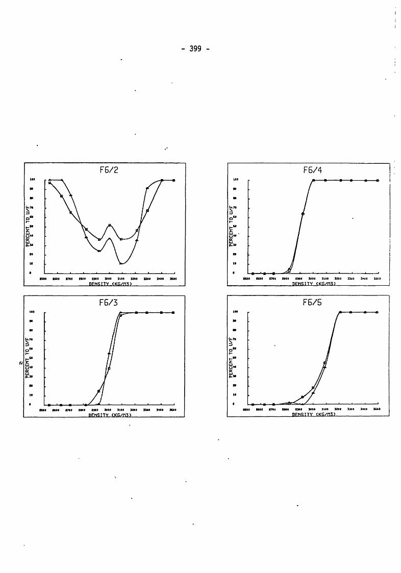
PERC

ENT

TO U

/F

OT N. Ln

I

I GO CO CO I

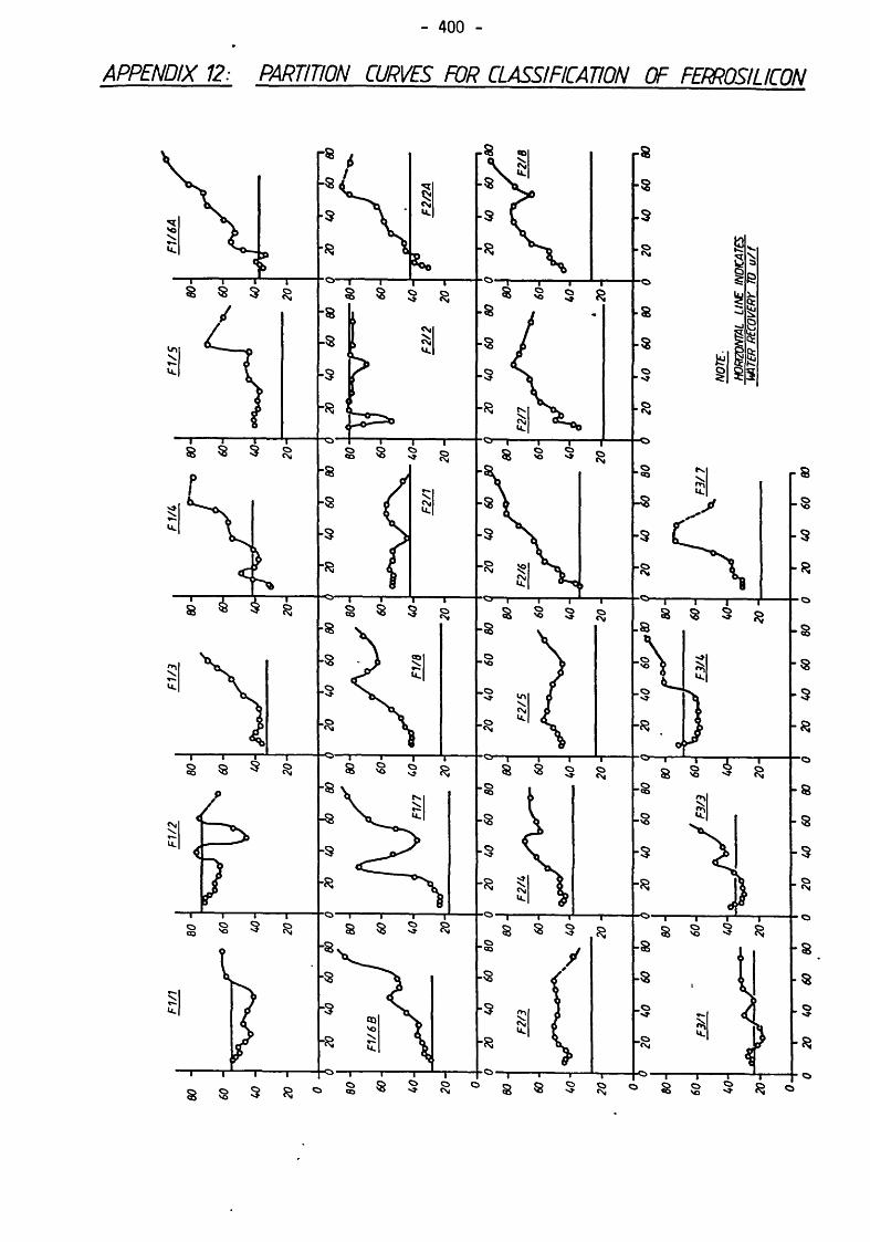
F1/1

. F1/

2 .

F1/3

, F1/U

.

F1/5

, F1/

6A

- 400

A P P E N D IX 12: PARTITION CURVES FOR CLASSIFICAT IO N OF FERROSILICON

r8

-8

-3

“ O

■ 8

-3

o- V?&8

■o

-8

-3

- 3

-8

- -O-(-3

-3

-3. o

_ o*v»

— r° 3

-o

- 3

- 3_ oVj-

-3

—j- oo

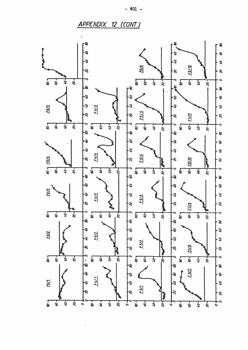
F6/1

80 ~t

F6/2

80 n

F6/3

80 n F6/U

_ ?

801

F6/5

- 401

A P P E N D IX 12 (CO NT J

rfi

-3

-5

"R

§

$

8s|

o&

3

R

8 8 $ 3

APPENDIX 13A - DERIVED DATA FROM MILLED FERROSILICON CYCLONE TESTS : SERIES Flt F2. F3 AND F6

TestNumber 1 - Cvf Rei L Pu/Pf (mVr ‘)

ResidenceT1me(s)

Pl/pf 9(m)

T’a(mln)

(m2 s-^fx 106)(m s-lZx 10“)

Fl/1 0.6427 30,856 2.123 0.936 5.11 1.052 2.832 2.984 1.35Fl/2 0.6615 20,305 2.303 0.958 3.64 1.481 1.551 3.222 1.48Fl/3 0.7064 70,628 2.601 1.114 5.72 0.941 4.345 1.459 1.64Fl/4 0.7087 57,064 3.161 1.025 3.50 1.539 1.972 1.103 1.88Fl/5 0.7513 105,343 2.562 1.296 6.12 0.880 4.889 1.045 1.89F1/6A 0.7535 74,060 2.741 1.151 3.69 1.457 1.907 0.898 2.84F1/6B 0.7563 61,455 2.936 1.203 3.74 1.440 2.094 1.095 2.57Fl/7 0.8169 124,363 2.577 1.642 6.94 0.776 6.321 1.004 2.48Fl/8 0.8185 70,988 2.855 1.495 4.40 1.223 2.820 1.116 3.37

F2/1 0.6608 47,922 2.416 1.098 4.93 1.093 2.988 1.850 2.15F2/2 0.6651 48,884 2.726 0.971 3.76 1.432 1.964 1.384 1.18F2/2A 0.6749 68,660 2.286 1.110 4.49 1.198 2.353 1.178 2.61F2/3 0.7086 111,339 2.230 1.293 6.02 0.894 4.119 0.973 2.36F2/4 0.7175 75,980 2.216 1.171 4.47 1.204 2.261 1.060 3.08F2/5 0.7536 112,650 1.869 1.423 6.88 0.783 4.507 1.099 2.92F2/6 0.7625 61,386 2.306 1.287 4.36 1.236 2.230 1.277 3.78F2/7 0.8137 145,838 2.348 1.663 6.50 0.829 5.052 0.802 3.33F2/8 0.8220 89,147 2.354 1.532 4.70 1.146 2.646 0.948 5.13

F3/1 0.6688 45,095 2.827 1.016 5.08 1.059 3.723 2.029 1.38F3/3 0.7128 66,820 3.393 1.030 5.50 0.979 5.236 1.482 1.11F3/4 0.7127 59,791 2.946 0.991 4.24 1.270 2.697 1.276 1.44F3/7 0.8198 118,913 3.664 1.378 6.67 .0.807 8.321 1.010 1.29

F6/1 0.6885 34,848 2.642 0.974 4.09 1.317 2.250 2.111 1.60F6/2 0.6711 28,927 2.501 0.935 4.25 1.267 2.304 2.645 1.38F6/3 0.7668 61,800 3.048 1.109 4.09 1.317 2.595 1.190 1.92F6/4 0.8162 65,784 3.156 1.306 4.06 1.326 2.653 1.111 2.65F6/5 0.7193 48,779 2.869 0.989 4.05 1.328 2.404 1.496 1.63F6/6 0.9416 - 3.268 1.979 4.74 1.137 3.743 - 5.17

Column 1 2 3 4 5 6 7 8 9

Notes : Col. 1 CVf a Volume cone, solids In feed medium.Col. 2 Ref =* Inlet Reynolds No. = pf D^/na(min).Col. 3 L ■ Pressure loss coefficient * P-|/(0.5 pf Vf2).Col. 4 pu/pf ■ Ratio of underflow and feed medium densities.Col. 5 V| * Inlet velocity.Col. 6 Bulk flow residence time ■ Cyclone volume/Qf.Col. 7 Pressure drop 1n m of pulp.Col. 8 Kinematic viscosity.Col. 9 z - Effective gravity sedimentation rate of feed medium, determined from eqn. 5.38

APPENDIX 13B - DERIVED DATA FROM ATOMISED FERROSILICON CYCLONE TESTS : SERIES F4 AND F5

TestNumber 1 - Cyf Rei L Pu/Pf

ResidenceT1me(s)

Pl/pf 9 (m)

n,(m1n)

(m2 s-*fx 106)(m s-^x lO1’)

F4/1 0.6558 92,726 2.858 1.155 5.61 0.959 4.591 1.090 1.51F4/2 0.6662 60,691 3.082 1.120 4.13 1.303 2.684 1.226 1.83F4/3 0.6966 109,354 3.059 1.347 6.00 0.897 5.613 0.988 1.62F4/4 0.7113 58,843 3.114 1.235 3.77 1.430 2.252 1.152 2.41F4/5 0.6511 82,976 2.812 1.135 5.58 0.965 4.465 1.211 1.47

F5/1 0.6533 74,298 3.797 0.991 5.15 1.044 5.144 1.249 0.982F5/2 0.6614 51,798 3.929 0.949 3.84 1.400 2.961 1.336 1.20F5/3 0.7143 91,955 3.526 1.082 5.84 0.923 6.122 1.142 1.02F5/4 0.7136 55,309 3.534 1.054 3.84 1.403 2.654 1.249 1.54F5/5 0.7677 102,148 3.822 1.218 6.14 0.877 7.338 1.081 1.03F5/6 0.7610 57,771 3.681 1.171 3.92 1.372 2.889 1.222 1.69F5/7 0.7572 104,829 3.550 1.394 6.09 0.884 6.715 1.046 1.84F5/8 0.7669 65,529 3.561 1.182 4.07 1.324 3.003 1.117 1.66F5/9 0.7644 58,770 3.635 1.171 3.96 1.361 2.900 1.212 1.71F5/10 0.7575 31,937 4.375 1.020 3.37 1.596 2.538 1.901 1.35F5/11 0.7671 27,723 3.716 1.093 3.88 1.389 2.848 2.518 1.49F5/12 0.7689 12,889 3.589 1.041 3.63 1.484 2.409 5.067 1.59

Column 1 2 3 4 5 6 7 8 9

For notes on derived quantities, see Appendix 13A.