Cost Effective Interference Management in Ultra-dense ...

Cost Effective InterferenceManagement in Ultra-denseHotspot Mobile Broadband

Systems

DU HO KANG

Licentiate Thesis in Information andCommunication Technology

Stockholm, Sweden 2012

Cost Effective Interference Management inUltra-dense Hotspot Mobile Broadband Systems

DU HO KANG

Licentiate Thesis in Information and Communication TechnologyStockholm, Sweden 2012

TRITA–ICT–COS–1211ISSN 1653–6347ISRN KTH/COS/R--12/11--SE

KTH Communication SystemsSE-164 40 Stockholm

SWEDEN

Akademisk avhandling som med tillstånd av Kungl Tekniska högskolan framläggestill offentlig granskning för avläggande av teknologie licentiatexamen i radiosystem-teknik fredagen den 27 November 2012 klockan 15.00 i sal C1, Electrum1, KungligaTekniska Högskolan, Isafjordsgatan 26, Kista.

© Du Ho Kang, November 2012

Tryck: Universitetsservice US AB

i

Abstract

Rapid mobile data traffic growth is becoming in a reality and sev-eral forecasts expect that it will be continued in upcoming years. Itis expected that significant indoor investment will be made not onlyby traditional operators but also by facility owners for their own pur-poses. A key challenge to such local network providers is provisioningever-increasing mobile traffic demand at the current level of productioncost per bit. A popular deployment strategy so far is deploying WLANnetworks. While denser indoor deployment is foreseen, the interferencefrom inside of a network as well as other neighboring operators can be alimiting factor for higher capacity. Tighter interference management willcertainly provide higher efficiency in network and spectrum usage. Nev-ertheless, costs to allow fast information sharing among access pointsare necessary for advanced interference coordination. Moreover, man-aging interference across networks owned by different operators raisesnot only infrastructure cost but also the network interrelatedness whichoperators are typically reluctant for business independency. When tak-ing into account the cost and barriers for interference coordination, itis still not so obvious that coordination in wireless broadband systemswill be advantageous to operators.

In this thesis, we address the operator benefit of downlink inter-ference coordination in two aspects: 1) multi-cell coordination withno interference from neighboring operators, and 2) inter-operator co-ordination in shared spectrum. In order to deal with interference andcost tradeoff analysis, we explicitly develop a techno-economic analy-sis framework and reform a traditional cost model. Numerical resultsindicate that the economic benefit of the multi-cell coordination sig-nificantly depends on propagation conditions and average user demandlevel. A self-deployed WLAN network can be the cheapest deploymentoption in closed areas up to certain average demand level. Over thedemand level or in open areas, advanced joint processing schemes ina cellular domain may be a viable solution. The drawback is thatit requires extremely accurate channel state information at transmit-ters for practical usage. When inter-operator interferences is present,asymmetric cellular networks will be likely to appear due to businessindependency and selfishly compete to access spectrum with no or lit-tle network-level coordination. A network designed for more fairnesswith higher transmission power will have more benefit against the othercounterpart. Although asymmetric competition lets operators unfairlyutilize spectrum, sharing spectrum with reasonable geographical separa-tion can outperform over static coordination, i.e., traditional spectrumsplit. Tight cooperation to maximize a common objective can furtheroffer the performance benefit to both involved partners. However, the

ii

cooperation gain quickly diminishes as network separation and size in-creases because self-interference becomes more dominant.

Acknowledgements

I appreciate my advisor Professor Jens Zander for accepting me in the doctoralprogram and great guidance both in technical research and the basic attitude ondiscussion. I would like to thank Dr. Ki Won Sung for his advising on manypractical aspects in research and scientific writing.

I am grateful to Dr. Claes Tidestav for reviewing my Licentiate proposal andfor all valuable comments to improve the quality of the thesis. My gratitude goesto Dr. Bogdan Timus of sincere and very sharp comments on the thesis draft. Iwould like to express my gratitude to Dr. Jaap Van De Beek for accepting the roleas an opponent on my defense.

I would like to take this opportunity to thank my colleagues at the Commu-nication Systems department: Sibel Tombaz, Ali Özyagzi, Evanny Obregon, LeiShi, Serveh Shalmashi, Saltanat Khamit, Luis Guillermo Martinez, Miurel Tercero,Pamela Gonzalez Sanchez, Dr. Tafzeel ur Rehman, Dr. Luca Stabellini, Dr. SangWook Han, Prof. Jan Markendahl, Prof. Claes Beckman, Prof. Ben Slimane, Prof.Anders Västberg, Prof. Guwang Miao, Göran Andersson, Mats Nilson, Dr. ÖstenMäkitalo and many more. For all the support in administrative issues and technicalmatters, I thank Irina Radulescu, Ulla Eriksson, Anna Barkered, Sarah Löwhagen.Special thanks to my friends for sharing good moments in KTH: Dr. Sunjae Chung,Jang-Kwon Lim, Dr. Sang Ho Yun.

I am deeply indebted to my wife Hyanjee for her sacrifice and support duringthe licentiate thesis work and dedicate this thesis to my family.

iii

Contents

Acknowledgements iii

Contents v

List of Tables vii

List of Figures vii

1 Introduction 11.1 Background and Motivation . . . . . . . . . . . . . . . . . . . . . . . 11.2 Brief Literature Review . . . . . . . . . . . . . . . . . . . . . . . . . 41.3 High-level Problem Formulation and Analysis Approach . . . . . . . 51.4 Overview of Thesis Contributions . . . . . . . . . . . . . . . . . . . . 61.5 Thesis Outline . . . . . . . . . . . . . . . . . . . . . . . . . . . . . . 8

2 Techno-economic Analysis Framework 92.1 Operator Strategies: A Conceptual Framework (Paper 1) . . . . . . 102.2 Extended Cost Model . . . . . . . . . . . . . . . . . . . . . . . . . . 12

3 Cost Benefit of Inter-cell Interference Coordination 173.1 Research Questions . . . . . . . . . . . . . . . . . . . . . . . . . . . . 173.2 Related Work . . . . . . . . . . . . . . . . . . . . . . . . . . . . . . . 183.3 Economical Viability of Self-deployment (Paper 2) . . . . . . . . . . 193.4 Worthiness of Multi-cell Joint Processing (Paper 3) . . . . . . . . . . 223.5 Dense WLANs vs. Cellular Network (Paper 4) . . . . . . . . . . . . 263.6 Summary . . . . . . . . . . . . . . . . . . . . . . . . . . . . . . . . . 35

4 Inter-operator Coordination in Shared Spectrum 374.1 Research Questions . . . . . . . . . . . . . . . . . . . . . . . . . . . . 374.2 Related Work . . . . . . . . . . . . . . . . . . . . . . . . . . . . . . . 384.3 System Model . . . . . . . . . . . . . . . . . . . . . . . . . . . . . . . 384.4 Temptation to Higher Power (Paper 5) . . . . . . . . . . . . . . . . . 404.5 Differentiated Service Provisioning (Paper 6) . . . . . . . . . . . . . 42

v

vi CONTENTS

4.6 Operator Cooperation Incentive (Paper 6,7) . . . . . . . . . . . . . . 424.7 Summary . . . . . . . . . . . . . . . . . . . . . . . . . . . . . . . . . 45

5 Conclusions 475.1 Lessons Learned . . . . . . . . . . . . . . . . . . . . . . . . . . . . . 475.2 Limitations and Future Directions . . . . . . . . . . . . . . . . . . . 48

Bibliography 51

Paper I: High Capacity Indoor & Hotspot Wireless System inShared Spectrum-A Techno-Economic Analysis 59

Paper II: Cost and Feasibility Analysis of Self-deployed CellularNetworks 75

Paper III: Is Multicell Interference Coordination Worthwhile inIndoor Wireless Broadband Systems? 81

Paper IV: Cost Efficient High Capacity Indoor Wireless Access:Denser Wi-Fi or Coordinated Pico-cellular? 89

Paper V: Impact of Asymmetric Transmission Power on Opera-tor Competition in Shared Spectrum 101

Paper VI: Operator Competition with Asymmetric Strategies inShared Spectrum 107

Paper VII: Cooperation and Competition between Wireless Net-works in Shared Spectrum 113

List of Tables

2.1 Changing business landscape and system design paradigm shift in sharedspectrum [1]. . . . . . . . . . . . . . . . . . . . . . . . . . . . . . . . . . 10

3.1 Average wall loss according to common building material [2] . . . . . . . 253.2 Examples of typical bit rate for video streaming [3] . . . . . . . . . . . 32

List of Figures

1.1 Global mobile traffic: voice and data, 2010-2017 (regenerated from [4]). 21.2 Increasing number of local access networks deployed by various small

operators in shared spectrum [1]. . . . . . . . . . . . . . . . . . . . . . . 3

2.1 A conceptual framework to navigate the operator strategies [1]. . . . . . 112.2 Examples of Ccoord according to the cooperation level [1]. . . . . . . . . 13

3.1 Total deployment cost in a closed environment (Lw=15 dB, δ=0.2) [5]. . 203.2 Total deployment cost in an open environment with tighter coverage

constraint (Lw=0 dB, δ=0.05) [5]. . . . . . . . . . . . . . . . . . . . . . 213.3 Permissible planning overhead (Lw=15 dB, δ=0.2) [5]. Note that higher

PPO means that the location planning is more preferable. . . . . . . . . 223.4 Indoor service area layout [6]. . . . . . . . . . . . . . . . . . . . . . . . . 233.5 Hypothetical interference coordination gain according to internal wall

loss Lw in different path loss exponent α and building shapes [6]. . . . . 26

vii

viii List of Figures

3.6 Service area layout with the example of AP deployments in nine parti-tions [7]. . . . . . . . . . . . . . . . . . . . . . . . . . . . . . . . . . . . . 27

3.7 Deployment density comparison according to average user demand sub-ject to ν < β (α=2, Lw=0 dB) [7]. . . . . . . . . . . . . . . . . . . . . . 31

3.8 Outage probability ν in densification (α=2, Lw=0 dB) [7]. . . . . . . . . 313.9 The maximum rate supported by an AP according to system bandwidth

W (AP density=1 AP/100 m2, Lw = 0) [7]. . . . . . . . . . . . . . . . . 333.10 Deployment density comparison according to average user demand sub-

ject to ν < β (α=4, Lw=10 dB with wx=wy=4) [7]. . . . . . . . . . . . 33

4.1 Two neighboring cellular networks owned by different operators in sharedspectrum [8]. . . . . . . . . . . . . . . . . . . . . . . . . . . . . . . . . . 39

4.2 NE characteristics according to the power asymmetry [8]. . . . . . . . . 404.3 Benefit of sharing spectrum according to the power asymmetry [8]. . . . 414.4 Break-even power asymmetry to lower power network [8]. . . . . . . . . 424.5 Comparison between asymmetric and symmetric competition [9]. . . . . 434.6 Relative average performance difference from the symmetric objective

according to network separation [9]. . . . . . . . . . . . . . . . . . . . . 434.7 Average cooperation gain of each operator over competition according

to network size and separation [10]. . . . . . . . . . . . . . . . . . . . . . 444.8 Cooperation possibility for mutual benefits with proper weight selec-

tion [9]. . . . . . . . . . . . . . . . . . . . . . . . . . . . . . . . . . . . . 45

5.1 An economic system solution map for indoor and hotspots deployment [7]. 48

Chapter 1

Introduction

1.1 Background and Motivation

When commercial mobile voice service was first introduced a couple of decades ago,it drastically changed our lifestyles by freeing us from fixed line communications.In a wireless system design perspective, a highly centralized cellular network wasdesired for robust coverage to guarantee the real-time voice service quality whichdirectly affects revenue generation and customer churn. As the voice subscriptionpenetration was already saturated in most of developed countries and price compe-tition among operators are continued, wireless service became a commodity in ourdaily life. In this moment, smartphones were introduced in a terminal market, andthe second wave of wireless innovations has been triggered. With the combinationsof mobile broadband service, they made everyone enjoy various applications withbeing always connected to Internet cloud. The flat rate pricing even acceleratesthe success of mobile broadband service. It changes our lifestyles much faster thanwhen the mobile voice communication service was commercialized.

Changing Business Landscape: Emergence of Small Operators

The success of mobile broadband access is already creating severe capacity prob-lems for many operators by causing a virtual data tsunami. As foreseen by manyindustry players in Fig. 1.1 [4,11], explosive traffic growth is expected to be contin-ued in upcoming years. New types of bandwidth-hungry applications, e.g., cloudcomputing or web storage service will even speed up the needs for higher capacityand faster mobile broadband access. The only feasible long-term solution to sat-isfy the order of magnitude potential traffic increase is to densify wireless networkswhile link spectral efficiency almost reaches the Shannon bound and spectrum it-self is scarce [12]. Since data traffic grows much more significantly indoors thanoutdoors [13], considerable new indoor network investments are predicted in a longterm. In business perspective, a key question is who will invest such indoor net-works. Some indoor networks are now being deployed in public hotspot areas,

1

2 CHAPTER 1. INTRODUCTION

2010 2011 2012 2013 2014 2015 2016 2017

2000

4000

6000

8000

Mon

thly

Pet

aByte

s

Data:

mobile PCs/tablets

Data:

mobile phones

Voice

Figure 1.1: Global mobile traffic: voice and data, 2010-2017 (regenerated from [4]).

e.g., shopping malls or stadium, by traditional wide-area mobile network operators(MNOs) for offloading to mitigate the burden of the existing outdoor wide-areasystems. However, direct deployment by traditional MNOs may be hindered bylimited access to the various private indoor sites and the lack of new revenue gen-eration for the extra indoor deployment. Instead, it is found and expected thatmost of the indoor network investments will be made by the other market actorsfor various reasons. For instance, hotspot operators, e.g., Boingo, Wayport andtheCloud, focus on providing nomadic Internet access to professional users at pub-lic indoor areas with subscription-free pricing. There is also an increasing interestin dedicated indoor networks by non-telecom players, e.g., facility managers, realestate owners, and private companies [14]. The main driver is to own dedicated net-works inside their own buildings to attract more tenants or their own customers,e.g., office suppliers or hotels, regardless of their subscription contracts with ex-isting MNOs. Therefore, the white-labeled hotspot operators or even the facilityowners themselves emerge as new important players in the indoor capacity provi-sion. With this shift in network ownership, a number of distinct local area networksowned and managed by non-traditional business entities are appearing at the closedistance of each other under the umbrella of existing wide-area networks as illus-trated in Fig. 1.2. In terms of existing MNOs, the indoor investment by other actorswill be advantageous as well since traffic generated from their subscribers will besignificantly alleviated by non-traditional actors.

1.1. BACKGROUND AND MOTIVATION 3

Existing Wide-area

Networks

Picocell

network by

enterprises

WiFi network by

shopping malls,

restaurants

WiFi network

of hotels/

conference

centers

Public WiFi

network by

authorities

Femtocell

networks by

hotspot

operators

Inter-network

interference

Urban areas in high demand

WiFi networks

by MNOs for

offloading

lll

Figure 1.2: Increasing number of local access networks deployed by various smalloperators in shared spectrum [1].

Interference Management and Cost Challenges

In order for such small-sized operators to provide high-capacity in a specific loca-tions, securing spectrum is essential. However, it would be unrealistic that everyfacility owner has an exclusive access right to dedicated spectrum as traditionallicensees. In addition, unlike traditional wide-area network where coverage is a keydriver for network deployment, large spectrum is needed only in particular geo-graphical locations where the small operators have site control and want to providehigh-capacity. Accordingly, shared spectrum is inevitable for local service provi-sioning, e.g., unlicensed band or secondary access. Industrial, scientific and medi-cal (ISM) radio band used for WLAN deployment already demonstrates one earlyexample. While the ISM band becomes overpopulated by the successful WLANdeployment, the demand for commonly accessible spectrum by the small operatorscontinues to grow. Thus, regulatory bodies recently also envisage various waysof shared spectrum for local usage [15, 16], e.g., authorized shared access (ASA),licensed shared access (LSA).

In technology perspective, an IEEE 802.11 based WLAN system has so fargained success thanks to its low cost and easy configuration. However, as WLANdeployment is denser and more small-sized operators appear in the close vicinity,considerable interference will be generated and have negative impacts on the indi-vidual network performance due to limited interference coordination both within a


network and between networks. Instead, interference has been more carefully dealtin a traditional cellular network at the expenses of equipment and installationcosts, potentially increasing network capacity. Recent advances in technologies alsodemonstrated that real-time multi-cell joint processing further increases resourceefficiency by ideally eliminating interference. However, it inevitably necessitateshigh-speed backhaul and complex central baseband processing units which alsoraise deployment costs [17, 18]. Besides of the technical cost for coordination, co-ordinating inter-operator interference also needs cooperation in a business domain.In other words, the high-level executive decisions should be predetermined beforeengineering networks for inter-network interference management. However, opera-tors are typically very reluctant to make business alliance due to the uncertainty offuture business although explicit advantages are identified, as reported in previousstudies in [19,20]. In the presence of technical cost and strategic barriers, it is stillnot so obvious if interference coordination can give an operator benefit. Therefore,the performance gain by coordination should be quantitatively assessed to iden-tify the lowest cost deployment strategy in such ultra-dense indoor and hotspotnetworks. This is the point of departure in this thesis.

1.2 Brief Literature Review

Interference management has been one of major research areas over decades in wire-less communications. Various techniques were proposed and studied from classicalfixed partitioning of resource to recent precoding strategies in different resourcedomains, e.g., transmit power, media access probability, beamforming matrix, andphysical antenna tilt. The level of coordination also differentiates them by staticcoordination and dynamic coordination. Several survey papers in [18, 21] inten-sively overview a number of method of interference coordination. However, typicalresearch directions in such technical analysis were developing algorithms or schemesto provide the higher network performance at the given idealized access point (AP)deployment rather than minimizing network cost offering the same network ca-pacity. Therefore, cost factors to enable different coordination technologies werenot explicitly considered in a number of existing analysis. A few number of costcomparison between existing wireless systems was mainly contributed by a techno-economic literature with realistic cost figures from industries or specific markets.However, they typically simplified the technical performance evaluation for analysisconvenience, e.g., capacity estimation based on arithmetic calculation [14, 22, 23].More considerations on technical aspects in network cost comparison have beendone in a few studies, but with overly simplified interference models, e.g., averagedconstant interference [24,25].

Implementing advanced coordination techniques certainly affects a network ar-chitecture and need costly extra infrastructure, e.g., fiber installation. However, ifcost to enable tight coordination can pay off the performance gain is still not ex-plicitly discussed yet although interference becomes a key limiting factor in massive

1.3. HIGH-LEVEL PROBLEM FORMULATION AND ANALYSIS APPROACH5

indoor deployment in shared spectrum. Accordingly, the network cost comparisonamong system solutions with distinct coordination techniques is still missing with-out a proper cost model depending on the level of coordination. Besides of thetechnical cost for coordination, the strategic concern is one of major barriers inthe case of inter-operator coordination. Nonetheless, only a few number of studiesqualitatively discussed this [19, 20]. None of previous work modeled it with ourbest knowledge for the quantitative comparison between different strategic deci-sions. Most of system performance analysis in co-primary shared spectrum hasfocused on a particular WLAN technology rather than the usage of cellular net-works to increase system capacity. One of major differences in WLAN technologyfrom the cellular network is that the capacity of wireless networks may be furtherincreased by internally controlling self-interference by using the means of traditionalcoordination techniques. Nevertheless, performance analysis on potential cellularsolutions in shared spectrum itself is a challenging task and is in the early stage ofresearch due to non-traditional potential selfishness between networks where intra-network interference is coupled with interference from neighbors. In addition, whenuncertain interference from nearby operators is present, the performance of an in-dividual cellular network becomes non-trivial. Only a few number of studies areidentified in the literature regarding network-level coordination in non-overlappinggeographical areas [26–28]. However, they assumed symmetric network deploymentwhich may not be so realistic in various local environments. Their analysis wasmainly intended to characterize the performance in competition rather than com-paring the cost of candidate solutions with the different levels of coordination whichis our main focus in this thesis.

1.3 High-level Problem Formulation and AnalysisApproach

We mainly focus on an in-building scenario in urban areas which require a high-capacity wireless access network. The time line behind this scenario is a near futurewhen much more wireless capacity is needed than current traffic demand. An un-derlining assumption here is that network providers do not have access to dedicatedspectrum for local service provisioning. Existing MNOs still operate their wide-areanetworks in exclusive licensed band so that interactions between the local networksand traditional wide-area networks are the out of scope in this thesis. The keyanalysis problem which this thesis concentrates on is the tradeoff relation betweeninterference coordination and its cost in order to design an affordable wireless accessnetwork in shared spectrum. While the performance benefit of interference coordi-nation is certainly expected, if its advantages to operators is sufficient to realize itin practical systems is not so obvious since related cost and strategic concerns forcooperation are also increased with tighter interference coordination. In this thesis,we address a following high-level research question:

• When and where does interference coordination provide cost advantages and


strategic benefits in the ultra-dense hotspot wireless networks?

To answer this high-level question, we introduce a techno-economic analysisframework in shared spectrum that first defines a solution space in terms of tech-nical coordination and strategic decisions. Then, we divide the high-level probleminto two subproblems to reduce problem complexity: intra-network coordinationand inter-operator coordination. The potential cost benefit of the intra-networkcoordination is assessed by using an idealized radio network model. Since the net-work cost is dependent on a specific market, our approach is assessing the requirednumber of base stations (BSs) of representative solutions as a function of increasingtraffic demand. We use these results as an input for the cost comparison by usinga simple cost model. Afterwards, we develop a simplified inter-operator coordi-nation model where two neighboring cellular networks are internally coordinatedin order to understand the non-traditional cellular operation in shared spectrum.Then, competition and cooperation strategies are analyzed in various asymmetricnetwork deployment and compared to examine the strategic benefit. The impactof different propagation conditions of both intra-building and inter-building is fur-ther assessed. Based on quantitative results obtained from the simplified models,we will identify key factors to significantly affect the cost and strategic benefits ofinterference coordination and draw general implications on the affordable systemdesign in shared spectrum.

1.4 Overview of Thesis Contributions

We now provide the overview of thesis contributions in the order of presentationsin this thesis. The contributions mainly consist of three parts: an overall techno-economic analysis framework in shared spectrum (Chapter 2), the cost benefitanalysis of inter-cell coordination (Chapter 3), and analysis on cellular networkcompetition and cooperation in shared spectrum (Chapter 4).

Chapter 2

Unlike the traditional single operator in exclusive licensed band, the solution spacefor the system design in shared spectrum is coupled with both strategic decision in abusiness domain and different technical solutions. Thus, we provide a new analysisframework to navigate the potential candidate solutions in a more systematic way.In the framework, we explicitly define the key concepts as criteria to create thesolution space: coordination as a technical solution and cooperation as a strategicdecision. Then, an extended cost model to capture new cost factors from potentialinter-operator relation is discussed. Full descriptions will be found in:

• Paper 1. D. H. Kang, K. W. Sung, and J. Zander, “High Capacity Indoor &Hotspot Wireless System in Shared Spectrum-A Techno-Economic Analysis",submitted to IEEE Communications Magazine, 2012.

1.4. OVERVIEW OF THESIS CONTRIBUTIONS 7

The author of this proposal, acted as the lead author, mainly wrote a paper andelaborated the main concepts of the framework. The conceptual framework andcost models were jointly developed with Ki Won Sung and Jens Zander who alsoparticipated in editing the paper.

Chapter 3

The cost benefit of inter-cell interference coordination is assessed based on a simplecost model. Specifically, if cost for location planning and cost for installing opticalfiber for advanced MAC and PHY techniques can pay off the performance gainis quantitatively investigated. The answer is that it can pay off for a given plan-ning and backhaul cost per AP particularly when user demand level becomes veryhigh. However, results show that the answers significantly depends on propagationcondition since relatively obstructed indoor environments considerably reduce theperformance gain of coordinated cellular systems. More detail results and modelassumptions can be found in the following papers:

• Paper 2. D. H. Kang, K. W. Sung, and J. Zander, “Cost and Feasibil-ity Analysis of Self-deployed Cellular Networks", in Proc. IEEE PIMRC,Toronto, Canada, Sep. 2011.

• Paper 3. D. H. Kang, K. W. Sung, and J. Zander, “Is Multicell InterferenceCoordination Worthwhile in Indoor Wireless Broadband Systems", to appearin IEEE Globecom, Anaheim, USA, Dec. 2012.

• Paper 4. D. H. Kang, K. W. Sung, and J. Zander, “Cost Efficient High Ca-pacity Indoor Wireless Access: Denser Wi-Fi or Coordinated Pico-cellular?",submitted to IEEE transactions on wireless communications, 2012.

The original problem formulation and the simulation methodologies were imple-mented by the author of this thesis, who also acted as the main author of writingpapers. However, these ideas were refined in close collaboration with Ki Won Sungand Jens Zander who offered valuable feedbacks on writing and conclusion.

Chapter 4

In this chapter, coordination on inter-operator interference was analyzed in twosolution domains, i.e., competition and cooperation. Two key questions are mainlyasked: 1) what is the impact of independent network configurations on a competingcellular network particularly in terms of transmit power capability and fairnessobjective? and 2) can the potential cooperation incentive be sufficient to suppressthe strategic cost? It is shown that independent network configuration leads toperformance loss in one competing network. However, the spectrum sharing canbe beneficial than fixed spectrum split with proper regulation on transmit power.Under the same power constraint, positive cooperation gain can be identified even


when different types of fairness is required. However, it quickly diminishes withrealistic inter-building propagation loss. The more detailed results of these studiesare provided in the following papers:

• Paper 5. D. H. Kang, Z. Li, Q. Luo, F. Fathali, A. Vizcaino, and J. Zan-der, “Impact of Asymmetric Transmission Power on Operator Competitionin Shared Spectrum", in Proc. IEEE Swedish Communication TechnologiesWorkshop (SWE-CTW), Lund, Sweden, Oct. 2012.

• Paper 6. D. H. Kang, K. W. Sung, and J. Zander, “Operator Competitionwith Asymmetric Strategies in Shared Spectrum", in Proc. IEEE WCNC,Paris, France, Apr. 2012.

• Paper 7. D. H. Kang, K. W. Sung, and J. Zander, “Cooperation and Com-petition between Wireless Networks in Shared Spectrum", in Proc. IEEEPIMRC, Toronto, Canada, Sep. 2011.

The first paper was coauthored with the students of IK2511 wireless project course(the course was given during the Winter of 2011). The author of this thesis proposedthe original problem formulation and acted as the leading author for the paper.Ideas were refined with the other student coauthors, who implemented simulationcode to obtain the numerical results. Jens Zander revised the abstract and guidedthe conclusions of the paper. In the second and the third paper, the author of thisthesis proposed the problem statement. Ki Won Sung and Jens Zander gave thevaluable feedback during the discussions on the results and insights in the directionof the paper.

1.5 Thesis Outline

The remainder of this thesis is organized in five chapters. Chapter 2 provides theconceptual framework for defining a solution space in shared spectrum. In Chap-ter 3, coordinating self-interference within a network and its cost is examined bycomparing different system solutions when deployment density is very high. Then,the impact of independent network deployment in shared spectrum and cooperationincentive between operators are assessed in Chapter 4 when two neighboring cellu-lar networks interfere each other. Finally, we conclude this thesis with discussionson limitation and future work in Chapter 5.

Chapter 2

Techno-economic AnalysisFramework

Recall that our scenario is typical urban areas where multiple buildings are nearbyand local operators desire to provision very high capacity in shared spectrum. Fun-damentally, operators aim to maximize the return on investment by providing wire-less access services. While profit in future is generally hard to predict due to marketuncertainty, a basic network design problem that the operators are facing is mini-mizing total network cost to satisfy expected user demand in a particular physicalenvironment. In order to achieve this, the cost of different system design candidatesshould be compared under a certain technical requirement. The indoor and hotspotsystem design in shared spectrum is inherently a multi-dimensional problem wheretechnology, business, and regulatory issues are interwined. We provide Fig. Ta-ble 2.1 to show fundamental differences between a design problem in a traditionalsingle operator network and one in shared spectrum. Consequently, the analysisfor the low cost system design is not so trivial due to the involved business andregulatory complexity unlike traditional wide-area network in dedicated spectrumwhich mainly concern a technology domain. In spite of the importance of investi-gating the different levels of interference coordination, it has been mainly regardedas the part of a model assumption rather than the object to be compared. Also,a proper cost model should be in place for the cost-performance tradeoff analysisespecially to reflect new dominant inter-operator cost factors. Existing cost modelswere thus far developed for the conventional single operator, e.g., [29]. Despitethe increasing number of interfering local networks, we thus far lack a systematicframework for quantitatively analyzing different system design options which areinter-winded with decision makings in both technology and business domains. Wein this chapter develop analysis tools for the cost comparisons of possible systemdesign options. To effectively navigate potential design candidates, we first providea new conceptual framework with explicit definitions of key criteria. Then, we dis-cuss and give an extended cost model including non-traditional inter-operator cost

9

10 CHAPTER 2. TECHNO-ECONOMIC ANALYSIS FRAMEWORK

for techno-economic comparison.

Table 2.1: Changing business landscape and system design paradigm shift in sharedspectrum [1].

Traditional wide-area

single operator system

Local-area system in shared

spectrum

Business

landscape

Who

&

Why?

· MNOs: revenue generation

from service provisioning

· MNOs: data offloading

· Facility owners: complements to

facility services

· Hotspot operators: new revenue

generation in niche markets

Where? Large-scale public outdoors Mainly private/public indoors

controlled by facility owners

Inter- operator

relation

Service/price competition in

markets

· Service/price competition in

markets

· Cooperation/competition for inter-

network interference coordination

Major network

related cost

· Network cost

· Spectrum cost

· Network cost

· Inter-operator cost

System

design

Design

problem

Minimizing network cost

at a given traffic demand

Minimizing network cost+inter-

operator cost


Decision

domain Mainly technology Both technology and business

Main decision

maker MNO Both an operator and a regulator

Coordination

target Nodes (e.g., BSs) Networks

2.1 Operator Strategies: A Conceptual Framework (Paper1)1

The neighboring network deployments will create local competition inflicting mu-tual interference to each other. Instead, operators can cooperate to manage togetherthe inter-network interference using latest advances in technology, e.g., joint mul-ticell processing, or coordinated scheduling. Since the cooperation is intrinsically

1The explicit definitions of the level of cooperation and coordination are from the paper [1]where the author of this thesis acted as one of the co-authors.

2.1. OPERATOR STRATEGIES: A CONCEPTUAL FRAMEWORK (PAPER1) 11

Strategy IV

Centralized

Network Rivalry

Strategy I

Distributed

Network Rivalry

Strategy II

Centralized

Network Alliance

Strategy III

Distributed

Network Alliance

Operator AAAA

Operator B

CooperationCompetition

Tight Coordination

Loose Coordination

Figure 2.1: A conceptual framework to navigate the operator strategies [1].

involved with strategic decisions in the business domain, the decision domain ofoperator strategies should include both the technology and business aspects. Inthis section, we provide a conceptual framework to effectively categorize potentialstrategies with the explicit definitions of key concepts. As shown in Fig. 2.1, it ischaracterized on one side by the strategic decision of the operators, i.e., cooperationand competition, and on the other side by the technical solution expressed as thelevel of coordination.

Strategic Decision: Cooperation or Competition

The strategic decision in the business domain influences the way for an individ-ual network to be coordinated. In this regard, we differentiate cooperation andcompetition based on the technical objective function which each of the involvedoperators aims to maximize. We define two types of strategies:

• Cooperation: the operators aim at maximizing a common objective functionagreed between partners.

• Competition: the operator aims at maximizing its own objective functionin a selfish manner.

Cooperating operators synchronize their overall technical behaviors for networkalliance by engineering their networks. This could involve additional investment.


Agreement on a common objective function itself could be challenging, particularlywhen partners have distinct main service types, e.g., rate guaranteed video ser-vices in offices versus best-effort services in shopping malls. Cooperative networksbehave as a conventional single operator network from a radio resource allocationperspective. In contrast, competition creates a non-traditional system design sinceintra-network can be centrally coordinated whereas external interference is uncon-trollable. Note that a popular WLAN system does not differentiate interferencefrom the inside of a network and from others deployed by neighbors. Regulatorscan provide the guidelines for inter-network coordination by issuing various co-existence rules ("etiquettes"). Traditional licensing or auction of spectrum is oneway to coordinate inter-operator interference. However, in our scenario where anumber of small operators are locally distributed, applying such traditional waysof regulation itself could be challenging or hinder local deployment.

Technical Solutions - Coordination between Networks

In each strategic decision, technical solutions can be different depending on availabletechnical means. We define coordination in a technical domain as the process ofsharing relevant information. The level of coordination is measured by the amountof information shared in the process. The information can be statistical or in-stantaneous and have different sources, e.g., traffic load or path gains between allthe involved access points and user terminals. The optimal system performancecan be a function of the level of global knowledge in a system and more accurateand frequent information exchange increases the knowledge in the whole system. Asystem with complete information sharing can be implemented as a centralized net-work since it can provide real-time resource allocation based on the fast sharing oflocal information, e.g., beamforming or coordinated scheduling [18]. Alternatively,average propagation conditions or the number of users per cell can be shared whichrequires significantly simpler equipment and less information exchange. Thus, dis-tributed resource allocation and network architectures can be feasible and mayreduce the system cost. Conventional CSMA/CA based WLAN system can be seenas one system where interference coordination is doen at a node level.

2.2 Extended Cost Model

Recall the assumption that the network design objective is finding the operatorstrategy to offer the lowest total cost for the required capacity. For this, besidesquantifying the performance of candidate strategies, proper cost models should bein the place. Although there are several cost models for traditional single operatorwide-area networks [29,30], cost factors arising in our shared spectrum scenario havenot explicitly studied yet. Particularly, there will be new technical and strategiccosts due to inter-operator coordination. In this section, we highlight new inter-operator costs and discuss the necessity of modifying and extending the traditionalcost model.

2.2. EXTENDED COST MODEL 13

Coordination Cost

Installing a central

coordinator and a

dedicated inter-

network line

Using existing IP

connectionInstalling a central

coordinator

Using existing IP

connection

Using existing IP connection

Cost for moderate coord.

Cost for tight coord.

Negligible cost

for loose coord.

Main Ccoord

drivers

Figure 2.2: Examples of Ccoord according to the cooperation level [1].

Inter-network coordination requires additional network complexity and infras-tructure cost from from the technical point of view. We define network relatedtechnical cost for cooperation as coordination cost Ccoord. Since we define the co-ordination as the process of sharing information between networks, Ccoord is phys-ically spent for acquiring relevant information for resource allocation. Dependingon the amount of information to be shared, Ccoord can be neglectable or signif-icant to achieve this. Fig. 2.2 shows the examples of Ccoord for coordination inMAC or PHY layer. The extra cost mainly emanates from installing dedicatedbackhaul or intermediate entity to coordinate the interference between networks.For instance, expensive dedicated backhaul should be installed in both inside andbetween buildings to allow for reliable low-latency information sharing. An inter-network coordinator, which is physically separated, can be introduced for fast and


synchronized resource allocation. In the level of moderate coordination, using ex-isting in-building IP connection may be sufficient to control individual network ornodes. Still, intermediate coordination equipment may be demanded because of aregulatory constraint, e.g., spectrum-broker, or due to the trust reason in a businessdomain. As long as the performance improvement is surely expected, operators canexchange information between operators without any intermediate nodes based onmutual trust. Distributed resource allocation can be made in this case.

(Invisible) Strategic Cost

In general, firms have been reluctant to cooperate across business boundaries be-cause the cooperation may limit their future decisions or business flexibility. Inmanagement literature, such barriers against strategic alliances with competitorshave been widely studied, e.g., see [31]. This is also true even for wireless operatorsas identified in several reports or a recent European project [19, 20, 32]. Some keynetwork-related obstacles can be identified2:

• Management overhead: decision-making on network deployment/upgrade canbe delayed because it requires an agreement with the cooperation partner.

• Limited network controllability: an operator may lose control over the deploy-ment and operation of its own network, which can restrict individual networkdimensioning and make its service not differentiable from the competitors inmarkets.

• Risk of information leakage: the coordination may unveil customer statisticsand know-how on network optimization to the other operator.

• Lack of trust: an operator may suspect that the cooperation partner deliversfalse information to take advantage of the coordination.

Although there are strategic barriers for cooperation, operators still open acooperation possibility for the case where large economic gain from cooperation isexpected. In traditional wide-area networks, cooperation took place in rural areasin the form of sharing the part of networks, e.g., site or tower sharing. Thus,analysis with considering such invisible cost in cooperation is necessary. We modelsuch uncertainty or risk by introducing an additional fictitious cost, denoted by thestrategic cost Cstex. Notice that Cstex may not be strictly measurable since it isrelated to the perceived uncertainty to the future. Nonetheless, this is not a newconcept in a strategic decision making process. A decision maker often considersan uncertainty margin, e.g. using a fictitious “required rate of return" or “hurdlerate" before investment when comparing different strategies [33]. Consequently, the

2The texts of examples in strategic concerns are from the paper [1] where the author of thisthesis acted as one of the co-authors.

2.2. EXTENDED COST MODEL 15

traditional single operator cost model should be extended in shared spectrum as:

Ctot = Cinfra + Cspectrum + Ccoord + Cstex. (2.1)

Chapter 3

Cost Benefit of Inter-cell InterferenceCoordination

3.1 Research Questions

In this chapter, we focus on managing the downlink inter-cell interference coordina-tion when inter-operator interference is absent. While tighter coordination certainlyincreases performance benefit from more efficient network/spectrum utilization, re-lated cost also increases. Therefore, whether or not such interference coordinationwill provide aggregate cost benefit compared to uncoordinated or loosely coordi-nated systems with more BSs is not so apparent. Inter-cell interference coordinationcan be examined in two different aspects: 1) AP location planning and 2) MACand PHY layer coordination.

In indoor environments, the locations of BSs are often expected to be randomlydeployed since planning them itself requires costly processes, e.g., the location op-timization or extending wires to a backhaul infrastructure. In such self-deploymentstrategy, the serious degradation of capacity or the infeasibility of coverage con-straint are predicted although interference mitigation techniques controlled by acentral coordinator are employed. The performance degradation without carefulplacement will need more BSs to meet the coverage and capacity requirements. Thesaving of the planning cost increases extra equipment cost in the self-deploymentat a given capacity demand. Therefore, it is not trivial if the self-deployment hasthe cost benefit in terms of total network cost.

Besides of the location coordination, interference coordination was typically con-sidered as coordination in medium access or in PHY layer. In this regard, a WLANnetwork has been thus far a dominating indoor solution due to its low cost and easyinstallation compared with cellular solutions. Increasing WLAN access point (AP)density creates more interference with more frequent media access contention amongco-channel APs for downlink transmission. Due to the fully distributed nature inIEEE 802.11 MAC, a denser WLAN network may suffer from severe interference,

17

18CHAPTER 3. COST BENEFIT OF INTER-CELL INTERFERENCE

COORDINATION

potentially with more deployment cost due to increased number of required APsthan cellular networks. Instead, a centralized interference management has beenimplemented in a conventional cellular network at the more expensive equipmentand installation costs than the WLAN network. Furthermore, various multicell jointprocessing in PHY layer have been recently paid an attention as a promising solu-tion toward higher capacity with much less deployment density than a conventionalcellular network [21]. However, it essentially needs pricey high-speed backhaul andextra system complexity for instantaneously exchanging the knowledge betweenBSs. Moreover, the wide variety of partitions and obstacles in indoor environmentsmay also affect its performance benefit differently. Specifically, we aim to addressthe following three questions in this chapter:

1. Which can be economic at a given average area throughput under coverageconstraint, self-deployment or planned-deployment?

2. Is the multi-cell joint processing in a cellular network worthwhile in presenceof indoor walls?

3. Will WLAN densification provide the lowest cost deployment option for ever-increasing user demand? If not, what can be an alternative option in a cellulardomain?

3.2 Related Work

Interference coordination in a multi-cell environment has been one of major re-search topics. Significant research efforts have been thus far devoted to developmore efficient algorithms and transmission technologies in a particular radio re-source domain, e.g., time or frequency, rather than analyzing the cost benefit ofone system over the others for the given capacity requirement [21, 34–37]. Theytypically showed the performance benefit of coordination techniques in a particu-lar deployment density, e.g., the number of APs or transmitters. However, it isnot so obvious that the performance benefit is maintained with denser deploymentsince it increases or change whole interference environment in the system. In otherwords, at a given network capacity requirement, a system with loose coordinationneeds more deployment density than a coordinated system. However, the increaseddensity of the loosely coordinated system changes the interference situation. Thus,cost saving from coordination at the same capacity requirements cannot be directlyinduced from the performance gain of coordination at the same deployment.

In techno-economic literature, there were a relatively few number of system costcomparisons between WLAN and a conventional picocell network based on empir-ical cost figures from a specific market or country [23, 25, 38]. Nevertheless, theircomparisons relied on simplified network capacity estimation which disregarded thedistinct interference coordination mechanisms. For instance, an overall network ca-pacity was obtained by simply scaling average per-cell throughput by the numberof placed APs [23, 38]. The authors in [25] estimated more accurately the network

3.3. ECONOMICAL VIABILITY OF SELF-DEPLOYMENT (PAPER 2) 19

capacity by reflecting non-uniform user distribution and propagation conditions.Still, the time dynamics of interference was not explicitly modeled which is consid-erably affected by the difference in the involved coordination, e.g., randomness inthe CSMA/CA of WLAN. Instead, a link-level data rate was approximated as thefunction of received average signal to average interference plus noise ratio. There-fore, the cost comparison based on more refined coordination models should be inthe place although existing approaches are efficient to estimate the capacity of acomplex large network. Moreover, they often ignored obstructed indoor environ-ments that may weaken the performance benefit of employing advanced coordina-tion while the wide variety of in-building structures create different interferencecharacteristics [2].

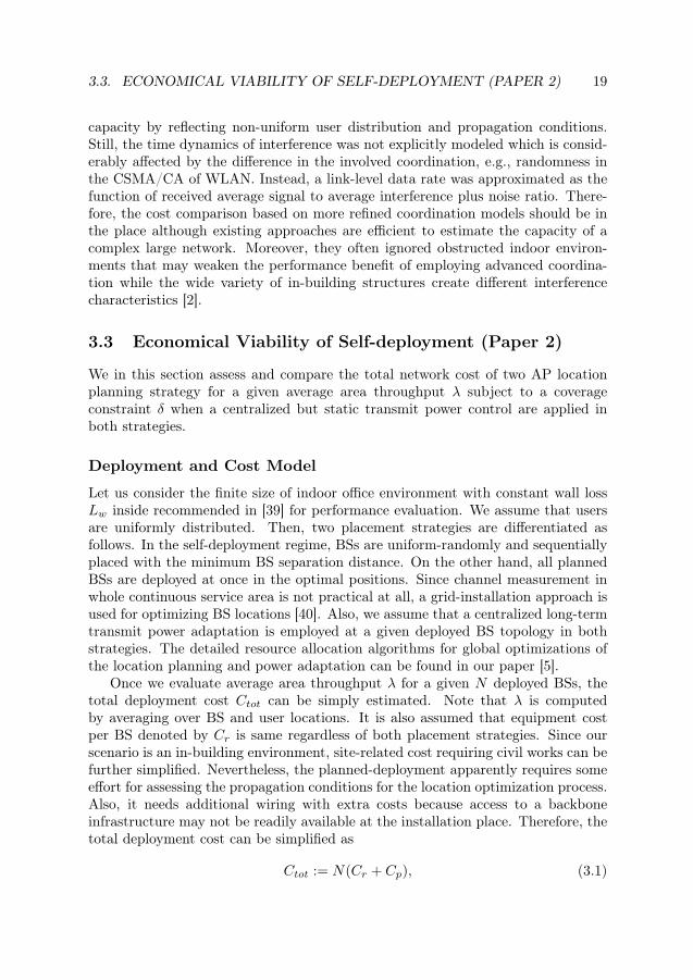
3.3 Economical Viability of Self-deployment (Paper 2)

We in this section assess and compare the total network cost of two AP locationplanning strategy for a given average area throughput λ subject to a coverageconstraint δ when a centralized but static transmit power control are applied inboth strategies.

Deployment and Cost Model

Let us consider the finite size of indoor office environment with constant wall lossLw inside recommended in [39] for performance evaluation. We assume that usersare uniformly distributed. Then, two placement strategies are differentiated asfollows. In the self-deployment regime, BSs are uniform-randomly and sequentiallyplaced with the minimum BS separation distance. On the other hand, all plannedBSs are deployed at once in the optimal positions. Since channel measurement inwhole continuous service area is not practical at all, a grid-installation approach isused for optimizing BS locations [40]. Also, we assume that a centralized long-termtransmit power adaptation is employed at a given deployed BS topology in bothstrategies. The detailed resource allocation algorithms for global optimizations ofthe location planning and power adaptation can be found in our paper [5].

Once we evaluate average area throughput λ for a given N deployed BSs, thetotal deployment cost Ctot can be simply estimated. Note that λ is computedby averaging over BS and user locations. It is also assumed that equipment costper BS denoted by Cr is same regardless of both placement strategies. Since ourscenario is an in-building environment, site-related cost requiring civil works can befurther simplified. Nevertheless, the planned-deployment apparently requires someeffort for assessing the propagation conditions for the location optimization process.Also, it needs additional wiring with extra costs because access to a backboneinfrastructure may not be readily available at the installation place. Therefore, thetotal deployment cost can be simplified as

Ctot := N(Cr + Cp), (3.1)


COORDINATION

where Cr and Cp are the equipment cost and the planning cost per BS, respectively.Note that the self-deployed network has Cp=0.

Results

0 200 400 600 800 1000 12000

5

10

15

20

25

30

35

40

45

λ (Mbps)

Cto

t

Planned w/ Cp=1

Planned w/ Cp=0.5

Self−dep.

Infeasible

Cost−effective

Uneconomical

Figure 3.1: Total deployment cost in a closed environment (Lw=15 dB, δ=0.2) [5].

Without the loss of generality, we assume Cr = 1. We can simply compare Ctotof two placement strategies as illustrated in Fig. 3.1. With Cp = 0.5, three distinctcapacity regions are identified: 1) infeasible, 2) cost-effective, and 3) uneconomical.Between 150 Mbps and 450 Mbps, the coverage constraint cannot be fulfilled bythe self-deployment. In this region, the planning is inevitably required. When thegiven coverage constraint is met, the region is categorized into two cases. In thecost-effective region (450 Mbps–820 Mbps), the self-deployment is cheaper than theplanned network. When the deployment density becomes high, self-deployed BSsare more likely to be in OFF state to reduce outage caused by high interference thanthe planned BSs since they are more likely placed at the proximity of other BSs.As a result, uneconomical region (after 820 Mbps) appears where such redundantself-deployed BSs in OFF state become dominant. Note that higher Cp enlargesthe cost-effective region of the self-deployed network.

Some indoor environments such as department stores or stadiums may not havemany walls so that interfere characteristic can be different. With wall loss Lw = 0,we can assess such wall shadowing effect. Fig. 3.2 illustrates that tighter coverageconstraint, i.e., δ = 0.05, can be easily met. At the same time, the infeasible regionis hardly noticeable. This is because the signal from a BS is easily reachable to mostof the service area without barriers whereas obstructed environments with plenty of

3.3. ECONOMICAL VIABILITY OF SELF-DEPLOYMENT (PAPER 2) 21

100 200 300 400 500 600 700 800 900 10000

10

20

30

40

50

60

70

80

90

λ (Mbps)

Cto

t

Planned w/ Cp=3

Planned w/ Cp=2

Planned w/ Cp=1

Self−dep.

Cost−effective Uneconomical

Figure 3.2: Total deployment cost in an open environment with tighter coverageconstraint (Lw=0 dB, δ=0.05) [5].

wall shadowing create coverage holes by weakening signal strength. However, thelow propagation loss also creates higher interference. Thus, it has more redundantBSs in OFF state to reduce interference to meet the coverage constraint. Therefore,the self-deployment cannot be cost-effective even with very high planning cost, e.g.,Cp = 3, in the figure. At the end, the infeasible region becomes smaller but withthe larger uneconomical region as the internal wall shadowing fades out.

When λ is given, let Np(λ) and Ns(λ) stand for the number of deployed BSs forthe planned and the self-deployed network, respectively. Then, the extra numberof self-deployed BSs can be estimated by ∆N(λ) = Ns(λ) − Np(λ). In order forthe self-deployment to be an economic strategy, ∆N(λ)Cr should be less than thetotal planning cost Np(λ)Cp. For a given λ and Cr, permissible planning overhead(PPO) can be defined as

PPO(λ) :=∆N(λ)

Np(λ)Cr × 100 (%).

For instance, 50% PPO means that the location planning is economical as long asCp ≤ 0.5. Otherwise, the self-deployment can save the total network cost. Fig. 3.3illustrates how PPO changes depending on λ for a given Cr = 1. The result indicatesthat the location coordination becomes more preferable as λ increases because theself-deployed network has more redundant BSs in OFF state to meet the coveragein denser deployment.


COORDINATION

0 200 400 600 800 10000

50

100

150

λ (Mbps)

Pe

rmis

sib

le P

lan

nin

g O

ve

rhe

ad

(P

PO

) (%

)

Infeasibility by self−deployment

Figure 3.3: Permissible planning overhead (Lw=15 dB, δ=0.2) [5]. Note that higherPPO means that the location planning is more preferable.

3.4 Worthiness of Multi-cell Joint Processing (Paper 3)

In this section, we discuss how much the best performance can be achieved by coor-dination in MAC and PHY layer in order to investigate the potential of interferencecoordination. It is well known that multi-cell interference in a cellular network canbe ideally removed by the joint processing of data symbols at PHY layers whenchannel state information at transmitters (CSITs) are available. Although suchjoint processing is not available in a commercial system, the hypothetical interfer-ence canceled system can provide us a reference yielding the best performance byinterference coordination. Especially, the performance gain over classical static co-ordination may be very dependent on in indoor environments since complex wallsand obstacles will create distinct interference characteristics. Therefore, at thegiven cost of fiber installation, employing such advanced interference coordinationschemes may not have the economic advantage anywhere. By quantifying the hy-pothetical coordination gain in different indoor propagation conditions, we aim toinvestigate the worthiness of the joint processing in various indoor environments.

Hypothetical Coordination Gain

In order to quantify the potential coordination gain, we consider two interferencecoordination systems: 1) a hypothetically interference-free system where both BSsand users fully cooperate and have ideal knowledge, and 2) a loosely coordinatedsystem where the transmit probability of a cell is statically coordinated.

3.4. WORTHINESS OF MULTI-CELL JOINT PROCESSING (PAPER 3) 23

15m

7.5m

(a) Corridor building shape (NBS = 6)

15m

15m

15m

15m

(b) Square building shape (NBS = 3 × 3)

Figure 3.4: Indoor service area layout [6].

Let us consider two building shapes described in Fig. 3.4. We assume that eachBS and user employ single antenna and single serving user at a given BS is uniformlydistributed and randomly selected at a given time. Then, each radio link is affectedby the path loss attenuation and Rayleigh fading. For the path loss between BS iand user j, we adopt a general Indoor Multi-wall and Floor (IMF) model whichconsiders all walls intersecting the direct ray between a BS and a user [2, 41]. Byassuming single floor, the path loss between BS i and user j can be dependent onthe internal wall and distance as given in

L(dB)ij = L0 + 10αlog10(dij) + φijLw (dB), (3.2)

where L0, α, dij , and φij represent the constant loss, a pathloss exponent, thedistance in meter between BS i and user j, and the number of walls across a BS iand a user j, respectively. Also, α depends on the size or the surroundings of thepartitions or operating frequency. In general, the bigger size of partitions with hardobstacles at higher frequency creates the higher α [2, 42]. Additionally, we assumea independent and identical small-scale Rayleigh fading channel component zij ∼CN (0, σ2

z). By assuming rich scattering, all channels are perfectly uncorrelated.Then, let us define the complex channel response between BS i and user j as

hij =√Lijzij . (3.3)


COORDINATION

Note that Lij represents the linearly scaled path gain, i.e., Lij = 10−L

(dB)ij10 . Then,

a complex channel coefficient matrix is denoted by H = hij for all active links ina given time. Also, the channel power gain gij can be computed from squaring theamplitude of hij , i.e., gij = |hij |2. We also consider a block fading model, where Hremains static within a fading block but changes between consecutive fading blocks.

In this hypothetical system, it is well known that the optimal solution to maxi-mize aggregate data rates is water-filling power allocation at transmitters, i.e., BSsfor our case, with appropriate joint precoding and decoding [43, 44]. The opti-mal precoding and decoding vectors are obtained by singular value decomposition(SVD) in H matrix. Therefore, the system performance of the hypothetical systemis given by

Cideal = E

∑

j∈U

Ridealj

, (3.4)

where U and Ridealj represent the user set served by the BSs at a given time andthe optimal data rate in the interference free link j. Ridealj can be computed from

Ridealj = log2 (1 + SNRj) (bps/Hz), (3.5)

where

SNRj =λ2jP∗j

N0. (3.6)

Here, λj and N0 are the channel eigenvalue corresponding to user j of H andnoise power, respectively. Note that P ∗j can be obtained from water-filling powerallocation on the channel eigenvalue [43]:

P ∗j =

µ−

(λ2j

N0

)−1

+

, (3.7)

where µ is chosen such that∑j P∗j = Ptot = NBSPt. Note that (·)+ is zero if its

argument is negative.For the comparison purpose, we consider a statistical information based interfer-

ence coordination. In this system, each BS is randomly activated with an activationprobability p. Then, let us define the system performance for a given p probabilityas

Cprob(p) = E

∑

j∈Up

Rj

(bps/Hz), (3.8)

where

Rj = log2 (1 + SINRj) = log2

(1 +

gijPtIj +N0

)(bps/Hz) (3.9)

3.4. WORTHINESS OF MULTI-CELL JOINT PROCESSING (PAPER 3) 25

Table 3.1: Average wall loss according to common building material [2]

Material Type Loss (dB) Center Frequency (MHz)

All metal 26 815Concrete block wall 13-20 1300Empty cardboard 3-6 1300

Light textile 3-5 1300

and Up represents the user set served by activated BSs at a given time. Notethat Ij represents aggregate interference received at a serving user j from all activeneighboring BSs which transmit with fixed power Pt at a given time. For any indoorenvironments, p∗ is optimized by solving the following problem:

maximize Cprob(p)

subject to νprob(p) < β

θmin ≤ p ≤ θmaxwhere νprob(p) = Pr(SINRj < γt) represents the outage probability of servingusers from the activated BSs with minimum SINR threshold γt. Note that θmin,θmax, and β represent the minimum activation probability, the maximum activationprobability, and outage probability threshold, respectively.

By comparing Cprob(p∗) with Cideal of the hypothetical system where ideal

MIMO channel capacity can be achieved, we can quantify hypothetical coordinationgain defined as

Coordination gain :=Cideal

Cprob(p∗).

This reflects the performance improvement by ideal coordination over static coor-dination. Higher coordination gain means the larger cost benefit of coordinationfor a given cost for fiber installation.

Results

Fig. 3.5 illustrates the effects of different α and building shapes on the coordinationgain, respectively. Lower α generates more interference since interference can reachfurther users. Besides, the corridor shape has less coordination gain than the squareshape since users in the corridor hurts only from horizontally deployed BSs due tothe building structure. Thus, the figures show that the square shape and the smallerα have higher coordination gain since they create larger interference which can betotally removed in the hypothetical system. Nevertheless, the gain significantlydrops as Lw increases regardless of the building shape and α. In Table 3.1, severalexamples of average wall loss are listed according to the typical materials at differentcenter frequency. It shows that 10 dB attenuation corresponds to typical concreteblock walls which are usually used for dividing large areas, e.g., office divisions orhouseholds in apartments.


COORDINATION

0 5 10 15 201

3

5

7

9

11

13

15

(b) Lw

(dB) w/ α=3

Square

Corridor

0 5 10 15 201

3

5

7

9

11

13

15

(a) Lw

(dB) in Corridor

Coord

ination g

ain

(x facto

r)

α=2

α=3

α=4

Figure 3.5: Hypothetical interference coordination gain according to internal wallloss Lw in different path loss exponent α and building shapes [6].

3.5 Dense WLANs vs. Cellular Network (Paper 4)

A WLAN network can be a practical wireless system with lowest coordination level.In this section, we quantify the cost benefit of cellular network over the popularWLAN network. For this, we compare the required AP density of a WLAN networkand two cellular systems as average user demand increases, i.e., a conventionalfrequency planned cellular network and a hypothetical system with multi-cell zero-forcing (ZF) beamforming.

System Model

As presented in Fig. 3.6, we consider a finite square service area Ω whose size is lxby ly in meters. We assume that there are barriers which are equally placed andcreate the constant signal strength loss Lw (dB). Note that we here also use thegeneral IMF propagation model as previous section. wx and wy barriers are placedvertically and horizontally, respectively, in the following locations:

xw =lxa

wx + 1and yw =

lyb

wy + 1,

where a = 1, ..., wx and b = 1, ..., wy. Users with single antenna are assumed tobe uniformly and independent distributed and its average density is given as E[λu](users/km2). As for the association, each user attaches to the AP with singleantenna offering the highest average signal strength. By assuming that all users

3.5. DENSE WLANS VS. CELLULAR NETWORK (PAPER 4) 27

lx

lyAPs in frequency 1

APs in frequency 2

Co-channel

interference

User

Signal

ij=2

Figure 3.6: Service area layout with the example of AP deployments in nine parti-tions [7].

are equally served in an average sense during a busy hour, let us denote a feasibleaverage user throughput as µ (Mbps/user) during the busy hour. Then, a networkis assumed to be deployed to meet average demand E[λs] = µE[λu] (Mbps/km2)during a peak hour. Note that λs =

∑Rj represents aggregate data rates of

served users and a function of channel realization and coordination techniques. Byassuming that ω portion of a daily traffic is intensified during one busy hour, averageuser demand D in GB/month/user which can be supported by the network can besimply computed from µ by

D :=c0ωµ (GB/month/user),

While assuming 30 days a month, c0 represents the scaling constant to transformMbps/user unit to GB/month/user.

WLAN Network Model

In general, a dense WLAN network performance evaluation is mathematically veryhard to accurately analyze and extremely time-consuming in a packet-level simu-lation. In this section, we offer a simplified MAC and PHY model which at leastcan capture the key features in CSMA/CA with respect to inter-AP interference inorder to estimate the optimistic network performance. We focus a baseline IEEE802.11a/b/g based WLAN network which is widely deployed and incorporated inmost mobile handsets. However, the main MAC operation in its standard variants,e.g., 802.11n, is basically same because it relies on a basic CSMA/CA mecha-nism [45]. Since we suppose that a network is dimensioned to meet up the peak


COORDINATION

data rate during a busy hour and our focus is put on the best performance, per-sistent downlink traffic is presumed with no or negligible upstream traffic. Theseassumptions can lead the minimal WLAN AP density for a given user demand.

Let us define a set of WLAN APs operating in a frequency channel k as Ak. Ata given data transmission time, the only subset of Ak can be concurrently activedue to CSMA/CA operation. Let us denote the contending AP set of active AP xin a channel k as Akx, and it can be mathematically expressed as follows:

Akx := i ∈ Ak|gixPt > CSlithr,

where CSlithr represents a linearly scaled carrier sensing threshold CSthr in dB. Notethat in Akx, only AP x in channel k transmits which disregards redundant collisionsby unlucky simultaneous transmissions. The set of all active APs elected by theMAC protocol in a frequency channel k can be represented as Φk ⊂ Ak. Since Φk

plays an important role in the performance of a WLAN network, a simple model ofthis set is necessary while capturing the important features of CSMA/CA. For this,we consider a Simple Sequential Inhibition (SSI) process which is more appropriateto model CSMA/CA networks and originally developed for finite continuous spatialdomain [46,47]. Let us define a SSI process Ψ as a constructive point process on afinite and discrete set Ak. Ψ(n) is composed of a sequence of n random variablesdenoted by X1, ..., Xn which are independently and uniformly distributed in Ak.X1 is initially added to Ψ(1). Xi is added to Ψ(i) if and only ifXi /∈ ∪Xj∈Ψ(i−1)AkXj

.The process stops whenever entire APs in Ak belong to Φk or ∪x∈ΦkAkx. A sampleof active APs Φk can be built by such SSI process. This process always let APstransmit unless it is in the range of the contention domain of other active APs,contrary to popular Matern point process [48,49].

For a given sample realization Φk, each active AP x ∈ Φk randomly selects userj to transmit data. Then, the data rate can be ideally achieved as

Rwlanj = min

wwlani log2

(1 +

gijPt∑x∈Φk\i gxjPt + σ2/Kwlan

), Rwlan

max

(Mbps),

(3.10)

where σ2 and Kwlan represent the noise power and the number of non-overlappingfrequency channel, respectively. Here, wwlan

i = WKwlan and Rwlanmax = wwlan

i ηwlan areassumed for total available system bandwidth W . Note that the rate in a practicalWLAN system is given in a discrete level according to the variants of standard andthe rate adaptation is also imperfect due to the lack of explicit channel informationfeedback from users unlike the cellular systems [45].


Cellular Network Model

Conventional Cellular System with Static Planning

The interference management in a traditional cellular network is a partition-basedstatic coordination. In this case, total system bandwidth W is divided into K non-overlapping equal-width bands in a centralized planning process adaptive to thepathloss exponent. Note that Kwlan is fixed regardless of it due to the limitationof fully distributed MAC design unlike the conventional planned cellular network.Each AP i transmits at full power Pt using one out of K disjoint bands:

wstai =

W

K(MHz).

Its variants in emerging systems, e.g., (soft or partial) fractional frequency planning,are also categorized into this approach. Then, a user j randomly selected at a giventime can achieve data rate

Rstaj = min

wstai log2

(1 +

gijPt∑x∈Ak\i gxjPt + σ2/K

), Rsta

max

(Mbps), (3.11)

where Rstamax = wsta

i ηsta.

Hypothetical Cellular System with ZF

Let us denote the vector of signals transmitted by N single antenna APs by x ∈C[N×1]. Then, the vector of received signals y ∈ C[M×1] in M single antenna userscan be described as

y = Hx + n,

where channel coefficient matrix H ∈ C[M×N]. A noise vector n ∈ C[M×1] is inde-pendent and identical zero-mean Gaussian with variance E[nn†] = σ2I. Supposedthat H is perfectly known at the network side without any feedback delay andestimation/quantization errors, x can be reconstructed with linear beamformingmatrix W ∈ C[N×M] as:

x = Wu = H†(HH†)−1u,

where the j-th element in the vector u ∈ C[M×1] is the information-containing datasymbol for the j-th user. We also assume that the elements of u are independentzero-mean complex Gaussian random variables with variance E[uju

†j ] = pj (mW).

Then,y = Hx + n = HH†(HH†)−1u + n = u + n.

User j receives yj = uj + nj so that it can achieve data rate

Rzfj = min

Wlog2

(1 +

pjσ2

), Rzf

max

(Mbps), (3.12)


COORDINATION

where Rzfmax = Wηzf represents the maximum link data rate supported by the net-work. For the fair comparison with the WLAN and conventional cellular network,we disregard the multiuser diversity gain by randomly select single active user perAP in a given time. Thus, all channel matrices considered in the sequel are N -by-Nby setting N = M . Because data symbols intended different users are independentand zero-mean Gaussian, per-AP power constraint (PAPC) can be expressed aslinear constraints, i.e. E[|xi|2] =

∑j |wij |2pj ≤ Pt for AP i. Moreover, aggregate

rates∑j Rj are concave in the symbols power vector pj . Then, power allocation

for the sum rate maximization becomes a convex programming problem which isefficiently solvable by standard optimization techniques [50].

Although CSIs at users are ideally estimated and reported without any quan-tization errors, some of CSIT may be outdated due to an inherent elapsed timebetween the estimation of CSI and the actual transmission of data due to back-haul/air feedback delay or relatively fast channel dynamics, potentially leadingimperfect precoding strategy. To model this, we introduce the outdate probabilityδ. We assume only fading component zij varies in consecutive fading blocks withoutchange in Lij . Then, at a given feedback delay τ between channel estimation anddata transmission from time t, let us define δ:

δ := Pr(|ztij − zt−τij | > 0

).

If the CSIT is outdated, the correlation after τ delay can be modeled as the first ofautoregressive process (AR1) [51]:

ztij = ρzt−τij +√

1− ρ2qtij

where qtij ∼ CN (0, σ2z) is independently and identically distributed for arbitrary

links. Thus, the power allocation and precoding W in ZF are designed based onthe partly outdated channel coefficient matrix.

Numerical Results

In Fig. 3.7, we investigate the difference in required deployment density in the lineof sight (LoS) condition, i.e., α=2 and Lw = 0. Baseline WLAN densification withCSthr=-85 dBm has almost no capacity expansion. By setting CSthr=-65 dBmin the aggressive WLAN, the contention domain can be reduced, slightly increas-ing the capacity limit at the expenses of more collisions (less than β) as shownin Fig. 3.8. Nonetheless, when user demand exceeds the limit, additional WLANdesification can be the waste of investment and alternative cellular solutions areessential. While a WLAN densification hits the capacity wall, the cellular densi-fication at least almost linearly increases the network capacity. When comparedwith the conventional cellular network, the hypothetical system ideally providessame capacity with much less AP density as corroborated in many existing stud-ies [17]. For instance, it has 25 times less densification than conventional cellularnetwork when demand is 40 GB/month/user. However, the hypothetical system is


0 10 20 30 40 500

0.1

0.2

0.3

0.4

0.5

0.6

0.7

0.8

0.9

1

Expected average user demand (GB/month/user)

Deplo

ym

ent density (

# o

f A

Ps/1

00 m

2)

Baseline WLAN

Agg. WLAN w/ CSthr

=−65 dBm

Static coordination w/ K=23

Ideal ZF

Bounded WLAN capacity

x25densification

Figure 3.7: Deployment density comparison according to average user demand sub-ject to ν < β (α=2, Lw=0 dB) [7].

0 0.2 0.4 0.6 0.8 10

0.05

0.1

0.15

0.2

0.25

0.3

0.35

Deployment density (# of APs/100 m2)

Outa

ge p

robabili

ty ν

Baseline WLAN

Agg. WLAN w/ CSthr

=−65 dBm


Ideal ZF

2% erroneous ZF

Outage due to CSIT inaccuracy

Figure 3.8: Outage probability ν in densification (α=2, Lw=0 dB) [7].


COORDINATION

Table 3.2: Examples of typical bit rate for video streaming [3]

Device type Screen size Typical Typical H.264/screen resolution MPEG4 Bit rate1

Smartphones 3-3.5′′ 480×320 500 K to 1 MbpsPMP 4-7′′ 800×480 800 K to 1.5 Mbps

Tablet PCs 7-9′′ 800×480, 1 to 2 Mbps1024×600

Laptops 12-17′′ 1280×800, 3 to 4 Mbps1920×1200

shown to be extremely sensitive to the accuracy of CSIT particularly with respectto SINR outage probability ν in Fig. 3.8. The result from the marginal loss ofCSIT is magnified as more APs are involved in the joint processing at the givenδ. Supposed that it is not feasible due to the difficulties on high CSIT accuracy,a remaining solution is the conventional cellular network densfication in high de-mand. Without regard to this, K in α = 2 becomes much higher than α = 3 orα = 4. This leads W to be much more fragmented in order to protect edge usersfrom outage. In mobile broadband era, one of main drivers for the growing demandis video traffic [11]. Table 3.2 provides typical required bit rate depending on thedevice types. As shown in Fig. 3.9, a single smartphone user requires more than5 MHz for video when α = 2. In the case of laptops, at least 25 MHz is necessary.This indicates the sufficient spectrum in the conventional cellular system should besecured. Particularly, the densification may lead the more often LoS conditions.

Whereas LoS condition likely occurs in wide open areas, e.g., shopping mallsor outdoor hotspots on streets, most of indoor environments may have walls andhigher α due to scattering from rich obstacles [2]. Fig. 3.10 offers the quantifieddeployment density in this environment. The baseline WLAN densification cansupport more user demand thanks to more spatial reuse (reduced contention do-main) from high propagation loss compared with the open environment. Still, therequired deployment density exponentially increases after a certain demand levelas average user demand linearly grows. At the end, the WLAN network capacity isbounded due to the fundamental CSMA/CA property. Beyond the WLAN limit,90 GB/month/user for baseline WLAN, the ideal ZF can satisfy the user demandwith fewer AP density than conventional network. In our parameter settings, thedeployment density of the ideal ZF ratio over the conventional cellular network sig-nificantly drops from 25 to 3.3 by closed areas based on comparison between Fig. 3.7and Fig. 3.10. In the expenses of the advanced equipment and additional opticalfibers installation, the joint processing becomes a much less attractive solution inclosed environments.

1These rates include typical IP overhead, but do not include audio (which may add a few 10sof Kbps depending on audio encoding)


0 10 20 30 40 50 600

1

2

3

4

5

6

7

8

9

10

System bandwidth W (MHz)

Maxim

um

perm

issib

le r

ate

(M

bps/u

ser)

α=4, K*=5

α=3, K*=8

α=2, K*=23

Video streaming in smartphones

Video streaming in laptops

Figure 3.9: The maximum rate supported by an AP according to system bandwidthW (AP density=1 AP/100 m2, Lw = 0) [7].

0 50 100 150 200 250 300 350 400 4500

0.1

0.2

0.3

0.4

0.5

0.6

0.7

0.8

0.9

1

Expected average user demand (GB/month/user)

Deplo

ym

ent density (

# o

f A

Ps/1

00 m

2)

Baseline WLAN

Agg. WLAN w/ CSthr

=−60 dBm


Ideal ZF

x3.3densification

Figure 3.10: Deployment density comparison according to average user demandsubject to ν < β (α=4, Lw=10 dB with wx=wy=4) [7].


COORDINATION

Economic Implications from Numerical Results

A simple form of total network cost can be the linear function of the number ofdeployed APs:

Citot = Cibh +N iapC

ir,

where Cibh, Niap, and Cir represent total backhaul cost, the number of deployed

APs, and the radio equipment cost per AP of system type i, respectively. For thenotation simplicity, we refer to the WLAN, the conventional cellular, and the jointprocessing as w, c, and j, respectively. With the estimated required number ofAPs, we can compute the total network cost of each system and compare them.Since most of in-buildings have already fixed line Internet connections, Nw

apCwr is

dominant for the WLAN system. Likewise, a conventional cellular system can alsoreuse the existing backhaul connections supposed that real-time inter-AP signalingfor mobility support is not required for nomadic or stationary indoor users. In otherwords, we can assume

Cibh ≈ 0, ∀i ∈ w, cAs identified in both Fig.3.7 and 3.10, Nap of the WLAN rapidly increases after aceratin demand level regardless of propagation conditions. Therefore, total networkcost of WLAN will outweigh than the conventional cellular network although Cwris lower than Ccr , i.e.,

N capC

cr Nw

apCwr ≈ ∞.

Let us define the cost benefit (CB) of the joint processing over the conventionalcellular network can be defined as

CB := N capC

cr −N j

ap(Cjr − Cjbh)

We refer to the ratio of the required deployment density between the hypotheticalsystem and the conventional system as η =

Ncap

Njap

for a given traffic demand. If weassume Ccr = 1 without loss of generality, the cost benefit of the joint processingcan be reformed by

CB = N jap(η − Cjr )− Cjbh.

If relative cost Cjr is more expensive than the cost saving by reducing the APdensity, i.e., Cjr > η, the joint processing does not certainly have economic benefit.Otherwise, it depends on the backhaul cost. Let us define a normalized backhaulcost per AP as cbh :=

Cjbh

Njap. Then, the CB can be reformed by

CB = N japη − (Cjr + cbh).

In our numerical examples, we have ηl = 25 and ηo = 3.3 for the LoS and theobstructed environments, respectively. Then, for a given deployment cost per APwhich is ηo < (cbh + Cjr ) < ηl, the joint processing may not be cheaper in theobstructed environments while it can be economic in the LoS.

3.6. SUMMARY 35

3.6 Summary

We in this chapter investigated the cost benefit of interference coordination whenno interference from neighbors is imposed. This issue was studied in terms of APlocation planning and coordination in MAC and PHY layer. We analyzed the totaldeployment cost and the coverage feasibility of self-deployment when comparingwith a planned network when static power control is employed. Then, the impor-tance of considering indoor propagation conditions was investigated by assessingthe hypothetical coordination gain for a given involved cost for coordination. Af-terwards, we quantitatively compared the required AP density of a popular WLANnetwork and two cellular systems at the given average user demand: a static fre-quency planned network, and multi-cell zero-forcing.

Answers to the Research Questions

We here provide answers for the research questions asked in the beginning of thischapter.

1. Which can be economic at a given average area throughput under coverageconstraint, self-deployment or planned-deployment?

It heavily depends on average user demand level and indoor wall loss. Inlow demand level, the self-deployment can be economic at the given plan-ning cost. However, it becomes uneconomical since redundant BSs turned offrapidly increases for very high user demand.

2. Is the multi-cell joint processing in a cellular network worthwhile in presenceof indoor walls?

The multi-cell joint processing is not always worthwhile. In open areas suchas conference halls, the coordination can ideally provide the substantial gain.However, even hypothetically ideal gain considerably declines with marginalincrease in wall loss between BSs regardless of other environmental factors,e.g., 60-70% drop in the presence of 10 dB wall loss.

3. Will WLAN densification provide the lowest cost deployment option for ever-increasing user demand? If not, what can be an alternative option in a cellulardomain?

WLAN densification can be the lowest cost indoor deployment option as ofnow when expected user demand is relatively low. However, after a certaindemand level, total required WLAN deployment cost will be rapidly increaseddue to the fundamental time sharing mechanism in CSMA/CA. The alterna-tive cellular solutions are necessary in long-term regardless of propagationconditions. In closed environments with high pathloss exponent and walls,


COORDINATION

the conventional cellular network can be more economic compared with thejoint processing because the performance benefit of it significantly drops evenwith ideal CSIT. In LoS condition, the joint processing will be only a viablesolution. However, the drawback of this is that it requires the extremelyaccurate CSIT.

Chapter 4

Inter-operator Coordination inShared Spectrum

4.1 Research Questions

In the previous chapter, one of crucial findings is that the current WLAN solutiondoes not work due to the lack of central coordination regardless of local propaga-tion conditions so that densifying WLANs will be the waste of investment after acertain traffic demand. Beyond the WLAN network limit, a new wireless systemsolution with sophisticated coordination is required to meet future high-capacitydemand. However, a cellular network in shared spectrum itself is not well un-derstood yet since it has been always analyzed in dedicated spectrum. Unlike theconventional WLAN system which does not differentiate interference from the samenetwork and from other operators, a cellular network in shared spectrum can beinternally coordinated in presence of inter-operator interference. In this system,the impact of uncertain interference from independent neighbors is not trivial sinceself-interference is tightly coupled with inter-network interference. Thus, under-standing the impacts of inter-operator interference in shared spectrum is a crucialstep before the cost comparison among candidate system solutions. Especially,independent business scenarios or local environments naturally lead to asymmet-ric deployment strategies, e.g., different network configurations of target services.Such network asymmetry may seriously degrade the performance of one compet-ing network. Then, assessment on the potential of cooperation is necessary evenif asymmetric requirements make cooperation even difficult. Moreover, local net-works may be also separated geographically or by physical obstacles, forming thedifferent level of inter-network interference. In this chapter, the following threespecific research questions are answered:

1. Can sharing spectrum be beneficial over classical fixed spectrum split to allcompeting operators in presence of the difference in transmission power capa-bility?

37

38CHAPTER 4. INTER-OPERATOR COORDINATION IN SHARED

SPECTRUM

2. Who will have performance advantage between competing operators with asym-metric service requirement?

3. How much is the cooperation incentive and where is the cooperation valuable?

In order to obtain insights into the basic principles, we consider a simplified twoneighboring cellular networks in shared spectrum which are linearly placed andmodel competition and cooperation in terms of network-level power control.

4.2 Related Work

Sharing has been studied one of promising ways for securing spectrum. Two mainstreams of spectrum sharing scenarios were identified. The secondary access basedon intelligent cognitive features have been heavily discussed in both academia andindustries to gain spatial-temporal opportunity [52]. In network economics, dy-namically allocating spectrum based on real-time auction was paid an attention asanother research track in spectrum sharing (e.g., see [53,54]). Nevertheless, sharingscenario for collective usage in non-overlapping spatial domain has been relativelyignored although we already see its implementation in the WLAN deployment usingunlicensed band. In addition, most of studies on interference management have con-sidered link-level coordination [26,55,56]. When it comes to inter-network interfer-ence management, it is not so trivial since intra-network interference is coupled withinter-network interference unlike traditional single operator multi-cell interferencecoordination. There are a few pioneering works [27,28,57,58] which investigated in-terference issues between cellular networks composing multiple base stations (BSs)in each network. Intensive studies on two networks in overlapping areas were con-ducted in [28,57], implicitly assuming WLAN networks without intra-network coor-dination. In [57], the authors specifically investigated the effect of the asymmetricload and deployment density in overlapping geographical area. Instead, [27, 58]studied the pilot power competition for coverage in traditional outdoor cellularnetworks at the country border. Nevertheless, interference coordination betweennearby cellular networks in shared spectrum for higher data rates has not beendiscussed yet to the best of our knowledge despite of the importance of developingnew spectrum policy making and local deployment strategies.

4.3 System Model

Two Neighboring Cellular Networks in Shared Spectrum

As shown in Fig. 4.1, two adjacent cellular networks, denoted by network A andB, are deployed in neighboring offices by different owners. We denote the set ofBS in each network by Bi. Then, it is assumed that two BSs are equally spaced ineach network. At a given time slot, one user per BS uniformly arrives. In otherwords, each network always has interference from competitor, i.e., a fully loaded

4.3. SYSTEM MODEL 39

Figure 4.1: Two neighboring cellular networks owned by different operators inshared spectrum [8].

network. Each operator experiences intra-network interference Iintra between itsown BSs as well as unmanageable inter-network interference Iinter from its neigh-boring operator without cooperation. Especially, strategies on the cooperation andthe competition are considered in terms of downlink transmit power control. Intra-network interference is supposed to be internally coordinated by an independentnetwork controller. We use this model in following subsections unless additionalvariations are not specified.

Competition and Cooperation Model

As an inter-network interference mitigation scheme, a non-traditional network-levelpower control is modeled where self-interference is interwined with interferenceacross networks. Note that for a given network i are coordinated via an individualnetwork controller. The controller is presumed to know the complete information ofchannel gains between its BSs and users so that each network i can adjust a transmitpower vector pi simultaneously rather than individual transmit power per BS. Letus define the feasible transmit power vector of a network i as pi ∈ Ωi = Π

j∈Bi

Piwhere Pi = pj | 0 ≤ pj ≤ pimax and Π stands for Cartesian product. Note thatthe transmit power pj of BS j belonging to a network i is limited to the maximumtransmission power pimax. In competition, each network aims to maximize only itsobjective regardless of how much interference it harms to the other network. Weanalyze the outcomes of competition by using a strategic game model [59]. A simpleform of strategic game can be formulated and denoted by G. The competitive powercontrol game G is described as follows:

• Player:M• Action space: pi ∈ Ωi for i ∈M• Payoff function: Ui(pi,p−i) for i ∈M.

Note that p−i represents the transmit power vector of the other network aside fromnetwork i.


SPECTRUM

0 5 10 15 200.88

0.9

0.92

0.94

0.96BS1 @ LP Net

θasy

(dB)

BS

activity p

rob

ab

ility

0 5 10 15 200.72

0.74

0.76

0.78BS2 @ LP Net

0 5 10 15 200.4

0.5

0.6

0.7

0.8BS3 @ HP Net

0 5 10 15 200,7

0,75

0,8

0,85

0,9BS4 @ HP Net

Figure 4.2: NE characteristics according to the power asymmetry [8].

A system with cooperative network-wide power control is modeled as a multi-cell network employing real-time power allocation to maximize a common objectivefunction U coop. Note that performance measure is still E[Ui] although two operatorsjoint build up single composed network for cooperation. Transmit power vector pof all BSs can be defined in a feasible power vector space Ω = Π

j∈BA∪BB

Pj . Since weassume the cooperation is capable of sharing all local information in both networks,the power allocation in the cooperation can be obtained by solving the followingproblem:

maximize U coop(p),

subject to p ∈ Ω.

4.4 Temptation to Higher Power (Paper 5)

Without any cooperation or proper regulation on spectrum sharing, each networkmay increase its transmission power for improving its throughput whereas givingdamage to its competitors. In presence of such power asymmetry, spectrum uti-lization between networks can be unfair, i.e., one giving more interference damagethan the others. Intuitively, a network with lower power (LP) is in disadvantage dueto excessive interference from competitors with higher power (HP) so that it mayprefer the competition-free environment, e.g., fixed spectrum split. In contrast, the

4.4. TEMPTATION TO HIGHER POWER (PAPER 5) 41

0 5 10 15 20−20

−10

0

10

20

30

40

50

60

70

80

Gain

over

spectr

um

split

(%

)

θasy

(dB)

HP Net

LP Net

Break−even θasy

Mutual spectrum sharing benefit

Figure 4.3: Benefit of sharing spectrum according to the power asymmetry [8].

HP network may benefit by easily defeating the LP network. We assume that twonetworks aim to maximize aggregate data rates, i.e., sum rate (SR) maximization.By fixing pAmax, let us denote the maximum transmission power asymmetry θasy

and define it as

θasy := pBmax − pAmax (dB)

There exist three possible best responses for a given Iinter as proven in [60].In any responses, each BS either transmits with the maximum power or not. Inorder to obtain a better insight about the chosen action of each BS at NE, Fig. 4.2illustrates activity probability, i.e., the probability that each BS transmits with themaximum power. The above two sub-plots express the behavior of BSs in LPnetwork. As θasy increases, the activity probability of BSs in the LP network alsogrows in order to defeat Iinter from the HP network. This is because Iintra is not sodominant as Iinter in high power asymmetry. On the other hand, in the below twosub-plots, two BSs in the HP network are less likely to be turned on because theyare dominated by Iintra to make the HP network more likely turn off one of its BSsto remove dominant Iintra. Due to such aggressive behavior, Fig. 4.3 representsthat sharing spectrum without any cooperation can at least out-perform the fixedspectrum split, also for the LP network, provided the power asymmetry θasy isbelow a certain limit, i.e., break-even θasy. However, the break-even θasy is shownto strongly depend on network separation, i.e., additional constant path loss inchannel links across two networks, as illustrated in Fig. 4.4.


SPECTRUM

0 5 10 15 20 25 3010

15

20

25

30

35

40

45

50

Network separation (dB)

Bre

ak−

eve

n θ

asy (

dB

)Negative asymmetry/separationdomain for the LP network

Positive asymmetry/separationdomain for both LP and HP network

Figure 4.4: Break-even power asymmetry to lower power network [8].

4.5 Differentiated Service Provisioning (Paper 6)

Even under equal transmission power, it may not be uncommon in real businessscenarios that operators have different quality of service (QoS) for differentiated ser-vice, e.g., rate guaranteed service versus elastic data service. In a network perspec-tive, the asymmetric strategies may bring the objective function difference betweentheir networks. The objective asymmetry may or may not be beneficial dependingon competing networks. We assume that each network has the sum rates (SR) andthe minimum rate (MR) as an objective function in competition, respectively:

UA =∑

j∈BA

Ri, UB = minj∈BB

Rj.

As shown in Fig. 4.5, the MR network benefits from the objective asymmetrythanks to the adaptability of its competitor, i.e., no constraint in the SR objec-tive. On the other hand, the SR network takes disadvantage since the fairnessrequirement reflected in the MR objective of its competitor attempts to be aggres-sive. However, Fig. 4.6 displays that the average performance difference of network ifrom the symmetric objective becomes negligible with marginal network separation.

4.6 Operator Cooperation Incentive (Paper 6,7)

We here quantify the potential cooperation incentive in both symmetric and asym-metric objective case when pAmax = pBmax = pmax. In the symmetric objective

4.6. OPERATOR COOPERATION INCENTIVE (PAPER 6,7) 43

0 0.2 0.4 0.6 0.8 10

0.5

1

Normalized UA w/ SR

CD

F

0 0.2 0.4 0.6 0.8 10

0.5

1

Normalized UB w/ MR

CD

F

Asymmetry comp.

SR symmetry comp.

Resource division

Asymmetry comp.

MR symmetry comp.

Resource division

Figure 4.5: Comparison between asymmetric and symmetric competition [9].

0 10 20 30 40 50 60−6

−4

−2

0

2

4

6

8

10

12

14

Network Seperation (dB)

Rela

tive a

vera

ge p

erf

orm

ance d

iffe

rence (

%)

Net. A w/ SR

Net. B w/ MR

Figure 4.6: Relative average performance difference from the symmetric objectiveaccording to network separation [9].


SPECTRUM

1 2 35

10

15

20

25

30

35

40

The number of BSs per network

Co

op

era

tio

n g

ain

of

ne

two

rk A

(%

)

0 20 40 600

2

4

6

8

10

12

14

16

18


α=3.5

α=3.0

α=2.5

Figure 4.7: Average cooperation gain of each operator over competition accordingto network size and separation [10].

case, both networks aim to maximize SR objective. Then, we evaluate the averagecooperation gain over competition by setting U coop = UA + UB . Fig. 4.7 showsthat the average cooperation gain of network A, which is defined as relative dif-ference between the average performance of two strategies, according to differentnumber of BSs in a given network and the network separation. The cooperationgain drastically shrinks as the network size increases regardless of α so that co-operation becomes not so attractive with a larger network. This is because theservice area over dominantly affected by the inter-network interference is reducedor intra-interference is relatively more dominant. In addition, deploying a networkat the neighboring building may not be critical without cooperation since typicaldouble-walled building penetration loss is reasonably high [61]. In the figure, thecooperation gain at 40 dB network separation turns less than 2% in a highly inter-ference coupled situation with α = 2.5. In other words, the incentive of cooperationbetween networks may lose a value when typical urban buildings share spectrumwith reasonable separation.

In the asymmetric case, we assume that network A and B pursue SR and MRobjective, respectively. Finding a proper U coop itself can be a challenging task whenthey fundamentally have distinct criteria. Thus, we examine the potential of usinga weighted linear sum of UA and UB for a common objective which is given as:

U coop = wUANA

+ (1− w)UB ,

where w ∈ [0, 1] and NA = |BA|. Note that we normalize UA with NA to makeit comparable with UB since the sum rate objective aggregates multiple users’

4.7. SUMMARY 45

0.1 0.2 0.3 0.4 0.5 0.6 0.7 0.8 0.9−70

−60

−50

−40

−30

−20

−10

0

10

20

30

w

Coopera

tion g

ain

(%

)

Net. A w/ SR

Net. B w/ MR

Mutual Cooperation Incentive

Figure 4.8: Cooperation possibility for mutual benefits with proper weight selec-tion [9].

rates. Fig. 4.8 plots the average cooperation gain of network i by varying w. It isidentified that the cooperation does not always give positive gain to both operators.In most of w, either one of operators has negative cooperation incentive. However,there at least exists a proper w which simultaneously improves performance of bothoperators. Although the asymmetry requirements are difficult to be aligned, twooperators can still enhance their performance with adequate cooperation.

4.7 Summary

We studied the inter-operator interference in co-primary spectrum sharing betweentwo neighboring local operators. For the analysis of potential operator strategies,we considered two hypothetical systems affected by operator strategies: a compet-itive system with network-level power control and a cooperative system with jointmulti-cell power allocation. In the competition domain, the impact of asymmetricnetwork competition by maximum transmission power and fairness requirement wasanalyzed. By comparing the NE and the social optimal, we also assessed the coop-eration incentive for managing the inter-operator interference and further exploredeffects of network separation.

Answers to the Research Questions

Research questions are answered as follows based on numerical results.


SPECTRUM

1. Can sharing spectrum be beneficial over classical fixed spectrum split to allcompeting operators in presence of the difference in transmission power capa-bility?

The answer is “Yes" up to a certain power asymmetry limit. Sharing spectrumcan be beneficial over fixed spectrum split even without any coordination be-cause the lower power network becomes more aggressive by activating moreBSs to block inter-network interference as the higher power network increasesits maximum power.

2. Who will have more performance advantage between competing operators withasymmetric service requirement?

The operator with more strict QoS requirement has performance benefit. Asystem design for more guaranteed service such as voice or video makes anetwork more protect users at the network boundary by creating more inter-ference to neighbors with relatively flexible data services.

3. How much is the cooperation incentive and where is the cooperation valuable?

The potential cooperation gain over competition ranges 15 % to 35 % depend-ing on pathloss exponent with symmetric QoS requirements. In asymmetricQoS requirement, finding a proper common objective is highly important tohave mutual cooperation benefit. However, its incentive is drastically reducedwith marginal increase of network separation and size due to growing domi-nance of self-interference accordingly.

Chapter 5

Conclusions

In this thesis, we studied the cost-effective way for interference management forhigh-capacity wireless systems in indoors or hotspots areas. Both inter-cell in-terference at a given network and inter-operator interference between neighboringcellular networks were discussed. Tradeoff between coordinating interference andrelated barriers was analyzed based on quantitative performance evaluation in or-der to provide insights on the low-cost hotspot system design. In this chapter, wehighlight lessons learned form the analysis works and discuss limitations and futurework.

5.1 Lessons Learned

The analysis showed that interference coordination becomes more desirable in termsof total network cost as an local deployment becomes densified. In addition, it wasfound tat the cost benefit of coordination is very sensitive to the local propagationconditions created by the variety of indoor environments. These two importantfindings are schematically represented in Fig. 5.1 with the mapping of three repre-sentative wireless systems. In low user demand, the self-deployed WLAN networkcan have cost benefit due to its low AP equipment cost and almost free deploy-ment cost, i.e., no location planning and free existing IP connections for backhaul-ing. However, as the demand increases, the WLAN network cannot be economicany more due to fundamental time sharing mechanism in CSMA/CA. Beyond theWLAN limit, the conventional cellular solution based on static coordination, e.g.,fixed frequency partitioning, can be cheaper than advanced joint processing at PHYlayer in closed environments, e.g., furnished offices with many walls because evenideal joint processing may not have sufficient performance gain to compensate theexpenses of advanced systems and pricey fiber installations. In open environmentssuch as concert halls or department stores where LoS condition likely occurs, thejoint processing can support the high demand with lower cost than the conventionalcellular network. Nevertheless, extremely high CSIT accuracy needs to be assured.

47

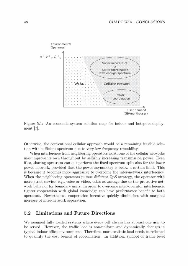
48 CHAPTER 5. CONCLUSIONSFeasible system solution

User demand (GB/month/user)

Super accurate ZF or

Static coordination with enough spectrum

Static coordination

WLAN

Environmental Openness

α-1, ϕ -1 ij, L

-1 w

Cellular network

Figure 5.1: An economic system solution map for indoor and hotspots deploy-ment [7].

Otherwise, the conventional cellular approach would be a remaining feasible solu-tion with sufficient spectrum due to very low frequency reusability.

When interference from neighboring operators exist, one of the cellular networksmay improve its own throughput by selfishly increasing transmission power. Evenif so, sharing spectrum can out-perform the fixed spectrum split also for the lowerpower network, provided that the power asymmetry is below a certain limit. Thisis because it becomes more aggressive to overcome the inter-network interference.When the neighboring operators pursue different QoS strategy, the operator withmore strict service, e.g., voice or video, takes advantage due to the protective net-work behavior for boundary users. In order to overcome inter-operator interference,tighter cooperation with global knowledge can have performance benefit to bothoperators. Nevertheless, cooperation incentive quickly diminishes with marginalincrease of inter-network separation.

5.2 Limitations and Future Directions

We assumed fully loaded systems where every cell always has at least one user tobe served. However, the traffic load is non-uniform and dynamically changes intypical indoor office environments. Therefore, more realistic load needs to reflectedto quantify the cost benefit of coordination. In addition, symbol or frame level

5.2. LIMITATIONS AND FUTURE DIRECTIONS 49

coordination may not be so feasible in near future since channel dynamics arefaster than an information gathering process. Instead, relatively slowly changinglocal information can be used for moderate coordination without fiber installationas a short-term solution, e.g., the number of users per cell, distance pathloss, shadowfading. A quantitative analysis on the performance benefit of such moderate levelof coordination is needed to see how much network cost it can save and if it isvaluable to develop practical systems. As the extensions of inter-cell interferencecoordination, following questions can be further discussed:

• How does the gain of inter-cell interference coordination change in the pres-ence of spatial-temporally varying load?

• How much equipment costs can be saved by the moderate level of coordinationaccording to increasing average user demand?

Models for the inter-operator coordination analysis was limited since we con-sidered only two cellular networks with a few number of BSs although it gave usinsights on a general trend according to network separation and the impacts ofnetwork asymmetry. Also, even if the instantaneous power control was used for thecomparison purpose, cooperation gain by using more realistic coordination tech-niques need to be envisaged. In a typical urban scenario, there will be multitudenetworks deployed not only in neighboring buildings but also on different floors inthe same building. In addition, neighboring local environments and user demandlevel are hardly symmetric so that cooperation gain can be different. The impact ofnetwork asymmetry and cooperation gain may be also magnified due to increasingdeployment density. A key question is if the increasing user demand and neighborswill give a significant impact for decision making on cooperation. This questioncan be reformulated as follows:

• How much can strategic cost be accepted by the means of different level ofcoordination techniques? How does it change with the increasing number ofcooperation partners and user demand?

• How much different is the strategic cost according to the asymmetry level inuser demand between neighbors?

In order to answer those potential questions, there are several things to be done inthe methodology perspective. Refined cost models for physical coordination costand strategic cost are necessary. We only used a simplified relative cost model forcoordination without any explicit model for strategic cost. Which cost drivers arespecifically related to interference coordination and how the cost benefit can bemeasured or expressed should be further discussed. Moreover, spatia-temporallyvarying traffic needs to be modeled for more realistic performance comparison, andmodels for the moderate level of coordination should be developed.

Bibliography

[1] D. H. Kang, K. W. Sung, and Jen, “High capacity indoor & hotspot wirelesssystem in shared spectrum - a techno-economic analysis,” submitted to IEEECommunicaitons Magazine, 2012.

[2] T. S. Rappaport, Wireless Communications: Principle and Practice, 2nd ed.Prentice-Hall, 2002.

[3] “Opportunity and impact of video on LTE networks,” White Paper, Motorola,2009.

[4] “Traffic and market report on the pulse of the networked society,” White Paper,Ericsson, Jun. 2012.

[5] D. H. Kang, K. W. Sung, and J. Zander, “Cost and feasibility analysis ofself-deployed cellular network,” in Proc. IEEE PIMRC, Toronto, Canada, Sep.2011.

[6] ——, “Is multicell interference coordination worthwhile in indoor wirelessbroadband systems?” in Proc. IEEE Globecom, Anaheim, USA, Dec. 2012.

[7] ——, “Cost benefit of interference coordination: Denser WLAN versus cellularnetwork,” submitted to IEEE Transactions on Wireless Communications, 2012.

[8] D. H. Kang, Z. Li, Q. Luo, F. Fathali, A. Vizcaino, and J. Zander, “Impact ofasymmetric transmission power on operator competition in shared spectrum,”in IEEE Swedish Communication Technologies Workshop (SWE-CTW), Lund,Sweden, Oct. 2012.

[9] D. H. Kang, K. W. Sung, and J. Zander, “Operator competition with asym-metric strategies in shared spectrum,” in Proc. IEEE WCNC, Paris, France,Apr. 2012.

[10] ——, “Cooperation and competition between wireless networks in shared spec-trums,” in Proc. IEEE PIMRC, Toronto, Canada, Sep. 2011.

[11] “Cisco visual networking index: Global mobile data traffic forecast update,2010-2015,” White Paper, Cisco, 2010.

51

52 BIBLIOGRAPHY

[12] M. Dohler, R. Heath, A. Lozano, C.B.Papadias, and R.A.Valenzuela, “Is thePHY layer dead?” IEEE Communications Magazine, vol. 49, no. 4, pp. 159–165, 2011.

[13] “Small cells-what’s the big idea?: Femtocells are expanding beyond the home,”White Paper, Small Cell Forum, Feb. 2012.

[14] J. Markendahl and M. Nilson, “Business models for deployment and operationof femtocell networks: Are new cooperation strategies needed for mobile op-erators?” in 21st European Regional ITS Conference, Copenhagen, September2010.

[15] R. S. P. Group, “Report on collective use of spectrum (CUS) and otherspectrum sharing approaches,” RSPG11-392, Nov. 2011, online availableat:http://rspg.groups.eu.int/.

[16] S. Forge, R. Horvitz, and C. Blackman, “Perspectives on the value of sharedspectrum access: Final report for the european commission,” Tech. Rep., Feb.2012, online available at: http://ec.europa.eu/.

[17] K. Karakayali, G. J. Foschini, and R. A. Valenzuela, “Network coordinationfor spectrally efficient communications in cellular systems,” IEEE WirelessCommunications Magazine, vol. 13, no. 4, pp. 56–61, Aug. 2006.

[18] B. D. Gesbert, S. G. Kiani, A. Gjendemsjø, and G. E. Øien, “Adaptation, co-ordination, and distributed resource allocation in interference-limited wirelessnetworks,” Proceedings of the IEEE, vol. 95, no. 12, pp. 2393–2409, 2007.

[19] I. Chatzicharistou and F. Berkers, “Overview of regulators and operators viewson resource sharing (initial),” EU FP7 Project Sharing Physical Resources -Mechanisms and Implementations for Wireless Networks (SAPHIRE), Deliv-erables D7.1a, Jun. 2010.

[20] “Successful network sharing,” White Paper, Ericsson, Sep. 2010.

[21] D. Gesbert, S. Hanly, H. Huang, S. S. Shitz, O. Simeone, and W. Yu, “MulticellMIMO cooperative networks: A new look at interference,” IEEE Journal onSelected Areas in Communications, vol. 28, no. 9, pp. 1380–1408, Dec. 2010.

[22] H. Claussen, L. Ho, and L. Samuel, “Financial Analysis of a Pico Cellular HomeNetwork Deployment,” in Proc. IEEE ICC, Glasgow, Scotland, Jun. 2007.

[23] J. Markendahl and O. Makitalo, “A comparative study of deployment options,capacity and cost structure for macrocellular and femtocell networks,” in Proc.IEEE International Workshop on Indoor and Outdoor Femtocells, Istanbul,Turkey, Sep. 2010.

BIBLIOGRAPHY 53

[24] K. Johansson, A. Furuskär, and C. Bergljung, “A methodology for estimat-ing cost and performance of heterogeneous wireless access networks,” in Proc.IEEE PIMRC, Athens, Greece, Sep. 2007.

[25] K. Johansson, “Cost effective deployment strategies for heterogeneous wirelessnetworks,” Ph.D. dissertation, Royal Institute of Technology (KTH), 2007.

[26] R. Etkin, A. Parekh, and D. Tse, “Spectrum sharing for unlicensed bands,”IEEE Journal on Selected Areas in Communications, vol. 25, no. 3, pp. 517–528, 2007.

[27] M. Felegyhazi and J. Hubaux, “Wireless operators in a shared spectrum,” inProc. IEEE INFOCOM, Barcelona, Spain, Apr. 2006.

[28] L. H. Grokop and D. N. C. Tse, “Spectrum sharing between wireless networks,”IEEE/ACM Transactions on Networking, vol. 18, no. 5, pp. 1401–1412, Oct.2010.

[29] K. Johansson and J. Zander, “Modeling the cost of heterogeneous wirelessaccess networks,” Int. J. Mobile Network Design and Innovation, vol. 2, no. 1,pp. 58–66, 2007.

[30] J. Zander, “On the cost structure of future wideband wireless access,” in Proc.IEEE VTC, Phoenix, USA, May 1997.

[31] M. Bengtsson and S. Kock, “Coopetition in business networks - to cooperateand compete simultaneously,” Industrial Marketing Management, vol. 29, pp.411–426, 2002.

[32] F. Berkers, G. Hendrix, I. Chatzicharistou, T. de Haas, and D. Hamera, “Toshare or not to share? business aspects of network sharing for mobile networkoperators,” in 14th International Conference on Intelligence in Next Genera-tion Networks (ICIN), Oct. 2010.

[33] A. K. Dixit and R. S. Pindyck, Investment under uncertainty. Princeton NJ:Princeton University Press, 1994.

[34] R. Bosisio and U. Spagnolini, “Interference coordination vs. interference ran-domization in multicell 3GPP LTE system,” in Proc. IEEE WCNC, Las Vegas,Apr. 2008.

[35] V. Chandrasekhar and J. G. Andrews, “Spectrum allocation in tiered cellularnetworks,” IEEE Transactions on Communications, vol. 57, no. 10, pp. 3059–3068, Oct. 2009.

[36] M. Andrews, V. Capdevielle, A. Feki, and P. Gupta, “Autonomous spectrumsharing for mixed LTE femto and macro cells deployments,” in Proc. IEEEINFOCOM, San Diego, USA, Mar. 2010.

54 BIBLIOGRAPHY

[37] K. Son, S. Lee, Y. Yi, and S. Chong, “REFIM: A practical interference man-agement in heterogeneous wireless access networks,” IEEE Journal on SelectedAreas in Communications, vol. 29, no. 6, pp. 1260–1272, Jun. 2011.

[38] J. Markendahl, “Mobile network operators and cooperation,” Ph.D. disserta-tion, Royal Institute of Technology (KTH), 2011.

[39] ITU-R M.2135, Guidelines for evaluation of radio interface technologies forIMT-Advanced., ITU-R, Dec. 2008.

[40] M. Unbehaun and M. Kamenetsky, “On the deployment of picocellular wirelessinfrastructure,” IEEE Wireless Communications Magazine, vol. 10, no. 6, pp.70–80, Dec. 2003.

[41] M. Lott and I. Forkel, “A multi-wall-and-floor model for indoor radio propa-gation,” in Proc. IEEE VTC, New Jersey, USA, Oct. 2001.

[42] M. Tolstrup, Indoor Radio Planning, A practical guide for GSM, DCS, UMTSand HSPA. John Wiley & Sons Ltd, 2008.

[43] E. Telatar, “Capacity of multi-antenna gaussian channels,” AT&T-BellLabs Internal Tech. Memo., Jun. 1995, available: http://mars.bell-labs.com/papers/proof/proof.pdf.

[44] G. J. Foschini and M. J. Gans, “On limits of wireless communication in a fadingenvironment when using multiple antennas,” Wireless Personal Communica-tions, vol. 6, no. 3, pp. 311–335, 1998.

[45] IEEE 802.11-2007, Part 11: Wireless LAN Medium Access Control (MAC)and Physical Layer (PHY) specifications, IEEE std., 2007.

[46] A. Busson and G. Chelius, “Point processes for interference modeling inCSMA/CA ad-hoc networks,” in PE-WASUN, 2009.

[47] A. Busson, G. Chelius, and J. Gorce, “Interference modeling in CSMA multi-hop wireless networks,” INRIA, Research Report 6624, Feb. 2009.

[48] H. Nguyen, F. Baccelli, and D. Kofman, “A stochastic geometry analysis ofdense IEEE 802.11 networks,” in Proc. IEEE INFOCOM, Anchorage, USA,May 2007.

[49] G. Alfano, M. Garetto, and E. Leonardi, “New insights into the stochastic ge-ometry analysis of dense CSMA networks,” in Proc. IEEE INFOCOM, Shang-hai, China, Apr. 2011.

[50] S. Boyd and L. Vandenberghe, Convex Optimization. Cambridge Univ. Press,2004.

BIBLIOGRAPHY 55

[51] K. E. Baddour and N. C. Beaulieu, “Autoregressive modeling for fading channelsimulation,” IEEE Transactions on Wireless Communications, vol. 4, no. 4, pp.1650–1662, Jul. 2005.

[52] K. G. Shin, H. Kim, A. W. Min, and A. Kumar, “Cognitive radios for dynamicspectrum access: from concept to reality,” IEEE Wireless CommunicationsMagazine, vol. 17, no. 6, pp. 64–74, 2010.

[53] D. Niyato and E. Hossain, “A game theoretic analysis of service competitionand pricing in heterogeneous wireless access networks,” IEEE Transactions onWireless Communications, vol. 7, no. 12, pp. 5150–5155, Dec. 2008.

[54] B. Jabbari, R. Pickholtz, and M. Norton, “Dynamic spectrum access and man-agement,” IEEE Wireless Communications Magazine, vol. 17, no. 4, pp. 1536–1284, Aug. 2010.

[55] E. G. Larsson and E. A. Jorswieck, “Competition Versus Cooperation on theMISO Interference Channel,” vol. 26, no. 7, pp. 1059–1069, 2008.

[56] M. Bennis, M. Debbah, S. Lasaulce, and A. Anpalagan, “A Hierarchical GameApproach to Inter-Operator Spectrum Sharing,” in Proc. IEEE Globecom, Hon-olulu, USA, Nov. 2009.

[57] O. Queseth, “Coexistence and competition in unlicensed spectrum,” Ph.D. dis-sertation, Royal Institute of Technology (KTH), 2005.

[58] M. Felegyhazi, M. Cagalj, D. Dufour, and J.-P. Hubaux, “Border games incellular networks,” in Proc. IEEE INFOCOM, Anchorage, USA, May 2007.

[59] S. Lasaulce, M. Debbah, and E. Altman, “Methodologies for analyzing equi-libria in wireless games,” IEEE Signal Processing Magazine, pp. 41–52, 2009.

[60] A. Gjendemsjø, D. Gesbert, G. E. øien, and S. G. Kiani, “Binary power controlfor sum rate maximization over multiple interfering links,” IEEE Transactionson Wireless Communications, vol. 7, no. 8, pp. 3164 –3173, Aug. 2008.

[61] 3GPP TR 36.814, 3rd Generation Partnership Project; Technical SpecificationGroup Radio Access Network; Evolved Universal Terrestrial Radio Access (E-UTRA); Further advancements for E-UTRA physical layer aspects (Release9), 3GPP, Mar. 2010.

Paper Reprints

57

Paper I: High Capacity Indoor &Hotspot Wireless System in Shared

Spectrum-A Techno-EconomicAnalysis

Du Ho Kang, Ki Won Sung, and Jens Zandersubmitted to IEEE Communications Magazine, 2012.

59

1

Abstract— Predictions for wireless and mobile Internet access show an almost

exponential increase in traffic. The only feasible long-term solution to satisfy this need in

an affordable way is to use heterogeneous networks where the cell sizes are carefully

adapted to the traffic. Since the majority of the traffic is in indoors, significant new

network investments are foreseen in this environment. While conventional wide-area

operators may not have access to indoor environments, non-traditional actors, e.g.,

hotspot operators and facility owners, will also operate networks. Such small operators

are not likely to have dedicated spectrum. Thus, sharing spectrum with neighboring

networks may be necessary. In order to reach very high capacities in these local networks,

a key issue is the management of inter-network interference. Little or no coordination

with adjacent networks possibly inflicts harmful interference to each other reducing their

performances. Tighter inter-network coordination naturally provides higher capacity.

However, this comes at the expense of increased infrastructure cost as well as business

related barriers. Proposing a framework for analyzing these tradeoffs in various

scenarios is the purpose of this paper. We modify the traditional single operator cost

model by introducing new inter-operator cost factors. Then, we provide an example to

demonstrate how the proposed framework can help us comparing different individual

operator strategies. Finally, we suggest areas for future research.

Index Terms—Operator strategy, Techno-Economic analysis framework, Shared

spectrum, Indoor and hotspot deployment

High Capacity Indoor & Hotspot Wireless System in Shared Spectrum

- A Techno-Economic Analysis Du Ho Kang, Ki Won Sung, and Jens Zander

KTH Royal Institute of Technology, Wireless@KTH Stockholm, Sweden

60

2

I. INTRODUCTION

A. Emergence of Small Operators in Shared Spectrum

Over the last few years, mobile broadband access has gained tremendous success.

Mobile handset innovations, e.g., smartphones and tablet PCs, have caused a virtual

“data tsunami” that is already creating severe capacity problems for many operators.

New types of bandwidth-hungry applications, e.g., cloud computing or web storage,

accelerate the needs for higher capacity and even faster mobile broadband access. The

only feasible long-term solution to satisfy this need is to densify the wireless networks.

The way to this without running into rapidly growing costs is to use heterogeneous

networks where the cell sizes are carefully adapted to the traffic.

Since the majority of the traffic is generated in indoors, significant new indoor

network investments are foreseen. Some networks are now being deployed by

traditional (wide-area) mobile network operators (MNOs) as complements to mitigate

the burden of the existing outdoor systems. However, it is not obvious that MNOs can

gain access to the various indoor sites. It is also expected that most of the new indoor

network investments are made by the other market actors. For instance, hotspot

operators will focus on new niche market segments. There is also an increasing interest

in dedicated indoor networks by non-telecom players, e.g., facility managers, real estate

owners, and private companies [1]. The main driver is to own dedicated networks

inside their own buildings to attract more tenants or their own customers, e.g., hotels or

office suppliers. This is a business model very close to the one seen in current fixed

network access – a public operator provides connections to the facility, whereas

networks inside are deployed and managed by the facility owner.

With this shift in network ownership, a number of distinct local area networks are

appearing at the close distance of each other as illustrated in Fig. 1. A problem for such

small-sized operators1 is that they do not have access to licensed spectrum. One of the

proposed options is locally sharing spectrum with other operators, e.g., using

unlicensed bands or secondary sharing of licensed spectrum [2].

B. Techno-Economic Challenges for the Small Operators

One of the central issues for achieving very high capacity (beyond what is possible by

Wi-Fi deployment [3]) is interference management between adjacent operators. With

1 For the remainder of the paper, an operator refers to any business entity that owns and operates its

own network. In this context, the facility owners can be considered as operators.

61

3

loose inter-network regulation, the side-by-side network deployments will create local

competition inflicting mutual interference to each other, which may in turn lead to poor

performance. Instead, operators could cooperate to manage the inter-network

interference using latest advances in technology, e.g., interference cancellation, joint

multicell processing, or coordinated scheduling. Such tight inter-network coordination

can be also enforced by regulators with a new spectrum policy, e.g., real-time spectrum

auction [4].

Improvement in technical performance is obviously expected from the inter-network

coordination. However, additional cost and various business constraints are the hidden

barriers mostly overlooked. The coordination may increase infrastructure cost in order

to provide extra network resources for the reliable exchange of coordination

information. Tighter coordination requires better infrastructure, which corresponds to

higher cost. Thus, there exists a tradeoff between performance and cost regarding the

inter-network coordination. Furthermore, the technical coordination inevitably requires

strategic cooperation agreement in a business domain. An operator may perceive

limitations after alliance with its neighbor because it could lose the freedom of network

operation/upgrade and eventually competitive advantages [5], [6]. Including such

non-technical barriers may not be straightforward in the operator decision-making.

Fig. 1. Increasing number of local access networks deployed by various small operators in shared spectrum

62

4

Associating a “strategic cost” to these limitations will be our way of including the

business barriers to the performance-cost tradeoff analysis.

As summarized in Table 1, the system design in shared spectrum is inherently a

multi-dimensional problem where technology, business, and regulatory issues are

intertwined unlike a conventional operator case isolated from business and regulatory

issues. The problem of how to design a system and choose an operator strategy brings

up several research challenges that have rarely been addressed in the literature. First,

analysis of operator-wise competition or cooperation is not trivial due to the involved

business complexity although the competition between individual users inside a

network has been extensively studied [7]. Second, in spite of the importance of

investigating the different levels of coordination, it has been mainly regarded as a part

of a model assumption rather than the object to be compared due to the lack of the

Table 1. Changing business landscape and system design paradigm shift in shared spectrum

Traditional wide-area single operator system

Local-area system in shared spectrum

Business landscape

Who &

Why?

• MNOs: revenue generation from service provisioning

• MNOs: data offloading • Facility owners: complements to

facility services • Hotspot operators: new revenue

generation in niche markets

Where? Large-scale public outdoors Mainly private/public indoors controlled by facility owners

Inter- operator relation

Service/price competition in markets

• Service/price competition in markets

• Cooperation/competition for inter-network interference coordination

Major network related cost

• Network cost • Spectrum cost

• Network cost • Inter-operator cost (see Sec. III-B)

System design

Design problem

Minimizing network cost at a given traffic demand

Minimizing network cost+inter-operator cost


Decision domain Mainly technology Both technology and business

Main decision maker MNO Both an operator and a regulator

Coordination target Nodes (e.g., BSs) Networks

63

5

explicit and systematic evaluation methodologies. Third, a proper cost model should be

in place for the tradeoff analysis. There are some attempts to estimate the network cost

in the conventional single operator heterogeneous network [8]. However, the cost of the

inter-network coordination towards a commercially successful indoor deployment has

not been explicitly covered yet.

C. Contribution of This Article

Despite the increasing number of interfering local networks, we thus far lack a

systematic framework for quantitatively analyzing which operator strategy on the

system design is better than others under a certain set of circumstance. To effectively

navigate and compare potential strategies, we provide a new techno-economic analysis

framework including an extended cost model. Then, the validity of our framework is

schematically shown with a tangible example. Finally, we outline important research

areas to be addressed for future studies.

II. OPERATOR DEPLOYMENT STRATEGIES – A CONCEPTUAL FRAMEWORK

A fundamental network design problem that the operators are facing is minimizing

total network cost to satisfy expected user demand in a particular physical environment.

In order to achieve this, the cost of different deployment options should be compared

under a certain performance (e.g., capacity) requirement. This comparison becomes

more complicated in the shared spectrum environment because both the cost and

performance are closely related to the neighboring operators.

Since the cooperation is intrinsically involved with strategic decisions in the business

domain, a new strategy combining the technology and business aspects is needed for

the small operators. In this section, we provide a conceptual framework to effectively

categorize potential strategies. As shown in Fig. 2, the various operator strategies are

characterized on one side by the strategic decision of the operators, i.e., cooperation and

competition, and on the other side by the technical solution expressed as the level of

coordination.

A. Strategic Decision: Cooperation or Competition

The strategic decision in the business domain influences the way for an individual

network to be coordinated. In this regard, we differentiate between cooperation and

competition based on the technical objective function which each of the involved

64

6

operator aims to maximize. We define two types of strategies:

• Cooperation: the operators aim at maximizing a common objective function

agreed between partners.

• Competition: the operator aims at maximizing its own objective function in a

selfish manner.

Cooperating operators synchronize their overall technical behaviors for network

alliance by re-configuring their networks. This could involve additional investment.

Agreement on a common objective function is in itself challenging, particularly when

the cooperation partners have chosen different criteria for the quality of service (QoS),

e.g., rate guaranteed video service versus best-effort service. From a radio resource

allocation perspective, cooperative networks behave as a conventional single operator

network because the coordination issues are the same as in the traditional network. On

the other hand, competition requires a non-traditional system design. Regulators must

provide the guidelines for inter-network coordination by issuing various co-existence

rules (“etiquettes”) which coordinate the network rivalry to some extent. Game theory

Fig. 2. A conceptual framework to navigate the operator strategies.

65

7

has been widely adopted for the analysis of competition in wireless systems. For the

case of network-wide competition, inter-network interference management is coupled

with intra-network interference control, which creates new challenges.

B. Technical Solutions - Coordination between Networks

The technical solutions of the operators to implement their strategic decisions

directly affect the performance. We define coordination in a technical domain as the

process of sharing relevant information. The level of coordination is measured by the

amount of information shared in the process. The information relevant to the

interference coordination can be the statistical or instantaneous traffic load or path

gains between all the involved access points and user terminals, usually referred to as

channel state information (CSI).

More accurate and frequent information exchange increases the global knowledge in

the whole system. A system with complete information sharing can be interpreted as a

centralized network (whether decisions are computed centrally or not). Such system is

desirable from a performance perspective since it can provide real-time resource

allocation based on the fast sharing of local information, e.g., beamforming or

coordinated scheduling [9]. On the other hand, only slowly-varying information, e.g.,

average propagation conditions and the number of users per cell, may be shared. This

requires considerably less sophisticated equipment, and the information may be

exchanged using existing IP connections.

III. COST MODELS

Recall that the network design objective is finding the operator strategy to offer the

lowest total cost for the required capacity. As briefly discussed in the introduction, the

network cost in the shared spectrum environment has an additional element with regard

to technical inter-operator relations. In addition, there is also “strategic cost”

representing the business uncertainty caused by the decision to cooperate. In this

section, we first recap the traditional single operator cost model and highlight new

inter-operator costs to be included for the strategy comparison.

A. Traditional Single Operator Cost Model

For a legacy operator in wide area, the cost of the wireless network mainly consists of

two parts, i.e., infrastructure and spectrum, as described in [10]:

66

8

,tot infra spectrum BS r wC = C +C = N C +WC (1)

where NBS, Cr, W, and Cw are the number of total deployed BSs, the annualized cost per

BS [€/BS], the allocated spectrum [MHz], and the annualized cost per spectrum

[€/MHz], respectively. Here, Cr includes all capital expenditure (CAPEX) and

operational expenditure (OPEX) aspects. CAPEX is mostly related to deployment, e.g.,

BSs or core network equipment, site installation/build-out, and antenna systems. Cost

during operation, e.g., backhaul transmission, site rental, operation and maintenance

(O&M), and electricity, is categorized as OPEX.

Indoor and hotspot systems may have simpler cost structure than the conventional

macro networks. However, we can still employ the linear model as a function of the

number of BSs as in Eq. (1). As identified in [8], most of costs comprise two parts, i.e.,

the BS cost and the backhaul cost. This is because the smaller physical size of

equipment does not need dedicated deployment space with relatively relaxed site

constraints in inbuilding environment. By sharing spectrum, spectrum cost also

becomes negligible or even free depending on the country-wise spectrum policy.

B. Inter-operator Cost in Shared Spectrum

1) Coordination Cost

From the technical point of view, information sharing between networks requires

additional complexity and infrastructure cost. The coordination cost Ccoord is spent for

acquiring relevant information for resource allocation. Depending on the amount of

information to be shared, Ccoord can be neglectable or significant. As exemplified in Fig.

3, the extra cost mainly emanates from installing dedicated backhaul or intermediate

entity to coordinate the interference between networks. For instance, real-time

interference coordination may necessitate expensive dedicated backhaul in both inside

and between buildings to allow for reliable low-latency information sharing. In addition,

an inter-network coordinator should be put in place for fast and synchronized resource

allocation. While in-building dedicated backhaul may be paid by individual operator,

the common cost, i.e., inter-building backhaul or the intermediate equipment, can be

shared. In a moderate coordination scenario, each network may use its existing

in-building IP connection to control its own BSs. Even in this case, intermediate

coordination equipment may be introduced by the third party due to a regulatory

67

9

Fig. 3. Examples of Ccoord according to the cooperation level.

constraint, e.g., spectrum-broker, or due to the trust reason in a business domain.

Without any additional equipment or backhaul cost, neighboring operators can still

directly exchange information to share spectrum cooperatively based on mutual trust as

long as the performance improvement is assured than competition. In this case,

resource allocation can be done in a distributed manner. Depending on the coordination

level, required NBS per operator will be different for a given traffic demand. Thus,

finding the proper level of coordination to give the lowest total per-operator cost is an

important issue.

2) (Invisible) Strategic Cost

Operators have traditionally been reluctant to share networks or to tightly cooperate

across business boundaries mainly due to the limitations and uncertainty they perceive

regarding their marketing strategies. Cooperation takes place only if large economic

gains are foreseen, e.g., mobile broadband in rural areas where a too small customer

base cannot support two or more parallel access networks. In management literature,

68

10

such barriers against strategic alliances with competitors have been widely studied, e.g.,

see [11]. A recent European project SAPHIRE also addressed a similar issue in the

context of outdoor network sharing [6]. Some key network-related obstacles are:

• Management overhead: decision-making on network deployment/upgrade can

be delayed because it requires an agreement with the cooperation partner.

• Limited network controllability: an operator may lose control over the

deployment and operation of its own network, which can restrict individual

network dimensioning and make its service not differentiable from the

competitors in markets.

• Risk of information leakage: the coordination may unveil customer statistics

and know-how on network optimization to the other operator.

• Lack of trust: an operator may suspect that the cooperation partner delivers

false information to take advantage of the coordination.

One way to model this uncertainty or risk is to introduce an additional fictitious cost,

denoted by the strategic cost Cstex. Notice that Cstex may not be strictly measurable

because it is related not only to objectively computable risk but also to the perceived

uncertainty to the future. This is not a new concept in strategic decision making in

business domain where one often considers an uncertainty margin, e.g. using a

fictitious “required rate of return” or “hurdle rate” when comparing investment

options [12]. Consequently, traditional single operator cost model should be extended

with the new inter-operator cost factors as:

i i i i itot infra spectrum coord stexC = C +C +C +C . (2)

Note that the superscript i represents the cost for the ith operator sharing the spectrum.

In the following section, we demonstrate how to use our proposed techno-economic

modeling approach in a typical scenario.

IV. COMPARISON OF OPERATOR STRATEGIES

A. Urban Enterprise Scenario

Let us consider a scenario with two nearby office buildings as illustrated in Fig 2. We

69

11

assume that one building has a dedicated high-speed wireless access network which is

provided and maintained by a hotspot operator B. Another small operator, namely

operator A, comes into the next building to deploy and run an enterprise network. We

further assume that the regulator has arranged a spectrum band to which this type of

small operators can have cost-free access. Both operators use this frequency band in

order to avoid spending huge amount of money for dedicated spectrum. Therefore,

inter-operator interference is a major concern to the new coming operator as well as the

existing operator B.

B. Candidate Operator Strategies

The operator A needs to determine its deployment and operation strategy in the

shared spectrum. With the aid of the conceptual framework, we can systematically

create several candidate strategies as follows:

• Strategy I (S-I): since the operator A is concerned about the inter-dependency

and the risk of revealing the network operation information, it decides to

operate its own network by selfishly configuring radio parameters only for

internal network coordination without the consideration on the harmfulness to

operator B.

• Strategy II (S-II): operator A wants to cooperate with the moderate level of

coordination. Since the main type of service in both offices is elastic data, two

operators first agree to maximize average aggregate data rates of all of users

in both buildings. However, it wants to lower the coordination level due to the

concern of upgrade cost for installing optical fibers. In this case, the two

operators share only statistical traffic load information via Internet

connection to yield the part of spectrum to a highly loaded network.

• Strategy III (S-III): in order to obtain the highest achievable performance,

operator A makes an agreement with operator B for tight cooperation. In this

strategy, the operators jointly decide to employ dynamic interference

management by instantaneously sharing all CSIs, e.g., coordinated

beamforming. For this, they need to install dedicated high speed backhaul and

to share the cost to build a centralized coordination entity.

C. Cost Comparison of Strategies

Fig. 4 schematically illustrates CAtot of Strategy I to III depending on inter-network

70

12

Inter-network separation Open areas Small office

buildings Offices inside a

building

S-I

S-II

S-III

S-II at high Cstex

S-III at high Cstex

AtotC

Fig. 4. Schematic illustration of the cost comparison of operator strategies; the best strategy minimizing the total network cost differs depending on the environment.

separation, i.e., inter-building propagation loss caused by obstacles or inter-building

distance.

When the separation is small, it is expected that more BSs are needed under Strategy

I to compensate increased inter-network interference. Thus, CAinfra will dominate the

total cost. The tight cooperation will exhibit a significant capacity gain in the open area

where no inter-network obstacles exist and line of sight condition is possibly imposed,

e.g., public outdoor hotspots. It will result in much fewer numbers of BSs for fulfilling

the same capacity requirement. Then, the cost saving in CAinfra can be sufficiently high

to compensate extra CAcoord to make total cost of Strategy III lower than Strategy I. In

the intermediate level of separation, e.g., offices are separated in floor levels or directly

attached buildings, the moderate level of cooperation can save CAinfra without any extra

CAcoord by reusing existing fixed IP connections. Contrary to the former cases, the

inter-operation coordination does not bring about a performance improvement when

there exists enough separation between the operators. Naturally, no cooperation

(Strategy I) will be desirable in this situation.

The strategic cost Cstex can make a heavy influence on the above discussion. If

operator A is very reluctant to cooperate with operator B, Cstex may be significantly

high enough to outweigh any cooperation strategy as depicted by the dotted lines in Fig.

71

13

4. Interested readers can refer our recent work to find relevant quantitative results

[13]-[14].

V. RESEARCH CHALLENGES

Although substantial work has to be done in realizing affordable high capacity

system, research on the design of a small operator network in shared spectrum is still in

its early stage. In the following, we suggest some high-level research challenges to be

addressed in the future.

1) System Performance at Different Levels of Cooperation

The quantitative comparison of the system performance for the different forms of

coordination has still to be explicitly discussed. In [13]-[14], we have scratched the

surface regarding this issue. A main analysis task is categorizing relevant information

to be shared and quantifying network performance in various local environments and

user demand. The performance improvement by the coordination can be converted into

cost saving in terms of the reduced number of BSs. Then, operators can examine if it

compensates the associated coordination cost. Different coordination schemes may also

involve different business risk and uncertainty affecting the cost-performance tradeoff

analysis.

2) Impact of Network Separation

Unlike wide-area networks which seamlessly cover a large area, indoor and hotspot

networks are usually separated with a certain distance as depicted in Fig. 2. Therefore,

mutual interference between the networks may be overshadowed by self-interference

generated inside a network depending on the separation between the networks. This

means that the benefit of inter-network coordination relies on the network separation,

which requires thorough investigation.

3) Asymmetric Demand and Deployment Environment

It is hardly likely that each network has the same user demand, QoS requirements, or

inbuilding propagation conditions as neighboring networks. Such potential

asymmetries in demand and physical environments may lead to unequal incentives or

even negative coordination gain to one side of participants. Moreover, finding a proper

common objective function for the cooperation is a challenging task especially when

72

14

the partners aim at the different QoS requirements.

4) Multitude of Interfering Networks/Cooperation Partners

It is quite common that a single multi-story building accommodates several networks

and a building is surrounded by a few neighboring buildings. Thus, the number of

networks generating interference can be substantial. As the number of potential

cooperation partners increases, the performance gain could be even higher since more

interference could be technically controlled. However, it would come at the expense of

inflating business complexity. Therefore, the relation between cooperation incentive

and the number of involved partners needs to be further explored.

VI. CONCLUSION

We proposed an analysis framework to explore the tradeoff between performance

benefits of operator cooperation in shared spectrum and involved technical and

strategic costs. In the framework, the implication of operator strategic decisions to

cooperate or compete and the related costs of inter-network coordination level are

explicitly modeled. With the aid of our framework, the provided research challenges

should be further investigated to identify the operator strategy in various business

situations and physical environments that gives the lowest cost satisfying performance

requirements.

Our conceptual framework was motivated by and developed for a scenario of small

operators in shared spectrum. Nonetheless, the proposed analysis method can be

applied to more general resource sharing scenarios in wireless networks, e.g.,

infrastructure sharing among a multitude of wide-area and small operators. Overall,

understanding the driving forces and hurdles of multi-operator resource sharing is one

of the major challenges for the design of affordable wireless systems in the coming

years.

REFERENCES

[1] J. Markendahl, M. Nilson, “Business Models for Deployment and Operation of Femtocell Networks;

Are New Cooperation Strategies Needed for Mobile Operators?,” 21st European Regional ITS

Conference, Copenhagen, 13-15 Sep. 2010.

[2] J. M. Peha, “Approaches to spectrum sharing,” IEEE Communications Magazine, vol. 43, no. 2, pp.

10 –12, Feb. 2005.

73

15

[3] H. Nguyen, F. Baccelli, and D. Kofman, “A stochastic geometry analysis of dense IEEE 802.11

networks,” in Proc. IEEE INFOCOM Anchorage, USA, May 2007.

[4] B. Jabbari, R. Pickholtz, and M. Norton, “Dynamic Spectrum Access and Management,” IEEE

Wireless Communications Magazine, vol. 17, no. 4, pp. 6 –15, Aug. 2010.

[5] “Successful network sharing,” White Paper, Ericsson, Sep. 2010.

[6] I. Chatzicharistou and F. Berkers, “Overview of Regulators and Operators Views on Resource

Sharing (initial),” EU FP7 Project Sharing Physical Resources - Mechanisms and Implementations

for Wireless Networks (SAPHIRE), Deliverables D7.1a, Jun. 2010.

[7] J. Zander, “Competitive Wireless Multi-access - Implications and Research Issues,” in Proc. IEEE

PIMRC, Helsinki, Finland, Sep. 2006.

[8] K. Johansson and J. Zander, “Modeling the cost of heterogeneous wireless access networks,” Int. J.

Mobile Network Design and Innovation, vol. 2, no. 1, pp. 58-66, 2007

[9] D. Gesbert, S. G. Kiani, A. Gjendemsjø, and G. Egil Øien, “Adaptation, Coordination, and

Distributed Resource Allocation in Interference-Limited Wireless Networks,” in Proc. IEEE ICC,

Glasgow, Scotland, Jun. 2007.

[10] J. Zander, “On the Cost Structure of Future Wideband Wireless Access,” in Proc. IEEE VTC,

Phoenix, USA, May 1997.

[11] M. Bengtsson and S. Kock, “Coopetition in Business Networks – to Cooperate and Compete

Simultaneously,” Industrial Marketing Management, vol. 29, pp 411–426, 2002

[12] A. K. Dixit and R. S. Pindyck, “Investment under uncertainty,” Princeton NJ: Princeton University

Press, 1994.

[13] D. H. Kang, K. W. Sung, and J. Zander, “Cooperation and Competition between Wireless Networks

in Shared Spectrum,” in Proc. IEEE PIMRC, Toronto, Canada, Sep. 2011.

[14] D. H. Kang, K. W. Sung, and J. Zander, “Is Multicell Interference Coordination Worthwhile in

Indoor Wireless Broadband Systems?,” to appear in Proc. IEEE Globecom, LA, USA, Dec. 2012.

74

Paper II: Cost and FeasibilityAnalysis of Self-deployed Cellular

Networks

Du Ho Kang, Ki Won Sung, and Jens Zanderin Proc. IEEE Personal, Indoor and Mobile Radio Communications (PIMRC),Toronto, Canada, Sep. 2011.

©2011 IEEE. Personal use of this material is permitted. Permission from IEEEmust be obtained for all other uses, in any current or future media, includingreprinting/republishing this material for advertising or promotional purposes, cre-ating new collective works, for resale or redistribution to servers or lists, or reuseof any copyrighted component of this work in other works.

75

Cost and Feasibility Analysis of Self-deployedCellular Network

Du Ho Kang, Ki Won Sung, and Jens ZanderWireless@KTH, Royal Institute of Technology (KTH)

Electrum 229, 164 40 Kista, SwedenEmail: dhkang, sungkw, [email protected]

Abstract—A self-deployed network is considered to be oneof cost-efficient deployment solutions by skipping an expensivenetwork planning process. However, it may result in the seriousdegradation of capacity or the infeasibility of coverage constraintdue to the rise of interference although radio adaptation tech-niques are employed. Therefore, deployment decision makers,e.g., operators, need to identify when and where the self-deployednetwork is feasible and economical compared with the plannednetwork. For this, we estimate the average network throughputof the self-deployed network subject to a coverage constraint andcompare it with the planned network. Three distinct regions ofself-deployment are identified where different deployment strate-gies are required: infeasible, cost-effective, and uneconomical.We evaluate how the regions alter according to different channelenvironments and make suggestions for economical deployment.

I. INTRODUCTION

As a gap between capacity in wireless cellular networksand the revenue of operators increases due to soaring trafficdemand with flat pricing schemes, cost-saving deploymentstrategies become more and more essential. While equipmentcost turns cheaper due to equipment vendor’s competitionand technology evolution, site-related cost relatively remainsdominant in total deployment cost [1]. One of major cost-driving factors in the site-related cost is planning the locationsof base stations (BSs) which requires expensive engineeringefforts. For reducing the planning cost, the concept of a self-deployed network is recently of great interest and has activelybeen studied [2], [3].

Unlike conventionally planned networks, BSs in the self-deployed networks are not carefully deployed by engineersor sometimes randomly placed by unskillful end-users. Con-sequently, self-deployed BSs may be inefficiently deployedsuch that they cannot offer the minimum required rate to someusers owing to coverage gap or excessive interference from celloverlap. This requires installing more BSs to fill the coveragegap in some areas. It also needs to turn off some BSs toreduce the excess interference in other areas. In a nutshell,the saving of the planning cost leads to extra equipment costin the self-deployment. In some cases, the unplanned BSlocations may not fulfill the capacity or coverage requirementeven with intercell interference mitigation/avoidance schemes.Thus, deployment decision makers, e.g., operators, shouldinvestigate whether the self-deployed networks can providethe minimum required rate in the service area, i.e., coverage.

Then, they need to explore if the self-deployed network ismore economical than the planned network in terms of thetotal deployment cost.

Most of existing studies on the self-deployed networksfocused on technical aspects such as capacity or coverage anal-ysis, optimal interference mitigation and avoidance schemes,and network architecture designs [2], [3]. In contrast, relativelyfew studies have been done in the economic perspective [4],[5]. In [4], a cost comparison between self-deployed networksand conventional networks is presented in a particular usagescenario by assuming constant capacity and coverage per BS.The author of [5] intensively analyzed the total deploymentcost when the self-deployed network is mixed with differenttypes of networks. However, as acknowledged in [6], botheconomic and technical aspects need to be considered to-gether for the design of cellular networks. For the plannednetworks, a cost optimization problem was addressed thatjointly considered various technical aspects such as transmitpower and antenna heights [7], [8]. However, the techno-economically integrated analysis has not been in place for theself-deployed network which requires a different cost structureand deployment model.

In this paper, we assess the cost of a self-deployed net-work with a throughput requirement subject to a coverageconstraint. Particularly, we consider inter-cell interference mit-igation/avoidance techniques in the analysis by employingtransmit power control and frequency selection. This willbridge the gap between technological and economic studieson the self-deployment. We address the following question:

• Can the self-deployment satisfy the coverage constraint?If this is the case, the second question is posed:

• Is the cost of self-deployment cheaper than the planned-deployment for a given throughput requirement?

In order to answer these, we first examine the average networkthroughput subject to the coverage constraint as a function ofthe number of deployed BSs. If the coverage is satisfied, weassess the total deployment cost of the self-deployed networkand compare it with that of the planned network.

The main contributions of this paper are summarized asfollows. Firstly, we identify under which performance require-ments or environments the self-deployment stay economicalthan planned-deployment. Secondly, we investigate the sensi-tivity of the coverage constraint on the technical feasibility.

76

Thirdly, we explore how deployment decisions should beadjusted according to various shadowing and multichannelenvironments. The remainder of this paper is organized asfollows: we describe a system model and a performance metricin Section II and III, respectively. Section IV presents asimulation model, and numerical results are given in Section V.Then, Section VI concludes this paper.

II. SYSTEM MODEL

We consider a finite service area set Ω ⊆ R2. When N BSlocations are given by a set l ⊆ Ω, Ω is divided into severalcells Ωi occupied by BS i ∈ B which is defined as

Ωi := x|pr,i(x) ≥ pr,j(x), x ∈ Ω, ∀j = i, (1)

where pr,i(x) is the received power at x ∈ Ω from BS i. Notethat pr,i(x) is calculated by gi(x)pi where gi(x) and pi are achannel gain from BS i to location x and transmit power ofBS i. When a user locates in x ∈ Ωi, signal to interferenceand noise ratio (SINR) can be obtained as,

γi(x) =pr,i(x)∑

j∈B\i θ(fi, fj)pr,j(x) + no, (2)

where no and θ(fi, fj) are noise power and an orthogonalityfunction of operating frequencies fi and fj of BS i and j,respectively. θ(fi, fj) gives 1 when BS i and j operate in thesame frequency channel and otherwise, 0. We also calculate arate ri(x) from Shannon formula as

ri(x) = min(log2(1 + γi(x)), rmax) (bps/Hz), (3)

where parameter rmax reflects the maximum sustainable ratein practice. When assuming that users are uniformly dis-tributed in Ω, we define conditional expected network through-put λc for a given BS location set l as

λc :=∑

i∈BWiE[ri|l] (Mbps), (4)

where Wi represents bandwidth (MHz) allocated in BS i.Let γ and γt be SINR of a user and its threshold for theminimum required rate. Then, users can experience outagewhen γ ≤ γt due to high co-channel interference or weaksignal strength. Thus, the coverage for a given l can bedescribed by conditional outage probability defined as

νc := Pr[γ ≤ γt|l]. (5)

A. BS Deployment Strategy

According to how carefully BSs are placed, we differentiatetwo deployment strategies as follows.

1) Self-deployment: We assume that the self-deployed net-work is built by end-users with self-configurable BSs [3]. Inorder to make the end-users capable of deploying BSs, weassume that BSs are plug-and-play based small equipmentswhich do not need dedicated installation space [3]. Since theend-users do not have any professional radio network planningknowledge and tools, they deploy several BSs without effortin a place where a wired backbone infrastructure is accessible.Typically, they sketch a network topology to ensure that BSs

are quasi-uniformly distributed by visually inspecting pre-placed BSs or following some basic guidelines given in atechnical manual. Thus, the case that BSs are co-located in thesame position is unlikely to happen and is a too pessimisticscenario. Accordingly, we model that BSs are randomly placedwith uniform distribution but with the minimum BS separationdistance in a sequential manner.

2) Planned-deployment: In this case, all BSs are deployedat once in the optimal positions acquired by a locationoptimizing process based on costly channel measurements.Since channel measurements in Ω is not practical at all, weinstead adopted a grid-installation approach for optimizing BSlocations [9]. In this model, M and K equally-spaced pointsare pre-selected out of Ω for the candidate locations of N BSsand for measurement points, respectively (i.e., N < M < K).We formulate this into a general combinatorial problem se-lecting N BS locations out of M candidate locations. Theobjective of location planning aims at maximizing averagesignal qualities in the entire measuring points in a set K,i.e.,

∑i∈K log2(1 + SNRi). Note that SNRi represents signal

to noise ratio at measurement point i from BS offering thestrongest signal quality when fixed transmit power is used.

B. Interference Mitigation and Avoidance

Most of cellular networks use advanced radio resourcemanagement schemes, e.g., link adaptation or dynamic chan-nel allocation, to ensure the achievable performance for agiven network topology. Therefore, it is necessary to considerinterference mitigation/avoidance schemes regardless of thedeployment strategies. In particular, we assume that a jointtransmit power control and frequency channel selection isemployed in the considered network. Once the BS locationset l is determined by either planned-deployment or self-deployment, the transmit power vector p and the frequencyvector f of BSs need to be adjusted for managing inter-cellinterference. In practice, after BSs are configured to connectthe central server via a infrastructure backbone, the centralserver gathers local measurement information from each BSin order to assign the best power-frequency profile to eachBS. Since instantaneously updating p and f is impractical dueto a time-varying channel and limited processing capability,we consider a long-term adaptation in order to compensatethe irregular pattern of BS topology. Let us consider a cellularnetwork which targets to maximize λc subject to νc < δ. Notethat δ denotes the constant outage threshold. Then, for a givenl, we formulate this problem as follows:

maximize λc(p,f)subject to 0 ≤ pi ≤ pmax, fi ∈ F , ∀ i

νc ≤ δ

Note that F = 1, ..., nf represents a frequency set with nf

available frequency channels while pi and pmax are referredto as the transmit power of BS i and the maximum transmitpower, respectively.

77

III. PERFORMANCE METRIC

Since our objective is investigating technical feasibility anddeployment cost, we consider not only a technical metric butalso an economic metric.

A. Technical Measure

As we can have different realizations of BS location set l fora given N deployed BSs, we measure the outage probabilitywhich is defined as ν=Pr[γ < γt]. The coverage of N BSsis considered as feasible regardless of deployment costs ifthe network can provide ν ≤ δ. Otherwise, we call N BSsinfeasible. Likewise, in order to estimate the total deploymentcost for given network throughput, we also measure thenetwork throughput in an average sense for a given N BSs. Forthis, we simply obtain average network throughput λ = E[λc]by averaging over different BS location realizations of l.

B. Economic Measure

Once we have λ for a given N deployed BSs, we canacquire the total deployment cost Ctot under the followingcost structure. The total deployment cost of a general cellularnetwork consists of radio equipment cost and site-related costwhich are the linear function of N [10]. We presume thatthe radio equipment cost per BS is same regardless of thedeployment strategies since same BS equipments and networkarchitectures are used in both cases. Since we assume booksized BS equipments with plug-and-play functionalities, wecan also save site-related cost requiring civil works. Forinstance, cost for antenna titling, site acquisition, and initialparameter configurations can be ignored. Nevertheless, theplanned network apparently needs more effort for installationfrom the channel measurement and the location optimizationprocess. Also, access to a backbone infrastructure may not bereadily available at the installation place so that it requiresadditional wiring with extra costs. Accordingly, we assumethat the site-related cost is essentially dominated by theplanning cost which includes the location optimization andwiring cost. From this, we simplify the total deployment costas

Ctot := N(Cr + Cp), (6)

where Cr and Cp are the radio equipment cost per BS and theplanning cost per BS, respectively. Note that the self-deployednetwork has Cp=0 since we assume that it does not demandany efforts for planning.

IV. SIMULATION MODEL

A. Numerical Optimization Method

For given N BSs, by applying Monte-Carlo method, weestimate λ and ν by simply averaging λc and νc from 100different BS location realizations. In each simulation run,we generate (optimize) BS location l for the case of theself-deployment (planned-deployment). In the case of theplanned-deployment, we apply a well-known heuristic sim-ulated annealing [11] to find the sub-optimal BS locations.This can yield near-optimum performance which serves as an

120m

50m

15x15m

Fig. 1. Indoor office layout for a closed environment.

approximate upper bound on the performance as a referencefor comparison.

Then, we optimize p and f in both deployment strategies.For mathematical approximation, we first discretize irregularcontinuous area Ω into K measurement points as used inthe grid-installation. Then, we numerically evaluate the rateand SINR over the K points. Also, we quantize pi into np

discrete levels. Then, we reformulate the joint transmit powerand frequency control problem into a discrete optimizationproblem which selects the best power-frequency profile outof npnf possible combinations. Since the considered problemstill has νc ≤ δ constraint, we need a procedure for checkingthe feasibility of the problem. Therefore, we divide thisproblem into two subproblems with different objectives: 1)minimizing νc until it finds a feasible power-frequency profileand 2) maximizing λc subject to νc ≤ δ. Once the firstsubproblem finds a feasible profile, the second subproblem istriggered from the identified feasible power-frequency profile.Otherwise, the first subproblem terminates by simply returningthe minimum estimated νc.

For each subproblem, we apply an iterative constrainedrandom search algorithm [12]. The brief description of thealgorithm is provided as follows:

Initializing: all BSs randomly select an initial power-frequency profile.Repeat:

1) Randomly choose one of BSs, say i.2) For the selected BS i:

a) Randomly choose a power-frequency profile thatimproves the objective and satisfy a constraint if it exists.b) If it does not have any better solution, it simplypersists the previous profile.

Until: if the objective function converges1 or the number ofiteration exceeds a threshold, it stops the iteration.

B. Simulation Environment

We consider an indoor office environment recommendedin [13], and its layout is shown in Fig. 1. It consists of sixteen15 m by 15 m cubics which are arranged along the side of the6000 m2 rectangular shape of service area. A channel gainbetween a receiver and a BS is only distance-dependent andis given by PLw = 37 + 30 log10(d) + kLw [14]. Note that

1The algorithm is known to converge within a finite number of iteration [12]

78

d, k, and Lw represent a distance from a BS, the number ofpenetrated internal wall, and the wall loss, respectively. pi isselected from as a set −∞ ∪ −20 : 2 : 20 dBm, and γt

is fixed to 3 dB. M BS candidate points are equally spacedby 10 m while K measurement points are evenly arranged by5 m. Also, the minimum separation between adjacent BSs inthe self-deployment is set to 5 m. Total system bandwidth Wis given with 10 Mhz and Wi assigned to each BS is obtainedby W

nf.

V. NUMERICAL RESULTS

A. Differentiable Deployment Regions

Fig. 2 shows how λ changes as the number of deployedBSs increases when nf = 1. The result shows that the self-deployed network is more sensitive to δ. In the case of δ =0.10, the self-deployed network is infeasible in most of theevaluated density whereas the planned network mostly remainsfeasible. When δ is relaxed to 0.20, the feasible region of theself-deployed network appears, but low BS density still doesnot fulfill the δ constraint. λ of the self-deployed networkalso increases as the network density increases with the aid ofinterference mitigation technique. However, it provides less λthan the planned network for a given network density.

By assuming Cr = 1 without the loss of generality, wecan simply compare Ctot of two deployment strategies fordifferent Cp as illustrated in Fig. 3. In particular, when Cp

is fixed to 0.5, we can identify three distinct deploymentregions: 1) infeasible, 2) cost-effective, and 3) uneconomical.In the infeasible region (150 Mbps–450 Mbps), the self-deployment does not fulfill the coverage constraint so thatplanning BSs is desired. When the self-deployed network cansatisfy the given coverage constraint, the region is dividedinto two cases from the cost perspective. The cost-effectiveregion (450 Mbps–820 Mbps) represents the range of λ wherethe self-deployed network is relatively economical than theplanned network. When the deployment density is high, theself-deployed BSs are placed at the proximity of adjacent BSswith high probability. As a result, they are more likely to be inOFF state to reduce outage caused by high interference thanthe planned BSs. Thus, uneconomical region (after 820 Mbps)starts to appear in which redundant self-deployed BSs inOFF state become dominant so that the planned network ispreferable. Note that the relative size of each region variesdepending on Cp. Higher Cp enlarges the cost-effective regionof the self-deployed network.

Thus, when λ is given in Fig. 2, let Np(λ) and Ns(λ)stand for the number of deployed BSs for the planned andthe self-deployed network, respectively. Then, we can com-pute the extra number of self-deployed BSs by ∆N(λ) =Ns(λ) − Np(λ). In order that the self-deployed network iscost-effective, ∆N(λ)Cr should be less than the total planningcost Np(λ)Cp. From this condition, we can define permissibleplanning overhead (PPO) for a given λ and Cr as

PPO(λ) :=∆N(λ)

Np(λ)Cr × 100 (%).

0 0.05 0.1 0.15 0.2 0.25 0.3 0.350

200

400

600

800

1000

1200

Network density (# of BS/100m2)

λ (

Mb

ps)

Planned w/ δ=0.10

Planned w/ δ=0.20

Self−dep. w/ δ=0.20

Fig. 2. Average network throughput as a function of network density fordifferent outage thresholds (Lw=15 dB, nf =1). Note that the self-deploymentis infeasible in the entire evaluated network density when δ=0.1

0 200 400 600 800 1000 12000

5

10

15

20

25

30

35

40

45

λ (Mbps)

Cto

t

Planned w/ Cp=1

Planned w/ Cp=0.5

Self−dep.

Infeasible

Cost−effective

Uneconomical

Fig. 3. Total deployment cost in a closed environment (Lw=15 dB, δ=0.2,nf =1).

For example, 50% PPO means that the planned network iseconomical as long as Cp ≤ 0.5. Otherwise, the self-deployednetwork is economical. Fig. 4 illustrates how PPO changesdepending on λ for a given Cr = 1. It indicates that theplanned-deployment becomes more preferable as λ increases.This is because the self-deployed network has more redundantBSs in OFF state to meet the coverage in denser deployment.

B. Shadowing and Multichannel Effects

When the indoor environment is an open area such asdepartment stores or stadiums, wall shadowing effects shrink.By setting Lw = 0, we evaluate the shadowing effects asshown in Fig. 5. It shows that tighter coverage constraint,i.e., δ = 0.05, can be easily satisfied and infeasible regionis hardly noticeable. Since the signal from a BS is easilyreachable to most of the service area without barriers, theservice area hardly has coverage hole which typically occursin environments with plenty of wall shadowing. However, thefurther signal propagation also creates higher interference sothat many BSs are in OFF state to reduce interference to meetthe coverage constraint. As a result, λ of the self-deployed

79

0 200 400 600 800 10000

50

100

150

λ (Mbps)

Pe

rmis

sib

le P

lan

nin

g O

verh

ea

d (

PP

O)

(%)

Infeasibility by self−deployment

Fig. 4. Permissible planning overhead for the planned network (Lw=15 dB,δ=0.2, nf =1). Note that higher PPO means that planned-deployment is morepreferable.

100 200 300 400 500 600 700 800 900 10000

10

20

30

40

50

60

70

80

90

λ (Mbps)

Cto

t

Planned w/ Cp=3

Planned w/ Cp=2

Planned w/ Cp=1

Self−dep.

Cost−effective Uneconomical

Fig. 5. Total deployment cost in an open environment (Lw=0 dB, δ=0.05,nf =1).

network drastically diminishes as well. Even with very highplanning cost, e.g., Cp = 3, the self-deployment cannot becost-effective in most of evaluated regions in the figure. Tosum up, we have the smaller infeasible region but the largeruneconomical region as the internal wall shadowing fades out.From this observation, we can find that the self-deployment isa suitable solution in a highly shadowed environment.

In order to reduce the interference, we can consider fre-quency selection by dividing whole frequency bandwidth intomultiple sub-bands. Then, the self-deployed network can befeasible with tighter δ since more BSs transmit with higherpower while not interfering each other. This means thatinfeasible region is reduced and the need for turning off theBSs also decreases. Thus, frequency selection can make theself-deployed network an economical solution when δ is tightdespite of sacrificing full frequency reuse gain. We omit thequantitative result of this case due to the limitation of space.

VI. CONCLUSION

We analyzed the total deployment cost and the technicalfeasibility of a self-deployed network when comparing witha planned network. For this, we compared quasi-randomly

placed BSs with near-optimally deployed BSs by employingtransmit power control and frequency selection which aretypically ignored in techno-economic studies. Then, we es-timated the average network throughput subject to a coverageconstraint and the total deployment cost of two deploymentstrategies. For a given planning cost per BS, we identified thatthere are three distinct deployment regions of the self-deployednetwork comparing with the planned network: 1) infeasible(when the coverage constraint is tight), 2) cost-effective (whenrequired network throughput is moderate) and 3) uneconom-ical (when high network throughput is demanded). Conse-quently, deployment decision makers should have differentstrategies according to required network throughput as well asa coverage constraint. Furthermore, we observed that the self-deployed network is more useful in an environment with plentyof wall shadowing than in an open area. This work employeda centralized interference management. The analysis underdistributed interference mitigation remains as future work.

ACKNOWLEDGMENT

This work was supported by Wireless@KTH projectMBB++.

REFERENCES

[1] T. Giles, J. Markendahl, J. Zander, and P. Zetterberg, “Cost Driversand Deployment Scenarios for Future Broadband Wireless Networks -Key research problems and directions for research,” in Proc. IEEE VTC,Milan, Italy, May 2004.

[2] F. J. Mullany, L. T. W. Ho, L. G. Samuel, and H. Claussen, “Self-deployment, Self-configuration: Critical Future Paradigms for WirelessAccess Networks,” Lecture Notes in Computer Science (LNCS), vol.3457, pp. 58–68, 2005.

[3] V. Chandrasekhar, J. G. Andrews, and A. Gatherer, “Femtocell networks:a survey,” IEEE Commun. Mag., vol. 46, no. 9, p. 5967, 2008.

[4] J. Markendahl and O. Makitalo, “A Comparative Study of DeploymentOptions, Capacity and Cost Structure for Macrocellular and FemtocellNetworks,” in Proc. IEEE International Workshop on Indoor and Out-door Femtocells, Istanbul, Turkey, Sep. 2010.

[5] K. Johansson, “Cost effective deployment strategies for heterogeneouswireless networks,” Ph.D. dissertation, Royal Institute of Technology(KTH), 2007.

[6] Q. Hao, B.-H. Soong, E. Gunawan, J.-T. Ong, C.-B. Soh, and Z. Li,“A Low-Cost Cellular Mobile Communication System: A HierarchicalOptimization Network Resource Planning Approach,” IEEE J. Select.Areas Commun., vol. 15, no. 7, pp. 1315–1326, 1997.

[7] A. Ligeti and J. Zander, “Minimal cost Coverage Planning for SingleFrequency Networks,” IEEE Trans. Broadcast., vol. 45, no. 1, pp. 78–87,Aug. 2002.

[8] D. Avidor, D. Furman, J. Ling, and C. Papadias, “On the FinancialImpact of Capacity-enhancing Technologies to Wireless Operators,”IEEE Wireless Commun. Mag., vol. 10, no. 4, pp. 62–65, Aug. 2003.

[9] M. Unbehaun and M. Kamenetsky, “On the Deployment of PicocellularWireless Infrastructure,” IEEE Wireless Commun. Mag., vol. 10, no. 6,p. 7080, Dec. 2003.

[10] J. Zander, “On the Cost Structure of Future Wideband Wireless Access,”in Proc. IEEE VTC, Phoenix, USA, May 1997.

[11] H. Anderson and J. McGeehan, “Optimizing Microcell Base StationLocations Using Simulated Annealing Techniques,” in Proc. IEEE VTC,Stockholm, Sweden, Jun. 1994.

[12] W. L. Price, “Global Optimization by Controlled Random Search,”Journal of Optimization Theory and Applications, vol. 40, no. 3, pp.333–348, 1983.

[13] ITU-R M.2135, Guidelines for Evaluation of Radio Interface Technolo-gies for IMT-Advanced., ITU-R, Dec. 2008.

[14] ITU-R M.1225, Guidelines for Evaluation of Radio Transmission Tech-nologies for IMT-2000, ITU-R, Feb. 1997.

80

Paper III: Is Multicell InterferenceCoordination Worthwhile in Indoor

Wireless Broadband Systems?

Du Ho Kang, Ki Won Sung, and Jens Zanderto appear in IEEE Global Communications Conference (Globecom), Anaheim,USA, Dec. 2012.

81

Is Multicell Interference Coordination Worthwhilein Indoor Wireless Broadband Systems?

Du Ho Kang, Ki Won Sung, and Jens ZanderKTH Royal Institute of Technology, Wireless@KTH, Stockholm, Sweden

Email: dhkang, sungkw, [email protected]

Abstract—The rapid growth in demand for mobile and no-madic wireless access forces the use of more and more basestations (BSs). In such dense networks, various techniques formulticell interference coordination have been investigated. How-ever, whether or not the interference coordination provides costbenefit compared with a loosely coordinated system is not obviousbecause the tight coordination at PHY-layer is likely to needan expensive high-speed backbone infrastructure. In this paper,we assess the worthiness of the tight interference coordination,referred to as coordination gain, in various indoor environments.We compare a hypothetical interference-free system as an upperbound with a simple interference-limited system opportunisticallyavoiding interference. The range of possible coordination gain isexamined for various wall losses, path loss exponents, buildingshapes, and deployment density. Results show that substantialgain can be achieved in dense deployment at open areas withlow path loss exponent, e.g., lightly furnished offices partitionedwith soft walls. Nevertheless, the coordination gain significantlydrops in the presence of marginal wall loss regardless of theother environmental factors.

I. INTRODUCTION

As a mobile broadband access widely spreads out, a recentsurvey reports that the orders of magnitude of more mobiledata traffic will be generated at indoors in the near future [1].Obviously, operators will seek a low-cost and high data rateindoor system to meet the unrelenting capacity demand. Inter-cell interference is one of the limiting factors for a downlinktransmission in multicell environments. For enhancing thesystem capacity, various multicell interference coordinationschemes were proposed [2]. Several studies investigated thesystem capacity in the ideal case where all base stations (BSs)know global knowledge by instantaneously exchanging in-formation via the backhaul with unlimited capacity [3]–[6].The authors of [7], [8] also considered a more realistic finitebackhaul capacity for interference coordination. However,such tightly coordinated system needs dedicated backhaulinstallation to share channel state information (CSI) or userdata streams among BSs in order to mitigate or cancel inter-cell interference.

Alternatively, the extent of interference coordination can belowered by means of fully distributed operations or limitedinformation sharing via existing IP connections [9]. A prob-abilistic approach has been adopted in the widely deployedWi-Fi systems, i.e., distributed coordination function (DCF).A number of different distributed schemes have also been pro-posed in cellular systems [10]–[16]. The authors of [10]–[12]proposed distributed iterative algorithms based on broadcast

message in the air, e.g., the gradient of interference whenchannel state varies slowly enough until the algorithm con-verges. In [13], [14], the random shuffling of resource blocksfor transmission was considered to opportunistically avoid co-channel interference. Beside, [15], [16] proposed algorithms toexploit the statistical information, e.g., the average number ofusers per cell, which can be exchanged via low-cost backhaul.

Although the tighter interference coordination with moreknowledge certainly provides better system capacity [9], thiscomes along with extra infrastructure cost in the deploymentperspective, e.g., dedicated optical fibers to instantaneouslyshare information among BSs [6]. Accordingly, it is crucialto know if such tight interference coordination is worthwhilecompared with the loosely coordinated system. Moreover, dueto the wide variety of in-building structures that leads todifferent interference characteristics [17], the tightly coordi-nated system may lose its performance advantage in someenvironments. Overall, the benefit of interference coordinationhas not been explicitly assessed yet despite the importance ofquantitative analysis in the multitude of indoor environments.

In this paper, we aim to explore the worthiness of coordina-tion by explicitly quantifying the performance gain of multicellinterference coordination with different environmental factors,which have been largely ignored in the literature. We aim toaddress the following questions:

• How much interference coordination gain can be poten-tially achieved?

• In which type of indoor environments is the coordinationworthwhile?

For this, we compare a hypothetical interference-free systemand a loosely coordinated system which employs probabilisticinterference mitigation. Two simplified building structures areconsidered where we assess the coordination gain dependingon wall loss, path loss exponent, and deployment density. Theremainder of the paper is organized as follows: we describethe general network model and indoor environments in Sec-tion II. In Section III, we discuss two inter-cell interferencecoordination models. Section IV provides numerical results,and then we draw a conclusion in Section V.

II. SYSTEM MODEL

A. Radio Network Model

For simplicity of the exposition, we investigate two indoorbuilding shapes as depicted in Fig. 1 where internal walls

82

15m

7.5m

(a) Corridor building shape (NBS = 6)

15m15m

15m

15m

(b) Square building shape (NBS = 3 × 3)

Fig. 1. Indoor models and BS deployment examples

evenly divide a finite service area to create the equal size of15 m × 15 m partitions. Note that real indoor environmentsmay be irregular, e.g., uneven partition size and asymmetricbuilding shapes. More various indoor environment scenarioscan be explored as a future work. Then, we assume that NBS

single-antenna BSs are deployed in both building shapes onthe same frequency band. As illustrated in Fig. 1(a)–(b), BSsare placed such that the same per-BS coverage is maintained.Although this may not be the optimal deployment due toboundary effects in the finite service area, it can reflect oneof realistic indoor deployment cases which follow a basicplanning guideline given in a technical manual [18]. In theabove premise, let us focus the downlink transmission. Then,users experience distinct inter-cell interference characteristicdepending on the building shape. A user at the corridorshape in Fig. 1(a) can be surrounded by the fewer numberof neighboring interferers than one at the square shape inFig. 1(b) where interferers exist on the vertical side as well.

It is also assumed that single user with single-antenna isuniformly distributed in a given cell at a given time. Notethat the cell covered by a BS is defined as the service areain which the BS provides the highest average received signalstrength to a user. This represents a fully loaded system andequal time-sharing scheduling among users in a given cellwhen a number of users arrive. The full load assumption mayresult in the optimistic gain of interference coordination sinceit creates the maximal interference to neighboring cells onaverage. However, this can provide us with a good referencescenario for upper bound analysis.

B. Propagation Model

Each radio link is affected by the path loss attenuation andRayleigh fading. For the path loss between BS i and user j,we adopt a general Indoor Multiwall and Floor model whichconsiders all walls intersecting the direct ray between a BS

and a user [17], [19]. By assuming single floor, the path lossbetween BS i and user j can be dependent on the internal walland distance as given in

L(dB)ij = L0 + 10αlog10(dij) + kLw (dB), (1)

where L0, α, dij , and k represent the constant loss, thepathloss exponent, the distance in meter between BS i anduser j, and the number of walls across a BS i and a user j,respectively. Note that Lw is the constant loss per wall sincewe assume the homogenous indoor materials for the analysissimplicity. Also, α depends on the size or the surroundingsof the partitions as well as operating frequency. In general,the bigger size of partitions with hard obstacles at higherfrequency creates the higher α [17], [20], [21].

Additionally, we assume a small-scale Rayleigh fadingchannel component zij which is characterized by independentzero-mean unit-variance complex Gaussian distribution. Byassuming rich scattering, all channels are perfectly uncorre-lated. This can be justified by a fact that BSs and users aresufficiently separated. Then, let us define the complex channelresponse between BS i and user j as

hij =√

Lijzij . (2)

Note that Lij represents the linearly scaled path gain, i.e.,

Lij = 10−L

(dB)ij

10 . Then, a complex channel coefficient matrixis denoted by H = hij. Due to independent channel fadingand user placement, H becomes a NBS by NBS square matrixwith the full rank. Also, the channel gain gij can be computedfrom squaring the amplitude of hij , i.e., gij = |hij |2.

III. INTER-CELL INTERFERENCE COORDINATION

In order to quantify the coordination gain in the downlinktransmission, we consider two interference coordination sys-tems as an upper bound and a lower bound, respectively: 1)a hypothetically interference-free system where both BSs andusers fully cooperate and know ideal knowledge, and 2) aloosely coordinated system which probabilistically mitigatesinter-cell interference.

A. Hypothetical Coordination with Ideal Knowledge

The aim of this subsection is to explore the maximumachievable performance of intercell interference coordinationfor the network configurations described in the previous sec-tion. In this regard, we employ several assumptions which areideal and somewhat impractical to fulfill in real environments.

First, we assume that users report the perfect CSI of bothsignal and interfering links to their serving BSs via idealfeedback channels and BSs share them for joint processing.The availability of CSI allows BSs to coordinate their signal-ing strategies, e.g., power allocation and beamforming direc-tions [22]. Second, the BSs are connected by high-capacitydelay-free backhaul so that they can share the data stream oftheir respective users as well as the CSI information [6]. Then,a tight interference coordination can be achieved such that allBSs jointly transmit designed waveforms to the users. In this

83

case, the concept of an individual serving BS for one userdisappears since multiple antennas belonging to different BSscan be simultaneously utilized to send data streams to a user.Besides the ideal knowledge at the BSs, we further assumethat users fully cooperate to share CSIs and received signals.

In principle, such a full cooperation transforms the multicellnetwork into a NBS by NBS virtual MIMO channel. Inpractical systems, full cooperation and ideal knowledge byusers may not be realized due to considerable signaling over-head. Also, BSs can be linked by limited-capacity backhaul.However, the hypothetical system provides the upper boundof system performance below which the performance of anypractical systems stays. The practical constraints on users andbackhaul capacity need to be further investigated as a futurework.

In this hypothetical system, it is well known that the optimalsolution to maximize aggregate data rates is water-fillingpower allocation at transmitters, i.e., BSs for our case, withappropriate joint precoding and decoding [23], [24]. To obtainthe optimal precoding and decoding vectors, we can simplyapply singular value decomposition (SVD) in H matrix. Theprecoding and decoding vectors make H diagonalized by cre-ating NBS interference-free channels. Then, we can computethe optimal data rate in the interference-free link for a user jas follows:

Ridealj = log2 (1 + SNRj) (bps/Hz), (3)

where

SNRj =λ2

jP∗j

N0. (4)

Here, λj is the channel eigenvalue corresponding to user jof H . Note that P ∗

j can be obtained from water-filling powerallocation on the channel eigenvalue [23]:

P ∗j =

µ −

(λ2

j

N0

)−1

+

, (5)

where µ is chosen such that∑

j P ∗j = Ptot. Note that (·)+

is zero if its argument is negative. We here presume the sumpower constraint which reflects the power pooling among BSs.For the comparison with a lower bound, let us restrict our-selves to Ptot = NBSPt where Pt denotes constant individualBS transmit power in the loosely coordinated system in thefollowing subsection. Therefore, the system capacity of thehypothetical system is given by

Cideal = E

∑

j∈U

Ridealj

, (6)

where the user set served by the BSs at a given time is denotedby U.

B. p-persistent Opportunistic Transmission

The forementioned hypothetical system needs, besides theother challenging requirements, costly dedicated backhaul onwhich information can be instantaneously shared among BSs.

An option to lower the dedicated backhaul cost is to use IP-based broadband connections already built in the buildings.Generally, these broadband connections are provided in a best-effort basis. Thus, it is difficult to share instantaneous channelmatrix or user data stream in a guaranteed manner. It will beonly the long-term local information, e.g., user distribution orload statistics per cell, that can be consistently shared amongBSs to aid the statistical multicell interference coordination.

As the representative of a loosely coordinated system,we consider a statistical information based interference co-ordination which we compare with the hypothetical MIMOsystem. Specifically, we adopt probabilistic multicell interfer-ence mitigation where BSs opportunistically avoid concurrenttransmissions in fully shared frequency band [11], [13], [14].In this scheme, each BS is randomly activated by followingan activation probability p which can be initially configured inthe deployment phase or be automatically adapted accordingto environmental changes, e.g., the change of BS topology orthe statistics of user distribution. It is worth to noting that pis chosen once at the deployment phase since we restrict ourattention to a stationary system in a sense that user statisticsand BS topology remain same. At a given time, the data rateof a user j served by its activated BS i can be computed by

Rj = log2 (1 + SINRj) (bps/Hz), (7)

whereSINRj =

gijPt

Ij + N0. (8)

Note that Ij represents aggregate interference received at aserving user j from all active neighboring BSs which transmitwith fixed power Pt at a given time. Then, let us define thesystem capacity for a given p probability as

Cprob(p) = E

∑

j∈Up

Rj

(bps/Hz). (9)

We here use a term Up for the user set served by activatedBSs at a given time.

While leaving the practical method of configuring p out ofscope in this paper, we assume that all BSs are always assignedwith the optimal p∗ to provide the best performance in a givenindoor environment. For any indoor environments, p∗ can beobtained by solving the following optimization problem:

maximize Cprob(p)

subject to νprob(p) < β

θmin ≤ p ≤ θmax

where νprob(p) = Pr(SINRj < γt) represents the outageprobability of serving users from the activated BSs withminimum SINR threshold γt. Note that θmin, θmax, and βrepresent the minimum activation probability, the maximumactivation probability, and outage probability threshold, re-spectively. In order to obtain Cprob(p

∗), we employ the fine-grained quantization of p, and perform an exhaustive searchto find the best estimated Cprob(p) subject to νprob(p) < β.

84

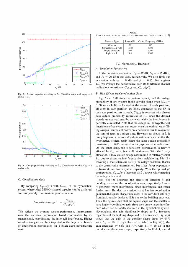
0 5 10 15 20 25 30 35 400

20

40

60

80

100

120

Lw

(dB)

Syste

m c

ap

acity (

bp

s/H

z)

Cideal

Cprob

(p*)

Cprob

(0.5)

Cprob

(1)

Fig. 2. System capacity according to Lw (Corridor shape with NBS = 6and α = 3).

0 5 10 15 20 25 30 35 400

0.05

0.1

0.15

0.2

0.25

0.3

0.35

0.4

Lw

(dB)

Outa

ge p

robabili

ty

Ideal

νprob

(p*)

νprob

(0.5)

νprob

(1)

Fig. 3. Outage probability according to Lw (Corridor shape with NBS = 6and α = 3).

C. Coordination Gain

By comparing Cprob(p∗) with Cideal of the hypothetical

system where ideal MIMO channel capacity can be achieved,we can quantify coordination gain defined as

Coordination gain :=Cideal

Cprob(p∗).

This reflects the average system performance improvementover the statistical information based coordination by in-stantaneously coordinating the inter-cell interference. Highercoordination gain can be interpreted as the larger cost benefitof interference coordination for a given extra infrastructurecost.

TABLE IAVERAGE WALL LOSS ACCORDING TO COMMON BUILDING MATERIAL [17]

Material Type Loss (dB) Center Frequency (MHz)

All metal 26 815Concrete block wall 13-20 1300

Empty cardboard 3-6 1300Light textile 3-5 1300

IV. NUMERICAL RESULTS

A. Simulation Parameters

In the numerical evaluation, L0 = 37 dB, N0 = −95 dBm,and Pt = 20 dBm are used, respectively. We also limit ourevaluation with γt = 6 dB and β = 0.05. For a givenLw, we average the performance over 1000 different channelrealizations to estimate Cideal and Cprob(p

∗).

B. Wall Effects on Coordination Gain

Fig. 2 and 3 illustrate the system capacity and the outageprobability of two systems in the corridor shape when NBS =6. Since each BS is located at the center of each partition,all users in each partition are likely connected to the BS inthe same partition. As a result, Cideal is constant with almostzero outage probability regardless of Lw since the desiredsignals are not weakened by the walls while the interference isperfectly eliminated. Note that the outage in the hypotheticalinterference-free system can occur when the optimal waterfill-ing assigns insufficient power on a particular link to maximizethe sum of rates at a given time. However, as shown in 3, itrarely happens in the considered evaluation scenario so that thehypothetical system easily meets the same outage probabilityconstraint β = 0.05 imposed in the p-persistent coordination.On the other hand, the p-persistent coordination is heavilyaffected by Lw due to inter-cell interference. With the fixed pallocation, it may violate outage constraint β in relatively smallLw due to excessive interference from neighboring BSs. Bylowering p, the system can satisfy the outage constraint thanksto the conservative transmission, but it has fewer opportunityto transmit, i.e., lower system capacity. With the optimal p∗

configuration, Cprob(p∗) increases as Lw grows while meeting

the outage constraint.Fig. 4(a)–(b) illustrates the effects of different α and

building shapes on the coordination gain, respectively. Lowerα generates more interference since interference can reachfurther users. Besides, the corridor shape has less coordinationgain than the square shape since users in the corridor hurts onlyfrom horizontally deployed BSs due to the building structure.Thus, the figures show that the square shape and the smaller αhave higher coordination gain since they create larger interfer-ence which can be totally removed in the hypothetical system.Nevertheless, the gain significantly drops as Lw increasesregardless of the building shape and α. For instance, Fig. 4(a)shows that the gain in the corridor shape drops by 63%with Lw = 10 dB regardless of α. Also, in Fig. 4(b), thegain decreases by 63% and 70% with Lw = 10 dB in thecorridor and the square shape, respectively. In Table I, several

85

0 5 10 15 201

3

5

7

9

11

13

15

(b) Lw

(dB) w/ α=3

Square

Corridor

0 5 10 15 201

3

5

7

9

11

13

15

(a) Lw

(dB) in Corridor

Coord

ination g

ain

(x facto

r)

α=2

α=3

α=4

Fig. 4. Coordination gain according to wall loss (NBS = 6).

0 2 4 6 8 10 12 14 16 181

3

5

7

9

11

Lw

(dB)

Coord

ination g

ain

(x facto

r)

NBS

=8

NBS

=6

NBS

=2

Weakened signals

More exposed BSs

20

Fig. 5. Coordination gain in different deployment density (Corridor shapewith α = 3).

examples of average wall loss are listed according to thetypical materials at different center frequency. It shows that10 dB attenuation corresponds to typical concrete block wallswhich are usually used for dividing large areas, e.g., officedivisions or households in apartments.

C. Deployment Density and Coordination Gain

Depending on the user demand, operators can deploy more(fewer) number of BSs to increase (decrease) the system ca-pacity in a given service area. However, more BSs cause moredownlink interference in general. We explore the effects ofdeployment density on the coordination gain. Fig. 5 provideshow the coordination gain is changed with more or fewer BSsdeployment in the corridor shape. Note that each BS is evenlyplaced in a horizontal axis to cover the same geographical area.Since there are six partitions with five walls, at least one ofBSs faces with another BS without any wall separation when

NBS = 8. In the p-persistent transmission, such exposed BSloses any benefit from wall shielding so that the performancedeterioration is inevitable due to the more conservative trans-mission setting. Consequently, the coordination gain curve isshifted toward right in the figure. On the other hand, there canbe multiple walls between serving users and associated BSswhen NBS = 2. Due to the wall penetration loss in traversingsignals, some of users positioned in partitions without BSsexperience much weakened signals which do not occur whenNBS is more than the number of partitions. Accordingly,the capacity of the hypothetical system drops regardless ofthe interference elimination to let the coordination gain curveshifted leftward.

V. CONCLUSION

We investigated the potential benefit of practical multicellinterference coordination. For this, we quantitatively assessedthe optimistic performance gain of coordination on purposein the various range of indoor environments. We compared ahypothetical interference-free system as the upper bound anda loosely coordinated system with probabilistic interferencemitigation as the lower bound. The coordination gain was eval-uated under various wall loss, path loss exponents, buildingshapes, and deployment density.

Numerical results demonstrate that the multicell interferencecoordination is not always worthwhile. In open areas such asconference halls, the coordination can ideally provide the sub-stantial gain especially when BSs are densely deployed. How-ever, the gain considerably declines with marginal increasein wall loss between BSs regardless of other environmentalfactors, e.g., 60–70% drop in the presence of 10 dB wallloss which corresponds to the typical brick wall in offices.This suggests that the cost of dedicated backhaul to enablethe tight coordination may not be compensated in networkdeployments with reasonable wall losses. As a future work, therefined coordination gain should be evaluated especially wheresignificant gain is identified by comparing a more practicalupper bound with a lower bound in a more realistic load andshared backhaul scenarios.

REFERENCES

[1] “Traffic and market data report,” White Paper, Ericsson, Nov. 2011.[2] K. Karakayali, G. J. Foschini, and R. A. Valenzuela, “Network coordi-

nation for spectrally efficient communications in cellular systems,” IEEEWireless Communications Magazine, pp. 56–61, 2006.

[3] S. Shamai and B. Zaidel, “Enhancing the cellular downlink capacityvia co-processing at the transmitting end,” in Proc. IEEE VTC, Rhodes,Greece, May 2001.

[4] W. Yu and T. Lan, “Transmitter optimization for the multi-antennadownlink with per-antenna power constraints,” IEEE Transactions onSignal Processing, vol. 55, no. 6, pp. 2646–2660, Jun. 2007.

[5] S. Jing, D. Tse, J. B. Soriaga, J. Hou, J. E. Smee, and R. Padovani,“Multicell downlink capacity with coordinated processing,” EURASIPJournal Wireless Commun. Networking, 2008.

[6] D. Gesbert, S. Hanly, H. Huang, S. S. Shitz, O. Simeone, and W. Yu,“Multicell MIMO cooperative networks: A new look at interference,”IEEE Journal on Selected Areas in Communications, vol. 28, no. 9, pp.1380–1408, Dec. 2010.

[7] O. Simeone, O. Somekh, H. V. Poor, and S. Shamai, “Downlinkmulticell processing with limited-backhaul capacity,” EURASIP Journalon Advances in Signal Processing, vol. article ID 840814, May 2009.

86

[8] R. Zakhour and D. Gesbert, “Optimized data sharing in multicell MIMOwith finite backhaul capacity,” IEEE Transactions on Signal Processing,vol. 59, no. 12, pp. 6102–6111, Dec. 2011.

[9] S. Landstrm, A. Furuskr, K. J. on, L. Falconetti, and F. Kronestedt,“Heterogeneous networks increasing cellular capacity,” Ericsson Re-view, 2011.

[10] D. A. Schmidt, C. Shi, R. A. Berry, M. L. Honig, and W. Utschick,“Distributed resource allocation schemes,” IEEE Transactions on SignalProcessing, vol. 26, no. 5, pp. 53–63, Sep. 2009.

[11] M. Andrews, V. Capdevielle, A. Feki, and P. Gupta, “Autonomousspectrum sharing for mixed LTE femto and macro cells deployments,”in Proc. IEEE INFOCOM, San Diego, USA, Mar. 2010.

[12] K. Son, S. Lee, Y. Yi, and S. Chong, “REFIM: A practical interferencemanagement in heterogeneous wireless access networks,” IEEE Journalon Selected Areas in Communications, vol. 29, no. 6, pp. 1260–1272,Jun. 2011.

[13] R. Bosisio and U. Spagnolini, “Interference coordination vs. interferencerandomization in multicell 3GPP LTE system,” in Proc. IEEE WCNC,Las Vegas, Apr. 2008.

[14] V. Chandrasekhar and J. G. Andrews, “Spectrum allocation in tieredcellular networks,” IEEE Transactions on Communications, vol. 57,no. 10, pp. 3059–3068, Oct. 2009.

[15] I. Ashraf, H. Claussen, and L. T. Ho, “Distributed radio coverageoptimization in enterprise femtocell networks,” in Proc. IEEE ICC, CapeTown, South Africa, May 2010.

[16] J.-H. Yun and K. Shin, “Adaptive interference management of OFDMAfemtocells for co-channel deployment,” IEEE Journal on Selected Areasin Communications, vol. 29, no. 6, pp. 1225 –1241, Jun. 2011.

[17] T. S. Rappaport, Wireless communications principles and practice.Pearson Education, 2002.

[18] M. Unbehaun and M. Kamenetsky, “On the Deployment of Picocellu-lar Wireless Infrastructure,” IEEE Wireless Communications Magazine,vol. 10, no. 6, pp. 70–80, Dec. 2003.

[19] M. Lott and I. Forkel, “A multi-wall-and-floor model for indoor radiopropagation,” in Proc. IEEE VTC, New Jersey, USA, Oct. 2001.

[20] H. Hashemi, “The indoor radio propagation channel,” in Proceedings ofthe IEEE, vol. 81, no. 7, Jul. 1993.

[21] M. Tolstrup, Indoor Radio Planning, A practical guide for GSM, DCS,UMTS and HSPA. John Wiley & Sons Ltd, 2008.

[22] B. D. Gesbert, S. G. Kiani, A. Gjendemsj, and G. E. ien, “Adaptation,coordination, and distributed resource allocation in interference-limitedwireless networks,” Proceedings of the IEEE, vol. 95, no. 12, pp. 2393–2409, 2007.

[23] E. Telatar, “Capacity of multi-antenna gaussian channels,” AT&T-Bell Labs Internal Tech. Memo., Jun. 1995, available: http://mars.bell-labs.com/papers/proof/proof.pdf.

[24] G. J. Foschini and M. J. Gans, “On limits of wireless communications ina fading environment when using multiple antennas,” Wireless PpersonalCommunications, vol. 6, no. 3, pp. 311–335, Mar. 1998.

87

Paper IV: Cost Efficient HighCapacity Indoor Wireless Access:Denser Wi-Fi or Coordinated

Pico-cellular?

Du Ho Kang, Ki Won Sung, and Jens Zandersubmitted to IEEE Transactions on Wireless Communications, 2012.

89

Cost Efficient High Capacity Indoor WirelessAccess: Denser Wi-Fi or Coordinated Pico-cellular?



Abstract—Rapidly increasing traffic demand has forced indooroperators to deploy more and more Wi-Fi access points (APs). AsAP density increases, inter-AP interference rises and may limitthe capacity. Alternatively, cellular technologies using centralizedinterference coordination can provide the same capacity with thefewer number of APs at the price of more expensive equipmentand installation cost. It is still not obvious at what demand levelmore sophisticated coordination pays off in terms of total systemcost. To make this comparison, we assess the required AP densityof three candidate systems for a given average demand: a Wi-Finetwork, a conventional pico-cellular network with frequencyplanning, and an advanced system employing multi-cell jointprocessing. Numerical results show that dense Wi-Fi is thecheapest solution at a relatively low demand level. However, theAP density grows quickly at a critical demand level regardless ofpropagation conditions. Beyond this “Wi-Fi network limit”, theconventional pico-cellular network works and is cheaper than thejoint processing in obstructed environments, e.g., furnished officeswith walls. In line of sight condition such as stadiums, the jointprocessing becomes the most viable solution. The drawback isthat extremely accurate channel state information at transmittersis needed.

Index Terms—Wi-Fi densification, Interference coordination,Networked MIMO, Cost-capacity analysis, Network deployment.

I. INTRODUCTION

Wireless data traffic has rapidly increased over the last fewyears triggered by mobile handset innovation, e.g., tablet PCsor smartphones. The trend of traffic growth is even acceler-ated by bandwidth-hungry applications, e.g., real-time cloudcomputing or web-storage service. A significant investment inindoor network deployment is anticipated in upcoming yearsbecause most of such traffic increase is expected to come fromindoors [1]. An interesting question to operators is what will bethe cheapest indoor deployment strategy for such high-capacityprovisioning.

Wi-Fi access points (APs) based on IEEE 802.11 standardhave been so far successful due to its significantly lower unitcost than other cellular solutions. However, the contention-based system may lead to a negative impact on overall networkcapacity because of the fundamental lack of interferencecoordination. On the other hand, advanced joint process-ing techniques, often dubbed as networked MIMO, recentlyemerge as one evolutionary path in the cellular track [2]–[5]. Theoretically, it can perfectly remove interference, greatlyincreasing spectral efficiency. Nonetheless, this requires costlydedicated optical fibers for the fast and accurate exchange of

channel state information (CSI) and user data between APs1

which may outweigh equipment costs. Conventional pico-cellular systems with moderate interference coordination, e.g.,static resource partitioning, are placed in the middle both fromcost and performance perspectives. While tighter interferencecoordination in the cellular system certainly provides requirednetwork capacity with the fewer number of APs, it is stillnot so straightforward if it will have economic gain overthe denser Wi-Fi network in terms of total system cost.Moreover, the wide variety of in-building structures createsdifferent interference characteristics so that the performancebenefit of coordination may diminish in some obstructedenvironments [6]. Therefore, quantitative comparison amongthe candidate solutions is an important research task in variousindoor environments.

In order to make the comparison, the both cost and perfor-mance of a system should be estimated under the same localenvironment. In techno-economic literature, we find only thelimited number of cost comparisons between a Wi-Fi and aconventional pico-cellular system that are based on empiricalcost figures from a specific market [7]–[10]. These studiesmostly relied on simplified performance estimation whichdisregarded the distinct interference coordination mechanisms,e.g., CSMA/CA randomness in the Wi-Fi. For instance, in [7],[8], an overall network performance was obtained by scalingaverage per-cell throughput by the number of placed APs.In [9], [10], it was estimated more precisely by reflectingthe statistics of user distribution and propagation conditions.Still, a link-level data rate was approximated as the function ofreceived average signal to average interference plus noise ra-tio (SINR). In contrast, significant technology-oriented studiesevaluated performance of either W-Fi or cellular systems withmore refined coordination models [11]–[21]. For instance, au-thors in [11]–[14] estimated a performance of a Wi-Fi networkby using different mathematical tools. The others in [15]–[17]studied the theoretical capacity of the cellular network by thedifferent means of multi-antenna techniques or proposed morepractical interference management algorithms [18]–[21]. How-ever, they have thus far overlooked the importance of analyzingthe economic benefit of cellular systems than the Wi-Fi systemfor a given data rate requirement. This led the performance of

1Without the loss of generality, we use a term AP for any type offixed transmitters, e.g., either stand-alone type or remote radio head, at theremainder of paper instead of using base station which is often used in acellular literature.

90

each system to be assessed in parallel in different environmentswith unsynchronized working assumptions and performancemetrics.

The objective of our study is providing an insight into thepotential way towards the future lowest-cost indoor deploy-ment by explicitly comparing both Wi-Fi and cellular systemswhich have distinct interference coordination mechanismsand cost structures. While exact cost figures for equipmentsand backhaul are market and vendor specific, estimating therequired AP density to meet an average traffic demand isour way to compare total network cost of systems which isapproximately linear to the AP density [22]. For comparisonpurpose, the AP density of three systems is quantitativelyassessed for a given average traffic demand: a Wi-Fi network,a conventional pico-cellular network with frequency planning,and an advanced cellular network with an emerging jointprocessing technique. The main contribution of this work isthree-fold:

1) First, the required AP density of the three aforemen-tioned systems is estimated as a function of increasingaverage user demand under outage constraint, partic-ularly taking into account technical differences in theinterference coordination. The impact of indoor prop-agation conditions, i.e., indoor wall loss and pathlossexponent, are further examined in order to see how theeconomic gain of one system deviates accordingly.

2) Secondly, we develop a framework for evaluating theoptimistic performance of a Wi-Fi network which is ap-plicable to obstructed environments but still retaining theCSMA/CA mechanism. In the framework, an ideal MACand PHY layer are explicitly modeled based on randomsequential packing process [23]–[25] which maximallyexploits spatial reuse without redundant collisions inorder to estimate the minimally required Wi-Fi APdensity.

3) Thirdly, we provide a solution map of future indoordeployment which intuitively guides operators to choosethe lowest-cost option. It is characterized by trafficdemand and environmental openness with identifiedpractical bottlenecks.

The rest of this paper is organized as follows. Section II pro-vides an overall system model including network dimensioningand traffic assumptions. Then, Wi-Fi and cellular networkmodels are presented in Section III and IV, respectively.Section V describes a simulation methodology to estimatean individual system performance. Numerical results illustrateimplications on the economic indoor system in Section VI.Finally, we draw conclusions in Section VII.

II. SYSTEM MODEL

A. Service Area Layout

As depicted in Fig. 1, we consider a finite square servicearea Ω with the size of lx by ly in meters. We assume that thereare walls which are equally placed and create the constantsignal strength loss Lw (dB). This represents the homogenous

lx

lyAPs in channel 1

APs in channel 2

Co-channel interference

User

Signal

ij=2

Fig. 1. Service area layout with the example of AP deployment in ninerooms.

indoor materials for simplicity. The numbers of walls arewx and wy, which are placed vertically and horizontally,respectively, in the following locations:

xw =lxa

wx + 1and yw =

lyb

wy + 1,

where a = 1, ..., wx and b = 1, ..., wy .

B. Traffic Assumptions

We focus on downlink traffic which is the main consid-eration of network deployment. Mobile users equipped withsingle antenna are assumed to be uniformly and independentlydistributed with the average density of E[λu] (users/km2).Typically, the traffic load pattern varies drastically on an hourlybasis [26]. Thus, a busy hour, which refers to the time duringa day with the most traffic, is a commonly used conceptin telecommunications for network dimensioning [10], [27].We assume that the ω fraction of the day are busy hourswhen the traffic is intensified. By assuming that all usersare equally served during the busy hour in an average sense,a network can support a feasible average user throughputdenoted by µ (Mbps/user) during the busy hour. In addition,average monthly traffic volume per user in GB/month/user hasbeen used as the conventional metric of measuring networkusage in telecommunication business since it provides anintuitive understanding of customer behavior. For instance,the mobile broadband usage today is 1-2 (GB/month/user) inmost developed countries [28]. Following this convention, ourwork adopts this metric instead of classical system spectralefficiency in bps/Hz which is common in most of technicalanalysis. Then, average user demand D (GB/month/user) canbe defined by

D :=c0

ωµ (GB/month/user),

where c0 represents the scaling constant to transformMbps/user unit to GB/month/user. It is 1

1024 × 18 × 3600 × 30

by assuming 30 days a month. Although average user demandper month strongly depends on user statistics in local places,i.e., ω and E[λu], the comparison of deployment density is

91

still valid since it is mainly affected by system performanceand physical propagation conditions.

C. Propagation Model

We assume that both an AP and a user have single antennafor the analysis simplicity. Then, each radio link is affected bythe path loss attenuation and Rayleigh fading. For the path lossbetween AP i and user j, we adopt a general Indoor Multiwalland Floor model which considers all walls intersecting thedirect ray between an AP and a user [6], [29]. By assumingsingle floor, the path loss between AP i and user j can bedependent on the internal wall and distance as given in

L(dB)ij = L0 + 10αlog10(dij) + ϕijLw (dB),

where L0, α, dij , and ϕij represent the constant loss, apathloss exponent, the distance in meter between AP i anduser j, and the number of walls across a AP i and a user j,respectively. Also, α depends on the size or the surroundingsof the rooms or operating frequency. In general, the biggersize of rooms with hard obstacles at higher frequency createsthe higher α [6], [30].

Additionally, we assume an independent and identical small-scale Rayleigh fading channel component zij ∼ CN (0, σ2

z).By assuming rich scattering, all channels are perfectly un-correlated. This can be justified in a fact that APs or usersare sufficiently separated and many scattering objects in in-doors [31], e.g., furniture or uneven wall surfaces. Then, letus define the complex channel response between AP i anduser j as

hij =√

Lijzij .

Note that Lij represents the linearly scaled path gain, i.e.,

Lij = 10−L

(dB)ij

10 . Then, a complex channel coefficient matrixis denoted by H = hij for all active links in a given time.Then, the channel power gain gij can be computed fromsquaring the amplitude of hij , i.e., gij = |hij |2. We alsoconsider a block fading model, where H remains quasi-staticwithin a fading block, but varies between contiguous fadingblocks.

D. Performance Measure

The overall network capacity is evaluated with respect toaverage area throughput density E[λs] (Mbps/km2) subject tothe outage probability constraint ν = Pr(SINRj < γt) < β.γt represents the minimum SINR for feasible transmission.Note that λs =

∑Rj (Mbps/km2) represents aggregate data

rates of all served users per unit area which is governed by aninvolved coordination mechanism and the channel realization.For average user density E[λu] (users/km2), we assume that adeployed network can support µ (Mbps/user) during the busyhour on average:

E[λs] = µE[λu] (Mbps/km2).

E. Network Dimensioning

The APs should be dimensioned to support µ during thebusy hour for a given average user density E[λu] under theconstraint of ν < β. We assume that the APs are placedregularly in order to maintain the equal geographical area perBS. That is, nx by ny APs are placed as shown in Fig. 1. Thelocation planning could be further optimized considering thebuilding geometry and its indoor structure. Since our objectiveis comparing systems employing the distinct interference co-ordination mechanisms, we leave the location optimality issueout of the scope. Instead, we refer interested readers to ourprevious work on this aspect [32]. We simply assume thelocations (xap, yap) of deployed APs are given as

(xap, yap) =

(lxnx

(1

2+ (a − 1)

),

lyny

(1

2+ (b − 1)

))

where a = 1, ..., nx and b = 1, ..., ny .

III. WI-FI NETWORK MODEL

The performance evaluation of a Wi-Fi network itself isa challenging task since the mathematical modeling of thecomplex behavior of multiple APs is difficult. An accuratepacket-level simulation is also very time-consuming particu-larly in a dense network. Thus, we propose a Wi-Fi networkmodel where practical impairments in MAC and PHY layerare idealized, but the key features of CSMA/CA operation arecaptured. This model can be used to estimate the optimisticperformance of a multi-channel Wi-Fi network in obstructedindoor environments to yield the minimal number of APs fora given user demand.

A. 802.11 Channel Model

Depending on the IEEE 802.11 standard variants, a numberof orthogonal frequency channels are defined. The 802.11b/gstandard provides a set of 14 frequency channels among whichonly 3 non-overlapping channels are possible, whereas 802.11aoffers around 8 non-overlapping channels depending on thespectrum availability in 5 GHz [33]. Thus, the frequency reusenumber Kwifi for Wi-Fi is different counting on the operatingfrequency and a specific standard. Then, we assume that eachAP i access one of non-overlapping channels whose bandwidthwwifi

i is given for the total system bandwidth W by

wwifii =

W

Kwifi(MHz).

B. MAC and PHY Layer Model

In principle, the MAC operation is based on CSMA/CAmechanism regardless of the operating frequency and standardvariants. We also assume that all APs transmit data at thesame fixed power Pt (mW). Since we suppose that a networkis dimensioned to meet average user throughput during abusy hour, persistent downlink traffic is presumed with no ornegligible upstream traffic. Let us define a set of APs operatingin a frequency channel k as Ak. As for the association, eachuser attaches to the AP offering the highest Lij . Note thateach user may instantaneously have worse signal strength from

92

the associated AP than nearby APs due to fading componentzij . However, this assumption reflects the practical associationcriteria which is based on average signal strength.

At a given data transmission time, only a subset of Ak canbe concurrently active due to CSMA/CA operation. Let Ak

x

be the set of all co-channel APs which are in the contentiondomain of AP x operating in a channel k. It is mathematicallyexpressed as follows:

Akx := i ∈ Ak, i = x|gixPt > CSli

thr,

where CSlithr (mW) represents the linearly scaled carrier

sensing threshold of CSthr (dBm), i.e., CSlithr = 10

CSthr10 .

The collision probability (outage in a cellular context) and thespatial reuse gain are affected by CSthr since it defines thesize of the contention domain. Intuitively, the higher CSthr

makes APs aggressively reuse the space domain, i.e., moresimultaneous transmission for higher capacity but with morecollision. Typically, the IEEE 802.11 standard suggests CSthr

for equal transmission opportunity in unlicensed band [33].For this, we use CSthr=-85 dBm as defined in [33] which isnamed as Baseline Wi-Fi. Nevertheless, there may be a strongmotivation for operators to adjust CSthr for striking their ownbalances between capacity and collision probability. Thus, wealso examine lower CSthr for the comparison purpose whichis referred to as Aggressive Wi-Fi.

In a practical Wi-Fi network, collisions among APs in acontention domain can occur because of the mismatch in thetiming of carrier sensing and actual transmission. However, weassume that all APs in Ak

x always listen when AP x transmitsdata. Although the perfect carrier sensing removes the im-pairment due to temporal mismatch, collisions due to spatialmismatch between carrier-sensing APs and receiving users,a so-called hidden node problem, can still occur. However,the impact of the hidden node problem becomes negligiblewith denser deployment because the distance between a userand its serving AP is much closer than the carrier-sensingrange [12]. Likewise, the conservative transmission due to anexposed node problem also diminishes with densification.

Let us refer to the set of all active APs elected by theMAC protocol in a frequency channel k at a given timeas Φk ⊂ Ak. We here omit the time index t unless anyambiguity is introduced. Since Φk plays an important rolein the performance of a Wi-Fi network, a precise and yetsimple model describing this set is necessary while capturingthe important features of CSMA/CA. Matern hard core pointprocess has been recently paid an attention to estimate datarates of a generic CSMA/CA network. This is theoreticallyfounded on Poisson point process (PPP) with an additionalthinning process [34]. Several studies used this to model theMAC operation for estimating data rates of a dense Wi-Finetwork [12], [13]. However, the classical homogeneous PPPassumption suffers from several drawbacks in practical indoorsituations, as argued in [34]–[36]. First of all, the effect ofobstructed indoor environment, which creates spatially varyinginterference, is hard to be analyzed even if it is one ofcrucial factors to affect the performance of indoor deployment.

Transmitting APs

Listening APs

Contention domain

User

Coverage

Co-channel interference

Signal

Fig. 2. An example of realization of active Wi-Fi APs when single channelis available without any walls.

Secondly, it probabilistically permits some APs out of the con-tention domains to be silent. This leads to the reduced spatialreuse gain, i.e., fewer number of simultaneous transmission.Thirdly, the spatial average of AP locations in infinite serviceareas is estimated by assuming homogeneous interference.Practical indoor Wi-Fi networks have finite service areas suchthat users near the boundary experience lower interferencelevel than those at the center. Lastly, it is only applicableto single channel operation which overestimates the collisionprobability than multi-channel Wi-Fi deployment in practice.

These motivate us to consider a Simple Sequential Inhibition(SSI) process which is applicable to more realistic indoorenvironments by empirical simulation [25]. As a family of ran-dom sequential packing process, the SSI is known to be moreappropriate to model CSMA/CA networks and was originallydeveloped for a finite continuous spatial domain [23], [24]. Letus define a SSI process Ψ in a constructive manner on a finiteand discrete set Ak rather than arbitrary points in the servicearea. Ψ(n) is composed of a sequence of n random variablesdenoted by X1, ..., Xn which are independently and uniformlydistributed in Ak. Initially, X1 is added to Ψ(1). Then, Xi

is systematically added to Ψ(i) if and only if it does notbelong to the contention domain of any APs in Ψ(n−1), i.e.,Xi /∈ ∪Xj∈Ψ(i−1)Ak

Xj. The process stops whenever entire APs

in Ak are either active APs or in the contention domain of anyactive APs. A sample of active APs Φk can be built by suchSSI process as exemplified in Fig. 2. This process always letsAPs transmit unless it is in the range of the contention domainof other active APs, contrary to Matern point process. Notethat a recent work in [14] also proposed a simulation-basedmodel to approximate a data rate in a multi-channel dense Wi-Fi network. Although the data rate is modeled as a function ofAP density, it still assumed the pessimistic interference whereany active APs always experience interference form all APsin Ak.

For a given realization Φk, each active AP x ∈ Φk randomlyselects user j to transmit data. Then, the data rate can be

93

ideally achieved as

Rwifij = min

wwifi

i log2

(1+

gijPt∑x∈Φk\i gxjPt + σ2/Kwifi

), Rwifi

max

(Mbps), (1)

where Rwifimax = wwifi

i ηwifi and σ2 (mW) is average noise powerfor whole system bandwidth W . A practical Wi-Fi system usesa discrete rate and the rate adaptation is also imperfect due tothe lack of explicit channel information feedback from usersunlike the cellular systems [33]. In this regard, the rate modelimplicitly assumes the perfect rate adaptation without anyquantization. Thus, our approach again gives us the optimisticperformance of the dense Wi-Fi network.

IV. CELLULAR NETWORK MODEL

For comparative analysis with the Wi-Fi network, we con-sider two representative indoor cellular systems with distinctcoordination techniques: a conventional pico-cellular systemwith static frequency planning and an advanced system em-ploying multi-cell zero-forcing (ZF) beamforming.

A. Conventional Frequency Planning

The frequency planning is the one of static coordinationtechniques which were used in a conventional cellular net-work to mitigate multi-cell interference. In the conventionalplanning, whole system bandwidth W is partitioned into Knon-overlapping equal-width bands in a centralized planningprocess. Then, each AP i transmits at full power Pt using oneout of K disjoint bands whose amount is given as:

wstai =

W

K(MHz).

Recall that Kwifi in the Wi-Fi network is fixed irrespectiveof propagation conditions due to the restrictions in standardswhereas K in the conventional cellular coordination can beadaptively determined. For a given K, a user j is randomlyselected at a given time and achieves data rate of Rsta

j as

Rstaj = min

wsta

i log2

(1+

gijPt∑x∈Ak\i gxjPt + σ2/K

), Rsta

max

(Mbps), (2)

where Rstamax = wsta

i ηsta. There are also other variants inthe static coordination approach such as fractional frequencyreuse [4], [37]. However, we confine our study to the staticfrequency planning as a reference since our objective is tocompare representative cellular systems with the Wi-Fi system.

B. Multi-cell Zero Forcing Beamforming

While co-channel interference still exists in the conventionalpico-cellular network, it can be ideally removed by the meansof advanced multi-cell joint processing techniques. Severalprecoding strategies in the joint processing have been proposedand studied [2], [5]. In general, dirty paper coding (DPC)is known as the precoding strategy to yield the informationtheoretical upper bound [38], [39]. Alternatively, suboptimallinear precoding based DPC, commonly referred to as ZF-DPC, deals with the part of interference with a linear pre-coding strategy whereas remaining interference still relies onnonlinear DPC coding [40]. However, it is generally verycomplex to implement such non-linear precoding techniquesin a practical system. Instead, zero forcing (ZF) beamformingwhich is entirely a linear processing is considered both inacademia and industries as one way of practical implementa-tions of the joint processing [2], [41]–[43]. The ZF techniquebecomes near-optimal in high SNR regime which is at thefocus of our interest, i.e., a dense indoor network. Thus, wewill employ the linear ZF as the representative joint-processingtechnique.

Although the ZF has a great potential to improve theperformance of the indoor network, it may be sensitive toimperfect channel estimation or feedback delay [15]–[17].Therefore, we consider two cases for the ZF: ideal ZF withperfect CSI at transmitters (CSIT) and one with CSIT errors.

1) Ideal ZF: Let us refer to the vector of signals transmittedby N single antenna APs as x ∈ C[N×1]. Then, the vector ofreceived signals y ∈ C[M×1] in M single antenna users canbe described as

y = Hx + n,

where H ∈ C[M×N] and n ∈ C[M×1] is referred to as anadditive white noise vector with covariance E[nn†] = σ2I.

Suppose that H is perfectly known at the network sidewithout any feedback delay and estimation/quantization errors.x can be now reconstructed with linear beamforming matrixW ∈ C[N×M] as:

x = Wu = H†(HH†)−1u,

where the j-th element in the vector u ∈ C[M×1] is theinformation-bearing data symbol intended for the j-th user.We also assume that the elements of u are independentzero-mean complex Gaussian random variables with varianceE[uju

†j ] = pj (mW). Then,

y = Hx + n = HH†(HH†)−1u + n = u + n.

User j receives yj = uj + nj so that it can achieve data rate

Rzfj = min

W log2

(1 +

pj

σ2

), Rzf

max

(Mbps), (3)

where Rzfmax = Wηzf represents the maximum link data

rate supported by the network. For the fair comparison withother systems, we disregard the multiuser diversity gain byrandomly selecting single active user per AP in a given

94

time. Thus, all channel matrices considered in the sequelare N -by-N by setting N = M . Because we assume thatdata symbols heading to different users follow independentand zero-mean Gaussian distribution, per-antenna power con-straint (PAPC) can be expressed as linear constraints, i.e.E[|xi|2] =

∑j |wij |2pj ≤ Pt. Moreover, aggregate rates∑

j Rzfj are concave in the symbols power vector pj . Then,

power allocation for the sum rate maximization becomes aconvex programming problem which is efficiently solvable bystandard optimization techniques [44].

2) δ-erroneous ZF: When ZF is used in a practical cellularnetwork, the interference may not be perfectly removed sincesome elements of H can be outdated due to the channeldynamics and feedback delay. This leads to inaccurate symbolpower allocation and the beamforming matrix W selection.We propose a simple method to model this by introducingthe probability δ that CSIT is outdated for a given link. Weassume that only fading component zij varies in consecutivefading blocks with consistent Lij . Then, at a given feedbackdelay τ between channel estimation and data transmission attime t, let us define δ as

δ := Pr(|zt

ij − zt−τij | > 0

).

If the CSIT is outdated, we also assume that there is correlationof ρ between zt

ij and its delayed version zt−τij . This is modeled

as the first order of autoregressive process [45]:

ztij = ρzt−τ

ij +√

1 − ρ2qtij

where qtij ∼ CN (0, σ2

z) is independently and identically dis-tributed for arbitrary links. We here consider CSIT inaccuracyonly due to feedback delay by latency of backhaul and CSIreport. Including other practical barriers for using ZF, e.g.,estimation errors and pilot channel/CSIT report overhead inthe air, may bring out additional performance degradation.Nevertheless, analyzing one of dominant barriers still allowsus to investigate the feasibility of ZF in practice.

V. SIMULATION METHODOLOGY

Recall that our objective is the quantitative comparison ofthe required AP densities of three wireless systems to satisfya certain traffic demand. Thus, estimating E[λs] accordingto different number of deployed APs is essential. In thissection, we provide a simulation methodology to estimateE[λs] subject to the outage constraint ν < β by facilitating asnap-shot based Monte-Carlo simulation.

A. Numerical Optimization for Resource Allocation

For a certain Kwifi, the frequency assignment in a Wi-Fi network needs to be optimized. Traditionally, the multi-cell frequency assignment was formulated as a graph-coloringproblem. However, it is generally known as a NP-hard problemdue to its combinatorial property [46]. Thus, when the largenumber of APs are deployed, a search for the optimal solutionis prohibitive. Instead, we employ a heuristic algorithm whereeach AP is randomly and sequentially chosen and is allocated

the frequency channel generating the minimum aggregateinterference. In the frequency planned cellular network, boththe frequency reuse number K and its assignment should beoptimized. In the classical Wyner model where hexagonalcell patterns are infinitely repeated, K can be determinedby the closed-form of expressions [47]. However, it cannotbe applicable to our indoor layout which is composed offinite service areas with indoor walls. Instead, we exhaustivelysearch the lowest K∗ subject to ν < β by evaluating networkperformance for all possible K. The network performance foreach possible K is evaluated by applying the same frequencyassignment algorithm used for the Wi-Fi network. While thefrequency assignment to the Wi-Fi and conventional cellularsystem is performed based on average propagation loss, thesymbol power allocation in ZF is optimized in every snapshotof channel realization by using a convex optimization packageto exploit the dynamic coordination [48].

B. Simulation ProcedureWhen APs are deployed, Kwifi and K orthogonal fre-

quency channels are assigned in the Wi-Fi network and theconventional cellular network, respectively. Then, a snapshotbased Monte-Carlo method is applied to estimate the averageperformance of three systems. In each snapshot, a simulationprocedure is described as follows:

1) A set of users are uniformly and independently droppedand each user associates with the AP providing thestrongest average signal strength. Each AP randomlyselects one user to be served. The channel gain matrixH is generated for the chosen users.

2) For the case of a Wi-Fi network, one realization of Φk isgenerated by the SSI process to create the active set ofAPs. The optimal symbol power in ZF is also computedand allocated for selected users.

3) Then, we evaluate Eq. (1), (2), and (3) for all servedusers and the sample values of aggregate data rates λs

in each system and count the number of active users inoutage.

We estimate E[λs] and ν by averaging the independent samplevalues. Afterward, we enumerate E[λs] by increasing thenumber of APs and apply the same simulation procedure todifferent Lw and α.

VI. NUMERICAL RESULTS

In this section, we provide numerical results obtained bysimulation with the parameters summarized in Table I. Weillustrate the required AP density which meets the averageuser demand under the outage probability constraint. This isfurther examined in two different propagation conditions: theline of sight (LoS) conditions without any walls and higherpathloss exponent with walls.

2We assume ηwifi achievable in popular 802.11a/b/g systems whichsupport up to 54 Mbps for 20 MHz bandwidth.

3It is assumed that ηsta and ηzf are equivalent to the link spectral efficiencyrequired in IMT-Advanced systems in single antenna configuration [49]

4We implicitly assume three non-overlapping channel as 802.11b/g in 2.4GHz.

95

TABLE ISIMULATION PARAMETERS

Parameter Name ValuesService area size lx = ly=100 mTraffic intensity portion during abusy hour ω

0.2

Average number of users E[λu] 105 users/km2

Constant pathloss L0 37 dBThe maximum link spectral effi-ciency in the Wi-Fi system2 ηwifi 2.7 bps/Hz

The maximum link spectral effi-ciency in the cellular system3 ηsta,ηzf

3.75 bps/Hz

Boltzmann constant k 1.38 × 10−23 J/KTemperature T 300 KFading variance σ2

z 1Correlation factor in feedbackdelayρ

0.9

Average transmission power Pt 100 mWThe minimum required SINR γt 3 dBThe minimum outage probabilityconstraint β

0.05

The number of available non-overlapping channel for the Wi-Fi4Kwifi

3

A. Deployment Options in Open Environment

In this subsection, we compare the deployment density ofthe Wi-Fi network and the other two cellular solutions whenα=2 and Lw = 0, which is more likely to occur with networkdensification.

1) Wi-Fi Network Limit: We can identify from Fig. 3 thatthe baseline Wi-Fi densification has almost no capacity expan-sion. This can be explained as follows. Since all co-channelAPs in Ω are in the contention domain in our parametersetting, only one AP in each channel can be active in a giventime regardless of AP density. Thus, there can be three activeAPs at maximum which is equal to Kwifi. In addition, everyserved user can reach the highest rate Rwifi

max regardless of itslocation in Ω because high received signal strength can beachieved due to very low propagation loss. Consequently, thedensification does not result in network capacity expansion,i.e., no gain from spatial reuse and shorter service range. Inthe aggressive Wi-Fi with CSthr=-65 dBm, extra capacity isgained with more collisions (less than β). It is noticeablein Fig. 4 that the densification decreases the collision sinceit lets APs stay closer to their users while interference ismaintained by CSthr. Still, the deployment density rapidlygrows again when average user demand exceeds a certain level,i.e., roughly 7 GB/month/user. Beyond this level, additionalWi-Fi densification marginally increase the network capacityso that alternative cellular solutions are essential.

2) Practical Challenge in Networked MIMO: When com-pared with the conventional cellular network, the multi-cell ZFbeamforming ideally provides the same capacity with muchless AP density which was corroborated in many existingstudies [2], [41], [42]. For instance, it requires 25 times lessdensification than conventional cellular network when userdemand is 40 GB/month/user. In total cost perspective, the

0 10 20 30 40 500

0.1

0.2

0.3

0.4

0.5

0.6

0.7

0.8

0.9

1

Average user demand D (GB/month/user)

Dep

loym

ent d

ensi

ty (

# of

AP

s/10

0 m

2 )

Baseline Wi−FiAgg. Wi−Fi w/ CS

thr=−65 dBm

Static coordination w/ K=23Ideal ZF

x25densification

Bounded Wi−Fi capacity

Fig. 3. The comparison of deployment density in an open environment (α=2,Lw=0 dB).

0 0.2 0.4 0.6 0.8 10

0.05

0.1

0.15

0.2

0.25

0.3

0.35


Out

age

prob

abili

ty ν


thr=−65 dBm

Static coordination w/ K=23Ideal ZF2% erroneous ZF


Fig. 4. Outage probability according to densification (α=2, Lw=0 dB).

joint processing can be economic unless deployment cost perAP is 25 times more expensive than the conventional cellularsystem. However, only 2% errors in H results in very largeoutage and it is magnified with densification for the given δas shown in Fig. 4. Accordingly, extremely high accuracy onCSIT is required to maximally exploit the cost benefit of thejoint processing.

3) Spectrum Bottleneck in Static Coordination: If the multi-cell ZF may not be feasible due to imperfect CSIT, the con-ventional cellular network could be a only remaining solutionfor high-capacity indoor service. However, the maximum datarate may be limited to support future high data rate servicesalthough densification of the conventional cellular system canincrease the average network capacity. For instance, videostreaming services, as one of main drivers for traffic growthin near future [50], requires the various ranges of consistentminimum data rate according to the type of devices and

96

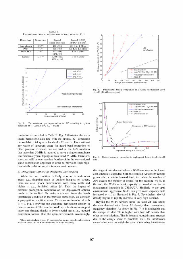
TABLE IIEXAMPLES OF TYPICAL BIT RATE FOR VIDEO STREAMING [51]

Device type Screen size Typical Typical H.264/screen resolution MPEG4 Bit rate5

Smartphones 3-3.5′′ 480×320 500 K to 1 MbpsPMP 4-7′′ 800×480 800 K to 1.5 Mbps

Tablet PCs 7-9′′ 800×480, 1 to 2 Mbps1024×600

Laptops 12-17′′ 1280×800, 3 to 4 Mbps1920×1200

0 10 20 30 40 50 600

1

2

3

4

5

6

7

8

9

10

System bandwidth W (MHz)

Max

imum

per

mis

sibl

e ra

te (

Mbp

s/us

er)

α=4, K*=5

α=3, K*=8

α=2, K*=23

Video streaming in smartphones

Video streaming in laptops

Fig. 5. The maximum rate supported by an AP according to systembandwidth W (1 AP/100 m2, Lw = 0 dB).

resolution as provided in Table II. Fig. 5 illustrates the max-imum permissible data rate with the optimal K∗ dependingon available total system bandwidth W and α. Even withoutany waste of spectrum usage for guard band protection orother protocol overhead, we can find in the LoS conditionthat more than 5 MHz is required to serve a single smartphoneuser whereas typical laptops at least need 25 MHz. Therefore,spectrum will be one practical bottleneck in the conventionalstatic coordination approach in order to provision such high-bandwidth real-time service in open environments.

B. Deployment Options in Obstructed Environment

While the LoS condition is likely to occur in wide openareas, e.g., shopping malls or outdoor hotspots on streets,there are also indoor environments with many walls andhigher α, e.g., furnished offices [6]. Thus, the impact ofdifferent propagation conditions on the deployment optionsneeds to be studied. To make a contrast from the harshinterference condition in the previous subsection, we considera propagation condition where 25 rooms are introduced withα = 4. Fig. 6 provides the quantified deployment density inthis environment. The baseline Wi-Fi densification can supportmore user demand thanks to better spatial reuse, i.e., reducedcontention domain, than the open environment. Accordingly,

5These rates include typical IP overhead, but do not include audio (whichmay add a few 10’s of Kbps depending on audio encoding)

0 50 100 150 200 250 300 350 400 4500

0.1

0.2

0.3

0.4

0.5

0.6

0.7

0.8

0.9

1

Average user demand D (GB/month/user)

Dep

loym

ent d

ensi

ty (

# of

AP

s/10

0 m

2 )


thr=−60 dBm

Static coordination w/ K=3Ideal ZF

x3.3densification

Fig. 6. Deployment density comparison in a closed environment (α=4,Lw=10 dB with wx=wy=4).

0 0.2 0.4 0.6 0.8 10

0.05

0.1

0.15

0.2

0.25

0.3

0.35


Out

age

prob

abili

ty ν


thr=−60 dBm

Static coordination w/ K=3Ideal ZF2% erroneous ZF

Outage due to noise


Fig. 7. Outage probability according to deployment density (α=4, Lw=10dB).

the range of user demand where a Wi-Fi can stay as the lowestcost solution is extended. Still, the required AP density rapidlygrows after a certain demand level, i.e., when the number ofAPs exceed the number of rooms for the baseline Wi-Fi. Inthe end, the Wi-Fi network capacity is bounded due to thefundamental limitation in CSMA/CA. Similarly to the openenvironment, aggressive Wi-Fi can give more capacity withincreased ν < β as illustrated in Fig. 7. Nevertheless, the APdensity begins to rapidly increase in very high demand.

Beyond the Wi-Fi network limit, the ideal ZF can satisfythe user demand with fewer AP density than conventionalfrequency planning. As shown in Fig. 7, it is noticeable thatthe outage of ideal ZF is higher with low AP density thanother system solutions. This is because reduced signal strengthdue to the energy spent to penetrate walls for interferencecancellation may outweigh the gain of removing interference.

97

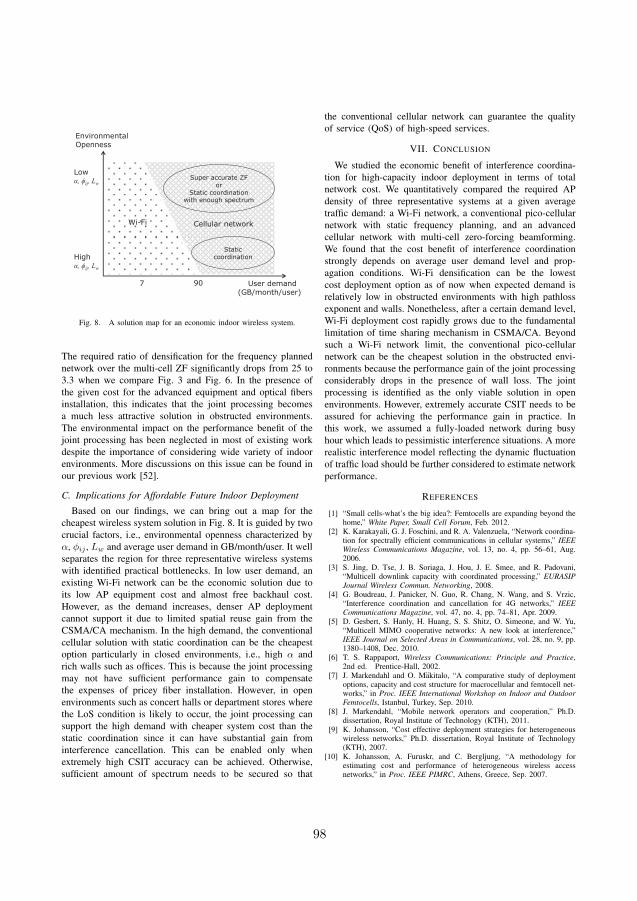
Feasible system solution

User demand (GB/month/user)

7 90

Super accurate ZF or

Static coordination with enough spectrum

Static coordination

Wi-Fi

High α, ϕij, Lw

Environmental Openness

Low α, ϕij, Lw

Cellular network

Fig. 8. A solution map for an economic indoor wireless system.

The required ratio of densification for the frequency plannednetwork over the multi-cell ZF significantly drops from 25 to3.3 when we compare Fig. 3 and Fig. 6. In the presence ofthe given cost for the advanced equipment and optical fibersinstallation, this indicates that the joint processing becomesa much less attractive solution in obstructed environments.The environmental impact on the performance benefit of thejoint processing has been neglected in most of existing workdespite the importance of considering wide variety of indoorenvironments. More discussions on this issue can be found inour previous work [52].

C. Implications for Affordable Future Indoor Deployment

Based on our findings, we can bring out a map for thecheapest wireless system solution in Fig. 8. It is guided by twocrucial factors, i.e., environmental openness characterized byα, ϕij , Lw and average user demand in GB/month/user. It wellseparates the region for three representative wireless systemswith identified practical bottlenecks. In low user demand, anexisting Wi-Fi network can be the economic solution due toits low AP equipment cost and almost free backhaul cost.However, as the demand increases, denser AP deploymentcannot support it due to limited spatial reuse gain from theCSMA/CA mechanism. In the high demand, the conventionalcellular solution with static coordination can be the cheapestoption particularly in closed environments, i.e., high α andrich walls such as offices. This is because the joint processingmay not have sufficient performance gain to compensatethe expenses of pricey fiber installation. However, in openenvironments such as concert halls or department stores wherethe LoS condition is likely to occur, the joint processing cansupport the high demand with cheaper system cost than thestatic coordination since it can have substantial gain frominterference cancellation. This can be enabled only whenextremely high CSIT accuracy can be achieved. Otherwise,sufficient amount of spectrum needs to be secured so that

the conventional cellular network can guarantee the qualityof service (QoS) of high-speed services.

VII. CONCLUSION

We studied the economic benefit of interference coordina-tion for high-capacity indoor deployment in terms of totalnetwork cost. We quantitatively compared the required APdensity of three representative systems at a given averagetraffic demand: a Wi-Fi network, a conventional pico-cellularnetwork with static frequency planning, and an advancedcellular network with multi-cell zero-forcing beamforming.We found that the cost benefit of interference coordinationstrongly depends on average user demand level and prop-agation conditions. Wi-Fi densification can be the lowestcost deployment option as of now when expected demand isrelatively low in obstructed environments with high pathlossexponent and walls. Nonetheless, after a certain demand level,Wi-Fi deployment cost rapidly grows due to the fundamentallimitation of time sharing mechanism in CSMA/CA. Beyondsuch a Wi-Fi network limit, the conventional pico-cellularnetwork can be the cheapest solution in the obstructed envi-ronments because the performance gain of the joint processingconsiderably drops in the presence of wall loss. The jointprocessing is identified as the only viable solution in openenvironments. However, extremely accurate CSIT needs to beassured for achieving the performance gain in practice. Inthis work, we assumed a fully-loaded network during busyhour which leads to pessimistic interference situations. A morerealistic interference model reflecting the dynamic fluctuationof traffic load should be further considered to estimate networkperformance.

REFERENCES

[1] “Small cells-what’s the big idea?: Femtocells are expanding beyond thehome,” White Paper, Small Cell Forum, Feb. 2012.

[2] K. Karakayali, G. J. Foschini, and R. A. Valenzuela, “Network coordina-tion for spectrally efficient communications in cellular systems,” IEEEWireless Communications Magazine, vol. 13, no. 4, pp. 56–61, Aug.2006.

[3] S. Jing, D. Tse, J. B. Soriaga, J. Hou, J. E. Smee, and R. Padovani,“Multicell downlink capacity with coordinated processing,” EURASIPJournal Wireless Commun. Networking, 2008.

[4] G. Boudreau, J. Panicker, N. Guo, R. Chang, N. Wang, and S. Vrzic,“Interference coordination and cancellation for 4G networks,” IEEECommunications Magazine, vol. 47, no. 4, pp. 74–81, Apr. 2009.

[5] D. Gesbert, S. Hanly, H. Huang, S. S. Shitz, O. Simeone, and W. Yu,“Multicell MIMO cooperative networks: A new look at interference,”IEEE Journal on Selected Areas in Communications, vol. 28, no. 9, pp.1380–1408, Dec. 2010.

[6] T. S. Rappaport, Wireless Communications: Principle and Practice,2nd ed. Prentice-Hall, 2002.

[7] J. Markendahl and O. Makitalo, “A comparative study of deploymentoptions, capacity and cost structure for macrocellular and femtocell net-works,” in Proc. IEEE International Workshop on Indoor and OutdoorFemtocells, Istanbul, Turkey, Sep. 2010.

[8] J. Markendahl, “Mobile network operators and cooperation,” Ph.D.dissertation, Royal Institute of Technology (KTH), 2011.

[9] K. Johansson, “Cost effective deployment strategies for heterogeneouswireless networks,” Ph.D. dissertation, Royal Institute of Technology(KTH), 2007.

[10] K. Johansson, A. Furuskr, and C. Bergljung, “A methodology forestimating cost and performance of heterogeneous wireless accessnetworks,” in Proc. IEEE PIMRC, Athens, Greece, Sep. 2007.

98

[11] G. Bianchi, “Performance analysis of the IEEE 802.11 distributed co-ordination function,” vol. 18, no. 3, pp. 535–547, Mar. 2000.

[12] H. Nguyen, F. Baccelli, and D. Kofman, “A stochastic geometry analysisof dense IEEE 802.11 networks,” in Proc. IEEE INFOCOM, Anchorage,USA, May 2007.

[13] G. Alfano, M. Garetto, and E. Leonardi, “New insights into thestochastic geometry analysis of dense CSMA networks,” in Proc. IEEEINFOCOM, Shanghai, China, Apr. 2011.

[14] L. Simic, M. Petrova, and P. Mhnen, “Wi-Fi, but not on steroids:Performance analysis of a Wi-Fi-like network operating in TVWS underrealistic conditions,” in Proc. IEEE ICC, Ottawa, Canada, Jun. 2012.

[15] G. Caire, S. A. Ramprashad, and H. C. Papadopoulos, “Rethinkingnetwork MIMO: Cost of CSIT, performance analysis, and architecturecomparisons,” in Information Theory and Applications Workshop (ITA),San Diego, USA, Feb. 2010.

[16] S. A. Ramprashad and G. Caire, “Cellular vs. network MIMO: Acomparison including the channel state information overhead,” in Proc.IEEE PIMRC, Toyko, Japan, Sept 2009.

[17] P. Marsch, A. Fehske, and G. Fettweis, “Increasing mobile rates whileminimizing cost per bit - cooperation vs. denser deployment,” in Proc.Internationl Symposium on Wireless Communication Systems (ISWCS),York, United Kingdom, Sep. 2010.

[18] R. Bosisio and U. Spagnolini, “Interference coordination vs. interferencerandomization in multicell 3GPP LTE system,” in Proc. IEEE WCNC,Las Vegas, Apr. 2008.

[19] V. Chandrasekhar and J. G. Andrews, “Spectrum allocation in tieredcellular networks,” IEEE Transactions on Communications, vol. 57,no. 10, pp. 3059–3068, Oct. 2009.

[20] M. Andrews, V. Capdevielle, A. Feki, and P. Gupta, “Autonomousspectrum sharing for mixed LTE femto and macro cells deployments,”in Proc. IEEE INFOCOM, San Diego, USA, Mar. 2010.

[21] K. Son, S. Lee, Y. Yi, and S. Chong, “REFIM: A practical interferencemanagement in heterogeneous wireless access networks,” IEEE Journalon Selected Areas in Communications, vol. 29, no. 6, pp. 1260–1272,Jun. 2011.

[22] J. Zander, “On the cost structure of future wideband wireless access,”in Proc. IEEE VTC, Phoenix, USA, May 1997.

[23] A. Busson and G. Chelius, “Point processes for interference modelingin CSMA/CA ad-hoc networks,” in PE-WASUN, 2009.

[24] A. Busson, G. Chelius, and J. Gorce, “Interference modeling in CSMAmulti-hop wireless networks,” INRIA, Research Report 6624, Feb. 2009.

[25] N. T. Viet and F. Baccelli, “Generating functionals of random packingpoint processes: From Matern to ∞-Matern,” Apr. 2012. [Online].Available: http://arxiv.org/pdf/1202.0225v2.pdf

[26] “Mobile traffic forecasts 2010-2020 report,” UMTS Forum, 2011.[Online]. Available: http://www.umts-forum.org

[27] K. Johansson, J. Zander, and A. Furuskr, “Cost efficient deployment ofheterogeneous wireless access networks,” in Proc. IEEE VTC, Dublin,Ireland, Apr. 2007.

[28] “Traffic and market report on the pulse of the networked society,” WhitePaper, Ericsson, Jun. 2012.

[29] M. Lott and I. Forkel, “A multi-wall-and-floor model for indoor radiopropagation,” in Proc. IEEE VTC, New Jersey, USA, Oct. 2001.

[30] M. Tolstrup, Indoor Radio Planning, A practical guide for GSM, DCS,UMTS and HSPA. John Wiley & Sons Ltd, 2008.

[31] G. J. Foschini and M. J. Gans, “On limits of wireless communication ina fading environment when using multiple antennas,” Wireless PersonalCommunications, vol. 6, no. 3, pp. 311–335, 1998.

[32] D. H. Kang, K. W. Sung, and J. Zander, “Cost and feasibility analysis ofself-deployed cellular network,” in Proc. IEEE PIMRC, Toronto, Canada,Sep. 2011.

[33] IEEE 802.11-2007, Part 11: Wireless LAN Medium Access Control(MAC) and Physical Layer (PHY) specifications, IEEE std., 2007.

[34] P. Cardieri, “Modeling interference in wireless ad hoc networks,” IEEECommunications Surveys & Tutorials, vol. 12, no. 4, pp. 551–572, FourthQuarter 2010.

[35] M. Haenggi, “Outage and throughput bounds for schocastic wirelessnetworks,” in Proc. IEEE IEEE International Symposium on InformationTheory (ISIT), Adelaide, Australia, Sep. 2005.

[36] R. K. Ganti and M. Haenggi, “Regularity, interference, and capacity oflarge ad hoc networks,” in 40th Asilomar Conference of Signals, Systems,Computers, 2006.

[37] A. L. Stolyar and H. Viswanathan, “Self-organizing dynamic fractionalfrequency reuse in OFDMA systems,” in Proc. IEEE INFOCOM,Phoenix, USA, Apr. 2008.

[38] M. Costa, “Writing on dirty paper,” IEEE Transactions on InformationTheory, vol. 29, no. 3, pp. 439–441, May 1983.

[39] W. Yu and T. Lan, “Transmitter optimization for the multi-antennadownlink with per-antenna power constraints,” IEEE Transactions onSignal Processing, vol. 55, no. 6, pp. 2646–2660, Jun. 2007.

[40] G. Caire and S. Shamai, “On the achievable throughput of a multiantennaGaussian broadcast channel,” IEEE Transactions on Information Theory,vol. 49, no. 7, pp. 1691–1706, Jul. 2003.

[41] T. Yoo, “On the optimality of multiantenna broadcast scheduling usingzero-forcing beamforming,” IEEE Journal on Selected Areas in Com-munications, vol. 24, no. 3, pp. 528–541, Mar. 2006.

[42] O. Somekh, O. Simeone, Y. Bar-Ness, A. Haimovich, and S. Shamai,“Cooperative multicell zero-forcing beamforming in cellular downlinkchannels,” IEEE Transactions on Information Theory, vol. 55, no. 7, pp.3206–3219, Jul. 2009.

[43] Ericsson, “Performance evaluation of intra-site DL CoMP,” SanFrancisco, USA, Feb. 2010. [Online]. Available: http://www.3gpp.org/ftp/tsg ran/WG1 RL1/TSGR1 60/Docs/

[44] S. Boyd and L. Vandenberghe, Convex Optimization. Cambridge Univ.Press, 2004.

[45] K. E. Baddour and N. C. Beaulieu, “Autoregressive modeling for fadingchannel simulation,” IEEE Transactions on Wireless Communications,vol. 4, no. 4, pp. 1650–1662, Jul. 2005.

[46] B. D. Gesbert, S. G. Kiani, A. Gjendemsj, and G. E. ien, “Adaptation,coordination, and distributed resource allocation in interference-limitedwireless networks,” Proceedings of the IEEE, vol. 95, no. 12, pp. 2393–2409, 2007.

[47] J. Zander and S. L. Kim, Radio Resource Management for WirelessNetworks. Norwood, MA: Artech House, 2001.

[48] M. Grant and S. Boyd, “CVX: Matlab software for disciplined convexprogramming, version 1.21,” http://cvxr.com/cvx/, Apr. 2011.

[49] ITU-R M.2134, Requirements related to technical performance for IMT-advanced radio interface(s), ITU-R, Aug. 2008.

[50] “Cisco visual networking index: Global mobile data traffic forecastupdate, 2010-2015,” White Paper, Cisco, 2010.

[51] “Opportunity and impact of video on LTE networks,” White Paper,Motorola, 2009.

[52] D. H. Kang, K. W. Sung, and J. Zander, “Is multicell interferencecoordination worthwhile in indoor wireless broadband systems?” inProc. IEEE Globecom, Anaheim, USA, Dec. 2012.

99

Paper V: Impact of AsymmetricTransmission Power on OperatorCompetition in Shared Spectrum

Du Ho Kang, Ki Won Sung, and Jens Zanderin Proc. IEEE Swedish Communication Technologies Workshop (SWE-CTW),Lund, Sweden, Oct. 2012.

101

Impact of Asymmetric Transmission Power onOperator Competition in Shared SpectrumDu Ho Kang, Zhe Li, Qiuchan Luo, Farnaz Fathali, Alexandre Vizcaino, and Jens Zander

KTH Royal Institute of Technology, Wireless@KTH, Stockholm, SwedenEmail: dhkang, zheli, qiuchan, farnazf, alvl, [email protected]

Abstract—To maintain affordable access for the rapidly in-creasing mobile traffic, base station deployment has to be tailoredto hot-spot areas and primarily indoors where facility owners,e.g., shopping malls or hotels, mostly provide wireless service.Since such local access providers (LAPs) do not have accessto exclusive spectrum, one proposed option is sharing spectrumwith other nearby LAPs, e.g. unlicensed or secondary spectrum.Due to limited or no coordination between the LAPs, theyselfishly access the spectrum, causing harmful interference tothe neighboring networks. Especially by increasing transmissionpower, one operator may attempt to improve its own throughputat the expense of its neighbors. In this paper, we explore theimpact of power asymmetry on competition between LAPs. Wemodel the competition between two networks with differentmaximum power constraints as a network-wide power controlgame. By analyzing the pure Nash equilibria, we find that alower power (LP) network becomes more aggressive to overcomethe inter-network interference. Due to the aggressive behavior,sharing spectrum can out-perform fixed spectrum split even forthe LP network, provided that the power asymmetry is below acertain limit. On the other hand, a higher power (HP) networkis mainly affected by its own “self-interference” so that it haslittle incentive to employ complicated inter-operator interferencemanagement schemes. In addition, we demonstrate that thepower asymmetry limit strongly depends on the inter-networkpropagation conditions, e.g., inter-building distance or buildingpenetration loss.

I. INTRODUCTION

As mobile broadband access traffic rapidly grows, wirelessaccess should be provisioned in indoor or hotspot areas wheremost of mobile traffic will be created. Unlike the conventionalwireless service by traditional operators, the indoor accessservice is mainly provided by facility owners, e.g., shoppingmalls, hotels, or airports for better customer relations orhotspot business [1]. Since those local access providers (LAPs)cannot have access to exclusive spectrum due to its limitedavailability or expensive license fee, regulatory bodies and re-search communities have recently considered the various waysof spectrum sharing, e.g., unlicensed/secondary access [2], [3].From this paradigm shift, various novel network operationmodels are envisaged [4]. An example is shown in Fig. 1 wheresmall-sized indoor wireless networks managed by differentLAPs each provide services at adjacent locations in sharedspectrum. However, it creates a new interference environmentin which each network has interference from not only its ownbase stations (BSs) but also other BSs in other networks. Withlimited (or no) coordination between them, LAPs may accessspectrum in a selfish way by creating harmful interference to

Local Access

Provider A

Local Access

Provider B

Wide Area Network

Fig. 1. An example of spectrum sharing scenarios where two LAPs offerservice in neighboring buildings while an existing macro-cellular system stillprovides outdoor coverage in exclusive spectrum.

the neighboring networks.In particular, each network may increase its transmission

power for improving its throughput whereas giving damage toits competitors unless any regulatory guidelines or operator-wise agreements are imposed. In presence of such powerasymmetry, spectrum utilization between networks can be un-fair, i.e., one giving more interference damage than the others.Intuitively, a network with lower power is in disadvantagedue to excessive interference from competitors with highertransmission power so that it may prefer the competition-freeenvironment, e.g., spectrum split. In contrast, the network withhigher power may benefit by easily defeating the networkwith lower transmission power. Thus, it is greatly appealinginvestigating the impact of power asymmetry in the sharedspectrum on individual network performance.

Most of existing studies on multi-operator operation haveconsidered financial price competition for user or spectrumacquisition without any interference between involved opera-tors [5], [6]. Relatively few studies researched an interferenceproblem between competing wireless operators in shared spec-trum [7]–[11]. Authors of [7], [8] addressed a coverage com-petition problem for attracting freely roaming users. Accessprobability competition between WLAN networks has beenanalyzed in [9]. [12] studied the achievable capacity of twocompeting wireless links with asymmetric power constraintrather than one of competing networks where self-interference

102

Fig. 2. The example interference environment of two networks (User 2 perspective).

exists as well. In our previous work [10], [11], we studiedcompetition between two LAPs on shared spectrum in termsof downlink power control. [10] investigated the incentiveof cooperation between LAPs under a symmetric conditions.In [11], the operator competition with different quality ofservice (QoS) requirements was explored under the symmetricpower constraint. To our best knowledge, a network-widecompetition between LAPs with the asymmetric transmissionpower has not been studied yet.

In this paper, we study power control competition betweentwo wireless networks with asymmetric transmission powerconstraints. We aim to answer the following research ques-tions:

• Can the spectrum sharing be beneficial to both competingnetworks in presence of asymmetric transmission power?

• How differently does the asymmetric transmission poweraffect the competition between networks?

In order to obtain insights into basic principles, we investigatethe power asymmetry effect based on a simplified model.Depending on the level of the asymmetry, individual net-work performance in the competition is compared with twocases: a fixed spectrum split and a random power controlin shared spectrum. We also examine the effects of inter-network propagation conditions and the power asymmetry.The rest of the paper is outlined as follows. Section IIprovides a system model. Section III and Section IV statea simulation methodology and evaluation results, respectively.Finally, Section V concludes this study with future work.

II. SYSTEM MODEL

A. Radio Network ModelLet us consider two neighboring offices. In the inside of

each office building, we assume that multiple interfering BSsin the same frequency channel are deployed by an office owner.Since the co-channel operation of networks is presumed,LAPs are rational to avoid excessive interference from othernetworks. Thus, it is a too pessimistic scenario that BSs ineach network are placed along with other BSs in the neighbornetwork. Instead, each network is deployed at the one vicinityof the other network. In addition, we assume that the numberof BSs is same in each network for the analysis simplicity.Environments with different number of BSs per network willbe addressed as future work.

Under these assumptions, let us denote two independentnetworks as a set M = A,B, which are individually

managed by each LAP. Network i has two BSs which belongto its BS set Bi. Note that BS 1 and 2 belong to network Awhile BS 3 and 4 are operated by network B. All BSs inboth networks are equally spaced along an one-dimensionalgeometry as shown in Fig. 2. This can represent a lineardeployment along the corridor in buildings. The closest BSs intwo networks are separated at least with inter-BS distance ina given network. Also, BSs in a given network are controlledvia its network manager so that the transmit powers of BSsare internally coordinated. Here, each manager is presumed toknow the complete channel state information between its BSsand users based on local measurement reports.

At a given time, one user per BS uniformly arrives within itscell radius R. This presumes a fully loaded system under equaltime-sharing among users in a given BS. For the convenienceof notations, we assume that user j associates with BS j.Note that we restrict ourselves to two LAPs and the linear BStopology in order to provide an insight into the basic principlesof the multi-operator competition. Let us consider a downlinktransmission. Then, each user is exposed in two interferenceenvironments. For instance, User 2 served by BS 2 is affectednot only by interference from BS 1 belonging to the samenetwork, i.e., intra-network interference, but also in the rangeof interference from BS 3 and 4 in the other network, whichis referred to as inter-network interference.

Let us denote a channel gain between BS j and its user jby gj . gj consists of propagation loss and log-normal shadowfading with standard deviation σ. Propagation loss is describedas PL = 127 + 30 log10(dj) (dB) where d accounts fordistance (km) from a transmitter [13]. Signal to interferenceand noise ratio (SINR) at user j, referred to as γj , can beobtained by

γj =gjpj

Iintraj + Iinter

j + No, (1)

where pj and No represent the transmit power of BS j andnoise power, respectively. Note that Iintra

j and Iinterj are

referred to as aggregate intra-network interference and inter-network interference received at user j, respectively. For agiven γj , we simply compute the data rate rj from

rj = log2(1 + γj) (bps/Hz). (2)

Each competitive network i has its own objective functionUi. In real business case, each LAP may have differentiatedtarget services or fairness objectives which possibly leadasymmetric objectives [11]. Since we are interested in the

103

network performance due to the transmit power asymmetry,we here assume that both networks have the same type ofobjectives. We consider each network aims to maximize theaggregate data rates, i.e.,

Ui =∑

j∈Bi

rj .

B. Competitive Network Power Control

Without any inter-operator coordination, each network maycompete for maximizing only its objective function regardlessof how much interference it harms the other network. Let usdefine the feasible transmit power vector of a network i aspi ∈ Ωi = Π

j∈Bi

Pi where Pi = pj | 0 ≤ pj ≤ pimax and Π

stands for Cartesian product. Note that the transmit power pj

of BS j belonging to a network i is limited to the maximumtransmission power pi

max. In a practical system, network imay adapt pi only depending on monitored inter-networkinterference when the other network employs a power vectorp−i. Then, the other network reconsiders its power vector sincethe network i updates pi. Here, note that the transmit powers ofmultiple BSs in a given network are assumed to be simultane-ously coordinated, i.e., internal coordination. Such interactivepower vector adaptation process will be continued until theyreach a stable point or the monitoring phase ends. This can beanalyzed by using a game model [14]. We formulate this as astrategic game denoted by G. The competitive power controlgame G is described as follows:

• Player: M• Action space: pi ∈ Ωi for i ∈ M• Payoff function: Ui(pi, p−i) for i ∈ M.

Note that p−i represents the transmit power vector of the othernetwork aside from network i.

C. Transmission Power Asymmetry

Due to the independence between two LAPs, network Aand B can have different pi

max since one LAP may be greedyto use higher transmission power capability by adopting dif-ferent hardware specifications, e.g., power amplifier capability.Let us assume pA

max < pBmax for the analysis convenience.

Then, we call network A and B as a lower power (LP) networkand a higher power (HP) network, respectively. Then, wedefine the power asymmetry as

θasy := pBmax − pA

max.

III. SIMULATION METHODOLOGY

A. Numerical Evaluation of Competition

In the case of the competitive power control, we analyzepure strategy Nash equilibria (NEs) as a solution concept. Bydefinition, it is the action profile that no players can yield abetter payoff from unilateral deviation. The NEs can be foundfrom the intersections of the best response curves of both play-ers [14]. Also, the closed form solution for the best responsefunction is generally unknown when the payoff function isnon-convex for a given inter-network interference. However,[15] showed that binary power control is optimal in two links

0 5 10 15 204

6

8

10

12

θasy

(dB)

Ave

rag

e a

gg

reg

ate

ra

tes (

bp

s/H

z)

Global

HP Net

LP Net

Fig. 3. Average aggregate data rates according to the transmit powerasymmetry at Nash equilibrium (NE).

setting for maximizing the sum of data rates. Therefore, thebest response can be easily obtained by examining all threepossible power allocation combinations: (0,pi

max), (pimax,0),

and (pimax,pi

max). Therefore, we can exhaustively search thenine feasible action profiles at a given user realization to obtainthe NE. It is noteworthy that the pure NE may not exist fora given channel realization since the quasi-concavity in ourpayoff function does not always hold for any channel realiza-tions. In this case, we randomly select one from the feasibleprofiles pi if no NE exists. There can be more than one NEdepending on the payoff matrix. Then, we randomly chooseone NE. The random outcome selection can reflect a practicalsystem which employs a finite distributed decision processafter random power initialization. By intensive experiments,we identify that our evaluation mainly yields the unique NE.Thus, the impact of randomly selected outcomes is negligiblein the average network performance.

B. Simulation Parameters

We implement a Monte-Carlo simulation with 10000 chan-nel realizations. The cell radius is set as 100 m. The noisepower is set to -95 dBm. σ is given as 6 dB. For the powerasymmetry, we keep pA

max at the fixed value of 20 dBm, whilethe range of θasy varies.


A. Network Behavior at Pure Nash Equilibrium

In Fig.3, we evaluate E[Ui] according to θasy. Here, globalrepresents the average aggregate rates of both networks. Asθasy increases, the performance of the LP network decreaseswhile one of the HP network increases. However, the aggregaterates of both networks do not change much although the powerasymmetry increases. As discussed earlier, there exist threepossible best responses for a given Iinter. In any responses,each BS either transmits with the maximum power or not.

104

0 10 200.88

0.9

0.92

0.94

0.96BS1 @ LP Net

θasy

(dB)

BS

activity p

rob

abili

ty

0 10 200.72

0.74

0.76

0.78BS2 @ LP Net

0 10 200.4

0.5

0.6

0.7

0.8BS3 @ HP Net

0 10 200,7

0,75

0,8

0,85

0,9BS4 @ HP Net

Fig. 4. Characteristics of BS activity at Nash Equilibrium according to power asymmetry.

0 5 10 15 20−20

−10

0

10

20

30

40

50

60

70

80

Gain

over

spectr

um

split

(%

)

θasy

(dB)

HP Net

LP Net

Break−even θasy

Mutual spectrum sharing benefit

Fig. 5. Benefit of sharing spectrum according to the power asymmetry.

In order to obtain a better insight about the chosen action ofeach BS at NE, Fig.4 illustrates activity probability, i.e., theprobability that each BS transmits with the maximum power.The left two sub-plots express the behavior of BSs in theLP network. As θasy increases, i.e., higher transmit powerin the HP network, the activity probability of BSs in the LPnetwork also increases in order to defeat Iinter from the HPnetwork since Iintra is not so dominant as Iinter in highpower asymmetry. On the other hand, in the right two sub-plots, two BSs in the HP network are less likely to be turned onbecause they are dominated by Iintra to make the HP networkmore likely turn off one of its BSs to remove dominant Iintra.

B. Shared Spectrum vs. Spectrum Split

One simple way of fully eliminate Iinter is permanentlydividing whole spectrum at the expense of the reduced amountof spectrum availability in each LAP. We compare the averageaggregate rates from the competition in shared spectrum withone from the spectrum split case. Fig. 5 plots average spectrumsharing gain over the spectrum split according to θasy. Bothnetworks have positive spectrum sharing gain up to a certainlimit in the power asymmetry, i.e., break -even θasy. Afterthis limit, the gain of spectrum sharing in the LP networkis negative due to too strong Iinter from the HP network.Consequently, the LP network becomes favorable to use thespectrum split.

C. Selfish Decision vs. Random Power Control

In order to mitigate or avoid Iinter, extra complexity isnecessarily required in practical implementation, e.g., iterativeprocess to converge the NE. Alternatively, a simple algorithmwithout such iteration overhead may be employed which maysacrifice a certain network performance. The random powercontrol without any optimization efforts is one way of thiswhere each network uniform-randomly chooses one of threepower allocation combinations for a given channel realizationregardless of interference [16]. Fig. 6 plots average aggregaterates gain from competition over the random power control.It demonstrates that the HP network has less motivation toimplement a Iinter scheme than the LP network as it hassufficiently high transmission power to defeat the competitionwithout it. On the other hand, the LP network has moreincentive of employing the sophisticated Iinter managementscheme than the HP network since the LP network canadditionally weaken Iinter by intentionally turning on bothtwo BSs.

D. Network Separation Effects

One of realistic assumptions for indoor network deploy-ments is that each network somehow is separated, e.g., ge-ographically or with high wall penetration. Fig.7 plots thebreak-even θasy according to network separation, i.e., addi-tional constant path loss in channel links across both networks.

From this figure, we can observe that the break-even θasy

is strongly dependent on the network separation. It showsthat spectrum sharing is beneficial to both LAPs if θasy

and network separation is below the line, whereas it givesadvantage to only the HP network above the line.

V. CONCLUSION

We addressed the effects of asymmetric maximum transmis-sion power on network-wide power control competition whereinterference is created both from the inside of a network andfrom an neighboring network. Two linearly deployed networkswith lower power (LP) and higher power (HP) constraintswere considered. We modeled the network-level competitionas a strategic game and examined the average aggregate ratesof individual network at Nash equilibrium according to thedifference of the maximum power. We found that the LPnetwork becomes more aggressive by activating more BSsto overcome inter-network interference from the HP network.Thanks to the aggressive behavior in competition, spectrumsharing can provide substantial benefit over a static spectrum

105

0 5 10 15 2020

30

40

50

60

70

θasy

(dB)

Ga

in o

ve

r ra

nd

om

po

we

r co

ntr

ol (%

)

LP Net

HP Net

Fig. 6. Gain over the random power control according to the powerasymmetry.

0 5 10 15 20 25 3010

15

20

25

30

35

40

45

50


Bre

ak−

even θ

asy (

dB

)

Negative asymmetry/separationdomain for the LP network

Positive asymmetry/separationdomain for both LP and HP network

Fig. 7. Break-even θasy according to network separation.

split approach even to the LP network within the tolerablelevel of power asymmetry. In contrast, the HP network morelikely deactivates some of its own BSs for lowering dominantintra-network interference. This weakens the incentive of em-ploying a complex inter-interference management scheme. Itis also observed that the break-even power asymmetry heavilydepends on inter-network propagation conditions, e.g., inter-building distance or penetration loss. We obtained these resultsin the case of the symmetric number of BSs and their locations.

Thus, the effect of a more realistic asymmetric deploymentneeds to be further explored.

ACKNOWLEDGMENT

Authors would like to thank Dr. Mikael Prytz from EricssonAB for sharing his view on the operator competition. Also, thevaluable comments on the initial idea from Dr. Ki Won Sungin KTH Royal Institute of Technology are appreciated.

REFERENCES

[1] J. Markendahl and O. Makitalo, “Business models and business roleinteraction for wireless broadband access services provided by non-telecom actors and mobile network operators,” in International Telecom-munications Society 17th Biennial Conference, Montral, Canada, Jun.2008.

[2] M. Johnsson and J. Markendahl, “Ambient networking and relatedbusiness concepts as support for regulatory initiatives and competi-tion,” in Conference of Telecommunication, Media and Internet Techno-Economics (CTTE), Athens, Germany, Jun. 2006.

[3] P. Lin, J. Jia, Q. Zhang, and M. Hamdi, “Cooperation among wirelessservice providers: Opportunity, challenge, and solution,” IEEE WirelessCommunications Magazine, vol. 17, no. 4, pp. 55–61, Aug. 2010.

[4] J. Zander, “Competitive wireless multi-access - implications and researchissues,” in Proc. IEEE PIMRC, Helsinki, Finland, Sep. 2006.

[5] D. Niyato and E. Hossain, “A game theoretic analysis of servicecompetition and pricing in heterogeneous wireless access networks,”IEEE Transactions on Wireless Communications, vol. 7, no. 12, pp.5150–5155, Dec. 2008.

[6] B. Jabbari, R. Pickholtz, and M. Norton, “Dynamic spectrum access andmanagement,” IEEE Wireless Communications Magazine, vol. 17, no. 4,pp. 1536–1284, Aug. 2010.

[7] M. Felegyhazi and J. Hubaux, “Wireless operators in a shared spectrum,”in Proc. IEEE INFOCOM, Barcelona, Spain, Apr. 2006.

[8] M. Felegyhazi, M. Cagalj, D. Dufour, and J.-P. Hubaux, “Border gamesin cellular networks,” in Proc. IEEE INFOCOM, Anchorage, USA, May2007.

[9] L. H. Grokop and D. N. C. Tse, “Spectrum sharing between wirelessnetworks,” IEEE/ACM Transactions on Networking, vol. 18, no. 5, pp.1401–1412, Oct. 2010.

[10] D. H. Kang, K. W. Sung, and J. Zander, “Cooperation and competitionbetween wireless networks in shared spectrums,” in Proc. IEEE PIMRC,Toronto, Canada, Sep. 2011.

[11] ——, “Operator competition with asymmetric strategies in shared spec-trum,” in Proc. IEEE WCNC, Paris, France, Apr. 2012.

[12] R. Etkin, A. Parekh, and D. Tse, “Spectrum sharing for unlicensedbands,” IEEE Journal on Selected Areas in Communications, vol. 25,no. 3, pp. 517–528, 2007.

[13] 3GPP TR 36.814, 3rd Generation Partnership Project; Technical Spec-ification Group Radio Access Network; Evolved Universal TerrestrialRadio Access (E-UTRA); Further advancements for E-UTRA physicallayer aspects (Release 9), 3GPP, Mar. 2010.

[14] S. Lasaulce, M. Debbah, and E. Altman, “Methodologies for analyzingequilibria in wireless games,” IEEE Signal Processing Magazine, pp.41–52, 2009.

[15] A. Gjendemsjø, D. Gesbert, G. E. øien, and S. G. Kiani, “Binary powercontrol for sum rate maximization over multiple interfering links,” IEEETransactions on Wireless Communications, vol. 7, no. 8, pp. 3164 –3173,Aug. 2008.

[16] T.-S. Kim and S.-L. Kim, “Random power control in wireless ad hocnetworks,” IEEE Communications Letters, vol. 9, no. 12, pp. 1046–1048,2005.

106

Paper VI: Operator Competitionwith Asymmetric Strategies in

Shared Spectrum

Du Ho Kang, Ki Won Sung, and Jens Zanderin Proc. IEEE Wireless Communications and Networking Conference (WCNC),Paris, France, Apr. 2012.


107

Operator Competition with Asymmetric Strategiesin Shared Spectrum



Abstract—As the regulation in wireless communications ismoving toward a more flexible and efficient way of managingradio spectrum, it is envisaged that multiple small-sized cellularnetworks owned by different operators, e.g., facility ownersor local operators, will operate in close vicinity on sharedspectrum. In this environment, the networks may compete fortheir own utilities in a selfish manner with giving harmful inter-network interference to competitors. In practice, it is not sounusual that each operator has different fairness criteria orquality of service (QoS) strategies by employing distinct objectivefunctions from competitors. Particularly, we in this paper studypower control competition between two networks with the sumof rates (SR) and the minimum rate (MR) as their objectivefunctions, respectively. By exploring Nash equilibria, we identifythat the MR network benefits from the objective asymmetrythanks to the adaptability of its competitor, i.e., no constraintin the SR objective. On the other hand, the SR network takesdisadvantage due to the fairness requirement reflected in the MRobjective of its competitor. However, such asymmetry effects incompetition becomes negligible with marginal network separa-tion, e.g., indoor deployment in adjacent buildings. Additionally,we identify cooperation potential with the proper choice of acommon objective function although the asymmetric objectivesare difficult to be aligned.

I. INTRODUCTION

A migration toward flexible spectrum management becomeseminent to alleviate spectrum scarcity for a rapidly growingmobile broadband access. Accordingly, regulatory bodies re-cently consider the various ways of spectrum deregulationsuch as spectrum trading/borrowing or temporal/geographicalsharing [1], [2]. From this paradigm shift, various novelnetwork operation models are envisaged [3]. An example isshown in Fig. 1 where small-sized cellular networks managedby different operators each provide services in shared spectrumat adjacent locations. This will create business opportunitiesto new entrants by lowering the barrier of expensive spectrumcost. However, it induces a new interference environmentwhere each network has interference from its own base stations(BSs) as well as from other BSs in other networks. Thesenetworks may compete with others to maximize their ownutilities in a selfish manner.

In real business scenarios, it may not be uncommon thatoperators have different quality of service (QoS) or fairnessstrategies for differentiated service from their competitors, i.e.,competitive advantages [4]. In a network design perspective,this asymmetric strategies may bring the objective functiondifference between their networks. Unlike the symmetry casewhere objective functions aim at the same type of QoS or

Local Area Operator B

Local Area Operator A

Wide Area Operator

r A

Fig. 1. An example of spectrum sharing scenarios where local area operatorsA and B serve indoor coverage or capacity on shared spectrum while aconventional macro-cellular operator still provides outdoor seamless coveragein exclusive spectrum.

fairness criteria, the objective asymmetry may or may not bebeneficial to competing networks since conflicts in spectrumutilization can be alleviated or worsen due to the antitheticoptimization purpose. At the same time, the disaccord ofobjectives may be challenge for operators to agree on acommon objective function for cooperation. Thus, it is greatlyappealing investigating how the objective asymmetry affectson the network operation in the shared spectrum.

Most of existing studies on the multi-operator operationhave considered price competition for user or spectrum ac-quisition without any interference between operators [5], [6].For instance, authors in [5] investigated access competitionbetween heterogeneous networks in non-overlapping channelsfor maximizing their revenues. [6] considered dynamic spec-trum sharing among operators in the form of spectrum re-source exchange without harmful interference. Relatively fewstudies researched an interference problem between competingwireless operators in shared spectrum [7]–[10]. A coveragecompetition problem has been addressed for attracting freelyroaming users [7], [8]. Access probability competition betweenWLAN networks has been explored in [9]. In our previouswork [10], we investigated cooperation and competition innetwork-wide power control with a symmetric objective func-tion, i.e., the sum of rates, in terms of the network size anddeployments. However, those studies implicitly assumed thatcompeting operators provide the similar level of QoS. To ourbest knowledge, operator competition with asymmetric QoSstrategies in shared spectrum has not been investigated yet.

108

Fig. 2. Example interference environment of two networks (User 2 perspective).

In this paper, we study the operator competition on sharedspectrum in terms of downlink power control. For the asym-metric strategies, we consider two networks aiming differentobjective functions: the sum of rates and the minimum rate.We aim to answer following research questions:

• How do different objective functions affect the competi-tion between networks?

• How does the network performance compare with asymmetric situation?

In order to obtain insights into the basic principles, we inves-tigate the objective asymmetry effects based on a simplifiedmodel. This is analyzed according to the practical networkseparation scenarios. We also examine the possibility of co-operative power control with a common objective function.The rest of the paper is outlined as follows. Section IIprovides a system model. Section III and Section IV statea simulation methodology and evaluation results, respectively.Finally, Section IV concludes this study with future work.

II. SYSTEM MODEL

A. Topology Model

Since the co-channel operation of networks is presumed,the co-deployments in a fully overlapping geographical regionis not realistic as long as operators are rational to avoidexcessive interference from other networks. Likewise, it is alsoa too pessimistic scenario that all BSs in each network areplaced along with other BSs in the other network. Instead,we consider that each network is deployed at one vicinity ofother networks’ service area. As one of practical settings, thiscan be interpreted as neighboring buildings with BSs installedby different building owners, e.g., hotels, shopping malls, orenterprizes.

Under these assumptions, let us consider two independentnetworks, denoted by a set M = A,B, which are indi-vidually managed by each operator. Each network i has twoBSs which belong to its BS set Bi. Note that BS 1 and 2belong to network A while BS 3 and 4 are operated bynetwork B. All BSs in two networks are equally spaced alongan one-dimensional geometry. As one of practical realizations,this can represent a linear deployment along the corridor inbuildings. The closest BSs in two networks are separated atleast with inter-BS distance in a given network. Also, BSs ina given network are connected via a network controller so thatthe transmit powers of BSs are internally coordinated. Here,

each controller is presumed to know the complete informationof channel gains between its BSs and users based on localmeasurement reports.

At a given time, one user per BS arrives along one-dimensional geometry within the its cell radius R, followingthe linear distribution with a probability density function:

f(r) =|r|R2

, |r| ≤ R, (1)

where∫ R

−Rf(r) = 1 with r representing a relative location

from its serving BS. This can correspond to the projectionof two-dimensional uniform distribution into one-dimensionalgeometry for the analysis simplicity. It also presumes a fullyloaded system under equal time-sharing among users in a givenBS. For the convenience of notations, we assume that user jassociates with BS j. Note that we restrict ourselves to twooperators and the linear topology in order to provide an insightinto the basic principles of the multi-operator competition.

Let us consider a downlink transmission. Then, each user isexposed in two interference environments as shown in Fig. 2.For instance, User 2 served by BS 2 is affected not only byinterference from BS 1 belonging to the same network, i.e.,intra-network interference, but also in the range of interferencefrom BS 3 and 4 in the other network, which is referred to asinter-network interference.

B. Asymmetric Operator Strategies

Let us denote a channel gain between BS j and its user jby gj . Signal to interference and noise ratio (SINR) receivedat user j, referred to as γj , can be obtained by

γj =gjpj

Iintraj + Iinter

j + No, (2)

where pj and No represent the transmit power of BS j andconstant noise power, respectively. Note that Iintra

j and Iinterj

are intra-network interference and aggregate inter-networkinterference received at user j, respectively. For a given γj , wesimply compute an achievable rate rj from Shannon formulagiven by

rj = log2(1 + γj) (bps/Hz). (3)

At a given user realization, each network i wants to maximizeits own objective function Ui. Due to differentiated targetservices, UA and UB can be a different type, i.e., asymmetrystrategies. As extreme representatives, we consider two typesof objective functions: the sum of its users’ rates (SR) and

109

the minimum rate among its users (MR). SR objective cancorrespond to the data-like service without any QoS or fairnessconstraint while MR objective aims to protect low qualityusers rather than overall capacity. In particular, we assume thatnetwork A and B aim to maximize SR and MR, respectively.Then, the objective functions of two networks can be computedfrom:

UA =∑

j∈BA

rj and UB = minj∈BB

rj,

respectively.

C. Network Power Control Model

With the asymmetry strategies in two networks, they maycompete selfishly or cooperate for mutual benefits. In thissubsection, we model the competition and cooperation in thedownlink power control perspective.

1) Competitive Network Power Control: Without any reg-ulation constraints or operators agreement, each network maycompete for maximizing only its objective regardless of howmuch interference it harms to the other network. In a practicalsystem, network i may adapt its transmit power vector pi

only according to monitored interference resulting from othernetwork. Note that each network is still capable of internallycoordinating the transmit powers of two BSs so as to max-imize its objective. Then, the other network reconsiders itspower vector since the network i changes pi. Such interactiveadaptation process between two networks will be continueduntil they reach into the equilibrium or the monitoring phaseends. This can be analyzed by using a game model [11].Thus, we formulate this as a strategic game denoted by G.Let us define the feasible set of pi as Ωi = Π

j∈Bi

Pj where

Pj = pj | 0 ≤ pj ≤ pmax and Π stands for Cartesianproduct. For practicability, we here assume that the transmitpower pj in all BSs is limited to the maximum allowed powerpmax. Since G is composed of triplets, the competitive powercontrol game of two networks is described as follows:


Note that p−i represents the transmit power vector of the othernetwork aside from network i. Since network A and B employasymmetry strategies, we refer to this situation as asymmetrycompetition. For comparison purpose, symmetry competition isalso regarded as a reference case where two networks attemptto maximize the same type of objective functions. In thiscase, we have two reference cases, i.e., SR or MR symmetrycompetition.

2) Cooperative Network Power Control: Two networksmay want to cooperate by agreeing a common objective func-tion U coop as long as mutual benefits is identified. However, itis so difficult to find a proper U coop which can improve bothUA and UB since they fundamentally have distinct criteria.Instead, we examine the potential of using a weighted linear

sum of UA and UB:

U coop = wUA

NA+ (1 − w)UB,

where w ∈ [0, 1] and NA = |BA|. Note that we normalize UA

with NA to make it comparable with UB since SR objectiveaggregates multiple users’ rates.

In order to maximize U coop, two networks may adjusttransmit powers in a decentralized manner by employing anpenalty function due to architectural simplicity or considerableextra cost for an additional inter-network coordinator [12]. Inthis case, they follow pre-agreed protocols or behave basedon a statistical information of the other network. On the otherhand, they cooperate in a centralized manner via the explicitinter-network coordinator. As the upper bound performanceof the cooperation, we consider the centralized case sincethe local information given in the distributed approach ismore limited than the information available to the centralcontroller. Then, this can be seen as a conventional centralizedwireless system owned by single operator with respect toimplementation and network behavior. A difference from thesingle operator case is that each operator is still interestedin its individual performance, i.e., UA or UB , even thoughthe unified network behaves to maximize U coop. Transmitpower vector p of all four BSs can be defined in a feasiblepower vector space Ω = Π

j∈BA∪BB

Pj . Then, we formulate the

corresponding cooperative power control problem as follows:

maximize U coop(p),


D. Performance Metric

In order to investigate how the asymmetry strategies in twonetworks affect on their performances, we measure Ui as eachoperator’s utility according to different situations. Let us differ-entiate Ui in the situations of asymmetry (symmetry) compe-tition and cooperation by marking the superscript asy(sym)and coop, respectively. To evaluate how the performance inthe competition is different from the symmetry case, we alsodefine the average performance difference of network i as

∆diffi =

E[Uasyi ] − E[Usym

i ]

E[Usymi ]

× 100 (%).

Note that network A and B target to maximize MR and SR,respectively. Accordingly, Usym

A means the SR of network Ain the SR symmetry competition, and Usym

B represents the MRof network B in the MR symmetry competition. Similarly, wecan measure the cooperation gain or loss in an average senseby comparing the performance in the asymmetry competition.For this, we define average cooperation gain of network i ata given w as

∆coopi =

E[U coopi ] − E[Uasy

i ]

E[Uasyi ]

× 100 (%).

110

III. SIMULATION METHODOLOGY

A. Nash Equilibria in CompetitionIn the case of the competitive power control, we analyze

pure strategy Nash equilibria (NEs) as a solution concept.By definition, it is the action profile that no player canyield a better payoff from unilateral deviation. The NEscan be determined by finding the intersections of the bestresponse curves of two players [11]. Also, the closed formsolution for the best response function is generally unknownwhen the payoff function is non-convex for a given inter-network interference. For brevity, our approach is adoptingthe numerical approximation by quantizing transmit powerinstead of analytically finding NEs. In a practical system,power control algorithms may generate different outcomesdepending on implementations. While remaining this issue outof the scope, we apply an exhaustive search to obtain all NEsin the quantized action space for a given user realization. It isalso noteworthy that the pure NE does not necessarily exist inthe quantized action space and there might be more than oneNE depending on the payoff matrix. Accordingly, we randomlyselect pi to give non-zero payoff if no NE exists and randomlychoose one NE if multiple NEs are identified1. This reflectsthe finite iteration and the random initialization of transmitpowers in a real system.

B. Social Optimum in CooperationThe cooperative network power control aims to obtain the

globally optimal solutions. However, solving the cooperativenetwork power control problem is also inherently challengingdue to the lack of convexity in U coop for a given w [13] eventhough an centralized algorithm is applied. Thus, we againapproximate the optimal power allocation by solving a discreteoptimization problem based on discrete power levels. Then,we find the optimal solution of cooperative networks by anexhaustive search as an upper bound of performance.

C. Simulation ParametersWe perform Monte-Carlo simulation with 1000 randomly

generated user locations and channel realizations. All relevantsimulation parameters are followed. The cell radius is setas 100 m so that distance between the closest BSs in theneighboring networks are set as 200 m. Path loss is describedas PL = 127 + 30 log10(d) (dB) where d accounts fordistance (km) from a transmitter [14]. Additionally, log-normalshadow fading with standard deviation σ = 6 dB is included.P is quantized into a finite set −∞, −3, 8.5, 20 dBm. Thenoise power No is assumed to be −95 dBm.


A. Effects of Asymmetry CompetitionFig. 3-(a) and (b) provide the cumulative distribution func-

tion (CDF) of normalized UA and UB as the result of asym-

1With any channel realization, the existence and the uniqueness of NE arenot guaranteed due to the lack of quasi-concavity in our payoff function.By intensive experiments, we identify the considered system model mainlyyields the unique NE, and thus the impact of randomly selected outcome isnegligible to the performance.

0 0.2 0.4 0.6 0.8 10

0.5

1

(a) Normalized UA w/ SR

CD

F

0 0.2 0.4 0.6 0.8 10

0.5

1

(b) Normalized UB w/ MR

CD

F

Asymmetry comp.

SR symmetry comp.

Resource division

Asymmetry comp.

MR symmetry comp.

Resource division

Fig. 3. Performance difference of the asymmetry competition from thesymmetry case.

0 10 20 30 40 50 60−6

−4

−2

0

2

4

6

8

10

12

14


∆idiff (

%)

Net. A w/ SR

Net. B w/ MR

Fig. 4. Average performance difference according to network separation.

metry competition, respectively. Note that resource divisionrepresents that two networks equally divide the spectrum sothat the rate of each user is simply reduced by half. This casesketches a conventional static spectrum allocation betweennetworks or an orthogonal spectrum usage agreement betweennetworks [2]. Two sub-figures illustrate how different theaverage utilities of two operators is from the symmetry case.Interestingly, Fig. 3-(a) shows that the performance of networkA with SR objective worsens than SR symmetry competition.In terms of network B with MR objective, this result becomesconversed. As shown in Fig. 3-(b), network B has betterperformance than MR symmetry competition.

This can be interpreted from the nature of SR and MR ob-jective. Since MR objective function maximizes the minimumrate out of two users, it cannot abandon up any users. Onthe other hand, SR objective may give up either one of twousers for reducing intra-interference as long as it benefits thesum of two users’ rates. In our topology model, network B

111

0.1 0.2 0.3 0.4 0.5 0.6 0.7 0.8 0.9−70

−60

−50

−40

−30

−20

−10

0

10

20

30

w

∆ico

op (

%)

Net. A w/ SR

Net. B w/ MR

Mutual Cooperation Incentive

Fig. 5. Cooperation possibility for mutual benefits with proper weightselection.

attempts to protect user 3 due to the tight fairness conditionwith causing stronger inter-network interference to network A.Conversely, network A is more likely to deactivate BS 2since user 2 experiences strong inter-network interference fromnetwork B thanks to the flexibility of SR objective, i.e., nofairness constraint. In return, this creates less inter-networkinterference to network B.

One of realistic assumptions in multi-operator deploymentsis that each network somehow is separated, e.g., geographi-cally or with high wall penetration. By simply adding con-stant path loss in channel gains across two networks, i.e.,network separation, we can evaluate this effect. Fig 4 plots∆diff

i according to the network separation. As the networkseparation increases, the interference coupling effect betweenneighboring networks is drastically reduced to make the effectsof the objective asymmetry become marginal.

B. Possibility of Cooperation

In order for operators to decide whether or not to cooperate,they first need to inspect its potential possibility. Fig. 5 plots∆coop

i by varying w. We can identify that the consideredcooperative power control does not always give positive gainto both operators at the same time. In most of the rangeof w, either one of operators has negative cooperation gain.However, we recognize that there at least exists a proper wwhich can simultaneously improve utilities of both operators.Although the asymmetry strategies is difficult to be agreed,this implies that two operators can still enhance their utilitieswith adequate cooperation.

V. CONCLUSION

When small-sized cellular networks owned by differentlocal operators are deployed in interference range on sharedspectrum, we addressed a competitive power control problembetween operators with asymmetry strategies. The asymmetrystrategies was modeled as different objective functions incompeting networks. As representative cases, we considered

two competing networks: one aiming to maximize the sumof rates (SR) of its users, and the other one maximizing theminimum rate (MR) of its users. We modeled this competitionas a strategic game. By analyzing the Nash equilibria of thegame, we identified that the MR network benefits thanksto the flexible nature of SR objective in its competitor. Onthe other hand, the SR network experienced a disadvantagedue to the protective strategy of its competitor. We alsoobserved that the performance difference from a symmetrycase quickly vanishes as networks are reasonably separated,e.g., deployment in neighboring buildings. Furthermore, wefound that two operators can have the mutual performanceimprovement with the proper level of cooperation. The resultswere obtained using a specific network topology and equalmaximum output power constraints in two networks. Thus, amore general multiple networks scenario needs to be studiedas a future work.

ACKNOWLEDGMENT


REFERENCES

[1] M. Johnsson and J. Markendahl, “Ambient networking and relatedbusiness concepts as support for regulatory initiatives and competi-tion,” in Conference of Telecommunication, Media and Internet Techno-Economics (CTTE), Athens, Germany, Jun. 2006.

[2] P. Lin, J. Jia, Q. Zhang, and M. Hamdi, “Cooperation among wirelessservice providers: Opportunity, challenge, and solution,” IEEE WirelessCommun. Mag., vol. 17, no. 4, pp. 55–61, Aug. 2010.

[3] J. Zander, “Competitive wireless multi-access - implications and researchissues,” in Proc. IEEE PIMRC, Helsinki, Finland, Sep. 2006.

[4] J. Markendahl, “Mobile network operators and cooperation: A tele-economic study of infrastructure sharing and mobile payment services,”Ph.D. dissertation, Royal Institute of Technology (KTH), 2011.

[5] D. Niyato and E. Hossain, “A game theoretic analysis of servicecompetition and pricing in heterogeneous wireless access networks,”IEEE Trans. Wireless Commun., vol. 7, no. 12, pp. 5150–5155, Dec.2008.

[6] B. Jabbari, R. Pickholtz, and M. Norton, “Dynamic spectrum accessand management,” IEEE Wireless Commun. Mag., vol. 17, no. 4, pp.1536–1284, Aug. 2010.

[7] M. Felegyhazi and J. Hubaux, “Wireless operators in a shared spectrum,”in Proc. IEEE INFOCOM, Barcelona, Spain, Apr. 2006.

[8] M. Felegyhazi, M. Cagalj, D. Dufour, and J.-P. Hubaux, “Border gamesin cellular networks,” in Proc. IEEE INFOCOM, Anchorage, USA, May2007.

[9] L. H. Grokop and D. N. C. Tse, “Spectrum sharing between wirelessnetworks,” IEEE/ACM Trans. Networking, vol. 18, no. 5, pp. 1401–1412,Oct. 2010.

[10] D. H. Kang, K. W. Sung, and J. Zander, “Cooperation and competitionbetween wireless networks in shared spectrums,” in Proc. IEEE PIMRC,Toronto, Canada, Sep. 2011.

[11] S. Lasaulce, M. Debbah, and E. Altman, “Methodologies for analyzingequilibria in wireless games,” IEEE Signal Processing Mag., pp. 41–52,2009.

[12] M. Xiao, N. B. Shroff, and E. K. P. Chong, “A utility-based power-control scheme wireless cellular systems,” IEEE/ACM Trans. Network-ing, vol. 11, no. 2, pp. 210–221, apr 2003.

[13] V. G. Douros and G. C. Polyzos, “Review of some fundamentalapproaches for power control in wireless networks,” Elsevier ComputerCommunications, vol. 34, no. 13, pp. 1580–1592, 2011.

[14] 3GPP TR 36.814, 3rd Generation Partnership Project; Technical Spec-ification Group Radio Access Network; Evolved Universal TerrestrialRadio Access (E-UTRA); Further advancements for E-UTRA physicallayer aspects (Release 9), 3GPP, Mar. 2010.

112

Paper VII: Cooperation andCompetition between WirelessNetworks in Shared Spectrum

Du Ho Kang, Ki Won Sung, and Jens Zanderin Proc. IEEE Personal, Indoor and Mobile Radio Communications (PIMRC),Toronto, Canada, Sep. 2011.


113

Cooperation and Competition betweenWireless Networks in Shared Spectrum

Du Ho Kang, Ki Won Sung, and Jens ZanderWireless@KTH, Royal Institute of Technology (KTH)

Electrum 229, 164 40 Kista, SwedenEmail: dhkang, sungkw, [email protected]

Abstract—As the regulation in wireless communications ismoving toward a more flexible and efficient way of managingradio spectrum, it is envisaged that multiple small-sized cellularnetworks owned by different operators will operate in closevicinity on shared spectrum. This brings a new interference envi-ronment where a cell is interfered by not only base stations in ownnetwork but also those in other networks. These networks maycompete for their own utilities in a selfish manner or cooperate inorder to minimize the mutual interference. Since a cooperationbetween the networks requires a business-wise agreement orextra infrastructure cost, the operators have to identify howmuch they will benefit from the cooperation. In this paper, wecompare the effects of competition and cooperation between thecellular networks. The competition and cooperation are modeledas a transmit power control in downlink. It is observed thatthe cooperation in an average sense gives better network utility.However, as the network size increases, the cooperation gaindiminishes significantly. Furthermore, the marginal separationof network deployments, e.g., indoor deployments in adjacentbuildings, can notably shrink the cooperation incentive.

I. INTRODUCTION

A migration toward flexible spectrum management becomeseminent to alleviate spectrum scarcity for a rapidly grow-ing mobile broadband access. Accordingly, regulatory bod-ies recently consider various ways of spectrum managementsuch as spectrum trading/borrowing or temporal/geographicalsharing [1]. From this paradigm shift, various novel networkoperation models are envisaged. An example is shown in Fig. 1where small-sized cellular networks share the spectrum andprovide services in adjacent locations [2]. We assume that thenetworks are owned and managed by different operators each.This will create a business opportunity to new entrants bylowering the barrier of expensive spectrum cost. However, itinduces a new interference environment that each network hasinterference from its own base stations (BSs) as well as fromother BSs in other networks.

These networks may compete with others to maximize theirown utilities in a selfish manner or cooperate together toachieve a common objective. The competition may lead tothe increase mutual interference as the result of a powercombat, i.e., each network increases transmit power to beatthe interference from other networks. On the other hand, thecooperation requires a business accordance or additional costto build up an extra infrastructure for a synchronized decision.Consequently, it is essential investigating that the cooperationincentive is sufficient to suppress operators’ concerns of the

Local Area Operator B

Local Area Operator AAAA

Wide Area Operator

Fig. 1. An example of spectrum sharing scenarios where local area operatorsA and B serve hotspot data traffic on shared spectrum while a conventionalmacro-cellular operator still provides coverage-based services in exclusivespectrum.

business-wise dependency.Most of existing studies have intensively discussed the com-

petitive and cooperative interference management [3]–[5]. Forinstance, authors in [3] analytically examined a competitivepower control problem between two communication links.A beamforming vector selection problem has been studiedin [4] with a game-theoretic approach when two wirelessBSs have multiple antennas. [5] also addressed a powerallocation problem to multiple frequency channels betweentwo asymmetry competitive links. Even though there aresome studies considering the cooperation not between wirelesslinks but networks, most of them assumed infrastructure oruser sharing in a non-shared spectrum situation where nointerference issue between networks arises [6]–[8]. Relativelyfew studies researched competing wireless networks in sharedspectrum [9]–[11]. A coverage competition problem has beenaddressed for attracting freely roaming users [9], [10]. Accessprobability competition between WLAN networks has beenexplored in [11]. To our best knowledge, competitive andcooperative interference mitigation between cellular networkshas not been investigated yet.

In this paper, we study the effects of competition and coop-eration between networks owned by different cellular operatorson shared spectrum. In particular, we consider the cooperationand the competition in terms of transmit power control indownlink between two neighboring cellular networks. We aim

114

BS 1 BS 2 BS 3 BS 4

Network A controller

Weak Inter-network Interference

Strong Intra-network

Interference

Strong Inter-network

Interference

Network B controller

User 1 User 2 User 3 User 4

Fig. 2. Interference environment of two networks (nA = nB = 2).

to answer following research questions:• How much is the utility gain of the cooperative power

control between cellular networks in shared spectrum?• When or where should the networks cooperate for the

power control?In order to obtain insights into the basic principles, wecompare two power control schemes based on a simplifiedmodel. This is also analyzed with respect to individual networkperformance as well as overall performance of two networkswhich may be meaningful in shared network scenarios. Weinvestigate how the cooperation incentive changes accordingto a network size and suggest a deployment guideline for thefuture small-sized mobile operators whether to compete orcooperate. The rest of paper is outlined as follows. Section IIprovides a system model. Section III and Section IV present asimulation model and evaluation results, respectively. Finally,Section IV concludes this study with future work.

II. SYSTEM MODEL

A. Topology Model

Since the co-channel operation of networks is presumed, itis hard to imagine that the deployments of different networksare fully overlapped in the same geographical region as longas operators are rational to avoid excessive interference fromother networks. Likewise, it is also a too pessimistic scenariothat all BSs in each network are placed along with other BSsin other network. Instead, we consider that each network isdeployed at the vicinity of other networks’ service area. Asone of practical settings, this can be interpreted as neighboringbuildings with BSs installed by different building owners, e.g.,hotels, shopping malls, or enterprizes. In addition, we assumethat the number of BSs is same in each network for the analysissimplicity. Asymmetric environments with different number ofBSs per network will be addressed as future work.

Under these assumptions, let us consider two independentnetworks, denoted by a set M = A,B, which are individu-ally managed by each operator. Network i has ni BSs whichbelong to BS set Bi. The all BSs in two networks are equallyspaced along an one-dimensional geometry. This reflects thatthe closest BSs in two networks are separated at least with

inter-BS distance in a given network. Also, BSs in one operatorare connected via a network controller so that the transmitpowers of BSs are internally coordinated. At a given time, oneuser per BS uniformly arrives along one-dimensional geometrywithin the its cell radius. This presumes a fully loaded systemand equal time-sharing scheduling among users in a givenBS. For the convenience of notations, we assume that user jbelongs to BS j and is orderly indexed from the leftmostin a given one-dimensional topology. Note that we restrictourselves to two operators and the linear topology in orderto provide an insight into the basic principles of cooperationand competition in a multi-operator context.

Fig. 2 illustrates the considered model when nA = nB = 2.In this figure, BS 1 and 2 belong to network A while BS 3and 4 are the part of network B. Let us consider a downlinktransmission. Then, each user is exposed in different inter-ference environments. User 1 and user 4 are mostly affectedby interference from the BSs belonging to the same network,i.e., intra-network interference, whereas they receive weakinterference from the other network. On the other hand, user 2and user 3 are not only coupled with intra-network interferencebut also in the range of strong interference from the othernetwork, which is referred to as inter-network interference.

B. Network Utility Function

Let us denote a channel gain between BS j and its user jby gj . Signal to interference and noise ratio (SINR) at user j,referred to as γj , can be obtained by

γj =gjpj

Iintraj + Iinter

j + No, (1)

where pj and No represent the transmit power of BS j andconstant noise power, respectively. Note that Iintra

j and Iinterj

are aggregate intra-network interference and inter-networkinterference received at user j, respectively. For a given γj , wesimply compute an achievable rate rj from Shannon capacitygiven by

rj = log2(1 + γj) (bps/Hz). (2)

In the case of competitive networks, each network i has itsown utility function referred as Ui. Also, UA and UB can

115

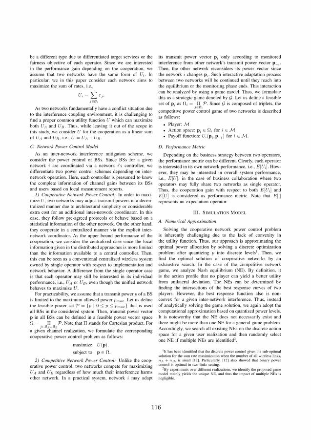
be a different type due to differentiated target services or thefairness objective of each operator. Since we are interestedin the performance gain depending on the cooperation, weassume that two networks have the same form of Ui. Inparticular, we in this paper consider each network aims tomaximize the sum of rates, i.e.,

Ui =∑

j∈Bi

rj .

As two networks fundamentally have a conflict situation dueto the interference coupling environment, it is challenging tofind a proper common utility function U which can maximizeboth UA and UB . Thus, while leaving it out of the scope inthis study, we consider U for the cooperation as a linear sumof UA and UB , i.e., U = UA + UB .

C. Network Power Control Model

As an inter-network interference mitigation scheme, weconsider the power control of BSs. Since BSs for a givennetwork i are coordinated via a network i’s controller, wedifferentiate two power control schemes depending on inter-network operation. Here, each controller is presumed to knowthe complete information of channel gains between its BSsand users based on local measurement reports.

1) Cooperative Network Power Control: In order to maxi-mize U , two networks may adjust transmit powers in a decen-tralized manner due to architectural simplicity or considerableextra cost for an additional inter-network coordinator. In thiscase, they follow pre-agreed protocols or behave based on astatistical information of the other network. On the other hand,they cooperate in a centralized manner via the explicit inter-network coordinator. As the upper bound performance of thecooperation, we consider the centralized case since the localinformation given in the distributed approaches is more limitedthan the information available to a central controller. Then,this can be seen as a conventional centralized wireless systemowned by single operator with respect to implementation andnetwork behavior. A difference from the single operator caseis that each operator may still be interested in its individualperformance, i.e., UA or UB , even though the unified networkbehaves to maximize U .

For practicability, we assume that a transmit power p of a BSis limited to the maximum allowed power pmax. Let us definethe feasible power set P = p | 0 ≤ p ≤ pmax that is usedall BSs in the considered system. Then, transmit power vectorp in all BSs can be defined in a feasible power vector spaceΩ = Π

j∈BA∪BB

P . Note that Π stands for Cartesian product. For

a given channel realization, we formulate the correspondingcooperative power control problem as follows:

maximize U(p),


2) Competitive Network Power Control: Unlike the coop-erative power control, two networks compete for maximizingUA and UB regardless of how much their interference harmsother network. In a practical system, network i may adapt

its transmit power vector pi only according to monitoredinterference from other network’s transmit power vector p−i.Then, the other network reconsiders its power vector sincethe network i changes pi. Such interactive adaptation processbetween two networks will be continued until they reach intothe equilibrium or the monitoring phase ends. This interactioncan be analyzed by using a game model. Thus, we formulatethis as a strategic game denoted by G. Let us define a feasibleset of pi as Ωi = Π

j∈Bi

P . Since G is composed of triplets, the

competitive power control game of two networks is describedas follows:


D. Performance Metric

Depending on the business strategy between two operators,the performance metric can be different. Clearly, each operatoris interested in its own network performance, i.e., E[Ui]. How-ever, they may be interested in overall system performance,i.e., E[U ], in the case of business collaboration where twooperators may fully share two networks as single operator.Thus, the cooperation gain with respect to both E[Ui] andE[U ] is considered as performance metric. Note that E[·]represents an expectation operator.

III. SIMULATION MODEL

A. Numerical Approximation

Solving the cooperative network power control problemis inherently challenging due to the lack of convexity inthe utility function. Thus, our approach is approximating theoptimal power allocation by solving a discrete optimizationproblem after quantizing p into discrete levels1. Then, wefind the optimal solution of cooperative networks by anexhaustive search. In the case of the competitive networkgame, we analyze Nash equilibrium (NE). By definition, itis the action profile that no player can yield a better utilityfrom unilateral deviation. The NEs can be determined byfinding the intersections of the best response curves of twoplayers. However, the best response function also is non-convex for a given inter-network interference. Thus, insteadof analytically solving the game solution, we again adopt thecomputational approximation based on quantized power levels.It is noteworthy that the NE does not necessarily exist andthere might be more than one NE for a general game problem.Accordingly, we search all existing NEs on the discrete actionspace for a given user realization and then randomly selectone NE if multiple NEs are identified2.

1It has been identified that the discrete power control gives the sub-optimalsolution for the sum rate maximization when the number of all wireless links,nA + nB , is small [12]. Particularly, [12] also showed that binary powercontrol is optimal in two links setting.

2By experiments over different realizations, we identify the proposed gamemodel mainly yields the unique NE, and thus the impact of multiple NEs isnegligible.

116

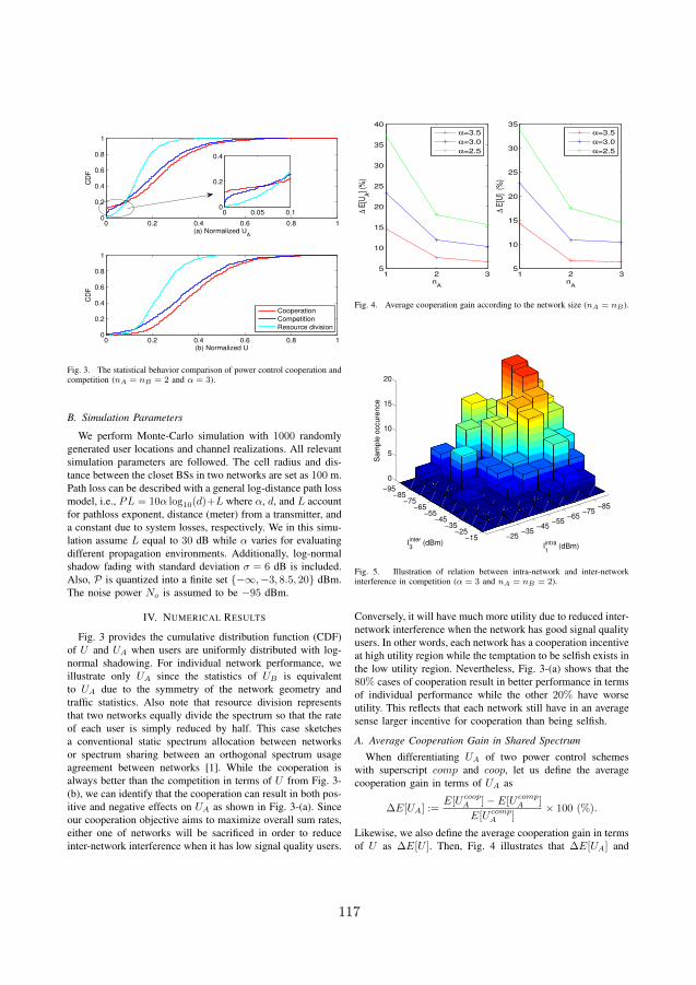
0 0.2 0.4 0.6 0.8 10

0.2

0.4

0.6

0.8

1

CD

F

(a) Normalized UA

0 0.2 0.4 0.6 0.8 10

0.2

0.4

0.6

0.8

1

(b) Normalized U

CD

F

Cooperation

Competition

Resource division

0 0.05 0.10

0.2

0.4

Fig. 3. The statistical behavior comparison of power control cooperation andcompetition (nA = nB = 2 and α = 3).

B. Simulation Parameters

We perform Monte-Carlo simulation with 1000 randomlygenerated user locations and channel realizations. All relevantsimulation parameters are followed. The cell radius and dis-tance between the closet BSs in two networks are set as 100 m.Path loss can be described with a general log-distance path lossmodel, i.e., PL = 10α log10(d)+L where α, d, and L accountfor pathloss exponent, distance (meter) from a transmitter, anda constant due to system losses, respectively. We in this simu-lation assume L equal to 30 dB while α varies for evaluatingdifferent propagation environments. Additionally, log-normalshadow fading with standard deviation σ = 6 dB is included.Also, P is quantized into a finite set −∞, −3, 8.5, 20 dBm.The noise power No is assumed to be −95 dBm.


Fig. 3 provides the cumulative distribution function (CDF)of U and UA when users are uniformly distributed with log-normal shadowing. For individual network performance, weillustrate only UA since the statistics of UB is equivalentto UA due to the symmetry of the network geometry andtraffic statistics. Also note that resource division representsthat two networks equally divide the spectrum so that the rateof each user is simply reduced by half. This case sketchesa conventional static spectrum allocation between networksor spectrum sharing between an orthogonal spectrum usageagreement between networks [1]. While the cooperation isalways better than the competition in terms of U from Fig. 3-(b), we can identify that the cooperation can result in both pos-itive and negative effects on UA as shown in Fig. 3-(a). Sinceour cooperation objective aims to maximize overall sum rates,either one of networks will be sacrificed in order to reduceinter-network interference when it has low signal quality users.

1 2 35

10

15

20

25

30

35

40

nA

∆ E

[UA] (

%)

1 2 35

10

15

20

25

30

35

nA

∆ E

[U]

(%)

α=3.5

α=3.0

α=2.5

α=3.5

α=3.0

α=2.5

Fig. 4. Average cooperation gain according to the network size (nA = nB).

−85−75

−65−55

−45−35

−25

−95−85

−75−65

−55−45

−35−25

−15

0

5

10

15

20

Iintra

1 (dBm)I

inter

3 (dBm)

Sa

mp

le o

ccu

ren

ce

Fig. 5. Illustration of relation between intra-network and inter-networkinterference in competition (α = 3 and nA = nB = 2).

Conversely, it will have much more utility due to reduced inter-network interference when the network has good signal qualityusers. In other words, each network has a cooperation incentiveat high utility region while the temptation to be selfish exists inthe low utility region. Nevertheless, Fig. 3-(a) shows that the80% cases of cooperation result in better performance in termsof individual performance while the other 20% have worseutility. This reflects that each network still have in an averagesense larger incentive for cooperation than being selfish.

A. Average Cooperation Gain in Shared Spectrum

When differentiating UA of two power control schemeswith superscript comp and coop, let us define the averagecooperation gain in terms of UA as

∆E[UA] :=E[U coop

A ] − E[U compA ]

E[U compA ]

× 100 (%).

Likewise, we also define the average cooperation gain in termsof U as ∆E[U ]. Then, Fig. 4 illustrates that ∆E[UA] and

117

0 20 40 600

2

4

6

8

10

12

14

16

18


∆ E

[UA] (

%)

α=3.5

α=3.0

α=2.5

0 20 40 600

2

4

6

8

10

12

14

16

18

20


∆ E

[U]

(%)

α=3.5

α=3.0

α=2.5

Fig. 6. Network separation effect (nA = nB = 2).

∆E[U ] drastically drops as the network size increases re-gardless of α. This implies that cooperation between mutuallyinterfering networks may not be highly attractive as the net-work size increases. This effect can be explained in two ways.As the network size increases, the service area over whichthe inter-network interference affects is reduced so that moreusers in a given network relatively becomes decoupled fromother BSs in other network. In addition, when each networkowns multiple BSs, the intra-network interference mitigationbenefits lowering inter-network interference. In other words,the selfish behavior to its own network can also reduce theharmful interference to other network. Fig. 5 illustrates anexample statistics of NEs where reduced interference to itself,i.e., user 1, benefits other user, i.e., user 3 in the other network.This reflects that mutually beneficial decisions occur evenduring network-wide competition. Note that this phenomenonnever happens in the case of nA = nB = 1 where each BSalways gives full interference to the other BS if they are incompetition.

B. Deployment Principle in Shared Spectrum

As discussed in Section II, one of realistic assumptions formulti-operator deployments is that each network somehow isseparated, e.g., geographically or with high wall penetration.∆E[UA] and ∆E[U ] are plotted in Fig. 6 according to addi-tional constant path loss in channel gains across two networks,i.e., network separation. When typical outer building wallpenetration loss is presumed as 20 dB [13], equivalently 40 dBnetwork separation between two adjacent buildings, deployinga network at the neighboring building may not be criticalwithout agreed cooperation. In the figure, the cooperation gainat 40 dB network separation turns very marginal, i.e., less than2% in a highly interference coupled situation with α = 2.5. Inother words, the incentive for cooperation between networksmay lose a value when an operator deploys a network in closebuildings.

V. CONCLUSION

When small-sized cellular networks owned by differentoperators are deployed in interference range on shared spec-

trum, we addressed a cooperative and a competitive powercontrol problem. From the evaluation results, we identifiedthat there exist both cooperative and competitive incentivesfor each network sum rate maximization according to a utilityregion. By comparing Nash equilibria and the social optimalpower allocation, we also found in an average sense that thecooperation improves not only an overall system performancebut also an individual network performance. Nevertheless, thecooperation incentive is drastically reduced as the size ofnetwork increases since interference between two networkscan be mitigated by self-motivated interference reductioninside of each network. From this, operators may not haveenough motivation for cooperation to suppress strategic costsuch as business-wise agreement. Additionally, by exploringthe network separation effect, we identified that only marginalseparation, e.g., deployments in adjacent buildings, makes thecompetition comparable to the cooperation due to sufficientlydecoupled interference from adjacent networks. These resultsare under a network symmetry assumption. Thus, asymmetricnetworks need to be studied as a future work.

ACKNOWLEDGMENT


REFERENCES

[1] P. Lin, J. Jia, Q. Zhang, and M. Hamdi, “Cooperation among Wire-less Service Providers: Opportunity, Challenge, and Solution ,” IEEEWireless Commun. Mag., vol. 17, no. 4, pp. 55–61, Aug. 2010.

[2] J. Zander, “Competitive Wireless Multi-Access - Implications and Re-search Issues,” in Proc. IEEE PIMRC, Helsinki, Finland, Sep. 2006.

[3] R. Etkin, A. Parekh, and D. Tse, “Spectrum Sharing for UnlicensedBands,” IEEE J. Select. Areas Commun., vol. 25, no. 3, pp. 517–528,2007.

[4] E. G. Larsson and E. A. Jorswieck, “Competition Versus Cooperationon the MISO Interference Channel,” IEEE J. Select. Areas Commun.,vol. 26, no. 7, pp. 1059–1069, 2008.

[5] M. Bennis, M. Debbah, S. Lasaulce, and A. Anpalagan, “A HierarchicalGame Approach to Inter-Operator Spectrum Sharing,” in Proc. IEEEGlobecom, Honolulu, USA, Nov. 2009.

[6] M. M. Halldorsson, J. Y. Halpern, L. Li, and V. Mirrokni, “On SpectrumSharing Games,” in Procedings of the Twenty-Third Annual ACMSymposium on Principles of Distributed Computing, 2004.

[7] K. Johansson, M. Kristensson, and U. Schwarz, “Radio ResourceManagement in Roaming based Multi-operator WCDMA Networks,”in Proc. IEEE VTC, Milan, Italy, May 2004.

[8] J. Hultell, “Cooperative and non-cooperative wireless access: Resourceand infrastructure sharing regimes,” Ph.D. dissertation, Royal Instituteof Technology (KTH), 2008.

[9] M. Felegyhazi and J.-P. Hubaux, “Wireless Operators in a SharedSpectrum,” in Proc. IEEE INFOCOM, Barcelona, Spain, Apr. 2006.

[10] M. Felegyhazi, M. Cagalj, D. Dufour, and J.-P. Hubaux, “Border Gamesin Cellular Networks,” in Proc. IEEE INFOCOM, Anchorage, USA, May2007.

[11] L. H. Grokop and D. N. C. Tse, “Spectrum Sharing Between WirelessNetworks,” IEEE/ACM Trans. Networking, vol. 18, no. 5, pp. 1401–1412, Oct. 2010.

[12] A. Gjendemsjϕ, D. Gesbert, G. E. ϕien, and S. G. Kiani, “Binary PowerControl for Sum Rate Maximization over Multiple Interfering Links,”IEEE Trans. Wireless Commun., vol. 7, no. 8, pp. 3164 –3173, Aug.2008.

[13] 3GPP TR 36.814, Technical Specification Group Radio Access Net-work; Evolved Universal Terrestrial Radio Access (E-UTRA); Furtheradvancements for E-UTRA physical layer aspects (Release 9), 3GPP,Mar. 2010.

118

Cost Effective Interference Management in Ultra-dense ...

Documents

Transcript of Cost Effective Interference Management in Ultra-dense ...