Simulation of air flow in the IEA Annex 20 test room—validation of a simplified model for the...

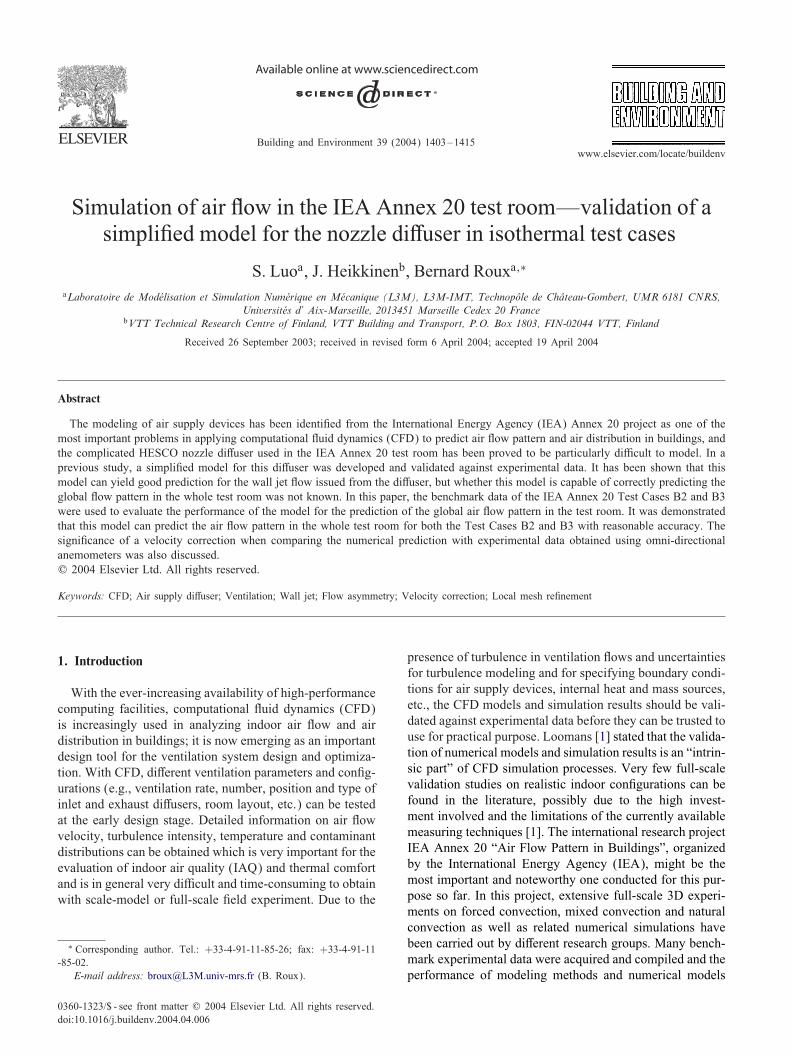
Building and Environment 39 (2004) 1403–1415www.elsevier.com/locate/buildenv

Simulation of air "ow in the IEA Annex 20 test room—validation of asimpli)ed model for the nozzle di+user in isothermal test cases

S. Luoa, J. Heikkinenb, Bernard Rouxa ;∗

aLaboratoire de Mod�elisation et Simulation Num�erique en M�ecanique (L3M), L3M-IMT, Technopole de Chateau-Gombert, UMR 6181 CNRS,Universit�es d’ Aix-Marseille, 2013451 Marseille Cedex 20 France

bVTT Technical Research Centre of Finland, VTT Building and Transport, P.O. Box 1803, FIN-02044 VTT, Finland

Received 26 September 2003; received in revised form 6 April 2004; accepted 19 April 2004

Abstract

The modeling of air supply devices has been identi)ed from the International Energy Agency (IEA) Annex 20 project as one of themost important problems in applying computational "uid dynamics (CFD) to predict air "ow pattern and air distribution in buildings, andthe complicated HESCO nozzle di+user used in the IEA Annex 20 test room has been proved to be particularly di;cult to model. In aprevious study, a simpli)ed model for this di+user was developed and validated against experimental data. It has been shown that thismodel can yield good prediction for the wall jet "ow issued from the di+user, but whether this model is capable of correctly predicting theglobal "ow pattern in the whole test room was not known. In this paper, the benchmark data of the IEA Annex 20 Test Cases B2 and B3were used to evaluate the performance of the model for the prediction of the global air "ow pattern in the test room. It was demonstratedthat this model can predict the air "ow pattern in the whole test room for both the Test Cases B2 and B3 with reasonable accuracy. Thesigni)cance of a velocity correction when comparing the numerical prediction with experimental data obtained using omni-directionalanemometers was also discussed.? 2004 Elsevier Ltd. All rights reserved.

Keywords: CFD; Air supply di+user; Ventilation; Wall jet; Flow asymmetry; Velocity correction; Local mesh re)nement

1. Introduction

With the ever-increasing availability of high-performancecomputing facilities, computational "uid dynamics (CFD)is increasingly used in analyzing indoor air "ow and airdistribution in buildings; it is now emerging as an importantdesign tool for the ventilation system design and optimiza-tion. With CFD, di+erent ventilation parameters and con)g-urations (e.g., ventilation rate, number, position and type ofinlet and exhaust di+users, room layout, etc.) can be testedat the early design stage. Detailed information on air "owvelocity, turbulence intensity, temperature and contaminantdistributions can be obtained which is very important for theevaluation of indoor air quality (IAQ) and thermal comfortand is in general very di;cult and time-consuming to obtainwith scale-model or full-scale )eld experiment. Due to the

∗ Corresponding author. Tel.: +33-4-91-11-85-26; fax: +33-4-91-11-85-02.

E-mail address: [email protected] (B. Roux).

presence of turbulence in ventilation "ows and uncertaintiesfor turbulence modeling and for specifying boundary condi-tions for air supply devices, internal heat and mass sources,etc., the CFD models and simulation results should be vali-dated against experimental data before they can be trusted touse for practical purpose. Loomans [1] stated that the valida-tion of numerical models and simulation results is an “intrin-sic part” of CFD simulation processes. Very few full-scalevalidation studies on realistic indoor con)gurations can befound in the literature, possibly due to the high invest-ment involved and the limitations of the currently availablemeasuring techniques [1]. The international research projectIEA Annex 20 “Air Flow Pattern in Buildings”, organizedby the International Energy Agency (IEA), might be themost important and noteworthy one conducted for this pur-pose so far. In this project, extensive full-scale 3D experi-ments on forced convection, mixed convection and naturalconvection as well as related numerical simulations havebeen carried out by di+erent research groups. Many bench-mark experimental data were acquired and compiled and theperformance of modeling methods and numerical models

0360-1323/$ - see front matter ? 2004 Elsevier Ltd. All rights reserved.doi:10.1016/j.buildenv.2004.04.006

mailto:[email protected]

1404 S. Luo et al. / Building and Environment 39 (2004) 1403–1415

evaluated against the benchmark data. It was identi)ed thatthe modeling of turbulence and the modeling of the air sup-ply devices are two critical problems for the correct predic-tion of ventilation "ows in buildings.In the IEA Annex 20 project, for evaluating the capability

of CFD as a design tool for practical ventilation "ows andfor providing realistic benchmark data for evaluating CFDcodes, a complicated HESCO-type nozzle di+user was pur-posely chosen as the air supply device. The intention wasto test how such a complicated air supply di+user which isrepresentative of modern air supply devices can be modeledin numerical simulations and what are the consequences ofdi+erent modeling approaches [2]. It was proved that such acomplicated di+user is particularly di;cult to model [3]. Afull resolution of the di+user in the numerical simulation isnot practical because that would necessitate a prohibitivelylarge number of grid cells in the region near the di+userand would then demand a too large computational resourceto carry out the simulation. Several simpli)ed models, i.e.,the “basic model”, the “box model”, the “prescribed veloc-ity model” and the “momentum model” for the di+user havebeen proposed and tested in the IEA Annex 20 framework.These models can give somewhat qualitatively or quantita-tively correct prediction for the benchmark test cases butnone of them is very satisfactory [2,4–6]. Recently, Chenand Srebric [4] re-examined the momentum model and thebox model for the modeling of the nozzle di+user, they con-cluded that the box model is the best model for this kindof di+user in the numerical simulation of ventilation "ows.Their box model necessitates the measured velocity pro)les(also temperature pro)les for non-isothermal cases and con-centration pro)les for cases with species transport) to beused as the boundary conditions on the box surfaces whichare in general not readily available, and signi)cant e+ortsare required to specify the measured data on the box surfacesas the boundary conditions. A more general and easy-to-usemodel for this kind of di+user is highly desirable for widerapplications of numerical simulation of ventilation "ows.In a previous study [7], a simpli)ed model for the IEA

Annex 20 nozzle di+user has been developed and validatedagainst the experimental measurements of Ewert et al. [8]and Heikkinen [5]. It was demonstrated that the model canyield good prediction for the wall jet "ow issued from thedi+user, especially for the streamwise velocity pro)les, thecorrelation between the prediction and experimental mea-surements is excellent. It was also noticed that the velocityat the lower part of the wall jet is somewhat under-predicted,which is mainly the consequence of the incorrect predictionof the spanwise and crosswise velocity components, i.e., the3D development of the wall jet. Because the jet momen-tum is mainly contained in the jet center plane which is themain driving force of the isothermal room air motion [4], itwas believed that this under-prediction of the wall jet "owwould not greatly a+ect the prediction of the global "owpattern inside the room. This needs to be validated againstexperimental data. The aim of the present study is to further

evaluate the capability of this model for the prediction ofthe global air "ow pattern in the whole test room by com-parison with the benchmark data of the IEA Annex 20 TestCases B2 and B3 reported by Heikkinen [9]. The simulationresults as well as the comparison with experimental data arereported in detail.

2. Experiment setup

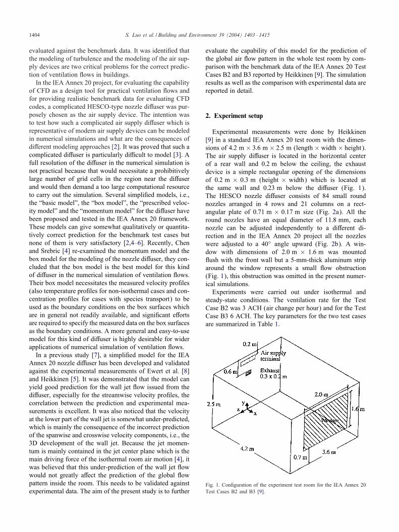
Experimental measurements were done by Heikkinen[9] in a standard IEA Annex 20 test room with the dimen-sions of 4:2 m × 3:6 m × 2:5 m (length × width × height).The air supply di+user is located in the horizontal centerof a rear wall and 0:2 m below the ceiling, the exhaustdevice is a simple rectangular opening of the dimensionsof 0:2 m × 0:3 m (height × width) which is located atthe same wall and 0:23 m below the di+user (Fig. 1).The HESCO nozzle di+user consists of 84 small roundnozzles arranged in 4 rows and 21 columns on a rect-angular plate of 0:71 m × 0:17 m size (Fig. 2a). All theround nozzles have an equal diameter of 11:8 mm, eachnozzle can be adjusted independently to a di+erent di-rection and in the IEA Annex 20 project all the nozzleswere adjusted to a 40◦ angle upward (Fig. 2b). A win-dow with dimensions of 2:0 m × 1:6 m was mounted"ush with the front wall but a 5-mm-thick aluminum striparound the window represents a small "ow obstruction(Fig. 1), this obstruction was omitted in the present numer-ical simulations.Experiments were carried out under isothermal and

steady-state conditions. The ventilation rate for the TestCase B2 was 3 ACH (air change per hour) and for the TestCase B3 6 ACH. The key parameters for the two test casesare summarized in Table 1.

Fig. 1. Con)guration of the experiment test room for the IEA Annex 20Test Cases B2 and B3 [9].

S. Luo et al. / Building and Environment 39 (2004) 1403–1415 1405

Fig. 2. The HESCO nozzle di+user used in the IEA Annex 20 project[4,13]. (a) HESCO nozzle di+user, (b) orientation of the nozzles.

Table 1Key parameters for the IEA Annex 20 Test Cases B2 and B3 [9]

Case Ventilation Air"ow Supply Reynoldsrate (ACH) rate (m3=s) air temperature numbera

(◦C)

B2 3 0.0315 20 2620B3 6 0.0630 20 5240

aThe Reynolds numbers in the table are based on the diameter of thesmall nozzles.

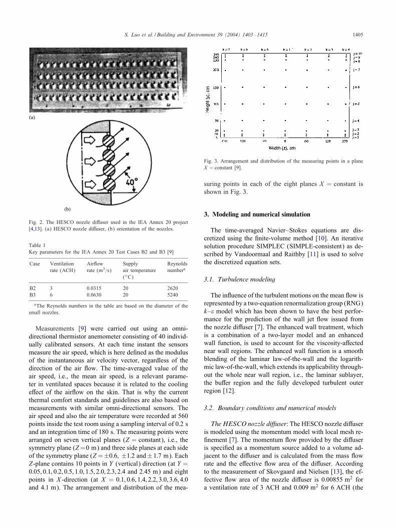
Measurements [9] were carried out using an omni-directional thermistor anemometer consisting of 40 individ-ually calibrated sensors. At each time instant the sensorsmeasure the air speed, which is here de)ned as the modulusof the instantaneous air velocity vector, regardless of thedirection of the air "ow. The time-averaged value of theair speed, i.e., the mean air speed, is a relevant parame-ter in ventilated spaces because it is related to the coolinge+ect of the air"ow on the skin. That is why the currentthermal comfort standards and guidelines are also based onmeasurements with similar omni-directional sensors. Theair speed and also the air temperature were recorded at 560points inside the test room using a sampling interval of 0:2 sand an integration time of 180 s. The measuring points werearranged on seven vertical planes (Z = constant), i.e., thesymmetry plane (Z=0 m) and three side planes at each sideof the symmetry plane (Z=±0:6; ±1:2 and±1:7 m). EachZ-plane contains 10 points in Y (vertical) direction (at Y =0:05; 0:1; 0:2; 0:5; 1:0; 1:5; 2:0; 2:3; 2:4 and 2:45 m) and eightpoints in X -direction (at X = 0:1; 0:6; 1:4; 2:2; 3:0; 3:6; 4:0and 4:1 m). The arrangement and distribution of the mea-

Fig. 3. Arrangement and distribution of the measuring points in a planeX = constant [9].

suring points in each of the eight planes X = constant isshown in Fig. 3.

3. Modeling and numerical simulation

The time-averaged Navier–Stokes equations are dis-cretized using the )nite-volume method [10]. An iterativesolution procedure SIMPLEC (SIMPLE-consistent) as de-scribed by Vandoormaal and Raithby [11] is used to solvethe discretized equation sets.

3.1. Turbulence modeling

The in"uence of the turbulent motions on the mean "ow isrepresented by a two-equation renormalization group (RNG)k–� model which has been shown to have the best perfor-mance for the prediction of the wall jet "ow issued fromthe nozzle di+user [7]. The enhanced wall treatment, whichis a combination of a two-layer model and an enhancedwall function, is used to account for the viscosity-a+ectednear wall regions. The enhanced wall function is a smoothblending of the laminar law-of-the-wall and the logarith-mic law-of-the-wall, which extends its applicability through-out the whole near wall region, i.e., the laminar sublayer,the bu+er region and the fully developed turbulent outerregion [12].

3.2. Boundary conditions and numerical models

The HESCO nozzle di@user: The HESCO nozzle di+useris modeled using the momentum model with local mesh re-)nement [7]. The momentum "ow provided by the di+useris speci)ed as a momentum source added to a volume ad-jacent to the di+user and is calculated from the mass "owrate and the e+ective "ow area of the di+user. Accordingto the measurement of Skovgaard and Nielsen [13], the ef-fective "ow area of the nozzle di+user is 0:00855 m2 fora ventilation rate of 3 ACH and 0:009 m2 for 6 ACH (the


total gross "ow area of the small nozzles is 0:00918 m2).At the supply opening, the total mass "ow rate and the "owdirection are speci)ed. It was established from a previousstudy [7] that the volume of the momentum source cells isan important parameter for the correct prediction of the walljet pro)les. For a ventilation rate of 3 ACH, the dimensionof the momentum source cells in the streamwise directionshould be between 0.014 and 0:018 m. In the present study,the dimension of the momentum source cells in the stream-wise dimension is chosen as 0:015 m for both the ventilationrates of 3 and 6 ACH. The detail of the modeling methodfor the di+user was reported in [7].Exhaust opening: The exhaust opening is speci)ed as a

pressure outlet, i.e., the gauge pressure at the outlet is set aszero (Dirichlet condition).Turbulence quantities: According to Skovgaard and

Nielsen [13] and Lemaire [3], the inlet turbulence intensityis assumed to be 10%. At the exhaust opening, a turbu-lence intensity of 5% is assumed which will be used only ifthere is back"ow at the outlet in the early iteration stage tominimize the convergence problems. The boundary condi-tions for k and � are obtained by specifying the turbulenceintensity and hydraulic diameter of the di+user [12,13]:

kinlet = 1:5I 2U 2inlet ;

�inlet = C3=4� k3=2inlet=l;

where I is the turbulence intensity, l is the length scale ofthe di+user (l= 0:07D [12,13], D is the hydraulic diameterof the di+user (D = 0:35 m); Uinlet is the average velocityat the inlet and C� is a constant which is 0.09.Discretization schemes: The second-order upwind

scheme is used for the discretization of the convection termsand the second-order central-di+erencing scheme for thedi+usion terms. For the discretization of the pressure, thePRESTO! (pressure staggering option) scheme is used [12].The SIMPLEC scheme is used for the pressure–velocitycoupling.A "ow solver FLUENT 6 is used to carry out the

simulations.

3.3. Computation grids

Flow asymmetry was observed in the numerical simula-tions for a ventilation rate of 3 ACH in a previous study [7].In the full-scale experiment of Heikkinen [9], "ow asymme-try was also observed for both the Test Cases B2 and B3.For this reason, simulations are carried out in both the half-and full-room con)gurations with the aim to evaluate thein"uence of the symmetry boundary condition often used tosave the computation time.It was determined from [7] that for a ventilation rate of

3 ACH, a mesh grid of 55× 57× 38 for the half-room con-)guration and 55 × 57 × 76 for the full-room con)gura-tion (the other half mesh of the full room is mirrored fromthe half-room mesh) represent a good compromise between

the mesh resolution requirements and the available compu-tational resources, these meshes are adopted in the presentstudy for both Test Cases B2 and B3. The mesh grids aremore condensed near the walls and in the jet "ow region,where more steep velocity gradients are expected. For thehalf-room con)guration, a symmetry boundary condition isapplied at the symmetry plane (Z = 0 m) of the test room.

3.4. Local mesh reBnement

A local mesh re)nement was applied in the region nearthe di+user which has been proven to be crucial for thecorrect prediction of the wall jet pro)les [7] and the smallrecirculation "ow between the di+user and the room ceilingobserved by smoke visualization [5].For the half-room con)guration, the local mesh re)nement

is applied in the region from X = 0 to 0:3 m; Y = 2:13 to2:5 m and Z =0 to 0:355 m; for the full room con)gurationthe mesh in the region of X=0–0:3 m; Y=2:13–2:5 m; Z=0:355–0:355 m is locally re)ned. Each grid cell in the regionis halved in each coordinate direction; thus, each cell isdivided into eight cells, which results in a total of 140 690cells for the half-room con)guration and 281 380 cells forthe full room con)guration. The detail of the local meshre)nement is described in [7].

3.5. Velocity correction

The measurement [9] was carried out using conventionalomni-directional hot sphere sensors to obtain the mean airspeed Vo that is the average of the instantaneous velocitymodulus during the measuring period of 180 s. To comparewith the steady-state CFD simulations one must note thatthe mean air speed is always higher than the velocity vectormodulus Vv because of velocity "uctuations, as explained in[14,15]. The latter quantity is directly obtained from com-puted mean velocity components, with the following de)-nition: Vv =

√Tu 2 + Tv2 + Tw2. The di+erence between these

two velocities may become considerable when the local tur-bulence intensity is high and the air speed is slow [14,15].For this reason, a correction formula to calculate Vo from

Vv and turbulence intensity was developed in [14,15]. Thecorrection is based on a model for isotropic turbulence andwas validated on extensive measurements of room air "ows.This correction formula is adopted in the present study tobetter compare the simulation results with experimental data,it has the following form [15]:VoVv

= 1 + I 2v (for Iv6 0:45); (1)

VoVv

=1:596× I 2v + 0:266× Iv + 0:308

0:173 + Iv

(for Iv¿ 0:45); (2)

where Vo is the omni-directional mean air speed and Vvis the modulus of the mean velocity vector. Iv is the


turbulence intensity which by de)nition can be obtainedfrom the turbulent kinetic energy k and Vv:

Iv =1Vv

√23k: (3)

The above correction formula was coded into the "ow solverto obtain Vo from Vv.

3.6. Comparison of the predicted velocity proBles withmeasurements

The pro)les of the mean air speed (i.e., the predictedvelocity modulus modi)ed according to Eqs. (1) and (2) are

Room Length (m)

Mea

n A

ir S

pee

d (

m/s

)

0 0.6 1.2 1.8 2.4 3 3.6 4.20

0.04

0.08

0.12

0.16

0.2

Room Length (m)

Mea

n A

ir S

pee

d (

m/s

)

0 0.6 1.2 1.8 2.4 3 3.6 4.20

0.04

0.08

0.12

0.16

0.

Room Length (m)

Mea

n A

ir S

pee

d (

m/s

)

0 0.6 1.2 1.8 2.4 3 3.6 4.20

0.05

0.1

0.15

0.2

0.25

Room Length (m)

Mea

n A

ir S

pee

d (

m/s

)

0 0.6 1.2 1.8 2.4 3 3.6 4.20

0.05

0.1

0.15

0.2

0.25

Room Length (m)

Mea

n A

ir S

pee

d (

m/s

)

0 0.6 1.2 1.8 2.4 3 3.6 4.20

0.08

0.16

0.24

0.32

0.4

Room Length (m)

Mea

n A

ir S

pee

d (

m/s

)

0 0.6 1.2 1.8 2.4 3 3.6 4.20

0.08

0.16

0.24

0.32

0.4

Y=0.05m, Z=0mHalf RoomFull RoomHeikkinen (1991)




Y=1m, Z=0mHalf RoomFull RoomHeikkinen (1991)


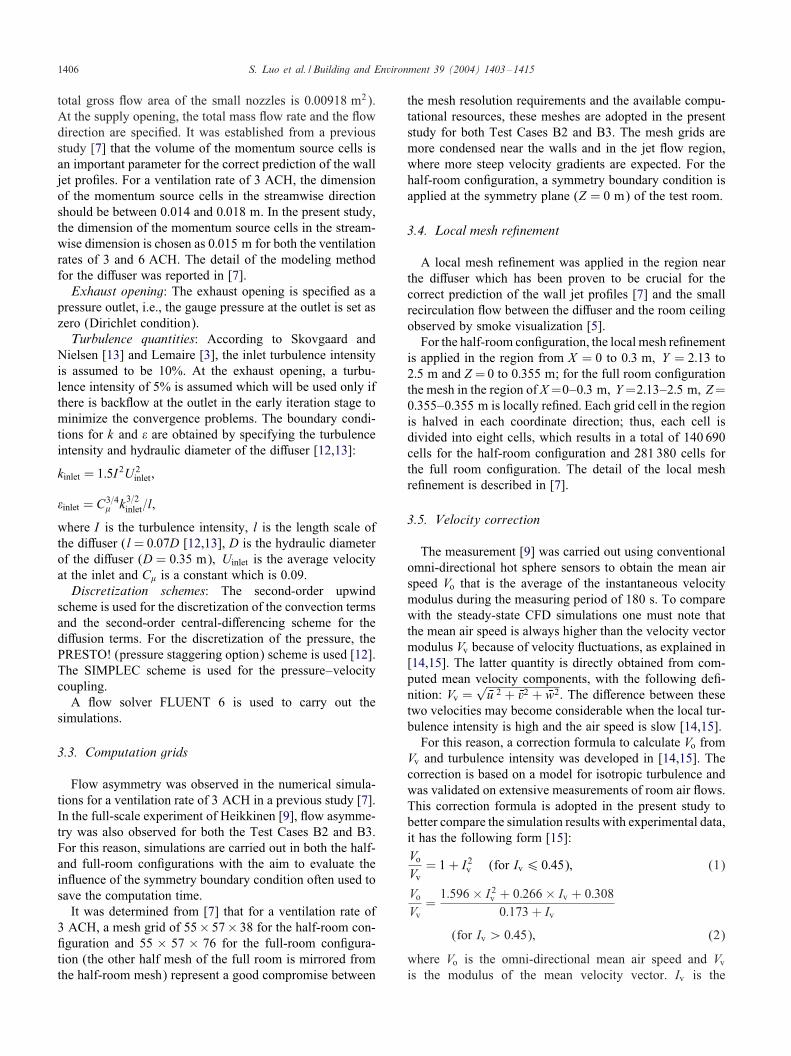
Fig. 4. Comparison between the predicted mean air speed pro)les for half- and full-room simulations, and the experimental data, in the symmetry plane(Test Case B2).

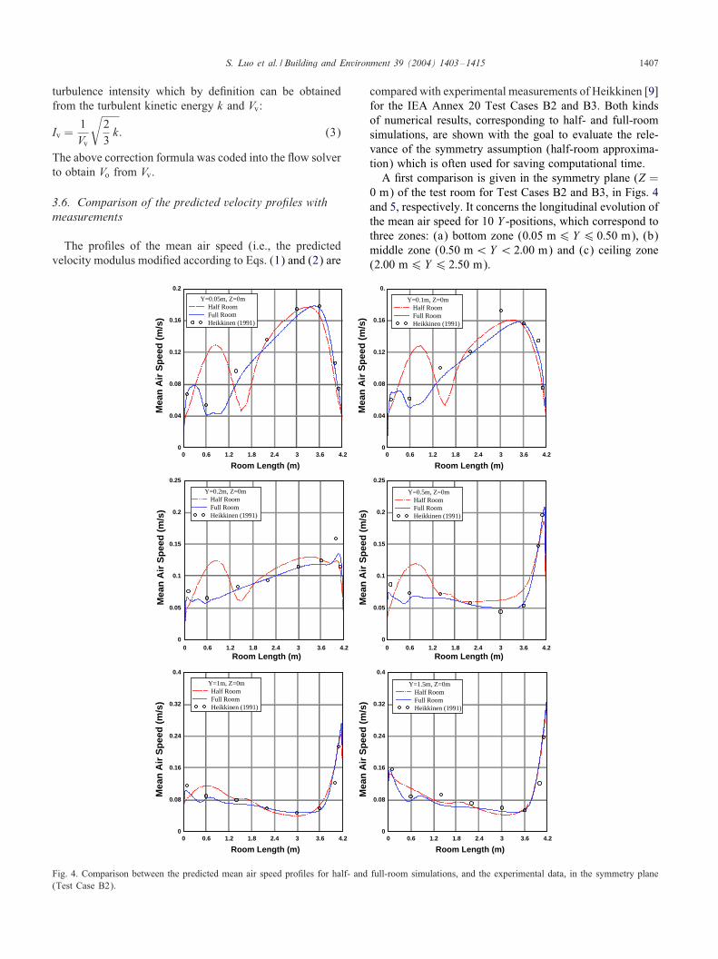
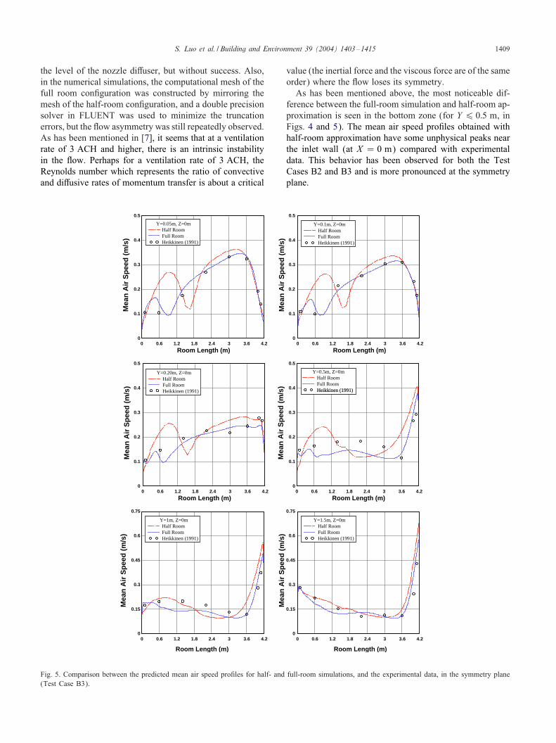
compared with experimental measurements of Heikkinen [9]for the IEA Annex 20 Test Cases B2 and B3. Both kindsof numerical results, corresponding to half- and full-roomsimulations, are shown with the goal to evaluate the rele-vance of the symmetry assumption (half-room approxima-tion) which is often used for saving computational time.A )rst comparison is given in the symmetry plane (Z =

0 m) of the test room for Test Cases B2 and B3, in Figs. 4and 5, respectively. It concerns the longitudinal evolution ofthe mean air speed for 10 Y -positions, which correspond tothree zones: (a) bottom zone (0:05 m6Y 6 0:50 m), (b)middle zone (0:50 m¡Y ¡ 2:00 m) and (c) ceiling zone(2:00 m6Y 6 2:50 m).


Room Length (m)

Mea

n A

ir S

pee

d (

m/s

)

0 0.6 1.2 1.8 2.4 3 3.6 4.20

0.08

0.16

0.24

0.32

0.4

Room Length (m)

Mea

n A

ir S

pee

d (

m/s

)

0 0.6 1.2 1.8 2.4 3 3.6 4.20

0.4

0.8

1.2

1.6

2

Room Length (m)

Mea

n A

ir S

pee

d (

m/s

)

0 0.6 1.2 1.8 2.4 3 3.6 4.20

0.4

0.8

1.2

1.6

2

Room Length (m)

Mea

n A

ir S

pee

d (

m/s

)

0 0.6 1.2 1.8 2.4 3 3.6 4.20

0.4

0.8

1.2

1.6

2





Fig. 4. (continued).

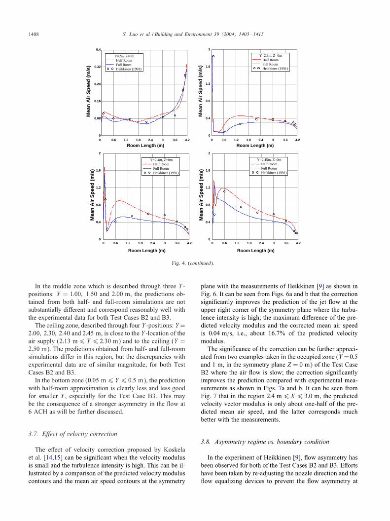
In the middle zone which is described through three Y -positions: Y = 1:00; 1:50 and 2:00 m, the predictions ob-tained from both half- and full-room simulations are notsubstantially di+erent and correspond reasonably well withthe experimental data for both Test Cases B2 and B3.The ceiling zone, described through four Y -positions: Y=

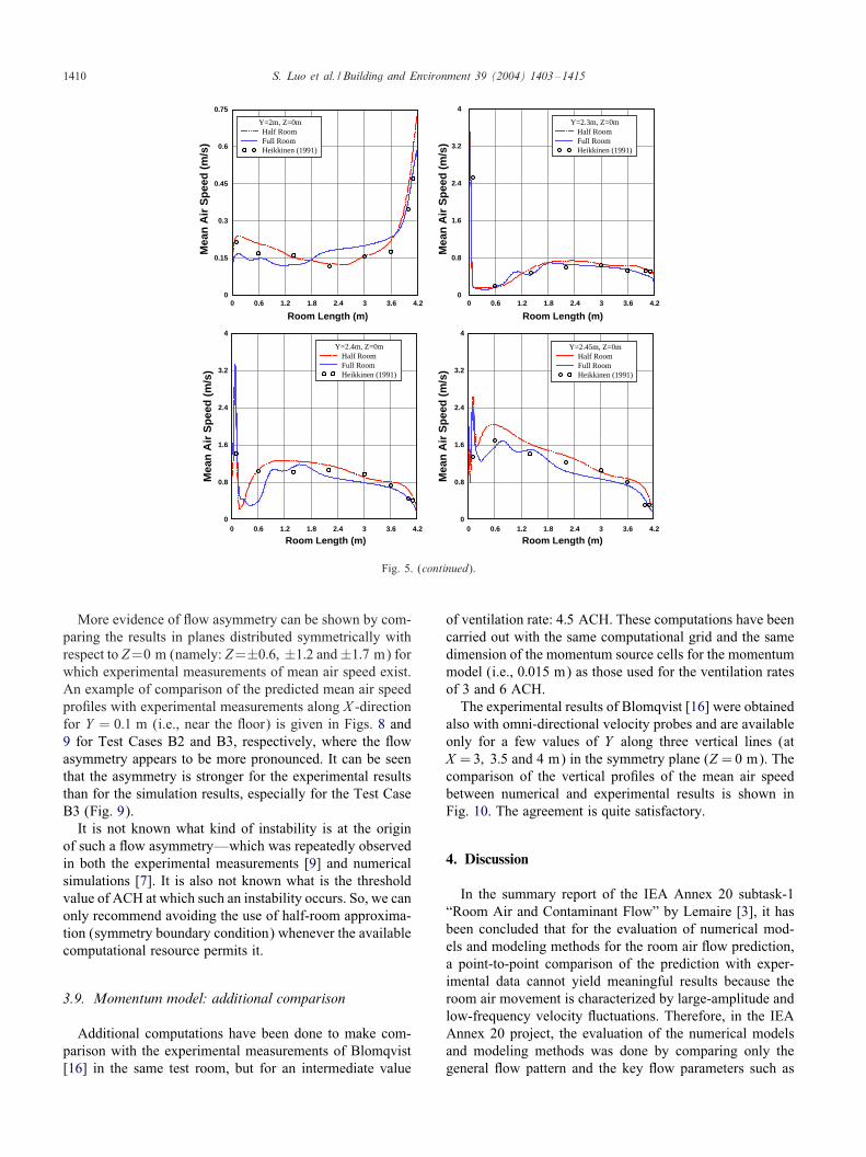
2:00; 2:30; 2:40 and 2:45 m, is close to the Y -location of theair supply (2:13 m6Y 6 2:30 m) and to the ceiling (Y =2:50 m). The predictions obtained from half- and full-roomsimulations di+er in this region, but the discrepancies withexperimental data are of similar magnitude, for both TestCases B2 and B3.In the bottom zone (0:05 m6Y 6 0:5 m), the prediction

with half-room approximation is clearly less and less goodfor smaller Y , especially for the Test Case B3. This maybe the consequence of a stronger asymmetry in the "ow at6 ACH as will be further discussed.

3.7. E@ect of velocity correction

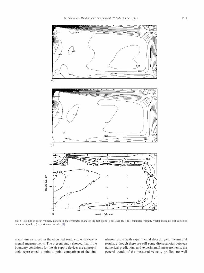
The e+ect of velocity correction proposed by Koskelaet al. [14,15] can be signi)cant when the velocity modulusis small and the turbulence intensity is high. This can be il-lustrated by a comparison of the predicted velocity moduluscontours and the mean air speed contours at the symmetry

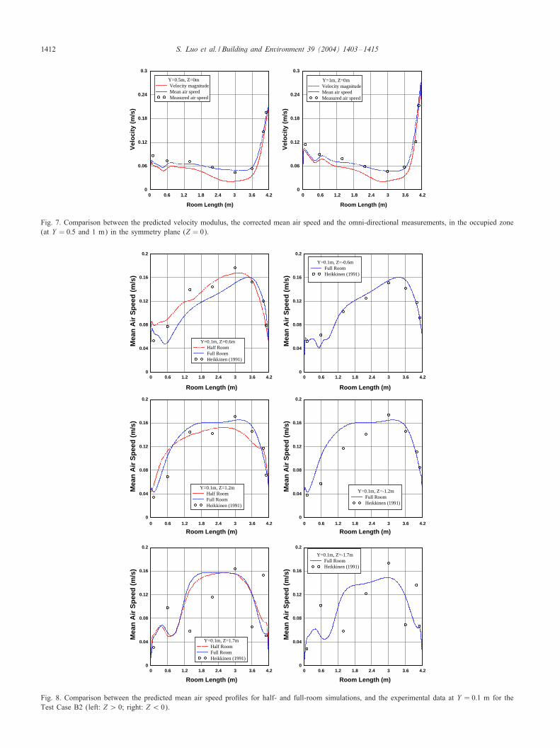
plane with the measurements of Heikkinen [9] as shown inFig. 6. It can be seen from Figs. 6a and b that the correctionsigni)cantly improves the prediction of the jet "ow at theupper right corner of the symmetry plane where the turbu-lence intensity is high; the maximum di+erence of the pre-dicted velocity modulus and the corrected mean air speedis 0:04 m=s, i.e., about 16.7% of the predicted velocitymodulus.The signi)cance of the correction can be further appreci-

ated from two examples taken in the occupied zone (Y =0:5and 1 m, in the symmetry plane Z = 0 m) of the Test CaseB2 where the air "ow is slow; the correction signi)cantlyimproves the prediction compared with experimental mea-surements as shown in Figs. 7a and b. It can be seen fromFig. 7 that in the region 2:4 m6X 6 3:0 m, the predictedvelocity vector modulus is only about one-half of the pre-dicted mean air speed, and the latter corresponds muchbetter with the measurements.

3.8. Asymmetry regime vs. boundary condition

In the experiment of Heikkinen [9], "ow asymmetry hasbeen observed for both of the Test Cases B2 and B3. E+ortshave been taken by re-adjusting the nozzle direction and the"ow equalizing devices to prevent the "ow asymmetry at


the level of the nozzle di+user, but without success. Also,in the numerical simulations, the computational mesh of thefull room con)guration was constructed by mirroring themesh of the half-room con)guration, and a double precisionsolver in FLUENT was used to minimize the truncationerrors, but the "ow asymmetry was still repeatedly observed.As has been mentioned in [7], it seems that at a ventilationrate of 3 ACH and higher, there is an intrinsic instabilityin the "ow. Perhaps for a ventilation rate of 3 ACH, theReynolds number which represents the ratio of convectiveand di+usive rates of momentum transfer is about a critical

Room Length (m)

Mea

n A

ir S

pee

d (

m/s

)

0 0.6 1.2 1.8 2.4 3 3.6 4.20

0.1

0.2

0.3

0.4

0.5

Room Length (m)

Mea

n A

ir S

pee

d (

m/s

)

0 0.6 1.2 1.8 2.4 3 3.6 4.20

0.1

0.2

0.3

0.4

0.5

Room Length (m)

Mea

n A

ir S

pee

d (

m/s

)

0 0.6 1.2 1.8 2.4 3 3.6 4.20

0.1

0.2

0.3

0.4

0.5

Room Length (m)

Mea

n A

ir S

pee

d (

m/s

)

0 0.6 1.2 1.8 2.4 3 3.6 4.20

0.1

0.2

0.3

0.4

0.5

Room Length (m)

Mea

n A

ir S

pee

d (

m/s

)

0 0.6 1.2 1.8 2.4 3 3.6 4.20

0.15

0.3

0.45

0.6

0.75

Room Length (m)

Mea

n A

ir S

pee

d (

m/s

)

0 0.6 1.2 1.8 2.4 3 3.6 4.20

0.15

0.3

0.45

0.6

0.75





Y=0.5m, Z=0mHalf RoomFull RoomHeikkinen (1991)Heikkinen (1991)


Fig. 5. Comparison between the predicted mean air speed pro)les for half- and full-room simulations, and the experimental data, in the symmetry plane(Test Case B3).

value (the inertial force and the viscous force are of the sameorder) where the "ow loses its symmetry.As has been mentioned above, the most noticeable dif-

ference between the full-room simulation and half-room ap-proximation is seen in the bottom zone (for Y 6 0:5 m, inFigs. 4 and 5). The mean air speed pro)les obtained withhalf-room approximation have some unphysical peaks nearthe inlet wall (at X = 0 m) compared with experimentaldata. This behavior has been observed for both the TestCases B2 and B3 and is more pronounced at the symmetryplane.


Room Length (m)

Mea

n A

ir S

pee

d (

m/s

)

0 0.6 1.2 1.8 2.4 3 3.6 4.20

0.15

0.3

0.45

0.6

0.75

Room Length (m)

Mea

n A

ir S

pee

d (

m/s

)

0 0.6 1.2 1.8 2.4 3 3.6 4.20

0.8

1.6

2.4

3.2

4

Room Length (m)

Mea

n A

ir S

pee

d (

m/s

)

0 0.6 1.2 1.8 2.4 3 3.6 4.20

0.8

1.6

2.4

3.2

4

Room Length (m)

Mea

n A

ir S

pee

d (

m/s

)

0 0.6 1.2 1.8 2.4 3 3.6 4.20

0.8

1.6

2.4

3.2

4





Fig. 5. (continued).

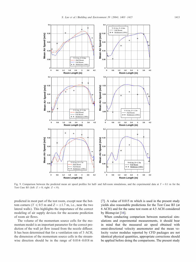
More evidence of "ow asymmetry can be shown by com-paring the results in planes distributed symmetrically withrespect to Z=0 m (namely: Z=±0:6; ±1:2 and±1:7 m) forwhich experimental measurements of mean air speed exist.An example of comparison of the predicted mean air speedpro)les with experimental measurements along X -directionfor Y = 0:1 m (i.e., near the "oor) is given in Figs. 8 and9 for Test Cases B2 and B3, respectively, where the "owasymmetry appears to be more pronounced. It can be seenthat the asymmetry is stronger for the experimental resultsthan for the simulation results, especially for the Test CaseB3 (Fig. 9).It is not known what kind of instability is at the origin

of such a "ow asymmetry—which was repeatedly observedin both the experimental measurements [9] and numericalsimulations [7]. It is also not known what is the thresholdvalue of ACH at which such an instability occurs. So, we canonly recommend avoiding the use of half-room approxima-tion (symmetry boundary condition) whenever the availablecomputational resource permits it.

3.9. Momentum model: additional comparison

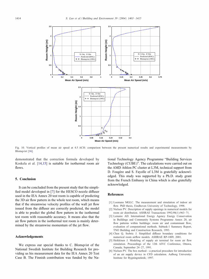
Additional computations have been done to make com-parison with the experimental measurements of Blomqvist[16] in the same test room, but for an intermediate value

of ventilation rate: 4:5 ACH. These computations have beencarried out with the same computational grid and the samedimension of the momentum source cells for the momentummodel (i.e., 0:015 m) as those used for the ventilation ratesof 3 and 6 ACH.The experimental results of Blomqvist [16] were obtained

also with omni-directional velocity probes and are availableonly for a few values of Y along three vertical lines (atX =3; 3:5 and 4 m) in the symmetry plane (Z =0 m). Thecomparison of the vertical pro)les of the mean air speedbetween numerical and experimental results is shown inFig. 10. The agreement is quite satisfactory.

4. Discussion

In the summary report of the IEA Annex 20 subtask-1“Room Air and Contaminant Flow” by Lemaire [3], it hasbeen concluded that for the evaluation of numerical mod-els and modeling methods for the room air "ow prediction,a point-to-point comparison of the prediction with exper-imental data cannot yield meaningful results because theroom air movement is characterized by large-amplitude andlow-frequency velocity "uctuations. Therefore, in the IEAAnnex 20 project, the evaluation of the numerical modelsand modeling methods was done by comparing only thegeneral "ow pattern and the key "ow parameters such as


Fig. 6. Isolines of mean velocity pattern in the symmetry plane of the test room (Test Case B2): (a) computed velocity vector modulus, (b) correctedmean air speed, (c) experimental results [9].

maximum air speed in the occupied zone, etc. with experi-mental measurements. The present study showed that if theboundary conditions for the air supply devices are appropri-ately represented, a point-to-point comparison of the sim-

ulation results with experimental data do yield meaningfulresults: although there are still some discrepancies betweennumerical predictions and experimental measurements, thegeneral trends of the measured velocity pro)les are well


Room Length (m)

Vel

oci

ty (

m/s

)

0 0.6 1.2 1.8 2.4 3 3.6 4.20

0.06

0.12

0.18

0.24

0.3

Room Length (m)

Vel

oci

ty (

m/s

)

0 0.6 1.2 1.8 2.4 3 3.6 4.20

0.06

0.12

0.18

0.24

0.3

Y=0.5m, Z=0mVelocity magnitudeMean air speedMeasured air speed

Y=1m, Z=0mVelocity magnitudeMean air speedMeasured air speed

Fig. 7. Comparison between the predicted velocity modulus, the corrected mean air speed and the omni-directional measurements, in the occupied zone(at Y = 0:5 and 1 m) in the symmetry plane (Z = 0).

Room Length (m)

Mea

n A

ir S

pee

d (

m/s

)

0 0.6 1.2 1.8 2.4 3 3.6 4.20

0.04

0.08

0.12

0.16

0.2

Room Length (m)

Mea

n A

ir S

pee

d (

m/s

)

0 0.6 1.2 1.8 2.4 3 3.6 4.20

0.04

0.08

0.12

0.16

0.2

Room Length (m)

Mea

n A

ir S

pee

d (

m/s

)

0 0.6 1.2 1.8 2.4 3 3.6 4.20

0.04

0.08

0.12

0.16

0.2

Room Length (m)

Mea

n A

ir S

pee

d (

m/s

)

0 0.6 1.2 1.8 2.4 3 3.6 4.20

0.04

0.08

0.12

0.16

0.2

Room Length (m)

Mea

n A

ir S

pee

d (

m/s

)

0 0.6 1.2 1.8 2.4 3 3.6 4.20

0.04

0.08

0.12

0.16

0.2

Room Length (m)

Mea

n A

ir S

pee

d (

m/s

)

0 0.6 1.2 1.8 2.4 3 3.6 4.20

0.04

0.08

0.12

0.16

0.2

Y=0.1m, Z=0.6mHalf RoomFull RoomHeikkinen (1991)

Y=0.1m, Z=-0.6mFull RoomHeikkinen (1991)





Fig. 8. Comparison between the predicted mean air speed pro)les for half- and full-room simulations, and the experimental data at Y = 0:1 m for theTest Case B2 (left: Z ¿ 0; right: Z ¡ 0).


Room Length (m)

Mea

n A

ir S

pee

d (

m/s

)

0 0.6 1.2 1.8 2.4 3 3.6 4.20

0.08

0.16

0.24

0.32

0.4

Room Length (m)

Mea

n A

ir S

pee

d (

m/s

)

0 0.6 1.2 1.8 2.4 3 3.6 4.20

0.08

0.16

0.24

0.32

0.4

Room Length (m)

Mea

n A

ir S

pee

d (

m/s

)

0 0.6 1.2 1.8 2.4 3 3.6 4.20

0.08

0.16

0.24

0.32

0.4

Room Length (m)

Mea

n A

ir S

pee

d (

m/s

)

0 0.6 1.2 1.8 2.4 3 3.6 4.20

0.08

0.16

0.24

0.32

0.4

Room Length (m)

Mea

n A

ir S

pee

d (

m/s

)

0 0.6 1.2 1.8 2.4 3 3.6 4.2

0

0.08

0.16

0.24

0.32

0.4

Room Length (m)

Mea

n A

ir S

pee

d (

m/s

)

0 0.6 1.2 1.8 2.4 3 3.6 4.2

0

0.08

0.16

0.24

0.32

0.4






Y=0.1m, Z=-1.7mY=0.1m, Z=-1.7mFull RoomFull RoomHeikkinen (1991)Heikkinen (1991)

Fig. 9. Comparison between the predicted mean air speed pro)les for half- and full-room simulations, and the experimental data at Y = 0:1 m for theTest Case B3 (left: Z ¿ 0; right: Z ¡ 0).

predicted in most part of the test room, except near the bot-tom corners (Y 6 0:5 m and Z =±1:7 m, i.e., near the twolateral walls). This highlights the importance of the correctmodeling of air supply devices for the accurate predictionof room air "ows.The volume of the momentum source cells for the mo-

mentum model is an important parameter for the correct pre-diction of the wall jet "ow issued from the nozzle di+user.It has been determined that for a ventilation rate of 3 ACH,the dimension of the momentum source cells in the stream-wise direction should be in the range of 0.014–0:018 m

[7]. A value of 0:015 m which is used in the present studyyields also reasonable predictions for the Test Case B3 (at6 ACH) and for the same test room at 4:5 ACH consideredby Blomqvist [16].When conducting comparison between numerical sim-

ulations and experimental measurements, it should bearin mind that the measured air speed obtained withomni-directional velocity anemometer and the mean ve-locity vector modulus reported by CFD packages are notidentical physical quantities, appropriate corrections shouldbe applied before doing the comparisons. The present study


Mean Air Speed (m/s)

Ro

om

Hei

gh

t (m

)

0 0.2 0.4 0.6 0.8 10

0.5

1

1.5

2

2.5


Ro

om

Hei

gh

t (m

)

0 0.15 0.3 0.45 0.6 0.750

0.5

1

1.5

2

2.5


Ro

om

Hei

gh

t (m

)

0 0.08 0.16 0.24 0.32 0.40

0.5

1

1.5

2

2.5

X=3m, Z=0mPredicted (RNG)Blomqvist (1991)

X=4m, Z=0mPredicted (RNG)Blomqvist (1991)

X=3.5m, Z=0mPredicted (RNG)Blomqvist (1991)

Fig. 10. Vertical pro)les of mean air speed at 4:5 ACH: comparison between the present numerical results and experimental measurements byBlomqvist [16].

demonstrated that the correction formula developed byKoskela et al. [14,15] is suitable for isothermal room air"ows.

5. Conclusion

It can be concluded from the present study that the simpli-)ed model developed in [7] for the HESCO nozzle di+userused in the IEA Annex 20 test room is capable of predictingthe 3D air "ow pattern in the whole test room, which meansthat if the streamwise velocity pro)les of the wall jet "owissued from the di+user are correctly predicted, the modelis able to predict the global "ow pattern in the isothermaltest room with reasonable accuracy. It means also that theair "ow pattern in the isothermal test room is mainly deter-mined by the streamwise momentum of the jet "ow.

Acknowledgements

We express our special thanks to C. Blomqvist of theNational Swedish Institute for Building Research for pro-viding us his measurement data for the IEA Annex 20 TestCase B. The Finnish contribution was funded by the Na-

tional Technology Agency Programme “Building ServicesTechnology (CUBE)”. The calculations were carried out onthe AMD Athlon PC cluster at L3M, technical support fromD. FougUere and S. Fayolle of L3M is gratefully acknowl-edged. This study was supported by a Ph.D. study grantfrom the French Embassy in China which is also gratefullyacknowledged.

References

[1] Loomans MGLC. The measurement and simulation of indoor air"ow. PhD thesis, Eindhoven University of Technology, 1998.

[2] Nielsen PV. Description of supply openings in numerical models forroom air distribution. ASHRAE Transactions 1992;98(1):963–71.

[3] Lemaire AD. International Energy Agency Energy Conservationin Buildings and Community Systems Programme Annex 20, air"ow patterns within buildings: room air and contaminant "ow,evaluation of computational methods. Subtask-1 Summery Report,TNO Building and Construction Research, 1993.

[4] Chen Q, Srebric J. Simpli)ed di+user boundary conditions fornumerical room air"ow models. ASHRAE RP-1009, 2001.

[5] Heikkinen J. Modeling of supply air terminal for room air "owsimulation. Proceedings of the 12th AIVC Conference, Ottawa,Canada; September 24–27, 1991.

[6] Nielsen PV. The box method—a practical procedure for introductionof an air supply device in CFD calculation. Aalborg University:Institute for Bygningsteknik; 1997.


[7] Luo S, Roux B. Modeling of the HESCO nozzle di+user used inIEA Annex 20 experiment test room. Building and Environment2004;39(4):367–84.

[8] Ewert M, Renz U, Vogl N, Zeller M. De)nition of the"ow parameters at the room inlet devices—measurements andcalculations. Proceedings of the 12th AIVC Conference, Ottawa,Canada; September 24–27, 1991.

[9] Heikkinen J. Measurement of test case B2, B3, E2 and E3(isothermal and summer cooling cases), Research item No. 1.16SFand 1.17SF. Report No. AN20.1-SF-91-VTT08, Annex Report,Technical Research Centre of Finland (VTT), 1991.

[10] Versteeg HK, Malalasekera W. Introduction to computational "uiddynamics. New York: Longman Group Ltd.; 1995.

[11] Vandoormaal JP, Raithby GD. Enhancements of the SIMPLE methodfor predicting incompressible "uid "ows. Numerical Heat Transfer1984;7:147–63.

[12] Fluent Inc. Fluent 6 User Manual 10-1∼102. Fluent Inc. Nov. 28,2001.

[13] Skovgaard M, Nielsen PV. Modeling complex geometries in CFD—applied to air "ow in ventilated rooms. Proceedings of the 12thAIVC Conference, Ottawa, Canada; September 24–27, 1991.

[14] Koskela H, Heikkinen J. Calculation of thermal comfort fromCFD-simulation results. Indoor air 2002, Ninth InternationalConference on Indoor Air Quality and Climate, vol. 3, Monterey,CA; June 30, 2002. p. 712–7.

[15] Koskela H, Heikkinen J, NiemelXa R, Hautalampi T. Turbulencecorrection for thermal comfort calculation. Building and Environment2001;36:247–55.

[16] Blomqvist C. Measurements of Test case B (Forced Convection,Isothermal), Research item 1.16. Report No. AN20.1-S-91-SIB1,Working Report, The National Swedish Institute for BuildingResearch, May 1991.

Simulation of air flow in the IEA Annex 20 test room—validation of a simplified model for the...

Documents

Transcript of Simulation of air flow in the IEA Annex 20 test room—validation of a simplified model for the...