i

Energy Technology Systems Analysis Programme

http://www.iea-etsap.org/web/Documentation.asp

Documentation for the TIMES Model

PART III

July 2016

Authors:

Gary Goldstein

Amit Kanudia

Antti Lehtilä

Uwe Remme

Evelyn Wright

ii

General Introduction to the TIMES Documentation

This documentation is composed of five Parts.

Part I provides a general description of the TIMES paradigm, with emphasis on the model’s

general structure and its economic significance. Part I also includes a simplified mathematical

formulation of TIMES, a chapter comparing it to the MARKAL model, pointing to

similarities and differences, and chapters describing new model options.

Part II constitutes a comprehensive reference manual intended for the technically minded

modeler or programmer looking for an in-depth understanding of the complete model details,

in particular the relationship between the input data and the model mathematics, or

contemplating making changes to the model’s equations. Part II includes a full description of

the sets, attributes, variables, and equations of the TIMES model.

Part III describes the organization of the TIMES modeling environment and the GAMS

control statements required to run the TIMES model. GAMS is a modeling language that

translates a TIMES database into the Linear Programming matrix, and then submits this LP to

an optimizer and generates the result files. Part III describes how the routines comprising the

TIMES source code guide the model through compilation, execution, solve, and reporting; the

files produced by the run process and their use; and the various switches that control the

execution of the TIMES code according to the model instance, formulation options, and run

options selected by the user. It also includes a section on identifying and resolving errors that

may occur during the run process.

Part IV provides a step-by-step introduction to building a TIMES model in the VEDA-Front

End (VEDA-FE) model management software. It first offers an orientation to the basic

features of VEDA-FE, including software layout, data files and tables, and model

management features. It then describes in detail twelve Demo models (available for download

from the ETSAP website) that progressively introduce VEDA-TIMES principles and

modeling techniques.

Part V describes the VEDA Back-End (VEDA-BE) software, which is widely used for

analyzing results from TIMES models. It provides a complete guide to using VEDA-BE,

including how to get started, import model results, create and view tables, create and modify

user sets, and step through results in the model Reference Energy System. It also describes

advanced features and provides suggestions for best practices.

iii

PART III: THE OPERATION OF THE

TIMES CODE

iv

TABLE OF CONTENTS FOR PART III

LIST OF FIGURES ................................................................................................... VI

LIST OF TABLES ..................................................................................................... VI

1 INTRODUCTION .................................................................................................. 7

1.1 Summary of components .......................................................................................................................... 7

1.2 Minimum computer requirements .......................................................................................................... 9

1.3 General layout of the software............................................................................................................... 10

1.4 Software installation ............................................................................................................................... 12

1.5 Organization of Part III ......................................................................................................................... 13

2 THE TIMES SOURCE CODE AND THE MODEL RUN PROCESS ................... 13

2.1 Overview of the model run process ....................................................................................................... 14

2.2 The TIMES source code ......................................................................................................................... 16

2.3 Files produced during the run process ................................................................................................. 19

2.3.1 Files produced by model initiation .................................................................................................. 20

2.3.2 GAMS listing file (.LST) ................................................................................................................ 24

2.3.3 Results files ..................................................................................................................................... 29

2.3.4 QA check report (LOG) .................................................................................................................. 32

2.4 Errors and their resolution .................................................................................................................... 36

3 SWITCHES TO CONTROL THE EXECUTION OF THE TIMES CODE ............. 37

3.1 Run name case identification ................................................................................................................. 37

3.2 Controls affecting equilibrium mode .................................................................................................... 38

3.2.1 Endogenous elastic demands [TIMESED] ...................................................................................... 38

3.2.2 General equilibrium [MACRO] ...................................................................................................... 39

3.3 Controls affecting the objective function .............................................................................................. 40

3.3.1 Objective function cost accounting [OBJ] ...................................................................................... 40

3.3.2 Objective function components ....................................................................................................... 41

3.4 Stochastic and sensitivity analysis controls .......................................................................................... 43

3.4.1 Stochastics [STAGES] .................................................................................................................... 43

3.4.2 Sensitivity [SENSIS]....................................................................................................................... 43

3.4.3 Hedging recurring uncertainties [SPINES] ..................................................................................... 44

3.5 Controls for time-stepped model solution ............................................................................................ 45

v

3.5.1 Fixing initial periods [FIXBOH] ..................................................................................................... 45

3.5.2 Limit foresight stepwise solving [TIMESTEP]............................................................................... 46

3.6 TIMES extensions ................................................................................................................................... 47

3.6.1 Major formulation extensions ......................................................................................................... 47

3.6.2 User extensions ............................................................................................................................... 49

3.7 The TIMES reduction algorithm .......................................................................................................... 50

3.7.1 Reduction measures ........................................................................................................................ 50

3.7.2 Implementation ............................................................................................................................... 51

3.7.3 Results ............................................................................................................................................. 52

3.8 GAMS savepoint / loadpoint controls ................................................................................................... 53

3.9 Debugging controls ................................................................................................................................. 54

3.10 Controls affecting solution reporting .................................................................................................... 55

3.11 Miscellaneous controls ........................................................................................................................... 58

vi

List of Figures

Figure 1: Components of the TIMES Modeling Platform Under VEDA ............................ 9

Figure 2: Layout of the ANSWER Folders ........................................................................ 10

Figure 3: Layout of the VEDA-FE Folders........................................................................ 11

Figure 4: VEDA-FE Case Manager Control Form ............................................................ 15

Figure 5: Example of a VEDA-FE TIMES <case>.RUN file ............................................ 23

Figure 6: Requesting Equation Listing and Solution Print ................................................ 24

Figure 7: GAMS Compilation of the TIMES Source Code ............................................... 25

Figure 8: GAMS Compilation Error .................................................................................. 26

Figure 9: GAMS Execution of the TIMES Source Code ................................................... 26

Figure 10: CPLEX Solver Statistics ................................................................................... 27

Figure 11: Equation Listing Example ................................................................................ 27

Figure 12: Variable Listing Example ................................................................................. 28

Figure 13: Solution Dump Example .................................................................................. 28

Figure 14: Solver Solution Summary ................................................................................. 29

Figure 15: GAMSIDE View of the GDXDIFF Run Comparison...................................... 30

Figure 16: VEDA Setup for Data Only GDX Request ...................................................... 31

Figure 17: Sequence of Optimized Periods in Time-stepped Solution .............................. 46

List of Tables

Table 1: TIMES Model Variants and GAMS Solvers ....................................................... 13

Table 2: TIMES Routines Naming Conventions ............................................................... 16

Table 3: Files Produced by a TIMES Model Run .............................................................. 20

Table 4: TIMES Quality Assurance Checks (as of Version 3.9.3) .................................... 32

Table 5: RUN_NAME TIMES Files .................................................................................. 38

Table 6: Objective Function Formulation Options ............................................................ 40

Table 7: Objective Function Component Options ............................................................. 41

Table 8: TIMES Extension Options ................................................................................... 47

Table 9: Reduction Model Comparison ............................................................................. 52

Table 10: Save/Load Restart Switches ............................................................................... 53

Table 11: Debug Switches ................................................................................................. 54

Table 12: Solution Reporting Switches.............................................................................. 55

Table 13: Solution Cost Reporting Attributes .................................................................... 56

Table 14: BENCOST Reporting Attributes ....................................................................... 56

Table 15: RPT_OPT Options Settings ............................................................................... 58

Table 16: Miscellaneous Control Options Settings ............................................................ 58

7

1 Introduction

1.1 Summary of components

The TIMES model environment under VEDA is depicted in Figure 1. For ANSWER the

underlying model management flow is very similar, with the addition of a <Case>.ANT file

being dumped by the TIMES GAMS report writer for importing of the model results into

ANSWER, if desired, though model TIMES users tend to rely on the extra power brought to bear

by VEDA-BE.

It is composed of five distinct components described below.

The TIMES Model Generator (as well as MARKAL1) comprises the GAMS source

code that processes each dataset (the model) and generates a matrix with all the

coefficients that specify the economic equilibrium model of the energy system as a

mathematical programming problem. The model generator also post-processes the

optimization to prepare results that are suitable to be read by the model management

systems (and other tools). It is shown in Figure 1 labelled as TIMES. The TIMES model

generator is available from ETSAP by executing a Letter of Agreement2.

The model is a set of data files (spreadsheets, databases, simple ASCII files), which fully

describes an energy system (technologies, commodities, resources, and demands for

energy services) in a format compatible with an associated model management shell.

Each set of files comprises one model (perhaps consisting of a number of regional

models) and is "owned" by the developer(s). It is shown in Figure 1 as the Data and

Assumptions box in the upper left. Instances of global models include the IEA's Energy

Technology Perspectives (ETP3), the TIMES Integrated Assessment Models (TIAM4),

and that of the European Fusion Development Agreement (EFDA5). Large multi-region

models exist in the form of the Pan-European TIMES (PET6) model covering EU27 +

Norway, Switzerland and Iceland, and the Framework for Analysis of Climate-Energy-

Technology Systems (FACETS7) for the US. Finally, there are numerous national models

assembled by the ETSAP Partner institutions8, and various national, regional, and

municipal models developed by other institutions9.

1 MARKAL is the legacy ETSAP model generator that has been superseded by its advanced

TIMES successor. 2 http://www.iea-etsap.org/web/AcquiringETSAP_Tools.asp 3 http://www.iea.org/etp/etpmodel/ 4 http://www.iea-etsap.org/web/applicationGlobal.asp 5https://www.euro-fusion.org/wpcms/wp-content/uploads/2015/02/EFDA-TIMES_Global.pdf 6 http://www.kanors-emr.org/Website/Models/PET/Mod_PET.asp 7 http://facets-model.com/overview/ 8 http://iea-etsap.org/web/applicationNational.asp 9 http://iea-etsap.org/web/Applications.asp

8

A Model Management "shell" is a user interface that oversees all aspects of working

with a model, including handling the input data, invoking the Model Generator, and

examining the results. It is shown in Figure 1 labelled VEDA-FE and VEDA-BE for the

parts handling the input data and model results respectively. It thereby makes practical

the use of robust models (theoretically, simple models can be handled by means of ASCII

file editors, if desired). The first shell, MUSS, was developed in 1990 by DecisionWare

Inc. for use with MARKAL (and is no longer available). Two shells currently in use for

TIMES are ANSWER, originally developed by ABARE and subsequently the property of

Noble-Soft Systems Pty Ltd10, and VEDA, developed by KanORS-EMR. Both

ANSWER and VEDA handle MARKAL as well as TIMES. Both shells were partly

developed using ETSAP resources, along with substantial contributions of the developers

and other projects employing the systems. Note that as shown in Figure 1, VEDA-FE

interacts with GAMS by means of the *.RUN/DD files and GAMS interacts with VEDA-

BE by processing the GDX file to produce the run VD* files. VEDA-BE can write to

XLS or other file types. See Sections IV and V for a description of VEDA, and the

separate ANSWER documentation respectively.

The General Algebraic Modeling System (GAMS)11 is the computer programming

language in which the MARKAL and TIMES Model Generators are written. GAMS is a

two-pass language (first compiling the input data and source code, then executing for the

data provided) designed explicitly to facilitate the formulation of complex

mathematically programming models. GAMS integrates smoothly with various solvers to

generate the mathematic programming problem and seamlessly pass it to the solvers for

optimization, then post-process the optimization to produce the TIMES results report for

the "shells." It is shown in Figure 1 GAMS together with the final component, Solvers.

During a run, GAMS produces a LST file with an echo of the model run steps and

solution. The LOG file in the figure is actually produced by TIMES, listing the quality

assurance checks. GAMS is the property of GAMS Development Corporation,

Washington D.C. Information on GAMS may be found at www.gams.com. More specific

GAMS - ETSAP information can be obtained from the ETSAP Liaison Officer, Gary

Goldstein.

A solver is a software package integrated with GAMS which solves the mathematical

programming problem produced by the Model Generator for a particular instance of the

10 Note that as of December 2016 ANSWER will no longer be actively developed and only

limited support will be provided, so although mentioned here in Part III, users should carefully

consider their longer-term needs when considering using ANSWER as their TIMES model

management platform going forward. 11 Anthony Brooke, David Kendrick, Alexander Meeraus, and Ramesh Raman, GAMS – A

User’s Guide, December 1998, www.gams.com.

9

TIMES model. Solvers are discussed further in Section 1.4. More information on solvers

may be found at www.gams.com.

Figure 1: Components of the TIMES Modeling Platform Under VEDA

The rest of this Part describes in more detail how the computer environment is organized and

operates to make working with TIMES viable and effective.

1.2 Minimum computer requirements

The minimum basic software requirements consist of the GAMS modeling language and an

associated solver, a model management "shell" (which while technically optional has been used

for every application of TIMES to date) comprised of either VEDA (Front-End (FE) for handling

input data and Back-End (BE) for processing results) or ANSWER (where ANSWER users often

also employ VEDA-BE for results). The "shells" are Windows based Visual-Basic turnkey

applications that are distributed as part of a TIMES installation package, see Parts IV and V for

VEDA and the separate ANSWER documentation for a discussion on the model management

systems.

In terms of the Windows operating system, any version (32 or 64 bit) from Version 7 on is

supported by both ANSWER and VEDA. Both ANSWER and VEDA require that a properly

licensed version of Microsoft Excel be installed on the computer. Both shells may be run on

Apple computers within a Windows emulator; however, they are not supported on Linux/Unix

platforms.

For hardware, a "high-end" personal computer with a minimum of 8GB RAM (16GB or

more for larger models), ideally a multi-core/CPU processor (dual quad core for large models),

10

and up to 250GB (depending upon the size of the model and studies to be undertaken) of hard

disk storage for the modeling is recommended.

1.3 General layout of the software

Each of the components mentioned above – GAMS, VEDA, and ANSWER – reside in their own

Windows folder of the ROOT on whatever drive the user wishes. When installing the software,

the user is strongly encouraged to follow this "install in the root" recommendation, as the

complex nature of the software systems and their interdependencies are most smoothly handled

when the system is setup in this manner (rather than installing under Program Files for example). The various components discussed above "talk" with each other primarily by means of ASCII

text files deposited in common locations (folders) and passed between said components. The

specific folder layout for each component is discussed below and later in the Section a look at

the specific files involved with the inter-component communication is provided. This

handshaking is virtually seamless from the users' perspective, as long as all the component paths

are properly identified for each component.

For GAMS, the system is self-contained in a \GAMS\<os>\<version> system folder (if

installed in the default location, as recommended) and is connected to VEDA-FE and ANSWER

through the Windows Path Environment Variable. This GAMS path is either set during

installation automatically (by requesting Advanced Installation Mode and requesting Add GAMS

Directory to Path Environment Variable) or manually via the Windows Control Panel. Full

(simple) instructions are provided for installing

and properly configuring GAMS for use with

TIMES with the software distribution

notification email and are summarized in

Section 1.4 below.

For ANSWER, the core of the system must

reside in a single folder \AnswerTIMESv6

(encouraged to be right off the root). A full

description of the folder structure that

ANSWER employs may be found in the

separate ANSWER documentation, with the

basic layout shown in Figure 2 below. From the

perspective of connecting ANSWER with

GAMS and VEDA-BE (if used) the key

subfolders the user needs to be aware of are the

GAMS_SrcTI and GAMS_WrkTI default

TIMES source code and model run folders

respectively. Upon initiating a model run,

ANSWER needs to inform GAMS where the TIMES model source code is, that being

GAMS_SrcTI (or any variant the user chooses to setup). For the model results to find their way

to VEDA-BE, it must be informed of the model run folder, that being GAMS_WrkTI (or any

Figure 2: Layout of the ANSWER

Folders

11

variant the user chooses to set up, say for different projects), through the VEDA-BE Import

Results/Manage Input File Location operation. The location of these folders for each model is set

within ANSWER, through the Tools/File Locations option. (In the example shown in Figure 2,

several GAMS_Wrk<model> folders have been created so that different models (or projects) are

run in distinct folders.)The other folder the user will interact with is the Answer_Databases

where by default the user's ANSWER TIMES database (MDB) and usually Excel input

templates would reside. In this regard the user is encouraged to make subfolders under

Answer_Databases (or any other location they wish) for each of their models or project, as

shown in Figure 2.

For VEDA, the core of the system must reside in a single folder

\VEDA (encouraged to be right off the root), with the basic required

folder structure shown in Figure 3. From the perspective of connecting

VEDA-FE with GAMS, the key subfolders the user needs to be

particularly aware of are the GAMS_SrcTIMESv### and

GAMS_WrkTIMES (or other run folders for each project if desired),

the default TIMES source code and model run folders respectively.

Both reside in the \VEDA\VEDA_FE folder. Upon initiating a model

run, VEDA-FE needs to inform GAMS where the TIMES model source

code is, that being GAMS_SrcTIMES### (or any variant the user

chooses to setup). For the model results to find their way to VEDA-BE

it must be informed of the model run folder, that being

GAMS_WrkTIMES (or any variant the user chooses to set up, say for

different projects or model instances), through the VEDA-BE Import

Results/Manage Input File Location operation. The location of these

folders for each model is set within VEDA-FE, through

Tools/User Options settings.

To complete the inter-connection picture between components

of VEDA, VEDA-FE maintains each model instance in the

VEDA_Models folder where the user assembles the model input Excel templates. The other

folder the user will need to be aware of is the VEDA_BE\Databases\<project> where the user's

the VEDA-BE results databases reside. In order for VEDA-FE to use Sets defined in VEDA-BE

for user constraint and/or scenario specifications, the former must be pointed to the latter – by

means of clicking on the VEDA-BE database reference up at the top of the VEDA-FE

application window.

Figure 3: Layout of the

VEDA-FE Folders

12

1.4 Software installation

This section provides an overview of the installation process for GAMS, which is required for all

TIMES installations12

GAMS employs “soft” licensing. That is, each system is licensed for a certain Windows PC

or Server or Linux and requested solvers to a particular institution for a requested number of

users. The license is not to be shared outside the authorized institution and the number of users is

to be adhered to – all based upon trust (and the very active GAMS and MARKAL/TIMES user

community).

Note that GAMS provides two kinds of licenses for working with TIMES, the conventional

license which provides the user with the actual TIMES GAMS source code, and a Runtime

license where the source code is precompiled and therefore may not be changed. The Runtime

license ONLY permits GAMS to be used in conjunction with TIMES. That is, no other GAMS

models may be run using a ETSAP TIMES Runtime license. The Runtime license is sold at half

the price of a corresponding full license. To obtain GAMS for use with MARKAL/TIMES

contact the ETSAP Liaison Officer, Gary Goldstein.

The basic procedure for installing GAMS is:

1. Copy your GAMS license file, GAMSLICE.txt, provided as part of the licensing process

by the Liaison Officer, someplace on your computer.

2. Head to http://www.gams.com/download/ and select the Windows download option for

either Win-64/32, as appropriate.

3. Run Setup by clicking on it in Windows Explorer

a) Check “Use advanced installation mode” at the bottom of the GAMS Setup form.

b) Let GAMS get installed into the default folder (\GAMS\<Win#>\<ver>.

c) Check the Add GAMS directory to PATH environment variable.

d) Have the GAMSLICE.TXT copied from wherever it currently resides.

If you are using a non-default solver (e.g., CPLEX is the default for LP and MIP models and

CONOPT for NLP) then there is one further step that must be carried out to complete the setup

procedure:

4. If using a non-default solver, upon completion use Windows Explorer to go to the GAMS

system folder and run the GAMSINST program to set the default solver for each type to

the solvers supported by your license GAMSLICE file by entering the associated number

in the list and hitting return or just hitting return (if your solver is the default or not

listed).

Which solver to use is a function of the TIMES model variant to be solved and the solver(s)

purchased by the user with GAMS. Basically the solvers used for TIMES fall into three

12 Instructions for installing VEDA are available at http://support.kanors-

emr.org/VEDAInstallation. Instructions for ANSWER can be obtained from Noble-Soft

Systems.

13

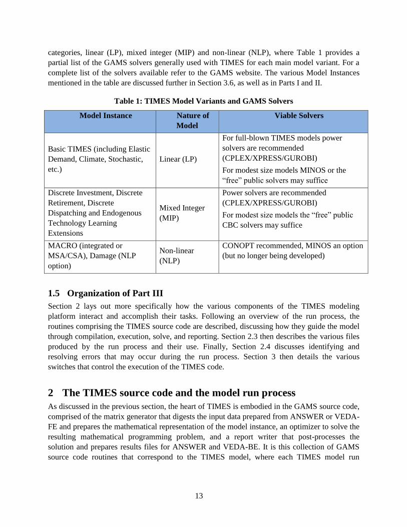
categories, linear (LP), mixed integer (MIP) and non-linear (NLP), where Table 1 provides a

partial list of the GAMS solvers generally used with TIMES for each main model variant. For a

complete list of the solvers available refer to the GAMS website. The various Model Instances

mentioned in the table are discussed further in Section 3.6, as well as in Parts I and II.

Table 1: TIMES Model Variants and GAMS Solvers

Model Instance Nature of

Model

Viable Solvers

Basic TIMES (including Elastic

Demand, Climate, Stochastic,

etc.)

Linear (LP)

For full-blown TIMES models power

solvers are recommended

(CPLEX/XPRESS/GUROBI)

For modest size models MINOS or the

“free” public solvers may suffice

Discrete Investment, Discrete

Retirement, Discrete

Dispatching and Endogenous

Technology Learning

Extensions

Mixed Integer

(MIP)

Power solvers are recommended

(CPLEX/XPRESS/GUROBI)

For modest size models the “free” public

CBC solvers may suffice

MACRO (integrated or

MSA/CSA), Damage (NLP

option)

Non-linear

(NLP)

CONOPT recommended, MINOS an option

(but no longer being developed)

1.5 Organization of Part III

Section 2 lays out more specifically how the various components of the TIMES modeling

platform interact and accomplish their tasks. Following an overview of the run process, the

routines comprising the TIMES source code are described, discussing how they guide the model

through compilation, execution, solve, and reporting. Section 2.3 then describes the various files

produced by the run process and their use. Finally, Section 2.4 discusses identifying and

resolving errors that may occur during the run process. Section 3 then details the various

switches that control the execution of the TIMES code.

2 The TIMES source code and the model run process

As discussed in the previous section, the heart of TIMES is embodied in the GAMS source code,

comprised of the matrix generator that digests the input data prepared from ANSWER or VEDA-

FE and prepares the mathematical representation of the model instance, an optimizer to solve the

resulting mathematical programming problem, and a report writer that post-processes the

solution and prepares results files for ANSWER and VEDA-BE. It is this collection of GAMS

source code routines that correspond to the TIMES model, where each TIMES model run

14

proceeds through the appropriate path in the source code based upon the user specified runtime

switches, described in Section 3, and the provided input data.

For the most part, this process is seamless to the user, as the model management shells

extract the scenario data and prepare ASCII text files in the layout required by GAMS, set up the

top level GAMS control file, and initiate the model run (in a Command Prompt box). GAMS

then compiles the source and data, constructs the model, invokes the solvers, and dumps the

model results for importing back into the model management environment. However, knowledge

of the run process and the files produced along the way can be helpful in diagnosing model

errors (e.g., a division by zero may necessitate turning on the source code listing

($ONLISTING/$OFFLIST at the top/bottom of the routine where the error is reported) to

determine which parameter is causing the problem) or if a user is considering modifying the

model formulation to, say, add a new kind of constraint (note that any such undertaking should

be closely coordinated with ETSAP).

2.1 Overview of the model run process

Once a model is readied, a run can be initiated from the model management systems by means of

the Case Manager in VEDA-FE or the Run Model option on the ANSWER Home screen. In both

systems the user assembles the list of scenarios to comprise the model run, taking care to ensure

that the order of the scenarios is such that all RES components are first declared (that is their

item name and set membership specified) and then assigned data.

In the model management shells, the user can also adjust the TIMES model variant, run

control switches, and solver options. For VEDA-FE this is done through the Case Manager, via

the Control Panel, RUNFile template, and solver settings. Figure 4 shows an example of the

VEDA-FE Control Panel. See Part IV for more on the use of the Case Manager in VEDA-FE.

In ANSWER, the Run Model button brings up the Run Model Form, from which the model

variant and most run control switches can be set. (The others need to be set using the Edit GAMS

Control Options feature.) However the <Solver>.OPT file needs to be handled manually outside

of ANSWER. See the separate ANSWER documentation for more details on these ANSWER

facilities.

When a model run is initiated, three kinds of files are created by VEDA and ANSWER. The

first is a Windows command script file VTRUN/ANSRUN.CMD (for VEDA/ANSWER

respectively), which just identifies the run name, indicates where the source code resides, and

perhaps any restart (see Section 3.8), and then calls the VEDA/ANSWER driver command script

(VT_GAMS/ANS_RUN.CMD). The second is the top-level GAMS command file

<Case>.RUN/GEN (for VEDA/ANSWER), which is passed to GAMS to initiate and control the

model run. It sets the model variant, identifies the Milestone (run) years, lists the scenario data

files (DD/DDS) to include, and invokes the main GAMS routine to have the model actually

assembled mathematically, solved, and reported upon. It is discussed further in Section 2.3.1.

The third group of files comprise the data dictionary <scenario>.DD/DDS file(s), which contain

the user input sets and parameters in the format required by GAMS to fully describe the energy

system to be analyzed.

15

GAMS is a two pass language, first compiling and then executing. In the first pass, GAMS

reads the input data prepared by ANSWER or VEDA-FE, and then proceeds to compile the data

as well as the actual TIMES source code to ready it for execution (unless a Runtime license is

employed in which case only the data is compiled).

In the second pass, GAMS then proceeds to execute the complied data and code to declare

the equations and variables that are to make up this particular TIMES incarnation and generate

the appropriate coefficients for matrix intersection, that is the multiplier for the individual

variables comprising each equation. With the matrix assembled GAMS then turns over the

problem to the solver.

Figure 4: VEDA-FE Case Manager Control Form

As a result of a model run a listing file (<Case>.LST), and a <case>.GDX file (GAMS

dynamic data exchange file with all the model data and results) are created. The <Case>.LST file

may contain compilation calls and execution path through the code, an echo print of the GAMS

source code and the input data, a listing of the concrete model equations and variables, error

messages, model statistics, model status, and solution dump. The amount of information

displayed in the listing file can be adjusted by the user through GAMS options in the

<Case>.RUN file.

The <Case>.GDX file is an internal GAMS file. It is processed according to the information

provided in the TIMES2VEDA.VDD to create results input files for the VEDA-BE software to

16

analyze the model results in the <case>.VD* text files. A dump of the solution results is also

done to the <case>.ANT file for importing into ANSWER, if desired. At this point, model results

can be imported into VEDA-BE and ANSWER respectively for post-process and analysis. More

information on VEDA-BE and ANSWER results processing can be found in Part V and the

separate ANSWER documentation respectively.

In addition to these output files, TIMES may create a file called QA_CHECK.LOG to inform

the user of possible errors or inconsistencies in the model formulation. The QA_CHECK file

should be examined by the user on a regular basis to make sure no “surprises” have crept into a

model. The content and use of each of these files is discussed further in Section 2.3.

For the ETSAP Runtime GAMS license, which does not allow for adjustments to the TIMES

source code by users (which in general is not encouraged anyway), a special TIMES.g00 file is

used that contains the declaration of each variable and equation that is part of the model

definition, thereby initializing the basic model structure.

2.2 The TIMES source code

The TIMES model generator is comprised of a host of GAMS source code routines, which are

simple text files that reside in the user's \VEDA\VEDA-FE\GAMS_SrcTIMESv### folder, as

discussed in Section 1.3 (or \AnswerTIMESv6\GAMS_SrcTI). Careful naming conventions are

employed for all the source code routines. These conventions are characterized, for the most part,

by prefixes and extensions corresponding to collections of files handling each aspect of the code

(e.g., set bounds, prepare coefficients, specify equations), as summarized in Table 2.

Table 2: TIMES Routines Naming Conventions

Type Nature of the Routine

Prefix

ans ANSWER TIMES specific pre-processor code

bnd set bounds on model variables

cal calculations performed in support of the preprocessor and report writer

coef prepare the actual matrix intersection coefficients

eq equations specification (that is the actual assembling of the coefficients of the

matrix)

err Error trapping and handling

fil handles the fundamental interpolation/extrapolation/normalization of the original

input data

init initialize all sets and parameters potentially involved in assembling a TIMES

model

main Top level routines according to the model variant to be solved

mod the declaration of the equations and variables for each model variant

17

Type Nature of the Routine

timeslices Handles the aggregation / inheritance of timeslices to the various levels

pp

preprocess responsible for preparing the TIMES internal parameters by

assembling, interpolating, normalizing, and processing the input data to prepare the

data structures needed to produce the model coefficients

put components of the results report writer that actually writes the output lines

qa Quality assurance checking and reporting

rpt main reporting components performing the calculations needed and assembling the

relevant parameters from the model results

solve manage the actual call to solve the model (that is the call to invoke the optimizer)

uc handles the user constraints

Extension

ANS ANSWER specific code

CLI climate module routines

CMD Windows command scripts to invoke GAMS/GDX2VEDA in order to solve and

afterwards dump the model results

DEF setting of defaults

DSC discrete (lumpy) investment routines

ETL endogenous technology learning routines

GMS lower level GAMS routines to perform interpolation, apply shaping of input

parameters, etc.

RUN/GEN

VEDA-FE/ANSWER specific GAMS TIMES command templates for dynamic

substitution of the switches and parameters needed at run submission to identify

the model variant and other options that will guide the current model run

IER routines and extensions prepared by the University of Stuttgart (Institute for the

Rational Use of Energy, IER) (e.g., for more advanced modeling of CHPs)

LIN routines related to the alternative objective formulations

MOD core TIMES routines preparing the actual model

MSA code related to the MSA implementation enabling TIMES and MACRO to iterate

in harmony

RED reduction algorithm routines

RPT report writer routines

STC code related to stochastics

STP code related to time-stepped or partially fixed-horizon solution

TM the core TIMES MACRO code

VDA routines related to new TIMES features implemented under the VDA extension

18

Note that these don’t cover every single routine in the TIMES source code folder, but do

cover most all of the core routines involved in the construction and reporting of the model. They

guide the steps of the run process as follows:

GAMS Compile: As mentioned above, GAMS operates as a two-phase compile then

execute system. As such it first reads and assembles all the control, data, and code files

into a ready executable; substituting user and/or shell provided values for all GAMS

environment switches and subroutine parameter references (the %EnvVar% and

%Param% references in the source code) that determine the path through the code for the

requested model instance and options desired. If there are inconsistencies in input data

they may result in compile-time errors (e.g., $170 for a domain definition error), causing

a run to stop. See Section 2.4 for more on identifying the source of such errors.

Initialization: Upon completion of the compile step, all possible GAMS sets and

parameters of the TIMES model generator are declared and initialized, then established

for this instance of the model from the user’s data dictionary file(s) (<Case>.DD13).

Model units are also initialized using the UNITS.DEF file, which contains the short

names for the most common sets of units that are normally used in TIMES models, and

which can be adjusted by the user.

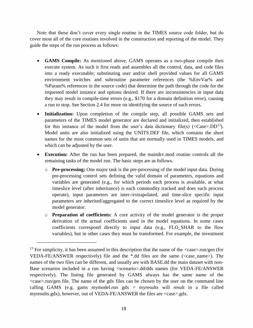
Execution: After the run has been prepared, the maindrv.mod routine controls all the

remaining tasks of the model run. The basic steps are as follows.

o Pre-processing: One major task is the pre-processing of the model input data. During

pre-processing control sets defining the valid domain of parameters, equations and

variables are generated (e.g., for which periods each process is available, at what

timeslice level (after inheritance) is each commodity tracked and does each process

operate), input parameters are inter-/extrapolated, and time-slice specific input

parameters are inherited/aggregated to the correct timeslice level as required by the

model generator.

o Preparation of coefficients: A core activity of the model generator is the proper

derivation of the actual coefficients used in the model equations. In some cases

coefficients correspond directly to input data (e.g., FLO_SHAR to the flow

variables), but in other cases they must be transformed. For example, the investment

13 For simplicity, it has been assumed in this description that the name of the <case>.run/gen (for

VEDA-FE/ANSWER respectively) file and the *.dd files are the same (<case_name>). The

names of the two files can be different, and usually are with BASE.dd the main dataset with non-

Base scenarios included in a run having <scenario>.dd/dds names (for VEDA-FE/ANSWER

respectively). The listing file generated by GAMS always has the same name of the

<case>.run/gen file. The name of the gdx files can be chosen by the user on the command line

calling GAMS (e.g. gams mymodel.run gdx = myresults will result in a file called

myresults.gdx), however, out of VEDA-FE/ANSWER the files are <case>.gdx.

19

cost (NCAP_COST) must be annualized, spread for the economic lifetime, and

discounted before being applied to the investment variable (VAR_NCAP) in the

objective function (EQ_OBJ), and based upon the technical lifetime the coefficients

in the capacity transfer constraint (EQ_CPT) are determined to make sure that new

investment are accounted for and retired appropriately.

o Generation of model equations: Once all the coefficients are prepared, the file

eqmain.mod controls the generation of the model equations. It calls the individual

GAMS routines responsible for the actual generation of the equations of this

particular instance of the TIMES model. The generation of the equations is controlled

by sets, parameters, and switches carefully assembled by the pre-processor to ensure

that no superfluous equations or matrix intersections are generated.

o Setting variable bounds: The task of applying bounds to the model variables

corresponding to user input parameters is handled by the bndmain.mod file. In some

cases it is not appropriate to apply bounds directly to individual variables, but instead

applying a bound may require the generation of an equation (e.g. the equation

EQ(l)_ACTBND is created when an annual activity bound is specified for a process

having a diurnal timeslice resolution).

o Solving the model: After construction of the actual matrix (rows, columns,

intersections and bounds) the problem is passed to an optimizing solver employing

the appropriate technique (LP, MIP, or NLP). The solver returns the solution of the

optimization back to GAMS. The information regarding the solver status is written by

TIMES in a text file called END_GAMS, which allows the user to quickly check

whether the optimisation run was successful or not without having to go through the

listing file. Information from this file is displayed by VEDA-FE and ANSWER at the

completion of the run.

o Reporting: Based on the optimal solution the reporting routines calculate result

parameters, e.g. annual cost information by type, year and technology or commodity.

These result parameters together with the solution values of the variables and

equations (both primal and dual), as well as selected input data, are assembled in the

<case>.GDX file. The gdx file is then processed by the GAMS GDX2VEDA.EXE

utility according to the directives contained in TIMES2VEDA.VDD control file to

generate files for the result analysis software VEDA-BE14. The <case>.ANT file for

providing results for import into ANSWER may also be produced, if desired.

2.3 Files produced during the run process

Several files are produced by the run process. These include the files produced by the shell for

model initiation, the .LST listing file, which echoes the GAMS compilation and execution

14 The basics of the TIMES2VEDA.VDD control file and the use of the result analysis software

VEDA-BE are described in Part V.

20

process and reports on any errors encountered during solve, results files, and the QAcheck.log

file. These files are summarized in Table 2 and discussed in this section.

Table 3: Files Produced by a TIMES Model Run

Extension Produced By Nature of the Output

ant TIMES report writer ANSWER model results dump

gdx GAMS Internal (binary) GAMS Data eXchange file with all the

information associated with a model run

log TIMES quality check

routine

List of quality assurance checks (warnings and possible

errors)

lst GAMS

The basic echo of the model run, including indication of

the version of TIMES being run, the compilation and

execution steps, model summary statistics and error (if

encountered), along with optionally an equation listing

and/or solution print

vdd GDX2VEDA utility

The core model results dump of the solution including

the variable/equations levels/slack and marginals, along

with cost and other post-processing calculations

vde GDX2VEDA utility The elements of the model sets (and the definition of the

attributes)

vds GDX2VEDA utility The set membership of the elements of the model

vdt VEDA-FE or ANSWER The RES topology information for the model

2.3.1 Files produced by model initiation

As discussed in Section 2.1, three sets of files are created by VEDA and ANSWER upon run

initiation, the command script file VTRUN/ANSRUN.CMD, the top-level GAMS command file

<Case>.RUN/GEN (for VEDA/ANSWER), and the data dictionary <scenario>.DD/DDS text

file(s) that contain all the model data to be used in the run.

The VTRUN/ANSRUN.CMD script file calls GAMS, referring to the <case> file and

identifying the location of the TIMES source code and gdx file. For VEDA-FE the CMD file

consists of the line:

Call ..\<source_code_folder>\vt_gams <case>.run <source_code_folder> gamssave\<case>

along with a 2nd line to call the GDX2VEDA utility to process the TIMES2VEDA.VDD file to

prepare the <case>.VD* result files for VEDA-BE. The ANSRUN.CMD file has a similar setup

21

calling ANS_GAMS.CMD in the source code folder which invokes GAMS and subsequently the

GDX2VEDA utility.

The <case>.RUN/GEN file is the key file controlling the model run. It instructs the TIMES

code what data to grab, what model variant to employ, how to handle the objective function, and

other aspects of the model run controlled by the switches discussed in Section 3. An example

.RUN file is displayed in Figure 5. Rows beginning with an asterisk (*) are comment lines for

the user's convenience and are ignored by the code. Rows beginning with a dollar-sign ($) are

switches that can be set by the user (usually by means of VEDA/ANSWER).

Both VEDA and ANSWER have facilities to allow the user to tailor the content of the

RUN/GEN files, though somewhat differently. In VEDA-FE the Case Manager RUNFile_Tmpl

button allows the basic RUN template to be brought up, and if desired carefully edited. However,

the Case Manager also has a Control Panel, shown in Figure 4, where many of the more common

switches can be set.

At the beginning of a <case>.RUN file the version of the TIMES code being used is

identified and some option control statements that influence the information output (e.g.,

SOLPRINT ON/OFF to see a dump of the solution, OFF recommended) are provided. The

LIMROW/LIMCOL options allow the user to turn on equation listing in the .LST file (discussed

in the next section) by setting the number of rows/columns of each type to be shown.

Then compile-time dollar control options indicating which solver to use (if not the default to

the particular solution algorithm), whether to echo the source code ($ON/OFFLISTING) by

printing it to the LST file, and that multiple definitions of sets and parameters ($ONMULTI) are

permitted (that is they can appear more than one time, which TIMES requires since first there are

empty declarations for every possible parameter followed by the actual data provided by the

user). Further possible dollar control options are also described in the GAMS manual.

Afterwards the content of several so-called TIMES dollar control (or environment) switches

are specified. Within the source code the use of these control switches in combination with

queries enables the model to skip or activate specific parts of the code. Thus it is possible to turn-

on/off variants of the code, e.g. the use of the reduction algorithm, without changing the input

data. The meaning and use of the different control switches is discussed in Section 3. Again these

are generally set using the Case Manager/Run form in VEDA/ANSWER.

After the basic control switches, the definition of the set of all timeslices is established by

means of the call to the <case>_TS.DD file before any other declarations carried out in the

initialization file INITSYS.MOD. This is necessary to ensure the correct ordering of the

timeslices for seasonal, weekly, or daynite storage processes. After the definition of the

timeslices, the files INITSYS.COM and INITMTY.MOD, which are responsible for the

declaration and initialization of all sets and parameters of the model generator, are included.

22

{continued on next page}

23

Figure 5: Example of a VEDA-FE TIMES <case>.RUN file15

The line containing the include command for the file initmty.mod can be supplemented by

calls for additional user extensions that trigger the use of additional special equations or report

routines. The use of these extension options are described in more detail in Section 0.

Afterwards the data dictionary file(s) (BASE.DD, …, CO2_TAX_HIGH.DD in Figure 5)

containing the user input sets and parameters are included, inserted automatically by VEDA-

FE/ANSWER according to the list of scenarios in the Case Manager/Run forms by means of the

$INCLUDE statements. It is normally advisable to segregate user data into “packets” as

scenarios, where there may be a single Base scenario containing the core descriptions of the

energy system being studied and a series of alternate scenario depicting other aspects of the

system. For example, one <scenario>.DD file may contain the description of the energy system

for a reference scenario, and additional <alt_scenario>.DD files (.DDS for ANSWER) may be

15 The ANSWER GEN file will have similar content though with some syntax and perhaps

slightly augmented scripts.

24

included containing additions or changes relative to the reference file, for example CO2

mitigation targets for a reduction scenario, or alternative technology specifications.

The SET MILESTONYR declaration identifies years for this model run based upon those

years identified in in VEDA via the Period Defs selected on the Case Manager (and maintained

in SysSettings) and the Milestone Years button on the ANSWER run form. The dollar control

switch RUN_NAME contains the short name of the scenario, and is used for the name of the

results files (<case>.VD*) passed to VEDA-BE.

Next in the example shown in Figure 5, some runtime switches are activated to request

levelized cost reporting and splitting of investment costs into core and the incremental additional

cost arising from any technology based discount rate specified in the data. See Section 3 for the

full description of these and other control switches.

The last line of the <case>.RUN file invokes the file main driver routine (maindrv.mod) that

initiates all the remaining tasks related to the model run (pre-processing, coefficient calculation,

setting of bounds, equation generation, solution, reporting). Thus any information provided after

the inclusion of the maindrv.mod file will not be considered in the main model solve request,

though if the user wishes to introduce specialized post-processing of the result that could be

added (or better yet handled externally by GAMS code that processes the GDX file).

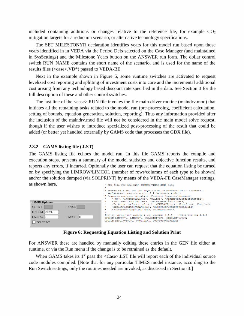
2.3.2 GAMS listing file (.LST)

The GAMS listing file echoes the model run. In this file GAMS reports the compile and

execution steps, presents a summary of the model statistics and objective function results, and

reports any errors, if incurred. Optionally the user can request that the equation listing be turned

on by specifying the LIMROW/LIMCOL (number of rows/columns of each type to be shown)

and/or the solution dumped (via SOLPRINT) by means of the VEDA-FE CaseManager settings,

as shown here.

Figure 6: Requesting Equation Listing and Solution Print

For ANSWER these are handled by manually editing these entries in the GEN file either at

runtime, or via the Run menu if the change is to be retrained as the default,

When GAMS takes its 1st pass the <Case>.LST file will report each of the individual source

code modules compiled. [Note that for any particular TIMES model instance, according to the

Run Switch settings, only the routines needed are invoked, as discussed in Section 3.]

25

A small snippet from the LST file compilation trace from an ANSWER-TIMES model run of

is shown in Figure 7, where the "..." shows the nesting as one GAMS routine calls another with

the appropriate parameters needed.

Figure 7: GAMS Compilation of the TIMES Source Code

If an error is encountered during the compilation operation GAMS will tag where the error

occurred and report an error code. Most common in this regard is a Domain Error ($170) where

perhaps there was a typo in an item name, as in the example shown in Figure 8, or the scenarios

were not in the proper order and data was attempted to be assigned to a process before it was

declared. Further discussion of errors encountered at this and other stages of the run process is

found in Section 2.4.

26

Figure 8: GAMS Compilation Error

Once the data and code have been successfully complied, execution takes place, with GAMS

calling each TIMES routine needed according to the switches and data for this particular run.

Again the LST file echoes this execution phase, as shown in Figure 9. It is possible, though

unlikely, to encounter a GAMS Execution error. The most common cause of this is the explicit

specification of zero (0) as the efficiency of a process. An execution error is reported in the

<Case>.LST file in a manner similar to a compilation error, tagged by “Error” at the point that

the problem was encountered.

Figure 9: GAMS Execution of the TIMES Source Code

27

Once execution of the matrix generator has completed GAMS reports the model run statistics

(Figure 10), and automatically invokes the solver.

Figure 10: CPLEX Solver Statistics

If the OPTION LIMROW/LIMCOL is set to non-0 the equation mathematics are displayed in

the list file, by equation block and/or column intersection, as shown in Figure 11 and Figure 12

respectively.

Figure 11: Equation Listing Example

28

Figure 12: Variable Listing Example

And if the SOLPRINT=ON option is activated then the level and marginals are reported as

shown in Figure 13.

Figure 13: Solution Dump Example

29

Upon successful solving the model the solution statistics are reported (Figure 14), where in

this case CPLEX was used to solve a MIP model variant (in this example), and the report writer

invoked to finish up by preparing the report. If the solver is not able to find an optimal solution, a

non-Normal solve status will be reported, and the user can search the LST file for the string

"INFES" for an indication of which equations are preventing model solution. Again, further

information on the possible causes and resolution of such errors is found in Section 2.4.

Figure 14: Solver Solution Summary

The actual production of the dump of the model results is performed by the report writer for

ANSWER resulting in a <Case>.ANT file which is imported back into ANSWER after the run

complete and/or the GDX2VEDA utility prepared by GAMS and DecisionWare to facilitate the

exchange of information from GAMS to VEDA-BE, which may be used with both VEDA-FE

and ANSWER.

2.3.3 Results files

The TIMES report writing routine produces two sets of results-related outputs (along with the

quality control LOG discussed in the next section). The <case>.ANT file is an ASCII text file,

with results ready for import into ANSWER. The GAMS Data eXchange file (GDX) contains all

the information associated with a model run [input data, intermediate parameters, model results

(primal and dual)] in binary form. The GDX file may be examined by means of the GAMSIDE,

available from the Windows Start Menu in the GAMS folder (or as a shortcut from the desktop if

put there), if one really wants to dig into what’s happening inside of a TIMES run (that is, the set

members, preprocessor calculations, the model solution and the reporting parameters calculated).

A more powerful feature within the GAMSIDE is a GDXDIFF facility under Utilities. As

seen in Figure 15, the utility shows the differences between all components, comparing two

model runs. Within the GDXDIFF utility, the user identifies the GDX files from the two runs and

30

requests the resulting comparison GDX be prepared. The display then shows any differences

between the two runs. The GDXDIFF is most effectively used by instructing VEDA to Create

DD for the two runs via the Options and Case Manager forms, as shown in Figure 16. Once the

comparison GDX has been created, it is viewed in the GAMSIDE. By sorting by Type and

scanning down one Symbol at a time, one can determine exactly what input data being sent to

GAMS for the two runs is different.

Figure 15: GAMSIDE View of the GDXDIFF Run Comparison

However, the most common use of the GDX is its further processing to generate files for the

result analysis software VEDA-BE16. ETSAP worked with GAMS a number of years ago to

develop a standalone utility (GDX2VEDA) to process the GAMS GDX file and produce the files

read into VEDA-BE. The GDX2VEDA utility process a directives file (TIMES2VEDA.VDD) to

determine which sets and model results are to be included and prepare said information for

VEDA-BE. A general default version of the VDD is distributed with TIMES in the source code

folder (for core TIMES, Stochastics, and MACRO), but may be augmented by the user if other

information is desired from the solution. However, the process of changing the VDD should be

done in consultation with someone fully familiar with the GAMS GDX file for TIMES and the

16 The basics of the TIMES2VEDA.VDD control file and the use of the result analysis software

VEDA-BE are described in Part V.

31

basics of the GDX2VEDA utility. See Part V, Appendix B, for further information on the

GDX2VEDA utility and VDD directives file.

Figure 16: VEDA Setup for Data Only GDX Request

The call to the GDX2VEDA routine is embedded in the VTRUN/ANSRUN.CMD command

routines. There are three files produced for VEDA-BE by the GDX2VEDA utility: the

<Case>.VD data dump with the attributes, and associated VDE (set elements), VDS (sets

definition). In addition, VEDA-FE and ANSWER produce a <Case>.VDT (topology) file with

the RES connectivity information. These files never require user intervention, though users

wishing to post-process the GDX2VEDA results with their own tailored software, rather than

VEDA-BE, might choose to parse the VD* files to extract the desired information.

Note that for both ANSWER and VEDA-BE, for the most part low-level (that is

commodity/process) results are reported, along with some aggregate cost numbers (such as

regional and overall objective function). It is left up to the user to construct relevant sets and

tables in VEDA-BE to organize and aggregate the results into meaningful tables. Refer to Part V

for a discussion of how to go about assembling report tables in VEDA-BE. For ANSWER the

user is left with only the raw results and thereby needs to come up with their own approach to

producing useful usable reporting tables, or use VEDA-BE.

In addition, as discussed in Section 3.10, there are a number of switches that control the

report writer itself in terms of how it calculates certain outputs and prepares the results as part of

the post-processing. Collectively these mechanisms provide the user with a wide range of

reporting results and tools for dissecting and assembling the modeling results as part of

effectively using TIMES to conduct energy policy analyses.

32

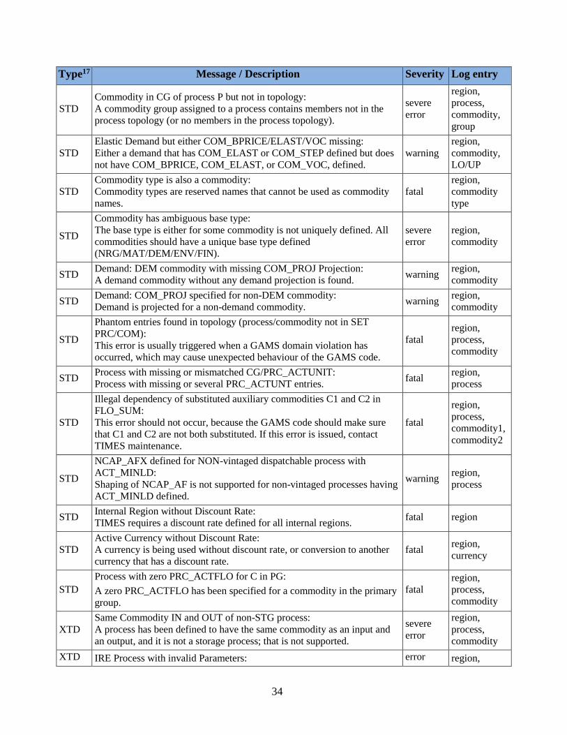
2.3.4 QA check report (LOG)

In order to assist the user with identifying accidental modelling errors, a number of sanity

checks are done by the model generator. If incorrect or suspicious specifications are found in

these checks, a message is written in a text file named QA_CHECK.LOG, in the working folder.

The checks implemented in TIMES Version 3.9.3 are listed in Table 5. The “Log entry” column

shows the identification given for each suspicious specification.

Table 4: TIMES Quality Assurance Checks (as of Version 3.9.3)

Type17 Message / Description Severity Log entry

STD

Delayed Process but PAST Investment:

Process availability has been delayed by using PRC_NOFF or

NCAP_START, but also has existing capacity.

warning region,

process

STD

Commodities/processes defined at non-existing TSLVL:

PRC_TSL or COM_TSL has been specified on a timeslice level not used

in the model.

severe

error

number of

COM/PRC

reset to

ANNUAL

STD

NCAP_TLIFE out of feasible range:

NCAP_TLIFE specified has a value of either less than 0.5 or greater than

200. Values less than 0.5 are reset to 1.

warning

region,

process,

vintage

STD

Flow OFF TS level below variable TS level:

A PRC_FOFF attribute with a timeslice below the flow level has been

specified; the OFF specification is ignored.

warning

region,

process,

commodity,

timeslice

STD

COM_FR does not sum to unity (T=first year):

The sum of COM_FR over all timeslices at the COM_TSL level is not

equal to 1, and is therefore normalized to 1.

warning

region,

commodity,

milestone

STD

Unsupported diverging trade topology:

The model generator detects an unsupported complex topology of an IRE

process, which cannot be properly handled

error region,

process

STD

FLO_EMIS with no members of source group in process:

A FLO_EMIS with a source group that has no members for the process

has been specified. The parameter is ignored.

severe

error

region,

process,

group,

commodity

STD

Unsupported FLO_SHAR: C not in RPC or CG:

The commodity in FLO_SHAR is either not in the process topology or not

a member of the group specified

error

region,

process,

commodity,

group

STD

FLO_SHAR conflict: Both FX + LO/UP specified, latter ignored:

Too many FLO_SHAR bounds are specified, if both FX and LO/UP are

specified at the same time.

warning

region,

process,

vintage,

commodity,

group

17 STD=standard QA check (always done), XTD=extended QA check (activate with XTQA)

33

Type17 Message / Description Severity Log entry

STD

Inconsistent sum of fixed FLO_SHARs in Group:

All flows in a group have a fixed share, but the sum of the fixed

FLO_SHAR values is not equal to 1.

warning

region,

process,

vintage,

group

STD

Defective sum of FX and UP FLO_SHARs in Group:

All flows in a group have either a fixed or an upper share, but the sum of

the FLO_SHAR values is less than 1.

warning

region,

process,

vintage,

group

STD

Excessive sum of FX and LO FLO_SHARs in Group:

All flows in a group have either a fixed or a lower share, but the sum of

the FLO_SHAR values is greater than 1.

warning

region,

process,

vintage,

group

STD NCAP_AF/ACT_BND Bounds conflict:

Value at PRC_TS level and below, latter ignored warning

region,

process,

vintage,

timeslice

STD NCAP_AF Bounds conflict:

FX + LO/UP at same TS-level, latter ignored warning

region,

process,

vintage,

timeslice

STD FLO_SHAR/FLO_FR Bounds conflict:

Value at RPCS_VAR level and below, latter ignored warning

region,

process,

vintage,

timeslice

STD FLO_SHAR Bounds conflict:

FX + LO/UP at same TS-level, latter ignored warning

region,

process,

vintage,

commodity,

group

STD COM_BNDNET/COM_BNDPRD/IRE_BND Bounds conflict:

Value at COM_TS level and below, latter ignored warning

region,

milestone,

commodity,

timeslice

STD

IRE_FLO import commodity not in TOP_IRE:

An invalid IRE_FLO with the imported commodity not in the process

topology has been specified

error

region,

process,

commodity

STD

CHP process with zero CEH but only upper bound on CHPR:

A CHP process has only an upper bound on NCAP_CHPR, but a zero or

missing NCAP_CEH, which indicates a modelling error

error region,

process

STD

Year Fraction G_YRFR is ZERO!

A timeslice with G_YRFR is within the timeslice tree. This should

actually never happen, because TIMES automatically removes timeslices

with a zero year fraction from the active timeslices.

fatal region,

timeslice

STD

Illegal system commodity in topology:

ACT / ACTGRP is a reserved name which should never be used as a

commodity in the model topology.

fatal region,

process

34

Type17 Message / Description Severity Log entry

STD

Commodity in CG of process P but not in topology:

A commodity group assigned to a process contains members not in the

process topology (or no members in the process topology).

severe

error

region,

process,

commodity,

group

STD

Elastic Demand but either COM_BPRICE/ELAST/VOC missing:

Either a demand that has COM_ELAST or COM_STEP defined but does

not have COM_BPRICE, COM_ELAST, or COM_VOC, defined.

warning

region,

commodity,

LO/UP

STD

Commodity type is also a commodity:

Commodity types are reserved names that cannot be used as commodity

names.

fatal

region,

commodity

type

STD

Commodity has ambiguous base type:

The base type is either for some commodity is not uniquely defined. All

commodities should have a unique base type defined

(NRG/MAT/DEM/ENV/FIN).

severe

error

region,

commodity

STD Demand: DEM commodity with missing COM_PROJ Projection:

A demand commodity without any demand projection is found. warning

region,

commodity

STD Demand: COM_PROJ specified for non-DEM commodity:

Demand is projected for a non-demand commodity. warning

region,

commodity

STD

Phantom entries found in topology (process/commodity not in SET

PRC/COM):

This error is usually triggered when a GAMS domain violation has

occurred, which may cause unexpected behaviour of the GAMS code.

fatal

region,

process,

commodity

STD Process with missing or mismatched CG/PRC_ACTUNIT:

Process with missing or several PRC_ACTUNT entries. fatal

region,

process

STD

Illegal dependency of substituted auxiliary commodities C1 and C2 in

FLO_SUM:

This error should not occur, because the GAMS code should make sure

that C1 and C2 are not both substituted. If this error is issued, contact

TIMES maintenance.

fatal

region,

process,

commodity1,

commodity2

STD

NCAP_AFX defined for NON-vintaged dispatchable process with

ACT_MINLD:

Shaping of NCAP_AF is not supported for non-vintaged processes having

ACT_MINLD defined.

warning region,

process

STD Internal Region without Discount Rate:

TIMES requires a discount rate defined for all internal regions. fatal region

STD

Active Currency without Discount Rate:

A currency is being used without discount rate, or conversion to another

currency that has a discount rate.

fatal region,

currency

STD

Process with zero PRC_ACTFLO for C in PG:

A zero PRC_ACTFLO has been specified for a commodity in the primary

group.

fatal

region,

process,

commodity

XTD

Same Commodity IN and OUT of non-STG process:

A process has been defined to have the same commodity as an input and

an output, and it is not a storage process; that is not supported.

severe

error

region,

process,

commodity

XTD IRE Process with invalid Parameters: error region,

35

Type17 Message / Description Severity Log entry

Some FLO_FUNC, FLO_SUM, FLO_SHAR or UC_FLO parameter not

supported for IRE processes has been specified.

process,

com-group

XTD

Invalid Commodity / Group used in ACT_EFF - parameter ignored:

An invalid ACT_EFF attribute with a CG not containing members on the

shadow side or in the PG has been specified.

error

region,

process,

group

XTD

FLO_SUM Commodity Not in RPC - parameter ignored:

An invalid FLO_SUM has been defined where the commodity is not in the

process topology.

error

region,

process,

group,

commodity

XTD

FLO_SUM Commodity Not in CG1 - parameter ignored:

An invalid FLO_SUM has been defined where the commodity is not a

member of the first group, CG1.

error

region,

process,

group,

commodity

XTD

PTRANS between CG1 and CG2 in both directions:

A FLO_FUNC or FLO_SUM between groups CG1 and CG2 has been

specified in both directions.

severe

error

region,

process,

group1,

group2

XTD

RPC in TOP not found in any ACTFLO / FLO_SHAR / FLO_FUNC /

FLO_SUM:

Some commodity in the topology does not seem to be tied to anything, at

least by means of any of the most common attributes; the user is advised to

check that this is not a modelling error.

warning

region,

process,

commodity,

IN/OUT

XTD

Empty Group in FLO_SUM/FLO_FUNC/FLO_SHAR:

A group that has no members in the process topology has been used for a

process attribute. Detects also an empty primary group.

severe

error

region,

process,

group

XTD

Both NCAP_AF and NCAP_AFA specified for same process:

Specifying both NCAP_AF(bd) and NCAP_AFA(bd) for an ANNUAL

level process is ambiguous and should be avoided.

warning

region,

process,

vintage

XTD Too Long Commodity Lead Time:

A value of NCAP_CLED > NCAP_ILED has been specified warning

region,

process,

commodity

XTD

CHP parameter specified for Non-CHP process:

An NCAP_BPME, NCAP_CHPR or NCAP_CEH parameter has been

specified for a process that is not defined to be CHP.

error

region,

process,

vintage

XTD

PG of CHP process consists of single commodity yet has a CHP-ratio:

A CHP process has a NCAP_CHPR specified but has only a single

commodity in the primary group.

warning region,

process

XTD Found CHP processes without CHP-ratio defined:

A CHP process has no NCAP_CHPR defined warning

number of

such

processes

XTD

Found CHP processes with PG commodity efficiencies - unsupported:

Specifying ACT_EFF on some flow(s) in the PG is not supported for CHP

processes, and may lead to unexpected results.

warning region,

process

XTD Found CHP processes without electricity in the PG:

A CHP process is found with no electricity commodity in the PG. warning

region,

process

36

2.4 Errors and their resolution

Errors may be encountered during the compilation, execution (rarely), or solve stages of a

TIMES model run. During the compilation step, if GAMS encounters any improperly defined

item the run will be halted with a Domain or similar error and the user will need to examine the

TIMES quality control LOG or GAMS listing (LST) files to ascertain the cause of the problem.

While such problems are not normally encountered, some that might occur include:

an item name was mistyped and therefore not defined;

an item was previously defined in one scenario but defined differently in another;

an item was not properly declared for a particular parameters (e.g., a non-trade process

using an IRE parameter), and

scenarios were specified for the run in the wrong order so a data reference is encountered

before the declaration (e.g., a bound on a new technology option is provided before it has

been identified).

During the execution phase, if GAMS encounters any runtime errors it will halt and report

where the error occurred in the LST file. While such problems are not normally encountered

some causes of an execution error might be:

an explicit 0 is provided for an efficiency resulting in a divide by 0, and

there is a conflict between a lower and upper bound.

Most commonly errors are encountered during the solve process, resulting in an infeasibility.

Some causes of the model not being able to solve might be:

due to bounds, the energy system cannot be configured in such a way as to meet the limit;

owing to mis-specifying the demand serviced by a device, there is no or not enough

capacity to satisfy said demand, and

the RES is not properly connected so a needed commodity is not able to reach the

processes needing it.

To identify the cause of a solve error, if using CPLEX the user can activate the Infeasibility

Finder (set in the CPLEX.OPT as default (via the IIS command) in VEDA-FE Case Manager or

said file distributed with ANSWER). The CPLEX Infeasibility Finder will identify the explicit

row/columns corresponding to the first infeasibility encountered and list the conflict involved in

the <Case>.LST file, such as shown here where the electricity balance equation can’t be satisfied

(due to a limit being imposed on the first year electric grid capacity that is too small).

This helps with tracking down the culprit, but the user still needs to figure out why the

problem occurred. When using a solver other than CPLEX, or if the Infeasibility Finder is not

37

activated, then the solution dump will be tagged for all the potentially interrelated model

variables/equations that were not in equilibrium at the time the solve stopped. The user can find

these by searching the LST file for the string "INFES".

As a last resort, the model can be run with the equation listing turned on by setting

LIMROW/LIMCOL to, say, 1000 in the <case>.RUN (via the Case Manager) / GEN (via Edit

the GEN from the Run form) file, although the equations in this form can be challenging to

interpret.

3 Switches to control the execution of the TIMES code

This Section describes the various GAMS control variables available in TIMES as control

switches that can be set by the user in the model <case>.RUN/GEN file for VEDA-

FE/ANSWER respectively. As discussed in Section 2, VEDA-FE and ANSWER, in most cases

automatically take care of inserting the proper switches into the run file, so the user normally

does not have to modify the run file at all. The switches are set in the highly user-friendly GUI

interface of the user shell, which uses a run file template and inserts all run-specific switches

correctly into the run file of each model run. These are managed by the user via the

CaseManager (Control Panel) and Run/Edit GEN Template parts of VEDA-FE and ANSWER

respectively.

In the sub-sections that follow, unless otherwise stated, the basic syntax for the inclusion of

control switch options in the main <case>.RUN/GEN GAMS directive file is $SET <option>

<value>. The various options are grouped according to the nature of their usage by sub-section.

3.1 Run name case identification

The use of the RUN_NAME control variable is practically mandatory when running TIMES. By

setting the RUN_NAME control variable, the user gives a name to the model run, which will be

used when generating various output files and/or loading information from a previously

generated file that has the same name. The control variable is used in the following way:

$SET RUN_NAME runname

Here the runname identifier (corresponding to the run <case> name) is a string of letters,

numbers and other characters (excluding spaces), such that the name complies with the rules for

the base name of files. It will be used to construct names for the various files comprising a model

run, as listed in Table 5.

38

Table 5: RUN_NAME TIMES Files

Extension* Description

ANT ANSWER results dump

GDX GAMS data exchange file (for GAMS2VEDA processing)

*_BP.GDX Base prices to seed a TIMES elastic demand policy run

LOG

Optional GAMS file producing a trace of the model resource usage

(activated by lo=1 on the GAMS call line in

ANS_GAMS/VT_GAMS.CMD, which needs to be added by the user

manual if needed)

LST

GAMS output file with the compile/execute/solve trace, and optional

solution dump (via SOLPRINT=YES on the OPTIONS line at the top of

the RUN command script)

*_P.GDX Save/Load point GAMS restart files

RUN Top level routine calling GAMS (and for VEDA-FE the GDX2VEDA

routine)

*_RunSummary.DD Run summary for the associated model run

*_TS.DD Timeslices declaration for the associated model run

VD* Suite of results/Set definition(S)/Element description(E)/topology(T) for

VEDA-BE

3.2 Controls affecting equilibrium mode

TIMES has a number of variants or model instances embedded in the within the full set of

GAMS source code files. Which path through the code is taken is determined mainly the

activation (or not) of various control switches, as summarized in this section.

3.2.1 Endogenous elastic demands [TIMESED]

The TIMESED control variable is one of the most important TIMES control variables. It has to

be used whenever the full partial equilibrium features of TIMES (that is, employing elastic

demands) are to be utilized. For running a baseline scenario to be subsequently used as the

reference scenario for partial equilibrium analyses with elastic demands, the following setting

should be used:

$SET TIMESED NO

This setting indicates that the user plans to use the resulting price levels from the current run

as reference prices in subsequent runs with elastic demands. The setting causes the model

generator to create the following (identical) two files from the Baseline run (the second file is a

backup copy):

39

Com_Bprice.gdx

%RUN_NAME%_DP.gdx

For running any policy scenarios with elastic demands, using price levels from a previous run

as reference prices, one must use the following setting:

$SET TIMESED YES

The reference price levels are read from a file named ‘Com_Bprice.gdx’, which is expected

to reside in the current directory folder where the model run takes place. Therefore, the Baseline

scenario using the setting $SET TIMESED NO has to be run before running the policy scenarios,

or the correct ‘Com_Bprice.gdx’ be otherwise restored from some backup copy.

The VEDA-FE CaseManager(BasePrice) and ANSWER Run(ModelVariant) buttons allow

the user to easily control setting of the TIMESED switch and thereby creating/including the

Com_Bprice.GDX as appropriate. If neither the base prices are to be written out, nor a policy

scenario with elastic demands to be run, the user should not set the TIMESED control variable.

3.2.2 General equilibrium [MACRO]

The general equilibrium mode of TIMES can be activated in two different ways, using the

following MACRO control switch settings:

$SET MACRO YES – activate the standard MACRO formulation

$SET MACRO MSA – activate the MACRO decomposition formulation

For further information about the standard MACRO formulation, see the TIMES-MACRO

documentation available at the ETSAP site: http://www.iea-etsap.org/web/documentation.asp

In both formulations, the use of the MACRO mode for evaluating policy scenarios requires

that so-called demand decoupling factors (DDF) and labor growth rates first have to be calibrated

for the Baseline scenario and corresponding GDP growth projections. The calibration produces a

file containing the calibrated parameters, which must then be included in the policy scenarios to

be evaluated.

Until TIMES v3.3.9, the standard MACRO formulation included a separate utility for

calibrating the DDF factors and labor growth rates (see the TIMES-MACRO documentation for

details). However, the calibration is much easier using the new MACRO decomposition

formulation, where you can use the following MACRO control switch setting for carrying out

the Baseline calibration:

40

$SET MACRO CSA – calibration with the MACRO decomposition method

The “CSA” calibration facility produces a file called MSADDF.DD, which is automatically

included in any subsequent policy run activated by the MACRO=MSA control switch. In order

to carry out the calibration, one must also include the necessary MACRO parameters in the

model input data (see the TIMES-MACRO documentation for a description of the MACRO

parameters). The only mandatory parameters are the initial GDP and GDP growth parameters.

The DDF file produced by CSA can be used for the original TIMES-MACRO formulation,

where one may re-calibrate it a few times more with the Baseline scenario to verify the

calibration for TIMES-MACRO. The re-calibration is automatically done by TIMES-MACRO at

the end of each run, whereupon a new file DDFNEW.DD is written, which can then be renamed

for inclusion in the subsequent TIMES-MACRO policy runs.

When using the MACRO decomposition formulation (with MACRO=MSA or

MACRO=CSA), and when the partial equilibrium runs of the Baseline and policy scenarios have

already been made, using the LPOINT/RPOINT control settings (in combination with SPOINT)

may also be useful (see Section 3.8 and 0). If the RPOINT setting is used, the initial solution for

the decomposition algorithm is taken directly from the GDX file without having to re-run the

previously solved LP model again.

3.3 Controls affecting the objective function

3.3.1 Objective function cost accounting [OBJ]

The user can choose to use several alternative objective function formulations instead of the

standard objective function. See Part I, Section 5.3.4 and the documentation for the Objective

Function Variants for details. The alternative objective formulations can be activated using the

$SET OBJ <option> as described in Table 6.

Table 6: Objective Function Formulation Options

OBJ

Option Description

ALT Uses modified capacity transfer coefficients that improve the independency of

investment costs on period definitions.

AUTO

(default)

TIMES automatically selects the objective function among the standard formulation

or the ‘MOD’ alternative formulation according to the B(t) and E(t) parameters

specified by the user. If those parameters comply with the assumptions used in the

standard formulation, then the standard formulation is used, but if not then the

alternative formulation ‘MOD’ is used.

LIN Assumes linear evolution of flows and activities between Milestone years, but is

otherwise similar to the ALT formulation.

41

OBJ

Option Description

MOD

Period boundaries B(t) and E(t) are internally set to be halfway between Milestone

years, giving flexibility to set Milestone years to be other than the middle of each

period. Investments in Cases I.1.a and I.1.b only of the objective function investment

decision are spread somewhat differently across years.

STD To ensure that the standard formulation is unconditionally used, even if the B(t) and

E(t) parameters do not comply with the standard assumptions.

3.3.2 Objective function components

In addition to controlling how the objective function is assembled, as described in the previous

section, the user has control of the handling of specific components of the objective functions, as

described in Table 7.

Table 7: Objective Function Component Options

Option

<value> Description

DAMAGE

<LP(default)

/NLP/NO>

The TIMES model generator supports the inclusion of so-called damage costs

in the objective function. By default, if such damage costs have been defined in

the model input data, they are also automatically included in the objective

function in linearized form (LP). However, if the user wishes the damage costs

to be included in the solution reporting only, the DAMAGE control variable

can be set to 'NO'. Non-linear damage functions can be requested by setting the

control variable to 'NLP'. See Part II, Appendix B, for more on the damage cost

function extension.

OBJANN

<YES>

Used for requesting a period-wise objective formulation, which can be used e.g.

together with the MACRO decomposition method for enabling the iterative

update of the period-wise discount factors (See the documentation titled Macro

MSA, on the MACRO Decomposition Algorithm, for details).

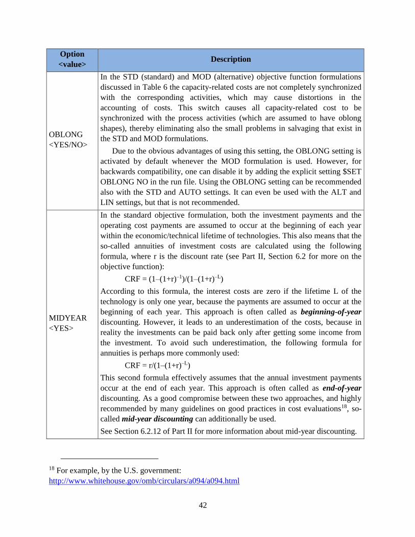
42

Option

<value> Description

OBLONG

<YES/NO>

In the STD (standard) and MOD (alternative) objective function formulations

discussed in Table 6 the capacity-related costs are not completely synchronized

with the corresponding activities, which may cause distortions in the

accounting of costs. This switch causes all capacity-related cost to be

synchronized with the process activities (which are assumed to have oblong

shapes), thereby eliminating also the small problems in salvaging that exist in

the STD and MOD formulations.

Due to the obvious advantages of using this setting, the OBLONG setting is

activated by default whenever the MOD formulation is used. However, for

backwards compatibility, one can disable it by adding the explicit setting $SET

OBLONG NO in the run file. Using the OBLONG setting can be recommended

also with the STD and AUTO settings. It can even be used with the ALT and

LIN settings, but that is not recommended.

MIDYEAR

<YES>

In the standard objective formulation, both the investment payments and the

operating cost payments are assumed to occur at the beginning of each year

within the economic/technical lifetime of technologies. This also means that the

so-called annuities of investment costs are calculated using the following

formula, where r is the discount rate (see Part II, Section 6.2 for more on the

objective function):

CRF = (1–(1+r)–1)/(1–(1+r)–L)

According to this formula, the interest costs are zero if the lifetime L of the

technology is only one year, because the payments are assumed to occur at the

beginning of each year. This approach is often called as beginning-of-year

discounting. However, it leads to an underestimation of the costs, because in

reality the investments can be paid back only after getting some income from

the investment. To avoid such underestimation, the following formula for

annuities is perhaps more commonly used:

CRF = r/(1–(1+r)–L)

This second formula effectively assumes that the annual investment payments

occur at the end of each year. This approach is often called as end-of-year

discounting. As a good compromise between these two approaches, and highly

recommended by many guidelines on good practices in cost evaluations18, so-

called mid-year discounting can additionally be used.

See Section 6.2.12 of Part II for more information about mid-year discounting.

18 For example, by the U.S. government:

http://www.whitehouse.gov/omb/circulars/a094/a094.html

43

Option

<value> Description

DISCSHIFT

As a generalization to the MID_YEAR setting, alternate time-of-year

discounting, including the end-of-year discounting mentioned above, can be

achieved by using the DISCSHIFT control variable. The control variable

should be set to correspond to the amount of time (in years) by which the

discounting of continuous streams of payments should be shifted forward in

time, with respect to the beginning of operation. Setting it to the value of 0.5

would be equal to the setting $SET MID_YEAR YES, and setting it to the

value of 1.0 would be equal to end-of-year discounting, as follows:

$SET DISCSHIFT 1

VARCOST

<LIN>

The standard dense interpolation and extrapolation of all cost parameters in

TIMES may consume considerable amounts of memory resources in very large

models. In particular, the variable costs, which may also be to a large extent

levelized onto a number of timeslices, usually account for the largest amount of

cost data in the GAMS working memory.

If desired, TIMES can be advised to interpolate and extrapolate the variable

cost parameters only sparsely for the Milestone years. The values at the

intermediate years will then be derived “on the fly”, by piecewise linear

interpolation, and will not be stored in the GAMS memory. This option may

thus be useful when running very large models on computers with limited

memory.

3.4 Stochastic and sensitivity analysis controls

3.4.1 Stochastics [STAGES]

The stochastic mode of TIMES can be activated with the STAGES control variable, by using the

following setting:

$SET STAGES YES

This setting is required for using the multi-stage stochastic programming features of TIMES. It

can also be used for enabling sensitivity and tradeoff analysis features. See Part I for more details

on stochastic programming and tradeoff analysis in TIMES.

3.4.2 Sensitivity [SENSIS]

Many useful sensitivity and tradeoff analysis features are available in TIMES, and they can be

enables by activating the stochastic mode of TIMES (see above). However, such sensitivity and

tradeoff analyses are often based on running the model in a series of cases that differ from each

44

other in only in a few parameter values. In such cases the so-called warm start features can

usually significantly speed up the model solution in the successive runs.

The use of the warm start facilities can be automatically enabled in sensitivity and tradeoff

analysis by using the following setting instead of $SET STAGES YES:

$SET SENSIS YES

As the variables then remain the same, warm start is automatically enabled by GAMS

according to the BRATIO value (BRATIO can be set in VEDA-FE, or added manually to the

ANSWER GEN template as a $OPTION BRATIO=1; as well).

See the documentation on stochastic programming and tradeoff analysis in TIMES for more

information on the use of this switch. The documentation is available at the ETSAP site:

http://www.iea-etsap.org/web/documentation.asp

3.4.3 Hedging recurring uncertainties [SPINES]

For modeling recurring uncertainties, such as hydrological conditions or fuel-price volatilities,

the stochastic mode can be activated also in such a way that the SOW index will be inactive for

all capacity-related variables (VAR_NCAP, VAR_CAP, VAR_RCAP, VAR_SCAP,

VAR_DRCAP, VAR_DNCAP). This modification to the standard multi-stage stochastic

formulation makes it possible to use the stochastic mode for hedging against recurring

uncertainties, and for finding the corresponding optimal investment strategy.

This variant of the stochastic mode can be activated by using the following control variable

setting:

$SET SPINES YES

In addition, under the SPINES option all the remaining equations that define dynamic or

cumulative relationships between variables can additionally be requested to be based on the

expected values instead of imposing the inter-period equations separately for each SOW. Doing

so will ensure that the uncertainties represented by the SOW-indexed variables will be

independent in successive periods. This further model simplification can be requested by using

the SOLVEDA switch, as follows:

$SET SOLVEDA 1

In addition, under the SPINES option this SOLVEDA setting will, for now, also cause all the

results for the activities and flows to be reported on the basis of the expected values only, and not

separately for each SOW. After all, the recurring uncertainties are rather aleatory by nature, and

therefore the user should probably be most interested in the optimal investment strategy, and

45

only in the average or normal year results for the activities and flows. If requested, an option to

produce results for all SOWs even under the period-independent variant can later be added.

Unlike the basic stochastic option STAGES, the SPINES option may be used also together

with the time-stepped mode (see Section 3.5.2).

The SPINES control variable is available only in TIMES versions 3.3.0 and above, and

should currently be considered experimental only.

3.5 Controls for time-stepped model solution

3.5.1 Fixing initial periods [FIXBOH]

The purpose of the FIXBOH option is to bind the first years of a model run to the same values

determined during a previous optimization. The approach first requires that a reference case be

run, and then by using FIXBOH the model generator sets fixed bounds for a subsequent run

according to the solution values from the reference case up to the last Milestone year less than or

equal to the year specified by the FIXBOH control variable. The FIXBOH control has to be used

together with the LPOINT control variable, in the following way:

$SET FIXBOH 2050

$SET LPOINT <run_name>

Here, the value of FIXBOH (2050) specifies the year, up to which the model solution will be

fixed to the previous solution, and the value of LPOINT (run_name) specifies the name of the

previous run, from which the previous solution is to be retrieved. Consequently, either a full

GDX file or a GAMS “point file” (see section 3.8) from the previous run should be available. If

no such GDX file is found, a compiler error is issued. The Milestone years of the previous run

must match those in the current run.

As a generalization to the basic scheme described above, the user can also request fixing to

the previous solution different amounts of first years according to region. The region-specific

years up to which the model solution will be fixed can be specified by using the TIMES

REG_FIXT(reg) parameter. The FIXBOH control variable is in this case treated as a default

value for REG_FIXT.

Example: Assume that you would like to analyze the 15-region ETSAP TIAM model with

some shocks after the year 2030, and you are interested in differences in the model solution only

in regions that have notable gas or LNG trade with the EU. Therefore, you would like to fix the

regions AUS, CAN, CHI, IND, JPN, MEX, ODA and SKO completely to the previous solution,

and all other regions to the previous solution up to 2030.

In the RUN file you should specify the control switches described above:

$SET FIXBOH 2030

$SET LPOINT <run_name>

46

In a model DD file you should include the values for the REG_FIXT parameter:

PARAMETER REG_FIXT /

AUS 2200, CAN 2200, CHI 2200, IND 2200

JPN 2200, MEX 2200, ODA 2200, SKO 2200

/;

3.5.2 Limit foresight stepwise solving [TIMESTEP]

The purpose of the TIMESTEP option is to run the model in a stepwise manner with increasing

model horizon and limited foresight. The TIMESTEP control variable specifies the number of

years that should be optimized in each solution step. The total model horizon will be solved by

successive steps, so that in each step the periods to be optimized are advanced further in the

future, and all periods before them are fixed to the solution of the previous step. Figure 17

illustrates the step-wise solution approach.

Figure 17: Sequence of Optimized Periods in Time-stepped Solution

The amount of overlapping years between successive steps is by default half of the active

step length (the value of TIMESTEP), but it can be controlled by the user by using the TIMES

G_OVERLAP parameter. Consequently, the specifications that can be used to control a stepped

TIMES solution are the following:

$SET TIMESTEP 20 (specified in the run file)

PARAMETER G_OVERLAP / 10 /; (specified in a DD file)

1

2

3

4

5

6

7

Ru

n s

tep

1 2 3 4 5 6 7 8

Periods in model horizon

Fixed periods Active periods

47

In this example, the TIMESTEP control variable specifies the active step length of each

successive solution step (20 years), and the G_OVERLAP parameter specifies the amount of

years, by which the successive steps should overlap (10 years). They may be set in the VEDA-

FE Control Panel, like almost all control switches, or in ANSWER by manually adding the

parameter to the Run GEN Template.

Because the time periods used in the model may be variable and may not always exactly

match with the step-length and overlap, the actual active step-lengths and overlaps may

somewhat differ from the values specified. At each step the model generator tries to make a best

match between the remaining available periods and the prescribed step length. However, at each

step at least one of the previously solved periods is fixed, and at least one remaining new period

is taken into the active optimization in the current step.

3.6 TIMES extensions

3.6.1 Major formulation extensions

There are several powerful extensions to the core TIMES code that introduce advanced modeling

features. The extension options allow the user to link in additional equations or reporting

routines to the standard TIMES code, e.g. the DSC extension for using lumpy investments. The

entire information relevant to the extensions is isolated in separate files from the standard

TIMES code. These files are identified by their extensions, e.g. *.DSC for lumpy investments or

*.CLI for the climate module. The extension mechanism allows the TIMES programmer to add

new features to the model generator, and test them, with only minimal hooks provided in the

standard TIMES code. It is also possible to have different variants of an equation type, for

example of the market share equation, or to choose between different reporting routines, for

example adding detailed cost reporting. The extension options currently available in TIMES are

summarized in Table 8.

VEDA-FE Case Manager and ANSWER Run Model Options form along with the GEN

template will both set the appropriate switches and augment the initialization calls, as described

in Table 8 (unless noted otherwise), with the user being fully responsible to provide the

necessary data for each extension option employed in a run.

Table 8: TIMES Extension Options

Extension Description

CLI

The climate module estimates change in CO2 concentrations in the atmosphere,

the upper ocean including the biosphere and the lower ocean, and calculates the

change in radiative forcing and the induced change in global mean surface

temperature. It is activated with the following setting in the <case>.run file:

$SET CLI YES

See Parts I–II for more information on the use of the Climate Module and this

switch.

48

Extension Description

DSC

Option to use lumpy investment formulation. Since the usage of the discrete

investment options leads to a Mixed-Integer Programming (MIP) problem, the

solve statement in the file solve.mod is automatically altered by the user shell.

To activate this extension manually, the following control switch needs to be

provided in the <Case>.run file :

$SET DSC YES

See Part I, Chapter 10 for more information on the use of Lumpy Investment.

ETL

Option to use endogenous technology learning formulation. Since the usage of

this option leads to a Mixed-Integer Programming (MIP) problem, the solve

statement in the file solve.mod is automatically altered by TIMES. To activate

this extension manually, the following control switch needs to be provided in the

<Case>.run file, as follows:

$SET ETL YES

See Parts I–II for more information on the use of Endogenous Technology

Learning.

MACRO

Option to use the MACRO formulation. Since the usage of the MACRO options

leads to a Non-linear Programming (NLP) problem, the solve statement in the

file solve.mod has to be altered. To activate this extension manually, the $SET

MACRO <value> control switch needs to be provided in the <Case>.run file,

with the following valid values:

YES – activate the integrated MACRO algorithm

MSA – activate Macro decomposition algorithm (MSA)

CSA – activate the calibration algorithm for MSA

See the separate MACRO documentation for more on using this option.

RETIRE

The RETIRE control variable can be used for enabling early and lumpy retire-

ments of process capacities. The valid switch values for this control variable are

shown below:

NO - Disables all early and lumpy retirements;

LP - Enables continuous early retirements for all those processes that are

included in the set PRC_RCAP(r,p);

MIP - Enables early retirements for the processes that are included in the

set PRC_RCAP(r,p), and additionally enables the retirements to be lumpy

for those of these processes that also have RCAP_BLK (the lumpy block

size) defined, and

YES - Enables early retirements for any processes that have at least one

instance of the parameter RCAP_BND defined. In this variant, activating

lumpy retirements for those processes that have also RCAP_BLK defined

49

Extension Description

requires that the setting $SET DSC YES is used as well. Consequently,

when using the $SET RETIRE YES switch, using the set PRC_RCAP is

not needed at all (and it will have no effect).

See Part II for more information on the use of the Early Retirement feature.

VDA

The VDA control variable can be used to enable the VDA pre-processor

extension of TIMES, which implements new features and handles advanced

parameters specified by VEDA-FE/ANSWER that are transformed into their

equivalent TIMES core parameters to make specification easier (e.g.,

VDA_FLOP becomes FLO_FUNC/FLO_SUM), with the following setting:

$SET VDA YES

The VDA extension is always automatically enabled by both VEDA-FE and

ANSWER.

See separate documentation titled New Parameters under VEDA (TIMES-

VDA.pdf) on the new attributes available under the VDA extension.

3.6.2 User extensions

Besides the core extensions discussed in the previous section, the model management system

allows user extensions to be introduced for extended pre-processing of advanced parameter

specifications that make the specification of (complex) input parameters much simpler, and to

refine features describing technology operations (e.g., for CHPs).

The user extension(s) that are to be included in the current model run need to be activated in

the <case>.run file, and passed to inimty.mod, e.g.:

$BATINCLUDE initmty.mod IER FIA

As shown in this example, it is possible to add several extension in the $BATINCLUDE line

above at the same time. In this case two user extensions, IER and FIA, are incorporated with the

standard TIMES code.

The GAMS source code related to an extension <ext> has to be structured by using the

following file structure in order to allow the model generator to recognize the extension19 (see

also Section 2.2). The placeholder <ext> stands for the extension name, e.g. CLI in case of the

climate module extension.

initmty.<ext>: contains the declaration of new sets and parameters, which are only

used in the context of the extension;

19 This structure is only of interest for those modellers who want to programme their own

extensions. The modeller who uses an extension in his model does not need to know these

programming details.

50

init_ext.<ext>: contains the initialization and assignment of default values for the

new sets and parameters defined in initmty.<ext>;

prep_ext.<ext>: contains primarily calls to the inter-/extrapolation routines

(prepparm.mod, fillparm.mod);

pp_prelv.<ext>: contains any preprocessing after inter-/extrapolation but before

levelizing;

ppm_ext.<ext>: contains any preprocessing after levelizing of standard parameters

but before calculation of equation coefficients; it might contain calls to levelizing

routines for the new input parameters implemented in the extension;

coef_ext.<ext>: contains coefficient calculations used in the equations or reporting

routines of the extension;

mod_vars.<ext>: contains the declaration of new variables;

equ_ext.<ext>: contains new equations of the extension;

mod_ext.<ext>: adds the new defined equations to the model;

rpt_ext.<ext>: contains new reporting routines.

Not of all these files have to be provided when developing a new extension. If for example no

new variables or no new report routines are needed, these files can be omitted.

An example of a user extension is the IER extension included in the TIMES distribution. It

contains several extensions to the equation system introduced specifically for the modelling

needs by Institute for Energy Economics and the Rational Use of Energy (IER, University of

Stuttgart), such as market/product share constraints, and backpressure/condensing mode full load

hours.

3.7 The TIMES reduction algorithm

The motivation of the reduction algorithm is to reduce the number of equations and variables

generated by the TIMES model, reducing memory usage and solution time. Since there is no

downside the having the TIMES reduction algorithm applied by the pre/post-processors, it is the

default set via VEDA/ANSWER.

An example for a situation where model size can be reduced is a process with one input and

one output flow, where the output flow variable can be replaced by the input variable times the

efficiency. Thus the model can be reduced by one variable (output flow variable) and one

equation (transformation equation relating input and output flow).

3.7.1 Reduction measures

The effects arising from activating the reduction algorithm are each described below.

1. Process without capacity related parameters does not need capacity variables:

51

No capacity variables VAR_CAP and VAR_NCAP created.

No EQL_CAPACT equation created.

2. Primary commodity group consists of only one commodity:

Flow variable VAR_FLO of primary commodity is replaced by activity variable.

No EQ_ACTFLO equation defining the activity variable created.

3. Exchange process imports/exports only one commodity:

Import/Export flow VAR_IRE can be replaced by activity variable (might not be

true if exchange process has an efficiency).

No EQ_ACTFLO equation defining the activity variable created.

4. Process with one input and one output commodity:

One of the two flows has to define the activity variable. The other flow variable can

be replaced by the activity variable multiplied/divided by the efficiency.

No EQ_PTRANS equation created.

5. An emission flow of a process can be replaced by the sum of the fossil flows multiplied

by the corresponding emission factor:

No flow variables for the emissions created

No EQ_PTRANS equation for the emission factor.

6. Upper/fixed activity bound ACT_BND of zero on a higher timeslice level than the

process timeslice level is replaced by activity bounds on the process timeslice level. Thus

no EQG/E_ACTBND equation is created.

7. Process with upper/fixed activity bound of zero cannot be used in current period. Hence,

all flow variables of this process are forced to zero and need not be generated in the

current period. Also EQ_ACTFLO and EQx_CAPACT are not generated. If the output

commodities of this process can only be produced by this process, also the processes

consuming these commodities are forced to be idle, when no other input fuel alternative

exists.

8. When a FLO_FUNC parameter between two commodities is defined and one of these

two commodities defines the activity of the process, the other flow variable can be

replaced by the activity variable being multiplied/divided by the FLO_FUNC parameter.

One flow variable is replaced.

No EQ_PTRANS equation for the FLO_FUNC parameter is created.

3.7.2 Implementation

To make use of the reduction algorithm one has to define the environment variable

$SET REDUCE YES/NO

52

in order to turn on/off the reduction. This environment variable controls in each equation where

the flow variable occurs whether it should be replaced by some other term or not. If the control

variable is not defined at all, the default is to make partial model reduction by eliminating

unnecessary capacity variables and substituting emission flows only. This third option can thus

be more useful if full model reduction is not wanted.

The possibility of reduction measures is checked in the file pp_reduce.red. If reduction is

turned on, flow variables that can be replaced are substituted by a term defined in cal_red.red.

The substitution expression for the import/export variable VAR_IRE is directly given in the

corresponding equations. In addition the $control statement controlling the generation of the

equations EQ_PTRANS, EQ_ACTFLO, EQx_CAPACT has been altered. Also bnd_act.mod has

been changed to implement point 6 above.

To recover the solution values of the substituted variables, corresponding parameters are

calculated in the reporting routines and are then written to the VEDA-BE file.

3.7.3 Results

The main solution and solver statistics for model runs of a USEPA9r-TIMES model with and

without reduction algorithm are given in Table 9 for CPLEX (GAMSv24.4.1), using a call to the

solver for Barrier for initial solve and Primal Simplex crossover to finish up.

Table 9: Reduction Model Comparison

Statistic Reduce Not Set Reduce=NO Reduce=YES

Block / Single Equations 92 / 1,652,677 92 / 1,796,525 92 / 870,814

Block / Single Variables 14 / 2,429,348 14 / 2,564,039 14 / 1,645,631

Total Non-Zeros 7,432,490 8,048,546 5,853,371

Generation 49.499 SECONDS 62.681 SECONDS 45.802 SECONDS

Execution 102.462 SECONDS 115.394 SECONDS 95.972 SECONDS

Memory 2,075 MB 2,180 MB 1,957 MB

Iteration Count 126 116 110

Objective Value 88503425.2162 88151566.0679 88503425.2162

Resource Usage / Solution Time 1323.824 2656.557 1320.111

Comparing the non-setting of REDUCE vs. REDUCE=YES the number of equations and

variables in the reduction is around 47% lower than in the non-reduced case. Since the smaller

number of equations and variables require less memory, the memory usage in the reduction run

decreases by 6.4%. The solution time is only reduced slightly compared to the non-reduced

model run.

53

Issues Using the Reduction Algorithm

In some cases the reduced problem may produce an “optimal solution with unscaled

infeasibilities”.

Shadow price of non-generated EQ_PTRANS equations are lost.

Reduced cost of upper/fixed ACT_BND of zero are lost. If one needs this information,

one should use a very small number instead, e.g. 1.e-5, as value for the activity bound.

3.8 GAMS savepoint / loadpoint controls

TIMES includes GAMS control variables that can be used to utilize the GAMS savepoint and

loadpoint facilities. The savepoint facility makes it possible to save the basis information (levels

and dual values of variables and equations) into a GDX file after model solution. The loadpoint

facility makes it possible to load previously saved basis information from a GDX file and utilize

it for a so-called warm start to speed up model solution.

The GAMS control variables that can be used for the savepoint and loadpoint features in

TIMES models are SPOINT and LPOINT. These control variables are completely optional, but

can be set in the following ways as described in Table 10 if desired:

Table 10: Save/Load Restart Switches

Option Description

SPOINT

Not

provided

(default)

Does not save or load a restart point.

1 (or YES)

The final solution point from the model run should be saved in the file

%RUN_NAME%_p.gdx, where %RUN_NAME% is the GAMS control variable

that should always be set to contain the name of the current TIMES model run in

the run file for the model.

2

The model generator should make an attempt to load the solution point from the

file %RUN_NAME%_p.gdx, where %RUN_NAME% is the GAMS control

variable that should always be set to contain the name of the current TIMES

model run in the run file for the model. If the control variable LPOINT has

additionally been set as well, this attempt will be made only if the loading from

the file %LPOINT%_p.gdx fails.

3 Combines both of the functionalities of the settings 1 and 2.

54

LPOINT

LPOINT

filename

Indicates that the model generator should load the solution point from the file

%LPOINT%_p.gdx. If the control variable SPOINT has additionally been set to

2 or 3, a subsequent attempt to load from %RUN_NAME%_p.gdx is also made if

the loading from the file %LPOINT%_p.gdx fails.

In VEDA-FE the LPOINT can be set from the Case Manager by requesting the loading of a

previously GDX, and in ANSWER by means of Run Model Restart files specifications, as shown

in Figure 18.

3.9 Debugging controls

By using the DEBUG control, the user can request dumping out all user/system data structures

into a file, and turn on extended quality assurance checks. The switch is activated by means of:

$SET DEBUG YES

with actions performed according to the settings described in Table 11.

Table 11: Debug Switches

Switch

<value> Description

DUMPSOL

YES

Dump out selected solution results into a text file (levels and marginals of

VAR_NCAP, VAR_CAP, VAR_ACT, VAR_FLO, VAR_IRE, VAR_SIN,

VAR_SOUT, VAR_COMPRD, EQG_COMBAL, EQE_COMBAL,

EQE_COMPRD).

SOLVE_NOW

NO

Only check the input data and compile the source code, but do not solve the

model.

XTQA YES Turn on extended quality assurance checks [this setting is automatically enabled

whenever $SET DEBUG YES is used].

Figure 18 - Setting LPOINT

55

3.10 Controls affecting solution reporting

The various $<switch> <value> switches controlling reporting of the model results are

summarized in Table 12.

Table 12: Solution Reporting Switches

Switch

<value> Description

ANNCOST

LEV

Until TIMES v3.4.9, the values reported for each of these cost components

have been calculated strictly for the associated Milestone year of a period.

However this can result in investments made in other years within a period not

being reflected, and for longer periods may not properly reflect changes in the

other annual expenditures over that timeframe. A consequence of this is that it

has not been possible to reconstruct the objective function value from the

annualized costs reported. Additionally, these reported costs cannot be thought

of as “representative” of the entire period, but only of the Milestone year. To

redress this, from TIMES v3.5.0 the annual costs based upon the levelized costs

over process lifetimes or periods can be requested. The various annualized cost

report parameters are found in

Table 13.

In this way all expenditures during the period are captured and the total

objective function can be reconstructed from the levelized annual costs with a

very high accuracy (when using $SET OBLONG YES). There is also a new

attribute Time_NPV, which gives the period-wise discount factors, and a UC

tag = LEVCOST/COST indicating whether the annual costs reported for each

scenario are levelized or not. That is, when said Attribute = LEVCOST for a

scenario, then the annualized costs for said scenario represent the levelized

average annual values.

BENCOST

YES

TIMES includes also a basic benefit-cost reporting for new technologies. When

the benefit-cost reporting is requested, the TIMES reporting attribute

VAR_NCAPR includes the benefit-cost indicators listed in Table 14.

RPT_FLOTS

COM /

ANNUAL

Used for controlling the timeslices that will be used for reporting the levels of

the TIMES flow variables. By default, the timeslices of the original TIMES

flow variables are used also for reporting. However, in many cases it may be

more desirable to have all the flow levels reported at the commodity timeslices

(COM), or, for very large models, at the ANNUAL timeslice only. The

RPT_FLOTS setting has no effect on the reporting of marginal costs for flows.

SOLANS

YES Produce the solution reports that can be imported into the ANSWER.

56

Switch

<value> Description

SOLVEDA

YES / 1

Prepare the solution reporting values that are to be imported into the VEDA-

BE. The standard setting is $SET SOLVEDA YES, which works with all

TIMES extensions. Sometimes it may be useful to request that TIMES reports

also the results from non-stochastic runs with an extra dummy SOW index ‘1’,

such that the results can be imported into a database that contains results from

both deterministic and stochastic runs. The inclusion of the extra index can be

activated by the setting $SET SOLVEDA 1.

XTQA YES Turn on extended quality assurance checks [this setting is automatically

enabled whenever $SET DEBUG YES is used].

Table 13: Solution Cost Reporting Attributes

Attribute Description

Cost_Act Annual activity costs

Cost_Comx Annual commodity taxes/subsides

Cost_Els Annual loss of consumer surplus (for elastic demand)

Cost_Flo Annual flow costs (including import/export prices)

Cost_Flox Annual flow taxes/subsidies

Cost_Fixx Annual fixed operating and maintenance taxes/subsidies

Cost_Fom Annual fixed operating and maintenance costs

Cost_Inv Annual investment costs

Cost_Invx Annual investment taxes/subsidies

Cost_ire Annual implied costs of endogenous trade

Cost_Salv Salvage values of capacities at EOH+1

Reg_ACost Regional annual costs by component

Table 14: BENCOST Reporting Attributes

Attribute Description

COST the total unit costs of VAR_NCAP (in terms of investment costs)

COST the total unit costs of VAR_NCAP (in terms of investment costs)

CGAP competitiveness gap (in terms of investment costs), obtained directly from the

VAR_NCAP marginals (and optional ranging information)

GGAP competitiveness gap (in terms of investment costs), obtained by checking also

57

Attribute Description

the VAR_ACT, VAR_FLO and VAR_CAP marginals, in case VAR_NCAP

happens to be basic at zero

RATIO benefit / cost ratio, based on CGAP

GRATIO benefit / cost ratio, based on GGAP

RNGLO ranging information (LO) for VAR_NCAP (when CPLEX ranging is

activated; in terms of investment costs)

RNGUP ranging information (UP) for VAR_NCAP (when CPLEX ranging is activated;

in terms of investment costs

For the BENCOST report, all of the absolute indicators are expressed in terms of

undiscounted investment costs (like those specified by NCAP_COST). For example, the

competitiveness gap represents the amount of change in investment costs that would bring the

technology competitive (the VAR_NCAP variable would enter the solution basis). Ranging

information can only be reported when the CPLEX ranging option has been used. The ranging

option can be activated by adding the following two lines into the CPLEX options file

(CPLEX.OPT):

objrng VAR_NCAP

rngrestart timesrng.inc

When available, the LO ranging information is also used for calculating the competitiveness

gap indicators, because the VAR_NCAP variables can occasionally be basic at zero, making the

reduced cost information useless. In such cases the LO ranging value can be used to derive the

amount of change required in the VAR_NACP cost coefficient to cause a change in the basis.

Various reporting options can also be set by specifying values for the RPT_OPT parameter.

Although it is actually not a GAMS control variable, for completeness it is described here. Like

the control switches, these options can be specified in the RUN file, but they can also be

included in the DD files, if the user shell implements their use that way. Specifying the options

in the RUN file can be done with any of the three following alternative ways:

$SET RPT_OPT KEY1.N1 <value1>, KEY2.N2 <value2>, ….

PARAMETER RPT_OPT / KEY1.N1 <value1>, KEY2.N2 <value2>, …. /;

RPT_OPT(’KEY1’,’N1’) = <value1>; RPT_OPT(’KEY2’,’N2’) = <value2>; …

Here, KEY1, KEY2, … refer to the main option group and N1, N2, … refer to sub-groups

within that group, as indicated in Table 15.

58

Table 15: RPT_OPT Options Settings

Option group Sub-group Value Description

ACT 2 <0 Suppress reporting of activity marginals

FLO 1 >0 Report process flows at commodity TS level

FLO 3 >0 Report value flows by process (implies

(FLO,1)=1)

FLO 5 >0 Report electricity supply by energy source

FLO 7 >0 Report process topology indicators

COMPRD 1 >0 Report VAR_COMPRD for all commodities

NCAP 1 <>0 Activate levelised cost calculation (see

separate documentation for details)

OBJ 1 <>0 Split investment costs according to hurdle rate

3.11 Miscellaneous controls

Various other $<option> switches control miscellaneous aspects of a TIMES model run, as

described Table 16.

Table 16: Miscellaneous Control Options Settings

Option <value> Description

BOTIME /

EOTIME

<year>

These controls can be used for adjusting the total available time span of

years available in the model. All years related to the data and model must

lie between BOTIME and EOTIME, inclusive. The default for BOTIME

(‘Beginning of Time’) is 1850 and the default for EOTIME (‘End of

Time’) is 2200. [A large model may see slightly faster runtimes if the

BO/EOTIME horizon is narrowed to that actually needed for the model

run.]

59

Option <value> Description

GDX_IREBND /

GDX_IPRIC

<file>

These control flags can be used to import bounds and prices on

exogenous imports/exports from a previous run, and thereby override any

user-defined bounds/prices. Only bounds and prices for such imports and

exports flows are imported that were endogenous in the previous run but

are exogenous for the current run.

The first setting tells TIMES to import the flow-levels of imports and

exports from the file ‘boundfile.gdx’, and use these levels as fixed

bounds on the imports and exports in the current run (if they are

exogenous in the current run and were endogenous in the earlier run).

The second setting tells TIMES to import the marginal prices of imports

and exports from the file ‘pricefile.gdx’, and define these prices on the

imports and exports in the current run (if they are exogenous in the

current run and were endogenous in the earlier run). The earlier run may

have different Milestone years than the current run.

RELAX_PRC_CG

<YES>

Used to relax the requirement that all genuine commodity groups that are

used in process-related attributes have to be explicitly associated with the

processes, using the set PRC_CG. All PRC_CG definitions can be

omitted in the model when the setting is enabled.

RPOINT <YES>

Used for reproducing the solution of a previous run, without actually

solving the model at all. It should be used together with the LPOINT

control, which specifies the GDX file where the previous solution is

retrieved. The model generator then only loads the solution and generates

the reports.

SHELL

<ANSWER>

Indicates the ANSWER-TIMES user shell is being used for running this

TIMES models.

VALIDATE <YES>

A greatly simplified formulation of the objective function and capacity

constraints, emulating the MARKAL model generator, may be requested

– however, use of the VALIDATE control switch is discouraged.

VAR_UC <YES>

Used to enable or disable the explicit use of slack variables in user

constraints. By default, no explicit slack variables are used and all the

user constraints are either equalities or inequalities, depending on the

bound type specified. However, if the slack variables are enabled, all the

user constraints are defined as equality constraints, using bounds on the

slack variables to define the actual type of the constraint. This can be

useful for e.g. more efficient specification of ranges, and is required

when using the stochastic or sensitivity modes.

60

Option <value> Description

VINTOPT <1 / 2>

Any technology characteristics defined for a vintaged process describe

the characteristics of new capacity installed in the year specified.

However, in TIMES the characteristics at the Milestone year are by

default used for all the capacity installed in the corresponding period,

which can lead to accelerated technology development, depending on the

lengths of periods. To avoid such distortions caused merely by period

length definitions setting VINTOPT 1 is used, all vintaged characteristics

of technologies are automatically adjusted so that the average

characteristics of new capacity installed for each period correspond to the

original data. When the setting VINTOPT 2 is used, all vintaged

processes are modeled using a different approach, which preserves the

average characteristics of new capacity installed for each period, as

originally defined by the TIMES attributes. The VINTOPT control

variable is currently for experimental use only.

WAVER <YES>

Usually the TIMES model generator interpolates the user-defined time-

series data only for the Milestone years, and then uses the value at the

Milestone year as a representative value for the whole period. An

important exception to this common rule are the cost parameters, which

are all interpolated densely, and are thus always fully taken into account.

However, in some cases it might be desirable to have some other

parameters densely interpolated, such that the calculated weighted

average over each projection period would be used as the representative

value for the period, instead of the value at the Milestone year. Perhaps

the most suitable candidates for applying this kind of an interpolation

method are parameters representing projected absolute values, such as

demands or remaining residual capacities. There is a switch for

activating the Weighted Average Interpolation method described above,

to be applied for the demand projections (COM_PROJ) and residual

capacities (PRC_RESID), as well as the NCAP_PASTI parameters

reflecting the available capacity of the installation period.