Design Handbook for Reversible Heat Pump ... - IEA EBC

IEA

-EC

BC

S A

NN

EX

48

Rev

ersi

ble

Air-

Con

ditio

ning

Design Handbook for Reversible Heat Pump Systems with and without Heat

Recovery

Authors :

Wolfram STEPHAN, IEG, Nürnberg, Germany Arno DENTEL, IEG, Nürnberg, Germany Thomas DIPPEL, TEB GmbH, Germany Madjid MADJIDI, TEB GmbH, Germany

Jörg SCHMID, HLK Stuttgart GmbH, Germany Bing GU, HLK Stuttgart GmbH Germany

Philippe ANDRE, Université de Liège, Belgium

Internal Reviewers : Jean LEBRUN, JCJ Energetics, Belgium

Pascal STABAT, Mines Paritech, France

Date : 2011-05-24

2

Foreword

This document reports on a piece of work carried out in Subtask 2 “Design” of IEA Annex 48 and is based upon the contribution of the participating countries. This publication is an official Annex Report. It presents the different steps of a detailed design procedure to achieve reversibility or recovery-based heat pumping solutions in new building projects of for the renewal of existing non residential building projects . It is aimed at building and HVAC designers as well as at researchers in the field. Philippe ANDRE Editor

Operating agents :

Jean LEBRUN, Laboratoire de thermodynamique – Campus du Sart-Tilman B49 (P33) B-4000 Liège ([email protected]) Philippe ANDRE, Département des sciences de l’environnement – Avenue de Longwy, 185 B6700 Arlon ([email protected])

Subtask leaders :

Wolfram STEPHAN, Arno DENTEL: Georg-Simon-Ohm University of Applied Science Nuremberg, Institut für Energie und Gebäude ieg, Kesslerplatz 12, D - 90489 Nuremberg ([email protected] ) M. MADJIDI, T. DIPPEL: Transferzentrum Energieeffizientes Bauen GmbH, Kehlstr. 27/1, D - 71665 Vaihingen/Enz ([email protected] ; [email protected] ) Jörg SCHMID: HLK Stuttgart GmbH, Pfaffenwaldring 6A, D - 70569 Stuttgart ([email protected] )

3

Preface

International Energy Agency The International Energy Agency (IEA) was established in 1974 within the framework of the Organization for Economic Co-operation and Development (OECD) to implement an international energy program. A basic aim of the IEA is to foster cooperation among the twenty-five IEA participating countries and to increase energy security through energy conservation, development of alternative energy sources and energy research, development and demonstration (RD&D). Energy Conservation in Buildings and Community Systems The IEA sponsors research and development in a number of areas related to energy. The mission of one of those areas, the ECBCS - Energy Conservation for Building and Community Systems Program, is to facilitate and accelerate the introduction of energy conservation, and environmentally sustainable technologies into healthy buildings and community systems, through innovation and research in decision-making, building assemblies and systems, and commercialization. The objectives of collaborative work within the ECBCS R&D program are directly derived from the on-going energy and environmental challenges facing IEA countries in the area of construction, energy market and research. ECBCS addresses major challenges and takes advantage of opportunities in the following areas:

• exploitation of innovation and information technology;

• impact of energy measures on indoor health and usability;

• integration of building energy measures and tools to changes in lifestyles, work environment alternatives, and business environment.

The Executive Committee Overall control of the program is maintained by an Executive Committee, which not only monitors existing projects but also identifies new areas where collaborative effort may be beneficial. To date the following projects have been initiated by the executive committee on Energy Conservation in Buildings and Community ((*) indicates work is completed): Annex 1: Load Energy Determination of Buildings (*) Annex 2: Ekistics and Advanced Community Energy Systems (*) Annex 3: Energy Conservation in Residential Buildings (*) Annex 4: Glasgow Commercial Building Monitoring (*) Annex 5: Air Infiltration and Ventilation Centre Annex 6: Energy Systems and Design of Communities (*) Annex 7: Local Government Energy Planning (*) Annex 8: Inhabitants Behaviour with Regard to Ventilation (*) Annex 9: Minimum Ventilation Rates (*) Annex 10: Building HVAC System Simulation (*) Annex 11: Energy Auditing (*) Annex 12: Windows and Fenestration (*) Annex 13: Energy Management in Hospitals (*) Annex 14: Condensation and Energy (*) Annex 15: Energy Efficiency in Schools (*) Annex 16: BEMS 1- User Interfaces and System Integration (*) Annex 17: BEMS 2- Evaluation and Emulation Techniques (*)

4

Annex 18: Demand Controlled Ventilation Systems (*) Annex 19: Low Slope Roof Systems (*) Annex 20: Air Flow Patterns within Buildings (*) Annex 21: Thermal Modelling (*) Annex 22: Energy Efficient Communities (*) Annex 23: Multi Zone Air Flow Modelling (COMIS) (*) Annex 24: Heat, Air and Moisture Transfer in Envelopes (*) Annex 25: Real time HEVAC Simulation (*) Annex 26: Energy Efficient Ventilation of Large Enclosures (*) Annex 27: Evaluation and Demonstration of Domestic Ventilation Systems (*) Annex 28: Low Energy Cooling Systems (*) Annex 29: Daylight in Buildings (*) Annex 30: Bringing Simulation to Application (*) Annex 31: Energy-Related Environmental Impact of Buildings (*) Annex 32: Integral Building Envelope Performance Assessment (*) Annex 33: Advanced Local Energy Planning (*) Annex 34: Computer-Aided Evaluation of HVAC System Performance (*) Annex 35: Design of Energy Efficient Hybrid Ventilation (HYBVENT) (*) Annex 36: Retrofitting of Educational Buildings (*) Annex 37: Low Exergy Systems for Heating and Cooling of Buildings (LowEx) (*) Annex 38: Solar Sustainable Housing (*) Annex 39: High Performance Insulation Systems (*) Annex 40: Building Commissioning to Improve Energy Performance (*) Annex 41: Whole Building Heat, Air and Moisture Response (MOIST-ENG) (*) Annex 42: The Simulation of Building-Integrated Fuel Cell and Other Cogeneration Systems (FC+COGEN-SIM) (*) Annex 43: Testing and Validation of Building Energy Simulation Tools (*) Annex 44: Integrating Environmentally Responsive Elements in Buildings Annex 45: Energy Efficient Electric Lighting for Buildings Annex 46: Holistic Assessment Tool-kit on Energy Efficient Retrofit Measures for Government Buildings (EnERGo) Annex 47: Cost Effective Commissioning of Existing and Low Energy Buildings Annex 48: Heat Pumping and Reversible Air Conditioning Annex 49: Low Exergy Systems for High Performance Buildings and Communities Annex 50: Prefabricated Systems for Low Energy Renovation of Residential Buildings Annex 51: Energy Efficient Communities Annex 52: Towards Net Zero Energy Solar Buildings Annex 53: Total Energy Use in Buildings: Analysis & Evaluation Methods Annex 54: Analysis of Micro-Generation & Related Energy Technologies in Buildings Working Group - Energy Efficiency in Educational Buildings (*) Working Group - Indicators of Energy Efficiency in Cold Climate Buildings (*) Working Group - Annex 36 Extension: The Energy Concept Adviser (*) Participating countries in ECBCS: Australia, Austria, Belgium, Canada, P.R. China, Czech Republic, Denmark, Finland, France, Germany, Greece, Italy, Japan, Republic of Korea, the Netherlands, New Zealand, Norway, Poland, Portugal, Spain, Sweden, Switzerland, Turkey, United Kingdom and the United States of America.

5

What is Annex 48? Environmental concerns and the recent increase of energy costs open the door to innovative techniques to provide heating and cooling in buildings. Among these techniques, heat pumps represent an area of growing interest. Heat pumping is probably today one of the quickest and safest solutions to save energy and to reduce CO2 emissions. Substituting a heat pump to a boiler may save more than 50% of primary energy, if electricity is produced by a modern gas-steam power plant. The heat pump market was, till now, concentrated on residential buildings. A growing attention is now given to new and existing non-residential buildings where heating and cooling demands co-exist. In many non-residential buildings, an attractive energy saving opportunity consists in using the refrigeration machine for heat production. This can be done by condenser heat recovery whenever there is some simultaneity between heating and cooling demands. When there is no simultaneity, reversibility has to be looked for. What were the main aims of Annex 48? The aim of the project was to promote the most efficient combinations of heating and cooling techniques in air-conditioned buildings, thanks to heat recovery and reversible systems. The main goals were:

− To allow a quick identification of heat pumping potentials in existing buildings; − To help designers in preserving the future possibilities and in considering “heat

pumping” solutions; − To document the technological possibilities and heat pumping solutions; − To improve commissioning and operation of buildings equipped with heat pump

systems; − To make available a set of reference case studies. −

Which tasks were covered by Annex 48? Subtask 1: Analysis of building heating and cooling demands and of equipment performances.

− Classification and characterization of existing building stock; − Characterization of existing HVAC systems; − Evaluation of the potential of heat recovery and heat pumping systems, in order

to save energy and reduce CO2 emissions; − Development and use of simulation models to identify the heating and cooling

demands and the best heat pumping potentials. Subtask 2: Design

− Development of a design handbook for heat pump systems; − Development of innovative design tools addressed to architects, consulting

engineers and installers, in such a way to reach a global optimisation of the whole HVAC system.

Subtask 3 and 4: Commissioning, Case studies and demonstration

− Documentation of reference case studies; − Use of case studies to test the methods and tools developed in the annex; − Conversion of most successful case studies into demonstration projects.

Subtask 5: Dissemination

− Website; − Paper work (leaflet, handbooks); − Workshops, seminars and conferences.

6

Participants:

Université de Liège, Belgium

CEA – INES, France

Ecole des Mines de Paris, France

Greth, France

J.Lebrun

Co-operating Agent S.Bertagnolio

Laboratoire de Thermodynamique

Campus du Sart-Tilman B49 B - 4000 Liège

mail: [email protected] [email protected] web: www.labothap.ulg.ac.be

P.André

Co-operating Agent Département des sciences de

l’environnement Avenue de Longwy, 185

B-6700 Arlon mail: [email protected]

web: www.dsge.ulg.ac.be/arlon

D. Corgier, V; Renzi Co - Leader of Subtask 1

CEA – INES RDI Laboratoire d'Intégration

Solaire Savoie Technolac - BP 332 50 Avenue du Lac Léman

F - 73377 Le Bourget du Lac mail: [email protected]

[email protected] web: www.cea.fr

D.Marchio, P.Stabat Co - Leaders of Subtask 1

Centre Énergétique et Procédés -

École des Mines de Paris 60 Bd St Michel

F - 75272 Paris Cedex 06 mail :

[email protected] [email protected]

web: www.cep.ensmp.fr

B. Thonon Leader of Subtask 5

Greth Savoie Technolac - BP 302 50 Avenue du Lac Léman

F - 73377 Le Bourget du Lac mail: [email protected]

web: www.greth.fr

Hochschule Nürnberg, Germany

HLK Stuttgart GmbH, Germany

TEB GmbH, Germany

Politecnico di Torino, Italy

W. Stephan

Co - Leader of Subtask 2 Ieg Institut für Energie and

Gebäude Kesslerplatz 12

D - 90489 Nürnberg mail: wolfram.stephan@ohm-

hochschule.de web: www.ieg.ohm-

hochschule.de

J. Schmid Co - Leader of Subtask 2

HLK Stuttgart GmbH Pfaffenwaldring 6A D - 70569 Stuttgart

mail: [email protected]

web: www.hlk-stuttgart.de

M. Madjidi, T. Dippel Co - Leaders of Subtask 2

Transferzentrum Energieeffizientes

Bauen GmbH Kehlstr. 27/1

D - 71665 Vaihingen/Enz mail: [email protected] web: www.teb-online.de

M. Masoero Leader of Subtask 4

Politecnico di Torino Dipartimento di Energetica

Corso Duca degli Abruzzi 24 I - 10129 Torino

mail: [email protected] web: www.polito.it

INSA Rennes, France

P. Byrne

Laboratoire de Génie Civil et de Génie Mécanique

Equipe Matériaux et Thermo-Rhéologie

20, Avenue des Buttes de Coësmes CS 70839

F - 35708 Rennes Cedex 7 mail: paul.byrne@insa-

rennes.fr web: www.insa-rennes.fr

7

Abstract

A global design methodology is developed, starting from comfort requirements, environmental, economical constrains and an analysis of heating and cooling demands. Ecological and economical objectives are evaluated. So the designer could do the best choices at an early stage of a project. Innovative design tools will be proposed to architects, consulting engineers and installers, in such a way to reach a global optimisation of the whole heat pump and HVAC system. This handbook includes flow charts and check lists, to help in taking right decisions in right time.

8

Table of Contents

Preface......................................................................................................................................3 Abstract ....................................................................................................................................7 Table of Contents .....................................................................................................................8 Glossary .................................................................................................................................11 1 Introduction ....................................................................................................................16

1.1 Scope ......................................................................................................................16 1.2 Background ............................................................................................................16 1.3 Main Goals of the Design Handbook .....................................................................16 1.4 Design Procedure ...................................................................................................17 1.5 Application .............................................................................................................19 1.6 Methodology ..........................................................................................................19 1.7 Examples ................................................................................................................19

1.7.1 Information on Design Example 1 ......................................................................21 1.7.2 Information on Design Example 2 ......................................................................22 1.7.3 Information on Retrofit Example 3 .....................................................................24

1.8 Literature Chapter 1 ...............................................................................................27 2 Basic Information for Design and Retrofit ......................................................................28 3 Load Analysis - Building and System Energy Demands.................................................32

3.1 Load Analysis based on Simulation Work..............................................................33 3.2 Simulation and Evaluation Tools ...........................................................................35 3.3 Building and System Typology ..............................................................................36

3.3.1 Heat Recovery and Reversibility Potential .........................................................37 3.4 Steps in Load Analysis ...........................................................................................38 3.5 Examples – Building and System Load Analyses ...................................................39

3.5.1 Design Example 1 – Reversible Heat Pump System ...........................................39 3.5.2 Design Example 2 – Reversible Heat Pump System with Heat Recovery ...........46 3.5.3 Design Example 3 - Retrofit ................................................................................50 3.5.4 Conclusions from the load analysis ....................................................................51

3.6 References Chapter 3 ..............................................................................................52 4 Criteria and Objectives for Concept Decision .................................................................54

4.1 Economical Objectives – Life-Cycle Costs ..............................................................54 4.1.1 General Aspects for the Economy of Reversible Heat Pump Systems ................54 4.1.2 Energy Rates and COP’s .....................................................................................55 4.1.3 Investment Costs ................................................................................................55 4.1.4 Maintenance and Operation Costs......................................................................56 4.1.5 Economy evaluation methods ............................................................................56

4.2 Ecological Objectives ..............................................................................................60 4.2.1 Primary Energy ..................................................................................................60 4.2.2 CO2 – Emission ..................................................................................................62 4.2.3 Environmental Impact of Heat Pump Working Fluids .......................................62

4.3 Examples ................................................................................................................62 4.3.1 Load Example 1 with Reversible Air to Water Heat Pump, No Heat Recovery and without Passive Cooling ..........................................................................................63 4.3.2 Load Example 1 with a Reversible Water to Water Heat Pump, with Heat Recovery and with Passive Cooling ................................................................................64 4.3.3 Load Example 2 with Reversible Air to Water Heat Pump without Heat Recover and without Passive Cooling ..........................................................................................65

9

4.3.4 Load Example 2 with Reversible Water to Water Heat Pump, with Heat Recovery and with Passive Cooling ................................................................................66 4.3.5 Weighting of the Objectives and Conclusions ....................................................67

4.4 References Chapter 4 ..............................................................................................68 5 Main Concept Decision ...................................................................................................69

5.1 Heat Pump System Classification...........................................................................69 5.2 Reversible Systems .................................................................................................72

5.2.1 Reversible Air Water Heat Pump .......................................................................72 5.2.2 Reversible Water to Water Heat Pump...............................................................73 5.2.3 DX Ground-Coupled Heat Pump System...........................................................74 5.2.4 Extracted Air Heat Pumps..................................................................................75 5.2.5 Air to Air Heat Pump System (Split / Multisplit, VRF Systems)........................75

5.3 Reversible Systems with Heat Recovery.................................................................76 5.3.1 Air to Water Heat Pump Systems with Water Heat Recovery /5.1/ ..................76 5.3.2 Water to Water Heat Pump ................................................................................78 5.3.3 Water Loop Heat Pump Systems........................................................................81

5.4 Water Cooled Chillers with Heat Recovery............................................................82 5.5 Heat Pump Concept Decision.................................................................................82 5.6 Examples of Chapter 3............................................................................................83 5.7 Literature Chapter 5 ...............................................................................................85

6 Detailed System Design ..................................................................................................86 6.1 Sizing of reversible heat pump systems .................................................................86

6.1.1 Heat Pump System .............................................................................................86 6.1.2 Mono or Bivalent System....................................................................................92 6.1.3 Single or Multi-Unit Systems..............................................................................93 6.1.4 Calculation of the Annual Performance by Dynamic Simulation .......................93 6.1.5 Water to Water Heat Pumps with Ground Source Heat Exchangers..................94

6.2 Selection and sizing of heat sources and heat sinks................................................95 6.2.1 Outdoor Air as Heat Source/Heat Sink..............................................................95 6.2.2 Ground as Heat Source / Heat Sink ...................................................................95 6.2.3 Water as Heat Source / Heat Sink ....................................................................100

6.3 Hydraulic, Thermal Storage and Operating Management ...................................101 6.3.1 Requirements....................................................................................................101 6.3.2 Consequences for the Hydraulic Scheme .........................................................101 6.3.3 Consequences for the Operating Management.................................................104 6.3.4 Thermal Storage ...............................................................................................105 6.3.5 Thermal Storages Connected in Series..............................................................107 6.3.6 Cold Water Tank ..............................................................................................107 6.3.7 Pipes, Pumps and Valves..................................................................................107

6.4 Control and Operation of a Reversible Water to Water Heat Pump System ........108 6.5 Selection, Sizing and Control of HVAC Components ..........................................110

6.5.1 Hydraulic Schemes for Heating, Cooling and Air Conditioning Systems ........110 6.5.2 HVAC Components..........................................................................................113 6.5.3 Ceiling Heating and Cooling Panels.................................................................114 6.5.4 Radiators and Convectors.................................................................................115 6.5.5 Fan Coils ...........................................................................................................116 6.5.6 Heat Exchangers in Air Handling Units ...........................................................116

6.6 Optimization ........................................................................................................118 6.6.1 Integration of Passive Cooling in Reversible Heat Pump Systems ...................118

6.7 References – Chapter 6 .........................................................................................119 7 Detailed System Analysis..............................................................................................121

7.1 Thermal Behaviour of the HVAC and Heat Pump System...................................121

10

7.2 Simulation and Evaluation Tools .........................................................................123 7.3 Examples ..............................................................................................................124

7.3.1 Example 1 .........................................................................................................124 7.3.2 Retrofit Example (Example 3) ...........................................................................130

7.4 References – chapter 7 ..........................................................................................134 8 Objectives for Evaluation of the Detailed System Design .............................................135

8.1 Evaluating of the objectives for Example 1- Design Case 1 (100 % cooling) .........136 8.2 Evaluating of the Objectives for Example 1- Design Case 2 (50% Cooling) ..........137

9 Special Submission Aspects ..........................................................................................138 9.1 Standards..............................................................................................................138 9.2 Responsibility and Support of the Designer and Manufacture.............................138 9.3 Documentation Completeness..............................................................................139

10 Commissioning, Tuning, Fault Detection and Maintenance ....................................139 10.1 Commissioning ....................................................................................................139

10.1.1 General Aspects of Commissioning..............................................................139 10.1.2 Instrumentation Requirements .....................................................................141 10.1.3 Conditions for Commissioning.....................................................................143 10.1.4 Data Collection and Storage .........................................................................143 10.1.5 Control Issues ...............................................................................................144 10.1.6 Commissioning Procedure ...........................................................................144

10.2 Fault Detection and Tuning ..................................................................................147 10.3 Maintenance .........................................................................................................149

11 Operation .................................................................................................................149 11.1 References – Chapter 11........................................................................................151

12 Appendix Simulation Models...................................................................................152 13 Appendix Hydraulic Schemes..................................................................................158

11

Glossary

Heat Pump Unit In the context of the annex 48, the term heat pump unit, or simply heat pump (HP), is a general term referring to a reversible or non-reversible thermodynamic machine. It is composed of one or more compressors, two or more heat exchanger, an expansion valve and a refrigerant circuit. A HP can work in heating mode, in cooling mode or in simultaneous cooling and heating mode, depending on the type. Water loops, heat source, heat sinks and the building distribution system are not part of a heat pump, but are separate components. A classification of heat pumps based on the transfer media is given in table 1. The units are denominated in such a way that the heat transfer medium for the outdoor heat exchanger is indicated first, followed by the heat transfer medium for the indoor heat exchanger, as defined in the norm EN 14511. Reversible heat pump Unit Heat pump unit with a refrigerant change-over Heat recovery (from EN 1451) Rrecovery of heat rejected by the unit(s), whose primary control is in the cooling mode, by means of either an additional heat exchanger (e.g. a chiller with an additional condenser), or by transferring the heat through the refrigerating system for use to unit(s), whose primary control remains in the heating mode (e.g. VRF). Heat pump system System composed of: o one or several heat pump units; o a building distribution system; o one or several heat sources / sinks; o if needed, some components or circuits to link the HP to the heat source/sink (water loops, cooling towers). Direct expansion exchanger Exchanger in which the refrigerant is in direct contact with the final heat source/sink (ground-coupled heat pump systems) or with the terminal units (split / multisplit / VRF systems). Chiller The term chiller refers generally to a central thermodynamic machine used for cooling only. Normally, a chiller is used to cool water, which is then distributed into the building or sent to the cooling coil of a AHU. The term “reversible chiller” is sometimes used in the annex instead of reversible heat pump, in the case of central air-to-water or water-to-water reversible heat pumps sized on the base of the peak cooling load rather than of the peak heating load. Free cooling / Passive cooling PC Passive Cooling

Providing cooling energy without any refrigerant cycle but using auxiliary energy, i.e. cooling energy from a cooling tower or from a ground heat exchanger.

FC Free Cooling

Providing cooling without auxiliary equipment or auxiliary energy (e.g. natural ventilation). Change over System to switch from a mode to another. It can be of three types: refrigerant change-over (in the refrigerant circuit of the heat pump), water change-over (in the water circuit) and, rarely, air change-over.

12

EER Energy Efficiency Ratio Energy Efficiency Ratio, efficiency of a heat pump unit in cooling mode. It is defined as the ratio of the instantaneous cooling power at evaporator side and the effective power input of the unit in steady-state conditions. The effective power input is the sum of: • the power input of the compressor; • the power input for all controls and safety devices of the unit; • for units with an air condenser, the power input of the condenser fans; • for mono-split units, the power input of the indoor unit; For modular multi-split and VRF systems, where the number of indoor units is variable, catalogue data usually report the EER of the outdoor unit only (condenser fans + compressor) and separately the indoor unit power consumption. Rating Conditions Evaporator-side and condenser-side temperatures at which the EER and the COP of a heat pump are evaluated. Standard rating conditions are defined by Eurovent and they are reported in the following table:

Temperature Application

Cooling (EER) Heating (COP)

Evaporator Condenser Evaporator Condenser Standard air-conditioning 12 / 7 °C 35 °C 40 / 45 °C 7 °C

Cool-heating floor 23 / 18 °C 35 °C 30 / 35 °C 7 °C COP Coefficient of Performance Coefficient Of Performance, efficiency of a heat pump in heating mode. It is defined as the ratio of the instantaneous heating power at condenser side and the effective power input of the unit in steady-state conditions. The effective power input is the sum of: • the power input of the compressor; • the power input for defrosting; • the power input for all controls and safety devices of the unit; • for units with an air condenser, the power input of the condenser fans; • for mono-split units, the power input of the indoor unit; For modular multi-split and VRF systems, where the number of indoor units is variable, catalogue data usually report the COP of the outdoor unit only (condenser fans + compressor) and separately the indoor unit power consumption. SEER Seasonal Energy Efficiency Ratio Seasonal Energy Efficiency Ratio is the seasonal efficiency of a heat pump in cooling mode, defined as the ratio of the total cooling energy at evaporator side delivered to the building (including distribution heat losses) and the electrical consumption of the heat pump in cooling mode. It depends on the building cooling load profile and on the heating sink temperature over the year. ESEER European Seasonal Energy Efficiency Ratio For air-cooled and water-cooled chillers EuroVent has proposed a seasonal cooling index, the ESEER (European Seasonal Energy Efficiency Ratio), aiming to give a measure of the load performances in cooling mode. Additionally, the index takes into account the variation of outdoor temperature in European Climates. The ESEER is calculated, based on four working points, as follows:

%25%50%75%100 EERDEERCEERBEERAESEER ⋅+⋅+⋅+⋅=

13

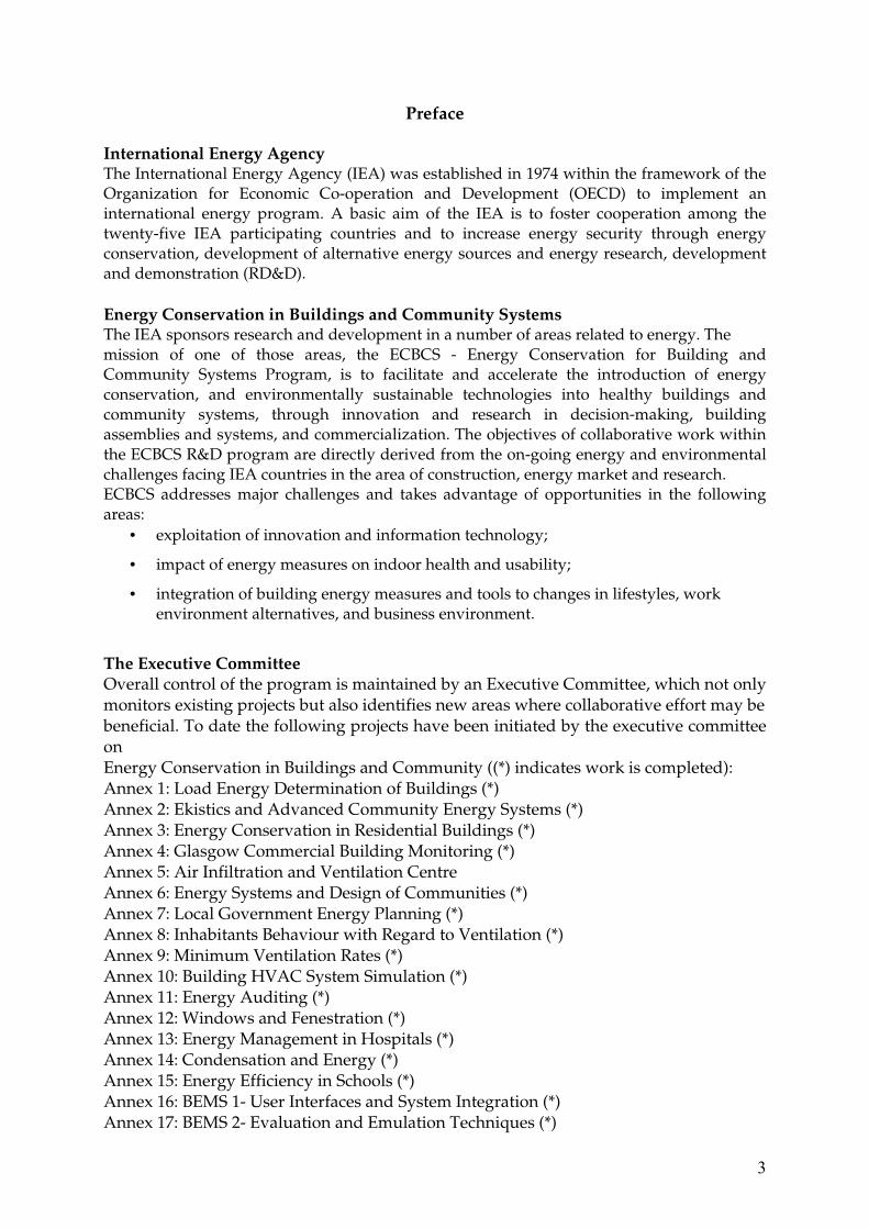
The following table shows the test conditions of the four working points and the weighting factors defined for the air-cooled units.

Test conditions for ESEER definition

Part load ratio Air

temperature (°C)

Water outlet temperature

(°C)

Weight coefficient:

100% 35 7 A = 0,03 75% 30 7 B = 0,33 50% 25 7 C = 0,41 25% 20 7 D = 0,23

SCOP Seasonal Coefficient of Performance Coefficient Of Performance, is the seasonal efficiency of a heat pump in heating mode, defined as the ratio of the total heating energy at condenser side delivered to the building (including distribution heat losses) and the electrical consumption of the heating pump in heating mode. It depends on the building heating load profile and on the heating source temperature over the year. Eurovent It is a consortium that certifies the performance ratings of air-conditioning and refrigeration products according to European and international standards. The objective is to build up customer confidence by levelling the competitive playing field for all manufacturers and by increasing the integrity and accuracy of the industrial performance ratings. Water loop (from EN 14511) Closed circuit of water maintained within a temperature range on which the units in cooling mode reject heat and the units in heating mode take heat GHX Ground heat exchanger Heat Recovery and Reversibility In context of IEA-Annex 48 two ratios are very important. Therefore are short introduction of the heat recovery potential (REC) and the reversibility potential (REV) is given. More detailed information gives [1.2]. REC Heat Recovery Potential Heat recovery potential is shown in the following figure:

14

0 1 2 3 4 5 6 7 8 9 10 11 12 13 14 15 16 17 18 19 20 21 22 23 24Time [h]

-30

-20

-10

0

10

20

30

40D

eman

d [k

W]

Heating DemandHeating Demand

Cooling DemandCooling DemandRecovery PotentialRecovery PotentialMaximum RecoveryMaximum Recovery

(EER + 1) / EER x QC(EER + 1) / EER x QC

The heat recovery potential (REC) is expressed as the ratio between the heat energy recovered (yellow area) and the total heat demand. If priority is given to cooling mode, the heat recovery potential is defined as:

h

h

1min Q ;

Heat Recovery Potential REC Q

CEER Q dtEER

dt

+ ⋅ = =

∫

∫

& &

&

If full heat recovery is achieved, the heat recovery potential is equal to 1. The heat recovery potential could be improved, if there is a storage capability.

15

REV Reversibility Potential The reversibility potential is shown in following figure:

0 1 2 3 4 5 6 7 8 9 10 11 12 13 14 15 16 17 18 19 20 21 22 23 24Time [h]

-20

-10

0

10

20

30

40

Dem

and

[kW

]

Heating DemandHeating Demand

Cooling DemandCooling DemandReversibility PotentialReversibility Potential

maximum heating power of the chiller in heat pump modemaximum heating power of the chiller in heat pump mode

priority to the cooling modepriority to the cooling mode

The reversibility potential (yellow area) gives the percentage of the heating demand that can be delivered by the reversible heat pump. Due to priority to the cooling mode no heat can delivered during a period of cooling demand. The heat delivery is limited by the maximum heat power in heat pump mode. The maximum heating and cooling capacities are very sensible to the operation temperatures. Usually the maximum heating capacity is only 1.1 of the maximum cooling capacity. The reversibility potential is equal to 1 if the total heat demand can be covered by a fully reversible heat pump. Fully reversible means that there is a total switch over from the heating to the cooling mode. A reasonable range of reversibility potential may be around 0.5 and 1. The reversibility potential is defined as:

( )h,max h

c

h

min Q ;QReversibilty Potential REV if Q 0

Q

dt

dt= = =∫

∫

& &&

&

cReversibilty Potential REV 0 if Q 0= = >&

16

1 Introduction

1.1 Scope

A global design methodology will be developed, starting from comfort requirements, environmental, economical constrains and an analysis of heating and cooling demands. Ecological and economical objectives are evaluated. So the designer could do the best choices at an early stage of a project. Innovative design tools will be proposed to architects, consulting engineers and installers, in such a way to reach a global optimisation of the whole heat pump and HVAC system. This will include flow charts and check lists, to help in taking right decisions in right time. 1.2 Background

In non residential buildings the demand for mechanical cooling increases, caused by: − higher internal loads (more information technology equipment, and closely occupied

offices) − increasing requirement for indoor air quality − increased need for cooling for servers and telecommunication devices − glass facades and modern architecture − climate-changing

Besides the cooling demand, there is still a demand for heating. Heat pumps and refrigeration devices offer the possibility to produce heating and cooling with one machine. Therefore an attractive energy and cost saving opportunity consists in using the refrigeration machine for heat production. This can be done by condenser heat recovery whenever there is some simultaneity between heating and cooling demands. Heat recovery is possible in most of the water to water machines. “Reversible Heat Pump Systems” can produce heating and cooling alternatively, they work either in “heating or in cooling (reversible) mode“. Typical examples are air to water machines, where the refrigerant cycle is reversible. But also water to water machines can be operated in both modes; here the water cycle can be reversible. The correct estimation of the potentials of heat recovery and reversibility and the correct choice of the system is a main task during the design process. 1.3 Main Goals of the Design Handbook

The main goals of the design handbook are: 1. to help the designers and decision makers in preserving future possibilities, in not making

irreversible choices, in not making new mistakes, but in optimising the whole HVAC and heat pump systems

2. to document the basic design procedures for reversibility and heat recovery technologies, their components and typical HVAC systems

3. to identify most important design rules for each system types 4. to document the design steps in reference to selected case studies 5. to distribute calculation tools for load analysis and life cycle calculation (LCC)

17

1.4 Design Procedure

The design of such reversible heat pump or heat recovery systems is integrated in a building and HVAC design procedure. The proposed design procedure is shown in Figure 1-1.

Figure 1-1: Design procedure for reversible heat pump systems

Step 1: Basics (see chapter 2)

To start the design process basic information has to be considered, e.g.:

− regulations and laws − energy rates − investment cost − etc.

Step 2: Load Analysis (see chapter 3) and evaluation according to objectives (chapter 4)

A first load analysis is necessary to decide in an early part of the design process, whether a reversible heat pump or a recovery system is reasonable.

Of course first building and system loads have first to be minimized. The analysis of the building systems heating and cooling demands in the purpose of assessing the reversibility and heat recovery potentials has been done by Stabat in Subtask 1 of this project [1.2], [1.3]. Additional work has been done by ieg [3.10]. Chapter 3 gives an overview on the methods for load calculation and methods for analyzing the reversibility and heat recovery potentials.

18

Step 3: Main concept decision (see chapter 5)

A first concept decision (focus on reversibility or focus on heat recovery) has to be made, based on a configuration matrix, design rules and objectives.

A comprehensive description of the reversibility and heat recovery technology description is given S. Bertagnolio and V. Gennen [1.4]. A system overview and system application matrix will help to do a first choice. Life Cycle Costs and environmental impacts as objectives for concept decision Cost and economics and a look to the environmental impacts are also important facts for the concept decision. Therefore a method of life cycle cost (LCC) prediction is integrated in the design guide (Chapter 4).

The evaluation procedure results in a system proposal.

Step 4: Detailed System design (see Chapter 6)

Detailed information on the system design is given for the following topics: − Sizing of reversible heat pump systems (see chapter 6.1).

Check lists and design rules for selection, dimensioning and specification of the primary components. Simulation models are discussed.

− Heat sources and heat sinks Air, water and ground are typical heat sources or heat sinks. Selection rules help to identify the best sources or sinks. In this design guide a focus is given on the dimensioning of ground source heat exchangers (GSHX) like Borehole Thermal Energy Storage Systems (BTES) (see chapter 6.2).

− Hydraulic, thermal storage and operating management Thermal storage systems may improve the whole system performance, e.g. increase the heat recovery potential. Multi unit systems need a operating management to guarantee an efficient operation (see chapter 6.3 ).

− Control Control strategies and operation laws determine the success of the whole system. General rules and examples for a water /water heat pump with ground source heat exchanger are given (see chapter 6.4).

− HVAC-System Design Of great importance to the efficiency of the heat pump system are the temperatures in the heating and cooling systems. These temperatures are strongly connected to the design and operation of heat exchangers in the AHU and the zone heating and cooling devices (radiators, floor heating systems etc.). Also the hydraulic and control schemes are of great importance (see chapter 6.5).

− System optimization In the field of system design and component selection several optimization possibilities exist. A checklist helps to find the optimal solution (see chapter 6.6).

Step 5: Detail System Analysis (chapter 7 and chapter 8) An overall system analysis gives the guaranty, that the objectives are achieved. A detailed load analysis and cost estimation is described Simulation and evaluation tools will support this work.

19

Step 6: Submission Guideline (chapter 9)

The Submission Guide helps in the field of

− Component Specifications

− Materials

Step 7: Commissioning Strategy and Fault Detection (chapter 10)

And the Commissioning Strategy give advises for fault detection and auditing for a successful operation.

Step 8: Operation A continuous monitoring process has to ensure, that the system gets the promised results. The design procedures and the design rules are mostly derived from the case studies documented within this Annex [1.5]. 1.5 Application

The systematic and most of the rules shown in the design guide are applicable in general. Of course there are building and system dependent constrains. The design guide was initially developed for the design of new office buildings with new heat pump

systems working in heat recovery or reversibility mode but retrofit aspects are also considered. 1.6 Methodology

The design guide is based on:

− Literature review

− Analysis of the case studies within the Annex Erreur ! Source du renvoi introuvable.]

− Simulation work with parametric studies

1.7 Examples

The design procedure is explained for three cases: two new buildings cases and one retrofit case − Design Example 1: Reversible heat pump system − Design Example 2: Reversible heat pump system with heat recovery − Retrofit Example 3: Reversible heat pump system in an existing office building

For the two design examples the same building type is chosen. The building represents a medium office building which is north-south orientated [1.3]. It refers to a glazed office building (50 % glazing ration) with thin partition walls. It includes twelve identical floors as shown in Figure 1-2. As mentioned above five zones are considered on each floor: offices (orientation: south and north), conference rooms (orientation: south), toilets (orientation: east) and circulations (orientation: east-west). The first and the top floor are modelled separately. The other ten floors are similar. The total

20

floor area of the building is 15.000 m². The calculations are done for a typical metrological year (location: Passau, German TRY 13)

Figure 1-2: Floor plan of the office building

The building envelope characteristics such as thermal insulation, thermal inertia, solar heat gain and infiltration have been chosen, in accordance to the German energy regulation ENEV. The building envelope characteristics are listed below:

− U-value outside wall: 0.35 W/m²K − U-value window: 1.30 W/m²K − g-value window: 0.59

The solar protection system (external blinds) and lighting system are described in [1.3]. The installed lighting power is assumed to be 18 W/m². The equipment load in the office areas is 15 W/m². The occupancy area is 12 m² per person in the offices and 3.5 m² per person in the conference rooms. The following room set point temperatures are defined for heating and cooling respectively:

− Heating: 21 °C with 6 K night set back − Cooling: 24 °C between 6 am and 8 pm

The infiltration rate is set to 0.15 ach for all investigated zones. To meet the comfort requirements two different HVAC-systems are compared in the design examples:

− Design example 1: Natural ventilation in combination with radiators and chilled ceiling − Design example 2: Central air handling unit with a CAV system

More information’s about the design examples are listed in the following two subchapters. For the retrofit example, a typical multistorey office building is selected in which a “classical” HVAC system made of a boiler and an air-cooled chiller as primary plant is present. The geometry of a typical floor of this building is shown by Figure 1-5.

21

1.7.1 Information on Design Example 1

Building-Type The investigated building is a medium office building as shown in Figure 1-2 [1.3]. Ventilation-Infiltration There is no mechanical ventilation system, only natural infiltration caused by leakage (0.15 ach) and window opening during office hours occur:

− Office rooms: 1.5 ach − Conference rooms: 3.0 ach

HAVC-System All zones are heated (21 °C) and cooled (25 °C) during the office hours by separate heating and cooling systems. In design example 1, the zones are conditioned by a low temperature radiator system and a chilled ceiling (alternatively a fan coil system). The system is designed for the following supply and return temperatures:

− system temperatures for heating: 35 °C / 30 °C − system temperature for cooling 16 °C / 19 °C

building zonebuilding zone

Figure 1-3: HVAC system, example 1: zone heating and cooling with fan coil for heating and cooling

served by a 4-pipe network (alternatively: radiators and ceiling cooling)

Standard Load Calculation In parallel with the dynamic load analysis a standard load calculation of the peak loads is done. The heating load is calculated according to the technical standard DIN EN 12831 [1.6] and the cooling load is determined according to the German VDI guideline 2078 [1.7]. The following design loads are calculated:

− Heating load: 1.263 kW (84 W/m²) − Cooling load: 787 kW (52 W/m²)

Dynamical Load Analysis A dynamical load analysis, based on thermal building and system simulation, calculates the seasonal heating and cooling demands. The load analysis is specified in chapter 3. The load profiles for heating and cooling shows a high reversibility potential and a low heat recovery potential. This means that the heating and cooling loads are mostly not simultaneous.

22

Table 1-1: Heating and Cooling Loads for Example 1

Total Load Specific Load

annual cooling load c totalQ 301 288 kWh/a 20.09 kWh/m²

annual Heating load h totalQ 593 649 kWh/a 39.58 kWh/m²

max. cooling load •

c totalQ 811 kW 54 W/m²

max. heating load •

h totalQ 1 275 kW 85 W/m² Reversibility Potential REV 99.0 %

Heat Recovery Potential REC 0.1 % First conclusions Out of the load analysis the fist conclusions are:

− medium loads − seasonal heating and cooling demand − high reversibility and very low heat recovery potential

First concept decision Out of the load analysis a fist concept decision is made. The plant design is a reversible air to water heat pump without heat recovery.

− Reversible air to water heat pump − No heat recovery option needed − Heat source / sink: air (ground source should be checked) − Passive cooling (option for ground source heat exchanger)

Constraints An assumption for the plant design (air to water heat pump) is moderate rates for electricity. The electricity rates are important inputs for the economical calculations (see chapter 3). Case Study References The design example 1 is similar in the following case studies, which are investigated in the context of this Annex:

− Case study B2: Office building in Charleroi (Belgium) − Case study F 1: Office building in Lyon (France) − Case study G1: Office building in Münster (Germany)

1.7.2 Information on Design Example 2

Building-Type The investigated building is the same building as in design example 1 (see Figure 1-2 and [1.3]. Ventilation-Infiltration There is a mechanical ventilation system ensuring the minimum outside air supply of 30 m³/h per person during the office hours. This results in the following air changes:

− Office rooms: 1.2 ach − Conference rooms: 2.9 ach

The natural infiltration caused by leakage is set to 0.15 ach.

23

HAVC - System To heat and cool the rooms of the building, a central air handling unit is installed. Beside heating and cooling, the AHU also humidifies and dehumidifies the air. In the AHU an air to air heat recovery with a recovery efficiency of 75 % is installed. The air changes and the supply temperature of 18 °C are constant. Additionally all zones are heated (21 °C) and cooled (24 °C) during occupancy with zonal heating and cooling devices. In design example 2, the zones are conditioned by a low temperature radiator system and a chilled ceiling. The system is designed for the following supply and return temperatures:

− system temperatures for heating: 45 °C / 35 °C − system temperature for cooling 6 °C / 12 °C

RETSUP

EXT

ODA

building zone

Figure 1-4: HVAC system, example 2: central air handling unit and zone heating and cooling (fan coils)

Standard Load Calculation In parallel with the dynamic load analysis a standard load calculation of the peak loads is done. The heating load is calculated according to the technical standard DIN EN 12831 [1.6] and the cooling load is determined according to the German VDI guideline 2078 [1.7]. The following design loads are calculated:

− Heating load: 1.045 kW (70 W/m²) − Cooling load: 957 kW (64 W/m²)

Dynamical Load Analysis A dynamical load analysis, out of a thermal building simulation, calculates the seasonal heating and cooling demand. The load analysis is specified in chapter 3. The load profiles for heating and cooling shows a non negligible heat recovery potential. This means that the heating and cooling loads are sometimes simultaneous

24

Table 1-2: Heating and Cooling Demands and Loads for Example 2

Total Load / Demand Specific Load / Demand

Annual Cooling Demand c totalQ 365 801 kWh/a 24.39 kWh/m²

Annual Heating Demand h totalQ 296 680 kWh/a 19.78 kWh/m²

Max. Cooling Load •

c totalQ 833 kW 56 W/m²

Max. Heating Load •

h totalQ 980 kW 65 W/m² Reversibility Potential REV 89.2 %

Heat Recovery Potential REC 8.3 % First conclusions Out of the load analysis the fist conclusions are:

− medium loads − Simultaneous heating and cooling demand in summer − High reversibility and moderate heat recovery potential

First concept decision Out of the load analysis a fist concept decision is made. The following plant design is chosen:

− Reversible air to water heat pump with heat recovery − Heat recovery system − Heat source / sink: air (ground as source should be checked)

Constraints Assumption for the plant design is moderate rates for electricity. The electricity rates are important inputs for the economical calculations (see chapter 4.1). Case Study References The design example 2 is similar to the following case studies, which are investigated in the context of this Annex:

− Case study B1: Office building in (Belgium) − Case study B3: Office building in Arenberg (Belgium) − Case study I2: Office building in Chieri (Italy)

1.7.3 Information on Retrofit Example 3

Building description

It is a 9 storey building with about 7 220 m² of air-conditioned offices and meeting rooms and underground parking lots.

It is located at an altitude of 306 m where the climate is characterized by the following data:

- Heating sizing temperature: - 10°C

- Cooling sizing temperature 30°C with 50 % relative humidity

- 15/ 15 heating degree-days: 2000 K*d.

Local comfort temperature set points can independently be adjusted by occupants within a range of +/- 3°C around a fix value (21°C).

25

Figure 1-5: Floor plan of the building (example 3)

Ventilation strategy The system provides around 32 000 m³/h of fresh air to floor 4, 5, 6 and 7. The ventilation of the offices is forced by 3 units:

- AHU2 : 4th to 7th floors - AHU3 and AHU4 : meeting rooms and manager offices located at the 7th floor

Heat transfer coefficients and nominal heat losses

Each façade module at the front is 16 m² large including 3.12 m² of glazing. The global heat transfer coefficient of the module is estimated to 19.2 W/K. For the whole front side, the global heat transfer coefficient can be estimated to 3 596 W/K. Nominal ventilation flow rate is 32 000 m³/h. The system runs approximatelly 15h per day, 5 days a week. Fresh air flow rate is 6 400 m³/h with 2 144 W/K of sensible heat. In nominal conditions: ambient temperature of 22°C 40% relative humidity ∆t = 30°C ∆hair = 43 kJ/kg

kWQ

kWQ

kWQ

latent

sensible

transfer

9.27

3.64

8.107

=

=

=

&

&

&

The heat demand is equal to 200 kW, and the installed power is equal to 318 kW. HVAC system There are two technical zones in this building: one in the 3rd floor and one in the 8th floor.

• 3rd floor technical zone is equipped with two small supply and extraction groups including speed control, two chillers, a buffer and a terminal cooling coil

26

• 8th floor technical zone has a general electric panel including a feeder, two 250A circuit breakers to supply the chiller and other utilities (fan, pumps and a multisplit group)

There are also 3 air supply and extraction groups, a hot water production (3 gas boilers) and distribution system and 2 chillers. Terminal units Each room has one or more VAV boxes for air heating and cooling. These boxes are located in the false ceiling downstream of the post-heating coils. The following table gives the number of VAV boxes and post-heating coils as given in the as built drawings.

Table 1-3: VAV Boxes (example 3)

Post-heating coils and VAV boxes are connected with air ducts in the false ceilings. There are 2 or 4 VAV boxes per post-heating coil, which opening can vary from 30 to 100%. Air handling units 3 AHU units supply about 32 000 m3/h for the floors 4, 5,6 and 7:

− AHU2 – VAV boxes from 4th to 7th floor − AHU3 – 2 meeting rooms at 7th floor − AHU4 – manager offices at 7th floor

AHU2 has extraction fan, economizer with damper, preheating coil, adiabatic humidifier, cooling coil, and supply fan. Fans are equipped with frequency drivers. Heating and cooling plants There are 3 classical gas boilers (318 kW - no condensation) and 2 chillers.

Nominal water temperatures at the boilers are 70/90 °C (-5°C in external air).

27

Figure 1-6: Boilers scheme view, (from screen computer)

1.8 Literature Chapter 1

In the IEA ECBCS-Annex 48 a lot of documents are written. The content of these documents are not completely included in the design handbook, but within the paper reference is given to these documents.

[1.1] Stabat P.: Annex 48 Glossary 1. Ecole des Mines de Paris. France. June 2008 [1.2] André P. Bertangolio S. et al.: Analysis of building heating and cooling demands in the purpose of assessing the reversibility and heat recovery potentials. IEA Annex 48 Final Report. Universtiy of Liège, Belgium. Ecole des Mines de Paris, France. December 2008. [1.3] Stabat P.:Analysis of building heating and cooling demands in the purpose of assessing the reversibility and heat recovery potentials - Annexes. Ecole des Mines de Paris. France. December 2008. [1.4] Bertagnolio S., Gennen V.: Reversible heat pumps technology description and market overview. University of Liège. Belgium. June 2008. [1.5] Masoero M.: IEA-Annex 48 Case Study overview. Politecnico di Turino. Italy June, 2008. [1.6] DIN EN 12831. Heating systems in buildings - Method for calculation of the design heat load; German version EN 12831. Beuth, Berlin, Germany. August 2003. [1.7] VDI 2078. Cooling load calculation of air-conditioned rooms. Beuth, Berlin, Germany. July 1996.

28

2 Basic Information for Design and Retrofit

For the design and retrofit of primary heating and cooling systems basic information has to be collected. The following information is important for the pre design and concept decision. Available energy resources:

− Gas, fuel available − District heating available − Electricity available

Heat and cold - source:

− Outside air (noise level allowed) − Ground water (available, drilling rights) − Ground heat exchangers (special remark on geological conditions, composition of the

ground, drilling rights) Regulation and laws:

− Energy performance − Drilling rights for ground Heat exchangers

Economics:

− Electric and fuel specific costs − Price index

Comfort:

− Air temperature − Air quality − Noise

If already available, in this design phase, information on building loads and HVAC systems has to be given. Building Loads:

− Peak heating and cooling loads − Monthly / annual heating and cooling demands

(a method to calculate and evaluate building loads is shown in chapter 3) HVAC-Systems:

− Installation area required − Classification:

� Air handling units � Water based heating and cooling � Nominal conditions of the heat exchangers � Control of the heat exchangers � Hydraulic scheme

A list of the required inputs for the design of reversible heat pump systems is given in Table 2-1. Up to approx. 60 single inputs have to be known, to start the decision process and to make the economical calculations. Most of these input values are basics for the design process at a later stage.

29

Table 2-1: List of basic inputs for the design of reversible heat pumps

(design example 1 and 2)

Input Value Unit Comment

1 Location

Passau (Germany) TRY 13

2 Latitude 48.46 degree geographical latitude 3 Longitude 11.26 degree geographical longitude 4 Altitude 409 m geographical height Local Energy Rates 5 Electricity 12 Cent/kWh all taxes included

6 Oil 60 Cent/l all taxes included (not used in ex. 1)

7 Natural Gas 60 Cent/m³ all taxes included

8 Biomass Energy 5 Cent/kWh all taxes included (not used in ex. 1)

Local Equivalent CO2-Emission Rates

9 Electricity 617 g/kWh prEN 15603: 2007

10 Oil 330 g/kWh prEN 15603: 2007 (not used in ex. 1)

11 Natural Gas 277 g/kWh prEN 15603: 2007

12 Biomass Energy 4 - 20 g/kWh prEN 15603: 2007 (not used in ex. 1)

Local Climate Conditions

13 Minimum Outdoor Temperature -16 °C design value for heating systems

14 Maximum Outdoor Temperature 32 °C design value for air-conditioning cooling systems

15 Weather Data (hourly values) TRY 13 test reference year as a data file (ASCII, XLS)

16 Local Interest Rate 4 % average value

Indoor Thermal Comfort Requirements

17 Minimum Indoor Temperature 21 °C design value for heating 18 Maximum Indoor Temperature 24 °C design value for cooling

19 Minimum Indoor Relative Air Humidity 30 %

design value for air-conditioning systems

20 Maximum Indoor Relative Air Humidity 60 %


21 Minimum Fresh Air Volume Rate per Person 30 m3/h


22 Maximum Indoor Air Velocity 0.2 m/s design value for air-conditioning systems

30

Table 2-1 continued:


Temperature Level (zonal heating and cooling)

23 Heating system 45 / 35 °C Low temperature radiator 24 Cooling system 16 /19 °C Chilled ceiling 25 Ventilation (supply) 18 °C AHU not in ex. 1, only in ex. 2

Alternative Heat Sources / Heat Sinks

26 Exhaust Airflow 49 500 m³/h not used in ex. 1 (value for ex. 2)

27 Return Waterflow - kg/h

if domestic/industrial water flow available (not used in ex. 1 and 2)

Geothermal Heat Sources /Heat Sinks

28 Ground Heat Conductivity 2 W/mK 29 Ground Heat Capacity 900 J/kgK 30 Ground Density 1800 kg/m³ 31 Ground Water Depth 10 m 32 Ground Water Velocity 1 m/day

33 Ground Water Minimum Temperature 8 °C

34 Ground Water Maximum Temperature 12 °C

35 Thermal Response Test Results - no results for both examples Building Peak Loads

36 Heat 1 275 kW Ex. 1 37 Cold 811 kW Ex. 1 38 Electricity - kW no results for both examples 39 Domestic Water - m3/h no results for both examples Building Energy Demand

40 Heat 593 649 kWh/a Ex. 1 41 Cold 301 288 kWh/a Ex. 1 42 Electricity - kWh/a no results for both examples

Heat Pump Application Potentials

43 Reversibility Potential 99.0 % REV (Ex. 1) 44 Heat Recovery Potential 0.1 % REC (Ex. 1)

45 Heat and Cold Load Profile (hourly values)

one year heat and cold demands calculated (see Chapter 3)

31

Table 2-1 continued:


Investment Costs see also Chapter 4.1

46 Chiller (air-water) 450 €/kW cost per maximum cooling power

47 Heat Pump (water-water) 600 €/kW cost per maximum thermal power

48 Oil Boiler - €/kW cost per maximum heating power

49 Natural Gas Boiler 200 €/kW cost per maximum heating power

50 Wood Boiler - €/kW cost per maximum heating power

51 Cogenerator (Oil, Gas) - €/kW cost per maximum heating power

52 Cogenerator (Biofuel) - €/kW cost per maximum heating power

53 Ground Heat Exchanger 40 €/m cost per ground pipe length 54 Thermal Buffer 1 000 €/m³ cost per storage space volume 55 Thermal Building Activation 30 €/m² cost per floor area 56 CAV-HVAC (central unit) 20 €/(m³/h) cost per air volume flow 57 VAV-HVAC (central unit) 20 €/(m³/h) cost per air volume flow 58 VAV-Controller (local unit) - €/(m³/h) cost per air volume flow 59 Fan Coil Unit 1500 €/unit cost per air volume flow 60 Cooling Panel 175 €/m² cost per cooling panel area

61 Cooling Tower - €/kW

cost per maximum cooling power (in chiller-costs included)

62 Radiator 45 €/kW cost per maximum heating power

63 Water pump - €/kW cost per maximum electrical power

64 Hydronic Network 30 - 50 €/m² specific value for floor heating

65 (Air) Duct Network - €/m duct length specific value (in AHU costs included)

66 Local Loop Controller - € cost per controller 67 Direct Digital Controller - € cost per controller

68 Supervisory Controller - €

depends on HVAC components and control stategy

69 Sensor (T,P) - € cost per data point 70 Meter (H) - € cost per data point

32

3 Load Analysis - Building and System Energy Demands

In an early design phase, the analysis of the heating and cooling loads helps to decide whether a reversible heat pump system or a reversible heat pump system with heat recovery is reasonable. This leads to a first system design and sizing. A detailed analysis of the heating and cooling demand of typical buildings and an evaluation of the reversibility and recovery potential is done in Subtask 1 of this Annex [3.1] The required inputs for a load analysis are:

− Geometry data of the building with typical loads and operation conditions − HVAC-system design and operation conditions of the building

The load analysis gives the following outputs and results:

− Reversible potential − Heating energy delivered by the heat pump

− Recovery potential − Heating energy recovered − Max heating load − Max cooling load − Yearly heating load − Yearly cooling load

The analysis delivers also system dependent outputs:

− Heat from heat pump (max. and yearly amount) − Heat from additional heater (max. and yearly amount) − Cold from heat pump (max. and yearly amount) − Cold from additional heater (max. and yearly amount)

Out of the load analysis and the heat pump system dependent outputs two decisions have to be drawn (see also chapter 5.1). The first one is the heat pump system type and the second one is the kind of heat source type. For the first design approach one of the following heat pump system type are possible:

− Chiller with heat recovery or

− Reversible System (air/water or water/water) or

− Reversible system with heat recovery (water/water or brine/water) Possible and common heat source types are:

− Outside air or

− Ground source or

− Water Also other configurations, besides the listed heat pump system types and heat sources are imaginable.

33

3.1 Load Analysis based on Simulation Work

The heating and cooling loads should be given in hourly values. An efficient way to get these load profile of a building, is a building and system simulation. An Evaluation on a longer integration time (i.e. monthly values) gives an overestimation of the heat recovery potential [3.2]. Figure 3-1 shows the three steps of a typical simulation:

1. Building simulation 2. HVAC system simulation 3. Plant simulation

As a comparison between building and system loads shows that building loads differ significantly from system loads [3.1]. At least both building and HVAC system simulations have to be done (see Figure 3-2) to generate a useful load profile. A plant simulation is not necessary in this step of the design procedure, but first assumptions on the plant behaviour (SCOP, SEER) have to be made. With these assumptions the energy demand and operating costs can be roughly predicted.

Building Simulation

HVAC System Simulation

Plant Simulation

•Hourly heating and cooling loads•Maximum and yearly values•Full load hours for heating and cooling

•Hourly heating and cooling loads•Maximum and yearly values•Full load hours for heating and cooling •Temperatures (cold- and hot water)•Mass flow rates

•Heating, cooling delivered (HP-system)•Heating, cooling delivered (secondary system)•Maximum and yearly values•COP, purchased electricity, fuel…•Operation behavior •Operating hours

Figure 3-1: General procedure of a load calculation

34

Distribution

•Losses

•Temperatures

•Mass flow rate

Building Loads

System Loads to Reversible Heat Pump Systems

Water based terminal units

•Control losses

Air handling unitsheating and cooling coils

DX terminal units (VRF)

•Control losses

Distribution

•Losses

•Temperatures

•Mass flow rate

Figure 3-2: Procedure of calculating system loads for different kind of HVAC components

Conclusion Hourly building and system loads have to be used for further load evaluations.

35

3.2 Simulation and Evaluation Tools

Within IEA ECBCS Annex 48 the following tools are developed to generate a load profile for a specific building with the HVAC-System and to identify the REV- and REC-potential for the application of a reversible heat pump [3.2], [3.3], [3.4], [3.10]. 1.) In the audit of existing buildings and before any retrofit: "BENCHMARK": This tool is developed in the frame of the HARMONAC project and is used to compute the "theoretical" (or "ideal") consumptions of the building when equipped with a very typical system allowing temperature and humidity control. The building is seen as a unique zone and is briefly described by the user. The results offer a first and very rough interpretation of the measured consumptions. "SIMAUDIT": This tool is also developed in the frame of the HARMONAC project and offers a larger range of available HVAC equipment. The building is seen as a unique zone. The system includes an equivalent global AHU and several types of terminal units (radiators, fan coils, cooling ceiling etc.). The computed consumptions have to be compared to the measured consumptions. The parameters of the model have to be adjusted to reproduce these consumptions as well as possible. 2.) In order to identify the heating and cooling demands of both new and existing buildings: "SIMZONE": This tool allows simulating a given zone of the building (a storey; a peripheral zone or a central zone of a given storey or a building wing) and compute the heating and cooling demands of the studied zone. The accuracy of this simulation is guaranteed by the adjustment of the parameters realized with SIMAUDIT. "AGGREGATE": The different heating and cooling demand profiles generated with SIMZONE are aggregated. The reversibility and recovery potentials are computed as done in Subtask 1 of this Annex [3.1]. 3.) In the design process of the new or renewed systems: 5. "Sizing and Assessment Tool": A detailed simulation of reversible heat pump systems is possible with this tool. Detailed information gives the IEA 48 simulation reference book [3.18]. Also other simulation programs like TRNSYS [3.6] and EnergyPlus [3.7] can be used to calculate the building and system loads. The TRNSYS16 simulation environment is used in the context of the examples, presented in this design handbook [3.10]. The following TRNSYS 16 types can be used:

Calculation of H/C demands: − TRNSYS Building Model: Type 56 (multi-zone building model) [3.11] − System AHU and HVAC- Simulation: Type 303 (air handling unit) [3.12] New system design: − Heat Pump Simulation Type 401 (heat pump) [3.13] − Ground source heat exchangers Type 557 (DST-Model) [3.14]

36

3.3 Building and System Typology

Typical loads and load profiles are analyzed in the context of subtask 1 and are available for office and health care buildings [3.1]. The following tables represent the building and systems types.

Table 3-1: Building typology for office buildings, proposed by STABAT [3.1]

Building type 1a 1b 1c 2 3

buildings of huge areas mainly glazed

description Broad open space offices

Broad partitioned

offices

Thin geometry -

glazed meeting

room

Medium size retrofitted buildings

Small buildings of industrial suburban

zones

Stock share in % of surface 14% 20% 33% 8% 25%

Total surface area1 15 000 m² 5 000 m² 1 000 m² Floors (including ground

floor) 12 4 2

Height under ceiling 3 m 3 m 2.7 m % of surface area by type of use (with respect to useful total surface area)

Offices 78% 55% 60% 55% 58% Meeting rooms 16% 22% 21% 22% 18%

WC 3% 3% 3% 3% 3% Circulations 3% 20% 16% 20% 21%

% of outside walls surface area (with respect to useful total surface area)

Total 45% 50% 66% 67% 104% Vertical walls (opaque and

glazed) 37% 42% 58% 42% 54%

Roof 8% 8% 8% 25% 50% 13% 17% 26% 9% 21%

Glazed surfaces (vertical) 50% of vertical surfaces with window2

27.5% of vertical surfaces with

window²

34% of vertical surfaces with

window²

Table 3-2: Share of air conditioning systems in percentage of air conditioning surface [3.1], [3.15]

CAC* + Water

distribution

CAC + air distribution

CAC split CAC roof

top CAC VRF RAC**

Office building

45.5% 27.7% 2.5% 1% 2.3% 21%

Health care institutions

58.6% 35.6% 0% 0% 0% 5.8%

* Central Air conditioner ** Room Air conditioner

The central air conditioners using chillers are predominant in office buildings and health care institutions. Often air/water systems (i.e. CAC and fan coils) are used. The chiller market is dominated by air cooled chillers compared to water cooled chillers, they represent 86% of the market [EEC, 2003] [3.15]. VRF and reversible multi-split systems are marginal on the market.

1 Area net: Sum of all areas between the vertical building components (walls, partitions,…), i.e. gross floor area reduced by the area for structural components 2 This ratio is defined for the main facades (E/W or N/S), the other facades are assumed without any windows.

37

Table 3-3: HVAC system type matched to building type, proposed by STABAT [3.1], [3.16]

Refrigerant-based systems

FCU + SF

FCU + DF

VAV CAV

VRF Reversible Multi Split

Air to Air Heat Pump

Office type 1a ��

Office type 1b ��

Office type 1c ��

Office type 2 ��

��

Office type 3 ��

��

Hospital type 1 ��

Rest home type 2 ��

FCU: fan coil unit SF: single flux ventilation DF: double flux ventilation

3.3.1 Heat Recovery and Reversibility Potential

The heat recovery and the reversibility potential are calculated for different climate zones in Europe [3.1]. The following table compares the energy saving potential for different HVAC systems in different climate zones due to reversibility. In office buildings, the heat recovery potential is very low, therefore a independent table will be omitted.

Table 3-4: Energy saving in office building, due to reversibility: [3.1]

Climatic zone HVAC system

PARIS TORINO ATHENS MUNICH LISBON

SF + FCU ☺☺ ☺☺ ☺ ☺☺ � DF + FCU ☺☺ ☺☺ ☺ ☺☺ �

VAV ☺☺☺☺ ☺☺☺☺ ☺☺☺ ☺☺☺ ☺☺ CAV ☺☺☺ ☺☺☺ ☺☺ ☺☺ ☺☺

General conclusions on reversibility (REV): - Reversibility is high in moderate and cold climate zones - Reversibility is more likely if AHU (VAV or CAV without dehumidification) are in operation - Reversible is typical for office buildings

General conclusions on heat recovery (REC): - In office buildings, the heat recovery potential is very low. - Only in data centre, the cooling demand is high and faintly dependent of weather conditions.

Thus, the potential of heat recovery in winter would be quite high. - The heat recovery on chiller condenser for hot domestic water (HDW) preparation can save a

lot of fuel, in particular in health care institutions where HDW consumptions are high.

38

3.4 Steps in Load Analysis

For the load analysis the following working steps have to be done:

1. Define the inputs for building and system simulation: − The inputs depend on the simulation tool used [3.3] [3.4] [3.6] [3.7].

⇓ 2. Run the simulation and calculate the hourly heating and cooling loads:

− Calculate separately, if different heating and cooling systems with different temperatures are used

⇓ 3. Analyze the heating and cooling loads:

− Use the analyzing tools described in [3.10] − Calculate REV and REC values

⇓ 4. Make a first concept decision (see chapter 4 and 0):

− Reversible system (yes/no) � Reversibility on refrigerant side –air/water heat pump � Reversibility on water side – water/water heat pump

− Heat recovery system (yes/no) − Heat source / heat sink (air, water, ground etc.)

⇓ 5. Sizing of the heat pump:

− Maximum cooling capacity (100%, 80%, 60% 40% etc. of peak cooling load) − Mean COPHeating3, COPCooling4 and heating capacity in reversed mode

� Depend on mean evaporator (entering air temperature (EAT) or entering water temperature (EWT)) and condenser (leaving water temperature (LWT))

− Mean COPHeating, COPCooling and heating capacity in recovery mode � Depend on mean temperatures on evaporator (entering temperature) and

condenser (leaving temperature) ⇓

6. Calculate the energies (outgoing from heat pump and additional heating systems): − Cooling energy delivered by the heat pump − Heating energy delivered by the heat pump − Heating energy delivered by additional heating system

⇓ 7. Estimate the potential of passive cooling:

− Depending on the supply temperature for cooling − Only possible if the cold source temperature is lower than supply temperature for the

cooling system ⇓

8. Calculate the final energies: − Electricity − Fuel, gas etc.

The following two examples will illustrate this procedure.

3 COPHeating: nominal conditions EAT= 7 °C; RH 87%, EWT/LWT= 40/45 °C, find more information on rev. air/water heat pumps in [3.17] ( 4 COPCooling: nominal conditions EAT = 35 °C, EWT/LWT = 7/12 °C, find more information on rev. air/water heat pumps in [3.17]

39

3.5 Examples – Building and System Load Analyses

For the two design examples the same building type is chosen. The building represents a hypothetical office building, which is described in chapter 1.7 of this handbook. On a typical metrological year (location: Passau, German TRY 13) a building and system load analysis is done for the two cases:

− Design example 1: reversible heat pump system − Design example 2: reversible heat pump system with heat recovery

3.5.1 Design Example 1 – Reversible Heat Pump System

For example 1 an hourly analysis is done. As described in chapter 1.7.1 the investigated office building have the following key features:

− Total floor area: 15 000 m² − Natural ventilation − Low temperature heating (45/35 °C) and chilled ceiling (or fan coils) (18/14 °C) − Night set back

The yearly loads are shown in Figure 3-3 and the cumulative frequency of the heating and cooling loads is plotted in Figure 3-4.

Jan Feb Mar Apr May Jun Jul Aug Sep Oct Nov Dec

0

200000

400000

600000

800000

1000000

1200000

1400000

Load

[W]

Heating LoadHeating Load Cooling LoadCooling Load

Annual Heating and Cooling LoadsDesign Example 1

Figure 3-3: Design example 1 - hourly system heating and cooling loads

The simulated values correspond with the values out of the standard load calculation for heating and cooling (Table 3-5). If storage possibilities are used the peaks could minimized.

40

0 400 800 1200 1600 2000 2400 2800 3200 3600 4000

0

200000

400000

600000

800000

1000000

1200000

1400000

Load

[W]


Cumulative Frequency of Heating and Cooling LoadsDesign Example 1

Figure 3-4: Design example 1 – cumulative frequency of heating and cooling loads

Table 3-5: Design example 1 – annual and maximum heating and cooling loads


Annual cooling load ,C totalQ 301 288 kWh/a 20.09 kWh/m²

Annual Heating load ,H totalQ 593 649 kWh/a 39.58 kWh/m²

Max. cooling load ,C totalQg

811 kW 54 W/m²

Max. heating load ,H totalQg

1 275 kW 85 W/m² Reversibility Potential REV 99.0 %

Heat Recovery Potential HRP 0.1 % First conclusions Out of the load analysis the fist conclusions are:

− Medium specific heating and cooling loads − Only a few hours in the year with simultaneous heating and cooling demand − High reversibility and very low heat recovery potential

First concept decision Out of the load analysis a fist concept decision concerning the heat pump type is made:

− Reversible heat pump system: � Air to water heat pump (heat source/sink: air)

reversibility on refrigerant side (see Figure 3-5) or

� Water to water heat pump (heat source/sink: ground soil) reversibility on water side with passive cooling option by the ground (see Figure 3-6)

− No heat recovery If it is an existing building, the existing HVAC systems should be considered for a concept decision.

41

Approach to example 1: - A comparison between two heat pump system types is done - Air to water heat pump with reversibility on refrigerant side - Water to water heat pump with reversibility on water side

1

2

3

4

5

Heating System

air

1: heat exchanger water/refrigerant

2: expansion valve

3: heat exchanger air/refrigerant

4: compressor

5: 4-way-valve

Reversible air to water heat pump system

Heating mode

1

2

3

4

5

Cooling System

air


2: expansion valve


4: compressor

5: 4-way-valve


Cooling mode

Figure 3-5: Functional scheme of a reversible air to water heat pump

3.5.1.1 Heat Pump Sizing and Effectiveness – Heat Pump Option 1 : Air to Water Heat Pump in Reversible Mode

The classical solution for reversible heat pumps is to use an air to water heat pump with reversibility on refrigerant side. The heat pump is sized to meet 100% of the cooling demand.

Table 3-6: Sizing and effectiveness parameters –air to water heat pump in reversible mode

Heat Pump Type Air to Water Condenser

Temperature [°C]

Evaporator Temperature

[°C]

Cooling capacity heat pump , ,C HP sQg

810 kW 35 40 12 7

Relation heating/cooling capacity , , , ,/H HP s C HP sQ Qg g

1.10 -

Heating capacity heat pump , ,H HP sQg

891 kW

Mean COP during heating mode HCOP 3.00 - 40 45 4 0

Mean COP during cooling mode CCOP EER= 3.50 - 25 30 18 14

Mean efficiency of additional heater Hη 0.90 -

42

Considering this design the following results are achieved (for further details see [3.10]): Table 3-7: Design example 1 – results of a first load analysis – HP-sizing to 100% cooling –air to water

heat pump in reversible mode


Cooling from heat pump annual ,C HPQ 301.286 kWh/a 20,09 kWh/a*m²

Max. cooling capacity from HP , ,maxC HPQg

810 kW 0,05 kW/m²

Additional cooling annual ,C addQ 0 kWh/a 0,00 kWh/a*m²

Max additional cooling ,C addQg

0 kW 0,00 kW/m²

Condenser heat annual , ,C HP condQ 586.911 kWh/a 39,13 kWh/a*m²

Max. condenser heat , ,C HP condQg

891 kW 0,06 kW/m²

Heat from heat pump annual ,H HPQ 586.911 kWh/a 39,13 kWh/a*m²

Max. heating capacity from HP , ,maxH HPQg

891 kW 0,06 kW/m²

Additional heating annual ,H addQ 6.739 kWh/a 0,45 kWh/a*m²

Max additional heating ,H addQg

385 kW 0,03 kW/m²

Factor heat recovery, annual REC 0,00 % Factor reversibility, annual REV 98,86 %

Percentage heat and cool from HP , , , ,( ) /( )C HP H HP C total H totalQ Q Q Q+ + 99,25 %

Percentage cool from HP , ,/C HP C totalQ Q 100,00 %

Percentage heat from HP , ,/H HP H totalQ Q 98,86 %

Percentage additional cooling , ,/C add C totalQ Q 0,00 %

Percentage additional heating , ,/H add H totalQ Q 1,14 %

Percentage of passive cooling Fpassiv 0,00 % max 20% (air)

Electricity demand heating mode annual , ,/ Hel H H HP

W Q COP= 195.637 kWh/a 13,04 kWh/a*m²

Electricity demand cooling mode annual , , 1 /

100passiv

Cel C C HP

FW Q COP

= −

g

86.082 kWh/a 5,74 kWh/a*m²

Total electricity demand ,el totalW 281.719 kWh/a 18,78 kWh/a*m²

Total fuel demand , , /H f H add HQ Q η= 7.487 kWh/a 0,50 kWh/a*m²

First conclusions example 1: - Almost no additional heat production is needed - COP and EER have to be optimized to get low electricity demand - Passive cooling option have to be checked – depending on the temperature levels in the

HVAC systems

43

3.5.1.2 Heat Pump Sizing and Effectiveness – Heat Pump Option 2 : Water to Water Heat Pump

An alternative solution is to use a water (or brine) to water heat pump with ground as heat source or sink. Better COP’s and a higher passive cooling potential are the promised advantages. A typical scheme of a reversible water to water ground source heat pump is shown in Figure 3-6.

1

2

4

Heating

Reversible water and water to water heat pump system

Water-tor water / ground source heat pump

System

3

Cooling System

HX

heat sink/source

- ground vertical boreholes

HX

HP

Heat StorageCold Sorage

P2

P4

V3

V2

V4

P5

V1P1

P3

A

B

A

B

AB

AB

Y2Y1

Y3

Figure 3-6 : Water to water ground source heat pump

Table 3-8: Sizing and effectiveness parameters – water to water heat pump in reversible mode and heat

recovery mode

Heat Pump Type Water to Water Condenser

Temperature [°C]

Evaporator Temperature

[°C]

Cooling capacity heat pump , ,C HP sQg

810 kW 35 40 12 7

Relation heating/cooling capacity , , , ,/H HP s C HP sQ Qg g

1.10 -

Heating capacity heat pump , ,H HP sQg

891 kW

Mean COP during heating mode HCOP 3.00 - 40 45 4 0

Mean COP during cooling mode CCOP EER= 5.00 - 20 25 18 14

Mean efficiency of additional heater Hη 0.90 - Considering this design the following results are achieved (for further details see [3.10]):

44

Table 3-9: Design example 2 – Results of a first load analysis – HP-sizing to 100% cooling – water to water

heat pump in reversible mode – heat recovery option


Cooling from heat pump annual ,C HPQ 301.286 kWh/a 20,09 kWh/a*m²

Max. cooling capacity from HP , ,maxC HPQg

810 kW 0,05 kW/m²

Additional cooling annual ,C addQ 2 kWh/a 0,00 kWh/a*m²

Max additional cooling ,C addQg

2 kW 0,00 kW/m²

Condenser heat annual , ,C HP condQ 988.626 kWh/a 65,91 kWh/a*m²

Max. condenser heat , ,C HP condQg

1.080 kW 0,07 kW/m²

Heat from heat pump annual ,H HPQ 587.555 kWh/a 39,17 kWh/a*m²

Max. heating capacity from HP , ,maxH HPQg

891 kW 0,06 kW/m²

Additional heating annual ,H addQ 6.094 kWh/a 0,41 kWh/a*m²

Max additional heating ,H addQg

385 kW 0,03 kW/m²

Factor heat recovery, annual REC 0,11 % Factor reversibility, annual REV 98,86 %

Percentage heat and cool from HP , , , ,( ) /( )C HP H HP C total H totalQ Q Q Q+ + 99,32 %

Percentage cool from HP , ,/C HP C totalQ Q 100,00 %

Percentage heat from HP , ,/H HP H totalQ Q 98,97 %

Percentage additional cooling , ,/C add C totalQ Q 0,00 %

Percentage additional heating , ,/H add H totalQ Q 1,03 %

Percentage of passive cooling Fpassiv 60,00 % (ground) Electricity demand heating mode annual , ,

/ Hel H H HPW Q COP= 195.852 kWh/a 13,06 kWh/a*m²

Electricity demand cooling mode annual

, , 1 /100passiv

Cel C C HP

FW Q COP

= −

g

24.103 kWh/a 1,61 kWh/a*m²

Total electricity demand ,el totalW 219.955 kWh/a 14,66 kWh/a*m²

Total fuel demand , , /H f H add HQ Q η= 6.771 kWh/a 0,45 kWh/a*m²

45

3.5.1.3 Comparison and Evaluation

The heat pump operation is evaluated for the following three operation modes and compared with a conventional system (boiler and chiller):

− Heat recovery − Reversibility − Heat recovery and reversibility

Table 3-10 and Figure 3-7 shows the results of the evaluation.

Table 3-10: Design example 1 – comparison and evaluation the results of a first load analysis

Operation Mode

Convent-

ional Boiler

and Chiller

Heat

Recovery Reversibility

Heat

Recovery and

Reversibility

Heat pump type water(brine) / water

air / water water(brine) / water

Reversibility no on refrigerant side

on water side

Heat source / sink ground air ground Type heat source / sink borehole direct

expansion borehole

Heat pump cooling capacity kW 812 812 812 812 Cooling sizing ratio % 100% 100% 100% Heat pump heating capacity kW 1.276 1.083 893 1.083 Heating sizing ratio % 85% 70% 85%

COPHeating - 3,00 3,00 3,00 COPCooling = EER - 5,00 3,50 5,00

Cooling from heat pump annual kWh/

a 0 301.288 301.288 301.288

Additional cooling annual kWh/a

301.288 0,00 0 0

Heat from heat pump annual kWh/a

0 644 586.986 587.630

Additional heating annual kWh/a

593.650 593.005 6.664 6.020

Factor heat recovery annual % 0 0,11 0 0 Factor reversibility annual % 0 0,00 99 99 Percentage of passive cooling % 0 0,00 0 60 Electricity demand heating mode annual kWh/

a 0 195.662 195.877

Electricity demand cooling mode annual kWh/a

60.258 86.082 24.103

Total electricity demand kWh/a

168.654 60.258 281.744 219.980

Total fuel demand kWh/a

659.611 658.895 7.404 6.688

The result of the comparison is that the operation mode “heat recovery and reversibility”, together with the option for passive cooling, has a high fuel saving potential. The ground coupled system with only heat recovery shows a very low fuel saving potential. Further economical (life cycle costs) and ecological (CO2-emission) objectives are needed for a final decision.

46

0

100000

200000

300000

400000

500000

600000

700000

Ene

rgy

Dem

and

[kW

h/a]

Total Electricity DemandTotal Electricity Demand

168654168654

5659556595

281744281744

219980219980

Total Fuel DeamandTotal Fuel Deamand

659611659611 658895658895

74047404 66886688

Energetically Evaluation of different Heat Pump ModesDesign Example 1

Conventional Boiler and Chiller

Heat Recovery Reversibility Heat Recovery andReversibility

Figure 3-7: Design example 1 – energetically evaluation of three operation mode

3.5.2 Design Example 2 – Reversible Heat Pump System with Heat Recovery

Also for example 2 an hourly analysis is done. As described in chapter 1.7.2 the investigated office building have the following key features:

− Total floor area: 15 000 m² − Mechanical ventilation with air to air passive heat recovery − Temperature level heating for the air handling unit: 60/50 °C − Temperature level cooling for the air handling unit: 6/12 °C − Temperature level heating for the terminal units: 45/35 °C − Temperature level cooling for the air terminal units: 14/18 °C − Night set back

The yearly loads are shown in Figure 3-8 and the cumulative frequency of the heating and cooling loads is plotted in Figure 3-9. The simulated values correspond with the values out of the standard load calculation for heating and cooling (Table 3-11). If storage possibilities are used the peaks could minimized.

47

Jan Feb Mar Apr May Jun Jul Aug Sep Oct Nov Dec

0

200000

400000

600000

800000

1000000

1200000

1400000

Load

[W]


Annual Heating and Cooling LoadsDesign Example 2

Figure 3-8: Design example 2 - hourly system heating and cooling loads

0 400 800 1200 1600 2000 2400 2800 3200 3600 4000

0

200000

400000

600000

800000

1000000

1200000

1400000

Load

[W]


Cumulative Frequency of Heating and Cooling LoadsDesign Example 2

Figure 3-9: Design example 2 - cumulative frequency of heating and cooling loads

48

Table 3-11: Heating and cooling loads for example 2


Annual cooling load ,C totalQ 365 801 kWh/a 24.39 kWh/m²

Annual Heating load ,H totalQ 296 680 kWh/a 19.78 kWh/m²

Max. cooling load ,C totalQg

833 kW 56 W/m²

Max. heating load ,H totalQg

980 kW 65 W/m² Reversibility Potential REV 89.2 %

Heat Recovery Potential HRP 8.3 % First conclusions Out of the load analysis the fist conclusions are:

− Medium loads − Simultaneous heating and cooling demand in summer − High reversibility (89%) and moderate condenser heat recovery potential (8%) − Higher heating system temperature level in comparison to example 1

(heating coil AHU) − No passive cooling possible, due to system temperature levels in the AHU

(6/12 °C) First concept decision Out of the load analysis a fist concept decision is made. The following plant design is chosen:

− Reversible water to water heat pump with heat recovery option − Heat source / sink: air (ground as source should be checked) − No passive cooling

The heat pump is sized to the cooling capacity: 100% of the cooling load: 835 kW As the operating conditions are different, heat recovery and reversibility modes are analysed separately:

Reversibility Mode:

− Heat pump heating capacity (110% of cooling capacity): 924 kW Heat Recovery Mode:

COPHeating during heat recovery: 3.5

− Heat pump heating capacity ,1

1

CH HP

H

QQ

COP

=

−

g

g

1 169 kW

Considering this design the following results are achieved (For further details see [3.10]):

49

3.5.2.1 Comparison and Evaluation

The heat pump operation is evaluated for the following three operation modes:

− Condenser heat recovery − Reversibility − Condenser heat recovery and reversibility

The results of the three different operation modes are compared to a conventional system. Table 3-12 and Figure 3-10 shows the results.

Table 3-12: Design example 2 – comparison and evaluation, results of a first load analysis

Operation Mode Conventional

Boiler and Chiller

Heat Recovery

Reversibility

Heat Recovery and Reversibility

Heat pump type

water(brine) / water air / water

water(brine) / water

Reversibility

no

on refrigerant side on water side

Heat source / sink ground air ground Type heat source / sink

borehole direct expansion borehole

Heat pump cooling capacity kW 833 835 835 835 Cooling sizing ratio % 100% 100% 100% Heat pump heating capacity kW 980 1.169 919 1.169 Heating sizing ratio % 119% 94% 119%

COPHeating - 2,50 2,50 2,50 COPCooling = EER - 4,50 3,20 4,50

Cooling from heat pump annual kWh/a 0 365.802 365.802 365.802 Additional cooling annual kWh/a 365.802 0,00 0 0 Heat from heat pump annual kWh/a 0 24.789 264.506 289.294 Additional heating annual kWh/a 296.681 271.892 32.175 7.386

Factor heat recovery annual % 0 8,36 0 8 Factor reversibility annual % 0 0,00 89 89 Percentage of passive cooling % 0 0,00 0 0 Electricity demand heating mode annual kWh/a 0 105.802 115.718 Electricity demand cooling mode annual kWh/a 81.289 114.313 81.289 Total electricity demand kWh/a 196.286 81.289 220.115 197.007 Total fuel demand kWh/a 329.645 302.102 35.750 8.207

Reversibility and the heat recovery mode with reversibility have a higher fuel saving potential than only the recovery mode. An additional option for passive cooling should have a higher energy saving potential. But it was not considered in these cases, due to the improper temperature levels. For a final decision further economical (life cycle costs) and ecological (CO2-emission) objectives are needed.

50

0

100000

200000

300000

400000

500000

600000

700000

Ene

rgy

Dem

and

[kW

h/a]

Total Electricity DemandTotal Electricity Demand

196286196286

8128981289

220115220115197007197007

Total Fuel DeamandTotal Fuel Deamand

329645329645

302102302102

3575035750

82078207

Energetically Evaluation of different Heat Pump ModesDesign Example 2


Heat Recovery Reversibility Heat Recovery andReversibility

Figure 3-10: Design example 2 - Evaluation of three operation mode and comparison with a conventional

system

3.5.3 Design Example 3 - Retrofit

Hourly calculation of heating and cooling demands of the retrofit example yields the results shown by Figure 3-11.

Figure 3-11 : Hourly calculation of heating and cooling demands (example 3)

51

There from, the reversibility and recovery potentials are calculated as follows:

− Reversibility potential: 52% − Recovery potential: 13%

These results confirm a situation frequently observed in mid climate office buildings: Relatively high reversibility potential and very low recovery potential.

3.5.4 Conclusions from the load analysis

If a reversible heat pump with heat recovery is used, the cooling demand is served by 100% and it is estimated, that 97% of the heating demand is served by the heat pump. Only a little additional heating (fuel) is needed in most cases. Passive cooling has a significant effect, but depends strongly on the temperature levels of cold source and heating system.

General conclusion for the load analysis: - Building and HVAC-system load analysis based on simulation work gives the fundamental

values for system design and evaluation - But attention: assumptions on seasonal COP, EER and passive cooling potential have to be

checked further (i.e. in a detailed heat pump simulation)

52

3.6 References Chapter 3

[3.1] Pascal STABAT: Analysis of building heating and cooling demands in the purpose of

assessing the reversibility and heat recovery potentials, Final report, Dec. 08, Ecole des Mines de Paris, France

[3.2] Philippe ANDRE, Stéphane BERTAGNOLIO, Pierre-Yves FRANCK, Jean LEBRUN – ULg ; Marco CACIOLO, Pascal STABAT – Ecole des Mines de Paris: Development of a performance index for chiller reversibility and heat recovery potential assessment, IEA-Annex-48, Meeting, Münster, April 2008

[3.3] André, P., Bertagnolio, S., Franck, P-Y., Lebrun, J. 2008. Performance assessment of heat

pumping in nonresidential buildings by means of dedicated simulation models. Proceedings of the first Heat Pump Symposium, Mechelen, Belgium

[3.4] Bertagnolio S.: Reversibility and Recovery Potentials Identification, Thermodynamics

Laboratory, University of Liege, April 2004

[3.5] Gennen, V. 2008. Modelling of reversible air-to-water heat pump systems. Electromechanical engineering, thesis, University of Liege

[3.6] TRNSYS 16-01: A TRaNsient System Simulation Programme, Solar Energy Laboratory,

Univ. of Wisconsin-Madison; TRANSSOLAR Energietechnik GmbH; CSTB – Centre Scientifique et Technique du Bâtiment; TESS – Thermal Energy Systems Specialists, 2006

[3.7] EnergyPlus: „EnergyPlus building energy simulation software”, US Department of

Energy, 2008

[3.8] Ehrensberger, K.: „Analyse von Heiz- und Kühllasten unterschiedlicher Bürogebäude für Wärmepumpensysteme zum Heizen und Kühlen“, Thesis, Hochschule Nürnberg, Sept. 2008

[3.9] Künzig, M: Entwicklung von Simulationsmodellen für reversible Wärmepumpen mit

TRNSYS, Thesis, Hochschule Nürnberg, March. 2009

[3.10] Dentel. A. and Stephan W.: Detailed Building System and Plant Simulation for Evaluating the Potential of reversible Heat Pump Systems using TRNSYS 16 Simulation Environment, April 2009

[3.11] TRNSYS 16: a TRaNsient SYstem Simulation program, Volume 6; Multizone Building

modelling with Type56 and TRNBuild, 2006 [3.12] Arno Dentel, Wolfram Stephan: Berechnung des Energie und Stoffaufwands von RLT-

Anlagen .: TRNSYS Usertag – Stuttgart; 18. März 2005

[3.13] Wetter, Th. Afjei, . U. Schonhardt:. TRNSYS TYPE 201 Kompressions-wärmepumpe inklusiv Frost- und Taktverluste Modellbeschreibung und Implementation in TRNSYS, erstellt im Auftrag des Bundesamtes für Energiewirtschaft: Juli 2002

[3.14] TRNSYS Type TYPE 557: VERTICAL GROUND HEAT EXCHANGER, TESS Library, TESS

– Thermal Energy Systems Specialists, 2006

[3.15] Energy Efficiency and Certification of Central Air Conditioners study (EECCAC) for the D.G. Transportation- energy (DGTREN) of the Commission of the E.U.. Co-ordinator: ADNOT J. Janvier 2005

53

[3.16] FILFLI S. : Optimisation bâtiment/système pour minimiser les consommations dues à la climatisation. Thèse de doctorat, Ecole des Mines de Paris, décembre 2006

[3.17] S. Bertagnolio & V. Gennen: REVERSIBLE HEAT PUMPS TECHNOLOGY DESCRIPTION

AND MARKET OVERVIEW; June 2nd , 2008 Thermodynamics Laboratory, University of Liège

[3.18] S. Bertagnolio et. al: IEA 48 Simulation Reference Book; 2009 Thermodynamics Laboratory,

University of Liège

54

4 Criteria and Objectives for Concept Decision

Beside the energy evaluation (see chapter 3) costs, economics and environmental impacts are important facts for the concept decision. Therefore a method for life cycle cost (LCC) prediction and a calculation of CO2-emission and of primary energy consumption is integrated in the design guide. The focus of this design guide is primarily on new buildings. 4.1 Economical Objectives – Life-Cycle Costs

4.1.1 General Aspects for the Economy of Reversible Heat Pump Systems

The total costs of HVAC systems result from the following individual costs: 1. Investment Costs

If a reversible heat pump system is used, conventional systems (boilers and chillers) are replaced by the heat pump. The cost intensive components are:

− The reversible heat pump system (market analysis show higher costs for reversible heat pump systems)

− The exploiting of the heat sources/sinks: especially water or ground as heat source/sink often implies high investment costs

− The implementation of passive cooling often results in higher costs − Additional heating generation (if the reversible heat pump system is designed to the

max. cooling demand, an additional heat source is needed, but this not mandatory in a new installation)

2. Energy (Fuel and Electricity) Costs

Energy costs depend mainly on the annual heating and cooling demand, on the COP’s, on the heat recovery potential and passive cooling opportunities and on energy rates.

3. Operation and Maintenance Costs

The maintenance costs are calculated in percentages of the investment costs.

Additional cost can be calculated, if the indoor discomfort and the CO2 emissions are considered:

4. Discomfort Costs A penalty, if the room temperature is not in the desired comfort range, e.g. temperature peaks in the summer. 5. CO2 Emission Costs A penalty, for the emitted mass of CO2 by the heat pump system. For life cycle cost evaluation the time period, the interest rate and the price indexes have to be fixed. Details, concerning the calculation procedure and calculation tools, are shown in [3.10].

55

4.1.2 Energy Rates and COP’s

Beside the amount of electricity or/and fuel demands the energy rates (electricity, oil, gas, district heating) have a big influence on the energy costs. There are big differences in the energy rates within the IEA countries [4.5]. The electricity price varies from 0.055 €/kWh (China-Tapei, USA) to 0.16 €/kWh (Italy). The fuel price also varies also significantly from one country to another one (0.02 - 0.06 €/kWh). The price index is about 5 - 8 % for fuel and 3-5 % for electricity. If the heat is provided by a heat pump system in reversible mode, the energy costs with heat-pump operation should be lower than the energy costs with boiler operation. For the operation of the heat pump in heating mode the following conclusions can be drawn: Conclusion for heat pump in heating mode: The energy costs of the heat pump have to be lower than the energy costs of the boiler.

The seasonal COP has to be greater than a minimum value. This value can be derived from:

Heating DemandHeat Pump Electricity

Heating DemandBoiler Fuel

Boiler

ElectricityBoiler

Fuel

QEnergy Costs Costs

SCOPQ

Energy Costs Costs

CostsSCOP

Costs

η

η

= ⋅

= ⋅

> ⋅

General Conclusion: Moderate electric rates and reasonable high SCOP values have to be achieved, to get an economical heat pump system.

4.1.3 Investment Costs

Conventional boilers or/and chillers are replaced by a reversible heat pump system. Usually the cooling capacity is chosen to meet 100% of the cooling demand. Reliable Investment costs have to be based on a detailed design process and cost estimation. Costs estimates are given in Table 4-1. Reversible heat pump systems are more expensive than conventional water to water chillers. The costs of heat sources/sinks are also of great importance.

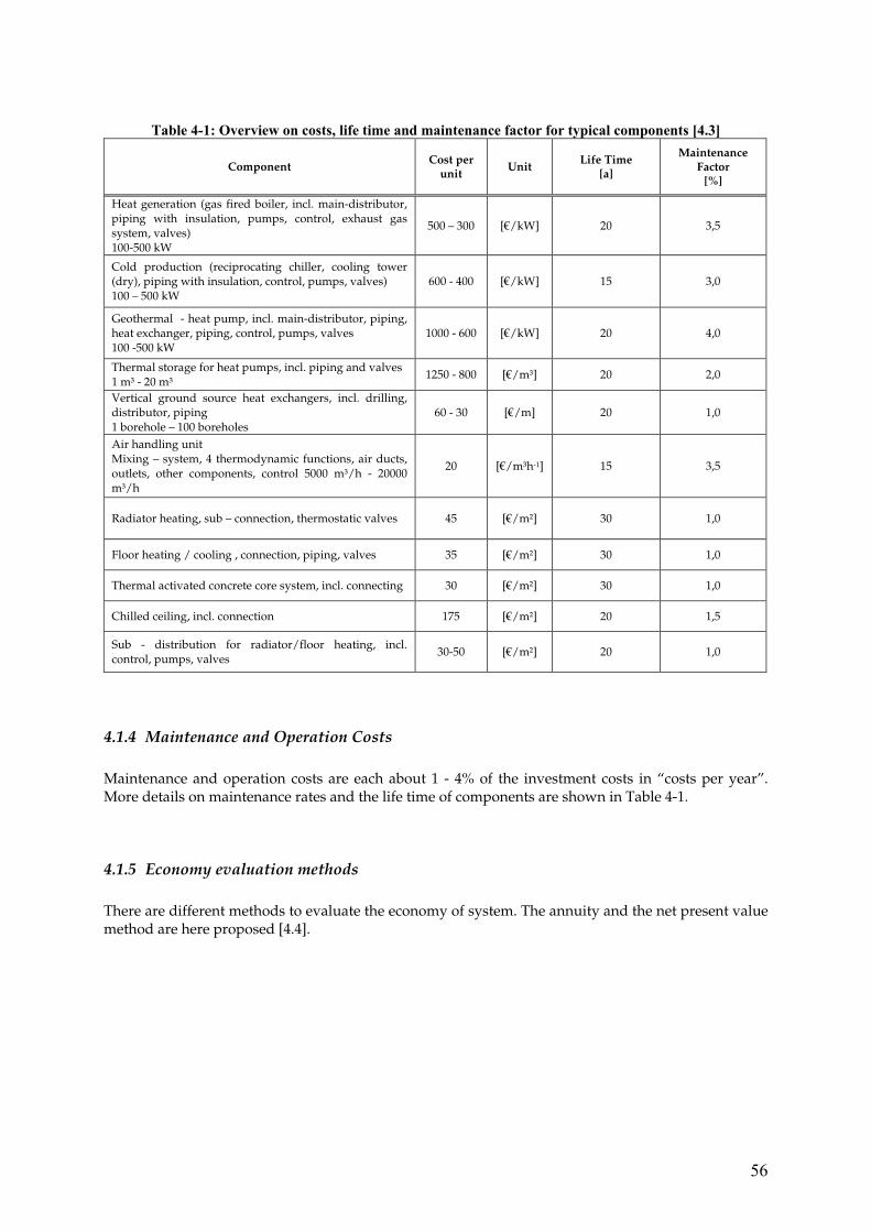
56

Table 4-1: Overview on costs, life time and maintenance factor for typical components [4.3]

Component Cost per

unit Unit

Life Time [a]

Maintenance Factor

[%]

Heat generation (gas fired boiler, incl. main-distributor, piping with insulation, pumps, control, exhaust gas system, valves) 100-500 kW

500 – 300 [€/kW] 20 3,5

Cold production (reciprocating chiller, cooling tower (dry), piping with insulation, control, pumps, valves) 100 – 500 kW

600 - 400 [€/kW] 15 3,0

Geothermal - heat pump, incl. main-distributor, piping, heat exchanger, piping, control, pumps, valves 100 -500 kW

1000 - 600 [€/kW] 20 4,0

Thermal storage for heat pumps, incl. piping and valves 1 m³ - 20 m³

1250 - 800 [€/m³] 20 2,0

Vertical ground source heat exchangers, incl. drilling, distributor, piping 1 borehole – 100 boreholes

60 - 30 [€/m] 20 1,0

Air handling unit Mixing – system, 4 thermodynamic functions, air ducts, outlets, other components, control 5000 m³/h - 20000 m³/h

20 [€/m³h-1] 15 3,5

Radiator heating, sub – connection, thermostatic valves 45 [€/m²] 30 1,0

Floor heating / cooling , connection, piping, valves 35 [€/m²] 30 1,0

Thermal activated concrete core system, incl. connecting 30 [€/m²] 30 1,0

Chilled ceiling, incl. connection 175 [€/m²] 20 1,5

Sub - distribution for radiator/floor heating, incl. control, pumps, valves

30-50 [€/m²] 20 1,0

4.1.4 Maintenance and Operation Costs

Maintenance and operation costs are each about 1 - 4% of the investment costs in “costs per year”. More details on maintenance rates and the life time of components are shown in Table 4-1.

4.1.5 Economy evaluation methods

There are different methods to evaluate the economy of system. The annuity and the net present value method are here proposed [4.4].

57

4.1.5.1 Annuity method

The annuity method implies the calculation of a regular yearly payment over a time period (T), considering the interest rate (k) and price index (p). The investments are done in the first year (year 0). The annual costs of the investment calculated by:

InvestA a INV= ⋅ with:

( ) T

T

q qa

q

1

1

− ⋅=

−

INV: investment at time 0 a: annuity factor: q: discount factor q = 1 + k k interest rate [0 - 1] T time period

The Annual cost of the energy, maintenance and operation costs over the time period (T) calculated by: Step 1: Considering the price increase index p the cash flow in the year n:

The cash flow in the year n is calculated:

( )n

nCV CV p1

1 1−= ⋅ +

with: p: rate of price increase CV1: cash flow in the first year (no increase in the first year)

If the price indexes are different, this step has to be done separately for energy, maintenance and operation costs. Step 2: Considering the index rate p the discounted present value DPV is calculated over a period T:

Tn

nn

CVDPV

k1 (1 )=

=+∑

58

Step 3: Considering the annuity rate a: The mean cash flow over the period T is calculated by the following equation:

DPVA DPV a= ⋅ Step 4: Calculate the total annuity Atotal:

total Invest DPVA A A= + Attention!!! As there is a big uncertainty in the interest rate and in the rate of price increase than it is proposed to use the CV1 in the first year. Considering the cash flow of the first year, the total annuity is calculated by:

total InvestA A CV1= +

4.1.5.2 Life Cycle Costs - Net Present Value

In the net present value method all future cash flows are calculated considering the price index and discounted to give them a present value. Step 1: Considering the price indexes p, the cash flow in the year n is calculated:

( )n

nCV CV p1

1 1−= ⋅ +

with:

CV1 = cash flow in the first year (no increase in the first year)

If the price indexes are different, this step has to be done separately for energy, maintenance and operation costs. Step 2: Considering the index rate p the discounted present vValue DPV is calculated over a Period T:

Tn

nn

CVDPV

k1 (1 )=

=+∑

59

Step 3: The net present value is calculated by comparing the discounted net present value to the investment:

NPV INV DPV= − + The net present value is often called life cycle cost LCC. Conclusions Use life cycle costs for the economical evaluation of reversible heat pump systems. Important arguments are: - investment costs - energy, maintenance and other cost in the first year - interest rate - time period

0 1 2 3 4 5 6 7 8 9 10 11 12 13 14 15 16 17 18 19 20

0

300000

600000

900000

1200000

1500000

1800000

2100000

2400000

2700000

Cos

ts [C

]

Case 1: Conventional SystemCase 1: Conventional SystemCase 2: Heat Pump SystemCase 2: Heat Pump System

Life Cycle CostsNet Present Values

Figure 4-1: Typical example of life cycle costs, comparison of 2 systems

60

4.2 Ecological Objectives

The operating of heating and cooling system results in an environmental impact. For the design process two values are usually calculated:

- primary energy and - CO2-emission.

For systems with a huge primary energy demand and with high CO2-emissions a penalty is introduced. So systems with less primary energy demand and low CO2-emissions are preferred.

4.2.1 Primary Energy

The primary energy approach makes it possible to add the different types of energies (e.g. thermal and electrical), because primary energy includes the losses of the whole energy chain. The losses outside the building system boundary are included. There are two conventions for defining the primary energy factor: a) Total primary energy factor: The conversion factor represents all the energy, which is needed to deliver the energy to the point of use (production outside the building system boundary, transport, extraction). In this case the primary energy conversion factor is always greater than 1. b) Non-renewable primary energy factor: The conversion factor represents all the energy, which is needed to deliver the energy to the point of use, but exclude the renewable energy component. In this case the primary energy conversion factor can be less than 1. The primary energy factors shall include at least:

− Energy to extract the primary energy carrier − Energy to transport the energy carrier from the production site to the utilisation site − Energy used for processing, storage, generation, transmission, distribution, and any other

operations necessary for delivery to the building in which the delivered energy is used. The primary energy factors may also include:

− Energy to build the transformation units; − Energy to build the transportation system; − Energy to clean up or dispose the wastes.

A proposal for primary factors is given in the European Standard PREN 15603 (E) 2007 (see Table 4-2) and the German Standard DIN 18599-10 2005 (see Table 4-3). Especially for fuel oil and gas different primary factor are proposed:

− European standard: fP = 1.35 − German standard: fP = 1.10

61

Table 4-2: Primary energy factors and CO2-production coefficients PREN15603 (E)-2007 [4.1]

Energy carrier Primary energy factors fp

CO2 production coefficient

K

Non-

renewable Total [kg/MWh]

Fuel oil 1.35 1.35 330 Gas 1.36 1.36 277 Anthracite 1.19 1.19 394 Lignite 1.40 1.40 433 Coke 1.53 1.53 467 Wood shavings 0.06 1.06 4 Log 0.09 1.09 14 Beech log 0.07 1.07 13 Fir log 0.10 1.10 20 Electricity from hydraulic power plant

0.50 1.50 7

Electricity from nuclear power plant 2.80 2.80 16 Electricity from coal power plant 4.05 4.05 1340 Electricity MIX UCPTE 3.14 3.31 617

Table 4-3: Primary energy factors according DIN 18599 [4.2]

Energy carrier Primary energy factors fp

Total Non-renewable

Fuels Fuel oil 1.1 1.1 Gas 1.1 1.1 Liquid gas 1.1 1.1 Black cole 1.1 1.1 Brown cole 1.2 1.2 Wood 1.2 0.2 District heating with cogeneration

Fossil fuel 0.7 0.7

Renewable fuel 0.7 0.0 District heating conventional power plants

Fossil fuel 1.3 1.3

renewable fuel 1.3 0l1 Electricity Electricity - mix 3.0 2.7

62

4.2.2 CO2 – Emission

The emitted mass of CO2 is calculated from the delivered and exported energy for each energy carrier. The CO2-emission coefficients shall include all CO2-emissions associated with the primary energy used by the building. It shall be defined at national level whether the CO2-emission coefficients include also the equivalent emissions of other greenhouse gas emissions e.g. methane. Therefore national differences are found. Example values are shown in Table 4-2.

4.2.3 Environmental Impact of Heat Pump Working Fluids

The environmental impact of the working fluids within the heat pump systems can be expressed by the ozone depletion potential (ODP) and global warming impact (GWP). An overview gives VDI guideline 4640-1 /5.4/. 4.3 Examples

For both examples two solutions for reversible heat pumps are compared with a conventional system: Air to water heat pump, only reversibility, no heat recovery, no passive cooling Water to water reversible heat pump, with heat recovery and with passive cooling For further details, see also chapter 3.5.1 and 3.5.2. The procedure is described in [3.10]. Basic assumptions are used as described in chapter 2.

63

4.3.1 Load Example 1 with Reversible Air to Water Heat Pump, No Heat Recovery and without Passive Cooling

An analysis of the life cycle costs (see Figure 4-2) and the environmental impact (see Figure 4-3 ) shows the advantage of the reversible heat pump system.

0 1 2 3 4 5 6 7 8 9 10 11 12 13 14 15 16 17 18 19 20

0

300000

600000

900000

1200000

1500000

1800000

2100000

2400000

2700000

Cos

ts [C

]



Figure 4-2: Life cycle cost comparison between a conventional system and a reversible air to water heat

pump with no heat recovery and no passive cooling, loads from example 1

0

100

200

300

400

500

600

700

800

900

1000

1100

1200

1300

1400

1500

CO

2 [t/

a],

QP [M

Wh/

a]

CO2-Emission [t/a]CO2-Emission [t/a]

287287

204204

Primary Energy [MWh/a]Primary Energy [MWh/a]

11891189

891891

Enviromental ImpactDesign Example 1 - Ait to Water REV-HP


Reversibility Heat Pump System

Figure 4-3: Environmental impact comparison between a conventional system and a reversible air to

water heat pump without heat recovery and without passive cooling, loads from example 1

64

4.3.2 Load Example 1 with a Reversible Water to Water Heat Pump, with Heat Recovery and with Passive Cooling

An analysis of the life cycle costs (see Figure 4-4) show that the reversible heat pump system, due to the high costs of the ground source heat exchanger, has higher life cycle costs than conventional system (on a period of twenty years). But the environmental impact (see Figure 4-5) shows the advantage of the reversible heat pump system.

0 1 2 3 4 5 6 7 8 9 10 11 12 13 14 15 16 17 18 19 20

0

300000

600000

900000

1200000

1500000

1800000

2100000

2400000

2700000

Cos

ts [C

]



Figure 4-4: Life cycle cost comparison between a conventional syst em and a reversible water

to water heat pump with heat recovery and with passive cooling usi ng the ground source, loads from example 1

0

100

200

300

400

500

600

700

800

900

1000

1100

1200

1300

1400

1500

CO

2 [t/

a],

QP [M

Wh/

a]


287287

149149


11801180

650650

Enviromental ImpactDesign Example 1



Figure 4-5: Environmental impact comparison between a conventional system and a reversible

water/water heat pump with heat recovery and with passive cooling using ground source, loads

from example 1

65

4.3.3 Load Example 2 with Reversible Air to Water Heat Pump without Heat Recover and without Passive Cooling

An analysis of the life cycle costs (see Figure 4-6) and the environmental impact (see Figure 4-7 ) shows the advantage of the reversible heat pump system.

0 1 2 3 4 5 6 7 8 9 10 11 12 13 14 15 16 17 18 19 20

0

300000

600000

900000

1200000

1500000

1800000

2100000

2400000

2700000

Cos

ts [C

]



Figure 4-6: Life cycle cost comparison between a conventional system and a reversible air to water heat

pump without heat recovery and without passive cooling, loads from example 2

0

100

200

300

400

500

600

700

800

900

1000

1100

1200

1300

1400

1500

CO

2 [t/

a],

QP [M

Wh/

a]


212212180180


893893

784784

Enviromental ImpactDesign Example 2 - Ait to Water REV-HP



Figure 4-7: Environmental impact comparison between a conventional system and a reversible air to

water heat pump without heat recovery and without passive cooling, loads from example 2

66

4.3.4 Load Example 2 with Reversible Water to Water Heat Pump, with Heat Recovery and with Passive Cooling

An analysis of the life cycle costs (see Figure 4-8) show that the reversible heat pump system, due to the high costs of the ground source heat exchanger the heat pump system have higher life cycle costs than a conventional system. But the environmental impact (see Figure 4-9) shows the advantage of this reversible heat pump system, too.

0 1 2 3 4 5 6 7 8 9 10 11 12 13 14 15 16 17 18 19 20

0

300000

600000

900000

1200000

1500000

1800000

2100000

2400000

2700000

Cos

ts [C

]



Figure 4-8: Life cycle cost comparison between a conventional system and a reversible water to water heat

pump with heat recovery and with passive cooling using ground source, loads from example 2

0

100

200

300

400

500

600

700

800

900

1000

1100

1200

1300

1400

1500

CO

2 [t/

a],

QP [M

Wh/

a]


212212

107107


893893

789789

Enviromental ImpactDesign Example 2 - Water to Water REV-REC-HP



Figure 4-9: Environmental impact comparison between a conventional system and a reversible water to

water heat pump with heat recovery and with passive cooling using ground source.

67

4.3.5 Weighting of the Objectives and Conclusions

Economical Evaluation In both cases the system with a reversible air to water heat pump without heat recovery and without passive cooling is the best solution. Ecological Evaluation Here the reversible water to water heat pump, with heat recovery and with passive cooling (ground source) is the better solution.

0

10

20

30

40

50

60

70

80

90

100

110

120

LLC

, CO

2, P

rimar

y E

nerg

y [%

]

Life Cycle Cost (NPV 20 a)Life Cycle Cost (NPV 20 a)

100100

6767

101101

CO2-EmissionsCO2-Emissions

100100

7171

5252

Primary EnergyPrimary Energy

100100

7575

5555

Costs and Environmental EvaluationDesign Example 1


Reversible Heat PumpSystem withoutHeat Recovery

Reversible Heat PumpSystem with

Heat Recovery Figure 4-10: Load ex. 1: comparison of life cycle costs, CO2-emissions and primary energy

0

10

20

30

40

50

60

70

80

90

100

110

120

LLC

, CO

2, P

rimar

y E

nerg

y [%

]

Life Cycle Cost (NPV 20 a)Life Cycle Cost (NPV 20 a)

100100

7676

116116

CO2-EmissionsCO2-Emissions

100100

8585

5151

Primary EnergyPrimary Energy

100100

8888

5353

Costs and Environmental EvaluationDesign Example 2


Reversible Heat PumpSystem withoutHeat Recovery

Reversible Heat PumpSystem with

Heat Recovery Figure 4-11: Load ex. 2: comparison of life cycle costs, CO2-emissions and primary energy

68

4.4 References Chapter 4

[4.1] prEN 15603: 2007(E) Energy performance of buildings — Overall energy use, CO2 emissions and definition of energy ratings, 04- 2007

[4.2] DIN EN 18599-1, (2005) Energy efficiency of buildings, Calculation of the net, final and primary energy demand for heating, cooling, ventilation, domestic hot water and lighting, Part 1: General balancing procedures, terms and definitions, zoning and evaluation of energy sources

[4.3] Kennziffernkatalog 2004: Investitionsvorbereitung in der Energiewirtschaft, Energieconsulting, Gesellschaft für Energiemanagement, Berlin 2004

[4.4] VDI 2067 Economic efficiency of building installations, Part 1, Fundamentals and economic calculation, Verein Deutscher Ingenieure, Beuth Verlag GmbH, Berlin, September 2000.

[4.5] 30 key energy trends in the IEA & worldwide, International Energy Agency, Paris, 2007.

[4.6] IWU Institut Wohnen und Umwelt GmbH Darmstadt, Primärenergie- und CO2-Emissionsfaktoren von Energieträgern, http://www.iwu.de/downloads/fachinfos/energiebilanzen, June 2007.

69

5 Main Concept Decision

5.1 Heat Pump System Classification

An overview over heat pump system is shown in Table 5-1. Efficiency ratios and a marked overview are given by Bertagnilio and Geenen et. al /5.1/, /5.1/. Three types of heat pump systems are distinguished:

1. Reversible system 2. Reversible systems with heat recovery 3. System with heat recovery

And eight classifications are used

1. Heat pump type − air to water − Water to water − DX to water − Air to DX (multi split) − Air to air

2. Heat source / sink − Outdoor air − Ground − Surface water − Ground water − Extracted air

3. Reversibility − Yes − No

4. Condenser heat Recovery • Yes • No

5. Passive Cooling • Yes • No

6. Change over • Refrigerant side • Water side

7. Distribution to the heat source / sink • Direct • One water (or brine) loop • Two water (or brine) loops

8. Distribution fluid to the building • Water (2, 3, 4-pipe) • Air • Refrigerant (DX)

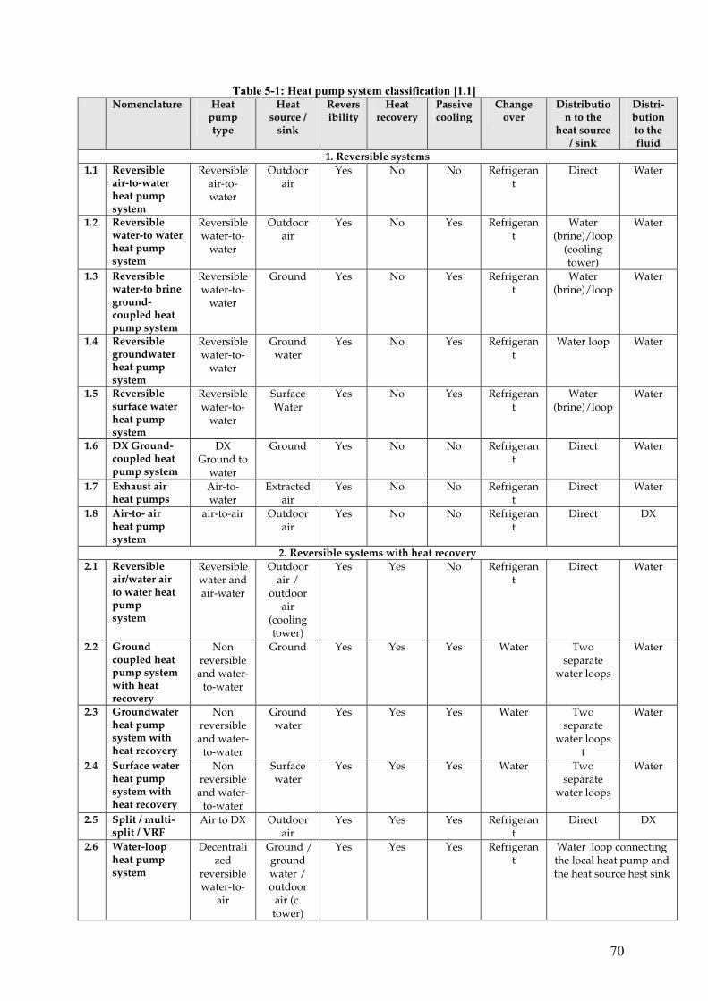
70

Table 5-1: Heat pump system classification [1.1] Nomenclature Heat

pump type

Heat source /

sink

Reversibility

Heat recovery

Passive cooling

Change over

Distribution to the

heat source / sink

Distri-bution to the fluid

1. Reversible systems

1.1 Reversible air-to-water heat pump system

Reversible air-to-water

Outdoor air

Yes No No Refrigerant

Direct Water

1.2 Reversible water-to water heat pump system

Reversible water-to-

water

Outdoor air

Yes No Yes Refrigerant

Water (brine)/loop

(cooling tower)

Water

1.3 Reversible water-to brine ground-coupled heat pump system


water

Ground Yes No Yes Refrigerant

Water (brine)/loop

Water

1.4 Reversible groundwater heat pump system


water

Ground water


Water loop Water

1.5 Reversible surface water heat pump system


water

Surface Water


Water (brine)/loop

Water

1.6 DX Ground-coupled heat pump system

DX Ground to

water

Ground Yes No No Refrigerant

Direct Water

1.7 Exhaust air heat pumps

Air-to-water

Extracted air


Direct Water

1.8 Air-to- air heat pump system

air-to-air Outdoor air


Direct DX

2. Reversible systems with heat recovery

2.1 Reversible air/water air to water heat pump system

Reversible water and air-water

Outdoor air /

outdoor air

(cooling tower)

Yes Yes No Refrigerant

Direct Water

2.2 Ground coupled heat pump system with heat recovery

Non reversible and water-

to-water

Ground Yes Yes Yes Water Two separate

water loops

Water

2.3 Groundwater heat pump system with heat recovery


to-water

Ground water

Yes Yes Yes Water Two separate

water loops t

Water

2.4 Surface water heat pump system with heat recovery


to-water

Surface water

Yes Yes Yes Water Two separate

water loops

Water

2.5 Split / multi-split / VRF

Air to DX Outdoor air

Yes Yes Yes Refrigerant

Direct DX

2.6 Water-loop heat pump system

Decentralized

reversible water-to-

air

Ground / ground water / outdoor

air (c. tower)

Yes Yes Yes Refrigerant

Water loop connecting the local heat pump and the heat source hest sink

71

Continuance of Table 5-1: 3. System with heat recovery

3.1 Water-cooled chiller with heat recovery

Water cooled chiller

Outdoor air

(cooling tower)

No Yes No - Water loop Water

3.2 Dual condenser chiller

Dual condenser

chiller

Outdoor air or /

and water

No Yes No - Direct Water

3.3 Temperature amplifier

Water to water heat

pump

Water No Yes No - Direct Water

72

5.2 Reversible Systems

A heat pump system, which operates alternatively in heating or cooling mode, is called reversible heat pump system.

5.2.1 Reversible Air Water Heat Pump

(See also Table 5-1, heat pump type 1.1) The simplest system is based on the use of reversible air-water heat pump. Today, a large offer of reversible units is proposed, with investment costs comparable to these of non-reversible units. The system is reversed by means of a refrigerant side change-over (Figure 5-1), which inverses the flow passage into the two exchangers. In cooling mode, the air exchanger works as condenser, rejecting heat, while the water-exchanger works as evaporator, transferring cooling power to the distribution system. In heating mode, the air exchanger works as evaporator, absorbing heat from external air, while the water exchanger works as condenser, transferring heat to the distribution system /5.1/.

1

2

3

4

5

Heating System

air


2: expansion valve


4: compressor

5: 4-way-valve


Heating mode

1

2

3

4

5

Cooling System

air


2: expansion valve


4: compressor

5: 4-way-valve


Cooling mode

Figure 5-1: Functional scheme of a reversible air to water heat pump /5.1/

A reversible air-cooled unit has generally to be combined with a backup boiler, due to the following reasons:

− When the chiller works in cooling mode, it cannot provide any heating power

− In heating mode, the air-water heat pump can generally not cover the maximal heating demand (the heating power at –5°C can be 30% lower than heating power in rating conditions)

− In extremely low outdoor temperature, boiler performances can become better than air to

water unit performances Passive cooling is mostly not possible with air to water heat pumps. They have to be combined with a cooling tower.

73

Coupling to the Heating and Cooling System /5.1/ In system #1 (Figure 5-2), the reversible air to water heat pump can be coupled to both hot and cold water networks, using only a refrigerant change-over to switch between heat and cold production. In this configuration, the cold and hot water networks are respectively only used for cooling and heating respectively. In configuration #2 (Figure 5-2), a water-circuit change-over is used to satisfy the heating demand. The heat pump is only connected to the cold water network and uses this circuit to satisfy alternatively the cooling and heating demands of the building. Of course, this configuration cannot be used when heating and cooling demands co-exist. The main advantage of this solution is that the large heat transfer areas of the cooling HVAC equipment are used for low-temperature heating.

Figure 5-2: Coupling of a reversible air to water heat pump systems to distribution network

#1 (left): refrigerant change over-coupling alternatively to cold water or hot water network

and

#2 (right) refrigerant and water (double) change over - coupling to only to the cold water

network /5.1/.

5.2.2 Reversible Water to Water Heat Pump

(See also Table 5-1, heat pump type 1.2, 1.3, 1.4 and 1.5) In a water to water heat pump, both the condenser and evaporator are water/refrigerant heat exchangers. Different heat sources (heating mode) and heat sinks (cooling mode) can be used:

− Outdoor air − Ground (horizontal or vertical pipes) − Surface water − Ground water

The differences among these heat sources/sinks are:

− Availability − Temperature levels − Costs

If frosting is possible instead of water a water/brine fluid has to be used. Ground used as heat source/sink has a long term storage effect; this effect can improve the seasonal behaviour of the system. If reversibility is done on the refrigerant side, no heat recovery is possible.

74

1

2

3

4

5

Heating


2: expansion valve


4: compressor

5: 4-way-valve

Reversible water to water heat pump system

Heating mode

1

2

3

4

5

Cooling


2: expansion valve


4: compressor

5: 4-way-valve


Cooling mode

System System

heat source

- ground- ground water- surface water

heat sink


No passive cooling

- outdoor air- outdoor air

Figure 5-3: Reversible water-to-water heat pump systems, operating in heating and cooling modes, with

different heat sources/sinks

Using Passive Cooling If the temperature of the heat sink is lower than the temperature of the cooling system a passive cooling is possible. Up to 80 % of the yearly cooling demand can be delivered using a vertical borehole heat exchanger. Ground regeneration (cooling down the ground during heating mode) may improve the passive cooling capabilities. Figure 5-4 shows the principle scheme of using the heat sink for passive cooling.

1

2

3

4

5

Cooling


2: expansion valve


4: compressor

5: 4-way-valve


Cooling mode

System

heat sink


With passive cooling

- outdoor air1

2

3

4

5

Cooling


2: expansion valve


4: compressor

5: 4-way-valve


Cooling mode

System

heat sink


No passive cooling

- outdoor air

Figure 5-4: Reversible water to water heat pump systems, operating in cooling mode, with and without passive

cooling

5.2.3 DX Ground-Coupled Heat Pump System

(See also Table 5-1, heat pump type 1.6)

75

Only a few systems exist using a direct expansion heat exchanger in the ground.

5.2.4 Extracted Air Heat Pumps

(See Table 5-1, heat pump type 1.7) Extracted air offers a heat source/sink at almost constant temperature. The system is similar to heat pump type 1.1.

5.2.5 Air to Air Heat Pump System (Split / Multisplit, VRF Systems)

(See also Table 5-1, heat pump type 1.8) For heating and cooling of small residential and non residential areas, air to air heat pumps are often used (see Figure 5-5).

1

2

3

4

5

air

1: heat exchanger refrigerant/air (DX)

2: expansion valve


4: compressor

Reversible air to air heat pump system

Heating mode

air1

2

3

4

5

air

1: heat exchanger refrigerant/air (DX)

2: expansion valve


4: compressor

Reversible air to air heat pump system

Cooling mode

air

Figure 5-5: Reversible air to air heat pump systems with only one indoor unit

76

5.3 Reversible Systems with Heat Recovery

Reversible systems with heat recovery work in three operation modes:

− Heating mode − Cooling mode − Heat recovery mode (simultaneous heating and cooling)

Usually the condenser heat is recovered, and the system is operated according to the cooling demand.

5.3.1 Air to Water Heat Pump Systems with Water Heat Recovery /5.1/

(See also Table 5-1, heat pump type 2.1) Air to water heat pump system, with reversibility on the refrigerant side, have a dual condenser or evaporator (water/refrigerant heat exchanger in parallel to air/refrigerant heat exchanger) to allow a heat or a cold recovery. Figure 5-6 show the four possible operation modes. Most systems are running in priority to the cooling mode, but only three modes are used in practise:

− Heating mode − Cooling mode − Condenser heat recovery

77

1

2

4

5

Heating

Reversible air and water to water heat pump system

Heating mode

System3Cooling

system

air3*

1

2

3

4

5

Cooling


Cooling mode

SystemHeating System

air3*

dual evaporator

3Cooling system

air3*

evaporator heat recovery (cooling)

1

2

4

5

Heating


Heating mode

System

air3*

dual condensor

condensor heat recovery (heating)

1

2

3

4

5

Cooling


Cooling mode

SystemHeating System

1: heat exchanger water/refrigerant 2: expansion valve 3: heat exchanger water / refrigerant 3*: heat exchanger air/refrigerant 4: compressor 5: 4-Way valve

1: heat exchanger water/refrigerant 2: expansion valve 3: heat exchanger water / refrigerant 3*: heat exchanger air/refrigerant 4: compressor 5: 4-Way valve

Figure 5-6 : Reversible air to water heat pump system with water heat recovery

#1 (top left): heating mode, no heat recovery

#2 (bottom left): heating mode, with heat recovery (cooling)

#3 (top right): cooling mode, no heat recovery

#4 (bottom right): cooling mode, with heat recovery (heating)

For the recovering of the condenser heat the following aspects have to be considered:

− Heating system with low temperatures (i.e. thermal activated ceilings, low temperature radiators, floor heating etc.)

− Max. temperature limited to 50-60 °C − Thermal buffer should be used (allow short term storage)

For recovering of the evaporator cold the following aspects have to be considered:

− Cooling system with low temperature differences (i.e. thermal activated ceilings, convectors, fan coils, ceiling / floor cooling)

− Min. water temperatures are limited to 6 - 12 °C (for lower temperatures use brine) − Thermal buffer should be used (allow short term storage)

78

5.3.2 Water to Water Heat Pump

(See also Table 5-1, heat pump type 2.2, 2.3 and 2.4) Reversible systems can be made with water to water heat pumps without refrigerant change over. The reversibility can be realized thanks a change over on the water side. Evaporator and condenser are then alternatively connected to both heat source and sink. So this system can operate in:

− Heating mode − Cooling mode − Passive cooling mode − Heating and cooling mode (heat recovery)

Figure 5-7 shows typical schemes for this four working modes. In most cases an additional heater is needed (not shown in Figure 5-7). In the heat source/sink network often brine is used, so a heat exchanger is necessary. The heat exchangers and the thermal storages give a hydraulic and time decoupling respectively between the heat source/sink and the heating/cooling system. The thermal storages guarantee a minimum operation time of the heat pump in each mode. Also the heat recovery potential is improved.

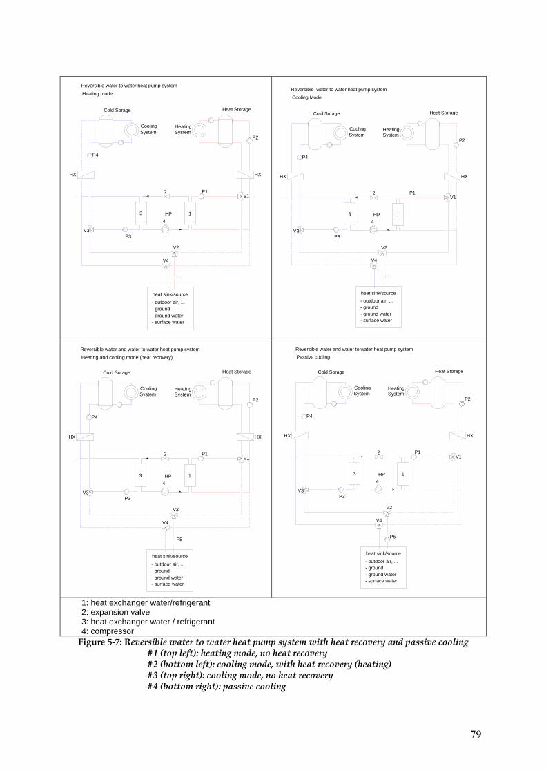
79

1

2

4

Heating


Heating mode

System

3

Cooling System

HX

heat sink/source


- outdoor air, ...

HX

HP


P2

P4

V3

V2

V4

P5

V1P1

P3

1

2

4

Heating


Cooling Mode

System

3

Cooling System

HX

heat sink/source


- outdoor air, ...

HX

HP


P2

P4

V3

V2

V4

P5

V1P1

P3

1

2

4

Heating


Heating and cooling mode (heat recovery)

System

3

Cooling System

HX

heat sink/source


- outdoor air, ...

HX

HP


P2

P4

V3

V2

V4

P5

V1P1

P3

1

2

4

Heating


Passive cooling

System

3

Cooling System

HX

heat sink/source


- outdoor air, ...

HX

HP


P2

P4

V3

V2

V4

P5

V1P1

P3

1: heat exchanger water/refrigerant 2: expansion valve 3: heat exchanger water / refrigerant 4: compressor

Figure 5-7: Reversible water to water heat pump system with heat recovery and passive cooling #1 (top left): heating mode, no heat recovery #2 (bottom left): cooling mode, with heat recovery (heating) #3 (top right): cooling mode, no heat recovery #4 (bottom right): passive cooling

80

5.3.2.1 Exhaust Ventilation Air Heat Pumps

Extracted air represents a very interesting heat source because of its good availability, its good coincidence with needs and its very constant temperature. Condensing the water contained in extracted air allows also recovering a part of the latent energy and increases the capacity of the extracted air as heat source. In cooling mode, condenser heat can also be easily rejected in the exhaust ventilation air flow, which is often at lower temperature than outdoor air. However, the exhaust ventilation source capacity is limited and an additional heat source or sink is very often required. At least two configurations are possible when using extracted air as heat source. The first configuration is based on the use of an air to air reversible heat pump. The other configuration is based on the use of a water to water or a dual condenser heat pump (Figure 5-8). With a water to water heat pump, the extracted air is used as heat source in heating mode and as heat sink in cooling mode. The heat pump is not reversible but a change-over is made on the water circuit to allow heat pumping or heat rejection in the exhaust air. With dual-condenser heat pumps, the extracted air can be used only as heat source for heating and the air condenser can be used to reject heat in cooling mode (Figure 5-8). But caution to frosting risk. With the use of brine, one more heat exchanger is necessary.

Figure 5-8: Exhaust ventilation air source water to water heat pump system with dual condenser /5.1/

(See also Table 5-1, heat pump type 2.5) If DX expansion heater or cooler are served by an split, multisplit or variable refrigerant flow heat pump reversibility and heat recovery is possible. The change over is done on the DX – unit. A wide range of prefabricated systems are on the market. No further work on these systems is done in this design guide.

81

5.3.3 Water Loop Heat Pump Systems

(See also Table 5-1, heat pump type 2.6) Decentral reversible water to air heat pump systems are served by a common water loop. The reversibility is done on the refrigerant side. Each unit can work either in heating or in cooling mode. Different heat sources are possible. A scheme of heat pumps in heating and cooling mode is shown in Figure 5-9.

1

2

3

4

5

1: heat exchanger refrigerant/air

2: expansion valve


4: compressor

5: 4-way-valve

Water loop heat pump systems

Heating and cooling mode

heat source


- outdoor air

air

13

4

5

13

4

5

DX 1 (heating)

DX 2 (cooling)

DX n (cooling)

Figure 5-9: Water loop decentralise heat pump systems

82

5.4 Water Cooled Chillers with Heat Recovery

(See also Table 5-1, heat pump type 3.1) The condenser heat of water to water chillers is rejected via cooling towers. This heat can be used for heating, too. Usually an additional heater is needed, as the condenser temperatures are often below 35 °C.


2: expansion valve


4: compressor

1

2

4

Heating

Chiller, water to water with heat recovery

System3Cooling System

ChillerCooling Tower

Figure 5-10 : Chillers with heat recovery

5.5 Heat Pump Concept Decision

There is no general way to find a system. First the reversible and recovery potential (REV and REC) have to analyzed. The next step is to check the objectives as life cycle cost and environmental impact (see chapter 4). And at last other aspects have to be considered:

− Temperature ranges (heating, cooling mode) − Passive cooling − Temperature range passive cooling − Investment costs − Operation and maintenance − Additional heating/cooling needed

Table 5-2 summarizes the aspects for the heat pump concept decision.

83

Table 5-2 : Aspects for heat pump concept decision

Temperature

Heating Cooling Passive Cooling

Investment Costs

Operation and Maintenance

1. Reversible systems

1.1 Reversible air-to-water heat pump system

< 50 °C > 6 °C - ☺☺☺ ☺☺

1.2 Reversible water-to Water heat pump system

< 50 °C > 6 °C 0 - 20 °C ☺☺ ☺☺☺

1.3 Reversible water-to Water ground-coupled heat pump system

< 50 °C > 6 °C 8 -1 2 °C ☺ ☺☺☺

1.4 Reversible groundwater heat pump system

< 50 °C > 6 °C 8. - 12 °C ☺☺ ☺☺☺

1.5 Reversible surface water heat pump system

< 50 °C > 6 °C 5 - 20 °C ☺☺ ☺☺☺

1.6 DX Ground-coupled heat pump system

< 50 °C > 6 °C - ☺☺ ☺☺☺

1.7 Extracted air heat pumps < 50 °C > 6 °C - ☺☺ ☺☺ 1.8 Air-to- air heat pump

system < 50 °C > 6 °C - ☺☺☺ ☺☺

2. Reversible systems with heat recovery

2.1 Air-water heat pump system with water heat recovery

< 50 °C > 6 °C 0 – 20 °C ☺☺☺ ☺☺

2.2 Ground coupled heat pump system with heat recovery

< 50 °C > 6 °C 8-12 °C ☺☺☺ ☺☺☺

2.3 Groundwater heat pump system with heat recovery

< 50 °C > 6 °C 8. -12 °C ☺☺☺ ☺☺☺

2.4 Surface water heat pump system with heat recovery

< 50 °C > 6 °C 5 - 20 °C ☺☺☺ ☺☺

2.5 Split / multi-split / VRF < 50 °C > 6 °C - ☺☺☺ ☺☺ 2.6 Water-loop heat pump

system < 50 °C > 6 °C - ☺☺☺ ☺☺

3. System with heat recovery

3. Water-cooled chiller with heat recovery

< 40 °C > 6 °C - ☺☺☺ ☺☺

5.6 Examples of Chapter 3

For both presented examples (see Chapter 3) a water to water heat pump is proposed. Design example 1: Reversible system (see Chapter 3.5.1)

− Reversible water to water heat pump system − Reversible water to water ground-coupled heat pump system

Design example 2: Reversible system with heat recovery (see Chapter 3.5.2)

− Air to water heat pump system with water heat recovery − Ground coupled heat pump system with heat recovery

Design example 3: Retrofit example - different heat pump solutions are investigated:

− Air to water reversible heat pump − Ground coupled reversible heat pump

84

− Exhaust air heat pump A comparison of these solutions done at the primary system level yields the following results:

Figure 5-11 : CO2 emissions for different heat pump solutions (example 3)

Figure 5-12 : Primary energy consumption for different heat pump solutions (example 3)

85

Figure 5-13 : Life cycle costs for different heat pump solutions (example 3)

5.7 Literature Chapter 5

/5.1/ S. Bertagnolio & V. Gennen: REVERSIBLE HEAT PUMPS TECHNOLOGY DESCRIPTION

AND MARKET OVERVIEW June 2nd , 2008 Thermodynamics Laboratory, University of Liège

/5.2/ S. Bertagnolio, J. Lebrun, P. André, P.Y. Franck, J. Hannay and C. Aparecida Silva: Heat recovery and reversible heat pumping potentials in non-residential buildings, Thermodynamics Laboratory University of Liège , paper ??? conference 2008

/5.3/ P. Stabat,M. Caciolo, S. Bertagnolio IEA-ECBCS Annex 48 : DELIVERABLE 1.4. Reversibility and heat recovery technology description; April 2008

/5.4/ VDI 4640: Utilization of the subsurface for thermal purposes, Underground thermal energy storage, part 3,June 2001

/5.5/ Stéphane Bertagnolio, Marcello Caciolo, David Corgier, Pascal Stabat: Operating Review of heat recovery and heat pumping solutions Subtask 1.4 of subtask 1 : “Analysis of heating and cooling demands and equipment performances”, April 2009

86

6 Detailed System Design

If a first concept decision is done, the detailed system design is necessary. This work includes: − Selection and sizing of components

o Heat pump, boiler, chiller o Heat source, heat sink

− Integration in the building design and HVAC System design − Hydraulic, thermal storage and operating management − Control design − Optimization

A detailed system design should pay attention on the relation between the COP and the temperature difference! A heat pump is a machine that moves heat from one location to another location using mechanical work. In heating, ventilation, and air conditioning (HVAC) applications, a heat pump normally refers to a vapor-compression refrigeration device that includes a reversing valve and optimized heat exchangers so that the direction of heat flow may be reversed. The working fluid, in its gaseous state, is pressurized and circulated through the system by a compressor. On the discharge side of the compressor, the hot and highly pressurized gas is cooled in a heat exchanger, called condenser, until it condenses into a high pressure, moderate temperature liquid. The condensed refrigerant then passes through a pressure lowering expansion valve. This device then passes the low pressure, (almost) liquid refrigerant to another heat exchanger, the evaporator where the refrigerant evaporates into a gas via heat absorption. The refrigerant then returns to the compressor and the cycle is repeated. In such a system it is essential that the refrigerant reaches a sufficiently high temperature when compressed, since the second law of thermodynamics prevents heat from flowing from a cold fluid to a hot heat sink. Practically, this means the refrigerant must reach a temperature greater than the condenser. Similarly, the fluid must reach a sufficiently low temperature when allowed to expand, or heat cannot flow from the cold region into the fluid, i.e. the fluid must be colder than the evaporator. In particular, the pressure difference must be great enough for the fluid to condense at the hot side and still evaporate in the lower pressure region at the cold side. The greater the temperature difference, the greater the required pressure difference, and consequently the more energy needed to compress the fluid. Thus as with all heat pumps, the energy efficiency decreases with increasing temperature difference. Examples for the hydraulic integration of a heat pump and the secondary systems are listed in the appendix (see chapter 13) of this handbook. 6.1 Sizing of reversible heat pump systems

6.1.1 Heat Pump System

Similar to other heat and cold generators the size of the heat pump depends on the peaks heating and cooling loads. But strong attention should be paid to operation temperatures and their impact on expected energy consumptions such as electricity for electrical compressors. Often multi packaged units operates better than a single package unit. As heat pump systems are more expensive than a single boiler, often bivalent systems are more cost efficient.

87

6.1.1.1 Typical Performance of Heat Pumps

The term coefficient of performance (COP) is used to describe the ratio of useful heat movement to work input. A market overview is given by Bertagnolio [6.1] Operation in heating and cooling mode has to be distinguished. For the nominal conditions, given from the manufacture, the COP and EER values often differ.

Table 6-1 : Typical nominal conditions COP / EER values are given (W: water; A: air, B: brine)

Heating Cooling Air to water A7 / W45 A35 / W7 Brine to water B0 / W35 B20 / W10 Water to water W10 / W45 W20 / W10 For design work the real conditions (source and system temperatures) have to be considered and performance curves have to be used. Figure 6-1 and Figure 6-2 shows typical COP values for heating and cooling mode for an air to water and a brine to water heat pump.

88

Figure 6-1 : Typical performance characteristic of a reversible air to water heat pump (www.Trane.com)

89

Figure 6-2 : Typical performance characteristic of a reversible water to water heat pump

(www.dimplex.de)

For further design work beside the COP the following data is needed:

− Pressure drop over the condenser − Pressure drop over the evaporator − Minimum mass flow rate over the condenser − Minimum mass flow rate over the evaporator

90

6.1.1.2 Compressor Type

Usually scroll compressors are used in heat pumps up to 150 kW heating capacity. But also piston compressors are on the market. For capacity ranges greater 150 kW screw compressors and turbines are available.

6.1.1.3 Selection of refrigerant

Table 6-2 gives a overview on refrigerants used in heat pump and chiller systems. Also the capacities and the minimum and maximum pressure on the evaporator and condenser are strongly influenced by the refrigerant.

Table 6-2: Refrigerants used and environmental impact

6.1.1.4 Sizing of Heat pumps

For the sizing procedure of a heat pump the following information, out of the load analysis (see chapter 3), is needed:

− Design temperatures at evaporator in/outlet for peaks of cooling and heating demands − Design temperatures at condenser inlet for peaks of cooling heating and heating demands − Peak system cooling load coolingQmax,

&

− Peak system heating load heatingQmax,&

− Peak load to an additional heating generation An overview on the cumulative frequency of the heating and cooling load is shown in Figure 6-3.

91

0 400 800 1200 1600 2000 2400 2800 3200 3600 4000

0

200000

400000

600000

800000

1000000

1200000

1400000Lo

ad [W

]


Figure 6-3: Typically cumulative frequency of the heating and cooling load

As a heat pump (or chiller) is more expensive than a boiler the heat pump system is designed according to the cooling load. An additional heater has to be planned. But attention on the life cycle costs and the environmental impact. The sizing of heat pumps is oriented on the peak cooling demand. Heat Pump cooling capacity HP coolingQ ,

& :

For a monovalent cooling system the maximum cooling capacity HP coolingQ ,& is equal to the peak cooling

demand coolingQmax,& .

Heat pump heating capacity HP HeatingQ ,

& :

The heat pump heating capacity in reversible mode has to be found in manufactures data. For the COP value the worst conditions (lowest evaporator and highest condenser temperatures during the time period of maximum heating load) should be used. The heat pump heating capacity in recovery mode can be calculated from the evaporator capacity, using the EER value for the cooling mode.

Condenser capacity: Condensor cooling e evaporator cooling eQ QEER, _ mod , _ mod

11 = ⋅ +

& &

This condenser heat is usually not available during the time period of the maximum heating load. Therefore this load is not considered for calculating the additional heater capacity.

92

Additional heater capacity additional heatingQ _&

: The minimum capacity needed for an additional heater results out of the difference between the peak

heating heatingQmax,&

load and the heating capacity of the heat pump, during peak load time HP HeatingQ ,&

. Usually the heating system is oversized, to get a backup heating system.

6.1.2 Mono or Bivalent System

The total installed thermal power of a heat pump could be equal or different from the peak building load for heating or cooling.

heat pump potentialheat pump potential

secondary powersecondary powergeneration potentialgeneration potential

0 730 1460 2190 2920 3650 4380 5110 5840 6570 7300 8030 8760

Operatrion Hours [h/a]

0

10

20

30

40

50

60

70

80

90

100

Pow

er [%

]

Figure 6-4: Cumulative frequency curve of heating or cooling demand

The frequency curves show, that a sizing to 60% (instead of 100%) results in a reduction of the yearly energy produced by the heat pump of less than 10%. Different reasons can force a bivalent system:

− Economical aspects: heat pumps and their heat sink/sources are more expensive than conventional systems.

− Temperature not reached: condenser and evaporator temperatures of heat pumps are limited and an additional chiller (or heater) is needed to lower / rise the temperature.

− Low efficiencies: especially in heating mode and in air as heat source the COP decreases for low outdoor temperatures. If the specific costs for the fuel is low and the electricity costs are high, it is more cost effective to use a secondary heater. Also in cooling mode this case can occur.

93

6.1.3 Single or Multi-Unit Systems

A practical strategy in HVAC system design is splitting the supply of the total power needed for heat or cold into several modules. Especially, if the difference between heat and cold demand is large, it could be more economical to have more than one single heat pump installed in the system. Another advantage of a multi heat pump system could be a better ability to satisfy simultaneous demand for heat and cold which often happens in large commercial buildings during mid seasons. Of course there exist also disadvantages of such systems: The plant structure and the control systems become more complex and small heat pumps could have a lower efficiency. For bivalent and multi-unit systems the hydraulic scheme and the operating management is of great importance, to ensure that the heat pump works a basic generator and that additional heat and cold generation is minimized (for more details see chapter 6.3 of this guide).

6.1.4 Calculation of the Annual Performance by Dynamic Simulation

After the main plant components have been chosen it is strongly recommended to test the annual performance of the concept and to tune some of the design parameters by running system simulations. Heat pump models are available for most of system simulation packages. A well tested black-box model, based on TRNSYS 16, is documented in [6.3]. The power of the condenser and the evaporator are calculated with characteristic curves. The curves show the condenser power and the electric power as a function of the evaporator inlet temperature and the condenser outlet temperature. For air to water heat pumps defrosting and losses due to cycling are considered. The boundary conditions are the evaporator and condenser inlet temperature, the evaporator and condenser mass flow rate and the control signal. Models, based on EES are proposed by Lebrun (2009) [6.25] and Madjid (2009) [6.24] An overview on available simulation tools gives “D1.5 Models Library” of the Annex 48 project [7.1] and the appendix of this handbook [LINK].

94

6.1.5 Water to Water Heat Pumps with Ground Source Heat Exchangers

Special attention is spent to water/water heat pumps with ground source heat exchangers. A geothermal system for building heating and cooling allows the periodical exchange of energy (heat and cold) between a building and the ground. This annual cycle makes the system more energy efficient than traditional heating and cooling systems. The underground has a more moderate annual temperature swing with less amplitude than the ambient air temperatures when compared to air source heat pump systems. Even in coldest winter periods the undisturbed underground temperature remains higher than the frost limit. Furthermore, water or brine as the working fluid is more energy efficient and geothermal systems are expected to have less maintenance costs than air source heat pump systems. Figure 6-5 shows an example of a typical geothermal plant scheme with a vertical borehole heat exchanger, heat pump and hydraulic. The two major components of such a system are the heat pump and the ground heat exchanger.

Figure 6-5: Typical plant scheme of a monovalent geothermal system with heat and cold source

95

6.2 Selection and sizing of heat sources and heat sinks

In reversible heat pump system the heat transfer capacities needed from the heat sinks and heat sources depend from the operating mode: Heating Mode

Heat source capacity heat source evaporator HP heatingQ Q QCOP_ ,

11 = = ⋅ −

& & &

Cooling Mode:

Heat sink capacity heat k condensor HP coolingQ Q QEER_ sin ,

11 = = ⋅ +

& & &

Usually the following heat sources/sinks are considered:

− Outdoor air − Ground (vertical heat exchanger or horizontal heat exchanger) − Water (surface water or ground water)

6.2.1 Outdoor Air as Heat Source/Heat Sink

Outdoor air has a high availability but the temperature varies a lot. Consider a temperature difference of less than 10 K between air inlet and air outlet. For the design please consider the following aspects:

− A constant outside air flow (pressure) at the air inlet − Wind effects (i.e. flow around buildings) often results in over- and under pressuring areas.

Ensure that the air inlet is positioned in an area of constant pressure. − Consider the influence of local climate (Temperature and humidity) − No air inlet nearby “cold air sinks” or “warm air spots” − Local climate can effect the air temperature, Cold air sinks lower the efficiency in heating

mode. Warm air spots lower the efficiency in cooling mode. − Consider the noise requirements, design noise absorber − Air /refrigerant heat exchanger or cooling towers are equipped with a fan and a noise

level of about 50 – 70 dB(A) occurs. Noise upper limits requirement are usually between 30 and 40 dB(A) (window of the neighborhood building nearby).

6.2.2 Ground as Heat Source / Heat Sink

Ground source is a very reliable and temperature constant (8-12 °C) heat source and heat sink. The temperature in the ground (> 10 m) can be estimated to the mean yearly outdoor temperature. Due to the low temperature this heat sink is in European climate usable for passive cooling. But high costs are related to these systems and for design work the ground parameters have to be known. Information about the design ground heat exchangers can be found in COWI 2004 [6.9] and VDI 4640 [6.4]

96

Two different ground heat exchanger types exist: 1) A horizontal loop with piping parallel and close to the surface. The undisturbed ground temperature changes seasonally depending upon the depth of the loops. Horizontal loops are easier to install but require much more ground area than vertical loop types. 2) A vertical loop with perpendicular to the surface and the boreholes can be more than hundred meters deep. At these depths, the undisturbed ground temperature does not change during the year. The purpose of the ground heat exchanger design is to estimate the required loop length. In literature [6.4] the extraction rates per ground area (horizontal - W/m²) and per length (vertical - W/m) are given to design a heat pump for heating purpose. No values are given to design a ground source heat exchanger in cooling mode. The leaving temperatures from the heat source/sink must be estimated. In heating mode an average of 0 °C with a minimum of -10 °C is proposed. The larger the loop for a known load, the warmer the supply fluid temperature will be and higher fluid temperatures improve the heat pump efficiency. In cooling mode an increase of the pipe length in the ground will reduce the fluid temperatures. The thermal heat pump power and the ground heat exchange rate should brought into balance. The needed ground heat exchanger power leads to a certain pipe length in the ground, depending on heat conductance, heat diffusivity, distance to ground water and heat exchanger type (vertical or horizontal). But a ground heat exchanger is also a thermal storage system. Therefore, the size of the ground heat exchanger does not only depend on the peak power demand for heating or cooling but also on the yearly energy demand for heating or cooling. Therefore, the best way to find the optimal dimensions of a ground heat exchanger is applying thermal system simulations. Linked via a heat pump model to hourly building demands for heating and cooling (or directly linked to a building and system model) the ground heat exchanger model can provide the designer with a good forecast of the later (dynamic) behaviour of the system. Special attention should pay on a balanced heat and cold extraction out of the ground.

6.2.2.1 Simulation Based Design

Simulations and also measurements show that it could take several years to reach a final annual equilibrium of heat input and heat extraction in the ground. Therefore, simulation is the only practical method to verify the optimum size of a ground heat exchanger. Practically, the maximum size remains limited by the investment costs and the result of a lifecycle calculation.

6.2.2.2 Available Simulation Models

A detailed and well-documented ground heat exchanger model has been developed by Bernier, Pinel and Bertagnolio and implemented in EES by Bertagnolio [6.12]. Other simulation models have been implemented in TRNSYS. Some references are given in the following list.

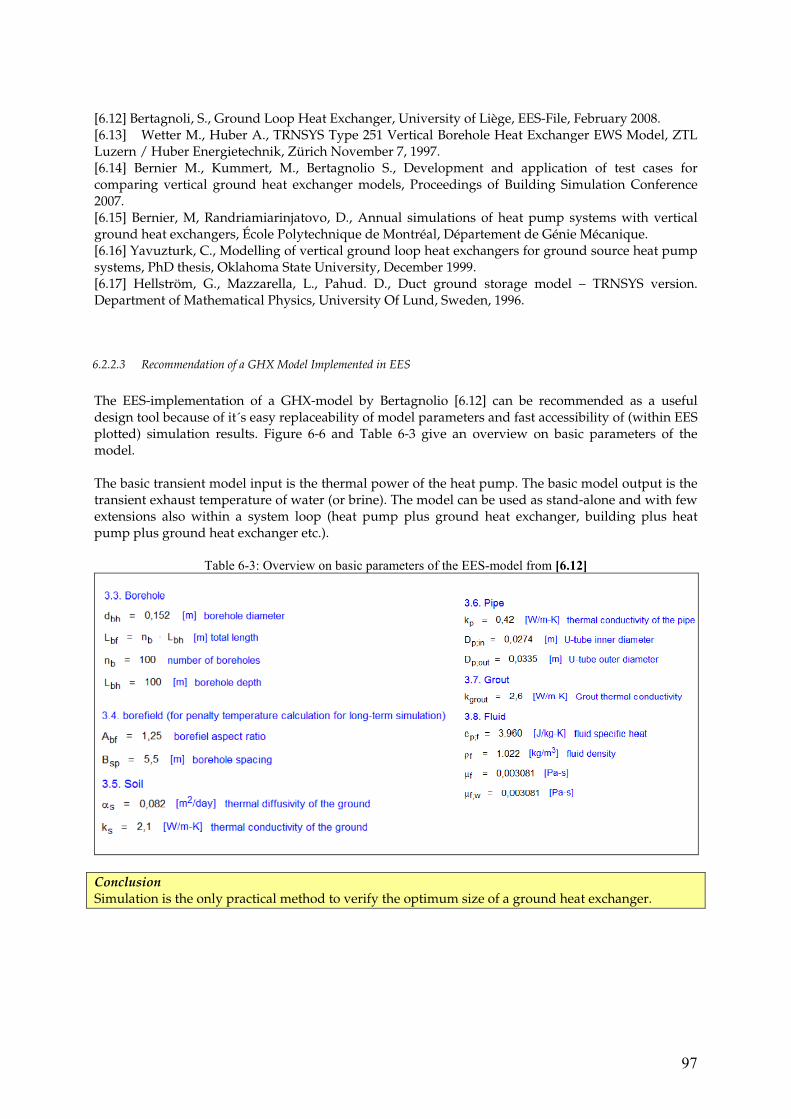
97

[6.12] Bertagnoli, S., Ground Loop Heat Exchanger, University of Liège, EES-File, February 2008. [6.13] Wetter M., Huber A., TRNSYS Type 251 Vertical Borehole Heat Exchanger EWS Model, ZTL Luzern / Huber Energietechnik, Zürich November 7, 1997. [6.14] Bernier M., Kummert, M., Bertagnolio S., Development and application of test cases for comparing vertical ground heat exchanger models, Proceedings of Building Simulation Conference 2007. [6.15] Bernier, M, Randriamiarinjatovo, D., Annual simulations of heat pump systems with vertical ground heat exchangers, École Polytechnique de Montréal, Département de Génie Mécanique. [6.16] Yavuzturk, C., Modelling of vertical ground loop heat exchangers for ground source heat pump systems, PhD thesis, Oklahoma State University, December 1999. [6.17] Hellström, G., Mazzarella, L., Pahud. D., Duct ground storage model – TRNSYS version. Department of Mathematical Physics, University Of Lund, Sweden, 1996.

6.2.2.3 Recommendation of a GHX Model Implemented in EES

The EES-implementation of a GHX-model by Bertagnolio [6.12] can be recommended as a useful design tool because of it´s easy replaceability of model parameters and fast accessibility of (within EES plotted) simulation results. Figure 6-6 and Table 6-3 give an overview on basic parameters of the model. The basic transient model input is the thermal power of the heat pump. The basic model output is the transient exhaust temperature of water (or brine). The model can be used as stand-alone and with few extensions also within a system loop (heat pump plus ground heat exchanger, building plus heat pump plus ground heat exchanger etc.).

Table 6-3: Overview on basic parameters of the EES-model from [6.12]

Conclusion Simulation is the only practical method to verify the optimum size of a ground heat exchanger.

98

Figure 6-6: Input and output water temperatures (50 boreholes, each 100 m)

6.2.2.4 Design Rules for Ground Source Heat Exchangers

VDI 4640 [6.4] shows a list of average values for specific heat extraction (see Table 6-4). The listed specific power refers to the pipe length and has been experienced only for the heat extraction case. A distance between the boreholes of 4 to 6 m is recommended. In a reversible system with cooling it can be expected slightly higher values should be achieved. For small units (up to 30kW) a nomogramm (Figure 6-7) has been constructed which can be also used for large systems by rescaling the axes. VDI 4640 also describes alternative applications for the use of the ground heat exchanger as an energy storage as shown in Figure 6-8. Important aspects according VDI 4640: Do simulation work for the design of ground source heat exchangers, if - the system is greater than 30 kW - the full load hours are less than 1800 h/a or more than 2400 h/a - the ground parameters differ from VDI 4640 table values - there is no undisturbed ground (i.e. building nearby) Other design aspects are:

− do a “Thermal Response Test” to get the get the thermal resistance of the ground source heat exchanger

− Mass flow rates and pipe diameters are to be designed to get a laminar / turbulent flow characteristic

− Use brine when evaporation temperatures are below 0°C − Use certified filling material to increase and ensure the thermal conduct of the pipes to the

ground

99

Table 6-4: Specific heat extraction of vertical boreholes based on underground material and operation

time [6.4]

Figure 6-7 : Nomogramm for vertical ground heat exchangers [6.4]

100

Figure 6-8: Scheme example for ground heat exchanger applications in heat pump systems [6.4]

6.2.3 Water as Heat Source / Heat Sink

Ground and surface water is available as heat source / sink. Usually open loop systems draw water directly from the ground into the heat pump. . Minerals and other water contaminants could affect the equipment. If the quality of the water is critical a heat exchanger has to be used. The following aspects for ground or surface water have to be considered: Ground water:

− Volume flow rate about 150 to 300 l/kWhth − Consider that the ground water level can lower − Temperature changes are usually from 6 to 15 °C − High temperature in city areas (heat emissions of the basements) − Operation license is often limited (to 15-20 years) priority to potable water − Ground water offer a good cooling potential for passive cooling − Consider the quality of water (heat exchanger material)

Surface (river) water:

− Consider the quality of water (heat exchanger material) − Volume flow rate about 300 to 600 l/kWhth

101

6.3 Hydraulic, Thermal Storage and Operating Management

For the individual components (heat pump, back up heater, storage etc.) of the heat pump system a hydraulic scheme and a control strategy have to be developed.

6.3.1 Requirements

The requirements in this context are: 1. Minimize the energy consumption by maximizing the operating time of the heat pump.

A bivalent system is more efficient (energy consumption, stand-by losses, emissions) through a longer heat pump operation time. One possibility for longer operation times is thermal storage. And also avoid short term operation in relation to the life time of the heat pump.

2. Control the temperature of each unit

The supply temperature of each heat generators (heat pump and boiler) have to be adjustable. 3. Constant mass flow rates for evaporator and condenser

Many heat pumps need a constant mass flow rate on the evaporator and condenser side. Often a hydraulic decoupling is necessary.

4. Minimize the boiler operation The boiler operation is peak load orientated.

6.3.2 Consequences for the Hydraulic Scheme

Hydraulic decoupling One reason for the hydraulic decoupling is the different mass flow on the primary (heat generation) and secondary site (consumers) in the piping network. Another aspect is to maximize the capacity of the heat pump, to meet the peak load, by a stratified storage tank. A typical scheme is shown in Figure 6-9, where the storage tank is connected parallel to the heat pump modules.

Figure 6-9: Stratified thermal storage tank in parallel to the heat pump system

102

Constant mass flow rate A separate pump for each heat pump module guarantees a constant flow. Each module is hydraulically decoupled by a three-way tempering valve. This is important, during the start-up stage, to quickly achieve the required supply temperature. An example for this hydraulic circuit is represented in Figure 6-10.

Figure 6-10: Temperature adjustment and limitation of return temperature to a heat generator by

recirculation of supply water

There are two possibilities to adjust the return temperature:

− One valve for each module (Figure 6-12) − All modules are controlled by one valve (Figure 6-11)

The concept according to Figure 6-11 requires additionally a starting circuit for each module. This guarantees a minimum supply temperature through coupling the heat pump, by a valve, to the hydraulic network.

Figure 6-11 : Common temperature adjustment for

HP modules

Figure 6-12 : Individual temperature adjustment

for HP modules

103

Connecting a peak load boiler In order to be able to increase the temperature of the basic generator (heat pump) on cold days, the peak load boiler must be connected in series to the modules of basic heat generator and the thermal storage in the supply branch. The individual modules of peak load boiler must be connected in parallel to each other. Analog to the basic heat generators, start-up circuits and separate pumps are required. The peak load boilers are hydraulic decoupled with by a hydraulic shunt (Figure 6-13 and Figure 6-14). By installing stratified storage tanks, the boiler efficiency can be increased. Figure 6-15 and Figure 6-16 exemplarily show the total hydraulic circuit of a heat pump plant respectively with two basic and two peak load heat generator modules (2-2-plant).

Figure 6-13 : Two heat generators, decoupled by

hydraulic shunt

Figure 6-14 : Two heat generators, decoupled by

connecting distributor and collector

Figure 6-15 : total hydraulic circuit of a heat pump

system with two basic and two peak load

heat generator modules – hydraulic shunt

Figure 6-16 : total hydraulic circuit of a heat pump

system with two basic and two peak load

heat generator modules, connecting

distributor and collector

104

6.3.3 Consequences for the Operating Management

6.3.3.1 Co-Operation of Heat Pump and Peak Load Boiler

The peak load boiler (or HP) is required if the set point temperature of basic boiler is not achieved; this can occur in the following operation stages:

− Capacity too low The consumers, on the secondary side, exceed the heat capacity of the basic boiler

− Maximum temperature of basic heat generator lower than set point temperature If the desired supply temperature from the network is greater than the allowable outlet temperature of the heat pump, it necessary that the peak load boiler is switched on.

6.3.3.2 Operating Management of the Heat Pump and Thermal Storage

The operation of the heat pump is orientated to the temperature in the supply branch. This temperature results out of the flow from the storage tank and the heat pump (see Figure 6-17). A control strategy, based on the top and bottom temperatures in the stratified tank, is needed (see chapter 6.4).

Figure 6-17: Stratified thermal storage

105

6.3.4 Thermal Storage

The tasks of the thermal storage in combination with heat pumps are:

− Decoupling the primary and secondary loop − Increase the operation time − Minimize the start/stop intervals − Met peak loads

For the hydraulic decoupling between the generation and consumption side no thermal storage is required. In order to fulfill this task, a hydraulic shunt would be sufficient basically. Thermal storages have only a little impact on the operation time of the heat pump, when the heating demand and heat production differ only a little. The influence on the operation time is greater than the heat production is much higher than the heat demand. In this case thermal storage becomes more important. The operation time of the heat pump becomes very short, when the heat is nearly zero, respectively when the load is only little higher than the output of one of the power steps. Not the volume of storage, but the “in operation usable storage capacity SpQ “ is important!

The storage capacity is calculated for a stratified storage using:

Sp Hm St Hm RQ V c max( )ρ ϑ ϑ= ⋅ ⋅ ⋅ −

with Hmρ density of heating medium

StV storage volume

Hmc specific thermal capacity of heating medium

Rϑ return temperature

maxϑ storage load temperature With a certain volume of the tank the in operation usable storage capacity depends thus basically on the difference between the storage load temperature and the return temperature. Because of the ambient temperature dependent supply temperature on less cold days, the temperature spread typically decreases, therefore the effective storage capacity is during that time lower. Special interest has to be given to ensure a great temperature spread in the heating / cooling system!

Furthermore it can be derivate that the volume of thermal storage must increase proportional to output of basic module (HP). Without limitation this is available only for one-module-equipment. By multi-module-equipment the required volume doesn’t depend on the total output, but on the output of the individual modules. If modules of very different capacities are combined with each other, it is then appropriate to judge the dimensioning according to the maximum output of the biggest module. If one module is operated in several ranges, the maximum range has to be considered.

106

Example: Under the assumption that the module operation time minτ is at least 30 minutes (1.800 sec) per cycle, the dimensioning of thermal storage is defined by the following example:

− Maximal module capacity 1500 kW − Nominal temperature difference 70°C/40°C

When shortly after the start-up of the heat pump the heat demand falls against zero, then this constitutes a specific critical operation situation, because the heat output must be buffered nearly completely by the storage. Independent from the actual network supply temperature the usable temperature difference of the storage is at least 10 K.

(ca. 43 l/kW and eff = 10 K)

(ca. 21.5 l/kW and eff = 20 K)

Thermal storage sizing: Operating time: min : 1800 sec

Max. module heat capacity:

Effective usable temperature difference in the storage:

The highest on-off frequency appears by a load of ca. 50%. The energetic quality is also influenced through the starting losses during each starting process. For residential buildings Afjei et al. [6.18] propose a thermal storage size of max. 30 l/kW.

Figure 6-18: Spec. storage volume as a function of the effective temperature difference

107

Particularly, the application of thermal storage for covering peak loads is interesting. Investigations show that the volume of the thermal storages must be about twice the value of the “normal” dimensioning. With thermal buffers a peak capacity reduction up to 40% is possible!

For reversible heat pump systems with heat recovery thermal storages for heat and cold allow a better

heat recovery. Especially a daily change over from heat to cold demand could be covered. The usage of PCM could reduce the thermal buffer volume. More details could found in the Italien case study No. 2 “Chieri” [Link].

6.3.5 Thermal Storages Connected in Series

Storage tanks, serial connected, increase the thermal capacity of the system. The effective temperature difference is lower than with parallel tanks and there is no hydraulic decoupling. It is hard to ensure a constant mass flow rates on the evaporator and condenser site. Do not use serial thermal storage tanks in reversible heat pump systems!

6.3.6 Cold Water Tank

The main parameter is the cooling capacity of the heat pump / chiller system (evaporator). Also the effective temperature spread in the storage tank and the desired minimum operating time influences the storage volume. Cold water tanks are often operated as mixed tanks. Due to the temperatures (8 – 15 °C) heat losses are low, if the tank is buried in the ground.

6.3.7 Pipes, Pumps and Valves

To get an economic design please ensure the following aspects: Pipes:

− Max. pressure drop in pipes: 250 Pa/m − Max velocity: 1 m/s − Insulation (thickness of the insulation = diameter of the pipe) − For ground HX: laminar or turbulent flow − Use brine if evaporator temperatures lower 0 °C are possible

Pumps: − Use high efficiency pumps − Consider that constant volume in evaporator and condenser loop is desired − Use only variable volume (speed control) pumps, if there are a mass flow control of the

heat exchanger Valves:

− Consider a valve authority of about 30%

108

6.4 Control and Operation of a Reversible Water to Water Heat Pump System

For a reversible water to water heat pump system (see Figure 6-19) the control scheme is explained. Five operating modes have to be distinguished:

1. Heating 2. Off 3. Heating and cooling 4. Cooling 5. Passive cooling

At least three controller signals are needed: Y1: Cold storage demands energy Y1=1 if temperature in the cold storage is higher than set point temperature Y2: Heat storage demands energy Y2=1 if temperature in the heat storage is higher than set point temperature Y3: Passive cooling is possible

Y3=1 if temperature in the cold storage is higher than leaving water temperature of ground heat exchanger

Figure 6-19 : Reversible water to water heat pump system

109

This results in a control scheme, illustrated in Table 6-5.

Table 6-5: Control scheme of the heat pumps, valves and pumps

MODE Y1 Y2 Y3 Heat Pump

Heat-Storage Pump

Cold-Storage Pump

Condenser Diverter

Valve

Evaporator Diverter

valve

GHX Diverter Valve

GHX Mixin

g Valve

passive Cooling

HP, P1, P3

P2 P4 V1 V3 V2 V4 P5

1 (heating) 0 0 -1 1 1 0 0 1 0 0 0

2 (off) 0 1 -1 0 0 0 0 0 0 0 0

3 (heating /cooling)

1 0 -1 1 1 1 0 0 0 0 0

4 (cooling) 1 1 0 1 0 1 1 0 1 1 0

5 (passive cooling)

1 1 1 0 0 1 0 0 0 0 1

For pumps: 0: off; 1: on For Valves: 0: Pos A; 1: Pos B

Operation modes:

− 1 HP-Heating: in winter time (only heating demand) the heat-buffer is loaded by the heat pump. As heat source first the cold-buffer is used. If the cold buffer is full loaded the ground source heat exchanger is directly used as heat source for the heat pump.

− 4 HP-Cooling: in summer time (only cooling demand) the heat pump works in reversible

mode. The cold buffer is loaded. As cold source first the heat buffer is used. If the heat buffer is full loaded the ground source heat exchanger is directly used as cold source for the heat pump.

− 3 HP-Heating and HP-Cooling: In case of heat recovery (heating and cooling demand)

both buffers are loaded.

− 5 Passive-Cooling: another pump (P5) runs if, there is a passive cooling possibility.

In real system there is a minimum delay time needed to switch between the modes.

110

6.5 Selection, Sizing and Control of HVAC Components

A wide range of HAVC components exist. For reversible heat pump systems, some requirements have to be fulfilled:

1. The nominal temperatures of the HVAC heating components should be as low as possible. The COP of a heat pump system increase with lower condenser temperature. A range between 25 °C and 50 °C is possible (with conventional heat pumps). High temperature heat pumps are operated up to 65 °C.

2. The nominal temperatures of the HVAC cooling components should be as high as possible. The EER of heat pump systems in cooling mode increase with higher evaporator temperature. For HVAC application 6°C to 18 C are needed. Please notice, that there is a minimum temperature difference between evaporator and condenser (ca. 10 K for systems with mech. expansion valves).

3. The hydraulic and the control scheme should result in a large temperature spread between supply and return. There are different principle hydraulic schemes to supply and control a heat exchanger (see chapter 6.5.1).

4. A change over from heating to cooling and visa versa should be possible.

6.5.1 Hydraulic Schemes for Heating, Cooling and Air Conditioning Systems

Four principles are possible:

1. Throttling with a 2-way valve 2. Throttling with a three way valve 3. Mixing with a three way mixing valve 4. Mixing and injection valve

Mass flow control Throttling control, using a 2 way or 3-way mixing valve is shown in Figure 6-20. Radiators, zonal coils, floor heating and cooling panels are controlled by a throttling 2-way valve (figure left). The common supply temperature is controlled using a 3-way mixing valve. Coils in a air conditioning unit are controlled by a motor drive two-way (figure in the middle) or a three-way diverting valve (figure to the right). A bypass valve as shown case 2 and the throttling by a 3-way valve (case 3) will decrease the temperature spread and should be avoided. The characteristics of this hydraulics are:

− Mass flow control − High temperature spread in case 1 und 2 (if no bypass valve is used) − Low temperature spread for case 3 in part load conditions − Variable volume flow to the heat pump system in case 1 and 2

A hydraulic balanced system is always necessary to guarantee the function of the system. Mass flow control with 2-way mixing valves is preferred for heat pump applications!

111

to HP system

1

3

1: heat exchanger (heating, cooling coils, ...)

2: 3-way diverting valve

3: pump

Μ 4 Μ

2 Μ

1: Throttling by 2-way thermostatic valves

2: Throttling by 3-way motor driven valves 3: Throttling by 3-way motor driven valves

2

3

45

1: heat exchanger (heating, - cooling coils, ...)

2: 2-way motor valve

3: pump

4: 3-way mixing valve

5 throttling valve

to HP system

1

1

1

2

2

2

3

5

1: heat exchanger (radiator, zonal coil, ...)

2: 2-way thermostatic valve

3: pump


5 throttling valve

Μ

to HP system

1

Figure 6-20: Throttling control of a heat exchanger

Temperature Control Two possibilities for a temperature control of the heating coils are shown in Figure 6-21:

− Mixing control (case 4) − Mixing and injection control (case 5)

to HP system

1

3

1: heat exchanger (heating coils..)


3: pump

2 Μ

to HP system

1

3

1: heat exchanger (heating coils, ...)


3: pump

2 Μ

4: Mixing control 5: Mixing and injection

Figure 6-21 : Temperature control of heating coils

The characteristics of this hydraulics are:

− Temperature control − Low temperature spread in part load conditions − Variable volume flow to the heat pump system in case 4 − Constant volume flow to the heat pump system in case 5

112

Preheat coils are usually temperature controlled (mixing and injection) and a low temperature spread is achieved. Reheat coils over better conditions for heat pump systems, as the throttling control gives a great temperature spread. Cooling coil are mass flow controlled.

Heating coils

+ ++

Rehaeat coil Reheat coilPreheat coil

Cooling coils

Figure 6-22 : Typical hydraulic connection of heating and cooling coils

Change over in air conditioning units Heating coils are designed for high temperature levels (up to 75 °C). This downgrades the use of heat pump energy. The heat exchanger is too small. In some cases the cooling coil can be used as a heating coil (in winter time) and a lower supply temperature (below 50 °C) can be used. A proposal for this kind of change over is done by Lebrun et al. [6.21]. A change over of cooling coils to heating coils increase the use of the heat pump energy!

113

Figure 6-23 : Change over of a cooling coil to a heating coil

6.5.2 HVAC Components

Some HVAC components usually used in the context of heat pump systems are described and evaluated.

6.5.2.1 Concrete Core Activation –Thermal Activated Building Systems

Thermal activation of the concrete core (TABS) is a newly developed technique which enables efficient use of energy. The building structure is used actively to reach thermal comfort inside the building. This is obtained by integrating water tubes in the structural floors and slabs, which serve as an energy storage for both heating and cooling. The result is a flattening of the peaks in energy demand, which results in a lower installed power for heating and cooling. Water supply temperatures in the tubes are low for heating, 23°C to 26°C, and high for cooling, 17°C to 20°C. TABS combined with ground coupled heat pumps result in energy efficient installations, both in heating regime, through a high performance of the heat pump, as in cooling regime, through the direct use of the ground storage capacity for providing the cooling energy. On the other hand, the use of TABS introduces requirements for the building and another dynamic behaviour of the global system, which has to be understood and controlled in order to implement this technique with success. One of the consequences is the need for a high quality building envelope, because of the low available heating and cooling power of TABS. Another difficulty is the control of thermal comfort inside the building. Heat is emitted or rejected through natural convection and radiation inside the building. This heat transfer to or from the TABS can only be controlled by working on the surface temperature of the element, which can be influenced by the water supply temperature with a time constant in the order of 10 to 15 hours. This is much larger than the

114

dominating time scales of internal and external gains (occupation, electrical devices, solar radiation etc.).

6.5.2.2 Characteristics and Design Rules for TABS

The following characteristics should be considered:

− Pipes are embedded in the natural zone (strength) of a concrete building element − Pipe diameters is usually DN 20-25 − Pipe distance: 15-30 cm − Used for heating and cooling, a change over is possible − Supply temperature in between 18 und 25 °C − Supply temperature control, constant mass flow − Threat of condensation − Max. specific capacity 25-35 W/m² − No quick control of the room temperature − Self control effect − Active Charging and decharging during night and of load periods is possible − Adapted control strategy is important to fulfill comfort limits

A precise control strategy is proposed by Dippel /LINK/ Due to low temperature differences, TAB systems should be preferred in combination with heat pump systems!

6.5.3 Ceiling Heating and Cooling Panels

In floor, wall or ceiling integrated heating and cooling systems the pipes are mounted near to the surface of the building elements. The main influences on the heat transfer rate are:

− Supply and return temperature − Pipe spacing of the pipes − Conductivity of the system materials

The heat transfer is limited by the maximum surface temperature or the maximum surface temperature asymmetry. The following temperature and power limits exists:

− Floor heating systems: 29 °C, max. 90-100 W/m² − Ceiling cooling: max. temperature asymmetry: >20K,

limited by the dew point, 60-80 W/m² − Ceiling heating: max. temperature asymmetry: > 5 K, 30-50 W/m²

115

6.5.3.1 Characteristics and Design Rules – Cooling and Heating Panels

The following characteristics should be considered: − Pipes integrated near the surface a building element − Pipe diameters DN 15-20 − Pipe distance 25-30cm − For heating and cooling, a change over is possible − Supply temperature in between 14 und 45°C − Supply temperature control, + zonal mass flow variation − Threat of condensation − Max. Heating 60-80 W/m² q= 8,92 (surface -Room)1,1 − Max. Cooling 30-50 W/m² − quick control of the room temperature − Self control effect − Operating during building operation

Floor heating and chilled ceilings have low temperature differences and give a reasonable combination with heat pump systems!

6.5.4 Radiators and Convectors

Radiators and Convectors are very popular heat transfer components. The design calculation of the thermal behaviour can be done according to VDI 6030 [6.23] (see Figure 6-24).

Figure 6-24 : Heating-surface design diagram, for n = 1,33, b = 1,0 (as per DIN 4703-3 for heating

appliances with inlet connected at the top, horizontal distribution, and vertical, natural or forced flow)

116

6.5.4.1 Characteristics Design Rule – Radiators, Convectors


− A great number of types and manufacturers − For heating only − Supply temperature in between 40 und 75°C − Supply temperature control and zonal mass flow variation − Quick control of the room temperature − Operating during building operation (user demand)

Reasonable combination of radiators with heat pumps only if max supply temperature is less than 55 °C!

6.5.5 Fan Coils

Fan coils are zonal heating and cooling components, usually used for heating and cooling, with one or two heat exchangers, powered by a fan. For the fan coils a two-, three or four pipe connection can be realized. With four pipe connection a full change over is possible in each zone, if two pipe connection is used only a central change over is possible.

6.5.5.1 Characteristics Values and Design Rules – fan coils


− Supply / return temperature: Heating: 55/45 °C; Cooling: 14/17 °C − Room temperature 22-26 °C − Connection types: (two, three, four –pipe) − For heating and cooling, change over possible − Supply temperature control and zonal mass flow variation − Quick control of the room temperature − Operating during the building operation

Fan coils gives a reasonable combination with heat pump systems, if the heating temperature is lower than 55 °C and the cooling temperature is greater 14 °C!

6.5.6 Heat Exchangers in Air Handling Units

Central air handling units can be distinguished according to Standard EN 13779 [6.22]): − Ventilation − Heating − Cooling − Humidifying − Dehumidifying

For control and hydraulics see chapter 6.5.

117

RET

SUP

EXT

ODA

Building

Figure 6-25 : Central air handling unit (components) with all functions of air treatment

Usually finned plate heat exchangers (Figure 6-26 ) are used for:

− Heat recovery (run around heat recovery system) − Preheating Coils − Cooling Coils − Reheating Coils

Figure 6-26 : Finned plate heat exchanger

Cost effectiveness (min. investment costs) often leads to minimize the size of the heat exchanger and maximize the temperature differences of the coils. The nominal conditions traditionally used are: − Heat recovery coils: return air / outdoor air: 20°C/-16°C − Preheating coil: supply water / return water / outdoor air: 75°C/65°C/-16°C − Cooling coil supply water / return water / outdoor air 6°C/12°C/+32°C − Reheating coil supply water / return water / outdoor air 75°C/65°C/+5°C The recommended nominal conditions for reversible heat pump systems: − Heat recovery coils return air / outdoor air: 20°C/-16°C) − Preheating coils supply water / return water / outdoor air: 45°C/35°C/-16°C) − Cooling coils supply water / return water / outdoor air 10°C/14°C/+32°C) − Reheating coils supply water / return water / outdoor air 45°C/35°C/+5°C)

118

6.5.6.1 Characteristics and Design Rules – Central AHU


− Use finned water / air HX − Prefer low heating supply temperature (< 45 °C) − Prefer high cooling supply temperature (>10 °C)

Heating temperatures lower than 45 °C and cooling temperature greater 10 °C gives a reasonable combination of heating and cooling coils in AHU with heat pump systems.

6.6 Optimization

At last an optimization procedure should be done. The procedure concern:

− The optimal integration of passive cooing in the system (see chapter 6.6.1) o Size of the heat source / heat sink heat exchanger o Control of the heat source / heat sink using a load management strategy

− Number of units (heat pumps) − Sizing ratio of the basic heat generation component (heat pump and boiler) − Sizing of the cold and hot water storage tank − Design and operating temperature of the HVAC components

A detailed analysis and further simulation will lead to an objective decision (see chapter 7 and 8).

6.6.1 Integration of Passive Cooling in Reversible Heat Pump Systems

A cold source (outside air, water, soil) is connected by a heat exchanger to the heat pump system, so a passive cooling is possible. Passive cooling with ground water The rise of the water temperature should not be greater than 6 K, the max. return temperature less then 20 °C. Passive cooling with horizontal ground source heat exchangers This cold source is not reliable in summer, as the mean temperature in July is about 15 °C. Passive cooling with vertical ground source heat exchangers (boreholes) Use of the almost constant temperature of the deep ground (10 °C) is possible. For the dimensioning simulation studies are needed. A typical scheme is shown in Figure 6-27.

119

Figure 6-27 : Typical hydraulic scheme for passive cooling with brine/water heat pumps – VDI 4640 [6.4]

6.7 References – Chapter 6

[6.1] S. Bertagnolio & V. Gennen: REVERSIBLE HEAT PUMPS TECHNOLOGY DESCRIPTION

AND MARKET OVERVIEW June 2nd , 2008 Thermodynamics Laboratory, University of Liège

[6.2] IEA ECBCS Annex 48, Heat pumping and reversible air conditioning, 3rd progress report of the working phase, Philippe André and Jean Lebrun Operating Agents, University of Liège, November 2007.

[6.3] Afjei T., Wetter M., TRNSYS Type 201 compressor heat pump including frost and cycle losses, INFEL Zürich / ZTL Luzern, June 23, 1997.

[6.4] VDI 4640 - Thermal use of the underground, Düsseldorf, September 2001 (available in English and German).

[6.5] Stabat, P., IEA ECBCS Annex 48 working document Liquid Chilling Package Performance, September 2007.

[6.6] Eurovent certification, collection of certified products in 2005, http://www.euroventcertification.com.

[6.7] Afjei, Th., Wemhöher, C., Seasonal performance calculation for residential heat pumps with combined space heating and hot water production (FHBB method), University of Applied Sciences Basel, Institute of Energy, Final Report, Oct. 2003.

[6.8] Hellström, G., Mazzarella, L., Pahud. D., Duct ground storage model – TRNSYS version. Department ofMathematical Physics, University Of Lund, Sweden, 1996.Instrumentation and Control Strategies

[6.9] COWI 2004: Pre-Desing Guide for ground source cooling systems with thermal energy storage, EU Commision SAVE Programm & Nordic Energy Research, October 2004,

[6.10] VITOCAL Heat pumps, Viessmann, Allendorf, www.viessmann.com

[6.11] Dimplex: Projektierungshandbuch Heizen und Kühlen mit Wärmepumpen, Nov. 200

[6.12] Bertagnoli, S., Ground Loop Heat Exchanger, University of Liège, EES-File, February 2008.

[6.13] Wetter M., Huber A., TRNSYS Type 251 Vertical Borehole Heat Exchanger EWS Model, ZTL Luzern / Huber Energietechnik, Zürich November 7, 1997.

[6.14] Bernier M., Kummert, M., Bertagnolio S., Development and application of test cases for comparing vertical ground heat exchanger models, Proceedings of Building Simulation Conference 2007.

120

[6.15] Bernier, M, Randriamiarinjatovo, D., Annual simulations of heat pump systems with vertical ground heat exchangers, École Polytechnique de Montréal, Département de Génie Mécanique.

[6.16] Yavuzturk, C., Modelling of vertical ground loop heat exchangers for ground source heat pump systems, PhD thesis, Oklahoma State University, December 1999.

[6.17] Hellström, G., Mazzarella, L., Pahud. D., Duct ground storage model – TRNSYS version. Department of Mathematical Physics, University Of Lund, Sweden, 1996.

[6.18] H. Bach, Schmid. J.: Entwicklung optimierter Anlagenkonzepte und Auslegungsgrößen für kombinierte Wärmeerzeugersysteme durch Betriebssimulation (CAE), AIF – Nr. 7537, Forschungsbericht HLK-2-1992.

[6.19] Afjei, Th. et.al: Standardschaltungen für Kleinwärmepumpen STASCH, Schlussbericht, Bundesamt für Energie, Schweiz, 2002

[6.20] M. Sourbron1*, R. De Herdt2, T. Van Reet2, W. Van Passel2, M. Baelmans1 and L. Helsen: Thermal Activated Building Systems (TABS): Current Practice Katholieke Universiteit Leuven, Departement of Mechanical Engineering, Celestijnenlaan 300A, B-3001 Leuven, Belgium

[6.21] Stéphane Bertagnolio, Jules Hannay and Jean Lebrun: IEA 48-about change over :, , Liège, 25 September 2007.

[6.22] DIN EN 13799-2004: Ventilation for non-residental buildings . Performance requirements for ventilation and room-conditioning systems;

[6.23] VDI 6030 Designing free heating surfaces, Fundamentals,Designing of heating appliances, Beuth Verlag, Berlin, 2002

[6.24] Madjid Madjidi: Heat Pump Models Based on ph-Charts,presented at the IEA-ECBCS Annex 48 meeting in Torino, April 2009

[6.25] Jean Lebrun : Modelling of a reversible system IEA-ECBCS Annex 48, Heat Pumping and reversible air conditioning, Liège, 30 March 2009

121

7 Detailed System Analysis

After or in parallel to the detailed system design (see chapter 6) a detailed system analysis have to be made. In the preliminary load analysis in chapter 3 building and system loads are analyzed, using first assumption for the behaviour of the heat pump and of the total system. In example the COP and EER values have to be estimated. In this stage of the design process all components are chosen, their sizes are fixed and a first operating strategy is proposed. After first design decisions there is still an optimization potential and it have to be proofed again, if the economical and ecological objectives are fulfilled. Especially the following aspects should be checked:

1. Thermal behaviour of the HVAC system The sizing and operation of the HVAC components influences strongly the system temperatures and mass flow rates. These values have a big influence on the COP and EER of the heat pump system

2. Energy consumption Electric and fuel consumption depends on the sizing and operating of the heat pump, boiler, the heat sources/sinks and of the storage modules.

It is proposed to use comprehensive analysis tools, as component based simulation programs [7.1] to do this detail system analysis (see also chapter 7.2). 7.1 Thermal Behaviour of the HVAC and Heat Pump System

HVAC system The building and system simulation gives for each component the hourly load.These are:

− Zonal heat exchanger: o Radiators o Floor heating systems o Wall and ceiling panels (heating and cooling) o Thermal activated building components o Heating and cooling coils in fan coil units or induction systems

− AHU - components o Preheat coil o Reheat coil o Cooling coil

Building and system simulation tools give only the hourly loads. The temperatures and the mass flow rates, depends on the nominal and operating conditions and have to be calculated in a second step. The temperature and mass- flow rates depend on:

− The design parameters of the heat exchanger − The kind of control of the heat exchanger − The hydraulic schemes

122

As already discussed in chapter 6.4, four different hydraulic control schemes for heat exchangers are distinguished (see also Figure 6-20: Throttling control of a heat exchanger and Figure 6-21 : Temperature control of heating coils):

1. Control due to mass flow variation with a 2-Way throttling valve 2. Control due to mass flow variation with a 3-Way diverting valve 3. Control due to temperature variation with a 3-Way mixing valve 4. Control due to temperature variation with a 3-Way mixing valve and an internal circuit

(injection scheme) An EES tool and a TRNSYS type will be available to do this work [7.1] and [7.2]. Reversible heat pump system The interaction of system loads, the behaviour of the heat source/sink and the heat pump system results in the total system behaviour. Especially the resulting electricity and fuel consumption are of interest. Therefore the operating characteristics of every component have to be known. Heat pump:

− Nominal power for heating and cooling mode − COP and EER curves − Part load characteristics − Evaporator and condenser mass flow rates − Min. and max- operating temperatures

Boiler:

− Nominal power − Efficiency

Storage tank:

− Volume − Stratified or mixed − Spec. heat losses

Heat source/sink (here vertical borehole):

− Number of boreholes and length − Quality of soil − Thermal resistance (from thermal response test) − Mass flow rates

Control:

− Heating and cooling set points Whole system simulation The simulation work is done in three steps. Step 1: Read the hourly building and HVAC system loads and convert the heating and cooling loads to supply and return temperatures and mass flow rates. Step 2: Simulate the heat pump system, including the following components:

− Heat pump module

123

− Heat source / heat sink − Thermal storage − Additional heater

Step 3: Evaluate the results:

− Electricity − Fuel consumption − Mean COP and EER − Operating hours − Heat transfer by condenser, evaporator and free cooling

7.2 Simulation and Evaluation Tools

A TRNSYS simulation environment is available For reading and converting of loads the TRNSYS Types 311 (heating) and 312 (cooling) are available. If there are different kind of HAVC components, i.e. ceiling cooling and heating coils in a AHU and zonal radiators and cooling panels these types have to be used for each system separately.

Figure 7-1: Part of TRNSYS simulation environment using heat and cooling transfer types (311 and 312)

The plant simulation includes the following parts:

− heat pump model (i.e. TRNSYS Type 401: compressor heat pump) − heat source/sink model (i.e. TRNSYS Type 557: vertical U-tube heat exchanger) − thermal storage model (i.e. TRNSYS Type 4: stratified storage tank) − control (i.e. TRNSYS type 40: microprocessor controller) − hydraulic components (pumps, valves, pipes, …)

A simulation environment have been developed, in the frame of the IEA Annex 48 [7.1], the configuration of the simulation types is shown in the appendix of this handbook [Link].

124

7.3 Examples

7.3.1 Example 1

For example 1 (see chapter 3) a detailed system analysis is done for the following components: − Water to water heat pump − Storage tank (35 l/kW) − Vertical ground source heat exchanger (50 W/m)

The system is designed according to Figure 7-2. Two sizing alternative is evaluated: Case 1: Mononovalent heat pump system, (100 % cooling capacity) Case 2: Bivalent heat pump system (50 % cooling capacity)

This design is chosen to minimize the invest cost. Because the costs of the boreholes are extraordinary expensive.

For both cases the passive cooling option is chosen.

1

2

4

Heating


Water-tor water / ground source heat pump

System

3

Cooling System

HX

heat sink/source

- ground vertical boreholes

HX

HP


P2

P4

V3

V2

V4

P5

V1P1

P3

A

B

A

B

AB

AB

Y2Y1

Y3

Figure 7-2 : Water to water ground source heat pump

125

7.3.1.1 Results for a Monovalent System (100 % Cooling Capacity with Passive Cooling)

Table 7-1 gives an overview on the boundary conditions for case 1:

Table 7-1: Boundary conditions for example 1- case 1; monovalent, 100% cooling, passive cooling

Boundary conditions Max. heating load 1.275.759 [W] Max. cooling load 811.806 [W] HVAC heating circuits type: TABS system temperatures tsu/tR: 35/28 [°C] type: AHU Coil

system temperatures tsu/tR - [°C] HVAC cooling circuits type: BKT system temperatures tsu/tR: 17/20 [°C] type: - system temperatures tsu/tR - [°C] Heat source / -sink type: ground soil number of boreholes: 160 [-]. depth per borehole: 100 [m] extraction rate (heating): 50 [W/m] Cold storage max. temperature: 17 [°C] min. temperature: 14 [°C] specific storage volume: 35 [l/kW] Hot storage max. temperature: 42 [°C] min. temperature: 35 [°C] specific storage volume: 35 [l/kW] Additional heating/-cooling: yes No Simulation time step: 6 Minutes

Operation mode parallel bivalent

Heating capacity HP ( Qh) 1000 [kW]

∆ϑ passive cooling 6 °C Hydraulic mode 1 (mass flow)

126

The results for example 1- design case 1 are shown in Table 7-2.

Important design parameters: − Design capacity heat source Q0 = 750 kW − Max. mass flow rate = 228680 kg/h − Number of boreholes = 160

Table 7-2: Results for example 1- design case 1 - (100% cooling, passive cooling)

Operating mode 1 Heating

2 Off

3 Heating and

Cooling

4 Cooling

5 Passive Cooling

Running time [h/a]

907 7540 1 172 141

Running time [%/a]

10,35 86,07 0,01 1,96 1,61

Yearly COP/EER 3,24 - 7,14 4,29 -

Max. COP/EER

4,05 - 7,77 4,69 -

Q evaporator [kWh/a]

437.380 - 564 139.824 -

Q condenser [kWh/a]

633.075 - 748 172.428 -

Q compressor [kWh/a]

195.695 - 184 32.603 -

Q additional [kWh/a]

30.947 - - 0 162.024

Percentage passive cooling [%/a]

- - - - 53,58

Sum Q heating [kWh/a] 664.771

Sum Q cooling [kWh/a] 302.412

Sum system heating load [kWh/a] 593.650

Sum system cooling load [kWh/a] 301.290

Conclusion case 1:

− Over 50% of the cooling load is covered by the passive cooling option.

127

7.3.1.2 Results for a Bivalent System (50 % Cooling Capacity with Passive Cooling)

Table 7-3 gives an overview on the boundary conditions for case 2.

Table 7-3 : Boundary conditions for ex. 1- design case 2 ; bivalent, 50% cooling

Boundary conditions Max. heating load 1.275.759 [W] Max. cooling load 811.806 [W] HVAC heating circuits type: TABS system temperatures tsu/tR: 35/28 [°C] type: AHU Coil

system temperatures tsu/tR - [°C] HVAC cooling circuits type: BKT system temperatures tsu/tR: 17/20 [°C] type: - system temperatures tsu/tR - [°C] Heat source / -sink type: ground soil number of boreholes: 75 [-]. depth per borehole: 100 [m] extraction rate (heating): 50 [W/m] Cold storage max. temperature: 17 [°C] min. temperature: 14 [°C] specific storage volume: 35 [l/kW] Hot storage max. temperature: 42 [°C] min. temperature: 35 [°C] specific storage volume: 35 [l/kW] Additional heating/-cooling: yes No Simulation time step: 6 Minutes

Operation mode parallel bivalent

Heating capacity HP ( Qh) 500 [kW]

∆ϑ passive cooling 6 °C Hydraulic mode 1 (mass flow)

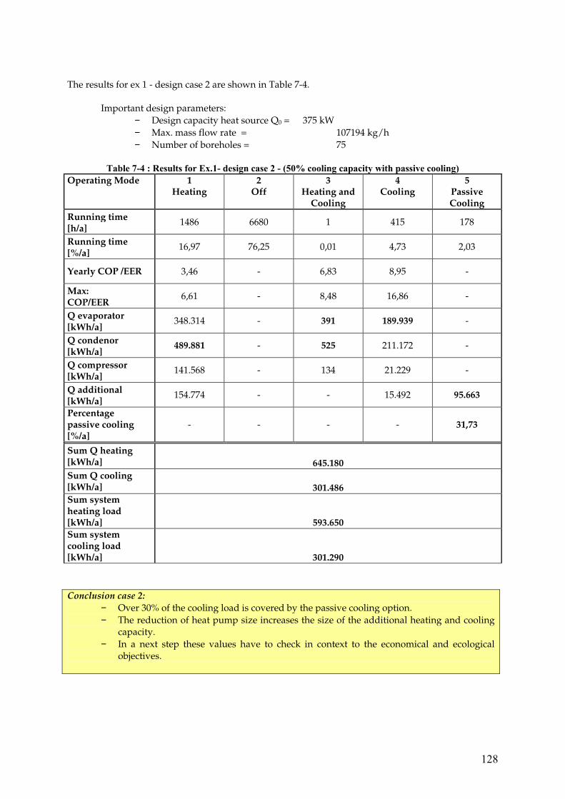
128

The results for ex 1 - design case 2 are shown in Table 7-4.

Important design parameters: − Design capacity heat source Q0 = 375 kW − Max. mass flow rate = 107194 kg/h − Number of boreholes = 75

Table 7-4 : Results for Ex.1- design case 2 - (50% cooling capacity with passive cooling)

Operating Mode 1 Heating

2 Off

3 Heating and

Cooling

4 Cooling

5 Passive Cooling

Running time [h/a]

1486 6680 1 415 178

Running time [%/a]

16,97 76,25 0,01 4,73 2,03

Yearly COP /EER 3,46 - 6,83 8,95 -

Max: COP/EER

6,61 - 8,48 16,86 -

Q evaporator [kWh/a]

348.314 - 391 189.939 -

Q condenor [kWh/a]

489.881 - 525 211.172 -

Q compressor [kWh/a]

141.568 - 134 21.229 -

Q additional [kWh/a]

154.774 - - 15.492 95.663

Percentage passive cooling [%/a]

- - - - 31,73

Sum Q heating [kWh/a] 645.180

Sum Q cooling [kWh/a] 301.486

Sum system heating load [kWh/a] 593.650

Sum system cooling load [kWh/a] 301.290

Conclusion case 2:

− Over 30% of the cooling load is covered by the passive cooling option. − The reduction of heat pump size increases the size of the additional heating and cooling

capacity. − In a next step these values have to check in context to the economical and ecological

objectives.

129

The detailed simulation gives also temperatures and capacity curves over the one year (see Figure 7-3and Figure 7-4).

Figure 7-3 Yearly capacities and COP values, design case 1, 100% cooling capacity

Figure 7-4: Yearly system temperatures and COP values, design case 1, 100% cooling capacity

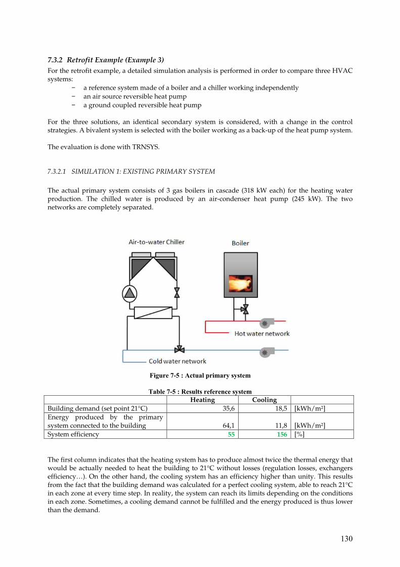
130

7.3.2 Retrofit Example (Example 3)

For the retrofit example, a detailed simulation analysis is performed in order to compare three HVAC systems:

− a reference system made of a boiler and a chiller working independently − an air source reversible heat pump − a ground coupled reversible heat pump

For the three solutions, an identical secondary system is considered, with a change in the control strategies. A bivalent system is selected with the boiler working as a back-up of the heat pump system. The evaluation is done with TRNSYS.

7.3.2.1 SIMULATION 1: EXISTING PRIMARY SYSTEM

The actual primary system consists of 3 gas boilers in cascade (318 kW each) for the heating water production. The chilled water is produced by an air-condenser heat pump (245 kW). The two networks are completely separated.

Figure 7-5 : Actual primary system

Table 7-5 : Results reference system

Heating Cooling

Building demand (set point 21°C) 35,6 18,5 [kWh/m²] Energy produced by the primary system connected to the building 64,1 11,8 [kWh/m²] System efficiency 55 156 [%] The first column indicates that the heating system has to produce almost twice the thermal energy that would be actually needed to heat the building to 21°C without losses (regulation losses, exchangers efficiency…). On the other hand, the cooling system has an efficiency higher than unity. This results from the fact that the building demand was calculated for a perfect cooling system, able to reach 21°C in each zone at every time step. In reality, the system can reach its limits depending on the conditions in each zone. Sometimes, a cooling demand cannot be fulfilled and the energy produced is thus lower than the demand.

131

7.3.2.2 SIMULATION 2: HPSAT MODEL 1

Figure 7-6 : Reversible heat pump primary system

Table 7-6 : Results system 1

Heating Cooling

Building demand (set point 21°C) 35,6 18,5 [kWh/m²] Energy produced by the primary system connected to the building 62,2 11,8 [kWh/m²] System efficiency 57 157 [%] The HPSAT model 1 is composed of a reversible heat pump which is able to produce either cooling or heating water. However, the two productions cannot be simultaneous and the priority is given to cooling capabilities. That’s why an auxiliary boiler is needed, for the cases when heating and cooling demands occur at the same time, or when the heat pump heating capacity is not sufficient. The results of the simulation are listed in table 2. They are very similar to the first system. However it has to be noticed that the secondary system needs to be somehow adapted to the new primary system. Indeed, the heat exchangers have to deal with far lower temperatures in heating mode (≈ 45°C instead of ≈ 80°C). In these simulations, the heating coils (pre-heating and post-heating) have been designed to adequately transmit the energy to the air stream. They thus have to be oversized compared to the first case.

132

7.3.2.3 SIMULATION 3: HPSAT MODEL 5

Figure 7-7 : Ground heat exchanger and reversible heat pump system

The model 5 is based on a reversible water to water heat pump of which heat/cold sink is a vertical ground heat exchanger (see figure 9). As for the model 1, the device is not able to supply heat and cold at the same time, and the priority is given to cold. In case of simultaneous demands, the heating is achieved thanks to an auxiliary gas boiler, also used when the heating demand is too high to be fulfilled by the heat pump alone.

Table 7-7 : Results system 5

Heating Cooling

Building demand (set point 21°C) 35,6 18,5 [kWh/m²] Energy produced by the primary system connected to the building 62,1 11,7 [kWh/m²] System efficiency 57 158 [%]

133

Figure 7-8 : Primary energy comparison

The results obtained can be converted into primary energy consumptions and compared to HPSAT figures, scaled to match the TRNSYS simulation configuration. The primary energy factors used are 3.31 and 1.35 for respectively electricity and gas. Figure 7-8 shows such a comparison. The graph clearly indicates that the gas consumption for the reference model is predominant. On the contrary the electricity represents the biggest part of the reversible systems consumptions. The TRNSYS results are logically higher than their corresponding results in HPSAT, because they take into account the secondary system. The consumptions are more or less multiplied by two if the secondary system is considered. This important difference can also be explained by the real indoor conditions reached, as discussed before, and by the differences in seasonal COP and EER (see Table 7-8). This table seems to indicate that the hypothesis made about the heat pump performances in HPSAT were too optimistic. Another interesting fact is that the reversible heat pump performances are always higher in cooling mode than in heating mode, showing the lack of maturity of these devices in the domain.

Table 7-8 : Heat pump performances

Model 0 Model 1 Model 5

HPSAT TRNSYS HPSAT TRNSYS HPSAT TRNSYS

COP / / 2,84 2,52 4,25 2,64 EER 4,81 2,94 4,76 2,94 5,65 4,56

For both simulations schemes, the primary energy consumption of the reversible system is lower than the classical system (-20% in HPSAT, -15% in TRNSYS). The primary energy consumption of the GHX system is the lowest (-42% in HPSAT, -23% in TRNSYS). Table 7-9 : Total primary energy consumption (ref system = 100)

HPSAT TRNSYS

Model 0 100 100 Model 1 80,28 84,49 Model 5 58,03 77,55

134

7.4 References – chapter 7

[7.1] IEA Annex 48: Model Library, 2009 [7.2] Dentel. A. and Stephan W.: Detailed Building System and Plant Simulation for

Evaluating the Potential of reversible Heat Pump Systems using TRNSYS 16 Simulation Environment, March 2009

[7.3] Fabry, B.; Dolisy, V., Bertagnolio, S.; André, Ph. Detailed simulation of the performance of heat pump systems in an office building, March 2010

135

8 Objectives for Evaluation of the Detailed System Design

In step 3 (see chapter 4) of the design process the design has already checked against economical (LLC) and ecological (primary energy and CO2) objectives. Basic assumptions are documented in the following table and the heat pump system is compared against a conventional system (chiller and boiler).

Table 8-1: Boundary conditions for evaluating reversible heat pump systems

Investment costs Cost Unit

Chiller with reciprocating compressor 450 €/kW

Condensing gas boiler (incl. distribution network and exhaust) 200 €/kW

brine/water heat pump (incl. distribution and heat exchanger) 500 €/kW

Hot water storage 1000 €/m³

Cold water storage 1000 €/m³

Heat source /sink (boreholes incl. piping ) 1000 €/kW

Other piping, control 50 €/kW

Kind of Energy Rate Rate Unit

Gas price 60 €/MWh Hu Electricity price 120 €/MWh

Time period 20 [a]

Interest rate 4 [%]

Annuity factor a 0,074

Price index: fuel 6 [%]

Price index electricity 5 [%]

CO2 –emission factor fuel 0,277 kg/kWh Primary energy factor fuel 1,100 Co2 -emission factor electricity

0,617 kg/kWh Primary energy factor for electricity 2,700

136

8.1 Evaluating of the objectives for Example 1- Design Case 1 (100 % cooling)

Table 8-2 : Comparison of Life Cycle costs (Ex 1 – design case 1)

1 2 NPV value 20 years

Conventional System Reversible Heat Pump System

Invest Costs 724.938 € 1.332.143 € Fuel Costs 996.944 € 47.065 € Electricity Costs 364.932 € 604.531 € mMaintenance Costs 265.975 € 322.093 € Operating and other costs 116.654 € 214.364 € NPV (Net Present Value) 2.469.443 € 2.520.196 €

0 1 2 3 4 5 6 7 8 9 10 11 12 13 14 15 16 17 18 19 20

0

300000

600000

900000

1200000

1500000

1800000

2100000

2400000

2700000

Cos

ts [C

]



Figure 8-1 : Comparison of life cycle costs (ex. 1 – design case 1- 100% cooling)

Table 8-3 : Comparison of the environmental impact (Ex 1 – design case 1)

1 2 Environmental impact Conventional

System reversibles Heat Pump

System

CO2-emissions [t/a] 287.47 156.73 Primary energy [MWh/a] 1177.61 682.07

The monovalent heat pump system is, due to the high investment costs more expensive than a conventional system. The advantage of this system is the low CO2 emissions and the low primary energy consumption.

137

8.2 Evaluating of the Objectives for Example 1- Design Case 2 (50% Cooling)

Table 8-4 : Comparison of Life Cycle costs (Ex 1 – design case 2)

1 2 NPV value 20 years

Conventional System Reversible Heat Pump System

Invest Costs 724 744 € 1 053 332 € Fuel Costs 917 574 € 113 590 € Electricity Costs 426 892 € 562 814 € Maintenance Costs 265 897 € 306 186 € Operating and other costs 116 623 € 169 499 € NPV (Net Present Value) 2 451 730 € 2 205 421 €

0 1 2 3 4 5 6 7 8 9 10 11 12 13 14 15 16 17 18 19 20

0

300000

600000

900000

1200000

1500000

1800000

2100000

2400000

2700000

Cos

ts [C

]



Figure 8-2 : Comparison of life cycle costs (ex. 1 – design case 2 - 50% cooling)

Table 8-5 : Comparison of the environmental impact (ex. 1 – design case 2)

1 2 Environmental impact Conventional

System Reversible Heat Pump

System

CO2-emissions [t/a] 286.77 159.81 Primary energy [MWh/a] 1180.94 690.18

The bivalent heat pump system is, due to the lower investment costs cheaper than a conventional system. The advantage of this system are the low CO2 emissions and low primary energy consumption. In comparison to the design case 1, the CO2 emission of case 2 rises by about 10%.

138

9 Special Submission Aspects

The commissioning process (CxP) starts with the submission. In the submission contract, the CxP had to be determined, in order to clarify the responsibility and the, perhaps, additional costs for the procedure. Therefore a detailed description of the expected functions and characteristics of the technical system and for the excepted testing equipment to check the guaranteed features is necessary. For a HP-system, special emphasis is laid on:

− reaction on transition states − behaviour on extreme conditions − interface to control equipment

The description of the commissioning procedure comprises the conditions of the HP system which has to be established to check the correct function, including the emulation of summer, winter conditions and a transition period. For the desired testing procedure, it might be advantageous to have a control system with the possibility of emulation (simulated sensor data, designed operation cycle). This could be an additional external control system, just for the CxP, or it is included as a special mode in the normal control system, which can be used also for later on testing. 9.1 Standards

In respect to national laws, a certain quality of commissioning is fixed, but in addiction to the interaction of building and technical design and the demands of the owner, this might not be sufficient for high-quality projects. Therefore, to avoid misunderstandings on both sides, the CxP must be described in detail in the contract. At present, in Italy and Germany, the commissioning procedure is seldom specified in the design documents; generally, commissioning is performed by the installer, independently on the contract’s requirements, sometimes under the supervision of the design team. 9.2 Responsibility and Support of the Designer and Manufacture

Within the CxP, guaranteed features of the equipment, especially the HP, had to be checked under different conditions as water temperatures, pressures, flow rates, hydraulic change over situations etc. In most cases, these equipments were handled as black box systems and nor the planner neither the installation engineer have the knowledge and the information of detailed inner functions. A special theme are the operation of the control software, who check inner states, for safety reasons or just to follows a certain operation strategy of the manufacture. Sometimes, this information was not accessible earlier and the manufacture will not share this information. In the commissioning process these kind of information from the inner of the “black box” is necessary to evaluate the performance of the whole installation. It is the role of the manufacturer, when for normal operation or even for optimisation a manipulation in the embedded software or hardware is absolutely necessary.

139

9.3 Documentation Completeness

As a part of the commissioning process, the complete documentation of the technical system including the protocol of the CxP is handed over to the owner. Besides the standard documentation of the technical design this mean especially:

− the control system: concept, input, output, parameter − interface solutions − hydraulic adjustments − electrical signal path

The commissioning protocol should contain:

− a description of the test procedures − possible additional test equipment − a scheme of the whole system with hydraulic and electrical components and

measuring points − detailed hydraulic and thermodynamic data as: temperature, power, volumetric flow

rate − quality of operation: pressure drop, temperature shift, accuracy of the control, energy

efficiency − comparison to reference values from the design

10 Commissioning, Tuning, Fault Detection and Maintenance

10.1 Commissioning

10.1.1 General Aspects of Commissioning

Commissioning of HVAC systems has been the subject of IEA-ECBCS Annex 40 “Commissioning of Building HVAC Systems for Improved Energy Performance” and of its continuation Annex 47 “Cost-effective Commissioning for Existing and Low Energy Buildings”. Therefore, a reference is made to terminology, approach, tools and findings of the above projects.

10.1.1.1 Definition

The definition of commissioning given in the final document of Annex 40 is: Clarifying building system performance requirements set by the owner, auditing different judgments and actions by the commissioning related parties in order to realize the performance, writing necessary and sufficient documentation, and verifying that the system enables proper operation and maintenance through functional performance testing. Commissioning should be applied through the whole life of the building. Commissioning is performed under the supervision of a qualified commisioning agent (CA) for the purpose of ensuring that building systems are designed, installed and functionally tested, and are capable of being operated and maintained to meet the owner's project requirements (OPR) from viewpoints of environment, energy and facility usage. These viewpoints mean to maintain the indoor environment in healthy and comfortable conditions, to minimize the amount of energy consumed and discharged, to conserve the urban/global environment, to keep maintainability of the building systems and to give a long life to the building systems.

140

10.1.1.2 Retrofitted vs. new Buildings

The document of Annex 40 also distinguishes between four distinct types of commissioning activities: Initial Commissioning (I-Cx): I-Cx is a systematic process applied to production of a new building and/or an installation of new systems that begins with the program step and ends with the post-acceptance step. In cases where new equipment is installed in an existing building (e.g., installing a cooling system in an existing building which previously had only a heating system), it should be referred to as I-Cx. Basically, the range of the commissioning process (CxP) implemented depends on the owner’s desires and can be defined in a contract between the owner and a commissioning authority. It is strongly recommended that consistency be maintained in the I-Cx process, but before commissioning becomes business-as-usual in a society, there will be cases where commissioning in the predesign and design phases have not been implemented as mentioned in the definition and explanation of ‘Preparation Procedure for Commissioning Starting at Construction Phase’. In such cases, the I-Cx can be called ‘Partial Initial Commissioning’. Retro-Commissioning (Retro-Cx): Retro-Cx is the first time Commissioning in an existing building in which a documented CxP was not previously implemented. In many cases, design documents of the existing building have been lost or they don’t match the current situation. Therefore, the Retro-Cx process may or may not include verification of the design shown in the I-Cx. Re-Commissioning (Re-Cx): Re-Cx is a CxP implemented after the I-Cx or the Retro-Cx process when the owner hopes to verify, improve and document the performance of building systems. Reasons to re-commission a building are diverse. It could result from a modification in the user requirements, the discovery of poor system performance, the desire to fix faults found during the I-Cx, etc. Periodic Re-Cx ensures that the original performance persists. Re-Cx is the event that reapplies the original Commissioning in order to maintain the building systems’ performance. On-Going Commissioning (On-Going Cx): On-Going Cx is a CxP conducted continually for the purpose of maintaining, improving and optimizing the performance of building systems after I-Cx or Retro-Cx. The large difference between On-Going Cx and periodic Re-Cx is that the Re-Cx refers to the original building systems performance, while On-Going Cx lays emphasis on the performance optimization. The On-Going Cx is a successive CxP during the operation and maintenance stage to resolve operational problems, improve comfort, optimize energy use, and recommend retrofits if necessary.

10.1.1.3 Commissioning vs. Monitoring

One of the key factors of commissioning – possibly the most important one – is the availability of reliable measured data of system performance. This leads to the concept of “system monitoring” which may be considered as an integral part of the commissioning process. There are basically two approaches to system monitoring:

− Permanent monitoring, which can be practically achieved by using the existing BMS, provided its hard- and software characteristics are suitable for the purpose; this is obviously the only viable approach for On-going Cx.

− Limited-time monitoring, using purpose-provided instrumentation installed for specific purposes, depending on system characteristics and on the goals of the CxP.

The main requirements for instrumentation will be further discussed in this chapter.

141

10.1.1.4 Commissioning vs optimisation

Another important aspect of the CxP is system operation optimisation. This is particularly relevant to innovative, complex plants – as HP-based systems often are – in which the actual energy performance depends primarily on the efficacy of the control strategy being implemented.

10.1.2 Instrumentation Requirements

The instrumentation requirements include the type, accuracy, acquisition frequency and sensor placement.

10.1.2.1 Fixed vs. Portable Instruments

Fixed instruments should be specified during the design phase in a functional diagram. Their function may be purely for monitoring purposes (e.g. electrical meters), or may be part of the system control logics (e.g. temperature sensors in thermostatic control). In the latter case, instruments may sometimes be provided by the HP manufacturers, and the possibility of exporting data from them should be ascertained. As far as portable instruments are concerned, the CA should verify the practical aspects of installation in the existing system; examples of possible problems are:

− Access to the supply board for metering the electric consumption of the main system components (refrigerating compressors, fans, pumps, etc.)

− Existence of pressure taps on refrigerant circuit of the HP for condensation / evaporation pressure monitoring

− Existence of insertion points for fluid temperature sensors on pipes (alternatively, a lower accuracy measurement may be achieved with contact thermometers)

10.1.2.2 Electricity Meters

There are basically three types of electric meters that may be used in monitoring and commissioning: − Power analysers are multi-function instruments, equipped with an internal memory

and with dedicated software for data processing, that may perform a wide range of analyses such as: load analysis (instantaneous active and reactive electric power absorption), energy analysis over specified time periods (day, week, month, year), power quality analysis (harmonic distortion), etc. They are usually installed in the main electrical board and connected to the power cables by clamps of suitable size, depending on the absorbed power of the equipment being monitored.

− Energy loggers are simpler instruments, to be installed in the electric board, equipped with a digital display that indicates the instantaneous electric power absorption; they do not usually include an internal memory, but may be interfaced to an external data logger.

− Even simpler instruments are on-off monitors that record the running time of an electric device; they may be useful for monitoring constant absorption devices such as constant speed electric motors.

In HP systems, electric meters are needed to measure the electric consumption of:

− Refrigerating compressor (in all types of HPs) − Evaporator / condenser fan of air heat pumps (in air-to-air or air-to-water HPs) − Water circulation pumps on the primary side (e.g. well water in open-loop systems,

borehole water / brine in closed loop GSHP, etc.) − Hot / chilled water circulation pumps on the secondary side

142

10.1.2.3 Flow Meters

Fluid flow measurements are an essential step for assessing the performance of any HP system. While a reliable measurement of air flow in air HPs is often virtually impossible (unless the air flow is achieved through ductwork, which is however a rather uncommon circumstance), water flow measurements may be carried out either with permanently installed instrumentation or with portable flow meters. Permanent flow meters are sometimes prescribed in the design stage for thermal energy measuring purposes, in conjunction with water temperature sensors on the supply and return sides of a given hydraulic loop (typically on the secondary side). Flow meter types that are mostly suitable for this application belong to the following categories:

− Turbine type meters, in which a rotating device is inserted in the pipe; the flow rate is measured by a pulse counter which determines the rotation speed of the sensor; this type of meter has a typical accuracy of 1 % at full scale.

− Restricted section meters (e.g. venturi tubes, calibrated diaphragms, etc.); the output of the instrument is the differential pressure between the full and restricted sections of the pipe, from which the water flow rate can be determined based on a calibration curve determined by laboratory tests

− Both the above described meter types are invasive and there installation should therefore be preferably decided at the system design or construction stages.

Non-invasive sensors are also available in the market that may be employed either as permanent or as purpose-provided instrumentation for the commissioning procedure. Such devices may be based on the following physical principles: Ultrasonic sensors, consisting of two transducers mounted on the outside of the tube, measures the flow velocity by recording the ultrasonic runtime, which depends on the speed of the fluid. This type of meter has a typical accuracy of 2 % at full scale. Air flow rate measurements are seldom foreseen as a permanent monitoring feature. During commissioning, air flow may be measured with different types of instruments, depending on the practical circumstance: Flow rates in ductworks is typically made with pitot tube, or hot wire anemometer probes inserted inside the duct; the measurement should be made in a straight section of the ductwork, at a distance of at least three equivalent diameters from any turbulence-inducing singularity (fan exhaust, curves, branches, balancing dampers, fire dampers, re-heat coils, etc.); at least 3-5 measurement points should be taken and the value averaged. Flow rates at supply or extract diffusers / grilles of simple geometry (e.g. rectangular) may be made by taking a suitable number of point measurements with pitot, hot wire or fan-type anemometers. Better results, specifically for complex geometry diffusers, are achieved with hoods that collect the air flow to a suitable measuring section.

10.1.2.4 Fluid Temperature Sensors

Water temperature sensors should preferably be provided in the design / construction stage and installed in such a way to achieve a very good thermal contact with the fluid flow. Sensor types may be thermocouples, PRT (platinum resistance thermometers), or thermistors (solid-state integrated circuits), with typical accuracy of +- 0.3 °C (PT100), +-1.5 °C (thermocouples) and +-0.3 °C (thermistors). A lower-accuracy procedure, which is however the most practical solution for measurements on existing pipework, is to install a contact thermometer directly on the outer surface of the metal pipe. Air temperature sensor installation is much easier in practice, but care should be taken in order to minimise errors due to radiation effects.

10.1.2.5 Sensor Emulations

To test the performance of the HVAC system in a first step, one has to be sure, that especially a complex control strategy is working correct. Therefore the inputs of the control are connected to emulated, simulated signals like weather data (temperature, solar radiation) or hydraulic data (temperature, flow). Now the answer, output of the control, can be compared to the theoretical values.

143

The emulation must work for static and dynamic test cases. In the next step, the reaction of the whole HVAC system can be tested with simulated control data. The critical point is the load of the building. If it is necessary for the CxP, a thermal building load (cooling and heating) has to be emulated too (cooling tower, heater).

10.1.3 Conditions for Commissioning

10.1.3.1 Indoor Environment Condition (ambient temperature sensors, RH and CO2 sensors,)

Monitoring the indoor environmental parameters is essential in order to evaluate the effective performance of any HVAC system. Simple, self powered loggers with internal memory capacity are readily available on the market for long-term monitoring of ambient temperature and relative humidity. CO2 sensors may also be employed for estimating the effectiveness of the ventilation system. Global comfort parameters, such as the PMV and PPD indices adopted by the EN ISO 7730 standard for thermal indoor climate, may be measured with ad-hoc instrumentation, if necessary for specific commissioning requirements.

10.1.3.2 Outdoor Climate Condition

Outdoor weather stations typically include temperature, relative humidity, atmospheric pressure, wind speed, direction and sometimes solar irradiation on the horizontal surface. Knowledge of such data (particularly temperature and RH) is of particular help for interpreting the energy performance data using well established tools such as the energy signature, carpet plots, etc.

10.1.3.3 Building Occupancy / Schedules

Present-day tendency towards high-performance building envelopes is determining an ever increasing importance of internal loads in the thermal balance of tertiary buildings: internal-load dominated conditions are already normal in the warm-hot seasons, but will become more and more usual even in winter. Monitoring of internal loads (due to lighting, appliances and occupancy) is therefore an important feature of any monitoring system and should not be overlooked during the commissioning process.

10.1.4 Data Collection and Storage

10.1.4.1 General Requirements

The data points had to be explained: − Short but expressive comment − Measuring points: where located in the technical plan, which sensor, meter etc. − Calculated points: what is the equation behind − Data unit in SI standard − logical data with the range − accuracy

The data points consist of:

− Unique name − Time mark − Value

144

The time mark had to be constant step width, maximum time step 15 minutes, without gap. Any breakdown of the data collection had to be reported. The data can be stored on any standard data storage medium

10.1.4.2 Data Format

All data of the same type must have the same data format, i.e. time, temperature, flow, pressure. A readable data format should be used: text-format or comma separated files.

10.1.4.3 BMS Functions

If the BMS is used for data collection and storage, the BMS must have the capability and capacity to handle a small monitoring system. This in respect to easily programming a sequence for real time data acquisition, handle the additional traffic on the local net, manage the data storage and transfer. The interfaces in hard- and software from the sensors to the BMS had to be suitable; the electrical transfer must be protected against unwanted disturbance (electrical noise).

10.1.4.4 Stand-alone Data Logger

If a separate stand-alone system for data collection and storage is installed, this equipment should show the quality of:

− Commercial equipment, with operating manual, hotline, etc. − Easily programming − Build for endurance test situation, safety for interference − High accuracy, calibrated − Extensible − Remote control

10.1.5 Control Issues

The overall system control strategy has several functions; the implementation should be check carefully while commissioning:

− Adapted to ambient situations (weather) and internal loads (user profiles), the control interacts with the HVAC system to establish the desired room condition

− Minimize the energy consumption − Safety monitoring

In the case of a heat pump system, the HP is normally equipped with an own, independent control system with a vendor software. It is essential to integrate the control of the HP in the global system, to have an adapted interface module, to communicate to the key functions of the HP and to allow the overall control to act in master mode. The internal safety surveillance of the HP will not be overruled and any fault signals will past to the overall control system and handled there.

10.1.6 Commissioning Procedure

10.1.6.1 Planning the Commissioning Procedure

Normally, commissioning is planned in the construction phase, when calibration and measurement devices are provided to assist the commissioning process. A detailed program of the tests is generally prepared according to general commissioning procedure, including checklists and data gathering forms that are adapted each time to the specific system to be commissioned.

145

10.1.6.2 Checking Installation Quality

The following aspects should be controlled during system construction: − Conformity checks between project and execution, compliance with design specifications

(e.g., pipe diameter, insulation thickness, condensate drainage, hydraulic lay out, instrumentation, etc.)

− Hydraulic tightness tests on all primary and secondary water circuits − Well water flow rate and quality (hardness, purity, temperature) − General functional and performance checks on main components

It should also be checked that the system components are installed in such a way that future maintenance and substitution actions will be easily achieved.

10.1.6.3 Heat Pump Start-up

Normally, the initial start-up is performed by the HP manufacturer customer assistance service, according to manufacturer’s instructions. The presence and operation of all safety equipment is checked, and the operation parameters of the HP are verified:

− Refrigerant thermodynamic properties (temperature and pressure) on the low-pressure and high-pressure side of the refrigerant circuit, particularly at compressor start / stop

− Temperature and flow rate of the secondary fluid (air or water) and of the heat carrier fluid (from heat source),

− Electrical absorption of the compressor and auxiliaries − noise level − Electrical absorption, working pressures, fluid flow rates − Correct installation of hydraulic components − Correct interfacing with the general control system, electrical connections of sensors and

actuators to the main power supply or control board − Field check of actuators and sensor readings − Safety devices intervention and communication

10.1.6.4 Heat Pump Tuning

Once the control strategy has been defined, the control laws are programmed and inserted in the CPU of the digital controllers. Then, the correct wiring of all sensors and actuators are individually checked. The calibrations of specific controllers are generally performed by the system manufacturer in a latter phase, since this is a very specific type of job. It is generally advisable to check and calibrate the PID controllers of the HP (thermostatic valve, part load control / thermostatic controllers, condenser maximum pressure control). As far as the system is concerned, problems are mostly related to incorrect water flow rates, absence of storage and / or insufficient water volume with respect to the HP power, air duct geometry (excessive losses). An aspect worth of attention is the usage of HP systems with heat recovery. An example may be a GSHP providing heating, cooling and domestic hot water. When such equipment is adopted, particular care should be taken in verifying the interaction between the internal control logics of the HP and the overall control strategy of the system and of other components, in order to avoid conflicts.

10.1.6.5 Data Analyse

The analyse of the collected data can help to understand the behaviour of the complex system: control – HVAC – building. In comparison with the calculated or simulated data, the installation can be tuned, or modified, to the expected performance. The recorded data are a part of the commissioning documentation. Before the analyse could start, a first check on the reliability of the data is essential:

− are the connection of the sensors to the data points according to the design? − are the sensors correct installed? − does the sensor accuracy fit the required quality?

146

The critical and of most interest data are:

− control o correct programming, parameters o working under dynamic conditions

− heat pump o temperature, pressure o power, energy, COP o function under transition states

− storage o temperature stratification

− bore hole heat exchanger o temperature distribution o temperature change o power

− hydraulic o heat exchanger, pipe, valve, pump, mixer o temperature o flow

− building o room climate condition

10.1.6.6 Commissioning Development

Depending on system size and on the encountered problems, the commissioning phase may last from a few days up to several months (if serious problems are encountered, it is necessary to suspend the activity, try to solve the problem and then re-start). Furthermore, commissioning should include both: the heating season and the cooling seasons. After initial verification, regular long-term monitoring is performed with the BMS or using remote data acquisition by high speed internet protocols and dedicated websites. Specific problems may be encountered with open-loop water systems (e.g. clogging of intermediate heat exchanger, submerged pumps operation, authorisation procedure for extraction and return wells, etc.) Filtration is the main problem. Generally, no other specific problems have been encountered. Normally, no treatments are applied to ground water other then filtration, also because the water must be returned to the water table without physical / chemical alterations and with a maximum temperature difference of 5°C. Based on water quality, a decision is made about the hydraulic loop design (with or without intermediate HX); filter maintenance is a key factor in preventing operation problems.

10.1.6.7 The Commissioning Report

In the commissioning report, ongoing or final, the state of the installation is documented, in detail and summarized. This report is communicated with the building owner.

− Compliance with contract requirements − Compliance with the planning − Checking of the manufacturers data − Check of the system under a dynamic test procedure (check Annex 40 material − Hydraulic testing procedures − General performance − HP performance (COP) − Potentials for energetic optimisation − Checkpoints for maintenance and inspections

147

10.2 Fault Detection and Tuning

A fault or a malfunction means that the actual behavior of the installation does not correspond to the expected one. Therefore the first step in fault detection is to subdivide the complete system in subunits, and to compare the status of these subunits with theoretical benchmark data. The next step looks at the interaction and reactions. Some subunits, as the heat pump, have their own control system. Here a malfunction can also originate from unsuitable parameters in the vendors software. A more easily to detect fault are the ones who occur on static conditions. More difficult are the ones who occur only under dynamic conditions, or in a transient state. The key for a systematic optimization procedure, used as a generic term for fault detection and tuning, is the installation of a monitoring system. A practical objective function for the optimization procedure is a minimal energy consumption and at the same time a maximal thermal comfort in the building. It is the task of the monitoring to provide the necessary data to derive all the information concerning energy consumption and thermal comfort. With a short data collection period (< 5 min) also the transient states of the HVAC system under dynamic conditions can be analyzed. As a high quality energy concept results often in a technical prototype solution, modifications, for example in the control strategy or in the hydraulic arrangement, can be derived from the monitoring data and may be part of the optimization process. Since the reaction of the building as load for the HVAC system is time dependant (weather, use etc.), sometime malfunction occur seldom under very special condition, hardly reproducible. Then, running a monitoring system permanently in the background of the BMS, the data gives the necessary information how to handle the problem. In the table below, some possible subunits of a complex HVAC system are listed, together with corresponding, theoretical or expected, benchmark data. The listing is not complete and can be adjusted to the present design.

148

Table 10-1: Possible subunits of a complex HVAC system

subunit Benchmark data control Input output correlation parameters Regulation of supply temperature Control of energy supply strategy: HP mode, additional

energy systems Mode DHW, room heating/cooling hydraulic Control performance Temperature Flow rate storage Temperature stratification pump On/off state energy Domestic hot water (DHW) Flow rate Temperature Room heating system 1 Flow rate temperature Room heating system 2 Flow rate temperature Supply for room ventilation Flow rate temperature Room cooling system 1 Flow rate temperature Room cooling system 2 Flow rate temperature Heat exchanger Temperature Flow rate Energy Energy system 1 = Heat pump Mode: on/off, power, reversible state Temperature Flow rate energy, COP Internal conditions HP control: parameters Energy system 2 = e.g. gas burner Mode: on/off, power Temperature Flow rate energy Bore hole heat exchanger Flow rate Temperature of the ground and of the brine/water Temperature relaxation time

149

10.3 Maintenance

The maintenance of the technical system is on one side a periodic standard procedure and on the other side a special test scenario. The standard check includes the function of all hydraulic components, the energy systems like the heat pump and the control. System parameters as temperature and pressure were revised. The quality of the storage water or the brine in the ground heat exchanger had to be measured and if applicable they had to be renewed. For components like the heat pump the maintenance instructions of the manufacture are obligatory and described in the warranty document. The check of the control depends on the quality of the internal fault indication. Here, the manufacture had to provide the information about testing and maintenance. With a special test scenario the quality and function of the whole system or part of it can be checked. The control in an emulation mode provides selective outputs to the system (questions) and the monitored data (answers) are compared to an expected behavior. This is similar to the above described commissioning procedure. The advantage is a quick overlook of the status of the HVAC system.

11 Operation

There are only a few studies of the operation of existing heat pump systems available. On the part of the user or facility management, the following main points are mentioned: Positive feedback

− low energy costs − unproblematic system with low operating expense − temperature in the ground heat exchanger stable − in the combination with tabs good room temperatures

Negative feedback

− Unexpected high energy costs − high share of the second energy source like district heating or gas burner − Sudden failure or malfunction of the heat pump − dissatisfied thermal room comfort

Detailed analysis on realized heat pump systems show the following results Erreur ! Source du renvoi

introuvable.] which are essential for an optimized operation: • Ground heat exchanger

o Wrong dimensioning of the ground source heat exchangers (exchanging area, pipe dimensioning): temperature shift to large

o geothermal data of the ground and the ground water flow not exactly known (thermal respond test)

o thermal contact between the pipes and the ground not high enough • Heat pump

o avoid too frequent on/off operation o heat pumps in cascade: useful power regimes o Many high pressure cut offs

� Low mass flow rate (wrong dimensioning, fauling) � Overstraining of the heat source (wrong dimensioning) � Hydraulic problems in bivalent systems (wrong circulation)

o Low pressure cut offs (low evaporator capacity) � Low mass flow rate

150

� Heat source temperature lower than expected � Dimensioning of the heat source (too low) � Higher condenser capacity as expected (lower heat demand of the building)

o The transient state of the system, this means the switching between heating, neutral and cooling mode, is almost a critical operation mode. The hydraulic requirement of the hp often forces a total switch off for several minutes.

• Hydraulics o incorrect (dynamic) mass flow o standard hydraulic schemes not applicable or not available o the hydraulic integration of the heat pump in the system: building, storage, ground

heat exchanger is not optimal. The main focus has to be the transition state (see above) with the request of a stable hp operation (no switch off)

o the energy consumption of the ground brine pump in an intermediated power regime of the heat pump not well adapted

o heat exchanger with low efficiency • Storage

o wrong hydraulic connection o stratifying storage for optimal temperature levels for the heat pump o dimension (m³/kW) o insulation

• Control o the behavior of the internal control of the heat pump is not known and can not be

manipulated from outside o not well adapted control strategy for the interaction of heat pump and tabs o wrong control strategy for the regulation of the supply temperature (heating and

cooling mode) o adaption of the heat pump operation (heat cooling mode, power output) is often a too

complex (confusing) algorithms, difficult to understand, and do not work reliable • Monitoring

o Bad or missing monitoring o Wrong sensors (accuracy) o missing sensors o incomplete analysis of the thermal and energetically behavior, no clear easy

understandable conclusion • Documentation

o Wrong or missing details o Not up-to-date o Not in an understandable clear format

Field test on realized heat pump system show the following results Erreur ! Source du renvoi

introuvable.]: • Good operation behaviour, reliable • Avoid on/off operation • Problems with hydraulics (low mass flow rates) • Use standard hydraulic schemes • Wrong dimensioning of ground source heat exchangers (pipe dimensioning) • Wrong heating and cooling curves • Many high pressure cut offs

o Low mass flow rate (wrong dimensioning, fauling) o Overstraining of the heat source (wrong dimensioning) o Hydraulic problems in bivalent systems (wrong circulation)

• Low pressure cut offs (low evaporator capacity) o Low mass flow rate o Heat source temperature lower than expected o Dimensioning of the heat source (too low) o Higher condenser capacity as expected (lower heat demand of the building)

151

• Bad or missing monitoring • No optimization of the system

11.1 References – Chapter 11

152

12 Appendix Simulation Models

12.1.1.1 Black-Box-Models vs. Grey-Box-Models

Heat pump simulation models are available for most of the system simulation packages. They can be split into two categories: 1) black-box-models and 2) gray-box-models. Black-Box-Models calculate the heating power of the condenser and the electrical power of the compressor based on characteristic curves. These curves can be constructed from manufacturer data if the condenser power and the electric power are given for certain conditions as a function of the evaporator inlet temperature and the condenser outlet temperature (e.g. model of Wetter/Afjei [6.3]). Grey-Box-Models are based on mechanistic engineering equations (e.g. model of Lemort/Lebrun [6.25]). Originally, they are physical models (white-box-models) with tune-able parameters (steady-state input values). Therefore, these models must be adapted to real measurements (catalogue/lab data), too. But the advantage of grey-box-models is the physical meaning of their parameters and usually the lower number of required inputs and parameters. Furthermore, physical models might help to give the system designer a better understanding for the physical relationships involved in his problem and the best possibility to tune black box models. Table 12-1: Wetter/Afjei model interface as an example of typical parameters of a black-box- model [6.3]

153

Table 12-2: Lemort/Lebrun model interface as an example of typical parameters of a grey-box-model

[6.25]

12.1.1.2 Ph-Charts and Typical Equations

Within the grey-box-modelling approach the consideration of the refrigerant cycle within a ph-chart (ph: pressure-enthalpy) helps reducing the number of equations needed for a heat pump model. Ph-charts describe graphically the relationships of thermodynamic properties of a certain refrigerant. In the vapour compression cycle a mixture of cold and saturated liquid and saturated vapour enters the evaporator. The liquid part of the mixture boils in the evaporator. The refrigeration effect increases the enthalpy across the evaporator. In the ideal case where there are no heat losses from the compressor and no friction the whole process of compression is adiabatic, reversible and isentropic. The compressor sucks dry saturated vapour from the evaporator. In this ideal case the power of the compressor is equal to the enthalpy increase across the compression. Furthermore, the outlet conditions of the compressor can be identified by assuming the outlet pressure as to be the same as the condensing pressure and (in the ideal case) the compressor outlet entropy as to be the same as the entropy of the dry saturated vapour entering the compressor. But of course the real compression process is not isentropic. So, one or more correction factors (e.g. compression efficiency, red section in Table 5) should be introduced to the simulation model. Table 12-3 shows the basic equations needed for modelling a heat pump cycle. In this simple model pressure losses within the evaporator, condenser and linking pipes have been neglected and the process within the expansion valve is assumed as to be isenthalpic.

154

Table 12-3: Basic model equations in EES [6.24]

12.1.1.3 Example of a Heat Pump Model for Case Study LVM (No. G1)

Manufacturer’s data have been used to model one of the two heat pumps for the German case study LVM. Table 12-4 shows the basic performance data. The data listed for 35 °C condenser outlet temperature of Table 12-4 are the base for adopting the parameters of a ph-chart heat pump model in EES. The basic equations are listed in Table 12-3. The only 4 tuning parameters (Table 12-5) are the compressor efficiency, two heat transfer parameters (UA) and the volume flowrate of the refrigerant. The aim of this exercise is to prove the usability of the whole approach described in the last section. No detailed heat transfer functions for the condenser and the evaporator are implemented for this example, however, if needed, they can be easily introduced with few classical heat exchanger equations (e.g. ɛ(NTU)).

Table 12-4: Performance data, LVM heat pump 1

Condenser Outlet Temperature [°C] 35 50

Power Stage [%]

Evaporator Inlet

Temperature [°C]

Heating Power [kW]

Electrical Power [kW]

Heating Power [kW]

Electrical Power [kW]

100 -5 121 34.4 118 47.7 100 0 146 35.5 127 49 100 5 151 35.6 144 49 100 10 173 36.3 163 50 100 15 200 37 186 51

Additional information according table 6-6:

− Water/glycol − Piston compressors − Capacity (Heating): condenser (40/50°C): 136 kW; evaporator (5/1°C): 96 kW; elect. Power: max. 40 kW − Refrigerant: R 134 a − Water flow rates evaporator: 50% capacity: 18 m³/h; 100% capacity: 21 m³/h − Water flow rates condenser: 50% capacity: 7 m³/h; 100% capacity: 13 m³/h

155

Table 12-5: Input data, LVM heat pump 1

The results of a one-year-period simulation are illustrated in Figure 12-1. The heat source temperature (water temperature at the evaporator side, e.g. leaving a ground heat exchanger) and the water supply temperature (at the condenser side) have been given as transient inputs. The basic model output is the COP of the heat pump and has been computed here for the heating mode only (red line and red dots in Figure 12-1). The average annual COP is needed for system evaluation purposes which can be achieved by the integration of the hourly COP values and dividing the result by the number of hours (8760 h/a). Cooling performance for reversible systems can also be estimated by exchanging the water temperature inputs on the evaporator and condenser sides.

156

Figure 12-1 : Results of the system simulation of a one-year-period

Simulation environment for heat pump system simulation

157

Unit Conversion 2 kJ/Watt

Type109-User

Heatpump

Geothermal HX

Cond. Pump

Heat Storage

T_Top_Storage

Heat HX

Cond. Diverter Valve

Heat Storage Pump

Cond. Tee-Piece

Cond. Diverter Valveout 1: Y = 0 --> to HX

out 2: Y = 1 --> to GHX

GHX Mixing ValveGHX Diverter Valve

GHX Diverter Valveout 1: Y = 0 --> to HP Evaporatorout 2: Y = 1 --> to HP Condenser

Cold HX

Cold Storage

Evap. PumpEvap. Diverter Valve

Evap. Tee-Piece

Cold Storage Pump

GHX Mixing Valvein 1: Y = 0 --> from HP Evaporatorin 2: Y = 1 --> from HP Condenser

Evap. Diverter Valveout 1: Y = 0 --> to HX

out 2: Y = 1 --> to GHX

HP-Control

HP

Unit Conversion 1 kJ/W Energy

Endenergie Summary Endenergie

Verbrauchskosten Summary Verbrauchskosten

Primärenergie Summary Primärenergie

CO2 Summary CO2

COP,NMODE

Type24

Type25b

result

FreeCooling Div.Valve-V

FreeCooling Div.Valve-R

FreeCooling Div.Valveout 1: Y = 0 --> to Evap. Tee-Piece

out 2: Y = 1 --> to GHX

FreeCooling Mixing Valve-R

FreeCooling Mixing Valvein 1: Y = 0 --> from Evap. Div. Valve

in 2: Y = 1 --> from FreeCooling

FreeCooling Mixing Valve-V

FreeCool.Pump

FreeCooling Mixing Valve-Vin 1: Y = 0 --> from Evap.Div.Valvein 2: Y = 1 --> from FreeCool.Pump

FreeCooling Div.Valveout 1: Y = 0 --> to GHX Div.Valveout 2: Y = 1 --> to FreeCool.Pump

Type65d

C-Transfer-Distribution-AHU

H-Transfer-distr-AHUH-Transfer-distr-zone

C-Transfer-Distribution-zone

Load-Multiplication

H-and _C_Loads

EqualTransfer Cooling-zone

Transfer Heating-zone Type6Auxiliary Heater

Unit Conversion 3 kJ/Watt-3

Type92Auxiliary Cooler

Summ

Figure 12-2 : Simulation environment for heat pump system simulation [7.2]

158

13 Appendix Hydraulic Schemes

According to the case studies, the following hydraulic schemes are listed:

− Case study F1 – building in Lyon: Heat pump and Boiler

Hydraulic scheme of the French case study F1 in Lyon

Design Handbook for Reversible Heat Pump ... - IEA EBC

Documents

Transcript of Design Handbook for Reversible Heat Pump ... - IEA EBC