Case study buildings - IEA EBC

International Energy Agency Programme on Energy in Buildings and Communities

Case study buildings Separate Document Volume III

Total energy use in buildings analysis and evaluation methods

Final Report Annex 53 November 14, 2013 Yi Jiang, Qingpeng Wei, He Xiao, Chuang Wang, Da Yan

1

Volume III Case study buildings

Authors: Yi Jiang, Qingpeng Wei, He Xiao, Chuang Wang, Da Yan (China)

With contributions from: For III-1 (office building) Azra Korjenic, Naomi Morishita, Thomas Bednar

(Austria), Roberto Ruiz, Sephane Bertagnolio, Vencent Lemont (Belgium), Yi Jiang, Yingxin Zhu, Qingpeng Wei, He Xiao, Cary Chan, Jean Qin (China), Vincenzo Corrado (Italy), Hiroshi Yoshino, Shigehiro Ichinose, Ting Shi (Japan), Natasa Nord (Norway)

For III-2 (residential building) Markus Dörn, Naomi Morishita, Thomas Bednar, Azra Korjenic (Austria), Yi Jiang, Yingxin Zhu (China), Hiroshi Yoshino, Ayako Miura (Japan), Philippe Andre, Cleide Aparecida Silva, Jules Hannay, Jean Lebrun (Belgium)

Reviewed by: Carl-Eric Hagentoft, Seung-eon Lee

Tianzhen Hong, Jean Lebrun, Ad van der Aa

2

Contents

III-1 Technical report “Occupant behavior and impact of energy in office buildings” III-2 Technical report “Occupant behavior and impact of energy in residential buildings” III-3 Questionnaire sample III-4 Case abstract III-5 Case source book

3

III-1

Technical report “Occupant behavior and impact of energy in office buildings”

4

Contents

Abstract ..................................................................................................................................... 5

1. Boundary of the energy and occupant behavior in office building ....................... 6

2. Typology of office building........................................................................................ 8

2.1 Classification of office building................................................................................................8

2.2 Review of floor area regulations of office building..................................................................9

3. International comparison of energy use in office building................................... 12

3.1 Basic information of case buildings........................................................................................12

3.2 International comparison of office building energy use .........................................................15

3.3 Weather condition of case buildings.......................................................................................16

3.4 Energy use comparison of case buildings ...............................................................................17

4. Lighting system ........................................................................................................ 21

4.1 Occupancy/Lighting use patterns............................................................................................24

4.2 Occupant behavior impact factor ............................................................................................33

5. Office appliances ...................................................................................................... 41

5.1 Literature review.....................................................................................................................41

5.2 Night status survey of case buildings......................................................................................43

6. Ventilation and window operation ......................................................................... 46


6.2 Field survey of case building ..................................................................................................47

7. Heating and cooling ................................................................................................. 50


7.2 Simulation on a case building .................................................................................................51

8. Summary and conclusions....................................................................................... 55

9. Reference................................................................................................................... 57

5

Abstract

The energy use of office building has been attracting great attentions due to its significant role in total building energy consumption worldwide nowadays. The influencing factors of energy consumption in office buildings were gradually clarified by researchers in recent years. Generally speaking, those factors can be summarized into two categories, including six factors: (1) Physical factor, consists of Climate (e.g. outdoor ambient temperature, humidity, solar radiation,

etc.), Envelope (e.g. structure, K-value, etc.) and Technical system (e.g. lighting, office device, service system, especially HVAC system, etc.)

(2) Human factor, including Set point (e.g. indoor control temperature, carbon dioxide concentration, fresh air volume, etc.), Operation (e.g. on-off schedule of central systems, etc.) and Occupant behavior (e.g. switch on-off of lighting, equipment status in after-hours, window opening, etc.)

A number of present studies were more focusing on the latter three factors, especially the related occupant behavior in the office building. These researches are trying to answer what is the driving force of the energy-related occupant behavior. While, this IEA ECBCS ANNEX 53: Total energy use in buildings-Analysis and evaluation methods, is trying to answering what is the energy-related occupant behavior, and what is the direct/indirect impact of the behavior (through material/building culture, energy practice and cognitive norms of energy consciousness of energy use) to the energy consumption. This technical report is under the framework of subtask B1: case study of office and residential buildings, but only focused on office building. 12 office buildings are contributed by researchers from seven countries, including Austria, Belgium, P.R. China, France, Italy, Japan and Norway. There are five small-scaled office buildings and seven large-scaled high-rise office buildings in subtask B1. The basic information and total energy use of these 12 office buildings are compared. In this report, we also present a literature review of energy-related occupant behavior of lighting system, office appliances, ventilation and window opening, as well as heating and cooling system, also its’ impact on office building, as well as the key findings through twelve case studies by contributors. There are three major conclusions of occupant behavior impact on energy consumption in office building, based on case study: (1) There is weak relationship between external illuminance and the use of artificial lighting in large-

scaled office building. Occupants usually turn on artificial lightings during the working hours. But occupants in small-scaled office buildings use more natural lighting and save more electricity.

(2) The electricity consumption of centralized system is higher than de-centralized system (especially to lighting system and HVAC system). For example, the energy use of ventilation and air-conditioning system in large-scaled office building is larger than small-scaled office buildings due to the limitation of operable external windows. The building operator behavior (i.e. set point, air change rate, control strategy of circulating pumps and fans, etc.) is the decisive factor of electricity consumption of AC systems as well as cooling consumption.

(3) The energy loss can be caused by three aspects: 1) energy waste caused by equipment inefficiency, 2) energy loss caused by steam or heat leaking, 3) electricity waste caused by stand-by power during off duty hours. Thus, it is found that the occupant behavior of night-time standby status is the key decisive factor of appliances in office building according to the on-site investigation.

6

1. Boundary of the energy and occupant behavior in office building

The energy-related occupant behavior is hugely complex, shaped and influenced by many factors, some of which are intrinsic to the individual, and others are more related to society or culture. The need to use energy more efficiently is ever more pressing in the face of urgent calls to reduce GHG emissions (Stern, 2007) and to address current anticipated constraints in energy resources (IEA, 2009). The various investigations and researches involved in several domains: social sciences, economics, natural sciences, as well as engineering sciences. Three key questions are studied by multiple researchers:

1) What is the driving force of the energy-related occupant behavior? 2) What is the energy-related occupant behavior? 3) What is the direct/indirect impact of the behavior on energy consumption?

Since the oil shocks of the 1970s, there have been numerous studies of the driven force of the energy-related behaviors from a wide range of disciplinary perspectives. Multiple researchers (Lutzenhiser,1993, Marechal, 2003, Wilson, 2007and as well as J. Stephenson et al, 2010) have reviewed these perspectives, as shown in Figure 1-1. These perspectives includes microeconomics, behavioral economics, technology adoption models, social and environmental psychology and sociological theories.

Figure 1-1: Driving forces of energy-related occupant behavior

The existing mass of literature relating to occupant behavior is a bit skewed towards thermal and adaptive comfort (J.F. Nicol, 1973, J.F. Nicol, 2002, H.B. Rigal, 2007, P.O.Fanger, 2002).

7

For example, the Fanger’s Predicted Mean Vote (PMV) Model, combines four physical variables (air temperature, air velocity, mean radiant temperature, and relative humidity), and two biological variables (clothing insulation and activity level) into an index that can be used to predict the average thermal sensation of a large group of people. The Fanger’s another Draught Model, predicts the percentage of occupants dissatisfied with local draught, from three physical variables (air temperature, mean air velocity, and turbulence intensity). The occupant behavior in air conditioned buildings and naturally ventilated ones are quite different, and can be partially predicted by these two models. Another example is the natural ventilation. The Humphreys algorithm (Rijal el al, 2007) has been established for modeling window opening adaptive behavior in buildings. The model is based on the indoor temperature and outdoor temperature both. Then the model has been applied and developed by other researchers (Nicol, 2004). However, most of those researches focus on the driven force (i.e. outdoor/indoor environment, personal requirement, etc.) of the occupant behavior, rather than the impact of behaviors on building energy use. Thus, under the framework of ANNEX 53: Total energy use in buildings-Analysis and evaluation methods, the research boundary of this study should be emphasis as following chart. This report is trying to answer the latter two questions at the beginning: What is the energy-related occupant behavior, and what is the direct/indirect impact of the behavior (through material/building culture, energy practice and energy consciousness of energy use) to the energy consumption? But ignore the sophisticated driven force behind occupant behaviors.

Energy-relatedOccupant Behaviour

Building design

Energy practice

Cognitive norms

Energy consumption

Driving force

Boundary

Figure 1-2: Boundary about energy-related occupant behavior in this research

Besides, the unified definition for basic items related to building energy use is defined in Subtask-A (The detailed definition refers to the interim report of Subtask-A). Three boundaries of energy consumption in buildings are explained and used for international comparison. The three boundaries are:

1) Eb: Energy actual attained by building space or the occupant’s activities in the building through various end usages in the building.

2) Et: Energy delivered to the technical systems and appliances of one building. 3) Ed: Energy delivered to the central plant of the district heating and cooling systems.

This report is composing as follows: Session 2 introduces typology of office building. Session 3 compares the energy use of office building in several countries, based on the energy boundary definition. Session 4 to 7 illustrates the literature review and research result of different systems in office building, including lighting, office appliance, ventilation and window opening, heating and cooling system. Session 8 summarizes the key conclusions and Session 9 encloses the reference survey questionnaire for energy-related occupant behavior in office building in future research.

8

2. Typology of office building

2.1 Classification of office building

Energy use and occupant behavior depends on type, size, primary activity, as well as design and operation of the building. For example, a skyscraper office with banks and companies headquarters will consume much more energy per square meter than a two-floor small office building. The British Government’s Energy Efficiency Best Practice programme (BRE, 2000) has defined four generic types of office building as Type 1: naturally ventilated cellular, Type 2: naturally ventilated open-plan, Type-3: air-conditioned standard and Type 4: air-conditioned prestige. The characters of each type are shown in the Table 2-1.

Table 2-1 Comparison of four office types defined by existing research

Type Floor area ranges (m2)

Energy use related Occupant behavior related

Type 1: naturally ventilated cellular

100~3000 Lower illuminance levels; Few common facilities

Individual windows; Local light switches; Heating controls

Type 2: naturally ventilated open-plan

500~4000

Illuminance levels, lighting power densities and hours of use are higher than type-1; More office equipment and vending machines.

Lights and shared equipment tend to be switched in larger groups and to stay on for longer.

Type 3: air-conditioned standard

2000~8000 More intensively used; VAV air-conditioning with air-cooled water chillers.

Occupancy is similar with type-2; Deeper floor plan, and tinted or shaded windows which reduce daylight.

Type 4: air-conditioned prestige

4000~20000

Usually including catering kitchens or data center; VAV air-conditioning with air-cooled water chillers.

Occupancy hour is longer; Higher quality design and environment control parameter standard.

The U.S. Department of Energy is also designing an Advanced Energy Design Guide for Small to Medium Office Buildings (DOE, 2011), which defined as up to 100,000 square feet (equals to 9,290 square meters), including a wide range of office type and related activities such as administrative, professional, government, bank or other financial services, and medical offices without medical diagnostic equipment. Hence, it can be concluded that the office building can be divided based on scale, energy consumed equipment (especially air-conditioning system), occupancy hours and energy-related occupant behavior. Based on characters of case buildings contributed worldwide, an office building in this ANNEX can be defined as one of two types: a small-scaled office building or a large-scaled high-rise office building.

1) O1-Small-scaled office building. The total floor area is less than 10,000 square meters. Usually, using natural ventilation as a priority, accompanied with packaged air-conditioner or small scaled centralized air-conditioning system (Fan Coil Unit and Primary Air Unit with water chillers). Moderate floor plan (the single floor area is usually ranges 200~1,000 square

9

meters) with simple floor area divisions, such as cubicles, shared offices or team rooms. Only a local controlled lighting system and necessary office equipment are used.

2) O2-Large-scaled high-rise office building. The total floor area starts with 10,000 square meters. Designed with a centralized air-conditioning system (Fan Coil Unit or Variable Air Volume air-conditioning with water chillers). Deeper floor plan (the single floor area is usually larger than 1,000 square meter) with multiple functioning area, such as open spaces, cubicle, meeting rooms, support spaces (print and copy area, filling space, storage space, etc.), coffee lounge, etc. Automatic controlled lighting system and massive of office equipment.

2.2 Review of floor area regulations of office building

Building area mentioned in this report covers a wide range, including gross floor area (GFA), net floor area (NFA), heated floor area and conditioned floor area (CFA). By reviewing the building area definition of different countries, we have noticed that the building area varies a lot by countries. In this session, the building area of each country is reviewed and compared. It should not be neglected in the following analysis. In this report, the item of “gross floor area” is used based on the definition method of each country. The data of gross floor area can be obtained from architecture drawings or on-site survey. (1) China

EXTERNAL SURFACE

GFAML-GFAHK GFAHK CFA

Figure 2-1: Building area definition in China

1) Gross floor area - Mainland-inside external surface of external wall (Fig. 2-1) - Hong Kong SAR-The aggregate internal floor area (excluding external wall/glazing

thickness) of a building or a building space. 2) Conditioned floor area

The floor area of conditioned floor space is measured at the floor level within the internal surfaces of walls enclosing the conditioned space.

(2) France

10

5

18200.00

16150.00 1200.00

3347.06

4547.06

CORRIDOR

5900.00

PARKING

AREA

(Non-AC)

Mechanical

Room

2540.00

Lift

5400.00

OFFICE 1

5400.00

OFFICE 2

4500.00

OFFICE 3

INTERNAL LINE

办公室

71 平方米

办公室

22 平方米

办公室

7 平方米

办公室

4 平方米

办公室

6 平方米

GFA TFA NFA

Figure 2-2: Building area definition in France

1) Gross floor area (SHOB) Total building area includes external walls and from the top of the floor including roof, balconies, loggias.

2) Treated floor area Treated floor area is defined as the internal area of the building which is heated. Roof spaces below 1m height are not included and from 1-2m they are included only 50%. Treated floor area is used for normalization.

3) Net floor area (SHON) Net floor area is defined as gross area less no equipped roof spaces and basements.

(3) Japan

Figure 2-3: Building area definition in Japan

Building floor area is calculated as the total floor by the horizontal projection of the centre line of the compartment floor or other part of the wall. (4) Norway

1) Gross floor area Gross floor area is defined as the sum of gross area of each floor. Gross floor area of each floor is calculated including external walls.

2) Net floor area Net floor area is calculated within the internal dimensions of finished building.

11

3) Conditioned floor area Conditioned floor area is a part of gross floor area that is supplied by heating and cooling and where set indoor temperature is 19-21 Deg.C in heating period and 22 Deg. C in cooling period.

7

1

5

3

0

0

.

0

0

1

3

2

0

3

.

7

1

4

5

5

0

.

0

0

1

2

5

0

.

0

0

5

8

0

0

.

0

0

C

O

R

R

I

D

O

R

向

上

1

3

2

0

0

.

0

0

2

1

1

6

.

6

7

5

5

0

0

.

0

0

7

5

5

0

.

0

0

4

9

0

0

.

0

0

1

5

3

0

0

.

0

0

1

3

2

0

3

.

7

1

4

5

5

0

.

0

0

1

2

5

0

.

0

0

5

8

0

0

.

0

0

C

O

R

R

I

D

O

R

向

上

1

3

2

0

0

.

0

0

2

1

1

6

.

6

7

5

5

0

0

.

0

0

7

5

5

0

.

0

0

4

9

0

0

.

0

0

18200.00

16150.00 1200.00

3347.06

4547.06

CORRIDOR

5900.00

PARKING

AREA

(Non-AC)

Mechanical

Room

2540.00

Lift

5400.00

OFFICE 1

5400.00

OFFICE 2

4500.00

OFFICE 3

INTERNAL LINE

办公室

71 平方米

办公室

22 平方米

办公室

7 平方米

办公室

4 平方米

办公室

6 平方米

GFA NFA CFA

Figure 2-4: Building area definition in Norway

12

3. International comparison of energy use in office building

3.1 Basic information of case buildings

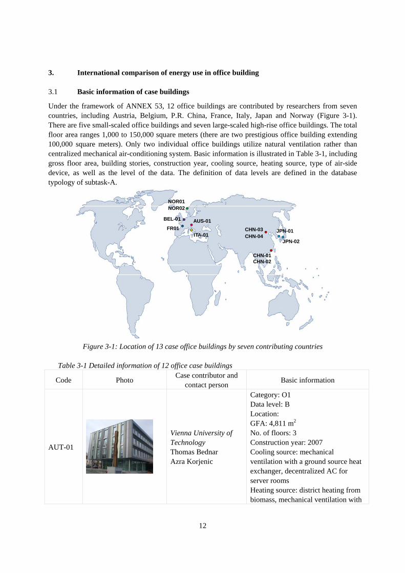
Under the framework of ANNEX 53, 12 office buildings are contributed by researchers from seven countries, including Austria, Belgium, P.R. China, France, Italy, Japan and Norway (Figure 3-1). There are five small-scaled office buildings and seven large-scaled high-rise office buildings. The total floor area ranges 1,000 to 150,000 square meters (there are two prestigious office building extending 100,000 square meters). Only two individual office buildings utilize natural ventilation rather than centralized mechanical air-conditioning system. Basic information is illustrated in Table 3-1, including gross floor area, building stories, construction year, cooling source, heating source, type of air-side device, as well as the level of the data. The definition of data levels are defined in the database typology of subtask-A.

JPN-02

JPN-01

CHN-01CHN-02

CHN-03CHN-04

NOR01NOR02

ITA-01

AUS-01BEL-01

FR01

Figure 3-1: Location of 13 case office buildings by seven contributing countries

Table 3-1 Detailed information of 12 office case buildings

Code Photo Case contributor and

contact person Basic information

AUT-01

Vienna University of Technology Thomas Bednar Azra Korjenic

Category: O1 Data level: B Location: GFA: 4,811 m2 No. of floors: 3 Construction year: 2007 Cooling source: mechanical ventilation with a ground source heat exchanger, decentralized AC for server rooms Heating source: district heating from biomass, mechanical ventilation with

13

a ground source heat exchanger

BEL-01

University of Liège Stephane Bertragnolio

Category: O2 Data level: A Location: GFA: 18,700 m2 No. of floors: 9 Construction year: 1970’s AC: AHU, CAV, VAV Cooling source: water-cooled chiller Heating source: natural gas boiler

CHN-01

Swire Properties, Hong Kong Tsinghua University Cary CHAN Qingpeng WEI

Category: O2 Data level: C Location: Hong Kong, P.R.China GFA: 30,968 m2 No. of floors: 23 Construction year: 1998 AC: AHU, CAV, VAV, FCU, PAU Cooling source: water-cooled chiller Heating source: no heating demand

CHN-02

Swire Properties, Hong Kong Tsinghua University Cary CHAN Qingpeng WEI

Category: O2 Data level: C Location: Hong Kong, P.R.China GFA: 141,968 m2 No. of floors: 68 Construction year: 2008 AC: AHU, CAV, VAV, FCU, PAU Cooling source: water-cooled chiller Heating source: no heating demand

CHN-03

Tsinghua University Qingpeng WEI

Category: O2 Data level: C Location: Beijing, China GFA: 111,984 m2 No. of floors: 26 Construction year: 2004 AC: FCU, PAU Cooling source: water-cooled chiller Heating source: district heating

CHN-04

Tsinghua University Qingpeng WEI

Category: O2 Data level: C Location: Beijing, China GFA: 54,500 m2 No. of floors: 21 Construction year: 1980’s AC: VAV, PAU Cooling source: water-cooled chiller

14

Heating source: district heating

FRA-01

INSA de Lyon-CETHIL Cécile ERMEL

Category: O1 Data level: A Location: Lyon, France GFA: 1,290 m2 No. of floors: 2 Construction year: 1970 Renovation year: 1993 Cooling source: natural ventilation Heating source: no heating demand

ITA-01

Politecnico di Torino Francesco Causone

Category: O1 Data level: A Location: GFA: 1,096 m2 No. of floors: 5 Cooling source: natural ventilation Heating source: natural gas boiler

JPN-01

Chubu Electric Power Co., Inc. Shigehiro Ichinose

Category: O1 Data level: B Location: GFA: 2,734 m2 No. of floors: 4

JPN-02

Chubu Electric Power Co., Inc. Shigehiro Ichinose

Category: O1 Data level: B Location: GFA: 3,695 m2 No. of floors: 4

JPN-03

Building Research Center China Vanke Co., Ltd Ting SHI

Category: O1 Data level: B Location: Sendai, Japan GFA: 4,090 m2 No. of floors: 3

NOR-01

Norwegian University of Science and Technology Natasa Djuric

Category: O2 Data level: A Location: GFA: 27,623 m2 Construction year: 2008 AC: AHU, VAV, FCU Cooling source: water-cooled chiller Heating source: district heating

15

NOR-02

Norwegian University of Science and Technology Natasa Djuric

Category: O2 Data level: C Location: GFA: 16,200 m2 No. of floors: 6 Construction year: 2009 AC: AHU, VAV, FCU Cooling source: heat pump Heating source: district heating

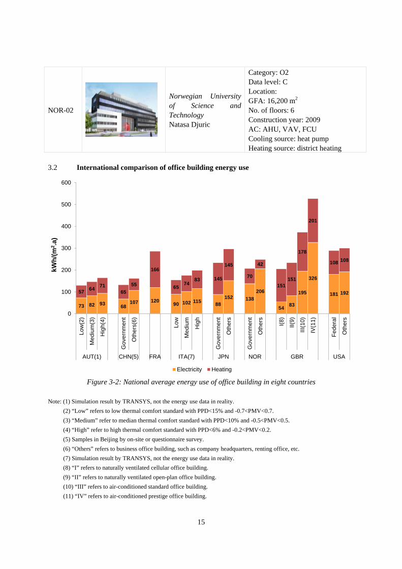
3.2 International comparison of office building energy use

73 82 93 68 107 120

90 102 115 88 152 138

206

54 83

195

326

181 192 57 64 71

65

55

166

65 74

83 145

145

70

42

151 151

178

201

108 108

0

100

200

300

400

500

600

Low

(2)

Med

ium

(3)

Hig

h(4)

Gov

ernm

ent

Oth

ers(

6)

Low

Med

ium

Hig

h

Gov

ernm

ent

Oth

ers

Gov

ernm

ent

Oth

ers

I(8)

II(9)

III(1

0)

IV(1

1)

Fed

eral

Oth

ers

AUT(1) CHN(5) FRA ITA(7) JPN NOR GBR USA

kWh

/(m

2 .a)

Electricity Heating

Figure 3-2: National average energy use of office building in eight countries

Note: (1) Simulation result by TRANSYS, not the energy use data in reality.

(2) “Low” refers to low thermal comfort standard with PPD<15% and -0.7<PMV<0.7.

(3) “Medium” refer to median thermal comfort standard with PPD<10% and -0.5<PMV<0.5.

(4) “High” refer to high thermal comfort standard with PPD<6% and -0.2<PMV<0.2.

(5) Samples in Beijing by on-site or questionnaire survey.

(6) “Others” refers to business office building, such as company headquarters, renting office, etc.

(7) Simulation result by TRANSYS, not the energy use data in reality.

(8) “I” refers to naturally ventilated cellular office building.

(9) “II” refers to naturally ventilated open-plan office building.

(10) “III” refers to air-conditioned standard office building.

(11) “IV” refers to air-conditioned prestige office building.

16

National average total energy use of office building in Austria, China, France, Italy, Japan, Norway, UK and U.S is shown in Figure 3-2. What needs to be emphasized is that, the energy data of Austria and Italy is by simulation, and others are by medium-large range survey or monitoring. Simulation results compared the electricity and heating consumption under three thermal comfort standards of office building in Austria and Italy (Santamouris, 2009). According to the results of a regional survey in 52 government office buildings in Beijing China, the annual electricity consumption averages 68 kWh/(m2.a) for electrical end-user (He, 2011) and 65 kWh/(m2.a) for district heating. The results of 84 business office building in Beijing shows that, the annual electricity consumption averages 107 kWh/(m2.a) for electrical end-user (He, 2011) and 55 kWh/(m2.a) for district heating. By crosscheck of two national energy survey (BEMA, 2007; DECC, 2010) of Japan office buildings, the annual electricity use of government is 88 kWh/(m2.a) and heating energy use is 145 kWh/(m2.a). Meanwhile, the annual electricity use of other kind of office building is 152 kWh/(m2.a) and heating energy use is 145 kWh/(m2.a). The national average energy use of federal office building in U.S (IEA, 2010) is 181 kWh/(m2.a) by electricity and 108 kWh/(m2.a) by heating. As a comparison, the electricity use of other kind of office building is 192 kWh/(m2.a), higher than federal offices. BRE has announced investigation result of energy consumption of office building in U.K (BRE, 2000). The electricity consumption ranges 54~83 kWh/(m2.a) for small scaled office building, and 195~326 for medium or large-scaled office building. The heating consumption is 151~201 kWh/(m2.a), similar with the one of France and Japan. Data collected in the framework of Norway statistics (Statistics Norway, 2008) presents that the electricity consumption average of government office building in Norway is 138 kWh/(m2.a) and 206 kWh/(m2.a) of other office building. While, the heating consumption of government office building is 70 kWh/(m2.a), higher than 42 kWh/(m2.a) of others office types. 3.3 Weather condition of case buildings

Heating degree day (HDD) and cooling degree day (CDD) are parameters designed to reflect the demand for energy needed to heat and cool a building. HDD and CDD are defined relative to a base temperature-the outside temperature above or below which a building needs no heating or cooling. The base temperature of this research is 65 Deg. F (17.6 Deg. C). The following table compares the annual HDD65F and CDD65F of case buildings. The outdoor temperature and relative humidity of eight cities are shown in Figure 3-3. The weather condition of Lyon (France), Melk (Austria), Trondheim (Norway) and Liege (Belgium) is similar with high humidity and moderate temperature. Weather in Hong Kong is high humidity and hot year round. Beijing is dryer than other cities, and temperature difference is more obvious than other cities during a year.

Table 3-2 HDD65F and CDD65F of case buildings Country Case building code HDD65F CDD65F

Hong Kong, China CHN-01, CHN-02 193 3734

17

Beijing, China CHN-03, CHN-04 5156 1421 Lyon, France FRA-01 4141 264 Melk, Austria AUS-01 6112 341 Brussel, Belgium BEL-01, BEL-02 11044 0 Shimada, Japan JP-01 2616 1548 Suzuka, Japan JP-02 3558 1307

40

60

80

100

-10 0 10 20 30 40

Re

lati

ve

Hu

mid

ity

(%

)

Outdoor temperature (Deg.C)

Hong Kong,China

Beijing, China

Lyon, France

Trondheim, Norway

Liège,Belgium

Melk, Austria

Shimada city, Japan

Suzuka city, Japan

Sendai,Japan

Figure 3-3: Outdoor temperature (Deg.C) and relative humidity (%) of cases (Monthly average)

3.4 Energy use comparison of case buildings

A matrix of office building information defined by Subtask-A is shown in Table 3-3. For clarifying a same definition of energy data collected by different countries, a unified energy flow chart tool has been circulated to participants (Figure 3-4). The electricity and heating consumption per square meter (here used as GFA) is compared in Table 3-3. The electricity consumption by end-users is shown in Figure 3-6. The “ventilation” illustrates the electricity consumption of equipment including fans exhausting fans in garage, toilets, etc., but excluding air conditioning fans, primary air unit (or outdoor fresh air unit) fans.

18

Figure 3-4: Example of energy flow charts-unified example

Figure 3-5: More detailed energy flow chart developed by contributor (refering to Appendix E.1.1)

Table 3-3 Total energy use of eleven case study office buildings

AUT-01 BEL-01 CHN-01 CHN-02 CHN-03 CHN-04

Typology O1 O2 O2 O2 O2 O2

19

Total site energy use (MWh.a) 411.0 2171.1 5531.3 22520.0 15171.7 8872.6

Heating use (MWhh.a) 213.8 1074.9 0 0 6873.7 2452.5

Electricity use(MWhe.a) 197.2 1096.8 5531.3 22520.0 8298.0 6420.1

FRA-01 JPN-01 JPN-02 JPN-03 NOR-02

Typology O1 O1 O1 O1 O2

Total site energy use (MWh.a) 359.3 - - - 1353.5

Heating use indicator (MWhh.a) 220.7 N.A N.A N.A 609.7

Electricity use indicator (MWhe.a) 138.6 451.3 392.5 366.9 743.8

The total electricity consumption is relative to the gross floor area of buildings. Figure 3-6 compares total electricity use of building less than 30000 square meters and more than 30000 square meters separately. The total electricity consumption of office buildings less than 5000 square meters (AUT-01, FRA-01, JPN-01, JPN-02) is less than 500 MWhe per year; the total electricity consumption of office buildings around 17000 square meters (BEL-01, NOR-02) is 700~1200 MWhe per year; the total electricity consumption of office buildings more than 30000 square meters is more than 5000 MWhe per year. It can be found that the electricity use of ventilation and cooling system of a large-scaled office building is obviously larger than individual offices, by comparing the electricity use per square meter.

0 200 400 600 800 1000 1200

AUT-01

BEL-01

FRA-01

JPN-01

JPN-02

NOR-02

MWhe.a

Lighting

Office appliances

IT room

Ventilation

Pumps

Chiller or indoor unit

Cooling tower or outdoor unit

Catering

Miscellaneous

(a) Total electricity of case buildings (less than 1200 MWhe per year)

20

0 5000 10000 15000 20000

CHN-01

CHN-02

CHN-03

CHN-04

MWhe.a

Lighting

Office appliances

IT room

Ventilation

Pumps

Chiller or indoor unit

Cooling tower or outdoor unit

Catering

Miscellaneous

(b) Total electricity of case buildings (more than 1200 MWhe per year)

Figure 3-6: Electricity consumption of case study office buildings (Unit: MWhe.a).

21

4. Lighting system

Artificial lighting contributes a large part to the primary energy use of an office building. The total consumption of artificial lighting worldwide is 1,133 TWh in 2006 (IEA, 2006), and approximately 19% is distributed in office buildings. Comprehensive literature review: “ANNEX 45- Guidebook on energy efficient electric lighting for buildings” identifies and accelerates the widespread use of appropriate energy efficient high-quality lighting technologies and their integration with other building systems, making them the preferred choice of lighting designers, owners and users. The research has reviewed the human performance and productivity chain, which is a significant fundamental of this Session. Lighting should be designed to provide people with the right visual conditions that help them to perform visual tasks efficiently, safely and comfortably. The luminous environment acts through a chain of mechanisms on human physiological and psychological factors, which further influence human performance and productivity (Gligor, 2004).

LUNIMOUS ENVIRONMENT

Illuminance&

IlluminanceUniformity

Illuminance&

IlluminanceDistribution

Flicker

Glare

DisabilityGlare

DiscomfortGlare

VeilingReflections

DayLight

SpectrumAmount

oflight

LightingControl

ArtificialLightingControl

DayLightingControl

Pa

ram

ete

rs o

f Lu

min

ou

s E

nv

iro

nm

en

t

Visibility

Acceptability&

Satisfaction

Visual &Task

Performance

Social Interaction &

Communication

PsychologicalEffect

VisualComfort

Preferences

EyestrainHu

ma

n F

acto

rs

HUMAN PERFORMANCE & PRODUCTIVITY

ArtificialLighting

UsePattern

Boundary

Individual&

GroupDecision

Tw

o k

ey

pro

ble

ms A

NN

EX

53

focu

sed

on

Figure 4-1: The relationship between ANNEX 45 and this session in ANNEX 53

There are massive researches focused on occupant’s lighting control behavior, and tried to formulate the user behavioral models. Field data further suggests that individual control is partly governed by a number of basic behavioral switching patterns i.e., quantitative correlations that relate user manipulations to external stimuli, like temperature and illuminance levels or arrival/departure at the work plane. The key findings from the previous research are summarized in Table 4-1.

22

Table 4-1 Key findings of occupant behavior of lighting control in office building

Code Occupant behavior of artificial lighting Reference Type of office

People usually pertain to either of the following two

behavioral classes:

People who switch the lights for the duration of the working

day and keep it on even in times of temporarily absence;

Open space

office

L1

People who use electric lighting only when indoor

illuminance levels due to daylight are low.

Love, 1998

Private office

L2 All lights in a room are switched on or off simultaneously Hunt, 1979 Private office

L3 Switching mainly takes place when entering or vacating a

space.

Hunt, 1979

Love, 1998

Pigg, 1998

Private office

L4

The switch-on probability on arrival for artificial lighting

exhibits a strong correlation with minimum daylight

illuminances in the working area.

Hunt, 1979

Love, 1998

Private office

L5 The length of absence from an office strongly relates with the

manual switch-off probability of the artificial lighting system Pigg, 1998

Private office

Those existing researches can be summarized by two kinds of models: the static threshold model and the dynamic and stochastic model. The former one focus on the formula between lighting environment (i.e. illuminance level on the work plane or duration period) and switching-on probability, while the latter one using the instantaneously occupancy status as the model input instead. The relationship between these two models is shown in the following figure.

static threshold models dynamic and stochastic models

Researchers focus on building functions between

user manipulations and external stimuli

Newsham, 1994 Hunt, 1980

Pigg, 1998

minimum daylight

illuminances in the

working area

minimum illuminance

level on the work plane

the length of absence

from an office

Newsham, 1995

“Lightswitch”,

user occupancy

profiles, predicts

electric lighting use

based on probabilistic

behavioral patterns

Reinhart, 2004

“Lightswitch-2002”,

the intermediate

switch-on probability

function that depends

on the work plane

illuminance

Dynamic: 5 min time steps throughout the year

Stochastic: stochastic process is initiated that

determines the outcome of on/off decision

Figure 4-2: Logistical schematic map of existing researches about occupants’ lighting behavior

The first study on manual switching patterns of artificial lighting system in offices is carried out by Hunt in the late 1970s (Hunt, 1979, 1980). The result indicated that switching mainly takes place when entering or vacating a space, and that the switch-on probability on arrival for artificial lighting exhibits a strong correlation with minimum daylight illuminances in the working area. Based on a switch-on probability function for electric lighting and annual frequency distributions of indoor illuminances, and an assumption that lighting is switched on at the start of a period of occupation, left on throughout

23

the day and switched off at the end, Hunt used a prediction method and deduced mean hours of daily usage for the electric lighting at a given workplace. Newsham (1994) revised Hunt’s model to simulate manual lighting control. He considers the switch-on probability on arrival to be a function of minimum illuminance level on the work plane instead of minimum daylight illuminances in the working area as in Hunt’s model. According to Newsham’s model, the electric lighting is switched on in the morning and after lunch if the minimum illuminance level on the work plane lay below 150 lux. As the assumption in Hunt’s model, the lighting was switched off at the end of the working day and switch-on events during a period of occupation were not taken into account. Following Hunt and Newsham, there are numerous researchers bending themselves to occupant behavior of artificial lighting system in offices, among them are Love and Pigg who pay attention on occupants’ temporarily departure. Love (1998) classifies manual switching patterns into two main behavioral classes: one is switching the lights for the duration of the working day and keeping it on even in times of temporarily absence; while the other is using electric lighting only when indoor illuminance levels due to daylight are low. Pigg (1998) studies the occupant behavior during their temporarily departure, finding that the length of absence from an office strongly relates with the manual switch-off probability of the artificial lighting system. Throughout these studies, the type of office is found to be a notable point which may influence our perception. Most of the research is carried out in private offices, which means that the patterns and conclusions reached might be only suitable for this particular type of office. In private offices, occupants are more likely to be close to external windows, resulting in daylight playing a more influential role on occupant behavior. In open plan offices, the situation becomes quite different since most occupants have slight exposure to daylight; thus, it might no longer be a decisive factor. The above-mentioned manual switching pattern models of artificial lighting systems all use static thresholds. However, when the “use of controls is clearly influenced by physical conditions, it tends to be governed by a stochastic rather than a precise relationship” (Nicol, 2001). Newsham, Mahdavi and Beausoleil-Morrison (1995) develops a model called Lightswitch which adopted a stochastic approach to simulate manual lighting control based on measured field data in an office building in Ottawa, Canada. The model predicts electric lighting use based on probabilistic behavioral patterns which have all been observed in actual office buildings. The resulting user occupancy profiles are then used to estimate the energy benefit of occupancy sensor controlled system, in which the lighting is switched on upon occupant arrival and switched off whenever the user left the workplace for a time longer than the delay time of the occupancy sensor. Based on Newsham’s original model, Christoph F. Reinhart proposes a dynamic and stochastic algorithm named Lightswitch-2002. Dynamic indicates that instead of looking at an average day in a year or month, user occupancy, indoor illuminances and the resulting status of the electric lighting and blinds are considered in 5 min time steps throughout the year. Stochastic means that whenever a user is confronted with a control decision, i.e. to switch on the lighting or not, a stochastic process is initiated that determines the outcome of the decision (Reinhart, 2004).

24

The algorithm modeled the intermediate light switch-on probability, i.e. the probability that a user switches on the artificial lighting without leaving or arriving in the office. It uses a probability function that depends on the work plane illuminance, derived from previous work by the author of the algorithm (Reinhart, 2003). For 5-minute time steps, it finds that the intermediate switch-on probability is about 2% between 0 and 200 lux work plane illuminance, and sharply drops to about 0.002 for higher illuminances. The algorithm cannot be readily transferred to open plan office concepts in which individuals have on perception of personal control over their immediate environment. As Figure 4-1 shows, the study about occupants’ lighting behavior of ANNEX-53 Subtask-B is only focus on the right part of the boundary and excluding the “Human Factor” as the driven force. Owing to the energy consumption is only happened when the artificial lighting switched on, the “day-light” and “lighting control” studied in the ANNEX-45 can be concluded as one parameter “Artificial lighting use pattern” as the key research target of the ANNEX-53. Meanwhile, occupant behavior of two parameters studied in ANNEX-45: “Day-light utilizing” and “Lighting control” have their impact on lighting energy consumption through “Individual and group decision”, which is also studied in this ANNEX. 4.1 Occupancy/Lighting use patterns

4.1.1 Literature review

Geun Young Yun, et al. (2011, 2012) investigates the lighting use pattern of the open plan offices, as shown in Figure 4-3. Two investigations both show that the artificial lighting is first on since the occupant’s first arrival in the morning. There is a close link between the start of daily occupancy and switching-on lighting. First light switch-on events in the investigated offices occurs within 11 minutes after the start of daily occupancy, and occupants will partially turn off lights during lunch time. There is no relationship between external illuminance and the use of artificial lighting. The research also implies that automatic lighting controls to turn off the artificial lighting when there is sufficient daylight indoors would have significant energy saving potentials. These results in open plan offices are very different from the results summarized in the private or 2-person offices studied by Reinhart (Reinhart, 2004).

25

Figure 4-3: The proportion of frequency that the lighting was on for each hour of typical working day: (a) east-facing zone of the second floor (b) west-facing zone of the second floor (c) east-facing zone of

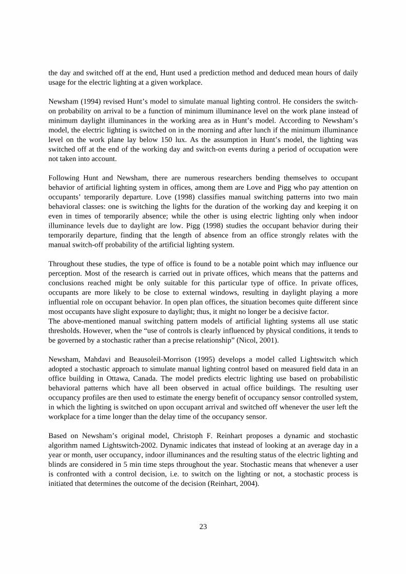
the sixth floor (d) west-facing zone of the sixth floor A.M. Egan (2009) simulates the typical daily patterns of lighting and small power electricity of office buildings, based on the field survey information and real energy use data. The measured data shows that the electricity of lighting and small power comes to the peak from 9:00 A.M to 16:00 P.M. Meanwhile, between 8:00 P.M to 6:00 A.M when the building is unoccupied, the average load is approximately 30% of the measured average. It indicates that there is lighting or office equipment still be used during the night (Figure 4-4).

26

(a) Case building 1 (b) Case building 2

Figure 4-4: Daily pattern of tenant light and power usage A case study of the Phillip Burton Federal Building (DOE, 2000) compares the lighting energy consumption under three automatically controlling method, as shown in Figure 4-5. In private offices, the use of occupancy sensors alone reduced lighting energy by 25% on weekdays. Automatic daylight dimming saved an average of 27% of lighting energy, and the combination of both the sensors and dimming saved approximately 45%. In open daylit offices, savings from daylighting alone were also substantial, particularly in the first and second cubicle rows from windows (especially south-facing ones). In open areas close to windows, automatic day light saved about 10% over wall switched alone. In open areas close to windows, automatic day light saved more than a quarter of previous lighting energy, and more than a third when combined with either occupancy sensing or time scheduling.

Figure 4-5: Comparison of lighting use pattern in a federal office building in U.S, under different

automatically control method The Lawrence Berkeley National Laboratory has also studied the occupancy and lighting profiles of the office building whose lighting system is controlled by occupancy sensor. In terms of average occupancy behavior across all rooms, Figure 4-6 give the average probability of occupancy for all private offices on the 3rd and 5th floors at hourly intervals during the day. The graphs show similar results, with peak occupancy periods between the hours of 8am and 5pm, and a reduced occupancy during the lunch hour (12-1pm). Because this office building is controlled by occupancy sensor based on the occupancy pattern, the trend for artificial lighting is similar as the Figure 4-5. The conclusion is that, the prime opportunity of save lighting energy is the middle of the day and during off-peak hours.

27

(a) 3rd floor (b) 5th floor

Figure 4-6: Probability of occupancy by hour for all regular weekdays averaged across all 21 offices 4.1.2 Field survey by contributors

Norway, China and Belgium have done the measurement or investigation of the occupancy/lighting curve of office buildings. The following sections illustrates typical cases in Norway and China. (1) Norway Basic Information The case building of Norway is located in Trondheim at the address Professor Brochs gate 2. The gross floor area is 16,200 m2, with 6 floors. The GFA of typical floor is 1500 to 2500 m2. Occupancy Curve The occupancy curve of Norway’s case building is shown in Figure 4-7. The office building is rented to different companies, usually companies have working time between 8 a.m. until 4 p.m. But some companies could extend working time until 5 or 6 p.m. Figure 4-7 is established based on the presence sensor for ventilation. This presence sensor is located in the part of the building that was all the time in use.

Figure 4-7: Presence schedule during working days

Lighting Use Pattern

28

0

1

2

3

4

5

11-1 0:00 11-2 0:00 11-3 0:00 11-4 0:00 11-5 0:00 11-6 0:00 11-7 0:00 11-8 0:00

W/m

2

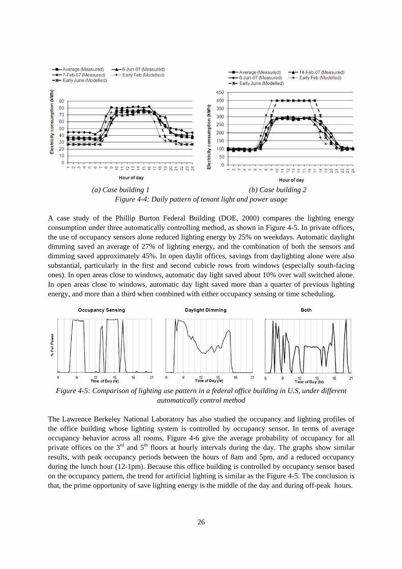
Figure 4-8: Hourly lighting profile of lighting during typical weekday and weekend (Unit: W/m2)

There are two control strategies for the lighting system of the case building. The one is using presence sensors to control artificial lighting during working time. The other is turn off lights during non-working time. The total electricity use profile of the building is presented in Figure 4-8. Meanwhile, by calculating the average and standard deviation of weekday and weekend separately, the representative profile of weekday and weekend is shown as following charts. Two features are shown of the case building in Norway:

1) The peak lighting hours is between 9am and 16pm (average lighting use percentage≥90%) during the weekday. The lights were not turned off during the lunch break.

2) There is a constant lighting load during off hours (6pm to 6am), based on the presence schedule shown in Figure 4-9. 20% of the lights will stay switched on during the off hours.

0%

20%

40%

60%

80%

100%

120%

1 3 5 7 9 11 13 15 17 19 21 23

Lig

hti

ng

use

per

cen

tag

e

+STDAverage-STD

0%

20%

40%

60%

80%

100%

120%

1 3 5 7 9 11 13 15 17 19 21 23

Lig

hti

ng

use

per

cen

tag

e

+STDAverage-STD

(a) Weekday profile (b) Weekend profile

Figure 4-9: Average lighting profile of weekday and weekend of case building in Norway

29

(2) China Basic Information Three typical large-scaled office buildings are chosen in China. The basic information illustrated as follows: (1) Case Building 1 (CB-2). CHN-02 (CB-1) is located in TaiKoo Place in Hong Kong, China. The

gross floor area is 141,000 m2, with 68 floors. The usable floor area of typical floor is 1950 m2 approximately.

(2) Case Building 2 (CB-2). CHN-03 (CB-2) is located in Beijing, China. The gross floor area is 54,500 m2, with 21 floors.

(3) Case Building 3 (CB-3). CHN-04 (CB-3) is located in Beijing, China. The gross floor area is 111,984 m2, with 26 floors. The usable floor area of typical floor is 1781 m2

Occupancy Curve Owing to the investigation limitation, typical offices are chosen to do the questionnaire survey, in order to find the representative feature of the whole building. CB-1 and CB-3 are large open space, with central service area and office area around it. CB-2A and CB-2B are small open space offices, located in the north and west of the building. The basic information of surveyed offices is shown in the following figure and table.

BJ-2B

BJ-2A

(a) CB-1A/CB-1B (b) CB-2A/CB-2B (c) CB-3A/CB-3B Figure 4-10: Sketch map of offices chosen in the case building

Table 4-2 Summary of key data information of investigated offices

CB-11

CB-1A CB-1B CB-2A CB-2B CB-3A CB-3B

City located Hong Kong Hong Kong Peking Peking Peking Peking Net floor area (sq.m.) 1915 1915 243 950 950 250 Number of workers 120 90 36 158 194 27 Work description Management Market R&D Mgmt. R&D Type L2 S S L L Percentage of valid questionnaire

76% 75% 85% 60% 68%

30

*Note: (1) Because CB-1A and 1B belongs to the same company and questionnaires reclaimed anonymous, CB-

1A and 1B are combined together as a whole office in the following analysis. (2)L, Large open space; S, Small

open space. The schedule of five offices appears “double-square wave” characteristic, which is a typical schedule of office building. The official working time of five offices is 9:00 A.M. to 18:00 P.M. While the average working time of two management offices, CB-1 and CB-3, is 8.6 hours/weekday and 6.8 hours/weekend. While the other three Research & Development (R&D) offices, works 9~10 hours/weekday.

0%

20%

40%

60%

80%

100%

120%

0:00 6:00 12:00 18:00 0:00

Occ

up

ancy

HK-1 BJ-1A BJ-1B BJ-2A BJ-2BCB-1 CB-3A CB-3B CB-2A CB-2B


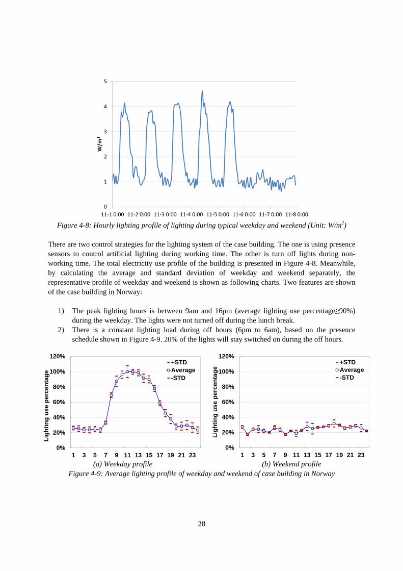
Lighting Use Pattern Lighting use pattern is investigated by both questionnaire survey and on-site measurement. The questionnaire asks when occupants usually switch on/off the lighting on the top of their work plane. Three basic modes of lighting schedule are revealed based on the results. The first mode is named “ordinary mode”, represented by CB-2B, CB-3A and CB-3B, which the lighting switch on when occupants arrival and off at night. The second mode is “energy-saving mode”, office CB-1, the lighting switch off during lunch break. The third one is “preferred natural lighting mode”, like office CB-3A, which the lighting only switched on when illuminance of workplace cannot be satisfied by natural lighting.

31

0%

20%

40%

60%

80%

100%

120%

0:00 6:00 12:00 18:00 0:00

Lig

hts

op

en p

erce

nta

ge

HK-1 BJ-1A BJ-1B BJ-2A BJ-2BCB-1 CB-3A CB-3B CB-2A CB-2B

Figure 4-12: Lighting schedule based on questionnaire statistical data

Based on the on-line benchmarking system of CB-2 and CB-3. The lighting use profile is analysed and presented in the following chart.

0

2

4

6

8

10

12

14

3-9 0:00 3-11 0:00 3-13 0:00 3-15 0:00

W/m

2

0

2

4

6

8

10

12

14

3-2 0:00 3-4 0:00 3-6 0:00 3-8 0:00

W/m

2

(a) CB-1 (b) CB-2

Figure 4-13: Hourly lighting profile of lighting during typical weekday and weekend (Unit: W/m2) The lighting in CB-2 and CB-3 are controlled manually. The lighting profile of CB-2 and CB-3 are similar to Norway’s case building, but there are two differences. The one is lighting electricity use intensity is obvious larger than Norway’s case building. The other is part of lighting of CB-2 will turn off during lunch break, compared to case building in Norway.

32

0%

20%

40%

60%

80%

100%

120%

140%

160%

1 3 5 7 9 11 13 15 17 19 21 23

Lig

hti

ng

use

per

cen

tag

e

+STDAverage-STD

0%

20%

40%

60%

80%

100%

120%

140%

160%

1 3 5 7 9 11 13 15 17 19 21 23

Lig

hti

ng

use

per

cen

tag

e

+STDAverage-STD

(a) Weekday profile (b) Weekend profile

Figure 4-14: Average lighting profile of weekday and weekend of case building-1 in China By calculating the average and standard deviation of weekday and weekend separately, the representative profile of weekday and weekend is shown as previous charts. Two features are shown of the case building in CB-2 in China:

1) The peak lighting hours is between 10am and 18pm (average lighting use percentage≥90%) during the weekday. The lights turn off during lunch break.

2) There is a constant lighting load during off hours (7pm to 7am), based on the presence schedule shown in Figure-16(a). There is 20% lights will stay switching on during the night.

0%

20%

40%

60%

80%

100%

120%

1 3 5 7 9 11 13 15 17 19 21 23

Lig

hti

ng

use

per

cen

tag

e

+STDAverage-STD

0%

20%

40%

60%

80%

100%

120%

140%

160%

1 3 5 7 9 11 13 15 17 19 21 23

Lig

hti

ng

use

per

cen

tag

e

+STDAverage-STD

(a) Weekday profile (b)Weekend profile

Figure 4-15: Average lighting profile of weekday (a) and weekend (b) of case building-2 in China The representative profile of weekday and weekend of case building-2 in China is shown in Figure-17. Certain features can be compared with other case buildings:

1) The peak lighting hours is between 10am and 18pm (average lighting use percentage≥90%) during weekdays. The lights are turned off during lunch breaks and turn on gradually in the afternoon.

2) There is a constant lighting load during off hours (7pm to 7pm). 20% lights will stay switching on during the night.

3) 40% of the lights will switch on from 10am to 21pm during weekends, and 20% of the lights will stay switching on during the night.

33

4.2 Occupant behavior impact factor

4.2.1 Daylight utilization and automatically control ligh ting

Literature review: Daylight utilization in office building is widely recognized as an important energy-conservation design strategy. The amount of daylight entering a building is mainly determined by the window openings that provide the dual function of admitting light to the indoor environment for a more attractive and pleasing atmosphere, and allowing people to maintain visual contact with the outside world (Li and Tsang, 2008). The level of day light highly depends on comprehensive building design and glazing facade (Wilson et al., 2002). The daylight performance of a building is always assessed in terms of the Daylight Factor (DF) (Hopkinson et al., 1966). In relation to DF, the decision criteria are often expressed in terms of DFave as a way to judge a daylight space. According to the British Council for Offices (BCO, 2005) guide, a DFave from 2 to 5% is recommended for an office workplace. A recent survey is conducted within 270 occupants in 16 office buildings in UK. The result shows that the proper range of DFave is 2 to 5%. People are more likely to be dissatisfied with the daylight when the design DFave is over 5%. At these high daylight levels, the complaints of sun and sky glare increased (Roche et al., 2000). Lighting controls in connection to day lighting can save lighting energy demands by 20-40% (G.Y.Yun et al., 2011). Automatic controls switch or dim lighting based on time, occupancy, lighting-level strategies, or a combination of all threes. In situation where lighting may be on longer than needed, left on in unoccupied areas, or used when sufficient daylight exists, the installation of automatic controls as a supplement or replacement for manual controls should be considered. The general control strategies used by lighting designers include:

1) Occupancy sensing, in which lights are turned on and off or dimmed according to occupancy; 2) Scheduling, in which lights are turned on and off according to a schedule; 3) Tuning, in which light output is reduced to meet current user needs; 4) Daylight harvesting, in which electric lights are dimmed or turned off in response to the

presence of daylight; 5) Demand response, in which power to electric lights is reduced in response to utility

curtailment signals or to reduce peak power charges at a facility; and 6) Adaptive compensation, in which light levels are lowered at night to take advantage of the fact

that people need and prefer less light at night than they do during the day. 4.2.2 Mechanism of occupant behavior and its impact on energy

Based on the investigated artificial lighting schedule (as shown in Figure 4-16(a) and (b)), more than 60% lighting has been turned on during working hours. A questionnaire survey about lighting control behavior has been conducted in CHN-01, CHN-02, CHN-03 and CHN-04. The result shows that occupants turn on their overhead lights frequently but seldom close them by themselves (Figure 4-16) in large open space offices.

34

0%10%20%30%40%50%60%70%80%90%

100%

HK-1 BJ-1A BJ-1B BJ-2A BJ-2B1-Never 2 3-Often 4 5-Frequently

0%10%20%30%40%50%60%70%80%90%

100%

HK-1 BJ-1A BJ-1B BJ-2A BJ-2B

1-Never 2 3-Often 4 5-Frequently

(a) Roof light open frequency (b) Roof light close frequency Figure 4-16: Control frequency of roof lighting by questionnaire survey

The following figure explains the mechanism of how occupant behavior impacting the final energy consumption of electrical lighting. Due to the existing building design, natural lighting usage of each workplace is fixed, combining an occupancy schedule, it exits a physical demand of a certain workplace. Thus, stage-I depends on building design (shape, color of external windows, direction, occupancy, etc.). While, someone will still turn on lights based on their psycho demand even if the illuminance on their workplace is enough, this is defined as the second stage. Then, lighting system is usually controlled by zones, so the psychological demand has been blurred as stage III. Finally, if the control logic or manager has controlled extensively, it is the stage IV-actual supply and finally causing the electricity consumption. Hence, the difference between the stage I and stage IV is the impact of occupants’ behavior, which will be discussed quantitatively by simulation.

• Energy conservation

consciousness

• Service class

• Design density

• Occupancy

• Building design

(shape, direction…)

Natural LightingCannot use NL

IPhysical-demand

Lights open

IIPsycho-demand

Lights open

IIISpace demand

Lights open

• Group decision impact

• Zoning

ActualSupply

Lights open

• System zoning

• Manager behavior

Occupant scheduleOn work

Ideal Supply

Lights open

Occupant Open space office

Figure 4-17: Sketch map on occupant behavior impact on lighting energy

35

For understanding the impact of occupant behavior in each stage, CHN-02, CHN-03 and CHN-04 are chosen as the simulation target. Considering the building structure, CHN-02 is modeled as a cylinder, CHN-03 and CHN-04 are modeled as a cuboid as the following figure. The natural lighting of CHN-02 is homogeneous in each direction. The natural lighting of CHN-03 and CHN-04 only illuminates from the external window of one direction.

(a) Model of CHN-02 (b) Model of CHN-03 and CHN-04 Figure 4-18: Model of three case buildings

(4) Schedule and sitting position

A. Occupant Schedule

9:00 11:30 12:30 17:008:00 20:00

6:00 16:00

B. Lighting schedule based on dayighting

C. Physical-demand of lighting

△ta △tl

Figure 4-19: Schedule of occupants and artificial lighting

Occupant and artificial lighting schedule are designed as Figure 4-19. Figure A illustrates occupant arrives at office from 8:00 to 11:30 and go out for lunch, then comes back to work from 12:30 to 20:00. Figure B means the natural lighting cannot be used during 16:00 to 6:00 next day. Thus, setting on the two schedules, the artificial lighting should be used from 16:00 to 20:00. Considering the control pattern of occupants, the physical-demand of each occupant is obtained, as shown in Figure C△tarrive fits for Poisson distribution and △tleave fits for Continuous Uniform distribution. In probability theory and statistics, the Poisson distribution is a discrete probability distribution that expresses the

36

probability of a given number of events occurring in a fixed interval of time and/or space if these events occur with a known average rate and independently of the time since the last event. The Poisson distribution can also be used for the number of events in other specified intervals such as distance, area or volume. Meanwhile, the continuous uniform distribution or rectangular distribution is a family of probability distributions such that for each member of the family, all intervals of the same length on the distribution's support are equally probable. The floor plan of three office building is shown in the following figure. Office occupants are distributed based on the distance from the external window.

BJ-2B

BJ-2A

Occ

upan

t num

ber

Distance from external window, meter

CHN-02

Occ

upan

t num

ber


CHN-03

Occ

upan

t num

ber


CHN-04

Figure 4-20: Plan of typical floor and occupant distribution of simulation input

(5) Physical-demand

CHN-02

Figure 4-21: Time duration of artificial lighting in different deeper of occupants

37

Physi-demand Psycho-demand Space demand Supply

CHN-02 CHN-03 CHN-04

to C4 to C3 to C4 to C2 to C2 to C3

Figure 4-22: Physi-demand comparison if changed to other buildings’ scenarios Figure 4-21 simulates the artificial lighting period of different occupants distributed. It shows that, the closer to the external window, the shorter period of artificial lighting. If only changing the building model (Figure 4-19 and Figure 4-20) to other buildings, the comparison of physic-demand of each office building is compared as Figure 4-22. It can be concluded that, CHN-04 is the most effective of natural lighting utilization because of the less depth. Although both of CHN-02 and CHN-03 are designed with longer depth, the larger external window area making the CHN-02 is more effective than CHN-03 in natural lighting utilization. (6) Phycho-demand

Table 4-3 Three types of occupant behavior on artificial lighting usage and the percentage of each office building by survey Definition CHN-02 CHN-03 CHN-04

Type O-A Switch on lights only when natural lighting is not enough. 0.15 0.4 0.9

Type O-B Switch on during working time. 0.8 0.6 0.1

Type O-C Always switch on. 0.05 0 0

Three types of occupant behavior on artificial lighting usage are defined as Table 4-3. The percentage of each type in three office buildings is surveyed by questionnaire survey. 80% of occupants in CHN-02 and 60% of CHN-03 switch on during working time; 90% of occupants in CHN-04 switch on lights only when natural lighting is not enough. It means occupants in CHN-04 are more energy conservative than other two office buildings. If changing to other buildings’ switching on behavior, the simulation result is shown in Figure 4-23. Thus, the energy-saving consciousness has obvious effect on using times of artificial lighting.

38

0

2

4

6

8

10

12

Present to BJ-1 to HK-1

BJ-2

Supply

Space demand

Psycho-demand

Physi-demand


to C4 to C3 to C4 to C2 to C3 to C2

Figure 4-23: Phycho-demand comparison if changed to other buildings’ scenarios (7) Space demand According to Figure 4-24, building structure design, lighting zoning design and control zoning design are crucial factors impacting space demand. The simulation defines lighting zones as Zr and control zones as Cr (Cr≥Zr), as shown in Figure 4-25. It can be concluded that, the more of Zr and Cr, the better of the energy conservation of lighting system. The differences of parallel and vertical design methods are also compared. The correct division-vertical with natural light direction, is effective to reduce artificial lighting hours (Fig. 4-25).

Figure 4-24: Space demand comparison if changed Zr and Cr

(Note: [ ] is the present condition by survey.)

Parallel

Vertical 0

2

4

6

8

10

12

14

16

[4,3,P] 4,3,V 10,10,P 10,10,V

Lig

htin

g h

ours

(h)

BJ-2

Supply

Space demand

Psycho-demand

Physi-demand

CHN-04

Figure 4-25: Space demand comparison if changed division design

(Note: [ ] is the present condition by survey.)

39

(8) Supply

Table 4-4 Four types of manager behavior on artificial lighting control Definition Type M-A Neglecting space demand, switch on lights only when natural lighting is not enough. Type M-B Satisfying space demand only. Type M-C Satisfying occupant pycho-demand and space demand simultaneously. Type M-D Always switch on, don’t control.

Table 4-5 Three modes of manager behavior on artificial lighting control

Space demand Manager control behavior Module 1- Energy saving Zr=8, Cr=8 M-B Module 2- Regular Zr=8, Cr=3 M-C Module 3- Extensive Zr=8, Cr=3 M-D

0

2

4

6

8

10

12

14

16

[Extensive] Regular Energy-saving*

Lig

htin

g h

ou

rs (h

)

BJ-1

0

2

4

6

8

10

12

14

Energy-saving [Regular] Extensive

Lig

htin

g h

ou

rs (h

)

HK-1

Supply

Space demand

Psycho-demand

Physi-demand

CHN-02 CHN-03

Figure 4-26: Supply comparison if changed manager behavior mode

(Note: ① [ ]-present condition by survey. ② * After increasing the physical division at the same time.)

Four types of manager behavior modes are defined, as shown in Table 4-4. Further considering space demand (Zr and Cr), three modules are defined as Module 1-energy saving, Module 2-regular and Module 3-extensive. If changed modules of each office building, the lighting hours are simulated and compared as Figure 4-26. Hence, the lighting energy is very sensitive to manager control behavior and supply mode. (9) Summary

40

0

5

10

15

20

25

0 5 10 15 20

W/m

2

Hour

0

5

10

15

20

25

0 5 10 15

W/m

2

Hour

0

5

10

15

20

25

0 5 10 15 20

W/m

2

Hour

Building design Occupant behavior Physical/Control division Manager behavior


W/m

2

W/m

2

W/m

2

Hour Hour Hour

Figure 4-27: Quantitative decomposition of four stages of occupant behavior impact on artificial

lighting utilization Based on on-site survey and simulation, the lighting energy use of three office case buildings are compared as Figure 4-27. The lighting energy use indicator on a typical working day of CHN-02 is 240 Wh/(m2.day), larger than 180 Wh/(m2.day) of CHN-03 and 50 Wh/(m2.day) of CHN-04. However, the reason of high energy consumption of CHN-02 and CHN-03 is different. The reason of the former one is the high design capacity of lighting system (20 W/m2 lighting capacity), while the reason of the latter one is the high physical-demand and energy extensive manager behavior causing the longer lighting hours. The lighting system design capacity of CHN-04 is 10 W/(m2), not obvious smaller than CHN-03, but the smaller depth of building design decreasing lighting hours of artificial lighting effectively.

41

5. Office appliances

5.1 Literature review

Office appliances include PCs, desktop computers, CRT displays, LCD displays, copiers, laser printers, and so on. To meet the requirement of working activity, office appliances usually have to keep switching on during working hours. However, some studies illustrate the importance of night status for energy conservation. Figure 5-1 shows several scenarios, highlighting the dramatic effect of night status. “Disabled/Enabled” refers to power management functioning on both the PC and monitor. “On”, “Low” and “Off” refer to the night status of the PC and monitor. The result illustrates that, unreasonable usage of computer and monitor during off hours may cause huge energy waste.

Figure 5-1: Effect of night status on annual energy use of a PC/Monitor (Bruce, 2005)

In this study, the author also reviews four methods used in night status research, including on-site survey, daytime audits, night audits and time-series data analysis. Several related studies are shown in Table 5-1.

Table 5-1 Studies on night status of office appliances (Bruce, 2005) Study Reference Data Method PNNL Syzdlowski & Chvála 1994 1990-92 Time-series data NRC Tiller & Newsham 1993 1992 Time-series data (activity) LBNL1 LBNL 1994 Daytime audit LBNL2 IHEM, 1994 1994 Survey; Daytime audit LBNL3 LBNL 1994 Daytime audit MIT Norford & Bosko 1995 1995 Daytime audit LBNL4 Nordman, Piette & Kinney 1996 1995 Daytime audit; Night audit LBNL5 LBNL 1996 Night audit Defender JJulinot, Fogg & Julinot 2000 1996 Daytime audit; Night audit AEC Arney & Frey 1996 1996 Time-series data Thai Mungwititkul & Mohanty 1997 Prob. 1996 Not specified

42

Bayview Schanin 1997 1997 Night audit EIM Becht, Pleijster & de Vree, 1998 1997 Surveys Dalarna Bryntse & Enoksson, 1998 1997 Surveys DEFU Nielsen 1998 1997-98 Surveys LBNL6 Nordman, Picklum & Kresch 1999 1997-98 Daytime audit; Night audit LBNL7 Nordman 2000 1999 Daytime audit; Night audit About the impact of occupant behavior on office appliances’ energy consumption, some existing researches study the Power Management (PM), which is a built-in function that reducing the power use of office equipment when it is idling. After a set time of not being used (the “delay time”), the device enters a low-power “sleep” mode. The energy savings of PM hinges on the delay time set by each user as well as the saturation level of PM capability. The following figure shows the result that, the shorter “delay time”, the larger energy saving of office appliances (K. Kawamoto, et al., 2004). Some research even shows that, in the U.S, the energy saving potential of the complete saturation of PM is estimated as 37 TWh per year for 2000 (LBNL, 2001).

Figure 5-2: Energy use of PCs and displays by the level of power management

43

5.2 Night status survey of case buildings

In order to investigate the power states of computer and monitors at night, the office equipment enabling was checked in after hours. The power states of office equipment are characterized as “on”, and “off” in this study. The total number of computer and monitors in each office was recorded by night audit, as well as the exact number of equipment in each status is counted. The turn off rates of computer and monitors is calculated based on those survey results. According to similar investigation done by LBNL in several office buildings in U.S., the original data was used to calculate the same rate in U.S. office buildings as a comparison.

Table 5-2 Turn-off rates of computer and screen by on-site survey

Computer Screen Device Office Total On Off Total On Off CHN-02-A 93 86 7 93 68 25 CHN-02-B 120 116 4 120 88 32 CHN-03-A 62 54 8 80 52 28 CHN-03-B 93 72 21 92 61 31 CHN-04-B 28 12 16 32 10 22 U.S[14] 1464 524 940 1600 471 1129

0% 50% 100%

U.S

HK-1A

HK-1B

BJ-1A

BJ-1B

BJ-2A

BJ-2B

Computer 'OFF' Computer 'ON'

CHN-04-B

CHN-04-A

CHN-03-B

CHN-03-A

CHN-02-B

CHN-02-A

0% 50% 100%

U.S

HK-1A

HK-1B

BJ-1A

BJ-1B

BJ-2A

BJ-2B

Screen 'OFF' Screen 'ON'

CHN-04-A

CHN-03-B

CHN-03-A

CHN-02-B

CHN-02-A

CHN-04-B

(a) computer screen

Figure 5-3: Turn-off rate of computers and screens of case building during off-hour Table 5-2 and Figure 5-3 shows that the turn-off rate of computers in CHN-02 is higher than other offices. More than 77% computers are shut off at night. However, the turn off rate of CHN-04-B is close to offices in U.S., less than 36% computers are turned off at night. The turn off rates of monitors is lower than computers’, only 30% monitors are turned off during night in U.S. and CHN-04-B, and 65% to 75% monitors are turned off in CHN-03 and CHN-02. Due to all of occupants use lap top in CHN-02-A, almost 100% computers are shut off at night. F.G. Han once investigated and concludes that turn off rates of computers in campus building in China is usually higher than in U.S.

44

0%

20%

40%

60%

80%

100%

HK-1 BJ-1A BJ-1B BJ-2A BJ-2BRemote control Job requirement Follow the othersHabit Unknown

CHN-02 CHN-03-A CHN-03-B CHN-04-A CHN-04-B

Figure 5-4: The reason of why occupants don’t shut off computers

Figure 5-4 shows the reason why occupants leave their computers stand-by during afterhours based on questionnaire survey. More than 43% occupants in CHN-04-B, CHN-03 and CHN-02 keep their computers on owing to energy saving unconsciousness or careless. The rest of occupants answer that the job responsibilities requires computers to be always on. It reminds us that energy consumption is not the only discriminating principle, the essential requirement of service quality should also be equally considered. If we use the office equipment power capacity per worker to represent the fundamental service provided to each occupant, total number of each type of personal office equipment is investigated, as shown in Table 5-3.

Table 5-3 Power capacity of personal office equipment in surveyed offices

CHN-02 CHN-03-A CHN-03-B CHN-04-A CHN-04-B Occupant number 99 37 41 18 17 Computer 114 20 18 2 2 Lap top 10 19 24 16 24 20’ Monitor 9 4 5 0 4 14’ Monitor 89 17 14 2 24 CRT 0 1 0 0 0 Copier 10 1 2 0 0 Fax machine 1 1 0 0 0 Power capacity (W per worker)

127 84 74 46 137

There is obvious difference of office equipment power capacity in those five offices. Because most of occupants use lap top rather than computer, the power capacity of CHN-04-A is 46 W per worker, less than other offices. As a contrary, the computer and larger monitor percentage of CHN-02 is larger than others, which the power capacity of is 127 W per worker.

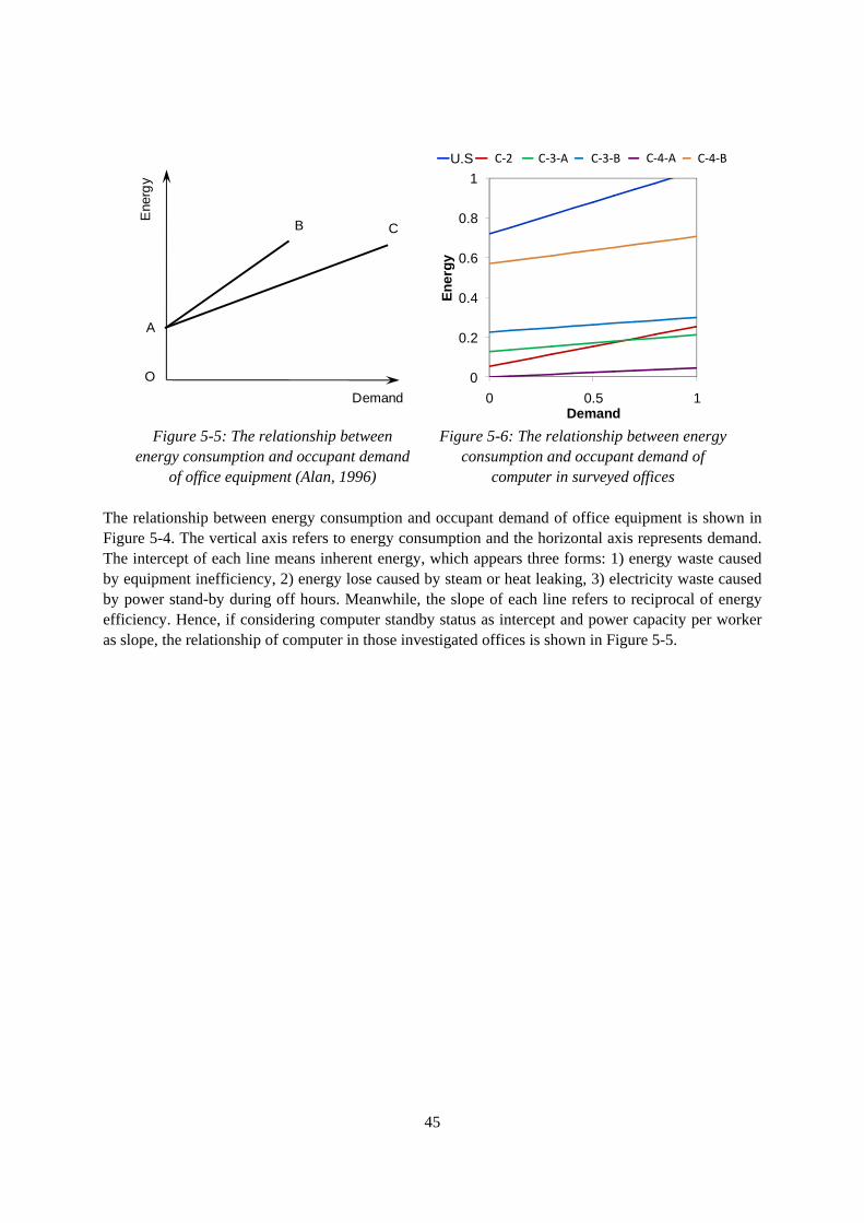
45

Ene

rgy

Demand

O

A

B C

0

0.2

0.4

0.6

0.8

1

0 0.5 1

En

erg

y

Demand

U.S HK-1 BJ-1A BJ-1B BJ-2A BJ-2BC-2 C-3-A C-3-B C-4-A C-4-B

Figure 5-5: The relationship between

energy consumption and occupant demand of office equipment (Alan, 1996)

Figure 5-6: The relationship between energy consumption and occupant demand of

computer in surveyed offices The relationship between energy consumption and occupant demand of office equipment is shown in Figure 5-4. The vertical axis refers to energy consumption and the horizontal axis represents demand. The intercept of each line means inherent energy, which appears three forms: 1) energy waste caused by equipment inefficiency, 2) energy lose caused by steam or heat leaking, 3) electricity waste caused by power stand-by during off hours. Meanwhile, the slope of each line refers to reciprocal of energy efficiency. Hence, if considering computer standby status as intercept and power capacity per worker as slope, the relationship of computer in those investigated offices is shown in Figure 5-5.

46

6. Ventilation and window operation


Pioneering researches about occupant behavior and its driving force are conducted in residential building from early 1970s. While, the first attempt to study the occupant behavior of window operation is started from early 1990s. The discrete-time Markov process and logistic function are used in the prediction of window opening. It is found that both the indoor and outdoor temperature having strongly relationship with window opening proportion. The milestone map of the initial stage is shown as follows.

1991

Fritsch et al. (Fritsch, 1990;

Roulet, 1991)

Markov process model

Prediction of opening angle

1998

Raja et al. (Raja, 1998, 2001)

Field survey of the thermal

comfort of workers in natural

ventilated building in UK.

2001

Nicol et al. (Nicol, 2001)

Logistic functions

Recommended the

outdoor temperature as an

input parameter

2004

Nicol et al. (Nicol, 2004)

Logistic functions

Indoor temperature is a more

coherent predictor

2007

Rijal et al. (Rijal, 2007, 2008)

Logistic regression analysis

The proportion of windows

open depends on indoor and

outdoor temperature.

Figure 6-1: Development of interactions with window openings in office building Besides, Nicol and Humphreys (Nicol, 2002) indicate that people with more opportunities to adapt themselves to the environment or the environment to their own requirements will be less likely to suffer discomfort. Among all studies concern about how people adopt environmental control strategies and identifies the influential variables, window opening behavior has become of a specific concern of indoor environment analysis and energy evaluation. Yun and Steemers (Yun, 2008) conduct a field survey on window opening control by occupants in six offices at two buildings during the summer. A result is found that window opening behavior patterns has a strong relationship with indoor air temperature. A time-dependent window opening behavior model has been developed for building simulation, considering indoor temperature, time of day and the previous window status.

Figure 6-2: Observed proportion of windows open for specified bandwidths as a function of different

measured physical parameters

47

Haldi and Robinson (Haldi, 2009) investigate the influence of occupancy patterns, indoor temperature and outdoor climate parameters on window opening and closing behavior. 14 south-facing cellular offices of an office building have been equipped with sensors. Local indoor temperature, occupancy, window openings and closings have been measured. Three different modeling methods are developed and compared for the prediction of actions on windows. The major findings of window opening proportion functions shows in Figure 6-2. 6.2 Field survey of case building

Among case buildings in China, only CHN-03 has 25% external windows can be opened manually, as shown in Figure 6-3. External windows of CHN-01, CHN-02 and CHN-04 cannot be opened and fully controlled by mechanical ventilation system. The frequency of window opening is investigated by questionnaire survey. Figure 6-4 illustrates that: 1) occupants in office CHN-03-B open window more frequent than office-A; 2) occupants open window more frequently during transitional seasons than summer or winter.

3

4.5

2

2.5

4

1.5

-5 -3 -1 1 3 5

Summer (Jun.~Aug.)

Transitional (Mar.Apr.Sep.Oct.)

Winter (Nov.~Feb.)

BJ-1A BJ-1BC-03-A C-03-B

Figure 6-3: Several external windows can be opened

manually of CHN-03

Figure 6-4: Survey result of window opening frequency (1=Always close, 3=often open, 5=open frequently)

0% 50% 100%

BJ-1A

BJ-1B

Overheat Unfresh air Needs air moving

C-03-B

C-03-A

0% 50% 100%

BJ-1A

BJ-1B

Cannot open Far from windowDiscomfortable air moving Dirty air

C-03-B

C-03-A

(a) Open window (b) Close window

48

Figure 6-5: Survey result of reason why occupant chooses to open or close external windows Detailed reason why occupants choose to open or close the closed external windows is also investigated by questionnaire. 40%-50% occupants open window because the uncomfortable indoor air quality or temperature. While others think they requiring air movement in the office. Meanwhile, 50%-80% occupants close window because the discomfort air moving or terrible air quality outside. What needs to be emphasis is that 20%-50% occupants who never control external window are those seated in the internal area.

Building Design Manager behavior Occupant behaviorinteraction

Window inoperable

PAU/ AHUOperation hours

Occupant behaviorComplaint

Window operable

Window in public area

PAU/ AHUHours

Window in office

Direct influence Control InteractionIndirect impact

Figure 6-6: Logistical diagram of the relationship between window opening and mechanical ventilation system

The upper frame explains the relationship between window opening and mechanical ventilation system. For buildings designed with inoperable window, ventilation can only be realized by mechanical system such as Air Handling Units, Primary Air Units or Fan Coil Units. The operation hours are only controlled by building operator/manager if there is no interacting complaint mechanism in the building. For buildings designed with operable window, building operator/manager can control mechanical ventilation system, as well as windows in public and office area. So a good feedback mechanism should be set up to balance window opening and mechanical ventilation system. For example, if lots of occupants open window in the office, then Primary Air Units should be decreased or shut down accordingly by building operator to realized energy conservation. But according to our investigation, few office buildings set up the special control logic connecting window opening and mechanical ventilation system. The latter one is usually controlled manually by building operator or automatically by BMS system with the fixed control logic. For instance, the following table compares control logic of mechanical Primary Air Units. Based on the energy benchmarking system and field measurement, the electricity consumption is breakdown into unified five items, including PAU, AHU, chiller plant, lighting & plug-in and special equipment (i.e. garage vent, data center, kitchen device, etc.). The annual electricity use intensity of PAU in

49

CHN-02 is 13.2 kWh/(m2.a), higher than 5.8 kWh/(m2.a) in CHN-04 and 0.2 kWh/(m2.a) in CHN-03, as shown in Figure 6-7. Building manager of CHN-03 has shorten the operation hours of PAU due to partial external windows can be manual opened by occupants, which greatly reduced energy consumption of mechanical ventilation.

Table 6-1 Basic information of PAU of three investigated office buildings in China

CHN-02 CHN-03 CHN-04 Window operable or not

No Yes No

Design style of PAU

2~4 PAUs each zoon (8~12 floors) connected in parallel, independent air intake

1 PAU each floor, unified air intake by shaft

1 PAU each floor, independent air intake

Control logic VFD, controlled by CO2 concentration of returned air

VFD VFD, controlled by return air temperature

Operation period 6:00-20:00 (annual) 8:00-9:00, 12:00-13:00 (annual)

7:00-19:00 (summer, winter) 8:30-14:30 (transitional season)

Operation hours (hour/day)

14 2 12-summer,winter 6-transitional season

Rated air volume for single PAU (m3/h)

58428 4000 6200

Power capacity (kW) 45 1.1 2.2

0

20

40

60

80

100

120

140

HK-1* BJ-1 BJ-2

kWh

/(m

2 .a)


0

1

2

3

4

5

6

7

8

HK-1* BJ-1 BJ-2

kWh

/(m

2 .m

on

th)

OthersLgt&Plug-inPlantAHUPAU


(a) Annual (b) Transitional season (April) Figure 6-7: Electricity use intensity of PAU of three office buildings in China

50

7. Heating and cooling


The traditional heating, ventilating and air conditioning (HVAC) system in office building is designed to provide a steady environment which will be acceptable to 80% of the occupants (ASHRAE, 1992). However, the philosophy has changed in recent years. More and more occupants have a strong desire to control the thermal environment by themselves. Thus, the impact of occupant controlling indoor temperature or humidity set point, lighting, shading device attracts great attention by researchers. Leon et al. (Leon et al., 1997) develop a simple model of the thermal environment of an open space office created by a task conditioning system and simulate the impact on energy consumption. The model allows the occupant of each work station to select a single temperature for his or her microclimate. Then the HVAC equipment will then maintain that temperature by adjusting the cooling air volume flow at a fixed supply temperature to compensate for the space load and the heat exchange with other cells and the ceiling area. The result shows that the occupancy rate and the amount of task lighting and the floor-to-ceiling heat transfer coefficient are significant to energy consumption of HVAC system. Figure 7-1 and 7-2 shows high occupancy and task lighting will cause more energy use. 5%-16% energy will be saved by simulation, due to stratification and reduce conditioning in unoccupied areas.

Figure 7-1: Effect of OB on HVAC energy use for a task conditioning system with occupant sensors relative to a conventional system without them

Figure 7-2: Task lighting effect on energy use-HVAC energy and total energy (HVAC +lights+

plug loads) Note: “x” represents the “occupancy rate”, which is the probability that a particular occupant presenting at any

given time; “y” refers to the “equipment leave-on rate”, which describes the tendency of occupants to shut off

task lights and personal computers when they depart. Other researchers (Drik, 2011) also simulate the influence of the impact of occupancy rate, the shading device use and switching of the lights on HVAC system energy consumption. The yearly energy performance and thermal comfort of a 30 square meter open plan office is simulated by TRNSYS. The result shows implementing occupant behavior has a considerable influence on the cooling demand and thermal comfort in the offices. It is shown that encouraging people to actively switch off the lights not only saves on the energy demand for lighting but also reduces the cooling demand and overheating issues.

51

7.2 Simulation on a case building

Occupant behavior towards cooling equipment can be divided into users’ behavior and operators’ behavior. The building users can change the indoor temperature set point and the building operators are usually on charge of controlling centralized HVAC equipment. For understanding the impact of those behaviors, three experiments are simulated by DeST tools, based on the investigation of case building in China (CHN-03).

(a) Typical floor of office tower (b) Podium floor 1-5

Figure 7-3: Simulation model sketch map of CHN-03 Simulation model of the building is shown in Figure 7-3. Envelope information (referring to Table 7-1), installed capacity and schedule of artificial lighting system, and occupancy schedule are based on field survey result (referring to Table 7-2). The office equipment load is 150 W/person. The indoor room temperature set point of B3 to F20 is 25~27 Deg.C, and 27~29 Deg.C for high levels. The controlled schedule of AHUs and PAUs is shown in Table 7-3.

Table 7-1 Envelope information of CHN-03 Visible Light

(%) Solar Energy

(%) U-value(W/m2.K)

Reflect Trans

Out In

Trans Reflect Winter Night Summer Day

SC SHGC RHG (W/m2)

25 27 18 16 22 1.56 1.55 0.29 0.26 197

Table 7-2 Internal load based on survey

Floor Stuff No. Area (m2) m2/person W/m2 4 150 893.76 0.17 33.57 5 0 893.76 0 0 6 0 893.76 0 0 7 80 943.07 0.08 16.97 8 80 943.07 0.08 16.97

52

9 90 943.07 0.1 19.09 10 40 471.54 0.08 16.97 11 120 943.07 0.13 25.45 12 150 943.07 0.16 31.81 13 140 943.07 0.15 29.69 14 150 943.07 0.16 31.81 15 120 943.07 0.13 25.45 16 150 943.07 0.16 31.81 17 150 943.07 0.16 31.81 18 100 943.07 0.11 21.21 19 150 943.07 0.16 31.81 20 150 829.59 0.18 36.16 21 100 829.59 0.12 24.11 22 100 829.59 0.12 24.11 23 60 829.59 0.07 14.47 24 50 943.07 0.05 10.6 25 100 26 20

Cannot be investigated.

7~19 average 1520 11788.42 0.13 25.79 20~23 average 410 3318.35 0.12 24.71

Table 7-3 Control schedule of AHUs and PAUs

No. Equip. Air Volume

(m3/h)

OA

volume

(m3/h)

Serving area Serving

volume

AER

(ach) Operation time

1 PAU 20000 20000 KTV B1 6708 2.98 10:00-14:30 17:00-0:00

2 PAU 20000 20000 Restaurant B1 2491.3 8.03 10:00-14:30 16:30-21:00

3 PAU 20000 20000 Restaurant B2 2883.6 6.94 11:00-13:30 16:30-20:00

4 PAU 4000 4000 Restaurant B2 2883.6 1.39 11:00-13:30 16:30-20:00

5 AHU 20000 2000 F1 7140.4 0.28 7:30-18:30

6 PAU 4000 4000 B1, B2 3000 1.33 7:30-17:30

7 AHU 20000 2000 Podium F3 4596.15 0.44 7:30-9:00 13:30-15:00

8 AHU 20000 2000 Podium F4 4596.15 0.44 7:30-9:00 13:30-15:00

9 AHU 30000 3000 Podium club 1858.2 1.61 7:30-9:00 13:30-15:00

10 AHU 30000 3000 Podium TowerB 3592.238 0.84 7:30-18:30

11 AHU 30000 3000 Office, L2, TB 1374.82 2.18 7:30-18:30

12 AHU 30000 3000 Office, L3, TB 3449.484 0.87 7:30-18:30

13 PAU 13500 13500 West restaurant N.A N.A Close

14 PAU 20000 20000 Restaurant B1 N.A N.A Close

53

15 PAU 20000 20000 B2 office 5534.52 3.61 7:30-18:30

16 AHU 20000 2000 Podium 2 meeting

room 4596.15 0.44 7:30-9:00 13:30-15:00

17 AHU 20000 2000 Chinese restaurant 2817.7 0.71 10:00-14:30 16:30-21:00

18 AHU 20000 2000 Podium F1 7140.4 0.28 Close

19 AHU 30000 3000 Office, L2, TA 1371 2.19 7:30-18:30

20 AHU 30000 3000 Office, L1, TA 3283.78 0.91 7:30-18:30


room 2116.08 1.42 Close


room 3449.484 0.87 7:30-18:30

23 PAU 2000 2000 Swimming pool 3194.2 0.63 Close

24 PAU 2000 2000 B3 2265.112 0.88 7:30-18:30

Note: “AER” represents the “Air Exchange Rate”. The cooling consumption from May, 2010 to Sep, 2010 is measured. The difference between monthly measurement and simulation result is less than 5% (as shown in Figure 7-4), which calibrates the reliability of the simulation model. Three cases are simulated as follows:

1) Case 1 (User behavior, Figure 7-5). It can be concluded that the monthly cooling consumption will increase 12% to 20% if decreasing indoor temperature set point by 1~3 Deg.C.

2) Case 2 (Operator behavior, Figure 7-6). If increasing the operation time of PAUs from 4 hours/day to 6 hours/day, the cooling consumption will increase 21% within the whole cooling season.

3) Case 3 (Operator behavior, Figure 7-7). If increasing the operation time of AHUs from 3 hours/day to 11 hours/day, the cooling consumption will increase 44% within the whole cooling season.

0

2

4

6

8

10

12

14

16

May Jun Jul Aug Sep

kWh

c/(m

2 .m

on

th )

Cooling consumption DeST simulation result

4.1

10.1

14.9 14.0

3.6 4.7

11.6

16.9 15.9

4.4

02468

1012141618

May Jun Jul Aug Sep

kWh

c/(m

2 .m

on

th )

Before After

Figure 7-4: Comparison of cooling consumption by measurement and simulation

Figure 7-5: Case 1(User behavior)-decreasing indoor room temperature setpoint from 25~27

Deg.C and 27~29 Deg.C to 24~26 Deg.C

54

4.1

10.1

14.9 14.0

3.6 3.7

11.7

19.8 17.8

3.7

0

5

10

15

20

25

May Jun Jul Aug Sep

kWh

c/(m

2 .m

on

th )

Before After

4.1

10.1

14.9 14.0

3.6 4.1

13.8

23.6

21.1

4.7

0

5

10

15

20

25

May Jun Jul Aug Sep

kWh

c/(m

2 .m

on

th )

Before After

Figure 7-6: Case 2 (Operator behavior)-Increasing PAU operation period from present

(8:00-9:00 and 12:00-13:00) to 7:30-13:30

Figure 7-7: Case 3 (Operator behavior)- Increasing AHU operation period from present (7:30-9:00, 13:30-15:00) to 7:00-18:00 within

the whole cooling season

55

8. Summary and conclusions

The energy use of office building has been attracting great attentions due to its significant role in total building energy consumption worldwide nowadays. The influencing factors of energy consumption in office buildings were gradually clarified by researchers in recent years. Generally speaking, those factors can be summarized into two categories, including six factors: (1) Physical factor, consists of Climate (e.g. outdoor ambient temperature, humidity, solar radiation,

etc.), Envelope (e.g. structure, K-value, etc.) and Technical system (e.g. lighting, office device, service system, especially HVAC system, etc.)

(2) Human factor, including Set point (e.g. indoor control temperature, carbon dioxide concentration, fresh air volume, etc.), Operation (e.g. on-off schedule of central systems, etc.) and Occupant behavior (e.g. switch on-off of lighting, equipment status in after-hours, window opening, etc.)

A number of present studies were more focusing on the latter three factors, especially the related occupant behavior in the office building. Those studies intended to solve two kinds of problems. Firstly, to improve building energy prediction models, so as to give more accurate results. Secondly, to optimize building control logic, in order to minimize energy consumption. The researches focus on occupant schedule, lighting and blind utilizing, office equipment using in after-hours, window opening, etc. The existing researches have combined methods of field measurement, questionnaire survey and simulation, concentrated on quantizing occupant behavior in office building and tried to set up connection between environmental parameters. There are 12 office buildings are contributed by researchers from seven countries, including Austria, Belgium, P.R. China, France, Italy, Japan and Norway, including five small-scaled office buildings and seven large-scaled high-rise office buildings in subtask B1. The basic information and total energy use of these 12 office buildings are compared. The main purpose of this report is to review the key literatures relating to the impact of occupant behavior on energy consumption and the key findings of the Subtask B1 of ANNEX 53 by contributors. The energy use of occupants in office buildings has been grouped in the following categories: lighting, office appliance, ventilation and window operation, as well as heating and cooling. For those office energy use categories, the relevant types of occupant behavior have been discussed. There are three major conclusions of occupant behavior impact on energy consumption in office building, based on case study: (1) There is weak relationship between external illuminance and the use of artificial lighting in large-

scaled office building. Occupants usually turn on artificial lightings during the working hours. But occupants in small-scaled office buildings use more natural lighting and save more electricity.

(2) The electricity consumption of centralized system is higher than de-centralized system (especially to lighting system and HVAC system). For example, the energy use of ventilation and air-conditioning system in large-scaled office building is larger than small-scaled office buildings due to the limitation of operable external windows. The building operator behavior (i.e. set point, air change rate, control strategy of circulating pumps and fans, etc.) is the decisive factor of electricity consumption of AC systems as well as cooling consumption.

56

(3) The energy loss can be caused by three aspects: 1) energy waste caused by equipment inefficiency, 2) energy lose caused by steam or heat leaking, 3) electricity waste caused by stand-by power during off duty hours. Thus, it is found that the occupant behavior of night-time standby status is the key decisive factor of appliances in office building according to the on-site investigation.

57

9. Reference

[1] Alan Meier. Toward More Efficient Energy Use Through Demand-side Management [M]. LBNL, University of California, 1996.

[2] A.M.Egan, 2009. Three case studies using building simulation to predict energy performance of Australian office buildings, 11th International IBPSA Conference, 2009.

[3] ASHRAE, 1992. ASHRAE, ANSI/ASHRAE Standard 55-1992, Thermal environmental conditions for human occupancy, American Society of Heating, Refrigeration and Air Conditioning Engineers, Atlanta, GA, 1992.

[4] BCO. 2005. BCO Guide 2005. Daylight in urban canyons: planning in Europe. In proceedings of PLEA 2006, the 23rd Conference, Geneva, Switzerland.

[5] BRE, 2000. Energy consumption guide 19: Energy use in offices. The Government’s Energy Efficiency Best Practice programme, BRE, 2000.

[6] Bruce Nordman, 2005. Bruce Nordman, Alan Meier, Mary Ann Piette. PC and monitor night status: power management enabling and manual turn-off, Information and electronic technologies, 7: 89-99.

[7] C.F. Reinhart, Lightswitch-2002: a model for manual and automated control of electric lighting and blinds, Solar Energy, 77(2004):15-28.

[8] C.J.Koinakis, Combined thermal and natural ventilation modelling for long-term energy assessment: validation with experimental measurements, Energy and Buildings, 37(2005):311-323.

[9] DECC, 2010. The Japanese Association for Sustainable Development, Energy Consumption of Commercial building (DECC). http://www.jsbc.or.jp/decc download/.

[10] Dirk, 2011. Dirk Saelens, Wout Parys, Ruben Baetens. Energy and comfort performance of thermally activated building systems including occupant behavior, Building and Environment, 46 (2011): 835-48.

[11] DOE, 2011. The advanced Energy Design Guide for Small to Medium Office Buildings, 2011.

[12] EIA, 2010. Energy Information Administration, Commercial Building Energy Consumption Survey (CBECS). http://www.eia.gov/emeu/cbecs/cbecs2003/.

[13] E. Gratia, A.D. Herde, Design of low energy office buildings, Energy and Buildings, 35(2003):473-491.

[14] E. Gratia, A. D. Herde, Natural cooling strategies efficiency in an office building with a double-skin facade, Energy and Buildings, 36(2004):1139-1152.

[15] Fritsch 1990. Fritsch R, Kohler A, Nygard-Ferguson M, et al. A stochastic model of user behavior regarding ventilation. Building and Environment, 25 (2): 173-181.

[16] Gligor, V., 2004. Luminous environment and productivity at workplaces. Thesis, Helsinki University of Technology, Espoo.

58

[17] G.Y.Yun, J.Y.Shin,J.T.Kim, 2011. Influence of window views on the subjective evaluation of discomfort glare, Indoor and Built Environment, 20 (2011):65-74.

[18] G.Y.Yun, H.Y.Kong, H.Kim, J.T.Kim, 2012. A field survey of visual comfort and lighting energy consumption in open plan offices, Energy and Buildings, 46(2012): 146-151.

[19] Haldi F, 2009. Haldi F, Robinson D. Interactions with window openings by office occupants. Building and Environment, 44 (2009): 2378-2395.

[20] H.B.Rijal, H. Yoshida, Winter thermal improvement of a traditional house in Nepal, Proceeding of the Ninth International IBPSA Conference, 3(2005):1035-1042.

[21] H. Breesch, A. Bossaer, A. Janssens, Passive cooling in a low-energy office building, Solar Energy, 79(2005):682-696.

[22] H.B.Rigal, P. Tuohy, M.A. Humphreys, J. F. Nicol, et al. Using results from field surveys to predict the effect of open windows on thermal comfort and energy in buildings, Energy and Buildings, 39(2007):823-836.

[23] Hunt DRG. The use of artificial lighting in relation to daylight levels and occupancy. Building Environment, 1979(14):21-33.

[24] Hunt DRG. Predicting artificial lighting use: a method based upon observed patterns of behavior. Lighting Research Technology, 1980(12):7-14.

[25] Hopkinson GR, Petherbridge P, Longmore J. 1966. Daylighting. Heinemann: London.

[26] H. Xiao, Q. Wei, Y. Jiang, 2012. The reality and statistical distribution of energy consumption in office buildings in China, Energy and Buildings, 50: 259-265.

[27] H. Yinong, S. Hokoi, N. Nakahara, et al. Influence of air exchange through small openings between rooms-consideration of resident’s lifestyle, Journal of Asia Architecture and Building Engineering 1 (2) (2002):79-86.

[28] H.Yoshida, T. Kono, Analysis of natural ventilation effect for an office building considering moisture absorption by materials, Advances in Building Technology, 2(2002):1199-1206.

[29] IEA, 2006. International Energy Agency. Light’s Labour’s Lost. IEA Publications, France.

[30] IEA, 2009. World Energy Outlook, International Energy Agency, Paris, 2009.

[31] I.Rajapaksha, H.Nagai, M. Okumiya, A ventilated courtyard as a passive cooling strategy in the warm humid tropics, Renewable Energy, 28(2004):1139-1152.

[32] Janet Stephenson, Barry Barton, Gerry Carrington, et al. 2010. Energy cultures: A framework for understanding energy behaviors, Energy Policy, 38 (2010), 6120-6129.

[33] J.F. Nicol, M.A. Humphreys, Thermal comfort as part of a self-regulating system, Building Research and Practice, 6(1973):191-197.

[34] J.F. Nicol, M.A. Humphreys, Adaptive thermal comfort and sustainable thermal standards for buildings, Energy and Buildings, 34 (2002):563-572.

59

[35] J.L.M.Hensen, On the thermal interaction of building structure and heating and ventilating system, Thesis, University of Strathclyde, 1991.

[36] K. Kawamoto, 2004. K. Kawamoto, Y. Shimoda, M. Mizuno. Energy saving potential of office equipment power management. Energy and Buildings, 36 (2004): 915-923.

[37] LBNL, 2001. K. Kawamoto, 2001. K. Kawamoto, J. Koomey, etc. Electricity used by office equipment and network equipment in the U.S: detailed report and appendices, LBNL-45917, Lawrence Berkeley National Laboratory, Berkeley, CA, February, 2001.

[38] Li DHW, Tsang EKW, 2008. Daylighting Resources-Design Guides. Rensserlaer Polytechnic Institute: Troy, NY. http://www.lrc.rpi.edu/programs/daylighting.

[39] Lutzenhiser, L.,1993. Social and behavioral aspects of energy use. Annual reviews. Energy Envionment, 18 (1993): 247-289.

[40] Marechal, K. An evolutionary perspective on the economics of energy consumption: the crucial role of habits. Sovaly Businees School, Brussels. 2003.

[41] M.E. Mankibi, F. Cron, P. Michel, C. Inard, Prediction of hybrid ventilation performance using two simulation tools, Solar Energy, 80(2006):908-926.

[42] M.M. Eftekhari, L.D.Marjanovic, Application of fuzzy control in naturally ventilated buildings fro summer conditions, Energy and Buildings, 35(2003):645-655.

[43] Nicol, F. and Raja, I. (1997). Modelling temperature and human behavior in buildings-scoping study IBPS News 9(1) pp 8-10 International Building Performance Simulation Association, Reading, UK.

[44] Nicol, J.F., Raja, I.A., et al. Climatic variations in comfort temperatures: the Pakistan projects Energy and Buildings, 30(1999): 261-279.

[45] Nicol, 2001. Nicol JF. Characterising occupant behavior in buildings: towards a stochastic model of occupant use of windows, lights, blinds, Heaters and fans. In: Seventh international IBPSA conference proceedings, Rio de Janeiro; 2001.

[46] Nicol J, 2002. Nicol J, Humphreys M, Adaptive thermal comfort and sustainable thermal standards for buildings. Energy and Building, 34 (2002): 563-572.

[47] Nicol, J.F. 2004, Adaptive thermal comfort standards in the Hot-Humid Tropics. Energy and Buildings, 36(7):628-637.

[48] Nicol, 2004. Nicol JF, Humphreys MA. A stochastic approach to thermal comfort: occupant behavior and energy use in buildings. ASHRAE Transactions, 110 (2): 554-68.

[49] P.O. Fanger, J. Toftum, Extension of PMV model to non-air conditioned buildings in warm climates, Energy and Buildings, 39(2002):533-536.

[50] Rijal 1998. Rijal A, Nicol JF, McCartney KJ, et al. Natural ventilated buildings: use of controls for chaning indoor climate. Renewable energy, 15: 391-4.

60

[51] Rijal 2001. Rijal A, Nicol JF, McCartney KJ, et al. Thermal comfort: use of controls for changing indoor climate. Energy and buildings, 33 (3): 235-44.

[52] Rijal, 2007. Using results from field surveys to predict the effect of open windows on thermal comfort and energy use in buildings, Energy and Buildings, 39 (7):823-836.

[53] Rijal, 2008. Rijal HB, Tuohy P, Nicol JF, et al. Development of an adaptive window-opening algorithm to predict the thermal comfort, energy use and overheating in buildings. Journal of Building Performance Simulation, 1(1): 17-30.

[54] Roulet, 1991. Roulet CA, Cretton P, Fritsch R, et al. Stochastic model of inhabitant behavior with regard to ventilation. Technical report, 1991.

[55] Roche L, Dewey HE, Littlefair HP. 2000. Occupant reactions to daylight in offices. International Journal of Lighting Research and Technology, 32(3): 119-126.

[56] Statistics Norway, 2008. Indicators for energy use in office buildings in central government and others. http://www.ssb.no/entjen_statres_en/.

[57] Stern, 2007. N.H., The economics of climate change: the Stern Review. Cambridge University Press, Cambridge, UK, 2007.

[58] T.Frank, Climate change impacts on building heating and cooling energy demand in Switzerland, Energy and Buildings, 37(2005):1175-1185.

[59] U.Eicker, M.Huber,P.Seeberger, et al. Limits and potentials of office building climatisation with ambient air, Energy and Buildings, 38(2006):574-581.

[60] Wilson, C.,2007. Dowlatabadi, H., Models of decision making and residential energy use. Annual Review of Environment and Resources, 32 (2007): 169-203.

[61] Wilson M, Walker JH, Santamouris M, et al. 2002. Design Process for Energy Efficient New and Refurbished Housing. University of North London: London.

[62] Wilson, C.,2007. Dowlatabadi, H., Models of decision making and residential energy use. Annual Review of Environment and Resources, 32 (2007): 169-203.

[63] W. Liping, W.N.Hien, The impacts of ventilation strategies and facade on indoor thermal environment for naturally ventilated residential buildings in Singapore, Building and Environment (2006).

[64] Yun G, Steemers K. Time-dependent occupant behavior models of window control in summer. Building and Environment, 43 (2008): 1471-1482.

[65] Y. Zhang, K.Lin, Q.Zhang, H.Di, Ideal thermophysical properties for free-cooling (or heating) buildings with constant thermal physical property material, Energy and Buildings, 38(2006):1164-1170.

61

III-2

Technical report “Occupant behavior and impact of energy in residential buildings”

62

Contents

Abstract ................................................................................................................................... 63

1. Boundary of the energy and occupant behavior in residential building............. 64

2. Comparison of residential building energy consumption .................................... 65

2.1 Classification of case buildings ..............................................................................................65

2.2 Classification of case buildings ..............................................................................................65

2.3 Comparison of climate............................................................................................................68

2.4 Comparison of energy consumption .......................................................................................69

3. Heating ...................................................................................................................... 74


3.2 Measurement and simulation ..................................................................................................74

4. Cooling ...................................................................................................................... 79


4.2 Measurement and simulation ..................................................................................................80

5. Lighting ..................................................................................................................... 83


5.2 Case study and results.............................................................................................................84

6. Household appliances .............................................................................................. 88


6.2 Case study and results.............................................................................................................89

7. Summary and Conclusions...................................................................................... 91

8. References ................................................................................................................. 92

63

Abstract

The energy use of residential building has been attracting great attentions due to its significant role in total building energy consumption worldwide nowadays. The influencing factors of energy consumption in residential buildings were gradually clarified by researchers in recent years. Generally speaking, those factors can be summarized into two categories, including six factors:

• Physical factor, including Climate (e.g. outdoor ambient temperature, humidity, solar radiation, etc.), Envelope (e.g. structure, K-value, etc.) and Technical system (e.g. lighting, office device, service system, especially HVAC system, etc.)

• Human factor, including Set point (e.g. indoor control temperature, carbon dioxide concentration, fresh air volume, etc.), Operation (e.g. on-off schedule of central systems, etc.) and Occupant behavior (e.g. switch on-off of lights, window opening, etc.)

The present case studies in this report are focusing on the latter three factors, especially the related occupant behavior in the residential building. These studies intended to solve two kinds of problems. Firstly, to improve building energy prediction models, so as to give more accurate results. Secondly, to optimize building control logic and system choice, in order to minimize energy consumption. They have combined methods of field measurement, questionnaire survey and simulation, concentrated on quantizing occupant behavior in residential building and tried to set up connection between environmental parameters. The main purpose of this report is to review the key literatures relating to the impact of occupant behavior on energy consumption and the key findings of the Subtask B1 of ANNEX 53 by contributors. The energy use of occupants in residential buildings has been focused on the following categories: heating, cooling, lighting and home appliances. For those residential energy use categories, the relevant types of occupant behavior have been discussed. The results show that there are obvious individual differences on occupant behaviors and different patterns of occupant behavior have significant impact on residential building energy use.

64

1. Boundary of the energy and occupant behavior in residential building

Occupant behaviors affect building energy usage. Since the oil shocks of the 1970s, there have been numerous studies of the relationship between building energy consumption and occupant behaviors from a wide range of disciplinary perspectives. Multiple researchers have reviewed these perspectives, which were grouped into biological, psychological, social, time, and physical parameters of the environment and buildings. Thus, the manifold issue of behavior demands interdisciplinary work between engineering and social sciences. But what is meant by behavior? With respect to the energy-related issues of this report, the term ‘behavior’ is predominantly meant by the following: observable actions or reactions of a person in response to external or internal stimuli, such as temperature, indoor air quality or sunlight. In this definition of behavior, attitudes and motives of an individual which lead to a specific action are not included. Data concerning behavior often stem from sensors (e.g. for window opening) in terms of indicators for observed behavior. Through this definition approach of occupant behavior, a clear link can be established (see Figure) between building engineering and social, economic, psychological, physiological, and human-factor engineering sciences. Although human behavior is usually in the research fields of the latter and is explained as a deep mechanism, the occupant behavior description is first needed and used in the building simulation technique which can evaluate the influence degree of occupant behaviors on building system performance.

Figure 1-1. the relationship among different research fields.

This report starts with a discussion of the boundary of energy use and occupant behavior when looking at the total energy use of residential buildings. To achieve a deep view how occupant behavior impact building energy use, several case studies were taken. In the following chapters: Session 2 compares the energy use of residential building in several countries. Session 3 to 6 illustrates the literature review and research result of different energy systems in residential building, including heating, cooling, lighting and household appliances. Session 7 summarizes the key conclusions.

65

2. Comparison of residential building energy consumption

2.1 Classification of case buildings

Energy use and occupant behavior depends on type, size and primary activity of building. It has been found from existing research that there are big differences of energy consumption for detached house and multi-family building, due to the main differences of the two types of residential buildings: 1) the shape factor of detached house is usually higher than the multi-family building; 2) the density of occupant, light and equipment in detached house is usually lower than the multi-family building. The characters of each type of building are shown in the Table 2-1.

Table 2-1. Comparison of two residential building types defined by existing research Type Floor area ranges (m2) Energy use related Type 1: detached 72 ~ 385 72 ~ 144 Type 2: multi-family Larger than 1200 75 ~ 200 The type of detached house is common in Europe, USA, and Japan, while the type of multi-family building is common in China. The building energy service system and energy-related behaviors might differ for the two types of buildings. To catch this feature, the case residential buildings in this ANNEX are also defined as two types: detached house and multi-family building.

1) R1-Detached house. There is only one family in detached house and the occupied spaces usually have a roof top and a basement. The total floor area of the house is usually larger than 100 square meters.

2) R2-Multi-family building (apartment building). There are several families in one building and the total floor area of each family is usually smaller than 100 square meters.

2.2 Classification of case buildings

Twelve residential buildings are contributed by researchers from four countries, including Austria, Belgium, P.R. China and Japan. Six detached house and six multi-family apartments are included. The total floor area of detached houses ranges from 159 to 389 square meters. Basic information is illustrated in Table 2-2.

Table 2-2. Detailed information of twelve residential buildings Code Photo Case contributor and

contact person Basic information

AUT-01

Vienna University of Technology Markus Dörn, Naomi Morishita, Thomas Bednar & Azra Korjenic

Category: R1 Location: Vorarlberg, Austria No. of floors: 2 GFA: 280.6 m2 Construction year: 1987 Data level: B

66

AUT-02



AUT-03



AUT-04


Category: R1 Location: Vienna, Austria No. of floors: 2 Construction year: 1930 Data level: A

AUT-05


Category: R1 Location: Vienna, Austria No. of floors: 2 GFA:389.4 m2

Construction year: 2004 Data level: A

AUT-06


Category: R2 Location: Vienna, Austria No. of floors: 13 GFA: 1330 m2 Construction year: 2007 Data level: B

BEL-01

University of Liège Bertrand Fabry Vincent Dolisy Nicolas Pignon Philippe Andre

Category: R2 Location: Hondelange, Belgium Data level: A

BEL-02

University of Liège Bertrand Fabry Vincent Dolisy Nicolas Pignon Philippe Andre

Category: R2 Location: Arlon, Belgium No. of floors: 6 Heated area: 1330 m2 Construction year: 2005 Data level: B

67

BEL-03

JCJ Energetics, Cleide A. Silva Jules Hannay Jean Lebrun

Category: R2 Location: Belgian coast No. of floors: 8 Data level: A

CHN-01

Tsinghua University Yi Jiang Yingxin Zhu Da Yan Chuang Wang

Category: R2 Location: Beijing, China No. of floors: 20 Construction year: 2000 Data level: B

JPN-01

Tohoku University, Japan Hiroshi Yoshino

Category: R1 Location: Sendai, Japan No. of floors: 2 Heated area: 285 m2 Construction year: 2008 Data level: C

JPN-02

Tohoku University, Japan Hiroshi Yoshino

Category: R1 Location: Fukushima, Japan No. of floors: 15 GFA: 72.3 m2 Construction year: 2000 Data level: C

Similar with office building, Table 2-3 presents the information status of each residential building.

Table 2-3. Case studies’ information of six categories A

1 A 2

A 3

A 4

A 5

A 6

B 1

B 2

B 3

C 1

J 1

J 2

Climate HDD ● ● ● ●

68

CDD ● ● ● ● Whole building characteristics Year built ● ● ● ● ● ● ● ● ● ● ● No. of floors ● ● ● ● ● ● ● ● ● ● ● ● GFA ● ● ● ● ● ● ● ● ● ● ● ● No. of occupants ● ● ● ● ● ● ● ● ● ● ● Building envelope Material ● ● ● ● ● ● ● ● ● ● ● U-value ● ● ● ● ● ● ● ● ● ● ● ● Window to wall ratio ● ● ● ● ● ● ● ● ● Building services and energy systems Heating system ● ● ● ● ● ● ● ● ● ● ● ● Air-conditioning system ● ● ● Ventilation ● ● ● ● ● Lighting ● ● ● ● ● Domestic hot water ● ● ● ● ● ● ● ● ● Cooking ● ● ● ● Building operation Occupancy schedule ● ● ● ● ● ● ● ● Space heating ● ● ● ● ● ● Space cooling ● ● ● Ventilation ● ● ● ● ● ● ● Lighting ● ● ● Cooking ● ● ● Domestic hot water ● ● Energy indicator Energy carrier ● ● ● ● ● ● ● ● ● ● ● Aggregation of energy ● ● ● ● ● ● ● ● ● ● ● Normalized energy use ● ● ●: Related information is collected and provided by contributors. 2.3 Comparison of climate

Climate conditions of the places where the buildings are located are quite different, as listed in Table 2-4.

Table 2-4. Climate conditions of the places Places HDD CDD

Vorarlberg 4035.34 0.00 Vienna 6808.11 0.00

Hondelange 4574.17 0.00 Arlon 3557.68 0.00

Belgian Coast 3809.92 0.00 Beijing 2789.98 70.73 Sendai 2580.44 7.93

69

2.4 Comparison of energy consumption

All the 12 case buildings locate in the cold climate region, so heating demand makes the main energy consumption. The source type for space heating and DHW in the case buildings covers widely, including gas boiler, oil boiler, wood burning oven, solar panel, gas furnace, air-to-water heat pump, air conditioner (air-to-air heat pump), urban heat supply network, direct electric heater, and electric thermal storage heater. Table 2-5 and Figure 2-1 compare the heating energy use and electricity use of the 12 buildings. According to the result, electricity use of China (northern city Beijing), Austria, Belgium and Japan is around 17.5 to 44.6 kWhe/(m

2.a); heating energy use of them is around 45.0 to 155.4 kWh/(m2.a). There is no big difference of total energy consumption for the case buildings from the above 4 countries. Besides, there is no strong evidence that the apartment building consumes less than residential house.

Table 2-5. Energy use indicator of 12 case study residential buildings

No. type source Electricity (excluding heating)

Heating (space heating

& DHW)

DHW (kWh/ca)

A1 house gas boiler + wood burning oven 19.2 81.8 N/A

A2 house oil boiler + solar panel 17.5 80.2 N/A

A3 house gas boiler + wood burning oven 23.7 51.2 N/A

A4 house gas furnace (for heating & DHW)

38.8 77.0 N/A

A5 house oil boiler + wood burning stove + solar water heater

22.0 101.4 N/A

A6 apartment gas boiler (heating floor) 30.0 45.0 N/A

B1 house air-to-water heat pump (heating floor)

N/A 71.9 1,605.3

B2 apartment gas boiler (6 radiators, thermostat in living room)

28.1 57.3 901.0

B3 apartment Electric heater 36.8 N/A

C1 apartment City heating network 32.1 100.4 341.6

J1 house Electric thermal storage heater + electric water heater

31.4 112.6 2,293.8

J2 apartment air conditioner for heating + city gas for DHW & oven

44.6 155.4 2,775.9

70

Figure 2-1. Electricity & heating energy consumption indicator of residential case buildings (Unit:

kWh/(m2.a); electricity use for heating is directly converted to heat by calorific value) Occupant behaviors, like occupancy schedule, window opening, use of air conditioner, use of lights, use of household appliances has been studied by questionnaire survey or on-site measurement, in order to explore how occupant behaves in home and the impact of occupant behaviors on building energy use. There are three major findings: a) Occupancy, heating operation time and set point has big difference and results in big difference

of building energy consumption Occupant schedule is the major investigation target which has been surveyed. Figure 2-2 shows the detailed investigation result of worker and housewife behavior in Japan. According to questionnaire survey, three scenarios named “Energy-saving”, “Normal” and “Energy-wasting” are compared. In a conclusion, reducing the operating time or equipment number of space heating and domestic hot water can decrease 40% to 46% space heating energy use compared to “energy-wasting” scenario (see Figure 2-3).

OutingSleeping Staying

at home

0%

20%

40%

60%

80%

100%

1 2 3 4 5 6 7 8 9 10 11 12 13 14 15 16 17 18 19 20 21 22 23

Time

Outing

SleepingStayingat home

0%

20%

40%

60%

80%

100%

1 2 3 4 5 6 7 8 9 10 11 12 13 14 15 16 17 18 19 20 21 22 23 24

Time (a) Worker (b) Housewife

Figure 2-2. Typical occupant behavior surveyed in residential buildings in Japan

71

Energy saving

Normal

Energy wasting

0 10 20 30

N=189N=36N=20

N=207N=26N=15

N=205N=27N=18

Energy consumption for space heating[GJ/year]

Reduce operating time of the heating equipments

Reduce the number of rooms with the heating equipments working

Set lower temperatures of the heating equipments

13.9

23.3

14.0

26.1

14.7

17.2

－40%

－46%

“Always” or “Often” → Energy-saving“Sometimes” → Normal“Seldom” or “Never” → Energy-wasting

Figure 2-3. Statistical impact of behavior on space heating energy use in residential buildings in

Japan b) Different countries have big difference in use of DHW Due to different hot water demand (shower, bath, washing hand, etc.), the per capita energy use of domestic hot water (DHW) in China, Belgium, and Japan has big difference (see Figure 2-4). The DHW use of Japan is highest, followed by Belgium, China is lowest. According to investigation, the Japanese like tub bath very much, while the Chinese often take showers rather than bathing, which leads to 7~9 times differences in use of DHW.

Figure 2-4. DHW energy consumption indicator of residential case buildings (Unit: kWh/(ca.a))

c) Typical behavior patterns can be found in real cases Different behavior patterns related to huge difference of energy use have been found in residential buildings. Table 2-6 and Figure 2-5 show several heating patterns and their heating energy use from Japanese residential database. The four heating patterns are found from 4 detached houses, where for heating space ‘all rooms’ include both living room and bedroom, ‘part rooms’ include living room or bedroom only; for heating time ‘24h’ mean continuous heating all day, ‘occupied’ mean periodic heating when the spaces are occupied. The measured heating energy use due to the four patterns has about 5 to 20 times difference.

72

Table 2-7 and Figure 2-6 show several cooling patterns and their AC energy use. The cooling patterns are found from Chinese residential buildings using split AC unit, where for cooling space ‘all rooms’ include both living room and bedroom, ‘part rooms’ include living room or bedroom only; for cooling time ‘24h’ mean continuous cooling all day, ‘occupied’ mean periodic cooling when the spaces are occupied, ‘feel hot’ mean periodic cooling when the spaces are occupied and the indoor temperature is higher than some comfort level. The simulated cooling energy use due to the four patterns has about 3 to 10 times difference.

Table 2-6. Heating patterns in residential buildings

Heating pattern Time and space

1 All rooms heated for 24h during winter

2 All rooms heated when occupied

3 Only part rooms heated for 24h during winter

4 Only part rooms heated when occupied during winter

Figure 2-5. Measured energy use of heating patterns in Japan (Unit: kWhe/a)

Table 2-7. Cooling patterns in residential buildings

Cooling pattern Time and space

1 All rooms cooled for 24h during summer

2 All rooms cooled when occupied

3 Only part rooms cooled when occupied

4 Only part rooms cooled when feel hot

73

Figure2-6. Simulated energy use of cooling patterns in China, Beijing (Unit: kWhe/(m

2.a))

74

3. Heating


All residential cases in this project use heating devices in winter. Heating schedule, set point are two main factors related to heating behavior. By simulating possible daily routines of occupants, a data set of heating-related behaviors was generated randomly. As heating behavior is influenced by and related to secondary behaviors such as window opening, internal heat gains, DHW use, and presence, these factors were also considered. Ref. [1] uses the Akaike Information Criterion (AIC) and Nagelkerkes R2-index in order to develop a multivariate regression model for the probability of AC-unit usage for heating. By consequently adding variables, which lead to a higher R2-index and a lower AIC-value, they improved the model fit to the data from an R2-index of 0.04 for the univariate model including outdoor temperature alone up to 0.48 for the multivariate model. The final model includes in total 19 variables related to physical parameters of the surrounding as well as individual parameters such as the preference. Ref. [2] applied the same procedure and presents a multivariate regression model for the choice of set-point temperature for heating in wintertime. 3.2 Measurement and simulation

Some detailed measurements have been made in Japan to compare heating energy consumption with different heating modes, the basic information about which is shown in Table 3-1. Different heating modes are described in Table 3-2. The houses are all detached, and are measured at an interval of 15 min for heating power, indoor and outdoor temperature. Relative residential energy database can be found at http://tkkankyo.eng.niigata-.ac.jp/HP/HP/database/japan2/index.htm.

Table 3-1. Information about families measured in Japan Case Location Area Heating system Family no. N,D7 Northeast 140 Electric thermal storage heater 3 N,D4 Northeast 109 Electric heat pump 3 K,D9 Kanto 114 Electric heat pump 4 K,D1 Kanto 92 Electric heat pump 3

0

500

1000

1500

2000

2500

Jan-03 Feb-03 Mar-03 Apr-03 May-03 Jun-03 Jul-03 Aug-03 Sep-03 Oct-03 Nov-03 Dec-03

k

W

h

e

l

e

c

t

r

i

c

i

t

y

N,D7 N,D4 K,D9 K,D1

9.0

2.5

1.1

0.4

0

2

4

6

8

10

N,D7 N,D4 K,D9 K,D1

M

W

h

e

l

e

c

t

r

i

c

i

t

y

N,D7 N,D4 K,D9 K,D1

Monthly heating and AC energy Annual heating energy

Figure 3-1. Heating and AC energy consumption

75

Table 3-2. Heating modes of the measured families Mode Time and space Temp. control case 2 Full time full space Full capacity N,D7 4 Scheduled time for full space Full capacity N,D4 5 Occupied space only Const. T K,D9 7 Occupied space only Full capacity K,D1

The 4 families represent 4 different types of heating modes respectively, varying in heating time and space. Figure 8 shows the monthly heating and AC energy, and annual heating energy in each family. Figure 3-2 shows the indoor temperature and heating electric power of Family no.N-D7 and no.N-D4 in winter typical day. It can be found that indoor temperature of Family no.N-D7 is almost steady due to continuous heating, while that of Family no.N-D4 fluctuates obviously since heating is off unless during getting up to leaving for work, and coming back from work to sleeping. Compared with these two families where both bedroom and living room are heated, heating energy consumption is lower in Family no.K-D9 and K-D1, where only bedroom or living room is heated.

Figure 3-2. heating curve of Family no.N-D7 (left) and no.N-D4 (right)

At the same time, heating simulation is made to compare with the measured data. The simulated residence is located in Sendai, Japan. Heat transfer coefficients of different exterior parts of the building envelope are summarized in Table 3-3. The residence is a two-story wood construction, with a total floor area of 153.4m2. There are 4 occupants, a couple with two children, and one living room (including a dining room) and 3 bedrooms (main room) in the residence. The climate condition in Sendai is shown in Figure 3-3.

Table 3-3. Information about the building envelope

WallWallWallWall

K K Sc East West North South

W/m2/K W/m2/K

1.24 4 0.7 0.2 0.2 0.2 0.2

WindowWindowWindowWindow Area ratio of window to wallArea ratio of window to wallArea ratio of window to wallArea ratio of window to wall

Building EnvelopeBuilding EnvelopeBuilding EnvelopeBuilding Envelope

76

0

00

0

5

55

5

10

1010

10

15

1515

15

20

2020

20

25

2525

25

1

11

1 2

22

2 3

33

3 4

44

4 5

55

5 6

66

6 7

77

7 8

88

8 9

99

9 10

1010

10 11

1111

11 12

1212

12

U

n

i

t

(

℃

)

U

n

i

t

(

℃

)

U

n

i

t

(

℃

)

U

n

i

t

(

℃

)

Month

MonthMonth

Month

Monthly average dry ball temperatureMonthly average dry ball temperatureMonthly average dry ball temperatureMonthly average dry ball temperature

Figure 3-3. Monthly average dry ball temperature in Sendai, Japan

Figure 3-4. An outside view of the residence

Figure 3-5. The plan of the residence

77

Four operating modes are assumed, listed in Table 3-4. Mode A represents an operating mode that all rooms are heated all the time, and Mode B is that only main room are heated but all the time, while Mode C, D, E are described as part-time and part-space modes, the schedules of which are illustrated in Table 3-5. Figure 3-6 shows the model for simulation.

Table 3-4. Setting description of different modes

Mode Setting description

A All room full time

B Main room full time

C Main room scheduled 1 time

D Main room scheduled 2 time

E Only living room scheduled2 time

Table 3-5. Different schedules for each type of rooms

78

Figure 3-6. Residence model for simulation

It can be found from the simulation results that different operation mode can make great differences in heating load and energy consumption, and that The simulation result range (red arrow) covers the real energy consumption data (green arrow).

Figure 3-7. A comparison between simulation results and real EC data

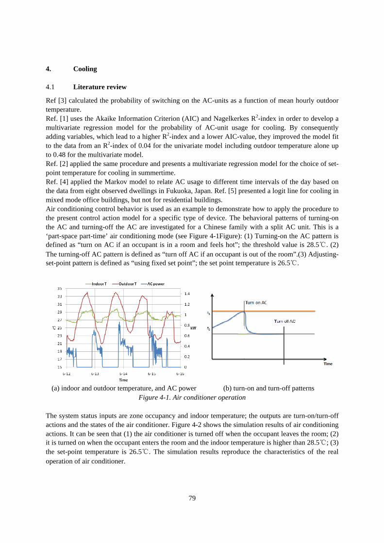
79

4. Cooling


Ref [3] calculated the probability of switching on the AC-units as a function of mean hourly outdoor temperature. Ref. [1] uses the Akaike Information Criterion (AIC) and Nagelkerkes R2-index in order to develop a multivariate regression model for the probability of AC-unit usage for cooling. By consequently adding variables, which lead to a higher R2-index and a lower AIC-value, they improved the model fit to the data from an R2-index of 0.04 for the univariate model including outdoor temperature alone up to 0.48 for the multivariate model. Ref. [2] applied the same procedure and presents a multivariate regression model for the choice of set-point temperature for cooling in summertime. Ref. [4] applied the Markov model to relate AC usage to different time intervals of the day based on the data from eight observed dwellings in Fukuoka, Japan. Ref. [5] presented a logit line for cooling in mixed mode office buildings, but not for residential buildings. Air conditioning control behavior is used as an example to demonstrate how to apply the procedure to the present control action model for a specific type of device. The behavioral patterns of turning-on the AC and turning-off the AC are investigated for a Chinese family with a split AC unit. This is a ‘part-space part-time’ air conditioning mode (see Figure 4-1Figure): (1) Turning-on the AC pattern is defined as “turn on AC if an occupant is in a room and feels hot”; the threshold value is 28.5℃. (2) The turning-off AC pattern is defined as “turn off AC if an occupant is out of the room”.(3) Adjusting-set-point pattern is defined as “using fixed set point”; the set point temperature is 26.5℃.

(a) indoor and outdoor temperature, and AC power (b) turn-on and turn-off patterns Figure 4-1. Air conditioner operation

The system status inputs are zone occupancy and indoor temperature; the outputs are turn-on/turn-off actions and the states of the air conditioner. Figure 4-2 shows the simulation results of air conditioning actions. It can be seen that (1) the air conditioner is turned off when the occupant leaves the room; (2) it is turned on when the occupant enters the room and the indoor temperature is higher than 28.5℃; (3) the set-point temperature is 26.5℃. The simulation results reproduce the characteristics of the real operation of air conditioner.

80

Figure 4-2. Simulation of air-conditioning behavior.

4.2 Measurement and simulation

A residential building in Beijing, China is measured in 2006 for cooling energy consumption. The air conditioning electricity use in each apartment is shown in Figure 4-3, and the average electricity use is 2.3kWh/m2, while a wide range of consumption can be seen.

0123456789

101112131415

1 2 3 4 5 6 7 8 9 10 11 12 13 14 15 16 17 18 19 20 21 22 23 24 25

住住户户

空空空空

调调

(kW

h/m

2 )

平平值2.3 kWh/m2 Average 2.3kWh/m2

En

erg

y C

on

sum

pti

on

of

Co

olin

g S

yste

m

(kW

h/m

2)

Apartment No.

0123456789

101112131415

1 2 3 4 5 6 7 8 9 10 11 12 13 14 15 16 17 18 19 20 21 22 23 24 25

住住户户

空空空空

调调

(kW

h/m

2 )


En

erg

y C

on

sum

pti

on

of

Co

olin

g S

yste

m

(kW

h/m

2)

Apartment No.

Ele

ctri

city

Co

nsu

mp

tio

n o

f C

oo

ling

Sys

tem

0123456789

101112131415

1 2 3 4 5 6 7 8 9 10 11 12 13 14 15 16 17 18 19 20 21 22 23 24 25

住住户户

空空空空

调调

(kW

h/m

2 )


En

erg

y C

on

sum

pti

on

of

Co

olin

g S

yste

m

(kW

h/m

2)

Apartment No.

0123456789

101112131415

1 2 3 4 5 6 7 8 9 10 11 12 13 14 15 16 17 18 19 20 21 22 23 24 25

住住户户

空空空空

调调

(kW

h/m

2 )


En

erg

y C

on

sum

pti

on

of

Co

olin

g S

yste

m

(kW

h/m

2)

Apartment No.

Ele

ctri

city

Co

nsu

mp

tio

n o

f C

oo

ling

Sys

tem

Figure 4-3. The measured energy consumption of AC in every unit of a residential building in Beijing,

2006, split unit Why there is such a big difference between apartments in electricity consumption? The causes are analyzed as follows: the operation hours per summer per unit are measured quite different, varying from 3000 hours to 50 hours, and the different AC using modes also contribute to the difference significantly. For example, AC system may be only operated for occupied time or occupied space, and window may be open when outside condition (e.g. temperature and humidity) is fair, while also may be operated all the time regardless of occupation or weather condition. Difference in AC temperature

81

is another cause. The starting temperature, at which one starts to use an AC system feeling hot, is not the same, and the set point also varies, such as 28℃, 26℃ or 24℃. These factors lead to a big difference in AC consumption. The measurement on natural ventilation rate has been taken in Beijing, and the result shows a huge difference, as is shown in Figure 4-4.

Figure 4-4. measured natural ventilation rate in Beijing

Figure 4-5. Measured indoor and outdoor temperature, AC power

Figure 4-6. A schedule of the operation of AC

To study the differences further and quantitively, a simulation model of the residence is made and energy consumption is simulated. The building plan is shown in Figure 4-7. And the heat transfer coefficient of the exterior wall is 0.622 W/m2.K, while for window the value is 2.8 W/m2.K.

82

Figure 4-7. Building plan of the residence for simulation

Simulation cases are listed in Table 4-1. There are 6 cases in total, taking different operating modes into consideration, including full time, full space or part time, part space, different set point and different window opening modes (ventilation rates).

Table 4-1. Description of different simulation cases Case No. Description

Case 0 (Standard case) Full time, full space, set point 24℃, 1ACH Case 1 (raise set point by 2K) Full time, full space, set point 26℃, 1ACH

Case 2 (part time) Part time, full space, set point 26℃, 1ACH Case 3 (starting temp.) Part time, full space, starting point 29℃, set point 26℃, 1ACH Case 4 (open window) Part time, full space, starting point 29℃, set point 26℃, with

window opening (1~20 ACH) Case 5 (part space) Part time, part space, starting point 29℃, set point 26℃, with

window opening (1~20 ACH) A comparison between the simulation results and the measurement is shown in Figure 4-8. In standard case, the electricity consumption is 15.6 kWh/(m2.a), and in case 5, with a quite different operating mode, it can be decreased to 0.2 kWh/(m2.a). The simulation results are compatible with the measured data, thus it is concluded that it may decrease the AC system consumption when a reasonable AC operating mode is taken.

Figure 4-8. Simulation results of different lifestyle and the measured results

83

5. Lighting


Lighting schedule is a traditional way to describe the occupant impact on lighting system. Figure 5-1 shows results obtained from measured lighting energy use in 100 UK residences in half-hour intervals. It shows how the lighting demand profile during a typical weekday changes with season.

. Figure 5-1. Daily lighting profiles (monthly averages, weekdays) at different times of the year

(averaged over 100 homes)—showing demand in June (dashed grey line), September (solid grey line), December (solid black line) and March (dashed black line), Ref. [6].

The profile in Figure 5-1 falls into four discrete periods during which occupant behavior remains relatively similar for each half-hour – nighttime, morning peak, daytime, and evening peak. By assuming an underlying function for each period, annual trends may be stored for the parameters that describe each of these functions. The morning peak, for example, was modeled by a Gaussian function in terms of peak height, width, and peak time. The evening peak was modeled by a more intricate function, which included the description of leading and falling edges. Further relationships were investigated to model the annual trends for each of these parameters. For example, the leading edge parameter for the evening lighting peak was found to be a sine wave, whilst the trailing edge parameter was constant throughout the year. The developed model also allowed representation of diversity by employing scaling factors for differences in occupancy, income, lifestyle, etc. To further represent the uncertainty and feedback feature of lighting behavior, a high-resolution stochastic model of multiple electricity-dependent activities in households (including lighting) and the associated electricity demand has been developed in Ref. [7]- [10]. This model produces activity patterns for individual occupants as well as the domestic electricity demand based on these patterns. The activity patterns are based on a nine-state Markov chain (absence, sleeping, cooking, dishwashing, washing, TV, computer, audio, and other). The Markov chain transition probabilities are based on extensive Swedish measurements between 2005 and 2007 in monthly or annual periods in 14 households, and time-use data for five of these households. Based on these transition probabilities, at each time step in the calculation a stochastic process determines which activity will take place. Using a relatively simple conversion model, generalized load patterns for various electricity end-uses are

84

related to the activities to calculate the power demand for the end-uses. Figure 5-2 shows the measured switch-on probability functions.

Figure 5-2. (a) Measured switch-on probability function upon arrival [11]. (b) Intermediate or within-

day switch-on probability for electric lighting [12]. 5.2 Case study and results

In literature, the lighting profiles or individual lighting behavior are usually progressive averaged from a lot of houses or families. However, their differences on lighting use are not considered. In this project, we investigated more than 70 Japanese families and recorded the lighting power in a 15-minute interval. The big differences among the lighting energy use of these families and the reasons are analyzed. Finally, a uniform model is proposed to describe the lighting behavior for residential cases. The measured lighting energy use is shown in Figure 5-3. From the measure data, some conclusions are obtained. The lighting energy consumption in apartments, typically 13~35 kWh/(m2.a) is larger than that in detached houses, which varies from 0.8 to 15 kWh/(m2.a), and the difference is more than 10 times. When compared by district, a difference of 3~5 times in each district can be seen.

By house type By district Figure 5-3. Measured results of lighting energy use

The average daily lighting profile, and peaks during the day are shown in Figure 5-4. There are 1, 2 or 3 peaks during the day for different occupants, and the value of peaks mostly relates with occupant behaviors.

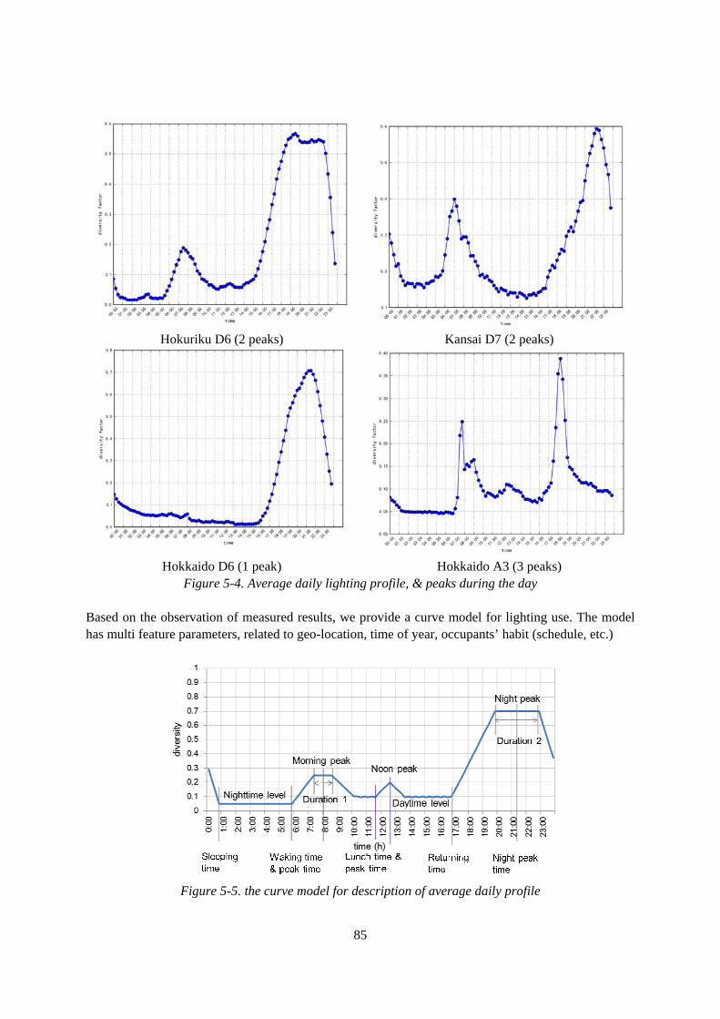
85

Hokuriku D6 (2 peaks) Kansai D7 (2 peaks)

Hokkaido D6 (1 peak) Hokkaido A3 (3 peaks) Figure 5-4. Average daily lighting profile, & peaks during the day

Based on the observation of measured results, we provide a curve model for lighting use. The model has multi feature parameters, related to geo-location, time of year, occupants’ habit (schedule, etc.)

Figure 5-5. the curve model for description of average daily profile

86

Table 5-1. Parameters of lighting curve model for the above 4 cases Parameter Hokuriku D6 Kansai D7 Hokkaido D6 Hokkaido A3

Waking-up time 5:30 5:00 7:00 7:00 Morning peak 0.19 0.40 0.05 0.25

Morning peak duration (h) 0 0 0 1 Morning peak time 7:30 7:00 8:00 8:30

Daytime level 0.06 0.14 0.05 0.09 Lunch time N/A N/A N/A 12:00 Noon peak N/A N/A N/A 0.12

Noon peak time N/A N/A N/A 12:30 Returning time 15:00 17:00 16:00 17:00

Night peak 0.55 0.60 0.71 0.39 Night peak duration (h) 3.5 0.5 0.5 0

Night peak time 22:00 22:15 21:15 18:15 Sleeping time 0:30 1:00 1:00 22:00 Night level 0.1 0.16 0.05 0.05

The verification of the curve model was taken. It can be seen from Figure 5-6 that the derived profile from the curve model fits well with the measured profile. Table 5-2 and Figure 5-7 compare the simulated and measured equivalent operating hours and daily electricity usage and they matched well.

Hokkaido D6 Hokkaido D7

Figure 5-6. Derived profiles from lighting curve model

Table 5-2. Equivalent operating hours & daily energy usage

Parameter Hokuriku D6 Kansai D7 Hokkaido D6 Hokkaido A3

Area (m2) 176.37 125 128 99 Lighting Density (W/m2) 1.73 3.5 1.70 4.19

Simulated 4.57 6.22 4.34 2.82 Operating hours (h/d)

Measured 4.72 6.02 4.08 2.47 Simulated 1.39 2.72 0.94 1.17

Electricity use (kWh/d) Measured 1.44 2.63 0.89 1.03

87

Figure 5-7. Simulated and Measured electricity use

88

6. Household appliances


Models of residential appliance electricity consumption have been developed in Ref. [13], where data from two Danish cities, an island, and two measurement projects are used to create profiles for relative consumptions. The electricity consumption profiles are shown in 32 and Figure33, where groupings of “workdays” and “not workdays” are conducted. This was a result of an investigation made on 4 houses from Energiparcel in Tilst (energy renovated houses) and 3 houses in Skibet in Vejle (passive houses).

Figure 6-1: Relative electrical energy consumption day-profiles for “workdays” divided into four

seasons. See Ref. [13]. The profiles show that electricity is used the least from 0 to 6 am and use is somewhat stable from 8 to 16 (working hours). From hours 16 to 18, a significant increase in consumption is visible, which is believed to be a result of people coming home from work and starting to make dinner. The daily pattern does not seem to deviate much between seasons, as actual electrical energy consumption does, (see Figure 6-2). For the “not workdays”, the same tendencies are observed. From around hour 6, an increase in consumption is visible and is again visible at hour 16. During midday, the level of consumption is higher, which results in a lower peak value at dinner time in the evening.

89

Figure 6-2: Relative electricity consumption day profiles for “not workdays” divided into four seasons.

See Ref. [13]. 6.2 Case study and results

In this project, we investigated a Chinese family for a whole year and found the differences between individuals. Take two TV sets in bedroom 1 and master bedroom for example. Figure 6-3 shows the measured real-time electric power and the daily schedule of the two TV sets. It can be seen that TV in the bedroom 1 is more often used than that in master bedroom.

0

10

20

30

40

50

60

70

80

P

o

w

e

r

(

W

)

TV in Bedroom 1

0

10

20

30

40

50

60

70

80

90

P

o

w

e

r

(

W

)

TV in Master Bedroom

Figure 6-3. Measured electric power and daily schedule of two TV sets

90

According to the measurement, the usage of the two TV sets can be named as “Scheduled Pattern” and “Random Pattern”. For scheduled pattern, the usage probability of TV set at each moment can be represented by a scheduled profile while it cannot for the random pattern. The average daily usage profile is summarized in Figure 6-4.

Figure 6-4. Schedule pattern of TV For the scheduled pattern of using home appliances (like TV, computer, rice cooker, etc.), a schedule table can be used as follows:

For the random pattern of using home appliances, a random description (like usage frequency, usage duration, etc.) needs be used as follows:

For more details, please see Ref. [14].

91

7. Summary and Conclusions

The energy use of residential building has been attracting great attentions due to its significant role in total building energy consumption worldwide nowadays. The influencing factors of energy consumption in residential buildings were gradually clarified by researchers in recent years. Generally speaking, those factors can be summarized into two categories, including six factors:

• Physical factor, including Climate (e.g. outdoor ambient temperature, humidity, solar radiation, etc.), Envelope (e.g. structure, K-value, etc.) and Technical system (e.g. lighting, office device, service system, especially HVAC system, etc.)

• Human factor, including Set point (e.g. indoor control temperature, carbon dioxide concentration, fresh air volume, etc.), Operation (e.g. on-off schedule of central systems, etc.) and Occupant behavior (e.g. switch on-off of lights, window opening, etc.)

The present case studies were more focusing on the latter three factors, especially the related occupant behavior in the residential building. These studies intended to solve two kinds of problems. Firstly, to improve building energy prediction models, so as to give more accurate results. Secondly, to optimize building control logic and system choice, in order to minimize energy consumption. They have combined methods of field measurement, questionnaire survey and simulation, concentrated on quantizing occupant behavior in residential building and tried to set up connection between environmental parameters. The main purpose of this report is to review the key literatures relating to the impact of occupant behaviour on energy consumption and the key findings of the Subtask B1 of ANNEX 53 by contributors. The energy use of occupants in residential buildings has been focused on the following categories: heating, cooling, lighting and home appliances. For those residential energy use categories, the relevant types of occupant behavior have been discussed. The results show that there are obvious individual differences on occupant behaviors and different patterns of occupant behavior have significant impact on residential building energy use. However, it still need better model to understand and describe the difference and uncertainty of occupant behavior patterns. This topic is further discussed in the Task Force report “Total energy use in residential buildings – the modeling and simulation of occupant behavior” that would help for future research.

92

8. References

[1] M. Schweiker, M. Shukuya, Comparison of theoretical and statistical models of air-conditioning-unit usage behavior in a residential setting under Japanese climatic conditions, Building and Environment 44, 2137-2149, 2009.

[2] M. Schweiker, M. Shukuya, Comparative Effects of Building Envelope Improvements and Occupant Behavioral Changes on the Exergy Consumption for Heating and Cooling, Energy Policy 38(6), 2976-2986, 2010.

[3] M. Hart, R. deDear, Weather Sensitivity in Household Appliance Energy End-Use, Energy and Buildings 36, 161-74, 2004.

[4] J. Tanimoto, A. Hagishima, State transition probability for the Markov Model dealing with on/off cooling schedule in dwellings, Energy and Buildings 37, 181-187, 2005.

[5] J.F. Nicol, M.A. Humphreys, A Stochastic Approach to Thermal Comfort - Occupant Behavior and Energy Use in Buildings, ASHRAE Transactions 110 Part II, 554-68, 2004.

[6] Statistik Austria, Familien- und Haushaltstatistik, Ergebnisse der Mikrozensus Arbeitskräfteerhebung, 2012, Statistik Austria: Vienna (in German).

[7] S. Wang, S. and X. Xu, Parameter estimation of internal thermal mass of building dynamic models using genetic algorithm. Energy Conversion and Management, 2006. 47(13–14): p. 1927-1941.

[8] J. Widén, M. Lundh, I. Vassileva, E. Dahlquist, K. Ellegård, E. Wäckelgård, Constructing load profiles for household electricity and hot water from time-use data – Modeling approach and validation, Energy and Buildings 41, 753-768, 2009.

[9] J. Widén, A.M. Nilsson, E. Wäckelgård, A combined Markov-chain and bottom-up approach to modeling of domestic lighting demand, Energy and Buildings 41, 1001-1012, 2009.

[10] J. Widén, E. Wäckelgård, A high-resolution stochastic model of domestic activity patterns and electricity demand, Applied Energy 87, 1880-1892, 2010.

[11] Hunt, D.R.G. The use of artificial lighting in relation to daylight levels and occupancy. Building and Environment. Vol. 14, pp 21-33. 1979

[12] C.F. Reinhart, K. Voss, Monitoring manual control of electric lighting and blinds, Lighting Research and Technology 35, 243-260, 2003.

[13] R. L. Jensen, J. Nørgaard, O. Daniels, R. O. Justesen, Person- ogforbrugsprofiler - Bygningsintegreretenergiforsyning (Person and consumption profiles – Building integrated energy supply.), ISSN 1901-726X DCE Technical Report No. 69, 2010.

[14] C. Peng, D. Yan, R.H. Wu, C. Wang, X. Zhou and Y. Jiang. Quantitative description and simulation of human behavior in residential buildings. Building Simulation 5, 85-94, 2012.

93

III-3

Questionnaire sample

94

Contents

1. Survey Questionnaire for Occupant Behavior in Office Building....................... 95

2. Survey Questionnaire for Occupant Behavior in Residential Building ............ 100

95

1. Survey Questionnaire for Occupant Behavior in Office Building

Building_______Code_______ Dear Sir/Madam,

This survey in progress is about the relationship between occupant behavior and energy consumption in office building. We are appreciated if you can answer our certain questions for our analysis.

This is an anonymous and zero-risk survey. We will never reveal your information to others, follow the rules of Statistics Act. Please follow the rules below when answering: 1) Put a check mark before the proper choices (e.g. �); 2) Fill the blanks with appropriate answers; 3) Draw a line on the time ruler according to your working schedule, e.g.

---6------7------8------9------10------11------12------13------14------15------16------17------18------19------20------21------22------23------24---

4) Draw a line on the scale by your own choice, e.g.

Never Often Frequent 1------2------3------4------5

Best wishes!

96

Part A: Basic Information

1． Your gender: □Male □Female 2． Your age: □<20 □20-30 □31-40 □41-50 □51-60 □>60 3． Your position: □Manager □Research & Development □Sales □HR □Secretary □Researcher □Others___________

4． Your office type: □Large open space □2~6 person shared room □Single room □Others______________

Part B: Working schedule

A．Weekday 5． Your weekday is: □Monday □Tuesday □Wednesday □Thursday □Friday □Saturday □Sunday

6． When you usually arrive at your office in the morning? ----6------7------8------9------10------11------12------13------14------15------16------17------18------19------20------21------22------23------24----

7． Do you usually stay at the office for your lunch? □Yes □No Jump over Topic 8 if you choose ‘Yes’

8． When do you usually leave your office at noon? ----6------7------8------9------10------11------12------13------14------15------16------17------18------19------20------21------22------23------24----

9． When do you usually arrive at your office (or begin to work) after lunch? ----6------7------8------9------10------11------12------13------14------15------16------17------18------19------20------21------22------23------24----

10. When do you usually get off work? ----6------7------8------9------10------11------12------13------14------15------16------17------18------19------20------21------22------23------24----

11. In the weekday, do you often work overtime in the evening? Never Often Extremely frequent

1--------2--------3--------4--------5

12. When you work overtime in the evening, you usually get off work at: ----6------7------8------9------10------11------12------13------14------15------16------17------18------19------20------21------22------23------24----

B. Weekend 13. Do you usually work overtime at the weekend? □Yes □No

Jump over Topic 14-20 if you choose ‘No’ 14. When do you usually work overtime at the weekend:

□Monday □Tuesday □Wednesday □Thursday □Friday □Saturday □Sunday

15. Do you often work overtime at the weekend? Never Often Extremely frequent

1--------2--------3--------4--------5

16. At the weekend, when do you usually arrive at your office in the morning? ----6------7------8------9------10------11------12------13------14------15------16------17------18------19------20------21------22------23------24----

17. At the weekend, do you usually stay at the office for your lunch? □Yes □No Jump over Topic 18 if you choose ‘Yes’ 18. At the weekend, when do you usually leave your office at noon? ----6------7------8------9------10------11------12------13------14------15------16------17------18------19------20------21------22------23------24----

19. At the weekend, when do you usually arrive at your office (or begin to work) after lunch?

97

----6------7------8------9------10------11------12------13------14------15------16------17------18------19------20------21------22------23------24----

20. At the weekend, when do you usually get off work? ----6------7------8------9------10------11------12------13------14------15------16------17------18------19------20------21------22------23------24----

98

Part C: Small Power Equipment Using

A．Lighting

21. The lighting equipment you using includes: □Desk lamp □Ceiling light □Others______________

22. Your working face usually uses: □Nature lighting □Ceiling light □Desk lamp

23. Can you control ceiling lights? □Yes □No

24. Who usually switches on your ceiling lights? □Myself □Colleague □Secretary □Cleaner □Auto-control □Unknown

25. When does ceiling light usually open? ----6------7------8------9-----10------11------12------13------14------15------16------17------18------19------20------21-----22-----23-----24---

26. When does ceiling light usually closed? ----6------7------8------9-----10------11------12------13------14------15------16------17------18------19------20------21-----22-----23-----24---

27. When does your desk lamp usually open? ----6------7------8------9-----10------11------12------13------14------15------16------17------18------19------20------21-----22-----23-----24---

28. How frequent do your switch on your ceiling lights and desk lamp on work?

29. How frequent do your switch off your ceiling lights and desk lamp off work?

30. If you do not switch off ceiling lights sometimes, the possible reasons are: □Certain people will switch off. □Others is still working. □Forget □Switcher is not convenient. □Unknown □Others______________

B．Small power equipment

31. Your personal office equipment includes: □Laptop: _____(number) □Computer: _____(no.) □Printer: _____(no.) □LCD monitor>20’: _____(no.) □CRT monitor: _____(no.) □Fax machine: _____(no.) □LCD monitor 14-20’: _____(no.) □Others(name/no.): ________________________

32. Your common office equipment includes: □Printer/copier: _____(number) □PC/server: _____(no.) □Fax machine: _____(no.) □Drinking machine _____(no.) □Coffee machine:

_____(no.) □ Others (name/no.)__________

Switch on ceiling lightsSwitch on ceiling lightsSwitch on ceiling lightsSwitch on ceiling lights Switch on desk lampSwitch on desk lampSwitch on desk lampSwitch on desk lamp

Never Often Extremely frequent

1------2------3------4------5 Never Often Extremely frequent

1------2------3------4------5

Switch Switch Switch Switch off ceiling lightsoff ceiling lightsoff ceiling lightsoff ceiling lights Switch off desk lampSwitch off desk lampSwitch off desk lampSwitch off desk lamp

Never Often Extremely frequent

1------2------3------4------5 Never Often Extremely frequent

1------2------3------4------5

99

33. The frequency of your PC, laptop or monitor shutting down or standing by when the certain events happening is: PC (or laptop) Monitor of PC

a) Off work

1-------2-------3-------4--------5-------6-------7

1-------2-------3-------4--------5-------6-------7

b) Lunch/dinner 1-------2-------3-------4--------5-------6-------7 1-------2-------3-------4--------5-------6-------7 c) Meeting 1-------2-------3-------4--------5-------6-------7 1-------2-------3-------4--------5-------6-------7 d) Noon break 1-------2-------3-------4--------5-------6-------7 1-------2-------3-------4--------5-------6-------7

34. The frequency of using the following common equipment is: □ Common printer/copier: _____times/day □ Drinking machine: _____times/day

35. If you do not shut off your computers sometimes, the possible reasons are: □Need remote control □Working requirement □Others don’t shut down. □My habit □Unknown □Others____________________________

C．Windows and shades

36. Are you closed to external window? □Yes □No

37. Does your external window have curtain/shade? □Yes □No Jump over Topic 38-39 if you choose ‘No’

38. The frequency of pulling down the curtain is:

Never Often Extremely frequent 1--------2--------3--------4--------5

39. The possible reasons you pull down the curtain are: □Sun scorching □Sun dazzling □Screen glaring □Prevent temperature rising □Others____________________________

40. If the room changes dark, you will choose in prior:

□Pull open shade/curtain □Switch on desk lamp □Switch on ceiling light The survey is finished. Thanks for your great supporting!

Always

shut down

Always

stand by Half-half

Always

shut down

Always

stand by Half-half

100

2. Survey Questionnaire for Occupant Behavior in Residential Building

1. Household energy consumption information Required Information is as follows: 1) electricity fee per year, and per month in winter (from Nov. to Feb.), in summer (from Jun. to Sep.), in spring and autumn; 2) gas fee per year, and per month in winter, in summer, in spring and autumn. If payment cards or bills are available, please fill in additionally. 1) In your family, annual electricity fee is about ______ yuan/year.

In winter about ______ yuan/year, in summer about ______ yuan/year, in spring and autumn about ______ yuan/year. In your family, annual gas fee is about ______ yuan/year. In winter about ______ yuan/year, in summer about ______ yuan/year, in spring and autumn about ______ yuan/year.

2. Occupant behaviors and Lifestyle

a. Air conditioning equipment and using mode

2) Is there a humidifier in your home? □Yes, and used every day □Yes, but used occasionally □Yes, but never used □No

3) Which air conditioning equipment is used in winter in your home? (Multiple, please fill in the number) Central air conditioning system □District heating □Household central air conditioning □Floor heating with air source heat pump □Floor heating with electricity □Floor heating with gas □Wall-mounted gas boiler Split air conditioner □Wall-mounted or package air conditioner, the number is ______ Local electric heating equipment □Oil heater or electric heater, number: ____ □Warm air blower, number: ____ □Electric foot warmer, number: ____ □Electric warm pack, number: ____ □Electric blanket, number: ____ □other equipment, number: ____

4) When heating starts in your home (any equipment is used)? (Early, Mid, Late) ______ (month) 5) When heating ends in your home (no equipment is used)? (Early, Mid, Late) ______ (month)

If air conditioning equipment (central or split air conditioning system) is uniformly controlled (with only one switch), please answer Questions 6~7, otherwise please skip to Question 8. 6) How do you use the heating equipment? (Single)

□Always on in winter (never switched off until winter passes) □Rarely used □At fixed time every day: Switch on at ____, for ____ hour(s) □Switch on when there is an occupant, and off when no occupant □Switch on only feeling cold, and off when no occupant

101

□Other ________________ 7) How do you adjust the set point? (Single)

• □Fixed set point, always ____ degree

• □Set to the highest point when switched on, and turn down to ____ degree when feeling hot

• □Set to ____ degree when switched on, and turn to ____ degree when sleeping

• □Set to ____ degree when there is an occupant, and turn to ____ degree when no occupant

• □Other ________________________

If air conditioning equipment (central or split air conditioning system) is separately controlled, please answer Questions 8~11, otherwise please skip. 8) How do you use the air conditioning equipment while staying in rooms as follows? (Single)

8.1 Living room 8.2 Bedroom

□Always on in winter □Rarely used □At fixed time every day:

Switch on at ____, for ____ hour(s) □Other

□Always on in winter □Rarely used □At fixed time every day:

Switch on at ____, for ____ hour(s) □Other

If you choose “Other” in Question 8, please answer Questions 9~11, otherwise please skip to Question 12. 9) In which case do you switch on the air conditioning equipment while staying in rooms as follows?

(Multiple)


□Always on as long as there is an occupant □On when feeling cold □On when there is a guest □Other: ________________

□Always on as long as there is an occupant □On when feeling cold □On when there is a guest □Other: ________________

10) In which case do you switch off the air conditioning equipment while staying in rooms as follows? (Multiple)


□Off when leaving □Off when sleeping at night □On for a while, and off when the temperature is appropriate □Off at fixed time □Other: ________________

□Off when leaving □Off when sleeping at night □On for a while, and off when the temperature is appropriate □Off at fixed time □Other: ________________

102

11) How do you adjust the set point while staying in rooms as follows? (Single)


□Fixed set point, always ____ degree □Set to the highest point when switched on, and

turn down to ____ degree when feeling hot □Set to ____ degree when switched on, and turn

to ____ degree when sleeping □Other: ________________

□Fixed set point, always ____ degree □Set to the highest point when switched on, and

turn down to ____ degree when feeling hot □Set to ____ degree when switched on, and turn

to ____ degree when sleeping □Other: ________________

b. Windows opening behavior

12) Which is your habit of opening window? (Single)


□Always open (fully/partly open) □Always closed □Open at fixed time: Open at ____ (fully/partly open) Closed after ____ hour(s) (fully/with a crack) □Other

□Always open (fully open/partly open) □Always closed □Open at fixed time: Open at ____ (fully/partly open) Closed after ____ hour(s) (fully/with a crack) □Other

If you choose “Other” in Question 12, please answer Questions 13~14, otherwise skip to Question 15. 13) In which case and how do you open the window while staying in rooms as follows? (Multiple)


□Always open as long as in the room (fully/partly open)

□when getting up (fully/partly open) □when leaving home (fully/partly open) □when smelly or stuffy (fully/partly open) □when feeling hot (fully/partly open) □when bright or warm outdoors (fully/partly

open) □Other

□Always open as long as in the room (fully/partly open)

□when getting up (fully/partly open) □when leaving home (fully/partly open) □when smelly or stuffy (fully/partly open) □when feeling hot (fully/partly open) □when bright or warm outdoors (fully/partly

open) □Other

14) In which case do you close the window while staying in rooms as follows? (Multiple)


103

□Always closed as long as in the room (fully/with a crack)

□when leaving home (fully/with a crack) □when sleeping (fully/with a crack) □After opening for some time_____ (fully/with a

crack) □when feeling cold (fully/with a crack) □when using air conditioning equipment (fully/with a crack) □when noisy outdoors (fully/with a crack) □when bad outdoor condition, e.g. windy and

rainy (fully/with a crack) □Other

□Always closed as long as in the room (fully/with a crack)

□when leaving home (fully/with a crack) □when sleeping (fully/with a crack) □After opening for some time_____ (fully/with a

crack) □when feeling cold (fully/with a crack) □when using air conditioning equipment (fully/with a crack) □when noisy outdoors (fully/with a crack) □when bad outdoor condition, e.g. windy and

rainy (fully/with a crack) □Other

c. Lighting

15) Are there any energy saving lamps in your home? □Yes, all are energy saving □Yes, some are energy saving □No

16) In which case do you switch on the lamp while staying in rooms as follows? (Single)


□Always switch on as long as entering the room □when too dark □Other

□Always switch on as long as entering the room □when too dark □Other

17) In which case do you switch off the lamp while staying in rooms as follows? (Multiple)


□When leaving the room □When sleeping □When bright enough during daytime □When watching TV or movie □Other: ________________

□When leaving the room □When sleeping □When bright enough during daytime □When watching TV or movie □Other: ________________

d. Curtain

18) Are there curtains in your home? □Yes □No (Please skip to Question 33)

19) Which is your habit of opening curtains?

104


□Always open (fully/partly open) □Always closed □Open at fixed time: Open at ____ (fully/partly open) Close at ____ □Other: ________________

□Always open (fully/partly open) □Always closed □Open at fixed time: Open at ____ (fully/partly open) Close at ____ □Other: ________________

If you choose “Other” in Question 19, please answer Questions 20~21, otherwise skip to the end of the questionnaire. 20) In which case do you open the curtain while staying in rooms as follows? (Multiple)


□When getting up (fully/partly open) □When leaving home (fully/partly open) □As long as entering the room (fully/partly open) □Too dark during daytime (fully/partly open) □When opening the window (fully/partly open) □Other: ________________ (fully/partly open)

□When getting up (fully/partly open) □When leaving home (fully/partly open) □As long as entering the room (fully/partly open) □Too dark during daytime (fully/partly open) □When opening the window (fully/partly open) □Other: ________________ (fully/partly open)

21) In which case do you close the curtain while staying in rooms as follows? (Multiple)


□When back home □When leaving home □When sleeping □When sunshine is too strong □When feeling cold during night □When closing the window □When watching TV or movie □Other: ________________

□When back home □When leaving home □When sleeping □When sunshine is too strong □When feeling cold during night □When closing the window □When watching TV or movie □Other: ________________

The survey is finished. Thanks for your great supporting!

105

III-4

Case abstract

106

Contents

1. Office building ........................................................................................................ 107

1.1 AUT-01.................................................................................................................................107

1.2 BEL-01..................................................................................................................................109

1.3 CHN-01.................................................................................................................................111

1.4 ITA-01 ..................................................................................................................................113

1.5 JPN-01, JPN-02.....................................................................................................................115

1.6 JPN-03 ..................................................................................................................................117

1.7 NOR-01.................................................................................................................................119

1.8 NOR-02.................................................................................................................................121

2. Residential building ............................................................................................... 123

2.1 AUT-01.................................................................................................................................123

2.2 AUT-02.................................................................................................................................127

2.3 AUT-03.................................................................................................................................129

2.4 AUT-04.................................................................................................................................131

2.5 BEL-01..................................................................................................................................133

2.6 BEL-02..................................................................................................................................135

2.7 BEL-03..................................................................................................................................137

2.8 CHN-01.................................................................................................................................139

2.9 JPN-01 ..................................................................................................................................141

2.10 JPN-02 ..................................................................................................................................143

107

1. Office building

1.1 AUT-01

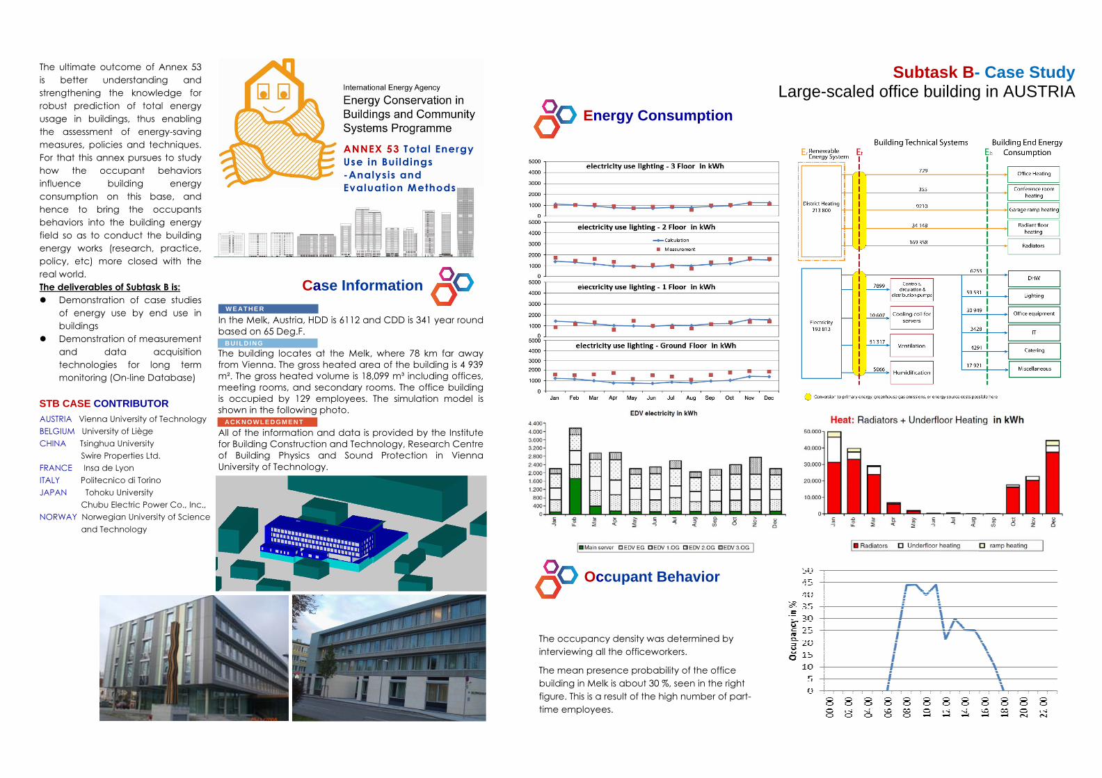
108

The ultimate outcome of Annex 53

is better understanding and

strengthening the knowledge for

robust prediction of total energy

usage in buildings, thus enabling

the assessment of energy-saving

measures, policies and techniques.

For that this annex pursues to study

how the occupant behaviors

influence building energy

consumption on this base, and

hence to bring the occupants

behaviors into the building energy

field so as to conduct the building

energy works (research, practice,

policy, etc) more closed with the

real world.

The deliverables of Subtask B is:

� Demonstration of case studies

of energy use by end use in

buildings

� Demonstration of measurement

and data acquisition

technologies for long term

monitoring (On-line Database)

Subtask B- Case Study Large-scaled office building in AUSTRIA

Case Information

In the Melk, Austria, HDD is 6112 and CDD is 341 year round

based on 65 Deg.F. The building locates at the Melk, where 78 km far away

from Vienna. The gross heated area of the building is 4 939

m². The gross heated volume is 18,099 m³ including offices,

meeting rooms, and secondary rooms. The office building

is occupied by 129 employees. The simulation model is

shown in the following photo.

All of the information and data is provided by the Institute

for Building Construction and Technology, Research Centre

of Building Physics and Sound Protection in Vienna

University of Technology.

W E AT H E R

B U I L DI NG

AC K N O W L E DGM E N T

The occupancy density was determined by

interviewing all the officeworkers.

The mean presence probability of the office

building in Melk is about 30 %, seen in the right

figure. This is a result of the high number of part-

time employees.

STB CASE CONTRIBUTOR

AUSTRIA Vienna University of Technology

BELGIUM University of Liège

CHINA Tsinghua University

Swire Properties Ltd.

FRANCE Insa de Lyon

ITALY Politecnico di Torino

JAPAN Tohoku University

Chubu Electric Power Co., Inc.,

NORWAY Norwegian University of Science

and Technology

ANNEX 53 Total Energy

Use in Buildings

-Analysis and

Evaluation Methods

Energy Consumption

Occupant Behavior

109

1.2 BEL-01

110

The ultimate outcome of Annex 53 is

better understanding and



usage in buildings, thus enabling the

assessment of energy-saving





consumption on this base, and hence

to bring the occupants behaviors into

the building energy field so as to

conduct the building energy works

(research, practice, policy, etc) more

closed with the real world.


� Demonstration of case studies of

energy use by end use in

buildings


and data acquisition

technologies for long term


Subtask B- Case Study Large-scaled office building in BELGIUM

Case Information

Belgium has a temperate maritime climate influenced by

the North Sea and Atlantic Ocean, with cool summers

and moderate winters. In Brussels, Belgium, HDD is 3148

and CDD is 180 year round based on an indoor

temperature of 18 Deg.C.

The building (DM 28) comprises 10 storeys above ground

and 3 underground, with a conditioned area of 11277m2

each floor. Its HVAC system comprises heating plant (3

gas boilers), cooling plant (2 water cooled chillers and

their respective cooling towers), ventilation system (9

AHUs for different purposes), terminal units (FCUs) and 2

air heaters located in parking spaces.

All of the information and data is provided by the

Thermodynamics Laboratory in the University of Liège.

W E AT H E R

B U I L DI NG







FRANCE Insa de Lyon




NORWAY Norwegian University of

Science and Technology


Use in Buildings

-Analysis and

Evaluation Methods

Energy Consumption

Occupant Behavior

[UNIT: kWhe] Et Eb

1,096,782

1,345,838

1,074,906

Conversion factor

1 MJ hot water= 0.2317 MJ equivalent electricity

Electricity Equivalent Approach (kWhee)

Technical System Building Consumption

ELECTRICITY (kWhe)

Appliances

175,485

IT room

263,228

Lighting

361,938

Pumps

65,807

HEAT (kWhh)

Ventilation

Cooling (kWhc)

FCUs

171,985

153,549

HVAC Auxiliaries

10,968

Liquid Chilling Package

54,839

Cooling Tower

10,968

54,839

354,719

AHUs

548,202

Heaters - Parking

The hourly profile of whole building electricity consumption (showed

below) is used to evaluate the global building occupancy. There are two

periods (6h to 22h for weekdays and 10h to 19h for weekends/holidays),

which correspond to a “switch-on allowance period” defined by BEMS

system where lighting fixtures manually operated can be switched ON or

OFF. In DM 28, working day starts from 8:00 tol 18:00 during the weekdays. It

can be observed that the profile has sort of symmetry during all the

working day and is centered at 13h (lunch time).

Whole Building Electricity Consumption - [kW]

(Hourly Profile - Weekday)

0 1 2 3 4 5 6 7 8 9 10 11 12 13 14 15 16 17 18 19 20 21 22 23

0

100

200

300

400


111

1.3 CHN-01

112

0

2

4

6

8

10

12

14

16

18

20

1 2 3 4 5 6 7 8 9 10 11 12

Ele

c. C

ons.

(kW

h/(m

2.m

onth

))

Publi Lighting and Others AC PlantAHU PAUCarpark Ventilation

[UNIT:mill kWhe] Et Eb

22.53

22.53

Ed Exhaust Fans 0.56

0.00

HEAT (kWhh)42.69

0.00Primary Air Unit

1.87

ElectricityEquivalentApproach

(mill kWhee)


ELECTRICITY(mill kWhe)

Appiances

1.12

Service+Technical sys.

Ventilation

Cold (MWhc)

Heat

DHW

0.56

Lighting

3.93

0.00

Chilled water pump

1.07

Condensor water pump

0.84

Cooling tower

1.06

Chiller

7.81

Air Handling Unit

3.70



strengthening the knowledge for robust

prediction of total energy usage in

buildings, thus enabling the assessment

of energy-saving measures, policies

and techniques. For that this annex

pursues to study how the occupant

behaviors influence building energy









energy use by end use in buildings


and data acquisition technologies

for long term monitoring (On-line

Database)

The building is the 6th skyscraper over 1,000 ft. (305

m) completed in Hong Kong. Part of the site was

previously occupied by Melbourne Industrial

Building (23 floor office tower demolished 2005)

and Aik San Factory Building (22 floor commercial

building demolished 2005) which were acquired by

the developer in 2002 and 2001 respectively.

Subtask B- Case Study Large-scaled office building in CHINA

Case Information

Energy Consumption

Publi Lighting and Others

39.8 25%

AC Plant76.6 48%

AHU26.2 16%

PAU13.2 8%

Carpark Ventilation

4.0 3%

The building consumes 22.5

million kWh electricity annually

(not including the electricity use

of tenant). The breakdown of

major devices is shown in the

right figure (unit: million kWhe).

The annual total cooling

consumption is approximately

42,687 MWh, equals to 302.7

kWhc/(m2.a).

Occupant Behavior

Hong Kong is a humid subtropical climate. The heating degree days

(65F) is around 193, and cooling degree days (65F) is approximately

3717 year round.

One Island East is a supertall skyscraper that is located in TaiKoo Place

on Island East, Hong Kong. The skyscraper is a commercial office

building, completed on March 2008, rises 298.35 (979 ft) and has 69

stories of habitable office space and two basement levels. There is a sky

lobby on the 37th and 38th floors. In addition, there are 28 high speed

passenger lifts, 6 high speed shuttle lifts between Main (G-1F) and Sky

(37-38/F) Lobbies, 1 passenger lift between main lobby and basement

carpark and 2 service lifts.

All of the case building information is provided by Swire Properties Ltd.,

Hong Kong. Sincerely thanks for the supporting of the Technical Service

& Sustainability Department.

W E AT H E R

B U I L DI NG


0%

10%

20%

30%

40%

50%

60%

70%

80%

90%

100%

0:00 6:00 12:00 18:00 0:00

Occ

upan

cy

0%

10%

20%

30%

40%

50%

60%

70%

80%

90%

100%

0:00 6:00 12:00 18:00 0:00

Ligh

ts o

pen

perc

enta

ge

Two representative offices in this large-scaled office building have been chosen to pursue the

questionnaire survey. This two offices take up two floors, serves to the same company. The Gross Floor

Area of two office is 3830 sqm with 210 employees. The percentage of valid questionnaire is 76%. The

following charts show the occupancy and lights open percentage during the typical weekday.

STB CASE CONTRIBUTOR AUSTRIA Vienna University of Technology




FRANCE Insa de Lyon






ANNEX 53 Total Energy Use

in Bui ldings

-Analysis and Evaluation

Methods

113

1.4 ITA-01

114

The ultimate outcome of Annex 53 is better

understanding and strengthening the knowledge

for robust prediction of total energy usage in

buildings, thus enabling the assessment of energy-

saving measures, policies and techniques. For that

this annex pursues to study how the occupant

behaviors influence building energy consumption

on this base, and hence to bring the occupants

behaviors into the building energy field so as to

conduct the building energy works (research,

practice, policy, etc) more closed with the real

world.


� Demonstration of case studies of energy use by

end use in buildings

� Demonstration of measurement and data

acquisition technologies for long term


Subtask B- Case Study Small-scaled office building in ITALY

Case Information

The building is located at Livorno Ferraris (Vercelli), Italy, where HDD is

2549. For standard typical meteorological year, the maximum dry bulb

temperature is 31.0 °C and minimum dry bulb temperature is -7.0 °C.

The case building (Palazzo Ciocca) has 5 floors in total (3 floors over

ground, 1 floor underground and 1 attic). Its gross floor area is 1096 m2

and net floor area is 756 m2. Height of the building is 15.5m.

All of the information and data is provided by the TEBE Research

Group, Department of Energetics, Politecnico di Torino.






FRANCE Insa de Lyon





and Technology

WEATHER

ACKNOWLEDGMENT

BUILDING

Occupant Behavior label Occupancy profile Equipment

A

1 person from Monday to

Friday. Hours: 8 am to 2

pm and 3 pm to 6 pm

1 pc and 1 printer

B

2 persons from Monday

to Friday. Hours: 8 am to 2

pm and 3 pm to 6 pm

2 personal computers

and 2 printers

C Occasionally occupancy 2 printers

D Occasionally occupancy

E

2 persons from Monday

to Friday. Hours: 8 am to 2

pm and 3 pm to 6 pm

2 personal computers

and 2 printers

F

1 fridge, 1 microwave

oven, 1 automatic coffee

dispenser, electric hot

water boiler

G

1 person from Monday to

Friday. Hours: 8 am to 2

pm and 3 pm to 6 pm

H Occasionally occupancy


Use in Buildings


Methods

115

1.5 JPN-01, JPN-02

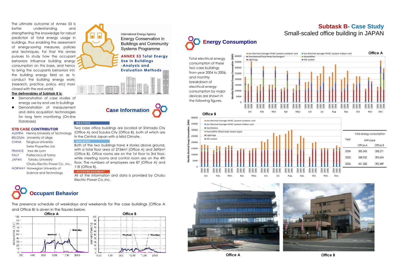
116






















Database)

Subtask B- Case Study Small-scaled office building in JAPAN

Case Information

Two case office buildings are located at Shimada City

(Office A) and Suzuka City (Office B), both of which are

in the Central Japan with a Mild Climate.

Both of the two buildings have 4 stories above ground,

with a total floor area of 2734m2 (Office A) and 3695m2

(Office B). Office rooms are on the 1st floor to 3rd floor,

while meeting rooms and control room are on the 4th

floor. The numbers of employees are 87 (Office A) and

118 (Office B).

All of the information and data is provided by Chubu

Electric Power Co.,Inc.

W E AT H E R

B U I L DI NG






FRANCE Insa de Lyon







Use in Buildings

-Analysis and

Evaluation Methods

Energy Consumption

Occupant Behavior

Office A Office B

The presence schedule of weekdays and weekends for the case buildings (Office A

and Office B) is given in the figures below.

Office A

0

5000

10000

15000

20000

25000

30000

35000

40000

2004

2005

2006

2004

2005

2006

2004

2005

2006

2004

2005

2006

2004

2005

2006

2004

2005

2006

2004

2005

2006

2004

2005

2006

2004

2005

2006

2004

2005

2006

2004

2005

2006

2004

2005

2006

Jan Feb Mar Apr May Jun Jul Aug Sep Oct Nov Dec

Mo

nth

ly E

lect

rica

l En

erg

y C

on

sum

pti

on

[k

Wh

] Ice thermal storage HVAC system outdoor unit Ice thermal storage HVAC system indoor unit

Ventilation(Total Heat Exchanger) Humidifier

Lightings OA socket

0

5000

10000

15000

20000

25000

30000

35000

40000

2004

2005

2006

2004

2005

2006

2004

2005

2006

2004

2005

2006

2004

2005

2006

2004

2005

2006

2004

2005

2006

2004

2005

2006

2004

2005

2006

2004

2005

2006

2004

2005

2006

2004

2005

2006

Jan. Feb. Mar. Apr. May. Jun. Jul. Aug. Sep. Oct. Nov. Dec.

Mo

nth

ly E

lect

rica

l En

ergy

Co

nsu

mp

tio

n [

kWh

]

Ice thermal storage HVAC system outdoor unit

Ice thermal storage HVAC system indoor unit

Ventilation

Humidifier [Electrode steam type]

Lightings

OA socket

Office B

Office A

Office B

Year

Total energy consumption

kWh/year

Office A Office B

2004 285,543 358,271

2005 348,925 393,654

2006 451,328 392,489

Total electrical energy

consumption of these

two case buildings

from year 2004 to 2006,

and monthly

breakdown of

electrical energy

consumption by major

devices are shown in

the following figures.

117

1.6 JPN-03

118

The ultimate outcome of Annex 53

is better understanding and









consumption on this base, and

hence to bring the occupants

behaviors into the building energy

field so as to conduct the building

energy works (research, practice,

policy, etc) more closed with the

real world.


� Demonstration of case studies

of energy use by end use in

buildings

� Demonstration of

measurement and data

acquisition technologies for

long term monitoring (On-line

Database)

Subtask B- Case Study Small-scaled office building in JAPAN

Case Information

Sendai is cold and snowy in winter, while hot and humid

in summer. Minimum and maximum temperatures are

1.5 Deg.C. in January and 24.1 Deg.C. in August.

The case building is a three-storey office building which

covers a floor area of 4090 m2. The office building is

constructed in wood with the purpose to reduce the

CO2 emissions. High quality air-conditioners with COP

value over 5.0 are installed for heating and cooling,

while mechanical ventilation system with air change

rate of 0.5 times per hour is used for ventilating.

All of the information and data is provided by Tohoku

University.

W E AT H E R

B U I L DI NG






FRANCE Insa de Lyon







Use in Bui ldings


Methods

Energy Consumption

There are 20 workers in total, and all of them can take two days off in one week. One day is

on Sunday, and for the other day, half of them take Wednesday, while the other half of them

take Saturday. The presence schedule in one day is showed in the left figure. Although the

business hour starts at 9:00am, 100% of the workers come to the office around 8:30am. The

workers take a one-hour lunch break, and thus the percentage at 1:00pm was assumed as

50%. The business hour finishes at 6:00, but some work until 8:00pm. The air-conditioners are

operated from 8:00am to 18:00Pm.

The following figure shows the annual energy consumption in this office building, with the comparison to the statistical

data of 2005 and 2007. The convector coefficient of electricity consumption to primary energy consumption was

10.25MJ/kWh. Lighting, the largest energy user, accounted for about 43% of the total electricity consumption and it was

followed by OA (Office Appliance) machines which accounted for 25%. Annual heating and cooling electricity

consumption accounted for 12% and 2% of the total electricity consumption, respectively. Annual energy consumption of

the measured office building (921 MJ/m2.year) was 47% lower than the statistical data (1739 MJ/m2.year).

The monthly energy

consumption by different

end-users of the case

building is shown in the

right figure. Energy

consumption increased

during the heating (from

November till the end of

April next year) and

cooling period (August

and September).

Occupant Behavior

119

1.7 NOR-01

120


better understanding and strengthening

the knowledge for robust prediction of

total energy usage in buildings, thus

enabling the assessment of energy-

saving measures, policies and

techniques. For that this annex pursues to

study how the occupant behaviors

influence building energy consumption

on this base, and hence to bring the

occupants behaviors into the building

energy field so as to conduct the building

energy works (research, practice, policy,

etc) more closed with the real world.




� Demonstration of measurement and

data acquisition technologies for

long term monitoring (On-line

Database)

Subtask B- Case Study Large-scaled office building in NORWAY

Case Information

In Norway, CDD is not an actual parameter. HDD is 4856

of year 2010. HDD was calculated for the base indoor

temperature of 17oC.

The case is an office building in Stavanger. There are 5

floors and basement. The Gross Floor Area is 19,623 m2.

Height of the building is 15 m assumed according to the

number of floors.

All the information and data is provided by Energy and

Process Engineering of Norwegian University of Science

and Technology.

W E AT H E R

B U I L DI NG


The building was design for 1200 occupants. In general, there are 1000 occupants every day

in the building. This office building is rented to one company. Most of the employees are

engineers, researchers, and administration. Since the installed ventilation system is VAV, the

presence schedule can be assumed based on the fan input signal. This assumed occupancy

schedule based on the fan input signal is given in the left Figure.






FRANCE Insa de Lyon





and Technology

Energy Consumption

Occupant Behavior


Use in Bui ldings


Methods

121

1.8 NOR-02

122






















Database)

Subtask B- Case Study Large-scaled office building in NORWAY

Case Information

In Norway, CDD is not an actual parameter. HDD is 4856 of

year 2010. HDD was calculated for the base indoor

temperature of 17oC.

The case is an office building in Professor Brochs gate 2.

Height of the building is 21 m (the front block) and 14 m

(the back block). The Gross Floor Area and conditioned

building both are 16,200 m2

All the information and data is provided by Energy and

Process Engineering of Norwegian University of Science

and Technology.

W E AT H E R

B U I L DI NG


The presence schedule for the office building in Trondheim is given in the following figure. This office building is rented to

different companies, usually companies have working time between 8 a.m. until 4 p.m. But some companies could

extend working time until 5 or 6 p.m. In general, it can be assumed that working hours is about 2000 hours for light and

ventilation in the building. Light in the corridors and common area is working longer. Working hours of the IT server room is

8760 hours.





FRANCE Insa de Lyon







Use in Bui ldings


Methods

Energy Consumption

Occupant Behavior

123

2. Residential building

2.1 AUT-01

124

The ultimate outcome of Annex

53 is better understanding and





measures, policies and

techniques. For that this annex

pursues to study how the

occupant behaviors influence

building energy consumption on

this base, and hence to bring

the occupants behaviors into


conduct the building energy

works (research, practice, policy,

etc) more closed with the real

world.


� Demonstration of case

studies of energy use by end

use in buildings




long term monitoring (On-

line Database)

Subtask B- Case Study A Single Family House in AUSTRIA (1 of 3)

Case Information

The detached single family house is located in the

Vorarlberger Highlands close to the western border of

Austria. Average monthly temperatures range between -

4°C to 24°C and is within the cool/temperate Alpine

climate zone.

This case study house is the first in a series of three that

have been compared in a study investigating the

relationship between the energy certificate calculations,

the impact of actual thermal renovations on energy use,

and user behaviour in the individual houses.

W E AT H E R

B U I L DI NG





FRANCE Insa de Lyon





and Technology


Use in Buildings

-Analysis and

Evaluation Methods

Energy Consumption

Occupant Behavior

Ground and upper floor indoor temperatures 19.5 °C

People 0.53 W/m² TFA Internal loads

Appliances and lighting 2.08 W/m² TFA 2.61 W/m²TFA

Domestic hot water 4.54 kWh/m²a

125


















world.




use in buildings





line Database)


Case Information

The detached single family house is located in the

Vorarlberger Highlands close to the western border of



climate zone.

This case study house is the second in a series of three that

have been compared in a study investigating the

relationship between the calculations in the energy

certificate, the impact of actual thermal renovations on

energy use, and user behaviour in the individual houses.

W E AT H E R

B U I L DI NG





FRANCE Insa de Lyon





and Technology


Use in Buildings

-Analysis and

Evaluation Methods

Energy Consumption

Occupant Behavior

Room temperature 19.5 °C

People 0.53 W/m²TFA Internal loads

Appliances and lighting 2.08 W/m²TFA 2.61 W/m²TFA


Air change rate n [h-1]

Month 1 2 3 4 5 6 7 8 9 10 11 12 Single-sided window ventilation 0.08 0.08 0.09 0.09 0.10 0.10 0.10 0.10 0.10 0.10 0.09 0.08

Cross ventilation 0.09 0.08 0.09 0.15 0.18 0.26 0.23 0.22 0.21 0.11 0.11 0.10 Base case 0.5 0.5 0.5 0.5 0.5 0.5 0.5 0.5 0.5 0.5 0.5 0.5

Infiltration through gaps Renovated 0.25 0.25 0.25 0.25 0.25 0.25 0.25 0.25 0.25 0.25 0.25 0.25

Hourly opening time in minutes with an outdoor temperature of 10°C

Floor Room Area m²

Opening 1 2 3 4 5 6 7 8 9 10 11 12 13 14 15 16 17 18 19 20 21 22 23 24

Kitchen 1.7 Fully open 6 Living Room A 2.3 Tilted 6 Living Room B 1.3 Fully open 5

Study 1.9 Fully open 6 Entry 1.7 Fully open 5 5 5

Ground floor

Bathroom 0.9 Fully open 5 Bedroom 1 1.9 Fully open 6 Bedroom 2 2.3 Fully open 6 Bedroom 3 1.3 Fully open 6

Upper floor

Bathroom 0.9 Fully open 6 5 6 Cross ventilation Window areas

Ground floor 4.0 & 5.0 12

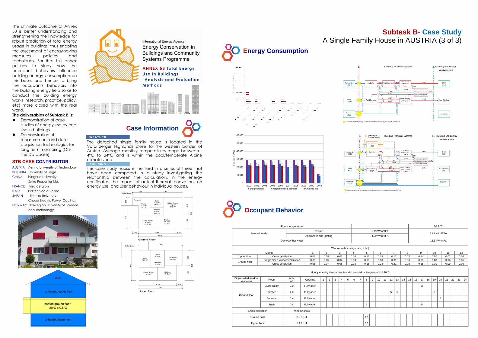
126


















world.




use in buildings





line Database)


Case Information

The detached single family house is located in the Vorarlberger Highlands close to the western border of Austria. Average monthly temperatures range between -4°C to 24°C and is within the cool/temperate Alpine climate zone. This case study house is the third in a series of three that have been compared in a study investigating the relationship between the calculations in the energy certificates, the impact of actual thermal renovations on energy use, and user behaviour in individual houses.

W E AT H E R

B U I L DI NG STB CASE CONTRIBUTOR AUSTRIA Vienna University of Technology




FRANCE Insa de Lyon





and Technology


Use in Bui ldings


Methods

Energy Consumption

Occupant Behavior

Room temperature 20.3 °C




Window – Air change rate, n [h-1]

Month 1 2 3 4 5 6 7 8 9 10 11 12 Upper floor Cross ventilation 0.06 0.05 0.06 0.10 0.13 0.19 0.17 0.17 0.14 0.07 0.07 0.07

Single-sided window ventilation 0.05 0.05 0.07 0.08 0.09 0.10 0.09 0.10 0.08 0.08 0.06 0.06 Ground floor

Cross ventilation 0.08 0.07 0.08 0.13 0.16 0.23 0.21 0.19 0.18 0.10 0.09 0.09

Hourly opening time in minutes with an outdoor temperature of 10°C

Single-sided window ventlation Room Area

m² Opening 1 2 3 4 5 6 7 8 9 10 11 12 13 14 15 16 17 18 19 20 21 22 23 24

Living Room 2.0 Fully open 3

Kitchen 2.0 Fully open 5 5 5

Bedroom 1.4 Fully open 3 Ground floor

Bath 0.4 Fully open 5 5

Cross ventilation Window areas


Upper floor 1.4 & 1.4 12

127

2.2 AUT-02

128


















world.




use in buildings





line Database)

Subtask B- Case Study A Single Family House in Austria

Case Information

Hourly weather data for Vienna was used for the dynamic

simulation. The source data includes exterior temperature,

relative humidity, wind speed and direction, precipitation,

atmospheric pressure, solar radiation (both orientation and

angle dependent) for each hour. The exterior temperature

and the global horizontal radiation are presented in Fig. 1.

The demonstration dwelling was built in Austria in 1930 −

1932 and is located in an urban area. Figure 2 presents the

location and orientation of the investigated house.

W E AT H E R

B U I L DI NG





FRANCE Insa de Lyon





and Technology


Use in Bui ldings


Methods

Energy Consumption

Occupant Behavior

� Lifestyle 1 Lifestyle 1 Lifestyle 1 Lifestyle 1 ((((L1L1L1L1)))):::: only the living room is heated to a

room temperature of 20℃ in the morning and

evening.

� Lifestyle 2 (L2Lifestyle 2 (L2Lifestyle 2 (L2Lifestyle 2 (L2)))):::: all rooms are kept at a minimum

temperature of 15℃; the living room has a room

temperature of 20℃ in the morning and evening.

� Lifestyle 3 Lifestyle 3 Lifestyle 3 Lifestyle 3 ((((L3L3L3L3)))):::: all rooms are kept at a minimum

temperature of 15℃; the living and occupied rooms

are heated when occupied to 22℃; the bedroom

temperature is 20℃.

� Lifestyle 4 Lifestyle 4 Lifestyle 4 Lifestyle 4 ((((L4L4L4L4)))):::: all rooms have an interior

temperature of 22℃.

129

2.3 AUT-03

130


















world.




use in buildings





line Database)

Subtask B- Case Study A Single Family House in Austria

Case Information

Heated ground area: 389.40 m²

Heated building volume: 887.83 m³

Cellar (unheated): 189.3 m², ground floor: 211.9 m², first floor:

177.4 m²

Cellar ceiling= 189.3 m², U-value=0.41 W/m²K

Exterior wall= 326.00 m², U-value=0.18 W/m²K

Roof area= 226.60 m², U-value=0.20 W/m²K

Windows: U-value= 1.10 W/m²K, g=0.6

Area [m²]

North 9,66

South 11,67

West 5,99

Windows

East 6,69

34,01

B U I L DI NG





FRANCE Insa de Lyon





and Technology


Use in Bui ldings


Methods

Energy Consumption

Occupant Behavior

pressure difference (Pa)

air change rate (1/h)

Heating energy demand [kWh/(m² a)]

Sim-standard user profile Bil-Standard user profile Sim-real user profile

House is occupied since November 2004: 4 Adults, 1 Child. A person (housewife) is continuously at home. At least, four people regularly sleep in the house. Short trips are taken only during the holidays and Christmas (about two weeks). The Wood-House cools down in this time from 22-23 °C to 18-19 °C, without being heated. Partially is the heating night setback activated. Cellar is unheated: Indoor temperature is about 15 °C, except Kettle room All other rooms are heated to about 22 °C, except bedroom of the parents. There are four stoves in the house. The stove in the living room is in constant operation. The temperature is measured only in the work room.

Area [m²] North 0 South 18,72 West 6,4675

Doors

East 3,8 28,9875

131

2.4 AUT-04

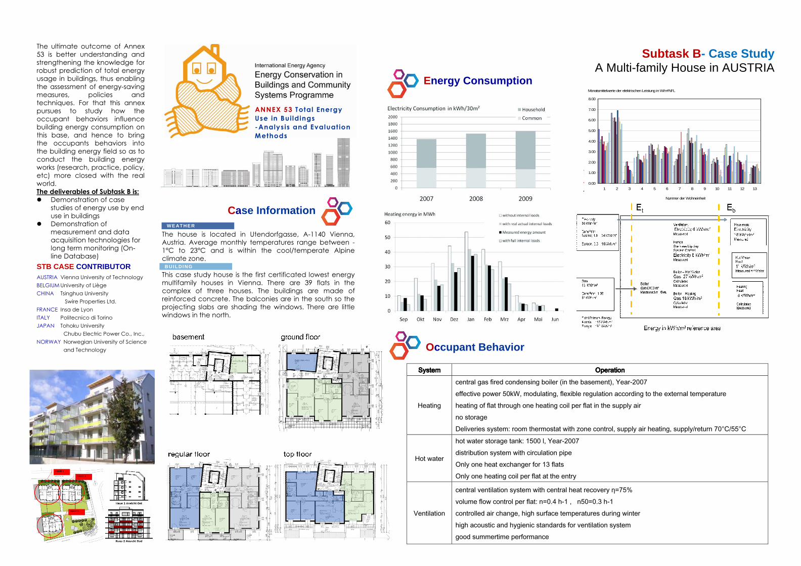
132

SystemSystemSystemSystem OperationOperationOperationOperation

Heating

central gas fired condensing boiler (in the basement), Year-2007

effective power 50kW, modulating, flexible regulation according to the external temperature

heating of flat through one heating coil per flat in the supply air

no storage

Deliveries system: room thermostat with zone control, supply air heating, supply/return 70°C/55°C

Hot water

hot water storage tank: 1500 l, Year-2007

distribution system with circulation pipe

Only one heat exchanger for 13 flats

Only one heating coil per flat at the entry

Ventilation

central ventilation system with central heat recovery η=75%

volume flow control per flat: n=0.4 h-1 , n50=0.3 h-1

controlled air change, high surface temperatures during winter

high acoustic and hygienic standards for ventilation system

good summertime performance


















world.




use in buildings





line Database)

Subtask B- Case Study A Multi-family House in AUSTRIA

Case Information

The house is located in Utendorfgasse, A-1140 Vienna,



climate zone.

This case study house is the first certificated lowest energy

multifamily houses in Vienna. There are 39 flats in the

complex of three houses. The buildings are made of

reinforced concrete. The balconies are in the south so the

projecting slabs are shading the windows. There are little

windows in the north.

W E AT H E R

B U I L DI NG STB CASE CONTRIBUTOR AUSTRIA Vienna University of Technology




FRANCE Insa de Lyon





and Technology


Use in Bui ldings


Methods

Energy Consumption

Occupant Behavior

0.00

1.00

2.00

3.00

4.00

5.00

6.00

7.00

8.00

1 2 3 4 5 6 7 8 9 10 11 12 13

Monatsmittelwerte der elektrischen Leistung in W/m²NFL

Nummer der Wohneinheit

133

2.5 BEL-01

134


53 is better understanding and strengthening the knowledge for

robust prediction of total energy usage in buildings, thus enabling the assessment of energy-saving

measures, policies and techniques. For that this annex pursues to study how the

occupant behaviors influence building energy consumption on this base, and hence to bring

the occupants behaviors into the building energy field so as to conduct the building energy

works (research, practice, policy, etc) more closed with the real world.


� Demonstration of case studies of energy use by end

use in buildings � Demonstration of


acquisition technologies for long term monitoring (On-

line Database)

Subtask B- Case Study A Single Family House in Belgium

Case Information

The climate in Belgium is temperate. The heating degrees day value (15°C) is around 2726 K.h/year and the cooling degrees days (18.3 °C) value is only 173 K.h/year. This house has been built in 2008 and has a occupiable surface of 285 m² and a volume of 741m³. The compactness is 1.29 m and the mean heat transfer coefficient is 0.32 W/K.m². There are around 53 m² of windows. The house is heated with an air/water heat pump and a low inertia floor heating. This heat pump produces also the domestic hot water. Three adults live in this house. There is no monitoring on the total electrical consumption, but the electrical power used by the heat pump and the heating power produced by it are monitored. One indoor temperature is monitored as well. All of the case building information is provided by the BEMS team of the University of Liège.

W E AT H E R

B U I L DI NG






FRANCE Insa de Lyon





and Technology


Use in Bui ldings


Methods

Energy Consumption

Occupant Behavior During the analyzed period, the control of the indoor temperature was quite simple (and not really energy efficient) as it was set to 23 °C (on the thermostat) all along the year. The graph here represents the monthly electrical energy quantities absorbed by the heat pump and the calorific energy quantities produced with it. These energy flows are separated in two categories: heating of the house and domestic hot water production.

Energy balances [kWh]

Heat pump House

Air 11011 Heating gains 17237

Electricity 9752 Solar gains 12233

Heating -17237 Human gains 1818

DHW -3526 Electrical gains 5356

Infilt. & man. Vent. losses -6310

Mech. ventilation losses -2682

Transmission losses -27650

Sankey Diagram

These to bar plot have been

created with the results of a TRNSYS

simulation. Estimations have been

done for the unknown parameters.

The values chosen for these

parameters are the ones which

minimize the difference between

the real and the estimated monthly

energy consumptions (kWh) and

over-heatings (K.h).

On the analyzed year, the heat

pump consumed 9752 kWh of

electricity and produced 20763

kWh of calorific energy. This energy

is used to heat the house and the

domestic hot water.

The indoor electrical consumption

(including lighting, cooking,

appliances, etc.) is not monitored

and then not included in the

following calculus.

The yearly annual surface

consumption for the heating and

the DHW is 34 kWh/m².

In primary energy (factor 2.5 for the

electricity) it gives 84 kWh/m².

The yearly CO2 emission is

0.456*9752 = 4447 kg/CO2 or 15 kg

CO2/m²

135

2.6 BEL-02

136


53 is better understanding and strengthening the knowledge for

robust prediction of total energy usage in buildings, thus enabling the assessment of energy-saving

measures, policies and techniques. For that this annex pursues to study how the

occupant behaviors influence building energy consumption on this base, and hence to bring

the occupants behaviors into the building energy field so as to conduct the building energy

works (research, practice, policy, etc) more closed with the real world.


� Demonstration of case studies of energy use by end

use in buildings � Demonstration of


acquisition technologies for long term monitoring (On-

line Database)

Subtask B- Case Study A Single Family House in Belgium

Case Information

The climate in Belgium is temperate. The heating degrees day value The climate in Belgium is temperate. The heating degrees day value (15°C) is around 2726 K.h/year and the cooling degrees days (18.3 °C) value is only 173 K.h/year. This apartment has been built in 2004 and has a surface of 95 m² and a volume of 237 m³. It is quite compact (3.1 m) and insulated (Um = 0.51 W/K.m²). There are around 9 m² of windows. The apartment is heated with a gas boiler (which is inside the protected volume). This boiler is also used to produce the domestic hot water. A young couple lives in this apartment and they work both five days a week. The electrical consumption and the indoor temperature are recorded every five minutes and the gas consumption once a day. All of the case building information is provided by the BEMS team of the University of Liège.

W E AT H E R

B U I L DI NG






FRANCE Insa de Lyon





and Technology


Use in Bui ldings


Methods

Energy Consumption

Occupant Behavior The two occupants work during the weekdays, so there are away from the apartment between 9am and 6pm. During the weekend, they stay normally in the apartment during the day. The apartment is heated in a homogeneous way (same indoor temperature in all the volume).

Sankey Diagram

These bar plots and the energy

balances tables have been

created with the results of a TRNSYS

simulation. Estimations have been

done for the unknown parameters.

The values chosen for these

parameters are the ones which

minimize the difference between

the real and the estimated monthly

energy consumptions (kWh) and

over-heatings (K.h).

The apartment consumes 5442

kWh/year of gas and 2652 kWh of

electricity. The gas is used to heat

the apartment and to produce the

domestic hot water. There is no

cooling system.

The annual surface consumption is

57 kWh/m² of gas and 28 kWh/m² of

electricity.

In primary energy (factor 1 for the

gas and

2.5 for the electricity) it gives:

57+2.5*28 = 127 kWh/m²

The total yearly CO2 emission is

0.251*5442+0.456*2652=2575

kg/CO2 or 27 kg CO2/m²

Energy balances [kWh]

Boiler House

Gas 5442 Heating gains 3654

Heating -3654 Solar gains 2109

DHW -1461 Human gains 829

Losses -257 Electrical gains 2652

Infiltration losses -806

Ventilation losses -4864


137

2.7 BEL-03

138


















world.




use in buildings





line Database)

Subtask B- Case Study Thermal Simulation and Monitoring of a Dwelling

Case Information

This dwelling located on the Belgian coast (Figure 1) has a

total floor area of 95 m2. It can be subdivided into 9

different zones (with toilet and boiler room aggregated

into only one zone) as indicated in Figure 2. The living room

is oriented to the North (i.e. on see side).Two of the

sleeping rooms are oriented to the South; a third one is

“blind”.

The dwelling is equipped with a simple mechanical

ventilation system: exhaust openings are located in the

kitchen, in the shower corners of two rooms, in the bath

room, in the toilet and in the boiler room.

Direct electric heaters are available in all rooms, except

the kitchen, the corridor, the toilet and the boiler room.

This work is supported by the Walloon Region of Belgium..

B U I L DI NG






FRANCE Insa de Lyon





and Technology


Use in Bui ldings


Methods

Energy Consumption

Occupant Behavior Only the living room is supposed to

be heated all along daily

occupation periods.

According to the occupancy rate of

the dwelling, the bath room and the

shower corners of two sleeping

rooms might be heated during

limited morning and evening

periods.

The dwelling is surrounded by four

other dwellings which are not always

occupied

139

2.8 CHN-01

140


















world.




use in buildings





line Database)

Subtask B- Case Study Multi-family Apartment-Source Book

Case Information

The apartment building is located in Tsinghua University

Campus, Beijing, China. Beijing is the capital of China, with

latitude: 39° 55'N and longitude: 116° 23'. Its climate is

rather dry, monsoon-influenced humid continental climate,

hot, humid summers due to the East Asian monsoon, and

generally cold, windy, dry winters that reflect the influence

of the vast Siberian anticyclone. The monthly daily

average temperature in January is −3.7 °C, while in July it is

26.2 °C. Precipitation averages around 570 mm annually,

with the great majority of it falling in the summer months.

Extremes have ranged from −27.4 to 42.6 °C.

This case study house is compared in a study investigating

the relationship between the energy use and occupant

behavior in the multi-family apartment.

The authors from Tsinghua University highly appreciate

great helps from the residents to provide her family as case

study for IEA ECBCS ANNEX 53.

W E AT H E R

B U I L DI NG






FRANCE Insa de Lyon





and Technology


Use in Bui ldings


Methods

Energy Consumption

Occupant Behavior

141

2.9 JPN-01

142

Sendai


















world.




use in buildings





line Database)

Subtask B- Case Study Example of a detached house in Japan

Case Information

Fig.1 shows the location of Sendai in Japan. Fig.2 shows the

monthly mean temperatures and mean humidities in

Sendai, Montreal and Berlin. Sendai is cold and snowy in

winter, but hot and humid in summer. The raining season of

Japan is from June to July. Minimum and maximum

temperatures are 1.5 0C in January and 24.1 0C in August

respectively. The main objectives of this investigation are, 1) to show an

example of case study for residential building, 2) to clarify

actual conditions of the total energy use and factors

influencing energy use. This investigated house is a well-

insulated detached house with energy source of electricity

exclusively. This is a typical type of detached house in

Japan as shown in Fig.3

W E AT H E R

B U I L DI NG





FRANCE Insa de Lyon





and Technology


Use in Bui ldings


Methods

Energy Consumption

Occupant Behavior

8190

8190

1001010010

Bath room Entrance

Storeroom

HallLavatory

Living roomDining roomKitchen

Main bed room

Bed room 2

Bed room 1

Store room

Hall

8190

8190

1001010010

Bath room Entrance

Storeroom

HallLavatory


Main bed room

Bed room 2

Bed room 1

Store room

Hall

Heat sourceElectricity 3.6 MJ/kWh

Conversion value

143

2.10 JPN-02

144


















world.




use in buildings





line Database)

Subtask B- Case Study Example of an apartment house in Japan

Case Information

Fig.1 shows the location of Fukushima in Japan. Fig.2 shows

the monthly mean temperatures and mean humidities in

Fukushima, Montreal and Berlin. Fukushima is cold and

snowy in winter, but hot and humid in summer. The rainning

season of Japan is from June to July. Minimum and

maximum temperatures are 1.4 0C in January and 25.2 0C

in August respectively

The main objectives of this investigation are, 1) to show an

example of case study for residential building, 2) to clarify

actual conditions of the total energy use and factors

influencing energy use. The investigated apartment is a

typical type of house unit in Japan (cf. Fig.3) and it is

situated on the 6th floor of a 15-story multi-family building

with energy sources of electricity and city gas.

W E AT H E R

B U I L DI NG





FRANCE Insa de Lyon





and Technology


Use in Bui ldings


Methods

Energy Consumption

Occupant Behavior

0 1 2 3 4 5 6 7 8

Dec-02Jan-03Feb-03Mar-03Apr-03May-03Jun-03Jul-03

Aug-03Sep-03Oct-03Nov-03

Energy consumption[GJ/month]

Lighting & Others HealthcareAudio visual & information Hot water supply/KitchenSpace heating/cooling

0 10 20 30 40 50 60 70

Dec02～Nov03

Energy consumption[GJ/year]

Heat sourceElectricity 3.6 MJ/kWh

Gas（4A～7C） 20.4 MJ/Nm3

Conversion value

0

2

4

6

0:00 12:00 0:00 12:00 0:00 12:00

Audio visual & informationHealthcareLighting & Others

2003. 3/3 3/4 3/5

0

15

30

45

En

erg

y co

nsu

mp

tion

［M

J/h］

. Space heating/cooling

Hot water supply/KitchenOthers

-100

102030

Tem

p.［℃

］

Living room

Outdoor air

Coldest day

0

10

20

30

En

erg

y co

nsu

mp

tion

［M

J/h］

.

Others Hot water supply/Kicthen Space heating/cooling2025303540

Tem

p.［℃

］

Living roomOutdoor air

0.0

1.0

2.0

3.0

4.0

0:00 12:00 0:00 12:00 0:00 12:00


2003. 8/3 8/4 8/5

Hottest day

145

III-5

Case source book

146

Contents

1. AUT-01: Office Building in Austria ..................................................................... 151

1.1 Introduction...........................................................................................................................151

1.2 Location and climate conditions ...........................................................................................151

1.3 Building description and building systems ...........................................................................152

1.4 Experimental and computational investigations ...................................................................154

1.5 Occupants and equipment operation.....................................................................................154

1.6 Measurements .......................................................................................................................155

1.7 Comparison between measurements and simulations...........................................................158

1.8 Conclusions...........................................................................................................................162

1.9 References.............................................................................................................................162

2. BEL-01: Office building in Belgium..................................................................... 163

2.1 Building introduction............................................................................................................163

2.2 Building specification ...........................................................................................................165

2.3 Energy consumption issue ....................................................................................................166

2.4 Occupant behavior ................................................................................................................171

2.5 Detailed system description ..................................................................................................173

2.6 References.............................................................................................................................179

2.7 Appendix...............................................................................................................................180

3. CHN-01: Office building in China........................................................................ 182



3.3 Database description by the definition of Subtask A............................................................186

4. ITA-01: Office building in Italy............................................................................ 217

4.1 Basic Information of Building ..............................................................................................217

4.2 Detailed information .............................................................................................................221

5. JPN-01, JPN-02: Office building in Japan........................................................... 224

5.1 Building Introduction............................................................................................................224

5.2 Annual Electrical Energy Consumption ...............................................................................224

5.3 Monthly Breakdown of Electrical Energy Consumption by Major Devices ........................225

5.4 Occupant Behavior................................................................................................................226

147

6. JPN-03: Office building in Japan ......................................................................... 227

6.1 Introduction...........................................................................................................................227

6.2 Location ................................................................................................................................227

6.3 Climatic conditions ...............................................................................................................227

6.4 Outline of the office building................................................................................................228

6.5 Occupants and operation of the equipment...........................................................................228

6.6 Investigated items and measurement systems.......................................................................229

6.7 Measured energy consumption and indoor environment ......................................................229

7. NOR-01: Office building in Norway.....................................................................232




7.4 Occupant behavior description .............................................................................................244

7.5 Details system description ....................................................................................................251

8. NOR-02: Office building in Norway.....................................................................262



8.3 Occupant behavior ................................................................................................................265

9. AUT-01: Single Family House in Austria ............................................................ 267

9.1 Introduction...........................................................................................................................267


9.3 Overview of the detached house ...........................................................................................267

9.4 HVAC overview ...................................................................................................................270

9.5 Family members and occupant behavior ..............................................................................271

9.6 Investigation methodology....................................................................................................272

9.7 Energy demand calculations and actual energy use..............................................................273

9.8 Conclusions...........................................................................................................................276

9.9 References.............................................................................................................................277


10.1 Introduction...........................................................................................................................278



148

10.4 HVAC overview ...................................................................................................................280

10.5 Family members and occupant behavior ..............................................................................281



10.8 Conclusions...........................................................................................................................289


11.1 Introduction...........................................................................................................................290



11.4 HVAC overview ...................................................................................................................292

11.5 Family members and occupant behaviour ............................................................................293



11.8 Conclusions...........................................................................................................................300


12.1 Introduction...........................................................................................................................301

12.2 Background...........................................................................................................................302

12.3 Climate conditions ................................................................................................................303

12.4 Input data and structure of the calculation model .................................................................304

12.5 Research conducted and results achieved .............................................................................306

12.6 Discussion and conclusions ..................................................................................................309

12.7 References.............................................................................................................................310



13.2 Occupant’s Interview and data collection.............................................................................312

13.3 Energy Consumption: ...........................................................................................................314

13.4 Calculations ..........................................................................................................................314

13.5 Result – Blower-Door- measurement ...................................................................................315

13.6 Thermal building simulation.................................................................................................315

14. AUT-06: Multi-storey residential building in Austri a........................................ 317

14.1 Introduction...........................................................................................................................317


149

14.3 Overview of the building ......................................................................................................318

14.4 HVAC overview ...................................................................................................................321


15. BEL-01: Single Family House in Belgium ........................................................... 326

15.1 General overview of the building..........................................................................................326

15.2 Climate..................................................................................................................................328

15.3 Building envelope .................................................................................................................328

15.4 Building equipment and system............................................................................................330

15.5 Simulation and Calibration ...................................................................................................334

15.6 Results...................................................................................................................................338

15.7 Conclusions...........................................................................................................................342

15.8 References.............................................................................................................................343

16. BEL-02: Multi-storey residential building in Belgium....................................... 344

16.1 Overview...............................................................................................................................344

16.2 Climate..................................................................................................................................345

16.3 Available data .......................................................................................................................345

16.4 Monitoring ............................................................................................................................349

16.5 Simulation and calibration ....................................................................................................349

16.6 Results...................................................................................................................................354

16.7 Conclusions...........................................................................................................................358

16.8 References.............................................................................................................................358

17. BEL-03: Multi-storey residential building in Belgium....................................... 359

17.1 Introduction...........................................................................................................................359

17.2 The dwelling .........................................................................................................................359

17.3 Assembling of the simulation model ....................................................................................360

17.4 First simulation results: Influence of occupancy rates..........................................................369

17.5 Monitoring and comparative simulation ...............................................................................375

17.6 Records on longer periods and correlations..........................................................................391

17.7 Conclusions...........................................................................................................................397

17.8 References.............................................................................................................................397

18. CHN-01: Multi-storey residential building in China. ......................................... 398

18.1 Introduction...........................................................................................................................398

150

18.2 Location and climate.............................................................................................................398

18.3 Householder Information ......................................................................................................399

18.4 Investigation Methodology ...................................................................................................401

18.5 Energy usage.........................................................................................................................404

18.6 Occupant behaviors...............................................................................................................405

18.7 Conclusions...........................................................................................................................408

19. JPN-01: Single Family House in Japan................................................................ 409

19.1 Introduction...........................................................................................................................409

19.2 Location & Climatic conditions............................................................................................409

19.3 Outline of the detached house...............................................................................................409

19.4 Family members and occupants’ behavior............................................................................410



19.7 Conclusion ............................................................................................................................414

20. JPN-02: Multi-storey residential building in Japan ........................................... 415

20.1 Introduction...........................................................................................................................415

20.2 Location & Climatic conditions............................................................................................415

20.3 Outline of the apartment .......................................................................................................415

20.4 Family members and occupants’ behavior............................................................................416



20.7 Conclusion ............................................................................................................................420

151

1. AUT-01: Office Building in Austria

Authors: Thomas Bednar and Azra Korjenic 1.1 Introduction

Whole building energy consumption, HVAC, and electrical appliances were noted in detail and reproduced in dynamic simulations. The building was constructed in 2007, and is comprised of a basement with three aboveground stories, see Figure 1-1. The gross heated area of the building is 4 939 m². The gross heated volume is 18,099 m³ including offices, meeting rooms, and secondary rooms. The office building is occupied by 129 employees.

Figure 1-1: Case study Small Office Building in Austria

1.2 Location and climate conditions

Figure 1-2: Building location in Melk, Niederösterreich (Lower Austria)

152

Geographical Data: Geographical position Longitude Latitude Elevation Melk 15.32° East 48.22° North 255 m Melk is a small city in Austria with 5257 residents according to Statistik Austria 2011 census, see Figure 1-2. The distance from Melk to Vienna is approximately 78 km. Climatic conditions for Simulations: The simulation was carried out using representative TRY (Test Reference Year) data sets based upon the 1991 to 2005 climate data from the St. Pölten weather station (next Air Station). Test Reference Years (TRY) are specially mixed records that include meteorological data for each hour of a year. They are a mean, but represent typical weather conditions for a specified region over a year 1.3 Building description and building systems

Figure 1-3: Building façade

Offices are situated at the facades, as seen in Figure 1-3. The restrooms, kitchen, small archives, IT room and the staircase are in the core. Offices and primary work areas are heated to 22 °C. The corridors and interior secondary rooms are heated indirectly by the conditioned office spaces and internal loads. Room heating is provided by district heating from biomass (wood chips and tree bark). Mechanical ventilation supplies fresh air through outlets in all rooms. The fresh air supply is preheated during the winter and precooled during the summer using a 500 m ground-coupled heat exchanger (earth tube). The use of a heating coil is not necessary as the ground tube heat exchanger is sufficient. The building is protected from overheating by a fan installation on the flat roof. Decentralized air conditioning is only provided in the computer server rooms. The cooling fan operates in summer from 12 pm until 7 am and has an airflow volume of 40 m³/h. Domestic hot water is provided by small point-of-use water heaters. The estimated consumption is 5 L per working day and person. Building envelope: The main characteristics of the building envelope are presented in Table 1-1.

Table 1-1: The U-values of the external walls and the flat roof have better insulation values than national legislation requirements.

153

Main window specifications are summarized in Table 1-2 below.

Table 1-2: Window characteristics of the investigated building

Frame Glass SHGC (solar heat gain coefficient) Frame Window

spacer Installation Uf Ug g b ΨRV Ψinstallation W/m²K W/m²K - m - - Wood/Aluminium Offices 1.4 1.1 0.5 0.05 -0.12 0.06 0.35 Aluminium Window Public Help Desks 2.2 1.1 0.37 0.05 0.06 0.35

EW_external wall Thickness

(m) Heat conductivity

(W/mK) Storage capacity

(J/kgK) Density (kg/m³)

wood 0.10 0.13 2500 550

mineral wool 0.10 0.04 500 23

reinforced concrete 0.20 2.30 1080 2300

plaster 0.01 0.80 1130 1500

U=0.188W/m²K

EW_TF_ external wall – top floor

Thickness (m)

Heat conductivity (W/mK)

Storage capacity (J/kgK)

Density (kg/m³)


OSB 0.02 0.13 1700 680

wood or 7_MW 0.16 0.13 2500 550

OSB 0.02 0.13 1700 680

gypsum board 0.03 0.21 1050 900

U=0.283W/m²K

D1_flat roof Thickness

(m) Heat conductivity

(W/mK) Storage capacity

(J/kgK) Density (kg/m³)

EPS-W30 0.28 0.04 1400 17


U=0.122W/m²K

D1_flat roof_suspended ceiling

Thickness (m)

Heat conductivity (W/mK)

Storage capacity (J/kgK)

Density (kg/m³)

EPS-W30 0.28 0.04 1400 17


air_above_46-50mm 0.05 0.31 1008 1.20

gypsum board 0.01 0.21 1050 900

U=0.119W/m²K

154

1.4 Experimental and computational investigations

Hourly measurements were carried out for 1 year (2009) and are still ongoing. Energy consumption for space heating, ventilation, hot water, electricity, lighting, and equipment is metered separately. Additionally, occupancy was carefully monitored by interviewing employees, and all details noted for reproduction in the simulation. The technical equipment in each room was also documented with partial metering of equipment electricity consumption. Measured values were simulated by modeling the entire building in the “BuildOpt_VIE” software developed at the Research Centre of Building Physics and Sound Protection, Vienna University of Technology (Figure 1-4). This program was validated using data from Annex 41.

Figure 1-4: “BuildOpt_VIE” building model.

1.5 Occupants and equipment operation

The occupancy density was determined by interviewing all office workers. Daily work patterns on a room by room basis were documented along with the electrical equipment in use. All the equipment on-site was logged with their energy consumptions and reproduced in the simulation. Table 1-3 shows an example of the office equipment energy load.

Table 1-3: Equipment and their energy loads in the office

Office: Power in W Power in W

1x per Work time Standby

Colour laser printer office 103.0 15.4

Battery chargers office 0.8 0.2

Radio office 9.0 0.0

Luxmat lighting controller office 1.5 1.5

Fire alarm work station 0.5 0.5

Exterior shading controller work station 1.5 1.5

Night ventilation work station 1.5 1.5

Phone work station 3 3

155

Computer work station present 2.3

Monitor work station present 0.35

Full Load by presence Always Per work station in W full-standby standby Computer 56.0 53.7 2.3 Monitor 18.5 18.1 0.4 The required workplace illumination during occupancy was simulated using 500 lux, following the specifications in DIN 18599 or EN 12464-1. The mean presence probability of the office building in Melk is about 30 %, see Figure 1-5. This is a result of the high number of part-time employees.

Figure 1-5: Average presence in offices of the case study building

A standard presence probability for office buildings is about 70%. Use of emergency exit, fire alarm box etc. is constant. 1.6 Measurements

Electricity meters were installed for all electrical devices. Hourly energy consumption data for all sources were collected. Figure 1-6 shows the building load and the annual energy consumption for computers and computer related equipment per floor. Higher energy consumption in the server room was recorded in February as moisture damage occurred and an additional electric heater was required.

156

Figure 1-6: Measured electricity consumption of computers and computer-related equipment per floor

(EG—Ground floor, 1.OG—1st Floor, 2.OG—2nd Floor, 3.OG—3rd Floor). The building has underfloor (radiant floor) heating with supplementary radiators in some rooms. Figure 1-7 shows the extra measured energy consumption for radiators, underfloor heating, and garage ramp heating.

Figure 1-7: Measured energy consumption of radiators, underfloor heating, and ramp heating

157

Heat for the building is supplied from the Melk city district heating system using renewable wood biomass from wood chips and tree bark (Grünberger, 2009), and supplies heating directly to the offices, conference room, garage ramp, radiant floor and radiators throughout the building. Figure 1-8 summarizes the heat and electricity use in the building. Electricity is used for both building technical services (Et) and direct end uses by office workers. Electricity is used to heat DHW in on-demand water heaters. The other electricity categories are office lighting, catering, office equipment including computers, and IT, where the server room is monitored separately, as well as a miscellaneous category. The miscellaneous category includes elevators; garage, exterior and basement lighting.

Figure 1-8: Energy flow diagram in kWh/m²·a for 2009 showing Ed, Er, Et, and Eb.

Table 1-4 below shows electricity use per floor and subcategory. The overall building energy use per category is summed at the bottom of each column. The category sums concur with the values in Figure 1-8.

158

Table 1-4: Electricity use breakdown by floor and category in kWh. Floor Total

Energy (kWh)

Lighting Office Equipment

DHW Catering IT Building Services

Other

Basement 74 888 3 428 74 888 Ground 40 926 19 183 7 345 2 398 12 000 1st Floor 19 404 13 331 6 758 1 067 -1 752 2nd Floor 27 237 15 788 9 036 1 168 1 245 3rd Floor 27 930 11 229 4 382 1 600 6428 59 531 30 949 6 233 4 291 3 428 74 889 17 921 1.7 Comparison between measurements and simulations

The measured results compared to simulated results are presented in Table 1-5, Figure 1-9, Figure 1-10, Table 1-6 and Figure 1-11.

Table 1-5: Heating energy demand—comparative calculations (left) and measurements (right)

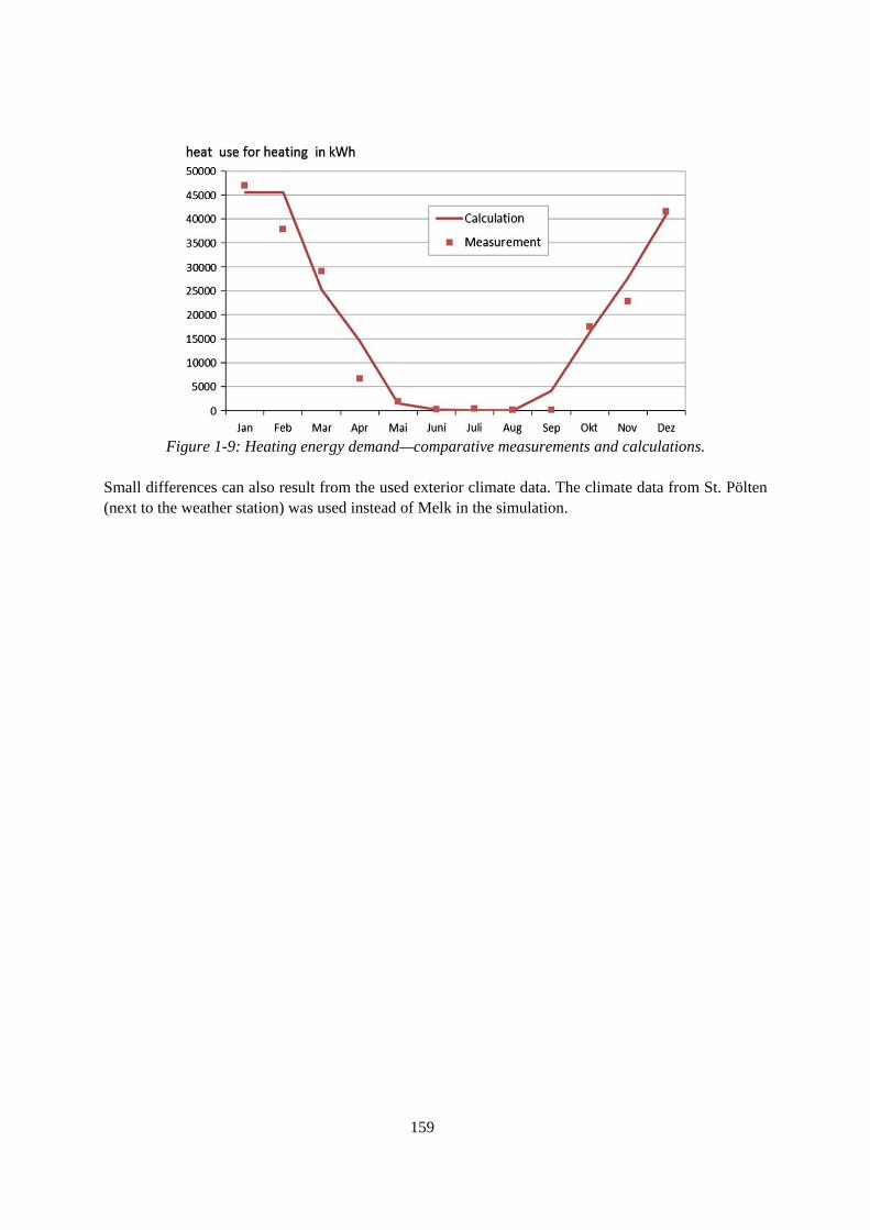
159

Figure 1-9: Heating energy demand—comparative measurements and calculations.

Small differences can also result from the used exterior climate data. The climate data from St. Pölten (next to the weather station) was used instead of Melk in the simulation.

160

Figure 1-10: Lighting electricity consumption—comparative measurements and calculations.

161

Table 1-6: Lighting: Measurements for each floor

Figure 1-11: Primary energy in kWh/m² GFA—comparative measurements and calculations.

The primary energy factor used for district heating is 1.1 kWh/kWh and for electricity is 3.5 kWh/kWh. The energy consumptions of the individual parts of the HVAC system (pumps, humidification, reheating after dehumidification, etc.) are disregarded in the calculations.

162

1.8 Conclusions

The simulation results which included details such as building use, equipment, lighting type and use, agree well with the measurements. Small variations in the results from case study are due to differences between the annual reference year climate file and the actual climate. The results of this analysis suggest that very good agreement is achievable when exact input data are available, especially building occupancy patterns and activities. It is recommended to run a series of variations using different potential building use and equipment scenarios to estimate a range of energy uses in the building during the design phase as the actual building use and equipment is unknown. 1.9 References

[1] Korjenic, T. Bednar: "Validation and Evaluation of Energy Use in Office Buildings - A Case Study"; Automation in Construction, 23 (2012), S. 64 - 70.

[2] GRÜNBERGER, H. 2009. Gelebte Zusammenarbeit [Online]. Melk: Stadt Melk. Available: http://www.melk.gv.at/system/web/news.aspx?detailonr=220382533&sprache=1 [Accessed 3 September 2012 2012].

163

2. BEL-01: Office building in Belgium

Roberto RUIZ (*), Stéphane BERTAGNOLIO, Vincent LEMORT 2.1 Building introduction

Studied building corresponds to an office building which accommodates the facilities of the European commission for energy and transport. It is located at Brussels, Belgium, specifically at Rue de Mot 28, 1040 Brussels. For this reason, is commonly called “DM 28”.

Figure 2-1: Exterior scene of DM 28 DM 28 was built in the 70’s and was largely refurbished in 1998. The refurbishment included a complete modification of the HVAC system and a renovation of the facade and of the indoor space. The building was recently awarded with an energy performance certificate (see Appendix 2.7.1) with a mark of D+ (i.e. just above the average for similar buildings in Brussels area), corresponding to an annual primary energy consumption of about 316 kWh/m²/yr and annual CO2 emissions of 54 kg CO2/m

2.

Geographical position : Brussels

Latitude : 50°51’0’’

N

Longitude : 4°21’0’’E

ASL : 13 m

Figure 2-2: Location of DM 28

164

According to weather conditions, Belgium has a temperate maritime climate influenced by the North Sea and Atlantic Ocean, with cool summers and moderate winters. Since the country is small there is little variation in climate from region to region, although the marine influences are less inland1. The heating degree days (18 C) are around 3148 and cooling degree days (18 C) are approximately 130 year round. Monthly average climate data is shown in Table 1 and daily average ambient temperature and humidity is shown in Figure 2-3.

Table 1: Climate data of Brussels Jan Feb Mar Apr May Jun Jul Aug Sep Oct Nov Dec Year

Average high (C) 5.7 6.6 10.4 14.2 18.1 20.6 23.0 22.6 19.0 14.7 9.5 6.1 14.2

Daily mean (C) 3.3 3.7 6.8 9.8 13.6 16.2 18.4 18.0 14.9 11.1 6.8 3.9 10.5

Average low (C) 0.7 0.7 3.1 5.3 9.2 11.9 14.0 13.6 10.9 7.8 4.1 1.6 6.9

HDD18C 481 420 381 284 174 103 65 70 123 236 364 447 3148

CDD18C 0 0 0 1 11 24 45 41 8 0 0 0 130

Note: Data presented in Table 1 correspond to Uccle (city located in the suburbs of Brussels). Data relative to

average temperatures and relative humidity were extracted from the website of Royal Meteorological Institute of

Belgium (RMI). HDD and CDD were calculated from tmy2 file obtained from TRNSYS weather library.

Figure 2-3: Average ambient temperature and humidity climate data of Uccle

1 http://www.weatheronline.co.uk/reports/climate/Belgium.htm

165

2.2 Building specification

Main Orientation : SW-NE

Height : 30.9 m

Length : 54.8 m

Depth : 22.9 m

Floors : 13

Indoor Height : 2.8 to 3.552

Conditioned Floor Area : 11277 m2

Net Floor Area : 11277 m2

Gross floor area : 18700 m2

Figure 2-4: External dimensions DM 28 comprises 10 storeys above ground and 3 underground. Basement levels -3 to -1 mainly include parking areas. The ground floor (level 0) includes the entrance hall, a library, some meeting rooms and offices. Levels +1 to +8 mainly include office cells. In level +9 are placed all the technical rooms. At each office level, the core zone is split in two parts and has a similar composition. It includes some utility areas (stairs, elevators, sanitary, storage, kitchen, copy rooms, etc.). Peripheral zones are separated by light walls (plaster boards) while core zones walls are mainly heavy concrete walls. Figure 2-5 and Figure 2-6 show two plants of the building corresponding to ground and 5th floor.

Figure 2-5: Ground floor layout (Level 0)

2 2.8 m from the floor to ceiling panels and 3.55 is the total indoor height

166

Figure 2-6: Typical intermediate floor layout (Level 5)

HVAC system comprises heating plant (3 gas boilers), cooling plant (2 water cooled chillers and their respective cooling towers), ventilation system (9 AHUs for different purposes), terminal units (FCUs) and 2 air heaters located in parking spaces. Figure 2-7 shows a simplified scheme of HVAC system. A detailed description is provided in chapter 2.5.

Figure 2-7: Primary and Secondary HVAC configuration (Simplified Scheme)

2.3 Energy consumption issue

Monthly natural gas and electricity bills are available from January 2008 to, respectively, November and September 2011. Normalizing the annual consumptions by means of the net indoor area (about 11277 m²), the natural gas consumption varies between 76.2 and 95.3 kWh/m²/yr while the total electricity consumption is included between 95.7 and 97.3 kWh/m²/yr. These values are very near the average values provided at the regional and national levels for the tertiary sector (Gas: 40 to 150 kWh/m²/yr and Electricity: 100 to 160 kWh/m²/yr; BBRI, 2001).

167

2.3.1 Electricity consumption

Regarding to electricity consumption, only whole building profile (quarter hour) for several years is available. From these profiles, monthly electricity consumption was obtained (see Figure 2-8).

Figure 2-8: Whole building electricity consumption. Monthly basis

Disaggregation on single consumptions was obtained by applying a calibration methodology proposed and carried out by Bertagnolio (2012). See Figure 2-9.

Figure 2-9: Annual electricity consumption breakdown

Table 2-2 provides information about annual single electrical consumptions.

Table 2-2: Annual electricity consumption breakdown. Corresponding to year 2009.

Total Consumption (MWh)

EUI (kWh/m²/yr)

Lighting Off/Meet 121 10.7

Lighting Circ/Park 241 21.4

Appliances 175 15.6

IT Room 263 23.3

Ventilation Fans 154 13.6

168

Pumping 66 5.8

Liquid Chilling Package 55 4.9

Cooling Tower 11 1.0

HVAC Aux 11 1.0

Annual 1097 97

Area used in EUI is Net floor area.

2.3.2 Cooling consumption

Cooling consumption is provided by means of a disaggregation of the annual cold water demands (see Figure 2-10). It is divided among its single consumers: FCUs (North and South façades) and AHU (cooling coil).

Figure 2-10: Annual cold water demand disaggregation

According to Table 2-2, cooling consumption reached a value of 55 MWh/yr (4.9 kWh/m²/yr) in the year 2009. 2.3.3 Heating consumption

Figure 2-11 shows the recorded values of the natural gas consumptions. These values are not actual “monthly” consumptions since the billing period may be shorter or longer than the corresponding calendar month. Despite this fact, the trend is very clear and the natural gas consumption is strongly related to the outdoor climate. The seasonal effect is very clear: peak consumptions occur in December/January while the summer consumptions (July/August) are almost null (see Figure 2-11).

169

Figure 2-11: Monthly gas consumption

Figure 2-12 shows a disaggregation of the annual hot water demand obtained by Bertagnolio, 2012.

Figure 2-12: Annual hot water demand disaggregation

In the year 2009, whole building fuel consumption reached a value of 1075 MWh/yr (95.3 kWh/m²/yr). 2.3.4 Energy flow demonstration

Considering energy flow through building, categories of energy use and corresponding boundary is defined as following: 1) Ed: energy delivered to the energy conversion system outside the building; 2) Et: energy delivered to the technical system of the building; 3) Er: energy provided by renewable energy system integrated with the building for technical

systems; 4) Eb: energy consumed by end usages of the building. According to the definition, the energy flow can be demonstrated in Figure 2-11. The total electricity consumption is 1097 MWhe, including 954 MWhe on Eb boundary (for building requirements, i.e.

170

lighting, appliances, IT room and ventilation) and 143 MWhe on Et boundary (for technical system, i.e. circulating pumps, liquid chilling package, cooling tower HVAC auxiliaries). The annual cooling consumption is 54.8 MWhc, generated by the chiller plant of the building. The annual heat consumption is 1075 MWhh, generated by the heating plant. Considering different energy source cannot be summed up directly, electricity equivalent approach is commonly used to calculate the total consumption, which is 1346 MWhee in OIE.

[UNIT: kWhe] Et Eb

1,096,782

1,345,838

1,074,906

Conversion factor

1 MJ hot water= 0.2317 MJ equivalent electricity

Electricity Equivalent Approach (kWhee)


ELECTRICITY (kWhe)

Appliances

175,485

IT room

263,228

Lighting

361,938

Pumps

65,807

HEAT (kWhh)

Ventilation

Cooling (kWhc)

FCUs

171,985

153,549

HVAC Auxiliaries

10,968

Liquid Chilling Package

54,839

Cooling Tower

10,968

54,839

354,719

AHUs

548,202

Heaters - Parking

Figure 2-13: Energy Flow Diagram of the Case Building

171

2.4 Occupant behavior

This building has been part of a monitoring campaign carried out during 2010 and part of 2011. Some information and conclusions provided by this report come from of the analysis of these measures performed by Bertagnolio (2012). 2.4.1 Occupancy

The total number of occupants of the building is approximately 350. Numerous office cells are shared by two, three or four employees. No official information is available on the occupancy rate of the building. Maybe the only one way to evaluate global building occupancy is by means of analyzing an hourly profile of whole building electricity consumption (see Figure 2-14).

0 1 2 3 4 5 6 7 8 9 10 11 12 13 14 15 16 17 18 19 20 21 22 23

0

100

200

300

400



0 1 2 3 4 5 6 7 8 9 10 11 12 13 14 15 16 17 18 19 20 21 22 23

0

50

100

150

200


(Hourly Profile - Weekend)

Figure 2-14: Hourly profile for whole building electricity consumption

Profiles described by blues dots (mean values) correspond to an indirect representation of one day building’s occupancy (week and weekends). In both graphs is easy to recognize two periods (6h to 22h for weekdays and from 10h to 19h for weekends and holidays). It corresponds to a “switch-on allowance period” defined by BEMS system where lighting fixtures manually operated can be switched ON or OFF. In DM 28, working day starts at 8h until 18h during the week. It can be observed that the profile has sort of symmetry during all the working day and is centered at 13h (lunch time).

172

For weekend during “switch-on allowance period”, the profile remains flat which allows inferring that in this period, occupancy provides a marginal effect. 2.4.2 Lighting use

In offices, lighting fixtures can be switched on/off by the occupants during the “switch-on allowance period” defined above. So, artificial lighting use rates can vary a lot from one occupant to another and from one day/week/month to another. Figure 2-15 shows the average profile for a weekday deduced from 4 weeks of data collected in 5 offices. Such profile corresponds to offices that are occupied in a regular manner from Monday to Friday and should also reflect, in an indirect way, the occupancy rate of the considered offices. As expected, lighting use during weekend is null since it is not allowed by the BEMS.

Figure 2-15: Average (weekday) lighting use sub-hourly profile in offices (blue) and derived hourly

profile (red)

Figure 2-16: Estimated weekly lighting electricity consumption

It is also interesting to have a look to the estimated lighting consumption for the zones were measurements have been performed. Recorded operation times have been multiplied by the observed installed lighting power (Figure 2-16). In offices, about 18% of the consumption is due to operation of the lighting fixtures out of the normal working period (08:00 to 18:00, Monday to Friday). It is likely that this consumption is mainly due to forgetting switching off the lights at the end of the day so that the lighting stays on till the automatic switch off at 22:00. In the circulation area (operated by BEMS), it is interesting to note that only 38% of the related consumption occurs during normal working period (08:00 to 18:00, Monday to Friday). The remaining consumption occurs during nights and weekends.

173

2.4.3 Appliances use

Appliances electricity consumption has been monitored during 5 weeks in 6 (daily) occupied offices and in the copy room. Average normalized consumption profiles have been derived from these data and are shown in Figure 2-17. As expected, the power density in the copy room is largely higher than in offices and reaches 35 W/m². Peak power density in offices is largely dependent on the zone and can vary approximately between 3 to 10W/m². Considering the nominal power densities, distinct normalized daily operation profiles have been identified for the operation of electrical appliances in offices and copy room, during weekdays and weekends.

Figure 2-17: Average appliances power density in several zones

2.5 Detailed system description

2.5.1 Air system

Air system comprises supply and extraction air handling Units (AHUs). In total, they are nine. Five main AHUs (#1 to #5) serve the three main conditioned zones of the building:

• The Entrance hall • The ground floor peripheral zones (meeting zones, offices and library) • The offices located at Levels +1 to +8

AHUs #1 and #2 serve the office cells located at levels +1 to +8. Both units are Constant Air Volume (CAV) units and include a pre heating coil, an adiabatic humidification system, a cooling coil, a postheating coil, a supply fan and a return fan. A fraction of the air extracted by these two units is sent back to the parking levels -1 and -3. AHUs #3 and #4 are Variable Air Volume (VAV) units and serve the peripheral zones located at the ground floor. The fifth AHU (#5), serving the entrance hall, consists in a small ventilation unit supplied with vitiated air extracted from the zone and a small fraction of fresh air coming from the AHU3.

174

Figure 2-18: Link between AHUs and zones they serve

Figure 2-19: Scheme of components of AHU #1 and 2 Figure 2-20: AHU #1

For the four ventilation units which work in extraction mode, AHU #6 extracts about 8200 m³/h from sanitaries of levels 0 to +8. The AHU #7 extracts a mix of vitiated and fresh (infiltrated) air from the three parking levels in order to maintain them at an acceptable temperature and air quality level. The intermediate parking level (-2) is also equipped with two large hot water fan coil units (70.5 kW each) in order to avoid freezing risk of the fire safety piping system.

175

The small AHU #8 is used only to ventilate the high tension transformer with fresh outdoor air and is directly controlled by a thermostat. The AHU #9 is totally dedicated to the print shop located at the ground floor. Nominal supply and exhaust air flow rates of the nine ventilation units are summarized in Table 2-3.

Table 2-3: AHUs setpoints

SuFlow ExFlow Min

Fresh Tsu -10 Tsu +10 RH

AHU Zone Type

m³/h m³/h % °C °C %

1 Offices CAV 12660 9000 100 25 20 50

2 Offices CAV 12480 8960 100 25 20 50

3 Ground floor VAV 12565 8430 30 25 19 50

4 Ground floor VAV 11890 10250 30 25 19 50

5 Hall CAV 3500 3500 6 (AHU3) Thermostat (min. 16°C) -

6 Sanitaries CAV 0 8200 0 - - -

7 Parking CAV 0 37600 0 - - -

8 Elec. Box CAV - - 100 - - -

9 Printshop (0) CAV 0 2700 0 - - -

The main characteristics of the AHUs components available in the as-built documents are summarized in Table 2-4.

Table 2-4: Air handling unit components and sizes ExFan Econo PreH Humid. Cool PostH SuFan

AHU kW - kW - kW kW kW

1 2.2 No 182.5 85% eff. 98.5 23 5.5

2 2.2 No 180 85% eff. 97 23 5.5

3 2.2 Yes 25.5 85% eff. 64 20 5.5

4 3 Yes 23 85% eff. 60 20 5.5

5 No No No No 14 17.5 1.1

6 2.2 No No No No No No

7 11 No No No No No No



Total 24.05 - 411 - 333.5 86 23.1

2.5.2 Local heating and cooling (Terminal units)

The peripheral zones located at the ground floor are equipped with VAV boxes controlling the supply air flow rate. Hot water convectors are installed all along the external walls (one per 2.4m of façade) to provide local heating to the peripheral zones. Cooling of the zones is ensured by increasing the supply air flow. In a few zones, some electrical reheat boxes have been added to ensure backup heating if the capacity of the hot water convectors is insufficient. It has to be noticed that these additional electrical coils operate a very limited number of hours per year. Table 2-5 provides information about operation conditions of VAV boxed located at ground floor.

176

Table 2-5: Ground floor VAV boxes Supply Exhaust Electrical coil

Min Max Nbr Min Max Nbr Pwr Nbr VAV Boxes Ground floor

AHU

m³/h m³/h - m³/h m³/h - W -

Office 1 3 28 280 1 23.2 232 1 - -

Office 2 3 139 1390 2 115.5 1155 2 - -

Meeting 30 3 202 2020 2 167.5 1675 2 4000 2

Office 3 3 26.5 265 1 22 220 1 - -

Printshop 3 120 1200 2 - - - - -

Storage 1 3 222 2220 1 195 1950 1 - -

Storage 2 3 60 600 1 50 500 1 - -

Office 4 3 67.5 675 1 56 560 1 - -

Total 1326 – 13260 m³/h 912.2 - 9122 m³/h 4000 2

Meeting 40 4 121

182

1210

1820

1

2

106

160

1060

1600

1

2

2500

4000

1

2

Meeting 20 4 222 2220 1 195 1950 1 4500 1

Meeting 4 165 1650 1 145 1450 1 - -

Meeting 4 67.5 675 1 59 590 1 1500 1

Meeting 4 67.5 675 1 59 590 1 1500 1

Meeting 4 162 1620 1 142 1420 1 - -

Total 1169 - 11690 m³/h 1026 - 10260 m³/h 18000 6 Peripheral zones at levels +1 to +8 are equipped with vertical concealed 4-pipes heating/cooling fan coil units (one per façade module of 1.2m width).

Figure 2-21: Concealed vertical fan coil unit

2.5.3 Hot water system

Hot water production is ensured by three natural gas boilers (Table 2-6) of 465 kW each. Two classical boilers (#1 and #2) provide hot water to the AHUs heating coils and to the two air heaters located in the parking space. The third boiler is a condensing boiler and provides hot water to all the FCUs installed in the office zones (levels +1 to +8). In normal operation, the two hot water networks

177

are decoupled (Figure 2-23) and the isolating valves are closed. Boilers nominal efficiencies are given in Table 2-6.

Table 2-6: Hot water boilers

Name Fuel Brand Type Nominal Pwr LHV Effic.

Boiler 1 Natural gas Ygnis Optimagaz E465 - Classical 465 kW 92 – 95% Boiler 2 Natural gas Ygnis Optimagaz E465 - Classical 465 kW 92 – 95% Boiler 3 Natural gas Ygnis TBT E465 - Condensing 465 kW 96 – 104%

The characteristics of all the hot water pumps are summarized in Table 2-7.

Figure 2-22: Hot water production plant Figure 2-23: Hot water production plant components

Table 2-7: Heating plant water pumps

Name Type Flowrate (m³/h) Power (W) Description

PC1 WILO TOP-S 50/7 22.2 375-470-610 Boiler 1



PC4 WILO TOP ED 40/1-10 10.2 30-570 FCUs

PC5 WILO TOP ED 40/1-10 10 100-600 FCUs

PC6 WILO TOP-S 65/13 32 1450 AHUs & others

PC7 WILO TOP-S 30/10 9.67 205-290-395 AHU1 PreH coil

PC8 WILO TOP-S 30/10 9.46 205-290-395 AHU2 PreH coil

PC10 WILO RS25/50 r 1.12 38-48-60-74 AHU3 PreH coil

PC11 WILO TOP SD 32/7 2.05 90-130-200 Convectors (0)

PC12 WILO RS25/50 r 1.03 18-31-48 AHU4 PreH coil

PC13 WILO TOP SD 32/7 1.6 90-130-185 Convectors (0)

2.5.4 Chilled water system

Chilled water production is ensured by two water cooled chillers of 512.4 kW of cooling capacity each (Figure 2-24). The nominal EER of these components is about 4.27 (Table 2-8). Two indirect contact cooling towers equipped with two speeds fans ensure the cooling on the condenser side (Figure 2-25).

178

The main characteristics of all the pumps and circulators ensuring chilled water circulation are given in Table 2-9.

Table 2-8: Cooling plant components

Name Brand Type Compressor / Fan Power

Temperatures Nominal Power

Absorbed Power

Chiller 1 Trane RWTA 215 2 x Screw 7/12°C

29/34°C 512.4 120.1

Chiller 2 Trane RWTA 215 2 x Screw 7/12°C

29/34°C 512.4 120.1

Tower 1 BAC Balticare VFL 963-O Two speeds 34/29°C 665 kW 7/30 kW

Tower 2 BAC Balticare VFL 963-O Two speeds 34/29°C 665 kW 7/30 kW

Figure 2-24: Water-cooled chilling package Figure 2-25: Chilled water production plant

components

Table 2-9: Cooling plant water pumps Name Type Flowrate (m³/h) Power (W) Description PF1 WILO IPn 100/200-3/4 87.5 3100 Chiller 1 – Evaporator

PF2 WILO IPn 100/200-3/4 87.5 3100 Chiller 2 – Evaporator

PF3 WILO IPn 100/160-7.5/2 123.8 7500 Chiller 1 - Condenser

PF4 WILO IPn 100/160-7.5/2 123.8 7500 Chiller 2 – Condenser

PF5 WILO IPE 65/4-20 55.4 3900 FCUs

PF6 WILO IPE 65/4-20 49.9 3800 FCUs

PF7 WILO IPE 80/125-3/2 49.7 3800 AHUs

PTR1 Balticare 87.12 2200 CT1 – spray pump

PTR2 Balticare 87.12 2200 CT2 – spray pump

179

2.6 References

[1] BBRI. 2001. Kantoor2000: Study of Energy Use and Indoor Climate in Office Buildings. [2] Bertagnolio, S. 2012. Evidence-Based Model Calibration For Efficient Building Energy Services.

PhD thesis, University of Liege, Belgium. [3] Demarche, F. 2011. Application of an Evidence-Based Calibration Methodology to a Typical

Office Building in Brussels. Master thesis, University of Liege, Belgium.

180

2.7 Appendix

2.7.1 Energy performance certificate

Energy performance certificate delivered in 2010.

181

2.7.2 HVAC system

182

3. CHN-01: Office building in China

3.1 Building introduction

Figure 3-1: Location of One Island East

The building is the 6th skyscraper over 1,000 ft. (305 m) completed in Hong Kong. Part of the site was previously occupied by Melbourne Industrial Building (23 floor office tower demolished 2005) and Aik San Factory Building (22 floor commercial building demolished 2005) which were acquired by the developer in 2002 and 2001 respectively.

Table 3-1: Climate data of Hong Kong Jan Feb Mar Apr May Jun Jul Aug Sep Oct Nov Dec Year Average high (℃)

18.6 18.6 21.5 25.1 28.4 30.4 31.3 31.1 30.2 27.7 24.0 20.3 25.6

Daily mean (℃) 16.1 16.3 18.9 22.5 25.8 27.9 28.7 28.4 27.6 25.3 21.4 17.8 23.1 Average low (℃) 14.1 14.4 16.9 20.6 23.9 26.1 26.7 26.4 25.6 23.4 19.4 15.7 21.1 HDD65F 166 15 32 17 8 4 193 CDD65F 5 74 139 204 450 546 631 541 508 405 147 67 3717 Hong Kong is a humid subtropical climate. The heating degree days (65F) is around 193, and cooling degree days (65F) is approximately 3717 year round. Monthly average climate data is shown in Table 3-1 and daily average ambient temperature and humidity is shown in Figure 3-2.

183

0

10

20

30

40

50

60

70

80

90

100

Average Ambient (Deg.C) Average Humidity (%)

Figure 3-2: Average ambient temperature and humidity climate data of Hong Kong


Figure 3-3: Exterior scene of One Island East

One Island East is a supertall skyscraper that is located in TaiKoo Place on Island East, Hong Kong. The skyscraper is a commercial office building, completed on March 2008, rises 298.35 (979 ft) and has 69 stories of habitable office space and two basement levels. There is a sky lobby on the 37th and 38th floors. In addition, there are 28 high speed passenger lifts, 6 high speed shuttle lifts between Main (G-1F) and Sky (37-38/F) Lobbies, 1 passenger lift between main lobby and basement carpark and 2 service lifts.

Table 3-2: Basic information of One Island East, Hong Kong Gross floor area 141,000 sqm Typical lettable floor area (Fig. 2) Approx. 21,000 sq ft (approx. 1,950 sqm) No. of floors 68 Typical finished floor to false ceiling height clear headroom 2.925m to 3.925m Air-conditioning Variable Air Volume system (VAV) with Direct

184

Digital Control (DDC)

Lifts 28 passenger lifts, six shuttle lifts, two service lifts and one carpark lift

Computer room cooling Dedicated 24-hour chilled water supply with backup generator

Accessible carpark spaces 1,420

Figure 3-4a: Typical floor plan of One Island East

Figure 3-4b: 23/F of One Island East, the TEC Hong Kong Executive Center

One Island East has deluxe class office/commercial with basement carparks consisting of the following:

Table 3-3: Functional area information

185

Basement 2 to Basement 1 Loading/unloading areas and plant rooms G Floor Escalator lobby, fireman’s lift homing lobby, plant rooms 1 Floor Entrance Foyer 2nd floor to 19/F Zone 1 office floors, lift machine room at 2/F, 18/F&19F 20th floor E&M plant room, TPMO workshops 21st floor Refuge floor, FS plant rooms 22nd to 34th floor Zone 2 office floors 35th floor E&M plant room 36th floor E&M plant room & lift machine room 37th floor & 38th floor Sky Lobby 39th floor to 48th floor Zone 3 office floors, lift machine room at 41/F & 42/F 49th floor Refuge floor, FS plant rooms, A/C plant room 50th to 67th floor Zone 4 office floors. Lift machine room at 56/F, 57/F&64F Roof/upper roof E&M plant rooms & Lift machine room 1/F in Cornwall house Condenser water make-up pump room Roof in Cornwall house Cooling tower plant rooms Hoi Yu Street Sea water pump room

Grand Lobby at 1/F, OIE Sky Lobby at 37/F, OIE

Sky Lobby at 38/F, OIE Elevator hall of each floor, OIE

186

3.3 Database description by the definition of Subtask A

SUBTASK B: DATABASE OF A LARGE-SCALED OFFICE BUILDING IN CHINA Following File “Three Level Database Definitions for Office Buildings” in Subtask A This file follows the definition of subtask A, defining the influencing factors and energy use in three level database of a typical large-scaled office building in Hong Kong, China. For the detailed level B and C, the relevant excel files are attached. NOTICE: The information of the case study office building in China following the STA definition format is written in RED characters. ACKNOWLEDGEMENT: All of the case building information is provided by Swire Properties Ltd., Hong Kong. Sincerely thanks for the supporting of the Technical Service & Sustainability Department. 3.3.1 Simple version – Level A database

In the simple version, climate, whole building characteristics, building envelope, building services, and input into energy performance indicators are defined. 3.3.1.1 Climate

Code Item Definition Annual (Acceptable)

HDD65F Indicate the heating degree days (65F)

193 1.1.1

CDD65F Indicate the cooling degree days (65F).

3717

3.3.1.2 Whole building characteristics Code Item Definition Case building

1.2.1 Year built Indicate year built in the format 19XX or 20XX.

2005

1.2.2 Number of floors

Indicate the number of floors. 68

1.2.3 Number of businesses

Indicate the number of companies occupying the building.

37

1.2.4 Conditioned or heated floor area

The floor area of conditioned floor space, as measured at the floor level within the external surfaces of walls enclosing the conditioned space. It includes the attached space, such as basement, attic, if they are conditioned.

141000 sqm

1.2.5 Gross floor area

Gross floor area is calculated including external walls. The attached space should also be included, such as basement, attic, etc.

141000 sqm

1.2.6 Type of building

Indicate the type of building: 1) Government office; 2) Business/professional office; 3) Multi-use complex; 4) Other

2

1.2.7 Other Garage/ data center/ food sales/ service/ Data

187

building activities

shopping mall/ retail/ corridor/ lobby/ restroom/ parking/ storage/ vacant/ other

center/corridor/lobby/restroom

3.3.1.3 Building envelope

Code Item Definition Case building

1.3.1 Building air tightness

Air change rate provided in times/hour.

1) Office area:0.5 air changes

for perimeter zone of 3.6

meters deep;

2) Toilet: 15 air changes per

hour;

3) M&E room: 10 air changes

per hour.

1.3.2 Material This includes walls, ceiling, floor and window materials.

Windows: triple glazing-single glazing + cavity w/blind + double glazing.

1.3.3 U-value Provided for all of the building envelop materials (wall, ceiling, windows, etc.) using the units: w/(m2*k).

1) Office floors

- Triple glazing=1.12 W/(m2K)

- Spandrel=0.68 W/(m2K)

- Roof=1.15 W/(m2K)

2) Podium floors

- Glazing=5.6 W/(m2K)


- Podium roof=1.15 W/(m2K)

1.3.4 Window to wall ratio

Select one of the following: 1) 25 % or less; 2) 25%-35%; 3) 35%-45%; 4) more than 45%. This should exclude the roof area.

4 (77%)

3.3.1.4 Building services and energy systems


1.4.1 Space heating - centralized

Type of central space heating system (district steam or hot water or boilers inside the building)

Fuel type Total power (w)

Heat capacity of the building (w)

No space heating

1.4.2 Space heating - decentralized

Type of decentralized space heaters (individual space heaters, furnaces or other heating equipment)


Heat capacity (w)

No space heating

1.4.3 Air conditioning - centralized

Type of central air conditioning systems.


Cooling capacity (w)

YES

188

Water side: chilled water system for normal and essential cooling Air side: Air Handling Unit + Primary Air Unit + VAV system

electricity Refer to Table 3.4.

1.4.4

Air conditioning - decentralized

Type of the decentralized air conditioners.


Heat/cooling capacity (w)

No decentralized AC

Type of centralized ventilation system


YES

1.4.5 Ventilation - centralized

1) Toilet exhaust and

general exhasut

system for office

floors

2) Carpark ventilation

electricity Refer to Table 3.4.

1.4.6 Ventilation - decentralized

Type of local fans Fuel type Total power (w)

No decentralized ventilation

Types of lighting (incandescent bulbs, fluorescent bulbs, compact fluorescent bulbs, and other bulbs)



YES

1.4.7 Lighting

Compact fluorescent bulbs in majority

electricity

65 W/m2 plus small power

Refer to Table 3.4.

Type(s) of appliances Fuel type Total power (w)

Refer to Table 3.4.

YES

1.4.8 Office appliances Computer, laptop,

screen, printer, copier, etc.

electricity

65 W/m2 plus lighting

Refer to Table 3.4.

1.4.9 Other

Types of other equipment used in the building (kitchen appliances, water heating appliances, elevator, security monitors, etc.)


YES

189

3.3.1.5 Building operation


1.5.1 Business Hours

Typical business hours on weekdays, weekends and holidays.

1) 8.6 hours on weekday

2) 0.4 hours on weekend

1.5.2 Occupancy schedule

Number of employees at the office during business hours, non-business hours (overtime and weekends) and holidays.

Typical occupancy during business hours

0%

10%

20%

30%

40%

50%

60%

70%

80%

90%

100%

0:00 6:00 12:00 18:00 0:00

Occ

upan

cy

3.3.1.6 Input into energy performance indicators Building energy use can be expressed in the three ways according to attachment 3, which are: (1) Energy use of each energy resource, (2) Aggregation of energy of primary energy, equivalent electricity, and equivalent CO2 emissions, (3) Normalized energy use in the above two approaches

Code

Item Definition

Frequency

Case building

Annual (acceptable)

1) Annual total: 22.5 million kWh electricity

2) EUI: 159.8 kWhe/(m2.a)

1.6.1

Step 1: Energy carrier

Indicate the energy use of each energy resource. Electricity

Monthly (preferred)

Monthly electricity consumption: Jan Feb Mar Apr May Jun Million kWhe

1.36 1.47 1.36 1.56 1.75 2.15

Jul Aug Sep Oct Nov Dec Million kWhe

2.35 2.50 2.57 2.04 1.87 1.54

1.6.2

Step 2: Aggregation of energy

Provide the aggregation of

Annual (acceptable)

1) Primary energy=61.3 million kWh

2) Equivalent electricity=22.5 million kWhe

3) Equivalent CO2 emission=15700 tonne-CO2

(Conservion factor: 1 kWhe=0.6956 kg-CO2).

190

energy of primary energy, equivalent electricity, and equivalent CO2 emissions.

Monthly (preferred)

1) Monthly primary energy

Jan Feb Mar Apr May Jun Million kWh 3.69 4.01 3.71 4.25 4.78 5.86 Jul Aug Sep Oct Nov Dec Million kWh 6.39 6.82 6.99 5.57 5.09 4.20

2) Monthly equivalent electricity

Jan Feb Mar Apr May Jun Million kWhe

1.36 1.47 1.36 1.56 1.75 2.15


2.35 2.50 2.57 2.04 1.87 1.54

3) Monthly equivalent CO2 emissions

Jan Feb Mar Apr May Jun Thou. Tonne-CO2

0.94 1.02 0.95 1.09 1.22 1.50


1.63 1.74 1.78 1.42 1.30 1.07

1.6.3

Step 3: Normalized energy use

Normalized energy use using the above two approaches

Annual (acceptable)

Refer to the following energy flow chart.

191

[UNIT:mill kWhe] Et Eb

22.53

22.53

Ed Exhaust Fans

0.00

HEAT (kWh h)42.69

0.00Primary Air Unit

1.87

ElectricityEquivalentApproach

(mill kWhee)


ELECTRICITY(mill kWhe)

Appiances

1.12

Service+Technical sys.

Ventilation

Cold (MWhc)

Heat

DHW

0.56

Lighting

3.93

0.00

Chilled water pump

1.07

Condensor water pump

0.84

Cooling tower

1.06

Chiller

7.81

Air Handling Unit

3.70

3.3.2 Intermediate version for office buildings – Level B database

The intermediate version is more detailed and includes more items, when compared with the simple version. It defines the influencing factors of seven categories: climate, indoor thermal environment, building characteristics, building envelope, building service and energy system, building operation and occupant behavior, and indirect factors. In each category, the important items that affect energy use are listed and defined. 3.3.2.1 Climate and indoor thermal environment The following table lists the items used to describe the climate and indoor thermal environment. For each item, the measured frequency and location are defined.

Code Item Frequency Location Case building

Monthly (preferred) N/A YES

2.1.1 HDD18°C and CDD26°C

Jan Feb Mar Apr May Jun Jul Aug Sep Oct Nov Dec HDD65F 116 15 32 17 0 0 0 0 0 0 8 4 CDD65F 5 74 139 204 450 546 631 541 508 405 147 67

2.1.2 Weather data

Daily (preferred) or monthly (acceptable) (Indicate if hourly weather data are available (yes/no)).

Provide weather data including ambient temperature, humidity, and direct/diffuse solar radiation at

Monthly Hourly (available)

192

the nearest weather station.

2.1.3 Indoor temperature (°C)

Daily (preferred) or seasonal, weekday/weekend or day/night (acceptable).

Indicate the indoor temperature for each HVAC zone (preferred) or the whole building (acceptable).

Not available.

2.1.4 Indoor humidity


Indicate the indoor humidity for each HVAC zone (preferred) or the whole building (acceptable).

Not available.

2.1.5 Indoor illumination


Indicate the indoor illumination for each functional zone (preferred) or the whole building (acceptable).

Not available.

3.3.2.2 Whole building characteristics Code Item Definition Case building

2.2.1 Year built Indicate year built in the format 19XX or 20XX.

2005

2.2.2 Number of floors

Indicate the number of floors. 68

2.2.3 Conditioned or heated floor area

The floor area of conditioned floor space, as measured at the floor level within the external surfaces of walls enclosing the conditioned space. It includes the attached space, such as basement, attic, if they are conditioned.

141000 sqm

2.2.4 Gross floor area

Gross floor area is calculated including external walls of the building. The attached space should also be included, such as basement, attic, etc.

141000 sqm

2.2.5 Number of businesses

The number of companies occupying the building.

37

2.2.6 Number of employees per business

Not available.

2.2.7 Type of building

Indicate the type of building: 1) Government office; 2) Business/professional office; 3) Multi-use complex; 4) Other

2

2.2.8 Other building activities

Garage/ data center/ food sales/ service/ shopping mall/ retail/ corridor/ lobby/ restroom/ parking/ storage/ vacant/ other

Data center/corridor/lobby/restroom

2.2.9 Ownership Indicate whether the home or apartment is: 1) 1

193

rented; 2) owned; 3) leased

2.2.10 Net floor area

Calculated using the internal dimensions of building.

103259 sqm

2.2.11

Gross floor area occupied by each activity

Not available.

2.2.12 Building geographical position

Provide the longitude, latitude and ASL. N: 22.3º, E: 114.2º ASL: Not available.

3.3.2.3 Building envelope Code Item Definition Case building

2.3.1 Building air tightness

Air Change Rate provided in times/hour.

1) Office area:0.5 air changes for

perimeter zone of 3.6 meters

deep;

2) Toilet: 15 air changes per

hour;

3) M&E room: 10 air changes

per hour.

2.3.2 Material This includes walls, ceiling, floor and window materials.

Windows: triple glazing-single glazing + cavity w/blind + double glazing.

2.3.3 U-value Provided for all of the building envelop materials (wall, ceiling, windows, etc.) using the units: w/(m2*k)

1) Office floors

- Triple glazing=1.12 W/(m2K)


- Roof=1.15 W/(m2K)

2) Podium floors

- Glazing=5.6 W/(m2K)


Podium roof=1.15 W/(m2K)

2.3.4

Comprehensive shading coefficient of the windows

This can also be solar factor and should be provided.

SC=0.19

2.3.5 Window to wall ratio

Select one of the following: 1) 25 % or less; 2) 25%-35%; 3) 35%-45%; 4) more than 45%. This should exclude the roof area.

4 (77%)

2.3.6 Shape factor

The ratio of surface area that is exposed to the outside area to the enclosed volume, and the surface area does not include the floor area, door area and internal wall area of the

Surface area=49504 sqm, SF≈0.1

194

stairwells without district space heating.

3.3.2.4 Building services and energy systems (Refer to Table 3.4)

Code

Item Definition Individual office

Centralized office

2.4.1

Space heating - centralized

Type of central space heating system (district steam or hot water or boilers inside the building)

Number of systems

Fuel type

Total power (w)


Floor area of zone served by each type of system

N/A X

2.4.2

Space heating - decentralized

Type of decentralized system

Number of each type of heater

Fuel type

Total power (w)

X X

2.4.3

Air conditioning - centralized

Type of central air conditioning systems including (heat sources, cold sources, chilled water pump, cooling water pump, AHU fan, FCU fan, cooling tower, pumps of cooling storage system, heat exchanger, etc.)

Number of systems

Fuel type

Total power (w)

Heat/ cooling capacity of the building (w)

Floor area of zone served by each type of system

N/A X

2.4.4

Air conditioning - decentralized

Type of the decentralized air conditioner

Number of each type of air conditioner

Fuel type

Total power (w)

Heat/cooling capacity (w)

X X

2.4.5

Ventilation - centralized

Type of centralized system

Number of systems

Fuel type

Total power (w)

N/A X

2.4.6

Ventilation - decentralized

Type of local fans Number of fans

Fuel type

Total power (w)

X X

195

2.4.7

Lighting Types of lighting (incandescent bulbs, fluorescent bulbs, compact fluorescent bulbs, and other bulbs) including indoor and outdoor lighting

Number of lighting appliances

Fuel type

Total power (w)

Control method (photo/occupancy/scheduling)

X X

2.4.8

Office appliances

Type(s) of appliances

Number of appliances

Fuel type

Total power (w)

X X

2.4.9

Other Types of other equipment used in the building (kitchen appliances, water heating appliances, elevator, security, monitors, etc.)

Number of appliances

Fuel type

Total power (w)

X X

3.3.2.5 Building operation and occupant behavior Part 1: Occupancy

Code Item Space mode

Time mode

Schedule Set point

Case building

2.5.1 Business Hours

N/A N/A

Typical business hours on weekdays, weekends and holidays.

N/A 1) 8.6 hours on weekday

2) 0.4 hours on weekend

2.5.2 Occupancy schedule

N/A N/A

Number of employees at the office during business hours, non-business hours

N/A Typical occupancy during business hours

196

(overtime and weekends) and holidays.

0%

10%

20%

30%

40%

50%

60%

70%

80%

90%

100%

0:00 6:00 12:00 18:00 0:00

Occ

upan

cy

Part 2: Technical building systems In office buildings, both building managers and occupants can control the operation of technical building systems. Therefore, definitions of building operation and occupant behavior are suitable for both building managers and occupants, and building operation and controls by both building managers and occupants should be recorded.

Code Item Space mode

Time mode Schedule Set point Case building

2.5.3 Space heating

Select one of the following for space mode: 1) Heating used in full space; 2) Heating used in part of the space (only occupied space).

Select one of the following for time mode: 1) Heating used for full time; 2) Heating used part of the time (only when people are at the office).

Provide the following: 1) Running hours during business/non-business hours for each season; 2) Running hours during weekday/weekend hours for each season; 3) Hours when indoor temperature is set back on weekday/weekend, separately.

Provide the following: 1) Set point; 2) Range of set points; 3) If possible indicate set points when occupied and unoccupied.

No space heating

2.5.4 Space cooling Select one of the following for space mode: 1) Cooling used in full space; 2) Cooling

Select one of the following for time mode: 1) Cooling used for full time; 2) Cooling

Provide the following: 1) Running hours during business/non-business hours for each season; 2) Running hours during weekday/weekend

Provide the following: 1) Set point; 2) Range of set points; 3) If possible indicate set

YES

197

used in part of the space (only occupied space).

used part of the time (only when people are at the office).

hours for each season; 3) Hours when indoor temperature is set back on weekday/weekend, separately.

points when occupied and unoccupied.

1 2

Running hour is usually the same during the year: 7:00~19:00 If the company needs overtime working, they will negociate with the operator individually.

Summer setpoint: 24 Deg., 55% RH Winter setpoint: 20 Deg.,55% RH.

N/A

Select one of the following for time mode: 1) Ventilation used for full time; 2) Ventilation used part of the time (only when people are in toilet/office).

Provide the following: 1) Times of use on weekday/weekend and minutes per time; 2) Hours on weekday/weekend.

N/A YES

2.5.5 Ventilation (mechanic) -Toilet/kitchen

Toilet 2 7:00 AM ~ 19:00 PM 12 hours per day during weekday and weekend.

2.5.6 Ventilation (mechanic) -basement/garage

Select one of the following for space mode: 1) Ventilation used in full space; 2) Ventilation

Select one of the following for time mode: 1) Ventilation used for full time; 2) Ventilation

Provide the following: 1) Number of hours turned on during weekday/weekend; 2) Portion of appliances running on weekday/weekend

Power level used

YES

198


used part of the time (only when people are at the office).

hours.

1 1 24 hours, but the garage ventilation is VSD controlled.

Select one of the following for space mode: 1) Ventilation used in full space; 2) Ventilation used in part of the space (only occupied space).

Select one of the following for time mode: 1) Ventilation used for full time; 2) Ventilation used part of the time (only when occupied).

Provide the following: 1) Number of hours turned on during weekday/weekend; 2) Portion of appliances running on weekday/weekend hours.

N/A YES

2.5.7

Ventilation (mechanic) - centralized - rooms

2 2 4 hours Not available

2.5.8

Ventilation (mechanic) - decentralized - rooms

N/A N/A

Provide the following: 1) Times of use per day; 2) Hours of use per day in each season; 3) Time per season.

N/A

No decentralized ventilation rooms

2.5.9 Lighting Select one of the following for space mode: 1) Lighting used in full space; 2) Lighting

Select one of the following for time mode: 1) Lighting used for full time (24 hours); 2)

Provide the following: 1) Range of running hours for business/non-business hours and weekdays/weekends; 2) Number of lights on when occupied and unoccupied and

N/A YES

199


Lighting used part of the time (only when people are in the office, or only at night, etc.).

on weekday and weekend.

1 2

7:30~18:30 in the office area 90% lights on during the working hours in weekday of the offcie area; less than 20% lights on during off hours in the weekday night (21:00 PM~7:00 AM).

Select one of the following for space mode: 1) Office appliances running in full space; 2) Office appliances running in part of the space (only occupied space).

Select one of the following for time mode: 1) Used for full time (24 hours, standby when not in use); 2) Used part of the time (only when in use, off when not in use).

Provide the following: 1) Range of running hours for business/non-business hours and weekdays/weekends; 2) Number of appliances on when occupied and unoccupied and on weekday and weekend.

N/A YES

2.5.10 Office appliances

2

“2” for office area and “1” for common device such as printer, copier, etc.

Working hours during weekday: 8.6 hours More than 90% computers are turned off during the off hours in weedkay.

2.5.11

Other (Cooking appliances, water heating appliances, elevator, security monitor

N/A N/A

Provide the following: 1) Range of running hours; 2) Portion of appliances running weekday and

N/A YES

200

system, etc.) weekend.

Part 3: Windows, shading and curtains Code Item Space

mode Time mode

Schedule Set point

Case building

2.5.12 Windows N/A N/A Provide the following: 1) Times of use per day and minutes per use; 2) Hours open during day/night and week/weekend.

N/A All of the external windows cannot be opened.

2.5.13 Curtains/blinds N/A N/A Provide the following: 1) Times of use per day and minutes per use; 2) Hours open during day/night and week/weekend.

N/A 1 time per day. 4 hours open during the morning, and more than 6 hours closed during the afternoon and night.

3.3.2.6 Input into energy performance indicators Building energy use can be expressed in the three ways according to attachment 3, which are: (1) Energy use of each energy resource, fuel, electricity, cooling and heating, and peak electric demand (2) Aggregation of energy of primary energy, equivalent electricity, and equivalent CO2 emissions (3) Normalized energy use in the above two approaches

Code Item Definition Frequency Scope Case

building

2.6.1 Fuel

consumption

Indicate fuel

consumption in J,

MJ, or GJ.

Daily (preferred) or

monthly

(acceptable)

Per end use

(preferred) or whole

building (acceptable).

No fuel

consumption.

Indicate electricity

consumption in J,

MJ or GJ.

Daily (preferred) Not

available.

kWh e monthly

(acceptable)

Per end use


building (acceptable). Refer to the

following

charts. 2.6.2

Step 1:

Energy

Carrier

Electricity

consumption

Jan Feb Mar Apr May Jun

AC Plant 452631 563258 514904 651138 826841 1114854

Lighting &

appliances 383454 484964 426295 487229 495621 571825

201

AHU 303383 225402 224404 227680 235975 269330

PAU 155520 155520 155520 155520 155520 155520

Carpark

Ventilation 61622 42812 43062 38398 40026 39487

Jul Aug Sep Oct Nov Dec

AC Plant 1296515 1425237 1457763 1061554 837606 592833

Lighting &

appliances 467456 496695 531961 368163 493635 405034

AHU 384351 388103 391363 393634 324699 329973

PAU 155520 155520 155520 155520 155520 155520

Carpark

Ventilation 41454 39062.4 28952 65720 58212 60473

Indicate cooling

consumption in J,

MJ or GJ.

Daily (preferred)

Per end use



Refer to the

following

charts.

0

1000

2000

3000

4000

5000

6000

1-1 1-15 1-29 2-12 2-26 3-12 3-26 4-9 4-23 5-7 5-21 6-4 6-18

kW

Total Cooling Load (kW)

kWhc monthly

(acceptable)

Per end use



Refer to the

following

table.

2.6.3 Cooling

consumption

Jan Feb Mar Apr May Jun

MWhc 2226 2540 2726 2959 3618 4270

Jul Aug Sep Oct Nov Dec

MWhc 4675 4621 4786 4297 3246 2723

2.6.4 Heating

consumption

Indicate heating

consumption in J,

MJ or GJ.


monthly

(acceptable)

Per end use



No heating

consumption.

2.6.5

Peak

electric

demand

Indicate peak

electric demand in

W or kW.


monthly

(acceptable)

N/A Not

available.

202

Provide the

aggregation of

energy of primary

energy, equivalent

electricity, and

equivalent CO2

emissions.

Monthly (preferred)

Per end use



Refer to the

following

table.

2.6.6

Step 2:

Aggregation

of Energy

1) Monthly primary energy Jan Feb Mar Apr May Jun Million kWh 3.69 4.01 3.71 4.25 4.78 5.86 Jul Aug Sep Oct Nov Dec Million kWh 6.39 6.82 6.99 5.57 5.09 4.20

2) Monthly equivalent electricity Jan Feb Mar Apr May Jun Million kWh e 1.36 1.47 1.36 1.56 1.75 2.15 Jul Aug Sep Oct Nov Dec Million kWh e 2.35 2.50 2.57 2.04 1.87 1.54

3) Monthly equivalent CO 2 emissions Jan Feb Mar Apr May Jun Thou. Tonne-CO2

0.94 1.02 0.95 1.09 1.22 1.50

Jul Aug Sep Oct Nov Dec Million kWh e 1.63 1.74 1.78 1.42 1.30 1.07

2.6.7

Step 3:

Normalized

Energy Use

Factors

related to

energy

performance

indicators

Normalized

energy use using

the above two

approaches.

Monthly (preferred)

or annual

(acceptable)

Per end use



Refer to the

energy flow

chart in the

page 4.

3.3.2.7 Indirect factors

Code Category Parameter Description Case building

2.7.1 Energy price The price of unit energy. Electricity: 1.03

HKD/kWh e3

2.7.2 Fuel mix

This is expressed as an average

percent of each energy source in

each city.

Year 2009: 4

Electricity-53%

Oil & Coal products-

32%

Town gas & Liquefied

petroleum gas-15%

2.7.3

Social factors

Gas popularization

rate

The ratio of population using gas to

the total population in the city. Not available.

3 Source:

https://www.clponline.com.hk/myBusiness/CustomerService/TariffOverview/BulkTariff/Pages/Default.aspx 4 Source: Hong Kong Energy End-use data 2011, EMSD, Table 7.

203

2.7.4 GDP per capita 36758 USD per capita

2.7.5

Energy-

related

attitude of

occupants

Concern for saving

energy

Subjective assessment of

consciousness of occupants of

energy conservation. Potential

survey categories: 1) Very

concerned; 2) Concerned; 3)

Indifferent; 4) Not so concerned; 5)

Not concerned at all

Subjective judgment=1

2.7.6

Energy-

related

attitude of

occupants

Concern for

environmental

protection

Subjective assessment of

consciousness of occupants of

environmental protection. Potential

survey categories: 1) Very

concerned; 2) Concerned; 3)

Indifferent; 4) Not so concerned; 5)

Not concerned at all


3.3.3 Complex version for office buildings – Level C database

3.3.3.1 Climate and indoor thermal environment

Code Item Frequency Location Case

building

3.1.1 HDD18°C and

CDD26°C

Monthly (preferred) or annual

(acceptable). N/A

Refer to

Table

2.1.1.

3.1.2 Weather data

Daily (preferred) or monthly

(acceptable) (Indicate if hourly

weather data are available

(yes/no)).

Provide weather data including

ambient temperature, humidity,

direct/diffuse solar radiation at the

nearest weather station.

Hourly

data is

available.

3.1.3

Indoor

temperature

(°C)

Daily (preferred) or seasonal,

weekday/weekend or day/night

(acceptable).

Indicate the indoor temperature for

each HVAC zone (preferred) or the

whole building (acceptable).

Not

available.

3.1.4 Ventilation rate



(acceptable).

Indicate the indoor ventilation rate

for each HVAC zone (preferred) or

the whole building (acceptable).

Not

available.

3.1.5 Indoor humidity



(acceptable).

Indicate the indoor humidity for each

HVAC zone (preferred) or the whole


Not

available.

3.1.6 Indoor

illumination



(acceptable).

Indicate the indoor illumination for

each functional zone (preferred) or

the whole building (acceptable).

Not

available.

3.3.3.2 Whole building characteristics


3.2.1 Year built Indicate year built in the format 19XX or 20XX. 2005

3.2.2 Number of Indicate the number of floors. 68

204

floors

3.2.3

Conditioned or

heated floor

area

The floor area of conditioned floor space, as

measured at the floor level within the external

surfaces of walls enclosing the conditioned space.

It includes the attached space, such as basement,

attic, if they are conditioned.

141000 sqm

3.2.4 Gross floor

area

Gross floor area is calculated including external

walls of the building. The attached space should

also be included, such as basement, attic, etc.

141000 sqm

3.2.5 Number of

businesses The number of companies occupying the building. 37

3.2.6

Number of

employees per

business

Not available.

3.2.7 Type of

building

Indicate the type of building: 1) Government office;

2) Business/professional office; 3) Multi-use

complex; 4) Other

2

3.2.8 Other building

activities

Garage/ data center/ food sales/ service/ shopping

mall/ retail/ corridor/ lobby/ restroom/ parking/

storage/ vacant/ other

Data

center/corridor/lobby/restroom

3.2.9 Ownership Indicate whether the home or apartment is: 1)

rented; 2) owned; 3) leased 1

3.2.10 Net floor area Calculated using the internal dimensions of

building. 103259 sqm

3.2.11

Gross floor

area occupied

by each

activity

Not available.

3.2.12

Building

geographical

position

Provide the longitude, latitude and ASL. N: 22.3ºººº, E: 114.2ºººº

ASL: Not available.

3.2.13 Curtains/blinds Provide the material and color of curtains/blinds. uPVC, brown and yellow.

3.2.14 Planar graph Provide an elevation drawing for simulation use.

Elevation drawing is not

available, but floor plan is

referred to the following chart.

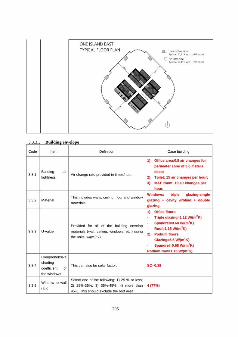
205

3.3.3.3 Building envelope


3.3.1 Building air

tightness Air change rate provided in times/hour.

1) Office area:0.5 air changes for

perimeter zone of 3.6 meters

deep;

2) Toilet: 15 air changes per hour;

3) M&E room: 10 air changes per

hour.

3.3.2 Material This includes walls, ceiling, floor and window

materials.

Windows: triple glazing-single

glazing + cavity w/blind + double

glazing.

3.3.3 U-value

Provided for all of the building envelop

materials (wall, ceiling, windows, etc.) using

the units: w/(m2*k).

1) Office floors

- Triple glazing=1.12 W/(m 2K)

- Spandrel=0.68 W/(m 2K)

- Roof=1.15 W/(m 2K)

2) Podium floors

- Glazing=5.6 W/(m 2K)

- Spandrel=0.68 W/(m 2K)

Podium roof=1.15 W/(m 2K)

3.3.4

Comprehensive

shading

coefficient of

the windows

This can also be solar factor. SC=0.19

3.3.5 Window to wall

ratio

Select one of the following: 1) 25 % or less;

2) 25%-35%; 3) 35%-45%; 4) more than

45%. This should exclude the roof area.

4 (77%)

206

3.3.6 Shape factor

The ratio of surface area that is exposed to

the outside area to the enclosed volume, and

the surface area does not include the floor

area, door area and internal wall area of the

stairwells without district space heating.

Surface area=49504 sqm,

SF≈0.1

207

3.3.3.4 Building services and energy systems Code Item Definition Cen

3.4.1

Space

heating -

centralized

Type of centralized

systems (boilers, heat

pumps, etc.)

Number of

systems

Fuel

type Heat media Heat capacity of the building (w)

Floor area of zone served by

each type of system

No space

heating.

3.4.2

Space

heating -

decentralized

Type of decentralized

system (local space

heaters)

Number of

each type

of heater

Fuel

type

Total

power (w) Power rating (w) Other performance

No space

heating.

Type of centralized

system (heat sources,

cold sources, chilled

water pump (indicate

primary or secondary),

cooling water pump,

AHU fan, FCU fan,

cooling tower, pumps

of cooling storage

system, heat

exchanger, etc.)

Number of

each type

of

component

Energy

type

Power

rating (w)

Other performance (water volume, pump lift for

pumps, heat exchange efficiency, area of heat

exchange for heat exchangers, etc.)

YES

4 1800 TR

1 1030 TR A. Electrical chiller

2 530 TR

-

B. Primary chilled

water pump 18

Refer to the following Table.

Designation Function

Qty Flow

(l/s)

Head

(M)

Power Motor Rating

(kW)

CHWP-B1-1 to 5 5 201 36.7 110

CHWP-B1-6 to 7 2 115 37.8 55

CHWP-B2-E1 to E3

Primary chilled water pump

3 81 37.9 75

CHWP-35-1 to 5 5 102.1 31.3 18.5

CHWP-35-E1 to E3

Secondary chilled water

pump 3 38 29 15 5 90 kW Flow: 269.2 l/s. Head: 22.5 M

2 45 kW Flow: 154 l/s. Head: 28.5 M

3.4.3

Air

conditioning -

centralized

C. Condensing

water pumps

3

Elec.

30 kW Flow: 79.2 l/s. Head: 21.4 M

208

2 90 kW Flow: 48.3 l/s. 110M

D. Cooling tower 17 Heat rejection: 2147 kW. Water flow: 75.3 l/s

E. Primary Air Unit

(PAU) 12 Elec.

Refer to the following Table.

Designation Qty Served area Air Flow

(l/s)

Fan Motor Rating

(kW)

Total Cooling

(kW)

PAU-RF-01&02 2 59 to 67/F 9900 30 473.5

PAU-49-01&02 2 50 to 58/F 9900 30 473.5

PAU-35-01&02 2 37 to 48/F 13440 37 254.8

PAU-20-01 to

04

4 2 to 19/F & 22 to 34/F 16230 55 790.5

PAU-B1-01&02 2 G to 1/F 1600 4 82.7

F. Air Handling Unit

(AHU) 133 Elec.

Refer to the following table.

Designation Qty Served area Air Flow

(l/s)

Total cooling

(kW)

Fan Motor

Rating (kW)

AHU-67-1 1 67/F, office 9130

AHU-67-2 1 67/F, office 9130 30 238.5

AHU-66-1 1 66/F, office 9130

AHU-66-2 1 66/F, office 9130 22 238

AHU-65-1 1 65/F, office 7180

AHU-65-2 1 65/F, office 7180 18.5 196.2

AHU-50-1 to 64-1 & AHU-

50-2 to 64-2 30 50-64/F, office 7530 18.5 205.4

AHU-48-2 1 48/F, office 7510

AHU-48-1 1 48/F, office 7510 18.5 205.4

AHU-39-1 to 47-1 & AHU-

39-2 to 47-2 18 39-47/F, office 7510 18.5 195.8

AHU-38-1 to 2 2 38-37/F, sky lobby 8120 18.5 115.7

AHU-38-3 1 38-37/F, sky lobby 6800 18.5 180.6

AHU-37-1 1 38-37/F, sky lobby 8400 15 172.6

AHU-22-1 to 34-1 & AHU-

22-2 to 34-2 26 22-34/F, office 7340 18.5 195.8

AHU-2-1 to 19-1 & AHU-2-2

to 19-2 36 2-19/F, office 7250 18.5 195.8

209

AHU-1-1A &1-1B 2 1/F, Foyer & G/F,

Escalator lobby 8050

AHU-1-2A & 1-2B 2 1/F, Foyer & G/F,


AHU-G-2A & G-2B 2 1/F, Foyer & G/F,


AHU-G-1 1 1/F, Foyer & G/F,


Not provided

AHU-B1-3 1 Chilled water pump room 3370 4 91.9

AHU-B2-1 1 Chiller Plant room 3370 91.1 4

AHU-B2-2 1 H.V. Switch room &

transformer room 2980 83.1 4

AHU-B2-3 1 Chiller & HV Switch room 2980 83.1 4

3.4.4

Air

conditioning-

decentralized

Type of local air

conditioner(s),

humidifier &

dehumidifier

Number of

each type

of air

conditioner

Fuel

type

Power

rating (w) Heat/cooling capacity (w)

Other performance

(humidification/dehumidification

capacity)

No

decentralized

AC.

Type of centralized

system (separate

ventilation systems

(i.e. separate system

for basement/garage),

heat exchanger and

local

humidifier/dehumidifier

(if used together with

separate ventilation

systems), mechanical

exhaust and Plenum

systems.

Number of

each type

Energy

type

Power

rating (w) Design of subsystem Other performance YES 3.4.5

Ventilation -

centralized

Ventilation fans for

mechanical room and

chiller plant

16 Elec. Refer to the following table.

Designation Qty Maximum air flow (L/s) Fan Motor Rating (kW)

EAF-49-1 1 6800 11

210

EAF-49-2 1 6160 11

EAF-49-5 1 2650 0.21

EAF-B1-1 to 3 3 8250 18.5

EAF-B1-4 1 2130 1.715

EAF-B1-5 1 1000 2.7

EAF-B1-6 1 3200 6.25

EAF-B1-7 1 2180 2.455

EAF-B1-8 1 250 0.5

EAF-B2-1 to 2 2 9375 22

EAF-B2-4 1 2400 5.2

EAF-B2-5 1 430 2.455

EAF-B2-6 1 1500 1.715

Ventilation fans for

carpark 10 Elec.

Refer to the following table.

Designation Qty Served area Maximum air flow (m 3/s)

EAF-B1-01 1 11

EAF-B1-02 1 11

EAF-B1-03 1

B1 Carpark, loading and unloading area

11

EAF-B2-01 1 12.5

EAF-B2-02 1 B2 Carpark, loading and unloading area

12.5

FAF-B1-01 1 0.88

FAF-B1-02 1 0.88

FAF-B1-03 1

B1 Carpark, loading and unloading area

0.88

FAF-B2-01 1 10

FAF-B2-02 1 B2 Carpark, loading and unloading area

10

3.4.6 Ventilation -

decentralized Type of local fans

Number of

fans

Fuel

type

Power

rating (w)

No

decentralized

ventilation.

3.4.7 Lighting Types of lighting

(incandescent bulbs,

fluorescent bulbs,

compact fluorescent

bulbs, and other bulbs)

including indoor

Number of

lighting

appliances

Fuel

type

Total

power (w)

Control method (photo/occupancy/scheduling) YES

211

(ceiling, task and

public) and outdoor

lighting.

Compact fluorescent

lamp

Incandescent bulbs

Not

provided/ Elec.

65 W/m2

including

office

appliances

Scheduling. 7:00~19:00 in the weekday usually.

Type(s) of appliances Number of

appliances

Fuel

type

Power

rating (w) Other performance YES

3.4.8 Office

appliances Refer to the following

table by on-site

investigation.

Not

provided

of the

whole

building.

Elec. Not

provided.

The percentage of each kind of office device is inv estigated as follows.

Cmpt+14'

LED

Cmpt+20'LED Multiple

cmpt, LED

Laptop Laptop+LED

HK-1 72.7% 7.1% 18.2% 0.0% 2.0%

3.4.9 Other

Types of other

equipment used in the

building (kitchen

appliances, water

heating appliances,

elevator, security

monitors, etc.)

Number of

appliances

Fuel

type

Total

power (w) X

212

3.3.3.5 Building operation and occupant behavior As for the description of building operation and occupant behavior, there are four ways to describe their characteristics and rules, with several subschemas to provide a more specific description. 1) Schedule: The change of an object’s status depends on a certain schedule. 2) Set point: The occupant changes the status of an object based on a set point. 3) Control: The occupant changes the status of an object based on a control objective. 4) Space: The occupant operates an object in either the full space or part space. 5) Random: The change of objects’ status has no certain discipline and runs randomly. Part 1: Subschema definitions

Item Mode Code Definition

1.1 Full time or part time (when occupied) in each month for the space

heating or cooling season.

Subschema 1:

Time mode 1.2

Number of weeks in each month for the space heating or cooling

season, and one time period (from time A to time B) or several time

periods (from time C to time D AND from time E to time F, etc.) on

typical days.

Subschema 2:

Event mode 2 Number of times per day/week/month and minutes per time for use.

Subschema 3:

Load mode 3 At which time periods for full load; at which time periods for partial load.

Schedule

Subschema 4:

Portion mode 4 % of the objects (fan, lighting, window, etc.) that are opened or used.

Subschema 5:

Single point

mode

5 Always set at a certain temperature (x℃), pressure or concentration.

Subschema 6:

Range mode 6

Usually set the temperature, pressure or concentration in the range of x -

y (If possible, please indicate the specific set points of indoor

temperature when occupied and not occupied.).

Subschema 7:

Load mode 7 Set at the full load or a certain % of load.

8.1 When the outside temperature is higher than x℃, set the temperature at

x℃ or in the range of x℃-x℃.

Set point

Subschema 8:

Outdoor

temperature

mode 8.2

When the outside temperature is lower than x℃, set the temperature at

x℃ or in the range of x℃-x℃.

9.1 When the temperature higher than x℃, open or use it.

9.2 When the temperature lower than x℃, open or use it.

9.3 When the temperature lower than x℃, close it.

Subschema 9:

Temperature

mode 9.4 When the temperature in the range of x℃-x℃, open it.

10.1 When there is a certain level of CO2 or CO, open it. Subschema

10: Air quality

mode 10.2 When there is a certain level of CO2 or CO, close it.

Control

Subschema 11.1 Fixed frequency

213

11.2 Variable frequency 11: Frequency

mode 11.3 Gear limit (i.e. high/low speed only)

Subschema

12: Illumination

mode

12 When the illumination outside is < x lux, open it.

Subschema

13: Personnel

mode

13 When there are the occupants, open or use it.

Subschema

14: Solar

irradiation

mode

14 When solar irradiation is strong (such as > xJ/(cm2*min)), close it.

15.1 When not in use, turned off (appliances and lighting).

15.2 When not in use, in stand by mode (appliances and lighting).

Subschema

15: On/off

mode 15.3 When not in use, left on (appliances and lighting).

16.1

When the outdoor temperature (such as chillers) or outlet temperature

(such as cooling towers) is higher than x℃, open one machine; when

the temperature is higher than x℃, open two machines, etc.

Subschema

16:

Temperature +

# of machines

running mode 16.2

When the outdoor temperature (such as chillers) or outlet temperature

(such as cooling towers) is lower than x℃, open one machine; when the

temperature higher than x℃, open two machines, etc.

Subschema

17: Flow

volume + # of

machines

running mode

17 When the flow volume is larger than Xm3/s, open one machine; when the

flow volume is larger than x m3/s, open two machines, etc.

18.1 Maintain a constant indoor temperature/humidity by variable air volume,

variable water volume and variable refrigerant volume.

Subschema

18: Indoor

temperature

control mode 18.2

Maintain a constant indoor temperature/humidity by adjusting the

opening of the valves.

Subschema

19: Order

control of

different

appliance use

mode

19 1. Open the window first, then use the air conditioner; 2. Use electrical

fan, then use the air conditioner

Subschema

20: Full space

mode

20 When heating, cooling or other appliance is used in the full space.

Space Subschema

21: Part space

mode

21

When heating, cooling or other appliance is only used in part of the

space. Indicate the percentage of area in each zone where the

appliances are used.

Random Subschema

22: Random 22

The change of object’s status has no certain discipline, and runs

randomly.

214

mode

Building system operation modes, schedule, set point and control In this part, three modes can be used to describe the operation schedule, set points and control of technical building systems. Part 2: Building system operation schedule, set point, control and space

Potential subschemas Code Item

Schedule Set point Control Space

1.2; 2; 4 N/A N/A 20; 21

3.5.1 Business hours 1.2-No space heating. Space cooling is usually

from 7:00-19:00 during weekday. 20

1.2; 2; 4 N/A N/A 20; 21 3.5.2 Occupancy schedule

1.2-8:30 to 18:30 is the usual business hours. 20

1.1; 1.2; 3 5; 6; 7; 8 9; 13; 17; 18; 19 20; 21 3.5.3 Space heating - centralized

No space heating.

3.5.4 Space heating - decentralized 1.1; 1.2; 3 5; 6; 7; 8 9; 13; 19 20; 21

1.1; 1.2; 3 5; 6; 7; 8 9; 10; 11; 13; 16;

17; 18; 19 20; 21

3.5.5 Space cooling - centralized 1.1- Space

cooling is usually

from 7:00-19:00

during weekday.

5=24Deg.C 9.1; 10.1; 11.2 20

1.1; 1.2; 3 5; 6; 7; 8 9; 10; 13; 19 20; 21 3.5.6 Space cooling - decentralized

No decentralized space cooling.

1.1; 1.2; 2; 3; 4 5; 6; 7; 8 9; 10; 11; 13; 19 20; 21

3.5.7 Ventilation (mechanic) - Toilet/kitchen 1.1-Full time

toilet exhaustion. 7 11.1 21

1.1; 1.2; 2; 3; 4 5; 6; 7; 8 9; 10; 11; 13; 19 20; 21

3.5.8 Ventilation (mechanic) -

Basement/garage 1.1-Full time

garage

ventilation.

5 10.1;11.2;13 21

1.1; 1.2; 2; 3; 4 5; 6; 7; 8 9; 10; 11; 13; 19 20; 21 3.5.9

Ventilation (mechanic) - Centralized –

M&E rooms 2 6 9.1;11.1;13 21

3.5.10 Ventilation (mechanic) -

Decentralized - rooms 1.1; 1.2; 2; 3; 4 5; 6; 7; 8 9; 10; 11; 13; 19 20; 21

1.2; 2; 4 N/A 12; 13; 15; 19 20; 21 3.5.11 Lighting

13 12;13 21

3.5.12 Office appliances 13 N/A 15.1;15.2;15.3 N/A

215

3.5.13 Other 2 N/A 15 20; 21

1.2; 2; 4 N/A 9; 10; 12; 13; 14;

18; 19 20; 21

3.5.14 Windows

Cannot be opened.

1.2; 2; 4 N/A 13; 14; 19 20; 21 3.5.15 Curtains/blinds

2 14 21

3.3.3.6 Input into energy performance indicators Building energy use can be expressed in the three ways according to attachment 3, which are (1) Energy use of each energy resource, fuel, electricity, cooling and heating, and peak electric

demand (2) Aggregation of energy of primary energy, equivalent electricity, and equivalent CO2 emissions (3) Normalized energy use in the above two approaches

Code Item Definition Frequency Scope Case

building

3.6.1 Fuel

consumption

Indicate fuel

consumption

in J, MJ, or

GJ.

Hourly (preferred) or

monthly plus daily for

typical weeks each

season (acceptable)

For each

business

(preferred) or

whole building

(acceptable).

No fuel

consumption.

3.6.2 Electricity

consumption

Indicate

electricity

consumption

in J, MJ or

GJ.



typical weeks each

season (acceptable)

For each

business

(preferred) or

whole building

(acceptable).

Hourly data

is not

available, as

well as the

typical day

hourly data.

3.6.3 Cooling

consumption

Indicate

cooling

consumption

in J, MJ or

GJ.



typical weeks each

season (acceptable)

For each zone

(preferred) or

whole building

(acceptable).

Hourly data

is available.

Refer to

Table 2.6.3.

3.6.4 Heating

consumption

Indicate

heating

consumption

in J, MJ or

GJ.



typical weeks each

season (acceptable)

For each zone

(preferred) or

whole building

(acceptable).

No heating

consumption.

3.6.5

Step 1:

Energy

Carrier

Peak

electric

demand

Indicate

peak electric

demand in

W or kW.



typical weeks each

season (acceptable)

N/A Not

available

216

3.6.6 Step 2:

Aggregation

of Energy

Provide the

aggregation

of energy of

primary

energy,

equivalent

electricity,

and

equivalent

CO2

emissions.



typical weeks each

season (acceptable)

For each

business

(preferred) or

whole building

(acceptable).

Hourly data

is not

available.

3.6.7 Step 3:

Normalized

Energy Use

Factors

related to

energy

performance

indicators

Normalized

energy use

using the

above two

approaches.



typical weeks each

season (acceptable)

For each

business

(preferred) or

whole building

(acceptable).

Hourly data

is not

available.

3.3.3.7 Indirect factors Code Category Parameter Description Case building

3.7.1 Energy price The price of unit energy. Electricity: 1.03 HKD/kWh e5

3.7.2 Stability of energy supply

Stability of energy supply is expressed as an average percent of each energy source in each city.

Year 2009: 6 Electricity-53% Oil & Coal products-32% Town gas & Liquefied petroleum gas-15%

3.7.3 Gas popularization rate

The ratio of population using gas to the total population in the city. Not available.

3.7.4

Social factors

GDP per capita

36758 USD per capita

3.7.5 Concern for saving energy

Subjective assessment of consciousness of occupants of energy conservation. Potential survey categories: 1) Very concerned; 2) Concerned; 3) Indifferent; 4) Not so concerned; 5) Not concerned at all


3.7.6

Energy-related attitude of occupants

Concern for environmental protection

Subjective assessment of consciousness of occupants of environmental protection. Potential survey categories: 1) Very concerned; 2) Concerned; 3) Indifferent; 4) Not so concerned; 5) Not concerned at all


5 Source:

https://www.clponline.com.hk/myBusiness/CustomerService/TariffOverview/BulkTariff/Pages/Default.aspx 6 Source: Hong Kong Energy End-use data 2011, EMSD, Table 7.

217

4. ITA-01: Office building in Italy

4.1 Basic Information of Building

4.1.1 Overview of the building

The case study is public office “Palazzo Ciocca”, built in 1860, situated in Livorno Ferraris (VC), Italy. The building floor has an area of 130 m2 with a ceiling height of 3.5 m. The simulation and the monitoring were performed at the second floor. The building structure is in bearing solid brick masonry. On the floor below the monitored zone are heated rooms (through autonomous heating systems) and also used for offices and similar, while locals on the upper floor are used for archives and use the heating system is generally off. In Table 4-1 the main building data are presented.

Table 4-10. Main building data.

Building name Palazzo Ciocca Building type Small office

Floor numbers 5 floors in total, 3 floors over ground, 1 floor underground, 1 attic

Building height 15,5 m

Gross floor area

Underground floor: 96 m2

Ground floor: 334 m2 1st floor: 334 m2 2nd floor: 334 m2 Attic: 334 m2 Total: 1096 m2

Net floor area

Underground floor: 68 m2

Ground floor: 219 m2 1st floor: 225 m2 2nd floor: 244 m2 Attic: 244 m2 Total: 756 m2

S/V 0,36

Structure type weight-bearing brickwork walls

Construction ear XIV-XIX centuries

Address Livorno Ferraris (Vercelli), Italy Via Martiri della Libertà 100

4.1.2 Geographical environment

Livorno Ferraris is a town located in North-Western Italy in Piedmont region. the number of degree days is 2549 °C d.

218

For detailed data refer to http://www.comuni-italiani.it/002/071/clima.html.

Table 4-11. Geographical and climatic data. Geographical position Longitude Latitude ASL HDD Livorno Ferraris (Vercelli), Italy

East 08°4'42"60

North 45°17'6"00

188 m 2549

Table 4-12. Statistics of extremes for standard typical meteorological year.

Outdoor meteorological parameters Unit Value maximum dry bulb temperature °C 31,0

minimum dry bulb temperature °C -7,0 4.1.3 Geometry information

In the following figures are reported the plans of each floor. The measures are expressed in meters.

Figure 4-26. Plan of the ground floor

219

Figure 4-27. Plan of the first floor

Figure 4-28. Plan of the second floor

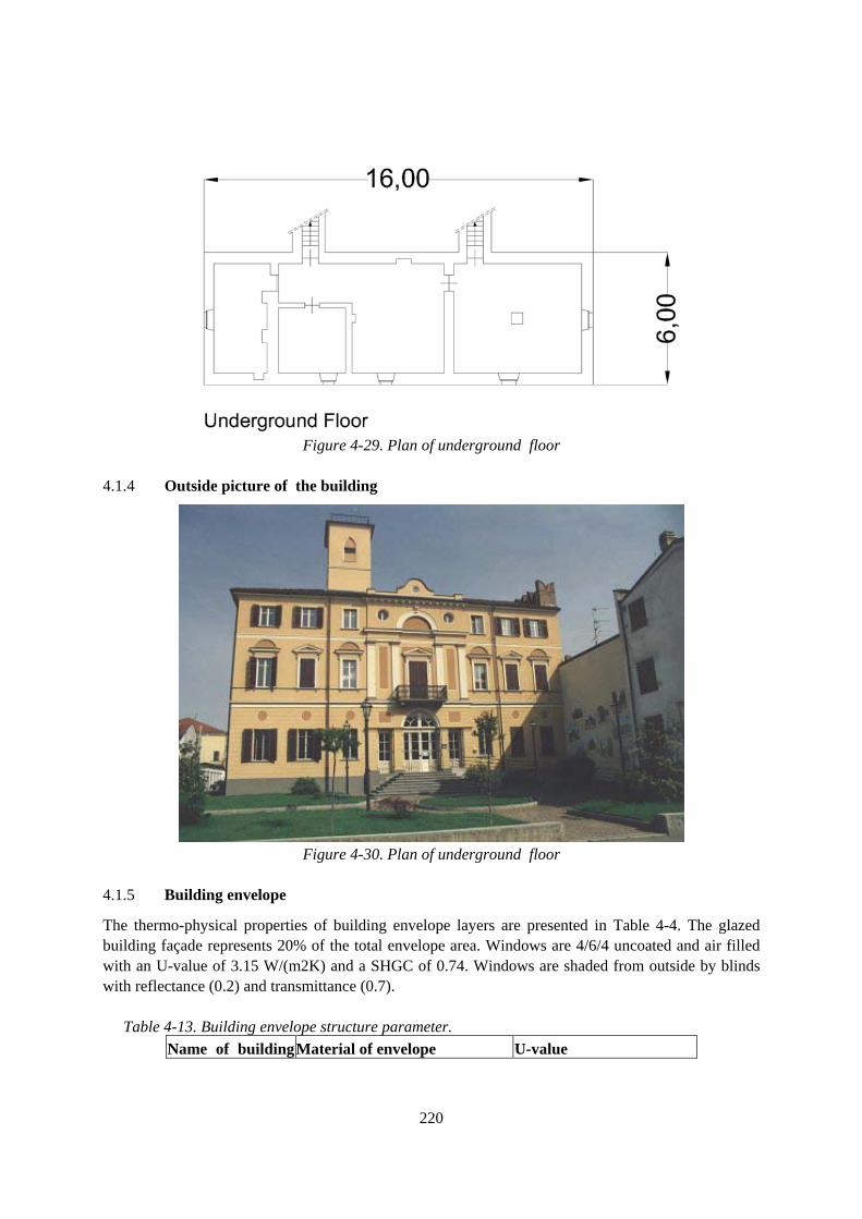
220

Figure 4-29. Plan of underground floor

4.1.4 Outside picture of the building

Figure 4-30. Plan of underground floor

4.1.5 Building envelope

The thermo-physical properties of building envelope layers are presented in Table 4-4. The glazed building façade represents 20% of the total envelope area. Windows are 4/6/4 uncoated and air filled with an U-value of 3.15 W/(m2K) and a SHGC of 0.74. Windows are shaded from outside by blinds with reflectance (0.2) and transmittance (0.7).

Table 4-13. Building envelope structure parameter.

Name of building Material of envelope U-value

221

envelope （（（（W/ m2.K））））

External wall Brickworks wall 0.7

Roof Roof tile -

Separating wall Brickworks -

Floor slab Brickworks -

External window Single pane glass + wood frame 6.0

Shutter External wood shutter - 4.1.6 Building systems

Table 4-14. Description of the building technical systems. Number System type Type Controller

1 Domestic hot water

Electrical heater -

2 Heating system Two natural gas Boiler (one for each floor) Centralized on/off system, driven by one zone sensor per floor

3 Ventilation system

Natural ventilation -

4 Lighting Fluorescent lighting, bulb desk light - 5

Common appliances

Pcs, printers, fax -

6 Peculiar appliances

Elevator -

4.2 Detailed information

4.2.1 Heating system

The heating system is centralized type equipped with a cast iron heat generator of which the main characteristics are reported in Table 4-6:

Table 4-15. Equipment in Heating Equipment Room in the unheated attic. Number Name Performance Parameter Controller Notes

1 Natural gas boiler

Net thermal power: 29,0 kW Nominal production efficiency: 91%

- The boiler serves Ground Floor

1 Natural gas boiler

Net thermal power :29,0 kW Nominal production efficiency: 91%

- The boiler serves 1st Floor

2 Water circulator

Electric alimentation: 220 V Pmax : 132/99 W Pmin 49/22 W

- Manual control with a fixed speed

20 Terminal device

Radiator -

222

4.2.2 Information Statistics

Function rooms layout of first floor for monitoring purposes is shown in Figure 4-6.

Figure 4-31. Function rooms layout of the first floor

4.2.3 Occupancy schedule and equipments

Table 4-16. Occupancy schedule and equipment description. Label Occupancy

profile Equipment Note

A 1 person from Monday to Friday. Hours: 8 am to 2 pm and 3 pa to 6 pm

1 pc and 1 printer

B 2 persons from Monday to Friday. Hours: 8 am to 2 pm and 3 pa to 6 pm

2 personal computers and 2 printers

The doors separating the room 2 and 3 are open for most of the occupancy period

C Occasionally occupancy

2 printers

D Occasionally occupancy

-

E 2 persons from Monday to Friday. Hours: 8 am to 2 pm and 3 pa to 6 pm

2 personal computers and 2 printers

F 1 fridge, 1 microwave oven, 1 Restroom e and service

223

automatic coffee dispenser, electric hot water boiler

local

G 1 person from Monday to Friday. Hours: 8 am to 2 pm and 3 pa to 6 pm

H Occasionally occupancy

224

5. JPN-01, JPN-02: Office building in Japan

5.1 Building Introduction

Table 5-1 Two Sample Office Buildings Outline Building Name Office A Office B

Location & Climate Shimada City, Central Japan, Mild Suzuka City , Central Japan , Mild

Structure & Stories Steel, 4 stories above ground Steel, 4 stories above ground

Total Floor Area 2,734m2 (2,368m2) 3,695m2 (3,358m2)*

Number of People 87 employees 118 employees

Building Use1st floor to 3rd floor : Office , 4th floor, meeting room and another use

Including Control room for distribution network etc(special use for electric power company).

*()Total floor area except for special use of electric power company

Photo 1 Shimada Sales Office (Office A)

(Completed in June, 2001) Photo 2 Suzuka Sales Office (Office B)

(Completed in June, 2001)

Figure 5-1 Location of Two Sample Office Buildings

5.2 Annual Electrical Energy Consumption

(1) Office A

Nagano Pref.

Shizuoka Pref.

Gifu Pref.

Aichi Pref.

Shimada Sales Office Mie Pref.

Suzuka Sales Office

Cold Climate

Mild Climate

Sendai City

Central Japan

225

Table 5-2 Detail of Annual Electrical Energy Consumption of Office A during 2004 to 2006

Year Total Sockets Lightings Electr ic water Heater

Another Lightings

and Sockets

HVAC Ice

Thermal Storage System

HVAC No Ice


Total Heat Exchan

ger

Electrode Steam

Humidi fier

Another Power Use

2004 285,543 32,007 106,207 6,754 16,300 73,136 39,201 3,885 6,025 2,027

2005 348,925 34,717 123,656 6,809 16,703 82,314 49,058 19,392 12,150 4,127

2006 451,328 36,355 127,374 6,965 18,413 91,867 55,372 65,183 46,300 3,500

*Units : kWh/year (2) Office B

Table 5-3 Detail of Annual Electrical Energy Consumption of Office B (2004 to 2006)

Year Total Sockets Lightings Electric water Heater

Another Lightings

and Sockets

HVAC Ice


HVAC No Ice


Total Heat Exchan

ger

Electrode Steam

Humidi fier

Another Power Use

2004 358,271 47,581 110,956 13,985 13,648 73,226 85,118 0 4,169 9,589

2005 393,654 46,959 116,919 13,258 15,420 81,315 102,230 0 6,022 11,532

2006 392,489 47,402 119,984 13,951 17,475 82,949 96,321 0 3,560 10,847

*Units : kWh/year

5.3 Monthly Breakdown of Electrical Energy Consumption by Major Devices

(1) Office A

0

5000

10000

15000

20000

25000

30000

35000

40000

2004

2005

2006

2004

2005

2006

2004

2005

2006

2004

2005

2006

2004

2005

2006

2004

2005

2006

2004

2005

2006

2004

2005

2006

2004

2005

2006

2004

2005

2006

2004

2005

2006

2004

2005

2006

Jan Feb Mar Apr May Jun Jul Aug Sep Oct Nov Dec

Mo

nth

ly E

lect

rica

l E

ne

rgy

Co

nsu

mp

tio

n

[kW

h] Ice thermal storage HVAC system outdoor unit Ice thermal storage HVAC system indoor unit

Ventilation(Total Heat Exchanger) Humidifier

Lightings OA socket

Figure 5-2 Monthly Electrical Energy Consumption of Office A during 2004 to 2006

(2) Office B

226

0

5000

10000

15000

20000

25000

30000

35000

40000

2004

2005

2006

2004

2005

2006

2004

2005

2006

2004

2005

2006

2004

2005

2006

2004

2005

2006

2004

2005

2006

2004

2005

2006

2004

2005

2006

2004

2005

2006

2004

2005

2006

2004

2005

2006

Jan. Feb. Mar. Apr. May. Jun. Jul. Aug. Sep. Oct. Nov. Dec.

Mo

nth

ly E

lect

rica

l E

ne

rgy

Co

nsu

mp

tio

n

[kW

h]

Ice thermal storage HVAC system outdoor unit

Ice thermal storage HVAC system indoor unit

Ventilation

Humidifier [Electrode steam type]

Lightings

OA socket

Figure 5-3 Monthly Electrical Energy Consumption of Office B during 2004 to 2006

5.4 Occupant Behavior

0

10

20

30

40

50

60

70

80

90

100

0:00 4:00 8:00 12:00 16:00 20:00

Atte

nded

Rat

io ［％

］

Weekdays

Weekend

Figure 5-4 Attended Ratio of Office A, 2nd Floor, during July 28th to August 3rd in 2009

0

10

20

30

40

50

60

70

80

90

100

0:00 2:00 4:00 6:00 8:00 10:0012:0014:0016:0018:0020:0022:00

Atte

nded

Rat

io[％

]

WeekdaysWeekend

Figure 5-5 Attended Ratio of Office B, 2nd Floor, during September 12th to 18th in 2009

227

6. JPN-03: Office building in Japan

6.1 Introduction

Field measurements and investigations on energy consumption and indoor environment have been carried out in a sustainable designed office building. Figure 6-1 shows the façade of the said office building. 6.2 Location

Sendai City, Japan (Figure 6-2)

SendaiSendai

Figure 6-1: Building façade Figure 6-2: Location 6.3 Climatic conditions

Figure 6-3 shows the monthly mean temperature and humidity in Sendai, Montreal and Berlin. Sendai is cold and snowy in winter, while hot and humid in summer. Minimum and maximum temperatures are 1.5 degree C in January and 24.1 degree C in August, respectively.

-15

-10

-5

0

5

10

15

20

25

30

50 60 70 80 90 100

Humidity (%RH)

Tem

per

atur

e (

℃)

Berlin

Montreal

Sendai

Figure 6-3: Monthly mean temperature and humidity

228

6.4 Outline of the office building

Figure 6-4 shows the floor plan of the investigated office building. It is a three-storey office building and covers a floor area of 4090 m2. The building is constructed in wood with the purpose to reduce the CO2 emissions. In order to improve the indoor thermal environment while reducing the energy consumption used in heating, the whole building is well insulated: high performance insulators are fitted in the exterior walls (180 mm thick) and on the roof (200 mm thick); windows are fourfold-glazing with high insulated sash. Besides, sun-shading technology is well utilized in this building to reduce the energy consumed by cooling.

19,1

10

27,3

00

58,240

17,290

10,290

19,1

10

27,3

00

58,240

17,290

10,290

N

19,1

10

27,3

00

58,240

17,290

10,290

19,1

10

27,3

00

58,240

17,290

10,290

N

Figure 6-4: Plan of the office building (1F)

6.5 Occupants and operation of the equipment

There are 20 workers in total, and all of them work on Monday, Tuesday, Thursday and Friday. All of them can take two days off in one week. One day is on Sunday, and for the other day, half of them take Wednesday, while the other half of them take Saturday. Table 6-1 shows the numbers of the workers in one typical week. Figure 6-5 shows the density of the occupants in one day. Although the business hour starts at 9:00am, 100% of the workers come to the office around 8:30am. The workers take a one-hour lunch break, and thus the percentage at 1:00pm was assumed as 50%. The business hour finishes at 6:00, and some of the workers go home, but some of them work until 8:00pm.

Table 6-1: Number of workers in one week

Day Sunday and Holidays Monday Tuesday Wednesday Thursday Friday SaturdayWorkers 0 20 20 10 20 20 10

8 8:30 13 18:30 20

100%

50% 50%

100%

8 8:30 13 18:30 20

100%

50% 50%

100%

Figure 6-5: Percentage of the occupants in one day

229

For the HVAC system, high quality air-conditioners with COP value over 5.0 are installed for heating and cooling, while mechanical ventilation system with air change rate of 0.5 times 1/h is used for ventilating. The energy source is electricity. Table 6-2 shows the operation of air-conditioners.

Table 6-2: Operation of air-conditioners Period Time Setting Tepmerature Relative Humidity

Heating 1st January ~ 30th April 8:00am ~ 8:00pm 23℃ 40%

Cooling 30th July ~ 30th September8:00am ~ 8:00pm 26℃ 50% 6.6 Investigated items and measurement systems

Table 6-3 shows the investigated items and methods. The investigation items include electricity consumption, indoor/outdoor temperatures and humidity, as well as behaviors of occupants. Investigation methods were classified into simplified measurements, detailed measurements and questionnaire survey. Table 6-3: Investigated items and methods

c

Machines Location Period

Electricity Consumption Special Moniter 10min

Indoor/outdoor temperatureand humidity

Data loggers with temperature and humidity sensorsIndoor：+FL0.6m；Outdoor

15min

Vertical temperaturedifference

Data loggers with temperature and humidity sensors 0.1m、0.6m、1.1m 15min

Globe ball

THERMIC2100A

Temperature and humidity Data loggers with temperature and humidity sensors 0.1m、0.6m、1.1m

Air velocity VIVO20T35 (DENTEC) 0.1m、0.6m、1.1m

Air velocity

Thermal sensation

Acceptance

Preference

Productivity

0.6ｍ

10sec

Questionnaire sheet

Items

SimplifiedMeasurements

Questionnaire

Detailed Measurements

Globe temperature

6.7 Measured energy consumption and indoor environment

6.7.1 Monthly and annual energy consumption

Figure 6-6 shows the monthly energy consumption by different end-users, while Figure 6-7 shows the annual energy consumption in this office building, with the comparison to the statistical data of 2005 and 2007. The convector coefficient of electricity consumption to primary energy consumption was 10.25MJ/kWh. Energy consumption increased during the heating (from November till the end of April next year) and cooling period (August and September). Lighting, the largest energy user, accounted for about 43% of the total electricity consumption and it was followed by OA (Office Appliance) machines which accounted for 25%. Annual heating and cooling electricity consumption accounted for 12% and 2% of the total electricity consumption, respectively. Annual energy consumption of the

230

measured office building (921 MJ/m2・year) was 47% lower than the statistical data (1739 MJ/m2

・

year).

0

20

40

60

80

100

Jul

Aug Sep

Oct

Nov

Dec Ja

n

Feb

Ma

r

Apr

May Ju

n

Jul

Aug Sep

Oct

Nov

DecE

nerg

y co

nsum

ptio

n (M

J/m2 ) cooling

heating

lighting

OAmachinesventilation

others

2006 2007

0

20

40

60

80

100

Jul

Aug Sep

Oct

Nov

Dec Ja

n

Feb

Ma

r

Apr

May Ju

n

Jul

Aug Sep

Oct

Nov

DecE

nerg

y co

nsum

ptio

n (M

J/m2 ) cooling

heating

lighting

OAmachinesventilation

others

2006 2007 Figure 6-5: Monthly energy consumption

Office building A(Jul. 2006~ Jun.2007)

0

400

800

1200

1600

2000

2400

Ele

ctric

ity C

ons

umpt

ion

(MJ/㎡

・Y

ea

r)

Office Appliance & others Lighting Ventilation Heating & Cooling

(Japan, 2005) (Tohoku, 2007)

38%

44%

14%21%

43%47% Low

9211739 1720

31%

1945

(Japan, 2007)0

400

800

1200

1600

2000

2400

Ele

ctric

ity C

ons

umpt

ion

(MJ/㎡

・Y

ea

r)

Office Appliance & others Lighting Ventilation Heating & Cooling

(Japan, 2005) (Tohoku, 2007)

38%

44%

14%21%

43%47% Low

9211739 1720

31%

1945

(Japan, 2007)

Figure 6-6: Annual energy consumption 6.7.2 Profile of energy consumption, indoor and outdoor temperatures during three days in

winter/summer

Figure 6-7 shows the profile of energy consumption, indoor and outdoor temperatures during three days in winter/summer including the coldest day (Feb 25th) and hottest day (Aug 6th). However, here only shows the electricity consumption in Office A. Coldest days: It was a weekend from Feb 24th to 25th, there were fewer people working in Office A or C, and thus, temperatures in these two offices during the weekend were about 2 to 3� lower than during the weekdays. However, in contrast, temperature in Office B, where workers came even on weekends, did not change much between weekends and weekdays. During weekends, temperatures in Office A and C changed with the solar radiation. On the other hand, during the weekdays, temperatures in each office start to increase when the air-conditioners were turned on around 8:00am ~ 9:00am for heating and stayed around 22 to 26� during the business hours. Temperature in Office B was about 3 to 4� higher than in the other two offices, due to the relatively higher densities of occupants and office appliances. In addition, relative humidity in each office was lower than 25%, which resulted in extreme dryness. As mentioned above, there were fewer workers in Office A on Feb

231

24th and 25th than on Feb 26th. Therefore, energy consumption on weekends was about half less than that on weekdays. Hottest days: It was Sunday on Aug 5th, workers in Office B were working even during the weekends, and therefore temperature in Office B did not change much between weekends and weekdays. However, temperatures in Offices A and C was about 2 to 3� higher during weekends than that during weekdays. During the weekdays, Temperatures in Offices A and C started to decrease around 8:00 ~ 9:00am when the air-conditioners were turned on for cooling and stayed around 25 to 27� during the business hours. Temperature in Office B was about 1~2� higher than the other two offices because of relatively higher densities of occupants and office appliances. Relative humidity in Office B was around 55% to 65%. However, it was higher than 70% in Offices A and C most of the time; it was higher than 60% even when the air-conditioners were working. There was no worker in Office A on Aug 5th and thus, no electricity was consumed for cooling this day.

Coldest days Hottest days

07/2/24 (Sat) 2/25 (Sun) 2/26 (Mon)

5

10

15

20

25

30

RH

(%

)

Office A Office B Office C

10

14

18

22

26

30

Te

mp

. (℃

)

0

200

400

600

800

1000

Glo

bal

Sol

ar

Rad

iatio

n(W

h/㎡

)

0

4

8

12

16

Ele

ctric

ity C

on

sum

ptio

n(k

Wh

/h)

Others VentilationOA Machines LightingHeating

20

22

24

26

28

30

Tem

p. (℃

)

0

200

400

600

800

1000

Glo

bal S

olar

Ra

diat

ion

(Wh/

㎡

)

0

20

40

60

80

100

RH

(%

)

Office A Office B Office C

0

4

8

12

16

Ele

ctric

ity C

on

sum

ptio

n(k

Wh

/h)

Others VentilationOA Machines LightingCooling

07/8/5 (Sun) 8/6 (Mon) 8/7 (Tue)

Figure 6-7: Profile of energy consumption, indoor and outdoor temperatures during three days [Upper side: the coldest day (Feb 25th); Lower side: the hottest day (Aug 6th)]

Acknowledgement: Authors would like to acknowledge Hokushu Housing Corporation to give us an opportunity for measurement of indoor environment and energy use of the head quarter office.

232

7. NOR-01: Office building in Norway


Figure 7-32. Location of the case building in Trondheim

The case building is located in Trondheim at the address Professor Brochs gate 2, as shown in Figure 7-32. The building is marked with the yellow mark with number 1. The building extends along the main road, marked with the red color in Figure 7-32. The building is rented as an office building to nineteen different companies. Height of the building is 21 m (the front block) and 14 m (the back block). The building has six floors and a basement floor. The Gross Floor Area and conditioned building both are 16,200 m2.

Table 7-17. Climate data of Trondheim Jan Feb Mar Apr May Jun Jul Aug Sep Oct Nov Dec Year

Average high (˚C) 3.9 3.4 7.9 13.4 21.7 20.1 25.8 25.7 22.8 17.2 9.7 4.4 14.7

Daily mean (˚C) -7 -5.7 -0.1 4.5 7.4 10.4 15.3 14.5 9.9 6.3 -3.9 -7.3 3.7

Average low (˚C) -21.9 -24.3 -12.5 -2 -1.5 2.3 6.3 4.4 -0.3 -7.1 -16.8 -18.8 -7.7

Relative humidity (%) 78 76 85 71 74 77 75 79 77 76 78 82 77.3

HDD 742.9 634.4 529.5 375.3 297.3 197.8 64.6 89.2 212.5 332.8 627.6 752.3 4856.2

In Norway, CDD is not an actual parameter. HDD is 4856 of year 2010. HDD was calculated for the base indoor temperature of 17oC. Outdoor temperature, relative humidity, and solar irradiation for 2011 are given in Figure 7-33 to 4 respectively.

233

Figure 7-33. Outdoor temperature in Trondheim in 2011

Figure 7-34. Relative humidity in Trondheim in 2011

234

Figure 7-35. Solar irradiation in Trondheim in 2011


Figure 7-36. Office building in Trondheim

The office building in Figure 7-36 has been in use since autumn 2009. The building was built according to the low energy building standard. The low energy standard implies the U-value for the outdoor wall of 0.18 W/m2K and U-value for windows of 1.2 W/m2K. Further, this standard implies the infiltration of 0.1 air change per hour. Basic information about the building is given in Table 7-18. The building consists mostly of cell offices, meeting rooms, and common areas. Simplified and typical floor plans are given in Figure 7-37 and 7, respectively. The size of the cell office is about 10 m2, while the size of the meeting rooms can be about 30 m2. The floor plan was developed by using so called “the room solution”, so it is possible to connect few offices if necessary. This gives possibility to change the floor plan upon tenant requirements. The simplified plan as in Figure 7-37 will be used further in the text to explain installed building equipment. Labeling as in Figure 7-37 is used to label some energy meters, too.

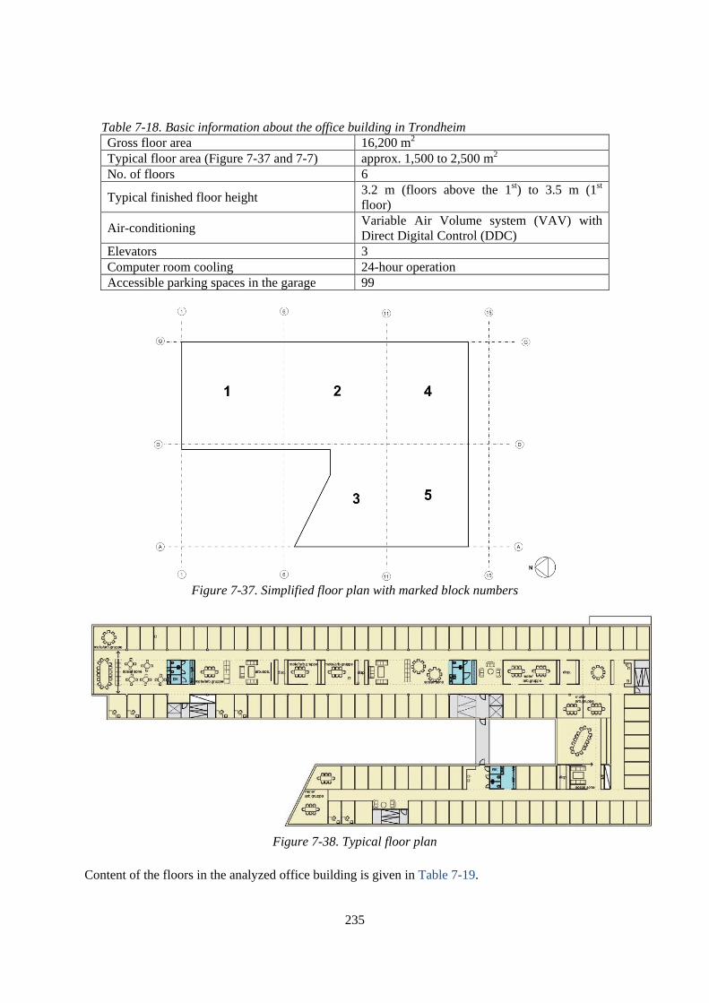
235

Table 7-18. Basic information about the office building in Trondheim Gross floor area 16,200 m2 Typical floor area (Figure 7-37 and 7-7) approx. 1,500 to 2,500 m2 No. of floors 6

Typical finished floor height 3.2 m (floors above the 1st) to 3.5 m (1st floor)

Air-conditioning Variable Air Volume system (VAV) with Direct Digital Control (DDC)

Elevators 3 Computer room cooling 24-hour operation Accessible parking spaces in the garage 99

Figure 7-37. Simplified floor plan with marked block numbers

Figure 7-38. Typical floor plan

Content of the floors in the analyzed office building is given in Table 7-19.

236

Table 7-19. Functional area information Basement Garage, plant rooms, showers and toilets, IT room, and storages 1st floor Entrance, restaurant, lecture room, and offices 2nd to 6th floor Offices 5th floor Ventilation plant room 7th floor Ventilation plant room


7.3.1 Electricity use

The building is equipped with a high number of energy meters, which include measurement of electricity for light, appliances, ventilation, etc. The building is equipped with 74 energy meters, where 66 meters are for electricity and eight meters are for heating and cooling measurements. The technical platform for the energy measurement was separated from the building energy management system (BEMS). Therefore, there is no history of the energy measurements in the BEMS of the case building. These energy measurements were transferred to an energy savings company database. The use of two different technical platforms for building management and energy monitoring, where energy consumption had not been logged in the BEMS, could be an issue. This issue can be explained with poor functional integration, because the labelling of the system and components in the energy service company was slightly different than in BEMS and it might be that what was shown as the compressor electricity use was that of another equipment. Specifically, it can be difficult to estimate energy use of equipment that has its own control unit. Such equipment can be heat pumps, cooling plants, and air handling units. Even though equipment manufacturers guarantee good data transfer from the equipment control unit to the BEMS, there can be many problems in the data transfer. Since data from the energy saving company were only available data, they were used here to present the building energy use. In Figure 7-39, electricity use measurements from 66 meters were organized into nine groups: compressors, electricity in the substation, elevators, appliances, fans, light, electrical cars, a storage room, and IT server. The same electricity use as in Figure 7-39 is given in Table 7-20. In Figure 7-39, Storage room is an electricity meter that measures electricity use in one room rented by one company. This was installed as a test for electricity use measurement.

237

Figure 7-39. Total electricity use break down in 2010

In Figure 7-39 “El.Substation” is measurement of electricity use in the substation. This electricity use should include electricity for circulations pumps and control equipment in the substation. It could happen that this electricity use considered some additional users, but it was not possible to define all of them. For the purpose of this analysis, it was assumed that “El.Substation” is the electricity use for running the circulations pumps for heating and cooling, and control equipment in the substation. In Figure 7-39 “Appliances” is electricity use used by all the equipment that was plugged in, such as PCs, printers, coffee machines, and all the other devices that were necessary in an office building. “Fans” present the electricity use in the air handling units (AHUs) and it can include some additional users, but it was not possible to identify that. “Compressors” present the electricity use of the compressors in the two heat pumps. “El.cars” presents the electricity use for the electrical cars. Detailed description of the substation, air handling units, and heat pumps is given in Section 5. Table 7-20 gives numerical values for the results shown in Figure 7-39. In addition in Table 7-20, the total electricity use measured by the main electricity meter is given. By comparing the total electricity use measured by the sub-meters and by the main electricity meter, difference between these measurements can be noticed. The measurement of the main electricity meter is higher than measurement of the sub-meters. The main electricity meter measured electricity use that should be paid to the electricity deliverer. The reasons for different measurements could be the following: the sub-meters did not measured all the electricity use in the building; the sub-meters had problem in data transferring that caused missing of data.

Table 7-20. Electricity use Period Total

(kWh) Compre

ssors (kWh)

Pumps (kWh)

Elevators

(kWh)

Appliances

(kWh)

Fans (kWh)

Light (kWh)

El. Cars (kWh)

Storage room* (kWh)

IT room (kWh)

Jan 81 664 6 819 2 693 371 19 183 4 059 17 632 13 0 7 035

Feb 89 191 10 840 2 252 350 17 615 4 039 16 727 13 6 5 863

Mar 79 399 13 285 1 746 400 17 513 4 798 17 930 22 0 6 908

238

Apr 68 635 10 358 1 527 379 16 737 5 236 17 603 37 11 6 581

May 68 547 10 448 1 358 368 17 010 5 438 17 577 42 3 6 638

Jun 74 095 10 601 1 300 433 18 326 8 535 18 248 60 5 6 128

Jul 67 528 10 208 1 336 259 15 474 9 011 14 708 74 0 6 564

Aug 71 951 10 206 1 362 291 15 496 9 315 15 390 105 11 6 554

Sep 69 618 10 338 1 162 409 17 457 7 173 19 705 127 22 8 122

Oct 76 182 10 765 1 153 438 18 520 6 861 21 002 120 12 9 177

Nov 78 725 10 896 1 151 460 19 209 6 292 20 804 72 13 10 407

Dec 76 557 8 793 1 169 405 20 018 8 089 17 367 111 2 10 524

Total 902 092 123 557 18 209 4 564 212 558 78 847 214 693 796 85 90 502

The problem of missing data and its influence on the energy use measurement is shown in Figure 7-40. The measurements of the main meter were treated as the correct in Figure 7-40. The sum of the sub-meter measurements were compared to the main meter measurements. Since the problem of missing data was identified, the sub-meter data were corrected by using neural networks. Finally, these corrected data were used for the analysis of electricity use shown in Figure 7-39 and Table 7-20. The results in Figure 7-40 show that the summarized corrected measurements had values closer to the total electricity use measured by the main meter. Since the main meter measurements were used to pay the building electricity bill, these measurements are used in Section 3.3. Energy flow demonstration to present energy delivered to the building.

Figure 7-40. Influence of missing data on the electricity use measurement

Specific electricity use per m2 in 2010 for the eight groups of electricity users is shown in Table 7-21. Since the electricity use of the storage room was very low, it was not considered in Table 7-21. The building was in use since autumn 2009 and the number of users increased during 2010. This could explain increase in the monthly energy use in Figure 7-39. This issue related to number of occupants

239

will be discussed in Section 4. The increase in the number of occupants could also change specific energy for different users in Table 7-21.

Table 7-21. Specific electricity use in 2010

Purpose Light Applia

nces

Compres

sors IT server Fans Substation Elevators El.cars

Specific use (kWh/year/m2)

13.25 13.12 7.63 5.59 4.87 1.12 0.28 0.05

Area used in EUI is Gross floor area.

7.3.2 Heating energy use

Heating energy for ventilation, space heating, snow melting, and domestic hot water is supplied by district heating and supported by two heat pumps. The heating and cooling supply is explained in Section 7.5.1 and Figure 7-56. One heat pump is actually a cooling plant marked with 35.02. This cooling plant supplied the cooling for the IT rooms. Condenser heat from this cooling plant is used to support building heating. In the further text this cooling plant is named as cooling plant/heat pump or 35.02. The second heat pump marked with 35.01 is only used for the ventilation systems. This heat pump provides heating for heating/cooling coils in the winter and cooling for heating/cooling coils in the summer. In addition, these heating/cooling coils, the AHUs are equipped with heating coils supplied by district heating. The space heating includes radiator heating in the offices and floor heating in the showers. Detailed description if the heating and cooling energy supply system is given in Section 5. Heating energy break down in 2010 is given in Figure 7-41. Condenser heat from the cooling plant/heat pump 35.02 is used to support the building heating and with that it decreased total heating demand provided from the district heating. Therefore, this condenser heat is treated as negative in Figure 7-41. Unfortunately, since building had low occupancy level and cooling load in the IT rooms was low, the delivered condenser heat was low. Issues in the operation of the cooling plant/heat pump are explained in Section 5.1. The same heating energy use as in Figure 7-41 is given in Table 7-22.

240

Figure 7-41. Total heating energy use break down in 2010

In Figure 7-41, heating energy use for snow melting is not shown, because there is no energy meter for the snow melting equipment. Total heating energy use is also given in Table 7-22. This total heating energy use was measured by the district heating producer.

Table 7-22. Heat use

Period Total (kWh)

Radiators (kWh)

Ventilation (kWh)

Tap water (kWh)

Floor heating (kWh)

Condenser heat (kWh)

Jan 121 330 65 290 23 500 2 900 0 -240

Feb 88 410 47 878 13 943 2 829 1 198 -115

Mar 59 840 33 737 10 894 2 973 1 655 -449

Apr 27 780 17 142 6 820 3 214 69 -710

May 12 670 8 921 5 807 3 100 1 -488

Jun 5 920 5 268 8 010 3 469 29 -488

Jul 2 240 6 582 7 989 2 483 0 -486

Aug 3 300 6 822 8 132 2 590 0 -508

Sep 19 350 17 071 6 516 4 639 646 -286

Oct 31 790 19 812 6 175 5 197 812 -239

Nov 90 980 45 840 17 250 5 430 4 445 -350

Dec 146 040 73 320 43 150 4 510 6 750 -130

Total 609 650 347 683 158 186 43 334 15 605 -4 489

In Table 7-22, the total heating energy use for each month is different than the sum of the values for radiators, ventilation, tap water, floor heating, and condenser heat. The reasons for this could be similar as explained in the case of electricity use: the sub-meters did not measured all the heating energy use in the building; the sub-meters had problem in data transferring that caused missing of data;

241

the sub-meters were oversized for this purpose. During an in-situ survey, it was noticed that there is no energy meter for the snow melting equipment. Therefore, this part of the heating energy use was not registered and was not calculated in the heat balance in Figure 7-41. Comparing total heating energy use measured by the district heating producer in the summer months from June to August in Table 7-22, it is possible to notice the problem of oversized heating energy meters. The radiators and ventilation were not in use in the summer months. Small water circulation might happen, but it could not cause high heating energy use as shown under Radiators in Table 7-22. This is a problem caused by an oversized heat energy meter. Similarly as for the measurement quality of electricity use shown in Figure 7-40, the measurement problem of the heating energy use is shown in Figure 7-42. The measurements of the main meter were treated as the correct in Figure 7-42. The sum of the sub-meter measurements were compared to the main meter measurements. Since the problem of missing data was identified, the sub-meter data were corrected by using neural networks. Finally, these corrected data were used for the analysis of heating energy use shown in Figure 7-41 and Table 7-22.

Figure 7-42. Influence of missing data on the heating energy use measurement

The results in Figure 7-42 are measurements for November when missing of data did not happen. Therefore, the difference between the red and blue lines in Figure 7-42 could be treated as energy use for the snow melting equipment. Since the main meter measurements were used to pay the building heating energy bill, these measurements are used in Section 3.3. Energy flow demonstration to present energy delivered to the building. Specific heating energy use per m2 in 2010 for the four groups of heating energy users is shown in Table 7-23. In addition, the condenser specific heat per m2 is also shown in Table 7-23. As explained before, this condenser heat was provided from the cooling plant condenser to support the building heating. The results in Table 7-23 are sorted from the highest to the smallest specific heat. Specific heating energy use for ventilation is lower than expected, because of AHUs solution, look at Figure 7-

242

65 in Section 7.5.2. Detail description of AHUs and their control is given in Section 5.2. Just to recall here, each AHU is equipped with the heat recovery wheel, the heating/cooling coil connected to the heat pump, and heating coil connected to the district heating. A sequence control of the AHUs gave priority to the heating/cooling coil connected to the heat pump 35.01. Therefore, heating energy for ventilation is partially supplied by the heat pump. The electricity use of the heat pump for ventilation was defined in Section on electricity use Figure 7-39.

Table 7-23. Specific heating energy use in 2010

Purpose Radiators Ventilation Hot water Floor

heating Condenser heat

Specific use (kWh/year/m2)

21.46 9.76 2.67 0.96 -0.28

7.3.3 Energy flow demonstration

According to the definition of energy flow boundaries, the energy flow can be demonstrated as in Figure 7-43. The total electricity use in 2010 was 902 MWhe, including 523 MWhe on Eb boundary (for building requirements such as lighting, appliances, elevators, and IT server room) and 221 MWhe on Et boundary (for technical system such as heat pumps, circulation pumps, and supply and exhaust fans in the AHUs). The annual cooling consumption for cooling the IT rom was 167 MWhc, generated by one cooling plant. The same cooling plant produced 4 489 kWhh useful condenser heat that was used to support building heating. The annual cooling consumption for the AHUs was 4 000 kWhh that was produced by the second heat pump. This heat pump gave 87 MWhh of heating energy for AHUs. The total heating energy use was 610 MWhh, including heating by radiators, the heating coils in the AHUs, floor heating, snow melting, and hot water heating. In Figure 7-43 for the total delivered energy at Et boundary, the measurements from the main electricity and heating meters were used. The total energy use for electricity and heating is higher than the summarized value of the sub-meters, but the total energy use delivered at the building boundary should be treated as a measurement of the delivered energy. Electricity equivalent approach was used to calculate the total energy use. If the conversion factor of 0.2317 equivalent electricity/hot water was implementer, the total energy use of the case building in 2010 was 1 043 MWhee.

243

Figure 7-43. Energy use on Ed, Et, Er and Eb boundary of a typical building (Note: kWhe�electricity, kWhh�heating consumption, kWhc�cooling consumption, kWhee�energy consumption by electricity

equivalent approach)

244

7.4 Occupant behavior description

7.4.1 Occupancy level and number of occupants

The presence schedule for the office building in Trondheim is given in Figure 7-44. This office building is rented to different companies, usually companies have working time between 8 a.m. until 4 p.m. But some companies could extend working time until 5 or 6 p.m. Figure 7-44 was established based on the presence sensor for ventilation. This presence sensor was located in the part of the building that was all the time in use and rented by a consultant company.

Figure 7-44. Presence schedule during working days

In our study we did not follow detailed when and how many occupants came to the building. In addition, there is no mean to follow exactly number of occupants. However, we got data on the total number of occupants in the building. Since this building is in use since autumn 2009, the entire building was not rented immediately. Development of the number of occupants in the building is given in Figure 7-45.

Figure 7-45. Development of the number of occupants in the office building in Trondheim

245

In general, it can be assumed that working hours is about 2000 hours per year for light and ventilation in the building. Light in the corridors and common areas is ON longer time than light in the offices. Working hours of the IT server room is 8760 hours. Since it could be difficult to assume exactly occupancy level, we suggest use of the hourly electricity profiles and hot tap water profile to detect occupancy level. In the case of the office building in Trondheim, electricity use was independent of the outdoor temperature, but instead determined by the building users. In average over the year, hourly electricity profiles were varying from 70 kW during non-occupied periods to 200 kW during occupied periods. The hourly summarized profiles of the electricity use are shown in Figure 7-46.

Figure 7-46. Hourly profiles of electricity use in the office building in Trondheim

The electricity use marked with “Fans” in Figure 7-46 presents the total electricity use for all the AHUs. The electricity use of the fans was determined by the building users as it is possible to notice in Figure 7-46. The VAV systems were controlled by presence sensors, meaning the fans were operating only when there were users in the building as explained in Section 7.5.2. The electricity consumption of the heat pump compressors was quite constant as shown in Figure 7-46 with “Compressors”. The reason for this was that the heat pumps were oversized and the compressors were in operation all the time at the lowest step and thereby using constant power. The heat pumps are introduced in Section 7.5.1. In Figure 7-46, it is possible to notice that appliances, light, compressors, and IT server contributed mostly to the hourly profiles during non-occupied periods as well as during occupied periods. The hourly profiles of the electricity use for the light, appliances, AHUs, hot tap water are presented in the further text. Issues in measurement, extent of measurement, and accuracy are also explained briefly. 7.4.2 Lighting system

246

For this case building it was not possible to obtain data about installed equipment for the electricity use. However, use of the hourly profiles could help to identify amount of energy and schedules used for the lighting system. The control strategy for the lighting system was the following:

• During working time, presence sensors are implemented to control the light; • During non-working time, the light should be OFF.

As explained before, the working time could be between 8 a.m. until 4 p.m. But some companies could extend working time until 5 or 6 p.m. We did not have possibility to collect data about common areas and security entrance that use light all the time. In Figure 7-37, a schema with the building blocks was introduced. There was an idea that this schema as in Figure 7-37 should be used to mark building energy meters. However, due to a problem to rent the building before it was opened, the block 2 in Figure 7-37 was divided into two parts, so that the left part of the block 2 was joined to the block 1 and the right part of the block 2 was joined to the block 4. Based on this, the energy measurement in the next Figures is marked as Part1, Part 3, Part 4, and Part 5. Related to the results this means the following:

• The results marked as Part 1 present energy use for the block 1 and the left part of the block 2 in Figure 7-37;

• The results marked as Part 3 present energy use for the block 3 in Figure 7-37; • The results marked as Part 4 present energy use for the block 4 and the right part of the block

2 in Figure 7-37; • The results marked as Part 5 present energy use for the block 5 in Figure 7-37.

The electricity use hourly profiles are presented in Figure 7-47. The block 4 or Part 4 in Figure 7-47 is occupied by a consultancy company that has possibility to use light system longer. The block 5 is occupied by a governmental company.

Figure 7-47. Hourly profiles for light effect at the fourth floor

247

The electricity use for the entire building organized by blocks is presented in Figure 7-48. The block 3 or Part 3 in Figure 7-48 includes the glass area and entrance. This could be reason for random peaks in the electricity use of this zone. The total light electricity use profile is given in Figure 7-49.

Figure 7-48. Hourly profiles of light effect by zones for the entire building

Figure 7-49. Hourly profile for the total light effect

7.4.3 Appliance

The electricity use for the appliances in the building is organized in the same way as the light electricity use introduced in Section 7.4.2. It is difficult to estimate which building appliances were installed in the building, but it could be assumed that these typical office equipment. The hourly profiles of the appliances effect organized the building block are given in Figure 7-50. The hourly

248

profile of the total electricity use for the appliances is given in Figure 7-51. The profiles of the appliance use can be used to detect building use, but still in Figure 7-50 and 20 it is possible to notice that a half part of the appliances was ON during non-working hours.

Figure 7-50. Hourly profiles of the appliance effect by zones for the entire building

Figure 7-51. Hourly profiles the total appliance effect

7.4.4 Ventilation

Electricity use for the ventilation system is presented for each AHU. The detail description and control of the AHUs is introduced in Section 7.5.2. Further in Section 7.5.2 in Table 7-29, the capacities of the AHU equipment are given. The served zones by each AHU are presented in Figure 7-64. The results in the following Figures are from the first week in November 2010. At that time the entire building was not rented as shown in Figure 7-45. However, all the building was ventilated with a low amount of air. In Figure 7-52 and 22, the hourly profiles of the AHU electricity use are shown. The total AHU

249

electricity use is given in Figure 7-54. In the building, the electricity meters for the entire AHU were introduced. Therefore, it was not possible to separate electricity use only for fans.

Figure 7-52. Hourly electricity profiles for AHUs 36.01 to 36.04

Figure 7-53. Hourly electricity profiles for AHUs 36.05 to 36.08

Based on the results in Figure 7-53, it could be concluded that the AHU 5 or 36.05 was in use more than other AHUs. Consequently, this indicated that this part of the building was more occupied than the other part of the building. In an on-situ survey and talk with the building operator, we found out the same. The part of the building supplied with the AHU 36.05 was occupied since the building was in use. In Figure 7-53, it can be noticed that the hourly profile for the AHU 36.05 had maximum values about 10 kW. The maximum installed effect for the supply and exhaust fan in the AHU 36.05 is 8.96 kW. Consequently, it can be concluded that this additional effect of about 1 to 2 kW is the

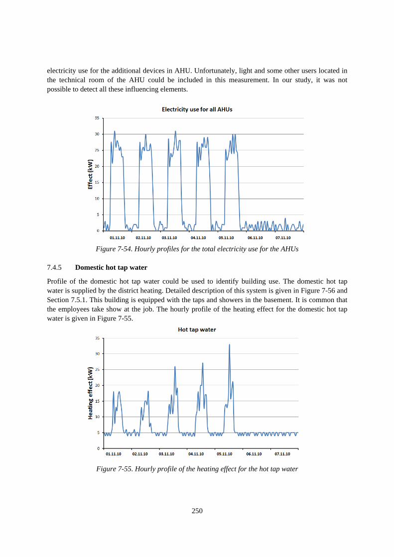
250

electricity use for the additional devices in AHU. Unfortunately, light and some other users located in the technical room of the AHU could be included in this measurement. In our study, it was not possible to detect all these influencing elements.

Figure 7-54. Hourly profiles for the total electricity use for the AHUs

7.4.5 Domestic hot tap water

Profile of the domestic hot tap water could be used to identify building use. The domestic hot tap water is supplied by the district heating. Detailed description of this system is given in Figure 7-56 and Section 7.5.1. This building is equipped with the taps and showers in the basement. It is common that the employees take show at the job. The hourly profile of the heating effect for the domestic hot tap water is given in Figure 7-55.

Figure 7-55. Hourly profile of the heating effect for the hot tap water

251

7.5 Details system description

7.5.1 Main substation

In the low energy office building in Trondheim heating was provided by radiators and floor heating, while cooling of the IT rooms was provided by fan-coils. The heating energy for ventilation, space heating, snow melting, and domestic hot water was supplied by district heating and heat pumps. The schematic of the entire substation in the building is given in Figure 7-56. The two installed heat pumps, 35.01 and 35.02 in Figure 7-56, were providing heating and cooling as explained in the further text. The heat pump 35.02 was a cooling plant that provided cooling for IT rooms, while the condenser heat was utilized to support heating. In this way, the district heating demand should be decreased. District heating is the main heating energy source to the building. The supply and return supply temperature of the district heating at the supplier side are 120/70 oC. The building was provided with two heat exchangers to receive heating energy. A heat exchanger of 900 kW, 320.001.LV01 in Figure 7-56, was installed for building conditioning, while a heat exchanger of 200 kW, 313.001.LV01 in Figure 7-56, was installed for the domestic tap water. The district heating parameters 120/70 oC are constant over the year, while building adjusted the building supply temperature by using an outdoor compensation curve. The outdoor compensation curve can be changed over the year by the building operators, depending on achieved thermal comfort and occupant requirements. The domestic hot water had a constant supply temperature of 55 oC. The building was provided with taps in toilets and showers in the basement. An exact number of the taps and showers is unknown.

252

Figure 7-56. Building heating and cooling energy supply – schematic of the entire substation

253

The main branch 320.001 in Figure 7-56 supplied the heating energy to the floor heating, radiators, the snow melting, and ventilation. Served area by the equipment in Figure 7-57 and their capacities are given in Table 7-24. Control principals and temperature levels in the main branch are shown in Figure 7-57. The entire main branch was controlled by using outdoor temperature compensation principle as shown in Figure 7-58. In Figure 7-57 it is shown that the floor heating branch was controlled based on the outdoor temperature. However, by an on-situ survey and by using BEMS data, it was discovered that the floor heating was controlled based on the air temperature in the entrance as shown in Figure 7-59. The radiator branch was controlled by using outdoor compensation curve as given in Figure 7-60. The snow melting equipment was using when necessary. Unfortunately, heating energy meter was not installed to measure the energy for snow melting. The heating coils in AHUs were controlled by using the main compensation curve shown in Figure 7-58.

Figure 7-57. Schematic of the main branch

In Figure 7-57, the main heating branch and the cooling plant 35.02 are shown. These two are shown together because the condenser heat from the cooling plant was used to support the main heating branch. The cooling plant 35.02 was design and installed to provide 200 kW of cooling load at the rated conditions. However, only 63 kW was installed for fan-coils as shown in Figure 7-57, because it was a current building cooling need in the IT rooms. In the case of building extension and occupant requirement, there is possibility to install new fan-coils for the IT room cooling. Because of this low cooling load, the provided condenser heat to support the main heating branch was also low and with low temperature. Further, occupancy level and utilization of the building was lower than planned in 2010 as shown in Figure 7-45. All this is the reason for providing the low condenser heat as shown in Figure 7-41 and Table 7-23.

254

Table 7-24. Installed heating capacity

Brach name Served area Installed capacity (kW)

Temperature level (oC)

Floor heating Basement and Entrance hall 25 35/30

Radiators All the offices 397 70/50

Snow melting Entrance to the parking 131 35/20

Ventilation All the offices 483 70/50

Figure 7-58. Outdoor temperature compensation curve for the main branch 320.001

Figure 7-59. Floor heating supply temperature compensation curve

255

Figure 7-60. Outdoor compensation curve for the radiator branch

The performance data for the cooling plant 35.02 are given in Figure 7-61 to 32. The evaporator load is a parameter in Figure 7-62 and 23. In Figure 7-62 and 23, the black line at 40 bar shows the pressure limit above which the cooling plant cannot perform. In this case this means that the cooling plant 35.02 cannot provide condenser heat above these temperatures.

Figure 7-61. COP vs. condenser temperature for the cooling plant 35.02

Figure 7-62. Condenser heat vs. condenser temperature for the cooling plant 35.02

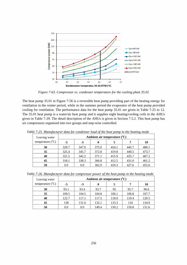
256

Figure 7-63. Compressor vs. condenser temperature for the cooling plant 35.02

The heat pump 35.01 in Figure 7-56 is a reversible heat pump providing part of the heating energy for ventilation in the winter period, while in the summer period the evaporator of the heat pump provided cooling for ventilation. The performance data for the heat pump 35.01 are given in Table 7-25 to 12. The 35.01 heat pump is a water/air heat pump and it supplies eight heating/cooling coils in the AHUs given in Table 7-29. The detail description of the AHUs is given in Section 7.5.2. This heat pump has six compressors organized into two groups and step-wise controlled.

Table 7-25. Manufacturer data for condenser load of the heat pump in the heating mode

Ambient air temperature (oC) Leaving water

temperature (oC) -5 -3 0 5 7 10

30 329.7 347.0 375.0 424.1 445.7 480.1

35 325.4 345.7 372.8 419.8 440.5 473.7

40 321.5 342.2 371.1 415.9 435.7 467.2

45 318.1 338.3 366.8 412.5 431.0 461.2

50 0.0 0.0 362.9 410.3 427.6 455.6

Table 7-26. Manufacturer data for compressor power of the heat pump in the heating mode

Ambient air temperature (oC) Leaving water

temperature (oC) -5 -3 0 5 7 10

30 93.1 93.4 93.7 95 95.7 96.6

35 109.5 104.5 104.8 106.1 106.8 107.7

40 122.7 117.1 117.5 118.9 119.4 120.5

45 138 131.6 132.1 133.3 134 134.9

50 0.0 0.0 149.4 150.2 150.8 151.6

257

Table 7-27. Manufacturer data for evaporator load of the heat pump in the cooling mode

Condenser entering air temperature (oC) Leaving water

temperature (oC) 25 30 32 35 40 44 46

5 415.0 395.0 386.6 373.7 347.4 331.2 315.0

6 427.4 406.5 398.1 384.7 357.8 341.0 324.3

7 439.8 418.4 409.5 396.0 368.0 350.9 333.7

8 450.8 429.0 420.0 405.9 377.4 359.8 342.2

9 462.1 439.6 430.1 416.2 386.9 368.8 350.7

10 473.7 450.2 440.6 426.1 395.7 377.4 359.0

12 495.6 471.5 461.7 446.4 414.8 395.4 375.9

15 529.4 504.0 493.3 476.6 443.3 422.4 401.6

Table 7-28. Manufacturer data for compressor power of the heat pump in the cooling mode

Condenser entering air temperature (oC) Leaving water

temperature (oC) 25 30 32 35 40 44 46

5 111.4 122.3 126.8 133.6 148.4 157.8 167.3

6 112.7 123.7 128.2 135.1 149.9 159.5 169.0

7 114.1 125.1 129.7 136.5 151.5 161.1 170.6

8 115.4 126.5 131.1 138.0 152.9 162.6 172.2

9 116.8 128.0 132.6 139.4 154.4 164.1 173.8

10 118.3 129.4 134.1 141.1 156.0 165.8 175.6

12 121.2 132.6 137.2 144.1 159.4 169.3 179.2

15 125.9 137.1 141.9 149.1 164.4 174.4 184.5

7.5.2 Ventilation system

The ventilation system consisted of eight variable air volume (VAV) systems, with a maximum air volume from 12,500 m3/h to 22,000 m3/h. In total about 540 VAV air valves are installed in the buildings. A brief overview of the installed ventilation systems is given in Table 7-29. The overview gives the performance of the installed ventilation systems including the air flow rate, the fan power, the specific fan power of the entire ventilation system (SPFe), heating/cooling coil capacity and the heating coil capacity. The AHUs in Table 7-29 are equipped with a rotary heat recovery exchanger with an efficiency of 80 % at the rated conditions.

Table 7-29. Ventilation systems in the office building in Trondheim Air flow rate Fan power

Ventilation system

Supply fan

(m3/h)

Exhaust

fan

(m3/h)

Supply fan

(kW)

Exhaust

fan

(kW)

SFPe (kW/(m 3/s)

Heating coil capacity

(kW)

Heating/cooling coil capacity (kW)

36.01 22,000 22,000 7.47 6.89 2.17 70 92

36.02 22,000 22,000 7.47 6.89 2.17 70 92

36.03 20,000 20,000 6.30 5.83 2.01 59 84

36.04 20,000 20,000 6.30 5.83 2.01 59 84

258

36.05 15,000 15,000 4.68 4.28 1.97 42 63

36.06 18,000 18,000 6.50 5.88 2.30 58 75

36.07 14,500 14,500 5.07 4.53 2.21 31 47

36.08 12,500 12,500 3.97 3.52 1.99 71 38

All the ventilation systems in Table 7-29 were VAV systems with modern Static Pressure Reset Demand Control Ventilation (SPR-DCV) that is frequently called optimized VAV. This means that the supply air pressure is optimized in that way that one VAV is always open. Further, this means that the higher the air flow rate, the higher the input signal to the fan. Supplied zones and areas by each ventilation system are given Figure 7-64. In Figure 7-64, the zones supplied by each AHU are shown in different colors.

Figure 7-64. Ventilation zones

The AHUs 36.01 to 36.06 consist of the same components, except that capacities are different as given in Table 7-29. The schematic of the AHUs 36.01 to 36.06 is shown in Figure 7-65. The symbols as shown in Figure 7-65 to 36 are used in the further text to explain the work principal and the control strategies.

259

Figure 7-65. Schema of the ventilation system. This schema is valid for the 36.01 to 36.06 ventilation

systems There are small differences in the construction of the AHUs 36.07 and 36.08 are shown in Figure 7-66 and 36. This difference in the construction is due to requirements of the supplied zones. For example, the AHU 36.08 is supplying the glass area that is not occupied and that is located between occupied zones. Therefore there was no necessity to heat air for the glass area more than it would be warmed up by the heat recovering.

260

Figure 7-66. Schema of the ventilation system 36.07

In Figure 7-65 it is shown that the supply air temperature, RT40, is controlled based on the exhaust air temperature. The relation between the exhaust air temperature, RT50, and the supply air temperature RT40, can be defined differently as shown in Figure 7-68. The control strategy for the supply air temperature has been adjusted based on the experience and occupant requirements. Depending on the achieved supply air temperature, RT40, the heat recovery LX01, the heating/cooling coil LK40, and the heating coil LV40 were used. The sequence control for these three devices is as shown in Figure 7-65 to 36. In the heating mode (winter period), if the supply air temperature is not achieved, the input signal, LR01, to the heat recovery wheel, LX01, is increasing. Further, the input to the heating/cooling coil LK40 is increasing, and finally if additional heat is necessary the input signal to the heating coil LV40 is increasing. In this sequence control, the heating/cooling coil LK40 was prioritized. The LK40 is supplied by the heat pump 35.01, introduced in Table 7-25 to 12. The sequence control giving priority to the heat pump was implemented because the district heating in Norway does not have a competitive price compared to the electricity. The price of the district heating can be about 0.6 to 0.9 of the electricity price depending on period and supplier. In the cooling mode (summer period), if the supply temperature, RT40, is higher than the desired value the input signal to the heat recovery LX01 is decreasing and the input signal to the heating/cooling coil, LK40, is increasing.

261

Figure 7-67. Schema of the ventilation system 36.08

Figure 7-68. The supply air temperatures in the ventilation systems: a) for all the ventilation systems,

b) supply air temperature limits

The supply air pressure, RP40 in Figure 7-65 and 35, is controlled Static Pressure Reset Demand Control Ventilation (SPR-DCV) that is frequently called optimized VAV as explained before.

262

8. NOR-02: Office building in Norway


Figure 8-1: Building Photo

(a) Statoil office building in Stavanger. (b) Building photo: as shown in Figure 8-1. (c) There are 5 floors and basement. The drawing with building height was not available. Base on the

floor numbers, it could be assumed that the building height is about 15 m. The gross floor area is 19,623 m2.

(d) In Norway, CDD is not an actual parameter. HDD is given for 2010. HDD was calculated for the base indoor temperature of 17ºC. Mean relative humidity is given in Table 8-1.

Table 8-1: Climate data of Stavanger in 2010 Jan Feb Mar Apr May Jun Jul Aug Sep Oct Nov Dec Year

Average high

(℃) 6.4 5.9 13.9 15.5 18 22.9 26.6 24.5 20.1 16.3 11 8.1 15.8

Daily mean

(℃) -4 -1.8 3.8 6.9 8.7 12.2 16.1 15.5 12.6 8.7 1.5 -3 6.4

Average low

(℃) -17.7 -12.8 -9.2 -1.4 -1.5 5.8 8.8 6.5 2.1 -1.2 -11.7 -15.5 -4.0

Relative humidity (%) 649.9 525.8 408.9 302 257.5 145.1 39.4 52.6 131.2 256.8 466.4 621 3856.6

HDD 6.4 5.9 13.9 15.5 18 22.9 26.6 24.5 20.1 16.3 11 8.1 15.8

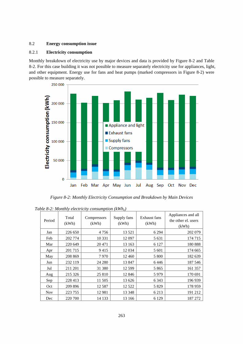
263


8.2.1 Electricity consumption

Monthly breakdown of electricity use by major devices and data is provided by Figure 8-2 and Table 8-2. For this case building it was not possible to measure separately electricity use for appliances, light, and other equipment. Energy use for fans and heat pumps (marked compressors in Figure 8-2) were possible to measure separately.

Figure 8-2: Monthly Electricity Consumption and Breakdown by Main Devices

Table 8-2: Monthly electricity consumption (kWhe)

Period Total

(kWh)

Compressors

(kWh)

Supply fans

(kWh)

Exhaust fans

(kWh)

Appliances and all

the other el. users

(kWh)

Jan 226 650 4 756 13 521 6 294 202 079

Feb 202 774 10 331 12 097 5 631 174 715

Mar 220 649 20 471 13 163 6 127 180 888

Apr 201 715 9 415 12 034 5 601 174 665

May 208 869 7 970 12 460 5 800 182 639

Jun 232 119 24 280 13 847 6 446 187 546

Jul 211 201 31 380 12 599 5 865 161 357

Aug 215 326 25 810 12 846 5 979 170 691

Sep 228 413 11 505 13 626 6 343 196 939

Oct 209 896 12 587 12 522 5 829 178 959

Nov 223 755 12 981 13 348 6 213 191 212

Dec 220 700 14 133 13 166 6 129 187 272

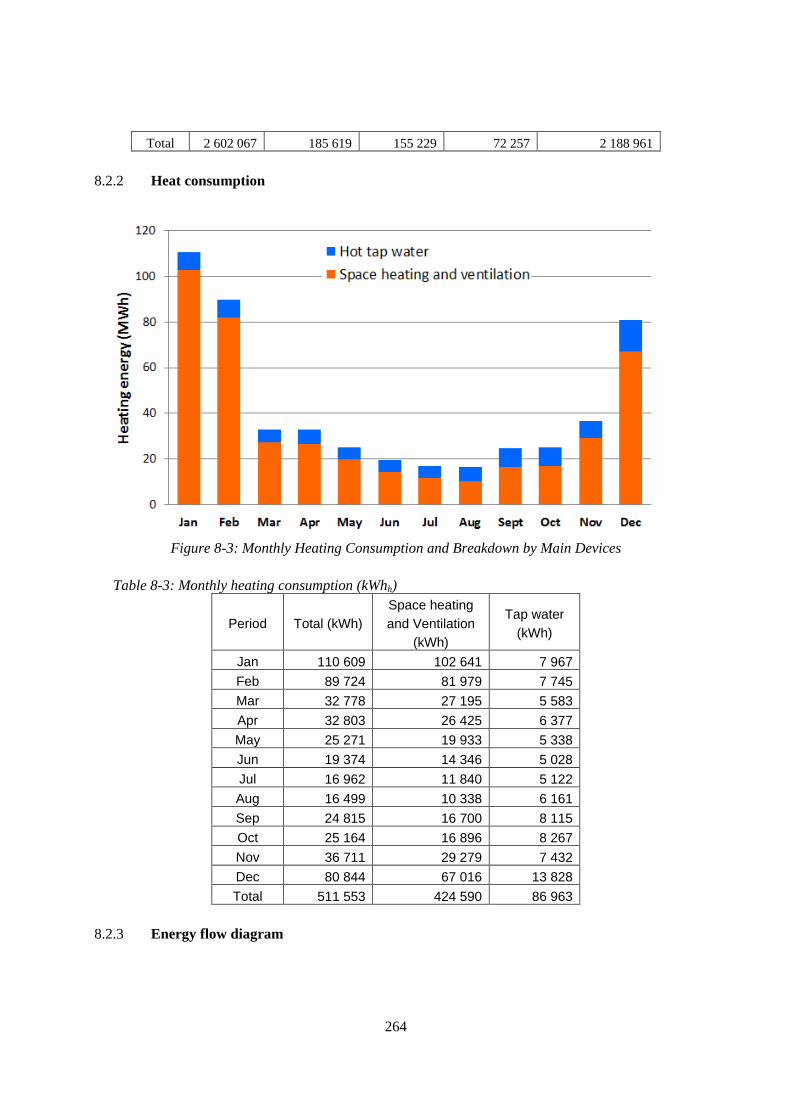
264

Total 2 602 067 185 619 155 229 72 257 2 188 961

8.2.2 Heat consumption

Figure 8-3: Monthly Heating Consumption and Breakdown by Main Devices

Table 8-3: Monthly heating consumption (kWhh)

Period Total (kWh) Space heating and Ventilation

(kWh)

Tap water (kWh)

Jan 110 609 102 641 7 967

Feb 89 724 81 979 7 745

Mar 32 778 27 195 5 583

Apr 32 803 26 425 6 377

May 25 271 19 933 5 338

Jun 19 374 14 346 5 028

Jul 16 962 11 840 5 122

Aug 16 499 10 338 6 161

Sep 24 815 16 700 8 115

Oct 25 164 16 896 8 267

Nov 36 711 29 279 7 432

Dec 80 844 67 016 13 828

Total 511 553 424 590 86 963 8.2.3 Energy flow diagram

265

Figure 8-4: Energy Flow Diagram of the Case Building

8.3 Occupant behavior

The building was design for 1200 occupants. In general, there are 1000 occupants every day in the building. This office building is rented to one company. Most of the employees are engineers, researchers, and administration. In our study we did not follow detailed when and how many occupants came to the building. In addition, there is no mean to follow exactly number of occupants. Since the installed ventilation system is VAV, the presence schedule can be assumed based on the fan input signal. This assumed occupancy schedule based on the fan input signal is given in in Figure 8-5. In general, it can be assumed that working hours is about 2000 hours for light and ventilation in the building. Light in the corridors and common area is working longer. Working hours of the IT server room is 8760 hours.

266


267

9. AUT-01: Single Family House in Austria

9.1 Introduction

This case study house is the first in a series of three that have been compared in a study investigating the relationship between the energy certificate calculations, the impact of actual thermal renovations on energy use, and user behaviour in the individual houses. 9.2 Location and climate conditions

Figure 9-1: House location in Vorarlberg, Austria

The detached single family house is located in the Vorarlberger Highlands close to the western border of Austria as seen in Figure 9-1. Average monthly temperatures range between -4°C to 24°C and is within the cool/temperate Alpine climate zone. 9.3 Overview of the detached house

The single family house was built in 1987 and has a heated building volume of 709.8 m³ and a gross floor area of 280.6 m². The massive construction heated basement has an area of 91.7 m² and the upper floors are moderately massive construction with an area of 189 m². Figure 9-2 shows the floor plans.

268

Figure 9-2: Ground floor, upper floor and basement floor plans Figure 9-3 shows a schematic cross section of the house with heated, partially heated, and unheated zones. The attic is unheated and shown in blue. The ground and upper floors are heated to 19 °C ± 0.5 °C and are shown in yellow. The partially heated basement is heated within a temperature range of 14 °C to 18 °C. The site is sunny and is in a semi-rural area.

Figure 9-3: House 1 cross-section showing heated zones.

Table 9-1 summarizes the U-values and areas for the opaque building envelope assemblies in the base case and renovated scenarios that were used in the calculations.

Table 9-1: House 1 base case and renovated opaque building assemblies Base Case Renovated Area

A

Correction Factor

f U-Value A x U x F U-Value A x U x F Building assembly

[m²] [-] [W/m²K] [W/K] [W/m²K] [W/K]

AD01 Ceiling to unheated closed attic

61.4 0.9 0.27 15.0 0.15 8.4

EW01 North exterior wall 7.2 1 0.31 2.2 0.31 2.2

EW02 Ventilated exterior wall 133.5 1 0.26 34.3 0.22 29.5

EW03 Basement wall - aboveground

29.5 1 0.67 19.6 0.67 19.6

269

EW04 Exterior wall by entrance 4.3 1 1.00 4.3 1.00 4.3

DD01 Exterior slab, Downward heat flow

3.1 1 0.20 0.6 0.20 0.6

AT01 Ventilated pitched attic 47.8 1 0.23 10.9 0.23 10.9

EC01 Slab on grade 93.0 - 0.94 - 0.94 -

EW01 Exterior wall below grade (in heated rooms)

50.7 - 0.69 - 0.69 -

IW01 Interior wall to Garage, Ground floor

13.4 0.7 0.37 3.4 0.37 3.4

IW02 Interior wall to Garage, Upper floor

7.6 0.7 0.26 1.4 0.26 1.4

IW03 Interior wall to Garage, Basement floor

4.1 0.7 0.63 1.8 0.63 1.8

W/D Windows & doors 29.1 1 - 43.6 - 43.6

The windows are double-paned insulating glass with an Ug value of 1.2 W/m²K and solar heat gain coefficient of 0.62. The windows have a softwood frame with Uf value of 1.6 W/m²K and ψ-value (heat transfer coefficient) of 0.06 W/mK for the window spacer. Table 9-2 summarizes the window areas and transmittances according to cardinal direction.

Table 9-2 Window areas (House 1).

A

[m²] A · U · f [W/K]

North 4.36 6.40

East 8.78 13.71

South 7.83 13.19

West 4.98 5.40

East roof lights 0.98 1.48

West roof lights 2.21 3.38

Total 29.14 43.56 In total, there were three stages to the thermal renovations. The impermeability of the exterior envelope was averaged between the airtight basement with small windows partially under ground level, and the partially massive construction and wood frame construction of the above ground floors.

270

Figure 9-4: Thermographic image of the floor slab connection between the first and upper floors.

As seen in Figure 9-4, thermal bridges exist at the beam connections supporting the ground floor ceiling and the junction with the exterior wall. First renovation, January 2005 In 2005, the hot water boiler for heating and DHW was replaced and radiant floor heating was installed in both the kitchen and bathroom with programmable thermostatic controls. Second renovation, January 2008 The exterior envelope was renewed in two stages. In January 2008, 10 cm of fiberglass insulation was added to the attic space. Third renovation, September 2009 In September 2009, 5 cm of EPS was added to the basement ceiling along with 3 cm of fiberglass to the exterior walls as part of the renewal of the ventilated exterior façade. The overall airtightness is estimated to have increased from an n50-value of 3.5 h-1 prior to the renovations to an n50-value of 3 h-1 after the façade renewals. 9.4 HVAC overview

The base case heating system is a water-based radiator system using a gas boiler (built in 1978) to provide both DHW (domestic hot water) and room heating. The DHW tank and the gas boiler are located in the boiler room in the heated portion of the basement and have insulated piping with insulation thickness of 1/3 of the pipe diameter. All heating controls in the basement are manually controlled valves. A closed stove is located in the kitchen and the firewood used is calculated using an energy expenditure factor, FEAZ of 0.55. The pipe insulation default value of 2/3 was used for all pipe runs from ÖNORM H 5056 for calculating the heating system energy demand.

271

Base case HVAC equipment A Junkers gas boiler (1978) with power consumption of 11 kW provided heat for both DHW and heating. Room heat was distributed through radiators with thermostatic radiator valve controls in each room of the ground and first floors. The portions of the basement with room heating were heated using radiators with manual valves. Renovated HVAC equipment A Viessmann gas boiler for both DHW and heating replaced the previous gas boiler in 2005 and has variable power consumption between 4.5 and 12 kW. Radiant floor heating with programmable thermostatic zone control was installed in the ground floor kitchen and the bathroom. All other parts of the HVAC system remained the same as the base case scenario. 9.5 Family members and occupant behaviour

An elderly couple live in the house and are present on average 18 hours a day. The average indoor temperature in the primary rooms is 19.5 °C; and the remaining rooms are heated only when in use. Table 9-3 summarizes the values used in the energy certificate calculations to represent occupant behaviour. TFA is the total floor area.

Table 9-3: Occupant behaviour for energy certificate calculations

The occupants smoke in the kitchen. When present, the kitchen is ventilated hourly. The rest of the house is ventilated when necessary. Table 9-4 summarizes the monthly air change rates in relation to ventilation pattern.

Table 9-4: Air change rate Air change rate n [h-1]

Month 1 2 3 4 5 6 7 8 9 10 11 12

Single-sided window ventilation

0.07 0.07 0.08 0.09 0.09 0.10 0.09 0.10 0.09 0.09 0.08 0.07


Base case 0.35 0.35 0.35 0.35 0.35 0.35 0.35 0.35 0.35 0.35 0.35 0.35 Infiltration through gaps Renovated 0.3 0.3 0.3 0.3 0.3 0.3 0.3 0.3 0.3 0.3 0.3 0.3

Table 9-5 shows the self-reported individual hourly ventilation patterns over a 24 hour time period per room.

Table 9-5: Hourly user ventilation profile per room Hourly opening time in minutes with an outdoor temperature of 10°C

Floor Room Area m²

Opening 1 2 3 4 5 6 7 8 9 10 11 12 13 14 15 16 17 18 19 20 21 22 23 24

Ground and upper floor indoor temperatures 19.5 °C

People 0.53 W/m² TFA Internal loads

Appliances and lighting 2.08 W/m² TFA 2.61 W/m²TFA


272

Boiler Room 0.5 Tilted 2

Stairs 0.5 Tilted 2

Laundry 0.5 Fully open

5 5

Hobby Room 0.5 Fully open

5

Basement

Cellar 0.5 Tilted 5

Kitchen 1.5 Fully open

10 5 5 5 5 5 5 5 5

WC 0.3 Tilted 5 10 10

Office 0.9 Fully open

10 10

Stairs 4.1 Fully open

2 2 2 2 2

Ground Floor

Music Room 0.9 Tilted 5

Bedroom 1 0.3 Fully open

10

WC 1.5 Tilted 10 5

Bath 0.2 Tilted 10 5


10

Upper Floor

Guest Bedroom 0.9 Fully open

2

The hot water demand is estimated as 25 litres per day per person or 50 litres per day (for two inhabitants). 9.6 Investigation methodology

The total energy use was estimated using standard energy certificate calculations and adapted energy certificate calculations which were then compared to actual heating energy use. A regional climate profile for the province of Vorarlberg is used for the standard energy certificate calculations, along with a single standardized user profile as per ÖNORM 8110-5. The regional climate profile used in the standard calculations is based upon weather data from 1951 to 1980. The annual mean outdoor temperature has risen since then, which is why actual climate data from the Feldkirch weather station was used in the adapted energy certificate calculations. The weather station is located within 18 km from the house. The values for the standard user profile used in the Austrian energy certificate calculations are given in Table 9-6.

Table 9-6: User profile for single family homes as per ÖNORM 8110-5

Indoor temperature

20 °C

Temperature in the unheated areas

13 °C

Air change rate

0.4 1/h

Internal gains

3.75 W/m²TFA

Domestic hot water demand

35.0 12.8

Wh/d m²TFA kWh/m² a

273

Personal interviews and a questionnaire were completed to obtain information about user habits and also incorporated within the adapted energy certificate calculations to increase the accuracy of the user profile. 9.7 Energy demand calculations and actual energy use

Gas and electricity energy bills were obtained over a period of nine years from 2001 to 2010 from the inhabitants as outlined in Table 9-7. Actual energy consumption is listed in the table.

Table 9-7: Natural gas and electricity consumption for House 1.

Period Gas m³

Electricity kWh

October 2001 – September 2002 2121 4971








October 2009 – April 2010 1355

In the kitchen, 0.5 to 1.5 m³ mixed wood is burnt per year in a closed wood burning stove. Figure 9-5 shows the quantitative energy flows through the heating system between the base case scenario and the renovated case. The largest change is the heating system energy demand which is almost halved (46%) in the renovated case compared to the base case decreasing by 5002 kWh/a. The fuel requirement also decreased by 5437 kWh/a. Relative to the heat losses from the heating system energy demand, the 18% change in the fuel requirement is less dramatic.

274

Figure 9-5: Comparison of energy flows in kWh/a.

Figures 9-6 and 9-7 show the schematic energy flows through the hot water heating system for DHW and room heating including electricity and household electricity supply for the base case and renovated scenarios. To the left of the dashed red boundary are the energy sources that are delivered to the house for room heating and DHW: firewood, natural gas, and electricity. The yellow circles represent the point where the values can be converted to primary energy values. At this point, greenhouse gas emissions and fuel costs can also be calculated. To the right of the dashed red boundary is the building services (technical) equipment contained in the house for generating room heating and DHW, Et. The blue arrows show the delivered energy to the building and the distribution to the building services to the left of the Eb boundary. The red arrows indicate the flow of generated heat from each part of the system. The grey arrows indicate energy losses in the technical equipment and system due to combustion, storage and distribution. The resulting usable heat for DHW and room heating are shown to the right of the dashed green boundary, Eb, along with household electricity which is also used in the building by the inhabitants.

275

Figure 9-6: Energy flow analysis in kWh for 2004 in the base case scenario.

The delivered energy values have been taken directly from household energy bills. The energy used by technical equipment and the household is calculated. A comparison of both energy flow diagrams shows that although the wood input in the wood burning stove remains constant, the natural gas input is decreased by approximately a quarter, whereas the boiler heat losses by combustion, heat distribution and storage are halved due to the renovation measures of additional thermal insulation, upgraded hot water boiler, and installation of radiant floor heating in the kitchen and bathroom.

Figure 9-7: Energy flow analysis in kWh for 2010 in the renovated scenario.

276

Figure 9-8 shows an overview of the differences between the original energy certificate calculations, the adjusted values with more accurate climate and user profile data together with the actual heating energy consumption of the house for the years between 2002 and 2009. The fuel requirement was calculated using the monthly balance method with the weather station climate data. Energy demand estimations for 2010 and 2011 were also calculated and are in the two rightmost columns.

Figure 9-8: Comparison of energy certificate calculations and energy certificate calculations using

adapted climate and user data to actual fuel use. There is little change between the original and adjusted calculated values in comparison with the actual heating energy use. Actual use is lower than both sets of estimated values by a range of 20% to 37%. Heating energy bills for 2010 and 2011 were not available, and are thus excluded from the graph. In House 1, total annual heating energy use decreases by 7800 kWh/a between 2002 and 2007, then increases the following year by 3200 kWh/a. A possible explanation for the difference between predicted and actual energy use is that the estimated indoor temperatures for the secondary rooms was too high. The higher energy use in 2008 and 2009 occur after all the renovations have been completed. It may reflect a rebound effect whereby the inhabitants become accustomed to a higher comfort level and energy savings as seen in the lowered energy costs, and therefore change their behaviour to heat less frugally than previously, e.g. heating secondary rooms that were previously unheated, or heating primary rooms for a longer period of time. An economic rebound effect is defined as the partial realization of potential energy savings caused by the homeowner’s perception of cost savings (Biermayr et al., 2005). 9.8 Conclusions

The combined effect of improving the thermal envelope, updating HVAC systems, and conscientious user behaviour can significantly decrease overall energy use in residential buildings. The accuracy of prediction tools can be increased by better consideration of user behaviour by using more sophisticated

277

statistical models that consider the presence probability of people and more detailed knowledge about indoor temperature. 9.9 References

[1] BIERMAYR, P., SCHREIFL, E., BAUMANN, B. & STURM, A. 2005. Maßnahmen zur Minimierung von Reboundeffekten bei der Sanierung von Wohngebäuden (MARESI). Nachhaltig Wirtschaften. Vienna, Austria: Bundesministerium für Verkehr, Innovation und Technologie.

278


10.1 Introduction

This case study house is the second in a series of three that have been compared in a study investigating the relationship between the calculations in the energy certificate, the impact of actual thermal renovations on energy use, and user behaviour in the individual houses. 10.2 Location and climate conditions



The single family house was built in 1965 and has a heated building volume of 520.1 m³ and a gross floor area of 185.2 m². The basement is massive construction and unheated. The heated ground and upper floor are moderately massive construction. Figure 10-2 shows the floor plans.

Figure 10-2: Ground floor and upper floor plans

279

Figure 10-3 shows a cross section of the house with heated and unheated zones. The attic and basement are unheated and shown in blue. The ground and upper floors are heated to 20 °C ± 0.5 °C and are shown in yellow. The site is sunny and is in a semi-rural area.



Table 10-1: House 2 base case and renovated opaque building assemblies Correction

factor f

Base case Renovated Area A

U-Value A x U x F U-Value A x U x F Building assembly

[m²] [-] [W/m²K] [W/K] [W/m²K] [W/K]

EW01 Exterior wall 175.2 1 0.58 101.6 0.12 21.0

AT01 Ventilated pitched attic 51.5 1 0.28 14.4 0.28 14.4

AD01 Ceiling to unheated closed attic 55.4 0.9 0.86 10.0 0.20 10.0

BD01 Floor slab to unheated uninsulated basement

99.4 0.7 0.55 38.3 0.17 11.8

DD01 Ceiling over entrance 1.8 1 0.58 1.1 0.12 0.2

W/D Window & Door 29.0 1 2.62 75.8 0.89 25.7

The base case windows are double-paned clear insulating glass (6-8-6) with a Ug-value of 2.7 W/m²K and solar heat gain coefficient of 0.71. The windows have a softwood frame with Uf value of 1.8 W/m²K and ψ-value (heat transfer coefficient) of 0.07 W/mK for the window spacer. The windows were replaced as part of the renovation. The new windows are triple-paned insulating glass with a Ug-value of 0.5 W/m²K and a solar heat gain coefficient of 0.53. The windows have a combined wood-aluminium frame with Uf value of 1.4 W/m²K and ψ-value of 0.03 W/mK for the window spacer. Table 10-2 summarizes the window areas and transmittances according to cardinal direction.

280


A

[m²]

Base case A · U · f [W/K]

Renovated A · U · f [W/K]

North 10.3 25.38 9.76

East 2.8 7.43 2.39

South 12.0 32.26 10.16

West 4.0 10.77 3.42

Total 29.0 75.84 25.73 In total, there were two stages to the thermal renovations. The estimated exterior envelope airtightness was n50 = 5 h-1 due to the high infiltration rate through the base case windows. First renovation, March 2008 In March 2008, the heating system was renewed and extended by installing solar thermal panels and installing a new hot water tank. At that time, the attic was also insulated with 22 cm fibreglass insulation. Second renovation, September 2009 The exterior walls were thermally insulated with 20 cm EPS-F and the ground floor slab to the basement was insulated with 12 cm EPS-F. New windows were also installed as part of the thermal renovation of the exterior walls. Due to the combined renovation measures, the estimated house airtightness n50 value is 2.55 h-1. 10.4 HVAC overview

The base case heating system is located in the unheated portion of the basement. The pipe insulation default value of 2/3 was used for all pipe runs from ÖNORM H 5056 for calculating the heating system energy demand. Base case HVAC equipment A heating oil boiler (extra light) from 1978 with power consumption of 20 kW provided heat for both DHW and heating. The hot water heating supply temperature is 60°C and the return temperature is 50°C. Room heat was distributed through radiators with thermostatic radiator valve controls in each room. A DHW tank with 300 litre capacity was installed in 1978. Renovated HVAC equipment In 2008, a low temperature Vissmann Vitola 200 light heating oil boiler with variable power consumption between 18 and 63 kW replaced the old boiler. The circulating hot water heating supply temperature was lowered to 40°C and the return temperature to 30°C. The room heat distribution remains the same: radiators with thermostatic radiator valve controls in each room. The DHW tank was replaced with a larger 500 litre tank as part of the 2008 renovation. 4.8 m² of thermal solar panels were installed on the west side of the roof. The roof pitch is 30°.

281

10.5 Family members and occupant behaviour

The detached single family house is occupied by three inhabitants who are present on average 16 hours a day. Table 10-3 summarizes the values used in the energy certificate calculations to represent occupant behaviour. TFA is the total floor area.

Table 10-3: Occupant behaviour for energy certificate calculations in House 2 Room temperature 19.5 °C




The occupants air the house each morning for 10 to 15 minutes and open windows when the indoor air is perceived to be stuffy. Table 10-4 summarizes the monthly air change rates in relation to ventilation pattern.

Table 10-4: Air change rate

Air change rate n [h-1]

Month 1 2 3 4 5 6 7 8 9 10 11 12 Single-sided window ventilation

0.08 0.08 0.09 0.09 0.10 0.10 0.10 0.10 0.10 0.10 0.09 0.08


Base case 0.5 0.5 0.5 0.5 0.5 0.5 0.5 0.5 0.5 0.5 0.5 0.5 Infiltration through gaps Renovated 0.25 0.25 0.25 0.25 0.25 0.25 0.25 0.25 0.25 0.25 0.25 0.25



Floor Room Area m²

Opening 1 2 3 4 5 6 7 8 9 10 11 12 13 14 15 16 17 18 19 20 21 22 23 24


6

Living Room A 2.3 Tilted 6

Living Room B 1.3 Fully open

5

Study 1.9 Fully open

6

Entry 1.7 Fully open

5 5 5

Ground floor

Bathroom 0.9 Fully open

5


6

Bedroom 2 2.3 Fully open 6

Bedroom 3 1.3 Fully open 6

Upper floor

Bathroom 0.9 Fully open

6 5 6



282

10.6 Investigation methodology

The total energy use was estimated using standard energy certificate calculations and adapted energy certificate calculations with weather station data and user data from questionnaires which were then compared to actual heating energy use. A regional climate profile for the province of Vorarlberg is used for the standard energy certificate calculations, along with a single standardized user profile as per ÖNORM 8110-5. The regional climate profile used in the standard calculations is based upon weather data from 1951 to 1980. The annual mean outdoor temperature has risen since then, which is why actual climate data from the Feldkirch weather station was used in the adapted energy certificate calculations. The weather station is located within 18 km from the house. The values for the standard user profile used in the Austrian energy certificate calculations are given in Table 10-6.


Indoor temperature

20 °C


13 °C

Air change rate

0.4 1/h

Internal gains

3.75 W/m²TFA


35.0 12.8


Personal interviews and a questionnaire were completed to obtain information about user habits and also incorporated within the adapted energy certificate calculations to increase the accuracy of the user profile. 10.7 Energy demand calculations and actual energy use

The heating oil consumption for the heating period of 2006 to 2007 and 2007 to 2008 were estimated using the filled oil level in the oil tank and were 3442 litres and 2623 litres respectively. Monthly oil consumption and heat gains began to be recorded in April 2008 with the combined heating system renewal and thermal solar panel montage. Table 10-7 shows the heating oil and electricity consumption with solar heat gains from the thermal solar panels.

Table 10-7: Heating oil and electricity consumption combined with thermal solar heat gains from the solar panels for House 2.

Period Heating Oil

litres Electricity kWh

Solar heat gains from the solar

panels

October 2006 – September 2007 3442

October 2007 – March 2008 2623

April 2008 256 432

283

May 2008 10 704

June 2008 13 409

July 2008 6 539

August 2008 4 822

September 2008 86 307

October 2008 161 237

November 2008 284 30

December 2008 417 0

January 2009 471 2

February 2009 376 30

March 2009 339 298

April 2009 92 648

May 2008 33 704

June 2009 6 614

July 2009 6 809

August 2009 1 822

September 2009 8 307

October 2009 91 272

November 2009 143 77

December 2009 206 2

January 2010 236 11

February 2010 192 322 110

March 2010 166 326 495

April 2010 92 273 765

May 2010 57 287 555

June 2010 18 287 708

July 2010 7 323 827

August 2010 17 342 698

September 2010 26 284 474

October 2010 105 260 336

November 2010 181 262 66

December 2010 173 277 3

January 2011 297 274 16

February 2011 195 274 161

March 2011 156 286 508

April 2011 28 132 463

As electricity consumption prior to February 2010 is unknown, an average value of 301 kWh per month was used based upon an average value from the recorded months of February 2010 to April 2011. Figure 10-4 compares the transmission heat losses in the base and renovated cases of the house. Due to the exterior façade renewal and ground floor slab insulation, the transmission heat losses are

284

significantly reduced for all building assembly categories, from slightly lower than 50% improvement for thermal bridges to up to 77% for the aboveground exterior walls.

Figure 10-4: Base and renovated case comparison of transmission heat losses for building assembly

groups. Figure 10-5 shows a comparison of the energy flows between the base case scenario and the renovated case. Similar to the calculated transmission losses, there are significant changes from the base case scenario in almost all categories aside from DHW heating demand and internal gains which remain constant. The largest change is the heating energy demand which decreases by more than two-thirds (68%) in the renovated case compared to the base case decreasing by 17 933 kWh/a. The fuel requirement, transmission heat losses, and heating system energy demand also decrease by over 60%, with changes of 67%, 65%, and 63% respectively. Here it is visible that the combination of increasing the exterior envelope thermal insulation combined with increased airtightness significantly reduces the energy demand of the entire heating system.

285


Figures 10-6 and 10-7 show the schematic energy flow through the hot water heating system for DHW and room heating including electricity and household electricity supply for the base case and renovated scenarios. To the left of the dashed red boundary are the energy sources that are delivered to the house for room heating and DHW: heating oil and electricity. The yellow circles represent the point where the values can be converted to primary energy values. At this point, greenhouse gas emissions and fuel costs can also be calculated. To the right of the dashed red boundary is the building services (technical) equipment contained in the house for generating room heating and DHW, Et. The blue arrows show the delivered energy to the building and the distribution to the building services to the left of the Eb boundary. The red arrows indicate the flow of generated heat from each part of the system in kWh. The grey arrows indicate energy losses in the technical equipment and system due to combustion, storage and distribution. The resulting usable heat for DHW and room heating are shown to the right of the dashed green boundary, Eb, along with household electricity which is also used in the building by the inhabitants.

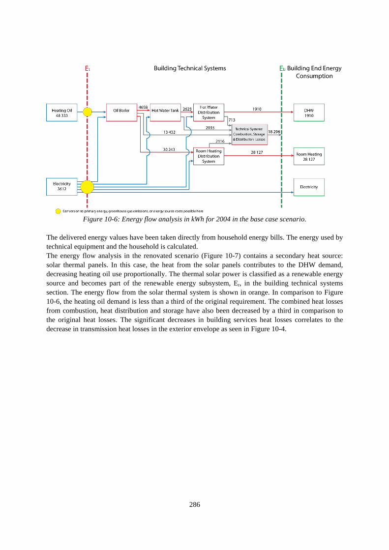
286


The delivered energy values have been taken directly from household energy bills. The energy used by technical equipment and the household is calculated. The energy flow analysis in the renovated scenario (Figure 10-7) contains a secondary heat source: solar thermal panels. In this case, the heat from the solar panels contributes to the DHW demand, decreasing heating oil use proportionally. The thermal solar power is classified as a renewable energy source and becomes part of the renewable energy subsystem, Er, in the building technical systems section. The energy flow from the solar thermal system is shown in orange. In comparison to Figure 10-6, the heating oil demand is less than a third of the original requirement. The combined heat losses from combustion, heat distribution and storage have also been decreased by a third in comparison to the original heat losses. The significant decreases in building services heat losses correlates to the decrease in transmission heat losses in the exterior envelope as seen in Figure 10-4.

287


The importance of collecting local climate data for ascertaining accurate estimations is seen in Figure 10-8 which compares the difference between the solar gains as per the historic weather data file, the weather station, and the solar gains recorded from the solar panels. The local solar gains are significantly higher, as indicated by the blue line. The difference varies by up to 78% from the regional climate profile in the energy certificate.

288

Figure 10-8: Solar gains from the solar panels in kWh/month.

Figure 10-9 shows actual and calculated annual heating energy uses for the house over four years from 2006 to 2010. Both sets of energy certificate calculations overestimate actual energy use, especially during the last recorded year after the exterior envelope was insulated. The graph also shows that in this case, thermal renovations have a greater impact on overall heating energy use than efficiency improvements in heating equipment. Energy use prediction accuracy increases with thermal envelope improvements, and deviations from actual energy use for the adjusted calculated values decreases from 35 % in 2008 to 12% in 2009. Annual heating energy use decreases overall by 21,922 kWh/a between 2006 and 2010.

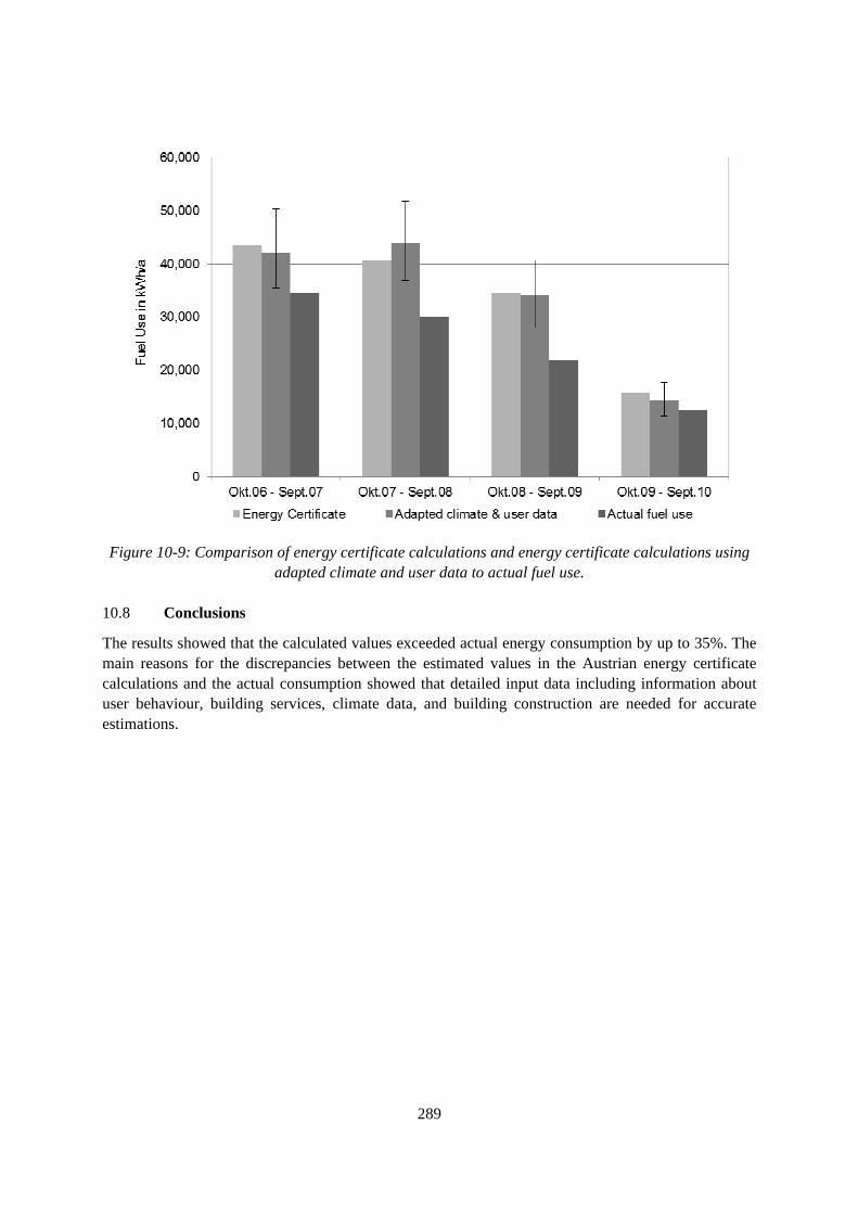
289

Figure 10-9: Comparison of energy certificate calculations and energy certificate calculations using

adapted climate and user data to actual fuel use. 10.8 Conclusions

The results showed that the calculated values exceeded actual energy consumption by up to 35%. The main reasons for the discrepancies between the estimated values in the Austrian energy certificate calculations and the actual consumption showed that detailed input data including information about user behaviour, building services, climate data, and building construction are needed for accurate estimations.

290


11.1 Introduction

This case study house is the third in a series of three that have been compared in a study investigating the relationship between the calculations in the energy certificates, the impact of actual thermal renovations on energy use, and user behaviour in individual houses. 11.2 Location and climate conditions



The single family house was built in 1957, and is located at an altitude of 540 m above sea level in a semi-rural area. The heated building volume is 455.8 m³ and gross floor area is 164.4 m². The basement is massive construction and unheated. The ground, first, and attic stories are moderately massive construction. Figure 11-2 shows the floor plans.

291

Figure 11-2: Ground, upper, and basement floor plans. Figure 11-3 shows a cross section of the house with heated and unheated zones. The attic, upper floor, and basement are unheated and shown in blue. The ground floor is heated to 20 °C ± 0.5 °C and is shown in yellow. The site is sunny and is in a semi-rural area.



Table 11-1: House 3 base case and renovated opaque building assemblies Base case Renovated Area

A

Correction factor

f U-Value A x U x F U-Value A x U x F

Building assembly

[m²] [-] [W/m²K] [W/K] [W/m²K] [W/K]

EW01 Exterior wall 79.1 - - 0.6 0.13 -

AD01 Ceiling to unheated closed attic 80.7 - 0.25 - 0.13 - Upper Floor

EW02 Exterior wall to buffer zone 11.7 - 0.79 - 0.79 -

EW01 Exterior wall 74.6 1 0.60 44.9 0.13 10.0 Ground Floor

IW01 Ceiling to upper floor 83.7 - 0.75 - 0.75 -

292

FS01 Ground floor slab to unheated uninsulated basement

83.68 - 0.68 - 0.19 -

IW02 Wall to garage 17.1 0.7 0.79 9.4 0.79 9.4

EW02 Aboveground exterior wall 31.0 - 1.2 - 0.15 -

UW01 Underground exterior wall 60.6 - 1.3 - 1.26 - Base-ment

EC01 Basement floor slab 80.7 - 4.13 - 4.13 -

The base case windows are double-paned clear insulating glass with a Ug-value of 1.13 W/m²K and solar heat gain coefficient of 0.63. The PVC windows were manufactured by Internorm and the frame has Uf-value of 1.2 W/m²K and ψ-value (heat transfer coefficient) of 0.046 W/mK for the window spacer. The windows were not replaced as part of the renovation referred to in this study. The windows were changed in 1998. Table 11-2 summarizes the window areas and transmittances oriented to cardinal direction.


A

[m²] A · U · f [W/K]

Northeast 1.04 1.40

Southeast 3.38 4.50

Southwest 5.07 6.54

Northwest 2.72 3.50

Totals 12.21 15.94 Prior to the thermal renovation, the estimated exterior envelope airtightness was n50 = 3.5 h-1. Renovation, September 2010 In September 2010, the exterior façade was renewed and solar thermal panels were installed. The exterior walls were insulated with 18 cm EPS-F, the ground floor slab to the unheated basement was insulated with 12 cm EPS-F, and the ceiling to the unheated attic was insulated with 12 cm Heralan-FP mineral wool insulation. Due to the combined effect of thermally upgrading the exterior envelope, the building airtightness increased resulting in a lower n50 value of 2.5 h-1. 11.4 HVAC overview

The base case heating system (boiler and DHW tank) is located in the unheated basement. The pipe insulation thickness default value of 2/3 from ÖNORM H 5056 was used for all pipe runs for calculating the heating system energy demand. Base case HVAC equipment A Junkers natural gas boiler (2001) with variable power consumption from 7 kW to 25 kW provided heat for both DHW and heating. The hot water heating supply temperature is 40°C and return temperature is 30°C. Room heating is distributed through radiators with thermostatic radiator valve controls in each room.

293

The living room, kitchen and corridors on the ground floor are heated by a modern wood-burning stove. The firewood used in the base case scenario is 7 m³ per year. The excess heat from the stove is used to heat DHW. The DHW tank has a storage capacity of 400 litres, and was built in 2001. Renovated HVAC equipment On the southeast side of the roof, a 10 m² thermal solar array was installed. The roof pitch is 30°. After upgrading the exterior envelope, firewood use decreased to 2.5 m³ per year. 11.5 Family members and occupant behaviour

The detached single family house is occupied by two inhabitants who are present 18 hours a day on average. Table 11-3 summarizes the values used in the energy certificate calculations to represent occupant behaviour. TFA is the total floor area.

Table 11-3: Occupant behaviour for energy certificate calculations in House 3 Room temperature 20.3 °C




The upper floors have been unused for many years and are not heated. The heated ground floor area is 83.7 m². The estimated DHW use is 30 liters per day.

Table 11-4: Air change rate Window – Air change rate, n [h-1]

Month 1 2 3 4 5 6 7 8 9 10 11 12

Upper floor

Cross ventilation

0.06 0.05 0.06 0.10 0.13 0.19 0.17 0.17 0.14 0.07 0.07 0.07

Single-sided window

ventilation 0.05 0.05 0.07 0.08 0.09 0.10 0.09 0.10 0.08 0.08 0.06 0.06

Ground floor

Cross ventilation

0.08 0.07 0.08 0.13 0.16 0.23 0.21 0.19 0.18 0.10 0.09 0.09

Air infiltration through the building envelope was also calculated and is found in Table 11-5.

Table 11-5: Air infiltration rate, House 3

Air change rate, n [h-1]

Base case Renovated Upper floor to outdoor

air 0.30 0.26 Upper

floor

0.40 0.35

Ground to first floor 25%

0.10 0.09

Ground floor to outdoor air

50% 0.20 0.18

Infiltration

Ground floor

Ground floor to 25%

0.40

0.10

0.35

0.09

294

basement Basement Basement to outdoor

air

0.30 0.20

0.30 0.21



Single-sided window ventlation

Room Area m²

Opening 1 2 3 4 5 6 7 8 9 10 11 12 13 14 15 16 17 18 19 20 21 22 23 24

Living Room 2.0 Fully open

3


5 5 5

Bedroom 1.4 Fully open

3 Ground floor

Bath 0.4 Fully open

5 5



Upper floor 1.4 & 1.4 12

11.6 Investigation methodology

The total energy use was estimated using standard energy certificate calculations and adapted energy certificate calculations, both which were compared to actual heating energy use. A regional climate profile for the province of Vorarlberg is used for the standard energy certificate calculations, along with a single standardized user profile as per ÖNORM 8110-5. The standardized energy certificate calculations considers the house as one zone, and thus, the unused upper floor and attic space are calculated together as part of the heated zone at 20°C. The ground floor slab to the unheated basement is simplified in the calculations to a floor slab bordering on an unheated and uninsulated basement with a temperature correction factor of Fi,h = 0.7. The regional climate profile used in the standard calculations is based upon weather data from 1951 to 1980. The annual mean outdoor temperature has risen since then, which is why actual climate data from the weather station was used in the adapted energy certificate calculations. 11.7 Energy demand calculations and actual energy use

The values for the standard user profile used in the Austrian energy certificate calculations are given in Table 11-7.


Indoor temperature

20 °C


13 °C

Air change rate

0.4 1/h

Internal gains

3.75 W/m²TFA

295


35.0 12.8


Climate data from the Feldkirch weather station was used for the adapted energy certificate calculations. The weather station is located within 18 km from the house. Personal interviews and a questionnaire were completed to obtain information about user habits and also incorporated within the adapted energy certificate calculations to increase the accuracy of the user profile. The total area of the upper floor and attic (164.4 m²) was used to calculate the specific energy flows in the following figures. The actual fuel requirement has been calculated from the natural gas bills from October 2001 to September 2010. The heating season from October 2006 to September 2007 was not available. The firewood consumption was between seven to 10 m³ for the wood burning stove in the base case scenario. The quality of the firewood varied greatly and depended upon the source for overall burning efficiency. Table 11-8 summarizes the natural gas consumption from the October 2001 to April 2011.

Table 11-8: Natural gas consumption for House 3.

Period Natural Gas

kWh






October 2006 – September 2007




31 December 2010 – 18 April 2011 2420

The electricity company estimated 3900 kWh electricity consumption. Figure 11-4 shows the effect of the thermal renovations on the indoor temperatures of different zones. The grey line shows the the outdoor temperature for each month of a year. Aside from the ground floor set-point temperature which is kept constant due to heating, the other unheated zones fluctuate following the outdoor temperature, and show the effect of thermal insulation with the basement temperature cooler in the renovated case reflecting less heat loss through the ground floor slab; and a higher indoor temperature during the cold months in the unheated upper floor in the renovated case.

296

Figure 11-4: Calculated minimum winter temperatures in individual zones.

Figure 11-5 compares the transmission heat losses in the base and renovated cases of the house. Due to the exterior façade renewal with ceiling and ground floor slab insulation, the transmission heat losses are significantly reduced for the exterior walls with a calculated improvement of over 77% improvement. Significant improvements follow for the ground floor slab to the unheated basement, thermal bridges, and the floor slab to the upper floor. The changes are 66%, 44% and 26% respectively. The windows and doors were not changed in this renovation, and no change was made to the interior wall to the garage, which shows minimal improvements, less than 1%.

297

Figure 11-5: Base and renovated case comparison of transmission heat losses for building assembly groups.

Figure 11-6 shows a comparison of the energy flows between the base case scenario and the renovated case. Similar to the calculated transmission losses, there are significant changes from the base case scenario in several categories, namely, the annual fuel demand, the heating energy demand, transmission heat losses, and the heating system energy demand, which show reductions of 61%, 58%, 49%, and 44% respectively. The largest change is the heating energy demand which decreases by 14 066 kWh/a in the renovated case compared to the base case. Here it is visible that the combination of increasing the exterior envelope thermal insulation not only reduces transmission heat losses to the exterior, but also significantly reduces the energy demand of the heating system.


Figures 11-7 and 11-8 show the schematic energy flows through the hot water heating system for DHW and room heating including electricity and household electricity supply for the base case and renovated scenarios.

298


To the left of the dashed red boundary are the energy sources that are delivered to the house for room heating and DHW: firewood, natural gas, and electricity. The yellow circles represent the point where the values can be converted to primary energy values. At this point, greenhouse gas emissions and fuel costs can also be calculated. To the right of the dashed red boundary is the building services (technical) equipment contained in the house for generating room heating and DHW, Et. The blue arrows show the delivered energy to the building and the distribution to the building services to the left of the Eb boundary. The red arrows indicate the flow of generated heat from each part of the system in kWh. The grey arrows indicate energy losses in the technical equipment and system due to combustion, storage and distribution. The resulting usable heat for DHW and room heating are shown to the right of the dashed green boundary, Eb, along with household electricity which is also used in the building by the inhabitants.

299


The delivered energy values have been taken directly from household energy bills. The energy used by technical equipment and the household is calculated. Figure 11-8 is the energy flow analysis for the renovated scenario with the addition of the solar thermal panels. In comparison to Figure 11-7, natural gas consumption is approximately a third of original use, as the majority of the heated water is provided by the solar panels. Heat from the solar panels also contributes to the room heating system via the hot water tank. The heat from solar thermal panels is classified as a renewable energy source and becomes part of the renewable energy subsystem, Er, in the building technical systems section. The energy flow from the solar thermal system is shown in orange. The combined heat losses from combustion, heat distribution and storage decrease to 44% of the original heat losses. The significant reductions in heating equipment heat losses correlates to lowered transmission heat losses in the exterior envelope as seen in Figure 11-5. Figure 11-9 shows actual and calculated annual heating energy uses for the house over nine years from 2002 to 2011. Both sets of energy certificate calculations overestimate actual energy use, however, the difference between the energy certificate calculations with adjusted climate and occupant behaviour data shows a far better correlation to the actual heating energy use with differences ranging between 2% to 13%. The graph also shows that in this case, the combined effect of better insulation and solar thermal gains using solar panels have a marked impact on energy use.

300

Figure 11-9: Comparison of energy certificate calculations, energy certificate calculations with

adapted climate and user data to actual fuel use. 11.8 Conclusions

The results show that the combined effect of thermally insulating the exterior envelope, incorporating a solar thermal array, using accurate climate data, and using an accurate user profile better predicts heating energy use for room and DHW heating in the energy certificate calculations. The main reasons for the discrepancies between the estimated values in the Austrian energy certificate calculations and the actual consumption showed that detailed input data including information about user behaviour, building services, climate data, and building construction are needed for accurate estimations.

301


Abstract

The building sector is one of the highest energy consumers in Austria. The potential to save energy in existing buildings is very high. Current Austrian policy incentives encourage home owners to renovate buildings to meet the European requirements, reduce energy consumption, and reduce CO2 emissions. Nevertheless, there are often discrepancies between the measured and calculated energy consumption results despite efforts to take parameters into account such as the exact geometry and thermal properties of the building, energy demand for hot water, heating, cooling, ventilation systems, and lighting in the planning phase for selecting the best reconstruction option. To find the answer to this problem, many buildings are carefully investigated with the help of measurements, interviews, and simulations. This paper presents the analysis and results of the investigation of the impact of lifestyle on the energy demand of a single family house. The impact on energy performance of the most important parameters was observed by systematically changing parameters such as changing from a decentralized to a centralized heating system, considering various technologies and fuels for producing electricity and heat, use of renewable energy sources. Different occupant behaviours were changed systematically. The effects of these measures are analysed with respect to primary energy use, CO2 emissions and energy costs. The results of these investigations show that the lifestyle and occupants’ living standard is mainly responsible for the differences between the calculated and measured energy consumption. 12.1 Introduction

By energy efficiency it is to be understood in relation to how to meet the specific building comfort requirements with low energy expenditure and different energy sources. Currently, several different methods are used to characterize energy efficiency. In Europe, the calculation of primary energy is very commonly used in energy consumption calculations. To calculate the primary energy need, national conversion factors must exist for the conversion of a measured or calculated total energy demand into primary energy. Energy consumption is determined by the occupants’ lifestyles and the increase of energy efficiency. Many of our investigations show that the user’s lifestyle and their behaviour can have an enormous impact on real energy consumption. In practice, energy-related improvements are only useful if they are accepted by the users. Therefore, for residential buildings, mainly passive or user-friendly active measures are meaningful. Currently, procedures considered in the standardized assessment are based upon an assumption of a very high lifestyle standard that often does not reflect practice. Therefore, very detailed cross sectional data of several Austrian households were investigated with the help of measurements, interviews, and simulations. The results were used as input data for our simulated investigations and validation. The present investigation analyses impact parameters on residential energy consumption demonstrated by the single family house model in Vienna. It has been observed that greater energy savings have mostly been achieved after the implementation of a thermal renovation of a building rather than the expected theoretical, technical assessment reported by Vine et al. (1994). The main reason for these miscalculations is the lack of consideration of user behaviour. One of the main focuses of the study of energy requirements of household consumption by Biesiot et al. (1999) was consumer activities. Knowledge of the dynamics of the lifestyles should be involved. A wide range of lifestyles and their dynamic characteristics directly and indirectly influence energy flows and energy consumption.

302

The impacts of lifestyles on energy demand and related air-borne emissions have been investigated by Weber and Perrels (2000). There determined energy and emission profiles and influencing factors have given an easily interpretable image of the energy and emission consequences of consumer behaviour and thus contribute to an increased transparency of complex economic and ecological interconnections. The impact of consumer lifestyle in the US has been studied by Bin and Dowlatabadi (2005). They proposed an alternative hypothesis, called the Consumer Lifestyle Approach (CLA), to explore the relationship between consumer activities and environmental impacts in the US. The impact of lifestyle and user behaviour on energy consumption patterns became an important common point in the analysis topics at the Annex 53 (2010) (www.ecbcsa53.org). All afore listed studies have only concentrated on a few parameters, such as room temperature, ventilation, and energy consumption. In this study, all coupled factors (building dimensions, building equipment and appliances, occupant lifestyle, etc.) were taken into account and the impact of the above parameters were analyzed and evaluated in detail. The heat exchange between different zones with different temperature levels and solar shading from adjacent buildings and overhangs has also been calculated. The impact of user behaviour on energy consumption is reflected by the choice of indoor temperature, occupied time, ventilation habits, temperature adjustment, use of different equipment and other behavioural parameters. In this research, the increased energy efficiency of the investigated house is studied, as along with the change from decentralized to a centralized heating systems, various technologies and fuels for the production of electricity and heat, use of renewable energy sources, and different occupant behaviours. The effects of these measures are analysed with respect to primary energy use, CO2 emissions, and energy costs. According to the “Energy Performance of Building Directive” (EPBD), building geometry, building thermal properties, space heating and hot water installations, air conditioning systems, lighting, solar shading systems, external and internal environmental conditions, and the energy consumption by appliances are taken into account in the dynamic simulation. Additionally, it was necessary to determine the occupancy at various times of a day. “BuildOpt_VIE” software, developed at the Vienna University of Technology, was used for the dynamic building simulation in this investigation. It is a multi-zone model for hygrothermal calculations of the whole building which can calculate more than 1000 interconnected zones. Special attention is paid to calculate the solar radiation for each single window and wall according to shading by adjacent buildings and overhangs. This software was validated with the data from Annex 41 (2008) and many experimental validations on real buildings (Schöberl et al. 2005; Korjenic and Bednar 2010). All direct comparisons of the measured to the calculated results show a good agreement. 12.2 Background

This paper presents the results of a recent study of the impact of lifestyle on the energy demand and CO2 emissions of a case study single family house in Vienna. The demonstration dwelling was built in Austria in 1930 −1932 and is located in an urban area. Figure 12-1 presents the location and orientation of the investigated house. There are four occupants, a couple and two children. The house has three stories with a basement and total floor area of 100 m2. There are various ceiling heights, and the house is poorly insulated in its existing state. The facade of the house is built with a double-leaf cavity brick wall construction and the windows are single glazed. All floors, roofs, and ceilings are timber construction. Figure 12-2 shows the elevations and floor plans of the investigated house.

303

The building was heated using a single furnace per room and only the living room is heated to 20� in the morning and evening. Austrian houses are most often renovated with a central heating system with individual radiators in each room; therefore, this variant was our reference example. In order to achieve an energy efficient restoration of a historical building, the aims of this project were to find the effective solutions to reduce energy consumption; reduce CO2 emissions; minimize additional costs; use renewable energy sources; maintain a good thermal indoor climate and; minimize risks for construction failures after renovation. 12.3 Climate conditions

Hourly weather data for Vienna was used for the dynamic simulation. The source data includes exterior temperature, relative humidity, wind speed and direction, precipitation, atmospheric pressure, solar radiation (both orientation and angle dependent) for each hour. The exterior temperature and the global horizontal radiation are presented in Fig. 3.

Fig. 1 Location of the Rietveld house, a row house in the urban core in Vienna (Krischanitz and Kapfinger 1985)

304

Fig. 2 The front facade of the building, elevations, floor plans, and building section

Fig. 3 Exterior temperature and global radiation for Vienna

12.4 Input data and structure of the calculation model

All existing construction parameters for the base case scenario used in this investigation are based on the real measurement data. The real occupancy of the house had been used to calculate the internal loads. The occupancy profile reflects the actual user behaviour. The house is occupied during the work week, from 5 pm until 7:30 am. During the weekends, the family is only away for a few hours at a time. The family is away on holiday for two weeks in winter and three weeks in summer. The time-dependent internal occupant heat load data, appliance type, capacity and frequency of use, and natural ventilation rate were determined from occupant interviews. The air change rate at 50 Pa (n50) varies between 5 ACH in cases without any modifications for energy efficiency (for all lifestyles), and 0.6 ACH in cases with all energy saving measures (roof-, external wall insulation and insulating glass). After the insulation of the roof it was accepted an air change rate (n50) of 3 ACH and after the implementation of the insulating glass of 1.5 ACH.

305

In the hourly simulation, window ventilation was used in the mornings and evenings as well as during lunch breaks on the weekends. The airflow is simulated using the following equation according Austrian standard ÖNORM B8110-3:

where V—volume of airflow (m3/h), A—area of opening (m2), H—height of opening (m), ∆T—temperature difference (K), Cref —exchange coefficient: Cref �100 (without height difference, Fig. 4 left), Cref �350 (at existing height difference, Fig. 4 right) (m0.5/(h•K0.5)) The input data that was not obtainable from measurements or interviews was calculated with the help of standard data according ISO/FDIS 13790:2007. The solar shading from neighboring buildings and overhangs has been calculated in detail for each window. The SHGC (solar heat gain coefficient) of the glazing is 0.93 for the existing window and 0.53 for the insulated glass pane. The four person household examined here is equipped conventionally with electric appliances: a refrigerator, a deep freezer, two CRT televisions, three radios, a washing machine, a clothes dryer, a PC with a CRT monitor, an electric cooker, a coffee machine, a microwave oven, a hot water kettle, and a heating fan. All lighting is provided by incandescent lamps. The clothes dryer is only used in winter. The usage frequency of the electrical home appliances and the amount of warm water were not varied in this investigation.

Fig. 4 Definition of A and H for open and tilted windows

The U-values of exterior constructions used in the simulation were as follows: Building element U-value (W/(m2·K)) in the existing house U-value (W/(m2·K)) after thermal insulation

Flat roof 0.60 0.168

Exterior wall 0.49 0.168

UW - Windows 5.00 1.00

The simulation model that represents this single family house is shown in Fig. 5.

306

12.5 Research conducted and results achieved

The described single family house was used for investigating the influence of lifestyle, various constructive measures, and building services changes on the total energy use, the primary energy, CO2 emissions and the energy costs. The conversion factors that have been used in our calculations are presented in Table 12-1. The calculated energy demand is carried out by a dynamic multizone simulation, taking into account occupant habits, building use, ventilation, heat dissipation, heat distribution, heat supply etc. Here, the activities of the residents and their observed room temperature can be included. In this study only the set point for room temperature has been changed! For this work, the following four lifestyles types have been defined: Lifestyle 1 (L1): only the living room is heated to a room temperature of 20� in the morning and evening. Lifestyle 2 (L2): all rooms are kept at a minimum temperature of 15�; the living room has a room temperature of 20� in the morning and evening. Lifestyle 3 (L3): all rooms are kept at a minimum temperature of 15�; the living and occupied rooms are heated when occupied to 22�; the bedroom temperature is 20�. Lifestyle 4 (L4): all rooms have an interior temperature of 22�. The influence of these four lifestyles is shown in Table 12-2. The heat demand increases by 190 kWh/m2, from 62 kWh/m2 in Lifestyle 1, to 252 kWh/m2 in Lifestyle 4. Common renovations in Austria upgrade to a central heating system using room radiators. The effect of a change of single furnace to a central heating system with or without the support of a solar collector is shown in Table 12-3. In the third variant, both Lifestyle 3 and Lifestyle 4 have been shown. As was shown in Table 12-2, a central heating system has a significant influence on the lifestyle in the base case (without thermal insulation). The effects of these changes are presented in Table 12-3. To minimize CO2 emissions, a pellet boiler could be used instead of natural gas. Pellets were stored in the cellar and delivery to the cellar would also be possible. This variant is shown in the last two columns in Table 12-3. Another possible technical measure would be the integration of a solar collector for hot water.

Fig. 5 Building model (the walls to the neighbouring house have adiabatic boundary conditions)

307

Table 12-1 Conversion factors Conversion factors according to standard ÖNORM EN 15603

Costs a (€/kWh) CO2 emission coefficient b (g/kWh) Primary energy factor b (kWh/kWh)

Pellets 0.049 20 1.06

Gas 0.054 277 1.36

Electricity 0.141 617 3.3

a Estimated current prices in Austria. b Conversion factors according to EN 15603.

Table 12-2 Impact of lifestyles in the existing state, without a thermal retrofit

Lifestyle L1 L2 L3 L4

Building Existing Existing Existing Existing

Heat dissipation Single furnace Single furnace Single furnace Single furnace

Energy source Gas Gas Gas Gas

Heat demand (kWh/m2 GFA)

Heating 62 111 173 252

Hot water 15 15 15 15

Costs (Euro/year)

Heating 476 867 1356 1982

Hot water 124 124 124 124

Appliance 547 547 547 547

Total 1148 1539 2028 2653

CO2 emissions (tonnes/yea r)

Heating 2.4 4.4 7.0 10.2

Hot water 0.6 0.6 0.6 0.6

Appliance 2.4 2.4 2.4 2.4

Total 5.5 7.5 10.0 13.2

Primary energy (kWh/m2 GF A)

Heating 120 218 342 499

Hot water 31 31 31 31

Appliance 128 128 128 128

Total 279 378 501 658

Table 12-3 Change to central heating system with / without solar collector (without alterations to construction)

Lifestyle L4 L4 L3/L4

Building Existing Existing Existing

Heat dissipation

Radiators Radiators Radiators

308

Solar collector No No 8 m2

Energy source Gas Pellets Pellets


Heating 252 252 173/252

Hot water 15 15 15/15

Costs (Euro/year)

Heating 1785 1620 1074/1532

Hot water 258 234 88/80

Appliance 547 547 547/547

Total 2589 2402 1709/2160

CO2 emissions (tonnes/year)

Heating 9.1 0.7 0.5/0.7

Hot water 1.3 0.1 0.1/0.1

Appliance 2.4 2.4 2.4/2.4

Total 12.9 3.2 3.0/3.2

Primary energy (kWh/m2

GFA)

Heating 449 351 232/332

Hot water 65 51 19/18

Appliance 128 128 128/128

Total 642 529 380/477

The influence of various construction measures on the different parameters is shown in Table 12-4. In addition, the lifestyles of both Lifestyle 3 and Lifestyle 4 are represented in the fourth variation. Changing the original single glazing with modern thermal insulation glass with very low Ug-values would be a good constructive measure to improve energy efficiency. The external walls, roof, and ceilings, as well as the terrace will be insulated to reduce the heat losses. If the building is well insulated and the heat loads are very small, a heat pump may be used. In this case, a highly efficient heat pump instead of a boiler could be used (see the last column in Table 12-4). It is clearly shown that in a building with very low heat loss in winter (i.e., after the implementation of energy conservation measures) the difference between a temporal or spatial heating is very small. The total primary energy consumption from ca. 270 kWh/m2 GFA in Lifestyle 1 in the existing state can be achieved in Lifestyles 3 or 4 after the installation of thermal insulation and changing the heating system and energy source, as shown in Fig. 6. The investment costs for the thermal renovation and revitalization of the heating system are financed by the Austrian Government. Depending on the energy savings achieved, it is possible to recoup up to one third of the investment costs.

Table 12-4 Impact of construction measures

309

Lifestyle L4 L4 L4 L3 / L4

Building Roof insulation

Roof insulation

+ insulating glass

Roof and external wall insulation

+ insulating glass

Roof and external wall insulation

+ insulating glass

Heat dissipation

Radiators Radiators Radiators Underfloor heating

Solar collector No No No No

Energy source Pellets Pellets Pellets Heat pump


Heating 226 106 57 47/57

Hot water 15 15 15 15/15

Costs (Euro/year)

Heating 1452 685 385 157/191

Hot water 236 245 253 125/121

Appliance 547 547 547 547/547

Total 2235 1477 1185 828/859

CO2 emissions (tonnes/year)

Heating 0.6 0.3 0.2 0.7/0.8

Hot water 0.1 0.1 0.1 0.5/0.5

Appliance 2.4 2.4 2.4 2.4/2.4

Total 3.1 2.8 2.7 3.6/3.8

Primary energy (kWh/m2 GFA)

Heating 314 148 83 37/45

Hot water 51 53 55 29/28

Appliance 128 128 128 128/128

Total 493 329 266 194/201

12.6 Discussion and conclusions

The results of several of our investigations, here presented as an example of one single family house, show that the lifestyles of occupants and occupancy type of a building have a significant influence on the total energy consumption and CO2 emissions of buildings. Lifestyle also has to be taken into consideration in energy efficient building renovations as the energy consumption is a consequence of family lifestyle. Taking the user’s behaviour as a constant into the calculation is a mistake. This is especially the case for a heating system renovation. A household, which provides its space heating needs with individual room stoves, is confronted with numerous barriers (fuel transport from the cellar to the pellet oven, unpleasant odours, dust exposure, constant pellet oven maintenance). If during the course of the renovation, the heating system is converted to a central heating system, it is certainly a

310

change of user behaviour due to the much simpler operation and expected handling of the heating system. The lifestyle, living standards, and occupant behaviour has an important impact on energy use especially if the building has poor thermal performance. This is the result of several studies of our institute, here presented an example of a house. Therefore, it is absolutely necessary to take into account these important parameters for assessing the energy efficiency of a building. The choice of heating system and energy source in the building has a greater effect on the primary energy use and CO2 emissions. Education on how to use building automation is very important for buildings with low thermal performance. The occupancy type and the expected lifestyle may have a strong impact on the renovation concept of a building.

Fig. 6 Comparison of different technology scenarios for Lifestyle 4 compared with Lifestyle 1

12.7 References

[1] Annex 41 (2008). Whole Building Heat Air, Moisture Response: Modelling Principles and Common Exercises. International Energy Agency, Energy Conservation in Buildings and Community Systems.

[2] Annex 53 (2010). Total Energy Use in Buildings-Analysis and evaluation methods. International Energy Agency, Energy Conservation in Buildings and Community Systems.

[3] Biesiot W, Noorman KJ (1999). Energy requirements of household consumption: A case study of The Netherlands. Ecological Economics, 28: 367383.

[4] Bin S, Dowlatabadi H (2005). Consumer lifestyle approach to US energy use and the related CO2 Emissions. Energy Policy, 33: 197208.

[5] Korjenic A, Bednar T (2010). Transformation of fundamental parameters for energy demand and indoor temperature from room level to building level. Journal of Building Physics, 33: 327355.

[6] Krischanitz A, Kapfinger O (1985). Die Wiener Werkbundsiedlung. Compress. (in German)

311

[7] Schöberl H, Hutter S, Bednar T, Jachan C (2005). Anwendung der Passivtechnologie im sozialen Wohnbau. Stuttgart: Fraunhofer IRB. (in German)

[8] Vine EL, Misuriello H, Hopkins ME (1994). A research agenda for demand-side management impact measurement. Energy, 19: 11031111.

[9] Weber C, Perrels A., (2000). Modeling lifestyle effects on energy demand and related emissions. Energy Policy, 28: 549566.

312



Ground floor First floor Figure 13- 1 Plan of the building

Table 13-1 Floor area and room volume Heated ground area 389.40 m² Heated building volume 887.83 m³ Cellar (unheated) 189.3 m² ground floor 211.9 m² first floor 177.4 m² Table 13-2 U-value and area of building materials Area m² U-value W/m²K Cellar ceiling 189.3 0.41 Exterior wall 326.0 0.18 Roof 226.6 0.20 Windows 1.10 Table 13-3 Area of windows and doors Windows

m² Doors

m² North 9.66 0.00 South 11.67 18.72 West 5.99 6.47 East 6.69 3.80 Total 34.01 28.99 13.2 Occupant’s Interview and data collection

a) Building data and building use House is occupied since November 2004: 4 Adults, 1 Child.

313

A person (housewife) is continuously at home. At least, four people regularly sleep in the house. Short trips are taken only during the holidays and Christmas (about two weeks). The Wood-House cools down in this time from 22-23 °C to 18-19 °C, without being heated. Partially is the heating night setback activated. Cellar is unheated: Indoor temperature is about 15 °C, except Kettle room All other rooms are heated to about 22 °C, except bedroom of the parents. There are four stoves in the house. The stove in the living room is in constant operation. The temperature is measured only in the work room. b) Heating Boiler: Nominal power: 25 kW, Boiler room (in winter, a window always tilted) Boiler description, central-heating boiler MULTIJET B-I (25) System temperature range: 80°C/60°C 58 L water content Chimney, 4 tiled stove No secondary heaters c) Domestic hot water: In summer is showered, bathed in winter. Two people take a bath in the summer too. d) Pipes: Copper pipes with red foam insulation. Fittings not insulated e) Solar collector: SOLAR-EK / GFK 6 Equipped since spring 2006, Constancy outcome value = 465 kWh/m²a, 10 m² absorber surface, setting angle = 40° Orientation = -10 % East irregularity, the average outcome value over the year = 200 kWh/m² f) Type of ventilation (tilt / open) in winter / summer? In winter: Once a days in the morning a quarter to half hour are windows completely open and all rooms aired. Otherwise, the windows are not more tilted – more open. g) Cooking: Mostly daily, at noon, evening seldom h) Clothes: Winter: clothes drying on the balcony, at night in the bath, Heated towel rail in bath Summer: clothes drying on the balcony i) Curtains: Color gray, almost never closed

314

Sun protection: window shutters - never closed 13.3 Energy Consumption:

Fuel oil: consumption from November 2004 to May 2006, 3.366 liters for heating and hot water Fuel wood: ca. 6 - 7 m³ beechwood per Winter for the tiled stove Electricity: 26.12.2004 - 23.11.2006 16.415 kWh Night electricity: 26.12.2004 - 23.11.2006 3.375 kWh A solar system for hot water with 10 m² collector area reduces fuel consumption by 4650 kWh/year, according to manufacturer's instructions. Assuming that the daily consumption is about the same, we obtain the heating requirements for the house: Total heating energy demand about 37000-42000 kWh/a An accurate estimate of energy consumption is not possible because the output of the solar system cannot be precisely defined. Considering the unheated cellar, we obtain the following energy demand: Total heating energy demand = 95 - 110 kWh/(m² a) The part of heat demand on total energy demand is quantitatively not so easy to assess. The increased electricity consumption results from the fact that a laundry dryer is placed in the cellar, which is taken daily in operation. 13.4 Calculations

Monthly balance method A survey of people living in the house has shown that the ventilation window in the winter is limited to about 0.25 h in the morning. From the n50 value gives a false air change rate of nx = 0.10 h-1. This means that the air change rate is in the heating season significantly lower than 0.40 h-1 (standard). Therefore, the calculation was carried out with an air change rate of n = 0.14 h-1. The air change rate n = 0.14 h-1 was determined from the hygienic air change. Furthermore, according to ÖNORM B 8110-5, 3.75 W/m² should be taken as thermal internal gains. This appears too high, because the whole day only one person is permanently present. Therefore, 2.20 W/m were applied. This value is calculated taking into account the occupancy of the house throughout the day. The thermal gains from people inside the building are then 0.70 W/m². If we allocate the electricity consumption to the surface of the heated space, we obtain a power of 1.50 W/m². With these new input parameters, we get a heating demand of 35.82 kWh/(m² a) and a total energy demand of 125.1 kWh/(m² a).

315

To determine the air tightness of surrounding components of the family house, a blower door measurement was performed. The measurement was carried out according to ÖNORM EN 13829:2001 05 01. The building volume, including unconditioned basement is: State during the measurement in 1980 m³ 13.5 Result – Blower-Door- measurement

Figure 13- 2 Result of measurements

After evaluating the data, the ventilation rate n50 = 2.22 h-1 13.6 Thermal building simulation

The geometry of the investigated house has been defined according to the existing house.

Figure 13- 3“BuildOpt_VIE”-Building model of the house

pressure difference (Pa)

air change rate (1/h)

316

Actually energy consumption of the house was also calculated by a dynamic building simulation. It was once the standard user behavior from the ÖNORM B 8110-5 used and once used the actual user behavior. Comparison between the results of monthly balance method and building simulation is shown in the following diagram:

Figure 13- 4 Heating energy demand [kWh/(m2a))

The comparison between the balance and simulation shows that the monthly balance method, reflects the actual energy consumption quite well.

Sim-Standard User profile

Bil-Standard User profile

Sim-real User profile

Bil-real User profile

317

14. AUT-06: Multi-storey residential building in Austri a

14.1 Introduction

This case study house is the first certificated lowest energy multifamily houses in Vienna. Utendorfgasse are social tenements. There are 39 flats in the complex of three houses. The buildings are made of reinforced concrete. The balconies are in the south so the projecting slabs are shading the windows. There are little windows in the north. 14.2 Location and climate conditions

Figure 14-1: House location in Utendorfgasse, A-1140 Vienna, Austria

Geographical environment: Geographical position Longitude latitude ASL Vienna East Longitude 16 Degrees North Latitude 48 Degrees 220 m Average monthly temperatures and global horizontal solar radiation is presented in Figure 14-2.

318

Figure 14-2: Average monthly temperatures and global horizontal solar radiation

14.3 Overview of the building

Start of occupation: 2007 Number of flats: 13 Gross floor area = 1330 m² Area inside flats = 901 m² Heated gross volume: 4039 m³

319

Figure 14-3: Complex of the three lowest energy houses in Vienna (Utendorfgasse)

320

Figure 14-4: Floor plans: basement, ground floor, regular and top floor

Building envelope: The buildings are made of reinforced concrete with 30cm heat insulation on the exterior wall, 45cm heat insulation on the roof and 35cm heat insulation on the celling between basement garage an heated rooms. The thermal uncoupling of the base point from the supporting walls is made of aerated concrete with punctual steel or reinforced concrete supports. For the windows were triple glazing used.

Area (m²) U-Value (W/m²K)

g

roof reinforced concrete

insulated 722 0.09

321

external wall (without windows) concrete wall + ETICS 568 0.13 Windows south Triple glazing 90 0.86 0.48 Windows east/west Triple glazing 10 0.86 0.48 Windows north Triple glazing 50 0.86 0.48

basement ceiling reinforced concrete

insulated 270 0.1

14.4 HVAC overview

The heat production for heating and hot water occur from a gas-fired condensing boiler with a domestic hot water accumulator with circulation pipe. Heating: central gas fired condensing boiler (in the basement), Year-2007 effective power 50kW, modulating, flexible regulation according to the external temperature heating of flat through one heating coil per flat in the supply air no storage Deliveries system: room thermostat with zone control, supply air heating, supply/return 70°C/55°C length (m) insulation fittings distribution / cellar 50 3/3 uninsulated standpipe 89 3/3 uninsulated 3/3: the thickness of the insulation is the same as the dimension of the uninsulated pipe Hot water: hot water storage tank: 1500 l, Year-2007 distribution system with circulation pipe length (m) insulation fittings distribution / cellar 25 3/3 uninsulated stand pipe 54 3/3 uninsulated circulation return pipe 25+54 3/3 uninsulated stub pipe 117 1/3 uninsulated To reduce costs: Only one heat exchanger for 13 flats Only one heating coil per flat at the entry

322

Figure 14-5: Heat exchanger and heating coil

Ventilation: central ventilation system with central heat recovery η=75% volume flow control per flat n=0,4 h-1 , n50=0,3 h-1 Design objectives were: low energy consumption – lowest energy house: heating demand ≤ 15 kWh/m²a heat load ≤ 10 W/m² airtightness n50 ≤ 0.6 h-1 primary energy demand ≤ 120 kWh/m²a high indoor comfort: controlled air change, high surface temperatures during winter high acoustic and hygienic standards for ventilation system good summertime performance Measures:

323

Figure 14-6: Air tightness measurement

14.5 Energy demand calculations and actual energy use

To obtain the total energy use, the electricity use by household equipment and the ventilation system, and the auxiliary electricity demand for staircase lighting and distribution pumps, was measured using electricity meters. The heating energy use was recorded with a meter for gas consumption. The heat exchanger between the district heating system and the building system was part of the measured energy use.

324

Figure 14-7: Electricity and gas consumption

325

Figure 14-8: Measured and calculated heating energy demand (with different scenarios for the

internal loads and with distribution losses) for the winter 2008/2009.

Figure 14-9: Year-2007: Total energy consumption

326

15. BEL-01: Single Family House in Belgium

15.1 General overview of the building

The building of interest is a classical family house (Figure 15-1) located in Hondelange (close to Arlon), Belgium (Figure 15-2). The base is more or less a square (13m x 12m) and the front facade is west oriented. The roof is pyramid-shaped with an edge on the North-South axis. The north and south sections are 45°C tilted, while the front and back sections have a smoother slope of 35°C.

Figure 15-1 : Photograph of the house during the winter

Figure 15-2 : Belgium Map, Arlon (Province of Luxembourg)

The house was built in 2008. It has two levels as well as an attic above first floor. A garage and a storage space are next to the house (65m²). They are accessible through the scullery. Plans of the

327

ground floor and first floor are shown on the Figure 15-3 and Figure 15-4. The attic is not occupied, but the mechanical ventilation system (with heat exchanger) is installed there.

Figure 15-3 : Plan of the ground floor (Willaime, et al., 2007)

328

Figure 15-4 : Plan of the first floor (Willaime, et al., 2007)

15.2 Climate

Arlon is situated in Belgium, the climate is “warm temperate and fully humid with warm summer”, according to Köppen-Geiger climate classification. In the Table 15-1, there are some characteristics of the weather for the year 2010 in Arlon.

Table 15-1 : Climate for the year 2010 in Arlon

Year Jan Feb Mar Apr May Jun Jul Aug Sep Oct Nov Dec

Mean min Temp [C°] 12.4 -3.4 -1.3 1.6 4.8 6.9 12.2 14.8 12.4 9.4 5.8 3.2 -4.2

Mean Temp [C°] 8.6 -1.5 1.1 5 9.7 10.8 17.2 19.7 16.1 12.8 8.9 5 -2.2

Mean max Temp [C°] 5.2 0.2 3.6 8.9 15.1 15.3 22.4 25.4 20.5 17 13.2 6.9 -0.3

Mean Humidity [%] 78.3 88.2 88.3 67.7 62.5 59.7 73.9 74.5 79.1 79.8 85.1 82 90.3

HDD15 [Day.C°] 2726 513 390 311 175 152 31 9 30 87 196 299 533

CDD18.3 [Day.C°] 173 0 0 0 5 10 46 85 21 4 1 0 0

15.3 Building envelope

The evaluation of the energy consumption of the building requires a precise knowledge of the envelope. This section will briefly describe the composition of the different walls.

329

15.3.1 Walls

The external walls, the intermediate floors and the roof have a wooden framework, with insulation between the wood elements. These elements weaken the insulation; they have to be taken into account in the calculus of the heat transfer coefficient. (1) External walls The resulting U value of the external walls is 0.211 W/(m².K), taking the wood fraction into account.

Table 15-2 : Composition of the external walls Material Thickness (mm)

Plaster board 12,5 Lathing & cellulose insulation 40

OSB board 18 Wooden framework & cellulose insulation 140

Wood fiber board 25 (2) Internal walls The internal walls are either 17 cm either 12 cm thick. The wooden framework is filled with wood wool (14 cm and 9 cm respectively). On both sides, there is a plaster board or an OSB board. The U value obtained for the 17 cm wall with plaster boards is 0.33 W/(m².K). (3) Floors The ground floor is composed of a 12 cm concrete slab. On the garage side, there is a 4 cm XPS layer, a 6 cm concrete screed and tiling. On the kitchen side, there is a 10 cm cellular glass insulating layer, an OSB board and the heating floor. The U values are 0.773 and 0.389 W/(m².K) respectively. The floor between the ground floor and the first floor is composed of (from bottom to top) a plaster board, the wooden framework filled with wood wool (20 cm), an OSB board, an acoustic protection layer, another OSB board and finally the heating floor (floating parquet). This structure has a U value of 0.177 W/(m².K). The attic floor is simply composed of a wooden framework filled with wood wool (20 cm). The upper layer is an OSB board, while the lower layer is a plaster board. The corresponding U value is 0.216 W/(m².K). (4) Roof The roof part above the garage has the same structure and U value as the attic floor. The main roof, on the other hand, is composed of (from inside to outside) a vapor barrier (with variable permeability), a 20 cm thick insulation layer (wood wool) between rafters, a rigid wood fiber board, a ventilated lathing and the tin roofing. The global U value is 0.214 W/(m².K). 15.3.2 Doors and windows

(1) Windows

330

The windows are composed of a high efficiency double glazing (4/15/4, argon) and a frame in aluminum. The ratio between frame and glazing varies from one window to another, but a mean repartition of 30% of frame and 70% of glazing is considered. The main characteristics of the windows are listed in Table 15-3.

Table 15-3 : Windows main characteristics U glazing [W/(m².K)] 1.1 U window [W/(m².K)] 1.6 solar factor (-) 0.61

(2) Main hall door The main hall door has the same frame than the French windows, but the glazing is replaced by boards. These boards consist in two external aluminum layers (1.5 mm each) and a central 25 mm PU foam layer. The corresponding U value is 1.36 W/(m².K). (3) Garage door The garage door has a 40 mm PUR layer included between aluminum sheets. The U value is 1.5 W/(m².K). (4) Windows orientation The windows are mainly south and east oriented. Apart from limited overhangs in the south-west and east, the house does not present any natural solar protection. External window blinds are installed only at the first floor. 15.4 Building equipment and system

An air-to-water heat pump is used for the heating and the production of the hot domestic water. The whole house is heated with a low inertia heating floor (Figure 15-5). There is also a hearth in the living room, but it is rarely used.

Figure 15-5 : Installation of the low inertia heating floor system

The external module is shown on Figure 15-6. It is able to modulate its speed with regards to the demand and external temperature, allowing an electrical consumption as low as possible. The heat

331

pump keeps its nominal power with temperatures higher than -15°C and is able to produce heat with temperature up to -25°C. This heat pump gives priority to constant heating power at low temperatures, increasing the electrical consumption as a counterpart.

Figure 15-6 : External unit of the air-to-water heat pump

The main characteristics of the heat pump are listed in Table 15-4.

Table 15-4 : Main characteristics of the heat pump Global features Heating power at +7°C - nom/max kW 12/14 Nominal electrical power (A-7/W55) kW 2,79 (6,63) Nominal COP (A-7/W55) - 4,30 (1,69) Heating power at -7°C kW 12 Heating power at -15°C kW 11

On the Figure 15-7, the monthly mean internal temperature is plotted. The set point is not optimized as it is the same 24/24 and 7/7. The overheating is quite important during the summer months for a house in Belgium.

332

Figure 15-7 : Monthly mean internal temperature of the house

15.4.1 Ventilation system

Controlled mechanical ventilation with heat recovery is present. Indoor air is rejected outside through a heat exchanger and the outdoor fresh air is thus pre-heated before being injected in the house. This system reduces drastically the ventilation losses. A by-pass is present to inject outdoor air directly during summer months. An anti-freeze valve is also present. Pulsing and extracting air vents are placed throughout the house. The air is injected in dry rooms and is evacuated from wet rooms. The group can work at three different speeds, with different efficiencies, listed in Table 15-5.

Table 15-5 : Mechanical ventilation performances Speed Flow rate Efficiency Electrical power

1 75 m³/h 95.3% 7.8 W 2 225 m³/h 88.0% 52.6 W 3 325 m³/h 86.1% 156.5 W

15.4.2 Lighting

The number of lights in each room is defined in Table 15-6. The expected power values are: 50 W for spotlights and wall lights, 60 W for incandescent light bulbs and 58W for neon tubes.

Table 15-6 : Lighting equipment Room Type Number Garage Neon 8 Storage Neon 2

Spotlight 6 Living room

Wall light 2 Dining room Spotlight 5

333

Wall light 2 Entrance hall Spotlight 5

Kitchen Spotlight 11 Scullery Light bulb 1

WC ground floor Spotlight 2 Bathroom Spotlight 7

Light bulb 1 Bed room 2

Wall light 2 Dressing Spotlight 5

WC first floor Light bulb 1 Library Light bulb 1

Night hall, fitness Light bulb 1 Bed room 3 Light bulb 1

Laundry room Light bulb 1 Shower Light bulb 1

Bed room 1 Light bulb 1 Bed room 4 Light bulb 1

Attic Light bulb 1 15.4.3 Monitoring equipment

Several sensors have been installed in the house and in the heat pump. They measure flow rates, temperatures, electrical consumptions, etc. A list of sensors is available in Table 15-7. The data is stored with a 5-minute time step since Mai 2009.

Table 15-7 : List of the sensors Description Supply temperature (start of the heating pipe)

Return temperature (end of the heating pipe)

External temperature, taken next to the garage door (North-West)

Inside temperature of the kitchen

Floor temperature between circuit 2 supply pipe and circuit 1 return pipe

Floor temperature between circuit 1 supply pipe and circuit 2 return pipe

Supply temperature (collector, ground floor)

Return temperature (collector, ground floor)

Floor temperature above circuit 1 supply pipe

Floor temperature above circuit 1 return pipe

Floor temperature above circuit 2 supply pipe

Floor temperature above circuit 2 return pipe

Heat pump total electrical consumption (including auxiliaries). Pulse counter: 1 pulse = 5 Wh.

Heat pump total hot water production (floor heating + DHW). Pulse counter: 1 pulse = 1 kWh.

Water flow (floor heating + domestic hot water). Pulse counter: 1 pulse = 1 liter.

334

15.5 Simulation and Calibration

The software TRNSYS is used to achieve the simulation. The file used is an adaptation of the one created for the subtask D of this annex 53. The aim of the simulation is to be able to calibrate the model, this way it is possible to estimate the value (which are not monitored or known) of some parameters (ventilation and infiltration rate, domestic hot water consumption, etc.). The different steps to arrive at this calibration are listed in the Figure 15-8.

Figure 15-8 : Global scheme for the calibration

The model of the house is calibrated according two kinds of results:

• Monthly heat pump production [kWh] • Monthly over-heating [K.h]

It means that there are 12*2=24 results to calibrate. It is of course more reliable two calibrate on a monthly basis than an annual one, because it would be too easy (and then imprecise) two calibrate the model with only two annual values. The problem is that even several different solutions could arrive to the same result. With a monthly basis, none calibration will be perfect, but the one chosen is the one with the simulated results closer to the real ones. Of course, a weight has to be given for the heat pump production and the over-heating in the calibration process. There is no perfect repartition of the weights; the one chosen depends of the importance of the results. Here, the heat pump production is more interesting for the analysis of the house, so it will have a larger weight than the over-heating. Furthermore, the model is designed more specifically to estimate the heating consumption than the over-heating. By example, the shadings are not analyzed precisely because they are nearly negligible for the heating consumption, although there are important for the over-heating, The simulation runs from the 1st of June 2010 to the 31st of May 2011, so it is a complete year. The internal temperature is the real ones recorded during this period by the loggers in the house. But, the heating is disabled when the internal temperature is over 24 °C (as the maximum heating set point is 23 °C). Because in this case, the house is heated only by the others gains. The unknown parameters have to be estimated. The results used to calibrate the model are the monthly heat pump production and the monthly over-heating (calculated from 25 °C). The aim is to find the set

335

of parameters that minimizes the difference between the real results and the ones of the simulation. The result which has to be minimized is described in Equation 1. Before this minimization, a regression is realized to find the vectors β for each kind of result: heat pump production (for heating and DHW) and overheating for each month. This way, a linear system is created to estimate the heating consumption and the overheating for each month. The advantage of this technique is its quickness. Indeed, there no need to run a new simulation at each step of the minimization process, it is the linear system which is used to estimate the new result.

Equation 1 : x is the vector of inputs that minimizes the error As shown in Table 15-8, there are three categories of parameters:

• Monitored (climate and internal temperature) • Known (physical characteristics of the house and the heating system) • Unknown (in red) => minimal and maximal values instead of an unique one

Table 15-8 : List of the parameters and theirs categories

Parameter Monitored Known Unknown Value

External temperature Defined by the monitored value

Wind class 2

Um [0.29 0.33] W/(K.m²)

Infiltration + Man. Vent. rate [0.1 0.3] 1/h

Volume 741 m³

Windows surf./Occupiable surf. 0.179

Compactness 1.29 m

Wall thickness 0.04 m

Part of south windows 0.75

Pump control Yes

Heat exchanger Yes

Boiler location Inside

Radiative part 0.6

DHW [0.5 1] l/(day.m²)

Electrical power [1.32 2.64] W/m²

Shading factor [0 0.2]

Part of unoccupied volume [0 0.3]

Internal gains [0.5 1] W/m²

Internal air temperature Defined by the monitored value

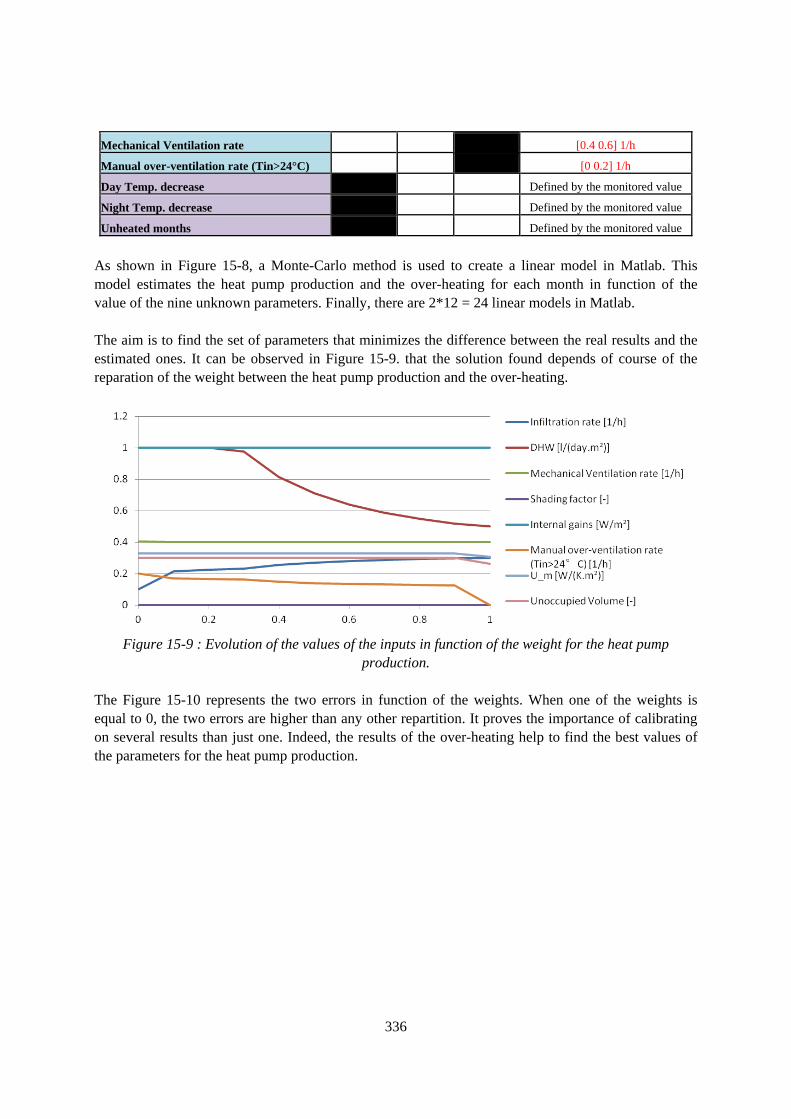
336

Mechanical Ventilation rate [0.4 0.6] 1/h

Manual over-ventilation rate (Tin>24°C) [0 0.2] 1/h

Day Temp. decrease Defined by the monitored value

Night Temp. decrease Defined by the monitored value

Unheated months Defined by the monitored value

As shown in Figure 15-8, a Monte-Carlo method is used to create a linear model in Matlab. This model estimates the heat pump production and the over-heating for each month in function of the value of the nine unknown parameters. Finally, there are 2*12 = 24 linear models in Matlab. The aim is to find the set of parameters that minimizes the difference between the real results and the estimated ones. It can be observed in Figure 15-9. that the solution found depends of course of the reparation of the weight between the heat pump production and the over-heating.

Figure 15-9 : Evolution of the values of the inputs in function of the weight for the heat pump

production. The Figure 15-10 represents the two errors in function of the weights. When one of the weights is equal to 0, the two errors are higher than any other repartition. It proves the importance of calibrating on several results than just one. Indeed, the results of the over-heating help to find the best values of the parameters for the heat pump production.

337

Figure 15-10 : Evolution of the error in function of the weight for the heat pump production

For each weight, a simulation is launched with the values of the parameters found by the Matlab model. Some results of these simulations are shown in Figure 15-11 and Figure 15-12. As said before, it is possible to observe that the results with a null weight for the heat pump production or the over-heating are always worse than the results with any other weights.

Figure 15-11 : Monthly heating consumptions for different heat pump production weights

338

Figure 15-12 : Monthly over-heating for different over-heating weights

The values of the parameters found to minimize the error on the heat pump production and the over-heating are written in the Table 15-9. Of course, the minimal and maximal possible values for the unknown parameters have to be carefully chosen. Unrealistic values should not be allowed in the calibration process. Here, by example, the theoretical mean heat transfer coefficient is 0.31 W/(K.m²), but as the real one could be slightly different, minimal and maximal values of 0.29 and 0.33 have been set. The value found by the calibration process is finally 0.33 W/(K.m²).

Table 15-9 : Values of the unknown parameters with weight heat pump production = 0.9


Um 0.33 W/(K.m²)

Infiltration + Man. Vent. rate 0.2162 1/h

DHW 1 l/(day.m²)

Electrical power 2.64 W/m²

Shading factor 0

Part of unoccupied volume 0.3

Internal gains 1 W/m²

Mechanical Ventilation rate 0.4 1/h

Manual over-ventilation rate (Tin>24°C)

0.1684 1/h

15.6 Results

Here are the results found after the calibration process (Figure 15-13 and Figure 15-14). It can be remarked that the simulation results are closer for the energy produced by the heat pump than the overheating, it is normal, because the model is designed mainly to estimate the heating consumption (rather than the overheating). In addition, in the minimization, the weight for the energy produced by the heat pump is heavier than for the overheating (0.9 vs. 0.1).

339

Figure 15-13 : Real and simulated energy produced by the heat pump [kWh]

Figure 15-14 : Real and simulated overheating [K.h]

The energy balances are shown on the Figure 15-15 and the Figure 15-16. The incomes are of course equal to the outcomes. The losses by the mechanical ventilation are very low because of the presence of the heat exchanger. As the house is not really compact, it induces a large surface of external walls and then a relatively high quantity of transmission losses, even if the walls are insulated.

340

Figure 15-15 : Yearly energy incomes [kWh] Figure 15-16 : Yearly energy outcomes [kWh]

To have a better idea of the repartition of the energy balance during (or not) the heating season, Figure 15-17 and Figure 15-18 represent the balance for every month. Once again, the incomes and the outcomes are equal for every month. The repartition of the incomes during the year seems logical (variation of the energy produced by heat pump and of the solar gains all along the year). For the outcomes, the losses for the infiltration and the manual ventilation are higher during the winter than the summer. The transmission losses are proportional to the difference of temperature between the inside and the outside. And finally, thanks to the heat exchanger, the losses of the mechanical ventilation are low even in winter. The losses are even higher in summer than in winter, this is induced by the by-pass that helps to keep the house as cool as possible in summer. In fact, these losses are useful as they limit the overheating.

Figure 15-17 : Monthly energy incomes [kWh]

341

Figure 15-18 : Monthly energy outcomes [kWh]

The Table 15-10 shows the two yearly balances of this house. There is one balance for the heating system (the boiler) and another one for the building itself. There are the two equations of the balances:

Table 15-10 : Energy balances for the heat pump and the house

Air 11011 Heating gains 17237

Electricity 9752 Solar gains 12233

Heating -17237 Human gains 1818

DHW -3526 Electrical gains 5356

Infilt. & man. Vent. losses -6310

Mech. ventilation losses -2682


Energy balances [kW h]

H eat pump H ouse

Finally, with the sankey diagram (Figure 15-19), Figure 15-17 and Figure 15-18 are summarized. The values of the flows are not written to keep the figure simple, but the widths of the arrows are proportional to the values of the flows. The two balances are respected (heat pump and Building) and the sum of the inputs is equal to the sum of the outputs.

342

Figure 15-19 : Sankey diagram for the building and the heat pump (for the all year)

The Figure 15-20 and the Figure 15-21 represents the sankey diagrams for one cold month (December) and one hot month (June). The thicknesses of the arrows are proportional to the energy flow and the thickness is twelve times more important in these monthly diagrams than in the annual one. Thus the three diagrams can be directly compared. By example, the DHW, Human gains and electrical gains flows which are more or less constant all along the year has nearly the same thickness on the three diagrams.

Figure 15-20 : Sankey diagram for the building and the heat pump (for December)

Figure 15-21 : Sankey diagram for the building and the heat pump (for June)

15.7 Conclusions

Some parameters, especially for the human behavior, are hardly measurable in a dwelling. But with the help of the known and monitored parameters and some results (as here, the monthly heat pump production and over-heating), it is possible to estimate the unknown parameters that give the estimated results (from the simulations) as close as possible to the real ones. It has been shown that is really an advantage to be able to calibrate on two results and not only one. The difference between the reality

343

and the simulation for the heat pump production is smaller if the calibration is done on the heat pump production and on the over-heating, than if the calibration is done only on the heat pump production. Once the model is calibrated, it is possible to realize simulations which can give an estimation of the real energy balances in the house. It could be also possible to estimate the variation of the consumption with a variation of some parameters (related to the occupant behavior or not) and thus give some piece of advices to reduce the heating consumption. It is important to keep in mind that the solution found by the calibration process is maybe not the exact one. There are several set of parameters which give simulated heat pump production close to the real one. It is important to know what the really important results are and to give the appropriate weights to the different results in the calibration process. Finally, some inputs stays constant all along the year during the simulation (electrical power by example), but it is not the case in the reality. To improve the precision of the results, it could have been interesting to add a captor to measure the real electrical power used in the house. 15.8 References

[1] Dolisy, V., IEA/Annex53/Subtask D: an example of sensitivity analysis with TRNSYS, University of Liège, November 2010.

[2] FABRY, B., DOLISY, V., ANDRE, P., Presentation of the Belgian Residential Case Study n°1, September 2010

[3] Pignon N., André P., Case study BE 02: Apartment in Arlon, University of Liège , September 2012

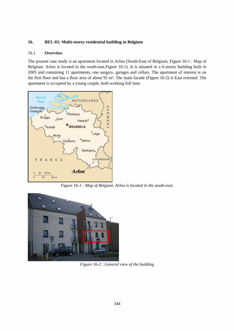
344

16. BEL-02: Multi-storey residential building in Belgium

16.1 Overview

The present case study is an apartment located in Arlon (South-East of Belgium, Figure 16-1 : Map of Belgium. Arlon is located in the south-east.Figure 16-1). It is situated in a 6-storey building built in 2005 and containing 11 apartments, one surgery, garages and cellars. The apartment of interest is on the first floor and has a floor area of about 95 m². The main facade (Figure 16-2) is East oriented. The apartment is occupied by a young couple, both working full time.

Figure 16-1 : Map of Belgium. Arlon is located in the south-east.

Figure 16-2 : General view of the building

345

Figure 16-3 : 3D model of the case study

16.2 Climate

Arlon is situated in Belgium, the climate is “warm temperate and fully humid with warm summer”, according to Köppen-Geiger climate classification. In the Table 16-1, there are some characteristics of the weather for the year 2010 in Arlon.

Table 16-1 : Climate for the year 2010 in Arlon

Year Jan Feb Mar Apr May Jun Jul Aug Sep Oct Nov Dec

Mean min Temp [C°] 12.4 -3.4 -1.3 1.6 4.8 6.9 12.2 14.8 12.4 9.4 5.8 3.2 -4.2

Mean Temp [C°] 8.6 -1.5 1.1 5 9.7 10.8 17.2 19.7 16.1 12.8 8.9 5 -2.2

Mean max Temp [C°] 5.2 0.2 3.6 8.9 15.1 15.3 22.4 25.4 20.5 17 13.2 6.9 -0.3

Mean Humidity [%] 78.3 88.2 88.3 67.7 62.5 59.7 73.9 74.5 79.1 79.8 85.1 82 90.3

HDD15 [Day.C°] 2726 513 390 311 175 152 31 9 30 87 196 299 533

CDD18.3 [Day.C°] 173 0 0 0 5 10 46 85 21 4 1 0 0

16.3 Available data

16.3.1 Plan

The plan of the apartment is available on Figure 16-4. The kitchen and the living room form a large open-space of 45 m². The "OFFICE B" room is a laundry, equipped with a washing machine and a tumble drier. The "CHAMBRE 1B" is the bedroom and the "CHAMBRE 2B" is used as a study.

346

Figure 16-4 : Plan

16.3.2 Envelope

The building's structure is composed of concrete blocks for the main walls, and of concrete slabs for the floors. An external rendering has been installed on the different fronts. The composition of the external walls and intermediate floors is detailed in the Table 16-2 and the Table 16-3 respectively. The windows main characteristics are listed in the Table 16-4.

Table 16-2 : Composition of the external walls Material Thickness [mm] Plaster 10 Concrete block 140 Glass wool 75 Air 5 Concrete block 140 External coating 20 Global U value: 0.35 W/m²K

347

Table 16-3 : Composition of the intermediate floors

Material Thickness [mm] Pavement 10 Concrete slab 50 PUR foam 40 Concrete slab 150 Plaster 10 Global U value: 0.51 W/m²K

Table 16-4 : Characteristics of the windows

Structure 4/15/4 Uglass 1.1 W/m²K gglass 0.61 Uframe 1.3 W/m²K

16.3.3 Heating and DHW

The heating load is supplied by an individual condensing gas boiler, with direct production for domestic hot water. There are 6 radiators equipped with thermostatic valves in the apartment: 3 in the kitchen/living, 1 in the study, 1 in the bedroom and 1 in the bathroom. There is also a global control panel in the living room, which allows definition of set points and weekly schedules. The temperature set point is 21°C when someone is present and 18°C when there is no occupant or at night. The schedules for week days and week-end are shown on Figure 16-5. This figure contains also the electrical power used hour by hour during the week days and the week-end. This gives information about the presence of the occupant.

Figure 16-5 : Electrical power and indoor temperature in function of the hour of the day.

The monthly mean internal temperature is shown in the Figure 16-6. The wanted internal temperature (set point) does not change during the year, but there is (small) over-heating during the summer as there no cooling system.

348

Figure 16-6 : Monthly mean internal temperature of the apartment

16.3.4 Energy consumption

Each apartment in the building has its own electricity counter (day/night) and gas counter. For the apartment of interest, the consumptions have been recorded during nearly three years and are listed in the Table 16-5.

Table 16-5 : Energy consumption records Dec 08 - Nov 09 Dec 09 - Nov 10 Nov 10 - Oct 11

Gas [m³] 586 588 483 Electricity, day [kWh] 1382 1285 1089 Electricity, night [kWh] 1098 1221 1582

Remark: regarding the electricity, the night counter is turning from 10PM to 7AM on week days and 24/24 on week-ends. 16.3.5 Lighting

There are halogen light bulbs (50 W each) in the study, the bedroom and the living/kitchen, and classical light bulbs elsewhere. The details are visible in Table 16-6.

Table 16-6 : Lighting details Type Total power [W] Area [m²] Living/kitchen halogen 600 46 Laundry incandescent 60 4 Hall incandescent 120 9 Bathroom incandescent 360 7 Bedroom halogen 150 13 Study halogen 150 11 WC incandescent 60 2

349

16.3.6 Ventilation

There are mechanical extractions in the kitchen (hood), in the bathroom and WC (linked to the lighting switch). Otherwise, the ventilation is natural and controlled by the occupant (opening of the windows). 16.4 Monitoring

16.4.1 Installed material

To record the electricity consumption, an energy counter has been installed on the main electrical panel. It records the energy consumed through a data logger every ten minutes (1 pulse = 10 Wh). In addition to that, 5 stand-alone temperature and humidity sensors have been placed in the apartment (2 in the living/kitchen, 1 in the bedroom, 1 in the bathroom and 1 in the study). These sensors record a value every 10 minutes and have been working since the end of October 2010. 16.4.2 Manual monitoring

To complete this automatic monitoring, a manual reading of the individual gas counter is performed daily as there is no logger for this. 16.4.3 Meteorological data

The data used for the simulations come from a meteorological station located on the campus of the University of Liège in Arlon (2 km away from the case study building). 16.5 Simulation and calibration

The software TRNSYS is used to achieve the simulation. The file used is an adaptation of the one created for the subtask D of this annex 53. The aim of the simulation is to be able to calibrate the model, this way it is possible to estimate the value (which are not monitored) of some parameters (ventilation and infiltration rate, temperature of the boundary apartments…). The different steps to arrive at this calibration are listed in the Figure 16-7.

Figure 16-7 : Global scheme for the calibration

The model of the apartment is calibrated according two kinds of results:

• Monthly gas consumption [kWh] • Monthly over-heating [K.h]

350

It means that there are 12*2=24 results to calibrate. It is of course more reliable two calibrate on a monthly basis than an annual one, because it would be too easy (and then imprecise) two calibrate the model with only two annual values. The problem is that even several different solutions could arrive to the same result. With a monthly basis, none calibration will be perfect, but the one chosen is the one with the simulated results closer to the real ones. Of course, a weight has to be given for the gas consumption and the over-heating in the calibration process. There is no perfect repartition of the weights; the one chosen depends of the importance of the results. Here, the gas consumption is more interesting for the analysis of the apartment, so it will have a larger weight than the over-heating. Furthermore, the model is designed more specifically to estimate the heating consumption than the over-heating. By example, the shadings are not analyzed because they are nearly negligible for the heating consumption, although there are important for the over-heating, The simulation runs from the 1st of November 2010 to the 31st of October 2011, so it is a complete year. The internal temperature and the electrical power are the real ones recorded during this period by the loggers in the apartment. But, the heating is disabled when the internal temperature is over 22 °C (as the maximum heating set point is 21 °C). Because in this case, the apartment is heated only by the others gains. The unknown parameters have to be estimated. The results used to calibrate the model are the monthly gas consumption and the monthly over-heating (calculated from 23 °C). The aim is to find the set of parameters that minimizes the difference between the real results and the ones of the simulation. The result which has to be minimized is described in Equation 1. Before this minimization, a regression is realized to find the vectors β for each kind of result: gas consumption and overheating for each month. This way, a linear system is created to estimate the heating consumption and the overheating for each month. The advantage of this technique is its quickness. Indeed, there no need to run a new simulation at each step of the minimization process, it is the linear system which is used to estimate the new result.

Equation 1 : x is the vector of inputs that minimizes the error As shown in Table 16-7, there are three categories of parameters:

• Monitored (climate, internal temperature and electrical power) • Known (physical characteristics of the apartment and the heating system) • Unknown (in red) => minimal and maximal values instead of an unique one

351

Table 16-7 : List of the parameters and theirs categories


External Temp. Defined by the monitored value

Boundary Temp. difference [-2;2] °C

Wind class 3

Um 0.51 W/(K.m²)

Infiltration rate [0.04;0.2] h-1

Volume 237 m³

Windows surf./Occupiable surf. 0,0945

Compactness 3.1 m

Wall thickness 0.19 m

Part of south windows 0

Efficiency of the boiler [0.93;0.97]

Pump control Yes

Heat exchanger No

Boiler location Inside

Radiative part 0.3

DHW [0.6;1.5] l/(day.m²)

Electrical power Defined by the monitored value

Part of unoccupied volume 0

Internal gains [1;2] W/m²

Internal air temperature Defined by the monitored value

Ventilation rate at 0 °C [0.2;0.5] h-1

Ventilation rate at 20 °C [0.5;0.8] h-1

Over-ventilation rate (Tin>22 °C) [0;0.1] h-1/K

Day Temp. decrease Defined by the monitored value

Night Temp. decrease Defined by the monitored value

Unheated months Defined by the monitored value

As shown in Figure 16-7, a Monte-Carlo method is used to create a linear model in Matlab. This model estimates the gas consumption and the over-heating for each month in function of the value of the eight unknown parameters. Finally, there are 2*12 = 24 linear models in Matlab. The aim is to find the set of parameters that minimizes the difference between the real results and the estimated ones. It can be observed in Figure 16-8 that the solution found depends of course of the reparation of the weight between the gas consumption and the over-heating.

352

Figure 16-8 : Evolution of the values of the inputs in function of the weight for the gas consumption.

The Figure 16-9 represents the two errors in function of the weights. When one of the weights is equal to 0, the two errors are higher than any other repartition. It proves the importance of calibrating on several results than just one. Indeed, the results of the over-heating help to find the best values of the parameters for the gas consumption.

Figure 16-9 : Evolution of the error in function of the weight for the gas consumption

For each weight, a simulation is launched with the values of the parameters found by the Matlab model. Some results of these simulations are shown in Figure 16-10 and Figure 16-11. As said before, it is possible to observe that the results with a null weight for the gas consumption or the over-heating are always worse than the results with any other weights.

353

Figure 16-10 : Monthly heating consumptions for different heating consumption weights

Figure 16-11 : Monthly over-heating for different over-heating weights

The values of the parameters found to minimize the error on the gas consumption and the over-heating are written in Table 16-8. The weight given for the gas consumption (0.9) is larger than the one for the over-heating (0.1).

Table 16-8 : Values of the unknown parameters with weight heating consumption = 0.9


Boundary Temp. diff. 0.73 °C

Infiltration rate 0.116 h-1

Efficiency of the boiler 0.925

DHW 0.95 l/(day.m²)

Internal gains 1 W/m²

Ventilation rate at 0 °C 0.5 h-1

Ventilation rate at 20 °C 0.659 h-1

354

Over-ventilation rate (Tin>22 °C) 0.1 h-1/K

16.6 Results

Here are the results found after the calibration process (Figure 16-12 and Figure 16-13). It can be remarked that the simulation results are closer for the gas consumption than the overheating, it is normal, because the model is mainly designed to estimate the heating consumption rather than the overheating. In addition, in the minimization, the weight for the gas consumption is heavier than for the overheating (0.9 vs. 0.1).

Figure 16-12 : Real and simulated gas consumption [kWh]

Figure 16-13 : Real and simulated overheating [K.h]

The energy balances are shown on Figure 16-14 and Figure 16-15. The incomes are of course equal to the outcomes. It can be remarked that the ventilation represents the largest part of the outcomes, but it

355

is important to understand that a part of this outcomes are useful as they allow limiting the over-heating in summer. The energy balances are calculated all along the year, not only during the heating season.

Figure 16-14 : Yearly energy incomes [kWh] Figure 16-15 : Yearly energy outcomes [kWh] To have a better idea of the repartition of the energy balances during (or not) the heating season, Figure 16-16 and Figure 16-17 represent the balance for every month. Once again, the incomes and the outcomes are equal for every month. It can be observed that the ventilation losses are nearly as large in summer as in winter, because as mentioned previously, the ventilation losses during the summer are useful. The ventilation rate increases with the external temperature and there is also an “over-ventilation rate” in summer when the internal temperature is over 23 °C. On the other hand, the losses by transmission are larger in winter than in summer, because this result is not related to the human behavior and depends mainly of the external temperature.

Figure 16-16 : Monthly energy incomes [kWh]

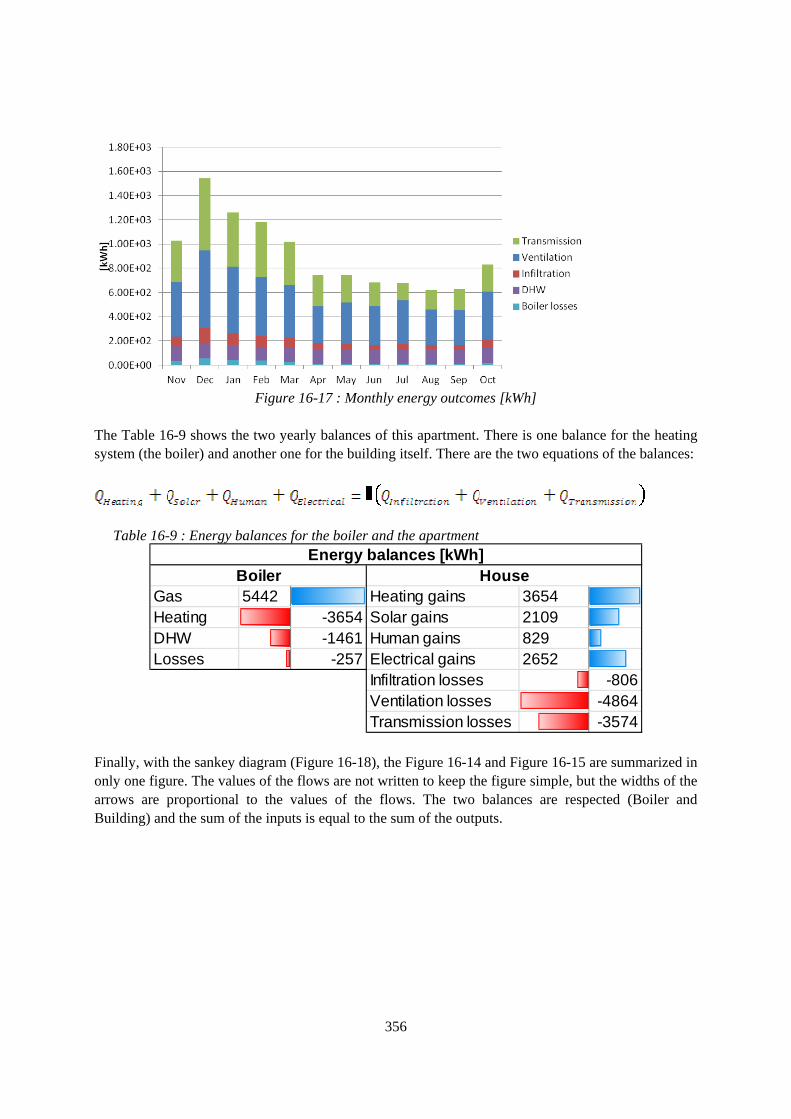
356

Figure 16-17 : Monthly energy outcomes [kWh]

The Table 16-9 shows the two yearly balances of this apartment. There is one balance for the heating system (the boiler) and another one for the building itself. There are the two equations of the balances:

Table 16-9 : Energy balances for the boiler and the apartment

Gas 5442 Heating gains 3654Heating -3654 Solar gains 2109DHW -1461 Human gains 829Losses -257 Electrical gains 2652

Infiltration losses -806Ventilation losses -4864Transmission losses -3574

Energy balances [kWh]Boiler House

Finally, with the sankey diagram (Figure 16-18), the Figure 16-14 and Figure 16-15 are summarized in only one figure. The values of the flows are not written to keep the figure simple, but the widths of the arrows are proportional to the values of the flows. The two balances are respected (Boiler and Building) and the sum of the inputs is equal to the sum of the outputs.

357

Figure 16-18 : Sankey diagram for the building and the boiler (for the all year)

The Figure 16-19 : Sankey diagram for the building and the boiler (for December) and the Figure 16-20 represents the sankey diagrams for one cold month (December) and one hot month (June). The thicknesses of the arrows are proportional to the energy flow and the thickness is twelve times more important in these monthly diagrams than in the annual one. Thus the three diagrams can be directly compared. By example, the DHW flow which is more or less constant all along the year has the same thickness on the three diagrams.

Figure 16-19 : Sankey diagram for the building and the boiler (for December)

Figure 16-20 : Sankey diagram for the building and the boiler (for June)

358

16.7 Conclusions

Some parameters, especially for the human behavior, are hardly measurable in a dwelling. But with the help of the known and monitored parameters and some results (as here, the monthly gas consumption and over-heating), it is possible to estimate the unknown parameters that give the estimated results (from the simulations) as close as possible to the real ones. It has been shown that is really an advantage to be able to calibrate on two results and not only one. The difference between the reality and the simulation for the gas consumption is smaller if the calibration is done on the gas consumption and on the over-heating, than if the calibration is done only on the gas consumption. Once the model is calibrated, it is possible to realize simulations which can give an estimation of the real energy balances in the apartment. It could be also possible to estimate the variation of the consumption with a variation of some parameters (related to the occupant behavior or not) and thus give some piece of advices to reduce the heating consumption. It is important to keep in mind that the solution found by the calibration process is maybe not the exact one. There are several set of parameters which give simulated gas consumption close to the real one. It is important to know what the really important results are and to give the appropriate weights to the different results in the calibration process. 16.8 References

[1] Dolisy, V., IEA/Annex53/Subtask D: an example of sensitivity analysis with TRNSYS, University of Liège, November 2010.

[2] Fabry, B., Case study: an apartment building in Arlon. Monitoring, simulation and sensitivity analysis, University of Liège, January 2010.

[3] Pignon N., André P., Case study BE 01: House in Hondelange, University of Liège , September 2012

359

17. BEL-03: Multi-storey residential building in Belgium

17.1 Introduction

The objective of this study is to develop a new way of comparing simulation with measurements, in the perspective of two very practical applications: (1) Validation and tuning a simulation model; (2) “Intelligent” energy counting with the help of parallel simulation. The second application seems of particular interest as a possible feed-back offered to the building occupants and helping them to reach an energy efficient behavior and to detect any energy waste. The new approach consists in using indoor temperatures recorded inside different building zones and integrated energy demands as simulation input and output variables, respectively. More details about the methodology are given in a companion report [1]. 17.2 The dwelling

This dwelling located on the Belgian coast (Figure 17-1) has a total floor area of 95 m2.

Figure 17-1: The dwelling

It can be subdivided into 9 different zones (with toilet and boiler room aggregated into only one zone) as indicated in Figure 17-2. The living room is oriented to the North (i.e. on see side). Two of the sleeping rooms are oriented to the South; a third one is “blind”.

360

Figure 17-2: the dwelling subdivided in 9 zones

The dwelling is equipped with a simple mechanical ventilation system: exhaust openings are located in the kitchen, in the shower corners of two rooms, in the bath room, in the toilet and in the boiler room. Direct electric heaters are available in all rooms, except the kitchen, the corridor, the toilet and the boiler room. Only the living room is supposed to be heated all along daily occupation periods. According to the occupancy rate of the dwelling, the bath room and the shower corners of two sleeping rooms might be heated during limited morning and evening periods. The dwelling is surrounded by four other dwellings which are not always occupied. 17.3 Assembling of the simulation model

The simulation model is built in three steps with the help of the EES software [2] and according to a method already tested on another building [3]. 17.3.1 First step

The first step consists in subdividing the building and its surroundings into different zones and in identifying all internal and external walls. The internal zones are distinguished among themselves according to occupancy schedules and to indoor environmental requirements. A matrix of zones interconnections is easy to build on basis of building pictures and geometrical data. Each interconnection corresponds to one or to several walls, doors and windows, whose characteristics are defined in the next step (§ 3.2). In the example considered here, a total of 15 zones are distinguished (8 internal and 5 external), with 5 of these ones actually heated. The interconnections among these zones make appear a total of 30 walls. Air flow rates are supposed to be imposed at the level of 5 exhaust openings, connected to a through a common duct to a fan located on the building roof.

361

Other air flow rates are deduced from these 5 values, by mass balances and on the basis of a few circulation hypotheses:

17.3.2 Second step

The second step consists in identifying the R and C components to be used to represent the internal and external zone “partitions”. The solution obtained from the first step is here used (by “copy and paste”) as input data. In the example considered, each heavy wall is represented by a R-C-R (first order) model. For example, the thermal characteristics R and C of any internal wall are given by the two following equations:

Windows and doors are represented as purely resistive. 17.3.3 Third Step

The third step consists in interconnecting all the R-C-R circuits and establishing the energy balances of all nodes. This doesn’t require any graphic tool: the matrix established in the first step allows the user knowing which (internal or external) zones are interconnected through each wall. Again here, the solution of the previous step is used (by “copy and paste”) as input data. In the example considered, the whole building model corresponds to a set of 822 equations: 769 algebraic and 53 integral. These equations are repeated and adapted, step by step, with help of the classical “copy”, “paste”, “find” and “replace” functions for all walls and all zones.

364

The heavy walls connecting zone 1 to adjacent zones 11, 12, 13 14 and 15 are simulated in the same way as the wall 1-8…

Various hypotheses can be made on the temperature of the stair case. For example, it can be assumed that this temperature is, at least, 5 C higher than the outdoor temperature and never lower than 5 C:

365

The outdoor environmental temperature is supposed to take the effect of long wave sky radiation into account (the sky is usually colder than the air, depending on sky clarity):

( for a vertical surface) Various hypotheses can also be done on the temperatures of the other adjacent zones, depending mainly on the occupancy rate or the surrounding apartments:

(This would mean that only two of the four adjacent apartments are actually occupied). The thermal balances of the other 7 internal zones are established in the same way…

366

All power and energy consumptions can be defined as follows:

367

And, as all consumptions are in the same energy form (electricity), they may be added together:

Hourly values of outdoor air temperature and of (global and diffuse) solar radiations incident to an horizontal surface are given in lookup tables:

These terms are combined as follows, in order to define the solar radiations incident to surfaces of different orientations:

368

Pre-calculated hourly values of the orientation factors (for the given latitude) are also given in a lookup table:

The long wave sky infrared radiation is estimated, day by day, by empirical correlation with the “sky clarity”, which is defined a ratio between actual and maximal number of hours of sunshine (the maximum corresponds to full clear sky conditions):

Daily values of the number of hours of sunshine are also given in a lookup table:

The maximal number of hours of sunshine corresponds to the day duration; for the latitude considered, it can be calculated as follows:

369

17.4 First simulation results: Influence of occupancy rates

The possible influences of both (internal and surrounding) occupancy rates are here observed by simulation on a reference year. Three and four levels are distinguished, for internal and surrounding occupancies respectively. The three levels of internal occupancy rates correspond to the use of one, two or three rooms, by two, four or six persons, respectively. The four levels of surrounding occupancy correspond to the number of surrounding dwellings actually occupied. In this first sensitivity analysis, the occupancy levels are still supposed to be constant all along the year. Examples of simulation results are presented in Figures 17-3 to 17-11; they correspond to the following cases: (1) Full internal occupancy and no surrounding occupancy (Figure 17-3) (2) Partial internal occupancy and no surrounding occupancy (Figures 17-4 to 17-7) (3) Full internal and surrounding occupancies (Figures 17-8 to 17-10) (4) Partial internal occupancy and full surrounding occupancy (Figure 17-11).

370

Figure 17-3: Total heating demand when the dwelling is fully occupied and the adjacent four dwellings unoccupied

Figure 17-4: Total heating demand when the dwelling is partially occupied and the adjacent four

dwellings unoccupied

Figure 17-5: Heating demands of the whole dwelling (in black), of the living room (in blue) and of the

bath room (in red) in same conditions as Figure 17-4

371

Figure 17-6: Outdoor and indoor temperatures in the conditions of Figure 17-4

Figure 17-7: zoom of Figure 17-6

Figure 17-8: Total heating demand when the dwelling considered and also the four adjacent dwellings

are fully occupied

372

Figure 17-9: Outdoor and indoor temperatures in the conditions of Figure 17-8

Figure 17-10: Zoom of Figure 17-9

373

Figure 17-11: Total heating demand when the dwelling considered is partially occupied and the four

adjacent dwellings fully occupied It appears that the surrounding occupancy level is here the most influencing factor. The actual variations of the heating demand could even be stronger than indicated here: when the surrounding dwellings are empty (and just heated enough to maintain their indoor temperature above 5°C), it appears (Figures 17-6 and 17-7), that the indoor temperature of the (supposed-to-be unheated) sleeping room is currently rather low (between 5 and 10°C) in winter time. It also appears (on the same Figures) that the transient heating of the bath room is not sufficient to bring the indoor temperature to an acceptable level. This means that a higher heating demand has to be expected when the surrounding dwellings are empty. The heating demand is probably also (as much in relative value, but less in absolute value) underestimated when the surrounding dwellings are occupied: in that case, the (optimistic) hypothesis is that their indoor temperature is identical to the living room temperature of the dwelling considered… A total of 11 combinations have been considered in this sensitivity analysis; a synthesis of the results is presented in Table 17-1. The variables included in the different columns are: Column 1: dwelling occupancy rate (corresponding to the number of rooms occupied) varying from 0.33 (one room occupied) to 1 (all the three rooms occupied) Column 2: occupancy rate of the surrounding dwellings (corresponding to the number of surrounding dwellings occupied) varying from 0 (no surrounding dwelling occupied) to 1 (all the four surrounding dwellings occupied) Columns 3 to 6: specific energy consumptions Column 7: total energy consumption. All these results stay hypothetical, but the variations are rather impressive. The runs 9 and 10 should not be directly compared with other ones, because they are based on different combinations of surrounding dwellings.

374

Table 17-1: synthesis of simulation results

Examples of regressions are presented in Figures 17-12 and 17-13.

Figure 17-12: Influence of the dwelling occupancy rate on the heating demand

375

Figure 17-13: Influence of the surrounding occupancy rate on the heating demand

These regressions established on the basis of the simulation results are no more than a provocation: such building “signatures” should be experimentally established on shorter time bases and for different weather conditions. Both internal and external occupancy rates are indeed varying a lot all along the year. At least, this first parametric study demonstrates how much the heating demand can be affected, not only by the occupancy rate in the dwelling considered, but also by the occupancy rate in each of the four surrounding dwellings. 17.5 Monitoring and comparative simulation

The dwelling is equipped with (peak and off-peak) electrical and water counters. These counters are read at different times when the dwelling is occupied. Indoor air temperatures are continuously and automatically recorded in four zones of the dwelling: the living room, two sleeping rooms and the bath room. Weather data are taken from the nearest meteorological station. Other recordings are taken about the actual occupancy level in the dwelling considered and in the four surrounding dwellings. 17.5.1 On short time period

A first detailed comparison between simulation and measurements was established on a short time period corresponding to one day with night set back [4]. 17.5.1.1 Recording of indoor climate, consumptions and schedules Examples of recordings are presented in Figures 17-14 to 17-17. Indoor and outdoor temperatures recorded on a period of one week are presented in Figure 17-14. The dwelling stays unoccupied during the first six days of that week. The occupancy period starts on the

376

evening of the sixth day. A zoom on that last 25 hours period is presented in Figure 17-15. The shapes of the curves correspond to the following events:

• Arrival of the occupants on December 3rd around 19h (the 8083rd hour of the year), starting of the heating in three zones of the dwelling (living, sleeping and bath rooms);

• Shutting down of the heating in the evening (first in the living room and a little later in the two other zones) around the 8087th hour;

• Re-starting of the heating on the next morning (first in the bath room and two hours later in the living room) for a while;

• Shutting down again a few hours later (first in the bath and sleeping rooms and then in the living room).

Figure 17-14: Indoor and outdoor temperatures recorded on one week

Figure 17-15: zoom on the right side of Figure 17-14 (last 25 h time period)

Cumulated peak, off-peak and total electricity consumptions manually recorded on a 5000 hours period are presented in Figure 17-16.

377

The points of the diagram correspond to occasional readings of the counters. Off-peak periods are from 10 pm to 7 am and weekends. The smooth slopes of the three curves on the left side of the diagram correspond to the non-heating period. On the right side of the diagram, the sharper slope increases correspond to occupancy periods with (growing) heating needs. The zoom presented in Figure 17-17 corresponds to the same 25 hours period as in Figure 17-15. The peak counter is here only working during the very first period (on Friday evening). The apparent superposition of peak and off-peak demands occurring between the hour 8085 and 8086 is due to the fact that the counters were not read at change-over time.

Figure 17-16: Electrical consumptions recorded on a period of 5000 hours

Figure 17-17: zoom on the same 25 hours period as in Figure 17-15

17.5.1.2 Simulation

378

The simulation is performed by using the four indoor air temperatures as input data: this eliminates any control uncertainty and should make the measured and simulated consumption directly comparable. The other (unheated) zones are simulated as in “free floating” temperatures. The heating demands of the four zones whose temperatures are imposed are plotted in Figure 17-18. As to be expected, their shapes are similar to the shapes of the curves of Figure 17-15, except for the time variations which are here a bit sharper. Indeed, in each room, the temperature response to any variation of heating power is damped by the walls thermal mass. Significant simulation mistakes also appear in this Figure: a non negligible heating demand is calculated before occupant arrival (hours 8080 to 8083); this fictitious heating demand reaches 1000 W in the living room (blue curve), probably due to some erroneous estimate of boundary conditions (mainly the temperatures of the surrounding dwellings). A slightly negative heating demand is also calculated later in the unoccupied room (red curve), probably also because of erroneous boundary conditions. The simulation model should be tuned on the whole observation periods and mainly when the dwelling is empty. The heating powers of Figure 17-19 are integrated in Figure 17-20, in order to make them easier to compare with the energy records. It appears that the accumulation of energy in the walls produces a very significant increase of the heating energy demand on the first evening and still on the whole 25 hours period considered…

Figure 17-18: Simulated heating demands as functions of the four indoor temperatures of Figure 17-

15.

379

Figure 17-19: Dynamic and static heating demands and energy storage in walls

Figure 17-20: Integration of the curves of Figure 17-19

17.5.1.3 Comparison between simulation and measurements A fairly satisfactory comparison between the measured electrical consumption and the simulated heating demand is presented in Figure 17-21. The total consumption of electricity is over-passing the heating demand because of: - Electrical energy not used to heat the dwelling (of the order of 5 kWh per day, for hot water production); - Modeling inaccuracies (mainly static and dynamic characteristics and temperatures in surrounding dwellings). These differences should be reduced thanks to a more detailed analysis of all information available and also by a better tuning of the simulation model.

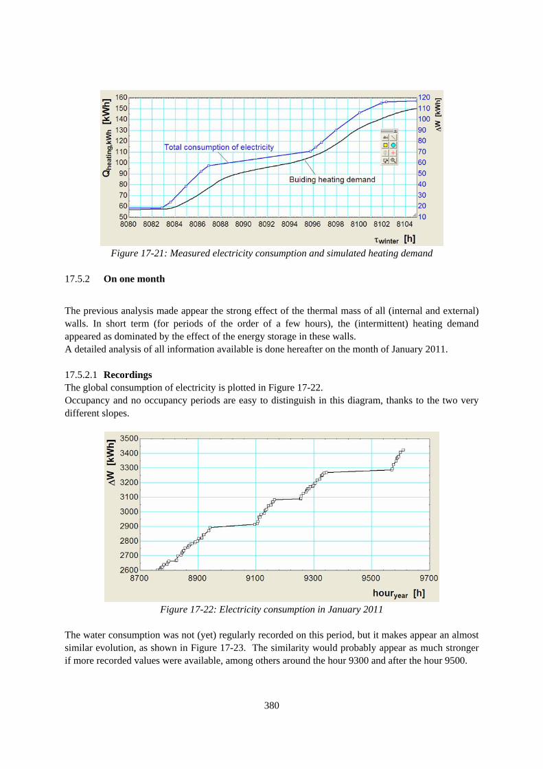
380

Figure 17-21: Measured electricity consumption and simulated heating demand

17.5.2 On one month

The previous analysis made appear the strong effect of the thermal mass of all (internal and external) walls. In short term (for periods of the order of a few hours), the (intermittent) heating demand appeared as dominated by the effect of the energy storage in these walls. A detailed analysis of all information available is done hereafter on the month of January 2011. 17.5.2.1 Recordings The global consumption of electricity is plotted in Figure 17-22. Occupancy and no occupancy periods are easy to distinguish in this diagram, thanks to the two very different slopes.

Figure 17-22: Electricity consumption in January 2011

The water consumption was not (yet) regularly recorded on this period, but it makes appear an almost similar evolution, as shown in Figure 17-23. The similarity would probably appear as much stronger if more recorded values were available, among others around the hour 9300 and after the hour 9500.

381

Figure 17-23: Water consumption in January 2011

Even with this still limited information about water consumption, the idea of using it as “historical” variable in place of the time is already tested in Figure 17-24: It gives a much smoother curve of energy consumption, even becoming almost linear. A linear regression can be established on this basis and the slope of this regression can be considered as a very simple characterization of the heating demand for the month considered (i.e. for the average weather and the average surroundings occupancy rate of that month). The interesting point is that the (variable) occupancy rate of the dwelling considered is now included in this characteristic.

Figure 17-24: Electricity consumption as function of water consumption in January 2011

Actual occupancy rates in and around the dwelling are plotted in Figures 17-25 and 17-26.

382

Figure 17-25: Dwelling occupancy rate and water consumption

Figure 17-26: Dwelling and surroundings occupancy rates

As previously, four indoor air temperatures are continuously recorded and the outdoor temperature is extracted from a nearby weather station. The evolutions of these temperatures are shown in Figure 17-27. It appears that the outdoor temperature is, most of the time, fluctuating around 5°C, with maxima over-passing 10 °C and minima going well below 0°C. Indoor temperatures are, most of the time, fluctuating between 10 and 20 °C, with maxima reaching 25 °C (t6: bath room) and minima approaching 7 °C at the end of the period considered (dwelling empty and exposed to cold weather) conditions. One curve (t3 in red) of Figure 17-27 is not issued from measurement, but from simulation: it corresponds to an empty room, which is not indirect contact with the outdoor environment and never heated. This explains its very smooth appearance: no violent perturbation and no digitalization discontinuity.

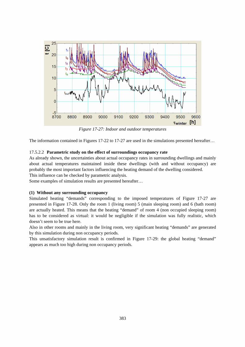
383

Figure 17-27: Indoor and outdoor temperatures

The information contained in Figures 17-22 to 17-27 are used in the simulations presented hereafter… 17.5.2.2 Parametric study on the effect of surroundings occupancy rate As already shown, the uncertainties about actual occupancy rates in surrounding dwellings and mainly about actual temperatures maintained inside these dwellings (with and without occupancy) are probably the most important factors influencing the heating demand of the dwelling considered. This influence can be checked by parametric analysis. Some examples of simulation results are presented hereafter… (1) Without any surrounding occupancy Simulated heating “demands” corresponding to the imposed temperatures of Figure 17-27 are presented in Figure 17-28. Only the room 1 (living room) 5 (main sleeping room) and 6 (bath room) are actually heated. This means that the heating “demand” of room 4 (non occupied sleeping room) has to be considered as virtual: it would be negligible if the simulation was fully realistic, which doesn’t seem to be true here. Also in other rooms and mainly in the living room, very significant heating “demands” are generated by this simulation during non occupancy periods. This unsatisfactory simulation result is confirmed in Figure 17-29: the global heating “demand” appears as much too high during non occupancy periods.

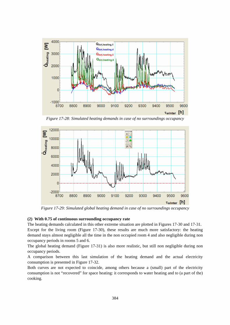
384

Figure 17-28: Simulated heating demands in case of no surroundings occupancy

Figure 17-29: Simulated global heating demand in case of no surroundings occupancy

(2) With 0.75 of continuous surrounding occupancy rate The heating demands calculated in this other extreme situation are plotted in Figures 17-30 and 17-31. Except for the living room (Figure 17-30), these results are much more satisfactory: the heating demand stays almost negligible all the time in the non occupied room 4 and also negligible during non occupancy periods in rooms 5 and 6. The global heating demand (Figure 17-31) is also more realistic, but still non negligible during non occupancy periods. A comparison between this last simulation of the heating demand and the actual electricity consumption is presented in Figure 17-32. Both curves are not expected to coincide, among others because a (small) part of the electricity consumption is not “recovered” for space heating: it corresponds to water heating and to (a part of the) cooking.

385

From other part, a (very small) part of the free heat is provided by non electrical sources: sensible metabolism of the occupants and also solar heat gains through the window of the living room (it is North oriented, but still collects some diffuse radiation).

Figure 17-30: Simulated heating demands in case of continuous occupancy in three of the

surroundings dwellings

Figure 17-31: Simulated global heating demand in case of continuous occupancy in three of the

surrounding dwellings

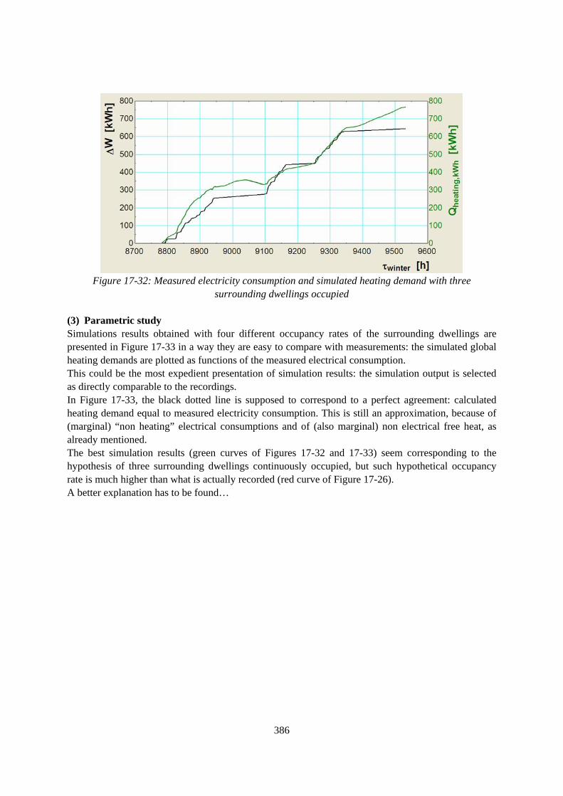
386

Figure 17-32: Measured electricity consumption and simulated heating demand with three

surrounding dwellings occupied (3) Parametric study Simulations results obtained with four different occupancy rates of the surrounding dwellings are presented in Figure 17-33 in a way they are easy to compare with measurements: the simulated global heating demands are plotted as functions of the measured electrical consumption. This could be the most expedient presentation of simulation results: the simulation output is selected as directly comparable to the recordings. In Figure 17-33, the black dotted line is supposed to correspond to a perfect agreement: calculated heating demand equal to measured electricity consumption. This is still an approximation, because of (marginal) “non heating” electrical consumptions and of (also marginal) non electrical free heat, as already mentioned. The best simulation results (green curves of Figures 17-32 and 17-33) seem corresponding to the hypothesis of three surrounding dwellings continuously occupied, but such hypothetical occupancy rate is much higher than what is actually recorded (red curve of Figure 17-26). A better explanation has to be found…

387

Figure 17-33: Calculated heating energy demand as function of measured electricity consumption

17.5.2.3 Introducing more realistic hypotheses The temperatures in the surrounding dwellings and in the stair case are not measured. When any one of the surrounding dwellings is occupied, its temperature is conventionally supposed to stay equal to the living room temperature of the dwelling considered. In non occupancy time, the temperature of the surrounding dwellings is supposed to follow the (very hypothetical) law applied to the stair case:

According to this hypothesis, the temperature of the stair case is “floating” 5 C above the outdoor temperature and above a minimum of 5 C. A new parametric study was performed about the effect of this minimum. The best results of this analysis are presented in Figures 17-34 and 17-35. It appears that the assumption of a minimal surroundings temperature of 12 °C can provide a global reconciliation between simulated and measured consumptions (Figure 17-35), but with, time to time, unrealistic negative values of instantaneous heating demand (Figure 17-34). It’s obvious that a minimal temperature of 12 °C is unrealistic and, again, a better explanation has to be found…

388

Figure 17-34: Global Heating demands calculated with more realistic hypotheses

Figure 17-35: Simulated heating demand as function of the electricity consumption

In another parametric analysis, various (more realistic) minimal temperatures were combined with various heat transfer coefficients of the envelope (windows, walls, floor and ceiling). The best results, presented in Figures 17-36 to 17-38, were obtained with the following combination of (still very hypothetical) inputs: minimal surroundings temperature of 10 °C, significantly reduced heat transfer coefficients and local outdoor temperature staying 0.5 K above its value measured at the weather station (slight microclimate effect). After careful tuning of all the parameters, a satisfactory agreement is found between simulated heating demand and electricity consumption, as shown in Figure 17-38. During non occupancy periods, a more realistic global heating demand is also obtained, as shown in Figure 17-37, but there remains a non negligible and unexplained heating demand in the living room, as shown in Figure 17-36.

389

The still unexplained oscillations of simulated the heating demand might, among others, be due to a too simple dynamical modeling: each heavy wall is represented by first order symmetrical R-C-R schema. A multi-layer schema had been more accurate. Moreover, indoor thermal masses are only represented in the rooms where the indoor temperatures are not set at their measured values. This is for simulation easiness: it’s much easier to calculate the temperature of a thermal mass as function of the thermal power than the contrary.

Figure 17-36: Simulated heating demands after best tuning of all parameters

Figure 17-37: Global heating demand after best tuning of all parameters

390

Figure 17-38: Simulated heating demand as function of the electricity consumption

A first idea about the possible influence of such simplification is given hereafter, by moving a bit all external walls thermal masses towards the inside of the dwelling. The new results presented in Figures 17-39 to 17-41 where obtained with dissymmetrical schemas 0.5*R-C-1.5*R, i.e. with a ratio of 3 between outside and inside thermal resistances. This increases the internal heat storage effects. As to be expected, higher heating peaks and strong “noise” (associated to the digitalization of temperature measurements) are then generated in the simulation (Figures 17-39 and 17-40), but the final agreement between simulation and measurements is not significantly improved. More detailed analyses, including other observation periods, would be welcome…

Figure 17-39: Simulated heating demands with thermal mass shifted to inside (to be compared with

Figure 17-36)

391

Figure 17-40: Global heating demand (to be compared with Figure 17-37)

Figure 17-41: Simulated heating demands as function of the electricity consumption

17.6 Records on longer periods and correlations

17.6.1 Records

The recordings of temperatures and (electricity and water) consumptions were extended until February 2012 (almost two year). Examples of last temperature records are presented in Figures 17-42 to 17-44.

392

Figure 17-42: Temperature recorded in the living room (last time period)

Figure 17-43: Temperature recorded in one of the sleeping rooms (last time period)

Figure 17-44: Temperature recorded in the bath room (last time period)

All the records of (peak, off peak and global) electricity consumptions are presented in Figure 17-45. Corresponding water consumptions are plotted in Figure 17-46.

393

Figure 17-45: Electrical consumption on the whole monitoring period

Figure 17-46: Water consumption on the whole monitoring period

At first look of Figures 17-45 and 17-46, the strong relationship between electricity and water consumption doesn’t immediately appear. It’s more obvious when making a zoom on a shorter period, during which the outdoor temperature is not varying too much. An example of such superposition is presented in Figure 17-47.

394

Figure 17-47: Electricity and water consumptions on one month without space heating demand

17.6.2 New correlations

The electricity consumption can be expressed as function of the water consumption, as shown in Figure 17-48. This curve is much smoother than when expressing the electricity consumption as function of the time (Figure 17-45). The local slope of the curve is directly related to the impact of the space heating, i.e. to the outdoor temperature.

Figure 17-48: Electricity consumption as function of the water consumption on the whole monitoring

period As already suggested, very significant linear correlations can be identified on shorter time periods during which the outdoor temperature doesn’t vary too much, as shown in Figures 17-49 to 17-53. The slope of each regression line is related to the average outdoor temperature, which determines the heating demand. When this outdoor temperature is high enough, as for example in August (Figure 17-50), there is no space heating demand and the electricity consumption is only due to other uses: hot water, cooking,

395

lighting and other appliances. The slope of the regression line is then of the order of 35 kWh per m3 of water consumption. In colder weather conditions, the regression slope increases because of the space heating demand. In January, for example (Figure 17-49), it reaches 60 kWh per m3 of water consumption...

Figure 17-49: Electricity consumption as function of the water consumption in January 2011

Figure 17-50: Electricity consumption as function of the water consumption in August 2011

396

Figure 17-51: Electricity consumption as function of the water consumption in September 2011

Figure 17-52: Electricity consumption as function of the water consumption in October 2011

397

Figure 17-53: Electricity consumption as function of the water consumption in October 2011

17.7 Conclusions

Using all measured temperatures as input data in the simulation makes possible a direct calculation of the net space heating (or cooling) demand, without concern about the actual behavior of the control system. Heating (and cooling) demands can also be converted, through system simulation, into corresponding energy consumptions, to be compared with information got (by direct reading or automatically) from the energy counters available. In the example considered, the heating demand is strongly affected by both “internal” and “external” (surroundings) occupancy rates. Recorded water consumptions might help a lot in identifying these occupancy rates and also the “non-heating” consumptions. In case of very variable occupancy rate, water consumptions can be preferred to time as “historical” variable, in order to get a “smoother” curve of energy consumption. This curve can even be approached by a linear regression in each seasonal period. The slope of this regression might be used as “seasonal signature” of the system considered. 17.8 References

[1] Aparecida Silva, Cl., Hannay, J. and Lebrun, J.: “Methodology for smart counting” IEA-ECBCS final report, December 2012.

[2] Klein S., “Engineering Equation Solver” F-Chart Sofware 2012 [3] Aparecida Silva, Cl., Hannay, J., Lebrun, J, Building renovation; example of preliminary study

performed with the help of an engineering equation solver, Palenc, Rhodes October 2010 [4] Aparecida Silva, Cl., Hannay, J. and Lebrun, J.: “Thermal simulation and monitoring of

dwelling”ISHVAC 2011, Shanguai, November 2011 Acknowledgements

This work is supported by the Walloon Region of Belgium.

398

18. CHN-01: Multi-storey residential building in China

18.1 Introduction

This case study house is compared in a study investigating the relationship between the energy use and occupant behavior in the multi-family apartment. 18.2 Location and climate

The apartment building is located in Tsinghua University Campus, Beijing, China. Beijing is the capital of China, with latitude: 39° 55'N and longitude: 116° 23'. Its climate is rather dry, monsoon-influenced humid continental climate, hot, humid summers due to the East Asian monsoon, and generally cold, windy, dry winters that reflect the influence of the vast Siberian anticyclone. The monthly daily average temperature in January is −3.7 °C, while in July it is 26.2 °C. Precipitation averages around 570 mm annually, with the great majority of it falling in the summer months. Extremes have ranged from −27.4 to 42.6 °C.

Figure 18-1. The geographic position of Beijing in China

399

Figure 18-2. The outside view of the investigated building

The measured climate data is the dry bulb temperature, which shows below:

Figure 18-3. The measured dry bulb temperature during a year

18.3 Householder Information

This family consists of five people, a couple, a nurse, a grand mom, and a son.

Table 18-1. The composition of the investigated family NO. Name Own room Remark

1 husband IT officer 2 wife

master bedroom teacher

3 grand mother

bedroom 1 retired

4 son bedroom 2 middle school student 5 nurse bedroom 3 nurse for cooking and cleaning

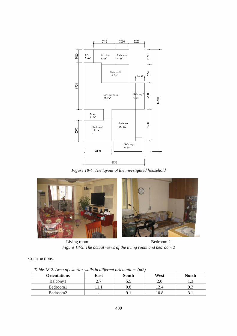
400

Figure 18-4. The layout of the investigated household

Living room Bedroom 2

Figure 18-5. The actual views of the living room and bedroom 2 Constructions:

Table 18-2. Area of exterior walls in different orientations (m2) Orientations East South West North

Balcony1 2.7 5.5 2.0 1.3 Bedroom1 11.1 0.8 12.4 9.3 Bedroom2 - 9.1 10.8 3.1

401

W.C. 4.3 11.4 9.4 11.4 Balcony2 5.1 1.8 - 1.8 Bedroom3 5.9 10.7 7.2 -

Living Room - - 18.1 2.5 Bedroom4 4.5 5.4 5.8 5.4 Kitchen - 8.4 5.8 8.4

Table 18-3. Area of exterior windows in different orientations (m2)

Orientations East South West North Balcony1 2.7 5.5 2.0 1.3 Bedroom2 - 1.7 - - Balcony2 5.1 1.8 - 1.8 Bedroom3 1.3 - - - Bedroom4 1.3 - - -

Table 18-4. U-values of walls and windows

Material layers Total Area(m2)

U-value (W/m2K)

Exterior walls porous ceramisite hollow brick 300mm

insulated 50mm 54.2 0.46

Internal partition walls cement mortar of 60mm 44.2 3.15 Interior wall

(with insulation) 200mm porous ceramisite hollow

brick, with 20mm Composite silicate insulation materials

adjacent to stairwell, elevator and corridor

90.7 0.86

Windows Aluminum alloy, double-paned insulating glass

24.4 2.8

18.4 Investigation Methodology

We use both questionnaires and measurements to investigate energy use and occupant behaviors. The questionnaire is attached in the document list of Subtask B1. Temperature and power meters are used to record the indoor conditions and states of electrical appliances at every minute. The measurement was started from 2010/12/28.

402

Figure 18-6. The meters are distributed in each room and monitor all the electrical appliances.

Figure 18-7. Distribution of electric appliances and measure points for temperature

Table 18-5. Measuring points of thermometers

No. position Remark 1 Bedroom1 - Balcony1 On a bar 2 Bedroom1 - Bedside On the head of bed 3 Bedroom1 - Bookcase Top of bookcase beside TV 4 Bedroom2 - Bookcase 5 Living room - Side Cabinet Cabinet beside TV 6 Living room - Main area On chair of dining-table 7 Living room - Cabinet Top of cabinet beside dining-table 8 Bedroom3 - Wardrobe Top of wardrobe 9 Bedroom4 - desk

403

Table 18-6. Measuring points of T&RH meters No. position Remark 1 Bedroom1 - Bookcase Top of bookcase beside TV 2 Bedroom2 - Bookcase 3 Living room - Cabinet Top of cabinet beside dining-table

Table 18-7. Measuring points of power meters

No. position Remark 1 Bedroom1 - Desk Computer, screen, sound box, lamp 2 Bedroom1 - Bedside Bedside lamp, alarm clock, recharger 3 Bedroom1 - TV TV, DVD, wireless router, recharger 4 Bedroom1-Air conditioner 5 Living room - Christmas tree Lighting for Christmas tree

5-2 Living room - Air conditioner With air conditioner in bedroom3 6 Living room - TV TV, sound box, CD player, wireless

router, humidifier 7 Bedroom2 - TV TV, telephone, lamp 8 Bedroom2 - Air conditioner 9 Bedroom4 - TV TV, electric fan 10 Kitchen - Washing machine 11 Kitchen - Electric cooker Electric cooker, toaster oven 12 Kitchen - Exhaust fan Gas water heater exhaust fan 13 Kitchen - Kitchen ventilator 14 Living room - refrigerator 15 Living room - microwave oven Microwave oven, coffeemaker 16 Total scaled meter 1 Live line 17 Total scaled meter 2 Neutral line

Power meter for Bedroom 1 - desk : including computer, screen, sound box and lamp

Power meters in Living room: including refrigerator, microwave oven and coffee

maker

404

Power meters : Total scaled meter 1 and 2

Figure 18-8. Actual views of some power meters 18.5 Energy usage

We calculated the whole year electricity consumption of 2011. It shows below:

Figure 18-9. The monthly electricity consumption of the whole year 2011

AC and lighting curves for one period are shown below:

405

Figure 18-10. The indoor and outdoor temperature and AC power for one period

Figure 18-11. The lighting power for one period

18.6 Occupant behaviors

18.6.1 OB from Questionnaires

Analyze OB characteristic parameters from questionnaires data. Including: movement events and parameters, and actions on window, lights, ACs, TVs, etc. The questionnaire survey is carried out in summer. From the questionnaires, there are three types of AC usage patterns: 1) the couple turn on AC when feeling hot and turn it off when leaving room; 2) the son turn on AC once entering his room and seldom turn it off when leaving room; 3) the grandma turn on AC only when feeling very hot and turn it off after the indoor temperature is dropped. All people open the window when getting up and only close it if AC turned on. The lights are turned on only when feeling dark and turned off when leaving room and getting asleep.

406

18.6.2 OB from Measurements

Analyze OB characteristic parameters from continuous monitoring data. This is used to compare and check the availability of investigating OBs by questionnaires. An example of AC behavior analysis:

Figure 18-12. The indoor and outdoor temperature and AC power for four days

Figure 18-13 The statistical cooling status of the main bedroom

407

Figure 18-14. The analysis of the starting and operating temperatures

20.0

22.5

25.0

27.5

30.0

32.5

35.0

0 1 2 3 4 5 6 7 8 9 10 11 12 13 14 15 16 17 18 19 20 21 22 23

℃℃℃℃

Time

Turn-offIndoor T Outdoor T Operating T

Figure 18-15. The analysis of the temperature when turned off

Occupied space only (part time part space): (1) Turn on: Starting temp: feedback, threshold value. (2) Turn off: Scheduled (after getting up in the morning, or before sleeping in the night) or When leaving. (3) with a fixed set point. This AC usage pattern is for the couple living in the main bedroom and it matches the result from questionnaire. 18.6.3 OB modes for residents

Through comparison of analysis results from questionnaires and measurement, we conclude several typical behavior modes for AC and TV usage in this family.

408

Table 18-8. Description of AC action based models Object OB mode Description Characteristic

Parameters Mode 1: part-time

part-space Turn on when occupant is in room

and feel hot; Turn off when leaving or getting up;

With a fixed set point.

Occupancy schedule; Starting point;

Set point.

Split AC

Mode 2: Turn on when occupant is in room; Turn off when leaving; With a fixed set point.

Occupancy schedule; Set point

Mode 1 Turn on randomly, turn off randomly.

Occupancy schedule; Mean watching-TV time

per day

TV

Mode 2 Turn on at night, turn off before sleeping.

Occupancy schedule; Starting time

18.7 Conclusions

Occupant behaviors (e.g. window opening, use of air conditioners, use of lights, etc.) have significant impact on building energy consumption, especially for low energy buildings that rely more on natural ventilation, passive heating, and daylighting, and have become a key factor in building energy simulation. However, due to the uncertainty and complexity of occupant behaviors, how to accurately describe and model them such behaviors is still a big challenge. In this case study, use of air conditioners (ACs), lights, and appliances in residential buildings are discussed. Measured data reveal that the main characteristics of occupant behaviors can be well described from the action-based viewpoint: 1) Occupant behavior related to each type of object (AC, light, appliance, etc.) is just the action that can change the state of the object. For example, the use of a two-state device (e.g. light) can be decomposed by two actions: turn-on and turn-off; 2) the turn-on or turn-off action by each occupant has certain patterns that can be defined with specific quantitative parameters; and 3) Different occupants may have different patterns of actions. Based on these findings, an action-based model is proposed in this paper as a common description method for all sorts of occupant behaviors in buildings. Due to its simplicity, individuality, accuracy and expandability, this model is expected to help advance the definition, investigation, analysis, and simulation of occupant behaviors to help the design and operation of energy efficient buildings. Acknowledgements

The authors from Tsinghua University highly appreciate great helps from the residents to provide her family as case study for IEA ECBCS ANNEX 53.

409

19. JPN-01: Single Family House in Japan

19.1 Introduction

The main objectives of this investigation are, 1) to show an example of case study for residential building, 2) to clarify actual conditions of the total energy use and factors influencing energy use. This investigated house is a well-insulated detached house with energy source of electricity exclusively. This is a typical type of detached house in Japan as shown in Figure 19-1.

Figure 19-1 View of the house

19.2 Location & Climatic conditions

Figure 19-2 shows the location of Sendai in Japan. Figure 19-3 shows the monthly mean temperatures and mean humidities in Sendai, Montreal and Berlin. Sendai is cold and snowy in winter, but hot and humid in summer. The raining season of Japan is from June to July. Minimum and maximum temperatures are 1.5 0C in January and 24.1 0C in August respectively.

Sendai

-15

-10

-5

0

5

10

15

20

25

30

50 60 70 80 90 100

Humidity (%RH)

Tem

pera

ture

(℃)

Berlin

Montreal

Sendai

Figure 19-2 Location of the house Figure 19-3 Monthly mean temperature and humidity

19.3 Outline of the detached house

Figure 19-4 shows the floor plan of the investigated house. The detached house is a two-story wood construction with the total floor area of 153.44m2. It is an all-electric house built in 1999. The value of equivalent leakage area per floor area is 0.93 cm2/m2, while the value of heating transmission rate calculated based on the design plans is 1.79 W/m2K . Electric thermal storage heaters for space heating, using midnight electricity, are installed in the living room and bedroom 1 with the capacities

410

of 6kW and 4kW respectively. Air conditioners for space cooling are also installed in the living room and bedroom 1 with the capacities of 900W(COP:4.60) and 705W(COP:3.12) respectively. Hot water is supplied by electric water heaters using midnight electricity .

8190

8190

1001010010

Bath room Entrance

Storeroom

HallLavatory


Main bed room

Bed room 2

Bed room 1

Store room

Hall

8190

8190

1001010010

Bath room Entrance

Storeroom

HallLavatory


Main bed room

Bed room 2

Bed room 1

Store room

Hall

Figure 19-4 Floor plan of the detached house

19.4 Family members and occupants’ behavior

The total number of occupants is four, i.e. a couple with two children. Table 19-1 shows occupant (housewife) behaviour during weekdays, while Table 19-2 shows all the domestic appliance used in the house, and theirs capacities as well as using frequency.

Table 19-1 Occupant behaviour (housewife, weekdays) Place

OutdoorBedroom

Living roomLavatoryBedroomBathroom

Living roomLiving roomLiving roomLiving roomLiving roomLiving room

LavatoryBed room 1Living room

KitchenLiving room etc.

PlaceOutdoorBedroom



LavatoryBed room 1Living room

KitchenLiving room etc.

Culture lesson

Culture lesson

Sports

Sports

Dining

Change of clothing

TV

Work/Study

Laundry

Clothes iron

Cleaning

OutingSleep

Face-wash

Bath

Reading

Family dialogue

Hang out washing

Cooking

4:00 5:00

12:00 14:0013:00

TVReading

Work/Study

Family dialogue

0:00 3:001:00 2:00Action 9:00 12:008:00 10:00 11:00

Face-washChange of clothing

Bath

6:00

17:00

Cleaning

7:00

LaundryHang out washing

Clothes ironCooking

OutingSleep

Dining

22:00 23:00 0:00Action 21:0015:00 16:00 18:00 19:00 20:00

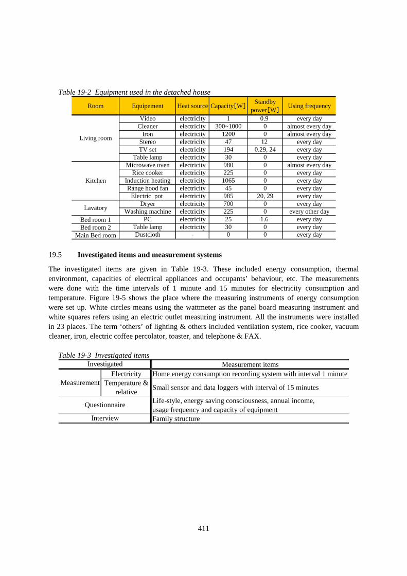
411

Table 19-2 Equipment used in the detached house

Room Equipement Heat source Capacity［W］Standby

power［W］Using frequency

Video electricity 1 0.9 every dayCleaner electricity 300~1000 0 almost every day

Iron electricity 1200 0 almost every dayStereo electricity 47 12 every dayTV set electricity 194 0.29, 24 every day

Table lamp electricity 30 0 every dayMicrowave oven electricity 980 0 almost every day

Rice cooker electricity 225 0 every dayInduction heating electricity 1065 0 every dayRange hood fan electricity 45 0 every day

Electric pot electricity 985 20, 29 every dayDryer electricity 700 0 every day

Washing machine electricity 225 0 every other dayBed room 1 PC electricity 25 1.6 every dayBed room 2 Table lamp electricity 30 0 every day

Main Bed room Dustcloth - 0 0 every day

Living room

Kitchen

Lavatory

19.5 Investigated items and measurement systems

The investigated items are given in Table 19-3. These included energy consumption, thermal environment, capacities of electrical appliances and occupants’ behaviour, etc. The measurements were done with the time intervals of 1 minute and 15 minutes for electricity consumption and temperature. Figure 19-5 shows the place where the measuring instruments of energy consumption were set up. White circles means using the wattmeter as the panel board measuring instrument and white squares refers using an electric outlet measuring instrument. All the instruments were installed in 23 places. The term ‘others’ of lighting & others included ventilation system, rice cooker, vacuum cleaner, iron, electric coffee percolator, toaster, and telephone & FAX.

Table 19-3 Investigated items Measurement items

Electricity Home energy consumption recording system with interval 1 minuteTemperature &

relativeSmall sensor and data loggers with interval of 15 minutes

Life-style, energy saving consciousness, annual income,usage frequency and capacity of equipmentFamily structure

Investigated

Measurement

Questionnaire

Interview

412

IH cooking heater

Dishwasher

Clothes washing machine

Clothes dryer

2F Shower toilet

1F Shower toilet

Dinning room

Children room 1

Microwave oven

Water heater

TV set

Stereo

Video

Lighting&others

Main power

Lighting&othersBed room

Lighting&others

PC

Toilet

Air condition in bed room

Thermal storage heater

Children room 2

Air condition in living room

Living room

Total

Thermal storage water heater

Lighting&others

Refrigerator

Entrance

Lighting&others

Wattmeter on electric outlet

Wattmeter in electricity distribution panel

Audio visual &information

Kitchen

Space heating & air conditioning

Hot water supply

Healthcare

Figure 19-5 Energy distribution system


19.6.1 Annual and monthly energy consumption

The energy consumption is expressed by using the energy conversion value for each heat source, as shown in Table 19-4. Figure 19-6 shows the monthly and annual energy consumptions by the end use from Nov. 2002 to Nov. 2003. The monthly energy consumption varied from 3.2 to 11.8 GJ/month. The energy consumptions of space heating and hot water supply were higher in winter. On the other hand, energy consumptions of audio & information and healthcare were stable throughout the year. The annual energy consumption was about 80GJ/Year. Hot water supply was the largest energy users, which accounted for about 42% of the total annual energy consumption. Air-conditioning, which accounted for about 37% of the total annual energy consumption, was the second largest energy user. Energy consumptions of audio & information, healthcare and lighting & others accounted for 2%, 2% and 12.5% respectively.

Table 19-4 Energy conversion value Heat source

Electricity 3.6 MJ/kWhConversion value

413

0 2 4 6 8 10 12 14

Dec-02Jan-03Feb-03Mar-03Apr-03

May-03Jun-03Jul-03



Lighting & Others HealthcareAudio visual & information KitchenHot water supply Space heating/cooling

0 20 40 60 80 100

Dec02～Nov03

Energy consumption[GJ/year] Figure 19-6 Monthly and annual energy consumptions

19.6.2 Annual amount of CO2 emission

The amount of CO2 emission is expressed by using the CO2 equivalent value for each heat source, as shown in Table 19-5. Figure 19-7 shows the annual amount of CO2 emission from Nov. 2002 to Nov. 2003. The annual amount of CO2 emission was about 9.4 t-CO2/Year. Hot water supply was the largest CO2 emission, which accounted for about 42% of the total. Space heating/cooling, which accounted for about 37% of the total, was the second largest CO2 emission. Amount of CO2 emission of kitchen, audio & information, healthcare and lighting & others accounted for 6%, 4%, 2% and 10% respectively.

Table 19-5 CO2 equivalent value

Electiricity

CO2 equivalent［t-CO2/GJ］

0.118

0 5 10

Dec02～Nov03

Amount of CO2 emission[t-CO2/year]

Lighting & Others Healthcare

Audio visual & information Kitchen

Hot water supply Space heating/cooling

Figure 19-7 Amount of CO2 emission

414

19.6.3 Profiles of energy consumption, indoor and outdoor temperatures during three days in

winter/summer

The profiles of energy consumption and temperature during three days in winter/summer are shown in Figure 19-8. The peak energy consumptions of Space heating and Hot water supply appeared in the middle of the night, due to the usage of late night electricity. On the other hand, the energy consumptions of Audio visual & information and Healthcare did not change so much.

0

5

10

0:00 12:00 0:00 12:00 0:00 12:00

KitchenRefrigeratorAudio visual & informationHealthcareLighting & others

0

10

20

30

Ene

rgy

cons

umpt

ion ［［［［

MJ/

h］］］］

Space heating/coolingHot water supplyOthers

202530

3540

Tem

p. ［［［［℃℃ ℃℃

］］］］

2003. 8/4 8/5 8/6

Living room Outdoor air

Others

Hottest day

Figure 19-8 Three days temperature and energy consumption profiles in winter and summer 19.7 Conclusion

In this investigation, the annual energy consumption was about 80GJ/Year. Hot water supply was the largest energy users, which accounted for about 42% of the total annual energy consumption. Air-conditioning, which accounted for about 37% of the total annual energy consumption, was the second largest energy user. Reducing the energy consumptions of hot water supply and space heating/cooling will be very important to reduce the total energy consumption in future. Acknowledgement: Authors would like to acknowledge the occupants to give us an opportunity for measurement of indoor environment and energy use of the house.

0

5

10

0:00 12:00 0:00 12:00 0:00 12:00

KitchenRefrigeratorAudio visual & informationHealthcareLighting & others

Others

0

20

40

60

80

Ene

rgy

cons

umpt

ion ［［［［

MJ/

h］］］］

Space heating/coolingHot water supplyOthers

-10

0

10

20

Tem

p. ［［［［℃℃ ℃℃

］］］］

2002. 12/26 12/27 12/28


Coldest day

415

20. JPN-02: Multi-storey residential building in Japan

20.1 Introduction

The main objectives of this investigation are, 1) to show an example of case study for residential building, 2) to clarify actual conditions of the total energy use and factors influencing energy use. The investigated apartment is a typical type of house unit in Japan (cf. Figure 20-1) and it is situated on the 6th floor of a 15-story multi-family building with energy sources of electricity and city gas.

Figure 20-1 View of the apartment building

20.2 Location & Climatic conditions

Figure 20-2 shows the location of Fukushima in Japan. Figure 20-3 shows the monthly mean temperatures and mean humidities in Fukushima, Montreal and Berlin. Fukushima is cold and snowy in winter, but hot and humid in summer. The rainning season of Japan is from June to July. Minimum and maximum temperatures are 1.4 0C in January and 25.2 0C in August respectively.

Fukushima

-15

-10

-5

0

5

10

15

20

25

30

50 60 70 80 90 100

Humidity (%RH)

Tem

pera

ture

(℃)

Berlin

Montreal

Fukushima

Figure 20-2 Location of the building Figure 20-3 Monthly mean temperature and humidity

20.3 Outline of the apartment

Figure 20-4 shows the floor plan of the investigated apartment. It is made of concrete and built in 2000. The floor area is 72.3 m2. The value of equivalent leakage area per floor area measured by the pressurization method is 1.74 cm2/m2, while the value of heating transmission rate calculated based on the design plans is 2.47 W/m2K . Air conditioners for space heating and cooling are installed in the living room and bedroom 1. The apartment uses city gas for hot water supply and oven. The

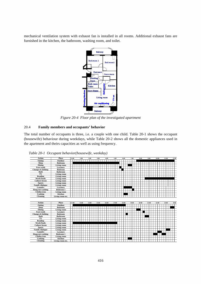
416

mechanical ventilation system with exhaust fan is installed in all rooms. Additional exhaust fans are furnished in the kitchen, the bathroom, washing room, and toilet.

Balcony

Balcony

Store ｒｒｒｒoomEntrance

Washingｒｒｒｒoom

Bath room Toilet

Store Room

Living room

Kitchen

Air conditioning

Was

hing

Mac

hine

Bed ｒｒｒｒoom1

TV

set

Ref

riger

ator

Balcony

Balcony

Bed ｒｒｒｒoom 2

Entrance

Washing

Bath room Toilet

Store ｒｒｒｒoom

Living room

Kitchen

Air conditioning

Was

hing

ｍｍｍｍac

hine

TV

set

Ref

riger

ator

Balcony

Balcony

Store ｒｒｒｒoomEntrance

Washingｒｒｒｒoom

Bath room Toilet

Store Room

Living room

Kitchen

Air conditioning

Was

hing

Mac

hine

Bed ｒｒｒｒoom1

TV

set

Ref

riger

ator

Balcony

Balcony

Bed ｒｒｒｒoom 2

Entrance

Washing

Bath room Toilet

Store ｒｒｒｒoom

Living room

Kitchen

Air conditioning

Was

hing

ｍｍｍｍac

hine

TV

set

Ref

riger

ator

Figure 20-4 Floor plan of the investigated apartment

20.4 Family members and occupants’ behavior

The total number of occupants is three, i.e. a couple with one child. Table 20-1 shows the occupant (housewife) behaviour during weekdays, while Table 20-2 shows all the domestic appliances used in the apartment and theirs capacities as well as using frequency.

Table 20-1 Occupant behavior(housewife, weekday) Place

OutdoorBedroom



LavatoryBedroom 1

Living roomKitchen

Living room etc.

PlaceOutdoorBedroom



LavatoryBedroom 1

Living roomKitchen

Living room etc.

22:00 23:00 0:00Action 21:0015:00 16:00 18:00 19:00 20:0017:00

Cleaning

7:00

LaundryHang out washing

Clothes ironCooking

OutingSleep

DiningFace-wash

Change of clothing Bath

6:00 9:00 12:008:00 10:00 11:000:00 3:001:00 2:00Action

Cooking

4:00 5:00

12:00 14:0013:00

TVReading

Work/Study

Family dialogue

Laundry

Clothes iron

Cleaning

OutingSleep

Face-wash

Bath

Reading

Family dialogue

Hang out washing

Culture lesson

Culture lesson

Sports

Sports

Dining

Change of clothing

TV

Work/Study

417

Table 20-2 Equipment used in the apartment

Room EquipementHeat

sourceCapacity［W］

Standbypower［W］

Using frequency

Video electricity 15 0.9 every dayRadio electricity 26 2 every dayTV set electricity 147 0.18，20 every day

Table lamp electricity 30 0 every dayCleaner electricity 250～1000 0 almost every day

Iron electricity 1200 0 almost every dayRice cooker electricity 225 0 every day

Microwave oven gas 9070 0 every dayElectric pot electricity 985 20，29 every day

Tableware washing machine electricity 1150 0 summer and middleDryer electricity 450 0 every day

Washing machine electricity 140 0 every dayClothes dryer electricity 1250 0 winterElectric heater electricity 1200 0.0 winter

Table lamp electricity 30 0 every dayDustcloth - 0 0 every day

Living room

Kitchen

Bed room

Wash room

20.5 Investigated items and measurement systems

The investigated items are given in Table 20-3. These include energy consumption, thermal environment, electric capacity of domestic appliances and occupants’ behaviour, etc. The measurements were done with the time intervals of 1 minute, 5 minutes, and 15 minutes for electricity consumption, gas consumption and temperature. Figure 20-5 shows the energy distribution system together with the locations where the measuring instruments of energy consumption were placed. Black circles denotes that the wattmeter is installed in the electricity distribution panel, while gray square refers to the wattmeter on an electric outlet and white triangle represents gas measure.

Table 20-3 Investigated items Measurement items

Electricity Home energy consumption recording system with interval 1 minuteGas Digital camera signal data logger with interval of 5 minutes

Temperature &relative

Small sensor and data loggers with interval of 15 minutes

Life-style, energy saving consciousness, annual income,usage frequency and capacity of equipmentFamily structure

Measurement

Investigated

Questionnaire

Interview

418

Electricity

Japanese room＆＆＆＆Living room

Air condition in European style room


Entrance/Washing room

Kitchen

Store roomTotal


Air condition in Japanese room

Intercom TV/Radio

Electric carpet

Refrigerator

Wash machine

Warm water toilet

Lighting/Others

Concentric plug

Wattmeter for panel boards

Gas

Lighting/Others

Lighting/Others

Lighting/Others

Rice cooker････Microwave

Dishwasher

Electricity





Kitchen

Store roomTotal



Intercom TV/Radio

Electric carpet

Refrigerator

Wash machine

Warm water toilet

Gas

Lighting/Others

Concentric plug


Gas

Lighting/Others

Lighting/Others

Lighting/Others


Dishwasher

Audio visual & information

Space heating

Healthcare

Kitchen

Washing room

Kitchen Oven

Hot water supply

Kitchen

Hot water supply

Electricity





Kitchen

Store roomTotal



Intercom TV/Radio

Electric carpet

Refrigerator

Wash machine

Warm water toilet

Lighting/Others

Concentric plug


Gas

Lighting/Others

Lighting/Others

Lighting/Others


Dishwasher

Electricity





Kitchen

Store roomTotal



Intercom TV/Radio

Electric carpet

Refrigerator

Wash machine

Warm water toilet

Gas

Lighting/Others

Concentric plug


Gas

Lighting/Others

Lighting/Others

Lighting/Others


Dishwasher


Space heating

Healthcare

Kitchen

Washing room

Kitchen Oven

Electricity





Kitchen

Store roomTotal



Intercom TV/Radio

Electric carpet

Refrigerator

Wash machine

Warm water toilet

Lighting/Others

Concentric plug


Gas

Lighting/Others

Lighting/Others

Lighting/Others


Dishwasher

Electricity





Kitchen

Store roomTotal



Intercom TV/Radio

Electric carpet

Refrigerator

Wash machine

Warm water toilet

Gas

Lighting/Others

Concentric plug


Gas

Lighting/Others

Lighting/Others

Lighting/Others


Dishwasher


Space heating

Healthcare

Kitchen

Washing room

Kitchen Oven

Electricity





Kitchen

Store roomTotal



Intercom TV/Radio

Electric carpet

Refrigerator

Wash machine

Warm water toilet

Lighting/Others

Concentric plug


Gas

Lighting/Others

Lighting/Others

Lighting/Others


Dishwasher

Electricity





Kitchen

Store roomTotal



Intercom TV/Radio

Electric carpet

Refrigerator

Wash machine

Warm water toilet

Gas

Lighting/Others

Concentric plug


Gas

Lighting/Others

Lighting/Others

Lighting/Others


Dishwasher


Space heating

Healthcare

Kitchen

Electricity





Kitchen

Store roomTotal



Intercom TV/Radio

Electric carpet

Refrigerator

Wash machine

Warm water toilet

Lighting/Others

Concentric plug


Gas

Lighting/Others

Lighting/Others

Lighting/Others


Dishwasher

Electricity





Kitchen

Store roomTotal



Intercom TV/Radio

Electric carpet

Refrigerator

Wash machine

Warm water toilet

Gas

Lighting/Others

Concentric plug


Gas

Lighting/Others

Lighting/Others

Lighting/Others


Dishwasher


Space heating

Healthcare

Kitchen

Washing room

Kitchen Oven

Hot water supply

Kitchen

Hot water supply

Figure 20-5 Energy distribution system


20.6.1 Annual and monthly energy consumption

The energy consumption is expressed by using the energy conversion value for each heat source, as shown in Table 20-4. Figure 20-6 shows the monthly and annual energy consumptions by the end use from Nov. 2002 to Nov. 2003. The monthly energy consumption varied from 2.1 to 7.2 GJ/month. The energy consumptions of space heating and hot water supply were higher in winter. On the other hand, energy consumptions of audio & information and healthcare were stable throughout the year. In addition, energy consumption of lighting & others from November to January was higher than that of the summer months, because the necessary lighting is influenced by different sunshine hours in various seasons. The annual energy consumption was about 59GJ/Year. Hot water supply and kitchen were the largest energy user, which accounted for about 60% of the total annual energy consumption. Air-conditioning, which accounted for about 20% of the total annual energy consumption, was the second largest energy user. Energy consumptions of audio & information, healthcare and lighting & others accounted for 2%, 2% and 12.5% respectively.

Table 20-4 Energy conversion value Heat source

Electricity 3.6 MJ/kWh

Gas（4A～7C） 20.4 MJ/Nm3

Conversion value

419

0 1 2 3 4 5 6 7 8

Dec-02Jan-03Feb-03Mar-03Apr-03May-03Jun-03Jul-03



Lighting & Others HealthcareAudio visual & information Hot water supply/KitchenSpace heating/cooling

0 10 20 30 40 50 60 70

Dec02～Nov03

Energy consumption[GJ/year] Figure 20-6 Monthly and annual energy consumptions

20.6.2 Annual amount of CO2 emission

The amount of CO2 emission is expressed by using the CO2 equivalent value for each heat source, as shown in Table 20-5. Figure 20-7 shows the annual amount of CO2 emission from Nov. 2002 to Nov. 2003. The annual amount of CO2 emission was about 4.6 t-CO2/Year. Hot water supply and kitchen were the largest CO2 emission, which accounted for about 45% of the total. Space heating/cooling, which accounted for about 30% of the total, was the second largest CO2 emission. Amount of CO2 emission of audio & information, healthcare and lighting & others accounted for 3%, 4% and 19% respectively.

Table 20-5 CO2 equivalent value

Electiricity

City gas

0.118

0.0506

CO2 equivalent［t-CO2/GJ］

0 1 2 3 4 5

Dec02～Nov03

Amount of CO2 emission[t-CO2/year]

Lighting & Others Healthcare

Audio visual & information Hot water supply/Kitchen

Space heating/cooling

Figure 20-7 Amount of CO2 emission

420

20.6.3 Profiles of energy consumption, indoor and outdoor temperatures during three days in winter/summer

The profiles of energy consumption and temperature during three days in winter/summer are shown in Figure 20-8. The peak energy consumptions of Hot water supply and Kitchen appeared in the morning and evening. On the other hand, the energy consumption of Audio visual & information and Healthcare did not change so much.

0

2

4

6

0:00 12:00 0:00 12:00 0:00 12:00


2003. 3/3 3/4 3/5

0

15

30

45

En

erg

y co

nsu

mp

tion

［M

J/h］

. Space heating/cooling

Hot water supply/KitchenOthers

-100

102030

Tem

p.［℃

］

Living room

Outdoor air

Coldest day

0

10

20

30

En

erg

y co

nsu

mp

tion

［M

J/h］

.

Others Hot water supply/Kicthen Space heating/cooling2025303540

Tem

p.［℃

］


0.0

1.0

2.0

3.0

4.0

0:00 12:00 0:00 12:00 0:00 12:00


2003. 8/3 8/4 8/5

Hottest day

Figure 20-8 Three days temperature and energy consumption profiles in winter and summer

20.7 Conclusion

In this investigation, the annual energy consumption was about 59GJ/Year. Hot water supply and kitchen were the largest energy user, which accounted for about 60% of the total annual energy consumption. Air-conditioning, which accounted for about 20% of the total annual energy consumption, was the second largest energy user. Reducing the energy consumptions of hot water supply and space heating/cooling will be very important to reduce the total energy consumption in future. Acknowledgement: Authors would like to acknowledge the occupants to give us an opportunity for measurement of indoor environment and energy use of the house.

© Copyright Institute for Building Environment and Energy Conservation 2013

All property rights, including copyright, are vested in Institute for Building Environment and Energy

Conservation, on behalf of the Contracting Parties of the International Energy Agency Implementing

Agreement for a Programme of Research and Development on Energy in Buildings and Communities.

In particular, no part of this publication may be reproduced, stored in a retrieval system or transmitted in any

form or by any means, electronic, mechanical, photocopying, recording or otherwise, without the prior written

permission of Institute for Building Environment and Energy Conservation.

Published by Institute for Building Environment and Energy Conservation, Zenkyoren building Kojimachikan,

3-5-1, Kojimachi Chiyoda-ku, Tokyo 102-0083 Japan

Disclaimer Notice: This publication has been compiled with reasonable skill and care. However, neither

Institute for Building Environment and Energy Conservation nor the EBC Contracting Parties (of the

International Energy Agency Implementing Agreement for a Programme of Research and Development on

Energy in Buildings and Communities) make any representation as to the adequacy or accuracy of the

information contained herein, or as to its suitability for any particular application, and accept no responsibility

or liability arising out of the use of this publication. The information contained herein does not supersede the

requirements given in any national codes, regulations or standards, and should not be regarded as a substitute

for the need to obtain specific professional advice for any particular application.

ISBN: 978-4-9907425-4-6

Participating countries in EBC:

Australia, Austria, Belgium, Canada, P.R. China, Czech Republic, Denmark, Finland, France, Germany,

Greece, Ireland, Italy, Japan, Republic of Korea, the Netherlands, New Zealand, Norway, Poland, Portugal,

Spain, Sweden, Switzerland, Turkey, United Kingdom and the United States of America.

Additional copies of this report may be obtained from:

EBC Bookshop

C/o AECOM Ltd

Colmore Plaza

Colmore Circus Queensway

Birmingham B4 6AT

United Kingdom

Web: www.iea-ebc.org

Email: [email protected]

Case study buildings - IEA EBC

Documents

Transcript of Case study buildings - IEA EBC