Energy Conversion and Management 51 (2010) 2808–2815

Contents lists available at ScienceDirect

Energy Conversion and Management

journal homepage: www.elsevier .com/locate /enconman

Second law analysis of compressible flow through a diffuser subjectedto constant heat flux at wall

Mohammad H. Arshad a, Ramazan Kahraman a,*, Ahmet Z. Sahin b, Rached Ben-Mansour b

a Chemical Engineering Department, Qatar University, Doha, Qatarb Mechanical Engineering Department, King Fahd University of Petroleum & Minerals, Dhahran, Saudi Arabia

a r t i c l e i n f o

Article history:Received 30 June 2009Received in revised form 18 May 2010Accepted 2 June 2010Available online 29 June 2010

Keywords:Entropy generationCompressible flowDiffuserCFDConstant heat flux

0196-8904/$ - see front matter � 2010 Elsevier Ltd. Adoi:10.1016/j.enconman.2010.06.018

* Corresponding author. Address: Chemical EngUniversity, P.O. Box 2713, Doha, Qatar. Tel.: +974 440

E-mail address: ramazank@qu.edu.qa (R. Kahrama

a b s t r a c t

Entropy generation is equivalent to destruction of available work (exergy). The useful energy is destroyeddue to the intrinsic irreversibility associated within thermodynamic systems. Exergy analysis can be usedas an effective basis for the development and improvement of systems design not only in the overall per-spective but also in the individual component level. Second law analysis provides a useful tool to identifythe irreversibility in any thermal system. This study presents the investigation of local and total entropygeneration in compressible flow through a diffuser. Air is used as the fluid. Uniform heat flux boundarycondition is applied at the wall. Two dimensional solution of velocity and temperature fields are obtainedusing the CFD code FLUENT. Distribution of entropy generation rate is investigated throughout the vol-ume of the fluid as it flows through the diffuser. Regions of high entropy generation in the diffuser havebeen predicted. The angle of expansion of diffuser is varied and its desire value corresponding to mini-mum entropy generation is determined at fixed flow conditions.

� 2010 Elsevier Ltd. All rights reserved.

1. Introduction

Efficient utilization of energy is primary objective in designing athermodynamics system. This useful energy can be destroyed dueto the intrinsic irreversibility associated within the process compo-nents. Unfortunately irreversibility cannot be avoided, but it can beminimized in order to save the available energy. The minimizationcan be achieved if the irreversibility can be identified in the processcomponents.

Heat transfer enhancement techniques and power maximiza-tion methods in general cause excessive pressure losses and entro-py production, which in turn increase exergy destruction. Throughproper identification of local sources of losses or irreversibilities,better designs of machinery can be developed. The performanceimplications of the irreversibilities due to heat transfer and fluidflow have become an important concern for the designers. Thermo-dynamic optimization (minimization of the entropy production)can deliver better physical configuration of flow systems and theircomponents.

Therefore, in recent years, entropy minimization has become atopic of great interest in the thermo-fluid area. Bejan [1,2] com-bined the concept of fluid flow and heat transfer with second lawof thermodynamics. He presented the basic step for the procedure

ll rights reserved.

ineering Department, Qatar3 4124; fax: +974 4403 4131.n).

of entropy generation minimization at the system component le-vel. He proposed to divide the system into smaller unit and analyzeeach one separately for entropy generation.

Sahin [3] investigated analytically the second law analysis oflaminar viscous flow through a duct subjected to constant wall tem-perature. He considered viscosity of fluid to be temperature depen-dent. He determined that pumping power to heat transfer ratiodecreased along the duct length. In addition, it is found that entropygeneration was increased with increasing non-dimensional temper-ature difference between the inlet fluid and surface temperature.

Sahin [4] made a comparison based on second law analysis fordifferent geometries such as circular, rectangular, square, triangle,and sinusoidal. He demonstrated that triangular and rectangularduct geometries are in general the worst choices for both entropygeneration and pumping power requirement.

Demirel and Kahraman [5] obtained entropy generation forrectangular packed duct with wall heat flux. They found that theirreversibility distributions are not continuous through the walland core. Sahin [6] carried out analytical entropy generation inves-tigation for a fully developed turbulent flow through a smooth ductsubjected to constant wall temperature for variable viscosity case.They found that assumption of constant viscosity produced a con-siderable deviation for the entropy generation and pumping powerresults.

Sahin and Mansour [7] performed numerical analysis of entropygeneration in laminar fluid flow through a circular pipe for con-stant heat flux case CFD code FLUENT.

Nomenclature

Br Brinkman number = v2ol/(Tw � To)

D1 inlet diameter of diffuser, mD2 outlet diameter of diffuser, mEuo Euler number, Patm/ðqov2

oÞK thermal conductivity, W/(km)Keff effective thermal conductivity, W/(km)_m mass flow rate, kg/s

Ns entropy generation numberp pressure, N/m2

pn normalized pressure (p/patm)q heat flux at wall (W/m2)_Q heat transfer rate, Wr radial distance, mR dimensionless radial distance, (r/R1)R1 inlet radius of diffuser, m_Sgen entropy generation rate, W/K_S000gen local rate of entropy generation per unit volume, W/

(m3 K)s specific entropy, W/(m3 K kg)

T static temperature, KTo inlet temperature, KVR dimensionless radial velocityvz axial velocity, m/svr radial velocity, m/svo inlet velocity, m/sVZ dimensionless axial velocityz axial distance, mZ dimensionless axial distance (z/R1)l viscosity, kg/(ms)leff effective viscosity, kg/(ms)lt turbulent viscosity, kg/(ms)H dimensionless static temperatureHo dimensionless reference temperatureq density (kg/m3)qo reference density (density at 298 K)qn normalized density = (q/qo)

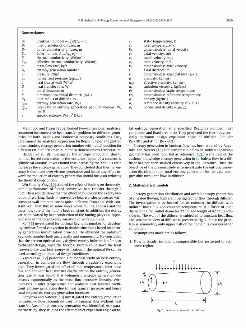
Fig. 1. Schematic view of the diffuser.

M.H. Arshad et al. / Energy Conversion and Management 51 (2010) 2808–2815 2809

Mahmood and Frazer [8] performed two-dimensional analyticaltreatment for convective heat transfer problem for different geom-etries for both iso-flux and isothermal boundary conditions. Theydetermined the analytical expression for Bejan number and plotteddimensionless entropy generation number with radial position fordifferent ratio of Brickman number to dimensionless temperature.

Haddad et al. [9] investigated the entropy production due tolaminar forced convection in the entrance region of a concentriccylindrical annulus. It was found that increasing the annulus ratioincreases the entropy generation. They concluded that thermal en-tropy is dominant over viscous generation and hence any effort to-ward the reduction of entropy generation should focus on reducingthe thermal contribution.

Wu Shuang-Ying [10] studied the effect of fouling on thermody-namic performance of forced convective heat transfer through aduct. Their results show that the effect of fouling on the exergy var-iation of working fluids in convective heat transfer processes withconstant wall temperature is quite different from that with con-stant wall heat flux in some ways when fouling appears and themass flow rate of the fluid is kept constant. In addition, the exergyvariation caused by heat conduction of the fouling plays an impor-tant role in the total exergy variation of working fluids.

Ko [11] investigated for optimal Reynolds number for develop-ing laminar forced convection in double sine ducts based on entro-py generation minimization principle. He obtained the optimumReynolds number both analytically and numerically. He concludedthat the present optimal analysis gives worthy information for heatexchanger design, since the thermal system could have the leastirreversibility and best exergy utilization if the optimal Re can beused according to practical design conditions.

Yapici et al. [12] performed a numerical study on local entropygeneration in compressible flow through a suddenly expandingpipe. They investigated the effect of inlet temperature, inlet massflux and ambient heat transfer coefficient on the entropy genera-tion rate. It was found that volumetric entropy generation de-creases exponentially as the mass flux decreases linearly. Withincreases in inlet temperature and ambient heat transfer coeffi-cient entropy generation due to heat transfer increase and hencetotal volumetric entropy generation increases.

Adeyinka and Naterer [13] investigated the entropy productionfor subsonic flow through diffuser for laminar flow without heattransfer. Area of high entropy generation was identified. As a para-metric study, they studied the effect of inlet expansion angle on to-

tal entropy generation at a specified Reynolds number, inletconditions and fixed area ratio. They predicted the thermodynam-ically optimum design expansion angle of diffuser (3.5� forRe = 301 and 4� for Re = 602).

Entropy generation in laminar flow has been studied by Adey-inka and Naterer [13] and compressible flow in sudden expansiongeometry has been reported as reference [12]. To the best of theauthors’ knowledge entropy generation in turbulent flow in a dif-fuser has not been studied extensively in the literature. Thus, theobjective of the present study is to investigate the entropy gener-ation distribution and total entropy generation for the case com-pressible turbulent flow in diffuser.

2. Mathematical models

Entropy generation distribution and overall entropy generationof a heated flowing fluid are investigated for flow through diffuser.The investigation is performed for air entering the diffuser withuniform mass flux and constant temperature. A diffuser of inletdiameter 11 cm, outlet diameter 22 cm and length of 62 cm is con-sidered. The wall of the diffuser is subjected to constant heat flux.The schematic view of diffuser is presented Fig. 1. Since the prob-lem is symmetric, only upper half of the domain is considered forsimulation.

Assumptions made are as follows:

1. Flow is steady, turbulent; compressible but restricted to sub-sonic region.

2810 M.H. Arshad et al. / Energy Conversion and Management 51 (2010) 2808–2815

2. Fluid (air) is considered to be an ideal gas and Newtonian.3. Viscosity and thermal conductivity is taken as temperature

dependent.4. The thickness of the pipe is neglected.5. The gravity effect is negligible.6. No-slip condition is assumed at the pipe wall.

2.1. Governing equations

2.1.1. Continuity equationContinuity equation is nothing but mass conservation equation

which is to be obeyed by all components of the flow system. Gen-eral continuity equation for turbulent flow is as follows [14]

DqDtþ qr � v ¼ 0 ð1Þ

where v is the actual velocity.For our problem the equation reduces to

1r@

@rðqrv rÞ þ

@

@zðqvzÞ ¼ 0 ð2Þ

where v r is the radial average velocity and vz is the axial averagevelocity.

Introducing the dimensionless variables as follows

R ¼ rR1; Z ¼ z

R1; qn ¼

qqo; VR ¼

v r

vo; VZ ¼

vz

vo

R: dimensionless radial distance, Z: dimensionless axial distance,qn: normalized density, qo: reference density (density at 298 K),VZ: dimensionless axial velocity, VR: dimensionless radial velocity,R1: inlet radius of diffuser, vo: reference velocity (inlet velocity).

Continuity equation in dimensionless from

1R@

@RðqnR�VRÞ þ

@

@Zðqn

�VZÞ ¼ 0 ð3Þ

2.1.2. Momentum equationComponents of momentum equation are as flows [14]r-component

q �v r@�v r

@rþ �vz

@�v r

@z

� �¼ @

�p@rþ 1

r@

@rr2leff

@�v r

@r

� �� 2

3leff

��

� 1r@

@rðr�v rÞ þ

@�vz

@z

� ��þ leff

@�v r

@zþ @

�vz

@r

� ��ð4Þ

r-component in dimensionless form

qn�VR@ �VR

@Rþ �VZ

@ �VZ

@Z

� �¼ �Euo

@�pn

@Rþ 1

R@

@R2Rln

@�VR

@R

��

� 23ln

1R@

@RðR�VRÞ þ

@ �VZ

@Z

� ��þ ln

@ �VR

@Zþ @

�VZ

@R

� ��ð5Þ

where �pn: normalized pressure �ppatm

� , Euo: Euler number patm

qov2o

� .h-

component

@�p@h¼ 0 ð6Þ

z-component

q �v r@�v r

@rþ �vz

@�vz

@z

� �

¼ � @�p@zþ

leff

r@

@rr@�v r

@zþ @

�vz

@r

� �� �þ @

@z2leff

@�vz

@z

� �� ��

þ 23leff

� �1r@

@rðr�v rÞ þ

@�vz

@z

� ��ð7Þ

where leff ¼ lþ lt , l: molecular viscosity, lt: turbulent viscosity,ln: normalized effective viscosity leff

lo

� , lo: reference effective vis-

cosity (at inlet).z-component of momentum equation in dimension-less form

qn�VR@ �VR

@Rþ �VZ

@�Vz

@Z

� �

¼ �Euo@�pn

@Zþ

lnR

@@R R @ �VR

@Z þ@�Vz@R

� n oþ @

@Z 2ln@ �Vz@Z

� þ 2

3 ln

�1R

@@R ðR�VRÞ þ @�VZ

@Z

� n o264

375ð8Þ

Boundary conditions

VZ ¼ 0 @ R ¼ R1 ðwallÞ

VR ¼ 0 @ R ¼ R1 ðwallÞ

@VZ

@R¼ 0 @ R ¼ 0 ðbecause of symmetryÞ

VZ ¼ Vo @ Z ¼ 0 ðinletÞ

2.1.3. Energy equationEnergy equation for ideal gas flow through variable area circular

duct will be [14]

qCP �v r@T@rþ �vz

@T@z

� �¼ 1

r@

@rKeff r

@T@r

� �þ @

@zKeff

@T@z

� �� �þ leff u ð9Þ

where u is the viscous heating function, given by [10]

u ¼ 2@�v r

@r

� �2

þ�v r

r

� �2

þ @�vz

@z

� �2" #

þ @�v r

@zþ @

�vz

@r

� �2

� 23

1rðr�v rÞ þ

@�vz

@z

� �2

ð10Þ

Introducing the dimensionless variable H ¼ T�ToTw�To

, where T: sta-tic temperature (K), To: inlet temperature (K), Tw: wall temperature(K), q: heat flux at wall (W/m2).

Energy equation in dimensionless form

qn�VR@H@Rþ �VZ

@H@Z

� �¼ 1

Pe1R@

@RKnR

@H@r

� �þ @

@zKn

@H@z

� �� �

þ BrPe

lnun ð11Þ

where n is the normalized viscous heating function given by the fol-lowing equation

u ¼ 2@ �VR

@R

� �2

þ�VR

R

� �2

þ @�VZ

@Z

� �2" #

þ @ �VR

@Zþ @

�VZ

@R

� �2

� 23

1R@

@RðR�VRÞ þ

@ �VZ

@Z

� �2

ð12Þ

where Pe: Peclet number (voRcpq/K), Br: Brinkman number (v2ol/

(Tw � To)), Kn: normalized effective thermal conductivity (Keff /Ko),Ko: reference effective thermal conductivity (at inlet).

Boundary conditionsConstant heat flux condition

k@T@r¼ qo @ r ¼ R1

@T@r¼ 0 @ r ¼ 0

M.H. Arshad et al. / Energy Conversion and Management 51 (2010) 2808–2815 2811

T ¼ To @ z ¼ 0

Boundary conditions in non-dimensional form

@H@R¼ 1 @ R ¼ 1

@H@R¼ 0 @ R ¼ 0

H ¼ 0 @ Z ¼ 0

0

2

4

6

8

10

12

14

0 2 4 6 8 10 12

Z

Ns

Grid 40×200

Grid 50×300

Grid 60×400

Grid 70×500

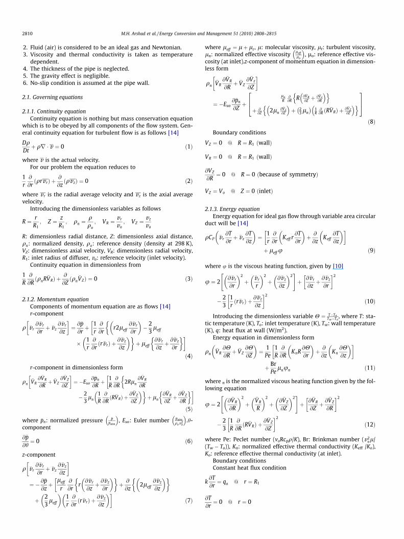
Fig. 2. Axial variation of entropy generation number at R = 0.95 in diffuser fordifferent mesh sizes.

2.1.4. Two additional equations for the RNG k–e turbulence model [15]In the present study RNG k–e model has been used. Keff in the

energy equation is calculated by RNG k–e model as follows

Keff ¼ aCpleff ð13Þ

Inverse effectively Prandtl number a is computed using the fol-lowing formula derived analytically by RNG theory.

a� 1:3929ao � 1:3929

��������

0:6321 a� 2:3929ao þ 2:3929

��������

0:3679

¼ lleff

ð14Þ

where ao ¼ KlCp

RNG k–e model calculate the turbulent viscosity by the follow-ing expression

lt ¼ qClk2

eð15Þ

where turbulence kinetic energy, k, and its rate of dissipation rate, e,are determined using the following equations, respectively.

@

@rðqv rkÞ ¼

@

@rakleff

@k@r

� �þ Gk � qe� YM ð16Þ

@

@zðqvzkÞ ¼ @

@zakleff

@k@z

� �þ Gk � qe� YM ð17Þ

@

@rðqv reÞ ¼

@

@raeleff

@e@r

� �þ e

k½C1eGk � C2eqe� � v ð18Þ

@

@zðqvzeÞ ¼

@

@zaeleff

@e@xi

� �þ e

k½C1eGk � C2eqe� � v ð19Þ

where the term Gk represents the production of turbulent kineticenergy, and it is evaluated according to the following expression

Gk ¼ ltS2 ð20Þ

where S is the modulus of mean rate of strain tensor, defined as

S ¼ffiffiffiffiffiffiffiffiffiffiffiffiffiffi2SrzSzr

pð21Þ

The mean strain rate, Srz, is given by

Srz ¼12@v r

@xzþ @uz

@xr

� �ð22Þ

ak and ae appearing in Eqs. (16)–(19) are the inverse effectively pra-ndtl number for k and e respectively and they are calculated by Eq.(14) assuming ao = 1.Cl, C1e, C2e in the above equations are the mod-el constants and v is:

v ¼ Clqg3 1� g

g0

� 1þ bg3

e2

jð23Þ

where

g ¼ Ske

ð24Þ

go = 4.38 and b = 0.012

YM in Eqs. (16) and (17) represents the contribution of the fluc-tuating dilation in compressible turbulence to over all dissipationrate and it is calculated by the following expression

YM ¼ 2qeM2t ð25Þ

where Mt is the turbulent Mach number, defined as

Mt ¼ffiffiffiffiffika2

rwhere a ¼

ffiffiffiffiffiffiffiffifficRT

pis the speed of sound:

A polynomial relationship for viscosity and thermal conductiv-ity with temperature is chosen to study the effect of viscosity andthermal conductivity dependency on temperature [12].

K ¼ 3:93145� 10�3 þ 7:89143� 10�5T � 1:546631� 10�8T2

l ¼ 3:59059� 10�6 þ 5:3986� 10�8T � 1:43383� 10�11T2

2.2. Numerical solution

The solution of the problem has been carried out by FLUENTCFD software. The FLUENT computer code uses a finite-volumeprocedure to solve the Navier–Stokes equations of fluid flow inprimitive variables such as u-velocity, v-velocity, and pressure.The method used by FLUENT is well documented in the literature[16]. A variety of turbulence models is offered by the FLUENT com-puter code. A detailed description of turbulence models and itsapplication to turbulence can be found in Ref. [15]. In the case ofthe k–e models, two additional transport equations, Eqs. (16) and(17) with sub Eqs. (20)–(25), (for the turbulent kinetic energyand the turbulence dissipation rate) are solved, and turbulent vis-cosity, lt is computed as a function of k and e. The RNG k–e modelbelongs to the k–e family of turbulence models; however, unlikethe standard k–e model, the RNG k–e model was derived using astatistical technique called renormalization group methods. Themodel equations are similar to the standard k–e model, but the sta-tistical derivation results in different values for the various con-stants in the equations. A more comprehensive description ofRNG theory and its application to turbulence can be found in Refs.[17,18]. The RNG-k–e model was used as a turbulence model in thisstudy. The model constants for the RNG-k–e model are Cl = 0.0845,C1e = 1.42, C2e = 1.68 and wall Prandtl number = 0.85. The solutionmethod for this study is axisymmetric.

A grid refinement study was conducted to check the validity ofnumerical study based on that it was found that 60 � 400 grid isenough to obtain good results as shown in the Fig. 2.

The grid used was constructed out of a structured mesh with 60nodes in the radial direction and 400 nodes in longitudinal direc-

6.64 16.88 22.56 24.84 25.9 8

37.3533.94

28.2518.0113.4623.70

Z

R

0 2 4 6 8 100

1

2

3

Fig. 5. Contours of dimensionless static temperature in diffuser.

30.37

1.65

8.68 49.8913.01

28.20

0.761.92

1.15

Z

R

0 0.5 1 1.5 2

0.5

0.75

1

Fig. 6. Contours of entropy generation number for air flowing in diffuser for z = 0–2(ratio of outer diameter to inlet diameter = 2, length = 10.3).

2812 M.H. Arshad et al. / Energy Conversion and Management 51 (2010) 2808–2815

tion. To capture the boundary layer, smaller spacing was put closeto the wall with a successive ration of 1.04 away from the wall. Thesolution was run on a Pentium workstation with double precisionoption and was converged until the residuals were smaller than10�6 for the continuity and momentum equations, turbulence ki-netic energy, k, and its rate of dissipation rate, e, and smaller than10�10 in the energy equation.

2.3. Validation of fully developed turbulent velocity profile

Numerical results obtained by CFD code have been validatedagainst experimental data.

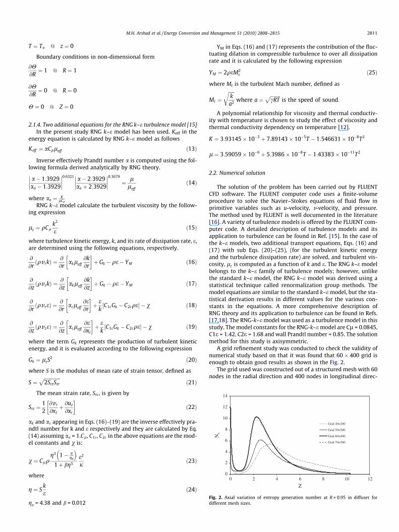
A numerical result for the case of incompressible turbulent flowin pipe is compared with the experimental data. Fig. 3 shows thevariation of dimensionless axial velocity in radial direction nearthe end of 17 m smooth pipe of inner diameter 127 mm. Air is usedas fluid and Reynolds number based on mean velocity and pipediameter is 5450. Particle image velocimetry measurement wasused to get experimental velocity profiles [19]. Fig. 3 representsthe comparison of computed fully developed dimensionless turbu-lent velocity profile with the experimentally measured profile. Thefigure suggests that the profile predicted by CFD code is very closeto the experimental one.

8.68

0.13

0.19

3.26

6.51

0.08

0.10

1.15

2.173.76 3.26

0.07

0.16

1.71

3.26

3.26

1.15

2.17

R

5 6 7

0.75

1

1.25

1.5

3. Results and discussion

Two-dimensional solutions for velocity and temperature fieldsare obtained. Contours of Mach number and temperature in dif-fuser are shown in Figs. 4 and 5. Change of temperature is a resultof two contributions, the heat flux and the viscous dissipation. Theviscous dissipation function is equal to the product of temperatureand entropy generation by the Gouy–Stodola theorem (see Chapter2 of [1]). Figs. 6 and 7 show the contour plots of entropy genera-

0

0.2

0.4

0.6

0.8

1

1.2

0 0.1 0.2 0.3 0.4 0.5 0.6

r/D

VZ comp

exp

Fig. 3. Radial variation of dimensionless axial velocity computed by FLUENT andexperimental values in literature.

0.42 0.290.24 0.21

0.180.07

0.35

Z

R

0 2 4 6 8 100

1

2

3

Fig. 4. Contours of Mach number in diffuser.

Z

Fig. 7. Contours of entropy generation number for air flowing in diffuser for Z = 4.5–8 (ratio of outer diameter to inlet diameter = 2, dimensionless length = 10.3).

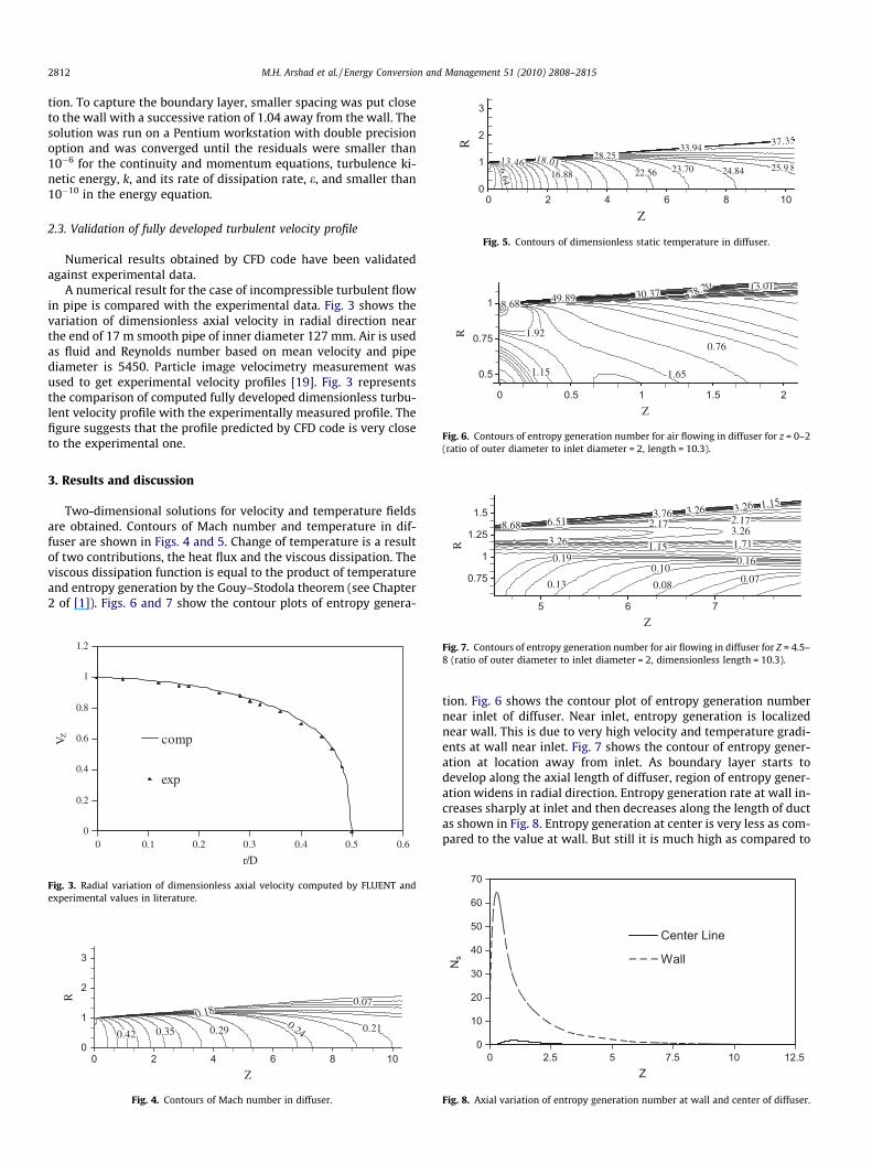
tion. Fig. 6 shows the contour plot of entropy generation numbernear inlet of diffuser. Near inlet, entropy generation is localizednear wall. This is due to very high velocity and temperature gradi-ents at wall near inlet. Fig. 7 shows the contour of entropy gener-ation at location away from inlet. As boundary layer starts todevelop along the axial length of diffuser, region of entropy gener-ation widens in radial direction. Entropy generation rate at wall in-creases sharply at inlet and then decreases along the length of ductas shown in Fig. 8. Entropy generation at center is very less as com-pared to the value at wall. But still it is much high as compared to

0

10

20

30

40

50

60

70

0 2.5 5 7.5 10 12.5Z

Ns

Center Line

Wall

Fig. 8. Axial variation of entropy generation number at wall and center of diffuser.

0

0.5

1

1.5

2

0 5 10 15 20

R

Z=3.3Z=6.6Z=10.0

M.H. Arshad et al. / Energy Conversion and Management 51 (2010) 2808–2815 2813

the case of incompressible flow through constant area duct re-ported in literature [20]. That can be explained in the followingway. Temperature and velocity gradients in radial direction arezero because of axis-symmetric case. But velocity gradient in axialdirection exist because of decrease of velocity along the length ofdiffuser. Therefore comparatively high value of entropy generationat centerline is complying with physics of the problem.

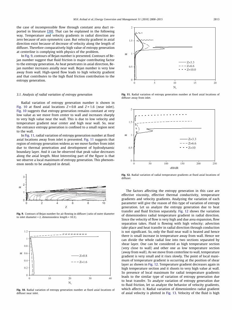
In Fig. 9, contours of Bejan number is presented. Contours of Be-jan number suggest that fluid friction is major contributing factorto the entropy generation. As heat penetrates in axial direction, Be-jan number increases axially near wall. Bejan number is very lowaway from wall. High-speed flow leads to high velocity gradientand that contributes to the high fluid friction contribution to theentropy generation.

Ns

Fig. 11. Radial variation of entropy generation number at fixed axial locations ofdiffuser away from inlet.

0

0.5

1

1.5

2

0 50 100 150 200 250

R

Z=3.3Z=6.6Z=10

3.1. Analysis of radial variation of entropy generation

Radial variation of entropy generation number is shown inFig. 10 at fixed axial locations Z = 0.8 and Z = 1.6 (near inlet).Fig. 10 suggests that entropy generation remains constant at verylow value as we move from center to wall and increases sharplyto very high value near the wall. This is due to low velocity andtemperature gradient near center and high near wall. So, nearthe entrance entropy generation is confined to a small region nextto the wall.

In Fig. 11, radial variation of entropy generation number at fixedaxial locations away from inlet is presented. Fig. 11 suggests thatregion of entropy generation widens as we move further from inletdue to thermal penetration and development of hydrodynamicboundary layer. And it can be observed that peak value decreasesalong the axial length. Most Interesting part of the figure is thatwe observe a local maximum of entropy generation. This phenom-enon needs to be analyzed in detail.

0.090.020.03

0.01

0.140.110.02 0.04

Z

R

0 2 4 6 8 100

1

2

3

Fig. 9. Contours of Bejan number for air flowing in diffuser (ratio of outer diameterto inlet diameter = 2, dimensionless length = 10.3).

0

0.2

0.4

0.6

0.8

1

1.2

0 10 20 30 40

Ns

R

Z=0.8

Z=1.6

Fig. 10. Radial variation of entropy generation number at fixed axial locations ofdiffuser near inlet.

dΘ/dR

Fig. 12. Radial variation of radial temperature gradients at fixed axial locations ofdiffuser.

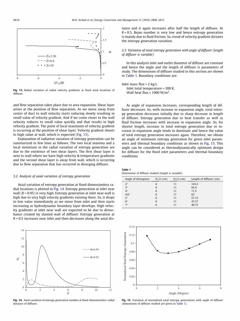
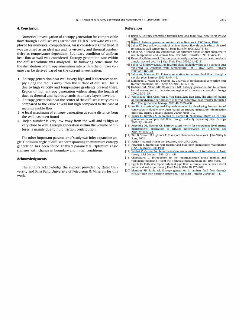
The factors affecting the entropy generation in this case areeffective viscosity, effective thermal conductivity, temperaturegradients and velocity gradients. Analyzing the variation of eachparameter will give the reason of this type of variation of entropygeneration. Let us analyze the entropy generation due to heattransfer and fluid friction separately. Fig. 12 shows the variationof dimensionless radial temperature gradient in radial direction.Since the velocity of flow is very high and due area expansion, flowseparation takes. Fluid is flowing with high velocity; advectiontake place and heat transfer in radial direction through conductionis not significant. So, only the fluid near wall is heated and hencethere is small increase in temperature away from wall. Hence wecan divide the whole radial line into two sections separated byshear layer. One can be considered as high temperature section(very close to wall) and other one as low temperature section(away from wall). As we move from centerline to wall, temperaturegradient is very small and it rises slowly. The point of local maxi-mum of temperature gradient is occurring at the position of shearlayer as shown in Fig. 12. Temperature gradient decreases again inhigh temperature section and it shoots to very high value at wall.So presence of local maximum for radial temperature gradientsleads to the similar type of variation of entropy generation dueto heat transfer. To analyze variation of entropy generation dueto fluid friction, let us analyze the behavior of velocity gradients,which affects it. Radial variation of dimensionless radial gradientof axial velocity is plotted in Fig. 13. Velocity of the fluid is high

0

0.5

1

1.5

2

-8 -6 -4 -2 0

dVZ/dR

R

Z=3.30Z=6.6Z=10

Fig. 13. Radial variation of radial velocity gradients at fixed axial locations ofdiffuser.

2814 M.H. Arshad et al. / Energy Conversion and Management 51 (2010) 2808–2815

and flow separation takes place due to area expansion. Shear layerarises at the position of flow separation. As we move away fromcenter of duct to wall velocity starts reducing slowly resulting insmall value of velocity gradient. And if we come closer to the wallvelocity reduces to small value quickly and that results in highvelocity gradient. The point of local maximum of velocity gradientis occurring at the position of shear layer. Velocity gradient shootsto high value at wall, which is expected (Fig. 13).

Explanation of radiation variation of entropy generation can besummarized in few lines as follows. The two local maxima and alocal minimum in the radial variation of entropy generation aredue to the existence of two shear layers. The first shear layer isnext to wall where we have high velocity & temperature gradientsand the second shear layer is away from wall, which is occurringdue to flow separation that has occurred in diverging diffuser.

Table 1Dimensions of diffuser studied (length is variable).

Angle of divergence D1/2 (cm) D2/2 (cm) Length of diffuser (cm)

2� 6 11 143.23� 6 11 95.44� 6 11 71.54.6� 6 11 625� 6 11 57.156� 6 11 47.577� 6 11 40.72

3.2. Analysis of axial variation of entropy generation

Axial variation of entropy generation at fixed dimensionless ra-dial locations is plotted in Fig. 14. Entropy generation at inlet nearwall (R = 0.95) is very high. Entropy generation at inlet near wall ishigh due to very high velocity gradients existing there. So, it dropsto low value immediately as we move from inlet and then startsincreasing as hydrodynamic boundary layer develops. High veloc-ity gradients at inlet near wall are expected to be due to distur-bance created by slanted wall of diffuser. Entropy generation atR = 0.5 increases near inlet and then decreases along the axial dis-

0

2

4

6

8

10

12

14

0 2 4 6 8 10 12Z

Ns

R=0.50

R=0.95

Fig. 14. Axial variation of entropy generation number at fixed dimensionless radialdistance of diffuser.

tance and it again increases after half the length of diffuser. AtR = 0.5, Bejan number is very low and hence entropy generationis mainly due to fluid friction. So, trend of velocity gradient dictatesthe entropy generation variation.

3.3. Variation of total entropy generation with angle of diffuser (lengthof diffuser is variable)

In this analysis inlet and outlet diameter of diffuser are constantand hence the angle and the length of diffuser is parameters ofstudy. The dimensions of diffuser studied in this section are shownin Table 1. Boundary conditions are:

Inlet mass flux = 2 kg/s.Inlet total temperature = 300 K.Wall heat flux = 1000 W/m2.

As angle of expansion increases, corresponding length of dif-fuser decreases. So, with increase in expansion angle, total entro-py generation decreases initially due to sharp decrease in lengthof diffuser. Entropy generation due to heat transfer as well asfluid friction increases with increase in expansion angle. So, forshorter length, increase in total entropy generation due to in-crease in expansion angle tends to dominate and hence the valueof total entropy generation increases again. Therefore, we obtainan angle of minimum entropy generation for given inlet param-eters and thermal boundary conditions as shown in Fig. 15. Thisangle can be considered as thermodynamically optimum designfor diffuser for the fixed inlet parameters and thermal boundaryconditions.

0

0.02

0.04

0.06

0.08

0.1

0.12

0.14

0 2 4 6 8

Angle (Degree)

Nor

mal

ized

Tot

al E

ntro

py G

ener

atio

n ..

Fig. 15. Variation of normalized total entropy generations with angle of diffuser(dimensions of diffuser studied are given in Table 1).

M.H. Arshad et al. / Energy Conversion and Management 51 (2010) 2808–2815 2815

4. Conclusion

Numerical investigation of entropy generation for compressibleflow through a diffuser was carried out. FLUENT software was em-ployed for numerical computations. Air is considered as the fluid. Itwas assumed as an ideal gas and its viscosity and thermal conduc-tivity as temperature dependent. Boundary condition of uniformheat flux at wall was considered. Entropy generation rate withinthe diffuser volume was analyzed. The following conclusions forthe distribution of entropy generation rate within the diffuser vol-ume can be derived based on the current investigation.

1. Entropy generation near wall is very high and it decreases shar-ply along the radius away from the surface of diffuser. This isdue to high velocity and temperature gradients present there.Region of high entropy generation widens along the length ofduct as thermal and hydrodynamic boundary layers develop.

2. Entropy generation near the center of the diffuser is very less ascompared to the value at wall but high compared to the case ofincompressible flow.

3. A local maximum of entropy generation at some distance fromthe wall has been found

4. Bejan number is very low away from the wall and is high atvery close to wall. Entropy generation within the volume of dif-fuser is mainly due to fluid friction contribution.

The other important parameter of study was inlet expansion an-gle. Optimum angle of diffuser corresponding to minimum entropygeneration has been found at fixed parameters. Optimum anglechanges with change in boundary and initial conditions.

Acknowledgments

The authors acknowledge the support provided by Qatar Uni-versity and King Fahd University of Petroleum & Minerals for thiswork.

References

[1] Bejan A. Entropy generation through heat and fluid flow. New York: Wiley;1982.

[2] Bejan A. Entropy generation minimization. New York: CRC Press; 1996.[3] Sahin AZ. Second law analysis of laminar viscous flow through a duct subjected

to constant wall temperature. J Heat Transfer 1998;120:76–83.[4] Sahin AZ. A second law comparison for optimum shape of duct subjected to

wall temperature and laminar flow. Heat Mass Transfer 1998;33:425–30.[5] Demirel Y, Kahraman R. Thermodynamic analysis of convective heat transfer in

annular packed bed. Int J Heat Fluid Flow 2000;21:442–8.[6] Sahin AZ. Entropy generation in a turbulent liquid flow through a smooth duct

subjected to constant wall temperature. Int J Heat Mass Transfer2000;43:1469–78.

[7] Sahin AZ, Mansour RB. Entropy generation in laminar fluid flow through acircular pipe. Entropy 2003;5:404–16.

[8] Mahmood S, Frazer RA. Second law analysis of fundamental convective heattransfer problems. Int J Therm Sci 2003;42:177–86.

[9] Haddad OM, Alkam MK, Khasawneh MT. Entropy generation due to laminarforced convection in the entrance region of a concentric annulus. Energy2004;29:35–55.

[10] Wu Shuang-Ying, Chen Yan, Li You-Rong, Zeng Dan-Ling. The effect of foulingon thermodynamic performance of forced convective heat transfer through aduct. Energy Convers Manage 2007;48:2399–406.

[11] Ko TH. Analysis of optimal Reynolds number for developing laminar forcedconvection in double sine ducts based on entropy generation minimizationprinciple. Energy Convers Manage 2006;47:665–70.

[12] Yapici H, Kayatas S, Kahraman N, Gamez B. Numerical study on entropygeneration in compressible flow through suddenly expanding pipe. Entropy2005;7(1):38–67.

[13] Adeyinka OB, Naterer GF. Entropy-based metric for component-level energymanagement: application to diffuser performance. Int J Energy Res2005;29:1007–24.

[14] Bird B, Stewart B, Lightfoot E. Transport phenomena. New York: John Wiley &Sons; 2002.

[15] FLUENT manual. Fluent Inc. Lebanon, NH (USA); 2003.[16] Patankar S. Numerical heat transfer and fluid flow, hemisphere. Washington

(USA): MaGraw-Hill; 1980.[17] Yakhot V, Orszag SA. Renormalization group analysis of turbulence: I. Basic

theory. J Sci Comput 1986;1(1):1–51.[18] Choudhury, D. Introduction to the renormalization group method and

turbulence modeling. Fluent Inc. Technical memorandum TM-107; 1993.[19] Eggels JG. Fully developed turbulent pipe flow: a comparison between direct

numerical and experiment. J Fluid Mech 1994;28:175–209.[20] Mansour RB, Sahin AZ. Entropy generation in laminar fluid flow through

circular pipe with variable properties. Heat Mass Transfer 2005;42:1–11.