A finite point method for adaptive three-dimensional compressible flow calculations

INTERNATIONAL JOURNAL FOR NUMERICAL METHODS IN FLUIDSInt. J. Numer. Meth. Fluids 2009; 60:937–971Published online 17 October 2008 in Wiley InterScience (www.interscience.wiley.com). DOI: 10.1002/fld.1892

A finite point method for adaptive three-dimensional compressibleflow calculations

Enrique Ortega∗,†, Eugenio Onate and Sergio Idelsohn‡

International Center for Numerical Methods in Engineering (CIMNE), Universidad Politecnica de Cataluna,Edificio C1, Campus Norte, UPC, Gran Capitan, s/n, 08034 Barcelona, Spain

SUMMARY

The finite point method (FPM) is a meshless technique, which is based on both, a weighted least-squaresnumerical approximation on local clouds of points and a collocation technique which allows obtainingthe discrete system of equations. The research work we present is part of a broader investigation into thecapabilities of the FPM to deal with 3D applications concerning real compressible fluid flow problems. Inthe first part of this work, the upwind-biased scheme employed for solving the flow equations is described.Secondly, with the aim of exploiting the meshless capabilities, an h-adaptive methodology for 2D and 3Dcompressible flow calculations is developed. This adaptive technique applies a solution-based indicator inorder to identify local clouds where new points should be inserted in or existing points could be safelyremoved from the computational domain. The flow solver and the adaptive procedure have been evaluatedand the results are encouraging. Several numerical examples are provided in order to illustrate the goodperformance of the numerical methods presented. Copyright q 2008 John Wiley & Sons, Ltd.

Received 28 January 2008; Revised 27 June 2008; Accepted 13 July 2008

KEY WORDS: meshless methods; finite point method; adaptivity; collocation; compressible flow; timeintegration explicit

1. INTRODUCTION

Numerical simulation has come into the focus of interest of applied sciences and engineering in thelast decades. As a result, the development of numerical techniques for solving partial differentialequations (PDEs) has been growing continuously, mainly stimulated by increasing computational

∗Correspondence to: Enrique Ortega, International Center for Numerical Methods in Engineering (CIMNE), Univer-sidad Politecnica de Cataluna, Edificio C1, Campus Norte, UPC, Gran Capitan, s/n, 08034 Barcelona, Spain.

†E-mail: [email protected]‡ICREA Research Professor at CIMNE.

Contract/grant sponsor: European Union Programme of High Level Scholarships for Latin America; contract/grantnumber: E04D027284AR

Copyright q 2008 John Wiley & Sons, Ltd.

938 E. ORTEGA, E. ONATE AND S. IDELSOHN

resources and ever-challenging demands for practical and theoretical applications. Nowadays, thereare two main types of numerical techniques for solving PDEs. On the one hand, there exist mesh-based or conventional discretization methods; among them the classical finite differences (FD),finite volume (FV) and finite element (FE) methods are of singular interest. These techniques aremostly employed in practice due to their robustness, efficiency and high confidence gained throughyears of continuous use and enhancement. On the other hand, there exist meshless methods. Havingtheir pros and cons, meshless methods offer an alternative to mesh-based techniques. Meshlessmethods are conceptually attractive; however, their practical implementations have not succeededso far to prove their efficiency and this is a fact which can explain the comparatively little attentionthat has been devoted to these techniques. In spite of this, over the last 10 years, some difficultiesthat arose in conventional mesh-based methods when performing particular applications havebrought meshless methods into the focus of attention.

The first meshless methods appeared in the mid-seventies and numerous formulations havebeen proposed since then. A retrospective view of the evolution of the most relevant meshlessmethods as well as their connections is presented by Belytschko et al. [1]. In their work, the mainfeatures of typical meshless methods, their implementation issues and practical applications areoffered. An interesting work by Fries and Matthies [2] classifies and analyses the most importantmeshless methods considering their different origins and viewpoints. The authors highlight themain characteristics and implementation details as well as the advantages and disadvantages ofeach technique. Some outstanding reviews on meshless methods can also be found in the literature;see for instance those due to Li and Liu [3], Gu [4], Duarte [5], Liu et al. [6] and Dolbow andBelytschko [7].

The present work deals with a meshless technique called the finite point method (FPM), whichwas introduced by Onate et al. [8–10]. In the FPM, the numerical approximation to the problemvariables and their derivatives is based on a weighted least-squares (WLSQ) procedure known asfixed least squares (FLS). The strong form of the governing PDEs is sampled at each point byreplacing the continuous variables with their approximated counterparts and the resulting systemof algebraic equations is obtained by means of a collocation technique.

Since the FPM appeared in the literature towards the mid-nineties, it has been successfullyapplied to solve convective–diffusive problems, incompressible and compressible fluid flow prob-lems [9–14] and solid mechanics problems [15–17] among others. As regards to fluid flow prob-lems, the first application of the FPM to the solution of the 2D compressible flow equations waspresented by Onate et al. [8, 9] and Fischer [12]. In those works, topics such as the constructionof local clouds of points and the effects of the weighting function on the numerical approximationwere studied using first- and second-order approximation bases. In addition, the compressible flowequations were solved using a Taylor–Galerkin scheme. More recently, Sacco [13] presented adetailed analysis of the finite point (FP) approximation in conjunction with a multi-dimensionalapplication for solving the incompressible flow equations. Outstanding achievements from thatwork, such as a definition of local and normalized approximation bases, a procedure for constructinglocal clouds of points as well as a criterion for evaluating their quality, have given the FPM amore solid base. In relation to the solution of the incompressible flow equations, a fractional stepalgorithm stabilized via a technique known as Finite Calculus (FIC) [18] has also been successfullyemployed. The FP solution of the 3D compressible flow equations was presented in a pioneer workby Lohner et al. [14]. There, two contributions are well worth mentioning: a reliable procedure forconstructing the local clouds (based on a Delaunay technique) and a well-suited upwind-biasedscheme for solving the flow equations. This scheme is based on a symmetrized discrete expression

Copyright q 2008 John Wiley & Sons, Ltd. Int. J. Numer. Meth. Fluids 2009; 60:937–971DOI: 10.1002/fld

A FPM FOR ADAPTIVE 3D COMPRESSIBLE FLOW CALCULATIONS 939

of the advective flux-divergence vector, which is composed of a central difference-like expressionplus a corrective term. In this scheme, the central difference-like flux term is replaced by an upwindnumerical flux obtained through an approximate Riemann solver. In the meshless context, thisapproach is preferable to artificial dissipation methods as it is not necessary to define any kindof geometrical measure in the cloud of points. Other meshless approaches found in the literatureshare this philosophy, see for instance [19, 20] and the references cited therein.

All these works, though different, have made remarkable contributions to enhance the perfor-mance of the FPM; giving clear evidence of its potential and, in some cases, also revealingimportant weaknesses. Nowadays, most meshless techniques, and in particular the WLSQ-basedmethods, are characterized by a lack of solid theoretical and practical arguments regarding localcloud construction, approximation bases selection and weighting function setting, among otherimportant issues. In addition, methods like the FPM, which use the strong form of the differentialgoverning equations, must face some other well-known stability and robustness problems arisingfrom the collocation procedure. Unfortunately, the robustness and the accuracy of the numericalapproximation in the cloud of points are dependent on the previously mentioned features. To makematters worse, meshless methods are typically computationally expensive, which requires devel-oping more efficient algorithms and data structures. All these considerations become crucial whendealing with real 3D problems of practical application in engineering. Consequently, improvementin robustness and efficiency seems to be the key to the success of meshless methods in the future.

As regards robustness, some modifications to the FPM have been proposed by Boroomandet al. [21] with the aim of reducing instabilities in the minimization procedure, especially thosearising from non-appropriate local clouds of points. In addition to that, but from another perspective,we have recently presented an alternative approach towards robustness [22] intended to reducethe local approximation dependence on both the spatial distribution of the cloud of points and theweighting function parameters. This ad hoc procedure, which is based on a QR factorization inconjunction with an iterative adjustment of the local approximation parameters, allows obtaininga satisfactory minimization problem solution for cases where usual approaches fail and avoidsmodifying the geometrical support where the local approximation is based on.

Regardless of the difficulties meshless methods present for practical use, they have potentialadvantages over conventional discretization techniques, which explain the scientific interest ofmany researchers in this area (cf. [1–3]). Indeed meshless techniques facilitate the treatment ofproblems involving moving discontinuities and computational domains whose boundaries changewith time and the development of h- and p-adaptivity schemes, among other advantages. In ouropinion, these topics constitute key opportunities for the development and promotion of meshlessmethods.

Along the lines of investigation just mentioned, Perazzo et al. [23] have recently presented anh-adaptive technique for solid mechanics problems which is based on the approximation errorobtained at each point by the WLSQ functional. In addition, in a previous work [22] we havedealt with high-order FP discretizations in a preliminary manner, exploring the FPM capabilitiesregarding p-adaptivity. This time, with the same objective in mind, i.e. exploiting the FPM potential,we present an h-adaptive methodology for 2D and 3D compressible flow problems.

The rest of the work is organized as follows. In Section 2, the FP approximation is presented.Section 3 is concerned with the domain discretization and the construction of local clouds ofpoints. Next, in Sections 4 and 5, the upwind-biased scheme employed for solving the 3D Eulerequations using the FPM is described. Section 6 provides several numerical calculations to showthe performance of the flow solver. Then, an h-adaptive FPM for compressible flow calculations is



developed in Section 7 and the performance of this adaptive methodology is evaluated by meansof several numerical examples in Section 8. Finally, some conclusions of this work are presentedin Section 9.

2. NUMERICAL FINITE POINT APPROXIMATIONS ON CLOUDS OF POINTS

In this section, we present an FP approximation to an unknown function u(x) defined in a closeddomain �∈�d (d=1, 2 or 3), which is discretized by a set of points xi , i=1,n. In order to obtaina local approximation for function u(x), the domain � is divided into subdomains �i (henceforthtermed clouds of points) so that ��i represents a covering for �. Each local cloud of pointsconsists of a point xi called star point and a set of points x j , j =2,3, . . . ,np surrounding xi ,which complete �i . Assuming that function u(x) is smooth enough in �i , it is possible to statethe following approximation:

u(x)∼= u(x)=m∑l=1

pl(x)�l =pT(x)a (1)

where p(x) is a vector whose m-components are the terms of a complete polynomial base in �d

(cf. [22] for details) and a is an a priori unknown vector. These vectors are given by

pTj = [p1(x j ) p2(x j ) . . . pm(x j )] (1×m)

a = [�1 �2 . . . �m]T (m×1)(2)

Next, at each point x j ∈�i the unknown function is obtained as follows:

uh =

⎡⎢⎢⎢⎢⎢⎢⎣

uh1

uh2...

uhnp

⎤⎥⎥⎥⎥⎥⎥⎦

∼=

⎡⎢⎢⎢⎢⎢⎣

u1

u2

...

unp

⎤⎥⎥⎥⎥⎥⎦=

⎡⎢⎢⎢⎢⎢⎢⎣

pT1

pT2...

pTnp

⎤⎥⎥⎥⎥⎥⎥⎦a=Pa (3)

where uhj =uh(x j ) is the value of the unknown function u(x) at x=x j , u j = u(x j ) is the approxi-mated value at that point and

P=

⎡⎢⎢⎢⎣pT1...

pTnp

⎤⎥⎥⎥⎦=

⎡⎢⎢⎢⎣

p1(x1) p2(x1) . . . pm(x1)

...

p1(xnp) p2(xnp) . . . pm(xnp)

⎤⎥⎥⎥⎦ (np×m) (4)

In order to solve the equation system (3) the condition np=m must be fulfilled. This penalizes theapproximation flexibility and does not suit a meshless methodology. Thus, np�m is adopted andthe equation system becomes overdetermined. Consequently, an approximate solution is sought bymeans of a WLSQ technique. This solution minimizes a discrete L2 error norm in the approximationto u(x) in �i .



The WLSQ approximation features depend on the shape of the chosen weighting function andthe manner in which the latter is applied. In the FPM a fixed weighting function, centred on thestar point of the cloud, is chosen so that it satisfies the following conditions:

�i (x j ) > 0 ∀x j ∈�i

�i (x) = 0 ∀x /∈�i

�i (xi ) = 1

(5)

This kind of approximation, known as FLS method, can be considered as a particular case ofthe moving least-squares (MLS) method introduced by Lancaster and Salkauskas in the contextof interpolation and data fitting [24]. When the FLS procedure is applied, the approximationmethodology is considerably simplified and its computational cost reduced. It should be noticed,though, that FLS approximations lead to multivalued shape functions depending on the cloudin which the approximation is calculated, i.e. Nn(x j ) �=Nm(x j ) (subscripts m and n indicateneighbouring clouds of points). Therefore, the numerical approximation is globally and locallydiscontinuous and must be considered as valid only at the star point of the cloud where theweighting function is located. Hence, a collocation technique becomes the natural choice in theFPM.

Going back to the minimization procedure, the following discrete functional is defined:

J(xi )=Ji =np∑j=1

�i (x j )[u j −uhj ]2=np∑j=1

�i (x j )[pTj a−uhj ]2 (6)

in which �i (x j )=�(x j −xi ) is a compact support weighting function. Equation (6) can berewritten as

J=(Pa−uh)T/(x)(Pa−uh) (7)

where /(x)=diag(�(x j −xi )). The minimization of Equation (7) with respect to a leads to thefollowing equation system:

(PT/(x)P)a−(PT/(x))uh =0 (8)

known as normal equations in the least-squares (LSQ) literature. Introducing the matrices

A = (PT/(x)P), Akl =np∑j=1

�i (x j )pk(x j )pl(x j ) (m×m)

B = (PT/(x)), Bl j = pl(x j )�i (x j ) (m×np)

(9)

it is possible to express the normal equations (8) as follows:

Aa=Buh (10)

As a fixed weighting function is chosen, the unknown coefficients � j are constant in �i . Thesecoefficients can be found by

a=A−1Buh (11)



Equation (11) must be solved via matrix A inversion because vector uh is not known in advance.Thus, depending on the spatial distribution of the local cloud of points (especially for the 3D case),matrix A can become ill-conditioned, making it very difficult to invert it with accuracy.

Then, supposing that Equation (11) is solved accurately enough and replacing the coefficients� j in Equation (1), the approximation to the unknown function at the star point is obtained as

u(xi )= pT(xi )A−1B︸︷︷︸NTi (x) (1×np)

uh (12)

where NTi (x)=[Ni,1,Ni,2, . . . ,Ni,np] is the shape function vector of point xi in �i . The adoption

of an FLS scheme, where matrices A and B are constant in �i , simplifies the calculation of theshape functions derivatives. Consequently,

�lNTi (x)

�xlk= �lpT(xi )

�xlkA−1B (13)

and the approximation to the unknown function derivatives at xi is given by

�l u(xi )

�xlk= �lNT

i (x)

�xlkuh = �lpT(xi )

�xlkA−1Buh (14)

The solution of Equations (8) by direct inversion of matrix A is not the most accurate way ofsolving the LSQ problem. Thus, it must be restricted to cases when the condition number ofmatrix A is moderate. In this work, the procedure adopted to calculate the shape function and itsderivatives is the following (cf. [22] for a detailed description). Given a certain cloud of points,first the direct inversion of matrix A is attempted. If the condition number of A is smaller thana given maximum admissible value, and if the calculated shape functions satisfy some qualitytests, then the shape functions are accepted. If some of the preceding requirements are not met,Equations (8) are solved by an alternative procedure based on QR factorization. The aim of using aQR factorization technique is to get an acceptable solution for cases where the usual procedure failswithout having to modify the geometrical structure of the cloud. The WLSQ problem solution viaQR factorization may cost, in terms of CPU-time, up to twice as much as the solution via matrixA inversion if np�m [25]. However, this extra amount of time is quite unimportant in the overalltime, as the alternative QR-based procedure is only applied to problematic clouds of points thatrepresent only a small percentage of the whole clouds in the domain. The QR factorization-basedprocedure applied for solving the normal equations system (8) can be summarized as follows:

If matrix P (given by Equation (4)) has rank m and np>m, it can be uniquely factored as

P=QR (15)

where matrix Q∈�np×m is orthogonal (QTQ=I) and matrix R∈�m×m is upper triangular withpositive diagonal elements (a similar procedure, based on columns pivoting, can be applied forcases where matrix P is rank deficient or near rank deficient). In order to apply the QR factorizationfor solving our WLSQ problem, it is necessary to obtain an equivalent unweighted problem. Thus,the next factorization is proposed

/(x)=√/(x) such that /

T/=/ (16)



and also the following modification of matrix P :P= /P (17)

After that, it is possible to write an equation system equivalent to the one given by Equation (8) as

(PTP)a=(PT/)uh (18)

Then, the modified matrix (17) is factorized, i.e. P=QR, and replaced in the equivalent unweightedproblem (18). This leads to

Ra=QT/uh (19)

from which the unknown coefficients � j can be obtained

a=R−1(QT/)uh (20)

Here, matrix R is generally well-conditioned and its inverse is easy to obtain with accuracy, evenfor the cases when matrix P is near rank deficient. The described procedure allows us get shapefunctions of quite good quality in cases where they cannot be obtained via inversion of matrix A.This reduces the dependence of the approximation on the spatial distribution of points and on thefunctional shape of the weighting function significantly, giving robustness to the FP approximationmethodology.

2.1. The weighting function

In the present work, the following normalized Gaussian weighting function is adopted:

�i (x j )=e−(d j/�)k −e−(�/�)k

1−e−(�/�)k(21)

where d j =‖x j −xi‖, �=�/w and �=�dmax (�>1.0). The support of this function is isotropic,circular and spherical in two- and three-spatial dimensions, respectively. A detailed description ofthe effects of the free parameters w,k and � on the numerical approximation and some guide-lines for their setting was presented in [22]. However, an important remark about the parameter �should be mentioned. The parameter � determines the size of the weighting function’s supportand, in consequence, a larger value of � could be interpreted as an enlargement of the over-lapping zone between neighbouring clouds of points. This provides a mechanism for improvingthe approximation quality where sudden changes in the distance between neighbouring pointshappen, e.g. near localized adaptive-refined zones and certain details of 3D geometries. In thesecases, which generally lead to highly distorted clouds of points, good results are obtained setting1<�<1.25.

3. DISCRETIZATION OF THE DOMAIN AND LOCAL CLOUD CONSTRUCTION

An adequate support of points is essential for setting a good local approximation for each cloud.Even though the iterative QR-based technique described above attempts to reduce this dependence,the spatial support of the approximation continues playing a major role. At present, there is not a



unique criterion to determine the size, shape and structure of the local spatial support and severalprocedures have been proposed by meshless practitioners. Concerning the FPM, an appropriatemethodology for constructing local clouds of points (based on a Delaunay technique) has beensuggested by Lohner et al. [14]. In the present work we follow the general criteria proposed there.

3.1. Domain discretization

The point discretization of the analysis domain � is obtained by means of a modification of thealgorithm presented in [26]. It starts from a Delaunay triangulation that bounds the domain andinserts new points in the centre of empty spheres filling �. This incremental quality technique,known as optimization driven point insertion, allows achieving a fast point discretization of theanalysis domain well-suited for FP calculations.

3.2. Local cloud construction

The local clouds of points are constructed as follows. Given a point discretization of the computa-tional domain and a set of normal vectors belonging to the triangulation that bounds this domain,a maximum (npmax) and minimum (npmin) allowable number of points in the cloud and an initialsearch radius are set. Then, for each star point xi , all neighbours within the search radius (rs) arefound through an octree technique. Any local cloud of points inside the computational domain isconstructed with the closest neighbouring points from the star point. However, if a star point xi islocated either over or close enough to a solid boundary, the points included in its cloud (admissiblepoints) must also satisfy the conditions described below.

Case 1: Star point located over a solid boundary.In this particular case (sketched in Figure 1), every point x j located within the search radius is

admissible if it meets the following conditions:

cos(�)�cos(�/2+�), cos(�)= ni ·r j‖ni‖‖r j‖ (22)

‖rtj‖<�rsearch (23)

Condition (22) defines an admissible zone around the start point, which is defined in the normaldirection to the surface and � is a small angle dependent on the surface curvature. The secondcondition (23) imposes a certain aspect ratio in the cloud, given by the parameter � �=0.

Case 2: Cloud of points intercepting a solid boundary.In this case the point x j located over a surface (x jnea), nearest to the star point xi , must be

sought (see Figure 1). Then, every point within the search radius is admissible if

cos(�)�cos(�/2+�), cos(�)= n jnea ·r j‖n jnea‖‖r j‖

(24)

and no restriction is imposed to the aspect ratio of the cloud of points.If the number of admissible points found within the search radius is not enough, the latter is

increased until condition npmin�np�npmax is satisfied. Otherwise, if the number of admissiblepoints goes beyond npmax, only the npmax points nearest to xi are added to the cloud.

It is very helpful to force the first layer of Delaunay nearest neighbours of xi into the localcloud of points when sudden variations in the distance between neighbouring points occur insidethe analysis domain. For each star point this is accomplished by performing a local Delaunay grid



Figure 1. The construction of local clouds near the boundaries. Left: the star point located over a solidboundary and right: a cloud of points intercepting a solid boundary.

with all the points falling within the octree search area. Only the first layer of nearest neighbours isretained and used to initialize the local cloud of points. Finally, admissible nearest points are addeduntil the condition npmin�np�npmax is fulfilled. This procedure, that follows the lines proposed byLohner et al. [14], avoids non-overlapping neighbouring clouds of points and improves the qualityof the local discretization. Furthermore, the information concerning the first layer of neighbouringpoints for each star point is useful for improving several computational procedures. In the presentwork such information is needed for the adaptive procedure presented in Section 7.

4. THE EULER EQUATIONS

The first-order hyperbolic system of Euler equations can be written in several equivalent forms.Their conservative differential form is given by

�U�t

+ �Fk

�xk=0 (25)

where k=1,d being d the number of spatial dimensions of the problem. U is the conservativevariables vector and Fk is the advective flux vector in the spatial direction xk . These vectors aredefined as

U=⎡⎢⎣

ui

et

⎤⎥⎦ , Fk =

⎡⎢⎣

uk

uiuk+�ik p

(et+ p)uk

⎤⎥⎦ (26)

where , p and et , respectively, denote the density, pressure and total energy of the fluid; ui isthe i-component of the velocity vector, �ik is the Kronecker delta and subscripts i,k=1,d . Thefollowing state relation for a perfect gas closes the system of equations (25)

p=(�−1)[et− 12uiui ] (27)

in which �=Cp/Cv is the specific heats ratio (in the present work we adopt �=1.4).The solution of Equation (25) in a closed domain �∈�d with boundaries �=�∞∪�w requires

appropriate initial and boundary conditions. The initial conditions only start the explicit calculation



and they are simple to implement. In general, they could be taken from the far-field state U∞.Regarding the boundary conditions, those employed in the present work are of two different kinds.The first one is concerned with far-field conditions applied on the outer boundaries �∞ and thesecond one is concerned with slip wall conditions applied on the solid boundaries �w. In the caseof far-field boundary conditions, the prescribed fluxes at each boundary point are obtained solvingan approximate Riemann problem in the outward normal direction to the boundary, between theboundary point state Ui and the far-field state U∞. Over solid boundaries, slip wall conditions areapplied forcing the fluxes to remain tangent to the boundaries, i.e. cancelling their components inthe boundary normal direction.

5. THE FLOW SOLVER

In this section, the numerical strategy adopted for solving the compressible flow equations is setforth. Despite some modifications to the way in which the divergence of the advective fluxes isdiscretized in the local cloud of points, the overall scheme follows the general lines proposed byLohner et al. [14].

Recalling the FPM approximation procedure described in Section 2, for each star point xi ∈�we can write the following approximations:

U(xi ) = Ui = ∑j∈�i

Ni jUhj

Fk(xi ) = Fki = ∑

j∈�i

Ni j (Fkj )h

(28)

where Ni j =Ni (x j) is the shape function of the star point xi evaluated at the cloud’s point x j

and (Fkj )h =Fk(Uh

j ). Then, the one-dimensional semi-discrete counterpart of Equation (25) can beexpressed for each star point xi by

�Ui

�t=−�Fi

�x=− ∑

j∈�i

�Ni j

�xFhj =− ∑

j∈�i

bi jFhj (29)

where Fhj is the advective flux vector calculated at a point x j ∈�i and the coefficient bi j stands

for the shape function derivative of xi evaluated at the same point x j .It is important to note that the (·)h parameters do not coincide with the approximated ones

( ·) because in the FP method the shape functions do not interpolate point data. These values arerelated by Equation (28), which implies that a linear system must be solved in order to get the(·)h parameters. Fortunately, this equation system has excellent properties and can be solved by afew iterations of a Gauss–Seidel method or similar. Henceforth, the markers ( ·) and (·)h will beomitted for the sake of simplicity.

Taking advantage of the partition of nullities property of the shape function derivatives it ispossible to infer ∑

j∈�i

bi j =bii + ∑j �=i

bi j =0 → bii =− ∑j �=i

bi j (30)



Replacing Equation (30) in Equation (29), the following semi-discrete expression is obtained:

�Ui

�t=− ∑

j �=ibi j (F j −Fi ) (31)

Equation (31) is unstable and needs to be stabilized. For that purpose, a more suitable equivalentform is sought scaling by a factor of 1

2 the stencil of points [20] used for its calculation. In thisway, we obtain a totally equivalent semi-discrete expression, which is given by

�Ui

�t=−2

∑j �=i

bi j (Fi j −Fi ) (32)

where Fi j is an a priori unknown numerical flux vector, evaluated at the midpoint of the linesegment connecting the star point xi with another point x j ∈�i (see Figure 2). Many possibilitiesfor calculating Fi j can be found in the literature. Following the ideas presented in [14], the Roe’sapproximate Riemann solver [27] is adopted in this work. Then, the numerical flux results

Fi j = 12 (F j +Fi )− 1

2 |A(Ui ,U j )|(U j −Ui ) (33)

where A(Ui ,U j ) is the flux Jacobian matrix evaluated at the Roe average-state between the pointsxi and x j , i.e. UL=Ui and UR =U j . In order to calculate the absolute value of the Roe matrix theprocedure suggested by Turkel [28] is applied. This procedure avoids costly matrix–matrix andmatrix–vector multiplications in the calculation of the dissipative term |A(Ui ,U j )|(U j −Ui ).

The multi-dimensional extension of the scheme presented above is straightforward. For eachpair of points (xi ,x j ), a one-dimensional problem is solved in the direction of vector l j i =x j −xito obtain the midpoint numerical flux Fi j . Then, Fi j is projected onto the Cartesian axis and thesemi-discrete scheme (32) results

�Ui

�t=−2

∑j �=i

bki j [Fki j −Fk

i ] (34)

where k=1,d being d the number of spatial dimensions of the problem. The Cartesian componentsof the midpoint numerical flux are obtained by

Fki j = 1

2 (Fkj +Fk

i )− 12 |An(Ui ,U j )|(U j −Ui ) · nk (35)

where n is a versor in the direction of the vector l j i and |An(Ui ,U j )| denotes the absolute value ofthe Roe matrix calculated in the same direction. The stencil of points employed in the derivationof expression (34) is presented in Figure 3.

5.1. Increasing spatial accuracy

The low-order scheme we have developed is useless in practice. In order to make this schemesuitable for capturing all the flow features with precision, it is necessary to increase its spatial

Figure 2. The one-dimensional stencil of points.



Figure 3. The multi-dimensional stencil of points.

order of accuracy. This is accomplished by replacing the zero-order extrapolation of the vari-ables (UL=Ui and UR=U j ) at the midpoint xi j by a higher-order extrapolation. The MonotoneUpstream-centered Schemes for Conservation Laws (MUSCL) methodology [29] allows achievingaccurate second- and third-order schemes using linear and quadratic reconstruction of the variables,respectively. Unfortunately, this high-order methodology does not guarantee an oscillation-freesolution and monotonicity should be enforced by introducing non-linear limiters into the recon-struction process. In brief, these limiters recognize any local extrema of the solution field andautomatically switch, at these points, the high-order extrapolation to a zero-order extrapolation,avoiding the appearance of under and overshoots in the numerical solution.

Taking into consideration the high-order approach proposed in [14], in this work we adopt aMUSCL reconstruction of the variables in conjunction with the Van Albada limiter. This resultsin the following set of reconstructed variables:

U+i = Ui + si

4[(1−)(Ui −Ui−1)+(1+)(U j −Ui )]

U−j = U j − s j

4[(1−)(U j+1+U j )+(1+)(U j −Ui )]

(36)

where U+i and U−

j are, respectively, the leftward and rightward extrapolations to the conservativevariables vector at point xi j . In the above expressions the choice of the parameter =−1 leads toa second-order, leftward-biased scheme for Ui and a rightward-biased scheme for U j . For =1and = 1

3 , a second-order centred scheme and a third-order scheme are obtained, respectively. TheVan Albada limiters si and s j are given by [14]

si = max

[0,

2(Ui −Ui−1)(U j −Ui )+�

(Ui −Ui−1)2+(U j −Ui )2+�

]

s j = max

[0,

2(U j+1−U j )(U j −Ui )+�

(U j+1−U j )2+(U j −Ui )2+�

] (37)



Figure 4. Implementation of the multi-dimensional reconstruction of the variables.

where �≈1.0E−5 is a small constant included to avoid divisions by zero. The variables Ui−1 andU j+1 are obtained by a centred approximation to the ∇U at the points i and j

Ui −Ui−1 = 2l j i ·∇Ui −(U j −Ui )

U j+1−U j = 2l j i ·∇U j −(U j −Ui )(38)

in which l j i =x j −xi is the vector linking the points i and j (see Figure 4).Once the high-order extrapolations (36) have been calculated, the midpoint numerical flux (35)

is modified according to

Fki j = 1

2 (Fk(U+

i )+Fk(U−j ))− 1

2 |An(U+i ,U−

j )|(U−j −U+

i ) · nk (39)

and then, replacing Equation (39) in Equation (34) the high-order semi-discrete scheme is obtained.

5.2. Time discretization

Following the ideas in [14], the temporal discretization of Equation (34) is done in a fully explicitmanner by means of a multi-stage method that is a subset of the Runge–Kutta family of schemes.Assuming that the vector of conservative variables Uh is known at time t= tn , the right-hand sideof Equation (34) is calculated for each point (RHSi ). Then, it is possible to advance the solutionin time from tn to tn+1 by means of the following s-stage scheme:

U(0)i = Un

i

...

U(s)i = Un

i +�s�tiRHS(s−1)i

...

Un+1i = U(smax)

i

(40)



where �ti is the time-step evaluated at the star point xi and �s are integration coefficients thatdepend on the number of stages employed (smax). For two-, three- and four-stages schemes theseparameters are set as follows:

2-stages →�1= 12 and �2=1.0

3-stages →�1= 35 , �2= 3

5 and �3=1.0

4-stages →�1= 14 , �2= 1

3 , �3= 12 and �4=1.0

The difference between the (·)h parameters and the approximated ones ( ·) has already been pointedout in Section 5. Taking into account that RHSi = f (Uh

j )∇x j ∈�i , the following linear system hasto be solved at the end of each integration stage:

MUh = U (41)

whereM∈�n×n is the mass matrix of the system, which results from the assembly of the Ni j coef-ficients (see Equation (28)). Fortunately, as mentioned before, this system has excellent propertiesand can be solved by a few iterations of a Gauss–Seidel method or similar.

It should be noticed that, even though the numerical scheme presented in this section is intendedto solve the inviscid compressible flow equations, with minor modifications the same scheme canbe applied for solving the viscous flow equations.

6. NUMERICAL EXAMPLES

In this section, some 3D compressible flow calculations are presented with the aim of illustratingthe performance of the proposed methodology. The first example concerns a subsonic flow past asphere. Although this example has barely any practical interest, it allows assessing the low Machnumber behaviour of the scheme as well as evaluating its intrinsic dissipation. Then, a transonicflow around the ONERA M6 wing is solved. This example, which is a classic CFD validation testfor external flows, allows demonstrating the applicability of the present methodology to practicalaerodynamics problems. With the same objective in mind, by the end of this section anothertransonic flow calculation concerning an NACA wing-body configuration is presented.

6.1. Subsonic flow around a sphere

In this example, subsonic inviscid flow past a sphere is solved for a freestream Mach numberM∞ =0.2. The computational domain is discretized by a non-structured distribution of 30 013points and second-order spatial approximations are obtained in clouds of points with 30�np�40.Next, coefficient of pressure (Cp) and Mach number isolines on the sphere are shown in Figure 5.The calculated Cp distribution around the sphere (in the streamwise direction) is compared withanalytical potential flow results in Figure 6. Good agreement between the numerical and potentialresults can be observed. Note that the separation point on the sphere, obtained by the FP calculation,is almost coincident with the potential rear stagnation point. This fact gives a cue of the lowinherent dissipation of the proposed numerical scheme. The point discretization over the sphereand over a cut along the symmetry plane of the computational domain is shown in Figure 7.



Figure 5. Mach number and Cp isolines on the sphere, M∞ =0.2.

Figure 6. Cp distribution around the sphere; a comparison between the FP calculation and theanalytical potential solution. M∞ =0.2.

6.2. Transonic flow over the ONERA M6 wing

This validation test [30] was developed by ONERA in 1972 with the objective of providingexperimental support for studies regarding transonic flows at high Reynolds numbers. Since then,these experimental results, which cover a wide range of subsonic and transonic flows, have turnedinto a classical reference data for code validation assessments. The ONERAM6 is a semi-span wingwith a sweepback �LE=30◦, an aspect ratio A=3.8 and a taper ratio �=0.562. The wing-sectionis an ONERA ‘D’ symmetrical airfoil constant along the span and the wing has not geometricaltwist. In this example we solve the test case # 2308 (cf. [30]) which concerns transonic flowover the ONERA M6 wing set at an incidence angle �=3.06◦. The freestream Mach number is



Figure 7. The sphere and the symmetry plane of the problem. Left: points displaying Mach number resultsand right: Mach number isolines. M∞ =0.2.

Figure 8. Cp isolines on the upper surface of the ONERA M6 wing and thesymmetry plane. M∞ =0.84 and �=3.06◦.

M∞ =0.84 and the Reynolds number is Re=11.7E6. The most relevant data about this test casecan also be found in [31].

Owing to the fact that in the present work we are solving the Euler equations, our simulationassumes the fluid to be inviscid. The computational domain is discretized by an unstructured



Figure 9. Surface discretization of the ONERA M6 wing (upper surface view); coloured points displayMach number values. M∞ =0.84 and �=3.06◦.

distribution of 512 141 points and second-order approximation bases are employed for calculatingthe shape functions and their derivatives in clouds with 30�np�45. Next, Cp and Mach numbernumerical results are shown in Figures 8 and 9, respectively.

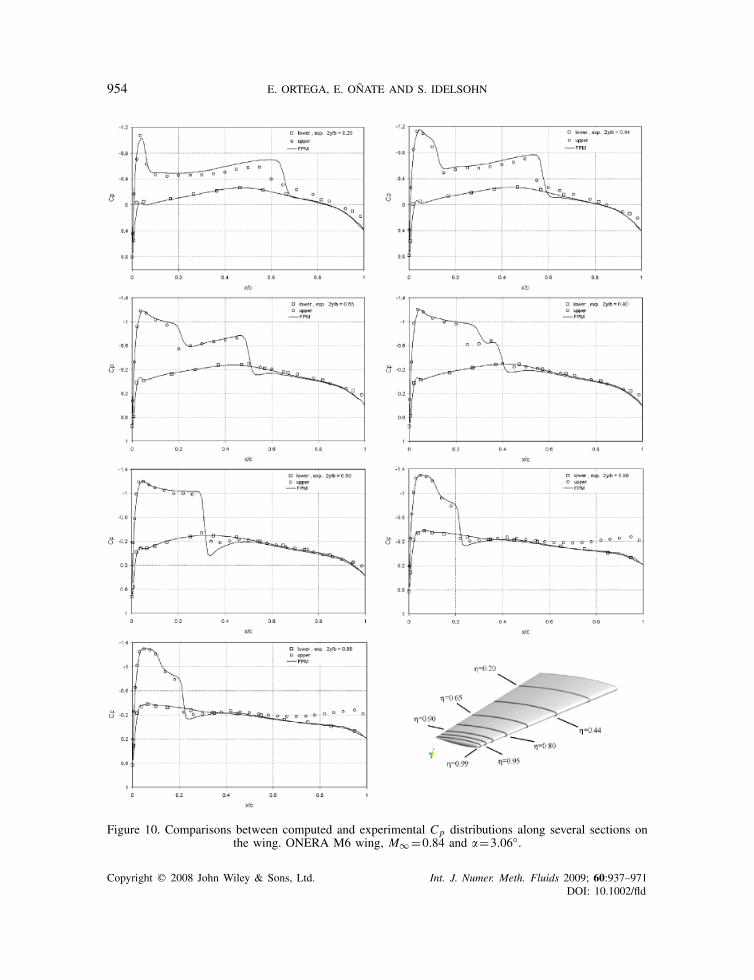
A comparison between numerical and experimental Cp distributions along several sections onthe wing is shown in Figure 10. In accordance with the available experimental data [30], thesesections are located at the following spanwise stations: =0.2, 0.44, 0.65, 0.8, 0.9, 0.95 and 0.99being =2y/b. A good agreement between computed and experimental results can be observedin Figure 10 and, as it was expected, the inviscid computation gives a shock wave, which isslightly stronger than the true shock wave and is located close behind the latter. Notice that theexperimental data measured at =0.99 reveals separated flow behind the shock wave on the upperside of the wing. Consequently, experimental and calculated Cp distributions do not match in theseparated flow region.

6.3. Transonic flow over an NACA wing-body configuration

This example involves the computation of an inviscid transonic flow over a wing-body configuration[32]. The wing has a sweepback �1/4=45◦, an aspect ratio A=4, a taper ratio �=0.6 and it hasnot geometrical twist; moreover, the wing-section is an NACA 65A006 airfoil constant along thewing span. The fuselage has a circular cross-section and its rear part is attached to a sting, whichsupports the model in the wind tunnel test section.

The numerical calculation presented here regards a freestream Mach number M∞ =0.9 and themodel incidence angle is �=4◦. The discretization of the computational domain consists of anunstructured distribution of 512 553 points and second-order approximations are built on cloudswith 35�np�45. Next, Cp and Mach number results computed for the proposed flow conditionsare presented in Figures 11 and 12, respectively.

Figure 13 shows a comparison of Cp distributions calculated at two spanwise stations =0.4and =0.8 on the wing with experimental measurements [32]. Additionally, the longitudinal



Figure 10. Comparisons between computed and experimental Cp distributions along several sections onthe wing. ONERA M6 wing, M∞ =0.84 and �=3.06◦.



Figure 11. Cp distribution on the NACA wing-body configuration (only half of the model has beencalculated, the other part is simply included for visualization purposes). M∞ =0.90 and �=4.0◦.

Figure 12. Mach number isolines on the NACA wing-body configuration andthe symmetry plane. M∞ =0.90 and �=4.0◦.

Cp distribution along the fuselage symmetry plane is compared with experimental results inFigure 14.

As in the previous case, minor differences (due to the inviscid assumption adopted for thecomputational flow model) exist between numerical and experimental results. In spite of this, bothresults match very well as it can be observed in Figures 13 and 14.



Figure 13. A comparison between computed and experimental Cp distribution along two spanwise wingstations =0.4 and 0.8. NACA wing-body configuration, M∞ =0.90 and �=4.0◦.

Figure 14. Comparison between computed and experimental Cp distribution along the fuselage symmetryplane. NACA wing-body configuration, M∞ =0.90 and �=4.0◦.

7. AN h-ADAPTIVE PROCEDURE FOR FP CALCULATIONS

There are several reasons that explain the appeal of mesh (or point) adaptive strategies in thedifferent fields of numerical simulation. Adaptivity reduces the effort needed to obtain a properdiscretization for numerical analysis as regards man-hours, CPU-time and memory requirementssignificantly. In addition, adaptive procedures make the accurate computation of the smaller scalesof the flow field easier, especially when we do not have a priori information concerning thesolution, and become essential for non-stationary problems involving moving discontinuities.

In the introduction to this work we have referred to some topics in numerical computationwhere meshless approaches seem to have certain advantages over mesh-based approaches and



adaptivity is one of them. The fact that meshless techniques do not need to keep a conformingmesh makes them specially well-suited for implementing adaptive procedures. With the purposeof exploiting this capability, in this section we develop an adaptive FP procedure for compressibleflow problems.

7.1. The refinement criterion

The FP solution at a previous time-step is employed with the aim of identifying local clouds of pointswhere new points should be inserted or existing points could be removed from the computationaldomain. This is accomplished by a normalized indicator that evaluates, in an approximate manner,the curvature of the solution at each point

�i =1

�m

nn∑j=1

|l j i ·(∇ j −∇i )|, �m =max(�i ), i=1,n (42)

In the expression above nn is the number of points in the first layer of Delaunay nearest neighboursof xi (already obtained in the local cloud construction stage), l j i =x j −xi is the vector linkingeach pair of points (xi ,x j ) and is the density of the fluid. Naturally, another flow variable ora combination of flow variables can be adopted for calculating the refinement indicator (42). Thelast option could be appropriate for the treatment of viscous fluid flows.

The refinement criterion is applied as follows. Based on Equation (42), new points are insertedaround xi when �i>�max and, conversely, point xi is removed from the computational domain if�i<�min. The limits �max and �min depend on the problem under consideration; in the numericalexamples presented here �max≈0.1 and �min≈0.005 are chosen. It should be noticed that inparticular cases, the proposed normalization causes a lack of sensitivity to relative small gradientsin the flow field. When this happens, it could be useful to avoid the normalization by setting �m =1or taking another local maximum for normalizing the indicator.

7.2. The strategy

Once the refinement criterion has been applied, the remaining of the proposed adaptive procedurecan be reduced to three main steps: the insertion of new points, the removal of existing points andan update. The latter makes reference to the construction of the data associated with each newpoint and the re-construction of the data associated with the affected existing points, respectively.We consider that an existing point is affected when a new point falls inside its cloud, or the spatialposition of any point in its cloud changes due to smoothing.

7.2.1. Insertion of new points. When a star point xi is marked to refine (�i>�max), its Delaunaygrid of nearest neighbours is used to calculate the Voronoi vertices surrounding xi . Next, new candi-date points xc are set at these vertices, i.e. at the centre of the empty circumcircle/circumspherecalculated for each triangle/tetrahedron (2D/3D) composing the Delaunay grid of nearest neigh-bours. Each candidate point xc is accepted if it meets the following requirements:

r1. The radius of the empty circumcircle/circumsphere (rc) complies with rc>rmin, being rmina user-defined parameter which stands for the minimum admissible distance between points.

r2. The radius rc is smaller than a certain internal measure (de) of the triangle/tetrahedron fromwhich the empty circumcircle/circumsphere originates. The internal measure de is calculated as



Figure 15. Refinement of a bi-dimensional cloud of points. The filled points xc meet the requirementsr1–r3 and, in consequence, are inserted around the star point xi .

de=max(|e j · i|, |e j · j|, |e j ·k|), where subscript j stands for each edge of the triangle/tetrahedronand i, j, k are unit vectors in each spatial direction.

r3. The distance from the candidate point xc to another new point previously accepted is greaterthan the minimum admissible distance between points rmin.

If any of the edges/triangles of the local Delaunay grid of nearest neighbours lies on theboundaries, a new candidate boundary point is obtained as an average of the position of the pointsdefining this edge/triangle. The candidate boundary point is accepted if the distance to the nearestpoint is greater than rmin. In our algorithm we perform the boundary refinement first and thenwe refine the discretization into the domain. Note that when the initial boundary discretization isvery coarse, the straightforward procedure proposed for boundary refinement could deteriorate theboundaries, resulting in a lack of reliability of the computational model. In such cases, the positionof new boundary points can be obtained using a higher-order interpolation of the underlyingexisting boundary points (cf. [33]). Figure 15 sketches the refinement procedure for a 2D cloudof points.

7.2.2. Removal of existing points. Point removal capabilities are indispensable for treating non-stationary problems. In this work, the removal of points is restricted only to the existing pointsthat have been inserted in prior refinement levels. In other words, the initial set of points (originalcoarse discretization) is conserved through the calculation, though the spatial position of thesepoints could change due to smoothing. This criterion avoids several time-consuming verificationsand guarantees a minimum appropriate geometrical support for the calculation.

7.2.3. Update. Once the insertion and removal of points are finished, a few steps of a Laplaciansmoothing are carried out on the affected area. This is particularly helpful when points have beenremoved in large quantities. After that, the clouds of points and shape functions concerning thenew points are constructed. In addition, the data concerning existing clouds of points affected by



the insertion of new points or smoothing are re-constructed. Finally, the flow variables at newpoints are calculated as an average of the variables at their previously existing nearest neighbours.

8. SOME EXAMPLES OF ADAPTIVE FP CALCULATIONS

In this section several numerical examples are presented in order to illustrate the performance ofthe proposed FP adaptive procedure. We begin with two computation cases intended to verify theadaptive numerical solution. The first example concerns a 2D adaptive calculation of a supersonicflow around a double-wedge airfoil and the second one deals with the solution of a shock-tubeproblem in a 2D domain. A third example is related to the solution of a transonic flow over anNACA 0012 airfoil and the fourth and last example involves a 3D flow calculation over the ONERAM6 wing. The two final calculation cases give an idea about the possibilities of application of thepresent adaptive FP meshless technique to practical engineering problems.

8.1. Supersonic flow past a double-wedge airfoil

This example resolves the flow around a double-wedge airfoil immersed in a supersonic flow.The airfoil has a unitary chord c=1 and the wedge angle is �=20◦; the upstream Mach numberis M∞ =2 and the airfoil is set at an incidence angle �=0◦. The initial coarse discretization iscomposed by an unstructured distribution of 1279 points and second-order spatial approximationsare built in clouds where 15�np�20. The final adapted discretization, achieved after 70 refinementlevels, consists of 51 907 points. Next, the initial and the final adapted discretizations are shownin Figure 16.

Figure 17 presents a comparison between the analytical solution of the problem, calculatedalong an x-cut in the domain located 0.1c above the airfoil chord-line, and the numerical solutioncomputed at successive refinement levels. How the numerical solution of successive refined-discretizations converges into the analytical solution of the problem can be observed. Finally, thetime convergence of the problem is shown in Figure 18 where the complete process of the adaptivenumerical computation can be seen. When the simulation starts, some time-steps are performedusing the low-order scheme in order to initialize the flow field around the airfoil. Then, the flowsolver switches to the high-order scheme and, even though it affects the convergence, the latteris recovered after a few time-steps. For a value of the density temporal residual of 1.0E−5, thefirst refinement level is performed. Then, consecutive refinement levels are carried out every 200time-steps. Note that the peaks of the convergence curve correspond to each refinement levelperformed during the computation.

8.2. The shock-tube problem

The shock-tube problem is a one-dimensional non-stationary Riemann problem proposed by Sodin 1978 [34]. In this example we adopt a unitary-length bi-dimensional domain and carry out anadaptive shock-tube simulation defined by the following initial conditions:

U(x, t0)={UL=(1,0,0,2.5)T, x�0.5

UR=(0.125,0,0,0.25)T, x>0.5(43)



Figure 16. Supersonic flow past a double-wedge airfoil. Left: original coarse discretization and right: finaladapted discretization (70 refinement levels). The coloured points show Cp results. M∞ =2.0 and �=0◦.

which give a pressure ratio across the diaphragm pL/pR=10 (notice that the diaphragm positionis x=0.5). According to the given initial conditions, the intensity of the shock is moderate andthe flow regime after the expansion is subsonic.

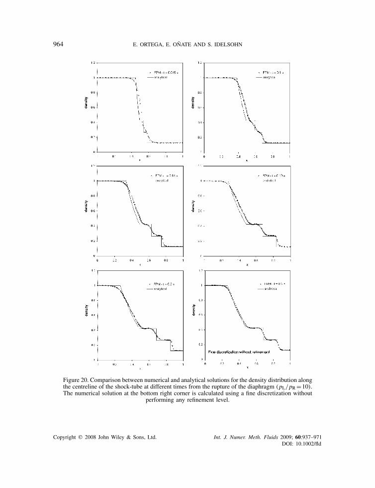
The computational domain is initially discretized by a coarse homogeneous distribution of 217points and second-order spatial approximations are calculated in clouds with 12�np�20. Afterthe rupture of the diaphragm, successive refinement levels are performed at regular periods. Thesimulation time in this example is t=0.2 s, forwhich the adapted discretization reaches a total of 1761points. Next, Figure 19 presents some snapshots of adapted discretizations taken at different timesfrom the rupture of the diaphragm. There, the coloured points show flow density numerical results.

Figure 20 displays several comparisons between the numerical and the analytical solution forthe density variable along the tube, corresponding to the simulation times pointed out in Figure 19.

In Figure 20, a considerable smoothing of the numerical solution can be observed in the firstrefinement levels (t=0.045 and 0.1 s), for which the discontinuities are noticeably smeared. Thisfact can be explained to a great extend by the coarse discretization employed in order to startthe simulation. Note that the number of points to be added in a given refinement level dependsupon the flow field variables but also on the existing point discretization (cf. Section 7.2.1).Consequently, certain geometrical restrictions limit the maximum number of new points insertedat a given refinement level, which makes the discretization unable to adapt instantaneously to theflow variables in a proper manner. Nevertheless, a closer agreement between the numerical andthe analytical solution is obtained for the simulation times t=0.14, 0.19 and 0.20 s. In these cases,an improved flow resolution but also minor inaccuracies in the discontinuities location can be



Figure 17. A comparison between the analytical Cp distribution along an x-cut on the domain andcomputed numerical results obtained at different refinement levels. The cut is located at y/c=0.1 and

the airfoil leading edge coincides with the point (x, y)=(0,0). M∞ =2.0 and �=0◦.

observed. We suspect that this behaviour could be related either to the straightforward procedureproposed to interpolate the numerical solution between the old and the new refined-discretizationor to the Laplacian smoothing performed after each addition and/or removal of points. However,the solution should not be sensitive to the smoothing operations if a proper interpolation procedureis employed.

A numerical calculation performed with a fixed homogeneous discretization, having a pointdensity similar to that in the final adapted discretization of Figure 19, is presented at the bottom rightcorner of Figure 20. Comparing the latter result with its counterpart obtained using the adaptivesimulation, it is possible to observe that the numerical dissipation introduced by the refinementprocedure is quite small. It should be noticed that the problem setting employed in both calculationsis the same. Finally, it can be observed that the normalization adopted for calculating the refinementindicator may cause some detriment to the contact discontinuity resolution as stronger gradientsare present at the shock location. In cases like this, it would be useful to adopt a local criterionfor calculating the refinement indicator.

8.3. Transonic flow around an NACA 0012 airfoil

This example concerns the computation of a transonic inviscid flow past an NACA 0012 airfoil.The freestream Mach number is M∞ =0.8 and the incidence angle is �=1.25◦. The initial spatial



Figure 18. Convergence history of the double-wedge airfoil calculation(70 refinement levels). M∞ =2.0 and �=0.0◦.

discretization involves an unstructured distribution of 976 points and second-order spatial approx-imations are calculated in clouds with 15�np�20. The finest adapted discretization consists of4938 points and is achieved after 15 refinement levels. Both, the initial and the final discretizationsare shown in Figures 21 and 22 respectively.

Notice that the adaptive procedure captures all the flow features with precision. The strongshock wave on the upper side of the airfoil, the weaker shock on its lower side and the leading andtrailing edge regions are appropriately captured via the refinement procedure. Figure 23 shows theCp field around the airfoil calculated for the final adapted discretization.

The computed Cp distribution on the airfoil is compared with numerical reference results [35]in Figure 24, where good agreement can be observed. Finally, the time convergence history of theproblem is presented in Figure 25.

8.4. A 3D example: the ONERA M6 wing

This example solves the 3D flow around the ONERA M6 wing adopting the freestream conditionsgiven in Section 6.2. The initial coarse discretization consists of an unstructured distribution of66 864 points and second-order approximation bases are employed in clouds with 30<np<45.In this simulation the adapted discretization reaches a total of 102 592 points after 35 refinementlevels. Next, Figure 26 shows the original and final discretizations of the wing; coloured pointsdisplay Cp results.

The initial discretization of the wing consists of 14 221 points and 28 314 triangle elements,whereas the final adapted discretization is composed of 15 537 points and 30 942 triangles.Note that new points are mainly concentrated around the strong shock wave spanning the wingwhere large gradients are detected. In order to make the refinement indicator (42) also sensitive



Figure 19. Adapted discretizations obtained for the shock-tube problem (pL/pR=10) at different times fromthe rupture of the diaphragm (the top image shows the initial coarse discretization).

to the smaller gradients in the flow field, we can decrease the parameter �max or change thenormalization criterion. However, as the indicator becomes more sensitive, the refinement proce-dure loses its local character. This would lead to an insertion of large sets of new points foreach refinement level and the convergence of the problem could be seriously affected in somecases. Thus, the adoption of local maxima for normalizing the indicator seems a more adequatechoice.

Figure 27 compares the Cp distributions along two sections of the wing calculated with the orig-inal and the finest discretization. In the same figure, a view of the finest adapted point discretizationfor a cut in the plane x–z of the domain (passing through the same spanwise stations) is presented.Finally, the convergence history of the problem is shown in Figure 28.

Regarding the computational cost of the proposed FP adaptive technique, numerical experimentsshow that the CPU-time required by each refinement level is approximately equal to the timeinvolved for the update stage (cf. Section 7.2.3) and the cost of inserting and removing points isalmost negligible. In general, the overall CPU-time involved for each refinement level is only afraction of the time required for advancing the problem solution a single time-step.



Figure 20. Comparison between numerical and analytical solutions for the density distribution alongthe centreline of the shock-tube at different times from the rupture of the diaphragm (pL/pR=10).The numerical solution at the bottom right corner is calculated using a fine discretization without

performing any refinement level.



Figure 21. A view of the original coarse discretization in the proximity of the NACA 0012 airfoil.

Figure 22. A view of the finest adapted discretization in the proximity of the NACA0012 airfoil obtained after 15 refinement levels.

9. CONCLUSIONS

An adaptive finite point method (FPM) for compressible flow calculations has been presented. Onthe basis of a robust WLSQ procedure and an iteratively improved local approximation, an upwindsemi-discrete scheme is constructed for each cloud of points. This methodology, in conjunctionwith a multi-stage time integration scheme, allows solving real 3D problems minimizing the



Figure 23. Cp isolines in the near field of the NACA 0012 airfoil obtained with the finest adapteddiscretization. M∞ =0.80 and �=1.25◦.

Figure 24. Cp distribution on the NACA 0012 airfoil obtained with the finest adapted discretization.A comparison between computed and numerical reference results [35]. M∞ =0.80 and �=1.25◦.

dependence of the numerical results on the spatial discretization of the analysis domain, the localcloud topology and the parameters of the local approximation. All these are important achievements,which make possible further enhancement and extension of the FPM capabilities for practical 3Dapplications.



Figure 25. Convergence history of the NACA 0012 airfoil calculation(15 refinement levels). M∞ =0.80 and �=1.25◦.

Figure 26. A view of the upper side of the ONERA M6 wing. Left: original coarse discretization. Right:finest adapted discretization (35 refinement levels). M∞ =0.84 and �=3.06◦.

In the introduction to this article we made reference to certain topics in numerical simulation,which offer good opportunities for the development and promotion of meshless techniques. Withthe aim of exploiting these opportunities, an adaptive FPM for compressible flow calculations hasbeen developed. Several test cases involving stationary and non-stationary flow problems havebeen presented with the purpose of exemplifying the performance of the proposed technique. Allthe examples demonstrate that an adaptive FPM is capable of properly resolve the essential flowfeatures, achieving robust and reliable adaptive solutions with a low computational cost. Although



Figure 27. Left: Cp distributions along two wing sections =0.44 (top) and =0.95 (bottom) calculatedwith the original and the final adapted discretization. Right: cuts x–z of the finest refined domain passingthrough wing stations =0.44 (top) and =0.95 (bottom). ONERA M6 wing M∞ =0.84 and �=3.06◦.

some numerical tests (of which a few have been reported here) highlight the need for more accuraterefinement criteria and an improved treatment of moving discontinuities, the overall performanceof the proposed adaptive FPM is highly satisfactory and this can be seen as the main achievementof this work.

Real viscous flow involves certain features where meshless techniques, and especially adaptivemeshless techniques, could make important contributions, e.g. boundary layer discretization andshock-boundary layer interaction problems. In this sense, we have developed the basic tools fortackling these kinds of problems and solving them constitutes our next short-term goal.

Regarding computational efficiency we must say that at present we still lack precise performancecomparisons between the FPM described here and conventional discretization techniques. However,we estimate that the computational cost of a 3D FP computation using the methodology presentedin this paper would typically exceed a similar FE-based computation by a cost factor of 3 being 5a typical value. Hence, if a competitive FPM is to be achieved, an improvement in computationalefficiency is indispensable. In that respect, numerous techniques can be implemented in orderto accelerate convergence to the steady state. Combining these techniques with a suitable datastructure and an optimized way to perform the numerical calculations, it is possible to enhance



Figure 28. Convergence history of the ONERA M6 wing adaptive calculation(35 refinement levels). M∞ =0.84 and �=3.06◦.

the efficiency of the present FPM considerably. Moreover, performance comparisons between thepresent FPM and other meshless techniques accomplishing similar tasks are essential for placingthe FPM into the actual meshless methods scenario. In conclusion, the results obtained with theFPM are very encouraging, though efficiency is still a pending matter. Consequently, future researchefforts will take highly into consideration the improvement of this key point.

ACKNOWLEDGEMENTS

The first author would like to acknowledge the support of Alßan Program, the European Union Programmeof High Level Scholarships for Latin America, scholarship No. E04D027284AR. We express our gratitudeto Dr Nestor Calvo for helping with the point generation technique employed in this work. Last but notleast, the many valuable contributions of Dr Roberto Flores to this work are also gratefully acknowledged.

REFERENCES

1. Belytschko T, Krongauz Y, Organ D, Fleming M, Krysl P. Meshless methods: an overview and recent developments.Computer Methods in Applied Mechanics and Engineering 1996; 139:3–47.

2. Fries T, Matthies H. Classification and Overview of Meshfree Methods. Department of Mathematics and ComputerScience, Technical University of Braunschweig. Inf. 2003-3, 2004.

3. Li S, Liu WK. Meshfree and particle methods and their applications. Applied Mechanics Reviews 2002; 55:1–34.4. Gu YT. Meshfree methods and their comparisons. International Journal of Computational Methods 2005; 4:

477–515.5. Duarte CA. A review of some meshless methods to solve partial differential equations. TICAM Report 95-06,

Texas Institute for Computational and Applied Mathematics, 1995.



6. Liu WK, Chen Y, Jun S, Belytschko T. Overview and application of the reproducing Kernel particle method.Archives of Computational Methods in Engineering 1996; 5(1):3–80.

7. Dolbow J, Belytschko T. An introduction to programming the meshless element free-Galerkin method. Archivesof Computational Methods in Engineering 1998; 5(3):207–241.

8. Onate E, Idelsohn S, Zienkiewicz OC, Taylor RL, Sacco C. A finite point method for analysis of fluid mechanicsproblems. Applications to convective transport and fluid flow. International Journal for Numerical Methods inEngineering 1996; 39:3839–3866.

9. Onate E, Idelsohn S, Zienkiewicz OC, Fisher T. A finite point method for analysis of fluid flow problems.Proceedings of the 9th International Conference on Finite Elements Methods in Fluids, Venice, Italy, 1995;15–21.

10. Onate E, Idelsohn S, Zienkiewicz OC, Taylor RL, Sacco C. A stabilized finite point method for analysis of fluidmechanics problems. Computer Methods in Applied Mechanics and Engineering 1996; 139:315–346.

11. Onate E, Sacco C, Idelsohn S. A finite point method for incompressible flow problems. Computing andVisualization in Science 2000; 3:67–75.

12. Fischer TR. A contribution to adaptive numerical solution of compressible flow problems. Ph.D. Thesis, UniversitatPolitecnica de Catalunya, 1996.

13. Sacco C. Development of the finite point method in fluid mechanics (in Spanish). Ph.D. Thesis, School of CivilEngineering, Universitat Politecnica de Catalunya, 2001.

14. Lohner R, Sacco C, Onate E, Idelsohn S. A finite point method for compressible flow. International Journal forNumerical Methods in Engineering 2002; 53:1765–1779.

15. Onate E, Perazzo F, Miquel J. A finite point method for elasticity problems. Computers and Structures 2001;79:2151–2163.

16. Perazzo F, Miquel J, Onate E. A finite point method for solids dynamic problems (in Spanish). RevistaInternacional de Metodos Numericos para Calculo y Diseno en Ingenierıa 2004; 20(3):235–246.

17. Perazzo F, Oller S, Miquel J, Onate E. Advances in the finite point method for solid mechanics (in Spanish).Revista Internacional de Metodos Numericos para Calculo y Diseno en Ingenierıa 2006; 22(3):153–167.

18. Onate E. Derivation of stabilized equations for numerical solution of advective–diffusive transport and fluid flowproblems. Computer Methods in Applied Mechanics and Engineering 1998; 151:233–265.

19. Sridar D, Balakrishnan N. An upwind finite difference scheme for meshless solvers. Journal of ComputationalPhysics 2003; 189:1–29.

20. Praveen C. A positive meshless method for hyperbolic equations. Report 2004-FM-16, ARDB Centre of Excellencefor Aerospace CFD, Department of Aerospace Engineering, Indian Institute of Science, 2004.

21. Boroomand B, Tabatabaei AA, Onate E. Simple modifications for stabilization of the finite point method.International Journal for Numerical Methods in Engineering 2005; 63:351–379.

22. Ortega E, Onate E, Idelsohn S. An improved finite point method for three-dimensional potential flows.Computational Mechanics 2007; 40:949–963.

23. Perazzo F, Lohner R, Perez-Pozo L. Adaptive methodology for meshless finite point method. Advances inEngineering Software 2007; 39:156–166.

24. Lancaster P, Salkauskas K. Surfaces generated by moving least squares methods. Mathematics of Computation1981; 37:141–158.

25. Demmel JW. Applied Numerical Linear Algebra. Society for Industrial and Applied Mathematics: Philadelphia,1997.

26. Idelsohn S, Calvo N, Onate E. Polyhedrization of an arbitrary 3D point set. Computer Methods in AppliedMechanics and Engineering 2003; 192:2649–2667.

27. Roe PL. Approximate Riemann solvers, parameter vectors and difference schemes. Journal of ComputationalPhysics 1981; 43:357–372.

28. Turkel E. Improving the accuracy of central difference schemes. ICASE Report 88-53, 1988.29. Van Leer B. Towards the ultimate conservative difference scheme. V-A second-order sequel to Godunov’s method.

Journal of Computational Physics 1979; 32:101–136.30. Schmitt V, Charpin F. Pressure distributions on the ONERA-M6-wing at transonic Mach numbers. Experimental

data base for computer program assessment. Report of the Fluid Dynamics Panel Working Group 04, AGARDAR 138, 1979.

31. NPARC Alliance CFD verification and validation web site. Web page: http://www.grc.nasa.gov/WWW/wind/valid/archive.html (26 October 2007).



32. Loving D, Estabrooks B. Transonic-wing investigation in the Langley 8-foot high-speed tunnel at high subsonicMach numbers and at a Mach number of 1.2. Analysis of pressure distribution of wing-fuselage configurationhaving a wing of 45◦ sweepback, aspect ratio 4, taper ratio 0.6, and NACA 65A006 airfoil section. ResearchMemorandum NACA RM L51F07, National Advisory Committee for Aeronautics, 1951.

33. Zorin D, Schroder P, Sweldens W. Interpolating subdivision for meshes with arbitrary topology. Proceedings ofSIG-GRAPH 1996; 96:189–192.

34. Sod GA. A survey of several finite-differences methods for systems of nonlinear hyperbolic conservation laws.Journal of Computational Physics 1978; 27:1–31.

35. Pulliam TH, Barton JT. Euler computations of AGARD Working Group 07 Airfoil Test Cases. AIAA 23rdAerospace Summer Meeting, Reno, NE, AIAA Paper 85-0018, 1985.


A finite point method for adaptive three-dimensional compressible flow calculations

Documents

Transcript of A finite point method for adaptive three-dimensional compressible flow calculations